Numerical Modelling of an H-type Darrieus Wind Turbine ...

American Journal of Energy Research, 2017, Vol. 5, No. 3, 63-78 Available online at http://pubs.sciepub.com/ajer/5/3/1 ©Science and Education Publishing DOI:10.12691/ajer-5-3-1

Numerical Modelling of an H-type Darrieus Wind Turbine Performance under Turbulent Wind

Ahmed Ahmedov1, K. M. Ebrahimi2,*

1Thermotechnics, Hydraulics and Ecology, University of Ruse, Ruse, Bulgaria 2Aeronautical and Automotive Engineering, Loughborough University, Loughborough, UK

*Corresponding author: [email protected]

Abstract This paper presents the force interaction between fluid flow and a rotating H-type Darrieus vertical axis wind turbine. The main goal of this study is to determine the wind rotor’s performance characteristics under turbulent wind: torque M = f (n), normal force FN = f (n), output power P = f (n) and the aerodynamic characteristics CM = f (λ), CN = f (λ), CP = f (λ). The flow passing through the turbine has a complex structure due to the rotation of the rotor. The constantly changing angular position of the turbine’s blades is leading to a variation in the blades angle of attack. This angle can vary from positive to negative values in just a single turbine revolution. The constant fluctuations of the angle of attack are the main factor which leads to the unsteady nature of the flow passing through the turbine. At low tip-speed ratios, the phenomena deep dynamic stall occurs which leads to intensive eddy generation. When the turbine is operating at higher tip-speed ratio the flow is mainly attached to the blades and the effect of the dynamic stall over the turbine performance is from weak to none. The Darrius turbine performance characteristics are obtained through a numerical investigation carried out for several tip-speed ratios. The used CFD technique is based upon the URANS approach for solving the Navier-Stokes equations in combination with the turbulence model k – ω SST. Also, a numerical sensitive study concerning some of the simulation parameters is carried out.

Keywords: H-Darrieus VAWT, CFD modelling, turbulence models, performance characteristics, aerodynamic characteristics

Cite This Article: Ahmed Ahmedov, and K. M. Ebrahimi, “Numerical Modelling of an H-type Darrieus Wind Turbine Performance under Turbulent Wind.” American Journal of Energy Research, vol. 5, no. 3 (2017): 63-78. doi: 10.12691/ajer-5-3-1.

1. Introduction

The constantly increasing prices of the fossil fuels, restraint of the factors contributing to global warming and the different agreements between the industrialize countries for decreasing the carbon emissions gave the renewable energy sources significant boost in the production of green energy.

The wind energy sector is rapidly growing worldwide, as in near future it will take place as one of the major concepts for sustainable economic development. It can be noticed that besides the commercial megawatt turbines, the interest in low power wind turbines is growing. They are suitable either for urban conditions and distant areas deprived by a commercial electrical grid.

The wind turbines can be divided into two major groups according to their axis of rotation – wind turbines with a horizontal axis of rotation (HAWT) and vertical axis wind turbines (VAWT). VAWT have lower efficiency in comparison with the HAWT, but they haven’t been that intensively investigated as their counterparts. A representative of the VAWT is the H-Darrieus rotor, which consists of several straight blades parallel to the rotor axis. The blades

are placed on a certain radius from the turbine shaft with fixed pitch angle. Some of the advantages of VAWT over HAWT are: VAWT can receive the wind from any direction without the need of additional mechanism; VAWT are less sensitive to the wind gusts and turbulence intensity of the flow. Due to those advantages, the low power turbines can be mounted close to the ground or on building rooftops in urban areas where the wind flow is highly turbulent and constantly changes its direction.

Despite its geometrical simplicity, the aerodynamics of the H-Darrieus turbine is complicated involving highly unsteady flow passing through its rotor. The unsteadiness is caused mainly by the large variations of the blade angle of attack during the rotor operation. High rotor solidity (turbines with more than two blades) additionally contributes to the unsteadiness of the flow passing through the turbine by increasing the angle of attack fluctuations.

A consequence of the aforementioned features is the occurrence of dynamic stall. The dynamic stall phenomenon influences the turbine performance and the distribution of the blade loads - lift and drag forces. The dynamic stall is characterized by vortex generation, shedding and fluctuation in the lift force acting on the blades in correspondence with the change in the angle of attack. The dynamic stall occurs at an angle of attack that exceeds the

64 American Journal of Energy Research

angle at which the static stall is occurring. The static stall represents the drastic decrease in the lift force acting on a static airfoil (none fluctuating, rotating) when the critical angle of attack of the airfoil is exceeded. The critical angle of attack is typically about 15 degrees, but it may vary significantly depending on the fluid, airfoil shape and Reynolds number. The structure of the complex unsteady flow is shown on Figure 1, the flow visualization is achieved by Brochier [1] depicting a deep dynamic stall regime.

Figure 1. Vortex generation and shedding during the rotation of a Darrieus turbine

Figure 2. Darrieus turbine power coefficient curve

Figure 2 presents the dimensionless characteristic CP = f (λ) the power coefficient against the tip-speed ratio. This graph is divided into three areas corresponding to different processes. In the first one, the dynamic phenomena are dominant. In the third area, the viscous phenomena are dominant while the second (middle) area is a transient one. At low tip-speed ratios, the blades are undergoing deep dynamic stall which leads to the appearance of significant variations in the aerodynamic loads acting on the blades. In this area, the aerodynamic losses can be contributed mainly to the intensive generation and separation of large vortices. At high tip-speed ratios, the losses are mainly attributable to the viscous friction. This is due to the small changes in the angles of typical for the higher values of the tip-speed ratio. At these circumstances, no or only light dynamic stall is observed. The middle section is the transient at which the maximum of the power coefficient is situated.

2. Literature Review

2.1. Analytical Performance Prediction Models

During the seventies and the eighties, several analytical models for Darrieus wind turbine performance prediction were developed. They were called momentum prediction models. The single stream tube model [2], the multiple stream tube model [3] and the double multiple stream tube model [4] were developed on the basis of the actuator disk theory, firstly applied for wind turbines from Glauert. According to this theory, the stream tube models are valid for wind turbines with solidity less than 0.2 and which operates in a small range of tip-speed ratios [5]. The main assumption made in these models is that the flow passing through the turbine rotor is treated as quasi-steady. Furthermore for the modeling of the aerodynamic forces acting on the blades a tabular experimental data regarding the static lift and drag force coefficients is used. All these assumptions lead to the inaccurate modeling of the forces acting on the blades. The momentum models aren’t capable of adequate modeling of the flow in the near blade region and downstream vortex structures [6].

Another type of analytical models are the so called vortex models, they are developed on the assumption for potential incompressible flow. They are allowing for the blade vortex trail to be taken into account in the performance prediction. The turbine blades are represented as vortex filaments.

The concept for the vortex models was firstly introduced by Larsen [7]. He developed a two-dimensional model, applicable only for turbines operating in regimes characterized by small fluctuation in the angle of attack. The model doesn’t take into account the stall phenomena. Furthermore, the model is restricted to be applied only for the analysis of H-Darrieus turbines.

Strickland6 extended upon the Larsen’s vortex model by incorporating 3D flow taking into account the influence of the dynamic stall. The results given by the model regarding the forces acting on the blades and the vortex trail behind the rotor are in good agreement with the experimental data. In the model developed by Lishman [8] a static drag and lift experimental coefficients are used in order to calculate the bound vortices strengths.

All of the aforementioned vortex models are more computational intensive in comparison with the momentum models. This is due to the calculation of Biot-Savart law for every detached vortex in the flow passing through the rotor. The results obtained by the vortex models are more realistic in comparison with the momentum models, despite the usage of static aerodynamic coefficients and the assumption for inviscid flow.

2.2. Computational Fluid Dynamics (CFD) Computational fluid dynamics (CFD) arises as an

approach that can overcome the aforementioned deficiencies of the momentum and vortex models. All CFD algorithms are developed on the basis of numerical schemes designated for solving the Navier-Stokes partial differential equations, computational grid generation and

American Journal of Energy Research 65

turbulence modelling. The most popular approach for solving the governing equations is the Reynolds Averaged Navier-Stokes technique (RANS). In this approach, only the main flow is solved directly by the governing equations while the turbulence is modelled by introducing additional stress tensors, called Reynolds stress tensors. In conditions of isotropic turbulence, the Reynolds tensors are introduced as scalars acting like additional turbulence viscosity. In this approach, the turbulence viscosity is connected with one or two turbulence parameters. For both of the turbulence parameters, a semi-empirical transport dependencies need to be solved (turbulent kinetic energy k, dissipation ε or specific dissipation ω). The most widely used turbulence models are Spallart-Allmaras with one equation and the two equations models k ε− and k ω− [9].

Hamada et al. [10] and Howell et al. [11] conducted two and three-dimensional simulations on straight bladed VAWT by using the three different subtypes of the k ε− turbulence model which are available in the commercial software ANSYS Fluent. From the standpoint of the torque results the authors observed that the standard k ε− model presented data that deviates from the one obtained by the k ε− Realizable and k ε− RNG models. They concluded that the standard variant of the turbulence model fails to accurately predict the unsteady nature of the flows which involves detached eddies and turbine rotation. The k ε− Realizable model tends to result in predicting unrealistic turbulent viscosity in the case of modelling rotational areas. The results show that the k ε− RNG model always tends to overestimate the value of the power coefficient in the 2D simulations whereas in the 3D simulation it always underestimates it. Nevertheless, the 3D results had shown good agreement with the experimental data.

Raciti Castelli et al. [12,13] carried out two and three-dimensional analysis over a three straight bladed VAWT in order to develop a performance prediction modelling strategy through CFD modelling. The introduced methodology is verified with experimental data. The experimental investigation of the low solidity turbine was carried out in a wind tunnel. Evaluation of the applicability of the incorporated turbulence models was also carried out through estimation of the near wall y+ criteria. The dimensionless criteria y+ represents the distance from the wall (the blade) to the first computational node which is situated in the boundary layer. This node is chosen to be the center of the nearest to the blade computational cell. The k ε− Realizable model was used with a combination of the near wall treatment function at values of the near wall criteria y+ > 30. The simulation with direct solving of the boundary layer (y+ < 5) the k SSTω− model was used. After a statistical analysis of the y+ criteria, the authors concluded that the accuracy of the turbulence modelling is highly influenced by the y+ value. Comparison of the power coefficient curves shows that the 2D model overestimates the experimental result, but reproduces well the shape of the curve.

Amet et al. [14] carried out 2D simulation over a straight bladed turbine for two very different values of the tip-speed ratio λ = 2 and λ = 2. The lift and drag

coefficients for a full turbine revolution where compared with the experimental data obtained by Laneville and Vittecoq [15]. Although that the shape and the trend of the theoretical and experimental curves were similar there were some noticeable differences between their values. The researchers used the k ω− turbulence model which major disadvantage is the unrealistic modelling of large vortices separating from the blades. The authors pointed this disadvantage of the turbulence model as the main reason for the discrepancy between the theoretical and experimental results.

In 2011 Nobile et al. [16] compared the applicability of the k ω− , k ε− , and k SSTω− models for VAWT performance prediction. They compared the vortex structures modelled by the k ω− turbulence model with the experimental PIV (Particle Image Velocimetry) data acquired by Simao Ferreira [17]. The comparison showed a major difference between the theoretical result and the experiment. While the point of flow separation over the blade and the dynamic stall modelling is better in comparison with the k ε− model it is noticed that the development of the vortices detached from the blades is suppressed. This is leading to high vortex dissipation. Also, it is noted that there is no vortex structure shedding from the blade trailing edge which occurs in the dynamic stall process.

The hybrid turbulence model k SSTω− is one step ahead in the performance modelling of VAWT, due to the combination of the good near wall modelling given by the k ω− and the good main flow modelling given by the k ε− model.

In 2009 Consul et al. [18] carried an investigation over the solidity of a straight bladed vertical axis hydrokinetic turbine. The results from the 2D modelling are verified against experimental data. For comparison, the authors used the experimental data published by Sheldahl and Klimas [19] regarding flow over static airfoils. Two turbulence models were applied in their investigation – Spalart-Allmaras and the k SSTω− model. The results showed minimal differences between the values of the drag and lift forces given by the two models. The theoretical result differs from the experimental in regard to the maximum value of the lift force and the value of the angle of attack at which the flow separates from the blades. At high angles of attack k SSTω− manages to successfully reproduce the periodicity of the vortex trail behind the turbine. The results obtained by the Spallart-Allmaras model are inconsistent. The k SSTω− model performs better because it is specially developed for the purpose of modelling flow separation.

In 2011 McLaren et al. [20] had put the flow separation modelling abilities of the k SSTω− model to the test by performing an analysis over a static blade with airfoil section NACA 0015 at Reynolds number of Re = 360000. The results obtained for the drag and lift forces given by three different turbulence models were compared with experimental data. The k SSTω− model gave the most precise results in comparison with the standard k ω− and k ε− models. The theoretical results obtained by the k ω− and k ε− models in regard to the maximum value


of the lift force and the angle of attack at which the flow separates are exceeding the experimental data. The theoretical data obtained by the k SSTω− model is in good agreement with the experiment.

Edwards et al. [21] developed a CFD procedure for investigation of VAWT and verified it with experimental data regarding the aerodynamic forces acting on the blades and the flow development behind the turbine. They carried out a numerical investigation over oscillating airfoil by incorporating different turbulence models. Thy compared the theoretical results with the experimental investigation of Lee and Gerontakos [22]. Edwards et al. conceded that the best-suited model for modelling the flow around oscillating airfoils is the .k SSTω− The numerical results given by the modelling of a VAWT were compared with PIV (Particle Image Velocimetry) data. The data obtained by the k SSTω− model showed a slight delay in the modelling of the dynamic stall in the upwind area of the turbine. A delay in the reattachment of the flow to the blades is also observed in the downwind area of the turbine rotor.

More realistic computational modelling can be achieved through direct solving of the turbulent structures by the governing equations. The LES (Large Eddy Simulation) turbulent model is capable of detailed realistic modelling of large vortex structures. In this model, the large vortices are directly solved through the governing equations while the smaller structures are modelled. LES is applicable only for three-dimensional simulations, mainly due to the 3D nature of the vortices. This type of simulation is much more grid and computational demanding in comparison with the RANS approach. The main reason for that is the direct solving of the turbulence parameters for the large eddies. Variation of the LES model is the DES (Detached Eddy Simulation) model. This model is a combination of two approaches - the RANS approach, which is applied for the boundary layer modelling and the LES approach which is applied in areas that are distant from the walls.

Iida et al. [23] are one of the first researchers of VAWT that used the LES numerical modelling. They proved that the LES approach is capable of modelling the operation of a VAWT much more accurate than the momentum models, especially in the operational range of low tip-speed ratios where dynamic stall occurs. They used a computational grid consisted approximately of eight million cells, which is relatively low grid count according to the needs of the LES simulations.

In 2007, Simao Ferreira et al.17 published a research concerning the numerical modelling of VAWT with different turbulence models: Spalart-Allmaras, k ε− , LES and DES. In comparison with Iida’s numerical model, this one is comprised of twice the number of grid elements, approximately 1.6x106. The authors concluded that the mesh is still not fine enough for the needs of the LES modelling. The results obtained by the DES modelling shows that the density of the used computational mesh is sufficient. As main reason for that, the authors points the better near wall modelling provided by the DES model. The comparison of the LES and DES theoretical results with the experiment showed clearly that those models are superior to the RANS approach in terms of realistic large eddy structures modelling.

A literature overview about the theoretical performance prediction models for VAWT was carried out. It can be concluded that that CFD modelling is superior in comparison with the classical momentum and vortex models. The analysis of the different CFD approaches showed that URANS k SSTω− modelling is capable of modelling the unsteady nature of the flow passing through an H-Darrieus wind turbine. Despite the better results presented by the LES and DES modelling their main drawbacks are the high hardware and computational demands. At flows with moderate and high Reynolds numbers, the DES model uses the URANS approach for modelling the flow in the near wall areas. In this case, the flow near the blades modelled by the DES is similar to the one obtained by the URANS approach.

3. Goal and Objectives

On the basis of the presented literature review arises the goal of the present study:

Carrying out an investigation of the force interaction between a fluid flow and the revolving rotor of an H-Darrieus wind turbine in order to obtain its theoretical performance and aerodynamic characteristics.

To accomplish the goal of the study the following objectives must be fulfilled:

1. Carrying out a two-dimensional numerical modeling over the operation of an H-Darrieus wind turbine by applying a CFD approach.

2. Carrying out a computational sensitivity study toward some of the simulation parameters.

3. Simulating the operation of the wind turbine at regimes with different tip-speed ratios. Presenting visualization of the flow passing through the turbine’s rotor.

4. VAWT Parameters

One of the VAWT main parameters is the tip-speed ratio λ or TSR. This parameter depicts the ratio between the peripheral velocity of the turbine rotor and the wind velocity. The TSR can be defined as:

,uλϑ∞

= (1)

where u = ω.R is the turbine rotor peripheral velocity, R is the rotor radius, ϑ∞ is the wind velocity.

The aerodynamic forces and the main flow velocity components acting on the turbine blades are presented on Figure 3. The main flow velocity is denoted by ϑ∞ . The turbine rotation is causing fluctuations in the magnitude of the relative velocity W. The magnitude of the relative velocity can be expressed as:

. .W OMϑ ω∞= −

(2)

The relative velocity application point M lies on the blade flight path which corresponds to OM R=

according to Figure 3. Point M is located at a distance 0.25 ÷ 0.3 from the blade chord length c which is


measured from the blade leading edge. Figure 3 shows the interaction between the relative velocity and the turbine blades at different angular positions. In the upstream area (270° - 90°) the relative velocity is acting on the suction side of the blade. As the turbine rotates the blade are traveling from the upstream to the downstream area (90° - 270°) where the relative velocity is starting to act on the pressure side of the blades. The constant changes of the relative velocity are causing dynamic changes in the values of the angle of attack, α. As the turbine rotates the values of the angle of attack are changing periodically from positive to negative. The relative velocity and the angle of attack can be defined as:

21 2W ϑ λθ λ∞= + + (3)

sincos

arctg θαθ λ

= + (4)

where θ is the turbine angular position.

Figure 3. The main velocity components and the aerodynamic force acting on the wind turbine blades

The occurrence and intensity of the dynamic stall phenomena can be examined with the aid of the reduced frequency k∗ 15 and the angle of attack α. The reduced frequency k∗ is the ratio of the time for which the flow passes over an airfoil (c / ω.R) and the time for which the angle of attack changes from positive to negative. The reduced frequency can be expressed as:

( )

( )

* /,

2/

MAX

MAX

c Rk

d dt

ω

αα

=

(5)

where c is the blade chord length. The lower index “MAX” indicates the maximum value of the parameter (angle of attack) at a full rotation of the turbine rotor. The reduced frequency regarding H-Darrieus wind turbine is derived from the dependency originally developed for helicopter rotor operating with a constant angle of attack15. After substituting in eq. 3 in eq. 5 for k* follows:

* 210.5 / 1/ 1 .1

ck arctgR

λλ

= − − (6)

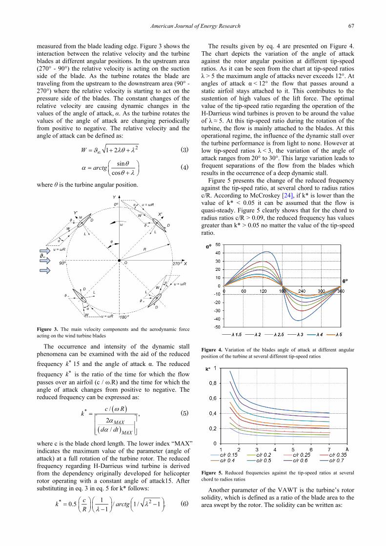
The results given by eq. 4 are presented on Figure 4. The chart depicts the variation of the angle of attack against the rotor angular position at different tip-speed ratios. As it can be seen from the chart at tip-speed ratios λ > 5 the maximum angle of attacks never exceeds 12°. At angles of attack α < 12° the flow that passes around a static airfoil stays attached to it. This contributes to the sustention of high values of the lift force. The optimal value of the tip-speed ratio regarding the operation of the H-Darrieus wind turbines is proven to be around the value of λ ≈ 5. At this tip-speed ratio during the rotation of the turbine, the flow is mainly attached to the blades. At this operational regime, the influence of the dynamic stall over the turbine performance is from light to none. However at low tip-speed ratios λ < 3, the variation of the angle of attack ranges from 20° to 30°. This large variation leads to frequent separations of the flow from the blades which results in the occurrence of a deep dynamic stall.

Figure 5 presents the change of the reduced frequency against the tip-sped ratio, at several chord to radius ratios c/R. According to McCroskey [24], if k* is lower than the value of k* < 0.05 it can be assumed that the flow is quasi-steady. Figure 5 clearly shows that for the chord to radius ratios c/R > 0.09, the reduced frequency has values greater than k* > 0.05 no matter the value of the tip-speed ratio.

Figure 4. Variation of the blades angle of attack at different angular position of the turbine at several different tip-speed ratios

Figure 5. Reduced frequencies against the tip-speed ratios at several chord to radios ratios

Another parameter of the VAWT is the turbine’s rotor solidity, which is defined as a ratio of the blade area to the area swept by the rotor. The solidity can be written as:


,N c L N cS D

σ = = (7)

where N is the number of the blades, L is the blade length, c is the chord length, D is the turbine diameter and S = DL is the rotor swept area. The solidity affects greatly the performance of VAWT. The low solidity wind turbines are operating effectively at high tip-speed ratios for which the curves of their performance characteristics have moderate slopes and drops. The turbines with high solidity operate effectively at low tip-speed ratios for which the curves of their performance characteristics have sharp slopes and drops.

The H-Darrieus turbine output power is calculated by the equation:

. ,P M ω= (8)

where M is the turbine torque and ω is the turbine angular velocity.

5. Numerical Modeling Procedure

The object of the theoretical study is an H-Darrieus type VAWT. The investigated turbine has four straight blades with airfoil profile NACA 0021. The geometrical parameters of the studied H-Darrius rotor are presented in Table 1. The 3D geometrical model of the turbine is shown on Figure 6. The two-dimensional 2D numerical procedure has been developed to simulate the operation of a rotating VAWT. The numerical modeling is carried out by the commercial CFD software ANSYS Fluent 14.0. The theoretical analysis of the H-Darrieus type wind turbine starts with the development of a 2D geometrical model of the wind rotor. The geometrical model consists two separate areas. The firs one is a circular rotational area in which the turbine is located. This area rotates with the same angular velocity ω as the turbine’s rotor. The second one is a stationary, rectangular area which represents the flow field around the turbine.

All of the theoretical studies are carried out at a wind speed of 20 /m sϑ∞ = . Which guarantees that the flow passing through the turbine rotor is fully turbulent. This gives us the ability to recalculate the turbine performance under different constant wind speeds ( 15, 10, 5 / )m sϑ∞ = by using the data from the dimensionless aerodynamic characteristics.

Figure 6. 3D geometric model of the H-Darrieus turbine

Table 1.

Geometrical parameters of the H-Darrieus turbine

Diameter D, m 0.4

High of the rotor H, - 1 (2D model)

Number of blades N, - 4

Chord c, m 0.07

Airfoil Section - NACA 0021

Solidity σ, - 0.7

Mounting Point MP, - 0.3c

Figure 7. Initial position of the turbine rotor defined by the angular position of blade 1

Figure 8. Computational domain size and boundary conditions

McLaren [25] investigated the influence of the stationary area size over the computational independence of the solution. The author concluded that the distances of 4D (four times the diameter) in front and 8D (eight times the diameter) behind the turbine rotor are sufficient to allow full flow development and thus to ensure solution independence regarding the size of the computational domain. In order to minimize the blocking effect, McLaren accepts 8D for the computational domain width. According to the research of Ferreira17 the distances of 10D and 14D in front and behind the rotor are sufficient to allow full flow development behind the turbine. In the present study, the following dimensions for the computational domain are adopted: length in front of the turbine 10D, length behind the turbine 14D, domain width 10D is set as domain width. A velocity inlet boundary condition is applied on the vertical wall of the stationary domain situated in front of the turbine. A pressure outlet boundary condition is set on the opposite wall. Symmetry boundary conditions are applied on the two horizontal walls. In the contact zone between the rotational area and the stationary area, an interface boundary condition is set. This boundary condition ensures the flow continuity through this neighboring zones. Figure 8 shows all of the dimensions regarding the computational domain and the applied boundary conditions. The initial position of the rotor is


defined by the angular position of blade 1 as shown on Figure 7. The middle plane section of the turbine is chosen to be the reference section. All of the results and flow visualizations are referred to the turbine middle section. In the developed 2D model the turbine’s support arms and the central shaft are neglected in order to keep the geometry model as simple as possible.

An unstructured computational mesh is generated for both of the model areas – the rotational and the stationary. According to the research of Cummings [26] regarding the modeling of turbomachinery the unstructured type of mesh guarantees a constant solution accuracy throughout the whole computational process. Some of the main advantages of the unstructured meshes are their flexibility and adaptivity which makes those types of meshes highly applicable to complex geometries. The computational mesh generated for the current study is shown on Figure 9. As it can be seen from the figure an unstructured quadrilateral mesh is used for the stationary area, whereas an unstructured triangular mesh is used for the rotating area. The accuracy of the numerical results is greatly influenced by the mesh density in the near blade regions. Therefore, the computational mesh is set to be denser and refined in the near blade zones. A high quality (mesh with high orthogonality) structured quadrilateral mesh is used in the region of the blades boundary layer. Thus, ensuring an accurate modeling of the flow development inside the blades boundary layer. The different computational cell sizes assigned to the stationary and rotational zones are given in Table 2.

The y+ criteria values depict the feasibility of the near blade mesh to accurately handle the boundary layer modeling. The value of near wall criteria also greatly affects the turbulence model performance. This

dimensionless parameter depicts the distances from the blade surface to the first row of computational cells. The near wall criteria is defined as:

,U y

y τρµ

+ = (9)

where ρ is the air density, y is the distance in a normal direction measured the blade wall to the first computational node, /Uτ ωτ ρ= is the friction velocity,

( )/u yωτ µ= ∂ ∂ is the wall shear stress defined by the near wall velocity gradient, μ is the air dynamic viscosity. Typical values of the y+ criteria are listed below: • 30 < y+ < 300 in this range the simulations are carried

out with activated wall function treatment, which means that the computational mesh allows modeling of the flow only to the turbulent boundary sublayer y+ > 30. • 1 < y+ < 5 this range of y+ values is typical for the

computational meshes fine enough to allow modeling of the both laminar and turbulent boundary sub-layers.

Table 2.

Stationary area

Maximum size 30 mm

Size at the Interface boundary 5 mm

Rotating area

Maximum size 5 mm

Size in the near blade area 1 mm

Length of cells on the blades 1 mm

First computational row high 0.01 mm

Growth rate 1.1

Figure 9. Generated computational mesh for the H-Darrieus wind turbine


The incompressible form of the Navier-Stokes equations is considered suitable to be applied to the VAWT operation modeling. Due to the fact that the velocity of the flow through the turbine rotor never exceeds 0.3 Mach. The operation of the H-Darrieus turbine is characterized by the unsteady nature of the flow that passes through the turbine’s rotor. The flow unsteadiness is especially pronounced in the range of the low tip-speed ratios, λ < 3. Due to the aforementioned specifics of the H-Darrieus operation, an unsteady form of the governing equations is adopted in the numerical model.

The discretized momentum equations, along with the continuity equation are solved by the aid of a segregated algorithm. The SIMPLEC algorithm was chosen to solve the velocity-pressure coupled equations. The SIMPLEC scheme converges faster than SIMPLE algorithm. The operation of the SIMPLEC algorithm is more stable in comparison with the operation of the PISO algorithm in the processing of relatively small time step sizes [27]. A second order upwind scheme is applied to the time discretization. For the space discretization the PRESTO! algorithm is used to calculate the pressure distribution. The calculation of all other variables a second order upwind scheme is adopted. As a result, of the numerical procedure setup, the solution is set to be of the second order of accuracy in both time and space domains. The numerical procedure setup used in the current study is summarized in Table 3.

Table 3.

Solution parameters Numerical scheme Pressure-Velocity Coupling Scheme

Semi-Implicit Method for Pressure-Linked Equations Corrected (SIMPLEC)

Spatial Discretization Gradient Last Square Cell Based

Spatial Discretization Pressure PRESTO!

Spatial Discretization Momentum Second Order Upwind

Spatial Discretization Turbulent Kinematic Energy

Second Order Upwind

Spatial Discretization Turbulent Dissipation Rate Second Order Upwind

Transient Formulation Second Order Upwind

The time step size used in the current study corresponds

to the time for which the turbine rotor revolves around its axis on Δ θ = 1°. This time, step size is applied to all of the simulations. Castelli et al.12 and Amet et al. [28] had carried out studies on the influence of the time step size on the numerical results. The authors concluded that the time steps which corresponds to Δθ < 1° didn’t have any significant effect on the theoretical results. The numerical results are set to be saved at every tenth time step (Δθ = 10°) in order to avoid gaining vast amounts of computational data. The number of the inner iterations carried out per each time step is set to be 100. This number of iterations guarantees the solution convergence at the order of 10-4 regarding the scaled residuals. For all of the simulations, the turbulence intensity of the main flow is set to be 10%. The numerical study of the H-Darrieus wind turbine operation is carried out at seven different tip-speed ratios.

The numerical modeling is carried out on a PC with the following hardware configuration: Two Processors – Intel Xenon CPU E7-4820 2 GHz with a total number of 32 computational cores; RAM 128 GB; VGA – NVIDIA Quadro 4000; HDD - 1.6 TB. Each one of the 2D simulations took approximately from 26 to 28 hours of computational time.

6. Results

A mesh independence study regarding the numerical results is carried out. Four distinct computational meshes with different cell density were created. For each of the tested meshes the properties of the near blade boundary layer computational grid was kept the same. All of the meshes were tested at the same turbine operating conditions – tip-speed ratio λ = 1.5 and wind velocity of

20 /m sϑ∞ = . The flow Reynolds number is defined in regard to the

wind turbine’s blade chord length

Re ,Ccuρµ

= (10)

where u Rω= is the turbine rotor peripheral velocity, ω is the rotor angular velocity, R is the turbine radius, ρ is the air density, μ is the air dynamic viscosity, c is the blade chord length.

The pre-set height of the first-row computational cells results in values for the near wall criteria y+ < 5 for all of the studied turbine operational regimes. The values for the Reynolds number, as well as, the average and maximum values for the y+ criteria at all of the studied operational regimes are shown in Table 4. The values for the y+ criteria are obtained after processing the near blade mesh data in regard of blade 1 at four distinct angular positions

0 ,90 ,180 ,270θ ° ° ° °= . Figure 10a presents the theoretical results for the turbine torque regarding four computational meshes with densities: Mesh 1 - 6.6 104 cells, Mesh 2 - 2.15 105 cells, Mesh 3 - 2.78 105 cells and Mesh 4 – 3.32 105 cells. As it can be seen the torque curves obtained by the application of Mesh 3 and Mesh 4 are overlapping precisely. The difference between these results is evaluated to be ∆ ≈ 1.04%. This clearly shows that Mesh 3 has the sufficient properties to ensure mesh-independent results. Further on in the study, all of the computational meshes are set to be equivalent to Mesh 3.

Table 4. Near wall y+ criteria values

λ (TSR) 0.1 0.25 0.5 1 1,5 2 2.5

ReC 9600 24000 48000 96000 144000 192000 240000

y+ aver 0.92 0.97 1.17 1 1.6 1.62 1.74

y+ max 1.64 1.92 2.1 1.8 3 3 3.17

A result independence study is carried out regarding the

number of the turbine full revolutions. Figure 10b shows the change in the turbine torque for seven full revolutions. The chart shows that a periodicity of the results is achieved after the sixth revolution. The difference between the results for the 5-th, 6-th and 7-th revolutions


is estimated to be less than a percent, ∆ < 1%. According to the findings of the revolution independence study all of the simulations are carried out for six full turbine revolutions. All of the presented results are in regard to the sixth turbine revolution.

Figure 10. Solution independence study in regard of some of the computational parameters

The results shown on Figure 11 depict the instantaneous values of the torque generated by blade 1 for a full turbine revolution at different tip-speed ratios. Figure 11a presents the instantaneous torque distribution for blade 1 at the lowest of the studied tip-speed ratios λ = 0.1; 0.25; 0.5. As can be seen from the chart the torque has a pronounced pulsation nature throughout the two distinct rotor areas - the upstream area (270° ≤ θ ≤ 90°) and the downstream area (90° ≤ θ ≤ 270°). The strong pulsation nature of the torque generated by blade 1 is due to the large variation of the angle of attack, α > ± 90° (Figure 4) which leads to the occurrence of the dynamic stall. The peaks of the negative torque values are observed in the range of the turbine angular positions θ = 60° ÷ 140°. The negative peak values of the torque are larger than the positive ones. With the increase of the tip-speed ratio the torque pulsations are diminishing rapidly (Figure 11b). At the operational regimes with higher values of the tip-speed ratio the variation of the angle of attack decreases, α < ± 30° (Figure 4). This allows the flow to stay attached to the blades throughout most of the turbine revolution which to the occurrence of a light dynamic stall. Most of the active (positive) torque is generated in the upstream turbine area. In which the turbine blades are able to extract more energy from the upcoming undisturbed flow. It can be seen that in the downstream area the value of the torque is mostly negative or really small, which is due to the interaction of the blades with the vortex structures generated and

separated in the upstream area. The vortices interference with the blades is mostly pronounced in the operational regimes characterized by low and medium tip-speed ratio. The main factor that causes a decrease in the energy extraction at the operational regimes with high tip-speed ratios is the turbine’s rotor high solidity, σ = 0.7. The high solidity leads to decrease in the rotor permeability which forces the flow to go around the rotor and thus decreasing the energy exchange between the flow and the blades.

Figure 11. Instantaneous values of the torque generated by blade 1

The torque generated for a full turbine revolution at different tip-speed ratios is presented on Figure 12. Figure 12a shows the variation of the torque at the small values of the tip-speed ratio. The diagram depicts the unsteady nature of the torque and the succession of positive and negative peaks. In the range of the higher tip-speed ratios (Figure 12b) a significant improve over the torque, unsteadiness can be seen. Throughout these operational regimes, the negative influence of the dynamic stall is weakening. Furthermore, the aerodynamic processes that take place during a full turbine revolution are being repeated on every 90° which corresponds to the number of the turbine blades (four blades). This feature of the turbine operation explains the four peaks and drops of the torque curves. At tip-speed ratio λ = 2, the torque has a harmonic distribution and positive values through the whole turbine revolution. With the increase of the tip-speed ratio, the periodicity of the torque curves is preserved but the amplitude is decreasing. Furthermore, zones with negative torque values arise with the further increase of the tip-speed ratio. This is due to the operation of the H-Darrieus turbine characterized by small variations in the angle of attack. The small angles of attack result in a decrease of the aerodynamic lift force


acting on the turbine blades. As it can be seen from the chart the optimal torque distribution diagrams are obtained at tip-speed ratios λ = 1.5 ÷ 2 for turbine rotor solidity σ = 0.7.

Figure 12. Torque distribution for a full turbine revolution

Figure 13. H-Darrieus wind turbine performance characteristics

The performance characteristics of a full turbine revolution are shown on Figure 13. As can be seen from Figure 13a the torque has a maximum value of Mmax ≈ 3 Nm at a rotational velocity of n ≈ 1500 min-1. The wind rotor generates active (positive) torque in the range of rotational velocities of n > 100 min-1. Figure 13b presents the power performance characteristic for the investigated wind turbine. The output power of the turbine is calculated by eq. (8). The turbine maximum power is Pmax = 480 W reached at a rotational velocity of n ≈ 1800 min-1. The torque and power coefficients are calculated by the equations:

2 2 ,MMCR Hρϑ

= (11)

3 ,PPCRHρϑ

= (12)

where R is the turbine radius, H is the turbine high (in the case of 2D modeling it is assumed H = 1).

Figure 14. H-Darrieus wind turbine aerodynamic characteristics

The aerodynamic characteristics of the power and torque coefficients are presented on Figure 14a and Figure 14b. The maximums for both of the charts are situated in a narrow area of tip-speed ratios, λ = 1.5 ÷ 2. In the range of tip-speed ratios λ = 1.5 ÷ 2, the performance curves grow steeply while in the range of λ > 2 the curves declines rapidly. This kind of performance is typical for high solidity wind rotors. The maximum for the power coefficient max 0.25PC ≈ is reached in the TSR interval of λ = 1.5 ÷ 2.


All of the theoretical studies are carried out at a wind speed of 20 /m sϑ = which according to Table 4 ensures that the flow passing through the turbine rotor is fully turbulent. This fact enables the recalculation of the turbine performance characteristics at different constant wind speeds, ϑ = 15, 10, 5 m/s. The aerodynamic characteristics are used for the purpose of the recalculation. The torque recalculation is carried out by the following dependencies:

2 2 ,MM C R Hρϑ= (13)

30 .nRϑ λ

π= (14)

The results are presented on Figure 15a. With the decrease of the wind speed, the maximum value of the torque is plummeting and its curves are moving toward the range of lower rotational speeds. By using the same principal the power performance characteristics are obtained at different constant wind speeds. The results are shown on Figure 15b. It is clear that with the decrease of the wind speed the magnitude of the output power is plummeting while moving toward the range of the small rotational speeds.

Figure 15. H-Darrieus wind turbine performance characteristics under different wind speeds

Figure 16 presents the diagrams of the instantaneous normal force distribution acting on the turbine blade 1 at different angular positions, θ. In the range of the small tip-speed ratios the normal force is varying chaotically due to the dominating influence of the turbine drag operational principal. The operation of the turbine is characterized by the generation and separation of massive vortices structures which are causing dynamic changes in the pressure

distribution over the blade surface. The maximum of the normal force is reached when blade 1 is situated perpendicular to the wind direction at angular positions θ = 90° and θ = 270°. With the increase of the tip-speed ratios, the variation of the normal force is diminishing due to the increasing domination of the turbine lift operational principal. The angle at which the flow is attacking the blade is decreasing and thus, the flow stays attached to the blade longer during the turbine’s rotor full revolution. The main portion of the normal force is generated at the turbines upstream area. The values of the normal force acting on the blade at the turbine downstream area are significantly lower. This is due to the interference of the blade with the vortices generated in the upstream area.

The distribution of the normal force over the wind turbine rotor at different angular positions is shown on Figure 17. As it can be seen in the range of the small tip-speed ratios the normal force is fluctuating chaotically with a large amplitude. The normal force values are changing in the range FN ≈ 40 - 140 N. With the increase of the tip-speed ratio the fluctuations are beginning to follow a sinusoidal distribution. Thus, the average value of the normal force is increasing. The sinusoidal nature of the force distribution is highly noticeable at tip-speed ratios λ > 2. The fluent sinusoidal pulsations are due to the small changes in the angle of attack typical for the turbine operation at high tip-speed ratios. At these operational conditions, the intensity of the vortex generation is weak thus the dynamic stall is subtle. The increase in the normal force average value is proportional to the tip-speed ratio. This is due to the decrease in the wind turbine rotor permeability in regard to the flow that passes through it.

Figure 16. Instantaneous distribution of the normal force action on blade 1


Figure 17. Normal force distribution for a full turbine revolution

Figure 18. Normal force performance and aerodynamic characteristics

Figure 18a presents the performance characteristic of the normal force acting on the turbine’s rotor. The

diagram curve has an ascending nature through the whole operational range of the turbine angular velocities. The maximum value of the normal force max 130NF N≈ is reached at the highest rotational velocity nmax≈2500min-1.

Figure 19. Normal force at different constant wind speeds

The normal force coefficient is calculated by the equation:

2 .NFN

FC

RHρϑ= (15)

The aerodynamic characteristic of the turbine normal force coefficient is shown on Figure 18b. The aerodynamic characteristic is used to recalculate the values for the normal force and the rotational velocity at different constant wind speeds, ϑ = 15, 10, 5 m/s. The recalculation is carried out by the equations:

2 ,N FNF C RHρϑ= (16)

30 .nRϑ λ

π= (17)

As a result, of the recalculation, a family of the normal force operational characteristics are acquired at different constant wind speeds. Figure 19 presents the recalculated diagrams. As can be seen from the graphic with the decrease of the wind speed the magnitude of the normal force is diminishing. The recalculated curves of the normal force are moving non-linearly towards the range of the small values.

In order to elucidate the aerodynamic phenomena occurring during the wind turbine operation, the flow around blade 1 is visualized at different angular positions. The flow patterns for two distinct operational regimes characterized by the tip-speed ratios λ = 0.5 and λ = 2 are studied. At tip-speed ratio λ = 0.5 the angle of attack is varying between 0° and 90° according to eq. (4). The wide range of change of the angle of attack is leading to intensive flow separation and thus the occurrence of the deep dynamic stall. At tip-speed ratio λ = 2 the angle of attack is changing in the range from 0° to 30° in which case the flow separation intensity is weak to moderate and only light dynamic stall occurs. Figure 20 depicts the turbulent intensity of the flow around blade 1 in the range of angular positions θ = 0° ÷ 180° with an increment of Δθ = 10°.


Figure 20. Turbulent intensity of the flow around blade 1 at tip-speed ratios λ = 0.5 and λ = 2

At tip-speed ratio λ = 0.5 while the blade passes through the range of angular positions θ = 0° ÷ 40° the flow stays attached to it. This leads to a gradual rise of the

torque due to the increase of the angle of attack. At blade angular position θ = 40° the beginning of a vortex development near the blade trailing edge can be seen. The


corresponding angle of attack according to eq. (4) at this angular position is α ≈ 27°. On the next angular step θ = 50° begins the development of a vortex structure near the blade leading edge. During the following angular positions, the vortex structures are growing and significantly altering the blade surface. This affects the pressure distribution over the blade surface which results in an increase of the lift and drag forces. The peak value of those forces is observed at θ = 90°. In the next blade angular step, the vortices are shedding which leads to a sudden drop in the lift force. Wright after that the development of a new vortex structure begins in the blade leading edge area which causes consequent growth in the lift force. The growth of the lift force is lesser than the previous one because of the smaller size of the vortex. As the blade passes through the range of angular positions θ = 100° ÷ 150° intensive vortex generation and shedding both from the blade leading and trailing edge is observed. This leads to severe fluctuations in the lift and drag forces. In the range of θ = 150° ÷ 180° the blade begins to interfere with the vortices generated in the turbine upstream area. The upstream vortices are carried by the flow to the downstream area before the blade manages to pass through the latter area. The passage of the blade through the whole upstream area is characterized by intensive vortex shedding. This results in high-frequency fluctuations of the aerodynamic forces that act on the blade. The high-frequency fluctuations are quantitatively presented on Figure 11, Figure 12, Figure 16 and Figure 17.

As it can be seen at tip-speed ratio λ = 2 the flow structures around blade 1 are significantly simpler in comparison with the previous operational regime. This is due to the turbine high peripheral velocity at which the angle of attack changes in a small range.

The flow stays attached to the blade in the range of angular positions θ = 0° ÷ 100°. During this range the torque generated by the blade gradually rises. At angular position θ = 110° a vortex development near the blade trailing begins. The corresponding angle of attack at this position is α ≈ 30°. As the blade travels toward angular position θ = 180° the vortex structure grows in size and consequently detaches. At this operational regime (λ = 2) the pressure distribution over blade 1 does not undergo abrupt changes while passing through the turbine upstream area. This results in a reduction of the aerodynamic forces fluctuations during the turbine rotation. The blade vortex detachment is weak which leads to the occurrence of the light dynamic stall.

The visualization of the flow passing through the turbine rotor at two distinct operational regimes is shown on Figure 21. The presented flow fields depict the turbulent intensity at the turbine angular position θ = 50°. The visualizations show the significant difference in the flow structures between the two operational regimes. At tip-speed ratio λ = 0.5 (Figure 21a) after turbine angular position of θ = 90° the developed massive vortex structures are detaching from the blades. The vortices travel through the turbine rotor and interfere with the blades in the downstream area. This leads to energy exchange deterioration between the turbine rotor and the flow. At tip-speed ratio λ = 2 (Figure 21b) the intensity of the vortex generation significantly decreases. The detached vortex structures are small in size and their interference with the blades in the downstream area is less pronounced.

Figure 21. Vortex structures and flow velocity distribution through the turbine rotor


Figure 21c and Figure 21d presents the flow velocity fields through the turbine rotor at angular position θ = 50°. At tip-speed ratio λ = 0.5, the turbine rotor permeability is high. The flow that passes through the rotor has pronounced unsteady velocity field. At tip-speed ratio λ = 2 the turbine rotational velocity increases which leads to flow velocity drop through the turbine rotor. This results in the rise of the blades local tip-speed ratio throughout the downstream area28. The local tip-speed ratio is defined by the magnitude of the near blade velocity at a given angular position and the turbine rotor peripheral velocity.

The local tip-speed ratio can be written as:

,LL

uλϑ

= (18)

where u is the turbine peripheral velocity, ϑL is the local near blade velocity at a given angular position.

According to Figure 21d the near blade velocity magnitude in the range of angular positions θ = 220° ÷ 310° does not exceed ϑL ≈ 4 m/s. The turbine peripheral velocity at tip-speed ratio λ = 2 is u = 40 m/s and according to eq. (18) the local blade tip-speed ratio is λL = 10. The high local tip-speed ratio leads to decrease in the angle of attack range of change (α = ± 5.5° at λL = 10). Thus resulting in blade lift force decrease especially in the turbine downstream area.

The vortex trails behind the turbine rotor are presented on Figure 22. At tip-speed ratio λ = 0.5, the vortex trail is massive spreading on a long distance behind the turbine. Whereas at tip-speed ratio λ = 2 the vortex trail has weak intensity. This leads to the vortex trail fast dissipation on a relatively short distance behind the turbine.

Figure 22. Flow visualization through and behind the turbine rotor

7. Conclusions

A full 2D numerical study of the operation of the H-Darrieus wind turbine under turbulent wind was carried out. The investigated turbine configuration has four straight blades with airfoil sections NACA 0021. The

URANS approach is applied for the modeling of the unsteady flow through the turbine rotor in combination with the k SSTω− turbulence model. The computational mesh used in the numerical procedure is fine enough to guarantee the modeling of the viscous laminar sublayer. The values for the near wall (blade) criteria are estimated to be y+ < 5. The CFD software ANSYS Fluent 14.0 was used for the modeling of the H-Darrieus turbine operation. The turbine operation was modeled at seven different regimes characterized by tip-speed ratios λ = 0.1; 0.25; 0.5; 1; 1.5; 2; 2.5.

Independence studies regarding the influence of the mesh density and turbine number of revolutions over the numerical results were carried out. On the basis of those studies, the optimal mesh density for the current study was found to be 2.78 105 cells. Also, it was found that periodicity in the results is achieved after the sixth turbine revolution.

As a result, of the numerical modeling, the turbine performance and aerodynamic characteristics are acquired. The performance characteristics are the turbine torque M = f (n), the normal force acting on the turbine rotor FN = f (n) and the output power P = f (n). The aerodynamic characteristics are the torque coefficient CM = f (λ), the normal force coefficient CFN = f (λ) and the power coefficient CP = f (λ). After analyzing the aerodynamic torque and power characteristics it can be concluded that the investigated turbine with solidity σ = 0.7 operates efficiently in a narrow range of tip-speed ratios λ ≈ 1.5 ÷ 2.3. The maximum of the power coefficient CPmax ≈ 0.25 is reached at λ ≈ 1.9. The aerodynamic characteristic curves have sharp slopes and drops. The normal force aerodynamic characteristic follows a moderate upward trend with the increase of the tip-speed ratio. The normal force maximum CFNmax ≈ 1.3 is reached at λ ≈ 2.5.

The distribution of the torque generated by a single blade for a full turbine revolution at different tip-speed ratios is also analyzed. The results show that the maximum values of the torque are generated mainly during the blade passage through the turbine upstream area.

The applied 2D numerical procedure successfully manages to model the complex vortex structures and their interaction with the blades. The flow development through the turbine rotor has been studied at two distinct operational regimes characterized by tip-speed ratios λ = 0.5 and λ = 2.

At tip-speed ratio λ = 0.5 the flow passing through the turbine is characterized by intensive vortex generation. This causes energy exchange deterioration between the flow and the turbine rotor resulting in a drop of the efficiency. At tip-speed ratio λ = 2, the flow passing through the turbine is characterized by weak vortex generation. With the increase of the tip-speed ratio the turbine rotor permeability decreases. The rotor high solidity σ = 0.7 contributes to the decrease in the permeability. A significant drop in the flow velocity magnitude through the turbine rotor is observed. This leads to increase in the blades local tip-speed ratio especially during their passage through the turbine downstream area. The increase in the local tip-speed ratio causes a decrease in the angle of attack range of change. Thus resulting in a drop of the blades lift force.


References [1] Brochier G, Fraunié P, Béguier C, Paraschivoiu I. Water channel

experiments of dynamic stall on Darrieus wind turbine blades. Journal of Propulsion and Power 1986; 2(5):445e9.

[2] Templin RJ. Aerodynamic performance theory for the NRC vertical axis wind turbine. National Research Council of Canada Report June 1974. LTR-LA-160.

[3] Strickland J. H. The Darrieus turbine: a performance prediction model using multiple streamtubes. Sandia Laboratories Report October 1975. SAND75-0431.

[4] Paraschivoiu I., Delclaux F. Double multiple streamtubes model with recent improvement. Journal of Energy 1983; 7(3): 250-5.

[5] Paraschivoiu, I., 2002, Wind Turbine Design with Emphasis on Darrieus Concept, Polytechnic, Brooklyn, NY.

[6] Strickland, J. H., Webster, B. T., Nguyen, T., 1979, “A Vortex Model of the Darrieus Turbine: An Analytical and Experimental Study,” ASME J. Fluids Eng., 101, pp. 500-505.

[7] Larsen HC. Summary of a vortex theory for the cyclo-giro. Proceedings of the second US national conferences on wind engineering research, Colorado state university, 1975. p. V8-1-3.

[8] Lishman J., Challenges in modelling the unsteady aerodynamics of wind turbines. Wind Energy 2002; 5(2-3): 85-132.

[9] Versteeg H., Malalasekera W., An Introduction to Computational Fluid Dynamics, Pearson Education Limited, 2007, ISBN: 978-0-13-127498-3.

[10] Hamada, K., Smith, T. C., Durrani, N., Qin, N., Howell, R., 2008, "Unsteady Flow Simulation and Dynamic Stall around Vertical Axis Wind Turbine Blades," 46th AIAA Aerospace Sciences Meeting and Exhibit, Reno, Nevada, USA.

[11] Howell, R., Qin, N., Edwards, J., and Durrani, N., February 2010, "Wind Tunnel and Numerical Study of a Small Vertical Axis Wind Turbine," Renewable Energy, 35(2), pp. 412-422.

[12] Castelli R., Ardizzon M., Battisti G., Benini L., Pavesi G., 2010, "Modeling Strategy and Numerical Validation for a Darrieus Vertical Axis Micro-Wind Turbine," ASME Conference Proceedings, 2010, pp. 409-418.

[13] Castelli R., M., Englaro, A., and Benini, E., 2011, "The Darrieus Wind Turbine: Proposal for a New Performance Prediction Model Based on CFD," Energy, 36(8), pp. 4919-4934.

[14] Amet E., Maître T., Pellone C., 2D numerical simulations of blade-vortex interaction in a Darrieus turbine. Journal of Fluids Engineering 2009, 131/111103: 1-15.

[15] Laneville A., Vittecoq P. Dynamic stall: The case of the vertical axis wind turbine. Journal of Solar Energy Engineering 1986; 108:140-5.

[16] Nobile, R., Vahdati, M., Barlow, J., and Mewburn-Crook, A., 2011, Dynamic Stall for a Vertical Axis Wind Turbine in a Two-Dimensional Study, World Renewable Energy Congress - Sweden, Linköping, Sweden.

[17] Simão Ferreira, C. J., Van Zuijlen, A., Bijl, H., Van Bussel, G., Van Kuik, G., 2010, "Simulating Dynamic Stall in a Two-Dimensional Vertical-Axis Wind Turbine: Verification and Validation with Particle Image Velocimetry Data," Wind Energy, 13(1), pp. 1-17.

[18] Consul, C. A., Willden, R. H. J., Ferrer, E., and Mcculloch, M. D., 2009, "Influence of Solidity on the Performance of a Cross-Flow Turbine " Proceedings of the 8th European Wave and Tidal Energy Conference., Uppsala, Sweden.

[19] Sheldahl, R. E., Klimas, P. C., 1981, "Aerodynamic Characteristics of Seven Symmetrical Airfoil Sections through 180-Degree Angle of Attack for Use in Aerodynamic Analysis of Vertical Axis Wind Turbines" Technical Report No. SAND80 - 2114, Sandia National Laboratories, Albuquerque, New Mexico.

[20] McLaren K., Tullis S., Ziada S., 2011, "Computational Fluid Dynamics Simulation of the Aerodynamics of a High Solidity, Small-Scale Vertical Axis Wind Turbine," Wind Energy, 15(3), pp. 349-361.

[21] Edwards, J. M., Danao, L. A., Howell, R. J., 2012, "Novel Experimental Power Curve Determination and Computational Methods for the Performance Analysis of Vertical Axis Wind Turbines," Journal of Solar Energy Engineering, 134(3), pp. 11.

[22] Lee, T., and Gerontakos, P., 2004, "Investigation of Flow over an Oscillating Airfoil," Journal of Fluid Mechanics, 512, pp. 313-341.

[23] Iida, A., Mizuno, A., and Fukudome, K., 2007, "Numerical Simulation of Unsteady Flow and Aerodynamic Performance of Vertical Axis Wind Turbines with Les," 16th Australasian Fluid Mechanics Conference, P. Jacobs, et al., eds. Gold Coast, Australia, pp. 1295-1298.

[24] McCroskey WJ., Dynamic stall of airfoils and helicopters rotors. Technical Report, AGARD April 1972; 8595:2.1-7.

[25] McLaren K., A numerical and experimental study of unsteady loading of high solidity vertical axis wind turbines. McMaster: McMaster University; 2011.

[26] Cummings, R.M., Forsythe, J.R., Morton, S.A., Squires, K.D., Computational Challenges in High Angle of Attack Flow Prediction, 2003, Progr Aerosp. Sci. 39(5):369-384.

[27] ANSYS Fluent 14.0, Fluent User’s Guide. [28] Maître T., Amet E., Pellone C. Modeling of the flow in a Darrieus

water turbine: wall grid refinement analysis and comparison with experiments. Renewable Energy 2012; 51:497-512.

Numerical Modelling of an H-type Darrieus Wind Turbine ...

Documents

Transcript of Numerical Modelling of an H-type Darrieus Wind Turbine ...