*Corresponding author: erkan.oterkus@strath.ac.uk

Structural Health Monitoring of an Offshore Wind Turbine Tower Using iFEM Methodology

Mingyang Li1, Adnan Kefal2,3,4,5, Erkan Oterkus1,*, and Selda Oterkus1 1Department of Naval Architecture, Ocean and Marine Engineering, University of Strathclyde,

Glasgow, United Kingdom 2Faculty of Engineering and Natural Sciences, Sabanci University, Tuzla, Istanbul 34956, Turkey

3Integrated Manufacturing Technologies Research and Application Center, Sabanci University, Tuzla,

34956, Istanbul, Turkey 4Composite Technologies Center of Excellence, Istanbul Technology Development Zone, Sabanci

University-Kordsa Global, Pendik, Istanbul 34906, Turkey 5Faculty of Naval Architecture and Ocean Engineering, Istanbul Technical University, Maslak-Sariyer

34469, Istanbul, Turkey.

Abstract: With the increasing popularity of wind energy, offshore wind turbines

(OWTs) are currently experiencing rapid development. The tower is one of the most

significant components of the OWT. However, the tower will not only stand its own

weight and weight of the top structure, but also be surrounded by harsh wave and

wind loading conditions. Therefore, it is necessary to apply a structural health

monitoring (SHM) system to monitor the health condition of the OWT towers in real-

time. In this study, inverse Finite Element Method (iFEM) is applied to monitor the

tower of an OWT under both static and dynamic loading conditions. The total

displacements and von Mises stresses obtained from iFEM analysis are compared

against reference results and optimum sensor locations are determined.

Keywords: Offshore Wind Turbine; iFEM; Tower; Structural Health Monitoring

1. Introduction

In order to control climate change and decrease the emission of greenhouse gases,

governments and industry are trying to replace fossil fuel with renewable energy.

Among different sources of renewable energy, wind energy, one of the most

environmental-friendly energy without any pollution to the environment, is playing an

increasingly important role. Since the technology of utilizing wind energy is well-

established compared to other types of renewable energy sources and the cost of

electricity generated from wind is relatively inexpensive, wind energy is expected to

experience fast and tremendous development during the following decades [1,2].

Currently, a large number of wind turbines have been installed and majority of them

2

are located onshore [3]. However, due to the fact that suitable locations with ideal

wind conditions are becoming limited and onshore wind turbines also cause some

visual and noise problems, OWTs are becoming a popular option in the industry.

OWTs placed at remote positions along the coast are usually surrounded by strong

and stable wind resources and they can generate more electricity than onshore wind

turbines. With the improvement of technology, OWTs are tending to move into

deeper water and the capacity of the turbines becomes larger.

The OWT is a kind of unmanned and remote-controlled structure [4]. However,

OWTs usually suffer from unpredictable and harsh environments. Apart from

common loads like strong wind and severe waves, OWTs are also facing some short-

term extreme loadings caused by storms, heavy snow, and even earthquakes [4].

Besides, OWTs are also bearing the thickness reduction caused by corrosion and

sometimes marine accidents like collision. The structural damage of each component

of the OWTs may result in catastrophic collapse of the whole structure. In order to

gain more energy, the size of the OWTs is becoming larger and complex. It is

undoubted that the maintenance of OWTs is more difficult and expensive.

Additionally, OWTs are usually difficult to be accessible for maintenance. Large

lifting equipment and vessels are usually required which will increase the expense of

the repairing process. There may also be a period of shut down of the OWTs caused

by the failure and delay of the repair. All of these factors will lead to maintanance

cost of OWTs roughly over twice of the onshore wind turbines [5]. It is estimated that

the cost of maintenance and operation may occupy 10%-15% of the general income of

the OWTs [6]. When it comes to the end of the OWTs’ lifetime, this percentage may

rise to 35% of the whole OWT project cost [1]. For the sake of ensuring the safety

conditions of the OWTs and decreasing the cost of the maintenance, accurate and

robust SHM systems are quite necessary to be installed on OWTs. For the typical

SHM process, initially, the sensing systems will be installed on the structure at proper

locations. Then, the sensing systems will collect the required real-time data from the

structure and report the data to the SHM systems. Finally, utilizing the collected data,

the SHM systems can obtain the global or local state of the monitored structure [7].

According to Gherlone et al. [8], a good SHM system should easily treat the

complicated structures and their boundary conditions. Moreover, the loading

conditions, material properties and even some inherent errors (cannot be avoided

3

during the process of measuring data) should not affect the stability and accuracy of

the system. In addition, the SHM system must be fast enough to perform real-time

monitoring process. [8] With the help of the SHM system, unusual behaviors, such as

unhealthy conditions and structural failure, of the structure can be accurately detected.

Furthermore, additional management including inspection, maintenance, and repair of

the structure can also be enhanced under the guidance of SHM systems [6]. The

process of maintenance can be scheduled in a more orderly manner, which will reduce

the unnecessary inspection and repair. For an OWT, SHM systems can contribute to

generate stable and reliable electricity by decreasing the time of downtime. Therefore,

productivity and financial benefit can be maximized. Even if there are no abnormal

deformations or damage occurance, SHM can also be beneficial to investigate the

behavior of the OWTs under complex loadings during the daily operation which can

improve the design and manufacturing of the future OWTs [9].

For an OWT, Rotor Nacelle Assembly (RNA), tower and foundation are the main

sections. Recently, there are studies which have been carried out to explore the

application of SHM systems to these components. Weijtjens et al. [10] provide an

SHM system based on both linear and non-linear regression models for the monopile

foundation of an OWT in-service condition. The data generated by the SHM system is

compared against the data collected in reality. The feasibility of this type of SHM

system has been verified after the comparison. Mieloszyk et al. [3] selected an

experimental method to test the practicality of applying the SHM systems to a tripod

foundation by using Fiber Bragg Grating (FBG) sensors to collect the required data.

Benefiting from their research, the SHM process for the foundations of the OWTs

becomes more clear and practical. For the concrete foundations, Currie et al. [11]

successfully monitored the displacements of the foundation of an onshore wind

turbine by using a network of wireless sensors. Although there are some structural

differences between the concrete foundations of the offshore and onshore turbines,

this novel SHM approach can be an indicator for the research about the SHM system

for the concrete foundations of the OWTs. Yi et al. [12] used strain gauges together

with accelerometers and tiltmeters to form a SHM system which can be used for a

long period of time for the jacket foundation. Devriendt et al. [13] and Rolfes et al.

[14] both focused on health monitoring of the tower of the OWTs. Rolfes et al.

explored the use of limited wireless sensors for damage detection. Differently, the

4

dynamic behaviors of the tower were monitored by Devriendt [13]. Since the blades

are one of the most critical components of RNA, Schroeder et al. [15] gave their

attention to this component and they successfully utilized FBG sensors to achieve a

SHM system for the estimation of the loading conditions on the blades of the OWTs.

[15]

Different strategies and different methods have been investigated for the application

of SHM systems to the OWTs. Usually, these studies focus on one specific

component of the OWTs. Because of the complex topology of the OWTs and the

complex loads caused by wind and wave, most of the current existing SHM systems

do not concentrate on monitoring 3-dimensional full-field displacements and stresses

of the OWTs. For the purpose of fulfilling this request, iFEM, developed by Tessler

and Spangler [16-18], can be used as the state-of-the-art methodology for the SHM

system of the OWTs. iFEM uses the strain data obtained by sensors to numerically

restore the displacements, strains, and stresses of the structure in real-time. Based on

the deformation information, the structural safety conditions can be judged. After

comparing with other types of SHM methods, the advantages of iFEM can be

summarized as: (1) iFEM analysis can take complex topology and boundary

conditions of the structure into consideration, (2) the loading conditions together with

material properties of the structure are not necessary for the determination of the

displacement field, (3) iFEM can provide accurate and reliable results for the health

condition in real-time regardless of whether the collected strain data has some errors

or not and (4) if the locations of the sensors are logically and properly selected, it will

not be necessary to install sensors to the entire structure which will drastically reduce

the required number of sensors and make the SHM system more cost-effective [7,

19,20].

With the development of iFEM, different kinds of inverse finite elements have been

generated (beam [21,22], frame [8,23], and shell [18,20,24,25]). For the OWTs,

several shell elements would be more suitable to carry out the iFEM analysis. In the

first place, the i3-RZT element was specifically developed for the iFEM analysis of

structures made from composite materials [24,26]. The functionality and accuracy of

the i3-RZT element have been proven by two laminated composite examples [24].

Lately, Kefal developed a curved inverse element with 8 nodes (iCS8) by

5

incorporating the First-order Shear Deformation Theory (FSDT) to a shell element

[25]. Despite iCS8 have some advantages when dealing with curved structures, the

iQS4 element, also developed by Kefal et al. [20], can be easily used for iFEM

analysis with high accuracy for shell structures and the application of the iQS4

element is proficient and well-established especially in marine and offshore fields.

iQS4 element has been successfully applied by Kefal et al. [27-29] to perform SHM

of a chemical tanker, a Panamax containership and a bulk carrier and these vessels are

under different hydrodynamic loadings during the analysis. More importantly, the

iQS4 element has shown its potential to detect the damage of the structure during the

iFEM process [30]. Colombo et al. [31] continued this research by comparing the

strains at single/multiple test locations. A plate with various cracks under a variety of

loading conditions has been used to test the feasibility of this approach. By defining

extra judgement criterion, iQS4 element is promising for damage prediction.

FBG technology should also be highlighted because FBG sensors are very suitable for

SHM systems, especially for iFEM applications. FBG sensors have the advantages of

less-weight and less-size compared against conventional strain gauges. Massive data

can be collected by a single line which will effectively save the cost for data

collection. Furthermore, FBG sensors have better corrosion resistance in marine

environments than traditional sensors [32]. Currently, FBG sensors have already been

used to obtain strain data for different components of the OWTs [15,33-35].

This study focuses on the application of the iQS4 element for the tower of a reference

OWT [36]. The displacements and stresses of the tower under static and dynamic

loading conditions are monitored. In Section 2, the theory of the iFEM-iQS4 element

will be briefly described. Then, Section 3 will demonstrate the numerical procedure

including the model generation, sensor selections and iFEM analysis of both static

and dynamic cases. Finally, a summarized conclusion will be presented and future

research aspects will be suggested. To the best of our knowledge, this is the first study

using the iFEM-iQS4 element for the health monitoring of the tower of the OWTs.

6

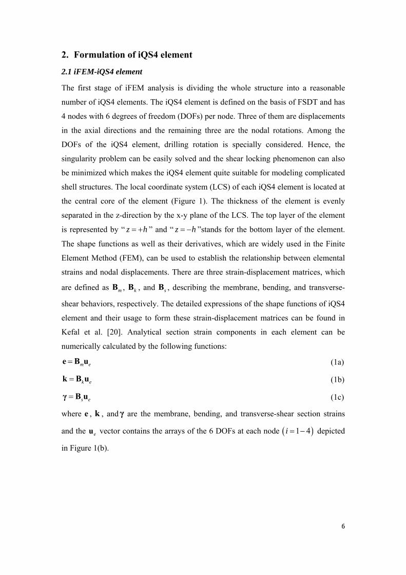
2. Formulation of iQS4 element

2.1 iFEM-iQS4 element

The first stage of iFEM analysis is dividing the whole structure into a reasonable

number of iQS4 elements. The iQS4 element is defined on the basis of FSDT and has

4 nodes with 6 degrees of freedom (DOFs) per node. Three of them are displacements

in the axial directions and the remaining three are the nodal rotations. Among the

DOFs of the iQS4 element, drilling rotation is specially considered. Hence, the

singularity problem can be easily solved and the shear locking phenomenon can also

be minimized which makes the iQS4 element quite suitable for modeling complicated

shell structures. The local coordinate system (LCS) of each iQS4 element is located at

the central core of the element (Figure 1). The thickness of the element is evenly

separated in the z-direction by the x-y plane of the LCS. The top layer of the element

is represented by “ z h ” and “ z h ”stands for the bottom layer of the element.

The shape functions as well as their derivatives, which are widely used in the Finite

Element Method (FEM), can be used to establish the relationship between elemental

strains and nodal displacements. There are three strain-displacement matrices, which

are defined as mB , kB , and sB , describing the membrane, bending, and transverse-

shear behaviors, respectively. The detailed expressions of the shape functions of iQS4

element and their usage to form these strain-displacement matrices can be found in

Kefal et al. [20]. Analytical section strain components in each element can be

numerically calculated by the following functions:

m ee B u (1a)

k ek B u (1b)

s eγ B u (1c)

where e , k , and γ are the membrane, bending, and transverse-shear section strains

and the eu vector contains the arrays of the 6 DOFs at each node 1 4i depicted

in Figure 1(b).

7

(a) (b)

Figure 1. (a) iQS4 element with local coordinate system (LCS) (x,y,z) at the central plane and global coordinate system (GCS) (X,Y,Z) of the structure (b) the total 6

DOFs in LCS [20]

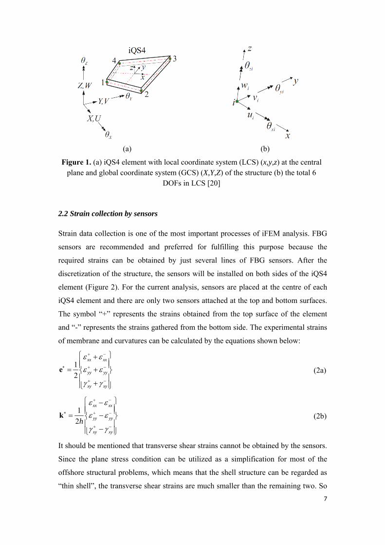
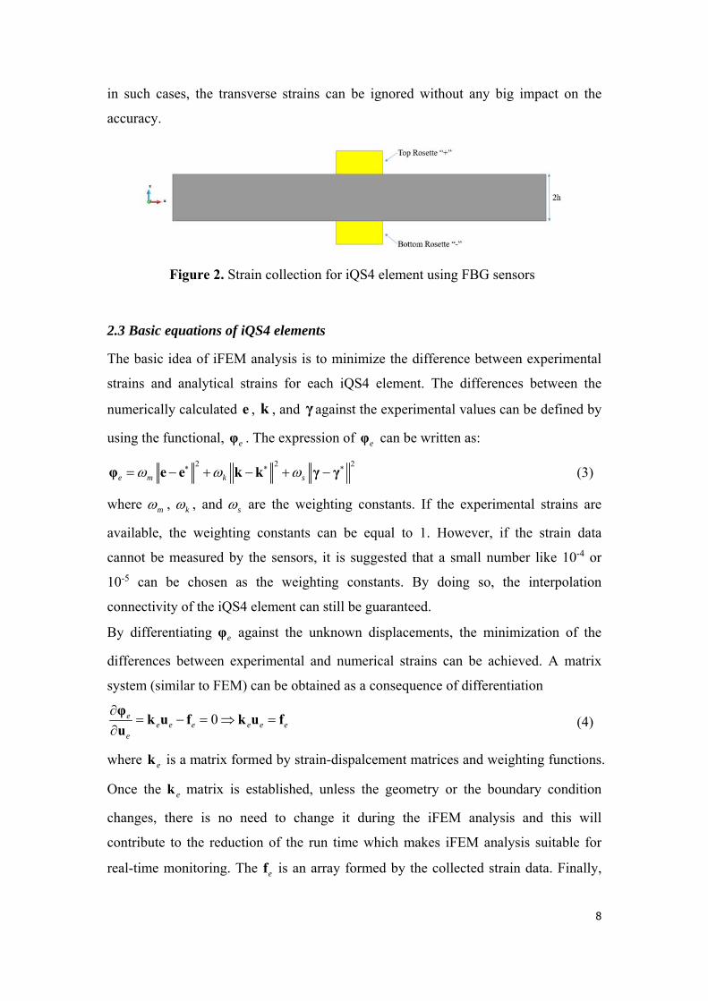
2.2 Strain collection by sensors

Strain data collection is one of the most important processes of iFEM analysis. FBG

sensors are recommended and preferred for fulfilling this purpose because the

required strains can be obtained by just several lines of FBG sensors. After the

discretization of the structure, the sensors will be installed on both sides of the iQS4

element (Figure 2). For the current analysis, sensors are placed at the centre of each

iQS4 element and there are only two sensors attached at the top and bottom surfaces.

The symbol “+” represents the strains obtained from the top surface of the element

and “-” represents the strains gathered from the bottom side. The experimental strains

of membrane and curvatures can be calculated by the equations shown below:

1

2

xx xx

yy yy

xy xy

e (2a)

1

2

xx xx

yy yy

xy xy

h

k (2b)

It should be mentioned that transverse shear strains cannot be obtained by the sensors.

Since the plane stress condition can be utilized as a simplification for most of the

offshore structural problems, which means that the shell structure can be regarded as

“thin shell”, the transverse shear strains are much smaller than the remaining two. So

8

in such cases, the transverse strains can be ignored without any big impact on the

accuracy.

Figure 2. Strain collection for iQS4 element using FBG sensors

2.3 Basic equations of iQS4 elements

The basic idea of iFEM analysis is to minimize the difference between experimental

strains and analytical strains for each iQS4 element. The differences between the

numerically calculated e , k , and γ against the experimental values can be defined by

using the functional, eφ . The expression of eφ can be written as:

2 2 2

e m k s φ e e k k γ γ

(3)

where m , k , and s are the weighting constants. If the experimental strains are

available, the weighting constants can be equal to 1. However, if the strain data

cannot be measured by the sensors, it is suggested that a small number like 10-4 or

10-5 can be chosen as the weighting constants. By doing so, the interpolation

connectivity of the iQS4 element can still be guaranteed.

By differentiating eφ against the unknown displacements, the minimization of the

differences between experimental and numerical strains can be achieved. A matrix

system (similar to FEM) can be obtained as a consequence of differentiation

0ee e e e e e

e

φk u f k u f

u

(4)

where ek is a matrix formed by strain-dispalcement matrices and weighting functions.

Once the ek matrix is established, unless the geometry or the boundary condition

changes, there is no need to change it during the iFEM analysis and this will

contribute to the reduction of the run time which makes iFEM analysis suitable for

real-time monitoring. The ef is an array formed by the collected strain data. Finally,

9

eu is the desired nodal displacements. After transforming from LCS to GCS,

applying boundary conditions and assembling the global system of equations, full-

field displacements can be reckoned.

2.4 Post-processing for iFEM analysis

The health condition of the structure can be assessed with the help of 6 regenerated

global displacements and rotations (U ,V ,W , x , y , z ). Moreover, by means of

additional parameters, such as total displacements, total rotations, and von Mises

strain/stress, the health condition can be determined with a step further. Total

displacements ( TU ) and von Mises stress ( vm ) are commonly used. The total

displacements can be forthrightly calculated as:

2 2 2TU U V W

(5)

Three independent displacements can be replaced by TU and the extreme values

combining with the plots of TU can give a comprehensive but brief illustration of the

deformation condition of the structure.

The strains of each iQS4 element can also be calculated after obtaining the nodal

displacements. Previously introduced mB , kB , and sB matrices can be used to

together with prediceted eu vectors to establish the individual strain components.

Then, the stress distribution of the iQS4 element can be computed utilizing the

constutive relations of the plane-stress condition. Finally, once the normal and shear

stresses components are obtained, they can be subsequently used along with the von

Mises stress criterion to make a reasonable failure assessments and identification of

structurally unhealthy condition.

3. Numerical results

3.1 Model generation

The geometry of the tower is determined based on the studies by Dagli et al. [36] and

Gücüyen [37]. The tower is divided into 26 sections. Usually, each section should

have its own thickness, height, and weight. But for simplification, the thickness of all

of the sections is 30 mm and the height of each section is 2.5 m. The total height of

10

the tower is 65 m with 20 m height underwater. The maximum diameter of the tower

is 4 m at the bottom and the diameter linearly decreases to 1.5 m at the top of the

tower. The material of the tower is entirely considered as steel regardless of the steel

grades. The Elastic Modulus is 210 GPa and the Poisson’s ratio is 0.3, respectively.

The density of the steel is 7850 kg/m3. However, in reality, there will be paints, cables,

and ladders attached to the surface of the tower. Therefore, the weights of these

components should also be included. It would be a reasonable way to transform the

extra weights being divided by the volume of each section to the density of the shell

element. Finally, the density of the structure is decided as 8500 kg/m3. During the

analysis, the weights of the structure itself will be applied by defining the

gravitational acceleration. Additionally, for static analysis, the weight of the RNA,

which is 83000 kg, is acted on the top of the tower. The aerodynamic and

hydrodynamic forces are further considered during the dynamic condition. The

bottom of the tower will be fixed as the boundary condition for both static or dynamic

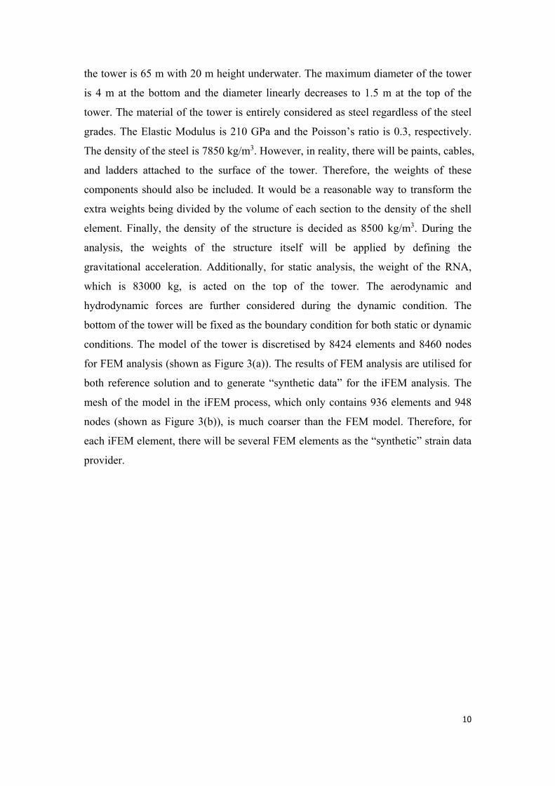
conditions. The model of the tower is discretised by 8424 elements and 8460 nodes

for FEM analysis (shown as Figure 3(a)). The results of FEM analysis are utilised for

both reference solution and to generate “synthetic data” for the iFEM analysis. The

mesh of the model in the iFEM process, which only contains 936 elements and 948

nodes (shown as Figure 3(b)), is much coarser than the FEM model. Therefore, for

each iFEM element, there will be several FEM elements as the “synthetic” strain data

provider.

11

(a) (b)

Figure 3. Mesh size (a) dense FEM mesh (b) coarse iFEM mesh

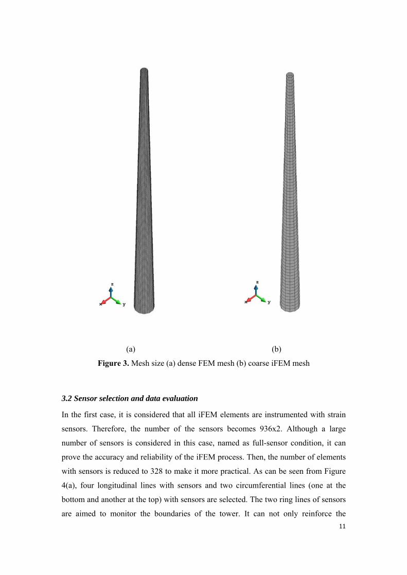
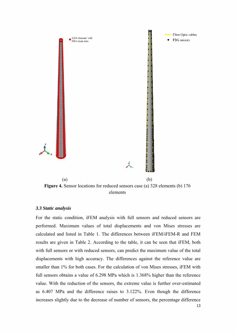
3.2 Sensor selection and data evaluation

In the first case, it is considered that all iFEM elements are instrumented with strain

sensors. Therefore, the number of the sensors becomes 936x2. Although a large

number of sensors is considered in this case, named as full-sensor condition, it can

prove the accuracy and reliability of the iFEM process. Then, the number of elements

with sensors is reduced to 328 to make it more practical. As can be seen from Figure

4(a), four longitudinal lines with sensors and two circumferential lines (one at the

bottom and another at the top) with sensors are selected. The two ring lines of sensors

are aimed to monitor the boundaries of the tower. It can not only reinforce the

12

boundary condition for the analysis but also monitor the extreme deformations

(especially in the z-direction) at the boundary. This distribution of sensors is used for

both static and dynamic analysis. Because the directions of the wave and wind are not

known in reality, symmetrical boundary conditions cannot be applied. Hence, the

purpose of the four vertical lines of sensors is to monitor the health condition of the

whole tower for any loading conditions. Besides, during the analysis, it was found that

connecting the sensors at different parts of the structure together has the ability to

improve the accuracy of the results and these four lines of sensors can strengthen the

quality of the deformation estimation. With the help of FBG sensors, since these

elements are located continuously, the strain data can be collected by just several lines

of FBG sensors. However, with the increase of the sensor locations, although FBG

technology can deal with collecting a great deal of data by just a single line, the

efficiency of the FBG sensors will be significantly influenced and the process of

separating the information to strains will also become complex. In order to relieve this

problem, strain data evaluation would be an appropriate method and the missing

strains can be estimated by the nearby strains. For the current analysis, after balancing

the accurate level of the evaluation and the minimized number of sensors, each

vertical line of sensors can be divided into four groups and different strategies can be

utilized. Actually, for each section, there are 3 layers of elements in the vertical z-

direction. First of all, for the sections around the boundary, all of the three elements

are chosen. Secondly, for the sections around the free water surface, all elements will

will also be selected because the strains around this region, especially in dynamic

conditions, usually experience large variations. Then for the remaining underwater

sections, the top and bottom elements are preferred to install the sensors. On the

contrary, for the sections subjected to the aerodynamic loads, the sensors are only

installed at the middle elements. The reason is that the strains of the sections above

water is much more stable than the underwater parts. Eventually, the number of

elements with sensors is decided as 176 and it only occupies about 2% of the total

quantity of the FEM elements. It means that 6x2 lines of FBG sensors are enough to

perform the iFEM analysis of the tower. This number can be further reduced, but it

can have a negative influence on accuracy.

13

(a) (b) Figure 4. Sensor locations for reduced sensors case (a) 328 elements (b) 176

elements

3.3 Static analysis

For the static condition, iFEM analysis with full sensors and reduced sensors are

performed. Maximum values of total displacements and von Mises stresses are

calculated and listed in Table 1. The differences between iFEM/iFEM-R and FEM

results are given in Table 2. According to the table, it can be seen that iFEM, both

with full sensors or with reduced sensors, can predict the maximum value of the total

displacements with high accuracy. The differences against the reference value are

smaller than 1% for both cases. For the calculation of von Mises stresses, iFEM with

full sensors obtains a value of 6.298 MPa which is 1.368% higher than the reference

value. With the reduction of the sensors, the extreme value is further over-estimated

as 6.407 MPa and the difference raises to 3.122%. Even though the difference

increases slightly due to the decrease of number of sensors, the percentage difference

14

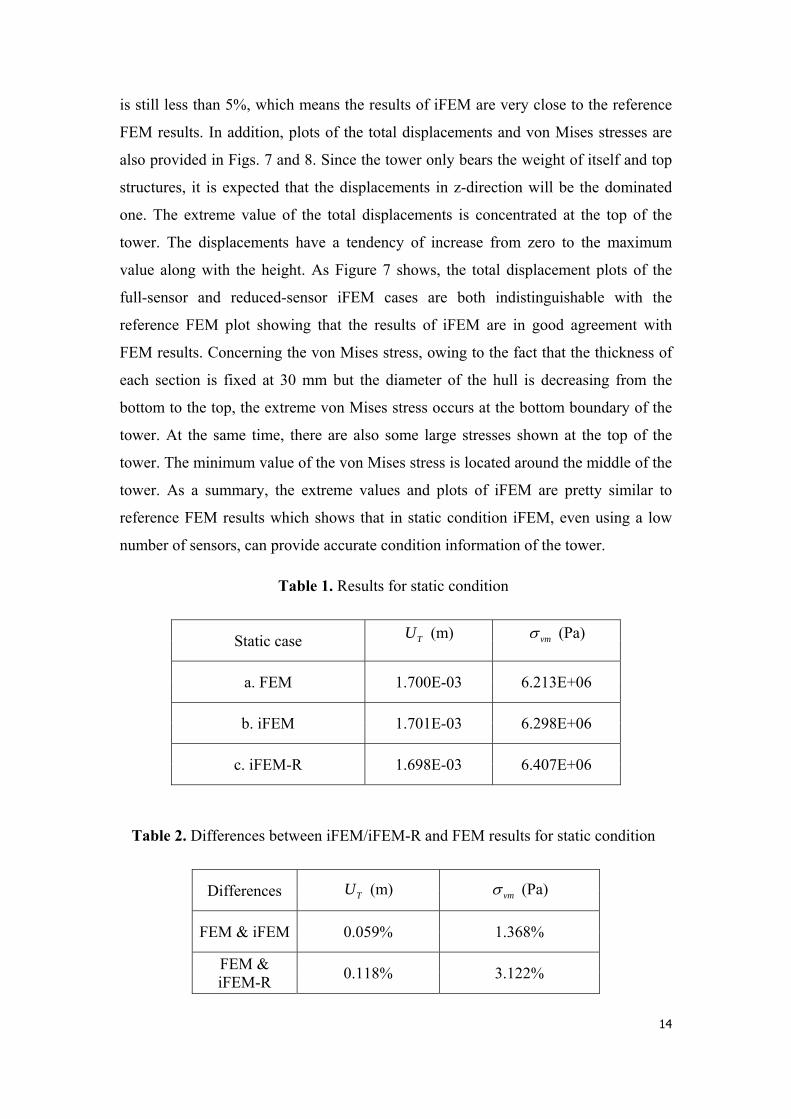
is still less than 5%, which means the results of iFEM are very close to the reference

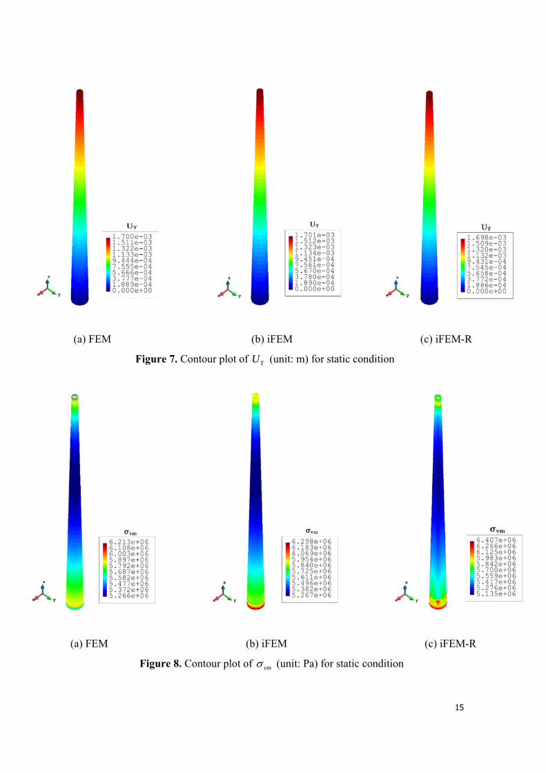
FEM results. In addition, plots of the total displacements and von Mises stresses are

also provided in Figs. 7 and 8. Since the tower only bears the weight of itself and top

structures, it is expected that the displacements in z-direction will be the dominated

one. The extreme value of the total displacements is concentrated at the top of the

tower. The displacements have a tendency of increase from zero to the maximum

value along with the height. As Figure 7 shows, the total displacement plots of the

full-sensor and reduced-sensor iFEM cases are both indistinguishable with the

reference FEM plot showing that the results of iFEM are in good agreement with

FEM results. Concerning the von Mises stress, owing to the fact that the thickness of

each section is fixed at 30 mm but the diameter of the hull is decreasing from the

bottom to the top, the extreme von Mises stress occurs at the bottom boundary of the

tower. At the same time, there are also some large stresses shown at the top of the

tower. The minimum value of the von Mises stress is located around the middle of the

tower. As a summary, the extreme values and plots of iFEM are pretty similar to

reference FEM results which shows that in static condition iFEM, even using a low

number of sensors, can provide accurate condition information of the tower.

Table 1. Results for static condition

Static case TU (m) vm (Pa)

a. FEM 1.700E-03 6.213E+06

b. iFEM 1.701E-03 6.298E+06

c. iFEM-R 1.698E-03 6.407E+06

Table 2. Differences between iFEM/iFEM-R and FEM results for static condition

Differences TU (m) vm (Pa)

FEM & iFEM 0.059% 1.368%

FEM & iFEM-R

0.118% 3.122%

15

(a) FEM (b) iFEM (c) iFEM-R

Figure 7. Contour plot of TU (unit: m) for static condition

(a) FEM (b) iFEM (c) iFEM-R

Figure 8. Contour plot of vm (unit: Pa) for static condition

16

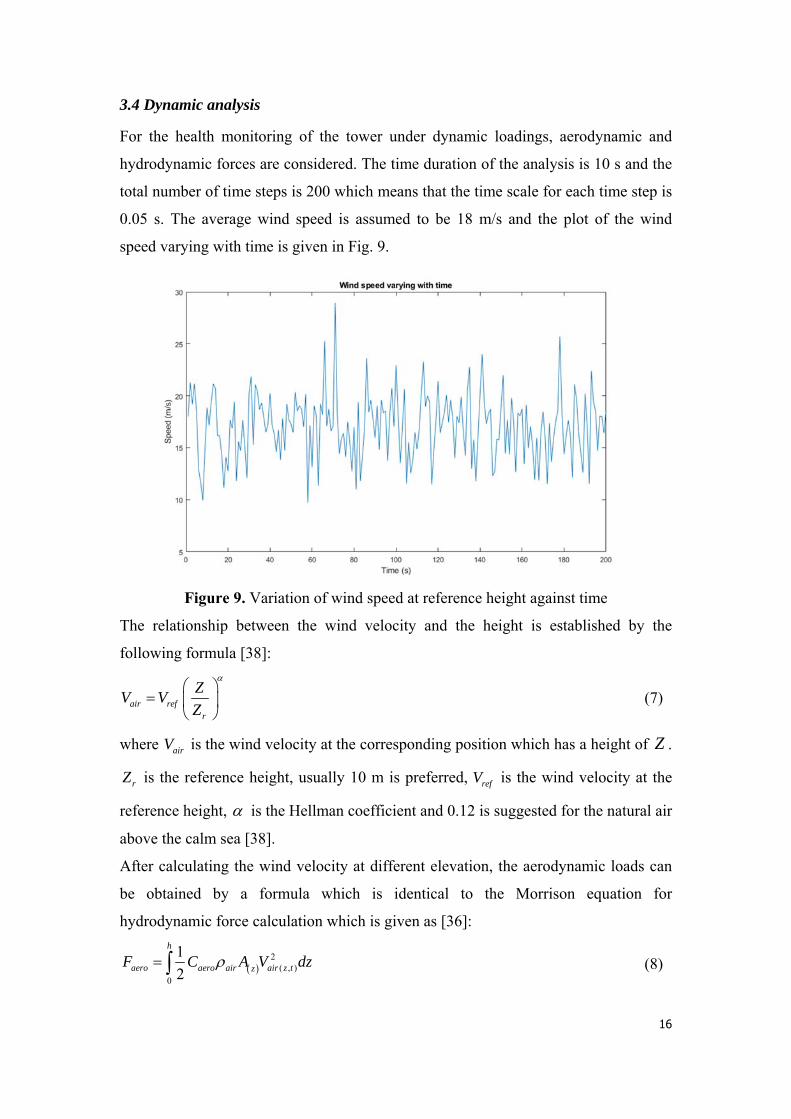
3.4 Dynamic analysis

For the health monitoring of the tower under dynamic loadings, aerodynamic and

hydrodynamic forces are considered. The time duration of the analysis is 10 s and the

total number of time steps is 200 which means that the time scale for each time step is

0.05 s. The average wind speed is assumed to be 18 m/s and the plot of the wind

speed varying with time is given in Fig. 9.

Figure 9. Variation of wind speed at reference height against time

The relationship between the wind velocity and the height is established by the

following formula [38]:

air refr

ZV V

Z

(7)

where airV is the wind velocity at the corresponding position which has a height of Z .

rZ is the reference height, usually 10 m is preferred, refV is the wind velocity at the

reference height, is the Hellman coefficient and 0.12 is suggested for the natural air

above the calm sea [38].

After calculating the wind velocity at different elevation, the aerodynamic loads can

be obtained by a formula which is identical to the Morrison equation for

hydrodynamic force calculation which is given as [36]:

2

( , )

0

1

2

h

aero aero air air z tzF C A V dz

(8)

17

where aeroF is the aerodynamic load at the height of Z , aeroC is the aerodynamic

coefficient which can be determined by the shape of the structure. For the current

analysis, 0.5 is used because of the cylindrical shape. air is the density of the wind

and 1.25 kg/m3 is used. zA is the exposed area of the structure at the height of Z .

airV is the wind velocity calculated by using Eq. 7.

The wind forces acting on the tower are calculated section by section and applied as

pressure to each section. The aerodynamic load on the blade of the OWT for the

working condition can also be estimated by the same equation. The swept area of the

blades is 624 m2 and this load is treated as a trust force and transformed to the top of

the tower (the height of the RNA is selected at 45 m above the water surface for

simplification). [36]

Morrison equation is used for the calculation of the hydrodynamic force. According to

the Morrison equation, the hydrodynamic forces are formed by Drag force ( DF ) and

Inertia force ( IF ). The detailed formula for these two forces when acting on the

cylindrical structure is given as:

0

( ) ( , ) ( , )

1

2D sea d z z t z t

d

F C A u u dz

(9)

02( ) ( , )

1

4I sea I z z t

d

F C A u dz

(10)

where sea is the density of the seawater and 1025 kg/m3 is used. The drag coefficient

( dC ) and inertia coefficient ( IC ) are 0.7 and 2.0, respectively, just as recommended

by ISO 1990-1 [39]. ( )zA is the area per unit height. ( , )z tu and ( , )z tu are the velocities

and the accelerations of the water particles, separately. For the current analysis, linear

wave theory is used and the information of the wave is given in Table 3:

18

Table 3. Wave parameters

Items Values Units

Wave height ( hW ) 1.8 m

Wave length ( lW ) 40 m

Wave period ( tW ) 5 s

Water depth ( dW ) 20 m

The ratio of water depth to wave height is 0.5, which is properly selected as between

deep water and middle water conditions. Then the velocity and acceleration of the

water particles can be calculated as:

( , )

cos

cos

si

2

n2

lhz t

td

l

h Z

h

WWu

WW

W

(11)

2

( , ) 2

cos

sin

s2

i

2

n

2 lhz t

td

lW

hW

ZW

uW

Wh

(12)

where Z is the water depth of the reference location. is the phase angle and it can

be calculated based on the position and time as:

2 2

l t

x tW W

(13)

The wave forces are calculated from the bottom of the tower to the free water surface

for simplification and they are also applied in the format of pressure to the tower. For

the current analysis, the hydrodynamic and aerodynamic forces are in the same

direction because it is the most severe loading condition which will lead to most

serious deformations.

Apart from extra loadings, the model is kept to be the same as the static case, i.e. not

only the parameters, but also the sensor locations are fixed for both conditions. Every

19

0.05 s the results of the iFEM analysis are recorded and then the total displacements

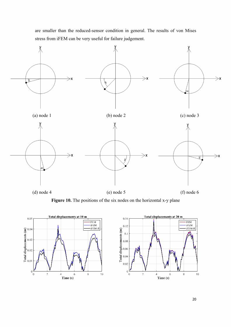
and von Mises stresses are subsequently calculated for comparison. Six nodes at 40 m

height (general height) are selected and the locations of the nodes are varying from

the windward direction to the leeward direction (Figure 10). Besides, another three

nodes, at the same position as node 6 (Figure 10(f)) but at different heights, are also

chosen. The heights are 10 m (underwater), 20 m (free water surface), and 60 m (near

top boundary).

The results of these nodes are collected and shown in Figs. 11-14. Figure 11 shows

the plots of the total displacements for the nodes at different heights. First of all,

iFEM with full sensors can obtain accurate results regardless of the heights of the

nodes. The reference FEM and iFEM with full sensors results match perfectly with

each other for the four diagrams. However, iFEM with reduced sensors (iFEM-R)

makes less estimation about the total displacement for all four nodes. However, it can

be seen that the differences are becoming smaller with the increase of the height of

the nodes. It should also be mentioned that the total displacements at 60 m are much

larger than the total displacements at 10 m, i.e. the total displacements will increase

with the height of the tower. The large deformations are given more attention because

they can obviously show the health condition of the structure. Therefore, the errors in

the total displacements at 10 m and 20 m are still reasonable. For the von Mises stress,

iFEM can predict the von Mises stress accurately for the nodes at 40 m and 60 m.

Even if the values of the von Mises stress are slightly over-valued for some zones by

iFEM with reduced sensors, for the majority parts they are still in good agreement

with reference FEM results. For the node at 20 m, the situation is becoming more

severe. It is interesting to find that the results of iFEM with reduced sensors are even

better than the iFEM with full sensors. The results are not always over-estimated for

this node and during the first two seconds, they are slightly less than FEM results.

Since this node is at the free water surface and the wave forces and wind forces are

both acting on this region, the strains around the free surface will suffer sharp changes

resulting in complex variation of results. But the main trend of the iFEM results is still

the same with the FEM results. Due to the complexity of loading conditions, the

maximum von Mises stress are located at the bottom of the tower for most of the

cases. At 10 m height, the results of both full-sensor and reduced-sensor iFEM are

bigger than the reference, but the differences between full-sensor condition and FEM

20

are smaller than the reduced-sensor condition in general. The results of von Mises

stress from iFEM can be very useful for failure judgement.

(a) node 1 (b) node 2 (c) node 3

(d) node 4 (e) node 5 (f) node 6

Figure 10. The positions of the six nodes on the horizontal x-y plane

21

Figure 11. Variation of total displacements TU (m) against time (s) for four nodes located at 10 m,

20 m, 40 m, and 60 m.

Figure 12. Variation of von Mises stresses vm (Pa) against time (s) for four nodes

located at 10 m, 20 m, 40 m, and 60 m.

22

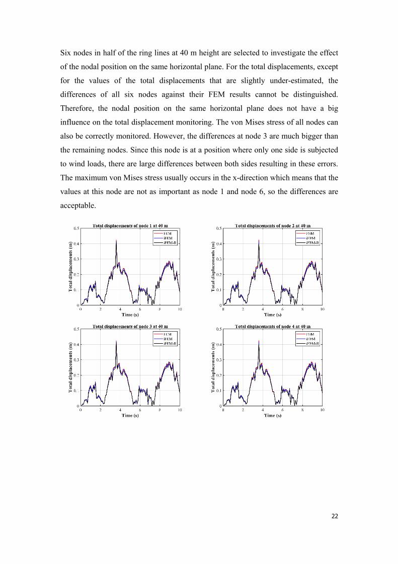
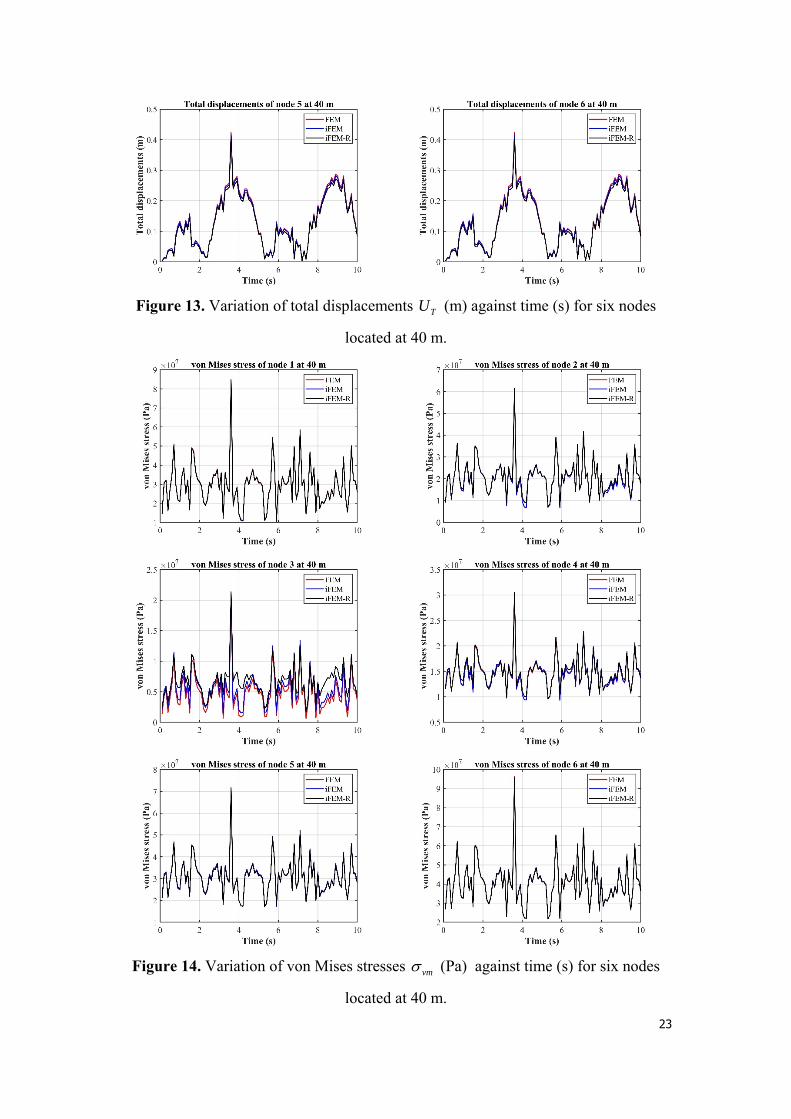
Six nodes in half of the ring lines at 40 m height are selected to investigate the effect

of the nodal position on the same horizontal plane. For the total displacements, except

for the values of the total displacements that are slightly under-estimated, the

differences of all six nodes against their FEM results cannot be distinguished.

Therefore, the nodal position on the same horizontal plane does not have a big

influence on the total displacement monitoring. The von Mises stress of all nodes can

also be correctly monitored. However, the differences at node 3 are much bigger than

the remaining nodes. Since this node is at a position where only one side is subjected

to wind loads, there are large differences between both sides resulting in these errors.

The maximum von Mises stress usually occurs in the x-direction which means that the

values at this node are not as important as node 1 and node 6, so the differences are

acceptable.

23

Figure 13. Variation of total displacements TU (m) against time (s) for six nodes

located at 40 m.

Figure 14. Variation of von Mises stresses vm (Pa) against time (s) for six nodes

located at 40 m.

24

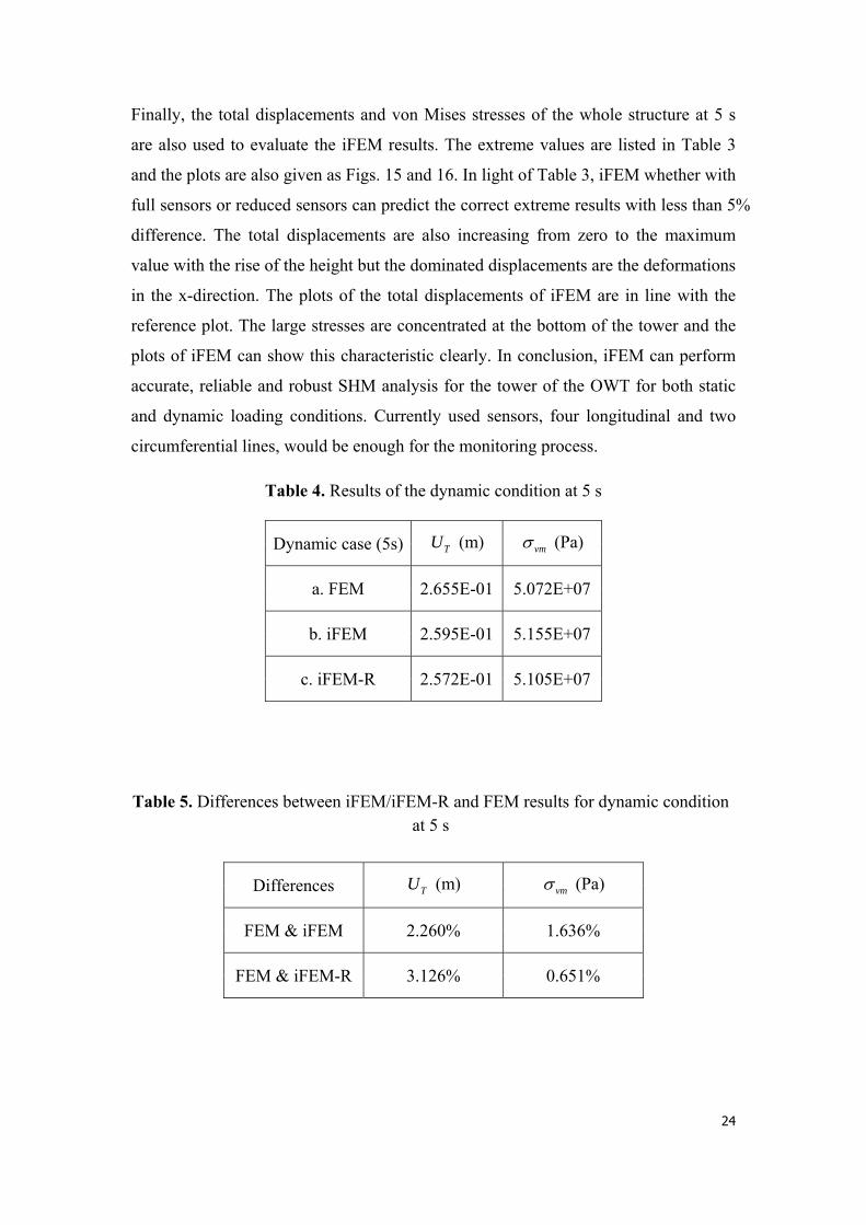
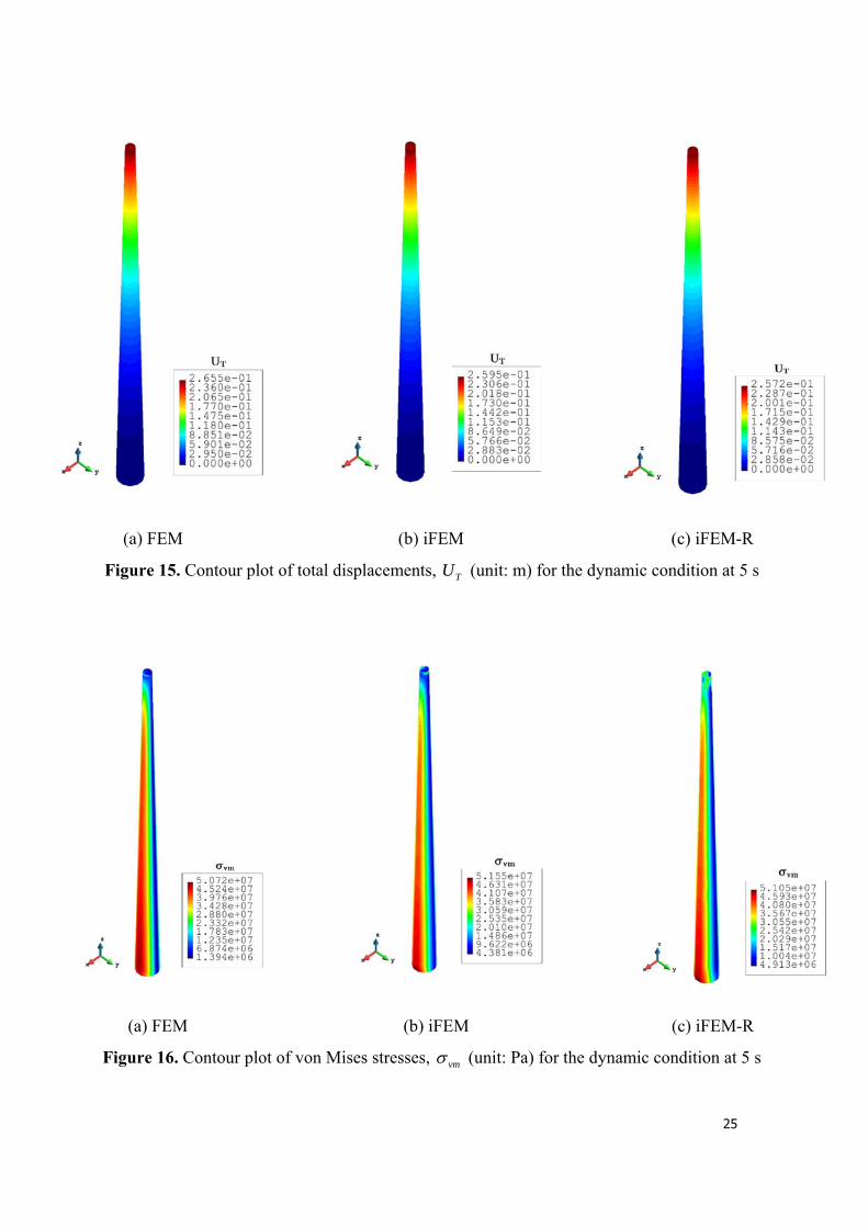
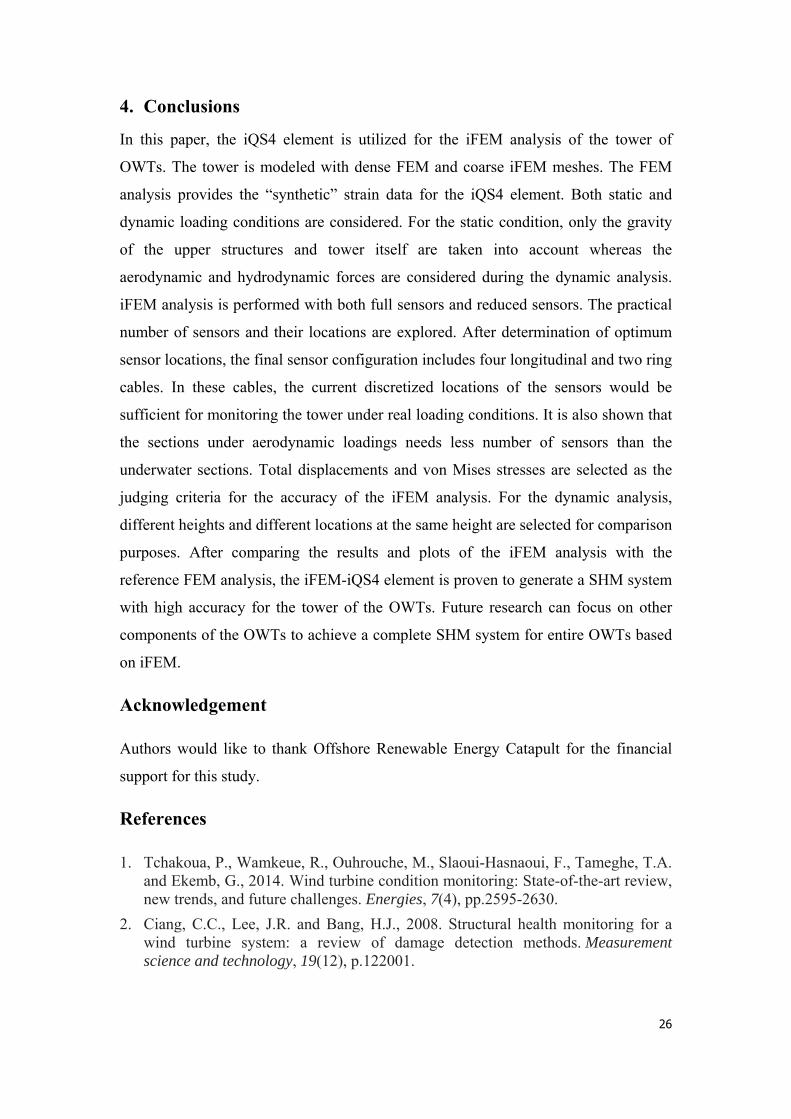
Finally, the total displacements and von Mises stresses of the whole structure at 5 s

are also used to evaluate the iFEM results. The extreme values are listed in Table 3

and the plots are also given as Figs. 15 and 16. In light of Table 3, iFEM whether with

full sensors or reduced sensors can predict the correct extreme results with less than 5%

difference. The total displacements are also increasing from zero to the maximum

value with the rise of the height but the dominated displacements are the deformations

in the x-direction. The plots of the total displacements of iFEM are in line with the

reference plot. The large stresses are concentrated at the bottom of the tower and the

plots of iFEM can show this characteristic clearly. In conclusion, iFEM can perform

accurate, reliable and robust SHM analysis for the tower of the OWT for both static

and dynamic loading conditions. Currently used sensors, four longitudinal and two

circumferential lines, would be enough for the monitoring process.

Table 4. Results of the dynamic condition at 5 s

Dynamic case (5s) TU (m) vm (Pa)

a. FEM 2.655E-01 5.072E+07

b. iFEM 2.595E-01 5.155E+07

c. iFEM-R 2.572E-01 5.105E+07

Table 5. Differences between iFEM/iFEM-R and FEM results for dynamic condition at 5 s

Differences TU (m) vm (Pa)

FEM & iFEM 2.260% 1.636%

FEM & iFEM-R 3.126% 0.651%

25

(a) FEM (b) iFEM (c) iFEM-R

Figure 15. Contour plot of total displacements, TU (unit: m) for the dynamic condition at 5 s

(a) FEM (b) iFEM (c) iFEM-R

Figure 16. Contour plot of von Mises stresses, vm (unit: Pa) for the dynamic condition at 5 s

26

4. Conclusions

In this paper, the iQS4 element is utilized for the iFEM analysis of the tower of

OWTs. The tower is modeled with dense FEM and coarse iFEM meshes. The FEM

analysis provides the “synthetic” strain data for the iQS4 element. Both static and

dynamic loading conditions are considered. For the static condition, only the gravity

of the upper structures and tower itself are taken into account whereas the

aerodynamic and hydrodynamic forces are considered during the dynamic analysis.

iFEM analysis is performed with both full sensors and reduced sensors. The practical

number of sensors and their locations are explored. After determination of optimum

sensor locations, the final sensor configuration includes four longitudinal and two ring

cables. In these cables, the current discretized locations of the sensors would be

sufficient for monitoring the tower under real loading conditions. It is also shown that

the sections under aerodynamic loadings needs less number of sensors than the

underwater sections. Total displacements and von Mises stresses are selected as the

judging criteria for the accuracy of the iFEM analysis. For the dynamic analysis,

different heights and different locations at the same height are selected for comparison

purposes. After comparing the results and plots of the iFEM analysis with the

reference FEM analysis, the iFEM-iQS4 element is proven to generate a SHM system

with high accuracy for the tower of the OWTs. Future research can focus on other

components of the OWTs to achieve a complete SHM system for entire OWTs based

on iFEM.

Acknowledgement

Authors would like to thank Offshore Renewable Energy Catapult for the financial

support for this study.

References

1. Tchakoua, P., Wamkeue, R., Ouhrouche, M., Slaoui-Hasnaoui, F., Tameghe, T.A. and Ekemb, G., 2014. Wind turbine condition monitoring: State-of-the-art review, new trends, and future challenges. Energies, 7(4), pp.2595-2630.

2. Ciang, C.C., Lee, J.R. and Bang, H.J., 2008. Structural health monitoring for a wind turbine system: a review of damage detection methods. Measurement science and technology, 19(12), p.122001.

27

3. Mieloszyk, M. and Ostachowicz, W., 2017. An application of Structural Health Monitoring system based on FBG sensors to offshore wind turbine support structure model. Marine Structures, 51, pp.65-86.

4. Yang, W., Tavner, P.J., Crabtree, C.J., Feng, Y. and Qiu, Y., 2014. Wind turbine condition monitoring: technical and commercial challenges. Wind Energy, 17(5), pp.673-693.

5. Fu, Z. and Yuan, Y., 2012. Status and prospects on condition monitoring technologies of offshore wind turbine. Dianli Xitong Zidonghua(Automation of Electric Power Systems), 36(21), pp.121-129.

6. Lu, B., Li, Y., Wu, X. and Yang, Z., 2009, June. A review of recent advances in wind turbine condition monitoring and fault diagnosis. In 2009 IEEE Power Electronics and Machines in Wind Applications (pp. 1-7). IEEE.

7. Kefal, A., 2017. Structural health monitoring of marine structures by using inverse finite element method (Doctoral dissertation, University of Strathclyde).

8. Gherlone, M., Cerracchio, P., Mattone, M., Di Sciuva, M. and Tessler, A., 2012. Shape sensing of 3D frame structures using an inverse finite element method. International Journal of Solids and Structures, 49(22), pp.3100-3112.

9. Adams, D., White, J., Rumsey, M. and Farrar, C., 2011. Structural health monitoring of wind turbines: method and application to a HAWT. Wind Energy, 14(4), pp.603-623.

10. Weijtjens, W., Verbelen, T., De Sitter, G. and Devriendt, C., 2016. Foundation structural health monitoring of an offshore wind turbine—a full-scale case study. Structural Health Monitoring, 15(4), pp.389-402.

11. Currie, M., Saafi, M., Tachtatzis, C. and Quail, F., 2013. Structural health monitoring for wind turbine foundations. Proceedings of the ICE-Energy, 166(4), pp.162-169.

12. Yi, J.H., Park, J.S., Han, S.H. and Lee, K.S., 2013. Modal identification of a jacket-type offshore structure using dynamic tilt responses and investigation of tidal effects on modal properties. Engineering Structures, 49, pp.767-781.

13. Devriendt, C., Magalhães, F., Weijtjens, W., De Sitter, G., Cunha, Á. and Guillaume, P., 2014. Structural health monitoring of offshore wind turbines using automated operational modal analysis. Structural Health Monitoring, 13(6), pp.644-659.

14. Rolfes, R., Zerbst, S., Haake, G., Reetz, J. and Lynch, J.P., 2007, September. Integral SHM-system for offshore wind turbines using smart wireless sensors. In Proceedings of the 6th International Workshop on Structural Health Monitoring (pp. 11-13). DEStech Publications Inc. Stanford, CA, USA.

15. Schroeder, K., Ecke, W., Apitz, J., Lembke, E. and Lenschow, G., 2006. A fibre Bragg grating sensor system monitors operational load in a wind turbine rotor blade. Measurement Science and Technology, 17(5), p.1167.

16. Tessler, A. and Hughes, T.J., 1983. An improved treatment of transverse shear in the Mindlin-type four-node quadrilateral element. Computer methods in applied mechanics and engineering, 39(3), pp.311-335.

28

17. Tessler, A. and Spangler, J.L., 2003. A variational principle for reconstruction of elastic deformations in shear deformable plates and shells. NASA/TM-2003-212445.

18. Tessler, A. and Spangler, J.L., 2004. Inverse FEM for full-field reconstruction of elastic deformations in shear deformable plates and shells. 2nd European Workshop on Structural Health Monitoring, 7-9 July 2004, Munich, Germany.

19. Kefal, A., Hizir, O. and Oterkus, E., 2015, August. A smart system to determine sensor locations for structural health monitoring of ship structures. In Proceedings of the 9th International Workshop on Ship and Marine Hydrodynamics, Glasgow, UK (pp. 26-28).

20. Kefal, A., Oterkus, E., Tessler, A. and Spangler, J.L., 2016. A quadrilateral inverse-shell element with drilling degrees of freedom for shape sensing and structural health monitoring. Engineering science and technology, an international journal, 19(3), pp.1299-1313.

21. Gherlone, M., Cerracchio, P., Mattone, M., Di Sciuva, M. and Tessler, A., 2011. Beam shape sensing using inverse finite element method: theory and experimental validation. POLITECNICO DI TORINO (ITALY).

22. Gherlone, M., Cerracchio, P., Mattone, M., Di Sciuva, M. and Tessler, A., 2014. An inverse finite element method for beam shape sensing: theoretical framework and experimental validation. Smart Materials and Structures, 23(4), p.045027.

23. Gherlone, M., Cerracchio, P., Mattone, M., Di Sciuva, M. and Tessler, A., 2011. Dynamic shape reconstruction of three-dimensional frame structures using the inverse finite element method. NASA/TP-2011-217315.

24. Kefal, A., Tessler, A. and Oterkus, E., 2017. An enhanced inverse finite element method for displacement and stress monitoring of multilayered composite and sandwich structures. Composite Structures, 179, pp.514-540.

25. Kefal, A., 2019. An efficient curved inverse-shell element for shape sensing and structural health monitoring of cylindrical marine structures. Ocean Engineering, 188, p.106262.

26. Cerracchio, P., Gherlone, M., Di Sciuva, M. and Tessler, A., 2015. A novel approach for displacement and stress monitoring of sandwich structures based on the inverse Finite Element Method. Composite Structures, 127, pp.69-76.

27. Kefal, A. and Oterkus, E., 2016. Displacement and stress monitoring of a chemical tanker based on inverse finite element method. Ocean Engineering, 112, pp.33-46.

28. Kefal, A. and Oterkus, E., 2016. Displacement and stress monitoring of a Panamax containership using inverse finite element method. Ocean Engineering, 119, pp.16-29.

29. Kefal, A., Mayang, J.B., Oterkus, E. and Yildiz, M., 2018. Three dimensional shape and stress monitoring of bulk carriers based on iFEM methodology. Ocean Engineering, 147, pp.256-267.

30. Kefal, A. and Oterkus, E., 2017. Shape and stress sensing of offshore structures by using inverse finite element method. Progress in the Analysis and Design of Marine Structures; Guedes Soares, C., Garbatov, Y., Eds, pp.141-148.

29

31. Colombo, L., Sbarufatti, C. and Giglio, M., 2019. Definition of a load adaptive baseline by inverse finite element method for structural damage identification. Mechanical Systems and Signal Processing, 120, pp.584-607.

32. Ren, L., Li, H., Zhou, J., Li, D.S. and Sun, L., 2006. Health monitoring system for offshore platform with fiber Bragg grating sensors. Optical Engineering, 45(8), p.084401.

33. Bang, H.J., Kim, H.I., Jang, M. and Han, J.H., 2012, February. Tower deflection monitoring of a wind turbine using an array of fiber Bragg grating sensors. In ASME 2011 Conference on Smart Materials, Adaptive Structures and Intelligent Systems (pp. 473-479). American Society of Mechanical Engineers Digital Collection.

34. Bang, H.J., Kim, H.I. and Lee, K.S., 2012. Measurement of strain and bending deflection of a wind turbine tower using arrayed FBG sensors. International journal of precision engineering and manufacturing, 13(12), pp.2121-2126.

35. Bang, H.J., Ko, S.W., Jang, M.S. and Kim, H.I., 2012, May. Shape estimation and health monitoring of wind turbine tower using a FBG sensor array. In 2012 IEEE International Instrumentation and Measurement Technology Conference Proceedings (pp. 496-500). IEEE.

36. Dagli, B.Y., Tuskan, Y. and Gökkuş, Ü., 2018. Evaluation of Offshore Wind Turbine Tower Dynamics with Numerical Analysis. Advances in Civil Engineering, 2018.

37. Gücüyen, E., 2017. Analysis of offshore wind turbine tower under environmental loads. Ships and Offshore Structures, 12(4), pp.513-520.

38. Van Der Tempel, J., 2006. Design of support structures for offshore wind turbines. PhD Thesis, Technical University of Delft.

39. ISO, P., 2005. natural gas industries. Specific requirements for offshore structures part 1: Metocean design and operating considerations. International Organization for Standardization, ISO, pp.19901-1.