DOE/NASAIOO58-79/2 - Vol. I NASA CR-i 59495 DO NOT DESTROY

RETURN TO LIBRARY

MOD-I WIND TURBINE GENERATOR ANALYSIS AND DESIGN REPORT

General Electric Company Space Division

March 1979

Prepared for NATIONAL AERONAUTICS AND SPACE Lewis Research Center Under Contract NAS 3-20058

DMINISTRATION 1 AU(.1980

MCDCN NELL D.AJGLAS RESEARCH & ENCINCERING LiBRARY

ST. LOUIS

for U.S. DEPARTMENT OF ENERGY Office of Energy Technology Division of Distributed Solar Technology

F18O-I43I

NOTICE

This report was prepared to document work sponsored by the United States

Government. Neither the United States nor its agent, the United States

Department of Energy, nor any Federal employees, nor any of their contractors,

subcontractors or their employees, makes any warranty, express or implied,

or assumes any legal liability or responsibility for the accuracy, completeness,

or usefulness of any information, apparatus, product or process disclosed,

or represents that its use would not infringe privately owned rights.

DOE/NASA 10058-7912-Vol I

NASA CR-159495

MOD-i WIND TURBINE GENERATOR

ANALYSIS AND DESIGN REPORT

General Electric Company

Space Division

Advanced Energy Systems Philadelphia, Pennsylvania 19101

March 1979

Prepared for

National Aeronautics and Space Administration

Lewis Research Center

Cleveland, Ohio 44135

Under Contract NAS 3-20058

for

U. S. DEPARTMENT OF ENERGY

Office of Energy Technology

Division of Distributed Solar Technology

Washington, D. C. 20545

Under Interagency Agreement EX-77-A-29-1010

TABLE OF CONTENTS

Section Page

1.0 INTRODUCTION ............................ 1-1

2.0 SYSTEM DESCRIPTION ......................... 2-1

2.1 General Configuration .................... 21

2.2 Rotor ............................ 2-1

2.3 Drive Train ......................... 2-1

2.4 Power Generation Equipment .................. 2-4

2.5 Nacelle Structure ...................... 2-4

2.6 Yaw Drive .......................... 2-4

3.0 S TRUCTURAL DYNAMICS ........................ 3-1

3.1 Requirements/Objectives/Approach ............... 3-1

3.2 System Synthesis ........................ 35

3.2.1 System Dynamic Analysis ................ 35

3.2.2 Analytical Substructure Description ......... 3-5

3.2.3 Stiffness Links ................... 3-7

3.2.4 Coupled Dynamic Model ................ 3-9

3.2.5 Determination of Forced Response ........... 3-9

3.2.6 Code Verification .................. 3-12

3.3 Sensitivity Analysis and Frequency Placement ......... 3-13

3.4 System Natural Frequencies and Loads ............. 3-18

3.4.1 Dispersion Factors .................. 3-26

3.5 Conclusions of the Structural Dynamics Analysis ....... 3-30

4.0 STABILITY ANALYSIS ........................ 4-1

4.1 Requirements, Objectives and Approach ............ 4-1

4.1.1 Statement of Work and Derived Requirements ..... 4-1

4.1.2 Wind Characterization ................ 4-2

4.1.3 Objectives ...................... 4-5

4.2 Modeling and Block Diagrams ................. 4-6

4.2.1 Overall Model .................... 4-6

4.2.2 Generator ...................... 47

4.2.3 Excitation System .................. 4-7

4.2.4 Utility Grid Connection ............... 4-7

4.2.5 Wind .......................... 4-13

4.2.6 Aerodynamic Torque .................. 4-13

4.2.7 Rotor ........................ 4-13

4.2.8 Drive Train ...................... 4-15

4.2.9 Pitch Change Mechanism ................ 4-16

4.2.10 Speed Controller ................... 4-16

4.2.11 Power Controller ................... 4-16

4.2.12 Wind Feed Forward ................... 4-18

4.2.13 Speed Stabilizer ................... 418

4.2.14 Reactive Power Controller .............. 4l8

4.2.15 Miscellaneous .................... 4-18

4.3 Subsystem Analysis Cases ................... 4-20

4.3.1 Frequency Domain ................... 4-20

(i)

Section Page

4.3.2 Pitch Mechanism Amplifier .............. 4-20 4.3.3 Root Locus Variables ................. 4-20 4.3.4 Deviational Response Variables ............ 4-20 4.3.5 Transient Response Variables ............. 4-21 4.3.6 Small System Analysis ................ 4-21 4.3.7 Site Analysis .................... 4-21

4.4 Compensation ......................... 4-21 4.4.1 Filtering ...................... 4-21 4.4.2 Wind Feed Forward (WFF) ............... 4-21 4.4.3 Speed Stabilizer .................... 4-24 4.5 Results ........................... 4-24 4.5.1 Speed Control Loop .................. 4-24 4.5.2 Excitation System .................. 4-26 4.5.3 Stabilizer ...................... 4-32 4.5.4 Power Control and Combined Loops ........... 4-34 4.5.5 Transient Response .................. 4-47 4.5.6 Sensitivities...................... 4-53

4.6 Conclusions.......................... 4-55 5.0 MECHANICAL SUBASSEMBLIES DESIGN .................. 5-1 5 .1 Blade ............................ 5-1 5 .1.1 Requirements ..................... 5-]. 5 .1.2 Description ...................... 5-2 5.1.3 Performance Characteristics of the Mod-1

(Boeing) Blade .................... 5-11 5 .1.4 Analyses ......................... 5-15 5 .1.5 Tests ........................ 5-25 5 .2 Rotor Hub .......................... 5-30 5 .2.1 Requirements ..................... 5-30 5 .2.2 Hub ......................... 5-30 5.2.3 Blade Interface & Retention Bearing ......... 5-32 5.2.4 Main Bearing ..................... 5-32 5 .2.5 Rotor Lock ...................... 5_35 5.2.6 Instrumentations ................... 5_35 5.2.7 Rotor Hub Analysis .................. 5-36 5.3 Pitch Change Mechanism .................... 5-38 5 .3.1 Requirements ..................... 5-38 5 .3.2 Description ..................... 5-42 5 .4 Drive Train ......................... 5-49 5 .4.1 Requirements ..................... 5..49 5.4.2 Design Description .................. 5-50 5.4.3 Drive Train Maintenance ............... 5-58 5.4.4 Drive Train Stress Analysis ............. 5-59 5.4.5 Drive Train Stiffness Sensitivity Analysis ...... 5-62 5 .5 Nacelle ........................... 5-65 5 .5.1 Bedplate and Fairing ................. 5-65 5.5.2 Lubrication and Environmental Control ........ 5-74 5.5.3 YawSubsystem ................... 5-78 5.5.4 Yaw Hydraulic System ................. 5-95 5.5.5 PCM Hydraulic System .................. 5-97 5.5.6 Nacelle Stress Analysis ............... 5-99

(ii)

Section Page

5-112 5.6 Tower .............................

5-112 5.6.1 Requirements ....................5.6.2 Design Definition .................. 5-112

5.6.3 Design Evolution and Trade-Offs ........... 5-112

5.6.4 Foundation Design .................. 5-120

5.6.5 Personnel Lift and Access Provisions ........ 5-122

5.6.6 Tower Stress Analysis ................ 5-122

6.0 POWER GENERATION SUBSYSTEM .................... 6-1

6-1 Requirements and System Overview .............. 6-1

6.1.1 Statement of Work Requirements ........... 6-1

6.1.2 System Overview ................... 6-2

6-2 Generator and Power Generation Auxiliaries ......... 6-5

6-3 Switchgear and Transformer ................. 6-7

6.3.1 Elements of Switchgear ............... 6-7

6.3.2 Generator Circuit Breaker and Isolation Switch . 6-8

6.3.3 Power Equipment ................... 6-10

6.3.4 Switchboard ..................... 6-10

6.3.5 Transformer ..................... 6-17

6-4 Auxiliary Power Distribution ................ 6-18

6.4.1 Load Buses ..................... 6-18

6.4.2 Protection and Control ............... 6-18

6-5 Station Battery and FAA Lighting .............. 6-21

6.6 Wiring and Slip Rings .................... 6-25

6.6.1 Wiring ....................... 6-25

6.6.2 Slip Rings ..................... 6-25

6.6.3 Cable Reel ..................... 6-28

6.7 Instrumentation ....................... 6-28

6.8 Lightning Protection .................... 6-28

6.9 Control Enclosure ...................... 6-31

7.0 CONTROL AND INSTRUMENTATION SUBSYSTEM .............. 7-1

7-1 Overview ........................... 7-1

7-2 Functional Description

7.2.1 Control Functions .................. 7.2.2 Manual Functions

7.2.3 Backup Overspeed Shutdown .............. 7-9

7.2.4 Support Functions .................. 79

7.2.5 Test Features .................... 7-16

7.3 Equipment Description .................... 7-16

7.3.1 Equipment Locations ................. 7-16

7.3.2 Multiplexer Racks .................. 7-16

7.3.3 Control and Recording Unit (CRU) and Peripheral Racks .................. 734

7.4 Sensors ........................... 7-39

7.4.1 Wind Speed and Direction Sensor ...........7-39

7.4.2 Shaft Speed Transducer ............... 739

7.4.3 Blade Position Angle Transducer ...........7-46

7.4.4 Rotor Shaft and Nacelle Position Sensor .......7-46

7.5 Engineering Data Acquisition System ............. 7-46

(iii)

Section Page

7.5.1 Remote Multiplex Units 7.5.2 Stand Alone Instrument Rcorder ........... 7.5.3 Portable Instrument Vehicle .............

7.6 Software Description 7.6.1 Functional Flow ................... 7.6.2 System Functional Allocation 7.6.3 Module Functional Descriptions . .......... 7.6.4 Storage Allocation 7.6.5 Final Software Validation ..............

8.0 GLOSSARY

7-46 7-46 7-46 7-47 7-47 7-48 7-48 7-54 7-54

8-1

(iv)

SECTION 1

INTRODUCTION

SECTION 1

INTRODUCTION

Background

The extraction of power from the wind is not a new concept, especially in the application of mechanical power to pump water or to mill grains. However, the generation of electrical, power from the wind dates only from the turn of the century. Wind turbine generators achieved a measure of technical and economic practicality in rural and remote areas of the country during the 1920's, but the gradual extension of electrical utility networks and the availability of law cost fossil fuels led to their abandonment by the 1940's.

The early wind turbine generators were generally limited to power levels below 10 kilowatts and were operated independently of an electric utility network. The Smith-Putnam machine of the 1940's was the singular attempt in this country to develop a large-scale unit with the capability of being connected to an electric utility network. Interest in wind power waned until the 1970's when shortages in energy and the increasing costs of fossil fuels forced the nation to reassess all forms of available energy. A national wind energy program was established to develop the technology necessary to enable wind energy systems to be cost competitive with conventional power generation systems and to be capable of rapid commercial expansion for producing significant quantities of electrical power. As part of that program, General Electric's Space Division was contracted to design and build, under the direction of NASA - Lewis Re-search Center and sponsored by the Department of Energy, a wind turbine gen-erator having a nominal rating of 1.8 megawatts, designated Mod 1.

History of the Mod 1 Program

The Mod 1 program is being conducted in six phases: Analysis and Preliminary Design (culminating in a Preliminary Design Review), Detail Design (ending with a Final Design Review), Fabrication and Assembly, System Testing, Site Prepa-ration, and Installation and Checkout. Major milestone dates for these phases are shown in Table 1-1. This report is intended to describe only the results of the first two phases; that is, activities leading to the completion of Detail Design. Although this report places emphasis on a description of the design as it finally evolved, it is of some interest to trace the steps through which the design progressed in order to understand the major design decisions.

The design requirements specified by NASA for the Mod 1 wind turbine generator in the contract Statement of Work reflected the conclusions of two previous design studies by contractors, aswell as the experience of NASA-LeRC in de-signing, building, and operating the Mod 0 unit. These specifications, sum-marized in Table 1-2, were utilized as the design starting point. Therefore, during the Analysis and Preliminary Design phase, only certain parameters were optimized and certain design options were investigated. A major decision was the selection of a rigid rotor hub as opposed to a teetered hub. A trade-off study was conducted in which the effects on rotor hub, supporting structure, and tower as a resultof load reduction from teetering were weighed against the increased complexity and programmatic risks of a teetered hub design. Support-ing this study, detailed layouts were prepared'of rigid hub and teetering hub

1-1

concepts, with corresponding load analyses for selected critical wind and gust conditions. In the process of conducting this study, it was discovered that the pitch control mechanism, because of its required location and its role in determining blade torsional stability, had to be much more robust than had been anticipated and greatly influenced the size, weight, and cost of all ad-joining mechanical components. As a result, an in-depth design study was initiated to evaluate various mechanism concepts, resulting in selection of the system that will be described later. Undoubtedly, the size and complexity of the pitch control mechanism was the deciding factor that made it difficult to incorporate a teetering feature and so tipped the scales in favor of a rigid hub design.

A major analytical task of the first program phase was the verification of analytical computer codes used for dynamic simulation and load analyses. The results of this task are reported in Appendix "A". The results of this and other analytical tasks, as well as the conclusions of the teetered hub study, were orally presented to NASA at a First Phase Formal Review, just prior to the Preliminary Design Review (PDR).

At PDR, the results of the Analysis and Preliminary Design tasks were presented as follows:

a. Design features were described. b. Analyses, completed and planned were discussed. c. Any design deficiencies established by analysis were identified. d. Failure modes were reviewed. e. Material selection and justification were discussed. f. Fabrication procedures were discussed. g. Inspection and testing techniques and criteria were discussed. h. Approval to deviate from specifications was obtained, where required. i. Approval for procurement of long-lead items was obtained.

Approval of the Preliminary Design permitted the next phase, Final Design, to proceed.

During Preliminary Design and through the initial stages of Final Design, re-sponsibility for the blade, rotor hub, and pitch control mechanism was sub-contracted to Hamilton-Standard in Windsor Locks, Conn., along with relate& analytical tasks. Hamilton-Standard proposed a filament wound, glass fiber reinforced plastic blade with fabrication in turn subcontracted to Allegheny Ballistics Laboratory. When it became evident that the filament wound blade would not live up to its expectations, a back-up design study for a metal blade was initiated with Lockheed Aircraft Co. Subsequently, Hamilton-Standard's participation was terminated and the design and fabrication of a metal blade was subcontracted to Boeing Engineering Company.

At this stage in the program, the opportunity was taken to reassess the design requirements at a point when the final design had not been frozen. Among the requirements re-examined at this time were rated power, rated wind speed, blade ground clearance, design gust conditions, blade profile, downwind rotor place-ment, and ambient temperature extremes. As a result, recommendations to change certain of the requirements were made to NASA and the negotiated changes. are reflected in Table 1-2. A review of the total program costs at this time

1-2

resulted in the cancellation of the option to fabricate a second unit.

While a new metal blade design was initiated, final design of the remainder

of the wind turbine generator system was completed and a Final Design Review

was held. However, final drawing releases of some components whose design de-pended on the blade were delayed until the required information was available. The blade design progressed through PDR and FDR., similar to the steps taken

for the remainder of the system.

Two tasks that supplemented the Detail Design tasks were the Safety Review and the Failure Modes and Effects Analysis (FTIEA). The Safety Review was

imposed as an internal General Electric-Space Division requirement, a pre-

requisite to approval of the final design. This review was conducted by

qualified specialists within the Space Division but not associated with the

Mod 1 program. The FMEA was directed towards prevention of failures that presented a hazard to operating personnel or the general public, and failures resulting in major damage to the wind turbine generator. Results of the FNEA are presented in a separate report but the highlights are in the next sub-section.

Table 1-1

Mod 1 Program Milestones

Program Go-Ahead

First Phase Formal Review

Preliminary Design Review (less blade)

Reassessment of Design Requirements

Final Design Review

Metal Blade Go-Ahead

Blade Preliminary Design Review

Blade Final Design Review

Assembly Start

Site Preparations Start

System Test Start

Shipment to Site (less blade)

Sub-system Checkout

Blade Shipment to Site

System Checkout

July, 1976

December, 1976

January, 1977

June, 1977

August, 1977

September, 1977

December, 1977

March, 1978

May, 1978

June, 1978

August, 1978

September, 1978

March, 1979

April, 1979

May, 1979

1-3

Table 1-2

Summary of Design Parameters

Rated Power--------------------------------- 2000 kWe @ 11.4 m sec1 (25.5 mph) 1800 kWe @ 11.0 m sec' (24.6 mph)

Cut-In Wind Speed--------------------------- 5 m sec_ i (ii mph) max. Cut-Out Wind Speed--------------------------- 15.9 m sec_ i ( 35 mph) Maximum Design Wind Speed--------------'-'---- 67 m sec (150 mph at shaft

center line - assume no wind shear)

Rotorsper Tower----------------------------Location of Rotor -------------------------- Downwind of Tower Direction of Rotation ---------------------- CC (looking upwind) Blades per Rotor ---------------------------- 2-ConeAngle --------------------------------- 9 Inclination of Axis Rotation --------------- None Rotor Speed Control ------------------------- Variable Made Pitch Rotor Speed -------------------------------- 347 RPM Blade Diameter ----------------------------- 61 meters nom. (200 ft. nom,) Airfoil ------------------------------------ 44)CC series Blade Twist 110 Linear Tower -------------------------------------- Steel Truss Blade Tip to Ground Clearance -------------- 12 meters (40 ft.) Hub---------------------------------------- Rigid Transmission ------------------------------- Fixed Ratio Gear Generator ---------------------------------- 60 Hz/Synchronous Yaw Rate ----------------------------------- .25°/sec Control System ------------------------------ Electro Mechanical/Microprocessor System Life

Dynamic Components ------------------------ 30 years (with maintenance) Static Components ------------------------- 30 years (with maintenance)

NOTE

1. All wind velocities measured at 9 meters (30 ft.) elevation.

1-4

Failure Modes and Effects Analysis

The FMEA was directed primarily at identifying those critical failure modes that would be hazardous to life or would result in major damage to the system. As a result, the analysis was conducted from the "top down", minimizing the extent of analysis that would lead to trivial conclusions, had the analysis been approached from the "bottom up". For example, a component-by-component analysis of the lubrication system was not pursued, once it had been established that all single lubrication system failures lead to the same, non-critical conclusion.

The criteria used for evaluation during the FMEA is that none of the following in-juries or damage shall occur because of a single failure or a single failure following an undetected failure of the wind turbine system.

Category I: Failures which would result in death or serious injury to the operator or general public.

Category II: Failures which would result in major or significant damage to the wind turbine system, extended outage, or damage to the connected

utility.

The F1?IEA worksheets went through several stages of review, including review by qualified GE specialists outside of the Mod 1 program and two reviews by know-ledgeable NASA LeRC personnel. Corrective action was taken whenever recommended.

Maintainability

This topic was addressed on a continuing basis during the design phase, and pro-visions were built-in for ease of maintenance. Whenever possible, standardized off the shelf components were chosen for minimum maintenance, with the normal maintenance cycle initially set at 6 months.

1-5/6

SECTION 2

SYSTEM DESCRIPTION

SECTION 2

SYSTEM DESCRIPTION

2 . 1 GENERAL CONFIGURATION

The general configuration of the Mod 1 wind turbine generator is shown in Figure 2-1. The two-bladed rotor is approximately 200 feet (61 m) in dia-meter and is located downwind of the tower 140 feet (46 m) above the ground. The nacelle, enclosing all equipment mounted on top of the tower, is driven to rotate about the vertical axis of the tower in response to changes in the wind direction. The truss tower is made up of tubular and channel structural shapes with bolted joints. It is 12 feet (4 m) square at the top and 48 feet (16 m) square at the bottom, and is anchored to reinforced concrete footings at each leg. At ground level is located an environmentally controlled enclo-sure for sensitive control and power generation equipment as well as elements of the data system. Within the fenced area are also located the back-up battery system, the step-up transfotner connecting to the utility, and the lift device that provides access to the top of the tower.

The total weight of all equipment above ground level is approximately 650,000 pounds (290,000 kg) of which 310,000 pounds (140,000 kg) is the weight of the tower. In order to facilitate transportation and erection, the system is de-signed to permit shipment in a number of subassemblies not exceeding 100,000 pounds (45,000 kg) each. The approach requires more high elevation assembly, but eliminates the need for a costly, high capacity crane at the site. See Table 2-1.

Equipment mounted on top of the tower is shown in more detail in Figure 2-2. Major components identified below are also discussed in more detail in subse-

quent sections of this report.

2.2 ROTOR

The steel blades are attached to the hub through a three-row roller bearing that permits the pitch angle of each blade to be varied 105 degrees from feather to full power. Blade pitch is controlled by hydraulic actuators operating through a mechanical linkage with sufficient capacity to feather the blades at a rate of 14 degrees per second. The rotor is supported by a single bearing

with two rows of tapered rollers.

2.3 DRIVE TRAIN

Torque from the rotor is carried by a floating shaft to a speed increaser gear-box. The gearbox increases the speed through three stages to match the 1800 rpm synchronous generator, also connected to the gearbox through a floating shaft with flexible gear couplings. The high speed shaft incorporates a dry disk slip clutch protecting against torque overloads, and a disk brake that stops the rotor and holds it in a parked position. The gearbox lubrication system also provides oil to the rotor bearing and dissipates waste heat by means of a passive cooler suspended below the nacelle.

2-1

YtCC'1Y iI.fCT,od

OO'DIR.E

1Mw Aq(

I _M14'l A$$f

It

-z j&AM

iTO'

- -I - ____'!ii.. ____ ________

U •''•__________________ 'I

7IL

2-2

(OC £.tzara& aY

I-,-i IJJi14\__ flr IL -.. -__

Figure 2-1 Mod 1 WTG General Configuration

TABLE 2-1

SYSTEM WEIGHT BREAKDOWN

ROTOR ASSEMBLY 103,000 lb

Hub 15,000

Blades 36,000

Bearings, supports 29,000 Pitch Control Mechanism 11,000 Pitch Control Hydraulics 12,000

NACELLE ASSEMBLY 171,000 lb

Bedplate 68,000

Fairing 5,000

Generator 14,000 Power Generatipn Equipment 1,000 Shafts and Couplings 18,000

Gearbox 58,000 Lube, Hydraulic System 4,000 Control and Instrumentation 1,000 Cables, Lights, etc 2,000

YAW ASSEMBLY 56,000 lb

Yaw Structure 34,000 Bearing 13,000 Yaw Brake 1,000 Yaw Frive 8,000

TOWER ASSEMBLY 320,000 lb

Structure 313,000 Lift Device 1,000 Cable, Conduit 6,000

TOTAL (Excluding Ground Equipment)

650,000 lb

GROUND EQUIPI€NT (Including Transformer 54,000 lb

TOTAL 704,000 lb

2-3

The low apeed shaft and the gearbox first stage shaft are hollow to permit passage of electrical cables from the rotor to a slip ring assembly.

2.4 POWER GENERATION EQUIPMENT

A synchronous ac generator is driven at 1800 rpm by the high speed shaft. A shaft-mounted, brushless exciter, controlled by a solid-state regulator and power stabilizer, provides voltage control. Generator output at 4160 volts is brought by cables and a slip ring at the yaw bearing down the tower to the ground enclosure. Surge capaciters and related power generation equip-ment are mounted in a caged enclosure below the generator.

2.5 NACELLE STRUCTURE

The welded steel bedplate is the primary nacelle structure, supporting all equipment mounted on top of the tower and providing a load path between the rotor and the yaw structure. Equipment mounted on the bedplate includes the pitch control and yaw drive hydraulic packages, the control and data system units, access ladders and walIays, oil coolers, lubrication pumps, hydraulic plumbing, and cables for electrical power and instrumentation. A removable fairing en-closes the nacelle, incorporating inlet and outlet louvers for cooling air. The fairing also provides mounting for wind sensors, obstruction lights, and inter-ior lighting.

2.6 YAW DRIVE

Rotation of the nacelle about a vertical axis is provided by the yaw drive system, consisting of upper and lower structures, a cross-roller bearing, dual hydraulic drive motors, and six hydraulic brakes. Each yaw motor drives a pinion meshing with a gear on the inner race of the yaw bearing. The yaw brakes control dynamic excitations in yaw by maintaining a rigid connection, and assist in damping yaw motions while the nacelle is being driven. Power and signal data are transferred to the tower-mounted cables by slip-rings.

2-4

I

_

0

1

0 -1

4J c'1

I-I

Cl)

I-I

'-I

C)

cj

z

C'.'

21

2-5/6

SECTION 3

STRUCTURAL DYNA?1ICS

SECTION 3

S TRUCTURAL DYNAMICS

3.1 REQUIRENENIS / OBJECTIVES /APPROACH

The objective of the structural dynamic analysis is to assure the dynamic ade-quacy of the system design for the range of operating conditions experienced in service. Key factors which influence the system dynamic design adequacy

are:

1. Accurate prediction of operational loads and deflections

2. Proper system resonant frequency placement 3. Selection of a design approach which minimizes sensitivity to

variations in parameters and alleviates dynamic loading

Because of the many dynamic interactions within the WTG system, proper placement of the system resonant frequencies is not directly related to the subassembly dynamic characteristics. Similarly, the design loads can be amplified by the structural response to cyclic excitation. The design approach can provide para-meters which are variable and difficult to predict, and can increase dynamic loading. By analyzing the system dynamic characteristics for specified sub-assembly characteristics considering the variability of key parameters, the dynamic adequacy of the system can be evaluated early in the design phase and modifications made to assure the adequacy of the final design. The purpose of the dynamic analysis is to examine the system dynamic characteristics and to assure the compatibility of the system with the service conditions.

The frequency placement and operational design load requirements for the Mod-1 Wind Turbine Generator are sununarized in Table 3-1. The frequency requirements are an outgrowth of the original NASA specification and frequency placement sensitivity studies, which are discussed in Paragraph 3.3. The fatigue design is based on the Case A loading conditions. Because of the high number of cycles accumulated over 30 years at the high wind speeds, the cyclic loads at the cut-out speed (35 mph) are used to design the system for infinite life. The steady state vibratory loads calculated at this speed are multiplied by dispersion factors to account for gusts and wind directional changes. Cases B through D represent limit loading conditions which the system must withstand.

The approach used to analyze the system dynamic behavior is to synthesize the system from substructures and analyze the system for anticipated operating con-ditions in service. Modal synthesis is used to assemble the WTG system from its major substructures: the tower, bedplate, shaft, hub and two blades shown in Figure 3-1. The mode shapes and resonant frequencies of these substructures are combined using stiffness coupling. Finite element models of the substruc-tures are used for both stress and dynamic analysis and are sufficiently de-tailed to capture the dynamic behavior of component structures. By using this substructure definition, the system characteristics can readily be determined for various yaw and rotor positions. In addition, the bearing stiff-ness, which is difficult to predict, can be readily varied to determine its influence on the structural response characteristics.

3-1

Figure 3-1 WTC Analytical Model Synthesized from Substructures

3-2

Table 3-1

WTG Frequency Placement and Operational Design Load Requirements

Frequency Placement

1. Blade Flapise 2.15-2.7P

2. Blade Edgewise 4.l5-4.7P

3. Tower Bending )2.8P

4. Tower Torsion ) 6.5P

All blade modes are to be removed from integers of per Rev. (i.e., 1P, 2P,

3P, etc.).

All tower modes are to be removed from even integers of per Rev. (i.e., 2P, 4P, 6P, etc.).

Load Cases

Case A - Accumulated fatigue over entire wind duration regime from cut-in to cut-out velocity. Inf low angles to 20° included. Above is met by basing fatigue design on dispersed cyclic loads at cutout, 35 mph

Case B - Maximum upgust 35-50 mph, rotor disk fully immersed. Blade pitch at trim for 35 mph, ± 410 inflow.

Maximum downgust 35-20 mph, rotor disk fully immersed. Blade pitch at trim for 35 mph, ± 41 0 inflow.

Case C - Overspeed (Emergency Feather). 157. overspeed, zero torque at 50 mph.

Case D - Hurricane, parked at 120 mph.

3-3

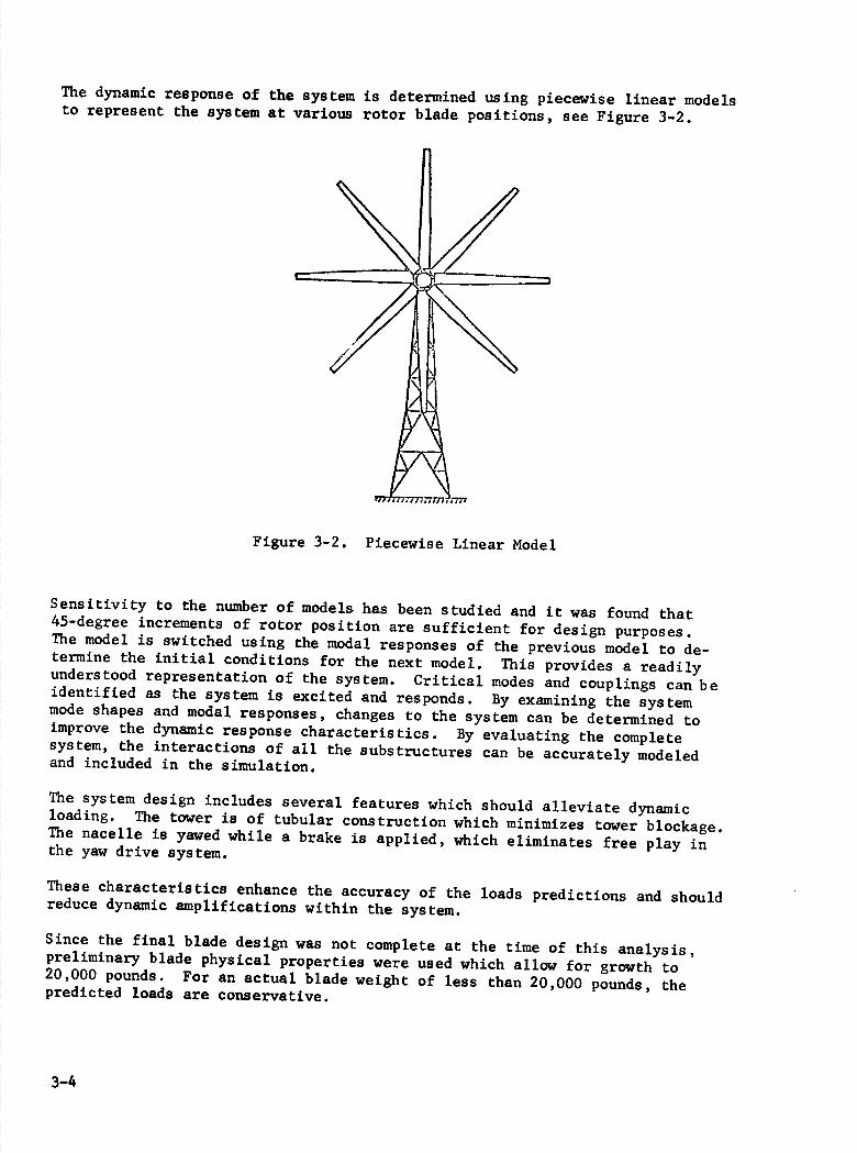
The dynamic response of the system is determined using piecewise linear models to represent the system at various rotor blade positions, see Figure 3-2.

Figure 3-2. Piecewise Linear Model

Sensitivity to the number of models has been studied and it was found that 45-degree increments of rotor position are sufficient for design purposes. The model is switched using the modal responses of the previous model to de-termine the initial conditions for the next model. This provides a readily understood representation of the system. Critical modes and couplings can be identified as the system is excited and responds. By examining the system mode shapes and modal responses, changes to the system can be determined to improve the dynamic response characteristics. By evaluating the complete system, the interactions of all the substructures can be accurately modeled and included in the simulation.

The system design includes several features which should alleviate dynamic loading. The tower is of tubular construction which minimizes tower blockage. The nacelle is yawed while a brake is applied, which eliminates free play in the yaw drive system.

These characteristics enhance the accuracy of the loads predictions and should reduce dynamic amplifications within the system.

Since the final blade design was not complete at the time of this analysis, preliminary blade physical properties were used which allow for growth to 20,000 pounds. For an actual blade weight of less than 20,000 pounds, the predicted loads are conservative.

3-4

3.2 SYSTEM SYNTHESIS

3.2.1 SYSTEMDYNAMIC ANALYSIS

The analysis of the WTG system by substructures was accomplished by the separa-tion of the system into major substructural segments. This system naturally divided at: the bearing attachments located at each rotor blade, at the hub, the low and high-speed drive shaft supports, and the bedplate/tower interface. A natural division was also made at the the blade pitch actuator attachment and the yaw drive/brake mechanism. This division resulted in five major substructures: the tower, bedplate, hub/shaft and two rotor blades.

Each major substructure was then analyzed separately, using finite element models to obtain substructure vibration mode shapes and frequencies with free attach-ment coordinates. Then, the stiffness coupling method of modal synthesis was used to assemble the complete structure through stiffness links (stiffness matrices) representing the bearings and drive mechanisms. This assembly of component modes and frequencies through flexible links was then used to derive the eigenvalues and corresponding eigenvectors representing the system dynamic model.

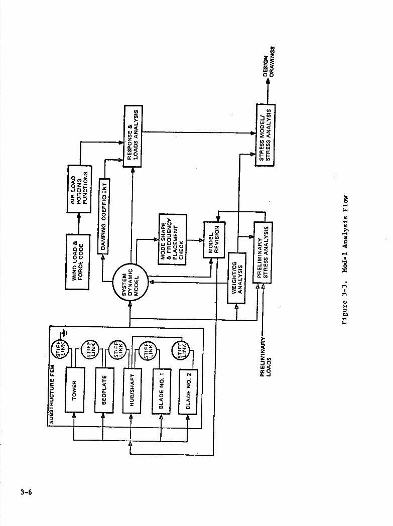
The flow of the dynamic model assembly is shown in the block diagram of Figure 3-3. This diagram gives the sequence of assembly for the model and the sub-sequent input of the modal parameters into the response and dynamic loads ana-lysis programs. Revisions to the dynamic model were made after frequency place-ment checks and preliminary stress analysis, where necessary, to meet the design criteria. Results of the dynamic loads analysis were then used to check the loads used in the final stress analysis.

3.2.2 ANALYTICAL SUBSTRUCTURE DESCRIPTIONS

Finite element models were developed for each of the five substructures iden-tified in Figure 3-3. Each of these substructure models is described as follows:

1. Tower. The tower model consisted of approximately 250 curved and straight beam elements representing each tubular member connected at 120 nodes. This representation provided the structural detail necessary to describe the dynamic behavior of the tower structure. Through nodal compression methods, it was possible to reduce the quantity of nodes used in the sub-structure eigenvalue solution to 16 nodes, each with three linear degrees of freedom.

2. Bedplate. The bedplate model consisted of approximately 400 curved and straight beam elements representing the I-beam and channel basic frame members and plate elements representing the closed frame sections. Large mass component mounts were also represented explicity to provide realistic mass loading points. These components included the gearbox, generator and the yaw and hub bearings. This representation resulted in 196 nodes which were reduced to 27 nodes with a total of 96 degrees of freedom.

3-5

C,

00

I,,

U,

wz

riU) 0.0 wo

U) -. U) U,-: 0< 0z (I) U) U)V) w w I—p.

I—z LI w

<J.U. u ______

LI. U, 0 C., >-

?

1 0. 2 2 iWZ IID WV)

sw Ow 00

Iw cr

00 -'U 00 z U —0

U.

•1" ________________

r('Ir('

ii I I1f1 I . 1I1 I I 101 101 I'I.Ii D I jj 1 01101 <11<1 I I -

U.

U) tco C.-,

F—I >-I >-J 2<

tn-0.(I)

I-I Cl) ...1 Cl)

'-I

'-4 0 x

C.) Ii bO .1-I 114

3-6

3. Hub/Shaft. The hub was modeled using NASTRAN as described in Paragraph 5.2, Stress Analysis; while the high and low-speed shafts were modeled by straight beam elements. Nodes were selected to correspond to the bearing attachment locations, flex-coupling, gearbox, bearing support and other mass loading points. Gearbox flexibility was included in the form of beam elements which considered effects of gear ratio. Eighteen nodes were used to represent this complete assembly from the hub

to the generator.

4. Rotor Blades. Rotor blade mass and stiffness properties received from Boeing were used as input data for a vibration analysis computer program, STRAP. This program calculated free mode shapes and frequencies of the blade considering twist angle and centri-

fugal stiffening. Twelve nodes with six degrees of freedom each

were used to represent a single blade. The analytical modes obtained were rotated 180° to obtain the modal deflections for

the second rotor blade.

3.2.3 STIFFNESS LINKS

The stiffness links used to assemble the WTG system consisted of several stiffness matrices which contained the actual stiffness properties of the bearings that physically connect the substructures. It also included flexi-bility of the blade pitch change mechanism and the yaw drive/brake flexibility as used in the physical assembly. These stiffness matrices thus related each substructure at the attachment coordinates.

1. Blade to Hub. A single blade retention bearing was used to attach the blade to the hub. This bearing provided linear restraint in three directions (one axial and two radial), and rotational restraint about the two radial axes. Rotational restraint about the blade axial direction was defined by the stiffness of the pitch change mechanism.

2. Hub Shaft to Bedplate. A single hub retention bearing was used to attach the hub segment of the hub/shaft assembly to the bedplate. Rotational stiffness about the two radial axes were derived from the linear values and rotational stiffness about the axial direction, which was set to zero to permit free rotation of the hub/shaft.

A rotational stiffness about the axial direction was included at the generator to represent the on-line configuration. This rotational stiffness was set to zero for off-line evaluation.

3. Bedplate to Tower. Assembly of the bedplate structure to the tower is accomplished by a 12-foot yaw drive bearing. This bearing provides restraint in all degrees of freedom except ro-tation about the yaw axis. Bearing stiffness data, obtained directly from the bearing vendor, was used for the stiffness matrix. For the yaw axis rotational restraint, the brake was

3-7

considered to be hbontt such that the yaw drive system flexibility was shorted. Rotational stiffness for this condition was assumed to be sufficiently high to place the first bedplate mode (bedplate rotation about yaw axis) greater than the tower first torsion mode (7.2 P).

4. Tower to Ground. The tower assembly was modeled considering the tower base cantilevered to the ground through linear springs attached to each of the four tower legs. These springs represented soil flexibility derived from down loads (soil compression) and up-loads (pier shear of the foundation). The lowest stiffness values from a range of values was selected from calculations based on con-crete footing and pier area. These values were used in the stiffness matrix relating the tower attachment coordinates to ground. Bearing stiffnesses are sununarized in Table 3-2.

Table 3-2

Bearing Stiffnesses

Stiffness Component (lb/in or in-lb/rad) Source

xial

adial2.47XlO8 l.37X108

Mesainger Bearing Co

Yaw Bearing 3ending 6.62X1011 Torsion Brake 6.4X1011 GE Analysis

on Torsion Brake 4.5X109

of f

Axial 2.48X107 Hub Bearing Radial l.73X107 J. Rumbarger

Bending 2.25X1010 (Franklin Institute) Torsion 0

Blade Retention Axial 4.38X].07 Bearing Radial 8.0X106 J. Rumbarger

Bending 2.52X1010 & GE Analysis Torsion l.2X108(Pitch

Actuator)

Generator Bearing Radial 2.5X107 Elec. Field Torsion 2.88x105 GE Analysis

3-8

3.2.4 COUPLED DYNAMIC MODEL

The modal synthesis method selected for the WTG analysis is a technique that has been used extensively at the General Electric Space Division for space-craft analysis. The method uses the free substructure vibration modes and frequencies to determine the coupled system modes of the entire system. These substructures, as defined by the stiffness coupling method, have no conmon degrees of freedom and are coupled together by the stiffness links described which relate the free attachment coordinates of the substructures.

In other methods of modal synthesis, the stiffness coupling method provides an approximate coupled solution where high frequency modes are truncated. Instead of truncating (or omitting the high frequency modes), a Dynamic Trans-formation is used to include modes in the solution that would otherwise be truncated. This transformation relates the unused (truncated) modes to the retained modes at a selected system frequency. This transformation is then used to reduce the generalized mass and stiffness matrices which describe the dynamic behavior of the coupled system. Details of the dynamic trans-

formation are documented in Reference 1.

The wind turbine generator was assembled using a computer program, SCAMP (Stiffness Coupling Approach to Modal-Synthesis Program), which contained the stiffness coupling method with the Dynamic Transformation. The complete WTG model consisted of 423 degrees of freedom, of which 235 were used to synthesize the coupled model. The final size of the coupled eigenvalue problem (60 DOF) was determined from the total number of "modes kept". Selection criterion for the number of modes "kept" was determined on the basis of participation factors. System modes were thus calculated for the four totor positions (00, 450 , 900,

135°) depicted for the piecewise linear model in Figure 3-2. Of the 60 modes, the first 20 were used to calculate the system forced response.

3.2.5 DETERMINATION OF FORCED RESPONSE

The flow of the system loads analysis is shown in Figure 3-4. The specified wind conditions are first used to define the system forces considering the system to be rigid. These rigid system loads are used as preliminary design loads for initial sizing of the tower and bedplate structures. The forced response analysis is then performed using the rigid system forces with motion-dependent aerodynamic coefficients to excite the system modes from SCAMP, described in Paragraph 3.2.4. The modal responses are then used to determine critical interface loads, acceler-ations and deflections for evaluation of the structural adequacy.

The WINDLD code determines the aerodynamic and inertial forces acting on the system as a function of rotor position. The aerodynamic forces are determined at ten stations along each blade using quasi-steady aerodynamics based on smooth airfoil characteristics. The wind shear profile is included as a power function with an exponent of 0.167 as indicated in the Statement of Work. The tower shadow

'Kuhar, E.J., "Selected System Modes Using the Dynamic Transformation With Modal Synthesis," Shock & Vibration Bulletin, August 1974, pp . 91-102.

3-9

.( I.-, U)

. UI

I - 1

_ I I I I I U)

-,•1 U)

-ci:

U)

0

E U U U)

U)

f;oisU)\

U) Li Lii

I

I' >- I V)L) Li (DC)

I --4-4

I O(CL&J __sw I UiOuI.i Li C) 1 .J _j U.

I LUUJ '

C) C.) _______

ij

• U,

/ C)

U) / 41) I I•-- I >-LU I (, I W.(

' I-' V) ' >•

C) 1/) -j jc

U)

p.. C)'-.

C-, 8 Li 0. U)

Li V C) U) - Li V C.) C)> cQ. C) U) U. LU

a-U,

I-

----I

I

J I(

JO 1w Icc

L.

Lii

C)

_1

3-10

ADE

DOW EDGE

is defined in system coordinates by a series of cosine functions aligned with the tower geometric position, providing a three dimensional velocity retarda-tion that permits initial entry of the inboard blade section, Figure 3-5. With inflow, the shadow is shifted laterally to align the edges of the shadow with the projected edges of the tower., accounting for the downstream position of the rotor. The centrifugal and gravitational forces are also determined at each blade station. The forces are calculated in system coordinates for one revolu-tion of the rotor. For initial design of the system, the integrated hub forces

and moments are also calculated. • For the forced response analysis, the forces

at each of the ten stations on the two blades are used to excite the system.

The QAERO code determines the modal damping for the system modes considering the aerodynamic forces on the blades. The code uses a linearized solution based on the angle of attack at each blade station for each system model calculated in the WINDLC code. The fully coupled modes (i.e., flap, lag, and torsion) are used to determine the quasi-steady aerodynamic forces proportional to the gener-alized coordinate velocities. Then, modal damping ratio is determined from the integrated aerodynamic forces considering the total kinetic energy of the system, including the bedplate and tower structure. Additional structural or electrical damping of a selected value is then added to the aerodynamic damping.

WIND SHEAfl

/ \ .161 V0 - Vft

V - ItEFERENCE VELOCITY

- 8EFEI4ENCE NEIGHT

TOWER ShADOW

- TOWED WIOTFI

SRADOWVDTU

I -

Figure 3-5. Tower Shadow Representation

3-11

The modal response to aerodynamic and inertial excitation is calculated using the WTGRSP code. The analysis considers the syStem to be piecewise linear for each model position. The solution for a 450 interval is obtained using the subroutine MERTA (Matrix Extra Routine for Transient Analysis). MERTA provides a closed form Laplace solution in modal coordinates treating the excitation forces as a series of ramp functions. For the WTG analysis, time increments corresponding to three degree rotor positions are used to define the forcing function. The initial conditions at the model switching positions are determined using the modal displacements and velocities at that time step for the previous model. A sufficient number ofrevolutions is analyzed to achieve a steady-state condition. The generalized coordinate displacements, velocities and accelerations determined at each time step for each model are the output from this code.

The WTGLOD code processes the modal responses from the WTGRSP code to determine the interface loads, accelerations and deflections at selected points of the WTG system. The code uses the modal displacement method. The load coefficients are determined on a modal basis to calculate the loads at nine interfaces. The inter-faces consist of the 257, 507w, and 757 blade stations, the blade root, the ro-tating shaft, the stationary shaft, the main rotor bearing, the yaw bearing and the tower base. To aid in understanding the results, the maximum modal contri-butions to each interface load are tabulated with the associated rotor angular position. In addition, the major mode contributing to the maximum interface load is also tabulated.

3.2.6 CODE VERIFICATION

A key element in the program was the development and verification of the GETSS (GE Turbine System Synthesis) computer code. Cost effective design of the WTG requires the accurate determination of the loads throughout the structure and the influence of critical resonant frequency placement. These data are provided by the GETSS code which was verified by comparing analytical predictions with measured results for the Mod-O WTG under various operation conditions. The development of the Mod-O dynamic model followed the same methods used in the Mod-1 analysis.

The final solution resulted in 20 modes under 10 Hz. These modes were used to compare directly with the results reported in NASA TNX-7l879, 3426, and the final report by the University of Cincinnati on the modal testing. This comparison showed agreement in modal frequency within less than 1 percent for the first tower bending (N-S), first tower torsion and second tower bending (N-S). The first rotor flatwise and edgewise modes differed by only 3 to 4 percent and the others by not greater than 9 percent. A check of modal displacements also showed good agreement for the tower bending modes (Modes 4 and 5). The upper bay motion showed similar diagonal motion as that measured on the test, along with a similar amount of displacement.

The procedure used to verify the GETSS computer code is presented in Appendix A.

3-12

3.3 SENSITIVITY ANALYSIS AND FREQUENCY PLACEMENT

The coupling between the various WTG structures is significant and makes the influence of component structural changes on the system dynamic response a complex problem for analysis. The structural coupling exists between the rotor, shaft, bedplate, and tower such that as the rotor position changes, the dynamic characteristics of the system change. An understanding of the system sensitivity to these interactions was aided considerably by the modal synthesis approach which was used in the evaluation of the modal contributions to the dynamic loads. The identification of critical tuning parameters thus comprised a major contract study effort. The parameters investigated included blade/tower frequence place-ment and bearing stiffness variations at the major interfaces. The sensitivity to bearing stiffnesses are particularly important because these are difficult to predict accurately. The results of this study are summarized in Table 3-3.

Table 3-3. Summary of Sensitivity Analyses

. Soil Stiffness - Not Significant

• Yaw Drive Torsional Stiffness - Critical

• Tower/Blade Tuning - Critical

• Blade Retention Bearing Stiffness - Significant

• Main Rotor Bearing - Significant

• Yaw Bearing Stiffness - Not Significant

• Shaft Bearings - Not Significant

• Bedplate CC - Statically Significant

A brief discussion of the significant parameters follows:

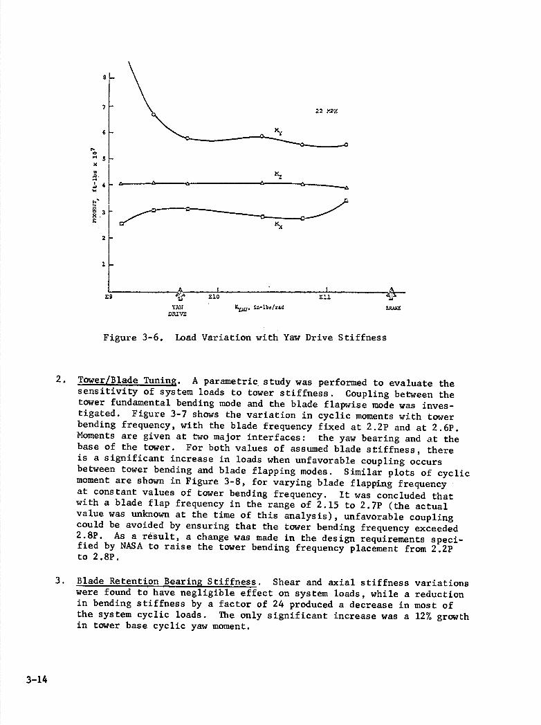
1. Yaw Drive Torsional Stiffness. The variation in hub bending moment with yaw drive stiffness is illustrated in Figure 3-6. Large increases in flapwise moment are evident for decreases in yaw drive stiffness below the design value. Less dramatic increases in load occur at the yaw bearing and tower root. With the yaw brake engaged €here is more than sufficient stiffness.

3-13

8

7

6

0 x .Q.

I4

0•

2

1

1fAZ iIad

Figure 3-6. Load Variation with Yaw Drive Stiffness

2. Tower/Blade Tuning. A parametric study was performed to evaluate the sensitivity of system loads to tower stiffness. Coupling between the tower fundamental bending mode and the blade flapwise mode was inves-tigated. Figure 3-7 shows the variation in cyclic moments with tower bending frequency, with the blade frequency fixed at 2.2 p and at 2.6P. Moments are given at two major interfaces: the yaw bearing and at the base of the tower. For both values of assumed blade stiffness, there is a significant increase in loads when unfavorable coupling occurs between tower bending and blade flapping modes. Similar plots of cyclic moment are shown in Figure 3-8, for varying blade flapping frequency at constant values of tower bending frequency. It was concluded that with a blade flap frequency in the range of 2.15 to 2.7P (the actual value was unknown at the time of this analysis), unfavorable coupling could be avoided by ensuring that the tower bending frequency exceeded 2.8p . As a result, a change was made in the design requirements speci-fied by NASA to raise the tower bending frequency placement from 2.2p to 2.8P.

3. Blade Retention Bearing Stiffness. Shear and axial stiffness variations were found to have negligible effect on system loads, while a reduction in bending stiffness by a factor of 24 produced a decrease in most of the system cyclic loads. The only significant increase was a 12% growth in tower base cyclic yaw moment.

3-14

0

cc - £l1-J.d '.LMaWOW DI1DAD

in tJ)

I I 0 0 ,-.l r-4

in

— /

— . -S - --b

in

0 rl

if o 0 ,-4 -

0 I N /m

cc I . 0 - t

N I I 0 I Np:;

—— ---:>c 0 - - N

——

\ N 1)

I N — — .- — —. —

I — -, - .1'.l >•4'4

c.4P 00

fi Z

z:1

0

C) w

I-i

I.4 w

Cl

.1-I a)

z C)

C)

C-)

r

a) s-I

cc -'.4 11.4

jm

N

NO

N N

0

'-4 rlcc

N

il'I-Ll LN14OW 3I'IDA

3-15

;Er I-0 0 0 0

'0 ('1

0 .1

.4

14

0

N'-4

• z

0•

• 11. N

N

0

N

-4-'

0 >4 C-, Cl Z

0•

N

0

0 0 0 '0

N 0 N

0 1 0 0

\ /' / c c / c.l c..l ..• /' / 40 / \ / '0 Z

I I 0•

I I

N

I I - N

C)

w

4,

C',

z

C',

r.x

4,

C',

U)

Cl)

6 0 z C.) -1

I—I

U,

0

'C.,

U

-'-4 114

3-16

4. Main Rotor Bearing Stiffness. Loads were relatively insensitive to changes in radial and axial stiffnesses; reductions by a factor of 100 were necessary to produce any noticeable change. A decrease in bending stiffness from the design value of 2.25 x 1010 to 4.0 x i09 did not significantly affect the majority of the loads; some reductions were noted. The largest change was a 65% increase in tower base cyclic

bending moment.

5. Foundation Stiffness. A parametric study was performed to evaluate the effects of soil or foundation stiffness. Tower natural frequencies were computed for a range of foundation stiffnesses that varied from approximately one-half to twice the anticipated values, laterally as well as vertically, as shown in Table 3-4. The results are summarized in Table 3-5, which shows tower frequencies for the first ten modes varied less than 57 from the expected value.

Table 3-4

Foundation Stiffnesses used for Parametric Analysis

Vertical Lateral

(lb/in) (lb/in)

Low 8.58 x 106 7.33 x 10

Mid Range 14.33 x 10 6 12.17 x 106

High 28.58 x i06 24.42 x io6

Th1e 3-5 WTG 1500-MOD 1 Tower Natural Frequencies

Mode No. Description

I Tower 1ling-Y axis

2 Tower Bcnding-Z axis

3 Tower Torsion

4 Tower 2nd Bending-Y axis

5 Tower 2nd Bending-Z axis

6 Tower Axial-X axis

7 Tower 2nd Torsion

8 Tower 3rd Bcnding-Y axis

9 Tower 3rd Bending-Z axis-

10 Tower 3rd Torsion

Natural Frequency, Per Rev.

___Low K Mid-Rangc

KHigh K ___ __ __

2.9260 3.0384 3.1306

2.9405 3.0543 3.1478

7.3405 7.3484 7.3542

11.868 12.002 12.108

13.848 14.151 14.397

15.931 16.748 17.376

17.592 17.974 18.306

19.485 19.580 19.639

19.793 20.013 20.207

30.843 30.993 31.054

3-17

3.4 SYSTEM NATURAL FREQUENCIES AND LOADS

The final design coupled system natural frequencies at the four rotor azimuth positions needed for the piecewise linear model are contained in Table 3-6. Selected mode shapes appear in Figure 3-9A through 3-9G.

Table 3-6

Systems Frequencies and Modes

Mode Description Freq (/Rev) Criteria

00 450 900 135°

1. Rotor Rotation .67 .67 .67 .67

2. 1st Rotor Flapwise Cyclic 2.4 2.7 2.3 2.3 2.15-2.7

3. 1st Rotor Flapwise Collect 2.6 2.6 2.6 2.6

4. Tower Bending - Y 3.1 3.1 3.2 3.1 2.8

5. Tower Bending - Z 3.3 6.0 3.3 3.3 2.8

6. 1st Rotor Edgewise Cyclic 4.2 4.0 4.2 4.4 4.15-4.7

7. 2nd Rotor Flapwise Cyclic 5.6 5.4 5.0 5.0

8. Shaft Torsion 6.9 6.9 6.9 6,9

9. 2nd Rotor Flapwise Collect 6.2 6.2 6.2 6.2

10. Tower Torsion 7.2 7.2 7.9 7.5 6.5

11. 2nd Rotor Edgewise Collect 12.9 12.9 12.9 12.9

12. 3rd Rotor Flapwise Cyclic 11.0 11.7 11.6 11.7

13. 3rd Rotor Flapwise Collect 11.3 11.3 11.3 11.3

14. Tower 2nd Bending Z 14.7 14.3 14.1 14.2

15. Tower 2nd Bending Y 14.9 15.0 15.0 14.9

16. Blade Torsion Antisynunetric 11.6 11.6 11.5 11.6

17. Blade Torsion Symmetric 11.6 11.6 11.6 11.6

18. 2nd Rotor Edgewise Cyclic 15.6 15.2 14.8 15.1

19. Tower Longitudinal 16.4 17.7 17.2 17.2

20. Tower 2nd Torsion 17.0 16.4 16.5 .16.5

3-18

OCT 8 3977

11T413R

FREOUENcYHZ) .389

FREUUENCYL/REV) .667 TOWERBOPL FHY5 X 2

MODi REV413

hUGE NUMBER 1.000

H/BOEING STOI

x

V2

Figure 3-9A. Rotor Rotation

3-19

x

Y

11001 REV4I3

N/BOEING STOI OCT 8 1977

FREQUENCYLHZ) 1.421 TDWER+BOr[. X 2

1100E NUMBER 2.000

WT4 I 3A

FREQUENCI(/REV) 2.435

Figure 3-9B. First Rotor Flatwise, Cyclic

3-20

/

/

4/ x

Y

ti00 REV4t3

W/DOEIUG 5101

Dcl. S 1977

FREQUENCY(HZ) 1.519

TOWER+BOPL PHYS X 2

IIOOE NW1BER 3.000

1414 13A

FREQUEUCY(/REV) 2.604

Figure 3-9C. First Rotor Flatwise, Collect

3-21

11002 REV413

U/0EIN& STO! OCT 8 1977 FREDUENCY(HZ) 1.809 TOI4ER+BDPL FtIYS X 2

IIODE NWIBER 4.000

NT423R FREOUEUCI(/REV) 3.lOi

Figure 3-9D. Tower Bending, Y-Axjs

3-22

r

I x

.7

V

Figure 3-9E. Tower Bending, Z-Axis

MOOt REV4I3

TOWER+BOFL PHI'S X 2

W/BOEIUO STOL

MODE NUMBER .00O

OCT 8 1977

WT4I3R

FREOUENCY(HZ) &.91.E

FREOUENCY/REV 3.27.

3-23

OCT 8 1977

WT4I3fu

FREQUEHCY(HZ) 2.429

FREOUEHCY(/REV) 4.164 TOWER+BOPL P1-uS X 2

0O1 REV413

110CC NWI8ER 6.000

W/5OEIN STO1

x

Y

Figure 3-9F. First Rotor Edgewise, Cyclià

3-24

FREQUENCT(H2) 4.179

FREOUENCT(/REV) 7.164

OCT 8 1977

WT413R PIODE P4IJIIBER 10.000 TflCR+B0PL FlITS X 2

VIODI REV4I3 H/BDEIN& STIJ1

x

Y

Figure 3-9G. Tower Torsion

3-25

The final design loads, for Cases A through D of Table 3-1, are contained in PIR WTG 1500-77-015 in Appendix B. These loads were generated before the blade precone change from 12 0 to 90 cone angle was made. The additional precone associated with these loads will not effect the cyclic loads. The steady loads for Cases B through D will be relieved somewhat.

3.4.1 DISPERSION FACTORS

3.4.1.1 Blade Loads

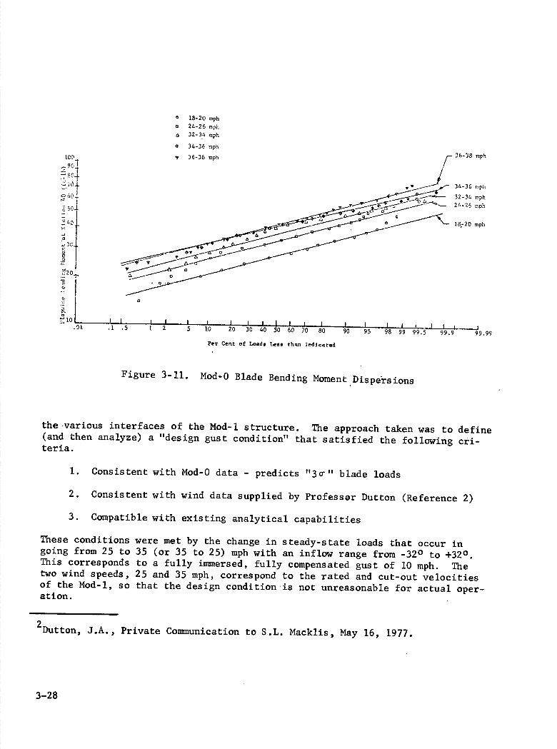
Analysis of measured data from Mod-0 revealed significant scatter of the blade cyclic load amplitudes. This scatter was observed to occur at any given wind speed as illustrated in Figure 3-10. The variation of these cyclic moments at various wind speeds is indicated by the shaded band of data in the figure. Evaluation of these nasurements shoved that the mean of the scatter band (broken line) was governed by the tower shadow, wind shear and gravity (which are always present) while dispersion from the mean was attributed to atmospheric turbulence (gusts).

To assure the regularity of the dispersion of the cyclic moments (illustrated by the band of data in Figure 3-10) from its mean, a probability plot was con-structed from the Mod-0 cyclic flap bending histograms. This plot, which is given in Figure 3-11, contains data for five velocity bands and has a log normal distribution as indicated by the straight line characteristic at each vindspeed group. From this plot it can be seen that the flap bending load at the 99.8 percentile (3C ) is approximately twice the load at the 50th percentile.

Referring back to the Mod-0 data given in Figure 3-10, it is observed that the General Electric GETSS program predicts the mean of the scatter. A data ?oit at 25 mph, which is plotted in the figure, illustrates this characteristic. Since standard practice for design to random loading is to base stress calcula-tions on the 99.8 percentile loads (3q for a normal distribution), those loads predicted by GETSS (which are at the 50th percentile) would have to be multi-plied by a factor to produce the maximum of the load dispersion observed on the Mod-0 data. Accordingly, these factors must be consistent with the data in Figure 3-1 to produc& the final load, which includes the effect of atmospheric turbulence.

For the Mod-1 design, the dispersion factors determined by the Figure 3-11 data were found to be 1.9 for the flap bending cyclic loads. Chord bending data ihich were similarly plotted suggested a factor of 1.5 for a cyclic load disper-sion factor. Since these factors are relatively insensitive to wind speed (as evidence.d by the nearly parallel lines in Figure 3-11) the same factors were usd in all of the blade load cases.

3.4.1.2 Structure Loads

It is clear that loads at other points , in the structure would have different dispersion factors. Unfortunately, only blade data have been extensively analyzed on Mod-0 so a means had to be developed to approximate the dispersion factors at

3-26

,.1i

+ CYCLIC - 6

FLATWIS E

SHANK MOMENT,± 4

LB-FT

*2

20 30 40 50

NOMINAL WIND SPEED, V0 , mph

Flatwise moment load (tower without stairs; locked yaw drive)

6

CYCLIC

EDGEWISE4

SHANK MOMENT,

M

LB-FT 2

[I]

10 20 30 40 50

NOMINAL WIND SPEED, V0 , mph

Edgewise moment load (tower without stairs; locked yaw drive)

Figure 3-10. Mod-0 Blade Loads

3-27

99

1

5C

0

3C

0

20

0

Ic.10

o 18-20 mph 24-25 mph

A 32-34 mph

• 34-36 mph''-no

Pir Cent of Loed. Le thqn lodicared

Figure 3-11. Mod-O Blade Bending Moment Dispers ions

the 'various interfaces of the Mod-i structure. The approach taken was to define (and then analyze) a "design gust condition" that satisfied the following cti-teria.

1. Consistent with Mod-0 data — predicts "3cr" blade loads

2. Consistent with wind data supplied by Professor Dutton (Reference 2)

3. Compatible with existing analytical capabilities

These conditions were met by the change in steady-state loads that occur in going from 25 to 35 (or 35 to 25) mph with an inflow range from -32° to +32°. This corresponds to a fully immersed, fully compensated gust of 10 mph. The two wind speeds, 25 and 35 mph, correspond to the rated and cut-out velocities of the Mod-i, so that the design condition is not unreasonable for actual oper-ation.

2Dutton, J.A., Private Communication to S.L. Macklis, May 16, 1977.

3-28

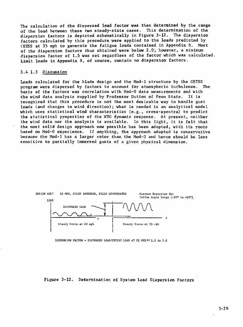
The calculation of the dispersed load factor was then determined by the range of the load between these two steady-state cases. This determination of the dispersion factors is depicted schematically in Figure 3-12. The dispersion factors calculated by this procedure were applied to the loads predicted by CETSS at 35 mph to generate the fatigue loads contained in Appendix B. Most of the dispersion factors thus obtained were below 2.0; however, a minimum dispersion factor of 1.5 was set regardless of the factor which was calculated. Limit loads in Appendix B, of course, contain no dispersion factors.

3.4.1.3 Discussion

Loads calculated for the blade design and the Mod-i structure by the GETSS program were dispersed by factors to account for atmospheric turbulence. The basis of the factors was correlation with Mod-0 data measurements and with the wind data analysis supplied by Professor Dutton of Penn State. It is recognized that this procedure is not the most desirable way to handle gust loads (and changes in wind direction); what is needed is an analytical model which uses statistical wind characteristics (e.g., cross-spectra) to predict the statistical properties of the WTG dynamic response. At present, neither the wind data nor the analysis is available. In this light, it is felt that the most solid design approach now possible has been adopted, with its roots based on Mod-0 experience. If anything, the approach adopted is conservative because the Mod-i has a larger rotor than the Mod-0 and hence should be less sensitive to partially immersed gusts of a given physical dimension.

DESIGN GUST 10 MPH, FULL? uORSED, FLY COMPENSATED Maxinurn Excursion for Inflow Angle Range (-32° to +320)

LOAD

DISPERSED LOAD -.

t

Steoy State at 25 inpi

Steady Stale-at 35 eph

DISPERSION FACTOR - DISPERSED LOAD/CYCLIC LOAD AT 25 MPHr 1.5 to 3.0

Figure 3-12. Determination of System Load Dispersion Factors

3-29

3.5 CONCLUS IONS OF THE S TRUCTURAL DYNAMICS ANALYSIS

The following major objectives of the structural dynamics analysis have been met:

1. A computer code (CETSS) has been developed to accurately predict system dynamic response in service. The code has been verified against Mod-O test data. Mod-i design operational loads have been computed to enable a detailed component stress analysis.

2. Favorable resonant frequence placements have been implemented into the design in order to minimize dynamic loads.

3. System sensitivity to variations in bearing stiffnesses have been established and critical parameters were identified.

3-30

SECTION 4

STABILITY ANALYSIS

SECTION 4

STABILITY ANALYS IS

This section describes the model and the analysis utilized in determining analog control system performance and stability. Both frequency and time domain regimes are examined. The power transfer path is examined from the wind to the rotor, then through the drive train shafts and gearbox to the generator and the utility grid.

4.1 REQUIREMENTS, OBJECTIVES AND APPROACH

4.1.1 STATEMENT OF WORK AND DERIVED REQUIREMENTS

A controls and performance analysis is specified by the following paraphrased requirements from NAS 3-20058, the MOD-i SOW:

Exhibit A

Task II - 8 Controls Analysis - Details of model, large and site systems,. graphical format.

Exhibit B

1.3.2 - Gust model time histories 2.2.1.1 - 8 Degrees per second pitch change rate 2.5.6 - Stability to wind gusts 2.7.1.1 - Safe starting and synchronization 2.7.1.2 - Maintain electrical stability 2.7.1.4.1 - Minimize torque variation

Two important derived requirements, voltage dip response and connection impe-dance rangeare the result of electric utility standards and practice at the distribution voltage level near 15 kV where Mod-1 will connect to an existing grid.

Voltage deviation is objectionable for a variety of reasons such as incandescent lamp flicker and television picture changes. Figure 4-1 is a typical flicker chart of voltage magnitude versus frequency of occurrence. The derived Mod-1 requirement of ± percent for infrequent occurrences down to ±1.5 percent at tower shadow frequency is indicated. This voltage performance is at a critical customer voltage measurement location, not at the generator terminals.

Electrical systems tied to a utility grid with generation are typically repre-sented •as having an impedance (resistance and inductive reactance) connection to a constant voltage, constant frequency source or infinite bus. Large-scale system analyses take one generator as reference and permit all voltages to vary magnitude and relative phase to the reference. In comparison with fossil or nuclear-powered generators in the hundreds of megawatts or gas turbine-powered units from 20-60 megawatts, the 2 megawatt Mod-i generator connecting to a radial feeder can be considered analytically as just the generator system, a connection impedance, and the reference infinite bus. Loss of detail due to

4-1

condensing the network to an impedance is very small. A range of connection reactance from 0.1 to 0.4 Pu (1 Pu = 9.23 Ohms)is considered typical for this type system with resistance to reactance ratios varying from 0.1 to 0.5.

. . I 11111 IiIII_!uII__11111 1IIIi!I!iI1I 11111 IiI!i!!N.IuIp

I—I 4

El 0

C.,

0

G S S l QO

4 ID ao

& 34 0

Fluctuettong per Hour

Fluctuattotie per MInute

Pluctuat ton, per Second

II I I

lARGE GUSTS SMALL GUSTS TWER FREQI'CY SHADQI

Figure 4-1, Voltage Flicker Characteristics

For maximization of energy capture, operation can be over the full power range of the generator. As the dynamic stiffness of the generator air gap is a function of real and reactive power level and connection impedance, a broad range of conditions is required to assess stability. The system range of condi-tions, without specific data on a site and nearby generation, is accommodated by the range of connection impedance. At the site on Howard Knob near Boone, NC, the effective impedance, is at the lower, more stable, end of the examined range.

4.1.2 WIND CHARACTERIZATION

Wind is an uncontrolled source of power that has large fluctuations in both amplitude and direction. The torque produced by the wind rotor and the struc-tural response of the entire wind turbine is strongly influenced by the vari-ability of •the wind.

Three-time domain forms of wind forcing function amplitude-histories were used during the course of design and analysis:

4-2

0 3. 2 3 4 5

1. 1-Cosine Model - from original SOW with amplitude envelope shown in Figure 4-2.

2. Probabilistic Time History - from present SCM shown in Figure 4-3.

3. Random Noise- based on probabilistic data with typical time history shown in Figure 4-4.

.1

U

.5

.3

.2

.1

PERIOD SECONDS

Figure 4-2. 1-Cosine Wind Model

4-3

1Eff Mf

251

50

L5

LO

35

30

25

125

FPS

0 2 4 6 8 10

TIME, SEC

Figure 4-3. Probabilistic Wind Model S

SECONDS

Figure 4-4. Typical Random Wind Model

4-4

,uI ._i lu .lI.l.0

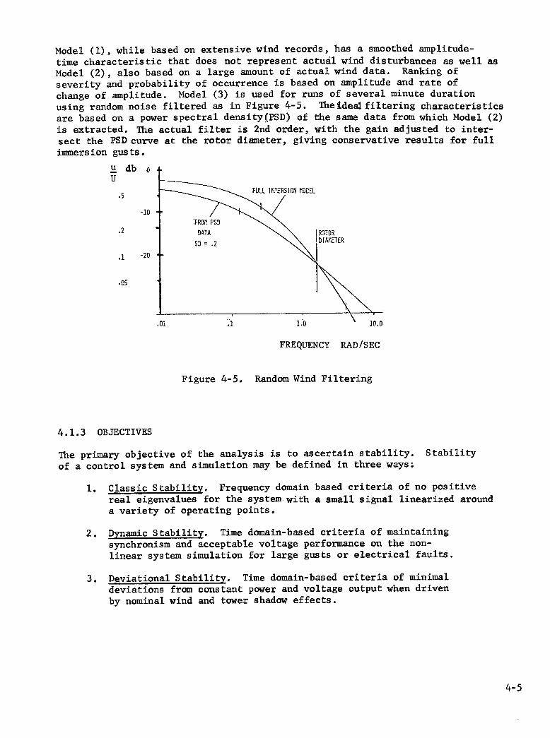
Model (1), while based on extensive wind records, has a smoothed amplitude-time characteristic that does not represent actual wind disturbances as well as Model (2), also based on a large amount of actual wind data. Ranking of severity and probability of occurrence is based on amplitude and rate of change of amplitude. Model (3) is used for runs of several minute duration using random noise filtered as in Figure 4-5. The ideal filtering characteristics are based on a power spectral density(PSD) of the same data from which Model (2) is extracted. The actual filter is 2nd order, with the gain adjusted to inter-sect the PSD curve at the rotor diameter, giving conservative results for full inmiers ion gusts.

db U

'5

-10

.2

.1 -20

.05

FREQUENCY RAD/SEC

Figure 4-5. Random Wind Filtering

4.1.3 OBJECTIVES

The primary objective of the analysis is to ascertain stability. Stability of a control system and simulation may be defined in three ways;

1. Classic Stability . Frequency domain based criteria of no positive real eigenvalues for the system-with a small signal linearized around a variety of operating points.

2. Dynamic Stability. Time domain-based criteria of maintaining synchronism and acceptable voltage performance on the non-linear system simulation for large gusts or electrical faults.

3. Deviational Stability. Time domain-based criteria of minimal deviations from constant power and voltage output when driven by nominal wind and tower shadow effects.

4-5

All three definitions were examined during the course of analysis.

As analysis and design are difficult to separate for a control system, addi-tional objectives were to identify filtering and inner control loop charac-teristics required to improve stability.

A responsive, high crossover frequency, closed loop systEn with adequate phase and gain margin for both an off-line speed control and an on-line power control outer loop is required.

Control of rotor torque is by servovalve-controlled hydraulic actuators with spool and blade position feedback loops. Gains, frequency response charac-teristics, and signal filtering requirements must be identified to the elec-tronics design group based on the simulation results.

4.1.4 APPROACH

The first task was development of suitable analytical models for rotor behavior and pitch change mechanism dynamics. Next, the results of the structural dynamics analysis were examined for modes significant to rotor torque and drivetrain behavior which were then incorporated primarily as blade flapwise bending. Yaw motion and inflow angle were assumed unimportant for drivetrain effects.

An overall simulation model was developed by combining a standard generator 'and grid model, drivetrain dynamics, and various control loop transfer functions. The model was coded for digital computer use for eigenvalue analysis and short-time response runs. Additionally, a hybrid (analog-digital) setup was patched and coded for interactive real time analysis and longer time runs.

Root locus plots from the digital model frequency analysis were used to set initial gains and time constants on the hybrid, then the hybrid model was used to add time responsive filtering and determine dynamic margins by increasing gains until instability was reached.

4.2 MODELING AND BLOCK DIAGRAJ,5

4.2.1 OVERALL MODEL

A simplified model configuration is shown in Figure 4-6, and the following sec-tions detail transfer functions for subloops in the model.

Flow through the model starts with the wind, which is modified to reflect shear and tower shadow, then impressed on the rotor. Blade torque uses a torque coeffi-cient curve computation and hub torque depends on the blade response with f lap-wise and drivetrain flexibilities included. After drivetrain response, the generator dynamics produce an electrical power output relative to an infinite bus voltage phasor. Output power is used to get an error signal through the con-troller to modulate blade pitch angle with a wind feed forward signal added in. Generator excitation is modulated by voltage, acceleration, and reactive power level. When of f line, speed is used as the variable to control blade pitch.

4-6

CONTROL

PITCH SYSTEM

PONER

SPEED

BLADE AND I GENERATOR

DRIVE TRAIN GENERATOR J AND GRID

MECHANICAL r—TORQUE U.] ELECTRICAL

DYNAMICS I DYNAMICS

WIND AND ROTOR AERODYNAMIcS

WIND

HUB 3PEED

FIELD EXCITATION

CONTROL SYSTEM VOLTAG

Figure 4-6. Basic Model Block Diagram

4.2.2 GENERATOR

The generator model is shown in Figure 4-7. Three integrators are used to represent the field and direct and quadrature axis rotor damper circuits. The model provides output voltage and current amplitudes but not the full 60

hertz waveform and is valid over the dynamic frequency range of interest. This is a conventional model used for detail power system analysis with saturation of the field circuit implemented. Values and the saturation characteristic are shown in Table 4-1 and Figure 4-8. Per unit reference is .1875 kVA.

4.2.3 EXCITATION SYSTEM

The generator excitation system has a 25 kW brushless exciter and solid state voltage regulator capable of negative field forcing shown in Figure 4-9. Ex-citer saturation is shown in Figure 4-10.

4.2.4 UTILITY GRID CONNECTION

As described in Paragraph 4.1.1, an impedance connection to an infinite bus was utilized for the majority of analysis. This is shown in Figure 4-11 which mates with the generator model in Figure 4-7. -

A small radial system with two wind turbine generators was also examined with characteristics shown in Figure 4-12. This model was used to evaluate inter-action between machines.

4-7

.-_3

'?'C

I

LItLir'I Ii

1rt1 L'i [?J fl<I

itLi

+ + _*--- I I'iI JJ\J

L

s-i 00

0

I-i 0

I.. a,

C, 0

I-

4 C, s-i

4-8

Table 4-1. Generator Values

General Electric Custom 8000 - 9.28 Ohms = 1 (PU) 1875 kVA Base

Rating: ATI - 4 Pole, 1800 rpm, 8409 Frame, 2188 kVA, 3 Phase,

60 Hz, 4160 Volts, .8 Power Factor

1. Synchronous Reactance (Xd) Direct Axis (PU) 2.552

2. Synchronous Reactance (Xq) Quadrature Axis (PU) 1.52

3. Transient Reactance (X'd) Direct Axis (PU)* 0.311

4. Transient Reactance (X'q) Quadrature Axis (PU) 1.52

5. Sub-Transient Reactance (X"d) Direct Axis (PU)* 0.230

6. Sub-Transient Reactance (X"q) Quadrature Axis (PU) 0.341

7. Negative Sequence Reactance (X2) (PU) 0.275

8. Zero Sequence Reactance (Xo) (PU) 0.0908

9. Armature Resistance (Ra) (PU), L-L at 25°C DC-OHMS Y Conn. 0. 1268

10. Open Circuit Transient Time Constant (T'do) (SEC) 3.36

11. Transient Time Constant (T'd) Direct Axis (SEC) 0.455

12. Sub-Transient Time Constant (T"d) Direct Axis (SEC) 0.023

13. Sub-Transient Time Constant (T"q) Quadrature Axis (SEC) 0.037

14. Speed of Response of Exciter (R) (SEC) Te = Open Circuit 0.52

15. No Load Field Current for Rated Voltage (IFC) (AMPS) 28.7

16. Field Current at Ceiling Excitation, Rated Conditions 195 Amps (IFR)

17. Short Circuit Ratio (SCR) 0.45

18. Efficiencies (4/4) Load Fraction, calculated 95.5 (3/4) 95.4 (1/2) 95.0

* .-Tolerance of l5/

4-9

£21 CI? 11* —12&20D

'- you Lao

:::r

(I2o lIe. /7 210.2)

a.0lI4/

I

':°r i 23

IAT 12*0

z.j S 10. 60 Il. 4260 V

I 4 P011 - 2140 P 212

Figure 4-8. Generator Saturation

LIMITER 19

••uI••t:IIEEIIIJ•_•••.I._•

EXCITER

E

FORWARD PATh

E lcr

(i s %)(i +.a4) FEEO RACK

SLDt'IING JUNCTION

VOLTAGE REGULATOI(

Figure 4-9. Excitation Block Diagram

4-10

Q )20-SIflS 00.1510 10* 3 1. 00 02. *540 V

I"454W

U)

.037 OW - (020102100. DCI)

100

5002 *73 0050ZIATD. 000)

u0

*23

100

7)

50

15

0 I I I I

1 4 0 S 10 12 54 *4

DCXIII 11154 rrfl. anus)

Figure 4-10. Exciter Saturation

AL

'4)

1

______ ______ cos

I ____ I I I

P4b4NlUtE

SU3 VOX.0

ci __________

XI

SIN

+— X

Figure 4-11. Utility Block Diagram

4-11

,— WG 2 87S MW

—j-se

.001 ..J.57

.êZ4 .0L04

Z.04d7 oS

.tpf .2pf

3M VAR

I-'

y l.75 MW

-+-,

+6

.O4I*T.e48

'I

O34 •1 l4i

IMVA IMVA IAIIA .etp .Zpf .9Zpf

.3MYA

SMVA

/2.5 KV DISTR/&IT/ON NETWOR/<

Figure 4-12. Small Utility System

At the site, the impedance and loads have been provided by Blue Ridge Electric Membership Cooperative (BREMC), the connecting utility, as shown in Figure 4-13.

( JT4

T(R TRA1MWT1---

6. øj

--1 LOADS

Z,.SO•6.37 -

AII *ffr

. l.l7 .68

#2.5

3P,1AL

6MVA ,. .L34jlJI

POblTSE SEQUEJC5 ew 1oa'lvA8s(, a,(l24,)AT,rg.l.s. jZ.71

Figure 4-13. Site Utility System

4-12

Cp

4.2.5 WIND

The wind model used on the hybrid system permitted addition of step, 1-cosine random, or wind tape perturbations to a mean hub wind level. Next, for each blade, wind shear and tower shadow variations were superimposed on the hub full immersion model wind in order to obtain a single blade time phased wind for

blade torque computation.

A wind shear exponent of .167 specified in the SOW was used as site data was not available. Tower shadow was modeled as a 60-degree half sinusoid with 35% maximum deficit in wind velocity. The shadow values are conservative.

4.2.6 AERODYNANIC TORQUE

A torque coefficient polynomial evaluation as a function of pitch angle and tip velocity ratio was utilized to compute the forcing torque of each blade. The

conventional power coefficient plot of the polynomial is shown in Figure 4-l4,and a power versus wind velocity plot at rated speed is shown in Figure

4-15.

Figure 4-4. Blade Power Coefficient

While this characteristic is not perfectly representative of the actual blade characteristic, the deviation is small enough to be ignored in the positive coefficient range. In the negative coefficient range, there is insufficient data on actual blade characteristics to evaluate deviation, but the model is believed to be reasonable.

4.2.7 ROTOR

A three-degree of freedom model is used to represent the torsional dynamics of the rotor plus an additional degree of freed*ii to represent pitch change dynamics. The model is shown in Figure 4-16. A central hub and blade inertia

4-13

hi 0

-J

l5

ZO 30

V30 'i

Figure 4-15. Blade Power

'; ? I FLAP/cNOD I r MOOA MAS*/,,JE7A

/ ¶

R

ROTO IWRT?A •7'lOcUr.'

(&

>-. r. g IIZTiA

A(RO 7RQJE (s)

LOW SPCO s'aFr I .Zl7tlo' c7Le4.,

/

/ IELAT/VE flODAL MOOIP'( ROTo /.JRT,A DEFEc7io&s-

(ABOUT 1%

.781-60.2 X!OTL8S&c' J8'7.5 XIO3 FTL8 SECt

STSFESS MID OAIIPIAJG FOR .3 OAP-tPI*14 A77O, So RADiA,J/3(cotjQ MOL FeEQu€iJC,ES

4-14 Figure 4-16. Rotor Model

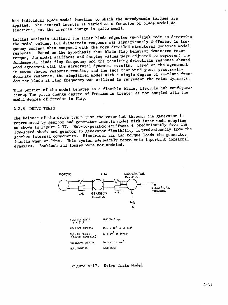
has individual blade modal inertias to which the aerodynamic torques are applied. The central inertia is varied as a function of blade modal de-

flections, but the inertia change is quite small.

Initial analysis utilized the first blade edgewise (:in-plane) mode to determine the modal values, but drivetrain response was significantly different in fre-quency content when compared with the more detailed structural dynamics model response. Based on the hypothesis that blade flap behavior dominates rotor torque, the modal stiffness and damping values were adjusted to represent the fundamental blade flap frequency and the resulting drivetrain response showed good agreement with the structural dynamics results. Based on the agreement in tower shadow response results, and the fact that wind gusts practically dominate response, the simplified model with a single degree of in-plane free-dom per blade at flap frequency was utilized to represent the rotor dynamics.

This portion of the model behaves as a flexible blade, flexible hub configura-tion.q The pitch change degree of freedom is treated as not coupled with the

modal degree of freedom in flap.

4.2.8 DRIVE TRAIN

The balance of the drive train from the rotor hub through the generator is represented by gearbox and generator inertia nodes with inter-node coupling as shown in Figure 4-17. Hub-to-gearbox stiffness ispredott1iflafltlY from the low-speed shaft and gearbox to generator flexibility is predominantly from the gearbox internal components. Electrical air gap torque loads the generator inertia when on-line. This system adequately represents important torsional

dynamics. Backlash and losses were not modeled.

ROTOR. GEME.PTO I P4ERTtP.

ELTR

ToRcua

c

GEAR BOX RATIO 1800/34.7 rpm

N - 51.9

GEAR. BOX INERTIA 15.7 x lb ft Sec2

}I.S. STIFFNESS 22 x ft lb/tad (MOSTLY GEAR. BOX)

GENERATOR INERTIA 50.5 ft lb Sec2

H.S. DAIPING NONE NEED

Figure 4-17. Drive Train Model

4-15

4.2.9 PITCH CHANGE MECHANISM

The pitch change mechanism is modeled as shown in Figure 4-18. A hydraulic actuator drive inertia is connected to the blade pitch change degree of free-dom and the hydraulic flow and servo valve spool dynamics are included in the model. Amplifier elements close the spool and actuator position loops and filter the input to avoid exciting the pitch mechanical degree of freedom, or responding to rated speed tower shadow excitation.

cJTOLLE OU7T3

WIND FEED

ZP NOTCH FILTL QMD 1.44

AepFecT,v MEC,.I,5M

1.44

VALiA.dO

I4OAAUL(C Cb41

Ta) DI

ACTL1ATO

Figure 4-18. Pitch Mechanism Model

4.2.10 SPEED CONTROLLER

For off-line speed control, a governor controller with proportional and integral characteristics plus a biquadratic notch filter at the rated speed fundamental is used as shown in Figure 4-19.

4.2.11 POWER CONTROLLER

When on line, the grid controls frequency (speed) and a power controller loop is used. The block diagram is shown in Figure 4-20, with a 10.0 radian per second transducer response utilized for power feedback. The error signal trans-fer function has a complex numerator to notch filter , attenuate the drivetrain response resonance and a pair of real le gs. This behaves as an integral charac-teristic below the notch and a derivative characteristic above it with flat re-sponse below and above the pair of lags.

4-16

E,JEZ4TOZ £PED AJO7CI rie

+—zo (i+4) (, 2(OS)

*

(ii-/1.5 7 PiTcH

mtc/4AA115P4

REFEEAJC

Ai/J 20 OEES/UWlT E0i

Figure 4-19. Speed Controller Block Diagram

Pee 4AIAI 0/ITCR.øQ.

I,

.4-

( ____

,..^\ /I#i\ T1( /01

J5EWS /07cH WITH DoUBLE LA 10 COMPLEX ZEZ AT D.T. FUJCAMAJTAL.

Pe.

Figure 4-20. Power Controller Characteristic Block Diagram

4-17

4.2.12 WIND FEED FORWARD

A wind signal from an up-wind sensor arrangement for feed forward purposes is modeled as shown in Figure 4-21. The sensor lag and upwind distance lead vary with wind velocity but were more simply modeled as fixed values with a constant .4 second lead time on the hybrid.

0 oP--.4c O.'tloAIT,AIci

W/'JDI Z3 I

vI k1 I . , I /-!ff. I I Vvik I

.2 SEC &57F'?S (St.'J5o& LAC)

.5'AIk! CHAIJ

Figure 4-2 1. Wind Feed Forward Block Diagram

4.2.13 SPEED STABILIZER

Use of a speed derived signal to produce generator torque modulation in phase with speed as a damping source is used on large power systems under the name of power system stabilizer (PSS). Such a system is adopted to Mod-i as shown in Figure 4-22 in order to improve the on-line fundamental frequency damping. The characteristic has a rate and washout plus double lead-lag and biquadratic filter-ing for dominant time excitations.

4.2.14 REACTIVE PMER CONTROLLER

A Var controller shown in Figure 4-23 is used to control the reactive power level by biasing the voltage regulator output based on power factor or reactive power reference settings.

4.2.15 MISCELLANEOUS

Hybrid logic was included to simulate synchronization, loss of load, and pull Out of synchronization transients. All hybrid results are for .2 pi reactance.

4-18

4AJ °/fJwrr (RROM

___ /000' /#./7. 1 , * cJ

[ / 2(.').i I

iioØ (/*.o,7i ( , 2(4J * )

A A &/I a/&

W4SM0uT CAD/LA4S T0S/0A1AL cicTE

I // 2(O5) $ .* I I / 7.25 "725 * / /45 _ ,45L

I ( a(.)/

z(.$) * a i F / I" Iz I

VSTA8

ZP F/L7Es

4P F/L7E

Figure 4-22. Speed Stabilizer Block Diagram

PoT

LIHITE

I

(Moo

DE.VICV.4& I

+

Figure 4-23. VAR Controller Block Diagram

4-19

4.3 SUBSYSTEMS ANALYSIS CASES

4.3.1 FREQUENCY DOMAIN

Prior to defining wind and electrical transient load cases, inner loop analysis and outer loop frequency domain analysis were performed. Small signal lineariza-tions of the system variables about selected operating points were subjected to eigenvalue analysis to generate root locus plots and transfer functions.

4.3.2 PITCH MECHANISM AMPLIFIER

Amplifier characteristics shown in Figure 4-18 were determined by the following criteria.

1. Avoid excitation of the mechanical degree of freedom around 54 radians/second (r/s) due to pitch inertia and mechanism stiffness.

2. Retain as high a crossover frequency as practical to reduce the effective time constant.

The values provide for inner loop (spool) crossover at 250 r/s and outer loop (actuator) crossover at 5 r/s with a quad lag filter at 25 r/s for rapid atten-uation before the blade frequency is reached. Crossover at 10 r/s with less margin is possible.

4.3.3 ROOT LOCUS VARIABLES

Gains were varied over the following ranges for frequency domain analysis:

1. Real Power 2. Reactive Power 3. Connection Reactance 4. Power Controller Gain 5. Speed Controller Gain 6. Stabilizer Gain

0 to 2000 kW 0 to 1000 KVA .1 to .4 Pu 0 to 200 degrees/pu error 0 to 1000 degrees/pu error 0 to 200 pu/pu

Result plots are shown in Paragraph 4.5.

4.3.4 DEVIATIONAL RESPONSE VARIABLES

For determination of steady state time response, the following variations were made:

20 to 90 fps at rotor (10 to 45 mph) 30 degrees by 35 percent to 60 degrees by 70 percent 5 to 1 range

1 to 2 million lb-ft-sec2 4 to 1 range 0 to .1 pu gustiness (pp) 0 to 100 pu/pu With and without wind feed forcard, stabilizer and VAR controller

1. Mean Wind 2. Tower Shadow

3. Inertia Change Coupling (Rotor)

4. Rotor Inertia 5. Shaft Stiffness 6. Random Wind 7. Stabilizer Gain 8. Multiple Loops

4-20

4.3.5 TRANSIENT RESPONSE VARIABLES

To determine response for large, infrequently occurring transients, the following

variations were made:

1. Step Wind 2. Continuous Frequency Wind

3. Step Voltage 4. Random Wind 5. Probabilistic Wind 6. Synchronization

7. Emergency Overspeed and Speed Control Step

.25 Pu step

.2 pu at 2.5 r/s (.4 Hz)

.1 Pu To .5 Pu (peak to peak) 0.1 percent gust (worst) On and off transients

.8 pu step wind plus load loss

4.3.6 SMALL SYSTEM ANALYSIS

Frequency and 1-cosine time analysis was performed on the small radial system described in Paragraph 4.2.4. Voltage dips along the system and critical clearing

time for a bus fault were analyzed.

4.3.7 SITE ANALYSIS

Detailed site behavior analysis had not been made at the time this report was prepared. The effective site impedance to an infinite bus from the generator terminals is .05 + j.11 pu which represents a stable system connection at the low end of the range analyzed. It is unlikely that significant detailed site analysis is required and component parameter adjustment ranges are adequate to accommodate the site values.

4.4 COMPENSATION

4.4.1 FILTERING

In most loops, when a need to attenuate response at a particular frequency had been identified, a filter with second order zero and pole characteristics was specified to provide a "notch". This type of design is conventional and readily adjustable over a limited range via potentiometer and fixed resistance changes. A typical Bode diagram for such a filter is shown in Figure 4-24.

4.4.2 WIND FEED FORWARD (WPF)

The injection of a signal to control blade pitch angle at the same time a wind disturbance arrives at the rotor is a form of compensation. Data from Mod-0 at NASA Lewis Research Center's Plumbrook Station indicates a benefit in prac-tice with a single wind sensor below 1 r/s (0.15 Hz) with analytical results predicting a benefit a decade higher. This is reasonable because the rotor responds to a much larger wind field and the sensor signal may represent local gustiness that does not affect the entire blade area.

On Mod-1, the average of multiple wind sensors is utilized as the control signal with computer controlled switching of the signal into the control loop. The WFF does not effect classical stability and in the nonachievable theoretical limit would provide constant rotor torque.

4-21

30 a • • - . • 4

20t• OQ

'PHASE

10 d : d• • 00 4 • - -, - - - - 4 •• •• • • • • if _____________

;c rnruç

z -10 1j d I-I •

•:

• . • •_ •w •,-•W0DA .o,_ •

..200r •:

.w°owc

.114D •ø . -

-309'

• ••.•(_I •

d :&', .01 .10

FREQUENCY (RAD/SEC)

GAIN

1.0 10 100

4-22 Figure 4-24 Filter Gain-Phase Diagram

4.4.3 SPEED STABILIZER

A speed stabilizer or power system stabilizer (PSS) is utilized to increase on-line fundamental torsional frequency damping to 30 percent of critical. This compensation provides nearly three times the damping available from just adjust-ing the voltage regulator by modulating the generator field, and thus air gap torque.

This compensation has filtering applied to minimize response to tower shadow-. produced steady state excitations. An increase in steady state and dynamic voltage fluctuation and reactive power flow is an undesirable byproduct of the stabilization but the amplitudes are not objectionally increased and the benefit is considerable.

Time responses of drivetrain, both without and with the stabilizer, are shown in Figure 4-25. An initial unbalanced drivetrain deflection representing 0.5 per unit torque is released at the start of the response traces and the more rapid decay in response due to the stabilizer augumented damping is readily evident.

Utilization of a fluid coupling was considered on Mod-i in the preliminary design stage and after one was added to Mod-0. This device behaves as a series damper in the drive train with steady state loss comparable to slip speed. A Mod-i sized device would weigh, cost as much and take up the same space as an-other generator in addition to having a need for coolant flow to dissipate 2-3 percent of total power. The stabilizer is a more cost-effective means of get-ting added damping on Mod-i and is used instead of a mechanical loss element.

4.5 RESULTS

4.5.1 SPEED CONTROL LOOP

4.5.1.1 Frequency Analysis

The basic speed control block diagram is shown in Figure 4-26. An off-line fundamental frequency at 11.5 r/s (1.83 Hz, 3.2 P) limits crossover of the loop as does the pitch mechanism effective lag at 5 r/s (.8 Hz). An integral plus proportional controller characteristic is designed to crossover around 1 r/s (.16 Hz).

Closed loop step response for a gain of 250 degrees/radian is shown in Figure 4-27, a Bode plot of the transfer function of generator speed to wind velocity. The blade torque characteristic has been approximated as linear with wind velocity and pitch angle by:

TA = Kl + K2 * VW + K3 * B

where

TA = Rotor Torque in ft-lb Kl = - 483086 ft-lb

4-24

TORQUE

TS(.o4)II.5/L5)

Ka

PITCH MECH I I SPEED COJ7OLLE. FIGURE I -1

4-18 ]

F,ueE 4-19

1R - 2 x io6 Ft-lb eec2

- 36536 Ft-lb/mph

KB - 28417 Ft-lb/degree

Figure 4-26. Speed Control Loop

-30 GAIN

CD • c.

-40 ; • CD • 0'

-50 i:; • C)

• .tu • .0

• •tJ • .0

z I— • 00 < -7Ooo. 0 ::

:

•W •-• W 00 i)

o, .cr .0: D'.'J .1-

.111 I

.' • U

. .7:0:

.... .c)u • •(_IIIJ • WOO UI t'

•VJ .0:(') • -

-90 ox

.0. •.Ji

• •0_.-4

• •4

• .7:

.0LL

-lOOo .0. -

.01 .10 1.0 10

FREQUENCY (RAD/SEC)

Figure 4-27 Speed Loop Gain-Phase Diagram

I-')

-.

D LOOP

a oo° / pu

•.4 .4.tt-J

III ItID

100

4-25

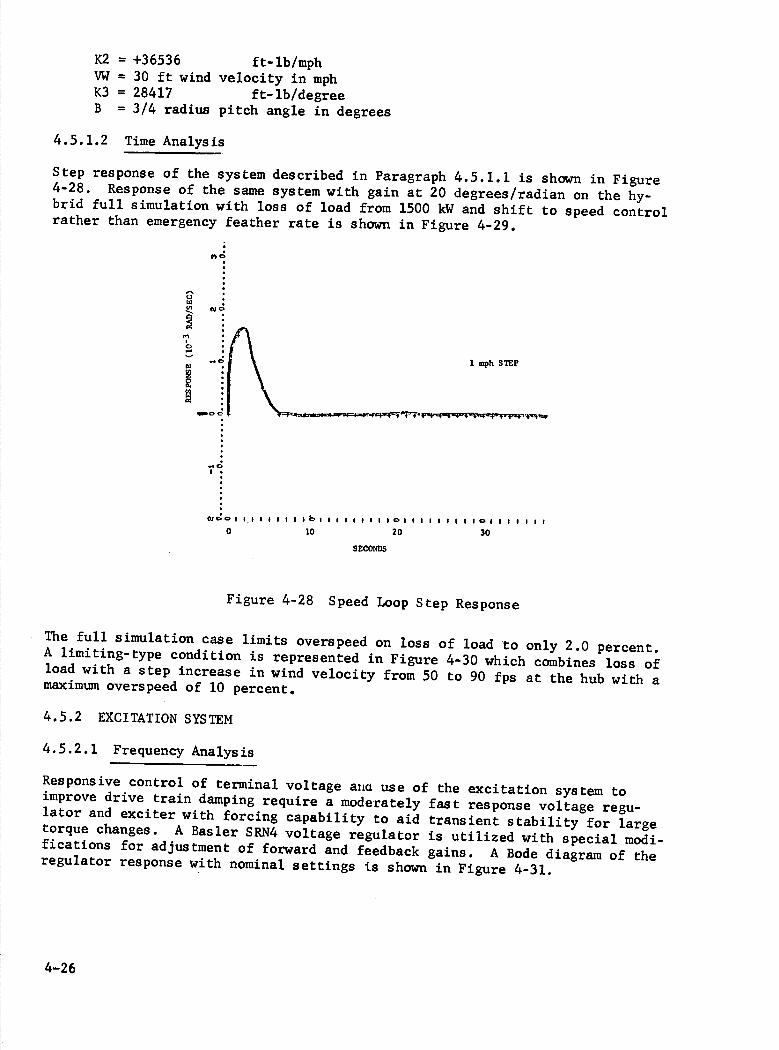
K2 = +36536 ft-lb/mph VW = 30 ft wind velocity in mph K3 = 28417 ft-lb/degree B = 3/4 radius pitch angle in degrees

4.5.1.2 Time Analysis

Step response of the system described in Paragraph 4.5.1.1 is shown in Figure 4-28. Response of the same system with gain at 20 degrees/radian on the hy-brid full simulation with loss of load from 1500 kW and shift to speed control rather than emergency feather rate is shown in Figure 4-29.

U £4

.•o

0 10 20 30

SECONDS

Figure 4-28 Speed Loop Step Response

The full simulation case limits overspeed on loss of load to only 2.0 percent. A limiting-type condition is represented in Figure 4-30 which combines loss of load with a step increase in wind velocity from 50 to 90 fps at the hub with a maximum overspeed of 10 percent.

4.5.2 EXCITATION SYSTEM

4.5.2.1 Frequency Analysis

Responsive control of terminal voltage aIict use of the excitation system to improve drive train damping require a moderately fast response voltage regu-lator and exciter with forcing capability to aid transient stability for large

torque changes. A Basler SRN4 voltage regulator is utilized with special modi-fications for adjustment of forward and feedback gains. A Bode diagram of the regulator response with nominal settings ts shown in Figure 4-31.

4-26

0 0 0 0 L Lf1 C

c.'J -

u0 0 o o .< - 0 o

iUIUUU1RHWffl!rIlli UUUIIUUNNIIIIIIfi ilUIIlUIMH ll

RIflfflI HHIIWII IUUIINUOI1HJfl

IRIlUUUU HIflHIUIIllIllhIIIII!IIIIHIIIIWlIIlHlll ••uiiaui I"HI1 IHllhIUll.11IllDUflIW1IIlll uiui•iva iim IHIIHWIU lUl•ISIUl D UIff OflI1UUifflNlHfflIlll •SUiiIU4 UUUI IUIU1fluhl1 ul.I.ulul miiiuiu iiiiiii u.IulI.uIl NUILlUII III •IUUUIUMI OIlllli3IINI iuiuuuii iiiiiiiiiiiriu• llh11U in•uuuui iiiiiiiiiiiiii••iu aiiiiuit IIIIIIUID I(IIIIIIIIIFISIUII 4LI •iuumuuui IllllhIIIIII•llUI m,lul •ui•uiiau iiiiiiiiiiiimuu UlUllNIOmrI •iIUIlUi4 IIthIJ1IJJIUUII III I.I•IuusIc :qi1lfl iiuiii i••UUUl oiiumoiuu.. UUHU1UIIII •uu•uuuuvi s•IUU IMI1IlI IululIulu

U

luIuuunu uuuutuuui uu•uuuuuum ,aniuuuuua uuuuuiuuuu uiuuuuuu oiuuuuuu. uuuurauuuu uIuuuuuuus uuI :: uuuuuu uuuiauuuui •uui•uuuu uuiiiuuu•uu uuuuuiuuumi 1111111 lIiulI•lI UBIUUIII IPUU.I ILP!IUU• uiuu!!luuiu

uium uuiiiuuui uUuiiUiuH UiuUuuUi liii iiiii 1I

U) 0 0 U)

I

U) U) 0

I-1

- Cl) 0

0 0

C/)

U)

-

rz 0

C.'

a)

4-27

4-29

rIf-IIj:1 R I I

125.0 —I[ I ..L.L1 -I .1

0.0 -H--I-- -

Ii

+-H- --H—E±-±-H--

1 ; 256 _ _

0.0

BLADE #1 WIND (F PS)

BLADE #1 TORQUE (FT-LB)

0.0

I -

_I_._J. ........ . _J-. .i.

SECONDS125.0 ..... .

iIiirii 1•

I,

WIND AT HUB 1.2 SECONDS BEFORE ROTOR (FPS)

GENERATOR POWER (PU)

PITCH ANGLE (DEGREES)

3.3

0.8

-1.7

50.0

cr OR SPEED (RPM)

Speed Loop Worst Case Response

Figure 4-30.

56.7

34.7

12.7

60

50

40

30

20

10

0

-10

= KF=.03

• a., . • V.

oGAIN

• 0(3 • 'p. • (9.

• 0(3 • (U. • •_ • .0 • .IJ • .0 • .0 o 000 • 0 .0 • .. .0 • .0 • .0 • .0 • 0(3

o u. .1-•

:: J' 0.q__PHASE

- --V - • •I; •z •z •.-. •0, •LdC'0W.

•(. .0:1 • Dx .0 .0. .W(4 • .0..-. • .(.0

.. D0x • •.-.c_' • .a • •Qw o . DlIIlII 1110111111111011111111 loll,, Ill, ID .01 .10 1.0 10 100

FREQUENCY (RAD/SEC)

Figure 4-31 Regulator Gain-Phase Diagram

4-30

C, ri U)

0

0 0

0

0

U 0

0 0

o • • V)

U)

(N

-1.-4

o

o c, 0 0

• •

0 U) 0 -4

C -

-4 C

4-31

A system multivariable root locus plot varying regulator feedback gain set-ting for the system through frequencies of interest is shown in Figure 4-32. Root migration with power level and connection impedance is also shown in Figure 4-32.

4.5.2.2 Time Analysis

Response of the full simulation to a change in reference voltage at 1500 kW is shown in Figure 4-33 for a 1.5 percent step. This closed loop loaded response includes saturation and is typical of an IEEE Type 2 brushless exciter and solid state voltage regulator system.

4.5.3 STABILIZER

4.5.3.1 Frequency Analysis

Stabilizer compensation design started by using generator speed as the control signal, but insurmountable difficulties occurred involving destabilization of the first torsional mode occurring while the fundamental mode was showing added damping. The reason became evident from examination of mode shapes with the generator inertia having the greatest participation in the first torsional mode.

A shift in speed sensor reference to the rotor bypassed the difficulty with the slight penalty of lower resolution due to a 52:1 speed difference. The rotor hub is essentially a node for all drive train related frequencies except the fundamental.

Figure 4-34 shows the stabilizer loop block diagram and i'iure 4-35 shows root ni;ration with gain change on both a high impedance connection syst.n of .4 pu, and a medium impedance connection system of .2 pu. The desired effect of almost pure increase in magnitude of negative real part of the fundamental root is evident with damping at 30 percent of critical for a 100 pu/pu gain. These plots reflect a lower inertia system with fundamental frequency near 3.5 r/s rather than presently calculated 2.5 r/s but the effect is essentially identical.

4.5.3.2 Time Analysis

Reference to Figure 4-25 will demonstrate the full simulation effect of the stabilizer. Also, in Figure 4-36, a random wind input time response is shown with and without the stabilizer loop closed. A filter in the power controller loop attenuates response at the fundamental frequency to permit improved performance at all other frequencies, but this makes the power con-troller "blind" to this input frequency.

Quasi-resonant response buildups and decays are evident without the stabilizer due to the blindness. With the added stabilizer damping, however, the buildup is less and the decay is more rapid which provides reduced fatigue loading on the gearbox and smoother power.

4-32

SECONDS

-H-F-- - -H-- - - -±-*- --- -4-H-- - -±---*

: t-ftL _______ - -H--f-- --4-f-- I -- --f--•

-

-:

-

-c-

TIJ[

'+:_ i+ r'i±L-f1

12.5

F IELD VOLTAGE (PU) 0.0

50.0 REGULATOR VOLTAGE (PU)

1.078 GENERATOR VOLTAGE (PU)

1.000

0.922

1.000 POWER ANGLE (COSINE) 0.0

-1.000

Figure 4-33. Excitation Step R2sponse

4-33

5

EMEA7OIEXCIT4TIOAI L 1++ I

___________ I SY5T1

I tr

Figure 4-34. Stabilizer Control Loop

4.5.4 POWER CONTROL AND COMBINED LOOPS

4.5.4.1 Frequency Analysis

Figure 4-37 is a Bode diagram of electrical torçie (or power at constant speed) relative to rotor torque. Without, the stabilizer, the poorly damped pole at 2.5 r/s would severely limit crossover frequency for an integral control characteristic. Utilizing a complex zero, double real pole charac-teristic minimizes the mechanical pole effect and provides an integral characteristic below the pole and improved gain above it relative to a straight integral function as shown on the Bode diagram of Figure 4-38.

A block diagram of the power control loop in Figure 4-39 shows the main elements described in the previous paragraph in addition to a second tor-sional frequency and the wind feed forward loop. Closed loop performance of the system to an impulse in wind velocity is shown in the Bode diagram of Figure 4-40.

Power controller gain variation root migration is shown in Figure 4-41 for the system.

4.5.4.2 Time Analysis

Single 1-cosine disturbances in wind velocity for various combinations of control loops are shown in Figure 4-42. The behavior is consistent with

4-34

0

0 0

C

0 r;4

C) 0

4J 0 0

a) N

•0.

-

•IJ

Lr

a)

1.1

00

0

C)

.T T"1T7 -I--- 4II___.I

-I I - I - -. I .. -S

SI. .. __ . : I

-. I_.._ I __ - I ..I.;,'i..i.-I -.1 --

I-

ilrHJ' ---4-1-t - j— --i-----

- ; 4T:1ij .. - •1 Q.

.1_....._.4____4_.. -'- -.-- --:-•--

-l--- :r-L ____

..L_1_.4__ _L_._._.

j

•___.• 1._I .. .L4]_.,.J41.+_ .i ., j4--i I ---- -1 -hI:

...4.j I -

. __.a.._,

- ii ilth -I-Li_ t: - HL

_L - - - IJ1

I - - J -, '_ --- 1---.- -

_ • ...• ._L....Z_...4 - .-.•---t-

H. , _I - - •. -, --I ••-- —

_1_.___.L_ r -.•-1

• ________ -

iiTTT: r - ' [_ 1.._1 ii---.-

__

t .; .. - __1

Th 0 1 o r-

-•4

I

:L Ef

............................r

I Li Ii I L I - : 1- 1 I.: iI ;

J _I 1 r1-'

-I'

I T T1

-

I

U

I I I I HiH I 11+ ++ '1

.:!.;Iji:i}I jJJ I .! H J. ;:JfflJ]j JI . .i .!1; j ijj

i

-4-35

HuH

111111

HllIllElluIIllllh1llIll IllllllflhIMllll1IffløHIQWI1

IllHQHhIlIUhIllhIll1llllhIJIIll1HilI IHullllllll

HR llllR!!JIll1llhIl1IIfi1

MIMI llIORllIUIUUb Ill MNffl1I1

llflIMHHIIIIIMIllhillh1QMMII HMHfflHIllHIliillUlluIIMIl IMIHMllMHLHIllflMIIUIl

MRllMUII

IHI IHJHHIHRUUI fflflfflflIMIIII MIIIflIlll

llfflHHkIIRIU

ThfluII

I

IlMUllIIlI$ fflllRllllRIMIU

iutjiuui

e e e e 0 0 0 0 0

KIiI!IMIllhIllhIHIIIIIllIllhIllhIIIIIIIIIII IllIIIIIIIIIJIIIIIIIIIIIllhIIIIIIIIIIIIIIIIIIIIl IIllhII!IIIIIIIIIIIIIIIIllhIllhIIIIIIIIIIIIIIIII

IIllhIIllllhIIIIIllhIIIIJiIIllhIllHIllhIO IIIIIIIIIIIIIIIIIIIIIIIIlluhlMHMIIffIIllhi DIllIllhllIHuIllhIIHIIIIIIIIIIllllMllIll

IIllhIWIUIIIMRIllhIIIIHllllllllll IIIIM;;iiilIHfflIIMRMMII

IJMIPIIIIIHIIIIIIIIllhIIIIIIIIIIllhIIIIII!I! IMIDIllhIIIIIIIllhIIUDHMIJllIHMUllJ IUIIR.illJHllhIIilIllhIIMll tllhIIIiIRMIllhIIIIIIIHhIllhIIIIIIIIIIllhI IIHhII!lIIlIIllhIIIIlIIfIIIIIIIlIllllhIIWffIII IIUIH.!cIIIIIRMIMIMll IIIllhUIIllhIIOhIIHIHllhIIIllhIIHIIllhIllR IMIIlluhIIIIllJ'IHII!"JtllIIll

HuIIllI WIHIflMHhlllhIMIIllhIIIIllhIHIIHu II!llhIllllhIIIIIMIIllhIIIIIRIOOhII IllhIHllIIIHIMHIIIIIIIIMHIllhIIMIM

4WllHfflMJHItIllhIIllMIffihIllH IllUIHJ.11IUIllhIRIDIllhIIJHIR 1IMMHHMIHIIIOR 111111111 IIIIIMIIIIthIIIMRIIMIMO

IIMU!II1IIIIRIWII1UI llIMWNMIIIIQIR

MuRMuR IMIIIFIllHfflUfflflIllHMIIll lPIflIIMfl MIJIffJMIHIR HIUhIii!HIIIIIOHllIHlIUIMIIMH

IIIIIIOIHIIHUIMHIIIIIIMIIIIII 4IIIIIIIIIIIIIDIIllIIllhIIllHhIllhIIlIl

RffltIllllhl11IIlIIIflMl1011hIll11hIIIIHM RIIIM0hIMQllIIIIOIMIIIIIIHIfl

IIIIMII0flIIIflhtMO11hIIIIIMIHIIR IMIIEdIIIIIMHIIMRMIMIIIHIIMIIIIII 0fflPâI11hI011IIII0IIIHUhlMIIIIlllhIJ

MllIIRIllIllMHIUfflhIMIIIHllI MIiiIillllMRIIIR

HuI:::IHIIIIHIMIHMMIIOIUHuIRM MIM' - IiIRM11RIIIfl IIIllOfflhIIHllllMIltIlItVIHMII II0IH11MIIIHIIIIIIIIffihIMUUII 0111111 IIMfflllHIflfflflH Ii Ml iIffb HliHIIll IIU lIiiIIU

llWVflIHllIMllIllllIMIHMIIIIIIIIR RM NHMRMIPI muP:iJii OliILIIIIIJIIMIIMRIIMMIIIIIIIIIIIIIIM HMUMUffl11M11MUI UlNUIIfl 11111ffUHMMRMMIIIIQMIIIIIIIIIIIIIR HuIffIMI I!IJft IIThIIIMII1MRIHHIIIIIIIIHIIMIIM HMHHIIUI11M0ffIllflHIflhIfflMIIIIM III

IIffIMfl IIIIIMOIIIIIHIIIIIJII MMI4IIIIllHUIHMHMlluIHIII HUEJUl11 41R111M11 IIIHIUIIHIIIIHMHIIIII RRIRiIIUILJIIMuIIUIHIIIIOUIHH 1IUUU

z C 0 cI

4-1 4-1 0

N

c/D

(1)

0

Cl) a)

a)

• -4 O

0 e w

a) N

.-1 '-4 -,-1

4-J Cl)

C

I—I H 0

c/

HO'-'0 H.

0 H.

0 0

)-1 • 0 HZ

4-36

ttiiiiiiiiiiiiiiiiiiii IllUIllhlIllO III 11111 . lIIIllhI

iuiiiiitiiiiii :QllIVhIJllIfl

IIIUIIIIIIIIIL hllIllIllhhhIll IllllhIhIIhhIII Qhhlifilhlifi :llAIhl hlhlhiMififli UUIII IIIIIIIIIIHIIL.. .N9i

lILllIIl IOuIffllIonhIIIgll:;'iIfluJ

1hhIUHIfflhIIhIIhIfl . .9!IhIhlhIhhIIhIhIIhhIllhI .IillhIuullIuffl gIhl •;umIflhtIllfllhhIlll IMVM

IhIUhIllIhhIllIhl!::lI r:IUlu UlIL•MI

aIIIuEIlUU •IUi!IlIII IOUUUI I •ui•iiiu

hlIIIIIIIIIHIIIIIIIII! 111111 IIIIIIlUl IlIIII: U UIL.IUIII HIIMflOHIMIfflIIIIIIII IHhIhhIhIIIIINhlHI IUUU I IIUIIIU

110 WllltllHhIOhIHIhIhhhIIllI IIhhIIhIIHhI00hIUKllhIllhI10ll 1UUUFU U II1UIUUU

I910hIffitWUllflhI1IIIllU hhIDIthhIMhIM00UIIUUl10I UIIIPIUUIU IlIIIIIU

IlL iflllhhhIlIlllluhIhhIUhI IhhhlhIlhIffi 11111 I10INI11 1FI UL-UIII UP!E .!UUUU

I

I

UUhl!iflhhIflI10hhhIhlllllhIIlfl H' ihItllhIMIHlflMIIhhIN IhhhhIhhIIIllhIU0IU10l

hIIhhhIhIlIhIMIUIIhImNtIU!biTU lhIhlIi1Ui1 UIlPPUI

11010! IIllhhIhhiüt

11111101110111h111111111 tHIM1IUllIUh1Lhl

IhhtIIohIHllllr '1111111111 UIUUF-i7i

huh• I=

U1I hhIIhhhIHOhIlmui. illIll

IlHhIHhIIhIflhIh!:4111111111111h0h11111111 -

IIOhIIIhIhIllIOhhIHi 111111111 IhhlIUIIUIUI IIflUIIU

110101111110!!!! hlIIhhhIIlhhhlllhlhhhlhhlIl llllhIOhlMUIHhhlt! !lmhIIhIUU I0UUUUIIIU U!!iL!11111'

IHll00hIlllhUVPhIhllllhIhIllhhhhIhl lIhhIlMlhhflI0UII0hhhIU 100IEIi4UUI UIIUUI

IIIIIII0hhlfllH '!fflUMIIIUMIIIIIIIOIII hIIlhlll0ll10U1fl0 11111 11111 lUll ll!1IUIUI

lhlffl01llhhI!IIUUllhlIllhIhlOhhhhlIIlll 1111111 1Ill1hlh1UIlUU UIIUUIiUIIU UIIUUIU

Iflhhhhlhllllh hI0hIllllHlhIlhhlllllhl lhhllI011hIhhIIllhr IUUU 101111 UII U 9idIUUI

fflhlI010l!PiIflbUhlQUIlllllUhhl101 lllUMllllNl10flPUUI01U UIUUU1UUUU UU1UUUU

HII1I!IIIHIP III0IUhIhhl IQIllflhIM

..lfl0llUhIIIIhIhhIIlII 1III0hI[IIIIHIIIOI

llOhIHIOHhhIIhIfl llhll01fl0ll1" • "'II10 1011111110111 11111 lIINI11hhlMl .:U0IU

lUUUB:UUU UII1IUUIU lUUUUiUIIU UUU1UIIUI UUUUI1UUU U.UIUUUUI

I 0 0

(I)

-

'4-1 0

$-i

N

-'-4

I 0 0

0 1-4

0 c 0• 0 c'i 0 r 0 c4

c 0 0 0 0 1-4 In

I-I - 0

0

0 1-4<

-10P.i Z0 P.1<'-'

c)

Cl)

0

Cl)

a)

a)

• -1 D

0

-'-4

a) N

•1-1

I-I

4J

rD

4-37

10

• • • •

0 :

j::

-° I •

_'+U OIL. - .1-.w i . • • •g. • .z ••4 •DC_) • •uw .• U 0 0 U •4t' .()

-50 cI

• .1-10

-60d :D

.01 .10 1.0 10

FREQUENCY (RAD/SEC)

z

I0

100

Figure 4-37 Torque Gain-Phase Diagram

4-38

20

10

[I]

-10

-20

-30

0 • 00 • 0. •• .4 . • . • .

a • 00 • I .a.c. • .

?

a• -. o •

• 0 0 • . ._+_ •-..-.----- --

• . • • .i AJ....A • .0 • .1 • .1±1 • .0 ..• \ • .0 0 000 • Q. .0 • I .0 • .0 • .0 • •4 : : GAIN

\ 9; : • W • • •za:

: : I WOO ILl c-i •c4'(. •q . oxi • :' :1

• .7: • DX • •s-.(_i • •ow

0 .(E £31 I I I I I I I 101 I I I I I I I ID I I I I I I I $ I £3 I I I I i i I tO

.01 .10 1.0 10 100

FREQUENCY (RAD/SEC)

Figure 4-38 Controller Gain-Phase Diagram

'I,]

4-39.

II? V

a.

'aJ

Q!I

z 1-4 z

QI

I 8 tU LI

+

+

14

U 0

'-4 0 '.4

4J

0 0

'.4

a.. C.,

14 Oc'i

.4.4

P.4 4.4

4-40

10

00

•

Pe

o : Vw

CLOSED LOOP

WFF PHASE -10

PHASE NOT SHOWN • ._4 • .0 : :

• e I • • .0

• .0 : • .- 4

• .• • .0

z t

.Ci.( .E -40 cii.-. .1-

.uJI •(

. • Ia

.-. •Du • .0W • Ia 00 Ui C.1 •Iit'. .()

-50 ox .o • O_ .W(4

.4 . • .x • 0cx

—60c

.01 .10 1.0 10 100

FREQUENCY (RAD/SEC)

Figure 4-40 Power Loop Gain-Phase Diagram 4-41

4-42

C C.) 0 0 0 0 -1 o - - -

9-,

L)

CI,

0

0 0 -4

C C

Cl)

-4

0 0

-4 0 1.1

0 0 L)

1.1 a)

-4

•'i

-

o I 9-1

Iej

I

iIIflhIlIIlIII;IIIIIIIIIIIIItIIIIIItIIIIIIllhIIIlI IIIIllhlllIllhIIIllhlHIIIII IIllIllhIIIIIIIIIIIIIIIlIItIIIIIIIIIIflhIIIIIIIII iniiiiiiiii;iiiniuiici lIIIIIllhIII[iiIIIIIIIIIIIIIIIItIIIIIIIIIIIIIIIIIi N1ID1tlluIlli1HhIlI 1I1IIIIIIIIIIUIIIIIIIIIIIIIIIIIIIIIIIIIIIIIIIIII IIllhItIIIIIIl;IIIIIIttIIIIIIlIIIIIItIIlIIIIIIIIII illh1InhIIItI;ItIIIIIluIllhI1IIIIIIIIIIIIIIIIIII IIUllIllhI! IIIIIIIIllhIIIIIIIIIIIIIIIIIIIIIIII iIiIIIIIIIllIIIIllIUIIlIIIIIIIIIIIIlIIIIIIIlIIl

IIllhIllhIQIIIIIIII IfflIHIllhIUIIIHI!aIPII!IIlIIllhIIIIII

liii' IIHIIIIIIIIIIIIIIIIIIIII

llIIIIHOIlIIllhi HIIIIIiIIIlIIIIllhI lIlllIIIll1II IlIIIllMIIIllhIMl

(fI IIUIllllllhIlII IIIII!llhIlEU IIAIltllIliU tIlII1flIllhIIIIIIIllhI IIHIiIIllIJlIl

uhIuIiIIII.IEIIN IIllIgIiinIiumffihIInhIllI

IIgIIIIIIQIiIIllhIllhIIllhIIIIlIIIIIIIIIIIIIIII IIIillhIllllhIIIllhIItIIllhIIlIIllhIllIllhlIIIII iInuiIIIInn:luhIoIllhIllhIIIIIIIIIIIIIIIIIIIi IiIIIflhIIIIIIlIIIIIffihIllhIIIIIIIllhIIIIi

IIlIllIIllhIIllhIIIIIIIIIIIlIIIllhIIIIllI IIWWllflIfflflhIIIQIHllhIIHIlIIIIIlI

IIIIIIIHI IIIIII IWItIQllhIllll QIIll1iIIhlUIIl

IIIIIIIWWI: llIIIIIIWI CIIIlllllIUSUI 1U1HWIIIP !IWIIUI IlUffllUIJIIl iiIIiIIILfIiU

llhIllllllIllflOIUIWIIIIOhItIIIIffl IIII1R'UIIlUI UIIIU1

llflhIllllhIQIllUIIllhIll •ULIIIIPIIR • QIDQIllhIllI lIIIullIU IkI1J

ImIuhIIIHfl •IIlHllhIHF

iuIILlIlU IIUII Ia1IfludIIui UIULWII

• uhuIwIHI • flILN

IIluI• PI:1lIiiII IIUI.•I•• BIiIIiEI

IIIIUhIlll lIIIlII lIU,1iUII•

• llhIIUUlU uuiuuum

IWIIHfl otutIIu

!IHHIUIUIIUl iuiiiiiiui III1I1.luII iuiium llll!!UUlNI •• I

•ilillllhIIlHllIt iIII•I iiiiu•••

( S

0 0 o C

LE•; 0cl

0 0 0

'-.4

IU) C/) Cl) Cl)

-1

cjctj 1) 1)00

I I I

.I- cx)cI4

1

0 U J e-4 I : 0 0. 00 0 0 ni I•i Z : Ii I

a)

'-4 .-1 '.4

C/) -.4 oE 0 -4 wç

4•J .1_i

o >a 0 C/) Q)

ni

a) Wd o o -4

II II

Q.4 ,.

a)

0

Ca, a)

4-a U,

0

r14 '-4 H 0

0 0 HO'-' Hi

0 0 Ze4H HL)4 - .0 -zr

4-43

IIIUIJIBHUI IWIIIUUIIIIIIIIIIIIIHQJ

IJRtIflftllI : tllIDllhIIIIlIllhIIJHIIDfl

flIllllllllf IIIJIIIIIIIIIHIIIIIIHHIIII

llh1IIllull ;hhIohhhhhhhhhIhhIHhhhhhI

IllhIIlIhllht hhhhIllhhhhhIIhhhIhhhhhIhIill

hIllMIIlhhhhI: hhIhhhIhhIflhIhhhhIhhhIhhhIH

IllhtfflllHhII hhIJHIflhhIhhIllhhhhhhhhIhhI

hllllHI1ItI hhhhhhIhhhhhhhIhhhIIIHHhIhI iIfflllIllH hlhhhhIhhhhhIJhhlHhhhhIhII

hIhIJhIIIhhhIhl. hIHhIhhIIhIHhhhhhIIllhIMI

IIlI1IllhhhhIO ihhihhIhIhhIhIhhIhhhhhhhhhhIJ

hhIIIIllhIII fIUhhIIhhhhhhJHIhIhllhhh

h11h1011h11hh111111:ODOhhhhhhhhhhhhhhhhhhhIhl!

MUIllhIllhhhhIhhIOhIIllhhIhIDhhhhIhhllhhIhIIl

IIIIIIfIMl

IllUhIllIlIllIf llhIllhIIlIIHIt

hIIhIhIOihIllI IIW1IQ

hIllhhIllhIllOI fJIh1 I

hiHhIllhIllIOr•

hhhhhhhhhhIllhI ;

hhJHhhhhIIIhlI

hhhhJhhJJhhJIll: ..; : !!flhI511j h

hhhhIhhIhhhIhi 1IIIIU

IllhlllhhhhI 1111 hllhIIIIllhIF

IllhhhhhhhIllIll

XII

UUP

IIIllflMt1R1UI iii• II llllhIll1ll1llIffthIflI

III I& III IIUlI 11111 111111 IIItI liii II III aIIui •II• iiU•II IIIIIUII UI III IlUU!!!$I UIUU UllIllilIll UI Ill 1111111 liii II Ill

I&1IUU IIIUIN lUll UI 1111 llIllIIIU 1111 U hhhhIOIflhtfflhllhlllJhiIIIl 11111 11111 1111 U

IlNffiDtllh1lHHIflhHhIhIhhhhIhflIllhhIMI

HIhIhhhhIVIhIUhhhllUIMhhIOhIIhIhHhhIhOhI

UUhhhIhIIflhIhhJMuhhhIhJHHhhIhhhIhhhhhhhJ

hIhllllIllhMIllllIHOIhllflhlUhIHHhhhhhhhhhI

IhhhhhIhIffJN!h1N1NUUlUl IIIUIIUUUI 1,IUIU hhUlhllhIhIMhNNNlUlUU IIIIIIUIUI l• Ill IlhhhhllHhIhIWINIlllIU IlIllhllIlU 111111 hhhhIOlUUlUlIl IUIIUJIIIIU 111111 hllflOIllllMl!MhhhHhhhIhhhJJJhhIfflhJhhIhhhl hhIllhhhIIhhIIUL9lUlUl 111111 U UV!lIl 011iUEORUhhhOhIllJIhIllhhhhhhhIhhhIllI OMlliUUlUlUl 111113 U

IU!Il

VHMfluIllllMhIthOUIIH UJOUTIIINIlIUl 1111111 II1IUI llUllJVlllIlllllllhJffluhN IUfflhIHNUIIIl UUUIUFIII IIIUUI llhMlllIOIHDQfflO MIIflIIUIIUM IUUU1UIII i I lIfflllJHOI 1H WillVUIllIIffl1ll iIUlIllWQI 1IUIIIH1llNIflllUlII 11111 lUll Fl fl 1llIIWIIhlUII 11111 lUll l-ii

111111 fflRhI]UWlllUUll lUlIl4Ulll UWIJIr- UUU lllllflhlll 111111

--

—-liE

0

(1 (0

c4

a)

a) a)

I I I I I I

o 0

o 0 II• i

o

0cc N. 0

-

0 0 0 .c.i ci

0

0 '-4

0 0 0 '-4

I

0 a)

ZO(0

Z 0

OZQ I p..—'

E W r 4-i (0

Ct

4-44

Figure 4-43 Small System 1-Cosine Response

4-45

Figure 4-44 Small System Response Without Stabilizer

4-46

• 12 MACHINE TERNINAL VOLTAGE

.11 '-S

o .1

.09 I-I

.08 U

0 >

.05LI 5.) LI .1 V 5.1.).) SkI 5.JLJ

.04

.03

.02

.01

tw VULi&.'I.

1 2 3 4 5 6 7 8 9 10

PERIOD OF GUST (SECONDS)

Figure 4-45 Voltage Dip Response

frequency analysis. A need for additional filtering at 2P and 4P in the power control and stabilizer loops was identified to decrease aggravated response to tower shadow induced continuous perturbations.

4.5.5 Transient Response

4.5.5.1 1-Cosine Gusts

The most severe period 1-cosine gust that can be applied has a period around 2 seconds, or the same as the on-line fundamental frequency of oscillation. In Figure 4-43, the response of the network of Figure 4-12 is shown to a 2-second gust. Note that interaction between machines is almost nonexistent but that a significant power swing occurs. This system has stabilizers but no wind feed forward control. Accelerating torque from the gust initially increases power, then action of the power controller changes pitch angle to decrease blade gain and reduce power. As the gust tails off, decelerating torque swings power low as the blade angle lags incoming torque.

Cases shown in Figure 4-42 are for:

A. Power Controller Only

B. No Control (No Pitch Change)

4-47

C. Power Control Plus Wind Feed Forward

D. Stabilizer Only (No Pitch Change)

E. Power Control Plus Stabilizer

F. Power Control Plus Stabilizer Plus Wind Feed Forward

Action of the stabilizer is evident in rapid damping of power oscillations in the time after 3 seconds. In Figure 4-44, the same case without the stabilizer is shown. Note the less well damped longer decay in oscillation of power.

As gust period increases, the control system is more able to correct blade gain at the same time that wind changes occur and less transient system dis-turbance results. Variations in WTG terminal voltage and system voltage versus gust period are shown in Figure 4-45.

4.5.5.2 Step Gusts

Step response analysis produced the same general results as discrete 1-cosine gusts. The long time steady state pitch angle will change to accommodate the new wind at the reference power, but the transient is similar to that resulting from a small period 1-cosine input.

System response is characterized by the relatively low 2.5 r/s (.4 Hz, .7P) fundamental frequency and small 1-cosine inputs look the same as a square pulse or an up step followed by a down step.

4.5.5.3 Probabilistic Gusts

Synchronism was maintained for the gusts of Figure 4-3 with all control loops active and even without the stabilizer and wind feed forward. Removal of the power control loop (fixed blade gain) caused loss of synchronism for the worst 0.1 percent gust.

4.5.5.4 Random Wind

Long time response to moderate amplitude random wind is illustrated in Figure 4-46. This extends the trace of Figure 4-36 with a stabilizer to the effect of adding the wind feed forward signal. Variation in output power is reduced to half the value resulting from not having wind feed forward. Wind field coherence variation was not modeled and site performance may not show as great a reduction.

Response to high amplitude random wind is shown in Figure 4-47 without the power control loop energized to simulate fixed pitch operation. The stabil-izer permits retaining synchronism for a short time, but a significant in-crease in wind velocity drives the generator out of synchronism with resultant circuit breaker opening and loss of load causing oscillations or "ringdown" of the generator inertia about the rotor due to the sudden removal of drive-train torque.

4-48

0 O•

It; 0 c4

0

0 c4

c

0 0

Q)

0

,-4 'D

0

a)

0

E-4L

0

z

U

I Ii

I I I

I IWI

nut

fflIIllHllllD

IIllhIllhI1llllIllhllllllR1 mnnmi

IIIIIlIllllI1IIllhIllIflhIIIIllhIIHllIllhIIIIIII I1llllUIllthllhIllhIllIllIIllhI llllIIfflllIllllHI

illuIfl1llUI! UIllUIllllllllIllhIJ fflIIIIWW1fflffl

rO i• imtiw

IIll•U IIQWøIflHfflIll IIII

LUMllllhIllh] UIIU IHIII UVNII •IhIIQ IIFII

IIIHII IIII I II%WIIIIMHWIIDV llIJII Ii

IIIWllIllhIllllhIlll IIIMIUHIIIUIII I

I

I

I

H IIIIII1[IIIIIII HHIHIUhIIII I lid ddUIflUIllU ddJUIlI I IFILIUIIIIIHIII IdlIllIll

fill IIHIHI 1111111011 ldIIIIII 111111001001 0101HIlihI1l

I I1I1l11I0l1101d 11IU IHIi010l ll[dlldlI

I lflhUlIIIlil l] ;I i 0100lIIlIlIl 1111lIll I 010IIIiIIIlI d11QIlIl1 I IFIlIUIlIUl H01HIHflHIUM001IlI I liIlIiIlIIHIil 111111111111 I IlIIIIlIII ll11IIlUI

cj

0

Ii

0

ClCrJ

Z4 0rz4

0

I—I

0

0

Cz0Q.i U

4-49

a Cl)

".4

0

Cl)

'4-1

0 C,)

0 ir 0 c..1

I I

0 O• u 0 c4

( 0

0

r-'t

0

a) Cl)

0 Cl)

a)

8-I <

Ii I—I

El U

0 Elm

a) x

--I 0 Eli

o

0 rz.i

U)Cl)

Oz4

E- U '-• Cl)

0

Cl)

Op-l0 E-4Orz

4-51

A lightly damped drive train model was used and site ringdown is expected to

be better damped.

Voltage response at the generator terminals was generally within 5 percent on the .2 Pu hybrid runs, although severe gust variations brought it as high as 10 percent. As the criteria of Figure 4-1 is defined at a critical bus removed from the terminals, the derived requirement is satisfied for this

system.

Variation in power is anticipated to be ± 30 percent for moderately gusty winds with all control loops active. Large gusts will excite a few swings of greater amplitude, possibly reaching ± 100 percent. Constant wind produces ± 6 percent power response due to tower shadow.

4.5.5.5 Emergency Feather

A series of loss of load and step gust cases were simulated with various programmed pitch change rates in order to evaluate operation of the emergency feather system. Too rapid a change in pitch angle creates large decelerating torques that are undesirable from a blade-to-tower clearance standpoint. The results of a rate schedule with initial value at 14 degrees per second, then shifting to 2 degrees per second after 1.5 seconds, then further shifting to speed control at 80 percent of speed are shown in Figure 4-48.

4.5.6 Sensitivities

4.5.6.1 Wind and Tower Shadow

A change in shadow width directly effects response as energy content is effected. The 60-degree width utilized in the simulation is severe. An increase in velocity deficit beyond the 35 percent reduction level does not linearly increase torque deficit due to the blade aerodynamic characteristics. Higher mean wind produces a more severe tower shadow effect for the same rea-son because a larger torque change results from the same percent reduction.

4.5.6.2 Inertia and Shaft Stiffness

Rotor inertia change effects system stability in that response to changes in torque are more or less rapid from the viewpoints of both wind disturbance and blade power gain. Overall, a larger inertia is more beneficial in tran-sient cases such as overspeed, where slower response time will reduce the maximum value for a given control strategy and time.

Shaft stiffness has a controlling effect on off-line frequency and contributes to the on-line fundamental and higher modes. A stiffer shaft is undesirable because it raises the on-line fundamental frequency closer to lP. Any blade unbalance in aerodynamic characteristics will cause a 1P torque excitation and a natural frequency at 1P is undesirable. Soft shafts reduce the steady response to tower shadow but do not improve gust response. As soft shafting implies an elastomer, the main benefit is added damping but with a thermal

dissipation problem.

4-53

4.5.6.3 Reactive Power Controller

Various simulation runs utilized the reactive power controller in a power factor mode directly connected through the regulator. This system showed no benefit and had greater reactive power response. Operation in the VAR mode or through a motor-operated control to introduce a large time constant similar to Mod-O is recommended and will be pursued.

4.5.6.4 Margins

Gain settings on the power and speed control loops provide over 10 DB gain margin and 60 degree-phase margin. Component value drift is expected to be minimal and not effect margins. Filtering was simulated at .1 to .2 r/s off ideal to approximate drift in frequency.

4.6 CONCLUSIONS

The requirements of the SOW are met and voltage response is predicted to be within desired limits. An effective multiloop control of blade gain and generator excitation has been applied to Mod-1 consistent with the state of the art in wind turbine as well as more conventional prime mover systems. Power fluctuations are relatively large due to the randomness of the wind and large blade gain but within reason and not predicted to be objectionable. Active control of excitation to improve damping is a cost-effective approach on a machine the size of the Mod-i and it is utilized instead of a loss-type device. In any event, some form of damping augmentation is necessary for satis factory performance.

4-55/56

SECTION 5

NEcRANICAL SUBASSENBLIES DESIGN

SECTION 5

MECHANICAL SUBASSEMBLIES DESIGN

5.1 BLADE

The Mod 1 WTG incorporates two blades in its rotor system, each of which is mounted to the hub via a pitch bearing and is capable of being controlled collectively in pitch by the pitch control mechanism.

5.1.1 REQUIREMENTS -

Design requirements on the blade include the following:

Rotor Diameter 200 feet nominal Blade Material Steel with foam supported Trailing edge Design Life 30 years Weight and CC 20,000 lbs each; *l7 variation between blades

Chordwise CG: 357. chord Sealing and Corrosion Protection Spar Sealed

Trailing edge - No cracks, openings Primer - all over Paint - outside (white and orange per

schedule) Dissimilar metal protection required

where applicable Balancing Weights Tip weights: 40 lb. increments to

500 lb. max. Location: Tip - either side quarter

chord line Static Balance: -467 ft-lbs

Lightning Provide conductive path to hub Environment Temp: -31°F to 120°F

Other: snow, rain, hail, sand, dust, salt spray

Damage Tolerance DesignMulti-load path structure where econo-

mically feasible Natural Frequencies With blade cantilevered:

1st Flap: 1.17-1.45 Hz (2P-2.5P) 1st Chord: 2.80-2.98 Hz (4.8P-5.1P) 1st Torsion: >17.5 Hz (30P)

Twist 11° Instrumentation Monitor strains at max. stress points

Obtain bending moment data Redundancy on inaccessible gages Internal wiring where possible Life: 5 years

5-1

Surface Condition

Lifting, Handling and Shipping

Loads

Stability

Upper surface: 125 max. microinches R1IS Elsewhere: 150 ± 50 microinches RNS Waviness: per specified schedule Provide for lift in horizontal attitude Handling: 4 attitude positions Shipping: Rail and highway Fatigue, gust, emergency shutdown-overs peed,

hurricane Detail definition: Para. 5.1.4.1 1.57. modal damping Detail definition: Para. 5.1.4.3

5.1.2 DESCRIPTION

The Mod 1 blade is 97.5 feet long, with a tapered planform and thickness. It utilizes a NACA 44XX series airfoil with a thickness ratio varying from l07 at the tip to 33°!. at the root, with an all steel hollow spar as prime load carrier. A description of the subassemblies of the blade follows.

5.1.2.1 Geometry

The overall blade geometry is shown in Figure 5.1-1. The blade is 1169.3 inches long, which includes the 81.3-inch transition section. The blade planform is tapered with a chord of 33.8 inches at the tip to a chord of 134.8 inches at Station 212. From Station 212 inboard to the blade/transition junction at Station 121, the trailing edge fairs to zero, resulting in a spar-only chord of 72 inches. From this point inboard, the transition section circularizes the spar to the 59.25-inch diameter bolt circle at Station 40.7. The blade thickness varies from 48.3 inches at Station 121 to 3.38 inches at the tip (Station 1210). The thickness to chord ratio (TIC) from the root to the tip is linear and equals .026/10% span. Blade twist is 11 0 from root to tip with a linear twist angle change versus span. When mounted, the 757. span section is the blade pitch angle reference with respect to the hub and pitch change mechanism.

The blade is assembled in six main sections each approximately 180 inches long. The spar welds are located at five station locations as are the trailing edge section splices. The transition section is welded to the spar at Station 121 and provides the blade continuity to the interface with the hub at Station 40.7.

5.1.2.2

The spar is a hollow, single cell, steel structure running continuously the entire length of the blade and is the ajor load carrying member. It is fabri-cated Erom A533 Grade B, Class 2 high strength, low carbon steel. A sketch of the spar is shown in Figure 5.1-2. The shape of the spar conforms to the NACA 44XX series airfoil from the leading edge rearward to the point where the trail-ing edge tie is effected. Thus, its shape varies from root to tip as the airfoil thickness varies from a T/C of 0.34 to a T/C of 0.10. From the spar leading edge to its trailing edge, its width is 50% of the local chord.

The spar consists of an upper and lower panel in each of six sections -- a total

5-2

rxi

\ I-1

Cl)

rD -:J•

C/) I-4i:I

____

c,O

r)

o

C'

L E-400 L '-4 v-I

C/)

HO Cl)

c4 C/) C

r

H

C/)C.1

p.,

z '-I

z

z

0

oI I co

iii cn C,-,

___ H __

Cl) 4 v-I

.1-) p4 1 0 0 a, z r

a,. 'C

1''-4

I '-I I I

/'-4

a, '.4

00 .'-I Li

0

z 0 -4 H '-I C/) 0

-d F-' v-I

5-3

Figure 5.1-2. Spar Configuration

of 12 pieces. Each of the sections is approximately 180 inches long. The upper panels are joined to each other by means of chordwise welds as are the lower panels. Each half -- approximately 90-3/4 feet long -- is then welded spanwise at the leading and trailing edges. The spanwise welds are located close to the section flapwise neutral axis to minimize stress due to flap bending. The chordwise welds in the lower panels are subject to compressive stresses and consist of a double Vee weld ground smooth. The upper chord welds are in an alternating tension stress field and also consist of double Vees with the welds ground smooth. In addition, to minimize weight, the upper panels are machined thinner between weld stations, thereby generating lands of thicker material at the weld joints. The thickness of the two halves of the spar vary as shown in Figure 5.1-3.

Between Station 1144 and the tip, a pocket is formed in the spar for the in-stallation of tip weight. Weights are located in this area to compenEate for blade-to-blade static moment unbalance and for dynamic tuning. The tip weight installations are discussed in Paragraph 5.1.2.6.

At Station 121, the spar and transition section generate a change in angle which induces radial loads. A bulkhead is located on the blade side of this junction at Station 123.5 to react these kick loads. The bulkhead is fabri-cated from A533, Grade B, Class 2 steel and is welded to the land on the ten-sion side of Station 121 and to the 0.37-inch thick panel on the compression side.

5-4

0

,-1

-1.

'-4 '-4

-CI.

0 '-I

0 z cc —cc

rt C', C,,

0

cc—

'-I 0 ___ -

r- -I - ,-i ,-i-

in

c CC'1 r

2 -Q -g 9 2 -r- r- ,-4

-4

-

i-I ,-4 in m cn c c'-, ci

- _-

ui

-

- Q Q0 0 r- r-. .o -i-

-g p -- r-.

-o cc

- -

- C,, C' Cfl ,-I .-1

-g - -g - -a' o- -

i-I

-

c o' o I C' C C .-4 I ,.4

-

0

C '-4 '--4 -.1W - . c..1 - c4 0 03 .O - 0 '-4

cn '- C' - '.0 cc -4 I

I

I',

s-I

-*+---jiY

5-5

5.1.2.3 Trailing Ed

The trailing edge consists of that portion of the blade which is aft of the spar. A sketch of a section of the trailing edge is shown in Figure 5.1-4. The interior of the trailing edge consists of four blocks of preformed foam with densities varying as shown in Figure 5.1-4. Each block is bonded to the other and to the .024-inch thick, .301 stainless steel skins with EC2216 (3M) adhesive. The foam-in-place foam is used adjacent to the spar to provide a continuous adherend joint between the interior foam and the spar. The structural continuity of the skin of the trailing edge is maintained by a spanwise splice to the spar. The splice material is .024-inch, 301 stainless steel with EC2216 adhesive used to bond it in place.

The trailing edge sections are the same span as the spar section to which they are joined. Chordwise splice plates are fastened mechanically at the T.E. (trailing edge) closure and run forward chordwise, around the leading edge of the blade, returning to the T.E. closure on the opposite side. Ten of these chordwise splice plates are bonded to the trailing edge sections and the spar to generate a redundant load path for the trailing edge sections in the event that a failure occurs in the T.E./spar attachment. The rearinost portion of the trailing edge is closed with a .024 Vee-shaped strip bonded to the upper and lower surfaces to close off the structure, and to prevent the entrance of moisture. Thin doublers are bonded and sealed over the spanwise splices for the same reason.

5.1.2.4 Transition

The transition section provides the structural link between the blade spar at the root end at Station 121 and the blade/hub interface at Station 40.7. A sketch of the transition section is shown in Figure 5.1-5. It consists of two A533, Grade B, Class 2 steel panels welded together near the flapwise neutral axis to minimize fatigue stress at the weld and an adapter ring. The upper half thickness tapers from 0.62 inch at the adapter ring to 0.47 inch at Station 121. The weld at both the adapter ring and at Station 121 is a double Vee with both weld surfaces groudd smooth.

The adapter ring is a A508, Class 2 steel forging which is welded to the trans-ition section at Station 50.98, and terminates with a flange at the blade/hub interface (Station 40.7). A sketch of the adapter ring is shown in Figure 5.1-6. An integral flange located near the junction with the transition section provides a surface for attachment of the bulkhead at Station 50. This bulkhead reacts the kick loads resulting from the angle change between the ring and the transition as well as providing a weather seal for the spar. In addition, the instrumentation connectors and pressure relief valves are mounted to the bulkhead. The bulkhead is relAovable to access the spar portion of the blade.

The ring increases in. thickness toward the flange to react the moment resulting from the bolted attachment eccentricity. The flange is 2 inches thick and contains fifty-six l.3l-inbh diameter holes equally spaced on a 59.25-inch bolt circle.

5-6

'

l\\ C/D

p. I-

.4 C

H '.0

L I HL\

HO

a.)

H

4

H

-.1-

H

In

$-i

"-4

0

H c'.i

H ..4

L1

/

0

I-

H

I-I

'.0

HO riD H

II I II 4I__ 0 H

C/DC

Jy '.0 - c/D

0

c.'1,-4 00

L

5-7

'-I

C

cn

/,c(

7, I,

I,

-R -

p4 p4

Figure 5.1-5 Transition Section

5-8

cI)

00

$4 V

uJ

V

$4

00

1x.i

z I-1

El

5-9

5.1.2.5 Tip Weights

Tip weights are installed as required in a pocket on the outboard end of the spar between Stations 1144. and 1210. Figure 5.1-7 is a sketch showing the in-stallation of the tip weights.

For variances in blade-to-blade weight, provisions have been made for installing up to 60 pounds of tip weights. Two pockets are available for the installation of tip weights to tune flap and chord frequencies, as well as to provide some measure of chordwise CC control. These points are 4 inches forward and 4 inches aft of the 1/4 chord line and will retain up to 500 pounds in increments of 40 pounds. All blade tip weights are ASTM B23, No. 8. The pocket is protected from the environment by a cover with seal; the cover is attached to the blade with bolts.

5.1.2.6 Instrumentation

Engineering instrumentation for the blade is divided into two groups:

1. 28 Strain gages wired into 4-leg bridges to obtain bending moments

2. 28 Strain gages, either single axis or rosettes, for monitoring max-imum stress at critical locations

ItIJ

Figure 5.1-7. Tip Weight Installation

5-10

For bending moment gages in the first group, twenty-eight gages are planned. These will be wired into two 4-leg bridges for flap and chord moment deter-mination for each of 3 locations -- Station 907.5 (757. span), Station 469 (397. span), and Station 120 (107. span). At Station 907.5, one set of gages is inaccessible, thereby requiring triple redundancy. The basic gages require 48 wires with 8 additional wires required for the redundancy. The bending gage wires will terminate in multiple pin potted connectors on the bulkhead at Sta-tion 50. The redundant wires will also terminate at the bulkhead with identi-fying numbers to be wired in if necessary.

The twenty-eight gages planned for monitoring the critical stress areas are noted on Table 5.1-1. Eighty-four wires are required (including the lead wire compensating leads), and these will terminate in additional connectors mounted to the same bulkhead as the bending gages.

Table 5.1-1. Critical Stress Instrumentation

Station 7.0 (LOC) Type Bridge/Wires Purpose

844 56(U) Axial 3 wires Max. T.E. 0 - skin

669 39(U) Axial 3 wires Max. spar o-.

669 39(U) Axial 3 wires Redundant gage

664 39(U) Axial 3 wires Max. spar - - weld

664 39(U) Axial 3 wires Redundant gage

649 39(U) Rosette 9 wires Max. spar a-

484 39(U) Axial 3 wires Max. spar o— - weld

469 39(U) Rosette 9 wires Max. spar -

316 56(U) Axial 3 wires Max. T.E. cT - skin

301 37(U) Axial 3 wires Max. spar a— - weld

286 37(U) Rosette 9 wires Max. sparO-

120 Axial 3 wires Max. spar - weld 120 Axial 3 wires Redundant gage

106 Rosette 9 wires Max. spar G

101 Rosette 9 wires Redundant gage

44 Intfce. Rosette 9 wires Max. flange a _________________ Flange __________ ______________ _____________________________

Total: S4 wires

Notes: U - upper camber Single axis gages require: 2 wires for gage

1 wire for lead compensation Rosettes require: 6 wires for gage

3 wires for lead compensation

5.1.3 PERFORMANCE CHARACTERISTICS OF THE MOD 1 (BOEING) BLADE

5.1.3.1 Blade Airfoil and Geometry

A parametric study was carried out to provide a basis for the final blade design selection. At the time this was accomplished, weight of the Boeing blade had

5-11

been reduced to 18,000 pounds. It incorporated the 230XX series airfoil and captured 1,435 kWe at 24.6 mph. This power was considerably less than 2,000 kWe at 24.6 mph captured by the "Revised RFP" blade based on Lockheed's LS(l) design. The study was aimed at recovering as much performance as possible within the weight, frequency, life and other requirements.

A significant loss in performance could be attributed to the change in airfoil family section from I.S(1) to the 230XX series which Boeing proposed because of ease of fabrication, i.e., the LS(l) has concave lower surfaces.

Evidence for this can be seenjn the Baseline Column of Figure_5.1-8, where simply changing the airfoil family to 44 series and to IS(l) increases the captured power from 1435 kWe to 1600 and 1650 kWe, respectively.

It was reasoned that, to a certain extent, this loss iu lift capability could be compensated for by increasing the chord. This increase was accomplished for Configurations 1 and 2, where the chord was everywhere increased over the baseline by 10% and 20°!., respectively. The section thickness was held constant and consequently the thickness ratio decreased at the tip from 12% to 11% and 10%, respectively. Comparable changes occurred all along the blades (see the chart of Figure 5.1-8). The impact of the increase in chord on the captured electric power at rated wind speed was to increase it from 1435 kWe to 1575 kWe for the 107. increase and to 1680 kWe for the 20% increase (all with the 230XX airfoil). Fourteen other combinations of geometrical changes were studied, but, of these, only three resulted in performance superior to Configuration 2 (chord increased by 20%). These were Configurations 6, 7 and 11. All of these cases involved reductions in the absolute thickness, usually an aerodynamically fruitful approach. However, the stresses on these thinner sections were un-acceptable and therefore configuration 2 geometry was selected for the final design.

The effect of airfoil section was then analyzed by calculating the performance of Configuration 2 with 44)OC and LS(l) series airfoils. The results show an increase from 1,680 kWe for the 230XX series to 1,818 kWe for the 44XX series and 1,871 kWe for the LS(l). Fabrication of the 44)OC series presented no pro-blems, while forming the recurved lower surface of the LS(l) family projected some difficulties. Because Configuration 2 with the 44XX series airfoil family exceeded the specification performance requirement of capturing 1,800 kWe at 24.6 mph, the 44)OC series was selected for the final blade design. The aero-dynamic performance of this configuration is shown in Figure 5.1-9.

Subsequent refinements in the computation for this configuration provide estimated power capture of 1,885 kWe, but none of these estimates include the effects of compressibility. The tip Mach number of the Mod 1 at rated speed will be in the neighborhood of M = .33. Normally one does not anticipate compressibility effects at such low Mach numbers; however, because of the high operating lift coefficients, the outer sections of the blade may be reaching their critical speed. Approximate theoretical consideration indicates they do. If they do reach this speed, per-formance will be lost. In addition, there is evidence that high lift coefficient performance is degraded even before the attainment of the critical speed because

5-12

-

--

coO c1 0 cO • • '-I ..1 0 C4 ..N •• m- • ci r-

c.i'-4 coco • .-4 q$ r- • -

I- e •I 1C'.1

ncccc • oc.i i-N •..im •i-I.. '-4

L*• c-i-'o ..-I4.) • Lfl

p-I C C C i4

-

cccccc • Oci . ,...J C'-bd i- c.i-IC'l •,.I4.J •

i-I c'i c5p.r-c'1

• Oo C'-, cc o• ' F1 0 m • •o.' • ,- p-i-I r, r , c '-I

i-I m-::tCn N

oa.% ir, o - cca'c' ••,40 N

• .OJ_I • r4 ,4 Cfl C • 4 C Lf) P-I

i-I -N

____ .- - - _____________________ - occo- a' ••-40

• • 04. • N C•• c•1 • • ,-I C1fl

i-I c-ci

O'fl -I

ONr-4\D' I •)0 N o,-ic',m • 1- • i-I ci'-1 fl • ..-I c .O i-I

'-I -c•

cc cc F-,-4N • -.z1C ) • cc

•4- -1 - p-I N Cflc/ N

co-s cc cc cc r-o'- •-dC'-I G)

cc4i-IC' •4-)

C p-I Cfl CflCJ) N '-I

0 -4 o- cc cc cc r- O- L11 Lfl

4-) p-4 i-I • (Y 45 • '4 0 c i-. ,-I ci • - 1'- cc c-5-i ,-i m c' u p-I p-i p-I

•i-I o-- cc cc cc 0.. '.0 0' i-I 0. 4-4 p.4 - • C 4) N a' cc

-I c • '.0 cc cc

o -I C'-) CflC,)

cc c'4 r4 cc cc 0.. r-a' fc - -c 5 4) •

Lfp-I,4 .4-) -1-p-I mci C-I

0 N -' cc cc o.. r-C.Cfl4) • 0

-- -d '-I CflC/ N p-I

-

oN-IcOc'-5 4) '.0 N N 0

'-0 i-I -4

o -d cc cc cc • 0 c-i 0 cc -I • .4

c-i c-i -I C'5 • • 4 4.1

• m p-1 c r- i-I .-4 i-i

o c-i '-I cc cc • 0 c--I m c' -d C) -i-I - I-

• In i-I m1-r-- i-i

-o.ir- uoo

4)Wooc-.iocc •.,-I.zto CI) N • C'- 4.1 • m -d '..o -.0 C-4 C1 r-4 cc cc • -,-i CII 1'- • i-I i-I i-I

1-i 110 0) 4) C) -.. ., 45 4) •.-I 0 -.d-Ecc s-is - . 0OOJ4J J-1

sc.1 -

45410øc.i

4.14.1 P-i'--'cn

cc

0

s-I

5-i

5.4

C.)

4.1

4.)

C,,

C) "-4 s-I

cc

p

In

4) s-i

cc ".4 c4

5-13

.5 Pitch Angle°

•

/_______ .3 - 2pztr 4ç—/mur

Cp.2•

.1.

/

A2 -Il-

Figure 5.1-9. Wind Turbine Performance

of local steepening of the adverse pressure gradient and consequent earlier separation. Since our analysis does not include these effects, it was consi -dered prudent not to anticipate performance above the initially estimated 1818 kWe.

5.1.3.2 Pre-Cone Angle

During the early stages of the program, a pre-cone angle of 120 was established for the rotor system primarily to provide blade tip/tower clearance for the WTG baseline fiberglass blades. With the introduction of the Boeing steel blade into the program the tip clearance increased. The pre-cone angle was then low-ered to 90 to reduce the blade mean flap bending moment to permit weight reduc-tions in the blade.

When the pre-cone angle was reduced from 12° to 90, performance of the rotor was re-estimated. To effects were noted. First, a minor improvement in the aerodynamic efficiency near rated wind velocity because of the reduced pre-cone angle. The second effect is due to the increased rotor radius from 98.63 to 99.59 feet. This 17. increase in radius causes a 17. increase in ? with a small efficiency rise and a 27. increase in power simply through the increased area. A further improvement is also effected through the increase in generator and transmission efficiency due to improved electromechanical efficiency attained at higher rotor power. The overall effect is an increase in power capture from 1,885 to 1,937 kWe, a 2.87. improvement due to cone angle alone.

5-14

The parametric study was not repeated following the cone angle change since the trend results are valid for both angles.

5.1.4 ANALYSES

The GEISS computer program, described in Paragraph 3.2, is used to determine blade loads. The stresses associated with these loads, along with the physical properties of the blade are computed by Boeing. General Electric has, however, made independent checks on the Boeing calculations. Blade aeroelastic stability has been verified using the GE computer code GETSTAB, which is described in

Paragraph 5.1.4.3.

5.1.4.1 Loads and Deflections

Blade loads and deflections have been calculated for the conditions which appear in Table 3-1 and Appendix B. The blades, like the rest of the WTG structure, are designed for infinite life at the 35 mph operating condition. Dispersion factors, which are based on Mod-0 data, are applied to the steady-state blade cyclid loads calculated by the GETSS program at 35 mph. These dispersion fac-tors are: 1.9 for flap bending moments and 1.5 for chord bending moments. Figure 5.1-10 contains the undispersed flap and chord cyclic bending moments at the 35 mph condition. The fatigue design is based on these cyclic loads times the appropriate dispersion factor. When calculating stresses, the factors are not applied to the mean (steady) loads since these result primarily from steady

+8

+7

+6

+5

+4

+3

'1' +2

0 - ±1

0, 0,0

- .2 x

-4

-8

-10

-12

-14

-16

35 MPH WIND CONDITION

1auaaaaRula

a

.2 .4 .6 .8 1.0

YACTORS TO BE ) CYCLIC LOADS

Blade Station r/R

Figure 5.1-10 Blade Fatigue Loads

5-15

airloads and centrifugal force effects. The most critical of the limit loads was found to occur at the overspeed (emergency feather) condition. The peak loads associated with this condition are shown in Figure 5.1-11. A maximum blade tip deflection, 6.0 feet toward the tower, also occurred at this condi-tion. The associated blade/tower clearance is 10 inches. The sign convention for blade loads is shown in Figure 5.1-12.

5.1.4.2 Stress, Weights, Margins of Safety

The strength philosophy adopted for the Mod-1 blade is predicated on the re-quirement that it will survive for 30 years. During this period it is expected to experience 4.5 x 108 stress cycles. Most of these cycles are low stress and repetitive in nature; however, a few loads occur on an infrequent basis which produce stress levels that are permitted to exceed those of the fatigue loading. The loads that produce these types of stresses are:

1. Severe positive gust - 35 mph to 50 mph

2. Severe negative gust - 35 mph to 20 mph

3. Hurricane condition - 120 mph @ 30 feet

4. Emergency feather - overspeed @ 39 rpm

Of the above four conditions, the emergency feather - overspeed is the most critical.

ERCENCY FEATHER - OJERSPEED CONDITION

- I- -

'._.. caoao

. .1 Blade Station r/R

+12

+10

X +6

+4

+2

0

z-5

0-10

-15

-20

-25

-30

-35

CONDITION

Figure 5.1-11. Peak Loads at Energency Feather

5-16

FLAPWISE MONT

ROTATION

I - POSITIVE YLO€NT VECTORS SHOWN

CHORDWISE MONT

ROTATION WIND

Figure 5.1-12. Sign Convention for Loads

The stresses resulting from the fatigue condition loads are limited to the crack growth threshold. With this approach, coupled with the NDT flaw accept-ance criteria, no flaws will grow which are sufficiently small to be accept-able, thereby insuring 30 years operational life. The allowable stress range for the different category welds are shown in Table 5.1-2.

Table 5.1-2. Allowable Fatigue Stress Range*

Category Allow Stress Range (ksi)

A' Base Metal (125 Finish) 28.6

A Base Metal (As Rolled) 24.2

B Ground Weld 16.0

C Fillet Weld 12.0

E Closeout Weld 5.0

*Stress Range = /S max - S mini

5-17

For the infrequent loading conditions (maximum positive and negative gusts, emergency feather, overspeed and the hurricane conditions), the allowable stress level is the proportional limit. In the case of the A533 steel, this is .9F or .9F t . In addition, there is a buckling factor of 1.25 which is used with the aplied compression stress to account for the usual uncertain-ties in accurately predicting allowable compressive buckling stresses.

For the fatigue condition, no elastic buckling is allowed. The factor to be applied to the fatigue stresses to insure this is 1.44.

As of August 1, 1978, the blade design report had not been received from Boeing; therefore, the stress data presented at the FDR is included here. A suunnary of the induced stresses in the spar with margins of safety are shown in Table 5.1-3 for the fatigue condition and in Table 5.1-4 for the infrequent emergency feather condition. Table 5.1-5 presents the stmmiary of the Trailing Edge Skin stresses.

In order to be assured that the blade ring adapter which retains the blade to the hub is structurally adequate, GE performed a finite element analysis of the ring. A three-dimensional model consisting of 765 elements and 1185 nodes was developed and the SAP V finite element computer program was used for the numerical determination. The mathematical model is shown in Figure 5.1-13, and boundary conditions and stress contours for the fatigue care are shown in Figure 5.1-14. As expected, the peak stresses in each case occurred at the root of the elliptical transition section on the outer surface of the ring, immediately adjacent to the bolt head location. For the fatigue case, the peak principal tensile (cyclic) stress was found to be 20,200 psi. For fatigue and emergency feather case, margins of safety were found to be +.416 and +.26, respectively. Also, the preload applied by the attachment bolts was not exceeded. The design on the WTG blade adapter ring is adequate.

The blade loads have been calculated with an extrapolated blade weight of 20,000 pounds. Current blade weight is 19,618 pounds (plus tip weights). A distribu-tion of the blade weight is shown on Figure 5.1-15.

5.1.4.3 Dynamics

The final blade design will meet the following frequency and chordwise CC requirements:

1. 1st Flap Natural Frequency 1.17 - 1.45 Hz

2. 1st Chord Natural Frequency 2.80 - 2.98 Hz

3. 1st Torsion 17.5 Hz

(Above frequencies are for a Non-Rotating Cantilevered Blade)

The frequency requirements are to preclude resonant response and are based on

5-18

w

w

I-I

4-I 0

I-I

w

0

'-I

-1

'-I

00

I:x4

5-19

U) I-i

0 U

U) U)

1.1 4.1

___________ cl

U)

.4.1

0

C.)

0

-:1 I—I

a)

114

5-20

0

ocI 0

P h o• cl cl --L-__Io o%,4 I-

I -

.

g o u

—I.0

______________ -----9-1

0, 9-1

I"-4

C, z I

I

Z

_______________ __I-IJ -

C,,

—4 •

________-- I

N '-4

9-4

TT

N

_____________-- -

-F I I I I 0

0 11s 0 N 0 N0 -

0

N -. aa swnoa

5-21

• DIfld•-4 ('1 N. C/) 00000 c'-, 0 c. s in 4 r4 r4 4 • . . . •

v.41-4 '-4

'U) C) a) N. it'i N. 0 c'.l N. v-I Q C C') C.1 C') Cfl

._.I 4) )-.4 . . c 14 C/) 1-' 1- I. 04 cj 4 S 0444 v-I o -I C') C') C') C') C') C') '-I i-I i-I v.4 -.4 v.4 1 v-I C')

C/)

a) 0 1-4 .

'.0 C')

II II '.0

C) C) II

0.

4CC) U rZ4

'-I - 4-)

in

a) a) 00 1-4

a) 00 ...4

-p10 4.J Cd caW

'C) U) U)

'-I 0 •.-I 4) Cd •r4 14 C)'C)U

0.. E

1.. 0 1-i o o in 4)

U

I-I

'C) U) in -.4 0 U) C') C' a)

•.-4 4) • .5 U 4) v-4v-Ir-I44444 0 s r-4r-I444$

C) .4 0 Cl 0 CC '.0 4 C'i 4 in c'.i 0 '.0 4 c'.i v-I C) Cd C) '-I v-I C' 4 '.0 CC 0 v-I '-I m 4 '.0 CC 0 Cd 140 U-I.,-4 _4v-4 .4

Cd0 14 • 'C). .1-I Cd cd 'C) 4.1 U

<Cd C) C/) Cl) U CdQ 14..4 •1-4

•-1 a)c4 'C) 00 4.) 0.Cd '-4 -v-I 0. 4) 0 14 0

O 0 v-I C') c' 4 in in 0 '-1 c') cfl 4 in v--I • v--I v-I v.4 v-I v-I i-I ,-I v-I ,4 v—I v-I v—I v—I

0 z C') U in C/) Cl) 000) 0

'-4 .,-4,C)

1.1Mj C')

U

a)

o 0.

0

0 --4

'C)

0 0

a)

-1 U

C)

4-i

14 0

Lr

4) '-I

--4 E

C/)

C/)

a)

--4

a)

5-22

•r4

-.-1

0 U

14 4)

4)

C.) 4) 00 14

4)

1-i 0

UI U

I-'

I-.

N . 4 N - 0 N - 4 UI 0' N 0 'fl N '.0 -d N •

Cl) 0'•• U1CflN0ON

Z N '-4

•N N .. Cfl 0 m UI N '0 N N '.0 '.0 N UI 0'. N

NCC - 4' .d Ill UI Cfl ('1 N N UI . UI UI Ifl UI UI -

Cl)

C) 141 i-I 0% 0'. 0'.

'-I•

cn Cfl 0 ('1 UI '.0 UI N '0'.O'0 '41 141 UI UI - UI

'.0 '-.4 ii ii ii ii ii ii ii H ii

U 01.4 ,-4rJ) 41:

'-4 - C',

C', UI UI

z

00 14 00

oo -

C.)

'-4 0 C •-4

çJ4)

4,1J 14 o 00 00 U 0 1.44)

L4

0 '-4 NUI UI 0

11 C.) 0-.1d44) u

••

141 0 N 0 '.0 '..? N . UI 0 N 0 '0 N LW 4.4C','0000v-1 • i-4,-4

as14 •

Cl 1J Cl) U Cl) Cl)

4)

0

NNC'I-Ul'.CN 0\0'0'-4NC'1-UIUI •1-4 I-I 1-4 I-I I-I

o '.0 Z N U 004) o -

'.0 ci N

N

U

U

a 0 C/)

C-)

5-23

Table 5.1-5. Stress Suninary on the Trailing Edge Skins

[HST. AFT STRESS ALL0WA1LE MAIG1R STATIDU CODITIO; L[A'JIIG KS! KS! OF

EDGE SAFITY

30135 MPH

73 27.9 .28.6 .03 FAT! GIJ E

[MERGEUCY 54 53.2 62.1 .17 lEATHER 93 -13.2 -14.2 .08

484 62.2 28.6 28.6 0

EIIERGEUCY 62.2 52.1 62.1 .19 FEATHER 62.2 -11.8 -14.2 .20

664 FATIGUE53.2 27.7 28.6 .03

E1ERGENCY 40.7 55.6 62.1 .12

65.1 -13.4 -14.2 .06

844 FATIGUE 35.7 24.3 28.6 - .18

EMERGE1CY35.7 60.4 62.1

-

.03

WIID 40.7 21.2 -23.3

--

.10

3 I'Pll

1024 FATIGUE._ 24 14.3 28.6 1.0

1IERCECY24

-

22.8 2.1 1.12

24

-

-13.2 -23.3- .77

5-24

the sensitivity analyses described in Paragraph 3.3 and the NASA contract requirements. The chordwise CC requirement is to insure blade aeroelastic stability. Blade stability has been analyzed with the CETSTAB computer code which is described in the following paragraphs.

General Electric has developed a comprehensive rotor/tower aeroelas tic sta-bility analysis called GETSTAB. The program is capable of analyzing blade flap-lag pitch instability, classical flutter, divergence, whirl flutter, and other instabilities which may occur due to rotor/tower coupling. Blade elas-tic degrees of freedom are represented by fully-coupled, three-dimensional natural modes. The blades can have arbitrary twist, taper, and chordwise CG distributions along with any specified precone or prelag at the blade root. In addition, modes corresponding to general root boundary conditions, such as teetering wherein the motions of two separate blades are coupled, can be analyzed. Quasi-steady aerodynamic strip theory is used, incorporating the Theordorsen unsteady aerodynamic terms with C(k) = 1. Aerodynamic coefficients

( CL, CD, CM) are obtained from a table lookup as a function of angle of attack, and airloads are numerically integrated along the blade span. Tables correspond-ing to the airfoil characteristics at various radial stations may be input, thereby allowing for airfoil thickness taper distributions. Solutions are for perturbations from a trim condition and the use of stallable airfoil tables allows one to estimate the stability for a fully or partially stalled trim con-dition. The program can be used for isolated blade studies or for a two-bladed rotor coupled to a flexible tower, the latter being represented by general three-dimensional natural modes. The number of blade and tower modes can be varied to meet particular analysis needs and computer storage capabilities. The pro-grain is also capable of analyzing nonrotating blades.

The equations of motion are linearized and an eigenvalue solution is used to determine the stability of an isolated blade. Floquet theory is used to extract exponential decay rates for the coupled rotor/tower case because periodic coef-ficients arise for 2-bladed rotors.

The blade design has been analyzed for flap-lag-pitch instability and classical flutter. A typical plot of blade modal damping versus control system stiffness is shown in Figure 5.1-16. It is evident that there is ample margin of safety for the design control system stiffness of 120 x 106. The blade has been ana-lyzed to be free of instability for the rpm operating envelope shown in Figure 5.1-17. The maximum rpm (52.5) is 1.5 times rated speed, although the maximum speed conservatively predicted at desynch is only 39 rpm, or 12% overspeed

5.1.5 TES1

Three areas of testing have been planned for the Mod-1 blade. These are:

1. Engineering Development Tests. Tests performed on subelement struc-tures to obtain early indication of design adequacy.

2. Blade Development Tests. Tests performed on full scale portions of the blade to ascertain structural adequacy. In most cases, the test data from these tests will be available after the final design is com-mitted.

5-25

V.40 MPH (15 MPH GUST) FOR 25 MPH TRIM

J__

STABLE

____

-

__

-

__

I

__

/ S.--

ç

r52.5 RPM H

35 RPM UNSTABLE

_

6

4

2

z

0

.2

-4

-6

DESICN STIFTNESS

CC AT 357 CHORD

LU 40 60 80 100 10 140

CONTROL SYSTEM STIFFNESS

Figure 5.1-16. Blade Modal Damping vs. Control System Stiffness

120 PABJD

OPERATIONAL ENVELOPE

- SYNCH SPEED - 35 RPM 50MPH

40

20 C',

0

9'////// 7//A' / CUTOUT WINDS PEED35M

10 20 30 40 50 60 70

ROTOR SPEED, RPM

Figure 5.1-17 Operational Envelope Cleared for Stability

5-26

3. Blade Tests. Tests which will be performed on the completed blade to determine dynamic characteristics or basic property data such as elastic axis location, static moment, chrodwise CC locations, and stress and deflection data versus load.

These tests are discussed in the following paragraphs.

5.1.5.1 Engineering Development Tests

Subelement engineering tests were performed on trailing edge joint specimens to obtain data on the adhesive strength of the bonded joints. Twenty lap shear specimens for the stainless steel to stainless steel and the A533 steel to stainless steel joints were tested for static strength. Five tests each were run at room temperature and 140°F. Fatigue tests were performed on four speci-mens representing two bonded joints. Temperature and humidity were imposed during the testing which was run at 30 Hz. Duration of the test was 5 x l0 cycles. There were no failures.

5.1.5.2 Blade Development Tests

Development tests were performed on various size elements of the blade to establish:

1. Manufacturing methods, techniques and procedures

2. StatIc strength capability

3. Fatigue strength of welds and bonded joints

Forming, machining and welding techniques were initially established on a 4-foot section of the spar. The upper and lower panels were machined, formed and then checked with a template. The weld joint was then prepared and span-wise welds performed. This development test was completed successfully.

Next, four 8-foot long sections of the spar were machined and formed. Chord-wise welds of the upper and lower panels were made. Each 16-foot panel was suc-cessfully fabricated, then the upper and lower panels were joined, with the pro-per twist induced. It was then instrumented, cantilevered off a fixture, and static tested. The area of interest in this test was the lower surface, critical in compression buckling.

Another specimen of the upper surface (including the weld lands with a length of base metal on either side) was formed, welded and coupons cut out across the weld joints for fatigue test. Six speciments were obtained including at least one with a weld repair and the others cut from areas determined by NDT to contain the most critical flaws. The test coupons were stressed for 1 x 10 8 cycles. There were no failures.

A fatigue test is also being run on a 6-foot section of the trailing edge attached to a simulated spar. The purpose of the test is to check the bonds within the trailing edge and the bond of the trailing edge to the spar. A steady plus a constant amplitude alternating load is being applied with the

5-27

spar loaded with its design bending moment at the section under test. The frequency of alternating load is 1 Hz resulting in 15 x 106 cycles in approx-imately 6 months.

5.1.5.3 Blade Tests

Tests planned for the completed blades include the following:

1. Weight and balance

2. Spanwise static moment

3. Chordwise CG location

4. Elastic axis determination

5. Static load tests including trailing edge bond verification.

6. Mode shapes, fundamental frequencies and structural damping measurements

The method of testing for each of the requirements listed are as follows:

l,2,&3. Weight (both blades)

The blade shall be weighed in a manner such that total weight, and the spanwise and chordwise centers of gravity can be determined. Two weighing devices can be attached to a fixture bolted to the hub, and one to a fixture bolted to the tip of the spar.

4. Elastic Axis (one blade)

To determine the elastic axis, the blade shall be rigidly fixed at the root, cantilevered in a horizontal position with the top of the airfoil up and the chord line at Station 844 horizontal. A fixture will be bolted to the tip of the spar in place of the lifting ring to apply the torsional loads. Deflection measurements shall be taken. Loads shall be applied in 20% increments. The structure shall not be flexure tested in either direction to more than 30°!. of the test requirement prior to the first test. The test shall be run three times in each direction.

5. Strain Gage Calibration (both blades) and Static Test (both blades)

The blade shall be rigidly fixed at the root as described above. A horizontal load of 5000 pounds shall be applied at the tip at the elastic center in increments of 10% of load. The direction of the load shall be toward the leading edge to cause a compressive stress in the leading edge. Deflection measurements shall be made at Sta-tions 121, 301, 484, 664, 844, 1024 and 1210 at the leading edge. Deflection measurements shall also be taken at four points on the

5-28

bolting ring, two points in line with the load, and two points at right angles to the load application direction. Strain Measurements shall be made with the strain gages located on the blade in order to calibrate these gages.

With the blade in the same position, a vertical load down of 2400 pounds shall be applied at the tip at the elastic center and 5000 pounds at Station 844 in increments of 10°!. of the loads. Deflection measurements shall be made at Stations 121, 301, 484, 664, 844, 1024, and 1210 at the 25% chord and at the tip of the trailing edge. Deflection measurements shall also be taken at four points on the bolting ring, two points in line with the load, and two points at right angles to the load application direction. Strain measurements shall be made as described

above.

In order to verify trailing edge (T.E.) bonds, the trailing edge skins will be inspected for evidence of wrinkling or local bucking after being loaded in com-pression during the static test. The T.E. lower surface will receive its compres-sion load during the vertical down load test. The T.E. upper surface will receive its load by applying a 2500 pound aft acting horizontal load, while the blade is supported to cancel gravity loads.

6. Modal Survey (one blade)

The blade shall be rigidly fixed at the root, cantilevered in a hori-zontal position with the top of the airfoil up and the chord line at Station 844 horizontal. A modal survey shall be made using fixed and portable shaker pots as required and portable vibration pickups. The first three flapwise modes, the first two chordwise modes, and one torsional mode shall be determined. Modal data shall be measured at 15 equally space spanwise locations. Damping coefficients shall be determined and recorded.

5-29

5.2 ROTOR HUB

5.2.1 REQUIREMENTS

The rotor hub is all bolted construction, which avoids the limitations placed on weldments. Thus the structural requirements for the rotor hub are that the fatigue stresses not exceed the endurance limit for the material, and that peak operating loads, or other functional loads, will not cause stresses that exceed the allowable stresses specified in the AISC code. Loads for determining the operating stresses are in the Design Loads Definition, Appendix B.

The rotor lock can hold the blades vertically or horizontally. The rotor lock is required to hold the rotor from turning when feathered in the 6-12 o'clock position against a broadside 50 mph wind, including wind shear. Main bearing friction is disregarded and the load is calculated to be 71,500 ft. - lb. This is a "worst case" condition and could result if there is a failure of the park-ing logic to put the blade in the 3-9 o'clock position.

Other Functional Requirements are:

1. Oil seals shall be replaceable without disassembly of major Components.

2. Fatigue critical threaded fasteners shall be selected from those produced for fatigue service, and preloaded hydraulically.

5.2.2 HUB

The hub carries the rotating blades and reacts the loads to the fixed bedplate. The hub consists of a cylindrical barrel with end rings at 9 degrees for blade coning. See Figure 5.2-1. The wall thickness of the barrel varies uniformly, and becomes thickest at the joint with the tailshaft. The tailshaft joins the barrel witha 120 degree saddle flange and a transition to the circular main bearing seat and flange. Both parts are machined from carbon steel forgings, ASTM A266, Grade 2. The fasteners around the joining flange are closely fit to transmit shear. Studs are installed through the circular flange because the distance to the bearing flange is not sufficient for the hydraulic tension-ing device used to accurately preload the fasteners, nor will it allow bolts to be installed from that side. Bolts are used around the perimeter of the joining flange and along the straight flange. The forward end of the tailshaft is closed by the torque plate which secures the main bearing inner race and transmits the rotor torque to the smaller driveshaft coupling flange. The torque plate is machined from steel plate of ASTM A516, Grade 70 (as are all other parts unless noted otherwise) and is fastened to the end of the tailshaft with 42 studs. The clearance between the end of the tailshaft and the torque plate is shimmed so that a tension load equal to 44% of the stud's yield strength closes the gap to clamp the bearing. Further tension to 88% of yield strength provides the clamping friction for the driving torque. The connection to the drive shaft coupling is with 22 studs. The surface of the torque plate and coupling are grit blasted and a thin copper shim is installed in the joint to provide additional friction capability. The selection of the copper shim is based on good experience in a similar application. The outboard surface of the barrel has an access hole with a gasketed cover plate. All joints in the hub are sealed with polysulfide sealant. Holes in either side of the barrel, the

5-30

Q

z H

0

I-I 0 4-i 0

c.1

In

z 0

E-4

z

5-31

lowest point when the rotor is at the feathered position, allow condensate to drain.

All bolts and studs for the blade attachment through the tailshaft joint have UTS of 180,000 psi because of the substantial alternating loads. The torque plate bolts are to ASTM A490 (150,00 psi). All of these bolts and studs have radiused root rolled threads.

5.2.3 BLADE INTERFACE AND RETENTION BEARING

The blade retention bearing is a 3-row roller bearing with one inner and two outer races made of AISI 4150 steel. See Figure 5.2-2. The roller paths are case hardened and 56 axial holes through the races. are provided f or attach-ment. The three rows of rollers are all of different size to accommodate the loading; the thrust row that carries blade moment and centrifugal force is the largest, and the radial row is the smallest. Because of the limited rotation the bearing is grease lubricated with feed points at 8 places on each of the roller rows. The lubricant is grease to Specification NIL-G-81322, and it is applied at one point on the forward side of the torque plate. Two stages of volumetric distributors connected by steel tubing distribute the grease equally to 48 points on the two bearings. Integral grease seals can be replaced without major disassembly. Studs secure the bearing to the hub barrel and bolts secure the piloted blade flange to the bearing. The calculated life of the bearing is 30 years.

5.2.4 MAIN BEARING

The single main bearing is a two-row angular contact roller bearing with the high contact angle of 45 degrees. See Figure 5.2-3. The two separate inner races and the single outer race are made of AISI 52100 through-hardened steel. The inner races are a shrink fit on the tailshaft. Roller clearances are established by a precisely fit spacer between the two inner races. The inner races are clamped axially by the torque plate, with shims to limit the clamping force. The two housings clamp the outer race and are held together by 8 bolts until the bearing is attached to the bedplate rotor adaptor.

The high contact angle causes high end load of the rollers against the inner race. The induced friction heat load is more than grease can accommodate so oil lubrication is required. The lubrication system shown schematically in Figure 5.2-4 draws oil from the speed increasing transmission, and it is used to lubricate and cool the main bearing.

The flow is divided and 15 gallons per minute is fed to 6 points in the upper side of the outer race. An annular groove distributes the oil to radial holes through the outer race. ' The oil passes through the roller paths and extracts heat from the races and rollers, then it collects in the bottom of the bearing housing. A scavenging pump withdraws the oil at the rate of 17 to 18 gallons per minute. A vent line from the top of the housing to the speed increaser equalizes the volumetric flow. A magnetic inspection plug in the drain line permits checking for ferrous debris without draining the system. The rotating shaft is sealed by three elastomeric lip seals on each side running on a nickel-iron weld costing on the hub flange and torque plate. The two inner seals have spring fingers to assist in retaining the oil. The outer seal without

5-32

BLADE

BLADE

(TRUNNI(

65.5" D]

HUB

Figure 5.2-2 Blade Retention

- ----...-.--...--- - ROTOR

62.00 HUB TAIL SHAFT

84.00.[ ! 18.00 SPACER

0. D. / _- SHIM

-

Figure 5.2-3 Main Rotor Bearing

5-33

OIL IN PPMD NSOR

ORIF:

FROM OIL COOLER

rd-cVENT

I MATN I TTA 1 'JE

TO GEAR BOX S lIMP

TO GEAR BOX S UMP

SCAVENGE PUMP

MAGNETIC INSPECTION

PLUG

LOW FLOW SENSOR

171

Figure 5.2-4 Rotor Bearing Lubrication System

5-34

spring fingers keeps debris out. Grease is injected at four circumferential points between the middle and outer seals to lubricate them and catch external debris. Grease for the forward and aft sides of the seal is piped separately, but both grease input points are accessable from within the nacelle.

5.2.5 ROTOR LOCK

The rotor lock is provided to disconnect elements of the drive train between the rotor and the highspeed brake, which normally locks the rotor when not operating. The rotor can be secured in any of four positions (blades hori-zontal or vertical) by manually installing eight 3/4 inch bolts between the locking plate on the upper aft side of the main bearing housing and the flange of the tailshaft. The locking plate is slotted so that the 8 bolts can be installed when the rotor stops within 5 degrees of normal.

5.2.6 INS TRUNENTATION

Operational Data Acquisition System (ODAS) instrumentation related to the rotor includes:

1. Rotor Bearing. Oil Flow. A flow switch in the oil line indicates 907. of oil flow rate.

2. Rotor Bearing Vibration. A single accelerometer installed on the main bearing housing with its sensitive axis skewed to the WTG principal axes.

3. Rotor Shaft Speed. Two induction pickups on opposite sides sense the passage of the toothed rim on the torque plate. (This speed sensor drives the backup Emergency Feather System).

Engineering Data Acquisition System (EDAS) Instrumentation includes:

1. Hub Strain Gages. Six locations on the hub for stress determina-tion of critical locations.

2. Main Rotor Bearing Inner Race Temperature. A thermocouple probe contacts the forward face of the inner race on the rotor axis through the torque plate.

3. Main Rotor Bearing Outer Race Temperature. A thermocouple probe contacts the outer diameter on the lower side of the bearing through the housing.

4. Inlet Oil Temperature. A thermocouple in the oil line indicates the temperature of the oil supplied to both the rotor bearing and the transmission.

5. Rotor Bearing Oil Outlet Temperature. A thermocouple in the scavenge line indicates the temperature of the oil as it leaves the main bear-ing.

5-35

5.2.7 ROTOR HUB ANALYS IS

The rotor hub is analyzed by use of a NASTRAN finite element structures model combined with standard hand calculations. The critical design requirements are strength and fatigue life, per AISC code, and stiffness for blade reten-tion bearing compliance requirements.

The hub structure is idealized with a NASTRAN finite element computer mo4l. The structure is divided into plate and beam elements. The plate elements are used to define most of the hub structure including the bearing races, main hub body, and the tail shaft. Beams are used as connectors between the tail shaft and the main hub body and as a ring stiffener on the tail shaft.

The model consists of 776 grid points, 325 (CTR1A2) homogeneous trianglar plate elements, 528 (CQUAD2) homogeneous quadrilateral plate elements, and 64 (CBAR) beam elements.

An orthographic projection of element connections is shown in Figure 5.2-5.

Figure 5.2-5 Rotor Hub Structural Analysis Model

Load Environment (Critical Design Loads)

The critical loading conditions are the following: (See Loads Appendix B for deta.L].$).

1. Cyclic Loading (Case A).

A spectrum loading determined by accumulated fatigue using Minorts rule, in combinations with a steel S-N curve shape.

5-36

2. Peak Loading (Cases B). Maximum up gust 35 to 50 mph +41° inflow and -410 inflow Maximum down gust 35 to 20 mph +41° inflow and _410 inflow with a fully immersed blade.

3. Emergency Feather (Case C). l57 overs peed

4. Hurricane Loads (Case D) were not critical.

The key areas of concern are the following:

1. Attachment of the blade retention bearing to the hub

2. Stresses at the pitch rod holes

3. Attachment of the tail shaft to the main hub body

Description of Computer Programs

NASTRAN - is a generalized and well known finite element system.

HUBLDS - was written specifically to produce the 120 NASTRAN load cards re-quired for each loading condition on the hub finite element model.

Stress Results - See Tabulation in Table 5.2-1 below.

Table 5.2-1

Hub Stress Analysis Summary

Component/Grid and Element

Number

Maximum Sire,.

- Allowable

Stress

Critical Stress Type

Minimsn 1thrglfl of Safety -

Critical Cottdittoi

CTR1A 1087 <33,000 33,600 Bending & >+.02 Tension

CTRIA 506 27,382 33,600 +.23

CTR1A 1169 24,34 33,600 +.38

CTRIA 1508 21,676 33,600 +.55

CTR1A 710 19,660 33,600 +.71

CTR1A 1055 32,525 33,100 +.03

CTR1A 1055 14,686 22,400 Shear +.52

CTR.1A 1056 25,342 33,600 Bending 6 +.32 Tension

CTR1A 1057 20,380 33,600I

+.65I..

CTR1A 1086 32,364 33,600 +.04

CTR1A 1087 16,178 22,400 Shear +.38

CTRIA 1115 26,083 33,600 Bending & +.29 Tens ion

CTKIA 1087 21,594 25,200 +.16

CTR1A 1087 14,820 17,000 Shear +.15

Blade Betention Bearing Bolts

Bearing to Hub 65,902 94,266 TensIon +.43 Bearing to Blade 77,743 94,266 Tension +.21

Tell Shaft to Carrel Bolts 93,866 113,088 Shear +.20

5-37

5.3 PITCH CHANGE MECHANISM

5.3.1 REQUIREMENTS

5.3.1.1 Function

The function of the pitch change mechanism (PCM) is to position the pitch angle of blades in response to commands from the control system. In the power genera-tion mode for example, this is such that the net aerodynamic torque on the rotor matches that required by the generator. Hydraulic fluid in four linear actua-tors provides the force and positions the blade angle as required through the PCM. The normal rate of change is one degree per second. During emergency feather however, the initial rate of change is 14 degrees per second, tapering off to 2 degrees per second to avoid over correction.

5.3.1.2 Structural Requirements

The structural requirements are established by the maximum force that the hydraulic actuators can exert against a jainmed blade, and the alternating loads that fatigue the structure. The hydraulic pressure of 2,000 psi at zero flow causes a load of 308,000 pounds in the feather direction and 231,000 pounds in the opposite direc-tion (piston rod area subtracted). This load is assumed to be reacted at the blade retention bearing. The eccentric loading is reacted by the swing links (see Figure 5.3-1).

The alternating pitch moment derived from the dynamic analysis is added to the friction torque of the blade retention bearing to determine the required alternating load from each bearing. The loads are summed at the actuator sleeve. Those loads that are in phase are reacted solely by the hydraulic actuators, while those Out of phase are reacted solely by the swing links. The alternating load is ± 520,000 inch pounds; the reactions are shown in Figure 5.3-2 for the PCM limit loads and Figure 5.3-3 for the PCM fatigue loads.

5.3.1.3 PCM Stiffness and Travel

Blade stability analyses established critical stiffness requirements in the operating, startup, and nonoperating (hurricane) modes. With at least 100 percent margin, the respective stiffness requirements per blade are 120, 62 and 10.75 (each) x 106 inch - pound per radian. The stiffness of the Mod-1 PCM versus stroke is shown in Figure 5.3-4.

The blade pitch in the feathered position is -96 degree the angle of the 75 percent radius section chord line from the plane of rotation. In this . position, the rotor aerodynamic shaft torque is essentially zero. The maximum blade pitch in the operating direction is 6 degrees, approximately 5 degrees greater than that required at rated wind speed. The mechanical stops at both extremes of travel are the bottoming of the piston at the ends of the actuator stroke.

5.3.1.4 Other Requirements

Other functional requirements include:

1. Manually operated lock secures the blades in the feathered position against hurricane winds when the pitch change mechanism is disconnected.

5-38

z

0 1-4

0

E .,-1

0

C)

z

00 I-1

cn H

HC)

p4 p4

Cl)

'-I

z I-I

C) I-I

j0 rl

Cl)

ccn

0 I-I

H <I-I

Cl)

5-39

± 26° 89,900 38,200

117,800

78,5O

308,000

+3.

±6,000

231,000

±35,000

±35,000

35,0

35,0'

Figure 5.3-2

PCM Limit Loads (Lbs)

Figure 5.3-3 PCN Fatigue Loads (Lbs)

17,500 (4 ACTIJATORS)

±,7O0

+26, 400

-±11,200

5-40

CALCULATED

0 1OPERATING 120 L____

I-I I

\ l00

REQUIREMENTS'\

80\

START-UP

•..-. 60 \

4o \ I-I

p4 \U)

20 ----SOW

HURRICANE

ACTUATOR PRESSURIZED

FEATHER LATCH

0 -20 -40 -60 -80 -96

BLADE PITCH ANGLE, DECREES

Figure 5.3-4

PCM Stiffness vs. Blade Pitch Angle

5-41

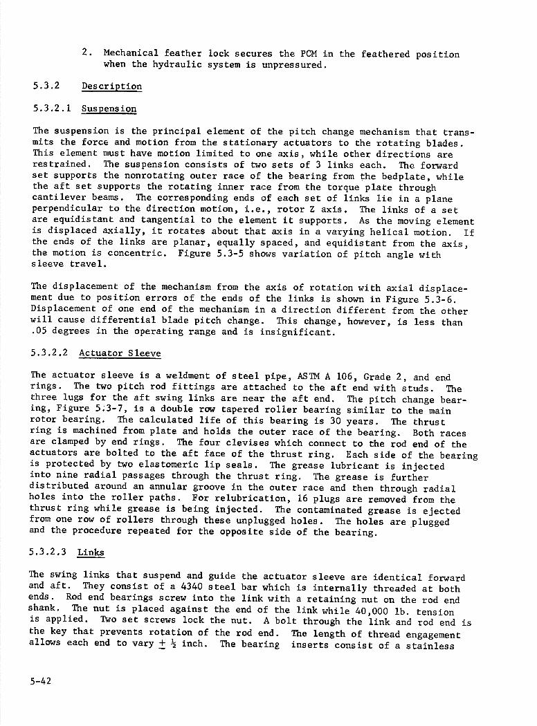
2. Mechanical feather lock secures the PCM in the feathered position when the hydraulic system is unpressured.

5.3.2 Description

5.3.2.1 Suspension

The suspension is the principal element of the pitch change mechanism that trans-mits the force and motion from the stationary actuators to the rotating blades. This element must have motion limited to one axis, while other directions are restrained. The suspension consists of two sets of 3 links each. The forward set supports the nonrotating outer race of the bearing from the bedplate, while the aft set supports the rotating inner race from the torque plate through cantilever beams. The corresponding ends of each set of links lie in a plane perpendicular to the direction motion, i.e., rotor Z axis. The links of a set are equidistant and tangential to the element it supports. As the moving element is displaced axially, it rotates about that axis in a varying helical motion. If the ends of the links are planar, equally spaced, and equidistant from the axis, the motion is concentric. Figure 5.3-5 shows variation of pitch angle with sleeve travel.

The displacement of the mechanism from the axis of rotation with axial displace-ment due to position errors of the ends of the links is shown in Figure 5.3-6. Displacement of one end of the mechanism in a direction different from the other will cause differential blade pitch change. This change, however, is less than .05 degrees in the operating range and is insignificant.

5.3.2.2 Actuator Sleeve

The actuator sleeve is a weldment of steel pipe, ASTM A 106, Grade 2, and end rings. The two pitch rod fittings are attached to the aft end with studs. The three lugs for the aft swing links are near the aft end. The pitch change bear-ing, Figure 5.3-7, is a double row tapered roller bearing similar to the main rotor bearing. The calculated life of this bearing is 30 years. The thrust ring is machined from plate and holds the outer race of the bearing. Both races are clamped by end rings. The four devises which connect to the rod end of the actuators are bolted to the aft face of the thrust ring. Each side of the bearing is protected by two elastomeric lip seals. The grease lubricant is injected into nine radial passages through the thrust ring. The grease is further distributed around an annular groove in the outer race and then through radial holes into the roller paths. For relubrication, 16 plugs are removed from the thrust ring while grease is being injected. The contaminated grease is ejected from one row of rollers through these unplugged holes. The holes are plugged and the procedure repeated for the opposite side of the bearing.

5.3.2.3 Links

The swing links that suspend and guide the actuator sleeve are identical forward and aft. They consist of a 4340 steel bar which is internally threaded at both ends. Rod end bearings screw into the link with a retaining nut on the rod end shank. The nut is placed against the end of the link while 40,000 lb. tension is applied. Two set screws lock the nut. A bolt through the link and rod end is

the key that prevents rotation of the rod end. The length of thread engagement allows each end to vary ± ½ inch. The bearine inserts consist of a stainless

5-42

100

90

80

70 Cl)

60

50

40

30

20

10

1ES

0.5 Cl)

0 z

0.4 El z

0

Cl) H 0.2

0.1

0.6

0 10 20 30

Figure 5.3-5

Blade Pitch Angle va. Sleeve Travel

Figure 5.3-6 Effect of Suspension Tolerances

on Sleeve Displacement

0.625 in.) OUT OF ( PLANE ( ERRORS

0.250 in.J

—0.625 in.

----4 40

IN PLANE ERROR

SLEEVE TRAVEL- INCHES

5-43

Shim

Inner Race

Seals

Housing

INE

Figure 5.3-7 Pitch Change Bearing

5-44

steel ball turning in a woven TFE liner. These bearings require no lubrication. Maintenance consists of periodic inspection for wear.

The pitch rods consist of 4340 steel bar with internal threads, different at each end. The end of the rod at the actuator sleeve receives a differential threaded nut into which a rod end bearing is threaded.

The length of each rod may be varied by half turns of the differential nut. The threads are preloaded in tension by jack bolts between the differential nut and the link and rod ends. The adjustment of the rod length allows each blade to be adjusted over approximately 3.8 degrees in 0.14 degree increments from inside the nacelle. The aft end of the pitch rod inside the hub is similar except that there is no differential nut.

5.3.2.4 Instrumentation

Operational Data Acquisition System (ODAS) instrumentation related to the Pitch

Control Mechanism includes:

1. (Blade) Pitch Angle No. 1 and No. 2. An RVDT at the attachment of. two forward swing links to the bedplate measures the position of the swing link, which is calibrated to blade pitch angle.

2. Pitch Change Bearing Vibration. A single accelerometer installed on the thrust ring with its sensitive axis skewed in the plane of the bearing.

3. Feather Latch Position. A switch to indicate the position of the

feather latch.

Engineering Data Acquisition System (EDAS) instrumentation includes:

1. Pitch Rods 1 & 2 Strain Gauges

2. Pitch Change Bearing Temperature TC probe on the inner race.

5.3.2.5 Pitch Control Mechanism Analysis

A schematic of the pitch control mechanism is shown in Figure 5.3-1 . The pitch control mechanism consists of statically-determinant components; stress margins and stiffness have been determined by means of conservative hand calcu-lations employing standard classical methods of analysis. The system was broken into several smaller sections; each of these sections was analyzed separately to determine their capability to withstand the loading environments.

The detailed analysis of the PCM system shows that the critical design criteria is the compliance of the system rather than strength. The stress requirements

are:

1. Fatigue stress below the endurance limit of the material and weld

category.

2. Meet all structural requirements per the AISC code under maximum operating pressure in the actuators reached by a single jammed blade

5-45

retention bearing. This condition exceeds peak operating loads.

3. The critical design loads used in the analysis of the individual components of the pitch control mechanism were derived from "Design Loads Definition" Appendix B to this report. For pressurized components, a proof ultimate loading of 6000 psi was used.

Results

The analysis of the pitch control mechanism shows that all the substructures meet the specified compliance, and the strength requirements of the AISC code, including fatigue for 30 years of life.

Figure 5.3-8 summarizes the system compliance analysis, and Table 5.3-1 summarizes those components with Minimum Margins of Safety, none of which is negative.

5-46

upj ia no - UT13 uoua 3PI

0 qnH

-I

'-I

0 JE4S tTL qnH

u11Ba ui

a[ idpy

sni a Td iadpy

sau P'1Td

spu po io:n:ov

poj UOSTd 1OBflJ,3'q

Uj 1flo —.. uT1a 9A3 9°Td

uiia "TS 41d C..'

9A9IS 4Ud

k(quiassy Utd UflON 4DId

) UV1 4Td0

SPU3 pO )I UTI tP1Td

UflON 4Td

ui13q uopuaaj ap0

I I •I C.,, 0 - 0 c-i - -. - .- C 0

_OI X SWI/MI —'- 3NVI1dWOD WaTSAS

a) C)

1

ii '.-1

E Lfl 0

0 0"-4

N c-I C C)

a) 0 0

0 0'

C) 0 -'-4

0 '-I .4-i

0C 0 -'-4

.4-4

-'-4

-1 4-i

0 0 0 4-4

C a) c-I C 0 0 0-

0

C

0 c-I Lr 0a) '-I

-'-4

C..' C 0

5-47

Table 5.3-1

Pitch Change Mechanism Summary of Minimum

Margins of Safety

Part DescriptionCritical Stress

Allowable Stress

M.S. (+)

1. Pitch Links (As a Column) 21,224 psi 32,185 psi +.52

2. Pitch Link to Actuator Sleeve Attachment Lugs A. Pin Bearing 28,880 32,400 +.12

3. Cantilever Support Beam A. Arm

I) Fatigue 4,400 15,000 +2.4 2) Limit 20,000 22,800 +.l4

B. Clevis 1) Bearing (Y direction) 20,714 34,200 +.65

C. Base Plate bolts 1) Bending (Limit Fatigue) 57,176 90,000 +.57

4. Swing Link to Actuator Sleeve 8,267 21,000 +1.5 Attachments

5. Rotating SwingLinks 28,648 74,619 +1.6

6. Actuator Sleeve A. Upper Lip 27,874 30,400 +.09

7. Thrust Ring A. Stationary Ring Lug

1) Limit 20,100 22,800 +.l2 B. Dowel Pin- Shear Limit 9,817 12,900 +.3l C. Actuator Lug Bolts 46,577 90,000 +.93 D. Actuator-Thrusting Lug

1) Bending 11,917 22,800 +.91 E. Actuator 308,000 lbs Pa=3X lO6 lbs +11.5 H. Pin in Stationary Lug

(Thrusting) 99,050 psi 160,000 psi +.62 Tens ion

8. Pitch Link Rotor Blade Mt. A. Top Plate

1) Bearing Horizontal Load 34,200 34,200 +0 B. Bottom Plate Tension 9,661 17,100 +.77

Vertical Load

5-48

5.4 DRIVE TRAIN

5.4.1 REQUIREMENTS

The function of the drive train is to transmit the power developed by the rotor to the generator. Specific requirements, including those of NASA defined in the SOW, as well as changes caused by uprating, are listed below.

1. Input speed 34.7 rpm

2. Output speed 1800 rpm

3. Fixed gear ratio

4. 30-year life (except for some gearbox components that require replacement at approximately 10-year intervals).

5. Startup and operation at -31°F to 120°F

6. Input power 2,945 hp

7. Maximum overload condition 5,520 hp (1,500 cycles in 30 years)

8. Minimum running efficiency 967

9. Provide a slip clutch on the high speed drive shaft to protect the drive train from electrical faults.

10. Provide a rotor brake on the high speed drive shaft.

11. Maximum breakaway torque 45,000 in-lb. at the low speed shaft

12. Provide a 6 in. diameter hole through low speed shaft for rotor to slip ring cable passage.

13. Torsional stiffness, off-line 3.5P.

By definition, the drive train begins with the rotor tail shaft and the mating flange on the low speed shaft, continues through the gearbox, slip clutch, and ends at the interface between the high speed shaft and the generator. Included in the definition is the rotor brake and the lubrication/cooling system.

In mid-1977, it was ascertained that the 1,500 kW rating originally specified could be uprated to 2,000 kW. Since the gearbox design, material procurement and fabrication had already been started, an evaluation of the 1,500 kW design at the increased power was made. At the higher power rating, three gears have a calculated life of 10 years, two of 15 years, and 8 bearings have calculated lives between 15 and 22 years. Thus, by calculation, the gearbox has less than the 30-year life originally required; therefore, the condition of the gearbox must be monitored for wear and/or failure after 10 years of operation. Component

5-49

replacement, when required, will permit continued operation of the gearbox at the uprated power to provide a 30-year life.

The low and high speed shafts are not significantly affected by the increased power because they were originally designed to a mean of 2,209 hp and a ± 337.. alternating load. Updated analyses indicate that the alternating load is only

107., thus the net increase in peak loading seen by the shafts is only 107.. A fatigue stress analysis (using very conservative allowables) shows the low speed shaft and the high speed shaft to have positive margins of safety.

The rotor brake design criteria is as follows:

1. Brake from rotor speed of 5 rpm to zero

2. 100,000 braking cycles

3. Static torque capability of 1127. at 2,000 kW rating (was 1507. for 1,500 kW)

It was further assumed as a design criteria that the rotor blades would be feathered but would provide no aerodynamic braking.

The design criteria for the slip clutch is as follows:

1. Speed 1,800 rpm

2. Torque 8,212 ft-lbs

3. Slip Torque 15,400 ft-lbs (1.88 x rated torque)

The design criteria for the low speed shaft is as follows:

1. Speed

34.7 rpm

2. Rated Torque

442,000 ft-lbs

3. Max. Overload

995,000 ft-lbs (1.88 x 1.2 S.F. x rated torque)

5.4.2 DESIGN DESCRIPTION

5.4.2.1 Floating Shaft Assembly (Low Speed)

Connecting the rotor to the gearbox is a floating shaft assembly, consisting of a drive shaft with flexible couplings mounted on each end. This assembly is of a type available from several coupling manufacturers as a standard pro-duct line. Flexible gear hubs are mounted on each end of the drive shaft and mate with a rigid flange on the rotor and a rigid hub on the gearbox, allowing the shaft to float and accommodate angular and lateral misalignments as well. as axial float. The assembly is shown in Figure 5.4-1 (Drawing l32D6268). The angular misalignment is limited to 1/2 degree per engagement plus a parallel off set of 0.50 inch. The gears are designed with a crown to accommodate these conditions.

5-50

I4JI

'-I

.j.

L1

w

'-I

I

5-51

The gear coupling at the rotor end is a modification of a standard design because of the special mounting flange with scallops to clear the pitch change mechanism. At the gearbox end, however, the coupling is of standard design and is mounted on the gearbox stub shaft. A nonstandard feature is the internal seal to prevent lubricating grease from entering the internal shaft bore. The Sier Bath Gear Co. of North Bergen, NJ, was selected to design and manufacture this shaft assembly.

The drive shaft is shown in Figure 5.4-2 (Drawing 163C5353). The ends ar' tapered to permit hydraulic mounting or removal of coupling hubs. An inter-ference fit of approximately 0.002 inch per inch diameter will permit full torque transfer without the stress concentration of a keyway. The 15-inch outside diameter shown provides a stiffness that results in a first torsional frequency for the entire drive train of 3.5P, off-line (12.72 r/s, 2.02 Hz).

5.4.2.2. Speed Increaser Gearbox

The gearbox is a three-stage, tandem articulated, parallel shaft gearbox with input and output shafts on a vertical centerline, and horizontal casing splits. The tandem articulated shafts permit the load path to be split with equal sharing of the load. The manufacturer is Philadelphia Gear Corporation of King of Prussia, PA. The envelope and external features are shown in Figure 5.4-3 (Drawing 132D6275). The gearing is designed for strength and durability for 30-year life to AGMA specifications with periodic maintenance.

The low speed stub shaft is tapered for keyless mounting and hydraulic removal of a rigid hub and has a 6-inch internal bore for passage of cables from the rotor to a slipring assembly, which is bolted to the face of the shaft exten-sion on the upwind side of the gearbox. The slipring stator is supported by a bracket on the gearbox casing.

Bearings and gears are lubricated by an electric pump-driven spray system. The pump has sufficient excess capacity to supply lubricating oil to the rotor bearing. The gearbox incorporates internal heaters in the sump for startup under ambient conditions of low temperatures.

There is an oil cooler external to the nacelle that cools the lubricating oil when operating a high temperature.

The gearbox third stage is designed with a casing split horizontally at the center line of the third stage shafts. This is intended to facilitate a change in the third stage speed ratio by installing a different set of pinions. The upper casing section can be lifted so the pinion can be replaced on site. This feature allows a speed adjustment of up to 107. to correct for any undesirable frequency placement that may be defined when operation begins at the site.

5.4.2.3. High Speed Shaft Assembly

The high speed shaft assembly includes the high speed brake disk, a slip clutch and a floating shaft that connects the speed increaser gearbox to the generator. A toothed wheel bolts to one face of the rotor brake disk; it provides the means to sense the rotational speed of the shaft electromagnetically. A hydraulically

5-52

44

t*I

- tQ

] qJ T

/Ak

Cl)

Cl)

cJ C;1

.r.l

-4

'u

z1

5-53

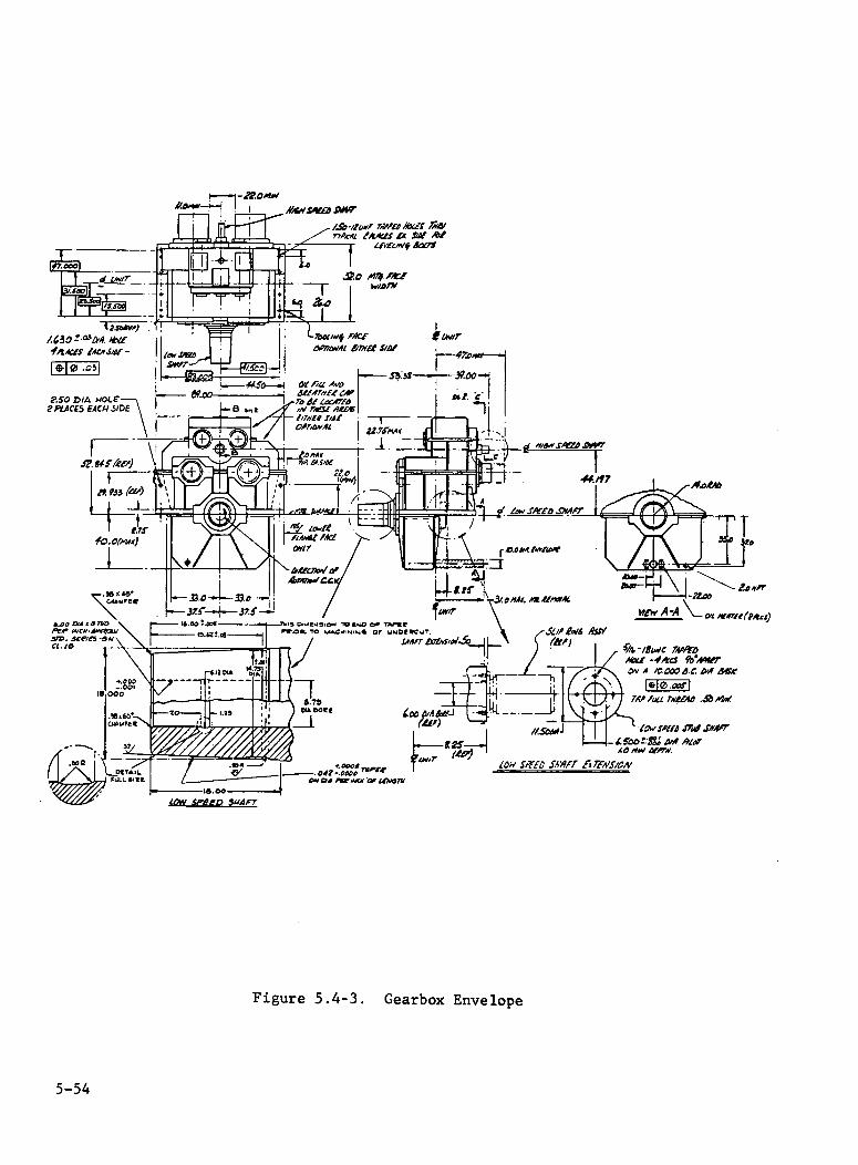
I_co 44'f3 i$ ?At-41 IWS £4 .I1 I

47

.O I.vr1t:F

zIt

- -bclw4 MI( awr Af1 £iw 1/.Of

47o.v-4

______ I e1 qrMfe 4° fTh 51 ciA7FO

- 1,)1 S,iI

- i --irT1kkJ--

1wt1

I '1M41 fl

\

—_- Mat. a* ¶W,Y \

Ot0.o. ¶0 I.D .

,,w A A \\_

OL

pelo re c*,... or oewc ASW £*AFT tb.tI

Hf -istwc A'cij .4.ç fbqQr

________I i' ,4 \ ______ ___i._ -

Thw -\ S.7b

/ 0A#0F

(51,)

- foot sgq q' 40 .m' flW.

t000s IOh STE 54/7 *$,*/

O* Dd **CN FU)151W

3o± 4tif

1#is lACiVJ4f -

II .°J

2.ffO DIA HOLE 2P1.AC(5 EACH5IDE

B

.4?.

19 933 ,i')

1 10. 0(1.141)

. ,(4•

-

.00 i K87WO

16.00 .xc P lC.4'(W

3m. Me,,5 -5*1..

R I'ri

LOW SPEEb 5W4FT

Figure 5.4-3. Gearbox Envelope

5-54

operated brake caliper is mounted from a bracket on the gearbox casing. The slip clutch provides overload protection for the entire drive train by slipping when torque exceeds l887 of rated torque, or 15,400 ft-lb. The slip clutch is the dry type with metallic friction plates, adjustable for torque level by means of adjusting bolts. Figure 5.4-4 shows the high speed shaft assembly less the

rotor brake disk.

The two flexible half couplings, separated by a floating spacer shaft, accomo-date both angular and offset misalignment between the gearbox and generator. Thrust plates and buttons on the spacer limit axial float. This is a common optional variation on couplings of this type, used when axial float must be limited because of the lack of thrust capability in the generator bearings. The spacer is removable by unbolting flanges at each end. Removing the spacer also permits access for removal of the other coupling components, including the clutch.

5.4.2.4 Rotor Brake

The brake used to bring the rotor to a stop and position the blades in a 3 - 9 o'clock position, consists of a stainless steel disk mounted on the high speed shaft and a hydraulically operated brake caliper attached to the gearbox housing. The brake caliper is a stmdard unit made by the Goodyear Corporation, Berea, Kentucky, for off-road vehicles, and is shown in Figure 5.4-5. The brake disk was made from stainless steel to avoid the possibility of irregular operation caused by rust build up during non-operating periods, as experienced on Mod 0.

The brake caliper is operated from an accumulator charged by the yaw drive hydraulic supply: Nominal pressure is 1300 psi and minimum 1000 psi. The brake torque is given by:

T = (Arp

where ,A<..= coefficient of friction = .21 A = total piston area = 24 in2 r = effective moment arm = 1 ft. p = brake pressure = 1000 psi

T = .21 x 24 x 1 x 1000

= 5240 ft-lb

This torque is well below the setting on the slip clutch, 15,440 ft-lb so that inadvertant brake operation cannot overload drive train components.

The kinetic energy dissipated by the brake in bringing it to a stop from 5 rpm (.523 radians/sec) is

K.E = I&2/2

2211 x i0 x (.523)2 /2

= 301,000 ft-lb.

5-55

I- -LI •1

U U) r1

a)

U) U) a)

I 4 It-I

a)

114

5-56

14

14 w

I-'

0

a)

In

4 In

a) 14

14

5-57

Although the published value for continuous operation without degradation is only 133,500 ft-lb., this value is based on a very conservative temperature rise of 8°F. If operation is intermittent (adequate cooling time between applications) and the disk temperature is allowed to rise 50°F, 327,000 ft-lb of energy can be dissipated. When the energy level exceeds 3 x 106 ft-lb, brake operation remains normal, although some reduction in brake life may occur. At higher energy levels, brake effectiveness will be lost, but not catastrophically. The limit is reached when the brake disk overheats and permanently distorts. Tests performed with this brake by General Electric's Locomotive Products Department showed that over 12 x 106 ft-lb could be dis-sipated in an emergency. Allowing for te smaller disk diameter used in these tests, it is estimated that over 20 x 10 ft-lb could be absorbed in an emer-gency shutdown of the wind turbine. This corresponds to a rotor speed of 61 rpm or 64% overspeed.

During normal operation, the time to come to a stop from 5 rpm will be:

t = I& where N = speed ratio TN

= 2211 x 1O3 x .523 / 5240 x 52

= 4.2 seconds

During this time the blade would travel 120°.

The static holding torque of the brake will be higher than the dynamic torque by virtue of the coefficient of friction (0.3 versus 0.21).

T = .3 x 24 x 1 x 1300

= 9350 ft-lb

This corresponds to 114% of rated tàrque.

5.4.3 DRIVE TRAIN MAINTENANCE

The drive train will be assembled, aligned and tested before it is shipped to the operational site. Although all components are designed for a 30-year life, provisions have been made to replace components without the need of removing the rotor or nacelle from the tower.

The gear couplings on both the low speed and high speed shaft are lubricated with grease and they will require relubrication annually. Grease fittings are provided in each coupling.

The lubricating oil in the gearbox requires only periodic checking, and the oil must be replaced only when it becomes contaminated. The sump heaters are mounted in a glycol-filled well and can be replaced without loss of lubricating oil.

5-58

The brake on the high speed shaft will require periodic inspection to measure wear. Although anticipated wear rates are low, replacement of brake pads can be done routinely, and even replacement of the brake disk is relatively simple. Inspection of the brake will include examination of hydraulic connections and

seals for indication of fluid leakage.

All components of the drive train except as previously noted are designed for a 30-year life, using conservative criteria that are standard for industrial components. Wear points are gear teeth and bearings. Gear durability is based on American Gear Manufacturers Association (AGMA) specifications, which pro-vide for stress levels below endurance limits. The gear couplings will benefit by operating at less than maximum misalignment limits under normal operation. Similarly, bearing life is based on conservative Anti-Friction Bearing Manufac-

turers Association (AFBMA) criteria.

Overload conditions that cause torques reaching 1.88 times rated values are expected to occur only infrequently. Under these conditions, stress levels throughout the drive train remain below yield so that no permanent damage will be incurred. The drive train is protected against overload torques by. the slip clutch in the high speed shaft assembly should torques exceed 1.88 rated.

5.4.4 DRIVE TRAIN STRESS ANALYSIS

All components of the drive train were analyzed for stresses at peak loading and for fatigue. Detailed analyses were performed of the gear teeth in the low speed shaft coupling by the supplier, Sier-Bath, and Philadelphia Gear Corporation used their proprietary computer codes to check strength and dura-bility of the gears in the gearbox. Critical sections in the drive train occur at the couplings on the load speed shaft. Further discussion of the stresses in these areas follows; in all other areas positive margins of safety of 50% or more were calculated by conservative analysis or were judged adequate by

inspection.

Where the coupling hubs are installed by interference fit on the low speed shaft, the first concern is that the contact pressure between hub and shaft is sufficient to transmit the design torque of 995,000 ft-lb., which includes

a 1.20 safety factor. The contact pressure is given by:

2T .17d2L/(.

where T = torque (in-lb)

d = diameter of fit = (14.978 + 14.309) x 1/2 = 14.644 in.

L = length of contact = 15.62 - .38 = 15.34 in.

,.Lt 0.2

5-59

The use of 0.2 for coefficient of friction is appropriate for carefully degreased surfaces. Substitution yields

p = 11,600 psi

The interference fit required to achieve this pressure can be computed using Birine's equations:

r ' rc 1-i) rI.c_>.J

E LI - eJ E L ,-where = diametrical interference

E = elastic modulus

= Poisson's ratio

c inside diameter outside diameter

are subscripts referring to outer ring (hub) and inner ring (shafts respectively

where E e = E , =

___ = 2_. r 1Ce1 ._ /t 6 Li e 2 I ..Z

for ce = 14.644 ,and. c = 5.75__ 23.5 14.644

= .0206 in.

The actual interference fit was obtained by heating the hub to a temperature of 300°F, or a differential temperature of 230°F, which provided approximately 10 mils clearance over a cold fit up. The hub was then moved axially a measured distance of .495 inches, corresponding to the correct interference fit on the conical surfaces having a taper of .0418 in/in.

The hoop stress in the hub at its bore can be computed by Lame's equation:

c = __

= 25,200 psi

5-60

This stress occurs in a 4140 steel hub having a minimum tensile yield strength of 132,000 psi, providing a very large margin of safety. Similarly, the hoop stress (compressive) in the shaft due to the interference fit, occurring at the bore, is 27,400 psi in a 4340 steel having a minimum tensile strength of 140,000 psi.

The critical section for the shaft is just beyond the hub where compressive hoop stresses are absent and f&tigue cracks can propagate. At this section, the torque at rated power of 2945 hp and 34.7 rpm is:

T = 63025P n

= 5.30 x 106 in-lb

The torsional shear stress is

2' = = l6Td0

J • (d 4 - d4)

= 8200 psi

Assuming an alternating load of 107 rated load, the maximum stress is 10,000 psi and the stress ratio R = .82. Bending stress due to the weight of the shaft will combine with torsional stresses; however, at the ends of the shaft these stresses are negligible.

In order to compute a margin of safety in fatigue, it is first necessary to com-pute an allowable alternating shear stress based on bending fatigue data, and apply appropriate stress reduction factors. The allowable tensile fatigue stress for unnotched 4340 steel at R = .82 and 108 cycles is 15,000 psi, corresponding to an alternating shear stress (one-half of the stress range) of 8667 psi. The factors to be applied are

kR = reliability factor = .76 (This factor relates the average value from test data to the 3 a- value normally used for design)

k = size factor = .6 (This factor relates test data for small diameter speci-mens to the 15 in. shaft diameter)

= surface finish factor = .9 (Appropriate for ground surface)

kT = shrink fit concentration factor = .57

kf = fretting factor = .5

5-61

The result is a combined factor k = .117, giving a reduced allowable of = 1010 psi, and a margin of safety:

MS = - 1 = +.23

Although this margin of safety may appear to be low, it is based on very conservative assumptions in both the loading and allowable stress. A similar fatigue analysis of the high speed shaft shows a margin of safety of +2.18.

5.4.5 DRIVE TRAIN STIFFNESS SENSITIVITY ANALYSIS

A sensitivity analysis was performed to assess the off-line torsional frequency of the drive train and to evaluate the effect on this frequency of critical system parameters (e.g. gearbox stiffness, generator inertia, and coupling stiffnesses and inertias). The baseline model was selected to represent the dynamic model used to calculate dynamic loads. The critical parameters were varied individually and the resulting frequencies evaluated. The analysis results indicated that the gearbox stiffness and the generator inertia have the greatest influences on the system frequency. It was also determined that if the gearbox stiffness is reduced from 8.62 x 108 in-ib/rad to 2.155 x 108 (757o drop), the off-line torsional frequency will reduce from 3.9P to 2.8P.

The drive train was modeled as a lumped mass and spring system to enable several iterations of model configurations to be evaluated in a convenient and economical manner. This model, shown in Figure 5.4-6, contained inertia representations for the blades, low-speed shaft coupling, gearbox and brake, high-speed shaft slip and flex couplings, and the generator. Inertia values were calculated based on the latest available drawings of the various compo-nents and from vendor data. Spring data were obtained in a similar manner and are listed along with the inertia data in Table 5.4-1.

In each case, the parameter of interest was varied to obtain its sole affect on the system torsional frequency.' All the other baseline model parameters were held constant while the parameter being examined was modified. These mod-ified values were divided by their baseline value to obtain a "parameter ratio". This ratio was used as the scale on the horizontal axis of the sensitivity anal-ysis graph in Figure 5.4-7. The new resulting first torsional frequency was divided, by the baselihe first torsional frequency (i.e., 3.255 cycles/rev.) to obtain the frequency ratio which was used as the scale on the vertical axis of the graph.

5-62

04J

2

4.280/A

4.'4 DIA

FLEX COUpL/frJ

SHAFT /5"

1.0. "

£.750iA

LOW SPEO COLJPUAI4 EIBOX

SLIP COt.JPL/A/

Figure 5.4-6. Baseline Drive Train Model

Table 5.4-1. Baseline Model Value

Values referenced to low speed shaft:

• Total Blade Inertia 1.721 x i0 7 in-lb sec2

• Overall Low Speed Stiffness 9.0 x l0 in-ib/rad

Coupling Inertia 1046.0 in-lb sec2

• Gearbox Stiffness 3.38 x 108 in-lb/rad

Inertia 105,500 in-lb sec

Values referenced to high speed shaft:

• Overall High Speed Stiffness 1.0 x i0 in-lb/rad

Slip Coupling Inertia 57.5 in-lb sec2

• High Speed Flex Stiffness 1.0 x 108 in-lb/rad

Coupling Inertia 5.95 in-lb sec2

• Generator Inertia 474.0 in-lb sec2

5-63

u-I

c..l

,-' __ '-I 0 .-4

0

.;

I '__ '_,

Io .4

jO

—I .-

Il-s

0

4' (I)

00

1-4 00

CO ..-1

CO

'—I

9-4

r4 .1-i

9-I

CO

4' Cl)

CO

CO

4'

4-I 4-4

9-I

Cl)

r-

4)

s-I

--I r14

-1 0 0% 00 .4 .40

opu uanb.t 1UU014.tOL

5-64

5.5 NACELLE

5.5.1 BEDPLATE AND FAIRING

5.5.1.1 RequirementS

The bedplate supports the rotor and transfers all loads to the tower through the yaw bearing and yaw structure. Its stiffness must be such that, when attached to the tower, tower bending modes satisfy the requirements for fre-quency placement as discussed in Section 2. The bedplate must also provide a stiff foundation for all equipment mounted in the nacelle, particularly sufficiently stiff in bending to limit misalignment of the drive train under loading to the capabilities of the shaft couplings. A further stiffness re-quirement is that deflections at the yaw bearing should not severely degrade bearing life or induce large friction torques; this requirement is of the order of .010 to .020 inch maximum deflection out of plane under maximum loading.

The stress criteria for the bedplate are dictated by the NASA Statement of Work and the AISC code. Critical conditions are those which occur frequently cover-ing a range of operating wind speeds, inflow and gust dispersion (Case A). For these loadings, stress levels must be maintained below the fatigue stress limits defined by Appendix B of the AISC code. Maximum loads are defined by the peak loads of Case B, up and down gust, from 35 to 50 and 35 to 20 mph. Application of the AISC code to the bedplate design represents a conservative approach that

will provide adequate Margins of Safety.

The nacelle fairing is not treated as primary structure and is not subjected to the same dynamic loading as the bedplate. Criteria for design of the fairing follows standard commercial practice and is based on loading at maximum wind conditions. No permanent deformation is permitted at maximum loads (limit loads)

and no failure allowed at 1.5 times design loads.

The NASA SOW requires the following provisions of the nacelle bedplate and

fair ing:

1. Provide environmental protection for equipment mounted in the nacelle.

2. Allow access from the top of the tower for maintenance.

3. Permit placement of equipment within the nacelle to locate the center of gravity on the tower axis.

4. Lightning protection.

5. Ventilation of the interior.

6. Exterior paint as defined by NASA.

7. Interior lights, convenience outlets and intercom.

5-65

A further design requirement for the bedplate and the fairing is that pro-visions be included for access to all components for maintenance and removal, even though components may be capable of a 30-year life without replacement.

5.5.1.2 Design Definition

The bedplate is defined by the assembly of Figure 5.5-1 (Drawing 298E460) and consists of several major subassemblies; a forward section shown in Figure 5.5-2 (Drawing 298E47l), and Figure 5.5-3, an aft section (Drawing 298E472) and a rotor adapter structure Figure 5.5-4 (Drawing 298E473). The base section is built up from plate and standard structural shapes to form a rectangular box. Transverse members distribute the principal loads to the yaw bearing structure and allow for interruption of longitudinal beams to accomodate the gearbox. A hatch through the base permits access to the nacelle from the upper level of the tower. At the forward end, members support the generator and associated equip-ment. The rotor support adapter provides a transition from the circular bearing to the square section of the base section. Local stiffness is provided around the bearing bolting surface to limit out-of-plane deflections.

The fairing assembly is made up of five flat panels (four walls and a roof) that are bolted at the edges to form a rigid enclosure for the nacelle. Construction consists of frame-stiffened skins with thermal insulation between framing members. Joints are sealed by the use of elastomeric tape between faying surfaces. The roof may be removed as a unit to permit access to the nacelle for replacement of major components such as the gearbox or generator.

The bedplate supports and interfaces with all equipment mounted in the nacelle. However, the critical interfaces are those with major subsystems, including:

1. Rotor assembly

2. Pitch control mechanism

3. Yaw Structure

4. Fairing

5. Gearbox

6. Generator

The rotor interface is through the rotor bearing adapter structure, as shown in Figure 5.5-5 (Drawing 298E456). The rotor bearing housing bolts directly to the structure and the alignmeit of therotor is determined entirely by the square-ness of this surface with the remainder of the bedplate structure.

The pitch control mechanism interfaces with the bedplate structure at four clevis fittings on the rotor adapter. At these points, the pitch control actuator thrusts

•are reacted directly into the rotor bearing. The forward swing links that sup-port the pitch change mechanism and react out-of-line thrusts from the actuators, are supported at three clevis fittings, shown in Section C-C of Figure 5.5-5.

5-66

rniI•iJIiiiiii __

w fl .iiH IIIi - I__

IL -iII IIdj I

270 's 2'I r#10

-+z

3F (.&) \ ,- ,/OTE 3

RE / L

RF StE A/0TE_L 20jJ

(SEE orE/1P,t/ v'6L1 I \SE1 E74'L L

20 DEc

—1

L — ---H

______ I

SPD TI L I

RO1OR —' YAW lN1RFA(E -j' REE €AL N I 7)-" RTERACE

/ O"°

3i0( v,w / t..' Aj 'SFE M

Figure 5.5-1. Bedplate Definition

5-67

B 0

.1-I

0

I-I

4J 4-4

11;

In

w

5-68

rt

3iT II q

—\,.---- :1

4i!- ;____

I ' I\ '

t___.__. I - ' - ' - I

-. ____________

II!J '+ç, __ ____

J, rç r

____ -1 ______L<' : -

" L> + + +. . I L ____________ ______________

_-1i r'_Et I---i

0 "-4

C)

Q)

C/)

a,

.1-I

Cj .-1

a,

It

L(1

a)

"-4

5-69

fl

a) 1.4

ci

1.4

c/

1.4

a)

0.

Ii

0

0

1 Il-I

I'-)

a) s-I

..4

C r

5-70

rJ

I L -

J1il I I a

9 !! $ i I j ri a za

t__: -

—r

I 13

ii

;' I

?'ft t:?1- ::; - '. 4!

+..+;jf$ 2\ --

4)

4) 4-)

s-I

0 .1-i

0

III

4) '-I

bO .,-1

I

5-71

The yaw structure is bolted directly to the bottom face of the bedplate. This face is machined flat and parallel to the gearbox mounting surfaces.

The fairing interfaces with the bedplate around its perimeter as a bolted connection through the sill plates of the fairing.

5.5.1.3 Assembly and Maintenance

The bedplate is comprised of three major subassemblies: a forward section, aft section and rotor adapter structure. Each of these subassemblies is a steel weldment designed in accordance with AISC requirements. Where members are required to be removable for maintenance or replacement of components, they are fastened by bolting.

The most critical alignment in the bedplate assembly is to maintain the mount-ing face of the rotor adapter structure perpendicular with the mounting pads for the gearbox. This alignment will ensure that the rotor assembly, defined by the rotor hub bearing forward face (on the outer bearing race) is perpen-dicular to the low speed shaft of the gearbox. Alignment is obtained by making a final machine cut of the rotor adapter structure after it has been installed to the bedplate. Tolerances on this alignment will result in a change in slope of the drive shaft between the rotor and the gearbox and must be accommodated by the flexible gear coupling halves on the drive shaft. The drive shaft couplings will also permit a certain degree of lateral misalign-ment between the two mounting surfaces; however, this subject is more appro-priately discussed as part of the rotor assembly installation requirements.

Misalignments between the gearbox mounting feet and the low speed stub shaft can be corrected for, to the extent that they are known in advance, by machining the bedplate mounting surfaces. However, the horizontal mounting pads also allow for shimming to reduce this misalignment, if required. Precise grinding is not required; a tolerance of 0.10 inch over the 100-inch diameter of the rotor adapter structure results in a slope error of 1 in 1000. This is well within the anticipated capability of the shaft coupling of 1/2 degree per engage-ment that will be required to accommodate dynamic deformation of the bedplate.

Since the drive shaft couplings can also accept some longitudinal misalignment, tolerances that locate the gearbox with respect to the rotor adapter structure in the longitudinal direction are not critical and will require no final machining of the bedplate assembly.

The fairing assembly will consist of a series of welded panel assemblies that ean be stacked for shipment. After a trial fit during the systems test, the fairing may be broken down for shipment. At the site, the fairing will be assembled by bolting and attached to the bedplate assembly.

Since the bedplate and fairing assemblies are essentially static structures, maintenance will consist of inspection for indications of fatigue cracks, buckling or other deformations, loose fasteners, corrosion, or other damage. It is anticipated that restoration of anticorrosive protection and external painting will be required at intervals from five to ten years.

5-72

5.5.1.4 Bedplate Desi gn Evolution

The final bedplate design differs considerably from the concept originally presented at the Preliminary Design Review. This is a result of a change in the design approach that occurred during the early stages of final design definition. The concept originally presented was a coiiplex truss, composed of standard rolled sections (mostly wide flange beams) of A36 low carbon steel. As the detail design progressed, it became apparnt that this con-cept presented several probiems

1. Weight. The use of standard sections for all members meant that it would not be possible to optimize each member for the design loads. This implied the need to overdesign, resulting in an inefficient, overweight structure.

2. Growth Capability. During the early stages of design, the entire wind turbine design exhibited a steady growth, as each new load analysis resulted in the addition of more structural weight. The use of standard sections required a complete redesign and new geo-metrical arrangement with each load increase.

3. Welded Joint Configurations. The intersection between standard sections defined complex weld joints that would be difficult to weld and inspect. Review of preliminary drawings by consultants at Lehigh University pointed out the difficulty in establishing an appropriate stress concentration factor to apply to such joints in order to design for cyclic loading. Without the benefit of a second order finite element model of each joint configuration, the only option was to assign the lowest allowable range stress speci-fied by AISC requirements. This constituted a severe design pen-alty in attempting to minimize structural weight.

4. Material Selection. Structural steel shapes are widely available in A36 steel. However, if suitable impact strength for low temp-erature operation is required, then testing costs added to A36 steel offset the low cost advantage of this steel as compared with other steels specifically intended for low temperature applications. The use of sheet or plate forms would open the selection to many other classes of steels that are not normally provided as struc-tural shapes.

As a result of these considerations, the bedplate was reconfigured to a box girder type construction, using plate forms for all but a few secondary de-tails. A5l6 Grade 70 steel was chosen, a material with good impact strength at low temperature, and less vulnerable to poor welding characteristics that sometimes occur as a result of the liberal chemical composition limits of A36. The plate design did not reduce the amount of welding required, but more of the welds could be accomplished as a continuous pass and could be categor-ized for higher allowable stresses. Since the configuration more closely resembled the box girder construction commonly used in bridge construction, it became easier to identify the appropriate weld joint category according

5-73

to AISC fatigue requirements (which are based largely on bridge construction). Optimization and design changes could be incorporated more easily by changing only the plate thicknesses without redefining the basic geometry.

5.5.1.5 Life

Failures affecting the life of the bedplate and fairing assemblies are fatigue, cracking and corrosion. The use of conservative strength criteria for these structures ensures that stress levels will remain below endurance limits and infinite fatigue life should be achieved. Periodic inspection of joints and other areas of high stress concentration should identify potential failures before they occur and while the damage is still repairable.

The bedplate structure follows standard practices for prevention of corrosion in steel structures as defined by AISC code. Design details consider the ne-cessity for drainage holes and avoiding enclosed spaces that can collect water or are difficult to protect and inspect. Concealed joints that are likely starting points for crevice corrosion are avoided. Protective coatings include a shop-applied zinc-rich primer and enamel finish coat, with an on site touch up.

5.5.2 LUBRICATION AND ENVIRONMENTAL CONTROL

5.5.2.1 Requirements

The lubrication oil system provides lubricant for the rotor bearing as well as the gearbox. The system is required to maintain a sufficient flow of oil within an acceptable viscosity range of 340 to 5,000 SUS at all operating temperatures. During startup when ambient temperatures are below 55°F, the oil must be heated and circulated before rotation can begin; at oil temperatures above 150°F, the oil must be cooled by circulation through an external cooler.

The heat dissipated in the gearbox and rotor bearing varies with the amount of power generated, which is a function of wind speed. As shown in Figure 5.5-6, the maximum heat dissipated is 147 hp or 374,000 Btuh. The temperature rise through the system, based on a flow rate of 66 gpm is 30.6°F.

The environmental control system, operating in conjunction with the oil lubri-cation system, is required to maintain the air temperature within the nacelle within acceptable limits. The most sensitive equipment within the nacelle is the nacelle multiplexer unit, which must operate within an ambient air temper-ature of 00 to 130°F. The generator draws cooling air from within the nacelle and exhausts externally, utilizing a built-in fan.

5.5.2.2 System Description

The lubrication system is shown scthematically in Figure 5.5-7. The lube oil and ventilation systems have three operational modes that include: startup, normal operation, and shutdown.

5-74

210

200

180

16C z 0 El .< 14C I-I Ct Ct I-I 12( H

10(

8(

6

4

2

EARING

0 .2 .4 .6 .8 1.0 1.2 1.4 1.6 1.8 2.0

PCMER GENERATED M W

Figure 5.5-6. Heat Dissipation

5-75

--

!i •__-.1 • • • . • ••

0 ..-1

cli E a,

C) C/)

E a,

.lJ

CO

C/)

0 '-I .1-i cli C)

1.4

In

a, 1-i

\\ \\\

4; - U

- - -:

r

I

' N

5-76

5.5.2.2.1 Startup

Startup is the interval between shutdown and normal operation during which time the oil is heated or cooled to the operating range of 60°F to 170°F, as measured at the high speed bearing of the gearbox.

(a) Cold Start (oil temperature in sump less than 70°F)

As soon as power is supplied by the utility the gearbox sump heaters and pipe trace heaters are turned on and continue to heat until their respective thermostats register 70°F. When the main lube pump thermostat located in the gearbox sump registers 60°F or greater, the main lube pump and the return pump will start pumping, if CODAS has supplied the enabling power. The main lube pump pumps oil from the sunip to the gearbox and rotor bearing, and the return pump returns the oil from the rotor bearing to the gearbox sump.

When the sensor located in the exit port of the critical high speed bearing in the gearbox registers between 60°F and 170°F, CODAS will

interpret this signal to mean that the lube oil system is ready and capable of providing adequate lubrication to the gearbox and rotor bearing.

(b) Hot Startup (oil temperature in the gearbox reservoir is equal to or greater than 70°F)

The main lube pump and return pump will start pumping as soon as CODAS supplies the enabling power.

When the temperature sensor located in the exit port of the high speed bearing in the gearbox registers between 60°F and 170°F, CODAS will interpret this signal to mean that the lube oil system is ready for operation.

5.5.2.2.2 Normal Operation

Normal operation follows from a successful completion of a startup sequence and continues until a shutdown occurs.

5.5.2.2.3 Shutdown

Shutdown dictated by a lube oil system symptom will occur during startup or normal operation when one of the following signals is received by CODAS:

a. Oil level sensor in the gearbox sump indicates that the running oil level is 10 gallons below the normal value.

b. The high speed bearing sensor in the gearbox indicates that the temperature is less than 60°F or greater than 170°F after startup.

5-77

c. The flow sensor at the inlet to the rotor •bearing registers flow less than 13.5 gpm after the main lube pump has started pumping.

The ventilation system consists of two inlet louvers on the forward face of the nacelle fairing, an exhaust fan with automatic louvers on the aft face of the fairing, and an exhaust duct that carries cooling air from the hood of the generator to the outside. The inlet louvers have fixed vanes and are protected by wire screens. They are sized to accommodate an inlet flow of 10,000 cfm. The exhaust fan is rated at 5,000 cfm and an additional 5,000 cfm is drawn by the generator for cooling. The exhaust fan is thermo-statically controlled to operate when the nacelle temperature exceeds 90°F.

5.5.3 YAW SUBSYSTEM

5.5.3.1 Function and Requirements

The yaw subsystem (YS) functions discussed in this section are at an overall subsystem level. Functions of the individual components of the YS are described in succeeding paragraphs.

The YS primary requirement is to position and align the nacelle assembly with the wind velocity vector. Changes in the wind direction would require the YS to follow the wind by repositioning the nacelle/rotor accordingly. The YS also provides the structural interface and transition between the top of the tower, and the rotating bedplate/nacelle.

During the design effort investigations into various wind cases, plus Mod-0 experience, indicated that structural load amplification would occur if the YS permitted any "free-play" in the rotational drive mechanism. Therefore,

pressure is applied to the brakes at all times: 1,000 psi while yawing, 3,000 psi when no yaw maneuver is taking place.

Another function provided by the YS is automatic relief from rotational over-load conditions that may occur from sudden changes in wind in-flow angles.

Additional design requirements of the YS are:

1. Provide ample stiffness, when attached to the tower and bedplate, so that the stiffness characteristics shall satisfy the frequency placement requirements.

2. Provide stiffness requirement of the primary structural members to limit deflections at the yaw bearing interface to .010 to .020 inch. This deflection prevents degradation of the bearing performance in terms of long life and increased friction torques.

3. Provide support structure for all YS components.

4. Provide manned access for maintenance, repair, installation and removal of all YS components.

5-78

5. Provide ingress/egress for the nacelle.

6. Satisfy AISC, ASTM, AFBMA and AWS requirements.

7. Compliance with NASA SOW:

a. Crossed roller bearing with internal gear

b. Worm drive or hydraulic drive

c. Yaw rate shall not exceed 2°/second

5.5.3.2 Design Description

GE Drawing 47J240701 (Figure 5.5-8) shows the overall yaw subsystems assembly. The basic YS occupies an envelope size of 176 inches in diameter by 93-7/8 inches high. The YS is positioned on the centerline of the tower which estab-lishes the centerline of rotation in a horizontal plane for yaw maneuvers. Positioning the nacelle/rotor assembly by a yaw maneuver is provided by a bull gear/ring bearing driven by two pinion gears at a constant rate of 0.25°/second.

The lower support structure for the bearing, referred to as the lower yaw structure, is provided by an annular ring weldment that attaches to the top of the tower. This ring serves to distribute the load reactions from the eight tower supports to the inner race of the yaw bearing, attached via a total of forty-eight 1-1/4 - 7 UNC high strength bolts. The upper flange is extended radially outward to form a circular disk for the yaw brakes to engage.

The upper yaw structure, located above the ring bearing, is also a weldment. The structure attaches to the outer race of the bearing via a total of forty-eight 1-1/4 - 7 UNC high strength bolts. The upper surface of the structure is then bolted to the nacelle bedplate structure. The nacelle, structure and outer bearing race assembly presents an integral configuration that is capable of rotating about the centerline of the tower. The upper structure also sup-ports the. two hydraulic drive motors with a pinion and shaft subassembly, via two individual bearings. These two bearings remove an overhung load condition from the shaft bearings in the hydraulic drive motor. Thus, extended life is gained for these bearings. The output shaft of the hydraulic drive motor is joined to the pinion drive shaft with flexible gear couplings, which are key mounted onto their respective shafts.

The yaw bearing will be manually lubricated using the grease fittings accessible from inside of the yaw structure.

5.5.3.2.1 Yaw Structure

GE Drawing 298E483 (Figure 5.5-9) shows details of the lower support structure for the YS. It is an annular ring weidment that serves to distribute the load reactions from the eight tower support points to the inner race of the yaw bearing. ASTM A516 Grade 70 structural steel is utilized for the fabrication and welding in accordance with Appendix B of the

5-79

5-80

-

I

r

'I

It-1

E a) Cl)

Cl)

E a.) 4)

Cl)

Cl)

Cl)

jI

Il-I

U

00

Il

a:

5-81

41 4 SI

4. t .1

_______ _____--____ _____________ ___________--

___1 4 -

t j4\I

•

(

\

S.

I4 ____

- !11 1- ___ __________

S N 4

4)

C.)

41

4)

ir

In

4)

s-I

tb .5-I

AISC Specification for fatigue loading.

All welded joint preparation, type of welding and heat treating and inspection procedures are in accordance with the Structural Welding Code published by the American Welding Society. Generally, all welding is full penetration using submerged arc technique, ultrasonically inspected and stress relieved prior to final machining.

The annular ring is 166.5 inches in diameter by 25 inches high. One lower flange is bolted to a prepared fitting that terminates the tubular structure at the top of the tower. The upper flange is extended radially outward and machined on both sides to form the disk for the yaw brake. Cap and web thick-nesses that provide the desired section properties were determined by stress analyses shown in paragraph 5.5.6.

A shroud encircles the yaw bearing and serves to retain the bearing grease. The shroud will rotate with the nacelle. A second closure is installed in a horizontal plane at the tower/YS interface. It also serves as a work plat-form for the YS. A hatch is provided in this closure for ingress/egress to and from the nacelle. Neither of the closures are sealed, but will weather protect the YS components and keep birds and animals from entering.

A ladder is provided from the upper section of the tower to reach the door in the lower yaw closure. The YS structure provides an extension of the ladder through to the lower hatch located in the nacelle bedplate.

The hydraulic power system, and controls for the yaw brakes and yaw drive motor, are located in the nacelle.

A cable raceway provides support for electrical cables from the slip ring to the junction boxes at the top of the tower. The cable raceway also serves as the anti-rotational structure that restrains the lower portion of the slip ring assembly in a fixed position.

If a total failure of the YS should occur (i.e., loss of driving, holding and braking pressure), a manually operated pump can be used to pressurize each yaw brake and thus provide the holding power. This feature can be used for emer-gency application and for repair/maintenance services during a normal shutdown period.

GE Drawing 298E48l (Figure 5.5-10) shows the upper support structure for the YS. It is similar to the lower support structure in that it also is a fabri-cated annular ring weidment. Welded joint configurations were also designed in accordance with AISC, ASIM and AWS requirements.

The annular ring is 175.7 inches across the brake support structure by 28.4 inches high. Secondary beams and branches have been welded, drilled and machined to provide the required mounting provisions for the hydraulic drive motor, pinion bearings, yaw brakes, external shield, hydraulic lines, and lubrication lines. (Reference GE brawing 47J240701, Figure 5.5-8).

5-82

-!. I 4.. //i.. Li LT9J KIh í ' '1 a

q

w

C)

4

0 I-I

LI;

a)

5-83

The primary load carrying members are the upper cap-to-bedplate interface and the lower cap-to-yaw bearing interface.

5.5.3.2.2 Yaw Drive Train

All elements that provide the motive power to turn the nacelle about the yaw axis are included under the term "yaw drive train". By extension, the yaw brakes, which provide damping to the yaw drive, and locking forces when the nacelle is at rest, are included in this discussion. The yaw drive train consists of a hydraulic supply (including accessories described below), hy-draulic motors with integral gearbox, splined coupling, drive pinion and bull gear integral with the yaw bearing. Yaw brakes are pressurized by the yaw hydraulic supply, located in the nacelle.

5.5.3.2.3 Yaw Bearing and Mating Pinion

GE Drawing 298E478 (Figure 5.5-11) shows the basic cross section of the crossed roller type bearing with an internal gear. This drawing accompanies Specification 273A64l6 as an outline configuration control document. All critical areas of the bearing design and definition that appear in the Speci-fication 273A64l6 were analyzed and confirmed by Mr. John Rumbarger of Franklin Institute Research Laboratories, a recognized authority in large bearing design.

The major contributor to the final envelope size of the bearing is the gear face size required to accommodate the tangential force that developa the torque necessary to position the nacelle.

The..maximum yaw torque each mot9r is capable of generating is 550,000 ft-lb. or a combined total of 1.1 x lO ft-lb. This driving torque, in combination with the damping torque of 760,000 ft-lb. provided by the yaw brakes, is suff i-cient to overcome the external dynamic torques. In calculating the gear tooth configuration, a torque of 600,000 ft-lb. was assumed.

With the gear pitch diameter at 124 inches, the tangential force requirement is calculated to be 58,064 pounds per pinion. Using the Lewis formula:

FW = IT where SY/DP

FW = Gear face width in inches

TF = Tangential force in pounds

S = Allowable fatigue stress = 48,000 psi ( R = 30, 100,000 cycles)

Y = Form factor for 200 full depth involute tooth pinion = 0.264

DP = Diainetrial pitch = 1.0

Therefore, the FW = 4.58 inches for a single pinion load application. (The yield strength of the gear teeth at R 30 will equal a minimum of 117,000 psi.) Thus there will be a positive margin of safety with the actual face width of 7.00 inches.

5-84

I

I

1!i '1 Jr z

,:•ti I

V I 1JL

! uIi )•i;;!

*1nh

-I -1

In

w

•H

/ 3 (

5-85

As a result of the trade-off involving the parameters shown above, and opti-mizing fatigue characteristics to achieve the long life requirement, a bull gear design incorporating 126 teeth was arrived at. For the pinion, thirteen involute gear teeth were accoinodated on a minimum pinion pitch diameter at 13 inches, with a DP of 1.0. The objective here was to minimize the torque requirements on the pinion drive shaft and subsequent requirements placed on the hydraulic drive motor. Thus, the gear ratio of 9.7 was established for the pinion to bull gear.

5.5.3.2.4 Yaw Brake

The rationale for the use of these brakes is as follows:

1. Locks out backlash (free-play) in the yaw drive train during the static and maneuvering modes. Advantages:

a. Increases stiffness in the yaw direction, thus eliminates dynamic loading of the WTG system.

b. Reduces fatigue loading on the gear teeth of the bearing bull gear and mating pinion gear, thus increasing their design life.

c. Removes fatigue loading on the gears and bearings located in the hydraulic motor, thus increasing their design life.

2. Reduces maximum loads for extreme wind conditions for the entire yaw drive train. Advantages:

a. Assists the hydraulic motors in overcoming peak yaw dynamic torques.

b. Eliminates the need for a safety clutch.

c. Maintains a gear face height that is compatible with the required bearing forging size.

3. Provides a yaw locking feature during maintenance periods.

4. Provides emergency stop.

The yaw brake is defined by CE Drawing 163C5355 (Figure 5.5-12). The cyclic yaw torques, as defined by dynamic analysis, can reach as high as 1.8 x 106 ft-lb. The torque generated by both yaw motors is 1.1 x 10 6 ft-lb. If the polarity of the external yaw torque is in opposition to the driving torque of the motàr, a worst case deficit of 700,000 ft-lb. of torque exists, with the possiblity that the nacelle would be driven, momentarily, counter to the commanded direction of rotation. With 1,000 psi on all brakes, an additional re-tarding torque of 760,000 ft-lb. is provided to oppose the external torque,

5-86

.O4 ?QI

eS I+I.'o8 0/Al

_____

z //

4 AC6$

3.85 I c2:/,::i

'Jo

wjjrx z 71 7V8 F/TT/Ne5

(7,,-2O UNF-2A (Iwlo INLET)

/.SO DISC-

0/SC

,. 9-'c

L4.ot'OJ - __-

L: t- I

£27/

Z. 7C4 -

-&5.o a.ic3'4l.4l A87/7

1 icic

Figure 5.5-12. Yaw Brake

5-87

thus the net torque on the nacelle, with 1,000 psi pressure, is zero, pre-venting a potential regressive motion of the nacelle. Similarly, when the polarity of the external yaw torque is of the same sign as the polarity of the yaw motor driving torque, an excessive torque level can be generated. The retarding torque of the engaged yaw brakes acts as a modifying fac-tor in this respect. It should be remembered that the yaw drive motors rotate at a constant speed. If the external torques should drive the nacelle ahead of the motor, the motor , torque will be reduced to zero, and even pro-vide negative (retarding) torque of up to a maximum of 1.1 x 106 ft-lb. This system has been evaluated with a computer simulation aixi appears satisfactory.

During shutdown periods and non-maneuvering modes, all six brakes are engaged in a static configuration that produces a holding force of 2.1 x i06 ft-lb. at an applied pressure of 3,000 psi.

The selected brake is an off-the-shelf, hydraulic actuated, disk caliper brake manufactured by the Goodyear Corp., Berea, Kentucky. It occupies an envelope size 17 inches long by 10.4 inches wide by 9 inches high. The total weight is approximately 2,000 pounds. This brake has been in service for over four years on 200-ton trucks and earth moving equipment. Clark Equipment Co. and Unit Rig Equipment Co. are the largest users of this brake. Goodyear Corp. has tested the brake with 200,000 on/off cycles at the rate of 3 cycles per minute using 3,000 psi hydraulic pressure without a failure. The brake has been successfully operated at 3,500 psi and pressurized to 8,000 psi in an attempt to burst the piston and/or cylinder housing, without failure. The operating pressure range for the WTG application is 1,000 to 3,500 psi.

5.5.3.2.5 Hydraulic Drive Motor

The requirements for a hydraulic drive motor were established as 55,000 ft-lbs. of torque at 2.5 degrees/second. The selected motor was manufactured by Cham-berlain Industries Limited, Staffa Works, London, England. It is available through a central office at Double A Products Co., Manchester, Michigan, and over 25 distributors throughout the United States. GE Drawing 132D6380 (Figure 5.5-13) is an outline envelope of a GB 1400 Series Staffa Motor. Looking at the left-hand profile view, the double bank of ten cylinders/pistons are iden-tified. In the central portion of the same view, a planetary gear transmission, with a 3.625 ratio, is connected to the output shaft of the Staffa motor. On the extreme right end of the same view, one half of a modified Koppers gear coupling presents the interface that will attach to a mating hub that will con-nect to the pinion shaft shown in Paragraph 5.3.2. The overall size of the GB 1400 motor assembly is approximately 2 feet in diameter by 4 feet long.

Characteristics of Staffa Motors include:

1. High energy conversion efficiency: 94 to 987. overall energy conversion efficiency is attainable in the operating torque and speed range.

2. High starting torques: up to 947. of maximum running torque at dead shaft stall.

5-88

P

IfC A? as ,te

MAcurn, WI5*UON

-PWS5 13A Z(AUA 3uAetAMb ,wsr ,.? at ?*RtCO 09 3C24rC#4(O

ReP DM

Figure 5.5-13. GB 1400 Series Staffa Motor

5-89

3. High reliability and long life due to balanced design and wear compensating sealing rings.

4. Low speed and high torques without the need for additional gearing.

5. Virtually silent operation throughout the speed and torque range.

For this motor, B-b bearing life calculations are based on the formulas pro-vided by the Timken Bearing Co. (Note: B-b life is the number of hours at which 107. of the bearings may be expected to. show some evidence of the end of their useful life.) However, Timken's formulas are intended for more severe operating conditions than normally encountered by hydraulic motors and the duty cycle of the Yaw Subsystem (YS). Experience among the hydraulic equip-ment manufacturing companies indicates that actual bearing life exceeds cal-culated values by a factor of 2 to 3. The YS design discussed in paragraph 5.3.2 removed the side load conditions that would have been seen by the Staffa motor by isolating the pinion on a separate shaft and bearings. Therefore, the B-ic bearing life is estimated to be 18,000 hours. This is based on a speed factor of 10 rpm, the lowest number listed in the speed factor table, for cal-culating bearing life.

Conservative calculation for 1 rpm would equal 70,800 hours of B-lO bearing life. The YS cycle of 30 years is assumed to be 12 minutes/day of operation or a total of 2,200 hours.

5.5.3.2.6 Hydraulic Pressure System

CE Drawing 298E479 (Figure 5.5-14) shows the overall schematic of the hydraulic pressure system. The pressure system depicts commonality in that hydraulic power from a central source is used to service three areas. These areas are: 1) yaw drive motors, 2) yaw brakes, and 3) high speed shaft brake. The require-ments for operating the motors differ from the two-brake systems since a closed loop servo system controls the motor functions, and a displacement fluid system operates both brakes. The operating fluid specifications are compatible for the motor and brakes.

To determine yaw hydraulic system performance over the expected temperature range, a thermal analysis indicates that oil and equipment temperatures less than 0°F can only be reached after prolonged soaking in a below-zero condition. Once the system has been started and is operating, equipment and oil tempera-ture will reach normal condition. To assist the pumps under low temperature conditions, the reservoir has been equipped with a 2 kW heater that will be turned on every time the oil temperature in the reservoir falls below 20°F. The Sundstrand pump is capable of pumping fluid with viscosity as high as 6,000 SSU. The pump and motor can operate with fluid viscosity as low as 100 SSU.

5.5.3.3 Yaw Drive System Stiffness

To evaluate the adequacy of the yaw drive, its stiffness was determined by calculations using the latest design data for the shaft and yaw drive pinion and manufacturer's data for the motor. Motor data included a stiffness value

5-90

'U /i

C)

I.' U

E ci)

C) II Cl)

E ci)

4.1

Cl)

Cl)

ci,

U)

U) ci)

p-I

C)

In

ci)

tILl

5-91

for the gearbox, and geometry and drawings for the remaining items. Using these data a combined or total sum for the system stiffness was calculated.

Figure 5.5-15 represents, in block diagram form, the individual components that make up the entire yaw drive train. The 20 hp electric motor is the prime mover, driving a hydraulic pump. The elastic elements in the pump and motor are their respective shafts and the compressibility of the fluid in the motor. The emf in the electric motor was considered to be a "damping" rather than "spring" force since an induction motor is used, and for that reason emf coupling can be ignored in the stiffness calculation. Anchoring of the electric motor and pump housing to ground is extremely stiff and for this reason it can also be ignored in the calculation. The transmission line contains two elements that contribute to compliance: 1) the compressibility of the fluid, and 2) the strain of the tubing. Compressibility of fluids in the transmission line was lumped together with the fluid in the hydraulic motor and valves, and the fluid in the pump, for compliance calculations. Compliance due to tubing strain was calculated separately, but, as shown in Table 5.5-1 and the attached calculations, it was two orders of magnitude lower than compliance due to compressibility.

HYD. I I GEAR MOTOR r-i

COUPLING __.__ SHAFT

-_-

flow

BULL CEAR

TRMS L.JJ HYD

f_.....4 GEAR J_••J COUPLINCJ........._ SHAFT PINION

ELEC L-J PUMP Nfl Jj LINE MOTOR BOX

Figure 5.5-15. Yaw Drive Block Diagram for Stiffness Analysis

5-92

- N ' N N N '-' c'.i

v-I v-I - 0

- 0. 0 v-I v-I v-I 0 0 - - - 0

.4. 0 0 -I - o o v-

v.4 v-I ,-4 v-I 4 - o

in o N in

c o • C.- • 0 m N • a' F- - r, v-I v-I - m

cv.' N v- a'

v-I cv.' N 0 v-I 0 CO CO

o v-I CO 0 v-I 0 v.4 0 0 - 0 0 v-I r-4 v-I i-I

v-I v-I:4

CO. N C' CO in

CO C' CO 0 • N • CO v-4 • • i-I • N

If., C' N -4 v-I N

. . .-' v vv Cd '0 U v-I - v-I '0 4C Cd '0'0CdId'0 $ Cd '0 .40

I I Cd 1.4 CdCd$4$4Cd -. 1-I Cd s-I • - $-i 1-I -. .. 1-I 0 -.. $4 v-I .,-4

' I .1 v-4 , -. - , ... v-I 0 ... 0 CO C) U.)I-4 ,Ov-4r I v-I U U

'0 '0v-4 v-I v-I $ r-I v-I I I v-I I v-I 0

Cd Cd..-.. I •r-I I I u •r-4 I 04) 1-I -i-I 0 '. v-4 .j-I -4 4 4_J

CO v-I • .CO v4 rI •,-I v-I •,4 -.. '.0 -v-I I -Sc -C '.0 rIC' C' CO v-I '.0 N $4

O I v-I N 0 '-4 0 N 0' 0 0 C' 0 0 CO '.0 0 '-I 0 CO "-4 0 '-1 CO v-I 0 0 v--I -I 0 v-I v-I 0 0 H

v-I 0 '-1 0 v.-1 v-I v-I v-I 0 ZN :4Z:4

0 X :4 0 in '.0 N v-I N .4. Q •v-I N v-I 0 - N '.0 v-I C'.' Ir N C' N 0' 0

• • • • • N v-I N 0 N N .4 N C') v-I N - v-I v-I L14

4) 4) U $4 Cd

4) 0 U v-I $4 C'.' $4

CO 0 4i •v.4 I--I 1.-I Cd .-. 4) E s v-I C'.' I 4.1

4) '-' ..- C/) 'O $4 . •v-IU-4 Cd

0 C'.' U-I 0 1-4 '0 CO Nr4 v-1v-4 Cd .c4

CO --1 v-I4- 4) • Nd) •,-I

'0 1-. -4. -' P4) i Q C'.' ., CO

0 1-i '4-1 4) U Cd -v-I U-, 0 . •v-4 4.1

'-4 -4 '-' Q-i 4) U-i o 01-i Cd $4Cd v-I

o 1-i v-I Cl) 'v-I Cl) v-I '-' 4) U •v-I Cd Cd U 0U-4 Cl) 1-i

UE-4 Cd C)

i-I $4 U

'-414 U

U-I, CdU-4 Cd4.1.00 U

o r-40-I '0 Cl) 'OCI) 4) H Pr-I 0 0 C/)WCd 4)

.r- Z CO HU4.J0 0 0 0 H U U ,C 1-. Cd 0 U 4.1 4) .r-I •v-I .4 •r4 U-I U-Icl)0$4 , •j4 ,4JU-4 $4OCO Cl) U) UI 1-i Cd CdCdU'O v-I ,0 v-IUICd QCdCdU$4 $4 1-1 1-1 Cd

, •v-I,0 0,-I0 0 0 0 4) ci c,ci CO El COP-icn l-40P-iOEl El H H

$4 4.1 14 0 1-I O U 0 U 0 o o z•-I

Cl) U C/)4) C) CO v-I -.$4 CO

-v-I •.-I v-I $4 E 0 U -v-I U UI Cd ,0 •,4C) v-I U 0 U 0.. 14 1-i U-I •,-I O E '0 Cd Cd '-I $4•r-I 0 04.1 0 , -v-I CO P- E-- 0 C/) 0 ci.' P-i

$40

U

4) 4) .- -I

-I U-I - ..-I

a- o U --I U o C, -• Cd

Cl) U

0

0

g

'.4 C-)

4)

0

-'-4 Z

'-4

U-I 0

Cl) 4)

-4

Cd

Cl)

4)

U-I '4-4

U C/)

-I

If.'

4)

C" H

U .r4 v-I

Cd 1-I

'0

--I

'0 4)

'0

v-I U

UI --I

4)

.'-I -4

0 "-I

0)

Cl) -v-I

a 0)

Cd 1-i 4)

Cd

0..

0..

-'-I

'0 -,-1

-4

ti-I

U-I

0

-'-4 4)

-r4 U-I -v-I -v-I 0)0) 41 1-114 EU 00 QE -3'

5-93

The hydraulic motor contains three major compliance contributors: compres-sibility of the fluid trapped in the motor, strain of piston and cylinder, and shaft compliance.

In calculating the effect of compressibility of the fluid in the motor, only 307 of the swept volume of the motor was included, since at any one time only five of the ten pistons are being pressurized, and these are at various stroke positions, such that the resulting "live" piston volume is a maximum of 3O7 of swept volume. To this value is added the amount of fluid trapped in the five (of ten) internal feed lines between valve and pistons. In calculating the effect of fluid compressibility, the fluid volume trapped in the motor was lumped with the fluid volume in the hydraulic lines and pump. Piston and cylinder strain was found to be insignificant and was ignored. Due to its geometry, compliance of the hydraulic motor shaft was very low. The gearbox (3.625:1) is coupled directly to the Staffa motor and contains five elements that contribute to compliance: the input and output shafts, torsion of the pinetary gear support structure, bending of the gear teeth, and bending of the planetary gear pinion. The gearbox, forming an integral structure with the hydraulic motor housing, is bolted to the nacelle platform. Compliance of the combined housing and housing/support structure interface was looked into and found to be extremely small (two orders of magnitude smaller than compliance of the gearbox) and was consequently ignored. The remaining com-ponents in the drive train are the coupling, pinion shaft and bending of pinion and bull gear teeth.

Examining the calculated compliances, shown in Table 5.5-1, it is apparent that the "controlling" compliance is that due to hydraulic fluid compressi-bility. It is four times higher than the compliance of the next "softest" element, the gearbox (or to look at it another way, the stiffness of the hydraulic fluid column is one fourth of the stiffness of the gearbox). In calculating hydraulic column stiffness (or compliance) a realistic figure for bulk modulus was used. Conventional, published data puts the bulk modulus of hydraulic oil at 225,000. However, actual user experience has shown that the bulk modulus, due to entrainment and absorption of gases can be much lower, with 140,000 being a more realistic number. This lower number was used in calculating hydraulic column stiffness. In calculating the overall stiffness, it is apparent that only the hydraulic motor stiffness (consisting primarily of hydraulic fluid compressibility effects), the gearbox, and, to a lesser extent, the pinion (shaft and gear teeth) have any effect on the overall num-ber. The "bottom line" of overall stiffness is 4.5 x l0 in-lb/rad, a value that offers sufficient margin for safe system operation.

The above analytical derivation of yaw drive stiffness value was confirmed by an actual stiffness test of key elements: the pump, hydraulic lines, and yaw drive hydraulic motor. Two different tests were performed. In one test, the output shaft was vibrated and resonances were recorded. These resonances are related to stiffness by the equation

1417 -FY

5-94

Stiffness is thus obtained from the measured natural frequency and calculated

moments of inertia.

The second was a static test in which the output shaft and gearbox frame were bolted to a common frame, thus restraining all movement in the output shaft. A differential pressure was applied to the input ports to power the motor (apply torque). Since the output shaft was restrained, the applied torque caused rotational strain of the motor crankshaft. This "twist" was measured by instrumenting the top end of the motor (shaft extension through ccdified

end cap) with a mirror. The movement of a reflected laser beam on a far wall

yielded the indication of motor strain.

In the first test (vibratory excitation) the hydraulic tubing was duplicated to fully simulate the actual nacelle installation. Thus, hydraulic fluid com-pressibility was included in the observed stiffness value. The second test, on the other hand, reflected mechanical component stiffness only. Test results yielded a structural stiffness for the Staffa motor assembly of 9.7 x l0 in-lb/

rad (vs 11.85 x 107 calculated) and a hydraulic fluid stiffness of 3.61 x l0 in-ib/rad (vs 2.95 x l0 calculated). The corresponding bulk moduli are 165,000 and 140,000, respectively. The above results indIcate that the required overall

stiffness will be met.

5.5.4 YAW HYDRAULIC SYSTEM

5.5.4.1 Yaw Hydraulic Pressure Supply

The hydraulic supply for the yaw motors and yaw brakes is provided by a separate hydraulic pressure system. (HPS) shown schematically on GE Drawing 298E479 (Figure 5.5-14). The HPS consists of an electric motor driven, variable displacement hydrotransmissiOfl pump, Sundstrand Type 20, a 45 gallon hydraulic fluid reservoir, containing a level switch, high and low oil temperature switches, suction filter and 10 micron supply filter. Since the pump is reversible, a filter is located in both output lines. The filters contain a return by-pass such that the filter which is carrying the return flow is not being back flushed. Cross-over relief valves in the pump and in the motor protect against over pressures in excess of 3,300 psi and 3,700 psi respectively. A low pressure alarm switch on the motor closes when the pump charge pressure drops below 155 psi and opens when the charge pressure exceeds 185 psi. A Dennison through-flow, four port valve con-trols the flow from the pump to the motor in an "on" - "of f" mode. However, this valve does not by itself determine motor operation.

5.5.4.2 Yaw Brake Circuits

The pressures to the yaw brakes, and to the high speed shaft brake, are supplied from a set of accumulators, each provided with pressure switches and pressure regulators (high speed shaft brake only). When any of the pressure switches serving a particular accumulator closes, indicating a low pressure condition, the pump is started and a two-way, two-port solenoid valve (N.C.), located in a branch line of the CW pump supply line, opens (simultaneously with pump startup) to recharge the accumulator. The recharging continues until all pressure require-ments are satisfied, i.e., pressure switch opens indicating desired accumulator

5-95

pressure has been reached. An interlock in the computer, however, puts prior-ity on yaw drive demand, i.e., whenever the system is in a yaw maneuvering mode, the system ignores accumulator recharging demand signals.

The 600 in3 yaw brake accumulator s.tores hydraulic fluid at 3,500 psig. It is p protected by a relief valve set to open at 3,850 ± 75 psig. A low pressure switch closes when the accumulator presssure drops to 3,000 * 50 psig and opens at 3,450 ± 50 psig. Closure of this switch starts the accumulator recharge action. A low pressure alarm switch, set to close when the pressure drops to 2,400 ± 50 psig, will generate a warning signal when the accumulator is not being recharged, or is losing pressure for any reason. The six brakes are supplied from either of two pressure manifolds. One manifold is connected to the accumulator directly. The other manifold is connected to the accumula-tor by means of a two-way, three-port solenoid valve. A set of six manual se-lector valves (one valve per brake) is- provided to allow connection to the proper manifold. Under normal operation, manual selector valves serving brakes No. 1 and No. 4 are positioned such that these brakes are "on" contin-uously. Selector Valves dedicated to brakes No. 2, No. 3, No. 5 and No. 6 are set to the manifold which is fed through the solenoid valve. An additional pressure switch downstream of the solenoid valve indicates the state of the brakes (brakes are "on" when the pressure is high).

5.5.4.3 Rotor Brake Supply

The high speed shaft brake is served by a separate accumulator circuit at 1,150 psi nominal pressure. Decelerating the blade from 5 rpm and holding it once it stopped is accomplished with this single pressure setting. The accu-mulator has a capacity of 1 gallon and is charged through a 1,300 psig (nominal) regulator. The signal for charging is generated by a pressure switch which closes at 1,050 ± 50 psig and opens at 1,250 ± 50 psig. A separate low pressure alarm switch closes at 800 * 50 psig to warn of any pressure losses or failure to recharge. A relief valve set for 1,500 psi protects this circuit from over-pressure. Pressure is applied to the brake manifold through a two-way, three-port solenoid valve. The brake is engaged (pressurized) when power is applied to the solenoid valve and is "off" (depressurized) when the solenoid valve is de-energized.

A pressure switch is provided downstream of the solenoid valve to indicate pres-ence or absence of high pressure in the brake manifold.

5.5.4.4 Yaw Hydraulics Failure Modes

Electrical Power Failure - In the event of loss of electrical power, the result will be loss of yaw maneuver capability, since the pump will be inoperative. The yaw brakes, however, will be 'on" since the control valve,"B", in the deener-gized position, pressurizes the 'brakes. -

The high speed brake will be "off" to prevent the rotor from stopping suddenly (loss of power also feathers the blades). The valve controlling this brake con-nects the high speed brake to the return line when deenergized.

5-96

If the hydraulic power supply becomes disabled for any reason, the effect will be loss of yaw maneuvering capability. This failure will be detected immediately since the pump contains a pump failed alarm switch that closes when the charge pressure drops below 160 psi. Since the brakes operate from their respective accumulators, the brake circuits will have sufficient reserve for ten "on-off" cycles, sufficient for a shutdown sequence. Failure in the yaw drive circuit for any other reason, such as a catastrophic leak, failure of one motor, or failure of control valve "A", to open (or Close) is not catastrophic but will initiate a shutdown. Pressure loss in the yaw brake circuit will initiate a shutdown, but the yaw motors will aid in holding yaw position, since they act as a brake up to a yaw moment of 1.3 million foot-pounds, and thus provide a measure

of redundancy to the yaw brakes.

5.5.5 PCM HYDRAULIC SYSTEM

The function of the PCM Hydraulic System is to provide the actuation to the pitch change mechanism and to permit feathering of the blades during an emergency situa-

t ion.

The system shown schematically in GE Drawing 848E810 (Figure 5.5-16) consists of five distinct elements, all interconnected and acting as an integral unit:

1. Hydraulic Supply

2. Emergency Feather Control

3. Servo Valve

4. Accumulators

5. Actuators

5.5.5.1 PCM Hydraulic Pressure Supply

The hydraulic supply located in the nacelle as shown on CE Dwg. 298E457 contains a slew and the accumulator charging pump, both connected to a common reservoir. The pumps are located below the reservoir to assure a net positive suction head at all times. The slew pump is a presst're compensated type and is running contin-uously during normal operation. It delivers 20 gpm between 0 and 1,500 psi. The slewing flow control is accomplished by the servo valve which receives its signal from the CODAS. In the event that the sieving control flow exceeds pump capability, the flow is supplemented by the main accumulators. The charging pump also operates continuously through an unloading valve to charge the accumulator when pressure drops to 2,550 psi (nominal) and to return the charging flow to the reservoir when

accumulator pressure exceeds 2,950 psi (nominal). The reservoir contains an immer-sion heater, low oil level switch, high and low oil temperature switches and an oil cooler (heat exchanger). The oil is filtered through a 74 micron filter on the suction side, and a 10 micron filter on the discharge side of both pumps. A

separate filter in the servo valve pilot supply line filters the oil to a level of 3 microns. The slew pump is protected by a "motor failed alarm" switch which closes when slewing pump pressure drops below 200 psi. The charging system is pro-tected by a "low pressure alarm" switch which closes when feather accumulator pressure drops below 2,250 psi.

5-97

5-98

C)

,-1

cj)

9-I

The emergency feather control permits slewing control flow to pass from the servo valve to the actuators without restriction. In an emergency, (or on command), the emergency feather control blocks the servo valve, by closing the block check valve and the feather lock valve, opens the feather dump valves and the feather valve. Opening the feather valve admits hydraulic fluid to the blind end of the actuators, precipitating actuator movement in the direction to feather the blades. Hydraulic fluid from the rod ends of the actuators is permitted to return to the hydraulic reservoir via the feather dump valve. Iwo separate, but identical, circuits are provided in the emer-gency feather control to assure reliability. Each circuit serves two actuators. Each actuator pair is capable of independently accomplishing blade feathering. The four-part, two-way solenoid valve, the feather solenoid valve in each circuit controls the piloted check valves. Hydraulic flow through each circuit is pro-vided by two pairs of accumulators, each pair dedicated to a pair of actuators.

5.5.5.2 PCM Hydraulics Startu

In the dormant mode, all valves and motors are deenergized, the blades are in the "feather' t condition and the feather lock is engaged to prevent retraction of the PCM. All hydraulic lines are filled, but depressurized. The actuators are fully extended.

To startup, the following sequence of events takes place: Remove power from all electrically actuated, or power components. Check oil temperature - reservoir oil temperature should be above 0°F. If oil temperature is below 0°F, turn on the immersion heater in hydraulic reservoir. When temperature rises above 0°F, generate, and apply to servo valve, a control signal corresponding to blade feathering. Start charge and slewing pumps. Observe output pressures. When emergency feather accumulators are fully charged (2,950 ± 50 psig), apply power to both feather solenoid valves. This precipitates the following action: The pitch lock mechanism is retracted, the feather dump valves and feather valves are closed, and the pitch lock and block check valves are opened. At this point, the system is effectively under control of the servo valve. A controlled blade pitch change can now be initiated.

5.5.6 NACELLE STRESS ANALYSIS

Stress analyses were performed for all structural elements of the nacelle. These analyses had several objectives:

1. Provide a detailed analysis of internal loads, stresses, and deflections.

2. Demonstrate the structural integrity by compliance with the requirements of AISC and other applicable codes.

3. Provide the mathematical models and stiffness matrices for the major structural elements, required for dynamic simulation analyses.

Where possible, analysis was performed with manual computations, using classical or recognized empirical formulas. However, for the major substructures, bedplate and rotor hub, due to their complexity and their critical roles in determining system stiffness, it was necessary to use finite element computer techniques. The

5-99

NASTRAN computer program was used to model and analyze both the bedplate and rotor hub. MASS, a similar program, was used to analyze the tower, as described in paragraph 5.6. Results of the rotor hub analysis are presented in paragraph 5.2.

5.5.6.1 edplate Analysis

The first step in analyzing the bedplate structure using NASTRAN was to define a finite element model. The model is shown graphically in Figure 5.5-17, con-sisting of 557 grid points, 714 beam elements (identified as CBAR), 538 quadrilateral plates (CQUAD), and 108 triangular plates (CTRIA). These elements have the follow-ing characteristics:

CBAR: A simple beam capable of resisting tensile or compressive axial load, bending about both axes, and torsion. It is used to represent cap members, structural angles, and panel intersections.

CQUAD: Quadrilateral panels, capable of resisting axial load and bending about both in-plane axes. It is used to represent regular bulkheads and webs.

CTRIA: Triangular panels, with capabilities the same as CQAD members, used to represent segments of irregularly shaped panels.

The critical design conditions used for analysis of the bedplate are cases A and B as defined in Appendix B. Case A is the cyclic load condition, used for fatigue analysis. Case B is an upgust case with inflow, resulting in peak loads. In addi-tion to the shear loads and moments defined at the bedplate interfaces, inertia loads due to dynamic response were added. As a conservative simplification, accelerations at the bedplate extreme corners were averaged, and these values applied to all elements in three principal directions.

Results of the NASTRAN analysis are summarized in Table 5.5-2. This table was assembled by scanning all output data for low margins of safety, based on arbitrarily assigned allowable stresses. Figure 5.5-18 shows a typical computer print-out page for beam elements. Listed are bending stresses about the principal axes of the element, and the axial stress (column 6). In column 8, it may be noted that the extreme fiber stress for member 759 is 7038 psi. The conservative assump-tion is made that the stress is completely reversed and that the computed value can be compared with one-half of the allowable stress range per Appendix B of AISC. Table 5.5-3 is a summary of stress range allowables, as amended by AISC in 1978. For member CBAR 759, located as shown in Figure 5.5-19, the allowable stress range is determined by the, joint to the rotor adapter structure, typified by Example No. 8 of the AISC code, shown in Figure 5.5-20. For this joint and Loading Condi-tion 4 (over two million cycles), the allowable stress range is Category B, 16,000 psi, or the margin of safety is:

MS = 8000 - 1 = +.14 7038

5-100

Q) 4-,

'-I

w

0

0

4-,

E Q)

0) 4-'

"-4

'-4

'I.'

0) '-1

"-4

1x.i

5-10 1

Table 5.5-2. Summary of Stress Analysis, Bedplate

Component/Crid & Element Number

Maximum Stress (psi)

Allowable Stress (psi)

Critical Stress Type

Minimum Margin of Safety

CBAR 712 <5000 *5000 Bending See Note #1

CBAR 755 ±6174 ±8000 Bending +.3l

CBAR 759 *7038 ±8000 Bending +.14

CBAR 773 *4858 ±8000 Bending +.65

CBAR 776 ±4295 ±8000 Bending +.86

CBAR 2087 ±3426 ±3500 Bending +.02

CBAR 2090 <5000 ±5000 Bending See Note #1

CQUAD 1708 ±1773 ±2500 Bending +.41

CQUAD 1722 ±1622 ±2500 Bending +.54

CTRIA 1825 ±1298 ±2500 Bending +.93

CTRIA 1825 ±3154 ±4000 Shear +.27

CTRIA 1855 *1020 ±2500 Bending +1.45

CTRIA 1855 ±2400 *4000 Shear +.67

CBAR 759 15,943 22,800 Bending +.43

CBAR 773 I 16,685 22,800 Bending +.37 0

CBAR 776 20,432 22,800 Bending +.11

CBAR 790 15,723 22,800 Bending +.45

Bolts at Joint Sta. 428 21,612 lbs 41,390 lbs. Tension +.96

Backup Angle at StaJ 409.5 19,631 psi 21,600 psi Bending ^.lO

Notes:

1. Stresses predicted by NASTRAN on these elements (CBAR 712 and CBAR 2090) are unrealistically high due to modeling induced eccentricity. The stresses are conservatively determined to be less than 5,000 psi.

5-102

I I I

o.t , .' UI . o a -, UI ''0 - - .- .1 I .1 1.1 I II

N N UI UI UI UI UI UI Nl N N . N UI UI UI UI N N N .1 00 N N C 0

NN 0 0

N CLI 0 0

N 00 0 0 00 C 0 0 0 0 0 0 0 0 0 0 0 0 C) 0 0 +4 C 0 +4 +4 +4 *+ +4 +!4

p.. a t+ 4+ +4 +4 4+ ++ +4 U LII

+4 U U

++ U U U U U U U U U) U U) U U LU LU LU

I... U) Z Z W LI N U'

UI UI C) UI

U LII UI U)

U) III UI CL.

III SI .Z 0

U) U .0 '0 C' N N UI C) 'S UI C) N N N UI C' U' C'

UI CL.0

N - - UI N UI 0 N .5 '0UI N C U) N UI N N '0 0 .5 0' 0 '00.

CO 0U' N UI N 0 Q U'

N I 0 III 'C U' 0 LII N P. UI .5 - II N III LII '0 UI 0' .50' UI

UI0' U) U' .

''O 0' N U) .110 UI U) US LII - C -C '0 -: - U' '.5 '0 0'.5

UI0' N CLI N

I" UI N 'S

-5 -, C' N N 'C 0' N '0 UI U' .0 N '0 UI C' ,N

UI .11 UI UI II 0' .5

U) N UI

U' 0' N N

C' N 0' .0.-

UI U' U) -t C C) C .- '0 '0 U) 'O UI 0 .5 0 -.0 UI N C .- -S N

.I'O -r r,- CII 0' .'.0 ,,i is II 4. •t • s, .i i, ii •,i • 1.1 i ,.

UI CLI UI UI N UI UI CCI CU CS) V UI N.- UI UI CS) CLI . UI CLI V 0 0 UI UI 0 CD

C) C') 0 0

V V 0 0

V CL) C) 0

N J 0.0

0 0 0 0 0 0 0 0 CD 0 0 0 0 CD 4* 0 0 +4 0 0 *4 0 CD 4+ +4 +4 *4 +4 4+ 4+ z • 4+ *4 4.4 +4 +4

UI U LII LU U) U U UI U U U U U U III LII U) U, UI.) UIW C Xfl U) LII UI LII U U UI III

C' C'U III U) -5 0 UI 11.0 UI UI UI 0 CLI UI C N III 0 COO '0 CO UI N

<C U)00 U).- -S 0

ON- C') .5 U) 0 - ,'- .Ot N 'OUI C' U) U' .5 .50 ILl N UI UI N CL)

V UI1110 UI U'

.0.0 NO

N I I ON 'ON U) N 0 U) 7 -S UI CL. UI U) UI 111,0 CL) U' N .-

ILl Q1 UI

V C) UI U) N U' N CO UI 0 N N-I

N .,.. < U) 00 --1 '0.0 0' UI U) UI P.. UI N'0

C UI UI C-.

U) -S CL) U'U) C) UI UI C) .0 CL) UI '5 UI .UI C' V DV

0. V

UI Ifl .0U' N U' C' -'O

ONP. C' UI.'.

'ON IC' U' U) C-. U' U) C''0 .110 U' UI UI C) '0-5 U' UI U) - . UI 0

N IL) V II. '.5 N N U' IS) C'.'. V N CII V U' '0.- ..'O UI N .O'5 U' .:.- -

I I I I I I

I I I I

U '0 UI '0 '0 N . UI i! - i 'O ii N! IV

I: i IL 1 L , , , s i

Pa a 1 n i 0 H H H H n

::

• 'ON N i II ,5UI N UI

P: H H H H H H H H H H H H H

COO C'U) NO V.0 C'U) VU' U) V.1 00 1119 UICO 09 09 CL-C) ON CU' U.N

UI I NO N C' CL) CLI N .- .- ..INI N N UI CO CS) UI C' UI UI U' CI) U) UI 'CU) V V

I!

H

O

HH H J

I I: I LI 'I I. I . I I 1 II II I

I . U) I . I . I

I U)C 00

gC Z

. '0 I P. CO . N UI.

-I UI -0 N U) 0' 0 .- CLI UI E '.4 U. U) .5 .5 L5 III. LII LA UI 111 III LII UI VI' '0 .0

P...0

CL.'C N

U) P. N U- N N N N N N N U. N NI UJUI . . ' I -J . .

LI).

5-103

a) 1-s a)

f-I

p.

U

4.4 0

0, .54 0,

-I a)

5-4

trs

a) 1.4

.54

000 r4

--i 1-i 14 0 N-'U-.-' 0) C'1 r-1 ,-4

0

0 -'-4 4.1 -'4 'U

a) 'U 0 0

0 Cl) '-I

1.i 4-i a)

•00

0) 0) a) 14

4.1 Cl)

a) '-I I',

a) '-4 'a

C

'U r'4 0

0) 0) 0 a) 14 4.4

Cl) 4.' 0 a) 00

000 a) -'4 4-1 1-i '.0 N- 0 '.0 C'1 C'4 '-4 'U '4 0) Cfl C4 v-I ,-I v-I

.0 t 0

o o

'-I

'-4

000 '4 r-1

"4 4.J 1-. 0 fl C"l N. v-I Lfl

'U -I '.0 - m c-i C-i r-I

0

14 c--i

000

W14a) U rz 4.1 v-I 'a

oF'

a)

a) 4-4 00

'U'-' a) 4-4

4.1 4.114 '4 0

a)

a) 01.0 "-I

1-I -'-I 4) CI) 'U

"-4 c400 '-4 4-40 0

0) a) 'U 00.--I

a)

1.i 0)4) ala) 1.44-i 4.1 4-4 U) 4.4

v-I 1.14-4

a) r40

5-104

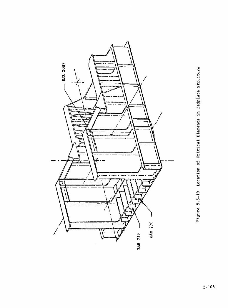
5-105

w $.i

1 U

Cl)

4.J

'-4

a)

Cl) .1.1

G) E a)

'-4

'-4

U

U

'.4-4 0

0 .-4

U

-4

Il-I

a) s-I

jO .1-I

100

8

Figure 5.5-20. Illustrative Example of Type 8 Joint from AISC Code

The margins of safety listed in Table 5.5-2 were computed using steps similar to this illustrative example. For peak loads, the allowable stress is 6O7 of yield strength or 22,800 psi, or for bolted joints, the allowable shear stress per Table 5.5-4, taken from the AISC code.

The minimum margin of safety in fatigue occurs at member CBAR 2087, located as shown in Figure 5.5-19. For this member, the weld joint is Category D with an allowable stress range of 7000 psi.

5.5.6.2 Yaw Section Analysis

It was not necessary to use a finite element computer analysis of the yaw structure because its simplicity and synunetry made it amenable to manual calculations. The upper and lower structures were treated as curved circular beams and analyzed using simple formulas. In addition, detailed analyses were made of secondary structural elements, such as the yaw brake mountings, yaw drive pinion supports, and yaw drive motor mountings. In this report, only the critical sections of the primary structural elements will be discussed.

The loading conditions considered in analysis of the yaw structure were:

1. Cyclic loading per Case A

5-106

Table 5.5-4. Allowable Working Stresses (ksi) for Bolted joints0-)

Class Surface Condition of Bolted Parts

Standard Holes

Oversize Holes and Short Slot- ted Holes

Long Slotted Holes

1 1

A325 A490 A325 A490 A325 A490

A Clean mill scale 17.5 22.0 15.0 19.0 12.5 16.0

B Blast-cleaned carbon and low alloy steel 27.5 34.5 23.5 29.5 19.5 24.0

C Blast-cleaned quenched and tempered 19.0 23.5 16.0 20.0 13.5 16.5

steel

D Hot-dip galvanized and roughened 21.5 27.0 18.5 23.0 15.0 19.0

E Blast-cleaned, organic zinc rich paint 21.0 26.0 18.0 22.0 14.5 18.0

F Blast-cleaned, inorganic zinc rich paint 29.5 37.0 25.0 31.5 20.5 26.0

G Blast-cleaned, metallized with zinc 29.5 37.0 25.0 31.5 20.5 26.0

H Blast-cleaned, metallized with aluminum 30.0 37.5 25.5 32.0 21.0 26.5

I Vinyl wash 16.5 20.5 14.0 17.5 11.5 14.5

Values from this table are applicable only when they do not exceed the lowest appropriate allowable working stresses for bearing-type connections, taking into account the position of threads relative to shear planes and, if required, the 207. reduction due to joint length.

0-) Reference "Specification for Structural Joints Using ASTM 325 or A490 Bolts", February 4, 1976, AISC.

5-107

EbP.LPTEMDU]

PIMT.LE VOUNT

x

Mz

yYCL

Table 5.5-5. Design Loads at Yaw Bearing

(Units are Lbs. for Shear and Ft-Lbs. for Moment)

Loads Mean Cyclic Peak CASE A

V, -- + 82161 --Fatigue Vy -- + 28046 --

V -- ± 35903 --Mx -- *984780 --M -- ± 539953 - - Mz - - * 150945 --

CASE BV - 339730 * 51158 - 390888

Peak V, - 55 ± 21051 - 21106 35-50 mph V - 48533 * 18458 - 66991 +41° Inflow N 157300 *1326800 1484100

1274900 * 661170 1936070 M - 728445 * 121360 - 849805

CASE D Headwind Sidewind V, -- -- - 338387 - 338387

Hurricane Vy - - - - -- - 38644 V -- -- - 14523 - - Mx -- - - -- 288638 M -- -- 245333 138831

-- -- -- - 283389

5-108

2. Peak loading per Case B

3. Hurricane loading per Case D

4. Maximum torque output of yaw hydraulic drive motors (55000 ft-lb)

5. Maximum brake loads due to hydraulic overpressure (3500 psi)

The critical loads appropriate to the yaw structure are summarized in Table 5.5-5 for Cases A, B, and D. Further details of these cases may be found in Appendix B. For bolted connections, the influence of tension preload was considered, based on the AISC recommendation of preloading all high strength bolts to approximately 707 of their minimum tensile strength.

Margins of safety were computed for all structural elements, based on the allowable stresses that have now been incorporated in the 1978 AISC code. A summary of the critical margins for both the upper and lower yaw structures

i8 given in Table 5.5-6. Margins listed as "adequate" are greater than l007; "very adequate" are greater than 200.

The following is a sample calculation for bending of the upper yaw structure, lower flange. The loading condition for cyclic loading is Case A, summarized in Table 5.5-5. It is convenient to convert the loading as a uniformly distri-buted load, equal to the peak intensity. This is accomplished by expressing the moments M and M2 as equivalent axial loads, then adding them to the ver-

tical loading V.

Nm = My+PMz

'T R2

where R = radius of yaw bearing = 69.6 in

Nm = 560xl03xl2

x (69.6)2

= 442 lb/in

N = Nm + Vx

2'flR

= 442 + 82 x l0 'i x os.o

= 630 lb/in

Local bending occurs at the lower flange because the inner race of the bearing, where the loads are introduced to the upper structure, is offset from the web of the upper structure. The lower flange is treated as a cantilever beam of

5-109

Table 5.5-6. Suimnary of Margins of Safety for Upper and Lower Yaw Structures

Location Loading Condition Minimum Margin of Safety

Upper Structure, web Case A, bending +.65

Upper Structure, upper flange Case A, bending +.42

Upper Structure, lower flange Case A, bending +.63

Brake outrigger Brake force, bending Very adequate

Motor support beam, flange Motor torque, bending Very adequate

Cross beam Motor torque, bending Very adequate

Pinion bearing support Motor torque, bending Adequate

Lower Structure, web Case A, bending ^.65

Lower Structure, upper flange Case A, bending +.42

Lower Structure, lower flange Case A, bending +2.29

Lower Structure, gussets Case A, tension +.90

Brake disk Brake force, buckling Very adequate

5-110

unit width, with free edges (see Figure 5.5-21).

=

I

= 630 x 2.863 x 2.100/2

(2.1) 3 / 12

= 2450 psi

The stress range is then double this value, or 4900 psi. The allowable stress range is conservatively taken as 8000 psi, assuming that the weld between the web and the lower flange classifies the joint as Type 21 by the AISC code, or Category F. It might be argued that the joint more closely resembles Type l5a, Category B, with a 16,000 psi allowable stress range.

MS = 8000 - = +.63 4900

Figure 5.5-21. Lower Flange of Upper Yaw Structure

5-111

5.6 TOWER

5.6.1 REQUIRENENTh

The design requirements for the tower specified in the NASA Statement of Work can be summarized as follows:

1. Open truss construction with members of structural carbon steel 2. Bracing generally designed for bolted field assembly 3. Provide a lift device of half-ton capacity for access to the nacelle 4. Provide a means for evacuation of personnel in the event of failure

of the lift device 5. Maximum design wind load of 150 mph (at hub height) 6. Seismic loads per Zone 3 7. First bending frequency shall be at least 2.8 times the rotor operating

frequency 8. First torsional frequency shall be at least 6.5 times the rotor operating

frequency.

In addition, the tower is required to have a design life of 30 years, operating in a range of environmental conditions, including temperature extremes from -31°F to +120°F. The low-temperature requirement is significant because it places the fracture-toughness requirements for the steel in the most severe class, Zone 3.

Comparison with loads determined by the system dynamic simulation has shown that the critical design conditions are Case A for fatigue and Case B for peak stresses, rather than the hurricane wind loads or seismic loading defined in the SOW.

5.6.2 DESIGN DEFINITION

The final design of the tower is illustrated in Figure 5.6-1 or GE Drawing 848E834. This drawing defines overall geometry, member sizes, materials, and general joint design. From this drawing and detailed loads data extracted from the finite element computer program, shop drawings were prepared by the tower fabricator for each member and joint in accordance with AISC specifications. The characteristics of the tower are summarized in Table 5.6-1.

5.6.3 DESIGN EVOLUTION AND TRADE-OFFS

During the detail design phase, the tower design evolved through several itera-tions in an attempt to satisfy strength and stiffness requirements at minimum cost, in the face of continual growth in system weight and design loads. As part of this design evolution, several trade-off studies were made on the se-lection of overall geometry, grade of steel, and structural form of members. To gain maximum bending stiffness, the tower height was reduced and the width increased as far as adequate blade clearances would allow. Beyond that point, it would have been necessary to introduce a tilt in the rotor axis or increase the rotor overhang in order to maintain clearance with the tower when the blade is at its maximum tip deflection. Having established the overall geometry, the only parameter to be varied to achieve the desired strength and stiffness was the cross-sectional area of the primary members.

For the four tubular leg members that comprise most of the tower weight, the selection of steel grade became a tradeoff between fracture toughness and cost.

5- 112

5-113

L._L.i I i H I

M'

0 C-)

rQ)

'

I a) U

___ jo

r.L4

1J r

I

d 1 Q•_

'ri : L ?7 _-::

I-tv

91.0

4..

3

LL /*

e0

z

1J 2•>

-.

U

c'4

4-) 4, 4,

Cl)

0

41 cj

I4-

0 C-)

a)

I—I

a)

-.-1

5-114

\-_J t

'/:i 'I \

-.5

. t

(Ii

4J w w -t Cl)

0

cj

0 0

a)

0

a) s-I

--I

V

1L.I4 =

t..

:

2 :

. ilS

I ILl) .k Hi - LJ 7

5-115

. \'fflM/.

/w a)

Cl)

0

I-i

tO ..4

0 0

'-I a)

E-i

li-I

a) $-i

I IM

OI (7

r •r' 4

I1 i,," WL I jK

Lr%x

•

- i A' __ __

7

1N

/

5-116

Table 5.6-1. Mod-i Tower Engineering craracteris

Total Height 131 ft

Width at Base 48 ft

Width at Pintle 12 ft

Design Life 30 yrs

Total Weight 360,000 lbs

Materials

Tubes ASTM A333

Shapes ASTM A36

First Bending Natural Frequency 3.2 P

First Torsional Natural Frequency 7.2 P

Design Codes AISC, AASHTO

5-117

Pipe of the required diameter and wall thickness is normally available to a limited number of specifications. The two candidate materials for the tower were ASTM specifications A53 and A333. As shown by the comparison summarized in Table 5.6-2, A333 has good, well-established fracture toughness but is higher in cost than A53 when compared for Zone 1 service temperatures (0°F and above). However, for Zone 3 service, the cost difference becomes uncertain. Suppliers are unwilling to guarantee the results of Charpy V-notch tests on A53 pipe because of the latitude in chemical composition of steel to this specification. Experience with bridge failures due to brittle fracture has led AASHTO (American Association of State Highway and Transportation Officials) to specify the test temperature for standard impact tests with steels similar to A36 at 70°F above the intended service temperature. For Zone 3 (-31 to -60°F), toughness must exceed 15 ft-lb at a test temperature of 10°F. As shown in Table 5.6-2, A333 would have no difficulty meeting this requirement while test results for A53 would be marginal and only selected heats would be ex-pected to pass. When a review of system requirements confirmed that service temperature limits were not to be compromised, selection of A333 for the tubular members of the tower became essential.

e Specifications

A53 A333 .de B Grade

Tensile Strength, Min(ksi) I 60 I 60

Yield Strength, Mm (ksi) 35 35

Minimum Impact Test Temperature Not required -50°F

Impact Strength, lO°F(ft-lb) 5 to 15 20 to 30

Carbon, Max. (7) I .30 I .30

Manganese, Max. (7) I 1.20 1.29 - 1.06

Phosphorus, Max. (%) I 0.05 I .048

Sulfur, Max. (7) I 0.06 I .058

Silicon, (7) NA .10 Mm.

Cost*, $Ilb. (Zone 1 Service) .39 .51

*Costs quoted April, 1977, for 20" diameter pipe.

Tubular members for the tower were specified because of their low drag coefficient as compared with other structural shapes. The objective was to keep the velocity decrement in the tower wake acceptably small, and to have confidence in the esti-mate of tower shadow by being able to relate it to wind tunnel measurements for all-tubular tower models and other data. Within the framework of overall geo-

metry and section properties selected to meet strength and stiffness requirements,

5-118

a study was made to determine if some of the members could be standard struc-tural shapes. The question to be answered was, would the lower cost of stan-dard shapes such as I's or channels justify a possible increase in the magni-tude of the tower shadow and hence, the magnitude of cyclic loading? Several variations were considered, but the choice narrowed to the two configurations compared in Table 5.6-3. The use of channel shapes for diagonal members below the blade tips does not significantly affect tower shadow and is economic.

Table 5.6-3. Tower Concept Comparison

Tower height, ft.

Concept "B" Concept "D"

131 131

Legs, size and type 20 in. pipe 20 in. pipe Material A333 A333

Weight, 1O3 lb 128 128 Projected area, Ft 2 309 309 Drag coefficient .42 .42

Diagonal Members, Pintle Section, Size and Type 12 in. pipe 12 in. pipe

Material A333 A333

Weight, l0 lb 30 30 Projected area, Ft 2 38 38

Drag coefficient .40 .40

Diagonal Members Below Pintle, Size and Type 8 & 10 in. pipe & 10 in. channel

Material A333 A36

Weight, l0 lb 112 128 2

Projected area, Ft 311 311 Drag coefficient .90 2.0

Diagonal Members Below Blade Tips, 3 & 10 in. 3 & 10 in. Size and Type thannel channel

Material A36 A36 Weight, 10 lb. 50 50

Total Weight, 1O 3 lb 320 336 Total Projected Area, Ft 2 658 658 Average Drag Coefficient .66 1.17

Relative Wake Energy 1.0 1.76 Relative Velocity Decrement 1.0 1.33

The cost difference for channel members in bays above the blade tips is stun-marized in Table 5.6-4. Because channel members are less efficient in buck-ling, a weight increase results when these members are used. Note that the cost figures in this conparison were quoted in April, 1977, and may not re-flect prices actually paid. Tower shadow characteristics of the two con-cepts were compared by calculating an average drag coefficient, weighted

5-119

T11 c A..L. Pr.r.i,- (.c,I Pr.-nr...p.4

Diagonal Members

Concept "B" Concept "D"

Pipe Channel Material A333 A36 Weight, 1O3 lb 112 128 Material Cost, $/lb .40 .215 Fabrication Cost $/lb .525 .462 Cost Difference, iO 3 $ +16.9 --Cost of Fairing Installa-

tion, l0 $ -- +15 to 20

NOTE: Comparison only diagonal members below pintle and above blade tips. All other members are the same.

according to the projected areas of each member shape. These calculations are summarized in Table 5.6-3, which shows that the wake energy for concept "D" would be 76% higher for "B", or the velocity decrement 33% higher. If ser-vice experience were to show that the more severe tower shadow were unacceptable, a solution would be to install sheet metal fairings to all channel members which would reduce the drag coefficient from 2.0 to perhaps 1.0 or less. How-ever, the costs of such modification are estimated at 15 to 20 thousand dol-lars and several weeks time. Because the risk was not justified by the poten-tial cost savings, concept "B" was selected.

An estimate of the anticipated velocity decrement can be made by comparison with wind tunnel data

V LVo x (k x Dl/CD0)½ whereVo = velocity decrement from wind tunnel test

= .225 k = solidity factor = 1.51

CD 1 = Mod 1 drag coefficient = .66 = Model drag coefficient = 1.2

LV = .205

This value agrees with the conservative assumption of a 24% tower shadow effect used in the system dynamic simulation.

5.6.4 FOUNDATION DESIGN

The tower is supported by separate foundations for each of its four legs, typically shown in Figure 5.6-3. Borings at the Boone, North Carolina, site showed the presence of foundation quality rock just below the surface. The foundation was designed by J.E. Sirrine Company, Raleigh, North Carolina, based on the core sample properties. Because of the dead weight of the wind turbine, relatively small tension loads are developed in the foundation. Each leg is secured by eight 1.50 in. diameter anchor bolts, hooked at a depth of 30 in.

5-120

4J U) a)

0 '-4 1.1 0 o a)

U)a)

r

0 $4

"-4 '4

C/)

0 z

cj a)

aj

'a ,-10 0

a) -.1$4 U a>

•,-lcd a)

a) QJWa) 0) C) C ooc rO x4I44$4

Ifl Qci 00

Li -4tM \ i r-0 '

U

bo

__L1I_I__.lIL

U"-4 U) 0)

bO In

a) "-I 14 (0

0 0

0). C/)

a) '.1

$4

-1H '-4

U "-4

H

140) C 0 $4

p4 UcO

'••- a)

U) r0

a) U)

0

- 0 4J •d-U t

4J 1-1 0p4 c1

E0 -1 C/) d

C) 0 Z ".1

a)

p4

a) U)

'4 a)

H

5-121

in the foundation. The shear load is reacted from the tower base plate through non-shrink grout to a lip on the foundation tied with No. 5 reinforcing bars to to the primary reinforcing bars in the foundation. Shear load is also trans-ferred to the anchor bolts through friction and epoxy grout in the base plate holes.

5.6.5 PERSONNEL LIFT AND ACCESS PROVISIONS

A personnel and equipment transfer device will be installed and used as a means of gaining access from ground level to a platform located approximately 120 feet above grade. Figure 5.6-2 (GE Drawing 298E458) shows the overall installation of this transfer device. It is identical to the unit installed by NASA on the Mod-O WTG at Sandusky, Ohio. It is Model No. ST-27 (Shafter) as manufactured by Spider Staging Sales Company, Renton, WA.

In the event of failure of the lift device, personnel can be evacuated from the tower by means of an emergency escape device supplied for use with Model ST-27. This unit is called "Rescumatic" and is an off-the-shelf device that meets OSHP requirements, ANSIB3O.1, ANSIB3O.2, ANSIB3O.3 and ANSIB3O.11, "Emergency Egress from Elevated Work Stations". It is a fully automatic, nonpowered device that provides a safe, constant descent speed of 3 fps. There is a personnel sling at each end of the descent cable whereby continuous operation can be offered without the need to rewind. Two of these units are planned for use with the lift device and another would be stored in the platform area at the base of the nacelle. A training program is recommended for potential users of the "Rescu-matic" unit.

The Rescumatic unit has undergone life expectancy tests conducted by Under-writers Laboratory. Rescumatic was operated continuously for three months at 24 hours/day. At the end of this period, the linings were worn out, but the unit was capable of safe use without the clutch lining. (The unit operated rather loudly, and the descent was not a smooth ride.)

Translating the life test to comparable WTG application, the Rescumatic unit could be used 20 times a month for 30 years before it showed signs of wear.

5.6.6 TOWER STRESS ANALYSIS

The analytical approach was to develop a detailed finite element computer model. The analysis of the model was performed with the use of the GE computer program called MASS.

The finite element computer model represents the entire 130-foot tower includ-ing every structural member plus the yaw bearing support. This model consists of 117-grid points having 701 degrees of freedom. The corner members and all upper bay diagonal and horizontal members are tubular. The bottom bay diagonal

5-122

c7T

Figure 5.6-2 Personnel Transfer Device

5-123

and horizontal members are back-to-back channels. Figure 5.6-4 shows the tower grid point locations. Figure 5.6-5 is a computer printout of this model.

Critical load cases for the tower were: Case A (fatigue) and Case B (peak dynamic load), as defined in Appendix "B".

The major area of concern is the range stress due to the oscillatory loading for the 30-year life requirement. Referring to the AISC code as shown in Figure 5.5-3, the range stress allowable depends on the number of cycles and type of joint. For a plate welded joint (Category E) having 2 x 10° stress reversals (Loading conditions 4), the range stress allowable is 5,000 psi.

The MASS program uses a three-dimensional finite element stiffness matrix solution and is capable of determining the static/dynamic and thermal behavior of a structure. Analysis of a wide spectrum of structural types including trusses, frames, shells of revolution and pressure vessels, as well as com-binations of these can be accomplished. The capability of the program is 20 substructures. Each substructure can have as many as 200 nodes for a total of 4,000, each with six degrees of freedom. Types of loading include point or lumped mass, distributed or pressure forces, thermal gradients and maneuver forces.

The program is most generally used to provide a detailed internal stress and distortion analysis based on the resultant load/thermal environment. A second purpose is to provide a stiffness matrix for specified nodes to be used in sub-sequent dynamic analysis.

Using Section 1.5 of the AISC Code, the maximum allowable stress for peak load-ing (infrequent conditions), is 60% of yield strength or 21,600 psi. The range stress allowables (cyclic loading) are per the AISC code.

Table 5.6-5 summarizes the results of the analysis by identifying only the members in the tower with low margins of safety. These members have been identi-fied on the computer model (Figure 5.6-4). There were no critical members or joints for the other cases analyzed. For the peak load condition, no combined stress exceeded 10,000 psi with 21,600 psi allowable.

Q........,...... .0 i.1 e i.. ,,. ------.

____________

Member _________________

- Stress

Range (psi) _________________

Allowable Stress Range (si

Margin of

Safety

477-486 2940* 5000** .70 479-486 2540* 5000** 97 481-490 2130* 5000** 1.35 483-492 3170* 5000** .58 477-492 2590* 5000** •93 401-516 4730 7000 .48 516-412 5130 7000 .36 404-514 6570 7000 .07 514-504 5340 7000 .31

All members had high margins of safety in buckling.

5-124

*Diagonal members at the to of the tower are reinforced with gussets providing an additional area of 30 in2 at the location of the Category E" weld.

**Category "E", loading condition 4, per AISC Code, 1978 Edition (in press)

As an illustrative example, consider member 404-514, which is a section of one of the four leg members, from the foot (404) to the intersection with the first horizontal brace members (514). Figure 5.6-6 is the computer printout for this methber, analyzed for Case A cyclic loads. Note that the maximum combined stress of 3285 psi occurs at joint 404, due primarily to the bending stresses intro-duced by diagonal members 404-513 and 404-515. Conservatively, the cross sec-tion at joint 404 is assumed to be that of the 20 in. diameter pipe only, with no credit taken for the addedarea of the four stiffening gussets. The stress range is assumed to be double the maximum combined stress, or 6570 psi. The allowable range stress for a Category D weld joint, loading condition 4 is 7000 psi. (Category D is applicable to base metal adjacent to a detail of limited length attached by a groove weld subjected to tranverse loading, when th detail length is less than 4 in., with no transition.) The margin of safety is:

MS = 7000 - 1 = + .07 6570

*To simplify computations, the loading was assumed to be completely reversed so that the stress range was conservatively taken as double the maximum combined stress, or 6570 psi.

5-125

Figure 5.6-4 Node Identification for Tower Finite Element Model

5- 12 6

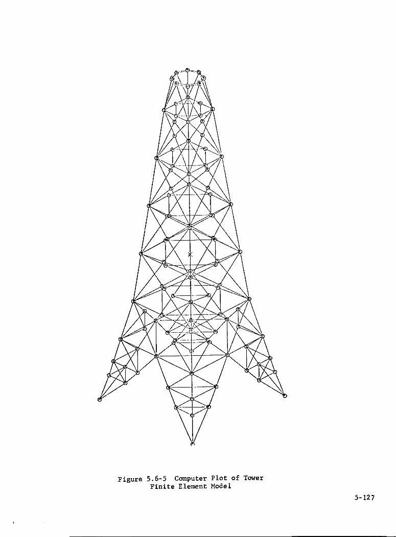
Figure 5.6-5 Computer Plot of Tower Finite Element Model

5-127

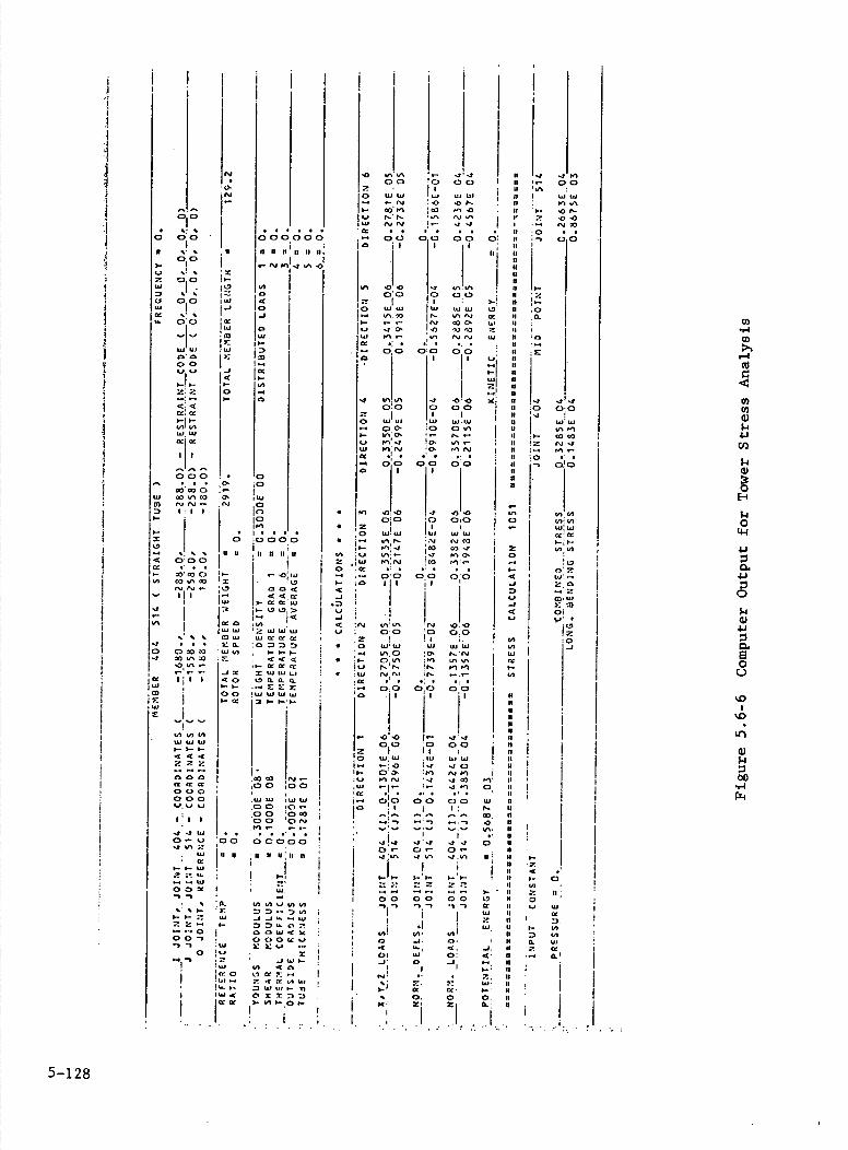
U',VS r-00 ! 00

WW us u,ui .N :o 'or-ap t-, 0 r-,-, •,-. r,jp,

*1*1

00 00 00 a: I I I

'0-0 , vs.p#S 00 0 00

U, tsp psi us eM tA, r- trpr,p a

N esi _7_O ,'O eo PS) , .- ,U N N uI

00 00 0?

I '-I

:

!.

00 cD 0:0

wiw ,LtJ 515W pAr- 'N rsiCP) ,n-., 1c0 5S)'4

vsU5 :r,I '0,0 0!0 tti'W W uJW tAO :05 r-r,, 015* rn ,i,u, 1'-'P- - ,S)IS) C'

ii J

cIa 00 00 U, I'.

0.4 ' •'C -,-t 0

I- i-1 P-

-4-- ..-- ,-_ I 00 00 00 I -,-, '-i-p -,-, a

I i ui 7

ii w. I U,. ñ 0 J. 0' 4 '-P <P _i. I 01 U, 0: 4

, II i

• CS)

• ,2 0

• I.-. I-.

U, :,,

0 •a

t- 0 4

'-I -I 4 usJ '5,

•2 • :o

*

* !w 'a

0

z

II-. •'5, • U, a

-4

2 0

p-I us a

0

Ce

'0

0

I-

U, a

Ce

- 5--7 C P- 0 PA

0 P-I eM

a

I- tn 0 in 15. US 7 a a:

U - 17

H , H pp II

ire 0

ZI 0

5-4 P -J

'I -I 4 '5

I

-t 0 0

US 511 U,

C', -t CA

c 0

U, U) in . In usW a a I-; I-• U, PA

S-i 7 US.-, 2, '-.7 alt,

01 s-P.

7 :0

0) -,-1

(I) '-S

0) 0) a) 1.1 4J

Cl) 1.5 a)

El $-i 0 l44

0 1.1 a)

Os E 0 0

CS.

.0 •0,

a) 1.1

.-1

,0

tsp IE

I 010

000000

N 00 I

* i 'X It-. 00 I. t'

* * 2 0 I 00 W 4 I

I-i 0 o' o a

'5' 0 -".' '0 eM

WeM eM 00 : I:D 00 (jtst ..I a

4 I--- - U, z: 0 -.

I- 0 a, a J-t I'-U, U eM. eM

1:1 p • 0

•5

*. S S

0 II II

10000 pI H 11:1, 000

O'C) .-,o'tu eotneo 'r . (eN '5 004 iii <<a

I eM ,-aew I. j4

euw ww 5 ' S 5 0 is, is., a Cr et • • • ,a oeo tuen

<4< ii- aa a

_Jrt XWWL,j S'S S 40 tDQ.OQ

' t-• 00 eM eM eM w I i-

en en us us us I- I- I-4<4

0 0 000 00

000 000 i5' eM : uS eM

' .00 0 • 00 0eo

I'S S 00 'ON -

0.-us 00 00000

us ii p5 5 U'II II -a

us 00x "fl

p

• S O• tnvipjyun i- -.

?-, I-

OOfl p 000Crus --p us a.us - 0 us .

' 'in <Ce

I -iii 7 .f a en U, i.• - :, us is, •- i

I itj< OXXDD Cra

5-128

SECTION 6

POWER GENERATION SUBSYSTEM

SECTION 6

P(MER GENERATION SUBSYSTEM

This section describes the electrical system of the Wind Turbine Generator. The main power transfer path through the generator, main breaker and step-up transformer are covered. In addition, the auxiliary power supply, control system interface equipment, interconnecting wiring, the ground control enclosure, and various protective devices are also described.

6.1 REQUIREMENTS AND SYSTEM OVERVIEW

6.1.1 STATEMENT OF WORK REQUIREMENTS

Requirements, as paraphrased from SOW NAS-320058, are:

Exhibit B

1.1 2000 kWe Rated Power, 60 Hertz synchronous generator, 30-year life

1.4 Availability, life, general environment

1.6.5 NEMA Standards

1.7.3 100,000 Startups

2.4.8.4.1 Nacelle Lightning Protection

2.4.8.5 Nacelle Lights, outlets & intercom

2.5.1 416OV, 2188 kVA, 40°C, .8 pf, more than 90% efficient, 105°C Rise for Class F, MG1-22 generator requirements.

2.5.2 Safe shutdown power

2.5.3 Slip rings

2.5.4 Mutual fault protection

2.5.5 Lightning protection of electrical equipment

2.5.7 FAA approved illumination

2.7.1.1 Synchronize

2.9 Lightning model for 2.4.8.4.1 of Exhibit B

Additionally, interconnection with the site utility and wiring of the Engineering Data Acquisition System (EDAS) is required.

6-1

6.1.2 SYSTEM OVERVIEW

A simplified one-line diagram of the basic power circuit is shown in Figure 6-1. The utility connection with Blue Ridge Electric Membership Cooperative (BREMC) is stepped down from 12.47 kV to 4.16 kV. Auxiliary power is obtained from the 4.16 kV bus through transformers to 4 and 208Y120 Volt distribution systems. The generator is connected or disconnected from the 4.16 kV bus de-pending on whether or not the wind is blowing.

GENCRATOR MAIN BREAKER STEPUP TRANSFORMER

FIELD SUP

\

4.N6Y2.4KV2240 EVA 12.47Y7.2RV

\2138 EVA

-[EH JJJJAJL

2KVA__.4 ) 1 45XVA

480V 2OXY120V

AUXILIARY CIRCUITS

PROTECTI3II AND COCIROL DEVICES NOT SHOWN

FIgure 6-1 Simplified One-Line Diagram

The full one-line diagram of power distribution and relaying is shown in Figure 6-2. A description of the function of each device appears in Paragraph 6.3. The relaying represents an economical protection scheme utilizing standard components and electrical utility practices.

A block diagram of the system location of major elements is shown in Figure 6-3. The generator and associated exciter, sensing and protective devices are located in the nacelle. An auxiliary control and power distribution box, several discrete sensors, and the nacelle multiplexer unit (NMU) are inter-connected and wired to the tower slip rings which provides for yaw rotation.

On the tower side àf the slip ring, conduit enclosed wiring runs to the control enclosure at the base of tower. The enclosure houses the remainder of the control system, the generator main breaker, additional sensing and indicating devices, and the auxiliary power transformers and distribution. A separate pad is located under the tower for mounting of the Generator Step-up (GSU) Trans-former which connects to the enclosure and to the BREMC.

6-2

h

C ( TTTT

( (

"I I 'I

ID Li

I!

LL :

'4 c'j

.-4

—1

ll ________

I !: I I I

-

I.

Lii][1 Li!i. __:L_Jli

3 r

TaU

I I ii

E1

1iI1tiI!iL IIii I @®®®®®®®®® ®®®®®

1

I I

a I . - 1. .1 1 1 ki

11111 i I I! I _ I1 I

i I L4

I I T I tj ( ( ( R( ( ,.(

I

I Vi I

a

c;1 0

{ccç- s-I

-'.4

6-3

NACELLE_______________________ I

AUX I II L41J E ' I x LOADS I I

GENERATOR(120V I [TJ I I

T DIST.) E ___

IENSE

L____L _

I SLIP -. RING I

TOWER

r --

MAIN GSU

BREAKER XFMR

SENSE SWITCH-

I GEAR

MOTOR AUX CONTROL LOADS BATTERY

CENTER I SUPPLY GMU

U T I L I T Y

- -----------J

Figure 6-3 Mod-i WTG Block Diagram

6-4

The individual elements of the Wind Turbine Generator system are described in the follocing paragraphs.

6.2 GENERATOR AND P(MER GENERATION AUXILIARIES

The generator, shown in Figure 6-4, is a 4-pole, 1800 rpm, 4160 Volt, Wye connected unit with shaft-mounted exciter. Class F (105°C rise over 400C ambient) insulation is used. The generator is rated 2188 kVA, .8 power factor and the exciter is rated at 25 kW at standard ambient. A cutaway illustration of the unit e s construction is shown in Figure 6-5.

Figure 6-5 The Cutaway of Generator

6-5

I-I 0

I-i

'0

6-6

Due to the above average number of starts anticipated, provisions have been made to supplement the normal sleeve bearing oil ring lubrication system with a flood-type system. The hydraulic package is not provided but can readily be

added if field experience indicates one is needed.

The sleeve-type bearings and their mounting are split for ease of replacement and this type of bearing has an excellent life record. Synchronous machines of this size have a relatively large air gap, on the order of 0.125 inches and con-siderable bearing wear can be tolerated before replacement is mandatory.

Generator characteristics and saturation curves are shown in Paragraph 4.2 of

this report.

The generator with accessories weighs 11,500 pounds in a frame that occupies 120 cubic feet of space. An open top frame construction is used with cooling air drawn Jr from the ends and discharged through the top via ducting.

RTD detectors are provided for monitoring stator winding and bearing temperatures. A space heating coil is also provided to prevent condensation. It will be ener-gized when the unit is not generati.ng.

Special tests are not called for as the machine design is mature. Design pro-blems are not anticipated. Standard commercial tests have been performed by the manufacturer and consist of:

1. Resistance of armature and field check 2. High potential and insulation resistance test 3. Phase rotation check 4. Shaft current check 5. No load excitation check 6. Mechanical balance check at rated speed 7. Bearing end play check

Auxiliary equipment is mounted in a caged area under the generator and consists of primary winding protective lightning arrestors and surge capacitors, a po-tential transformer, neutral side mounted current transformers, and a grounding transformer. The all six generator leads are brought out in order to mount the phase current transformers. A grounding resistor associated with the transformer is mounted on top of the generator. Current transformer and potential trans-former ratios and the resistor rating are shown on the one-line, Figure 6-2.

6.3 SWITCHGEAR AND TRANSFORNER

6.3.1 ELEMENTS OF SWITCHGEAR

Switchgear for control, protection and instrumentation of the system are mounted in the control enclosure and basically consist of:

1. Generator Circuit Breaker and Isolation Switch 2. 4160 Volt Bus and Protection Equipment 3. Instrument Transformers

4. Protective Relays 5. Transducers for signals to Data Systems 6. Auxiliary Power Supply Transformers

7. Main Protection for Auxiliary Power Supply

8. Terminations for High Voltage Cable

9. Grounded Metallic Enclosure 10. Visual Indicating Instruments 11. Generator Control Devices

6.3.2 GENERATOR CIRCUIT BREAKER AND ISOLATION SWITCH

The generator circuit breaker 52G is based on a large motor starter rated at 4160 Volts, 360 Amperes continuous, with 50 mVA interrupting capability with-

out fuses.

The WTG generator switching device will be operated frequently. Conventional air magnetic breakers (such as the GE AM 4.16 - 250) have a somewhat limited repetitive duty capability as defined by industry standards. For example, the maximum number of breaker operations between minor servicing is 2000. Further-more, conventional breakers are required to sustain no more than 10,000 no-load mechanical operations, or 5000 full-load non-fault operations before major servicing is required.

The breaker used is the air break contactor employed in GE LimitampR motor starters shown in Figure 6-6. This device is designed specifically for re-petitive operations and tests have shown that major maintenance of the con-tactor would not be required for at least one-half million operations.

The Limitamp contactor is frequently employed as an inexpensive small breaker substitute in situations where its 50 mVA symmetrical interrupting capability is sufficient (or where the use of fuses for current limiting in association with the contactor is satisfactory) and the contactor has a ten-cycle blocked withstand capability of 18,810 Amperes rms. A short circuit study was performed on the wind turbine generator system to verify that a Limitamp contactor would be satisfactory. This study assumed a stiff 1000 mVA source at the transformer and indicated that the interrupting duty on the contactor would be approximately 29 mVA and the momentary duty would be approximately 6963 Amperes, both of which are well within the tested capability of a Limitainp contactor.

Another consideration in using a Limitamp contactor for a generator breaker is that during synchronization, the voltage across the contactor tips will be twice system voltage. The 5 kV Limitamp contactor has an AC one-minute hipot rating across the contact tip of 20 kV, which is more than sufficient for this appli-cation.

In critical applications, it is advisable to employ a special form of contactor which includes two coils. One coil is a solenoid closing coil which causes the main contacts to close under control of the synchronizer and which engages a mechanical latch. After the main contacts are closed and the latch is engaged, the closing-coil circuit is interrupted. The contactor may be opened by ener-gizing the second coil which releases the mechanical latch. Therefore, the mechanically latched contactor performs just as a conventional stored-energy circuit breaker with close and trip coils. An antipump circuit is provided to prevent more than one closing operation for each close circuit pickup.

6-8

11 .rI-

I

The use of a mechanical latch contactor will make the wind turbine generator system secure from contactor dropout. However, it is also necessary to make sure that the contactor can be tripped open when this becomes necessary. During fault conditions, the voltage at the terminals of the generator will be depres-sed, and for a three-phase fault on the 4.16 kV bus, it will be zero. If the contactor is equipped with AC coils, there would be no control voltage to trip the contactor to clear the short circuit. For this reason, it is necessary that the contactor be equipped with a DC trip coil that can be operated from the sta-tion battery, which also serves as the system emergency power source.

DC-closed contactors are slower than AC-closed contactors due to the current build-up time associated with the solenoid, but, by using 208V AC closing (52 GCC) and 125V DC tripping, (52 GTC), the advantages of rapid closing (about 0.070 second) and reliable opening can both be obtained.

When the motor starter is provided with a separately energized latch, it has an expected 50,000 operations before major maintenance, or over 4 operations per day for 30 years. While over 500,000 operations have been demonstrated, contact tip replacement is normally recommended at 200,000 operations. The Limitamp should be virtually maintenance free for the life of the WTG. The awciliary transformer feeder contactors may be used for renewal parts if maintenance is required.

A drawout-type connection to the network bus and WTG generator terminals is provided for ease of starter inspection and maintenance. The network bus con-nection is provided with a shutter to prevent contact with the bus. Contactors are designed for use with motors where, when the contactor is open, there is no voltage on the load side terminals. Limitamp contactors are provided in enclosures which include interlocks to trip the contactor when the enclosure is opened but the load side terminals of the contactor are exposed. Synchron-. ous generators can provide full voltage if running, and thus, the "load" ter-minals can have voltage when the main contactor is open; therefore, a key inter-lock system and isolating switch are required so the contactor may be inspected safely.

6.3.3 PiER EQUIPMENT

An insulated bus structure is provided for the line side of the contactors. The bus colmects to the step-up transformer by cable and connects to the atciliary supply transformers, potential transformers, and lightning arrestors in adjacent compartments. As previously noted, the generator connects to the "load" side of the contactor. The arrangement of components within a four-bay lineup in the control enclosure is shown in Figure 6-7.

6.3.4 SWITCHBOARD

A freestanding cabinet houses the protective relays, generator excitation equipment and instrumentation transducers and indicating devices. The device locations are shown in Figure 6-8.

6-10

10"

AOl

45 &VR AUX )tFMR

112.5 KVR AUX XFMR

-

BOl

45 •KVR XFMR

FEEDER

COl

INC LINE L.A. P1'S

0 c

-

DOl

MAIN CONTR

& ISOLATION SWITCH

_____________ B02

112.5 KVR XFMR FEEDER

8'

208/ 120

480 TO MCC

PF

50" 44"

14' 2"

XFN CEN

Figure 6-7. Power Equipment Arrangement

6-11

= t= c= =

= = I-. = =J =

ki T

lle c LA__ . JL .c

rWT1rAIl

LJ L I C4gJ

r,, r—ii 327

41rz 4.7

-J I L_.J

___ 2J4

?±th' [n tCW GEN AtJ 5A ZA, TF52\

2. ____ Iuc ..I I lcv 111cv1 5Qyj 50/S lvi I

I IA

1 vi v GXS

25A

- :i _ " -- ___

LiJ

OI

ccr vi EW L)

cJ t1 !::— -

IRN I! iH&&j h-4 11i&; I I ii II

L224 L2 j O4 L2 Lz.i

1A k-1 LJ L1

325

—r p .tOL I

I I

L_L....L

1UI I I I

3a __

L__i^J

L__JJ

- -t

3I - 3c

\1vJ(?oc,R)

II L.iLA

A- ES-C c-Ak I - ic ^is^i

?igure 6-8 Switcitboaid \rrangemiL

6-12

6.3.4.1 Protective Relays

A cost-effective minimum set of protective relays is provided. Their designation, function and operation follows. Device numbers are from American National Standards Institute (ANSI) C37.2 and types are GE designations. The relays are mostly utility type drawout case devices that can be readily tested and maintained. A typical relay is shown in Figure 6-9.

G

6-13

Figure 6-9. Protective Relay

6-14

1. Device 25A, Synchronism Check, Type GXS. An up to 30 degree adjust-able, slip cutoff relay which closes its output contact to permit circuit breaker closure when generator and utility frequency and angle are in the accept band. If the 52G circuit breaker/contactor is closed outside an angle of about ± 10 degrees, potentially damaging torque levels could be imposed on the mechanical drive system; there-fore, the 25A device acts as a backup to the 25 device.

2. Device 25, Automatic Synchronizing Type GES. When enabled by the computer system, this relay compares frequency and angle across the 52G and outputs a close command anticipating the 52G closing time.

3. Device 32, Anti-Motoring, Type ICW. Operates through a time delay when directional power sensing indicates the generator is operating as a motor and taking, rather than delivering, power from the utility. This condition may occur due to power control loop error or mini-computer malfunction and is undesirable. Operation of the 32 device locks out the main contactor.

4. Device 41, Field Circuit Breaker. A motor starter in the Power Control and Distribution unit controls the voltage regulator system input power. While not strictly a "Field" circuit breaker control, it serves the same function because the brushless exciter static regulator combination cannot have the regulator output to the exciter field disconnected.

5. Device 47, Negative Sequence Voltage. Type NBV. Operates through an auxiliary time delay relay when either a phase-to-phase fault occurs on the utility connection or a fuse is blown on the step-up transformer primary. This device operates on negative sequence voltage which is only present during unbalanced conditions as noted. Initial opera-tion of the 47 device will not lock out the main contactor since uti-lity recloser operation will remove. A blown fuse will cause lockout by continuous pickup of the 47 device.

6. Device 49, Thermal Overload, Type IRT. Operates on excessive genera-tor winding temperature caused by overloads as indicated by an embedded RTD. The 49 device acts as a backup to the control system in order to protect the generator. Operation causes lockout.

The step-up transformer also has an overtemperature contact that causes lockout.

7. Device 5lV, Overcurrent, 'Type IJVC. Three relays, one on each phase, with current transformers on the neutral side of the generator operate on fault caused excessive current. These devices have instantaneous and time over-current functions with voltage restraint such that they become about four times more sensitive to current when voltage is less than normal. The instantaneous attachment provides high-speed opera-tion for generator terminal faults.

6-15

Internal generator faults are detected with the field energized before the main 52G is closed due to the CT placement, and operation of the 51 V effectively causes lockout of the system for a cable fault be-tween the generator and main contactor. The output contact wiring goes to the 94G trip relay.

8. Device 55, Power Factor, Type 1C3655A100. A synchronous motor loss of excitation relay is connected to detect generator loss of excita-tion or out of step and causes lockout. Loss of excitation detection by exciter field current monitoring is not reliable because exciter faults could cause loss of field without significant change in ex-citer field current. Operation cannot be tolerated unexcited as in-duced rotor currents will rapidly overheat the field damper windings and cause an unacceptable Var flow due to the large generator reactive power requirements from the connected distribution line.

9. Device 59T, Overvoltage, Type PJV. Operates on overvoltage on the 4.16. kV system to protect the step-up transformer and auxiliary trans-formers from excessive flux due to voltage regulator malfunction of utility overvoltage. Operation causes lockout.

10. Device 64G2, Ground Protective, Generator, Type lA y . Operates on voltage across the generator grounding resistor which permits 20 Amperes of fault current to flow. This device will operate on 4.16 kV system ground faults and cause lockout of the main contactor.

11. Device 64G3pund Protective, Utility, T ype NGV. An instantaneous current relay, sensing neutral current on the grid side of the trans-former, is set above the normal unbalanced load level and responds to utility ground faults. The main contactor is not locked out on 64G3 operation.

12. Device 71, Liquid Level, Transformer. Operates on loss of transformer oil to lockout the main contactor. If a fault subsequently develops, the fuses at the transformer will clear the fault.

13. Device 86G. Lockout. This device ' is a spring-operated, electrically released contact multiplying relay responsive to any of several parallel inputs and requiring m4nual reset.

14. Device 94G, Trip Relay. This device is provided for non-lockout main cóntactor' operation such as initiated by the 47 or 64G3 devices.

15. Utility Recloser Voltage Block. The automatic circuit recloser which prôtécts "the'' feeder circuit to which the WTG connects will be modified to incorporate a voltage block. If the recloser opens, but the WTG main'contactor does not, there will be voltage on the feeder due to the WTG and the recloser will be prevented from possible asynchronous closing by the block.

6.3.4.2 Transducers.and Meters

Transducers with current source output are mounted in the switchboard to provide

6-16

isolated signals to the operational and engineering data system. The indicated quantities are:

1. Utility frequency 2. Real power 3. Reactive power 4. Three-phase utility voltage 5. Single phase generator voltage 6. Three-phase primary current 7. Single phase auxiliary current 8. Exciter field current

Indicating DC miiliaxneters with appropriate scales are provided for the trans-ducers. Conventional utility practice is to provide a switch for most meters in order to read currents and voltages on only two meters by switching between phases. This practice reduces panel space and provides a slight cost saving. Panel space is not critical on the Mod-i WTG, and three meters will be provided, each for voltage and current, to minimize manual switching. While multiple un-attended sites could justify meter elimination, the type specified is inexpen-sive and desired for the Mod-i WTG's.

Watthour meters are provided for the main generator circuit and for the, auxil-iary power circuit. They back up the minicomputer totals kept on the'same quantities. The indicating instruments and scales consist of:

1. Real Power - Kilowatts (-500/0/+2500) 2. Reactive Power - Kiloqatts(-5O0/O/+i5OO) 3. Voltage - 3 Phases (0-6 kV) plus 1 phase generator (0-6 kV) 4. Current - 3 Phases (O-300A) 5. Current - Auxiliary (0-20A) 6. Synchroscope - Utility to generator 7. Frequency - (55 - 65 Hz) Utility and Generator 8. Power Factor - (-0.6/0/+O.6) on Device 55

6.3.4.3 Other Controls

Both the regulator and power factor controllers have reference operated motor-driven potentiometers for adjustment of no-load voltage and on-line VARS, respectively. The stabilizer system mounted in the ground peripheral rack provides additional damping of the drive train by varying the excitation with speed. The regulator is supplied with a special center tapped transformer and can negative field force. Frequency transduced signals are available to the con-trol system in addition to shaft speed to control frequency with suitable soft-ware implementation. When on-line, the signals will be monitored. to detect over! under frequency drift and trip the 52G main circuit breaker should a utility recloser operation go undetected by the relay protection sensing voltage.,

6.3.5 TRANSFORMER

The generator step-up (GSU) transformer provides voltage matching between BRENC 12,470-Volt distribution and the WTG 4160 Volt system. An oil-filled distribu-tion type unit with accessories in air insulated connection compartments is utilized with 2,000 kVA and 2240 kVA ratings at 55°C and 65° C rise respectively.

6-17

In Figure 6-10, the basic transformer tank and cooling tubes are shown.

A grounded wye connection is utilized on the BREMC side to limit line-to-ground potential imposed on the system. Lightning protection is provided for the transformer and a fused interlocked manually-operated air switch provides dis-connect capability. A line-side neutral current transformer is provided to feed the 64G3 current relay to sense line faults.

The secondary is Delta connected. A no-load tap changer and four primary taps, each 2.5 percent apart, are provided.

Accessories provided with the transformer include:

1. Resealing fault pressure vent 2. Ground pad 3. Handhole 4. Oil sampling device mounted on drain valve 5. Liquid level gage with alarm contacts 6. Temperature gage with alarm contacts 7. Anti-condensation heater 8. Key interlock on high-voltage fuse compartment

6.4 AUXILIARY PCMER DISTRIBUTION

6.4.1 LOAD BUSES

480 Volt, Three Phase - A 112.5 kVA, 3-phase transformer is used to supply a 480 Volt bus. The principal loads on this bus are:

1. Pitch change hydraulic pump 20 hp 2. Pitch slew hydraulic pump 20 hp 3. Yaw and brake hydraulic pump 20 hp 4. Gear and rotor lube pump 15 hp 5. EDAS PIV 30 kVA

208/120 Volt - - - A 45 kVA transformer supplies a 3-phase, 208 Volt bus that is also utilized to supply 120 Volt single phase loads by line to neutral connections. The principal loads are:

1. Nacelle 120 Volt power distribution 10 kVA 2. Scavenger pump 3 hp 3. Oil cooling fan (if required) 10 hp 4. Lift and gearbox heaters 8 kVA 5. Control enclosure 120 Volt power distribution, 15 kVA

6.4.2 PROTECTION AND CONTROL

A factory-wired motor control center is utilized for branch circuit protection and control. This unit is illustrated in Figure 6-11 and the individual element locations are shown in Figure 6-12.

Plug-in-type motor starters having circuit breaker protection, overload relays and main contactors with indicating lights are furnished for the hydraulic pump motors, the Portable Instrument Vehicle (PIV) power feed, and heavy heaters where computer control is needed. Manually-controlled circuits have protection and control combined in plug-in-type circuit breakers.

6-18

Figure 6-10. Step-up Transformer

6-19

Figure 6-11. Motor Control Center

6-20

The rear of the control center has a control panel, illustrated in Figure 6-13, with interposing relays between the computer and the starters. A second panel is utilized as a master terminal board for all tower and nacelle circuits except the 4,160 Volt and shielded signal leads.

6.5 STATION BATTERY AND FAA LIGHTING

A 50-Ampere hour, 125-Volt lead calcium station battery assembly with charger is provided in an insulated and heated enclosure mounted on the outside wall of the control enclosure. Appearance of this unit is shown in Figure 6-14. The dc supply provides tripping power for the main breaker, operates assorted relaying in the switchboard, and powers the aircraft warning lighting. A float charge at 2.12 Volt dc per cell is maintained to eliminate equalizing the battery periodically. The charger has a 9 Ampere continuous supply capability and is powered by a single phase 208 Volt ac supply.

Due to lack of room in the control building and to eliminate the concern for possible hydrogen collection, the batteries are mounted in a separate cabinet. The cabinet is a two-tiered device, providing access to all the cells and charger for ease of maintenance. Because of the -31°C ambient specification, heaters are supplied in the cabinet as well as insulation. This cabinet arrange-ment is standard.

Wind turbine FAA construction approval will be sought by BREMC based on pro-viding a double red obstruction light on the nacelle per prior discussion and recommendation with FAA-Washington and NASA. This lighting is based on the

6-21

CEI4A CE4B CEI4C

- QI

BLA ' MAir'J PERSONNEL LUBE L,Fr PUMP eoa NASA

_______ _______ AO C.Z

K YAW

kYAI PUMP ________ ____ AQ

BL.AtJK ________ SLEW

• ç 1L

P1t4 COOLa Ca&P$, EOtJE

PUMP iaov, '0 ________ PANEL

co8 6ANK ______

4P 4OV ________ =;&

AQ1 JQ O'JNO GOuND GROUND

US NEJAL _________ _________ BU5

Figure 6-12. Bus and Starter Location Motor Control Center

6-22

CONTROL INTERPOS ING

RELAYS

CONTACTORS

FUSE BLOCK

iaiaii I - IIkiIL

I IuIl I - JILI1 I

IIJ1 I I iiiiri I I II

- Ilpa ilUl

a -

iT

1= .g;•1 1•

__ I -I -I • _,I i 1. I • -U.

_______ I-' - Pill ._ 1' I IllhlIllIulIll

WIRE DUCT

TERNINAL BOARDS

Figure 6-13 Control Panel6-23

- - 1

Figure 6-14. Station Battery and Charger

6-24

presence of a meterorological tower with lighting within 500 feet of the WTG tower. A standard FAA approved Fresnel lensed, double lamp assembly is

mounted near the center top of the nacelle.

6.6 WIRING AND SLIP RINGS

This section describes interconnecting wiring. A slip ring is used on the tower to nacelle yaw interface to provide continuous rotation capability. Another yaw electrical interface, utilizing the limited rotational ability of a cable wrap, was considered during preliminary design, but set aside in favor of slip rings due to development cost and risk for Mod-l.

6.6.1 WIRING

Tower wiring is routed in voltage separated metallic conduit for protection from physical damage, electromagnetic interference, lightning strikes and

contact with personnel.

Junction and pull boxes are located on the tower legs at approximately 20-foot intervals. Insulating wire wedges areused to limit the length of free hang-ing wire, thus limiting strain on the wires induced by the vertical run.

The nacelle is prewired as much as possible using metallic conduit or wireway. The control enclosure interior is also prewired with a tower interface terminal board for ease of field wiring. Crimp lugs are used for terminal board type terminations and crimp pins are used for plug insert-type terminations. A dead-break-type connector is used on the slip ring terminations and air stress-cone termination is used elsewhere on the 4,160 Volt cables.

All high voltage (4,160 Volt) is wired with General Electric type "MV-90" Vulkene Power Cable with 15 kV shielded construction. Power wiring below 600 Volts is type THHN building wire. Series 44 Raychem wire is used for all instrumentation wiring due to the integrity and ease of shield terminations.

Belden coaxial and triaxial cables are used for all multiplexing functions.

6.6.2 SLIP RIN

6.6.2.1 Yaw Slip Ring

The yaw slip ring assembly shown in Figure 6-15 handles the electrical interface for all wire and cables between the nacelle and ground or tower. A position sensor gives the relative position between the tower and the nacelle. The

characteristics are listed as follows:

6-25

C')

L) LU

L)

LU

-4

00 .r4

1.1

.1-I

-zr I'.) i-I

•1-1

rl

C,, >CD

oo-

C/) -a

(D -

= _J

2: CD

LU- ______ C')

C.) _

6-26

ACCESS COVER

TANG

SHAFT

MOUNT

/ PLUG

SENSOR

UNT

___ Type

Power 4 rings 350 Ampere Capacity, 4,160 Volts, 60 Hz

Auxiliary 36 rings 50 Amperes, 480 Volts, 60 Hz

Signal 44 rings 10 Amperes, 150 VAC 60 Hz

Ring Material Coin Silver

Brush Material Silver Graphite

6.6.2.2 Rotor Slip Ring

The rotor slip ring assembly shown in Figure 6-16 is located on the gearbox in the nacelle. It is driven by the low speed shaft. A position sensor is built into the assembly as a means of determining the rotor position.

Figure 6-16. Rotor Slipring

6-27

The characteristics of the rotor slip ring are listed as follows:

I tern Type

Revolution Rate 34.7 rpm Number of Rings

30 Current

5 Amperes Voltage

125 V ac or dc Ring Material

Coin Silver Brush Material

Silvered Graphite

6.6.3 CABLE REEL

A cable take-up reel is utilized to manage power and control wires to the personnel lift. This unit is illustrated in Figure 6-17.

6.7 INSTRIJNENThTION

The method of routing of the various sensor wires from the individual sensors to either the operational (CODAS) or engineering (EDAS) data system interface is covered in Paragraph 6.6.1 and a description of electrical transducers and meters is covered in Paragraph 6.3.4.

The EDAS system wiring is separable from CODAS either because a sensor is used only in EDAS or because it is used in both systems and routed first to CODAS with a buffered output from CODAS to EDAS. Additional instrumentation discus-sion is given in Section 7.

6.8 LIGHTNING PROTECTION

The most probable lightning events are direct strikes on the WTG structure or electrical circuit incoming voltage surges due to strikes on the overhead distribution lines.

A ground wire-shielding scheme or rod attractor was discarded as too cumbersome to practically implement and structure strikes are accepted on the blade, na-celle, and tower structure.

Minimum earth resistance is specified at less than 5 Ohms and is provided by rods at the site. Each tower leg is tied to the rod arrangement and bridging straps are used at the main leg joints.

The blade, hub, and yaw bearings are potential current carrying paths for a lightning strike and are protected with an outer diameter located gap which will break down and carry most of any large discharge current due to the high rate of rise of current and inductive path through the bearing proper. A low-resistance brush bypass scheme is also being evaluated.

The lightning model specified (shown in Figure 6-18) has an initial peak current of 200 kA at a rate of rise of 100 kA/microsecond. Most data available indicates 100 kA or more peak is reached only 2 percent of the time and that a 50 percent

6-28

'-I

0,

'a 0

• -

Ii ___ _LJ Lti z I I

2 J 8

I

--

____

6-29

o o

.E.

I £

I ,i I g

1 I u ____ ..---,-.-.- E

I- In f06,

/o

, U -J ,

.-..----.---" . 0

.-J

C— buspo,u UJ2n3

,-1 a,

0

00

•1-4

.lJ

00 -'-4

r;4

a, s-I

00 -'-4

6-30

probable value is about 20 kA. Intense local heating will occur where the streamer strikes the structure but only superficial damage is expected.

A Faraday cage effect is present for equipment within the nacelle and local potential differences should not occur unless the current path is badly asym-metric. A strike on a tower leg will introduce some "near-strike" electro-magnetic coupling into conduit enclosed wiring and optical isolators have been applied to sensitive circuits. Gas discharge tubes are being evaluated as high energy bypass devices for, an added measure of protection. Low-voltage motors are not protected as their insulation level is normally adequate to survive surges unless directly connected to an overhead line.

The higher voltage apparatus is more sensitive to steep front surges due to larger size and capacitive division of a large percentage of the surge onto the first winding section. A lower ratio of test-to-normal voltage exists and lightning arrestors are applied at the BRENC terminals within the control en-closure at the 4,160 Volt bus, and at the generator terminals. A surge capaci-tor is also mounted at the generator terminals. This protection is deemed adequate for strikes on the incoming line or induced "near-strike" surges.

6.9 CONTROL ENCLOSURE

A van-type enclosure, shown in Figure 6-19, is used to house ground-mounted equipment. The interior arrangement is shown in Figure 6-20 with control electronics equipment mounted at one end and the previously described power equipment disposed at the other end to minimize EMI.

The construction, typically used for drilling platform or gas turbine control enclosures, is built up of a self-supporting base channel structure to which interior equipment is secured. A subfloor provides ample wiring space with separate trays run for signal level and power leads. Conduit interfaces are provided in the channel base for external wiring.

An insulated roof and wall structure is secured to the base with window-type air conditioners and resistance heaters to provide environmental control. Convenience outlets and interior and exterior lights are installed in the wall structure. The battery assembly mounts on the outside wall.

6-31

,0

/1

1:

a)

() J .,.4

t wE ø..E -1•

a - o i-ocj

o.w x QQ)

1

C) 0 wa ,-1 4J r cn.

N,-1 OOr-4C/)

c '0 '0 1.4 a) C -

. Cfl r4 '¼00 r- c-i w 1.4 c) c4 1.1

0

C)'. .4bO.. •.r40 4-41.1 1-iU)r1 .r.I ._0 .4-I

bOw wc ".IEU Q..1.IQ) W,-40

a) 1.4

0

ci

I-I 0 1-i

0 0

'-I

a) 1.4

ba

.1-I

6-32

'.4

0 •14

'.4

H

a, '.4

U3

0

C)

0 C;1

a, '.4

00 •1-4

r14

oz

0 Oral

'-4

6-33/34

SECTION 7

CONTROL AND INSTRUMENTATION SUBSYSTEM

SECTION 7

CONTROL AND INSTRUMENTATION SUBSYSTEM

7.1 OVERVIEJ

The Control and Instrumentation Subsystem performs all sensing (except switchgear), recording, utility communication, signal conditioning and buffer-ing, and control functions for the WTG. Figure 7-1 shows the overall func-tional arrangement of the equipment excluding the Engineering Data Acquisi-tion System (EDAS). In the Nacelle, there are sensors, the Nacelle Control Electronics (NCE), the Digital Interface Panel (DIP), and the Servo Control-ler which are described in Paragraph 7.3. On the ground, the Control Sub-system consists of sensors, the Ground Control Electronics, and the Ground Digital Interface Panel (DIP).

The WTG system requires; precision analog control of blade angle to satisfy power quality requirements, yaw position, generator excitation, power out-put and switching functions in response to wind speed, wind direction, machine capability, utility demand, and output power quality. The control of most functions is dependent on multiple inputs and varying "logic" depending on operating modes. Accordingly, the Control Subsystem, with its data gather-ing and processing capability is the system master controller. Central Pro-cessing Unit (CPU) logic is used to determine availability of power from wind conditions, as shown in Figure 7-2, the update of yaw position, when to enable the main circuit breaker, and when conditions require immediate WTG shutdown for safety purposes.

NACELLZ KULTIPLEXER RACK

DIC.I TAI. DIC I rAE SR NV 0 NACELLE MULTIPLEXER UNIT (NI4U) INTERFACE

PANEL (DIP)

RERVO ANGLE

SERVO CONTROLLER I I_j

VALVE

CRU 6 PER1rERL RACK

DEC WRITER

____ I G I ii

I REAL TIME CLOCK I I

>

r

AUTO CALLPHONE

f FAND MODDI

LINE

(VOIJND CONTROL

- CROW:D MUlTIPLEXER RACK

_______ DICITAL __________ SEND OS

LED KULT1PLF.XPR H DICITAL SE .3OR

ELECTRONICS (Ca)

FCPU UNIT ((.1(U)

INTERFACE

PANELCOl*tA(l _________________________ (DIP)

Figure 7-1. Control Subsystem Block Diagram

7-1

0 In

0

G)

0 '-I w

ci 0 C'-, E

r.40

04.4

1.4

w

"-4

0 cP. . c',I. 4-4 I

ci 1-4

.,-4

0

0

0 0 0 0 0 0 0 0 0 0 0' ,- O. In C

(sarnaa) ioia

Manual control is also processed through CPU logic to preclude unsafe opera-tion. Output power level is controlled by commands to the analog pitch control loop in the Servo Controller. This permits considerable flexibility in opera-tion. A discrete power level can be maintained, the system can track wind speed and maximize power output continuously, the system can be programmed to come on-line automatically and autonomously when wind conditions permit, or the system can be "manually" operated by keyboard inputs.

The Control Subsystem provides maximum energy capture capability with subrated wind speed while maintaining safe control of rotor speed and load. A remote dispatcher can receive data and issue commands over a conventional phone line. Sufficient diagnostic data is automatically recorded so that the cause of shut-downs can be readily determined.

Alternate implementation approaches were considered for logic and data pro-cessing. The Digital Equipment Corporation PDP-ll line was chosen to provide lowest program cost and highest operational flexibility both in system test-ing and at site.

7.2 FUNCTIONAL DESCRIPTION

7.2.1 CONTROL FUNCTIONS

The Control Subsystem has the following basic functions:

1. Control the rotor blade pitch angle to start up, supply sub-rated power at wind speeds between 11 and 24.6 mph, and rated powerat wind speeds between 24.6 and 35 mph;

2. Control the yaw drive and brake hydraulic subsystem to drive the Nacelle in yaw and apply the yaw and generator shaft brakes;

3. Condition and buffer sensor signals for internal use and the NASA Engineering Data Aquisition System;

4. Provide operator interface;

5. Record data, commands and status for diagnostic purposes;

6. Provide dispatcher control over telephone line.

These functions are performed fully automatically and unattended to accommodate internal system variables as well as wind changes in speed and direction. A detailed set of functions with descriptions is listed in Table 7-1.

The pitch control function is designed to control pitch angle to regulate

7-3

1-i 0

14 0

UCd

-v-I 4.) 14 1.4 1-1 Cd 0 U 14 1-i 4-1 14 0 1-4 0 1.1 Cd '4-4

4) o C 4) U 1-I '4-1 - .t 4) Cl) .4-1 Cd

o - 4) v-I U • 14 H Cl) -I >-i r4 r4 -v-I U Cd

4) v-I U ' v-I Cd 4) N Cd -v-I 4.1 U

-v-I c, Cl) 1-i

U444

r 1-'

r1 H - I 4)

Cd 4) 0Cl)

'- 4) •v-I 4) 1-4 ' 14 -v-I ,.0 Cl) '4-4 1.4 0 Q U a ) Ci Cd Z

o U 4-) 0 0 0 14 N .4-) H v-4 4) Cd 4J U v-1 0

U Cl) 4) U '-I • .i-4 4) U H ' 4) C 0 0 E 1-i

-v-I U 4) Cd 0 4) > 1-4 4) 4) 4-) Cd 1-4 1-i •rI U 14 1-4

C) Ca Cd a ') rz., II Ci C) U -v-I 14 U U) 0 Cd 0

4) 0 Cl) 0 4) -v-I II 14 H 4) p ca U 4) U 1-i 0 cr.j

U U S 4) 1-i U S 4) - '- U) 4) 0 Cd $4

Cl) P-i C.) v-4 i-I

U v-I

0 C1

C cô

U Cd

I-i 4)

Cd 4) LII U

U 4)

U U '-.-. Cd N $4 C 0 N -v-I cri

0'4-I 1-i

4) 01-i 0

4) 4) 0 .i f

H r4 $.4

4 0 Cd U H U U 4) U - U W-.1-C) U C.) v-I Cd 0 4) U 0 4) Cl)

Cd4) 0 14

•a Cd

v-I 1-i 0 N

-v-I UU Cd

0 a

4)C U ci

4) 4) P.ij H Z

Cl4) 4) i-I 0 Cd

ca

4)Cd

-v-Ica

41 U U0 1-i

z.0

.aj r-44)

U Cd

U U C) -v-I r4 C .aCC C 4) $4II o 1.i

rnv-I 0 1-i

E •v-I v-Iv-4 H

U 4)

U 4)

140 H

4) U

Cl) -i-I

4) Ur-4

P-i H P.i i-I ,-1 - Cl) ci) 4Q Cl) Hv-I

a) H 0

-v-I C) Cd U a) U -

o Cd H H cu C.) C C U C rn v-I U

N v-1 Cd

H Cd

Cl) 4) 1-i

E Cd

Cd

C) $-i H U4) 1-4 14

a)

0 Cd C/) U 0 c b U r4 I U) 0 Cd 4) 1-4 ' 1-4 -v-I U

v-I4) 4-1

-v-I U

1-i 4)

U 4.1

4) 0)

4) 4-)

U H

H ClO

4) U 4)

0 v-4 C Cd -r4 C Cd 0 0 0 Z H Cl) < P-i u > - cu P-i

0 .r.1

U

E 4) U

H 0 14

0 0

'-I

4) '-4

Cd

7-4

generator output to match the power reference. This is the main stream function which directly controls the power, but five other functions are required to make the machine practical. Table 7-2 describes all the pitch control modes of operation and lists their operating conditions. Figure 7-3 shows control functions required to perform "STARTUP".

Table 7-2. Pitch Control Modes of Operation

Operating Conditions __________ Con trol

Mode Functional Description Parameters Wind Speed (mph)

Startup Ramp Blade Pitch Angle to +72° o Time 11 to 35 With Shaft Brake On. Accelerate o Shaft Speed Rotor to Rated Speed by Pitching o Blade Angle Blade Using Speed. Schedule.

Rate Sync Closed Loop Control of Pitch to o Utility Frequency 11 to 35 Make f Utility f Generator o Generator Speed

Angle Sync Closed Loop Control of Pitch to o Utility Phase Angle 11 to 35 Make 0 Utility 0 Generator o Generator Phase Angle

Power Control CPU Ramps Power Reference o Time 11 to 35 Coranand to Set Desired Power o Generator Power Output o Blade Angle

Manual For Tcstir.g ar.d Periodic "exer- o Mrnual 0 :o 10.9 cising", the Blade can be corn- o Blado Angle manded Over the Full Range. o Time

Pitch Jam "Pitch Jam" Status to NMU if o Time Any Pitch Mechanism does not Re- o Voltage spor.d to Position Control

Power Down CPU Ramps Reference to Zero o Time 11 to 35 Power o Generator Power

o Blade Angle

Slow Down Reduce Rotor Shaft Speed to o Blade Angle Any 5 rpm by Sieving Blade at o Shaft Speed 1 Dog/Sec

The Nacelle must rotate about its vertical yaw axis to be able to collect the most wind energy possible. The second control function is involved with actuating the hydraulic yaw motor and yaw brake that holds the Nacelle when it is not being driven. Control logic for the four wind speed regimes is given in Table 7-3. After the average yaw error has been above five degrees for five minutes, the yaw hydraulic motors are turned on, in the appropriate direction, until the corrected angle is less than one degree. Because of

7-5

1)

0

.1-i

C,

0 I.4

0 C-)

4-I

Cu 1-I

Cl)

I-

a, 1-4

7-6

1/4 degree per second yaw rate, higher sensitivity is selected as the yaw error increases as shown in Figure 7-4. This change in sensitivity allows higher energy capture in a rapidly changing wind direction.

Table 7-3. Yaw Control

Wind Speed Drive 0

(mph)

Brake

_____________________

Notes

_________________ ______________________________

O to 11 Off On No Operation

11 to 35 Corrgcts for Yaw error of S for 5 minutes

Off when driving 0.25 deg/sec

Above 35 Of f On Shutdown

O to 25 Manual - to any angle Manual For test

The generator shaft brake can be controlled in three ways. During normal operation, the brake is applied after the generator shaft speed has dropped below 265 rpm. With brake applied, the deceleration (rpm/ T is computed while the shaft is coining to a stop. The brake is then released, the servo controller ramps the generator shaft speed up to 35 rpm, and applies the brake to stop at the 3-9 position after computing the required brake applica-

angle.

There are also two manual control modes. The on-site operator can position the rotor hub to any angle. This works by ramping the generator shaft speed to 35rpm, using the last deceleration value and applying the brake to stop at the selected angle. In addition, the brake can be turned on and off manu-ally from the keyboard.

7-7

- 0

c'4

C) r4

0 00 0

00

o 00

o

.2 14 C)

0 0

IIn

D

(saLnNIw) cioniaa iviay

7-8

Because the WTG is a complex electromechanical system, it must be protected from internal and external equipment failures, which would propagate into expensive damage, and wind speed/direction change combinations that could inflict damaging stresses or cause the pitch subsystem to lose control. For this reason, logic has been designed into the WTG for safe operation. Table 7-4 describes the types of system shutdown and gives the criteria for each. Figures 7-5 and 7-6 show the logic flow for normal and emergency shutdowns.

At present, the remote dispatcher has the capability to "reset" the software after a shutdown so that the system will attempt to restart. If the attempt finds an anomalous sensor value left over from the previous shutdown, the system will simply not proceed to startup. This logic will preserve safety and equipment in all cases except one. If a failure or other condition causes sufficient vibration at one of the ihree accelerometer locations to trigger a shutdown (lockout), it may be dangerous to attempt a restart from a remote location. One possible cause could be a shaft, bearing, PCM linkage, or blade failure which could propagate at the next restart. Therefore, on-site in-spection and testing is advisable and on-site restart is required.

7.2.2 MANUAL FUNCTIONS

Manual functions required for debug, calibration and test operations are listed in Table 7-5. These functions may be used by the on-site operator, one at a time, and will be continuously monitored by the computer to prevent any dangerous combinations.

7.2.3 BACKUP OVERS PEED SHUTDMN

A separate circuit is used to bypass all software to feather the blades. Figure 7-7 is a functional block diagram of the design approach. If, for any reason (including any computer failure), the hub should reach lO57, to llO7 of rated speed (field adjustable), the "Backup Overspeed Shutdown" device will open a contact in series with the emergency feather solenoid coil. Since these re-dundant solenoids are arranged in a "deadman" configuration where coil current is required to keep them closed, the interruption of the power line redundantly initiates emergency feather action. Startup is never permitted unless the hydraulic accumulators are full. In addition, since the Backup Overspeed reset action is momentary, a reset signal failure in the "ON" mode does not prevent the device from opening the feather solenoid circuit in response to an overspeed'.

7.2.4 SUPPORT FUNCTIONS

7.2.4.1 Reporting

An unsolicited on-site report wilibe automatically generated once an hour. Figure 7-8 is a representation of this report which will be printed out on the LA 36 DEC writer if its switch is on.

In addition, for development only, critical system parameters will be displayed (reported) on site via the VT-52 video display. These parameters will include System State, System Mode, Control Source (Local or Utility), Wind Speed, Current Power Set, and Current kW's being generated.

7-9

U .-1 00

0

w

'C) 'C) Ii

4J

!U) 'I-I E4-' P.i 0 -4O

.1-i cfl 4J C)

O'C)).-1 '-4 OO-'-' E 0

'C) 'C) U)

'I.4 ci 1-1 0 GJ,-4-iU-1 'C) C00 I.4O) 0 'C) 10'C) 4lx

0 w ) ,r-4

C/) 'C)0E0C,)U .1-I

ooco o000> E

ci) 00

4.J I 0) 'C) •-44-EU CTS 0

$4 4-3 I 00 Z 0 U) QJP.I 0'C)Q)-4 '-13

0 0ci)aJU)W>. Wa)c, '-1 Q,C)W,OWJ C) UQo) W1-.

$4 C/jC/)40DW ci) 1Jc,)',-1-1 .IJ 4.J -'-I .

4-3 $4'C)$4)-4 4.1,-4'C) cj r-4 •,4 U)G)EGjGj cci $4 1cci.-4Q)EQ 4-J.4Cci 43

ci) 00 $4

C)

cci p..ci) ' cci

, E 4-' o cci

ci)cci

Q)W 0 $4 C) 'C) G)U) '-44-i Q) ,,44-i

o i-1•,-4 0) ..-C) 4JCciLl4 •.-4 P.. cci cci$40 U p.. q)'-..' 000) Izi ci) 00

- $4 1c --40)0 0)4-i C) P.. E P.. C)9-4W E U) -1$40 4-4rI-.0 ro 0) $4 0)4J '4-4 0)41 ci) 0 0$4, CI 0.cn 00$.i4-'

Ucci $40' U 4.J

Eo,

'-4 c' c ifl rl '4 ,-4 '4

'C) ci) 00 4-I Cci

4-3 ,c C!) >'. 0 E U Cci 0 '-I 0) U 0)

Cci E

00 $4

-'-4 p-I C)

P.. $4 0

0) E '

z r4i

7-10

7-11

I.1 j bO

Lt:

U

I

7-12

0)

0

C)

I-I

Lt)

r

a)

H

C')s-I

o a)Lt

.I) C'1 .-4 'C) a) 'JI o 'C) o II a)

a) a) -

EE E

ifl in 14 1-4 CV) C4 C.'1

S S I I I I I

0) J 1I \J \1I \fl a)

I-I 'C) 'C) 'C) 'C) a) a) 'C) a) 0) 0) a) 0) a) a)

o C a) C C r1 C/) Cl) C C/) C/)

C/) •r-1 'C) 'C) 'C) 'C) a) 'C) •-4 •-1 •-I •-1 1-a

4-4 '-I-I 0

4-1 9-I _ 0 9-1

o 0) 1-i 4-1 0 14

0 C 4-I .-. C)- in 1-4 0 0 , 4-4 If)

1+ 0 0 14 C 4-1 4-4 in '-1 0 1-i 9-4 0 0 1+ 4-' 0 1+ .1-i 1-i 0 +1

0) - 4-4 '- 0 0 r-1

a) , P-i a) 0 ai 0 'C) r-4 CI) '-I C >-i 1-4 0) b Cl) P a) a)

C) P E > . i-I C) •-I P-i '-I 0 ci

P v-I C P-a P-a P P-a c

C.) U) c 0) o < - 1-4 < 14 -. 1-i < -Ii a) . a) 'C) C 0) a)

0 Cl) > 0 v--I C/) p- 0 , 4-I C 4-i U) C v-I 1-) C) 0) 0) 4-i a) .,-I 4-i r4 1-I v.1 , X v-4 r1 •,-4 C a) C 0 C 0 0 a) ol P-i P-i P-a Z

0)

a)

'C)

CO

0 -v-I 4-'. r4

'C)

0 0

4)

0

C.) 0

0 z

'C) a)

CO

0) 0)

Cl) 0)

I .

0 4J

H 0-

.rI CO .0

'v-I

C0'C)

0-4

7-13

U _____

0< I 1_I

dQ 0 I 'I

4: ::) < C1 C/I-I:>

00

_

z

0 U)

COO I] I I

I

___ I

1 o I

-EI 1-4 1 10 p4

z b-I

___ I

U)

I-) r __J4

0 0

___- J I :> - 0 04

' I 04

a'

04

ii

I I C.) I

-J s-I

s-I

F-iO

<0 0

- ______ ____

z

U)

U)

0 1-4 '-4

0

n

___1L — -

1-4

U)

-t 0

r-

z

I

4

- E-I 1-)C/)

04I- I

0

LH

C.) U I I

- -

7-14

CUMULATIVE DATA

1.75329E+04 HOURS

GENERATED I HRS

2.6298E+07

KVAR HRS

1.9285E+06

AUXILIARY KVA BBS

3.2123E+03

ELECTRICAL EFFICIENCY

0.2345 OVER TOTAL TINS

WIND MPH-IIRS

3.8570E+05

AVERAGE KW/MPH

6.9876E+Ol

TOTAL BREAKER OPERATIONS

8.7650E+03

BREAKER OPERATIONS PER HOUR

4.9999E-01

OVERSPEEDS

51 ABOVE 105 PERCENT

Figure 7-8. Report Example

7.2.4.2 Recording

For development only, historical operational data will be recorded on magnetic tape. The tape will consist of all traffic between the Control and Recording Unit (CRU) and each of the Remote Multiplexer Units (RMU's), all traffic be-tween the CRU and the Utility, all interface between the CRU' and the on-site operator when the system is in the Automatic Mode, and all internal state changes. Recorded data will be available to interested personnel via play-back processor when the WTG system is not operating.

An RKO5 disc is allocated to record operational data, in wrap-around fashion, to allow diagnosis of shutdowns when the magnetic tapes are no longer used.

7.2.4.3 Dispatcher Communications

Dispatcher Communications are comprised of a subset of Operator Communications and consist of:

1. Sign On/Sign Off - identify self to system

2. Utility Enable - authorize the system to go to Generate

3. Power Set - query and alter the level of generation to which the system is currently attempting to adhere

4. Shutdown - direct the system to idle and stay there until Utility Enable is received

7-15

7.2.5 TEST FEATURES

Tests are divided into two major categories: development and operational. Development testing involves module debug, subsystem test, system test and integration. To facilitate these activities, the DIP and the NCE/GCE inter-face panels provide the capability to select test data input from one of three sources: sensor simulation input, computer supplied input, or live sensor input. Sensor simulation is used in the module debug phase and part of the subsystem test activity; computer supplied input is used in subsystem and system level test; live sensor input is utilized at integration time.

Operation testing involves hardware validation and computer self-checking. Again, the DIP and the NCE/GCE play important roles. The hardware validation! fault detection activity can utilize the interfaces in the sensor simulation input mode. The periodically activated computer self-check mechanism utilizes the interface in the computer supplied input mode to determine the state of health of all of the system hardware interfaces.

7.3 EQUIPMENT DESCRIPTION

Hardware details of the Control and Instrumentation Subsystem are described in this paragraph in terms of circuit functions performed, hardward configuration and photographs of the equipment in its present state of development.

7.3.1 EQUIPMENT LOCATIONS

Except for the remote sensors, the Control and Instrumentation Subsystem equipment has been divided into:two groups. As much of this equipment as possible is located on the ground in the Control Enclosure but, in the interest of minimizing tower com-munication, some of the equipment had to be packaged into the Nacelle. This equipment, referred to as the Nacelle Multiplexer (MIJX) Unit Rack, is located against one Nacelle wall adjacent to the generator as shown in Figure 7-9. The rest of the equipment has been placed in one end of the Control Enclosure as indicated by the shaded boxes in Figure 7-10. The sensor locations are defined in various assembly drawings as indicated in Paragraph 7.4.

7.3.2 MULTIPLEXER RACKS

There are two multiplexer racks in the Control Subsystem, one in the Nacelle and one in the Control Enclosure. These racks are essentially alike except the Nacelle rack contains the Servo Controller, an air conditioner and heater, and is insulated with one-inch thick polyfoam. Therefore, the Nacelle Mux Unit Rack is described and a separate treatment of the Ground Mux Rack is not given. Figure 7-11 is a photograph of the NMU Rack with a description of each of the GE designed components on the right and the purchased components on the left side. The following paragraphs describe each of the components in the Nacelle Mux Rack.

7.3.2.1 Digital Interface Panel (DIP)

The Nacelle Digital Interface Panel (N-DIP) provides all the circuitry needed to interface 32 user subsystems' digital sensors, 32 command relays, and 32

7-16

E 4-) U)

U)

(I)

4-i

E .,-4

I-I

0 4-i

0 C-?

'4-. 0

0 -.-1 4-)

()

0

I-

w

s-I

"-I

7-17

E 4,

C,,

a )-1

0 C-, 00

I-i

0)

7- 18 —4

F-i z

p4

z

Cl)

0

C 4,0 1-ieI

'-4 0 C

.-4 4) OE

1

00 O1i

0 —4

4,

00 —4 1.'i

1 1

PCMER CONTROL PANELJ

RACK PCMER CONTROL • _____ • RACK P(MER S TATUS

. • . •........• • • a

ELAPSED OPERATING TIME

_iDIGITALINTERFACELI

• DIGITAL CMD, STATUS, & SENSOR INTERFACE TEST CONTROL LOGIC • -OCTAL WORJ) DISPLAY I, •CONTROL ELECTRONICS

• ANALOG SENSOR COND. _____________________ EDAS BFERS

TEST CONTROL LOGIC ACCEL. CALIB.

I

DVM

I'

r.tri r.i Ii

[R CONDITIONER 1

RACK COOLING RACK HEATING TEMP. CONTROLS KOOLTRONICS

I MULTIPLEXER

DATA ACQUISITION DATA COMPRESSION RECEIVE & ISSUE CMDS DEC PDP SELF TEST 11/04

[INTERFACE BOXj-

PARALLEL 1/F OPTO ISOLATORS TEST 1/F COMM. MICRO?S DEC BA 11 I -"H_SERVO CONTROLLER

ANALOG BLADE CONTROL RVDT MOD & DEMOD SHAFT SPEED TACK (Fly)

WIND TRANSLATOR it AC POWER INPUT PNL r_ -----i I I — — — — — — —_J

SYNCHRO-DC LINE FILTER CLIMATRONICS P P(MER CONTACTOR

Figure 7-11. Nacelle Mux Unit (NNU) Rack (Ice Box)

7-19

status feedback channels with the remote multiplexers in addition to test logic that allows both manual and automatic computer driven testing. Figure 7-12 illustrates how the N-DIP functions interface these signals from the user equipment to the multiplexer. The Ground DIP is identical except that the N-DIP has 32 channels and the C-DIP has 16 channels.

Figure 7-13 is a photograph of the DIP front panel showing the recessed design which allows a cover to protect the switch controls and displays when manual testing is not being performed. Two rows of switches are provided for manual sensor simulation. The four rows of lights at the top of the panel indicate the state of commands and their respective status. The lower two rows of lights indicate the state of each of the digital sensors. 'The DIGITAL INTERFACE OCTAL DISPLAY converts the binary word configuration to OCTAL for any selected com-mand, status or sensor line as indicated on the Leverwheel switch. The covered "ALL STOP" button commands Emergency Shutdown.

Figure 7-14 shows the command and status logic for a single channel. The DIP, shown in the middle block, receives a command signal from the multiplexer, it lights the status light, and drives the corresponding relay coil in the com-manded user subsystem. When the user status switch closes, the "debounce cir-cuit" prevents ambiguity and the "driver" lights the status light and drives the multiplexer's opto-isolator.

Figure 7-15 shows one channel of the digital sensor interface logic which allows both manual and computer driven testing. The MUX sets up the "OPER/TEST" com-mand so the DIP will receive either the real sensor signal or a test (simulated). signal. The "COMP/MAN" command determines whether the DIP receives a manual input from the front panel switch or a computer driven input. The "TEST CABLE" buffer allows the rest of the DIP to be tested in the absence of real sensors.

7.3.2.2 Control Electronics (CE)

The Control Electronics component is used to interface the analog sensor signals with the analog-to- digital (AID) converters in the multiplexers, receive com-mands for test mode selection, and buffer Servo Controller commands and remote Engineering data NASA Mux signals.

Figure 7-16 shows how the CE functions interface the various signals. The CE has capability to monitor 32 analog signals making full use of two 16-bit computer words. The buffer circuitry, however, is implemented only as required. A manual calibration signal is provided to each accelerometer which injects an accurate current into the internal calibration coil. This current is correlated with a known output so that trouble shooting can be carried out without re-moving the accelerometer.

Figure 7-17 is a photograph of the CE front panel showing the recessed design similar to the DIP. Two rows of toggle switches are provided to select either fixed or variable simulated input. The potentiometers shown provide this variable input. The digital voltmeter shown can be selected to read any of the internal power supply voltages; any of the 32 analog signals at the inter-face, as selected by the "SIGNAL SELECTOR" thumb wheel switch; the accelero-meter calibration currents; or it may be used to measure some external

7-20

- I I o I rf 00

H H c, .c1: L4 —•l Z H tL r4

ci cI)

H

Z H

0H 0

Z 0

H 0

00 H

I H

1:iiH 0

H 0

__ ___ ______

H H H

'1°? ill H FJ 0

H H

-., __ _

I IrH

0

!JL!.JH __ __

'1 0 P.. 0

P.4 p. H 0

H

U

w

I—I

00

7-21

S S •:'-

V

. 0 •• •• o. •& —.. ..

, •• •• •41 •1

... .. -•1 V. .. ••

i. .. .. .. . , •• -. •i

..... 0•• •••*

;.•• 9Ot

=.. ..

.. .. .* .• - a

I-I

-1

w U ctj

.-4

'-I

r

.. .. .. * .p

.. ..

S. ••

1*

S

7-22

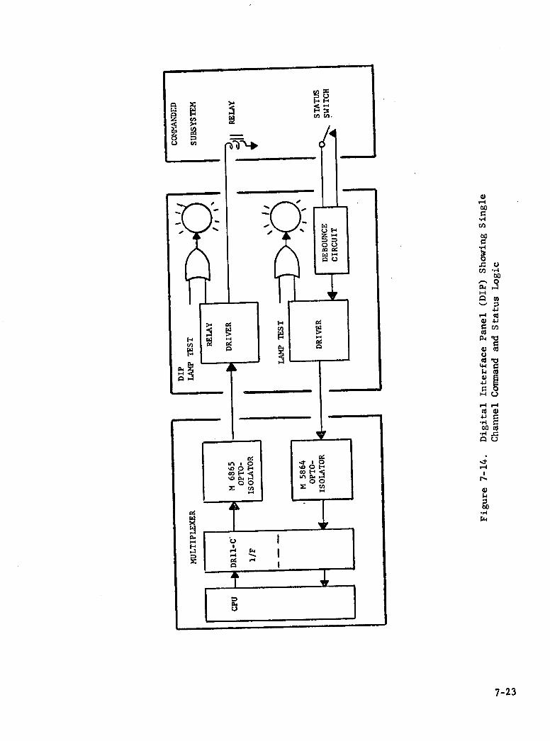
r0

z F-I

c,,cn.

a.- o

U

I I

-

00

f-I Cl)

I-I -

nsoI i0 %D0E I

I-I< III

x0jzo,

'-4

U

'3)

bO

r4 Cl)

bO

-'-4

Cl) •1

.-' 0

WI-h

C/)

WC

C.)

LF-4

I-i a)

.4-h

'—('-4

CW

-'-4

bOc -'-I

.J. '-4

C) '-I

7-23

7-24

H '-4

"-I Cl)

I I c I

,- 1-.

E' f 10

1-4

'.-1

rx I I -- I 'I

II Iii

IQ U)

I f I I

4.41.4

.U)

I 0'-

I !i 1

j

,-' C) "-4

1-4

('3

l-41.i

1-4

1-41-4 ('3W

•1-4

"4 '

Il-I '-I

I I iio I iu,EI I oiI IuI •ZIIL)

i

<crI.--IIQZ I I II-

cl

C.,

u-I

a)

H

Ii C.)

0

s-I

C) a)

H

H

0 5-i

.5-I

0

0

a) H H

a) C) Cd

z

H

ra) 5.4

"-4

7-25

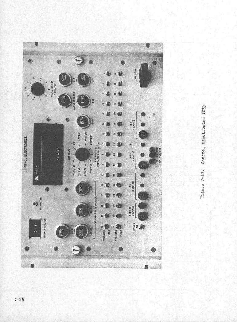
(I)

z 0

(II —j (LI

—J 0

z 0 C.)

I

• '• S

1T' : : ' áL .. T

S • S

,

+ +S

a . ,, ; • +

( \

>1 + 2$ zD

• • 01:;::r•

$g

•ii

:'

S

*

a a ...,

9

U

0 4-J

U

0

0 U

ci) 0

7-26

voltage through the jacks provided at the bottom of the panel. As on the DIP, the covered "ALL STOP" button instantly commands Emergency shutdown.

Figure 7-18 shows one channel of the CE signal conditioning, buffering, and logic ihich allows both manual and computer driven testing. The MUX sets up the "OPER/TEST" conmand so the CE will receive either the real sensor signal or a test (simulated) signal. The "COMP/MAN" conmand determines whether the CE receives a manual value from the front panel or a computer driven value through the D/A converter. The "FIXED/VAR" command selects either +5 Volts or the computer driven value. If a manual front panel test value is selected, it can be set to +5 Volts or placed on one of the potentiometers so that any specified value can be dialed.

7.3.2.3 Remote Multiplexer Unit (NNU or GNU)

The Remote Mux Unit whose functional arrangement is shown in Figure 7-19 con-sists of a PDP 11/04 computer built by Digital Equipment Corporation. The PDP 11/04 has 32K words of parity MOS memory, with the battery baókup feature (H775CA) so that data stored in MOS memory will be retained when power is off. The computer also has a KY11 LB programmer console so that the computer may be operated without a computer terminal. Figure 7-20 shows the hardware conf i-guration. The RMtJ is directly connected to the CRU via a DMC11 Network Link. This communications link will allow the PDP 11/04 to be down line loaded from a host processor (CRU). This feature allows the PDP 11/04 to receive all of its programming from the CRU and pass data to the CRU at a date rate of lMbs. In order to run the RSX-llS operating system, a programmable real time clock is provided (KW11P). Interface between sensors and computer are accomplished via four DR11C parallel I/O interfaces and two DR11-M parallel output inter-faces. All connections between sensors and interfaces are optically isolated via M5864 optical isolator input modules and M6865 optical isolator output modules.

7-27

I4

0iU z mz

0

4-4

1 1< I> I

1-IC)

0

U)

--4

c,l 41.4 Z 0 14

U)

> 0

00

4-1

0 0 0 --

'-4

-'.4 -o

.4-I 4.J ri C)

6w C/0

S.-

CIo

.r-I .I

00 I-I .I .0.0 C) -4

I-4

C.) 4--I 0 ,-4

4J 0 •I Oc,)

cc —4 r&

C-)

U) 0 '-4 z 0

0

0 I-' z o o o z

r —I

I <I 10 ZI IC)

7-28

H

z0

00

r I L)

<

I I I c1j I

104H

H ¼.

snii.rn oaci

I:D '1 I

IOc-1 o .< C,-'?.. o0

.1-I

I

I H

4)

1.4

00

.r4

7-29

G) ci

Fri -4Q -- 0

!

or

O.O0 -4<-. L))—Z 0 zo-4 zoz-

_____

__.-1 t11

Ou '0 0 0 O IIEIJ-•-----I4

-4}

1.1

'0 -4 oz

0 0

-4

_______ ________

- _______ p4 I

p4 OO

-

zo

cO

c,l -D u 0 -4 xo

o cU,

0 oz zo -4

0

j

c.'1

I-.. -,o . _________ <- I - 0 I 0

8 I z I ___ 0 ____ •-' - tl) —

Lt $

I-01-4 Z01

cz izi

7-30

7.3.2.4 Servo Controller

The Servo Controller performs the analog control of blade pitch angle in re-sponse. to mode and reference trim commands from the CRU and blade angle, hub speed, hydraulic valve spool position, and generator power from analog sen-sors as shown in Figure 7-21. The commanded modes of operation are listed and described back in Table 7-2.

Servo Controller regulates either generator shaft speed or power. A tacho-meter/precision reference combination provides an error signal when the genera-tor speed does not match the reference. In power mode, the error signal is the difference between a CPU supplied reference and the output of a power trans-ducer. The error signals are fed to an integrator and compensation circuits before they are amplified and converted to a current signal to drive the elec-tro-hydraulic servo valve. The Nacelle Mux Unit transmits the analog speed and power trim signals which are used for rate sync and for limiting power to a value below rated capacity. Because of the specialized electrical require-ments on the speed control tachometer, a second unit is used to provide gen-erator speed to the CPU for logic and recording purposes.

The servo valve control loop electronic design includes two displacement trans-ducers, a signal amplifier and a current amplifier. The main valve linear dis-placement transducer, an LVDT, provides a signal indicating hydraulic flow rate. The rotary displacement transducer, an RVDT, provides a signal indicating actual blade pitch angle. Both are magnetic devices requiring AC excitation and de-modulation. The signal amplifier is an operational amplifier, which provides a suituning junction, gain and compensation. The output is also used to pro-vide status to the CPU when the hydraulic pitch change mechanism does not re-spond to the error signal in a prescribed time. This condition, called Pitch Jam, causes the CPU to issue emergency shutdown commands, which feather and lock the blades and stop the shaft with the blades in a 3-9 o'clock position. The current amplifier is simply a linear, voltage-to-current converter which produces the 15 milliamperes required to drive the servo valve.

The Servo Controller is a combination of analog and digital circuits using off-the-shelf components to produce a low-cost, reliable design. The digital commands from the Nacelle Mux and the status back to the Nacelle Mux are handled by T05 relays. All resistors are low-temperature coefficient with 17. tolerance. The operational amplifiers are Bifet types (with high input im-pedance and low-drift characteristics with temperature and time) for long timing circuits like integrators and instrumentation types for critical off-set circuits like closed loop feedback amplifiers. The tachometers are de-signed using a Frequency to Voltage chip and a 1-pole active filter. The oscillator/demodulators for the linear (LVDT) and angular (RVDT) motion sen-sors are purchased off the shelf components. All circuitry is designed to give minimum offset (both current and voltage) drift over the ±20°F tempera-ture range controlled by the NMU Rack enclosure. Precision potentiometers are incorporated in all gain and feedback paths to allow field adjustment of critical parameters.

The generator control circuit consists of a tachometer which receives a signal from the generator shaft speed sensor and a reference. The tachometer has

7_311.

Gji.

£4,

U

2 1.1

14,0

Cl)

U

C.)

U .IJ

1-4

U I-. '

-0 I

I 1 ; I I IOOi,

- I>> I

z i I I IJ< I IuI

I I

H C)00

-'0 Uzo

o0 C'.

0

z 0 C)

0

ox

UI <II.I I-

(nZU 1.1 0

1.,

__;!Jj{

____ _____[Lr=

7-32

l7. accuracy at 1818 rpm to assure setting a small positive power reference in the event of an erroneous CPU command. An 1818 rpm reference will be pro-vided as the basic running reference. This reference and the tachometer user will use the same precision reference voltage to reduce drift errors. The tachometer basically consists of a precision charge dispenser that is triggered by the shaft speed pickup. On/off control of the loop will be controlled by a discrete command from the CPU via the NMUX. A ramp circuit controls the rise and fall of the speed reference signal to assure controlled startup and stop-ping. In addition to the reference signal, the CPU can set, via the D/A func-tion of the NMIJX, a trim on the speed reference to fine trim the speed to match the line frequency to enable breaker closure.

The error between the speed reference signal and the tachometer output is fed to an integrator along with the D/A output and the power signal. The integra-tor output voltage corresponds to a pitch angle setting on the rotor blades. Therefore, the integrator has a voltage limit to provide a maximum _O.50 pitch reference signal. This limit is required to assure rapid response to reduce pitch angle in the event of wind gusts or reduced speed commands. The sum-mary junction/integrator function is accomplished with a single operational am-plifier circuit. The clamp is done using an additional operational amplifier to clamp the integrator input when the voltage limit is reached. At normal operating speed, the error between speed reference and tachometer is nearly zero, so the integrator output is responding to the error between the D/A in-put (power reference) and the power signal, hence the generator output power is controlled.

7.3.2.5 Power Control and Input Panels

The power fed to the equipment racks is 115 Volts, single phase, 60 Hertz for all equipment except for the NNU rack air conditioner which is 208 Volts, single phase, 60 Hertz. The Power Control Panel at the top of the racks (see Figure 7-il) provides the on/off switch, status lights, and elapsed time meter. The AC Power Input Panel, together with its isolation transformer at the bottom of the rack, provides isolation, line filtering, and contains the power contactor which is controlled from the Power Control Panel.

7.3.2.6 Air Conditioner

The Nacelle Mux Unit Rack (Ice Box) is located in the Nacelle. It provides temperature control for its internal electronics. This heating and cooling is accomplished using a modified Model KAC-8 rear panel mounted electronic cab-inet air conditioner produced by Kooltronic, Inc. The internal heater is needed only for cold startup when the ice box air temperature is below 50°F. The ice box is an insulated enclosure which houses the Nacelle Control Sub-system electronics, and contains the air conditioner (nominally rated at 8000 Btuh) with a 500-watt heater. The ice box provides the cooling and heating to establish and maintain the ice box interior at 50°F to 90°F over the range of outdoor ambient temperature of 0°F to 124°F. The ice box is insulated with one-inch thick urethane foam insulation and has a K value of 0.25 Btu - in

hr - ft2-°F The electronics weight totals 750 lbs and, when operating continuously, gen-erates 1500 Watts of heat. The most temperature sensitive components have a

7-33

maximum operating temperature limit of 90°F. The air conditioner, heater, and circulating fan are contained in a single housing which mounts on the rear of the ice box.

7.3.3 CONTROL AND RECORDING UNIT (CRU) AND PERIPHERAL RACKS

The CRU and Peripheral Racks, which are located in the Control Enclosure contain the main process control computer, the mass storage disc drives, the real time clock for time tagging data, and the telephone line modem and auto caller. Also included in this section is the operator input/output device. Figure 7-22 is a photograph of the CRU and Peripheral Racks and lists a short description of each of the components.

7.3.3.1 Control and Recording Unit (CRU)

The Control and Recording Unit consists of a PDP 11/34 computer built by Digital Equipment Corporation. Figure 7-23 is a diagram of the functional arrangement showing the peripheral interfaces. The PDP 11/34 has 64K words of parity MOS memory, with the battery backup feature (H775CA) so that the data stored in MOD memory will be retained when power is off. The PDP 11/34 also has memory management so that up to 128K words of memory may be used. The central processing unit is further augmented by the use of the KE11-B extended arithmetic element and the FP11AU floating point unit. Both KE11-B and FP11AU units are required to run FORTRAN IV PLUS. In order to run the RSX-11M opera-ting system, a programmable real time clock is provided (KW11P). This unit provides interrupts up to 10 msec apart. Figure 7-24 is a diagram of the CRU hardware configuration showing the various interfaces.

7.3.3.2 Disc Units

The CRU utilizes two RKO5 disc units as RKO5 stores 2.5 megabytes of data. The as well as the archive disgnostic data,

7.3.3.3 Real Time Clock

the system program mass storage. Each REX 11M system and all system software, is stored on the disc units.

The CRU uses a Datum 9100 real time clock, with 1 msec resolution to indicate when events occur. The time is read using a DR11C interface. The Datum clock also has a battery backup to insure that an accurate time record may be main-tained despite power failure lasting 60 hours.

7.3.3.4 Auto Call and Modem

The CRU may contact a utility terminal or receive system status inquires via a VADIC 1601 Auto Calling Unit (ACU) and VADIC 301 Modem. The ACU is controlled by a DEC DN11-DA ACU interface. Serial communication is accomplished via a DL11-E serial interface at a data speed of 300 baud.

7.3.3.5 Operator Terminal

The device used for operator input and output is the DEC LA36 "DECwriter" shown in Figure 7-25. This keyboard printer prints messages and reports from the CRU

7-34

I

—4 ElOO 0El-4 rfl -QZ

01 O--4 i-1 ci O4 J OLlP o c,E--I E- fr.iI Z

P I H QXD II xIZ Z OZc,-I0 E-' ZE-40Q o 0cIr ZI 0-o PHc/

I i

p.' H 0

El p.1 0 Z I—I xE-

HZ

ri o

C) I—I < ,:Ip.'

-4 El

i-

-ii: Z IP4 ElE--4 ZE- tZ

Z 0 o

OEl o Oc,O

ji-4ElElo Elc II ri

xx10'H

Ic I IIZ o o I -zEl p-OZ

IZ' i-iI 'J¼J 4 I l-4<ZI-1 E-4

I I lI Qp OO I- riE- 101 H

r

I

C/)0Z r-1

I 0 -'-4

1-4

-'-4

4-I

0 0

0 Cd

1 Cd 1-. a,

4-I

a, p.'

Cd

0

C4 c.1

I—

a, 1-I

-'-4

7-35

OH 0

.1-i

a)

Ci s-I s-I

ci

0 .-

U

I—I

i-I

p-I

0

.1-I

5-i

0 C-,

a)

ci

0

5-I

0

0

ILcc

Iz

I I I

I l I.< <I

1

u>I

k 0

0 z 0 0

SflIRfl D2U

00

mZO H - 1-4

H

N

s-I

•r4

1-10

<I < 4- Z Z I-I

1-1 -

0. H H 0 <I—i

- 0 '-1 1-4

0. 0

z I-I

I--- -

C,,

I I m I __

rLFII L

7-36

____ fl I 1< &) C.)

_-4_ i—i I CI

1<

I - < I I -

T ] '-' 1-i

c 0 0 L_J uw Iz0

______ I-1

______ ___ E.4{u1 I_ I .-4

< i

I1 0 - 0 0 i

I I I - wl

i

L!__2_J1z

00 _____

0 z0 zz ________

•1-1 - 0 Cd

- < (1 I-i

0 0<<

I .r.4

______ 4-I 0 0 < <Z 0

_____ I 0 00 < 0,-w - - - -IO< - 0 @1

00 0I Z Z Z <-4

<0<0 .-<I4.) __________'0 Cd

_oi<zI 1.1

_______ _________Cd

L I C.-,

1 <0 I lio-- _________ I

- I-I

I 1-4 I0c'1u • cs1c,Z

I IIIZL

I 1-Z0H

I..-.4 •4-40P.4

p4

I__

0

T 1 4 L) C.)

I -4°-I< I O..00

iiii•1-1

-1--iC.) C)

00 I,.. IZ

U

0 IZ 4-4

z<o.1J

0

0

'0 )- l0

r

-o

I ) ____C)

I

4..C.) N.

.4-'

p4

7-37

ifl;

-

C-) as

C?

.:..;0 '1

I

.ø.

7-38

and gives commands typed in by the operator.

7.4 SENSORS

The WTG sensors are listed by number, type and location in Tables 7-6, 7-7,

7-8, and 7-9.

A brief description of each of the more important sensors on the WTG appears

in the following paragraphs.

7.4.1 WIND SPEED AND DIRECTION SENSOR

The Aerovane Transmitter is a combination anemometer and wind vane originally designed for the U.S. Navy as a durable and trouble-free instrument for measur-ing winds to 200 mph over a wide range of environmental conditions. The Aero-vane has been used world-wide in applications related to government, industry, research, and education. In the transmitter, the direction transducer is a synchro that operates on 115V 60 Hz; the speed transducer is a rugged DC magneto with a linear output. The 12-inch diameter, three-bladed molded rotor, coupled to the DC magneto, has a maximum threshold of 2.5 mph and distance constant of 15 ft. The output of the magneto, filtered to prevent radio interference, is linear; 9.2 VDC, into 1150 Ohms, at 87.1 mph (1800 rpm), and 10.56 Volts at 100 mph. Wind direction, measured by a streamlined vane with a damping ratio of approximately 0.28 and a distance constant of 34 ft., is transmitted by a Type IHG synchro, operating on 115 Volts, 60 Hz, to a DC converter.

7.4.2 SHAFT SPEED TRANSDUCERS

Shaft speeds of both rotor and generator are measured by using an Electro Corp-oration Di-Mag magnetic sensor along with ferromagnetic gear teeth on the shafts.

Di-Mag digital magnetic sensors are versatile, non-contact sensing devices. They combine active electronics with a magnetic sensor in a single shell to produce a constant amplitude output signal suitable for direct use in digital equipment. This combination results in a much lower noise factor. Because the digital signal conditioning is performed internally, interface circuitry with its associated costs is eliminated. Di-Mag's performance also offers several other benefits, the most important are:

1. The establishment of an extremely precise relationship between the physical position of any sensed object and the electrical signal produced.

2. Increased sensitivity with the capability to produce full output of +5 to +15 Volts at speeds as low as 3 inches per second at gaps of 0.050 inch, or 1 inch per second at gaps of 0.010 inch.

3. Excellent resistance to water, oil, shock and vibration damage which assures longevity and operating reliability.

7-39

4 -4 -4 .1:

*.-.

I P

14 -- N P-.41 o.c

p. IN in

C.. .-1

(N .1

1. .1 (0 1

0 ti

0 (N In

ID (0

'.0 in '0

'0

CC

in

'0 Si) in

(0 '.0 '

00 Li

(4 () 00 A

1< <'1 < I <1K'.o 0 (0

0' -. (0

(0 0 (0

4) -I '.0

I'. -.-4 001.)

'0 .

'0 '.0 .(

'0 -C

(C' 0

'0 0

'.C' L.

I CI

I C

I 0

-_ - -1 'J '0

-4.0 .4

SO -4

'0 '4

.o 1- 4) I-I PP

in r-

in N

en N

en N

in c-p

c-i In

c-i en

- c-i

- ('1

- in

. In N

' P.

IN

c-I N

ID P. IN c-i in c-i - in - c-i c-i c-i c-i

0,

1.4 1-0 04 04 1.4 3$

0)

1.4 04 04 0< 1.4 0< 14 04 0< 04 1.4 0< >4 14 1.4 1< 1.4 0< 1.4 1.4 04 04 >4 0'

• (0 10 '0 H o Z 0

in 0.

*51 0.

in P.

in 0.

.0 in

'0 in

.0 in

0'. 4

4 H

•.61 in 0'

in'0 0'. in (N c-i P E 01 33

0. 0. 33. P. 0. '0 r-.

0 n

I" c-i

141 .0

33 43

a (1 a a a a

01 .

01 4.1

41 14

01 41

33 0)

a 03

a 01

a 43

a .0

•a a

.010 00

14 H

14 H

43 14

41 14

41 44

41 4-4

03 14

H I_I .4 H 44 P-i

*1 (4

14 H

ii 1-4

.l P.4 44

(0 14

01 (4

01 44

--4(0 (0

H H H I-C H H 0

- 0

in 0

-'4 4 .4 .4 .4 '4 -'4 '0 sO '.0

H I-I I-i I-i

.11. 44 33

50 (0

(0 '0

N N

"3 (01

50 N

'.0 N

sO P.

'.0 N.

-0 N

'0 N

(0 in

0' '4'.

a'. Ii'.

a'. In In

41' ii'.

50 (51

50 P51

(0 IN

0 '0

4 10

.1 '0

in '0

14 0) 4101

0'. 0

41. P.)

(0 PSi

(0 10

'0 141

(0 1.1

'0 00

(0 14)

(0 (ii

'0 00

(0 In

N in

N c-i

c-. in

N c-i

P. in

50 0

'0 0

50 0

'0 00

4 30

.3 100

.3 0)

Z (0 .4

0 N.

(0 N.

'0 .3

'0 .3

(0) -4

(0 .3

'0 -3

'0 .3

'0 .3

'0 .3

in N

0 0

0 0

0 0

C) 0

ID 0

in (61

in IP

in in

01. .3

(0 0'.

CO 0'.

'0 0'

in H 10 (0 (0 (0 '0 '0 '0 (0 N 0 0 0 0 0 .14 in in '0 in c-i in

1s 61 IA

-4 00

.41 .41 14 01 03 61 61 01 01 01 'i-i 1.1

140101 .4

1) .,4

C' 4-i

C) .4

C) .4

C) .4

0) 44

C) 14

C) ,4 (0 44 0 C) 0 01 00

10 .01

61 41

o o 0344

I-) 1$ 14 'I

H P

.14 P

.4 P

H P

.4 P

H 0

01 04

01 61

61 C) .4

U '4

C) .4

1.i 14 0.

(0 111.

0144 0116

00 01

00 01

(0 41 14

4 I.

41 1.

10 1.

10 3.

10 3.

00 (Il.14 44 .4

3. 0

3. 0

14 0

in

0..14 H

14 U IC-I

0) 1.1 o

44 o

'.4 00 01

'0 In

'0 >'.

'0 1...

'0 In

'0 In

'0 1...

'0 1.'.

'0 1'.

'0 In

61 0-

01 0-

61 0-

'4 61

44 10

14 10 01

0) 14 61

41 .0

p.) (11 (41. 44 14

(0 (0 (00 0 0

14 01

I-I 43

1-4 01

13 0

3. 0

1. 41

10

000 iC'. 41 01 61

01010114'40101 0 0 01 C)

P. 0. 10 P. P. P. P. P. 33. P.PP 1.'

61 1'.

in c-i

161 c-i in ID (3 (3 El 00 (3 (3

Ii Ii

.061 C-i

3. 01

1. 0)

I-I 01 0

61 .4

(1 C-i

61 a

Ci o

C) 13

C) 0

(#3 0/) CO U) Cl) U).

.4 0 '0 '0 '0 03 01 0) 03 01 03 61 C) C) 0 14 061 CO

4. 01

1< >4 0< C-I 13

14

01. 13

0) (#3 1. 13

14 13

Ii 13

Ii 13

.1 14

0 1.

1 44

1. 03

146F-' F-P

.14

III04 61

01 10

01 01

01 61

01 01

01 01

p-I (2)

.-1 4)

01 10

01 10

04 30

(0 30

01 .01 C)

0) p.1 0)

01' 1/)

0 .

0 >

0 in

C) C)

01 3.

01 14

61 14

01 1.

01 Ii

0) 1. 01 61

03 11

03 1.

01 3.

01 14 g

00 00 0. '4 p. p. p. p. p. p. c-0 i-1. P. P. P. 0. 00 00 00 CI) (0

0.

01IA 54 01

61 01

(P 03

(21 14

10 03

01 Ii II

in1. P.

P.IA

14 P

0.03 P.)

'0 01

El01

'0 41

p10.

C.)03. (4

50 0) .

• 01 - H

.14

-'4 p-I 663100

44

'0 01

0 -.4 '4

03 0-

0) Li

.14 I c-I

..4

.14.0 ,4

IA p4

30 I)

3. P.

33 11 C)

03 01 1. '0 • 0. IC-i

00 '0 01 .14

0)

*14 • 0 41 14 1) C) 0) 41 01 C) 41 33 33 03 44 03 61 '4

'00 (0

0 (0 40 40

3. C)

C) 01

43 10

C) '4

I-I P.

p-i p-i 4)

.14 1

C) .4

in '4

13 C)

01 14

.01 10

'4.' -

0. (I)

0 P.

'44 41 .0

03 *4 03 01

01 .4

01 44

01 H

c4 43 01 C-i

0. 0)

4 0 41°

41 10. 01 01

C) .4 00 00 40 44 14 (/1 >

P .14 00

H 00

I. 1. 01 I-. 43.5

.0 .00.

.41 41 01 '4

01 44

01 '4

'4-1 '441. 1. (1.

*0 01 0114 0)

(4 0)

'0 '0

01 C) 61

.0 44 01 U . H Ii

(0 14

10 14

01 .41 '0 1. 11

03 .01 .01 0 0

01 .4 '0 10 0 CO .0 10 03 C) '4 44 3 10 '0 41 01 03 01 CI) 0) 19 44 01 10. CD 0 0- I. .4 03 01 03 CO

.0 C) i-i

.0 C) 49

1. 0 44

I.' 0 14

.01 C) 14

.0 C) '419

.01 (4

3..

'001 01

01 44 0

• '0

• '0

1.4 '44 03

i.i '44 41

10

II 01

'0

01

00

01

10 0 i-i

1. 0 19

Ii 01

.01

1. 01 01

14

P.

.4 0 00

0 00

.4 .4 44 '0 0 34

01 (0

In 1. (0

3.. (0

.01 10

.01 Cl)

41 1.

61 ID

01 (3

03 0 00

0 00

41 (3

01 (1. P. 0- P. P. (0 (3

.14 0

c-i 0

.-I 0

.3 0

in 0

(0 0

Ii'. 0

'0 0

N 0

10 0

0 in

*54 0

in 0

44 0

c-i 0

.3 0

p.1 0

.61 0

Ii'. 0

4'. 0

(0 0

N 0

0) 0

.0I

(0I

(0I

F-.S

F-II I S I

ZI I S S I I

F-II

F-iI 61

I 00

I 00

S 00

S 14

I F-.

I F-.

S F-I

H Li p.

0 p.

0 00

0 00 p. p. p. p. p. p. p.

-'4 .

->

00 0

00 0

.'4 >. P. P.

0 P.

00 0

00 .0

00 0

00 0)

• I I S S I S I I

.

I S I I I S I I I S S S I S

(0 (0 Z (0 (0 (0 (0 (0 (0 (0 (0 (0 (0 (0 (0 10 (0 '0 '0 (3 '0 Z z

0 -'4 4-i

-'4 4-I

0 Cl,

a, Cl,

'-4

0 .,4

'-I a,

0

r

a, I-I

,0

H

3.'

7-40

'-4 44 I

'.4 0

03 0 4. 0-) o 0 0. '0 0 0 0 0 N

-40 o

en en

00 en

00 en

00 en

00 en

B $ 44 1. 44 0000.

-

sOso en in

so en vs

SD en in

so en itS

so SO

e. >

en IA

en 'A ZJ1<1 1<1<1 en

sOen 50

en 50

en sO

en r-

- en 3

ess<l sO

0 en sO sO sO -

SO

- N - - - .4 N C - - -

en; x 4

U

en

4 4< 4< 4< 3< 34 #4 #4 34 34 #4 84 84 #4 34 34 #4 #4

0' - U

P. NU P. N

Ia P. N

-

- - - z .0 .0 .0 en en

'en CU

Q .-sH

i-i-'

o o e H P. H P. < P.H U 50.

en 5-'

en s

en '-.-' U '-

- 3 N - s. N 5-' ,-> U 5-'

en P. B BB 0) 50

B 44 N P. .0. r-

• 00 N 50 N .-450

N H50

N H enSD

B en U 4; SD U 6) SD U SD SD

o Z en •- .-)

S .0. '-

N B 4) 08 BE BE

B 6)B

H U HE

H 4-)

HE

5-)

4. N 0 N 0 SD

N N N U 444) 4444 40 UW - 44 - w .-iU H U

00 .0 8SD

S -' I 8 8 8 B H U U U U U U s-i U en so U en N )1

en 50 U en N H

IA 00 -4 H

00 0 0) r-. P. I'-. 4) 6; 44 W H H H H H H H -4 05 0' 05 0' 05 H

0 U N N U 5-.

U -4U H

U H

-D Os sODS so 0' itS 0' 0000' 0000' 0 05 en Os

H 0 0 0 0 N 0' N 0' N 05 000' IrS enO'

00itS 0005

en i-. -

In e-

os en

000' 0'00

U s-S sO S IA sO so sO '0 05 05 en 0' 00 05 en 05 00 0 CU

r- SD ,-I00 U -. 00 00 s-I CU 0 00

< .c B O

en as

0 en

en vs

0 so

50 SD

so SD

sO SD

'0 so

en en

CU CU en

CU U en en

CU CU en en en en N N SD

,-,,--.en,-5--.en--s N N SD N SDen en I"- SD

Z 4) CU .- In - U U U U en

0 N SD SD en en

SD SD en en

SD SD en en

r- SD .-S en -'--en -en en - en

o o

en SD

S en

N e-

I In

en Os

en as

en Os Os en HO HO H

P.O

4-5

P. 84HO P.84

< en 0 r'. 0 N N N 64 -. 084 034 0

4) B

'.5 5.3

00 .0 B U B

U 0 g g g SD SD SD SD SD SD SD SD

0 I-4

08. 44

0,4 -5 0 0 0 0 0 S 4. II 51

440. 0

II 0. 0

4-. 0

0 0

4.0 0 50 00 00 00 00 44 0

44 0

440 0 0 0 0 4)

00 44 U

p1. I-. 0. 1. .0 .0 .0 .0 .0 .0 .0 .0 0.

H

00 U B .-. 45 4) 6) 4) .0 .0 .0 .0 U

.0 U

. .0 .0

4455 0 44 0 .0 U

.0 U

.0 IJ

U U

U U

U U U U 1.5 U U B

6)40 B6)

B 0 0 0 44 0 5 U U .4 .4 .1 U U .4

.3 II 0 0. .-4 1-. 4) 45 05 01

I C en en en H 00 4-I 4)

I-. 0 U

4-4 4)

I. 44 4-. II 4-. 4. SD

U4-. .0

U65 44 44 4) 84 SD

#44) U

0 U C) U U U

.0.4

o U

0 U

0 0.

e 4-.

SD 3<

SD 84

SD #4

SD 34 1-

sO SD 4< II 00

0 4) H H 4) 4) 4) .0 .0 U P1 U 0

U 0. 0s Be-. O

0) U

0) 44 4)

.0 .4) .0 '4)

4)

8.

U

.44

U SD

00 U 4) IIU

0

4)

0

45 6)

4.5

P. 0 0 P.. 04 H 4 .3 8.

0.

.0

4-) 00

41 U U

00 00

.-3 S 4

00 4400

I N B U U U 00 '-

.s 4 00 0 H

B -) SD 0 .4

0 4)

0 44

0 4)

B '-I 4 0. 00 0

• 0 U 0. 4-. 0. 45 '-' 5-' 00

0. 4) U

5. 44 -. SD N Z Z U 5-. 0. 0. 00

5. 0. 4'U

0 8 I-) 45 6) 4) U .4

- • B 0 5.0 0

0 0

0 6)

14 U 0 4) 00 4) 4)

SD4- 4)

H .4 0 0 0 0 U s-I

0 UH

O 4) 3 44 Z ZU

U U

0. 0 .0

4 00

00 00

0 00

0P. P. s-S 0) 51

5. 0

00

0 s-i4;.

U SD SD U 0 4)

45 5-.

04-. 0. 0. 0. 5. 1.

0 .

0.

0 0

44 .4

00. 4)

04) 4)

4) 45

0 0. II U 0 0 0 0 0 0

U 4-. 4-. 0 .4 0. 0. U 4) '54 U U U U U Ia U 44

P.. B en en 0 0 - ..1

o 0.

so 5-. 5. 0. 0. 0. 5-. .4 .0. 44

.0 U

0)

B

44 B 'U SD SD SD 0 U 4) 4) 4) 0 41 0) s-I

U .4B 44

U 0 41 0 0 0 B B U II .4

B 4)

B 4)

B 45

B 4)

B 4)

0 44 U U 5-)

U 0. H

s-4 en

5. H

U U 3

U 3

.0. 3

0 Z 4 6) 6) 6) 6) (8 (8 H

8.

N en 00 SD H N In 50 N en 05 0 - N en H

so .-)

r-.-)

0 N H N ..4 0 0 0 0 0 0 0 0 0 I H IH I

s-i I I I

5-I S >

S H

I >

I H

S s- S >

I >

S-

I I 4;

I CI

S4 3. .1 .44 3 3 U C

0U P.

0 0

- CU CU 4-U 513

Z Is) P.. P. P 8. P. P. P. P. p. P.

4 P.I I I I I I I I I I I

I

S S

I

I

I

I

S

I

I

5

• -' -

.11.1114' A 0

I 0 0 0 (8 (8 (8 (8 (8

#5

7-41

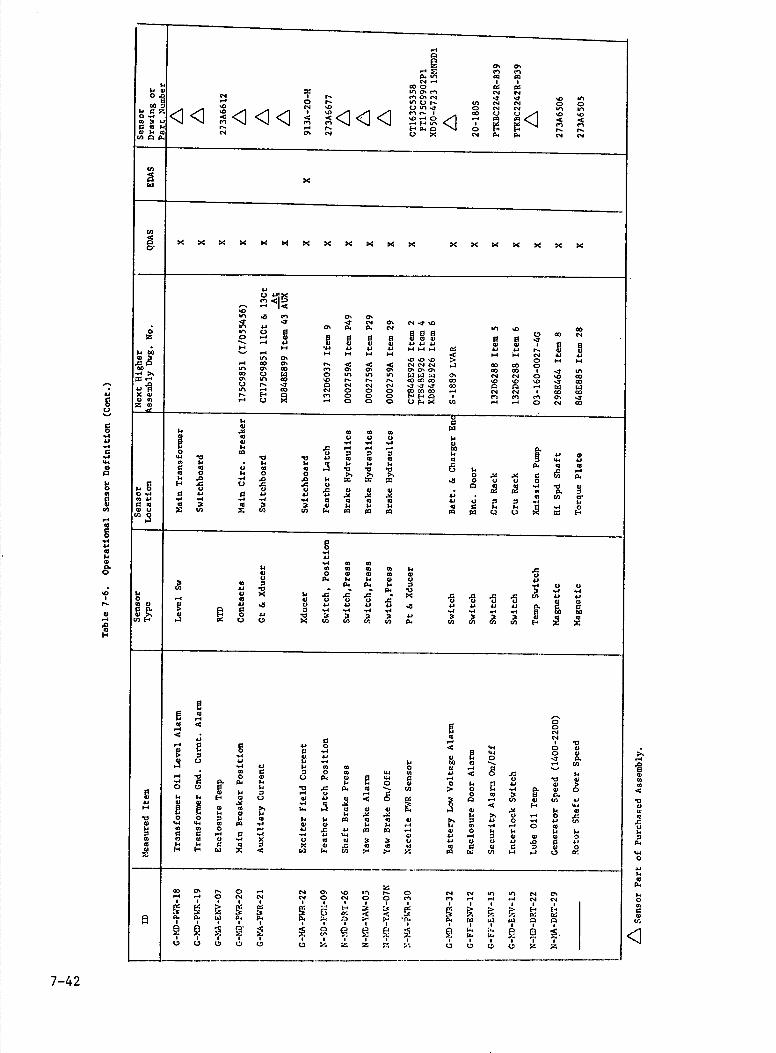
4.'

g C)

0

o'o' -z 0.4')

In 40

In 40

8.N '..' I S

841 Z400 IflOSIn

00 N 00

N o.0 4 -

S

0N N In Os N 40 40 40

SO N '0 400 N C) fl 40

'0-• 0

U) 0 -

N N '

N 454 0 40 40 4

0 40 'p

41 041I.. - F' " ' ?

I

4) I.' 41 N OS N (3 0 N

8" P.

8" P.

0. N 0.

N

U)

4')K

441K K K K K K K K K 04 04 K K K K 04 K K K 0'

'a C) 4.'0< 4., 44 -41

0 In .0 In Os Os

40 40 N 0' N-)D • o .rs

44 05 P. P. 454 In '0 40 N Z 0 -

41

• I-I44 4.8

4-4 41 '1.4

41 4) 4) 4a4.'4.4 4) 4) ' B B 8. 00 '. 4 I-I 4.'

I..'4.' 8.4

4.' 4-4

4-4 4-4 4 00 4.1 4-' N 4) 4) In 05 5050 50

.. 4-4 4-4 N 0

4.1 -4

4.' - 40 C' N 41 .41 .41 N N N ) 40 40 0 In 40

0' 40 C) 40

In 0

0' 40

C' Ifi05 Ifi C' 0'. C'

40 40 C'40 N 40 N 0 50

40 40 C' In 40 50 0. N 0. 404040 40 '0 50 '0 40 40 .0

4.1C) 40

N 40 '.8 40

0 N N 0

N 0

N 0

4040 40 41) 5041) 40 84 01 N 01 N

'.4 8 40 4)) K 41

4) 010. ..-4

1-' 01 (3 In 0 0

0 0

0 F' F' 0) 8 In In OS 40 0 C) P. 04 5)) .4 .4 0 N 40

1.U 0

4.41

.41 41 41 414')

41 U 0 0

0

4) 44 40

.0.4 "4

.4 '.4

-I '.

4) 00 0.

"-4 'C 'C 'C0 4.' 41 41 41

I-. '4

1.' 44-4

4) 4.' 0)

00. 41

• 0

4. 41

8. 41 -

I. 'C

8. 'C

8-, 'C C) 8.

P. '4 '4 41 0 8. 0 0 4". >s 0'. 0 .41 .41 0

.0 50

-. P.

8-.

8. 4-4

.0

.0 0

.1 C)

.0

.0 U

.0

.0 0

1. 41

.4 0 01

0 0 0 .4 'C 41

0'... 0 41 0 41 4.1.0 4-4

4) ,41

4) ,41

4) •41

• 41 41 41

0. 41) 8444 .'.I .8 '.4 .4 .4 41 41 41 41 41 5) 0 0 .4

41' 0. 041 410 41 441 41 4) 8. 8. 8. 41 0 8. 8. B .4 0 U) U) 4'. 40 40 40 40 40 Q C) K 4-.

C '.4 4,

8-.'.4 05

01 41

41 41 0) 8. .0

41

4) 0 0

0 P.

4) 8.

4) 8.

41 6)

6) 0

0 1.'

5)1 1.1 'C0.•

P. 8. P.

0 '0

'.4 4'

0 .4

5) .4 0.

0 440 41

04 14 4)

.0 0

.0 5)

.0 0

" .0

441 .0 U

.0 0

.0 .0 5)) 1.1 4.' 4141 4) 4 s4) 0 'a 'a 1- 4 .0 4' 4.'

0 4.1

0 44 0.

4) 0

6) 5)

4) 415) 0 4.'

0 'C

.4 4'

.4 '.4 .44.,

.4 .4 s-I 5-I 4 00 00 U) -) 00 C) 4 40 4'

5))4' 40

4' 5)) 0.

4' 40

4' 5))

4' 40 4' 5))

0) 4-4 41 41

-.-.5 0

41 41

0 N N '.4 4)

4-'

g 445) 0

"4 .41 '44

S 0

'C 6)

4' 0 .45) 5)

54 44 @1

B 8.

'4 0

0 6) C) 4.' 1. s-I 8. 00 41

40 '-4

0. 4.0 '.4 10 44

5)I-. 0

'4 0

41 15 44

0 04

41 4-4

'-4 <

5) 0 .5) I. '.4

.8'C 5) 0.

0 P.

6) 4.

C) P. 5) 8.

4-4 5) '-4 U 'C 41 0 (0 4 4. 'C .0 0.

0 '.

4) 0 .

1. 5) 1.'

4.' .4

0) 4)

11 0) 4.4

8. 4)

8.6) I-I

8. 6)

.41

0 (3

'-4 4) -4

1. 4-4 4)

.41

,-00

0 01

44 "4

4' U)

. 4 4)

0. U) 4.1

40 4'..

4 4) 4) . 4).41

.414-4

4.'44

41 '0 0

8. 0 0

w 8.'

1. 41 1, 8.

8. 40

.41 84

..4 4) 4'.

8. 0

0'. 4.)

0 0 .'4

.40 4.1

.0 6) 844 '44 4 40 4 6) 0) 8. 1.) .-4 44 15 '.4 '.4 0 41

4')

8. 0

0) 5)

0) 5)

0 4.' .0 41 40 40 ,..' 4) 0 8.' 8-1 8-1 8-1 41 4) 04

.0

5) 54 -8 K

.4 0

44 '4

'1-1 0) '4 4'

4.) U

44 4.1 U

0 0

4) 4.4

6) .0

4) 5)

0 4)

41 1.1 1-'

I. 4-.

5) 0 K 0) .0 41 44 4) '4 5) 6) 5) 0 4) 0 6) X .4 14. 4') 0' 0-' Z 40 40 4') 8-1 I-) (0 00

0) 0'. 0. 0 .4 N 05 50 84')z N C' N N In "4 N C'. '.4

S S0 N 654 N 0 N 0 0 1 In .-4 ..4 '.1 N P4

I'I

?

S E?

I 00

S C S I I S I I I I S El

I I-I

I I

01 'P. . I') P. P. P. 4'. 0) 4" 4'. 'P. P. 40 ) 4') 01 01 I 8-4 5 S I S I I I I I I S S I I S I I I 0. A

S (0

I C)

S (3

I (0

I (0

S (0

S I Z

I Z

I I I (5

S (3

S (0

I (3

I Z

S Z

7-42

N

I-I

H

1400 0 0 0 0 0 0 0 0 0 0 0 o .o

1.3 P1

0U '4)

- 00

- O '0

'-4 o4)

'- 00 .- 00

.- '0 N '0 N .0

0 01) 00 00 •o:

'0 -

00 -C

00 -

b '0

<

'0 .-

'0 .

'0 <

00

,.g 4) U '0 N '0 i'. '0 N '0 N

'0 N '0 N '0 N 4') 4'- '0 N on I'-

on N 4)) 03 I 1403 N N N' 4)4 N N N N N N N

Op..

C) 0

X 1< X 14 1.4 1.4 14 1.4 1.4 14 14 14 1.4 14 14 1< 1.414 1.4 1.4 1.4 1.4 14 C) '0

0' .-1 U .4 .4 U .4 U U .4 .-4 N N

• 0 0 0 0 0 0 0 0 0 0 0 o '0 '0 Z Z '0 '0 '0 '0 '0 '0 '0 z

g a

4.3 1.4 U 1.3 1.4 1.3 U U U U U

.4 '0

410 44

U) 0'1

010 4)1

U) 44

U) N U)

N410 N

U) N

On N

410 '0

00 4')

.4 4.4 .0

00 14)

00 '0

0' 14)

00 '0

0' 0)

00 0)

00 0)

00 0)

00 14

01. 14

00 19

IC 4)

'0 4

'0 -.t

'0 .4)

'0 .4)

'0 4

'0 4

'0 .4)

'0 4

'0 .4)

'0 4

'0 4

z '0 '0 '0 00 00 '0 '0 '0 '0 0) '0

0) E 0 03 1.) 0'14 4)

'0

0-41. 0.

'C) 41 -

14 0-.

.0 00

-1 0)o

N • 004) 00

'0

44 00 U 44.4 00 4.403 0)

0 14) '0

0 4) q

0 0

0 4) 0 0

0. U) .0 4)) 1'

00

OU'0 .4) .0 .0 .0 .0 .0 0 U 0 U 0 U 0 U'0

0,41 4)0 0 0 0 0 0 U)

0 U)

0 U) 0 0 0 0

0 U)

0 U)

0 U) '0

) '0 '0 '0

9 '0

9 '0 .

.1 p.

U P.

0 '0

.4 P.

4)0 0103.)

0) 41 03 03 41 03 03 00 4) 41 41 41 41 41 41 41 41 41 41 41 (1. 1.) (1. C.) C.) C.) C.) C.) C.) C.) C.) C.) C.) C.) C.) C.) C.) C.) C) C.) (1. C.) C.) 4)

U4) 4

14 0. 0. 04) 14

U14 U

I.. U

I. U

1U

1.3 44

14 1.4

14 U

04 1.4

0.3 U

I.. U

II U

1. U

0. U

1.. U

1. U

14 4.3 1U 1.. U 1. U I. 4.4 I 4.4 1. U 9 0 9 0 4) 1 C/) 03) U) U) Cl) U) U) U) 03) '0 '0 03) CO U) CO CO U) U) CO CO 00 Cl) U) C) 0 4)1-4

U) 00 00 00 00 00 00 00 00 00 00 00 00 00 . . . - 00 00 00 00 000

o . . , .4 . . . . . .0)

..3I. '0

1. 00

14 '0

14 00 . . . . 4) 4)

4 4 4 4 4 4 4 4 4 4 .3(4.3(4.330.4304 4 4 4 $ 4 .4) - 4

00 00 40 00 00 4)

00 4)

4) U

4) .4 00 4)

00 4)

C) U

C) U

U

•

.4 o

'0 4)

'0 4) 0)

U '0 4)

U '0 4)

'0 4) 0)

'0 0) 0) 0.

Cl) 00'0 0

'00) '0

'0 000.

• 0.

P 4) -

0) 4) 4) 0)4) 4) 4) 4) 0) 4) 4)

3- P

E0) o

4) 4)

•4)

00 .4

0) '.4

4) 0

4) 00

4) 0)

• 01 1)

0) -.4

0) '.4 0 0 0 0 0 0 0 0 C.) 3)

0) 3-4

U '.4 • .3

0 .4

04 U U • 0 '0 X.

0 U U 03

U 0,

U U lb

.4 0)

U 0,

S-'. . 00 4) 0) 00 00 10 03 03 00 1. 03 0)

0). 441 03 00 0) 4) (1

4) 000 I.) 4-4 '0 0 00 00 0 04 '-4 'CI 0 4) 4) 0) 0) 0) 4) 0 0) 0) U

14.'0 (4

U) 4

0 1-)

14. 19 H U 0.

'0 (4

'0 4

0 14

0-. 0.3 1.- 1.4 I.) 14 1.) 14 10 U (-3 3-4 1. 3.4

0-C 44 14 04 0 0 1.) 14 4-! 44 1.-! 0 0 0 0 0 0 0 00 0 0 0 0 U) U) U) 0 0 0 0 U) U) U) 0 0 0 C.) C.) C) 3-I . . 4-4

4-3 .-4 .-4 '.4 - U .-1 44 N N N N N N-

4) 0

'-- 4) 0

- 4) 0

'-- 4) 0

- (1 0

'.- 4) 0

U 4-40 Z 0

'0• 04)

40 00 -

o 0 0 0 0 0 0 .............

0 0 0 0 0 0 (0 4 04 .4 U .4 U 0) .4)

'0 0 '0

'0 0

4) I-. '0

03

'0 '0 '0 .) '0 Z '0 '0 '0 '0 '0 '0 '0 0) 4) 4) 4) 0) 4) '0 CI)

0) 43 4) 4) 4) 43 0) 4) 3) 4) 0) 3) 4) 3) 1-4 1-) 0-4 1-4 3-. I-I 14 .0) .4) 14 .0 'CI 4)

'0 4)

'0 01

'4) 41

'0 03

'0 04

'0 03

'0 00

'0 1.1

'0 Id

'4) '0

'Ci 0)

'0 04

'0 Ci .0 .0) .4) .0) .0 .0)

0 U

0 U

0 U

0 43

0 U

04 00

U 00

U '0

.4 00

U '0

U 00

•-4 '0

0 '0

II Cl)

.4 0)

.4 00

.4 00

U '0

'4 00

9 '0

9 '0

9 9 '0

9 - '0

9 '0

0 0)

U P.

'.4 P. 0

0)U p.

4) 1 0 U N 0') -4) U) 00 N 00 00 C) .4 4)4 0') -4) U) 4) 0 U N 1') 4 010 10 N '0 0' U U U U ..4 U U .4 4-4 4)4 ('3 N 4-4 N C')

s-I 0 .1-) 0

0 •0.1

.1-I

.4-4

•4-1

t44

a)

5-I

0

-'-4

5-4

a)

•1

7-43

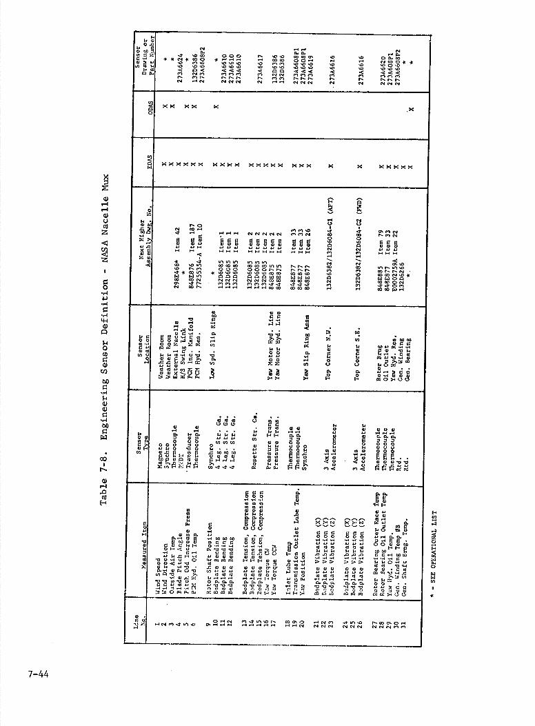
1.40 0.0

$4 000;j U N . LiLi N

0) U 0 Z -.t '0 10 0 0 0 N 10 U)4..P.. U) CO 05 '0 sO 0 4. CO Il C'1 10 0 0 '0 In 10

-. '-I - '0 U) U)

- '1-

U) U) 0 "4 - Li N 10 0 U) $3 1.. '0 '0 sO '010 '0 U)

In In U) U)

'0 U) U) U) U) U)

'0 50

50 U)

10 0 '0 014. -.

In01< <<< < 001 <<< <

0 U) U)

C'-.N In 1') r-. In In In

r- F-. r-In r..

N 01 In In In In In In In In N 'ON N ('101 01 In n

Li Lir-. 1'-. I'-. N C'l N N

NC-. 151 r-. F-. N

01151 N

cc

U '-4

C',

El1-I 4) 0) -3

U

4 5. U

.3 4)

0 U)

<4$4 $'X$.X Xd $4 4 $4$4$4XX

_-' I-I

% 0

0 z 5-

Ci. Li WI r-..0 0 0

N CO Li "4 Li Li Li N ('4 N N N In In 0 In In N

, U) U)

O In ('4 B

Eo -EBB

0 0 N In N Li OJP 4)0)

BE B 00 41

BEE 00141

U) 01

U) BEE Ii .0 Ii P 1-4 44 P 4.4 P P P P P P P P (4 01 €51 01010 P 4) 1) K U 0)01-1 1-4 - 1-1 Li 1-41-4 1-1 1-44-4 4-4 4-4 -4 In In 1-1 4-41-I

41 .<

I )'

U) U) InIn In In U) CO U)

(1 In 1(1 U) U) CO If) In N N N

1-4 '--. N U)

-I '01 0' U)

0 N In CO In

000 000 N N N N N InU) In

In N In U) CO N C-- ('1

$33 COIn, IOU) '0

00101U) '010 U) U) 0100000

CO U) U) 0140

U) 0

ID U) CO N 50 U) 10(4 (-4 1-4 N N N N In U) U) CO CO N

01 c-I

140000 CO U) 0151 OS - N

N U) N In In In Li Li Li In In In -.t -

Li Li- s In In - 0 In .-4 a) CO CO CO U) ,.4 Li CO U) $3) Li

41 4141 $0 00 B '0

4) Li0

s-Is-I..-i ,.).)

41 Li 0 41 Li.I01 •

$0 $40 E&1'-40a,

0. "4 .o. 00

0 Z 00 41..)4141 Li 1000 s-I Cl) 410000 415.4 r. p

0010 0000 11-4) 4.0

CI) $0 1.. 1 00P00si 414) .-i0 . . .

$414 00 0.

0) Cl 0

00 'OIL ILLi U) 0 0

Ci Ii 41 "4 0'0 '0 1) P "4 ii.1-41

U) P '0.-I 0) .- .0.0 101-'00

0. 00 Li 0 0 P1_la) CI) 1000 CI) U U 11000

0 0) K'- 0. 0

0. 0

0 P.0)00

00 10 4. 4. $4 El El0-.-I000) 000$400

41 414113 0

0) 0)000 1- Ci

Li .-I . . .

•4113

II $414 00 Li Li

0) 41 0) 0)0)0) 14 04)

4. 1. 0. U II 11 14 0 El El 4. 0. 0)41 4)

Li Li Li 0.0. 0.

011OU

0 00PPP U)U)U)

U)04)

U U UUU 0' 001) UC) 0 0) 1111

00 000

0 1.

0 1-. 000 C)14 0140 010 k.. P UU 001.4 410) 0)41 00)0 000 U) 0.0 10 .1-000000

000)0P 55CC 0 oss

..-lLi .,.lLi

50 0)0 0 $414 00, .0

0 C) WWG)'O'O 00 04) In< In-<

0.0. 00 U 4)

EU 4)4)

41(00) I-I 1-IF. 0)

0)01(0 4100 0 00 0)

41141.11

4. 0. 0..0 00)

140g

1- -s---..--.-s Li 0 Cl

P. c 0 000 P

I-1CI s-I C) 01-0 1-1-1-

)1( 05$ 0 El

'0 0)

4)4)0. 0.-4 13 130000

000)41-.

P '0 40 0000 411-00 Os-I-I--I

1- 1- 1- 000

'

.'4 P

0.000 '0 '0 --4 Lilip

000 -1 -.4 '-4 444)41

P.-l0,0. '0 U U

0000100 1.. U

0El., 0 'U'U'U•,4'0..-I 0503 s)C)

131)10 $4141.

13.341 Ci Ci Ci 0000 Ci

(0s-I 1-Li P 11.0 - .-I

01-0 44 0 C) 0)

1-0.0 0 4) 0) 0

El1-1- 0 0

.0.0.0 -I s-I '0

.0.0.0 01-Li5000 13 '0C)-.-IO 0 "4004)4) ElEL)-' 0)0) Os-I-.') -i.0

s-I "4 -.4 '.U-U'

-- -.4 -1 U 14)40-440 0) 0W<PV

0)4 s-I'U .'0 .0000)

UU 4)00)00'

,.341P 4)10 0"4 0..-I0B..O'U hIPPO 000)4)4 U)0'0

5)"4410)010 PO4' 000) POP 00) .013

(4)00 I'. '0 0.0

131Cr) Ci .0 .0 .0

4113000 130 131351 411313 '0 '0 50 '0 0 0 0. 0. 4.

.'l .0 ,O )-1 1-5 0. 0. (5.

44 0) 4. .'J .0 .-I .0 0. 4.. 0.

Li .0 Li 0.

$4 1. 00 0 1- P 41 P 10 -44lj.'4.44 4-' '.3'U'0 'U'0 '0 o 13 '0 '0 '0

4.. 0. '0 '0 '0

0 0 P P 0 1-00554)

0000004)4'.0''151 U)U)c-)...$4

Oh, - 0j) 0.5:' 1-I-s$4 U)U)U) 004)4)

01 0 0

Li(4In4In50 0 Li ('.1 Os.-ILi,.4 In 1(50 N LirI.-I.-).-4 100' 0 OLiN Li c-I In (4011-)

11 In '0 N 4) O. 0 Li NNN NC-4C-4InIn

w i-1 '-4

C) C)

z

z

0 .1-I

'-4

•1-4

'-4-I

U

0 Co

U Cl)

.1-I

U U

-I-I

7-44

r

U v-I

H

14 144) 0.0

14 U'0 .-4

QO 4' 4' 4' 4' 4) '0 '0 4) 4' 4)

C ..-)'0 -U

'0

0)4)1.1')

a. a.

:4: :4: 44 44 44

44 44 44 44 44 44 44 44 44 44 IC)

0 z

14 U--

-.4-1

4) 4) 4) 4) 4) N N4' 4) 4'

4.0 U

0 '0

0 '0

ZG) C'l N 0) 0

U) .-,

U)

-U

41 'C 'C 'C 'U .E

'U 4.' 03 C

o1. '4

44 v3

44'4

44 '4 03 v-I

1..-.-' 04

0 .0

0 .a

0 .0

0 .0

0 .0

0 .0

0 .0

a.

a'4 .0 .0 .0 .0 ,C .0 .0 f CC) U

4-'U 4-4

U C)

C) C)

U 4.'

44 4)

4. U

U 44

U 44

U) •.-) -) •-' -) -.4 ._. Co

.,-, i

40 0

0) Cl):4

U) (0 U) H H U) H

03 U

14 4)

44 44 1. 'UU

1a U U C

0) U C

4) U C

'4 C U

'0 C '4 .-4

• '-I

0) U

44 'C) 'C) '0 14 44 0) 0) '0 04)

I'4 C C

'4 C

H I-' U U

U U

'4 C

'4 '4 '4

Cd 14

. ,44. '4

H H H 1-' H 44

'-U '-U "4a. a. .4 '4 44

0,-U4)

HHHE 4-4 a o o 0 0 0 U) U) U) 0

U)

zo .

d z

c Z Z Z

4,-U .4 4) 0 ,- - 0) C) U U 4) U C) '0'

'0 '0 '•'.'4

4-' "

4.' -U '4

4.' '4

4-' '4

C)

C'4. C

1-4 C

4-' C

'' '-. U) U) U) U) U) C!) '4 -o a

44a 14 14

a 44 14

U 1.' 14

14 U

:4

44 4) Co

0 0 '4

0 0

-.-)

CI 0 -I

C 0

•.-I

Cl 0

•.-4C 0

-.-1

0

'U

Cd 41 .-I

0) C4-

0)) C C C 0 0 4-) 4-' 4-) 1. 4-' 4.' .-4 0

'0 0)

0 0 0 0. 0. '4 44

Cd 1.1-

03 1, 14

a 14

Cd 44

'4 '4

. -' 4-)

I.' 1-. 1.' 14 14 14 .0 - .0 .0 .0 .0 4--, I-. Cd C 0)

0 4-)

0 4.'

0 C)

0 44

0 4.'

--4 --4 -.-1 .-4 .4 •'-414

0 1.'

-C 0!)

a Cd '4 a a a U Cd

41 0) 14 14 C. 0. 44 44 U

C. U

54 4)

14 4)

14 4)

4.' •,-4

44 C) Z 4)

CU CI

4) C

4) C

4) C

43U Cl

U 0 0) 0

U 0.1

U 0

4) 0

U 0 H H H I-' 1-4 H I1 0.) (4

4) . 0 '-4 U) N.

Cl 0 .-4 0-4 4') 0) '0 0-. 0) 0' .-1 v-4 v-I .•4 ..-4

0 s-I

Cl)

z

0 -1

"-I

"-4

w

I-i 0 C))

w

Cl)

"-4 I-I w U

"-I

7-45

7.4.3 BLADE POSITION ANGLE TRANSDUCER

A KAVLICO RVDT (Rotary Variable Differential Transformer) is used to measure blade pitch angles by sensing the swing link position in rotation. The R502 type has been chosen with modifications to accommodate the 0 to +10 Volt output for 0 to 800 rotational range.

7.4.4 ROTOR SHAFT AND NACELLE POSITION SENSOR

The sensors for bathNacelle position and rotor shaft position are size 23 - standard military 23Cx6D, 60 Hz control transmitters (synchros) manufactured by the Vernitron Corporation. These units are accurate to 6 minutes of arc. The output signal is converted to a 0 to 10 Volt DC level by Interface Engin-eering's Model SA81O-B Synchro-to-Linear DC Converter.

7.5 ENGINEERING DATA ACQUISITION SYSTEM (EDAS)

The Engineering Data Acquisition System (EDAS) provides data for structural, aerodynamic, and electrical performance evaluation of the WTG System.

General Electric provides sensors, signal conditioning, buffering wher.e neces-sary, and cabling to the Mobile Data Acquisition System supplied by NASA.

This system is described in detail in NASA Statement of Work No. 3-783203, dated April 15, 1976. Basically, the system hardware consists of three 32-channel Remote Multiplexer Units (RMIJ), a Stand-Alone Instrument Recorder (SAIR), and a Portable Instrument Vehicle (PIV).

7.5.1 REMOTE MULTIPLEX UNITS

Three RNU's are used on each 2000 kW WTG, one in the rotor, one in the Nacelle and one in the control enclosure. Each RMU can process up to 32 inputs con-sisting of sensors or previously conditioned and buffered signals.

7.5.2 STAND-ALONE INSTRUMENT RECORDER (SAIR)

When the PIV is not at the WTG site, the SAIR is available to record approxi-mately 40 minutes of preselected inputs from each RMU on a continuous tape loop. Sixteen channels of data can be recorded from each RMILJ on each of 3 tracks; the fourth track records an internally generated time code. Signals and the remote stop command enter the SAIR via one 18-pin connector. The remaining 3-pin connector is for 120 Volt AC power input.

A momentary contact closure between pins B and C of the 18-pin connector stops the recorder, saving the last 40 minutes of data. Recording can be started again only by pushing the manual reset button.

7.5.3 PORTABLE INSTRUMENT VEHICLE (Ply)

The PIV provides data reduction facilities for the Engineering Data Acquisition System either in a real-time mode or in an off-line mode with playback of re-corded data.

7-46

Interfacing of the PIV to the WTG is through connectors on the exterior of the vehicle. Power (480 Volts, 3 Phase, 30 kVA) enters on the left side

of the Ply while FM multiplexed signals from the RMUX enter on the right side through Jl through J9 (6 jacks for signals and 3 for expansion capa-bility). Calibration commands to the RMUX are provided by J17.

7.6 SOF1ARE DESCRIPTION

7.6.1 FUNCTIONAL FLOW

The WTG software system is comprised of two parts, Process Control and Auxil-liary Functions as shown in Figure 7-26.

DATA CHANCE- DATA SENSOR

PROCESS DATA DATA

ACQUISITION CO4AND STATUS

CO*1AND

PROCESS I _______________ - CAND

OUTPUT

CRU

TEST -

PROCESS CONTROLAUXILIARY I

CONTROL DATA BASF.-

CHA'CEFUNCTIONS

FUNCTIONS REPORT

ETC.

IT

Figure 7-26. Software Overview Diagram

The Process Control function is performed in three computers, the Control and Recording Unit (CRU), the Nacelle Multiplexer Unit (NNIJ) and the Ground Multi-plexer Unit (GNU). The GNU and NNU are used for data collection and data con-centration. They provide the system link to the commands and sensors in the WTG. The CRU performs the analysis of sensor change data, and causes commands to be dispatched by the NMU and GNU as circumstances require. The Process Control function is clock-driven as opposed to interrupt-driven. A request is dispatched by the CRU to the GNU and NMU every 100 millisecond, which directs these multi-plexers to sample data, compress it and report predetermined changes to the CRU. Commands initiated by the CRU are output by the multiplexers. Command completion is monitored; retry, when necessary, is performed; status, either pass or fail, is reported back to the CRU. Conditions resulting in shutdown are monitored by

7-47

the CRU; when detected, the appropriate command sequences are initiated and sent to the. GNU and NNU. All inter-computer discourse and all significant events are recorded in the Archive file by the CRU.

Auxiliary Functions (which consist of operator interface routines, utility interface routines, data base inspect and change routines, archive replay, report control, and manual system exercise) are handled primarily in the CRU. They are implemented as "background" tasks and executed during time remaining between end of Process Control function and the next tick of the 100 millisecond Process Control Clock.

A functional representation of the Data Acquisition cycle and of the Command Output and Process cycle is contained in Figures 7-27 and 7-28 respectively. Figure 7-29 depicts the start to finish process of sensing an abnormal con-dition, generating the command to correct that condition, and sensing the fact that the command was initiated properly by the hardware.

7.6.2 SYSTEM FUNCTIONAL ALLOCATION

Three basic functions are performed by the WTG software system. They are: Process Control, Data Recording, and Auxiliary Functions. The Process Control Function is carried out in all three processors; the CRU, GNU and NMU. In the CRU, Process Control is performed by Data Acquisition, Control Task, State En-able and Data Process Modules. In the GNU and NWJ, Process Control is per-formed by Data Acquisition, Data Process, Output, Command Acquisition, Command Process, and Controls Interface Driver. Data Recording is performed entirely in the CRU via the Archive processor. Auxiliary functions are likewise carried out primarily in the CRU. The modules involved in the CRU include Display, Manual (Functions), Test (Build), Modify, Playback, Startup, and Report. Test Execute module executes in each of the CRU's.

7.6.3 MODULE FUNCTIONAL DESCRIPTIONS

7.6.3.1 Control and Recording Unit (CRU)

Data Acquisition/Control Task. Data Acquisition is activated whenever a data buffer is received in the CRU. It schedules ARCHIVE and the Control Task. The Control Task examines the buffer, strips out the data, event by event, and enters each event occurrence in the CRU Event Table. It then cycles through the Event Table, scheduling Data Process Modules (DPMS) for each newly tabled event. Four services are provided to the Data Process Modules. They are: the issuance of commands to the GMU/NMU, the initiation of one Data Process Task by another, the changing of the status of the runability of other DPMS, and the saving of computed variables for use by other DPNS.

State Enable. State Enable is the module which remembers which tasks must con-sent for the system to go from the IDLE state to the GENERATE state and reman-bers which modules still have not consented. When the system is in the

7-48

0 CI)

U)

a)

I

7-49

7-50

F I I

i

I I

H

I ! HI ZH

___

I ___

I°'' tJl

.4

0 .l-J

a)

H 0 0

c'J

a) s-I

b0

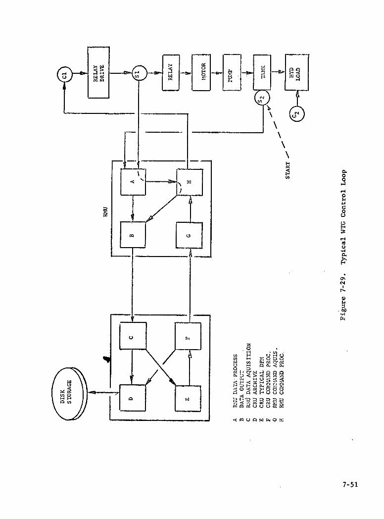
h4 -4

U H

0

CI)

'I < 'I

I I Q

0 0 '—I

0

4.J

0 0 0 El I-.' 0

-,-1

0' c1

0)

•r•l r4

z F/i C') 1-4 O)

C') o '-o C F 0' N p

i: > < •

. -4 . I-1 -1 ) E- 0 ,. . 0 'C >-. 0 0 0

..)c Qoo')

7-51

AUTOMATIC mode of operation, it is either in the GENERATE state trying to stay there, or in the IDLE state trying to go to GENERATE when conditions permit.

Data Process Modules. Data Process Modules examine change conditions as re-flected in sensor status changes being reported by the RNIJS and react to them as necessary. These reactions can include Command output, process shutdown, or notification to other modules.

Archive. Archive records all pertinent system data. This data includes tra-ffic to and from the RNUS, discourse with the operator when the system is in AUTOMATIC mode, interface with the Utility, and internal changes of state.

Display. Displays predefined groups of system (collected and monitored) data on the CRT and/or DEC writer. As the sensors that contribute to any current display change, the display is also updated.

Manual. Manual provides the on-site operator with the facility to exercise various component parts of the WTG environment. These manually exercisable functions are Pitch, Yaw, Blade Rotation Enable, Rate Sync, Angle Sync, and Normal Shutdown. This module prevents the operator from performing any func-tion which could conceivably cause damage to any part of the system.

Test. Test provides the on-site operator with the capability to alter the system sensor scan frequency and to alter the source of the incoming sensor data. Sensor data source can be Manual, Computer, or Live (Sensor).

Modify. Modify provides the operator with the capability of altering critical system parameters. Those items which the operator can modify include the present power setting, the present sample rate, the periodicity of the Self-Check function and individual sensor parameters.

Startup. Startup provides the linkage fOr the operator or utility dispatcher to take the system from a cold start to a condition of Automatic operation in the Idle mode: the scan cycle is initiated, the system is commended to a known initial condition, and the system will try to go to Generate if all is satisfactory.

Playback. Playback provides site personnel with the capability of looking at the archived data. The operator is queried, via the CRT or DEC writer when the WTG is nonoperational, for guidelines on what to extract from the ARCHIVE file and for what time frame. The operator can choose an event-related report or a statistical summary.

7.6.3.2 GMU/NMU

Data Process. Data Process is scheduled by the Data Acquisition Module at the termination of a sensor scan cycle. It first determines whether any discrete sensors have changed since the last cycle. If they have, the specific change sensor(s) are identified, their System Identification code is extracted from the RNU Data Process Table, and a notification of change is sent to OUTPUT. The Data Process Table is then updated to reflect the most current state of the sensor.

7-52

The final task is to determine if any analog sensors have either exceeded their permissible aperture change or crossed a predefined band limit. If either con-dition has occurred, OUTPUT is notified, and the Analog Process Table is up-

dated.

Output. Output is entered by all other RNU modules to send data in an orderly, buffered fashion, to the CRU. Data is buffered, and when Data Process completes its sensor scan, OUTPUT checks its current output buffer. If it is not empty, the buffer is terminated and sent to the CRU.

Comnand Acquisition. Command Acquisition receives all traffic coming from the CRU. Commands which alter process parameters such as Change Sample Rate and Force Route are executed immediately. Hardware commands, such as PCM Servo On/Off and Power Trim, are recorded in the Command Process Table. Command Pro-cess is scheduled to output the command.

Command Process. Upon being activated by Command Acquisition, the Command Pro-cess presents the command to the control interface. When activated by Data Process, Command Process scans the Command Process Table looking for Active commands. When found, the Running Delay Time field is decremented. When Delay Time goes to zero, the latest value of the related Command Completion sensor is extracted from the Data Process Table. If the latest status equals the desired status, OUTPUT is activated to send a Successful Command Completion to the CRU. Otherwise, retry procedures are initiated.

Controls Interface. The Control Interface is a group of general service rou-tines used by various RNU functions to communicate with the Windmill Command and sensor functions. These routines can be entered by RNU processors to per-form the following tasks:

1. Output a command

2. Write to all interfaces

3. Read from all interfaces

4. Alter the input source of the interfaces

7.6.3.3 Test Modules

Software test modules are provided to generate test data and to distribute test data in the Remote Units for the Final Software Validation Test.

Test Build/Modify accepts engineering data values for the analog sensors and ones and zeroes for the discrete sensors and will form the State Time data blocks. This module converts all the analog engineering data into their equivalent 12-bit analog values and places the analog and discrete data onto the RXO1 Floppy Discs for both the GMU and the NMU. Initial raw data will be input from the VT52. Later, this data can be modified on the Floppies through the VT52. Test Build! Modify will also list the test data contents of the Floppy for verification pur-poses.

7-53

In order to run the Operational Scenario Test and Anomalous Shutdown Tests. Test Execute will be down-line loaded to each remote. TXQT will retrieve the State Time data blocks and temporarily store them in the PDP 11/04 MOS memory for sequential processing. Upon receipt of a Data Acquisition request from the CRU, both Remote Units distribute a State Time data block to the appropriate input parts of their respective analog and discrete interface units. Then, control is passed back to the operational acquisition module to scan, acquire, and process the data as usual. DCQT continues to process all the State Time data blocks through last State Time when it signals the CRT and printer that the test is over

An operational test capability for the various hardware interfaces is provided by the Self-Test function. The sensor and command interfaces are periodically presented with known data values. They are then read and the input is compared to the output. Any detected anomolies between the two data sets result in an RMTJ initiated shutdown. This process is depicted in Figure 7-30.

7.6.4 STORAGE ALLOCATION

The RKØ5 disc will contain the following file structures:

1. CRU Initialization Data Base

2. GMU Initialization Data Base

3. NMU Initialization Data Base

4. DISPLAY skeleton tables

5. The DISC Archive file

6. The RSX11-S and RSX11-M operating systems

7. The RMU Test Execute Processors

8. A File of Error Code Expansions for reporting to the Utility and ON-site operator.

7.6.5 FINAL SOF1WARE VALIDATION

7.6.5.1 Introduction

The purpose of the Final Software Validation Test is to insure that the developed software meets all the operational and safety requirements of the Wind Turbine Generator. This means that the software system acquires and processes all sen-sor signals from the WTG, that it outputs the correct commands to the WTG sub-systems at the right time, that it properly archives, displays and prints out all messages and data for both the site and the utility operators and that it properly responds to all operator requests from either the site or the utility.

7.6.5.2 Test Processors

A test philosophy for the WTG process control system was developed predicated

7-54

11.71 p4 -I

0

I I I I ,-iIi I_Ir-I I I LILJ_L_

'-4

IIlj 0 I

________________________ '-I I No/ I< 0 100

z

z

U)

TI z

E-4E-4 0

ox

7-55

upon the following two assumptions:

1. Sensor rates of change (in particular, analog sensors) are constant and predictable over most of the WTG operational range and can, therefore, be described in a test data base.

2. Commands, when enacted, affect finite areas of interest and can, therefore, be associated in a test data base with sensors which are affected by the initiation of the commaixl.

In short, the test processor for the WTG system has the capability of allow-ing the test initiator to command sensor(s) to change at a rate compatible with the known characteristics of the sensor and with the characteristics of the parameter which the sensor is measuring,; furthermore, the processor in-corporates methods of simulating actual hardware response to the many and varied commands that the WTG software system has at its disposal for the purpose of controlling WTC operation.

The data designs required to implement the preceding are incorporated in the Command Profile Table and the Sensor Profile Table. These two tables will be built once and stored on the RKO5 disc. When test scenarios are defined and converted to records for inclusion ona floppy disc test input file, these t tables will be inserted at the beginning of the file on the floppy. They will be utilized by the test processor (TXQT) at test initialization time for de-fining the initial test operational environment. All subsequent sensor altera-tion records (Figure 7-31) included on the test data base will be applied against one or both of these tables. These records will be reread whenever a Reinitialization record is encountered while reading the Test Data Base during execution of DQT.

TBLD is a stand-alone processor that executes in the PDP 11/34 under RSX11-M. Its purpose is to build and/or modify test data bases on floppy discs. TXQT is a run-time routine that is dam-line loaded from the RXO5 to each RMU when the tester directs the TEST processor (under OIF) to do this. It per-forms Initialization, Sensor Modification, and Command Processing.

Initialization. Reads in (from the Test Floppy), the HDR record and prints pertinent information contained in it on whatever terminal is attached to the PDP 11/04. It then reads the Sensor Profile Table (SPT) and Command Profile Table (CPT) from the floppy and initializes them in memory. These two records provide DCQT with the initial baseline sensor and command environment for test initiation.

Sensor Modification. This code is executed each time the RMU receives a Data Acquisition request from the CRU. First, any sensor modification records for this cycle are read from the floppy disc and processed. Then, Sensor Para-meter Table entries are examined to determine SOURCE (of data). If required, the interface is changed to read from LIVE or DIP. These values are inserted, where required, in the proper Sensor Profile Table entries.

Next, any necessary Command Completion Sensors are processed for this cycle. The Sensor Profile Table is then cycled, and each value is moved to the DCQT output buffer. Finally, the interface is set to MODE MANUAL, SOURCE COMPUTER,

7-56

C)

CO

0 '-4

N.

w

$.1

2

0a

t- 0 I1 ' ytJ

I-a. 0

tO

tIL I 1

I- I I

cc

C)

k i fI C)

Ii) i() Li)

7-57

and the updated buffer is written. TXQT then exits for this cycle.

Conunand Processing. This code is executed whenever a "REAL" command is received in the RMIJ. If the conunand is being turned ON, sensor-related to the command are also turned on.

If the command is being turned OFF, the related sensors are likewise turned off.

Figure 7-32 presents an overall block diagram of the test process from Data Base Build through Test execute. Figures 7-33 and 7-34 are representations of the WTG command/sensor interface relationship and the relationship in the test en-vironinent, respectively.

7.6.5.3 Test Philosophy

Rigorous testing of a real-time sample data control system is complex by vir-tue of the time dependent nature of the system. The system being sampled is the WTG which provides approximately 60 unique and independent data sources to the computer. Upon receipt of these signals, the computer exercises con-trol over the WTG by sending it analog and discrete commands which change the WTG physical state. The changed state data is then returned to the computer for further evaluation and processing which may result in the issuance of addi-tional commands. However, at the time of software validation, there will be no WTG to either provide the time varying input data or to respond to commands. Therefore, in order to validate the software, the WTG data sources must be simu-lated. The planned tests permit a software self-test approach by which the WTG environment is simulated and which insures testing of all the computer software functions.

The approach in testing the software of CODAS is to exercise every automatically controlled and every manually controlled function through sets of known input conditions that will evoke known required responses. This exercise is accom-plished by a combination of actual manual inputs from site and utility (test) operators and by simulated sensor inputs representing the WTG subsystems. The test data will be input from the floppy test data base augmented by the manual sensor inputs of the digital interface panel and the control electronics panel. The test processor will then feed data to the remotes in a real time simulation.

This test scheme is also used for on-site testing. Once on site, all initial checkout or any required software changes in the parameter tables or CRU pro-cessing would have to be checked out before reconnecting to and driving any WTC subsystem hardware. By running CODAS from the simulated sensor data on the floppy discs, it can be verified that CODAS has been properly reconfigured and is outputting the correct command responses under the newly imposed requirements. Such a procedure is essential to protect system hardware from any software errors that could possibly occur whenever a programming change in the field be-comes necessary.

7.6.5.4 Operational Scenario Test

The Final Software Validation Test is designed to reflect as nearly as possible the same procedures and conditions that are found in the operational system.

7-58

I c'1

rL a) 14

a. .r-1

7-59

I Icc,I I I (41 ____ I°I lI ___ __ ___,

I / / 'S.

/ /

"S/ /

,.

"S 1/ S.' //

'-I I

\

(1 I I hI 0) 01

___0 .0 .0

4-' 4-' 0z I0

<(4

01 4-' c c'

I ..•0

I01 0)

'444.1

•0

___ __0) '4) 14 14 CO CO -4 '

0$ .0

14 0) 4.1 o

I01 4.4

•0 zz 01 '4) Io-4 .4 • 0) 4.'

C 00 U 11-'<Z O C 0 C 41 0 '-4 tO 14

$4 0

I.4 0 U

- 0 C 0. C 0 0 C

01 0 0/ 0 41 00 U -4 01 C 41 .0 01 4) .0

.0 4) C ci, C) 44 CO Cc)

4-' - C 00 0)

Io C 0) 0 C

I -.4 44

-.4 4.1

Ii 14

U 0 .4

I'-I 0) 0 4) 4'

01 U .0 -.4 Z I V) C $4- 1.1 0 -O 1.4 0 1401 0 0

U 000 1.1 .0 0 I U UC 4-' U

rI . (4 I U 4.4 01 Zc I 0 01 14.0 0 41 o .0 00) (0 .0 -4Z • 0 4-' '' E I-.O I 0 $4 4) 4-' Q-i I 44 00 440 0 44

I 4.) C 401 U CO 01)0 -.1 .4 .00 -4 .001

I

$4 -.44) CO U 44 C 0 0)01 0 0 4' 0 01 (04) COO U -.4 00) 0) (044 4)10

C 0..0 ) - 14 0

0 E

C'44-J 4) 144.4

0) (4 -4

-4 0)10 140

44(44 0)44 -40

44 1. 0 010 4.1 C 0 Z 10 4) 0) 0.14 00 (oC

C 0-4 Cl OJl.) 01 11 0)

CO 4)0)01

C

I

(.4000'

44

I -1:40 I 1-1)440 /

0 -'-I

C)

ci)

0 -C-I 4-) C.)

E a)

4-)

H

0 -0

ci) 1.1

-C-I

7-60

I-I 0

U)

I / /

4) 4.)

'-I 4.1 ".4 4)

o G) .

1.1 14 •4)

• 4.) •UU) '•4

U w aj•O '1.4 ..4 1.1 IJ 4) 0 11.1 14

C4OU U) 'U o 4 4.11.14)

C) 14 0)00 IJ

14 o U)

".11.1 4)l-1 Z

U) ,_4 $4.,4U 4

4) 014 U) 0 U)E 0)

'.4 $.1

14 4J 0144)

00 E-l'U U)U - 0 W 'U

".1 40 U)4) 4) Cl) 1-IC) • U)0) 4 Cl) 'U 00 U

,'0 0 W'U 0) U .W '.4 1.)t4 1-i

o '-'u I-I C414. $4 $4 (4 '.4 .-I U 0 0. •U- 'U 0)1-' U

0. 1-4 4 J E 0 U)O 0' c(j.,.l U < 'UU)

0) 0 4),-4

4) 0)

1-' 0. 4) .0 w . )'U . 4.) U Cl)

Cd .0 U)4)

'.4 1.1C4

1-4.,IE .0

'U 00 C.) 0) IiU • 4)

E Q'UO U

0.-W$4 4)0 0 (4 (41.10014 4)4) .4 ,- UUUO CdW U

.0)QJC4O ilU '4 '.44) 'U

•.-i.-I 1.iUO U U (404)0 4) 0

U$-i 'U Cdl) U (4Q4J 0'U'U •'•4

.'.l 0) 4)o(4U1.$4 4)

04) C4O 4) '.4$4 W 0U-I U)4.) .4.) 1.J$44).-1W0 l.)1414'UCd

W00'.40). 'U0 U(4(4U)U ClU U C4U) 4- U0 U)

04).4-'U) Ø4)U)-4'04-1 U. OO4)4U)144)

4)1.10, 4) ).. UU)1JU)>'U'U 14'4.44) O$44)W'-U)".' U)

0 14 14 .,.4 00 Cd 4 14 4) '.4 4)14.114 (4 cdO.04J U ZWZU)E C4'U 4) 'U 0 0.. 14 '.4 0 4) U 0 (6 U

C)$.40)U 14 o c4 QUO) 4)Q'WW

1-' (0ZO)'

UW.U.UU).0 .4 cdH.

U)0O U

ur'o

C) (4

'4.4 $4

4-i

I-1

4.) CO

$4 4)

0 ,-1 1-i C) (4

I.

.j.

4) $4

III

1H

'¼ I

: pZ ,O

_o O-C 01-'

7-61

This means that every manual and automatic software procedure to run the actual WTG hardware is tested. Each test is designed to reproduce a distinct portion of the operational system. For example, in its simplest form, a test data base issues all commands and checks responses. In a more complex format, a test data base will simulate actual real time conditions in idle or generate state and simulate system and/or environmental failures. The archived data will be used to verify that the software operation is correct.

It should be noted that all data to be processed as part of the Operational Scenario is an accurate representation of all WTG subsystems, assuming that all equipment is operating perfectly. The software will be evaluated against this data. Once the data has been thoroughly and accurately prepared, and bugs are removed from the operational software, the computer will successively command the simulated WTG through the modes of WAIT, IDLE, GENERATE, AND SHUTDOWN.

7.6.5.5 Anomalous Shutdown Tests

In contrast to the Operational Scenario, the test data associated with the Anomalous Shutdown Tests reflects equipment malfunctions and out-of-limit con-ditions of environmental parameters (wind speed, wind direction, ambient tem-peratures). It is estimated that there are 70 such test cases which will force normal shutdown, normal shutdown with lockout, emergency shutdown and emergency shutdown with lockout. Each of these cases will be tested in turn. After each shutdown, the simulated WTC is set in GENERATE mode to prepare for the next anomalous shutdown. The process is repeated until all the shutdown test cases have been run.

7-62

SECTION 8

GLOSSARY

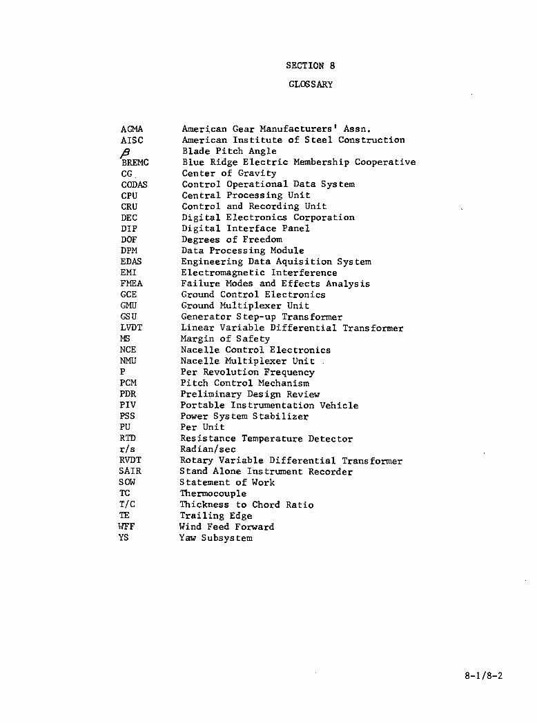
SECTION 8

GLOSSARY

AGMA American Gear Manufacturers' Assn. AISC American Institute of Steel Construction

Blade Pitch Angle BREMC Blue Ridge Electric Membership Cooperative CC . Center of Gravity CODAS Control Operational Data System CPU Central Processing Unit CRU Control and Recording Unit DEC Digital Electronics Corporation DIP Digital Interface Panel DOF Degrees of Freedom DPM Data Processing Module EDAS Engineering Data Aquisition System EMI Electromagnetic Interference FMEA Failure Modes and Effects Analysis CCE Ground Control Electronics GMIJ Ground Multiplexer Unit GSU Generator Step-up Transformer LVDT Linear Variable Differential Transformer MS Margin of Safety NCE Nacelle Control Electronics NMU Nacelle Multiplexer Unit P Per Revolution Frequency PCM Pitch Control Mechanism PDR Preliminary Design Review PIV Portable Instrumentation Vehicle PSS Power System Stabilizer PU Per Unit RTD Resistance Temperature Detector r/s Radian/sec RVDT Rotary Variable Differential Transformer SAIR Stand Alone Instrument Recorder SOW Statement of Work TC Thermocouple T/C Thickness to Chord Ratio TE Trailing Edge WFF Wind Feed Forward YS Yaw Subsystem

8-1/8-2

1. Report No. 2. Government Accsion No. 3. Recipient's Catalog No.

NASA CR-159495 __________________________

4. Title and Subtitle 5. Report Date

MOD-i WIND TURBINE GENERATOR May 1979 6. Performing Organization Code ANALYSIS AND DESIGN REPORT

7. Author(s) 8. Performing Organization Report No.

_____________________________________________________________________________ 10. Work Unit No.

9. Performing Organization Name and Address

General Electric Co.11. Contract or Grant No.

Space Division P0 Box 8661 NAS 320058

13. Typeof Reportand Period Covered

Contractor Report Philadelphia. Pa. 19101

12. Sponsoring Agency Name end Address

US Department of Energy14. Sponsoring Agency Code Report ?i Division of Distributed Solar Technology

Washington, DC 20545 DOE/NASA/O058'79/2'Vol I

15. Supplementary Notes Final Report - Vol. I Prepared under Interagency Agreement EC-77-A-29-l010 Project Manager, R. Puthoff Wind Energy Project Office NASA Lewis Research Center, Cleveland, Ohio 44135

16. Abstract

The MOD-i program is being conducted in six phases: Analysis and Prelimin-ary Design (culminating in a Preliminary Design Review), Detail Design (ending with a Final Design Review), Fabrication and Assembly, System Testing, Site Preparation, and Installation and Checkout. Major milestone

dates for these phases are shown in Table 1-1. This report is intended to

describe only the results of the first two phases; that is, activities leading to the completion of Detail Design. Although this report places emphasis on a description of the design as it finally evolved, it also traces the steps through which the design progressed in order to understand the major design decisions. This report is Vol. I; the Appendix containing supporting analyses and back-up material too voluminous for the Final Report is issued as Vol. II.

17. Key Words (Suggested by Author(s)) 18. Distribution Sttemcnt

Wind Turbine Generator; MOD-i WTG Unclassified - unlimited Final Report STAR Category 44

DOE Category UC-60

19.5ecurit CISSSIf. (of this report) 20. Se.urityClassit.(of this pane) 21. No. of Pages 122. PriceS

Unclassified Unclassified 320 L___________Fc sm' hy t :l:onI TchitcI Iltormato1 Sivice, SprinClie!d, Vu:nia 22161

* U.S. GOVERNMENT PRINTING OFFICE: 1980 -657-145/5227