SERI/TR~217-3036

DE88001132

UC Category: 261

The Turbi

D-2 Wind

Aeroacoustical Noise Sources, EmisSions, and Potential ~mpact

N. D. Kelley H. E. McKenna E. W. Jacobs R. R. Hemphill N. J. Birkenheuer

January 1988

Prepared under Task No. WE721201 FTP No. 562

Solar Energy Research Institute A Division of Midwest Research Institute

1617 Cole Boulevard Golden , Colorc;ldo 80401-3393

Prepared for the

U.S. Department of Energy Contract No. DE-AC02-83CH10093

NOTICE

This report was prepared as an account of work sponsored by the United States Government. Neither the United States nor the United States Department of Energy, nor any of their employees, nor any of their contractors, subcontractors, or their employees, makes any warranty, expressed or implied, or assumes any legal liability or responsibility for the accuracy, completeness or usefulness of any information, apparatus, product or process disclosed, or represents that its use would not infringe privately owned rights.

Printed in the United States of America Available from:

National Technical Information Service U.S. Department of Commerce

5285 Port Royal Road Springfield, VA 22161

Price: Microfiche A01 Printed Copy A10

Codes are used for pricing all publications. The code is determined by the number of pages in the publication. I nformation pertaining to the pricing codes can be found in the current issue of the following publications, which are generally available in most libraries: Energy Research Abstracts. (ERA): Government Reports Announcements and Index (GRA and I): Scientific and Technical Abstract Reports (S TA R): and publication. NTIS-PR-360 available from NTIS at the above address.

TR-3036

PREFACE

This report summarizes extensive research by the staff of the Solar Energy Research Institute into characteristics of acoustic noise emissions of the DOE/NASA MOD-2 wind turbine. The results of this study have shown that the MOD-2 noise levels are well below annoyance thresholds within residential structures a kilometer or more from the turbine rotor. It was also found that the inflow turbulent structure has a major influence on the level and charac­teristics of the low-frequency (2-160 Hz) range acoustic emissions which, in turn, have implications for the associated structural response of the rotor assembly. The high-frequency range (A-weighted) levels were found to vary primarily with the mean hub-height wind speed. In addition, the rotor inflow turbulence characteristics at the Goodnoe Hills Site were found to be con­trolled almost entirely by the diurnal variation in the vertical stability of the first 100 m of the atmospheric boundary layer.

Approved for

SOLAR ENERGY RESEARCH INSTITUTE

Robert J. No n, Manager Wind Energy Research Branch

, Solar Electric Research Division

Neil Do! Kelley I Principal Scientist Wind Energy Research Branch

111

TR-3036

ACKNOWLEDGMENTS

The authors wish to acknowledge the excellent support and assistance of the following organizations in SERIfs MOD-2 research effort:

• Boeing Aerospace Corporation

• Bonneville Power Administration

• Cornell University, Sibley School of Mechanical and Aerospace Engineering

• Engineering Dynamics, Inc.

• Fairchild-Weston, Inc.

• NASA Langley Research Center

• NASA Lewis Research Center

• Oregon State University, Atmospheric Sciences Department

• Pacific Northwest Laboratories

• B.C. Willmarth Co.

Special thanks are extended to Larry Gordon of NASA Lewis and Ron Holeman of the Bonneville Power Administration who provided the scheduling and support services so necessary to our effort.. The support of Ron Schwemmer and Don Fries of Boeing was without reproach. We salute the dedicated efforts of Ben Willmarth who expertly operated the tethered balloon system under very adverse circumstances. We also extend our deepest thanks to David Long of Fairchild­Weston who provided us with outstanding data support services.

~v

TR-3036

SUMMARY

Objective

This document $ummarizes the results of an extensive investigation by the Solar Energy Research Institute (SERI) into the factors relating to acoustic emissions associated with the operation of a MOD-2 wind turbine.. The MOD-2 was the sixth ~ a series of turbine designs developed for the u.s. Department of Energy (DOE) by the Lewis Research Center of the National Aeronautics and Space Administration (NASA) as part of the Federal Wind Energy Program. The MOD-2 turbine has a rotor diameter of 91 m (300 ft) and is capable of gener­ating 2.5 MW of electrical power at its rated wind speed of about 13 mls (28 mph), measured at a rotor hub elevation of 61 m (200 ft). A cluster of three MOD-2 turbines installed on the Goodnoe Hills near Goldendale, Wash., was used for the experiments described in this reporto

An investigation of the characteristics of the MOD-2's acoustic emissions was undertaken as a result of the experience SERI gained with its predecessor, the 2-MW MOD-l turbine" One of the primary motivations for designing the MOD-2 turbine with its rotor upwind of the support tower was to avoid the impulsive, low-frequency noise associated with the downwind MOD-I.. It was expected that placing the MOD-2 rotor upwind would largely eliminate the community annoyance problem that was characteristic of the impulsive MOD-1 emissions" It was not known, however, whether similar or perhaps greater levels of nonimpulsive, low-frequency noise that radiated from the large MOD-2 rotor as a result of inflow turbulence interactions would annoy the residents nearby We designed our MOD-2 test program to answer these questions, including the following specific objectives:

A general characterization of both low- (under 200 Hz) and high-frequency­range acoustic emissions

• The development of a methodology for making acoustic measurements 1n a windy environment

• The development of a methodology relating low-frequency acoustic emissions to the turbulent inflow structure

• The development of a methodology for predicting potential of nearby residential structures from frequency acoustic loadings

the interior annoyance a wind turbine's low-

• The application of the annoyance potential criteria using MOD-2 emission levels measured under a range of operating conditions and a comparison of the results with similar ones for the MOD-1 turbine.

Discussion

We undertook a series of five experiments from February 1981 to August 1986 to characterize the MOD-2' s acoustic emissions 9 The primary experiments, how­ever, were performed during May 1982 and August 1983, using Turbine No.2 at the Goodnoe Hills site. The 1982 experiments collected statistical measure­ments of high-frequency-range emissions as well as low-frequency data. The 1983 experiment was des igned to be more narrow in scope but included addi­tional parameters not available in 1982, such as rotor surface pressures and

v

TR-3036

high~frequency turbulence measurements made from a fixed tower location and a tethered balloon flown in the turbine inflow. Major modifications were made to Turbine No. 2 between the 1982 and 1983 experiments as a result of opera­tional instabilities. These included installing vortex generators along the rotor's leading edge over 70% of the blade span and establishing a different blade pitch sequence in the control system software. These changes required us to stratify the low-frequency data collected during these two experiments by year.

In order to make low-frequency noise measurements in a windy environment, we developed a technique that employs a pair of ground-mounted microphones spaced 15 m apart. Cross-correlation signal processing procedures were then used to obtain the in-phase acoustic portion of the signal while largely rejecting the random, turbulence-induced contribution" Inflow measurements were made from fixed meteorological towers located outside the turbine induction zone and from a tethered balloon flown approximately laS rotor diameters (1.5D) upwind of the rotor plane.. Both standard-response and high-frequency anemometers were us~d on both platformso Twelve surface-mounted pressure transducers were attached to the upper and lower surfaces of Blade No. 1 on Turbine No. 2 at two span locations during the 1983 experiment.

The data categories--acoustic, atmospheric, and blade surface pressures--each necessitated somewhat different processing procedures. Because of the random or stochastic nature of the inflow turbulence responsible for exciting the acoustic response of the turbine, we developed a statistical sampling approach for presenting and quantifying the radiated acoustic spectra. Consistent with this approach, we characterized the turbulent inflow using the methods of statistical fluid mechanics and calculated a range of "bulk" flow param­eters. We employed standard time-series analysis procedures in determining ~he MOD-2 aeroacoustic and surface pressure response functions.

Our detailed measurements of the inflow to Turbine No .. 2 revealed a regime that is often stably stratified and contains multiple, thin layers of small­scale, anisotropic turbulence. There is strong evidence of the development of an internal boundary layer within the rotor disk's vertical envelope, whose formation and depth vary diurnally. Further, the vertical layer encompassing the rotor disk is influenced by the presence and breakdown of internal wave motions, accompanied by intense, small-scale turbulence. For example, under stable condi t ions, typical longi tudinal or axial turbulence component length scales are in the neighborhood of 200 m, but those of the vertical or upwash (in-plane) component are often more than an order of magnitude smaller.

Measurements of emissions in the high-frequency range (400-8000 Hz) have shown that close to the rotor disk the radiation pattern resembles that of a classic quadrupole source. This pattern is then distorted by the prevailing wind at larger distances, i e e., extended downstream and contracted upstream of the rotor disk. Statistical measures of the A-weighted emissions over periods of several hours have shown the observed levels to be essentially normally dis­tributed. The decay of these emission levels with distance (at Goodnoe Hills) can be described by the following polynomial:

L (A) = -3.89464 x4 + 4606729 x3 - 191.884 x2 + 287.15 x - 28.4 , eq

Vl

TR-3036

where x is the loglO of the downwind distance, in feet. The departure from an r2 dependence is apparently the result of local propagation effects.. The average audible range of a single MOD-2 at the Goodnoe Hills site has been estimated to be 1220 m (4000 ft) downwind of the turbineo Statistical measurements of the acoustic environment downwind of the site with up to three turbines operating show that the turbine noise level experienced by an observer is dominated by the closest turbine The effects of multiple turbine operation, however, are most noticeable when the turbines are located at nearly the same upstream distance from the observer.

The A-weighted, equivalent sound pressure level or L (A) at a distance of 1.5D (137 m or 450 ft) from the rotor disk was found et~ vary primarily with the hub-height wind speed, though some slight dependency was noted on the vertical stability (Richardson number) and wind direction. The L (A) varia­tion, at this reference distance, can be expressed to 't'lithin e~0 .. 5 dB by 1/2 UH + 57 over a hub wind s (UH) range of 6~15 m/s (13 to 34 mph)@

An examination of the variation of 1/3-octave band spectra with inflow charac­teristics revealed that there was essentially a uniform increase in the observed average band pressure levels [L (f l / 3)] across the spectrum with wind speed and stabilityo A "peaking e~ehavlor" (distinct peaks in the exceedence level, 1/3-octave band spectra) was noted, principally in the L10 , L5 , and L1 levels of the 2500-Hz band This was most noticeable in measure­ments made in the plane of the rotor, and it appears to be load-related. We believe this peaking characteristic may be related to some form of oscillatory fluctuations in the rotor's aerodynamic boundary layere

Comparisons made between on-axis measurements taken during the 1982 and 1983 experiments revealed a sharp spectral cut-off in the 1983 emissions above 1600 Hz 0 Whi le some of the "peaking" behavior 1;-7e noted above was present in 1983, a downshift appears to have occurred in the 1/3-octave band in which it was dominant, ioe .. , 2500 Hz in 1982 to 1000 Hz in 1983. We have attributed the lower spectral cut-off and lower "peakingU frequency in the 1983 emissions directly to the vortex generators, with their inherent ability to limit boun­dary-layer separation. It is also possible that these changes may be somehow related to the modifications in the pitch angle schedule, lee., perhaps because they reduced the maximum attack angles encountered

No significant, steady-tone noise components were found in analyses of repre­sentative narrowband (25-Hz resolution) spectra. This indicates that mechanical noise sources associated with the drivetrain are well controlled and that there are no discrete aeroacoustic sources of consequence.

We measured the MOD-2 low-frequency (LF)-range acoustic transfer function directly by means of balloon-borne instruments flown in the turbine inflow. We found that the radiated acoustic spectrum changes characteristics at inflow turbulent scales less than the measured longitudinal or axial integral scale, i.e., for turbulent eddies less than this scale length. Statistical correlations between five characteristic scales of the inflow and the mean and the first three moments of the 1/3-octave band spectrum level distributions (expressed as the variance, skewness, and relative kurtosis coefficients) were derived from the 1983 data set. Using these five inflow scales as predictors in a linear, multivariate model of the band spectral levels, we found that a

V1.1.

TR-3036

high degree of convergence of the model could be obtained; 1 .. e., a high percentage of the observed variation of the mean and the first three moments could be explained.. The most efficient predictors included the following:

(1 )

(2)

(3)

(4)

A reference mean wind speed (U ) measured at a height z within the rotor disk layer (vertical laye; occupied by the rotor disk)

The gradient Richardson number (Ri) stability parameter measured over the rotor disk layer

The Monin-Obukov length scale, L (see Section 2.4.2), or

The vertical or in-plane turbulence component scale length along the vertical z-direction, Iwz , measured at the height noted in (3).

The statistical distributions of the emitted 1/3-octave band spectra were most highly. correlated with the Uz ' Ri, and Iwz predictors or scales. The inclusion of (1) and (4) agrees with the generalized theory of Homicz and George for subsonic rotor noise generated in homogeneous, isotropic turbulence. The need to include the Richardson number reflects the inhomogeneous, vertically stratified characteristics of the rotor inflow at the Goodnoe Hills site. We found that an increase in the stability above cri tical values (Ri > +0 .. 25) led to a decrease in the vertical or in-plane turbulence scales. This in turn had the effect of increasing the LF acoustic output below a frequency of 10 Hz, with a corresponding decrease above that.

We attempted to relate the spectral characteristics of the tower-measured axial and in-plane (upwash) turbulence components to the shape of the LF acoustic mean 1/3-octave band spectra. We suggest using

as a fixed to rotating space frequency (f') transformation, where Q

rotor rotation rate and Ro is the effective radius (75% span length). this conversion, we found that

1S the Using

(1) There is a small positive slope change in the mean acoustic pressure spectra, in the vicinity of the rotor effective chord length. This also seems to coincide with the isotropic turbulence region (indi­cated by the two turbulence component spectra becoming parallel).

(2) The acoustic pressure spectral roll-off approximates a -5/3 slope for reference wind speeds less than about 10 mise

Because of the substantive changes made to Turbine No. 2 between the 1982 and 1983 experiments, we made an effort to compare the acoustic emission charac­teristics and their relation to the inflow for both years. We were limited to comparing the LF-range results, since we did not have sufficient high­frequency (HF)-range acoustic data from the 1983 experiment. We determined that the 1983 configuration of the turbine was far more acoustically sensitive to inflow stability.. We also determined that the 1982 configuration was influenced by flow stability at all frequencies. We found that the 1983 emissions exhibited less coherent (impulsive) tendencies above 9-10 mls than those of the 1982 configuration. It is clear that, because of whatever instabilities were present, the upwind 1982 MOD-2 turbine at times performed

V111

TR-3036

acoustically in a manner similar to its predecessor, the downwind MOD-I. Thus, a definite improvement was achieved in reducing the degree of coherency in the LF-range emissions by adding the vortex generators and making the pitch schedule modifications.

In order to better understand the physical processes responsible for aero­acoustic noise generation, we performed a space-time correlation analysis using three parameters measured on the blade itself and the far-field acoustic pressure as measured in the 8-Hz octave band. Our results showed, at least at the 87% span station, that the processes related to the observed flap and chordwise moments, the blade normal surface pressures, and the radiated acoustic pressure field are correlated over time periods of 65-75 ms, which translate to a movement of the rotor through about 5 m 1n space.

Our experience with the MOD-l turbine reinforced the desirability of assessing the MOD-2' s potential to cause interior annoyance problems in- nearby resi­dential structures by means of low-frequency acoustical loads. Through a limited, interior low-frequency noise evaluation experiment, using volunteer subjects, we identified what we believe to be an efficient descriptor or metric for measuring the degree of annoyance from such stimuli. From data available to us, we modified the derivation of this descriptor to include internal dynamic pressure effects resulting from the application of external, low-frequency acoustical loads. Using this modified descriptor, we then developed a procedure for establishing a "figure-of-merit" for a given tur­bine, which attempted to take into account worst-case conditions of surface reflection and atmospheric focusing. By using 1/3-octave band acoustic spectra measured at a reference distance from a turbine's rotor plane, we were then able to establish a predicted worst-case figure for the MOD-2. We were then able to compare that result with the documented community annoyance asso­ciated with emissions from the MOD-l operating at both 35 and 23 RPM.

Conclusion

We determined from our analysis of both the high- and low-frequency-range acoustic data that annoyance to the community from the 1983 configuration of the MOD-2 turbine can be considered very unlikely at distances greater than 1 km (0.6 mile) from the rotor plane.

1X

TR-3036

TABLE OF CONTENTS

1.0 Introduction ........ e •••••••••••••• 9................................. 1

1.1 1.2

1.3

Characteristics of the MOD-2 Turbine •••••••••••••••••••••••••••• Background ••••••••••••••••••••••••••• 1.2.1 The MOD-1 Turbine ••••••••••••• 1.2.2 SERI's

Related Studies •••••••••••••••••••••••••••••••••••••••••• MOD-2 Acoustic Characterization Program Objectives •••••••

1 1 2 4 4

2.0 Investigative Procedure.............................................. 6

2.1

2 .. 3

2.4

MOD-2 2.1.1 2.1.2 2.1.,3 201.4

Field Studies."" February 1981 ... May 1982 0 • Q " • QQ. 0 0 • 0 •• e e 0 EJ e e 0 ••• ., •• 0 6) 0 0 • €I) 0 e e 0 0 • 49 ••• ., ., • e ••

Augus t 19830. 0 Q • e • G 0 •••• CD " 0 0 • "0 0 0 Ii) ., •• 0 0 ••• 0 •••••• e 0 •••• 1& ••

Augus t 1986" 0 • eo ... e 0 II ...... cD $I •• " ••• e 0 e •• " • Ill) • " ....... e •••• 4) •

Ins t rume n tat ion.. " 0 0 " " " e " ....... " " " • • .. .. " " " co .. " • .. " .... " .. co • " 0 0 " " " .. • " • .. .. .. ..

2.2.1 2 .. 2.2

Acoustic Measurement Instruments •• ".o ............. " •••••••

Atmospheric Measurement Instruments ................ ""." •• ". 2 .. 2.2.1 Tower-Mounted Measurements ..... " •• " ....... " •••••••• 202.2.2 Tethered Balloon Measurements ••••••••• " ......... .

2.2 .. 3 Turbine Rotor Surface Pressures ••• o •••••••••••••••••••••• 2.2.4 Turbine Operational Information •••••••••••••••••••••••••• 2.2.5 Data Recording ••• e •••••••••••••••••••••••••••••••••••••••

Experimental Procedures •••••••••••••••••••• e ••••••••••••••••••••

2.3.1 The 1982 Experiment •••••••••••••••••••••••••••••••••••••• 2.3.2 The 1983 Experiment •••••••••••••••••••••••••••••••••••••• Data Reduction Procedures ••••••••••••••••••••••••••••••••••••••• 2 G 4 • 1 Ac ou s tic Da t a • • @ .. " " G • " •••• " • " • " ....... " " ...... " ...... " ......... ..

2.4.1.1 Low-Frequency-Range, Coherent Random Sampling Technique." ••••• o ••••

High-Frequency-Range, Random Sampling Tee hn i que. 13 • 0 • til Q Ii) 0 • • e e 0 • e • II • e • Ii) • • " ., • • • ., • • • • • 1& • • e

2.4.2 Atmospheric Data"" .... "" •••• ".""" •• ,, .......................... .. 2.4.2.1 Mean Inflow Characteristics ..................... . 2.4.2.2 Turbulent Inflow Characteristicso •••••••••••••••

2.4 .. 3 Rotor Surface Pressures ••• e •• 0 ........................... .

6 6 6 6 7 7 7 8 8

10 12 12 12 12 14 19 19 20

22

25 25 25 35 36

3.0 Description of Goodnoe Hills Inflow Structure." ........................ 37

3.2

3.3 3.4

Identification of the Acoustically Important Inflow Properties... • .............. " ................................. . Determining the Vertical Distributions of UH, I.J, and w'2 •••• 302.1 Surface Layer Similarity Sca1ing .... Qo ••• : .............. .

3.2.2 The Vertical Distribution of UH (Vc ) ••••••••••••••••••••• 3.2.3 Variation of w' Spectra with Height ......... e ................ .

Inflow Data Statistical Summaries •••••••••• " .................... . 1983 45-m Inflow Turbulence Spectral Content ••••••••••••••••••••

x

37 41 41 42 42 43 45

TR-3036

TABLE OF CONTENTS (Continued)

305 Rotor Disk Inflow Vertical Profilesooooeoooooeoo ••• 0000 ••••••• 0 45 305.1 PNL Tower Vertical Profiles of Wind Speed and

Turbulence Intensityo ••. 00 •••••••• 0 ••••• 0 ••••• 00 ••••• 46 3.502 Representative Tethered Balloon Vertical Profiles

in Turbine No 2 Inflowooo ••• oo •• oo ••••• ooo •• e •• o ••• o •• 46

400 Characteristics of MOD-2 High~Frequency-Range Emissions •••• o.e •••• o 60

4.3

Observed Directivi Patternoo Statistical A-Weighted Emission Distributionsoe. 000 ••• 00.00 .••• 4 2.1 Single Turbine 4.2 2 Multiple Turbine Influence of Rotor Inflow on HF Noise Generationo" ... 0" 0" 0 0 0 ... 0 40301 A-Weighted, 40302 Spectral

Sound Pressure Level Variationeooo High~Frequency~Range Emissions @000

Typical

4 3,,2.1 40302 2 Establishment of

Measurement Locations00000@ Background Spectral

Reference 0 0 0 000000009 0 4 3 Rotor Inflow Influence on Spectral

Distribution~ 0 00 eo 0000000.00000.00 ••• Narrowband Spectra@oooaoooo .o@oooo

60 60 62 64 65 65 67 67

69

71 85

5.0 Characteristics of Emissions00o. 90

5.1 Influence of Rotor Inflow Structure on LF Noise Spectra e •• OO.00 90 5 1.1 HOD-2 Aeroacoustic Functiono. BOO" 0 • 0 0 ... 0.0 • 90

5 1el01 Di t Measurement Approach... • •• 000000.0 •• 0 90 5 1 1 2 Inflow Bulk Scaling Parameter/Multivariate

Model Approach oooo@ eeao ••••• 0 ••••••••• 0. 93 501.103 Model Interpretationoo 00 0.000 •••• 0 000.0@0000 114 501 104 Case Studies of the Role of Inflow Structure

on Radiated tral Characteristics.eee ••••••• 118 5 1.1.5 Relationship of Inflow Spectral

Characteristics to the Mean LF Acoustic trum. 000.0 " ••••• 0 .e ••• ooo •• 147

502 Comparison of 1982 and 1983 Results via Regression Modeling ••••• 151 5e2.1 Regression Modeling of 1982/83 Data o ••••• e ••••• e.e •• eo 151

5.3 Comparison of MOD~2 and MOD-2 LF Emissions Characteristicso ••••• 153 5.3.1 Statistical Measures of Impulsiveness or Coherency ••••••• 157

5.3.1 1 Band Correlated Spectral Levels.e •• oo •• 157 503 1 2 Statistical BSL Exceedence Values e ••••• eo •• 159

50302 Degree of 1982/83 MOD-2 vs. MOD-l Emissions Coherency •••• 159 5.3.3 Comparison of 1982/83 MOD~2 Exceedence Analysis •.•• 0 ••• 161

5.,4 Observed Physical Scales of MOD-2 LF Noise Generation. 0 •• e ". 161

Xl

TR-3036

TABLE OF CONTENTS (Concluded)

Page 6.0 Measuring the Annoyance Potential of a Single MOD-2 Turbine ••••••••• 168

6.1 Additional Comparisons of MOD-1 and MOD-2 Emissions Characteristics and Their Relationship to Interior Annoyance Potential"." 0 .......... " ... " ." ••• " ••• " •• " ...... It It It .... " .. ,," .. It .. 168

6.2 Use of the PLSL Metric in Assessing Potential Interior Annoyance Q •••• tit " • " •• 0: • l1li f) •••• e ... ,. •• e ••• " • ., • ., CIt ., •••••••• cD It 0 •• \9 • 0 • •• 170 6.2.1 Synopsis of Results of Interior Low-Frequency

Noise Evaluation Experiment ................................ 170 6.2.1.1 Identifying an Efficient Estimator of

Interior LF Annoyance ••••••••••••••••••••••••••• 171 6.2.1.2 Establishing an LSL Annoyance Scale ................ 173

6.2.2 A Methodology for Predicting Interior LSL Values ••••••••• 173 6.2.2.1 Predicting an Interior LSL Level .................. 173 6.2.2.2 Establishing a Reference External Acoustic

Load i ng 0 $ • e .... G e • e 0: e •• " •••• lit " • e e • ., EJ e • e •• Ii • lit €I • 4) eel 74

6.3 Estimating the Community Annoyance Potential of Both an Individual MOD-2 Turbine and Clusters of Turbines ................ 176 6.3 .. 1 Annoyance Potential from High-Frequency-Range

Emissions ....... " ................................................ " ......................... 176 6.3.2 Interior Annoyance Potential of Low-Frequency-Range

Em iss ion See 0 • e e e e e e 0 e e • • II • • $ • • CD • e 8: • e • e e e 0 e ., • e • 4) • • e e • ., • • e. 1 7 7

7.0 Conclusions ..... ee ••••• eee.e ••••• ee ••• ee •••••••••••••••••••••••••••• 178 7.2 Low-Frequency-Range Acoustic Characteristics ..................... 178 7.3 Comparisons of MOD-2 Low-Frequency Emission Characteristics

with Those of the MOD-I ............................................. 179 7.4 Community Annoyance Potential of a Single MOD-2 Turbine ••••••••• 179

8.0 Recommendat ions. " " ... " ............ " " ............. " ... " ......... " ...... " " .... " " " .... " 180

9 e 0 References 0 0 .... 0 • 0 • " 0 9 I!J 0 0 • e iii 0 e • 009 e 0 lit fit • e e 0 0 •• eo" " 0 ., 0 • 0" ..... e lit ••••• .,. 181

Xll

TR-3036

LIST OF FIGURES

1-1 The MOD-2 Wind Turbine.ee ••••• Qo ••••• e.eo ••• o ••• e •••••••••••••••••• 2

1-2 Schematic of the MOD-2 Configuration •••••• e •••••• e ••••••••••••••• 3

1-3 Cluster Arrangement of MOD-2 Turbines at Goodnoe Hills Site •••••••• 5

2-1 Microphone Measurement Station.GaGe. 0 •••••••••••••••••••• 0 •••••••• 8

2-2 Acoustic Instrumentation Configuration for 1982 Experiments •••••••• 9

2-3 Triad of VLF Microphones Used for 1983 Experiments ••••••••••••••••• 9

2-4 Site Layout Schematic Showing Locations of Meteorological Towers with Respect to the Turbines .0 ••••••••••••••••• e •• 0 ••••• @ •• 0 ••• 10

2-5 Detail of Inflow Instrumentation Carried by Tethered Balloon.o •• G00 11

2-6 Typical position of Tethered Balloon in Turbine No 2 Inflow •••••• @ 11

2-7 Data Flow Path for Inflow Measurements •••• o .000 •• 0.0 13

2-8 Surface Pressure Tap Installation at Blade No.1, Station 1562, 15% Chord Position ••• @ •••• 0.0 ••••• 00 0 •••• 0 •••••••• 0 ••••• 14

2-9 Data Sources and Recording Systems Configurationo ••• e ••• e ••••••••• 15

2-10 Schematic Representation of an Averaged Radiated Sound Pressure Spectrum from a Large Wind Turbinee ••• o •••••••••••••••••• e 21

2-11 Schematic Sound Spectrum of Figure 2-10 with Residential Construction Vibration Modes and Applicative Damping

2-12 Low-Frequency-Range Coherent Processing Flow o •• o.o.e ••••••

2-13 Example of Low-Frequency Acoustic Data Reduction Output: Observed Frequency Distributions of 8-Hz 1/3-0ctave Band Spectrum Level for Turbine Operating (Run #1) and Background

21

24

Conditions (Run #2) •••••••••••• 0 •••••••••••• 00000.0@0.000000 •• 26

2-14 Example of Low-Frequency Acoustic Data Reduction Output: Mean and Peak 1/3-0ctave BSL Spectra for Turbine Operating (Run #1) and Background Conditions (Run #2) 000 0 @0$00 GOe. 00.e •••••• 000e 27

2-15 Example of Low-Frequency Acoustic Data Reduction: Exceedence Level (L.) Comparison for Turbine Operating (Run #1) and.

1 Background Conditions (Run #2)0 ••• 0 ••••• 0 ••••••• 00 ••• 0 ••••••••• 0 •• 0 28

2-16 High-Frequency-Range Acoustic Data Processing .•• ooo •••••••••••••••• 29

Xll1.

~-~ /( I

"-~

LIST OF FIGURES (continued)

2-17 Example of High-Frequency Acoustic Data Reduction Output: Observed Frequency Distributions of A-Weighted BPL for Turbine Operating (Run #1) and Shut-Down Conditions (Run #2) in High

TR-3036

Winds., • 0 • e • e It " CD ., • e (} • 0 G .... 0 • $ • 8 CD •• " • lib • (} 0 ID 0 • e • 0 e e • G .... e CIt • CD •••• " \l!l • e • • • 30

2-18 Example of High-Frequency Acoustic Data Reduction Output: Mean and Peak 1/3-0ctave BPL Spectra for Turbine Operating (Run #1) and Shut-Down Conditions (Run #2) in High Windse ••••••••••••••••••• 31

2-19 Example of High-Frequency Acoustic Data Reduction Output: Exceedence Level (L i ) Distribution Comparisons for the Case of Figures 2-17 and 2-18 •••••••••••••••• 0 •••••••••••••••••••••••••• 32

3-1 Rotor Geometry Used by Homicz and George.e •••• o •••• e ••••••••••••••• 38

3-2 Schematic of L x, L x L z Length Scales with Respect to Turb1ne RotOr •• '.: •• ' ••• 0 ••• 0 •••••••••••••••••••••••••••••••• 40

3-3 BPA Tower 45-m Level Longitudinal (u) and Vertical (w) Inflow Spectra for 1983--Run ADS •••••••••••••••••••••••••••••••••••••••••• 47

3-4 BPA Tower 45-m Level Longitudinal (u) and Vertical (w) Inflow Spectra for 1983-Run A03 •••••••••••••••••••••••• e •••••••••••••••••• 48

3-5 BPA Tower 45-m Level Longitudinal (u) and Vertical (w) Inflow Spectra for 1983 Run A14-1.e ••••••••••••••••••••••••• ee ••••••• e •• e • 47

3-6 BPA Tower 45-m Level Longitudinal (u) and Vertical (w) Inflow Spectra for 1983-Run A14-2.e ••••••••• e •••• e •••••••••••••• eee8 ••• e •• 49

3-7 BPA Tower 45-m Level Longitudinal (u) and Vertical (w) Inflow Spectra for 1983-Run A18 •••••• e.e.e •••••••••• e •••••••• e •••••••••••• 48

3-8 BPA Tower 45-m Level Longitudinal (u) and Vertical (w) Inflow Spectra for 1983-Run All ••• ee ••••••••••••••• ee ••••••••••••••••••••• 49

3-9 Smoothed Vertical Profile (PNL Tower) of Uhub-Normalized Horizontal Wind Speed (a) and Turbulence Intensity (b) for 1 983""""" - Run A 03 (9 fit 0 0 fJ (I) e G 0 lit G • 0 • €I e e 0 lit 0 G 0 0 til e e e e 0 lit I) 0 e • 0 €I 0 0 • 0 •• 0 G • Cit fit • 13 ., ., • e 0 5 0

3-10 Smoothed Vertical Profile (PNL Tower) of Uhub-Normalized Horizontal Wind Speed (a) and Turbulence Intensity (b) for 1983--Run A14-1 e G • 19 0 e " 0 0 G 4) • " • e •• e 0 e 0 0 • e Ii) e e e 0 0 e G fJ e G •• 0. 0 • 0 • 0 ••• 0 e 0 e 0 51

3-11 Smoothed Vertical Profile (PNL Tower) of Uhub-Normalized Horizontal Wind Speed (a) and Turbulence Intensity (b) for 1983--Run A14""""2 €I G a CIt • G a 0 e 19 €I a • €I: CIt €I • 0 e I) 0 • G e G • II/) 1& 0 G fJ ., €I ., •••• 0 " ••• G " ••• 0 • 0 • 52

3-12 Smoothed Vertical Profile (PNL Tower) of Uhub-Normalized Horizontal Wind Speed (a) and Turbulence Intensity (b) for 1983-....... Run Al8 .. 0 e €I e 0 0 e €I: 0 e 0 Q e 0 0 it III e 0 0 m e 0 0.0 a a. 0 It 0 0. e e e €I e e ••• 0.0 •• e.. 53

X1V

TR-3036

LIST OF FIGURES (continued)

3-13 Smoothed Vertical Profile (PNL Tower) of Uhub-Norma1ized Horizontal Wind Speed (a) and Turbulence Intensity (b) for 1983--Run AlleeGooeooo 00000 0

3-14 Smoothed Vertical Profile (PNL Tower) of Uhub-Normalized Horizontal Wind Speed (a) and Turbulence Intensity (b) for 1983--Run A05 .. ". eo. e 0 00. • 0

3-15 Smoothed and High-Resolution Vertical Profiles of Wind Speed

54

55

for Run AOSOGeee00G 6000$000 0 e0eee r:g')e 130000000.006 •••• 000 •• 00 56

3-16 Smoothed and High-Resolution Vertical Profiles for Wind Direction for Run A05 ••••••• 00 •••• 0 57

3-17 Smoothed and High-Resolution Vertical Profiles of Sensible Temperature for Run AOSao 00 ••• e. 000 0 0 ••••• 0 ••• 0.00 ...... 0 ••• 58

3-18 Narrowband Longitudinal Turbulence Spectrum Measured at 78-m (±6 m) Height for Run AOS. 00 000 .0 ••• 0 ••• 00 ••••• 0 •• 0 •••••••• 59

4-1 Microphone Locations Used in High-frequency-Range Measurements.e ••• 65

4-2 A-Weighted Sound Pressure Level Directivity Pattern for a Single MOD-2 Turbine. 0.000 ••••• 000 •••••••• 62

4-3 Cumulative Distributions of A-Weighted SPL at Three Downwind Distances from a MOD-2 Turbineoe00@@ ••..• 000 ••••••••••• 90. 63

4-4 Average Tu:bine Leq(A) Emissions Decay Downwind of a Single MOD-2 Turb1neeoGoGGG QOtloCi 0 00 006 00000 @ GO<OO'lllloeoaGoG&eOeeOfi!l00 •• 63

4-5 Cumulative Distributions of A-Weighted 8PL at Site No.2 (see Figure 4-1) for Two and Three Operating MOD-2 Turbines ••••••••••••• 64

4-6 Leq(A) Levels as a Function of Hub-Height Wind Speed ••••••••• o ••••• 66

4-7 Observed Frequency Distributions of A-Weighted SPL for Highest and Lowest Mean Hub-Height Wind Speedse •• 0.0 ••••••• 0 ••••••••••••• 68

4-8 Comparison of Background Mean BPL Spectra for Highest and Lowest Mean Hub-Height Wind-Speed Condi t ions o. 0 • • •• .. •• " ............. 69

4-9 Comparisons of Observed Mean SPL Spectra for Operating and Background Condition~ in High Ca) and Low (b) Windso •••• o ••• o •••••• 70

4-10 Comparison of Background HF Acoustic Spectra at On-Axis Microphone Location for the Same Mean Hub-Height Wind Speed during 1982 and 1983 Experimentseeo GOOGe 000GGQlQ00Ge 0 GG0000"'000GOooooeeooO.e.OG 71

xv

TR-3036

LIST OF FIGURES (continued)

4-11 1982 HF-Range Acoustic Spectral Distribution for On-Axis (solid) and In-Plane (dashed) Locations as a Function of Wind Speed and

4-12

4-13

4-14

4-15

4-16

4-17

4-18

4-19

4-20

4-21

4-22

4-23

Stability. e • .,. o. e e G Il.t. fit 4) 0 e eo" e •• ., .... 0" 0 0 e Ii) (I) I/) 0 fiJ CD. 0 e 0 e. e e e 0 e •• " t!J CD ... e.. 72

Comparison of the On-Axis Component of the HF Spectral Distribution between 1982 and 1983 under High Loading Conditions •••

Comparison of On-Axis (solid) versus In-Plane (dashed) HF Spectral Emissions for Neutral to Slightly Stable Inflow Conditions •••••••••

Comparison of L1 , LS' LI0 , L20 , and LSO 1/3-0ctave Level Spectra at 1.5D at the On-Axis and In-Plane Measurement Locations for 1982 Runs: (a) 17-2; (b) 19-1; and (c) 26-1 ••••• 0 ••••••••••••••••••••••

Comparison of Mean 1/3-0ctave BPL Spectra for Mean Wind Speeds of 9.3 and 1003 mps under Stable Conditions •••••••••••••••• oo ••••••

Comparison of L1 , LS' L10 , L20 , and LSO 1/3-0ctave Level Spectra at 1.SD at the On-Axis (a) and In-Plane (b) Measurement Stations •••

Comparison of Mean 1/3-0ctave BPL Spectra for High and Moderate Wind Speeds under Stable Inflow Conditions •••••••••••••••••••••••••

Comparison of Ll , LS' LlO ' L20 , and L50 1/3-0ctave Level Spectra for High and Moderate W1nd Speeds under Stable Inflow Conditions •••

Comparison of Mean 1/3-0ctave BPL Spectra for a Mean Wind Speed of 13.3 mps and Stable Conditions (Run 27) and a Mean Wind Speed of 14.5 mps and Unstable Conditions (Run 25-1) •••••••••••••••••••••

Comparison of L1 , L5 , L10 , L20 , and L50 1/3-0ctave Level Spectra for High-Wind, Stable vs. High-Wind, Unstable Inflow Conditions ••••

Mean and L20 BPL Spectra for 1982 Run R27 and 1983 Run A-II ••••••••

Mean and L20 BPL Spectra for 1982 Run 26-1 and 1983 Run A18 ..... """".

Comparison of Acoustic Environment at 1.5D, On-Axis Measurement Location with and without the Turbine Operating under High Wind

74

75

76

77

78

79

80

81

82

83

84

Conditions 4) 0 g. 0" 0 It e 0 <it. 0., .... 000. e €t." 0 e e 11) • 0 0 •• ., 0.0.0" tit" 8 0. eo •• 8,. • .,... 85

4-24 Comparison of L1 , L5 , LI0 , LZO ' and L50 On-Axis 1/3-0ctave Level Spectra for Identical Mean W1nd Condit10ns during 1982 and 1983 Experiment See ... 0 e 0 0 e fill elite •••••• 0 0 13 0 0 II e 0 0 " e • 0 ..... 19 II) G • Q 4) 0 <11 Q • 0 ••• e <I) •• e • 86

4-25 Comparison of Ll , L5 , LI0 , L20 , and L50 On-Axis 1/3-0ctave Level Spectra for Sim1lar Wind Speed Regimes in 1982 and 1983 ••••••••• e •• 86

4-26 Representative 1982 HF-Range Narrowband (Be = 1e25 Hz) Spectra for Very Low Wind Conditions.e.e •••• ee ••••••••••••••••••••••••••••• 87

XV1

TR-3036

LIST OF FIGURES (continued)

4-27 Representative 1982 HF-Range Narrowband Spectra for Moderated but Below-Rated Wind Conditionso0G000000o •••••••••••••••••••••••••• 87

4-28 Representative 1982 HF-Range Narrowband Spectra for Above-Rated, Unstable Inflow Conditions .0 ••••• &00 •••• 0 •••• 000 •••••• 0 ••••••••••• 88

4-29 1983 On-Axis HF-Range Narrowband Spectra for Above-Rated, Very Stable Inflow Conditions.o ••• 0000 ••• 0 •• 88

4-30 1983 On-Axis HF-Range Narrowband Spectra for Near-Rated, Stable Inflow Conditions000 0000000 0000 Q00eO$Og$Oeeae.Cl00&o.oeeOGOoo •• 89

5-1 Relationship of Location of Measurements on Blade No.1, Rotor Disk Geometry, and Height of Elevated Turbulent Layer ••••••• oe •••• e 92

5-2 Measured Low-Frequency Acoustic Response Function.e •• e 0 •••• 0 ••••• 92

5-3 Measured Low-Frequency Acoustic Response as a Function of Turbulent Space Scale •••• oe •• 0000 ••••••••• 0 •••••••••• 0 •• 0 ••••••• 93

5-4 Comparisons of the Observed Run-to-Run Variations of the BSL Mean and First Three Statistical Moments and the Variations Expected from a Purely Random Process ••••••• 0 •• 00 ••••••••• 0 •••••••••••••• 94

(a) mean BSL comparlSOTIe (b) varlance coefficient comparisono (c) skewness coefficient comparison. (d) kurtosis coefficient comparison.

5-5 Spectral Run-to-Run Variation ANOVA Results for the 45-m Longitudinal (u) and Vertical or In-Plane (w) Turbulence Componen t S 8 e 0 e $ 0 I) G @" 0 $ €.I a a 0 @ <) e E:) 19 0 " 0 0 0 a 1& (If 0 e EI 0 I[) iii) e 0 e 0 • t!J •• e 0 G & 0 e tD • 97

(a) longitudinal component. (b) vertical or in-plane componento

5-6 Observed Variation of the Disk Gradient Richardson Number as a Function of the Time-of-Day for the Combined 1982/83 Experimental Periods" " •••• 0 0 ••• "

5-7 Observed Variation of the Disk Gradient Richardson Number as a

98

Function of the Time-of-Day for the 1983 Experimental Period ••••••• 98

5-8 Observed Variation of the Mean Hub-Height Wind Speed as a Function of the Disk Gradient Richardson Number for the Combined 1982/83 Experimental Periods 0 00 eo.., e e Q e 9 0 e e Ii) 0 0 Q e I;} 0 Q • e e .. a ., e (I) €.I 43 e e e 0 0 00 e e e e e 0 99

XVll

1.;-~

II II ~-~

LIST OF FIGURES (continued)

TR-3036

5-9 Observed Variation of the Mean Hub-Height Wind Speed as a Function of the Time-of-Day for the Combined 1982/83 Experimental Periods ••• 100

5-10 Observed Variation of the Height of the Mean Wind Speed Maximum as a Function of the Gradient Richardson Number for the 1983 Experimental Period ••••••••••••••••••••• a •••••••••••••••••••••••••• 101

5-11 Observed Rotor Disk Maximum Mean Wind Speed as a Function of the Richardson Number for the 1983 Experimental Period ••••••••••••••••• 101

5-12 Observed Rotor Disk Maximum Mean Wind Speed as a Function of the Time-of-Day for the 1983 Experimental Period ••••••••••••••••••••••• 102

5-13 Observed Variation in the Mean Wind Speed at the Five Levels of the PNL Tower as a Function of the Gradient Richardson Number for the 1983 Experimental Perioda •••••••••••••••••••••••••••••••••••••• 102

5-14 Observed Variation of the Mean 45-m Horizontal Wind Speed (U) and the Horizontal (luX) and Vertical (lwZ ) Length Scales as a Function of the Richardson Number •••••••• o ••••••••••••••••••••••••• 103

5-15 Observed Variation of the Mean 45-m Horizontal Wind Speed (U) and Horizontal (fmu ) and Vertical (fmw ) Spectral Peak Reduced Frequencies as a Function of the Richardson Number ••••••••••••••••• 103

5-16 Observed Variations of the 45-m Horizontal and Vertical Length Scales as Functions of the Spectral Frequency Reduced Frequencies. e II 0 g e Et e flJ (j) 0 0 0 e & 0 • e e 0 6) (} 0 e f!I (I) eo. CIt •• e • G 0 fl) eo. II e 11'1 Ilt 0 tit 0 0 .. eo. e • fit 0 104

(a) variation of luX versus f mu • (b) variation of lwz versus f mw •

5-17 Ratio of Hourly-to-Diurnal Mean Hub-Height Wind Speed as a Function of Time-of-Day for Summer and Winter of 1985/86 Wind Season •••• o ••• 105

5-18 Observed Diurnal Variation of Actual Hub-Height Mean Wind Speed for Summer and Winter of the 1985/86 Wind Season ••••••••••••••••••••••• 105

5-19 Observed Variat~on .. o~ the 45-m Mean Wind Speed (UH) and the Brunt-Vaisala Frequency (N) as a Function of the Disk Richardson Number •••••••••••••••••••••••••••••••••••••••••••••••••• 106

5-20 Observed Variation of the Brunt-Vaisala Frequency (N) and the Horizontal (luX) and Vertical (lwZ ) Length Scales as a Function

5-21

of the Disk Richardson Number •••••••••••••••••••••••••••••••••••••• 106

Same as Fig. 5-20 except for Spectral Peak Reduced Frequencies fm (Horizontal Component) and f mw (Vertical Component) •••••••••••••• ~. 107

XVlll

TR-3036

LIST OF FIGURES (cont nued)

5-22 ANOVA Analysis of the Observed Run-to-Run Variation in the Longitudinal or Axial (u) Turbulence ComponentOGOe ••• a ••••••••••• eo 108

5-23 Same as Figo 5-22 but for the Vertical or In-Plane (w) Turbulence Component.ooo •• o.

5-24 ANOVA Analysis of the Efficiency of Multivariate Models Using a Series of Predictors for the Observed Run-to-Run Variation of the

108

Acoustic MBSL Spectra ••••• 0 ••••• 0 ••• 0 ••••••••••• 0 ••••••• 0 ••••••••• 109

5-25 ANOVA Analysis of the Observed Run-to-Run Variation of the Acoustic MBSL Spectra as a Function of Four Inflow Predictor

5-26 Same as Figo 5-24 but for the Observed Variation ln the Acoustic BSL Variance Coefficient <b2> S pe c t r a Q G 0 !it 0 e 0 0 • () @ 0 e 0 Q G 6 ... 0 ,. • e 0 €I 0 0 I) e &

5-27 Same as Fig. 5-25 but for the Observed Variation ln the Acoustic BSL Variance Coefficient <b2> Spectra •• 00eo 0000." 0000$000 ••• eGO •• CD

5-28 Same as Fig. 5-24 but for the Observed Variation ln the Acoustic BSL Skewness Coefficient <b3> Spectra .. 0 00000 €JGGS €I 00 •••• 000000000 Itt

5-29 Same as Fig. 5-25 but for the Observed Variation ln the Acoustic BSL Skewness Coefficient <b3> Spectra e 0 19 Il'I 0 0 e G e /Ii) 0 9 fit " 0 • 0 0 0 G G 0 0 0 0 0 GO. 0

5-30 Same as Figo 5-24 but for the Observed Variation ln the Acoustic BSL Kurtosis Coefficient <b4> Spectra . 000'11000000&.0.008000000000 •

5-31 Same as Fig" 5-25 but for the Observed Variation in the Acoustic BSL Kurtosis Coefficient <b4> Spectra" ...... o •• &00000 00GOe00.00.8.

5-32 Characteristic Scaling Sensitivities for Mean Band Spectrum Leve 1 s ...... G G • 0 • 0 036$000 $O¢OElCllOOae0eOO00eeOOeQ0000eoeo •• oOOOO.e ••

5-33 Characteristic Scaling Sensitivities for BSL Variance

5-34 Characteristic Scaling Sensitivities for BSL Skewness

5-35 Characteristic Scaling Sensitivities for BSL Kurtosis CoefficientSoa0 0QGOalllteao@.ao 00 001900000 000000000009009

110

110

111

112

112

113

113

115

115

116

117

5-36 Normalized 45-m Turbulence Spectra for Runs AlB and A05 •••••••••••• 119

5-37 Ensemble Statistical Moments of 1/3-0ctave Acoustic Band Spectral Levels for Runs Al8 and A050oeo ••••• 0 .•••• 6 •••••••• 0 ••••• 120

X1X

TR-3036

LIST OF FIGURES (continued)

5-38a Smoothed (a) and High-Resolution (b) Vertical Profiles of Wind

5-38b Smoothed (a) and High-Resolution (b) Vertical Profiles of Wind Direction for Run A05 •••••••••••• o •••••••• e ••••••••••••• 9 •••••••••• 124

5-38c Smoothed (a) and High-Resolution (b) Vertical Profiles of Sensible Temperature for Run A05 •••••••••••••••••••••••••••••••••••••••••••• 125

5-39 Normalized 45-m Turbulence Spectra for Runs A18 and A14-l •••••••••• 126

5-40 Ensemble Statistical Moments of 1/3-0ctave Acoustical Band Spectrum Levels for Runs A18 and A14-l ••••••••••••••••••••••••••••• 127

5-41 Normalized 45-m Turbulence Spectra for Runs A14-2 and All •••••••••• 129

5-42 Ensemble Statistical Moments of 1/3-0ctave Acoustical Band Spectrum Levels for Runs A14-2 and All •••• a •••••••••••••••••••••••• 130

5-43 Normalized 45-m Turbulence Spectra for Runs A03 and A14-l •••••••••• 132

5-44 Ensemble Statistical Moments of 1/3-0ctave Acoustic Band Spectrum Levels for Runs A03 and A14-l ••••••••••••••••••••••••••••• 133

5-45 Normalized 45-m Turbulence Spectra for Runs A03 and A05 •••••••••••• 136

5-46 Ensemble Statistical Moments of Acoustic 1/3-0ctave Band Spectral Levels for Runs A03 and A05 ••••••••••••••••••••••••••••••• 137

5-47a Detailed Vertical Profiles (3-m Resolution) of Wind Direction for Runs A03 and A05 ••••••••••••••••••••••••••••••••••••••••••••••• 139

5-47b Detailed Vertical Profiles of Wind Speed for Runs A03 and A05 •••••• 139

5-47c Detailed Vertical Profile of Thermal Structure (Potential Temperature) for Runs A03 and A05 •••••••••••••••••••••••••••••••••• 140

5-48 Normalized 45-m Turbulence Spectra for Runs All and A18 •••••••••••• 141

5-49 Ensemble Statistical Moments of Acoustic 1/3-0ctave Band Spectrum Levels for Runs All and AlB ••••••••••••••••••••••••••••••• 142

5-50 Normalized 45-m Turbulence Spectra for Runs A14-l and A14-2 •••••••• 144

5-51 Ensemble Statistical Moments of Acoustic 1/3-0ctave Band Spectrum Levels for Runs A14-1 and A14-2.ee ••••••••• e •••••••••••••• 145

5-52 Relationship of Mean Acoustic Pressure Spectral Distribution Sap(f) to 45-m Axial Su(f') and Upwash Sw(fl) Turbulence Components for Run A05 ••••••••••••••••••••••••••••••••••••••••••••• 148

xx

TR-3036

LIST OF FIGURES (continued)

5-53 Relationship of Mean Acoustic Pressure Spectral Distribution Sap(f) to 45-m Axial Su(f') and Upwash Sw(f t

) Turbulence Components for Run A03.oGaG.a •••••••• o ••••••••••••••••••••••••••••• 148

5-54 Relationship of Mean Acoustic Pressure Spectral Distribution Sap(f) to 45-m Axial Su{fl) and Upwash Sw(f') Turbulence Components for Run A14-1 ••••••• oo •••••••••••••••••••••••••••••••••• 149

5-55 Relationship of Mean Acoustic Pressure Spectral Distribution Sap(f) to 45-m Axial Su(f') and Upwash Sw(f t

) Turbulence Components for Run A14-2 ••••••••••••••••• e ••••••••••••••••••••••••• 149

5-56 Relationship of Mean Acoustic Pressure Spectral Distribution Sap(f) to 45-m Axial Su(f') and Upwash Sw(f') Turbulence Components for Run A18 ••• eo ••• 0 ••••••••••••••• 00 •• 0.0 •••• 0 •••••••• 150

5-57 Relationship of Mean Acoustic Pressure Spectral Distribution Sap(f) to 45-m Axial Su{f') and Upwash Sw(f t

) Turbulence Components for Run Al1 ......... ,," ...... e .............................. 150

5-58 Difference in Mean Band Spectrum Levels for 1982 and 1983 •••••••••• 153

5-59 Results of ANOVA Analysis for Mean Band Spectrum Level Inflow Parameter Sensitivities ••• e.e •••••••••••••••••••••••••••••••••••••• 154

(a) 1982 turbine configuration (b) 1983 turbine configuration

5-60 Normalized Inflow Parameter Predictor Slopes for Observed Mean B and S p e c t rum Level s • • •• ••• 0 • • • " €I • • • • • • • • • • • • • • • • • • 0 • " • • " eo. • • 0 • •• 15 5

(a) 1982 (b) 1983

5-61 Relative MBSL Spectral Sensitivity to Inflow Stability (Richardson Number) for 1982 and 1983 Configurations ••••••••••••••• 156

5-62 Relative MBSL Spectral Sensitivity to Inflow Stability for Mean Hub-Height (UH) Wind Speeds •••••••••••••••••••••••••••••••••••••••• 156

5-63 Relative MBSL Spectral Sensitivity to Inflow Stability for Hub-Height Wind Speed Variance (Uf)oeoeoe 000.00 ••• 0 •• 0.0.0.0 •••••• 157

5-64 Comparison of 8/l6-Hz CBSLs vs. Hub-Height Wind Speed for 1982 and 1983 MOD-2 Configurations and the MOD-1 Turbineo ••••••••••••••• 159

5-65 Comparison of 16/31.5-Hz CBSLs vs. Hub-Height Wind Speed for 1982 and 1983 MOD-2 Configurations and MOD-1 Turbine •••••••••••••••••••• 160

XXI.

TR-3036

LIST OF FIGURES (concluded)

5-66 Comparison of 31.5/63-Hz CBSLs vs. Hub-Height Wind Speed for 1982 and 1983 MOD-2 Configurations and MOD-l Turbine •••••••••••••••••••• 160

5-67 Comparison of Inflow Predictor Sensitivities on Adjacent CBSLs and Ccoefs for 1982 nd 1983 Turbine Configurations ••••••••••••••••• 162

5-68 Sensitivity of Inflow Predictors on Adjacent CBSLs and Correlation Coefficients for 1983 MOD-2 Configurations ••••••••••••• 164

6-1 MOD-1 Mean 1/3-0ctave Band Acoustic Spectra Associated with Numerous Complaints of Community Annoyance at 1 km from the Turbine <it .. 0 e • G • " tit • e II CD " Q • 0 • 0 ... f) e (i) e •• ., • fit •••• " lit •• ., ••• ., " •• " ., ,. • ., •• flJ • cD .. .. •• 169

6-2 Comparison of MOD-l Acoustic Spectra of Figure 6-1 with Spectra from the 1983 MOD-2 under Lowest (Run AOS) and Highest (Runs All and A18) Wind Conditions ••••••••••••••••••••••••••••••••••••••••••• 169

6-3 Comparison of MOD-l Acoustic Spectra of Figure 6-1 with Spectra from the 1982 MOD-2 Operating in a Severe Off-Design Condition ( Run 25 -1 ) •. 0 e • <I •• CD ...... 4) ,. • '" •• ,. ... " .......... 4) •• CD eo ••••• " ••• ., • II II • II • •• 1 70

6-4 Low-Frequency Noise Metrics Spectral Weightings •••••••••••••••••••• 172

6-5 Typical Indoor/Outdoor Transmissibility Functions for Impulsive and Nonimpulsive Acoustic Loadings ••••••••••••••••••••••••••••••••• 175

6-6 Modification of Original LSL Frequency Weighting for Impulsive and Nonimpulsive PLSL Measurements ••••••••••••••••••••••••••••••••• 175

xx!.!.

TR-3036

LIST OF TABLES

1-1 MOD-2 Configuration Characteristics and Features................... 4

2-1 Original Test Matrix for 1982/1983 MOD-2 Experiment •••••••••••••••• 17

2-2 Excerpt of Run Configurations for 1982 Single Turbine Experiments •• 18

2-3 ISO Octave and 1/3-0ctave Low-Frequency Analysis Bands ••••••••••••• 22

2-4 ISO/l/3-0ctave Bands Used for High Frequency Analysis •••••••••••••• 23

2-5 Magnetic Recorder Bandwidths and Dynamic Ranges for HF Acoustic Recordings during 1982 and 1983 Experiments •••••••••••••••••••••••• 23

2-6 Bulk Surface Layer Parameters Measured during 1983 Goodnoe Hills Experiments from Towers and Tethered Balloon ••••••••••••••••••••••• 34

2-7 Pressure Tap Locations on Turbine No.2, Blade No.1 ••••••••••••••• 36"

3-1 Comparison of 1982 and 1983 Inflow Statistics from the BPA Meteorological Tower ••••••••••••••••••••••••••••••••••••••••••••••• 44

3-2 Summary BPA Tower Statistics of Reduced 1982/1983 Data Sets •••••••• 44

3-3a 1983 Mean Inflow Characteristics Summary from BPA Tower: Wind Speeds eo ••• e • ,. 4) e • II 0 ,. Q\ €I 0 •• e ... e €I • 0 .... II ••• e ••• a .. " ......... ., .... 0: ,. .. • • 45

3-3b 1983 Mean Inflow Characteristics: Characteristic Scaling Par arne t e r S It 0 4) ••• 0 • 0 • ., a 0 III 0 • tlI •• " e fit ..... 0 ••••• ., • 8 '" .. lit .... " ......... 8 • CD •• " • • 45

3-3c 1983 Mean Inflow Characteristics: Spectral Scaling and Rotor Disk Layer Parameters •••••••••••••••••••••••••••••••••••••••••••••• 46

4-1 Inflow Conditions and Resulting Leq(A) Levels for Representative 1982 and 1983 Data Runs at 1.5De.e ••••••••••••••••••••••••••••••••• 65

4-2 Multivariate Regression Correlations of MOD-2 <Leq(A» Levels with Hub-Height Wind Vector and Vertical Stability ••••••••••••••••• 66

5-1 Summary of Important Turbulence Excitation and Turbine Operating Flow Angles for the Analyzed Segment of Run ADS •••••••••••••••••••• 91

5-2 Bivariate Correlation Coefficients for Inflow Turbulence Scales and Intensities versus Stability, Velocity, and Roughness •••••••••• 96

5-3 Cross-Correlation Matrix for Stability, Velocity, and Roughnesse ••• 96

5-4 Inflow Structure Comparisons Data •••••••••••••••••••••••••••••••••• 118

5-5 Overlap Ranges of Reduced 1982/83 Inflow Data Sets ••••••••••••••••• 152

XXIII

TR-3036

LIST OF TABLES (concluded)

5-6 Comparison of Mean 1/3-0ctave Band Spectral Levels for the Conditions in Tables 3-2 and 5-9 for 1982 and 1983 Runs •••••••••••• 152

5-7 Statistical Summary of Correlated or Coherent Octave Band Spectrum Levels Measured On-Axis at 1.5D for 1982/83 MOD-2 Data Runs Compared with the MOD-l Turbine at 35 and 23 RPM ••••••••• 158

5-8 Comparison Summary of 1982/83 Adjacent-Band Correlated Spectrum Levels for Reduced Meteorological Data Set of

5-9

5-10

5-11

Table 3-2 and the 23-RPM Operation of the MOD-I •••••••••••••••••••• 163

Comparison Levels for the 23-RPM

Exceedence

MOD-2 Rotor Aeroelastic

Summary of 1982/83 LF-Range Octave Band Exceedence Reduced Meteorological Data Set of Table 3-2 and Operation of the MOD-l •••••••••••••••••••••••••••••••••• 165

Level Summary for 1983 LF-Range Octave BSL Values ••••••• 166

Space-Time Correlation Scales for Four Aeroacoustic/ Par arne t e r s ... " .......... " • " .. " •• " " " ..... to ....... " .. • • • • • • • • • .. .. .. .... 167

6-1 Low-Frequency Noise Environments Subjective Ranking Criteria ••••••• 172

6-2 Correlation Coefficients of Volunteer Ratings of Low-Frequency Noise Stimuli versus Six Noise Metrics ••• " ............................ 173

6-3 SERI Interior Low-Frequency Annoyance Criteria Employing the LSL Metrics .••••••••••••••••••••••••••••••••••••••••••••••.•••••••• 174

6-4 Predicted Interior LSL (PLSL) Values at 1 km from the MOD-2 Turbine (1983 Configuration) ........................................ 176

XX1V

A

ANSI

a o

B

b

b2 b3 b4 BAC

BPA

BPF

BPL

BSL

BUREC

C

c

CBSL

Ccoef

CNA

c p

D

dB

DOE

DOI

Dr

EDS

f

FM

f . ml

NOMEECLATURE

ISO "A" spectral weighting

American National Standards Institute

local acoustic velocity

Bowen ratio; number of blades ln rotor

blade span length

variance coefficient

skewness coefficient

kurtosis coefficient

Boeing Aerospace Corporation

Bonneville Power Administration

blade passage frequency

band pressure level

band spectrum level

Bureau of Reclamation

ISO "c" spectral weighting

rotor chord dimension

coherent octave band spectrum level

cross-correlation coefficient

community noise analyzer

rotor chord length at effective radius Ro

specific heat at constant pressure for air

turbine rotor diameter

decibel a

u.S. Department of Energy

u.S. Department of the Interior

rotor-surface force fluctuation spectral density

Engineering Data System

reduced frequency parameter, f=nz/U

frequency modulation

i-th component Si (f) peak reduced frequency

local gravity acceleration

proposed ISO spectral weightings

vertical heat flux

xxv

TR-3036

Hz

ISO

I x u

I x w

I z w

K

L1/ 3

Leq

LF

Li

LSL

LSPL

Mc

Mo

MOD-l

MOD-2

MSL

N

n

NASA

Pa

PG&E

Phub

Pi

PLSL

PNL

NOMENCLATURE (continued)

surface vertical heat flux

high frequency

SI unit of cyclic frequency (cycles per second)

International Organization for Standardization

longiLudinal length scale along x-axis

vertical length scale along x-aX1S

vertical length scale along vertical (z) axis

degrees Kelvin

von Karman constant

Monin-Obukov length

one-third octave band level

time-averaged sound pressure level

low frequency

sound level exceeded i-th percent of time

low-frequency sound level

low-frequency sound pressure level

axial convection Mach number

rotor speed Mach number

DOE/NASA 2-MW wind turbine design

DOE/NASA 2.S-MW wind turbine design

mean spectrum level

Brunt-Vaisala frequency

cyclic frequency (Hz); BPF harmonic number

National Aeronautics and Space Administration

rotational-broadband transition frequency

inflow/rotor scaling frequency

2:1 frequency ratio

SI unit of pressure

Pacific Gas and Electric Company

hub elevation barometric pressure

i-th component peak turbulence energy

predicted interior LSL value

Pacific Northwest Laboratories

XXVl

TR-3036

Psfc

Qo

R,r

Ri

R· . 1J

Ro

Sap

SERI

SI

S· 1

T

T,;'(

TBV T u

Tw

u l , w'

U45 UH Umax Uz

Vc

VLF

W4S WH x

z

Greek

NOMENCLATUEE (continued)

surface barometric pressure

surface kinematic heat flux

slant-range distance to observer

Richardson number

autocorrelation function

effective rotor radius

far-field acoustic pressure spectral density

Solar Energy Research Institute

International System of Units

i-th component logarithmic spectral density

absolute air temperature

surface layer temperature scale

Brunt-V~is~l~ period

longitudinal time scale

vertical time scale

1-10 Hz band, mean square turbulence values

friction velocity

mean along-wind component at 45 m height

mean horizontal windspeed at hub height

rotor-disk peak mean horizontal wind speed

mean horizontal wind speed at height z

axial convection velocity

very low frequency

mean vertical wind component at 4S m height

mean vertical wind component at hub height

along-the-ground downwind distance

geometric height above the ground

height of peak mean wind speed in rotortdisk

surface roughness length

local a1r density

rotor plane-to-observer angle

XXVll

TR-3036

NOMENCLATURE (concluded)

potential temperature

rotor disk mean potential temperature

surface Reynolds stress

rotor rotational frequency

non-dimensional turbulence wavenumber

ensemble statistical quantity

areferenced to 20 ~Pa unless usage indicates otherwise.

XXVlll

TR~3036

TR-3036

1.0 INTRODUCTION

This document summarlzes the results of an extensive investigation into the factors relating to the acoustic emissions associated with the operation of a MOD-2 wind turbine.. Three of the turbines used for the work reported here were located at the Goodnoe Hills Wind Turbine Site near Goldendale, Wash., which was operated by the Bonneville Power Administration (BPA) for the u.S. Department of Energy (DOE). The data for this study were taken primarily from the Unit No. 2 turbine at Goodnoe Hills. However, some measurements of high­frequency-range acoustic emissions from all three of the turbines were made and are reported on.. The investigations herein were conducted by the Solar Energy Research Institute (SERr) on the MOD-2 turbine since 1981 ..

1 .. 1 of the MOD-2

The sub ject of thi s study, referred to as the MOD-2 wind turbine, was the sixth in a series of turbine designs developed for DOE by the National Aero­nautics and Space Administration (NASA) Lewis Research Center as part of the Federal Wind Energy Program. Five turbines of this design were constructed by the Boeing Aerospace Corporation (BAC).. Three were located in a cluster at the Goodnoe Hills Wind Site near Goldendale, Wash.. One was installed near Medicine Bow, Wyoo for the u.s. Department of the Interior (DOl), Bureau of Reclamation (BUREC). A fifth and privately financed unit was installed in the Solano Hills near San Francisco, Calif for the Pacific Gas and Electric Company (PG&E). Only the PG&E unit remains in operation.

The MOD-2 turbine has a rotor diameter of 91 m (300 ft) and is capable of gen­eratil1g 2 .. 5 MW of power at its rated wind speed of about 13 mps (28 mph) The rotor is located upwind of the supporting tower and turns on a hub 61 m (200 ft) above the ground 0 Figures 1-1 and 1-2 show a photograph and a schematic of the turbine, respectively. Table 1-1 summarizes the turbine's design and mechanical specifications. Figure 1-3 illustrates the turbine cluster arrangement at the BPA Goodnoe Hills wind turbine site.

1 .. 2

An extensive investigation of the characteristics of the MOD-2 acoustic emis­sions was undertaken as a result of the experience we gained with the MOD-I, a large downwind turbine. One of the primary reasons for moving the MOD-2 rotor upstream of the support tower was to avoid the impulsive, low-frequency noise generated by its predecessor.. An extensive study of the MOD-l was made by SERI and others and is reported in Ref" [1] We expected that the MOD-2 upwind configuration would largely eliminate the low-frequency, impulsive characteristic of the MOD-l emissions.. We did not know, however, whether similar or perhaps greater levels of nonimpulsive, low-frequency noise (radiated from the larger MOD-2 rotor) would excite the interiors of nearby residential structures enough to reach or exceed the detection threshold of the occupantso SERI designed its MOD-2 test program to answer these q,ues tions"

1

TR-3036

1-1.. The MOD-2

1.2.1 The MOD-l Turbine

From the extensive investigation of the MOD-1 n01se situation detailed 1n Ref. [1], we arrived at the following conclusions:

• The annoyance to the affected residents near the turbine was caused by a low-frequency noise phenomenon

• The source of the phenomenon was a more or less steady stream of acoustic impulses, caused by the unsteady aerodynamic loading of the MOD-1 rotor blades as they passed through the wake of the support tower.

• The severity of the situation was enhanced by the focusing of this low­frequency, coherent acoustic energy on the homes of complaining residents by a combination of terrain reflection and atmospheric refraction.

2

• The impul s i ve resonances 1n both direct structurese

Wind

300 ft

Foundation

45 ft

Teetered rotor

200 ft

..... --- Controllable tip

Nacelle

Tower

10ftOD

20 ft OD

of HOD-2

lD (')

;;; o o

TR-3036

acoustic loading of the homes produced strong, short-lived the structures, which 'lrlere transmitted to the occupants by and secondary acoustic emissions within the vibrating

As a part of the MOD-l investigation, several analysis techniques were devel­oped along with criteria for measuring the degree of coherency in the radiated acoustic fielde On at least three occasions we had detailed responses from at least two of the affected homes when measurements at the turbine were avail­able We also were able to make simultaneous acoustic and vibration measure­ments indoors and outside on two of the homes, and correlate these along with residents' comments, during the varying acoustic loads of the turbine. Thus, we had a very good idea of what was responsible for the annoyance from the MOD-l turbine and were in a position to employ this knowledge in evaluating the annoyance potential of a , upwind turbine such as the MOD-2.

Table I-Ie MOD-2 Configuration Characteristics and Features

Parameter

Rated power Rotor diameter Rotor type Rotor airfoil shape Rotor orientation Rated wi~d at hub Cut-off wind speed at hub Rotor tip speed Rotor rpm Generator rpm Generator type Gear box Hub height Tower Pitch control Yaw control Electronic control System power coefficient

Design Feature

2,500 KW 91 m (300 ft) Teetered, tip controlled NACA 230XX Upwind, 2.5 0 tilt 13 mps (28 mph) 20 mps (45 mph)a 84 mps (275 fps) 17.5 1,800 Synchronous Compact planetary gear 61 m (200 ft) Soft-shell type Hydraulic Hydraulic Microprocessor 0" 382 (max)

TR-3036

aThe Medicine Bow and Solano turbines have cut-offs of 27 mps (60 mph)"

1.2.2 Related Studies

The NASA Langley Research Center has been involved in a companion effort in studying acoustic emissions and impacts of large wind turbines. The Center's primary focus has been on field measurements, propagation studies, and turbine characterization as well as studies of psychoacoustical response to wind tur­bine noise. A number of reports that summarize their efforts are available, including Refs. [2], [3], and [4] ..

1.3 SERIes MOD-2 Acoustic Characterization Program Objectives

SERI's program for MOD-2 noise characterization had the following objectives:

A general characterizing of both low- (under 200 Hz) and high-frequency­range acoustic emissions.

• The development of a methodology for making acoustic measurements in a windy environment.

• The development of a methodology for relating low-frequency acoustic emis­sions to the turbulent inflow structure.

• The development of a methodology for predicting the interior annoyance potential of nearby residential structures from acoustic loading from wind turbine emissions.

• The application of the annoyance potential criteria to measured MOD-2 emlS­Slons under a range of operating conditions and a comparison of the predic­tions with similar ones for the downwind MOD-1 turbine.

4

TR-3036

Figure 1-3. Cluster Arrangement of MOD-2 Turbines at Goodnoe Hills Site

5

TR-3036

2.0 INVESTIGATIVE PROCEDURE

2.1 MOD-2 Field Studies

Five field experiments were undertaken by SERI from February 1981 to August 1986 to support the characterization of MOD-2 acoustic emissions. Three of the five were major activities requiring up to four weeks in the field. These major experiments were performed in May 1982 and August 1983 at the Goodnoe Hills site and in October and November 1983 at the Medicine Bow site. Although wake measurements were the primary objective of the Medicine Bow experiment, acoustic emission characterization in that environment was also programrrled Unfortunately, the acoustic data were affected by the pres­ence of another large, downwind turbine which operated during the bulk of the MOD-2 data-taking periods, corrupting the recordings. The sole source of the MOD-2 acoustic data utilized in this report was Turbine No. 2 at the Goodnoe Hills sitee

2 .. 1..1

A brief survey was performed early, during the acceptance tests of Turbine No. 1 in February 1981 The purpose of these measurements was to see if any impulsiveness could be detected in the MOD-2 emissions, similar to those of the large downwind turbines An analysis of the resul ting tape records did not reveal a tendency for impulsive characteristics.

2 .. 1 .. 2.

A major field measurement was planned for May 1982 at the Goodnoe Hills site using all three turbines While continuous statistical distributions of high­frequency-range noise levels for one, two, and three operating turbines were collected, low-frequency-range noise data were collected from Turbine No.2 onlye SERI's tethered balloon system was used to obtain detailed descriptions of Turbine No.2 inflow on runs that were within its wind-speed operating range. Unfortunately, at that stage in the program's development the turbines were operating erratically, particularly in high winds. As a result, major reV1Slons were made in the control algorithms and vortex generators were installed on the rotors after our measurements were completed.

2.1.3 August 1983

A second major experiment was performed using Turbine No. 2 during the last two weeks of August 19830 While the experiment's scope was more limited than that of the previous year, considerably more information was collected. Twelve surface pressure taps were installed on Blade No 1 of the turbine and an improved hot-film anemometer was flown on the SERI tethered balloon system. A two-axis, hot-film anemometer was also installed at the 45-m level of the BPA meteorological tower, about 400 m from Turbine Noo 2.

A very limited amount of high-frequency-range acoustic data was collected since the primary objective of this test series was to ascertain low-frequency emission characteristics and their relationship to the turbulent inflow. As mentioned above, the turbine had undergone a number of major revisions, including a different pitch angle schedule and vortex generators installed on 70% of the rotor surface. These changes have made it very difficult to

6

TR-30J6.,

compare the 1982 and 1983 data sets since the operating characteristics of the turbine were substantially altered. Thus, the 1983 data set is considered a reference for the MOD-2; four of the five turbines were converted to essentially the same configuration.

2.1 August 1986

Analysis of the 1982 and 1983 inflow data revealed the existence of wave structures that would successively form and then break down into high­frequency turbulence over a period of 30 minutes to an hour., A monostatic acoustic sounder and minimal wind recording equipment were installed in August 1986 to aid in verifying that (1) the wave structure and breakdown were actually occurring, and (2) the phenomena were characteristic of the Goodnoe Hills site.

, 202 Instrumentation

To understand the complex noi ion processes, several kinds of instru­ments were necessary.. To characterize the turbine inflow structure both tower- and balloon-supported measurements were needed Surface pressure taps on one of the turbine blades had to be installed, to understand the unsteady blade loads responsible for low-frequency noise emissions. Multiple measuring microphone systems used to (1) determine the ,spatial. characteristics of the radiated acoustic pressure field and (2) to reduce the effects of the wind on individual microphones" Multiple data recording systems accommodated the number of data channels required to fully document the noise generation processes on the MOD-20

2 .. 2 .. t

TJo;·pai~sof ground-level, very-low-frequency (VLF) microphone systems (Biuel & KjaerMbdel 2631 preamplifiers with Type 4144 back-sealed micro­phones) were employed during the 1982 measurements. The microphorie ~air~ were spaced 15 m (50 ft) apart, or about a 1/4 acoustic wavelength at 5 Hz. During the 1982 program, one pair was placed on the rotor axis 1.,5 roto~ diameters (1.5D, 137 m or 450 ft) upwind, and one pair was placed in the rotor plane a similar distance from the turbine hub axis" A single, precision sound level rnet~r' (ANSI Type-I, Bruel & Kjaer Model 2209 with a Type 4165 microphone) was l6cated halfway b~tween the two low-frequency microphones. Figure 2-1 shows the ~ placement of one of the microphone stations" In addition to the fixed' rni~roph~fie stations, an averaging Type-l sound level meter was used to ·estab­lishthe directi~ity of the MOD-2 A-weighted acoustic emissions making mea­surement~ over a predetermined grid pattern around the turbine. Two community noise analyzers (CNA, GenRad Model 1945) were used to obtain stat'istical distribu'tions' of "the A-weighted emission levels at several locations" Figure 2-2 summarlzes the acoustic measurements used during the 1982 experiment"

A slightly different arrangement was employed during the 1983 experiment. A triad' of surface-mounted VLF microphones was located on the rotor axis as s,howrl. in Figure 2-3.. This arrangement allowed us to use acoustic ranging rnea- ' surement techniques, such as those discussed by Hemphill [5], for locating emission source regions within the rotor disk" While not part of the original test plan, a Type-l sound level meter was placed between the VLF ~icrophones

7

I­M

00 o o

Figure 2-1. Microphone Measurement Station

TR-3036

at the 137-m distance for a few data runs. The on-axis VLF microphone place­ment was the same as for the 1982 tests, to allow for direct comparisons between the two years.. All acoustic measurements taken in 1981, 1982, and 1983 were referenced to a Bruel &: Kjaer Type 4220 pistonphone corrected for the local barometric pressure.

2.2.2 Atmospheric Measurement Instruments

Information about the details of the turbine inflow during these experiments was very important if any quantitative relationship between the inflow struc­ture and the spectral emission levels was to be achieved. Historically, this information has been gathered from multiple, fixed measurement heights installed on a meteorological tower near the turbine.. Some attempts have been made to use remote probing devices such as bi -static acoustic sounders or laser velocimeters, but often with limited success because of operational limitations as well as the long averaging times required.. We chose to use both tower measurements and a package carried by a tethered balloon flown directly upwind of the turbine.

2.2.2 .. 1 Tower-Mounted Measurements

The Goodnoe Hills site has two meteorological towers. One, operated by the Pacific Northwest Laboratories (PNL), is 107 m tall with five levels instru­mented with cup and vane anemometry, sensible air temperature at 15 m, a 15-to 107-m temperature difference, and local barometric pressure at the 61 m (200 ft) hub-height level. This tower is located near Turbine No.1 on the

8

'4-", [I II ~-~

1.50 (450') ........ ---..., 60 (1800')

\ '

100 (3000') \

TR-3036

Turbine No.2 " 0.7500 (225') " \ \

o \ \ \

2-2

2-3 ..

'0"

/ .... -~-.... ' \ " \ \ ? 9 I

Q-cy.0 ? \ I o I

,.... /o~ ..... O+A.--" CNA

site #1'

.............. /

--- -0-....-

400'

3D (900')

\ o J

/ /

/ /0

135 0 //

"" ,/ /'

/' ,/

P

MOD-2 Unit #2

ttl t t Wind

I

~---------------------~.#1

I I

/

\ I

, 180

0 ? --fOIo­

Wind direction O~

: CNA, site #2

I

I I

I

I , I I I

I /

I I I I

+ Low-freqency microphone pair

High-frequency microphone (SLM)

Airborne hot-film probe

o Roving microphone position

"f' Tower-mounted microphone

~ Community noise analyzer (CNA) locations

Legend: A solid symbol indicates fixed measurements.

for 1982

Microphone systems

~--------------~.-----.#2

Tria.d of VLF Used for 1983 (Plan view)

9

TR-3036

east side of the site. The second tower, operated by BPA, is located on the west side of the site between Turbine Nos. 2 and 3. It has a maximum eleva­tion of 61 m with propeller-type anemometry at the 15- and S9-m levels, sens­ible temperature at 15 m, and surface barometric pressure.. A three-axis propeller anemometer, wi th a response of about 1 Hz, was al so temporari ly installed at the 61-m level.. SERI mounted a two-axis, hot-film anemometer with a response of 10 Hz at the 4S-m level. Figure 2-4 shows the location of the two towers with respect to Turbine No.2.

2.2.2.2 Tethered Balloon Measurements

In order to make detailed measurements of both the hub-height wind speed and direction, as well as the vertical distribution of the wind vector and temper­ature, SERI employed a commercial tethered balloon system (AIR, Inc.) which was modified to carry a O.IS-mm diameter, hot-film anemometer. The standard instrument package transmits wind speed and direction, dry- and wet-bulb temperatures, and barometric pressure (height) once every 10 seconds over a radio link to a ground receiving station where it is displayed and recorded. The hot-film anemometer transmits a nonlinear velocity signal with a 12S-Hz bandwidth over a special, digital FM-telemetry link.. This link provides a signal dynamic range (maximum Signal-to-noi se ratio or SNR) of 70 dB.. The received signal is converted to an analog voltage, linearized, and recorded. Figures 2-5 and 2-6, respectively, are photographs of the measuring system

. Prevailing wind direction for experimental periods

~ <00) / ~/ ~ BPA 61 m-tower

_ "9~9 '(('-

N

t

o ... ro o o

Turbine No.1

L:::. PNL 107-m tower

Figure 2-4. Site Layout Schematic Showing Locations of Meteorological Towers with to the Turbines

10

TR-3036

Figure 2-5 .. Tethered Balloon

Figure 2-6 .. ition :in No .. 2 Inflow

11

TR-3036

carried by the tethered balloon and its posltlon in the turbine inflow. Fig­ure 2-7 schematically shows the data flow paths associated with the hot-film anemometer and meteorological parameter measurements.

2.2.3 Turbine Rotor Surface Pressures

During the 1983 experiment, 12 surface-mounted, pressure transducers were attached to the upper and lower surfaces of Blade No. 1 of Turbine No.2. The transducers were subminiature, 35 kPa (5 psi) capacity semiconductor, strain gage type, each with a frequency response of at least 5 kHz. The site engi­neering data system (EDS) unfortunately limited the data bandwidth from these transducers to 37@5 Hz (-3 dB point).. Six transducers were installed at locations equalling 65% and 87% of the blade span at 15%, 40%, and 85% chord positions on the upper and lower surfaces. Figure 2-8 shows a typical installation at the outer span station.

2 .. 2.4 Information

A number of standard engineering measurements were recorded to support these tests.. The parameters included the rotor position angle, Blade No.1 pitch angle, generator power output, chordwise and flapwise moments at the 21%, 65%, and 87% span locations, and flapwise accelerations at the 21% and 67% span locations.

2,,2 .. 5 Data

Multiple recording systems were required to handle the volume and diversity of data sources for these experiments 0 Figure 2-9 summarizes the data sources and recording system configurations for the 1983 experiment.. Five separate systems were used. Acoustic data were recorded on SERI's l4-channel FM/direct tape together with two of the outer span station pressure taps, the corres­ponding chord and flapwise moments, and the linearized hot-film anemometer signal from the tethered balloon. The PNL minicomputer-based data logging system was used for the standard meteorological data from both towers. The data were later transferred to digital cassettes for transport to SERI.

The bulk of the pressure tap, aeroelastic information, and operational data from the turbine were recorded using the NASA Data Van in FM multiplex format. The standard 10-second data from the tethered balloon system were logged on its own recorder in serial-digital format. A 7-channel FM recorder was used to acquire the two-axis hot-film and the standard 59-m level wind speed and direction from the BPA tower All recording systems included time channels that were synchronized at the beginning of each experimental period" The maximum time uncertainty between recording systems is estimated at less than 5 seconds for a given run and less than 1 second for the NASA and SERI recording systems in particular.

2 .. 3 Procedures

A consistent objective of both the 1982 and 1983 experiments was to document the acoustic noise characteristics of an isolated MOD-2 rotor under a range of atmospheric inflow conditions.. The primary difference between the two years was that in 1983 the low-frequency-range emissions were of particular inter­est, rather than both high and low frequencies, which was the case in 1982.

12

Constant temperature

hot-film anemometer

Time-multiplexed meteorolog ical

data via UHFFM

radio link

Digitally encoded

UHF FM radio transmitter

/

10-sec duty cycle

Wind speed Magnetic heading

/ /

Balloon-borne

SERI data van

Dry bulb temperature Wet bulb temperature*/ Static pressure /

---

Calculator/ pri nter

UHF receiver ground station/ decoder

• Height • Wind speed • Wind direction • Temperature

*Not used.

I I

-- ----UHF FM receiver

Digital-to­analog

converter

v

1-20 Hz bandpass

filter

Mean square

converter

Cassette recorder

",

4th-order polynomial linearizer

100-Hz BW

14-track FM analog recorder

Time-of-day Acoustic data Blade dynamics data Operational data Voice annotation

Figure 2.1 Data Flow Path for Inflow Measurements

TR-3036

Figure 2-8. Surface Pressure Tap Installation at Blade No.1, Station 1562, 15% Chord position

Experience gained from acoustic surveys of other large wind turbines showed that the inflow turbulence structure was a major factor in determining not only the level and spectral content of radiated emissions, but the degree of coherence or impulsiveness as well" Furthermore, SERI v s wind-tunnel and atmospheric tests [1,6] showed that inflow turbulence length scales, the order of the rotor's mean chord length, were the most important in terms of low­frequency emissions. Therefore, the experimental procedures used were designed to document these key elements: the degree of rotor aerodynamic loading, and the turbulent inflow structure and its relationship to other atmospheric surface layer parameters.

2.3.1 The 1982 Experiment

The 1982 experiment was originally planned to document not only the acoustic emission characteristics of a single MOD-2, but the aggregate effects of the cluster triad as well. We recognized that these objectives would require at least two experimental periods. The original plan, therefore, was to complete the individual MOD-2 characterization in 1982 and the cluster effects in 1983.. The 1982 objective was basically met. Subsequent material changes in the turbine physical and operational configuration, however (an alteration of the pitch angle schedule and the installation of vortex generators on the rotor), necessitated a reassessment of the modified machine. Either or both of these modifications had the potential to substantially alter the characteristics of the radiated acoustic field.

14

Data Sources

Acoustics Low-frequency noise (0.1-200 Hz) High-frequency noise (400-8000 Hz)

Continuous unweighted A-weighted SPL

Statistically-sampled Spatially-sampled

Blade surface pressures/dynamics

d.c. - 37.5 Hz data bandwidth

Turbine operational data

d.c. - 37.5 Hz data bandwidth

----......,.p.. SERI single FM channel/track

-----i.p.. SERI single direct channel/track

----......,.p.. Community noise analyzer --------l.1II>_ Type-1 sound level meter

:

SER! single FM channel/track

-:-_-_-_-_---:-;: NASA data van 16 FM channels/track - Site EDS 16 FM channels/track

:

SERI single FM channei/track

-:-_-=--=--=--=-~: NASA data van 16 FM channels/track - ~ Site EDS 16 FM channels/track

BPA meteorological tower Hot-film anemometry (d.c. Wind direction/speed (d.c.

10 Hz) -----;.l1li>- SERI single FM channel/track

PNL meteorological tower

1 • SERI single FM channel/track "-----:.~ PNL site data system (2-s averages)

Wind direction/speed (2-s averages) Temperature/temp. difference

------r~)rlll>- PNL site data system

Tethered balloon

Available SNR*

55

40

95 50

55 35

30-35

55 35

30-35

45 45

46+

46+

Wind direction/speed, ---.,.-==JfIJ>- Stand-alone digital recording (10-s sampling) 60 Temperature, height (d.c.- 0.1 Hz) Hot-film anemometer (d.c. - 100 Hz)

*SNR = Signal-to-noise ratio

----...,-.111>- SERI single FM channel/track 55

Figure 2-9. Data Sources and Recording

.n .,. co 0 0

H :::0 I

W o W Q"\

TR-3036

The experimental test matrix had to be based not only on field-measurable parameters having a direct influence on the inflow turbulent structure and the degree of rotor aerodynamic loading, but also on the turbine's relative align­ments to assess the acoustic impacts of upwind turbine wakes on downwind machines. The turbulent structure reaching the turbine rotor is a function of the wind speed regime, the hydrodynamic stability of the vertical atmospheric layer occupied by the rotor disk, and the upwind fetch or surface conditions (landforms, vegetation, man-made structures, etc.). These parameters are not independent and may be a strong function of the local wind azimuth and time­of-day. The diurnal dependence was automat ically determined by the avai l­ability of sufficient winds for the turbine's operation and not included directly in the test conditions. The most commonly used measure of the vertical stability, which can be readily determined under field conditions, is the gradient Richardson number (Ri) defined in Eq. (2-1), where g is the local gravity acceleration, ~8 and 8

0 are the difference and mean potential

temperatures for the layer defined by ~z, and ~u is the difference in wind speed between those two levels.

(2-1)

The potential temperature 8 is given by

8(z) = T(z)[100/p(z)] 0.286 (2-2)

where T(z) and p(z) are the absolute temperature (K) and barometric pressure (kPa) at height z" Three turbulence regimes have often been assigned to ranges of the Richardson number and include the unstable (0 < Ri), the stable­turbulent (0 < Ri < 0.25), and the stable-laminar (Ri > 0.25). The turbulent structure has been observed to undergo distinct changes in each of these three regimes.

The test matrix elements chosen for these experiments then were based on 10-minute averages of three locally determined criteria: the hub-height (59 m) wind speed and direction from the BPA tower and the gradient Richardson number as measured from the 15- and 107-m levels on the PNL tower. Table 2-1 summarizes the test condition matrix originally planned to be used for the 1982/83 experiment. The original matrix in Table 2-1 employed three wind direction ranges (SW, W, and NW; see Figure 1-4), two wind-speed ranges (7-11 and 12-20 mps), and the three vertical stability regimes discussed above. The two wind-speed regimes were chosen to separate conditions below and above the turbine's rated operation (12 mps or 28 mph). The upper operational limit of SERI's tethered balloon system at that time was also about 11 mps, so runs in the high-speed regime of Table 2-1 were not planned to be supported with bal­loon inflow measurements (that limitation was removed by redesigning the bal­loon rigging system before the October 1983 experiment). Table 2-1 also lists the desired matrix conditions for the multiple turbine portions of the experi­ment by alignment (see Figure 2-4); i.e .. , 5 rotor diameters (D) or approxi­mately 450 m (1500 ft) with Turbine 2 and 3 within ±10° of on-axis alignment; 7D (640 m or 2100 ft) with Turbine Nos. 1 and 2 aligned; and 10 D (915 m or 3000 ft) with Turbine Nos. 1 and 3.

Table 2-2 presents an excerpt from the run configuration for the single tur­bine portion of the experiment. The probability of success was based on what was known about the climatology of the site. For example, while we wanted to

16

Table 2-1

Average Wind Direction

SW direct (205°-235°)

or

W direction (255°-285°)

or

7D spac (270°-290°

NltJ direction (300°-330°)

or

laD spac (245°-260°)

a, 1 b' slng e tur lne

for

Average Wind

range (7~~ 11 mps)

range (12-20 mps)

L01;,j'-S range

range

turbine

TR-3036

Ri Average, 15- to 107-m Layer

Unstable Stable-turbulent

Stable-laminar

Unstable

Stable-turbulent

Stable-laminar

Unstable

Stable-turbulent

Stable-laminar

Uns'table

Stable-turbulent

Unstable

Stable-turbulent

Stable-laminar

\

Unstable

. Stable-turbulent

Stable-laminar

evaluate the turbine under flow conditions flowing up out v.7inds are below

ratinge Each run background runs with the

of the Col umbia ) 9 a of the cut-in speed from this direction; thus, the 1 with the turbine was 30 minut long while turbine shut dOvin were 10 minutes

17

Table 2-2. Excerpt of Run Configurations for 1982 Single Turbine Experiments

;,;.;;;:::~

I I

Operating ~ - ~

Site Turbines Run Code Success WD/ ws Stability Airborne Acoustic Data

Number Priority Probe Spacing Range Range Config. - Config. Config. 1 2 3 Remarks

ST27 2 G W II SL AC1 SD1 -'-ST28 3 F NW L US AD ACI SDI ..,,<

ST29 1 G NW L US AC ACI SDI ~': background

ST30 1 G NW L US AC ACI SD1 * ST31 3 E NW L ST AD AC1 SDI

ST32 1 E NW L ST AC ACI SDI ,,;t~

ST33 1 E NW L ST AC ACI SDI * ~

00 ST34 3 E NW L SL AD ACI SDI background ST35 1 E NW L SL AC AC1 SDI * ST36 1 E NW L SL AC ACI SDI background ST37 2 G NW II US ACI SDI -'-

ST38 2 E NW II ST ACI SDI -'-ST39 2 E NW II SL ACI SDI

ST40 1 E W L US AD AC2 SD1 -'-ST41 1 E W L ST AD AC2 SD1 -'-ST42 1 G W L SL AD AC2 SDI -'-ST43 1 E W L ST AC AC2 SDI -,-

Success Probability

E Excellent 1-3

G Good ~ I F Fair w

P 0 Poor w ~

TR-3036

2 .. 3 .. 2 The 1983

The test matrix was slightly in 1983 in response to the reduced scope of the objectives and also to reflect the shorter testing period avail­ableo Because of structural cracks developing within the low-speed shaft of Turbine No Q 2, the actual time was very 1 imi ted. Enough data were collected during the 1982 experiment to that inflow turbulence played a major role in determining the ensi ,coherency, etc.) of the MOD-2 radiated emi ssions, for acoustic energy contained in frequencies below 200 Hz. A is indicated that many of these characteristics could be cted with some accuracy from a knowledge of (1) the mean hub-height wind , (2) the turbulence intensity or level, and (3) the vertical stabili of the occupied by the rotor disk.

The major objective of acoustic performance after a direct measurement of the respons The rotor The 1982 255°-285°, which opera t ing hours, previous year's parameter range bulent charac foll

o Unstable ) :

o Stable-turbulent ST)

o Stabl (

Thus, the modified 1983 test

Ri,

used s

in addi tion to re-evaluating modifications, was to attempt

t turbulence spectral this objective.,

wind~direction range, ioeo, the desired

reali ic, in view of the the Richardson number stability

of ion in the tur-redefined ranges included the

e wind-direction range, two hub-height ranges (same as the 1982 ) and the redefined vertical s cla ses US consisted of a 30-minute a IS-minute period of (used when the hub-level ii7inds vertical profile of the inflow conclusion with the instrument nominally 1 S-2 0 rotor

2

The acoustic, atma c each required somewhat different of the stochast of the

characterized us in terms of MOD-2 aeroacousti continuous time-series

defined aboveQ Each data run was ional concluded by

tions The tethered balloon system were less than 11 mps or 25 mph) produced a before the operational run and again at its

upstream

19

near the hub elevation and turbine operation.

hot-film inflow data Furthermore, because acoustic response of

been developed for presenting This is explained

the turbulent inflow was fluid mechanics and described

termine direct estimations of the response functions, standard

oyed

TR-3036

It was convenient and reasonable to separate the radiated acoustic spectra presentations into low- and high-frequency ranges.. The low-frequency range « 200 Hz) is essentially controlled by the unsteady airload driven by the inflow turbulence encountered in the rotor disk (rotational noise sources). The high-frequency range, whose emissions dominate the contributions to the A-weighted sound pressure level" is often influenced by so-called broadband "self-noise" mechanisms; i .. e., trailing edge vortex shedding, as an example, though rotor/turbulence interaction may still playa significant role. The two-level frequency range classification was further supported by our previous experience with the MOD-l turbine and an Oregon gas turbine peaking genera­tor [25]. Acoustic emissions in the 5 to 100-Hz range were found to produce resonant interactions with residential structures [1] causing annoyance to the occupants ..

Figure 2-10 illustrates schematically the typical characteristics of a large wind turbine's acoustic spectra, and Figure 2-11 schematically delineates the relationship of these emissions to acoustically sens1t1ve resonances in residential constructions. The 5- to 100-Hz, resonance-controlled modal range shown in the Figure 2-10 damping range can be reasonably described by the 8-, 16-, 31 .. 5-, and 63-Hz ISO (International Organization for Standardization) octave bands or, in more detail, by the corresponding ISO 1/3-octave bands. Table 2-2 lists these bands and their associated frequency ranges, with the frequency range covered by the 8-, 16-, 31.5-, and 63-Hz ISO octave bands highlighted. These four bands encompass 87% of the desired range of 95 Hz from 5 to 100 HZe Using the 1/3-octave bands as the minimum frequency resolu­tion is justified over this frequency range because (1) the frequency resolu­tion is small, ranging from 1.2 Hz for the 5-Hz band to 22 Hz for the 100-Hz band; and (2) even including the remainder of the bands shown in Table 2-3, the numerical and statistical processing demands remain tractable in compar­ison with performing the same operations with a narrowband resolution of 0.5 or even 1 Hz over the desired frequency range of 95 Hz. The bookkeeping may be compared by noting the volume of data required for summarizing the multi­dimensional statistics of 20 maximum (ISO 3 to 22) or 12 minimum (ISO 8 to 19) 1/3-octave bands versus 95 bands with I-Hz resolution and the 190 bands at Oo5-Hz resolution for the desired 5- to 100-Hz range.

The 1/3-octave band resolution was also employed for the high-frequency range emission spectra as well. Table 2-4 lists the ISO 1/3-0ctave Bands used for the high range as well as the corresponding A-scale weightings.. The high­frequency ranges available in terms of recorder channel bandwidths and dynamic ranges for the 1982 and 1983 experiments were limited, as shown in Table 2-5. The A-weighted values displayed in later sections are based on a truncated frequency range and should be considered estimates rather than strictly defined by ISO and American National Standards Institute (ANSI) standards. We do not believe the values used are seriously deficient, however, since the range of most sensi t i ve human hearing and nominal atmo­spheric absorption are covered by the bands of Table 2-4 for both experimental years.

20

r0-Il.

::::J.. 0 C\I (!) 1..

OJ :> (!) ..J (!) !..

:::I Iff) Iff) (!) 1.. Il. "C s:: :::I 0

U)

TR-3036

<D 'T

100 Rotational Noise s=-o_u_rc_e_s __ "t"'<---T=-rans.itio-n_,t,<------B roadband Noise ___ ....

Dominant RegIOn Sources Dominant

;;; o o

80

70

60

50

2-10

/ /

/

2-11

I

/

I I

I /

/

/

I I

/

Steady and Long Period Unsteady Loading Noise

r Short Period, Impulsive Loading Noise

/riTTf"/ /1 I I III "-

;1 I IIIII I I I II I

I I II I

I :: I I I I II I

I I I I

10 100

Non-Periodic, Incoherent Loading Noise

1000

Schematic of

21

Sound

TR-3036

Table 2-3 .. ISO Octave and 1/3-0ctave Low-Frequency Analysis Bands

Nominal Third-Octave Octave Center

Band No .. Frequency Passband Passband

(Hz) (Hz) (Hz)

3 2 1 .. 78- 2 .. 24 1 .. 41- 2 .. 82 4 2 .. 5 2 .. 24- 2 .. 82 5 3.15 2.82- 3 .. 55 6 4 3.55- 4 .. 47

a - ....... - ....... - - -- - ..... ........ ..... ....... ....... - ....... - - -- - - - ..... -7 5 4.47- 5 .. 62 8 6 .. 3 5.62- 7 .. 08 9 8 7.08- 8 .. 91 5 .. 62- 11.2

10 10 8 .. 91- 11.2 11 12 .. 5 11 .. 2- 14.1 12 16 14,,1~ 17 .. 8 11 .. 2- 22 .. 4 13 20 17 .. 8- 22 .. 4 14 25 22.4- 28 .. 2 15 31 .. 5 28.2- 35 .. 5 22.4- 44.7 16 40 35.5- 44 .. 7 17 50 44 .. 7- 56 .. 2 18 63 56 .. 2- 70 .. 8 44 .. 7- 89.1 19 80 70.8- 89 .. 1

....... -- - -=- ....... - ....- ...... - -- ...... - ................ -20 100 89.1- 112 21 125 112- 141 89 .. 1- 178 22 160 141- 178

aRegion within dashed lines represents the portion of the 5- to 100-Hz structural resonance range included by the 8-, 16-, 31.5-, and 63-Hz ISO octave bands used in the analysis ..

2 .. 4.1.1 Low-Frequency-Range, Coherent Random Sampling Technique

Figure 2-12 summarizes schematically the random, coherent processing technique used for the reduction of MOD-2 low-frequency-range data.. The purpose of this technique, which is explained more fully in Ref. [7], is to minimize the effects of wind-induced or "pseudo" noise on the results.. The approach is based on the assumption that (1) the wind-induced-noise components will exhibit a random phase characteristic at 5 Hz and above between two micro­phones spaced a minimum of a quarter wavelength apart at 5 Hz, as compared with the more coherent radiation from the wind turbine rotor; and (2) the use of random sampling will produce statistically significant differences between the turbine's operating acoustic pressure spectra and the local background.

The actual processing consisted of feeding the recorded signal from each of the two microphones into a dual-channel, narrowband (400-line, effective band­width of 0.5 Hz) spectrum analyzer and calculating the in-phase or cospectrum for the desired frequency range or time period, or both. The resulting ele­mental cospectrum frequency-band amplitudes were then summed into the appro­priate ISO 1/3-octave and octave bands listed in Table 2-3. Each 30-minute data collection run with the turbine operating was subdivided into three

22

TR-3036

Table 2-4 .. ISO Bands Used for High Analysis

Nominal Third-Octave A-Scale Band Center

Passband Weighting No .. Frequency (Hz) (Hz) (db)

23 200 178- 224 -11 24 250 224- 282 -9 25 315 282- 355 -7

a '""""'" '""""" """"" """"" """"" <='» """'" c=:I> ""'""" .....,. """"'"

26 400 355- 447 -5 27 500 447- 562 -3 28 630 562- 708 -2 29 800 708- 891 -1 30 1000 1- 1120 0 31 1250 1120- 1410 +1 32 1600 1410- 1780 +1 33 2000 1780- 2240 +1 34 2500 2240- 2820 1 35 3150 2820- 3550 1 36 4000 3550- 4470 +1 37 5000 4470- 5620 +1 38 6300 5620- 7080 0 39 8000 7080- 8910 1

aAvailable high-frequency-data range for the 1983 experiment (dashed area).,

Table 2-5

Recording Bandwidth Signal Dynamic Range (kHz) (dB)

1982 Racal 7DS o 1 to 19,,0 38

1983 0.4 to 62e5

a Honeywell 5600E 33

aSignal bandwidth limited to 20 kHz before recording ..

10-minute segments, and individual 1/3-octave and octave co spectra were calculated from 100 2-second, randomly sampled (wi th replacement) ensemble recordS0 The same processing procedure was applied to the corresponding back­ground recordings"

The statistical distributions of the band spectrum levels (BSL) up through the fourth moment were then calculated for each 1/3-octave and octave band listed in Table 2-3 In addition, both band-to-band cross and conditional correla­tions as well as frequency distributions were calculated for the four octave

23

Collection Configuration

VLF microphone

no.3

VLF microphone

no.2

FM recording

Data Reduction Process

Microphone 2 Microphone 3

400-line dual-channel narrowband

spectrum analyzer ·0.5-200 Hz

Co-spectrum estimate

Re {S23 (f)}

100 randomly sampled 2-second records from 10-minute

recording period

Obtain co-spectrum of S2 (f) & S3 (f)

Time-of­day

30-minute periods with turbine operating is-minute periods with turbine shut down

Desktop computer

SERf specialized

software

Sample statistics of 1/3 & i-octave band

Mean BSL <S1/3 (f» BSL variance coefficent <b2 (f» BSL skewness coefficient <b3 (f» BSL kurtosis coefficient <b4 (f»

8,16,31.5,& 63 Hz octave cross-correlation analysis

1/3-octave band exceedence levels,

Graphics &

printed output,

, Disk

storage

Figure 2-12. Low-Frequency-Range Coherent Processing Flow

co "<:t

00 o o

1-3 lA:l I

w o W 0'1

TR-3036

band amplitudes" The summary statistics as well as the raw band spectrum level distributions for each 10-minute record were then stored in disk files. The aggregate statistics for each 30-minute run were later arrived at from the ari thmetic average of these shorter segments.. Figures 2-13 through 2-15 present representative examples of the distributions and displays that are available from typical la-minute analysis segments.

A somewhat similar random sampling technique was used for the la-minute records of the measurements, and it is summarized in Fig­ure 2-16 For acoustic emissions in this range, only a single microphone was used" Band pressure levels (BPL) of the 1/3-octave bands listed in Table 2-4 were assembled from an 800-line, narrowband autospectrum with an effective bandwidth (B ) of 2S Hz Rather than the 100 random samples of a 2-second record, whicfi were used for 10'1:'1 frequencies, the high-frequency 1/3-octave spectra were calculated from 31 s of the average of three consecutive autospectra with a total record length of 0,,06 seconds.. The observed frequency distributions and carre 1/3-octave band statistical distri-butions were calculated (inc band level estimate dis-cussed in Section 2" 1) and stored in disk filea No band-to-band cross or conditional correlations were derived As before the statistics for a particular 3D-minute run were formed from the arithmetic mean of the individual statistics" 2-17, 2-18, and 2-19 are representative the result high-frequency-range statistical summaries"

2" ,,2

Two to relat the MOD-2 acoustic SSlons to the turbine inflow \Vere used in our evaluation. One stochastic is methods in which the statistical di ibutions of the 1/3-octave emission spectra were correlated using bivariate and multivariate linear regression techniques with characteristic bulk measures of the turbulent inflow.. The other approach relied on more-or-less conventional t techniques using continuous records as a basis of comparison With the exception of continuous analog recordings of the two-axis, hot-film anemometer and the hub-height wind vector on the BPA tower, the majori of the measurements from the two meteorological towers were used to determine the mean inflow characteristics for each 30-minute data collect SERI' tethered balloon system was used during many of the low- runs of Table 1 and its 1983 counterpart to estimate a mean vertical ile of the Turbine No 2 inflow, with a level of detail unavailable from the tower measurements The details of the tethered balloon operation and associated data processing may be found in Ref .. [8].

2.4 .. 2.1 Mean Inflow Characteristics

Table 2-6 lists the surface-layer bulk characteristic parameters for Goodnoe Hills measured from the PNL and BPA cal towers and SERI's tethered balloon system for the 1983 s The BPA tower measurements, except for the vertical stability (Richardson number), were used to correlate the test turbine acoustic emissions because of the tower's close proximity.. The PNL tower measurement were al so used in determining. the .. value and height of the rotor disk mean wind and the Brunt-Vaisala frequency (period)

25

1/3-octave BSL Frequency Distribution

Run #1: A05-C Run #2: A05-BG ----

1/3 oct. band = 8 Hz Upper freq. limit = 8.915 Hz Lower freq. limit = 7.085 Hz

25------~----~----~----~----,

..........

~ 20 (J) () c (J) "-~ 15 () ()

o '+-o

1/3-octave BSL (dB/Hz)

~tOO-Hz band distribution statistics

Run #1

Mean BSL (dB/Hz) 61.9 Peak BSL (dB/Hz) 72.7 Min. BSL (dB/Hz) 50.8 Coef. variance 0.50 Skewness coef. = 1.80 ReI. kurtosis coef. = 5.59 Mode BSL (dB/Hz) = 61.0 Median BSL (dB/Hz) = 61.0

Run #2

48.4 69.1 25.7 1.60 3.88

17.70 37.0 42.0

0) '<t

00 o o

TR-3036

Figure 2-13. Example of Low-Frequency Acoustic Data Reduction Output: Observed Frequency Distributions of 8-Hz 1/3-0ctave Band Spectrum Level for Turbine Operating (Run 11) and Back­ground Conditions (Run )

26

(l) > (l)

1/3-0ctave BSL Frequency Spectrum Run #1: A05-C Run #2: A05-BG ---~

Mean BSL comparison 100~~~~~~=-~~--r=~rM

85

70

55

~ 40 ctl !Il

u

25L-~~~~~~~~~~~~~

105

90

75

60

o 1/3-octave center frequency {log Hz)

1/3-0ctave BSL #1: A05-C

Run #2: A05-BG ~

Peak BSL comparison

c 45 ctl !Il

30 ,~~~-b~~ __ ~~~~~~w

o 2 3

1/3-octave center frequency (log Hz)

27

o LD

;;; o o

TR-3036

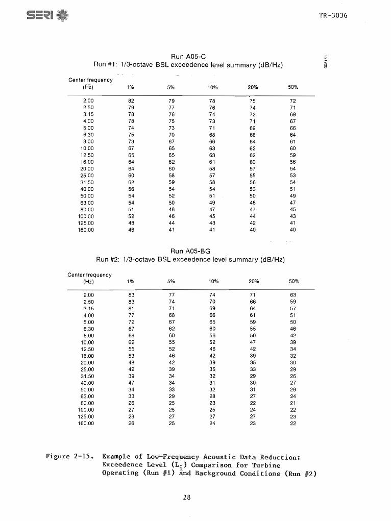
Run A05-C Run #1: 1/3-octave· BSL exceedence level summary (dB/Hz)

Center frequency (Hz) 1% 5% 10% 20% 50%

2.00 82 79 78 75 72 2.50 79 77 76 74 71 3.15 78 76 74 72 69 4.00 78 75 73 71 67 5.00 74 73 71 69 66 6.30 75 70 68 66 64 8.00 73 67 66 64 61

10.00 67 65 63 62 60 12.50 65 65 63 62 59 16.00 64 62 61 60 56 20.00 64 60 58 57 54 25.00 60 58 57 55 53 31.50 62 59 58 56 54 40.00 56 54 54 53 51 50.00 54 52 51 50 49 63.00 54 50 49 48 47 80.00 51 48 47 47 45

100.00 52 46 45 44 43 125.00 48 44 43 42 41 160.00 46 41 41 40 40

Run A05-BG Run #2: 1/3-octave BSL exceedence level summary (dB/Hz)

Center frequency (Hz) 1% 5% 10% 20% 50%

2.00 83 77 74 71 63 2.50 83 74 70 66 59 3.15 81 71 69 64 57 4.00 77 68 66 61 51 5.00 72 67 65 59 50 6.30 67 62 60 55 46 8.00 69 60 56 50 42

10.00 62 55 52 47 39 12.50 55 52 46 42 34 16.00 53 46 42 39 32 20.00 48 42 39 35 30 25.00 42 39 35. 33 29 31.50 39 34 32 29 26 40.00 47 34 31 30 27 50.00 34 33 32 31 29 63.00 33 29 28 27 24 80.00 26 25 23 22 21

100.00 27 25 25 24 22 125.00 28 27 27 27 23 160.00 26 25 24 23 22

Figure 2-15. Example of Low-Frequency Acoustic Data Reduction: Exceedence Level (L.) Comparison for Turbine

1 Operating (Run ) and Background Conditions (Run )

28

TR-3036

l[)

;x; 0 0

Collection configlJration

SLM Direct recording

Time-of­day

Data reduction process

800-line narrowband

spectrum analyzer

25-20,000 Hz

31 random samples of averaged spectra of three consecutive 0.02-s measurement

periods

computer

SERI specialized

software

Sample statistics of 400-800 Hz 1/3-octave bands

-Mean BPL <S1/3(f»

N l!)

;;; 0 0

-SPL standard deviation <S21/3>1/2

-SPL skewness coefficient <b3 (f» -BPL kurtosis coefficient <b4 (f»

distributions

Figure 2-16. High-Frequency-Range Acoustic Data Processing

I"l:j r-"

()Q

c Ii (1)

N I I

~

0\

~=:;; "-

~ ~ -

H ~ I

W o W 0\

I

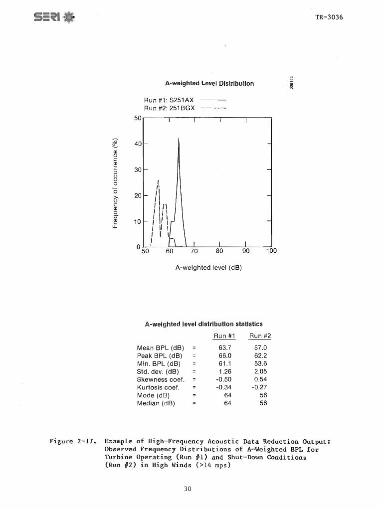
CI) (.) c CI) I... I...

:J (.) (.)

o '+-o ~ (.) c CI) :J 0-CI) l...

IJ..

A-weighted Level Distribution

Run #1: S251 AX Run #2: 251 BGX ----

50 , . .----~----,r----__ r-----...__-___,

40

30

'I 'I

20 / I , I {l I I, ,

10 I \1 \ I II I I r \ I

0 50 I 60 70 80 100

A-weighted level (dB)

.A-\I\U~IClnl[eCl level distribution statistics

Mean BPL (dB) Peak BPL (dB) = Min. BPL (dB) Std. dev. (dB) = Skewness coef. Kurtosis coef. Mode (dB) Median (dB)

Run #1

63.7 66.0 61.1 1.26

-0.50 -0.34

64 64

Run #2

57.0 62.2 53.6 2.05 0.54

-0.27 56 56

(') l()

;;; o o

TR-3036

Figure 2-11. Example of High-Frequency Acoustic Data Reduction Output: Observed Frequency Distributions of A-Weighted BPL for Turbine Operating (Run ) and Shut-Down Conditions (Run ) in High Winds (>14 mps)

30

(i) > (j)

Q) b,

:J CI) CI) Q) b,

Q.

1/3-octave

Run #1: S251 AX Run #2: 251 BGX

60F---r---r-'-1I---'---'-'-"

Mean BPL comparison

55

50

45

1/3-octave center frequency (log Hz)

Run #1: S251 AX 60 Run #2: 251 BGX

55

50

\ \ \ \ \

\""\ \

"-'..---

~ l!"J

co o o

TR-3036

"0 45 c (~

..a

350~---+---~~~d----L--·~~~~ t:..

1/3-octave center frequency (log Hz)

Figure 2-18e of Acoustic Data Reduction Output: Mean. and Peak BPL for Turbine Operating

) and Shut~Down ) in High Winds

31

TR-3036

Run S251AX

Run #1: 1/3-octave BPL exceedence level summary (dB)

Center frequency (Hz) 1% 5% 10% 20% 50%

400 59 58 58 57 55 500 57 57 57 56 55 630 56 56 55 54 53 800 55 55 54 53 52

1000 54 54 54 53 51 1250 54 54 52 52 50 1600 53 53 51 50 49 2000 52 52 52 50 49 2500 51 51 50 48 47 3150 48 47 47 46 45 4000 45 45 45 44 42 5000 43 43 42 42 42 6300 44 43 43 43 42 8000 44 44 44 43 43

A-weighted level 66 66 65 65 64

Run 251

Run #2: 1/3-octave BPL exceedence level summary (dB)

Center frequency (Hz) 1% 5% 10% 20% 50%

400 56 52 52 50 48 500 53 53 51 49 47 630 49 47 46 46 43 800 50 45 45 44 42

1000 48 46 44 43 41 1250 47 45 44 43 41 1600 46 43 43 42 40 2000 47 44 43 43 41 2500 47 43 42 42 40 3150 46 44 43 42 40 4000 45 43 42 42 40 5000 46 43 42 42 41 6300 46 44 43 43 43 8000 46 44 43 43 43

A-weighted level 62 61 59 59 56

Figure 2-19. Example of High-Frequency Acoustic Data Reduction Output: Exceedence Level (L.) Distribution Comparisons for the Case of Figures 2-1~ and 2-18

32

(

TR-3036

of the rotor disk Unless se specified, the parameters 1n Table 2-5 were calculated for the 3D-minute data collection period@

A number of parameters li ted in Table 2-6 and calculated for this experiment have not generally been used in research field programs. These parameters brief 10n of what they represent

ent which air is upstream fetch of 0.1 to 0 m Nos 2 and 3

Friction veloci

where i the IC VI

and a measure of portion of the

where ture; Karman constant; to latent heat flux

an a knowledge Eqs ( )

z/L Ri/(

L :: (

33

o

o

er s the s of the measure of the roughness over

the local wind 10n or to 10+ me Roughness lengths

imilar to that upwind of Turbine

veloci i defined

(2-3)

1 9 and \) is units of velocity

in the lower

number defined by to mechanical (shear) (unstable) correspond

thermal convec­which energy is

buoyancy-damped, of zero repre­

conditions for only

IS defined

07 )] (2-4)

(2-5)

(2-6)

TR-3036

Table 2-6. Bulk Surface Layer Parameters Measured during 1983 Coodnoe Hills Experiments from Towers and Tethered Balloon

Rotor Disk Mean Flow Quantities

Mean l5-m horiz. wind vector, U15 Mean 38-m horiz. wind vector, U38 Mean 45-m u-(long.) component, U45 Mean 45-m w-(vert.) component, W45 Mean hub-ht. horizo wind vector, UH Mean hub-ht. vert. component, WH Mean 84-m horiz. wind vector, U84 Mean 107-m horiza wind vector, U107 Surface roughness length, Zo

Friction velocity, u*

Gradient Richardson number, Ri

Monin-Obukov length, L

Rotor disk peak horizo wind speed, Umax Rotor disk peak velocity height, zmax

Rotor disk Brunt-V~is~l~ period, TBV Surface barometric pressure, Psfc

Hub-height barometric pressure, Phub

BPA 45 m Bulk Inflow Turbulence Quantities

BPA Tower

o

o

o

o

o

o

o

o

o

Longitudinal component (u), x-direction length scale,

Vertical r-omponent (w), z-direction length scale, I z w Vertical component (w), x-direction length scale, I x w Longitudinal (u) time scale, Tu

Vertical (w) time scale, Tw

Longitudinal (u) frequency spectral estimate, S (f) u

Vertical (w) frequency spectral estimate, Sw(f)

Longitudinal (u) spectra reduced frequency peak, fu

Vertical (w) spectra reduced frequency peak, fw

Longitudinal (u) peak turbulence energy, P u

Vertical (w) peak turbulence energy, Pw

34

I x u

PNL Tower

o

o

o

o

o

o

o

o

o

o

o

o

TR-3036

Table 2-6 .. Measured 1983 and Tethered

Tethered Balloon ities

wind

( )1/2 turbulence

inflow turbulence

ra, Suw(n)

scales, I

It IS

heignt is defined upward heat or downliilard an indicator

near zero positive generation [9]

i~ a measure of stratified f10vla

existence of such calculated for the rotor and local values from SERl i

2 4 2 2 Turbulent Inflow

~Nhere T· i the

uw resolution velocity 1es, U(z)

ical

ia1

co

profiles, dU/dz and du/dz

les, Rily(z)

iles 8(z)

les, 8s (z)

and Ri1o(z)

measure of the 10n is dominant L

are (negative or stratification exists (positive

io z/L can also be thought of as going on Large

dominant; and a shear

(2-7)

of of density-stable boundary

an measure of the in Table 2-6, it has been

tower measurements and layer les

The turbulent or

for i=1,2,3 , (2-8)

I . cross-correlatIon

time~scale for the ith-component and R· .(T) is the f . b h' d' h lJ . unctl0n _ etween t. elan J s T ere are n1ne

possible terms in the 1983

the . (T) matrix 0 Three of these have been computed for fromJthe hot~film anemometer measurements and listed in

TR-3036

Table 2-6" Iu xis a charac teri s tic scale length of the longi tudinal tur­bulence component, u, along the x-direction (positive east).. Similarly, I x is a scale length of the vertical component, w, along the x-directio~" Finally, I z is a scale length of the w-component in the vertical or z-direction~ The time and length scales were calculated from component veloc­ity signals over a frequency range of 0.05 to 10 Hz for the 30-minute data­collection periods.

Normalized turbulence spectra descriptors. Frequency spectra ampli tudes of the turbulent wind components (u, v, w) are often normalized by the cyclic frequency or nS{n). The corresponding cyclic frequency, n, is normalized by the ratio z/U{z) or nz/U{z) and referred to as the reduced frequency f, where U{z) is the mean wind speed at height z.. The quantities f and f in Table 2-6 represent the value of the reduced frequency where f'§{f) has

w its

maximum. Further, P and P parameters in Table 2-6 refer to the maximum values of nS (f) and ~S (f), ;espectivelye

u w

2.4.3 Rotor Surface Pressures

Table 2-7 lists the locations of the 12 semiconductor pressure transducers used on Blade No. 1 of Turbine No.2 in the 1983 experiment. In this volume, only the measurements near the leading edge of the rotor have been analyzed to any great extent.. This is because coherent, low-frequency acoustic radiation is associated with turbulence-induced, unsteady blade loads, whose greatest effects tend to be concentrated near the leading edge.

Table 2-7. Pressure Tap Locations on Turbine No.2, Blade No.1

Tap Blade Percent Percent No .. Station Span Chord Surface

1 1164a 65 15

2 1164 65 15 Lowerc

3 1164 65 40 Upper

4 1164 65 40 Lower

5 1164 65 85 Upper

6 1164 65 85 Lower

7 1562d 87 15 Upper

8 1562 87 15 Lower

9 1562 87 40 Upper

10 1562 87 40 Lower

11 1562 87 85 Upper

12 1562 87 85 Lower

~Fixed pitch portion of blade. Low pressure surface. ~High-pressure surface" Movable tip portion"

36

TR-3036

3@O DESCRIPTION OF GooDNOE HILLS INFLOW STRUCTURE

A knowledge of the details of the turbulent inflow structure is important if any statistical correlation between the inflow properties and the resulting acoustic emission characteristics is to be made. We must first establish what properties are most important In terms of acoustic noise generation by the MOD-2 in a turbulent atmo Summaries are then given of the available inflow properties for the 1982 and 1 experimental periodse

3 .. 1

Homicz and George [10,11] and theory using generalized functions blades in a turbulent determining the cri tical inflow

and Kim [17] have developed a unified of aeroacoustic noise generated by rotating

We will use their results as a basis for to be used as statistical pre-

dictors for correlations with the MOD-2 emlS 10ns

Homicz and have shown that radiated acoustic s (f) is givec

f)

ized function for the far-field localized disturbance source region

(n (3-1)

where f IS the acoustic IS the sound Po IS the alI" density, y is the distance between the observation and the rotor, n is

the harmonic number, n is the position vector of the disturbance on the rotor,

PL. L. is the cross~spec ral densi of the lift, and ~o i the unit vector albng Figure shows of the and associated angles

and symbols 0 shown that the characteristics of the radiated

acoustic spectrum on the quasi-static load due to mean loading conditions plus the fluctuat loads due to rotor-turbulence interaction. The far-field radiated spectrum due to a turbulent upwash spectrum is of the form

co n

2 CD

2 <s (f) OJ. f d C;; [ I G (c;;,n,l1,)J

nB_

l (fet) (3-2) ap Q

C;;

M J2 a

I x l1, rZ

w

where <S (f», the acoustic pressure , is expressed in the form of an ap .. integral over C;;, the turbulent velocl spectrum dlmensionless wavenumber, and where the two series involving Bessel functions arise because of the resolu­tion of the turbulence into polar coordinates and because of the Doppler shift due to the rotation0 The function G(c;;,n, ~) includes the ingested turbulence spectrum and unsteady aerodynamic effect and the finite span effect of the rotor bladeso r Z is the vertical or upwash turbulence integral scale; V is the axial convec;ion velocity of the turbulence (usually taken as O.8UH); ~ is the number of blades in the rotor and Mc is the axial convection Mach number, Hc = Vc/ao ·

Figure 3-1

Turbulent eddy

Microphone

~ ro o o

Rotor Geometry Used by Homicz and George [10,11]

TR-3036

The dynamic characteristics of the low-frequency portion of the radiated spec­trum is determined by the degree of blade-to-blade correlation with turbulent eddies passing through the rotor plane [10]. Larger eddies may be cut by more than one blade, producing peaked, essentially discrete tones in the low­frequency spectrum. Smaller eddies produce much higher frequency blade loads, but generally there is less likelihood of repeated encounters with the same eddy, and random, broadband noise is radiated. Homicz and George have shown that the frequency at which this transition to broadband takes place is

Bn (1 + Mo/Mc) f ~ (3-3)

o -2 (1 - Mo cosy) •

They also were able to show that the values of ~ that provide significant con­tributions to the acoustic spectrum at frequency fare

(fin) (1 - Mo cosy) (fin) (1 + Mo cosy) < ~ < (3-4)

(Vc/lun) (1 + Mo/Mc) Vc Iun

When (3-3) and (3-4) are combined, the lower limit of ~, which makes signif­icant contributions for f>f o 1S

~f o

> B I n/2 V • u c (3-5)

For the MOD-2 turbine with ~ dimensionalized by the chord Co at Ro ' the cor­responding turbulent eddy wavelength would be -10 m or 5 chord lengths for a longitudinal integral scale of 125 m.

Homicz and George assumed that the inflow turbulence could be considered homo­geneous and isotropic. This enabled them to use only one length scale. As we see in Sections 3.2.2 and 3.3, even treating the MOD-2 inflow two­dimensionally requires additional length-scale specification, because of the

38

TR-3036

degree of anisotropy that may be present in the (inflow) acoustically signif­icant eddy wavelengths.. In anticipation, we define three integral scales: lux, the longi tudinal or axial scale; I x, the scale length of the vertical turbulence or upwash component'J w, alon; the axial direction; and I z, the scale of the vertical component in the rotor planeo Figure 3-2 sketc~es the relationship of these length scales to the rotor plane

Homicz and George arrived at the following expression for the non­a turbulent envi ronment dimensionalized, one-sided acoustic from

moving through a rotor:

(3-6)

co

x f E. E E E E -lnt ~ turb aero span '

where

E. 1nt

J2 E :::::

ll- 1

E :::::

turb

[COS11

H 0

I

= {l

J2[ 0

:::::

s

/ )

1

2 2 J nB- l

f cosy) Q

2 2 4Tf r; )

kc and ks are the reduced aerodynamic ~ ies along _thr/2hord (c) and span (s) averaged over one blade revolution, and kT :::::( k~)

E2, the relative of the ll- loading modes for a given non-d1mensional wavenumber describes the acoustic of these upwash modes with the nB harmonic modes E t b establishes the . . ur. weighting ied to thecontrlbut1on from any turbulent wavenumber; b 1S the blade span; 11 i the between the 1 force vector and the vertical; n is the harmonic number of the blade passage ; Mt is the tip Mach number; and i the tip radius" The E and E terms reflect the .aero span . influence of rotor's unsteady aerodynam1c response and a spanWlse correc-tion to account for the loss of acoustic compactness at high frequencies .. Homicz and have developed expres ions for these terms under what we believe to be highly idealized conditions For now, we have chosen to lump these effects together with those fixed by design by experimentally determining the MOD-2 aeroacoustic transfer functions

'10

TR-3036

W(z)

U(x)

V(y)

Figure 3-2 ..

W

U

Schematic of I x, I x u w'

to Turbine Rotor

I~

I Z Length Scales with Respect w

The acoustically significant inflow properties, which need to be determined within a stochastic framework, can now be summarized and include these:

• Axial convection veloci ty, V , . c making UH an 1nflow parameter

which we will approximate by 0 .. 8UH, thus

'2 • Upwash velocity turbulence intensity, w

• Turbulence integral scale, which we have expanded into three components: I x, I x, and I z, by treating the problem two-dimensionally

u w w

Local atmospheric state (barometric pressure, temperature), which 1S used to calculate the air density, Po' and acoustic velocity, a o •

The remainder of the scaling parameters in Eq. (3-6) are fixed for the MOD-2 design and include the

• Rotor rotational frequency, Q

• Number of blades, B

• Rotor tip radius, Rt or D/2

• Blade span, b

Blade chord, co' at effective radius Ro (typically taken as 0.7SRt )

• Airfoil shape of the rotor blades.

Furthermore, a reference distance, r, and its relationship to the rotor disk must be chosen. We have decided to use the upwind, on-axis station located 1.SD ahead of the rotor disk or at an angle of 24° with respect to the turbine hub height as this reference point. It also allows this measuring station to

40

to CX) o o

TR-3036

"see" thrust and torque components of the acoustic radiation.. This location is also useful in verifying the predictive methods of Homicz and George by avoiding the complications associated with modeling the conditions in the vicinity of the rotor plane.

3 .. 2

In the lower portion of the earth's atmo~pheric boundary layer (usually referred to as the surface layer), UH, Ii J, and Wi 2 are all functions of height, z. The rotor blades of large, horizontal-axis wind turbines, such as the MOD-2, traverse deep vertical layers perhaps exceeding the height of the surface or constant flux (see Section 302.1) a percentage of the time. The existence of strong vertical shearing and layering associated with this layer, particularly under stable flow conditions, makes the specification of acoustically significant essentially impossible except for some well-defined reference atmo What is needed are characteristic or scaling parameters, which by physical processes are efficient predictors of the statistical distribution of the vertical or upwash velocity , w', spectrum (or, more generally, the three-dimensional and the horizontal wind velocity UH across the vertica.l depth of the turbine I s rotor disk. Such scaling is discussed below

3 .. 2 .. 1 Surface

It is known that, within a locally homogeneous and quasi-steady surface layer, the vertical fluxes of heat, momentum, a.nd moisture are essentially constant. Ideally, under such conditions, the turbulent structure should be related to vnly a few Monin and Obukov [13,14] proposed that tur-bulent motions in the surface layer scaled with the height z above the surface, the local buoyancy, giS, the kinematic surface stress Ls/po (where LS is the surface stress), and the surface kinematic heat flux Q = H Ip co By combining these parameters, they defined a series of surface-o 0 0 layer scaling factors (knovm as similarity or M-O scaling), including a veloc-ity scale, u)" (the friction velocity; see Section 2.4 2.1); a temperature scale, T* = -Qo/u*; the M-O length, L (defined in Section 2.4 .. 2 .. 1); and the geometric height, z

When surface layer flow properties are appropriately nondimensionalized (velocities by U~I(, temperatures by T~I.., etc.), M-O theory has shown that they become universal functions of z/L. It is generally accepted that the "uni­versal function" aspect of M-O similarity applies in surface layers over homo­geneous terrain [15]. In the real world, and that includes most wind plant sites, there is often a departure from strict M-O theory as a result of such influences as nonsteady boundary conditions, complex terrain features, local radiative effects, or inhomogeneous flow conditions due to upstream (fetch) effectse These "departures" usually have the effect of changing "universal functions" into site-specific ones.

41

TR-3036

3.2.2 The Vertical Distribution of UM (Vc )

Because of the effects of surface friction, the horizontal wind vector increases with height at least part of the way in the surface layer. Under neutral stability conditions (Ri = z/L = 0),. and over homogeneous terrain, this vertical profile of UH can be represented by the familiar log profile, or

(3-7)

where z is the roughness length defined in Section 2.402.1. Equation (3-7) is modi~ied for non-neutral surface layers by the diabatic wind profile [8], or

where

and

UH(z) = (u*/ka ) . [In(z/zo) - Wm(z/L)]

z/L

f zo/L

[1 - Ym (r,;)] dr,; l;;

(3-8)

The important point here is the influence of the M-O scaling parameters u*, L, and z on the value of UH' or equivalently V , as a function of height within the turbine's rotor disk. If the condition~ of true M-O scaling are met, u* and L are not functions of z 0 Thus,. we may think of these parameters as potential candidates for predictors of turbine acoustic emissions characteristics ..

3.2.3 Variation of with Height

If M-O scalin~ is applicable, Panofsky and Dutton [9] show the vertical varla­tion of Wi spectra, S (f,z), is of the form w

(3-9)

where n is the cyclic frequency and f is the reduced or normalized frequency given by f(z) = nz/UH(z). The relationship defined in Eq .. (3-9) has a dif­ferent form for unstable/neutral and stable environments. For stable condi­tions, Panofsky and Dutton recommend the equation developed by Kaimal [16]:

(3-10)

where P /u,,~2 is the maximum of S (f ,z) at f = f and is a function of z/L .. w " .. w m •

For unstable and neutral condltlons, they recommend the HOJstrup [18] model, or

nSw(n,z) 2

u ... }~

32f (~)2/3 + 2f (1+17f)5/3 -L (1 + 5 .. 3f)5/3

(3-11)

Assuming M-O similarity holds, Eqs. (3-9), (3-10), and (3-11) demonstrate the statistical dependency of the upwash velocity spectra on the UH(z), U,.o and z/L scale lengths characteristic of the flow.. Since the M-O length, L, can be estimated from a knowledge of the Richardson number (see Section 2.4.2.1), the Ri could be substituted for L.

42

TR-3036

In addition to the M-O similarity theory scale lengths discussed above, it is also possible to empirically determine characteristic length scales of the inflow itself. These scale lengths, called integral scales, are defined by

CD

Iij

= ui fo RUij(T)dT ,

where U· = [u,v,w] and j = [x,y,z), but Slnce 1

CD

(3-12)

(3-13)

Ii J contains information .about Sij(f) and should also be related to the M-O scales. The measured I.J scales contain information about the spectral con­tent of the flow, even il it does not strictly follow M-O similarity.

From the above, it is clear that one \vould expect S (f,z}) to have some rela-( )

' • 1.'1 ( tionship with S f,z2 ' vnth zl = z2' Slnce both S f and UH scale with 0:;.7. 'I'l •

height in the surface layer whlle u* and L do not. Thus, lt seems plausible that detailed spectral measurements made at a given height within the rotor disk layer should be at least statistically related to those at other heights if the scaling laws apply. Since we do not have the ability to gather direct measurements of the upwash or WI spectra throughout the entire disk, we have chosen to establish a reference to measure the actual flow scale lengths related to it as well as the normal M-O scaling parameters. These parameters include the following:

o Mean reference or hub-height wind speed, UH o Rotor disk gradient Richardson number, Ri

o Longitudinal (axial) velocity component length scale, lux

o Vertical (upwash) velocity component length scale along the axial (x) direc­. I x t lon, w

o Vertical component length scale parallel to the rotor plane Iwz •

Thus, the parameters above provide scales for Vc (1:25~H)' the surface layer vertical stability (Ri and/or z/L), and characterlstlc flm.; scale lengths related to Sw(f).

3.3 Inflow Data i tical Summaries

As previously stated, no detailed, high-frequency turbulence measurements ,.;ere taken during the 1982 experiment. This has limited our ability to establish adequate correlations with the MOD-2 acoustic emissions spectra for that experimental period. Hm.;ever, since the current MOD-2 configuration is the one in use during the 1983 series, we believe it is the more important. We have summarized be.low what information was available for the 1982 data runs. A reduced 1982 data set was selected based on available inflow properties whose values fell within the observed ranges of the same parameters in 1983. This '.vas done to try to establish a common inflow basis for year-to-year comparisons.

43

TR-3036

A comparison of the 1982 and 1983 overall inflow statistics are given in Table 3-1. While lower wind speeds were, on the average, encountered during 1983, Table 3-1 shows that these data runs were made in conditions that were, on the average, more stable and more turbulent than the 12 runs made in April­May 1982.. Table 3-2 lists the reduced data set summary statistics for 1982 and 1983, with its closely overlapping parameter rangese Missing from Table 3-2, of course, are the measured characteri s t ic scale lengths of the inflow ..

Tables 3-3a, b, and c summarize the detailed inflow data for the six 1983 data runs used for the low-frequency-range analysis in Section 5 .. 0. Table 3-3a lists the air motions data from three measuring heights on the BPA tower. The two-axis, hot-film anemometer was installed at the 45-m level, from which the high-frequency turbulence statistics were gathered. Eight runs were made in 1983, but one was lost to a failure in the recorder collecting the hot-film datae The other run was lost when the wind direction moved out of the desired 40° cone for the operation of the two-axis, hot-film anemometer. The inflow characteristic scaling parameters are listed in Table 3-3b; the air motions data were deri ved largely from the BPA tower but the stabili ty information came from the PNL tower. Table 3-3c summarizes the longitudinal and vertical component spectral scaling parameters P /u~2 and P /u~2 discussed in .... ··u .. w " Section 3.2 .. 3 as well as th~ Brunt-Vaisala period TBV " The peak mean wind speeds and heights listed in Table 3-3c were determined by vertically smoothing the five speeds available from the PNL tower.

Table )-1. Comparison of 1982 and 1983 from the BPA Meteorological

Parameter

Total number of data runs 59-m mean wind speed, mps 59-m mean wind speed variance, (mps)2 59-m mean turbulence intensity, % Mean Richardson number (PNL tower) Peak 59-m 10-min mean wind speed, mps Minimum 59-m 10-min mean wind speed, mps

Inflow Tower

Statistics

1982 1983

12 8 11 .. 4 9.5 1.51 1 .. 75

10 .. 8 13 .. 9 0 .. 30 2.36

14 .. 5 13 .. 6 7.5 6 .. 9

Table 3-2 .. BPA Tower Statistics of Reduced 1982/1983 Data Sets

Parameter 1982 1983

Number of data runs 6 4 59-m mean wind speed, mps 9.85 9 .. 58 59-m mean wind speed variance, (mps)2 1.15 0.99 59-m mean turbulence intensity, % 10 .. 9 10 .. 4 Mean Richardson number 0.25 0 .. 34 Mean M-O z/L parameter 2.86 3.02

44

~-~

II I ~-:-'

Table 3-3a .. 1983 Mean Inflow

59-m 59-m 59-m Data Wind

UH (U ,)1/2

Run Direction (deg) (mps) ~mps)

A05 268 7 .. 3 1 .. 02 A03 261 8 .. 1 1 .. 03 A14-1 261 9.2 1 .. 31 A14-2 256 9 .. 9 1 10 Al8 254 12 .. 4 0 .. 89 All 257 13 .. 6 0 .. 31

Means 260 10 .. 1 0 .. 94

TR-3036

from BPA Tower:

45-m 45-m 45-m 60-m (u,)1/2 (w,)l/2 u w

(mps) (mps) (mps) (mps)

8.7 1 .. 13 0,,16 0 .. 52 9 .. 0 1 .. 32 0 .. 19 0 .. 76 9 .. 6 1 .. 30 0,,19 0 .. 95

10 .. 5 1 37 0 .. 15 0 .. 78 13 .. 9 0 .. 90 0 .. 12 0 .. 99 14 .. 3 1 .. 10 0 .. 17 0 .. 52

11 .. 0 1 .. 19 0016 0 .. 75

Table 3-3b .. 1983 Mean Inflow Characteristics: Scaling Parameters

Data Ri z/L u,,;'( Zo I x I x I z Tu Tw Run (mps) (em) (~) (~) (~) (sec) (sec)

ADS 11 .. 7 5 .. 62 0635 56@7 136 125 7.5 15 .. 6 14 .. 4 A03 -0.12 -0 .. 12 .461 5.6 210 157 13 .. 3 23 .. 4 17.5 A14-1 0 .. 13 .. 334 1 01 11 .. 9 157 166 16 .. 5 16 .. 4 17 .. 3 A14-2 0 .. 26 5 .. 62 0,,736 25 .. 6 8605 8107 6.1 8.22 7.76 A18 1 .. 25 5 .. 62 0 .. 943 27,,4 125 123 8.8 9 .. 02 8 .. 84 All 6 .. 68 5 .. 62 1,,09 4603 336 86 .. 8 6 .. 8 23.4 6 .. 06

Means 3 .. 32 3 .. 78 .. 813 2809 175 123 9 .. 8 16 .. 0 12 .. 0

3 .. 4 Inflow Turbulence Content

The frequency spectra for six analysis runs of the longitudinal and vertical turbulence components measured at the 45-m level on the BPA tower are pre­sented in Figures 3-3 through 3-89 The corresponding Richardson number (Ri), mean hub-height wind speed (Uhub )' and longitudinal (IX) and vertical (I z ) integral scale lengths are listed on each plot.. u w .

3 .. 5 Rotor Disk Inflow Vertical Profiles

It is important to know the vertical distribution of wind speed and turbulence across the MOD-2 rotor disk.. Since the height of the BPA tower extended only to hub height, we were left with two other sources of vertical profiles of wind distribution information: the five levels of the PNL tower and SERI' s tethered balloon sounding system. The latter was limited, in 1982/83, to wind speeds under about 11 mps.. We have used both resources to assemble a picture of the distribution of the horizontal wind with height.

45

TR-3036

3.5.1 PNL Tower Vertical Profiles of Wind Speed and Turbulence Intensity

The vertical resolution (22.9 m or 75 ft) of the PNL tower is limited, but by regression smoothing we can achieve a reasonable estimate of a mean vertical profile. Also, it is clear that these profiles may not exactly agree with the vertical inflow structure into Turbine No. 2 because of the degree of spatial separation. However, they are useful because they track the vertical struc­ture (shape) of the profiles under the range of stability and speeds encoun­tered during the six 1983 data runs" Figures 3-9 through 3-: 14 plot the smoothed wind speed normalized by the hub-height value and the un-normalized turbulent intensity for each of the six data runs. We should point out that we consider the turbulent intensity plotted here to be the "long wave" contri­bution due to the lack of response of the cup anemometers at small wavelengths (high frequencies)"

3.5.2 Representative Tethered Balloon Profiles in Turbine NOG 2 Inflow

A number of 1982 runs were supported by the tethered balloon system but only three were available in 1983 because of equipment problems, high winds, or both. In 1983 the runs that were supported included A03, A03-1, and A05. The 45-m level turbulence data were unavailable from the A03-1 run because of an out-of-tolerance hub wind direction. Figures 3-15 through 3-17 present smoothed, high-resolution vertical profiles of wind direction and speed, sensible temperature, ana atmospheric stability taken just before the beginning of Run A05" It is interesting to compare the vertical wind-speed profile measured by the five discrete levels on the PNL tower in Figure 3-14 and the tethered balloon profiles taken in the inflow of Turbine No" 2 in Fig­ure 3-15.. A representative sample of a high-resolution inflow turbulence spectrum measured by the hot-film anemometer is plotted in Figure 3-18 for the same run.

Data Run

A05 A03 A14-1 A14-2 A18 All

Means

Table 3-3ce 1983 Mean Inflow Characteristics: Spectral Scaling and Rotor Disk Layer Parameters

fm fm 2 TBV Mean pu/U.,.", pw/u-;,,,,

2 u w (sec) Speed

(mps)

.081 .081 0 .. 836 0 .. 038 247 6 .. 8

.. 078 ,,078 0.729 0 .. 162 0 9.0

.. 147 .147 0 .. 489 0 .. 061 319 11.5

.. 134 .. 067 0 .. 941 0 .. 050 343 11 .. 3 ,,101 .. 051 0 .. 324 0 .. 031 234 13.6 .049 .167 2 .. 43 0 .. 043 177 13.2

.098 .099 0 .. 958 0 .. 064 264 10 .. 9

aDetermined from the PNL tower.

46

Peak Winda

Height (m)

44.8 107 107 107

97 .. 9 68 .. 4

8807

N I ~ en a. E '-'

c ~

:i (f)

.~ 10-1

c (\) '"0

~ "­..... () (\)

a. 10-2 en E I

L() '<:j"

1983 Run AOS BPA 4S-m inflow spectra

Sw(n)

Ri = Uhub = 7.3 mps lux = 136 m Iwz = 7.S m

10-3 ,L-. ____ -.L _____ "'-=-____ --L _____ _

10-2 10-1 10 102

Cyclic frequency, n (Hz)

Figure 3-3. BPA Tower 45~m Level and Vertical

N I ........ N

en a. E

c ~

:i (f)

>. ."t:: en c (\)

'"0

~ )... ..... l) (\) a. en E I

L() '<:j"

Inflow for 1983-~Run A05

10

10-1

10-2

Ri = -0.12 Uhub =8.1 mps lux=210m Iwz = 13 m

Cyclic frequency, n (Hz)

Figure 3-4. BPA Tower 45-m Level Inflow

47

-5/3 slope

and 1983--Run A03

TR-3036

co l{)

co o o

fii 00 o o

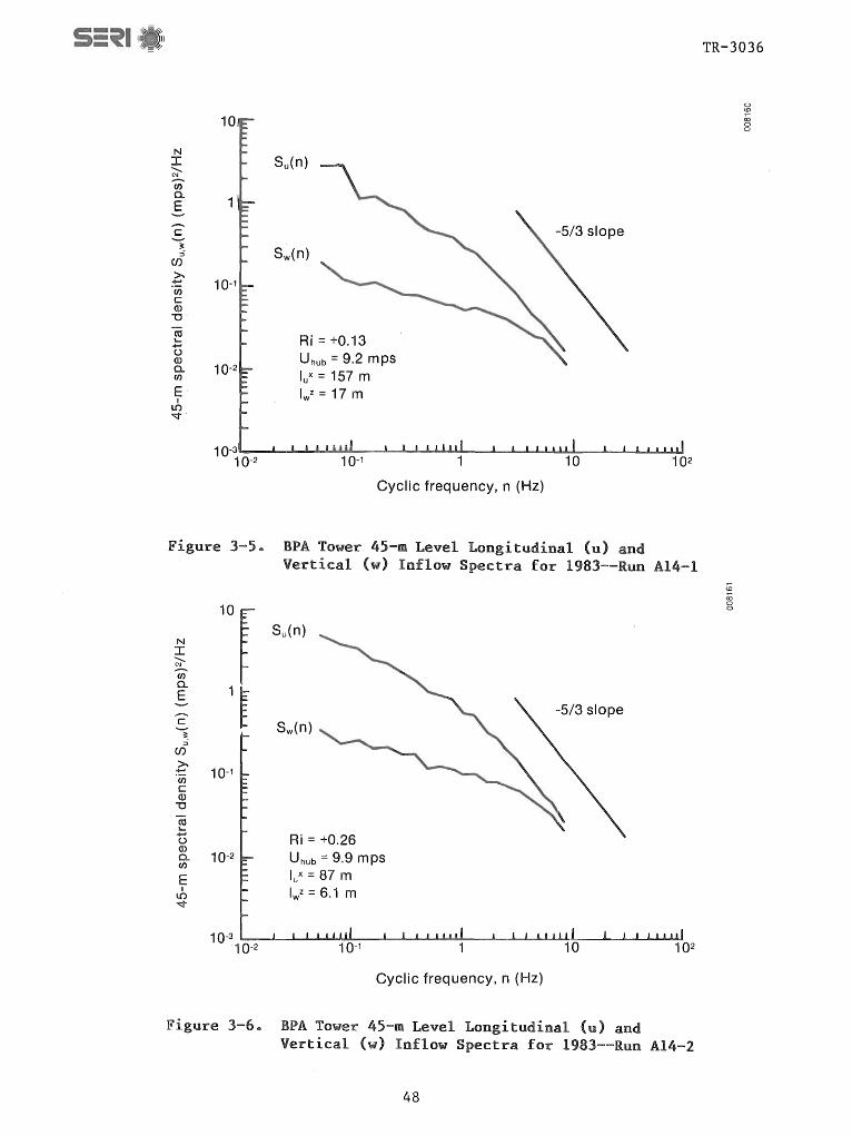
10

N I ........ C\J en 0.. E .........

...-... c -; ct >-

:!:: (/)

C <D '"0'

ro h... .... () <D 0.. (/)

E I

~,

10-3

10-2

Figure 3-5 ..

10 r N I ........ C\J en 0.. E

1 E .-c ---3_

en >-

:!:: 10-1 (/)

C <D '"0

ro h... .... ()

<D 10-2 0..

(/)

E I

L()

"'" 10-3

1 0-2

Figure 3-6 ..

Ri=+0.13 Uhub = 9.2 mps lux = 157 m Iwz = 17 m

Cyclic frequency, n (Hz)

-5/3 slope

BPA Tower 45-m Level Longitudinal (u) and Vertical (w) Inflow Spectra for 1983--Run

Su(n)

-5/3 slope Sw(n)

Ri = +0.26 Uhub = 9.9 mps lux = 87 m Iwz = 6.1 m

Cyclic frequency, n (Hz)

BPA Tower 45-m Level Longitudinal (u) and Vertical (w) Inflow Spectra for 1983--Run

48

A14-1

A14-2

TR-3036

<0

00 0 0

o <0

00 o o

N I .......... C\J

(j) Q.

E ,..-... c ~

10

-5/3 slope

of Sw(n) .£ 10-1

en c (l)

"'0

«l l.­+-' U (l) Q. en

E I

L() -<::t

10-2

Figure 3~1

N I .......... C\I

(j) Q.

E ......... c ---~

::i Cf)

10

~ :=: ~ 10-1

Q) "'0

cu l.­+-' U Q) Q. en

E I

L() -<::t

10-2

Figure 3-8

Ri = +1.25 Uhub 12.4 mps lux := 125 m Iwz = 8.8 m

Cyclic frequency, n (Hz)

BPA Tower 45-m Level

Ri = +6.68 UhUb = 13.6 mps lux 336 m Iwz = 6.8 m

Inflow

Cyclic frequency, n (Hz)

BPA Tower 45-m

49

and 1983--Run Al8

-5/3 slope

and 1983--Run All

TR-3036

C\I <0

00 o o

C') <0

00 o o

.......... E ........ Q) en ct1 ..a

Q)

> o ..a ct1

......

..c 0)

Q)

TR-3036

'<;f" <D

Profile for Run A03 ro o o

125 __ ----__ ----~----__ ----__ ----~

100

75

50

Profile ref. to WS at hub ht.

30-min. parameter means: Hub windspd. = 7.75 m/s Hub wind dir. = 273.4 deg. Grad. Rich. no. = -0.12

I 25

O~ ____ d_--__ ~ __ --~------~ __ ~

0.7 0.8 0.9 1.0 1.1 1.2

(a) UH normalized horizontal wind speed

If) to

ro o o

Run A03 PNl Turbulence Intensity Profile

125-------~------r----~.----~r-----,

E 100 Q) en ct1 ..a

Q) > o ..a ct1

......

..c 0)

75

50

Q) 25 I

3 6 9 12 15

Turbulence intensity (%)

(b) turbulence intensity

30-min. parameter means: Hub windspd. = 7.75 m/s Hub wind dir. = 273.4 deg. Grad. Rich. no. = -0.12

Figure 3-9 .. Smoothed Vertical Profile (PNL Tower) of Uh b-Normalized Horizontal Wind Speed (a) and Turbulence In~ensity (b) for 1983--Run A03

so

,.-..

E Q) en al .0 1.-Q)

~ 0

+='

(j)

> 0 .0 al

Q)

> o .0 al

)-10

100

75

50 -

25

0 0.7

100

75

50

25

TR-3036

Norm.PNl Wind Profile for Run A14-1 <D <D

00 o o

1.2

U/U H

3 6 9 12 15

Turbulence intensity (%)

51

Tower) of and Turbulence

Profile ref. to WS at hub ht.

30-min. parameter means: Hub windspd. = 8.98 m/s Hub wind dir. = 271.8 deg. Grad. Rich. no. = +0.13

r­<D

00 o o

30-min. parameter means: Hub windspd. = 8.98 m/s Hub wind dir. = 271.8 deg. Grad. Rich. no. = +0.13

Norm.PNL Wind ·<W'IIJ.I;;'I;U Profile for Run A14-2 TR-3036 125r-----r-----r-----r---~r_--__

......... 100 E Q) en ro .0

Q)

> o .0 ro +-' ..c 0)

Q)

I

75

50

25

o 0.7 0.8 0.9 1.0 1.1 1.2

U/U H

(a) UH normalized horizontal wind speed

Profile ref. to WS at hub ht.

30-min. parameter means: Hub windspd. = 9.78 m/s Hub wind dir. = 274 deg. Grad. Rich. no. = +0.26

Run A14-2 PNl Turbulence Intensity Profile 125~------------r----~r_--~r_--~

E 100 CD en ro .0 l...

CD 3 o +-'

CD > o .0 ro +-' ..c 0)

'Q) I

Figure 3-11 ..

75

50

25

0'-----'-----'-----11..---11'-----o 3 6 9 12 15

Turbulence intensity (%)

(b) turbulence intensity

30-min. parameter means: Hub windspd. = 9.78 m/s Hub wind dir. = 274 deg. Grad. Rich. no. = +0.26

Smoothed Vertical Profile (PNL Tower) of Uh b-Normalized Horizontal Wind Speed (a) and Turbulence In~ensity (b) for 1983--Run A14-2

52

ro <0

ro o o

en <0

ro o o

Q) (f)

ctI .Cl 10-Q)

3: 0 +-'

Q) > 0 J:l ctI +-' ..c 0)

Q)

I

TR-3036

Norm.PNL Wind Profile for Run A 18 :2 co o o

100

75

50

25

o 0.7 0.8 0.9 1.0 1.1

) normalized horizontal

1.2

Profile ref. to WS at hub ht.

30-min. parameter means: Hub windspd. = 12.8 m/s Hub wind dir. = 265.8 deg. Grad. Rich. no. = +0.72

;::. Run A18 PNl Turbulence Init,An~~ihl Profile co

o o 125 ~--"iF""""--~--....----...,.....----...

100

75

50

15

Turbulence intensity (%)

turbulence intensity

30.;.min. parameter means: Hub windspd. = 12.8 m/s Hub wind dir. = 265.8 deg. Grad. Rich. no. = +0.72

Smoothed Vertical Horizontal Wind 1983~-Run AlB

Tower) of Uh b-Normalized Turbulence In~ensity (b) for

53

Norm.PNL Wind Profile for Run A 11

TR-3036

C\J r--;;; o o

125~----~----~----~----~--~

Q) > o .c m +-' .c 0>

100

75

50·

Q) 25 I

o 0.7 0.8 0.9 1.0 1.1 1.2

Profile ref. to WS at hub ht.

30-min. parameter means: Hub windspd. = 13.1 m/s Hub wind dir. = 270.3 deg. Grad. Rich. no. = +6.68

(a) Us normalized horizontal wind speed

Run A 11 PNL Turbulence Intensity Profile 125 _--.,-----r---..,..---~-____,

-E 100 Q) CJ)

m .c

Q)

> o .c m +-' .c 0>

75

50

Q) 25 I

o o 3 6 9 12 15

Turbulence intensity (%)

(b) turbulence intensity

30-min. parameter means: Hub windspd. = 13.1 m/s Hub wind dir. = 270.3 deg. Grad. Rich. no. = +6.68

Figure 3-13. Smoothed Vertical Profile (PNL Tower) of Uhub-N?rmalized Horizontal Wind Speed (a) and Turbulence Intens1ty (b) for 1983--Run All

54

C'"J r--;;; o o

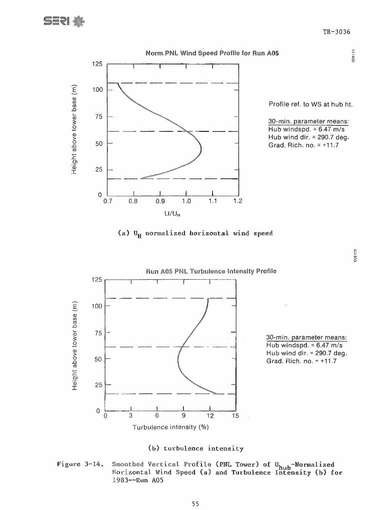
125

E 100 Q) C/)

ct:l ..a I.- 75 Q)

3: 0 ...... Q) > 0 50 ..a ct:l

25

o 0.7

100 Q) C/)

ct:l ..0 I.- 75 Q)

3: 0 ...... Q) > 0 50 ..0 ct:l

......

..c Ol Q) 25 I

o o

Figure 3-14 ..

TR-3036

Norm.PNL Wind Profile for Run A05 ;:: ;;; o o

Profile ref. to WS at hub ht.

30-min. parameter means: Hub windspd. = 6.47 m/s Hub wind dir. = 290.7 deg. Grad. Rich. no. = +11.7

0.8 0.9 1.0 1.1 1.2

normalized horizontal wind

Run A05 PNL Turbulence Profile

30-min. parameter means: Hub windspd. = 6.47 m/s Hub wind dir. = 290.7 deg. Grad. Rich. no. = +11.7

3 6 9 12 15

Turbulence intensity (%)

turbulence intensity

Smoothed Vertical Profile (PNL Tower) of Uh b-Normalized Horizontal Wind (a) and Turbulence In~ensity (b) for 1983--Run AOS

55

l{) I'--

OJ o o

100 100 CD r-oo 0 0

• • • • 80 • • • 80 • • • • • • Hub height Hub height

- 60 60 E E

VI ...... ----0'\ ..c • ...... 0> ..c (J)

0>

I (J)

40 I

40

20 20

o 4 5 6 7 8 9 10 11 12 o 4 5 6 7 8 9 10 11 12

Wind speed (m/s) Wind speed (m/s)

Figure 3-15. Smoothed and High-Resolution Vertical Profiles of Speed for Run A05

E I..n ---....J -c

0)

<D I

100r-----------------------------------~

80 '

Hub height 60

40

20

o 180

-----

•

•

Wind direction (deg)

) Smoothed profile

Figure 3-16. Smoothed and

100 p---------------------------------------~ ~ ;;; o o

80

Hub

60 E

---c 0)

<D I

40

20 •

o ~--~--~----~--~--~----~--~------~ 180 220 260 300 340

Wind direction (deg)

High-resolution vertical profile

Vertical Profiles for Wind Direction for Run AOS

V1 00 E

.....

..c. 0)

Q)

I

100 ~--------------------------------~

80

Hub height 60

40

20

016 17 18 19 20 21 22

Temperature (0 C)

E ..... ..c. 0)

Q)

I

100~--------------------------------------~

80

Hub height 60

40

20

17 18 20 21 22

Temperature (0 C)

a:J r--a:J o o

Figure 3-17. Smoothed and High-Resolution Vertical Profiles of Sensible Temperature for Run AOS

TR-3036

101 ........... g: c: 00 '--' 0

(f)

Mean sensor height = 78 m 0

c: ---->. Mean windspeed = 7.4 ms-1 +-'

(f) Integral scale = 2.9 m c: Q)

100 "0

cti l-

t> Q) a. (j)

I-Q)

$: 0 10-1 a. "0 Q)

.~ cti E b-

0 z 10-2

10-1 100 101 102

Frequency, n (Hz)

3-18" l"arrowband Turbulence Measured at 18-m 6 Run A05

59

TR-3036

4.0 CHARACTERISTICS OF MOD-2 HIGH-FREQUENCY-RANGE EMISSIONS

This section summarizes the characteristics of the high-frequency-range (HF) MOD-2 emissions found during both the 1982 and 1983 experiments. The bulk of the data presented reflects measurements made during the 1982 period. As previously stated, the objectives of the 1983 experiment were much more limited and focused on low-frequency-range (LF) emissionse Since an analysis of the 1982 data indicated a relatively small run-to-run variation in emission levels, no additional HF data were initially planned for the 1983 period .. During the end of this experimental period, an on-axis HF measurement was added, however.. The characteristics of the MOD-2 HF emissions include an estimate of the rotor (source) directivity, temporal statistics of the A­weighted emissions at various downwind distances for both single and multiple turbine operation, and a limited correlation of HF levels with various inflow regimes ..

4.1 Observed Directivity Pattern

A survey to estimate the rotor HF radiation pattern was accomplished during the 1982 experimental period.. A grid of markers was surveyed from the east to the southwest of Turbine No.2, as shown in Figure 4-1. Stakes were placed at a minimum range of 0.75D (69 m or 225 ft) to a maximum of 10D (915 m or 3000 ft). On the evening of May 13, 1982, between the hours of 1900 and 2100 (local time), a hand-held precision sound level meter was carried to each marker position as rapidly as practical and a 2-minute average value of the A­weighted sound pressure levels (SPL) was obtained. This period of the day was chosen because it was observed that local propagation effects (e.g., extensive refractive focusing) were at a relative minimum during these hours. The re­sulting A-weighted SPL directivity pattern is plotted in Figure 4-2 with the readings taken east and south of the turbine reflected to the north and west to form the symmetrical pattern shown. The shape of the contours in Figure 4-2 appears to resemble a classic quadrapole radiation pattern distort­ed by the prevai ling wind at larger di stances" i" e .. , extended downwind and contracted upwind of the rotor plane.

4.2 Statistical A-Weighted Emission Distributions

Important considerations in the future siting of turbines the size of the MOD-2 are the fall-off of the noise with distance and the temporal character­istics of the A-weighted SPL (a measure of loudness). It has been recognized that the A-weighted noise level received is a random variable because of the random nature of the turbulence driving many aeroacoustic mechanisms [10] and the modulation by atmospheric refraction between source and receivere In order to achieve a measure of both of these MOD-2 HF noise qualities at the Goodnoe Hills site, two community noise analyzers (CNA) were used at various positions downwind of the turbine rotor plane(s)e The CNA consists of an in­tegral measurement-quality microphone, a preamplifier, and a specialized com­puter that continuously calculates the statistical cumulative distribution of the A-weighted SPL over three contiguous preset collection periods ranging from 30 minutes to several hours. Data were collected from the CNAs for both single and multiple turbine operation.

60

.....-0 0

o , , ,

Turbine No.2

\

" "'-~

I .~ \

.........

1.50 (450')

r ,,;'"

---. -- - --0-- -

3D

\ d 0 --. J I 1800

I /

60 (1

\ \ ~ I , I I

I

o

•

100 (3000')

\ \ ,

~ Wind direction

Legend:

High-frequency microphonea

(fixed location)

site #2

Roving sound level meter location

Community noise analyzer (CNA) location

aSolid symbols indicate fixed measurements.

Figure 4-1. Microphone Locations Used in High-Frequency-Range Measurements

0 OJ

ro 0 0

~;;:~ [ I ~- ~

TR-3036

Wind direction

;;; co o o

Figure 4-2. A-Weighted Sound Pressure Level Directivity Pattern for a Single MOD-W Turbine. Levels shown are in dB(A).

4.2.1 Single Turbine Operation

For the single turbine evaluation, CNA data were collected from two locations (shown in Figure 4-1). One location was at the geometric center of the three­turbine cluster 1 e 75D (160 m or 525 ft) from Turbine No .. 2" The other was off-site and downwind of Turbine No .. 1 at a distance of about 3D (274 m or 900 ft). The majority of the data collected involved turbines cycling on and off during the recording periods, but enough information was obtained with a stable operational configuration (i.e., one, two, or three turbines constantly operating for the entire recording period) to summarize the results.

The fall-off of SPL observed with distance from a single turbine is shown in Figures 4-3 and 4-4. The cumulative distributions of the A-weighted SPL mea­sured at 1.75D, 3D, and 10D downwind distances are plotted in Figure 4-3 along with the equivalent SPL (LeQ) and a representative background distribution for a surface wind speed of 7-Y mps (15-20 mph). As shown, the observed levels remain essentially normally distributed (a linear decrease with increasing probabili ty level) at the 1 e 75D and 3D distances.. The effect of the back­ground noise becomes evident at the lOD distance, however, as this cumulative distribution shape approaches that of the reference background. It is likely that the HF turbine noises from a single MOD-2 would be heard only inter­mittently at this distance, under the reference background conditions.

Figure 4-4 plots the equivalent sound level or L as function of downwind distance. The L corresponds to the equivalent so~~d level of a steady sound which, over a gi~~n period of time, would contain the same noise energy as the time-varying sound as the fluctuating turbine or background sounds. The L eq

62

<{ co ""0 ----(f)

Q)

> ~ Q) l...

:::::l (f) (f) Q) l...

CL

""0 c :::::l 0 (f)

""0 C :::::l o (f)

+-' C Q)

cti > :::::l 0-W

70

65

60

55

50

45

40

35

30 ~

25

103 feet

0.1

Rotor diameters

10

1.5

30 50 70

1.750 (WT2) Leq = 59 dBA

-'-'-'_ 30 (WT1)

'-

Leq = 52 dBA

"" 100 (WT2) Leq 43 dBA

-- Background Leq 42 dBA

90 95 98 99

Cumulative probability

TR-3036

N co ;;; o o

of SPL at Three Downwind MOD-2 Turbine

3.0 6.0 12.0 24.0

Downwind distance

Emi Downwind of a Single

63

70

« 65 II) "'0 --en 60 (])

> ~ 55 (]) I.-

::::I en 50 en (]) l.-

n "'0 45 c ::J 0 40 en "'0

2 35 ..c

Ol (])

~ 30 I «

25 '10 30 50 70 90 95 9899

Cumulative probability

WTS 1, 2 & 3 operating Leq = 55 dBA

WTS 2 & 3 operating Leq = 51 dBA

Background Leq = 42 dBA

TR-3036

"<T oJ

oJ o o

Figure 4-5. Cumulative Distributions of A-Weighted SPL at Site No.2 (see Figure 4-1) for Two and Three Operating MOD-2 Turbines

1S a preferred noise level metric of the u.s. Environmental Protection Agency (EPA). The plot of Figure 4-5 indicates" on the average, the turbine emis­sions level and the background noise at the Goodnoe Hills Site become the same at a distance of about 1220 m (4000 ft) or 13+D downwind. This distance may be considered the average audible range for this site. The turbine emission­level decay curve of Figure 4-5 asymptotically approaches the mean background L instead of falling as the "r2u dependence shown. This is most likely the r~~ult of a varying background level and propagation effects. The departure from r2 dependence began about 5D or 457m (139 ft) downwind of the turbine. This means the detectability of HF-range emissions downwind in the outdoors is almost entirely controlled by the background level in the vicinity of the receiver, as indicated by the shallow LeQ slope. A polynomial that describes the curve of Figure 4-5 to better than 0.)% is

L (A) = -3.89464 x4 + 46.67294 x3 - 191.884 x2 + 287.1514 x - 28.4 e eq . , (4-1)

where x is the log10 of the downwind distance in feet.

4.2.2 Multiple Turbine Operation

The effect of multiple turbine operation at the CNA measuring point east of the site shown in Figure 4-1 is summarized in the L cumulative distribution plots of Figure 4-5. The effect on the local noise I~vel is raised by 3 dB by the operation of all three turbines over Turbine No.1 (WT1) operating alone. Similarly, the difference between Turbines No" 2 and No 0 3 operating and No.2 operating alone at this location is, on the average, +8 dB. Thus, the local noise environment is dominated by the closest turbine in the clus­ter, but the effects of multiple turbine operation are most noticeable when sounds are compared from turbines located nearly the same distance upstream from the observer.

64

TR-3036

4,,3

A total of nine data runs were selected from the two experimental years, seven from 1982 and the two available from 1983, to quantify the effects on turbine inflow on the HF noise level radiated from a single turbine rotor" With the exception of the two 1983 runs the were selected to cover a range of hub-height wind speeds, vertical stabilities, and all with the same micro­phone placemente Table 4~1 lists the inflow conditions and the on-axis and in-plane A-weighted values at the reference distance of 1.5D from the hub aX1S for these

3 1

Table 4-1 indicate , on on-axis and ditions lis low-wind flow (just vect unstable

lable in Table 1 is a systematic variation in stabili ,or experiment avai lable we ferences in the on-axis tions installed between the

Sound Variation

that there is little difference 1n the levels under the range of inflow con­

table (Ri :::: +24), (well above rated), con­

The information establish whether or not there is

levels with wind speed, , with only two cases from the 1983 any statistically significant dif­

result of the turbine modifica­ods"

The standard deviation of the entries 1n Table 4-1 was found to be ±2 dB for a wide range of rotor e, wind range covering cut-in to well above rated conditions There is a noticeable increase in the L level (6 dB) at a slightly more than doubl of the speed" This wi~~ speed dependence is plotted 4-6 for the on-axis and in-plane microphone positions, The correlation coefficient for the in-plane data is o 981, with standard of iO 3 dB for a linear regression. Similarly, the correlation coefficient the s readings is 00889, with a standard

Levels for

Run Hub-Height Wind Richardson On~Axis In-Plane

No Direction Number (A» <1 (A» Year (deg) ) t~B)

23-1 267 6 3 24 5geO 59,,9 1982 21-1 275 3 o 46 60 9 6183 1982 19-1 266 10 0,,18 61 8 6265 1982 17-2 2 8 11 ,,01 62 1 6285 1982 26-1 12 o 13 6104 6205 1982

18 2511 1 26 62 8 neaa 1983 27 0 62 8 63 7 1982 11 56 6 68 6208 nea" 1983

25-1 274 14 5 ~ 92 63 0 64 .. 1 1982

Means 264 11 60 62 0 62 .. 4

65

..-... co "0

66

64

62

60

58 4 6

---0 In-plane ---6 On-axis

8 10 12 14

Hub-height mean wind speed (mps)

l!) co ro o o

16

TR-3036

Figure 4-6. Leq(A) Levels as a Function of Hub-Height Wind Speed

error of ±0.7 dB. The regression relations describing the MOD-2 on-axis and in-plane <L (A» dependencies as a function of the mean hub-height wind speed eq (U

H) over a range of 6 to 15 mps are

<Leq(A» = 0.52005 UH + 56

<L (A» = 0.51327 UH + 57 eq

(on-axis)

(in-plane).

(4-2)

(4-3)

A closer examination of Table 4-1 reveals some correlations with the hub­height wind direction and vertical stability. Table 4-2 lists the correlation matrices for the on-axis and in-plane <L (A» values with the hub-height wind direction and speed and the rotor disk v~~tical stability. While of Table 4-2 confirms that the <L (A» levels are indeed related to the wind direction and vertical stability, tHese parameters would be site-dependent.

Table 4-2. Multivariate Regression Correlations of of MOD-2 <L (A» Levels with Hub-Height

. eq d . 1 bOlO W1nd Vector an Vert1ca Sta 1 1ty

Parameter

Wind direction Wind speed Richardson number

Correlation coefficient Standard error (dB)

66

On-Axis <L (A» eq

Level

-.468 0 .. 889 - .. 691

0 .. 945 0.61

In-Plane <L (A» eq

Level

- .. 037 0 .. 981 -.784

0.983 0 .. 36

TR-3036

Because of this dependency, there appears to be little advantage to including the wind direction as a predictor of the <L (A» for the MOD-2 in view of the high degree of correlation 1n the windeqspeed (loading) and stability. However, the relationship to the stability expressed here may be valid only for the Goodnoe Hills site. Thus, we suggest that only the hub wind speed be used" We suggest that the on-axis <L (A» value at rated wind speed be considered as a HF ssions figure-~~-merit for comparing MOD-2 class machines" For the MOD-2, thi s value would be 63 dB at the rated hub wind speed of 12.5 mps (28 mph) ..

An interesting characteris ic of the MOD-2 A-weighted levels is the very small temporal or sampl e ion under a given set of conditionse The frequency distributions of the <SPL(A» parameter for the highest and lowest wind runs (25-1 and 23-1) are plotted in Figure 4-7. As shown in the figure, the sample-to-sample variation is quite small in both cases, enabling us to support the statement that the MOD-2 HF ion is very steady (as opposed to that of the LF, which is discussed in Section 5.0).

4 3 .. 2 Emi

The spectral content of the emissions is important not only for its contribution to measures of community annoyance, such as the L (A) parameter, but whether there are potentially annoyinge~iscrete tone ions. presentation is also useful for evaluating the relative contributions of various aeroacoustic source mechanisms to the total emission levels Such knowledge may be very important if the emission levels are considered too great and some modifications are required

Two general presentations are current in use: narrowband and 1/3-octave" , high-frequency resolution of the narrowband spectrum is most useful for examining the turbine emissions for discrete tone noise. Because of the number of elemental frequency bands or spectral lines involved (typically anywhere from 200 to 800), narrowband spectra are not use­ful for statistical analysis procedures because of the large data volume as­sociated with their use To make the storage of the spectral representation more tractable for statistical analyses on smaller computers, the 1/10- or 1/3-octave bands are often employed. The elemgntal s pect

7ral frequency band is

then bounded by a frequency ratio of 21/ 10 or 21 3. The 1/3-octave bandwidths, besides having a smaller number of elemental bands to process and store, approximately correspond to the critical bandwidths used by psycho­acoustlclans to assess tonal noise.. We have chosen to use the 1/3-octave resolution for statistical analysis of both the low- and high-frequency-range MOD-2 emissions" The HF-range analysis bands are listed in Table 2-4" In addition, we have employed narrowband spectral techniques to examine the MOD-2 emlSSlons for the existence of discrete tonal noise.

Figure 4-1 shows the 10cat ions of the sound level meters used in the 1982 experimental series. One was aced 137 m (450 ft or 1e5D) upwind and along a line parallel to the rotor s. This measurement station, referred to as the on-axis location, makes a 24° angle with the rotor plane centered at the hub. The other microphone station, which will be referred to as the in-plane

67

TR-3036

Level Distribution <0 co 00 0 0

Run #1: 8251 AX Run #2: 8231AX ----

50

........ ~ ~ 40 0 -Q) 'I () II c Q) II 1.-1.- 30 , I ::J ()

II ()

0 , , -0 I I ~ 20 () , I c , I Q) ::J I I 0- , Q) 10 , 1.- , u.. \ I

I 0

50 60 70 80 90 100

A-weighted level (dB)

level distribution statistics

Run #1 Run #2

Mean BPL (dB) :;:: 63.7 58.0 Peak BPL (dB) 66.0 59.8 Min. BPL (dB) :;:: 61.1 56.3 Std. dev. (dB) :;:: 1.26 0.85 Skewness coef. :;:: -0.50 0.00 Kurtosis coef. :;:: -0.34 -0.33 Mode (dB) 64 58 Median (dB) :;:: 64 58

Figure 4-7. Observed Frequency Distributions of A-Weighted SPL for Highest and Lowest Mean Hub-Height Wind Speeds

68

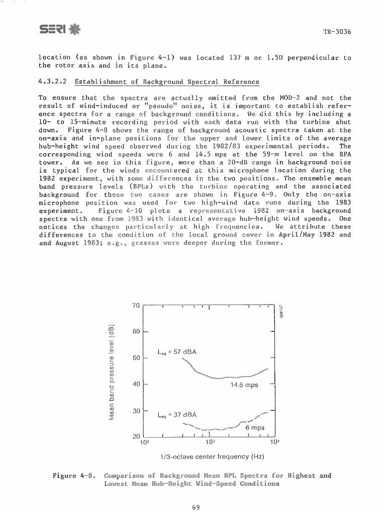
TR-3036

location (as shown in Figure 4-1) was located 137 m or 1.SD perpendicular to the rotor axis and in its plane.

4 .. 3.2 .. 2 Establi ----------------------~------~------------------

To ensure that the are actually emi tted from the MOD-2 and not the result of wind-induced or "pseudo" noise, it is important to establish refer-ence spectra for a range of conditions. We did this by including a 10- to IS-minute recording wi th each data run wi th the turbine shut down.. Figure 4-8 shows the range of background acoustic spectra taken at the on-axis and in-plane positions for the upper and lower limits of the average hub-height wind observed the 1982/83 experimental periods. The corresponding wind speeds were 6 and 14 .. 5 mps at the 59-m level on the BPA tower. As we see in this f , more than a 20-dB range in background noise is typical for the winds encountered at this microphone location during the 1982 experiment, with some differences in the two positionse The ensemble mean band pressure level (BPLs) wi th the turbine ing and the associated background for these two cases 4-9 Only the on-axis microphone position wa used for data runs during the 1983 experiment.. Figure 4-10 s a 1982 on-axis background spectra with one from 1983 with identical average wind speeds. One notices the s at hi leSe vIe attribute these differences to the condition in April/May 1982 and and August 1983; e.g.

60

50 Leq = 57 dBA

40 14.5 mps

30 Leq = 37 dBA

20 ~--~,~~~~~~~~~~~~~ 102 103 104

1/3-octave center frequency (Hz)

69

t­eo eo o o

and

TR-3036

70 (J) co c;; 0 0

.......... CO 60 '"0 - Turbine operating Q) > Leq = 60 dBA ~ 50 (]) lo...

:J C/) C/) (]) lo... 40 a.

'"0 c ccs .c c 30 Background ccs (])

Leq = 34 dBA ~

20 ",,""

102 103 104

1/3-octave center frequency (Hz)

(b) lowest wind speed observation (6 mps)

Figure 4-9. Comparisons of Observed Mean SPL Spectra for Operating and Background Conditions in High (a) and Low (b) Winds

70

TR-3036

70 0 CJ)

;;; 0 0

(l) "0 60 .........

ID > ~ (!) 50 I-

::l. CI) CI) (!) I-

Cl. 40 "0 c: G:S .0

1982 c: 30 G:S (!) 1983 ~

20102 103 104

V3-octave center frequency (Hz)

403 203 Rotor Inflow Influence on Distribution

In Section 40301 the on the mean wind speed was discussed One would a similar relationship to exist with the 1/3-octave spectral , since the A-weighted <Leq> value is a summation of these bands. 4-11 ots the ensemble-averaged 1/3-octave BPLs from the on-axis and in-plane positions for seven mean wind speeds from the 1982 experiment. The wind-speed dependency is less clear in the on-axis spectra than the in-plane. Also, the high-frequency level (above the 2500-Hz band) of the on-axis spectra rises because the local background noise exceeds the tur­bine radiation level. A comparison is made between two 1983 data runs and three runs from 1982 at similar wind speeds in Figure 4-12. We see that the turbine emission levels were 2-3 dB higher in the 630- to SOOO-Hz bands in 1983 for a mean=wind=speed range of 12-13 mps

We attempted, as in the case of the <L q(A» values, to determine if other in­flow parameters such as the rotor s~ vertical stability (and therefore the turbulence structure) had any influence on the MOD-2 mean and temporal charac­teristics of the HF acoustic spectral content. Unfortunately, the bulk of the data available was from the 1982 experiment, when we had only a minimal description of the inflow turbulenceo

We first examined data runs in which the mean hub-height wind speeds were similar but the stability (turbulence characteristics) varied. Using Table 4-1 as a guide, we chose to compare 1982 Runs 19-1, 17-2, and 26-10 These three runs involved mean wind speeds of 10.3, 11.7, and 1200 mps and

71

TR-3036

60 , ..........

co "0 - 55 Q) > ~ 0)

50 lo-

::::l Cf) Cf) 0) lo-

0. 45 "0

C ro ..c c ro 40

,0)

:2:

35 102

Leq

---. co "0 '-'"

0)

> 0)

0) lo-

::::l Cf) Cf) 0) lo-

0.

"0 C ro ..c c ro 0)

:2:

Run 21-1

50

45

40

35

Run 23-1

UhUb = 6.3 mps

Ri. = +24

--- On-axis = 60 dBA

- -- In-plane

30 ~--~--~~~~--~--~~~ 102 103 104

1/3-octave center frequency (Hz)

Leq = 61 dBA

" Run 19-1

Leq = 63 dBA

)I -...... .".-""', \ \ \ \

'\

" UhUb 9.3 mps ........ Uhub = 10.3 mps Ri. = +0.18

.....

Ri. = +0.46

103 104 102 103 104

1/3-octave center frequency (Hz) 1/3-octave center frequency (Hz)

Figure 4-11. 1982 HF-Range Acoustic Spectral Distribution for On-Axis (solid) and In-Plane (dashed) Locations as a Function of Wind Speed and Stability

72

0; co o o

Q)

> .S!2 Q) b

::l en en Q) b

0..

"0 C ct1 .c c ct1 Q)

:2

60

55

50

45

40

35

Leq = 63 dBA

Run 17-1

Uhub = 11.7 mps

Ri = -0.01

Leq 63 dBA

Run 26-1

Uhub = 12.0 mps Ri =+0.13

TR-3036

N en ro o o

102 103 104 102 103 104

1/3-octave center frequency (Hz)

55

50'

45

40

35 102

4~'11

Leq 64 dBA

Run 27 Uhub = 13.3 mps Ri = +0.42

103 104

1/3-octave center frequency (Hz)

1982 Acoustic (solid) and In-Plane ( Wind and Stabil

73

1/3-octave center frequency (Hz)

Leq = 64 dBA

Run 25-1 Uhub 14.5 mps Ri = -0.92

102 103 104

1/3-octave center frequency (Hz)

Distribution for On-Axis Locations as a Function of

(concluded)

---. III "'C ..........

Q) > ~ Q) I-

:::J (J) (J) Q) I-

0.. "'C c:: ro ..c c:: ro Q)

~

..-III "'C ..........

Q) > Q)

Q) lo....

:::J (J) (J) Q) lo....

0.. "'C c:: ro ..c c:: ro Q)

~

60 1982 ---

C') 0>

00 0

UhUb = 12.0 mps 0

55 Ri = +0.13 = 61 dBA

-"" \ 50 ,,"""\

"- ... .... ..... " " 1983 '\

45 --- \ Uhub = 12.7 mps

\ \ \ Ri = +1.26

'\ 40 Leq = 64 dBA , .... _ .....

35 102 103 104

1/3-octave center frequency (Hz)

60~---~--~~----------~--rl~

55

50

45

40

1982--­

Uhub = 13.3 mps Ri -= +0.42 Leq = 63 dBA

1983 -­

Uhub = 13.3 mps Ri = +6.68 Leq = 63 dBA

1/3-octave center frequency (Hz)

Figure 4-12. Comparison of the On-Axis Component of the HF Spectral Distribution between 1982 and 1983 under High Loading Conditions

74

TR-3036

TR-3036

Richardson numbers of 0 18, -0,,01, and 0.13, respectively" This range of Richardson numbers indicates a neutral to slightly stable surface layer which would be dominated by slightly buoyancy-damped, mechanically {shear} generated turbulence" Figure 4-13 presents the ensemble-averaged mean BPL spectra for the on-axis and in-plane measurement stations for these runse On the whole, these mean spectra show remarkably little run-to-run variation. The exception is the on-axis station of runs 17-2 and 19-1, where less acoustic energy is present in the bands of run 17-2 even though this run has the higher vllnd speed of the two. The ion of the 1/3-octave BPLs 1S as plots of the ensemble 1%, 5%, 10%, 20%, and 50% BPL exceedence, or <L20>, and <L50> level s in Figure 4-14" These levels represent of time the randomly sampled BPL equaled or exceeded that f For example, a 1000-Hz, 1/3-octave BPL <L20> of 55 dB means that 20% of the samples contained levels of 5S dB or more. The only obvious difference is the on-axis or 1% exceedence level, which is

in the 2500-Hz band with the others

Runs 19-1 and 1-1 res ively), but opposed to 0 18 The

60

<D 55 > ~ <D

50 ~

::J (J) (J)

<D ~

45 Cl.

u c co .c = 10.3mps c co (l)

::2:

1nce ffered the latter was more

BPLs plott 1n

Run 17-2 Run 26-1

vs. 9.3, ie, 0 46 as

4-15 and the

'3; 00 o o

UhUb ::: 11.7 mps Uhub = 12.0 mps

Ri = -0.01

104 103 104

1/3-octave center

75

Ri =+0.13

103

\ '\

104

) OF Inflow

en (J) > (J)

(J) u c (J)

"0 (J) (J) u x w

en (J)

> (J)

::::J (J) u c (J)

"0 (J) (J) u x w

(f)

(i) > (J)

::::J (J) u c (J)

"0 (J) (J) ()

x W

60

55

50

45

40

-"" \ \.-,

" UhUb = 11.7 mps ''- ........ Ri. = -0.01 ", L(1) = 0 L(s) = t::..

L(10) = 0

L(20) = • L(so) = dashed line

On-axis

,

35 l..----IL--..L-L-L...L..L--L_---'---'---I-..L...I.....L..II....II

60

55

50

45

40

35

60

55

50

45

40

1 02 1 03 1 04 1 02

102

L(1) = 0 L(s) = t::..

L(10) = 0

L(20) = • L(so) = dashed line

103

Uhub = 12.0 mps Ri.=+0.13 L(1) = 0 L(s) = t::..

L(10) = 0

L(20) = • L(so) = dashed line

(a)

On-axis

104 102

(b)

On-axis

102

103

103

\ \ \ \ \ \ \

103

\ ~ \ \

TR-3036

In-plane

104

In-plane

104

In-plane

104

(c) 1/3-octave center frequency (Hz) 1/3-octave center frequency (Hz)

Figure 4-14. Comparison of L1 , LS' L10 , LZO ' and LSO 1/3-octave Level Spectra at 1.5D at the On-Ax1S and In-Plane Measurement Locations for 1982 Runs: (a) 17-2; (b) 19-1; and (c) 26-1

76

l{) (J)

co o o

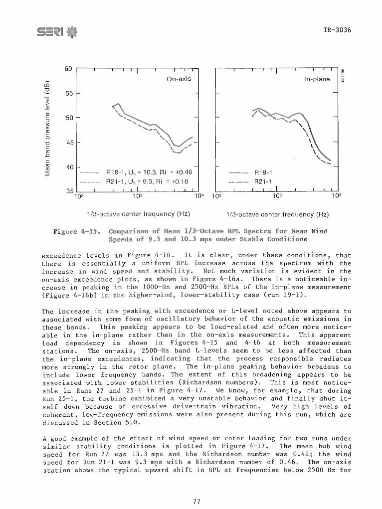
Q) > (J)

60

55

~ 50 ::l en en (J) b

a. "0 45 c (1j .D C (1j (J)

:2: 40

On-axis

R19-1, Uh = 10.3, Ri

1/3-octave center frequency (Hz)

4-15" of 9 3

1 10

TR-3036

R19-1 R21-1

103

In-plane

1/3-octave center frequency (Hz)

104

<0 (J)

0; o o

exceedence levels 4-160 It is clear, under these conditions, that there 1S essent uniform BPL across the spectrum with the increase in wind and stabili Not much variation is evident in the on-axis exceedence plots, as shown in 4-16a0 There is a noticeable in-crease in peaking in the IOOO-Hz and 2500-Hz BPLs of the in-plane measurement (Figure 4-16b) in the , lower-stability case (run 19-1)0

The increase in the peaking with exceedence or L-level noted above appears to associated with some form of oscillatory behavior of the acoustic emissions in these bands This peaking appears to be load-related and often more notice­able in the in-plane rather than in the on-axis measurements@ This apparent load dependency is shown in Figures 4-15 and 4-16 at both measurement stations. The on-axis, 2500-Hz band L-levels seem to be less affected than the in-plane exceedences, indicating that the process responsible radiates more strongly in the rotor plane. The in-plane peaking behavior broadens to include lower frequency bands @ The extent of this broadening appears to be associated with lower stabilities (Richardson numbers)e This is most notice­able in Runs 27 and 25-1 in Figure 4-170 We know, for example, that during Run 25-1, the turbine exhibited a very unstable behavior and finally shut it­sel f down because of exces s i ve dri ve-t rain vi brat ion Very high level s of coherent, low-frequency emissions were also present during this run, which are discussed in Section 5 0

A good example of the effect of wind speed or rotor loading for two runs under similar stability conditions is plotted in Figure 4-17.. The mean hub wind speed for Run 27 was 13 .. 3 mps and the Richardson number was 0 .. 42; the wind speed for Run 21-1 was 903 mps with a Richardson number of 0,,46. The on-axis station shows the typical upward shift in BPL at frequencies below 2500 Hz for

77

60 r

co 55 "0 ......... (/)

Q) > (])

(]) u c (])

"0 (]) (]) u >< w

50

45

40

UhUb == 10.3 mps Ri.=+0.18 L(1) 0 L(5) =!::::.

L(10) = 0

L(20) = .,

L(50) = dashed line

On-axis

Run 19-1

'--

35~--~~~~ww~------~~~~~u

102

60

..--... co 55 "0

(/)

(])

> (]) 50 ::J (]) u c 45 (])

"'0 (]) (]) u >< 40 w

103 104 102

1/3-octave center frequency (Hz)

/-, / '-, ,-­

'--;' \

Uhub = 10.3 mps Ri.=+0.18 L(1) = 0 L(5) =!::::..

L(10) = 0

L(20) = • L(50) = dashed line

\

Run 19-1

\ \ \

\ \

\ "-"

(a)

In-plane

Uhub = 9.3 mps Ri. = +0.46

103

TR-3036

Run 21-1

104

1/3-octave center frequencX' (Hz)

UhUb = 9.3 mps Ri. = +0.46

Run 21-1

t--­

'" 00 o o

co

'" 00 o o

102 103 104

1 /3-octave center freq uency (Hz) 1/3-octave center frequency (Hz)

(b)

Figure 4-16. Comparison of L1 , LS' LID' LZD ' and LSD 1/3-octave Level Spectra at I.SD at the On-Ax1S (a) and In-Plane (b) Measurement Stations

78

----co ~ 55 (j) > (j)

(j) I-

::::l C/) C/) (j) I-Q.

50

45

40

On-axis

Uh = 13.3 mps, Ri = +0.42 ~ R21-1, Uh ::: 9.3 ::: +0.46

35102 103 104 102

1/3-octave center (Hz)

4-11"

TR-3036

In-plane

103 104

1/3-octave center frequency (Hz)

and

the wind speed, but above that frequency band the levels become similar. There is a more or less uniform upward BPL shift in the rotor plane, except for the peaking or in the 1600 to 4000-Hz bands in the run with the higher rotor This difference is clearer in the peak BPL plots of Figure 4-18 To whether this fluctuating or as illatory condition is related to the inflow li, we looked at two high-wind runs (Run 25-1 at 1405 mps and Run 27 at 1303 mps) with Richardson numbers of -0 .. 92 and o 42 e The mean BPL spectra assoc wi th these two cases were plotted in Figure 4-190 While both the on-axis and in-plane mean BPL spectra are very similar, the peak BPLs shown in Figure 4-20 for each are quite different in the 2500-Hz region The unstable case shows a greater tendency for peaking in the on-axis measurement (Figure 4-20a), and while the more stable one has the same tendency in the rotor plane measurement (Figure 4-20b)@ While it appears that rotor loading is the major factor determining whether or not high­frequency oscillatory behavior will occur, the stability (and therefore the turbulence structure) seems to influence the directivity of the acoustic radi­ation. We did not experience the degree of turbine operational instability under the stable atmospheric conditions of Run 27 that we observed during Run 25-1 e

We attempted to compare the two available data runs of on-axis measurements taken in 1983 (with the modified turbine) with 1982 runs made under conditions as similar as possible. Run 27 (1982) and Run 11 (1983) had the same mean hub-height wind s (mean rotor loading), but in the latter inflow was much more stable; ieee, 0042 in 1982 and 6068 in 19830 The closest corresponding 1982 run to 1983 i S Run 18 was Run 26-1 e Run 26-1 had a mean wind speed of 12 mps and a Richardson number of 0 e 13, compared wi th 1207 mps and 1 e 26, respectively, for Run 18 Figures 4-21 and 4-22 plot the ensemble mean BPL and spectra for these two caseso The mean and <L20> BPL spectra of

79

60

co 55 "'0

(/)

(!)

> ~ 50 :J (!) ()

45 c (!)

"'0 (!) (!) ()

>< 40 w

Uhub = 13.3 mps Ri = +0.42 L(1) =0 L(5) = b.

L(10) = 0

L(20) = • L(50) = dashed line

On-axis

Run 27

UhUb = 9.3 mps Ri = +0.46

TR-3036

Run21-1

o o N co o o

102 103 104

co "'0

(/)

(!) > (!)

....J

(!) ()

c (!)

"'0 (!) (!) ()

>< w

60

55

50

45

40

1/3-octave center frequency (Hz)

Uhub = 13.3 mps Ri = +0.42 L(1) =0 L(5) = b.

L(10) =0

L(20) = • L(50) = dashed line

Run 27

1/3-octave center frequency (Hz)

(a)

In-plane

102

(b)

1/3-octave center frequency (Hz)

Uhub = 9.3 mps Ri +0.46

103

Run21-1

1/3-octave center frequency (Hz)

104

Figure 4-18. Comparison of L1 , LS ' L10 , L20 , and LSO 1/3-0ctave Level Spectra for High and Moderate Wind Speeds under Stable Inflow Conditions. On-axis measurements are shown in (a) and in­plane measurements in (b).

80

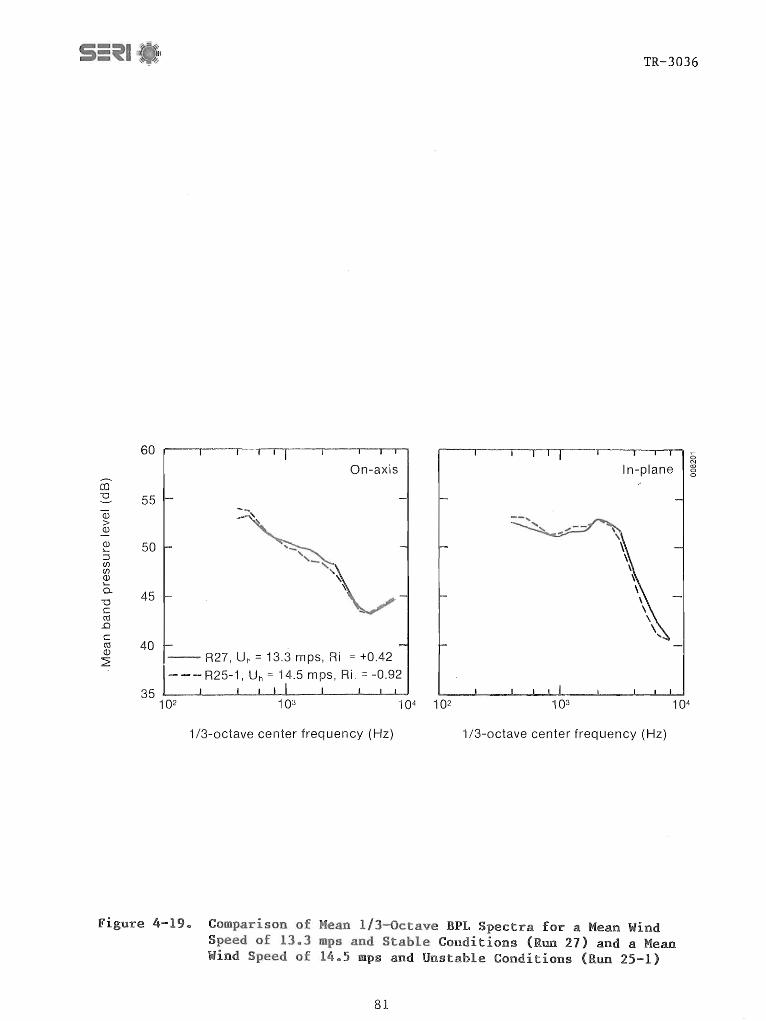
(l)

> (l)

(l) ~

::J (f) (f)

~ 0-

-0 C CI:l

..0 c CI:l (l)

~

On-axis

55

50

45

TR-3036

In-plane ;; N 00 o o

35 L-__ L-__ ~-L-LL-__ ~ __ ~~~

102 103 1 04 102 103 104

1/3-octave center frequency (Hz) 1/3-octave center frequency (Hz)

Mean 1 for a Mean Wind mps and Stable (Run 21) and a Mean

Wind of 14@5 mps and Unstable Conditions (Run 25-1)

81

CI)

(!)

> (!)

(!) () c (!)

"'0 (!) (!) ()

>< w

a:.l "'0 --CI)

(!)

> (!)

::J (!) () c (!)

"'0 (!) (!) ()

>< w

60

55

50

45

40

35 102

60

55

50

45

40

TR-3036

On-axis N o N co o

Uhub = 13.3 mps Ri = +0.42 L(1) =0 L(5) = b.

L(10) = 0

L(20) = • L(50) = dashed line

Run 27

1/3-octave center frequency (Hz)

(a)

In-plane

Run 27

Uhub = 13.3 mps Ri = +0.42 L(1) =0 L(5) = 1:!.

L(10) = 0

L(20) = • L(50) = dashed line

1/3-octave center frequency (Hz)

(b)

102

UhUb = 14.3 mps Ri = -0.92

103

Run 25-1

1/3-octave center frequency (Hz)

104

Run 25-1

Uhub = 14.5 mps Ri = -0.92

102 103

1/3-octave center frequency (Hz)

o

Figure 4-20 .. Comparison of Ll , LS' LlO ' L20 , and LSO 1/3-0ctave Level Spectra for High-Wind, Stable vs. High-Wind, Unstable Inflow Conditions. On-axis measurements are shown in (a) and in­plane measurements in (b).

82

o N

...J

60

50

40

30

1/3-octave center frequency (Hz)

mean BPL

-- R27 (1982), Uh = 13.3 mps, Ri. = +0.42

A 11 (1983), Uh = 13.3 mps, Ri = +6.68

20b---~--~--~~~--~--~--~~

102 103 104

1/3-octave center frequency (Hz)

BPL

4-21., Mean and BPL for 1982 Run R21 and 1983 Run A-II

83

TR-3036

60 LO 0

~ 0 0

...-co 55 u '-" -- ..... Q) ........... > '-., ~ Q) 50

, l>-

, :J , (J) (J) Q)

\ l>-

Cl. 45 \

u \ c: \ ctl

..0 \ c: \ ctl 40 \ Q)

~ \ \-

35 102 103 104

1/3-octave center frequency (Hz)

(a) mean 1/3-octave BPL spectra

60 <0 0 N co 0 0

...-.. 55 --CO ..... .... U ...... _"'"'\ ......... Q) \

\ > \ ~ 50 \ Q) l>-

\ :J (J)

A26-1 (1982), \ (J)

\ Q)

45 Uh = 12.0 mps, , l>-

Cl. \ u Ri = +0.13 \ c:

\ ctl ---- A18 (1983), \ ..0 \ 0 40 Uh = 12.4 mps, N ,

-' Ri +1.25 '-

35L---~---L~~~--~--~--~~

102 103 104

1/3-octave center frequency (Hz)

(b) L20 BPL spectra

Figure 4-22. Mean and L20 BPL Spectra for 1982 Run 26-1 and 1983 Run A18

84

TR-3036

Figure 4-21 show excellent agreement for the bands below 1600 Hz for the two years under the same mean loading conditions. Figure 4-22 shows the expected higher mean and <L28> levels for the 1983 run (since it has a higher wind speed) below the 160 Hz band. What is different is the sharp spectral cutoff above the l600-Hz band in both 1983 runSe There does seem to be a hint of the oscillatory peaking seen in the data for the 1982 higher wind-speed run, par­ticularly for run 11, as shown in the L-Ievel summaries of Figures 4-24 and 4-25.. In the 1983 runs, there appears to have been a downward shift in the frequency band, in which the peaking occurs, from 2500 Hz in 1982 to 1000 Hz in 1983 ..

4 .. 4

Averaged narrowband (25-Hz resolution) spectra were computed over a frequency range of 100 to 10,000 Hz for a 2-minute period located midway in each data run listed in Table 4-1 The purpose was to locate and identify the possible source(s) of any discrete tonal components found in the MOD-2 emissions .. Figures 4-26, 4-27, and 4-28 present a sample of the resulting narrowband on­axis and in-plane spectra for Runs 23-1, 17-2, and 25-1 from the 1982 experi­ment (1mfl, moderate, and high wind regimes). Figures 4-29 and 4-30 present the on-axis spectra from 1983 runs 11 and 18 in moderate to high winds. No significant, steady tone noise components were found This indicates that the mechanical noise sources associated with the drive train are well controlled, and there appear to be no discrete aeroacoustic sources of consequences

70 t-o N co

1983 RunA18 0

1983 Run A11 0

en Uhub = 13.3 mps Uhub = 12.7 mps u 60 m > ~ Q) 50 l...

Turbine Turbine ::l en en Q) l...

40 a.. "0 c co ..0 c 30 Background co Background Q)

:2: 20

102 103 104 102 103 104

1/3-octave center frequency (Hz) 1/3-octave center frequency (Hz)

4-23 Lom~lat~lson of Acoustic at I. Measurement Location with and without

under Wind

85

60

-III 55 "'0

CJ)

Q) > Q) 50 :::J Q) ()

~ 45 "'0 Q) Q) ()

~ 40

UhUb = 13.3 mps Ri = +0.42 L(1) = 0 L(5) = 0

L(10) = b..

L(20) = • L(50) = dashed line

1982 Run 27

35~--~~~~~~~--~~~~~~

102 103

1/3-octave center frequency (Hz)

102

UhUb = 13.3 mps Ri = +6.68

103

TR-3036

1983 Run A11

104

1/3-octave center frequency (Hz)

Figure 4-24. Comparison of Ll , L5 , LIO ' L20 , and L50 On-Axis 1/3-0ctave Level Spectra for Ident1cal Mean Wind Conditions during 1982 and 1983 Experiments

60

EO 55 "'0

CJ)

Q)

~ 50

Q)

g 45 Q) "'0 Q) Q) ()

~ 40

Uhub = 12.0 mps Ri=+0.13 L(1) = 0 L(5) = 0

L(10) = b.

L(20) =. L(50) = dashed line

1982 Run 26-1

1/3-octave center frequency (Hz)

102

Uhub = 12.7 mps Ri = +1.26

103

1983 Run A18

1/3-octave center frequency (Hz)

O"l o N co o o

104

Figure 4-25. Comparison of Ll , L5, LI0 , L20 , and L50 On-Axis 1/3-0ctave Level Spectra for S1milar Wind Speed Regimes in 1982 and 1983

86

co o ~ o o

4-26 ..

4-27

TR-3036

10 ~ ____ ~ ____ ~ __ -L __ L-~ ____ -L ______ ~ __ ~~~

102 103 104

Frequency (Hz)

Narrowband = 12 .. 5 Hz)

50

40

30

20

1982 Run 17-2 Uhub = 11.7 mps Ri = -0.01

On-axis

Background

10L-----~-----L---~~~L-----~-----L--~~~

102 103 104

Frequency (Hz)

1982 Narrowband Wind Conditions

87

for Moderate

<l)

> <l)

60 r-----.------.--.--.-.----__ ~----~--~~ N

N co o o

50

40

30

20

10 102

1982 Run 25-1 Uhub = 14.5 mps Ri = -0.92

On-axis

103

Frequency (Hz)

Background

104

TR-3036

Figure 4-288 Representative 1982 HF-Range Narrowband Spectra for Above­Rated, Unstable Inflow Conditions

<l)

> <l)

<l) l....

::l (/) (/) <l) l....

0..

"0 C a:l OJ

60

50

40

30

20

1983 Run A 11 Uhub = 13.3 mps Ri = +6.68

Background source

\

10L-----~----~--~--~~----~------~--~~~

102 103 104

Frequency (Hz)

(")

N co o o

Figure 4-298 1983 On-Axis HF-Range Narrowband Spectra for Above-Rated, Stable Inflow Conditions

88

60

50

co "0

Q)

> 40 ~ Q) ~

::J (f) (f) Q)

30 ~

CL

"0 C co 1983 Run A18 co

20 Uhub = 12.7 mps Ri = +1.26

10 102

Figure 4-30. 1983 On-Axis Stable Inflow

103

Frequency (Hz)

89

TR-3036

'<t

N co 0 0

source

\

104

for Near-Rated.,

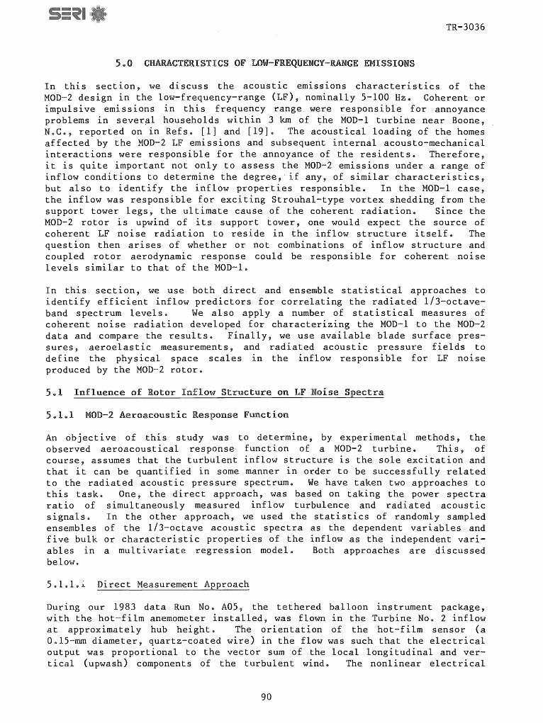
TR-3036

5eO CHARACTERISTICS OF LOW-FREQUENCY-RANGE EMISSIONS

In this section, we discuss the acoustic emissions characteristics of the MOD-2 design in the low-frequency-range (LF), nominally S-lOO Hz. Coherent or impulsive emissions in this frequency range were responsible for annoyance problems in sever~l households within 3 km of ~he MOD-l turbine near Boone, N.C., reported on in Refs. [1] and [19]. The acoustical loading of the homes affected by the MOD-2 LF emissions and subsequent internal acousto-mechanical interactions were responsible for the annoyance of the residents. Therefore, it is quite important not only to assess the MOD-2 emissions under a range of inflow conditions to determine the degree, if any, of similar characteristics, but also to identify the inflow properties responsible" In the MOD-l case, the inflow was responsible for exciting Strouhal-type vortex shedding from the support tower legs, the ultimate cause of the coherent radiation. Since the MOD-2 rotor is upwind of its support tower, one would expect the source of coherent LF noise radiation to reside in the inflow structure itself. The question then arises of whether or not combinations of inflow structure and coupled rotor aerodynamic response could be responsible for coherent noise levels similar to that of the MOD-l.

In this section, we use both direct and ensemble statistical approaches to identify efficient inflow predictors for correlating the radiated 1/3-octave­band spectrum levels. We also apply a number of statistical measures of coherent noise radiation developed for characterizing the MOD-l to the MOD-2 data and compare the results. Finally, we use available blade surface pres­sures, aeroelastic measurements, and radiated acoustic pressure fields to define the physical space scales ln the inflow responsible for LF noise produced by the MOD-2 rotor.

5.1 Influence of Rotor Inflow Structure on LF Noise Spectra

5.1.1 MOD-2 Aeroacoustic Response Function

An objective of this study was to determine, by experimental methods, the observed aeroacoustical response function of a MOD-2 turbine. This, of course, assumes that the turbulent inflow structure is the sole excitation and that it can be quantified in some manner in order to be successfully related to the radiated acoustic pressure spectrum. We have taken two approaches to this task. One, the direct approach, was based on taking the power spectra ratio of simultaneously measured inflow turbulence and radiated acoustic signals. In the other approach, we used the statistics of randomly sampled ensembles of the 1/3-octave acoustic spectra as the dependent variables and five bulk or characteristic properties of the inflow as the independent vari­ables ln a multivariate regression model" Both approaches are discussed below.

S.l.l.i Direct Measurement Approach

During our 1983 data Run No. AOS, the tethered balloon ins trument package, with the hot-film anemometer installed, was flown in the Turbine No. 2 inflow at approximately hub height.. The orientation of the hot-film sensor (a O.lS-mm diameter, quartz-coated wire) in the flow was such that the electrical output was proportional to the vector sum of the local longitudinal and ver­tical (upwash) components of the turbulent wind. The nonlinear electrical

90

TR-3036

signal was transmitted via a digital FM radio telemetry link to a ground receiver, where the signal was re-converted to an analog voltage, linearized, and recorded on FM magnetic tape. The dynamic range of the radio telemetry link was better than 70 dB with a data bandwidth of 125 Hz. The bandwidth of the final FM tape recording was limited to 100 Hz, however.

Because of the nonstationary nature of the inflow, the 3D-minute data run was divided into six 5-minute segments. The particular 5-minute period discussed here was chosen because it exhibi ted minimal variation in height of the anemometer (a standard deviation of ±6 m) and contained substantial levels of high-frequency turbulence. Table 5-1 summarizes the pertinent operational and inflow characteristics associated with this run segment.

We chose a vertical window of ±10 m from the mean hot-film anemometer height as the region of the rotor disk from which we would correlate the acoustic output at the 1.5D measuring station" This choice resulted in defining the two disk segments pictured in Figure 5-1 By delaying the data conversion and Fourier transformation a fixed amount from the time the rotor blade was par­allel to the tower base, we could start the Oe5-second conversion period to coincide vlith the windows shown in Figure 5-1" The inflow turbulence signal was delayed in time equivalent the mean convection speed, 7 .. 4 mps. The acoustic spectra were delayed an additional O.S-second with respect to the turbulence signal to allow for the sound propagation (retarded) time from the disk segment to the microphone array. The resulting averaged spectra were calculated from ten 4-second records containing 80 blade passages and 81,920 data points.

The measured LF acoustic response (spectral ratio) in Pa/mps is plotted in Figure 5-2 over a frequency range of 2-100 Hz with an effective bandwidth (resolution) of 2 Hz.. The abscissa has also been scaled in units of the reduced frequency parameter k def ined by k:= ncf /U, where cis the chord length and U the relative blade speed at 80% span. An interesting result is achieved if the response spectrum of Figure 5-2 is plotted against the turbulent wavelength (assuming the frozen turbulence hypothesis) as ln Figure 5-3, in which the location of the integral scale is also shown. Since one interpretation of the integral scale is that it represents the largest

Table 5-1 .. Turbulence Excitation and Turbine Operation for the of Run A05

Turbulent Layer Structure Parameters

Mean measurement height (above the tower base) Mean horizontal wind speed Turbulence intensity Layer turbulence integral scale length

Turbine Operating Angles

Indicated mean blade angle (ref at StaG 1260) Calculated mean angle of attack (Sta .. 1164) Calculated mean angle of attack (Sta. 1562)

91

78 ±6 m 7.39 mps 8.0% 2 .. 89 m

TR-3036

Measurements taken in these sectors

l' / I" {. \ / I '" ,/ \ \ --I " ,/ ~ I ,--__ __----, \

~ Blade sta. 116:5%)~ Blade sta. 1562 (87%)

Facing downwind

Figure 5-1. Relationship of Location of Measurements on Blade No.1, Rotor Disk Geometry, and Height of Elevated Turbulent Layer

c o t) C :J

"4-

~ 10-1 C o Q. CJ)

9:_ .~ in (j) E :J ____ 10-2

o C\l uCL C\l ...........

>­U C Q)

5- 10-3

Q) lo­

"4-

~ o ~

<D

N 00 o o

10-4 ~----~----~--~ __ ~~ ____ ~ ______ ~ __ L--L~

100 (10- 1) 101 (100 )

Frequency (Hz)

102 (10 1 ) (k)

Figure 5-2. Measured Low-Frequency Acoustic Response Function

92

l{)

N 00 o o

c o +"' () C :J -

10 8 I'­

N - co o

o

TR-3036

CG 10-1

u; C C'Cl l­+-'

5-3

Correlated turbulent eddies

10-4 ~ __ -L ____ ~-L_~J-~~ ____ ~~~~ ____ ~ __ -L~~~

10-1

Measured Turbulent

10 0 101

Turbulent wavelength (chords)

Acoustic

102

as Function of

correlated eddy size in the flow, it is clear from Figure 5-3 that the characteristics of the radiated spectrum appear to change at that boundary.

Parameter tivariate Hodel

As explained in Section 204, ensemble statistics (up through and including the 4th moments) of the LF emissions spectra in 1/3- and octave-band resolution listed in Table 2-2 were compiled from 100 random samples of the MOD-2 far­field acoustic signals for each of the three, 10-minute segments of each data rune The resulting statistics were then averaged together to form the aggregate statistical record for the run.. A similar approach was used for background measurements, but it was only 10 minutes in length and no averaging was necessarYe Measures of the inflow bulk or characteristic scaling parameters (e.g@, a reference-height mean horizontal wind speed UH, the rotor disk gradient Richardson number Ri, and various turbulence length scales measured at a reference height) were compiled as discussed in Section 2.4.2.

ficance of Observed Run-to-Run lons

Before attempting to correlate the observed run-to-run variations ln the measured far-field acoustic emissions spectral statistics with inflow characteristics, we compared the observed variations to what would be expected for completely random fluctuations Figures 5-4a, b, c, and d plot the observed run-to-run variations for the 1/-3 octave band means and variance, skewness, and kurtosis coefficientsa Also included in these figures are the variations which would be expected from a purely random noise process at the

93

14.0 CO ~

.§ 12.0

..., (1j .;:: ~ 10.0

V :> (])

...:l 8.0

S ;:J s... ...,

6.0 () (])

0... (f)

'"d 4.0 1=1 (1j

iIl

1=1 (1j 2.0 (])

:::::1

0.0

10 1=1

:§ (1j .;:: (1j

:>

~ (])

~ (]) 0

U

Ul rn Jl)

1=1 ;;: Q)

.!:<l (f)

v :> (])

...:l

'"(j

1=1 (1j

iIl

10 -1

1

\ \

-- ....

mbsl-rangQ-comp

observed variation range

co N co g

expected range (99%-level)

I I

k=1

- ....

- - -- ......... "

I I " I I I I I II i 10 10 2

1/3-0ctave Center Frequency (Hz)

(a) mean BSL comparison

i III

10 J

bl-BI:QW-rangQ-C017\p

0

observed variation range gJ gs 0

expected range (99%-level)

_J I I I I I I I

I I

\ I

" k=1

10 10 2 10 J

1/3-0ctave Center Frequency (Hz)

1=1 o

:;:::;

0.30

.~ 0.25 (1j :> ...,

1=1 (])

~ 0.20

(])

o u (]) 0.15 (.)

1=1 (1j .;:: ~ 0.10

V :> (])

...:l '"d 0.05

1=1 (1j

iIl k=1

\ ,. '" \

\ \ \ \

\ \

TR-3036

bl-covaT-Tangfl-C0771P

observed variation range

expected range (99%-level)

\ ,-

'- -"- ""

(J)

N co g

10 10 2

1/3-0ctave Center Frequency (Hz) 10 J

(b) variance coefficient comparison

10 2

1=1 .8 ..., (1j .;:: (1j :> ...,

1=1 (]) 10 'u S Jl)

0 U

.~ rn 0 ..., s... ;:J

:::.:::

v :> (])

...:l

'"d s:l (1j

iIl

10 -1

1

bl-kurf-rang8-comp

observed variation range

expected range (99% -level)

k=1

10 10 2

1/3-0ctave Center Frequency (Hz)

N N

~ o

10 J

(c) skewness coefficient comparison (d) kurtosis coefficient comparison

Figure 5-4 .. Comparisons of the Observed Run-to-Run Variations of the BSL Mean and First Three Statistical Moments and the Variations Expected from a Purely Random Process.

94

TR-3036

99% confidence level. These plots show that significant run-to-run variations did occur in the four statistical moment distributions. The k = 1 line, shown in these figures, represents the acoustic (cyclic) frequency corresponding to an aerodynamic reduced frequency, k, of unity where k = n Iv (c is the chord length and Vc the convection velocity at an effective span~is~ radius of 75%.

Choos Multivariate tic Inflow Predictors

In the specification of a multivariate regression model, one strives to choose independent variable predictors. While being sensitive to the predicted quan­tity, these variables are uncorrelated with one another; i.e., to minimize the degree of multicollinearity presente Unfortunately, in dealing with atmo­spheric inflow variables, this is often an impossible task. Under homogeneous flow conditions, the Monin-Obukov similarity theory gives us an independent set of turbulence predictors. However, for inhomogeneous flows, like those at the Goodnoe Hills site, the degree of collinearity between predictor variables can be minimized but not eliminated entirely.

Ideally, we would like to arrive at a set of independent variables which would adequately describe the inflow state in order to predict the ensemble statis­tical behavior of the observed spectral characteristics of the far-field acoustic emissions. We know from the work of Homicz and George (see Section 3.1) that these predictors should be representative of a mean axial convec tion veloci ty, V ') and the accompanying turbulence scales and inten­sities. Coupling thi~ requirement with the influence of surface layer similarity (see Section 3 .. 2), we saw that the hydrodynamic stability has a strong influence on these parameters. Thus, a set of inflow state predictors should include parameters which serve as a representative measure of the

mean inflow velocity; disk layer hydrodynamic stability;

• turbulence intensities; and • characteristic turbulence scales.

From Table 2-5, available measures of mean inflow (axial convection velocity) included observations near the hub-height (59 m) and at the hot-film ane­mometer, located at a 45-m elevation on the BPA Met Tower. The variation of mean wind speed with height was shown in Section 3.2.2. This parameter varys as a function of the surface shear-stress or friction velocity, U~IO and roughness (fetch) or z and stability" Measures of the inflow stability included the disk gradi~nt Richardson number, Ri, the Monin-Obukov length, L, and the z/L parameters. The vertical variation of turbulence intensi ty was shown in Section 3.2.3 It varys as a function of stability, mean wind speed, and U*0 Observations of the amount of small-scale turbulence present at the 45-m height are available as the 1-10 Hz-band mean square values for the longitudinal and vertical components 0 Available characteristic turbulence length scale measures include 45-m elevation observations of

• the I x, I x, and I z integral scales; and u . w . w •

the long1tud1nal and vert1cal reduced frequency spectral peaks, f and f • mu mw

The degree of bivariate correlation for the turbulence intensities and scales versus the representative mean velocity, stability, and roughness parameters are shown in Table 5-20 The cross-correlation matrix for the stability,

95

TR-3036

velocity, and roughness scales is shown in Table 5-3. As is apparent by the content of these tables, there are few inflow characteristic scales which are completely independent of one another, thus, raising the degree of multicol­linearity in multivariate models where they are used as independent variables.

Inflow Stability

Because of the lack of independence in most of the available inflow character­istics scales, we have more thoroughly examined the inter-relationships between these parameters" For example, using one-way analysi s of variance (ANOVA) techniques, we examined the percentage of observed variation in the longitudinal and vertical 45-m level turbulence components (u t

, Wi), explained by a multivariate model consisting of the

Table 5-2" Correlation Coefficients for Inflow Turbulence Scales and Intensities versus Stability, Velocity, and Roughne s s

a I x I x I z f mu f mw

<S >2 <S >2 u w w u w

Stabilitl Ri .332 - .. 277 -,,492 - .. 455 .. 170 - .. 249 -.604 z/L - .. 200 -.848 - .. 932 .132 -,,207 - .. 217 -.791 L -.225 -.248 - .. 134 .. 267 .342 ,,639 .937

Velocitr U45 .586 -.538 - .. 428 -.609 .202 .598 - .. 222 UH .593 -.541 -.365 -.502 .317 .697 -.084 u* .. 562 - .. 263 -0044 -.604 - .. 617 .. 733 .. 269

Roughness Zo .397 - .. 577 -.732 -.648 .116 -.191 - .. 710

a<S > = u,W 1-10 Hz band mean square value.

Table 5-3 .. Cross-Correlation Matrix for Stability, Velocity, and Roughness Predictors

Ri z/L L U45 UH U,t(' Zo

Ri .. 174 -.121 .. 118 - .. 017 .097 .517 z/L .374 .443 .297 .319 .103 .523 L -0121 .443 .. 175 .239 ,,475 .266 U45 .. 118 .297 .175 .981 .. 814 .460 UH -,,017 ,,319 .239 .981 .816 .403 U i ,: ,,097 e103 .475 .814 .816 .576 Zo .517 .523 .266 .. 460 .403 .576

96

100

'"C1 90

OJ .:: '(ij 80

P.. ~

rx:l 70

.:: ,~ 60 ...., ro 'C 50 ro :>-(ti 40 ...., 0

E-< 30 '+-< 0

..., 20 .:: OJ <:.) ... 10 OJ

0...

-10 10 -I

TR-3036

o M-O length scale, L; o disk Brunt-Y~is~l~ period, TBy ; o roughness length, z ; and the o 45-m mean wind spee~, U45 0

Figures 5-5a and b demonstrate that, on average, 90% of the observed spectral varianqe in these turbulence components is related to changes in the inflow stability. We have found that the hydrodynamic stability of the rotor disk layer, as expressed by the Richardson number parameter, strongly varies with the time-of-day at the Goodnoe Hills site. This can be seen for the period of 1600-2400 h local standard time (LST) in Figure 5-6. In the figure, the 30-minute disk Richardson number is plotted for 25 data runs from both the 1982 and 1983 experimental periods. The shift from unstable to stable inflow conditions is seen to take place rather abruptly in the vicinity of 1630 hours" The 1983 data set contained much more stable runs than those of 1982" These runs are ted as a function of time 1n Figure 5-7 with the most stable conditions occurring after 1930 h L8T.

uctnnp-anO'VR we omp-a,,01J a

'" 100 '" ~ 0 0 90

'"C1

~ Q)

.:: 80 '(ij PERCENTAGE OF OBSERVED VARIANCE P.. PERCENTAGE OF OBSERVED VARIANCE

EXPLAINED BY THE: ~ 70 EXPLAINED BY THE: o M-O length scale, L rx:l o M-O length scale, L tJ B-V period, Tbv .:: tJ B-V period, Tbv

Do Roughness length, Zo Do Roughness length, Zo :3 60 <> 45m. mean wind speed, U <> 45m meon wind speed, U

ro .. Unexplained residual .. Unexplained residual 'C 50

(\j :>-(ti 40 ...., 0

E-< 30 '+-< 0

~ 20

~ OJ <:.)

10 H OJ

0...

-10 10 -1 1 10 10 -. 10 -1 1

Cyclic Frequency, f (Hz) Cyclic Frequency, f (Hz)

) vertical or component

Figure 5-5 .. ANOVA Results for the 45-m or In-Plane Turbulence

97

~ '" 00 0 0

10

TR-3036

I ~

17 18 19 20 21 22 23 Local Standard Time (h)

Figure 5-69 Observed Variation of the Disk Gradient Richardson Number

• ..-1

0::

as a Function of the Time-of-Day for the Combined 1982/83 Experimental Periods

12

~~ 10 Q)

..0 El :;j Z 8

J:1 0 rIl

'"d ~ 6 <tl

..cl CJ

• ..-1

0:: -+-' 4 J:1 Q)

• ..-1

'"d <tl ~ 2 d

A ~ 0

-+-' A 0 0 0::

L[)

N N <Xl 0 0

-24-----------.----------,----------~----------r_--------~

14 16 18 20 22 Local Standard Time (Hours)

Figure 5-1. Observed Variation of the Disk Gradient Richardson Number for the Combined 1982/83 Experimental Periods

98

24

24

TR-3036

Influence of Stability on Mean Wind Speed

The change from unstable to stable inflow conditions was found to have a pro­nounc~d effect on the character of the mean wind speed profile. Figure 5-8 plots the combined 1982/83 hub-height mean wind speed values (UH) as a func­tion of the disk, Ri, between -1 and +2. The tendency for a step-up in speed under stable flow conditions is apparent. One reason why there are not many data points in the unstable region is that prior to about 1600 h the winds were generally below the turbine cut-in speed (~ 6 m/s). Figure 5-9 shows the 1982/83 variation of UH with the time span corresponding to our data collec­tion period. While at first glance there appears to be considerable scatter, a closer inspection reveals the tendency for a dual grouping of points into high- and low-speed sets in the stable flow, present after about 1900 h. The least-squares trend line reveals the tendency towards maximum UH values in the vicinity of 2000 h and a trend towards another maximum after 2230 h. The high mean wind point in the unstable region prior to 1630 h was related to a 1982 case in which a passing upper atmosphere disturbance was influencing the normal diurnal wind speed variations

14

'"'d ~ 12 p.. rn

'"'d ~ .,..,.

!3:

~ 10 Q)

:21

I/). il , I

<D C\J C\J co o o

6~--~--~----~--4----r--~----r---~---r--~----r-~

-1.00 -0.50 0.00 0.50 1.00 Disk Gradient Richardson Number,

5-8.. Observed Mean Hub-Height Wind Speed as a

99

Richardson Number for the Periods

-rn

14

"-.. 13 S ..........

'"d ~ 12 0.. rn

] 11

~

~ 10 Q)

::2l +J

9 ..d I:l.O

• ..-! Q)

tt:: I 8

..a ::J

::r: 7

6 15

\ \ \0 \ \ \ \ \

\ "-

D

unstable

16 17

Ri=O I I

10

I -1/

I 01

o

1:1

/

o

/ /

/ /

/

0

o

o o 0

o

...... ""'-

0

0 0

stable

o

~ , \

\ 0

0

18 19 20 21

\

Local Standard Time (h)

TR-3036

o

o

o

o

I \ I ,

/ .......

o

o

22 23

Figure 5-9. Observed of the Mean Hub-Height Wind Speed as a Function of the Time-of-Day for the Combined 1982/83 Experimental Periods

The 1983 variation of the observed height of the PNL Tower peak mean wind speed is plotted as a function of the disk Richardson number in Figure 5-10. The amplitude at this height and time of occurrence are shown in Figures 5-11 and 5-12, respectively. The horizontal dashed lines in the latter two figures correspond to the turbine cut-in (6 m/s) and cut-out (20 m/s) velocities. The variation of the mean wind speed vertical profile ,U(z}, as a function of the Richardson number is displayed in Figure 5-13.

Influence of Stability on Characteristic Turbulence Scales

The relative sensitivity of the 45-m mean wind speed (U45 ) and the characteristic turbulence scales to the disk Richardson number are shown in Figures 5-14 and 5-15" The relationship between U45 and the 45-m level longitudinal and ve:tical turbulence integral .scal~s lux and Iwz are plotted in Figure 5-14. F1gure 5-15 plots the relat10nsh1p for U45 and the reduced frequency peaks associated with the longitudinal and vertical component spectral peaks, f and f • The observed relationship between the component mu mw integral scale lengths (I x and I z) and the spectral peak reduced frequencies

u w are plotted in Figures 5-16a and b. While the expected inverse relationship between the longitudinal characteristic scales seems to exist, the scatter in the vertical component scales resists specific classification for this small sample.

Influence of Stably-Stratified Inflow on Turbulent Energy Distribution

The inflow structure at the Goodnoe Hills site follows a pronounced diurnal cycle, particularly in the summer month's when the peak energy production was achieved. Figure 5-17 plots the hourly mean wind speed normalized by the

100

r-­N N 00 o o

24

-" :-.

((

~ ;p -

120

..---S

'--J

S 100 ::1 S ...... ~ cO

80 ::2l '"d Q) Q)

~ en 60 '"d d ...... ~ 'H

40 0

+> ..c: blJ ...... Q)

~ 20

J

--~----------------

co TR-3036 N N co o o

O~------~--------~------~--------~------~--------.-------~

-2 0 2 4 6 8 10 12 Rotor Disk Gradient Richardson Number. Ri

Figure 5-10. Observed of the Height of the Mean Wind Speed

22

] 18 Q)

~ en 16 '"d d ~ 14

~ 12 Q)

::2l ~ 10

CIl

i5 8

Maximum as a Function of the Gradient Richardson Number for the 1983 Experimental Period

o

Rotor Disk Gradient Richardson Number. Ri

a> N

1il o o

Figure 5-11. Observed Rotor Disk Maximum Mean Wind Speed as a Function of the Richardson Number for the 1983 Experimental Period

101

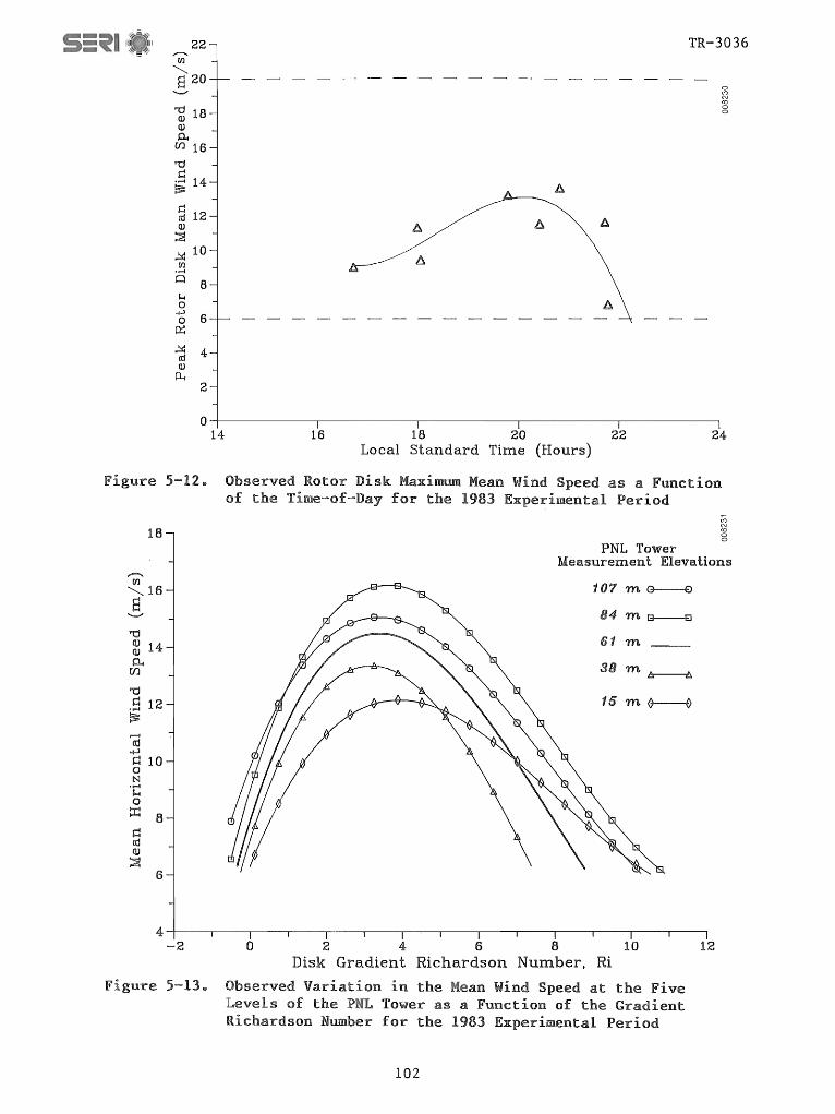
22

] 18 OJ 0..

(f) 16

"d d ~ 14

~ 12 OJ

::2l ~ 10 rn ......

Q 8 J-t o b 6 ~

~ 4 ttl OJ ~

2

TR-3036

o (')

~ o o

O~--------~----------'--------'-----------'----------I

Figure 5-12 ..

18

"d ~ 14 0..

(f)

"d .S 12 !3:

6

14 16 18 20 22 24 Local Standard Time (Hours)

Observed Rotor Disk Maximum Mean Wind Speed as a Function of the Time-of-Day for the 1983 Experimental Period

PNL Tower Measurement Elevations

107 Tn G---€)

11 4 Tn !3----£1

61 Tn __

311 Tn b:------A

15Tn~

4 ~-~--...----,----,-- I I I I I 12 -2 0 2 4 6 8 10

Disk Gradient Richardson Number, Ri

Figure 5-13. Observed Variation in the Mean Wind Speed at the Five Levels of the PNL Tower as a Function of the Gradient Richardson Number for the 1983 Experimental Period

102

450

....-!400 ~

1-1

w350 .... ttl ()

m 300

~ 200 0)

d & 150 S o u 100 bD d o

.....:l 50

o

~ 0.20 '+-I

0.18

1'Il- 0.16 0) • ..-1 ()

~ 0.14

& ~ 0.12 ~

"d 0)0.10 (J

~ "d W 0.08

0:: ,!:cI ttl 0.06 W ~

Cd 0.04 f..I ..., (J

~0.02 m

0.00

20

0)

Cd 15 ()

m .... ttl J..t b.O 0) ..., d - 10 ..., d 0)

d o 0.-S o u 5

161

~16l ! -:::> 14

..a 0) 0)

0.-m 12

"d d ~ d 10 ttl 0)

:::21

S 8 I.f.)

"I':!'"

6

u

/' /

Iu

"-\

\ \

\ \ \ \

TR-3036

N C') N co o

,0

o 44---~~--~--~--'--'--~--'--.---.--.---r--.--.---.--. -2 o 246 B

Disk Gradient Richardson Number. Ri

5-14 .. Variation Wind the (Iwz) Length

Scales a Number fmw C')

0.006 C')

.... - .... N

'" co .; 0 / \. 0

/ \ / \

I \ I \

~I \ \ Z I \ I

\ 0.005 I

\ I I \

I \ I:. I \

I \ I \

I \ I \

I "'- I \ ~ 0.004 ........ I

\ ttl "- I

\ I I'll "- I

I

)6 ·PI cd " :::> I

"- / \ I I \ ..., / "- / \ d /

/ "-~ 0 "- .;

"- / ~ ¢ ..... _- ,-tIl 0.003

0 ~ /

" / ,!:cI - -I'll jmu • ..-1

0

0.002 6 B 10

Disk Richardson Number. Ri 5-15 .. 45-m Horizontal Wind

(f ) • lOW

the as a Funct10n of

103

350

300

50

TR-3036

18

IJ 16

IJ

IJ

IJ

IJ

4+---~--~--~--~----~--~--~---jr----~~i 0.04 0.08 0.12 0.16 0.20 0.00 0.04 0.08 0.12 0.16 0.20

U-Comp Reduced Frequency Spectral Peak, fmu W-Comp Reduced Frequency Spectral Peak, fmw

(a) Variation of lux Versus fmu (b) Variation of lwz Versus fmw

Figure 5-160 Observed of the 45-m Horizontal and Vertical Length Scales as Functions of the Frequency Reduced

daily or diurnal mean for the summer or peak wind period (May through August) and winter or minimum wind period (November through January) of the 1985/86 wind season. The same data is plotted in absolute units in Figure 5-18 to show the relationship to the turbine cut-in speed.

The above figures clearly demonstrate that the maximum energy availability occurs between the hours of 1700-0600 1ST, during non-disturbed conditions" Even in winter, with its short days and low sun angle, the thermally-driven cycle is clearly discernible in Figure 5-17. From Figures 5-6 and 5-7, it is obvious that the period of maximum energy availability also coincides with a disk-layer inflow, which is stable and becomes increasingly so as the night progresses. Peak energy availability (at the hub elevation) typically occurs between 2000 and 2100 LST or 3-4 hours after sunset.. From Figures 5-6 and 5-7, the corresponding disk Richardson number ranges from about +0.5 to +7.0 for a geometric mean located between +300 and +4.0.

The thermal and kinematic fields are nearly in phase, indicated by the plots of the Brunt-Vaisala frequency (N) and the 45-m mean wind speed, as a function of the disk Richardson number in Figure 5-19. The phase relationship between the Brunt-Vaisala frequency and the characteristic turbulent scales (I x, I z, f ,and f ) in terms of the Richardson number are shown in Figures ~-20 ~nd my mw 5-l1.

From the foregoing series of graphs, it is clear that the structure of the stably-stratified inflow at Goodnoe Hills responds or tracks the disk gradient Richardson number. As the stability increases, an internal boundary layer

104

'"C w w P-t

1.30

1.20

rn 1.10 '"C d

• ..-1

13: d 1.00 ro w

::2! .-I 0.90 ro d J..4 ::l Q 0.80 ~ !>.

.-I J..4

2: 0.70 ::c:

5-11@

TR-3036

summer

winter / .....

" I " -, \

Wind Summer and Winter of

S'Um.:rner '85

winter '85-86

<D i:] OJ o o

3~~--~~~--~~~--~~~--~~~--~~~--~~-'--'-~-'--'-'

o 2 4 6 8 10 12 14 16 18 Local Standard Time (h)

5-180 Observed Diurnal Variation of Actual for Summer and Winter of the 1985

105

20 22 24

Mean Wind Season

0.006 18 TR....;3036

--- "-l!\ I.'l

t:d --- "-"-......" ~16

"/ I

I "-

450

400 ::J

1-4

W 350 -ItS ()

rn 300 -ItS ~

~250 ~

d 1-4

~ 200 d (!)

d & 150 S 0 u 100 b.O d 0

....:I 50

0

Z S ......"

~0.005 o 14 CJ d

rei (!)

& (!) (!)

(!) p.. s.. rn 12

13:..

!! 0.004 "d d

ItS • .-4

fIl 13: • .-4 10 ItS d :> ItS I (!) ~ :::2l d

, ::J S 8

cE 0.003 li.)

~ ~ fIl

• .-4 6 q

0.002 4 -2 o

Figure 5-19 .. Observed and the of the

20 0.006

---E! ---......" I.'l t:d ~ ......"

1-4

W Z

td 15 ~0.OO5 CJ CJ rn d

(!) - & ItS ~ b.O (!)

(!) ~ ~ 13:... d

1-4 10 !! 0.004 ~ ItS d fIl (!) • .-4

ItS d :> 0 I p.. ~

Ei d 0 ::J u 5 ~ to 0.003 -ItS ~ () fIl • .-4 • .-4 ~ q ~ (!)

:>

0 0.002 -2 o

I I ,

I

I I

I

I I

't:.

I I

I "-I "-

"- , I I

u

, ',N , , ,

" , "­'t\,

2 4 6 8 10 12 Disk Gradient Richardson Number, Ri

of the 45-m Mean Wind Speed (H) Frequency (N) as a Function

Richardson Number

N

I'lL ,. "-

\ \

\ \ \

\ Iw \

2 4 6 B 10 12 Disk Gradient Richardson Number, Ri

Figure 5-20. Observed Variation of the Brunt- Vaisala Frequency (N) and the Horizontal (1 x) and Vertical (1 z) length Scales . u.. Til as a Funct10n of the D1Sk R1chardson Number

106

co C')

~ o o

14

O"l C') N co 0 0

14

~ E 0.20 18 .... --/ " TR-3036

"H u ~ 0.18 ,.......

"H ~ 16

rnO.16 E Q) ---...... u :::> 14 & 0.14 ::s ..a tr Q)

I I \

I

I I

I

/' , / \

/ fmw " , \

9' \ \ \ \ \ \ \ \ \

~ 0.12 Q)

D.t \ I \

~ (f) 12

"g 0.10 "d c:l

u .,.., ::I ~

"d ' 10 Q) 0.08 c:l ~ ro

Q)

.!:d ::21 ro 0.06

S 8 Q)

O-t UJ

0.04 -.;fi

6 0.02

0.00

\ \

/"'\ \ \

-"- I

I I

I I

I

"- I

!~ \ /;( "-

¢ \ / "-, / "-0'--// "-

~ '-

/ /

4 Disk Gradient

10 Richardson Number. Ri

Peak Reduced (;OI!Up4)nE~n t) and

\ \ \ \ \ \ I

)~

forms within the rotor disk, accompanied by a wind speed maximum and increased vertical mean shear Under these conditions, as indicated by the peak in the Brunt-Vaisala frequency near an Ri of +4,,0, shear flow instabilities become well developed, including the possibili of breaking waves {Kelvin-Helmholtz instability)e 5-22 and 5-23 present an ANOVA analysis of the observed run-to-run variat ion of the longi tudinal and vertical 45-m elevation turbu­lence components These provide a crude presentation of the turbulent energy generation balance for each component" Roughly two-thirds of the observed run-to-run changes in the turbulent energy spectrum (at space scales of the rotor disk and smaller) can be explained from variations in the shear­stress {local shear generation)e The bulk of the remainder are due to variations in flow stability (buoyancy).

Inflow Predictors for Far-Field

s t ic scales, which would serve as independent A serles variables the MOD-2 turbine far-field acoustic spectral response Vla a linear multivariate model, were evaluated using ANOVA techniquese Three ctor {characteristic} scales, which exhibited maximum independence in Tables 5-2 and 5-3, were identified for evaluation. These included

M-O scaling length, L disk gradient Richardson number, Ri 45-m mean wind speed U45

• Vertical turbulence scale length, Iwz Richardson number, Ri 45-m mean wind speed, U45

o '<t

~ o o

-'" ~

II I ~-~

TR-3036 d 100 0

• .-1 ~ ttl

• .-1 90

&-t ttl

:>- 80 d :::1 p:: 70 I d :::1 60 p::

"lj 50 Q)

d • .-1

ttl .-I 40 0.. ~

t':iI - 30 0

Q) 20 bD ttl ~

d 10 Q) () &-t Q) 0 P..

-10 10 -1

Figure 5-22 ..

d 100 0

• .-1 ~ ttl 90

• .-1

&-t ttl

:>- 80 d :::1 p:: 70 I d :::1 60 p::

"lj 50 Q)

d • .-1

<d .-I 40 0.. ~

t':iI - 30 0

Q) 20 bD <d ~

d 10 Q) () ~ Q) 0 P..

-10 10 -1

total

u-ccnnp. an01Ja

I 9 0 0

u 0

lit 0 72J16 0 0

shear-stress 0 generated

t:. 26%

buoyancy generated

1 10 10 III

Rotor Disk Normalized Wave Number, Dn/U

ANOVA Analysis of the Longitudinal or Axial

total

U lit

N

L

U

o

t:.

0

0

o 0

o 9

0 A 01 0 0

& I $ &

Observed Run-to-Run Variation in the (u) Turbulence Component

o o 0 0

8 !;;I

8· 0

~ 0 ¢

o

o

0

0

0 0

w-ccnnp. an01Ja

o

o ~ 62J16 ~ shear-stress

o 0 0 generated

33% 0 buoyancy 0

0 generated

Q 0 o~

<!Ie 0 ~

1 10 10 III

Rotor Disk Normalized Wave Number, Dn/U

Figure 5-23.. Same as Figure 5-22 but for the Vertical or In-Plane (w) Turbulence Component

108

N <t N co o o

::;: N co 0 0

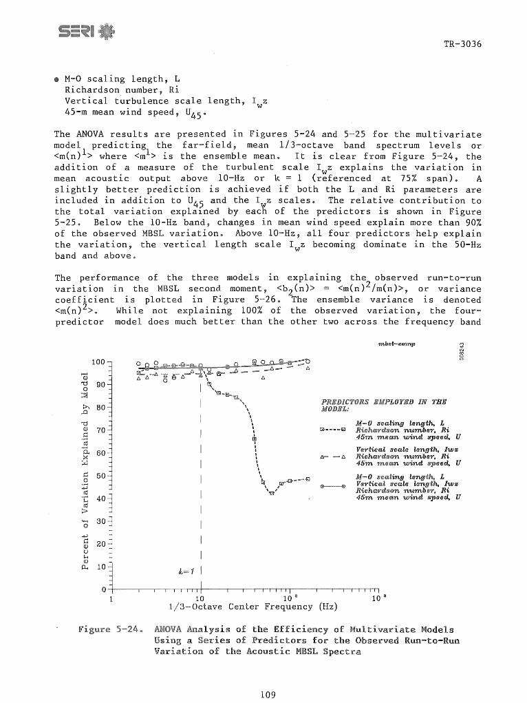
TR-3036

• M-O scaling length, L Richardson number, Ri Vertical turbulence scale length, Iwz 45-m mean wind speed, U45 0

The ANOVA results are presented in Figures 5-24 and 5-25 for the multivariate model predicting the far-field, mean 1/3-octave band spectrum levels or <m(n)l> where <ml> is the ensemble mean.. It is clear from Figure 5-24, the addition of a measure of the turbulent scale I z explains the variation in mean acoustic output above lO-Hz or k = 1 (r~ferenced at 75% span)" A slightly better prediction is achieved if both the Land Ri parameters are included in addition to U45 and the Iwz scalese The relative contribution to the total variation expla1ned by each of the predictors is shown in Figure 5-25. Below the lO-Hz band, changes in mean wind speed explain more than 90% of the observed MBSL variation. Above lO-Hz, all four predictors help explain the variation, the vertical length scale Iwz becoming dominate in the 50-Hz band and above ..

The performance of the three models in explaining the observed run-to-run variation in the MBSL second moment, <b2(n» = <m(n)2/m(n», or variance coefficient is plotted 1n Figure 5-26. The ensemble varlance 1S denoted <m(n)2>. While not explaining 100% of the observed variation, the four­predictor model does much better than the other two across the frequency band

100

(j) "d 90 0

::2! :>-.

..0 80

"d (J) 70 Q

'Cd .-<

0.. 60 ><: w Q 50 ,£ ...,J (1j

's:: 40 (1j

:> 'H 30 0

...,J

Q 20 (J)

u ~ (J)

P-. 10

0 1

L=1

PREDICTORS EMPLOYED IN THE MODEL:

C') ..;­C\J co o o

M-O I!waling length. L Richardson number. Ri 45m mean wind speed, U

Vertical scale length. Iwz Richardson number. Ri 45m mean wind speed, U

M-O scaling length. L Vertical sca.le length. Iwz Richa.rdson number. Ri 45m mean wind speed, U

10 10 10 :I

1/3-0ctave Center Frequency (Hz)

5-24@ ANOVA of Multivariate Models a Series of for the Observed Run-to-Run

Variation of the Acoustic MBSL Spectra

109

100 ......t (I)

'U 90 0

::2t ~ 80 ,0

'U (I) 70 r::

.,-4

cd ......t

0.. 60 ~

IiJ

r:: 50 0

.,-4

+J cd

.,-4 40 s... cd :> 'H 30 0

+J r:: 20 (I) CJ s... (I)

P-. 10

0

Figure 5-26 ..

mbsl-3Omin

I I I I I II I I I I I II

10 10 2

TR-3036

PERCENTAGE OF OBSERVED VARIANCE EXPLAINED BY THE:

o Richardson number, Ri o M-O length scale, L A Reference wind speed, U o Vertical turbulence scale, Iwz

.. Unexplained residual

I II

10 :3

1/3-0ctave Center Frequency (Hz) ANOVA Analysis of the Observed Run-to-Run Variation of the Acoustic MBSL Spectra as a Function of Four Inflow Predictor Scales

o

1-= 1

o

o l:::.

PREDICTORS EMPLOYED IN THE MODEL:

M-O scaling length, L Richardson num.ber. Ri 45m. m.ean wind speed, U

Vertical scale length, Iwz Richardson num.ber. Ri 45m. m.ean wind speed, U

M-O scaling length, L Vertical scale length, Iwz Richardson num.ber, Ri 45m. m.ean wind speed, U

10 1011 10 3

1/3-0ctave Center Frequency (Hz)

Same as Figure 5-24 but for the Observed Variation 1n the Acoustic BSL Variance Coefficnent <b2> Spectra

110

"'l"

~ co o o

lJ) "'l" N co o o

TR-3036

of interest" The performance of all three models. tends to drift downward above k = 1. The relative variation explained by each of the four predictors is shown in Figure 5-27. In contrast to the MBSL situation, in which changes in the mean wind speed explained the bulk of the observed variation at 10 Hz and below, all four predictors are necessary to cover the entire 2-160 Hz band range for the MBSL second moment.

Figures 5-28 and 5-30 present the performance of the three models in explaining the observed run-to-run variations in the MBSL third and fourth statijtical moments (skewness and kurtgsis coeffigients), or <b3(n» = <m(n) >/«m(n)2»3 and <b4 (n» = <m(n) >/«m(n)2».. Again, the four­predictor model performs better than the other two, particularly in explaining the spectral variation of the MBSL fourth moment or kurtosis coefficient co

Figures 5-29 and 5-31 display the relative variation explained by each of the four predictors for the skewness and kurtosis coefficients, respectively. Again, all four predictors are necessary to explain the bulk of the run-to-run variation in the 1/3-octave bands of interest.

Spectral Sensitivity to Inflow Characteristic Scales

The four predictors evaluated above were employed as independent variables in a linear, multivariate spectral regression model. In this model the response or dependent variables were the four statistical moments (mean and variance, skewness, and kurtosis coefficients) of the mean 1/3- and octave-band spectral levels (MBSL) for each data run. The model for the BSL mean is of the form

'+-< o

100 blc'IJ-30min

90

80

70

60

50

40

30

20

10

o

PERCENTAGE OF OBSERVED VARIANCE EXPLAINED BY THE:

o Richardson number, Ri D M-O length scale, L lJ. Reference wind speed, U (; Vertical turbulence scale, Iwz

.. Unexplained residual

, <D ~ C\J co o o

-10~--~--~~~~~----~~~~~~----~-'-'~~rn

1 10 10 2 10 3

1/3-0ctave Center Frequency (Hz)

5-27® Same as but for the Observed Variation in the <b2>

III

TR-3036 100

W '"d 90 0

:::!! l>. 80 ,.c

'"d (l) 70 s:l ..... ro ...... 0.. 60 ~

!:il

s:l 50 0 .....

+.l ro ..... 40 J... ro :> "H 30 0

+.l s:l 20 (l) C)

J... (l)

0... 10

0 1

000

o

D. o

Iv= 1

I 0

I

o

o

PREDICTORS EMPLOYED IN THE MODEL:

G----€l M-O scaling length, L Richardson number, Ri 45m mean wind speed, U

Vertical scale length. Iwz A- - D. Richardson number. Ri

45m mean wind speed, U

M-O scaling length, L Vertical scale length, Iwz Richa.rdson number, Ri 45m mean wind speed, U

10 10 II 10 3

1/3-0ctave Center Frequency (Hz)

Figure 5-28. Same as Figure 5-24 but for the Observed Variation in the

"H o

100

90

80

70

60

50

40

30

o+..l 20 s:l (l)

~ 10 (l)

0... o

Acoustic BSL Skewness Coefficient Spectra

bUik-30m:i:n

PERCENTAGE OF OBSERVED VARIANCE EXPLAINED BY THE:

o Richardson number, Ri tl M-O length scale, L A Reference wind speed, U o Vertical turbulence scale, Iwz

'* Unexplained residual

-10~----~--~~~~~~----'---'-'1-'1-'1 ~I'I'I~I-----.--'--'-'.-rrlnl I 1 10 10 2 10 3

Figure 5-29

1/3-0ctave Center Frequency (Hz)

5-25 but for the Observed Variation 1n the BSL Skewness Coefficient <b3> Spectra

112

co '<t N co o o

TR-3036

100 o

.-I OJ

'"'(j 90 0 ::a t>. 80

..0

'"'(j OJ 70 d .~

cd .-I

0. 60 ~ 0

CxJ

d 50 .S o4-l cd .~ 40 ~ cd

:> "H 30 0

o4-l d 20 OJ u ~ OJ

P-t 10

0

o 0

t;,.

t;,. 0

o (/il 0

0

0 0 t;,.

I t;,. ~

t;,.

o

o

k-= 1

10 1/3-0ctave Center

80 0

~ t;,.

PREDICTORS EMPLOYED IN THE MODEL:

(Hz)

M-O seeding length, L Richardson n'L/:mber. Ri 45m. m.eol.n wind speed, U

Vertical scale length, Iwz Richardson num.ber. Ri 45m. m.ean wind speed, U

M-O scaling Length, L Vertical scale length, Iwz Richardson num.ber, Ri 45m. m.ean wind speed, U

Figure 5-30. Same as 5-24 but for the Observed Variation 1n the

100 Acoustic BSL Kurtosi

(J) "0" N <Xl o o

PERCENTAGE OF OBSERVED VARIANCE 90 blkt-30m.in EXPLAINED BY THE:

Fcj 0 Richardson number, Ri (l) 0 M-O length scale, L d

• .-1 80 t;,. Reference wind speed, U cd .-I 0 Vertical turbulence scale, Iwz ~ ~ 70 .. Unexplained residual ~

d 0 60 • .-1 ~ cd

• .-1

50 S-t cd :> .-I 40 cd ~ 0 ~ 30 '+=t 0

~ 20 d (l) CJ 10 S-t (l)

p...

0

-10~--~---~~~~~·----~~~~-1-'~~--~--~~~1In

1 Center (Hz)

Figure 5-310 Same as 5-25 but for the Observed Variation 1n the Acoustic BSL Kurtosis Spectra

113

g ~ 0 0

TR-3036

where n is the band center frequency and E(n) is the residual error between the observed and predicted values.. The relationship for the second, third, and fourth statistical moments [b2(n), b3(n), and b4 (n)] would be similar but with a different coefficient vector [ao ,,,.,,,a4] for each.

501.1.3 Model Interpretation

The models discussed above allow us to examine not only the relationship of the mean acoustic spectral response to changing inflow conditions, but the variations of that response (the higher-order statistical moments) as well .. The elements of the model coefficient vector [al,ooe,a4] for each 1/3-octave frequency band listed in Table 2-2 reflect the change in the mean response per unit increase in the associated predictor variable, with the remainder of the predictors held constant or

a<sl 3(n»

aR. ~

If each coefficient ~s normalized by the predictor population mean or

(5-2)

then the relative spectral sensitivity of each inflow predictor scale can be measured on each frequency band response and the results compared" Thus, we can use these models to identify the characteristic scales or predictors which have the most influence over the statistical distributions of the MOD-2 LF emissions spectra. Those predictor scales, having substantial slopes relative to the remainder, can be considered indicative of the dominant physical processes responsible for acoustic radiation in a particular frequency band.

Mean Acoustic Band Spectrum Level. A plot of the normalized coefficients (response slopes) for the expected or mean BSL <Sl/3(n» model is shown in Figure 5-32. In this diagram the reference wind speed (U45 ) and disk gradient Richardson number (Ri) have the most influence on the average spectral far­field acoustic radiation below 10 Hz (k = 1).. Above that frequency, the vertical turbulent length scale, I z, gradually becomes more important. It is also interesting to note the cha~ge in sign for this parameter; i"e .. , band output increased with decreasing scale length below 10 Hz (k = 1) and the inverse occurred above 10 Hz ..

BSL Variance Coefficient.. The influence of the four inflow characteristic scales on the second moment (variance coefficient <b2» of the observed BSL distributions is shown in Figure 5-33" The <b2> statistic is a measure of the width or range of levels observed in a particular 1/3-octave band, relative to the band mean or expected level. Large values of <bZ> correspond to a very wide probability distribution, indicating the assoc~ated processes may be wideband random. Similarly, small <b2>s may indicate that some form of a narrowband random process (or processes) is responsible for the observed variation. A large run-to-run range of <b2> values are noted in the 3 .. 15, 10, and 12.S-Hz bands, as is indicated Figure 5-4b. The sensitivity plot of

114

.......... 0.15 N ::c ,~

III "d

IZl 0.10 (l)

04 0

...-I

en

,k\ I ~ 0.05

'{1 H 0

+> u 0.00 • ..-1

"d (l) H

Cl.i

"d (l) N -0.05 ·M

.--l

<d

S H 0 Z

-0.10

0.005

IZl (l)

04 0

.--I

en H 0.000 0

+> U

'M

'"d (l) H

Cl.i

'"d (l) N ......

(d -0.005 S H 0 Z

1

1

m.br!JT30

TR-3036

L[) (\J

OJ o o

.~~~~~~~~~~-------------------- .

Iv= 1

CHARACTERISTIC INFLOW SCALE PREDICTORS:

o Richardson number, Ri D Monin-Obukov length scale, L t;. Reference wind speed, U o Vertical turbulence scale length, Iwz

(Hz) for Mean Band

CHARACTERISTIC INFLOW SCALE PREDICTORS:

o Richardson number, Ri o Monin-Obukov length scale, L t;. Reference wind speed, U

Iv= 1 0 Vertical turbulence scale length, Iwz

10 10 2

1/3-0ctave Center Frequency (Hz)

for BSL

115

10 :'I

(\J L[) (\J

OJ o o

TR-3036

Figure 5-33 indicates the TJ45 and Ri (atmospheric structure) have the most influence in these bands with a moderate contribution from the vertical scale length I z. This time the <b2> sensitivity to the vertical turbulent scale remains ¥nverse below 12.5 Hz and becomes essentially zero until it achieves dominant influence and positive correlation with and above the 80-Hz band.

BSL Acoustic Skewness Coefficient. The relative spectral sensitivity of the characteristic inflow scaling parameters on the BSL distribution third moment, or skewness coefficient <b3>, is plotted in Figure 5-34. The skewness coefficient is a measure of the lack of symmetry in the sample probability density function. A normal or Gaussian distribution is symmetrical about the mean; therefore, the skewness is zero. A positive skewness coefficient in a particular frequency band reflects a predominance of large BSL values (peaks) over smaller ones; therefore, the distribution is "positively skewed .. " The run-to-run variation plot of <b3> in Figure 5-4c indicates a multi-band structure, with large variations in the 2-5, 8-20, 40, and 80-160 Hz bands. Figure 5-34 indicates parameter sensitivities similar to those that were found for the variance coefficient <b2>.

BSL Acoustic Kurtosis Coefficient.. The normalized BSL sensitivity of the fourth moment <b4>, or kurtosis coefficient, to the set of four inflow characteristic scales is shown in Figure 5-35. The kurtosis coefficient, or "flatness factor," is a relative measure of the magnitude of the BSL values in

rtl Q.)

P-t o

..-t (()

I-l o

o+=l ()

:B Q.) I-l

P-t

'"d Q.) N .......

blBkr30

0.005

0.000 ~~-s-=--t1~~~~~~~~~~--------------------.

] -0.005

CHARACTERISTIC INFLOW SCALE PREDICTORS:

I-l o Z

-0.010 1

Iv= 1

o Richardson number, Ri o Monin-Obukov length scale, L ll. Reference wind speed, U o Vertical turbulence scale length, Iwz

10 10 2

1/3-0ctave Center Frequency (Hz)

I I I 10 3

Figure 5-34& Characteristic Scaling Sensitivities for BSL Skewness Coefficients

116

TR-3036

the observed band probability distribution.. The kurtosis coefficient for a normal distribution is 3.. An observed BSL distribution void of sharp peaks will have a kurtosis of 3 or will possibly be negative (flat). A high value of <b4> in a particular frequency band indicates a substantial percentage of large values (peaks) relative to the mean band level and a distribution peaked at the mean. The band structure noted in Figure 5-4c of the <b3> statistic has become more discrete in the plot of <b4> in Figure 5-4d. The largest variations of <b4> occur in the 3.15-5, 8, 20, 40, and 100-160 Hz bands. The parametric sensltivity plots of Figure 5-35 indicate that atmospheric structure, as indicated by the Richardson number, is the dominant influence on <b4> below 10 Hz and inversely correlated (low stability)" High values of <b4> in the 100-160 Hz bands are positively correlated with very stable flows.

Empirical Agreement with the Theory of Homicz and George.. In general, there is excellent agreement between the theories of Homicz and George [10,11] and our measurement of the MOD-2 wind turbine. They identified the axial convec­tion velocity, V , the upwash or in-plane turbulence component intensity, and scale I z as t~e primary inflow properties that influence the mean band spectrumw<S (n» level emissions We found that the dominant characteristic inflow scal~~ were wind , U, the upwash or vertical turbulent scale, I z, measured within the rotor disk, and the gradient Richardson number stabilit; parameter measured across the vertical extent of the rotor disk. We agree with the axial flow component, since the axial and convection velocity

0.5

0.4

fIl Q)

~ 0.3 0 ,.....{

('f)

~ 0 0.2

+J u ......

'"d Q)

~ 0.1 Cl.t

'"d Q)

N 0.0 ...... ,.....{

cO

El ~

~ -0.1

-0.2

-0.3 1

CHARACTERISTIC INFLOW SCALE PREDICTORS:

o Richardson number, Ri tJ Monin-Obukov length scale, L /:;. Reference wind speed, U

blktr30

L=1 \) Vertical turbulence scale length, Iwz

10 10 2 10 3

l/3-0ctave Center Frequency (Hz) Sensitivities for BSL

117

'OJ" l{) (\J Q) o o

TR-3036

are approximately related by V = 0 .. 8U EO And, since I z is proportional to S (ni' as well as to the mean-~quare value of the integrated value of S (n) o~ w , again there is agreement. Including the Richardson number paramete~ is necessary to account for the seemingly unique, stratified flow structure present at the Goodnoe Hills siteo We must also include the M-O length scale, L, to provide the diabatic surface-layer scaling in the rotor disk discussed in Section 3 .. 2. These adjustments would not, however, be necessary in the homogeneous isotropic inflow turbulence assumed by Homicz and George in their models. Thus, including them is a concession to the real atmosphere ..

501.1.4 Case Studies of the Role of Inflow Structure on Radiated Spectral Characteristics

A series of case-study comparisons were made among the six usable data runs of 1983. Tables 3-3a, b, and c show that four inflow regimes were available for comparison: (1) low wind speed, low stability (LWLS); (2) low-to-moderate wind speed, low-to-moderate stability (LMWLS); (3) low wind, high stability (LWHS); and (4) high wind, high stability (HWHS). These cross-comparison run combinations and associated run data are listed in Table 5-4.

Low Wind, High Stability versus High Wind, High Stability Inflow Conditions. The normalized, longitudinal (axial) and vertical (upwash) 45-m level tur­bulence spectra for Runs A05 and Al8 are plotted 1n Figure 5-36" The cor­responding mean BSL <Sl/3(f», <b2(f», <b3(f», and <b4(f» acoustic spectra are shown in Figures 5-37a, b, c, and d. The lower abscissa is scaled in terms of the convection wave number, normalized by the rotor disk dimension,

Comparison Category

LWHS (3) HWHS (4)

LMWLS (2) HWHS (4)

LMWLS (2) HWHS (4)

LWLS (1) LMWLS (2)

LWLS (1) LWHS (3)

HWHS (4) HWHS (4)

LMWLS (2) LMWLS (2)

Table 5-4. Inflow Structure Comparisons Data

Run Numbers

A05 A18

A14-1 A18

A14-2 All

A03 A14-1

A03 A05

Al8 All

A14-1 A14-2

7.3 12.4

9.2 12 .. 4

9 .. 9 13 .. 6

8 .. 1 9.2

12 .. 4 13.6

9 .. 2 9 .. 9

Ri

11.7 1 .. 25

0 .. 13 1 .. 25

0026 6068

-0.12 0 .. 13

-0.12 11 .. 7

118

1 .. 25 6.68

0 .. 13 0 .. 26

L (m)

10 .. 7 10 .. 7

183 10,,7

10 .. 7 10 .. 7

-508 183

-508 10 .. 7

10 .. 7 10 .. 7

183 10 .. 7

136 125

157 125

86 .. 5 336

210 157

210 136

125 336

157 86 .. 5

7 .. 5 8 .. 8

16.5 8 .. 8

6 .. 1 6 .. 8

13 .. 3 16 .. 5

13 .. 3 7 .. 5

8.8 6 .. 8

16.5 6 .. 1

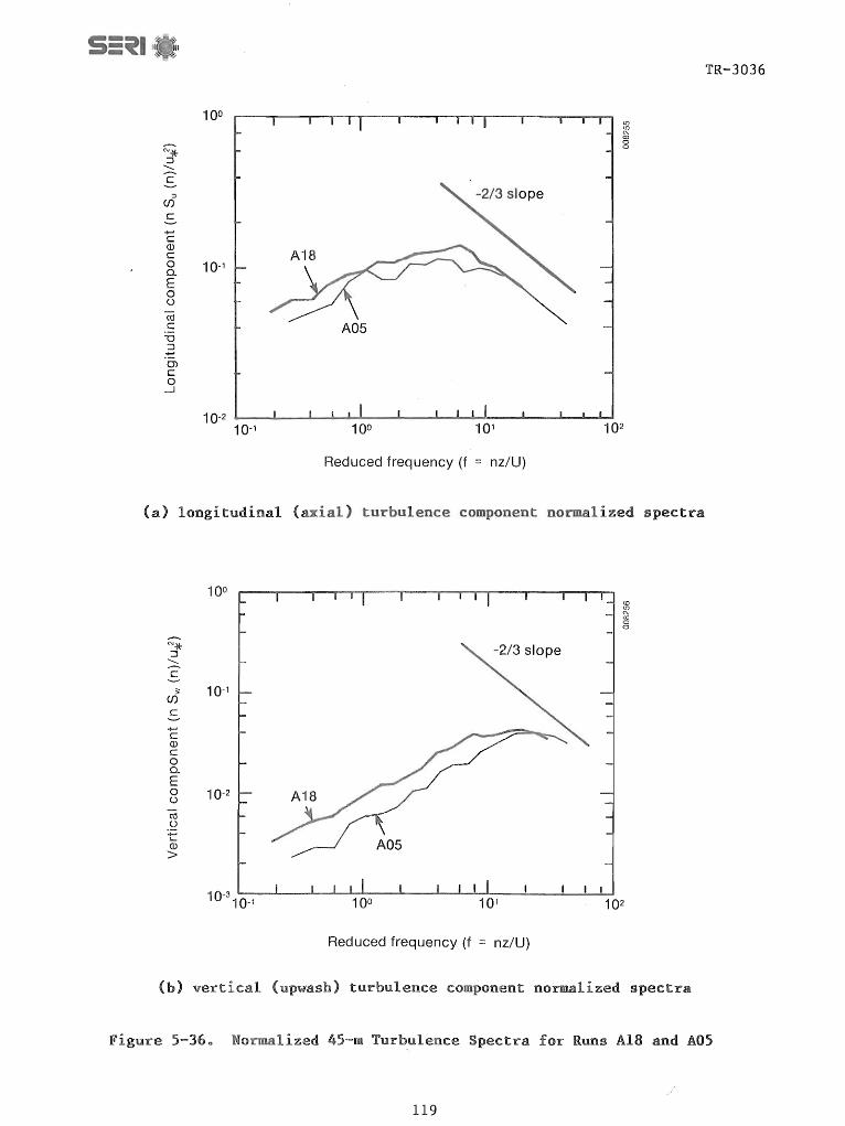
~ ::J ~ C '-'

::J

Cf)

C

..... C (l) C 0 a. E 0 ()

cti C

-0 ::J .~ 0) c 0 -l

100

10-1

10-2

10-1 100 101

Reduced frequency (f nz/U)

t2 N co o o

102

(a) longitudinal (axial) turbulence component normalized spectra

100 ill II) N co 0 0

N* -2/3 slope ::J

-----C

:;: 10-1 Cf)

C

C (l) c 0 a. E 0 10-2 ()

cti ()

:;:::; ~

(l)

>

I I 100 101 102

Reduced frequency (f = nz/U)

(b) vertical turbulence component normalized spectra

TR-3036

Figure 5-360 Normalized 45-m Turbulence Spectra for Runs AlB and A05

119

-/, ~

II J

~ ~ -80 1 ~I

aill/OS mbl ........ 1'-N

81 l{) ::c SI ~

"'- 0

~I ~ 0 III °1 Pt:/ .........

1 .......... 70 ........ d ......... 0. «I rn ......... ..... 60 III I> III

..J

a :;:I s.. 50 ., () III 0. rn Pt:/ d «I 40 run AtS III

d run AOS ______ IBIIli> __

«I III ~

30~----r--r-'-'I1I1'----.--.--r'-ITTT'----'--'-'-Tl-'rn

.......... ........ d .........

N e

i 1

1.0

d 0.8 III ..... ()

• .-4 <1M <1M III 0 u 0.6 III ()

d «I ..... s.. «I

:::> 0.4 ..J rn III

III

~ ., 0.2 ()

0 I

(I')

'-..... ..... 0.0

1

1

1

10 10 III 10 III

1/3-0ctave Center Frequency (Hz) I I I I I II I I iii i I I I Iii

10 10 III 10 III

~I

~I I I I I I I I I

...

Rolor Disk Normalized Wave Number, Dn/Ub

mean band spectrum levels

"', /\ , , \

" \ \ ...... "

... , '-- ...

ru.n AtS

run .AOS -- ------

10 10 III

1/3-0ctave Center Frequency (Hz)

10 Rotor Disk Normalized 'Wave Dn/Ub

(b) band spectrum level var1ance coefficient

10 III

co l{) N co o o

TR-3036

Figure 5-37. Ensemble Statistical Moments of l/3-0ctave Acoustic Band Spectral Levels for Runs AlB and A05

120

_2.5

~ t'J e +' ~ 2.0 ..... C) ..... --Q)

0 u (/)

1.5 (/) Q)

d ~ Q)

~ rf.)

1.0 ....:I rf.)

r:o Q)

P-ro +' 0.5 C)

0 I

t'J ~ rl

0.0 1

I 1

14 -,-, d ~ e 12

+' d Q) ..... C) 10 ..... --Q)

0 U

.~ 8

(/)

0 +' I-. :::1 6 ~

....:I rf.)

r:o Q) 4 P ro +' C)

0 2 I t'J ~ ..-t

0 1

I

1

)

,\ I \ I \ , \

, \ " \ ' ''' I \ '\ 0 ... I ,

... '\' ... '\ ", \' ......... I \

_ 1_ ~ - '- L - - _ ... - -'....-~' ,

run A

run A05

'"

I , I ,

I ,~ , " , ,\ , I ' , , \,

I \ ,

, '! I I

10 10 III

en l{) N 00 o o

1~ significance level

10 s 1/3-0ctave Center Frequency (Hz)

I I I Iii I I i I I II I I

10 10 II

Rotor Disk Normalized Wave Number, Dn/Ub

(c) band level skewness

ill

10 II

m18/05 Jd

;1 "dl run A18 1;

0

~I '5 1 <D N

run A05 ea~""",""""~_ - 00

1 0

1 0

, , I I I I ,

I I

" I 1\ I 1\ I i I I , I I I I I I I' , , I I

" I " I f ,

I I , I

significance level

'" '" 10 10 III 10 3

1/3-0ctave Center Frequency (Hz) I I I I I II I I i I I I I i I i I

10 10 II 10 s

Rotor Disk Normalized Wave Number, Dn/Ub

band level relative kurtosis

TR-3036

Figure 5-31$ Ensemble Moments for l/3-0ctave Acoustic Band Levels for Runs Al8 and A05

121

TR-3036

or Dn/Ub , where Ub is the relative rotor velocity at the effective radius of 75% span" The span and chord dimensions, in terms of the wave number, are indicated on the plots" The mean BSL plot of Figure 5-37a shows the influence of the higher axial wind speed below 20 Hz, but above that the two spectra are essentially the same. A similar situation exists for the <b2(f» spectra of Figure 5-37b, though the lower wind run becomes more discrete below 20 Hz .. The plots of the <b3(f» and <b4 (f» spectra in Figures 5-37c and d indicate some spectral shifts in the bands for the two runs.. The clear difference, however, is the strong peaking behavior being exhibited at 80 Hz and above in the A05 run data. We believe this to be associated with the intense vertical stratification present during this run as indicated by the detailed profiles measured by the tethered balloon shown in Figure 5-38.

Low-to-Moderate Wind, Low Stability versus High Wind, High Stability Inflow Condi t ions.. The 45-m axial and upwash spectra are shown in Figure 5-39 for Runs A14-l and A18. The mean BSL spectra of Figure 5-40a show a much sharper difference in the spectral slopes below 20 Hz than was true for the previous comparison, even though the lower wind run here has a higher mean velocity" Above 20 Hz, the curves again nearly overlap" The variance coefficient spectra of Figure 5-40b indicate less variation in the lower speed run in the bands between 6.3 and 25 Hz. The skewness and kurtosis spectra in Figures 5-40c and d indicate a much more discrete behavior in the bands below 10 Hz for the lower speed, lower stability run, though a harmonic relationship in the Al8 run does seem to e~iste

The A14-2 and All runs each fall into similar classifications in Table 5-4, but the inflow conditions are quite different from those of the previous pair. For example, both the axial and upwash turbulence spectra of run All exhibit a discrete feature near f = 0.6. This can indicate that atmospheric wave motions are present at the anemometer height.. Even though the hub-height mean wind speed of the All run is almost 50% higher than that for run A14-2, there is more turbulent energy in the inflow of the latter, as indicated in Figure 5-41. This seems to be reflected in the steeper slope of the mean BSL curve in Figure 5-42a and the variance coefficient spectra in Figure 5-42b" The skewness and kurtosis coefficient spectra shown in Figures 5-42c and dare also quite different from those of the A18 and A14-l runs. There is much more evidence of spectral peaking in the more turbulent A14-2 run below 20 Hz. The All run, however, shows evidence of peaks occurring often in the bands above 63 Hz, probably as a resul t of the discrete peak in the inflow spectra in Figure 5-410

Low Wind, Slightly Unstable versus Low Wind, Slightly Stable Inflow Conditions. The axial (longitudinal) and upwash (vertical) reduced-frequency spectra for Runs A03 and A14-l are compared in Figure 5-43" Again, even though the A14-l run has a higher associated mean wind speed, there is more turbulent energy in the A03 run's unstable inflow. This underscores the need to consider the stability characteristics of the inflow as well as the veloc­ity magnitudes. As before, this excess turbulent energy is reflected in the mean BSL spectra in Figure 5-44a as larger low-frequency emission levels and a steeper slope with increasing frequency. Above the 10-Hz band, however, the slightly stable A14-1 run emits slightly higher levels. The variance coefficient or <b2> spectra of Figure 5-44b show essentially the same behavior for this pair of runs" The effects of increased stability and a slightly greater mean wind speed in Run A14-1 are demonstrated in the <b3> and <b4>

122

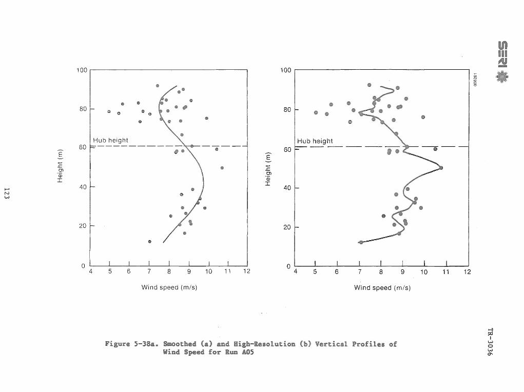
100 100 1.:i;::;~

~ I I co ~ :Y 0 -0

• • • • 80 • • 80 • • • • • • • • Hub height Hub height

60 60 E E

...... ....... .!: • O'l .r::.

Q) O'l Q) I I

.-. 40 40 N W

20 20

o 4 5 6 10 11 12 7 8 9 o 4 5 6 7 9 10 11 8 12

Wind speed (m/s) Wind speed (m/s)

5-38a. Smoothed and of Wind Speed for Run A05

E ....... ..c OJ (l)

I

...... N .p..

100

80

Hub height

60

40

20

o 180

----- -----

•

•

Wind direction (deg)

100

80

Hub height ----- ---- ----

60 E

......

..c OJ om I 40

20 •

o ~--~--~--~----~--~-~----~--~--~ 180 220 260 300 340

Wind direction (deg)

Figure S-38b. Saoothed and High-Resolution Vertical Profiles of Direction for Run AOS

N /.0 - ~

~ I J 0 ~ - ~ 0

E ...-..c CJ)

CJ.)

I

I-' N V1

100

80

60

40

20

o 16

100

80

Hub height 60

E ....... ..c CJ)

CJ.)

I 40

• 20

17 18 19 20 21 22

Temperature (0 C)

Figure 5-38c. Saoothed and Temperature for Run A05

Hub height

17 18 19 20 21 22

Temperature (0 C)

Profiles of

C") (!) C\J co 0 0

r-3 l=l:1 I

W o W 0\

h;;;:~

I I ~ ~ -

~ ::J

::::::. c

::J

Cf)

C

+-' C (]) C 0 Q.

E 0 ()

qs C

""0 ::J +-'

O'l C 0

.-J

100

10-1

10-2 10-1

Reduced frequency (f = nz/U)

"" <0 N co o o

(a) longitudinal (axial) turbulence component normalized spectra

+-' C (]) C o Q.

100

~ 10-2 ()

qs ()

+-' lo-(])

>

10-3

-2/3 slope

10-1 100 101 '

Reduced frequency (f = nz/U)

If) <0 N co o o

102

(b) vertical (upwash) turbulence component normalized spectra

TR-3036

Figure 5-39. Normalized 45-m Turbulence Spectra for Runs AlB and A14-l

126

S ::1 b 50 o Q)

0. {'f)

"d d ~ 40

d cd Q)

~

run ,,(18

run ,,(14-1 ---------

,,'11/14-' -millill

<0 <0 N co o o

30~----~--~~~~~~----~~~~~~~----~--~~~~~~

I 1

~ O.B ())

:§ 'H 'H ())

o U

()) CJ d cd .~

cd :> o-:l (f)

III

())

l> cd ...., CJ

0 I

C'J ~

0.6

0.4

0.2

0.0

I 1

1 10 10 II

1/3-0ctave Center Frequency (Hz) iii iii Iii iii Iii

10 10 II

Rotor Disk Normalized Wave Number, Dn/Ub

mean band spectrum levels

10 II

iii

10 :II

a1B/14-1 C01J

~I t:S ~I

I

run A18

~I o ~I

I

run A 14-1 -- - -- - -- -- -- -- Q

10 10 a

1/3-0ctave Center Frequency (Hz) I I I I I I I I I I I I I I I

10 10 II

Rotor Disk Normalized Wave Number, Dn/Ub

(b) band spectrum level variance coefficient

r­<0 N co o o

10 3

I II

10 3

TR-3036

Figure 5-40. Ensemble Statistical Moments of 1/3-0ctave Acoustical Band Levels for Runs AlB and A14-l

127

--. 2.5

3 C'J .e .p)

§ 2.0 .,... o .,... ..... ..... Q)

o u

Q)

:> cd

.p)

0 0 I

C'J ~ .-t

0.5

0.0

I 1

14

1

~I ~I

1

-1-

't31 ~I (,)

1

aIB/14-1 sk

00 <0 N 00 o o

1% significance level

run A 18

run A 14-1 - -

I I I I I I 10 10 1II

1/3-0ctave Center Frequency (Hz) I iii II I I I I Ii I I I

10 10 1II

Rotor Disk Normalized Wave Number, Dn/Ub

(c) band level skewness coefficient

"I 10 :I

"I 10 :I

atB/14-t kt

run A 18

run A 14-1 - - - - - - - -

,~ " ,I

I ' ~ I' 'I , I \ I I I I I \ , I

I I ~ " I " I \' I f I

I I \ \ \

OJ

~ 00 o o

- - - 1% significance level

O~----.---.-.-"~,,.-----r--.-.~=r""~~-'--'--'-'lIrrn

I 1

1

(d) band

10 10 1II

1/3-0ctave Center Frequency (Hz) I I I I II I I I I II I I I

10 10 II

Rotor Disk Normalized Wave Number, Dn/Ub

10 :I

"I 10 II

level relative kurtosis coefficient

TR-3036

Figure 5-40.. Ensemble Statistical Moments of 1/3-octave Acoustical Band Spectrum Levels for Runs A18 and A14-1

128

c ::J

(f)

c .....-c (l) c

10-1

8. 100 E o u ~ C

"0 ::J ...... Q) c o

...J

N* ::l

--...... C

:;: en c

C (l) c 0 0.. E 0 u ~ U

:.;::; I-(l)

>

10-2

10-1

-10°

10-1

10-2

A11

10-3

10-1

) vertical

Reduced frequency (f nz/U)

) turbulence normalized

10° 101

Reduced frequency (f nz/U)

~ co 0 0

102

o I'­N co o o

turbulence component normalized spectra

TR-3036

5-416 Normalized 45-m Turbulence for Runs A14-2 and All

129

......... 80 N ::c

""-III "d .........-

.......... 70 ......... J:l .........-~ cd

rIJ ...........

.-4 60 Q)

> Q)

....l

S ::; M

50 o+J () Q)

~ rIJ

"d J:l cd 40 III

J:l cd Q)

~

30 1

I

1

1.0 .......... ......... E.-N e ~ 0.8 Q)

'0 ..... '1-4 '1-4 Q)

0 u 0.6 Q) ()

J:l cd ..... M cd

::> 0.4 ....l rIJ III Q)

> cd

o+J 0.2 ()

0 I

CO')

""-.-I

0.0 1

I 1

I ~I cd 1/14-2 -ml!lIIll

51 ~I ~ C\J I'-

UI C\J co 0 .. ... I 0

"- ... I .... .... .... I ....

.... "- I ... ... , I ,

.... I .... ... .... ... ... ... ... .... ...... ......

... ~ , I ....

"- ... ... .... ...

.... runAt1 ....

.... ... run A 14-2 ---- ----- ...

10 1/3-0ctave

10 II 10 I

Center Frequency I I i i j i I i I I I II

10 10 II

Rotor Disk Normalized Wave Number,

(a) mean band spectrum levels

~I

~I I I I

run Att

run A14-2 ---------

~I

~I U

I I I

(Hz) I i

Dn/Ub

ill

10 I

C') I'­C\J co o o

10 10 II 10 I

1/3-0ctave Center Frequency (Hz) j j j I j j I j j j j j I j j j i I

10 10 II 10 I

Rotor Disk Normalized Wave Number, Dn/Ub

(b) band spectral level variance coefficients

TR-3036

Figure 5-42. Ensemble Statistical Moments of l/3-octave Acoustical Band Spectrum Levels fDr Runs A14-2 and All

130

/'- 2.5

:3 C")

e +l

~ 2.0

:§ 'H 'H Q)

o u CIl 1.5 CIl Q)

s:: ~ Q)

~ [f)

1.0 ....:l [f)

c:o Q)

P-cd +l 0.5 u 0 I

C")

~ ..-I

0.0

14 /'-~

3 ~

e 12 +l s:: Q)

:§ 10 'H 'H Q)

0 u

.~ 8

CIl 0 +l s.. ::l 6 ~

....:l [f)

c:o Q) 4 P-cd +l U

0 2 I C")

~ ..-I

0 1

~/

~/ /

1

-1-

run A 11

run A 14-2

Rotor

) band

AU

I I I I

"

'"d/

~/ (.)

/

" '\ '\

- ~/-l\.a"- '-""""',

Normalized Wave

\ \

\

A14-2= ==----

'"t:l/

S ~/

/

10 10 II

(Hz)

0.11/14-2 Ilk

1% significance level

10 :I

10 ::I

Dn/Ub

(2,11/14-2 kt

L()

J'-. N 00 o o

- - - - 1% significance level

10 :I

1/3-0ctave Center Frequency (Hz)

10 Rotor Disk Norma.lized Wave Dn/Ub

band level ku.rtosi

TR-3036

Acou.stical Band and All

131

100 <D f'-N

~ co

N* 0 0

::J ~ C ---en c +-' C (J.) C 0 10-1 0.. E 0 ()

n:s c A14-1

'"0 ::J

.-=: 0) c 0 -l

10-2

10-1 100 101

Reduced frequency (f = nz/U)

(a) longitudinal (axial) turbulence component normalized spectra

+-' C (J.) C o 0.. E o 10-2 ()

aj ()

+-' I-

~ A14-1

Reduced frequency (f = nz/U)

(b) vertical (upwash) turbulence component normalized spectra

TR-3036

Figure 5-43. Normalized 45-m Turbulence Spectra for Runs A03 and Al4-l

132

-~ ~

II I ~ - ~

TR-3036 ,-.... 80

~I m03/14- t ....,-nhl

N ttl &1 '-..... ~ o::l (JI co

~ r--N

I co 0 0 .---.. 70 ........

.E.. 0.. cd

IZl .......... - 60 (J)

t> (J)

...:I

El ::l J.4 50 +J 0 (J) Q.

IZl

'U s:l cd 40 ru1l

o::l

s:l run A14-1 -(Ij (J)

::!!

30 1 10 10 I 10 I

1 Rotor Norrnalized

band levels

1.0 0,03/14-1 CIW

~ ~I 't:!1 .::1l t

C\1 ~I 'fll (J) e I I r--N co 0

~ I 0

s:l 0.8 (J)

:§ '+-1 '+-1 (J)

0 u 0.6 (l) 0 s:l (Ij .~ (Ij

:> 0.4 ....:l IZl o::l (l)

t> (Ij ~ 0.2 run A03 (J

0 run A 14-1 I (iJ

'-..... ..-l

0.0 10 10 D 10 I

1/3-0ctave Center Frequency (Hz)

1 10 Rotor Disk Normalized Wave Dn/Ub

coefficients

Moments 1 Acoustic Band Runs A03 and Al/",-l

133

__ 2.5 ,...... E., C"J

e ...., ~ 2.0 ..... C) ..... ..... ..... w 0

U

rn 1.5 rn w d ~ w

,!:d U) 1.0 ....:l U)

CIl

w t> a:I ...., 0.5 C)

0

~ I

C"J

"" .-4

0.0 1

I 1

~I i:S ~I

I

I

# I'

f I' ,\ , ,. , \ 1\ ,. , \ I \ , , , \I \ , , , .. " , , '" , ~, , , , ,

I , I ,

I , , , , , ,

'ttl S ~I

I

- 1- - - - - - - - -

run A03

run A 14- 1 - - -------

I I I I I II II I I I II

10 10 II

1/3-0ctave Center Frequency (Hz)

a03/t4-t iliA: TR-3036

o co C\J co o o

19S significance level

I II

10 II

I I I I I II I I I I II I i I II

10 10 III 10 :I

Rotor Disk Normalized Wave Number, Dn/Ub

(c) band spectrum level skewness coefficients

...., d w ..... C) ..... ..... ..... w o u

14

10

8

6

4

2

~I ~I

run A03

run A 14- 1 - - ------

~ I, I, I,

" , I. , \ I' I ,

, , I , I ,

I ,I , I I

g , , , , , I , , " , , " I , " I , " , , • I

I I , , I \

I \ I \

\ \ ...

m03/14-1 A:t

00 iil o o

- - - 19S significance level

O~----'--'--~~~~-----'--~~~~~~~-.---.-.-..-"n

I 1

1 10 10 II

1/3-0ctave Center Frequency (Hz) I I I I I II I I I I II I I

10 10 II

Rotor Disk Normalized Wave Number, Dn/Ub

10 1\

I i I 10 :I

(d) band spectrum level relative kurtosis coefficients

Figure 5-44. Ensemble Statistical Moments of 1/3-octave Acoustic Band Spectrum Levels for Runs A03 and A14-1

134

TR-3036

spectra of Figures s-44c and de The frequency shift and characteristics are very noticeable. The distinct harmonic nature of the bands in which peaking occurs in the unstable A03 run gives way to very strong, but much more band­limited behavior in the slightly stable A14-1 run.

Low Wind, Unstable Inflow versus Low Wind, Very Stable Inflow Conditions. The normalized spectra associated with the two inflow components are shown 1n Figure 5-45. A -2/3 spectral slope at high frequencies is indicative of the turbulent inertial subrange III As one would expect, there is much less tur­bulent energy present in the very stable inflow. The slight discreteness in the band between f = 0.06 and 0.6 in the axial spectra of Run ADS hints that waves may be present The plot of the mean BSL spectra in Figure 5-46a is surprising, however. Even though Run AD5 has a lower mean wind speed and less energy in the turbulent inflow, its mean LF radiated acoustic levels are essentially identical to those of Run AD3

The reason for this behavior becomes apparent when we compare the detailed inflow structure The first hint is that the upwash scale length I z is 7.5 m

3 .w

for Run ADS, versus 13" m for run AD3 The transfer funct10n plot of Figure 5-4 shows ive slope (almost 2 dB/Hz/m in the 2-Hz 1/3-octave band) below 12 .. 5 Hz; i .. ee, the smaller the I z, the

• w greater the mean BSL below 12.5 Hz. Second, the peak wlnd speed occurs at a height of 45 m (as listed in Table 3-3c) with its attendant strong shears and just below the hub of the turbine., Finally, these features are clearly illus­trated in the detailed tethered balloon prof of Figure 5-47. The strong shear layer near 45 m is di tinctly evident.. It is the A05 run we discussed in connection with the direct measurement of the MOD-2 acoustical response function in Section 5 .. 1.1

The <b2> spectra of Figure 5-46b shows that the acoustic levels of Run AOs are related to a more narrowband random process than those of Run A03 below about 2D HZe While some frequency shifting has taken place in the <b3> and <b4> spectra of Figures 5-46c and d, the low-stability run exhibits the distinct harmonic structure while the high-frequency peaking is characteristic of the very stable case. Again these two runs underscore the role of vertical sta­bility in determining the aeroacoustic response of a large wind turbine.

High Wind, Moderate-to-High Stability vs. High Wind, Very-High-Stability Inflow Conditions. Here we compare the effects of increased stability under high wind conditions. Figure 5-48 plots the normalized axial and upwash tur­bulence spectra for Runs All and AlB. The discrete peak in the All spectra is evident and not present in the Al8 run data" The mean BSL spectra of Figure 5-4980 for both runs are almost linear in log acoustic pressure (dB) versus log cyclic frequencye Furthermore, only the effect of the increased wind speed for the All run appears to be responsible for the slightly higher levels associated with it" The variance coefficient spectra in Figure 5-49b are essentially the same, indicating that the processes operating are dynami­cally similar The skewness and kurtosis spectra of Figures 5-49c and d below about the 31 5-Hz band are very similar" We believe the peaking activity in the All data is a result of the high-frequency discreteness of the turbulence inflow spectra in Figures 5-48" This is reflected somewhat in the smaller upwash length scale for the All run"

135

100

~ :J

........ '2 '-'

:J

Cf)

C ......-+-' C Q) C 0 10-1 Q..

E 0 ()

cti c -0 :J +-'

O'l C 0

...J

10-2

-2/3 slope

A05

10-1 100 101

Reduced frequency (f nz/U)

N co N co o o

102

TR-3036

(a) longitudinal (axial) turbulence component normalized spectra

100 C') co ~ 0 0

;* ........ c

;;: 10-1 Cf)

C

+-' C Q) C 0 Q..

E 0 () 10-2

~ ()

+-' I.-

m >

10-3

10-1 100 101 102

Reduced frequency (f nz/U)

(b) vertical (upwash) turbulence component normalized spectra

Figure 5-45. Normalized 4S-m Turbulence Spectra for Runs AO) and AOS

136

TR-3036 80 flJJ3/06 mfull ..-...

N "d ::tl ~ ""-III u '<t

00 "d N ........ 00 0 0 - 70 ..-...

d ........ e:lt td rtl ...........

.-4 60 II)

I> II)

...::!

E ::1 M 50 o+J 0 III e:lt rn

"d d td 40 CO

d run ADS td II)

:::!I 30 I 1 j I( i j i I

1 10 III 10 III

(Hz)

1 10 ::l

Rotor Wave Dn/Ub

) mean band levels

1.0 a03/06 CO'll -----. ;1 "dl --3 t:i

~I ~I L() C\l 00 N e I I 00 0 0

o+J 0.8 d Q) .... . ~ 'PI 'PI

Q)

0 u 0.6

'" Q) '" " CJ " I \ d " \ I \ ttl , \

'J:: \ ...... " ttl \

::> 0.4 \ , ...::! --, rn co

Q)

I> ll:l

run AD3 o+J 0.2 CJ 0 run AOS ""''''''''''''''''''''"--'''''''''''''''' I c::l

""-M

0.0 1 10 10 I 10 3

1/3-0ctave Center Frequency (Hz) I I i i I I II I I i I II i I I I I

1 10 10 II 10 3

Rotor Disk Normalized Wave Number. Dn/Ub

( band level

Figure 5-46 Ensemble Stati Moments of Acoustic 1/3-0ctave Band Levels for Runs AO) and AOS

137

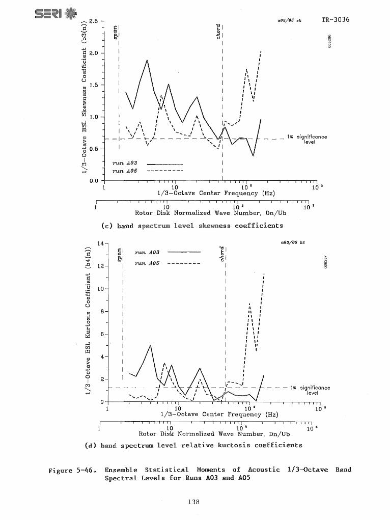
.......... 2.5 m03/05 sk TR-3036

......... E-M ..a .........-..., d 2.0 Q) .... 0 .... ..... ..... Q)

0 u fI)

1.5 fI) Q)

~ Q)

.!4 Cf.l 1.0 ....:J Cf.l o::l Q)

t> <t:I ..., 0.5 0

0 I

M '-.. ..-f

0.0

I 1

;1 ~I

-1-

, I, .. 1 ,

~/- \

run A03

"t:31

~I (.)

1

1 , , , , , ~ , , \ , ,\ , , , , , " , " , '! ,

I , ,

run AOS ---------

10 10 I

1/3-0ctave Center Frequency (Hz)

1% significance level

10 :I

I Iii I iii iii iii i I II 10 :3 10 10 I

Rotor Disk Normalized Wave Number. Dn/Ub

(c) band spectrum level skewness coefficients

14 m03/05 kt .......... Sl "t:31 ......... run A03 E- ~I ~I ~ -.::f4 run AOS

(.) N

e 12 I ..... _------ I co 0 0

..., I . d I Q) , .... I 0 10 ...... I ..... ..... I Q) I 0 I

U , 1\ I

.~ 8 "

, " I

fI) I I

, 0 ...,

" I

s... , , I :;:I 6

, , I ~ I I'

....:J I " Cf.l I " o::l I ,

4 I

(I) I t> I ltS , ...,

I 0

0 I

I 2 I

~ N co o o

C'J 1,:::"-:.:,,.'_ - - - 1% significance ~ ..-f level

O~----'---'-'-TlrrTT'-~~'--T~~-'''''~---'--~~~~~~

I 1

1

(d) band

10 10 II

1/3-0ctave Center Frequency (Hz) iii iii Iii iii Iii

10 10 I

Rotor Disk Normalized Wave Number. Dn/Ub

level relative kurtosis coefficients

10 :I

iii

10 :3

Figure 5-46. Ensemble Statistical Moments of Acoustic 1/3-octave Band Spectral Levels for Runs A03 and A05

138

E ...... ..c OJ

100

80

60

I 40

20

o 180

Run A03 Ri -0.12

220 260 300 340

Wind direction (deg)

S-41ae Detailed Profiles

100

80

E 60

......

..c 0)

Q)

I 40

20

o

-

7

for Runs A03 and AOS

Run A03 Ri = -0.12

8 9 10 11 12 13

Wind speed (m/s)

Figure S-41be Detailed

139

14

TR-3036

co

] Wave layer

~ 0 0

1 Wave layer • Run AOS Ri =+11.7

200 240 280 320 360

Wind direction (deg)

•

Run AOS Ri=+11.7

S 6

of Wind

of Wind Direction

m co N co 0 0

7 8 9 10 11 12

Wind speed (m/s)

for Runs A03 and AOS

20

o 301

•

302 303 304

Potential temperature (K)

TR-3036

305 297 298 299 300 302

Potential temperature (K)

Figure 5-41c. Detailed Vertical Profile of Thermal Structure (Potential Temperature) for Runs A03 and A05

Low-to-Moderate Wind, Slightly Stable versus Low-to-Moderate Wind, Slightly More Stable Inflow Conditions. Finally, Runs Al4-1 and A14-2 give us the opportunity to examine the acoustic effects of inflows with similar wind speeds but with subcritical (Ri <0.25) and above-critical stabilities. The normalized axial and upwash spectra are shown in Figure 5-50. The mean BSL spectra of Figure 5-51a shows what may be described as a rotation about the 10-Hz band; i.e., the A14-2 run emits higher levels below 10 Hz but less than the A14-1 run above 10 Hz. The characteristic inflow length scales (I x, I x, and I Z) listed in Table 5-4 indicate that the lengths associated ~ith ~he more ~table run (A14-2) are approximately half those of the less stable run. In particular, the in-plane scale length Iwz is only 6 .. 1 versus 16.5 m, respectively. Thus, this demonstrates that the effect of increasing the stability above the critical is to decrease the characteristic turbulence scales. This has the effect of increasing the LF acoustic output below 10 Hz while decreasing it above 10 Hz.

The <b2> spectra, plotted in Figure 5-51b, indicate that some form of a wide­band dynamic process is present at the lower stability which produces harmonic aeroacoustic excitation. The frequency shifts in the <b3> and <b4> spectra in Figures 5-51c and d are quite evident" The shift toward smaller turbulence scales appears to be illustrated by the growth of the peak in the 20-Hz band and the decrease in those below 10 Hz for the more stable run" A comparison of these two runs has given clear evidence of the role of varying stability conditions under similar mean loads.

140

TR-3036

100

a; N

~ co 0 0

::l ~ c -2/3 slope ----

::J

(J)

C ---+-' c· (l) C

10-1 0 Q.

E 0 ()

Reduced frequency (f = nz/U)

100 N (J) N co 0 0

N*

::l ......... .--. C

3: 10-1 (J)

C

+-' C (l) C 0 Q.

E 0 10-2 ()

cti ()

:;::; \,...

(l)

>

10-3

10_1

Reduced frequency (f = nz/U)

vertical turbulence

Figure 5-48., 45-m Turbulence for Runs All and A18

141

,...... N ::r:

"'--III "d '-' -,...... ~ '-'

Po. tt1 e

..... (l)

~ (l) ~

8 :;j J.4 ~ 0 (l)

Po. rn "d d tt1

III

d tt1 (l)

::!I

-,...... .E.. C\l e

80 I fll.1II/tt ""1111 TR-3036

~I al ~I C')

~I OJ

(.)1 N co 0 0

1 70 1

I I

60

50

40 run A 18

runAH -----"""" ..... _-

304-----~~_.~" .. rr----.__._.II_rTlTl----.__.--II_.TT~

I 1

1.0

1

~I

~I 1

10 10 II 10 II

1/3-0ctave Center Frequency (Hz) I i I Iii iii I II I iii iii

10 10 II 10 II

Rotor Disk Normalized Wave Number. Dn/Ub

(a) mean band spectrum levels

fll.tII/1 t C011

d 0.8 1

'<t OJ N co o o

(I) ..... 0 ..... --(I) 0 u (I) 0 d tt1

'i:: ro :> ~ U)

CIl (I)

P-ro ~ 0

0 I

C"1 "'--..--i

0.6

0.4

0.2

0.0 1 10 10 II

1/3-0ctave Center Frequency (Hz) r-- I I I I I I I I I I I II I I

1 10 10 II

Rotor Disk Normalized Wave Number. Dn/Ub

(b) band spectrum level variance coefficients

10 l!

I II

10 l!

Figure 5-49. Ensemble Statistical Moments of Acoustic 1/3-0ctave Band Spectrum Levels for Runs All and Al8

142

Figure

.-.. 2.5

£ t"J

e ...., ~ 2.0 '0 ..... ..... ..... cu o u I'Jl 1.5 I'Jl cu ; cu ~ rn

cu P-cd ...., (.)

0 I

t"J

""'-.-I

1.0

0.5

0.0

I 1

14 .-.. .--3 -.:J4 e 12 ...., t:l II.l '0 10 • .-4 ..... ..... II.l 0

U

.~ 8

rtl 0 ...., s... ::1 6 ~

~ rn CO

II.l 4 :> «:I ...., CJ

0 2 I C'J

""'-.-I

0

I 1

1

)

1

mtl/lt 11111: TR-3036 51 ~I

I I

~I

~I (.)

I

- 1- - - - - - - - - - - -

run AtB

run At t

10 10 I

1/3-0ctave Center Frequency (Hz)

l() (J> N co o o

1~ significance level

10 :II

j I I I I I I I I I II I I I I II

10 :II 10 10 I

Rotor Disk Normalized Wave Number. Dn/Ub

band level skewness

m18/11 11:'1

51 1!1 , run AtB

~I I

~I ,

(.) I run At t ----- - I I , ,

I I , , f , , , • I , I I I I I I , I I I I I

I I ,

<0 (J> N co 0 0

, significance

level

10 10 II 10 :II

1/3-0ctave Center Frequency (Hz) I I I I I I I I I I I I I i I I II

10 10 II 10 :I

Rotor Disk Normalized Wave Number, Dn/Ub

) band level coefficients

Ensemble Moments of Acoustic Ill-Octave Band Levels for Runs All and AlB

143

;;-~

II , ~-~

N* :::l

.........

C

::J

(f)

c +-' C Q.) C 0 a. E 0 ()

~ c "0 :::l

."!:: 0) C 0 -l

100 I'-en ~ 0 0

-2/3 slope

10-1

A14-1

10-2

10-1 100 101 102

Reduced frequency (f = nz/U)

(a) longitudinal (axial) turbulence component normalized spectra

c

of 10-1

C

+-' C Q.) C o a. E 8 10-2

~ ()

+-' ~

Q.)

> A14-1

-2/3 slope

00 en ~ o o

10-3L-__ L-__ ~-L-L~ __ ~ __ -L~~~ __ ~ __ ~ __ ~~

10-1 100 101 102

Reduced frequency (f nz/U)

(b) vertical turbulence component normalized spectra

TR-3036

Figure 5-500 Normalized 45-m Turbulence Spectra for Runs A14-l and A14-2

144

1

80

70

60

I I I

'" I

~I

~I °1

I I I I I I

TR-3036

0> 0> C\J eX) o o

.304---~~-r~·~·~~'---·~--~~'-~~.----r--.-.-~~~

1

1.0

1

1 10 II

)

145

o o C') eX) o o

Band

_2.5

3 C"J

e ...., ~ 2.0 .~

(J .~

OM OM Q)

o u

Q)

:> cd ...., (J

0 I

C"J

0.5

'---. ......

0.0

I

1

(c)

14 -----... ~

"'" e 12 ...., d Q) .~

(J 10 .~ OM OM Q)

0 U

fIl 8 .~

fIl 0 ...., I-. ;::I 6 ~

o-J (f)

OJ

Q) 4 :> cd ...., (J

0 2 I C"J '---. ......

~I

~I "t91

~I (.)

1 1

-1- ------

run A14-1

run A 14-2 ---------

1 10 10 II

1/3-0ctave Center Frequency I I I I "I I I I I II

10 10 II

Rotor Disk Normalized Wave Number,

TR-3036

0.14-1/14-2 1111:

1S!S

(Hz) I I

Dn/Ub

o C') co o o

significance level

10 II

I II

10 II

band spectrum level skewness coefficients

0.14-1/14-2 kt

el "t91 run A14-1 S

~I ~I N 0

run A14-2-------- C')

1 1 co 0 0

1

I ~

" " " I, ' , I , I , I , I I I , I I

I , I I

- - - - - 1S!S significance level

O~--~--~~~~~-----'--'-~~TTnr~--'--'-''-ITTn

I 1

) band

1 10 10 II 10 :I

1/3-0ctave Center Frequency (Hz) I I I I II I I I I /I I I I I I I

10 10 II 10 II

Rotor Disk Normalized Wave Number, Dn/Ub

level relative kurtosis coefficients

Figure 5-51. Ensemble Statistical Moments of Acoustic l/J-octave Band Spectrum Levels for Runs A14-1 and A14-2

146

5 .. 1 .. 1 .. 5

TR-3036

Relationship of Inflow Spectral Characteristics to the Mean LF Acoustic Spectrum

We attempted to relate the spectral characteristics of the reference level (45-m) axial (longitudinal) and upwash (vertical) turbulence to the shape of the acoustic mean BSL curves.. One immediate problem confronting such a com­parison is that the acoustic sources,. while perhaps generated by a linear dynamic process, are rotating within the surface boundary layer. The turbu­lence measurements, on the other hand, have been made at a fixed location, although within the rotor disk layer0 What is needed is to provide a scaling quantity to allow conversion from the fixed position to the rotating plane. We suggest the following ing space-frequency transformation:

(5-3)

where n' is the estimated cyclic frequency in rotating space (as seen by the rotor), n is the frequency space coordinates, n is the rotor rotation rate, Ro is the effect span), and I Z is the vertical or upwash turbulence Equatl'on 5-3 adjusts the fixed-position cyclic the former by the equivalent of the time span and quasi-horizontal) to traverse the stic vertical turbulent scale.. This transformation factor averages about 6 .. 4 for a mean Iwz of 9.8 m for the 1983 experimental data set.. Thus, a feature occurring at a cyclic frequency of 1 Hz in fixed coordinates would be est at 6.,4 Hz at span in the rotating frame for Iwz of 9.,8 m ..

The approximation of allows us to plot the acoustic pressure and inflow turbulence on the same with abscissa values of n (acoustic) and n' (transformed turbulent) 5-52 through 5-57 plot each of the six mean, acoustic densities observed in 1983, <S (n», with the corresponding 45-m axial, S (n e

), and upwash or in­plane, Safn'), mean turbulence spectra in logarithmi~ coordinates. A second abscissa w is also which i scaled in terms of the rotor convection wave number normalized the disk ion of Dn/Ub , where D is the rotor diameter and Ub the rotor veloci at the 75% span station (63 mps).. The wave number to the chord dimension at this span location is on the plots.. A line with a -5/3 slope is also included in these plots as a reference to the spectral slope as v1ith the turbulent inertial A turbulence spectrum with a -5/3 slope is necessary, but not to the isotropy of the inertial range.. An ion of these reveals, in , that

(1) There 1S a small t spectra in the vicinity of the rotor also seems to coincide with the (indicated the two turbulence parallel) and

in the mean acoustic pressure chord length which

1 turbulence region component spectra becoming

(2) The roll-off of the mean acoustic pressure spectrum approximates a -5/3 slope for reference wind speeds below about 10 mps.

147

/,-~

II I \l_~

TR-3036 10

, -5/3 slope 1 , , , , , , tj

" , 10 -1 ~ , , , , , til

4 Ul I:l

10 -I ~ ~

l!1 ' Sap(n) ~I

10 -'~--~~~~~~--~--~~~~~--~~~~~T---~~~~~~10-4 10 -1 1 10 10 II 10 :I

Cyclic Frequencies, nand n' (Hz) I

10 -1

I II1II iii I i III I I I i I II i i

1 10 10 III

Rotor Disk Normalized Wave Number, Dn/Ub

iii I 11 10 :I

.....;.

(") o (") <Xl o o

Figure 5-52 .. Relationship of Mean Acoustic Pressure Sap{f) to Su{f') and Upwash Co~ponents for Run A05

Distribution Turbulence

Su(n')

, -5/3 , " ,

"-

"

10

1

, tj

" " 10 -1 ~

" " " " "

til

4 Ul I:l

10 -1~ ~

I I I

"ttl ~I CJ

Sap(n)

10-·~--~~~-rrrnT---'--'-r1~In.---.-'-~rrrn~--'--'-'1I11~10-4 10 -1 1 10 10 III 10 II

Cyclic Frequencies, nand n' (Hz) I

10 -1

1111'1 iii 1111( I Ililif I I

1 10 10 III

Rotor Disk Normalized Wave Number, Dn/Ub

'" "1 10 II

.....;.

Figure 5-53.. Relationship of Mean Acoustic Pressure Spectral Distribution S ~(f) to 45-m Axial S (f') and Upwash S (fU) Turbulence a u w Co ponents for Run A03

148

'N'10 -1

::r:: ~

Cd

& ,........10 -II

-E.. Q, Cd

rr.l

W S 10 -3

(Il (Il

W f... 0..

C,) :;j 10 -4 (Il

;:1 o C,)

-< "d W 10 -II

~ I f... Cd ~

I 10 -1

'N'10 -1

::q

~ a:J e

11 10 -8

(!)

~ 10 -3

CIl CIl (!)

J... ~

:3 10 -~ CIl ::1 o CJ

<I!

"t:I W 10 -8

i;;:: I J... a:J

(::L,

Su(n')

Sw(n')

1 Cyclic

I IIIII

1 Rotor Disk

" -5/3 slope

" " " " " " " " "

10 10 II

Frequencies. n and n' (Hz) I I i I II I i I I j I II

10 10 II

"

run a14-t

" " "

Sap(n)

i j jiill

10 :I

Normalized Wave Number. DnjUb

Acoustic Pressure I) and

run 0.14-2 10

TR-3036

10

1

t::J 10 -1 ~

l'Jl ..... ("+

'<l

CJ.l ~

10 -Il~ t:3 .....;..

su(n'~

" -5/3 slope

to o (') CX) o o

" " " " " " Sw(n'

"

~I o ~I

" " " " " "

Sap(n)

t:I 10 -! ~

f!!. f'4" '< CJ.l ~

10 -8 ~ 'S' o

10 -B4----r-.-,,,"T1---r-.-.,-nnTl---.--rl~TTnT--_,--,_ITTTrrlr10 -.

5-55

10 -I 1 10 lOa 10 3

Cyclic Frequencies, nand n' (Hz)

I 10 -I

i i j Iii iii III1I i I I i ill I i Ii iij

1 10 lOs 10 3

Rotor Disk Normalized Wave Number, Dn/Vb

Acoustic Pressure Distribution ) and Turbulence

for Run

149

TR-3036 "'N10 -1 1""W"\ DotB 1:10 tt: t .po.

............ f- c.n ('q :3 .' a:S

~ Su(n') ()) ~ ,.........10 -II \. -5/3 slope "0

(l)

.E- o '- ("+

0.. \. '"'1 Id \. e'.. \. rf)

'-\. 0 (!)

\. 10 -1 ~ S 10 -3 '-

\. ~. tf) \. tf) ("+

(!) '- '<l I-. '-0.. \. ())

~ () 10 _si :;j 10 -4

tf) P :::1 --.::-0

()

-< S "d "0 W 10 -II 10 -5 ~

~ I N ............ I ~I Sap(n) ::r: I-.

~I N Id t::<.. C,)

10 -8 10 -4

10 -1 1 10 10 8 10 II

Cyclic Frequencies, n and n' (Hz) r I IIIII I I I I I I II I Ii IIII I I i I III

10 -1 1 10 10 II 10 s

Rotor Disk Normalized Wave Number, Dn/Ub

Figure 5-56. Relationship of Mean Acoustic Pressure Spectral Distribution S (f) to 45-m Axial S (f') and Upwash S (f') Turbulence ap u w Components for Run Al8

\. -5/3 SlOp63

\. \.

\. \.

\. \.

\. \.

\.

I

\. \.

\. \.

~I Sap(n) ~I

C,)

10

o 10 -1 ~

~. ("+

'<l

Ul ~

10 -lI-~ ::;---.::-

S "d

10 -9~ N

............

::r: N

10 -·~--~--~~~~,---.--r-r",,"---.--r-~IITr,---.--,-rTllTrr10-4 1 0 -I 1 10 10 II lOll

Cyclic Frequencies, nand n' (Hz) I

10 -I

11111/ I 1111111 "lil'l I I

1 10 1011 Rotor Disk Normalized Wave Number, Dn/Ub

I i I'I 10 a

Figure 5-51. Relationship of Mean Acoustic Pressure Spectral Distribution S (f) to 45-m Axial S (f') and Upwash S (f') Turbulence ap u w Components for Run All

150

TR-3036

5 .. 2

As previously stated, we at to compare the characteristics of the MOD-2 LF emissions before and after major modificat were installed. The changes that occurred between our 1982 data collection and that done in 1983 included modifying the schedule and talling vortex near the leading 70% the rotor span The primary objective of both modif 1 turbulent loads Unfortunately, we did not , hot-film anemometer data lable to us 1n ,. of the trumentation was the same for both years" Furthermore, the l!May 1982 runs tended to be more and those encountered in August 1983, as documented in Table 3-1 of overlap we needed to compare the

The lack new set From our wind

leas be a trend modified

5 .. 2 .. 1 Mult

trend to hi

We appl ied the same reduced 1982 and 5-5 as seal ANOVA analysi Richardson number inflow ctorso emission response 1982 the to-run band of interes A different Hz (k = 1), changes 1n variations are u' and the mean

us to identify a 1982 information"

li ,reference but only the var­used as a measure

information about the and no infor­

Because the overlap in limited, we were able to identify

Table 3-2 lists the mean wind speed,

Richardson number and the list the ranges of the

wind speed variance values observed, and condit listed in

in 5-58, with a table show, there appears to

mean emission levels above 10 Hz (in 1983) with the

I

1 1

Section 5 .. 1,.1,,2 to the listed in Table

and b present the results of an run-to-run ions using the

)l UH, and variance, u', as that the LF acoustics

than it was 1983 In , over the entire

inflow structure (Ri)" 1983 Below a frequency of 10

MBSL is explained by Above 10 Hz, the

with the variance,

TR-3036

Table 5-5. Overlap Ranges of Reduced 1982/83 Inflow Data Sets

Parameter 1982 Ranges 1983 Ranges

Richardson number -0 .. 01 to +0 .. 75 -0.12 to +0 .. 71

z/L parameter -0 .. 01 to 5 .. 62 -0 .. 12 to 5 .. 62

Hub-height wind -1 speed (ms ) 8.1 to 11 .. 9 8 .. 1 to 11.1

Hub-height variance (ms-1)2 0.24 to 3 .. 45 0.5 to 1 .. 31

M-O length L (m) 9 .. 5 to 638 -444 to 160

The relative spectral sensitivities to these three predictors for 1982 and 1983 are shown in normalized form in Figures 5-60a and be The coefficients of multiple determination, or r2' are also plotted as an indication of the applicability of the models in explaining the observed variation. It is quite clear from both figures that, at least for this choice of predictors, the vertical structure of the atmospheric inflow has the greatest influence on the spectral characteristics of the expected LF acoustic emission levels.. The 1983 MOD-2 configuration, with the incorporated pitch schedule and vortex generator modifications, displays a pronounced emissions level sensitivity to

Table 5-6 .. Comparison of Mean 1/3-0ctave Band Spectral Levels for the Conditions in Tables 3-2 and 5-9 for 1982 and 1983 Runs

Band 1982 1983 Center 1983-1982

Frequency <8(f» <8(f» Difference (Hz) (dB) (dB) (dB)

2.00 74 .. 2 73.8 -1.4 2 .. 50 72.4 72 .. 2 -0.2 3 .. 15 70 .. 9 70 .. 8 -0 .. 1 4.00 69 .. 0 68 .. 8 -0.2 5 .. 00 67 .. 7 67 .. 6 -0 .. 1 6.30 65 .. 2 65 .. 2 0 8.00 63.4 63 .. 0 -0 .. 4

10.0 61.4 61 .. 1 -0 .. 4 12.5 59 .. 0 59 .. 2 0.2 16.0 56.9 57 .. 6 0 .. 7 20 .. 0 54.8 55.6 0 .. 8 25.0 53 .. 2 53 .. 7 0 .. 5 31 .. 5 55 .. 2 54 .. 5 -0 .. 7 40.0 52 .. 1 52 .. 4 0 .. 3 50 .. 0 49.7 50.2 0 .. 5 63.0 47 .. 2 47.7 0 .. 5 80.0 43 .. 6 45 .. 4 1 .. 8

100 41 .. 7 43 .. 3 1,,6 125 39 .. 1 41.3 2 .. 2 160 37 .. 9 39 .. 2 1 .. 3

Mean: 0 .. 4

152

.--.. II) -0 -(J) () c (J) b (J) -~ -0 ...J

3

2

(f) 0 II)

C ct'l (J)

E -1 N co en T"""

c0 -2 co en

5-58

10 102

1/3-octave center frequency (Hz)

Q) o C') co o o

103

TR-3036

Band Level for 1982 and 1983

less stable flows below 10 Hz = 1) and just the opposite above that frequency to increasingly table flowse The 1982 conf ion, on the other hand, showed a lower overall stability sensitivity. In this case higher mean emission levels were as with less stable flows, reaching a peak in the 8-Hz frequency band.

The relative 1982/1983 normalized spectral sensitivities to the Ri, UH, and u' predictors are presented in Figures 5-61, 5-62, and 5-63, respectively. The much increased LF acoustic sensitivity to the Ri (atmospheric structure) in 1983 over that in 1982 is quite obvious in the presentation of Figure 5-61, suggesting a dramatic change in the responsible aeroacoustic mechanisms. The spectral sensitivities to the mean axial wind component, shown in Figure 6-62, supports the statement that the 1983 turbine was acoustically more sensitive to the mean attack angle below 10 Hz and less sensitive above that range. The plot of the variance sensitivities (k = 1) in Figure 6-63 seems to suggest that the 1983 rotor experienced a more stable boundary layer. This is indi­cated by the low turbulence sensitivity resulting in increased lift and higher radiated mean acoustic levels below 10 Hz over the 1982 data for the same inflow conditions.

5,,3 son of MOD-2 with MO~l LF Emi

The most dominant (and annoying) characteristic of the MOD-2 LF emlSSlons was their coherence or impulsiveness. We have developed several measures of the degree of coherence in wind turbine radiated emissions [1], including

The root-mean-square (rms) correlated 8- and 16-, 16- and 31.5-, and 31.5-and 63-Hz octave spectrum levels (CBSL) and corresponding correlation coef­ficient (Ccoef)

153

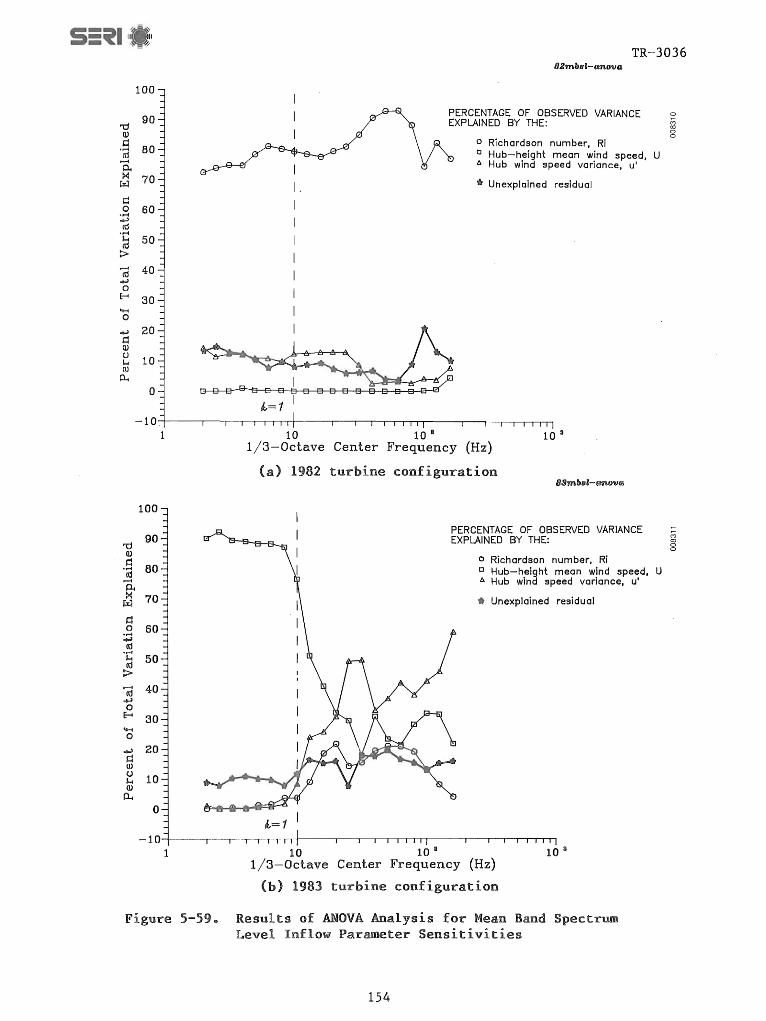
-/- "-II I ~ ~ - TR-3036

100

'U 90

Q)

d 80 • ..-4

It! ~

Q.. >< 70 w d 0 60 • ..-4 ~

It! • ..-4

l-4 50 It!

:> (tj 40 ~ 0

E-4 30 'H 0

~ 20 d Q)

CJ 10 l-4

Q)

p...

0

-10

100

'U 90

Q)

d 80 • ..-4

It! ~

Q.. M 70 w d 0 60

• .-4 ..., It!

• .-4

~ 50 It! :> ...-4 40 It! ..., 0

E-4 30 ..... 0

~ 20 d Q)

CJ 10 l-4 Q)

p...

0

-10 1

I.

1 t3---B---8-"9-SD DD

i=1 1

PERCENTAGE OF OBSERVED VARIANCE EXPLAINED BY THE:

o Richardson number, Ri o Hub-height mean wind speed, U t:. Hub wind speed variance, u'

.. Unexplained residual

10 10 III 10 a 1/3-0ctave Center Frequency (Hz)

(a) 1982 turbine configuration

Iv= 1 1

PERCENTAGE OF OBSERVED VARIANCE EXPLAINED BY THE:

o Richardson number, Ri o Hub-height mean wind speed, U t:. Hub wind speed variance, u'

.. Unexplained residual

10 10 III 10 II

1/3-0ctave Center Frequency (Hz)

(b) 1983 turbine configuration

Figure 5-59. Results of ANOVA Analysis for Mean Band Spectrum Level Inflow Parameter Sensitivities

154

o ~ co o o

~ co o o

20

10

o

... .s -10 o ..... "d (j)

6:: -20

"d (j)

.!::l -30

...-4 td e ... ~ -40

-50

2 R

u

1.00

0.75

0.50

0.25

-60·~----~--~~~~~+-----~~--~~~~----~---.-.-.~~~0.00

250

200

rfl 150 (l)

0.. 0 fjj 100 ... 0

-t=J 50 (J

:.a (l) ... 0 a..

"d (l) -50 N

...-4 ttl

e -100 ... 0 Z

-150

-200

-250

10 10 II 10 :II

Center (Hz)

) 1982

1.00

2 R

0.75

0.50

0.25

~----~--'-'-'-""+-----'--'--IIIT"nn-----.---.-.-..-,,~o.oo

1 10 10 1/3-0ctave Center Frequency (Hz)

1983

Inflow

155

Predictor Levels

10 II

for

TR-3036

N

;;; co o o

~ cry co o o

250

200

rJl 150 Q)

0.. 0

rn 100

l-t 0 ~ 50 CJ • ..-1

'"d Q)

l-t 0 0...

'"d Q) -50 N

• .-4 ...... «:I El -100 l-t 0 Z

-150

-200

-250

1983 Ri

1982 Ri

I 'k=t

I I I I I I Iii i I 10 10 I

l/3-0ctave Center Frequency (Hz)

TR-3036

I I I I 10 :II

"<t

;; co o o

Figure 5-61. Relative MBSL Spectral Sensitivity to Inflow Stability (Richardson Number) for 1982 and 1983 Configurations

2.00

1.50

rJl Q)

0.. 1.00 0 ......

[/)

l-t 0 0.50 ~ CJ

• ..-1

'"d Q) l-t 0.00

0...

'"d Q)

.~ -0.50 ...... «:I

S l-t ~ -1.00

-1.50

-2.00 --- I I I I

I 'k=1

I I I I I I II I 10 10 I

1982 Uh

1983 Uh

l/3-0ctave Center Frequency (Hz)

I I I 10 :II

l!)

;; co o o

Figure 6-62. Relative MBSL Spectral Sensitivity to Inflow Stability for Mean Hub-Height (UH) Wind Speed

156

We

I..t o

.pi (J

• pol

'1::::J CLl

10.00

5.00

0.00

rt -5.00

'1::::J CLl N

'M

Cd -10.00 S I..t o Z

15.00

Plot octave BSL

The observed and loS-Hz

increased in octave band phase relat to-band correlation or of annoyance of the affected structures simultaneous the same 18 on the conditions 1n consequences

5., .. 1

Table

to

1983 1.4.'

1982 1.4.'

w )

TR-3036

10

CD

~ <Xl o o

ions of the three

for the 8~, 16-,

of lveness or coherence ion of the adjacent

Thi indicated that a specific pressure field. The band­respons for the degree

it acoustically loaded the Therefore, we performed

em1S 10ns over the lable range of inflow them with those of the MOD-l and their known

octave band correlations for the available the reference 23- and 35-RPM

levels (CBSL) for the very three adjacent band

coefficient (Ccoef), however is not par-blade-to-blade passage ion in the

In 23-RPM case, on the other hand, the lower in frequency

sage )0 The coherency

157

TR-3036

Table 5-1 .. Statistical of Correlated or Coherent Octave Band Spectrum Levels Measured On-Axis at 1 .. 5D for 1982/83 MOD-2 Data Runs Compared with the MOD-1 Turbine at 35 and 23 RPM

Correlated Octave Band Spectrum Level

Run

MOD-2,

8T23-1 8T21-1 ST19-1 ST17-2 8T26-1 ST27 ST25-1

MOD-2

A05 AD3 A14-1 A14-2 A18 All

MOD-l

35 RPMc

23 RPMd

1982

8/16Hz CBSLa/Ccoefb

(dB/Hz)

44 .. 1/0 .. 645 57 .. 7/0 .. 464 5906/0 .. 705 7407/0 871 65.8/0,,768 6708/0 .. 776 75.2/0 813

55.1/0 .. 358 58.9/0,,712 52.3/0 .. 330 54.3/0 .. 466 65.6/0 .. 780 6607/0 776

70.8/0 .. 540 71.2/0 .. 825

16/31.5-Hz CBSL/Ccoef

(dB/Hz)

39.1/0 .. 768 53 .. 4/0 .. 564 48.9/0.258 69.4/0.869 5601/0.412 6009/0 .. 677 7004/0.735

51 .. 3/0.407 47.6/0 .. 270 46.8/0.174 46 .. 3/0.260 57 .. 3/0.631 59.2/0 .. 723

72.9/0.663 66.2/0.773

aCorrelated band spectrum level. bBand pair correlation coefficient ..

31.5/63-Hz CBSL/Ccoef

(dB/Hz)

33.4/0 .. 865 47 .. 0/0 .. 525 43 .. 5/0 .. 292 59 .. 9/0 .. 733 49,,3/0 .. 469 50 .. 4/0 .. 375 61.8/0.751

40 .. 5/0 .. 097 41.6/0 .. 194 46.1/0.352 41 .. 7/0 .. 273 47.6/0 .. 347 49 .. 0/0 .. 409

67.7/0.571 58 .. 1/0 .. 809

CExtreme level of interior annoyance in homes at 1 kIn. dModerate level of interior annoyance at 1 kIn ..

Hub Wind Speed (mps)

6.3 9.3

10 .. 3 11.7 12.0 13.3 14.2

7.3 8.1 9.0 9.9

12.4 13.6

17.0 13.9

Richardson Number

24 0,,46 0.18

-0.01 0 .. 13 0,,42

-0 .. 92

11 .. 7 -0 .. 12

0 .. 13 0.26 1.25 6.68

Stable Stable

actually exceeds (as indicated by the much greater correlation coefficients) that of the 35-RPM case, with slightly more correlated energy in the 8/16-Hz band pair than for the higher rotation rate.. We believe this is the reason that slowing down the rotor did not give the affected residents complete relief from the impulsive annoyance ..

We found that the annoyance threshold was reached when the impulse, measured outside an affected horne, in the 8/16-, 16/31.5-, and 31 .. 5/63-Hz CBSL simul­taneously exceeded 52, 47, and 35 dB/Hz, respectively, with associated cor­relation coefficients of 0 .. 200 or greater [1]" These figures correspond to CBSLs of 73, 68, and 56 dB/Hz at the reference distance of 1.5D (91.5 m) from the turbine, assuming only geometric spreading for propagation. We know that sometimes the combination of terrain and atmospheric focusing raised the level at one or more of the homes as much as 25 dB above the equivalent value that

158

would be expected from MOD-1 to other subsequent

5 3,,1.2

While not a use of poses"

environment

es 1n function of band rs

..... c ~ 60 (J)

.!:

8 55 (j)

"'0 C a:J .0

159

TR-3036

Thus, we can use the documented annoyance factor of the MOD-2 and

s or coherency, the comparati ve pur-

statistics: (1) the (2) level expressed in terms

ime criterion The percentile

values to identify values, which Thus, the LID

time The dif­the impulsiveness or

contribute to the noise

as a adjacent octave

corresponding MOD-l

rpm

75 (j) >

70 ~

E ::l 65 I-+J l) (1) Q.. 60 en +J

c,.-... 55 (1) N

I-I (1) .......... .em 0-0 50 l) ........

en "0 c 45 Cd

..Q

N 40 I ,-CV)

35 .......... <0

304

Figure 5-65 .. 1982

70 (j) > 65 ~

E 60 ::l I-

+J l) (1) 55 Q.. en +J ___

C N 50 ~I (1) ..........

.em 45 0-0

l)----

en "0 40 C (\j

..Q

N 35 I CV)

30 <0 .......... ,-CV)

25 4

TR-3036

/ / e 35 rpm co

/ ;;; D./'

co 0

° "/ 0

/ /~23 rpm

/ ,/'

,/' ,/'

,/' ,/'

D,/' /

6 L-0

6 /'

,/' / 1982 0---/

,/',(j 1983 6 / MOD-1 E9 /

6 8 10 12 14 16 18

Hub-height wind speed (mps)

son of .. 5-Hz CBSLs va .. Hub-Height Wind Speed for and 1983 MOD-2 Configurations and MOD-1 Turbine

/ /

/ ./'

/0

./

~/ /

6 8

1982 ° ---1983 6 ---

MOD-1 E9

Hub-height wind speed (mps)

5-66 of 31 .. 5/63-Hz CBSLs vs. Hub-Height Wind Speed for 1982 and 1983 MOD-2 Configurations and MOD-1 Turbine

160

values for 23~

plot" We bel reflects 1n vortex generators and the

emissions are les coherent below that were , the 1

the vortex

values

are

1

TR-3036

also included in each of the two trend lines

c response caused by the It is clear that the

mps and slightly more of whatever instabilities

to be much ID1te improvement

sSlons by adding

s (the wind speed and

and correlation , there is a

of the

years and com­of the

scales are radiated coher­

ionship to the scale length,

ile or L cases 1n

is clear why wi th the MOD-l

iveness associated with between the L10 and Leq

1983 MOD-2 results$

exceedence results run (ADS), which

Ala) between 60 and than those of

~-Je bel ieve

structural three param­

pressure in the chord and flap­measured on the 7% span)" The

time

<D Q. o

....... :!::: C ::I

.......... N I .......... II) "0

<D Q. 0 u; +-' c <D ()

~ ..... <D 0 ()

10

--_--0

--o --7-1::r------:::JI.d_--.....

0-:-.... :: .. : .. : ... : ... :....:...: .: .... :::.:.;,.c..:....:." • : ..... : .. : •• - • - - •••••••••••••••••

-10

-20

-30

Predictors

Richardson number 0

M-O z/L parameter 0

Hub-ht. wind speed ~

Hub-ht. variance "

1982 ---1983

-40 L-~ ________ ~ ____ ~ ____ ~ __ ~ __ ~~~~~

10 102

Octave band pair center frequency (Hz)

cOlmD.~r]SOn of inflow predictors on CBSL

0.4

0.0 . ..................... /'

,,--/'

/' ~-,/'"

-0.4 ' /' / ,/'" ,,/ / /

/ /

-0.8 / / Predictors /

b Richardson number 0

-1.2 M-O z/L parameter 0 1982 Hub-ht. wind speed ~ 1983 ---Hub-ht. variance "

-1.6 10 102

Octave band pair center frequency (Hz)

o C\J C') co o o

N C') co 0 0

TR-3036

of inflow on the adjacent octave band Ccoef

5-67 son of Inflow Predictor Sensitivities on Adjacent CBSLs and Ccoefs for 1982 and 1983 Turbine Configurations

162

Table 5-8

Octave Band

(Hz)

6

16/ 1 5

es first zero

mult Table 1 each

rotor

1 /63

MOD-2

1982

474

7

1

TR-3036

Correlated Set of

MOD-l

1983 23 RPM CBSL/Ccoef

(dB/Hz)

58 8/0 70 71.,2/0 .. 825

50

43

7/0 355

225

66 .. 2/0.,773

58,,1/0,,809

sociated wi th the to space coordinates

the 87% span station .. ) correlations found for

runs

span station, the pro­chordwise moment ,. normal and

of 65-75 ms, meters in space. Thus,

characteristic spatial effec on the unsteady

C ::::l

......... N I ......... CO "'0

(l) Q.

o (f) -c

3

2

o

(l) -1 () --(l)

8 -2

~~~~d8==~~~~ ..................... . o Predictors

Richardson number o Reference wind speed 0

lux scale length t:".

Iwx scale length \7

"lwZ scale length •

N N C') co o o

TR-3036

-3 L-__________ -L ______ J_ __ ~~ __ L__L __ ~J_~

0.10

---§ 0.05

......... N I ......... OJ "'0

(l) Q.

o

-c (l)

()

~ -(l) o o

0.00

-0.05

10 102

Octave band pair center frequency (Hz)

of inflow predictors on adjacent CBSL

X:;;:;~;:::;:;:::;::::~~;:::::::;::::====~ ................... . Predictors

Richardson number 0 Reference wind speed 0

lux scale length t:".

Iwx scale length \7

Iwz scale length •

~ C') co o o

-0.10 '--_____ --L-___ .L.-_--1_--1_--'---.JI....--....I.--...I--l

5-68

10 102

Octave band pair center frequency (Hz)

of inflow predictors on adjacent band Ccoef

of Inflow Predictors on Adjacent CBSLs and Coefficients for 1983 MOD-2 Configurations

164

Table

Octave Band Exceedence Levels {conditional on 8-Hz band level}

Octave Band Criteria

8-Hz BSL >60 dB/Hz >65 >70

l6-Hz SSL <,

315Hz BSL

Octave (Hz)

16=Hz L10 L20 Leq

3leS-Hz L10 L 20 Leq

63-Hz

1982 (Percent

81 47 21

80 1

14

81

81

)

59 7

54

49 48 47

165

of 1983

time

88 50 13

88 85 44 7

88 88 88 58

BSL

TR-3036

Band Exceedence Table 3-2 and the

MOD-l BSL exceeded)

100 82 60

100 100 84 66

100 100 100

72

BSL (dB/Hz) (dB/Hz)

68 81 66 79 63 70

61 76 60 74 58 66

56 67 55 64 54 57

50 58 49 57 48 50

TR-3036

Table 5-10. Exceedence Level for 1983 LF-Range Octave BSL Values

Run Percent of Time Exceeded Number

8-Hz Band BSL > 60 dB/Hz BSL > 65 dB/Hz BSL > 70 dB/Hz

ADS 97 54 4 A03 83 40 8

A14-l 77 24 3 A14-2 94 48 7

Al8 99 84 46 All 99 87 51

l6-Hz Band BSL > 55 dB/Hz BSL > 60 dB/Hz BSL > 65 dB/Hz

ADS 95 54 1 A03 76 32 1

Al4-l 76 36 3 A14-2 87 24 1

A18 98 75 28 All 99 80 27

3). 5-Hz Band

BSL > 45 dB/Hz BSL > 50 dB/Hz BSL > 55 dB/Hz

ADS 97 97 73 A03 83 83 43

A14-1 77 77 63 A14-2 94 94 27

Al8 99 99 77 All 99 99 84

166

Table 5-11 ..

Chord Moment Flap Moment Run No 1 1 tc

(m) (ms) (m') (ms)

A03~1 " 1 69 .. 5 5 .. 2 71,,0

A05 3 72 3 5 .. 7 0

A03 4 62 5 .. 73 ° 1 8 65 5 74 .. 6

.. 7 1 5 .. 72 7

1 73@0

8 7 1 7

All 4 8 66 0 5 8

8 4

021

Normal Force

1 tc (m) (ms)

4 .. 4 59 .. 6

5 0 68,,0

4 7 64 .. 8

407 64,,5

5 5 75 .. 0

4 .. 7

5,,1 70 .. 3

5 8 80 .. 0

5 4 73 .. 6

° 74 10 2

167

TR-3036

Scales for Four

Acoustic Pressurea

Ri UH 1 No .. (mps)

(m'1 tc

(ms)

4 .. 4 60,,5 0 .. 26 6 .. 9

4 .. 6 63 .. 3 12 7 .. 3

5 ° 68 .. 4 -0,,12 7e9

4,,6 62 .. 9 0 .. 13 8 .. 2

4 .. 8 65 2 0 .. 26 9 .. 9

4 .. 8 66 .. 0 0 .. 71 10 .. 3

407 64,,5 1.26 12 .. 9

4 .. 5 62 .. 5 6,,68 13 6

TR-3036

6®O MEASURING THE ANNOYANCE POTENTIAL OF A SINGLE MOD-2 TURBINE

Given our experience with the MOD-l downwind turbine near Boone, N. Co, sum­marized in Ref .. [1], the desirability of assessing the potential of MOD-2 emissions for interior, low-frequency annoyance problems in nearby homes is very important. Several approaches to assessing this annoyance potential are available to us and include

(1) Comparing the known physical properties of the radiated acoustic pressure fields at a specified reference distance from the turbines

(2) Assessing the interior annoyance potential from measurements of the MOD-2 emissions and compar1ng them with documented low-frequency annoyance situations.

The first of these was addressed to some extent in Section 5.3 and is expanded a bit more in this section. The real crux of the matter, however, lies with item (2), since the human element (ieee, the ultimate receptor of any annoy­ance) must somehow be brought into the equation. On this latter point, though considerable study has been done around the world, we have only a meager scientifi data base on exactly what constitutes interior low-frequency annoyance and what conditions must be present for it to occur. Human annoy­ance from low-frequency sound and associated stimuli is highly subjective by its very nature@ However, at some point the human element must be considered, and we have to do that in a companion study [7].. The results of that limited study have been applied to individual MOD-1 and MOD-2 turbine emlSS10n characteristics to estimate the potential for interior annoyance problems in homes near these machineso

1

In the previous section, we pointed out that the degree of impulsiveness or coherence in the MOD-l emissions was a major factor in the degree of annoyance described by occupants within 1-3 km (0.6-108 miles) of the turbine. This im­pulsiveness is manifested by a strong phase coherency in the radiated acoustic pressure field and can be measured by the degree of cross-correlation in the 8-, 16-, 31.5-, and 63-Hz octave band spectrum levels.. These four octave bands cover the structural resonance region of most home construction in the United States. Tables 5-13 and 5-14 showed that, with one exception, the MOD-2 emissions were much less correlated or impulsive than those of the MOD-1 running at 23 or 35 RPM.

The mean band pressure spectra of Figure 6-1 show an approximate annoyance envelope for the MOD-l at the reference distance of 1.5D. The upper curve (35 RPM) corresponds to the highest degree of interior annoyance at a far­field distance of 1 km and the lower one (23 RPM) to a moderate level.. The six available MOD-2 MBSL spectra are plotted over this envelope in Figure 6-2. As indicated, above the 5-Hz band all fall below the lower MOD-l curve. The fact that the two spectra associated with the highest winds do fall within the dotted area is insignificant, since this occurs below the lower structural resonance cut-off of 5 Hz. The 1982 MOD-2 case that we noted (Table 5-7) as having the potential to cause low-frequency annoyance is shown in Figure 6-3, overlaid on the MOD-l envelopee In this case, the MBSL spectrum falls

168

90

N 80 I "'-III -0

70 '-"

Q) >-~

60

50

-0 c (\j 40

.!:l C (\j Q)

30 ~ :2:

20 1

90

80

70 Q) >-~

60

50

-0 c (\j 40

.!:l C (\j Q)

30 :2:

TR-3036

'<t N (') 00 0 0

3S-rpm operation, maximum interior

annoyance

23-rpm moderate interior

annoyance

10 102

1/3-octave center frequency (Hz)

, "-

\ \

\ \ \

\ Run A11, -13.6 mps 0

Run A18, 12.4 mps 0

Run AOS, 7.3 mps

1/3-octave center frequency (Hz)

of MOD-1 Acoustic the 1983

1

169

U")

N (') 00 0 0

6-1 with A05) and

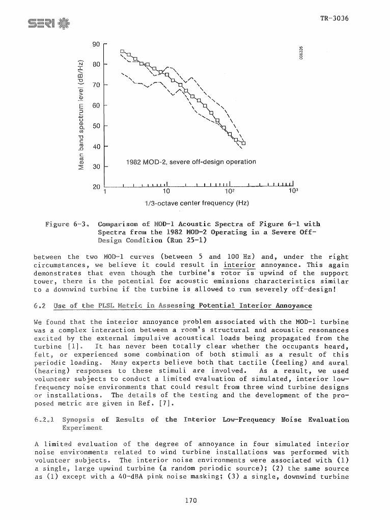
N I ........ CO "0 ........ Q) >

.SI2 E :J ~

+=' <.) Q) a.. C/)

"0 C ro .0

C ro Q)

~

6-3"

90

80

70

60

50

40

30

20 1

1982 MOD-2, severe off-design operation

1/3-octave center frequency (Hz)

<0 N (') co o o

COI~pclr]SOn of MOD-1 Acoustic of Figure 6-1 with from the 1982 MOD-2 Operating in a Severe Off-

Condition 25-1)

TR-3036

between the two MOD-l curves (between 5 and 100 Hz) and, under the right circumstances, we believe it could result in interior annoyance. This again demonstrates that even though the turbine's rotor s upwind of the support tower, there is the potential for acoustic emissions characteristics similar to a downwind turbine if the turbine is allowed to run severely off-design!

.. 2

We found that the interior annoyance problem associated with the MOD-1 turbine was a complex interaction between a room's structural and acoustic resonances excited by the external impulsive acoustical loads being propagated from the turbine [1]" It has never been totally clear whether the occupants heard, fel t, or experienced some combination of both stimul i as a resul t of thi s periodic loadingo Many experts believe both that tactile (feeling) and aural (hearing) responses to these stimuli are involved. As a result, we used volunteer subjects to conduct a limited evaluation of simulated, interior low­frequency noise environments that could result from three wind turbine designs or installationso The details of the testing and the development of the pro­posed metric are given in Refe [7].

2 1 of Results of the Interior Low-Frequency Noise Evaluation

A limited evaluation of the degree of annoyance in four simulated interior noise environments related to wind turbine installations was performed with volunteer subjectse The interior noise environments were associated with (1) a single, large upwind turbine (a random periodic source); (2) the same source as (1) except with a 40-dBA pink noise masking; (3) a single, downwind turbine

170

ing at 30 RPM (a turbines (a random impuls simulations, which were sys comparable to a small room of what they were

6,,2 1 1

The volunteers' responses terms of loudness

of

TR-3036

impulsive source); and (4) multiple downwind source)~ The volunteers listened to these

ly varied in intensity, in an environment cal home and provided written impressions

ient Estimator of

means of a five-level ranking in of annoyance and displeasure, any feel­

the sensing of any pulsations" Table 6-1 These ranked responses were then

low-frequency noise descriptors or suggested as measures of low-frequency

the following spectral

for Standards) propo ed weighting

Standards Ins itute} "Ii'ileight [23]

under 100 Hz for curves have been proposed c-range (less than 20 Hz)

was or developed to for pure tones at high sound

6-4, the ing" than the most common noise

Toki ta et al" [22] proposed two environments, the LSPL (low­

sound level)e The LSL ec three low-frequency noise

structural cal, and psychological complaint The L8L has been proposed as an appropriate descriptor for

interior environments that contain both and low-tic

regression; the results for the loud­s are listed in Table 6-2" Immediate­

of the five metric that contain significant low with the A-weighted scales The highest correlation

mean correlation coefficient of 0,,936 for We bel that the LSL weighting provides

the annoyance ial to persons exposed to low-in their homes"

171

TR--3036

Table 6-1" Environments Subjective Ranking Criteria

Stimuli Response Rating

Rank 0 1 2 3 4 5

Perception

Noise Can't Barely Weak, but Moderate High noise Very high Level Hear can hear definitely loudness level, loud noise level, (loudness) audible very loud

Annoyance/ None Barely Definitely Moderate Very Extremely Displeasure aware of aware of distraction/ annoying, annoying,

presence presence some irritating uncomfortable irritation

Vibration/ None Feel Definitely Moderate Very Severe Pressure presence feel vibration/ noticeable vibration

vibration/ pressure pressure feeling

Pulsations None Barely Definite Moderate Heavy Very heavy feel pulses or booming booming pulses, pulses bumping or or booms,

thumping thumps thumps -- ~ -- = = -- -- -- -- -- -- -- -- - -- - -- - -- -- -- -- -- - - - -- -- I- -- - - - -- - -- - -- -- - -- - -

Acceptable 77711717111111 Clearly unacceptable -- - -- -- -- - -- -- -- -- -- - -- - -- -----------

r--

20 N

~ 0 0

0 C co "0 A (i) -20 > ~ LSL, LSPL Q)

-40 C I-

::J U) U) Q) "- -60 Q.

"0 C ::J

-80 0 U)

Q)

> +-' -100 ~ Q)

a: -120

-140

1/3-octave center frequency (Hz)

6-4 Low-Frequency Noise Metrics Spectral Weightings

172

Ta.ble 6-2 ..

Metric

LSL

C

G1 LSPL

A

Noise Level

o 923

0 .. 91

o 891

0 ..

o 868

0.,307

TR-3036

versus

Annoyance/ Mean Displeasure

0 .. 948 0,,936

0,,938 0 .. 926

0 .. 920 0 .. 906

0 .. 913 0 .. 904

0,,887 0 .. 878

0 .. 270 o 289

Scale

The volunteer-con~ent four stimuli were summarized, and three final level for each" The ion threshold has been defined as the LSL value for an evaluation ranking of 1 .. The annoyance threshold s a ranking of 2,,5, and an unacceptable annoyance level ass of 4 or above The LSL values corresponding to the levels listed in Table 6-3 for the four stimuli evaluated.. As we can see in the upper ion Table 6-3, three of the four stimuli have sim-ilar threshold LSL values It is interest to note that even though many individually impulsive sources may be present, the net effect of a random sum­

two

odic source of an

6 2 .. 2 for

invokes a response similar to that from a random threshold is cons lower for a source con­

few impulsive sources" This is reflected by the of Table 6-3 ..

LSL Va.lues

Often we must predict the annoyance potential to a surrounding community from a new turbine or turbines before installation as part of the siting approval process" Since we will rarely have the opportunity to have actual measurements within residences, we needed to find a way to esti-mate or LSL levels ( low-frequency sound level or PLSL), given the stic low-frequency acoustic emission statistics of a given wind turbine design ..

Interior LSL Level

In order LSL levels, gl ven a representative external acoustic we needed to a typical indoor/outdoor acoustic transfer function for housing construction in the United States We identified a cal transfer function by using available data collected from two homes under MOD~l impul ive excitation, from five homes in Oregon experi-enclng sive, low-frequency acoustic loading (the exhaust stack from a gas turbine s [24]), and from an experiment utilizing a tandard~construction test home operated by SERIo We found that a different

173

TR-3036

Table 6-3e SERI Interior Low-Frequency Annoyance Criteria Employing the LSL Metric

Stimuli

Upwind turbines (random periodic)

Single or few downwind turbines (periodic impulsive)

Many downwind turbines (random impulsive)

Upwind turbines with 40 dBA masking

LSL Threshold Perception

(dB)

58

53

59

59

LSL Annoyance Threshold

(dB)

65

57

68

65

Considering Only General Source Characteristics

Nonimpulsive source 58 65

Impulsive source 53 57

LSL Unacceptable

Annoyance Level (dB)

68

60

70

67

68

60

spectral response is typical of homes undergoing impulsive loading (from the MOD-1 or a few downwind turbines) compared with random excitation (sources such as a single upwind turbine or many downwind ones)" Figure 6-5 plots these two typical transfer or acoustic transmissibility functions. As we can see, impulsive loading is characterized by much higher acoustic transmissibil­ities above about 10 Hz in comparison to random, external acoustic loads. The details related to the physics responsible for these curves are discussed in [1]. Using each of the transfer functions plotted in Figure 6-5, we modified and replotted the original frequency weighting of the LSL parameter in Figure 6-6" An interior estimate of the PLSL level is calculated by applying the appropriate weighting curve of FigQre 6-6 (impulsive or nonimpulsive) to an externally measured 1/3-octave band pressure spectrum.

6,,2.2,,2 Establishing a Reference External Acoustic Loading

The method of estimating a representative PLSL value requires a suitable measure of ~he external acoustic loading spectrum. Since most homes are located at some distance from the nearest wind turbine(s), a method must be devised to provide a reference spectrum that takes into account situations in which atmospheric refraction and surface reflection combine to increase the observed levels above that expected from spatial divergence alone. In order to achieve a Itfigure-of-merit lt PLSL value for a single MOD-2 turbine, a

174

(1) en c o 0. en (1) b

15

10

5

o

-5

-10

-15 1

6-5

20

(1)

> (1)

(1) b

:J en U) (1) l-

0. U C :J o en Q)

> cr; C5 a:

o

-20

-40

-60

6-6

10

\ \ \ \

Impulsive source

\ I", I L~_J \ A /

\ "'", \/ Nonimpulsive source

1/3-octave center frequency (Hz)

Original LSL definition Impulsive PLSL modification Non impulsive modification

1 /3-octave center frequency (Hz)

PLSL Measurements

175

co N C'l co o o

for

for

Ol N C'l co

'0 o

TR-3036

TR-3036

reference distance of 1 km (approximately 10D) was chosen. Table 6-4 lists the 1983 MOD-2 PLSL and PLSL10 values at the reference distance of 1 km propagated by spati~1 divergence alone and with an additional 15 dB of terrain/atmospheric focusing as a worst-case estimate.. The worst-case 1982 MOD-2 run (ST25-1) and the 35- and 23-RPM cases from the MOD-l are also listed for comparison in Table 6-4.

6 .. 3

community annoyance related to the acoustic emissions of a single MOD-2 turbine has two sources: (1) emissions in the high-frequency range generally heard outdoors or through open windows, and (2) interior annoyance arising from structural loading by acoustic energy in the low-frequency range.. We discuss both sources below ..

6 3 .. 1 from High-Frequency-Range Emissions

From the resul ts of our measurements of the high-frequency characteristics discussed in Section 4.0, we have reached the following conclusions ..

(1) The aural identification of a single turbine or a cluster of MOD-2 turbines as the source of HF, broadband sounds can be expected., on the average, 1.2-1.5 km (4000-5000 ft) downwind of the nearest turbine. This recognition distance depends on the state of the acoustic environment at the observer's location and the distance to the nearest turbine.

Table

Run PLSLeq Number (dB)

A03-l 37 AD3 41 AD5 39 A14-l 42 A14-2 40 A15-l 44 A18 43 All 43

Means 4T

1982 MOD-2 severe off-des

ST25-1

MOD-1 worst cases

35-RPM 23-RPM

56

65 54

Interior LSL (PLSL) Values at (1983 Configuration)

PLSLeq+15

(dB)

52 56 54 57 55 59 58 58

56

71

80 69

176

PLSL lO (dB)

39 43 44 45 43 47 46 46

44

60

68 58

1 kM from the

PLSL10+15

(dB)

54 58 59 60 58 62 61 61

59

75

83 73

TR-3036

(2) While the broadband sounds modulated at the blade passage frequency can often be distinguished above local acoustical background at distances exceeding 1 .. 6 km (1 mile) under the right atmospheric conditions (i"e .. , low wind speeds in the vicinity of the observer), there appears to be a very low probability of community annoyance from a single MOD-2 turbine at distances beyond 1 km (0 .. 6 mile).. Typical 1 levels measured at the Goodnoe Hills Site and 0 9 km downwind of Turbin~qNo" 2 were 43-45 dBA for representative recording periods of 6 hours, which included a wide range of inflow conditions.. The corresponding 1 10 and 190 levels were 53 and 43 dBA, respectively"

(3) A of narrowband (12 .. 5-Hz resolution) analyses of the high-frequency portion of the ed spectrum taken covering a range of inflow condi­tions showed no persistent tonal (discrete frequency) noise. This indi-cates that the noise sources are well controlled, making the rotor's aerodynamically sounds the dominant HF source

" .,2

Using the P1SL discussed in Section 6 .. 2, we concluded that the likeli­hood of interior annoyance result from acoustical loading produced by 1983 MOD-2 LF emissions on homes located a kilometer or more away is very remote. Even under the worst and propagation conditions (a home located where a 10n reflection and atmospheric refraction is

15 dB of enhancement), it is unlikely that the turbine would be detectable within a home with the windows closed a kilometer or more away ..

177

TR-3036

7.0 CONCLUSIONS

7 .. 1

At the Goodnoe Hills site, the average audible range of a single MOD-2 turbine was found to be about 1.2-105 km (4000-5000 ft). A polynomial which describes the average fall-off with distance for the Goodnoe Hills site is

Leq(A) = -3.89454 x4 + 46.6729 x3 - 191.884 x2 + 287.151 x - 28.4 ,

where L (A) is the equivalent sound pressure level in dB and x is the log10 of the ~gwnwind distance in feet. When multiple turbines were operating, the turbine noise level experienced by an observer is dominated by the nearest turbine"

The Leq(A) at a distance of 1.5 rotor diameters (1.5D, 137 m or 450 ft) from the roror plane was found to vary, primarily with the hub-height wind speed. This variation in dB can be expressed to within ±0.5 dB over a wind-speed range of 6-15 mls by

L (A) = 1/2 UH + 57 , eq

where UH is the hub wind speed in mise

A comparison of the 1982 and 1983 turbine configurations revealed an apparent upper-band-limiting of the 1983 emlSSlons as a result of the vortex generator installation and pitch schedule modifications.

No significant, steady tone noise components were found in the high-frequency­range narrowband (25-Hz) spectra. This indicates that the mechanical noise sources are well controlled, and there appear to be no discrete aeroacoustic sources of consequence.

7 .. 2

The varlances observed of the the ensemble mean and the first three statisti­cal moments of randomly sampled, low-frequency acoustic emission spectra in 1/3-octave band resolution were found to be adequately explained via a linear, multivariate regression model, with the following inflow scales as the most efficient predictors:

• A mean wind speed at a height within the rotor disk layer

The gradient Richardson number stability parameter (Ri) measured across the rotor disk layer

• The Monin-Obukov length scale, L

The vert ical or upwash turbulence integra}:~ scale, Iw Z 0

178

TR-3036

Comparisons made between the 1982 and 1983 emissions showed that the 1983 tur­bine was far more acoustically sensitive to inflow stability_

The physics of the rotor-turbulence interaction are such that unsteady blade loads are the most common source of radiated low-frequency acoustic emissions and much of the rotor aeroelastic response. We can achieve a high correlation with the former using bulk scaling measures of the inflow, so this technique might be successfully extended to the latter. This would allow a given rotor aeroelastic response to be expressed directly in terms of surface-layer tur.bulence bulk propert

The common origin of the rotor low-frequency acoustic and aeroelastic responses was demonstrated by space-time correlation measurements. We found that observed flap and chordwise bending moments, blade normal forces, and the 8-Hz band, acoustic pressures were similarly correlated over time periods of 65-75 mSe These periods suggest that the unsteady processes responsible for the fluctuations take place over a rotor travel distance of about 5 m for the MOD-2 blade

1 3

Measurements of the MOD-2 showed that the 1983 turbine configuration produced les coherent (impulsive) low-frequency acoustic radiation than the 1982 ver­sion and much less than the MOD-l turbine operating at ei ther 35 or 23 RPM under the worst impulsive conditions The degree of coherency (impUlsiveness) in the turbine emissions was found to be strongly related to the vertical atmospheric stabili (Richardson number), the vertical or upwash turbulence scale length, I z, and the blade loading, as indicated by the mean axial ve-

w locityo

It is clear in 1982, the MOD-2 rotor instabilities associated with unstable, high-veloci ty inflows were responsi ble for producing low-frequency acoustic emissions that resembled those of the downwind MOD-l turbine under the worst impulsive conditions A definite improvement was made in the levels and im­pulsiveness of the LF emissions by the addition of the vortex generators and pitch schedule changes

1 .. 4

While the broadband sounds modulated at the blade passage frequency can often be distinguished above the local acoustical background at distances exceeding 106 km (1 mile) under the right atmospheric conditions, there appears to be a very low probability that community annoyance will result from a single MOD-2 turbine in 1 ion beyond a distance of 1 kmo Even under the

propagat conditions (a home located where a combina-tion terrain reflection and atmospheric refraction produces 15 dB of enhancement), it is unlikely that the turbine noise would be detectable within a home with closed windows a kilometer or more away.

179

TR-3036

8.0 RECOMMENDATIONS

We strongly recommend that the techniques developed for the acoustic charac­terization of the MOD-2 Unit No .. 2 at Goodnoe Hills be applied to the one remaining MOD-2 turbine currently operating in California (Unit No.5).. This will permit the following to be accomplished:

(1) A verification of the atmospheric surface-layer bulk properties as accurate predictors of ensemble statistical distributions of low-frequency acoustic emlSSlons

(2) Comparisons of the statistically derived acoustic response functions for the Goodnoe and Solano Hills sites

(3) Detailed comparisons of the turbulent inflow properties for the two regimes.

We further recommend that the techniques developed for the MOD-2 turbine be applied to a range of wind turbine designs and sizes in order to isolate critical scaling parameters to be used in predicting acoustic noise and in developing control strategies.

180

9 .. 0 REFERENCES

1. Kelley, N.D., H.E. McKenna, ReR. Hemphill, CeL. Etter, R.L. N.C. Linn, Acoustic Noise Associated with the MOD-I Wind Source, Impact and Control, SERI/TR-635-1156, Golden, co: Research Institute (February 1985), 262 pp.

TR-3036

Garrelts, and Turbine: Its

Solar Energy

2. Hubbard, H.H., KeP. Shepherd, and FeW. Grosveld, Sound Measurements of the MOD-2 Wind Turbine Generator, NASA CR-165752, Hampton, VA: NASA Langley Research Center (July 1981), 29 pp.

3. Stephens, D.G.; K.P. Shepherd, H.H. Hubbard, and FeW. Grosveld, Guide to the Evaluation of Human Exposure to Noise from Large Wind Turbines, NASA TM-83288, Hampton, VA: NASA Langley Research Center (March 1982), 70 pp.

4. Shepherd, KeP .. , Detection of Low Frequency Impulsive Noise from Large Wind Turbines, NASA CR-172511, Hampton, VA: NASA Langley Research Center (January 1985), 23 pp.

5. Hemphill, R.R., An Acoustic Ranging Technique with Application to Assessment of Low-Frequency Acoustic Noise of Wind Turbines, SERI/TP-215-1954, Golden, co: Solar Energy Research Institute (May 1983), 10 pp.

6. Kelley, N.D., H.E. McKenna, and E.W. Jacobs, Observed Acoustic and Aeroelastic Spectral Responses of a MOD-2 Turbine Blade to Turbulence Excitation, SERI/TP-214-2374, Golden, co: Solar Energy Research Institute (June 1984), 7 pp.

7. Kelley, N.D. A Proposed Metric for Assessing the Potential of Community Annoyance from Wind Turbine Low-Frequency Noise, SERI/TP-217-3261, Golden, co: Solar Energy Research Institute (October 1987), 9 pp.

8. Simms, D .. A., N.D. Kelley, HeE. McKenna, and EeW. Jacobs, A Comparison of Micrometeorological Measurements Made from a Tethered Balloon and a Meteorological Tower, SERI Technical Report, in preparation.

9. Panofsky, H.A., and J.A. Dutton, _A_t_m_o~ _______ T_u_r_b_u_l_e_n __ c_e New York: John Wiley & Sons, Inc. (1984) 397 pp.

10. Homicz, G.F., Broadband and Discrete Frequency Noise Radiation from Subsonic Rotors, Ph.D. Dissertation, Ithaca, NY: Cornell University -::-( 1:-:9---7-::'""3 --) .----

11 .. Homicz, G"F .. , and AeR. George, Radiation from Subsonic Rotors," (1974), pp. 151-177.

"Broadband and Discrete Frequency J.. of Sound and Vibration, Vol.. 36

12 .. George, A.R .. , and S .. T .. Chou, "Comparison of Broadband Noise Mechanisms, Analyses, and Experiments on Helicopters, Propellers, and Wind Turbines," presented at AIM 8th Aeroacoustics Conference, Paper No. AIAA-83-0690, Atlanta, GA, 11-13 April 1983.

181

TR-3036

13. Monin, A.S .. , and A"Me Obukhov, "Basic Regularity in Turbulent Mixing in the Surface Layer of the Atmosphere," Trudy Geophys.. Inst. ANSSSR, No. 24, as referenced by J .. L. Lumley and H.A. Panofsky in The Structure of Atmospheric Turbulence, New York: John Wiley & Sons, Inc CD (1964), 239 pp.

140 Monin, A.S., and A.M. Yaglom, J.L. Lumley, ed", Cambridge, MA:

Statistical Fluid Mechanics, Vol. The MIT Press (1971), 769 pp.

I,

15. Businger, JoA .. , JoC. Wyngaard, Y. Izumi, and E.F .. Bradley, "Flux-Profile Relationships in the Atmospheric Surface Layer," J. Atmospheric Science, Volo 28 (1971), pp" 181-189.

16. Kaimal, J.C., "Turbulence Spectra, Length Scales and Structure Parameters in the Stable Surface Layer," Boundary-Layer Meteorology, Volo 4 (1973), ppe 289-309.

17. George, A .. Re, and Y .. N" Kim, "High-Frequency Broadband Rotor Noise," AIM Journal, Vol. 15, No.4 (April 1977), pp .. 538-545.

18" Hojstrup, J .. , "A Simple Model for the Adjustment of Velocity Spectra in Unstable Conditions Downstream of an Abrupt Change in Roughness and Heat Flux," Boundary-Layer Meteorology, Vol. 21 (1981), pp. 341-356 ..

19. Kelley, NoD .. , H .. E" McKenna, and R .. R .. Hemphill, itA Methodology for Assessment of Wind Turbine Noise Generation," J. Solar Engineering, Vol. 104 (May 1982), ppe 112-120.

20. Wyngaard, J" C" , "On Surface-Layer Turbulence," in Workshop on Micrometeorology, DoA. Haugen, ed., Boston, MA: American Meteorological Society (1973), pp. 101-149"

21. International Organization for Standardization (ISO), Draft Proposal for "Acoustics Methods for Describing Infrasound," ISO/DIS 7196, Geneva, Switzerland: ISO.

22. Tokita, Yo, A. Oda, and K. Shimizu, "On the Frequency Weighting Characteristics for Evaluation of Infra and Low Frequency Noise," Proc .. 1984 Confo on Noise Control Engineering, G.Co Maling, Jr., ~ Poughkeepsie, NY: Institute of Noise Control Engineering (1984), pp" 917-9200

23. American National Standards Institute (ANSI), "American National Standard Specification for Sound Level Meters," ANSI Sl.4-1983, New York, NY: ANSI (1983)"

24 Robin Towne, As soc., Envi ronmental Study of Low Frequency Noi se and Vibration, A Report to the Portland General Electric Co"' Portland, OR: Robin Towne Assoc (1974), 144 pp.

25. Kelley, N.D., A Detailed Examination of the Goodnoe Hills Microscale Turbulence Structure and Its Impact on Aeroacoustic Noise Generation, SERI Technical Report, (a proposed report).

182

TR-3036

26. Ffowcs Williams, JoE .. , and DaL .. Hawkings, "Theory Relating to the Noise of Rotating Machinery," J. Sound and Vibration, Vol.. 10 (1969), pp .. 10-21 ..

183

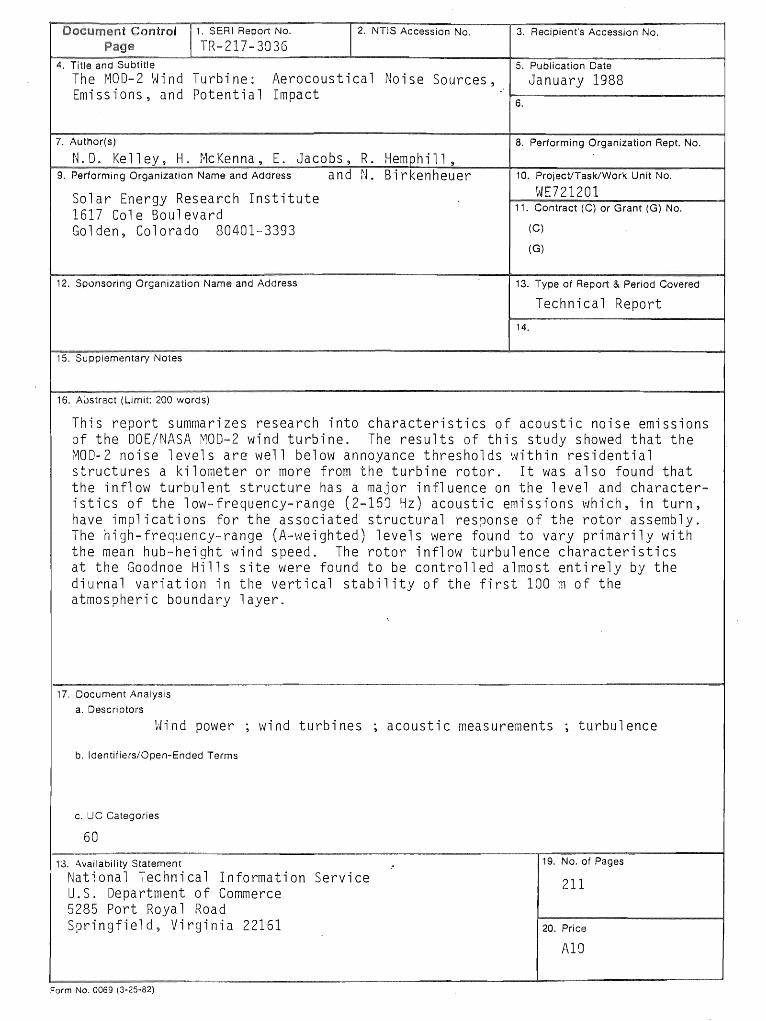
Document Control 11. SERI Report No.

Page TR-217-3036 1 2. NTIS Accession No.

4. Title and Subtitle

The MOD-2 Wind Turbine: Aerocoustical Noise Sources, Emi ss ions, and Potent i a 1 Impact

7. Author(s)

N.D. Kelley, H. fv1cKenna, E. Jacobs, R. Hemphill, 9. Performing Organization Name and Address and N. 8i rkenheuer

Solar Energy Research Institute 1617 Cole Boulevard Golden, Colorado 80401-3393

12. Sponsoring Organization Name and Address

15. Supplementary Notes

16. A0stract (Limit: 200 words)

3. Recipient's Accession No.

5. Publication Date

January 1988 6.

8. Performing Organization Rept. No.

10. Project/Task/Work Unit No.

t~E721201 11. Contract (C) or Grant (G) No.

(C)

(G)

13. Type of Report & Period Covered

Technical Report 14.

This report summarizes research into characteristics of acoustic noise emissions of the DOE/NASA MOD-2 wind turbine. The results of this study showed that the MOD~2 noise levels are well below annoyance thresholds within residential structures a kilometer or more from the turbine rotor. It was also found that the inflow turbulent structure has a major influence on the level and character­istics of the low-frequency-range (2-150 Hz) acoustic emissions which, in turn, have implications for the associated structural response of the rotor assembly. The high-freq~ency-range (A-weighted) levels were found to vary primarily with the mean hub-height wind speed. The rotor inflow turbulence characteristics at the Goodnoe Hills site were found to be controlled almost entirely by the diurnal variation in the vertical stability of the first 100 m of the atmospheric boundary layer.

17. Document Analysis

a. Descriptors

Wind power, wind turbines , acoustic measurements , turbulence

b. Identifiers/Open-Ended Terms

c. UC Categories

60

13. A.vailability Statement

National Technical Information Service U.S. Department of Commerce 5285 Port Royal Road Springfield, Virginia 22161

Form No. 0069 (3~25-82)

19. No. of Pages

211

20. Price

Ala