Numerical and experimental modelling of pollutant dispersion in a street canyon

Journal of Wind Engineering

and Industrial Aerodynamics 90 (2002) 321–339

Numerical and experimental modelling ofpollutant dispersion in a street canyon

Ana Pilar Garcia Sagrado, Jeroen van Beeck1, Patrick Rambaud,Domenico Olivari*

Department of Environmental and Applied Fluid Dynamics, von Karman Institute for Fluid Dynamics,

72 Chaussee de Waterloo, 1640 Rhode-Saint-Genese, Belgium

Abstract

The pollutant dispersion in a two-dimensional street canyon is studied in this project. The

principal parameter investigated is the height of the downstream building. The pollutant

source is situated in the middle of the street. The investigation is performed in two ways.

Experiments have been carried out in the L-2B wind tunnel at von Karman Institute and

numerical simulations have been done with the CFD software Fluent 5.2. The concentration

measurements have been performed by means of light scattering technique and the velocity

field has been measured with particle image velocimetry. In the numerical simulations, a

preliminary study about the backward-facing step has been performed in order to select the

best turbulence model in Fluent for these complex flows characterized by separation,

stagnation, recirculation, reattachment, etc. The best model appeared to be the realizable k–emodel with the two-layer zonal approach to the wall, which predicts the reattachment length

after the step with o1% error in comparison with the value obtained from direct numerical

simulation by Le, Moin and Kim (Direct numerical simulation of turbulent flow over a

backward-facing step, Report No. TF-58, 1996). This model has been applied in the street

canyon simulations. Comparison with the experimental results has been made.

Besides the height of the downstream building, the influence of a third building situated

upstream of the street canyon in the flow and dispersion inside the street has been investigated.

r 2002 Elsevier Science Ltd. All rights reserved.

Keywords: Pollutant dispersion; Numerical modelling; Wind tunnel experiments; CFD application;

Realizable k–e model

*Corresponding author. Tel.: +32-2-3599611; fax: +32-2-3599600.

E-mail addresses: [email protected] (J. van Beeck), [email protected] (D. Olivari).1Colour figures can be obtained upon request.

0167-6105/02/$ - see front matter r 2002 Elsevier Science Ltd. All rights reserved.

PII: S 0 1 6 7 - 6 1 0 5 ( 0 1 ) 0 0 2 1 5 - X

1. Introduction

One of the principal sources of contamination (nitrogen oxides and hydrocarbons)in the cities are the transport vehicles and a worsening of the situation may beexpected in view of the continuous increase in traffic. Along the same city streets(urban canyons) people are walking unprotected, and windows are open along theside buildings with people sitting inside often for long times. Therefore, it is of majorimportance to find out how these pollutants distribute in the streets and if, modifyingsome parameters, the pollution at pedestrian level and along the wall can bedecreased. Configurations like this have been investigated by Meroney et al. [2], Leitland Meroney [5], Murakami [10], Zhang et al. [7], Hwang et al. [8], Tsuchiya et al. [9]and many others.A limitation of direct field measurements of atmospheric phenomena [1] is

that all possible governing parameters are simultaneously operative and itis not simple to determine which are important, which are secondary or whichare insignificant. These parameters are: building geometry (height, width,roof shape), street dimensions (breadth, width), thermal stratification (solarinsulation and orientation, building and street thermal capacitance), vehicularmovement (size, number, frequency), plume buoyancy etc., and they are allintertwined.Wind tunnel experiments provide an opportunity to examine the effects of various

parameters individually or in combination. In this case, the street canyon has beenmodelled as two blocks of wood which extend over the whole width of the testsection. The wind direction is perpendicular to the street to preserve twodimensionality.The pollutant concentration has been measured using smoke as a tracer and

recorded by a video camera light scattering technique. The images have beenanalysed by a digital image processing system. This approach samples the whole two-dimensional flow field providing an instantaneous image of the distribution ofpollutant. The mean concentration field has been obtained after the processing of theimages. In order to examine the transport mechanism in the canyon, the velocity fieldhas been measured with particle image velocimetry (PIV). Simultaneously, thepossibility of predicting the pollutant concentration numerically has beeninvestigated. The flow field around ‘‘bluff bodies’’ such as buildings with sharpedges and corners is very complex to compute by a CFD code. In this researchproject, a systematic study about the numerical simulations has been done using thedifferent options available in the FLUENT 5.2 code. The best turbulence model forseparated and recirculating flows has been selected after a preliminary study on thewake of a backward-facing step and this model has been applied to the street canyonsimulations.The results presented in this paper are mostly concerned with the influence of the

relative height of the upstream and downstream buildings in the pollutant dispersioninside these canyons for an isolated street (open country) and for the case in which itis preceded by an upstream building and road (non-isolated street canyon) under awind coming normal to the main streets.

A.P. Garcia Sagrado et al. / J. Wind Eng. Ind. Aerodyn. 90 (2002) 321–339322

2. Street canyon model

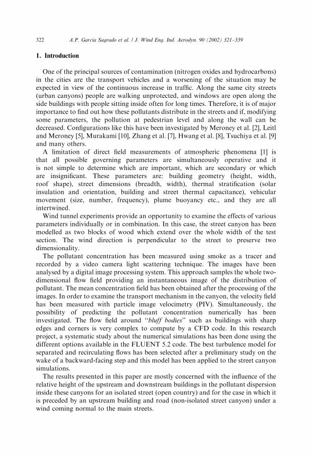
A simple geometry represented by two blocks of wood spanning the width of thewind tunnel has been used to model the street canyon in order to exclude three-dimensional effects. The blocks have been painted in black to avoid the reflections oflight from the laser sheet. The dimensions of the blocks were 3 cm� 3 cm� 34:8 cm:The height of the downstream building, as stated before, was the main variable.Three different values were used: 3; 4 and 5 cm: A sketch of the model withbuildings of equal height can be seen in Fig. 1.The open country configuration simulates an isolated street without other

buildings around and has been chosen to focus on the nature of the flow anddispersion inside the street. In the non-isolated street canyon configuration, a thirdbuilding has been added upstream of the street to investigate the influence of acanyon placed in the middle of an urban environment.

3. Experimental set-up

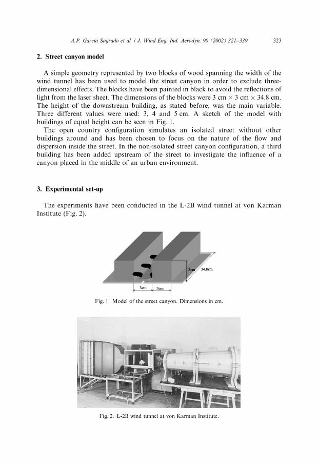
The experiments have been conducted in the L-2B wind tunnel at von KarmanInstitute (Fig. 2).

Fig. 1. Model of the street canyon. Dimensions in cm.

Fig. 2. L-2B wind tunnel at von Karman Institute.

A.P. Garcia Sagrado et al. / J. Wind Eng. Ind. Aerodyn. 90 (2002) 321–339 323

This facility is a low-speed, open-circuit wind tunnel of suction type. Itincorporates an air inlet, fitted with honeycombs, meshes and a two-dimensionalcontraction. The test section is a square of 0:35 m size and a length of 2 m: Themaximum achievable velocity is 35 m=s: The model of the street canyon is placed inthe middle of the test section and spans its full width.The free stream velocity for the present tests was 2:5 m=s which corresponds to a

Re number of 5100 based on the height of the upstream building.In order to generate a correct level of turbulence in the flow, a grid of 10 mm wide

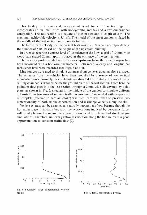
wood bars spaced 20 mm apart is placed at the entrance of the test section.The velocity profile at different distances upstream from the street canyon has

been measured with a hot wire anemometer. Both mean velocity and longitudinalturbulence level were recorded (see Figs. 3 and 4).Line sources were used to simulate exhausts from vehicles queuing along a street.

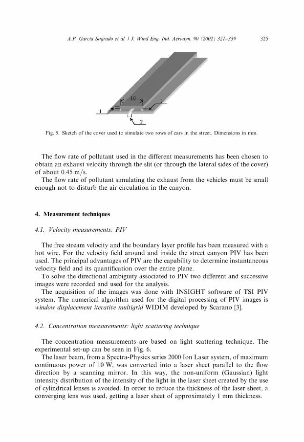
The exhausts from the vehicles have been modelled by a source of low verticalmomentum since normally these exhausts are directed horizontally. To model this, asettling chamber is installed below the ground plate of the test section. From here thepollutant flow goes into the test section through a 2 mm wide slit covered by a flatplate, as shown in Fig. 5, situated in the middle of the canyon to simulate uniformexhausts from two rows of moving traffic. A mixture of air seeded with evaporatedoil droplets (referred to here as smoke) was used; care was taken to preserve twodimensionality of both smoke concentration and discharge velocity along the slit.Vehicle exhaust can be assumed as neutrally buoyant gas flow, because though the

hot exhaust gas is initially buoyant, the accelerations induced by buoyancy forceswill usually be small compared to automotive-induced turbulence and street canyoncirculations. Therefore, uniform gasflow distribution along the line source is a goodapproximation to constant traffic flow [2].

0 0.1 0.2 0.3 0.4 0.5 0.6 0.7 0.8RMS (m/s)

0

0.05

0.1

0.15

0.2

Ver

tical

dis

tanc

e (m

)

Fig. 4. RMS experimental profile.

0 1 2 3 4 5 6X Velocity (m/s)

0

0.05

0.1

0.15

0.2

Ver

tical

dis

tanc

e (m

)

Fig. 3. Boundary layer experimental velocity

profile.


The flow rate of pollutant used in the different measurements has been chosen toobtain an exhaust velocity through the slit (or through the lateral sides of the cover)of about 0:45 m=s:The flow rate of pollutant simulating the exhaust from the vehicles must be small

enough not to disturb the air circulation in the canyon.

4. Measurement techniques

4.1. Velocity measurements: PIV

The free stream velocity and the boundary layer profile has been measured with ahot wire. For the velocity field around and inside the street canyon PIV has beenused. The principal advantages of PIV are the capability to determine instantaneousvelocity field and its quantification over the entire plane.To solve the directional ambiguity associated to PIV two different and successive

images were recorded and used for the analysis.The acquisition of the images was done with INSIGHT software of TSI PIV

system. The numerical algorithm used for the digital processing of PIV images iswindow displacement iterative multigrid WIDIM developed by Scarano [3].

4.2. Concentration measurements: light scattering technique

The concentration measurements are based on light scattering technique. Theexperimental set-up can be seen in Fig. 6.The laser beam, from a Spectra-Physics series 2000 Ion Laser system, of maximum

continuous power of 10 W; was converted into a laser sheet parallel to the flowdirection by a scanning mirror. In this way, the non-uniform (Gaussian) lightintensity distribution of the intensity of the light in the laser sheet created by the useof cylindrical lenses is avoided. In order to reduce the thickness of the laser sheet, aconverging lens was used, getting a laser sheet of approximately 1 mm thickness.

Fig. 5. Sketch of the cover used to simulate two rows of cars in the street. Dimensions in mm.


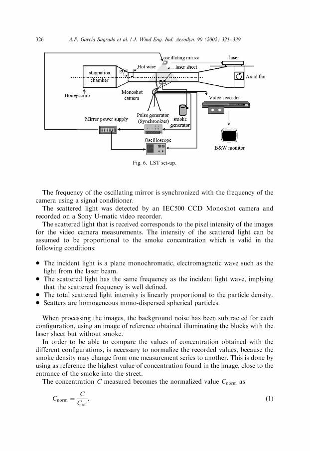
The frequency of the oscillating mirror is synchronized with the frequency of thecamera using a signal conditioner.The scattered light was detected by an IEC500 CCD Monoshot camera and

recorded on a Sony U-matic video recorder.The scattered light that is received corresponds to the pixel intensity of the images

for the video camera measurements. The intensity of the scattered light can beassumed to be proportional to the smoke concentration which is valid in thefollowing conditions:

* The incident light is a plane monochromatic, electromagnetic wave such as thelight from the laser beam.

* The scattered light has the same frequency as the incident light wave, implyingthat the scattered frequency is well defined.

* The total scattered light intensity is linearly proportional to the particle density.* Scatters are homogeneous mono-dispersed spherical particles.

When processing the images, the background noise has been subtracted for eachconfiguration, using an image of reference obtained illuminating the blocks with thelaser sheet but without smoke.In order to be able to compare the values of concentration obtained with the

different configurations, is necessary to normalize the recorded values, because thesmoke density may change from one measurement series to another. This is done byusing as reference the highest value of concentration found in the image, close to theentrance of the smoke into the street.The concentration C measured becomes the normalized value Cnorm as

Cnorm ¼C

Cref: ð1Þ

Fig. 6. LST set-up.


5. Wind tunnel results

5.1. Open country configuration

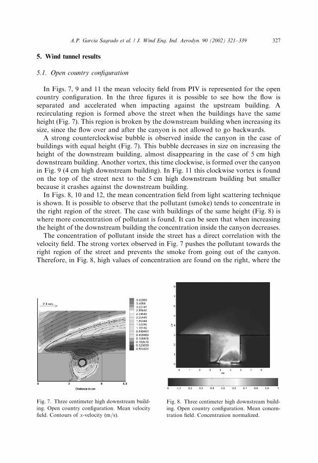
In Figs. 7, 9 and 11 the mean velocity field from PIV is represented for the opencountry configuration. In the three figures it is possible to see how the flow isseparated and accelerated when impacting against the upstream building. Arecirculating region is formed above the street when the buildings have the sameheight (Fig. 7). This region is broken by the downstream building when increasing itssize, since the flow over and after the canyon is not allowed to go backwards.A strong counterclockwise bubble is observed inside the canyon in the case of

buildings with equal height (Fig. 7). This bubble decreases in size on increasing theheight of the downstream building, almost disappearing in the case of 5 cm highdownstream building. Another vortex, this time clockwise, is formed over the canyonin Fig. 9 (4 cm high downstream building). In Fig. 11 this clockwise vortex is foundon the top of the street next to the 5 cm high downstream building but smallerbecause it crashes against the downstream building.In Figs. 8, 10 and 12, the mean concentration field from light scattering technique

is shown. It is possible to observe that the pollutant (smoke) tends to concentrate inthe right region of the street. The case with buildings of the same height (Fig. 8) iswhere more concentration of pollutant is found. It can be seen that when increasingthe height of the downstream building the concentration inside the canyon decreases.The concentration of pollutant inside the street has a direct correlation with the

velocity field. The strong vortex observed in Fig. 7 pushes the pollutant towards theright region of the street and prevents the smoke from going out of the canyon.Therefore, in Fig. 8, high values of concentration are found on the right, where the

Fig. 7. Three centimeter high downstream build-

ing. Open country configuration. Mean velocity

field. Contours of x-velocity ðm=sÞ:

Fig. 8. Three centimeter high downstream build-

ing. Open country configuration. Mean concen-

tration field. Concentration normalized.


pollutant is trapped. The smoke that is allowed to go out from the street is carried bythe flow towards the upstream building roof where important values of concentra-tion are found. From there, it is carried away along the shear layer. When increasingthe height of the downstream building this interior vortex is not so strong but smallerallowing the pollutant to go out from the street more easily and therefore lessconcentration is found inside (Figs. 10 and 12).

Fig. 9. Four centimeter high downstream build-






Fig. 12. Five centimeter high downstream build-







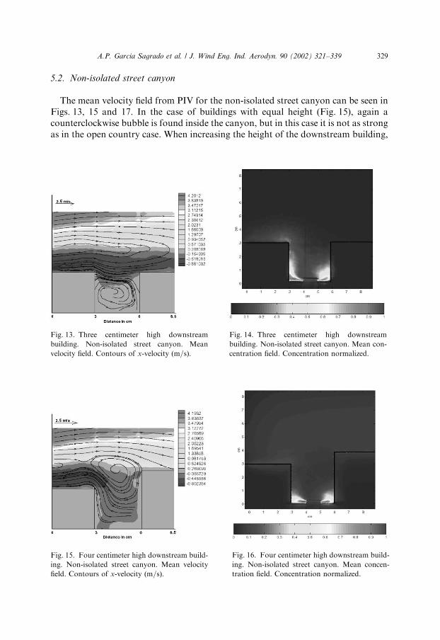
5.2. Non-isolated street canyon

The mean velocity field from PIV for the non-isolated street canyon can be seen inFigs. 13, 15 and 17. In the case of buildings with equal height (Fig. 15), again acounterclockwise bubble is found inside the canyon, but in this case it is not as strongas in the open country case. When increasing the height of the downstream building,

Fig. 13. Three centimeter high downstream

building. Non-isolated street canyon. Mean

velocity field. Contours of x-velocity ðm=sÞ:

Fig. 14. Three centimeter high downstream

building. Non-isolated street canyon. Mean con-

centration field. Concentration normalized.


ing. Non-isolated street canyon. Mean velocity



ing. Non-isolated street canyon. Mean concen-



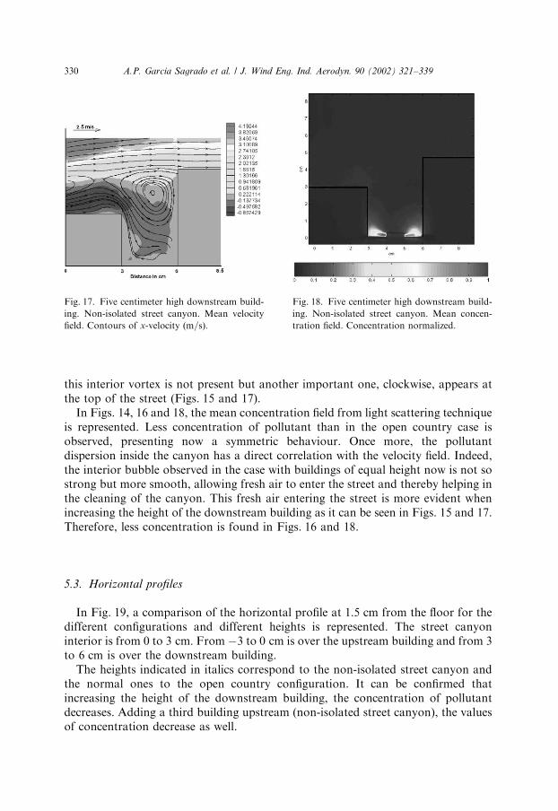
this interior vortex is not present but another important one, clockwise, appears atthe top of the street (Figs. 15 and 17).In Figs. 14, 16 and 18, the mean concentration field from light scattering technique

is represented. Less concentration of pollutant than in the open country case isobserved, presenting now a symmetric behaviour. Once more, the pollutantdispersion inside the canyon has a direct correlation with the velocity field. Indeed,the interior bubble observed in the case with buildings of equal height now is not sostrong but more smooth, allowing fresh air to enter the street and thereby helping inthe cleaning of the canyon. This fresh air entering the street is more evident whenincreasing the height of the downstream building as it can be seen in Figs. 15 and 17.Therefore, less concentration is found in Figs. 16 and 18.

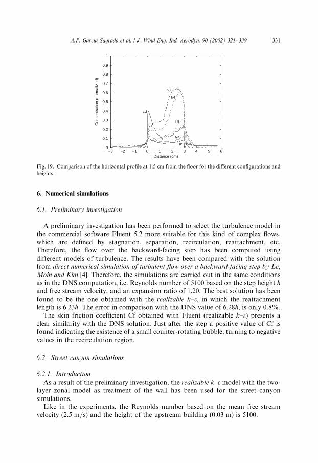
5.3. Horizontal profiles

In Fig. 19, a comparison of the horizontal profile at 1:5 cm from the floor for thedifferent configurations and different heights is represented. The street canyoninterior is from 0 to 3 cm: From �3 to 0 cm is over the upstream building and from 3to 6 cm is over the downstream building.The heights indicated in italics correspond to the non-isolated street canyon and

the normal ones to the open country configuration. It can be confirmed thatincreasing the height of the downstream building, the concentration of pollutantdecreases. Adding a third building upstream (non-isolated street canyon), the valuesof concentration decrease as well.


ing. Non-isolated street canyon. Mean velocity



ing. Non-isolated street canyon. Mean concen-



6. Numerical simulations

6.1. Preliminary investigation

A preliminary investigation has been performed to select the turbulence model inthe commercial software Fluent 5.2 more suitable for this kind of complex flows,which are defined by stagnation, separation, recirculation, reattachment, etc.Therefore, the flow over the backward-facing step has been computed usingdifferent models of turbulence. The results have been compared with the solutionfrom direct numerical simulation of turbulent flow over a backward-facing step by Le,Moin and Kim [4]. Therefore, the simulations are carried out in the same conditionsas in the DNS computation, i.e. Reynolds number of 5100 based on the step height h

and free stream velocity, and an expansion ratio of 1:20: The best solution has beenfound to be the one obtained with the realizable k–e; in which the reattachmentlength is 6:23h: The error in comparison with the DNS value of 6:28h; is only 0.8%.The skin friction coefficient Cf obtained with Fluent (realizable k–e) presents a

clear similarity with the DNS solution. Just after the step a positive value of Cf isfound indicating the existence of a small counter-rotating bubble, turning to negativevalues in the recirculation region.

6.2. Street canyon simulations

6.2.1. Introduction

As a result of the preliminary investigation, the realizable k–e model with the two-layer zonal model as treatment of the wall has been used for the street canyonsimulations.Like in the experiments, the Reynolds number based on the mean free stream

velocity (2:5 m=s) and the height of the upstream building (0:03 m) is 5100.

−3 −2 −1 1 2 3 40 5 6Distance (cm)

0

0.1

0.2

0.3

0.4

0.5

0.6

0.7

0.8

0.9

1

Con

cent

ratio

n (n

orm

aliz

ed)

h3

h4

h5

h3

h4

h5

Fig. 19. Comparison of the horizontal profile at 1:5 cm from the floor for the different configurations and

heights.


In Fig. 20, the basic geometry for the reference case is represented.It is similar for the rest of the cases but increasing the downstream building height.

In the non-isolated street canyon, the distance from the inlet of the mean flow to thefirst building is 10h; therefore to the upstream building of the street is 12h:In the final geometry used for the computations, a modification to approximate it

more to the experiments was done. This final geometry includes the box under thewind tunnel through which the smoke enters the street canyon. It is a square of0:03 m� 0:03 m:In all the cases the grid has been built based on the one from the backward-facing

step study. Therefore, a uniform grid has been used with 1 mm square cells.However, the grid has been refined more, near the entrance of the smoke into thewind tunnel.The grid for the open country configuration with buildings of equal height has

approximately 252 000 cells ð1200� 210Þ:The experimental profiles for velocity, turbulent kinetic energy ðkÞ and turbulent

dissipation rate (e) have been introduced as boundary conditions for the inlet. Theprofiles for k and e have been computed with the values of rms measured with the hotwire,

k ¼ 32ðuNIÞ2; ð2Þ

e ¼ C3=4m

k3=2

l; ð3Þ

where uN is the mean free stream velocity, I is the turbulence intensity (ffiffiffiffiffiffiu02

p=uN), l

is the turbulence length scale, estimated here as the height of the upstream buildingh ¼ 0:03 m and Cm is an empirical constant specified in the turbulence model(approximately 0.09).The boundary condition at the outlet is pressure outlet. The static pressure

(relative value) introduced is the default value of zero (atmospheric pressure). Thebackflow conditions for the outlet are a turbulence intensity of 10% and a turbulencelength scale of 0:03 m which is precisely the height of the step. Nevertheless, theseconditions were never used since in this case there was no backflow.The boundary condition in the upper wall is slip condition, i.e. the velocity at the

wall is the velocity of the adjacent cell.And for the inlet of the pollutant (through the box situated below the wind

tunnel), a uniform velocity computed from the value of flow rate of smoke indicatedby the Venturi has been introduced. A turbulence intensity of 1% and a turbulencelength scale of 1 mm has been used as boundary conditions for this inlet.

Fig. 20. Street canyon geometry for the open country configuration with 3 cm high downstream building.


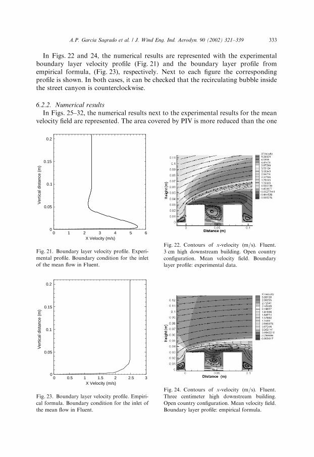
In Figs. 22 and 24, the numerical results are represented with the experimentalboundary layer velocity profile (Fig. 21) and the boundary layer profile fromempirical formula, (Fig. 23), respectively. Next to each figure the correspondingprofile is shown. In both cases, it can be checked that the recirculating bubble insidethe street canyon is counterclockwise.

6.2.2. Numerical results

In Figs. 25–32, the numerical results next to the experimental results for the meanvelocity field are represented. The area covered by PIV is more reduced than the one

0 1 2 3 4 5 6X Velocity (m/s)

0

0.05

0.1

0.15

0.2

Ver

tical

dis

tanc

e (m

)

Fig. 21. Boundary layer velocity profile. Experi-

mental profile. Boundary condition for the inlet

of the mean flow in Fluent.

Fig. 22. Contours of x-velocity ðm=sÞ: Fluent.

3 cm high downstream building. Open country

configuration. Mean velocity field. Boundary

layer profile: experimental data.

0 0.5 1 1.5 2 2.5 3X Velocity (m/s)

0

0.05

0.1

0.15

0.2

Ver

tical

dis

tanc

e (m

)

Fig. 23. Boundary layer velocity profile. Empiri-

cal formula. Boundary condition for the inlet of

the mean flow in Fluent.


Three centimeter high downstream building.

Open country configuration. Mean velocity field.

Boundary layer profile: empirical formula.


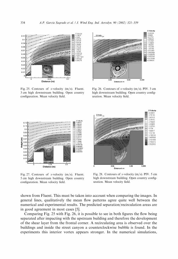
shown from Fluent. This must be taken into account when comparing the images. Ingeneral lines, qualitatively the mean flow patterns agree quite well between thenumerical and experimental results. The predicted separation/recirculation areas arein good agreement in most cases [5].Comparing Fig. 25 with Fig. 26, it is possible to see in both figures the flow being

separated after impacting with the upstream building and therefore the developmentof the shear layer from the frontal corner. A recirculating area is observed over thebuildings and inside the street canyon a counterclockwise bubble is found. In theexperiments this interior vortex appears stronger. In the numerical simulations,



configuration. Mean velocity field.

Fig. 26. Contours of x-velocity ðm=sÞ: PIV. 3 cmhigh downstream building. Open country config-

uration. Mean velocity field.



configuration. Mean velocity field.

Fig. 28. Contours of x-velocity ðm=sÞ: PIV. 5 cmhigh downstream building. Open country config-

uration. Mean velocity field.


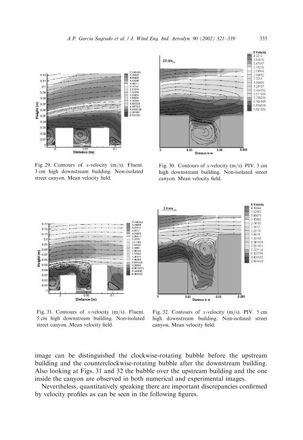
image can be distinguished the clockwise-rotating bubble before the upstreambuilding and the counterclockwise-rotating bubble after the downstream building.Also looking at Figs. 31 and 32 the bubble over the upstream building and the oneinside the canyon are observed in both numerical and experimental images.Nevertheless, quantitatively speaking there are important discrepancies confirmed

by velocity profiles as can be seen in the following figures.


3 cm high downstream building. Non-isolated

street canyon. Mean velocity field.

Fig. 30. Contours of x-velocity ðm=sÞ: PIV. 3 cmhigh downstream building. Non-isolated street

canyon. Mean velocity field.


5 cm high downstream building. Non-isolated

street canyon. Mean velocity field.

Fig. 32. Contours of x-velocity ðm=sÞ: PIV. 5 cmhigh downstream building. Non-isolated street

canyon. Mean velocity field.


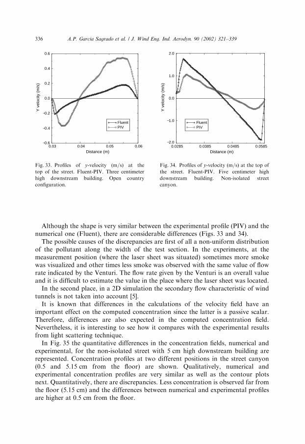
Although the shape is very similar between the experimental profile (PIV) and thenumerical one (Fluent), there are considerable differences (Figs. 33 and 34).The possible causes of the discrepancies are first of all a non-uniform distribution

of the pollutant along the width of the test section. In the experiments, at themeasurement position (where the laser sheet was situated) sometimes more smokewas visualized and other times less smoke was observed with the same value of flowrate indicated by the Venturi. The flow rate given by the Venturi is an overall valueand it is difficult to estimate the value in the place where the laser sheet was located.In the second place, in a 2D simulation the secondary flow characteristic of wind

tunnels is not taken into account [5].It is known that differences in the calculations of the velocity field have an

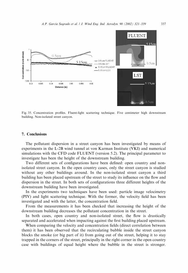
important effect on the computed concentration since the latter is a passive scalar.Therefore, differences are also expected in the computed concentration field.Nevertheless, it is interesting to see how it compares with the experimental resultsfrom light scattering technique.In Fig. 35 the quantitative differences in the concentration fields, numerical and

experimental, for the non-isolated street with 5 cm high downstream building arerepresented. Concentration profiles at two different positions in the street canyon(0:5 and 5:15 cm from the floor) are shown. Qualitatively, numerical andexperimental concentration profiles are very similar as well as the contour plotsnext. Quantitatively, there are discrepancies. Less concentration is observed far fromthe floor ð5:15 cmÞ and the differences between numerical and experimental profilesare higher at 0:5 cm from the floor.

0.03 0.04 0.05 0.06Distance (m)

−0.2

−0.4

−0.6

0.0

0.2

0.4

0.6

Y v

eloc

ity (

m/s

)

FluentPIV

Fig. 33. Profiles of y-velocity ðm=sÞ at the

top of the street. Fluent-PIV. Three centimeter

high downstream building. Open country

configuration.

0.0285 0.0385 0.0485 0.0585Distance (m)

−1.0

−2.0

0.0

1.0

2.0

Y v

eloc

ity (

m/s

)

FluentPIV

Fig. 34. Profiles of y-velocity ðm=sÞ at the top of

the street. Fluent-PIV. Five centimeter high

downstream building. Non-isolated street

canyon.


7. Conclusions

The pollutant dispersion in a street canyon has been investigated by means ofexperiments in the L-2B wind tunnel at von Karman Institute (VKI) and numericalsimulations with the CFD code FLUENT (version 5.2). The principal parameter toinvestigate has been the height of the downstream building.Two different sets of configurations have been defined: open country and non-

isolated street canyon. In the open country cases, only the street canyon is studiedwithout any other buildings around. In the non-isolated street canyon a thirdbuilding has been placed upstream of the street to study its influence on the flow anddispersion in the street. In both sets of configurations three different heights of thedownstream building have been investigated.In the experiments two techniques have been used: particle image velocimetry

(PIV) and light scattering technique. With the former, the velocity field has beeninvestigated and with the latter, the concentration field.From the measurements it has been checked that increasing the height of the

downstream building decreases the pollutant concentration in the street.In both cases, open country and non-isolated street, the flow is drastically

separated and accelerated when impacting against the first building placed upstream.When comparing the velocity and concentration fields (direct correlation between

them) it has been observed that the recirculating bubble inside the street canyonblocks the smoke (or big part of it) from going out of the street, helping it to staytrapped in the corners of the street, principally in the right corner in the open countrycase with buildings of equal height where the bubble in the street is stronger.

Fig. 35. Concentration profiles. Fluent-light scattering technique. Five centimeter high downstream

building. Non-isolated street canyon.


Therefore, in the cases where this recirculating bubble in the interior of the canyon ispresent, higher concentration is found inside the street. On the contrary, when thisflow pattern (bubble) is not present but fresh air enters the canyon (non-isolatedstreetFprincipally with 4 and 5 cm high downstream building), then lowerconcentration is observed inside.In relation to the numerical simulations, a preliminary investigation about the

backward-facing step has been made to select the turbulence model that works betterwith these complex flows defined by stagnation, separation, reattachment,recirculation etc. The realizable k–e model with the two-layer zonal approach tothe wall has been found to be the one that more accurately predicts the reattachmentlength after the step. The solution obtained presents o1% error in comparison withthe solution from direct numerical simulation of turbulent flow over a backward-facing step by Le, Moin and Kim [4]. This model gives a superior performance forflows under adverse pressure gradients, i.e., the pressure increases in the direction ofthe flow and causes the boundary layer to separate from the solid surface. Theconclusion is in agreement with previous studies carried out about the realizablemodel that showed it to be the best approach for separated flows and flows withcomplex secondary flow features.Flow obstacles (buildings or structures) exist in the flow field within the surface

boundary layer. These ‘‘bluff bodies’’ have sharp edges at their corners and very finegrid discretization is required to analyse such flow field with high precision [6]. Thedistribution of the strain-rate tensor is more complex than that of the simpleboundary layer. Compared to the flow fields traditionally treated in the field of CFD,such as channel or pipe flows, the flow field around a bluff body is much morecomplicated and difficult to analyse [6].Despite the difficulties in computing these flows, for most configurations it is

observed that qualitatively the numerical results are in good agreement with theexperiments. The mean flow patterns as well as predicted separation/recirculationareas agree well in general with the results from the modelling in the wind tunnel [5].Nevertheless, quantitatively there are important discrepancies confirmed by velocityand concentration profiles.Causes of the discrepancies between numerical and experimental results can be a

non-uniform and unsteady behaviour found in the pollutant distribution and thesecondary flow characteristic of wind tunnels which is not taken into account in a 2Dsimulation. Moreover, a high sensibility has been observed in the behaviour of theflow inside the street canyon when modifying the value of pollutant flow rate.With the proper information about all the data necessary to simulate the same

conditions as in the experiments, possibly similar mean flow field patterns would beobtained everywhere and quantitatively the results could be closer.Differences in the calculations of the velocity field have an important effect on the

computed concentration since it is a passive scalar. Therefore, because differenceshave been observed when comparing the velocity field between numerical andexperimental results, discrepancies are expected in the concentration field. Never-theless, good agreement has been found for the urban model case with 5 cm highdownstream building.


References

[1] H.W. Georgi, E. Busch, E. Weber, Investigation of the temporal and spatial distribution of the

emission concentration of carbon monoxide in Frankfort/Main, Report No. 11, Institute for

Meteorological and Geophysics of the University of Frankfurt/Main (Translation no. 0477,

NAPCA), 1967.

[2] R.N. Meroney, M. Pavageau, S. Rafadalis, M. Schatzmann, Study of line source characteristics for

2D physical modelling of pollutant dispersion in street canyons, J. Wind Eng. Ind. Aerodyn. 62 (1996)

37–56.

[3] F. Scarano, Improvements in PIV image processing application to a backward-facing step, Von

Karman Institute for Fluid Dynamics, Project Report 1997-01.

[4] H. Le, P. Moin, J. Kim, Direct numerical simulation of turbulent flow over a backward-facing step,

Report No. TF-58, Thermosciences Division, Department of Mechanical Engineering, Stanford

University and Department of Mechanical, Aerospace and Nuclear Engineering, University of

California, Los Angeles, September 1996.

[5] B.M. Leitl, R.N. Meroney, Car exhaust dispersion in a street canyon, Numerical critique of a wind

tunnel experiment, J. Wind Eng. Ind. Aerodyn. 67, 68 (1997) 293–304.

[6] M. Shuzo, Current status and future trends in computational wind engineering, J. Wind Eng. Ind.

Aerodyn. 67&68 (1997) 3–34.

[7] Y.Q. Zhang, A.H. Hubert, S.P.S. Arya, W.H. Snyder, Numerical simulation to determine the effects

of incident wind shear and turbulence level on the flow around a building, J. Wind Eng. Ind.

Aerodyn. 46&47 (1993) 129–134.

[8] R.R. Hwang, Y.C. Chow, Y.F. Peng, Numerical study of turbulent flow over two-dimensional

surface mounted ribs in a channel, Int. J. Numerical Methods Fluids 31 (1999) 767–785.

[9] M. Tsuchiya, S. Murakami, A. Mochida, K. Kondo, Y. Ishida, Development of a new k–e model forflow and pressure fields around bluff body, J. Wind Eng. Ind. Aerodyn. 67, 68 (1997) 169–182.

[10] S. Murakami, Comparison of various turbulence models applied to a bluff body, J. Wind Eng. Ind.

Aerodyn. 46, 47 (1993) 21–36.


Numerical and experimental modelling of pollutant dispersion in a street canyon

Documents

Transcript of Numerical and experimental modelling of pollutant dispersion in a street canyon