Numerical Investigations of Urban Pollutant Dispersion ... - MDPI

��

Citation: Li, Q.; Liang, J.; Wang, Q.;

Chen, Y.; Yang, H.; Ling, H.; Luo, Z.;

Hang, J. Numerical Investigations of

Urban Pollutant Dispersion and

Building Intake Fraction with Various

3D Building Configurations and Tree

Plantings. Int. J. Environ. Res. Public

Health 2022, 19, 3524. https://

doi.org/10.3390/ijerph19063524

Academic Editor: Cheng Yan

Received: 3 January 2022

Accepted: 12 March 2022

Published: 16 March 2022

Publisher’s Note: MDPI stays neutral

with regard to jurisdictional claims in

published maps and institutional affil-

iations.

Copyright: © 2022 by the authors.

Licensee MDPI, Basel, Switzerland.

This article is an open access article

distributed under the terms and

conditions of the Creative Commons

Attribution (CC BY) license (https://

creativecommons.org/licenses/by/

4.0/).

International Journal of

Environmental Research

and Public Health

Article

Numerical Investigations of Urban Pollutant Dispersion andBuilding Intake Fraction with Various 3D BuildingConfigurations and Tree PlantingsQingman Li 1,2,†, Jie Liang 1,2, Qun Wang 3,† , Yuntong Chen 1, Hongyu Yang 1,2, Hong Ling 1,2,* ,Zhiwen Luo 4 and Jian Hang 1,2

1 Southern Marine Science and Engineering Guangdong Laboratory (Zhuhai), School of Atmospheric Sciences,Sun Yat-sen University, Zhuhai 519082, China; [email protected] (Q.L.);[email protected] (J.L.); [email protected] (Y.C.); [email protected] (H.Y.);[email protected] (J.H.)

2 Key Laboratory of Tropical Atmosphere-Ocean System, Ministry of Education, Sun Yat-sen University,Zhuhai 519000, China

3 Department of Mechanical Engineering, The University of Hong Kong, Pokfulam Road,Hong Kong SAR, China; [email protected]

4 School of Construction Management and Engineering, University of Reading, Whiteknights,Reading RG6 6AH, UK; [email protected]

* Correspondence: [email protected]; Tel.: +86-20-84112436† These authors contributed equally to this work.

Abstract: Rapid urbanisation and rising vehicular emissions aggravate urban air pollution. Outdoorpollutants could diffuse indoors through infiltration or ventilation, leading to residents’ exposure.This study performed CFD simulations with a standard k-ε model to investigate the impacts ofbuilding configurations and tree planting on airflows, pollutant (CO) dispersion, and personalexposure in 3D urban micro-environments (aspect ratio = H/W = 30 m, building packing densityλp = λf = 0.25) under neutral atmospheric conditions. The numerical models are well validated bywind tunnel data. The impacts of open space, central high-rise building and tree planting (leaf areadensity LAD= 1 m2/m3) with four approaching wind directions (parallel 0◦ and non-parallel 15◦,30◦, 45◦) are explored. Building intake fraction <P_IF> is adopted for exposure assessment. Thechange rates of <P_IF> demonstrate the impacts of different urban layouts on the traffic exhaustexposure on residents. The results show that open space increases the spatially-averaged velocityratio (VR) for the whole area by 0.40–2.27%. Central high-rise building (2H) can increase windspeed by 4.73–23.36% and decrease the CO concentration by 4.39–23.00%. Central open space andhigh-rise building decrease <P_IF> under all four wind directions, by 6.56–16.08% and 9.59–24.70%,respectively. Tree planting reduces wind speed in all cases, raising <P_IF> by 14.89–50.19%. Thiswork could provide helpful scientific references for public health and sustainable urban planning.

Keywords: CFD simulation; ventilation; pollutant dispersion; open space; urban tree planting;personal intake fraction

1. Introduction

Rapid urbanisation has aggravated urban environmental problems over the past sev-eral decades. The rapidly increasing vehicular emissions in street networks deteriorateurban air quality and have become one of the main pollutant sources in modern cities [1–3].Urban air pollutant exposure has induced rising risks of respiratory and cardiovasculardiseases, or even premature mortality [4,5]. People spend more than 90% of their lifetimeindoors, on average. Moreover, outdoor air pollutants can diffuse into the indoor environ-ment by infiltration or ventilation via windows, vents, and so on. The indoor pollutantexposure is closely influenced by the outdoor air quality, especially for buildings with

Int. J. Environ. Res. Public Health 2022, 19, 3524. https://doi.org/10.3390/ijerph19063524 https://www.mdpi.com/journal/ijerph

https://doi.org/10.3390/ijerph19063524


https://creativecommons.org/

https://creativecommons.org/licenses/by/4.0/

https://creativecommons.org/licenses/by/4.0/

https://www.mdpi.com/journal/ijerph

https://www.mdpi.com

https://orcid.org/0000-0002-9166-6144

https://orcid.org/0000-0001-6231-2470

https://orcid.org/0000-0002-2082-3958


https://www.mdpi.com/journal/ijerph

https://www.mdpi.com/article/10.3390/ijerph19063524?type=check_update&version=2

Int. J. Environ. Res. Public Health 2022, 19, 3524 2 of 34

natural ventilation. Therefore, near-road residents usually suffer from much higher airpollutant exposure than those in other regions [4,6–8]. Special attention is required to de-velop sustainable urban designs to improve urban ventilation and reduce urban residents’exposure [9,10].

The urban canopy layer (UCL) represents the atmospheric layer from the ground tothe building rooftops, where most urban residents live. To mitigate the pollutant exposureof residents in the UCL, improving the ventilation and pollutant dilution capacity is oneof the major solutions [9,10]. Recently, field observations, computational fluid dynamic(CFD) simulations, and laboratory-scale physical modelling (wind tunnel or water channelexperiments) have been widely employed to investigate the ventilation and pollutantdispersion at the street scale (~100 m) or neighbourhood scale (~1 km) [11–18]. Fieldobservation can directly monitor the critical characteristics of air flow and dispersion in realcities, but is restricted by low spatial resolution, uncontrollable boundary conditions, andcomplicated building configurations [15]. Although laboratory-scale physical modellingtechniques can control boundary conditions and building configurations well, and havebeen widely used to validate numerical models, they have to meet the similarity criteriarequirements and the costs are relatively high [13,15,17,18]. Numerical modelling with ahigh temporal–spatial resolution turns out to be a more efficient and relatively low-cost toolto study the flow features and dispersion characteristics, but sometimes it has challenges inattaining satisfactory validation by experimental data [19–25]. In this work, CFD modellingis applied to simulate the flow field and pollutant dispersion at the street scale.

Key urban morphological parameters include street aspect ratio (AR = H/W, where H isthe building height, W is the street width) [26,27], tree planting [28–30], the direction of ap-proaching flow [31,32], building packing densities [33,34], building height variation [35,36],special building designs including open space [37–39] and high-rise building [40,41]. Previ-ous studies have investigated their impacts on the urban ventilation and pollutant disper-sion. Nevertheless, while most studies focused on the airflow and pollutant dispersion inthe street canyon, the integrated impacts of different urban layouts on residents’ exposurein three-dimensional (3D) urban models are still rare. Therefore, this study aims at eval-uating the synthetic impacts of these urban parameters (urban open space, tree plantingand central high-rise building in this work) on ventilation, pollutant dispersion and relatedhuman exposure. The work provides a scientific reference and effective methodologies forsustainable urban design and public health.

2. Methodology2.1. Definition of Crucial Parameters2.1.1. Velocity Ratio (VR)

Velocity ratio (VR) is used throughout the work to normalise and quantify the windenvironment experienced by pedestrians [11], defined by Equation (1):

VR = Vp/Vδ (1)

where Vp is the wind velocity at the pedestrian level (z = 2 m) and Vδ is the wind velocityat the top of the boundary layer. Here, Vδ = 4.34 m/s at z = 300 m [39].

2.1.2. Building Intake Fraction <P_IF>

The concept of the building intake fraction <P_IF>, derived from the personal in-take fraction P_IF, is employed to evaluate the impacts of urban layouts on the residents’pollutant exposure. P_IF represents the total pollutant inhalation per person, which iswidely adopted to quantify the indoor and street-scale (~100 m) vehicular pollutant expo-sure [42–44].


The intake fraction (IF) for a certain population is defined in Equation (2) [45–48]:

IF =N

∑i

M

∑j

Pi × Bri,j × ∆ti,j × Cej/m (2)

where N stands for the total number of population age groups considered in this research;M is the total number of micro-environment types; Pi is the number of the population inthe age group i; Bri,j (m3/s) is the volume-mean breathing rate for individuals of the agegroup i in the micro-environment group j; ∆ti,j is the time that group i stays in the micro-environment j; Cej (kg/m3) is the time-averaged concentration C of the certain vehicularpollutant in the micro-environment j; and m (kg) is the total emission of the vehicularpollutant over the research period.

The population in the research is divided into three groups (N = 3) according toLuo et al. [46]. The composition of the target population is: children (<18, i = 1), adults(18–60, i = 2) and elders (>60, i = 3). Chau et al. [49] considered four types of micro-environment (M = 4) in their work, including indoor at home (j = 1), other indoor locations(j = 2), near vehicles (j = 3) and other outdoor locations (j = 4). To simplify the computation,only one micro-environment (j = 1, indoor at home) is considered in this study, and thebuildings are assumed to be the residential type with natural ventilation. As Table A1 inthe supplement shows, the percentage of children, adults and elders are 21.2%, 63.3% and15.5%, respectively, in this paper. The breathing rate Br and time percentage spent indoorsat home for different age groups is 12.5 and 61.70% (children), 13.8 and 59.50% (adults) and13.1 and 71.60% (elders), respectively [46,49,50].

IF has been used to express the source-to-intake relationship for vehicular pollutants inrealistic street canyons [48]. Since IF would change linearly with the variation of the popula-tion, it has been optimised by defining personal intake fraction P_IF in Equation (3) [26,42].P_IF is independent of population size and density, and it represents the average IF foreach person.

P_IF = IF/M

∑j

Pi (3)

To estimate the influence of urban layouts on personal exposure, P_IF is employed inthis work to quantitatively evaluate the pollutant inhalation of residents.

Previous researchers [6,7] found that the ratio of indoor and outdoor pollutant con-centration (I/O) was approximately 1 for buildings with natural ventilation. Therefore,to reduce the number of grids and computational resources, the inner space of buildingsis not considered in simulations. The pollutant concentrations on building surfaces areadopted as the indoor concentrations in this work, and the vehicle emission is assumed asthe only source of the indoor environment [26,43,45]. Building intake fraction <P_IF> isthe spatial mean of P_IF at all building surfaces. Throughout this work, <P_IF> is usedto present the spatially-averaged personal intake exposure for the whole urban area. Thechange rate of <P_IF> could represent the varied exposure risks for the indoor residentsdue to the impacts of different urban layouts.

2.2. Set-Up for Numerical Modelling

CFD simulation has been widely used for urban micro-climate research in recentdecades [51–55]. Compared with Reynolds-averaged Navier–Stokes (RANS) approaches, largeeddy simulations (LES) are more accurate in simulating and predicting turbulence [54,56–60].However, LES models need enormous computational resources. Thus, RANS models arestill widely applied for turbulence simulation [61–65]. Among the RANS models, thestandard k-ε model has remarkable performance in predicting urban airflows and pollutantdispersion [27,33,44,66–68]. In this paper, the Ansys FLUENT 15.0 with standard k-ε modelis applied for airflow simulations under isothermal conditions.


2.2.1. CFD Model Description

The governing equations of mass, momentum, turbulent kinetic energy (k) and itsdissipation rate (ε) of the employed CFD model are shown in Equations (4)–(7), as follows:the mass conservation equation:

∂ui∂xi

= 0 (4)

the momentum equation:

uj∂ui∂xi

= −1ρ

∂p∂xi

+∂

∂xj

(v

∂ui∂xj− ui

′′ uj′′

)(5)

the transport equations of turbulent kinetic energy (k) and its dissipation rate (ε):

ui∂k∂xi

=∂

∂xi

[(v +

vt

σk

)∂k∂xi

]+

1ρ

Pk − ε (6)

ui

∂ε

∂xi

=∂

∂xi

[(v +

vt

σε

)∂ε

∂xi

]+

1ρ

Cε1

ε

k(

Pk + Cε3 Gb

)− Cε2

ε2

k(7)

where uj stands for time-averaged velocity components (uj = u, v, w as j = 1, 2, 3); v is

the kinematic viscosity; and vt is the kinetic eddy viscosity (vt = Cµk2

ε ). The constant Cµ

is 0.09. −u′′ iu′′ j = vt

(∂ui∂xi

+∂uj∂xj

)− 2

3 kδij is the Reynolds stress tensor. δij is the Kroneker

delta. δij = 1 when i = j and δij = 0 otherwise. Pk = vt × ∂ui∂xj

(∂ui∂xj

+∂uj∂xi

)is the turbulence

production term.The SIMPLE scheme is applied for coupling pressure and velocity. The under-

relaxation factors for pressure term, momentum term, k and ε terms are 0.3, 0.7, 0.5 and0.5, respectively. When all the absolute residuals are smaller than 10−6, the iteration isconverged.

2.2.2. Model Set-Up and Boundary Conditions

The 3D idealised full-scale UCL model with neutral atmosphere conditions is adoptedin this study. The whole UCL model has a 5 × 5 building matrix composed of 25 cubicmodels (H = B = W = 30 m) with moderate packing density (aspect ratio H/W = 1, buildingpacking density λp = λf = 0.25). The designed UCL model is an idealised typical urbanresidential area in miniature, especially relating to the communities in small and medium-sized towns, or the communities in the old town of modern cities. To evaluate the impactsof approaching winds with different directions, θ (the included angle of the approachingwind and axis x) is set as 0◦, 15◦, 30◦ and 45◦ for every scenario. The setup of the simulationdomain is shown in Figure 1a,b.

Figure 1a depicts the simulation area of the cases with parallel approaching wind(θ = 0◦), with the geometry of 1700 m (x) × 870 m (y) × 300 m (z). The distances fromthe UCL model to the domain inlet, outlet and lateral boundaries are 6.7H, 41H and 10H,respectively. The symmetry boundary condition is adopted at the domain top and thelateral boundaries, while the domain outlet takes the zero normal gradient boundarycondition [39,69,70].

The domain geometry of the cases with non-parallel approaching wind (θ = 15◦, 30◦

and 45◦) is 1700 m (x) × 1700 m (y) × 300 m (z) (Figure 1b). In this condition, the distancesfrom the UCL model to the domain inlets and outlets are 6.7H and 41H, respectively. Thesymmetry boundary condition is only adopted at the domain top.


Figure 1. Computational domain of (a) Case [Base, 0◦] and (b) Case [Base, θ] (θ = 15◦, 30◦, 45◦). (c) 3Dmodel description of open-space cases, base cases and high-rise-building cases. (d) Model descriptionand (e) grid arrangements from top view in base cases. (f) Setups of building, tree planting andpollutant source.


The boundary condition for the domain inlet is provided by Equations (8)–(10) [27,67,71,72]:

Uin(z) = Ure f × (z/H)0.16 (8)

kin(z) = u∗2/√

Cµ (9)

εin(z) = C34µ k

32in/(κvz) (10)

where at the building height (H = 30 m), the reference velocity Ure f is 3 m/s. The frictionvelocity u∗ is 0.24 m/s. The von Kármán constant κv is 0.41. The empirical constant Cµ is0.09.

Six building configurations are considered in the current study (Table 1). The UCLmodel of base cases is a building matrix with 5-row and 5-column blocks (Figure 1c). Forthe study of the open-space effect on city ventilation and human exposure, we removethe central building (Building 3-3) to obtain the open space (Location 3-3). For high-rise building scenarios, we double the height of Building 3-3. Each type of buildingconfiguration is combined with tree-planting and tree-free types. According to the settingsabove, the cases are named “Case [urban layout, wind direction]”, as shown in Table 1.

Table 1. Scenarios tested in this work. Different urban designing and wind direction are consideredfor the assessment.

Building Arrangement Vegetation Planning Wind Direction (θ) Case Name

BaseTree-free 0◦, 15◦, 30◦, 45◦ [Base, θ]With tree 0◦, 15◦, 30◦, 45◦ [Base-tree, θ]

Open space Tree-free 0◦, 15◦, 30◦, 45◦ [Open, θ]With tree 0◦, 15◦, 30◦, 45◦ [Open-tree, θ]

High-rise building Tree-free 0◦, 15◦, 30◦, 45◦ [High, θ]With tree 0◦, 15◦, 30◦, 45◦ [High-tree, θ]

For the comprehensive data analysis, we present the results both in the entire UCLRegion A1 (5 × 5 building matrix) and in the Region A2 (the central area of Region A1,including Building 3-3/Location 3-3 and the surroundings), as shown in Figure 1d. Forall tested cases, the minimum size of the hexahedral cells near wall surfaces is 0.2 m. Thetotal number of grids ranges from approximately 5 million and 15 million for the tree-planting and tree-free cases, respectively. Figure 1e illustrates the grid arrangement fromthe top view and side view. This grid arrangement is sufficient to ensure the requirementrecommended by CFD guidelines [69,70].

2.2.3. Description of Pollutant Dispersion Modelling

Scientists have found that traffic emissions have critical negative impacts on respiratoryand cardiovascular function [73,74]. The situation in Asian cities might be more severe dueto the very high population density and more residents living in close proximity to roadtraffic compared with those in European cities. To model the dispersion of traffic-relatedpollutants in the street canyon, reactive gaseous as primary particles [75], inert gas likeCO [76], as well as reactive gaseous pollutants such as NOx and VOCs [77] are adoptedin the simulation for investigating the dispersion of traffic-related air pollutants. Unlikevarious studies focusing on the reactive compounds from traffic such as NOx, VOCs andparticles, we adopted monoxide (CO) as an indicator of the traffic emissions. Although NOx,VOCs and particles have more significant health impacts than CO, these compounds aremore or less chemically or photo-chemically reactive, which means they could not be usedas a tracer for the variation of the traffic emissions. To numerically investigate the impacts ofvarious urban layouts on the physical dispersion of the traffic-related pollutants and relatedhuman exposure, a stable indicator is needed. As one of the main inert pollutants, CO has


been widely used as a tracer of traffic emissions [42,46,48]. This study mainly focuses on thedynamic dispersion of traffic pollutants influenced by different urban layouts. Depositionand chemical reactions are not considered. The CO emission source is settled from z = 0 mto 0.5 m, with a width of 16 m and is 7 m away from the kerbside building (marked withdark grey colour in Figure 1f).

The governing equation of time-averaged CO concentration C (kg/m3) is applied asEquation (11):

uj∂C∂xj− ∂

∂xj

[(Dm + Dt)

∂C∂xj

]= S (11)

where uj is the time-averaged velocity component in the direction of j. Dm and Dt aremolecular diffusivity and the turbulent diffusivity of the pollutant. Dt = νt/SCt, while νt isthe kinematic eddy viscosity, and SCt is the turbulent Schmidt number. It is a parameterdescribing an important property of the flow defined as the ratio of the eddy diffusivityof momentum to the eddy diffusivity of mass. Di Bernardino et al. [78] found that SCtincreased with the height above the canopy, with the maxima of about 0.6 in their water-channel experiments and simulations. In our preliminary work, we found that modellingwith SCt = 0.7 had the best performance compared with the wind tunnel experiment resultsfrom Gromke and Blocken [63]. Thus, SCt = 0.7 is used throughout this work. The COemission rate S is set as 1.25 × 10−6 kg/m3/s, derived from a field observation campaignin a real street of Hong Kong [79]. Such an emission source setting has been adopted inCFD simulations for many studies of urban pollutant dispersion [10,27,42,80].

2.2.4. Description of the Vegetation Modelling

Tree planting is simulated as a series of cubic blocks on both sides of the streets overthe whole urban area, except the surroundings of Building 3-3 (Figure 1f). Since the size ofthe tree trunk is much smaller than that of the crown, the impact of the trunk on the airflowis assumed to be negligible, therefore only the crowns are simulated in the tree-plantingcases. According to Yang et al. [80], the y-density is set to 1, which means that the tree crownis continuous in the y-direction. As shown in Figure 1f, the scale of the crown cubic isdesigned as 4 m × 6 m × 30 m. The distance between the crown bottom and the groundsurface is 4 m, and that between the crown and the adjacent building wall is 3 m.

Differing from solid obstacles such as buildings, the airflow can pass through thetree crown from spaces in between the branches and leaves. Previous studies found thatvegetation models with the porous medium for airflow and pollutant dispersion weremore consistent with the wind tunnel experimental results than those with a non-porousmedium [81–83]. Accordingly, we adopt the porous fluid zones to simulate tree planting,and the governing equations are listed in Equations (12)–(14).

Sui = −ρCdLADuiU (12)

Sk = ρCdLAD(

βpUui3 − βdUk

)(13)

Sε = ρCdLADε

k

(Cε4βpU3 − Cε5βdUk

)(14)

where Sui , Sk, Sε are the additional source and sink terms of momentum, turbulent kineticenergy and turbulent dissipation rate for trees, respectively. ρ (kg/m3) is the air density. Cdis the leaf drag coefficient, ranging from 0.1 to 0.3, which is related to the tree species.In this paper, we adopt the commonly used empirical value of Cd = 0.2 to avoid speciesparticularity [81]. LAD (m2/m3) is the leaf area density, which represents the one-side leafarea per unit volume of the crown [80,84]. It is related to tree species and crown-heightvariations, and ranges between 0.5 and 2.0 m2/m3 for deciduous trees. To simplify themodel, we supposed that the trees in the simulation domain were all deciduous trees witha homogeneous crown height, and thus set the LAD value to 1 m2/m3 for the simulation.ui is the time-averaged velocity component on direction i, and U is the magnitude of the


velocity. βp is the portion of turbulent kinetic energy converted from mean kinetic energyunder the influence of drag, and βd is the dimensionless coefficient of the Kolmogorovcascade. We adopt βp as 1.0, and βd as 5.1, according to [81,82], respectively. Both Cε4 andCε5 are empirical constants of 0.9.

2.2.5. Validations for Flow, Dispersion and Vegetation Modelling

The direct validation for the CFD model of real urban areas is difficult due to thevery limited field observation data. The uncontrollable boundary condition is anotherchallenge for repetitive experiments [85]. However, the wind tunnel experiment is acredible solution for model validation if the Reynolds number (Re) independence is satisfied(Re >> 11,000) [86–88]. We have implemented a series of comprehensive validations for theflow, the dispersion and the vegetation model applied throughout this work, based on thepublished wind tunnel experiment datasets [86,89,90]. Similar validation methods havebeen employed and proven valid in the literature [43,80,88].

• Flow validation by wind tunnel tests of cubic arrays

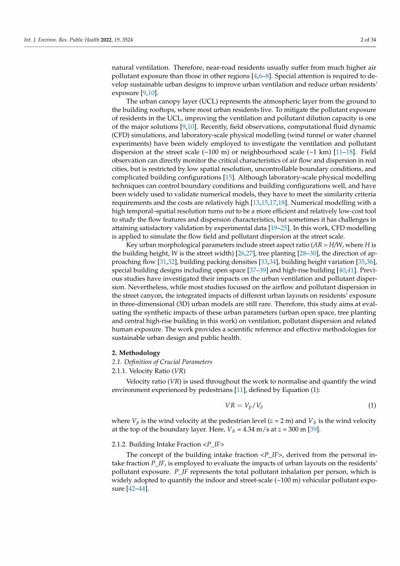
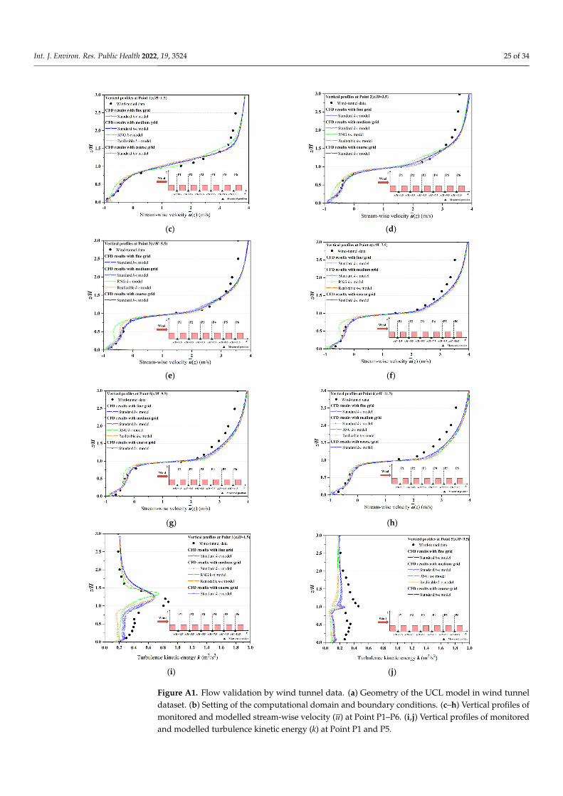
Figure A1 presents the results of the flow validation. The UCL model (moderatebuilding density) with a 7 × 11 building matrix was used in the employed wind tunneldataset [86]. The size of each building model is H = B = W = 15 cm. The measuring pointsfor the vertical profiles of the stream-wise velocity (u) and turbulence kinetic energy (k)are set in the centre of each street, named Pi (i = 1–6) (Figure A1a,b). As we described inSection 2.2.2, similar model configurations are set for the case studies: at full scale with ascale ratio of 200:1 (H = B = W = 30 m) to the wind tunnel scale. All settings are similar,except the length from the urban boundary to the domain outlet. Referring to the referencevelocity (Uref = 3 m/s) and the model geometry (H = 0.15 m or 30 m), Re is approximately3 × 104 and 6 × 106 at the wind tunnel scale and full scale, satisfying the requirements forReynolds number independence.

Figure A1c–j tests the grid independence (with a minimum grid size of 0.4 m, 0.2 mand 0.1 m) and the performance of different turbulence models (standard k-ε, RNG k-ε andrealisable k-ε models) with standard wall function. The results illustrate that differencesgenerated by the mesh setting are negligible. Thus, the moderate grid size (0.2 m forminima) is applied for all cases to save computational resources. Furthermore, the depictedvertical profiles of u and k verify that modelling using the standard k-ε model has betteragreement with the wind tunnel data than those using the RNG k-ε and realisable k-εmodels. Important statistics are summarised in Table A2, including the normalised meansquare error (NMSE), fractional bias (FB) and correlation coefficient (R). The results denotethat the standard k-ε model is employed in the study throughout this work.

• Pollutant dispersion validation by wind tunnel tests without tree models

Wind tunnel experiment data of inert gas dispersion [89] is employed in our work forthe validation of pollutant dispersion. The configurations of the experiment are illustratedin Figure A2a,b. The UCL model consists of a 3 × 3 model matrix, with each prism sizebeing Bx × By ×H = 27.6 cm× 18.4 cm× 8 cm. Inert gas C2H6 is used as the tracer, emittingfrom the line source (L = 18.8 cm, dx = 0.5 cm) settled in the UCL model area. Similar modelsettings at full scale (Bx × By × H = 138 m× 92 m× 40 m) are configured for the simulationto validate the dispersion. Fitting vertical profiles of monitored u, k and ε in the windtunnel experiments [89] are set for the domain inlet. The standard k-ε model and standardwall function are adopted in the simulation. Since the tracer gas concentration providedby the wind tunnel experiment is in a non-dimension form, the normalised concentrationK [89] is derived referring to Equation (15), in convenience for comparing the experimentaldata and simulation results.

K = C·H·Uref/E·dx (15)

where C is the inert gas concentration, and the emission rate E is 0.01 m/s. Importantstatistics are summarised in Table A3, including the NMSE, FB and R. The good agreement


between the results of the wind tunnel experiment and the CFD simulation confirm thatthe selected turbulence model and wall function is appropriate for evaluating the pollutantdispersion in our work.

• Pollutant dispersion validation by wind tunnel tests with tree models

The validation for vegetation modelling in this paper is performed on the basis ofthe wind tunnel experiment conducted by Gromke and Ruck [90]. The configurations andboundary conditions are set as in Figure A3a. The 2D street canyon is constructed by twoparallel building models, with the same sizes for both in the wind tunnel experiment andthe CFD simulation (L × W × H = 1.2 m × 0.12 m × 0.12 m). The standard k-ε modeland standard wall function coupled with the porous crown model (details in Section 2.2.4)are adopted in the simulation. The vertical profiles of u, k and ε for the domain inlet areprovided by Gromke and Ruck [90]. Uref = 4.7 m/s is applied; thus, the reference Re is38,630 >> 11,000. The normalised concentration K of the inert gas (SF6) is used to comparethe results of the wind tunnel experiment and the simulation. Vertical profiles of K arepresented in Figure A3b,c. Important statistics are summarised in Table A4, including theNMSE, FB and R. In general, the results satisfy the recommended criteria [91,92], exceptthat of y/H = 2 at the leeward wall. Nevertheless, as we focus on the pollutant dispersionin the 2D street canyon, the results of y/H = 0 (central region of the canyon with fullydeveloped turbulence) are more representative of the pollutant distribution features. Goodagreements of these statistics at y/H = 0 also confirm the modelling accuracy and reliabilityof the simulations. These results verify that the porous crown model with the standard k-εmodel and standard wall function has good performance, and is suitable for studying thetree-planting effects in this work.

3. Results3.1. Impacts of Building Configurations and Tree Planting on Flow Pattern3.1.1. Impact of Open Space and High-Rise Building on Airflow

Figure 2a,c,e presents the streamlines and velocity ratio (VR) at the pedestrian level(z = 2 m) of tree-free cases under the parallel approaching wind, named Case [Base, 0◦],Case [Open, 0◦] and Case [High, 0◦]. It shows the impacts of open space and high-risebuildings on the ambient airflows. Both building configurations are found to apparentlychange the structure of the vortex and airflow, especially within Region A2. VR in thedownstream regions of Case [Open, 0◦] is slightly strengthened compared with Case[Base, 0◦]. However, the mean wind speed of Case [Base, 0◦] and Case [Open, 0◦] in thewhole region are at the same level. New vortices are generated around Region A2 with theaddition of the open area. Comparing to the base cases, VR value increases significant0lywith the addition of high-rise building (Case [High, 0◦]), especially in Region A2. The flowstructure is changed in the whole urban area, and new vortices are found near the leewardwall or lateral wall of most buildings.

Figure 3 displays a detailed flow field in Region A2 at z = 2 m. As the axis of symmetryof the airflow field is the axis of y =135 m, Figure 3 only shows the streamlines in half ofthe zone. The urban design of open space decreases the wind speed and complicates therecirculation region (Figure 3c). On the contrary, the wind speed in Region A2 is stronglyenhanced by the high-rise building (Figure 3e). The VR in Region A2 increases obviouslycompared with the base case, with a maximum value increase of 0.20. Both building layoutscould deform the structure of the wind field around the building. Small vortices are formednear the windward side of the open space and the leeward side of the high-rise building.


(a) (b)

(c) (d)

Figure 2. Streamline and velocity ratio (VR) at z = 2m in (a) Case [Base, 0◦], (b) Case [Base-tree, 0◦],(c) Case [Open, 0◦], (d) Case [Open-tree, 0◦], (e) Case [High, 0◦] and (f) Case [High-tree, 0◦].


Figure 3. Streamline and velocity ratio (VR) at z = 2m in Region A2 in (a) Case [Base, 0◦], (b) Case[Base-tree, 0◦], (c) Case [Open, 0◦], (d) Case [Open-tree, 0◦], (e) Case [High, 0◦] and (f) Case[High-tree, 0◦].


To determine the impact of building configurations on the airflow and the vor-tices’ structure, Figure 4a,c,e depicts the airflow and streamlines at the central x-z plane(y = 135 m) with the parallel approaching wind of Case [Base, 0◦], Case [Open, 0◦] andCase [High, 0◦]. The designs of the open space and high-rise buildings have a significantinfluence on the geometry and the structures of the vortices in the street canyons, leadingto obvious changes in the flow field. With the open space (Figure 4c), the vortex on theright side of Location 3-3 extends and occupies the space where Building 3-3 was. Thevortex on the left side of Location 3-3 is compressed and the centre of the vortex rises up.Meanwhile, weakened airflows are observed compared with base case (Figure 4a). On thecontrary, with the high-rise building (Figure 4e), the wind speed is significantly enhanced,especially near the windward side of the high-rise building. Compared with the base case,the former vortex on the left side of Building 3-3 is concentrated to one-half of the originalsize and the right vortex has disappeared.

Figure 4. Normalised velocity (V/Vδ, Vδ = 4.34 m/s) at vertical plane (y = 135m) in Region A2 in(a) Case [Base, 0◦], (b) Case [Base-tree, 0◦], (c) Case [Open, 0◦], (d) Case [Open-tree, 0◦], (e) Case[High, 0◦] and (f) Case [High-tree, 0◦].


3.1.2. Influence of Tree Planting on Airflow

Figure 2b,d,f presents the flow field in the domain with tree planting. Whether for basecases (Figure 2a,b), open-space cases (Figure 2c,d) or high-rise building cases (Figure 2e,f),tree planting slightly changes the flow field in the entire domain (Region A1). Smallvortices are generated over the whole domain, and the continuity of the flow is obstructed.However, the overall wind speed in Region A1 remains a similar value with the addition ofvegetation under a parallel approaching wind.

This finding is further confirmed in Region A2, as presented in Figure 3. The windvector around trees and street corners becomes denser and more complex. Tree plantingslightly reduces the pedestrian-level wind speed in the central area of the base cases(Figure 3a,b) and open-space cases (Figure 3c,d). However, for high-rise building cases(Figure 3e,f), the VR value in Region A2 slightly increases with tree planting.

The vertical profiles of the flow field in Region A2 at y = 135 m are shown in Figure 4.We find that tree planting has a slight influence on the vertical airflow for all three buildingconfigurations. Compared with Case [Open, 0◦], the two-vortices structure of the flowfield is destroyed (Figure 4c,d). In the base cases (Figure 4a,b) and high-rise building cases(Figure 4e,f), the centre of the vortex on the left side of Building 3-3 rises up.

3.1.3. Quantitative Analysis of Impact of Different Urban Layouts on Velocity Field

To quantify the impacts of different urban layouts on the flow field, Figure 5a,b andTable A5 summarise the spatial mean VR at z = 2 m of Region A1 (<VR>A1) and A2(<VR>A2). Cases with different approaching wind directions (θ = 0◦, 15◦, 30◦ and 45◦) arediscussed as well. For Case [Base, θ], both 2 m <VR>A1 and <VR>A2 with the approachingwind direction of θ = 0◦ are much lower than those of other wind directions (θ = 15◦, 30◦ or45◦). The maximum <VR>A1 (0.21) and <VR>A2 (0.16) both appear at θ = 45◦.

For Case [Open, θ], the designed open space leads to a slight increase of 2 m VR on thespatial mean in Region A1 (Figure 5a) by 0.40–2.27%. However, in Region A2 (Figure 5b),the 2 m VR values in the open-space cases are decreased in comparison with those in basecases under the non-parallel approaching wind (θ = 15◦, 30◦ and 45◦), by 8.40–12.06%. Boththe 2 m <VR>A1 and <VR>A2 of the open-space cases increase with the rising θ, with amaximum value of 0.21 and 0.14 at θ = 45◦.

For Case [High, θ], the VR at z = 2 m has been significantly enhanced in both RegionA1 and A2 compared with Case [Base, θ]. The ambient airflow of the high-rise building(<VR>A2) is enhanced by 52.78–119.05%, more strongly than that in the whole buildingmatrix (<VR>A1) by 4.73–23.36%.

The results in Figure 5a,b and Table A5 show that tree planting reduces the VR in bothRegion A1 and A2 for different building configurations with all four approaching winddirections (θ = 0◦, 15◦, 30◦, 45◦), except Case [Base-tree, 0◦] and Case [High-tree, 0◦]. Treeplanting significantly decreases the urban wind speed at z = 2 m (<VR>A1) on the basis ofeither open space or high-rise building designs, by 4.63–14.99% or 2.04–16.68%, respectively.The <VR>A1 with non-parallel approaching wind directions (θ = 15◦, 30◦, 45◦) is reducedmore in comparison with parallel approaching wind (θ = 0◦). Taking Case [High-tree, θ]as an example, <VR>A1 is decreased by 6.87–16.68% compared with Case [High, θ] whenθ 6= 0◦, more than the 2.04% when θ = 0◦. These results are also consistent with the resultspresented in Figures 2–5. Contrary to the reductive effect of most tree-planting cases, treeplanting increases the <VR>A1 of Case [Base-tree, 0◦] and <VR>A2 of Case [High-tree, 0◦]by 6.27% and 8.98%, respectively. This phenomenon still needs more discussion in theongoing work.


Figure 5. Spatially-averaged VR in different scenarios at z = 2 m in (a) Region A1 and (b) Region A2.

3.2. Impacts of Building Configurations and Tree Planting on Pollutant Dispersion3.2.1. Influence of Open Space and High-Rise Building on Pollutant Dispersion

To investigate the impacts of building configurations on pollutant diffusion, Figure 6a,c,epresents the distributions of CO concentration (C) at the pedestrian level (z = 2 m) intree-free cases. Overall, the level of C in the three tree-free cases is similar, but the regionsof high C are affected by different building configurations. In general, open space enhancesthe CO accumulation on the leeward side of the buildings in the central and downstreamareas. Nevertheless, the high-rise building enhances the CO accumulation in the centraland upstream area significantly. However, CO in the central area is diluted to a quite lowlevel due to the strongly strengthened wind velocity surrounding the high-rise building.


Figure 6. CO concentration (C) at z = 2 m in (a) Case [Base, 0◦], (b) Case [Base-tree, 0◦], (c) Case[Open, 0◦], (d) Case [Open-tree, 0◦], (e) Case [High, 0◦] and (f) Case [High-tree, 0◦].

To better understand how building configurations affect the pollutant dispersion inthe central region (Region A2), Figure 7 shows the detailed vertical distribution of C at thex-z plane (y = 135 m). Comparing Figure 7c with Figure 7a, the low wind speed weakens thedilution and leads to high C levels in the open area. Particularly at the near-ground levelof the upwind area, C is higher than 13 mg/m3, while C in the same area of the base caseis about 5 mg/m3. In contrast, the strong airflow in the upwind of the high-rise buildingevidently decreases the C (Figure 7e). The near-ground C is decreased to about 2 mg/m3.Additionally, the CO distribution in the upwind of the high-rise building is reduced to avery limited vertical range, while that in the downwind is expanded due to the existence ofthe high-rise building.


Figure 7. Vertical profile of C in Region A2 at y = 135 m: (a) Case [Base, 0◦], (b) Case [Base-tree, 0◦],(c) Case [Open, 0◦], (d) Case [Open-tree, 0◦], (e) Case [High, 0◦] and (f) Case [High-tree, 0◦].

3.2.2. Influence of Tree Planting on Pollutant Dispersion

Figure 6b,d,f illustrates the C distribution in the urban area with tree planting, coupledwith the basic design, open-space and high-rise-building design, respectively. Comparingthem with Figure 6a,c,e, a significant increase of C is found in the whole urban area underthe tree-planting design, no matter which type of building configuration is considered. TheCO dispersion is significantly weakened by trees in the whole domain, and new hotspotswith high C appear.


Detailed vertical distributions of C surrounding Building 3-3 in the central region (Re-gion A2) with different building configurations are illustrated in Figure 7b,d,f. Comparedwith Figure 7a,c,e, tree planting evidently increases the near-ground C on the leeward sideof all buildings. Particularly in Case [Open-tree, 0◦], the near-ground C in the upwind ofthe open space increases to higher than 15 mg/m3. Trees around the high-rise building alsohave a significant influence on CO dispersion (Figure 7f). An area with a high C appears atthe upper layer of the building wall on the upwind of Building 3-3, corresponding to thevortex of the flow field in Figure 4. At the downwind of Building 3-3, the ground-level C ishigher than 15 mg/m3. Moreover, another hotspot with C higher than 15 mg/m3 appearsin the area of the tree crown.

3.2.3. Quantitative Analysis for Impact of Building Configurations and Tree Planting onPollutant Dispersion

Figure 8a,b and Table A6 summarise the mean CO concentration (C) at the pedestrianlevel (z = 2 m) in Region A1 (<CO>A1) and A2 (<CO>A2). The impacts of three buildingconfigurations, tree planting and wind directions (θ = 0◦, 15◦, 30◦ and 45◦) are quantitativelyassessed.

For the base cases, <CO>A1 slightly rises from 4.14 mg/m3 to 5.24 mg/m3 with theθ varying from 0◦ to 45◦. <CO>A2, with the range of 4.87–7.11 mg/m3, is higher than<CO>A1 with the same direction of approaching flows. Both <CO>A1 and <CO>A2 decreasein the cases with open space and high-rise buildings (Figure 8a,b). For the open-spacecases, <CO>A1 and <CO>A2 decrease rapidly with all four wind directions compared withthe base cases, by 7.83–20.54% and 0.08–24.43%, respectively. For the high-rise buildingcases, the decrement ranges from 4.39% to 23.00% for <CO>A1, and ranges from 43.88% to47.40% for <CO>A2, in comparison with base cases. The wind direction influences C moresignificantly for the area around the high-rise building (Region A2) than for the wholedomain (Region A1).

For cases with tree planting, the results show that both the <CO>A1 and <CO>A2evidently increase in all conditions with increasing rates of 2.84–31.88% and 2.85–35.46%,respectively. Taking θ = 0◦ as an example, <CO>A1 increases by 20.19%, 22.44% and 12.61%in Case [Base-tree, 0◦], Case [Open-tree, 0◦] and Case [High-tree, 0◦], compared with thetree-free cases. For the base cases, the largest increasing ratios of <CO>A1 and <CO>A2both appear when θ = 0◦. With tree planting, the CO concentration at the pedestrian leveland in the central area (<CO>A2) are higher than in the entire urban area (<CO>A1) forboth the base cases and open-space cases. The <CO>A2 is particularly high in open-spacecases with tree planting, with the values ranging from 6.59 mg/m3 to 7.89 mg/m3. For thehigh-building cases with tree planting, both <CO>A1 and <CO>A2 increase by 12.61–26.38%and 6.10–21.19%, respectively, compared with the tree-free cases. Regardless of the buildingconfiguration, the tree-planting design obviously weakens the dilution and dispersioncapacity of pollutants and remarkably increases the CO concentration.

3.3. Impacts of Building Configurations and Tree Planting on <P_IF>

As illustrated in Section 2.1.2, we use <P_IF> to quantify the influence of urban layoutson personal exposure in UCL. As the buildings are assumed to be a residential type withnatural ventilation, the pollutant concentration (C) on the building surfaces is adopted asthe indoor concentration due to I/O ≈ 1 [6,7].

Figure 9a–f plots C on the building surfaces in different cases when θ = 0◦. The Cdistribution is apparently influenced by different building configurations and tree planting,especially in the central area. Figure 10 and Table A7 summarise the parameter <P_IF> tospecify and quantify the CO exposure under scenarios with base conditions, open space,high-rise building and tree planting. Four wind directions (θ = 0◦, 15◦, 30◦, 45◦) are alsoconsidered in the evaluation.


Figure 8. Spatially-averaged CO concentration in different scenarios at z = 2 m in (a) Region A1 and(b) Region A2.


Figure 9. CO concentration (C) at building walls in 3D models: (a) Case [Base, 0◦], (b) Case [Base-tree,0◦], (c) Case [Open, 0◦], (d) Case [Open-tree, 0◦], (e) Case [High, 0◦] and (f) Case [High-tree, 0◦].

As displayed in Figure 6a,c,e, the open space and high-rise building change the Cdistribution on the building surfaces. Both layouts make CO accumulate in the centre of thebuilding matrix, while regions of high C in the base cases are in the downstream area of theapproaching flow (Figure 9a–f). Comparing Figure 6b,d,f with Figure 6a,c,e, tree plantingsignificantly increases the C on building surfaces, especially of the central 3 × 3 buildingmatrix.

Similar results can also be found in Figure 10 and Table A7. For tree-free cases, bothopen space and high-rise building could decrease <P_IF> with the wind from all four direc-tions by 6.56–16.08% and 9.59–24.70%, respectively. For different wind directions, the maxi-mum <P_IF> of the tree-free cases always appears when θ = 45◦, with <P_IF> = 2.53 ppm([Base, 45◦]), 2.19 ppm ([Open, 45◦]) and 1.90 ppm ([High, 45◦]), respectively. For caseswith tree planting, the personal exposure in all building configurations (~2.05–2.90 ppm) issignificantly increased compared with those of the tree-free cases (~1.54–2.53 ppm). Theincreasing ratio of <P_IF> ranges from 14.89% to 50.19% compared with tree-free cases. The


maximum <P_IF> among all cases is 2.90 ppm, appearing in Case [Base-tree, 45◦], whilethe maximum increasing ratio of <P_IF> is 50.19%, in Case [High-tree, 15◦].

Figure 10. Building intake fraction <P_IF> in all cases.

3.4. Velocity, CO Concentration and <P_IF> in Surrounding Area of A2 (Region A1−A2)

Tables A8 and A9 summarise VR and CO concentrations in the surrounding areaof A2 (Region A1−A2) in terms of spatial mean. In most of the scenarios, the buildingconfigurations and tree-planting plans have similar impacts as those in Region A2. How-ever, the opposite effects exist in Region A1−A2 with certain conditions, especially forCase [Open-tree]. The VR values are increased in this region with all four wind directions,while the VR values in Region A2 are restrained for Case [Open-tree]. Meanwhile, theCO concentration of Case [Open-tree] in Region A1−A2 is decreased accordingly. Thechanges of the flow and dispersion are probably induced by the channelling effect owingto the narrowed street between the boundary and the open space. The phenomenon stillneeds more discussion in the ongoing work. Furthermore, the CO concentration in RegionA1−A2 of Case [Open] is increased contrarily to that of Region A2, although most of the VRin Region A2 of Case [Open] is decreased. However, the open space improves the dilutionconditions in Region A2. Thus, open space has the opposite impact on CO dispersion in thecentral area (Region A2) compared with the surrounding area (Region A1−A2). Moreover,since the variation of <P_IF> is closely related to CO concentration, the <P_IF> of Case[Open] will increase and that of Case [Open-tree] will decrease in Region A1−A2. It is alsothe opposite of that in Region A2.

4. Discussion

As critical determinants for urban ventilation and pollutant dispersion, the impacts oftree-planting plans and varied aspect ratios of 2D street canyons have been investigated inprevious studies through both field experiments [93] and numerical simulations [80]. Chenet al. investigated the effect of different tree-planting parameters on the urban thermal andwind environment by conducting scaled outdoor field experiments [93]. Tree planting wasfound to reduce the pedestrian-level wind velocity in street canyons with all investigatedAR values. The decreasing rate ranged 29–70%. Although the experiments are conductedin 2D idealised street canyon models, we also find that tree planting has a restraining effecton the urban wind in our work as well. Yang et al. [80] evaluated the integrated impactof tree planting and various AR values in a full-scale street canyon by CFD modelling


(standard k-ε model) with the same emission settings as ours, and concluded that treeplanting can lead to the reduction of velocity by various magnitude and an increase in COexposure. In the canyon with AR = 1, the tree-induced CO increment is almost 70% (from9.63 mg/m3 to 16.30 mg/m3). However, in 2D street canyon models, only the conditionwith perpendicular approaching wind to the street axis is considered, which correspondsto the worst ventilation situation, since only air exchange across the street roof contributesto pollutant removal. In this work with a 3D urban canopy, the ventilation can be betterthan in 2D models and is closer to that of the real urban community. With our 3D UCLmodel, the largest decreasing rate contributed by the tree planting is about 22% in spatialmean (Case [Open-tree, 0◦] vs Case [Open, 0◦]). Meanwhile, the tree-induced CO incrementranges 2.84–35.46% in this work (Table A6). We can conclude that even with the sameAR (AR = 1) and tree-planting plan (tree planting on both sides of the street), the naturalventilation and dispersion conditions in the 3D building matrix are much better than thatin 2D street canyons.

Using dimensional variables to evaluate the variance of the residents’ exposure ow-ing to the varied impactors in different cities has huge challenges, because the emissionstrengths of different sources are not the same and may even be at different orders. Mean-while, the size of the target population in different studies may vary significantly. Asmentioned in Section 2.1.2, the variable IF has been used to express the source-to-intakerelationship for vehicular pollutants in realistic street canyons [48], but this would bestrongly affected by the population size and the spatial scale. For example, Habilomatisand Chaloulakou [45] found that the IF of vehicular ultrafine particles is 371 ppm in a2D street canyon in the central area of Athens. The IF at the city scale is relatively small.Marshall et al. [94] reported that the IF of particles in US cities ranges from 1 to 10 ppmand the IF of CO is 270 ppm in Hong Kong, with a huge population size [46]. The IF ofparticles at the regional scale are reported to range from 0.12 to 25 ppm in the entire UnitedStates [95].

Consequently, the variable <P_IF> is derived and applied for the exposure assessmentin this work. This normalised exposure index <P_IF> is more suitable for evaluating andcomparing the exposure risks in different areas, since the influence caused by differentorders of the population size and pollutant emission rates is avoided. Hang et al. found the<P_IF> of CO in the tree-free idealised 2D street canyon (AR = 1) was 5.21 ppm [42]. Yanget al. found the <P_IF> of CO in tree-planted 2D street canyons (AR = 1, LAD = 1) were5.60 and 5.58 ppm, and the values raised with increased AR. When AR is raised to 5, the<P_IF> is an order of magnitude larger than that with AR = 0.5, 1 and 3. Comparing theseworks in 2D street canyons, the <P_IF> of CO in the 3D UCL model ranges from 1.54 to2.87 with various tree-planting plans, building configurations and wind directions. Thevalues in all scenarios are much lower than those in 2D street canyons.

According to the comparison above, an important suggestion for the urban designeris to avoid building 2D street canyons either too deep or too long in urban districts. If itcannot be avoided, more leakages and a wider roadway could improve the ventilationconditions in 2D street canyons. Moreover, if the street canyon is designed longer than8H [17], the axis of the street should be approximately parallel to the prevailing winddirection.

To simplify the calculation process, we adopt idealised 3D UCL models in this paper.The building models are all assumed to be residential-type and are highly simplified withthe same configuration (in a 5 × 5 building array) for the case study. The trees are treatedas cubes of porous media. Neutral atmospheric conditions are adopted, and inert gas(CO) is considered as the tracer pollutant from the traffic emissions. Only four winddirections (θ = 0◦, 15◦, 30◦, 45◦) are considered in this research. Nevertheless, the realurban environment is affected by various parameters. Thus, it is worth mentioning thatthe results may be significantly different if urban morphologies, atmospheric conditions orother parameters are changed.


The impacts of urban morphological parameters in realistic urban areas are much morecomplicated than in such an idealised model. The study of different building coating plansand the direct radiation effect of the aerosol within urban canopy, as well as their impactson the urban thermal environment and human outdoor thermal comfort (Figures 3 and 4),is being implemented now. In future work, more kinds of realistic factors and conditionswill be carefully considered and evaluated, including non-neutral atmospheric conditionsand radiation impacts, the chemical reactions and composition of air pollutants, and morecomplicated urban morphological arrangements. Furthermore, the different tree speciesand the pollutant deposition on trees will also be considered in the ongoing work. CFDsimulations coupling turbulence and radiation models will be validated by our scaledoutdoor experiments (H = 1.2 m), as reported by Chen et al. [96,97]. These works will beadopted in numerical studies for full-scale realistic or idealised urban models. Our work isa step-by-step approximation of the real urban situation using the idealised model, and weare constantly improving our work on the way towards approaching the final target.

5. Conclusions

This paper is novel in that it numerically investigates the integrated impacts of openspace, high-rise buildings and tree planting on urban airflow, pollutant dispersion andrelated human exposure in 3D idealised UCL models (5-row and 5-column, aspect ratioH/W = 1, building plan area fraction λp = frontal area aspect ratio λf = 0.25) under neutralatmospheric conditions. Four approaching wind directions (parallel 0◦ and non-parallel15◦, 30◦, 45◦) are considered. The computational fluid dynamics (CFD) simulations withthe standard k-ε model are well validated by the wind tunnel data from the literature. Thepersonal intake fraction P_IF and its spatially-averaged value for the entire UCL buildingsurfaces <P_IF> are adopted to quantify the pollutant exposure on residents.

The CFD simulation results show that open space, high-rise building and tree plantingall have strong effects on the flow structure, pollutant dispersion and residents’ exposure.Some meaningful findings are concluded as follows:

(1) Without tree planting, in contrast to the general 5 × 5 uniform-height building cluster(H = B = W = 30m), open space (the central building is removed) increases the spatially-averaged velocity ratio (VR) for the whole urban area under all four approachingwind directions (0◦, 15◦, 30◦ and 45◦) by 0.40–2.27%. Designing the central building tobe taller (2H) than the surroundings (H) can increase the VR for the entire urban areaby 4.73–23.36%. In particular, the mean wind speed at the pedestrian level (z = 2 m)in the area around the high-rise building is significantly increased by 52.78–119.05%.However, tree planting significantly decreases the urban wind speed at z = 2 m on thebasis of either open space or high-rise building designs, by 4.63–14.99% or 2.04–16.68%,respectively.

(2) Pollutant dispersion is determined by urban airflow characteristics. CO is releasednear the ground as a surrogate of traffic emissions. Without tree planting, both openspace and central high-rise building would decrease the mean C at the pedestrianlevel for the whole urban area by 7.83–20.54% (0.32–0.97 mg/m3) and 4.39–23.00%(0.18–1.2 mg/m3) separately. This decreasing effect on C is significantly stronger forthe high-rise building in the central area, by 43.88–47.40% (2.14–3.18 mg/m3). On thecontrary, urban tree planting evidently weakens the pollutant dilution in all scenarios,with the increasing rate of 2.84–31.88% (0.15–1.2 mg/m3) for C at the pedestrian levelin the entire urban area.

(3) The traffic-related CO exposure on residents in kerbside buildings is evaluated by<P_IF>. For the tree-free scenarios, both open space and high-rise buildings could de-crease <P_IF> with the wind from all four directions by 6.56–16.08% and 9.59–24.70%,respectively. In contrast, tree planting obviously increases personal exposure in allscenarios by 14.89–50.19%. The <P_IF> of the tree-free cases ranges from 1.54 to2.53 ppm, while <P_IF> ranges from 2.05 to 2.90 ppm in cases with tree planting.


This work provides a practical and efficient method to investigate the impacts of syn-thetic urban layouts on urban ventilation and pollutant dispersion. This work also extendsthe application of the CFD methodology to the assessment of exposure, and consequentlyconnects to the area of public health. The method is applicable for further study couplingwith more kinds of urban configurations under various atmospheric conditions. The resultscan provide helpful references for urban designers developing the sustainability of the city.

Author Contributions: Conceptualization, J.H. and Z.L.; data curation, Q.L., J.L. and Y.C.; simulation,Q.L., J.L., Y.C. and H.Y.; validation, H.Y.; writing—original draft preparation, H.L., Q.L., J.L. andQ.W., writing—review and editing, H.L., J.H., Q.W., Q.L. and J.L. All authors have read and agreedto the published version of the manuscript.

Funding: This work was supported by the National Natural Science Foundation of China (NSFC,No. 42175094, 41805102 and 41875015), as well as the Special Fund for Science and TechnologyInnovation Strategy of Guangdong Province (International cooperation) (China, No 2019A050510021).The support from the UK GCRF Rapid Response Grant on ‘Transmission of SARS-CoV-2 virus incrowded indoor environment’ and the Innovation Group Project of the Southern Marine Science andEngineering Guangdong Laboratory (Zhuhai) (No. 311020001) are also gratefully acknowledged.

Conflicts of Interest: The authors declare no conflict of interest.

Nomenclature

AR, H/W aspect ratioB, H, W building width, building height and street width (m)Br volume-mean breathing rate (m3/s)C time-averaged pollutant (CO) concentration (kg/m3)Cd leaf drag coefficient<CO>A1, <CO>A2 the spatial mean CO concentration at z = 2 m in Region A1 and

in Region A2 (mg/m3)Dm, Dt molecular and turbulent diffusivity of the pollutant (m2/s)I/O indoor/outdoor pollutant concentration ratioIF intake fractionk, ε turbulent kinetic energy (m2/s2) and its dissipation rate (m2/s3)LAD leaf area density (m2/m3)m total pollutant emission over the considered period (kg)M, N total number of micro-environment types and population age groupsP number of the populationP_IF, <P_IF> personal intake fraction (ppm), building intake fraction (ppm)Re Reynolds numberS realistic CO emission rate (kg/m3/s)SCt turbulent Schmidt numberSui , Sk, Sε additional source and sink terms of momentum, k and ε (kg/m/s3)t time (s)uj time-averaged velocity component (m/s) on stream-wise (u),

span-wise (v, lateral) and vertical (w) directions, as j = 1, 2, 3U velocity magnitude (m/s)Uin(z) velocity profiles used at CFD domain inlet (m/s)Uref, u* reference velocity at building height and friction velocity (m/s)v, vt kinematic viscosity and kinetic eddy viscosity (m2/s)Vp, Vδ wind velocity at pedestrian-level and at the top of boundary layer (m/s)VR velocity ratio<VR>A1, <VR>A2 the spatial mean velocity ratio at z = 2 m in Region A1 and

in Region A2 (mg/m3)


xj spatial coordinates (m) on stream-wise (x), span-wise (y) andvertical (z) directions, as j = 1, 2, 3

βd portion of turbulent kinetic energy converted from mean kineticenergy under the influence of drag

βp dimensionless coefficient of the Kolmogorov cascadeθ wind direction (◦)κv von Kármán constantλp, λf building plan area density, frontal area densityρ air density (kg/m3)

Appendix A

1. Factors for exposure assessment

Table A1. Population composition and related factors for exposure assessment.

Item Juveniles Adults Elderly

Percentage of total population 21.2% 63.3% 15.5%Breathing rate Br indoors at home (m3/day) 12.5 13.8 13.1

Time spent indoors at home (percentage) 61.70% 59.50% 71.60%

2. Validation studies for the flow, dispersion and vegetation modelling

2.1. CFD validation of flow modelling

Int. J. Environ. Res. Public Health 2022, 18, x FOR PEER REVIEW 26 of 36

(a)

(b)

(c) (d)

(e) (f)

Figure A1. Cont.



(a)

(b)

(c) (d)

(e) (f)


(g) (h)

(i) (j)

Figure A1. Flow validation by wind tunnel data. (a) Geometry of the UCL model in wind tunnel

dataset. (b) Setting of the computational domain and boundary conditions. (c–h) Vertical profiles of

monitored and modelled stream‐wise velocity (𝑢) at Point P1–P6. (i,j) Vertical profiles of monitored

and modelled turbulence kinetic energy (k) at Point P1 and P5.

Table A2. Statistical analysis between wind tunnel data and CFD simulation results—flow valida‐

tion.

Variable (Position) Grid Size Turbulence Model NMSE * FB ** R ***

Criteria ≤1.5 −0.3–0.3 → 1.0

Stream‐wise velocity

at P1

Fine grid STD 0.054 0.084 0.990

Medium grid

STD 0.049 0.087 0.990

RNG 0.107 0.018 0.996

RKE 0.115 0.094 0.986

Coarse grid STD 0.038 0.081 0.991


at P2

Fine grid STD 0.007 0.002 0.999

Medium grid

STD 0.009 0.002 0.997

RNG 0.045 −0.090 0.994

RKE 0.016 −0.083 0.998

Coarse grid STD 0.011 0.013 0.997


at P3

Fine grid STD 0.012 −0.063 0.996

Medium grid

STD 0.005 −0.024 0.998

RNG 0.093 −0.179 0.996

RKE 0.022 −0.100 0.997

Coarse grid STD 0.005 −0.013 0.997


at P4

Fine grid STD 0.014 −0.057 0.999

Medium grid STD 0.014 −0.034 1.000

RNG 0.053 −0.175 0.998

Figure A1. Flow validation by wind tunnel data. (a) Geometry of the UCL model in wind tunneldataset. (b) Setting of the computational domain and boundary conditions. (c–h) Vertical profiles ofmonitored and modelled stream-wise velocity (u) at Point P1–P6. (i,j) Vertical profiles of monitoredand modelled turbulence kinetic energy (k) at Point P1 and P5.


Table A2. Statistical analysis between wind tunnel data and CFD simulation results—flow validation.

Variable (Position) Grid Size Turbulence Model NMSE * FB ** R ***Criteria ≤1.5 −0.3–0.3 → 1.0

Stream-wise velocity at P1

Fine grid STD 0.054 0.084 0.990

Medium gridSTD 0.049 0.087 0.990RNG 0.107 0.018 0.996RKE 0.115 0.094 0.986

Coarse grid STD 0.038 0.081 0.991


Fine grid STD 0.007 0.002 0.999

Medium gridSTD 0.009 0.002 0.997RNG 0.045 −0.090 0.994RKE 0.016 −0.083 0.998

Coarse grid STD 0.011 0.013 0.997


Fine grid STD 0.012 −0.063 0.996

Medium gridSTD 0.005 −0.024 0.998RNG 0.093 −0.179 0.996RKE 0.022 −0.100 0.997

Coarse grid STD 0.005 −0.013 0.997


Fine grid STD 0.014 −0.057 0.999


Coarse grid STD 0.015 −0.023 0.999


Fine grid STD 0.019 −0.051 0.998


Coarse grid STD 0.022 −0.009 0.997


Fine grid STD 0.037 −0.104 0.995


Coarse grid STD 0.035 −0.048 0.998

TKE at P1

Fine grid STD 0.137 0.177 0.820

Medium gridSTD 0.115 0.150 0.842RNG 0.275 0.343 0.662RKE 0.361 0.366 0.727

Coarse grid STD 0.091 0.115 0.867

TKE at P5

Fine grid STD 0.610 0.615 0.076

Medium gridSTD 0.621 0.615 0.135RNG 1.299 0.837 −0.105RKE 1.096 0.802 −0.378

Coarse grid STD 0.526 0.575 0.255

* normalised mean square error: NMSE = (Obs−Sim)2

Obs∗Sim. ** fractional bias-FB = Obs−Sim

0.5 ∗(Obs+Sim). *** correlation

coefficient–R =∑(Obs−Obs)(Sim−Sim)√

∑(Obs−Obs)2

∑(Sim−Sim)2 .

2.2. CFD validation of pollutant dispersion without tree models


Figure A2. Validation for pollutant dispersion. (a) Configurations of the wind tunnel experimentwith top view. (b) Configurations of the wind tunnel experiment with lateral view. (c) Vertical profilesof normalized inert gas concentration K at the roof top of the model. (d) Vertical profiles of K at theleeward and windward wall.

Table A3. Statistical analysis between wind tunnel data and CFD simulation results—dispersionmodelling.

Variable (Position) NMSE * FB ** R ***Criteria ≤1.5 −0.3–0.3 → 1.0

Leeward wall 0.021 −0.012 0.997Windward wall 0.064 −0.223 0.855

Central line 0.029 −0.13 0.998





∑(Obs−Obs)2

∑(Sim−Sim)2 .

2.3. CFD validation of pollutant dispersion with tree models


Figure A3. Validation for the vegetation modelling. (a) Configurations of the wind tunnel experimentwith vegetation model. (b) Vertical profiles of K at the leeward wall. (c) Vertical profiles of K at thewindward wall.

Table A4. Statistical analysis between wind tunnel data and CFD simulation results—vegetationmodelling.

Variable (Position) NMSE * FB ** R ***Criteria ≤1.5 −0.3–0.3 → 1.0

Leeward sidey/H = 0 0.159 0.011 0.918y/H = 2 1.306 0.594 0.987y/H = 4 0.108 0.128 0.974

Windward sidey/H = 0 0.055 −0.233 0.630y/H = 2 0.007 0.049 0.784y/H = 4 0.221 −0.256 0.700





∑(Obs−Obs)2

∑(Sim−Sim)2 .

3. Quantitative investigations of the flow, pollutant concentration and traffic-relatedexposure


Table A5. Spatial mean velocity ratio (VR) at z = 2 m in Region A1 (<VR>A1) and Region A2 (<VR>A2)of each scenario and the change rate.

Case<VR>A1 <VR>A2

0◦ 15◦ 30◦ 45◦ 0◦ 15◦ 30◦ 45◦

Case [Base]0.12 0.18 0.20 0.21 0.09 0.13 0.16 0.16

Case [Open] 0.12 0.19 0.21 0.21 0.10 0.11 0.14 0.14+0.40% +1.70% +2.27% +2.22% +14.53% −12.06% −8.40% −9.29%

Case [High] 0.15 0.19 0.22 0.23 0.19 0.21 0.24 0.24+23.36% +4.73% +7.30% +12.07% +119.05% +61.30% +55.06% +52.78%

Case [Base-tree]0.13 0.17 0.18 0.18 0.08 0.12 0.14 0.14

+6.27% −7.51% −11.59% −11.41% −10.76% −6.22% −11.08% −11.43%

Case [Open-tree] 0.12 0.17 0.18 0.18 0.08 0.11 0.13 0.12−4.63% −9.01% −13.65% −14.99% −21.92% −6.91% −7.84% −14.18%

Case [High-tree] 0.15 0.18 0.18 0.19 0.21 0.20 0.20 0.21−2.04% −6.87% −14.93% −16.68% +8.98% −4.42% −16.11% −13.44%

The percentage number in each cell denotes the change rate of each case. Case [Base] is the comparison referencefor Case [Open], Case [High] and Case [Base-tree]. The change rate of Case [Open-tree] refers to Case [Open], andthat of Case [High-tree] refers to Case [High].

Table A6. Spatial mean CO concentration (C) at z = 2 m in Region A1 (<CO>A1) and Region A2(<CO>A2) of each scenario and the change rate.

Case<CO>A1 (mg/m3) <CO>A2 (mg/m3)

0◦ 15◦ 30◦ 45◦ 0◦ 15◦ 30◦ 45◦

Case [Base]4.14 4.72 5.01 5.24 4.87 7.11 6.37 6.70

Case [Open] 3.82 3.75 4.24 4.44 4.86 5.92 4.94 5.06−7.83% −20.54% −15.31% −15.27% −0.08% −16.82% −22.48% −24.43%

Case [High] 3.96 3.99 4.12 4.04 2.73 3.80 3.36 3.52−4.39% −15.47% −17.78% −23.00% −43.88% −46.58% −47.24% −47.40%

Case [Base-tree]4.98 5.36 5.24 5.39 6.59 7.89 6.78 6.89

+20.19% +13.55% +4.73% +2.84% +35.46% +10.93% +6.47% +2.85%

Case [Open-tree] 4.67 4.95 4.74 5.00 5.55 6.61 5.60 5.97+22.44% +31.88% +11.80% +12.64% +14.09% +11.76% +13.35% +17.93%

Case [High-tree] 4.46 4.64 5.20 4.88 2.90 4.28 4.07 3.95+12.61% +16.31% +26.38% +20.88% +6.10% +12.57% +21.19% +12.04%

The percentage data denote the change rate of each case in contrast to Case [Base]. The change rate of Case[Open-tree] refers to Case [Open], and that of Case [High-tree] refers to Case [High].

Table A7. Building intake fraction <P_IF> and the change rate in different cases.

Case<P_IF> (ppm)

0◦ 15◦ 30◦ 45◦

Case [Base]1.71 2.23 2.32 2.53

Case [Open] 1.59 1.87 2.05 2.19−6.56% −16.08% −11.65% −13.19%

Case [High] 1.54 1.89 1.86 1.90−9.59% −15.00% −19.74% −24.70%


Table A7. Cont.

Case<P_IF> (ppm)

0◦ 15◦ 30◦ 45◦

Case [Base-tree]2.05 2.87 2.75 2.90

+19.94% +28.92% +18.24% +14.89%

Case [Open-tree] 2.00 2.65 2.51 2.68+25.67% +41.62% +22.22% +22.43%

Case [High-tree] 2.32 2.41 2.57 2.48+50.19% +27.28% +37.63% +30.51%

The percentage number in each cell denotes the rate of change of each case. Case [Base] is the comparison referencefor Case [Open], Case [High] and Case [Base-tree]. The change rate of Case [Open-tree] refers to Case [Open], andthat of Case [High-tree] refers to Case [High].

Table A8. Spatial mean velocity ratio (VR) at z = 2 m in the Region A1−A2 (<VR>A1−A2) of eachscenario and the change rate.

Case Name<VR>A1−A2

0◦ 15◦ 30◦ 45◦

Case [Base]0.55 0.83 0.90 0.92

Case [Open] 0.59 0.76 0.79 0.81+7.71% −7.61% −11.64% −11.41%

Case [High] 0.55 0.85 0.93 0.95−7.90% +11.35% +16.88% +16.60%

Case [Base-tree]0.53 0.77 0.79 0.81−2.94% −9.16% −14.14% −15.06%

Case [Open-tree] 0.63 0.83 0.92 0.99+19.69% +6.92% +15.91% +23.36%

Case [High-tree] 0.61 0.77 0.79 0.82−3.82% −7.20% −14.76% −17.11%


Table A9. Spatial mean CO concentration (C) at z = 2 m in the Region A1−A2 (<CO>A1−A2) of eachscenario and the change rate.

Case Name<CO>A1−A2

0◦ 15◦ 30◦ 45◦

Case [Base]4.05 4.42 4.84 5.06

Case [Open] 4.78 5.04 5.05 5.20+17.89% +14.07% +4.45% +2.83%

Case [High] 3.69 3.48 4.15 4.36−22.81% −31.00% −17.79% −16.13%

Case [Base-tree]4.56 4.74 4.63 4.88

+23.82% +36.15% +11.57% +11.87%

Case [Open-tree] 4.11 4.01 4.21 4.10−9.88% −15.29% −9.13% −16.01%

Case [High-tree] 4.65 4.69 5.34 5.00+13.15% +16.75% +26.89% +21.83%



References1. Chan, C.K.; Yao, X. Air pollution in mega cities in China. Atmos. Environ. 2008, 42, 1–42. [CrossRef]2. Fenger, J. Urban air quality. Atmos. Environ. 1999, 33, 4877–4900. [CrossRef]3. Pu, Y.; Yang, C. Estimating urban roadside emissions with an atmospheric dispersion model based on in-field measurements.

Environ. Pollut. 2014, 192, 300–307. [CrossRef] [PubMed]4. Ji, W.; Zhao, B. Estimating mortality derived from indoor exposure to particles of outdoor origin. PLoS ONE 2015, 10, e0124238.

[CrossRef] [PubMed]5. Peters, A.; Pope III, C.A. Cardiopulmonary mortality and air pollution. Lancet 2002, 360, 1184–1185. [CrossRef]6. Chen, C.; Zhao, B.; Zhou, W.; Jiang, X.; Tan, Z. A methodology for predicting particle penetration factor through cracks of

windows and doors for actual engineering application. Build. Environ. 2012, 47, 339–348. [CrossRef]7. Quang, T.N.; He, C.; Morawska, L.; Knibbs, L.D.; Falk, M. Vertical particle concentration profiles around urban office buildings.

Atmos. Chem. Phys. Discuss. 2012, 12, 5017–5030. [CrossRef]8. Zaeh, S.E.; Koehler, K.; Eakin, M.N.; Wohn, C.; Diibor, I.; Eckmann, T.; Wu, T.D.; Clemons-Erby, D.; Gummerson, C.E.; Green, T.;

et al. Indoor air quality prior to and following school building renovation in a mid-Atlantic school district. Int. J. Environ. Res.Public Health 2021, 18, 12149. [CrossRef]

9. Bady, M.; Kato, S.; Huang, H. Towards the application of indoor ventilation efficiency indices to evaluate the air quality of urbanareas. Build. Environ. 2008, 43, 1991–2004. [CrossRef]

10. Ng, W.-Y.; Chau, C.-K. A modeling investigation of the impact of street and building configurations on personal air pollutantexposure in isolated deep urban canyons. Sci. Total Environ. 2014, 468, 429–448. [CrossRef]

11. Ng, E. Policies and technical guidelines for urban planning of high-density cities-air ventilation assessment (ava) of Hong Kong.Build. Environ. 2009, 44, 1478–1488. [CrossRef] [PubMed]

12. Chang, C.H.; Meroney, R.N. Concentration and flow distributions in urban street canyons: Wind tunnel and computational data.J. Wind. Eng. Ind. Aerodyn. 2003, 91, 1141–1154. [CrossRef]

13. Chew, L.W.; Aliabadi, A.A.; Norford, L.K. Flows across high aspect ratio street canyons: Reynolds number independence revisited.Environ. Fluid Mech. 2018, 18, 1275–1291. [CrossRef]

14. Grimmond, C.; Roth, M.; Oke, T.R.; Au, Y.; Best, M.; Betts, R.; Carmichael, G.; Cleugh, H.; Dabberdt, W.; Emmanuel, R. Climateand more sustainable cities: Climate information for improved planning and management of cities (producers/capabilitiesperspective). Procedia Environ. Sci. 2010, 1, 247–274. [CrossRef]

15. Li, X.-X.; Liu, C.-H.; Leung, D.Y.C.; Lam, K.M. Recent progress in CFD modelling of wind field and pollutant transport in streetcanyons. Atmos. Environ. 2006, 40, 5640–5658. [CrossRef]

16. Peng, Y.L.; Buccolieri, R.; Gao, Z.; Ding, W. Indices employed for the assessment of “urban outdoor ventilation”—A review.Atmos. Environ. 2020, 223, 117211. [CrossRef]

17. Tominaga, Y.; Stathopoulos, T. CFD simulation of near-field pollutant dispersion in the urban environment: A review of currentmodeling techniques. Atmos. Environ. 2013, 79, 716–730. [CrossRef]

18. Vardoulakis, S.; Fisher, B.E.; Pericleous, K.; Gonzalez-Flesca, N. Modelling air quality in street canyons: A review. Atmos. Environ.2003, 37, 155–182. [CrossRef]

19. Antoniou, N.; Montazeri, H.; Wigo, H.; Neophytou, M.K.A.; Blocken, B.; Sandberg, M. CFD and wind-tunnel analysis of outdoorventilation in a real compact heterogeneous urban area: Evaluation using “air delay”. Build. Environ. 2017, 126, 355–372.[CrossRef]

20. Blocken, B.; Stathopoulos, T.; Carmeliet, J. CFD simulation of the atmospheric boundary layer: Wall function problems. Atmos.Environ. 2007, 41, 238–252. [CrossRef]

21. Gromke, C. A vegetation modeling concept for building and environmental aerodynamics wind tunnel tests and its applicationin pollutant dispersion studies. Environ. Pollut. 2011, 159, 2094–2099. [CrossRef] [PubMed]

22. Liu, J.L.; Zhang, X.L.; Niu, J.L.; Tse, K.T. Pedestrian-level wind and gust around buildings with a ‘lift-up’ design: Assessment ofinfluence from surrounding buildings by adopting LES. Build. Simul. 2019, 12, 1107–1118. [CrossRef]

23. Santiago, J.L.; Martilli, A.; Martin, F. CFD simulation of airflow over a regular array of cubes. Part I: Three-dimensional simulationof the flow and validation with wind-tunnel measurements. Bound.-Layer Meteorol. 2007, 122, 609–634. [CrossRef]

24. Yang, H.Y.; Lam, C.K.C.; Lin, Y.Y.; Chen, L.; Mattsson, M.; Sandberg, M.; Hayati, A.; Claesson, L.; Hang, J. Numerical investigationsof re-independence and influence of wall heating on flow characteristics and ventilation in full-scale 2d street canyons. Build.Environ. 2021, 189, 107510. [CrossRef]

25. Zhang, M.; Gao, Z.; Guo, X.; Shen, J. Ventilation and pollutant concentration for the pedestrian zone, the near-wall zone, and thecanopy layer at urban intersections. Int. J. Environ. Res. Public Health 2021, 18, 11080. [CrossRef]

26. He, L.; Hang, J.; Wang, X.; Lin, B.; Li, X.; Lan, G. Numerical investigations of flow and passive pollutant exposure in high-risedeep street canyons with various street aspect ratios and viaduct settings. Sci. Total Environ. 2017, 584, 189–206. [CrossRef]

27. Hang, J.; Xian, Z.; Wang, D.; Mak, C.M.; Wang, B.; Fan, Y. The impacts of viaduct settings and street aspect ratios on personalintake fraction in three-dimensional urban-like geometries. Build. Environ. 2018, 143, 138–162. [CrossRef]

28. Duarte, D.H.S.; Shinzato, P.; Gusson, C.D.; Alves, C.A. The impact of vegetation on urban microclimate to counterbalance builtdensity in a subtropical changing climate. Urban Clim. 2015, 14, 224–239. [CrossRef]

http://doi.org/10.1016/j.atmosenv.2007.09.003

http://doi.org/10.1016/S1352-2310(99)00290-3

http://doi.org/10.1016/j.envpol.2014.05.019

http://www.ncbi.nlm.nih.gov/pubmed/24954153

http://doi.org/10.1371/journal.pone.0124238


http://doi.org/10.1016/S0140-6736(02)11289-X

http://doi.org/10.1016/j.buildenv.2011.07.004

http://doi.org/10.5194/acp-12-5017-2012

http://doi.org/10.3390/ijerph182212149


http://doi.org/10.1016/j.scitotenv.2013.08.077



http://doi.org/10.1016/S0167-6105(03)00056-4

http://doi.org/10.1007/s10652-018-9601-0

http://doi.org/10.1016/j.proenv.2010.09.016


http://doi.org/10.1016/j.atmosenv.2019.117211


http://doi.org/10.1016/S1352-2310(02)00857-9





http://doi.org/10.1007/s12273-019-0541-5

http://doi.org/10.1007/s10546-006-9123-z

http://doi.org/10.1016/j.buildenv.2020.107510

http://doi.org/10.3390/ijerph182111080



http://doi.org/10.1016/j.uclim.2015.09.006


29. Moradpour, M.; Hosseini, V. An investigation into the effects of green space on air quality of an urban area using CFD modelling.Urban Clim. 2020, 34, 100686. [CrossRef]

30. Yang, X.; Peng, L.L.H.; Chen, Y.; Yao, L.; Wang, Q. Air humidity characteristics of local climate zones: A three-year observationalstudy in Nanjing. Build. Environ. 2020, 171, 106661. [CrossRef]

31. Gromke, C.; Ruck, B. Pollutant concentrations in street canyons of different aspect ratio with avenues of trees for various winddirections. Bound.-Layer Meteorol. 2012, 144, 41–64. [CrossRef]

32. Hang, J.; Chen, L.; Lin, Y.Y.; Buccolieri, R.; Lin, B.R. The impact of semi-open settings on ventilation in idealized building arrays.Urban Clim. 2018, 25, 196–217. [CrossRef]

33. Chen, L.; Hang, J.; Sandberg, M.; Claesson, L.; Di Sabatino, S.; Wigo, H. The impacts of building height variations and buildingpacking densities on flow adjustment and city breathability in idealized urban models. Build. Environ. 2017, 118, 344–361.[CrossRef]

34. Ramponi, R.; Blocken, B.; de Coo, L.B.; Janssen, W.D. CFD simulation of outdoor ventilation of generic urban configurations withdifferent urban densities and equal and unequal street widths. Build. Environ. 2015, 92, 152–166. [CrossRef]

35. Gu, Z.-L.; Zhang, Y.-W.; Cheng, Y.; Lee, S.-C. Effect of uneven building layout on air flow and pollutant dispersion in non-uniformstreet canyons. Build. Environ. 2011, 46, 2657–2665. [CrossRef]

36. Hang, J.; Li, Y.; Sandberg, M.; Buccolieri, R.; Di Sabatino, S. The influence of building height variability on pollutant dispersionand pedestrian ventilation in idealized high-rise urban areas. Build. Environ. 2012, 56, 346–360. [CrossRef]

37. Chen, L.; Wen, Y.; Zhang, L.; Xiang, W.-N. Studies of thermal comfort and space use in an urban park square in cool and coldseasons in shanghai. Build. Environ. 2015, 94, 644–653. [CrossRef]

38. He, Y.Y.; Tablada, A.; Wong, N.H. Effects of non-uniform and orthogonal breezeway networks on pedestrian ventilation inSingapore’s high-density urban environments. Urban Clim. 2018, 24, 460–484. [CrossRef]

39. Sha, C.; Wang, X.; Lin, Y.; Fan, Y.; Chen, X.; Hang, J. The impact of urban open space and ‘lift-up’ building design on buildingintake fraction and daily pollutant exposure in idealized urban models. Sci. Total Environ. 2018, 633, 1314–1328. [CrossRef]

40. Cheung, J.O.P.; Liu, C.-H. CFD simulations of natural ventilation behaviour in high-rise buildings in regular and staggeredarrangements at various spacings. Energy Build. 2011, 43, 1149–1158. [CrossRef]

41. Zhang, Y.; Kwok, K.C.; Liu, X.-P.; Niu, J.-L. Characteristics of air pollutant dispersion around a high-rise building. Environ. Pollut.2015, 204, 280–288. [CrossRef]

42. Hang, J.; Luo, Z.; Wang, X.; He, L.; Wang, B.; Zhu, W. The influence of street layouts and viaduct settings on daily carbonmonoxide exposure and intake fraction in idealized urban canyons. Environ. Pollut. 2017, 220, 72–86. [CrossRef]

43. Lin, Y.; Chen, G.; Chen, T.; Luo, Z.; Yuan, C.; Gao, P.; Hang, J. The influence of advertisement boards, street and source layouts onco dispersion and building intake fraction in three-dimensional urban-like models. Build. Environ. 2019, 150, 297–321. [CrossRef]

44. Zhang, K.; Chen, G.; Wang, X.; Liu, S.; Mak, C.M.; Fan, Y.; Hang, J. Numerical evaluations of urban design technique to reducevehicular personal intake fraction in deep street canyons. Sci. Total Environ. 2019, 653, 968–994. [CrossRef]

45. Habilomatis, G.; Chaloulakou, A. A CFD modeling study in an urban street canyon for ultrafine particles and populationexposure: The intake fraction approach. Sci. Total Environ. 2015, 530, 227–232. [CrossRef]

46. Luo, Z.; Li, Y.; Nazaroff, W.W. Intake fraction of nonreactive motor vehicle exhaust in Hong Kong. Atmos. Environ. 2010, 44,1913–1918. [CrossRef]

47. Nazaroff, W.W. Inhalation intake fraction of pollutants from episodic indoor emissions. Build. Environ. 2008, 43, 269–277.[CrossRef]

48. Zhou, Y.; Levy, J.I. The impact of urban street canyons on population exposure to traffic-related primary pollutants. Atmos.Environ. 2008, 42, 3087–3098. [CrossRef]

49. Chau, C.K.; Tu, E.Y.; Chan, D.W.T.; Burnett, C.J. Estimating the total exposure to air pollutants for different population age groupsin hong kong. Environ. Int. 2002, 27, 617–630. [CrossRef]

50. Allan, M.; Richardson, G.M.; Jones-Otazo, H. Probability density functions describing 24-h inhalation rates for use in humanhealth risk assessments: An update and comparison. Hum. Ecol. Risk Assess. 2008, 14, 372–391. [CrossRef]

51. Blocken, B. Computational fluid dynamics for urban physics: Importance, scales, possibilities, limitations and ten tips and trickstowards accurate and reliable simulations. Build. Environ. 2015, 91, 219–245. [CrossRef]

52. Gao, Z.L.; Bresson, R.; Qu, Y.F.; Milliez, M.; de Munck, C.; Carissimo, B. High resolution unsteady RANS simulation of wind,thermal effects and pollution dispersion for studying urban renewal scenarios in a neighborhood of Toulouse. Urban Clim. 2018,23, 114–130. [CrossRef]

53. Li, X.-X.; Britter, R.E.; Norford, L.K. Transport processes in and above two-dimensional urban street canyons under differentstratification conditions: Results from numerical simulation. Environ. Fluid Mech. 2015, 15, 399–417. [CrossRef]

54. Wang, W.; Ng, E. Air ventilation assessment under unstable atmospheric stratification-a comparative study for Hong Kong. Build.Environ. 2018, 130, 1–13. [CrossRef]

55. Zhang, Y.; Gu, Z.; Yu, C.W. Review on numerical simulation of airflow and pollutant dispersion in urban street canyons undernatural background wind condition. Aerosol Air Qual. Res. 2018, 18, 780–789. [CrossRef]

56. Blocken, B. LES over RANS in building simulation for outdoor and indoor applications: A foregone conclusion? Build. Simul.2018, 11, 821–870. [CrossRef]

http://doi.org/10.1016/j.uclim.2020.100686


http://doi.org/10.1007/s10546-012-9703-z









http://doi.org/10.1016/j.enbuild.2010.11.024









http://doi.org/10.1016/S0160-4120(01)00120-9

http://doi.org/10.1080/10807030801934796



http://doi.org/10.1007/s10652-014-9347-2


http://doi.org/10.4209/aaqr.2017.09.0303

http://doi.org/10.1007/s12273-018-0459-3


57. Meroney, R.N. Ten questions concerning hybrid computational/physical model simulation of wind flow in the built environment.Build. Environ. 2016, 96, 12–21. [CrossRef]

58. Zhong, J.; Cai, X.-M.; Bloss, W.J. Modelling the dispersion and transport of reactive pollutants in a deep urban street canyon:Using large-eddy simulation. Environ. Pollut. 2015, 200, 42–52. [CrossRef]

59. Fuka, V.; Xie, Z.-T.; Castro, I.P.; Hayden, P.; Carpentieri, M.; Robins, A.G. Scalar fluxes near a tall building in an aligned array ofrectangular buildings. Bound.-Layer Meteorol. 2018, 167, 53–76. [CrossRef]

60. McMullan, W.A.; Angelino, M. The effect of tree planting on traffic pollutant dispersion in an urban street canyon using large eddysimulation with a recycling and rescaling inflow generation method. J. Wind. Eng. Ind. Aerodyn. 2022, 221, 104877. [CrossRef]

61. Cui, D.J.; Mak, C.M.; Kwok, K.C.S.; Ai, Z.T. CFD simulation of the effect of an upstream building on the inter-unit dispersion in amulti-story building in two wind directions. J. Wind. Eng. Ind. Aerodyn. 2016, 150, 31–41. [CrossRef]

62. Cui, D.; Hu, G.; Ai, Z.; Du, Y.; Mak, C.M.; Kwok, K. Particle image velocimetry measurement and CFD simulation of pedestrianlevel wind environment around u-type street canyon. Build. Environ. 2019, 154, 239–251. [CrossRef]

63. Gromke, C.; Blocken, B. Influence of avenue-trees on air quality at the urban neighborhood scale. Part I: Quality assurance studiesand turbulent Schmidt number analysis for RANS CFD simulations. Environ. Pollut. 2015, 196, 214–223. [CrossRef]

64. Panagiotou, I.; Neophytou, M.K.A.; Hamlyn, D.; Britter, R.E. City breathability as quantified by the exchange velocity and itsspatial variation in real inhomogeneous urban geometries: An example from central London urban area. Sci. Total Environ. 2013,442, 466–477. [CrossRef] [PubMed]

65. Wang, W.; Xu, Y.; Ng, E.; Raasch, S. Evaluation of satellite-derived building height extraction by CFD simulations: A case study ofneighborhood-scale ventilation in Hong Kong. Landsc. Urban Plan. 2018, 170, 90–102. [CrossRef]

66. Ashie, Y.; Kono, T. Urban-scale CFD analysis in support of a climate-sensitive design for the Tokyo bay area. Int. J. Clim. 2011, 31,174–188. [CrossRef]

67. Hang, J.; Wang, Q.; Chen, X.; Sandberg, M.; Zhu, W.; Buccolieri, R.; Di Sabatino, S. City breathability in medium density urban-likegeometries evaluated through the pollutant transport rate and the net escape velocity. Build. Environ. 2015, 94, 166–182. [CrossRef]

68. Zhang, K.; Chen, G.W.; Zhang, Y.; Liu, S.H.; Wang, X.M.; Wang, B.M.; Hang, J. Integrated impacts of turbulent mixing and nox-o-3photochemistry on reactive pollutant dispersion and intake fraction in shallow and deep street canyons. Sci. Total Environ. 2020,712, 135553. [CrossRef]

69. Franke, J.; Hellsten, A.; Schluenzen, K.H.; Carissimo, B. The cost 732 best practice guideline for CFD simulation of flows in theurban environment: A summary. Int. J. Environ. Pollut. 2011, 44, 419–427. [CrossRef]

70. Tominaga, Y.; Mochida, A.; Yoshie, R.; Kataoka, H.; Nozu, T.; Yoshikawa, M.; Shirasawa, T. Aij guidelines for practical applicationsof CFD to pedestrian wind environment around buildings. J. Wind. Eng. Ind. Aerodyn. 2008, 96, 1749–1761. [CrossRef]

71. Lien, F.S.; Yee, E. Numerical modelling of the turbulent flow developing within and over a 3-d building array, part I: Ahigh-resolution reynolds-averaged navier-stokes approach. Bound.-Layer Meteorol. 2004, 112, 427–466. [CrossRef]

72. Lin, M.; Hang, J.; Li, Y.; Luo, Z.; Sandberg, M. Quantitative ventilation assessments of idealized urban canopy layers with variousurban layouts and the same building packing density. Build. Environ. 2014, 79, 152–167. [CrossRef]

73. Lu, Y.; Lin, S.; Fatmi, Z.; Malashock, D.; Hussain, M.M.; Siddique, A.; Carpenter, D.O.; Lin, Z.; Khwaja, H.A. Assessing theassociation between fine particulate matter (pm2.5) constituents and cardiovascular diseases in a mega-city of Pakistan. Environ.Pollut. 2019, 252, 1412–1422. [CrossRef]

74. Sinharay, R.; Gong, J.; Barratt, B.; Ohman-Strickland, P.; Ernst, S.; Kelly, F.; Zhang, J.; Collins, P.; Cullinan, P.; Chung, K.F.Respiratory and cardiovascular responses to walking down a traffic-polluted road compared with walking in a traffic-free areain participants aged 60 years and older with chronic lung or heart disease and age-matched healthy controls: A randomised,crossover study. Lancet 2018, 391, 339–349.

75. Blocken, B.; Vervoort, R.; van Hooff, T. Reduction of outdoor particulate matter concentrations by local removal in semi-enclosedparking garages: A preliminary case study for Eindhoven city center. J. Wind. Eng. Ind. Aerodyn. 2016, 159, 80–98. [CrossRef]

76. Lin, L.; Hang, J.; Wang, X.; Wang, X.; Fan, S.; Fan, Q.; Liu, Y. Integrated effects of street layouts and wall heating on vehicularpollutant dispersion and their reentry toward downstream canyons. Aerosol Air Qual. Res. 2016, 16, 3142–3163. [CrossRef]

77. Kwak, K.-H.; Baik, J.-J.; Lee, K.-Y. Dispersion and photochemical evolution of reactive pollutants in street canyons. Atmos. Environ.2013, 70, 98–107. [CrossRef]

78. Di Bernardino, A.; Monti, P.; Leuzzi, G.; Querzoli, G. Turbulent Schmidt number measurements over three-dimensional cubicarrays. Bound.-Layer Meteorol. 2020, 174, 231–250. [CrossRef]

79. Xia, L.P.; Shao, Y.P. Modelling of traffic flow and air pollution emission with application to Hong Kong island. Environ. Model.Softw. 2005, 20, 1175–1188. [CrossRef]

80. Yang, H.; Chen, T.; Lin, Y.; Buccolieri, R.; Mattsson, M.; Zhang, M.; Hang, J.; Wang, Q. Integrated impacts of tree plantingand street aspect ratios on co dispersion and personal exposure in full-scale street canyons. Build. Environ. 2020, 169, 106529.[CrossRef]

81. Buccolieri, R.; Santiago, J.-L.; Rivas, E.; Sanchez, B. Review on urban tree modelling CFD simulations: Aerodynamic, depositionand thermal effects. Urban For. Urban Green. 2018, 31, 212–220. [CrossRef]

82. Katul, G.G.; Mahrt, L.; Poggi, D.; Sanz, C. One- and two-equation models for canopy turbulence. Bound.-Layer Meteorol. 2004, 113,81–109. [CrossRef]

83. Sanz, C. A note on k-epsilon modelling of vegetation canopy air-flows. Bound.-Layer Meteorol. 2003, 108, 191–197. [CrossRef]



http://doi.org/10.1007/s10546-017-0308-4

http://doi.org/10.1016/j.jweia.2021.104877

http://doi.org/10.1016/j.jweia.2016.01.007





http://doi.org/10.1016/j.landurbplan.2017.11.008

http://doi.org/10.1002/joc.2226


http://doi.org/10.1016/j.scitotenv.2019.135553

http://doi.org/10.1504/IJEP.2011.038443


http://doi.org/10.1023/B:BOUN.0000030654.15263.35




http://doi.org/10.4209/aaqr.2016.04.0148


http://doi.org/10.1007/s10546-019-00482-z

http://doi.org/10.1016/j.envsoft.2004.08.003


http://doi.org/10.1016/j.ufug.2018.03.003

http://doi.org/10.1023/B:BOUN.0000037333.48760.e5

http://doi.org/10.1023/A:1023066012766


84. Abhijith, K.V.; Kumar, P.; Gallagher, J.; McNabola, A.; Baldauf, R.; Pilla, F.; Broderick, B.; Di Sabatino, S.; Pulvirenti, B. Airpollution abatement performances of green infrastructure in open road and built-up street canyon environments—A review.Atmos. Environ. 2017, 162, 71–86. [CrossRef]

85. Toparlar, Y.; Blocken, B.; Maiheu, B.; van Heijst, G.J.F. A review on the CFD analysis of urban microclimate. Renew. Sustain. EnergyRev. 2017, 80, 1613–1640. [CrossRef]

86. Brown, M.J.; Lawson, R.E.; Decroix, D.S.; Lee, R.L. Comparison of centerline velocity measurements obtained around 2d and 3dbuilding arrays in a wind tunnel. Int. Soc. Environ. Hydraul. Conf. 2001, 5, 495.

87. Snyder, W.H. Similarity criteria for the application of fluid models to the study of air pollution meteorology. Bound.-Layer Meteorol.1972, 3, 113–134. [CrossRef]

88. Zhang, Y.; Yang, X.; Yang, H.Y.; Zhang, K.; Wang, X.M.; Luo, Z.W.; Hang, J.; Zhou, S.Z. Numerical investigations of reactivepollutant dispersion and personal exposure in 3d urban-like models. Build. Environ. 2020, 169, 106569. [CrossRef]

89. Chang, C.H.; Meroney, R.N. Numerical and physical modeling of bluff body flow and dispersion in urban street canyons. J. Wind.Eng. Ind. Aerodyn. 2001, 89, 1325–1334. [CrossRef]

90. Gromke, C.; Ruck, B. Influence of trees on the dispersion of pollutants in an urban street canyon-experimental investigation of theflow and concentration field. Atmos. Environ. 2007, 41, 3287–3302. [CrossRef]

91. Chang, J.C.; Hanna, S.R. Air quality model performance evaluation. Meteorol. Atmos. Phys. 2004, 87, 167–196. [CrossRef]92. Di Sabatino, S.; Buccolieri, R.; Olesen, H.R.; Ketzel, M.; Berkowicz, R.; Franke, J.; Schatzmann, M.; Schlunzen, K.H.; Leitl, B.;

Britter, R.; et al. Cost 732 in practice: The must model evaluation exercise. Int. J. Environ. Pollut. 2011, 44, 403–418. [CrossRef]93. Chen, T.H.; Yang, H.Y.; Chen, G.W.; Lam, C.K.C.; Hang, J.; Wang, X.M.; Liu, Y.L.; Ling, H. Integrated impacts of tree planting

and aspect ratios on thermal environment in street canyons by scaled outdoor experiments. Sci. Total Environ. 2021, 764, 142920.[CrossRef]

94. Marshall, J.D.; Teoh, S.-K.; Nazaroff, W.W. Intake fraction of nonreactive vehicle emissions in us urban areas. Atmos. Environ.2005, 39, 1363–1371. [CrossRef]

95. Greco, S.L.; Wilson, A.M.; Spengler, J.D.; Levy, J.I. Spatial patterns of mobile source particulate matter emissions-to-exposurerelationships across the united states. Atmos. Environ. 2007, 41, 1011–1025. [CrossRef]

96. Chen, G.W.; Wang, D.Y.; Wang, Q.; Li, Y.G.; Wang, X.M.; Hang, J.; Gao, P.; Ou, C.Y.; Wang, K. Scaled outdoor experimental studiesof urban thermal environment in street canyon models with various aspect ratios and thermal storage. Sci. Total. Environ. 2020,726, 138147. [CrossRef]

97. Chen, G.W.; Yang, X.; Yang, H.Y.; Hang, J.; Lin, Y.Y.; Wang, X.M.; Wang, Q.; Liu, Y.L. The influence of aspect ratios and solarheating on flow and ventilation in 2d street canyons by scaled outdoor experiments. Build. Environ. 2020, 185, 107159. [CrossRef]


http://doi.org/10.1016/j.rser.2017.05.248

http://doi.org/10.1007/BF00769111


http://doi.org/10.1016/S0167-6105(01)00129-5


http://doi.org/10.1007/s00703-003-0070-7

http://doi.org/10.1504/IJEP.2011.038442






Numerical Investigations of Urban Pollutant Dispersion ... - MDPI

Documents

Transcript of Numerical Investigations of Urban Pollutant Dispersion ... - MDPI