Atmospheric Research 92 (2009) 1–17

Contents lists available at ScienceDirect

Atmospheric Research

j ourna l homepage: www.e lsev ie r.com/ locate /atmos

Review article

The state-of-art of the GILTT method to simulate pollutantdispersion in the atmosphere

D.M. Moreira a,b,⁎, M.T. Vilhena a, D. Buske a, T. Tirabassi c

a Federal University of Rio Grande do Sul — UFRGS — PROMEC — Porto Alegre, Brazilb Federal University of Pampa — UNIPAMPA — Bagé, Brazilc Institute ISAC of CNR — Bologna, Italy

a r t i c l e i n f o

⁎ Corresponding author. Federal University of PampE-mail address: davidson@pq.cnpq.br (D.M. Morei

0169-8095/$ – see front matter © 2008 Elsevier B.V.doi:10.1016/j.atmosres.2008.07.004

a b s t r a c t

Article history:Received 20 January 2008Received in revised form 27 May 2008Accepted 29 July 2008

In this work, we present a review of the GILTT (Generalized Integral Laplace TransformTechnique) solutions for the one and two-dimensional, time-dependent, advection–diffusionequations focusing the application to pollutant dispersion simulation in atmosphere, assumingboth Fickian and counter-gradient models for a wide class of problems. For sake ofcompleteness, we also report numerical simulations and statistical comparisons withexperimental data and results of literature.

© 2008 Elsevier B.V. All rights reserved.

Keywords:GILTTAdvection–diffusion equationPlanetary Boundary LayerLaplace TransformPollutant dispersionAir pollution modelingLow wind conditionsCounter-gradient turbulence closure

Contents

1. Introduction . . . . . . . . . . . . . . . . . . . . . . . . . . . . . . . . . . . . . . . . . . . . . . . . . . . . . . . . 22. The advection–diffusion equation and the GILTT method . . . . . . . . . . . . . . . . . . . . . . . . . . . . . . . . . . . . 2

2.1. The time-dependent one-dimensional advection–diffusion equation . . . . . . . . . . . . . . . . . . . . . . . . . . 22.2. The steady-state two-dimensional advection–diffusion equation . . . . . . . . . . . . . . . . . . . . . . . . . . . . 32.3. The two-dimensional, steady-state, advection–diffusion equation with ground deposition . . . . . . . . . . . . . . . . 42.4. The two-dimensional, time-dependent advection–diffusion equation with vertical advection . . . . . . . . . . . . . . 42.5. The two-dimensional, time-dependent, equation with longitudinal diffusion, vertical advection . . . . . . . . . . . . . 5

3. The advection–diffusion equation considering counter-gradient turbulence closure . . . . . . . . . . . . . . . . . . . . . . 64. Turbulent parameterization. . . . . . . . . . . . . . . . . . . . . . . . . . . . . . . . . . . . . . . . . . . . . . . . . 75. Wind profile. . . . . . . . . . . . . . . . . . . . . . . . . . . . . . . . . . . . . . . . . . . . . . . . . . . . . . . . 76. Performances against experimental data . . . . . . . . . . . . . . . . . . . . . . . . . . . . . . . . . . . . . . . . . . 8

6.1. Experimental data. . . . . . . . . . . . . . . . . . . . . . . . . . . . . . . . . . . . . . . . . . . . . . . . . . 86.2. Performance evaluation . . . . . . . . . . . . . . . . . . . . . . . . . . . . . . . . . . . . . . . . . . . . . . . 10

6.2.1. Copenhagen experiment results . . . . . . . . . . . . . . . . . . . . . . . . . . . . . . . . . . . . . . . 106.2.2. Prairie Grass experiment results . . . . . . . . . . . . . . . . . . . . . . . . . . . . . . . . . . . . . . . 116.2.3. Kinkaid experiment results . . . . . . . . . . . . . . . . . . . . . . . . . . . . . . . . . . . . . . . . . 126.2.4. INEL experiment results . . . . . . . . . . . . . . . . . . . . . . . . . . . . . . . . . . . . . . . . . . 12

a — UNIPAMPA — Bagé, Brazil.ra).

All rights reserved.

2 D.M. Moreira et al. / Atmospheric Research 92 (2009) 1–17

6.2.5. Hanford experiment results . . . . . . . . . . . . . . . . . . . . . . . . . . . . . . . . . . . . . . . . 126.2.6. Counter-gradient model and LES simulation . . . . . . . . . . . . . . . . . . . . . . . . . . . . . . . . 13

7. Conclusions . . . . . . . . . . . . . . . . . . . . . . . . . . . . . . . . . . . . . . . . . . . . . . . . . . . . . . . 15Acknowledgments . . . . . . . . . . . . . . . . . . . . . . . . . . . . . . . . . . . . . . . . . . . . . . . . . . . . . . . 15References . . . . . . . . . . . . . . . . . . . . . . . . . . . . . . . . . . . . . . . . . . . . . . . . . . . . . . . . . . 16

1. Introduction

In the last years, special attention has been given to theissue of searching analytical solutions for the advection–diffusion equation in order to simulate the pollutant disper-sion in the Planetary Boundary Layer (PBL). The solution of theadvection–diffusion equation can be written either in integralform and series formulations, with the main property thatboth solutions are equivalent. At this point we are aware ofthe existence of many closed-form solutions in the literature.Among them we mention the works of Rounds (1955), Smith(1957), Scriven and Fisher (1975), Demuth (1978), van Ulden(1978), Nieuwstadt and de Haan (1981), Tagliazucca et al.(1985), Tirabassi (1989), Tirabassi and Rizza (1994), Sharanet al. (1996), Lin and Hildemann (1997), Tirabassi (2003). Allthese solutions are valid for very specialized practicalsituations with restrictions on wind and eddy diffusivitiesvertical profiles. Recently appeared the ADMM (AdvectionDiffusion Multilayer Method) approach (Costa et al., 2006)that solves the multidimensional advection–diffusion equa-tion for more realistic physical scenario. The main idea relieson the discretization of the PBL in a multilayer system, wherein each layer the eddy diffusivity and wind profile assumeaveraged values. The resulting advection–diffusion equationin each layer is then solved by the Laplace Transform tech-nique. For more details about this methodology see therevision work by Moreira et al. (2006a). In this work, wefocus our attention to the state-of-the-art now for the seriessolution, of the advection–diffusion equation, known in theliterature as the GILTT (Generalized Integral Laplace Trans-form Technique) approach. The main idea of this methodol-ogy comprehends the steps: expansion of the concentrationin series of eigenfunctions attained from an auxiliaryproblem, replacing this equation in the advection–diffusionequation and taking moments, we come out with a matrixordinary differential equation that is solved analytically bythe Laplace Transform technique.

To reach our objective, we organize the paper as follows:in Section 2, we report the advection–diffusion equationsolutions by the GILTT approach. In Section 3, we present thesolution for counter-gradient turbulence closure. In Section 4,we report the turbulent parameterizations. In Section 5, wedisplay the wind profile used in the simulations. In Section 6,we display numerical simulations and statistical comparisonswith experimental data and results of literature. Finally, inSection 7, we make mathematical analysis and discussion ofthe results performance attained by this methodology in theconclusions.

2. The advection–diffusion equation and the GILTT method

In the sequel, we report the GILTT solution for the advection–diffusion equation for the problems: one-dimensional time-dependent equation, two-dimensional steady-state equation,

two-dimensional steady-state equation with deposition at theground, two-dimensional time-dependent equationwith advec-tion in the vertical direction and two-dimensional time-dependent equation with longitudinal diffusion and verticalvelocity.

2.1. The time-dependent one-dimensional advection–diffusionequation

Let us consider the following equation:

AcAt

¼ A

AzKz

AcAz

� �; ð1Þ

for 0bzbh and tN0, subject to the boundary conditions ofzero flux at the ground and PBL top, and a source withemission Q at height Hs:

KzAcAz

¼ 0 at z ¼ 0;h ð1aÞ

c z;0ð Þ ¼ Qδ z−Hsð Þ at t ¼ 0 ð1bÞ

where c represents the crosswind integrated concentration, his the PBL height, Kz is the eddy diffusivity variable with theheight z (Kz=K(z)) and δ is the Dirac delta function. Thediffusive term in the Eq. (1) is rewritten using the chain rule.This procedure was used by Wortmann et al. (2005) andallows a simplification of the auxiliary problem, whose choiceis made as customary in the use of GITT (Generalized IntegralTransform Technique) due to Cotta and Mikhaylov (1997).Then, we can write:

AcAt

¼ KzA2c

Az2þ K V

zAcAz

: ð2Þ

The formal application of GITT begins with the choice ofthe following auxiliary Sturm–Liouville problem:

WWn zð Þ þ λ2

nWn zð Þ ¼ 0 at 0bzbh ð3aÞ

W0n zð Þ ¼ 0 at z ¼ 0; h; ð3bÞ

which has the well-known solution Ψn(z)=cos(λnz), whereλn=nπ /h (n=0,1,2,…).

Next, we expand the concentration c(z,t) in the truncatedseries as follows:

c z; tð Þ ¼ ∑N

n¼0cn tð ÞWn zð Þ: ð4Þ

To determine the unknown coefficient c–n(t) we replaceEq. (4) in Eq. (2). This procedure leads to:

∑N

n¼0c

0n tð ÞWn zð Þ ¼ Kz ∑

N

n¼0cn tð ÞWW

n zð Þ þ K 0z ∑

N

n¼0cn tð ÞW0

n zð Þ: ð5Þ

3D.M. Moreira et al. / Atmospheric Research 92 (2009) 1–17

Here, prime and double prime means first and secondderivative respectively.

Now taking moments (that is, multiplying Eq. (5) by andintegrating the resultant equation from the ground to the topof the boundary layer), we come out with the result:

− ∑N

n¼0c

0n tð Þ

Z h

0WnWmdz− ∑

N

n¼0cn tð Þλ2

n

Z h

0KzWnWmdz

þ ∑N

n¼0cn tð Þ

Z h

0K 0zW

0nWm dz ¼ 0;

ð6Þ

which can be recast in matrix form like:

Y V tð Þ þ FY tð Þ ¼ 0 t N0; ð7Þsubject to the initial condition:

Y 0ð Þ ¼ cn 0ð Þ: ð7aÞHere Y(t) is the vector whose components are c–n(t) and

F=B−1 ·E; B={bn,m} and E={en,m} are the matrices whose

entries are, respectively:

bn;m ¼ −Z h

0WnWmdz and

en;m ¼Z h

0K 0zW

0nWmdz−λ2

n

Z h

0KzWnWmdz:

ð7bÞ

Likewise, we expand the initial condition in the series:

∑N

n¼0cn 0ð ÞWn zð Þ ¼ Qδ z−Hsð Þ; ð8Þ

and we apply the same moments in the Eq. (8). Using theorthogonality property of the eigenfunctions we get the result:

c0 0ð Þ ¼ QW0 Hsð Þh

for n ¼ 0; ð8aÞ

cn 0ð Þ ¼ QWn Hsð Þh=2

for n≠0: ð8bÞ

Now, applying the Laplace Transform technique to Eq. (7),we obtain:

sY sð Þ þ FY sð Þ ¼ Y 0ð Þ; ð9Þ

where Y sð Þ denotes the Laplace Transform of the vector Y(t).Observing that the matrix F has distinct eigenvalues, we canwrite:

F ¼ X D X−1: ð10ÞHere D is the diagonal matrix of eigenvalues of the matrix

F, X is the matrix of the respective eigenfunctions and X−1 it is

the inverse. Indeed, replacing Eq. (10) in Eq. (9) and usingstandard algebraic operations we obtain:

Y sð Þ ¼ X sI þ Dð Þ−1X−1Y 0ð Þ: ð11Þ

The elements of the matrix (sI+D) have the form {s+di}where di are the eigenvalues of the matrix F given in Eq. (7). It

is known that the inverse of a diagonal matrix is the inverse oftheir elements, in other words, the elements of (sI+D)−1 are1

sþdiwhose transformed inverse of Laplace is e−dit. G(t) being

the diagonal matrix with elements e−dit the final solution isgiven by:

Y tð Þ ¼ XG tð ÞX−1Y 0ð Þ: ð12ÞTherefore, the solution for the concentration given by

Eq. (7) is nowwell-determined because the vector cn(t) is known.

At this point, it is relevant to underline that we aware that

problem (7) has a well-known solution. However, we mustpoint out that the discussed solution is a robust algorithm,under computational point of view, to solve problem withlarge N (N of order of 1500) and a small computational effort.This kind of problem appears in the solution of the discreteordinates equation in a slab by the LTSN approach. Further-more, this methodology can also be readily applied for thesolution of Eq. (7) with boundary condition. For moreinformation, see the work of Segatto and Vilhena (1999).

2.2. The steady-state two-dimensional advection–diffusionequation

For the steady-state two-dimensional crosswind integratedadvection–diffusion equation, let us consider the problem:

uAcAx

¼ A

AzKz

AcAz

� �; ð13Þ

for 0bzbh and xN0, subject to the boundary conditions of zeroflux at the ground and PBL top, and a sourcewith emissionQ atheight Hs:

KzAcAz

¼ 0 at z ¼ 0;h ð13aÞ

uc 0; zð Þ ¼ Qδ z−Hsð Þ at x ¼ 0 ð13bÞwhere u is the longitudinal wind speed and varies with theheight (u=u(z); Kz=Kz(z)). Proceeding in similar manner of theprevious section we expand the pollutant concentration in aseries in terms of eigenfunctions attaining from the Sturm–

Liouville problem, and replacing this expansion in the Eq. (13),we obtain:

− ∑N

n¼0c

0n xð Þ

Z h

0uWnWm dz− ∑

N

n¼0cn xð Þλ2

n

Z h

0KzWnWm dz

þ ∑N

n¼0cn xð Þ

Z h

0K 0zW

0nWmdz ¼ 0;

ð14Þ

which can be recast in matrix form like:

Y0xð Þ þ FY xð Þ ¼ 0; ð15Þ

subject to the condition:

Y 0ð Þ ¼ cn 0ð Þ: ð15aÞHere Y(x) is the vector whose components are c n(x) and

F=B−1.E; B={bn,m} and E ¼ en;m� �

are the matrices whose

entries are respectively:

bn;m ¼ −Z h

0uWnWmdz and

en;m ¼Z h

0K 0zW

0nWmdz−λ2

n

Z h

0KzWnWmdz:

ð15bÞ

4 D.M. Moreira et al. / Atmospheric Research 92 (2009) 1–17

For the source condition (Eq. (13b)), after a similar pro-cedure, we have:

cn 0ð Þ ¼ QWm Hsð ÞA−1; ð16Þ

where A−1 is the inverse matrix of A given by

an;m ¼Z h

0uWn zð ÞWm zð Þdz: ð17Þ

Finally, the transformed problem represented by theEq. (15) can be solved by the Laplace Transform technique

and diagonalization (Segatto and Vilhena, 1999) as in theprevious section. For more details see theworks ofWortmannet al. (2005) and Moreira et al. (2005b).

2.3. The two-dimensional, steady-state, advection–diffusionequation with ground deposition

In order to construct the analytical solution for thediffusion–advection–deposition equation to simulate pollu-tant dispersion in atmosphere and dry deposition to theground, valid for any variable eddy diffusivities coefficientsand wind profile, let us consider the problem:

uAcAx

¼ A

AzKz

AcAz

� �; ð18Þ

subjected to the boundary conditions:

KzAcAz

¼ 0 at z ¼ h ð18aÞ

KzAcAz

¼ Vgc at z ¼ 0 ð18bÞ

and a continuous source condition:

uc 0; zð Þ ¼ Qδ z−Hsð Þ at x ¼ 0 ð18cÞ

where Vg is the deposition velocity (u=u(z); Kz=K(z)).In order to solve this problem by the GILTT method, we

initially construct the following Sturm–Liouville problem:

WWn zð Þ þ λ2

nWn zð Þ ¼ 0 at 0 b z b h ð19Þ

−KzW0n zð Þ þ VgWn zð Þ ¼ 0 at z ¼ 0 ð19aÞ

W0n zð Þ ¼ 0 at z ¼ h; ð19bÞ

which has the well-known solution Ψn(z)=cos(λn(h−z)),whose eigenvalues λn are the roots of the ensuing transcen-dental equation (Özisik, 1980):

λntan λnhð Þ ¼ H1; ð19cÞ

where H1 ¼ Vg

Kz. The eigenvalues are evaluated by the Newton–

Raphson solving technique.Finally, according the previous procedure (Section 2.2), we

get the solution for problem (18) given by:

c x; zð Þ ¼ ∑N

cn xð ÞWn zð Þ: ð20Þ

n¼0

2.4. The two-dimensional, time-dependent advection–diffusionequation with vertical advection

Let us consider the following equation:

AcAt

þ uAcAx

þwAcAz

¼ A

AzKz

AcAz

� �; ð21Þ

for 0bzbh xN0 and tN0. Here u and Kz are functions of heightand w is a constant (u=u(z); w=constant; Kz=Kz(z)). More-over, we introduce the usual boundary conditions of zero fluxat the ground and PBL top, and a continuous source conditionwith emission rate Q at height Hs:

KzAcAz

¼ 0 at z ¼ 0; h ð21aÞ

uc 0; z; tð Þ ¼ Qδ z−Hsð Þ at x ¼ 0 ð21bÞwe also assume that at the beginning of the pollutantreleasing the dispersion region is not polluted, we mean:

c x; z;0ð Þ ¼ 0 at t ¼ 0 ð21cÞIn order to solve problem (21), taking advantage of the

well-known solution of the stationary problem with advec-

tion in the x direction by the GILTT method (Moreira et al.,2005b), we apply the Laplace Transform technique in Eq. (21),in the t variable. This procedure leads to the stationaryproblem:

uACAx

þwACAz

¼ KzA2 CAz2

þ K VzA2 CAz2

− rC; ð22Þ

where C denotes the Laplace Transform technique of theconcentration in the t variable, we mean C(x,z,r)=L{c(x,z,t);t→r}. Now we are in position to solve the stationary problem(22) by the GILTT approach developed in Section 2.2. Similarprocedure leads to the following GILTT transformed equation:

− ∑N

n¼0c

0n x; rð Þ

Z h

0uWnWmdz− ∑

N

n¼0cn x; rð Þ

Z h

0wW

0nWmdz

− ∑N

n¼0λ2n cn x; rð Þ

Z h

0KzWnWmdzþ

þ ∑N

n¼0cn x; rð Þ

Z h

0K VzW

0nWmdz− ∑

N

n¼0rcn x; rð Þ

Z h

0WnWmdz ¼ 0:

ð23Þ

If the eddy diffusivity depend on the x and z variables, theEq. (23) reduces to an ordinary differential equation with

variable coefficients. Therefore, recasting Eq. (23) in matrixfashion, we have:

B xð ÞY V x; rð Þ þ E xð ÞY x; rð Þ ¼ 0; ð24Þ

where Y(x,r) is the columnvectorwhose components are cn(x,r)and the entries of matrices B and E are respectively given by:

bn;m ¼ −Z h

0uWnWmdz ð24aÞ

en;m ¼Z h

0K VzW

0nWmdz−λ2

n

Z h

0KzWnWmdz

−Z h

0wW

0nWmdz−r

Z h

0WnWmdz:

ð24bÞ

5D.M. Moreira et al. / Atmospheric Research 92 (2009) 1–17

Indeed, to solve the Eq. (24) by the Laplace Transformtechnique, likewise the work of Moreira et al. (2005b), firstly,we perform a stepwise approximation of the entries of thematrices B(x) and E(x) by taking average values for the eddydiffusivity and its derivative in the x variable. Here it isimportant to mention that no approximation is made on thederivatives appearing in the advection–diffusion equation. Itturns out that problem (24) simplifies to a set of ordinarydifferential equations in which B and E are matrices withconstant components. Henceforth, the previous solutionobtained by Wortmann et al. (2005) can be applied in astraightforward manner. For such we recast Eq. (23) as:

Y V x; rð Þ þ FY x; rð Þ ¼ 0; ð25Þwhere the matrix F is defined like F=B−1E.

For the source condition (Eq. (21b)), after a similarprocedure (applying the Laplace transform in the t variableand the GILTT to the resulting equation), we obtain:

cn 0; rð Þ ¼ QrWm Hsð ÞA−1; ð26Þ

where A−1 is the inverse matrix of A given by Eq. (17). Formore details about this methodology see the work of Moreiraet al. (2006b).

Once the coefficients of the series solution are determined,we are in position to invert the Laplace Transform solution.This procedure yields the result:

c x; z; tð Þ ¼ 12πi

∑N

n¼0

Z γþi∞

γ−i∞cn x; rð ÞWn zð Þertds: ð27Þ

Being impossible to determine the singularities of theintegrand appearing in the RHS of Eq. (27), it turns out that we

can not apply the residue theorem to evaluate analytically theintegral. Therefore, for sake of illustration in the sequel wepresent an approximated closed-form solution for the aboveline integral using the Gaussian quadrature scheme. By thisprocedure we get:

c x; z; tð Þ ¼ ∑M

k¼1

PktAk ∑

N

n¼0cn x;

Pkt

� �Wn zð Þ; ð28Þ

where Ak and Pk are the weights and roots of the Gaussianquadrature scheme tabulated in the book of Stroud andSecrest (1966). Regarding the issue of Laplace numericalinversion, it is important to mention, that this approach isexact if the transformed function is a polynomial of degree2 M−1 in the 1/ r variable.

We are aware of the existence in the literature of moreaccurate methods to evaluate this integral, like the multi-precision approach (Valkó and Abate (2004) and Abate andValkó (2004)). Indeed, specializing this procedure for thesolution of problem (27) we have:

c x; z; tð Þ ¼ ∑N

n¼0Wn zð Þ

� r⁎M

12cn x; rð Þert þ ∑

M−1

k¼1Re etS θkð Þ cn x; S θkð Þð Þ 1þ iσ θkð Þð Þh i( ) !

;

ð29Þwhere S(θk)= r⁎θ(cotθ+ i), −πbθb+π, σ(θk)=θk+(θkcotθk−1)cotθk, θk ¼ kπ

M and r⁎(r

⁎=2M /5t) is a parameter based on

numerical experiments. The control of the round-off error inthe computation of Eq. (29) is specified by the accuracy re-quirement, we mean, the number of decimal digits accuracy(M). In Section 6, we present numerical simulations forpollutant concentrations using, for the first time, the Eq. (29).

2.5. The two-dimensional, time-dependent, equation withlongitudinal diffusion, vertical advection

In this section, we display an unpublished applicationof the GILTT method in the field of pollution dispersionsimulation in atmosphere. For such let us consider theproblem:

AcAt

þ uAcAx

þwAcAz

¼ A

AxKx

AcAx

� �þ A

AzKz

AcAz

� �; ð30Þ

for 0bzbh, xN0 and tN0. Here u is a function of height, w is aconstant and Kx and Kz are also functions of source distance(u=u(z); w=constant; Kx=Kx(x,z);Kz=Kz(x,z)). Moreover, weintroduce the usual boundary conditions of zero flux at theground and PBL top, and a source with emission rate Q atheight Hs:

KzAcAz

¼ 0 at z ¼ 0;h ð30aÞ

uc 0; z; tð Þ ¼ Qδ z−Hsð Þ at x ¼ 0 ð30bÞ

Ac L⁎; z; tð ÞAx

¼ 0 at x ¼ L⁎ ð30cÞ

c x; z;0ð Þ ¼ 0 at t ¼ 0 ð30dÞ

where L⁎ is faraway from the source and Kx and Kz are thelongitudinal and vertical eddy diffusivities, respectively.

Using the Laplace Transform technique, transforming tinto r and c into C, the Eq. (30) becomes:

uACAx

þwACAz

¼ A

AxKx

ACAx

� �þ A

AzKz

ACAz

� �−rC: ð31Þ

Similar procedures used on the previous sections allow usto write Eq. (31) as:

YW x; rð Þ þ FY V x; rð Þ þ GY x; rð Þ ¼ 0; ð32Þ

where Y(x,r) is the columnvectorwhose components are cn(x,r)and the matrices F and G are defined, respectively, like F=B−1Dand G=B−1E. Here the eddy diffusivity used depend on the xand z variables, and the same procedure adopted before (inSection 2.4) is valid, that is, we perform a stepwise approxima-tion of the entries of the matrices F(x) and G(x) by takingaverage values for the eddy diffusivity and its derivative in the xvariable in the whole domain.

The matrices B, D and E are respectively given by:

bn;m ¼Z h

0KxWnWmdz; ð32aÞ

dn;m ¼ −Z h

0uWnWmdzþ

Z h

0K

0xWnWmdz; ð32bÞ

6 D.M. Moreira et al. / Atmospheric Research 92 (2009) 1–17

en;m ¼Z h

0K VzW

VnWmdz−λ2

n

Z h

0KzWnWmdz−

Z h

0wW VnWmdz

−rZ h

0WnWmdz: ð32cÞ

Applying the standard procedure of order reduction toEq. (32) we come out with the result:

Z0x; rð Þ þ HZ x; rð Þ ¼ 0; ð33Þ

subjected to the boundary conditions:

Z1 0; rð Þ ¼ QrWm Hsð ÞA−1 and Z2 L; rð Þ ¼ 0: ð33aÞ

Here Z(x,r) is the vector Z(x,r)=col(Z1(x,r),Z2(x,r)), A isgiven in Eq. (17) and the matrix H has the block form

H ¼ 0 −IG F

� �.

Similar procedure of the preceding sections allow us toperform the Laplace inversion yielding the solution

Z x; rð Þ ¼ X exp Dxð ÞX−1Z 0ð Þ ¼ M x; rð Þn; ð34Þwhere M(x,r)=Xexp(Dx) and ξ=X−1Z(0). By the choice of anew arbitrary constant vector ξ, we avoid the inversion ofX. To this point we must notice that all components of thearbitrary constant vector ξ are unknown.

Here X is the matrix of eigenvectors of matrix H and D is adiagonal matrix of the respective eigenvalues. As mentioned,to construct the solution of problem (33) we need to apply thecondition Z2(L,r)=0 and also Z1 0; rð Þ ¼ Q

r Wm Hsð ÞA−1 becausethe new constant vector definition (ξ). For such we recast thesolution given by Eq. (34) like:

Z1 x; rð ÞZ2 x; rð Þ

� �¼ M11 x; rð Þ M12 x; rð Þ

M21 x; rð Þ M22 x; rð Þ� �

n1n2

� �: ð35Þ

To determine the unknownvector ξ, we solve the followinglinear system resulting from the application of the boundary

conditions (33a) to the solution appearing in Eq. (35), namely

M11 0;rð Þ M12 0;rð ÞM21 L;rð Þ M22 L;rð Þ

� �n1n2

� �¼ Z1 0;rð Þ

Z2 L;rð Þ� �

: ð36Þ

Once the constant vector is obtained, the solution for thepollutant concentration is well-determined and given by the

classical result:

C x; z; rð Þ ¼ ∑N

n¼0cn x; rð ÞWn zð Þ; ð37Þ

where Ψn(z) is obtained from the solution of the Sturm–

Liouville problem (Ψn(z)=cos(λnz)) and c n(x,r) comes fromthe solution of the transformed problem (Eq. (32)). Finally, thetime-dependent concentration is obtained by invertingnumerically the transformed concentration C (x,z,r) as dis-cussed in the previous section.

Donning the analytical solutions goggles we promptlyrealize that in this section, for the first time, the GILTTtransform equation reduces to a linear second-order matrixdifferential equation. In fact, in all previous sections the GILTTtransform equations consist of linear first order matrixdifferent equations. Therefore we expect in this section to

have paved the roads of GILTT analytical solution constructionfor the advection–diffusion equation whose transform equa-tion comprises either linear second and first order matrixequation. Numerical results are depicted in Section 6 andinformation about the steady-state solution for this sort ofproblem is found in the work of Buske et al. (2007b).

In order to showpollutant numerical simulations for a time-dependent three-dimensional, we finalize reporting a simpli-fied solution for this sort of problem, reliable for some physicalscenarios. Indeed, we assume that the time-dependent three-dimensional solution iswritten in terms of the time-dependenttwo-dimensional solution multiplied by the Gaussian functionin the y-direction. This procedure yields:

C x; y; z; tð Þ ¼ c x; z; tð Þ e−y2=2σ2

yð Þffiffiffiffiffiffi2π

pσy

; ð38Þ

where c(x,z,t) is expressed by the previous discussedformulations.

3. The advection–diffusion equation consideringcounter-gradient turbulence closure

Already some decades ago it was noted that in the upperpart of convectively driven boundary layers, the flux of scalarsare counter to the gradient of the mean scalar profile(Deardoff, 1966). In order to describe diffusion also in theseregions, it was proposed to modify the usual applied flux-gradient relationship in K-theory approach according withcounter-gradient term (Deardoff 1966, 1972).

Many schemes and parameterization for counter-gradientterm have been developed (e.g., Wyngaard and Brost (1984);Fiedler and Moeng (1985); Holtslag and Moeng (1991);Wyngaard and Weil (1991); Holtslag and Boville (1993);Hamba (1993); Robson and Mayocchi (1994); Zilitinkevichet al. (1999). In this work, we use the parameterizationproposed by van Dop and Verver (2001):

1þ 0:5SkσwTlA

Az

� �w Vc V ¼ −Kz

AcAz

; ð39Þ

where Sk is the skewness, σw is the vertical turbulent velocitystandard deviation and Tl is the Lagrangian time scale. Thesecond term in the operator (in the brackets) represents thenon-local counter-gradient term. We analyze the solution ofthe following advection–diffusion equation:

uAcAx

¼ −Aw0c0

Az; ð40Þ

assuming the counter-gradient closure of turbulence, Eq. (39)is substituted in Eq. (40), leading to the steady-state equation:

uAcAx

¼ A

AzKz

AcAz

� �−A

Azβu

AcAx

� �; ð41Þ

where β=0.5SkσwTl, for 0bzbh and xN0, subject to theboundary conditions:

KzAcAz

¼ 0 at z ¼ 0;h ð41aÞ

7D.M. Moreira et al. / Atmospheric Research 92 (2009) 1–17

and a continuous source is assumed with rate of constantemission Q at the source height Hs:

uc 0; zð Þ ¼ Qδ z−Hsð Þ at x ¼ 0 ð41bÞwhere δ is the Dirac delta function and h is the boundary layerheight (u=u(z); Kz=Kz(z)).

The solutionof theadvection–diffusionequation for the casewhen Sk=0 (or β=0) reduces to the one shown in Section 2.2.It is observed that the second term on the right hand side ofEq. (41) is a diffusive term, where βu has an eddy diffusivity(m2/s) dimension (Moreira et al., 2004).

To solve the problem (41) by the GILTT method we recastthis equation as:

uAcAx

¼ KzA2c

Az2þ K V

zAcAz

−βuA2c

AzAx− βuð Þ V Ac

Ax: ð42Þ

Proceeding in similar manner of the previous section, weobtain:

Y0xð Þ þ FY xð Þ ¼ 0; ð43Þ

whose solution is determined in Section 2.2. Here Y xð Þ ¼cn xð Þf g; B={bn,m}; E={en,m}; F=B−1E;

bn;m ¼ −Z h

0uWnWmdz−

Z h

0βuW VnWmdz−

Z h

0βuð Þ VWnWmdz;

ð43aÞ

en;m ¼Z h

0K VzW

VnWmdz−λ2

n

Z h

0KzWnWmdz: ð43bÞ

For more details see the work of Buske et al. (2007a).

4. Turbulent parameterization

In the atmospheric diffusion problems the choice of aturbulent parameterization represents a fundamental aspectfor pollutant dispersion modeling (Moreira et al., 2005c). Thereliability of each model strongly depends on the way theturbulent parameters are calculated and is related to thecurrent understanding of the PBL (Mangia et al., 2002).

In order to calculate the three-dimensional concentrationin the ground-level centerline concentration (Eq. (38)) weneed to know the lateral dispersion parameter σy. For aConvective Boundary Layer (CBL), we used the lateraldispersion parameter σy derived by Degrazia et al. (1998a).It presents the following form:

σ2y

h2¼ 0:21

π

Z ∞

0sin2 2:26ψ1=3Xn V

dn V1þ n Vð Þ5=3n V2

ð44Þ

where X is a non-dimensional distance (X=xw⁎ /uh), w⁎ is theconvective velocity scale and h is the top of the CBL.

The Eq. (44) contains the unknown function ψ, the molec-ular dissipation of turbulent velocity is a leading destructionterm in equations for the budget of second-order moments,and according to Højstrup (1982), it has the form:

ψ1=3 ¼ 1−zh

2 z−L

−2=3þ0:75

� �1=2: ð45Þ

where L is the length of Monin–Obukhov defined in thesurface boundary layer.

For the stable case, the lateral dispersion parameter σy

can be written with the equation used to relate σy to σθ (rootmean square value of horizontal wind direction). Cirillo andPoli (1992) proposed the following relation to estimate σy

from σθ:

σy ¼ x sinh σ2θ

� � �1=2 ð46ÞIn terms of the convective scaling parameters, the vertical

eddy diffusivity can be formulated as (Degrazia et al., 1997):

Kz

w⁎h¼ 0:22

zh

1=31−

zh

1=31−exp −

4zh

� �−0:0003exp

8zh

� �� �ð47Þ

While for stable conditionswe used (Degrazia et al., 2000):

Kz ¼ 0:3 1−z=hð Þu⁎z1þ 3:7z=Λ

ð48Þ

where z is height; h is the thickness of the PBL; Λ=L(1−h)5/4

and u⁎is the friction velocity.

To represent the near-source diffusion in weak winds theeddy diffusivities should be considered as functions of notonly turbulence (e.g., large eddy length and velocity scales),but also of distance from the source (Arya, 1995). Followingthis idea, Degrazia et al. (1996) proposed for the StableBoundary Layer (SBL) an algebraic formulation for the eddydiffusivities. It takes the form:

Kα

u⁎h¼

2ffiffiffiπ

p0:64a2i 1−z=hð Þα1 z=hð ÞX V 2

ffiffiffiπ

p0:64a2i z=hð Þ þ 8ai fmð Þi 1−z=hð Þα1=2X V

j k2ffiffiffiπ

p0:64 z=hð Þ þ 16ai fmð Þi 1−z=hð Þα1=2X V

h i2ð49Þ

where u⁎ is the friction velocity, h is the height of the turbulentSBL, α1 is a constant that depends on the evolution state of theSBL, fmð Þi¼ fmð Þn;i 1þ 3:7 z

Λ

� �is the frequency of the spectral

peak (i standing for the turbulent velocity components u, vand w), (fm)n,i is the frequency of the spectral peak in theneutral stratification ((fm)n,w=0.33; (fm)n,u=0.045; (Sorbjan,1989)), z is the height above the ground, Λ=L(1−z/h)(1.5α1−α2)

(α1=1.5; α2=1; (Nieuwstadt, 1984)), ai=(2.7ci)1/2/(fm)n,i1/3,where cv,w=0.4 and cu=0.3 and finally, X' =xu⁎ /uz representsthe non-dimensional distance. The generalized eddy diffusiv-ity (49), as a function of downwind distance, is dependent on zand yields a description of turbulent dispersion in the nearfields of a source.

5. Wind profile

The equations used by the model to calculate mean windare those predicted by similarity theory (Panofsky andDutton,1984):

u ¼ u⁎

kln

zz0

−ψmzL

� �ð50Þ

where u⁎ is the scale velocity relative tomechanical turbulence,k the von Karman constant, zo is the roughness length and Ψm

the stability function expressed in Businger relations:

ψmzL

¼ −4:7

zL

for 1=Lz0

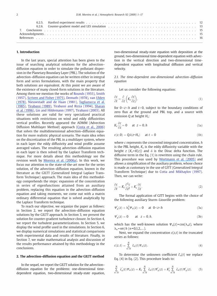
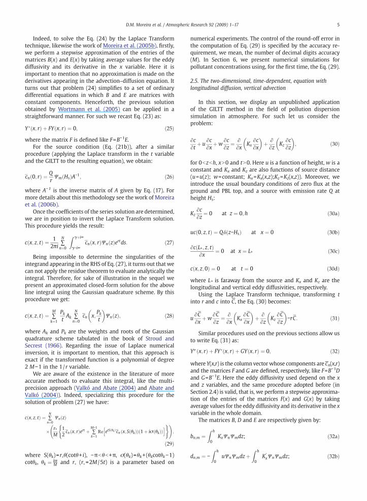
Fig. 1. Convergence of the GILTT method for three different source distances:a) x=1900 m; b) x=3900 m and c) x=5300 m.

8 D.M. Moreira et al. / Atmospheric Research 92 (2009) 1–17

ψmzL

¼ ln

1þ x2

2

� �þ ln

1þ x2

� �2

−2 arctan xþ π2

for 1=Lb0

with x=(1−15z /L)1/4.Also was used the wind speed profiledescribed by a power law profile (Panofsky and Dutton, 1984):

uz

u1¼ z

z1

� �n

ð51Þ

where u–z and u–1 are the mean wind velocity at the heights zand z1, while n is an exponent that is related to the intensity ofturbulence (Irwin, 1979).

6. Performances against experimental data

In order to illustrate the aptness of the discussed for-mulation to simulate contaminant dispersion in the PBL, weevaluate the performance of the discussed solutions againstexperimental ground-level concentration using differentdispersion experiments available in the literature.

6.1. Experimental data

In thisworkwe usedfive different dispersion experiments:Copenhagen, Prairie Grass, Kinkaid, INEL and Hanford.

The first one is carried out in the northern part ofCopenhagen (convective case), described by Gryning andLyck (1984). It consisted of tracer released without buoyancyfrom a tower at a height of 115 m, and collection of tracersampling units at the ground-level positions at the maximumof three crosswind arcs. The sampling units were positionedat 2 to 6 km from the point of release. The site was mainlyresidential with a roughness length of the 0.6 m.

Regarding the second experiment, we evaluate theperformance of the solution using the SO2 tracer from PrairieGrass dispersion experiments (convective case) carried out inO'Neill, Nebraska, 1956, described by Barad (1958). We usedhere the Prairie Grass results as reporter in the paper ofNieuwstadt (1980). The tracer was releasedwithout buoyancyat a height of 0.46 m, and collected at a height of 1.5 m at fivedownwind distances (50, 100, 200, 400 and 800 m). ThePrairie Grass site was quite flat and much smooth with aroughness length of 0.6 cm.

Concerning the third experiment, the solution wasevaluated against the Kinkaid experiment (Illinois — USA),relatively only convective conditions (for −h /LN10), appear-ing in the work of Hanna and Paine (1989), The Kincaid fieldcampaign concerns an elevated release in a flat farmland withsome lakes. During the experiment, SF6 was released from 187tall stacks and recorded on a network consisting of roughly200 samplers positioned in arcs from 0.5 to 50 km downwindof the source. The data set includes the meteorologicalparameters as friction velocity, Monin–Obukhov length andheight of boundary layer. The measured concentration level isfrequently irregular with high and low concentrationsoccurring intermittently along same arc, moreover there arefrequent gaps in the monitoring arcs. For the above reasons avariable has been assigned as a quality factor in order toindicate the degree of readability of data (Olesen, 1995). Thequality indicator (from 0 to 3) has been assigned. Here, onlythe data with quality factor 3 were considered.

Concerning the fourth experiment, the solution for lowwind conditions (Eq. (30)) was evaluated against dataobtained from the INEL experiment (Sagendorf and Dickson,1974) (stable case). The data used to evaluate the performanceof the model are constituted by a series of diffusion tests

9D.M. Moreira et al. / Atmospheric Research 92 (2009) 1–17

conducted under stable conditions for surface based releaseswith light winds over flat, even terrain (Sagendorf andDickson, 1974). Because of wind direction variability a full360° sampling grid was implemented. Arcs were laid out atradii of 100, 200 and 400 m from the emission point. Thereceptor height was 0.76 m. The tracer SF6 was released at aheight of 1.5 m. The 1 h average concentrations were deter-mined by means of an electron capture gas chromatograph.We used the hourly average wind speed, u, and the standarddeviation of the horizontal wind direction over the averagingperiod considered, σθ, reported at the 2 m level.

Regarding the fifth experiment, the GILTT method wasevaluated against data obtained at Hanford in stable condi-tions (Doran et al., 1984). This experiment was conducted inMay–June, 1983 on a semi-arid region of south easternWashington on generally flat terrain. The detailed description

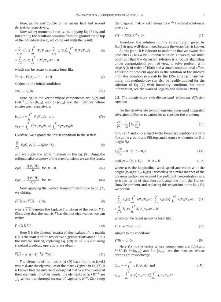
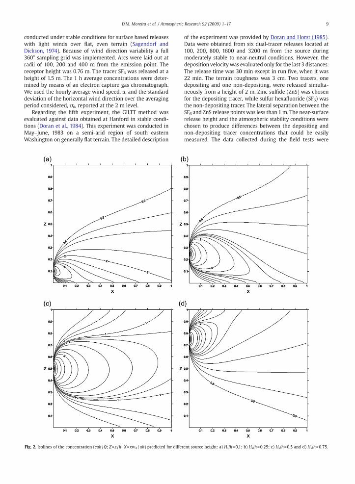
Fig. 2. Isolines of the concentration (cuh /Q; Z=z /h; X=xw⁎ /uh) predicted for differ

of the experiment was provided by Doran and Horst (1985).Data were obtained from six dual-tracer releases located at100, 200, 800, 1600 and 3200 m from the source duringmoderately stable to near-neutral conditions. However, thedeposition velocity was evaluated only for the last 3 distances.The release time was 30 min except in run five, when it was22 min. The terrain roughness was 3 cm. Two tracers, onedepositing and one non-depositing, were released simulta-neously from a height of 2 m. Zinc sulfide (ZnS) was chosenfor the depositing tracer, while sulfur hexafluoride (SF6) wasthe non-depositing tracer. The lateral separation between theSF6 and ZnS release points was less than 1m. The near-surfacerelease height and the atmospheric stability conditions werechosen to produce differences between the depositing andnon-depositing tracer concentrations that could be easilymeasured. The data collected during the field tests were

ent source height: a) Hs/h=0.1; b) Hs/h=0.25; c) Hs/h=0.5 and d) Hs/h=0.75.

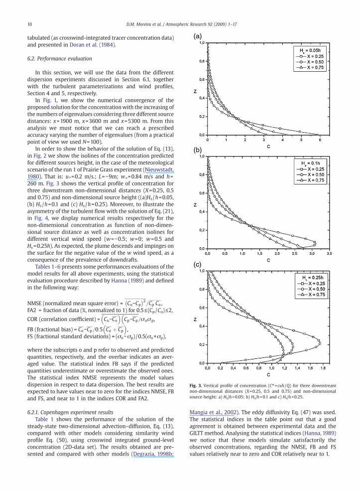
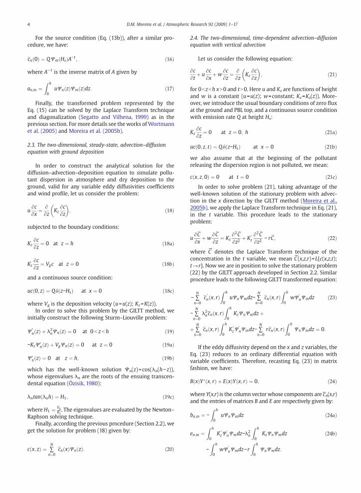
Fig. 3. Vertical profile of concentration (C⁎=cuh /Q) for three downstreamnon-dimensional distances (X=0.25, 0.5 and 0.75) and non-dimensionalsource height: a) Hs/h=0.05; b) Hs/h=0.1 and c) Hs/h=0.25.

10 D.M. Moreira et al. / Atmospheric Research 92 (2009) 1–17

tabulated (as crosswind-integrated tracer concentration data)and presented in Doran et al. (1984).

6.2. Performance evaluation

In this section, we will use the data from the differentdispersion experiments discussed in Section 6.1, togetherwith the turbulent parameterizations and wind profiles,Section 4 and 5, respectively.

In Fig. 1, we show the numerical convergence of theproposed solution for the concentrationwith the increasing ofthe numbers of eigenvalues considering three different sourcedistances: x=1900 m, x=3600 m and x=5300 m. From thisanalysis we must notice that we can reach a prescribedaccuracy varying the number of eigenvalues (from a practicalpoint of view we used N=100).

In order to show the behavior of the solution of Eq. (13),in Fig. 2 we show the isolines of the concentration predictedfor different sources height, in the case of the meteorologicalscenario of the run 1 of Prairie Grass experiment (Nieuwstadt,1980). That is: u⁎=0.2 m/s.; L=−9m; w⁎=0.84 m/s and h=260 m. Fig. 3 shows the vertical profile of concentration forthree downstream non-dimensional distances (X=0.25, 0.5and 0.75) and non-dimensional source height ((a)Hs /h=0.05,(b) Hs /h=0.1 and (c) Hs /h=0.25). Moreover, to illustrate theasymmetry of the turbulent flowwith the solution of Eq. (21),in Fig. 4, we display numerical results respectively for thenon-dimensional concentration as function of non-dimen-sional source distance as well as concentration isolines fordifferent vertical wind speed (w=−0.5; w=0; w=0.5 andHs=0.25h). As expected, the plume descends and impinges onthe surface for the negative value of the w wind speed, as aconsequence of the prevalence of downdrafts.

Tables 1–6 presents some performances evaluations of themodel results for all above experiments, using the statisticalevaluation procedure described by Hanna (1989) and definedin the following way:

NMSE (normalized mean square error) = Co−Cp� �2

=Cp Co ,FA2 = fraction of data (%, normalized to 1) for 0.5≤ (Cp/Co)≤2,

COR (correlation coefficient) =P

Co−Co

Cp−Cp=σoσp

,

FB (fractional bias) = Co−Cp=0:5 Co þ Cp

,

FS (fractional standard deviations) = (σo−σp) /0.5(σo+σp),

where the subscripts o and p refer to observed and predictedquantities, respectively, and the overbar indicates an aver-aged value. The statistical index FB says if the predictedquantities underestimate or overestimate the observed ones.The statistical index NMSE represents the model valuesdispersion in respect to data dispersion. The best results areexpected to have values near to zero for the indices NMSE, FBand FS, and near to 1 in the indices COR and FA2.

6.2.1. Copenhagen experiment resultsTable 1 shows the performance of the solution of the

steady-state two-dimensional advection–diffusion, Eq. (13),compared with other models considering similarity windprofile Eq. (50), using crosswind integrated ground-levelconcentration (2D-data set). The results obtained are pre-sented and compared with other models (Degrazia, 1998b;

Mangia et al., 2002). The eddy diffusivity Eq. (47) was used.The statistical indices in the table point out that a goodagreement is obtained between experimental data and theGILTT method. Analysing the statistical indices (Hanna, 1989)we notice that these models simulate satisfactorily theobserved concentrations, regarding the NMSE, FB and FSvalues relatively near to zero and COR relatively near to 1.

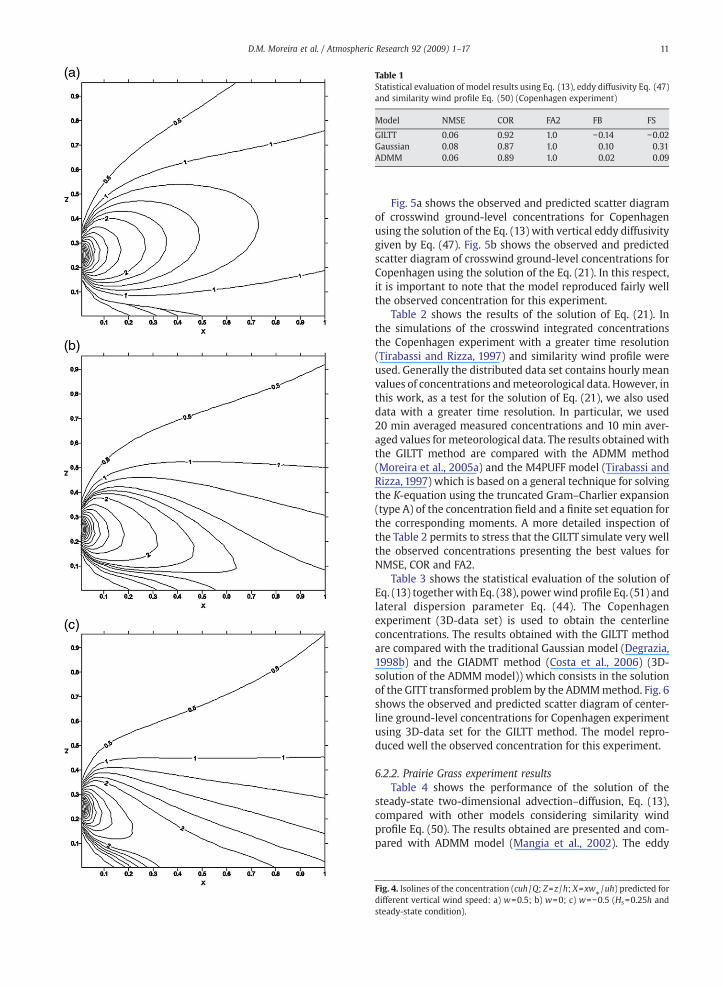
Table 1Statistical evaluation of model results using Eq. (13), eddy diffusivity Eq. (47)and similarity wind profile Eq. (50) (Copenhagen experiment)

Model NMSE COR FA2 FB FS

GILTT 0.06 0.92 1.0 −0.14 −0.02Gaussian 0.08 0.87 1.0 0.10 0.31ADMM 0.06 0.89 1.0 0.02 0.09

11D.M. Moreira et al. / Atmospheric Research 92 (2009) 1–17

Fig. 5a shows the observed and predicted scatter diagramof crosswind ground-level concentrations for Copenhagenusing the solution of the Eq. (13) with vertical eddy diffusivitygiven by Eq. (47). Fig. 5b shows the observed and predictedscatter diagram of crosswind ground-level concentrations forCopenhagen using the solution of the Eq. (21). In this respect,it is important to note that the model reproduced fairly wellthe observed concentration for this experiment.

Table 2 shows the results of the solution of Eq. (21). Inthe simulations of the crosswind integrated concentrationsthe Copenhagen experiment with a greater time resolution(Tirabassi and Rizza, 1997) and similarity wind profile wereused. Generally the distributed data set contains hourly meanvalues of concentrations andmeteorological data. However, inthis work, as a test for the solution of Eq. (21), we also useddata with a greater time resolution. In particular, we used20 min averaged measured concentrations and 10 min aver-aged values formeteorological data. The results obtainedwiththe GILTT method are compared with the ADMM method(Moreira et al., 2005a) and the M4PUFF model (Tirabassi andRizza, 1997) which is based on a general technique for solvingthe K-equation using the truncated Gram–Charlier expansion(type A) of the concentration field and a finite set equation forthe corresponding moments. A more detailed inspection ofthe Table 2 permits to stress that the GILTT simulate very wellthe observed concentrations presenting the best values forNMSE, COR and FA2.

Table 3 shows the statistical evaluation of the solution ofEq. (13) togetherwith Eq. (38), powerwind profile Eq. (51) andlateral dispersion parameter Eq. (44). The Copenhagenexperiment (3D-data set) is used to obtain the centerlineconcentrations. The results obtained with the GILTT methodare compared with the traditional Gaussian model (Degrazia,1998b) and the GIADMT method (Costa et al., 2006) (3D-solution of the ADMM model)) which consists in the solutionof the GITT transformed problem by the ADMMmethod. Fig. 6shows the observed and predicted scatter diagram of center-line ground-level concentrations for Copenhagen experimentusing 3D-data set for the GILTT method. The model repro-duced well the observed concentration for this experiment.

6.2.2. Prairie Grass experiment resultsTable 4 shows the performance of the solution of the

steady-state two-dimensional advection–diffusion, Eq. (13),compared with other models considering similarity windprofile Eq. (50). The results obtained are presented and com-pared with ADMM model (Mangia et al., 2002). The eddy

Fig. 4. Isolines of the concentration (cuh /Q; Z=z /h; X=xw⁎/uh) predicted for

different vertical wind speed: a) w=0.5; b) w=0; c) w=−0.5 (Hs=0.25h andsteady-state condition).

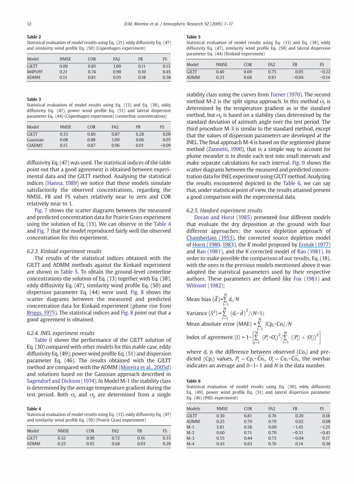
Table 2Statistical evaluation of model results using Eq. (21), eddy diffusivity Eq. (47)and similarity wind profile Eq. (50) (Copenhagen experiment)

Model NMSE COR FA2 FB FS

GILTT 0.09 0.85 1.00 0.11 0.13M4PUFF 0.21 0.74 0.90 0.10 0.45ADMM 0.15 0.81 0.95 0.18 0.38

Table 3Statistical evaluation of model results using Eq. (13) and Eq. (38), eddydiffusivity Eq. (47), power wind profile Eq. (51) and lateral dispersionparameter Eq. (44) (Copenhagen experiment) (centerline concentrations)

Model NMSE COR FA2 FB FS

GILTT 0.33 0.80 0.87 0.28 0.09Gaussian 0.08 0.88 1.00 0.06 0.07GIADMT 0.15 0.87 0.96 0.01 −0.09

Table 5Statistical evaluation of model results using Eq. (13) and Eq. (38), eddydiffusivity Eq. (47), similarity wind profile Eq. (50) and lateral dispersionparameter Eq. (44) (Kinkaid experiment)

Model NMSE COR FA2 FB FS

GILTT 0.40 0.69 0.75 0.05 −0.22ADMM 0.33 0.68 0.81 −0.04 −0.14

Table 6Statistical evaluation of model results using Eq. (30), eddy diffusivityEq. (49), power wind profile Eq. (51) and lateral dispersion parameterEq. (46) (INEL experiment)

12 D.M. Moreira et al. / Atmospheric Research 92 (2009) 1–17

diffusivity Eq. (47) was used. The statistical indices of the tablepoint out that a good agreement is obtained between experi-mental data and the GILTT method. Analysing the statisticalindices (Hanna, 1989) we notice that these models simulatesatisfactorily the observed concentrations, regarding theNMSE, FB and FS values relatively near to zero and CORrelatively near to 1.

Fig. 7 shows the scatter diagrams between the measuredand predicted concentration data for Prairie Grass experimentusing the solution of Eq. (13). We can observe in the Table 4and Fig. 7 that the model reproduced fairly well the observedconcentration for this experiment.

6.2.3. Kinkaid experiment resultsThe results of the statistical indices obtained with the

GILTT and ADMM methods against the Kinkaid experimentare shown in Table 5. To obtain the ground-level centerlineconcentrations the solution of Eq. (13) together with Eq. (38),eddy diffusivity Eq. (47), similarity wind profile Eq. (50) anddispersion parameter Eq. (44) were used. Fig. 8 shows thescatter diagrams between the measured and predictedconcentration data for Kinkaid experiment (plume rise fromBriggs, 1975). The statistical indices and Fig. 8 point out that agood agreement is obtained.

6.2.4. INEL experiment resultsTable 6 shows the performance of the GILTT solution of

Eq. (30) comparedwith othermodels for this stable case, eddydiffusivity Eq. (49), powerwind profile Eq. (51) and dispersionparameter Eq. (46). The results obtained with the GILTTmethod are compared with the ADMM (Moreira et al., 2005d)and solutions based on the Gaussian approach described inSagendorf and Dickson (1974). InModelM-1 the stability classis determined by the average temperature gradient during thetest period. Both σz and σy are determined from a single

Table 4Statistical evaluation of model results using Eq. (13), eddy diffusivity Eq. (47)and similarity wind profile Eq. (50) (Prairie Grass experiment)

Model NMSE COR FA2 FB FS

GILTT 0.32 0.90 0.72 0.16 0.33ADMM 0.25 0.92 0.68 0.03 0.20

stability class using the curves from Turner (1970). The secondmethod M-2 is the split sigma approach. In this method σz isdetermined by the temperature gradient as in the standardmethod, but σy is based on a stability class determined by thestandard deviation of azimuth angle over the test period. Thethird procedure M-3 is similar to the standard method, exceptthat the values of dispersion parameters are developed at theINEL. The final approachM-4 is based on the segmented plumemethod (Zannetti, 1990), that is a simple way to account forplume meander is to divide each test into small intervals andmake separate calculations for each interval. Fig. 9 shows thescatter diagrams between themeasured and predicted concen-trationdata for INEL experimentusingGILTTmethod. Analyzingthe results encountered depicted in the Table 6, we can saythat, under statistical point of view, the results attained presenta good comparison with the experimental data.

6.2.5. Hanford experiment resultsDoran and Horst (1985) presented four different models

that evaluate the dry deposition at the ground with fourdifferent approaches: the source depletion approach ofChamberlain (1953), the corrected source depletion modelof Horst (1980, 1983), the K model proposed by Ermak (1977)and Rao (1981), and the K corrected model of Rao (1981). Inorder to make possible the comparison of our results, Eq. (18),with the ones in the previous models mentioned above it wasadopted the statistical parameters used by their respectiveauthors. These parameters are defined like Fox (1981) andWilmott (1982):

Mean bias (d–)=∑

N

i¼1di=N

Variance (S2) = ∑N

i¼1di− d� �2

= N−1ð ÞMean absolute error (MAE) = ∑

N

i¼1jCpi−Coij=N

Index of agreement (I) = 1− ∑N

i¼1P0i−O

0i

� �2=∑N

i¼1jP0

i j þ jO0ij

� �2� �

where di is the difference between observed (Coi) and pre-dicted (Cpi) values, P0

i ¼ Cpi− Coi , O0i ¼ Coi− Coi, the overbar

indicates an average and 0b Ib1 and N is the data number.

Models NMSE COR FA2 FB FS

GILTT 0.30 0.81 0.76 0.20 0.18ADMM 0.25 0.79 0.79 0.02 0.08M-1 5.81 0.58 0.00 −1.45 −1.25M-2 0.60 0.71 0.70 −0.31 −0.41M-3 0.55 0.44 0.73 −0.04 0.17M-4 0.43 0.63 0.76 0.14 0.38

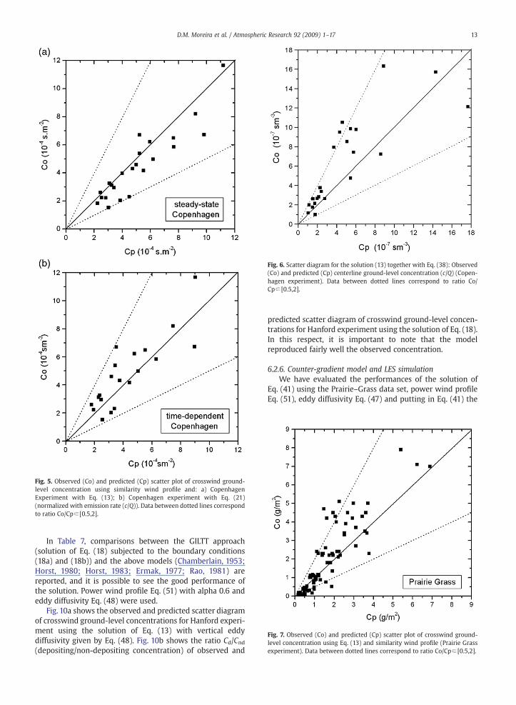
Fig. 5. Observed (Co) and predicted (Cp) scatter plot of crosswind ground-level concentration using similarity wind profile and: a) CopenhagenExperiment with Eq. (13); b) Copenhagen experiment with Eq. (21)(normalized with emission rate (c/Q)). Data between dotted lines correspondto ratio Co/Cp∈ [0.5,2].

Fig. 6. Scatter diagram for the solution (13) together with Eq. (38): Observed(Co) and predicted (Cp) centerline ground-level concentration (c/Q) (Copen-hagen experiment). Data between dotted lines correspond to ratio Co/Cp∈ [0.5,2].

Fig. 7. Observed (Co) and predicted (Cp) scatter plot of crosswind ground-level concentration using Eq. (13) and similarity wind profile (Prairie Grassexperiment). Data between dotted lines correspond to ratio Co/Cp∈ [0.5,2].

13D.M. Moreira et al. / Atmospheric Research 92 (2009) 1–17

In Table 7, comparisons between the GILTT approach(solution of Eq. (18) subjected to the boundary conditions(18a) and (18b)) and the above models (Chamberlain, 1953;Horst, 1980; Horst, 1983; Ermak, 1977; Rao, 1981) arereported, and it is possible to see the good performance ofthe solution. Power wind profile Eq. (51) with alpha 0.6 andeddy diffusivity Eq. (48) were used.

Fig. 10a shows the observed and predicted scatter diagramof crosswind ground-level concentrations for Hanford experi-ment using the solution of Eq. (13) with vertical eddydiffusivity given by Eq. (48). Fig. 10b shows the ratio Cd/Cnd(depositing/non-depositing concentration) of observed and

predicted scatter diagram of crosswind ground-level concen-trations for Hanford experiment using the solution of Eq. (18).In this respect, it is important to note that the modelreproduced fairly well the observed concentration.

6.2.6. Counter-gradient model and LES simulationWe have evaluated the performances of the solution of

Eq. (41) using the Prairie–Grass data set, power wind profileEq. (51), eddy diffusivity Eq. (47) and putting in Eq. (41) the

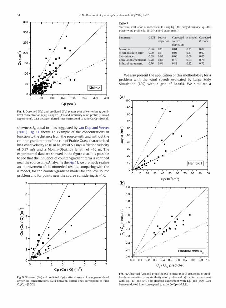
Fig. 8. Observed (Co) and predicted (Cp) scatter plot of centerline ground-level concentration (c/Q) using Eq. (13) and similarity wind profile (Kinkaidexperiment). Data between dotted lines correspond to ratio Co/Cp∈ [0.5,2].

Table 7Statistical evaluation of model results using Eq. (18), eddy diffusivity Eq. (48),power wind profile Eq. (51) (Hanford experiment)

Parameter GILTT Sourcedepletion

Correctedsourcedepletion

K model CorrectedK model

Mean bias 0.06 0.11 0.01 0.21 0.07Mean absolute error 0.09 0.11 0.05 0.21 0.07S=(variance)1/2 0.09 0.05 0.06 0.08 0.05Correlation coefficient 0.78 0.82 0.70 0.63 0.78Index of agreement 0.76 0.64 0.83 0.42 0.76

14 D.M. Moreira et al. / Atmospheric Research 92 (2009) 1–17

skewness Sk equal to 1, as suggested by van Dop and Verver(2001). Fig. 11 shows an example of the concentrations infunction to the distance from the source with and without thecounter-gradient term for a run of Prairie Grass characterizedby a wind velocity at 10 m height of 5.1 m/s, a friction velocityof 0.37 m/s and a Monin–Obukhov length of −10 m. Theexperimental data are showed in the figure also. It is possibleto see that the influence of counter-gradient term is confinednear the source only. Analyzing the Fig.11,we promptly realizean improvement of the numerical results, comparing with theK model, for the counter-gradient model for the low sourceproblem and for points near the source considering Sk=1.0.

Fig. 9. Observed (Co) and predicted (Cp) scatter diagram of near ground-levelcenterline concentrations. Data between dotted lines correspond to ratioCo/Cp∈ [0.5,2].

We also present the application of this methodology for aproblem with the wind speeds evaluated by Large EddySimulation (LES) with a grid of 64×64. We simulate a

Fig. 10. Observed (Co) and predicted (Cp) scatter plot of crosswind ground-level concentration using similarity wind profile and: a) Hanford experimentwith Eq. (13) and (c/Q); b) Hanford experiment with Eq. (18) (c/Q). Databetween dotted lines correspond to ratio Co/Cp∈ [0.5,2].

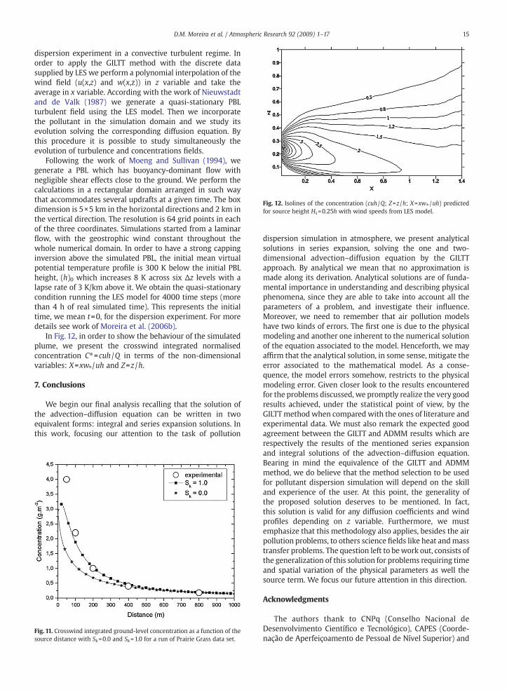
Fig. 12. Isolines of the concentration (cuh /Q; Z=z /h; X=xw⁎ /uh) predictedfor source height Hs=0.25h with wind speeds from LES model.

15D.M. Moreira et al. / Atmospheric Research 92 (2009) 1–17

dispersion experiment in a convective turbulent regime. Inorder to apply the GILTT method with the discrete datasupplied by LES we perform a polynomial interpolation of thewind field (u(x,z) and w(x,z)) in z variable and take theaverage in x variable. According with the work of Nieuwstadtand de Valk (1987) we generate a quasi-stationary PBLturbulent field using the LES model. Then we incorporatethe pollutant in the simulation domain and we study itsevolution solving the corresponding diffusion equation. Bythis procedure it is possible to study simultaneously theevolution of turbulence and concentrations fields.

Following the work of Moeng and Sullivan (1994), wegenerate a PBL which has buoyancy-dominant flow withnegligible shear effects close to the ground. We perform thecalculations in a rectangular domain arranged in such waythat accommodates several updrafts at a given time. The boxdimension is 5×5 km in the horizontal directions and 2 km inthe vertical direction. The resolution is 64 grid points in eachof the three coordinates. Simulations started from a laminarflow, with the geostrophic wind constant throughout thewhole numerical domain. In order to have a strong cappinginversion above the simulated PBL, the initial mean virtualpotential temperature profile is 300 K below the initial PBLheight, (h)0 which increases 8 K across six Δz levels with alapse rate of 3 K/km above it. We obtain the quasi-stationarycondition running the LES model for 4000 time steps (morethan 4 h of real simulated time). This represents the initialtime, we mean t=0, for the dispersion experiment. For moredetails see work of Moreira et al. (2006b).

In Fig. 12, in order to show the behaviour of the simulatedplume, we present the crosswind integrated normalisedconcentration C⁎=cuh /Q in terms of the non-dimensionalvariables: X=xw⁎ /uh and Z=z /h.

7. Conclusions

We begin our final analysis recalling that the solution ofthe advection–diffusion equation can be written in twoequivalent forms: integral and series expansion solutions. Inthis work, focusing our attention to the task of pollution

Fig. 11. Crosswind integrated ground-level concentration as a function of thesource distance with Sk=0.0 and Sk=1.0 for a run of Prairie Grass data set.

dispersion simulation in atmosphere, we present analyticalsolutions in series expansion, solving the one and two-dimensional advection–diffusion equation by the GILTTapproach. By analytical we mean that no approximation ismade along its derivation. Analytical solutions are of funda-mental importance in understanding and describing physicalphenomena, since they are able to take into account all theparameters of a problem, and investigate their influence.Moreover, we need to remember that air pollution modelshave two kinds of errors. The first one is due to the physicalmodeling and another one inherent to the numerical solutionof the equation associated to the model. Henceforth, we mayaffirm that the analytical solution, in some sense, mitigate theerror associated to the mathematical model. As a conse-quence, the model errors somehow, restricts to the physicalmodeling error. Given closer look to the results encounteredfor the problems discussed, we promptly realize the very goodresults achieved, under the statistical point of view, by theGILTT method when compared with the ones of literature andexperimental data. We must also remark the expected goodagreement between the GILTT and ADMM results which arerespectively the results of the mentioned series expansionand integral solutions of the advection–diffusion equation.Bearing in mind the equivalence of the GILTT and ADMMmethod, we do believe that the method selection to be usedfor pollutant dispersion simulation will depend on the skilland experience of the user. At this point, the generality ofthe proposed solution deserves to be mentioned. In fact,this solution is valid for any diffusion coefficients and windprofiles depending on z variable. Furthermore, we mustemphasize that this methodology also applies, besides the airpollution problems, to others science fields like heat andmasstransfer problems. The question left to bework out, consists ofthe generalization of this solution for problems requiring timeand spatial variation of the physical parameters as well thesource term. We focus our future attention in this direction.

Acknowledgments

The authors thank to CNPq (Conselho Nacional deDesenvolvimento Científico e Tecnológico), CAPES (Coorde-nação de Aperfeiçoamento de Pessoal de Nível Superior) and

16 D.M. Moreira et al. / Atmospheric Research 92 (2009) 1–17

the project “Laboratorio LaRIA” for the partial financial sup-port of this work.

References

Abate, J., Valkó, P.P., 2004. Multi-precision Laplace transform inversion. Int. J.Numer. Methods Eng. 60, 979–993.

Arya, P., 1995. Modeling and parameterization of near-source diffusion inweak winds. J. Appl. Meteorol. 34, 1112–1122.

Barad, M.L., 1958. Project Prairie Grass. Geophysical Research Paper, No. 59,vol. I and II. GRD, Bedford, MA.

Briggs, G.A., 1975. Plume rise predictions. In: Haugen, D.A. (Ed.), Lectures onAir Pollution and Environmental Impact Analyses. American Meteor-ological Society, Boston, MA, pp. 59–111.

Buske, D., Vilhena, M.T., Moreira, D.M., Tirabassi, T., 2007a. An analyticalsolution of the advection–diffusion equation considering non-localturbulence closure. Environ. Fluid Mech. 7, 43–54.

Buske, D., Vilhena, M.T., Moreira, D.M., Tirabassi, T., 2007b. Simulation ofpollutant dispersion for low wind conditions in stable and convectiveplanetary boundary layer. Atmos. Environ. 41, 5496–5501.

Chamberlain, A.C., 1953. Aspects of travel and deposition of aerosol andvapour clouds. UKAEA Report No. AERE-HP/R-1261, Harwell, Berkshire,England.

Cirillo, M.C., Poli, A.A., 1992. An inter comparison of semi empirical diffusionmodels under low wind speed, stable conditions. Atmos. Environ. 26A,765–774.

Costa, C.P., Vilhena, M.T., Moreira, D.M., Tirabassi, T., 2006. Semi-analyticalsolution of the steady three-dimensional advection–diffusion equationin the planetary boundary layer. Atmos. Environ. 40 (29), 5659–5669.

Cotta, R., Mikhaylov, M., 1997. Heat conduction lumped analysis, integraltransforms, symbolic computation. John Wiley Sons, Baffins Lane,Chinchester, England.

Deardoff, J.W., 1966. The countergradient heat flux in the lower atmosphereand in the laboratory. J. Atmos. Sci. 23, 503–506.

Deardoff, J.W., 1972. Numerical investigation of neutral and unstableplanetary boundary layers. J. Atmos. Sci. 29, 91–115.

Degrazia, G.A., Vilhena, M.T., Moraes, O.L.L., 1996. An algebraic expression forthe eddy diffusivities in the stable boundary layer: a description of near-source diffusion. Nuovo Cim. 19C, 399–403.

Degrazia, G.A., Campos Velho, H.F., Carvalho, J.C., 1997. Nonlocal exchangecoefficients for the convective boundary layer derived from spectralproperties. Contr. Atmos. Phys. 57–64.

Degrazia, G.A., Mangia, C., Rizza, U., 1998a. A comparison between differentmethods to estimate the lateral dispersion parameter under convectiveconditions. J. Appl. Meteor. 37, 227–231.

Degrazia, G.A.,1998b.Modellingdispersion fromelevated sources in a planetaryboundary layer dominated by moderate convection. Nuovo Cim. 21 (3),345–353.

Degrazia, G.A., Anfossi, D., Carvalho, J.C., Mangia, C., Tirabassi, T., CamposVelho, H.F., 2000. Turbulence parameterization for PBL dispersionmodels in all stability conditions. Atmos. Environ. 34, 3575–3583.

Demuth, C., 1978. A contribution to the analytical steady solution of thediffusion equation for line sources. Atmos. Environ. 12, 1255–1258.

Doran, J.C., Abbey,O.B., Buck, J.W.,Glover, D.W.,Horst, T.W.,1984. Fieldvalidationof Exposure Assessment Models. Data Environmental Science ResearchLab, vol. 1. Research Triangle Park, NC. 177 pp. EPA/600/384/092A.

Doran, J.C., Horst, T.W., 1985. An evaluation of Gaussian plume-depletionmodels with dual-tracer field measurements. Atmos. Environ. 19, 939–951.

Ermak, D.L., 1977. An analytical model for air pollution transport anddeposition from a point source. Atmos. Environ. 11, 231–237.

Fiedler, B.H., Moeng, C.H., 1985. A practical integral closure model for meanvertical transport of a scalar in a convective boundary layer. J. Atmos. Sci.42 (4), 359–363.

Fox, D.G., 1981. Judging air quality model performance: a summary of theAMS workshop on dispersion model performance. Bull. Am. Meteorol.Soc. 62, 599–609.

Gryning, S.E., Lyck, E., 1984. Atmospheric dispersion from elevated source inan urban area: comparison between tracer experiments and modelcalculations. J. Clim. Appl. Meteorol. 23, 651–654.

Højstrup, J., 1982. Velocity spectra in the unstable boundary layer. J. Atmos.Sci. 39, 2239–2248.

Hamba, F., 1993. A modified K model for chemically reactive species in theplanetary boundary layer. J Geophys. Res. 98 (3), 5173–5182.

Hanna, S.R., Paine, R.J., 1989. Hybrid plume dispersion model (HPDM)development and evaluation. J. Appl. Meteorol. 28, 206–224.

Hanna, S.R., 1989. Confidence limit for air quality models as estimated bybootstrap and jacknife resampling methods. Atmos. Environ. 23,1385–1395.

Holtslag, A., Boville, B.A., 1993. Local versus nonlocal boundary-layerdiffusion in a global climate model. J. Climate 6, 1825–1842.

Holtslag, A., Moeng, C.H., 1991. Eddy diffusivity and countergradienttransport in the convective atmospheric boundary layer. J. Atmos. Sci.48, 1690–1698.

Horst, T.W., 1980. A review of Gaussian diffusion–deposition models. In:Shriner, D.S., Richmond, C.R., Lindberg, S.E. (Eds.), Atmospheric SulphurDeposition. Ann Arbor Science, Ann Arbor, MI, pp. 275–283.

Horst, T.W., 1983. A correction to the Gaussian source depletion model.In: Pruppacher, H.R., Semonin, R.G., Slinn, W.G.N. (Eds.), PrecipitationScavenging, Dry Deposition and Resuspension. Elsevier North Holland,Amsterdam, pp. 1205–1218.

Irwin, J.S., 1979. A theoretical variation of the wind profile power-lowexponent as a function of surface roughness and stability. Atm. Environ.13, 191–194.

Lin, J.S., Hildemann, L.M., 1997. A generalised mathematical scheme toanalytically solve the atmospheric diffusion equation with dry deposi-tion. Atmos. Environ. 31, 59–71.

Mangia, C., Moreira, D.M., Schipa, I., Degrazia, G.A., Tirabassi, T., Rizza, U.,2002. Evaluation of a new eddy diffusivity parameterization fromturbulent Eulerian spectra in different stability conditions. Atmos.Environ. 36, 67–76.

Moeng, C.H., Sullivan, P.P., 1994. A comparison of shear and buoyancy drivenplanetary boundary layer flows. J. Atmos. Sci. 51, 999–1022.

Moreira, D.M., Rizza, U., Vilhena, M.T., Goulart, A.G., 2005a. Semi-analyticalmodel for pollution dispersion in the planetary boundary layer. Atmos.Environ. 39 (14), 2689–2697.

Moreira, D.M., Vilhena, M.T., Tirabassi, T., Buske, D., Cotta, R.M., 2005b. Nearsource atmospheric pollutant dispersion using the new GILTT method.Atmos. Environ. 39 (34), 6290–6295.

Moreira, D.M., Carvalho, J.C., Goulart, A.G., Tirabassi, T., 2005c. Simulation ofthe dispersion of pollutants using two approaches for the case of a lowsource in the SBL: evaluation of turbulence parameterizations. Water AirSoil Pollut. 161, 285–297.

Moreira, D.M., Tirabassi, T., Carvalho, J.C., 2005d. Plume dispersion simulationin low wind conditions in stable and convective boundary layers. Atmos.Environ. 39 (20), 3643–3650.

Moreira, D.M., Vilhena, M.T., Carvalho, J.C., Degrazia, G.A., 2004. Analyticalsolution of the advection–diffusion equationwith nonlocal closure of theturbulent diffusion. Environ. Model. Softw. 20 (10), 1347–1351.

Moreira, D.M., Vilhena, M.T., Tirabassi, T., Costa, C., Bodmann, B., 2006a.Simulation of pollutant dispersion in atmosphere by the Laplacetransform: the ADMM approach. Water Air Soil Pollut. 177, 411–439.

Moreira, D.M., Vilhena, M.T., Buske, D., Tirabassi, T., 2006b. The GILTT solutionof the advection–diffusion equation for an inhomogeneous and nonsta-tionary PBL. Atmos. Environ. 40, 3186–3194.

Nieuwstadt, F.T.M., 1980. An analytical solution of the time-dependent, one-dimensional diffusion equation in the atmospheric boundary layer.Atmos. Environ. 14, 1361–1364.

Nieuwstadt, F.T.M., de Haan, B.J., 1981. An analytical solution of one-dimensional diffusion equation in a non-stationary boundary layerwith an application to inversion rise fumigation. Atmos. Environ. 15,845–851.

Nieuwstadt, F.T.M., 1984. The turbulent structure of the stable nocturnalboundary layer. J. Atmos. Sci. 41, 2202–2216.

Nieuwstadt, F.T.M., de Valk, J.P.J.M.M., 1987. A large eddy simulation ofbuoyant and non-buoyant plume dispersion in the atmosphericboundary layer. Atmos. Environ. 21, 2573–2587.

Olesen, H.R., 1995. Datasets and protocol for model validation. Int. J. Environ.Pollut. 5, 693–701.

Özisik, M., 1980. Heat Conduction, 2 edition. John Wiley & Sons, New York.Panofsky, H.A., Dutton, J.A., 1984. Atmospheric Turbulence. John Wiley &

Sons, New York.Rao, K.S., 1981. Analytical solutions of a gradient-transfer model for plume

deposition and sedimentation. NOAA Tech. Mem. ERL ARL-109, AirResources Laboratories, Silver Spring, MD.

Robson, R.E., Mayocchi, C.L., 1994. A simple model of countergradient flow.Phys. Fluids 6 (6), 1952–1954.

Rounds,W.,1955. Solutions of the two-dimensional diffusion equation. Trans.Am. Geophys. Union 36, 395–405.

Sagendorf, J.F., Dickson, C.R., 1974. Diffusion under lowwind-speed, inversionconditions. U.S. National Oceanic and Atmospheric AdministrationTechnical Memorandum ERL ARL-52.

Scriven, R.A., Fisher, B.A., 1975. The long range transport of airborne materialand its removal by deposition and washout-II. The effect of turbulentdiffusion. Atmos. Environ. 9, 59–69.

Segatto, C.F., Vilhena, M.T., 1999. The State-of-the-art of the LTSN Method,Mathematics and Computation, Reactor Physics and EnvironmentalAnalysis in Nuclear Applications-International Conference, Madrid,Spain 2, pp. 1618–1631.

17D.M. Moreira et al. / Atmospheric Research 92 (2009) 1–17

Sharan, M., Singh, M.P., Yadav, A.K., 1996. A mathematical model for theatmospheric dispersion in low winds with eddy diffusivities as linearfunction of downwind distance. Atmos. Environ. 30, 1137–1145.

Smith, F.B., 1957. The diffusion of smoke from a continuous elevated pointsource into a turbulent atmosphere. J. Fluid Mech. 2, 49–76.

Sorbjan, Z., 1989. Structure of the atmospheric boundary layer. Prentice Hall,New Jersey. 317 pp.

Stroud, A.H. and Secrest, D., 1966. Gaussian quadrature formulas. EnglewoodCliffs, N.J., Prentice Hall Inc.

Tagliazucca, M., Nanni, T., Tirabassi, T., 1985. An analytical dispersion modelfor sources in the surface layer. Nuovo Cim. 8C, 771–781.

Tirabassi, T., 1989. Analytical air pollution and diffusion models. Water AirSoil Pollut. 47, 19–24.

Tirabassi, T., Rizza, U., 1994. Applied dispersion modelling for ground-levelconcentrations from elevated sources. Atmos. Environ. 28, 611–615.

Tirabassi, T., Rizza, U., 1997. Boundary layer parameterization for a non-Gaussian puff model. J. Appl. Meteor. 36, 1031–1037.

Tirabassi, T., 2003. Operational advanced air pollution modeling. PAGEOPH160 (1–2), 5–16.

Turner, D.B., 1970. Workbook of atmospheric dispersion estimates. EPA,Research Triangle Park, NC, USA. U.S.EPA Ref. AP-26 (NTIS PB 191–482).

Valkó, P.P., Abate, J., 2004. Comparison of sequence accelerators for the Gavermethod of numerical Laplace transform inversion. Comput. Math. Appl.48, 629–636.

van Dop, H., Verver, G., 2001. Countergradient transport revisited. J. Atmos.Sci. 58, 2240–2247.

van Ulden, A.P., 1978. Simple estimates for vertical diffusion from sourcesnear the ground. Atmos. Environ. 12, 2125–2129.

Wilmott, C.J., 1982. Some comments on the evaluation of model performance.Bull. Am. Meteorol. Soc. 63, 1309–1313.

Wortmann, S., Vilhena, M.T., Moreira, D.M., Buske, D., 2005. A new analyticalapproach to simulate the pollutant dispersion in the PBL. Atmos. Environ.39, 2171–2178.

Wyngaard, J.C., Brost, R.A., 1984. Top–down bottom–up diffusion of a scalar inthe convective boundary layer. J. Atmos. Sci. 41, 102–112.

Wyngaard, J.C., Weil, J.C., 1991. Transport asymmetry in skewed turbulence.Phys. Fluids, A Fluid Dyn. 3, 155–162.

Zannetti, P., 1990. Air Pollution Modelling. Computational MechanicsPublications, Southampton. 444 pp.

Zilitinkevich, S., Gryanik, V.M., Lykossov, V.N.,Mironov, D.V.,1999. Third-ordertransport and nonlocal turbulence closures for convective boundarylayers. J. Atmos. Sci. 56, 3463–3477.