Relative intensities of middle atmosphere waves

D. Offermann,1 O. Gusev,1,2 M. Donner,3 J. M. Forbes,4 M. Hagan,5 M. G. Mlynczak,6

J. Oberheide,1 P. Preusse,7 H. Schmidt,8 and J. M. Russell III9

Received 25 June 2008; revised 6 January 2009; accepted 21 January 2009; published 21 March 2009.

[1] Climatologies of gravity waves, quasi-stationary planetary waves, and tides arecompared in the upper stratosphere, mesosphere, and lower thermosphere. Temperaturestandard deviations from zonal means are used as proxies for wave activity. The sum of thewaves is compared to directly measured total temperature fluctuations. The resultingdifference is used as a proxy for traveling planetary waves. A preliminary climatology forthese waves is proposed. A ranking of the four wave types in terms of their impact onthe total wave state of the atmosphere is achieved, which is dependent on altitude andlatitude. At extratropical latitudes, gravity waves mostly play a major role. Travelingplanetary waves are found to play a secondary role. Quasi-stationary planetary waves andtides yield a lesser contribution there. Vertical profiles of total temperature fluctuationsshow a sharp vertical gradient change (‘‘kink’’ or ‘‘bend’’) in the mesosphere. This isinterpreted in terms of a change of wave damping, and the concept of a ‘‘waveturbopause’’ is suggested. The altitude of this wave turbopause is found to be mostlydetermined by the relative intensities of gravity waves and planetary waves. Theturbopause is further analyzed, including earlier mass spectrometer data. It is found thatthe wave turbopause and the mass spectrometer turbopause occur rather close together.The turbopause forms a layer about 8 km thick, and the data suggest an additional 3 kmmixing layer on top.

Citation: Offermann, D., O. Gusev, M. Donner, J. M. Forbes, M. Hagan, M. G. Mlynczak, J. Oberheide, P. Preusse, H. Schmidt, and

J. M. Russell III (2009), Relative intensities of middle atmosphere waves, J. Geophys. Res., 114, D06110, doi:10.1029/2008JD010662.

1. Introduction

[2] Various types of waves exist in the middle atmosphere(MA, 10–100 km). They are observed in atmosphericpressure, temperature, density, wind, and trace gas mixingratios. Very long as well as very short scales exist in theirperiods and their wavelengths. Amplitudes can be very large:in temperature, for instance, they can exceed 25% ofthe large-scale mean values (e.g., 57 K [Offermann et al.,2006a]). In consequence the atmospheric behavior as awhole cannot be understood if the waves are not taken intoaccount. In the present paper we therefore study MAwavesas seen in the temperature.

[3] A number of climatologies for atmospheric temper-atures have been developed in the past as for instance theCIRA, Mass Spectrometer and Incoherent Scatter Radar(MSIS), and NRLMSISE-00 empirical models [Fleming etal., 1990; Hedin, 1983; Picone et al., 2002]. They arebased on previous satellite and auxiliary data. Recentlymore than 4 years of Sounding of the Atmosphere usingBroadband Emission Radiometry (SABER) measurementson the Thermosphere, Ionosphere, Mesosphere, Energetics,and Dynamics (TIMED) satellite have become available[e.g., Mertens et al., 2001, 2004]. Reviews on temperaturemeasurements and temperature trends in the stratosphere andmesosphere have been given by Ramaswamy et al. [2001]and Beig et al. [2003, see also references therein].[4] Atmospheric waves have generally not been consid-

ered in the development of middle atmosphere temperatureclimatologies. One exception is Rees’s [1990] empiricalmodel (CIRA 1986) that contains a climatology of stationaryplanetary waves from Rees [1990]. More recently, climatol-ogies have been developed for migrating and nonmigratingtides and stationary planetary waves [Forbes et al., 2008]and for gravity waves [Preusse et al., 2009]. These data setswill be used in the present paper. Temperature climatologiesof tidal waves have only recently become available fromSABER data [i.e., Forbes et al., 2008] and thus we adoptmonthly tidal amplitudes from the Global Scale Wave Model[Hagan et al., 1999; Hagan and Forbes, 2002, 2003].

JOURNAL OF GEOPHYSICAL RESEARCH, VOL. 114, D06110, doi:10.1029/2008JD010662, 2009ClickHere

for

FullArticle

1Physics Department, University of Wuppertal, Wuppertal, Germany.2Deutsches Zentrum fur Luft-und Raumfahrt, Oberpfaffenhofen,

Germany.3Donner Tontechnik, Remscheid, Germany.4Aerospace Engineering Sciences, University of Colorado, Boulder,

Colorado, USA.5High Altitude Observatory, NCAR, Boulder, Colorado, USA.6NASA Langley Research Center, Hampton, Virginia, USA.7Institut fur Chemie und Dynamik der Geosphare I: Stratosphare,

Forschungszentrum Julich, Julich, Germany.8Max Planck Institute for Meteorology, Hamburg, Germany.9Center for Atmospheric Sciences, Hampton University, Hampton,

Virginia, USA.

Copyright 2009 by the American Geophysical Union.0148-0227/09/2008JD010662$09.00

D06110 1 of 19

[5] Fluctuations of atmospheric temperatures can be quitestrong and show systematic variations. Hence they are notnoise but rather the result of superposition of various waves.Fluctuation climatologies have been presented long ago byCole and Kantor [1978] and Chanin et al. [1990]. Fluctua-tions of Limb Infrared Monitor of the Stratosphere (LIMS)and Microwave Limb Sounder (MLS) temperatures havebeen interpreted in terms of gravity waves by Fetzer andGille [1994] and Wu and Waters [1996], respectively.Further analyses on the basis of Cryogenic Infrared Spec-trometers and Telescopes for the Atmosphere (CRISTA) andSABER measurements are given by Offermann et al.[2006a, see also references therein].[6] In the present paper we discuss the major wave types

including gravity waves GW, quasi-stationary planetarywaves, and tides, in sections 2 and 3. The intensities of eachof these wave types are compared in section 4. The effects oftides, gravity waves, and stationary planetary waves areadded and compared to that observed by SABER. Differ-ences are then interpreted as because of planetary waves and a‘‘climatology’’ for these waves is attempted in section 4.[7] The vertical profiles of measured fluctuation intensities

(temperature standard deviations) exhibit a kink or bend inthe upper mesosphere. This has been interpreted in terms ofwave damping by Offermann et al. [2006a, 2007]. The kinkhas been named the ‘‘wave turbopause’’ in these papers.The wave turbopause has been found in similar form indifferent data sets (CRISTA and SABER measurements,Hamburg Model of the Neutral and Ionized Atmosphere(HAMMONIA) model calculations). It was found that thealtitude at which the turbopause occurs can vary consider-ably. The variations depend on latitude and season, and theseasonal variations are latitude dependent. These resultshave recently been checked and confirmed by an indepen-dent data set and analysis [Hall et al., 2008]. The detailedreason for the bent structure of the vertical profiles has notbeen given by Offermann et al. [2006a, 2007]. It will beattempted here by analysis of the profile shapes of thevarious wave types (section 5). In section 6 the results arediscussed with respect to wave energy density, travelingplanetary waves, and the wave turbopause. Conclusions aredrawn in section 7.

2. Data

[8] Since 2002 the SABER instrument on the TIMEDsatellite has measured – and still measures, a wealth oftemperature data in the middle atmosphere up to about120 km. These data can be used for the analysis of middleatmosphere waves. The wave intensity can be quantifiedby the standard deviation s from the mean temperature T,or by its square s2, with s given by the wave amplitudedivided by the square root of two. A superposition of wavescan hence be described by the square root of the sum ofsquared standard deviations of the various waves, assumingthe waves are random

s2sab ¼ s2

gw þ s2M þ s2

spw þ s2tide: ð1Þ

[9] Here the index denotes the different waves: gw isgravity waves, M is traveling planetary waves, spw is

stationary planetary waves, and tide is tidal waves. For agiven temperature field the quantity ssab is basically thefluctuation intensity of that field. As ssab is easily calculatedin a given field we will use it as a proxy for wave activitythroughout this paper. It is very suitable for comparison ofdifferent waves.We use zonal bands of data at a given latitudewith a latitudinal width of 10� every 10�. The mean temper-ature in each band is calculated on a monthly basis including4 years of data, and ssab is the standard deviation of the datafrom this mean.[10] This method has been extensively used by Offermann

et al. [2006a, 2007, see also other references therein]. Dataaccuracy has been discussed in detail by Offermann et al.[2006a]. (Instrument noise is negligible in the present contextfor V1.04 and V1.06 SABER data [see Offermann et al.,2006a; Oberheide et al., 2006a].)[11] An example is shown in Figure 1 in which the altitude/

latitude distribution of temperature standard deviations(ssab) as measured by the SABER instrument are given forthe month of July. Mean values for 4 years of data (SABERdata Version 1.06 from 2002 to 2005) are presented. Notethat above 100 km the algorithm used to derive SABERtemperature requires atomic oxygen that is specified usingthe NRL-MSISE00 model. In addition the region above100 km is subject to large variations due to the sensitivityto solar ultraviolet flux and geomagnetic conditions. Theseissues do not affect the present analysis that is mostlyrestricted to below 100 km. Figure 1 shows pronouncedstructures including a large summer-winter difference atlower altitudes and a steep increase with altitude from lowto high values at high altitudes in both hemispheres.[12] If one takes a vertical cut through Figure 1 at a given

latitude (for instance 40�N) one obtains the curve shown inFigure 2 (green line, year 2002). We also use CRISTA datahere as a link to Offermann et al. [2006a, 2007] and showfor comparison a profile from the CRISTA 2 measurements(black curve [Offermann et al., 2007]). Correspondingresults from HAMMONIA model calculations [see Schmidtet al., 2006; Offermann et al., 2007] are also shown (redline). HAMMONIA is a general circulation and chemistrymodel extending from the surface to the thermosphere. Theresults presented here are from an arbitrarily chosen year ofa 20-year simulation for present-day solar minimum con-ditions described by Schmidt et al. [2006]. The threeprofiles in Figure 2 are in approximate agreement whichis quite encouraging. Each of them appears to consist oftwo parts: one with a moderate positive gradient at the loweraltitudes, and one with a steep gradient at the upperaltitudes. This is illustrated by the two straight lines (blue)which are fits (to the SABER data) in the altitude regions40–75 km and 95–110 km, respectively. The two linesintersect at about 90 km (square in Figure 2) where each ofthe profiles appears to have a ‘‘kink’’ or a ‘‘bend.’’ Thisprofile structure has been attributed to differences in wavedissipation at the lower and upper altitudes, and the kinkhas been denoted as the wave turbopause [Offermann etal., 2006a, 2007]. It will be further discussed in sections 5and 6.3.[13] In the subsequent parts of this paper vertical profiles

of wave intensity will be shown for various types of waves.Many of them show a kink structure like that in Figure 2.The major waves in the middle atmosphere are gravity

D06110 OFFERMANN ET AL.: MIDDLE ATMOSPHERE WAVE INTENSITIES

2 of 19

D06110

waves, traveling planetary waves, stationary planetarywaves, and tides. Their intensities depend on altitude andlatitude. In principle they all can be present at a given placesimultaneously. It is therefore difficult to disentangle theirsuperposition and to determine their relative importance.Recently, however, a number of wave climatologies havebeen developed. They will be used here to estimate therelative intensities of these waves.

2.1. Gravity Waves

[14] Preusse and collaborators have developed a gravitywave climatology on the basis of more than 4 years ofSABER data (2002–2006, version 1.06 [Krebsbach andPreusse, 2007; Preusse et al., 2009]). Altitude profiles ofSABER temperatures are detrended by subtracting a wavenumber 0–6 background atmosphere estimated by a Kalmanfilter [Preusse et al., 2002]. In this way gravity waves areisolated from the zonal mean, planetary waves, and thesignatures of breaking planetary waves [Ern et al., 2006].Tidal signatures are removed by detrending the dataseparately for ascending and descending orbit lags [Preusseet al., 2001].[15] Residual temperatures are analyzed by a combination

of the maximum entropy method applied to the entireprofiles and subsequent sinusoidal fits in a 10 km widerunning window. The analysis results in amplitude, phase,and vertical wavelength of the two leading wave compo-nents. Zonal means for various altitudes and latitude binsare calculated as RMS values.Wave amplitudes dependon altitude and latitude. Analyzed vertical wavelengths arebetween 5 and 30 km. Resulting climatotlogies agreefavorable with dedicated GW modeling and support theinterpretation of temperature residuals in terms of GWs[e.g., Eckermann and Preusse, 1999; Ern et al., 2006;Preusse et al., 2009]. It should be noted that a limb-scanning instrument with a limited altitude resolution like

SABER (2 km) has difficulties in measuring waves withwavelengths shorter than this [see Preusse et al., 2002]. Theshort wavelength part of the gravity wave spectrum istherefore not contained in the climatology. It means thatthe sum of the amplitudes or the standard deviations usedhere are lower limits. This needs to be kept in mind duringthe subsequent discussions, though the contribution of

Figure 1. Temperature standard deviations ssab from zonal mean temperatures (SABER version 1.06)are shown for July. Mean values are given for years 2002–2005. Isoline spacing is 3 K.

Figure 2. Vertical profiles of temperature standard devia-tions ssab from SABER (2002, green line) and CRISTA(1997, black line) measurements and HAMMONIA modelcalculations (red line). Data are for August at 40�N. Faintstraight lines (blue) are fits to the lower and higher-altitudeSABER data (see text for details).

D06110 OFFERMANN ET AL.: MIDDLE ATMOSPHERE WAVE INTENSITIES

3 of 19

D06110

waves with vertical wavelengths shorter than 5 km shouldbe small in the mesosphere [e.g., Smith et al., 1987; Ern etal., 2006].[16] Observable short horizontal wavelengths are limited

by the integration along the line of sight. The limit varieswith vertical wavelength and the relative orientation ofthe horizontal wave vector with respect to the line of sight[Preusse et al., 2002, 2008]. Typical waves with horizontalwavelengths longer than 100–200 km are visible. The upperlimit of the horizontal wavelength is zonal wave number 7,since the Kalman filter removes wave numbers 6 and lower.However, for the stratosphere CRISTA data indicate [Ern etal., 2004; Preusse et al., 2006] that GWs are limited inmaximum horizontal wavelength by the ratio of theintrinsic wave frequency omega and the Coriolis parameterf: omega/f > 1.4, inducing an upper limit of the horizontalwavelength of several thousand kilometers depending onvertical wavelength and latitude [Ern et al., 2006]. Anoverview of the observable range by limb sounding instru-ments is provided by Preusse et al. [2008].[17] Examples from the climatology are given in Figure 3

for the months of February and July at the latitudes of 70�N,50�N, and 20�N. The profile shapes are typical of the othermonths of the year. To make the picture comparable toFigure 2 the standard deviations of the gravity waves sgware shown instead of the amplitudes. The values aresomewhat smaller than in Figure 2. This indicates thatwaves other than gravity waves are present additionally inFigure 2. The restrictions concerning the detectability ofshort wavelength gravity waves also apply to the data shownin Figures 1 and 2 as they were measured by the sametechnique. Hence short waves are not the reason for thedifferences of Figures 2 and 3. The standard deviations inFigures 1 and 2 are lower limits for the same reasonsdiscussed for the gravity waves, i.e., the limited vertical

resolution of the limb sounding technique. The profilesshown in Figure 3 extend up to 100 km. The climatologydoes not contain data at higher altitudes. In consequencefitted lines like those in Figure 2 cannot be calculated inFigure 3. Nevertheless the profiles show a kink-like structureas their vertical gradients are flat at the lower altitudes, andare much steeper at the higher altitudes. This is especiallypronounced at middle to high latitudes.

2.2. Stationary Planetary Waves

[18] Figure 4 illustrates results of an analysis of stationaryplanetary waves (SPW) that have recently been obtainedfrom 1 year of SABER data (version 1.06, September 2003to September 2004). The method uses a two-dimensionalFourier analysis (in space and time) on 60-day runningmean values. The basic method has been given by Forbes etal. [2008]. Amplitudes and phases are available as afunction of altitude and latitude for zonal wave numbers 1to 4. As an example, Figure 4 shows the correspondingvertical profiles for the months of February and July and thelatitudes of 70, 50, and 20�N. The sum of the four wavenumbers 1–4 is given in this picture. It is calculated as thesum of the squared amplitudes, taking the square root of thissum (RMS). The basic assumption here is that the fourwaves mostly are superimposed in an incoherent manner. Toobtain the standard deviations the amplitude sums aredivided by square root 2 in Figure 4.[19] Figure 4 shows large differences in wave intensity at

different latitudes and times of the year, with very highvalues in northern winter. In northern summer the values aremuch smaller, which is discussed in section 4.

2.3. Tides

[20] As mentioned in section 1, a SABER based tidalclimatology has only recently become available (and only

Figure 3. Gravity wave climatology for (a) winter (February) and (b) summer (July). Latitudes shownare 20 (black), 50 (red), and 70�N (green). Wave amplitudes are represented by the standard deviationssgw (see text).

D06110 OFFERMANN ET AL.: MIDDLE ATMOSPHERE WAVE INTENSITIES

4 of 19

D06110

between 50�S and 50�N). To represent the tides we there-fore use here tidal definitions from the Global Scale WaveModel (GSWM) in its most recent version that contains atotal of 26 tidal components (13 diurnal and 13 semidiurnal,with one migrating and twelve nonmigrating componentsfor each frequency [Hagan et al., 1999; Hagan and Forbes,2002, 2003]). As a linear tidal model GSWM does notaccount for tides that are forced by nonlinear wave-waveinteractions. It only includes tidal components forced bysolar irradiance absorption and latent heat release in thetropical troposphere associated with deep convection activity.Hence the tidal wave intensities given in Figures 5, 6, and8 and section 4 must be considered as lower limits. A firstcross check with the new SABER based climatology, how-ever, indicates that using the model tides does not change theresults very much and leaves the basic findings of the presentwork unaffected.[21] Any instrument on board a satellite in a slowly

precessing orbit such as SABER observes tidal waves inthe local solar time frame and not in the Universal time frame.To account for this and to make the tidal standard deviationsgiven in Figures 5, 6, and 8 and section 4 directly comparableto the total fluctuations observed by SABER, we have com-puted the model tidal perturbations at the locations and timesof the SABER observations (‘‘flying the satellite through themodel’’). For details of the sampling method see Oberheideet al. [2003]. The tidal standard deviations are then derivedfrom the sampled model data set.[22] Examples for vertical profiles are shown in Figure 5

for the latitudes of 70�N, 50�N, and 20�N in the months ofFebruary and July. The tidal wave intensities are given asstandard deviations stide. They are relatively small whencompared to the other waves. Only in the tropics andsubtropics the amplitudes become large (not shown). The20�N February profile shows a kink structure in the vertical,

as indicated by the two fitted lines. This is frequently seen inthe profiles, if the amplitudes are not too small (see some ofthe other profiles in Figure 5). In the present paper we restrictourselves to latitudes 20–70�N. The tidal contributions toour analyses are therefore rather small.

2.4. Traveling Planetary Waves

[23] As a general test of equation (1) and of our method toderive a global climatology of traveling planetary waves(sections 3 and 4) we first use traveling planetary-scaledisturbances (planetary waves, PW) that have been ob-served at the local station of Wuppertal (51�N, 7�E) usingground based measurements of mesopause OH temperatures[Offermann et al., 2006b, and references therein]. The OHspectrometer measures the temperature at about 87 km at atime resolution of a few minutes during all nights of the yearwith suitable weather. The data for each night are averaged.Thus gravity wave signatures are mostly excluded. Gravitywaves are also suppressed because the light emitting OHlayer is about 8 km thick in the vertical, and thereforeshort wavelength waves cancel to a large degree in the mea-surements. The resulting nightly mean data still vary stronglyduring the course of the year and on a time scale of days. Toseparate the two different types of variations a harmonic fitto the data is calculated allowing for an annual, a semiannual,and a terannual component. This fit is subtracted from thenightly data, and thus the major part of data variance isremoved from the data set. The resulting residues still show aconsiderable variability (up to ±15 K). This has been ana-lyzed, for instance, by Bittner et al. [2000, 2002], and hasbeen interpreted as planetary waves with periods of a fewdays to weeks.[24] The standard deviations of these residues are therefore

taken as a measure of the planetary wave amplitudes. As theplanetary waves are estimated from the temporal variations at

Figure 4. Stationary planetary waves for (a) winter (February) and (b) summer (July). Latitudes shownare 20 (black), 50 (red), and 70�N (green). Wave amplitudes are represented by their standard deviationssspw. Details are given in text.

D06110 OFFERMANN ET AL.: MIDDLE ATMOSPHERE WAVE INTENSITIES

5 of 19

D06110

a fixed location the data should not see much influence fromthe (fixed) SPW. This is discussed in more detail in sections 3and 6.2. We therefore use these standard deviations sOH asproxies for PW in the present paper. In a search for a possibleseasonal variation of this proxy, i.e., of the PW intensity wecalculate means of sOH in each month of the year. We haveavailable 12 years of measurements of this type (OH spec-trometer, 1995–2006), which yield a moderate seasonalvariation. This is shown in Figure 6.[25] The data discussed here give a climatology of sOH

data. It is, however, restricted to one location. Global esti-mates of planetary wave intensity are given in sections 3and 4.

3. Relative Wave Intensities

[26] We now examine the wave intensities introduced insection 2 for all months of the year. We begin by looking attraveling planetary wave intensities at the latitude andlongitude (51�N, 7�E) of Wuppertal, Germany, determinedfrom measurements of temperature at 87 km derived fromOH airglow measurements at that location. These arecompared with wave intensities derived from SABER mea-surements made at the latitude of Wuppertal. This analysisis extended to cover the altitude range from 40 to 100 kmand latitudes from 20�N to 70�N in section 4.[27] Shown in Figure 6 are the seasonal variations of the

wave standard deviations at 88 km. The gravity wavevariations derived from SABER (sgw) are seen to be the mostintense. Their variations appear to be a mixture of annual andsemiannual variation [see Krebsbach and Preusse, 2007].The intensities of stationary planetary waves (sspw) are theincoherent summations of zonal wave numbers 1–4. Thesspw represents lower limits but we note that the contributions

from higher-wave-number SPWs are usually small. The SPWintensities are seen to be considerably smaller than those ofthe gravity waves in most part of the year. The SPW profileexhibits a deep minimum in summer, which is expected asplanetary waves cannot exist in the easterly wind field in thesummer stratosphere and mesosphere. Last we note the tidalintensities stide are also fairly small as seen in Figure 6. Theydo not contribute much to the total field fluctuation. Detailedanalysis (in section 4) shows that this is typical of mostlatitudes studied.[28] The traveling planetary wave intensities sOH shown

in Figure 6 are derived from 12 years of OH measurementsand are fairly large (�6 K), the largest after gravity waves,and exhibit only a small seasonal variation. This is surprisingwhen compared to the pronounced summer minimum of thestationary planetary waves. This effect might be due to someother wave origin such as baroclinic instability or ductingfrom the opposite hemisphere.[29] If we add the variances of the four types of waves

(sgw, sOH, sspw, and stide) we obtain the variance of the totalfluctuation field (ssum) as in equation (2)

s2sum ¼ s2

gw þ s2OH þ s2

spw þ s2tide: ð2Þ

The variation of sum ssum is shown in Figure 6 with valuesranging from 10 to 13 K. A moderate seasonal variation canbe identified that has a semiannual appearance.[30] These fluctuation sums ssum can be compared di-

rectly to the fluctuations measured by SABER (as shown inFigure 1). They are denoted ssab in Figure 6. The SABERdata have been detrended for seasonal and latitudinalvariations. This is because latitudinal or seasonal gradientswhen randomly sampled yield nonzero standard deviations

Figure 5. Tidal wave amplitudes as represented by their standard deviations for (a) February and (b) July.Latitudes shown are 20 (black), 50 (red), and 70�N (green). Data are taken from the Gobal Scale WaveModel and include 26 migrating and nonmigrating wave components (see text). Blue lines in Figure 5a arefits to the 20�N data.

D06110 OFFERMANN ET AL.: MIDDLE ATMOSPHERE WAVE INTENSITIES

6 of 19

D06110

even if the temperature field has no fluctuations at all.The latitudinal and seasonal gradients needed for the correc-tions were taken from the CIRA 1990 tables. Most of thecorrections were smaller than 1 K. The ssab curve in Figure 6is indeed close to the sum ssum as expected. Ideally these twowould be identical though some deviations are expectedbecause of interannual variations and because of differentanalysis periods used for the different wave types. Thegood agreement between ssum and ssab is encouraging, asit suggests that no major wave activity in the atmospherehas been omitted from our analysis, and the approach ofequation (2) is justified. This is discussed in more detail insection 6.2.[31] The procedure to estimate the traveling planetary

wave fluctuations (sOH) cannot be applied elsewhere becausethere appear to be no suitable long time series of OHtemperatures at locations other than Wuppertal. Therefore,it appears that comparisons as those shown in Figure 6 cannotbe done elsewhere (at this altitude). However, the goodagreement between ssum and ssab suggests that if weassume these are about equal everywhere that we can solveequation (1) for the traveling planetary wave fluctuationssOH. If we now call the traveling planetary wave fluctuationssM (to distinguish it from sOH derived atWuppertal) we have

s2M ¼ s2

sab � s2gw � s2

spw � s2tide: ð3Þ

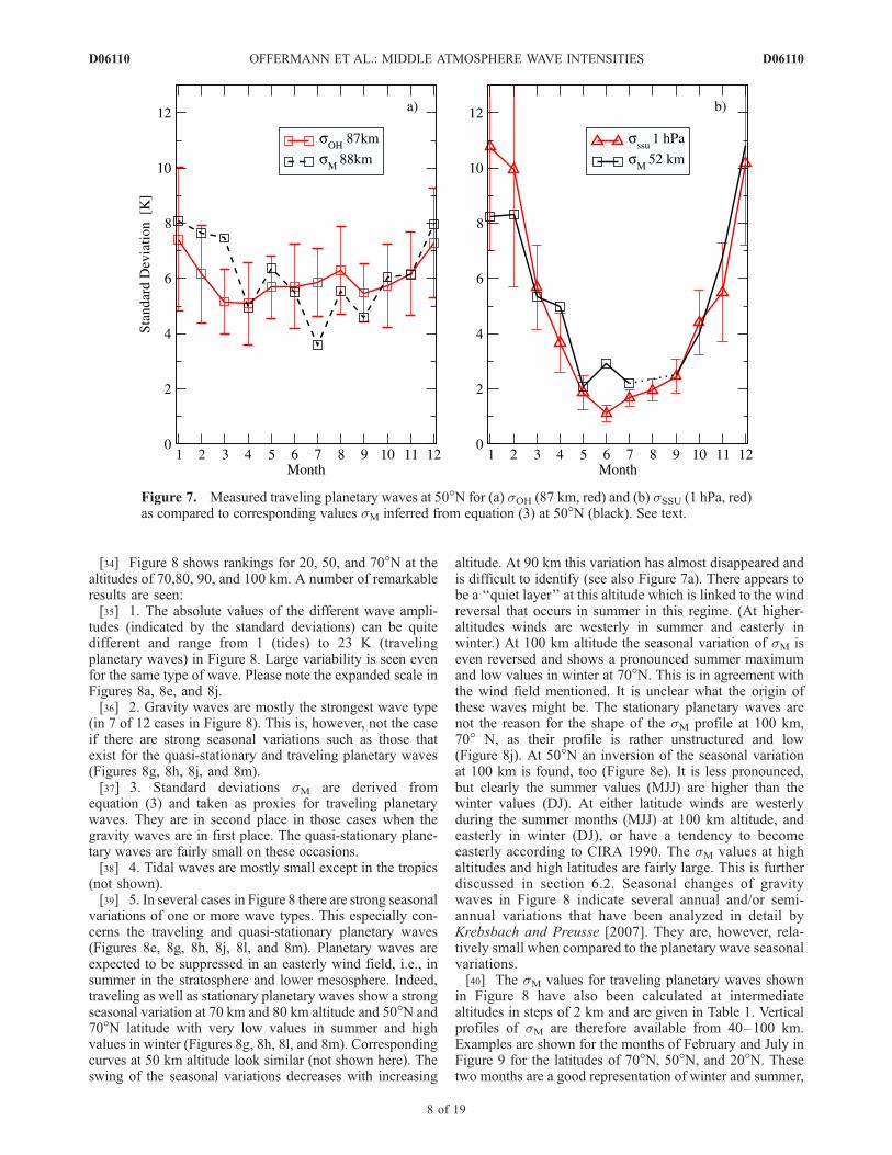
This approach allows us to estimate sM at other altitudesand latitudes. Using SABER data from 88 km and 50�N wecompare in Figure 7a sM derived from equation (3) (blacksquares, dashed line) with sOH (red squares, solid line)shown in Figure 6. The error bars of the sOH values are thestandard deviations of the monthly values from their meansover the 12 years of OH data at Wuppertal. The interannual

variability of the traveling planetary waves is high. The sMvalues derived from equation (3) and the measured sOHagree quite well when these interannual variations are takeninto account.[32] To further confirm the approach given in Figure 6 we

show in Figure 7b sM values obtained at 50�N and at 52 kmaltitude. At this location data from 17 years of stratosphericsounding unit (SSU) measurements taken between 1980 and1997 at 1 hPa are available (red triangles). The StratosphericSounding Unit (SSU) data could not be detrended for thezonal mean temperature variations within one month andtherefore have a slight high bias. Our computed sM and theobserved sSSU in Figure 7b agree quite well. We willtherefore use equation (3) to estimate sM as a proxy fortraveling planetary waves at other latitudes and altitudes.

4. Wave Ranking

[33] A wave ranking is given in Figure 6, that is, acomparison of the relative intensities of various wave typesas represented by the standard deviations of their amplitudesfor 50�N and 88 km altitude. Corresponding rankings cannow be established for other altitudes and latitudes since thetraveling planetary waves can be estimated from equation (3).Examples are given in Figures 8a–8m showing the standarddeviations of the SABER temperatures ssab on top of eachpicture, and below them the various waves: gravity wavessgw, traveling planetary waves sM, quasi-stationary planetarywaves sspw, and tides stide. The accuracies are believed to besimilar to those given in Figure 6. (For sM see section 6.2.)The SABER standard deviations have been corrected(detrended, see section 3) for seasonal and latitudinal meantemperature variations by means of corresponding gradientstaken from the CIRA 1990 tables. These corrections wererather small, and mostly much less than 1 Kelvin.

Figure 6. Comparison of four wave types during the course of the year at 88 km altitude and 50�N.Standard deviations are color coded as follows: gravity waves are green, traveling planetary waves areblack with squares, stationary planetary waves are blue, and tidal waves are safran. The sum of the fourwaves (following equation (2)) is given in black as the root mean square ssum. It is compared to thefluctuations ssab measured by SABER (red).

D06110 OFFERMANN ET AL.: MIDDLE ATMOSPHERE WAVE INTENSITIES

7 of 19

D06110

[34] Figure 8 shows rankings for 20, 50, and 70�N at thealtitudes of 70,80, 90, and 100 km. A number of remarkableresults are seen:[35] 1. The absolute values of the different wave ampli-

tudes (indicated by the standard deviations) can be quitedifferent and range from 1 (tides) to 23 K (travelingplanetary waves) in Figure 8. Large variability is seen evenfor the same type of wave. Please note the expanded scale inFigures 8a, 8e, and 8j.[36] 2. Gravity waves are mostly the strongest wave type

(in 7 of 12 cases in Figure 8). This is, however, not the caseif there are strong seasonal variations such as those thatexist for the quasi-stationary and traveling planetary waves(Figures 8g, 8h, 8j, and 8m).[37] 3. Standard deviations sM are derived from

equation (3) and taken as proxies for traveling planetarywaves. They are in second place in those cases when thegravity waves are in first place. The quasi-stationary plane-tary waves are fairly small on these occasions.[38] 4. Tidal waves are mostly small except in the tropics

(not shown).[39] 5. In several cases in Figure 8 there are strong seasonal

variations of one or more wave types. This especially con-cerns the traveling and quasi-stationary planetary waves(Figures 8e, 8g, 8h, 8j, 8l, and 8m). Planetary waves areexpected to be suppressed in an easterly wind field, i.e., insummer in the stratosphere and lower mesosphere. Indeed,traveling as well as stationary planetary waves show a strongseasonal variation at 70 km and 80 km altitude and 50�N and70�N latitude with very low values in summer and highvalues in winter (Figures 8g, 8h, 8l, and 8m). Correspondingcurves at 50 km altitude look similar (not shown here). Theswing of the seasonal variations decreases with increasing

altitude. At 90 km this variation has almost disappeared andis difficult to identify (see also Figure 7a). There appears tobe a ‘‘quiet layer’’ at this altitude which is linked to the windreversal that occurs in summer in this regime. (At higher-altitudes winds are westerly in summer and easterly inwinter.) At 100 km altitude the seasonal variation of sM iseven reversed and shows a pronounced summer maximumand low values in winter at 70�N. This is in agreement withthe wind field mentioned. It is unclear what the origin ofthese waves might be. The stationary planetary waves arenot the reason for the shape of the sM profile at 100 km,70� N, as their profile is rather unstructured and low(Figure 8j). At 50�N an inversion of the seasonal variationat 100 km is found, too (Figure 8e). It is less pronounced,but clearly the summer values (MJJ) are higher than thewinter values (DJ). At either latitude winds are westerlyduring the summer months (MJJ) at 100 km altitude, andeasterly in winter (DJ), or have a tendency to becomeeasterly according to CIRA 1990. The sM values at highaltitudes and high latitudes are fairly large. This is furtherdiscussed in section 6.2. Seasonal changes of gravitywaves in Figure 8 indicate several annual and/or semi-annual variations that have been analyzed in detail byKrebsbach and Preusse [2007]. They are, however, rela-tively small when compared to the planetary wave seasonalvariations.[40] The sM values for traveling planetary waves shown

in Figure 8 have also been calculated at intermediatealtitudes in steps of 2 km and are given in Table 1. Verticalprofiles of sM are therefore available from 40–100 km.Examples are shown for the months of February and July inFigure 9 for the latitudes of 70�N, 50�N, and 20�N. Thesetwo months are a good representation of winter and summer,

Figure 7. Measured traveling planetary waves at 50�N for (a) sOH (87 km, red) and (b) sSSU (1 hPa, red)as compared to corresponding values sM inferred from equation (3) at 50�N (black). See text.

D06110 OFFERMANN ET AL.: MIDDLE ATMOSPHERE WAVE INTENSITIES

8 of 19

D06110

respectively. Most of the sM profiles presented have a similarstructure with a slow to moderate increase or even a decreaseat the lower altitudes and a much steeper increase at altitudesabove 90 km. If fitted lines would be drawn to them as in

Figure 2 they would show a kink structure such as that seen inmany of the other wave profiles discussed so far. The summerprofile at 50�N does, however, not quite fit this picture as ithas a pronounced local maximum around 80 km altitude. As

Figure 8. Wave ranking (seasonal variations) at latitudes of 20, 50, and 70�N and altitudes of 70, 80,90, and 100 km. The four waves are gravity waves (green), traveling planetary waves (black squares),quasi-stationary planetary waves (blue), and tides (safran). Top curves are measured SABER fluctuations(red). Note the expanded scale in Figures 8a, 8e, and 8j.

D06110 OFFERMANN ET AL.: MIDDLE ATMOSPHERE WAVE INTENSITIES

9 of 19

D06110

gravity waves and traveling planetary waves are mostly thestrongest terms in Figure 8 the gravity wave intensities fromFigure 3 have been included in Figure 9 for comparison asdashed lines.[41] The intensities of the quasi-stationary planetary waves

sspw are mostly much smaller than those of the travelingplanetary waves sM (Figure 8). The vertical profiles of thequadratic sum of the two (sM0) are therefore essentially thoseof the traveling planetary waves. The difference between thetwo is mostly less than 1K. There are, however, exceptions asin the winter months at the lower altitudes and middle to highlatitudes (Figure 8h, 8l, and 8m). To illustrate this, anexample is given for February at 70�N in Figure 10, whichshows sM0 as compared to sM. The difference is up to 7 K,but this is essentially confined to a limited altitude range(65–90 km).[42] The corresponding gravity wave curve sgw is shown

for comparison as a red line (taken from Figure 3a). Therelative magnitude of the gravity waves sgw and (the sumof) the planetary waves sM0 are important for the waveturbopause. The intersection of the two curves sgw and sM isat the altitude zis, and will be discussed in sections 5 and 6.3.

5. Formation of the Wave Turbopause

[43] The remarkable structure of the vertical profiles ofstandard deviations ssab (Figure 2) is a flat increase withaltitude at the lower heights up to a kink, and a much steeperincrease at the greater heights. In an atmosphere where thewaves can freely propagate in the vertical direction, this steepincrease should occur at a much lower altitude (because ofenergy conservation). This has been discussed in detail byOffermann et al. [2006a]. The flatter than expected increasehas been interpreted as a consequence of wave damping at the

lower altitudes in that paper. It is connected with the negativebackground temperature gradient in the mesosphere. Ataltitudes above the kink (square in Figure 2) damping ismuch reduced and consequently the amplitude increase ismuch stronger. The kink has therefore been named the waveturbopause.[44] The altitude at which this turbopause occurs shows

considerable variations with season and latitude. This hasbeen analyzed in Offermann et al. [2007]. Offermann et al.[2006a, 2007] have presented a phenomenology of the waveturbopause and some relationship to other ‘‘turbopauses.’’The data shown in the present paper are meant to helpregarding how the kink, i.e., the turbopause comes about.[45] Many of the vertical intensity profiles of the different

waves discussed previously in the paper show a kink-likestructure themselves (e.g., Figures 3, 5, and 9). The flat(dissipation) part of the profiles at the lower altitudes isclearly seen. This means that at lower-altitudes wave dampingappears to be present quite generally. It is important tonotice that the superposition of two profiles each showing akink (at different altitudes) typically yields a profile with akink again. This results from the fact that the variances (i.e.,fluctuation squares) are added and the square root of the sumis taken. In consequence the strongest part of either profiledominates the result. This applies also in case the gradient atthe lower altitudes is somewhat negative as is sometimes thecase with the planetary waves (Figure 9). The use of twostraight fit lines further helps to identify a kink.[46] An example for this is shown in Figure 11. Here the

traveling planetary waves at high latitudes (70�N) fromFigure 9a and the corresponding gravity waves from Figure3a (also dotted lines in Figure 9a) are used. The root meansquare of the two curves is calculated and shown as a bluecurve in Figure 11. Linear fit lines to the lower altitudes

Figure 9. Vertical distributions of traveling planetary wave amplitudes (standard deviations sM, solidlines) for (a) February and (b) July. (Note the difference in scales.) Latitudes are 20 (black), 50 (red), and70�N (green). Corresponding data for gravity waves taken from Figure 3 are shown for comparison(dashed lines).

D06110 OFFERMANN ET AL.: MIDDLE ATMOSPHERE WAVE INTENSITIES

10 of 19

D06110

Table 1. Traveling Planetary Wave Activity as Derived From Equation (3)a

Altitude Steps(km) Jan. Feb. Mar. Apr. May. Jun. Jul. Aug. Sep. Oct. Nov. Dec.

20�N Latitude40 2.80 2.74 2.91 1.93 1.71 1.74 1.71 1.46 2.24 2.93 3.25 4.0342 3.29 2.58 2.92 2.05 1.89 1.88 1.53 1.49 2.44 2.39 3.43 3.8144 3.65 2.78 2.83 2.36 1.85 2.06 2.11 2.16 2.34 2.56 3.64 3.9346 3.20 3.05 3.02 2.77 2.08 2.31 2.16 2.90 2.41 2.58 3.34 3.8648 2.88 3.73 2.95 2.86 2.16 2.61 2.15 3.49 2.37 2.63 3.25 3.6450 2.56 4.08 3.08 2.76 2.32 2.33 2.20 3.88 2.35 2.43 2.56 3.5952 3.43 4.02 3.24 2.89 2.37 2.69 2.93 3.93 2.45 2.73 3.01 4.0654 4.96 4.43 3.24 2.86 2.66 3.72 3.60 4.06 2.71 3.22 3.78 4.1956 5.08 4.27 2.94 3.06 2.73 3.65 3.41 3.66 2.56 2.71 3.36 4.1358 4.25 4.04 2.71 2.69 2.51 3.53 3.59 3.00 2.14 2.38 3.08 4.1660 3.93 4.37 2.61 2.91 2.75 3.58 3.45 2.95 2.10 2.53 3.02 4.7362 3.92 4.70 2.34 2.59 2.45 3.42 2.96 2.51 1.85 2.54 3.05 5.4664 4.00 4.68 2.31 2.72 2.36 3.42 2.78 2.30 1.60 2.46 2.77 5.5966 3.97 4.28 2.85 2.87 2.17 3.78 2.73 2.27 1.41 2.05 3.59 5.7868 4.10 4.62 4.02 3.48 2.20 4.58 3.58 2.53 1.90 3.00 4.81 6.1470 5.00 5.48 5.14 4.47 2.94 5.85 5.05 3.34 3.17 4.45 5.12 6.6972 6.55 6.23 5.81 5.46 3.50 7.01 5.89 3.95 3.77 5.06 5.36 7.2374 7.58 6.94 6.11 5.68 4.25 7.44 6.72 4.73 4.11 4.67 7.18 7.0176 7.80 7.18 5.83 5.46 5.86 7.65 7.62 5.71 4.90 4.55 7.54 7.5678 7.61 6.76 5.42 5.75 7.00 7.48 7.65 6.40 5.15 5.33 6.97 7.9180 7.53 6.60 5.36 6.06 7.40 6.97 6.95 6.77 5.63 5.61 6.66 7.3682 7.94 6.74 5.47 6.39 7.11 6.57 6.69 7.00 6.12 5.74 6.52 7.1284 8.12 6.99 5.45 7.01 6.63 6.37 7.15 7.52 6.21 5.57 6.66 7.1886 7.63 6.68 5.59 7.00 6.51 6.48 7.25 7.76 6.14 5.23 6.74 7.4788 7.04 6.07 5.24 6.31 6.94 6.47 6.50 6.99 5.74 4.30 6.05 7.6190 5.15 6.85 4.38 5.34 7.03 6.30 6.30 5.70 5.13 0.03 4.64 7.9592 3.21 7.78 4.92 5.06 7.38 6.31 5.91 6.59 5.10 3.66 3.69 7.5094 4.82 8.21 5.35 6.75 7.06 7.05 5.92 7.52 6.85 7.68 4.04 8.1896 8.13 9.02 6.39 8.05 7.25 8.99 7.63 8.37 9.25 10.11 7.22 9.4098 10.62 11.43 7.96 10.01 9.23 11.76 11.00 10.58 11.87 12.16 10.61 10.84100 12.65 12.96 10.36 11.70 12.53 14.43 15.46 13.96 15.05 14.74 12.41 13.24

50�N Latitude40 9.32 10.80 6.63 5.30 2.28 2.08 1.69 1.29 2.87 4.56 7.98 13.7842 10.15 10.92 6.61 5.48 2.32 2.26 2.09 0.85 2.89 4.78 8.27 14.7444 10.82 10.30 6.08 5.28 2.31 2.62 2.17 1.00 2.90 4.61 8.18 14.8946 10.53 9.53 5.57 5.18 2.15 2.64 2.29 0.03 2.80 4.23 7.59 14.1348 9.55 8.78 5.13 5.07 2.20 2.84 2.52 0.82 2.81 3.87 6.81 12.6050 8.44 8.11 5.01 4.94 2.24 3.25 2.59 1.19 2.48 3.68 6.38 11.2752 8.23 8.32 5.33 4.99 2.07 2.93 2.21 0.03 2.53 4.02 6.79 10.8354 7.48 8.11 5.71 5.34 2.30 3.13 2.83 1.36 3.02 4.30 7.07 9.6856 7.09 7.73 5.60 5.09 2.75 3.65 3.63 2.24 2.73 4.20 7.09 8.4358 7.65 7.93 5.69 4.23 2.28 3.61 3.28 1.66 2.25 4.57 7.18 8.1660 8.38 8.46 5.95 3.72 1.98 3.33 3.34 1.93 2.29 5.00 7.11 8.1262 8.88 9.06 6.05 3.07 1.84 3.41 3.44 1.91 1.98 5.62 7.92 8.5264 9.70 9.84 6.27 2.40 2.09 3.42 3.37 1.73 1.55 6.38 9.08 9.1266 10.26 10.21 6.21 1.96 1.83 3.39 3.09 1.57 1.04 7.20 10.15 10.1068 10.15 10.06 6.07 2.30 2.17 3.36 3.11 1.75 1.16 7.73 10.60 10.8170 9.47 9.58 6.05 3.39 2.57 3.62 3.87 2.79 2.72 8.02 10.75 11.6572 9.44 9.35 6.17 4.41 3.51 4.13 5.35 4.28 4.46 8.25 10.44 11.8574 9.73 9.01 6.68 5.68 4.37 5.34 7.05 5.57 6.45 8.13 9.67 11.3876 10.42 8.89 7.08 6.40 5.91 7.09 8.52 6.69 8.15 7.93 9.34 10.7878 11.11 9.06 6.96 6.65 7.51 8.38 8.99 7.58 8.85 7.78 8.95 10.0680 12.02 9.56 6.93 6.21 8.89 8.58 8.02 7.78 8.59 7.40 8.62 10.1082 12.30 9.86 6.99 5.47 9.68 8.12 5.94 7.60 7.81 7.30 8.57 10.1684 11.13 9.53 7.23 5.33 9.54 7.02 4.39 7.61 6.74 7.20 7.95 9.4886 9.80 8.77 7.71 5.74 8.30 5.91 3.86 6.99 5.59 6.73 7.01 8.8588 8.09 7.66 7.47 4.96 6.38 5.49 3.59 5.55 4.59 6.05 6.12 7.9890 6.94 6.61 6.79 4.53 5.20 5.60 3.21 3.42 3.72 5.13 5.05 7.0092 6.03 6.06 6.23 4.76 4.47 4.20 0.03 0.03 1.55 4.30 4.37 5.0894 6.03 6.87 6.55 5.59 5.00 4.28 0.03 2.25 2.02 4.96 4.72 4.1096 4.31 7.50 6.78 6.48 6.32 7.42 3.41 3.81 2.63 6.71 6.04 5.0498 0.03 8.59 7.54 8.86 9.25 10.35 7.78 6.64 5.90 7.00 5.46 4.85100 3.52 10.88 8.14 12.09 11.88 12.86 10.73 10.66 8.25 8.15 5.83 6.52

70�N Latitude40 7.66 14.16 8.36 - 0.81 0.88 0.57 - 0.03 5.87 6.00 -42 9.94 14.70 7.97 - 0.94 1.06 0.72 - 0.03 6.02 6.12 -44 11.27 14.52 7.22 - 1.08 1.56 0.77 - 0.41 6.07 6.45 -46 11.62 13.92 6.85 - 0.93 1.48 0.94 - 1.02 6.13 7.15 -48 10.54 12.95 6.22 - 1.11 1.75 1.30 - 0.03 5.62 7.52 -

D06110 OFFERMANN ET AL.: MIDDLE ATMOSPHERE WAVE INTENSITIES

11 of 19

D06110

(40–75 km) and higher altitudes (above 90 km) are alsoincluded (black solid and dashed lines). The kinked structureis clearly visible. It is to be remembered that the measuredfluctuation intensity ssab is the square root of the sum of thevariances of all waves involved. It was shown in sections 2, 3,and 4 that the major contributors to the ssab profiles are the

gravity waves and the traveling planetary waves (Figures 3and 9), which mostly have kinked vertical profiles. Figure 2can thus be explained in principle.[47] Figure 11 suggests that the altitude of this turbopause

is essentially determined by the relationship between gravitywaves and planetary waves. The intersection point (Figure 10)

Table 1. (continued)

Altitude Steps(km) Jan. Feb. Mar. Apr. May. Jun. Jul. Aug. Sep. Oct. Nov. Dec.

50 9.87 12.25 5.72 - 1.26 1.43 1.37 - 0.03 5.20 7.93 -52 10.27 12.48 6.98 - 1.25 1.62 1.33 - 0.03 5.55 8.76 -54 10.23 11.68 7.77 - 1.17 1.79 1.57 - 0.03 5.32 8.58 -56 10.77 10.80 8.25 - 1.28 1.99 1.80 - 0.03 5.06 8.23 -58 11.66 10.46 8.79 - 1.98 2.46 2.33 - 0.77 5.44 8.19 -60 12.32 10.39 9.35 - 1.37 2.07 2.08 - 1.52 6.03 8.38 -62 12.61 10.19 9.59 - 1.09 1.92 1.86 - 1.23 6.69 8.46 -64 12.87 10.22 9.39 - 0.67 1.77 2.08 - 0.63 7.38 8.34 -66 12.38 10.22 9.08 - 1.33 1.75 1.95 - 1.14 7.79 8.39 -68 10.82 10.03 8.63 - 1.93 2.15 2.19 - 1.59 8.13 9.29 -70 9.31 10.03 8.29 - 2.63 2.51 2.55 - 2.48 8.66 10.81 -72 8.10 9.62 7.79 - 3.16 3.10 3.16 - 2.73 9.26 12.28 -74 6.70 9.01 7.27 - 3.62 3.52 3.34 - 3.65 9.30 12.19 -76 4.48 8.19 6.23 - 4.24 4.52 4.12 - 4.64 8.92 11.38 -78 3.76 7.93 5.39 - 5.12 5.27 4.09 - 5.30 8.55 10.57 -80 5.21 8.24 4.90 - 5.33 6.10 5.26 - 5.19 8.07 10.36 -82 6.87 8.55 5.28 - 5.83 6.32 4.74 - 5.07 7.86 10.26 -84 6.75 8.26 5.43 - 4.60 4.44 3.86 - 5.01 7.47 9.65 -86 6.21 7.74 5.76 - 3.65 4.60 5.71 - 4.77 7.05 8.90 -88 5.60 6.78 5.81 - 3.49 5.84 7.04 - 4.15 6.27 8.19 -90 5.30 5.83 6.03 - 4.07 6.37 7.15 - 2.94 5.24 7.09 -92 5.30 5.22 5.99 - 3.51 6.47 6.46 - 2.54 4.68 6.73 -94 6.42 5.95 6.27 - 4.51 7.37 5.58 - 4.06 5.70 7.05 -96 6.98 6.61 6.12 - 8.76 10.48 8.78 - 6.48 7.08 7.51 -98 7.18 7.60 7.30 - 14.74 14.82 15.90 - 8.68 8.55 8.36 -100 10.62 9.38 9.93 - 22.62 18.97 23.54 - 10.68 10.65 10.47 -

aTemperature standard deviations in Kelvin. For accuracies see section 6.2.

Figure 10. Comparison of traveling planetary waves sMwith the (quadratic) sum of stationary and traveling planetarywaves sM0. The corresponding gravity wave profile sgw isalso shown. The intersection altitude is zis. Data are forFebruary at 70�N.

Figure 11. A kinked curve (blue) resulting from the(quadratic) superposition of gravity waves and travelingplanetary waves, computed as sqrt(sgw

2 + sM2 ). Data shown

are for 70�N and February. The black lines are linear fits tothe lower and upper parts (see text).

D06110 OFFERMANN ET AL.: MIDDLE ATMOSPHERE WAVE INTENSITIES

12 of 19

D06110

of the two profiles that are the basis of Figure 11 is near totheir kink altitude (Figure 11) and hence to the turbopausealtitude. An increase of planetary wave intensity in its lowerpart would shift the intersection point and hence the turbo-pause altitude to greater heights, and vice versa. Changes inthe gravity wave profile would have corresponding conse-quences. Comparison of gravity waves and planetary wavesin Figure 9 shows that the variability of intensity is muchlarger for the planetary waves than for the gravity waves. Thissuggests that a major part of the altitude variations of theturbopause (section 6.3 [Offermann et al., 2006a, 2007]) isdue to changes in planetary waves.[48] To check these ideas we have determined the inter-

section points zis of all monthly gravity and planetary waveintensity profiles in the way sketched in Figure 10. In orderto take also into account the quasi-stationary planetarywaves we use now the (quadratic) sum of sM and sspwand denote it sM0. The results for the new altitudes zis areshown in Figure 12a for 70�N and in Figure 12b for 20�N.The bars shown with the March values are typical and givethe changes of zis that result if one of the temperatureprofiles (sgw or s0M) is shifted to higher/lower values by 1 K.At the low latitudes the altitude profiles become quite similarat low altitudes. Hence an intersection is sometimes difficultto define. These months (August, September) have beenomitted from Figure 12b. For comparison the altitudes ofthe wave turbopause are taken from Offermann et al. [2007]

and are also shown in Figure 12. The intersection altitudesare 5–10 km lower than the turbopause altitudes but theyshow a very similar seasonal variation. We therefore con-clude that both gravity waves and planetary waves are thebasic contributors to the formation of the wave turbopause.

6. Discussion

6.1. Potential Energy Density

[49] The deviations from the means of temperature T0 andwind speed u0 and v0 cannot only be used for fluctuationanalyses. Beyond that they have frequently been used in theliterature to estimate the potential and kinetic energy densi-ties of waves in the middle atmosphere. The energy densitiesper unit mass are given by equations (4a) and (4b), respec-tively [e.g., Tsuda et al., 2000],

Epot ¼ 1=2 g=Nð Þ2 T0=Tð Þ2 Joule=kgð Þ ð4aÞ

Ekin ¼ 1=2 u02 þ v02� �

Joule=kgð Þ; ð4bÞ

where T is the mean temperature, and N is the Brunt-Vaisalafrequency.[50] In the present paper we mostly use the basic mea-

surement parameter T0 and not the derived quantity Epot. Thisis because for the potential energy in equations (4a) we needa climatology of the mean temperature T, and for N we needa mean vertical temperature gradient. If we wanted to useequations (4a) for the various waves discussed in the presentpaper, it would not be clear which T climatology applies.Using SABER derived mean temperature is not as straightforward as one might expect because of asynoptical satellitesampling. (It may, for instance, contain tidal signatures; seeOberheide et al. [2003] for a detailed discussion.) Althoughit is not believed that different climatologies of temperatureavailable from different measurements are very differenttoday, using the directly measured fluctuations appeared tobe somewhat safer. (There are other publications that alsouse the fluctuations instead of the energy densities [see, e.g.,Dowdy et al., 2007, and references therein].)[51] The third term in equations (4a), i.e., (T0/T)2, is the

relative temperature variance s2(T). Hence the square rootof the potential energy density is approximately proportionalto the standard deviation s of the temperature fluctuationsused in this paper (normalized by T). The summationsaccording to equations (1) and (2) therefore are essentiallythe summations of potential energies, and the wave rankingsgiven in Figures 6 and 8 are rankings according to the(square root of the) potential energy density (at and below100 km).[52] To illustrate this we pick a few examples from the

literature. Wilson et al. [1991] present 4 years (1986–1989)of gravity wave potential energy densities from lidar data at44� N, 6�E in France (OHP). Their upper altitude range is60–75 km where an annual and semiannual change are seen[Wilson et al., 1991, Figure 9]. This compares well with thecorresponding gravity wave curve in Figure 8h. Wilson etal. [1991, Figure 16] give an annual mean for the potentialenergy density of about 105 J/kg in the altitude regime 60–75 km (Station OHP). We compare this with our 70 km

Figure 12. Seasonal variation of the altitude of intersectionpoints zis (from profiles sgw and s

0M, see text). Red curves are

for (a) 70 and (b) 20�N. Corresponding altitudes of thewave turbopause are shown for comparison (black curves,taken from Offermann et al. [2007, Figure 6]).

D06110 OFFERMANN ET AL.: MIDDLE ATMOSPHERE WAVE INTENSITIES

13 of 19

D06110

GW data (Figure 8h, 4.8 K). We estimate the Brunt-Vaisalafrequency by means of temperatures and temperature gra-dients taken from Rees [1990, Table 5.1] (i.e., CIRA 1986).The resulting potential energy density is 62 J/kg. This is nottoo far away and appears compatible with the differences ofthe data in altitude and latitude (not shown here).[53] Another set of 10 years of lidar data is presented by

Sica and Argall [2007] (43�N, 81�W). They derive kineticenergy densities for gravity waves at different altitudes.For the upper mesosphere (60–80 km) they present thefollowing seasonal variation (in mJ/m3, their Table 1):DJF 5.6; MAM 13.8; JJA 14.8; SON 12.0. The cor-responding annual mean is 11.7 mJ/m3. This seasonal vari-

ation is fairly different from that shown in Figure 8h.However, neither variation is really strong. The annual meanof 11.7 mJ/m3 is converted to 158 J/kg by means of theatmosperic density at 50�N, 70 km altitude as taken fromNOAA [1976] (i.e., USSA76). Our corresponding annualmean is T0 = 4.8 K in Figure 8h which means a potentialenergy density of 62 J/kg as shown above. This is consider-ably smaller than the value of Sica and Argall. However,Tsuda et al. [2000] have pointed out that the kinetic energydensity should be larger than the potential energy densityby a factor of 5/3 to 2. Some part of the difference couldalso be due to the difference of the two data sets in latitudeand especially in altitude. It should also be remembered thatthe GW climatology used here does not include verticalwavelengths below 5 km while the latter are included in thelidar based analysis. Manson et al. [1981] (52�N, 107�W)derived kinetic energy densities from radar measurementsof the wind components u0 and v0 according to equation (4b).They obviously, however, omitted the factor 1/2 in theequation. They give kinetic energy densities of two typesof gravity waves at 80 km and 97 km, respectively (theirFigure 13). The seasonal variations shown are – in theirrelative values – quite similar to our data in Figures 8gand 8e. We estimate the approximate annual mean fromtheir Figure 13 to be 5 mJ/m3 at 80 km and 0.7 mJ/m3 at97 km. Our corresponding values for the potential energydensity from Figure 8 are 2.2 mJ/m3 (80 km) and 0.25 mJ/m3

(100 km), respectively. This is lower by factors 2.3–2.8.Taking into account the above mentioned factor 1/2 and afactor 5/3 cited by Tsuda et al. [2000] our values should belower by a factor 3.3, which is not too far away. (For thesecomparisons we have again used temperatures, temperaturegradients, and densities from Rees [1990, Table 5.1] andNOAA [1976].)[54] A more recent paper [Dowdy et al., 2007] gives

gravity wave kinetic energy densities from radar windmeasurements at Arctic and Antarctic latitudes (more than5 years). We use here only the Arctic data from the stationsof Poker Flat (65�N, 147�W) and Andenes (69�N, 16�E)and compare them to our 70�N data. Dowdy et al. [2007]find considerable seasonal variations with basically anannual and a semiannual component that, however, stronglydepend on altitude and gravity wave period. The generalbehavior is similar to what we see in our Figure 8. The bestagreement is obtained for the station of Andoya which isnearest to our latitude of 70�N (their Figure 8, long gravitywave periods). Dowdy et al. [2007] give summer and wintermean data in their Figure 6. We use their Andoya data (70–100 km) to compare with our gravity wave February andJuly data shown in Figure 9. Dowdy et al. [2007] use thewind variances as a measure of the kinetic energy density,i.e., they do not apply the factor 1/2 in equation (4b). Theenergy densities are strongly altitude dependent in eitherdata set. The ratio of the Andoya data to those presentedhere is 1.9 in winter (range 1.5 to 2.4 for the differentaltitudes) and 2.4 in summer (range 0.83 to 6.2). Hence avery approximate agreement is obtained similar to the lowerlatitudes [Manson et al., 1981] considering the factor 1/2and the Tsuda factors cited (resulting in an expected ratio ofabout 4). We have compared the energy densities fromthe same measurement technique and different latitudes (at80 km altitude, annual mean). From the radar techniques we

Figure 13. Ar/N2 ratios as measured by mass spectro-meters. (a) Measured data (black with squares) as comparedto a constructed profile showing homogeneous mixingbelow 98 km (z0) and diffusive separation above (red withtriangles). (b) Difference of the two curves in Figure 13a.Distribution full width at half maximum is 11 km (red arrow).

D06110 OFFERMANN ET AL.: MIDDLE ATMOSPHERE WAVE INTENSITIES

14 of 19

D06110

obtain 5mJ/m3 at 52�N [Manson et al., 1981] and 2.4 mJ/m3

at 69�N [Dowdy et al., 2007]. This is a factor 2.1 decreasewithin a 17� increase in latitude. The present SABER data(Figures 8 and 9) yield 2.2 mJ/m3 at 50�N and 1.5 mJ/m3

at 70�N, i.e., a factor 1.5 decrease for a 20� latitudeincrease.[55] In summary the SABER energy densities shown here

are lower by a factor 1.7 to 2.8 than the data taken from theliterature. All of these literature values, except Wilson et al.[1991], are, however, kinetic energy densities. Before theycan be compared to potential energy densities they appar-ently need a down correction of a factor of 2 or more (seeabove and Tsuda et al. [2000]). The data of Wilson et al.[1991] are potential energies and a factor 1.7 higher than ourdata. This difference may be due to differences in latitudeand/or altitude as mentioned above. Interannual and long-term changes could also play a role. In addition to the alreadymentioned omission of short vertical wavelength GWs in theSABER climatology, the inherent horizontal smoothing ofthe limb scan technique may also play a role.

6.2. Traveling Planetary Waves

[56] A climatology of traveling planetary waves (PW) isnot yet available at present. We therefore present our sMvalues as a proxy for planetary wave intensities. But, wealso need to estimate how reliable this parameter is; i.e.,whether this proxy is contaminated for any reason. Thereare a number of possible contamination sources,which wediscuss herein.6.2.1. Gravity Waves[57] In our discussion of Figure 6 we argued that gravity

waves do not influence the sM proxy much because ofspatial and temporal filtering. This may be questionable forlarger-scale (inertial) gravity waves. We therefore used OHmeasurements from a second (twin) station that is operatedat the Observatory of Hohenpeissenberg (48�N, 11�E) some360 km away from Wuppertal, to look for simultaneouslarge-scale gravity waves over the two stations and foundvery few. These two stations are in completely differentgravity wave environments as the high mountains of theAlps are very near to Hohenpeissenberg. Hence we wouldexpect to see differences in sM at the two stations if theirmeasurements were noticeably influenced by gravity waves.We found a mean difference on the order of 3% over severalyears (to be published in a forthcoming paper). We thereforeconclude that the gravity wave influence on sM might be ofthis order of magnitude, which is small. Another argumentin support of this conclusion is derived from the seasonalvariations of sGW and sM illustrated in Figure 6. If therewas considerable gravity wave influence on sM, the twocurves should show some similarities, but they do not. Thecorrelation coefficient is –0.03. The same argument holdsfor the corresponding curves in Figure 8, which are alsofairly dissimilar. We therefore tentatively conclude thatgravity waves in general have little influence on sM.6.2.2. Tides[58] In Figure 6 the tidal values are considerably smaller

than sM. If some fraction of these tides should contribute tosM this contribution would be fairly small because of thequadratic summation. Also the seasonal curves should showsome similarity, which is not the case. Similarly, in Figure 8,sM is for the most part much larger than stide, except in

Figure 8b and 8e. However, the dissimilarity of the curvesmakes it again unlikely that the tides would influence sM.6.2.3. Stationary Planetary Waves[59] As mentioned in section 2.4, these waves are unde-

tectable in the OH measurements. However, SPW arefrequently only quasi-stationary. That is, their amplitudesbuild up or dissipate, or their positions shift (for instance inthe east–west direction). Such events may appear to betraveling planetary waves. Similar features are seen duringmajor and minor stratospheric warmings, vacillations, andother kinds of SPW modulations. It is long and well knownthat large-scale SPW changes/variations occur in the strato-sphere [e.g., Leovy et al., 1985]. Oberheide et al. [2006b]found similar structures in the mesosphere. The mesosphericstructures appear to be smaller, but whether this difference istypical remains unknown. An estimate for SPW changesin the mesosphere can be inferred from Figure 8. At mostaltitudes and latitudes sSPW is considerably smaller thansM, and hence the quasi-stationary waves cannot contributesignificantly to sM.However, at lower altitudes andmiddle tohigh-latitudes sspw are comparatively large, and changerapidly (Figures 8h, 8l, and 8m). The largest time change(decay) in this picture is seen in Figure 8l, where sSPWdecays here by 4.6 K per month over about two months.In a single month (for instance in April), this is equivalentto a standard deviation of 1.4 K and hence to a wavelikeoscillation with 2 K amplitude. In comparison, sM = 5 K inApril, corresponding to an amplitude of 7.1 K. The quadraticsum of these two amplitudes is 7.4 K; sM is changed by lessthan 4%. Hence the SPW changes seen in Figure 8 do notgenerally contribute much to sM.[60] As concerns major stratospheric warmings their

activity has been comparatively small during the 2002–2005 time window of our analysis [e.g., Labitzke et al.,2005]. Mesospheric signatures of stratospheric warmingsare much weaker than they are in the stratosphere, and mayeven appear as mesospheric coolings [e.g., Offermann et al.,1987]. We have checked the major warming periods citedby Labitzke et al. [2005] in our 87 km OH temperatures andfound no abnormal level of planetary wave activity duringany of these times.[61] Atmospheric vacillations are disturbances in high-

latitude winter that are also capable of contaminating oursM proxy. Stratospheric normal modes may be forced by theinteraction of planetary waves with the mean flow, or byspontaneous internal instabilities [e.g., Christiansen, 1999;Scott and Haynes, 2000, see also references therein]. Timescales are of the order of a few days to several weeks, whichare on the order of disturbances discussed herein. Strato-spheric warmings have also been discussed in terms ofvacillations. Vacillations analyses have focused on strato-spheric and lower mesospheric altitudes. The events appearto be small in the middle mesosphere to lower thermosphere.[62] Transient disturbances of stationary planetary waves

could quite generally contaminate our traveling planetarywave proxy sM (Figure 8 and Table 1). Experimentalknowledge about such temperature disturbances in themesosphere is limited, because it is difficult to distinguishbetween disturbed/modulated SPW and traveling PW. Thisdistinction can be achieved if the vertical phase structureof the waves is determined, requiring a large number ofvertical temperature profile measurements (for instance by

D06110 OFFERMANN ET AL.: MIDDLE ATMOSPHERE WAVE INTENSITIES

15 of 19

D06110

rocket flights or lidar soundings). Bittner et al. [1994],Bittner [1993], Offermann et al. [1987], and Scheer et al.[1994] reported about two northern winter campaignswith very many soundings of this kind (i.e., DYANACampaign, MAP/WINE Campaign). They determined thevertical phase structure of the waves and thus identifiedseveral SPW modulations that otherwise would have beenmistaken as traveling PW. We have used 260 data pointsbetween 40 and 87 km at 69�N and 44�N during severalmonths of winters 1990 and1983–1984 from these cam-paigns to estimate the contamination of our proxy sM inFigure 8 and Table 1. Several minor stratospheric warmingsoccurred during this time, along with a major warming inFebruary 1984. The result of our analysis including alldisturbances is as follows: 85% of the data points showed arelatively small contamination of sM (i.e., changes between0% and 20%). In 15% of the cases the disturbance of sM wasstronger: 20–65%. It thus follows that sM is a fairly reliableparameter with moderate contamination. (N.B., We usedcounting statistics to generate the contamination numbersabove. Average contamination values would be smaller.) Wealso addressed the question as towhether a plausible long-termtrend in sM might invalidate our supporting analyses of 15–20 year old campaign data. Specifically, we analyzed 87 kmaltitude measurements and did not find a significant trend inthe 1995 to 2004 time interval [Offermann et al., 2006b].[63] Referring to travelling planetary waves as sM in the

following, some of the intensities sM in Figure 8 need a moredetailed discussion. The sM values at high altitudes andlatitudes are fairly large. Especially the values in Figure 8j(70�N, 100 km) show a strong summer maximumwith valuesup to 23 K, with a relatively flat minimum superimposed inJune. The question arises whether this feature is real. Toestimate the accuracy of the sM curve we refer to Figure 7,which compares two inferred sM curves with two measuredones. These are at mid latitude (50�N), and at low altitude(52 km) and high altitude (88 km), respectively. The largestdifferences between the measured and the inferred curves are2.5 K or less. We tentatively adopt this value also as theaccuracy at high latitudes and altitudes (Figure 8j). Inconsequence the summer maximum can be taken as real.This is not so clear for the flat June relative minimum. It isabout 4 K deep, which is just within two times 2.5 K. Itsreality may thus be questionable. However, the two indepen-dent curves for sgw and ssab both show a similar Juneminimum, and something comparable is seen in Figure 8k.It may therefore be well possible that the minimum is a trueatmospheric feature. Pronounced traveling planetary wavesat high altitudes have been found many years ago in iono-spheric data [e.g., Takahashi et al., 2006; Lawrence andJarvis, 2003, and references therein]. Corresponding oscil-lations in the neutral atmosphere have been observed in uppermesosphere/lower thermosphere (UMLT) winds on manyoccasions [e.g., Murphy et al., 2007; Takahashi et al.,2006; Lawrence and Jarvis, 2003, and references therein].Planetary wave oscillations in UMLT temperatures have beeninferred from OH Meinel band emissions at 87 km altitude.Maximum amplitudes of 10–15 K have been observed [e.g.,Scheer et al., 1994; Murphy et al., 2007]. Meteor temper-atures have shown planetary wave type oscillations withamplitudes on the order of 10 K in the 85–95 km range[Kirkwood et al., 2002]. Temperature information at higher

altitudes on planetary waves are sparse. Riggin et al. [2006]have analyzed SABER temperature measurements up to110 km. They identified 5-day planetary waves withamplitudes larger than 12 K near 100 km. Amplitudes weremaximized in summer, with a relative minimum right inthe middle of summer. Corresponding model calculations(Thermosphere-Ionosphere-Mesosphere-ElectrodynamicsGeneral Circulation Model (TIME GCM)) showed ampli-tudes up to 16 K. A similar model analysis of a 6.5 dayplanetary wave showed a relative minimum in the middle ofsummer [Liu et al., 2004, see also references therein].[64] In summary large amplitude planetary waves at high

altitudes/high latitudes are well known. Temperature ampli-tudes, however, that have been measured so far are not ashigh as indicated in Figure 8j. However, gravity waveintensities in this picture are also very high, and in compar-ison the indicated planetary wave intensities appear not at allimpossible.[65] A special aspect needs to be noted that follows from

the way we infer the traveling wave intensities (sM): Thestandard deviation sM in Figure 8 results from the differ-ence of the measured ssab and the other wave intensities. Ifany of the latter should be biased low, in consequence sMwould be biased high. The quasi-stationary planetary wavessspw –as an example, are quite low in Figures 8e, 8f, 8j, and8k (below 4–5 K). Substantially higher values have beenobserved in measurements, as for instance by Steinbrecht etal. [2007] who saw a quasi-stationary wave of 12 Kamplitude at 87 km altitude and 50�N latitude. As theseasonal analysis of quasi-stationary planetary waves usedhere is based on a data set of 1-year duration only, a possiblelow bias cannot be excluded. Furthermore, tidal activity atmiddle to high latitudes may differ from the GSWMsimulations used here. The recent SABER tidal temperatureclimatology [Forbes et al., 2008] shows that a number ofnonmigrating tidal components peak at or poleward of40� latitude. This is only partly reflected in the GSWMsimulations that do not include tidal components forced bynonlinear wave-wave interaction. The net effect on theinferred traveling planetary waves needs to be further inves-tigated in the future but it is rather unlikely that it will removethe summer maximum in sM.

6.3. Turbopause Altitude/Turbopause Layer

[66] As already mentioned the wave turbopause is definedas the kink in the vertical fluctuation profiles ssab. Suchkinks are also found on many occasions for various wavetypes (Figures 3, 5, and 9). In Figure 10 the flat parts ofthe gravity and planetary wave profiles (i.e., at the loweraltitudes) indicate wave damping and the altitude rangewhere it occurs. If, on the one hand, the flat part of theplanetary wave profile is increased to a higher intensity thisis interpreted as higher wave activity accompanied byhigher dissipation (turbulence). At the same time intersec-tion altitude zis and turbopause altitude are increased. If, onthe other hand, the flat part of the gravity wave profile isextended to higher altitudes this means increased wavedissipation at these higher altitudes. Also in this case theintersection point and hence the turbopause is shiftedupward. Hence in our interpretation, in either case highwave dissipation corresponds to a high wave turbopausealtitude.

D06110 OFFERMANN ET AL.: MIDDLE ATMOSPHERE WAVE INTENSITIES

16 of 19

D06110

[67] The seasonal variation of the turbopause altitude at20�N shows a combination of an annual and a semiannualvariation (Figure 12b, black curve). This is found in a verysimilar way at 50�N (Figure 6 [Offermann et al., 2007]).Corresponding eddy diffusion coefficients have been derivedfrom radar measurements at 52�N in the upper mesosphere[Manson et al., 1981]. Their seasonal variation shows onemaximum inwinter and another one in summer. It is thus verysimilar to our variations of the turbopause altitudes. A verysimilar seasonal variation is observed in the OH* emissionintensities (D. Offermann, unpublished data, 2006) that arethe basis for derivation of the OH temperatures at 51�N inFigure 6. It suggests variations of vertical transports of traceconstituents. The three results (turbopause, eddy diffusion,OH* emission intensities) thus appear to be manifestations ofthe same dynamical feature in the mesosphere and lowerthermosphere.[68] As it is conceivable that the transition between

damped and undamped wave propagation will not occurat a single altitude, it is reasonable to assume that theturbopause forms a vertically extended layer rather than atwo-dimensional surface. This is in parallel to the loweratmosphere where the tropopause is nowadays discussed asa transition layer a few kilometers thick in the vertical [e.g.,Engel et al., 2006, and references therein]. It is important tomention that the turbopause was discussed years ago interms of a transition region [e.g., Hocking, 1990].[69] We have performed an analysis of the variation of the

wave turbopause altitude in winter (February) at 50�N. Theturbopause layer was found to be about 8 km thick (i.e.,plus/minus one standard deviation of the mean turbopausealtitude at a weekly time resolution). In summer (July) thislayer thickness is somewhat smaller. At higher latitudes(70�N) the corresponding values are somewhat larger.[70] To evaluate this, we analyzed a limited set of

measurements by rocket-borne mass spectrometers thatare available at around 40�N (various times of the year[Offermann et al., 1981]). Even though these are old datathey are nevertheless among the best we presently have: inthat paper eight measurements are collected that took placeright in the altitude regime where the turbopause isexpected. The mass spectrometers measured number densi-ties of Argon and Nitrogen, and hence the Ar/N2 ratio canbe used as a proxy for the Ar mixing ratio.We havereanalyzed these data. The Ar/N2 ratio in the lower atmo-sphere (homosphere) is 0.012. The altitude at which theratio deviates from this value is called the homopause z0(Figure 13).[71] The individual Ar/N2 profiles of the eight flights

show strong fluctuations. It is therefore difficult to assignindividual homopauses to the flights. Hence the range ofhomopause altitudes, i.e., the thickness of the homopauselayer (turbopause layer) cannot be derived. Therefore wehave taken another approach. The Ar/N2 columns between95 and 115 km have been calculated by Offermann et al.[1981] and have been found to efficiently smooth theindividual fluctuations. These columns are a measure ofthe homopause height, i.e., the larger the Ar/N2 column, thehigher the homopause height. (If in Figure 13a the red curve(triangles) is shifted to higher altitudes this means acorresponding shift of the homopause and an increase ofthe column between 95 and 105 km. See below.) The

column variability can therefore be used to estimate thehomopause variability. A layer thickness (2s) of about 8 kmis obtained this way. This value is the same as the layerthickness found above for the wave turbopause (note the10� latitude difference). The exact agreement must befortuitous, albeit remarkable, because the wave turbopauseshows considerable seasonal variations which presumablyare not well sampled by the eight rocket flights.[72] If the atmosphere is in diffusive equilibrium above

the homopause (first approximation) the Ar/N2 verticalprofile can be calculated once the homopause altitude z0is given [e.g., Offermann et al., 1981]. The mean profile ofthe eight measured Ar/N2 profiles has been calculated andis shown in Figure 13a (black curve with squares). Thevertical scatter bar at 100 km is the standard deviation, andis typical of the other altitudes. A diffusive equilibriumprofile is also shown (red curve, triangles) for which atentative homopause at 98 km was chosen. This choice wastaken because the two curves coincide at the highestaltitudes (110–115 km). This is interpreted such that atand above these altitudes the measured data are essentiallyin diffusive equilibrium. At the lower altitudes the meanmeasured curve is, however, found to substantially deviatefrom the diffusion equilibrium. The difference of the twocurves is shown in Figure 13b. The deviation profile showsa sharp peak which should, of course, not be taken too seriousconsidering the error bars shown. The vertical range of thedeviation is estimated to be about 11 km (full width at halfmaximum, 94–105 km, red bar with arrows in Figure 13b).The deviation is believed to be due to neutral turbulence. Ifturbulence stops at the homopause it decays above that level,and its action will be felt over some distance called ‘‘themixing length L.’’ The range of deviation from diffusiveequilibrium thus results from the combination of turbopause(homopause) variations and the mixing length. The homo-pause variations are estimated by the turbopause layer of8 km.We tentatively assume a linearly combined action of theturbopause layer with the mixing length L to form the 11 kmdeviation range. From this we estimate the mixing lengthL tobe 3 km (order of magnitude).[73] The seasonal mean of the wave turbopause at 40�N is

taken from Offermann et al. [2007] (Figure 6) and is foundto be at 91.5 km. The corresponding wave turbopause layerdepth is about 8 km, i.e., it extends from about 88 km to96 km. (The same layer depth as at 50�N has been usedhere.) The extension of the turbopause layer derived fromthe mass spectrometer data is 94–102 km. These two layershave considerable overlap and hence the turbopauses of thetwo techniques should not be far apart.[74] The combination of the turbopause layer thickness

and mixing length L yields a fairly extended reach ofturbulent impact. Many different methods have been usedin the past to determine the turbopause altitude, and quitedifferent altitudes have been obtained [e.g., Offermann et al.,2007, and references therein]. Part of these discrepancies maybe due to this large reach of turbulent impact.

7. Conclusions

[75] Temperature standard deviations from zonal meanvalues are used in the middle atmosphere as a proxy foratmospheric wave activity. Temperature fluctuations are

D06110 OFFERMANN ET AL.: MIDDLE ATMOSPHERE WAVE INTENSITIES

17 of 19

D06110

analyzed for the major wave types in the northern meso-sphere and lower thermosphere, and a wave ranking isobtained, to our knowledge, for the first time. The rankingshows some dependence on latitude and altitude (20–70�N,70–100 km). In most cases gravity waves play a major roleat these moderate to high latitudes. Traveling planetarywaves are in second place, and stationary planetary wavesand tidal waves yield a lesser contribution. (The latter arenot measured but come from a model simulation.)[76] Temperature variances are closely related to potential

energy density of the atmosphere. Gravity wave energydensities are compared to several examples given in theliterature. Reasonable agreement is obtained, with our databeing somewhat lower. This may be due to the fact that theSABER limb scan measurements cannot determine the shortwavelength gravity waves. In most of the paper we usetemperature standard deviations rather than energy densitiesto characterize the waves as calculation of these densitiesrequires climatologies of temperature and Brunt-Vaisalafrequencies that are not always at hand.[77] On the basis of the wave ranking an estimation of

traveling planetary wave intensities is attempted. A waveproxy is derived. It indicates a first and preliminary clima-tology of wave dependence on altitude and latitude. Possiblecontaminations of the proxy are discussed, and are found tobe relatively moderate. Proxy values at high altitudes/highlatitudes are rather large and might indicate an underestima-tion of other wave types here (stationary planetary waves,tides).[78] The concept of a wave turbopause has been developed

in earlier publications [Offermann et al., 2006a, 2007] on thebasis of vertical profiles of temperature fluctuations and akink or bend in the profiles (change of gradient) in the uppermesosphere. This concept is further analyzed here. Kinks arefound in the intensity profiles of many atmospheric wavetypes. All these waves appear to experience strong dampingof some kind in the lower part of the middle atmosphere andmuch reduced damping in its uppermost part.[79] The latter is presumably linked to the strong temper-

ature increase at the base of the thermosphere. Seasonal andlatitudinal variations of the turbopause height (kink altitude)have been described by Offermann et al. [2006a, 2007]. Inthe present analysis we find that these variations mostlyresult from changes of the relative intensities of gravitywaves and planetary waves. This result leads to the conceptof a turbopause layer rather than a surface as the waves arehighly variable. A layer thickness of 8 km is estimated fromthe data. The value is confirmed by an earlier set of rocket-borne mass spectrometer measurements. The latter dataindicate that their turbopause altitude appears to be rathernear to that of the wave turbopause. The mass spectrometerdata also suggest that above the homopause there is a mixinglayer with a thickness (mixing length) of about 3 km.[80] The total reach of turbulent impact is therefore quite

substantial (order 11 km) and may explain why previousmeasurements have yielded highly different turbopause alti-tudes. All of these turbulence results are coarse estimates.

[81] Acknowledgments. This work was supported by DeutscheForschungsgemeinschaft (DFG, Bonn) as part of the CAWSES priorityprogram. We acknowledge the support of the German Climate ComputingCentre (DKRZ, Hamburg) where the HAMMONIA simulations were per-formed. J. M. F. acknowledges support under grant NNX07AB74G from

the NASA TIMED Program. D.O. thanks Ralf Koppmann for continuousdiscussions and support.

ReferencesBeig, G., et al. (2003), Review of mesospheric temperature trends, Rev.Geophys., 41(4), 1015, doi:10.1029/2002RG000121.

Bittner, M. (1993), Langperiodische temperaturoszillationen in der unterenund mittleren atmosphare (0–100 km) wahrend der DYANA kampagne,Ph.D. thesis, Univ. of Wuppertal, Wuppertal, Germany.

Bittner, M., et al. (1994), Long period/large scale oscillations of temperatureduring the DYANA campaign, J. Atmos. Sol. Terr. Phys., 56, 1675–1700,doi:10.1016/0021-9169(94)90004-3.

Bittner, M., D. Offermann, and H. H. Graef (2000), Mesopause temperaturevariability above a midlatitude station in Europe, J. Geophys. Res.,105(D2), 2045–2058, doi:10.1029/1999JD900307.

Bittner, M., D. Offermann, H.-H. Graef, M. Donner, and K. Hamilton(2002), An 18-year time series of OH rotational temperatures and middleatmosphere decadal variations, J. Atmos. Sol. Terr. Phys., 64, 1147–1166,doi:10.1016/S1364-6826(02)00065-2.

Chanin, M. L., A. Hauchecorne, and N. Smires (1990), Contribution to anew reference atmosphere from ground-based lidar, Adv. Space Res.,10(12), 211–216, doi:10.1016/0273-1177(90)90398-J.

Christiansen, B. (1999), Stratospheric vacillations in a General CirculationModel, J. Atmos. Sci., 56, 1858–1872, doi:10.1175/1520-0469(1999)056<1858:SVIAGC>2.0.CO;2.

Cole, A. E., and A. J. Kantor (1978), Air Force reference atmospheres, Rep.AFGL-TR-78-0051, Air Force Geophys. Lab., Hanscom Air Force Base,Mass.

Dowdy, A. J., R. A. Vincent, M. Tsutsum, K. Igarashi, Y. Murayama,W. Singer, and D. J. Murphy (2007), Polar mesosphere and lower thermo-sphere dynamics: 1. Mean windsand gravity waves climatologies,J. Geophys. Res., 112, D17104, doi:10.1029/2006JD008126.

Eckermann, S. D., and P. Preusse (1999), Global measurements of strato-spheric mountain waves from space, Science, 286, 1534–1537.

Engel, A., et al. (2006), Highly resolved observations of trace gases in thelowermost stratosphereand upper troposphere from the SPURT project:An overview, Atmos. Chem. Phys., 6, 283–301.

Ern, M., P. Preusse, P. Alexander, and C. D. Warner (2004), Absolutevalues of gravity wave momentum flux derived from satellite data,J. Geophys. Res., 109, D20103, doi.:10.1029/2004JD004752.

Ern, M., P. Preusse, and C. D. Warner (2006), Some experimental con-straints for spectral parameters used in the Warner and McIntyre para-meterization scheme, Atmos. Chem. Phys., 6, 4361–4381.

Fetzer, E. J., and J. Gille (1994), Gravity wave variance in LIMS tempera-tures, part 1: Variability and comparison with background winds, J. Atmos.Sci., 51, 2461 – 2483, doi:10.1175/1520-0469 (1994)051<2461:GWVILT>2.0.CO;2.

Fleming, E. L., S. Chandra, J. J. Barnett, and M. Corney (1990), Zonalmean temperature, pressure, zonal wind and geopotential height as func-tions of latitude, Adv. Space Res., 10(12), 11–59, doi:10.1016/0273-1177(90)90386-E.

Forbes, J. M., X. Zhang, S. Palo, J. Russell, C. J. Mertens, and M. Mlynczak(2008), Tidal variability in the ionospheric dynamo region, J. Geophys.Res., 113, A02310, doi.:10.1029/2007JA012737.

Hagan, M. E., and J. M. Forbes (2002), Migrating and nonmigrating diurnaltides in the middle and upper atmosphere excited by tropospheric latentheat release, J. Geophys. Res., 107(D24), 4754, doi:10.1029/2001JD001236.

Hagan, M. E., and J. M. Forbes (2003), Migrating and nonmigrating semi-diurnal tides in theupper atmosphere excited by tropospheric latent heatrelease, J. Geophys. Res., 108(A2), 1062, doi:10.1029/2002JA009466.

Hagan, M. E., M. D. Burrage, J. M. Forbes, J. Hackney, W. J. Randel, andX. Zhang (1999), GSWM-98: Results for migrating solar tides, J. Geophys.Res., 104, 6813–6828, doi:10.1029/1998JA900125.

Hall, C. M., C. E. Meek, A. H. Manson, and S. Nozawa (2008), Turbopausedetermination, climatology, and climatic trends using medium frequencyradars at 52�N and 70�N, J. Geophys. Res., 113, D13104, doi:10.1029/2008JD009938.

Hedin, A. E. (1983), A revised thermospheric model based on mass spec-trometer and incoherent scatter data: MSIS-83, J. Geophys. Res., 88,10,170–10,188, doi:10.1029/JA088iA12p10170.

Hocking, W. K. (1990), Turbulence in the region 80–120 km, Adv. SpaceRes., 10, 153–161, doi:10.1016/0273-1177 (90)90394-F.

Kirkwood, S., V. Barabash, B. U. E. Brandstrom, A. Mostrom, K. Stebel,N. Mitchell, andW. Hocking (2002), Noctilucent clouds, PMSE and 5-dayplanetary waves: A case study, Geophys. Res. Lett., 29(10), 1411,doi:10.1029/2001GL014022.

Krebsbach, M., and P. Preusse (2007), Spectral analysis of gravity waveactivity in SABER temperature data, Geophys. Res. Lett., 34, L03814,doi:10.1029/2006GL028040.

D06110 OFFERMANN ET AL.: MIDDLE ATMOSPHERE WAVE INTENSITIES

18 of 19

D06110

Labitzke, K., B. Naujokat, and M. Kunze (2005), The lower arctic strato-sphere in winter since 1952: An update, Stratospheric Processes RoleClim. Newsl., 24, 27–28.

Lawrence, A. R., and M. J. Jarvis (2003), Simultaneous observations ofplanetary waves from 30 to 220 km, J. Atmos. Sol. Terr. Phys., 65, 765–777,doi:10.1016/S1364-6826 (03)00081-6.

Leovy, C. B., C.-R. Sun, M. H. Hitchman, E. E. Remsberg, J. M. RussellIII, L. L. Gordley, J. C. Gille, and L. V. Lyjak (1985), Transport of ozonein themiddle stratosphere: Evidence for planetary wave breaking, J. Atmos.Sci. , 42 , 230 – 244, doi:10.1175/1520-0469 (1985)042< 0230:TOOITM>2.0.CO;2.

Liu, H.-L., E. R. Talaat, R. G. Roble, R. S. Lieberman, D. M. Riggin, andJ.-H. Yee (2004), The 6.5-day wave and its seasonal variability in themiddle and upper atmosphere, J. Geophys. Res., 109, D21112,doi:10.1029/2004JD004795.

Manson, A. H., C. E. Meek, and J. B. Gregory (1981), Winds and waves(10 min–30 days) in the mesosphere and lower thermosphere at Saskatoon(52�N, 107�W, L = 4.3) during the year, October 1979 to July 1980,J. Geophys. Res., 86, 9615–9625, doi:10.1029/JC086iC10p09615.

Mertens, C. J., M. G. Mlynczak, M. Lopez-Puertas, P. P. Wintersteiner,R. H. Picard, J. R. Winick, L. L. Gordley, and J. M. Russell III (2001),Retrieval of mesospheric and lowerthermospheric kinetic temperaturefrom measurements of CO2 15 mm Earth limb emission under non-LTEconditions, Geophys. Res. Lett., 28(7), 1391 – 1394, doi:10.1029/2000GL012189.

Mertens, C. J., et al. (2004), SABER observations of mesospheric tempera-tures and comparisons with falling sphere measurements taken during the2002 summer MaCWAVE campaign, Geophys. Res. Lett., 31, L03105,doi:10.1029/2003GL018605.

Murphy, D. J., W. J. R. French, and R. A. Vincent (2007), Long-periodplanetary waves in the mesosphere and lower thermosphere above Davis,Antarctica, J. Atmos. Sol. Terr. Phys., 69(17 – 18), 2118 – 2138,doi:10.1016/j.jastp.2007.06.008.

NOAA (1976), U.S. Standard Atmosphere 1976, Tech. Rep. NOAA-S/T76-1562, Washington, D. C.

Oberheide, J., M. E. Hagan, and R. G. Roble (2003), Tidal signatures andaliasing in temperature data from slowly precessing satellites, J. Geophys.Res., 108(A2), 1055, doi:10.1029/2002JA009585.

Oberheide, J., D. Offermann, J. M. Russell III, and M. G. Mlynczak(2006a), Intercomparison of kinetic temperature from 15 mm CO2 limbemissions and OH* (3,1) rotational temperature in nearly coincident airmasses: SABER, GRIPS, Geophys. Res. Lett., 33, L14811, doi:10.1029/2006GL026439.

Oberheide, J., H.-L. Liu, O. A. Gusev, and D. Offermann (2006b), Meso-spheric surf zone and temperature inversion layers in early November1994, J. Atmos. Sol. Terr. Phys., 68, 1752 – 1763, doi:10.1016/j.jastp.2005.11.013.

Offermann, D., V. Friedrich, P. Ross, and U. von Zahn (1981), Neutral gascomposition measurements between 80 and 120 km, Planet. Space Sci.,29, 747–764, doi:10.1016/0032-0633 (81)90046-5.

Offermann, D., R. Gerndt, R. Kuchler, K. Baker, W. R. Pendleton,W.Meyer,U. von Zahn, C. R. Philbrick, and F. J. Schmidlin (1987), Mean state andlong term variations of temperature in the winter middle atmosphere abovenorthern Scandinavia, J. Atmos. Sol. Terr. Phys., 49, 655 – 674,doi:10.1016/0021-9169 (87)90011-0.

Offermann, D., M. Jarisch, J. Oberheide, O. Gusev, I. Wohltmann, J. M.Russell III, and M. G. Mlynczak (2006a), Global wave activity fromupper stratosphere to lower thermosphere: A new turbopause concept,J . Atmos. Sol . Terr. Phys . , 68 , 1709 – 1729, doi :10.1016/j.jastp.2006.01.013.

Offermann, D., M. Jarisch, M. Donner, W. Steinbrecht, and A. I. Semenov(2006b), OH temperature re-analysis forced by recent variance in-creases, J. Atmos. Sol. Terr. Phys., 68, 1924– 1933, doi:10.1016/j.jastp.2006.03.007.

Offermann, D., M. Jarisch, H. Schmidt, J. Oberheide, K.-U. Grossmann,O. Gusev, J. M. Russell III, and M. G. Mlynczak (2007), The ‘‘waveturbopause’’, J. Atmos. Sol. Terr. Phys., 69, 2139–2158, doi:10.1016/j.jastp.2007.05.012.

Picone, J. M., A. E. Hedin, D. P. Drob, and A. C. Aikin (2002),NRLMSISE-00 empirical model of the atmosphere: Statistical compari-sons and scientific issues, J. Geophys. Res., 107(A12), 1468,doi:10.1029/2002JA009430.

Preusse, P., S. D. Eckermann, J. Oberheide, M. E. Hagan, and D. Offermann(2001), Modulation of gravity waves by tides as seen in CRISTA tempera-tures, Adv. Space Res., 27, 1773 – 1778, doi:10.1016/S0273-1177(01)00336-2.

Preusse, P., A. Dornbrack, S. D. Eckermann, M. Riese, B. Schaeler,J. Bacmeister, D. Broutman, and K. U. Grossmann (2002), Space based

measurements of stratospheric mountain waves by CRISTA: 1. Sensitivity,analysis method, and a case study, J. Geophys. Res., 107(D23), 8178,doi:10.1029/2001JD000699.

Preusse, P., et al. (2006), Tropopause to mesopause gravity waves in August:Measurement and modeling, J. Atmos. Sol. Terr. Phys., 68, 1730–1751.

Preusse, P., S. D. Eckermann, and M. Ern (2008), Transparency of theatmosphere to short horizontal wavelength gravity waves, J. Geophys.Res., 113, D24104, doi:10.1029/2007JD009682.

Preusse, P., S. D. Eckermann, M. Ern, J. Oberheide, R. H. Picard, R. G.Roble, M. Riese, J. M. Russell III, and M. G. Mlynczak (2009), Globalray tracing simulations of the SABER gravity wave climatology, J. Geophys.Res., doi:10.1029/2008JD011214, in press.

Ramaswamy, V., et al. (2001), Stratospheric temperature trends: Observa-tions and model simulations, Rev. Geophys., 39, 71–122, doi:10.1029/1999RG000065.

Rees, D. (Ed.) (1990), COSPAR International Reference Atmosphere: 1986,Part II: Middle Atmosphere Models, Adv. Space Res., vol. 10, Elsevier,New York.

Riggin, D. M., et al. (2006), Observations of the 5-day wave in the meso-sphere and lower thermosphere, J. Atmos. Sol. Terr. Phys., 68, 323–339,doi:10.1016/j.jastp.2005.05.010.

Scheer, J., E. R. Reisin, J. P. Espy, M. Bittner, H. H. Graef, D. Offermann,P. P. Ammosov, and V. M. Ignatyev (1994), Large-scale structures inhydroxyl rotational temperatures during DYANA, J. Atmos. Terr. Phys.,56, 1701–1715, doi:10.1016/0021-9169 (94)90005-1.

Schmidt, H., G. P. Brasseur, M. Charron, E. Manzini, M. A. Giorgetta,T. Diehl, V. I. Fomichev, D. Kinnison, D. Marsh, and S. Walters(2006), The HAMMONIA chemistry climate model: Sensitivity of themesopause region to the 11-year solar cycle and CO2 doubling, J. Clim.,19, 3903–3931, doi:10.1175/JCLI3829.1.

Scott, R. K., and P. H. Haynes (2000), Internal vacillations in stratosphere-only models, J. Atmos. Sci., 57, 3233–3250, doi:10.1175/1520-0469(2000)057<3233:IVISOM>2.0.CO;2.

Sica, R. J., and P. S. Argall (2007), Seasonal and nightly variations ofgravity-wave energy density in the middle atmosphere measured by thePurple Crow Lidar, Ann. Geophys., 25, 2139–2145.

Smith, S. A., D. C. Fritts, and T. E. Vanzandt (1987), Evidence for a saturatedspectrum of atmospheric gravity waves, J. Atmos. Sci., 44, 1404–1410,doi:10.1175/1520-0469 (1987)044<1404:EFASSO>2.0.CO;2.

Steinbrecht,W., P.Winkler, andD.Offermann (2007), Temperaturschwankungenund Planetare Wellen in der Mittlere Atmosphare,Ozonbull. 115, Deutsch.Wetterdienstes, Offenbach, Germany.

Takahashi, H., C. M. Wrasse, D. Pancheva, M. A. Abdu, I. S. Batista, L. M.Lima, P. P. Batista, B. R. Clemesha, and K. Shiokawa (2006), Signaturesof 3–6 day planetary waves in the equatorial mesosphere and ionosphere,Ann. Geophys., 24(12), 3343–3350.

Tsuda, T., M. Nishida, C. H. Rocken, and R. H. Ware (2000), A globalmorphology of gravity wave activity in the stratosphere revealed by theGPS occultation data (GPS/MET), J. Geophys. Res., 105, 7257–7273,doi:10.1029/1999JD901005.

Wilson, R., M. L. Chanin, and A. Hauchecorne (1991), Gravity waves inthe middle atmosphere observed by Rayleigh lidar: 2. Climatology,J. Geophys. Res., 96, 5169–5183, doi:10.1029/90JD02610.

Wu, D. L., and J. W. Waters (1996), Satellites observations of atmosphericvariances: A possible indication of gravity waves, Geophys. Res. Lett.,23, 3631–3634, doi:10.1029/96GL02907.

�����������������������M. Donner, Donner Tontechnik, Gerstau 6, Remscheid D-42857,

Germany.J. M. Forbes, Aerospace Engineering Sciences, University of Colorado,

Boulder, CO 80309-0429, USA.O. Gusev, J. Oberheide, and D. Offermann, Physics Department,

University of Wuppertal, Gaußstrasse 20, Wuppertal D-42097, Germany.(offerm@uni-wuppertal.de)M. Hagan, High Altitude Observatory, NCAR, P.O. Box 3000, Boulder,

CO 80307-3000, USA.M. G. Mlynczak, NASA Langley Research Center, Hampton, VA 23681-

2199, USA.P. Preusse, Institut fur Chemie und Dynamik der Geosphare I:

Stratosphare, Forschungszentrum Julich, Wilhelm-Johnen-Strasse, D-52425Julich, Germany.J. M. Russell III, Center for Atmospheric Sciences, Hampton University,

Hampton, VA 23668, USA.H. Schmidt, Max Planck Institute for Meteorology, Bundesstrasse 53,

Hamburg D-20146, Germany.

D06110 OFFERMANN ET AL.: MIDDLE ATMOSPHERE WAVE INTENSITIES

19 of 19

D06110