Mediterr. j. math. 99 (9999), 1–121660-5446/99000-0, DOI 10.1007/s00009-003-0000c© 2009 Birkhauser Verlag Basel/Switzerland

Mediterranean Journalof Mathematics

Multi-state Systems with Graduate Failure andEqual Transition Intensities

Marija Mihova and Zaneta Popeska

Abstract. We consider unrecoverable homogeneous multi-state systems withgraduate failures, where each component can work at M + 1 linearly orderedlevels of performance. The underlying process of failure for each componentis a homogeneous Markov process such that the level of performance of onecomponent can change only for one level lower than the observed one, and thefailures are independent for different components. We derive the probabilitydistribution of the random vector X, representing the state of the system atthe moment of failure and use it for testing the hypothesis of equal transitionintensities. Under the assumption that these intensities are equal, we derivethe method of moments estimators for probabilities of failure in a given statevector and the intensity of failure. At the end we calculate the reliabilityfunction for such systems.

Mathematics Subject Classification (2000). Primary 62N05; Secondary 62N02.

Keywords. Multi-state system, minimal path set, minimal cut set, reliabilityfunction, failure intensities.

1. Introduction

The statistical approach towards reliability usually is based on determination ofprobability model that can give the best description of the work of the wholesystem without consideration of its structure [2]. Nevertheless, in the literatureone can find a lot of papers in which, in analyzing the system reliability, it is takenin consideration the components of the system and their interaction. But, usuallythey are binary systems or systems consisting of binary components [1], [3], [7],while the multi-state systems are less analyzed. Analysis of multi-state systemsis mainly based on expressing the reliability of the system using the reliabilityfor certain level of the components without the consideration of the time as adimension in the working process of the system [6] and [7]. In these papers onlythe influence of the structure of the system on its reliability is considered. Some

2 M. Mihova and Z. Popeska Mediterr. j. math.

of the rare attempts to analyze the reliability of the multi-state systems basedon the working process of the system are the papers [4] and [5], where the targetare monotone homogeneous recoverable systems. If the work of the multi-statesystem is considered as a continuous process through the time, then the calculationof the reliability function becomes very complex even in the simplest systems.Determination of some relationships between the unknown parameters can be usedto simplify the calculation of the reliability function.

2. Basic definitions

Consider a multi-state system with n components, such that each component canbe in one of the M + 1 levels, where M is the level of a perfect state of the com-ponent and 0 is the level of its total failure. The coordinate xi of the state vectorx = (x1, x2, . . . , xn) represents the state of the i-th component of the system, for0 ≤ xi ≤ M and 1 ≤ i ≤ n. Let S = {x|0 ≤ xi ≤ M, 1 ≤ i ≤ n} be the stateset of the system. The state vector for which all components are in a perfect stateM is denoted by M. All vectors in S that define a working state of the systemare called path vectors and the vectors in S for which the system does not workare called cut vectors. Let P be the set of all path vectors and C the set of all cutvectors.

Define an ordering of the set S by x ≤ y iff ∀i 1 ≤ i ≤ n, xi ≤ yi. We assumethat if x is a path vector, then all vectors greater than x are path vectors, andany vector smaller than some cut vector is also a cut vector. This means that ifthe system is in a working state x, it will work in all states greater than x andif it does not work in some state, then it does not work in all states smaller thanthis one. This kind of systems are known as monotone multi-state systems (MMS).In this paper we regard MMS systems that consist of components with graduatefailure, i.e. the process of failure is moving one ”step” at a time, by changingone component by one level down at each move. Moreover we assume that thecomponents can not be repaired during the work of the system, i.e. we considerunrecoverable systems. We give the following definitions:

Definition 2.1. A vector x is a minimal path vector iff it is a path vector and allvectors smaller than x are cut vectors. A vector x is a minimal cut vector iff it isa cut vector and all vectors greater than x are path vectors.

The set of all minimal path vectors, P, is called a minimal path set and theset of all minimal cut vectors, C, is called a minimal cut set.

Definition 2.2. A vector y is a fatal vector iff it is a cut vector and there is apath vector x such that x − y = ei, where ei is the unit n-vector with 1 as i-thcomponent, and 0 elsewhere.

The set of all fatal vectors is called a fatal set, denoted by Cf .

Vol. 99 (9999) Multi-state Systems with Graduate Failure 3

Example. For 3-component system with M = (2, 2, 2), P = {(1, 1, 1)} and C ={(0, 2, 2), (2, 0, 2), (2, 2, 0)}, the set Cf = {(0, 2, 2), (2, 0, 2), (2, 2, 0), (2, 1, 0), (1, 2, 0),(1, 1, 0), (0, 1, 2), (0, 2, 1), (0, 1, 1), (1, 0, 2), (2, 0, 1), (1, 0, 1)}.

The sequence: x = a0,a1, . . . ,ak = y where aj = aj−1 − ei for some i = 1, nis called a path from the state x to the state y, denoted by γa0,a1,...,ak . Let Γ(x)be the set of all paths from M to x and Γ(x,y), the set of all paths from x to y.

For each state vector x we define a vector x and a number nx by:

x = M− x, nx =n∑

i=1

xi. (2.1)

The number nx represents the length of the path from M to x, i.e. the numberof visited states from M to x. Each path is uniquely determined by a vector, viathe mapping ϕx : Γ(x) → {1, 2, . . . , n}nx defined by

ϕx(γM=a0,a1,...,anx=x) = v, where vj = i iff aj−1 − aj = ei. (2.2)

Note that the j-th coordinate of the vector v represents the component thatdegrades in the j-th step. The set ϕ(Γ(x)) is the set of all vectors in Nnx

n with theproperty, xi of its coordinates are equal to i. We denote the set ϕ(Γ(x)) by Vx andϕ(γ) = vγ .

Example. Let M = (3, 3, 3), x = (3, 2, 1) and the path γ from M to x is γ :(3, 3, 3), (3, 2, 3), (3, 2, 2), (3, 2, 1), then ϕ(γ) = (2, 3, 3).

The system starts at the perfect state and at the moment of failure it is insome state from the set Cf . We suppose that we can observe the time of failureof the system and its state vector at that moment, but the path to this state isunknown.

Let px,y be the transition probability from a state x to a state y and λi,j , i =1, n, j = 1,Mi, be the one step transition intensity from state j to state j − 1 ofthe i-th component. Then,

px,x−ei=

λi,xi∑1≤j≤n, xj 6=0

λj,xj

. (2.3)

By px = pM,x we will note the probability of all possible paths to state x.Note that if x is a cut vector which is not a fatal vector, then px = 0. For all otherstate vectors x, px > 0.

Let X be the random vector representing the state of the system at themoment of failure. As mentioned earlier, when the system fails, it is found in someof the elements of the set Cf . The probability that the system is in a state c ∈ Cf

at the moment of failure, P (X = c), is equal to pc.

Definition 2.3. The probability distribution of the random variable X on the setCf is called failure distribution.

4 M. Mihova and Z. Popeska Mediterr. j. math.

Let c ∈ Cf and γ = γM,a1,...,anc=c be a path from M to c. Then, the proba-bility that the system will fail throw the path γ, pγ is:

pγ =nc∏

j=1

paj ,aj+1 . (2.4)

Now, for pc we have:

pc =∑

γ∈Γ(c)

pγ . (2.5)

The formula derived can be used in order to test the hypothesis of equaltransition intensities.

3. Testing hypothesis of equal transition intensities

Suppose that we have N independent systems for which we look at their state atthe moment of failure, which is some state from the set Cf . By fc we denote theobserved frequency of the systems that fail in a given state c. If |Cf | = m, then∑

c∈Cf

(Npc − fc)2

Npc∼ χ2

m−1. (3.1)

Therefore, using χ2 test we can test the hypothesis that the intensities of thesystem are equal. In order to use this test, we have to derive the failure distributionof the system in which all of the one step transition intensities of the componentsare equal, i.e. ∀i = 1, n and ∀j = 1,M, λi,j = λ, for λ ∈ R+. Let kx be the numberof zero coordinates of the vector state x, then from (2.3) we have:

px,x−ei =λ

(n− kx)λ=

1(n− kx)

. (3.2)

Note that in this type of systems the one step transition probabilies do notdepend on the intensities.

Suppose that the set Cf is known and c ∈ Cf . For pc we have:

pc =∑

x∈P,x=c+ei

pxpx,c. (3.3)

Next we will find the probability px for all x ∈ S. Since the one level transitionprobabilities do not depend on λ, px does not depend on λ also. We consider twotypes of state vectors: the first one, when all coordinates of the vector are differentfrom zero and the second one, when some of them are equal to zero.

When all coordinates of the vector x are different from zero, all the pathsto this vector have equal probabilities, otherwise, from (3.2) it follows that theprobabilities are not equal. We will illustrate this by the following example.

Vol. 99 (9999) Multi-state Systems with Graduate Failure 5

Example. Let M = (3, 3, 3) and x = (2, 2, 0). Look at the paths: γ1 : (3, 3, 3),(3, 3, 2), (3, 2, 2), (3, 2, 1), (3, 2, 0), (2, 2, 0) and γ2: (3, 3, 3), (3, 3, 2), (3, 2, 2), (3, 2, 1),(2, 2, 1), (2, 2, 0). The probability pγ1 =

(13

)3 12 and the probability pγ2 =

(13

)4.Theorem 3.1. If, in a given MMS system, all coordinates of the vector x are dif-ferent from zero, then

px =nx!

nnx∏n

i=1 xi!. (3.4)

When the vector x has zero coordinates then

px = A(x)b(1)∑

j1=a(1)

b(2)∑j2=a(2)

. . .

b(kx)∑jkx=a(kx)

kx∏s=1

B(s, js). (3.5)

where

A(x) =kx!

(n− kx)nx

(nx − kxM)!∏xi 6=0 xi!

;

B(s, js) =(

js − (s− 1)M − 1M − 1

)(n− s

n− s + 1

)js

;

a(1) = M ;

a(s) = max(sM, js−1 + 1), s > 1;

b(s) = nx − (kx − s).

(3.6)

Proof. When all the coordinates of the vector x are different from zero, then allthe paths have probability

(1n

)nx . So, all we need is to find the number of paths,

i.e |Vx|. This number is equal to (Pni=1 exi)!Qni=1 exi!

. Consequently, we obtain (3.4):

px =(∑n

i=1 xi)!nnx

∏ni=1 xi!

=nx!

nnx∏n

i=1 xi!.

Now consider the case when the vector x has coordinates equal to 0. Theprobability of a path depends on the steps in which the components enter at thelevel of total failure. Let γ be a path from M to x. If the i-th coordinate of thevector x is equal to 0, then exactly M coordinates of the vector vγ have value i.So, if x has kx coordinates equal to 0, then there are exactly kx groups of M equalvalue coordinates in the vector vγ . In fact if the coordinates which are equal to0 in the vector x are: i1, i2, . . . , ikx , then the numbers i1, i2, . . . , ikx are found Mtimes in the vector vγ . We are interested in the M -th appearance of each one.

Let the M -th appearance of the number is, s = 1, kx in the vector vγ be at thejs-th place i.e. as the js-th coordinate. We can reorder the numbers i1, i2, . . . , ikx

such that j1 ≤ j2 ≤ . . . ≤ jkx . There are kx! ways of ordering of these numbers.The number of ways for obtaining the vector v such that the M -th appearance ofthe value is is at the js-th place is equal to

6 M. Mihova and Z. Popeska Mediterr. j. math.

(j1 − 1M − 1

)(j2 −M − 1

M − 1

). . .

(jkx − (kx − 1)M − 1

M − 1

)(nx − kxM)!∏

xi 6=0 xi!

=(nx − kxM)!∏

xi 6=0 xi!

kx∏s=1

(js − (s− 1)M − 1

M − 1

).

(3.7)There of the following inequalities must be satisfied:

M ≤ j1 ≤ nc − (kx − 1)max(sM, js−1 + 1) ≤ js ≤ nx − (kx − s), s > 1 (3.8)

The probability pγ is:

pγ =(

1n

)j1 ( 1n− 1

)j2−j1

· · ·(

1n− (kx − 1)

)jkx−1−jkx−2(

1n− kx

)nx−jkx

=(

1n− kx

)nx kx∏s=1

(n− s

n− s + 1

)js

(3.9)Using (3.7), (3.8), (3.9) and the fact that the numbers i1, i2, . . . , ikx can be orderedin kx! number of ways, we have:

px = A(x)b(1)∑

j1=a(1)

b(2)∑j2=a(2)

. . .

b(kx)∑jkx=a(kx)

kx∏s=1

B(s, js),

where A(x), B(s, js), a(1), a(s) and b(s) are given by (3.6). �

Equation (3.5) can be written as:

px = A(x)b(1)∑

j1=a(1)

B(1, j1)b(2)∑

j2=a(2)

B(2, j2) . . .

b(kx)∑jkx=a(kx)

B(kx, jkx).

This representation is useful for obtaining the algorithm for calculating pc, for agiven fatal vector c. The algorithm is given by:

1. Put the number of components n and the maximum working level M ;2. Define a function comb(x) =

∏xi 6=0(M − xi)!;

3. Define a function nx, given by (2.1);4. Define a function kx, number of zero coordinates of the state vector x;

5. Define a function A(x) =kx!

(n− kx)nx

(nx − kxM)!comb(x)

, given by (3.6);

6. Define B(s, j) =(

j − (s− 1)M − 1M − 1

)(n− s

n− s + 1

)j

, given by (3.6);

Vol. 99 (9999) Multi-state Systems with Graduate Failure 7

7. Define L(x, s, j) =

B(s, j), s = kx,

B(s, j)nx−kx+s+1∑

u=Max((s+1)M,j+1)

L(x, s + 1, u), s < kx;

8. px =

A(x), kx = 0,

A(x)nx−kx+1∑

u=M

L(x, 1, u), kx 6= 0;

9. Define the set Dc of all vectors c + ei ∈ S \ Cf ;

10. pc =∑

x∈P,x=c+ei

px

n− kx.

Next some experimental results are presented. We performed the test on twotypes of simulated systems: with equal intensities and with different intensities.The results are given below:

Example. Nine groups of 1000 3-component system with M = (3, 3, 3), C ={(3, 0, 1), (1, 2, 1), (0, 1, 3), (1, 3, 0), (3, 1, 0), (0, 3, 1), (1, 0, 3)} and all failure intensi-ties equal to 1 are simulated. The fatal set of this system is Cf = {(0,1,2), (0,1,3),(0,2,1), (0,3,1), (1,0,2), (1,0,3), (1,1,1), (1,2,0), (1,2,1), (1,3,0), (2,0,1), (2,1,0),(3,0,1), (3,1,0)}. In Table 1 the values of the χ2-statistics, (3.1), and the signifi-cant levels of acceptance, obtained from those experiments are given. It is obviousthat the hypotheses that all parameters are equal has been accepted in all cases.

exp 1 2 3 4 5 6 7 8 9χ2

13 10.38 23.17 13.71 8.01 11.17 14.67 13.28 21.87 3.3p 0.66 0.04 0.4 0.84 0.6 0.33 0.43 0.06 0.996

Table 1

Example. Two types of systems with M and C as in the previous example aresimulated. In the first type of system, the failure intensities q1,3 = 0.5 and q1;2 = 1.5and the other are equal to 1. In the second, q1;3 = q2;3 = q3;3 = 2, and the otherintensities are equal to 1. There are simulated 5 groups of 1000 systems of bothtype. Table 2 gives the value of the χ2-statistics given by (3.1). The significantlevel of acceptance is always close to 0 and the hypothesis is not accepted.

exp 1 2 3 4 5First system: χ2

13 208.19 188.32 176.21 235.458 254.78Second system: χ2

13 97.7 108.19 73.03 81.99 63.84

Table 2

8 M. Mihova and Z. Popeska Mediterr. j. math.

4. Failure intensity estimator

Suppose that we have indications that all of the intensities of the system are equal,i.e qi,j = q, ∀i, j (by using the test we explained earlier or in some other manner).Now we estimate this parameter. In this section we will give an estimator of theintensity of failure q, using the method of moments.

Theorem 4.1. Let t1, t2, . . . , tN be a random sample of failure times of the MMSsystem in which all transition intensities are equal. Then the estimator by methodof moments of intensity q is given by:

q =N∑Ni=1 ti

∑c∈Γ

∑x∈S\Cf ,x=c+ei

1n− kx

(Dx +

px

n− kx

), (4.1)

where

Dx =

nxpx

n− kx−A(x)

b(1)∑j1=a(1)

b(2)∑j2=a(2)

. . .

b(kx)∑jkx=a(kx)

kx∑s=1

js

∏kx

s=1 B(s, js)(n− s)(n− s + 1)

and A(x), B(s, js), a(s) and b(s) are given by (3.6) and px is given by (3.5).

Proof. First we define five random variables, T the time to failure of the system,G the path to failure and Tγ the time of failure through the path γ, Ux,y, thetransition time from the state x to the state y, and Ux = UM,x. Let F (t) =P (T < t), f(t) = F ′(t), Fγ(t) = P (Tγ < t) = P (T < t|G = γ) and Fγ(t) = F ′

γ(t).Then:

F (t) = P (T < t) = P

⋃γ∈Γ

(T < t,G = γ)

=∑γ∈Γ

P (T < t,G = γ)

=∑γ∈Γ

P (T < t|G = γ)pγ =∑γ∈Γ

P (Tγ < t)pγ =∑γ∈Γ

F ′γ(t)pγ .

(4.2)

andf(t) = F ′(t) =

∑γ∈Γ

F ′γ(t)pγ =

∑γ∈Γ

fγ(t)pγ . (4.3)

Using this, for the first moment we have

E(T ) =∫ ∞

0

tf(t)dt =∫ ∞

0

t∑γ∈Γ

fγ(t)pγ =∑γ∈Γ

∫ ∞

0

tfγ(t)pγ =∑γ∈Γ

E(Tγ)pγ .

(4.4)The last equation can be written as

E(T ) =∑c∈Cf

∑γ∈Γ(c)

E(Tγ)pγ =∑c∈Cf

E(Uc). (4.5)

Suppose that γ = γa0=M,a1,...,anc=c. Then

E(Tγ) = E

(nx∑i=1

Uai−1,ai

)=

nx∑i=1

E(Uai−1,ai). (4.6)

Vol. 99 (9999) Multi-state Systems with Graduate Failure 9

Let W ix be the random variable that represents the transition time of the i-th

component from the level xi to the level xi−1. W ix has an exponential distribution

with parameter λ, for all i and all x, for which xi 6= 0. Therefore, since thecomponents work independently and Ux,x−ei

= mini

W ix we have that Ux,x−ei

has

an exponential distribution with parameter (n− kx)λ. Then

E(Uc) =∑

γ∈Γ(c)

E(Tγ)pγ =∑

x∈S\Cf ,x=c+ei

∑γ∈Γ(x)

E(Tγ + Ux,c)pγpx,c

=∑

x∈S\Cf ,x=c+ei

px,c

∑γ∈Γ(c)

E(Tγ)pγ + E(Ux,c)∑

γ∈Γ(c)

pγ

=

∑x∈S\Cf ,x=c+ei

1n− kx

∑γ∈Γ(c)

E(Tγ)pγ +1

(n− kx)λpx

.

(4.7)

When x has no zero coordinates:

E(Tγ) =

n∑i=1

xi

nλ=

1λ· nx

n. (4.8)

To obtain the expression for E(Tγ) in the case when there are zero coordinatesin x, we use the vector vγ . If the coordinates which are equal to 0 in the vector xare: i1, i2, . . . , ikx , the numbers i1, i2, . . . , ikx are found M times in the vector vγ .Suppose that the M -th appearance of the number is, s = i, kx in the vector vγ isat the js-th position, then

E(Tγ) =j1nλ

+j2 − j1

(n− 1)λ+

j3 − j2(n− 2)λ

+ . . . +jkx − jkx−1

(n− kx + 1)λ+

nx − jkx

(n− kx)λ

=1λ

(nx

n− kx−

kx∑i=1

ji

(n− i)(n− i + 1)

).

(4.9)Now, for the state vector x ∈ P, we will find the sum

E(Ux) =∑

γ∈Γ(x)

E(Tγ)pγ . (4.10)

When there are no zeros in the vector x, from (3.4) this sum is equal to:

E(Ux) =nx

nλ

nx!nnx

∏ni=1 xi!

=1λ· nxnx!nnx+1

∏ni=1 xi!

(4.11)

When there are zeros in the vector x, the value of pγx is given by the (3.9), andbecause we can choose the order of failing of the components on the kx! differentways with equal probabilities, using (3.7), (3.8) and (4.9) we obtain

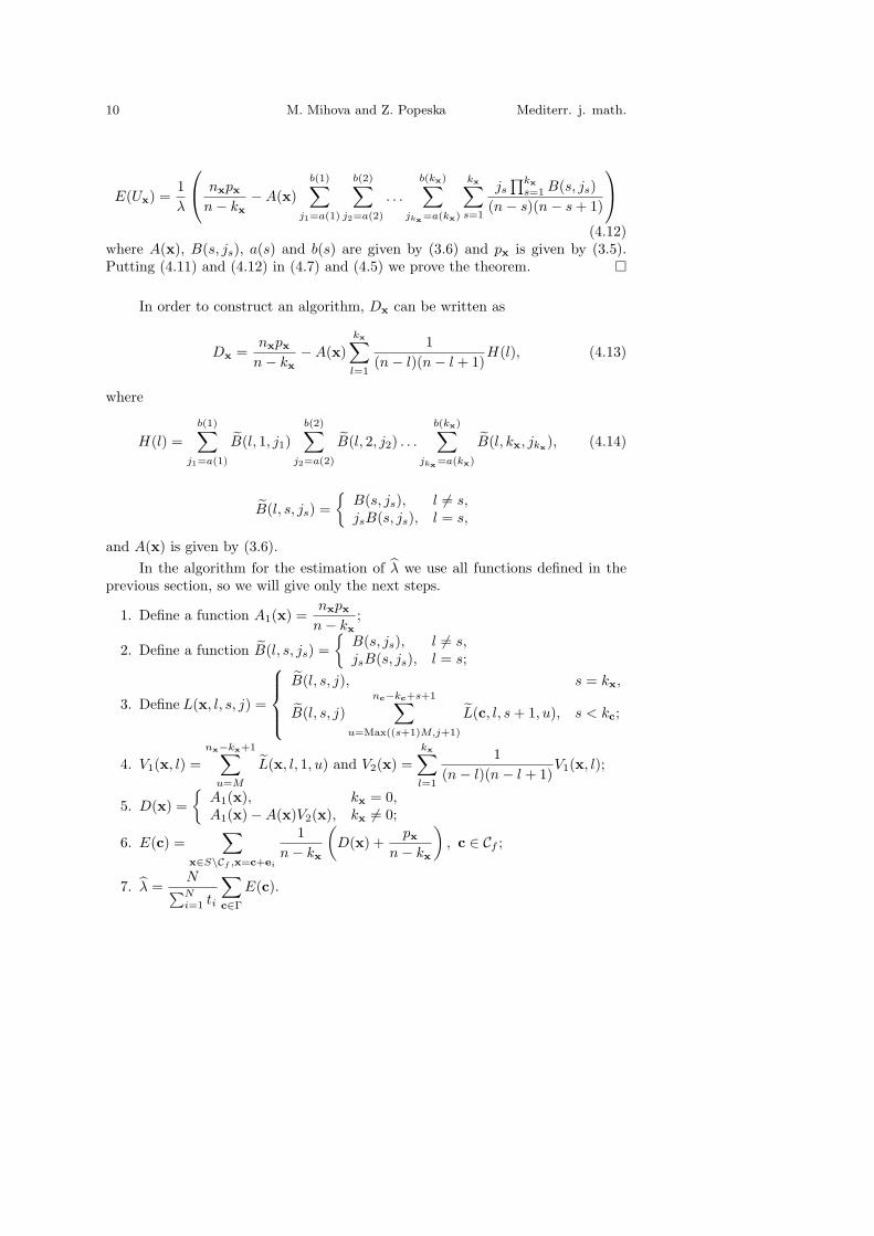
10 M. Mihova and Z. Popeska Mediterr. j. math.

E(Ux) =1λ

nxpx

n− kx−A(x)

b(1)∑j1=a(1)

b(2)∑j2=a(2)

. . .

b(kx)∑jkx=a(kx)

kx∑s=1

js

∏kx

s=1 B(s, js)(n− s)(n− s + 1)

(4.12)

where A(x), B(s, js), a(s) and b(s) are given by (3.6) and px is given by (3.5).Putting (4.11) and (4.12) in (4.7) and (4.5) we prove the theorem. �

In order to construct an algorithm, Dx can be written as

Dx =nxpx

n− kx−A(x)

kx∑l=1

1(n− l)(n− l + 1)

H(l), (4.13)

where

H(l) =b(1)∑

j1=a(1)

B(l, 1, j1)b(2)∑

j2=a(2)

B(l, 2, j2) . . .

b(kx)∑jkx=a(kx)

B(l, kx, jkx), (4.14)

B(l, s, js) ={

B(s, js), l 6= s,jsB(s, js), l = s,

and A(x) is given by (3.6).In the algorithm for the estimation of λ we use all functions defined in the

previous section, so we will give only the next steps.

1. Define a function A1(x) =nxpx

n− kx;

2. Define a function B(l, s, js) ={

B(s, js), l 6= s,jsB(s, js), l = s;

3. Define L(x, l, s, j) =

B(l, s, j), s = kx,

B(l, s, j)nc−kc+s+1∑

u=Max((s+1)M,j+1)

L(c, l, s + 1, u), s < kc;

4. V1(x, l) =nx−kx+1∑

u=M

L(x, l, 1, u) and V2(x) =kx∑l=1

1(n− l)(n− l + 1)

V1(x, l);

5. D(x) ={

A1(x), kx = 0,A1(x)−A(x)V2(x), kx 6= 0;

6. E(c) =∑

x∈S\Cf ,x=c+ei

1n− kx

(D(x) +

px

n− kx

), c ∈ Cf ;

7. λ =N∑Ni=1 ti

∑c∈Γ

E(c).

Vol. 99 (9999) Multi-state Systems with Graduate Failure 11

5. Reliability function

In order to find the reliability function for this type of system we define a function

Hh1,h2,...,hs(λ, t) = P (T1 + T2 + . . . + Ts < t), (5.1)

where hi are integers that satisfy h1 ≤ h2 ≤ . . . ≤ hs, T1 ∼ Gamma(h1, nλ) andTi ∼ Gamma(hi − hi−1, (n− i + 1)λ), i = 2, s.

Theorem 5.1. The reliability function of a MMS system in which all transitionintensities are equal is given by

R(t) = 1−∑c∈Cf

∑x∈S\Cf , x=c+ei

Dx(t), (5.2)

where

Dx(t) =

Hnc(λ, t)

(1n

)nc (∑n

i=1 xi)!∏ni=1 xi!

, kx = 0,

A(x)n− kx

b(1)∑j1=a(1)

b(2)∑j2=a(2)

. . .

b(kx)∑jkx=a(kx)

B(s, js)Hj1,j2,...,jkx ,nc(λ, t), kx 6= 0,

and A(x), B(s, js), a(1), a(s) and b(s) are given by (3.6).

Proof. Refer to (4.2).

F (t) = P (T < t) =∑γ∈Γ

P (Tγ < t)pγ =∑c∈Cf

∑γ∈Γ(c)

P (Tγ < t)pγ

=∑c∈Cf

∑x∈S\Cf ,x=c+ei

∑γ∈Γ(x)

P (Tγ + Tx,c < t)pγpx,c

=∑c∈Cf

∑x∈S\Cf ,x=c+ei

Dx(t).

(5.3)

In the case when there are no zero coordinates in x, i.e. kx = 0, P (Tγx + Tx,c <

t) = Hnc(λ, t), pγxpx,c =(

1n

)nc and the number of paths to x is (Pni=1 exi)!Qni=1 exi!

, so

Dx(t) = Hnc(λ, t)(

1n

)nc (∑n

i=1 xi)!∏ni=1 xi!

.

Consider the case when x has some coordinates equal to 0. Let the path γx

be such that the total failure of its components are at the steps js, s = 1, kx. Now

P (Tγx + Tx,c < t) = Hj1,j2,...,jkx ,nc(λ, t)

and from (3.9) we have that

pγxpx,c =(

1n− kx

)nc kx∏s=0

(n− s

n− s + 1

)js

.

12 M. Mihova and Z. Popeska Mediterr. j. math.

Using the number of ways in which we can order the numbers js and thenumber of paths for chosen numbers js, s = 1, kx, on similar way as in Theorem3.1, we can obtain that

Dx(t) =A(x)

n− kx

b(1)∑j1=a(1)

b(2)∑j2=a(2)

. . .

b(kx)∑jkx=a(kx)

B(s, js)Hj1,j2,...,jkx ,nc(λ, t),

where A(x), B(s, js), a(1), a(s) and b(s) are given by (3.6). �

References

[1] M.T. Abuelma’atti and I.S. Qamber, Reliability Analysis of a Redundant Systemwith Non-repairable Units and Common-Cause Failures Using the SPICE CircuitSimulation Program, Proc. Natl. Sci. Counc. ROC(A) 25 (no. 5) (2001), 322–328.

[2] M.J. Crowder, A.C. Kimber, R.L. Smith and T.J. Sweeting, Statistical Analysis ofReliability Data, Chapman and Hall, London, 1991.

[3] A. Dharmadhikari, S.B. Kulathinal and V. Mandrekar, An algorithm for the esti-mation of minimal cut and ath sets from field failure data, Statist. Probab. Lett. 58(no. 1) (2002), 1–11.

[4] B. Dimitrov and V. Rujkov, On Multi-state reliability system, Informacionniueprocessu, Tom2, No 2, 2002 246-251.

[5] B. Dimitrov, V. Rujkov and P. Stanchev, On multi-state reliability systems, in: Thirdinternational conference on Mathematical Methods in Reliability, MMR 2002, Trond-heim, Norway, 201–204.

[6] J. Huang, M.J. Zuo and Y. Wu, Generalized Multi-State k-out-of-n: G Systems, IEEETransactions on Reliability 49 (no. 1) (2000), 105–111.

[7] B.H. Lindqwist, Bounds for the reliability of the multi-state system with partiallyordered state spaces and stochastically monotone Markov transitions, preprint no.11, Norwegian University of Science and Technology, Trondheim, Norway, 2002.

Marija Mihova and Zaneta PopeskaFaculty of Natural Sciences and MathematicsGazibaba bb, P.O. Box 1621000 SkopjeMacedoniae-mail: marija@ii.edu.mk

zaneta@ii.edu.mk