Confidence interval estimation of overlap: equal means case

Computational Statistics & Data Analysis 34 (2000) 121–137www.elsevier.com/locate/csda

Con�dence interval estimation ofoverlap: equal means case

Madhuri S. Mulekar ∗, Satya N. Mishra

Department of Mathematics and Statistics, University of South Alabama, Mobile,AL 36688-0002, USA

Received 1 September 1998; received in revised form 1 October 1999

Abstract

The estimators of the commonly used measures of overlap are known to be biased by an amountwhich depends on the unknown overlap. In general it is di�cult to calculate the precision or bias of mostecological measures because there is no exact formula for the variance of the statistic and the samplingdistribution is unknown (Dixon, 1993. In: Scheiner, S.M., Gurevitch, J. (Eds.), Design and Analysisof Ecological Experiments. Chapman & Hall, New York, pp. 290–318.) Two resampling techniques,namely, Jackknife and Bootstrap along with the Taylor series approximation and transformation methodare considered for the construction of con�dence intervals. Three measures of overlap frequently usedin quantitative ecology and considered in this study are Matusita’s measure �, Morisita’s measure, �,and Weitzman’s measure, �. c© 2000 Elsevier Science B.V. All rights reserved.

Keywords: Overlap coe�cients; Bootstrap; Jackknife; Matusita’s measure; Morisita’s measure; Weitz-man’s measure

1. Introduction

Dixon (1993) commented that it is easy to calculate the value of many eco-logical indices or measures, but it is often hard to estimate their accuracy. Thispaper addresses the problem of making inferences about Overlap coe�cients basedon an independent bivariate data. Use of relatively simple and widely applicablecomputational techniques such as jackknife, bootstrap, transformation and Taylor se-ries approximation is discussed. Three measures of overlap �, �, and � for normalpopulations that are frequently used by ecologists are considered in this study. Some

∗ Corresponding author.

0167-9473/00/$ - see front matter c© 2000 Elsevier Science B.V. All rights reserved.PII: S 0167-9473(99)00096-1

122 M.S. Mulekar, S.N. Mishra / Computational Statistics & Data Analysis 34 (2000) 121–137

other applications of � include the lowest upper bound for the probability of failurein the stress-strength models of reliability analysis (Ichikawa, 1993), an estimate ofthe proportion of genetic deviates in segregating populations (Federer et al., 1963), ameasure of distinctness of clusters (Sneath, 1977). Additional references to applica-tions of such methodology are given by Mulekar and Mishra (1994) and the historyof such procedures is summarized by Inman and Bradley (1989).Various measures of similarity=diversity, coe�cients of overlap or indices of dis-

tance are used by ecologists (Magurran, 1998; Linton et al., 1981; Horn, 1966).Generally two di�erent approaches are used to quantify the ecological limitations anddegree of resource sharing by di�erent species or inequality in the observed plantsize. One approach is to derive indices using the frequency distribution of resourceuse by several categories (May, 1975; Slobodchiko� and Schulz, 1980; Hurlbert,1978). The second approach is to estimate measures, assuming samples of obser-vations are drawn from continuous distributions (Slobodchiko� and Schulz, 1980;Harner and Whitmore, 1977; MacArthur, 1972). Smith and Zaret (1982) studiedFreeman–Tukey measure (FT) developed by Matusita (1955) and percent similaritymeasure (PS) developed by Renkonen (1938) which are discrete versions of � and�, respectively. Slobodchiko� and Schulz (1980) and May (1975) studied measure�∗ which reduces to � under the con�guration considered here.Let f1(x) and f2(x) be the probability density functions describing the resource

use by two species. Using the second approach the overlap measures are de�ned asfollows:

(a) Matusita’s Measure (1955): �=∫ √

f1(x)f2(x) dx

(b) Morisita’s Measure (1959): �=2∫f1(x) f2(x) d x∫

[f1(x)]2 d x+∫[f2(x)]2 d x

(c) Weitzman’s Measure (1970): �=∫min[f1(x); f2(x)] dx

The overlap of two densities is the commonalities shared by both species and mea-sured on the scale of 0 to 1. The overlap value close to 0 indicates extreme inequalityof two density functions whereas overlap value of 1 indicates exact equality.Because of the complex mathematical structure of these measures, virtually no

results are available on their exact sampling distributions. Smith (1982) derivedformulas for estimating the mean and variance of discrete version of Weitzman’smeasure (also known as coe�cient of community and the percentage similaritymeasure) using the delta method. Mishra et al. (1986) gave the small and largesample properties of the sampling distributions for a function of � under the as-sumption of homogeneity of variances. Lu et al. (1989) studied sampling variabilityof some of these measures using simulation techniques and investigated bias as af-fected by di�erences in sample sizes and dimensionality. Mulekar and Mishra (1994)simulated the sampling distributions of overlap measures for normal densities withequal means and obtained the approximate expressions for the bias and varianceof the estimates. Dixon (1993) described the use of bootstrap and jackknife tech-niques for the Gini coe�cient of size hierarchy and the Jaccard index of communitysimilarity.

M.S. Mulekar, S.N. Mishra / Computational Statistics & Data Analysis 34 (2000) 121–137 123

Fig. 1. The overlap of densities f1 and f2 as de�ned by �.

The primary purpose of this study is to compare the con�dence intervals for theoverlap coe�cients, �; � and � computed using Jackknife, Bootstrap, Transformation,and Taylor series approximation methods. The background and mechanisms of so-lutions are described in Section 2. The results of Monte Carlo study are presentedin Section 3 along with a comparison of performance of four methods. Conclusionsare given in Section 4.

2. Statistical methods

Suppose f1(x) and f2(x) represent the normal densities with a common mean �and unknown variances �21 and �

22; respectively. Fig. 1 shows overlap of N (0; 1) and

N (0; 4) as de�ned by � (a continuous version of discrete measure used by Weitzman(1970)) and described by Bradley (1985) as OVL. De�ne C=�1=�2 (C¿ 0). Thenthe measures of overlap considered here can be expressed as a function of C asfollows (refer to Mulekar and Mishra (1994) for details):

�=

√2C

1 + C2; (2.1)

�=2√2√

1 + C2

(C

1 + C

); (2.2)

�=

{1− 2�(b) + 2�(Cb) if 0¡C¡ 1;

1 + 2�(b)− 2�(Cb) if C ≥ 1; (2.3)

where

b=

√−ln(C2)1− C2

and �(·) is the cumulative distribution function (c.d.f.) of a standard normal variate.Mulekar and Mishra (1994) also considered the MacArthur–Levin’s asymmetricmeasure (�12) modi�ed by Pianka (1973) and extended by Slobodchiko� and


Schulz (1980) to de�ne as

�∗ =∫f1(x) f2(x) dx∫

[f1(x)]2 dx

∫[f2(x)]

2 dx:

They have shown that for normal densities with equal means, �∗ = �.Let us denote these measures of overlap in general by �. Note that all these

measures are independent of the population means. Apart from computational easein applications, these measures also have nice properties, such as, symmetry in C,i.e., �(C)=�(1=C), and invariance under linear transformation, Y=aX+b; a 6= 0. Theappropriateness and the interpretations of these measures are discussed by Hurlbert(1978). The estimates of these measures can be obtained by using C = S1=S2, whereS2l = (nl − 1)−1

∑nlk=1(xlk − �xl)2 is the usual unbiased estimator of �2l based on a

sample of size nl from population l (l = 1; 2). Four di�erent methods includingtwo resampling techniques considered for constructing con�dence intervals for themeasures are as follows:

2.1. Jackknife

Quenouille (1949) introduced a technique for reducing the bias of an estimatorbased on splitting a sample into subsamples, popularly known as Jackknife technique.He proposed this procedure to eliminate a bias term of O(1=n) in the single-sampleproblem. There are two di�erent aspects of the jackknife technique, bias reductionand interval estimation, and we are interested in both. For recent developments andapplications of Jackknife procedures, the reader is referred to Shao and Tu (1995),Foster (1995), Maesono (1996, 1998), and Lahiri (1977).Suppose (X11; X12; : : : ; X1n1) and (X21; X22; : : : ; X2n2) is a pair of independent random

samples obtained from the populations under consideration, e.g. n1 and n2 observa-tions for the two species. Let � be an estimator of � based on this pair of samplesof sizes n1 and n2. Let �i: denote an estimate obtained using the �rst sample lessith observation (i = 1; 2; : : : ; n1) and the entire second sample. Similarly we use �:jto indicate an estimate obtained using entire �rst sample and second sample less jthobservation (j = 1; 2; : : : ; n2). The usual Jackknife estimate procedure gives,

�br = (n1 + n2)�−(n1 + n2 − 1

2n1

) n1∑i=1

�i: −(n1 + n2 − 1

2n2

) n2∑j=1

�:j: (2.4)

According to Farewell (1978), this estimate �br reduces bias but does not eliminatethe O(1=n1) and O(1=n2) bias terms. Cox and Hinkley (1974, Eq. (30)) recommendeduse of �bc to eliminate �rst two bias terms where

�bc = (n1 + n2 − 1)�−(n1 − 1n1

) n1∑i=1

�i: −(n2 − 1n2

) n2∑j=1

�:j: (2.5)

Note that Farewell (1978) refers to �br and �bc as T1(n) and T2(n); respectively.Computing the average �Q and the empirical variance Var(�Q) of the pseudo-values(Cox and Hinkley, 1974) the two-sided approximate (1 − 2�)100% con�dence


intervals are constructed as

[�Q + Z�√Var(�Q); �Q + Z1−�

√Var(�Q)]: (2.6)

Here Z� =�−1(�) and �(·) is a c.d.f. of a standard normal variate. Farewell (1978)suggested that the jackknife estimate should re ect any pattern or special structure inthe data in order to eliminate (not just reduce) the �rst-order bias correction terms.For any integer r ≥ 1, and n2=rn1, he suggested that a group of r observations fromsample 2 should be dropped for each observation deleted from sample 1 in orderto eliminate the �rst-order bias terms. He further indicated that n1 subestimates willresult from this process. Obviously, if there is a speci�c matching in the data, sucha grouping will be unique. In a recent communication, Farewell (1998) corroboratedour conclusion that this sampling scheme does not result in unique n1 subestimates.Let �ir be an estimator of � based on a pair of samples of sizes (n1 − 1) and

(n2 − r); respectively, obtained, by deleting ith observation from sample 1 and ithblock of r observations from sample 2 (i= 1; 2; : : : ; n1). Then the pseudo-values arede�ned as

�ir = n1�− (n1 − 1)�ir (2.7)

and ��Q =∑

i �ir=n1 becomes the Quenouille’s Jackknife estimator. Farewell (1978)calls this estimator T3(n). This estimate eliminates the O(1=n1) and O(1=n2) biasterms. The variance of this estimator is

Var( ��Q) = (n1)−1(n1 − 1)−1n1∑i=1

(�ir − ��Q)2: (2.8)

Following the argument of Efron (1982, p. 14, Eq. (3:4)), it can be shown that thestatistic

( ��Q − �)√Var(�Q)

∼ t(n1 − 1) (2.9)

approximately. Then using (2.9) as a pivotal statistic, the two-sided (1 − 2�)100%con�dence intervals are constructed as

��Q ± t�√Var( ��Q) (2.10)

where (t ¿ t�) = � with appropriate degrees of freedom.

2.2. Bootstrap

Efron (1979) describes this computationally intensive technique that uses sampledobservations as an empirical estimate of the unknown distribution function of thepopulation. For more information on bootstrap methods and their applications referto Efron (1982) and Davidson and Hinkley (1997).Suppose (X11, X12, : : :, X1n1) and (X21; X22; : : : ; X2n2) is a pair of random independent

samples from two populations. The sample overlap measure � is computed usingS21 and S

22 as described earlier. Treating each sample as a population of size n1

or n2 following discrete uniform distributions with mass (1=n1) or (1=n2) at each


observation, one thousand pairs of random samples of sizes (n1; n2) are selectedfrom these two empirical distributions. Observations in each sample are randomlychosen with replacement.Let �j (j = 1; 2; : : : ; 1000) be a bootstrap estimate of � computed from the jth

bootstrapped sample. For any real u ∈ (0; 1), let G(u) be the c.d.f. of 1000 bootstrapreplications �j,

G(t) = #{�j ¡u}=1000: (2.11)

Efron (1987) proposed the BCa intervals that are second-order correct for a widerclass of problems. The two-sided (1−2�)100% BCa interval for the overlap measureis given by

[G−1(�(�1)); G

−1(�(�2))] (2.12)

where �1 and �2 depend on two constants Z0 and a computed from the bootstrapresults. The bias correction is

Z0 = �−1(#{�j ¡ �}=1000) (2.13)

which measures the median bias of �. The acceleration a is the skewness of score for� which measures the rate of change of standard error on a normalized scale. Efron(1987) showed that a good approximation to constant a is (1=6)SKEW�=�(i�(�))where SKEW is the skewness of score function i�. Efron (1987) gives i�(�) =(@=@�)f�(�) where the real-valued statistic � has density f�(�). The constants �1and �2 are computed as follows:

�1 = Z0 +Z0 + Z�

1− a(Z0 + Z�) and �2 = Z0 +Z0 + Z1−�

1− a(Z0 + Z1−�) : (2.14)

The BCa interval is an improvement over the BC intervals proposed by Efron (1981).As a→ 0, BCa interval reduces to BC interval,

[G−1(�(2Z0 + Z�)); G

−1(�(2Z0 + Z1−�))]:

These bias corrected intervals are second-order accurate. If a and Z0 both are 0 thenthe BCa intervals reduce to the percentile intervals of Efron (1981, 1982).In situations where the sampling distribution of a standardized statistic depends

on parameters, in other words, where a pivot does not exist, Beran (1990) sug-gested use of double bootstrap for constructing simultaneous con�dence intervals.The technique of double bootstrap was later used by Vinod and McCullough (1995)and McCullough and Vinod (1998) to estimate parameters in economic applications.More information on double bootstrap can be found in Beran and Ducharme (1991).For some applications of double bootstrap refer to Shaw and Geyer (1997), Shi(1992), Shin (1995), and Newton and Geyer (1994). However for the coe�cientsconsidered here, the sampling distributions of estimators used are unknown. So thismay be a lack of pivot problem (existence questioned) or simply unknown pivotproblem.


2.3. Taylor series expansion

From a theorem of Mulekar and Mishra (1994, p. 173) the approximate samplingvariances of overlap measures can be obtained as follows:

�2�=�2

16C4

(1− C21 + C2

)2�2C ;

�2� =�2

4

((1− C)(1 + C + C2)(1 + C)(1 + C2)C2

)2�2C ;

�2�=

[(C�(Cb)− �(b))

(C2b2 − 1

C2b(1− C2)

)+bC�(Cb)

]2�2C ; (2.15)

where �(·) is the density function of a standard normal variate and

�2C =2C4(n1 + n2 − 4)(n2 − 1)2(n1 − 1)(n2 − 3)2(n2 − 5) ; n1¿ 1; n2¿ 5: (2.16)

Normal approximation to the sampling distributions of � works fairly well forsample sizes as small as 50 (Mulekar and Mishra, 1994) and generally in ecologicalexperiments for overlap estimation, it is quite common to use samples of sizes ≥ 50.Therefore assuming approximate normality of the sampling distributions, the (1−2�)con�dence intervals for the overlap measures are computed as

[�+ Z��; �+ Z1−��]: (2.17)

Although this is a simple method of obtaining con�dence intervals, it may not bethe best one because of the bias involved in the estimates. Theorem 1 of Mulekar andMishra (1994) gives Bn(�), the approximate bias estimators. Using these estimatesthe bias corrected interval can be computed as

[(�− Bn(�)) + Z��; (�− Bn(�)) + Z1−��]: (2.18)

2.4. Transformation technique

Let L and U be the lower and upper con�dence limits respectively of C2, corre-sponding to the inclusion probability 1− 2�, i.e., Pr(L¡C2¡U ) = 1− 2�. Then Land U can be easily determined using the fact that C

2=S21 =S

22 ∼ C2F(n1−1; n2−1).

Since there is a relation between C2 and �’s, the lower (L′) and upper (U ′) lim-its of the overlap measures can be obtained using an appropriate transformation asPr(L′¡�(C2)¡U ′) = 1− 2�. Here L′ = �(L) and U ′ = �(U ). Listed in Table 1arethe con�dence limits proposed by Mulekar and Mishra (1994) using

bL =

√−ln(L)1− L and bU =

√−ln(U )1− U : (2.19)


Table 1Con�dence limits for the overlap measures

� Lower limit (L′) Upper limit (U ′)

� L1=4√

21+L U 1=4

√2

1+U

� 21+

√L

√2L1+L

21+

√U

√2U1+U

� 1− 2�(bL) + 2�(bL√L) 1− 2�(bU ) + 2�(bU

√U )

if 0¡L¡ 1 if 0¡U ¡ 1

1 + 2�(bL)− 2�(bL√L) 1 + 2�(bU )− 2�(bU

√U )

if L ≥ 1 if U ≥ 1

Table 2Bias, length of interval and empirical con�dence level for C = 0:20 and con�dence coe�cient=0:95.The values are Mean±Standard deviation of 1000 intervals

OVL Jackknife Bootstrap Taylor series Transformation

n1 = n2 = 10� 0:012± 0:103 0:040± 0:104 0:046± 0:009 0:029± 0:099

0:138± 0:056 0:393± 0:119 0:678± 0:139 0:401± 0:0740.505 0.920 0.996 0.951

� 0:016± 0:104 0:027± 0:096 0:041± 0:003 0:024± 0:0930:134± 0:045 0:367± 0:099 0:604± 0:049 0:378± 0:0250.474 0.952 1.000 0.951

� 0:020± 0:137 0:044± 0:126 0:053± 0:007 0:035± 0:1280:174± 0:062 0:471± 0:115 0:784± 0:111 0:489± 0:0530.489 0.947 0.989 0.951

n1 = n2 = 25

� 0:003± 0:057 0:011± 0:058 0:013± 0:002 0:008± 0:0570:045± 0:010 0:218± 0:044 0:270± 0:034 0:227± 0:0280.311 0.939 0.982 0.959

� 0:003± 0:059 0:007± 0:059 0:013± 0:001 0:006± 0:0580:047± 0:011 0:218± 0:035 0:268± 0:015 0:231± 0:0120.305 0.948 1.000 0.959

� 0:004± 0:077 0:013± 0:076 0:017± 0:017 0:009± 0:0750:060± 0:015 0:284± 0:050 0:344± 0:034 0:298± 0:0270.304 0.947 0.971 0.959

n1 = n2 = 100

� 0:003± 0:028 0:002± 0:028 0:003± 0:000a 0:001± 0:0280:011± 0:001 0:107± 0:011 0:113± 0:007 0:109± 0:0070.156 0.940 0.957 0.946

� 0:003± 0:029 0:001± 0:029 0:003± 0:000a 0:001± 0:0290:011± 0:001 0:111± 0:010 0:117± 0:003 0:113± 0:0030.157 0.943 1.000 0.946

� 0.000a±0:037 0:002± 0:038 0:004± 0:000a 0:001± 0:0380:015± 0:002 0:143± 0:014 0:150± 0:008 0:145± 0:0080.156 0.944 0.950 0.946

aIndicates value ¡ 0:001.


Table 3Bias, length of interval and empirical con�dence level for C = 0:50 and con�dence coe�cient=0:95.The values are Mean ± Standard deviation of 1000 intervals


n1 = n2 = 10� 0:039± 0:188 0:019± 0:117 0:070± 0:007 0:031± 0:137

0:194± 0:065 0:532± 0:136 0:392± 0:109 0:431± 0:1560.462 0.972 0.998 0.991

� 0:020± 0:091 0:012± 0:072 0:032± 0:013 0:003± 0:0770:105± 0:049 0:668± 0:313 0:485± 0:173 0:271± 0:1060.389 0.947 1.000 0.991

� 0:028± 0:134 0:014± 0:103 0:046± 0:018 0:005± 0:1100:152± 0:060 0:711± 0:247 0:706± 0:244 0:386± 0:1460.380 0.957 0.903 0.994

n1 = n2 = 25

� 0:005± 0:091 0:011± 0:087 0:020± 0:001 0:018± 0:0890:072± 0:016 0:335± 0:076 0:418± 0:027 0:349± 0:0350.305 0.968 0.980 0.959

� 0:004± 0:055 0:005± 0:051 0:012± 0:002 −0:001± 0:0520:042± 0:012 0:363± 0:293 0:237± 0:045 0:196± 0:0390.288 0.952 1.000 0.9590:005± 0:081 −0:006± 0:074 0:017± 0:003 −0:001± 0:076

� 0:061± 0:017 0:417± 0:238 0:347± 0:062 0:285± 0:0540.285 0.960 0.945 0.959

n1 = n2 = 100

� 0:004± 0:044 0:002± 0:044 0:005± 0:000a 0:001± 0:0440:017± 0:002 0:167± 0:015 0:177± 0:006 0:170± 0:0060.159 0.947 0.954 0.946

� 0:000a ± 0:027 −0:002± 0:027 0:003± 0:000a −0:001± 0:0270:011± 0:001 0:107± 0:012 0:108± 0:009 0:103± 0:0030.166 0.954 1.000 0.946

� 0:000a ± 0:040 0:002± 0:039 0:004± 0:000a 0:001± 0:0390:015± 0:002 0:155± 0:016 0:158± 0:011 0:151± 0:0120.163 0.954 0.941 0.946


3. Results and discussion

A Monte Carlo study was conducted to compare the e�ectiveness of four methodsof constructing con�dence intervals for the overlap coe�cients. All the computationswere conducted on AREN (Alabama Research and Education Network) C94=264under two assumptions: (1) both the densities are normal and (2) the populationmeans are equal. One thousand sets, each containing two independent samples ofsizes 10, 25, 50, 100, and 200 were generated from the normal populations such thatC = 0:05(0:05)0:95. For these con�gurations, using each of the four methods, 90%,95% and 99% con�dence intervals were computed from each of the samples. Thenumber of such intervals containing the true overlap coe�cient value was countedas well as the length of intervals was recorded.


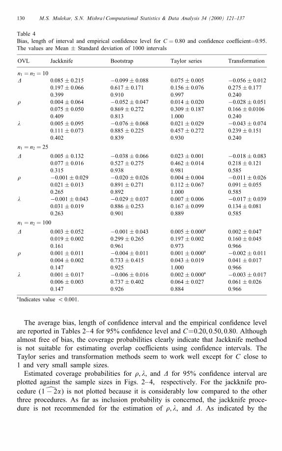
Table 4Bias, length of interval and empirical con�dence level for C = 0:80 and con�dence coe�cient=0:95.The values are Mean ± Standard deviation of 1000 intervals


n1 = n2 = 10� 0:085± 0:215 −0:099± 0:088 0:075± 0:005 −0:056± 0:012

0:197± 0:066 0:617± 0:171 0:156± 0:076 0:275± 0:1770.399 0.910 0.997 0.240

� 0:004± 0:064 −0:052± 0:047 0:014± 0:020 −0:028± 0:0510:075± 0:050 0:869± 0:272 0:309± 0:187 0:166± 0:01060.409 0.813 1.000 0.240

� 0:005± 0:095 −0:076± 0:068 0:021± 0:029 −0:043± 0:0740:111± 0:073 0:885± 0:225 0:457± 0:272 0:239± 0:1510.402 0.839 0.930 0.240

n1 = n2 = 25

� 0:005± 0:132 −0:038± 0:066 0:023± 0:001 −0:018± 0:0830:077± 0:016 0:527± 0:275 0:462± 0:014 0:218± 0:1210.315 0.938 0.981 0.585

� −0:001± 0:029 −0:020± 0:026 0:004± 0:004 −0:011± 0:0260:021± 0:013 0:891± 0:271 0:112± 0:067 0:091± 0:0550.265 0.892 1.000 0.585

� −0:001± 0:043 −0:029± 0:037 0:007± 0:006 −0:017± 0:0390:031± 0:019 0:886± 0:253 0:167± 0:099 0:134± 0:0810.263 0.901 0.889 0.585

n1 = n2 = 100

� 0:003± 0:052 −0:001± 0:043 0:005± 0:000a 0:002± 0:0470:019± 0:002 0:299± 0:265 0:197± 0:002 0:160± 0:0450.161 0.961 0.973 0.966

� 0:001± 0:011 −0:004± 0:011 0:001± 0:000a −0:002± 0:0110:004± 0:002 0:733± 0:415 0:043± 0:019 0:041± 0:0170.147 0.925 1.000 0.966

� 0:001± 0:017 −0:006± 0:016 0:002± 0:000a −0:003± 0:0170:006± 0:003 0:737± 0:402 0:064± 0:027 0:061± 0:0260.147 0.926 0.884 0.966


The average bias, length of con�dence interval and the empirical con�dence levelare reported in Tables 2–4 for 95% con�dence level and C=0:20; 0:50; 0:80. Althoughalmost free of bias, the coverage probabilities clearly indicate that Jackknife methodis not suitable for estimating overlap coe�cients using con�dence intervals. TheTaylor series and transformation methods seem to work well except for C close to1 and very small sample sizes.Estimated coverage probabilities for �; �, and � for 95% con�dence interval are

plotted against the sample sizes in Figs. 2–4, respectively. For the jackknife pro-cedure ( [1− 2�) is not plotted because it is considerably low compared to the otherthree procedures. As far as inclusion probability is concerned, the jackknife proce-dure is not recommended for the estimation of �; �, and �. As indicated by the


Fig. 2. Estimated con�dence for Rho (95%).

C = 0:8 case, a similar pattern is observed for all 3 measures as C gets closer to 1.As n increases ( [1− 2�) → (1 − 2�), in fact even n = 40 gives a good estimate of(1− 2�). In case of C ≤ 0:5, even samples of sizes as small as 10 give fairly goodestimate of con�dence level.


Fig. 3. Estimated con�dence for Lambda (95%).

The average length of con�dence interval for � is plotted in Fig. 5 as a functionof n and C. Although � and � show similar patterns, in general the jackknife, Taylorseries and transformation technique intervals for � are the shortest and those for � arethe longest. But for the bootstrap method this trend is reversed. Of the four methods,the jackknife gives the shortest intervals but also has lowest inclusion probability.


Fig. 4. Estimated con�dence for Delta (95%).

When using the bootstrap for C¿ 0:5 the length of con�dence intervals rises sharplygetting close to 1 and rendering the intervals useless in practice. Taking into accountboth the inclusion probabilities and the length of intervals, bootstrap seems to workbest for C ≤ 0:5, whereas Taylor series and transformation methods are recommendedfor all C ∈ (0; 1) values provided n is at least 40.


Fig. 5. Average length of con�dence interval for Rho (95%).

Fig. 6. Bias in estimation of Rho.

The bias in estimation of � is plotted in Fig. 6. The bias for �, and � show similarpatterns. For n ≥ 40, the amount of bias is negligible using all four methods andthe experimenter need not worry about it. To our delight, transformation techniquewhich is the easiest one to use in practice in the absence of appropriate computerhardware and software performs quite well and reduces bias to the order of 10−3.The Jackknife method also reduces bias considerably, but the Taylor series and


Table 5Con�dence intervals for OVLs and their lengths for n1 = n2 = 25; C =0:5, con�dence coe�cient=0:95

�= 0:6773 �= 0:8944 � = 0:8433

Taylor series 0:53− 0:88 0:80− 1:0 0:72− 1:0l= 0:35 l= 0:20 l= 0:28

Transformation 0:56− 0:86 0:81− 0:98 0:73− 0:97l= 0:30 l= 0:17 l= 0:24

Bootstrap 0:56− 0:84 0:82− 0:98 0:73− 0:96l= 0:28 l= 0:16 l= 0:23

Jackknife −0:18− 1:43 0:60− 1:51 0:39− 1:76l= 1:61 l= 0:91 l= 1:37

Jackknife 0:09− 0:32 0:29− 0:50 0:18− 0:40(log transformation) l= 0:22 l= 0:16 l= 0:23

transformation approximations seem to do even a better job. The Bootstrap estimatesalso show similar results, but they are not easy to obtain without any appropriatecomputer software.The jackknife technique gives sizable and frequent negative pseudo-values. These

tend to produce distorted point and interval estimates. We tried to use logarithmictransformation so that negative pseudo-values will not pull the aggregate to one side.But to our disappointment the variance was reduced to such a small quantity thatthe empirical estimate of con�dence level started fast approaching 0.Table 5 shows 95% con�dence intervals constructed from a pair of samples of

size n1 = n2 = 25 and their lengths. The jackknife method did not give sensiblecon�dence intervals and should be avoided. Bootstrap gave the shortest intervalswith transformation trailing closely behind it.Simulations were also performed using Jackknife estimator ��Q. The observed re-

sults were similar to those described for �Q in terms of the coverage probability andhence are not reported here.

4. Conclusions

In the problem posed here of estimating overlap coe�cients, there is neither anypattern or special structure in the data, nor is any particular favored way of pairingobservations. Therefore if all possible pairs of observations are deleted one at atime giving n1n2 di�erent pairs of jackknifed samples; the jackknife estimate �Qbased on all of these n1n2 pairs of pseudo-values fails to reduce bias and failsto eliminate �rst-order bias terms. Therefore such a procedure should be avoidedand any n1 subestimates should be used. All four methods were useful in reducingbias to a negligible level for n ≥ 40. When the coverage probability is taken intoconsideration, performance of the Jackknife procedure was inferior to the others.The bootstrap seems to work better for C ≤ 0:5 and n ≥ 40. The Taylor-series andtransformation methods performed considerably well for n ≥ 40.In general transformation technique and Taylor-series approximation provided

sensible and reasonably reliable con�dence intervals. These are also the simplest


methods to use in practice that do not need any computers, special softwares orextensive computations.

Acknowledgements

The authors are grateful to J.D. Baker, University of South Alabama, for his assis-tance in setting up required programs on the AREN. The authors are also thankful tothe referees and the editors for their useful comments that led to a much improvedversion of this manuscript.

References

Beran, R., 1990. Re�ning bootstrap simultaneous con�dence sets. J. Amer. Statist. Assoc. 85, 417–426.Beran, R., Ducharme, G.R., 1991. Asymptotic Theory for Bootstrap Methods in Statistics. Universityof Montreal, Center of Mathematics Research, Montreal.

Bradley, E.L., 1985. Overlapping coe�cient. In: S. Kotz and N.L. Johnson, Eds., Encyclopedia ofStatistical Sciences, Vol. 6. Wiley, New York, pp. 546–547.

Cox, D.R., Hinkley, D.V., 1974. Theoretical Statistics. Chapman & Hall, London, pp. 264–265.Davidson, A.C., Hinkley, D.V., 1997. Bootstrap Methods and their Applications. Cambridge UniversityPress, New York.

Dixon, P.M., 1993. The Bootstrap and the Jackknife: describing the precision of ecological indices. In:Scheiner, S.M., Gurevitch J. (Eds.), Design and Analysis of Ecological Experiments. Chapman &Hall, New York, pp. 290–318.

Efron, B., 1979. Bootstrap methods: another look at the jackknife. Ann. Statist. 6, 1–26.Efron, B., 1981. Nonparametric standard errors and con�dence intervals. Can. J. Statist. 9, 139–172.Efron, B., 1982. The jackknife, the Bootstrap, and other resampling plans. CBMS-NSF, RegionalConference Series in Applied Mathematics, Society for Industrial & Applied Mathematics.

Efron, B., 1987. Better Bootstrap con�dence intervals. J. Amer. Statist. Assoc. 82, 171–185.Farewell, V.T., 1978. Jackknife estimation with structured data. Biometrika 65, 444–447.Farewell, V.T., 1998. Personal communication by email.Federer, W.T., Powers, L.R., Payne, M.G., 1963. Studies on statistical procedures applied to chemicalgenetic data from sugar beets. Technical Bulletin 77, Agricultural Experimentation Station, ColoradoState University.

Foster, P., 1995. A comparative study of some bias correction technique for kernel-based densityestimation. J. Statist. Comput. Simulation 51, 137–152.

Harner, E.J., Whitmore, R.C., 1977. Multivariate measures of niche overlap using discriminant analysis.Theoret. Population Biol. 12, 21–36.

Horn, H.S., 1966. Measurement of “overlap” in comparative ecological studies. Amer. Naturalist 100,419–424.

Hurlbert, S.H., 1978. The measurement of niche overlap and some relatives. Ecology 59, 67–77.Ichikawa, M., 1993. A meaning of the overlapped area under probability density curves of stress andstrength. Reliab. Eng. System Safety 41, 203–204.

Inman, H.F., Bradley, E.L., 1989. The Overlapping coe�cienet as a measure of agreement betweenprobability distributions and point estimation of the overlap of two normal densities. Comm. Statist.-Theory Methods 18, 3851–3874.

Lahiri, S.N., 1977. On inconsistency of the Jackknife-after-bootstrap bias estimator for dependent data.J. Multivariate Anal. 63, 15–34.

Linton, L.R., Davis, R.W., Wrona, F.J., 1981. Resource utilization indices: an assessment. Ecology 50,283–292.


Lu, R., Smith, E.P., Good, I.J., 1989. Multivariate measures of similarity and niche overlap. Theoret.Population Ecol. 35, 1–21.

MacArthur, R.H., 1972. Geographical Ecology. Harper and Row, New York.Maesono, Y., 1996. Higher order comparisons of Jackknife variance estimators. J. Nonparametric Statist.7, 35–45.

Maesono, Y., 1998. Asymptotic properties of Jackknife skewness estimators and Edgeworth expansions.Bell Inform. Cybernet 30, 51–68.

Magurran, A.E., 1998. Ecological Diversity and its Measurement. Princeton University Press, Princeton.Matusita, K., 1955. Decision rules based on the distance for problems of �r, two samples, andestimation. Ann. Math. Statist. 26, 631–640.

May, R.M., 1975. Some notes on estimating the competition matrix, �. Ecology 56, 737–741.McCullough, B.D., Vinod, H.D., 1998. Implementing the double bootstrap. Comput. Econom. 12, 79–95.

Mishra, S.N., Shah, A.K., Lefante, J.J., 1986. Overlapping coe�cient: the generalized t approach.Commun. Statist. - Theory Methods 15, 123–128.

Morisita, M., 1959. Measuring interspeci�c association and similarity between communities. Memoirsof the faculty of Kyushu University. Series E. Biology 3, 65–80.

Mulekar, M.S., Mishra, S.N., 1994. Overlap Coe�cient of two normal densities: equal means case. J.Japan Statist. Soc. 24, 169–180.

Newton, M.A., Geyer, C.J., 1994. Bootstrap recycling: a monte carlo alternative to the nested bootstrap.J. Amer. Statist. Assoc. 89, 905–912.

Pianka, E.R., 1973. The structure of lizard communities. Ann. Rev. Ecol. Syst. 4, 53–74.Quenouille, M.H., 1949. Approximate tests of correlation in time-series. J. Roy. Statist. Soc. B 11,68–84.

Renkonen, O., 1938. Statiscich-okologidche Untersuchungen uber die terrestrische der �nnischenbruchmoore. Ann. Zoologici Societatis Zoologocae-Botanocae Fennicae Vanamo 6, 1–231.

Shao, J., Tu, D., 1995. The Jackknife and Bootstrap. Springer, Berlin, NY.Shaw, F.H., Geyer, C.J., 1997. Estimation and testing in constrained covariance component models.Biometrika 84, 95–102.

Shi, S.G., 1992. Accurate and e�cient double bootstrap con�dence limit method. Comput. Statist. DataAnal. 13, 21–32.

Shin, Y., 1995. Double bootstrap con�dence cones for spherical data based on prepivoting. J. KoreanStatist. Soc. 24, 183–195.

Slobodchiko�, C.N., Schulz, W.C., 1980. Measures of niche overlap. Ecology 61, 1051–1055.Smith, E.P., 1982. Niche breadth, resource availability, and inference. Ecology 63, 1675–1681.Smith, E.P., Zaret, T.M., 1982. Bias in estimating niche overlap. Ecology 63, 1248–1253.Sneath, P.H.A., 1977. A method for testing the distinctness of clusters: a test of the disjunction of twoclusters in Euclidean space as measured by their overlap. Math. Geol. 9, 123–143.

Vinod, H.D., McCullough, B.D., 1995. Estimating cointehration parameters: an application of the doublebootstrap. J. Statist. Plann. Inference 43, 147–156.

Weitzman, M.S., 1970. Measures of overlap of income distributions of white and negro families in theunited states. Technical Paper No. 22, Department of Commerce, Bureau of Census, Washington,U.S.

Confidence interval estimation of overlap: equal means case

Documents

Transcript of Confidence interval estimation of overlap: equal means case