Preference Intensities and Risk Aversion in School Choice: A Laboratory Experiment

Preference Intensities and Risk Aversion

in School Choice: A Laboratory Experiment∗

Flip Klijn† Joana Pais‡ Marc Vorsatz§

April 2010

Abstract

We experimentally investigate in the laboratory two prominent mechanisms that are

employed in school choice programs to assign students to public schools. We study

how individual behavior is influenced by preference intensities and risk aversion. Our

main results show that (a) the Gale–Shapley mechanism is more robust to changes

in cardinal preferences than the Boston mechanism independently of whether indi-

viduals can submit a complete or only a restricted ranking of the schools and (b)

subjects with a higher degree of risk aversion are more likely to play “safer” strate-

gies under the Gale–Shapley but not under the Boston mechanism. Both results

have important implications for the efficiency and the stability of the mechanisms.

Keywords: school choice, risk aversion, preference intensities, laboratory experi-

ment, Gale–Shapley mechanism, Boston mechanism, efficiency, stability, constrained

choice.

JEL–Numbers: C78, C91, C92, D78, I20.

∗We are very grateful for comments and suggestions from Eyal Ert, Bettina Klaus, Muriel Niederle,Al Roth, and the seminar audiences in Alicante, Braga, Maastricht, and Malaga.

†Corresponding author. Institute for Economic Analysis (CSIC), Campus UAB, 08193 Bellaterra(Barcelona), Spain; During academic year 2009–2010: Harvard Business School, Baker Library |Bloomberg Center 437, Soldiers Field, Boston, MA 02163, USA; e-mail: [email protected]. He grate-fully acknowledges a research fellowship from Harvard Business School and support from Plan NacionalI+D+i (ECO2008–04784), Generalitat de Catalunya (SGR2009–01142), the Barcelona GSE ResearchNetwork, and the Consolider-Ingenio 2010 (CSD2006–00016) program.

‡ISEG/Technical University of Lisbon and UECE–Research Unit on Complexity and Economics,Rua Miguel Lupi, 20, 1249-078, Lisboa, Portugal; e-mail: [email protected]. She gratefully ac-knowledges financial support from Fundacao para a Ciencia e a Tecnologia under project reference no.PTDC/ECO/65856/2006.

§Fundacion de Estudios de Economıa Aplicada (FEDEA), Calle Jorge Juan 46, 28001 Madrid, Spain;e-mail: [email protected]. He gratefully acknowledges financial support from the Spanish Ministry ofEducation and Science through the Ramon y Cajal program and project ECO2009–07530.

1

1 Introduction

In school choice programs parents can express their preferences regarding the assignment

of their children to public schools. Abdulkadiroglu and Sonmez [5] showed that promi-

nent assignment mechanisms in the US lacked efficiency, were manipulable, and/or had

other serious shortcomings that often led to lawsuits by unsatisfied parents. To overcome

these critical issues, Abdulkadiroglu and Sonmez [5] took a mechanism design approach

and employed matching theory to propose alternative school choice mechanisms. Their

seminal paper triggered a rapidly growing literature that has looked into the design and

performance of assignment mechanisms. Simultaneously, several economists were invited

to meetings with the school district authorities of New York City and Boston to explore

possible ways to redesign the assignment procedures. It was decided to adopt variants

of the so–called deferred acceptance mechanism due to Gale and Shapley [14] (aka the

Gale–Shapley mechanism) in New York City and Boston as of 2004 and 2006, respec-

tively.1 Since many other US school districts still use variants of what was baptized the

“Boston” mechanism,2 it is not unlikely that these first redesign decisions will lead to

similar adoptions elsewhere.3

Chen and Sonmez [10] turned to controlled laboratory experiments and compared the

performance of the Boston mechanism with the Gale–Shapley mechanism. One of their

main results is that the Gale–Shapley mechanism outperforms the Boston mechanism in

terms of efficiency. A few other experimental papers further studied the performance of

the mechanisms. In many real–life instances, parents are only allowed to submit a list

containing a limited number of schools. Calsamiglia, Haeringer, and Klijn [9] analyzed the

impact of imposing such a constraint and showed that, as a consequence, manipulation is

drastically increased and both efficiency and stability of the final allocations are negatively

affected. Another important issue concerns the level of information agents hold on the

preferences of the others. Pais and Pinter [21] focused on this comparing environments

where agents have complete information with environments where agents, while aware

of their own preferences, have no information at all about the preferences of their peers.

A different approach was taken in Featherstone and Niederle [12], where agents may

not know the preferences of the others, but are aware of their underlying distribution.

Both papers studied how strategic behavior is affected by the level of information agents

hold. Featherstone and Niederle [12] found that truth–telling rates of the two mechanisms

are very similar when agents receive information on the distribution of preferences, but

1Abdulkadiroglu, Pathak, and Roth [2, 3] and Abdulkadiroglu, Pathak, Roth, and Sonmez [4] reportedin more detail on their assistance and the key issues in the redesign for New York City and Boston,respectively.

2That is, the mechanism employed in Boston before it was replaced by the Gale–Shapley mechanism.3Interestingly, in March 2010 the San Francisco Board of Education approved an alternative mechanism

(based on Gale’s top trading cycles algorithm) for their new school choice system. For further recentdevelopments we refer to Al Roth’s blog on market design.

2

do not know their exact realization. In the same vein, in Pais and Pinter [21], truth–

telling is higher under the Gale–Shapley mechanism only when information is substantial,

so that the Gale–Shapley mechanism outperforms the Boston mechanism only in some

informational settings.

The need of reassessing the school choice mechanisms is reinforced by the recent the-

oretical findings in Abdulkadiroglu, Che, and Yasuda [1]. They showed that in typical

school choice environments the Boston mechanism Pareto dominates the Gale–Shapley

mechanism in ex ante welfare, which happens because the Boston mechanism induces

participants to reveal their cardinal preferences (i.e., their relative preference intensities)

whereas the Gale–Shapley mechanism does not.4 In view of this and other results Ab-

dulkadiroglu et al. [1] cautioned against a hasty rejection of the Boston mechanism in

favor of mechanisms such as the Gale–Shapley mechanism.5

Motivated by these recent findings, we experimentally investigate how individual be-

havior in the Gale-Shapley and Boston mechanisms is influenced by preference intensities

and risk aversion. We opt for a stylized design that has several important advantages.

First, by letting subjects participate repeatedly in the same market with varying payoffs,

we are able to investigate the impact of preference intensities on individual behavior and

welfare. Second, a special feature of our laboratory experiment is that before subjects

participate in the matching markets they go through a first phase in which they have

to make lottery choices. This allows us to see whether subjects with different degrees of

risk aversion behave differently in the matching market. Third, the complete information

and the simple preference structure form an environment that can be thought through

by the subjects. Hence, clear theoretical predictions about how preference intensities

and risk aversion should affect behavior can be made. Fourth, our setup purposely does

not include coarse school priorities in order to avoid possible problems in entangling the

causes of observed behavior.6 Finally, our experimental study also serves as a validation

device for results found in previous (less stylized) studies that are potentially closer to

practice but possibly not completely satisfactory in terms of identifying the motivation of

individual behavior.

Our main results are as follows. With respect to the effect of relative preference

intensities, the simple economic intuition that subjects tend to list a school higher up

(lower down) in the submitted ranking if the payoff of that particular school is increased

4On the other hand, the Gale–Shapley mechanism elicits truthful revelation of ordinal preferenceswhereas the Boston mechanism does not.

5Miralles [19] drew a similar conclusion based on his analytical results and simulations.6Coarse school priorities are a common feature of many school choice environments. Then, in order to

apply the assignment mechanisms, random tie–breaking rules are often used. However, the incorporationof such rules in our design would make it very hard to see whether individuals with different degrees ofrisk aversion behave differently because of strategic uncertainty or because of the random tie–breaking(see the discussion in Section 3). In other words, to study whether the behavioral effect of risk aversionis associated with strategic uncertainty we assume that the schools’ priority orders are strict.

3

(decreased) everything else equal, can be verified. Since we also find that every significant

change in behavior provoked by variations in the preference intensity under the Gale–

Shapley also happens under the Boston mechanism and since there are some significant

effects that occur under the Boston but not under the Gale–Shapley mechanism, we

can conclude that the Gale–Shapley mechanism is more robust to changes in cardinal

preferences than the Boston mechanism (Result 1). Using the distribution of submitted

rankings, we then calculate the welfare properties of the mechanisms. We find that the

Gale–Shapley mechanism tends to be more efficient than the Boston mechanism in the

unconstrained setting but that Boston outperforms Gale–Shapley in the constrained case

(Result 2). Also, Gale–Shapley is more stable and “stability–robust” to changes in payoffs

than Boston (Result 3).

Next, we employ Tobit ML estimations to see whether individual behavior in the

matching market is correlated with the degree of risk aversion obtained from the lottery

choices. Our analysis shows that subjects with a higher degree of risk aversion are more

likely to play protective strategies7 if the Gale–Shapley mechanism is applied but not

when the Boston mechanism is used (Result 4). Finally, we divide our subject pool into

two subgroups —one subgroup containing all subjects who revealed a “high” degree of risk

aversion in the lottery choice phase and one subgroup containing the remaining subjects

(with a “low” degree of risk aversion)— and analyze how behavior within each of the

two subgroups is affected by preference intensities. It turns out that the negative impact

of constraining the length of submittable rankings on efficiency and stability under the

Gale–Shapley mechanism is stronger for the highly risk averse (Result 5).

The remainder of the paper is organized as follows. The experimental design is ex-

plained in Section 2. In Section 3 we derive hypotheses regarding the effect of relative

preference intensities and risk aversion on strategic behavior. A first preliminary analysis

of aggregate behavior and the impact of changes in cardinal preferences is given in Sec-

tion 4. In Section 5 we look into the levels of efficiency and stability obtained under the

mechanisms, as well as their responsiveness to changes in cardinal preferences. Section 6

is devoted to risk aversion. In Section 7 we conclude with some possible policy implica-

tions. Instructions and some additional Probit ML estimation results are relegated to the

Appendices.

2 Experimental Design and Procedures

Our experimental study comprises four different treatments. Each treatment is divided

into two phases. In the first phase, which is identical for all treatments, we elicit the

subjects’ degree of risk aversion using the paired lottery choice design introduced by Holt

7Loosely speaking, a subject plays a protective strategy if she protects herself from the worst eventu-ality to the extent possible. Consequently, a protective strategy is a maximin strategy.

4

and Laury [18].8 To be more concrete, subjects are given simultaneously ten different

decision situations (see Table 1). In each of the ten situations, they have to choose one

of the two available lotteries.

Situation Option A Option B Difference

1 (1/10 of 2.00 ECU, 9/10 of 1.60ECU) (1/10 of 3.85ECU, 9/10 of 0.10ECU) 1.17ECU




5 (5/10 of 2.00 ECU, 5/10 of 1.60ECU) (5/10 of 3.85ECU, 5/10 of 0.10ECU) -0.18ECU





10 (10/10 of 2.00ECU, 0/10 of 1.60 ECU) (10/10 of 3.85ECU, 0/10 of 0.10 ECU) -1.85ECU

Table 1: The Holt and Laury [18] paired lottery choice design. For each of the ten decision situations, we also indicatethe expected payoff difference between the two lotteries. Since we did not want to induce a focal point, subjects were notinformed about the expected payoff difference during the experiment.

In the first decision situation of Table 1, the less risky lottery (Option A) has a higher

expected payoff than the more risky one (Option B). Hence, only very strong risk lovers

pick Option B in this situation. As we move further down the table, the expected payoff

difference between the two lotteries decreases and eventually turns negative in situation

5. Consequently, risk neutral subjects prefer Option A in the first four and Option B in

the last six decision situations. In the last decision situation, the subjects have to choose

between a sure payoff of 2.00ECU (Option A) and a sure payoff of 3.85ECU (Option B).

Since all rational individuals prefer the second option, all risk averse subjects will also have

switched by then from Option A to Option B. Finally, observe that rational individuals

switch from Option A to Option B at most once (they may always prefer Option B) but

never from Option B to Option A, and that the more risk averse an individual is the

further down the table she switches from Option A to B.

After subjects have decided which lottery to choose in each of the ten decision situ-

ations, they enter the second phase of the experiment in which they face the following

stylized school choice problem: There are three teachers (denoted by the natural numbers

1, 2, and 3) and three schools (denoted by the capital letters X, Y , and Z). Each school

has one open teaching position. The preferences of the teachers over schools and the

priority ordering of schools over teachers, both commonly known to all participants, are

8This procedure, called “multiple price list,” has been widely used. Recent applications includeBlavatskyy [8] and Heinemann, Nagel, and Ockenfels [17].

5

presented in the following table.9

Preferences Priorities

Teacher 1 Teacher 2 Teacher 3 School X School Y School Z

Best match X Y Z 2 3 1

Second best match Y Z X 3 1 2

Worst match Z X Y 1 2 3

Table 2: Preferences of teachers over schools (left) and priority orderings of schools over teachers (right).

It can be seen from Table 2 that the preferences of the teachers form a Condorcet cycle.

The priority orderings of the schools form another Condorcet cycle in such a way that

every teacher is ranked last in her most preferred school, second in her second most

preferred school, and first in her least preferred school. During the experiment, subjects

assume the role of teachers that seek to obtain a job at one of the schools. They receive

30ECU in case they end up in their most preferred school and 10ECU if they obtain a

job at their least preferred school. The payoff of the second most preferred school is the

same for all participants but varies in the course of the second phase. Initially it is set at

20ECU, then it becomes 13ECU, and finally it is 27ECU.

The task of the subjects in the second phase is to submit a ranking over schools (not

necessarily the true preferences) to be used by a central clearinghouse to assign teachers

to schools. So, schools are not strategic players. We consider a total of four different

treatment conditions (2 × 2 – design) that are known to be empirically relevant in this

type of market. The first treatment variable refers to the restrictions on the rankings

teachers can submit. We consider the unconstrained and one constrained setting. In the

unconstrained setting, teachers have to report a ranking over all three schools, while in

the constrained setting, they are only allowed to report the two schools they want to list

first and second. The second treatment variable refers to how reported rankings are used

by the central clearinghouse to assign teachers to schools. We apply here both Gale–

Shapley’s deferred acceptance algorithm (GS) and the Boston algorithm (BOS). For the

particular school choice problem at hand, they are as follows:

Step 1. Each teacher sends an application to the school she listed first in the ranking.

Step 2. Each school retains the applicant with the highest priority and rejects all other

applicants.

Step 3. Whenever a teacher is rejected at a school, she applies to the next highest listed

school.

9We “framed” the school choice problem for the parents from the point of view of teachers who arelooking for jobs because this presentation provides a natural environment that is easy to understand. Forexample, material payoffs can be directly interpreted as salaries (see Pais and Pinter [21]).

6

Step 4. The two algorithms differ only in the way they treat new applications:

(GS) Whenever a school receives new applications, these applications are considered to-

gether with the previously retained application (if any). Among the retained and

the new applicants, the teacher with the highest priority is retained and all other

applicants are rejected.

(BOS) Whenever a school receives new applications, all of them are rejected in case the

school already retained an application before. In case the school did not retain an

application so far, it retains among all applicants the one with the highest priority

and all other applicants are rejected.

Step 5. The procedure described in Steps 3 and 4 is repeated until no more applications

can be rejected. Each teacher is finally assigned to the school that retains her application

at the end of the process. In case none of a teacher’s applications are retained at the

end of the process, which can only happen in the constrained mechanisms, she remains

unemployed and gets 0ECU.10

Combining the two treatment variables we obtain our four treatment conditions; the

Gale–Shapley unconstrained mechanism (abbreviated, GSu); the Boston unconstrained

mechanism (BOSu); the Gale–Shapley constrained mechanism (GSc); and, the Boston

constrained mechanism (BOSc).11 Also, to maintain the notation as simple as possible,

GSc27 will refer to the situation in treatment GSc where the payoff of the second most

preferred school is 27ECU. All other situations are indicated accordingly.

The experiment was programmed within the z–Tree toolbox provided by Fischbacher

[13] and carried out in the computer laboratory at the Universitat Autonoma de Barcelona

between June and September 2009. We used the ORSEE registration system by Greiner

[15] to invite students from a wide range of faculties. In total, 218 undergraduates par-

ticipated in the experiment. We almost obtained a perfectly balanced distribution of

participants across treatments even though some students did not show up.

Each session proceeded as follows. At the beginning, each subject only received in-

structions for the first phase (that included some control questions) together with an

official payment receipt. Subjects could study the instructions at their own pace and any

doubts were privately clarified. Participants were also informed that they would play af-

terwards a second phase, without providing any information about its structure. Subjects

also knew that their decisions in phase 1 would not affect their payoffs in the other phase

10If teachers had to list only one school, the two constrained mechanisms would be identical; thatis, for all profiles of submitted (degenerate) rankings, the same matching would be obtained under theGale–Shapley and Boston algorithms.

11The instructions, which are translated from Spanish, can be found in Appendix A. It is well–known(Dubins and Freedman [11] and Roth [22]) that teachers have incentives to report their ordinal preferencestruthfully in treatment GSu. Since we wanted to put all four treatments at the same level, these incentiveswere neither directly revealed in the instructions nor were they indirectly taught by going over severalexamples.

7

(to avoid possible hedging across phases) and that they would not receive any information

regarding the decisions of any other player until the end of the session (so that they could

not condition their actions in the second phase on the behavior of other participants in

the first phase). In theory, therefore, the two phases are independent from each other.

After completing the first phase, subjects were anonymously matched into groups of

three (within each group, one subject became teacher 1, one subject teacher 2, and one

subject teacher 3) and entered the second phase of the experiment, where they faced one of

the four matching protocols. The roles within the groups remained the same throughout

the second phase. Subjects were informed that three different school choice problems

would be played sequentially under the same matching protocol within the same group,

but they did not know how the parameters would change in the course of the second

phase. It was also made clear that no information regarding the co–players’ decisions,

the induced matching, or the resulting payoffs would be revealed at any point in time.

No feedback whatsoever was provided. Apart from avoiding issues with learning, this

prevented subjects from conditioning their decisions on former actions of other group

members. We informed subjects about the first payoff constellation (the salary at the

second school is 20ECU) in the instructions. The case in which the second school pays

13ECU (27ECU) was always played second (last). When playing the second school choice

game, subjects had no information regarding the parameters in the third game.

To prevent income effects, either phase 1 or 2 was payoff relevant (one participant

determined the payoff relevant phase by throwing a fair coin at the end of the experiment),

which was known by the subjects from the beginning. If the first phase was payoff relevant,

the computer selected randomly one of the ten decision situations. Given the randomly

selected decision situation, the uncertainty in the lottery chosen by the subject then

resolved in order to determine the final payoff. If the second phase was payoff relevant,

the computer randomly selected one of the three payoff constellations. Subjects were

then paid according to the matching induced by the strategy profile for that particular

payoff constellation. At the end of the experiment, subjects were informed about the

payoff relevant situation and their final payoff. Subjects received 4Euro (40Eurocents)

per ECU in case the first (second) phase was payoff relevant. These numbers were chosen

to induce similar expected payoffs. A typical session lasted about 75 minutes and subjects

earned on average 12.21Euro (including a 3Euro show–up fee) for their participation.

3 Experimental Hypotheses

In this section, we derive our experimental hypotheses regarding the effects of preference

intensities and risk aversion. Since the school choice problem is set up symmetrically, the

three teachers face exactly the same decision problem and we can simplify the description

of the strategy spaces. For instance, in the unconstrained setting we will make use of the

8

notation (2,1,3) for the ranking where a teacher lists her second most preferred school

first, her most preferred school second, and her least preferred school last. The other five

strategies (1,2,3), (1,3,2), (2,3,1), (3,1,2), and (3,2,1) have similar interpretations. Also,

even though subjects are restricted to list only two schools in the constrained setting, the

strategy space has the same cardinality as in the unconstrained setting and in fact the

same notation can be used. For example, the notation (1,2,3) then means that the subject

lists her first school first, her second school second, and that she does not apply to her

last school. Finally, note that for all four mechanisms the strategies (3,1,2) and (3,2,1) are

strategically equivalent; that is, they always yield the same payoff independently of the

behavior of the other group members (they yield a payoff of 10ECU for sure). Although

possibly not all subjects were aware of the strategic equivalence of (3,1,2) and (3,2,1),

we nevertheless decided to pool these two strategies in our analysis through the notation

(3,×,×).

With respect to the question of which strategies could be observed, we note that

rational subjects do not play dominated strategies. Proposition 1 derives the set of un-

dominated strategies for each of the four mechanisms we employ.

Proposition 1 The sets of undominated strategies are as follows: 12

Mechanism Rankings

(1,2,3) (1,3,2) (2,1,3) (2,3,1) (3,×,×)

Gale–Shapley unconstrained ×

Gale–Shapley constrained × × ×

Boston unconstrained × ×

Boston constrained × × × × ×

We describe the underlying intuition of Proposition 1.13 It is well–known that the Gale–

Shapley mechanism is strategy–proof in the unconstrained setting (see Dubins and Freed-

man [11] and Roth [22]); that is, it never hurts to report preferences truthfully. One easily

verifies that with our particular profile of priorities any other strategy gives a strictly lower

payoff for some submittable rankings of the other two players. Therefore the only undom-

inated strategy in GSu is truth–telling. With respect to treatment GSc, Haeringer and

Klijn [16] showed that it never pays to report a constrained ranking where the two listed

schools are reversed with respect to the true preferences. In fact, one readily verifies that

in our particular situation (i.e., priority profile) the three strategies that “respect” the

true binary relations are the only undominated strategies.

Regarding BOSu, it never hurts to report school 3 —one’s truly last school— last

because the worst thing that can happen is ending up in that school. Since acceptance

12A strategy is undominated under a mechanism if and only if the corresponding entry is ×.13A formal proof is available from the authors upon request.

9

is no longer deferred, there are submittable rankings of the other two players for which

it is strictly better to report the ranking (2,1,3) than (1,2,3). Indeed, some simple but

tedious calculations show that these two strategies are the only undominated strategies in

BOSu. Finally, in BOSc, acceptance is not deferred, and in addition there is a constraint

on the length of submittable rankings. In this environment it can actually be better to

report a lower ranked school above a higher ranked one. As a consequence all strategies

are undominated in this treatment.

Our prediction about how variations in the cardinal preference structure affect indi-

vidual behavior in the matching market is as follows.

Prediction 1 Subjects no longer list school 2 or list school 2 further down in their sub-

mitted ranking if the payoff of this school decreases from 20ECU to 13ECU. Similarly,

subjects no longer exclude school 2 from their submitted ranking or list school 2 further

up in their ranking if the payoff of this school increases from 20ECU to 27ECU.

The economic intuition behind this prediction is fairly simple. Whenever the payoff of a

school decreases everything else equal, its relative attractiveness decreases. Consequently,

subjects who originally rank school 2 above some other school(s) may decide to push it

further down their ranking or not list it at all. A symmetric argument applies if the payoff

of school 2 is increased. Combining Proposition 1 and Prediction 1 we obtain Table 3,

which reflects our hypothesis of how the use of undominated strategies changes due to

variations in cardinal preferences.

Mechanism Rankings

(1,2,3) (1,3,2) (2,1,3) (2,3,1) (3,×,×)

Gale–Shapley unconstrained

Change from 20 to 13ECU =

Change from 20 to 27ECU =

Gale–Shapley constrained

Change from 20 to 13ECU − + −

Change from 20 to 27ECU + − +

Boston unconstrained

Change from 20 to 13ECU + −

Change from 20 to 27ECU − +

Boston constrained

Change from 20 to 13ECU ? + − − +

Change from 20 to 27ECU ? − + + −

Table 3: Hypothesis about how preference intensities affect the play of undominated strategies.

We explain the hypothesis for each mechanism for the case when the payoff of the

second school is reduced from 20ECU to 13ECU (the argument regarding an increase

to 27ECU is similar). We first consider the Gale–Shapley mechanism. There should not

10

be any effect in treatment GSu, simply because truth–telling is the only undominated

strategy for this mechanism. In treatment GSc, only the strategies (1,2,3), (1,3,2), and

(2,3,1) are undominated. Subjects who initially played (1,3,2) will also do so after the

reduction of the payoff of school 2. Also, subjects who initially told the truth may change

to play (1,3,2) instead. Finally, subjects who initially played (2,3,1) could be tempted

to play (3,2,1) or (3,1,2), as suggested by our prediction. However, these strategies are

dominated by (2,3,1) and (1,3,2), respectively. Hence, if a subject who initially played

(2,3,1) changes her strategy, then we expect her to play (1,3,2). So, when the second

school pays 13ECU the strategies (1,2,3) and (2,3,1) will be played less often and (1,3,2)

more often compared to the situation where the second schools pays 20ECU.

We now consider the Boston mechanism. According to Proposition 1, only the strate-

gies (1,2,3) and (2,1,3) are undominated in BOSu. Clearly, every individual who told the

truth under the original payoffs will still prefer to tell the truth when the payoff of school

2 is reduced. On the other hand, subjects who initially played the strategy (2,1,3) may

switch to telling the truth. Hence, our hypothesis states that the change in the payoffs

makes subjects report more often the ranking (1,2,3) and less often the ranking (2,1,3).

Finally, we consider BOSc. Here, every strategy is undominated. Similarly to GSc, sub-

jects who initially played (1,3,2) will also do so after the reduction of the payoff, and

subjects who initially told the truth may change to play (1,3,2) instead. Individuals who

submitted the ranking (3,×,×) opted for the school that guarantees access and hence a

payoff reduction of school 2 should not affect their choice. However, subjects who initially

chose (2,3,1) may now submit the riskless strategy (3,×,×) so that this strategy could

be played more often after the reduction of the payoff. Finally, subjects who initially

played (2,1,3) could possibly change to (1,2,3) or (1,3,2). All in all, strategies (1,3,2) and

(3,×,×) will be played more often, and strategies (2,1,3) and (2,3,1) will be played less

often. Since there are two opposite effects regarding strategy (1,2,3), we do not make a

prediction regarding the change in truth–telling.

The first phase of the experiment gives us the possibility to explain behavior in the

matching market in terms of the subjects’ attitude towards risk. Since the subjects receive

full information about individual preferences, priorities, and payoffs and, also, the four

mechanisms do not include any randomness, the only source of uncertainty is strategic:

Subjects have to form subjective beliefs about the other group members’ strategies. So,

for instance they have to ponder the economic benefits from working at their top school

against the probability that another subject with a higher priority for that school applies

and grabs the slot. To develop a prediction regarding the behavior of highly risk averse

subjects, we make use of the concept of protective strategies provided in Barbera and

Dutta [6].14 Loosely speaking, when an agent has no information about the others’ sub-

14Two settings in which protective strategies have been studied are two-sided matching markets (Bar-bera and Dutta [7]) and, more recently, paired kidney exchange (Nicolo and Rodrıguez-Alvarez [20]).

11

mitted preferences, she behaves in a protective way if she plays a strategy so as to protect

herself from the worst eventuality to the extent possible. In our setup this means, for any

distribution over the others’ strategy profiles: First, choosing a strategy that guarantees

access to a school; second, among these, if possible, one that maximizes the probability

of obtaining school 1 or 2; and finally, within this set of strategies and whenever possible,

picking one that maximizes the probability of being matched to school 1.

Prediction 2 Highly risk averse subjects tend to employ protective strategies in the match-

ing market.

We can easily check Prediction 2 since protective strategies in our matching market can

readily be calculated. In fact, since under GSu telling the truth never hurts and, for some

strategy profiles of the others, leads to a better school slot, truth–telling is the unique

protective strategy under this mechanism.15 In contrast, under BOSu, a subject gains by

manipulating the true preferences and submitting (2, 1, 3) against some complementary

preference profiles, while, against others, she ends up better off by submitting the true

preferences. This, together with the fact that by ranking school 3 at the bottom of the

list, the subject reduces the set of complementary profiles for which she is assigned to her

lowest ranked option, explains why (1, 2, 3) and (2, 1, 3) are (the only) protective strategies

under BOSu.

In what constrained mechanisms are concerned, protective behavior ensures in the first

place that a subject is not left unassigned for any profile of complementary strategies. This

implies using strategy (3,×,×) under BOSc —the unique protective strategy under this

mechanism— and, given that acceptance is deferred in GSc, ranking school 3 first or

second in the list under this mechanism. Moreover, given that ranking school 3 second

increases the chances of being assigned to a school better than 3, both (1, 3, 2) and (2, 3, 1)

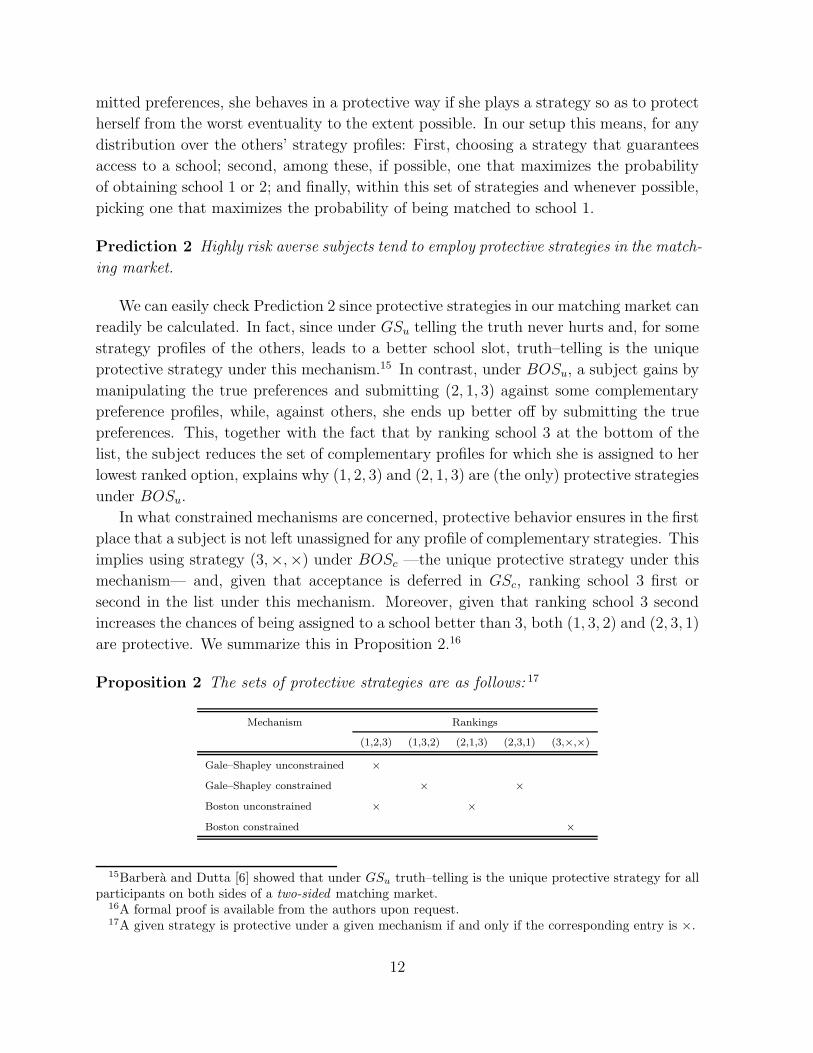
are protective. We summarize this in Proposition 2.16

Proposition 2 The sets of protective strategies are as follows: 17

Mechanism Rankings

(1,2,3) (1,3,2) (2,1,3) (2,3,1) (3,×,×)

Gale–Shapley unconstrained ×

Gale–Shapley constrained × ×

Boston unconstrained × ×

Boston constrained ×

15Barbera and Dutta [6] showed that under GSu truth–telling is the unique protective strategy for allparticipants on both sides of a two-sided matching market.

16A formal proof is available from the authors upon request.17A given strategy is protective under a given mechanism if and only if the corresponding entry is ×.

12

4 Preference Intensities

In this section, we present aggregate data and analyze how the empirical distribution of

submitted rankings changes according to the applied cardinal preferences.

Mechanism Submitted Rankings

(1,2,3) (1,3,2) (2,1,3) (2,3,1) (3,×,×)


20 ECU 0.5000 0.0000 0.4074 0.0370 0.0556

13 ECU 0.6481 0.0370 0.1852 0.0185 0.1110

27 ECU 0.4444 0.0000 0.4259 0.0741 0.0555


20 ECU 0.2407 0.1852 0.1481 0.3148 0.1110

13 ECU 0.1667 0.3148 0.0926 0.2778 0.1482

27 ECU 0.2037 0.1296 0.2593 0.3148 0.0926


20 ECU 0.4000 0.0182 0.4000 0.1636 0.0182

13 ECU 0.6182 0.0364 0.1455 0.0727 0.1273

27 ECU 0.3091 0.0000 0.5455 0.0909 0.0545

Boston constrained

20 ECU 0.2727 0.2000 0.1455 0.2545 0.1272

13 ECU 0.1818 0.3636 0.1273 0.1636 0.1636

27 ECU 0.1455 0.0545 0.2727 0.4364 0.0909

Table 4: Probability distribution of submitted rankings. The most salient rankings for a given mechanism and cardinalpreferences are indicated in boldface.

It can be seen from Table 4 that the most salient ranking is always an undominated

strategy. It follows from inspection of column (1,2,3) that for each payoff constellation

and among all four mechanisms, the level of truth–telling is highest in GSu. This is

not a surprise because it is the only mechanism for which truth–telling is the unique

undominated strategy (Proposition 1). However, since the level of truth–telling falls well

short of 100% in this treatment as well, several subjects did not recognize that it is in

their best interest to reveal preferences honestly.18

Now, we study the impact of cardinal preferences on individual behavior. The rele-

vant data is provided in Table 5, which shows the percentage changes in the probability

18In Chen and Sonmez [10], in their “random” and “designed” treatments of GSu, 56% and 72% of thesubjects, respectively, submitted their true preferences. The numbers are 58% and 57% in Calsamiglia et

al. [9]. Our numbers seem to be slightly lower but a real comparison is not possible due to the very differentenvironments. Using χ2 tests for homogeneity one verifies that for all cardinal payoff constellations, (a)the distribution of submitted rankings in treatment GSu (BOSu) is significantly different from the onein treatment GSc (BOSc) and (b) the distributions of submitted rankings in treatments GSu and BOSu

(GSc and BOSc) are not significantly different from each other. This might create the impression thatsubjects in treatment GSu (GSc) interpreted the matching algorithm in the same way as the subjectsin treatment BOSu (BOSc). However, Results 1 and 4 presented later on clearly show that the twomechanisms are perceived differently.

13

distribution of submitted rankings when the payoff of the second school decreases from

20 to 13ECU (top part of the table) and when it increases from 20 to 27ECU (bottom

part of the table). For the sake of completeness, we also present the p–values of the χ2

tests for homogeneity that analyze whether the respective distributions differ.19

Mechanism Rankings p–value

(1,2,3) (1,3,2) (2,1,3) (2,3,1) (3,×,×)

20ECU – 13ECU

Gale–Shapley unconstrained -0.1481 -0.0370 0.2222 0.0185 -0.0555 0.0300

Gale–Shapley constrained 0.0741 -0.1296 0.0556 0.0370 -0.0370 0.2300

Boston unconstrained -0.2182 -0.0182 0.2545 0.0909 -0.1091 0.0002

Boston constrained 0.0909 -0.1636 0.0182 0.0909 -0.0364 0.1450

20 ECU – 27ECU

Gale–Shapley unconstrained 0.0556 0.0000 -0.0185 -0.0370 0.0000 0.4650

Gale–Shapley constrained 0.0370 0.0556 -0.1111 0.0000 0.0185 0.3300

Boston unconstrained 0.0909 0.0182 -0.1455 0.0727 -0.0364 0.1400

Boston constrained 0.1273 0.1455 -0.1273 -0.1818 0.0364 0.0100

Table 5: Changes in the probability distribution of submitted rankings. A positive (negative) number indicates that thecorresponding ranking is used more (less) often when the payoff is 20ECU. We also present the one–sided p–value of theχ2 test for homogeneity that analyzes whether the empirical distribution depends on the relative preference intensities.

We see that a reduction of the payoff of school 2 from 20 to 13ECU changes the

distribution of submitted rankings in the unconstrained but not in the constrained setting,

while raising its payoff from 20 to 27ECU only affects the distributions in BOSc. To

analyze these findings in more detail, we run Wilcoxon signed–rank tests as they allow us

to see whether the use of a particular ranking changes.

First, we discuss significant changes in behavior related to the reduction of the payoff

of school 2. With respect to the unconstrained mechanisms, we find that the reduction

makes subjects use the strategy (2,1,3) significantly less often (p = 0.0163 in GSu and

p = 0.0053 in BOSu), while, at the same time, subjects also tell the truth significantly

more often (p = 0.0007 in GSu and p = 0.0003 in BOSu). These results have only

been predicted for BOSu because telling the truth is the unique undominated strategy in

GSu. We also find that in treatment BOSu, the ranking (2,3,1) is submitted significantly

less (p = 0.0294) and the rankings (3,×,×) significantly more often (p = 0.0072) after

the change of payoffs. Although according to Proposition 1 neither of the two strategies

should have been used at all, it seems “natural” that some of the subjects who did not

realize that these strategies are dominated switch from the ranking (2,3,1) to (3,×,×) as

the payoff of school 2 decreases (as indicated by our first prediction). With respect to the

constrained mechanisms, we find the same significant effect for both GSc and BOSc: The

strategy (1,3,2) is applied more often after the change (p = 0.0261 in GSc and p = 0.0145

19Throughout the analysis, p–values are one–sided.

14

in BOSc), which is in line with our hypothesis. So, all significant changes that take place

under the Gale–Shapley mechanism also occur under the Boston mechanism. Moreover,

there is no significant change in the submitted rankings that is in the opposite direction

to that of Prediction 1.

Second, we discuss significant changes in the probability distribution of submitted

rankings that are due to an increase of the payoff of school 2 from 20 to 27ECU. It can

be seen from the bottom part of Table 5 that individual behavior is mainly affected in

the Boston treatments. More precisely, in BOSu, the ranking (2,1,3) is submitted more

often after increasing the payoff of school 2 (p = 0.0105). Similarly, in treatment BOSc,

subjects play less often the strategies (1, 2, 3) (p = 0.0354) and (1,3,2) (p = 0.0105), and

they use more frequently the strategies (2,1,3) (p = 0.0354) and (2,3,1) (p = 0.0092) after

the payoff has been changed. Observe that none of the significant changes regarding the

Boston mechanism goes against our hypothesis. Finally, since the only significant effect

in the Gale–Shapley treatments is that subjects submit the ranking (2,1,3) more often

(p = 0.0289) after increasing the payoff of school 2 under GSc, it is again the case that

all changes in behavior caused by the variation in cardinal preferences under the Gale–

Shapley mechanism also take place under the Boston mechanism. Consequently, we can

summarize our findings as follows.

Result 1 (Cardinal preferences.) The Gale–Shapley mechanism is more robust to

changes in cardinal preferences than the Boston mechanism, independently of whether

choice is constrained or unconstrained.

5 Performance: Efficiency and Stability

Two prominent indicators of the performance of matching mechanisms are efficiency and

stability. While efficiency for teachers is the primary welfare goal,20 stability of the match-

ings reached should be met for the mechanism to be “successful.”21 In our setup, a

matching is blocked if there is a teacher that prefers to be assigned to some school with a

slot that is either available or occupied by a lower priority teacher. A matching is stable

if it is not blocked. An important advantage of our simple environment is that we can

actually compare the different mechanisms on these two important dimensions directly,

i.e., without recurring to (virtual) recombinations and estimations.22

20For efficiency we only consider the welfare of the teachers as the school slots are mere objects.21Stability is important to avoid potential lawsuits or the appearance of matches that circumvent the

mechanism.22Since we have the empirical distributions over all strategies, a sufficient number of recombinations

will ensure that the difference between any two mechanisms under consideration is significant.

15

5.1 Efficiency

To determine the levels of efficiency, we first calculate the likelihood of every profile of

submitted preference rankings from the empirical distributions over all possible strategies

presented in Table 4. For each such profile, we then determine the induced matching

and the corresponding payoff per teacher. Actual efficiency is finally computed as the

expected average payoff per teacher. To be able to make comparisons across different

cardinal preferences under the same mechanism, we also present normalized efficiency,

which is obtained by setting the payoff of school 2 to 20ECU independently of its actual

value. The results are depicted in Table 6.

Mechanism 20 ECU 13 ECU 27ECU

actual norm. actual norm.

Gale–Shapley unconstrained 21.1024 19.6129 22.6871 26.2672 20.6662

Gale–Shapley constrained 17.4156 14.8776 16.7522 21.6409 17.7509

Boston unconstrained 20.6802 20.1506 22.1641 25.3526 20.1635

Boston constrained 18.0584 16.2921 18.2426 22.9131 17.8447

Table 6: Expected average payoff per teacher in ECU. For the cases where the payoff of the second most preferred schoolis 13ECU or 27ECU, we indicate both actual and normalized efficiency.

Our first observation is that for both the Gale–Shapley and the Boston mechanisms,

the expected payoff per teacher is always higher in the unconstrained setting than in the

constrained setting, which reaffirms the findings in Calsamiglia et al. [9]. More interest-

ingly, payoffs under the Boston mechanism are not always lower than those under the

Gale–Shapley mechanism. In fact, whereas the Gale–Shapley has the tendency to create

a higher welfare than the Boston mechanism in the unconstrained case, it turns out that

efficiency is always higher in BOSc than in GSc.

Two elements contribute to the observed differences across mechanisms. First, the

mechanisms produce different outcomes for some strategy profiles. This can be accounted

for by looking at the actual efficiency levels when the same distribution of strategy profiles

is applied to the Gale–Shapley and Boston mechanisms. Second, even though neither GSu

and BOSu nor GSc and BOSc induce significantly different distributions of submitted

rankings,23 slight changes in individual behavior across mechanisms have an impact on

efficiency. For instance, BOSu20 yields a higher average payoff than GSu20, independently

of the exact (common) distribution of strategy profiles.24 This strongly suggests that the

observed difference in actual efficiency between these two treatments relies exclusively

on those slight differences in behavior and, in fact, an inspection of Table 4 reveals that

the proportion of truth–telling under GSu20 is higher than under BOSu20. Gale–Shapley’s

23See Footnote 18.24The slightly cumbersome calculations are available from the authors upon request.

16

advantage in truth-telling is also partially responsible for the efficiency advantage of GSu27

over BOSu27, whereas a less pronounced difference when school 2 is worth 13ECU is not

enough to compensate for an a priori efficiency advantage of BOS over GS.25 In what the

constrained mechanisms are concerned, both elements are again important in explaining

the observed differences in efficiency. BOS exhibits an efficiency advantage over GS when

the uniform distribution over strategy profiles is considered.26 In addition, whereas GSc

and BOSc lead to roughly the same strategic choices when school 2 is worth 20ECU,

differences are more pronounced for the other payoff constellations, resulting in a visible

efficiency advantage of BOSc over GSc.

Result 2 (Efficiency.) Imposing a constraint reduces efficiency. Moreover, GSu tends

to outperform BOSu, but BOSc outperforms GSc. Finally, increasing the payoff of school

2 leads to a reduction of efficiency, except for GSc.

5.2 Stability

Table 7 contains the total proportion of stable matchings reached given the empirical

distribution of submitted rankings in each treatment (in boldface), split into the three

stable matchings labeled teacher optimal, compromise, and school optimal. Under each of

these symmetric matchings, every teacher is assigned to its most preferred, second most

preferred, and least preferred school, respectively.

We can see that, for every mechanism, the frequency of the compromise stable match-

ing increases sharply as the payoff of school 2 rises. Under GSc, this is obtained mainly

at the expense of the school optimal stable matching —valued at 10ECU per teacher—

thus resulting in an improvement in efficiency, whereas under both GSu and BOSu, ef-

ficiency decreases as the teacher optimal stable matching —worth 30ECU per teacher—

is reached far less often. Simultaneously, the proportion of stable matchings reached as

a whole increases. Under BOSc, the increase in the proportion of the compromise stable

matching rests mainly on the number of unstable matchings, boosting stability as the

payoff of school 2 increases.

When comparing different treatments for the same payoff constellation, the numbers

suggest that imposing a constraint significantly reduces the probability of obtaining a

stable matching. The same result was obtained in Calsamiglia et al. [9] for the Gale–

Shapley mechanism. On the other hand, Gale–Shapley is in general more successful than

Boston in producing stable matchings. This is in line with theory in the unconstrained

25By this we mean that, in our setup, the average efficiency level when the uniform distribution overstrategy profiles is considered is higher under BOS, reaching 14.81ECU and 19.08ECU under BOSu13

and BOSu27, respectively, against 13.76ECU under GSu13 and 17.07ECU under GSu27.26The average efficiency level for the uniform distribution over strategy profiles is 14.91ECU,

13.03ECU, and 16.79ECU under BOS and 14.58ECU, 12.93ECU, and 16.24ECU under GS whenschool 2 is valued 20, 13, and 27ECU, respectively.

17

Mechanism Payoff second most preferred school

20ECU 13 ECU 27 ECU

Gale–Shapley unconstrained 0.8571 0.7196 0.8629

Teacher optimal 0.1250 0.3216 0.0878

Compromise 0.7173 0.3458 0.7545

School optimal 0.0148 0.0522 0.0205

Gale–Shapley constrained 0.5505 0.4944 0.5934

Teacher optimal 0.0773 0.1116 0.0370

Compromise 0.3344 0.1503 0.4621

School optimal 0.1388 0.2324 0.0943

Boston unconstrained 0.6558 0.4491 0.6760

Teacher optimal 0.0731 0.2805 0.0295

Compromise 0.5775 0.1039 0.6333

School optimal 0.0051 0.0647 0.0132

Boston constrained 0.3441 0.3089 0.6034

Teacher optimal 0.1056 0.1622 0.0080

Compromise 0.1949 0.0708 0.5760

School optimal 0.0435 0.0759 0.0194

Table 7: Proportions of stable matchings, split into the teacher optimal, the compromise, and the school optimal stablematchings.

case —since Gale–Shapley produces stable matchings when subjects are truthful, whereas

Boston does not— and again with Calsamiglia et al. [9]. Finally, note that when the

magnitude of the changes in the proportion of stable matchings is taken into account,

it appears to be the case that, very much in resemblance to Result 1, the Gale–Shapley

mechanism is less sensitive to changes in the payoff of school 2 than the Boston mechanism.

In fact, when comparing the percentage of stable matchings reached when school 2 is

worth 13 and 27ECU, differences in stability reach 0.1433 and 0.0990 under GSu and

GSc, respectively, against 0.2269 and 0.2945 under BOSu and BOSc.

Result 3 (Stability.) Imposing a constraint reduces stability. Moreover, GS is more

stable and “stability–robust” to changes in payoffs than BOS. Finally, increasing the

payoff of school 2 increases stability, mainly due to the compromise stable matching.

6 Risk Aversion

In this section, we analyze whether subjects with different degrees of risk aversion —

proxied by the switching point in the paired lottery choice phase— behave differently in

the matching market and whether this depends on the actual mechanism employed. To

investigate this question, we study how the distribution of submitted rankings changes

as the subjects with the lowest switching point in the paired lottery choice phase are

eliminated step–by–step from our subject pool. This procedure can be readily described

18

as follows: We start by considering the distribution of submitted rankings for the whole

subject pool. Then, in the first step of the process, we analyze how this distribution

changes as we eliminate from our subject pool all those subjects who, in the first phase

of the experiment, switch from Option A to Option B in the first decision situation.27

In the second step of the process, we eliminate from our subject pool all those subjects

who switch from Option A to Option B in the second decision situation. This process

continues until we are only left with the subjects who switch earliest in the ninth decision

situation, i.e., the most risk averse agents. The advantage of this procedure is that it

does not only allow us to determine if individual behavior depends on risk aversion, but

it also enables us to establish the degree of risk aversion from which on behavior differs.

The relevant data is presented in Figure 1. It consists of four panels, one for each treat-

ment. In every panel, the horizontal axis indicates switching points in the paired lottery

choice phase. On the vertical axis, we plot the percentage with which the subjects who

have a switching point that is at least as high as the number indicated on the horizontal

axis play any of the five possible strategies. As we move from the left to the right in a

given graph, the subjects with the lowest risk aversion among all those still considered are

discarded. This procedure has the potential drawback that the distributions of rankings

for high switching points are likely to be determined by only a few subjects. Indeed, it

turns out that in each treatment, less than ten subjects have a switching point in the

paired lottery choice phase of at least 9. To minimize this problem and to provide a clear

visual representation, we opted for pooling the data of all three payoff constellations.

We now discuss the graphs for each of the four mechanisms. Intuitively, the figure

should be looked at in the following way: If a curve is flat, then the use of that particular

strategy in that particular mechanism does not depend on the degree of risk aversion. On

the other hand, if a curve is increasing (decreasing), then the corresponding strategy is

used more (less) by the subjects with a higher degree of risk aversion. Our first general

observation is that all curves are rather flat until a switching point of 7 in the paired

lottery choice phase.

It can be seen in Table 4 that, in treatment GSu, subjects predominantly say the

truth or play the strategy (2,1,3). Truth–telling is the unique protective strategy for

this mechanism (Proposition 2) and we indeed see that it is played considerably more

often among the highly risk averse subjects. For example, the percentage of truth–telling

increases from 0.6000 for a switching point of 7 to 0.8000 if the selected switching point

is 9, while the corresponding percentage for (2,1,3) decreases from 0.3733 to 0.1300. The

graph for treatment GSc also provides clear evidence in favor of our hypothesis that

subjects with a higher degree of risk aversion play “safer” strategies more frequently.

27We consider this to be the first step because there is no subject who always chooses Option B.Observe that all subjects who behave inconsistently —that is, the individuals who switch at least oncefrom Option B to Option A— had to be eliminated from our analysis at this point.

19

Gale-Shapley unconstrained

0.0000

0.2000

0.4000

0.6000

0.8000

1.0000

1 2 3 4 5 6 7 8 9

(1,2,3)

(1,3,2)

(2,1,3)

(2,3,1)

(3,x,x)

Switching Point (Phase 1)

Per

cen

tag

e o

f Pla

y

Gale-Shapley constrained

0.0000

0.2000

0.4000

0.6000

0.8000

1.0000

1 2 3 4 5 6 7 8 9

(1,2,3)

(1,3,2)

(2,1,3)

(2,3,1)

(3,x,x)


Per

cen

tag

e o

f Pla

y


0.0000

0.2000

0.4000

0.6000

0.8000

1.0000

1 2 3 4 5 6 7 8 9

(1,2,3)

(1,3,2)

(2,1,3)

(2,3,1)

(3,x,x)


Per

cen

tag

e o

f Pla

y

Boston constrained

0.0000

0.2000

0.4000

0.6000

0.8000

1.0000

1 2 3 4 5 6 7 8 9

(1,2,3)

(1,3,2)

(2,1,3)

(2,3,1)

(3,x,x)


Per

cen

tag

e o

f Pla

y

Figure 1: The distribution of submitted rankings for all four mechanisms as the subjects with lowest degree of risk aversionare eliminated step–by–step from the subject pool. We took the average over all payoff constellations.

In this treatment, the use of the protective strategy (2,3,1) increases from 0.3492 for a

switching point of 7 to 0.6667 if the selected switching point is 9. The curve for (1,3,2),

the second protective strategy, is initially increasing and decreases sharply for switching

points higher than 8. The curves for the remaining three strategies, on the other hand,

are downward sloping.

Our findings for the Boston mechanism are more mixed. In treatment BOSu, subjects

mainly submit either of the protective rankings (1,2,3) and (2,1,3), and, among the two,

the highly risk averse subjects rather tend to say the truth. The main difference with

respect to GSu is that the dominated rankings (2,3,1) and (3,×,×) are now also submitted

to some lesser extent, and the graph shows that the highly risk averse subjects use more

often the “safety” strategy (3,×,×) and less often the strategy (2,3,1) than their co–

players. Finally, in treatment BOSc, all five strategies are submitted independently of

the degree of risk aversion and it is difficult to identify any clear pattern. If anything,

the strategies (1,2,3) and (2,1,3) are played more and the strategies (1,3,2), (2,3,1), and

(3,×,×) are played less by the highly risk averse subjects. In any case, our hypothesis

20

that the unique protective strategy (3,×,×) will be played more often by the subjects

with high risk aversion cannot be validated.

Next, we complement the previous general discussion with an econometric analysis.

We regress the probability with which a particular ranking is submitted (again the pooled

data for all three payoff constellations is considered) on a constant and the switching

point extracted in the first phase of the experiment.28 The parameter estimates of the

Tobit Maximum Likelihood estimation procedure for the switching point are presented in

Table 8. The errors are robust to heteroskedasticity.

Mechanism Rankings Observations

(1,2,3) (1,3,2) (2,1,3) (2,3,1) (3,×,×)

Gale–Shapley unconstrained 0.0587∗∗ −0.0033 −0.0056 −0.0021 −0.0474∗∗ 48(0.0269) (0.0034) (0.0263) (0.0065) (0.0215)

Gale–Shapley constrained −0.0330 0.0263∗ −0.0332 0.0448∗∗ −0.0048 49(0.0238) (0.0173) (0.0247) (0.0251) (0.0119)

Boston unconstrained 0.0083 −0.0166∗∗ 0.0001 −0.0027 0.0108 51(0.0270) (0.0099) (0.0267) (0.0156) (0.0181)

Boston constrained 0.0012 −0.0332∗ 0.0369∗ 0.0087 −0.0137 48(0.0307) (0.0188) (0.0225) (0.0240) (0.0221)

Table 8: Tobit ML estimation results on how risk aversion affects behavior in the matching market. Standard errors arein parentheses. Errors are robust to heteroskedasticity. ∗ Significant at the 10–percent level. ∗∗ Significant at the 5–percentlevel. ∗∗∗ Significant at the 1–percent level. OLS estimations yield similar results.

Table 8 confirms to a large extent the intuition from Figure 1. In the two treatments

related to the Gale–Shapley mechanism, the protective strategies are played more often

the more risk averse the subjects are.29 All other strategies are, if anything, played less

often in these two treatments. With respect to the two treatments using the Boston

mechanism, we find that risk aversion is uncorrelated with the use of the protective

strategies. Still, some of the other strategies are correlated to the switching point. In

particular, the ranking (1,3,2) is submitted less often by the highly risk averse (both in

BOSu and BOSc), while the strategy (2,1,3) is played more often in BOSc by them.

Result 4 (Risk aversion: protective behavior.) Subjects who are more risk averse

are more likely to play a protective strategy under the Gale–Shapley but not under the

Boston mechanism.

28Table 12 in Appendix B contains the results of Probit Maximum Likelihood estimations on thedecision of whether or not to submit a particular ranking for a given payoff constellation. In theseestimations, we took into account the sequential play of the three matching markets by controlling forearlier decisions. For example, in the estimations related to truth–telling in the situation GSu27, weadded whether the subject told the truth in GSu20 and GSu13 as additional explanatory variables. Theseestimations confirm the intuition provided by the Tobit estimations.

29It is interesting to see that in GSu, the highly risk averse are more likely to tell the truth and lesslikely to report the ranking (3,×,×). One possible explanation for this is that risk aversion is correlatedwith regret, which is minimized by being honest about one’s own preferences.

21

Finally, we ask whether subjects with different degrees of risk aversion react differently

to changes in cardinal preferences. We investigate this by dividing the subject pool of

each treatment into two groups according to when the subjects switch from lottery A to

lottery B in the paired lottery choice phase. The first group, which we will label as the

“high risk aversion” subjects, consists of the individuals who switched in or later than the

seventh decision situation. The other individuals switched in or before the sixth decision

situation and are labeled as the “low risk aversion” subjects.30

Mechanism Rankings

(1,2,3) (1,3,2) (2,1,3) (2,3,1) (3,×,×)


20 ECU 0.5200 0.0000 0.4400 0.0000 0.04000.5652 0.0000 0.3478 0.0000 0.0870

13 ECU 0.8000 0.0000 0.2000 0.0000 0.00000.5652 0.0435 0.1739 0.0000 0.2174

27 ECU 0.4800 0.0000 0.4800 0.0400 0.00000.4783 0.0000 0.3913 0.0435 0.0870


20 ECU 0.2381 0.1905 0.0952 0.3810 0.09520.2500 0.1786 0.1786 0.2857 0.1071

13 ECU 0.0952 0.4286 0.0952 0.2381 0.14290.2500 0.2500 0.1071 0.2500 0.1429

27 ECU 0.1905 0.1429 0.1905 0.4286 0.04760.2500 0.1071 0.3571 0.2500 0.0357


20 ECU 0.3000 0.0333 0.4667 0.1667 0.03330.5000 0.0000 0.3500 0.1500 0.0000

13 ECU 0.7000 0.0000 0.1667 0.0333 0.10000.5500 0.1000 0.1500 0.1000 0.1000

27 ECU 0.3000 0.0000 0.6333 0.0333 0.03330.3500 0.0000 0.5000 0.0500 0.1000

Boston constrained

20 ECU 0.2308 0.1538 0.1538 0.3846 0.07700.3636 0.2273 0.0909 0.0909 0.2273

13 ECU 0.1923 0.2692 0.1154 0.1923 0.23080.1818 0.4091 0.1364 0.1364 0.1365

27 ECU 0.1154 0.0000 0.3846 0.4231 0.07690.1364 0.0909 0.2273 0.4545 0.0910

Table 9: Probability distribution of submitted rankings for the high and the low risk averse subjects. The probabilitiesfor the high risk averse subjects are always presented on top of the probabilities for the low risk averse subjects. The mostsalient rankings for each group are highlighted in boldface.

30The common switching point has not been chosen arbitrarily. According to our data, the averageswitching point is 6.47 in GSu, 5.98 in GSc, 6.70 in BOSu, and 6.55 in treatment BOSc so that thedifference in the group sizes is minimal if the seventh decision situation is taken as the dividing line.As a consequence, the high risk aversion group consists of 25 subjects in treatment GSu, 21 subjects intreatment GSc, 31 subjects in treatment BOSu, and 26 subjects in treatment BOSc. The respectivenumbers for the group of low risk aversion subjects are 23, 28, 20, and 22.

22

Table 9 presents the probability distributions for the two groups under consideration.

To analyze the relation between risk aversion and cardinal preferences, we now apply

Mann Whitney U tests. The corresponding data is presented in Table 10, which should

be read as follows. Consider for example the element in the first row and the (2,1,3)

column, which equals 0.0661. This value can be obtained from Table 9 by calculating the

difference between how the subjects with the high risk aversion (0.4400−0.2000 = 0.2400)

and how the subjects with the low risk aversion (0.3478 − 0.1739 = 0.1739) change the

use of the strategy (2,1,3) when the payoff of the second school is reduced from 20 to

13ECU: 0.2400 − 0.1739 = 0.0661 (i.e., the difference from the high risk aversion group

minus the difference from the low risk aversion group). Consequently, Table 10 indicates

by how much the high risk averse subjects adapt their behavior in comparison to the low

risk averse subjects as cardinal preferences vary.

Mechanism Rankings

(1,2,3) (1,3,2) (2,1,3) (2,3,1) (3,×,×)

20 ECU - 13 ECU

Gale–Shapley unconstrained -0.2800 0.0435 0.0661 0.0000 0.1705

Gale–Shapley constrained 0.1429 -0.1667 -0.0714 0.1071 -0.0119

Boston unconstrained -0.3500 0.1333 0.1000 0.0833 0.0333

Boston constrained -0.1434 0.0664 0.0839 0.2378 -0.2448

20 ECU - 27 ECU

Gale–Shapley unconstrained -0.0470 0.0000 0.0035 0.0035 0.0400

Gale–Shapley constrained 0.0476 0.0238 0.0833 -0.0833 0.0238

Boston unconstrained -0.1500 0.0333 -0.0167 0.0333 0.1000

Boston constrained -0.1119 0.0175 -0.0944 0.3252 -0.1364

Table 10: Differences in the probability changes between the group of individuals with a high degree of risk aversion andthe group of subjects with a low degree of risk aversion. (See the text for an interpretation of the numbers.) The shiftsthat turned out significant for the whole population are highlighted in boldface.

Three of the shifts in behavior that turned out significant for the whole population are

primarily caused by different attitudes towards risk. First, the subjects with the high risk

aversion tell the truth with probability 0.5200 in GSu20 and with probability 0.8000 in

GSu13. Consequently, a decrease in the monetary payoff of school 2 causes these subjects

to increase the level of truth–telling by 28%. On the other hand, the subjects with the

low risk aversion tell the truth with probability 0.5652 in both GSu20 and GSu13. This

allows us to conclude that the high risk aversion subjects are responsible for the increase

in the level of truth–telling in treatment GSu as the payoff of school 2 decreases from 20 to

13ECU (p = 0.0315). Second, it can be seen from Table 9 that the same effect occurs in

BOSu. A decrease of the payoff of the second school induces the subjects with a high risk

aversion to increase their level of truth–telling from 0.3000 to 0.7000, the corresponding

change for the subjects with a low risk aversion is 0.5500 − 0.5000 = 0.0500 (so that the

23

difference–in–difference is 0.3500). Since this difference is significant (p = 0.0373), it is

again the more risk averse subjects who are responsable for the overall effect. Third, an

increase in the payoff of the second school from 20 to 27ECU makes individuals play more

often the strategy (2,3,1) in BOSc. Looking back at Table 4, we indeed see that the use

of this strategy increases from 0.2545 to 0.4364. This result is caused by the subjects

with a low risk aversion as they increase the use of that particular strategy by about 36%

from only 0.0909 to 0.4545. The crucial point is that the high risk aversion subjects are

not so responsive to that change in cardinal preferences because the strategy (2,3,1) is

already the most played one when the payoff of the second school is 20ECU. Indeed, this

subgroup plays the strategy (2,3,1) with probability 0.3846 before and with probability

0.4231 after the change of payoffs. The difference between the two subgroups is significant

at p = 0.0298.31

Clearly, these differences in behavior have noteworthy consequences in terms of effi-

ciency, which is reflected in Table 11. The behavior of the highly risk averse subjects

is mostly responsible for the ranking of the two mechanisms. In fact, higher levels of

truth–telling under GSu by the highly risk averse for every payoff constellation explain

the efficiency advantage of GSu over BOSu. Imposing a limited length on submittable

rankings decreases efficiency within both subgroups. Moreover, since under GSu effi-

ciency generally attains higher levels among the highly risk averse than among the low

risk averse, while the opposite happens under GSc, the negative impact of the constraint

is particularly important within the group of the highly risk averse.

Mechanism Efficiency Stability

20ECU 13ECU 27 ECU 20ECU 13ECU 27 ECU

Gale–Shapley unconstrained 21.3594 21.7040 27.3318 0.8894 1.0000 1.000021.5916 18.3070 25.8293 0.7824 0.5922 0.7931

Gale–Shapley constrained 17.2544 15.6880 21.9560 0.6016 0.4850 0.681417.7253 15.1851 23.9789 0.5414 0.4938 0.6918

Boston unconstrained 20.2667 21.1994 25.7298 0.7027 0.4700 0.727421.2500 20.0134 24.5106 0.6250 0.4641 0.5601

Boston constrained 17.9555 14.7508 24.5485 0.4374 0.3039 0.762318.6199 17.2503 22.3288 0.3235 0.3230 0.5445

Table 11: Actual efficiency (to the left) and probability of stable matchings (to the right) for the high and the low riskaversion subjects for every possible payoff of school 2. The values for the high risk aversion subjects are always presentedon top of the values for the low risk aversion subjects.

31In some instances, a change in cardinal preferences did not induce an overall effect in behavior but,nevertheless, the difference between the two subgroups is significant as they respond in a different directionto the change in payoffs. Decreasing the payoff from 20 to 13ECU leads to a significant difference betweenthe two subgroups for strategy (1,3,2) in BOSu (p = 0.0292), for strategy (2,3,1) in BOSc (p = 0.0338),and for strategy (3,×,×) in GSu (p = 0.0204) and BOSc (p = 0.0251). Similarly, increasing the payofffrom 20 to 27ECU leads to a significant difference between the two subgroups for strategy (2,3,1) inBOSu (p = 0.0377).

24

Some remarks on how stability is affected by the degree of risk aversion are due.

The relevant numbers are also presented in Table 11. In general, the differences in the

percentage of stable matchings obtained within each group of subjects follow roughly the

same rules as those obtained when the full sample is considered. Two points are worth

noticing, though. First, the levels of stability under the unconstrained mechanisms are

higher among the highly risk averse subjects, reaching 100% under GSu when the second

school is worth 13 and 27ECU. Second, as previously noted for efficiency, the constraint

reduces stability and this impact under the Gale–Shapley mechanism is more substantial

within the highly risk averse.

Result 5 (Risk aversion: efficiency and stability.) For both subgroups and under

almost all payoff configurations, GSu outperforms BOSu and BOSc outperforms GSc in

efficiency terms. Moreover, the negative impact of constraining the length of submittable

rankings on efficiency and stability under the Gale–Shapley mechanism is stronger for the

highly risk averse.

7 Concluding Discussion

In this paper, we have studied how cardinal preferences, i.e., relative preference intensities,

and risk aversion affect individual behavior in a stylized experimental matching market.

The clearest lesson is perhaps that cardinality is important in that it may shape individual

behavior and, in turn, affect both efficiency and stability of the mechanisms.

A second contribution of the present study to the ongoing debate on Gale–Shapley vs.

Boston is related to risk aversion. It is widely accepted that individual participants in a

market try to manage risk in ways that affect the market as a whole. Matching markets

are no exception. One reason for this lies in the fact that the Gale–Shapley mechanism

fosters the use of “safe” strategies by the highly risk averse. In fact, we observe that

there is a clear tendency for highly risk averse agents to resort to protective strategies

under this mechanism. Also, risk aversion is important when it comes to the evaluation of

the constraint on submittable rankings. Calsamiglia et al. [9] showed that introducing a

constraint is detrimental to the performance of the mechanisms. Our results suggest that,

under the Gale–Shapley mechanism, this negative impact especially affects the highly risk

averse.

All this serves as a word of caution for experimentalists (when considering new designs)

and theorists (when constructing new models) both alike, but perhaps more importantly,

it should be taken into account by market designers as our results unveil additional di-

mensions in which the Gale–Shapley and Boston mechanisms can be compared. The

Gale–Shapley mechanism is more efficient and more stable than the Boston mechanism

in the unconstrained setting, almost independently of the subject pool and the preference

25

intensities.32 One could conclude from this that the Gale–Shapley mechanism is to be

preferred for “small” markets where it is both allowed and no burden for the participants

to submit complete full rankings. Our message is different if the market is “large,” in the

sense that it is unfeasible for the participants to rank all schools, and a constrained mech-

anism has to be implemented almost necessarily. Now, the Boston mechanism performs

better in terms of efficiency not only for the whole subject pool (for all preference inten-

sities) but also within the more homogeneous subgroups (for most preference intensities).

The Gale–Shapley mechanism is still more stable and, therefore, the ultimate decision of

which mechanism to choose in the constrained setting would depend on whether efficiency

or stability is considered more desirable.

References

[1] A Abdulkadiroglu, Y-K Che, and Y Yasuda (2009). Resolving conflicting preferencesin school choice: The Boston mechanism reconsidered. American Economic Review,forthcoming.

[2] A Abdulkadiroglu, P Pathak, and A Roth (2005). The New York City high schoolmatch. American Economic Review, Papers and Proceedings 95(2): 364–367.

[3] A Abdulkadiroglu, P Pathak, and A Roth (2009). Strategy-proofness versus efficiencyin matching with indifferences: Redesigning the NYC high school match. American

Economic Review 99(5): 1954–1978.

[4] A Abdulkadiroglu, P Pathak, A Roth, and T Sonmez (2005). The Boston publicschools match. American Economic Review, Papers and Proceedings 95(2): 368–371.

[5] A Abdulkadiroglu and T Sonmez (2003). School choice: A mechanism design ap-proach. American Economic Review 93(3): 729–747.

[6] S Barbera and B Dutta (1982). Implementability via protective equilibria. Journal

of Mathematical Economics 10(1): 49–65.

[7] S Barbera and B Dutta (1995). Protective behavior in matching models. Games and

Economic Behavior 8(2): 281–296.

[8] P Blavatskyy (2009). Betting on own knowledge: Experimental test of overconfidence.Journal of Risk and Uncertainty 38(1): 39–49.

[9] C Calsamiglia, G Haeringer, and F Klijn (2009). Constrained school choice: Anexperimental study. American Economic Review, forthcoming.

32The only two exceptions are found in the efficiency levels for the full subject pool and the low riskaversion group when school 2 has a value of 13 ECU.

26

[10] Y Chen and T Sonmez (2006). School choice: An experimental study. Journal of

Economic Theory 127(1): 202–231.

[11] L Dubins and D Freedman (1981). Machiavelli and the Gale–Shapley algorithm.American Mathematical Monthly 88(7): 485–494.

[12] C Featherstone and M Niederle (2008). Ex ante efficiency in school choice mecha-nisms: An experimental investigation. Working paper, Stanford University.

[13] U Fischbacher (2007). Z-tree: Zurich toolbox for ready-made economic experiments.Experimental Economics 10(2): 171–178.

[14] D Gale and L Shapley (1962). College admissions and the stability of marriage.American Mathematical Monthly 69(1): 9–15.

[15] B Greiner (2004). The online recruitment system ORSEE 2.0 - A guide for the organi-zation of experiments in economics. Working Paper Series in Economics 10, Universityof Cologne.

[16] G Haeringer and F Klijn (2009). Constrained school choice. Journal of Economic

Theory 144(5): 1921–1947.

[17] F Heinemann, R Nagel, and P Ockenfels (2009). Measuring strategic uncertainty incoordination games. Review of Economic Studies 76(1): 181–221.

[18] C Holt and S Laury (2002). Risk aversion and incentive effects. American Economic

Review 92(5): 1644–1655.

[19] A Miralles (2008). School choice: The case for the Boston mechanism. Working paper,Boston University.

[20] A Nicolo and C Rodrıguez-Alvarez (2009). Transplant quality and patients’ prefer-ences in paired kidney exchange. Working Paper, Universita degli Studi di Padova.

[21] J Pais and A Pinter (2008). School choice and information: An experimental studyon matching mechanisms. Games and Economic Behavior 64(1): 303–328.

[22] A Roth (1982). The economics of matching: Stability and incentives. Mathematics

of Operations Research 7(4): 617–628.

27

Appendix A: Instructions (Translated from Spanish)1

Welcome

Dear participant, thank you for taking part in this experiment. It will last at most 90 minutes. If youread the following instructions carefully, you can – depending on your decisions – earn some more moneyin addition to the 3 Euro show-up fee, which you can keep in any case. In order to ensure that theexperiment takes place in an optimal setting, we would like to ask you to abide to the following rulesduring the whole experiment:

• do not communicate with your fellow students!

• do not forget to switch off your mobile phone!

• read the instructions carefully. If something is not well explained or you have any question now orat any time during the experiment, then ask one of the experimenters. Do, however, not ask outloud, raise your hand instead. We will clarify questions privately.

• you may take notes on this instruction sheet if you wish.

• after the experiment, remain seated till we paid you off.

If you do not obey the rules, the data becomes useless for us. In that case, we will have to exclude youfrom this experiment and you will not receive any compensation. Also, note that all participants receivethe same instructions.

The Experiment

This experiment consists of two phases. Now, we will only introduce the first phase. Once it has finished,we are going to explain the second phase. However, always remember the following very important points:

1. The two phases take place in a completely anonymous setting. So, you will neither know nor learnwhom you are playing with.

2. You will only be paid for phase 1 or phase 2, but not for the combined results. At the end ofthe whole experiment, the participant playing at terminal 9 will determine which phase is payoffrelevant by throwing a coin.

3. You will not receive any feedback about your decision or the decision of your co-players until thevery end of the experiment.

4. We will not speak of Euro during the experiment, but rather of ECU (experimental currency units).Your whole income will first be calculated in ECU. At the end of the experiment, the total amountyou have earned will be converted to Euro. We will always indicate the exchange rate between ECUand Euro.

The First Phase

First we introduce you to the basic decision situation. Then, you will learn how the experiment isconducted. Note that if phase 1 is randomly selected for payment, then you will receive 4 Euro for everyECU earned during this phase.

1We first provide the full instructions for GSu. After that, we only provide the instructions for the “Second Phase” ofthe other three treatments, since the rest of the instructions are exactly as in GSu.

28

The First Decision Environment

In the first phase of the experiment, your basic task is to choose several times between two lotterytickets that are denoted Option A and Option B, respectively. In particular, lottery ticket A gives you amonetary payoff of xA ECU with probability px(A) and a monetary payoff of yA ECU with the remainingprobability py(A) = 1− px(A). Similarly, lottery ticket B gives a you a monetary payoff of xB ECU withprobability px(B) and a monetary payoff of yB ECU with probability py(B) = 1 − py(B). As a simpleexample consider the lottery ticket A which is such that you get 5 ECU in 3 out of 10 cases and 10 ECU

in 7 out of ten cases. Then, xA = 5.00 ECU, px(A) = 0.3, yA = 10.00 ECU and py(A) = 0.7.

The First Experiment

The first phase includes the basic decision environment just described to you. In total, there are ten pairsof lottery tickets; so, you have to make ten choices. In all ten situations, monetary payoffs are such thatxA = 2.00 ECU, xB = 3.85 ECU, yA = 1.60 ECU, and yB = 0.10 ECU. However, the probabilities withwhich you are going to get each prize change across situations. The following figure shows the computerscreen you are going to encounter during the experiment.

The computer screen presents all ten situations simultaneously with the lottery ticket A to the left oflottery ticket B. For example, in situation number 4 lottery ticket A gives you 2.00 ECU in 4 out of 10

cases and 1.60 ECU in 6 out of 10 cases. You choose between the lottery tickets by clicking the desiredoption on the right hand side of the screen. Once you have made all ten choices, click on the button“Continue”.

If it happens that phase 1 is randomly selected for payment, one of the ten pairs of lotteries is randomlyselected by the computer (each pair is selected with the same probability). Given this random draw, yourpayoff is then determined by using the lottery you have chosen in that particular situation. For example,if situation 9 is randomly selected and you have chosen option A in that case, then you get 2 ECU withprobability 0.9 and 1.6 ECU with probability 0.1. Finally, please answer the question below. Once ready,please raise your hand.

QUESTION: Suppose lottery ticket A is such that it gives you 3 ECU with probability 0.7 and 1 ECUwith probability 0.3. Similarly, lottery ticket B gives you 3 ECU with probability 0.7 and 2 ECU withprobability 0.3. Which option do you choose?

29

The Second Phase (GSu)

First we introduce you to the basic decision situation. Next, you will find control questions that help youto understand the situation better. Finally, you will learn how the experiment is conducted. Note thatif phase 2 is randomly selected for payment, then you will receive 40 Eurocents for every ECU earnedduring this phase.

The Second Decision Environment

The basic decision environment in the second phase of the experiment is as follows: There are threeteachers —let us call them teacher 1, teacher 2, and teacher 3— who are looking for a new job. Thereare three schools in town (denoted X , Y , and Z) and every school happens to have one open teachingslot. Since the schools turn out to differ in their location and quality, teachers have different opinions ofwhere they want to teach. The desirability of schools in terms of location and quality is expressed in thefollowing table:

Teacher 1 Teacher 2 Teacher 3Most preferred school X Y Z

Second most preferred school Y Z X

Least preferred school Z X Y

For example, teacher 1 prefers school X to school Y and school Y to school Z. Schools when offeringpositions consider the quality of each applicant and the experience they have. On this basis, they builda priority ordering where all teachers are ranked. The following table summarizes the priority orderingof each school.

School X School Y School Z

Best candidate 2 3 1Second best candidate 3 1 2Worst candidate 1 2 3

For example, in school Z, teacher 1 is ranked first, teacher 2 is ranked second, and teacher 3 is rankedthird. To decide which teacher gets offered a position at which school, teachers are first asked to submittheir ranking of schools; that is, they have to indicate at which school they would like to work most, atwhich school they would like to work second most, and at which school they would like to work least.Observe that teachers can indicate whatever ranking they like, it does not have to coincide with theactual preferences. Given the submitted rankings, the following procedure is used to assign teachers toschools:

1. Every teacher applies to the school she/he listed first.

2. Each school temporarily accepts the applicant with the highest priority and rejects all other appli-cants (if any).

3. Whenever a teacher is rejected at a school, she/he applies to the next highest listed school.

4. Whenever a school receives new applications (from teachers that have been rejected in a previousround by other schools), these applications are considered together with the previously retainedapplication (if any). Among the previously retained application and new applications, the applicantwith the highest priority is temporarily accepted, all others are rejected.

5. This process is repeated until no more applications can be rejected and the allocation is finalized.Each teacher is assigned the position at the school that holds her/his application at the end of theprocess.

30

Example

Before we explain how the experiment is conducted, we would like to ask you to go over the following ex-ample. It helps illustrating how the allocation mechanism works. Once ready, please raise your hand, andone of the experimenters will check your answers. In case of questions, please contact any experimenteras well.

In the example, there are three teachers (1, 2, and 3) and three schools (A, B, and C) who have oneteaching position each. Suppose that the submitted school rankings are as follows:

Teacher 1 Teacher 2 Teacher 31st ranked school B C B

2nd ranked school C A C

3rd ranked school A B A

Also, suppose that the priority orderings of the schools are given by the following table:

School A School B School C

1st ranked teacher 2 2 12nd ranked teacher 3 1 33rd ranked teacher 1 3 2

Please, answer the following questions:

1. In the first round of the procedure, every teacher applies to the school she/he ranked first; that is,teacher 1 applies to school , teacher 2 applies to school , and teacher 3 applies toschool . Given these applications, every school temporarily accepts the applicant with thehighest priority and rejects all other teachers. Hence, school B retains teacher and rejectsteacher , while school C retains teacher .

2. In the second round, all teachers rejected in the first round apply to the school they ranked second;that is, teacher 3 applies to school . Now, schools compare the new applicants with thepreviously retained teachers. As a consequence, school C retains teacher and rejects teacher

.

3. In the third round, the teacher that got rejected in the second round applies to the next highestranked school. Hence, teacher applies to school . Since this school has still a freeplace all teachers are assigned to a school and the mechanism stops.

4. The final allocation of teachers to school is therefore as follows:

• Teacher gets a job at A.

• Teacher gets a job at B.

• Teacher gets a job at C.

The Second Experiment

In the beginning of the second phase, the computer randomly divides the participants into groups of 3.The assignment process is random and anonymous, so no participant will know who is in which group.Participants within the same group will only play among themselves. Then, each participant in a groupgets randomly assigned the role of a teacher in such a way that one group member will be in the role ofteacher 1, another group member will be in the role of teacher 2, and the final group member will be inthe role of teacher 3. Neither the division of participants into groups nor the assignment of roles withingroups is going to change during the second phase.

The basic decision situation explained above will be played three times with varying payoffs. In whatfollows, we will only explain the first payoff constellation in detail, the remaining two situations have

31

a similar structure. In particular, the first payoff constellation is such that you receive 30 ECU if youend up at the school you prefer most, 20 ECU if you are assigned to your second most preferred

school, and 10 ECU if you get a job at the school you prefer least. To clarify how the experimentproceeds, we will present next the computer screen you are going to encounter during the experiment.

On the top of the screen, we remind you of the preferences of the teachers over schools together withthe material consequences and the priorities of schools over teachers. Below you see that you are assignedthe role of teacher 1. Consequently, your payoff is highest if you end up working at school X , it secondhighest if you work at school Y , and it is lowest if you finally get a job at school Z.

At the bottom of the screen, you are asked to submit a ranking of schools. Remember that you areallowed to submit any ranking you want. On the left hand side you indicate the school that you rankfirst, in the middle you indicate the school you rank second, and to the right hand side you indicate theschool you rank last. The submitted rankings are then used by the computer to determine (by means ofthe procedure presented before) the final assignment of teachers to schools.

Finally, observe that if the second phase is randomly chosen to be payoff relevant, then the computeris going to determine randomly one of the three situations for payment (every situation is randomlyselected with the same probability). Also, note that you will never receive any feedback about decisionsuntil the very end of the experiment. Please answer the following final question. Once ready, please raiseyour hand.

QUESTION: Suppose that you prefer school X over school Z over school Y . Assume also that you submitthe following ranking of schools: X is listed higher than Y , which, in turn, is listed higher than Z. Usingthe same payoffs in ECU as in the example on the computer screen above, what will be your final payoffif you finally end up working at school Y ?

ANSWER: ECU.

32

The Second Phase (GSc)










For example, in school Z, teacher 1 is ranked first, teacher 2 is ranked second, and teacher 3 is rankedthird. To decide which teacher gets offered a position at which school, teachers are first asked to submittheir ranking of schools; that is, they have to indicate at which school they would like to work mostand at which school they would like to work second most. Observe that teachers can indicate whateverranking they like, it does not have to coincide with the actual preferences. Given the submitted rankings,the following procedure is used to assign teachers to schools:


2. Each school temporarily accepts the applicant with the highest priority and rejects all other appli-cants (if any).

3. Whenever a teacher is rejected at a school, she/he applies to the next highest listed school.

4. Whenever a school receives new applications (from teachers that have been rejected in a previousround by other schools), these applications are considered together with the previously retainedapplication (if any). Among the previously retained application and new applications, the applicantwith the highest priority is accepted, all others are rejected.

5. This process finishes when no more applications can be rejected or no teacher can send moreapplications. Each teacher is assigned the position at the school that holds her/his application atthe end of the process. If a teacher’s application was rejected by every school in her/his ranking,she/he will be unemployed.

33

Example


In the example, there are three teachers (1, 2, and 3) and three schools (A, B, and C) who have oneteaching position each. Suppose that the submitted school rankings are as follows:






Please, answer the following questions:

1. In the first round of the procedure, every teacher applies to the school she/he ranked first; that is,teacher 1 applies to school , teacher 2 applies to school , and teacher 3 applies toschool . Given these applications, every school temporarily accepts the applicant with thehighest priority and rejects all other teachers. Hence, school B retains teacher and rejectsteacher , while school C retains teacher .

2. In the second round, all teachers rejected in the first round apply to the school they ranked second;that is, teacher 3 applies to school . Now, schools compare the new applicants with thepreviously retained teachers. As a consequence, school C retains teacher and rejects teacher

.

3. In the third round, the teacher that got rejected in the second round applies to the next highestranked school. Hence, teacher applies to school . Since this school has still a freeplace all teachers are assigned to a school and the mechanism stops.

4. The final allocation of teachers to school is therefore as follows:

• Teacher gets a job at A.

• Teacher gets a job at B.

• Teacher gets a job at C.



The basic decision situation explained above will be played three times with varying payoffs. In whatfollows, we will only explain the first payoff constellation in detail, the remaining two situations havea similar structure. In particular, the first payoff constellation is such that you receive 30 ECU if you

34

end up at the school you prefer most, 20 ECU if you are assigned to your second most preferred

school, and 10 ECU if you get a job at the school you prefer least. If you end up unassigned becauseall of your applications have been rejected, you receive 0 ECU. To clarify how the experiment proceeds,we will present next the computer screen you are going to encounter during the experiment.

On the top of the screen, we remind you of the preferences of the teachers over schools together withthe material consequences and the priorities of schools over teachers. Below you see that you are assignedthe role of teacher 1. Consequently, your payoff is highest if you end up working at school X , it secondhighest if you work at school Y , and it is lowest if you finally get a job at school Z. Remember that youwill receive 0 ECU in case all of your applications are rejected.

At the bottom of the screen, you are asked to submit a ranking of schools. Remember that you areallowed to submit any ranking you want. On the left hand side you indicate the school that you rank firstand on the right hand side you indicate the school you rank second. The submitted rankings are thenused by the computer to determine (by means of the procedure presented before) the final assignmentof teachers to schools. Also, note that you will never receive any feedback about decisions until the veryend of the experiment.

Finally, observe that if the second phase is randomly chosen to be payoff relevant, then the computeris going to determine randomly one of the three situations for payment (every situation is randomlyselected with the same probability). Please answer the following final question. Once ready, please raiseyour hand.

QUESTION: Suppose that you prefer school X over school Z over school Y . Assume also that you submitthe following ranking of schools: X is ranked first and school Y is ranked second. Using the same payoffsin ECU as in the example on the computer screen above, what will be your final payoff if you finally endup working at school Y ?

ANSWER: ECU.

35

The Second Phase (BOSu)










For example, in school Z, teacher 1 is ranked first, teacher 2 is ranked second, and teacher 3 is rankedthird. To decide which teacher gets offered a position at which school, teachers are first asked to submittheir ranking of schools; that is, they have to indicate at which school they would like to work most, atwhich school they would like to work second most, and at which school they would like to work least.Observe that teachers can indicate whatever ranking they like, it does not have to coincide with theactual preferences. Given the submitted rankings, the following procedure is used to assign teachers toschools:Step 1


2. Each school accepts the applicant with the highest priority and rejects all other applicants (if any).

Step 2

1. Whenever a teacher is rejected at a school, an application is sent to the second listed school.

2. A school that received one or more applications in step 1 rejects the applications received in step2 (if any). A school that did not receive any applications in step 1 accepts the applicant with thehighest priority and rejects the other application received (if any).

Step 3

1. If a teacher’s application is rejected in step 2, she/he is assigned to the school she/he listed third.The other teachers are assigned to the schools that accepted their applications.

36

2. If no teacher’s application was rejected in step 2, each teacher is assigned to the school that acceptedher/his application.

Example


In the example, there are three teachers (1,2, and 3) and three schools (A, B, and C) who have oneteaching position each. Suppose that the submitted school rankings are as follows:



3rd ranked school A B A




Please, answer the following questions:Step 1

1. In the first round of the procedure, every teacher applies to the school she/he ranked first; that is,teacher 1 applies to school , teacher 2 applies to school , and teacher 3 applies toschool .

2. Given these applications, every school accepts the applicant with the highest priority and rejectsall other teachers. Hence, school B accepts teacher and rejects teacher , while schoolC accepts teacher .

Step 2

1. In the second round, all teachers rejected in the first round apply to the school they ranked second;that is, teacher 3 applies to school .

2. Each school that received an application in step 2 rejects the applications received in step 2 (if any).As a consequence, school rejects teacher .

Step 3

In the third round, the teacher that got rejected in the second round is assigned to his third ranked school.Hence, teacher is assigned to school . The other teachers are assigned to the schools thataccepted their applications. The final allocation of teachers to school is therefore as follows: teacher

gets a job at A; teacher gets a job at B; and teacher gets a job at C.


In the beginning of the second phase, the computer randomly divides the participants into groups of 3.The assignment process is random and anonymous, so no participant will know who is in which group.Participants within the same group will only play among themselves. Then, each participant in a groupgets randomly assigned the role of a teacher in such a way that one group member will be in the role ofteacher 1, another group member will be in the role of teacher 2, and the final group member will be in

37

the role of teacher 3. Neither the division of participants into groups nor the assignment of roles withingroups is going to change during the second phase.

The basic decision situation explained above will be played three times with varying payoffs. In whatfollows, we will only explain the first payoff constellation in detail, the remaining two situations havea similar structure. In particular, the first payoff constellation is such that you receive 30 ECU if youend up at the school you prefer most, 20 ECU if you are assigned to your second most preferred

school, and 10 ECU if you get a job at the school you prefer least. To clarify how the experimentproceeds, we will present next the computer screen you are going to encounter during the experiment.

On the top of the screen, we remind you of the preferences of the teachers over schools together withthe material consequences and the priorities of schools over teachers. Below you see that you are assignedthe role of teacher 1. Consequently, your payoff is highest if you end up working at school X , it secondhighest if you work at school Y , and it is lowest if you finally get a job at school Z.

At the bottom of the screen, you are asked to submit a ranking of schools. Remember that you areallowed to submit any ranking you want. On the left hand side you indicate the school that you rankfirst, in the middle you indicate the school you rank second, and to the right hand side you indicate theschool you rank last. The submitted rankings are then used by the computer to determine (by means ofthe procedure presented before) the final assignment of teachers to schools.


QUESTION: Suppose that you prefer school X over school Z over school Y . Assume also that you submitthe following ranking of schools: X is listed first, Y is listed second, and Z is listed third. Using thesame payoffs in ECU as in the example on the computer screen above, what will be your final payoff ifyou finally end up working at school Y ?

ANSWER: ECU.

38

The Second Phase (BOSc)










For example, in school Z, teacher 1 is ranked first, teacher 2 is ranked second, and teacher 3 is rankedthird. To decide which teacher gets offered a position at which school, teachers are first asked to submittheir ranking of schools; that is, they have to indicate at which school they would like to work mostand at which school they would like to work second most. Observe that teachers can indicate whateverranking they like, it does not have to coincide with the actual preferences. Given the submitted rankings,the following procedure is used to assign teachers to schools:Step 1


2. Each school accepts the applicant with the highest priority and rejects all other applicants (if any).

Step 2

1. Whenever a teacher is rejected at a school, an application is sent to the second listed school.

2. A school that received one or more applications in step 1 rejects the applications received in step2 (if any). A school that did not receive any applications in step 1 accepts the applicant with thehighest priority and rejects the other application received (if any).

Step 3

1. If a teacher’s application is rejected in step 2, she/he is left unassigned. The other teachers areassigned to the schools that accepted their applications.

2. If no teacher’s application was rejected in step 2, each teacher is assigned to the school that acceptedher/his application.

39

Example


In the example, there are three teachers (1,2, and 3) and three schools (A, B, and C) who have oneteaching position each. Suppose that the submitted school rankings are as follows:


2nd ranked school C A A




Please, answer the following questions:Step 1

1. In the first round of the procedure, every teacher applies to the school she/he ranked first; that is,teacher 1 applies to school , teacher 2 applies to school , and teacher 3 applies toschool .

2. Given these applications, every school accepts the applicant with the highest priority and rejectsall other teachers. Hence, school B accepts teacher and rejects teacher , while schoolC accepts teacher .

Step 2

1. In the second round, all teachers rejected in the first round apply to the school they ranked second;that is, teacher 3 applies to school .

2. Each school that received an application in step 2 rejects the applications received in step 2 (ifany). School did not receive any applications in step 1, but receives the application ofteacher in step 2. Since this is the only application it receives, it accepts the application.

Step 3

Since no teacher was rejected in step 2, each teacher is assigned to the school that accepted her/hisapplication. The final allocation of teachers to school is therefore as follows: teacher gets a job atA; teacher gets a job at B; and teacher gets a job at C.



The basic decision situation explained above will be played three times with varying payoffs. In whatfollows, we will only explain the first payoff constellation in detail, the remaining two situations have

40

a similar structure. In particular, the first payoff constellation is such that you receive 30 ECU if youend up at the school you prefer most, 20 ECU if you are assigned to your second most preferred

school, and 10 ECU if you get a job at the school you prefer least. If you are unassigned becauseall of your applications got rejected, you receive 0 ECU. To clarify how the experiment proceeds, we willpresent next the computer screen you are going to encounter during the experiment.

On the top of the screen, we remind you of the preferences of the teachers over schools together withthe material consequences and the priorities of schools over teachers. Below you see that you are assignedthe role of teacher 1. Consequently, your payoff is highest if you end up working at school X , it secondhighest if you work at school Y , and it is lowest if you finally get a job at school Z. Remember that youget 0 ECU in case all of your applications get rejected.

At the bottom of the screen, you are asked to submit a ranking of schools. Remember that you areallowed to submit any ranking you want. On the left hand side you indicate the school that you rank firstand to the right hand side you indicate the school you rank second. The submitted rankings are thenused by the computer to determine (by means of the procedure presented before) the final assignment ofteachers to schools.


QUESTION: Suppose that you prefer school X over school Z over school Y . Assume also that yousubmit the following ranking of schools: X is listed first and Y is listed second. Using the same payoffsin ECU as in the example on the computer screen above, what will be your final payoff if you finally endup working at school Y ?

ANSWER: ECU.

41

Appendix B: Probit ML Estimation Results

Treatment Rankings

(1,2,3) (1,3,2) (2,1,3) (2,3,1) (3,×,×)

GSu20 0.0795 0.0163 −0.2194(0.1019) (0.1011) (0.2246)

GSu13 0.3165∗∗∗ −0.2165∗∗∗ 0.0187 −0.6115∗∗∗

(0.1209) (0.0930) (0.1069) (0.2254)

GSu27 0.0779 −0.0984 −0.0687 −0.0639(0.1110) (0.1130) (0.1938) (0.1400)

GSc20 0.0043 0.0742 −0.2545∗∗ 0.2192∗∗ −0.1392(0.0949) (0.0874) (0.1186) (0.1000) (0.1209)

GSc13 −0.2545∗∗∗ 0.1359∗ −0.0187 0.0295 0.0833(0.0986) (0.0920) (0.1113) (0.1216) (0.1086)

GSc27 −0.1500∗ 0.0541 0.1143 0.0317 −0.0133(0.1049) (0.1004) (0.1156) (0.1164) (0.0895)

BOSu20 −0.0552 0.0514 −0.0335 0.0735 0.5424∗∗∗

(0.1100) (0.0424) (0.1034) (0.1222) (0.1704)

BOSu13 0.1949∗∗ −0.7892∗∗∗ −0.0188 −0.2290∗ 0.0183(0.1121) (0.1444) (0.1159) (0.1418) (0.1462)

BOSu27 0.0352 0.0924 −0.1227 −0.0069(0.1153) (0.1179) (0.1282) (0.1693)

BOSc20 −0.0564 −0.1179 0.0850 0.2496∗∗ −0.2476∗

(0.1241) (0.0986) (0.1661) (0.1207) (0.1722)

BOSc13 0.0046 −0.1086 0.0942 −0.1684 0.1451(0.1284) (0.1231) (0.1304) (0.1609) (0.1498)

BOSc27 0.1736 −0.1907∗∗∗ 0.2034∗ −0.1538 −0.2656∗

(0.1578) (0.1352) (0.1285) (0.1249) (0.1173)

Table 12: Probit ML estimation results on how risk aversion affects behavior in the matching market. In case the payoffof school 2 is 13 or 27ECU, we controlled for the behavior in the matching markets played until that point. Errors arerobust to heteroskedasticity. ∗ Significant at the 10–percent level. ∗∗ Significant at the 5–percent level. ∗∗∗ Significant atthe 1–percent level.

42

Preference Intensities and Risk Aversion in School Choice: A Laboratory Experiment

Documents

Transcript of Preference Intensities and Risk Aversion in School Choice: A Laboratory Experiment