Optimal Choice of Electoral Preference Data

by

Cees van der Eijk

University of Nottingham, Methods and Data Institute, cees.vandereijk@nottingham.ac.uk

and

Martin Kroh

German Institute for Economic Research

Socio-Economic Panel Study, mkroh@diw.de

Paper presented at Annual Meeting of the American Political Science Association, Boston, 28-31 August 2008

Panel 8-3: Methodological Innovations in the Study of Elections and Voting Behavior

2

Abstract Electoral researchers are so much accustomed to analyzing the choice of the single most preferred party as the left-hand side variable of their models of electoral behavior that they often ignore revealed preference data. Drawing on random utility theory, their models predict electoral behavior at the extensive margin of choice. Since the seminal work of Luce and others on individual choice behavior, however, many social science disciplines (consumer research, labor market research, travel demand, etc.) have extended their inventory of observed preference data with, for instance, multiple paired comparisons, complete or incomplete rankings, and multiple ratings. Eliciting (voter) preferences using these procedures and applying appropriate choice models is known to considerably increase the efficiency of estimates of causal factors in models of (electoral) behavior. In this paper, we demonstrate the efficiency gain when adding additional preference information to first preferences, up to full ranking data. We do so for multi-party systems of different sizes. We use simulation studies as well as empirical data from the 1972 German election study. Comparing the practical considerations for using ranking and single preference data results in suggestions for choice of measurement instruments in different multi-candidate and multi-party settings.

3

1. Introduction

Modeling individual electoral preferences and choice requires survey data. It has become

customary to use a single question for this purpose, which is formulated approximately

“which party did you vote for?”. This question yields a very partial rankorder of electoral

preferences for parties, in which only the party of first preference is juxtaposed versus all

other parties. Differences in first preferences are most commonly analysed with random

utility models, the foundations for which were laid down by Thurstone in 1927, and

which have in recent decades spawned into a plethora of logit, probit, and related models.

In this paper we argue that first preference data are a suboptimal basis for

modeling electoral preferences and choice. Although random utility models can usually

be estimated on the basis of such data, the logic of these models extends to second and

further preferences as well. Moreover, the efficiency of parameter estimates is greatly

enhanced if electoral preferences were to be measured more extensively than only by way

of first preferences.

We start with a brief review of random utility models and their implications for

electoral utilities for all parties. We then briefly review the use and the empirical basis of

random utility applications in electoral studies. We subsequently use simulated data to

assess the consequences of more extensive observation of electoral preferences for the

efficiency of explanatory models. This is followed by a brief dicussion of concerns about

the practical applicability of random utility models in electoral research, and by a

discussion of the implication of our findings for the usually competing budgetary

demands between sample size and questionnaire length.

2. Random utility models

The general random utility model holds that a decision maker, i.e. the voter i, would

obtain a certain level of utility from voting for alternative j, i.e. for each of the parties or

4

candidates.1 This utility, Uij, is known to the voter but not to the researcher. The voter

chooses the alternative that provides the greatest utility. The behavioral model is

therefore: choose party k if and only if Uik > Uij ∀ k � j. Utility is seen as decomposable

as follows: Uij = Vij + �ij, where Vij is obtained from a (representative) function that

specifies the effects of observable characteristics (independent variables) in conjunction

with the observed values for the independent variables for each combination ij . These

observable characteristics can be of different kinds: attributes of voters,2 attributes of

parties,3 and attributes of the elements of the Cartesian product ij of voters and parties.4

The residual term �ij captures the effects of unobserved factors that affect utility but are

not included in Vij. Treating the unobserved factors �i of each combination of voter and

party and candidate as a random variable, the joint density allows the electoral researcher

to make probabilistic statements about the determinants of voters’ choices. Different

specifications of this density result in different discrete choice models. The logit model is

derived under the assumption of f(�i) being IID extreme value distributed and the probit

model under the assumption of a multivariate normal distribution.

The random utility model relates the independent variables to the utilities of all

parties (j). This implies that when more than 2 alternatives are available, it regards voters’

choice behavior as a series of consecutive choices which jointly constitute the voters’

rank orderings of preferences (Luce 1959): Consider a choice set of, e.g., four parties A,

B, C, and D and a voter who prefers party A over party B, B over C, and C over D. One

can think of this ranking as a three-step choice situation: in a first step, s=1, the voter

chooses the most preferred party from the complete choice set of parties A, B, C, and D.

In the second step, s=2, a (first) choice is made again from the remaining three

alternatives, in the final step, s=3, the most preferred party is chosen from the remaining

two alternatives. In the case of our example, the voter selects party A from the choice set

{A,B,C,D}, then party B from the choice set {B,C,D}, and finally C from the set {C,D}.

1 In the remainder of this paper we will, for the sake of simplicity, us the term ‘parties’ for all kind of discrete choice options: political parties, candidates, referendum proposals, etc. 2 These are variable only across voters (i), invariant across parties (j), e.g., demographics, strictly individual attributes such as political cynicism, etc. 3 These are invariant across voters (i), but variable across parties (j), e.g., party size, incumbency, etc. 4 These vary across all combinations of voters and parties, e.g., voter-specific perceptions and evaluations of parties, distances between parties and voters on issue dimensions, etc.

5

Luce and Suppes (1965) show that the probability of observing the ranking of UiA

> UiB > UiC > UiD has the following form, which can be estimated if full rank orders of

preferences are available (see also Beggs et al. 1981; Hausman & Ruud 1987; Marden

1995):

P(UiA > UiB > UiC > UiD)

= 3

1s=∏ Prob(�ij – �ik < Vik – Vij ∀ k � j)

= , , , , , ,

exp( ) exp( ) exp( )

exp( ) exp( ) exp( )iA iB iC

ij ij ijj A B C D j B C D j C D

V V V

Vx Vx V= = =

× ×� � �

(1)

Full rank orders are not necessary to estimate the parameters of random utility

models. Suppose we observe only which two parties are most preferred. Continuing the

example of a four party system, the partial ranking of UiA > UiB > UiC , UiD has the

probability

P(UiA > UiB > UiC, UiD)

= 2

1s=∏ Prob(�ij – �ik < Vik – Vij ∀ k � j)

= , , , , ,

exp( ) exp( )

exp( ) exp( )iA iB

ij ijj A B C D j B C D

V V

Vx Vx= =

� �

(2)

The implication of equation 2 is, that instead of modeling three consecutive

discrete choice situations as in the case of the complete ranking of four options, we only

model two discrete choice situations in the case of partial ranking data. Even if the partial

ranking distinguishes only the single most preferred party, the parameters of the random

utility model can be estimated. The well known probability of observing UiA > UiB , UiC ,

UiD in the multinomial/conditional logit model has the following form (McFadden 1974,

Maddala 1983):

6

P(UiA > UiB, UiC, UiD)

= Prob(�ij – �iA < ViA – Vij ∀ A � j)

= , , ,

exp( )

exp( )iA

ijj A B C D

V

V=�

(3)

Intuitively, it will be clear that, although random utility models can be estimated

from partial rank orders (equations 2 and 3), it will be advantageous to use ‘richer’ data,

which contain full rank order information. We will demonstrate below that this advantage

takes the form of smaller standard errors of estimates, hence more precision in inferences

about the determinants of choices (the parameters that generate the Vij components in the

previous equations. Before we do that, however, we first elaborate the extent of

information loss when using partial rank orders instead of full ones.

How much less information a partial rank order yields is a function of the number

of parties, and the number of observed preferences. In the case of 4 parties, any

estimation of a random utility model yields for each voter predicted utilities for each of

the 4 choice options, which can therefore be rank-ordered. This predicted rankorder

contains 6 comparisons of preferences. If estimation was based on full rankorders (using

(1) above), then empirical observations pertaining to 6 preference comparisons are used

(producing a ratio of 1 between observed preference comparisons and revealed utility

comparisons). If, however, only the first preference is known, then the estimated model

(derived from (3) above) still yields 4 predicted utilities (and thus 6 preference

comparisons), which are in this case only based on the 3 empirical preference

comparisons implied in first-preference data). In this case the ratio of observed

preference comparisons to revealed utility comparisons is 0.5. A somewhat ‘richer’

partial rankordering would contain observations on first and second preference (leaving

the remaining 2 parties unordered qua preference). This would provide 5 observed

preference comparisons as a basis for predicting 6 revealed utility comparisons, a ratio of

0.83.

Table 1 presents these ratios between the observational basis of preference

comparisons on the one hand and revealed utility comparisons on the other. The first

column specifies the number of choice options, and the second the number of revealed

7

utility comparisons implied in an estimated model (irrespective whether the model is

based on full rankorders (based on (1) above) or on partial ones (based on formulations

analogous to (2) or (3) above). The third and fourth columns specify the information base

in the case that the observed preferences identify only the first preference, and the ratio of

observed preference comparisons to revealed utility comparisons. Column 4 clearly

shows how rapidly the empirical basis for estimating random utility models impoverishes

with increases in the number of choice options.

Table 1 Observed utility comparisons (on the basis of 1st preference and rank data), and total number of binary utility comparison as a function of the number of choice options (k)

[1]

# of parties J

[2] Total # of

utility comparisons revealed by estimated

model

[3] #

empirically observed

preference comparisons

from 1st preference

data

[4] Ratio of

column [3] to column

[2]

[5] # of

empirically observed

preferences in partial rankorder

G

[6] #empirically

observed preference

comparisons from partial preference

ranks

[7] Ratio of

column [6] to column[2]

2 1 1 1 1 3 3 2 .67 2 4 6 3 .50 3 5 10 4 .40 1 4 .40 2 7 .70 3 9 .90 6 15 5 .33 5 5 7 21 6 .29 6 6 8 28 7 .25 7 7 9 36 8 .22 8 8 10 45 9 .20 9 9 J ½ J (J-1) (J-1) 2/k G ½ G (G-1) +

G(J-G) (½ G (G-1) +

G(J-G)) / ½ J (J-1)

Columns 5 and 6 of Table 1 illustrate by what magnitude the empirical basis for

estimating a random utility model is enriched when additional observed preferences

beyond the bare minimum of first preference only. As the possible number of additional

preferences depends on the number of choice options, this has only been elaborated for

8

the 5-party case, and, in generalised terms, for the J-party case from which the first G

preferences are observed (G < J). Inspection of the 5-party case reveals that the ratio of

observations to revealed comparisons increases from 0.40 for first-preference data to 0.70

when the first two preferences are observed and to 0.90 when the first three preferences

are observed. In other words: additional observed preferences enrich the information base

from which a model can be estimated, but in a marginally decreasing fashion.

3. Random utility models in electoral studies

Random utility modeling has become one of the most popular methods in the analysis of

electoral choice. In its most general form it allows the estimation of the effects of a wide

variety of possible determinants of choice behavior: voter characteristics, party

characteristics and characteristics of voter-party combinations (see also footnotes 2, 3 and

4).5 The necessary empirical data can be obtained in a variety of ways, but are typically

derived from surveys.

Any review of the relevant literature will reveal that electoral analysts are much

more preoccupied with the development of the right hand side of their equations (which

contains the explanatory variables) than with the left-hand side (cf. van der Eijk 2002). In

view of the general level of methodological sophistication of empirical electoral research,

this lack of attention for the measurement of the dependent variable it is surprising. As a

consequence, models of electoral choice commonly use exceedingly sparse information,

mostly because available data are meager, but sometimes also because available data are

underutilised. Statistical inference is thus less precise than would be possible.

Most real-world electoral systems allow voters only to express their preference for

a single party.6 It almost seems as if this reality not only constrains voters, but also most

electoral analysts who evidently find it difficult to conceive of their core dependent

variable –electoral preference– in any other way than first preference. Many election

5 Some variants of random utility models allow only some of these kinds of determinants to be used as independent variables; multinomial logit models, for example, can handle only voter attributes. 6 Some electoral systems –e.g., STV, MMP, approval voting— allow the expression of multiple preferences, but they are comparatively rare, and even in those systems many surveys ask about electoral preference in a single-preference manner.

9

surveys contain only a single question about party choice: “which party did you (or

would you) vote for?” Even when surveys do provide more information, such as a

second-choice question,7 it is exceedingly uncommon for such information to be

integrated (in conjunction with first preference data) in empirical models of electoral

choice. This lack of attention to possibilities for enriching the empirical observations of

the dependent variable stands in sharp contrast to other areas of individual choice

analysis (consumer research, labor market research, travel demand, etc.; for a review see

e.g. Hensher et al. 1999; Merino-Castello 2003) which have extended their standard

inventory of observed preferences with, for instance, multiple paired comparisons,

complete or incomplete rankings, and multiple ratings. We will demonstrate in section 4

that, would electoral researchers adopt similar forms of more extensive measurement of

electoral preferences, considerable increases in the efficiency of estimated models would

be achieved.

The question arises on how to observe electoral preferences in such a way that the

empirical basis of intra-individual preference comparisons is enlarged. There are two

main approaches for doing this, which are not mutually exclusive. One way is by asking

respondents directly to rate their preference for each alternative in an absolute manner.

The second approach is to ask respondents to rank or partially rank parties in terms of

electoral preference.

Asking electoral preferences in an absolute manner requires the development of

appropriate survey instruments, that avoid the ambiguities of everyday language of terms

such as ‘preference’ and ‘utility’, and that yield valid measurements for the relevant

concepts in individual choice theory. Welfare economists, for instance, increasingly

accept survey–based happiness measures as proxies for absolute ratings of utility (Frey &

Stutzer 2002). In electoral studies, the question how likely it is that one will ever vote for

each of the parties has been used successfully as operationalisation of electoral

7 The 1992 and 1996 US national election studies, for instance, survey the second preference in those respondents who indicated that they considered two candidates during the race. Similarly, the second preference question is asked in the Dutch national election studies in 1998 to those who answered affirmatively to a previous question whether or not they had hesitated about their choice. In the German national election studies between 1961 and 1976, respondents were asked to rank all parties according to their preferences (phrased in terms of ‘liking’). To our knowledge, unfortunately, no election studies ask all respondents to rank all parties in a form that explicitly focuses on the act of voting: “Which party did you vote for?”, “Which party would you have voted for if not party X?”, etc.

10

preference, or ‘utility’ in the Downsean sense of the word (Downs 1957).8 One of the

challenges in this approach is how to formulate survey items so that they measure the

intended phenomenon, and not something else.9 If valid measures can be developed,

however, this approach leads to a different analytical tradition that random utility models.

Absolute ratings of preference provide continuous and non-ipsative measurements which

can be directly regressed on independent variables to assess the effects of the latter (cf.

van der Eijk et al. 2006).

The second approach, which we will focus on in this paper, is to observe electoral

preferences via expressed choices. The formulation of relevant survey items is

straightforward and raises fewer problems of validity than direct ratings of preferences.10

This approach yields ranking data, i.e., ordinal in character and ipsative, thus not

amenable to be directly regressed on explanatory variables. Analysing them requires

random utility models which regress the revealed (i.e., estimated) utilities on the

independent variables (see equations 1, 2 and 3, above). In electoral studies, the most

common format of such ranking questions is the question ‘which party did you vote for’

which yields a partial rankorder, setting apart the chosen party against all other ones.

Some surveys contain ‘second choice’ questions, but rarely do we see more extensive

rankings of electoral preferences for parties.

The two approaches –asking about absolute preference ratings on the one hand, and

asking about preference orders on the other– are not mutually exclusive. Ratings can be

converted to rankings, which will be partial if some of the ratings are tied. Although the

next sections focus in particular on ranked preferences, they are equally relevant for the

analysis of rating data if those are converted to (partial) rankings.11

8 See in this respect in particular van der Eijk et al. 2006. 9 In case of electoral preferences, this raises the question whether, e.g., thermometer scores (sometimes also referred to as sympathy scores) for political parties can be considered to reflect electoral preferences, or whether (and to what extent) they are contaminated by other factors. For an empirical assessment of the validity of a number of such survey instruments see van der Eijk and Marsh (2007). 10 Still, if research questions are about electoral preferences for parties, great care should be given to formulate rankorder items in terms of electoral choice, and not in other terms (such as, e.g. sympathy, or likeability). 11 Converting ratings to rankings will likely lead to some loss of information, however. As stated in the main text, the application of random utility models may not be the optimal mode of analysis for absolute preference ratings.

11

From equations 1 to 3 it will be clear that irrespective of the number of preferences

observed, statistical models such as multinomial or conditional logit can be applied. The

analysis of full and partial ranking data is not any different from the analysis of the single

most preferred party, except for the depth of the empirical basis of intra-individual

preference comparisons, as illustrated in Table 1. In the next section, we will demonstrate

the consequences of such differences in depth, expressed terms of the efficiency of the

estimates. In areas other than electoral analysis, the advantages of greater depth of intra-

individual preference comparisons as long been recognised, particularly in economics

(e.g., Chapman & Staelin 1982) and psychology (Croon 1989; Böckenholt 2001).

Electoral studies seem largely to ignore these benefits.12

4. Efficiency

Table 1 demonstrated the extent to which the empirical basis for estimating random

utility models increases when second and subsequent preferences are elicited over the

ubiquitous first electoral preference question. It can be expected that a larger empirical

basis results in increased efficiency when estimating models. We investigate how strong

this gain is by way of two simple simulations. The first is a simulation of electoral

preferences in a 5-party system, which serves as a first illustration of possible gains of

efficiency. The second is generalization to variable numbers of parties and variable depth

of preference ranking.

4.1 Simulation 1

We simulated 1000 samples of 1000 voters each, in a five party system where electoral

utilities are determined by 3 variables. The first – x1 – is a voter attribute: , a 5-point

ordinal scale that varies only across voters but not across parties. This could be social

class, for instance, ranging from lower to upper class. The second determinant, x2, is a

binary variable that indicates the match between a voter and a party in terms of some

attribute. One could think of, e.g., the match between parties and voters in terms of

12 It is therefore little surprising that the only published analysis of electoral research using full ranking data was published in an economic journal (Koop & Poirier 1994). See also Fieldhouse et al. 2006.

12

religion. The third determinant of each party’s utility, x3, is a normally distributed metric

variable, e.g., the distance between voters and parties on a policy continuum, such as

liberal-conservative.

Residual aggregate utility of parties in the electorate is captured in party specific

intercepts and unobserved individual utility of parties in the IID extreme value distributed

error term, �. Sixty percent of total variance is generated by these residual factors, which

is in accordance with the common observation in modeling empirical data that

approximately forty percent of the variance in the utilities can be explained by the

independent variables. Note that x2 and x3 vary across all combinations of voters and

parties while x1 only varies across voters. The estimation of the effect of x1 thus requires

party-specific parameters with respect to some reference category, i.e. by way of a

multinomial logit specification. We use party 5 as reference category. The estimation of

the effects of x2 and x3, however, can be performed for all parties concurrently, i.e. by

way of a conditional logit specification. We assign the following parameters to the

construction of electoral utilities:

1 1 11 31 1

2 1 22 32 2

3 1 23 23 3

4 1 24 24 4

5 25 35 5

0.75 0.35 0.50 0.25

0.70 0.65 0.50 0.25

0.30 0.10 0.50 0.25

0.80 0.60 0.50 0.25

0.50 0.25

U x x x

U x x x

U x x x

U x x x

U x x

εεε

εε

= − + + − += − + − += + + − += − + + − += − +

From the simulated electoral utilities was derived the full rank order of preferences that

could have been obtained in a survey. The full rank order was subsequently duplicated

and truncated to yield simulated responses for first preferences only (depth=2), for first

and second preferences (depth=3), first second and third preferences (depth=4). The full

rank order itself (depth=5) was also maintained for analysis.

The simulated preference rankings were analysed at each possible level of depth

(depth = 2, 3, 4, 5) for each of the 1000 simulated samples. Table 2 reports from these

analyses the mean and the empirical standard deviation of the parameter estimates of the

three independent variables, and of the estimates of the party-specific intercepts. The

13

model referred to as ‘depth = 2’ represents the situation in which only first preferences

are asked, as is ubiquitous in electoral studies. The model labeled ’depth = 5’ represents

the situation of complete individual preference rankings of all 5 parties. The ‘depth 3’

’depth = 4’ models represent intermediate forms of partial preference rankings.

Inspection of the means of the parameter estimates across the four models

suggests that irrespective of the depth of the ranking information, all models perform

quite well in yielding estimates that are not significantly different from the true

parameters (which are listed in the first column).13 Strong differences between the models

of different depth exist, however, in the variance of parameter estimates, i.e. in the

efficiency of these models. As expected from Table 1, more extensive preference

rankings result in smaller variances of the parameter estimates across the 1000 trials. As a

case in point, the standard error of the estimated intercept of the first party (�01) is 0.429

when only first preferences are used, and less than half this magnitude (0.209) when the

(full) rank order of preferences is available as empirical information.

Table 2 Means and the standard deviations of parameter estimates over 1000 trials of multinomial/conditional logit models with 1000 cases, 5 choice options, and 3 explanatory variables. Depth denotes the number of ranks included in preference rankings

True Depth = 2 Depth = 3 Depth = 4 Depth = 5 value mean sd mean sd mean sd mean sd

-0.75 -0.770 (0.429) -0.768 (0.298) -0.763 (0.232) -0.757 (0.209) �01 �11 0.35 0.357 (0.140) 0.355 (0.095) 0.354 (0.073) 0.352 (0.067)

�02 0.70 0.683 (0.559) 0.705 (0.372) 0.709 (0.291) 0.710 (0.240) �12 -0.65 -0.645 (0.213) -0.653 (0.137) -0.654 (0.104) -0.654 (0.082)

�03 0.30 0.285 (0.382) 0.293 (0.267) 0.294 (0.221) 0.296 (0.206) �13 0.10 0.107 (0.129) 0.103 (0.088) 0.103 (0.071) 0.102 (0.067)

�04 -0.80 -0.809 (0.379) -0.805 (0.276) -0.802 (0.228) -0.801 (0.215) �14 0.60 0.604 (0.123) 0.602 (0.088) 0.601 (0.074) 0.601 (0.070)

�2 0.50 0.498 (0.070) 0.500 (0.050) 0.500 (0.043) 0.500 (0.040) � 3 -0.25 -0.254 (0.037) -0.253 (0.028) -0.252 (0.024) -0.252 (0.022)

13 We assess bias differently than is customary in some of the econometric literature. There, the estimated parameter from a first-preference (depth=2) model is often used as benchmark against which the estimates from more extensive preference rankings are gauged (e.g., Hausman & Ruud 1987). As the specification of the simulations provides us with the true values of the parameters, we use those as benchmarks to assess bias.

14

These efficiency gains are achieved for all predictors of utility that were included in the

simulation: for ordinal voter attributes as well as for binary and the metric attributes of

voter�party combinations. Comparing the standard errors between models of different

depth shows clearly a declining marginal gain from additional preference rankings.

Adding to second preference information has the largest effect on efficiency while adding

–in this 5 party case– 4th preference data (i.e., obtaining a full rank order) yields only

moderately gains in efficiency over 3rd preference information. .

4.2 Simulation 2

In this simulation we analyse the consequences of increasing depths of preference

rankings for political systems that differ in terms of the number of parties. For simplicity,

we include only two metric predictors of utility. The first –x1– is a voter characteristic

(variable only across individuals) that affects only the utility of party 1. For instance,

voters may differ in their assessment of the qualities of the leader of party 1 while this

difference in evaluation only affects the utility of this party.

The second determinant of utility varies across combinations of voters and parties

and affects the utility of each party equally (e.g., utilities for all parties are affected

identically by the distance between voter and party on the liberal-conservative scale). The

first predicator is thus a multinomial logit type regressor, the second is a conditional logit

type regressor. The following specifications were used for simulating the utilities:

1 1 21 1

2 32 2

1 2 1 1

2

0.50 0.35

0.35

...

0.35

0.35J J J

J J J

U x x

U x

U x

U x

εε

εε

− − −

= − += − +

= − += − +

15

As in simulation 1, we generated 1000 samples of 1000 voters each, for all party

systems ranging from 2 to 12 parties.14 This yields 11000 simulated samples. In each of

these full individual rankorders of preferences were derived from the utilities. These

rankorders were transformed into partial ranking data for each possible depth in the given

party system: e.g., for a 6 party system, all depths from 2 to 6 (including). All in all this

leads to a total of 66000 estimated models.

As was the case in simulation 1, models at different depths were all yielded

parameter estimates that are, on average, not significantly different from the true values.

For the sake of brevity we do not report these. But, again, major differences were found

in terms of the standard errors of the parameter estimates. Table 3 reports the (empirical)

standard deviation of the parameters of x1 and x2, arranged by number of parties and the

depth of the preference ranking data. The standard error of the effect of x1, i.e. the

predictor of electoral utilities that varies only across voters and that only affects party 1,

increases by the number of parties. This is the consequence of the ever smaller size of

single parties in large party systems as opposed to two-party systems. The more

fragmented the dependent variable is, and thus the smaller the number of people ranking

a party first, the less efficient the parameter estimates will be of contrast effects vis-à-vis

a reference category in a multinomial logit setting. More importantly, however, in all

simulated party systems (ranging from 2 to 12 parties), comparison of results for different

depths of preference rankings demonstrates that large efficiency gains can be obtained by

extending the number of electoral preference rankings. This can easily be seen by

comparing within each column the standard errors from top –depth=2, i.e., single

preference data only– to bottom –greatest depth, i.e. full preference orders.

14 This range covers most representative democracies. 2-party systems are quite rare, even the US does sometimes not fit this type (as in 1992 and 1996 when Ross Perot mounted a third-candidate challenge which was unusually successful for US standards). Systems with 12 parties (or more) are actually less rare. Countries such as the Netherlands, Denmark and Italy frequently fit that type.

16

Table 3 Standard deviation of parameter estimates over 1000 samples of 1000 cases each for party systems of different size. x1 parameter is a multinomial logit type, and x2 is a conditional logit effect parameter. Results arranged by size of party system (across) and depth of Ranking Information (down).

Standard errors of parameter estimates of x1 Number of Parties Depth 2 3 4 5 6 7 8 9 10 11 12 2 0.069 0.072 0.077 0.082 0.087 0.090 0.091 0.095 0.099 0.104 0.103 3 0.056 0.059 0.062 0.064 0.065 0.067 0.068 0.073 0.076 0.078 4 0.050 0.051 0.055 0.055 0.056 0.058 0.061 0.063 0.065 5 0.045 0.048 0.050 0.051 0.053 0.055 0.055 0.058 6 0.045 0.046 0.047 0.048 0.050 0.051 0.063 7 0.043 0.044 0.044 0.046 0.049 0.050 8 0.041 0.042 0.043 0.045 0.046 9 0.040 0.041 0.043 0.044 10 0.040 0.041 0.042 11 0.039 0.040 12 0.038

Standard errors of parameter estimate of x2 Number of Parties Depth 2 3 4 5 6 7 8 9 10 11 12 2 0.051 0.041 0.038 0.038 0.035 0.034 0.035 0.035 0.033 0.033 0.034 3 0.033 0.028 0.027 0.025 0.025 0.025 0.025 0.024 0.024 0.024 4 0.024 0.023 0.021 0.021 0.020 0.020 0.021 0.019 0.020 5 0.021 0.019 0.018 0.018 0.018 0.018 0.017 0.017 6 0.018 0.017 0.017 0.016 0.016 0.015 0.015 7 0.016 0.015 0.015 0.015 0.014 0.014 8 0.015 0.014 0.014 0.013 0.014 9 0.013 0.013 0.013 0.013 10 0.013 0.012 0.012 11 0.012 0.012 12 0.011

The standard error of the effect of x2, i.e. the predictor of electoral utilities that varies by

voter� party combinations and that affects all party utilities equally, decreases by the

number of parties. This is in contrast to the effect of x1. This demonstrates that, at any

possible level of depth, a large party system provides more preference comparisons from

which conditional logit parameters can be estimated. For x2 we observe, just as we did for

x1, that the estimation of parameters gains in efficiency when more extensive preference

rankings are available. This holds for all party systems –with the obvious exception of a

2-party system where first preference only yields a complete rank order between the two

parties. The marginal benefit of additional ranking information is declining by depth,

however.

17

Figure 1 Standard deviation of parameter estimates over 1000 samples of 1000 cases each for a 4,

8, and 12 party system. x1 parameter is a multinomial logit type, and x2 is a conditional

logit effect parameter.

Figure 1 presents the increases in efficiency due to more ranking information

(expressed in declining standard errors) in a graphical way. It does so for a four-party

case, an eight-party case, and a twelve party case. Standard errors of the parameters of x1

and x2 are both plotted. It clearly shows that increasing depth results in decreasing

marginal gains.

It is obvious from Table 3 and Figure 1 that how exactly efficiency is increased

by larger numbers of preference rankings, depends on the size of the party system and the

kind of parameter to be estimated (multinomial logit vs. conditional logit). These

relationships can be specified easily by regressing the (log transformed) standard errors

from Table 3 on the (log transformed) number of parties, the (log transformed) depth of

the ranking information, and an interaction term of the number of parties and the depth of

the ranking information. These regressions yield almost perfect fit: for the standard errors

18

of the x1 parameter R2 = 0.973, and for the standard errors of the x2 parameter R2 = 0.988.

The estimated equations are:

1ln( ) 2.264 0.115ln( ) 0.830ln( ) 0.122 ln( ) ln( )x party depth party depthβσ ε= − + − + × +

2ln( ) 2.289 0.327 ln( ) 0.878ln( ) 0.120ln( ) ln( )x party depth party depthβσ ε= − − − + × +

In both cases, the efficiency gain from greater depth (i.e., more extensive

preference rankings) is of the same magnitude. The marginally decreasing benefit of

additional preference rankings is also similar for both kinds of parameters (reflected in

the interaction of party and depth). The impact of party system size is, as already

discussed, quite different, and even differently signed.

5. Practical considerations for using Rank Data – and an empirical illustration

The previous sections demonstrated that extending preference rankings beyond single

preference only provides a considerable advantage in terms of the efficiency of statistical

modeling. Yet, efficiency is not the only ground for judging models, practical

considerations and the plausibility of assumptions have also to be taken into

consideration. Some of the potential limitations of multinomial/conditional logit/probit

specification for single-preference data are equally relevant to rank-order logit/probit

specifications for ranking data. Other problems are particular for rank-order models but

not for single-preference discrete choice models and for yet other problems this is the

other way around.

In the following paragraphs we discuss the most well-known of these problems

and possible solutions. For illustrative purposes, we use empirical data from the 1972

German national election study in which respondents were asked to rank order five

parties in terms of electoral preferences (the question was actually formulated in terms of

sympathy or liking).15 We use these data to compare conditional/multinomial models

15 The data of the 1972 German election study (ZA0635) can be downloaded without any costs from the Central Archive for Empirical Social Research in Cologne (http://www.gesis.org/en/za/index.htm). Similar

19

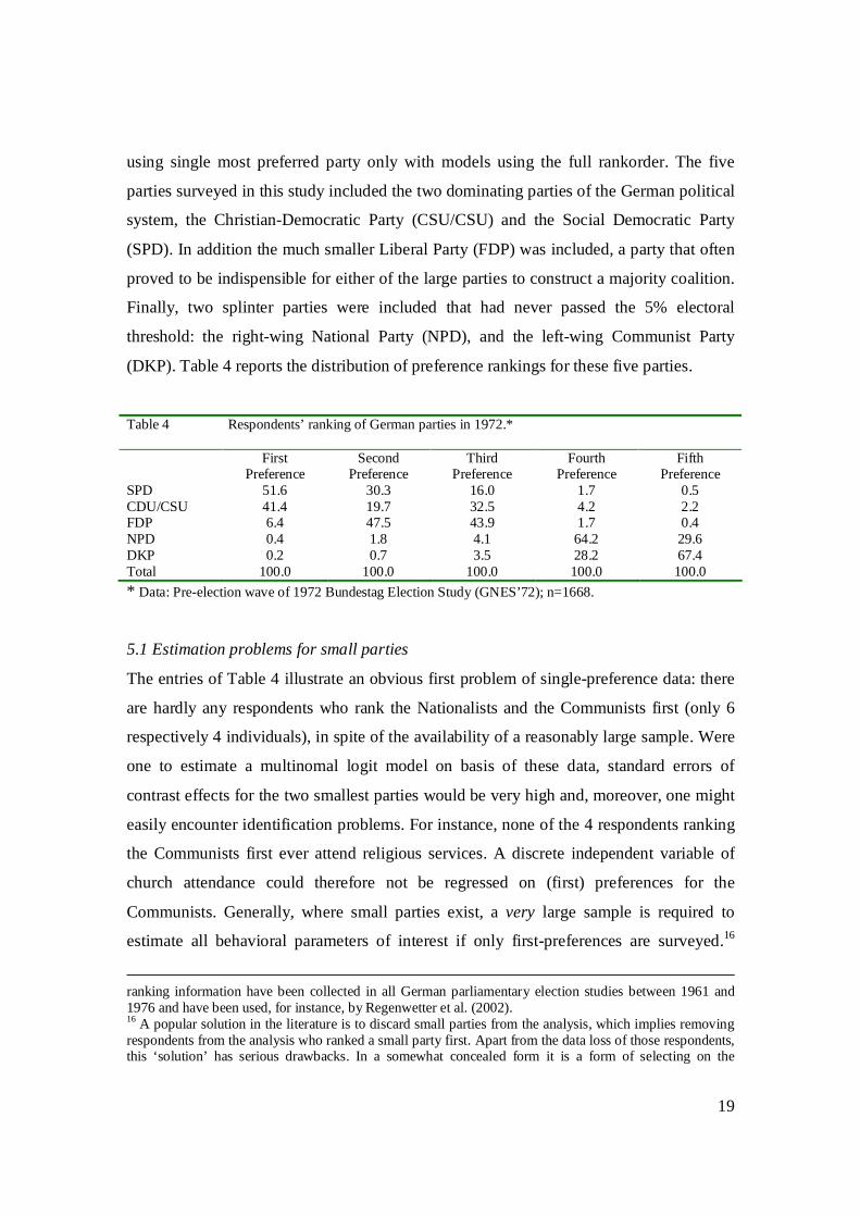
using single most preferred party only with models using the full rankorder. The five

parties surveyed in this study included the two dominating parties of the German political

system, the Christian-Democratic Party (CSU/CSU) and the Social Democratic Party

(SPD). In addition the much smaller Liberal Party (FDP) was included, a party that often

proved to be indispensible for either of the large parties to construct a majority coalition.

Finally, two splinter parties were included that had never passed the 5% electoral

threshold: the right-wing National Party (NPD), and the left-wing Communist Party

(DKP). Table 4 reports the distribution of preference rankings for these five parties.

Table 4 Respondents’ ranking of German parties in 1972.* First

Preference Second

Preference Third

Preference Fourth

Preference Fifth

Preference SPD 51.6 30.3 16.0 1.7 0.5 CDU/CSU 41.4 19.7 32.5 4.2 2.2 FDP 6.4 47.5 43.9 1.7 0.4 NPD 0.4 1.8 4.1 64.2 29.6 DKP 0.2 0.7 3.5 28.2 67.4 Total 100.0 100.0 100.0 100.0 100.0

* Data: Pre-election wave of 1972 Bundestag Election Study (GNES’72); n=1668.

5.1 Estimation problems for small parties

The entries of Table 4 illustrate an obvious first problem of single-preference data: there

are hardly any respondents who rank the Nationalists and the Communists first (only 6

respectively 4 individuals), in spite of the availability of a reasonably large sample. Were

one to estimate a multinomal logit model on basis of these data, standard errors of

contrast effects for the two smallest parties would be very high and, moreover, one might

easily encounter identification problems. For instance, none of the 4 respondents ranking

the Communists first ever attend religious services. A discrete independent variable of

church attendance could therefore not be regressed on (first) preferences for the

Communists. Generally, where small parties exist, a very large sample is required to

estimate all behavioral parameters of interest if only first-preferences are surveyed.16

ranking information have been collected in all German parliamentary election studies between 1961 and 1976 and have been used, for instance, by Regenwetter et al. (2002). 16 A popular solution in the literature is to discard small parties from the analysis, which implies removing respondents from the analysis who ranked a small party first. Apart from the data loss of those respondents, this ‘solution’ has serious drawbacks. In a somewhat concealed form it is a form of selecting on the

20

Beggs et al. (1981) note in this respect that one benefit of ranking data of greater depth

lies in the possibility to analyze unpopular choices.

But even if one replaces categorical regressors with metric ones to avoid

identification problems when analysing small parties, standard errors of effect parameters

pertaining to these parties will nonetheless be highly inflated. Table 5 illustrates this. This

table presents parameter estimates of two models, a conditional/multinomial logit model

and a rank-order logit model. Both models contain three explanatory variables.

Frequency of church attendance represents the religious cleavage, income represents the

class cleavage, and age of respondents represents the generational rift at the time of the

1972 election. The SPD is chosen as reference category in both models and effect

parameters thus indicate contrasts to this reference. From a substantive point of view, the

two models tell the same story: The Christian-Democrats and the Liberals attract the most

wealthy respondents, the Communists the least religious voters, the Christian Democrats

the most religious ones, and the Nationalists have relatively old supporters. But for the

purposes of this paper the standard errors of the estimates are more interesting. In the

multinomial/conditional logit model (using only first preference data) the standard errors

of the parameters of the independent variables are some 4 to 8 times larger for the two

small parties (NPD, DKP) than for the other three. This illustrates empirically the main

finding from the simulations: efficiency of estimates is considerably higher for complete

ranking data. This holds particularly for small parties that are almost never ranked first.

dependent variable, that will bias the estimated parameters of independent variables. For further discussion and empirical estimates of the extent of such bias in a particular case see van der Eijk et al. (2006).

21

Table 5 Discrete Choice Models of Electoral Preferences for Single-Preference and Ranking Data (GNES’72). Conditional Logit Model Rank-Order Logit Model SPD as Reference Category CDU -3.280 (0.318) -4.452 (0.288) CDU×Church 0.448 (0.036) 0.566 (0.032) CDU×Income 0.121 (0.028) 0.159 (0.026) CDU×Age 0.016 (0.004) 0.021 (0.003) FDP -3.835 (0.577) -2.586 (0.261) FDP×Church 0.090 (0.066) 0.116 (0.029) FDP×Income 0.229 (0.055) 0.089 (0.024) FDP×Age 0.002 (0.007) 0.017 (0.003) NPD -8.133 (2.343) -4.850 (0.427) NPD×Church -0.293 (0.296) 0.060 (0.049) NPD×Income 0.393 (0.215) 0.000 (0.041) NPD×Age 0.032 (0.026) 0.018 (0.005) DKP -1.180 (2.750) -4.445 (0.454) DKP×Church -0.707 (0.511) -0.091 (0.053) DKP×Income 0.107 (0.295) 0.026 (0.045) DKP×Age -0.092 (0.055) 0.001 (0.006) N 1668 1668 Log Likelihood 1404.7 4468.9

5.2 The Independence of Irrelevant Alternatives Assumption

The implausibility of the independence of irrelevant alternatives (IIA) assumption is

probably the most commonly cited objection against discrete choice models. This

assumption pertains to both the multinomial/conditional logit model and the rank order

logit model (McFadden 1973; Hausman McFadden 1984). The assumption holds that the

unobserved utilities are uncorrelated over choice alternatives, and that they have equal

variances for all alternatives. The IIA assumption enables a convenient form for the

choice probability and thus reduces computational costs considerably. In fact, IIA ensures

that the rank order logit model can be expressed as the product of consecutive

multinomial/conditional logit models (Beggs et al. 1981).

In electoral research, several scholars have argued that the IIA assumption is

unlikely to hold empirically for single-preference data (e.g., Alvarez & Nagler 1998) or

to the extent that voter groups exist that are positively attracted to several parties at the

22

same time (van der Brug et al 2007: 36). Probit models are often seen as a relevant

alternative as they permit the researcher to model correlations across alternatives in the

unobserved utilities in the full covariance matrix. However, they are computationally

more demanding than logit models. Moreover, as Glasgow (2001) points out, the

assumption of the unobserved factors being jointly normally distributed is likely to be

violated for electoral utilities. Mixed logit models are therefore a better alternative, as

they allow the unobserved utilities to be correlated across parties and to follow any

distribution (e.g., Train 2003). In other words, the IIA assumption can be avoided by

using computationally more intensive procedures than the standard

conditional/multinomial logit model.17

The implausibility of the IIA assumption extends also to electoral preferences

beyond first preference only. For such data, multinomial/conditional probit and rank-

order probit models (Hajivassiliou & Ruud 1994) do not assume IIA (but they do assume

multivariate normality), while mixed rank-ordered logit models (Calfee et al. 2001; Train

2003) provide complete freedom of specific distributional and correlational

assumptions.18 Thus, the IIA assumption can be avoided for first-preference as well as for

more extensive preference ranking data in basically the same way. (but see footnote 17).

Multinomial/conditional probit, rank-order probit and mixed logit models make it

also possible to model heterogeneity in effect parameters. However, all these methods

require some distributional assumption of random effects, while they also

computationally demanding. When using rank-order logit models, however, no

distributional assumption or computationally intense techniques are required if one is

interested in heterogeneity of effects (i.e., in order to model inter-individual differences

of effects). Beggs et al. (1981) demonstrated that effect parameters of party attributes can

be estimated for each respondent individually in rank-order models as long as the number

of heterogeneous effects is smaller than the number of ranked parties.

17 A yet unresolved problem is that these models are prone to problems of non-convergence. 18 Rank-order logit models are not limited to single random samples can be used in various settings. For instance, rank-order models exist for panel data (Dagsvik & Liu 2006) and hierarchical data in general (Skrondal & Rabe-Hesketh 2003).

23

5.3 Are respondents able to rank-order parties?

A concern that has already been voiced in early papers on rank-order logit models is

whether respondents are able to provide ranking if there are many choice alternatives

(Chapman & Staelin 1982; Hausman & Ruud 1987). Respondents may be unable to

complete such a task because of unfamiliarity with all alternatives. Alternatively, they

may be unmotivated to order multiple unattractive options. Respondents may lose

concentration when there are many options to be ordered. Ben-Akiva et al. (1992)

suggest that problems of motivation and ordering may not pertain to strongly disliked

parties, but rather for intermediate parties that are neither strongly liked nor despised. As

far as we know, no rigorous studies have been conducted into the conditions under which

these potential problems actually occur.

If respondents would be less attentive in ranking least preferred parties, this will

generate heteroscedasticity, which results in a downward bias of parameter estimates.19 In

order to avoid such problems, Chapman and Staelin (1982) suggested to only use the first

few preferences and ignore lower ones. The choice of the ‘appropriate’ cutoff point may

be based on likelihood ratio tests that indicate when model fit deteriorates significantly

due to additional ranking information. Hausman and Ruud (1987) make a similar

suggestion using Hausman tests. Yet another way to deal with potential heterogeneity of

error for different ranks is to estimate a weighted rank-order logit model in which less

weight is given to the lower preference rankings (Hausman and Ruud 1987).

Van Ophem et al. (1999) suggest a procedure to collect preference rankings that is

meant to increase the efficiency of discrete choice models while limiting the response

burden. In a first step, respondents are asked to choose the 50 percent of the alternatives

that they prefer most, in a second step, they select from this group the 50 percent

alternatives that again is most preferred, and only in the final step are respondents asked

to rank order the alternatives from the most preferred 25 percent. The resulting data can

be analyzed with van Ophem et al.’s (1999) multichoice logit model.

The solutions to error heterogeneity by rank that are proposed by Chapman and

Staelin (1982), Hausman and Ruud (1987) and van Ophem et al. (1999) have all in

19 Hausman & Ruud (1987) point out that, even if parameters would be biased downwardly, the ratio of parameters may still be correct irrespective of heteroscedastity caused by different levels error variance at different ranks.

24

common that they apply the same restrictions to all respondents. In contrast, van Dijk et

al. (2007) recognize that the ranking ability may differ across respondents. They therefore

suggest to model unobserved heterogeneity in respondents’ ranking ability in form of a

latent class rank-order logit model (van Dijk et al. 2007), in which the capability of

respondents to perform the ranking task is endogenous to the ranked preferences

themselves.

It is not often recognised that differences in error variance at different ranks of

preference (or between different groups of respondents, or for different parties) also

affect standard discrete choice models of first preferences. Chua & Fuller (1987) and

Hausman et al. (1998) suggest procedures to correct for error heterogeneity in the case of

single preference data. To the extent of our knowledge these procedures have never been

used in electoral studies, in spite of the wealth of random utility applications on the basis

of first preference data. In conclusion, for first electoral preferences as well as for more

extensive observations of preference rankings a variety of procedures exist to test for, and

to correct for the potential biasing effects of heterogeneity of error. To the extent that

such heterogeneity is located in depth of preference rankings, the identification of the

nature of this heterogeneity could be used to determine the optimal depth for a given

political system, so that it would not be necessary to collect full preference rankorder

data. Alternatively, if full rankorders are available one could ignore the biasing parts

thereof (following Hausman and Ruud), or explicitly model them (van Dijk et al.)

Yet, one may wonder how likely these problems are in electoral research. The

discussion of these problems in the literature was primarily motivated by applications in

market research where respondents were requested to provide preference rankorders for

very large sets of products, many of which are conceivably unknown to many

respondents. In many electoral contexts, however, the set of parties is smaller,20 and in

stable party systems cumulative learning allows most voters to become familiar with the

20 Nevertheless, in most countries ballots contain parties which are entirely unknown to most voters, and which generally win hardly any votes. In PR systems such as the Netherlands and Italy, the number of parties on the ballot can easily exceed 30 –of which less than 15 have any chance of winning seats in parliament. Even in US presidential elections the number of candidates for President may approach 10 in some states.

25

various parties.21 In the 1972 German election data, the very large majority of

respondents had no problems at all with the ranking task.

6. Costs and trade-offs

The simulations and empirical analyses presented in the previous sections lead to a single

and simple conclusion: asking more electoral preference questions in voter surveys than

only ‘what party did you vote for’ is the basis for dramatically increasing the efficiency

of empirical models of electoral preference and choice. Yet, in most surveys

questionnaire space is a scarce and costly commodity, and proposals to add more

preference questions have to compete with other proposals, which commonly involve

more extensive measurement of independent variables. In view of the long-standing

neglect for the measurement of the dependent variable in election studies, our default

expectation would be that requests for asking additional electoral preference questions

would tend to lose out in this competition. In our view, that would be unfortunate and it

would continue the discipline’s disregard for its ‘core’ business should be.22

There is, however, an argument that advocates of more extensive measurement of

electoral preferences could use that would not only increase their chances of being

successful, but even to acquire the warm support of proponents of competing

questionnaire proposals. Increased efficiency (in terms of smaller standard errors of

parameter estimates) implies that the same precision as would be obtained from only the

measurement of first-preferences, can be obtained with a smaller sample.

Since sample size and sampling error are related (in a non-linear fashion), the

required number of respondents to achieve some level of accuracy can often be

dramatically reduced if more extensive preference ranking data are available. For

instance, exactly the same precision that would be obtained from a sample of 1000

21 There are two interesting corollaries to the phenomenon of cumulative learning. The first is that young cohorts have had less time to learn and familiarise themselves with the parties on offer. They will thus, ceteris paribus, display higher error variance in their preference rankings. Second, inability to provide preference rankings for all parties may be a real problem for all voters when the party system is in flux, as is often the case in new democracies (cf. the countries of Central and Eastern Europe) or when a party system has recently collapsed (cf. Italy in the years following the implosion of the post-WW2 party system in 1992). 22 For a more elaborate discussion on this topic, see van der Eijk 2002.

26

respondents who are only asked about their first electoral preference could also be

achieved from a sample of 640 respondents if standard errors could be reduced by 20%.23

From Table 3 we know that such a gain in efficiency (and sometimes more) can be

obtained for multinomial as well as for conditional logit models by only adding to the

questionnaire an item about second electoral preference. Particularly in face-to-face and

telephone surveys the marginal costs of additional respondents is far greater than the

marginal costs of additional questionnaire items. In other words: a small reduction in

sample size, would easily pay for more extensive measurement of electoral preferences,

while even still leaving money to spare for extra questions on independent variables.

The apparent win-win situation sketched above might look a bit like

‘arithmethique Hollandaise’.24 Common objections to it would argue that the survey data

to be collected are intended to serve more purposes than only the estimation of

multivariate models of electoral preference. Whether or not that objection would be valid,

depends of course on what the research priorities were that motivated the study in the

first place. In the case of election studies per se it should not be valid, but such a verdict

requires an explicit perspective on their ‘core’ business (see also footnote 22).

7. Conclusion and discussion

The most important conclusions of the previous sections are, first, that voter surveys

should contain more questions about electoral preferences than the ubiquitous first

preference question, and second, that analysts should utilise such additional information

when available. This would greatly enhance the efficiency of empirical models of

electoral preference and choice. The costs for extending questionnaires with the required

small number of additional items could easily be compensated by slightly smaller

samples, which then would still provide more inferential power than if only first

23 The ratio of the standard errors in Table 3 at depth 2 (only first preference) and depth 3 (first plus second preference) gives the increase in efficiency. The square of this ratio times the original sample size gives the sample size that would yield the same inferential precision as the original sample if the additional depth of preference rankings would be available. 24 This derogatory term was coined in 1815, when the area currently known as Belgium was incorporated in the Kingdom of the Netherlands. A new constitution was rejected by a majority of a consultative group of distinguished citizens, but by counting the abstentions as being in favor King William I declared that the constitution enjoyed popular support.

27

preference had been asked. Alternatively, under tight budgets the increased efficiency

could be used to further reduce sample size in order to be able to afford more items on

other variables (usually independent variables), without sacrificing any statistical power

in comparison to a larger sample that would only be asked about first preferences.

These conclusions are of obvious importance for the design of questionnaires in

multi-party systems. In the US context they are of less relevance for the study of

Presidential and Congressional elections, which are overwhelmingly of a 2-party

character, thus not allowing greater depth than 2 in preference orders. In the few

instances, however, that viable 3rd party candidates appear, it would be invaluable to

probe for further electoral preferences than only the first. Moreover, primary elections are

very much like multi-party contests, and analysts of primaries would thus benefit greatly

from such more extended preference measurement.

Great care should be given to the formulation of such additional preference items,

particularly with respect to the focus of preferences. When studying electoral preference

and choice, the questions must be focused on the electoral context and voters choice

process therein, and not on something else. The German data that we used for illustrative

purposes in section 5 contained a preference ranking of parties that was –unfortunately–

worded in terms of sympathy or liking (depending on how one would like to translate the

German text). Yet, for all kinds of reasons it cannot be taken for granted that a ranking in

terms of liking is the same as a ranking in terms of electoral choice. An extensive

comparison of thermometer questions (as used in the American national election studies),

of like-dislikes of political parties (as used in the CSES), and of items explicitly focused

on the context of electoral choice revealed that ‘liking’ and ‘feeling’ are at best

contributing factors to utility, and thus to electoral choice, but they are not the same (van

der Eijk and Marsh 2007).

The efficiency gains that can be made from asking about additional preferences

derive from the increase in the number of observed intra-individual preference

comparisons. As mentioned in section 2, such intra-individual comparisons can also be

obtained from another observational approach than preference rankings, namely asking

respondents to rate (in absolute terms) their electoral preference for each of the parties.

That approach has become popular in European contexts, where it has become a standard

28

component in questionnaires of the European election studies (conducted every 5 years at

the time of the direct elections to the European Parliament), of the Dutch national

election studies, the Irish national election studies, and a variety of other voter studies. In

addition to providing the necessary intra-individual comparisons to enrich analyses of

voters’ choice calculus in much the same way as illustrated in this paper (albeit with the

use of different analytical models),25 the rating approach has been applied successfully

for analyses of electoral competition, and for overcoming analysis problems in

comparative studies, which arise from the unique character of each country’s party

system. Under which conditions which of these two approaches will be more appropriate

or more productive is a topic for further study, but it is abundantly clear that they both

allow analytical, theoretical and empirical progress by providing empirical information

on more intra-individual preference comparisons than would otherwise be available from

first preference questions.

25 As indicated earlier, these ratings can be converted into rankings, which are usually partial rankings owing to ties in the ratinmgs. Yet, the typical depth of preference rank information that would be obtained in this way is between 3 and 4 for the member states of the EU. As can be gauged from Table 3, such depth of preferential information will yield most of the efficiency gains that would accrue from full rankings.

29

8. References

Alvarez, R. Michael and Jonathan Nagler. 1998. When Politics and Models Collide:

Estimating Models of Multiparty Elections. American Journal of Political Science

42: 55-96.

Beggs, S., S. Cardell, and J. Hausman. 1981. Assessing the Potential Demand for Electric

Cars. Journal of Econometrics 16: 1-19.

Calfee, J., C. Winston, and R. Stempski. 2001. Econometric Issues in Estimating

Consumer Preferences From Stated Preference Data: A Case Study of the Value

of Automobile Travel Time. The Review of Economics and Statistics 83: 699-707.

Chapman, R. and R. Staelin. 1982. Exploiting Rank Ordered Choice Set Data Within the

Stochastic Utility Model. Journal of Marketing Research 19: 288-301.

Chua, T. and W. Fuller. 1987. A Model for Multinomial Response Error Applied to

Labor Flows. Journal of the American Statistical Association 82: 46-51.

Croon, Marcel A. 1989. Latent Class Models for the Analysis of Rankings. In Geert De

Soete, Hubert Feger and Karl C. Klauer (eds). New Developments in

Psychological Choice Modeling. Amsterdam: Elsevier, 99–121.

Dagsvik, J. and G. Liu. 2006. A Framework for Analyzing Rank Ordered Panel Data with

Application to Automobile Demand. Discussion Papers 480. Research Department

of Statistics Norway.

Downs, A. 1957. An Economic Theory of Democracy. New York: Harper and Row..

Fieldhouse, E., A. Pickles, N. Shryane, J. Johnson and K. Purdam. 2006. Modeling

Multiparty Elections, Preference Classes and Strategic Voting. CCSR Working

Paper.

Frey, B. S. and S. Alois. 2002. What Can Economists Learn from Happiness Research?

Journal of Economic Literature 40: 402-435.

Glasgow, G. 2001. Mixed Logit Models for Multiparty Elections. Political Analysis 9:

116-136.

Hajivassiliou, V. and P. Ruud. 1994. Classical Estimation Methods for LDV Models

using Simulation. In R. Enle and D. McFadden (eds.). Handbook of Econometrics,

Vol. 4. Amsterdam: Elsevier.

30

Hausman, J. 1978. Specification Tests in Econometrics. Econometrica 46: 1251-1271.

Hausman, J. and P. Ruud. 1987. Specifying and Testing Econometric Models for Rank-

Ordered Data. Journal of Econometrics 34: 83-104.

Hausman, J., J. Abrevaya, and F. Scott-Morton. 1998. Misclassification of the Dependent

Variable in a Discrete-Response Setting. Journal of Econometrics 87: 239-269.

Hensher, D. J. louviere and Swait, J. 1999. Combining sources of preference data.

Journal of Econometrics 89: 197-221.

Koop, G. and D. Poirier. 1994. Rank-Ordered Logit Models: an Empirical Analysis of

Ontario Voter Preferences. Journal of Applied Econometrics 9: 369-388.

Luce, R. Duncan. 1959. Individual Choice Behavior: A Theoretical Analysis. New York:

Wiley.

Luce, R. Duncan and Patrick Suppes. 1965. Preference, Utility, and Subjective

Probability. In R. Duncan Luce, Robert Bush, and Eugene Galanter (eds.).

Handbook of Mathematical Psychology, Vol. 3. New York: Wiley.

Manski, C. 1977. The Structure of Random Utility Models. Theory and Decision 8: 229-

254.

Marden, J. I. 1995. Analyzing and Modeling Rank Data. London: Chapman & Hall.

McFadden, D. 1974. The Measurement of Urban Travel Demand. Journal of Public

Economics 3: 303-328.

Merino-Castello, A. 2003. Eliciting Consumers Preferences Using Stated Preference

Discrete Choice Models: Contingent Ranking versus Choice Experiment. UPF

Economics and Business Working Paper No. 705.

Regenwetter, M., J. Adams and Grofman Bernard. 2002. On the (Sample) Condorcet

Efficiency of Majority Rule: An Alternative View of Majority Cycles and Social

Homogeneity. Theory and Decision 53: 153-186.

Skrondal, Anders and Sophia Rabe-Hesketh. 2003. Multilevel Logistic Regression for

Polytomous Data and Rankings. Psychometrika 68:267–287.

Thurstone, L.L. 1927. A Law of Comparative Judgement. Psychological Review 34 :

278-286.

Train, Kenneth E. 2003. Discrete Choice Methods with Simulation. Cambridge:

Cambridge University Press.

31

Van der Brug, Wouter , van der Eijk, Cees and Franklin, Mark. 2007. The Economy and

the Vote – Economic Conditions and Elections in Fifteen Countries. Cambridge:

Cambridge University Press

Van der Eijk, C. 2002. Design Issues in Electoral Research: Taking Care of (Core)

Business. Electoral Studies 21: 189-206.

Van der Eijk, C., W. van der Brug, M. Kroh and M. Franklin. 2006. Rethinking the

Dependent Variable in Voting Behavior — on the Measurement and Analysis of

Electoral Utilities. Electoral Studies 25: 424-47.

Van Dijk, Bram, Fok, Dennis, and Richard Paap. 2007. A Rank-Ordered Logit Model

with Unobserved Heterogeneity in Ranking Capabilities. Discussion Paper.

Erasmus University Rotterdam.

Van Ophem, H., P. Stam, and B. van Praag. 1999. Multichoice Logit: Modeling

Incomplete Preference Rankings of Classical Concerts. Journal of Business &

Economic Statistics 17: 117-128.