Utah State University Utah State University

DigitalCommons@USU DigitalCommons@USU

All Graduate Theses and Dissertations Graduate Studies

12-2017

Measurement of Agriculture-Related Air Pollutant Emissions Measurement of Agriculture-Related Air Pollutant Emissions

using Point and Remote Sensors using Point and Remote Sensors

Kori D. Moore Utah State University

Follow this and additional works at: https://digitalcommons.usu.edu/etd

Part of the Civil and Environmental Engineering Commons

Recommended Citation Recommended Citation Moore, Kori D., "Measurement of Agriculture-Related Air Pollutant Emissions using Point and Remote Sensors" (2017). All Graduate Theses and Dissertations. 6907. https://digitalcommons.usu.edu/etd/6907

This Dissertation is brought to you for free and open access by the Graduate Studies at DigitalCommons@USU. It has been accepted for inclusion in All Graduate Theses and Dissertations by an authorized administrator of DigitalCommons@USU. For more information, please contact digitalcommons@usu.edu.

MEASUREMENT OF AGRICULTURE-RELATED AIR

POLLUTANT EMISSIONS USING POINT

AND REMOTE SENSORS

by

Kori D. Moore

A dissertation submitted in partial fulfillment of the requirements for the degree

of

DOCTOR OF PHILOSOPHY

in

Civil and Environmental Engineering

Approved:

______________________________ ________________________________ Randal Martin, Ph.D. David Stevens, Ph.D. Major Professor Committee Member

______________________________ ________________________________ Rhonda Miller, Ph.D. Jiming Jin, Ph.D. Committee Member Committee Member

______________________________ ________________________________ Michael Wojcik, Ph.D. Mark R. McLellan, Ph.D. Committee Member Vice President for Research and

Dean of the School of Graduate Studies

UTAH STATE UNIVERSITY Logan, Utah

2017

ii

Not Copyrighted

Data collection funded by the Agriculture Research

Service, United States Department of Agriculture

iii

ABSTRACT

Measurement of Agriculture-Related Air Pollutant

Emissions using Point and Remote Sensors

by

Kori D. Moore, Doctor of Philosophy

Utah State University, 2017

Major Professor: Dr. Randal S. Martin Department: Civil and Environmental Engineering

Measuring air pollution emissions from agricultural sources is complicated by

their size and variability. Traditional point sensors may not adequately characterize

plumes as variability in the plume transport may affect which sensors are impacted.

Remote sensors, such a scanning light detection and ranging (lidar) system, provide

advantages due to their large sampling volumes, temporal resolution, and spatial scales.

Both point and remote sensors were used to characterize plumes and estimate

emissions from multiple agricultural operations. The purposes of this work were to

further develop methodologies for measuring agricultural air pollution emissions and to

report emissions for several varying types of operations.

The body of this dissertation is comprised of five chapters, where each chapter is

a separate paper submitted for publication in a peer-reviewed journal. Their topics

iv

include: an in-depth discussion of the mass conversion factor used to convert optical

measurements, such as backscatter lidar, to particulate matter (PM) mass

concentrations; calculating the PM emissions control efficiency of two conservation

management practices (CMP) over the traditional management practices using lidar,

particle size distribution, and filter-based PM data; the use of passive diffusion sampler

and open path-Fourier transform infrared spectrometer measurements to estimate

ammonia (NH3) emissions from an open-lot dairy; and the development, initial testing,

and first application of a backwards Lagrangian stochastic (bLS) dispersion model for use

in inverse modeling that allows particle behavior to deviate from the surrounding flow.

These papers contribute to emissions measurement methodologies for area

sources through the publication of the deposition-enabled bLS tested for near-source

inverse modeling and its impact on emissions estimates, the lidar-based methods used

in the tillage CMP studies, and the use of a scanning OP-FTIR system to measure NH3

levels downwind of a dairy. Calculated emissions were published for multiple tillage

activities, resulting in CMP reductions ranging from 25% to 90% over traditional

practices. Summer time emissions of NH3 from an open-lot dairy and PM10 from a beef

feedlot were calculated through inverse modeling and were similar to summer

emissions found in literature. Including particle behavior in the bLS increased PM10

emissions by 8-20% over the diurnal cycle.

(332 pages)

v

PUBLIC ABSTRACT

Measurement of Agriculture-Related Air Pollutant

Emissions using Point and Remote Sensors

Kori D. Moore

Measuring air pollution emissions from agricultural activities is usually difficult

because of their large area and variability. Traditional air quality sensors, called point

samplers, measure conditions in one location, which may not adequately measure a

plume. Remote sensors, instruments that measure pollution along a line rather than at a

single point, are better able to measure conditions around large areas. This dissertation

reports on four agricultural air emissions studies that used both point and remote

sensors for comparison. The methods used to calculate the emissions are based on

previous work and are further developed in these studies. In particular, an atmospheric

dispersion model was developed and tested that can account for a particle behaving

different than the surrounding gas due to gravity and inertia and depositing out of the

flow. Particulate matter (PM) emissions values are reported for two agricultural tillage

conservation management practices (CMPs) and the corresponding traditional tillage

methods in order to determine how well the CMP reduces emissions. In addition, gas-

phase ammonia (NH3) emissions for a dairy operation and PM emissions from a feedlot

operation are reported. These studies can help us better measure emissions from

agricultural operations and understand how much air pollution is being emitted.

vi

ACKNOWLEDGMENTS

I thank the Utah State University Research Foundation, Space Dynamics

Laboratory, Agriculture Research Service, Texas A&M AgriLife Research, and Utah Water

Research Laboratory for providing project funding and additional support. I also thank

the Space Dynamics Laboratory for the SDL Fellowship, as well as the Rocky Mountain

Section of the Air & Waste Management Association for a scholarship.

I wish to thank my committee members, Dr. Randy Martin, Dr. David Stevens, Dr.

Michael Wojcik, Dr. Rhonda Miller, and Dr. Jiming Jin, for their support, comments, and

suggestions throughout this entire process. A very special thank you is in order for my

major professor, Dr. Randy Martin, for his guidance, support, and example.

The following individuals deserve recognition for their support during this work:

Brooke McKenna and Scott Anderson with the Space Dynamics Laboratory; Dr. Gail

Bingham and Dr. Christian Marchant, formerly with the Space Dynamics Laboratory; Jeff

Muhs, formerly with the Energy Dynamics Laboratory; and Dr. Jerry Hatfield and Dr.

John Prueger with the Agriculture Research Service. I would like to acknowledge and

give thanks to the individuals too numerous to name involved in sample collection, data

processing, and support activities, particularly those involved in the long, off-site field

studies. Those field studies would not have been possible without the permission and

support from forward thinking agricultural producers and agricultural advocates.

I would particularly like to thank my wife, Liz, for her continued support, love,

encouragement, and prayers. I also thank our five children, Spencer, Matthew, Olette,

Conrad, and Lucy, for their constant encouragement and love. My family has been key

to my accomplishments. I acknowledge the continued encouragement of extended

family, especially from my parents, Daryl and Treena Moore and David and Becky Cook. I

would also like to thank my friends and peers for their encouragement. I must express

my gratitude towards my Heavenly Father – I am grateful for this blessing and journey.

Kori D. Moore

vii

CONTENTS

Page

ABSTRACT ...........................................................................................................................iii

PUBLIC ABSTRACT .............................................................................................................. v

ACKNOWLEDGMENTS ........................................................................................................ vi

LIST OF TABLES .................................................................................................................... x

LIST OF FIGURES ............................................................................................................... xiii

EXECUTIVE SUMMARY ..................................................................................................... xvi

CHAPTER

I. INTRODUCTION .......................................................................................................... 1

Background .............................................................................................................. 3 Objective .................................................................................................................. 6 Instrumentation ....................................................................................................... 8 Calculating Emissions ............................................................................................ 11 Manuscript Summaries .......................................................................................... 13 Literature Review .................................................................................................. 22 References ............................................................................................................. 25

II. DERIVATION AND USE OF SIMPLE EMPIRICAL RELATIONSHIPS BETWEEN AERODYNAMIC AND OPTICAL PARTICLE MEASUREMENTS ..................................... 32 Abstract ................................................................................................................. 32 Introduction ........................................................................................................... 33 Methodology ......................................................................................................... 35 Results and Discussion ........................................................................................... 47 Summary and Conclusions .................................................................................... 64 Acknowledgments ................................................................................................. 65 References ............................................................................................................. 66

viii

Page

III. PARTICULATE EMISSIONS CALCULATIONS FROM FALL TILLAGE OPERATIONS USING POINT AND REMOTE SENSORS .................................................................... 70 Abstract ................................................................................................................. 70 Introduction ........................................................................................................... 71 Materials and Methods ......................................................................................... 74 Results and Discussion ........................................................................................... 84 Conclusions ............................................................................................................ 98 Acknowledgments ................................................................................................. 99 References ........................................................................................................... 100

IV. PARTICULATE MATTER EMISSIONS ESTIMATES FROM AGRICULTURAL SPRING TILLAGE OPERATIONS USING LIDAR AND INVERSE MODELING ........................... 103 Abstract ............................................................................................................... 103 Introduction ......................................................................................................... 104 Methodology ....................................................................................................... 107 Results and Discussion ......................................................................................... 129 Conclusions .......................................................................................................... 149 Acknowledgments ............................................................................................... 150 References ........................................................................................................... 151

V. AMMONIA MEASUREMENTS AND EMISSIONS FROM A CALIFORNIA DAIRY USING POINT AND REMOTE SENSORS ................................................................................ 157 Abstract ............................................................................................................... 157 Introduction ......................................................................................................... 158 Materials and Methods ....................................................................................... 160 Results and Discussion ......................................................................................... 185 Conclusions .......................................................................................................... 209 Acknowledgments ............................................................................................... 210 References ........................................................................................................... 211

VI. USING A DEPOSITION-ENABLED BACKWARD LAGRANGIAN STOCHASTIC MODEL TO ESTIMATE PARTICULATE MATTER AREA SOURCE EMISSIONS THROUGH INVERSE MODELING ............................................................................................................... 217 Abstract ............................................................................................................... 217

ix

Page

Introduction ......................................................................................................... 218 Model Formulation .............................................................................................. 222 Model Testing ...................................................................................................... 230 Results and Discussion ......................................................................................... 241 Conclusions .......................................................................................................... 257 Acknowledgments ............................................................................................... 259 References ........................................................................................................... 259

VII. CONCLUSIONS ......................................................................................................... 264

VIII. ENGINEERING SIGNIFICANCE .................................................................................. 269

APPENDICES .................................................................................................................... 271

Appendix A: Data ................................................................................................. 272 Appendix B: Journal Copyright Releases ............................................................. 273 Appendix C: Permission-to-Use Letters ................................................................ 280 Appendix D: List of Acronyms and Symbols ........................................................ 296 Appendix E: Vitae ................................................................................................ 303

x

LIST OF TABLES

Table Page

1-1 Major field deployments within the Ag Program. ........................................... 6 2-1 Conditions during each field campaign for which the mass conversion factor (MCF) has been calculated and included in this manuscript. ............. 45 2-2 Statistical measures of the intra- and inter-instrument comparability test datasets (including outliers) conducted in March 2004 and July 2007. .............................................................................................................. 62 3-1 Sample schedule and sample period tillage and meteorological characteristics. ............................................................................................... 76 3-2 Manufacturer, precision, and accuracy information for deployed meteorological instrumentation. .................................................................. 78 3-3 Comparison of average particulate matter (PM) mass concentrations with respective 95% confidence intervals (CI) about the mean as reported by collocated MiniVol PM samplers, optical particle counters (OPCs), and lidar (light detection and ranging) at an upwind and downwind location for the 23 Oct. sample period. ...................................... 90 3-4 Mean emissions rates (ER) ± 95% confidence intervals (CIs) calculated using inverse modeling with AERMOD and filter-based particulate matter (PM) measurements and the mass balance technique applied to PM calibrated lidar data. ........................................................................... 91 3-5 Mean emission factors (EF) ± 95% confidence intervals (CIs) calculated via inverse modeling with AERMOD and filter-based particulate matter (PM) measurements and the mass balance technique with PM calibrated lidar data for each operation, as well as the calculated control efficiencies of the Combined Operations CMP method. .................. 92 4-1 Information for each sample period regarding tillage operations, equipment used, tractor operation time, area worked, and sample time. ............................................................................................................. 111

xi

Table Page 4-2 Manufacturer, precision, and accuracy information for deployed meteorological instrumentation. ................................................................ 116 4-3 Period-averaged meteorological measurements ± 1σ made at the upwind meteorological tower. .................................................................... 131 4-4 Mass conversion factors (MCFs) used to convert optical particle measurements to mass concentrations for each sample day and averaged for the whole campaign............................................................... 136 4-5 Comparison of period average PM mass concentrations as reported by collocated MiniVol filter samplers and OPCs, as well as the adjacent lidar bin, at measurement heights of 9 m agl at upwind and downwind tower locations for the 18 June sample period. ......................................... 144 4-6 Average particulate matter (PM) emission factors and 95% confidence intervals (CI) estimated for the conventional and conservation tillage management practices. ............................................................................... 146 5-1 Animal count, average animal mass, average feed characteristics, and estimated manure and nitrogen excreted for cattle on this dairy during the study period. ......................................................................................... 162 5-2 Meteorological instruments employed in this study. ................................. 169 5-3 Comparison of average meteorological conditions (±1 SD) measured at the dairy from 13-20 June 2008 and at a site in Kings County for the same period, the full month of June 2008, and June from 1998-2007. ..... 187 5-4 Statistics of emission factors (EFs) calculated for both NH3 measurement datasets using the following three optimization procedures: Unconstrained – EF values for pen and liquid manure system (LMS) are unconstrained; Constrained – constraints are imposed on the minimum values for pen and LMS EFs, based on minimum values found in literature; and Sequential – pen EF estimated first from samples impacted only by pens, then the LMS EF is estimated from samples impacted by both pens and LMS. ......................................... 198

xii

Table Page 5-5 Comparison of dairy NH3 emission factors (EFs) estimated from this study with EFs reported in literature. ......................................................... 201 6-1 The dp and the average vs values used in configuration testing of the LS models. ........................................................................................................ 246 6-2 Comparison of feedlot PM10 emissions(QPM10) and surface fluxes calculated in this study with some found in literature. .............................. 256

xiii

LIST OF FIGURES

Figure Page

1-1 The Aglite Lidar with the 532 nm laser beam visible. ..................................... 9 2-1 Scatter plots of data from Vk and PMk for the following values of k: a) 1.0 μm, b) 2.5 μm, c) 10 μm, and d) TSP. ...................................................... 48 2-2 A box and whisker plot of period averaged MCFk values. ............................ 50 2-3 Time series of PM10 concentrations measured immediately downwind of a dairy farm over two days as measured by a collocated MiniVol and OPC. ........................................................................................................ 54 2-4 Example of PM10 concentrations calculated from a single lidar scan through the use of the MCF. ......................................................................... 55 2-5 Comparison of PM2.5 and PM10 concentrations reported by the MiniVols and the respective FRM samplers. ................................................. 60 3-1 Sample layouts for particulate matter (PM) and meteorological measurements made during a) conventional tillage operations in Field A and b) the combined operations conservation management practice operations in Field B. ..................................................................................... 79 3-2 Period-averaged PM10 concentrations (μg m-3) resulting from the tillage activity on 23 Oct. along the vertical downwind lidar scanning plane as a) estimated by lidar (average downwind minus average upwind) and b) predicted by AERMOD using the Lidar-derived emission rate for this sample period. ............................................................................................... 88 3-3 Lidar measured downwind PM10 concentrations (μg m-3) from a single vertical scan on 23 Oct; a tillage plume is seen crossing the lidar scan at a range of 600 m and centered at 50 m above ground level. ....................... 96 4-1 Map of fields under study and the sample layout for each field. ............... 110 4-2 Process diagram for lidar PM calibration algorithm. .................................. 123

xiv

Figure Page 4-3 Wind rose for the hourly averaged wind observations during the days on which samples were collected. .............................................................. 130 4-4 Sample period-averaged upwind and downwind PSDs as measured by OPCs for (a) 17 May, strip-till operation, Field 5, (b) 18 May, chisel operation, Field 4, (c) 5 June, plant operation, Field 4, and (d) 7 June, plant and fertilize operation, Field 5. .......................................................... 134 4-5 Time series of PM10 concentrations as reported by the collocated OPC, MiniVol filter sampler, and lidar at 9 m agl on the downwind side of the tillage activity for the 18 June sample period (14:00 – 16:10). ............ 139 4-6 Lidar-derived PM10 in a time versus distance from the lidar concentration map (top) and a time series average concentration versus distance from the lidar graph (bottom). .......................................... 141 4-7 Image of plumes in a vertical scan on 5 June. ............................................. 142 5-1 Map of dairy pens, storage, and sampling locations. ................................. 163 5-2 Hourly average wind conditions measured at the dairy during the measurement periods, 13-20 June 2008. ................................................... 187 5-3 NH3 concentration (ppbv) measured by both the upwind and downwind OP-FTIR instruments at ~ 2m agl. .............................................. 190 5-4 Estimated diurnal emissions profiles for the pens, liquid manure system (LMS), and the entire facility based on 2 h averaged OP-FTIR data. ............................................................................................................ 207 6-1 Satellite image of the feedlot under study with particle and meteorological measurement locations shown, as well as the facility and pen borders. ......................................................................................... 232 6-2 Measured values for wind speed (u) and direction (θ) and calculated values for shear velocity (u*) and the inverse of Monin-Obukov length (1/L) as 30 min averages throughout the collection period. ...................... 242

xv

Figure Page 6-3 PM10 concentrations measured at the feedlot by the upwind (Site 7) and downwind (Sites 1, 2, 4, and 6) TEOMs as 30 min averages. ............... 243 6-4 (a) Example particle size distributions (PSDs) measured by the OPS at Site 3 averaged over 30 min periods and (b) the PM10 concentration calculated from the OPS PSD measured at Site 3 compared with TEOM PM10 from adjacent sites 2 and 4. ............................................................... 244 6-5 Touchdown and deposition counts as a function of dp for the fLS model and two bLS model runs with different particle release heights (zrel). ............................................................................................................. 247 6-6 Histograms of touchdowns and depositions versus distance from the source volume at [0,0,zrel] for bLS models with zrel = 2.0 m and 0.205 m and the fLS with zrel = 0.205 m for dp = 10 µm and a bin width of 100 m. .......................................................................................................... 249 6-7 The relative fLS (C/QVol)sim values for randomly selected sample periods for particles with dp of (a) 0 µm, (b) 1 µm, (c) 2.5 µm, (d) 5.0 µm, (e) 10 µm, (f) 20 µm, (g) 30 µm, (h) 40 µm, and (i) 50 µm. .............................. 251 6-8 Emission rates (Qm, count) calculated from the (a) fLS and (b) bLS models as applied to the Texas feedlot for a subset of 30 sample periods and assuming a particle concentration of 1.0 particles m-3 for each dp. ........... 252 6-9 Diurnal pattern of calculated Deposition feedlot PM10 emissions (QPM10) and Non-deposition QPM10 as two hour averages (left axis) and the number of QPM10 values in each half hour sampling period throughout the day (right axis). ...................................................................................... 254

xvi

EXECUTIVE SUMMARY

The purposes of the work described in this dissertation were to contribute to the

information on and methodologies for measuring air pollution emissions from large area

sources, specifically targeted toward agricultural facilities but also applicable to other

difficult to characterize area sources, and to provide emissions values for several

different agricultural processes/operations. The size and temporally and spatially

variable nature of these systems can significantly complicate efforts to quantify

emissions. Point sensors may be challenged to adequately represent concentrations

inside large plumes using relatively few sampling points at ground level. Remote

sensors, such the scanning light detection and ranging (lidar) and open-path Fourier

transform infrared spectrometer (OP-FTIR) systems employed herein, have an

advantage due to their large sampling volumes, spatial extents, and temporal

resolution. This work utilizes both point and remote sensors to measure plume

concentrations and estimate emissions from multiple agricultural operations.

The body of this dissertation is comprised of five chapters, where each chapter is

a separate paper that was submitted for publication in a peer-reviewed journal. The first

paper presents an in-depth discussion of the mass conversion factor (MCF) used to

convert optical particle measurements to particulate matter (PM) mass concentrations.

Examples of information gained through its application were provided, including

observations of PM dynamics at finer temporal and spatial scales and greater spatial

xvii

extents. Specifically, vertical PM-calibrated lidar scans mapped the concentrations in

plumes observed above the point sensor array.

The second and third papers utilized PM-calibrated lidar and optical particle

counter data to estimate the emissions control efficiency (η) of two conservation

management practices (CMP) over the traditional management practices. Emissions

were calculated with a mass balance method applied to vertical lidar scans and through

inverse modeling with point sensor data. The first study presented the first known

investigation of reductions from a combined operations CMP, calculating η of 29%, 60%,

and 25% for PM2.5, PM10, and TSP, respectively. The second study examined emissions

from a spring tillage conservation tillage CMP and found η of approximately 90% for

PM2.5, PM10, and TSP, similar to a previous conservation tillage CMP η measurement.

The fourth paper reported an NH3 emissions study of an open-lot dairy in the San

Joaquin Valley (SJV) of California, the first known summer time measurements in that

climate. Concentration measurements were made using multiple passive samplers and a

scanning system to achieve multiple OP-FTIR beam paths in a repeating series. This was

the first known implementation of such a system with OP-FTIR. Emissions were

estimated through inverse modeling with both datasets, yielding 140.7 ± 42.5 g d-1

animal-1 (113.5 ± 34.3 g d-1 AU-1) for the passive sampler data and 199.2 ± 22.0 g d-1

animal-1 (160.8 ± 17.8 g d-1 AU-1) for OP-FTIR data. These values were within the range of

emissions in the literature for an open-lot dairy.

xviii

The fifth manuscript presented the formulation and initial testing of a Lagrangian

stochastic (LS) atmospheric dispersion model for near-field inverse modeling that allows

for a particle’s movement in the air to deviate from the air motion due to settling

velocity and deposition. It is the first publication of a deposition-enabled LS model being

tested in a backward-in-time (bLS) configuration. A bLS has significant computational

and run time advantages over the forward-in-time (fLS) versions for an area source.

Initial evaluation of the modified bLS with a validation dataset yielded good results in a

non-depositional case. In addition, the modified fLS and bLS were applied to a PM

dataset from a commercial feedlot. Testing showed very consistent results between the

two for particle sizes ≤ 20 µm. Using the modified bLS produced PM10 emissions

between 8% and 20% higher than the non-deposition model throughout the diurnal

cycle, with total daily emissions being 12% larger at 62.5 ± 12.4 g animal-1 day-1.

This collection of papers fulfills the purposes of this work to contribute to the

field of emissions measurement methodology for large area sources and publication of

emissions values for various agricultural operations. First-of-a-kind data were published

on the deposition-enabled bLS for near-source inverse modeling, the η of a combined

operations CMP for the fall tillage sequence, the use of a scanning OP-FTIR system to

measure NH3 levels downwind of a dairy, and NH3 emissions from a SJV dairy during

summer. Additionally, the conservation tillage CMP η for spring tillage supported the

findings of the only other known study. PM10 emissions calculated from the feedlot

using the modified bLS were high compared to most in the literature but in line with

xix

another summer time measurement. The ability of the lidar to observe and measure

plumes not well sampled by point sensors or reproduced in the air dispersion model was

demonstrated in both tillage studies.

CHAPTER 1

INTRODUCTION

Over 100 epidemiological studies published over the past 30 years have linked

both short-term and long-term ambient air pollution exposure to a long and growing list

of increased human health and welfare risks, including increased hospitalization and

mortality rates (see Pope, 1989; Dockery et al., 1993; Davidson et al., 2005; Pope and

Dockery, 2006; Qian et al., 2007; Geer et al., 2012; Pope et al., 2013; O’Neal et al., 2017;

Turner et al., 2017; and many others). Exposure to air pollutants can also lead to acute

and chronic effects in animals, plants, and ecosystems. These effects have led

governments worldwide to set ambient concentration (C) and/or exposure limits for

many air pollutants. The limits in the United States are called the National Ambient Air

Quality Standards (NAAQS) and are set by the Environmental Protection Agency (EPA).

Currently, there are NAAQS for particulate matter (PM) with aerodynamic equivalent

diameters (da) ≤ 2.5 µm (PM2.5) and with da ≤ 10 µm (PM10), nitrogen dioxide (NO2),

sulfur dioxide (SO2), ozone (O3), lead (Pb), and carbon monoxide (CO) (EPA, 2017). If

these are exceeded, local air regulatory authorities are required to develop and

implement pollution remediation strategies to reduce concentrations to below the

NAAQS. Among other things, this necessitates a robust understanding of the emissions

(Q) of significant air pollutant sources.

Since the passage of the Clean Air Act in 1970, most anthropogenic pollutant

sources have been investigated and their emissions drastically reduced (Cooper and

2

Alley, 2002). The agricultural sector is one of few air pollution source categories not

highly regulated. However, impacts and potential reductions from agricultural sources

are increasingly being investigated as the cost of emissions reductions in non-

agricultural sectors grow. Agricultural sources of air pollution have been investigated for

their impact on local, regional, and global atmospheric pollution loadings since the

1990s. Studies have documented the following pollutants emitted from various

agricultural sources: particles of various sizes suspended in the air, also referred to as

PM; ammonia (NH3); hydrogen sulfide (H2S); oxides of nitrogen (NOx); oxides of sulfur

(SOx); methane (CH4); carbon monoxide (CO); carbon dioxide (CO2); nitrous oxide (N2O);

and volatile non-methane organic hydrocarbons (NMHCs) (Casey et al., 2006). None of

these pollutants are exclusive to agricultural activities – all are emitted by other

anthropogenic and natural sources.

Agricultural operations, however, may present challenges to determining

emissions generally not found in other air pollution sources. Difficulties arise due to

large spatial extents of the source(s), temporal and spatial variations in emissions, and

influences of meteorological and process conditions on measuring a source’s impact on

air pollutant levels in an often ill-defined plume. Typical approaches that have been

developed for estimating emissions of such large and open sources are the inverse

modeling, flux-gradient profiling, eddy covariance, and flux chamber methods. The first

three use the difference between measurements of upwind and downwind

concentrations and relate that value to emissions through different methods of

3

estimating or measuring the strength of atmospheric mixing. The fourth samples a small

portion of the source surface to measure emissions directly in multiple locations and

assumes the sample locations are representative of the source.

Another complication may arise from the use of point samplers due to their

relatively small sample volume and limited numbers feasibly deployed. Remote sensors,

such as light detection and ranging (lidar) and open path Fourier transform infrared

spectroscopy (OP-FTIR) systems, offer an advantage over point sensors in that they can

measure pollutant concentrations over a much greater volume, distance, and, usually,

time. This allows for a greater characterization of the downwind plume and emissions.

The work described in this dissertation includes developments and applications of

emissions quantification using both point and remote sensors to measure pollutant

levels. In addition, a modified air dispersion model that has not previously been

reported is detailed and tested against both validation and real-world datasets.

Background

The National Research Council (NRC) released a report in 2003 focusing on the

state of the science and future needs in livestock agriculture air pollutant emissions

(NRC, 2003). This document lists 13 findings and sets of recommendations, one of which

highlighted gaps in emissions measurement methodologies:

4

“FINDING 7: Scientifically sound and practical protocols for measuring air concentrations, emission rates, and fates are needed for the various elements (nitrogen, carbon, sulfur), compounds (e.g., ammonia [NH3], CH4, H2S), and particulate matter. RECOMMENDATIONS: • Reliable and accurate calibration standards should be developed, particularly for ammonia. • Standardized sampling and compositional analysis techniques should be provided for PM, odor, and their individual components.” - NRC (2003)

Several research efforts have been carried out in response to the NRC report,

such as the National Agriculture Emissions Monitoring Study (NAEMS, Heber et al.,

2008). A research effort to address the measurement methodology gap began in 2004

by the U.S. Department of Agriculture’s (USDA) Agricultural Research Service (ARS),

Utah State University Research Foundation’s Space Dynamics Laboratory (SDL), and

Utah State University (USU). A portion of the research efforts of this program, referred

to as “the Ag Program”, will be the focus of this dissertation.

SDL entered into a Cooperative Agreement with the ARS with the following

objectives:

“1) Develop new methods and improve existing methods to measure emissions of particulate matter and gases from animal feeding operations; 2) Develop and determine the effectiveness of management practices and control technologies to reduce emissions; and 3) Develop tools to predict emissions and their dispersion across a range of animal production systems, management practices, and environmental conditions.” - Specific Cooperative Agreement, No. 58-3625-4-121

5

SDL and USU have worked to accomplish these objectives in cooperation with the ARS

and under the direction of Dr. Jerry Hatfield, Laboratory Director for the National

Laboratory for Agriculture and the Environment, USDA ARS.

Through the Ag Program, a collection of both point and remote sensors were

assembled into a system capable of measuring PM and gaseous concentrations around

large, open agricultural sources. The main gaseous species of interest was NH3, though

capabilities were tested for NOx and methane (CH4). The PM size fractions the system

was capable of measuring were PM with da ≤ 1.0 μm (PM1), PM2.5, PM10, and total

suspended PM (TSP). These measurement systems were deployed in 12 field studies

between 2005 and 2012, as shown in Table 1-1.

Methods to estimate emissions have been developed or enhanced as part of the

Ag Program efforts and applied to most of the datasets in Table 1-1. One focus of the Ag

Program was to publish these methods and calculated emissions values in peer-

reviewed journals and books in order to contribute to the body of knowledge on

agricultural air pollutant emissions. To date, one book chapter has been published

(Wojcik et al., 2012) and nine papers (Bingham et al., 2009; Marchant et al., 2009, 2011;

Martin et al., 2008; Moore et al., 2013, 2014, 2015a, 2015b; and Zavyalov et al., 2009).

In addition, results from most of these tests have been presented at various scientific

conferences and meetings.

6

Table 1-1. Major field deployments within the Ag Program.

Measurement Period

State Facility/Operation Studied Pollutant(s) Measured

August – September 2005

IA Finishing swine facility PM, NH3

November 2005 UT Research dairy PM, NH3

September – October 2006

CA Almond harvesting PM

December 2006 CA Cotton ginning PM

September – October 2007

ID Wastewater holding ponds on a commercial dairy

NH3

October 2007 CA Fall tillage PM

May – June 2008 CA Spring tillage PM

June 2008 CA Commercial dairy PM, NH3

June 2009 UT Chemical/biological simulant release PM

October 2009 UT Hydrocarbon production wastewater evaporation treatments

PM, NOx, CH4

July 2011 UT Chemical/biological simulant release PM

August 2012 CA Commercial dairy PM

Objective

The objective of this dissertation work is to advance the state of the science

regarding methods to quantify air pollutant emissions from agricultural sources and to

contribute to the body of literature on emissions values. These were accomplished using

Ag Program activities involving both point and remote sensors. Specifically, this work

will demonstrate:

1) the development and/or application of variations on emission measurement

techniques not previously employed in either the Ag Program or by others;

7

2) the establishment of in depth descriptions of the techniques used by the Ag

Program; and

3) the publication of air pollutant emissions from various agricultural activities

in internationally-recognized scientific journals.

The body of this work is a collection of five manuscripts that have been

submitted for publication in scientific journals. Four have already been accepted and

published and the fifth was submitted in April 2017 for consideration. The manuscript

topics include: (1) a detailed description of the relation between the optical and

aerodynamic PM measurement techniques, referred to as the mass conversion factor

(MCF), and examples of how it has been used in Ag Program studies to monitor PM

levels and emissions in greater temporal and spatial scales versus using traditional

sensors; (2) differences in PM emissions between a traditional tillage management

practice and a combined operations conservation management practice (CMP) as

measured in the 2007 fall tillage study; (3) differences in PM emissions between a

traditional spring tillage management practice and a conservation tillage CMP as

measured in the 2008 spring tillage study; (4) dairy NH3 emissions based on NH3

concentration datasets from both point and remote sensing measurement techniques

employed in the 2008 commercial dairy study; and (5) the development and initial

testing of a backward Lagrangian stochastic (bLS) model, including algorithms for size-

dependent deposition, for particles that can be used in estimating PM emission rates

through inverse modeling. Chapters 2 through 6 of this dissertation present the

8

manuscripts as published (papers 1 through 4) or submitted (paper 5). Each contributes

new information on measuring plume concentrations and estimating emissions from

area sources and fulfills at least one stated objective in the Cooperative Agreement.

Instrumentation

This section provides a summary description of the instruments used in the Ag

Program to measure ambient air pollutant levels. The next section describes, generally,

how these measurements have been employed in the emissions calculation techniques.

Each field study utilized a different combination of sensors, configurations, and emission

estimation methodologies, as described in the following chapters.

The signature instrument of the Ag Program is Aglite, a custom-built elastic lidar

system described by Marchant et al. (2009) and shown in Figure 1-1. Aglite emits pulses

of light at three different wavelengths (355 nm, 532 nm, and 1,064 nm) simultaneously

and measures the amount of energy returned to the instrument from the particles and

molecules in the atmosphere, which is referred to as backscatter. Combining

backscatter data from the three wavelengths in a single analysis potentially allows for a

greater understanding of the physical and optical properties of the particles and

molecules in the beam. The lidar return signals were calibrated to PM concentrations

through an algorithm developed as part of the Ag program and described by Zavyalov et

al. (2009). In summary, the algorithm uses particle size distribution (PSD) data to

calibrate the lidar return signal to the PSD and the cumulative particle volume

9

Figure 1-1. The Aglite Lidar with the 532 nm laser beam visible.

concentrations (Vk), up to a particle diameter k. Vk is multiplied by MCFk to yield PMk,

where MCFk is a simple scalar value relating PMk and Vk. This relationship is the subject

of Chapter 2.

The PSDs were measured by battery-powered optical particle counters (OPCs)

(Aerosol Profilers, Model 9712, Met One Instruments, Inc., Grants Pass, OR). These OPCs

have eight size bins with lower bin limits ranging from 0.3 µm to 10.0 μm. An OPC

reports number of particles detected in each size bin over a sample period, usually set at

20 seconds for Ag Program activities. An OPC measures optical diameter (dop) with a

laser, utilizing the same measurement principle as an elastic lidar.

10

MiniVol Portable Air Samplers (Models 4.2 and 5.0, Airmetrics, Eugene, OR) were

used to measure PMk in Ag Program deployments. It is a portable, battery-powered unit

that collects ambient aerosol onto filters; PMk is calculated by measuring mass

accumulation on exposed filters and dividing by the volume of sampled air. Separation

of particles greater than a desired cumulative size k is accomplished by an impactor

plate assembly upstream of the filter. These systems can be configured to measure PM1,

PM2.5, PM10, or TSP.

Gaseous NH3 was measured using both passive samplers and an OP-FTIR. The

passive samplers employed were from Ogawa USA, Inc. (Pompano Beach, FL), which

utilize a filter infused with citric acid to collect gaseous NH3 for analysis through ion

chromatography (IC). The mass of detected NH3 is related to a period-averaged

concentration through the diffusion equations described by Roadman et al (2003).

The OP-FTIR was a monostatic unit manufactured by MDA used to measure NH3

levels within the units beam path (Model ABB-Bomen MB-100, Atlanta, GA, now Cerex

Monitoring Solutions, LLC, Atlanta, GA). A monostatic unit has the source,

interferometer, and detector at one end of the path and a retroreflecting mirror at the

other end to direct the beam back to the detector. A scanning system was designed for

use with this OP-FTIR with multiple retroreflectors in order to determine NH3 levels

along multiple path lines from a single instrument location. Quantification of the path-

length averaged concentration was performed using a partial least squares regression

11

technique with instrument-specific calibration parameters (Griffiths et al., 2009; Shao et

al., 2010).

Meteorological parameters monitored during system deployments include

vertical and horizontal wind speeds, wind direction, temperature, relative humidity, and

incoming solar radiation. This was accomplished through an assortment of

instrumentation that varied slightly between field studies. Specific configurations are

described in each paper.

Calculating Emissions

The pollutant concentration data were used to derive pollutant emission rates

(ERs) and emission factors (EFs). The definition of ER and EF generally vary by operation

type. In the case of the manuscripts, there are two ER and EF definitions utilized. For

those studies estimating emissions from agricultural tillage operations, EFs are

emissions based on a quantity of field processed (e.g., g m-2) and ERs are emissions that

include a time factor (e.g., g m-2 sec-1). In the studies estimating emissions from the

dairy and feedlot operations, EFs are emission values on a per animal or per animal unit

(AU) and per unit time basis (i.e., g d-1 animal-1, kg yr-1 AU-1), while ERs are based on

time but not per animal (i.e., kg d-1, g m-2 sec-1). References to an ER or EF are generic

through this section and do not have a specific set of associated units.

ERs and EFs were calculated in the Ag Program using inverse modeling and a

mass balance method. Inverse modeling uses an initial estimate of the emission rate

12

(Qsim) in an atmospheric dispersion model to predict the resulting downwind

concentration (Csim). The (C/Q)sim ratio is then used in the following equation with the

concentrations measured at the facility to calculate the observed emission rate (Qcalc):

sim

upwinddownwind

calcQC

CCQ

/

. (1-1)

In this equation, Cupwind is subtracted from Cdownwind to determine concentrations

resulting from the source(s). It is this difference that is compared against the modeled

(C/Q)sim ratio because the models do not generally account for Cupwind, unless a

background concentration is explicitly used as an input.

In cases where the dispersion model used yields a proportionally linear response

in Csim to changes in Qsim, the initial estimate of Qsim will not affect Qcalc as the (C/Q)sim

ratio describes the slope of the line relating the two terms and has neither local maxima

nor minima. In cases where the Csim response is not necessarily linear, local maxima or

minima are possible, requiring a wide range of Qsim to be tested.

There were two atmospheric dispersion models used to estimate (C/Q)sim. Most

studies used the American Meteorological Society/US Environmental Protection Agency

Regulatory Model (AERMOD), which is described by Cimorelli et al. (2005) and is a

current EPA-recommended regulatory model. The other model was a bLS model

modified from that described by Flesch et al. (2004) to account for particle settling

velocity (vs) and deposition. The development and initial testing of this model are the

subject of Chapter 6 in this dissertation. Flesch et al. validated their model for emissions

13

estimation through inverse modeling, a test that has not yet been applied to AERMOD

and reported in literature. Application of the model utilized in each emissions

estimation effort is described in the respective chapters.

The second method of calculating area source emissions in the Ag Program was a

mass balance approach applied to the PM-calibrated lidar data. Average upwind levels

were subtracted from those calculated in and around detected plumes in the downwind

vertical scans. The difference was multiplied by the component of the average wind

perpendicular to the vertical scanning plane to calculate the horizontal flux of PM

through the sampling plane. Fluxes were summed across the plane and averaged over

the length of the sample period to determine the net flux of particles through the lidar

measurement area. The emissions were related to the observed operation by dividing

the flux by a characteristic property (i.e., number of cattle on the feedlot). This method

of calculating emissions using lidar is described in detail in Bingham et al. (2009).

Manuscript Summaries

A brief summary of the papers comprising chapters 2 through 6 is provided in

this section, with new contributions to science highlighted. The reader is referred to

each chapter for detailed descriptions of the relevant published literature, the

concentration measurement and emissions estimation methodologies used, the results,

and the conclusions for each study. Note that the manuscripts are not presented in

chronological publication order. The paper describing calculation and use of the MCFk is

14

first to provide a stronger foundation for the two papers using this relationship in

converting lidar data to PMk. The other four papers are listed in chronological order of

data collection. The document styles vary slightly as the journal-specific formats have

been maintained for each paper.

Field studies reported in Chapters 3 through 5 were conducted in California’s San

Joaquin Valley (SJV) and the data reported in Chapter 6 were collected at a commercial

beef feedlot in the panhandle of Texas. Both regions have a very large agricultural

economy (USDA, 2009). The SJV also has a history of air pollution problems tied to

agricultural activities (Battye et al., 2003; Chow et al., 1992, 1993).

The SJV was a non-attainment area for the PM10 NAAQS from 1991 to 2008 (EPA,

1991, 2008). Designation as a non-attainment area requires an area’s air quality

governing body to develop and implement plans to reduce anthropogenic emissions to

the point that ambient pollutant levels meet the NAAQS. In the SJV, rules were put into

place mandating the use of CMPs, but the η of most CMPs were estimated as they had

not previously been measured. The two tillage studies in the SJV were conducted to

quantify η for more CMPs. The NH3 emissions study was conducted because NH3 directly

contributes to PM levels through photochemistry, and such measurements had not yet

been conducted in the summer climate of the SJV (Cassel et al., 2005; Finlayson-Pitts

and Pitts, 1999). The reductions in emissions achieved by various rules contributed

greatly to lowering ambient PM10 below the NAAQS and the change in the SJV’s PM10

status to attainment/maintenance in 2008. However, just one year later it was

15

designated as non-attainment for PM2.5, requiring a PM2.5 attainment plan be created

and implemented (EPA, 2009).

The data collected in the panhandle of Texas was from a 2015 study designed to

test the ability of a backscatter lidar to quantify PM levels in feedlot plumes. After a

successful demonstration, additional funding is being sought for studies to quantify the

η of various CMPs to reduce feedlot emissions.

Chapter 2, Paper #1

Title: Derivation and use of simple empirical relationships between aerodynamic and

optical particle measurements

Journal: Journal of Environmental Engineering

Manuscript Status: Published 2015 (Moore et al., 2015a)

Description: Several instruments measure optical properties of aerosols and use

empirical relationships based on historical data to convert to PM concentrations.

However, differences between the measured aerosol and the historical data aerosol

may significantly bias the reported PM mass-based levels. This paper presented a simple

empirical method internally developed for converting optical measurements to PM for

each individual sample period and locale. This relationship is referred to as the MCF and

was very briefly described in Zavyalov et al. (2009). However, a more in depth discussion

was needed. This paper describes the OPC data treatment, how the MCF is calculated,

what it represents, the potential influential variables it encompasses, and how it has

16

been used to create more temporally and spatially resolved PM level datasets. Issues

and anomalies found while using this approach are discussed. In the Ag Program, the

MCF is necessary to convert the lidar Vk data to PMk, which allows for the quantitative

assessment of particle size-based fluxes and facility/operation emissions. The MCF is

also used to convert OPC Vk into PMk to examine concentration and emissions trends on

a much more temporally resolved scale than is possible with the MiniVols. In addition to

the MCF, this paper also presents results verifying that the MiniVols yield PM

concentrations similar (usually within ±10%) to Federal Reference Method (FRM)

samplers under tested conditions.

Chapter 3, Paper #2

Title: Particulate emissions calculations from Fall tillage operations using point and

remote sensors

Journal: Journal of Environmental Quality

Manuscript Status: Published 2013 (Moore et al., 2013)

Description: A rule targeting reductions in primary PM10 emissions from agricultural

operations in the SJV, Rule 4550, Conservation Management Practices, was adopted in

2004 and required the use of approved CMPs (SJVAPCD, 2006). However, very little

literature data were available concerning the actual reductions from the CMPs for crop

production tillage activities. SDL and ARS partnered with the EPA Office of Research and

Development, National Exposure Research Laboratory to study the η of the combined

17

operations tillage CMP. The η is the decrease in emissions realized by utilization of the

CMP instead of the traditional management practice, relative to the emissions from the

traditional method. The combined operations CMP reduces the number of passes across

the field by combining two or more operations. Calculating η required deriving EF values

for both the conventional tillage management practice and the CMP. Measurements

made in October 2007 yielded η values for the CMP of 29% for PM2.5, 60% for PM10, and

25% for TSP based on lidar data. The filter based dataset was not sufficiently complete

to estimate η. These emissions reduction values were the first available in literature for

the combined operations CMP. Additionally, lidar measurements showed a significant

portion of the plumes were lofted above the point sensors, with some even detached

completely from the surface, and AERMOD did not effectively reproduce these elevated

plumes. This comparison study is the type of test meeting the second objective of the

Cooperative Agreement between ARS and SDL.

Chapter 4, Paper #3

Title: Particulate matter emission estimates from agricultural Spring tillage operations

using lidar and inverse modeling

Journal: Journal of Applied Remote Sensing

Manuscript Status: Published 2015 (Moore et al., 2015b)

Description: A companion study to the Fall tillage CMP study was funded by the San

Joaquin Valleywide Air Pollution Study Agency to examine η from a Spring tillage CMP.

18

Field measurements were collected in May and June of 2008. The selected CMP was the

conservation tillage CMP, which reduces the extent of disturbed soil. The conservation

tillage CMP in this study consisted of three operations totaling three passes across the

field. In comparison, the conventional tillage method had nine different operations

totaling 13 passes. Improper maintenance of the MiniVol sampler size separation

assemblies through the first portion of the study, combined with the short duration,

high intensity dust plumes resulting from the tillage activity, led to the rejection of most

of the downwind filter samples during the May sample periods. Therefore, EFs were

only estimated from filter-based samples for about half of the sample periods. The OPCs

deployed on the downwind side of the fields were not overloaded. The upwind MiniVol

and OPC samples, which were not compromised by the tillage plumes, were used to

calculate daily average MCFk values to convert both downwind OPC and lidar data to

PMk data. The η values calculated based on OPC and lidar data were 85% and 91% for

PM2.5, 87% and 94% for PM10, and 90% and 91% for TSP, respectively. These values were

similar to the only other conservation tillage CMP study in the literature. Like the

previous tillage CMP study, this study directly meets the second objective of the

Cooperative Agreement.

Chapter 5, Paper #4

Title: Ammonia measurements and emissions from a California dairy using point and

remote sensors

19

Journal: Transactions of the ASABE (American Society of Agricultural and Biological

Engineers)

Manuscript Status: Published 2014 (Moore et al., 2014)

Description: A significant portion of the PM2.5 and PM10 in the SJV is ammonium nitrate

(NH4NO3), which is formed through photochemical reactions in the atmosphere

involving NH3, NOx, and other compounds (Chow et al., 1992, 1993; Finlayson-Pitts and

Pitts, 1999). However, only wintertime NH3 emission levels had previously been

estimated under the SJV climactic conditions. The Ag Program conducted a summer PM

and NH3 emissions study on a commercial dairy in the SJV, in part to fill this gap in

knowledge. The passive Ogawa samplers and scanning OP-FTIR system were deployed.

The results of the PM study were published in Marchant et al. (2011). This paper

presents the results of the NH3 measurements and emissions calculations. Significant

improvements to data treatment, modeling inputs, and inverse modeling EF calculation

methodology were made in this paper compared to previous work in the Ag Program.

Also, this constitutes the first NH3 EF study published in peer reviewed literature based

on the scanning OP-FTIR system. A diurnal pattern in downwind NH3 was observed, with

the highest levels reported in the afternoon despite greater mixing and dilution. EFs

averaged 140.5 ± 42.5 g d-1 animal-1 from the passive sampler data and 199.2 ± 22.0 g d-1

animal-1 from OP-FTIR data, which are within the range of summer values from other

studies with similar housing and manure management practices in other locations.

20

Emissions exhibited a diurnal cycle similar to concentrations, with peak afternoon values

at least a factor of 10 higher than observed in the morning.

Chapter 6, Paper #5

Title: Using a deposition-enabled backward Lagrangian stochastic model to estimate

particulate matter area source emissions through inverse modeling

Journal: Atmospheric Environment

Manuscript Status: Submitted, April 2017

Description: Simulation of atmospheric dispersion using most dispersion models,

including AERMOD, assumes the molecule/particle of interest is inert and follows the

behavior of the carrier fluid. However, this assumption does not always hold with large

particles (dp ≥ 5 µm) due to effects of gravitational and momentum forces. Large

particles may have significant vs compared to the vertical wind velocity (w), causing

them to continually decrease in vertical position (z) relative to the associated carrier

fluid, thereby affecting both vertical and horizontal dispersion. In addition, particles may

be removed from the flow through deposition. Accounting for these deviations from the

carrier flow could be important. A type of model called the Lagrangian stochastic model

(LS) was used to account for vs and deposition in near-field (generally < 1,000 m) inverse

modeling.

An LS attempts to mimic atmospheric turbulence by simulating the movement of

marked fluid elements (MFEs) in a domain with known mean flow and by adding

21

random variations to the MFE movement to simulate the stochastic nature of

turbulence (Lin, 2012). Running the LS for thousands of MFEs provides a statistical

representation of the simulated dispersion and yields the (C/Q)sim ratio required to

calculate Qcalc using Eq. 1-1. LS models may be run forward in time (fLS), from the source

to the receptor, or backward in time (bLS), from the receptor towards the source. The

bLS has been shown to be much more computationally efficient than the fLS, often by

an order of magnitude or more. Flesch et al. (2004) validated a bLS model (that does not

take into account vs or deposition) for calculating emissions through inverse modeling.

This model has been used by many researchers to estimate agricultural emissions for

various pollutants in recent years (Bjorneberg et al., 2009; Bonifacio et al., 2013; Flesch

et al., 2009; Todd et al., 2008; Leytem et al., 2011, 2013; Yang et al., 2017; and others).

Others have accounted for vs and deposition in fLS models (Sawford and Guest, 1991;

McGinn et al., 2010; Wang et al., 1995, 2008; etc.), but no bLS accounting for particle

behavior was previously found in literature.

The last paper in this dissertation presents a modified bLS that allows for particle

depositional behavior to be taken into account. It is based on the model of Flesch et al.

(2004) with modifications from several papers on fLS models with vs and deposition. The

non-depositional case of this model (vs = 0.0 m s-1) was tested against a portion of the

validation dataset published by Flesch et al. and found to yield similar results with the

same uncertainty value. The modified bLS and fLS models were compared for a subset

of sample periods from a Texas panhandle cattle feedlot dataset collected in 2015 by

22

Texas A&M AgriLife Research and SDL. The modified bLS yielded slightly higher

emissions values at dp ≤ 20 µm with relative results remaining nearly constant across

sample periods. The modified bLS was assumed to be valid for estimating emissions for

particles with dp < 20 µm, the size range of interest for QPM2.5 and QPM10 (regulated

particle classifications). The modified bLS estimated QPM10 from the full feedlot dataset

at 62.5 g animal-1 day-1 when accounting for vs and deposition, 12% higher than in the

non-depositional case. Significant contributions to the science of measuring emissions

from large area sources include another validation of the bLS for use in estimating

emissions, the description of a modified bLS that can account for vs and deposition for

dp < 20 µm while yielding results consistent with the fLS, and the results of the model’s

first tests.

Literature Review

A literature review is provided in each chapter of the relevant publications. To

avoid duplication, only relevant literature published or found since the papers were

finalized are presented in this section. No additional papers are presented for the

modified bLS paper as it was submitted for publication consideration in April 2017.

No new discussions on the MCF or mass conversion algorithms has been

published recently. However, a conference paper by Shao et al (2016) reported on the

development and testing of an OPC that utilized instrument response at specific angles

relative to illumination to size particles. Particle density was not accounted for in the

23

mass calculation; instead, they focused on better measuring the optical diameter

because the effect of density scales linearly on PM while diameter scales to the third

power. Initial testing with a reference PM2.5 instrument showed very good correlations.

The number of publications on estimates of agricultural tillage emissions remains

small. Only one additional paper was found since Moore et al. (2015b) was published.

Agricultural tillage PM2.5 and PM10 emissions in northeastern China were estimated by

Chen et al. (2017) for planting, harvesting, and a combined operations CMP for spring

tillage. They estimated emissions with the flux profile method described by Holmén et

al. (2001) coupled with optical sensors utilizing a mass conversion algorithm to produce

PM2.5 and PM10 concentrations. Spring tillage CMP emissions ranged from 9 to 119 mg

m-2 for PM10 and 3 to 33 mg m-2 for PM2.5, with lower values associated with higher soil

moisture content. These values were in the same range as those reported for PM2.5 in

Table 4-6 in Chapter 4, but lower for PM10. Reported planting emissions had smaller

ranges than CMP tillage, 4 to 17 mg m-2 for PM10 and 3 to 4 mg m-2 for PM2.5, and were

smaller than those presented in Table 4-6. Harvesting emissions ranged from 18 to 33

mg m-2 for PM10 and 6 to 11 mg m-2 for PM2.5.

A few papers were found and/or published since publication of Moore et al.

(2014) on the topic of NH3 emissions from dairies. First, a very good review was given by

Hristov et al. (2011), covering NH3 sources, emissions mechanisms and processes, and

measurements from both dairy and beef feedlot operations. Included is a table

comparing dairy NH3 emissions from 26 published studies, many of which were not

24

directly listed in Table 5-5 in Chapter 5 from Moore et al., but some were included in the

review performed by Arogo et al. (2006). Only four of the studies listed by Hristov et al.

were from open-lot dairies, the type of facility investigated herein, and all were in Table

5-5. The mean ± 1 standard deviation (σ) for the values in Hristov et al. was 58.8 ± 65.0 g

animal-1 day-1.

An open-lot dairy NH3 emissions study was carried out in the High Plains area of

New Mexico and reported by Todd et al. (2015). They measured summer time NH3 levels

with tunable diode laser systems, and combined them with inverse modeling using

WindTrax to estimate emissions. They found a daily emission of 321 g animal-1 day-1,

higher than most other published studies except Leytem et al. (2013). A contributing

factor was postulated to be the herd at this dairy was entirely mature, which differs

from the study in Chapter 5 that had a mixed herd of calves, heifers, and mature cows.

Todd et al. found pen emissions dominated the total emissions like in Moore et al.,

accounting for 95% of the total emissions.

Yang et al. (2016) reported NH3 emissions measurements from pen surfaces at

two dairies near Beijing, China. The dairies were open-lot with a brick base and had

weekly manure removal. NH3 concentrations were measured using a tunable diode laser

system and emissions were estimated with WindTrax in inverse modeling. They found

average summer time emissions of 210.8 and 177.6 g animal-1 day-1, similar to those

reported in Chapter 5. The yearly averages were 139.7 and 122.1 g animal-1 day-1.

25

Liu et al. (2017) performed a meta-analysis study of NH3 emissions from beef

feedlots and dairy housing. They found positive correlations between both air

temperature and dietary crude protein content and NH3 emissions. They also observed

that the method used to measure emissions could affect the results, with flux chamber

methods usually underestimating emissions and the nitrogen balance method

overestimating them. Another meta-analysis study reported by Bougouin et al. (2016)

found that the greatest factor affecting NH3 emissions from dairy housing was flooring

type, followed by season and diet factors. An open-lot dairy was found to produce the

highest emissions of flooring type.

References

Auvermann, B., R. Bottcher, A. Heber, D. Meyer, C.B. Parnell, B. Shaw, and J. Worley. 2006. “Particulate matter emissions from animal feeding operations.” In Rice, J.M., D.F. Caldwell, and F.J. Humenik (eds.), Animal agriculture and the environment: National Center for Manure and Animal Waste Management white papers, American Society of Agricultural and Biological Engineers, St. Joseph, Michigan, 435-468.

Battye, W., V.P. Aneja, and P.A. Roelle. 2003. Evaluation and improvement of ammonia

emissions inventories. Atmospheric Environment, 37:3873-3883. Bingham, G.E., C.C. Marchant, V.V. Zavyalov, D.J. Ahlstrom, K.D. Moore, D.S. Jones, T.D.

Wilkerson, L.E. Hipps, R.S. Martin, P.J. Silva, and J.L Hatfield. 2009. Lidar based emissions measurements at the whole facility scale: method and error analysis. Journal of Applied Remote Sensing, 3(1); 033510.

Bjorneberg, D.L., A.B. Leytem, D.T. Westermann, P.R. Griffiths, L. Shao, and M.J. Pollard.

2009. Measurement of atmospheric ammonia, methane, and nitrous oxide at a concentrated dairy production facility in southern Idaho using open-path FTIR spectrometry. Transactions of the ASABE, 52:1749-1756.

26

Bonifacio, H.F., R.G. Maghirang, E.B. Razote, S.L. Trabue, and J.H. Prueger. 2013.

Comparison of AERMOD and WindTrax dispersion models in determining PM10 emission rates from a beef cattle feedlot. Journal of the Air and Waste Management Association, 63:545-556.

Bougouin, A., A. Leytem, J. Dijkstra, R.S. Dungan, and E. Kebreab. 2016. Nutritional and

environmental effects on ammonia emissions from dairy cattle housing: a meta-analysis. Journal of Environmental Quality, 45:1123-1132.

Casey, K.D., J.R. Bicudo, D.R. Schmidt, A. Singh, S.W. Gay, R. Gates, L.D. Jacobson, and S.

Hoff. 2006. “Air quality and emissions from livestock and poultry production/waste management systems.” In Rice, J.M., D.F. Caldwell, and F.J. Humenik (eds.), Animal agriculture and the environment: National Center for Manure and Animal Waste Management white papers, American Society of Agricultural and Biological Engineers, St. Joseph, Michigan, 1-40.

Cassel, T., L. Ashbaugh, and R. Flocchini. 2005. Ammonia emission factors for open-lot

dairies: direct measurements and estimation by Nitrogen intake. Journal of the Air and Waste Management Association, 55:826-833.

Chen, W., D.Q. Tong, S. Zhang, X. Zhang, and H. Zhoa. 2017. Local PM10 and PM2.5

emissions inventories from agricultural tillage and harvest in northeastern China. Journal of Environmental Sciences, in press.

Chow, J.C., J.G. Watson, D.H. Lowenthal, P.A. Solomon, K.L. Magliano, S.D. Ziman, and

L.W. Richards. 1992. PM10 source apportionment in California’s San Joaquin Valley. Atmospheric Environment, 26:3335-3354.

Chow, J.C., J.G. Watson, D.H. Lowenthal, P.A. Solomon, K.L. Magliano, S.D. Ziman, and

L.W. Richards. 1993. PM10 and PM2.5 Compositions in California’s San Joaquin Valley. Aerosol Science and Technology, 18:105-128.

Cimorelli, A.J., S.G. Perry, A. Venkatram, J.C. Weil, R.J. Paine, R.B. Wilson, R.F. Lee, W.D.

Peters, and R.W. Brode. 2005. AERMOD: a dispersion model for industrial source applications. Part I: general model formulation and boundary layer characterization. Journal of Applied Meteorology, 44:682-693.

Cooper, D.C., and F.C. Alley. 2002. Air pollution control: A design approach. 3rd ed.

Waveland Press Inc. Prospect Heights.

27

Davidson, C.I., R.F. Phalen, and P.A. Solomon. 2005. Airborne particulate matter and human health: a review. Aerosol Science and Technology, 39:737-749.

Dockery, D.W., C.A. Pope, X. Xu, J.D. Spengler, J.H. Ware, M.E. Fay, B.G. Ferris, and F.E.

Speizer. 1993. An association between air pollution and mortality in six U.S. cities. The New England Journal of Medicine, 329:1753-1759.

Environmental Protection Agency (EPA). 1991. Designations and classifications for initial

PM-10 nonattainment areas. Federal Register, 56(51):11101-11105. EPA. 2008. Approval and Promulgation of Implementation Plans; Designation of Areas

for Air Quality Planning Purposes; State of California; PM-10; Revision of Designation; Redesignation of the San Joaquin Valley Air Basin PM-10 Nonattainment Area to Attainment; Approval of PM-10 Maintenance Plan for the San Joaquin Valley Air Basin; Approval of Commitments for the East Kern PM-10 Nonattainment Area. Federal Register, 73(219):66,759-66,775.

EPA. 2009. Air Quality Designations for the 2006 24-Hour Fine Particle (PM2.5) National

Ambient Air Quality Standards. Federal Register, 74(218):58,688-58,781. EPA. 2017. Criteria Air Pollutants. Last modified: March 10, 2017. Accessed: April 2,

2017. Available: https://www.epa.gov/criteria-air-pollutants. Finlayson-Pitts, B. J. and J. N. Pitts, Jr. 1999. Chemistry of the upper and lower

atmosphere: theory, experiments, and applications. Academic Press, San Diego, California.

Flesch, T.K., J.D. Wilson, L.A. Harper, B.P. Crenna, and R.R. Sharpe. 2004. Deducing

ground-to-air emissions from observed trace gas concentrations: a field trial. Journal of Applied Meteorology, 43: 487-502.

Flesch, T.K., L.A. Harper, J.M. Powell, and J.D. Wilson. 2009. Inverse-dispersion

calculation of ammonia emissions from Wisconsin dairy farms. Transactions of the ASABE, 52:253-265.

Geer, L.A., J. Weedon, and M.L. Bell. 2012. Ambient air pollution and term birth weight

in Texas from 1998 to 2004. Journal of the Air and Waste Management Association, 62:1285-1295.

Grimm, H., and D.J. Eatough. 2009. Aerosol measurement: The use of optical light

scattering for the determination of particulate size distribution, and particulate

28

mass, including the semi-volatile fraction. Journal of the Air and Waste Management Association, 59:101-107.

Griffiths, P.R., L. Shao, and A.B. Leytem. 2009 Completely automated open-path FT-IR

spectrometry. Analytical and Bioanalytical Chemistry, 393:45-50. Heber, A.J., B.W. Bogan, J.‐Q. Ni, T.T. Lim, E.L. Cortus, J.C. Ramirez‐Dorronsoro, C.A.

Diehl, S.M. Hanni, C. Xiao, K.D. Casey, C.A. Gooch, L.D. Jacobson, J.A. Koziel, F.M. Mitloehner, P.M. Ndegwa, W.P. Robarge, L. Wang, and R. Zhang. 2008. The National Air Emissions Monitoring Study: Overview of barn sources. ASAE Paper No. 701P0408. In Proc. 8th International Livestock Environment Symposium, 199‐205. St. Joseph, Mich.: ASABE.

Hinds, W.C. 1999. Aerosol technology: properties, behavior, and measurement of

airborne particles, 2nd ed. Wiley-Interscience, New York, New York. Holmén, B.A., T.A. James, L.L. Ashbaugh, and R.G. Flocchini. 2001. Lidar-assisted

measurement of PM10 emissions from agricultural tilling in California’s San Joaquin Valley – Part I: lidar. Atmospheric Environment, 35:3251-3264.

Hristov, A.N., M. Hanigan, A. Cole, R. Todd, T.A. McAllister, P.M. Ndegwa, and A. Rotz.

2011. Review: Ammonia emissions from dairy farms and beef feedlots. Canadian Journal of Animal Science, 91:1-35.

Leytem, A.B., R.S. Dungan, D.L. Bjorneberg, and A.C. Koehn. 2011. Emissions of

ammonia, methane, carbon dioxide, and nitrous oxide from dairy cattle housing and manure management systems. Journal of Environmental Quality, 40:1383-1394.

Leytem, A.B., R.S. Dungan, D.L. Bjorneberg, and A.C. Koehn. 2013. Greenhouse gas and

ammonia emissions from an open-freestall dairy in southern Idaho. Journal of Environmental Quality, 42:10-20.

Lin, J., D. Brunner, C. Gerbig, A. Stohl, A. Luhar, and P. Webley. 2012. Lagrangian

Modeling of the Atmosphere, Geophysical Monograph Series 200. American Geophysical Union, Washington, DC.

Liu, Z., Y. Liu, X. Shi, J.P. Murphy, and R. Maghirang. 2017. Variations of ammonia

emissions from cattle operations: effects of air temperature and dietary crude protein content. Transactions of the ASABE, 60:215-227.

29

Marchant, C.C., T.D. Wilkerson, G.E. Bingham, V.V. Zavyalov, J.M. Andersen, C.B. Wright, S.S. Cornelsen, R.S. Martin, P.J. Silva, and J.L. Hatfield. 2009. Aglite lidar: A portable elastic lidar system for investigating aerosol and wind motions at or around agricultural production facilities. Journal of Applied Remote Sensing, 3(1):033511.

Marchant, C.C., K.D. Moore, M.D. Wojcik, R.S. Martin, R.L. Pfeiffer, J.H. Prueger, and J.L.

Hatfield. 2011. Estimation of dairy particulate matter emission rates by lidar and inverse modeling. Transactions of the ASABE, 54(4):1453-1463.

Martin, R.S., P.J. Silva, K. Moore, M. Erupe, and V.S. Doshi. 2008. Particle composition

and size distributions in and around a deep pit swine operation. Journal of Atmospheric Chemistry, 59(2), 135-150.

McGinn, S.M., T.K. Flesch, D. Chen, B. Crenna, O.T. Denmead, T. Naylor, D. Rowell. 2010.

Coarse particulate matter emissions from cattle feedlots in Australia. Journal of Environmental Quality, 39:791-798.

Moore, K.D., M.D. Wojcik, R.S. Martin, C.C. Marchant, G.E. Bingham, R.L. Pfeiffer, J.H.

Prueger, and J.L. Hatfield. 2013. Particulate emissions calculations from fall tillage operations using point and remote sensors. Journal of Environmental Quality, 42:1029-1038.

Moore, K.D., E. Young, C. Gurell, M.D. Wojcik, R.S. Martin, G.E. Bingham, R.L. Pfeiffer,

J.H. Prueger, J.L. Hatfield. 2014. Ammonia measurements and emissions from a California dairy using point and remote sensors. Transactions of the ASABE, 57:181-198.

Moore, K.D., R.S. Martin, W.J. Bradford, C.C. Marchant, D.S. Jones, M.D. Wojcik, R.L.

Pfeiffer, J.H. Prueger, and J.L. Hatfield. 2015a. Derivation and use of simple relationships between aerodynamic and optical aerosol measurements. Journal of Environmental Engineering, 141:04014078.

Moore, K.D., M.D. Wojcik, R.S. Martin, C.C. Marchant, D.S. Jones, W.J. Bradford, G.E.

Bingham, R.L. Pfeiffer, J.H. Prueger, and J.L. Hatfield. 2015b. Particulate-matter emission estimates from agricultural spring-tillage operations using LIDAR and inverse modeling. Journal of Applied Remote Sensing, 9:096066.

O’Neal, W.T., E.Z. Soliman, J.T. Efird, V.J. Howard, G. Howard, and L.A. McClure. 2017.

Fine particulate air pollution and premature ventricular contractions: the

30

REasons for Geographic And Racial Differences in Stroke (REGARDS) Study. Environmental Research, 154:115-119.

Pope, C.A. 1989. Respiratory disease associated with community air pollution and a steel

mill, Utah Valley. American Journal of Public Health, 79:623-628. Pope, C.A., and D.W. Dockery. 2006. Health effects of fine particulate air pollution: lines

that connect. Journal of the Air and Waste Management Association, 56:709-742.

Pope, C.A., M. Ezzati, and D.W. Dockery. 2013. Fine particulate air pollution and life

expectancies in the United States: the role of influential observations. Journal of the Air and Waste Management Association, 63:129-132.

Qian, Z., Q. He, H.-M. Lin, L. Kong, D. Liao, N. Yang, C.M. Bentley, and S. Xu. 2007. Short-

term effects of gaseous pollutants on cause-specific mortality in Wuhan, China. Journal of the Air & Waste Management Association, 57:785-793.

Roadman, M. J., J. R. Scudlark, J. J. Meisinger, and W. J. Ullman. 2003. Validation of

Ogawa passive samplers for the determination of gaseous ammonia concentrations in agricultural settings. Atmospheric Environment, 37:2317-2325.

San Joaquin Valley Air Pollution Control District (SJVAPCD). 2006. Conservation

Management Practices Program Report, San Joaquin Valley Air Pollution Control District (SJVAPCD). Available: https://www.valleyair.org/rules/currntrules/r4550.pdf. Accessed: 7 April 2017.

Shao, L., P.R. Griffiths, and A.B. Leytem. 2010. Advances in data processing for open-

path fourier transform infrared spectrometry of greenhouse gases. Analytical Chemistry, 82:8027-8033.

Shao, W., H. Zhang, and H. Zhou. 2016. “A new particle sensor based on true RMS value

measurement,” in Instrumentation and Measurement Technology Conference Proceedings, 2016 IEEE International, New York, New York.

Sawford, B.L., and F.M. Guest. 1991. Lagrangian statistical simulation of the turbulent

motion of heavy particles. Boundary Layer Meteorology, 54:147-166. Todd, R.W., N.A. Cole, R.N. Clark, T.K. Flesch, L.A. Harper, and B.H. Baek. 2008. Ammonia

emissions from a beef cattle feedyard on the southern High Plains. Atmospheric Environment, 42:6797-6805.

31

Todd, R.W., N.A. Cole, G.R. Hagevoort, K.D. Casey, and B.W. Auvermann. 2015.

Ammonia losses and nitrogen partitioning at a southern High Plains open lot dairy. Atmospheric Environment, 110:75-83.

Turner, M.C., A. Cohen, R.T. Burnett, M. Jerrett, W.R. Diver, S.M. Gapstur, D. Krewski,

J.M. Samet, and C.A. Pope. 2017. Interactions between cigarette smoking and ambient PM2.5 for cardiovascular mortality. Environmental Research, 154:304-310.

United States Department of Agriculture (USDA). 2009. 2007 Census of Agriculture:

United States Summary and State Data. AC-07-A-51. Wang, Y., D.R. Miller, D.E. Anderson, and M.L. McManus. 1995. A Lagrangian stochastic

model for aerial spray transport above an oak forest. Agricultural and Forest Meteorology, 76:277-291.

Wang, J., A.L. Hiscox, D.R. Miller, T.H. Meyer, T.W. Sammis. 2008. A dynamic Lagrangian,

field-scale model of dust dispersion from agricultural tilling operations. Transactions of the ASABE, 51:1763-1774.

Wojcik, M.D., R.S. Martin, and J.L. Hatfield. “Using lidar to characterize particles from

point and diffuse sources in an agricultural field,” pp. 299-332, in N.B. Chang (ed.), Environmental Remote Sensing and Systems Analysis. CRC Press, Boca Raton, FL, USA.

Yang, Y., W. Liao, X. Wang, C. Liu, Q. Xie, Z. Gao, W. Ma, and Y. He. 2016. Quantification

of ammonia emissions from dairy and beef feedlots in the Jing-Jin-Ji district, China. Agriculture, Ecosystems and Environment, 232:29-37.

Zavyalov, V.V., C.C. Marchant, G.E. Bingham, T.D. Wilkerson, J.L. Hatfield, R.S. Martin,

P.J. Silva, K.D. Moore, J. Swasey, D.J. Ahlstrom, and T.L. Jones. 2009. Aglite lidar: Calibration and retrievals of well characterized aerosols from agricultural operations using a three-wavelength elastic lidar. Journal of Applied Remote Sensing, 3(1):033522.

32

1 Citation: Moore, K.D., R.S. Martin, W.J. Bradford, C.C. Marchant, D.S. Jones, M.D. Wojcik, R.L. Pfeiffer, J.H. Prueger, and J.L. Hatfield. 2015. Derivation and use of simple relationships between aerodynamic and optical particle measurements. Journal of Environmental Engineering, 141:04014078.

CHAPTER 2

DERIVATION AND USE OF SIMPLE EMPIRICAL RELATIONSHIPS

BETWEEN AERODYNAMIC AND OPTICAL

PARTICLE MEASUREMENTS1

Abstract

A simple relationship, referred to as a mass conversion factor (MCF), is

presented to convert optically-based particle measurements to mass concentration. It is

calculated from filter-based samples and optical particle counter (OPC) data on a daily

or sample period basis. The MCF allows for greater temporal and spatial mass

concentration information than typical filter-based measurements. Results of MCF

calculations from several field studies are summarized. Pairwise comparisons from a

collocated study with multiple OPCs and mass samplers suggest the minimum variability

of the MCF is 5 to 10%. The variability of the MCF within a sample period during a field

study with distributed samplers averaged 17 to 21%. In addition, the precision of the

Airmetrics MiniVol Portable Air Sampler for particulate matter (PM) was found to be

typically < 10%. Comparisons with federal reference method (FRM) samplers showed

that MiniVols yield PM2.5 concentrations essentially equivalent to FRMs with slightly

greater deviations from the FRM for PM10 under tested ambient conditions.

33

Introduction

Many different properties can be used to describe a single particle. These

include shape, chemical speciation, density, index of refraction, aerodynamic diameter,

optical diameter, etc. Numerous measurement techniques have been developed to

quantify various properties, though most are capable of measuring only one or two

properties. Comparisons between simultaneous measurements of an aerosol mixture

made using different techniques may provide valuable information about relationships

between the measurement methodologies and the measured properties, as well as

additional information not measured.

Estimating specific particle properties even from a combination of measurement

techniques may be challenging both theoretically and in practice. For example, Schmid

et al. (2007) provides a detailed explanation of mathematical relationships between

density, shape, effective density, and various equivalent diameters for spherical and

non-spherical particles. Deriving a property from such methods requires significant

investment in equipment, as well as knowledge or assumptions of other pertinent

particle properties. However, comparisons between two or more measurement

techniques may be made in order to derive an empirical relationship that incorporates

all applicable properties into a more simple expression. While this method does not

provide insight into the values of specific properties, it can be very useful in calibrating

the output of a sensor to provide information not directly measured, such as the

34

calibration of an optical particle counter (OPC) to provide particulate matter (PM) mass

concentration. A significant advantage of an OPC over typical filter-based mass samplers

is that the OPC can provide a much more temporally resolved dataset and may yield

valuable information about changes in concentration.

Binnig et al. (2007) describes the calibration of an OPC to yield concentrations of

PM with an aerodynamic diameter (da) ≤ 2.5 μm (PM2.5) for a well-defined aerosol

utilizing known particle density and assuming uniform composition across the size

range. This procedure, however, should not be applied in situations with significant

fractions of particles that are not well-defined, as is often the case in ambient

measurements. Instead, researchers tend to rely on historical data to develop these

empirical relationships for converting optical measurements to PM mass concentrations

(Grimm and Eatough 2009). Several commercially available ambient PM monitors

currently utilize mass conversion relationships based on historical data to report PM

concentrations from optical systems, such as the Aerosol Spectrometer series by

GRIMM Technologies, Inc. (Ainring, Germany), the TSI Inc. DustTrak series (Shoreview,

MN, USA), and the Palas GmbH Fidas System (Karlsruhe, Germany).

The accuracy of PM concentrations calculated from optical data and converted

using relationships based on historical data is strongly influenced by how closely the

properties of the monitored aerosol match the properties of the historical dataset. For

instance, errors in PM estimates at a clean background site, rural site, or a site heavily

impacted by a single source could be significant if the employed PM calibration was

35

created from measurements in an urban area, all of which have different aerosol

sources and, thus, optical properties. Estimating this relationship based on

measurements of the aerosol of interest through an in situ calibration, referred to by

the authors as the mass conversion factor (MCF), can decrease the error due to

dissimilar aerosols. This method may also be used to provide a sample period PM

calibration for instruments that do not have a historical dataset. Zavyalov et al. (2009)

touched very briefly on how the MCF is calculated and potential uses. In this paper we

provide more details on calculating the MCF, present data collected during field

measurements that have been used to calculate MCFs, and give examples of how the

MCFs have been used to estimate PM mass concentrations from optical sensors on finer

timescales than filter-based measurements. In addition, results of multiple comparison

studies between the filter-based PM samplers used in these studies to Federal

Reference Method (FRM) samplers are presented.

Methodology

Instrumentation and Analysis

PM mass concentration data were collected using filter-based MiniVol Portable

Air Samplers from Airmetrics (Eugene, OR, USA). These are portable, battery operated

instruments with programmable sample times. Air is pulled into the sample head at a

nominal flow rate of 5.0 L min-1 where size separation occurs based on particle inertia

through the use of a removable impactor plate assembly. This inertial particle

36

separation method is the same principle as that used in FRM samplers for PM with da ≤

10 μm (PM10) and PM2.5, although the design is different and the collection efficiency

curve of the MiniVol assembly is not as steep as that of the FRM samplers (Hill et al.

1999). The MiniVol can sample PM10, PM2.5, or PM with da ≤ 1 μm (PM1), depending on

the impactor assembly used; total suspended particulate matter (TSP) may be collected

if the impactor assembly is not used. Impaction plates were coated with a thin layer of

high vacuum silicone grease to prevent particles removed from the airstream from

being re-entrained in the sample flow. A filter holder is located downstream of the size

separator to collect particles remaining in the airstream.

Sample flow is not actively maintained at 5.0 L min-1 by the MiniVol. Instead, it is

set using a calibrated rotameter before each run and verified during sample retrieval.

Flow calibrations were conducted yearly and prior to deployment for each instrument

used. The calibration equations and estimated sample period average pressure and

ambient temperature (Tamb) were used to calculate the sample period specific rotameter

settings necessary to achieve a sample flow of 5.0 L min-1. Occasional sampling or

handling irregularities occurred with MiniVol samples, all of which were noted. Any

sample with a noted issue was excluded from further calculations.

Teflon filters 47 mm in diameter were used to collect all samples herein

reported. Filters were pre-conditioned according to the protocols outlined in Title 40,

Part 50, Appendix J of the U.S. Code of Federal Regulations (40 CFR 50 Appendix J). Final

average filter weights for both pre- and post-test were calculated from three stable

37

weights within ±5 µg determined using a microbalance, Type MT5 (Mettler-Toledo, Inc.,

Columbus, OH, USA). Calculated concentration values represent a sample period

average. Balance accuracy was verified every 10 filter measurements using a 1.000 mg

calibration weight.

Aerosol Profilers, Model #9722 (Met One Instruments, Inc., Grants Pass, OR,

USA) were used to measure the optical diameter (dop) of individual particles. These OPCs

measure the amount of light scattered by a particle and compare that quantity to light

scattered by calibration particles of various sizes to determine the particle’s dop.

Measured dop are grouped into eight bins with the following size ranges: 1) 0.3–0.5 µm,

2) 0.5–0.6 µm, 3) 0.6–1.0 µm, 4) 1.0–2.0 µm, 5) 2.0–2.5 µm, 6) 2.5–5.0 µm, 7) 5.0–10.0

µm, and 8) > 10.0 µm. The OPC produces total particle counts per size bin over the

sample period of duration t, ranging from 2 sec to 60 sec. Note that PM mass

concentration calibrations based on historical data have not been developed for these

OPCs. OPC flow measurements, usually made before and after experiments using a soap

bubble displacement system (Gilian Gilibrator2 Calibration System, Sensidyne, LP,

Clearwater, FL, USA), reported that average flow rates (q) ranged from 0.8 to 1.2 L min-1

between OPCs but that the q for a given OPC was very stable. Sampled aerosol was not

preconditioned to control temperature or relative humidity (RH) in measurements

herein reported as they were made in dry climates. However, preconditioning is

suggested as high RH may have substantial effects on particle properties and

measurements, particularly for hygroscopic particles.

38

For a specific OPC (j), number concentration (Nij) per bin (i) is a function of raw

particle counts (pij), the measured average flow rate (qj), and the sample time (t) as

shown in Eq. 2-1.

tq

pN

j

ij

ij

(2-1)

In this equation the units for N are # cm-3, p is number (#), q is cm3 min-1, and t is min.

Inter-calibration of OPC particle counts was performed in post analysis to ensure

comparability between deployment sites. The inter-calibration equations, referred to by

the authors as Counting Correction Factors (CCFs), were calculated based on data

collected either as a collocated group before or after an experiment or, if a collocated

dataset did not exist, from multiple periods over the deployment during which the

source under study was not active and OPCs were measuring a consistent, uniform

background aerosol. As instrument response for each upper bin limit in each OPC must

be factory calibrated individually, so too the CCFs must be calculated for each bin of

each OPC. A CCFij is estimated through comparison of the average particle number

concentration (Ňij) over the identified period with the average particle number

concentration across all OPCs (Ňi). CCFs were applied to all Nij prior to further analysis.

Both scalar and linear function (y = mx + b) CCFs have been found to greatly

decrease inter-instrument variability. As an example, the variability between Ňij prior to

CCF application to a collocated dataset was 18.0%, calculated as the relative standard

deviation (RSD). Application of scalar CCFij values reduced the RSD to 6.8%, and

39

application of linear function CCFs yielded a RSD of 6.5%. Other types of CCF equations

may be used as deemed appropriate.

The volume concentration (V) of sampled particles based on N may be calculated

based on the following simplifying assumptions: 1) the particles are spheres, and 2) the

maximum measured dop is 20 µm. The assumption of a maximum measured dop provides

an upper bound for the largest-sized channel. The geometric mean dop per bin (GMDi)

was selected as the representative diameter of the particles in a given bin i with the

assumption of a log-normal distribution of particle counts. The cumulative V (Vk) up to a

particle diameter k (dk) may be calculated using Eq. 2-2:

k

dnVk

d

0

3 dd)d(6

(2-2)

where n(d) is the number concentration at diameter d. For application to the collected

OPC data, Eq. 2-2 is discretized and expressed in the following terms that have been

previously defined:

ki

i

iik NVdGMD

1

3GMD6

(2-3)

where GMDi is expressed in µm, Ni is in # cm-3, and Vk is in units of µm3 cm-3. In this case,

the Vk definition is similar to PMk concentrations: the total volume of particles whose dop

is ≤ k = 1 μm, 2.5 μm, 10 μm, and ∞ for TSP.

40

MCF Calculations

The MCF is calculated from optical and aerodynamic particle measurements. The

Vk data, as calculated in Eq. 2-3, are averaged over the corresponding MiniVol sample

time. The MCF, with units of density (g cm-3), for each PM size fraction k is calculated as

shown in Eq. 2-4.

k

k

kV

PMMCF

(2-4)

The MCF is typically averaged across sample locations. Note that this MCF is different

from the MCF described by Binnig et al. (2007). Binnig et al. include particle shape factor

and density, which must be supplied by the user. However, this MCF incorporates the

many properties from the particles, the environment, and the measurement techniques

that influence the reported PMk and Vk values without requiring explicit consideration.

Including these factors in the MCF may lead to significantly different values and larger

variability in MCFk across sample periods and instrumentation than other conversion

factors or mean density correction methods report.

Properties of particles that may influence optical and aerodynamic

measurements include, but are not limited to, chemical composition, effective density,

shape, and index of refraction, which are interdependent to varying degrees. Chemical

composition affects both the index of refraction and effective density. As OPC

measurements are influenced by a particle’s index of refraction, differences in indices of

41

refraction between measured ambient and calibration particles may result in significant

differences between a particle’s physical diameter (dp) and dop, leading to potentially

significant differences between calculated and actual V and Vk. The OPC dop sizing

calibrations were performed by the manufacturer with polystyrene latex (PSL) spheres.

These calibrations were used for all sample periods. No attempts were made to

calibrate the OPCs to local aerosol mixtures due to their complex and changing natures.

This may result in positive or negative biases in sizing, with the degree of impact varying

with ambient aerosol dp and chemical composition.

Particle properties also influence filter-based measurements. The MiniVol

impactor assembly separates particles based on da, which is influenced by dp, effective

density, and shape, among other factors. Combining optical and aerodynamic

measurements in calculating the MCF also combines the effects of particle properties,

with varying impacts. For instance, if a particle has a da larger than a MiniVol assembly

cut point but a dop smaller than the lower bin limit of the OPC channel corresponding to

the MiniVol assembly cut point, it may be included in Vk as a smaller particle but not in

PMk, leading to a smaller MCFk. The inverse situation with dop and da may also occur,

resulting in a larger MCFk.

Additional complications may arise from the past and current ambient

environments in which the particle(s) has (have) been suspended. For instance, Tamb

may affect chemical composition as volatile and semi-volatile compounds are found as

both gasses and particles over the typical range of Tamb. Also, some compounds common

42

in ambient particles, such as ammonium sulfate ((NH4)2SO4) and ammonium nitrate

(NH4NO3), readily absorb water at RH conditions above their deliquescence point, which

varies between compounds and with Tamb, and thus increase the particle size and

change the chemical composition (Finlayson-Pitts and Pitts 1999). Effects of Tamb and RH

will be different between optical- and filter-based samplers and may be large,

particularly for hygroscopic particles, depending on the similarity of sample period Tamb

and RH conditions to those used in filter conditioning. The MCF envelops all of these

effects without requiring their quantification.

The sampling properties of the instruments used to measure PMk and Vk also

influence the MCF. One factor is particle aspiration effectiveness, particularly for large

particles. This refers to how well particles of a given size are drawn into the system at

the inlet. It is a strong function of a particle’s inertia and da and the inlet design.

Marchant et al. (2011), based on conversations with Met One Instruments, Inc., stated

that particles with da larger than about 25 μm are not likely to enter the OPC inlet and

that the aspiration efficiency of particles down to 5 μm may be affected at wind speeds

greater than ~3 m s-1. Baldauf et al. (2001) reported that aspiration efficiencies for

MiniVols for particles with da = 10 μm vary from 100% at a wind speed of 1.4 m s-1 to

~70% at a wind speed of 16.7 m s-1.

One factor affecting mass measurement systems is the effectiveness of the size

selection mechanism. The FRM PM10 and PM2.5 size segregation sample heads have

been designed to mimic the particle removal efficiency of the human respiratory

43

system, with most utilizing a particle’s inertia for separation if it is above the designed da

cut point. The removal efficiencies can be represented by an S-curve with some particles

smaller than the targeted cut point being removed, half the particles at the cut point

being removed, and some particles larger than the cut point passing through the

removal mechanism. The MiniVol impactor removal efficiency is designed to be similar

to FRMs, though the slope is not as steep (Hill et al. 1999). Significant particle loading on

the MiniVol impactor plate may lead to particles impacting the surface and returning to

the airstream for collection on the filter. This is known as “particle bounce” and may

result in higher PMk being reported than is actually present. The manufacturer suggests

the use of a thin grease film on the impactor plate as a preventative measure, with a

cleaning and film renewal cycle based on sampling frequency and sampled

concentrations. If cleaning and renewal cycles are too infrequent, particle buildup may

occur and result in particle bounce (Tropp et al. 1998).

MCF values have been calculated from data collected during six field studies

conducted in the San Joaquin Valley (SJV) of California, in the Cache Valley along the

border between Utah and Idaho, and on the Colorado Plateau in eastern Utah.

Measurements were taken during summer and fall seasons between 2007 and 2012

under the meteorological and potential PM source conditions listed in Table 2-1. Field

study average Tamb were above 20 °C during all but one, and average RH values were in

the 30% to 40% range. Maximum RH values were between 60% and 80% and occurred

for short periods of time in early morning when Tamb was lowest. Typical point sensor

44

deployment on these field studies consisted of collocating an OPC with one to four

MiniVol samplers. Sampler inlets were arranged at approximately the same elevation

above ground level (AGL) and within a circle of radius ≤ 1.5 m with a minimum

separation distance between inlets of 0.3 m to prevent interference. Samples were

collected between 2 m and 10 m AGL. MiniVol sample periods ranged from 1 to 24 hr,

depending on sampling objectives, while OPCs recorded data continuously in 20 sec

intervals. Proper maintenance of the MiniVol impactor plate surface was a priority in

each deployment.

MiniVol Accuracy and Precision Tests

Several collocated ambient tests were conducted in which multiple MiniVols and

one or two FRM samplers were deployed to determine the precision and accuracy of the

MiniVols. The FRM instruments used were Anderson Regulated Air Sampler (RAS) units

operated by the authors for PM10, a Partisol Plus Model 2025 Sequential Air Sampler

operated by the State of Utah Division of Air Quality (UDAQ) for PM2.5, and a Partisol

FRM Model 2000 Air Sampler operated by UDAQ for PM10, all of which were

manufactured by Rupprecht and Patashnick Co., Inc. (now Thermo Fisher Scientific, Inc.,

Waltham, MA, USA). All filter samples collected by the authors were conditioned and

weighed as previously discussed. Filter treatment by UDAQ followed established U.S.

National Ambient Air Quality Standards (NAAQS) monitoring protocols. Samples were

45

Table 2-1. Conditions during each field campaign for which the mass conversion factor (MCF) has been calculated and included in this manuscript. Meteorological values are those recorded during sample periods only.

Location Month(s)

& Year Sample Periods

Meteorological Conditions Potential PM Sources References Avg ± SD Min Max

Cache Valley, Utah, USA

July 2007 5 Tamb (°C)

25 ± 7 11 36 Combustion, small

industrial processes, agriculture,

construction, mobile

NA

RH (%)

40 ± 22 12 86

Colorado Plateau, Utah, USA

October 2009

4 Tamb (°C)

9 ± 5 -4 18 Long range transport (Malm et al., 2004),

windblown dust, mobile, unpaved

roads

NA

RH (%) 41 ± 15 17 71

San Joaquin Valley, Cal., USA

October 2007

7 Tamb (°C)

23 ± 4 14 30

Samples collected around agricultural

operations

Others: Combustion, industrial processes, construction, mobile, and others (Held et

al., 2004)

Moore et al., 2013

RH (%)

38 ±14 17 79

May & June 2008

13 Tamb (°C)

30 ± 4 18 37 NA

RH (%)

28 ± 10 11 64

June 2008

7 Tamb (°C)

28 ± 7 15 39 Marchant

et al., 2011

RH (%)

39 ± 17 13 77

August 2012

5 Tamb (°C)

28 ± 6 13 37 NA

RH (%)

39 ± 18 20 85

Note: Avg = average, °C = degrees Celsius, Max = maximum, Min = minimum, NA = not applicable, PM = particulate matter, RH = relative humidity, SD = standard deviation

collected over 23 or 24 hr sample periods, with samplers arrayed to minimize horizontal

and vertical spread while maintaining a minimum of 0.5 m distance between samplers.

A PM2.5 comparison test was conducted in early March 2004 utilizing 15 MiniVol

samplers and UDAQ’s PM2.5 FRM over four days. A PM10 comparison test was then

46

conducted in late March 2004 over four sample periods with six MiniVols and the

Anderson RAS PM10 FRM. Samples were collected every two to three days to allow for

filter deployment and collection. Another comparison study was carried out in July 2007

over five consecutive days. In this test, 20 MiniVol samplers were arranged adjacent to

the UDAQ PM2.5 and PM10 FRMs. Three MiniVols sampled PM1, seven sampled PM2.5,

seven sampled PM10, and three sampled TSP. The UDAQ FRMs had multiple filter

cassettes with automated switching, allowing them to run nearly continuously. The

MiniVols, however, required manual filter swapping between each sample. Therefore,

the MiniVols sampled from 0:30 to 23:30, with the 1 hr break to allow time to switch

sample heads, record elapsed sample run time, and adjust sampler flows. Verified PM2.5

and PM10 values were obtained from UDAQ for all sample dates.

The accuracy and precision tests were carried out in the Cache Valley. Silva et al.

(2007) showed that periods of elevated PM2.5 in Cache Valley in early 2004 were

dominated by secondary particles, mostly NH4NO3, (NH4)2SO4, and organic carbon (OC),

with 90% of the mass present in the submicron range. Cache Valley and other nearby

mountain valleys experience episodic events of air pollution levels above NAAQS limits

during winter due to a combination of topographical, meteorological, and source

characteristics (Malek et al. 2006; Silva et al. 2007; Silcox et al. 2012; Lareau et al. 2013).

Summertime elevated PM has typically occurred due to impacts from wildfire or

windblown dust events.

47

Results and Discussion

Field Study MCF Results

Six field deployments have resulted in a total of 95 samples for comparison

between reported OPC and MiniVol values for PM1, 380 for PM2.5, 394 for PM10, and 208

for TSP. Fig. 2-1 presents scatter plots of all the data, separated into the four size

fractions. PMk was almost always greater than Vk as few points are below the 1-to-1

dashed line. Linear trends were evident in the k = 1 μm, 10 μm, and TSP graphs, with

slopes between 1.2 and 1.6 and 0.78 < R2 < 0.82. The linear fit to k = 2.5 μm data had a

slope of 1.4 but did not represent the data well (R2 = 0.06) due to a collection of low V2.5

values (< 10 μm3 cm-3) paired with high PM2.5 concentrations (> 100 μg m-3). The

majority of the high PM2.5/low V2.5 pairings come from a single field study. The cause of

these unusual values and their grouping is discussed at the end of this subsection. The k

= 2.5 μm values from this field study were removed and the remaining data were

plotted in the graph inset in Fig. 2-1b. The linear fit is significantly more representative

(R2 = 0.66) with a slope of 2.4 (n = 279).

PM chemical composition analyses were performed on select PM2.5 samples

from two of the six datasets and on select PM2.5, PM10, and TSP filters from one dataset,

all collected in the SJV. Water-soluble ions were quantified for all samples, while OC and

elemental carbon (EC) were quantified in PM2.5 samples only based on the assumption

that the majority of OC and EC were present in the PM2.5 fraction. The results showed

48

Figure 2-1. Scatter plots of Vk and PMk for the following values of k: a) 1.0 μm, b) 2.5 μm, c) 10 μm, and d) TSP. The plot inset in (b) shows the V2.5/PM2.5 pairs after excluding data from one field study.

that most of the mass in analyzed samples (50-85%) was composed of

elements/compounds not in the list of analytes. Malm and Hand (2007) used six particle

composition classes to represent PM2.5 dry mass based on the Interagency Monitoring

of Protected Visual Environments (IMPROVE) protocols: NH4NO3, (NH4)2SO4, OC, EC,

crustal, and sea salt. As NH4NO3, (NH4)2SO4, and sea salt were quantified in the water-

soluble ion test, the majority of PM during these field studies in the SJV was, therefore,

49

assumed to be associated with crustal material. Particle chemical composition for the

remaining three field studies is unknown.

A statistical summary of sample period average MCFk values for all periods with

more than two collocated comparisons is presented as a box and whisker plot in Fig. 2-

2. As points of reference, the average density of soil is 2.65 g cm-3, the density of

mercury is 13.5 g cm-3, and Peters (2006) provided several ambient PM density values

derived from field studies that range from 1.77 to 2.64 g cm-3 (USDA NRCS 2007). Note

that the y-axis in this figure has been limited in order to show details at the lower

values—one sample period had an average MCF2.5 of 23.5 g cm-3. Outliers are shown as

plus signs and calculated as greater than (less than) the 75th (25th) percentile value plus

(minus) 1.5 times the interquartile range (IQR). The IQR is calculated as the difference

between the 25th and 75th percentiles, which are shown by the top and bottom lines of

the boxes. The whiskers extend to the most distant data values from the box edges

within 1.5 times the IQR. The MCF10 and MCFTSP values were more tightly grouped than

the MCF1 and MCF2.5 values, as indicated by the smaller IQRs. This is also supported by

the locations of the mean values for MCF10 and MCFTSP, shown by the dots within circles,

being much closer to the median, shown by the center line in the boxes. The overall

mean ± one standard deviation (SD) and the median of the period average values,

respectively, were as follows: MCF1 = 4.3 ± 2.2 g cm-3 and 3.2 g cm-3 (n = 5); MCF2.5 = 5.0

± 1.1 g cm-3 and 3.2 g cm-3 (n = 36); MCF10 = 1.6 ± 0.3 g cm-3 and 1.5 g cm-3 (n = 38); and

MCFTSP = 1.6 ± 0.4 g cm-3 and 1.3 g cm-3 (n = 33). The absence of outliers for MCF1 is

50

likely due the calculations being based on just five data points from a single field

deployment.

The RSD between MCF values from different sample locations within a sample

period averaged between 17% and 21% for MCF2.5, MCF10, and MCFTSP, with maximum

and minimum values for each size around 60% and 5%, respectively. Samplers were

spread around various facilities/operations for five studies. The sixth study was

conducted as a part of the MiniVol precision and accuracy test in July 2007 and had

lower variability than the others. Seven OPCs were deployed with 20 MiniVols, providing

Figure 2-2. A box and whisker plot of period averaged MCFk values.

51

multiple pairwise collocated comparisons to determine the minimum variability of the

calculated MCFs. The RSD averages were 10% for MCF1, 8% for MCF2.5, and 5% for both

MCF10 and MCFTSP with maximum values of 17%, 11%, 8%, and 6% for MCF1, MCF2.5,

MCF10, and MCFTSP, respectively. The data from all deployments show that calculated

MCF values can be expected to have a minimum RSD of 5–10%, an average RSD ≤ 25%,

and maximum RSDs can be > 50%. High RSDs were found across the range of average

MCF values and the amount of variability was different across size fractions within a

sample period.

High individual MCF values were calculated during multiple field studies, but

were usually limited to the MCF2.5. Some factors potentially contributing to variations in

MCFk were discussed earlier, including the properties of the particles, past and present

environmental conditions, and sampling methodologies. Sample period average MCFk

values were graphically compared (not shown) with sample period average Tamb, RH,

wind speed, and percent of OC, EC, ionic, and unknown chemical composition. Trends

were not evident in any of these plots.

Sampling errors or irregularities may also influence the MCF. The majority of

MCF2.5 values above 5 g cm-3, including the maximum of 66.1 g cm-3, were from the field

study referenced previously with the high PM2.5/low V2.5 pairs. The cause of this

grouping of high MCF2.5 values is unclear, though sampling irregularities are suspected.

Meteorological conditions were hot and dry throughout, minimizing potential effects of

water absorption by hygroscopic particles. There was not a significant PM2.5

52

composition difference between periods with higher and lower MCFs within this study.

MCF10 and MCFTSP patterns tended to follow MCF2.5, having correlation coefficients (r) of

0.64 and 0.84, respectively, but with much smaller changes in amplitude. Comparing

MCF values with sample duration produced good negative correlations (-0.69 ≤ r ≤ -0.64)

for all MCFk, which means that MCFk tended to increase as sample duration decreased.

Contamination during filter handling and storage is a possible cause, one to which

samples with smaller mass catch, i.e. samplers with PM2.5 impactor configurations

and/or shorter sample times, would be more sensitive. Field and lab blanks,

unfortunately, were not taken to monitor for and quantify contamination.

Contamination mitigation and monitoring strategies have since been developed and

successfully implemented. It is believed that a poor quality PM2.5 dataset resulted in the

unusually high MCF2.5 values for a portion of this study.

The MCF method should be applied carefully and the quality of the data used in

its calculation should be verified, as shown in the example above. In cases with poor

quality data, the authors have occasionally chosen not to use the calculated MCF and

instead used density values for the dominant particulate chemical component. In the

example above, the average density of soil (2.65 g cm-3, USDA NRCS, 2007) replaced the

calculated MCF2.5 values as measurements were being made of agricultural tillage

plumes. If all the MCFk values for this field study were removed, the mean ± one SD and

median values become 3.2 ± 0.6 and 2.7 g cm-3 for MCF2.5 (n = 27), 1.4 ± 0.3 and 1.3 g

53

cm-3 for MCF10 (n = 28), and 1.1 ± 0.2 and 1.1 g cm-3 for MCFTSP (n = 21). MCF1 statistics

do not change as PM1 measurements were not made during this study.

Application of the MCF

Calculated MCFk values have been used to convert Vk data collected by multiple

optical instruments into PMk. The MCFs were applied to OPC data, allowing the

examination of temporal changes in mass loadings unresolved by filter-based MiniVols.

For example, PM10 concentrations measured by a collocated MiniVol and OPC

downwind of a commercial dairy over two days are shown in Fig. 2-3. The MiniVol

collected integrated samples from 00:30 to 23:30 each day, yielding a single average

concentration per sample period. The OPC provided a data point every 20 sec, which

have been have averaged up to 5 min and 23 hr, corresponding to the MiniVol sample

time, and multiplied by the average MCF10 for both days of 1.3 g cm-3. Note that the

diurnal PM10 patterns easily shown by the 5 min averaged OPC data are not evident in

the 23 hr average data that span the same time period. However, the influence of the

evening peak is included in the 23 hr average concentrations as they are higher than the

OPC 5 min average levels throughout most of the sample period. Applying the MCF in

this case allows for the analysis of PM10 at much smaller temporal scales, which may

help to explain emissions patterns and lead to more effective and efficient mitigation

strategies.

54

Figure 2-3. Time series of PM10 concentrations measured immediately downwind of a dairy farm over two days as measured by a collocated MiniVol and OPC.

A main objective of most of the field deployments was to estimate PM emissions

from a source. In all such cases, an emissions estimation methodology was employed

that used the difference between downwind and upwind MiniVol concentrations. OPC

data may also be used for this after the conversion to mass concentration and on a finer

temporal scale. For instance, Moore et al. (2011) estimated emissions during a wind

erosion event based on OPC PMk.

Another optical instrument to which the MCF has been applied is the Aglite

elastic light detection and ranging (lidar) system, as described by Marchant et al. (2009).

55

The Aglite lidar is a three wavelength system capable of scanning in both horizontal and

vertical directions that measures laser pulse returns from particles in the atmosphere.

The lidar data analysis algorithm, described by Zavyalov et al. (2009), utilizes OPC data

collected during the lidar operation to calibrate the lidar return signal, with the final

product being an estimate of Vk in each lidar bin. The MCFk values are then used to

convert lidar Vk to PMk, as shown in Fig. 2-4.

Figure 2-4. Example of PM10 concentrations calculated from a single lidar scan through the use of the MCF. This vertical scan was taken along the downwind edge of an agricultural field being tilled.

56

Comparisons between lidar and OPC data converted to PMk with the MCFk and

MiniVol PMk measurements have been made in most of the field campaigns involving

the lidar (Bingham et al., 2009; Zavyalov et al., 2009; Marchant et al., 2011; Moore et al.,

2013). In summary, the results have shown good agreement between the three at

upwind locations with more variability between the lidar and the other two point

measurements downwind of sources, particularly non-stationary ones such as

agricultural tillage operations. A large factor contributing to the observed differences is

that the lidar is normally operated in a scanning mode and, thereby, collects coincident

data at the downwind OPC and MiniVol location for only 5-10% of a given time period.

OPC PMk values have usually been closer to MiniVol measurements due to collocation

throughout the measurement period. For instance, the OPC 5 min average data in Fig. 2-

3 were averaged over the 23 hr MiniVol sample periods and plotted. As can be seen, the

23 hr average OPC PM10 values are indistinguishable from the MiniVol reported

concentrations, being only 2% higher. Refer to Moore et al. (2013) for more explanation

of possible reasons for differences between the three measurements.

Note that the SD of PMk is calculated as follows (Berthouex and Brown, 2002):

2

2

2

2

MCF

2

2

PM SD

MCF

SD

PM

SD

k

Vk

k

k

k

k

V

or 22

MCF

2

PM RSDRSDRSD Vkkk . (2-5)

In the case of the MCF datasets presented herein, the RSDPMk for the sample period

average minimum RSDMCFk (5%), RSDMCFk for an arrayed deployment (20%), and

maximum RSDMCFk (50%) were calculated as 21%, 28%, and 54%, respectively, assuming

57

a RSDVk value of 20%. If a RSDVk value of 10% is used, the RSDPMk values drop to 11%,

22%, and 51%, respectively.

Mass calibrated lidar data have also been used to estimate source emissions

through the application of a mass balance. Bingham et al. (2009) provide a description

of the sampling and analysis methodology utilized to perform the mass balance

emission calculations. Several papers have estimated emissions based on this technique

(Bingham et al. 2009; Marchant et al. 2011; Moore et al. 2011, 2013). A scanning, mass

calibrated lidar system such as this can provide PM concentration and emissions data

over a large area in time steps on the order of seconds or minutes, allowing the

identification of spatial inhomogeneity and temporal fluctuations and patterns on

horizontal and vertical extents not achievable through point measurements.

If one desires to use this MCF technique to provide a mass concentration

calibration for optical systems, it is recommended that the reliability and reproducibility

of the particle measurement systems be sufficiently characterized, particularly the

optical systems. The authors use calibrations in concert with collocated tests in typical

deployment conditions to accomplish this objective. The development and use of the

CCFij has proven key in normalizing OPC count data to RSD values of ≤ 10%—the

variability in counts between the OPCs employed by the authors during a collocated test

challenges the confidence in any one of them to provide the true absolute particle

count. While this reduces the confidence in calculated V and Vk, the MCFk provides a

58

stable point of reference for PMk. Additionally, the MCF should be applied with care as

described above.

MiniVol Precision and Accuracy Test Results

Collocated comparison tests between filter-based PM sensors were conducted in

three separate studies, each with replicate MiniVol samplers over four to five sample

periods. PM2.5 concentrations measured by the FRM units ranged from 7.4 μg m-3 to

53.4 μg m-3, while PM10 levels ranged from 4.0 μg m-3 to 40.7 μg m-3. The maximum and

minimum PM10 concentrations being lower than the PM2.5 values are not of concern—all

but one of the PM10 comparison tests were conducted on separate days from the PM2.5

tests and, in the case of the coincident test, the reported PM10 level was higher than the

PM2.5 level. All data were screened for noted sample handling and collection errors.

Fig. 2-5 presents both PM2.5 and PM10 comparisons with the MiniVol data along

the x-axis and the FRM data along the y-axis. As can be seen from this graph, most of

the MiniVol data are fairly well clustered, with most cluster cores within ± 10% of the 1-

to-1 line across the range of observed values. However, there are several points

significantly outside of the clusters. The extreme value test was used to determine if

these points were statistical outliers. Nineteen points were found to be statistical

outliers and have been marked on the graph by a dot inside the marker. Note that all

but two of the outliers were found in the PM2.5 dataset, and that 12 of those were in the

PM2.5 comparison test carried out in March 2004. Out of the four sample periods in this

59

study, one sampler contributed four statistical outliers, a second contributed three

outliers, and a third contributed two outliers. Multiple outliers resulting from a single

sampler is suggestive of sampler operational issues. Therefore, all data from these

samplers were removed from further analysis and the outlier analysis for this PM2.5

dataset was performed again, resulting in only three identified as statistical outliers for a

total of 10 from all datasets. All other samplers with outlier data points had just one

each. The following linear regression equations were developed based on the remaining

points: FRM = 0.99xMiniVol + 0.31, R2 = 0.962, for PM2.5; and FRM = 0.83xMiniVol +

3.90, R2 = 0.918, for PM10.

Potential causes of variability and outliers between the MiniVol samples may

include, but are not limited to, the following: 1) recording errors during weighing or

operation logging, 2) improper setting of the sample flow, 3) sample contamination, 4)

improper assembly of the sampler head, 5) non-uniform PM levels across the inlets, and

6) random variability in sampler operation and mass catch determination. Preventative

measures were taken to decrease the likelihood of the first five listed causes. Personnel

were trained on proper instrument assembly, instrument operation, sample handling,

filter weighing, and datalogging procedures to minimize human error. Filter exposure

during handling and transport was minimized to prevent contamination. Samplers were

deployed close together, in the ambient air, and within areas of uniform surface

andsource conditions to maximize uniformity in average PM concentrations. Random

60

Figure 2-5. Comparison of PM2.5 and PM10 concentrations reported by the MiniVols and the respective FRM samplers.

variability in sampler operation would likely result in relatively small variations in

reported concentrations, not the large differences seen in the case of some outliers. The

outliers seen in this study and not removed due to sampler operational issues, as

previously discussed, are likely the result of a combination of human error, instrument

operation anomalies, or random variations in PM concentration, though the exact

cause(s) were not identifiable. Unless otherwise noted, these data were not excluded

from further calculations due to the lack of an identified cause.

61

Table 2-2 lists various statistical measures of the variability between the MiniVol

samplers for each size fraction in each study. The variability of reported PM

concentrations between the MiniVols within a sample period, expressed as the RSD,

ranged from 1% to 27%. The variability between MiniVols was generally smaller across

all size ranges during the 2007 study compared to the 2004 studies with all average

RSDs below 10%. The bias of the MiniVols was calculated by subtracting the sample

period FRM concentration from the average MiniVol concentration and averaging across

the sample periods within each study. The average PM2.5 biases were less than ±1 μg m-

3, but the PM10 biases averaged -1.9 μg m-3 during the March 2004 study and +4.9 μg m-3

for the single PM10 sample period in the July 2007 study with a corresponding FRM

sample. The results of the FRM and MiniVol comparison from these collocated sample

periods are presented in Table 2-2 as a ratio. An FRM/MiniVol ratio of 1.0 shows the

MiniVol reported the same PM concentration as the FRM, while a ratio greater than 1.0

results from higher MiniVol concentrations and vice versa for ratios less than 1.0. The

average ratios from the two PM2.5 tests ± the 95% confidence interval (CI) were 1.03 ±

0.04 and 0.96 ± 0.04 for the 2004 and 2007 studies, respectively. These show the

MiniVols were, on average, in very good agreement with the PM2.5 FRM under these

conditions, even that the 95% CIs bound the value 1.00 in both cases. The PM10 ratios

showed a higher deviation from 1.00 with 1.15 ± 0.14 and 0.88 ± 0.01 for the two

studies, though the average values are still within 15% of 1.00.

62

Table 2-2. Statistical measures of the intra- and inter-instrument comparability test datasets (including outliers) conducted in March 2004 and July 2007.

Statistic Statistic Units

March 2004 July 2007

PM2.5 PM10 PM1 PM2.5 PM10 TSPa

Sample Periods count 4 5

FRM PM Concentration

Range Min μg m-3 7.6 4.0 --- 7.4 35.0b ---

Max μg m-3 53.4 24.9 --- 27.6 --- ---

MiniVol PM Concentration

Range Min μg m-3 6.6 1.8 7.4 7.6 17.9 45.3

Max μg m-3 56.5 29.3 25.5 30.2 49.5 78.8

RSD Avg % 10 13 8 7 4 3

Min % 5 4 3 3 1 3

Max % 14 27 14 10 8 3

Bias Avg μg m-3 -0.5 -1.9 --- +0.6 +4.9b ---

SD μg m-3 0.7 1.9 --- 1.4 --- ---

Samples count 48 18 15 33 33 12

Outliers count 3 2 0 5 0 0

FRM/MiniVol Ratio

Avg Unitless 1.03 1.15 --- 0.96 0.88 ---

SD Unitless 0.16 0.31 --- 0.11 0.01 ---

95% CI Unitless 0.04 0.14 0.04 0.01

Note: Avg = average, CI = confidence interval, Min = minimum, Max = maximum, RSD = relative standard deviation, SD = standard deviation, --- = no data or insufficient data a Based on only two sample periods with three valid samples each b Only one PM10 sample collected by the Federal Reference Method (FRM) sampler

Several previous MiniVol precision and accuracy studies have been reported in

multiple PM sampling configurations. Heal et al. (2000), Baldauf et al. (2001), and Chen

et al. (2007) reported very good MiniVol precision. Baldauf et al. (2001), Chow et al.

(2002), and Chen et al. (2011) found the MiniVols yielded PM levels very similar to the

63

comparison sampling systems. Hill et al. (1999) found that the PM2.5 MiniVol was

statistically “equivalent” to an FRM only when results were field blank corrected. Chow

et al. (2006) found differences between PM2.5 MiniVols and FRMs at multiple sites

ranging from 1.23 to 1.41 and had an overall average of 1.32. Heal et al. (2000) reported

the MiniVol correlated very well with a FRM PM10 sampler in indoor environments with

PM10 levels ~ 10 μg m-3, but on average reported mass concentrations 23% greater.

Salter and Parsons (1999) found a MiniVol did not correlate well in comparisons with a

tapered element oscillating microbalance (TEOM; Rupprecht & Patashnick Co. Inc., now

Thermo Fisher Scientific, Inc., Waltham, MA, USA) and a Partisol. Kingham et al. (2006)

found weak PM10 correlations with data from both a TEOM and a DustTrak during one

series of measurements and good correlations during a second series of measurements.

Insights gained through these tests and analyses with respect to obtaining

accurate and precise PM measurements with MiniVols (or any other PM system) should

be noted. First, proper maintenance and regular inspection of the MiniVol is required,

with particular focus on flow calibration and the impactor assembly. Second, occasional

collocated tests are suggested for comparisons between multiple MiniVols and, if

possible, an FRM to monitor for operational issues. If possible, these tests should be

carried out under conditions typical of deployments. Third, proper personnel training is

key to reducing human error.

64

Summary and Conclusions

Currently available PM monitoring systems based on optical measurements

generally use calibration factors calculated from historical data to estimate PM

concentrations. However, the applicability of these calibrations may be questionable

when properties of the measured aerosol are different from properties of the aerosols

used to estimate the calibration factor. In this paper we have presented a simple, on-

site procedure to determine the MCFk that may be used to convert data from an optical

instrument into PMk levels based on the actual measurement conditions. This procedure

may also be used with an optical system for which a PM calibration has not been

developed. Data from field measurements have been presented to demonstrate typical

MCFk values for k = 1 μm, 2.5 μm, 10 μm, and TSP. MCF1 and MCF2.5 values tend to be

higher than MCF10 and MCFTSP within a sample period. The average RSDs were about

20% for arrayed measurements made during multiple field studies and < 10% for

collocated measurements. The MCFk has been key in converting optical instrument data

to mass concentration, which has allowed for examination of concentration and

emissions data on much smaller time scales and, in the case of a scanning lidar, over

much greater spatial scales.

Results from studies examining the precision and accuracy of the MiniVol PM

sampler are given. The sample period RSDs were usually < 10% for PM1, PM2.5, PM10,

and TSP size fractions. Comparisons at the PM2.5 size fraction between MiniVols and

65

FRMs showed excellent agreement with average FRM/MiniVol ratios ± 95% CI of 1.03 ±

0.04 and 0.96 ± 0.04 and average biases < ±1 μg m-3. Results of the PM10 comparisons

were not as strong with average ratios of 1.15 ± 0.14 and 0.88 ± 0.01 and biases of -1.9

μg m-3 and +4.9 μg m-3. In conclusion, the MiniVols yielded PM2.5 values that were

essentially equivalent to PM2.5 concentrations reported by FRM samplers under these

test conditions, and PM10 values were in good agreement with PM10 FRM

measurements.

Acknowledgments

This material is partially based upon work supported by the U.S. Department of

Agriculture, Cooperative Agreement # 58-3625-9-743. Any opinions, findings,

conclusions, or recommendations expressed in this publication are those of the authors

and do not necessarily reflect the view of the U.S. Department of Agriculture. The State

of Utah, Department of Environmental Quality also provided funding and equipment

support for some of the data collection. The authors thank the teams involved in

conducting the field work. Mention of a trademark, proprietary product, or vendor is for

information purposes only and does not constitute an endorsement by the U.S.

Department of Agriculture, State of Utah, Utah State University, or Space Dynamics

Laboratory.

66

References

Baldauf, R. W., Lane, D. D., Marotz, G. A., and Wiener, R. W. (2001). “Performance evaluation of the portable MiniVOL particulate matter sampler.” Atmos. Environ., 35, 6087‐6091. doi: 10.1016/S1352-2310(01)00403-4.

Berthouex, P. M., and Brown, L. C. (2002). “Precision of calculated values.” Statistics for

Environmental Engineers, 2nd Ed. Lewis Publishers, Boca Raton, FL, 87-95. Bingham, G. E., Marchant, C. C., Zavyalov, V. V., Ahlstrom, D. J., Moore, K. D., Jones, D.

S., Wilkerson, T. D., Hipps, L. E., Martin, R. S., Hatfield, J. L., Prueger, J. H., and Pfeiffer, R. L. (2009). “Lidar based emissions measurement at the whole facility scale: Method and error analysis.” J. Appl. Rem. Sens., 3(1), 033510. doi: 10.1117/12.829411.

Binnig, J., Meyer, J., and Kasper, G. (2007). “Calibration of an optical particle counter to

provide PM2.5 mass for well-defined particle materials.” J. Aerosol Sci., 38, 325-332. doi: 10.1016/j.jaerosci.2006.12.001.

Chen, F.-L., Williams, R., Svendsen, E., Yeatts, K., Creason, J., Scott, J., Terrell, D., and

Case, M. (2007). “Course particulate matter concentrations from residential outdoor sites associated with the North Carolina Asthma and Children’s Environment Studies (NC-ACES).” Atmos. Environ., 41, 1200-1208. doi: 10.1016/j.atmosenv.2006.09.049.

Chen, F.-L., Vanderpool, R., Williams, R., Dimmick, F., Grover, B. D., Long, R., and

Murdoch, R. (2011). “Field evaluation of portable and central site PM samplers emphasizing additive and differential mass concentration estimates.” Atmos. Environ., 45, 4522-4527. doi: 10.1016/j.atmosenv.2011.02.006.

Chow, J.C., Watson, J.G., Edgerton, S. A., Vega, E., and Ortiz, E. (2002). “Spatial

differences in outdoor PM10 mass and aerosol composition in Mexico City.” J. Air Waste Manage. Assoc., 52, 423‐434. doi: 10.1080/10473289.2002.10470791.

Chow, J.C., Watson, J. G., Lowenthal, D. H., Chen, L.-W.A., Tropp, R. J., Park, K., and

Magliano, K. A. (2006). “PM2.5 and PM10 mass measurements in California’s San Joaquin Valley.” Aerosol Sci. Technol., 40, 796-810. doi: 10.1080/02786820600623711.

67

Finlayson-Pitts, B. J., and Pitts, J. N., Jr. (1999). Chemistry of the upper and lower atmosphere: theory, experiments, and applications. Academic Press, San Diego, CA.

Grimm, H., and Eatough, D. J. (2009). “Aerosol measurement: The use of optical light

scattering for the determination of particulate size distribution, and particulate mass, including the semi-volatile fraction.” J. Air Waste Manage. Assoc., 59, 101-107. doi: 10.3155/1047-3289.59.1.101.

Heal, M. R., Beverland, I. J., McCabe, M., Hepburn, W., and Agius, R. M. (2000).

“Intercomparison of five PM10 monitoring devices and the implications for exposure measurement in epidemiological research.” J. Environ. Monit., 2, 455-461.

Held, T., Ying, Q., Kaduwela, A., Kleeman, M. (2004). “Modeling particulate matter in the

San Joaquin Valley with a source-oriented externally mixed three-dimensional photochemical grid model.” Atmos. Environ., 38, 3689-3711. doi:10.1016/j.atmosenv.2004.02.053.

Hill, J. S., Patel, P. D., and Turner, J. R. (1999). “Performance characterization of the

MiniVol PM2.5 Sampler.” Proc., Air and Waste Management Association’s 92nd Annual Meeting, Air and Waste Management Association, Pittsburgh, PA, Paper 99-617.

Kingham, S., Durand, M., Aberkane, T., Harrison, J., Wilson, J. G., and Epton, M. (2006).

“Winter comparison of TEOM, MiniVol and DustTrak PM10 monitors in a woodsmoke environment.” Atmos. Environ., 40, 338-347. doi:10.1016/j.atmosenv.2005.09.042.

Lareau, N. P., Crosman, E., Whiteman, C. D., Horel, J. D., Hoch, S. W., Brown, W. O., and

Horst, T.W. (2013). “The persistent cold-air pool study.” Bull. Amer. Metero. Soc., 93, 51-63. doi: 10.1175/BAMS-D-11-00255.1.

Malek, E., Davis, T., Martin, R. S., and Silva, P. J. (2006). “Meteorological and

environmental aspects of one of the worst national air pollution episodes (January, 2004) in Logan, Cache Valley, Utah, USA.” Atmos. Res., 79, 108-122. doi:10.1016/j.atmosres.2005.05.003.

Malm, W. C., and Hand, J. L. (2007). “An examination of the physical and optical

properties of aerosols collected in the IMPROVE program.” Atmos. Environ., 41, 3407-3427. doi: 10.1016/j.atmosenv.2006.12.012.

68

Malm, W. C., Schichtel, B. A., Pitchford, M. L., Ashbaugh, L. L., and Eldred, R. A. (2004).

“Spatial and monthly trends in speciated fine particle concentration in the United States.” J. Geophys. Res., 109, D03306. doi: 10.1029/2003JD003739.

Marchant, C. C., Wilkerson, T. D., Bingham, G. E., Zavyalov, V. V., Andersen, J. M.,

Wright, C. B., Cornelsen, S. S., Martin, R. S., Silva, P. J., and Hatfield, J. L. (2009). “Aglite lidar: A portable elastic lidar system for investigating aerosol and wind motions at or around agricultural production facilities.” J. Appl. Rem. Sens., 3(1), 033511. doi: 10.1117/12.829412.

Marchant, C. C., Moore, K. D., Wojcik, M. D., Martin, R. S., Pfeiffer, R. L., Prueger, J. H.,

and Hatfield, J.L. (2011). “Estimation of dairy particulate matter emission rates by lidar and inverse modeling.” Trans. ASABE, 54, 1453-1463.

Moore, K. D., Wojcik, M. D., Marchant, C. C., Martin, R. S., Pfeiffer, R. L., Prueger, J. H.,

and Hatfield, J. L. (2011). “Comparisons of measurements and predictions of PM concentrations and emission rates from a wind erosion event.” Proc., Int. Symp. on Erosion and Landscape Evolution, American Society of Agricultural and Biological Engineers, St. Joseph, MI, Paper 11020.

Moore, K. D., Wojcik, M. D., Martin, R. S., Marchant, C. C., Bingham, G. E., Pfeiffer, R. L.,

Prueger, J. H., and Hatfield, J. L. (2013). “Particulate emissions calculations from fall tillage operations using point and remote sensors.” J. Environ. Qual., 42, 1029-1038. doi:10.2134/jeq2013.01.0009.

Peters, T. M. (2006). “Use of the Aerodynamic Particle Sizer to measure ambient PM10-

2.5: the coarse fraction of PM10.” J. Air Waste Manage. Assoc., 56, 411-416. Salter, L. F., and Parsons, B. (1999). “Field trials of the TEOM® and Partisol for PM10

monitoring in the St. Austell china clay area, Cornwall, UK.” Atmos. Environ., 33, 2111-2114.

Schmid, O., Karg, E., Hagen, D. E., Whitefield, P. D., and Ferron, G. A. (2007). “On the

effective density of non-spherical particles as derived from combined measurements of aerodynamic and mobility equivalent size.” J. Aerosol Sci., 38, 431-443. doi:10.1016/j.jaerosci.2007.01.002.

Silcox, G. D., Kelly, K. E., Crosman, E. T., Whiteman, C. D., and Allen, B. L. (2012).

“Wintertime PM2.5 concentrations during persistent, multi-day cold-air pools in a

69

mountain valley.” Atmos. Environ., 46, 17-24. doi: 10.1016/j.atmosenv.2011.10.041.

Silva, P. J., Vawdrey, E. L., Corbett, M., and Erupe, M. (2007). “Fine particle

concentrations and composition during wintertime inversions in Logan, Utah, USA.” Atmos. Environ., 41, 5410-5422. doi: 10.1016/j.atmosenv.2007.02.016.

Tropp, R., Jones, K., Kuhn, G., and Berg, N. (1998). “Comparison of PM2.5 saturation

samplers with prototype PM2.5 Federal Reference Method samplers.” Proc. Air and Waste Management Association’s 91st Annual Meeting, Air and Waste Management Association, Pittsburgh, PA, Paper 98-TA31A.04.

U.S. Department of Agriculture, Natural Resources Conservation Service (USDA NRCS).

(2007). National Soil Survey Handbook, 430-VI, <http://soils.usda.gov/technical/handbook/> (Dec. 20, 2007).

Zavyalov, V. V., Marchant, C. C., Bingham, G. E., Wilkerson, T. D., Hatfield, J. L., Martin,

R. S., Silva, P. J., Moore, K. D., Swasey, J., Ahlstrom, D. J., and Jones, T.L. (2009). “Aglite lidar: Calibration and retrievals of well characterized aerosols from agricultural operations using a three-wavelength elastic lidar.” J. Appl. Rem. Sens., 3(1), 033522. doi: 10.1117/12.833365.

70

1 Citation: Moore, K.D., M.D. Wojcik, R.S. Martin, C.C. Marchant, G.E. Bingham, R.L. Pfeiffer, J.H. Prueger, and J.L. Hatfield. 2013. Particulate emissions calculations from fall tillage operations using point and remote sensors. Journal of Environmental Quality, 42:1029-1038.

CHAPTER 3

PARTICULATE EMISSIONS CALCULATIONS FROM FALL TILLAGE

OPERATIONS USING POINT AND REMOTE SENSORS1

Abstract

Soil preparation for agricultural crops produces aerosols that may significantly

contribute to seasonal atmospheric particulate matter (PM). Efforts to reduce PM

emissions from tillage through a variety of conservation management practices (CMP)

have been made but the reductions from many of these practices have not been

measured in the field. A study was conducted in California’s San Joaquin Valley to

quantify emissions reductions from fall tillage CMPs. Emissions were measured from

conventional tillage methods and a “Combined Operations” CMP, which combines

several implements to reduce tractor passes. Measurements were made of soil

moisture, bulk density, meteorological profiles, filter-based TSP (total suspended PM),

PM10 (PM with an equivalent aerodynamic diameter ≤ 10 μm), and PM2.5 (PM with an

equivalent aerodynamic diameter ≤ 2.5 μm) concentrations, and aerosol size

distribution. A mass-calibrated, scanning, three wavelength lidar estimated PM through

a series of algorithms. Emissions were calculated via inverse modeling with mass

71

concentration measurements and applying a mass balance to lidar data. Inverse

modeling emission estimates were higher, often with statistically significant differences.

Derived PM10 emissions for conventional operations generally agree with literature

values. Sampling irregularities with a few filter-based samples prevented calculation of a

complete set of emissions through inverse modeling; however, the lidar-based

emissions dataset was complete. The CMP control effectiveness was calculated based

on lidar-derived emissions to be 29% ± 2%, 60% ± 1%, and 25% ± 1% for PM2.5, PM10,

and TSP size fractions, respectively. Implementation of this CMP provides an effective

method for the reduction of PM emissions.

Introduction

Agricultural air emissions of gaseous species and particles, such as ammonia

(NH3), volatile organic compounds (VOCs), and particulate matter (PM), are being

increasingly evaluated for their contributions to local and regional atmospheric loading

and their effects on air quality. Sources of these emissions include animal husbandry,

waste management, harvesting, and tillage operations. The USEPA has set National

Ambient Air Quality Standards (NAAQS) for ambient concentrations of designated

criteria pollutants (CO, NOx, O3, SOx, PM10 and PM2.5, and Pb). Air quality regulatory

agencies use the NAAQS to regulate emissions of pollutants that contribute to the

concentration of criteria pollutants, with more stringent emissions requirements in

areas determined to be in “nonattainment” with the NAAQS.

72

The San Joaquin Valley Air Basin was classified as being in nonattainment for

PM10 until November 2008, and as such, the San Joaquin Valley Air Pollution Control

District (SJVAPCD) was required to implement emission controls for all significant PM10

sources in order to reduce primary PM10 emissions. Agricultural operations above a

specified size that grow crops and/or have animal feeding operations were included in

the list of significant sources required to reduce emissions and subject to SJVAPCD Rule

4550, Conservation Management Practices (CMPs), passed in August 2004. In order to

meet targeted PM emissions reductions, producers were required to choose at least one

CMP from a list of several options for each applicable management area, submit the

planned CMP strategy, and implement it once the plan was approved. The small amount

of data available in the literature concerning the variety of CMPs for tillage activities

required that most control efficiencies were estimated from emissions measurements of

other operations (SJVAPCD, 2006). While the San Joaquin Valley Air Basin is currently

classified as in attainment with the PM10 NAAQS, its maintenance plan requires the

same strategies employed to bring it back into attainment continue to be applied. In

addition, other PM10 non-attainment areas such as Imperial Valley, CA and Phoenix, AZ

have CMP or best management practice (BMP) rules in place for agricultural tillage

practices.

Previous research on PM emissions from agricultural tillage operations (Flocchini

et al., 2001; Holmen et al., 1998, 2001a, 2001b; Kasumba et al., 2011; Madden et al.,

2008; Wang et al., 2010) have focused almost exclusively on PM10 emission rates (ERs)

73

and factors (EFs). A significant conclusion from Flocchini et al. (2001) found emission

factors were significantly influenced by environmental conditions, e.g., near-ground

temperature profile, relative humidity, and soil moisture, and the potential variability of

emissions from the same implement under opposing extreme environmental conditions

may be larger than the variation from the type of crop or equipment used for tilling.

Holmen et al. (1998) used elastic lidar (light detection and ranging) data collected during

tillage emissions measurements to track plume movements in the downwind vertical

plane and demonstrate plume depths were greater than the elevated point sensors

located downwind at 10 m above ground level (agl). They suggested the best method

for sampling fugitive dust includes a combination of elastic lidar and strategically placed

point samplers. Marchant et al. (2011) utilized point sensors and a mass calibrated lidar

to investigate fugitive dust emissions from a dairy. Madden et al. (2008) is the only one

to report PM10 emissions from standard tillage operations and a CMP (strip-till). The

California Air Resource Board (ARB) developed area source PM10 emission inventory

calculation methodologies for agricultural tillage and harvesting operations based on

the report by Flocchini et al. (California ARB, 2003a, 2003b).

A Regional Applied Research Effort (RARE) grant was awarded to the USEPA

Office of Research and Development, National Exposure Research Laboratory (NERL) in

order to investigate the control effectiveness of one or more of the listed SJVAPCD

CMPs using advanced measurement technologies in a field scale setting. The research

questions this study was designed to address were: 1) what are the magnitude, flux, and

74

transport of PM emissions produced by agricultural practices for row crops where tillage

CMPs are being implemented vs. the magnitude, flux, and transport of PM emissions

produced by agricultural practices where CMPs are not being implemented?; 2) what

are the control efficiencies of equipment being used to implement the “combined

operations” CMP?; and 3) can these CMPs for a specific crop be quantitatively

compared, controlling for soil type, soil moisture, and meteorological conditions? It is

important to note that the main focus of this research was to quantify the control

effectiveness of the selected CMP, which required the emissions to be quantified, and it

was not an effort to provide representative emission factors for any one of the

agricultural operations involved. This paper summarizes the results of the PM

measurements made during a field experiment, the calculated ERs, and addresses these

research questions. A full report detailing all of the sampling methodology and results is

given in Williams et al. (2012).

Materials and Methods

The fall tillage sequence after harvest of a row crop (cotton) was selected for this

comparison study. The experiment was carried out near Los Banos, California, during

October 2007 on two adjacent fields with nearly identical crop and irrigation treatment

over the previous several years. They were both planted in cotton for the 2007 growing

season, which had been harvested prior to tillage activities with the stalks shredded and

left on the ground (cooperating producer, personal communication, 2007). The site was

75

chosen based on producer cooperation, historically dominant northwest winds, and

field layout. The surrounding landscape was flat and dominated by agricultural crop

production. USDA-NRCS soil survey data list the soil in both fields as being dominated by

nearly identical distributions of three clay loam classifications: 103 – Alros clay loam,

partially drained; 139 – Bolfar clay loam, partially drained; and 170 – Dos Palos clay

loam, partially drained (Soil Survey Staff, 2007).

The CMP selected for investigation was the Combined Operations method, which

reduces the number of passes by combining multiple operations into one. The CMP

implement used was the Optimizer 5000 (Tillage Management, Tulare, California), which

incorporates all forms of conventional tillage into a single pass. The CMP was applied to

Field B (51.8 ha) and standard practices were used in Field A (25.5 ha). The sampling

schedule is given in Table 3-1, providing the date, operation, sample time, total tractor

time, total area tilled, and tillage rate. Most of the operations had two tractor and

implement pairs working the field at one time; total tractor time is the sum of time

spent by each tractor and implement pair tilling the field. Less than the full field was

tilled in each measurement period due to environmental, temporal, and equipment

factors. For example, there were two samples collected for the Disc 2 pass – farm

equipment malfunctions during the Disc 2A sample period halted the operation and it

was resumed the following day when the remainder of the field was tilled in the Disc 2B

sample period.

76

Table 3-1. Sample schedule and sample period tillage and meteorological characteristics. Meteorological parameters measured at 5 m above ground level.

Date Tillage Operation

Sample time

Total tractor time

Total area tilled

Tillage rate

Mean temp ± 1σ

Mean wind speed ± 1σ

Mean wind direction ± 1σ

hr hrtractor ha ha hrtractor

-

1 C m s-1 °

Combined Operations Practice – Field B

19 Oct.

Chisel 5.33 8.5 22.0 2.6 20.5 ± 2.8

1.1 ± 0.3

43 ± 62

20 Oct.

Optimizer 2.85 4.36 20.0 4.7 16.8 ± 1.3

6.9 ± 2.0

320 ± 1

Conventional Practice – Field A

23 Oct.

Disc 1 7.27 11.0 24.8 2.3 26.1 ± 2.6

1.6 ± 0.6

320 ± 7

25 Oct.

Chisel 4.24 6.5 19.5 3.0 27.4 ± 1.8

1.2 ± 0.8

338 ± 9

26 Oct.

Disc 2A 5.52 3.4 10.5 3.0 22.0 ± 1.9

2.9 ± 0.8

328 ± 5

27 Oct.

Disc 2B 4.09 5.75 14.2 2.5 22.7 ± 1.9

3.1 ± 1.3

10 ± 33

Total Disc 2

9.61 9.16 24.7 2.7 --- --- ---

29 Oct.

Land Plane

3.49 3.33 8.0 2.4 23.5 ± 1.6

1.7 ± 0.9

1 ± 19

Sample Layout

Sensors for PM and meteorology were distributed to measure upwind and

downwind conditions based on the historically dominant northwest wind.

Meteorological characterizations were performed at upwind, downwind, and crosswind

77

locations with the instrumentation in Table 3-2. Vertical temperature, humidity, and

wind speed profiles were measured using two 15.3 m towers, one upwind and one

downwind as shown in Figure 3-1. Each tower had five humidity/temperature sensors at

1.5, 2.5, 3.9, 6.2, and 9.7 m above ground level (agl) of and 3-cup anemometers at 2.5,

3.9, 6.2, 9.7, and 15.3 m agl. Wind direction was measured at 15.3 m using a wind vane.

Wind direction measurements were made at 15.3 m agl on the towers instead of 10 m,

as is typical, due to fact that lidar measurements were made at higher elevations (up to

200 m agl) and the 15.3 m measurement height was reasoned to provide a better

representation of both ground level and higher elevation wind direction than the 10 m

height. A meteorological station monitored wind speed, wind direction, temperature,

relative humidity, precipitation, barometric pressure, and solar radiation at 5 m agl at

the air quality (AQ) trailer locations in Figure 3-1. Four pairs of three-dimensional sonic

anemometers and infrared gas analyzers were deployed around the fields to

characterize upwind and downwind turbulence, as well as vertical fluxes of latent heat

(evaporation), sensible heat, carbon dioxide, and horizontal momentum. Bulk density

and soil moisture were quantified prior to each operation, with calculations performed

as described in Doran and Janis (1996).

Particulate matter was characterized by 30 MiniVol Portable Air Samplers

(AirMetrics, Eugene, Oregon), a filter-based mass concentration sampler, and by nine

Aerosol Profilers (model 9722, Met One Instruments, Grants Pass, Oregon), also known

as optical particle counters (OPCs). The MiniVol is a portable, programmable, filter-

78

Table 3-2. Manufacturer, precision, and accuracy information for deployed meteorological instrumentation.

Instrument Model Manufacturer

Measured Parameter Accuracy

HMP45C Vaisala, Oulu, Finland

temperature 0.2 C at 20 C

relative humidity 2% for values in the range

0% to 90% and 3% for values in the range 90% to 100%

Gill 3-cup anemometer

RM Young Co., Traverse City, Michigan

horizontal wind speed

0.2 m s-1 over 1 m s-1, threshold speed = 0.5 m s-1

024A Wind Vane Met One Instruments, Grants Pass, Oregon

wind direction 5°

Vantage Pro2 Plus Weather Station

Davis Instruments, Inc., Hayward, California

temperature 0.5 C for values greater

than -7 C, 1.0 C for values less than -7 C

relative humidity 3% for values 0% to 90%

and 4% for values 90% to 100%

horizontal wind speed

1 m s-1or 5%, whichever is greater

wind direction 3°

precipitation 3% or 0.02 mm per event, whichever is greater

barometric pressure

±0.8 mm Hg at 25°C

solar radiation 5% of full scale

CSAT Campbell Scientific, Inc., Logan, Utah

three dimensional wind vector

Offset error < ± 8 cm s-1

Gain error for wind vector within 20° of horizontal < ±6% of reading

7500 Infrared Gas Analyzer

LI-COR, Lincoln, Nebraska

gaseous H20 and CO2 concentrations

Dependent on calibration and environmental conditions

79

Figure 3-1. Sample layouts for particulate matter (PM) and meteorological measurements made during a) conventional tillage operations in Field A and b) the combined operations conservation management practice operations in Field B.

80

based sampler that yields mass concentration averaged over the sample time, with an

impactor plate assembly employed for a single-sized particle fractionation for PM2.5,

PM10, and TSP. MiniVol flow calibration was performed prior to deployment. Pre- and

post-weights for the 47 mm Teflon filters used in the MiniVols were quantified using a

calibrated microbalance (Type MT5, Mettler-Toledo, Inc., Columbus, Ohio) at the Utah

Water Research Laboratory in Logan, UT. Filter conditioning was carried out in

accordance with guidance in 40 CFR 50 Appendix J (USEPA, 1987). The OPCs sums

particle counts in eight size bins over nominal 20 s sample periods with lower bin limits

of 0.3, 0.5, 0.6, 1.0, 2.0, 2.5, 5.0, and 10.0 µm; the last channel counts particles greater

than 10.0 µm. OPC flow and count calibrations were performed on-site and applied in

post-analysis. These instruments were deployed in a sampling array surrounding the

field of interest, at 2 and 9 m agl. At most of the locations, multiple MiniVols with

different size-fractionation configurations and an OPC were collocated in order to

characterize particle size and mass distributions.

Particle volume concentrations (Vk) for each size fraction (k) were calculated

from OPC particle counts assuming a spherical shape. MiniVol-measured mass

concentrations in each size fraction (PMk) were divided by the corresponding period-

averaged Vk on a location-by-location basis. This ratio was termed a mass conversion

factor (MCF) by Zavyalov et al. (2009) and is a simple scalar representation of a complex

and varying relationship between optical and aerodynamic measurements. It

incorporates many factors, such as particle shape, porosity, density, indices of refraction

81

different from OPC calibration aerosols, and instrument sampling efficiencies, into a

single value. Average MCFs were calculated across sampling locations for each size

fraction on each day.

In addition to the point sensors, the Aglite lidar system was employed in

characterizing particulate emissions from each tillage activity. The Aglite lidar is a

portable system using a micro-pulsed Nd:YAG laser with three wavelengths (355 nm,

532nm, and 1064 nm) with the capability to scan 280° in azimuth and from -5° to +40°

in elevation. The effective range is 500 m to 15 km range bin size of 6 m. The Aglite lidar

was placed in a crosswind position 400+ m away from the nearest tillage area border. It

continuously performed vertical scans on the upwind and downwind sides of the field,

horizontal scans over the field, and calibration stares throughout tillage observation

periods. A calibration stare refers to short periods (60-120 s) when the lidar beam is

held adjacent to the upwind calibration tower, which is instrumented with collocated

OPC and MiniVols; calibration stares were performed routinely throughout the sample

period at 15-20 min intervals. In post-processing, lidar return signals were calibrated to

particle size distribution and particle volume concentrations based on upwind

calibration stares through Klett’s inversion (Marchant et al., 2009). Conversion from

particle volume concentration to mass concentration was accomplished through the use

of MCFs. This calibration method converts lidar data points along the beam path to

mass concentration, which allows a scanning lidar to estimate PM concentrations in the

volume of air surrounding an area of interest. Detailed descriptions of the lidar system,

82

inversion technique, and data analysis are provided by Marchant et al. (2009) and

Zavyalov et al. (2009).

Emission Calculation Methods

The ERs and EFs were calculated using two different methods from the collected

filter and lidar data in order to estimate the control efficiency of the combined

operations CMP in this study. The PM2.5, PM10, and TSP concentrations measured by the

MiniVols were coupled with an air dispersion model through inverse modeling. In

inverse modeling, the measured concentration attributable to the activity is known

(measured downwind concentrations minus upwind/background concentrations) while

the ER is unknown. The ER supplied to the model is adjusted in order to best match the

modeled concentrations to the measured contributions from the activity. AERMOD, the

current USEPA-recommended steady-state air dispersion model, was utilized to perform

the inverse modeling estimation of observed emission rates through AERMOD View, a

commercially available user-interface from Lakes Environmental, Inc. (Waterloo,

Ontario, Canada), with AERMOD version 07026. On-site measured wind speed, wind

direction, temperature, humidity, and solar radiation were used by AERMET, the

meteorological pre-processor for AERMOD, to create both surface and elevated

meteorological input files. In addition, percent cloud cover was set to zero based on

visual observations during the measurement periods and default agricultural land

autumn values of noon-time albedo (0.18) and surface roughness length (0.05 m) were

83

selected. A Bowen ratio value of 1.0 was used instead of the default autumn value of 0.7

due to the dry, bare soil surface. Tillage areas and sampler locations were measured by

a hand-held GPS unit and included as AERMOD inputs. Modeled plume edge effects on

the ER were avoided by eliminating locations with modeled concentrations less than

10% of the maximum modeled concentration from calculations, as per Arya (1998).

The second ER and EF calculation approach was a mass balance applied to the

mass concentration-calibrated lidar data. Assuming uniform background aerosol levels,

average upwind concentrations were subtracted from concentrations in and around

detected plumes in the downwind vertical scans. The difference was multiplied by the

component of the minute-averaged wind perpendicular to the beam, which is a function

of elevation, to calculate the horizontal flux of PM through the vertical plane. Fluxes

were summed across the vertical plane, averaged over the length of the sample period,

and then divided by the size of the tilled area to calculate the mean EF of PM from the

field surface. The EF was further divided by the total tractor time to calculate the mean

ER of each operation. This method of calculating ERs and EFs using lidar are provided in

detail in Bingham et al. (2009).

Vertical wind speed profiles up to 250 m agl were calculated to estimate the

horizontal flux of PM through the downwind vertical lidar scanning plane, though most

sample periods did not require data more than 150 m agl. Profiles were developed using

cup anemometer measurements from the tower in the northwest corner of Field A and

the following power law, as given by Cooper and Alley (2002):

84

p

z

zuu

1

212

(3-1)

where z1 is the lower elevation with units of m, z2 is the higher elevation in m, u1 and u2

are the wind speeds in m s-1 at the lower and higher elevations, respectively, and p is a

dimensionless number that varies with atmospheric stability. Cooper and Alley list p ≈

0.5 for very stable conditions and p ≈ 0.15 for very unstable conditions. Values of p used

to calculate vertical profiles were estimated by solving the above equation for p and

using average wind speeds, nominally from the 2.5 and 9.7 m measurement elevations.

Estimated period-average p values ranged between 0.16 and 0.22 and averaged 0.20.

Vertical profiles were calculated with u1 values taken from measurements at z1 = 9.7 m.

Wind direction over the vertical profile was assumed to be constant. Though

wind direction is known to change in a vertical profile, the influencing factors may be

complex and the magnitude and direction of change highly variable. Therefore, in the

absence of measured data, the assumption that wind direction didn’t change with

increasing elevation over the 250 m profile was used. Wind direction as measured by

the sonic anemometer on the northwest corner of Field A at 11.3 m agl was used for

these analyses.

Results and Discussion

Observed wind conditions throughout the field study were very similar to the

conditions observed during the month of October for previous years at Station #56 of

85

the California Irrigation Management Information System (CIMIS) located near Los

Banos, CA with dominant winds from the northwest. Mean temperature, wind speed,

and wind direction values ± 1σ for each sample period are given in Table 3-1.

Unfortunately, light and variable winds delayed and/or impacted sampling on several

occasions; one example of an impacted period is the 19 Oct. sample period, which had

an average wind speed of 1.1 m s-1 and a high wind direction standard deviation of 62°.

In addition, two precipitation events were recorded immediately prior to the first

sample period and one between the last two sample periods that affected soil surface

conditions. Evapotranspiration calculations from the downwind latent heat flux

measurements suggested no residual water was present in the soil from precipitation

events prior to the first sample period. However, it did suggest residual water was

present in the soil during the last sample period (land plane operation) from the rainfall

two days prior.

Soil bulk densities measured in the furrows and ridges averaged ± 1σ 1.47 ± 0.02

g cm-3 and 1.37 ± 0.03 g cm-3, respectively, for field B (Combined Methods CMP

treatment) and 1.52 ± 0.06 g cm-3 and 1.34 ± 0.05 g cm-3, respectively, for field A

(traditional treatment). Higher average soil moisture conditions ± 1σ were present in

furrows, at 10.3 ± 0.49 % for Field B and 11.34 ± 0.61% for Field A, while the ridges were

drier at 9.45 ± 0.06% and 8.08 ± 0.08% for fields B and A, respectively. Soil moisture was

highest in both fields prior to any tillage activity and decreased as the number of tillage

operations increased.

86

MiniVol sampler-measured PM2.5 concentrations ranged from 5.8 to 52.9 μg m-3;

PM10 concentrations ranged from 16.3 to 165.3 μg m-3; TSP concentrations ranged from

60.5 to 203.3 μg m-3. Filter samples were passed through a rigorous QA/QC process that

included examination of the filters during handling, of sampler run data, and of

calculated concentrations to identify potential data outliers. Only those filters that

passed QA/QC were used in emissions calculations.

Time-series OPC data were used to examine potential impacts on upwind

samplers. The majority of observed impacts on upwind samples were due to unpaved

road traffic associated with logistical support for the tillage operations. However,

significantly elevated PM levels of short duration were detected during a few periods of

variable wind conditions and an absence of nearby unpaved road traffic. These

anomalies are likely due to tillage plumes from the field under study being transported

to upwind sample locations. Most impacted upwind samples were removed from

further calculations. However, there were three sample periods in which non-impacted

background samples did not exist. In these instances, background PM levels for emission

calculation purposes were estimated through multiplication of the impacted MiniVol

concentration by a ratio of OPC Vk data (average Vk excluding time periods with impacts

divided by the period-average Vk). The assumption is that this ratio would remain

constant between volume and mass concentration and is based on similar chemical

compositions between the background and plume aerosols, as shown in chemical

analyses performed on collected particulates not herein reported, and supported by

87

similar MCFs calculated across all sites. These OPC Vk ratios averaged ± 1σ 0.98 ± 0.02

for PM2.5, 0.82 ± 0.12 for PM10, and 0.84 ± 0.13 for TSP over the three sample periods.

Period average MCFs for the PM2.5 size fraction ranged from 2.16 to 4.90 g cm-3

with a mean ±1σ of 2.95 ± 1.25 g cm-3. MCFs for the PM10 size fraction had a mean of

1.44 ± 0.44 g cm-3, with a range of 1.29 to 1.71 g cm-3, and TSP MCFs ranged from 0.63

to 2.77 g cm-3 with a mean of 1.53 ± 0.90 g cm-3. Day to day variation in the MCF is not

fully understood, but is likely due to changes in background aerosol sources and

composition, as the point samplers collected ambient aerosol for a much larger period

of the time than the non-stationary tillage plume. Lidar and OPC data were converted

from particle volume concentration to particle mass concentration using the sample

period average MCF values. An example of a downwind lidar scan with a tillage plume

present is given in Figure 3-2.

Comparisons of PM levels measured or estimated by collocated MiniVols, OPCs,

and the lidar bin adjacent to the tower were made at both upwind and downwind

elevated locations to verify estimated lidar and OPC PM concentrations. An example of

these comparisons is presented in Table 3-3. As can be seen in this example, the

calculated concentrations agree fairly well for PM2.5 and TSP at the upwind location,

though upwind PM10 lidar levels were 130% of the adjacent PM sampler concentrations

and 85% of the adjacent OPC values. Reported downwind concentrations were

significantly different at all size fractions, with the lidar greater than the adjacent PM

sampler by 421%, 257%, and 147% for PM2.5, PM10, and TSP, respectively, and greater

88

Figure 3-2. Period-averaged PM10 concentrations (μg m-3) resulting from the tillage activity on 23 Oct. along the vertical downwind lidar scanning plane as a) estimated by lidar (average downwind minus average upwind) and b) predicted by AERMOD using the Lidar-derived emission rate for this sample period. Note that the minimum elevation measurement of the lidar was 8 m due to safety concerns.

than the adjacent OPC by 326%, 305%, and 307% for PM2.5, PM10, and TSP, respectively.

Differences, particularly in downwind values, may be attributed to several factors,

600 700 800 900 1000 1100 12000

50

100

150

200

Range (m)

Heig

ht

(m)

PM

10 (

g m

-3)

a)

0

20

40

60

80

100

600 700 800 900 1000 1100 12000

40

80

120

160

200

PM

10 (

g m

-3)

b)

Heig

ht

(m)

Range (m)

0

20

40

60

80

100

89

including but not limited to, the following: sample volume differences (OPCs - 1 L min-1;

MiniVols - 5 L min-1; lidar - 6 m bin length x ~1 m beam diameter sampled at 10 kHz with

data averaged over 0.5 s), sampling frequency at the comparison location (MiniVol and

OPC - continuous; lidar - upwind: ~2 min per 15 min, and downwind: ~10 s per 15 min),

lidar sample timing/frequency with respect to plume location (i.e., simultaneous

presence of both the lidar beam and transient plume in the bin of interest adjacent to

the tower versus the total time the plume impacted the instrumented tower), and the

differences between the MCF values calculated at the comparison site and the average

MCF across all measurement sites used to convert OPC and lidar particle volume

concentrations to mass concentration.

Emissions Calculations

The average MiniVol-measured upwind PM concentrations were subtracted

from the individual downwind concentrations in order to determine the impact of the

operation on measured PM. Only downwind samples with levels greater than the

average upwind concentration plus the corresponding 67% confidence interval (CI),

selected to correspond with 1 standard deviation away from the mean, were used in

emissions calculations. This statistical difference was not achieved by any downwind

PM2.5 measurements from two sample periods: the chisel pass of the combined

operations treatment (19 Oct.) and the Disc 1 pass of the traditional treatment (23 Oct.).

Therefore, no PM2.5 emissions based on inverse modeling were calculated for these

90

Table 3-3. Comparison of average particulate matter (PM) mass concentrations with respective 95% confidence intervals (CI) about the mean as reported by collocated MiniVol PM samplers, optical particle counters (OPCs), and lidar (light detection and ranging) at an upwind and downwind location for the 23 Oct. sample period.

Measured Concentrations PM2.5 PM10 TSP

--------------------------------- μg m-3 ----------------------------

Upwind

PM sampler 17.0 35.9 60.5

Upwind PM sampler average ± 95% CI

16.1 ± 1.2 39.6 ± 7.2 60.5

OPC ± 95% CI 13.9 ± 0.2 54.5 ± 3.9 65.6 ± 6.3

Lidar ± 95% CI 13.8 ± 0.2 45.9 ± 0.9 60.1 ± 1.4

Downwind

PM sampler 9.9 75.5 203.3

Downwind PM sampler average ± 95% CI

11.8 ± 2.5 59.7 ± 8.4 203.3

OPC ± 95% CI 12.8 ± 0.2 63.5 ± 3.1 97.0 ± 13.0

Lidar ± 95% CI 41.7 ± 9.0 193.7 ± 47.7 297.7 ± 76.6

operations. Only two downwind PM10 samples passed this statistical comparison from

the chisel pass of the traditional tillage treatment on 25 Oct. and statistical measures

about the mean were omitted for that period.

A ratio of the measured over the modeled impact at each location with valid

measured values was calculated and then averaged across all locations. The average

ratio is the required scalar adjustment to the initial ER provided to the dispersion model

in order to yield an average measured-over-modeled ratio of 1.0, which then becomes

the estimated ER for that operation. This method was applied to all size fractions with

statistically significant measured differences between upwind and downwind for all

91

tillage operations using the AERMOD dispersion model. Average estimated ER values, in

units of mass per unit area per unit time, for each operation are listed in Table 3-4. EFs

in units of mass per unit area tilled were calculated by multiplying the ERs by total tillage

time and are listed in Table 3-5.

It should be noted that the PM2.5 and PM10 ERs and EFs for the Disc 2 pass are

averages over two sample periods, October 26th and 27th. Tillage equipment

malfunctions on the 26th delayed completion of the operation until the following day.

Additionally, due to the absence of a valid downwind TSP sample for October 26th and

the model predicted concentration at the downwind TSP sample location being about

7% of the maximum predicted concentration on October 27th, the TSP EF for the Disc 2

Table 3-4. Mean emissions rates (ER) ± 95% confidence intervals (CIs) calculated using inverse modeling with AERMOD and filter-based particulate matter (PM) measurements and the mass balance technique applied to PM calibrated lidar data.

Operation

PM2.5 ER PM10 ER TSP ER

AERMOD Lidar AERMOD Lidar AERMOD Lidar

---------------------------------------------- μg s-1 m-2 ---------------------------------------------------------

Combined Operations CMP Method

Chisel - 1.5 ± 0.4 5.2 ± 4.6*** 2.3 ± 0.7*** 9.1 8.7 ± 2.5

Optimizer 4.5 ± 7.0*** 2.1 ± 0.3*** 6.6 ± 7.7*** 2.7 ± 0.4*** 24.6 10.8 ± 1.7

Conventional Method

Disc 1 - 0.5 ± 0.1 3.2 ± 1.5*** 2.5 ± 0.3*** 25.7 4.0 ± 0.5

Chisel 1.5 ± 4.9ns† 1.5 ± 0.3ns 7.2 3.4 ± 0.6 18.1 10.0 ± 1.7

Disc 2 0.7 ± 0.2*** 1.2 ± 0.3*** 4.5 ± 2.8*** 2.4 ± 0.6*** 36.7 4.5 ± 1.2

Land plane

1.5 1.2 ± 0.3 3.4 ± 0.9*** 1.8 ± 0.5*** 3.2 2.8 ± 0.8

*** Difference between emission calculation methods is significant at the 0.001 probability level † ns, nonsignificant at the 0.20 probability level

92

Table 3-5. Mean emission factors (EF) ± 95% confidence intervals (CIs) calculated via inverse modeling with AERMOD and filter-based particulate matter (PM) measurements and the mass balance technique with PM calibrated lidar data for each operation, as well as the calculated control efficiencies of the Combined Operations CMP method.

Operation

PM2.5 EF PM10 EF TSP EF

AERMOD Lidar AERMOD Lidar AERMOD Lidar

---------------------------------------------------------- mg m-2 ------------------------------------------------------

Combined Operations CMP Method

Chisel - 45.3 ± 13.1

158.9 ± 140.1***

69.0 ± 19.9***

278.0 265.9 ± 76.6

Optimizer 71.2 ± 109.6***

32.5 ± 5.1***

103.5 ± 121.0***

42.7 ± 6.6*** 385.4 169.9 ± 26.2

Sum - 77.8 ± 14.0

262.4 ± 185.1***

111.6 ± 20.9***

663.4 435.8 ± 80.9

Conventional Method

Disc 1 - 20.4 ± 2.6

125.6 ± 57.9***

99.7 ± 12.5***

1018.2 159.8 ± 20.0

Chisel 34.5 ± 115.1ns†

35.8 ± 5.9ns 167.5 79.5 ± 13.1 423.2 235.1 ± 38.8

Disc 2 23.3 ± 7.4***

39.5 ± 11.2***

149.2 ± 91.8***

80.7 ± 20.5***

1210.0 149.3 ± 40.3

Land plane

18.4 13.8 ± 3.9 41.3 ± 10.6*** 21.9 ± 6.2*** 38.9 33.4 ± 9.4

Sum - 109.5 ± 13.5 483.6 281.9 ± 28.0 2690.2

577.6 ± 60.1

Control Effectiveness

---------------------------------------------------------- % -------------------------------------------------------

η ± 1σ - 28.9 ± 1.6 45.7 60.4 ± 0.7 75.3 24.6 ± 1.3

*** Differences between emission calculation methods is significant at the 0.001 probability level † ns, nonsignificant at the 0.20 probability level

pass was calculated by assuming that the PM10/TSP EF ratio observed during the Disc 1

pass of 0.12 was representative of disc passes under similar conditions and then dividing

the Disc 2 PM10 EF of 149.2 mg m-2 by 0.12 to yield a TSP EF of 1,210.0 mg m-2 for the

operation.

93

Emissions from lidar measurements were estimated using a simple mass balance

technique. Average flux values for each tillage operation were calculated, multiplied by

total tillage time, and divided by total area tilled to yield EF values in mass per unit area

tilled. These are presented in Table 3-5 with their associated 95% CIs. The EFs were then

divided by total tractor time to yield ERs in mass per unit area tilled per unit time of

operation and are given in Table 3-4. The reported Disc 2 ERs/EFs are weighted averages

of the two sample periods, with the weights calculated based on the number of total

valid downwind scans collected each day.

The lowest EF among the investigated operations for each PM size fractions and

EF calculation methodologies was derived for the land plane operation in the

conventional tillage method. EFs available in literature for land planing are generally

higher than all other activities by a factor of 10. This relationship between the EF for

land planing and discing/tilling/chiseling was not seen in this study. The much lower EFs

for land planing are likely due to the water remaining in the soil surface from the

precipitation event that occurred two days prior, as calculated from downwind latent

heat measurements.

Statistical comparisons between the mean reported ERs and EFs from the two

emission estimation techniques and within a PM size fraction and operation were made

via independent t-tests for all pairs in which n>2 for the inverse modeling technique,

i.e., all pairs reporting confidence intervals about both average values. The results are

presented in Table 3-4 and Table 3-5, showing that the differences between all but one

94

pair of averages with sufficient data points were statistically significant at the 0.001

probability level. The difference between the lone pair was found to not be significant at

the 0.20 probability level. Only one instance of tillage method sums with sufficient

statistical measures to perform an independent t-test exists in this dataset, the

Combined Operations CMP Method for the PM10 size fraction; the differences between

the summed emissions for the two techniques were found to be statistically significant

at the 0.001 probability level. For those pairs without sufficiently large n for the inverse

modeling technique to report a confidence interval, a more qualitative comparison may

be made between the inverse modeling estimates with the average lidar values ± the

95% CI. In the majority of such cases, the estimated inverse modeling value was greater

than the average lidar-based emission value plus the 95% CI, a pattern present

throughout the dataset. This pattern of higher inverse modeling emissions estimates

than lidar estimates is similar to the findings of Marchant et al. (2011) who investigated

PM emissions from a dairy using inverse modeling with AERMOD and mass balance

applied to lidar data.

While inverse modeling emissions are usually a factor of two to three higher, two

inverse modeling TSP ERs and EFs are significantly higher by factors of six (disc 1

operation) and eight (disc 2 operation). These large differences in the two disc operation

EFs lead to a much larger difference between emission estimation techniques in TSP EF

sums for the conventional tillage method than for the combined operations CMP

method, which in turn cause a large difference in calculated TSP control efficiencies

95

between emission calculation methodologies. In addition, ERs across tillage operations

for a given PM fraction and ER calculation method do not generally vary by more than a

factor of three, with the exception of the land plane TSP ER estimated through inverse

modeling. The ERs measured and reported for the Optimizer pass of the combined

operation CMP are among the higher values for each PM fraction herein reported,

though not always the highest. When the total tractor time is accounted for in the EF

calculation, the Optimizer emissions move toward the lower end of the measured EF

values due to its tillage rate being approximately twice that of the other operations (see

Table 3-1).

Methodology limitations may contribute, in part, to the differences observed

between reported ERs and EFs. First, the lidar was unable to monitor plumes below 8 m

agl in this test due to laser safety concerns, and may have thus underestimated

emissions due to the unmeasured PM leaving the field below 8 m agl. Second, the ability

of the model to simulate observed vertical dispersion appears to have been limited in

some cases, as demonstrated in Figure 3-2. These images compare average PM10

concentrations along the vertical downwind lidar scanning plane as calculated from lidar

return signal for the 23 Oct. measurement period and as predicted by AERMOD using

the lidar-derived PM10 ER from the same period. While the model predicts PM levels

decreasing exponentially with height, the lidar detected significant PM above 50 m agl.

The highest concentrations in some plumes were measured far above the surface, as

seen in Figure 3-3. This limited simulation of observed vertical dispersion decreases

96

predicted concentrations relative to the actual measured impact at elevations above the

release height, leading to higher inverse modeling estimated emissions to better match

elevated MiniVol measurements.

PM10 EFs for conventional tillage operations estimated during this study are

occasionally in agreement with values reported by Flocchini et al (2001), Kasumba et al.

(2011), Madden et al. (2008), and Wang et al. (2010), as well as those given by the

California ARB (2003a). While the values from all the previously published studies are

generally not in close agreement, they are within the range of the variability expected

Figure 3-3. Lidar measured downwind PM10 concentrations (μg m-3) from a single vertical scan on 23 Oct; a tillage plume is seen crossing the lidar scan at a range of 600 m and centered at 50 m above ground level. Note that the minimum elevation measurement of the lidar was 8 m due to safety concerns.

500 600 700 800 900 1000 1100 12000

50

100

150

200

250

30

350

Range (m)

Heig

ht

(m)

PM

10 (

g m

-3)

0

50

100

150

200

250

97

from measurements made under different meteorological and soil conditions, as

demonstrated by the wide range of values from Flocchini et al. (2001).

The EFs for each tillage method were quantified in order to compare the control

effectiveness (η) of the CMP, as calculated from the following equation based on the

approach described by Cooper and Alley (2002):

CT

COTCT

EF

EFEF

, (3-2)

where EFCT is the summed EF for the conventional tillage method and EFCOT is the

summed EF for the combined operations tillage method. Calculated values of η are

listed in Table 3-5 for each size fraction. The lack of a complete PM2.5 EF dataset from

the inverse modeling method prevents this comparison and the singular TSP data point

for each operation in the same method excludes statistical measure estimates.

However, emissions values based on lidar data are complete and were therefore used to

represent the CMP control efficiency for all size fractions. The particulate emissions

control efficiency of the Combined Operations CMP ± 1σ, as monitored by lidar in this

study, were 29% ± 2%, 60% ± 1%, and 25% ± 1% for PM2.5, PM10, and TSP, respectively.

Another important result of this investigation is the assessment of the utility of

lidar for measuring and AERMOD for simulating particulate emissions in an agricultural

setting. These lidar measurements clearly indicate that lidar is an effective tool for

visualizing plumes from tillage operations. When mass calibrated, it functions as a

virtual broad array of fast response point samplers. Specifically, the lidar captured far

98

more particulate matter suspended at heights above 20 m than AERMOD predicts (Fig.

3-2). This poses larger questions about the role of PM entrainment and transport away

from the tillage site, a question that is beyond the scope of this manuscript. Also, it is

difficult to accurately simulate the emission characteristics from these tillage studies

with AERMOD because it is being used at the limit of its designed performance. The

analysis of the emissions between the two methods differs in that a point sampler-

based model uses a mathematical function to estimate plume characteristics based on a

handful of data points whereas the lidar directly sums the results from all bins to

determine the extent and concentration of the plume and the strength of the source. It

is clear that the incorporation of lidar measurements is an important complement to

ground based sensors because ground based sensors cannot measure elevated plumes.

Conclusions

Aerosol concentrations resulting from traditional agricultural tillage activities

and the combined operations CMP were successfully measured with both point sensors

and a mass-calibrated, scanning lidar system. ERs and EFs for TSP, PM10, and PM2.5 were

calculated based on both point and the remote sensor datasets in order to quantify the

control effectiveness of the CMP. These EFs were generally in agreement with and

within the variability of those found in the literature, except for the EFs estimated for

the land plane operation. The estimated emissions from the inverse modeling

methodology were usually higher than those calculated from lidar data; most

99

differences between the two techniques were statistically significant where a statistical

comparison was possible. The CMP control effectiveness per PM size fraction was

estimated based on lidar-derived ERs due to dataset completeness. The control

effectiveness values ± 1σ were 29% ± 2%, 60% ± 1%, and 25% ± 1% for PM2.5, PM10, and

TSP, respectively.

The mass-calibrated lidar proved very effective in detecting downwind plumes

and, in combination with wind vector and upwind PM measurements, quantifying dust

emissions from the tillage activities. Downwind plumes of significant concentration were

frequently detected by Aglite at elevations much greater than that predicted by

AERMOD, even up to 200 m. This suggests that application of such air dispersion models

to activities similar in spatial and temporal variability to agricultural tillage should be

done carefully and conservatively.

Acknowledgments

The Space Dynamics Laboratory would like to thank the individuals and groups

whose efforts made this study and subsequent analysis possible. Funding was provided

by a USEPA Regional Applied Research Effort (RARE) grant. Cooperators include: the

USDA-ARS, National Laboratory for Agriculture and the Environment; Utah State

University; USEPA Region 9; USEPA Office of Research and Development, National

Exposure Research Laboratory; the San Joaquin Valleywide Air Pollution Study Agency,

the San Joaquin Valley Ag Technical Group, the San Joaquin Valley Air Pollution Control

100

District, California Air Resources Board, and the cooperative agricultural producers and

industry representatives. Mention of tradenames does not constitute endorsement by

the USDA-ARS, USEPA, Space Dynamics Laboratory, or Utah State University.

References

Arya, S.P. 1998. Air pollution meteorology and dispersion. Oxford University Press, New York.

Bingham, G.E., C.C. Marchant, V.V. Zavyalov, D.J. Ahlstrom, K.D. Moore, D.S. Jones, et al.

2009. Lidar based emissions measurement at the whole facility scale: Method and error analysis. J. Appl. Remote Sens.3(1):033510. doi: 10.1117/1.3097919

California Air Resources Board (ARB). 2003a. Area source methods manual, section 7.4:

Agricultural land preparation. California ARB. www.arb.ca.gov/ei/areasrc/fullpdf/full7-4.pdf (7 Nov. 2011).

California ARB. 2003b. Area source methods manual, section 7.5: Agricultural harvest

operations. California ARB. www.arb.ca.gov/ei/areasrc/fullpdf/full7-5.pdf (7 Nov. 2011).

Cooper, D.C., and F.C. Alley. 2002. Air pollution control: A design approach. 3rd ed.

Waveland Press Inc. Prospect Heights. Doran, J.W., and A. Jones. 1996. Methods for assessing soil quality. SSSA Special

Publication Number 49. Soil Science Society of America, Madison. Flocchini, R.G., T.A. James, L.L. Ashbaugh, M.S. Brown, O.F. Carvacho, B.A. Holmen, et al.

2001. Interim report: Sources and sinks of PM10 in the San Joaquin Valley. Crocker Nuclear Laboratory, UC-Davis, CA. www.arb.ca.gov/research/apr/reports/l2022.pdf (7 Nov. 2011).

Holmen, B.A., W.E. Eichinger, and R.G. Flocchini. 1998. Application of elastic LIDAR to

PM10 emissions from agricultural nonpoint sources. Environ. Sci. and Technol. 32:3068-3076.

101

Holmen, B.A., T.A. James, J.L. Ashbaugh, and R.G. Flocchini. 2001a. LIDAR-assisted measurement of PM10 emissions from agricultural tilling in California’s San Joaquin Valley—Part I. LIDAR. Atmos. Environ. 35:3251-2364.

Holmen, B.A., T.A. James, J.L. Ashbaugh, and R.G. Flocchini. 2001b. LIDAR-assisted

measurement of PM10 emissions from agricultural tilling in California’s San Joaquin Valley—Part II: Emission factors. Atmos. Environ. 35:3265-3277.

Kasumba, J., B.A. Holmen, A. Hiscox, J. Wang, and D. Miller. 2011. Agricultural PM10

emissions from cotton field disking in Las Cruces, NM. Atmos. Environ. 45:1668-1674.

Madden, N.M., R.J. Southard, and J.P. Mitchell. 2008. Conservation tillage reduces PM10

emissions in dairy forage rotations. Atmos. Environ. 42:3795-3808. Marchant, C.C., T.D. Wilkerson, G.E. Bingham, V.V. Zavyalov, J.M. Andersen, C.B. Wright,

et al. 2009. Aglite lidar: A portable elastic lidar system for investigating aerosol and wind motions at or around agricultural production facilities. J. Appl. Remote Sens. 3(1):033511. doi: 10.1117/1.3097928

Marchant, C.C., K.D. Moore, M.D. Wojcik, R.S. Martin, R.L. Pfeiffer, J.H. Prueger, et al.

2011. Estimation of dairy particulate matter emission rates by lidar and inverse modeling. Trans. ASABE 54:1453-1463.

San Joaquin Valley Air Pollution Control District (SJVAPCD). 2006. Conservation

management practices program report for 2005. San Joaquin Valley Air Pollution Control District, Fresno. http://www.valleyair.org/farmpermits/updates/cmp_program_report_for_2005.pdf (accessed 7 Nov. 2011).

Soil Survey Staff. 2007. Web Soil Survey 2.0. USDA-NRCS.

http://websoilsurvey.nrcs.usda.gov/app/ (accessed 2 Oct. 2007). USEPA. 1987. 40 CFR Appendix J to Part 50: Reference method for the determination of

particulate matter as PM10 in the atmosphere. Fed. Reg. 54: 24664. Wang, J., D.R. Miller, T.W. Sammis, A.L. Hiscox, W. Yang, and B.A. Holmen. 2010. Local

Dust Emission Factors for Agricultural Tilling Operations. Soil Sci. 175(4):194-200. Williams, D.J., S. Chilingaryan, and J. Hatfield. 2012. Los Banos, CA Fall 2007 Tillage

Campaign: Data Analysis. USEPA Rep. EPA/600/R-12/734. U.S. Gov. Print. Office,

102

Washington, D.C. Available: http://cfpub.epa.gov/si/si_public_record_report.cfm?dirEntryId=248752.

Zavyalov, V.V., C.C. Marchant, G.E. Bingham, T.D. Wilkerson, J.L. Hatfield, R.S. Martin, et

al. 2009. Aglite lidar: Calibration and retrievals of well characterized aerosols from agricultural operations using a three-wavelength elastic lidar. J. Appl. Remote Sens. 3(1):033522. doi: 10.1117/1.3122363

103

1 Citation: Moore, K.D., M.D. Wojcik, R.S. Martin, C.C. Marchant, D.S. Jones, W.J. Bradford, G.E. Bingham, R.L. Pfeiffer, J.H. Prueger, and J.L. Hatfield. 2015. Particulate-matter emission estimates from agricultural spring-tillage operations using LIDAR and inverse modeling. Journal of Applied Remote Sensing, 9: 096066.

CHAPTER 4

PARTICULATE MATTER EMISSION ESTIMATES FROM AGRICULTURAL SPRING

TILLAGE OPERATIONS USING LIDAR AND INVERSE MODELING1

Abstract

Particulate matter (PM) emissions from a typical spring agricultural tillage

sequence and a strip-till conservation tillage sequence in California’s San Joaquin Valley

were estimated to calculate the emissions control efficiency (η) of the strip-till

conservation management practice (CMP). Filter-based PM samplers, PM-calibrated

optical particle counters (OPCs), and a PM-calibrated light detection and ranging (lidar)

system were used to monitor upwind and downwind PM concentrations during May

and June 2008. Emission rates were estimated through inverse modeling coupled with

the filter and OPC measurements and through applying a mass balance to the PM

concentrations derived from lidar data. Sampling irregularities and errors prevented the

estimation of emissions from 42% of the sample periods based on filter samples. OPC

and lidar datasets were sufficiently complete to estimate emissions and the strip-till

CMP η, which were ~90% for all size fractions in both datasets. Tillage time was also

reduced by 84%. Calculated emissions for some operations were within the range of

104

values found in published studies, while other estimates were significantly higher than

literature values. The results demonstrate that both PM emissions and tillage time may

be reduced by an order of magnitude through the use of a strip-till conservation tillage

CMP when compared to spring tillage activities.

Introduction

As aerosols have been shown to have detrimental effects on human health and

visibility1, many governments have set regulations on allowable ambient concentrations.

In the U.S., the Environmental Protection Agency (EPA) has established National

Ambient Air Quality Standards (NAAQS) for particulate matter (PM) with aerodynamic

equivalent diameters ≤ 10 μm (PM10) and PM with aerodynamic equivalent diameters ≤

2.5 μm (PM2.5). If an area exceeds the NAAQS, the area’s air quality governing body is

required to identify the causes and restrict anthropogenic emissions in order to reduce

PM levels below the standard.

The San Joaquin Valley of California, USA, was designated as noncompliant with

the PM10 NAAQS in 1991 and given a “serious” classification in 19932,3. Rule 4550, one of

the regulations enacted by the San Joaquin Valley Air Pollution Control District

(SJVAPCD) to reduce ambient PM10 levels in the San Joaquin Valley, required agricultural

production operations to select several conservation management practices (CMPs)

from a provided list, submit their selections for SJVAPCD approval, and implement

approved CMPs. The CMPs were designed to reduce PM10 emissions from agricultural

105

animal and crop production activities. However, the small amount of data available in

the literature concerning the emissions reductions from the CMPs for crop production

tillage activities required that the control efficiency (η) of most tillage CMPs was

estimated from emissions measurements of other operations4. The η of a CMP is the

amount of particle emission reduction achieved relative to the conventional

management practice. While the San Joaquin Valley Air Basin has since been classified

as in attainment with the PM10 NAAQS, its maintenance plan requires the same

strategies employed to bring it back into attainment continue to be applied. In addition,

other PM10 non-attainment areas such as Imperial Valley, CA and Phoenix, AZ have CMP

or best management practice (BMP) rules in place for agricultural tillage practices that

are based on limited emissions measurements.

Previous agricultural tillage PM emissions studies5-12 have focused almost

exclusively on measuring PM10 emission rates (ERs) and factors (EFs) from conventional

tillage operations. For this discussion, EFs are emissions based on a quantity of

production (e.g., g m-2) and ERs are emissions that include a time factor (e.g., g m-2 s-1).

The California Air Resource Board (ARB) developed area source PM10 emission inventory

calculation methodologies for agricultural tillage and harvesting operations based on

the report by Ref. 513,14. References 10 and 11 are the only instances of reporting PM

emissions from standard tillage operations and a CMP (strip-till conservation tillage and

combined operations, respectively). Reference 6 used elastic lidar (light detection and

ranging) data collected during tillage emissions measurements to track plume

106

movements in the downwind vertical plane and demonstrated plume depths were

greater than the elevated point sensors located downwind at 10 m above ground level

(agl). The report suggested the best method for sampling fugitive dust includes a

combination of elastic lidar and strategically placed point samplers. Reference 11 used

both filter-based mass concentration point samplers and a lidar system to monitor

tillage emissions and estimated EFs from both datasets.

The study described in Ref. 11 was initiated specifically to provide more

emissions η data with respect to a CMP in Rule 4550. The focus was on a typical fall

tillage operation after a row crop harvest. A companion study funded by the San Joaquin

Valleywide Air Pollution Study Agency was conducted to measure η of a spring tillage

CMP using the same point sensor and lidar methodology. Research questions which this

study was designed to address include: 1) what are the magnitude, flux, and transport of

PM emissions produced by agricultural practices for row crops where tillage CMPs are

being implemented vs. the magnitude, flux, and transport of PM emissions produced by

agricultural practices where CMPs are not being implemented?; 2) what are the values

of η of equipment being used to implement the “combined operations” CMP?; and 3)

can these CMPs for a specific crop be quantitatively compared, controlling for soil type,

soil moisture, and meteorological conditions? It is important to note that the main focus

of this research was to quantify η of the selected CMP, which required the emissions to

be quantified, and it was not an effort to provide representative emission factors for any

one of the agricultural operations involved. This paper summarizes the results of the PM

107

measurements made during the field experiment, the calculated ERs, and addresses

these research questions. A full report detailing all of the sampling methodology and

results is given in Ref. 15.

Methodology

Site and Operation Description

This CMP η study was performed during the spring tillage sequence following the

harvest of a winter wheat crop in preparation for planting of corn. It was carried out in

the San Joaquin Valley of California during May and June 2008. Two adjacent fields were

used with identical crop and flood irrigation treatment over the previous several years.

Both fields were cultivated in winter wheat in late 2007 and were to be planted in corn

for the 2008 summer growing season. The wheat was harvested while still green for

silage four days before the tillage processes began, resulting in standing stubble but

little plant material left on the surface. The site was chosen based on producer

cooperation, historically dominant northwest winds, and field layout.

The surrounding landscape was topographically flat and dominated by

agricultural production, including grain and corn fields, almond orchards, grape

vineyards, and commercial dairy operations. Both fields were surrounded on all sides by

roads. These roads, with the exception of one, were unpaved roads used for field access

by farm machinery. The paved road, which was downwind of the fields during all

measurements, was heavily travelled. Railroad tracks were located to the north of this

108

site, with two to three trains passing by per day with a varying numbers of cars. USDA

NRCS soil survey data list the soil in both fields as soil type 130 – Kimberlina fine sandy

loam, saline-alkali16.

The CMP selected for this study was the Conservation Tillage method. As

described in Ref. 4, this CMP “involves using a system in which the soil is being tilled or

cultivated to a lesser extent compared to a conventional system” and it is “intended to

reduce primary soil disturbance operation such as plowing, discing, ripping, and

chiseling.” The Conservation Tillage CMP under study was a strip-till method which

combines multiple operations to reduce the number of passes required and only

disturbs the soil in strips 0.2 m wide centered every 0.8 m instead of disturbing the

entire surface. Strip-till reduced both the number of passes and the tilled surface by

about 75%, as well as left most of the wheat stubble still standing for ground cover. The

strip-till implement used in this study was the Orthman 1-tRIPr. The cooperating farm

had been using the Orthman 1-tRIPr for seedbed preparation on all of its fields for

several years, with the exception of Field 4 which was prepared by conventional tillage

methods.

The conservation tillage CMP applied in this study consisted of three tillage

activities totaling three operations across the field, excluding the building and removal

of ditches. All three were monitored in separate sample periods. In comparison, the

conventional tillage method as applied here had nine different tillage activities totaling

13 operations, excluding the building and removal of a ditch and field edge borders.

109

Monitoring of 12 of the operations occurred over nine sample periods. Note that not all

operations were active throughout sample periods in which multiple operations

occurred. Also, not all of the conventional tillage operations are intended to work the

entire field, such as breaking down in-field borders. The term in-field borders as used

here applies to low ridges of soil that separate the field into smaller areas for flood

irrigation. The conventional tillage method was employed in Field 4, shown in Fig. 4-1,

and the conservation tillage CMP was used in Field 5. The operations that were

performed in each management practice are shown in order in Table 4-1, with their

corresponding dates, equipment utilized, number of passes over a given area, tractor

run time, total area worked, and sample period length. In cases where multiple tractors

and implements were used within a sample period, they are listed in the order of use

with the area worked and tractor time being summed. The lister, also called a double

plow, prepares the soil for planting by creating furrows and ridges. The cultivator passes

in the conventional tillage sequence function as mechanical weed control, whereas a

chemical weed control (herbicide) is used in the CMP sequence.

During the first part of the lister operation, plant material not harvested along in-

field borders caused clogging of the lister, decreasing effectiveness. A second tractor

with the disc set was brought in to repeat the effort along the border lines to further

reduce the size of residual plant material. Also note that the cultivator passes 1 and 2

and the roller pass for the first sample period on 5 June were not finished when planting

in Field 4 began and the second sample period was started. The combination of the

110

Figure 4-1. Map of fields under study and the sample layout for each field. L1 and L2 represent lidar locations used during sampling and dashed lines emanating from L1 and L2 show positions of vertical lidar scans.

cultivator and roller positions and meteorological conditions prevented significant

impacts from these operations on downwind samples located near the southern end of

the field.

Additionally, cultivator pass 4 was carried out the day after cultivator pass 3, but

the emissions were not measured due to scheduling conflicts. It is assumed, in

calculating the total PM emissions, that the ERs of both passes 3 and 4 were equal. In

111

Table 4-1. Information for each sample period regarding tillage operations, equipment used, tractor operation time, area worked, and sample time.

Date Tillage Operation

Tractor Make and Model

Implement Make and Model

Number of Passes

Sample Time (hr)

Tractor Time (hrtractor)

Area Worked (ha)

Tractor Operation Rate (hrtractor/

ha)

Conservation Tillage (Field 5)

17 May

Strip-Till Case MX255

Orthman 1-tRIPr, 6 row, 0.8 m spacing

1 3.92 3.05 9.1 0.34

7 June

Plant and Fertilize

Case MX255

Monosem Twin-Row Planter Model 6x2, 6 rows, 0.8 m spacing

1 5.33 3.82 9.1 0.42

11 June

Herbicide Application

Kubota B-Series

Hardi ATV Sprayer, 12.2 m boom

1 1.58 0.93 9.1 0.10

Conventional Tillage (Field 4)

17 May

Break down in-field irrigation borders

Case Puma 195

Custom border buster (2 sets of 3 discs that move soil from center to edges)

2, in-field

border areas only

0.92 0.92 2.0 0.46

18 May

Chisel Case MX255

Custom chisel, 4.0 m wide, 0.6 m depth, w/ edged roller

1 6.58 6.18 8.5 0.73

19 May

Disc 1 Case Puma 195

International Offset Disc, 5.8 m wide, pulling a single axle (2 smooth road tires), pulling a 5.8 m wide spiked roller

1 4.92 4.83 10.1 0.48

112

Table 4-1 (continued) Date Tillage

Operation Tractor Make and Model

Implement Make and Model

Number of Passes

Sample Time (hr)

Tractor Time (hrtractor)

Area Worked (ha)

Tractor Operation Rate (hrtractor/

ha)

19 May

Disc 2 Case Puma 195

International Offset Disc, 5.8 m wide, pulling a single axle (2 smooth tires) pulling a 5.8 m wide spiked roller

1 5.25 4.73 10.1 0.47

20 May

Lister Case MX255

Custom lister, 6 row, 1.0 m spacing

1

3.83 5.07 12.5 0.41 Case Puma 195

International Offset Disc, 5.8 m wide

3, only in-field border areas

5 June

Break down ditch and field-edge borders, Cultivator passes 1 and 2, and Roller

Kubota M8030DT

Custom 1-way disc (1 set of 3 discs that move soil from one side to the other)

8, east side edge only

7.25 7.43 23.9 0.31

Case 870 Custom border buster (2 sets of 3 discs that move soil from center to edges)

4, east and west side

edges only

Case Puma 195

Lilliston Rolling Cultivator, 6 rows wide, 1.0 m spacing

2

Case 2290

Flat roller, 6 rows wide

1

113

Table 4-1 (continued) Date Tillage

Operation Tractor Make and Model

Implement Make and Model

Number of Passes

Sample Time (hr)

Tractor Time (hrtractor)

Area Worked (ha)

Tractor Operation Rate (hrtractor/

ha)

5 June

Plant Case Puma 195

Lilliston Rolling Cultivator, 6 rows wide, 1.0 m spacing

2

2.00 3.82 13.2 0.29

Case 2290

Flat roller, 6 rows wide

1

John Deere 4055

John Deere MaxEmerge 2 Row Planter, single row, 6 rows wide, 1.0 m spacing

1

18 June

Fertilize Case 2290

Custom side-dress fertilizer, 6 rows wide, 1.0 m spacing, pulling a fertilizer tank (1 axle, 2 small smooth tractor tires)

1 2.17 1.08 3.8 0.28

25 June

Cultivator pass 3

Case 1370

Lilliston Rolling Cultivator, 6 rows wide, 1.0 m spacing

1 4.25 4.02 10.1 0.40

114

general, two cultivator passes are performed in sequence in opposite directions down

the rows to ensure adequate weed control.

Ditches and field-edge borders were built and then broken down in both fields

between 20 May and 5 June to allow for flood irrigation prior to planting. Water for

irrigation was taken from the earthen holding pond of the adjacent dairy; drainage

ditches on the east side of both fields returned excess water to the same holding pond.

As the ditch and field-edge border construction and removal were not measured in the

CMP field, the corresponding step for the conventional tillage method was not

considered in the total emissions per method. Prior to any spring tillage activities, both

Fields 4 and 5 had in-field borders running in roughly an east/west direction. The in-field

borders in Field 5 were not broken down and smoothed out, but instead were used for

the summer corn crop. However, in Field 4 they were removed and the irrigation water

moved in the furrows created by the lister.

Field personnel observed operations continually and recorded notes on tractor

operation times, potential contamination issues due to traffic on surrounding dirt roads

and wind-blown dust, general meteorological observations, etc.

Instrumentation and Sample Layout

A very dominant northwest wind was found in historical data for the months of

May and June from a representative meteorological monitoring station in Stratford, CA,

in the California Irrigation Management Information System (CIMIS). Therefore, the PM

115

and meteorology sampling layouts were configured to measure upwind conditions to

the north and west and downwind conditions to the south and east.

Meteorological measurements were made at upwind and downwind locations

with the instrumentation in Table 4-2. Vertical temperature, humidity, and wind speed

profiles were measured using two 15.3 m towers, one upwind and one downwind as

shown in Fig. 4-1. Each tower had five humidity/temperature sensors at 1.5, 2.5, 3.9,

6.2, and 9.7 m agl and 3-cup anemometers at 2.5, 3.9, 6.2, 9.7, and 15.3 m agl. Wind

direction was measured at 15.3 m using a wind vane instead of the typical 10 m due to

fact that lidar measurements were made at higher elevations (up to 200 m agl) and the

15.3 m measurement height was reasoned to provide a better representation of both

ground level and higher elevation wind direction than the 10 m height. Additionally, a

meteorological station monitored wind speed, wind direction, temperature, relative

humidity, precipitation, barometric pressure, and incoming solar radiation at 5 m agl at

the air quality trailer (AQT) location. Three pairs of three-dimensional sonic

anemometers and infrared gas analyzers were deployed, one at an upwind location and

one each downwind of the two fields of interest, to characterize upwind and downwind

turbulence, as well as vertical fluxes of latent heat (evaporation), sensible heat, carbon

dioxide, and horizontal momentum. Bulk density and soil moisture were quantified

several times throughout the study, with calculations performed as described in Ref. 17.

116

Table 4-2. Manufacturer, precision, and accuracy information for deployed meteorological instrumentation.

Instrument Model

Manufacturer

Measured Parameter Accuracy

HMP45C Vaisala, Oulu, Finland

temperature 0.2 C at 20 C

relative humidity 2% for values in the range

0% to 90% and 3% for values in the range 90% to 100%

Gill 3-cup anemometer

RM Young Co., Traverse City, Michigan

horizontal wind speed

0.2 m s-1 over 1 m s-1, threshold speed = 0.5 m s-1

024A Wind Vane Met One Instruments, Grants Pass, Oregon

wind direction 5°

Vantage Pro2 Plus Weather Station

Davis Instruments, Inc., Hayward, California

temperature 0.5 C for values greater

than -7 C, 1.0 C for values less than -7 C

relative humidity 3% for values 0% to 90%

and 4% for values 90% to 100%

horizontal wind speed

1 m s-1or 5%, whichever is greater

wind direction 3°

precipitation 3% or 0.02 mm per event, whichever is greater

barometric pressure

±0.8 mm Hg at 25°C

solar radiation 5% of full scale

CSAT Campbell Scientific, Inc., Logan, Utah

three dimensional wind vector

Offset error < ± 8 cm s-1

Gain error for wind vector within 20° of horizontal < ±6% of reading

7500 Infrared Gas Analyzer

LI-COR, Lincoln, Nebraska

gaseous H20 and CO2 concentrations

Dependent on calibration and environmental conditions

117

PM mass concentrations were monitored by 20 MiniVol Portable Air Samplers

(models 4.2 and 5.0, AirMetrics, Eugene, Oregon), referred to hereafter as MiniVols.

They are a portable, programmable, filter-based sampler that is battery-powered and

yields an integrated sample over the exposure period. Filters were exposed for the

duration of each sample period (see Table 4-1), yielding a single mass concentration

measurement per sampler per sample period. Cumulative samples of particles up to

PM2.5 or PM10 is accomplished via an impactor plate assembly inserted just upstream of

the filter; TSP may be sampled without an impactor assembly in place. The MiniVol

impactor assembly is designed to operate a flow of 5.0 L min-1, though the flow rate is

neither actively monitored nor actively controlled by the system. It is set prior to

deployment by the user via a calibrated rotameter. Rotameter flow calibration was

performed prior to deployment. While several studies have found that PM2.5 and PM10

levels reported by MiniVols are very similar to concentrations measured by federal

reference method (FRM, see 40 CFR 50.6 and 50.7) monitors, the slope of the particle

removal efficiency versus particle size curve of the MiniVol impactor assembly is less

steep than required by FRM samplers18-21. Therefore, PM levels reported by the

MiniVols should be considered as close approximations to those that would be given by

FRM samplers.

Pre- and post-weights for the 47 mm Teflon filters used to collect particles were

quantified using a calibrated microbalance (Type MT5, Mettler-Toledo, Inc., Columbus,

Ohio). Filter conditioning was carried out in accordance with guidance in 40 CFR 50

118

Appendix J. Sample period average mass concentrations were calculated by dividing the

total mass catch (average post-weight minus average pre-weight) by the volume of air

sampled.

Particle size distribution (PSD) was measured by eight Aerosol Profilers (model

9722, Met One Instruments, Grants Pass, Oregon), also known as optical particle

counters (OPCs). The OPC sums particle counts in eight size bins over nominal 20 s

sample periods. The particle diameters (dp) for lower bin limits were 0.3, 0.5, 0.6, 1.0,

2.0, 2.5, 5.0, and 10.0 µm, with the last channel counting all particles ≥ 10.0 µm. The

factory calibrations of signal strength versus particle size using polystyrene latex (PSL)

beads of known size were used due to varying atmospheric aerosol composition. The

sample flows were not conditioned prior to passing through the sampling chamber

during these measurements due to the dry conditions, though this is suggested in

atmospheres with high relative humidity. OPC flow measurements and inter-OPC count

calibrations were performed on-site and applied in post analysis. Particle volume

concentrations (V) per bin were calculated from the counts, assuming spherical particles

and using the geometric mean diameter (GMD) as the representative dp. Values of V in

bins up to dp = k were summed to estimate the cumulative volume concentration (Vk).

The MiniVols and OPCs were deployed on towers and tripods upwind and

downwind of the fields, as shown in Fig. 4-1. Most downwind sensors were moved

between the downwind layouts, depending on the field being tilled. The AQT and the

associated samplers did not move. The AQT is a 5 m x 2.5 m x 2.5 m cargo trailer used as

119

the base of operations and equipped with tables, a refrigerator and dessicator for

sample storage, and a rooftop platform for sensor deployment. Samplers were placed

on tripods at 2 m agl at all locations except for those on top of the AQT at 5 m and those

at the top of the towers at 9 m. Not all sample sites shown for a given setup were used

in each sample period due to instrument availability limitations. However, samples were

collected at a minimum of two upwind and six downwind locations during each sample

period.

At most of the locations, multiple MiniVols with different impactor

configurations and an OPC were collocated in order to characterize particle size and

mass distributions. These data were used to calculate mass conversion factors (MCFs)

for each size fraction (k), as described in detail by Ref. 21. In summary, the MCFk is

calculated using PMk reported by MiniVols and Vk, averaged over the MiniVol sample

time, from each sample location through the following equation:

k

k

kV

PMMCF

(4-1)

where the units for PMk are µg m-3, Vk are µm3 cm-3, and MCFk are g cm-3. Daily average

MCFs were calculated across sampling locations.

The MCF is a simplified method to account for several complex and possibly

interdependent variables that affect how an aerosol mixture is measured/detected

based on both optical and aerodynamic properties. It incorporates many factors, such as

particle shape, density, indices of refraction different from OPC calibration aerosols, and

120

instrument sampling efficiencies, into a single scalar value. The MCF also includes effects

due to optical systems measuring particles in ambient conditions while mass

concentrations are calculated based on conditioned filters. This effect may be significant

in humid environments, but the effect is assumed to be negligible in warm and dry

conditions such as those found during this study. The MCFk values were used to convert

the OPC Vk into PMk to examine concentrations on a much finer temporal scale than

possible with the filter data.

The Aglite lidar system was deployed to characterize PM concentrations in

addition to point sensors. The Aglite lidar is a portable system using a micro-pulsed

Nd:YAG laser with three wavelengths (λ), 355 nm, 532nm, and 1064 nm. It has the

capability to scan 280° in azimuth and from -10° to +45° in elevation. The effective range

is 500 m to 15 km with each range bin approximately 6 m in length22. The lidar was

placed in crosswind positions 550 m away from the nearest tillage area border. It was at

L1, as shown in Fig. 4-1, from 17 May through 11 June and at L2 for the 18 June sample

period. Critical component failures prevented its use for the 25 June sample period.

The lidar continuously performed vertical scans on the upwind and downwind

sides of the field, horizontal scans over the field, and calibration stares throughout

tillage observation periods. Lines of approximate vertical scan locations are shown in

Fig. 4-1 by the dashed lines emanating from L1 and L2; horizontal scans moved between

upwind and downwind vertical scan positions at 0.75 degrees from horizontal. Vertical

scans started at 0.75 degrees and extended up to between 15 to 45 degrees. The

121

maximum vertical angle varied between sample periods but was usually ≤ 25 degrees.

Images resulting from vertical scans were monitored throughout each sample period to

ensure that the maximum vertical extent of the plumes were entirely captured;

modifications to the maximum vertical extent were made as needed. The lidar beam

was about 10 m agl at the closest edge of the fields at 0.75 degrees in elevation. The

beam was kept at or above this level due to eye safety concerns. The lidar system did

not measure plumes below this level and, therefore, may underestimate PM flux.

A calibration stare refers to short periods (60-120 s) when the lidar beam is held

adjacent to an upwind tower with collocated point sensors. Calibration stares were

performed routinely throughout the sample period at 10-20 min intervals. In post-

processing, lidar return signals collected during calibration stares were calibrated to PSD

and Vk measurements. The process used to accomplish this is described in detail by Refs.

23 and 24 and will now be summarized. The calibration process is illustrated in Fig. 4-2

and was carried out through the following steps:

1. The raw lidar signal was preprocessed to yield range (R) and background

corrected return power with R.

2. Relationships between backscatter (β), extinction (α), and Vk of the aerosol

components were established based on OPC data from both upwind and

downwind locations. The PSD of both the background and plume aerosol as

a function of time were calculated, after which the α and β coefficients at

the calibration range (Rc) at each lidar λ were calculated using Mie scattering

122

theory applied to the PSDs. Assumptions made in these calculations were 1)

all particles were spherical and 2) the bulk aerosol had a complex index of

refraction equivalent to a mineral particle type (1.53 – 0.008i; Ref. 25).

3. The inversion of the lidar data was performed using a form of Klett’s

solution25.a for two scatterers where α is proportional to β using the

relationships found in step 2, resulting in α and β as function of R and λ

(α(R,λ), β(R,λ)). The backward integration Klett method was applied to R < Rc

and the forward integration method was used for R > Rc. The backward

integration method yields more stable solutions than the forward

integration method and is, therefore, preferred. The calibration point Rc was

placed at the farthest range possible within property ownership/field of

view limitations to maximize the extent of the range of interest subject to

backward integration.

4. The relationships from step 2 were used to convert β(R, λ) into Vk(R) through

a least-squares method in the aerosol concentration retrieval step.

5. Conversion from Vk(R) to PMk(R) was accomplished through the use of MCFk.

This calibration method allows a scanning lidar to estimate PMk concentrations

surrounding an area/source of interest at a much finer spatial scale than possible with

point sensors.

123

Figure 4-2. Process diagram for lidar PM calibration algorithm.

Emission Calculation Methods

The PMk data from the point sensors and lidar were used to the estimate η of

the conservation tillage CMP in this study. The point sensor PMk concentrations were

coupled with an air dispersion model through inverse modeling. In typical air dispersion

model applications, a source ER is supplied to a model which then calculates the

resulting concentration (Csim) at a given receptor location. Inverse modeling involves

124

using a dispersion model and concentrations measurements around a source activity

(Cdownwind, Cupwind) in order to estimate the observed ER (Qmeas). An initial ER (Qsim) is

supplied to the model to calculate Csim, then the following equation is used to calculate

Qmeas:

sim

upwinddownwind

measQC

CCQ

. (4-2)

If the model used has a proportionally linear response in Csim to changes in Qsim, the

ratio (C/Q)sim is a scalar value independent of the given Qsim value, i.e. there are no local

maxima or minima that might influence the resulting value of Qmeas.

AERMOD (American Meteorological Society and U.S. EPA Regulatory Model), a

Gaussian air dispersion model that estimates Csim at a given receptor point based on

meteorological conditions, source strength, and the horizontal and vertical distance of

the receptor from the source, was selected to perform the inverse modeling estimation

of Qmeas26. It is an air dispersion model currently recommended for regulatory modeling

by the U.S. EPA. It operates in one hour time steps, has a proportionally linear response

in Csim to changes in Qsim, and assumes steady-state conditions, continuous emissions

during a time step, conservation of mass, and Csim resulting from multiple sources are

additive. Pollutant distribution is modeled as Gaussian in the stable boundary layer in

both the horizontal and vertical directions. In the convective boundary layer, horizontal

dispersion is modeled as Gaussian while vertical pollutant distribution is modeled as bi-

Gaussian. The spatial resolution of Csim is controlled by the user through discrete and/or

125

gridded receptor points. The commercially available user-interface AERMOD View from

Lakes Environmental, Inc. (Waterloo, Ontario, Canada), with AERMOD version 13350,

was employed.

On-site measured wind speed, wind direction, temperature, humidity, and solar

radiation were used by AERMET, the meteorological pre-processor for AERMOD, to

create both surface and elevated meteorological input files. Wind, temperature, and

humidity data were used from the upwind meteorology tower dataset, with wind speed

from 9.7 m agl and temperature and relative humidity from 2.5 m agl. Incoming solar

radiation was measured at the AQT location. Percent cloud cover was set to zero based

on visual observations during the measurement periods.

The land use classification on all sides of the site was cultivated land. Values

provided to AERMET for midday albedo and Bowen ratio of 0.18 and 1.5, respectively,

were suggested as average summer values under dry conditions for a fallow agricultural

field in Ref. 27. The surface roughness length (z0), also required by AERMET, was

calculated based on wind profile measurements at the upwind meteorological tower

using the following equation which relates wind speeds (u1, u2 in m s-1) at two heights

(z1, z2 in m) and was derived from the integrated logarithmic wind speed profile

equation:

126

0

1

0

2

1

2

ln

ln

z

z

z

z

u

u

. (4-3)

A least sum of squares of residuals methodology was used to determine the value of z0

that best fit measured wind speeds at the higher elevation of two paired wind speed

time series over the study period. A z0 value of 0.02 m was calculated as the arithmetic

average of the values that best fit six pairings of wind speeds measured at 2.5 m, 3.9 m,

6.2 m, and 9.7 m agl, i.e. 2.5 m and 3.9 m, 2.5 m and 6.2 m, 2.5 m and 9.7 m, 3.9 m and

6.2 m, 3.9 m and 9.7 m, and 6.2 m and 9.7 m. The cup anemometer at 15.3 m

malfunctioned during this deployment, rendering the data unusable for this analysis.

The upwind location was selected for this analysis as the downwind tower was removed

on 12 June to support another study nearby. The AQT was also removed from the

southern edge of Field 5 at this same time.

Tillage operations were modeled as ground level area sources with initial plume

heights of 0 m and areal extents equal to the actual tilled portions of the field. Most

operations covered all or most of the field within a sample period, but some, such as the

break down in-field borders operation, were intended to only work a small portion of

the field surface. Tilled areas and sampler locations were measured using a hand-held

GPS unit. The Qsim values for each modeled operation were based on a preliminary

average ER value across all tillage operations from Ref. 11 of 8.6 μg s-1 m-2 per operation

127

per pass multiplied by the number of passes over the field within a sample period.

Sources were activated or deactivated in hourly time steps throughout a simulated

sample period according to the tractor operation times as monitored by on-site

personnel. Discrete receptors were set at each sampling location to yield Csim for inverse

modeling comparisons. Uniform Cartesian receptor grids at 2 m agl and 15 m spacing

between points were set from upwind sampling locations to several hundred meters

downwind of the fields to visualize predicted plume movement, shape, and

concentration. Hourly Csim values were averaged over the modeled sample period.

Modeled plume edge effects were avoided by eliminating those locations with Csim less

than 10% of the maximum Csim, adapted from suggestions by Ref. 28, from emissions

calculations.

The second ER and EF calculation approach was a mass balance applied to the

lidar PMk data. Assuming uniform background aerosol levels, average upwind

concentrations were subtracted from concentrations in and around detected plumes in

the downwind vertical scans. The difference was multiplied by the component of the

wind perpendicular to the beam to calculate the horizontal flux of PM through the

downwind vertical scanning plane. Fluxes were summed across the vertical plane,

averaged over the length of the sample period, and then divided by the size of the tilled

area to calculate the mean EF of PMk from the field surface. The EF was further divided

by the total tractor time to calculate the mean ER of each operation. This method of

calculating ERs and EFs using lidar is described in detail in Ref. 29.

128

Vertical profiles of PM mass concentration, horizontal wind speed, and wind

direction are required to use the mass balance approach. The PM profile was provided

by the lidar PMk data. Profiles of wind speed were calculated using the wind speed

power law, as given by Ref. 30

p

z

zuu

1

212

, (4-4)

where z1 and z2 are the lower and upper elevations (m), respectively, p is a

dimensionless number that varies with atmospheric stability, and u1, u2, z1, and z2, have

been defined previously. Ref. 30 lists p ≈ 0.5 for very stable conditions and p ≈ 0.15 for

very unstable conditions. The horizontal wind speeds recorded at the upwind tower

were used to find the values of p that best fit the time series of measured profiles up to

9.7 m agl, with imposed minimum and maximum limits of 0.1 and 0.6, respectively.

Derived values of p across all sample periods ranged from 0.10 to 0.60 and averaged

0.19. These p values were then combined with the minute-averaged wind speeds in the

wind speed power law to calculate the vertical profile of horizontal wind speed up to

250 m agl, though most sample periods did not require data more than 150 m agl.

Wind direction over the vertical profile was assumed to be constant. Though

wind direction is known to change in a vertical profile, the influencing factors may be

complex and the magnitude and direction of change highly variable. Therefore, in the

absence of measured data, the assumption that wind direction didn’t change with

increasing elevation over the 250 m profile was used.

129

Results and Discussion

Results of the soil analyses were almost identical between the two fields,

suggesting little to no difference in the influence of soil properties on airborne PM

emissions. Bulk densities averaged 1.57 ± 0.05 g cm-3 for Field 4 and 1.57 ± 0.08 g cm-3

for Field 5. Unless otherwise noted, error values represent one standard deviation (σ).

Average soil moisture values in both fields measured immediately prior to May sample

periods varied between 1.0% and 3.3%, showing very little change across operations.

However, average soil moisture measured on June 5 in Field 4 was 6.1% and 8.2% in

Field 5 on June 7. This increase was likely due to flood irrigation in both fields shortly

after the May 20 sample period. A precipitation event occurred shortly after irrigation,

but the quantity was not measured and the effect was assumed to be masked by the

flood irrigation.

Wind conditions were favorable for the designed sampling layouts throughout

the study period, as shown in Fig. 4-3 and Table 4-3. The median, minimum, and

maximum values for sample period average winds were 4.0, 1.9, and 5.6 m s-1,

respectively, for speed and 321, 315, and 335°, respectively, for direction. Sample

periods were generally hot and dry, with median, minimum, and maximum sample

period average temperatures and relative humidity values of 31.4, 24.7, and 36.8 °C and

27, 16, and 40%, respectively.

130

Figure 4-3. Wind rose for the hourly averaged wind observations during the days on which samples were collected.

PM Concentration Measurements

A total of 296 filter samples were collected: 116 PM2.5 (39%), 116 PM10 (39%), and 64

TSP (22%). Calculated PM2.5 concentrations based on filter catch ranged from 23.2 to

3244.9 μg m-3; PM10 concentrations ranged from 38.1 to 1458.4 μg m-3; TSP

concentrations ranged from 73.6 to 2276.9 μg m-3. The average method detection limit

(MDL, n = 13), calculated based on sample period duration, the targeted flow of 5.0 L

min-1, and the minimum detectable difference between pre- and post-test filter weights

131

Table 4-3. Period-averaged meteorological measurements ± 1σ made at the upwind meteorological tower. Temperature, relative humidity, and wind speed were measured at 9.7 m agl and wind direction was measured at 15.3 m agl.

Date Operation, Field Ambient Temperature (C)

Relative Humidity (%)

Wind Speed (m/s)

Wind Direction (°)

17 May Strip-till, Field 5 32.3 ± 2.1 33 ± 4 3.6 ± 0.6

321 ± 15

17 May Break down in-field borders, Field 4

36.8 ± 0.2 24 ± 0.3 4.3 ± 0.6

321 ± 8

18 May Chisel, Field 4 33.8 ± 2.8 29 ± 4 4.3 ± 1.2

325 ± 16

19 May Disc 1, Field 4 31.4 ± 2.5 27 ± 3 2.9 ± 0.8

318 ± 22

19 May Disc 2, Field 4 35.3 ± 1.5 21 ± 3 3.3 ± 0.5

319 ± 16

20 May Lister, Field 4 29.1 ± 2.2 30 ± 10 5.1 ± 1.1

320 ± 10

5 June Break down ditch, Cultivator 1 and 2, and Roller, Field 4

24.7 ± 2.6 34 ± 7 3.3 ± 1.3

320 ± 30

5 June Plant, Field 4 27.6 ± 0.5 26 ± 2 4.0 ± 0.9

315 ± 7

7 June Plant and Fertilize, Field 5 22.5 ± 2.7 40 ± 9 4.0 ± 1.0

335 ± 20

11 June*

Herbicide, Field 5 29.1 ± 0.1 19 ± 1 3.8 ± 0.6

326 ± 17

18 June Fertilize, Field 4 34.1 ± 0.3* 16 ± 1* 5.6 ± 0.7

326 ± 4

25 June*

Cultivator 3 30.2 ± 2.5 29 ± 5 1.9 ± 0.8

328 ± 29

* Data taken from downwind tower due to missing data at upwind tower

of 5 µg, was 6.6 ± 4.9 µg m-3 and the median was 4.3 µg m-3, with a range of 2.3 µg m-3

for a run length of 7.3 hr to 17.3 µg m-3 for a run length of 1.0 hr.

Of the 296 filter samples collected, 98 (33%) did not pass quality analysis (QA)

checks applied to the dataset. QA checks included visual inspection of filter surfaces,

132

sample log inspection for noted problems, OPC time series examination for

contamination (used mostly at upwind sites), concentration consistency across sampling

locations, and concentration comparisons between PM2.5, PM10, and TSP at each sample

location. In-depth descriptions of the QA checks are found in Ref. 15. An investigation

into the cause(s) of this high rate of failure was conducted and a summary of

conclusions is provided in the following paragraph. A large number of failures of near-

source, downwind samples relative to the total number of downwind samples collected

were found in the sample periods from May 18 to May 20. This, when combined with

the results from the investigation into the large number of failures, cast doubt on the

validity of the remaining near-source downwind samples from those runs. Therefore, all

near-source downwind MiniVol samples for these sample periods were removed from

MCF and ER calculations, rendering the upwind and far-source downwind samples that

passed QA unusable for estimating PM emissions. The filter dataset used to calculate

ERs and EFs totaled 131 samples (44%). Concentration ranges for this dataset were 26.7

to 149.8 μg m-3 for PM2.5, 47.4 to 489.4 μg m-3 for PM10, and 102.9 to 1,896.9 μg m-3 for

TSP. The size fraction distribution of filters used to estimate emissions was nearly

identical to the total sample set: 51 (39%) were PM2.5, 50 (38%) were PM10, and 30

(23%) were TSP.

Filters that did not pass QA were found to have been contaminated during one

or more of the following stages: sampling, filter handling, and filter storage. Evidence of

“particle bounce” was found on many PM2.5 and PM10 samples collected during May

133

sample periods. Particle bounce occurs when particles that collide with the impactor

plate are re-entrained in the airstream and collected on the filter downstream and

result in higher reported levels than actually existed. This issue is most likely due to

exposing the MiniVol samplers to dust plumes exceeding the maximum recommended

exposure level and improper instrument maintenance and cleaning through the May

sample periods. Corrective action in the form of inspection after each deployment and

cleaning, if needed, was taken during the June sample periods; no issues associated with

particle bounce were observed in the second portion of the study. Additionally, some

particles were observed on top of and imbedded into the plastic annular ring around the

Teflon filter material – the plastic ring is covered by the filter holder assembly during

deployment. This was likely due to contamination during on-site filter storage or

handling. Efforts were made to minimize this issue throughout, especially during the

June sample periods. However, windblown dust did impact the handling and storage

area on May 20.

The collected OPC data were used to calculate PSD, V, and Vk values. Unlike the

downwind MiniVol samplers, the downwind OPCs were not overwhelmed by the dust

plumes from the tillage activities – the manufacturer specified range of the OPC of 0 to

3.18 x 108 particles m-3 was never exceeded – and thus provided usable data throughout

all sample periods. Background and downwind PSD and V profiles varied throughout the

study, as shown in Fig. 4-4. The particle concentrations in this figure were calculated as

the change in number (N) per change in natural logarithm of dp (dN/d(ln(dp))) where dp

134

is the GMD per bin. The particles emitted by the tillage activities were generally large (dp

> 5 μm) and, therefore, strongly dominated the volume and mass contributions of the

activity to near-source atmospheric particle loadings. Three to four OPCs were in

positions immediately downwind of the field under study in each sample period, with

between one and four OPCs in upwind locations.

OPC time series data at upwind locations were examined for contamination from

upwind activities, such as unpaved road traffic. Contamination was found in six of the 12

Figure 4-4. Sample period-averaged upwind and downwind PSDs as measured by OPCs for (a) 17 May, strip-till operation, Field 5, (b) 18 May, chisel operation, Field 4, (c) 5 June, plant operation, Field 4, and (d) 7 June, plant and fertilize operation, Field 5. Error bars represent the 95% confidence intervals about the average.

135

sample periods, with five of those occurring at the sample site adjacent to the upwind

meteorological tower and immediately downwind of an unpaved road. Large, short-

duration spikes indicative of contamination were removed from the upwind data in

these instances to estimate the background aerosol concentration. In each instance this

was performed, the estimated background levels were in very good agreement with

those measured by an OPC at a different, uncontaminated upwind location. Filter

samples collected at upwind locations with contamination indicated by OPC data were

removed from ER estimation.

Those filter samples that passed QA, including the upwind and far-source

downwind samples from May 18 to May 20, were used to estimate MCFk values if

collected adjacent to an OPC. Most of the daily average MCF10 and MCFTSP values were

within the expected range of 1 to 3 g cm-3. However, the daily average MCF2.5 values

were much larger than expected, with individual values ranging from 3.2 g cm-3 to 28.2 g

cm-3, having a mean of 14.6 ± 3.7 g cm-3 and a median of 10.1 g cm-3. For comparison,

the densities of pure nickel and mercury are 8.9 g cm-3 and 13.5 g cm-3, respectively. In

past field campaigns MCF2.5 has generally been higher than MCF10 and MCFTSP values,

but these MCF2.5 values were much higher than those seen before and account for the

majority of values above 5 g cm-3 reported in Ref. 21. Due to the non-physically large

numbers, the calculated MCF2.5 were not used. Instead, the average soil density of 2.65

g cm-3 given in the USDA NRCS National Soil Survey Handbook was used as a constant

MCF2.5 for all sample periods31. Using a constant MCF2.5 may affect the accuracy of

136

calculated PM2.5 concentrations, ERs, and EFs and the value of η2.5. However, as will be

shown later, the effect on η2.5 was assumed to be small as the values were very close to

those of η10 and ηTSP. Table 4-4 presents the daily MCFk values used to convert Vk

calculated from lidar and OPC measurements to PMk.

The cause of the high MCF2.5 values is unknown. No significant differences in

PM2.5 chemical composition were observed between sample periods with higher and

lower MCF2.5. While PSDs varied between sample periods, no trends in PSDs sufficient to

explain high/low MCF2.5 groupings were observed. Higher average MCF2.5 values were

not restricted to sample periods in which evidence of particle bounce was found (18-

20May); those filters exhibiting evidence of particle bounce were removed prior to MCF

Table 4-4 Mass conversion factors (MCFs) used to convert optical particle measurements to mass concentrations for each sample day and averaged for the whole campaign. Error values represent the 95% confidence interval for n ≥ 3. A constant MCF2.5 value equal to the average density of soil was used due to non-physically high values calculated for most of the sample days31.

Date

MCF2.5 MCF10 MCFTSP

Avg n Avg ± 95% CI n Avg ± 95% CI n

(g cm-3) count (g cm-3) count (g cm-3) count

17 May 2.65 --- 2.6 ± 1.3 9 4.4 ± 4.0 7

18 May 2.65 --- 1.6 2 1.6 ± 0.1 3

19 May 2.65 --- 1.7 ± 0.3 5 1.6 ± 0.3 8

20 May 2.65 --- 1.6 ± 0.5 5 1.4 ± 0.2 4

5 June 2.65 --- 1.8 ± 0.3 5 1.5 2

7 June 2.65 --- 1.5 ± 0.3 5 1.4 ± 0.2 4

11 June 2.65 --- 4.3 ± 1.2 4 2.9 ± 0.5 4

18 June 2.65 --- 1.8 ± 0.5 6 2.3 ± 1.0 4

25 June 2.65 --- 2.0 ± 0.3 6 2.2 ± 0.6 5

All --- --- 2.1 ± 0.3 49 2.3 ± 0.7 44

137

calculations. MCF10 and MCFTSP patterns tended to follow MCF2.5 patterns, having

correlation coefficients (r) of 0.64 and 0.84, respectively, but with much smaller changes

in amplitude. Good negative correlations (-0.69 ≤ r ≤ -0.64) were found when comparing

all MCFk with sample duration. This means that MCFk tended to increase as sample

duration decreased.

One potential explanation consistent with these relationships is contamination

during filter handling and storage. If filters were equally contaminated, the greatest

effect would be found on those samples with the smallest mass catch, i.e. samplers with

PM2.5 impactor configurations or shorter sample times. Unfortunately, field and lab

blanks were not collected to monitor for and quantify such contamination; this

oversight has been corrected in subsequent studies.

An alternate contamination test is a comparison with independent and

proximate PM measurements, though conclusions from this test are limited by

comparability of sample characteristics. The closest independent monitoring site was a

suburban monitoring station operated by the SJVAPCD, which reported 24-hr average

PM10 concentrations on three days during which tillage monitoring occurred. The

SJVAPCD 24-hr average PM10 and study site mean background PM10 pairs were,

respectively, 38 and 38 µg m-3 for 18 May, 34 and 47 µg m-3 for 5 June, and 38 and 163

µg m-3on 11 June. Differences in sample period (24-hr vs. 1.5-hr to 7.5-hr and limited to

daylight hours only), location setting and local sources (suburban vs. rural), and

instrumentation (FRM vs. MiniVol) existed between the two datasets and contributed to

138

observed differences. The differences in concentration between the two sites on 18

May and 5 June were within the range of expected values and do not support the

sample contamination hypothesis. At first glance, the large difference on 11 June may

be interpreted to support this hypothesis. However, all filters collected during this

sample period easily passed the visual filter inspection for particle bounce and particles

on and/embedded into the annular ring. If filter contamination did occur during this

field study, it does not appear to have been consistent based on the comparison with

proximate PM10 measurements nor evident in the applied QA tests. Therefore, the

cause of the high MCF2.5 values is unknown and no further data exclusions were made.

Sample period-averaged OPC PMk data ranged from 4.3 to 60.2 μg m-3 for PM2.5,

41.2 to 641.1 μg m-3 for PM10, and 95.3 to 3,271.9 μg m-3 for TSP. OPC PMk values at the

native 20 s averaging period had much higher ranges across all k as the plumes emitted

by the roving tillage activities impacted the point samplers in short bursts, the impact of

which was reduced when averaged with intervals measuring lower levels. Lidar-derived

PMk also had a high variability for the same reason. This is evident in Fig. 4-5, which

presents PM10 reported by all three systems at 9 m agl at the downwind tower for the

18 June sample period (14:00 – 16:10). The dashed black line represents the sample

period average PM10 value based on the MiniVol filter sample, the red line represents

the PM10 based on 20 s OPC data, and the blue markers represent the lidar-derived

PM10 for each 0.5 s signal averaging period. The higher temporal sampling frequency of

the optical systems show the timing and magnitude of individual plumes impacting the

139

collocated group not resolved by the single MiniVol sample. The lidar beam was not

continuously adjacent to the point sensors as it was performing upwind calibration

stares and downwind vertical scans, leading to the gaps seen the in the lidar time series.

The lidar reported elevated PM10 levels when collocated during plume impaction events.

It also reported elevated levels when the point sensors did not – this was due to part of

a plume being within the 6 m long lidar bin but not significantly impacting the tower.

Negative PMk values were occasionally reported by the lidar, as seen here. These were

artifacts of the optimization in the calibration procedure and are not real – negative PM

concentrations are not possible.

Figure 4-5. Time series of PM10 concentrations as reported by the collocated OPC, MiniVol filter sampler, and lidar at 9 m agl on the downwind side of the tillage activity for the 18 June sample period (14:00 – 16:10).

140

While the scanning lidar was at a disadvantage compared to the point sensors in

monitoring PM continuously at a given location in Fig. 4-5, a significant advantage of the

lidar over the point sensors is its ability to monitor plumes over a line or area. For

instance, the data shown in Fig. 4-6 were collected in a stare adjacent to the downwind

tower (location indicated by the solid black line at constant range) over approximately

one minute of the sample period in Fig. 4-5. The lidar detected multiple, highly-

concentrated plumes at varying distances, only one of which appears to impact the

tower. The bottom plot shows the average PM10 concentration with range during this

time. The vertical scanning profiles used to monitor plumes emitted by the tillage

activities allowed measurement of vertical and cross-beam horizontal plume extents.

Monitored plumes reached elevations up to 150 m agl at the downwind lidar scanning

plane, though most remained below 100 m. Plume widths also varied. Fig. 4-7 provides

an example of two plumes captured in a single vertical scan on 5 June when two

different tillage operations were performed in different areas of the field. The plume

closer to the lidar is lower and denser than the plume farther away.

Comparisons between PMk concentrations from MiniVol, OPC, and lidar data at

upwind and downwind locations were performed for each sample period as a check on

the use of the MCFk and the lidar calibration procedure. Accurate estimates of PMk are

necessary for accurate estimates of PM emissions. The MiniVol, as it measures PMk

directly at each point, is assumed to be more representative of the actual PMk than the

OPC and lidar. Most inter-instrument comparisons revealed upwind values agreed fairly

141

Figure 4-6. Lidar-derived PM10 in a time versus distance from the lidar concentration map (top) and a time series average concentration versus distance from the lidar graph (bottom). Data were collected in a stare past the downwind tower during the 18 June sample period.

well, but greater differences were found in comparisons at downwind sample sites.

Potential reasons for the similarities and differences at both upwind and downwind

point sampler locations will be discussed in the following paragraphs, with an example

comparison provided as well.

The similarity of PMk estimated by the OPC and lidar at the upwind site was

expected as this is the calibration point in the lidar PM retrieval algorithm and both are

converted to PMk through the same MCFk. The downwind sites, however, were not used

as direct calibration points and, thus, may exhibit greater differences between lidar and

142

Figure 4-7. Image of plumes in a vertical scan on 5 June.

OPC period-averaged values. On a side note, the proximity of all upwind OPC and lidar

PMk demonstrates the selected time interval between lidar calibration stares was

sufficient to adequately characterize changes in upwind PM. It also supports the

assumption made in the flux calculations that upwind PMk is relatively constant.

Differences in calculated PMk between instruments may result from a variety of

factors, including but not limited to, the following: sample volume differences (OPCs - 1

L min-1; MiniVols - 5 L min-1; lidar - 6 m bin length x ~1 m beam diameter sampled at 10

kHz with data averaged over 0.5 s); sampling frequency at the point sensor location

(MiniVol and OPC - continuous; lidar - upwind: 3-5 min per 15 min, and downwind: 1-3

min per 15 min); lidar sample timing with respect to plume location (i.e., simultaneous

presence of both the lidar beam and a transient plume impacting the instrumented

tower versus the total time the plumes impacted the tower); and the differences

143

between the MCFk values calculated at the comparison site and the average MCFk across

all measurement sites used to convert Vk to PMk. Lidar stare time used in the

comparison with continuously running, stationary OPCs and MiniVols was limited by the

need to perform vertical scans for flux estimation. Better agreement is expected on the

downwind side with an increasing proportion of time spent adjacent to downwind

samplers.

The error introduced in this inter-instrument comparison associated with using a

spatially-averaged MCFk was generally less than ±30% during this study based on the

95% CIs reported in Table 4-3. Large differences in PM2.5 between the filter- and optical-

based methods were observed across all sample periods due to the use of a constant

MCF2.5 value that was not derived from on-site PM measurements. However, OPC and

lidar PM2.5 levels were close.

An example of an inter-instrument comparison is provided in Table 4-5 for the 18

June sample period, the period shown in Fig. 4-5. In this instance, average upwind OPC

and lidar PM10 and TSP concentrations were within 15% and 7%, respectively, of the

values reported by the MiniVol. Downwind lidar PM10 and TSP values were 73% and 64%

of OPC levels, respectively, while the OPC PM10 was 6% higher than the PM10

concentration from the filter sample. The differences at the downwind location were

likely caused, in large part, by the relatively small amount of time the lidar sampled

adjacent to the point sensors. Longer stare periods at downwind locations are expected

to yield better PMk accuracy and are planned for future deployments.

144

Table 4-5. Comparison of period average PM mass concentrations as reported by collocated MiniVol filter samplers and OPCs, as well as the adjacent lidar bin, at measurement heights of 9 m agl at upwind and downwind tower locations for the 18 June sample period. Error values provided for OPC and lidar PMk represent the 95% confidence interval (CI).

PM2.5 (µg m-3) PM10 (µg m-3) TSP (µg m-3)

Upwind (T1)

MiniVol PM sampler 30.1 56.5 195.4

OPC ± 95% CI 4.9 ± 0.1 48.2 ± 1.1 185.4 ± 8.5

Lidar ± 95% CI 5.1 ± 0.1 50.8 ± 1.3 200.0 ± 6.7

Downwind (T2)

MiniVol PM sampler 63.2 87.5 ---

OPC ± 95% CI 6.4 ± 0.5 93.0 ± 15.1 442.3 ± 95.2

Lidar ± 95% CI 6.3 ± 0.1 68.1 ± 2.1 284.5 ± 10.2

Estimated Emissions and Control Efficiencies

The PMk data from the lidar, OPCs, and MiniVols were all used to calculate PM

emissions using mass balance and inverse modeling techniques. Table 4-6 provides the

results of these calculations, as well as the summed emissions from each tillage

management practice. Stated uncertainties are the 95% confidence intervals (CIs) about

the average and have been provided for cases where n ≥ 3.

The summed conservation tillage sequence emissions (EST) consists of the

following three passes: strip-till, plant, and herbicide application. The lidar did not

detect plumes in downwind vertical scans during the herbicide application, as indicated

by the no plumes observed (NPO) designation. However, downwind PM samplers

145

reported small increases in concentrations over background levels during this sample

period, leading to small EFs relative to the other operations investigated. The herbicide

application operation was performed by a small tractor pulling a spray applicator; as no

subsurface disturbance occurred, the only active PM sources were the tractor and

implement tires and the spray droplets.

The summed emissions for the conventional tillage method (ECT) includes the

following 13 passes in order: two break down in-field border passes, chisel, two disc

passes, lister, two cultivator passes, roll, plant, fertilizer injection, and two more

cultivator passes. The EFs for the break down in-field borders operation have been

distributed over the entire field area (10.1 ha) instead of just the area worked (1.0 ha) to

represent the emissions over the entire field in the ECT calculation. As the lidar system

was unavailable to take measurements during the last sample period for the third

cultivator pass, the emissions of the last two cultivator passes were assumed to be equal

to the observed emissions for the first two cultivator passes. The inverse modeling

method found that the third cultivator pass emitted from 0.6 to 3.6 times as much PM

as calculated for the first and second cultivator passes, with an average of 2.1.

Some of the lidar-derived EFs were much higher than those calculated by inverse

modeling within an operation and PM size fraction, particularly for the chisel, disc 1, and

lister passes. Others were not statistically different due to overlapping CIs. ECT and EST

EFs from the lidar dataset were significantly higher, based on the CIs, than those

calculated through inverse modeling in all cases but the PM2.5 EST. The lidar- and OPC-

146

Tab

le 4

-6. A

vera

ge p

arti

cula

te m

atte

r (P

M)

emis

sio

n f

acto

rs a

nd

95

% c

on

fid

ence

inte

rval

s (C

I) e

stim

ated

fo

r th

e co

nve

nti

on

al a

nd

co

nse

rvat

ion

till

age

man

agem

ent

pra

ctic

es. E

mis

sio

ns

wer

e ca

lcu

late

d t

hro

ugh

ap

ply

ing

a m

ass

bal

ance

tec

hn

iqu

e to

mas

s ca

libra

ted

lid

ar d

ata

and

inve

rse

mo

del

ing

wit

h A

ERM

OD

an

d b

oth

filt

er-b

ased

par

ticl

e sa

mp

ler

(Min

iVo

l) a

nd

mas

s ca

libra

ted

OP

C d

ata.

Co

ntr

ol e

ffic

ien

cy (

η)

resu

lts

are

also

pro

vid

ed f

or

the

con

serv

atio

n

tilla

ge m

anag

emen

t p

ract

ice.

NP

O =

no

plu

mes

ob

serv

ed.

Ave

rage

Em

issi

on

Fac

tors

± 9

5%

CI (

mg

m-2

)

PM

2.5

PM

10

TSP

Lid

ar

OP

C

Min

iVo

l Li

dar

O

PC

M

iniV

ol

Lid

ar

OP

C

Min

iVo

l

Co

nse

rvat

ion

Till

age

Me

tho

d

S

trip

-till

2

6.9

±

6.1

1

4.5

±3

.0

35

.7 ±

6

.1

52

3.8

±

11

7.8

4

52

.5 ±

8

5.7

3

15

.6 ±

8

6.9

4

,45

0.5

±

1,0

00

.9

2,1

80

.4 ±

5

83

.6

1,6

52

.9 ±

8

81

.6

P

lan

t 5

0.2

±

15

.0

6.6

±

3.3

1

33

.5

17

5.6

±

52

.6

17

3.5

±

36

.8

12

3.3

5

67

.6 ±

1

69

.9

88

1.8

±

23

4.5

8

57

.4 ±

5

23

.2

H

erb

icid

e A

pp

licat

ion

N

PO

0

.7 ±

0

.4

44

.0

NP

O

40

.9 ±

1

2.7

6

4.3

N

PO

1

14

.8 ±

55

.9

13

3.7

±

71

.9

Sum

7

7.1

±

16

.2

21

.8 ±

4

.5

21

3.2

6

99

.4 ±

1

29

.0

66

6.9

±

94

.1

50

3.2

5

,01

8.1

±

1,0

15

.2

3,1

77

.0 ±

6

31

.5

2,6

44

.0 ±

1

,02

7.7

Co

nve

nti

on

al T

illag

e M

eth

od

B

reak

do

wn

in-f

ield

bo

rde

rs

3.0

± 1

.8

0.7

±

0.1

--

- 3

3.6

± 2

0.8

5

1.2

± 7

.9

---

15

2.3

± 9

4.4

6

17

.6 ±

79

.8

5.8

C

his

el

10

1.1

±

11

.1

18

.3 ±

5

.4

---

1,1

32

.8 ±

1

23

.9

64

7.4

±

18

1.0

--

- 4

,99

7.9

±

54

6.8

3

,82

8.2

±

75

8.5

--

-

D

isc

1

21

0.1

±

49

.3

37

.0 ±

9

.4

---

3,4

10

.7 ±

7

99

.9

1,4

52

.5 ±

1

61

.9

---

17

,44

0.2

±

4,0

90

.4

9,6

93

.3 ±

7

44

.5

---

D

isc

2

58

.9 ±

1

6.2

3

6.4

±

13

.3

---

1,0

66

.4 ±

2

93

.2

1,7

97

.5 ±

7

03

.1

---

6,0

23

.4 ±

1

,65

5.8

1

0,4

83

.4 ±

2

,97

6.9

--

-

L

iste

r 3

02

.8 ±

1

27

.5

19

.4 ±

2

.9

---

4,6

08

.1 ±

1

94

0.8

8

49

.5 ±

1

50

.5

---

23

,37

5.6

±

9,8

45

.2

4,9

18

.9 ±

1

,16

9.8

--

-

B

reak

do

wn

dit

che

s,

Cu

ltiv

ato

r p

asse

s 1

an

d 2

, &

Ro

ller

22

.9 ±

4

.5

7.8

±

5.0

5

2.7

±

19

.8

10

9.4

±

21

.3

13

7.1

±

65

.5

10

7.9

±

47

.7

35

4.0

± 6

9.0

6

87

.1 ±

4

43

.8

---

147

Tab

le 4

-6 (

con

tin

ued

).

Ave

rage

Em

issi

on

Fac

tors

± 9

5%

CI (

mg

m-2

)

PM

2.5

PM

10

TSP

Lid

ar

OP

C

Min

iVo

l Li

dar

O

PC

M

iniV

ol

Lid

ar

OP

C

Min

iVo

l

P

lan

t 8

.3 ±

2.1

6

.4 ±

4

.1

86

.4

79

.5 ±

20

.2

17

0.7

±

81

.3

87

.6

28

5.3

± 7

2.4

9

10

.4 ±

4

87

.1

49

5.1

F

erti

lizer

Inje

ctio

n

9.4

± 6

.2

21

.5 ±

1

7.6

6

7.1

±

63

.1

13

9.4

± 9

1.9

6

42

.5 ±

3

80

.3

51

5.9

6

84

.1 ±

45

1.3

4

,60

2.1

±

2,3

70

.2

3,6

86

.7

C

ult

ivat

or

Pas

ses

3 &

4

---

11

.1 ±

4

.0

31

.9 ±

4

.1

---

36

9.8

±

15

7.7

2

34

.5

---

2,4

59

.4 ±

8

94

.9

2,0

63

.5 ±

4

36

.7

Sum

8

11

.1 ±

1

38

.7

18

6.2

±

27

.0

---

11

,05

1.2

±

2,1

26

.0

6,8

13

.4 ±

8

88

.8

---

54

,88

1.3

±

10

,81

4.4

4

2,6

51

.5 ±

4

,40

6.9

--

-

CM

P C

on

tro

l Eff

ect

ive

ne

ss

η, %

9

0.5

8

8.3

--

- 9

3.7

9

0.2

--

- 9

0.9

9

2.6

--

-

148

based PM2.5 EFs were smaller than the MiniVol-based PM2.5 EFs in all cases, which is

likely related to the use of the average soil density as the MCF2.5 in place of calculated

values as discussed earlier.

While the EFs from published studies are generally not in close agreement, a

high range of variability is expected from measurements made under different

meteorological and soil conditions, as demonstrated in Ref. 5. Some of the PM10 EF

values calculated from this study were in agreement with those given by Ref. 5 and Ref.

10, such as the cultivate, roll, strip-till, conventional tillage planting, and conservation

tillage planting passes. Other EFs were much larger than values previously reported,

especially the disc 1, disc 2, chisel, and lister passes. The results from this campaign

were, in general, not in as good agreement as previous studies have been.

The η values were also included in Table 4-6. They were calculated using the

following formula based on a collection efficiency equation found in Ref. 30 and

represents the PM emissions reduction of the conservation tillage compared to the

conventional tillage:

CT

STCT

E

EE

. (4-5)

The strip-till conservation tillage reduced PM emissions in all size fraction by about 90%.

The reduction in total tractor operation time per unit area of field was similar to PM

reductions at 84% (see Table 4-6). The η results had a small range of < 6% across

149

methodologies and size fractions, despite large differences in summed emissions

between methodologies.

Limitations of the PM sensors and AERMOD contribute to limitations and

uncertainties in the estimated EFs. For instance, the scanning lidar system did not

collect data below about 10 m agl at the range of the fields due to eye-safety concerns,

which results in portions of plumes not being sampled and included in EF estimates. Vice

versa, the inability to locate point sensors above 10 m limits their ability to characterize

the plume depth. In this case, the lidar and point sensors complement each other in

mapping the emitted plumes, as previously demonstrated by Ref. 6. In addition,

measurements at a few points may or may not represent the plume characteristics

sufficiently to accurately determine the EF, particularly for a roving source such as in

agricultural tillage. This was mitigated by deploying as many samplers at different sites

within the downwind plume as possible. Another limitation that was identified by Ref.

11 and was also present in this analysis is AERMOD’s poor simulation of elevated plumes

from agricultural tillage, particularly plumes completely detached from the ground.

Conclusions

A study was conducted in California’s San Joaquin Valley to estimate the PMk

emissions η of a CMP relative to the conventional tillage practices. PMk concentrations

resulting from a spring tillage sequence transitioning from a winter wheat silage crop to

a summer corn crop were monitored. The strip-till conservation tillage CMP, consisting

150

of three operations in three passes, was compared against the conventional tillage

sequence, consisting of nine operations in 13 passes. The CMP reduced the amount of

tractor operation time per unit area by 84%. Emissions were estimated through inverse

modeling with filter-based PMk and through a mass balance applied to mass-calibrated

lidar PMk.

A significant portion of the filter-based samples were rendered unusable for

emissions calculations due to sampling irregularities and errors. The incompleteness of

this PMk dataset prevented the calculation of total EFs per management practice and

the CMP η. However, the OPC- and lidar-based PMk and EF datasets were sufficiently

complete to calculate η values, which were all about 90%. Some of the calculated EFs

were within the range found in the literature, but others were significantly higher. The

total emissions per management practice and PM size fraction varied significantly,

based on the 95% CIs, between the measurement and emissions estimation

methodology combinations. This study demonstrated that the strip-till CMP can

significantly reduce PM emissions and tractor operation time during the investigated

spring tillage sequence.

Acknowledgments

We thank the individuals and groups whose efforts made this study and

subsequent analysis possible. Funding was provided by the San Joaquin Valleywide Air

Pollution Study Agency under contract 07-1 AG and the U.S. Department of Agriculture,

151

Cooperative Agreement # 58-3625-9-743. Cooperators include: the USDA ARS, National

Laboratory for Agriculture and the Environment; Utah State University; EPA Region 9;

EPA Office of Research and Development, National Exposure Research Laboratory; the

San Joaquin Valley Ag Technical Group; the San Joaquin Valley Air Pollution Control

District; the California Air Resources Board; and the cooperative agricultural producers

and industry representatives. Mention of tradenames does not constitute endorsement

by the USDA ARS, EPA, Space Dynamics Laboratory, or Utah State University.

References

1. Davidson, C.I., R.F. Phalen, and P.A. Solomon. 2005. Airborne particulate matter and

human health: a review. Aerosol Science and Technology 39:737-749.

2. Environmental Protection Agency (EPA). 1991. Designations and classifications for

initial PM-10 nonattainment areas. Federal Register 56(51):11101-11105.

3. EPA. 1993. Reclassification of moderate PM-10 nonattainment areas to serious area.

Federal Register 58(5):3334-3342.

4. San Joaquin Valley Air Pollution Control District (SJVAPCD). 2006. Conservation

Management Practices Program Report, San Joaquin Valley Air Pollution Control

District (SJVAPCD). Available:

http://www.valleyair.org/farmpermits/updates/cmp_program_report_for_2005.pdf

. Accessed: 8 May 2013.

152

5. Flocchini, R.G., James, T.A., Ashbaugh, L.L., Brown, M.S., Carvacho, O.F., Holmen,

B.A., Matsumura, R.T., Trezpla-Nabalgo, K., Tsubamoto, C. 2001. Interim Report:

Sources and sinks of PM10 in the San Joaquin Valley. Crocker Nuclear Laboratory,

UC-Davis, CA.

6. Holmén, B.A., Eichinger, W.E., Flocchini, R.G. 1998. Application of elastic LIDAR to

PM10 emissions from agricultural nonpoint sources. Environmental Science and

Technology 32:3068-3076.

7. Holmén, B.A., James, T.A., Ashbaugh, J.L., Flocchini, R.G. 2001a. LIDAR-assisted

measurement of PM10 emissions from agricultural tilling in California’s San Joaquin

Valley—Part I. LIDAR. Atmospheric Environment 35:3251-2364.

8. Holmén, B.A., James, T.A., Ashbaugh, J.L., Flocchini, R.G. 2001b. LIDAR-assisted

measurement of PM10 emissions from agricultural tilling in California’s San Joaquin

Valley—Part II: Emission factors. Atmospheric Environment 35:3265-3277.

9. Kasumba, J., Holmén, B.A., Hiscox, A., Wang, J., Miller, D. 2011. Agricultural PM10

emissions from cotton field disking in Las Cruces, NM. Atmospheric Environment

45:1668-1674.

10. Madden, N.M., Southard, R.J., Mitchell, J.P. 2008. Conservation tillage reduces PM10

emissions in dairy forage rotations. Atmospheric Environment 42:3795-3808.

11. Moore, K.D., M.D. Wojcik, R.S. Martin, C.C. Marchant, G.E. Bingham, R.L. Pfeiffer,

J.H. Prueger, and J.L. Hatfield. 2013. Particulate emissions calculations from fall

153

tillage operations using point and remote sensors. Journal of Environmental Quality

42:1029-1038. doi: 10.2134/jeq2013.01.0009.

12. Wang, J., Miller, D.R., Sammis, T.W., Hiscox, A.L., Yang, W., Holmen, B.A. 2010. Local

dust emission factors for agricultural tilling operations. Soil Science 175:194-200.

13. California Air Resources Board (ARB). 2003a. Area source methods manual, section

7.4: Agricultural land preparation. California ARB.

www.arb.ca.gov/ei/areasrc/fullpdf/full7-4.pdf (7 Nov. 2011).

14. California ARB. 2003b. Area source methods manual, section 7.5: Agricultural

harvest operations. California ARB. www.arb.ca.gov/ei/areasrc/fullpdf/full7-5.pdf (7

Nov. 2011).

15. Williams, D., Hatfield, J., Sweet, J., Chilingaryan, S. 2014. Atmospheric LiDAR coupled

with point measurement air quality samplers to measure fine particulate matter

(PM) emissions from agricultural operations, Part 2 of the California 2007-2008

tillage campaigns: Spring 2008 data analysis. EPA/600/R-14/191. Washington, DC:

EPA.

16. U.S. Department of Agriculture, Natural Resources Conservation Service (USDA

NRCS). 2009. Web Soil Survey 2.0. 2 January 2009.

http://websoilsurvey.nrcs.usda.gov/app/.

17. Doran, J.W., Jones, A. 1996. Methods for assessing soil quality. SSSA Special

Publication Number 49. Soil Science Society of America. Madison, Wisconsin.

154

18. Hill, J.S., P.D. Patel, and J.R. Turner. 1999. Performance characterization of the

MiniVol PM2.5 Sampler. Proceedings Air and Waste Management Association’s 92nd

Annual Meeting. Paper 99-617. Pittsburgh, PA: Air and Waste Management

Association.

19. Chow, J. C., Watson, J. G., Lowenthal, D. H., Chen, L.-W A., Tropp, R. J., Park, K.,

Magliano, K. A. 2006. PM2.5 and PM10 Mass Measurements in California’s San

Joaquin Valley. Aerosol Science and Technology 40(10):796–810.

20. Chen, F.-L., Williams, R., Svendsen, E., Yeatts, K., Creason, J., Scott, J., Terrell, D.,

Case, M. 2007. Coarse particulate matter concentrations from residential outdoor

sites associated with the North Carolina Asthma and Children’s Environment Studies

(NC-ACES). Atmospheric Environment 41:1200-1208.

21. Moore, K.D., R.S. Martin, W.J. Bradford, C.C. Marchant, D.S. Jones, M.D. Wojcik, R.L.

Pfeiffer, J.H. Prueger, and J.L. Hatfield. 2014. Derivation and use of simple

relationships between aerodynamic and optical particle measurements. Journal of

Environmental Engineering, accepted [doi: 10.1061/(ASCE)EE.1943-7870.0000893].

22. Marchant, C.C., T.D. Wilkerson, G.E. Bingham, V.V. Zavyalov, J.M. Andersen, C.B.

Wright, S.S. Cornelsen, R.S. Martin, P.J. Silva, J.L. Hatfield. Aglite lidar: A portable

elastic lidar system for investigating aerosol and wind motions at or around

agricultural production facilities. Journal of Applied Remote Sensing 3(1):033511

[doi: 10.1117/1.3097928].

155

23. Zavyalov, V. V., Marchant, C. C., Bingham, G. E., Wilkerson, T. D., Hatfield, J. L.,

Martin, R. S., Silva, P. J., Moore, K. D., Swasey, J., Ahlstrom, D. J., Jones, T. L. 2009.

Aglite lidar: Calibration and retrievals of well characterized aerosols from agricultural

operations using a three-wavelength elastic lidar. Journal of Applied Remote Sensing

3(1):033522 [doi: 10.1117/12.833365].

24. Marchant, C. 2008. Algorithm Development of the AGLITE-LIDAR Instrument. MS

Thesis, Utah State University.

25. Jursa, A. S. 1985. Handbook of Geophysics and the Space Environment, Hanscom Air

Force Base, Massachusetts: NTIS.

a. Klett, J.D. 1985. LIDAR inversion with variable backscatter/extinction ratio. Applied

Optics 24: 1638-43.

26. Cimorelli, A.J., S.G. Perry, A. Venkatram, J.C. Weil, R.J. Paine, R.B. Wilson, R.F. Lee,

W.D. Peters, and R.W. Brode. 2005. AERMOD: a dispersion model for industrial

source applications. Part I: general model formulation and boundary layer

characterization. Journal of Applied Meteorology 44:682-693.

27. EPA. 2008. AERSURFACE User’s Guide. EPA-454/B-08-001. Research Triangle Park,

N.C.: EPA Office of Air Quality Planning and Standards.

28. Arya, S.P. 1998. Air pollution meteorology and dispersion. Oxford University Press,

New York.

29. Bingham, G.E., Marchant, C. C., Zavyalov, V. V., Ahlstrom, D. J., Moore, K. D., Jones,

D. S., Wilkerson, T. D., Hipps, L. E., Martin, R. S., Hatfield, J. L., Prueger, J. H., Pfeiffer,

156

R. L. 2009. Lidar based emissions measurement at the whole facility scale: Method

and error analysis. Journal of Applied Remote Sensing 3(1):033510 [doi:

10.1117/12.829411].

30. Cooper, D.C., and Alley, F.C. 2002. Air pollution control: A design approach.

Waveland Press Inc. Prospect Heights, Illinois.

31. USDA NRCS. 2007. National Soil Survey Handbook, title 430-VI. Available:

http://soils.usda.gov/technical/handbook/.

157

1 Citation: Moore, K.D., E. Young, C. Gurell, M.D. Wojcik, R.S. Martin, G.E. Bingham, R.L. Pfeiffer, J.H. Prueger, J.L. Hatfield. 2014. Ammonia measurements and emissions from a California dairy using point and remote sensors. Transactions of the ASABE, 57:181-198.

CHAPTER 5

AMMONIA MEASUREMENTS AND EMISSIONS FROM A CALIFORNIA

DAIRY USING POINT AND REMOTE SENSORS1

Abstract

Ammonia (NH3) is an important trace gas species in the atmosphere that can

have negative impacts on human, animal, and ecosystem health. Agriculture has been

identified as the largest source of NH3, specifically livestock operations. NH3 emissions

from a commercial dairy in California were investigated during June 2008. Cattle were

held in open lot pens, except for young calves in hutches with shelters. Solid manure

was stored in the open-lot pens. Liquid manure from feed lanes was passed through a

solids settling basin and stored in a holding pond. Passive sensors and open path Fourier

transform infrared spectrometers (OP-FTIR) were deployed around the facility to

measure NH3 concentrations. Emissions from pens and the liquid manure system (LMS)

were estimated using inverse modeling. Mean emission factors (EFs) for the entire

facility were 140.5 ± 42.5 g d-1 animal-1 from the passive sampler data and 199.2 ± 22.0 g

d-1 animal-1 from OP-FTIR data, resulting in the facility’s summer time emissions

calculated at 265.2 ± 80.2 kg d-1 and 375.4 ± 27.1 kg d-1, respectively. These EFs are

within the range of values reported in the literature. Both concentrations and emissions

158

exhibited a strong diurnal cycle, peaking in the late afternoon. Total facility emissions

exhibited significant positive correlations with temperature and wind speed. The

findings of this study show that NH3 emissions from a commercial dairy 1) can vary by a

factor of 10 or more throughout the day and 2) EFs can vary by two orders of magnitude

when compared to other U.S. dairies, based on literature values.

Introduction

Gaseous ammonia (NH3) is a significant basic species in the atmosphere and a

compound of environmental concern based on two potentially major impacts. First, it

may combine with nitric or sulfuric acids to form small particles that contribute to fine

particulate matter (PM) concentrations, which has been shown to have adverse health

effects in humans and animals and impacts on visibility and climate (Davidson et al.,

2005). The second potential impact of NH3 is through deposition, either dry or wet, to

the land/water surface that may significantly contribute to local nitrogen budgets, which

in turn affect ecosystem health and stability (Paerl, 1985; Duce, 1991).

Ammonia is a by-product of the microbial degradation of substances containing

organic nitrogen, i.e. any plant or animal material. It is also manufactured for industrial

and fertilizer uses. Various emissions inventories estimate that agriculture related

activities contribute the largest portion of total NH3 emissions, with 50 to 75% from

livestock production (Battye et al., 2003; EPA, 2003). Livestock feed contains nitrogen

(N) for conversion to animal product, but the utilization of that N is relatively inefficient

159

– between 50 to 80% of N intake is excreted in urea and manure. Gaseous NH3

emissions originate from the excreted material, with substantial portions of it

potentially volatilized as NH3 within hours. Emission locations include animal housing,

manure storage and treatment facilities, and manure land application. Many different

factors have been shown to affect NH3 emissions and include, but are not limited to: pH,

temperature, wind speed, chemical and microbiological activities, total ammoniacal

concentration (TAN), and transport and dispersion characteristics (Arogo et al, 2006).

Given the potential negative environmental effects of NH3 and the large

contribution to total emissions from agricultural livestock operations, focus has

increased on quantifying emission rates (ERs) and emission factors (EFs) from a variety

of livestock facilities. For the purposes of this discussion, EFs are emission values on a

per animal or per animal unit (AU) and per unit time basis (i.e., g d-1 animal-1, kg yr-1 AU-

1), while ERs are based on time but not per animal (i.e., kg d-1, g m-2 s-1). This paper will

focus on NH3 emissions from a dairy cattle facility; dairies were estimated to contribute

24% of the total U.S. livestock NH3 emissions in 2002 (EPA, 2005). There is a wide variety

of climate, feeding, housing, facility operation, and manure management conditions in

the dairy industry, all of which potentially affects NH3 emissions and complicates

estimating the industry’s impacts on the environment. It is therefore important that

emissions measurements be made under as many conditions as possible. Several

published studies have investigated emissions from U.S. dairies under different

conditions and over varying periods of time, with estimated EFs ranging over two orders

160

of magnitude (Schmidt et al., 2002; Cassel et al., 2005; Moore, 2007; Mukhtar et al.,

2008; Rumburg et al., 2008a, 2008b; Bjorneberg et al., 2009; Flesch et al., 2009a;

Adviento-Borbe et al., 2010; Leytem et al., 2011, 2013). Note that only one study,

reported by Cassel et al. (2005) based on winter measurements, was conducted in

California, the state with the largest milk cow population in the U.S. at 20% of the

national population and with areas of significant air quality issues related to fine PM

formed from NH3 (Chow et al., 1993; USDA, 2009).

In an effort to contribute to the body of knowledge on air pollutants originating

from California dairies and their potential environmental impacts, a study was

conducted at a commercial dairy in the San Joaquin Valley to 1) characterize PM and

NH3 concentrations in and around the dairy using both point and remote sensors and 2)

quantify summer time PM and NH3 emissions from each source type present and from

the facility as a whole. The results of the PM portion of the study have been published in

Marchant et al. (2011). This paper reports on the NH3 measurements and emissions

calculations.

Materials and Methods

Ammonia concentrations and meteorological conditions were monitored in and

around a dairy operation in the San Joaquin Valley of California in June 2008. ERs and

EFs were estimated using an inverse modeling technique coupled with data from two

sampling techniques: 1) passive NH3 samplers, and 2) open path Fourier transform

161

infrared spectroscopy (OP-FTIR). The NH3 emissions were estimated for two potential

source groups, pens and a liquid manure system (LMS), and normalized by the number

of animals in the facility.

Site Description

The dairy was located in northern Kings County, California and was surrounded

by agricultural land. The dairy facility covered 24.7 hectares (ha), including all associated

storage areas and access roads, which were mostly unpaved. A paved county road

bordered the dairy on the east side, with crop land on the three other sides. Milking

cows, dry milking cows, bulls, steers, and heifers uniformly distributed between birth

and two years old were all housed on the dairy during the study period. Table 5-1 lists

the number of animals, number of AU, and the average mass in each animal category.

One AU is defined as one heifer, steer, or bull cattle and 0.7 milking or dry cattle (EPA,

2001), yielding a total of 2,335 AU on this dairy with 1,885 animals. The average size of a

cattle farm in Kings County in 2007 was 1,021 animals, while the average dairy had

1,169 milk cows (USDA, 2009).

The youngest calves were housed in individual small hutches, each with a

shelter. Milking cows, bulls, steers, dry cows, and heifers older than about four weeks

old were housed in open lot pens with a dirt base. Stocking density during this study

averaged 64.1 m2 animal-1. Most open lot pens were equipped with a canopy shelter

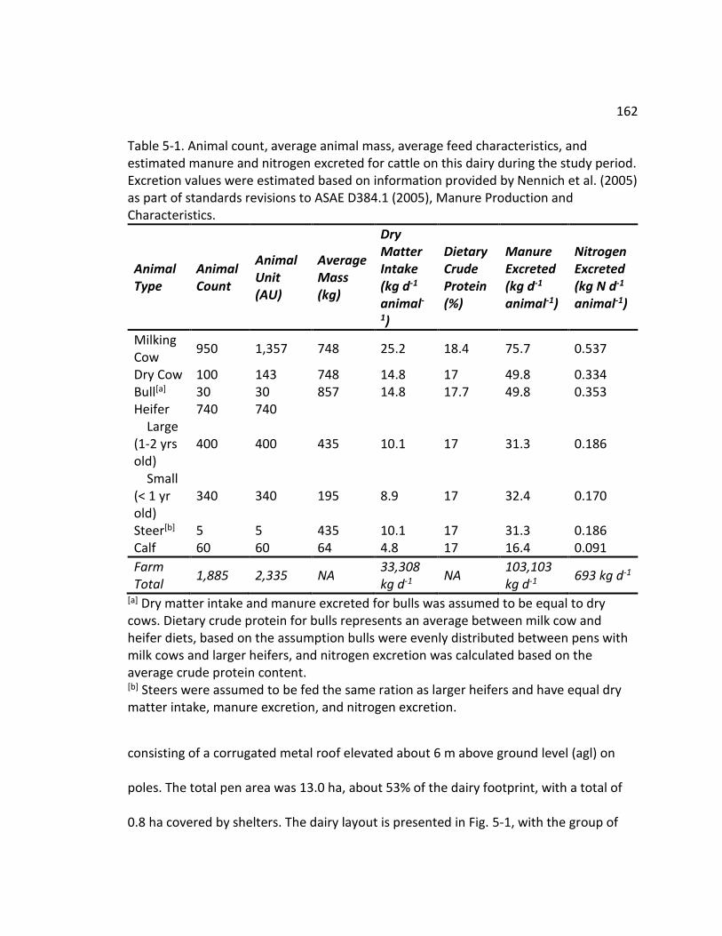
162

Table 5-1. Animal count, average animal mass, average feed characteristics, and estimated manure and nitrogen excreted for cattle on this dairy during the study period. Excretion values were estimated based on information provided by Nennich et al. (2005) as part of standards revisions to ASAE D384.1 (2005), Manure Production and Characteristics.

Animal Type

Animal Count

Animal Unit (AU)

Average Mass (kg)

Dry Matter Intake (kg d-1 animal-1)

Dietary Crude Protein (%)

Manure Excreted (kg d-1 animal-1)

Nitrogen Excreted (kg N d-1 animal-1)

Milking Cow

950 1,357 748 25.2 18.4 75.7 0.537

Dry Cow 100 143 748 14.8 17 49.8 0.334 Bull[a] 30 30 857 14.8 17.7 49.8 0.353 Heifer 740 740 Large (1-2 yrs old)

400 400 435 10.1 17 31.3 0.186

Small (< 1 yr old)

340 340 195 8.9 17 32.4 0.170

Steer[b] 5 5 435 10.1 17 31.3 0.186 Calf 60 60 64 4.8 17 16.4 0.091

Farm Total

1,885 2,335 NA 33,308 kg d-1

NA 103,103 kg d-1

693 kg d-1

[a] Dry matter intake and manure excreted for bulls was assumed to be equal to dry cows. Dietary crude protein for bulls represents an average between milk cow and heifer diets, based on the assumption bulls were evenly distributed between pens with milk cows and larger heifers, and nitrogen excretion was calculated based on the average crude protein content. [b] Steers were assumed to be fed the same ration as larger heifers and have equal dry matter intake, manure excretion, and nitrogen excretion.

consisting of a corrugated metal roof elevated about 6 m above ground level (agl) on

poles. The total pen area was 13.0 ha, about 53% of the dairy footprint, with a total of

0.8 ha covered by shelters. The dairy layout is presented in Fig. 5-1, with the group of

163

pens for each animal category labeled and the locations of feed, equipment, and

manure storage locations also shown. It should be noted that the five steers occupied

only a quarter of the northwestern most pen.

The cows were milked twice a day, with a milking schedule from 08:00 h to 17:00

h and from 20:00 h to 05:00 h local time. Milk production averaged 34.1 kg d-1 animal-1

during June 2008. A feed truck delivered feed to all pens from 05:30 h to 12:00 noon

and from 15:00 h to 17:00 h local time along concrete feed alleys adjacent to pens. Feed

Figure 5-1. Map of dairy pens, storage, and sampling locations.

164

lanes, areas where the cattle stand while feeding and along which cattle are moved,

were concrete and sloped for drainage. The remaining pen surfaces were unpaved. Feed

lanes in pens holding milking cows were flushed several times per day, while feed lanes

in the other open lots were scraped on a weekly basis with one scraping occurring

during this study on 18 June. Unpaved pen surfaces were scraped on an as-needed

basis; corral scraping occurred during equipment setup but not during the measurement

period. Gathered manure from both the feed lane and pen area were stored in each pen

for later removal. The liquids generated from both milk parlor washing and milking cow

feed lane flushing were first passed through an earthen solids settling basin (0.1 ha) and

was then stored in an earthen holding pond (0.6 ha). Separated solid manure was stored

in windrows. The windrows present at the time of the study were in the southwest area

of the solid manure handling area and dry at the surface. These windrows were not

disturbed during the measurement period, nor were solids removed from the separator

basin and windrowed.

Animal diets have been shown to be a significant factor in NH3 emissions (Smits

et al., 1995; Cole et al., 2005). As this study examined NH3 emissions from all cattle on

the dairy, the diets for each animal type should be considered. Cattle were fed different

mixed ration diets based on gender, age, and milking status, though all diets were based

on alfalfa and silage (green wheat silage for all animal types, with milking cows receiving

corn silage as well) with additives to meet energy and nutrient targets. Dry matter fed

(DM) and dietary crude protein content (CP) for each animal category are listed in Table

165

5-1. Milking cow DM and CP averaged higher than all others at 25.2 kg d-1 animal-1 and

18.4%, respectively, while CP for all others averaged 17%. Manure excreted (ME) and

nitrogen excreted (NE) were estimated per animal based on equations for different

categories of dairy cattle developed by Nennich et al. (2005) as part of standards

revisions to ASAE D384.1 (2005), Manure Production and Characteristics, and summed

over all cattle on the facility, as shown in Table 5-1. Due to a small dataset, Nennich et

al. did not provide equations for dry cows. It is unlikely that the average excretion values

provided by Nennich et al. would be representative for this dairy since the average DM

and CP for dry cows on this dairy were 43% and 28% greater, respectively, than mean

values reported by Nennich et al., though less than the maximum values reported.

Therefore, ME and NE were calculated based on linear fits to the reported mean,

minimum, and maximum values for ME and NE against the mean, minimum, and

maximum values of DM and CP, respectively, resulting in the following equations:

9967.0,63.878.2 2 RDMM E (5-1)

000.1,15.082.2 2 RCPNE (5-2)

ME and DM have units of kg d-1 animal-1, NE has units of kg N d-1 animal-1, and CP has

units of g of CP g-1of DM. Bulls were assumed to have similar DM intake and ME and NE

excretion rates as dry cows, but with an average CP of 17.7% based on the assumption

that bulls were evenly divided between pens with milking cows and older heifers. Steers

were assumed to have intake and excretion rates equal to the larger heifers. All of the

166

dry dietary components were stored in the feed storage area in the northern portion of

the dairy.

In order to meet PM10 emissions reductions required to bring the San Joaquin

Valley into compliance with PM10 National Ambient Air Quality Standards, the San

Joaquin Valley Air Pollution Control District (SJVAPCD) directed agricultural facilities

above a threshold size to select and implement Conservation Management Practices

(CMPs) designed to reduce PM10 emissions (Siong and Sheikh, 2006). The SJVAPCD-

accepted CMP plan for this dairy operation consisted of the following management

practices: 1) manure from open corrals shall be frequently scraped and/or removed; 2)

pull-type manure harvesting equipment shall be used; 3) shaded areas shall be provided

for cattle in open corrals; 4) wet material shall be placed in the feed wagon prior to

mixing; and 5) feed shall be wetted during mixing. While these target reducing direct

PM10 emissions, potential positive or negative impacts on NH3 emissions may occur. For

example, frequent scraping and or removal of manure in open corrals may produce

short bursts of NH3 releases due to the manure disturbance. Shaded areas provided for

cattle may affect cattle behavior and result in greater inhomogeneity in excretion

deposition across the pen surface. The CMPs dealing with feed mixing and the manure

harvesting equipment type are not expected to affect NH3 emissions.

167

Instrumentation

Historical wind measurements from June 2005-2007 were obtained from station

#15 of the California Irrigation Management and Information System (CIMIS) near

Stratford, California, as a representative site. These records showed that wind

conditions during the month of June were very consistent, with winds coming

dominantly from the northwest quadrant. Instruments were deployed to measure

background concentrations north and northwest of the facility and emission plumes

south and southeast of the dairy (Fig. 5-1). On-site measurements of wind direction

during the experiment confirmed the dominant wind direction to be from the

northwest. An air quality instrumentation trailer (dimensions approximately 5 m by 2.5

m by 2.5 m), located near the downwind OP-FTIR unit as shown in Figure 5-1, was used

for sample preparation, collection, and storage as well as data storage.

Two 15.3 m towers were erected at the site to hold meteorological instruments.

One was located 400 m west of the dairy and the other located just inside the southern

boundary of the dairy. Each tower was equipped with five cup anemometers mounted

at heights of 2.5, 3.9, 6.2, 9.7, and 15.3 m agl and five temperature and relative

humidity sensors at heights of 1.0, 2.5, 3.9, 6.2, and 8.2 m agl. A wind vane was

positioned on top of the towers at 15.3 m. Campbell Scientific (Logan, Utah) data-

loggers were used to record and store the data from instruments on the towers as one

minute averages. Incoming solar radiation, temperature, relative humidity, barometric

168

pressure, precipitation, wind speed, and wind direction were measured and reported as

five minute averages by a weather station at 5.0 m agl at the air quality trailer near the

downwind 15.3 m tower. Details for meteorological instruments used in this study are

presented in Table 5-2. Reported meteorological values and hourly averaged data used

for modeling were taken from measurements made downwind of the dairy. Due to an

error discovered in post analysis in the wind direction averaging procedure for the wind

vanes on the towers, wind directions reported by the weather station were used in all

calculations and modeling.

Ammonia concentrations were measured with two methods. The first method

was passive absorption onto citric acid-coated filters using passive samplers and pre-

coated filters from Ogawa USA, Inc. (Pompano Beach, Fla.). An in-depth description of

the sampler, the NH3 concentration calculation procedure, and results from

comparisons with an NH3 scrubber during collocated deployments in ambient air and

inside a poultry production house are provided by Roadman et al. (2003). Collection of

NH3 onto the pad is driven by a concentration gradient between the ambient air and the

filter surface; the concentration at the filter surface is maintained at zero due to its

reaction with the acid-coated filter surface and formation of a stable compound

(ammonium citrate) for subsequent analysis. Total sorption of NH3 is determined by the

ambient concentration, the exposure time, and the mass transfer coefficient. Calculated

concentrations represent the average concentration over the period of exposure.

Roadman et al. conducted two saturation and deployment time studies and found that

169

Table 5-2. Meteorological instruments employed in this study.

Instrument Company, City, State/Country

Parameter Measured

Accuracy

Gill 3-Cup Anemometer

R.M. Young Company, Traverse City, Mich.

Wind speed ±0.2 m/s over 1 m/s, threshold speed 0.5 m/s

HMP45C Vaisala, Oulu, Finland

Temperature ±0.2 °C at 20 °C

Relative Humidity

±2% for values in the range 0-90%, ±3% for values in the range 90-100%

024A Wind Vane

Met One Instruments, Grants Pass, Ore.

Wind Direction ±5 °

Pro2 Plus Weather Station

Davis Instruments, Hayward, Cali.

Temperature ±0.5 °C for values greater than -7 °C, ±1.0 °C for values less than -7 °C

Relative Humidity

±3% for values 0-90%, ±4% for values 90-100%

Solar Radiation ±5% of full scale

Precipitation ±3% or 0.02 mm per event, whichever is greater

Barometric Pressure

±0.8 mm Hg at 25°C

Wind Speed ±1 m/s or 5%, whichever is greater

Wind Direction ±3 °

the diffusion and sorption of NH3 on the pad is linear for total collected masses up to

12.1 μg of NH3, after which the mass transfer coefficient decreases with increasing mass

collected. In cases where the total mass collected exceeded the 12.1 μg threshold, the

estimated concentration would be lower than the actual average concentration.

170

The passive sampler exposure time selected for this study was 12 hours based on

the optimum time ranges (see Figure 5-2 in Roadman et al. (2003)) for background

concentrations assumed to be close to zero and instantaneous samples of up to 2 ppm

during active pumping into and taken immediately downwind of the solids separator

basin with a handheld NH3 gas sensor (Toxi Pro Biosystems, Middleton, Conneticut; 0 –

100 ppm range, 1 ppm resolution). Passive sampler sites were arrayed upwind,

downwind, and inside the dairy area as shown by the filled circles in Figure 5-1. Six were

established as upwind sites and located to the north and northwest of the dairy with

measurement heights of 1-2 m agl. The remaining 17 sites were placed at downwind

locations, based on the prevailing winds, along the southern dairy border, the eastern

dairy border, and between the pens with young heifers and the holding pond. Fourteen

of the downwind sites sampled at 1-2 m agl heights and three were set at 9 m agl on

towers at both ends of the southern dairy border and adjacent to the air quality trailer.

Note that passive samplers were located at both 2 m and 9 m on the towers, leading to

23 deployed samplers and 20 sites shown in Figure 5-1.

Analysis of the mass of NH3 collected on the pads as ammonium (NH4+) was

performed within the 28 day manufacturer suggested period of time after exposure. It

was accomplished via extraction through sonication in 8 mL de-ionized water and

quantification via ion chromatography (IC) at the Utah Water Research Laboratory

(UWRL) in Logan, Utah. The IC instrument (Dionex Corporation) was equipped with an

AS 40 Automated Sampler, CE20 Conductivity Detector, GP 40 Gradient Pump,

171

Membrane Suppressor, LC Chromatography Oven, IonPac® CS12A cation column, CG12A

cation guard column, and a 500 μL sample loop. The IC method used a 0.03 N sulfuric

acid (H2SO4) solution as eluent. Chemical standards, blanks, and continuous calibration

verification (CCV) standards utilized de-ionized water and reagent grade chemical

stocks. Blanks and CCVs were analyzed every 10 samples. A lab and field blank were

collected for each sample period and analyzed in the same manner. The mass of NH3

collected per sample and used to determine the period average concentration was

calculated as the total detected mass minus the average mass detected on the

corresponding lab and field blank. Duplicate analyses were run on 9% of the samples,

with the two concentration values averaged for further calculations; the average

differences between duplicate analyses, expressed as the percent of the average value,

was 1.4% and the median was 0.0%. The average method detection limit (MDL) ± 1σ for

the 12 h sample periods was 11.4 ± 0.4 ppbv (7.8 ± 0.4 μg m-3).

OP-FTIR was the second method of measuring ambient NH3 concentrations

utilized at the dairy. OP-FTIR is a real-time monitoring technique for remote detection

and quantification of multiple compounds simultaneously. The principle of operation is

based on the absorption of energy at different wavelengths by different compounds.

The OP-FTIR unit projects an infrared (IR) beam of light through a volume to be analyzed

and then captures this beam, generating a full infrared spectrum which can be used in

conjunction with reference spectra to identify the gases present and allows for their

concentration to be measured to ppb levels.

172

For this study, two OP-FTIR instruments were employed, with one located on

each of the dominantly upwind and downwind sides. The upwind OP-FTIR instrument,

manufactured by Industrial Monitoring and Control Corporation (IMACC, Round Rock,

Texas), was operated in a monostatic mode in which a single unit containing the IR

beam source, detector, and associated optics was used at one end of the path and a

passive corner-cube array retroreflecting mirror was at the other end. It consisted of a

0.125 cm-1 FTIR modulator, a zinc selenium beam splitter, a mercury cadmium telluride

detector cooled with liquid nitrogen, a helium neon laser for dynamic alignment control

and a 25 cm diameter Cassegrain telescope. The upwind measurement path was 2 m agl

along a transect from the northwest corner of the dairy over a field and totaling 250

meters (Fig. 5-1).

Spectra were collected at 1, 3, and 5 minute intervals and analyzed using the

IMACC FTIR Software Suite, Ver. 01/2005. The IMACC software was used to define an

analytical method for the selected analyte that was applied to each spectra to: 1)

perform a point-by-point comparison with a reference spectra to determine the spectral

line shift required to obtain the maximum correlation coefficient; 2) select portions of

the spectra for further analysis that contains minimal impacts from compounds with

potential interferences, based on comparisons between the collected spectra and

reference spectra for potentially interfering compounds; 3) account for background

levels of other compounds and dynamic changes in the measurement environment; and

4) calculate the path length concentration of the analyte of interest through a

173

calibration equation that accounts for response non-linearity over the full range of

analyte concentrations through a best fit curve fitted to reference standard

measurements across the full range. Background spectra were collected onsite during

times the system was upwind of the dairy using a 25 m path length to minimize NH3

absorption. The algorithm developed for NH3 was applied to each recorded transmission

spectra to generate a quantitative value of NH3 concentration.

The OP-FTIR on the downwind side of the dairy was a monostatic unit

manufactured by MDA (Atlanta, Ga., now Cerex Monitoring Solutions, LLC, Atlanta, Ga.)

that utilized a Bomem Michelson 100 interferometer, a 25 cm telescope, and a mercury

cadmium telluride detector cooled by a Stirling engine. Spectra were collected every 70

s. This OP-FTIR was set in a scanning system with multiple retroreflectors in order to

determine NH3 concentrations along multiple lines. The scanning system consisted of a

covered set of scaffolding, a rack upon which the OP-FTIR was positioned with the

output beam directed vertically through a hole in the roof and then onto a mirror

capable of rotational (270°) and elevational (-5° to +45° from horizontal) movement. The

mirror height was approximately 2.5 m agl. The IR beam was pointed toward each of 6

retroreflectors along the downwind side of the dairy using the steering mirror, with the

OP-FTIR centrally located on the southern border of the facility as shown in Figure 5-1.

Retroreflectors were located at about 140 m and 290 m away from the FTIR along an

east-west line, with far retroreflectors stationed at both 2-3 m agl and 9 m agl and near

retroreflectors at 2-3 m agl. Six spectra were collected at each position, with the first

174

two spectra collected not used due to interference from movement of the mirror

between positions and to allow system stabilization. Therefore, four consecutive 70 s

spectra were collected along each beam path on a 42 min cycle. Return signal strength,

expressed as a percent of the outgoing signal, varied between 50% and 15%, depending

on path length, alignment, and retroreflector cleanliness. Retroreflectors were cleaned

every two to three days as needed. Spectra analysis and quantification of the path-

length averaged NH3 concentrations were performed using a data analysis software

created by Dr. Peter Griffiths at the University of Idaho utilizing a partial least squares

regression technique (Griffiths et al., 2009; Shao et al., 2010) with instrument-specific

calibration parameters.

During the setup period, the OP-FTIR units were placed adjacent to each other at

the upwind OP-FTIR location for a collocated comparison test using adjacent beam

paths. Two tests, each 1.5 to 2.0 h in duration, were conducted. The units measured

incoming background levels during one test, averaging (±SD) 39.0 ± 7.7 ppb and 35.7 ±

4.7 ppb for the upwind and downwind units, respectively. Incoming background levels

were spiked by exposed liquid ammonium for the other test, resulting in average

concentrations of 120.3 ± 28.8 ppb and 121.1 ± 23.5 ppb for the upwind and downwind

units, respectively. These tests show that the units agreed very well at the higher level

and slightly less well at the lower background level.

175

Data Treatment and Filtering

Concentrations measured by the OP-FTIR instruments were averaged over 2 h

intervals throughout the measurement period for EF estimation. This averaging time

was selected to minimize the smoothing of potential trends in emissions while providing

two or more groups of samples on which to base a period average. Due to the low

cumulative sampling of the downwind scanning system along a given path (~4.5 min

every 42 min), the representativeness of an average value for the entire 2 h period was

of concern. Representativeness was assessed based on a period’s relative standard

deviation (RSD). Exclusion of data due to RSD levels > than 25%, 33%, 40%, 50%, and

75% was examined. Average values with a RSD > 33% were excluded from EF

calculations because the 33% level provided a conservative assessment of

representativeness. This resulted in the removal of ≤ 30% of the averaged data in six of

the seven employed OP-FTIR measurement paths from emissions calculations.

As previously stated, the sampler layout during this experiment was designed to

measure the dairy facility’s impact on downwind concentrations to the south and east.

However, winds from directions other than the prevailing northwest sector would

diminish the effectiveness of this setup. Dairy and sample layout geometry indicated

that periods with wind directions outside of -70 to +50° from North should be excluded

from EFs calculations. Hourly averaged wind direction measured on-site was used to

screen data periods. While wind direction may vary considerably over an hour and

176

render the hourly averaged wind direction insufficient for screening purposes, the wind

directions recorded during this study were very consistent over time spans of several

hours with periods of higher variability almost always resulting in hourly averages

outside of the optimal range. Therefore, hourly averaged wind direction values were

sufficient for screening in this instance. Additionally, determination of the upwind or

downwind status of each sample location/path was made based on hourly averaged

wind direction.

Values reported at upwind sites were averaged to calculate the background NH3

levels (CB) entering the facility. Concentrations resulting from the dairy activities (Cmeas)

were calculated on a location-by-location basis by subtracting CB from the measured

downwind concentration. This difference was determined to be significant if Cmeas was

greater than the 67% confidence interval (CI) about CB, corresponding to one SD. Only

Cmeas values found to be significant in this way were used in emissions calculations.

About 18% of the downwind OP-FTIR measurements lacked a corresponding OP-FTIR CB

value. In these cases, the average passive sampler CB and corresponding 67% CI were

used to estimate Cmeas.

Emissions Calculations

A dispersion model requires a user-input emission rate for a source in order to

predict downwind concentration values. However, this study seeks to determine the

dairy emission rate that resulted in the measured impact on downwind NH3

177

concentrations. This was accomplished through inverse modeling, a process of

comparing a measured impact on concentration (Cmeas) at a downwind site with a model

predicted impact on concentration (Csim) based on an initial emission rate supplied to

the model (Qsim) in order to estimate the actual emission rate (Qmeas). As given by

Faulkner et al. (2007) and Flesch et al. (2009b), the relationship for deriving Qmeas from a

single source, assuming a proportionally linear response between Qsim and Csim in the

model, may be mathematically expressed as:

sim

meas

measQC

CQ

(5-3)

Note that the ratio of (C/Q)sim is dependent upon both the source-receptor spatial

relationship and the meteorological conditions over the modeled period, and, therefore,

is only valid for the modeled scenario.

In the case where multiple sources are active and additive properties between

the impacts of the different sources on the total concentration at a given location may

be assumed, the multi-source inverse modeling technique described by Flesch et al.

(2009b) may be used to simultaneously estimate the emissions from each source. In

summary, a system of linear algebraic equations is created to estimate the emission rate

of each source i by calculating the modeled proportional impact on the total predicted

concentration at each receptor j. A system of linear equations with three sources and

three measurements is given in Equation 5-4 as an example, with number subscripts

178

representing different sources and letter subscripts representing different

measurement/receptor locations:

Cmeas

Bmeas

Ameas

meas

meas

meas

simCsimCsimC

simBsimBsimB

simAsimAsimA

C

C

C

Q

Q

Q

QCQCQC

QCQCQC

QCQCQC

,

,

,

3,

2,

1,

33,22,11,

33,22,11,

33,22,11,

(5-4)

If there are fewer measurements than sources (j < i), the system is under-determined

and a unique solution cannot be found. If more measurements exist than contributing

sources (j > i), the system is over-determined and the solution may be found through an

optimization approach. See Flesch et al. (2009b) for a more detailed description, as well

as a discussion on the effect of source-receptor spatial relationships on emission

estimates.

There are a variety of atmospheric dispersion models available for use in inverse

modeling. The one selected to carry out this inverse modeling exercise was the

American Meteorological Society/US Environmental Protection Agency Regulatory

Model (AERMOD) software, executable file Version 12345. It was chosen because it is a

current U.S. EPA recommended regulatory model, it has a proportionally linear

relationship between Qsim and Csim (see Cimorelli et al., 2005), and to maintain

continuity within the study (Marchant et al., 2011). Some recent agricultural NH3

emissions studies utilizing an inverse modeling methodology have used WindTrax

(Thunder Beach Scientific, www.thunderbeachscientific.com), a backward Lagrangian

stochastic model (Bjorneberg et al., 2009; Flesch et al., 2009a; Todd et al., 2008; Leytem

179

et al., 2011, 2013). Faulkner et al. (2008) utilized both AERMOD and WindTrax, in

addition to two other air dispersion models, to estimate NH3 emissions from a beef

cattle feedyard. They found that ERs and EFs were model specific, and that a simple

relationship did not exist between the estimated emissions. However, Bonifacio et al.

(2013) found strong linear correlations between AERMOD and WindTrax in estimating

PM emissions from a beef cattle feedyard and calculated AERMOD/WindTrax conversion

factors ranging between 1.3 to 1.6, depending on meteorological inputs.

The AERMOD model operates in one hour time steps and assumes steady-state

conditions, continuous emissions, conservation of mass, and concentrations predicted

at a receptor resulting from different sources are additive. Pollutant distribution is

modeled as Gaussian in the stable boundary layer in both the horizontal and vertical

directions and in the horizontal direction in the convective boundary layer; vertical

pollutant distribution in the convective boundary layer is modeled as bi-Gaussian

(Cimorelli et al., 2005). The interface used to run this model was the commercially

available AERMOD View package by Lakes Environmental Software (Waterloo, Ontario).

AERMOD requires hourly averaged meteorological data such as wind speed,

wind direction, temperature, and solar radiation. These data were supplied by

measurements made just south of and predominantly downwind of the dairy. Wind

direction and incoming solar radiation data recorded at 5.0 m agl by the Davis weather

station were utilized, along with wind speed data collected by the cup anemometer

mounted at 6.2 m on the nearby tower, the closest level corresponding to the wind

180

direction measurements at 5.0 m. Temperature data were taken from the 2.5 m agl

level on the tower. Cloud cover was set at zero for the entire study period, as there

were clear skies throughout the measurement campaign.

The meteorological preprocessor for AERMOD, AERMET, also requires that

values for Bowen ratio (β), noon-time albedo (α), and surface roughness length (z0) be

specified by the user. The average z0 was calculated from vertical wind speed profiles

measured downwind of the dairy using the following equation which relates wind

speeds (u1, u2 in m s-1) at two heights (z1, z2 in m) and was derived from the integrated

logarithmic wind speed profile equation:

0

1

0

2

1

2

ln

ln

z

z

z

z

u

u

(5-5)

A least sum of squares of residuals methodology was used to determine the value of z0

that best fit measured wind speeds at the higher elevation of two paired wind speed

time series over the study period. A z0 value of 0.09 m was calculated as the arithmetic

average of the values that best fit six pairings of hourly averaged wind speeds measured

at 3.9 m, 6.2 m, 9.7 m, and 15.3 m agl, i.e. 3.9 m and 6.2 m, 3.9 m and 9.7 m, 3.9 m and

15.3 m, 6.2 m and 9.7 m, 6.2 m and 15.3 m, and 9.7 m and 15.3 m.

Unlike z0, data were not collected that could be used to calculate the β and α

values. Instead, summer-time values were selected from tables with seasonal values

181

provided in EPA (2008). The selected β value was 4.0, the suggested summer-time value

for bare rock/sand/clay in an arid region under average soil moisture conditions. Despite

soil moisture measurements from pen and road surfaces revealing dry conditions at the

sample locations, the deposition of urine to pen surfaces by cattle and the presence of

the LMS were used as justification for selecting the suggested value for average soil

moisture conditions. The suggested noon-time α value of 0.20 for bare rock/sand/clay in

an arid region was used in this study.

Faulkner et al. (2008) found that maximum Csim as predicted by AERMOD from a

ground level area source were sensitive to, among other input parameters, α and z0 but

it was not sensitive to β. The lack of sensitivity to β was theorized to be due to the

dominance of mechanical mixing in the planetary boundary layer in their application.

Based on these findings, the sensitivity of Csim and the resulting Qmeas estimates in this

inverse modeling application to variations in α and β was investigated. The sensitivity to

z0 was not tested as it was calculated from measured data. Summer α values selected

were 0.18, the suggested value for fallow fields and supported by Hansen (1993) for

light colored, dry soil such as that in fields surrounding the dairy, and 0.25, the

suggested value for shrublands in an arid region. Two summer values for β were

selected as 1.5, suggested for both wet conditions in a bare rock/sand/clay surface in an

arid region and for fallow fields under dry conditions, and 6.0 for dry conditions in a

bare rock/sand/clay surface in an arid region (EPA, 2008).

182

Four consecutive passive sampler measurement periods, two morning and two

afternoon, were selected for the comparison. Changes in Csim and Qmeas were calculated

as a percentage of Csim and Qmeas calculated at the base case of α = 0.20, β = 4.0. Values

of Csim at all downwind sites varied between -3% and +5% from the base case, though

most were within ± 1%. Estimates of Qmeas under the different values of α and β varied

most for the LMS (-6% to +4%), while the changes in pen and combined EFs estimates

were about equal at -2% to +1%. Values of Csim increased, resulting in decreased Qmeas

estimates, with increasing α at constant values of β. Holding α constant while increasing

β had the opposite effect, leading to lower Csim values, and thus higher Qmeas estimates.

Therefore, in the case of this dairy and sampling layout, neither the Csim nor the Qmeas

estimated through inverse modeling with AERMOD were sensitive to the selected

ranges of α and β.

AERMOD requires the source type, size, location, and emission rate be specified,

as well as sampler/receptor locations. The pens, settling basin, and holding pond were

specified as ground level area sources with areal extents equal to their respective

dimensions and with an initial plume height of 0 m. The vertices of the sources and the

receptor locations were taken from multiple hand-held GPS measurements made during

the study and available satellite imagery. Pens not occupied by cattle were not included

in the model; for example, only the quarter of the northern-most group of pens that

was occupied by steers was specified as an active source.

183

Note that the value of the (C/Q)sim ratio in Equation 5-3 is the same across all

ranges of Qsim when using a model with a proportionally linear response in Csim to

changes in Qsim; this also applies to the ratio of each source/receptor pairing in Equation

5-4. This means that the ratio describes the slope of a straight-line relationship without

local maxima or minima and eliminates the dependency of the results on the input Qsim

values. However, the method used to determine the initial Qsim values for each source i

for this study is important to note as it was integrated into the optimization procedure.

An initial estimate of the pen EF (f) of 1.5 mg animal-1 s-1, the yearly average NH3 EF

reported for an open lot dairy by Leytem et al. (2011), was combined with animal

occupancy (m, number of cattle) and area (A, m2) as shown in Equation 5-6 to calculate

Qsim,i values (g s-1 m-2) for the pens:

i

i

isimA

fmQ ,

(5-6)

The emission rates of the solids settling basin and the holding pond were assumed to be

equal and given an initial value of 0.1 mg m-2 s-1, an average of the lower and upper

ranges reported by Rumburg et al. (2008b). The initial estimates of Qsim for each source

were supplied to AERMOD, which was then run for each sample period. Calculated

hourly Csim values were averaged over a sample period, for instance from 12 noon until

12 midnight to correspond with a p.m. passive sample period, for comparison with Cmeas.

The presence of the trailer on the downwind side of the dairy may have affected

measurements at that location due to flow disruption. However, the potential effects on

184

dispersion and nearby concentrations could not be modeled within AERMOD because

the software does not allow the modeling of building effects with area sources. In

addition, NH3 is known to deposit readily to most surfaces. Deposition likely occurred

during this study, to some degree, in the short distance between the sources and

measurement locations and resulted in lower Cmeas than if some NH3 had not deposited.

However, deposition was neither measured nor simulated in this study. As a lower Cmeas

results in a lower Qmeas, any depositional loss occurring between the source and the

measurement location that is not accounted for in emissions calculations would lead to

estimated EFs and ERs being lower than the actual values. In such cases, the calculated

EFs and ERs should be considered as effective ERs and EFs.

A total of 10 active sources were specified in the model. A sufficient number of

downwind passive sampler measurements existed to calculate an emission rate for each

individual source, but a maximum of six downwind OP-FTIR measurement paths yielded

an under-determined system. Simplification of the system was performed and reduced

the total number of emission rates solved for in the system to two based on the

following: 1) as the solids settling basin and the holding pond Qsim were assumed to be

equal, the change in Csim at a given location resulting from the entire LMS was assumed

to be linear compared to the change in the sum of the LMS emissions per area per unit

time (Qsim,LMS); and 2) as m and A in Equation 5-6 are constants for a given pen source i,

leaving only changes in f to change Qsim,i, and the same value of f was applied to each

pen, a linear change in Csim resulting from all the pens at a given location to a change in

185

the sum of the pen Qsim,i per unit area per unit time was assumed. Both assumptions

were verified to be true through modeling with different f and Qsim,LMS values.

Therefore, the system of linear algebra equations used to estimate the dairy NH3

ERs was designed to solve for fmeas and Qmeas,LMS, yielding an over-determined system for

both passive and OP-FTIR sampling configurations. The optimization method employed

to solve these systems was a least sum of squares of residuals comparing Csim and Cmeas.

Reported EFs on a per animal basis were calculated for the LMS by relating the

estimated ERs to the number of contributing animals, which was assumed to be limited

to those in the milking cow pens due to the lack of feed lane flushing in other pens. The

EF per animal for those in the milking cow pens was calculated as the sum of the pen EF

and the LMS EF. The average NH3 EF across the facility was calculated as a weighted

average of the pen EF and the summed EF for cattle in the milking cow pens, with

weights assigned based on the number of cattle in the two categories. In addition, the

overall study average EFs were calculated as weighted averages according to the

number of EF estimates during each sample period time throughout a day. For example,

the reported OP-FTIR based averages represent the sum of the estimated emissions

over a 24 h period using the average EFs for each 2 h block.

Results and Discussion

The measurement campaign began at 12:00 noon Pacific Standard Time (PST) on

13 June 2008, and ended at 00:00 h PST on 21 June 2008. A total of thirteen sample

186

periods, approximately 12 h each, were conducted using the passive samplers, with all

previous samples being collected and the next samples being deployed within 30 min of

00:00 h and 12:00 noon PST. The upwind OP-FTIR unit operated nearly continuously

from 14 June 04:20 h to 19 June 08:30 h. Data were collected by the downwind OP-FTIR

unit from 13 June 13:30 h to 21 June 00:00 h, operating for 118.9 h out of 178.5 total

hours (66.6%).

Meteorological conditions throughout the field study were hot and dry, with

diurnally consistent wind patterns. Low wind speeds with highly variable direction were

recorded each morning shortly before sunrise. The wind speed at 6.2 m agl from 05:00-

06:00 h varied between 0.6-1.5 m s-1 with a campaign average ± 1 SD of 1.1± 0.2 m s-1.

The SD is reported in this paper for all measurements unless otherwise noted to show

the variability in the reported values. During the remainder of the day winds came from

the northwest. Figure 5-2 shows the dominance of winds from the northwest sector

throughout the study, accounting for 74% of recorded values. Cloud cover was either

absent or extremely light and at high altitudes throughout with no recorded

precipitation events. Samples of the soil on unpaved roads and in dry-lot pens were

collected on 16 June and analyzed for percent moisture, resulting in averages of 0.56% ±

0.50% (n = 3) and 5.3% ± 5.1% (n = 7) for the unpaved roads and pens, respectively.

Campaign average meteorological conditions measured on-site are presented in

Table 5-3, as well as average conditions measured at the Stratford CIMIS site during the

study period, for all of June 2008, and for the month of June from 1998-2007. Average

187

Figure 5-2. Hourly average wind conditions measured at the dairy during the measurement periods, 13-20 June 2008.

Table 5-3. Comparison of average meteorological conditions (±1 SD) measured at the dairy from 13-20 June 2008 and at a site in Kings County for the same period, the full month of June 2008, and June from 1998-2007.

On-site

13-20 June 2008

Off-site

13-20 June 2008

Off-site

June 2008

Off-site

June of 1998-2007

Temperature (C) 26.5 ± 6.7 26.7 ± 7.4 24.8 ± 7.2 24.2 ± 6.7

Relative Humidity (%) 41 ± 18 30 ± 16 33 ± 17 45 ± 18

Wind Speed (m/s) 2.4 ± 1.1 2.9 ± 1.2 3.2 ± 1.7 2.8 ± 1.3

Wind Direction (°) 325 ± 42 326 ± 42 329 ± 42 330 ± 45

Total Precipitation (mm) 0.0 0.0 0.3 16.2

conditions on-site were indistinguishable from those measured at Stratford for

temperature, wind direction, and precipitation; wind speeds were slightly lower and

188

relative humidity values were higher at the dairy, with little difference between upwind

(data not shown) and downwind measurements. Comparison of the study period

conditions at Stratford with the remainder of the month and during previous years

reveals this period was slightly warmer and drier than monthly averages, but with

similar wind conditions. June 2008 was similar to past years in temperature and wind

direction, with slightly higher average wind speeds and lower relative humidity values. It

should be noted that the total precipitation in each column is a summation of all data

considered and that the sum of 16.2 mm comes from three recorded events from 1998-

2007 during the month of June and is strongly driven by a single event totaling 14.0 mm.

Concentration Measurements

A total of 298 samples were successfully collected upwind, downwind, and

within the dairy using the passive samplers deployed at 23 locations. The average

upwind concentration was 84.5 ± 19.2 ppbv (57.4 ± 13.4 μg m-3, n = 86) with a range of

52.9 to 128.3 ppbv. Concentrations measured downwind varied much more, with a

range of 69.3 to 1879.2 ppbv and an average of 412.4 ± 281.1 ppbv (280.0 ± 188.6 μg m-

3, n = 209). No passive samples exceeded the 12.1 μg collected NH3 threshold, after

which the collection efficiency becomes non-linear. There was a significant difference in

NH3 concentrations measured between morning (sampled from roughly 0:00 h to 12:00

noon) and afternoon (sampled from roughly 12:00 noon to 0:00 h) periods. Average

morning levels were 99.3 ± 16.5 ppbv (n=25) at upwind sites and 308.5 ± 181.0 ppbv

189

(n=89) at downwind sites. Afternoon concentrations averaged 78.7 ± 16.9 ppbv (n=60)

and 489.4 ± 315.3 ppbv (n=120) at upwind and downwind locations, respectively. The

highest concentrations in each period were measured between the holding pond and

the young heifer pens and downwind of the milking cow pens. These concentrations

were in the range of values reported by Cassel et al. (2005), Bjorneberg et al. (2009),

and Leytem et al. (2009) at open lot dairies in California and Idaho.

Ammonia concentrations recorded by the OP-FTIR units were more frequent

than the passive sampler measurements, thus providing more information about the

diurnal pattern and temporal variation in concentrations. However, these values are

volumetrically averaged concentrations across the beam area (diameter ≈ 0.3 m) and

along the length of the beam path (140 to 290 m, depending on pointing position). Thus,

the OP-FTIR units provide less spatial information than the passive samplers. Figure 5-3

presents a five-day time series of data collected at 2 to 2.5 m agl along five different

beam paths (see Figure 5-1 for beam path locations). Reported levels of NH3 are in the

same range as those calculated from passive sampler measurements, as well as

measurements given in literature from dairies with similar housing and manure

management systems (Cassel et al., 2005; Bjorneberg et al., 2009; Leytem et al., 2009).

Note that the highest NH3 concentrations throughout the period were detected to the

east of the centrally-located downwind OP-FTIR unit, which is immediately downwind of

both the LMS area and milking cow pens. Additionally, the highest concentrations

detected downwind of the dairy were recorded in the evening and shortly after

190

midnight while the lowest NH3 levels were measured from dawn until at mid-day. Sharp

increases and decreases in NH3 levels at the upwind beam path correspond with the

05:00-06:00 h periods of light winds of variable direction discussed previously.

The concentrations reported at upwind sites from both measurement

methodologies are high for ambient levels not immediately adjacent to a source, which

is indicative of the size and density of NH3 sources in the region. Kings County, the

county in which this dairy is located, and Fresno County, the county north and

northwest of Kings County, had a combined 2007 animal population (with animal

density given in parenthesis) of 789,612 cattle (41.1 km-2), including 278,368 milk cows

Figure 5-3. NH3 concentration (ppbv) measured by both the upwind and downwind OP-FTIR instruments at ~ 2m agl. Downwind beam paths are described by the direction from the monostatic unit to the retroreflector and the relative distance to the retroreflector.

06/14 06/15 06/16 06/17 06/18 06/190

200

400

600

800

1000

1200

1400

NH

3 C

oncentr

atio

n (

ppbv)

Upwind

Downwind, West Short

Downwind, West Long

Downwind, East Short

Downwind, East Long

191

(14.5 km-2) and 26,999 beef cows (1.4 km-2); 9,809 hogs (0.5 km-2); and 89,860,417

broiler chickens, all in Fresno County (4,682.9 km-2) (USDA, 2009). Battye et al. (2003)

provided a summary of three NH3 emissions inventories for the Fresno County area, all

of which estimated livestock’s contribution at 50 to 75% of the total emissions, which

ranged from 71,000 to 99,000 Mg yr-1. Winter time background NH3 measurements in

the San Joaquin Valley of California ranged from 16 to 96 μg m-3 (Cassel et al., 2005).

Robarge et al. (2002) reported a summer average NH3 concentration of 10.5 μg m-3 from

measurements taken in the agriculture-rich Inner Coastal Plain of North Carolina.

Walker et al. (2004) summarized literature values collected in agricultural, non-

agricultural, and urban land use settings from 11 studies, with average concentrations

ranging from 0.02 μg m-3 at high elevation during summer to 10.48 μg m-3 during fall at a

swine facility. Moore (2007) reported winter and summer average concentrations

throughout the Cache Valley, a heavily agricultural valley along the Utah/Idaho border

with significant dairy cattle and layer hen populations, of 28.8 and 24.7 μg m-3. Leytem

et al. (2009) reported background NH3 levels ranging from 10 to 60 μg m-3 in another

area of Idaho with a high dairy density.

On a path-by-path comparison, passive sampler NH3 levels were higher than OP-

FTIR measurements by an average of 1.38 ± 0.15 (n=50). One possible explanation for

the difference between the reported concentrations in the passive and OP-FTIR datasets

is the difference in methodology. Another possible cause is the effectiveness of a limited

number of discrete sampling points to represent a concentration field in close proximity

192

to strong sources, which is somewhat related to the first possible explanation. To

conduct these comparisons, the two to four passive samplers located along each OP-

FTIR beam path were used to calculate the path length average passive sampler

concentration, and OP-FTIR measurements were averaged over the passive sampler

deployment time to calculate the period average OP-FTIR concentration. The sample

heights of the passive samplers were set as close to the height of the OP-FTIR beam

path as possible, although some were up to 1 m lower. The crosswind scale of the

source in relation to the distance between sampling points, as well as the distance from

the source to the sampling points, could have significant impacts on how representative

the measured concentration field derived from a few sample points is compared to the

actual concentration field. While the spatial scales of most of the sources on the dairy

are large compared to the distances between samplers, the homogeneity of the

emissions from the pen and LMS surfaces may vary significantly on scales smaller than

the distance between sampling points and create emissions hotspots. The result is a

non-uniform concentration profile across the plume that may or may not be effectively

sampled by the point samplers. The path-integrated sample of the OP-FTIR has the

advantage in that it can sample the entire width of the plume, but spatial information

available from an adequate number of point sensors is sacrificed.

Going et al. (2008) found that passive sampler measurements were on average

55% greater than OP-FTIR measurements when the passive samplers were deployed as

directed by the manufacturer. Meng et al. (2011) compared seven-day NH3

193

concentration averages reported by Ogawa passive samplers and an active NOx/NH3

analyzer and found a strong correlation, yielding a linear fit slope of 1.21 with the active

analyzer as the independent variable and the passive sampler as the dependent

variable. Puchalski et al. (2011) compared two and three week long average NH3

concentrations from Ogawa passive samplers against other passive samplers and an

active analyzer over a 0.5 to 9.0 g m-3 range and found that the Ogawa sampler

reported values not statistically different from the other passive samplers in one study

and 36% lower than the active sampler in another study.

Estimated Emissions

The ERs and EFs for this study were estimated through inverse modeling.

Screening of the datasets to identify periods in which the wind direction was outside of

the optimal range of -70 to +50° from North yielded a total of 12 hours (8%) during 5 of

the 13 passive sampler deployment periods. One period, June 14 a.m. had six hourly

average wind direction values outside the optimal range; the remaining four periods had

1 to 2 hours each. The June 14 a.m. period was removed from ER and EF calculations,

while the other four passive sampler periods were not removed due to the limited

amount of time in each period that the sites were not impacted by the dairy and the

ability of the model to simulate the effects of these non-ideal wind directions on period

average concentrations.

194

The Cmeas values calculated for the two locations between the young heifer pens

and the holding pond, the locations with the largest reported concentration values

during all sample periods, were excluded from emissions estimation calculations

because of doubt that they were only influenced by the pens. It is hypothesized that the

feed lane fencing on the south side of the pen immediately upwind likely presented a

flow disturbance sufficient to allow some of the holding pond plume to be circulated in

the upwind direction. The samplers were located within a few meters of the northern

edge of the holding pond and had a sample height of 1 m. Removal of these two points

resulted in EF estimates with better fits to the remaining Cmeas data.

There were 78 potential OP-FTIR sample periods during the field study based on

2 h averages. Irregularities with instrument operation, alignment, and retroreflector

cleanliness reduced the number of periods with valid data from two or more downwind

beam paths to 48, or 62%. Of these, six were removed due to wind directions outside of

the optimal range, yielding a total of 42 sample periods from which to calculate ERs and

EFs. These irregularities and non-optimal wind directions disproportionately affected

the morning blocks (00:00 h through 12:00 noon), which had only two or three valid

datasets in most 2 h blocks for ER and EF calculations, about half as many as in the

afternoon. This likely contributed to the greater RSD in the average emissions from the

pens and the entire facility for morning blocks when compared to the afternoon blocks.

As previously mentioned, light and variable winds were observed each day during 05:00-

06:00 h, resulting in no valid data points for the block ending at 06:00 h. To provide an

195

emissions estimate for this period, a gap filling technique was used based on the

average of the 04:00 h and 08:00 h blocks.

The unconstrained least squares optimization method initially used in estimating

ERs and EFs generally performed well, but it yielded negative emissions from either the

pens or the LMS in a few instances. This phenomenon was neither observed in

measured data nor is it considered to be real. It is instead assumed to be an artifact of

the optimization method. Flesch et al. (2009b) suggests setting a minimum ER value in

such cases. This recommendation was applied to our emissions calculations, using a

minimum pen fmeas value of 0.5 g d-1 animal-1 and a minimum Qmeas,LMS value of 0.5 mg

m-2 d-1, which were estimated from minimum values shown in Leytem et al. (2011), an

NH3 and greenhouse gas emissions study conducted at an open lot dairy.

Flesch et al. (2009b) also suggests designing sampling layouts for multiple

sources in such a way that each measurement location is impacted by only one source.

If that ideal situation is not possible, as in the case of this dairy, and assuming at least

the same number of measurements as sources, they suggest that the measurement

sites be located such that the first site be impacted by only one source, the second site

by the first source plus the second source, the third site by the first, second, and third

sources, and so on. Emissions can then be estimated in a progressive manner. This

sequential ER estimation methodology was applied to the passive sampler dataset.

Some sites were impacted only by pens, while others were impacted by both pens and

the LMS, allowing first the pen fmeas and then the Qmeas,LMS to be calculated.

196

Determination of the sources impacting a given sample was made based on the range of

hourly average wind directions measured during the sample period. The number of sites

used to estimate the pen fmeas ranged from 3 to 7, while 6 to 13 sites were used to

estimate Qmeas,LMS. This sequential method was not applied to the OP-FTIR dataset

because the downwind OP-FTIR unit in the center of the configuration was rarely not

downwind of the LMS, resulting in all beam paths being impacted by both the pens and

the LMS most of the time.

Another important point discussed by Flesch et al. (2009b) concerns the matrix

conditioning number (κ), which is a measure of the sensitivity of the estimated Qmeas

vector in Equation 5-4 to changes in the (C/Q)sim ratios. If a change in Qmeas is

proportional to the change in a (C/Q)sim value, the system is referred to as well-

conditioned and has a low κ value (minimum κ = 1.0). A system is said to be ill-

conditioned if a large change in Qmeas is found from a small change in (C/Q)sim, which

would result in a large κ value. The value of κ also is related to the relative error in

estimates of Qmeas. The reader is referred to Flesch et al. (2009b) for an in depth

discussion with examples. An important conclusion was that accurate emissions

estimates in controlled release experiments with various source/receptor configurations

were strongly dependent on κ. Good ensemble averaged estimates of the total amount

released were calculated for (C/Q)sim matrices with κ values less than 50 and good

estimates of the individual source contributions were found for matrices with κ values

less than 10-20. Values of κ calculated for the matrices in this dairy emissions study

197

based on passive sampler data ranged from 1.5 to 2.7, suggesting good confidence in

the emissions estimates. Values of κ calculated for matrices based on OP-FTIR data

ranged from 4.5 to 25.6, again suggesting good confidence in the emissions estimates.

The averages, SDs, minimums, and maximums of the EFs calculated using the

three optimization methods discussed above for both datasets are presented in Table 5-

4. Average EF values estimated from the passive dataset for the unconstrained and

constrained values were very similar, but greater differences were found between

methodologies in the EF values based on OP-FTIR data. All reported statistics for the pen

and whole facility EFs predicted by the progressive methodology based on passive

sampler data were lower than for the other two methods; average estimated LMS EFs

were higher for the progressive method and had a greater range in individual values.

Average EFs based on OP-FTIR data for the pens, LMS, and the whole facility were

higher than those based on passive sampler data and had a wider range between

minimum and maximum values. One factor likely contributing to the larger range

between maximum and minimum values based on OP-FTIR data is the greater temporal

resolution in the OP-FTIR dataset, 2 h averages versus 12 h averages for passive

samplers, allowing it to show greater diurnal variation in estimated EFs with smaller

minimum values and larger maximum values that are smoothed out in the passive

sampler EFs.

As previously stated, negative EFs were calculated from both passive sampler

and OP-FTIR data using the unconstrained methodology. Negative EFs values are not

198

Table 5-4. Statistics of emission factors (EFs) calculated for both NH3 measurement datasets using the following three optimization procedures: Unconstrained – EF values for pen and liquid manure system (LMS) are unconstrained; Constrained – constraints are imposed on the minimum values for pen and LMS EFs, based on minimum values found in literature; and Sequential – pen EF estimated first from samples impacted only by pens, then the LMS EF is estimated from samples impacted by both pens and LMS.

Pen EF[a]

(g d-1 animal-1)

LMS EF

(g d-1 animal-1)

Facility EF

(g d-1 animal-1)

Avg SD Min Max Avg SD Min Max Avg SD Min Max

Passive Sampler Data

Unconstrained 134.2

41.4 32.5

313.0

12.7 9.9 -3.6 63.1

140.7

42.5 33.4

324.2

Constrained[b] 133.3

41.5 30.1

313.0

13.6 9.9 0.0 63.1

140.2

42.6 30.1

324.2

Sequential 106.4

25.5 8.4

230.8

18.8

14.5

-12.1 85.7

116.1

26.6 13.2

251.2

OP-FTIR Data

Unconstrained 158.7

37.6

-213.7

661.4

53.3

23.1

-40.2

521.2

186.0

28.7

-109.4

661.6

Constrained[b] 177.8

27.3

0.5 661.5

41.6

17.7

0.0 455.7

199.2

21.9

8.4 661.6

Sequential NA NA NA NA NA NA NA NA NA NA NA NA

[a] EF = emission factor, Avg = average, SD = standard deviation, Min = minimum, Max = maximum, NA = not applicable. [b] Optimization methodology selected as yielding the best EF estimates from this facility

considered to be real and are assumed to be an artifact of the optimization method.

Therefore, the EFs estimated through the constrained methodology were considered to

be better estimates despite having imposed minimum values, a conclusion supported by

the findings of Flesch et al., 2009b. Surprisingly, negative LMS EF values were also given

by the progressive methodology based on passive sampler data. These results may

suggest shortcomings in this inverse modeling procedure, including the following: 1) the

assumption of homogenous source strength across a pen or liquid surface is not valid for

this case; 2) the assumption of equal emissions per animal is not valid for this case; 3)

199

the combined dairy and sample layout employed in this study are not conducive to

estimating NH3 emissions from individual components; or 4) another factor not

accounted for in this analysis influenced NH3 emissions. The first assumption is required

without prior knowledge of the magnitude and spatial patterns of the inhomogeneity.

The second assumption is also required as this study seeks to determine emissions from

the entire facility and it is impractical to examine emissions from individual cattle. The

third shortcoming may have merit, though the low calculated κ values suggest the

systems of linear algebraic equations are, for the most part, very well-conditioned and

should yield good estimates of the total and individual source emissions. It is likely that

not all factors affecting NH3 emissions are accounted for in this analysis as there are

many factors that contribute (e.g., Arogo et al., 2006 and Rumburg et al., 2008a, 2008b).

Future NH3 emissions experiments should be designed to account for as many factors as

feasibly possible.

The negative results for individual components may cast doubt on the ability of

the present modeled scenario to quantify the emissions from individual sources.

However, as shown by Flesch et al. (2009b), application of a minimum EF limit can

significantly improve the ER estimation of individual components. In addition, the ER of

the facility as a whole can be estimated well even when negative ERs are calculated for

individual components. Therefore, the optimization methodology selected to best

represent the actual EFs from the individual components and from the dairy as a whole

was the constrained methodology. This resulted in an estimated summer time total

200

facility NH3 emission of 265.2 ± 80.2 kg d-1 and an average EF of 140.7 ± 42.5 g d-1

animal-1 based on the passive sampler dataset. Calculated values based on the OP-FTIR

dataset were 40% higher with a total facility emission of 375.4 ± 27.1 kg d-1 and an EF of

199.2 ± 21.9 g d-1 animal-1. These EF values are listed in Table 5-5, along with EF values

reported in other dairy NH3 emissions studies. The type of facility, geographical location,

methodology used to estimate EFs, and season of the year and ambient temperatures in

which measurements were made are also provided to allow for comparison between

the different housing, climate, and manure storage and treatment conditions that may

affect NH3 EFs. Seasonal EFs, specifically summer time EFs, are provided where available

for comparison against the values derived from the limited summer time dataset herein

described.

The summer time facility EFs calculated for this dairy based on data collected

over seven days are near the top of the range of EFs found in the literature, which spans

2 orders of magnitude, but within the range of values reported for facilities with open

lot pens and holding pond configurations (Mukhtar et al., 2008; Bjorneberg et al., 2009;

Leytem et al., 2011). Specifically, the summer EFs derived herein are close to the

summer EFs reported by Bjorneberg et al. (2009) and Leytem et al. (2011) from open lot

dairies, but generally higher than summer EFs reported for other housing and manure

management configurations. Not all studies found in the literature estimate emissions

from the entire dairy facility (housing, exercise area, manure storage and treatment

system) as was measured in this study, which is necessary in order to estimate

201

Table 5-5. Comparison of dairy NH3 emission factors (EFs) estimated from this study with EFs reported in literature. When necessary, conversions between reported emissions units and those used in this table were made.

Source Facility Type Studied

Location Methodology Measurement Period

Average TAmb

(°C)[a]

EF (g d-1 animal-1)

Arogo et al., 2006

Literature review of published EFs (n=11)

Europe Various Average

Minimum

Maximum

---[b] 22.7

18.0

28.5

Ngwabie et al., 2009

Free stall barn with manure gutter under a slatted floor

Sweden Ventilation rate (barn only)

Winter and Spring

1 to 16 29

Schrade et al., 2012

6 with similar facilities: barn and outdoor exercise area

Switzerland Tracer method (barn and outdoor exercise areas only)

Range of annual values

--- 28.9 to 32.6

Schmidt et al., 2002

Free stall barn

Minnesota, U.S.

Ventilation rate

(barn only)

Winter

Summer

-1.8

14

4.2

9.1

Cassel et al., 2005

Open lots with free stall and lagoon

California, U.S.

Micrometeorological integrated horizontal flux

Winter 8 to 15 50

Free stall barn with corrals and open lots with lagoon

7 to 18 103

Moore, 2007

Free stall barn and open pens with covered free stall with lagoon

Utah, U.S. Inverse modeling (ISCST3) with passive sampler measurements

Late Fall 1.0 193.0

202

Table 5-5 (continued)

Source Facility Type Studied

Location Methodology Measurement Period

Average TAmb

(°C)[a]

EF (g d-1 animal-1)

Mixed concrete and soil surface pens with partial covers and straw bedding

Utah, U.S. 1.0 235.0

Mukhtar et al., 2008

Open lots with lagoon

Texas, U.S. Flux chamber Winter 6 to 11.6 [c]

17.0

Summer 27 to 33.7

31.8

Annual --- 25.8

Rumburg et al., 2008a

Free stall barn only

Washington, U.S.

Nitrogen balance model verified with Summer remote sensor measurements

Annual simulation

--- 109.6

Rumburg et al., 2008b

Anaerobic lagoon only

Same dairy Nitrogen balance model verified with Summer remote sensor measurements

Annual simulation

--- 150.7

Sum of Rumburg et al., 2008a and 2008b

260.3

Bjorneberg et al. 2009

Open lot pens with lagoon and composting

Idaho, U.S. Inverse modeling (WindTrax) with remote sensor measurements

Winter -8.3 to 9.3

40

Spring -1.3 to 15.5

250

Summer 7.7 to 43.3

190

Fall 0.8 to 25.9

150

Annual --- 156

Bluteau et al., 2009

Tie-stall barn

Quebec, Canada

Ventilation rate (barn only)

Winter nd[b] 5.5

Tie-stall barn

Summer nd 14.3

203

Table 5-5 (continued)

Source Facility Type Studied

Location Methodology Measurement Period

Average TAmb

(°C)[a]

EF (g d-1 animal-1)

Flesch et al., 2009a

Free stall barn with lagoon

Wisconsin, U.S.

Inverse modeling (WindTrax) with remote sensor measurements

Annual --- 54.8

Summer 17.5 to 19.7 [c]

93

Free stall barn with lagoon

Annual --- 52.1

Summer 21.2 to 22.0

93

Free stall barn with lagoon

Annual --- 54.8

Summer 20.2 100

Adviento-Borbe et al., 2010

Free stall barn

Pennsylvania, U.S.

Flux chamber (barn only)

Winter/Spring nd 22.1

Summer/Fall 35.5

Leytem et al., 2011

Open lot pens with lagoon and composting

Idaho, U.S. Inverse modeling (WindTrax) with remote sensor measurements

Winter -4.0 to 4.8

136

Spring 5.0 to 20.6

157

Summer 20.8 to 24.4

146

Fall 8.4 to 15.3

162

Annual --- 150

Leytem et al., 2013

Free stall barn with exercise lots, anaerobic digester, and lagoons

Idaho, U.S. Inverse modeling (WindTrax) with point and remote sensor measurements

Winter -8.3 to -1.4 [c]

27

Spring 8.2 to 13.2

266

Summer 16.1 to 23.8

332

Fall 1.8 to 10.8

181

Annual --- 201

This study Open lot pens with lagoon

California, U.S.

Inverse modeling (AERMOD) with point and remote sensor measurements

Summer 26.5 Passives

141

OP-FTIR

199

[a] Average ambient temperature (Tamb) or temperature range only given for seasonal measurement periods if provided by the source [b] nd = no data or insufficient data, --- = data not provided for annual periods [c] Ranges provided for all seasons represent the range of sample period average Tamb.

204

emissions for an entire facility. If this dairy’s summer time emissions were calculated

based on literature EFs from the U.S. that reported EFs for the entire facility without

regard for housing, climate, and manure management system, it would range from 59.9

kg d-1 (from Mukhtar et al., 2008) to 625.8 kg d-1 (from Leytem et al., 2013). Note that

Mukhtar et al. utilized a flux chamber, a methodology that yields results for the

environment within the chamber and may not represent actual ambient conditions, as

well as being susceptible to insufficient sampling of the high variability in urine and

manure deposition, soil moisture, soil temperature, and other influential surface

conditions such as typically found in an open lot dairy configuration.

Pen emissions estimated during this study accounted for 95% of the total

emissions based on passive sampler data and 89% of the total based on OP-FTIR data.

This result is supported by both Cmeas datasets. Ammonia levels were consistently

highest immediately downwind of the milking cow pen areas on the eastern side of the

measurement layout and Cmeas from sites downwind of the LMS were also impacted by

the pen areas. As the optimization methods were designed to yield the best fit of Csim to

Cmeas, this lead to pen emissions accounting for a large portion of the facility’s emissions.

(Cmeas values from between the young heifer pens and the holding pond were excluded

from ER/EF calculations as previously described; however, if they were included the

pens had a higher contribution to total emissions.) As stated previously, NH3 emissions

originate from N excreted in the manure and urine (Arogo et al., 2006). The dominance

of the pens in total NH3 emissions may be explained by reviewing where manure and

205

urine are deposited and stored in this open lot system. Feces from about half of the

cattle on the facility, basically all but the milk cows, remain in the pen for up to one year

and do not enter the LMS. Only the feed lanes in the milk cow pens and the milking

parlor floors are flushed, which is a very small percentage of the potential feces

deposition area in the milking cow pen area. In addition, the feed lanes are not shaded,

which may affect cattle behavior by decreasing time spent in the feed lane eating and

increasing time spent in the shade on the open lot area of the pen, especially during the

summer. Direct solar radiation on the feed lane increases available energy at the surface

and likely increases emissions from deposited feces. Furthermore, intermittent flushing

throughout the day allows for the accumulation of feces in the feed lane and may

provide sufficient time for a significant portion of the N in the urine to volatilize as NH3

before being flushed into the LMS (Arogo et al., 2006).

Bjorneberg et al. (2009) and Leytem et al. (2011) also found that pen areas

produced most of the NH3 emissions on dairies with open lots and holding ponds, with

summer contributions of 88% and 70%, respectively. However, Rumburg et al. (2008a,

2008b), Flesch et al. (2009a), and Leytem et al. (2013) found that summer emissions

were generally dominated by the LMS for dairy systems using barns and holding

ponds/treatment lagoons and, in the case of Leytem et al. (2013), an anaerobic digester.

The difference in the manure management between the dairy systems would help

explain the difference in dominant sources between these groups. Manure is usually

206

stored in the open lot pens, with removal occurring once or twice yearly, while manure

is generally removed daily from the barns and stored or treated elsewhere.

The LMS ERs estimated from this dairy averaged 1.7 ± 1.3 g d-1 m-2 and 5.5 ± 2.3

g d-1 m-2 based on the passive sampler and OP-FTIR datasets, respectively, as calculated

from the daily total emissions. Both calculated ERs are within the range of values found

for dairy lagoons in literature. Mukhtar et al. (2008) measured a summer average ER of

0.45 g d-1 m-2 and a winter average of 0.03 g d-1 m-2. The range of NH3 ERs for an

anaerobic dairy lagoon reported by Rumburg et al. (2008b) was from 2.6 g d-1 m-2 to

13.0 g d-1 m-2. Flesch et al. (2009a) measured no emissions from lagoons that were

frozen over during winter and reported a range of 2.3 g d-1 m-2 to 8.7 g d-1 m-2 during

summer and fall. Moore (2007) calculated ERs for two holding ponds in series during

late fall to be 4.1 g d-1 m-2 and 1.3 g d-1 m-2 for the first and second ponds, respectively.

An average emission of 8.8 g d-1 m-2 was reported by Sheffield and Louks (2006). Zhao et

al. (2007) measured an average ER of 6.2 g d-1 m-2, a minimum of 0.5 g d-1 m-2, and a

maximum of 15.1 g d-1 m-2 from measurements collected one day per month over 10

months.

Similar to NH3 concentrations measured downwind of the dairy, a diurnal profile

was evident in the estimated emissions from both datasets. Figure 5-4 shows the

estimated emissions diurnal profile for the pens, the LMS, and the entire facility based

on the OP-FTIR data. Note that no 2 h block periods ending at 06:00 h were available

and the values shown in this figure for that time of day were calculated as the average

207

of the mean emissions values from the periods ending at 04:00 h and 08:00 h. Average

calculated facility NH3 emissions during early morning hours were 15 times lower than

peak emissions in the late afternoon and early evening. LMS emissions peaked during

mid-day and contributed a greater amount of the total hourly emissions during those

hours relative to the rest of the day. Cassel et al. (2005), Flesch et al. (2009a), and

Leytem et al. (2011, 2013) also reported diurnal NH3 emissions patterns, but with peaks

occurring during early afternoon and with emissions remaining high through the late

afternoon and early evening. Bjorneberg et al. (2009) reported peak pen emissions

during the evening in the spring and during late afternoon in the summer.

Figure 5-4. Estimated diurnal emissions profiles for the pens, liquid manure system (LMS), and the entire facility based on 2 h averaged OP-FTIR data.

0 6 12 18 240

5

10

15

20

25

30

35

40

Em

issio

ns (

kg h

r-1)

Hour of Day

Facility

Pens

LMS

208

Good temporal correlations were found between facility NH3 emissions and 2 h

block averaged ambient temperature (r=0.65) and wind speed (r=0.63), based on the

Pearson correlation coefficient (r). The LMS emissions did not have significant

correlations with temperature and wind speed, but it had a moderate correlation with

incoming solar radiation (r = 0.45). As incoming solar radiation directly affects several

surface and atmospheric properties, it is likely that this correlation exists because

ofsolar radiation’s effect on a property that more directly influences NH3 volatilization

but was not monitored, such as, for example, liquid surface temperature. Assuming that

the emissions calculated for individual source types are representative, these results

suggest different diurnal emissions cycles between the pens and LMS during this study.

The temporal emissions patterns and correlations found at this dairy may or may not

hold under different seasonal patterns – measurements at this dairy during other

seasons are needed to investigate the applicability of these patterns and correlations

throughout the year.

Air temperature and wind speed have been shown to be significant factors,

among others, that affect NH3 volatilization (Beauchamp et al., 1982; Sommer et al.,

1991; Sommer et al., 2003; Cassel et al., 2005; Arogo et al., 2006). Temperature is also a

factor in estimating volatilization based on Henry’s Law. The demonstrated effect of

temperature on NH3 emissions raises the question of the representativeness of the EFs

and total emissions calculated during this short period in June as representative for the

summer period. Daily and weekly temperature averages and ranges during the months

209

of July and August may be higher than those measured during this study. However, the

mean monthly average values reported by the CIMIS station near Stratford, California

for July and August 1998-2007 for the average temperature, average daily maximum

temperature, and average daily minimum temperature were each within 2° C of the

corresponding statistical values calculated from on-site measurements made during this

study. Therefore, the facility emissions and EFs herein presented are assumed to be

representative of monthly average summer values.

Conclusions

Summer gaseous NH3 concentrations were measured upwind, downwind, and

within an open lot dairy over seven days using passive samplers and OP-FTIR units to

estimate the facility’s total emissions and EFs. These are the first reported summer time

NH3 emissions measurements for California, the state with the nation’s largest dairy

cattle population. Background NH3 concentrations measured during this study were high

relative to ambient concentrations found in the literature, suggesting the San Joaquin

Valley is a very rich source area for NH3 which is supported by agricultural livestock

statistics reported in the 2007 Census of Agriculture (USDA, 2009). Emissions from both

the pens and the LMS were estimated from both concentration datasets using inverse

modeling with AERMOD and least squares optimization methods. Average emissions ±

one SD for the entire facility were calculated as 140.7 ± 42.5 g d-1 animal-1 (113.5 ± 34.3

g d-1 AU-1) from the passive sampler data and 199.2 ± 22.0 g d-1 animal-1 (160.8 ± 17.8 g

210

d-1 AU-1) from OP-FTIR data. The facility’s calculated summer emissions were 265.2 ±

80.2 kg d-1 and 375.4 ± 27.1 kg d-1 based on EFs calculated from passive and OP-FTIR

datasets, respectively. The pens were estimated to contribute 95% and 89% of the total

facility emissions for the passive sampler and OP-FTIR based EFs, respectively. Derived

EFs were within the range of EF values from U.S. dairies found in literature, a range

which spans two orders of magnitude. Mean LMS ERs were 1.7 ± 1.3 g d-1 m-2 based on

passive sampler data and 5.5 ± 2.3 g d-1 m-2 based on OP-FTIR data, which are within the

range of literature values from other dairy lagoons and holding ponds. A strong diurnal

cycle was observed in both concentrations and emissions datasets, with the highest

values occurring in the late afternoon and evening. Calculated daily maximum emissions

were 15 times greater than daily minimum values based on OP-FTIR data. Good

correlations between facility emissions and temperature and wind speed were found

with the 2 h block averaged OP-FTIR emissions data, while LMS emissions had a

moderate correlation with incoming solar radiation.

Acknowledgments

This material is based upon work supported by the U.S. Department of

Agriculture, Cooperative Agreement # 58-3625-9-743. Any opinions, findings,

conclusions, or recommendations expressed in this publication are those of the authors

and do not necessarily reflect the view of the U.S. Department of Agriculture. The

authors thank the producers for their cooperation, the team involved in conducting the

211

field work, and the reviewers, whose feedback has greatly enhanced the quality of this

manuscript. Mention of a trademark, proprietary product, or vendor is for information

purposes only and does not constituted an endorsement by the U.S. Department of

Agriculture, Utah State University, or Space Dynamics Laboratory.

References

Adviento-Borbe, M.A.A., E.F. Wheeler, N.E. Brown, P.A. Topper, R.E. Graves, V.A. Ishler, and G.A. Varga. 2010. Ammonia and greenhouse gas flux from manure in freestall barn with dairy cows on precision fed rations. Trans. ASABE 53:1251-1266.

Arogo, J., P.W. Westerman, A.J. Heber, W.P. Robarge, and J.J. Cassen. 2006. Ammonia emissions from animal feeding operations. In Animal Agriculture and the Environmental: National Center for Manure and Animal Waste Management White Papers, 41-88. J.M. Rice, D.F. Caldwell, and F.J. Humenik, eds. St. Joseph, Mich.: American Society for Agricultural and Biological Engineers.

Battye, W., V.P. Aneja, P.A. Roelle. 2003. Evaluation and improvement of ammonia emissions inventories. Atmospheric Environ. 37:3873-3883.

Beauchamp, E.G., G.E. Kidd, and G. Thurtell. 1982. Ammonia volatilization from liquid dairy cattle manure in the field. Can. J. Soil Sci. 62:11-19.

Bjorneberg, D.L., A.B. Leytem, D.T. Westermann, P.R. Griffiths, L. Shao, and M.J. Pollard. 2009. Measurement of atmospheric ammonia, methane, and nitrous oxide at a concentrated dairy production facility in southern Idaho using open-path FTIR spectrometry. Trans. ASABE 52:1749-1756.

Bluteau, C.V., D.I. Massé, and R. Leduc. 2009. Ammonia emission rates from dairy livestock buildings in Eastern Canada. Biosyst. Eng. 103:480-488.

Bonifacio, H.F., R.G. Maghirang, E.B. Razote, S.L. Trabue, and J.H. Prueger. 2013. Comparison of AERMOD and WindTrax dispersion models in determining PM10 emission rates from a beef cattle feedlot. J. Air and Waste Manage. Assoc. 63:545-556.

212

Cassel, T., L. Ashbaugh, and R. Flocchini. 2005. Ammonia emission factors for open-lot dairies: direct measurements and estimation by Nitrogen intake. J. Air and Waste Manage. Assoc. 55:826-833.

Chow, J.C., J.G. Watson, D.H. Lowenthal, P.A. Solomon, K.L. Magliano, S.D. Ziman, and L.W. Richards. 1993. PM10 and PM2.5 compositions in California’s San Joaquin Valley. Aerosol Sci. Technol. 18:105-128.

Cimorelli, A.J., S.G. Perry, A. Venkatram, J.C. Weil, R.J. Paine, R.B. Wilson, R.F. Lee, W.D. Peters, and R.W. Brode. 2005. AERMOD: a dispersion model for industrial source applications. Part I: general model formulation and boundary layer characterization. J. Applied Meteor. 44:682-693.

Cole, N.A., R.N. Clark, R.W. Todd, C.R. Richardson, A. Gueye, L.W. Greene, and K. McBride. 2005. Influence of dietary crude protein concentration on potential ammonia emissions from beef cattle manure. J. Animal Sci. 83(3): 722‐731.

Davidson, C.I., R.F. Phalen, and P.A. Solomon. 2005. Airborne particulate matter and human health: a review. Aerosol Sci. & Tech. 39:737-749.

Duce, R.A. 1991. The atmospheric input of trace species to the world’s oceans. Global Biogeochem. Cycles 5:193-259.

EPA. 2001. National pollutant discharge elimination system permit regulation and effluent limitation guidelines and standards for concentration animal feeding operations. Fed. Reg. 66(9): 2960-3138. Washington, D.C.: GPO.

EPA. 2003. National air quality and emissions trends report: 2003 special studies edition. EPA-454/R-03-005. Research Triangle Park, N.C.: EPA Office of Air Quality Planning and Standards.

EPA. 2005. National emission inventory – ammonia emissions from animal agricultural operations: revised draft report. Washington, D.C. Available at: ftp://ftp.epa.gov/EmisInventory/2002finalnei/documentation/nonpoint/nh3inventory_draft_042205.pdf. Accessed 17 October 2012.

EPA. 2008. AERSURFACE User’s Guide. EPA-454/B-08-001. Research Triangle Park, N.C.: EPA Office of Air Quality Planning and Standards.

213

Faulkner, W.B., J.M. Lange, J.J. Powell, B.W. Shaw, and C.B. Parnell. 2007. Sampler placement to determine emission factors from ground level area sources. Atmospheric Environ. 41:7672-7678.

Faulkner, W.B., B.W. Shaw, and T. Grosch. 2008. Sensitivity of two dispersion models (AERMOD and ISCST3) to input parameters for a rural ground-level area source. J. Air and Waste Manage. Assoc. 58:1288-1296.

Flesch, T.K., L.A. Harper, J.M. Powell, and J.D. Wilson. 2009a. Inverse-dispersion calculation of ammonia emissions from Wisconsin dairy farms. Trans. ASABE 52:253-265.

Flesch, T.K., L.A. Harper, R.L. Desjardins, A. Gao, and B.P. Crenna. 2009b. Multi-source emission determination using an inverse-dispersion technique. Boundary Layer Meteorol. 132:11-30.

Griffiths, P.R., L. Shao, and A.B. Leytem. 2009 Completely automated open-path FT-IR spectrometry. Anal. Bioanal. Chem. 393:45-50.

Going, C., G.B. Bingham, N.S. Pougatchev, E. Day, K. Moore, R. Martin, E. Reese. 2008. Multi path FTIR agricultural air pollution measurement system. ASABE Paper No. 084080. St. Joseph, Mich., USA: ASABE.

Hansen, F. V. 1993. Albedos. ARL-TR-57: Army Research Laboratory. Available at: www.dtic.mil/cgi-bin/GetTRDoc?AD=ADA268255. Accessed 15 November 2012.

Leytem, A.B., R.S. Dungan, and D.L. Bjorneberg. 2009. Case study: Seasonal and spatial distribution of ambient ammonia concentrations measured at a large open-lot dairy. Prof. Anim. Sci. 25:786-793.

Leytem, A.B., R.S. Dungan, D.L. Bjorneberg, and A.C. Koehn. 2011. Emissions of ammonia, methane, carbon dioxide, and nitrous oxide from dairy cattle housing and manure management systems. J. Environ. Quality 40:1383-1394. doi:10.2134/jeq2009.0515.

Leytem, A.B., R.S. Dungan, D.L. Bjorneberg, and A.C. Koehn. 2013. Greenhouse gas and ammonia emissions from an open-freestall dairy in southern Idaho. J. Environ. Qual. 42:10-10.

214

Marchant, C. C., K. D. Moore, M. D. Wojcik, R. S. Martin, R. L. Pfeiffer, J. H. Prueger, and J. L. Hatfield. 2011. Estimation of dairy particulate matter emission rates by lidar and inverse modeling. Trans. ASABE 54:1453-1463.

Meng, Z.Y., W.L. Lin, X.M. Jiang, P. Yan, Y. Wang, Y.M. Zhang, X.F. Jia, and X.L. Yu. 2011. Characteristics of atmospheric ammonia over Beijing, China. Atmos. Chem. Phys. 11:6139-6151.

Moore, K.D. 2007. Derivation of agricultural gas-phase ammonia emissions and application to the Cache Valley. MS thesis. Logan, Utah: Utah State University, Department of Civil and Environmental Engineering.

Mukhtar, S., A. Mutlu, S.C. Capareda, and C.B. Parnell. 2008. Seasonal and spatial variations of ammonia emissions from an open-lot dairy operation. J. Air and Waste Manage. Assoc. 58:369-376.

Nennich, T.D., J.H. Harrison, L.M. VanWieringen, D. Meyer, A.J. Heinrichs, W.P. Weiss, N.R. St-Pierre, R.L. Kincaid, D.L. Davidson, and E. Block. 2005. Prediction of manure and nutrient excretion from dairy cattle. J. Dairy Sci. 88:3721-3733.

Ngwabie, N.M., K.-H. Jeppsson, S. Nimmermark, C. Swensson, G. Gustafsson. 2009. Multi-location measurements of greenhouse gasses and emission rates of methane and ammonia from a naturally-ventilated barn for dairy cows. Biosystems Engineering 103:68-77.

Paerl, H.W. 1985. Enhancement of marine primary productivity by nitrogen enriched rain. Nature 315:747-749.

Pulchalski, M.A., M.E. Sather, J.T. Walker, C.M.B. Lehmann, D.A. Gay, J. Mathew, and W.P. Robarge. 2011. Passive ammonia monitoring in the United States: comparing three different sampling devices. J. Environ. Monit. 13:3156-3167.

Roadman, M. J., J. R. Scudlark, J. J. Meisinger, and W. J. Ullman. 2003. Validation of Ogawa passive samplers for the determination of gaseous ammonia concentrations in agricultural settings. Atmospheric Environ. 37:2317-2325.

Robarge, W.P., J.T. Walker, R.B. McCulloch, and G. Murray. 2002. Atmospheric concentrations of ammonia and ammonium at an agricultural site in the southeast United States. Atmospheric Environ. 36:1661-1674.

215

Rumburg, B., G.H. Mount, J. Filipy, B. Lamb, H. Westberg, D. Yonge, R. Kincaid, and K. Johnson. 2008a. Measurement and modeling of atmospheric flux of ammonia from dairy milking cow housing. Atmospheric Environ. 42:3364-3379.

Rumburg, B., G.H. Mount, D. Yonge, B. Lamb, H. Westberg, M. Neger, J. Filipy, R. Kincaid, and K. Johnson. 2008b. Measurements and modeling of atmospheric flux of ammonia from an anaerobic dairy waste lagoon. Atmospheric Environ. 42:3380-3393.

Schmidt, D. R., L. D. Jacobsen, and K. A. Janni. 2002. Continuous monitoring of ammonia, hydrogen sulfide and dust emissions from swine, dairy, and poultry barns. ASAE Paper No. 024060. St. Joseph, Mich.: ASAE.

Schrade, S., K. Zeyer, L. Gygax, L. Emmenegger, E. Hartung, and M. Keck. 2012. Ammonia emissions and emission factors of naturally ventilated dairy housing with solid floors and an outdoor exercise area in Switzerland. Atmospheric Environ. 47:183-194.

Shao, L., P.R. Griffiths, and A.B. Leytem. 2010. Advances in data processing for open-path fourier transform infrared spectrometry of greenhouse gases. Anal. Chem. 82:8027-8033.

Sheffield. R.E., and B. Louks. 2006. Diurnal variations of ammonia and hydrogen sulfide flux from a dairy manure storage pond in Idaho, 1131. In P.A. Viney et al., ed., Proceedings: Workshop on Agricultural Air Quality: State of the Science. Raleigh, N.C.: Department of Communication Services, North Carolina State University.

Siong, P. and S. Sheikh. 2006. Conservation Management Practices Program Report, San Joaquin Valley Air Pollution Control District (SJVAPCD). Available: http://www.valleyair.org/farmpermits/updates/cmp_program_report_for_2005.pdf. Accessed: 8 May 2013.

Smits, M.C.J., H. Valk, A. Elzing and A. Keen. 1995. Effect of protein nutrition on ammonia emission from a cubicle house for dairy cattle. Livestock Prod. Sci. 44(2): 147‐156.

Sommer, S.G., S. Génermont, P. Cellier, N.J. Hutchings, J.E. Olesen, and T. Morvan. 2003. Processes controlling ammonia emission from livestock slurry in the field. Europ. J. Agron. 19:465-486.

216

Sommer, S.G., J.E. Oleson, and B.T. Christensen. 1991. Effects of temperature, wind speed, and air humidity on ammonia volatilization from surface applied cattle slurry. J. Agric. Sci. 117:91-100.

Todd, R.W., N.A. Cole, R.N. Clark, T.K. Flesch, L.A. Harper, and B.H. Baek. 2008. Ammonia emissions from a beef cattle feedyard on the southern High Plains. Atmospheric Environ. 42:6797-6805.

United States Department of Agriculture (USDA). 2009. 2007 Census of Agriculture: United States Summary and State Data. AC-07-A-51.

Walker, J.T., D.R. Whitall, W. Robarge, and H.W. Paerl. 2004. Ambient ammonia and ammonium aerosol across a region of variable ammonia emission density. Atmospheric Environ. 38:1235-1246.

Zhao, L.Y., M. Darr, X. Wang, R. Manuzuo, M. Brugger, E. Imerman, G. Arnold, H. Keener, and A.J. Heber. 2007. Temporal variations in gas and odor emissions from a dairy manure storage pond. ASABE Paper No. 701P0507e. St. Joseph, Mich.: ASABE.

217

1 Citation: Moore, K.D., R.S. Martin, M.D. Wojcik, B. Auvermann, J.H. Prueger, J.L. Hatfield. Using a deposition-enabled backward Lagrangian stochastic model to estimate particulate matter area source emissions through inverse modeling. Atmospheric Environment, submitted.

CHAPTER 6

USING A DEPOSITION-ENABLED BACKWARD LAGRANGIAN STOCHASTIC

MODEL TO ESTIMATE PARTICULATE MATTER AREA SOURCE

EMISSIONS THROUGH INVERSE MODELING1

Abstract

Inverse modeling is a commonly used technique for estimating air pollutant emissions

(Q) from large area and volume sources, such as agricultural operations. This method

calculates Q based on pollutant measurements and atmospheric dispersion modeling.

Models frequently employed in inverse modeling are not capable of simulating dry

deposition or pollutant trajectory deviations from the carrier fluid trajectory, both of

which are common for particles with diameters (dp) > 1 µm. This work presents a

modified 3D Lagrangian stochastic (LS) model that accounts for particle settling velocity

(vs) and deposition in dispersion calculations. It can be run either forward (fLS) or

backward (bLS) in time, setting it apart from other LS models accounting for vs and

deposition that are fLS only; the advantage of a bLS is greatly reduced computational

time.

218

In non-depositional mode, the modified bLS was evaluated against a validation

dataset for the original bLS and reported nearly equal results. Application of the bLS and

fLS models to data collected at a commercial feedlot demonstrated the following: 1) the

similarity of the bLS deposition results to those of the fLS for dp ≤ 10 µm was dependent

on the proximity of their particle release heights (zrel); 2) the bLS:fLS ratio for Q was

consistently 1.15 to 1.3 during operational testing for dp ≤ 10 µm, including the non-

depositional case of dp = 0.0 µm; 3) Q for dp < 5 µm were equal to the value of Q at dp =

0.0 µm in both bLS and fLS; and 4) the upper dp limit for consistent bLS:fLS ratios in this

test scenario was 20 µm. These results suggest that for dp < 20 µm, the modified bLS

may be used to simulate the dispersion of particles, which is the range of interest for

PM2.5 and PM10.

The modified bLS was used to estimate QPM10 for the feedlot in both deposition

and non-deposition modes. The Deposition QPM10 was 62.5 ± 12.4 g animal-1 day-1, 12%

larger than the 55.9 ± 11.2 g animal-1 day-1 for Non-deposition QPM10. These are higher

than literature values based on year-round sampling, but are similar to that reported for

another summer-only sample period. The diurnal QPM10 profiles show Deposition QPM10

was always larger than Non-deposition QPM10, with a range from 8% to 20%.

Introduction

Greater focus on agricultural air quality impacts over the past two decades has

yielded a dramatic increase in the number of studies examining emission source

219

characteristics from various agricultural operations. Quantifying emission rates (Q) for

the large area and volume agricultural sources has generally been carried out using

inverse modeling, flux profile, eddy covariance, or flux chamber techniques. The first

three methods are similar in that each requires one or more measurements of the

source’s impact on ambient downwind concentrations of the pollutant/molecule of

interest (C), but they differ in the methodology for relating C to Q. The fourth encloses

multiple small areas within the source to measure Q from each location in order to

characterize Q of the entire system. Each method has strengths and weaknesses, as well

as limitations for proper use. In this paper, we will use the inverse modeling method.

Specifically, we examine inverse modeling of particulate matter (PM) Q from an

agricultural area source on a near-source scale (100s m).

Inverse modeling uses an atmospheric dispersion model to relate C measured

near a facility/operation of interest (Cdownwind, Cupwind) to Q (Cowherd, 2005). An initial Q

estimate is provided to the model (Qsim) in order to predict the C (Csim) at a given

location. The (C/Q)sim ratio can then be used with measured C to estimate Qcalc:

sim

upwinddownwind

calcQC

CCQ

/

. (6-1)

In cases where the dispersion model used yields a linear response in Csim to changes in

Qsim, the initial estimate of Qsim will not affect Qcalc because the (C/Q)sim ratio describes

the slope of the line relating the two terms and has neither local maxima nor minima.

Careful selection and testing of Qsim is required for models without such a linear

220

response. The (C/Q)sim ratio is unique to a given spatial source-receptor relationship and

must be calculated for each unique meteorological condition.

There are several air dispersion models that have been used in near-source

inverse modeling in agricultural settings (AERMOD, ISCST3, WindTrax, and other custom

models), but most have not been validated. However, Flesch et al. (1995, 2004)

described a 3D Lagrangian stochastic (LS) model that can be run forward (fLS) or

backward (bLS) in time and validated the bLS form for near-source inverse modeling for

a ground level area source with gaseous emissions. This is the basis of the modeling

software WindTrax (www.thunderbeachscientific.com). An LS model is intended to

mimic atmospheric transport and dispersion by simulating movement of tiny carrier

fluid parcels or marked fluid elements (MFE), each with a different path due to the

stochastic term. Running the LS model for many thousands of MFEs provides a

statistically robust simulation of the dispersion and yields the (C/Q)sim ratio required to

calculate Qcalc. LS models have been successfully used in a wide array of applications and

at a variety of scales (Lin et al., 2012).

Many agricultural ER studies of both gaseous and PM emissions have used the

3D WindTrax bLS model in inverse modeling (Bjorneberg et al., 2009; Bonifacio et al.,

2012, 2013a; Flesch et al., 2007, 2009; Leytem et al., 2009, 2011, 2013; Todd et al.,

2008, 2015; and others). Others have proposed 2D fLS formulations to model heavy

particle transport and dispersion for spores and pollen (Aylor et al., 2006; Aylor and

Ferrandino, 1989; Aylor and Flesch, 2001; Boehm and Aylor, 2005; Boehm et al., 2008;

221

Wilson, 2000). Particles may behave differently than the surrounding fluid due to a

gravity-induced settling velocity (vs). This may result in lower vertical positions relative

to the carrier MFE associated with the particle at the beginning of a given time step,

which may also change horizontal position based on changing wind speed with height

above ground level (agl). In addition, particles may deposit out of the flow. Neither vs

nor deposition are accounted for in the bLS from Flesch et al. (2004). McGinn et al.

(2010) included modifications for heavy particles from Wilson (2000) in the Flesch et al.

(2004) 3D fLS formulation to estimate PM10 (PM with aerodynamic equivalent diameters

≤ 10 µm) emissions from feedlots. The fLS model was run for a single particle diameter

(dp) of 7 µm, which was used as the mass median diameter of the plume based on

literature. Wang et al. (2008) estimated PM10 emissions from agricultural tillage

operations using a 3D fLS that accounted for vs and deposition. They modeled particle

transport for a particle with dp = 2 µm by calculating the 3D downwind C for that size

and then estimating the cumulative PM10 concentration contribution of particles with dp

from 0.007 to 10 µm by their respective number density relative to the 2 µm particle

density. In effect, these models accounted for vs and deposition for a single particle and

assumed it was representative of all dp ≤ 10 µm.

The bLS model has a significant computational efficiency advantage over the fLS

model, as reported by Flesch et al. (1995). However, a 3D bLS with modifications for

modeling particle dispersion is not found in the literature. In this paper, we present a

modified LS to account for vs and deposition of particles for use in inverse modeling that

222

can be run as both fLS and bLS. The results of the modified bLS are compared with the

fLS results for dp ranging from 1 µm to 50 µm. The modified bLS model is then used to

estimate PM10 Q (QPM10) based on summer time measurements at a commercial beef

feedlot.

Model Formulation

The 3D LS model selected for modification in this work is that described in Flesch

et al. (1995, 2004). A brief summary is provided here; the reader is referred to Flesch et

al. (1995, 2004) for an in-depth derivation and discussion. The discretized LS model

equations are the same for both fLS and bLS, as follows:

wwwvvvuu RbtawRbtavRbtau

twztvytuzUx

, (6-2)

where u, v, and w are the instantaneous wind velocities in the x, y, and z directions,

respectively; U(z) is the period average wind velocity at height z; U is aligned with the +x

axis; Δt is the model time step; Ru, Rv, and Rw are independent random numbers chosen

from a Gaussian distribution with a mean of zero and a variance of Δt; and au, av, aw, bu,

bv, and bw are functions of position, instantaneous velocity, and properties of the flow. It

is assumed that the mixing/turbulent state of the atmosphere can be described from

observations using Monin-Obukov similarity theory (MOST) through the friction velocity

(u*), Obukov length (L), surface roughness length (z0), and wind direction (θ)

223

parameters. While this assumption does not always hold, the application of this LS

model should be limited to conditions in which MOST is valid.

Forward Model

Unique equations for the a and b values in Eq. 6-2 do not yet exist for

multidimensional models and generally constitute the largest differences between

proposed LS models. Flesch et al. (2004) use the following equations for the fLS model,

which are derived for an ideal atmospheric surface layer and based on the well-mixed LS

model for Gaussian turbulence given by Thomson (1987):

𝑎𝑢 = −1

2(𝜎𝑢2𝜎𝑤

2 − 𝑢∗4)

𝑏𝑢2[𝜎𝑤

2 (𝑢 − 𝑈) + 𝑢∗2𝑤] + 𝑤

𝜕𝑈

𝜕𝑧

𝑎𝑣 = −1

2𝑏𝑣

2𝑣

𝜎𝑣2

𝑎𝑤 = −1

2(𝜎𝑢2𝜎𝑤

2 − 𝑢∗4)

𝑏𝑤2 [𝑢∗

2(𝑢 − 𝑈) + 𝑢𝑢2𝑤] +

1

2

𝜕𝜎𝑤2

𝜕𝑧+

1

2(𝜎𝑢2𝜎𝑤

2 − 𝑢∗4)

[𝑢∗2

𝜕𝜎𝑤2

𝜕𝑧(𝑢 − 𝑈)𝑤 + 𝜎𝑢

2𝜕𝜎𝑤

2

𝜕𝑧𝑤2]

(6-3)

and

𝑏𝑢 = 𝑏𝑣 = 𝑏𝑤 = 𝑏 = √𝐶0𝜀. (6-4)

𝜎𝑢2 (𝜎𝑣

2, 𝜎𝑤2 ) is the standard variance of the u (v, w) wind component. The variables ε and

C0 in Eq. 6-4 are, respectively, the turbulent kinetic energy dissipative rate and a

constant with reported values that range between 2 and 9. Flesch et al. (2004)

calculated C0 = 4.41 for their model. Δt is calculated as a fraction of the velocity

decorrelation time scale for a MFE, also known as the Lagrangian time scale τL, and

varies with z and the turbulent state of the atmosphere,

224

∆𝑡 = 0.025𝜏𝐿 where 𝜏𝐿 = 2𝜎𝑤

2

𝐶0𝜀. (6-5)

Assumptions made in deriving Eqs. 6-3 and 6-4 include: horizontally homogeneous

turbulence in which the MOST parameters are valid throughout the modeled domain; a

stationary atmosphere with average vertical wind component velocity W = 0; 𝑢′𝑤′̅̅ ̅̅ ̅̅ = -𝑢∗2,

where u’ (w’) is the instantaneous deviation from U (W) and 𝑢′𝑤′̅̅ ̅̅ ̅̅ is the covariance; and

𝑢′𝑣′̅̅ ̅̅ ̅ = 𝑣′𝑤′̅̅ ̅̅ ̅̅ = 0 because y is perpendicular to U. As formulated, this model assumes no

changes in elevation within the domain.

In the fLS, the (C/Q)sim ratio was calculated using the following equations:

(𝐶 𝑄𝑣𝑜𝑙⁄ )𝑠𝑖𝑚 = 𝑉𝑠𝑟𝑐

𝑉𝑠𝑒𝑛𝑠

1

𝑁∑ (𝑡𝑟𝑒𝑠)𝑉𝑠𝑒𝑛𝑠,𝑖

𝑛𝑖=1 (6-6)

for a volume source, where Vsrc is the volume of the source; and

(𝐶 𝑄𝑎𝑟𝑒𝑎⁄ )𝑠𝑖𝑚 = 𝐴𝑠𝑟𝑐

𝑉𝑠𝑒𝑛𝑠

1

𝑁∑ (𝑡𝑟𝑒𝑠)𝑉𝑠𝑒𝑛𝑠,𝑖

𝑛𝑖=1 (6-7)

for an area source with area Asrc. In both Eqs. 6-6 and 6-7, Vsens is the volume of air

sampled by the sensor, N is the total number of MFEs released, n is the number of MFEs

that passed through Vsens, and (𝑡𝑟𝑒𝑠)𝑉𝑠𝑒𝑛𝑠,𝑖 is the residence time of MFE i within Vsens. The

units for Qvol are mass length-3 time-1 and the units for Qarea are mass length-2 time-1.

Note that both the fLS and bLS models have linear responses in Csim to changes in Qsim.

225

Backward Model

As per Flesch et al. (2004), the bLS model equations differ from the fLS in only

two ways: 1) Δt is negative; and 2) the signs on the first terms on the RHS of Eq. 6-3 are

reversed. In addition, the (C/Q)sim ratio calculation in Eq. 6-7 is simplified to

(𝐶 𝑄⁄ )𝑠𝑖𝑚 = 1

𝑁∑ |

2

𝑤𝑖|𝑛

𝑖=1 (6-8)

when a ground level area source is assumed. In this case, the model tracks particles

backward in time and records instances when z < z0, i.e., the particle crosses the level at

which u = 0.0 m s-1. This is referred to as a touchdown. The x, y, and w values are

recorded for each touchdown, after which the particle is reflected above the z0 plane

and the model continues tracking it backwards in time. In Eq. 6-8, n is the total number

of touchdowns within the source area and the wi term is the w value recorded for

touchdown i within the source area. Touchdowns occur in the fLS and are reflected in

the same way, but their locations are not used to calculate (C/Q)sim.

Modeling Particle Motion

The LS model in Eqs. 6-2 through 6-4 describes the flow of a fluid, and applying

this formulation to model movement of emissions into the atmosphere requires the

assumption that the substance of interest adheres to the behavior of the fluid.

However, solid and liquid particles may behave differently than the carrier gas in the

atmosphere due to greater mass, inertia, and gravitational effects. Therefore,

226

adjustments to the model formulation were required to account for a particle’s

deviation from the fluid movement. Wilson (2000) and Aylor and Flesch (2001)

accounted for these effects by making several changes to the LS model formulation.

These same changes were applied to the Flesch et al. (2004) 3D model and the result

will be referred to as the modified LS model hereafter.

First, the vs (m s-1), as calculated in Hinds (1999), of a particle of diameter dp and

particle density ρp was added to the 𝛥𝑧 calculation in Eq. 6-2, becoming

∆𝑧 = (𝑤 − 𝑣𝑠)∆𝑡. (6-9)

Second, ∆𝑡 was reduced to minimize errors associated with differences between the

carrier fluid flow characteristics at the particle’s final z position and the final z position

of the MFE with which the particle was initially associated. Following Sawford and Guest

(1991) and Aylor and Flesch (2001), the new time step, ∆𝑡𝑝, was calculated as:

∆𝑡𝑝 = 𝑓∆𝑡

𝑓 = 1 √1 + (𝛽𝑣𝑠 𝜎𝑤⁄ )2⁄. (6-10)

β is an empirical constant with a value of 1.5. The magnitude of f for a constant vs varies

with z based on σw and reaches a minimum near z=0.

The final change was to allow the particle to be removed from the flow to

simulate deposition. Flesch et al. (2004) assume each MFE that crosses the z0 boundary

is reflected back into the atmosphere and continues within the domain. Aylor and Flesch

(2001) allowed dry deposition within a plant canopy and to the ground, as well as

washout by rain. In this application, only dry deposition to the ground as simulated

227

following Aylor and Flesch (2001) and Aylor and Ferrandino (1989) was employed. When

a particle’s z position dropped below the z0 plane, the probability of deposition (G) was

calculated as

𝐺 = {

2𝑣𝑠

𝑣𝑠−𝑤for 𝑤 < −𝑣𝑠

1 for |𝑤| < 𝑣𝑠

. (6-11)

G was then compared to a random number selected from a uniform distribution

between 0 and 1. If G is greater than the random number, the particle is deposited. If

not, the particle is reflected and the particle position and surrounding air velocity were

modified through

𝑧𝑛𝑒𝑤 = 𝑧𝑜𝑙𝑑 − 2𝑣𝑠∆𝑡

𝑢𝑛𝑒𝑤 = −(𝑢𝑜𝑙𝑑 − 𝑈(𝑧𝑜𝑙𝑑)) + 𝑈(𝑧𝑛𝑒𝑤)𝑤𝑛𝑒𝑤 = −𝑤𝑜𝑙𝑑

. (6-12)

where the “old” subscript represents the values before crossing the z0 plane and “new”

is for the values after reflection. Note that this is a different reflection method than

used by Flesch et al. (2004).

The modified fLS model stops simulating a particle’s movement if it is deposited,

logging the deposition in addition to x, y, and w. Deposition, therefore, potentially limits

the number of released particles that can pass through the downwind sensor volume,

which would decrease the (C/Q)sim ratio for a constant N and lead to a higher Qcalc. An

increase in N may be required to maintain the same level of confidence in the

simulation results.

228

However, the modified bLS model must reflect the particle in order to determine

the previous path and origin of the deposited particle. The deposition is logged and Eq.

6-12 is used to calculate the particle’s new position and instantaneous velocities.

Regardless of the number of depositions, a particle’s movement in the modified bLS is

simulated until it reaches an upwind distance beyond the area of interest.

Accounting for the effect of deposition in the bLS on Q was performed through

the use of a unitless scalar multiplier (adep) to the Qcalc estimated in Eq. 6-1,

𝑄𝑐𝑎𝑙𝑐,𝑑𝑒𝑝 = 𝑎𝑑𝑒𝑝𝑄𝑐𝑎𝑙𝑐. (6-13)

The reasoning behind this approach is as follows: each MFE/particle trajectory in a bLS

simulation represents a path that one or more gas molecules or particles could have

followed to arrive at the sampling volume of the sensor. The use of many thousands of

MFEs/particles in the bLS provides a statistically robust representation of the pathways

and/or origins of those detected by the sensor. As a result, the (C/Q)sim ratio calculated

with Eq. 6-8 and the corresponding Qcalc from Eq. 6-1 are representative of those

particles. When the bLS simulates a deposition, it is not simulating the deposition of the

particle that passed through the sensor volume but of a different particle with a similar

trajectory that did not pass through the sensor volume due to being deposited.

Therefore, the number of depositions associated with trajectories of particles having

touchdowns within the source volume must be examined for use in adjusting Qcalc to

Qcalc, dep. In this application, adep is calculated as:

229

𝑎𝑑𝑒𝑝 = 1 +𝑛𝑑𝑒𝑝

𝑛𝑡𝑑 (6-14)

where ntd is the number of touchdowns within the source area and ndep is the number of

depositions recorded after (in time) a touchdown within the source area. As adep ≥ 1.0,

Qcalc, dep will be ≥ Qcalc.

Emissions Calculations

The use of the modified models to estimate the emission rate of a PM mass

fraction of interest k, where k = 2.5 for PM2.5 or 10 for PM10, requires information about

the particle size distribution (PSD) and ρp in addition to Qcalc for fLS or Qcalc, dep for bLS

applications. These are used to estimate particle count emissions for each particle size

bin m (Qm, count), calculated with a variation of Eq. 6-1 in which C has units of particles

volume-1 instead of mass volume-1 and Q has units of particles volume-1 (or area-1) time-1

instead of mass volume-1 (or area-1) time-1. The (C/Q)sim values calculated from Eqs. 6-6

through 6-8 remain valid as the units for Q can be either mass or count. Then, QPMk is

calculated using the total particle volume in each size bin up to M, the bin containing dp

= k.

𝑄𝑃𝑀𝑘 = 𝜌𝑝 ∑ (4

3𝜋

𝐺𝑀𝐷𝑚3

8𝑄𝑚,𝑐𝑜𝑢𝑛𝑡)𝑀

𝑚=1 . (6-15)

230

Model Testing

Site Description

The modified LS models were tested using PM measurements collected at a

commercial cattle feedyard operation located in the panhandle of Texas, USA (Figure 6-

1). The feedyard had a capacity of 45,000 head with approximately 40,000 head on-site

during data collection. The entire facility had an area of 2.0 km2 with 0.9 km2 for the

pens, a rectangle of about 800 m x 1200 m with the long sides oriented roughly along

longitudinal lines. Feed was mixed onsite and distributed by truck twice daily. Manure

management practices consisted of scraping pens to move accumulated manure into

one mound in each pen, with mound removal occurring annually. Liquid runoff was

stored in an on-site evaporation pond, located to the east of the pens in Figure 6-1.

Historical meteorological observations have shown dominant wind directions in this

area are from the southern quadrant in summer, with most deviations related to low

pressure systems. Previous gaseous ammonia Q studies at this site were reported by

Flesch et al. (2007) and Todd et al. (2008), both of which used the bLS WindTrax

software. In addition, an open-path PM study at this site was reported by Upadhyay et

al. (2008).

231

Data Collection and Processing

Multiple sensors to measure particle and meteorological variables were deployed

around the facility, as shown in Figure 6-1. PM and meteorological data were collected

June 3-12, 2015. Seven tapered-element oscillating microbalance (TEOM) units, Model

1400a from Thermo Scientific, Inc., were set on the northern (downwind) and southern

(upwind) sides of the feedlot to measure PM10 concentrations. The TEOMs were

deployed at sampling sites 1-7. An Optical Particle Sizer (OPS), Model 3330 from TSI,

Inc., was collocated with a TEOM at Site 3 on the northern side and used to measure the

PSD. The OPS was deployed from June 10-12 during an intensive operation period (IOP).

TEOM data were recorded as 5-minute averages from June 3 through mid-day June 9,

then as 1-minute averages through the end of collection early on June 12; the OPS data

were recorded as 1-minute averages. All inlets were located at approximately 2 m agl.

TEOM and OPS data were aggregated into 30 minute averages for this analysis.

Meteorological variables were measured by two integrated weather stations and

a 3D sonic anemometer. One weather station and the 3D sonic anemometer were

located at 10 m agl on the northern side of the feedyard adjacent to Site 4. The second

weather station was deployed 800 m to the west of Site 4 at 2 m agl during the IOP.

Both weather stations provided values for barometric pressure, precipitation, air

temperature, relative humidity, solar radiation, wind speed, and wind direction. The

sonic anemometer reported the average and standard deviation of the sonic

232

Figure 6-1. Satellite image of the feedlot under study with particle and meteorological measurement locations shown, as well as the facility and pen borders.

temperature, u, v, and w components of the wind, wind speed, and wind direction.

Weather station data were archived as 1-minute averages throughout the study. Sonic

data were recorded as averages and standard deviations over 30 minutes for June 3

through early June 10 and over 1 minute for early June 10 through June 12 during the

intensive operating period. These values were averaged into 30 minute periods for

further calculations and analysis.

233

Meteorological inputs required by the LS model include period average wind

speed (U), wind direction (θ), surface roughness (z0), Monin-Obukov length (L), and the

shear velocity (u*). Raw, high frequency sonic anemometer data is typically used to

calculate this set of parameters using the eddy covariance method. Unfortunately, the

raw data were not saved during this experiment and these parameters were not

calculated by the datalogger, resulting in only U and θ being provided for a given sample

period and averaged over 30 minutes. Therefore, alternative methods for calculating u*,

z0, and L were required that did not require high frequency sonic anemometer data.

First, z0 = 0.08 m was set as a constant based on z0 values from Figure 7 in Flesch

et al. (2007), which presents a five-day time series of z0, u*, and L for this same facility in

June 2004. In addition, a displacement value of zero was assumed following Flesch et al.

(2007). Next, u* was calculated using Eq. 6-16 derived from the diabatically corrected

logarithmic wind profile equation with U from the sonic anemometer height of 10 m

𝑢∗ = 𝑈𝑘

𝑙𝑛(𝑧

𝑧0)+𝜑(

𝑧

𝐿) (6-16)

where k is the von Karman constant with a value of 0.4, z is the measurement height

(m), and ψ(z/L) is the correction term for stability. ψ(z/L) was calculated based on the

following equations from Dyer (1974) for stable conditions (L > 0) and Dyer and Hicks

(1970) for unstable conditions (L < 0).

𝜑 (𝑧

𝐿) = 1 + 5

𝑧

𝐿for 𝐿 > 0

𝜑 (𝑧

𝐿) = (1 − 16

𝑧

𝐿)

1/4

for 𝐿 < 0 (6-17)

234

L was calculated with the following equation, which is dependent on the heat flux (H, W

m-2), among other parameters,

𝐿 = −𝑇𝑎𝑢∗3

𝜌Cp

𝑘𝑔𝐻. (6-18)

Ta, ρ, and Cp are mean ambient temperature (K), air density (kg m-3), and specific heat of

air at constant pressure (J kg-1 K-1). The average sonic temperature (Ts) was used in place

of Ta, and ρ and Cp were calculated using TS and the data collected by the weather

station. H, which may be calculated through the eddy covariance method using raw

sonic data, is the last unknown parameter in Eq. 6-18. Prueger and Kustas (2005)

summarized a method to calculate H during daytime, convective conditions using the

variance of potential temperature θ (σθ):

𝐻 = 𝜌Cp (𝜎θ

𝑐)

3 2⁄

(𝑘𝑔𝑧

𝑇𝑆)

1 2⁄

, (6-19)

where c is an empirical constant assigned a value of 0.95 and g is the constant

acceleration due to gravity (m s-2).

As H is always positive when calculated using Eq. 6-19, an additional method for

calculating negative values of H was required for periods with low insolation. First, the

distinction between periods with positive and negative H values was made. The solar

elevation angle (β) was calculated at the center time of each sample period. These were

compared with the critical solar elevation angle (βcr), the point at which the changing

incoming solar radiation causes the heat flux to change signs. This was calculated as:

235

𝑠𝑖𝑛(𝛽𝑐𝑟) = (1

990) (

−𝑐1𝑇6+𝜎𝑆𝐵𝑇4+𝑐2𝑁𝑐𝑐

(1−𝑟𝛼)(1−3 4⁄ 𝑁𝑐𝑐3.4)

+ 30)

𝑟𝛼 = 𝛼 + (1 − 𝛼)𝑒𝑎𝛽+𝑏 (6-20)

where β and βcr have units of degrees, c1 is a constant with value 5.31 W m-2 K-6, c2 is a

constant with value 60 W m-2, T has units of Kelvin and Ta is used here, σSB is the Stefan-

Boltzmann constant with a value of 5.67 x 10-8 W m-2 K-4, Ncc is fraction of cloud cover, α

is albedo as a fraction, a is a constant with a value of -0.1 deg-1, and b = - (1-α2)/2. Cloud

cover was not measured on-site. Instead, observations from two meteorological stations

50-65 km away in opposite directions were averaged and assumed to be valid at the 30-

minute time scale in this application.

The methodology outlined in Eqs. 6-16 through 6-18 for calculating u* and L was

used for those sample periods for which β ≥ βcr. For sample periods with β < βcr, these

parameters were calculated with the method used for stable boundary layers in

AERMET, the meteorological preprocessor for the regulatory air dispersion model

AERMOD, as described by Cimorelli et al. (2005) and Hanna and Chowdhury (2014).

First, the turbulent temperature scale (θ*, K) was calculated based on Ncc as

follows as

𝜃∗ = 0.09(1 − 0.5𝑁𝑐𝑐2 ). (6-21)

The θ* value was used to calculate u* according to Eq. 6-22, and both are used to

calculate L and H using the following equations derived from a combination of Eqs. 6-18,

6-19, and 6-21:

236

𝑢∗ = (𝑢√𝐶𝐷𝑁

2) (1 + √1 − (

2𝑢0 𝑢⁄

√𝐶𝐷𝑁)

2

)

𝐶𝐷𝑁 = (𝑘 ln(𝑧 𝑧0⁄ )⁄ )2

𝑢0 = √𝛽𝑚𝑔𝑧𝜃∗ 𝑇⁄

(6-22)

𝐻 = −𝜃∗𝜌𝑐𝑝𝑢∗ (6-23)

𝐿 = 𝑇𝑠𝑢∗2

𝑘𝑔𝜃∗ . (6-24)

The period wind speed scale (u0) was then compared against the critical wind

speed (ucr), the minimum wind speed needed to maintain turbulence in a stable

atmosphere and below which MOST is not applicable (Hanna and Chowdhury, 2014).

𝑢𝑐𝑟 =2𝑢0

√𝐶𝐷𝑁. (6-25)

If u0 < ucr for a given sample period, u* and θ* were recalculated using the following

ratio equations and the H and L were then recalculated.

𝑢∗ = 𝑢∗ (𝑢𝑟𝑒𝑓

𝑢𝑐𝑟)

𝜃∗ = 𝜃∗ (𝑢𝑟𝑒𝑓

𝑢𝑐𝑟)

. (6-26)

Weather station data collected downwind of the feedlot and adjacent to Site 4 were

used in the calculations above, except for a period of six hours on June 10 due to a data

gap. This gap was filled using data from the second weather station.

Extreme values for L, u*, and z0 have been shown to indicate potential for an

inaccurate description of atmospheric conditions under the MOST assumptions, leading

to potentially large model errors. Therefore, the following criteria were used to identify

237

and exclude such periods following the methodology of Flesch et al. (2004, 2007).

Sample periods were removed from the ER calculation if u* ≤ 0.15 m s-1 (low wind

conditions) or |L| ≤ 10 m (strongly stable/unstable atmosphere). The measured wind

direction was used to identify sample periods in which the pens did not likely impact the

PM instrumentation sufficiently to yield a good ER estimate. To be designated a sample

period with sufficient upwind fetch within the source area, θ had to be such that the ray

drawn from a given sample site in the upwind direction (θ - 180°) was required to

intersect the east (west) edge of the overall pen area ≥ 250 m south of the northeast

(northwest) corner, approximately ¼ the length of the eastern/western edges.

Therefore, θ had to be between 112° and 251°. This criterion for θ differs from Flesch et

al. (2007) due to different C measurement types (point vs. line C measurement).

Modified LS Model Application

The modified LS models were run with the measured and calculated U, θ, L, and

u* values for the 10 m sonic anemometer height. The vs for each dp of interest was

calculated for use in the model using the following assumptions: the particles are

spherical; particles have a ρp of 1.71 g cm-3 following Sweeten et al. (1998) and McGinn

et al. (2010); and, if using data from the OPS, the geometric mean diameter (GMDi) is

representative of the mean dp for a given bin i. The modified models were run for each

dp of interest and for the non-depositional case of dp = 0.0 µm (vs = 0.0 m s-1) to provide

a reference (C/Q)sim value.

238

LS Model Sources. Homogeneous surface and meteorological conditions at a

given height z of 10 m were assumed throughout the area of interest. Therefore, the

modeled touchdowns from the bLS and the 3D tres matrix output by the fLS were

translatable in the [x,y] plane. This significantly increased computational efficiency by

allowing both models to be run for a single, small release volume per sample period.

The results were then copied and translated horizontally for application to each

source/receptor relationship. In the fLS, this allowed great flexibility in source number

(S) and location, allowing for a test of the minimum value of S that achieves the same

results as using a source covering the full pen extents. In the case of the bLS model, the

single generic configuration was run while logging touchdown and deposition positions

relative to the particle release point. This dataset was then applied to each sampling site

with valid TEOM data.

When running the bLS model, the MFEs were released from a cube with a center

located at [x,y,z] = [0.0,0.0,2.0] m, with the z value set to the PM sensor inlet heights.

Each side of the cube was 0.25 m in length and initial MFE locations within the cube

were set randomly using normal distributions in each direction. Particles were tracked

backwards in time until the x position was < -1,400 m to ensure the entire feedlot pen

surface area was contained within the modeled upwind fetch.

The source used with the fLS model had several similarities with the bLS

application: a cube with each side measuring 0.25 m in length; MFEs randomly placed

throughout the volume based on normal distributions in each direction; and particles

239

were tracked until x > 1,400 m. However, the cube was centered at [x,y,z] =

[0.0,0.0,0.205] m to represent the near-ground dust created by animal hoof action

assumed to be the main feedlot PM source. The bottom of the cube was placed at the z0

plane.

Emissions Quantification. The emission area for the feedlot facility was specified

as the pen areas. The pen vertices were determined using satellite imagery. The sensor

locations were measured with a hand-held GPS unit during the field study and adjusted

with values taken from Google Earth satellite imagery to ensure correct source-receptor

spatial relationships in the emissions quantification procedure. The feedlot pens were

divided into nine rows, each separated by feed lanes, as shown in Figure 6-1. The

emissions from on-site support activities, such as feed mixing, feed distribution, wind-

blown dust, and unpaved road emissions, were attributed to the animals and included in

this emissions calculation as their impact on downwind PM10 was indistinguishable from

the pen emissions.

As stated previously, the bLS and fLS model results were translatable in the [x,y]

plane, allowing a simulation with a small sensor or source volume to be applied

throughout the domain. The use of multiple fLS sources required the following

modification to Eq. 6-6 to calculate the (C/Q)sim ratio:

(𝐶 𝑄𝑣𝑜𝑙⁄ )𝑠𝑖𝑚 = 𝑉𝑠𝑟𝑐𝑆

𝑉𝑠𝑒𝑛𝑠

1

𝑁𝑆∑ (∑ (𝑡𝑟𝑒𝑠)𝑉𝑠𝑒𝑛𝑠,𝑖

𝑛𝑖=1 )

𝑉𝑠𝑒𝑛𝑠,𝑗

𝑠𝑗=1 (6-27)

240

where N is the total number of particles released per source, S is the total number of

small volume sources spread throughout the pen area, and n is the number of particles

that passed through Vsens from source sj. Unlike the fLS, no changes were required to

calculate the (C/Q)sim ratio for the bLS. However, accounting for deposition simulation in

the bLS required the use of adep and Eq. 6-13 to yield Qcalc, dep.

Information on the PSD during each sample period was required in order to

estimate QPM10. As the OPS was deployed from only June 10 through June 12, the PSD

was estimated for the remaining sample periods by assuming the measured PSDs were

representative of PSDs throughout the study. Relationships were found to relate

changes in OPS channel counts to changes in PM10. Both first order and second order

polynomial fits were calculated using TEOM data from sites 2 and 4. Site 3 TEOM data,

the TEOM collocated with the OPS, were invalid due to an inlet obstruction found at the

end of the study. Changes in particle counts in channels 1 and 2 varied relatively little

compared to changes observed in other channels and were very weakly correlated with

changes in PM10 levels. Therefore, particle counts in the first two channels were

attributed entirely to background aerosol and were not included in the emission

estimate. Second order polynomials provided better fits for channels 3 through 17,

particularly for PM10 < 1,000 µg m-3, and were selected instead of the first order

polynomials. These relationships were applied at each location, including the upwind

Site 7, to estimate the PSD based on measured PM10.

241

The PSDs were used to calculate QPM10 using two slightly different methods. First,

values for Qm, count and QPM10 were calculated as described in above and will be referred

to as the Deposition QPM10. Second, QPM10 was estimated through the typical method

used with a model that does not account for vs or deposition in inverse modeling

calculations. The (C/Q)sim ratios for dp = 0.0 µm from the modified model and PM10

calculated from the estimated PSDs were used in Eq. 6-1. The PSD-derived PM10 was

calculated by multiplying the volume per particle, based on the GMD of each size bin, by

the number of particles emitted by the facility in the respective size bin, and then

multiplied by ρp. The PSD-derived PM10 and the modified model results for dp = 0.0 µm

were employed in order to examine differences in Q solely due to account for vs and

deposition in the model and to avoid additional confounding factors introduced by a

different model or PM10 dataset. This second emission rate is termed the Non-

deposition QPM10.

Results and Discussion

Particulate Matter and Meteorological Characteristics

The wind and stability values measured and calculated for use in the models are

presented in Figure 6-2. Note that the full time series of these variables is shown,

including the extreme values of u* and L and θ outside of the limits required for

sufficient plume impact on the downwind TEOM sensors, as described above. Note that

many sample periods had u* below the criteria level of 0.15 m s-1. A total of 121 sample

242

periods passed all the meteorological filter specifications, 77 in unstable conditions (L <

0) and 44 in stable conditions (L > 0).

The PM10 time series reported by five of the seven deployed TEOMs are shown in

Figure 6-3. Sites 1, 2, 4, and 6 were generally downwind of the feedlot and Site 7 was

upwind, except early on June 8 when winds were briefly from the northern quadrant.

Concentrations at Site 7 averaged 10.1 µg m-3 throughout the study, with a standard

Figure 6-2. Measured values for wind speed (u) and direction (θ) and calculated values for shear velocity (u*) and the inverse of Monin-Obukov length (1/L) as 30 min averages throughout the collection period. Note that the dash-dot lines (--- -) parallel to the x-axis in the θ, u*, and 1/L graphs represent the criteria levels used to filter out periods for modeling with either insufficient impact on the sensors due to θ or meteorological periods with extreme values of u* and L.

243

deviation of 11.8 µg m-3. Examining the 121 sample periods that passed all the

meteorological filters, Site 7 averaged 14.1 ± 13.3 µg m-3. However, seven of those

periods did not have an upwind PM10 measurement, leaving 114 sample periods (70

with L < 0, 44 with L > 0) over which to calculate QPM10. As has been reported by others

at feedlots, downwind PM10 levels show a consistent diurnal pattern, peaking in the

evening and at a minimum in the early morning (Bonifacio et al., 2012, 2013a, 2013b;

McGinn et al., 2010; Purdy et al., 2007; Upadhyay et al., 2008; and others). Irregularities

found in data from TEOMs at Sites 3 and 5, related to a sample line obstruction and

instrument health invalidating the calibration, respectively, resulted in their exclusion

from calculations. Site 6 PM10 generally tracked other downwind levels until early

Figure 6-3. PM10 concentrations measured at the feedlot by the upwind (Site 7) and downwind (Sites 1, 2, 4, and 6) TEOMs as 30 min averages.

244

evening on June 11, after which it deviated substantially. Site 6 data after this point

were not used to estimate QPM10.

Several PSDs measured during the June 10-12 OPS deployment are presented in

Figure 6-4 (a), selected to represent the PSDs across a range of PM10 concentrations as

observed in the time series plot in (b). The greatest changes in particle counts with

increasing PM10 were in the channels with larger GMDs; also, counts in channels 1 and

2, with the smallest GMDs, did not appear correlated to changes in PM10. Note that Site

2 and Site 4 were used for comparison against the OPS-derived PM10 in Figure 6-4 (b).

The OPS PM10 follows the TEOM trends and matches the concentrations from the

adjacent sites fairly well throughout the OPS data record.

Figure 6-4. (a) Example particle size distributions (PSDs) measured by the OPS at Site 3 averaged over 30 min periods and (b) the PM10 concentration calculated from the OPS PSD measured at Site 3 compared with TEOM PM10 from adjacent sites 2 and 4.

245

Modified LS Model Testing

Testing of the modified LS model was conducted to: 1) test if the non-

depositional mode of the model yielded results similar to Flesch et al. (2004); 2)

examine the impact of including deposition on model results; and 3) determine optimal

configurations regarding application to the feedlot.

The first test was to determine if the modified bLS yielded similar results as the

bLS in Flesch et al. (2004) for a common dataset. A subset of their published data, the

TA3-5 sample run with eight 15-minute sample periods, was selected. Flesch et al.

report an average Qcalc:known Q ratio of 0.96 with a standard deviation of 0.10. The

modified bLS yielded a slightly higher average ratio of 1.15 but with the same standard

deviation of 0.10. While these results are slightly different, they provide evidence the

modified bLS does a good job at estimating emissions. Few differences exist between

the model formulations, the largest likely being how the new position of a particle that

crosses the z0 boundary is calculated. The significance of this and other differences were

not investigated but could be part of future work.

The remaining tests were conducted using a subset of 30 sample periods from

the full Texas feedlot dataset described above. Fifteen sample periods were randomly

selected from both stable (L > 0) and unstable (L < 0) conditions. Both bLS and fLS

models were run for each period with N = 50,000 and using the dp values in Table 6-1. A

range of dp were selected to test the models’ response across a range of vs. The vs values

246

shown in Table 6-1 are the average of the 30 sample periods and change by four orders

of magnitude between 1 and 50 µm.

One test examined the number of particle touchdowns and depositions for bLS

and fLS results as a function of dp. In addition to the formula differences between bLS

and fLS models, there was a difference in the height agl of the release point (zrel) under

normal operation. As shown in Figure 6-5, a difference of a factor of approximately 2

was found between touchdown counts averaged across the sample period subset at dp <

10 µm for fLS with zrel = 0.205m and bLS with zrel = 2.0m. Note that the touchdown and

deposition results for dp = 0.0 µm are shown in the graphs at 0.5 µm since a value of 0.0

cannot be shown on a log scale. If the bLS model is run with zrel = 0.205 m, the number

of average touchdowns is essentially equal to the fLS model for dp from 0 to 5 µm, but

then approaches the lower values of bLS with zrel = 2.0 m as dp increases.

The relative results between models for average deposition counts are very

similar to average touchdowns for dp < 10 µm, including the counts for fLS and bLS, with

zrel = 0.205 m being roughly twice as much as depositions for bLS with zrel = 2.0 m. The

behavior of deposition counts for dp > 10 µm is markedly different between the bLS and

fLS results. The fLS deposition counts approach 50,000, the maximum number of

depositions possible in the fLS model runs because a total of 50,000 particles were

Table 6-1. The dp and the average vs values used in configuration testing of the LS models.

dp (µm) 0 1 2.5 5 10 20 30 40 50

vs (m s-1) 0 6.4x10-5 3.5x10-4 1.3x10-3 5.2x10-3 2.0x10-2 4.6x10-2 8.1x10-2 1.3x10-1

247

Figure 6-5. Touchdown and deposition counts as a function of dp for the fLS model and two bLS model runs with different particle release heights (zrel). Note that results at dp = 0.5 µm are actually those for non-depositional case of dp = 0.0 µm as 0.0 µm is not shown on a logarithmic axis.

released. The vs values at higher dp become sufficient to overcome nearly all w values

and lead to general downward particle movement and near-total deposition with fewer

total touchdowns. The same cause leads to slightly different results from the bLS. As vs

increases with increasing dp, the particles generally move upward due to the use of a –

Δt in Eq. 6-9, resulting in the bLS number of touchdowns and depositions at dp > 10 µm

decreasing relative to the fLS results.

In addition to total counts, the number of touchdowns and depositions as a

function of distance from the release point were examined for similarity between the

fLS and bLS models. Figure 6-6 presents the average counts as a function of radius,

248

binned in 100 m intervals, for dp = 10 µm. Note that the left figures give the total

touchdown and deposition counts while the right figures show the counts per bin

relative to the counts in the 0-100 m bin. The fLS logged more touchdowns and

depositions than both bLS models at all radii; both bLS models had similar counts per bin

at distances > 100 m and the number of fLS touchdowns was within 10% of the bLS

counts for distances > 800 m. Looking at the counts per bin relative to the first bin for

both touchdowns and deposition, the bLS and fLS with zrel = 0.205 m showed very

similar levels. The bLS with zrel = 2.0 m had the lowest counts per bin, but recorded

higher relative values. Histograms for dp < 10 µm (not shown) have better agreement

between the bLS with zrel = 0.205m and the fLS results, while those for dp > 10 µm (not

shown) have greater divergence between the fLS and bLS models.

The results of these two analyses on touchdown and deposition patterns suggest

small differences between touchdowns and depositions from fLS and bLS models with

the same zrel for dp ≤ 10 µm and non-depositional cases. In addition, for cases with

different zrel values, the touchdown and deposition counts have a similar ratio for dp <

10 µm and the differences between the two models are strongly influenced by

differences in zrel. As dp increases above 10 µm, the logarithmically increasing vs rapidly

gains influence on particle motion to yield varying differences between bLS and fLS

model results. Therefore, the use of a fLS is recommended for modeling particles with vs

approaching or greater than the magnitude of w. In the case of the feedlot

measurements, this effect was noticeable at dp = 10 µm and strong for dp ≥ 20 µm.

249

Figure 6-6. Histograms of touchdowns and depositions versus distance from the source volume at [0,0,zrel] for bLS models with zrel = 2.0 m and 0.205 m and the fLS with zrel = 0.205 m for dp = 10 µm and a bin width of 100 m. The left two graphs show average counts across the subset and the right two figures show average counts per bin relative to the 0-100 m bin.

Another test investigated the number of small, surface-based volume sources (S)

needed in the feedlot fLS application to represent the pens like one large source

covering each pen. As stated previously, the fLS model was run for a single volume

source at [x,y,z] = [0,0,0.205], the resulting tres matrix was applied at each source

location, and the overall (C/QVol)sim value for a given sampler location was calculated

using Eq. 6-6. The metric used for this test was the spread of the relative individual

(C/QVol)sim values between the 30 sample periods using a range of source densities

(sources per 100 m2 of pen area) for each dp. The relative (C/QVol)sim values for each

250

sample period were found by dividing the (C/QVol)sim calculated at each source density

by the value from the greatest density tested; a relative value of 1.0 would provide the

same answer at the lower source density as at the highest density. Sources were

approximately equally spaced within the total source area, with tested densities varying

from 0.01 to 33 sources per 100 m2. The results are presented in Figure 6-7. Note that

the average (C/QVol)sim ratio approaches 1.0 as source density increases and the density

at which all individual sample period ratios are within 10% of 1.0 increases with

increasing dp. For dp ≤ 20 µm, all sample period ratios are within 5% of 1.0 by 1.1 sources

per 100 m2 and within 2% of 1.0 by 6.6 sources per 100 m2. Based on this, remaining

feedlot applications of the fLS were conducted at a source density value of about 5

sources per 100 m2, corresponding to an S value of 38,411, evenly distributed

throughout the pen areas.

The final test was to determine how well the bLS Qm, count solution matched the

fLS Qm, count solution for the feedlot across the test dp using the 30 sample subset. The

modified fLS was used as the standard based on the good agreement with measured

spore concentration profiles and accurate calculated emissions by the fLS in Aylor and

Flesch (2001), and all other applications of an LS accounting for vs and deposition having

been fLS formulations (Aylor and Ferrandino, 1989; Aylor and Flesch, 2001; Boehm et

al., 2008; McGinn et al., 2010; Wilson, 2000; and others). The Qm, count values were

calculated using a particle concentration of 1.0 particles m-3 for each dp.

251

Figure 6-7. The relative fLS (C/QVol)sim values for randomly selected sample periods for particles with dp of (a) 0 µm, (b) 1 µm, (c) 2.5 µm, (d) 5.0 µm, (e) 10 µm, (f) 20 µm, (g) 30 µm, (h) 40 µm, and (i) 50 µm. The relative (C/QVol)sim values were calculated by dividing by the (C/QVol)sim at each source density by the (C/QVol)sim at the highest density for each sample period.

The results in plots (a) and (b) of Figure 6-8 show Qm, count for dp ≤ 10 µm nearly

equal to Qm, count for the non-depositional case at dp = 0.0 µm (shown at 0.5 µm due to

the lack of a zero value on a log scale). The bLS results begin to show departures from

the non-depositional values at slightly lower dp than the fLS. It is interesting to note that

Qm, count as Qcalc from Eq. 6-1 for the bLS is more similar in shape to the fLS Qm, count than

the Qm, count as Qcalc, dep from Eq. 6-13 as shown here. This due to the use of the scalar adep

to account for deposition adjustment, which increased logarithmically from 1.00 at dp =

2.5 µm to average values of 1.01, 1.04, 1.11 and 1.17 at dp = 5, 10, 20, and 30 µm,

252

respectively. Despite the more similar shape of the bLS Qcalc, the Qm, count as Qcalc, dep is

reported in order to directly account for the effects of deposition. Qm, count lines at all dp

were grouped into stable and unstable atmospheric conditions, with the average value

lying between them.

The bLS Qm, count were divided by the fLS Qm, count to yield the unitless ratios in

Figure 6-8 (c). The ratios were stable between 1.15 and 1.3 for dp ≤ 10 µm and increased

in both mean and spread thereafter. The ratio statistics show the bLS model, as herein

applied in this subset, yields Qm, count consistently 15-20% higher than the fLS Qm, count for

all dp ≤ 5 µm, including the non-depositional case. The bLS Qm, count for dp = 10 µm and 20

Figure 6-8. Emission rates (Qm, count) calculated from the (a) fLS and (b) bLS models as applied to the Texas feedlot for a subset of 30 sample periods and assuming a particle concentration of 1.0 particles m-3 for each dp. The ratios of the Qm, count are presented in (c) to show comparability for this dataset. Note that results for dp = 0.0 µm (vs = 0.0 m s-

1) are shown at 0.5 µm.

253

µm were 31% and 56% higher than fLS Qm, count. The ratio behavior changes drastically

for dp > 20 µm between the two stability classifications, diverging significantly and bLS

results differing from the fLS by factors of up to 10. This could be attributed, at least in

part, to the relative sizes of w and vs at those dp and the general downward and upward

particle movement induced in the fLS and bLS models, respectively, as noted previously

in regard to total touchdown and deposition count. The use of the fLS is, therefore,

suggested for modeling larger dp. The upper dp at which the modified bLS can be

effectively used will vary based on particle and meteorological characteristics, as well as

other potential factors not investigated here. Based on these results, the bLS is assumed

to be valid for dp < 20 µm for the Texas feedlot used for this study.

Feedlot PM10 Emissions

The Deposition QPM10 and Non-deposition QPM10 values were estimated for each

downwind sampling site with an estimated PSD in the 114 sample periods. These values

were then grouped by sample period position in a 24-hour day to calculate the diurnal

profiles of QPM10, as shown in Figure 6-9. The bars represent the number of data points

in each 30-minute sample period. These were aggregated into 2-hour averages for

display and further calculations. Deposition QPM10 was larger at all times, with averaged

values ranging from 8% higher around midday to 20% higher in the late evening and

middle of the night. Accounting for vs and deposition is most influential on QPM10 at the

highest number concentrations of large particles.

254

Figure 6-9. Diurnal pattern of calculated Deposition feedlot PM10 emissions (QPM10) and Non-deposition QPM10 as two hour averages (left axis) and the number of QPM10 values in each half hour sampling period throughout the day (right axis). The empty markers represent the values estimated to fill the 04:00-06:00 data gap.

Diurnal patterns are present in the QPM10 datasets, as was observed in the TEOM

PM10 levels during this study and reported in both PM concentrations and Q in other

published studies. The maximum values in the evening are approximately a factor of 20

greater than the minimum values estimated in the early morning. The dip present at

10:00-12:00 in both profiles is atypical of smoother patterns reported by others. This

may be due to a small sample size (n = 3) from a single sample period on June 4.

Unfortunately, the meteorological filter removed most, if not all, of the sample periods

for early morning (02:00-06:00), midday (10:30-13:00), and during the evening

atmospheric transition period from unstable to stable conditions (19:00-20:00), limiting

the robustness of the dataset on which these diurnal profiles are based. However, the

255

pattern consistency with other studies, coupled with the similarity to the measured

PM10 concentrations, justify its use in calculating an integrated daily emission. The lack

of data for the 04:00-06:00 period required estimates to complete the diurnal profile.

Using the PM10 concentrations shown in Figure 6-3 as a guide, missing values for both

the Deposition QPM10 and Non-deposition QPM10 were estimated as the average of the

two adjacent data points in each respective dataset. These values are shown in Figure 6-

9 as the hollow markers.

The daily summer emissions calculated for this feedlot were 62.5 ± 12.4 g animal-

1 day-1 for Deposition QPM10 and 55.9 ± 11.2 g animal-1 day-1 for Non-deposition QPM10.

The corresponding surface fluxes were 3.23 ± 0.65 g m-2 day-1 for Deposition and 2.89 ±

0.58 g m-2 d-1 for Non-deposition. The integrated Deposition values were 12% higher

than the Non-deposition ones. These QPM10 and surface flux values are higher than most

found in the literature, as shown in Table 6-2. Note that those from Bonifacio et al. are

for 17 or 24 month datasets. The QPM10 at the same level was measured during summer

conditions at one of the feedlots investigated by McGinn et al. (2010), which had a QPM10

of 60 g animal-1 d-1. Note that both QPM10 and surface fluxes can vary based on, among

other characteristics, measurement technique, emissions estimation technique, stocking

density, surface moisture content, feedlot surface type, and manure management.

The uncertainty values in the reported daily QPM10 represent the standard

deviation of the spread of the data about the average. The uncertainty of the inverse

modeling method using the modified LS model was not quantified. It is not expected to

256

Table 6-2. Comparison of feedlot PM10 emissions (QPM10) and surface fluxes calculated in this study with some found in literature.

Source QPM10 [g animal-1 d-1] Flux [g m-2 d-1] Notes

This study

62.5 ± 12.4 3.23 ± 0.65 Texas, USA; Summer 2015; Deposition (± 1σ)

55.9 ± 11.2 2.89 ± 0.58 Texas, USA; Summer 2015; Non-deposition (± 1σ);

McGinn et al., 2010

Feedlot 1 - 60 ± 100

Feedlot 2 - 31 ± 52

Feedlot 1 – 1.45

Feedlot 2 – 1.61

Queensland, Australia; Feb-Mar 2008, Summer; Method – Inverse Modeling with fLS with deposition

Bonifacio et al., 2012

Median Values:

Feedlot 1 - 27

Feedlot 2 - 30

Median Values:

Feedlot 1 - 1.60

Feedlot 2 - 1.10

Kansas, USA; Jan 2007 – Dec 2008; Method – Inverse Modeling with AERMOD

Bonifacio et al., 2013a

Median Values:

26.0 to 41.3

Median Values:

1.32 to 2.10

Kansas, USA; May 2010 – Sept 2011; Method – Inverse Modeling with AERMOD and WindTrax

Bonifacio et al., 2013b

Median Values:

35.6

Median Values:

1.81

Kansas, USA; May 2010 – Sept 2011; Method – Flux-Gradient

be better than the ±20% standard deviation values from the dataset due the uncertainty

contributed by meteorological and PM measurements, parameter calculations, and

deviations of modeled dispersion from actual conditions, any one of which could be

larger than 20%. Specifically, issues regarding the accuracy of and errors in reported

values from typical PM sensors measuring ambient PM near sources with significant

mass fractions at dp > 5 µm, such as the TEOM and OPS deployed here, has not been

taken into account (for examples, see Auvermann et al., 2006; Buser et al., 2007;

andWanjura et al., 2008). This is beyond the scope of this analysis and could be pursued

in future work. Another potential subject of future work is the use of this modified

model to test the simulation of dry deposition of gasses.

257

Conclusions

This manuscript presents the formulation and initial test results of a 3D LS model

modified to account for vs and deposition of particles in order to estimate area/volume

source emissions through inverse modeling. The base model is that presented by Flesch

et al. (1995, 2004), with changes based on the fLS models of Aylor and Ferrandino

(1989), Wilson (2000), and Aylor and Flesch (2001). The modified LS model allows for

simulating the dispersion and deposition for particles across a range of dp, including the

non-depositional case of dp = 0.0 µm (vs = 0.0 m s-1). The novel contribution of this work

is the development and use of the modified LS in a backward-in-time simulation,

including developing an emissions quantification method to account for deposition

estimates. The bLS is preferred over the fLS when possible due to significant

computational and memory-usage savings.

The modified bLS formulation was run in a non-depositional mode for a subset of

the validation dataset from by Flesch et al. (2004). The modified bLS yielded an average

emission estimate for the subset that was slightly larger than Flesch et al. but still in

close proximity to the actual value and with the same standard deviation. This

demonstrated its ability to estimate emissions based on the near-field dispersion

simulation.

An initial application of the modified LS model to data collected during the

summer at a commercial feedlot also yielded promising results. For a 30 sample subset,

258

the bLS model yielded similar touchdown and deposition counts to those of the

modified fLS for the same zrel and dp ≤ 10 µm. Touchdown and deposition counts were

reduced relative to the fLS when the bLS release height was set at the higher

operational zrel. The bLS consistently yielded emission estimates 1.15 to 1.30 times

higher than the fLS model for all tested dp ≤ 10 µm, including dp = 0.0 µm. The Qm, count

values for dp < 5 µm in both bLS and fLS were nearly equal to the value at dp = 0.0 µm,

suggesting that vs and deposition were not significant for smaller particles. In addition,

the upper dp limitation for behavioral consistency between bLS and fLS results was

found to be about 20 µm in this test scenario, above which they produced very different

results. The test results suggest that for dp < 20 µm the bLS may be used to simulate

dispersion of particles. This is the range of interest when estimating Q of PM2.5 or PM10.

The daily summer mean QPM10 values were estimated using both deposition-

enabled and non-depositional model runs. The Deposition QPM10 was 62.5 ± 12.4 g

animal-1 day-1, 12% larger than the 55.9 ± 11.2 g animal-1 day-1 calculated for Non-

deposition QPM10. These are higher than QPM10 in the literature based on year-round

sampling but are similar to that reported for another summer-only sample period. The

diurnal profiles show Deposition QPM10 was always larger than Non- deposition QPM10,

with a range of 8% to 20%. Calculated diurnal profiles were similar to those previously

reported.

259

Acknowledgments

The research reported in this paper is partially based upon work supported by

the USDA, Cooperative Agreement No. 58-3625-9-743 and by a project under Texas

A&M AgriLife Research titled “Measuring Path-Averaged PM Concentrations Over

Intermediate Path Lengths.” Both funding sources contributed to part of the technical

development, data analysis, and manuscript preparation, with Texas A&M AgriLife

Research funding data collection. Any opinions, findings, conclusions, or

recommendations expressed in this paper are those of the writers and do not

necessarily reflect the view of the USDA, Texas A&M AgriLife Research, or Space

Dynamics Laboratory. The writers thank the team involved in conducting field work and

the cooperating producers for permission to perform the study. Mention of a

trademark, proprietary product, or vendor is for information purposes only and does

not constitute an endorsement by the USDA, Utah State University, Texas A&M AgriLife

Research, or Space Dynamics Laboratory.

References

Auvermann, B., R. Bottcher, A. Heber, D. Meyer, C.B. Parnell, B. Shaw, and J. Worley. 2006. “Particulate matter emissions from animal feeding operations,” p 435-468, in: Rice, J.M., D.F. Caldwell, and F.J. Humenik, eds., Animal Agriculture and the Environment: National Center for Manure and Animal Waste Management White Papers. St. Joseph, Michigan: American Society of Agricultural and Biological Engineers, Pub. Number 913C0306.

Aylor, D.E., M.T. Boehm, and E.J. Shields. 2006. Quantifying aerial concentrations of

maize pollen in the atmospheric surface layer using remote-piloted airplanes and

260

Lagrangian stochastic modeling. Journal of Applied Meteorology and Climatology, 45:1003-1015.

Aylor, D.E., and F.J. Ferrandino. 1989. Dispersion of spores released from an elevated

line source within a wheat canopy. Boundary-Layer Meteorology, 46:251-273. Aylor, D.E., and T.K. Flesch. 2001. Estimating spore release rates using a Lagrangian

stochastic simulation model. Journal of Applied Meteorology, 40:1196-1208. Bjorneberg, D.L., A.B. Leytem, D.T. Westermann, P.R. Griffiths, L. Shao, and M.J. Pollard.

2009. Measurement of atmospheric ammonia, methane, and nitrous oxide at a concentrated dairy production facility in southern Idaho using open-path FTIR spectrometry. Transactions of the ASABE, 52:1749-1756.

Boehm, M.T., and D.E. Aylor. 2005. Lagrangian stochastic modeling of heavy particle

transport in the convective boundary layer. Atmospheric Environment, 39:4841-4850.

Boehm, M.T., D.E. Aylor, and E.J. Shields. 2008. Maize pollen dispersal under convective

conditions. Journal of Applied Meteorology and Climatology, 47:291-307. Bonifacio, H.F., R.G. Maghirang, B.W. Auvermann, E.B. Razote, J.P. Murphy, and J.P.

Harner III. 2012. Particulate matter emission rates from beef cattle feedlots in Kansas – reverse dispersion modeling. Journal of the Air & Waste Management Association, 62:350-361.

Bonifacio, H.F., R.G. Maghirang, E.B. Razote, S.L. Trabue, and J.H. Prueger. 2013a.

Comparison of AERMOD and WindTrax dispersion models in determining PM10 emission rates from a beef cattle feedlot. Journal of the Air and Waste Management Association, 63:545-556.

Bonifacio, H.F., R.G. Maghirang, S.L. Trabue, L.L. McConnell, J.H. Prueger, and E.B.

Razote. 2013b. Particulate emissions from a beef cattle feedlot using the flux-gradient technique. Journal of Environmental Quality, 42:1341-1352.

Buser, M.D., C.B. Parnell, B.W. Shaw, and R.E. Lacey. 2007. Particulate matter sampler

errors due to the interaction of particle size and sampler performance characteristics: background and theory. Transactions of ASABE, 50:221-228.

Cimorelli, A.J., S.G. Perry, A. Venkatram, J.C. Weil, R.J. Paine, R.B. Wilson, R.F. Lee, W.D.

Peters, and R.W. Brode. 2005. AERMOD: A dispersion model for industrial source

261

applications. Part I: General model formulation and boundary layer characterization. Journal of Applied Meteorology, 44:682-693.

Cowherd, C. 2005. Chapter 28: Fugitive dust emissions. In Aerosol Measurement:

Principles, Techniques, and Applications, 845‐858. 2nd ed. P. A. Baron and K. Willeke, eds. Hoboken, N.J.: John Wiley and Sons.

Dyer, A.J. 1974. A review of flux-profile relationships. Quarterly Journal of the Royal

Meteorological Society, 96:715-721. Dyer, A.J., and B.B. Hicks. 1970. Flux-gradient relationships in the constant flux layer.

Quarterly Journal of the Royal Meteorological Society, 96:715-721. Flesch, T.K., J.D. Wilson, and E. Yee. 1995. Backard-time Lagrangian stochastic dispersion

models and their application to estimate gaseous emissions. Journal of Applied Meteorology, 34:1320-1332.

Flesch, T.K., J.D. Wilson, L.A. Harper, B.P. Crenna, and R.R. Sharpe. 2004. Deducing

ground-to-air emissions from observed trace gas concentrations: a field trial. Journal of Applied Meteorology, 43: 487-502.

Flesch, T.K., J.D. Wilson, L.A. Harper, R.W. Todd, N.A. Cole. 2007. Determining ammonia

emissions from a cattle feedlot with an inverse dispersion technique. Agricultural and Forest Meteorology, 144:139-155.

Flesch, T.K., L.A. Harper, J.M. Powell, and J.D. Wilson. 2009. Inverse-dispersion

calculation of ammonia emissions from Wisconsin dairy farms. Transactions of the ASABE, 52:253-265.

Hanna, S.R., and B. Chowdhury. 2014. Minimum turbulence assumptions and u* and L

estimation for dispersion models during low-wind stable conditions. Journal of the Air & Waste Management Association, 64:309-321.

Hinds, W. C. 1999. Aerosol Technology: Properties, Behavior, and Measurement of

Airborne Particles, 2nd Edition. John Wiley & Sons, New York. Pp. 233-242. Leytem, A.B., R.S. Dungan, and D.L. Bjorneberg. 2009. Case study: Seasonal and spatial

distribution of ambient ammonia concentrations measured at a large open-lot dairy. Professional Animal Science, 25:786-793.

262

Leytem, A.B., R.S. Dungan, D.L. Bjorneberg, and A.C. Koehn. 2011. Emissions of ammonia, methane, carbon dioxide, and nitrous oxide from dairy cattle housing and manure management systems. Journal of Environmental Quality, 40:1383-1394.

Leytem, A.B., R.S. Dungan, D.L. Bjorneberg, and A.C. Koehn. 2013. Greenhouse gas and

ammonia emissions from an open-freestall dairy in southern Idaho. Journal of Environmental Quality, 42:10-20.

Lin, J., D. Brunner, C. Gerbig, A. Stohl, A. Luhar, and P. Webley. 2012. Lagrangian

Modeling of the Atmosphere, Geophysical Monograph Series 200. American Geophysical Union, Washington, DC.

McGinn, S.M., T.K. Flesch, D. Chen, B. Crenna, O.T. Denmead, T. Naylor, D. Rowell. 2010.

Coarse particulate matter emissions from cattle feedlots in Australia. Journal of Environmental Quality, 39:791-798.

Prueger, J.H., and W.P. Kusta. 2005. Aerodynamic methods for estimating turbulent

fluxes, p. 407-436, in: J.L. Hatfield and J.M. Baker, eds., Micrometeorology in Agricultural Systems, Agronomy Monograph 47; American Society of Agronomy, Crop Science Society of Agronomy, Soil Science Society of America, Madison, WI, USA.

Purdy, C.W., R.N. Clark, and D.C. Straus. 2007. Analysis of aerosolized particulates of

feedyards located in the Southern High Plains of Texas. Aerosol Science and Technology, 41:497-509.

Sawford, B.L., and F.M. Guest. 1991. Lagrangian statistical simulation of the turbulent

motion of heavy particles. Boundary Layer Meteorology, 54:147-166. Sweeten, J.M., C.B. Parnell, Jr., V.W. Shaw, and B.W. Auvermann. 1998. Particle size

distribution of cattle feedlot dust emission. Transactions of the ASAE, 41:1477-1481.

Thomson, D.J. 1987. Criteria for the selection of stochastic models of particle

trajectories in turbulent flows. Journal of Fluid Mechanics, 180:529-556. Todd, R.W., N.A. Cole, R.N. Clark, T.K. Flesch, L.A. Harper, and B.H. Baek. 2008. Ammonia

emissions from a beef cattle feedyard on the southern High Plains. Atmospheric Environment, 42:6797-6805.

263

Todd, R.W., N.A. Cole, G.R. Hagevoort, K.D. Casey, and B.W. Auvermann. 2015. Ammonia losses and nitrogen partitioning at a southern High Plains open lot dairy. Atmospheric Environment, 110:75-83.

Upadhyay, J.K., B.W. Auvermann, A.N. Paila, and N. Hiranuma. 2008. Open-path

transmissometry to determine atmospheric extinction efficiency associated with feedyard dust. Transactions of the ASABE, 51:1433-1441.

Wang, J., A.L. Hiscox, D.R. Miller, T.H. Meyer, T.W. Sammis. 2008. A dynamic Lagrangian,

field-scale model of dust dispersion from agricultural tilling operations. Transactions of the ASABE, 51:1763-1774.

Wanjura, J.D., B.W. Shaw, C.B. Parnell, R.E. Lacey, and S.C. Capareda. 2008. Comparison

of continuous monitor (TEOM) and gravimetric sampler particulate matter concentrations. Transactions of the ASABE, 51:251-257.

Wilson, J.D. 2000. Trajectory models for heavy particles in atmospheric turbulence:

comparisons with observations. Journal of Applied Meteorology, 39:1894-1912.

264

CHAPTER 7

CONCLUSIONS

The purposes of this dissertation work were to enhance the methods and tools

available for measuring air pollution emissions from large agricultural sources and to

quantify emissions for different agricultural processes/operations. These were

accomplished through work presented in a collection of five chapters that were papers

submitted to peer-reviewed scientific journals for publication. Each paper makes a

contribution to methodology, reports emissions estimates based on field data, or both.

This work was carried out through the Ag Program at the Space Dynamics Laboratory

and Utah State University, in part accomplishing two of the program’s purposes of

improving emissions quantification methods and determining the effectiveness of

management practices and control technologies to reduce air emissions.

The first paper described the mass conversion factor (MCF) and demonstrated its

usefulness in Ag Program activities. The MCF is a simple, empirical relationship between

collocated optical and mass concentration measurements that can be used to convert

optical measurements to PM concentrations. The MCF allows PM concentration

dynamics to be investigated at the optical instrument’s finer sampling resolution. The

MCF also enables the use of an elastic backscatter lidar, like Aglite, to quantify PM mass

concentrations and emissions over a much greater spatial extent (100s to 1,000s of m),

both horizontally and vertically, and at both finer spatial and temporal scales than

265

possible with point sensors alone. This paper provides examples of how the MCF and

lidar together provide greater insight into PM concentration and emission dynamics.

The next two papers utilize the MCF to produce PM mass-calibrated OPC and

Aglite lidar, which are used to estimate the emissions control efficiency of agricultural

tillage management practices that are designed to reduce total emissions, referred to as

Conservation Management Practices (CMP). The first field study measured emissions

from fall tillage operations after a row crop harvest for the traditional management

practice and the combined operations CMP. The traditional method made six passes

across the field and the CMP made two passes. Emissions were calculated using a mass

balance applied to the PM-calibrated lidar data and inverse modeling in combination

with filter based PM measurements. The results showed the combined operations CMP

reduced PM2.5 emissions by 29%, PM10 emissions by 60%, and TSP emissions by 25%.

The lidar provided a full set of emissions estimates even when the point sensors were

unable to resolve downwind impacts in a couple of instances. In addition, the lidar

observed plumes far above the sampling heights of the point sensors, plumes not

reproduced by in inverse modeling.

The other tillage study compared operations in spring tillage after harvest of a

winter wheat and in preparation for planting corn. The traditional method consisted of

nine different operations with a total of 13 passes over the field. The conservation

tillage CMP, designed to reduce the field area disturbed through tillage by >80%, was

comprised of three operations in three passes. Issues with sampler maintenance after

266

exposure to some high-intensity plumes and windblown dust contaminated nearly one

third of the downwind filter samples. Therefore, PM emissions were estimated using the

PM-calibrated lidar and OPC datasets through the mass balance and inverse modeling

approaches, respectively. The conservation tillage CMP reduced emissions by

approximately 90% for PM2.5, PM10, and TSP. The lidar provided more evidence of the

temporally and spatially non-homogeneous nature of tillage plumes.

The third emissions study was for summer time NH3 from an open-lot dairy in

the SJV of California. Despite having 20% of the national dairy herd, only one previous

NH3 emissions study had previously been conducted in the state of California, and that

study was performed during winter months on a dairy with similar management

practices. NH3 does not have a NAAQS, but it reacts with other gases in the atmosphere

to form particles and has been shown to be an important factor in SJV PM.

Concentration measurements were collected using passive samplers and open path-

Fourier transform infrared spectrometers (OP-FTIR). The OP-FTIR on the downwind side

of the facility measured NH3 along multiple paths in a repeating series with a scanning

system, the first known implementation of such a system with OP-FTIR. Inverse

modeling was performed with AERMOD to estimate atmospheric dispersion, which was

then combined with the two NH3 concentration datasets to estimate the emissions

using a least sum of squares optimization approach. This approach yielded NH3

emissions of 140.7 ± 42.5 g d-1 animal-1 (113.5 ± 34.3 g d-1 AU-1) from the passive

267

sampler data and 199.2 ± 22.0 g d-1 animal-1 (160.8 ± 17.8 g d-1 AU-1) from OP-FTIR data,

both within the range of summer time values reported for other open lot U.S. dairies.

The last paper presented the formulation and initial testing of a Lagrangian

stochastic (LS) atmospheric dispersion model that accounts for a particle’s deviation

from the behavior of the carrier fluid due to settling velocity and deposition. While the

modified model was based on work by others, this is the first instance in published

literature where a deposition-enabled LS was run in both forward-in-time (fLS) and

backward-in-time (bLS) configurations – all other such models are exclusively fLS. Initial

testing of the modified bLS demonstrated its ability to estimate emissions through

inverse modeling, yielding an average estimated-to-known emission ratio of 1.15 for a

validation dataset when run in a non-deposition mode. Testing of the fLS and bLS on a

subset of a PM dataset collected at a commercial beef feedlot revealed the bLS has an

upper particle size limitation of about 20 µm for results to be consistent with the fLS.

Behaviors between the model configurations diverged dramatically above this diameter.

The impact of accounting for settling velocity and deposition in the bLS was an

enhancement of between 8% and 20% throughout the diurnal PM10 emissions profile

over the non-depositional run. The deposition-enable daily emissions were 62.5 ± 12.4 g

animal-1 day-1, 12% larger than the 55.9 ± 11.2 g animal-1 day-1 calculated for the non-

deposition case.

In summary, contributions to the knowledge and practice of the science of

measuring emissions from large area sources made in this dissertation include the

268

description and examples of applying the MCF, a demonstration of the ability of the

lidar to observe and measure tillage emissions plumes not reproduced in the air

dispersion model, the use of a scanning system with the OP-FTIR to measure NH3 levels

downwind of a dairy, and the results showing the deposition-enabled bLS yielded similar

results as the fLS for particles ≤ 20 µm. In addition, the tillage study papers present two

more examples of the application of the mass balance method to PM-calibrated lidar

data to estimate emissions. The lidar produced a full dataset when the deployed point

sensors were unable to do so. These papers also contributed emissions estimates of

agricultural operations to literature. The fall tillage study yielded the first set of

emissions reduction measurements for the combined operations CMP and the spring

tillage study confirmed results from a similar study; both herein reported showed

significant reductions in PM emissions by the investigated CMPs. The NH3 emissions

value were the first reported for a California dairy during the summer, helping to

provide a better picture of yearly emissions. The last paper reported summer time

emissions from a beef feedlot in Texas, contrasting calculated emissions when particle

behavior is taken into account versus when it is not.

269

CHAPTER 8

ENGINEERING SIGNIFICANCE

The work described in this dissertation advances scientific knowledge in the field

of emissions measurement and estimation, particularly for large area sources. The use

of the MCF allows PMk to be calculated with optical instruments, including an elastic

lidar system. This was key to developing the mass balance approach to estimate

emissions with the Aglite elastic backscatter lidar, as applied in the papers examining

emissions from agricultural tillage operations. The tillage PM emission control efficiency

studies provided measurements of the reductions in PM emissions, which can replace

estimated values previously used in CMP rule development. The dairy NH3 emissions

study represents the first peer-reviewed publication of the scanning OP-FTIR system, as

well as presenting significant improvements over previous Ag Program analyses in the

inverse modeling methodology (data filtering; optimization of data fitting using least

sum of squares; and using multiple sources). In addition, this was the first published

summer time NH3 emissions study from the state of California; combined with the

winter time value from literature, an estimate of the yearly average NH3 emissions can

be calculated. The last paper presents the first bLS model found in literature that

accounts for settling velocity and deposition – other LS models accounting for these

terms in order to model particle dispersion are fLS models. In addition, the results of

evaluating the modified bLS with a validation dataset have shown it estimates emissions

270

well in near-field inverse modeling. Another important finding of testing the modified

bLS was that the modified bLS may be used in inverse modeling for dp < 20 µm.

Accounting for deposition in the feedlot dataset increased emissions by 8% to 20% in

the diurnal emissions cycle, with the daily emission rate being 12% greater than the

non-depositional case.

271

APPENDICES

272

Appendix A: Data

The data supporting the published papers is not supplied in this document due

to the enormous amount collected. In addition, some datasets require approval for

release from the Space Dynamics Laboratory. Interested parties should contact the

author, Kori Moore, at kori.moore@sdl.usu.edu.

273

Appendix B: Journal Copyright Releases

274

Paper #1: Response from Journal of Environmental Engineering

275

Paper #2: Response from Journal of Environmental Quality

276

Paper #3: Response from Journal of Applied Remote Sensing

277

Paper #4: Response from Transactions of the ASABE

278

Paper #5: Response from Atmospheric Environment

279

280

Appendix C: Permission-to-Use Letters from Coauthors

281

Brent Auvermann

282

Gail Bingham

283

William Bradford

284

285

Cassi Gurell

286

Jerry Hatfield

287

288

Derek Jones

289

290

Christian Marchant

291

Richard Pfeiffer

292

293

John Prueger

294

295

Emyrei Young

296

Appendix D: List of Acronyms and Symbols

3D Three dimensional

α Noon-time albedo, unitless fraction

β Bowen ratio, unitless ; solar elevation angle above the horizon

βcr Critical solar elevation angle

Δt Time step in LS, sec

Δtp Time step in LS for particles, sec

ε Turbulent kinetic energy dissipative rate

η Control efficiency, unitless

θ Average wind direction, °; potential temperature

θ* Turbulent temperature scale, K

κ Matrix conditioning number

λ Wavelength, units vary

ρ, ρ Air density, kg m-3

ρp, ρp Particle density, kg m-3

σ (also SD) Standard deviation, units vary

σθ Standard deviation of potential temperature

σSB Stefan-Boltzmann constant, 5.67 x 10-8 W m-2 K-4

σu, σv, σw Standard deviation of instantaneous wind velocity in x, y, and z directions

τL Lagrangian time scale, sec

ϕ(z/L) Correction term for stability in wind speed profile equation

µg Microgram = 1x10-6 g

µm Micrometer = 1x10-6 m

° Degrees

a Constant, -0.1 K-1

Ai Area of pen i

ai Variables for i = u, v, and w in the LPDM equations

adep Scalar multiplier for Qcalc to account for depositions in bLS

Asrc Area of an area source

AERMET Meteorological preprocessor for AERMOD

AERMOD American Meteorological Society/EPA Regulatory Model

AGL, agl Above ground level

AQ, AQT Air quality trailer

297

ARB State of California, Air Resources Board

ARS Agricultural Research Service, USDA

ASAE, ASABE American Society of Agricultural and Biological Engineers

AU Animal unit

Avg Average

b Calculated based on fraction of α, unitless

bi Variables for i = u, v, and w in the LPDM equations

bLS backward Lagrangian stochastic dispersion model

BMP Best management practice

C, °C Degrees Celsius

C Concentration of a pollutant

C0 Constant in equation for b in LS model

c1 Constant, 5.31 W m-2 K-6

c2 Constant, 60 W m-2

Cdownwind, Cmeas Concentration measured downwind of a source

Cp Specific heat of air at constant pressure, J kg-1 K-1

Csim Concentration predicted by an air dispersion model

Cupwind, CB Concentration measured upwind of a source

CCF Counting correction factor

CCV Continuous calibration verification sample

CFR U.S. Code of Federal Regulations

CH4 Methane

CI Confidence interval

CIMIS California Irrigation Management Information System

cm Centimeter = 1x10-2 m

CMP Conservation management practice

CO Carbon monoxide

CO2 Carbon dioxide

CP Crude protein, in a dairy cattle diet

d Day

da, da Aerodynamic particle diameter

dk, dk Particle diameter of size k

dop, dop Optical particle diameter

dp Physical particle diameter

DM Dry matter

298

EC Elemental carbon

EF Emission factor, various units

EFCMP Summed EF for a CMP

EFCOT Summed EF for combined operations tillage CMP

EFCT Summed EF for conventional tillage management practice

EFST Summed EF for strip-till tillage CMP

EPA U.S. Environmental Protection Agency

ER Emission rate, various units

f Initial estimate of pen NH3 emissions; Δt adjustment factor for particles

fLS Forward Lagrangian stochastic dispersion model

FRM Federal Reference Method

G Probability of particle deposition

g Gram

g, g Constant acceleration due to gravity, m s-2

GMD Geometric mean diameter, µm

GPS Global positioning system

H Heat flux, W m-2

ha Hectare = 1x104 m2

Hg Mercury

H2SO4 Sulfuric acid

h, hr Hour

hrtractor Hour of tractor operation

H2S Hydrogen sulfide

IC Ion chromatography

IMPROVE Interagency Monitoring of Protected Visual Environments

IOP Intensive operating period

IQR Interquartile range

IR infrared

J Joule,

k Placeholder for various particle diameters

K Degrees Kelvin

kg kilgogram

kHz kilohertz = 1x10-3 sec

km Kilometer = 1x103 m

299

L Monin-Obukov length, m

L Liter

lidar Light detection and ranging

LMS Liquid manure system

LS Lagrangian stochastic dispersion model

M Upper size bin for calculating volume from a PSD

m Size bin indicator

mi Animal occupancy in pen i

m Meter

ME Manure excreted

Max Maximum

MCF Mass conversion factor

MCFk MCF for k size fraction

MDL Method detection limit

MFE Marked fluid element

mg Milligram = 1x10-3 g

Min Minimum

min Minute

mm Millimeter = 1x10-3 m

N, n(d) Number concentration, units vary

N Number of particles/MFEs released in LS model

Ň Average number concentration over a sample period

n Number of samples

N Nitrogen

Ncc Fraction of cloud cover

NE Nitrogen excreted

NA Not applicable

NAAQS National Ambient Air Quality Standards

NAEMS National Agriculture Emissions Monitoring Study

nd No data

ndep Number of depositions recorded downwind of a touchdown within a source

Nd:YAG Neodymium-doped yttrium aluminium garnet

NERL National Exposure Research Laboratory

NH3 Ammonia

300

NH4NO3 Ammonium nitrate

(NH4)2SO4 Ammonium sulfate

nm Nanometer = 1x10-9 m

NMHC Non-methane hydrocarbon

NO2 Nitrogen dioxide

NOx Oxides of nitrogen

N20 Nitrous oxide

NPO No plumes observed

NRC National Research Council

NRCS National Resource Conservation Service, USDA

ns Not significant, nonsignificant

ntd Number of touchdowns logged within the source area of an LS

O3 Ozone

OC Organic carbon

OPC Optical particle counter

OP-FTIR Open path-Fourier transform infrared spectrometer

p Dimensionless constant in wind speed power law

pij Raw particle counts provided by OPC i for size channel j

Pb Lead

PM Particulate matter

PM1 PM with da ≤ 1 µm

PM2.5 PM with da ≤ 2.5 µm

PM10 PM with da ≤ 10 µm

PMk Cumulative PM for particles with da ≤ k

ppb, ppbv Parts per billion volume

PSD Particle size distribution

PSL Polystyrene latex sphere

PST Pacific standard time

q Flow rate, units vary

Q Emission rate, emissions

Qarea ER from an area source

Qcalc, Qmeas, Qcalc,dep

Calculated ER

QLMS

Qm, count ER per PSD bin m, counts per volume or area per time

301

QPM2.5 ER for PM2.5

QPM10 ER for PM10

QPMk ER for PMk

Qsim ER used in an air dispersion model

Qvol ER from a volume source

QA Quality assurance

QC Quality control

r Correlation coefficient

R Lidar range bin

Ri Independent random numbers in LPDM equations for i = u, v, and w

R2 Coefficient of determination

RARE Regionally Applied Research Effort

Rc Calibration range for lidar

RH Relative humidity, %

RSD Relative standard deviation, %

S Number of LS sources used to model emissions from an operation

s, sec Seconds

SD (also σ) Standard deviation

SDL Space Dynamics Laboratory

SJV San Joaquin Valley

SJVAPCD SJV Air Pollution Control District

SO2 Sulfur dioxide

SOx Oxides of sulfur

t Sample time, units vary

T, Ta, Tamb Ambient temperature, C

TAN Total ammonical nitrogen concentration

TSP Total suspended particulate

u' Instantaneous wind velocity in x direction or measured wind velocity

u* Shear velocity, m s-1

u0 Period wind speed scale

ucr Critical wind speed

ū(z), U(z) Period average wind speed at height z

UDAQ State of Utah, Division of Air Quality

USDA U.S. Department of Agriculture

302

USEPA,

U.S. EPA

U.S. Environmental Protection Agency

USU Utah State University

UWRL Utah Water Research Laboratory

V Particle volume concentration; period average wind velocity in y direction

v' Instantaneous velocity in y direction

Vk Cumulative volume of particles with dop ≤ k

vs Particle settling velocity, m s-1

Vsens Volume of the sensors in LS model

Vsrc Volume of the source in LS model

VOC Volatile organic compounds

W Period average vertical wind velocity

w' Instantaneous vertical wind velocity

wi Instantaneous vertical wind velocity of MFE/particle i that touched down within a source area

x Along-wind position

y Cross-wind position

yr Year

z Vertical position

z0 Surface roughness

zrel Particle/MFE release height in LS model

303

Appendix E: Vitae

KORI D. MOORE August 2017

CURRENT POSITION

Scientist Phone: (435) 713-3848

Space Dynamics Laboratory Mobile: (435) 890-8306

North Logan, UT 84341 Email: kori.moore@sdl.usu.edu

EDUCATION

Ph.D. Civil and Environmental Engineering 2017

UTAH STATE UNIVERSITY, Logan, UT

2010 Utah State University Research Foundation Ph.D. Tomorrow Fellowship

Dissertation: Measurement of Agriculture Related Air Pollutant Emissions using Point and Remote Sensors

M.S./B.S. Civil and Environmental Engineering (Concurrent Program) 2007

UTAH STATE UNIVERSITY, Logan, UT

M.S. Thesis: Derivation of Agricultural Gas-Phase Ammonia Emissions and Application to the Cache Valley

B.S. Design Projects

Senior Thesis: Feasibility Study of Constructing a Spawning and Rearing Channel on the Virgin River for Woundfin Minnow Population Restoration

Air Quality Management: Feasibility Study of Implementing a Vehicle Inspection and Maintenance Program in Cache County, UT

RELEVANT EMPLOYMENT HISTORY

2007 - Pres. Space Dynamics Laboratory and Energy Dynamics Laboratory

Utah State University Research Foundation

North Logan, UT

Scientist, Civil/Environmental Engineer

304

2005 - 2007 Utah Water Research Laboratory

Utah State University

Logan, UT

Research Assistant

2003 - 2005 Summer Undergraduate Research Experience (SURE)

Global Change Education Program

Summers 2004, 2005 Aerodyne Research, Inc.

Billerica, MA

Summer 2003 Pacific Northwest National Laboratory Richland, WA

SURE Fellow

2002 - 2005 Utah Water Research Laboratory

Utah State University

Logan, UT

Research Technician

TEACHING EXPERIENCE

Air Pollution Control – 23 lectures

Environmental Impacts of Agriculture Systems – 1 lecture

Environmental Management – 4 lectures

AWARDS

2011 Utah State University Research Foundation Achievement Award

2010 Rocky Mountains Section, Air & Waste Management Association, Scholarship

2010 Utah State University Research Foundation Ph.D. Tomorrow Fellowship

3rd Place, 2011 ASABE International Symposium on Erosion and Landscape Evolution, Student Poster Competition.

1st Place, Annual AWMA Undergraduate Paper and Poster Competition, 2004 and 2005

Utah State University Blue Light Award, October 2004

305

SOFTWARE/CODING LANGUAGES

ArcGIS MODTRAN Windows MS Office

MATLAB AERMOD View Linux CAMx

Simulink CALPUFF View C/C++ GrADS

CERTIFICATES/TRAINING

Atmospheric Codes (MODTRAN, FASCODE, and HITRAN) for Sensor Development and Evaluation, SPIE Short Course, April 2015

Atmospheric Lidar Engineering, Georgia Tech Research Institute, 2014

Hazardous Waste Operations and Emergency Response, May 2013

CAMx Training, ENVIRON, June 2012

Technical Management Institute, Krannert School of Management, Purdue University, Oct. 2011

AERMOD Dispersion Modeling Course, Lakes Environmental, May 2009

CALPUFF Dispersion Modeling Course, Lakes Environmental, May 2009

AFFILIATIONS

Air and Waste Management Association, since 2004

American Association for Aerosol Research, since 2007

American Geophysical Union, since 2009

American Society of Agricultural and Biological Engineers, since 2007

Cache County PM2.5 SIP Development Workgroup, 2011-12

SPIE, since 2015

PEER REVIEWER

Archives of Agronomy and Soil Science

Atmospheric Environment

Journal of Atmospheric and Oceanic Technology

Journal of Environmental Quality

Journal of Environmental Sciences

306

PEER REVIEWED ARTICLES

Moore, K.D., R.S. Martin, M.D. Wojcik, B. Auvermann, J.H. Prueger, J.L. Hatfield. Using a deposition-enabled backward Lagrangian stochastic model to estimate particulate matter area source emissions through inverse modeling. Atmos. Environ., submitted.

Moore, K.D., M.D. Wojcik, R.S. Martin, C.C. Marchant, D.S. Jones, W.J. Bradford, G.E. Bingham, R.L. Pfeiffer, J.H. Prueger, and J.L. Hatfield. 2015. Particulate-matter emission estimates from agricultural spring-tillage operations using LIDAR and inverse modeling. J. Appl. Remote Sens., 9:096066.

Moore, K.D., R.S. Martin, W.J. Bradford, C.C. Marchant, D.S. Jones, M.D. Wojcik, R.L. Pfeiffer, J.H. Prueger, and J.L. Hatfield. 2015. Deriving simple empirical relationships between aerodynamic and optical particulate matter measurements and their application. J. Environ. Eng., 141:04014078.

Moore, K.D., E. Young, C. Gurell, M.D. Wojcik, R.S. Martin, G.E. Bingham, R.L. Pfeiffer, J.H. Prueger, and J.L. Hatfield. 2014. Ammonia measurements and emissions from a California dairy using point and remote sensors. Trans. ASABE, 57:181-198.

Williams, L.R., L.A. Gonzalez, J. Peck, D. Trimborn, J. McInnis, M.R. Farrar, K.D. Moore, J.T. Jayne, W.A. Robinson, D.K. Lewis, T.B. Onasch, M.R. Canagaratna, A. Trimborn, M.T. Timko, G. Magoon, R. Deng, D. Tang, E. de la Rosa Blanco, A.S.H. Prévôt, K.A. Smith, and D.R. Worsnop. 2013. Characterization of an aerodynamic lens for transmitting particles greater than 1 micrometer in diameter into the Aerodyne aerosol mass spectrometer. Atmos. Measur. Tech., 6:3271-3280.

Moore, K.D., M.D. Wojcik, R.S. Martin, C.C. Marchant, G.E. Bingham, R.L. Pfeiffer, J.H. Prueger, and J.L. Hatfield. 2013. Particulate emissions calculations from fall tillage operations using point and remote sensors. J. Environ. Qual., 42:1029-1038.

Marchant, C.C., K.D. Moore, M.D. Wojcik, R.S. Martin, R.L. Pfeiffer, J.H. Prueger, and J.L. Hatfield. 2011. Estimation of dairy particulate matter emission rates by lidar and inverse modeling. Trans. ASABE, 54:1453-1463.

Rogers, P.C., K.D. Moore, and R.J. Ryel. 2009. Aspen succession and nitrogen loading: a case for epiphytic lichen as bioindicators in the Rocky Mountains, USA. J. Veg. Sci., 20: 498-510.

307

Bingham, G.E., C.C. Marchant, V.V. Zavyalov, D.J. Ahlstrom, K.D. Moore, D.S. Jones, T.D. Wilkerson, L.E. Hipps, R.S. Martin, P.J. Silva, and J.L Hatfield. 2009. Lidar based emissions measurements at the whole facility scale: method and error analysis. J. Appl. Remote Sens., 3: 033510.

Zavyalov, V.V., C.C. Marchant, G.E. Bingham, T.D. Wilkerson, J.L. Hatfield, R.S. Martin, P.J. Silva, K.D. Moore, J. Swasey, D.J. Ahlstrom, and T.L. Jones. 2009. Aglite lidar: calibration and retrievals of well characterized aerosols from agricultural operations using a three-wavelength elastic lidar. J. Appl. Remote Sens., 3: 033522.

Martin, R.S., P.J. Silva, K. Moore, M. Erupe, and V.S. Doshi. 2008. Particle composition and size distributions in and around a deep pit swine operation, J. Atmos. Chemistry, 59:135-150.

Liu, P.S.K., R. Deng, K.A. Smith, L.R. Williams, J.T. Jayne, M.R. Canagaratna, K. Moore, T.B. Onasch, D.R. Worsnop, and T. Deshler. 2007. Transmission efficiency of an aerodynamic focusing lens system: comparison of model calculations and laboratory measurements for the Aerodyne aerosol mass spectrometer. Aerosol Sci. & Tech., 41:721-733.

PROCEEDINGS/REPORTS

Moore, K., A. Bird, M. Wojcik, and R. Lemon. 2015. “Compact Eyesafe Lidar System (CELiS), rapid detection and quantification of fugitive particulate emissions using a 1.5 μm wavelength lidar,” Paper #58, presented at the A&WMA 108th Annual Conference and Exhibition, Raleigh, NC, June 2015.

Bird, A., K. Moore, M Wojcik, R. Lemon, and A. Weibe. 2015. “Single-wavelength lidar retrieval algorithm of particulate matter concentration using CELiS (compact eyesafe lidar system) a 1.5 µm elastic lidar system,” Paper #9455-18, presented at the 2015 SPIE DSS Conference, Baltimore, MD, April 2015.

Moore, K., M. Wojcik, R. Martin, R. Pfeiffer, J. Prueger, J. Hatfield. 2013. “Application of a backwards Lagrangian stochastic model to Lidar data to estimate particulate matter emissions,” Paper EW1A.5 in Renewable Energy and the Environment, OSA Technical Digest (online), Optical Society of America.

Wojcik, M.D., R.S. Martin, K. Moore, J.L. Hatfield, J.H. Prueger. 2012. “Lidar based particulate flux measurements of agricultural field operations,” Paper # EM4C.3

308

in Renewable Energy and the Environment Optics and Photonics Congress, Eindhoven, Netherlands, November 2012.

Moore, K.D., M.D. Wojcik, C.C. Marchant, R.S. Martin, E. Young, R.L. Pfeiffer, J.H. Prueger, J.L. Hatfield. 2012. “Emissions calculated from particulate matter and gaseous ammonia measurements from a commercial dairy in California, USA,” Paper #ILES12-2246 in 9th International Livestock Environment Symposium, Valencia, Spain, July 2012.

Wojcik, M., J. Hatfield, R. Martin, K. Moore, R. Pfeiffer, J. Prueger. 2012. Aglite: A 3-wavelength lidar system for quantitative assessment of agricultural air quality and whole facility particulate emissions,” Paper #ILES12-1538 in 9th International Livestock Environment Symposium, Valencia, Spain, July 2012.

Wojcik, M.D., R.S. Martin, K. Moore, J.L. Hatfield, J.H. Prueger. 2012. “Lidar based particulate flux measurements of agricultural field operations,” Paper # 83790G in M.D. Turner and G.W. Kamerman (eds.), Proceedings of SPIE 8379, Laser Radar Technology and Applications XVII, Baltimore, Maryland, April 2012.

Moore, K.D., M.D. Wojcik, C.C. Marchant, R.S. Martin, R.L. Pfeiffer, J.H. Prueger, J.L. Hatfield. 2011. “Comparisons of measurements and predictions of PM concentrations and emission rates from a wind erosion event,” Paper, Presentation, and Poster #11020, ASABE International Symposium on Erosion and Landscape Evolution, Anchorage, AK, September, 2011. – 3rd Place, Student Poster Competition.

Martin, R., K. Moore, M. Mansfield, S. Hill, K. Harper, H. Shorthill. Final Report: Uinta Basin Winter Ozone and Air Quality Study. EDL/11-039. Submitted to Uintah Impact Mitigation Special Service District.

Wojcik, M.D., K.D. Moore, R.S. Martin, J. Hatfield. 2010. “Strategies for lidar characterization of particulates from point and area sources,” in: C.M.U. Neale and A. Maltese (Ed.), Proceedings of SPIE, Vol. 7824: Remote Sensing for Agriculture, Ecosystems, and Hydrology XII. SPIE, Bellingham, WA. doi: 10.1117/12.865079.

Zavyalov, V.V., G.E. Bingham, M. Wojcik, J.L. Hatfield, T.D. Wilkerson, R.S. Martin, C. Marchant, K. Moore, W. Bradford. 2010. “Integration of remote lidar and in-situ measured data to estimate particulate flux and emission from tillage operations,” in : U.N. Singh and G. Pappalardo, (Ed.), Proceedings of SPIE, Vol. 7832: Lidar Technologies, Techniques, and Measurements for Atmospheric Remote Sensing VI. SPIE, Bellingham, WA. doi: 10.1117/12.865140.

309

Wojcik, M.D., K.D. Moore, R.S. Martin. 2010. “Successful strategies for using lidar for particle characterization of point and diffuse area sources”, Paper # 352, AWMA International Specialty Conference on Leapfrogging Opportunities for Air Quality Improvement, Xi’an, Shaanxi Province, China.

Wojcik, M.D., G.E. Bingham, C.C. Marchant, V.V. Zavyalov, D.J. Ahlstrom, K.D. Moore, T.D. Wilkerson, L.E. Hipps, R.S. Martin, J.L. Hatfield, and J.H. Prueger. 2008. “Lidar based particulate flux measurements” Proceedings of the IEEE, IGARSS, Boston, MA: pp. IV, 263-266.

Going, C., G. Bingham, N. Pougatchev, E. Day, K. Moore, R. Martin, and E. Reese. 2008. “Multi path FTIR agriculture air pollution measurement system,” Paper Number 08, 2008 ASABE Annual International Meeting, Providence, RI, June, 2008.

Martin, R.S., V.S. Doshi, and K. Moore. 2006. Determination of particulate (PM10 and PM2.5) and gas-phase ammonia (NH3) emissions from a deep-pit swine operation using arrayed field measurements and inverse Gaussian plume modeling, pp. 890-894, in: Aneja, V.P. et al. (Ed.), Proceedings: Workshop on Agricultural Air Quality: State of the Science. Dept. of Communication Services, North Carolina State University, Raleigh, NC.

Silva, P., R.S. Martin, V.S. Doshi, K. Moore, and M. Erupe. 2006. Variations in particle composition and size distributions in and around a deep pit swine operation, pp. 584-585, in: Aneja, V.P. et al. (Ed.), Proceedings: Workshop on Agricultural Air Quality: State of the Science. Dept. of Communication Services, North Carolina State University, Raleigh, NC.

PRESENTATIONS

Moore, K., A. Bird, M. Wojcik, R. Lemon, A. Weibe, and J. Hatfield. 2015. “Compact Eyesafe Lidar System (CELiS), rapid detection and quantification of fugitive particulate emissions using a 1.5 μm wavelength lidar,” paper #58, presented at the ASABE 2015 Annual International Meeting, New Orleans, LA, July 2015.

Moore, K., M. Wojcik, R. Martin, J. Prueger, and J. Hatfield. “Application of a modified Lagrangian stochastic model to estimate particulate matter emissions from a dairy,” paper #153, presented at A&WMA 108th Annual Conference and Exhibition, Raleigh, NC, June 2015.

310

Moore, K. 2014. “Contributions of co-curricular summer research programs to my professional growth,” poster #ED23E-3515, presented at the 2014 AGU Fall Meeting, San Francisco, CA, December 2014.

Moore, K., A. Bird, M.D. Wojcik, R. Lemon, J. Hatfield. 2014. “CELiS (Compact Eyesafe Lidar System), a portable 1.5 µm elastic lidar system for rapid aerosol concentration measurement: Part 2, retrieval of particulate matter concentration,” poster #A21D-3062, presented at the 2014 AGU Fall Meeting, San Francisco, CA, December 2014.

Bird, A., M.D. Wojcik, K.D. Moore, R. Lemon, A. Weibe. 2014. “CELiS (Compact Eyesafe Lidar System), a portable 1.5 µm elastic lidar system for rapid aerosol concentration measurement: Part 1, instrument design and operation,” poster # A21D-3061, presented at the 2014 AGU Fall Meeting, San Francisco, CA, December 2014.

Moore, K., E. Young, C. Gurell, M. Wojcik, R. Martin, G. Bingham, R. Pfeiffer, J. Prueger, and J. Hatfield. “Ammonia measurements and emissions estimates from a California, USA dairy using both point and remote sensors,” presentation #256-1, presented at the 2014 Agronomy Society of America, Crop Science Society of America, and Soil Science Society of America International Annual Meetings, Long Beach, CA, November 2014.

Moore, K., M. Wojcik, A. Bird, R. Lemon. 2014. “CELiS: Compact Eyesafe Lidar System, a 1.5 μm elastic lidar system for aerosol measurement,” presentation #12.IM.1, presented at the 33rd Annual AAAR Conference, Orlando, FL, October 2014.

Martin, R., and K. Moore. “Wintertime Indoor and Outdoor PM2.5 in Northern Utah’s Cache Valley,” poster #2.IA.11, presented at the 33rd Annual AAAR Conference, Orlando, FL, October 2014.

Moore, K., M. Wojcik, R. Martin, R. Pfeiffer, J. Prueger, J. Hatfield. 2014. “Application of a modified backwards Lagrangian stochastic model to estimate particulate matter emissions from a dairy,” presentation #141913971, 2014 ASABE Annual International Meeting, Montreal, Quebec, July, 2014.

Moore, K., M. Wojcik, R. Martin, R. Pfeiffer, J. Prueger, J. Hatfield. 2013. “Application of a backwards Lagrangian stochastic model to estimate particulate matter emissions from Lidar data,” poster #A31C-0065, 2013 AGU Fall Meeting, San Francisco, CA, December 2013.

311

Moore, K., R. Martin, K. Harper, S. Lyman. 2012. “Wintertime distributed ozone measurements in Utah’s Uintah Basin during UBWOS 2012,” poster #A23B-0224, presented at the 2012 AGU Fall Meeting, San Francisco, CA, December 2012.

Merkley, W., M. Wojcik, R. Martin, K. Moore. 2012. “Development and Validation of an Isokinetic Calibration System for Cross Correlation of Differing Aerosol Measurement Methodologies,” poster #8.IM.7, presented at the 31st Annual AAAR Conference, Minneapolis, MN, October 2012.

Banta, R.M., W.A.. Brewer, R.S. Martin, K. Moore, G. Petron, C. Sweeney, A. Karion, D. Helmig, E.J. Williams, C.J. Senff, S.P. Sandberg, R.J. Alvarez, A.M. Weickmann, A.O. Langford, R.M. Hardesty, J.M. Roberts, A. Conley. 2012. “Wintertime high O3 and local within-basin flows in the Uintah Basin in eastern Utah,” presented at the 15th AMS Conference on Mountain Meteorology, Steamboat Springs, CO, August 2012.

Moore, K.D., E. Young, R.S. Martin, M.D. Wojcik, R.L. Pfeiffer, J.H. Prueger, J.L. Hatfield. 2012. “Gaseous ammonia emissions estimated from measurements taken at a commercial dairy in California, USA,” presentation #121337635, 2012 ASABE Annual International Meeting, Dallas, TX, July, 2012.

Wojcik, M., J. Hatfield, R. Martin, K. Moore, R. Pfeiffer, J. Prueger. 2012. “Aglite: A 3-wavelength lidar system for quantitative assessment of agricultural air quality and whole facility particulate emissions,” presentation #121337637, 2012 ASABE Annual International Meeting, Dallas, TX, July, 2012.

Moore, K.D., C. Marchant, R.S. Martin, M.D. Wojcik, R.L. Pfeiffer, J.H. Prueger, J.L. Hatfield. 2012. “Particulate matter emission estimates for a commercial dairy in California, USA,” presentation #121337636, 2012 ASABE Annual International Meeting, Dallas, TX, July, 2012.

Martin, R.S., K.D. Moore, S. Hill, K. Harper. 2011. “Elevated wintertime ozone in Utah’s Uinta Basin,” presentation #A14B-08, AGU 2011 Fall Meeting, San Francisco, CA, December 2011.

Wojcik, W., J. Hatfield, R. Martin, K. Moore, J. Prueger, C. Marchant. 2011. “Using multi-wavelength elastic lidar to quantify whole-facility PM emission rates,” poster #A41B-0074, AGU 2011 Fall Meeting, San Francisco, CA, December 2011.

Moore, K.D., R.S. Martin, S. Hill, H. Shorthill. 2011. “O3, VOC, NOx, PM2.5, and meteorological measurements during an inversion episode in Utah’s Uinta

312

Basin,” poster #A51A-0261, 2011 AGU Fall Meeting, San Francisco, CA, December 2011.

Wojcik, M., K. Moore, R. Martin, J. Hatfield. 2011. “Whole-facility particulate emissions measurement of a process water treatment facility using Aglite: A 3-wavelength elastic lidar,” presented at Optical Society of America Renewable Energy and the Environment Congress, Austin, TX, November 2011.

Wojcik, M.D., K. Moore, C.C. Marchant, V.V. Zavyalov, R.S. Martin, J.L. Hatfield, J.H. Prueger. 2011. “Lidar based particulate flux measurement of agricultural field operations,” presented at Air Quality VIII International Conference on Carbon Management, Mercury, Trace Substances, Sox, NOx, and Particulate Matter, Washington, DC, October, 2011.

Moore, K., R. Martin, M. Wojcik, R. Pfeiffer, J. Prueger, J. Hatfield. 2011. “Effects of various representations of temporally and spatially variable agricultural processes in air quality dispersion modeling,” presentation #1111847, 2011 ASABE Annual International Meeting, Louisville, KY, August, 2011.

Wojcik, W., J. Hatfield, J. Prueger, R. Pfeiffer, K. Moore, R. Martin. 2010. “Aglite: A 3-wavelength lidar system for assessment of agricultural air quality, whole facility emission rates and fluxes,” poster # B33C-0422, AGU 2010 Fall Meeting, San Francisco, CA, December 2010.

Moore, K., M. Wojcik, J. Jin, J. Hatfield. 2010. “High-Resolution WRF-Chem simulations of particulate matter emitted by different agricultural tillage under different weather conditions,” poster #A31C-0076, AGU 2010 Fall Meeting, San Francisco, CA, December 2010.

Moore, K., R. Martin, W. Bradford, C. Marchant, M. Wojcik. 2010. “Deriving empirical relationships between aerodynamic and optical aerosol measurements”, poster #2.F.29, AAAR 29th Annual Conference, Portland, OR, October 2010.

Moore, K., E. Reese, R. Martin, C. Marchant, M. Wojcik, C. Going, R. Pfeiffer, J. Prueger, J. Hatfield. 2010. “Preliminary ammonia measurements and emission calculation results from a California dairy”, poster #12, ASABE International Symposium on Air Quality and Manure Management for Agriculture, Dallas, TX.

Marchant, C., K. Moore, M. Wojcik, R. Martin, R. Pfeiffer, J. Prueger, J. Hatfield. 2010. “Preliminary particulate matter measurements and emission calculation results from a California dairy”, poster #13, ASABE International Symposium on Air Quality and Manure Management for Agriculture, Dallas, TX.

313

Moore, K., M. Wojcik, R. Martin, C. Marchant, D. Jones, J. Hatfield, R. Pfeiffer, J. Prueger, W. Bradford, V. Zavyalov, D. Ahlstrom, T. Jones, P. Silva, G. Bingham. 2010. “Particulate emissions from fall tillage operations as determined via inverse modeling and lidar mass balance techniques”, presentation # 1009283, 2010 ASABE Annual International Meeting, Pittsburgh, PA.

Moore, K., R. Martin, W. Bradford, D. Jones, M. Wojcik. 2009. “Comparisons and relationships between aerodynamic and optical aerosol measurements”, poster # 3G.6, AAAR 28th Annual Conference, Minneapolis, MN, October, 2009.

Price, D.J., R.S. Brown, K.D. Moore, P.J. Silva. 2009. “Measurement of particulate matter during dairy operations in California”, poster # 3C.23, AAAR 28th Annual Conference, Minneapolis, MN, October, 2009.

G.E. Bingham, R.S. Martin, V.V. Zavyalov, T.D. Wilkerson, C.C. Marchant, K. Moore, D. Jones, P. Silva, C. Going, J. Bowman, and N. Pougatchev. 2007. “Agricultural pollutant emissions determined via standard emission rate estimation methods and lidar techniques,” presentation #17A.2, AAAR 26th Annual Meeting, Reno, NV, September, 2007.

Bingham, G.E., T. Wilkerson, V. Zavyalov, J. Bowman, C. Marchant, K. Moore, R. Martin, P. Silva, L. Hipps, and J. Hatfield. 2007. “Integrated whole facility aerosol fluxes,” presented at Western Dairy Air Quality Symposium, Las Vegas, NV, April, 2007.

Martin, R.S., and K. Moore. 2006. “Seasonal and spatial distributions of ambient ammonia in the Cache Valley of northern Utah and southeastern Idaho,” poster #A31C-0919, 2006 AGU Fall Meeting. San Francisco, CA, December, 2006.

Moore, K. & V. Doshi. 2005. “Indoor/Outdoor particulate matter concentration and composition at four schools in the Cache Valley,” presented at the Air & Waste Management Association’s 98th Annual Conference, Student Poster/Paper Competition. Minneapolis, MN, June, 2005. - 1st Place, Undergraduate Division

Moore, K. 2004. Monitoring vertical temperature inversions in Utah’s Cache Valley using HOBO® Temperature Sensors/Dataloggers. Presented at the Air & Waste Management Association’s 97th Annual Conference, Student Poster/Paper Competition. Indianapolis, IN, June, 2004. - 1st Place, Undergraduate Division