Revista Brasileira de Meteorologia, v.22, n.1, �-9, 2007

A GLOBAL ANALYSIS OF THE ATMOSPHERIC POLLUTANT MODELING

UMBeRto Rizza�, Jonas C. CaRvalho2, DaviDson M. MoReiRa3, MaRCelo R. MoRaes4 & antônio G. GoUlaRt5

� CnR-isaC institute of atmospheric sciences and Climate, itália, e-mail�� u.ri��a�isac.cnr.it., e-mail�� u.ri��a�isac.cnr.it.2, 3 Universidade luterana do Brasil, eng. ambiental, PPGeaM, Canoas-Rs, Brasil,

e-mail�� 2 jonascc�yahoo.com.br; 3 davidson�mecanica.ufrgs.br.4 ePaGRi, Centro de informações de Recursos ambientais e de hidrometeorologia, Florianópolis-sC, Brasil.

5 Universidade Federal do Pampa, alegrete-Rs, Brasil, e-mail�� agoulart�smail.ufsm.br., e-mail�� agoulart�smail.ufsm.br.

Recebido Maio 2004 - aceito Junho 2005

ABSTRACTin this article is carried out a comparison between lagrangian and eulerian modelling of the turbulent transport of pollutants within the Planetary Boundary layer (PBl). the lagrangian model is based on a three-dimensional form of the langevin equation for the random velocity. the eulerian analytical model is based on a discreti�ation of the PBl in n sub-layers; in each of the sub-layers the advection-diffusion equation is solved by the laplace transform technique. in the eulerian numerical model the advective terms are solved using the cubic spline method while a Crank-nicholson scheme is used for the diffusive terms. the models use a turbulence parameteri�ation that considers a spectrum model, which is given by a linear superposition of the buoyancy and mechanical effects. observed ground-level concentrations measured in a dispersion field experiment are used to evaluate the simulations.Keywords: atmospheric pollutant modelling, turbulence parameteri�ation, model evaluation.

RESUMO: UMa anÁlise GloBal Da MoDelaGeM Da PolUiÇÃo atMosFÉRiCa.neste trabalho é reali�ada uma comparação preliminar entre as modelagens lagrangeana e euleriana para descrever o transporte turbulento de poluentes dentro da Camada limite Planetária (ClP). o modelo lagrangeano é baseado na forma tridimensional da equação de langevin para a velocidade aleatória. o modelo euleriano analítico é baseado na discreti�ação da ClP em n subcamadas, onde em cada uma das subcamadas a solução é obtida pela técnica de transformada de laplace. o modelo euleriano numérico é composto por um conjunto de equações unidimensionais dependentes do tempo, onde os termos advectivos são resolvidos usando um método baseado em uma interpolação cúbica enquanto um esquema de Crank-nicholson implícito é utili�ado para os termos difusivos. os modelos utili�am uma parametri�ação da turbulência que considera um modelo do espectro de turbulência, o qual é considerado como uma superposição dos efeitos térmico e mecânico do campo turbulento. Concentrações observadas ao nível da superfície em um experimento de dispersão são utili�adas para avaliar as simulações..Palavras-chave: modelagem da poluição atmosférica, parametri�ação da turbulência, avaliação de modelos.

1. INTRODUCTION

the pollutant dispersion is usually investigated by two main approaches�� eulerian and lagrangian. While the eulerian reference system is fixed in relation to earth the Lagrangian system follows the atmospheric movement. each one of these models presents advantages and disadvantages, which have been intensively investigated along last twenty years by the scientific community.

in this paper it is carried out a comparison between a lagrangian stochastic particle model and the numerical and analytical solutions of the time dependent eulerian equation to describe the turbulent transport of pollutants emitted in a Planetary Boundary layer (PBl). the lagrangian model is based on a three-dimensional form of the langevin equation for the random velocity field. The Eulerian analytical model is based on a discreti�ation of the PBl in n sub-layers; in each sub-layers the advection-diffusion equation is solved by the

2 Umberto Ri��a et al. volume 22(�)Umberto Ri��a et al. volume 22(�) volume 22(�)

laplace transform technique, considering an average value for eddy diffusivity and wind speed. in the eulerian numerical model the time dependent eulerian equation is splitted in a set of one-dimensional time-dependent equations, then the advective terms are solved using the cubic spline method and a Crank-nicholson implicit scheme is used for the diffusive terms.

a fundamental issue in all kind of dispersion modelling is the parameteri�ations of PBl turbulence. this is very important as they define the dispersion properties, that is how pollutant is transported inside the PBl. the main question is thus to relate the pollutant spreading with the spectral characteristic of the PBl turbulence when it is generated by the two forcing mechanisms�� buoyant and mechanical. in this work we utili�e a formulation for turbulence spectra functions, which take into account these concepts.

in this study, we perform a comparison between models first, then a comparison with measured crosswind-integrated concentrations obtained from the well-known Copenhagen field experiment. This is used to compare observed and predicted concentrations. the results are evaluated through a statistical analysis suggested by hanna (�989).

2. DESCRIPTION OF THE MODELS

2.1 Eulerian Numerical Model

a typical problem in air pollution studies is to seek the solution for the cross-wind (y direction) integrated concentration of pollutant emitted by a continuous source (being lateral concentration distribution usually assumed Gaussian), that is��

∂∂+∂∂+

∂∂=∂∂

∂∂+∂∂

∂∂+

C

tU

C

xW

C

z xK

C

x zK

C

zSx z q (�)

where sq = Qδ(x)δ(� – hs) is the source term, δ is the Dirac delta function, Q is the emission rate, hs is source height, U, v, W are mean wind velocity components and Kx, Ky, K� are the eddy diffusivities.

C C x y z t dy C x z t= ( ) = ( )−∞

+∞

∫ , , , , , (2)

is the cross-wind integrated concentration.a further simplification is obtained by considering

longitudinal diffusion much smaller than longitudinal advection that is�� ∂ ∂( ) ∂ ∂( )x K C xx << U C z∂ ∂( ) and W C z∂ ∂( )≡ 0 so the eq. (�) can be written as��

∂∂+∂∂=∂∂

∂∂+

C

tU

C

x zK

C

zSz q (3)

The coefficients U and K� of eq. (3), are functions of the different parameters characterising the turbulent regimes of the PBl.

We will derive the full 2-D numerical scheme for the eq.� and then the equivalent scheme for eq.3. this is not trivial because of numerical noises generates non-physical results. The difficulties stem from the radically different character of the advection and the turbulent diffusion operators. even though eq. (�) is formally parabolic in most PBl flows, transport is dominated by advection, leading to hyperbolic like characteristic.

the 2-D numerical algorithm consists in splitting eq. (�) into a set of locally one-Dimensional (loD) time dependent equations (Yanenko, �97�; Ri��a et al., 2003)��

∂∂= +

C

tC Cx zΛ Λ (4)

where

Λx x x xA D Ux x

Kx

= + =−∂∂+∂∂

∂∂

(5a)

Λz z z zA D Wz z

Kz

= + =−∂∂+∂∂

∂∂

(5b)

this allows to reduce the magnitude of computational task and to transform the multidimensional problem into a sequence of one-dimensional equations. In this context, the numerical code is easier to develop and each single operator may be or not switched off. the matrices arising from the one-dimensional spatial discreti�ation are usually tridiagonal, so the cost of using stable implicit procedures is small.

Using Crank-nicholson time integration we have

C It

It

It

It

n

x x

z

+−

−

= −

+

−

+

11

1

2 2

2

∆Λ

∆Λ

∆Λ

∆22Λz

nC

(6)

or equivalently

C T T Cn

xn

zn n+

=1

(7)

where I is the unity matrix. To obtain second order accuracy, it is necessary to reverse the order of the operators at each alternate step to cancel the two non-commuting terms. therefore, it is possible to replace the scheme (7) with the following double-sequence equations

C T T Cn

xn

zn n

=−1 (8a)

C T T Cn

xn

zn n+

=1

(8b)in order to develop a scheme that preserves peaks,

retains positive quantities, and does not severely diffuse sharp gradients, a filtering procedure must be applied after each advective step. this is necessary in order to damping out the small-scale perturbations before they completely corrupt the basic solution. the general 2-D numerical scheme may be written as following��

abril 2007 Revista Brasileira de Meteorologia 3

C A fD A fD Cn

x x z z

n=( )( )

−1 (9a)

C A fD A fD Cn

z z x x

n+=( )( )

1 (9b)

where the operator f represents the filter operation described by Forester et al. (�979). in our case, as a consequence of hypothesis leading to eq. (4), the effective 2-D scheme is��

C A f D Cn

x z

n=( )( )

−1 (�0a)

C D A f Cn

z x

n+=( )( )

1 (�0b)

the advective term (operator ax), which is usually plagued by numerical noises is here solved using a method based on cubic spline interpolations, while a Crank-nicholson implicit scheme is used for the diffusive term D� (Ri��a et al., 2003).

2.2. Eulerian Analytical Model

the mathematical description of the dispersion problem represented by the Eq. (3) is well defined when it is provided by initial and boundary conditions. it is indeed assumed that at the beginning of the contaminant release the dispersion region is not polluted, this means��

C x z( , , )0 0= at t = 0 (��)The boundary conditions are zero flux at ground and

PBl top��

KC

zz

∂∂= 0 at � = 0, h (�2)

where h is the PBl height.Bearing in mind the dependence of the K� coefficient

and wind speed profile U on variable z, the height zi of a PBl is discreti�ed in n sub-intervals in such a manner that inside each interval K� and U assume an average value. therefore the solution of eq. (3) is reduced to the solution of n problems of the type��

∂∂+ = ≤ ≤ +

C

tU

C

xK

C

zz z z

m

m

m

m

m

m m

∂∂

∂∂

2

2 1 (�3)

for m = ���n.the analytical solution is obtained by using the laplace

transform method (vilhena et al., �998; Moreira et al., 2004). indeed the solution can be readily written as��

C s, z, p =A e +B e +Q

2R Ke em n

R zn

R z

m m

R z H R z Hm m m s m s( ) ( )( ) ( )

(�4)(�4)

w h e r e C s z p L C x z t x s t pm ( , , ) ( , , ); ,= → →{ } a n d R p K sU Km m m m= ( )+( ) .

now, given a closer look to the solution in equation (�4), we promptly reali�e that 2n integration constants are present. therefore, to determine these integration constants, we impose (2n-2) interface conditions, namely the continuity

of concentration and flux concentration at the interface. These conditions are expressed as:

C Cm m= +1 m = �, 2,...(n-�) (�5a)

KC

zK

C

zmm

mm∂

∂=

∂∂++

11 m = �, 2,...(n-�) (�5b)

Finally, applying the interface and boundary conditions we obtain a linear system for the integration constants. henceforth the concentration is obtained inverting numerically the transformed concentration C

_ by Gaussian quadrature scheme��

C x z t ap

ta

p

xA em i

i

i

k

jj

m

p

tKi

m( , , )=

=

− +

∑1

pp U

xKz

m

p

tK

p U

xKj m

m

i

m

j m

mB e

+

+

− − +

+

+

z

i j mm

z Hp

tK

p U

xKQ

pt

p U

xK

es

i

m

j m

m1

2

( )

− +

−

e

z Hp

tK

p U

xKsi

m

j m

m

( )

−( )

=∑ H z Hsj

v

1

C x z t ap

ta

p

xA em i

i

i

k

jj

m

p

tKi

m( , , )=

=

− +

∑1

pp U

xKz

m

p

tK

p U

xKj m

m

i

m

j m

mB e

+

+

− − +

+

+

z

i j mm

z Hp

tK

p U

xKQ

pt

p U

xK

es

i

m

j m

m1

2

( )

− +

−

e

z Hp

tK

p U

xKsi

m

j m

m

( )

−( )

=∑ H z Hsj

v

1

C x z t ap

ta

p

xA em i

i

i

k

jj

m

p

tKi

m( , , )=

=

− +

∑1

pp U

xKz

m

p

tK

p U

xKj m

m

i

m

j m

mB e

+

+

− − +

+

+

z

i j mm

z Hp

tK

p U

xKQ

pt

p U

xK

es

i

m

j m

m1

2

( )

− +

−

e

z Hp

tK

p U

xKsi

m

j m

m

( )

−( )

=∑ H z Hsj

v

1

(�6)(�6)

where h (� – hs) is the heaviside function. the solution is only valid for x > 0 and t > 0, as the quadrature scheme of Laplace inversion does not work for x = 0 and t = 0. The values of ai, aj (weights) and pi, pj (roots) of the Gaussian quadrature scheme are tabulated in the book by stroud and secrest (�966) and k and v are the quadrature points. in this work was utilised k, v = 8, because these values provides the required accuracy with small computational effort (Moreira et al., 2004).

2.3. Lagrangian Particle Model

lagrangian stochastic particle model are based on a three-dimensional form of the langevin equation for the random velocity (thomson, �987). the velocity and the displacement of each particle are given by the following equations (Rodean, �996)��du a t dt b t dW ti i ij j= +( , , ) ( , , ) ( )x u x u (�7)and

d dtx U u= +( ) , (�8)where i, j = �, 2, 3, x is the displacement vector in the directions (x, y, z), U is the mean wind velocity vector (U, v, W) in each direction, u is the lagrangian velocity vector in each direction (u, v, w), ai(x, u, t)dt is a deterministic term and bij(x, u, t)dWj(t) is a stochastic term and the quantity dWj(t) is the incremental Wiener process. the Wiener process is a continuous but not

4 Umberto Ri��a et al. volume 22(�)Umberto Ri��a et al. volume 22(�) volume 22(�)

differentiable time integral of the “white noise”, ξ(t). ξ(t) is a hypothetical stationary, Gaussian, stochastic process with constant spectral density on the real frequency axis.

thomson (�987) considered the Fokker-Planck equation as eulerian complement of the langevin equation to obtain the deterministic coefficient ai(x, u, t)��

a Px

b b P ti Ei

ij jk E i=∂∂

+ ( )1

2φ x u, , (�9a)

and∂∂=−∂∂−∂∂( )φi

i

E

ii Eu

P

t xu P (�9a)

subject to the conditionφ → 0 when u → ∞. (20)where Pe(x, u, t) is the non-conditional PDF of the eulerian velocity fluctuations. While in the two horizontal directions the Pe is considered to be Gaussian, in the vertical direction the PDF is assumed to be non-Gaussian (to deal with non-uniform turbulent conditions and/or convection). For the vertical direction the Gram-Charlier PDF has been chosen. Gram-Charlier PDF is a particular type of expansion that uses orthonormal functions in the form of hermit polynomials (Kendall and stuart, �977; anfossi et al., �997; Ferrero and anfossi, �998).

Comparing the lagrangian velocity structure functions obtained from langevin equation with that determined according to Kolmogorov’s theory of local isotropy in the inertial subrange, thomson (�987) determined b Cij ij= δ ε0 , where C0 is a Kolmogorov constant and ε is the rate of turbulence kinetic energy dissipation. the product (C0ε)½ can also be written as a function of the turbulent velocity variance σ2

i and the lagrangian decorrelation time scale τli (hin�e, �975)��

C i

Li

0

2

2εστ

= . (2�)

the discreti�ation of the eqs. (�7) and (�8) is necessary for their practical application. the present model uses an explicit Euler scheme for velocities and an implicit scheme for displacement (Flash and Wilson, 1995). The concentration field is determined by counting the particles in a cell or imaginary volume in the position x, y, z.

3. TURBULENCE PARAMETERIZATION

the eulerian models [eqs. (�0a and �0b) and (�6)] and the lagrangian model [eqs. (�7 and �8)] depend on turbulent parameters like the eddy diffusivities, lagrangian decorrelation time scales and wind velocity variances. in this section we present the derivation of these parameters using a model for the turbulence spectra. these are modelled by a superposition of a buoyancy-produced part and a shear-produced part,

neglecting the interaction between them through the localness hypothesis (hin�e, �975, p. 232; højstrup, �982; Frisch, �995, p. �05). the linear superposition of the two mechanisms occurs only when there is statistical independence between their Fourier components; this happens when the energy-containing wavenumber ranges of the two spectra are well separated (Mangia et al., 2000).

on the basis of taylor´s theory, Batchelor (�949) proposed the following time-dependent relationships for the eddy diffusivities��

Kd

dtF n

n t

ndni i

iE

αασ σ β

π

π β= = ( )

( )∞

∫1

2 2

2 2

0

sen, (22)

where α = x,y,z, i = u,v,w, n is the frequency, Fei (n) is the

eulerian spectrum normali�ed by the eulerian velocity variance σ2

i , sin2 (nπt/βi)/n2 is a low-pass filter function that accounts for the travel time of the plume and βi is the ratio of the lagrangian to the Eulerian integral timescales of the turbulence field. according to Wandel and Kofoed-hansen (�962), βi can be written as

βπσi

i

U=

16

2

2

1 2

(23)

where U_ is the mean wind.

For large diffusion times, the low-pass filter function in eq. (22) selects the characteristic frequency (n → 0) describing the energy-containing eddies. in this case, Fe

i (n) ≈ Fei (0) so that

the eddy diffusivity becomes independent of the travel time from the source and can be expressed as a function of the local properties of turbulence��

KFi i i

E

α

σ β=

( )2 0

4. (24)

From the eq. (24) we can also determine the lagrangian decorrelation time scale, given by��

TK F

Lii

i iE

= =( )α

σ

β2

0

4. (25)

assuming the hypothesis of linear superposition of the buoyancy and mechanical process, we can model the dimensional eulerian spectra as��

S n S n S niE

ibE

isE( )= ( )+ ( ) , (26)

where the subscripts b and s indicate buoyancy and shear production terms, respectively.

the adimensional eulerian spectra is obtained normalising the dimensional eulerian spectra with its total variance (σi

2 = σ2ib + σ2

is)��

F nS n S n S n S n

iE ib

EisE

i

ibE

isE

ib is

( )=( )+ ( )

≡( )+ ( )+σ σ σ2 2 2

. (27)

abril 2007 Revista Brasileira de Meteorologia 5

it is important to point out that when dealing with both components (buoyancy and shear) sometimes it is easier to normalise each spectral component with own variance, as suggested by Degra�ia et al. (2000) (eq. �2, page 3577), but this is not possible as in this case it would be

[( ) ( )]S S dnibE

ib isE

isσ σ2

0

2 2+ =∞

∫ .

according to olesen et al. (�984), seib(n) can be given

by

nS n

w

c f z h

ff

f

ibE

i b

m i

m i

( ) .

( ) .∗

∗∗

=( )

+( )

2

2 2 3

5 3

0 98

1 1 5

3ψε

5 3, (28)

where w* is the convective velocity scale, Ψεb = εbh/w3*

is the nondimensional molecular dissipation rate function associated to buoyancy production, εb is the buoyant rate of tKe dissipation given by højstrup (�982), h is the convective PBl height, f = n�/U is the reduced frequency, (fm

* )i = �/(λm)i is the reduced frequency of the convective spectral peak, (λm)i is the peak wavelength of the turbulent velocity spectra obtained according to Kaimal et al. (�976) and ci = αiαu(2πκ)–2/3 with αu = 0.5 ± 0.05 and αi = �,4/3,4/3 for u, v and w components, respectively.

Following Degra�ia and Moraes (�982), seis(n) can be

written as

nS n

u

c f

ff

f

isE

i s

m i

m i

( ) .

( ) .∗

=

+( )

2

2

5 35 3

5 3

1 5

1 1 5

3Φε (29)

where u* is the local friction velocity, φεs = (εs

κ�)/u3* is the

dissipation rate function associated to mechanical production, εs is the mechanical rate of tKe dissipation given by højstrup (�982), κ is the von Karman constant and (fm)i is the reduced frequency of the neutral spectral peak obtained according to olesen et al. (�984). the values of (fm)i, (λm)i, εb and εs are found in the appendix.

By considering eqs. (24) and (25) and assuming the hypothesis of linear superposition given by eq. (26), the expressions for the eddy diffusivities and Lagrangian decorrelation time scales for large travel times (diffusion regime) can be obtained as��

K S SiibE

isE

α

β= ( )+ ( )

4

0 0 (30)

and

TS S

Lii ib

EisE

i

=( )+ ( )

βσ4

0 02

. (3�)

taking the limit of the eqs. (28) and (29) when n → 0, we can obtain the expressions for the dimensional spectra near the origin se

ib (0) and seis (0)��

S S nc z u w z h

fibE

n ibE i b

m i

( ) lim ( ).

( )0

0 980

2 2 2 3

5 3= =

( ) ( )→

∗∗

3ψε (32a)

and

S S nc z u u

fisE

n isE i s

m i

( ) lim ( ).

( )0

1 50

2 2

5 3= =

( )→

∗ 3Φε . (32b)

By analytically integrating the eulerian spectra given by eqs. (28) and (29) over whole frequency domain, we can obtain the buoyant and mechanical wind velocity variance components��

σψε

ib ibE i b

m i

S n dnc z h w

f2

0

2 2 3 2

2 3

1 06= =

( )∞∗

∗∫ ( ).

[( ) ]

3

(33a)

and

σφε

is isE i s

m i

S n dnc u

f2

0

2 3 3 2

2 3

2 32= =

( )∞∗

∫ ( ).

[( ) ]

2

. (33b)

From which we get the total variance σ2i = σ2

ib + σ2is.

In Figure 1 a-b it is depicted the vertical profiles of eddy diffusivities coefficients and Lagrangian decorrelation time scales. Figure �a is obtained by inserting eqs. (32a) and (32b) into eq. (30). Figure �b is obtained by using again eqs. (32a) and (32b) and total variance into Eq. (31). This figure shows a tipical PBL profile for both quantities.

4. RESULTS

in this section we report numerical simulations and comparisons with measured data. in a first step a comparison between the models is done considering two source configurations, as it is usually done in air pollution context that is for low and tall sources. as second step we compare the models with Copenhagen data set. We consider this test particularly suited for this validation, since the tracer experiments were performed in Copenhagen area under neutral to convective conditions. The profiles of eddy-diffusivity coefficient and lagrangian decorrelation time scale were calculated according the Eqs. (30) and (31), respectively. Wind speed profile has been parameterized following the classical logarithmic profile (Berkowic� et al., �986).

4.1. Comparisons Between the Models

Figure 2 a-b shows the longitudinal profiles of Cy as predicted by the three models for an elevated (��5 m ) and low source (30 m), respectively. if we consider the location and the value of maximum Cy, we can see that the three models are

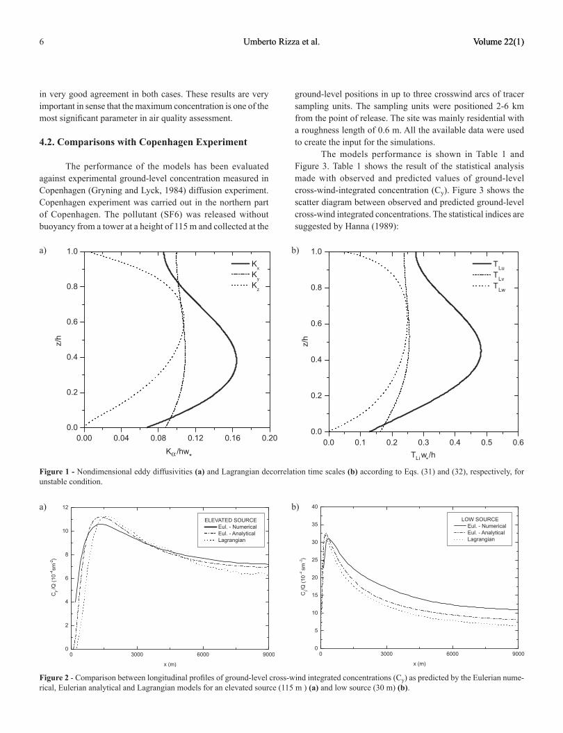
6 Umberto Ri��a et al. volume 22(�)Umberto Ri��a et al. volume 22(�) volume 22(�)

Figure 1 - nondimensional eddy diffusivities (a) and lagrangian decorrelation time scales (b) according to eqs. (3�) and (32), respectively, for unstable condition.

a) b)

Figure 2 - Comparison between longitudinal profiles of ground-level cross-wind integrated concentrations (Cy) as predicted by the eulerian nume-rical, eulerian analytical and lagrangian models for an elevated source (��5 m ) (a) and low source (30 m) (b).

a) b)

in very good agreement in both cases. these results are very important in sense that the maximum concentration is one of the most significant parameter in air quality assessment.

4.2. Comparisons with Copenhagen Experiment

the performance of the models has been evaluated against experimental ground-level concentration measured in Copenhagen (Gryning and Lyck, 1984) diffusion experiment. Copenhagen experiment was carried out in the northern part of Copenhagen. the pollutant (sF6) was released without buoyancy from a tower at a height of ��5 m and collected at the

ground-level positions in up to three crosswind arcs of tracer sampling units. the sampling units were positioned 2-6 km from the point of release. the site was mainly residential with a roughness length of 0.6 m. all the available data were used to create the input for the simulations.

the models performance is shown in table � and Figure 3. table � shows the result of the statistical analysis made with observed and predicted values of ground-level cross-wind-integrated concentration (Cy). Figure 3 shows the scatter diagram between observed and predicted ground-level cross-wind integrated concentrations. the statistical indices are suggested by hanna (�989)��

abril 2007 Revista Brasileira de Meteorologia 7

NMSE C C C Co p o p= −( ) /2

(normali�ed Mean square error)

FB C C C Co p o p= − +( ) /( . ( ))0 5(Fractional Bias)

F FS o p o p= −( ) +( )2 σ σ σ σ(Fractional standard Deviation)

R R C C C Co o p p o p= − −( )( ) /σ σ(Correlation Coefficient)

FA C Co p2 0 5 2= ≤ ≤.(Factor 2)

where C is the analy�ed quantity (concentration) and the subscripts “o” and “p” represent the observed and the predicted values, respectively. the overbars in the statistical indices indicate averages. The statistical index FB indicates if the predicted quantity underestimates or overestimates the observed one. The statistical index NMSE represents the quadratic error

of the predicted quantity in relation to the observed one. the statistical index FS indicates the measure of the comparison between predicted and observed plume spreading. the statistical index FA2 provides the fraction of data for which 0.5 ≤ Co / p ≤ 2. as nearest �ero are the nMse, FB and Fs and as nearest one are the R and Fa2, better are the results.

analysing the statistical indices in tables � it is possible to notice that the model simulates quite well the observed concentrations, with nMse, FB and Fs values relatively near to �ero and R and Fa2 very close to �. Fractional bias (FB in table �) shows under-prediction for lagragian model and over-prediction for Eulerian models. This also confirmed by visual inspection of Figure 3. For the other statistical indices, there are not considerable differences between the results. all the values for the indices are within ranges that are characteristics of those found for other state-of-the-art models applied to other field datasets, thus showing that the models and the turbulence parameteri�ations are quite effective.

5. CONCLUSIONS

We utili�ed both eulerian and lagrangian approaches to air pollution problems to make a comparison between these different techniques. Furthermore the eulerian conservation equation for a passive contaminant has been solved both numerically than analytically. a fundamental recipe in all kind of modelling is the parameteri�ation of turbulent quantities describing the dispersion properties of PBl. We proposed a new parameteri�ation for eddy diffusivity and lagrangian decorrelation time scales that properly model both generation mechanisms of PBl turbulence. a sensitivity analysis has been conducted between the three models first and then with experimental data. Such comparison show an excellent agreement between the three models showing that they can be incorporate in a global modelling system for air-quality estimates. this work is just preliminary. a more detailed comparison will be made using more concentration datasets in different PBl stability conditions.

6. APPENDIX

Physical Constraintsthe convective velocity scale w* is given by��

w uh

L∗ ∗= −

κ

1 3

.

the values of the reduced frequency of the neutral spectral peak are (table � of olesen, �984)��(fm)u = 0.045 (fm)v = 0.�6 (fm)w = 0.35.

the spectral peaks depending on height and stability are determined according Caughey and Palmer (�979):

Figure 3 - scatter diagram between observed and predicted ground-level cross-wind integrated concentrations (Cy) for the Copenhagen data set.

Table 1 - statistical indices of the model performances for the Copenhagen experiment.

Model NMSE FB FS R FA2eulerian – numerical 0.07 -0.06 0.26 0.86 0.96eulerian – analytical 0.08 -0.�5 0.04 0.88 0.96lagrangian 0.07 0.�2 0.27 0.89 �.00

8 Umberto Ri��a et al. volume 22(�)Umberto Ri��a et al. volume 22(�) volume 22(�)

(λm)u = (λm)v = �.5hand

λm w

z z L z L

( ) ≈

−( ) ≤ ≤0 55 0 38 0

5

. . ,

.. ,9z

1.8h 1 exp -4z h 0.0003exp -8z h

L z h

h z h

≤ ≤

( ) ( ) ≤ ≤

0 1

0 1

.

, .

the buoyancy-shear ensemble average rates of dissipation of tKe are from højstrup (�982)��

εb

w

h=( ) ∗0 75

3 23

. εκs

u

z

z

h= −

∗3 3

1 .

7. ACKNOWLEDGEMENTS

The authors acknowledge the financial support provided by CNPq. (Conselho Nacional de Desenvolvimento Científico e tecnológico) and FaPeRGs (Fundação de amparo à Pesquisa do estado do Rio Grande do sul).

8. REFERENCES

anFossi, D.; FeRReRo, e.; saCChetti, D.; tRini Castelli, s. Comparison among empirical probability density functions of the vertical velocity in the surface layer based on higher order correlations. Bound.-layer Meteor. 82, �997, �93-2�8.

BatCheloR G. K. 1949: Diffusion in a field of homogeneous turbulence, eulerian analysis. aust J.sci.Res., 2, 437-450.

BeRKoWiCz R. R.; olesen h. R.; toRP U. �986�� the Danish Gaussian air pollution model (oMl)�� Description, test and sensitivity analysis in view of regulatory applications, air Pollution Modeling and its application, C. De Wispeleare, F.a. schiermeirier and n.v. Gillani eds., Plenum Publishing Corporation, 453-480.

DeGRazia G.a. and MoRaes o.l.l., �992�� a Model for eddy Diffusivity in a stable Boundary layer, Boundary-layer Meterology 58, 205-2�4.

DeGRazia G.a., anFossi D., CaRvalho J.C., ManGia C., tiRaBassi t., CaMPos velho h.F., 2000�� turbulence parameteri�ation for PBl dispersion models in all stability conditions, atmos. environ. 34, 3575-3583.

FeRReRo, e., anFossi, D., �998. Comparison of PDFs, closures schemes and turbulence parameteri�ations in lagrangian stochastic Models. int. J. envinm. and Poll. 9, 384-4�0.

FlesCh t. K. and Wilson J. D., �995�� Backward-time lagrangian stochastic Dispersion Models and their application to estimate Gaseous emissions, J. appl. Meteorol. 34, �320-�332.

FoResteR, C.K., �979�� higher order monotonic convective difference schemes. J.Comp.Phys 23, �-22.

FRisCh U., �995�� turbulence. Cambridge University Press. 296 pp.

GRYninG s.e. and lYCK e., �984�� atmospheric Dispers ion f rom elevated source in un Urban Area: Comparision between tracer experiments and model calculations, J. Climate appl. Meteor. 23, 65�-654.

hanna s.R. and Paine R.J., �989�� hibrid plume dispersion model (hPDM) development and evaluation, J. appl. Meteorol. 28, 206-224

hinze J.o., �975�� turbulence. Mc Graw hill, 790 pp.

høJstRUP J., �982�� velocity spectra in the unstable boundary layer, J. atmos. sci. 39, 2239-2248.

KaiMal J.C., WYnGaaRD J.C., haUGen D.a., CotÉ o.R., izUMi Y., CaUGheY s.J. and ReaDinGs C.J., �976�� turbulence structure in the Convective Boudary layer, J. atmos. sci. 33, 2�52-2�69.

KenDall, M., stUaRt, a., �977. the advanced theory of statistics. MacMillan, new York.

WanDel C.F. and KoFoeD-hansen o., �962�� on the eulerian-lagrangian transform in the statistical theory of turbulence. J. Geophys. Res. 67, 3089-3093.

ManGia C., DeGRazia G.a., Rizza U., 2000�� an integral formulation for the dispersion parameters in a shear/buyancy driven planetary boundary layer for use in a Gaussian model for tall stacks. J. appl. Meteorol. 39, 67-76.

abril 2007 Revista Brasileira de Meteorologia 9

RoDean h.C., �996�� stochastic lagrangian Models of turbulent Diffusion. american Meteorological society, Boston, 84 pp.

thoMson D.J., �987�� Criteria for the selection of stochastic Models of Particle trajectories in turbulent Flows, J.Fluid Mech. �80, 529-556.

vilhena Mt, Rizza U, DeGRazia Ga, ManGia C, MoReiRa DM, tiRaBassi t., �998�� an analytical air pollution model�� development and evaluation. Contribution to atmospheric Physics 7�, 3�� 3�5-320.

YanenKo nn. the Method of Fractional steps. springer-verlag, Berlin, new York, �97�.

MoReiRa, D.M, FeRReiRa neto, P.v. and CaRvalho, J.C., 2004. analytical solution of the eulerian dispersion equation for nonstationary conditions�� development and evaluation, environmental Modelling and software. in press.

olesen h.R., laRsen s. e. and hJstRUP J., �984�� Modelling velocity spectra in the lower Part of the Planetary Boundary layer, Boundary-layer Meteorol. 29, 285-3�2.

Rizza U., Gioia G., ManGia C., MaRRa G.P., 2003�� Development of a grid-dispersion model in a large-eddy-simulation-generated planetary boundary layer. nuovo Cimento 26, 3, 297-309.