1

Modeling Uncertainty about Pollutant Concentration and Human Exposure using Geostatistics and a Space-time Information System:

Application to Arsenic in Groundwater of Southeast Michigan

P. Goovaerts*, G. Avruskin*, J. Meliker**, M. Slotnick**, G. Jacquez*, J. Nriagu** * Biomedware, Inc.

516 North State Street Ann Arbor, MI 48104, USA

Ph. (734) 913-1098; Fax: (734) 913-2201 E-mail: goovaerts@biomedware.com

** School of Public Health

The University of Michigan Ann Arbor, MI 48109-2029, USA

Keywords: indicator kriging, arsenic, cross validation, exposure Abstract The last decade has witnessed an increasing interest in assessing health risks caused by exposure to contaminants present in the soil, air, and water. A key component of any exposure study is a reliable model for the space-time distribution of pollutants. This paper compares the performances of multiGaussian and indicator kriging for modeling probabilistically the space-time distribution of arsenic concentrations in groundwater of Southeast Michigan, accounting for information collected at private residential wells and the hydrogeochemistry of the area. This model will later be combined with a space-time information system to compute individual exposures and analyze its relationship to the occurrence of bladder cancer. Because of the small changes in concentration observed in time, the study has focused on the spatial variability of arsenic, which can be considerable over very short distances. Factorial kriging was used to filter this short-range variability, leading to a significant increase (17 to 65%) in the proportion of variance explained by secondary information, such as type of surficial rock formation and proximity to Marshall Sandstone subcrop. Cross validation of 8,212 well data shows that accounting for this regional background does not improve the local prediction of arsenic, indicating the presence of unexplained sources of variability and the importance to model the uncertainty attached to these predictions. 1. Introduction Assessment of the health risks associated with exposure to elevated levels of contaminants has become the subject of considerable interest in our societies. Environmental exposure assessment is frequently hampered by the existence of multiple confounding risk-factors (e.g. smoking, diet, stress, ethnicity, home and occupational exposures) leading to complex exposure models, and the mobility of the population which can interact with many different sources of exposure over the lifetime. A rigorous study thus requires modeling the study subjects as spatio-temporally referenced objects that move through space and time, their cumulative exposure increasing as they come in contact with sources of contamination. The computation of human exposure is particularly challenging for cancers because they usually take years or decades to develop, especially in presence of low level of contaminants. In this case contaminant concentrations are not available for every location and time interval visited by the subjects; therefore data gaps need to be filled-in through space-time interpolation.

Geostatistical spatio-temporal models provide a probabilistic framework for data analysis and predictions that build on the joint spatial and temporal dependence between observations (e.g. see Kyriakidis and Journel, 1999, for a review). Geostatistical tools have been applied for modeling spatio-temporal distributions in many disciplines, such as environmental sciences (e.g., deposition of atmospheric pollutants), ecology (characterization

2

of population dynamics) and health (patterns of diseases and exposure to pollutants). These tools are increasingly coupled with GIS capabilities (Burrough and McDonnell, 2000) for applications that characterize space-time structures (semivariogram analysis), spatially interpolate scattered measurements to create spatially exhaustive layers of information and assess the corresponding accuracy and precision. Of critical importance when coupling GIS data and environmental/exposure models is the issue of error propagation, that is how the uncertainty in input data (e.g. arsenic concentrations) translates into uncertainty about model outputs (e.g. risk of cancer). Methods for uncertainty propagation (Heuvelink, 1998; Goovaerts, 2001), such as Monte-Carlo analysis, are critical for estimating uncertainties associated with spatially-based policies in the area of environmental health, and in dealing effectively with risks (Goodchild, 1996).

A bladder cancer case-control study is underway in Michigan (11 counties) to evaluate risks associated with exposure to low levels of arsenic in drinking water (typically 5-100 µg/L). A key part of this study is the creation of a space-time information system (STIS) to visualize and analyze the spatio-temporal mobility of study participants and their surrounding environment (Jacquez et al., 2004), leading to the estimation of individual-level historical exposure to arsenic. Generations of Michiganders have depended on ground water as their source of drinking water and many have experienced lifetime exposures to elevated concentrations of arsenic, an unwanted chemical in their water supply derived from local rocks (Kolker et al., 1998). A model of the space-time distribution of arsenic in groundwater is thus an important layer of the STIS. Geostatistics has recently been used to evaluate the spatial variability of arsenic contamination in the groundwater of Bangladesh. In Karthick et al. (2001), semivariogram analysis suggested that the complex spatial distribution of high-level arsenic concentrations is a consequence of interactions among multiscale geologic and geochemical processes. Serre et al. (2003) also found that most of the variability in arsenic concentrations across Bangladesh occurs within a distance of 2 km, which makes spatial interpolation very challenging.

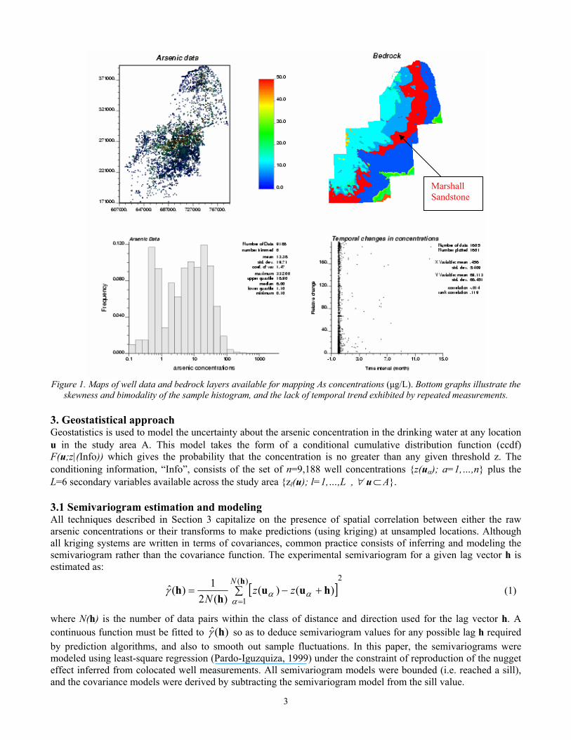
This paper presents a study of the space-time variability of arsenic concentrations in groundwater of Southeast Michigan, accounting for information collected at private residential wells and the hydrogeochemistry of the area. Variants of traditional semivariogram estimators and kriging systems are introduced to tackle specific features of the dataset, such as the preferential sampling of high concentrations, the existence of repeated measurements at hundreds of wells, and the presence of high variability over very short distances. Cross-validation is used to assess the prediction performances and quality of uncertainty models provided by multiGaussian and indicator approaches. 2. The Dataset Elevated concentrations of arsenic in drinking water have been identified in ground-water supplies of 11 counties in southeastern Michigan: Genesee, Huron, Ingham, Jackson, Lapeer, Livingston, Oakland, Sanilac, Shiawassee, Tuscola, and Washtenaw (Kim et al. 2002; Kolker et al. 2003; Slotnick et al. 2003). The space-time distribution of arsenic over these 11 counties was modeled using 9,188 data recorded at 8,212 different wells and stored in the Michigan Department of Environmental Quality (MDEQ) database of arsenic measurements (1993-2002), see Figure 1 (top graph). The sample histogram is positively skewed, with a mean that is more than twice the median value of 6 µg/L. It is noteworthy that a mere log-transform does not make the distribution symmetric although it reveals the existence of two modes, one mode corresponding to half the detection limit of 1.0 µg/L.

At 662 wells, concentrations were measured multiple times (2 to 14 times) at the same moment or up to 113 months apart, with an average time interval of 14 days. These data allowed one to investigate any temporal trend in the data. The scatterplot in Figure 1(bottom graph) indicates that the relative change in concentration is not a function of the length of the time interval; hence the temporal dimension was ignored in the remainder of the study.

Well data are supplemented by secondary information that is available everywhere in the study area: type of bedrock and surficial rock formation, proximity to Marshall Sandstone subcrop where the highest concentrations of arsenic were found (Kim, 1999), and ground-water recharge classes (from 0 to more than 8 inches/day). Figure 1 (top right graph) shows the map of rock formation, with the Marshall Sandstone in red.

3

Figure 1. Maps of well data and bedrock layers available for mapping As concentrations (µg/L). Bottom graphs illustrate the

skewness and bimodality of the sample histogram, and the lack of temporal trend exhibited by repeated measurements. 3. Geostatistical approach Geostatistics is used to model the uncertainty about the arsenic concentration in the drinking water at any location u in the study area Α. This model takes the form of a conditional cumulative distribution function (ccdf) F(u;z|(Info)) which gives the probability that the concentration is no greater than any given threshold z. The conditioning information, “Info”, consists of the set of n=9,188 well concentrations {z(uα); a=1,…,n} plus the L=6 secondary variables available across the study area {zl(u); l=1,…,L , ∀ u⊂A}. 3.1 Semivariogram estimation and modeling All techniques described in Section 3 capitalize on the presence of spatial correlation between either the raw arsenic concentrations or their transforms to make predictions (using kriging) at unsampled locations. Although all kriging systems are written in terms of covariances, common practice consists of inferring and modeling the semivariogram rather than the covariance function. The experimental semivariogram for a given lag vector h is estimated as:

[ ]2)(

1)()(

)(21)(ˆ ∑ +−=

=

hhuu

hh

Nzz

N αααγ (1)

where N(h) is the number of data pairs within the class of distance and direction used for the lag vector h. A continuous function must be fitted to )(ˆ hγ so as to deduce semivariogram values for any possible lag h required by prediction algorithms, and also to smooth out sample fluctuations. In this paper, the semivariograms were modeled using least-square regression (Pardo-Iguzquiza, 1999) under the constraint of reproduction of the nugget effect inferred from colocated well measurements. All semivariogram models were bounded (i.e. reached a sill), and the covariance models were derived by subtracting the semivariogram model from the sill value.

Marshall Sandstone

4

3.2 MultiGaussian approach Under the multiGaussian (MG) model, the ccdf at any location u is Gaussian and fully characterized by its mean and variance which can be estimated by kriging (Goovaerts, 2001). The approach typically requires a prior normal score transform of data to ensure that at least the univariate distribution (histogram) is normal. The normal score ccdf then undergoes a back-transform to yield the ccdf of the original variable. 3.2.1 Normal score transform Normal score transform is a graphical transform that allows one to normalize any distribution, regardless of its shape. It can be seen as a correspondence table between equal p-quantiles zp and yp of the z-cdf F(z) (cumulative histogram) and the standard Gaussian cdf G(y). In practice, the normal score transform proceeds in three steps:

1. The n original data z(uα) are first ranked in ascending order. Since the normal score transform must be monotonic, ties in z-values must be broken, which may be a problem in presence of a large proportion of censored data (i.e. non detects). In this paper, such untying or despiking has been done randomly as implemented in GSLIB software (Deutsch and Journel, 1998).

2. The sample cumulative frequency of the datum z(uα) with rank k is then computed as *kp =k/n - 0.5/n.

3. The normal score transform of the z-datum with rank k is matched to the *kp -quantile of the standard

normal cdf: ( ) ( )[ ] [ ]*11 )()()( kpGzFGzy −− === ααα φ uuu (2) 3.2.2 MultiGaussian kriging The probability distribution of the normal score variable Y at location u is Gaussian, and its mean and standard deviation are the ordinary kriging (OK) estimate )(* uOKy and simple kriging (SK) standard deviation )(* uSKσ computed from the normal score data:

( )[ ])(/)())Info(|;( ** uuu SKOKY yyGyF σ−= (3)

The OK estimate is computed as a linear combination of n(u) surrounding normal score data:

∑==

)(

1

* )()(u

uun

OK yyα

ααλ (4)

The kriging weights are calculated by solving the following system of linear equations:

[ ]

∑ =

∑ =−=+−−

=

=)(

1

)(

10,

1

)(,1, )()(

u

uuuuuu

n

nnCbC

ββ

βαβαβαβ

λ

αµδλ K

(5)

where C(uα- uβ) is the covariance function of the normal score variable Y for the separation vector hαβ=uα- uβ, µ is a Lagrange multiplier that results from minimizing the estimation variance subject to the unbiasedness constraint on the estimator, δαβ=1 if uα= uβ, and 0 otherwise. The parameter b0 is the nugget effect (i.e. variability for a distance of zero) which was estimated using the set of colocated observations at 662 wells. This system is modified from the traditional OK system in order to allow for incorporation of data with the same spatial coordinates. The standard deviation of the distribution is computed as:

2/1)(

1

'* )(1)(

∑ −−==

uuuu

nSK C

αααλσ (6)

where the kriging weights 'αλ are obtained by solving a system similar to (5) except that no constraint is imposed

on the weights.

5

3.2.3 Accounting for secondary information Several approaches are available for incorporating the secondary data in the estimation procedure (e.g., see Goovaerts, 1997). Since in this study the secondary data are available everywhere, they were used to compute the local means of the normal score variable, *

Ym (u), at any location. The ccdf means were then estimated using simple kriging with local means (SKlm) as:

[ ] )()()()( *)(

1

** uuuuu

Yn

YSKlm mmyy +∑ −==α

αααλ (7)

The weights are the solution of the following system:

[ ]∑ =−=+−−=

)(

10, )(,1, )()(

uuuuuu

nRRR nCbC

βαβαβαβ αµδλ K (8)

where CR(uα- uβ) is the covariance function of the normal score residuals R(u)=Y(u)- *Ym (u) for the separation

vector hαβ=uα- uβ, and b0R is the corresponding nugget effect. The ccdf variance is computed as the sum of the SKlm variance (equation (6) using the residual covariance CR(h)) and the variance of the local mean estimator. In this paper the local means were predicted by multivariate regression on the secondary variables Zl and a quadratic function of the spatial coordinates, see the results section for more details. The independent variable was the local mean of normal score data estimated by factorial kriging (Matheron, 1982; Goovaerts et al., 1993) using an estimator of type (4) where the weights are the solution of kriging system (5) with right-hand-side covariance terms, C(uα- u), set to zero (Goovaerts, 1997, p. 135). 3.2.4 Back-transform of results The probability of non-exceeding any arsenic concentration z can be easily computed as: { } ))Info(|)(;())Info(|;()Info(|)(Prob zFzFzZ Y φuuu ==≤ (9)

where φ(z)=y is the normal score transform of the threshold of interest. The mean and variance of the probability distribution of Z are estimated using the following empirical expressions:

( )∑=∑==

−

=

K

kp

K

kpMG y

Kz

Kz

1

1

1

* )(1)(1)( uuu φ (10)

[ ]∑ −==

K

kMGpMG zz

K 1

2**2 )()(1)( uuuσ (11)

where zp(u) are p-quantiles of the z-ccdf obtained by a normal score back-transform of the corresponding p-quantiles of the y-ccdf, yp(u., with p = k/100 – 0.5/100. An implicit assumption of multiGaussian kriging is that the multi-point cdf of the random function Z(u) is Gaussian. Unfortunately, the normality of the one-point cdf (histogram), which is achieved by the normal score transform, is a necessary but not sufficient condition to ensure the normality of the multi-point cdf (Goovaerts, 1997). Although graphical procedures exist for checking the appropriateness of the normality assumption for the two-point cdf (Deutsch and Journel, 1998), there is no formal statistical test. Furthermore, to be complete one should also check the normality of the three-point, four-point,…, N-point cumulative distribution functions, which is unfeasible in practice. For all these reasons the MG approach is usually adopted with little regard to the underlying assumptions. 3.3 Indicator approach Although the normal score transform makes the sample histogram perfectly symmetric it is not well suited to censored data since it requires a necessarily subjective ordering of all equally-valued observations. Indicator kriging (Journel, 1983) is an alternative to the use of multiGaussian kriging to infer the ccdf F(u;z|(Info)) and the corresponding E-type estimate:

6

0.5/100100/)(100

1)(100

1

* −=∑==

kpzzk

pIK uu (12)

Estimates (10) and (12) differ in the way the ccdf is modeled and so in how the series of quantiles zp(u) are computed. Instead of assuming that the ccdf is Gaussian and fully characterized by two parameters (parametric approach), the indicator approach estimates the conditional probabilities for a series of threshold zk discretizing the range of variation of z, and the complete function is obtained by interpolation/extrapolation of the estimated probabilities. 3.3.1 Indicator transform The first step is to transform each observation z(uα) into a vector of K indicators defined as:

Kkzz

zi kk ,,2,1

otherwise 0)( if 1

);( K= ≤

= αα

uu (13)

In this paper K=22 threshold values were selected, including the nineteen 0.05-quantiles of the sample histogram to cover uniformly the range of variation of arsenic concentrations and three thresholds (47, 70 and 100 µg/L) in the upper tail of the distribution. 3.3.2 Indicator kriging (IK) Ccdf values at unsampled location u are estimated as a linear combination of n(u) surrounding indicator data:

∑==

)(

1);(})Info{|;(

uuu

nkkkIK zizF

αααλ (14)

The kriging weights are computed by solving a kriging system of type (5) where the normal score covariance terms are replaced by covariance of indicator variables. Like in the multiGaussian approach secondary information was incorporated using simple kriging with local means (SKlm). The estimator is the following:

[ ]∑ −+==

)(

1);();();(})Info{|;(

uuuuu

nkkkkkSKlm zjzizjzF

ααααλ (15)

The probabilities j(uα;zk) are referred to as “soft” indicators since they are valued between zero and one, while indicators (13) are termed “hard”. They were derived from the soft information as:

{ } ( )( )[ ])(/)()Info Sec.(|)(Prob);( ** uuuu σφ Ykkk mzGzZzj −=≤= (16)

where *Ym (u) and σ*(u) are the mean and standard error of the prediction using multivariate regression. In other

words, the distribution of the regression estimator is used as a prior probability distribution for arsenic concentration at that location, and the soft probabilities are directly retrieved for normal score transforms of the target thresholds zk. The weights in expression (15) are computed by solving a kriging system of type (8), where the residuals are now defined as the difference between hard and soft indicator variables R(u;zk)=I(u;zk)-J(u;zk). 3.3.3 Modeling of the ccdf Because the K probabilities have been estimated individually (i.e. K indicator kriging systems are solved at each location) the following constraints, which are implicit to any probability distribution, might not be satisfied by all sets of K estimates:

k 1})Info{|;(0 ∀≤≤ kIK zF u (17)

kkkIKkIK zzzFzF ≤≤ '' if })Info{|;(})Info{|;( uu (18)

All probabilities that are not within [0,1] are first reset to the closest bound, 0 or 1. Then, condition (18) is ensured by averaging the results of an upward and downward correction of ccdf values (Deutsch and Journel, 1998).

7

Once conditional probabilities have been estimated and corrected for potential order relation deviations, the set of K probabilities must be interpolated within each class (zk,zk+1] and extrapolated beyond the smallest and the largest thresholds to build a continuous model for the conditional cdf. In this paper, the resolution of the discrete ccdf was increased by performing a linear interpolation between tabulated bounds provided by the sample histogram of arsenic concentrations (Deutsch and Journel, 1998). 3.4 Comparison criteria Relative performances of the multiGaussian versus indicator approaches, as well as the benefit of incorporating secondary information in the prediction, were assessed using cross-validation whereby one observation is removed at a time and re-estimated using neighboring non-colocated well data (i.e. repeated measurements in time were not used when estimating arsenic concentration). 3.4.1 Prediction errors The ability of different techniques to estimate arsenic concentration was quantified using the mean absolute error of prediction (MAE) defined as:

∑ −==

nzz

nMAE

1

* )()(1α

αα uu (19)

where n is the number (8,212) of individual wells. 3.4.2 Model of uncertainty At any location u knowledge of the ccdf F(u;z|(Info)) allows the computation of a series of symmetric p-probability intervals (PI) bounded by the (1-p)/2 and (1+p)/2 quantiles of that ccdf. For example, the 0.5-PI is bounded by the lower and upper quartiles [F-1(u;0.25|(Info)), F-1(u;0.75|(Info))]. A correct modeling of local uncertainty would entail that there is a 0.5 probability that the actual z-value at u falls into that interval or, equivalently, that over the study area 50% of the 0.5-PI include the true value. Cross-validation yields a set of z-measurements and independently derived ccdfs at the n locations uα, allowing the fraction of true values falling into the symmetric p-PI to be computed as:

∑==

np

np

1);(1)(

ααζζ u (20)

where );( pαζ u equals 1 if z(uα) lies between the (1-p)/2 and (1+p)/2 quantiles of the ccdf, and zero otherwise.

The scattergram of the estimated, )( pζ , versus expected, p, fractions is called “accuracy plot”. Deutsch (1997) proposed to assess the closeness of the estimated and theoretical fractions using the following “goodness” statistics: [ ][ ]dppppaG )(2)(31 1

0 −∫ −−= ζ (21)

where a(p) =1 if )( pζ >p, and zero otherwise. Twice more importance is given to deviations when )( pζ <p (inaccurate case). The weight |3a(p) - 2 |=1 instead of 2 for the accurate case, that is the case where the fraction of true values falling into the p-PI is larger than expected.

Not only should the true value fall into the PI according to the expected probability p, but this interval should be as narrow as possible to reduce the uncertainty about that value. In other words, among two probabilistic models with similar goodness statistics one would privilege the one with the smallest spread (less uncertain). Different measures of ccdf spread can be used: variance, interquartile range, entropy. Following Goovaerts (2001) the average width of the PIs that include the true value are plotted for a series of probabilities p. For a probability p the average width is computed as:

( ) ( )[ ]2)1(;2)1(;);()(

1)( 11

1pFpFp

pnpW

n−−+∑= −−

=αα

ααζ

ζuuu (22)

8

4. Results and discussion

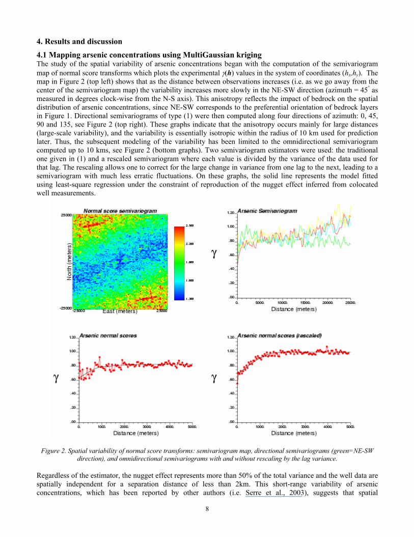
4.1 Mapping arsenic concentrations using MultiGaussian kriging The study of the spatial variability of arsenic concentrations began with the computation of the semivariogram map of normal score transforms which plots the experimental γ(h) values in the system of coordinates (hx,hy). The map in Figure 2 (top left) shows that as the distance between observations increases (i.e. as we go away from the center of the semivariogram map) the variability increases more slowly in the NE-SW direction (azimuth = 45° as measured in degrees clock-wise from the N-S axis). This anisotropy reflects the impact of bedrock on the spatial distribution of arsenic concentrations, since NE-SW corresponds to the preferential orientation of bedrock layers in Figure 1. Directional semivariograms of type (1) were then computed along four directions of azimuth: 0, 45, 90 and 135, see Figure 2 (top right). These graphs indicate that the anisotropy occurs mainly for large distances (large-scale variability), and the variability is essentially isotropic within the radius of 10 km used for prediction later. Thus, the subsequent modeling of the variability has been limited to the omnidirectional semivariogram computed up to 10 kms, see Figure 2 (bottom graphs). Two semivariogram estimators were used: the traditional one given in (1) and a rescaled semivariogram where each value is divided by the variance of the data used for that lag. The rescaling allows one to correct for the large change in variance from one lag to the next, leading to a semivariogram with much less erratic fluctuations. On these graphs, the solid line represents the model fitted using least-square regression under the constraint of reproduction of the nugget effect inferred from colocated well measurements.

Figure 2. Spatial variability of normal score transforms: semivariogram map, directional semivariograms (green=NE-SW direction), and omnidirectional semivariograms with and without rescaling by the lag variance.

Regardless of the estimator, the nugget effect represents more than 50% of the total variance and the well data are spatially independent for a separation distance of less than 2km. This short-range variability of arsenic concentrations, which has been reported by other authors (i.e. Serre et al., 2003), suggests that spatial

9

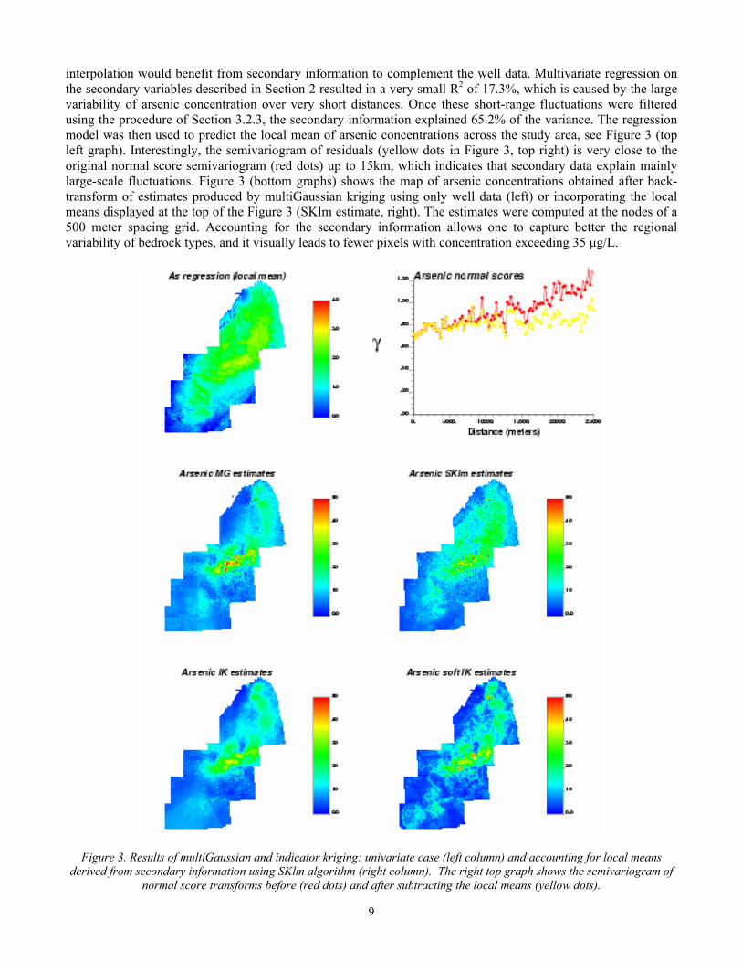
interpolation would benefit from secondary information to complement the well data. Multivariate regression on the secondary variables described in Section 2 resulted in a very small R2 of 17.3%, which is caused by the large variability of arsenic concentration over very short distances. Once these short-range fluctuations were filtered using the procedure of Section 3.2.3, the secondary information explained 65.2% of the variance. The regression model was then used to predict the local mean of arsenic concentrations across the study area, see Figure 3 (top left graph). Interestingly, the semivariogram of residuals (yellow dots in Figure 3, top right) is very close to the original normal score semivariogram (red dots) up to 15km, which indicates that secondary data explain mainly large-scale fluctuations. Figure 3 (bottom graphs) shows the map of arsenic concentrations obtained after back-transform of estimates produced by multiGaussian kriging using only well data (left) or incorporating the local means displayed at the top of the Figure 3 (SKlm estimate, right). The estimates were computed at the nodes of a 500 meter spacing grid. Accounting for the secondary information allows one to capture better the regional variability of bedrock types, and it visually leads to fewer pixels with concentration exceeding 35 µg/L.

Figure 3. Results of multiGaussian and indicator kriging: univariate case (left column) and accounting for local means derived from secondary information using SKlm algorithm (right column). The right top graph shows the semivariogram of

normal score transforms before (red dots) and after subtracting the local means (yellow dots).

10

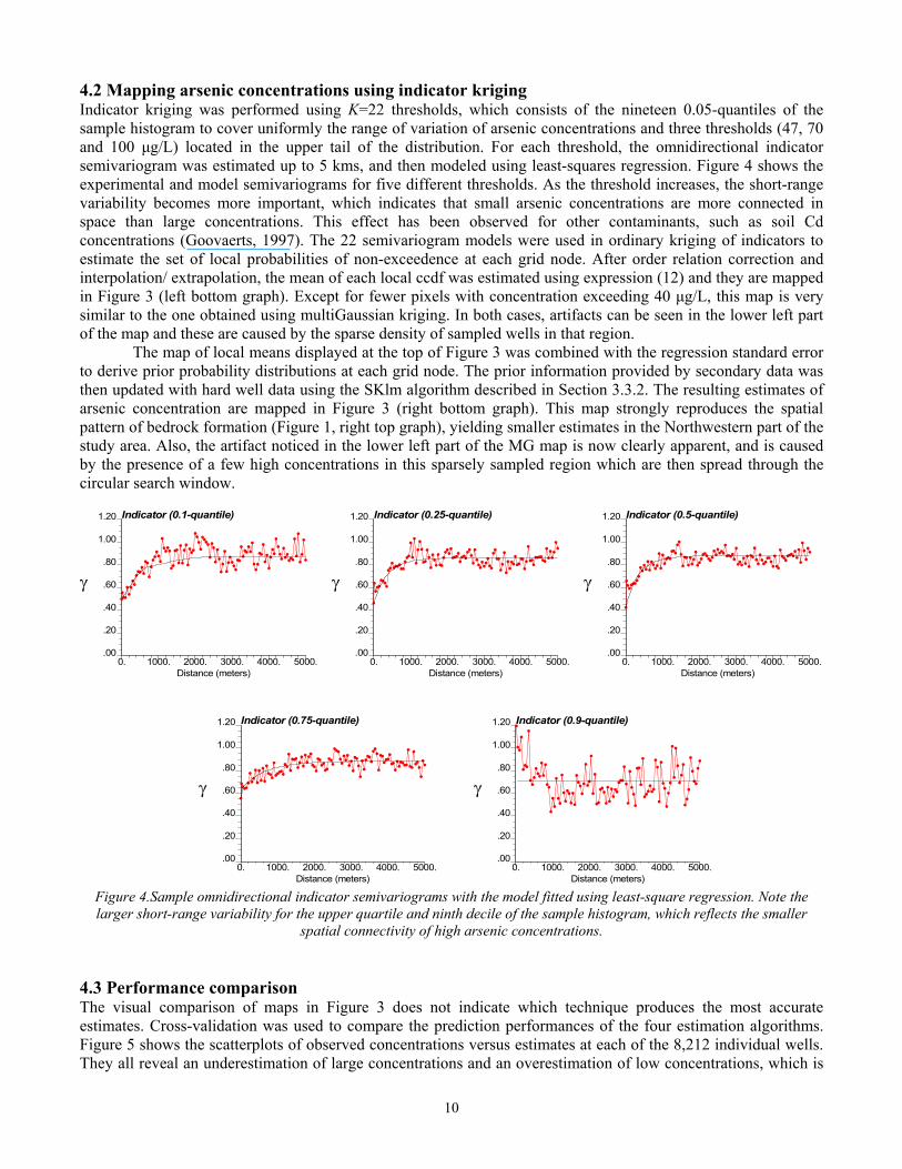
4.2 Mapping arsenic concentrations using indicator kriging Indicator kriging was performed using K=22 thresholds, which consists of the nineteen 0.05-quantiles of the sample histogram to cover uniformly the range of variation of arsenic concentrations and three thresholds (47, 70 and 100 µg/L) located in the upper tail of the distribution. For each threshold, the omnidirectional indicator semivariogram was estimated up to 5 kms, and then modeled using least-squares regression. Figure 4 shows the experimental and model semivariograms for five different thresholds. As the threshold increases, the short-range variability becomes more important, which indicates that small arsenic concentrations are more connected in space than large concentrations. This effect has been observed for other contaminants, such as soil Cd concentrations (Goovaerts, 1997). The 22 semivariogram models were used in ordinary kriging of indicators to estimate the set of local probabilities of non-exceedence at each grid node. After order relation correction and interpolation/ extrapolation, the mean of each local ccdf was estimated using expression (12) and they are mapped in Figure 3 (left bottom graph). Except for fewer pixels with concentration exceeding 40 µg/L, this map is very similar to the one obtained using multiGaussian kriging. In both cases, artifacts can be seen in the lower left part of the map and these are caused by the sparse density of sampled wells in that region. The map of local means displayed at the top of Figure 3 was combined with the regression standard error to derive prior probability distributions at each grid node. The prior information provided by secondary data was then updated with hard well data using the SKlm algorithm described in Section 3.3.2. The resulting estimates of arsenic concentration are mapped in Figure 3 (right bottom graph). This map strongly reproduces the spatial pattern of bedrock formation (Figure 1, right top graph), yielding smaller estimates in the Northwestern part of the study area. Also, the artifact noticed in the lower left part of the MG map is now clearly apparent, and is caused by the presence of a few high concentrations in this sparsely sampled region which are then spread through the circular search window.

γ

Distance (meters)

Indicator (0.1-quantile)

0. 1000. 2000. 3000. 4000. 5000..00

.20

.40

.60

.80

1.00

1.20

γ

Distance (meters)

Indicator (0.25-quantile)

0. 1000. 2000. 3000. 4000. 5000..00

.20

.40

.60

.80

1.00

1.20

γ

Distance (meters)

Indicator (0.5-quantile)

0. 1000. 2000. 3000. 4000. 5000..00

.20

.40

.60

.80

1.00

1.20

γ

Distance (meters)

Indicator (0.75-quantile)

0. 1000. 2000. 3000. 4000. 5000..00

.20

.40

.60

.80

1.00

1.20

γ

Distance (meters)

Indicator (0.9-quantile)

0. 1000. 2000. 3000. 4000. 5000..00

.20

.40

.60

.80

1.00

1.20

Figure 4.Sample omnidirectional indicator semivariograms with the model fitted using least-square regression. Note the larger short-range variability for the upper quartile and ninth decile of the sample histogram, which reflects the smaller

spatial connectivity of high arsenic concentrations.

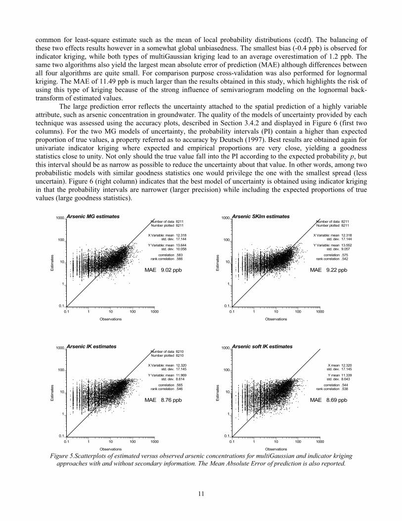
4.3 Performance comparison The visual comparison of maps in Figure 3 does not indicate which technique produces the most accurate estimates. Cross-validation was used to compare the prediction performances of the four estimation algorithms. Figure 5 shows the scatterplots of observed concentrations versus estimates at each of the 8,212 individual wells. They all reveal an underestimation of large concentrations and an overestimation of low concentrations, which is

11

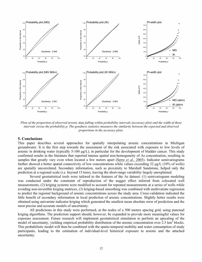
common for least-square estimate such as the mean of local probability distributions (ccdf). The balancing of these two effects results however in a somewhat global unbiasedness. The smallest bias (-0.4 ppb) is observed for indicator kriging, while both types of multiGaussian kriging lead to an average overestimation of 1.2 ppb. The same two algorithms also yield the largest mean absolute error of prediction (MAE) although differences between all four algorithms are quite small. For comparison purpose cross-validation was also performed for lognormal kriging. The MAE of 11.49 ppb is much larger than the results obtained in this study, which highlights the risk of using this type of kriging because of the strong influence of semivariogram modeling on the lognormal back-transform of estimated values. The large prediction error reflects the uncertainty attached to the spatial prediction of a highly variable attribute, such as arsenic concentration in groundwater. The quality of the models of uncertainty provided by each technique was assessed using the accuracy plots, described in Section 3.4.2 and displayed in Figure 6 (first two columns). For the two MG models of uncertainty, the probability intervals (PI) contain a higher than expected proportion of true values, a property referred as to accuracy by Deutsch (1997). Best results are obtained again for univariate indicator kriging where expected and empirical proportions are very close, yielding a goodness statistics close to unity. Not only should the true value fall into the PI according to the expected probability p, but this interval should be as narrow as possible to reduce the uncertainty about that value. In other words, among two probabilistic models with similar goodness statistics one would privilege the one with the smallest spread (less uncertain). Figure 6 (right column) indicates that the best model of uncertainty is obtained using indicator kriging in that the probability intervals are narrower (larger precision) while including the expected proportions of true values (large goodness statistics).

Est

imat

es

Observations

Arsenic MG estimates

0.1 1 10 100 10000.1

1

10

100

1000Number of data 8211Number plotted 8211

X Variable: mean 12.318std. dev. 17.144

Y Variable: mean 13.644std. dev. 10.058

correlation .583rank correlation .566

MAE 9.02 ppb Est

imat

es

Observations

Arsenic SKlm estimates

0.1 1 10 100 10000.1

1

10

100

1000Number of data 8211Number plotted 8211

X Variable: mean 12.318std. dev. 17.144

Y Variable: mean 13.552std. dev. 9.057

correlation .575rank correlation .542

MAE 9.22 ppb

Estim

ates

Observations

Arsenic IK estimates

0.1 1 10 100 10000.1

1

10

100

1000Number of data 8210Number plotted 8210

X Variable: mean 12.320std. dev. 17.145

Y Variable: mean 11.969std. dev. 8.614

correlation .565rank correlation .546

MAE 8.76 ppb Estim

ates

Observations

Arsenic soft IK estimates

0.1 1 10 100 10000.1

1

10

100

1000

X mean 12.320std. dev. 17.145

Y mean 11.339std. dev. 8.643

correlation .544rank correlation .538

MAE 8.69 ppb

Figure 5.Scatterplots of estimated versus observed arsenic concentrations for multiGaussian and indicator kriging

approaches with and without secondary information. The Mean Absolute Error of prediction is also reported.

12

Plots of the proportion of observed arsenic data falling within probability intervals (accuracy plot) and the width of these intervals versus the probability p. The goodness statistics measures the similarity between the expected and observed

proportions in the accuracy plots. 5. Conclusions This paper describes several approaches for spatially interpolating arsenic concentrations in Michigan groundwater. It is the first step towards the assessment of the risk associated with exposure to low levels of arsenic in drinking water (typically 5-100 µg/L), in particular for the development of bladder cancer. This study confirmed results in the literature that reported intense spatial non-homogeneity of As concentration, resulting in samples that greatly vary even when located a few meters apart (Serre et al., 2003). Indicator semivariograms further showed a better spatial connectivity of low concentrations while values exceeding 32 µg/L (10% of wells) are spatially uncorrelated. Secondary information, such as proximity to Marshall Sandstone, helped only the prediction at a regional scale (i.e. beyond 15 kms), leaving the short-range variability largely unexplained. Several geostatistical tools were tailored to the features of the As dataset: (1) semivariogram modeling was conducted under the constraint of reproduction of the nugget effect inferred from colocated well measurements, (2) kriging systems were modified to account for repeated measurements at a series of wells while avoiding non-invertible kriging matrices, (3) kriging-based smoothing was combined with multivariate regression to predict the regional background of arsenic concentrations across the study area. Cross-validation indicated the little benefit of secondary information in local prediction of arsenic concentrations. Slightly better results were obtained using univariate indicator kriging which generated the smallest mean absolute error of prediction and the most precise and accurate models of uncertainty.

All predictions in this study were performed, at the nodes of a 500 meters spacing grid, using punctual kriging algorithms. The prediction support should, however, be expanded to provide more meaningful values for exposure assessment. Future research will implement geostatistical simulation to perform an upscaling of the model of uncertainty, yielding empirical probability distribution of the arsenic concentration over 2.5 km2 blocks. This probabilistic model will then be combined with the spatio-temporal mobility and water consumption of study participants, leading to the estimation of individual-level historical exposure to arsenic and the attached uncertainty.

Pro

porti

on in

this

inte

rval

Probability p

Probability plot (MG)

.00 .20 .40 .60 .80 1.00.00

.20

.40

.60

.80

1.00

Goodness 0.944

Pro

porti

on in

this

inte

rval

Probability p

Probability plot (IK)

.00 .20 .40 .60 .80 1.00.00

.20

.40

.60

.80

1.00

Goodness 0.985

Wid

th o

f PI

Probability p

PI-width plot

MG

IK.00 .20 .40 .60 .80 1.00

.0

10.0

20.0

30.0

40.0

50.0

60.0

70.0

Pro

porti

on in

this

inte

rval

Probability p

Probability plot (MG SKlm)

.00 .20 .40 .60 .80 1.00.00

.20

.40

.60

.80

1.00

Goodness 0.951

Pro

porti

on in

this

inte

rval

Probability p

Probability plot (IK SKlm)

.00 .20 .40 .60 .80 1.00.00

.20

.40

.60

.80

1.00

Goodness 0.903

Wid

th o

f PI

Probability p

PI-width plot

MG (sklm)

IK (sklm).00 .20 .40 .60 .80 1.00

.0

10.0

20.0

30.0

40.0

50.0

60.0

70.0

13

ACKNOWLEDGEMENTS This study was supported by grant R01 CA96002-10, Geographic-Based Research in Cancer Control and Epidemiology, from the National Cancer Institute. Development of the STIS software was funded by grants R43 ES10220 from the National Institutes of Environmental Health Sciences and R01 CA92669 from the National Cancer Institute. REFERENCES Burrough, P.A. and R.A. McDonnell. 2000. Principles of Geographical Information Systems. Oxford, New York. Deutsch, C.V. 1997. Direct assessment of local accuracy and precision. In Geostatistics Wollongong '96. Eds.

E.Y. Baafi and N.A. Schofield. Kluwer Academic Publishers, Dordrecht, pp. 115-125. Deutsch, C.V. and A.G. Journel. 1998. GSLIB: Geostatistical Software Library and User's Guide: 2nd edn.

Oxford Univ. Press, New York. Goodchild, M.F. 1996. The application of advanced information technology in assessing environmental impacts.

In Application of GIS to the Modeling of Non-point Source Pollutants in the Vadose Zone, SSSA Special Publication No. 48, pp. 1-17.

Goovaerts, P. 1997. Geostatistics for Natural Resources Evaluation. Oxford University Press, New York. Goovaerts, P. 2001. Geostatistical modelling of uncertainty in soil science. Geoderma 103, pp. 3-26. Goovaerts, P., Ph. Sonnet, and A. Navarre. 1993. Factorial kriging analysis of springwater contents in the Dyle

river basin, Belgium. Water Resources Research 29(7), pp. 2115-2125. Heuvelink, G.B.M. 1998. Error Propagation in Environmental Modeling with GIS. London: Taylor and Francis. Jacquez, G.M., G. AvRuskin, E. Do, H. Durbeck, D.A. Greiling, P. Goovaerts, A. Kaufmann, and B. Rommel.

2004. Complex systems analysis using space-time information systems and model transition sensitivity analysis. In Accuracy 2004: Proceedings of the 6th International Symposium on Spatial Accuracy Assessment in Natural Resources and Environmental Sciences.

Journel, A.G. 1983. Non-parametric estimation of spatial distributions. Mathematical Geology 15(3), pp. 445-468. Karthik, B., Islam, S. and C.F. Harvey. 2001. On the spatial variability of arsenic contamination in the

groundwater of Bangladesh. Eos. Trans. AGU, 82(20), Spring meeting Suppl., Abstract H61C-01. Kim, M.J. 1999. Arsenic Dissolution and Speciation in Groundwater of Southeast Michigan. Ph.D. Dissertation

thesis. University of Michigan, Ann Arbor, MI. Kim M.J., J. Nriagu and S. Haack. 2002. Arsenic species and chemistry in groundwater of Southeast Michigan.

Environmental Pollution 120, pp. 379-390. Kolker, A., W.F. Cannon, D.B. Westjohn, and L.G. Woodruff. 1998. Arsenic-rich pyrite in the Mississippian

Marchall Sandstone: source of anomalous arsenic in southeastern Michigan ground water. Abstract from 1998 National Meeting of the Geological Society of America Oct. 25-29, Toronto, Ontario, Canada.

Kolker, A., S.K. Haack, W.F. Cannon, D.B. Westjohn, M.J. Kim, J. Nriagu, and L.G. Woodruff. 2003. Arsenic in southeastern Michigan. In Arsenic in Groundwater: Geochemistry and Occurrence. Eds. A.H. Welch and K.G. Stollenwerk. Kluwer Academic Publishers, Norwell, Massachusetts, pp 281-294.

Kyriakidis, P.C. and A.G. Journel. 1999. Geostatistical space-time models: a review. Mathematical Geology 31(6), pp. 651-684.

Matheron, G. 1982. Pour une Analyse Krigeante de Données Régionalisées. Internal note N-732, Centre de géostatistique, Fontainebleau.

Pardo-Iguzquiza, E. 1999. VARFIT: a Fortran-77 program for fitting variogram models by weighted least squares. Computers and Geosciences 25, pp. 251-261.

Serre, M.L., A. Kolovos, G. Christakos, and K. Modis. 2003. An application of the holistochastic human exposure methodology to naturally occurring arsenic in Bangladesh drinking water. Risk analysis 23(3), pp. 515-528.

Slotnick M.J., J. Meliker, and J. Nriagu. 2003. Natural sources of arsenic in Southeastern Michigan groundwater. Journal de Physique IV 107, pp. 1247-1250.