Air pollutant emissions scenario for India
190
The Energy and Resources Institute EDITORS Sumit Sharma Atul Kumar Air pollutant emissions scenario for India
-
Upload
khangminh22 -
Category
Documents
-
view
0 -
download
0
Transcript of Air pollutant emissions scenario for India

The Energy and Resources Institute
EDITORS
Sumit SharmaAtul Kumar
Air pollutant emissions scenario for India

Air pollutant emissions scenario for
India


EDITORSSumit Sharma
Atul Kumar
Air pollutant emissions scenario for
India
The Energy and Resources Institute

© The Energy and Resources Institute 2016
Suggested format for citation
Sharma S., Kumar A. (Eds), 2016, Air pollutant emissions scenario for India,.The Energy and Resources Institute. New Delhi.
Chapter Citation
Chapter Authors, Chapter name, In : Sharma S., Kumar A. (Eds), 2016, Air pollutant emissions scenario for India, The Energy and Resources Institute
For information
T E R I Tel. 2468 2100 or 2468 2111
Darbari Seth Block E-mail [email protected]
IHC Complex, Lodhi Road Fax 2468 2144 or 2468 2145
New Delhi – 110 003 Web www.teriin.org
India India +91 • Delhi (0)11
Printed in India

Introduction • v
Chapter1 Introduction ..................................................................................1
Chapter 2 Energy Outlook for India ..............................................................7
Chapter 3 Residential ...................................................................................21
Chapter 4 Industries .....................................................................................49
Chapter 5 Power ..........................................................................................83
Chapter 6 Transport ....................................................................................93
Chapter 7 Diesel Generator Sets ................................................................111
Chapter 8 Open Burning of Agricultural Residue .......................................121
Chapter 9 Evaporative Emissions ................................................................133
Chapter 10 Other Sectors ............................................................................149
Chapter 11 Summary and Conclusions .......................................................163
CONTENTS


Editors Sumit Sharma, Atul Kumar
Reviewers
Dr Prashant Gargava (Central Pollution Control Board, New Delhi), Prof. Mukesh Khare (Indian
Institute of Technology, Delhi), Prof. Mukesh Sharma (Indian Institute of Technology, Kanpur),
Prof. Suresh Jain (TERI University, New Delhi), Prof. B S Gurjar, (Indian Institute of Technology,
Roorkee), Prof. Prateek Sharma (TERI University, New Delhi), and Mr Zbigniew Klimont (IIASA,
Austria).
Chapter contributors
Sumit Sharma, Atul Kumar, Arindam Dutta, Ilika Mohan, Saptrishi Das, Arindam Dutta, Richa
Mahtta, C Sita lakshami, Sarbojit Pal, and Jai Kishan Malik
GIS Vivek Ratan
TERI PressAnushree Tiwari Sharma, Rajiv Sharma, Spandana Chatterjee, and R K Joshi
CONTRIBUTORS


Introduction • ix
PREFACE


Introduction • xi
ACKNOWLEDGEMENTS
We gratefully acknowledge the support provided by the UK Aid for carrying out research to develop air pollutant emission inventories in India and coming up with this publication. The support was crucial in developing this important database of spatially distributed multi-sectoral air pollutant emission inventories for India. However, the views expressed do not necessarily reflect the official policies of the UK government.
The project team thankfully acknowledges the cooperation extended by various government departments/organizations in providing relevant data and information. We gratefully acknowledge the reviewers of the book who provided their unconditional and unbiased comments and suggestions to improve the quality of the estimates. Finally, the project team thankfully acknowledges the kind support, guidance and cooperation by TERI colleagues during the entire study duration.


1CHAPTER
India is following a steep trajectory of economic
growth. This makes it essential to plan for
optimal energy use and reduced impact over
the environment. Energy consumption in different
sectors is linked to emissions of various air pollutants
that deteriorate air quality at different scales.
Some of the pollutants are linked to inefficiency
in the combustion processes and others are due
to inadequate tail-pipe controls required for their
treatment. There are market-driven improvements
that have happened on energy efficiency fronts in
the industrial sector, which have led to some control
of pollutant emissions. Some efforts have been made
to control emission of air pollutants and betterment
of air quality at the city and national scale. However,
rapid growth in different sectors has negated the
effects of these interventions and led to further
deterioration of air quality.
The health impacts of the deteriorating ambient
air quality, especially in urban cities of India are of
serious concern. Violation of ambient air quality
IntroductionSumit Sharma and Atul Kumar
standards for particulate matter (PM) in about 80 per
cent of the Indian cities conveys a grim picture of
the prevalent ambient air quality across the country
(CPCB 2014). Air pollutants, such as PM, carbon
monoxide (CO), oxide of sulphur (SO2), hydrocarbons
(HCs), oxide of nitrogen (NOX), are emitted from
variety of sources and have adverse health effects.
The impacts of some of the pollutants can be seen
at the regional scale. Ground level ozone formed
by reactions of NOx and HC can lead to detrimental
impacts on agricultural productivity of a region. The
various impacts of air pollution are documented in a
number of studies.
One of the preliminary step towards forming an air
quality management plan is to generate source-wise
emission inventories of different pollutants. These
inventories are generally compiled for emissions
from energy use in different sectors such as transport,
industries, power, residential, etc., and fugitive
emissions from non-energy sources, such as road
dust, storage and handling of fuels, etc. The emission

2 • Air Pollutant Emissions Scenario for India
inventories are developed for a base year and
could be projected for future years under different
growth scenarios. Emission inventory is one of the
fundamental components of air quality management
plan to assess the progress or changes over time to
achieve the cleaner air goal. Also, emission inventories
are an important input to the atmospheric models for
simulation of atmospheric pollutants.
For India, efforts have been made in past (Chatani
et al. 2014; EDGAR 4.2 ((http://edgar.jrc.ec.europa.
eu/); Garg and Shukla 2002; Garg et al. 2006; Klimont
et al. 2009, Kurokawa et al. 2013; Lu et al. 2011; Ohara
et al. 2007; Purohit et al. 2010; Sahu et al. 2012;
Sharma et al. 2015; Streets et al. 2003; Zhang et al.
2009) to estimate emissions for different sources
and pollutants. However, limited efforts are being
made to understand the possible future trajectory of
emissions for different sectors and pollutants, using
integrated modelling approach. This study has used
an integrated modelling approach for achieving the
above-mentioned goal. The integration of energy
modelling exercise with emission assessment models
helps to understand the overall energy mix in India
and inventorize the air pollutant loads from different
sectors (from energy-based and non-energy-based
sources) at a suitable resolution after taking into
account all the macro-economic changes in future in
an integrated manner. In this study, the TERI MARKAL
Figure 1.1: Overall framework for emission estimation
Model is linked with the emission estimation models
to develop multi sectoral emission inventories in an
integrated manner.
Goal To develop and document air pollutant emission
inventories for different sources in India for a base
year and future. This study does not include emissions
of greenhouse gases and only focusses on air
pollutant inventories.
Research Objectives P To prepare a baseline of emission inventories of air
pollutant loads across different energy- and non-
energy-based sources.
P To prepare grid-wise high-resolution dataset of air
pollutant emissions inventory for India.
P To project the future emission inventories using
integrated energy and emission modelling
approaches.
P To draft specific policy recommendations for
emission control in India.
Approach and MethodologyThe overall framework used in this study is shown
in Figure 1.1. Energy system modelling is carried out
using the MARKet ALlocation (MARKAL) model (Loulu

Introduction • 3
et al. 2004) for India, which is fed into the emission
model to estimate emissions. The estimated emissions
are spatially allocated at the finest possible resolutions.
The broad approach used in this study is further is
explained by Equation 1.
Ek=ΣiΣm
ΣnA
k,l,m.(1—η
l,m,n)X
k,l,m,n (1)
where,
k, l, m, n are region, sector, fuel, or activity type,
abatement technology; E denotes emissions of
pollutants (kt); A the activity rate; ef the unabated
emission factor (kt per unit of activity); η the removal
efficiency (%); and X the actual application rate of
Figure 1.2: Overall framework for emission estimation
control technology n (%) where ∑X = 1 (Klimont et al.
2002).
Energy use information from the MARKAL model
results is fed into the emission modelling equations
to derive emission estimates for India. The main
sectors considered in the analysis are residential,
transport, industries, power, and non-energy under
the fuel categories of coal, diesel, gasoline, natural
gas, liquefied petroleum gas, and biomass. The
emission inventory was prepared for pollutants, such
as PM, NOx, SO2, CO, and NMVOC. PM emissions are
also speciated into different fraction of PM10, PM2.5,
black carbon (BC), and organic carbon (OC).
The schematic for steps followed for emission
inventorization is presented in Figure 1.2. This includes

4 • Air Pollutant Emissions Scenario for India
a literature review of the existing inventories in India
and identification of key sources. These sources
include energy and non-energy sources contributing
to atmospheric pool of pollutants. Activity data are
collected at the finest possible resolution for different
sectors, and data quality checks are performed.
A detailed review of emission factors is carried out for
all the major sources. Emission factors are selected
from the literature (mainly indigenous sources).
Baseline emission inventories are prepared for the
year 2011 for different administrative regions and are
gridded using geographic information system (GIS).
Future energy scenarios till 2051 are developed using
the TERI MARKAL model results. Emission projections
are made for the next four decades till 2051. Based
on assessment of emission inventories, some
recommendations are made for reduction in emissions.
Structure In this publication, baseline and future trends of
emissions are presented for various sectors in
India. Chapter 2 focuses on current energy use
patterns in India and future projections using the
TERI-MARKAL models. Thereafter, Chapter 3 to 10
present the emissions inventories for Residential,
Industries, Power, Transport, DG sets, Agricultural
residue burning, Evaporative, and others sectors,
respectively. The final Chapter 11 summarizes
the report and presents overall findings including
sectoral contributions to the emission inventories.
Emission intensities are discussed in global context
and finally recommendations are provided for
control. The chapters also presents spatial distribution
of emissions at a fine grid resolution of 36 × 36 km2.
ReferencesCPCB. 2014. National ambient air quality status & trends – 2012. New Delhi: Central Pollution Control Board.
Chatani, S., M. Amann, A. Goel, J. Hao, Z. Klimont, A. Kumar, A. Mishra, S. Sharma, et al. 2014. Photochemical roles of rapid economic growth and potential abatement strategies on tropospheric ozone over South and East Asia in 2030. Atmospheric Chemistry and Physics 14:9259–9277.
Garg, A. and Shukla, P. R., Emission Inventory of India, Tata McGraw-Hill, New Delhi, 2002.
Garg, A., P. R. Shukla, and M. Kapshe. 2006. The sectoral trends of multigas emissions inventory of India. Atmospheric Environment 40:4608–4620.
Klimont, Z., J. Cofala, J. Xing, W. Wei, C. Zhang, S. Wang, J. Kejun, et al. 2009. Projections of SO
2, NOx
and carbonaceous aerosols emissions in Asia. Tellus B 61(4):602–617.
Klimont, Z., D. G. Streets, S. Gupta, J. Cofala, L. Fu, and Y. Ichikawa. 2002. Anthropogenic emissions of non-methane volatile organic compounds in China. Atmospheric Environment 36(8):1309–1322.
Kurokawa, J., T. Ohara, T. Morikawa, S. Hanayama, J.-M. Greet, T. Fukui. 2013. Emissions of air pollutants and greenhouse gases over Asian regions during 2000–2008: Regional Emission inventory in Asia (REAS) version 2, Discussion. Atmospheric Chemistry and Physics 13:11019–11058, 10049–10123.
Loulou R., G. Goldstein, K. Noble, 2004. Documentation for the MARKAL Family of Models, URL: http://www.iea-etsap.org/web/MrklDoc-I_StdMARKAL.pdf
Lu, Z., Q. Zhang, and D. G. Streets. 2011. Sulfur dioxide and primary carbonaceous aerosol emissions in China and India, 1996–2010. Atmospheric Chemistry and Physics 11:9839–9864, doi:10.5194/acp-11-9839- 2011.
Purohit, P., M. Amann, R. Mathur, I. Gupta, S. Marwah, V. Verma, I. Bertok, et al. 2010. GAINS ASIA scenarios for cost-effective control of air pollution and greenhouse gases in India. Laxenburg, Austria: International Institute For Applied Systems Analysis.
Ohara, T., H. Akimoto, J. Kurokawa, N. Horii, K. Yamaji, X. Yan, and T. Hayasaka. 2007. An Asian emission inventory of anthropogenic emission sources for the period 1980–2020. Atmospheric Chemistry and Physics 7:4419–4444, doi:10.5194/acp-7-4419-2007.
Sahu, S. K., G. Beig, and N. S. Parkhi. 2012. Emerging pattern of anthropogenic NOx emission over Indian subcontinent during 1990s and 2000s . Atmospheric Pollution Research 3(2012):262–269.
Sharma, S., A. Goel, D. Gupta, A. Kumar, A. Mishra, S. Kundu, S. Chatani, et al. 2015. Emission inventory of non-methane volatile organic compounds

Introduction • 5
from anthropogenic sources in India. Atmospheric Environment 102:209–219.
Streets, D. G., T. C. Bond, G. R. Carmichael, S. Fernandes, Q. Fu, D. He, et al. 2003. An inventory of gaseous and primary aerosol emissions in Asia in the year 2000. Journal of Geophysical Research 108(D21):8809
Zhang, Q., D. G. Streets, G. R. Carmichael, K. B. He, H. Huo, A. Kannari, Z. Klimont, et al. 2009. Asian emissions in 2006 for the NASA INTEX-B mission. Atmospheric Chemistry and Physics 9:5131–5153.


2CHAPTER
Energy Outlook for IndiaIlika Mohan, Atul Kumar, and Saptarshi Das
Introduction
India’s commercial energy consumption has
almost doubled in the past decade growing at
a rate of 7 per cent per annum from 179 Mtoe
(million tonnes of oil equivalent) in 2001–02 to 354
Mtoe in 2011–12 (TERI 2006a; 2015a). India is one of
the fastest growing economies in the world. Energy
consumption is among the key inputs in attaining
such growth. India’s growth experience is somewhat
different from that of the developed countries
as its energy requirements are growing faster,
leading to energy insecurity and pollution impacts.
(Ramakrishna & Rena 2013). Being a developing
country, with 27 per cent of its population below
the poverty line, access to energy is yet another
important issue that requires attention (Planning
Commission 2009). Commercial energy supply in
India is highly dependent on fossil fuels. In 2011–12,
97 per cent of our commercial supply was from fossil
fuels (coal, oil, and natural gas). Figure 2.1 below
provides a break-up of the commercial energy
supply by fuel share. With the current consumption
mix the role of fossil fuels is expected to grow.
Energy consumption has environmental
implications as well. Increased usage of fossil fuels
leads to a rise in air pollutants emission load in the
country. India’s greenhouse gas emissions grew by 2.9
per cent per annum between 1994 and 2007, with total
emissions, including land use, land-use change, and
forestry, being 1,728 million tonnes of CO2 equivalent
in 2007 (MOEF 2010). In 2011, the CO2 emissions due to
energy usage from the power, residential, commercial,
industry, transport, and agriculture sectors was 1.7
billion tonnes, which was equivalent to 1.38 tonnes per
capita.

8 • Air Pollutant Emissions Scenario for India
Figure 2.1: Commercial energy supply mix in 2011–12Source: (TERI 2015a)
Modelling Framework and Scenario Description1
The scenario analysis and energy projections for
the Indian energy sector have been carried out
with the aid of the MARKet ALlocation (MARKAL2)
model. This study builds on and integrates work
that has already been undertaken by TERI using
the MARKAL modelling framework for India and
the knowledge base existing within TERI. TERI has
developed a relatively detailed bottom-up MARKAL
model database for India over the last two decades
and has been using it extensively for the analysis of
energy technology at the national level. The following
sections describe the modelling framework, the
rationale for choosing this model, how the reference
energy scenario has been structured, and the
assumptions that define it.
Modelling FrameworkMARKAL is a bottom-up dynamic linear programming
model. It depicts both the energy supply and demand
sides of the energy system, providing policy makers
1 It should be noted this exercise builds on the database set up for the publication ‘Energy Security Outlook - defining a secure and sustainable future for India’ (TERI, 2015b). Authors would like to acknowledge the support and input received from several research professionals and sector experts across TERI.
2 MARKAL was developed in a cooperative multinational project over a period of almost two decades by the Energy Technology Systems Analysis Programme (ETSAP) of the International Energy Agency. Available at <http://www.iea-etsap.org/web/Markal.asp>.
and planners in the public and private sectors with
extensive details on energy producing and consuming
technologies. It also provides an understanding of the
interplay between the various fuel and technology
choices for given sectoral end-use demands. As a
result, this modelling framework has contributed
to national and local energy planning and to the
development of carbon mitigation strategies. The
MARKAL family of models is unique with applications
in a wide variety of settings and global technical
support from the international research community.
MARKAL interconnects the conversion and
consumption of energy. This user-defined network
includes:
P All energy carriers involved in primary supplies
(e.g., mining, petroleum extraction, etc.),
P Conversion and processing (e.g., power plants,
refineries, etc.), and
P End-use demand for energy services (e.g.,
automobiles, residential space conditioning, etc.).
These may be disaggregated by sector (i.e.,
residential, manufacturing, transportation, and
commercial) and by specific functions within a sector
(e.g., residential air conditioning, lighting, water
heating, etc.).
The optimization routine used in the model’s
solution selects from each of the sources, energy
carriers, and transformation technologies to
produce the least-cost solution, subject to a variety
of constraints. The user defines technology costs,
technical characteristics (e.g., conversion efficiencies),
and energy service demands.
As a result of this integrated approach, supply-
side technologies are matched to energy service
demands. Some uses of MARKAL include
1 Identifying least-cost energy systems and
investment strategies;
2 Identifying cost-effective responses to restrictions
on environmental emissions and wastes under the
principles of sustainable development;
3 Evaluating new technologies and priorities for
research and development;
4 Performing prospective analysis of long-term
energy balances under different scenarios;

Energy Outlook for India • 9
5 Examining reference and alternative scenarios in
terms of the variations in overall costs, fuel use,
and associated emissions.
A detailed representation of the modelling
framework is shown in Figure 2.2.
The MARKAL database for this exercise has been set
up over a 50-year period extending from 2001 to 2051
at five-yearly intervals coinciding with the duration of
the Government of India’s Five-Year plans. The base
year of the exercise is 2001–02 and the data for 2001–
02, 2006–07, and 2011–12 has been calibrated and
matched to the existing and published data.
In the model, the Indian energy sector is
disaggregated into five major energy consuming
sectors, namely agriculture, commercial, industry,
residential, and transport. Each of these sectors is
further disaggregated to reflect the sectoral end-use
demands. The model is driven by the demands from
the end-use side.
On the supply side, the model considers the
various energy resources that are available both
domestically and from abroad for meeting various
end-use demands. This includes both conventional
energy sources, such as coal; oil; natural gas; hydro
and nuclear; as well as the renewable energy
sources, such as wind, solar, etc. The level of domestic
availability of each of these fuels is represented as
constraints in the model.
The relative energy prices of various forms and
sources of fuels dictate the choice of fuels, which play
an integral role in capturing inter-fuel and inter-factor
substitution within the model. Furthermore, various
conversion and process technologies characterized
by their respective investment costs, operating
and maintenance costs, technical efficiency, life,
etc. to meet the sectoral end-use demands are also
incorporated in the model.
The model run and analysis that has been
carried out provides outcomes in terms of fuel
mix, technology deployment, primary energy
requirement, power generation, and CO2 emission
levels. In order to understand the model results, it is
important to understand the assumptions made to
construct the scenario.
Reference Scenario (RES)This scenario is structured to provide a baseline
that shows how the nation’s energy trajectory could
evolve provided current trends in energy demand and
supply are not changed. It takes into account existing
policy commitments and assumes that those recently
announced are implemented. However, wherever
necessary, a diversion from government projections
and forecasts has been assumed. The key assumptions
made to construct the RES have been made in
consultation and discussion with several organizations,
relevant stakeholders, and sector experts across the
country. These are described in the following sections.
Macroeconomic parametersThe energy demand of the end-use sectors are an
exogenous input in to the model. The calculation of
each of these end-use energy demands is in itself an
extensive exercise. The demands are primarily derived
as a function of the gross domestic product (GDP)
and population. For this, both GDP and population
have been projected and the same have been used
across all sectors in this publication.
Gross Domestic Product (GDP)The GDP is assumed to grow at a rate of about 8 per
cent rising from INR 19.7 trillion in 2001 to INR 741.58
trillion in 2051 at 1999–2000 prices. The sectoral GDP
has been calculated based on a regression analysis
that establishes the relationship between sectoral GDP
and the total GDP. The share of agriculture, industry,
and services GDP in the total GDP is seen to vary over
the years. The share of agriculture falls from 26 per
cent in 2001 to 6 per cent in 2051 while the share of
industry rises from 23 per cent in 2001 to 34 per cent
in 2051 and the service sector rises from 51 per cent in
2001 to 60 per cent in 2051. Table 2.1 shows the gross
GDP (in trillion, at 1999–2000 prices) and shares of
various sectors in the GDP.

10 • Air Pollutant Emissions Scenario for India
Fig
ure
2.2
: MA
RK
AL
mo
del
ling
fram
ewo
rkSo
urc
e: (
TER
I 200
6b)

Energy Outlook for India • 11
Table 2.1: Gross GDP (in trillion, at 1999–2000 prices) and sector shares
Year Gross GDP
Sector Shares
Agriculture (%) Industry (%) Services (%)
2001 19.7 26 23 51
2011 43.4 19 26 55
2021 97.6 16 28 56
2031 211.7 12 30 58
2041 414.1 9 32 59
2051 741.5 6 34 60
Source: TERI Analysis
PopulationThere are many studies that have projected
population of India at national and state level. The
Population Foundation of India (PFI) has carried
out projections in two scenarios, viz scenario A and
Scenario B (PFI, 2007). PFI has used a component
method to make the projections. The Component
Method is the universally accepted method of
carrying out population projection where the
population is broken down into its three major
components- survived population, number of births
taking place and net migration. This method takes
into account separately future course of fertility,
mortality and migration and is therefore considered
more accurate than any mathematical method
based on past trends. The ability to provide age sex
break-up of the projected population is an added
advantage of this method.
Among all the projections studied, PFI scenario B
assumptions have been agreed upon as the most
likely trajectory for India after expert consultation
and extensive literature review. This study has
therefore used PFI scenario B projection.
The Scenario B of the PFI projections, assume that the
states of India with total fertility rate (TFR) more than
that of the replacement level TFR will reach a target
level of 1.85 by 2101, while those states with very low
levels of TFR like Kerala and Tamil Nadu are assumed
to have a constant TFR at the existing level. Table 2.2
shows the decadal population (in billion) of India.
End-use demand The end-use demands, as described earlier, are
divided in to five sectors: agriculture, industry,
residential, commercial, and transport. Future
demand for each of these sectors is calculated using
different econometric methods and is then fed in to
MARKAL as input.
The population and GDP projections are used as
the main driving force for estimating the end-use
demands in each of the energy-consuming sectors.
Also, on the demand side, assumptions are
made on the end-use technological levels. It
involves inclusion of new technologies, efficiency
improvements in the existing ones, and their
changing penetration levels.
Demand for the industry sector has been
calculated for 10 of its most energy-consuming
sub-sectors, namely iron and steel, cement, brick,
glass, aluminium, textile, fertilizers, chlor-alkali,
petrochemicals, and paper. Other energy-consuming
industries that include small-scale industries, such
as food-processing, ceramics, sugar mills, foundry,
leather/tanning, etc., are grouped in a single sub-
sector collectively called ‘other industries’. Production
(as a proxy of demand) in each of these industrial
sub-sectors is projected using econometric
techniques. Econometric analysis has been carried
out for each of the major industry sub-sectors, taking
production as the dependent variable and using
various macroeconomic indicators, such as GDP
(aggregate), GDP of industrial sector, services, and
agriculture, etc. as independent variables.
Table 2.2: Population (in billion) of India
Year Total Rural Urban
2001 1.03 0.74 0.29
2011 1.20 0.84 0.36
2021 1.37 0.93 0.44
2021 1.37 0.93 0.44
2031 1.52 1.01 0.52
2041 1.65 1.06 0.59
2051 1.75 1.09 0.67
Source: (PFI 2007)

12 • Air Pollutant Emissions Scenario for India
In the RES, efficiency improvement is considered
as per the past trend and in line with commercially
available technological options in the industry sector.
Due to liberalization and opening up of domestic
markets, large scale industries, such as cement, iron
and steel, petrochemicals, and other chemicals,
assumed to improve their energy efficiency levels
by adoption of state-of-art technologies. Small-scale
manufacturing enterprises adopt energy efficient
technologies at slower rate.
The transportation demand (disaggregated
further into mode-wise passenger kilometre demand
and freight kilometre demand) is projected using
various socioeconomic indicators, such as per-capita
income (indicator of purchasing power), population,
and so on. To project the passenger and freight
kilometres from each mode, their estimated vehicle
population is multiplied with the occupancy rates
and utilization levels. The estimation of occupancy
rates and efficiency for each mode of transport has
been made after extensive stakeholder consultation
and discussion with sector experts.
Assumptions regarding fuel and technology
penetration in RES for the transport sector have been
made keeping the present situation in mind. We
consider that the share of CNG (Compressed Natural
Gas) in cars and public transport rises to 4 per cent,
from present levels of 1 per cent, by 2051. Share of
railways in passenger movement is taken to drop
from 14 per cent in 2011 to 12 per cent in 2051 while
that in freight is assumed to decrease to 23 per cent
(2051) from 39 per cent (2011). An increase in electric
traction in freight movement from 65 per cent (2011)
to 70 per cent (2051) and in passenger movement
from 50 per cent (2011) to 52 per cent (2051) has
been built in the model. Role of biofuels is minimal in
the RES.
In the agriculture sector, demand is estimated for
land preparation and irrigation pumping. Demand
for land preparation is calculated by estimating the
number of tractors and tillers that will be required
in future. The demand for irrigation pumping is
calculated by estimating the future water demand
of the agriculture sector. This has been done in
accordance to the current and expected cropping
patterns.
In the RES, the share of efficient tractors in land
preparation is assumed to be the same as the current
levels with no improvement. The share of efficient
electric pump sets in irrigation is assumed to rise from
negligible levels in 2011 to about 40 per cent in 2051.
In the residential sector, the demand is projected for
lighting, cooking, space conditioning, and refrigeration
separately for urban and rural households to account
for the differences in lifestyle and choice of fuel and
technology options. Each of these end-use demands
is estimated using a bottom-up methodology wherein
they are calculated across different monthly per capita
expenditure classes and these are further aggregated
to give the final demand.
Various assumptions have been made on the
level of penetration of efficient appliances in the RES.
The share of efficient air conditioners, fans, coolers,
and refrigerators is taken to rise in both the rural and
urban households from about 9 per cent in 2011 to 50
per cent in 2051. It is also assumed that 100 per cent
electrification will be achieved post 2016. By 2031, we
assume that 90 per cent of the lighting demand would
be met by CFLs (Compact Fluorecscent Lamps). The
share of improved cook stoves rises to 20 per cent from
negligible levels in 2011 by 2051 in the RES.
In the commercial building sector, the demand
is projected for cooking, lighting, and space
conditioning based on built-up area, energy
performance index (EPI), and the value added by
the services sector as an explanatory variable. Along
with the energy demand arising from commercial
buildings, energy demand for public lighting, public
water and sewage pumping is included in the
commercial sector. The commercial buildings sector’s
energy demand for the study was calculated using
EPI numbers and the built-up area.
In the RES, we assume no improvement in the EPI
and limited GRIHA3 penetration in the new buildings
(from 1 per cent in 2011, 3 per cent by 2021, 6 per cent
by 2031, and 10 per cent by 2051).
3 GRIHA is an acronym for Green Rating for Integrated Habitat Assessment. Available at <http://grihaindia.org/>. last accessed on July 1, 2015.

Energy Outlook for India • 13
Energy supplyAs a result of problems currently constraining the
production of coal, it is assumed that the production
of non-coking coal will reach a maximum of about 700
MT by 2021 (i.e., representing a compounded annual
growth rate (CAGR) of 3.7 per cent) and increase by 3
MT annually up to 2031. It is assumed that the present
trend in the production of metallurgical coal will
continue, and the production will reach a maximum of
19 MT by 2021–22 and stay at that level thereafter. We
see that the overall constraints in production of coal
will impact the production of non-metallurgical coal
as well. Therefore, it is assumed that the production
of non-metallurgical coal will peak at nearly 50
MT by 2021–22 and increase by 0.5 MT each year
thereafter till 2031. For the production of lignite, we
take conservative estimates, with projections that the
production will increase at a rate of 4 per cent between
2011–12 and 2021–22, reaching approximately 63 MT
by 2021–22. Thereafter, it is assumed to grow by 2 MT
each year. Total domestic coal production reaches a
maximum of about 880 MT by 2036.
In order to estimate constraints on our domestic
crude oil production for the RES, we assume that in
the short term (up to 2021) ONGC’s offshore crude
output remains constant, and its onshore crude
output continues to decline steadily. OIL’s onshore
crude production stays at around 4.5 MT. Private/joint
venture (JV) onshore crude output increases steadily
up to 10 MT in 2015–16 and offshore crude output by
private/JV companies continues to decline as has been
the case over 2000–01 to 2011–12.
In the medium to long term (2021–51),
assumptions are made on the total domestic crude
oil production and not on production by individual
companies. Total production remains relatively
stagnant at a little above 40 MT after 2021.
Natural gas assumptions are based on a similar
analysis. In the short term (up to 2021), we assume
Reliance’s KG-D6 gas output continues to fall steadily.
Private/JV companies’ production of natural gas
remains constant at 11 billion cubic metres (BCM)
from 2016 to 2017. ONGC’s gas output stays constant
and increases moderately after 2015–16 due to new
discoveries coming on-stream, and OIL’s natural gas
output stays constant at 2.8 BCM.
In the medium to long term (2021–51),
assumptions are made on total domestic gas
production and not on production by individual
companies. If the natural gas scenario continues as
usual, we do not consider a very significant rise in
domestic gas production. Domestic production is
assumed to reach a maximum of 50 BCM by 2031.
With regards to technology penetration in the
power sector, large scale deployment of supercritical
technology for coal-based generation is considered.
Further, it is also assumed that ultra-supercritical
technology would be available at commercial scale
Table 2.3: Tentative programme for capacity additions to grid-interactive renewable power under the XII Five-Year Plan (2012–17) and XIII Five-Year Plan (2017–22)
Source/system Capacity addition (MW), XII Plan
Capacity addition (MW), XIII Plan
Wind power 15,000 15,000
Biomass power 2,100 2,000
Small hydropower 1,600 1,500
Solar power 10,000 16,000
Waste to energy 500
Tidal power 7
Geothermal power 7
Total 29,214 34,500
only by 2031. In view of increasing concern about
rehabilitation and relocation issues, the capacity
realizations of large hydroelectric plants to a
moderate level of around 94 GW by 2031 and 148 by
2051 is predicted.
Nuclear energy in the RES is projected to rise
from an installed capacity of 5 GW in 2011 to 28
GW in 2031 and 103 GW in 2051. Delays in land
acquisitions, slow expansion, and commercialisation
of Fast Breeder technology and uncertainties (from
the supplier’s perspective) surrounding the nuclear
liability law are the major considerations for such
modest projections.
Till now, renewable energy capacity addition
targets have always been achieved in each of the five-

14 • Air Pollutant Emissions Scenario for India
year plans. This scenario assumes that this positive
trend will continue and there will be no shortfall in
targets. The targets of the five-year plans taken in to
consideration are mentioned in Table 2.3.
Modelling Results for the RESThe following sections enumerate the results
obtained from the model for the RES.
Primary Energy Supply4
Figure 2.3 reflects the primary energy supply by fuel.
The primary energy supply in the RES grows almost
4 As per the glossary of statistical terms of the Organisation for Economic Co-operation and Development (OECD), primary energy consumption refers to the direct use at the source or supply to users without transformation, of crude energy, that is, energy that has not been subjected to any conversion or transformation process.
five times over from 717 Mtoe in 2011 to 3,851 Mtoe
by 2051 at a CAGR of 4.3 per cent. In the RES scenario,
coal continues to remain the dominant fuel in the
supply mix throughout the modelling period with
its share rising from 39 per cent in 2011 to 50 per
cent by 2031 and remaining so for the rest of the
modelling period. Coal supply grows from 280 Mtoe
in 2011 to a staggering 1,897 Mtoe in 2051. The share
of oil in the supply mix rises from 22 per cent in 2011
to 26 per cent in 2031 and 31 per cent by 2051. Even
though it is projected that the magnitude of natural
gas in the supply mix will increase about five times
from 58 Mtoe in 2011 to 271 Mtoe by 2051, its share
in the mix drops from 8 per cent in 2011 to 7 per cent
by 2051. Share of nuclear energy is predicted to see a
slight increase from 1 per cent in 2011 to 5 per cent
by 2051. Thus by 2051, 88 per cent of the primary
commercial energy comes from coal, oil, and gas; 4
Figure 2.3: Primary energy supplySource: TERI Analysis, 2015

Energy Outlook for India • 15
per cent from traditional biomass;5 5 per cent from
nuclear energy; and remaining from renewables and
large hydro.
Power GenerationFigure 2.4 shows the growth of power generation
capacity (centralized and decentralized). In the
RES, the generation capacity grows thrice from 239
GW to 821 GW in 2031 and almost eight times over
to 1,884 GW by 2051. In 2051, 54 per cent of this
generation capacity is based on coal and the share
of gas-based generation capacity rises from 11 per
cent in 2011 to 19 per cent in 2051. Diesel-based
generation is seen to slowly disappear. Nuclear
capacity grows over 21 times from 5 GW in 2011 to
103 GW by 2051. It is also seen that even though the
target potentials for hydro power are realized and
its capacity grows from 42 GW in 2011 to 142 GW
by 2051. As was the assumption, targets set out in
5 Traditional biomass includes fuel wood, animal dung, and crop residue.
the XII and XIII five-year plans for the development
of renewable energy capacity have been achieved,
increasing the renewable-based capacity from 22
GW (sum total of solar, wind, biomass, waste, tidal,
and geothermal energy-based capacity) in 2011
to 142 GW in 2031 and to 265 GW by 2051; hence,
their share rises from 9 per cent (2011) to 14 per
cent (2051).
Final Energy Demand6
Figure 2.5 shows the final energy demand by sectors
over the modelling framework. Our energy demand in
the RES grows from 549 Mtoe in 2011 to 1,460 Mtoe in
2031 and 2,812 Mtoe in 2051, increasing by five times
in 40 years. Energy consumption of the commercial
sector grows at the fastest pace, with a CAGR of 8 per
cent. In terms of magnitude, industry and transport
sector are the two main energy-consuming sectors
with the energy consumption of the transport sector
increasing by about 10 times by 2051.
6 End use energy demand.
Figure 2.4: Power generation capacity (centralized and decentralized)Source: TERI Analysis, 2015

16 • Air Pollutant Emissions Scenario for India
Figure 2.5: Final energy demand (inclusive of traditional biomass)Source: TERI Analysis, 2015
Figure 2.6: Final energy demand by fuel—Industry sectorSource: TERI Analysis, 2015

Energy Outlook for India • 17
The energy consumption trajectories, by fuel, of
each demand sector are discussed in details below.
Industry sectorFigure 2.6 shows the final energy demand by
the industry sector by fuel. Industry demand has
been projected to grow from 221 Mtoe in 2011
to 697 Mtoe in 2031 to 1,215 Mtoe by 2051 at a
CAGR of 4 per cent over 40 years. This rapid growth
in energy consumption in the industrial sector is
largely on account of the growth in infrastructural
demands of the country (steel, cement, and brick
demands). Coal is used to meet more than half of
the sector’s energy demand and its consumption
increases by seven times over in 40 years.
Coal in this sector is also used to generate
decentralized electricity. Petroleum products and
natural gas are the next most popular fuels that
are used in the sector. The share of petroleum
products, however, is seen to decrease slightly
from 16 per cent in 2011 to 11 per cent by 2051,
while that of natural gas from 12 per cent in 2011 to
10 per cent by 2051.
Transport sectorFigure 2.7 reflects the final energy demand by the
transport sector by fuel. The energy demand of the
transport sector grows from 86 Mtoe in 2011 to 360
Mtoe in 2031 and over 10 times to 900 Mtoe by 2051.
This sizeable growth in the transport sector can be
attributed to a shift towards more energy-intensive
modes of transport for both passenger and freight
movement. This 10-fold increase is mainly due to
the rapid growth in the consumption of petroleum
products in the transport sector, which has grown at a
CAGR of 6 per cent. In 2011, petroleum products were
used to meet over 97 per cent of the sector’s energy
demand and this falls to 95 per cent in 2051, which
still is a very significant share. There is a slight increase
in the use of CNG and electricity. Role of biofuels in
this scenario is minimal.
Figure 2.7: Final energy demand by fuel—Transport sectorSource: TERI Analysis, 2015

18 • Air Pollutant Emissions Scenario for India
Figure 2.8: Final energy demand by fuel- Residential sectorSource: TERI Analysis, 2015
Figure 2.9: Final energy demand by fuel—Commercial sectorSource: TERI Analysis, 2015
Residential sectorFigure 2.8 depicts the final energy demand by the
residential sector by fuel. The final energy demand
of the residential sector increases from 206 Mtoe
in 2011 to 269 Mtoe in 2031 and about 1.6 times to
325 Mtoe in 2051. About 40 per cent of the energy
demand in the sector is met by traditional biomass
even in 2051. Traditional biomass is an important

Energy Outlook for India • 19
fuel primarily used for cooking in the residential
sector. Also, due to greater appliance penetration and
electrification, the electricity consumed by the sector
rises over 11 times from 15 Mtoe in 2011 to 161 Mtoe
in 2051.
Commercial sectorFigure 2.9 reflects the final energy demand of the
commercial sector by fuel. The final energy demand
of the sector grows from 16 Mtoe in 2011 to 77 Mtoe
in 2031 and grows by 19 times to 295 Mtoe in 2051.
Petroleum products and electricity are the two most
popular fuel choices of the sector. Use of petroleum
products is inclusive of DG sets used in the sector. It
should be noted that in the RES no reduction of EPI
of commercial buildings is considered and limited
penetration of GRIHA-rated buildings is assumed in
new buildings. Thus, we see that the use of electricity
grows by about 24 times and its share in the sector’s
fuel mix grows form 61 per cent in 2011 to 79 per
cent by 2051. Hence, electricity is the prime fuel used
to fulfil energy demands of this sector.
Agriculture sectorFigure 2.10 depicts the final energy demand of the
agriculture sector by fuel. The final energy demand of
the sector rises almost three times over from 21 Mtoe
in 2011 to 58 Mtoe in 2031 and 76 Mtoe by 2051 in
the RES. Electricity and petroleum products are the
only two fuels used to meet the energy demand of
the sector, with diesel being used mainly for land
preparation and electricity for irrigation purposes.
Overtime, the share of petroleum products is seen to
fall while that of electricity rises.
CO2 emissions
Figure 2.11 shows the level of CO2 emissions
throughout the modelling period. The CO2
emission
levels reported by the model are the emissions that
result from fuel use across the economy both for
energy and non-energy purposes. In the RES, the CO2
emission levels rise from 1.7 billion tonnes (2011) to
5.5 billion tonnes in 2031 and 11.3 billion tonnes in
2051. Thus, the per capita emissions grow from 1.38
tonnes (2011) to 3.64 tonnes (2031) and 6.45 tonnes
(2051). Our per capita emissions in 2051 still are
Figure 2.10: Final energy demand by fuel—Agriculture sectorSource: TERI Analysis, 2015

20 • Air Pollutant Emissions Scenario for India
lower than then the present per capita emissions of
many developed nation but whether or not the RES
is a most sustainable pathway is subject to debate in
light of the results shown in the preceding sections.
There is no doubt that a lot more needs to be done
for India to move towards an energy secure future.
ConclusionThe modelling exercise clearly points towards
India’s increasing dependence on fossil fuels in a
‘Business-As-Usual’ scenario. It indicates that coal
would continue to play a key role in meeting the
country’s energy requirements. This may push India’s
dependence on import of fossil fuels. The growth in
usage of fossil fuels is coupled by a ten-fold increase
in the level of CO2 emissions in 40 years.
India’s demand energy is also going to grow
tremendously in the future. It is seen that one of
the major consumers of commercial energy in
India is the transport sector. The sector is also the
largest consumer of petroleum-based fuels. This
is a particular cause of concern owing to the large
dependence of the country’s refining sector on
imported crude oil. The Industry sector is also a
major consumer of coal. Another point to note is
the continued reliance of the residential sector on
traditional biomass to meet its cooking needs.
Thus, it is imperative that efforts are focussed
towards focussing simultaneously on the demand
Figure 2.11: CO2 emission levels
Source: TERI Analysis, 2015
and supply sides for the economy to attain the most
efficient utilization of its resources and moving
towards a sustainable growth.
References MOEF. 2010. India: Greenhouse gas emissions 2007. New Delhi: INNCA: Indian network for Climate Change Assessment, Ministry of Environment and Forests, Government of India.
PFI. 2007. The future population of India: A long-range demographic view. New Delhi: Population Foundation of India.
Planning Commission. 2009. Report of the expert group to review the methodology for estimation of poverty. New Delhi: Planning Commission, Government of India.
Ramakrishna, G., & R. Rena. 2013. An empirical analysis of energy consumption and economic growth in India: Are they casually related? Studia Oeconomica, 58(2):22–40.
TERI. 2006a. TERI energy data directory and yearbook (TEDDY). New Delhi: TERI Press.
TERI. 2006b. National energy map for India: Technology vision 2030. New Delhi: TERI Press.
TERI. 2015a. TERI energy and environment data directory and yearbook (TEDDY). New Delhi: TERI Press.
TERI. 2015b. Energy security outlook: Defining a secure and sustainable energy future for India. New Delhi: TERI Press.

CHAPTER
ResidentialArindam Datta, Ilika Mohan, and Sumit Sharma
IntroductionEnergy use in the residential sector has drawn
global concerns in the past decades for its effect on
atmospheric pollution, human health, and climate
change due to the emission of particulate matter and
other pollutants (Koe et al. 2001). The sector is one
3
of the largest consumers of energy, especially the
traditional biomass-based energy in the developing
and underdeveloped countries around the world
(ABS 2012; EEA 2012; EIA 2014; Howley et al. 2008;
TERI 2014). Inefficient combustion process leads to
emissions of different air pollutants with varying
degree of effects on the air quality and health
(Bingemer et al. 1991). While ambient air pollution
is an issue, pollutant concentrations in the indoor
environment sometime go 100 times higher than
the outdoors (EPA 2013). In general, people spend
more than 70% of their daily time in the indoor
environment (elderly and children spend even more
time indoors) (Myers and Maynard 2005), and hence,
are exposed to the prevailing indoor air pollutant
levels. Many studies have linked inefficient cooking,
lighting, and heating activities in the residential
sector with ill health of the residents (Smith et al.
2000a). Countries around the world have developed
their ambient air quality standards based on the WHO

22 • Air Pollutant Emissions Scenario for India
Air Quality Guidelines (WHO 2000); however, there
are limited efforts to develop standards for indoor
air quality.
Energy use in the residential sector can broadly
be classified as (i) energy used for the cooking,
(ii) energy used for the lighting, and (iii) energy
used for space heating. Variety of fuel (solid, liquid,
and gaseous) is used in the sector on a variety of
cooking/lighting devices that usually have different
combustion efficiencies. Solid fuels, generally used
in the residential sector include fuel wood, dung
cake, crop residue, and coal. Kerosene is generally
used as liquid fuel and LPG, natural gas, biogas are
used as gaseous fuels in the sector. Among different
biomass materials, fuel wood remained the main
solid biomass fuel since the historical time. Fuel
wood is derived from the forest residues (such
as dead trees, branches, and tree stumps), yard
clippings, wood chips, and even municipal solid
waste. However, dry dung cake and crop residues
are also used in the residential sector as a source of
solid biomass energy for cooking. Fuel wood use in
India was even higher than that of China and Brazil
in 2013 (FAOSTAT 2014). TERI (2014) also reported
similar high figures for fuel wood consumption in
India. This is mainly because more than 60% of the
rural households rely on fuel wood followed by
crop-residues (12%) and cow dung cakes (11%)
(India Census 2011). Other than this, an estimated
500 million households rely on kerosene or other
liquid fuels for lighting around the world, which
amounts to ~7.6 billion litre consumption of liquid
fuel annually (Mills 2005). In India, 31.4% households
use kerosene for the lighting and nearly 3%
households (mainly in the urban areas) use kerosene
for cooking (India census 2011).
Combustion of the solid biomass fuels and
kerosene is rather incomplete in the type of burning
system (e.g., cook stove or wick lamp) that are
mainly used in the developing countries. This leads
to emissions of pollutants in significant quantities.
Various studies have reported the mean 24-hour
concentration of particulate matter (PM) in the
indoor environment in the range of 300–3,000 mg/
m3 (Bruce et al. 2000), whereas the ambient PM2.5
standard of USEPA for 24 hours mean concentration
is 35 mg/m3 (USEPA 2012). Patel and Aryan (1997)
have estimated the indoor levels of CO in an Indian
kitchen during cooking with dung cake, wood, coal,
kerosene, LPG, and reported their concentrations as
3.56, 2.01,0.55, 0.23, and 0.13 mg/m3, respectively. In
a similar study, Gautam et al. (2013) have reported
the indoor concentrations of PM2.5
and PM10
with
different types of cooking fuels (Figure 3.1).
Carbonaceous fine fraction of PM is generally
partitioned into two major classes, organic carbon
(OC) and black carbon (BC). About 40–45% of
global emission of BC is originated from the
residential sector (Bond et al. 2004; Kulkarni et
al. 2015). Globally, residential sector accounts for
about 42% of atmospheric non-methane volatile
organic compounds (NMVOC) (Li et al. 2014). Among
different countries of Asia, the contribution of the
residential sector to the total atmospheric NMVOC is
significantly higher in India (Li et al. 2014). Incomplete
fuel combustion in the residential sector also emits
large amount of carbon monoxide (CO). Generally,
while it caters to the basic necessity of cooking,
lighting, and heating, the residential sector in India is
one of the biggest sources of atmospheric pollutants
(Jayalakshmi 2015; Sharma et al. 2015).
There are some studies carried out to estimate
emissions from residential sector in India
(Klimont et al. 2002; Pandey et al. 2014; Reddy and
Venkataraman 2002a,b) and large uncertainties
have been reported in estimation of residential
sector emissions on account of varying estimates
of energy use and emission factors due to variety of
fuel-wood usage. In this study, bottom-up estimates
for energy consumption have been made for spatial
distribution of national level estimates derived
from TERI MARKAL Energy model. The emissions of
different pollutants from residential sector in India
are estimated using indigenous emission factors
based on literature review. Projections have also
been made for the future emissions from the sector.
The uncertainties in this emission inventory have
also been evaluated.

Residential • 23
Methodology The national level estimates of energy consumption
in residential sector are presented in chapter 2. The
spatial distribution of energy use and emissions in
the residential sector is carried using a bottom-up
approach. The basic equation employed for emission
estimation from the residential sector is
Ep = ∑35
(S=1) ∑ n
(D=1)▒∑n
(f=1)A
f ×EF
p,f
3.1
where, Ep = Emission of a particular
pollutant (p) with a particular fuel type (f);
Af = Activity data of the particular fuel type (f); EF
p,f =
Emission factor of the particular pollutant (p) of the
Figure 3.1: Fuel-wise estimation of pollutant concentrations in a rural kitchen of Ballabhgarh, India A. PM2.5
;
B. PM10
Source: Gautam et al. (2013)
particular fuel type (f). D is the number of district
in a particular state (S). There are 35 states/union
territories in India at present.
Estimation of Activity DataAs discussed earlier, five different types of fuel (e.g.,
biomass, coal, kerosene, electricity, and LPG) are
mainly consumed in the residential sector in India.
The consumption of different types of fuels in India
was estimated based on following equations:
Ac(f, Y)
= P(Y) 3.2
Al(f, Y)
= P(Y) × Cl(f,Y)
3.3

24 • Air Pollutant Emissions Scenario for India
Af = A
c(f,Y) + A
l(f,Y) 3.4
where, Ac(f,y)
and Al(f,y)
are the activity data of
a particular type of fuel in a district (D) during a
particular year (Y) for cooking (c) and lighting (l)
purposes, respectively. P is the total population
distributed in urban or rural regions in a district
(D) during the year (Y). Cc(f,y)
and Cl(f,y)
are the per
capita consumption of fuel for cooking and lighting
purposes, respectively, for a particular fuel (f) in the
state (s) during the year (Y). We have calculated the
Ac(f,y)
and Al(f,y)
separately for the rural and urban area
of a district using the Equation 3.2 and 3.3. However,
the sum of Ac(f,y)
and Al(f,y)
was used to derive the Af of
the particular district (D). Af was derived separately
for the rural and urban areas of every district to use
the value in the Equation 3.1.
The dataset of district wise rural and urban
population in India was collected from the India
census data of the year 2001 and 2011 (www.
censusindia.gov.in). Per capita consumption of
different types of fuel for residential use in rural and
urban areas of different states of India is collected
from different sources (MoHA 2014; NARI 2013;
NSSO 2007; 2010; 2012). This was used to estimate
energy consumption in the sector during 2001 and
2011. The energy use estimates were compared with
other existing estimates.
Emission FactorsEmission factors of different pollutants (e.g., PM
10,
PM2.5,
OC, BC, SOx, NO
x, NMVOC, and CO) emitted
during combustion of different types of fuel in the
residential sector were derived from an exhaustive
literature review. Emissions of different pollutants
depend on the types of fuel used and the devices
used for domestic cooking and lighting in different
parts of India. A comprehensive literature review is
carried out to collate the emission factors reported
in recent (after 2000) research studies focussed on
India. However, there is paucity of reported literature
on emission factors from burning of coal, kerosene,
and LPG in the residential sector of India (Pandey
et al. 2014). Reported emission factors of different
pollutants emitted during burning of these fuels
in other south Asian countries, China, and other
developing countries were included. While kerosene
has been used as a fuel for both cooking and
lighting in India, there are large differences in the
emission of PM and BC from the two activities (Lam
et al. 2012a, b). Hence, separate estimates of PM and
BC emission from kerosene combustion in cooking
and lighting have been made. Detail of the literature
review for emission factors of different pollutants
from different fuels used in the residential sector
is given in Annexure 3.1. The variation of emission
factors as reported in different studies is presented
in Figure 3.2.
There are wide variations in the reported
emission factors of different pollutants. The full
range of collated emission factors along with
a mean value (EFp,f
) was used in the present
study. Few studies earlier have also used the
mean of the collated emission factors from
literature to estimate emission from burning of
biomass fuel in the residential sector (Saud et
al. 2012; Sen et al. 2014). A Monte Carlo analysis
was performed with the activity data (Af) and
different emission factors (EFp,f
) of a pollutant
from a specific fuel collated from the literature
to estimate the range of emissions from the
residential sector.
Future ProjectionsFuture energy scenarios were developed
considering the current plans and policies of the
government of India and are used to estimate the
emissions. These are based on the results of energy
modelling exercise based on TERI-MARKAL model
results (TERI 2015).
Energy Use and Emissions from Residential Sector of IndiaThis section presents the estimates of fuel
consumption and emission of air pollutants from
the residential sector. The pollutant emissions
from the residential sector are estimated for the
years 2001–2051 at an interval of 10 years. While,

Residential • 25
the years 2001 and 2011 correspond to the actual
population and fuel use information, the future year
projections are based on energy projections using
TERI-MARKAL model.
Energy Used in Residential Sector The main factors influencing emissions from the
residential sector are population growth, availability
of fuels in urban and rural regions, affordability
Figure 3.2: Collated emission factors of different pollutants based on literature reviewKerosene (Cook): Kerosene used for cooking; Kerosene (Light): Kerosene used for lighting. The emission factors of the
Kerosene (Light) were not collated from literature for the pollutants in the left hand side and Kerosene indicates Kerosene (Cook) for them.
‘×’ indicates values from literature survey and the bar indicates standard deviation of the mean.
26 • Air Pollutant Emissions Scenario for India
and their consumption patterns (Elias and Victor
2005). Average decadal population growth in India
after independence is 35.1% and 18.7% in urban
and rural areas, respectively (Figure 3.3). However,
there is a decline in the population growth rate in
both urban and rural areas during 2001 to 2011
(India census 2001; 2011). There is a high rate of
migration from rural areas to urban cities (Masanad
2008). In India, 13.7% people in the urban areas
live below the poverty line (INR 1,000/month),
whereas about 25.7% population in the rural area
is below poverty line (INR 816/month) (RBI 2012).
According to the 68th round of the Household
Consumer Expenditure Survey (NSSO 2012), rural
India’s average monthly per capita expenditure
(MPCE) rose to INR 1,278.94 in 2012, while that of
urban India stood at INR 2,399.24. However, the
rural-urban division is much smaller (35.2%) when
the MPCE on energy consumption is considered
(NSSO 2012). The rural population primarily
use conventional fuels for cooking and lighting
energy due to lack of access to cleaner fuels. Fuel-
wise energy use pattern in India is discussed in
following sections.
Solid biomass fuel There is significant variation in the type of solid
biomass fuel used in different parts of the country
based on their availability and cultural practices
Figure 3.3: Decadal growth of rural and urban population of India
Source: India census (2011); TERI (2015a)
(Saud et al. 2011a, b). The per capita consumption of
fuel wood in the rural area was higher in the north-
eastern states (e.g., Nagaland, Arunachal Pradesh,
Mizoram, and Tripura) ranging from 681 to 774 kg/
year during 2011. While per capita consumption of
crop residue and dung cake was significantly higher
in the states of Bihar (244.9 kg/year) and Uttar
Pradesh (193.8 kg/year), respectively (NSSO 2012).
KeroseneSince the mid-19th century, kerosene (synonyms:
paraffin, paraffin oil, fuel oil no. 1, lamp oil) has
become a major commercial household fuel with
the belief that it is a much cleaner fuel than the
conventional solid biomass and fossil fuels (Mills
2005). In India, 31.4% households use kerosene for
lighting and nearly 3% households (mainly in the
urban areas) use kerosene for cooking (India census
2011). Total consumption of kerosene in India
has decreased by ~68% during last two decades;
whereas, the consumption has decreased by 36.3%
in the rural areas compared to ~84% decrease in
the urban areas (Figure 3.4). Compared to the urban
areas, the monthly per capita kerosene consumption
in the rural area has increased nearly four times
during the last two decades (Figure 3.4). During
the first half of the 20th century, the prevalence
of kerosene for lighting has greatly reduced, as
electrification and availability of gaseous fuels

Residential • 27
spread, particularly in developed countries. Towards
the beginning of 20th century, liquid petroleum gas
(LPG) was introduced for cooking, the consumption
of kerosene in the urban areas gradually declined.
Gaseous and other fuels LPG is considered as a relatively cleaner and efficient
cooking option presently available in India (D’Sa and
Murthy 2004). There is a steady growth of 8% p.a. in
LPG consumption during the last decade in India.
At present, 28.5% (rural: 11.4% and urban: 65.0%)
of total households in India use LPG for cooking
purpose (India census 2011). Rural areas showed an
increase of 83% in the proportion of LPG-consuming
households and an increase of 75% in the
consumption of LPG per person during 2004–05 and
2011–12. Urban areas has shown a rise of 20% both
in the proportion of LPG-consuming households
and in the quantity of LPG consumption per person
during the period (NSSO 2012).
Apart from these, about 1.4% households in India
use coal as a fuel for cooking purpose (India census
2011). The use of coal (including coke and charcoal)
in the residential sector has increased in both rural
and urban areas during 2001 to 2011. Increased
use of coal in Jharkhand, Odisha, and Bengal may
be attributed to the availability in these states. The
rate of increase in the coal consumption in urban
areas of Bengal was significantly higher during
Figure 3.4: Annual changes in the monthly per capita consumption of kerosene in the rural and urban areas of India. Compiled from NSSO dataset
the period. However, with respect to other fuels,
the consumption of coal in the residential sector
is small.
About 74% households in the rural area and
96% households in urban areas use electricity for
the lighting purpose (NSSO 2012). There was a rise
of 36% in the electricity consuming household
in the rural areas during the period 2004–05 and
2011–12, (compared to a rise of 6% in urban areas).
Electricity at the users end is generally regarded
as the ‘cleanest fuel’ (Brander et al. 2011); however,
consumption of electricity in the hotplates/burners
for the cooking purpose may produce NOx (EPA
2007). In India, such uses of electricity for cooking
purpose in the residential sector is minimal (<1%),
so the emissions due to the consumption of
electricity were not considered in the present study.
Similarly, solar power and wind power was not
considered in the estimation of pollutant emission
from the residential sector. Burning of biogas
although releases some pollutants; its consumption
in India is also negligible.
Fuel Consumption in Residential Sector using bottom-up approach Figure 3.5 shows the use of different kinds of
fuel in the residential sector in different states of
India during 2001 and 2011. The consumption of
different fuels in the residential sector has increased

28 • Air Pollutant Emissions Scenario for India
significantly during 2001 to 2011. Especially, the
consumption of fuel wood in the rural areas has
increased by 12.5%. The consumption of dung
cake has significantly increased in Bihar and Uttar
Pradesh (more than five times) followed by Madhya
Pradesh, West Bengal, and Punjab during 2001–11.
Consumption of crop residue in the rural areas
has also significantly increased in the states like
Bihar, Assam, Uttar Pradesh, Maharashtra, Madhya
Pradesh, and Bengal (Figure 3.5). The use of coal in
the residential sector has increased in the states of
Jharkhand, Odisha, and West Bengal. This may be
attributed to local availability of coal.
The present estimation suggests that the
total consumption of biomass (fuel wood, crop
residue, and dung cake) in the domestic sector
during 2011 was 436 Mt (Figure 3.5) (TERI 2015).
Total consumption of fuel wood in the residential
sector was earlier reported as 307 Mt during 2011
(FAOSTAT 2014). On the other side, Woodbridge et
al. (2011) have reported the annual consumption of
fuel wood in the residential sector of India as 206 Mt
based on the NSSO (2007). However, Ravindranath
and Hall (1995) have reported 218 Mt of fuel wood
consumption in the residential sector of India
during 1990. They have also reported that the total
crop residue consumption in the residential sector
as 96 Mt during 1990.
Emission Inventory for Residential Sector The district-wise annual activity data (A
f) of different
types of fuel derived through the Equation 3.4 was
fed into Equation 3.1 along with the respective
Figure 3.5: Consumption of different fuels in the residential sector in the rural and urban areas of different states and in the country during 2001 and 2011 as estimated using the bottom-up approach (following
Equation 3.4).FW: fuel wood; CR: crop residue; CDC: dung cake; LPG: liquid petroleum gas. ANDA: Andaman & Nicobar Islands; ANPR: Andhra
Pradesh; ARPR: Arunachal Pradesh; ASSA: Assam; BIHR: Bihar; CHAN: Chandigarh; CHHA: Chhattisgarh; DANA: Dadra & Nagar Haveli; DADU: Daman & Diu; DELH: Delhi; GOA: Goa; GUJA: Gujarat; HARY: Haryana; HIMA: Himachal Pradesh; JAKA: Jammu &
Kashmir; JHAR: Jharkhand; KARN: Karnataka; KERA: Kerala; LAKH: Lakshadweep; MADH: Madhya Pradesh; MAHA: Maharashtra; MANI: Manipur; MEGH: Meghalaya; MIZO: Mizoram; NAGA: Nagaland; ODIS: Odisha; PUDU: Puducherry; PUNJ: Punjab; RAJA:
Rajasthan; SIKI: Sikkim; TAMI: Tamil Nadu; UTPR: Uttar Pradesh; UTKR: Uttarakhand; BENG: West Bengal.

Residential • 29
pollutant emission factor to estimate emissions of
different pollutants from the residential sector in
rural and urban areas. Total emission of different
pollutants from residential sector of the rural area
was more than 10 times higher than that in the
urban areas during 2001 and 2011 (Figures 3.6 and
3.7). Emissions of different atmospheric pollutants
increased significantly by 2011 as compared
to 2001, which can be attributed to increased
consumption of different fuels in 2011. Emissions of
the particulates (e.g., PM10
, PM2.5
, BC, and OC) were
significantly higher from fuel wood combustion.
Gaseous emissions, such as SO2, from the rural area
were significantly higher with the consumption of
kerosene. This is attributed to significant increase
in the consumption of kerosene during 2011 in the
rural area. On the other side, the NOx emissions were
significantly higher from LPG/PNG stoves in the
urban area compared to others (Figure 3.7).
During both years total PM10
and PM2.5
emissions
from the rural areas of different states followed
the order; Uttar Pradesh > Bihar > Karnataka >
Rajasthan. Saud et al. (2011a, b) have also reported
significantly higher particulate matter emission
from the rural areas of the state of Uttar Pradesh
followed by Bihar; however, they had considered
only the solid biomass fuel in their estimation. This
study also indicates that nearly 95% of total PM10
and PM2.5
emission from the residential sectors
due to consumption of solid biomass fuel in rural
areas (Figure 3.6). PM10
and PM2.5
emissions from
residential sector in rural area have increased by
more than 40% during the period of 2001–2011. This
may be attributed to increase in the consumption
of solid biomass fuel in the rural area. Significant
increase in OC emission (more than 50%) in rural
areas during the period also points to the increased
consumption of solid biomass fuel. Among the
gaseous pollutants, SO2 emission has nearly doubled
in the rural areas (Figure 3.7) due to substantial
increase in the consumption of kerosene during
2001–2011. Similarly, increased consumption
of kerosene in the rural area also attributed to
significantly higher increase in the emission of
NOx (37.3%) and CO (38.9%) from the rural areas
compared to that in the urban areas (Figure 3.7).
Table 3.1 summarizes the total emission of different
pollutants due to combustion of various fuels in the
residential sector of India during 2011.
The baseline estimates of PM2.5
, BC, CO, and
NMVOC are comparable to those reported by
Pandey et al. (2014) for the year 2010. They have
reported the PM2.5
, BC, CO, and NMVOC as 2,656 Kt,
488 Kt, 30,594 Kt, and 5,100 Kt, respectively. On the
other hand, the estimation of OC, SOx, and NO
x were
higher in the present study compared to that of the
Pandey et al. (2014). However, Sharma et al. (2015),
Pandey et al (2014) have reported that the NMVOC
emission from the residential sector of India as 5,863
Kt and 5100Kt, respectively, during 2010, which are
comparatively lesser present estimation (6,637 Kt).
This may be attributed to different emission factors
of NMVOCs reported in recent studies.
The emissions are spatially distributed using GIS
at a resolution of 36×36 km2. The spatial distribution
of different pollutant emissions in the residential
sector of India is presented in Figure 3.8. Among the
640 districts (India census 2011) of India, higher PM10
emission (19.41 kt) was estimated from the rural
area of 24 paraganas (S), West Bengal during 2011
(Figure 3.8).
Future ProjectionsFuture energy consumption estimates from the
residential sector are adopted from TERI-MARKAL
model results (vide Chapter 2) to estimate emissions
in the future. The residential energy consumption
data as projected by the TERI-MARKAL indicates
(Figure 3.9) a decrease of traditional biomass energy
use in the residential sector after 2021. This is due
to enhanced penetration of the fossil fuel in the
residential sector.
The same set of emission factors for each pollutant
(Figure 3.4) was used to estimate the future emission
of different pollutants using Equation 3.1. Figures 3.10
and 3.11 show that the total emission of all pollutants
from the residential sector will decrease after 2021,
as the use of traditional biomass fuel (e.g., fuel wood,

30 • Air Pollutant Emissions Scenario for India
dung cake, crop residue) decreases. The PM10
and
PM2.5
emissions from residential sector are projected
to decrease by 14% over the period 2001–51. The
projected emissions of BC and OC also follow the same
Figure 3.6: Total emission of PM and its constituents from the rural and urban areas of India during 2001 and 2011using the bottom-up approach
Note: The x-axis scale of the urban area is 10 times lower than that of the rural area.
pattern (Figure 3.10). However, NOx emissions due
to panetration of LPG in the rural areas is expected
to increase more than 10 times during the 50 years
period. Significant decrease in the consumption of

Residential • 31
Figure 3.7: Total emission of NOx, SO
x, NMVOC, and CO from the domestic sector in the rural and urban areas
of India during 2001 and 2011 using the bottom-up approachNote: The x-axis scale of the urban area is 10 times lower than that of the rural area.

32 • Air Pollutant Emissions Scenario for India
Table 3.1: Emission inventory (Kt/yr) of different pollutants from the residential sector of India during 2011 using TERI-MARKAL energy consumption estimates
PM10
PM2.5
OC BC NOX
SOx NMVOC CO
Fuel wood 1,671 1,152 820 161 424 198 4,671 16,801
Crop Residue 928 1,141 545 86 287 93 1,544 12,511
Dung cake 259 110 121 8 25 18 358 1,579
Kerosene (Light) 252 252 0 266 0 21 0 81
Kerosene (Cook) 5 4 2 1 2 1 0 64
LPG 1 1 0 0 29 0 64 348
TOTAL 3,115 2,660 1488 521 766 330 6,637 31,385
Figure 3.8: Estimated spatial distribution of emission of different pollutants (Kt/yr) from the residential sector of India during 2011

Residential • 33
kerosene will lead to 27% decrease in the SO2 emission
from the sector (Figure 3.11).
Uncertainty of EstimationAs mentioned earlier, the mean of collated emission
factors was used to estimate the emission of
pollutants from the residential sector using Equation
3.1. When EFp,f
of the equation is constant then Ep is
directly proportional to the activity data (Af). This
indicates that the estimation uncertainty of emission
of pollutants from the residential sector is directly
related to the uncertainty in the fuel consumption
data.
The uncertainties in fuel consumption in the
residential sector for a given fuel used for cooking
consisted of uncertainties in food consumption,
specific cooking energy, the fraction of households
using that fuel type, stove efficiency, and calorific
value of the fuel. However, the use of bottom-up
approach to estimate the fuel consumption in the
residential sector, has reduces the uncertainty in
the estimation of fuel consumption in the present
study.Apart from this, there lies uncertainty related
to emission factor itself. In this analysis, an attempt
has been made to estimate uncertainties in the
emission factors. The upper bound and lower bound
along with the mean value of the collated published
emission factors have been used to estimate the
estimation uncertainty of different pollutants.
Emission factor-related uncertainty estimation in the
emission budget of pollutants from the residential
sector indicates that the uncertainty in the estimation
Figure 3.9: Future projections of energy consumption in the residential sectorSource: TERI-MARKAL model output.
is significantly higher with OC among the different
pollutants (Figure 3.12); whereas, the estimation
uncertainty is lower with CO (0.5), NMVOC (0.6), and
PM2.5
(0.6).
ConclusionResidential sector in India is one of the largest
consumers of energy (see Chapter 2). Large amounts
of pollutants are released in the atmosphere due to
inefficient consumption of fuels in the residential
sector. These pollutants lead to adverse effects on
human health. In this study, a bottom-up approach
was used to estimate the fuel consumption in
the residential sector. Emission factor of different
pollutants were derived by collating emission factor
data from the published literature. District-wise and
thereafter grid-wise (36 × 36 km²) emission estimates
are prepared for different pollutants from the
residential sector. The analysis shows that currently
the emissions are very high from the residential
sector mainly due to dependence on solid fuels. The
analysis clearly highlights the need for strategies
to reduce emissions form the sector. Some of the
strategies that can be employed for reduction of
emissions from residential sector are :
P Enhanced and faster penetration of cleaner fuels
such as LPG.
P Increased penetration of improved biomass
based challahs with higher efficiencies and lower
emissions.
P R&D efforts to develop clean technologies.

34 • Air Pollutant Emissions Scenario for India
Figure 3.10: Future projection of different PM constituents from the domestic sector
ReferencesABS, 2012. Household energy consumption survey. Australian Bureau of Statistics, Australia Report 4670.0. Available at <www.abs.gov.au>, last accessed on 20 January, 2015.
Akagi, S.K., Yokelson, R.J., Wiedinmyer, C., Alvarado, M.J., Reid, J.S., Karl, T., Crounse, J.D., Wennberg, P.O. 2011. Emission factors for open and domestic biomass
burning for use in atmospheric models. Atmos. Chem. Phys. 11 (9), 4039 - 4072.
Andreae, M. O., Merlet, P. 2001. Emission of trace gases and aerosols from biomass burning, Global Biogeochem. Cy., 15(4), 955–966, doi:10.1029/2000GB001382.
Apple, J., R. Vicente, A. Yarberry, N. Lohse, E. Mills, A. Jacobson, and D. Poppendieck. 2010. Characterization of particulate matter size distributions and indoor

Residential • 35
Figure 3.10: Future projection of different PM constituents from the domestic sector Figure 3.11: Future projection of NOx, SOx, NMVOC, and CO from the domestic sector
concentrations from kerosene and diesel lamps. Indoor Air 20:399–411.
Apte, M. G., G. W. Traynor, D. A. Froehlich, H. A. Sokol, and W. K. Porter. 1989. The impact of add-on catalytic devices on pollutant emissions from unvented kerosene heaters. Journal of the Air Pollution Control Association 39:1228–30.
Arora, P., S. Jain, and K. Sachdeva. 2014a. Laboratory based assessment of cookstove performance using
energy and emission parameters for North Indian cooking cycle. Biomass & Bioenergy 69:211–21.
Arora, P., S. Jain, and K. Sachdeva. 2014b. Physical characterization of particulate matter emitted from wood combustion in improved and traditional cookstoves. Energy for Sustainable Development 17:497–503.
Arora, P., S. Jain, and K. Sachdeva 2013 Physical characterization of particulate matter emitted from

36 • Air Pollutant Emissions Scenario for India
wood combustion in improved and traditional cookstoves. Energy for Sustainable Development 17; 497–503.
Balakrishnan, K., S. Sankar, J. Parikh, R. Padmavati, K. Srividya, V. Venugopal, S. Prasad, Pandey , V.L. 2002 Daily average exposures to respirable particulate matter from combustion of biomass fuels in rural households of southern India. Environ. Health Perspect., 110; 1069–1075
Bingemer, H., J. M. Lobert, G. Schebeske, D. Scharffe, M. O. Andreae, and P. J. Crutzen. 1991. Biomass burning as a source of sulfur to the atmosphere. Eos, Transactions American Geophysical Union 72:86.
Bisen, H. B., and Y. R. Suple. 2013. Experimental investigations of exhaust emissions of four stroke SI engine by using direct injection of LPG and its analysis. International Journal of Modern Engineering and Research 3(5):2600–05.
Bond, T. C., D. G. Streets, K. F. Yarber, S. M. Nelson, J. H. Woo, and Z. Klimont. 2004. A technology-based global inventory of black and organic carbon emissions from combustion. Journal of Geophysical Research 109:2156 - 2202.
Brander, L. M., I. Brauer, H. Gerdes, et al. 2011. Using meta-analysis and GIS for value transfer and scaling up: Valuing climate change induced losses of European wetlands. Environmental and Resource Economics 52(3):395–413.
Bruce, N., P. R. Padilla, and R. Albalak. 2000. Indoor air pollution in developing countries: A major environmental and public health challenge. Bulletin of the World Health Organization 78(9):1078–92.
D’Sa, A., and K. V. N. Murthy. 2004. LPG as a cooking fuel option for India. Energy for Sustainable Development 8(3):91–105.
EEA. 2012. Energy efficiency and energy consumption in the household sector. European Environment Agency (ENER 022). Available at: <http://www.eea.europa.eu/data-and-maps/indicators/energy-efficiency-and-energy-consumption-5/assessment>, last accessed July 2015.
EIA. 2014. Annual energy outlook, 2014. Energy Information Administration. Available at <http://www.eia.gov/oiaf/aeo/>, last accessed 10January 2015.
Elias, R. J., and D. G. Victor. 2005. Energy transitions in developing countries: A review of concepts and literature. Stanford, CA: Center for environmental Science and Policy, University of Stanford.
EPA. 2007. Electricity emission factors. Energy Information Administration Form EIA-1605. Environmental Protection Agency, US Department of Energy. Available at: <http://cfpub.epa.gov/>, last accessed 10 January, 2015.
EPA. 2013. Questions about your community: Indoor air. Environmental Protection Agency, US Department
Figure 3.12: Emission factor related uncertainty in the estimation of different pollutants using the Equation 3.1
Residential • 37
of Energy. Available at: <www.epa.gov>, last accessed 10 January, 2015.
FAOSTAT. 2014. Food and Agriculture Organization of United Nation, Statistics Division. Available at: <http://faostat3.fao.org/>, last accessed January, 2015.
Gadi, R., U. C. Kulshestha, A. K. Sarkar, S. C. Garg, and D. C. Parashar. 2003. Emissions of SO
2 and NOx from biofuels
in India. Tellus 55B:787–95.
Garg, A., P. R. Shukla, S. Bhattacharya, and V. K. Dadhwal. 2001. Sub-region (district) and sector level SO
2 and
NOx emissions for India: Assessment of inventories and mitigation flexibility. Atmospheric Environment 35:703–13.
Gautam, S. K., R. Suresh, V. P. Sharma, and V. P. Sehgal. 2013. Indoor air quality in the rural India. Management of Environmental Quality: An International Journal 24(2):244–55.
Girman, J. R., M. G. Apte, G. W. Traynor, J. R. Allen, and C. D. Hollowell. 1982. Pollutant emission rates from indoor combustion appliances and sidestream cigarette smoke. Environment International 8:213–21.
Guofeng, S., W. Siye, W. Wen, et al. 2012. Emission factors, size distributions, and emission inventories of carbonaceous particulate matter from residential wood combustion in rural China. Environmental Science & Technology 46(7):4207–14.
Habib, G., C. Venkataraman, T. C. Bond, and J. J. Schauer. 2008. Chemical, microphysical and optical properties of primary particles from the combustion of biomass fuels Environmental Science & Technology 42(23):8829–34.
Hobson, G., and G. Thistlethwaite. 2003. Emission factors programme Task 7 – Review of residential & small-scale commercial combustion sources. Report AEAT/ENV/R/1407/Issue 1. Northern Ireland: Department for Environment, Food and Rural Affairs, Wales, The Scottish executive and Dept of Environment.
Howley, M., B. Galachoir, and E. Dennehey. 2008. Energy in Ireland during 1990 to 2007. Report of Sustainable Energy Ireland (SEI). Available at: <http://www.seai.ie/Publications/Statistics_Publications/>, last accessed 15 July 2015.
India Census. 2001. Available at: <http://censusindia.gov.in/>, last accessed 10 January, 2015.
India Census. 2011. Available at: <http://censusindia.gov.in/>, last accessed 10 January, 2015.
IPCC. 2006. Precursors and indirect emissions. In: Eggleston, S., Buendia, L., Miwa, K., Nagara, T., Tanabe, K. (eds.) 2006 IPCC guidelines for national greenhouse gas inventories. Intergovernmental Panel on Climate Change, Institute of Global Environmental Strategies, Hayama, Japan ISBN 4-88788-032-4
Jayalakshmi, K. 2015. India: Transport and residential sectors ahead in GHG emissions. International Business Times. March 2015.
Kandpal, J. B., R. C. Maheswari, and T. C. Kandpal. 1995. Indoor air pollution from residential cook stoves using coal, Kerosene and LPG. Energy Conversion and Management 36(11):1067–72.
Klimont, Z., D. G. Streets, S. Gupta, J. Cofala, L. X. Fu, and Y. Ichikawa. 2002. Anthropogenic emissions of non-methane volatile organic compounds in China. Atmospheric Environment 36:1309–22.
Koe, L. C. C., A. F. Arellano Jr., and J. L. McGregor. 2001. Investigating the haze transport from 1997 biomass burning in Southeast Asia: Its impact upon Singapore. Atmospheric Environment 35:2723–34.
Kulkarni, S., N. Sobhani1, J. P. Miller-Schulze, et al. 2015. Source sector and region contributions to BC and PM
2.5
in Central Asia. Atmospheric Chemistry and Physics 15:1683–705.
Kumari, H., V. Joon, A. Chandra, and S. C. Kaushik. 2011. Carbon monoxide and nitrogen oxide emissions from traditonal and improved biomass cook stoves used in India. Proceedings of International Conference on Chemistry and Chemical Process 7 – 9 May, Bangkok, IPCBEE 10, IACSIT press, Singapore.
Lam, N. L., Y. Chen, C. Weyant, et al. 2012a. Household light makes global heat: High black carbon emissions from kerosene wick lamps. Environmental Science & Technology 46:13531−38.
Lam, N. L., K. R. Smith, A. Gauthier, and M. N. Bates. 2012b. Kerosene: A review of household uses and their hazards in low- and middle-income countries. Journal of Toxicology and Environmental Health, Part B: Critical Reviews 15(6):396–432.
Larson, T., and J. Koenig. 1993. A summary of the emissions characterization and noncancer respiratory

38 • Air Pollutant Emissions Scenario for India
effects of wood smoke. EPA-453/R-93-046- US EPA. Available at: http://nepis.epa.gov/Exe/ZyPURL.cgi?Dockey=2000IK0H.TXT. Accessed on 15 July 2015.
Leaderer, B.P. 1982 Air pollutant emissions from kerosene space heaters. Science. 218:1113–1115.
Leaderer BP, Naeher L, Jankun T, Balenger K, Holford TR, Toth C, Sullivan J, Wolfson JM, Koutrakis P. 1999 Indoor, outdoor, and regional summer and winter concentrations of PM10, PM2.5, SO4(2)−, H+, NH4+, NO3−, NH3, and nitrous acid in homes with and without kerosene space heaters. Environ Health Perspective.;107:223–231.
Lemieux, P. M., Lutes, C. C., and Santoianni, D. A. 2004 Emissions of organic air toxics from open burning: a comprehensive review, Prog. Energ. Combust., 20, 1–32.
Li, Z.-H., Y. He, H. Zhang, J. Wang 2009 Combustion characteristics of n-heptane and wood crib fires at different altitudes. Proceedings of Combustion Institute, 32; 2481–2488
Li, M., Q. Zhang, D. G. Streets, et al. 2014. Mapping Asian anthropogenic emissions of non-methane volatile organic compounds to multiple chemical mechanisms. Atmospheric Chemistry and Physics 14:5617–38.
Lu, Z., Q. Zhang, and D. J. Strets. 2011. Sulfur dioxide and primary carbonaceous aerosol emissions in China and India, 1996–2010. Atmospheric Chemistry and Physics 11:9839–64.
Masanad, A. 2008. The rural-urban divide in India. Available at: <http://www.scribd.com/doc/7849672/>, last accessed 25 April, 2015.
Mills, E. 2005. The specter of fuel-based lighting. Science 308:1263–64.
MoHA. 2014. New Delhi: Ministry of Home Affair, Govt. of India. Available at: <www.mha.nic.in>. Accessed on 15 June 2015.
Mukherji, S., A. K. Swain, and C. Venkataraman. 2002. Comparative mutagenicity assessment of aerosols in emissions from biofuel combustion. Atmospheric Environment 36:5627–35.
Myers, I., and R. L. Maynard. 2005. Polluted air—outdoors and indoors. Occupational Medicine 55:432–38.
NARI. 2013. Lanstove for rural households. Phaltan, Maharastra, India: Nimbkar Agricultural Research Institute.
NSSO. 2007. Household consumption of various goods and services in India, 2004-05. NSS 61st round. Report number 509 (61/1.0/2). New Delhi: National Sample Survey Organization, Ministry of Statistics and Program Implementation (MoSPI), Govt. of India.
NSSO. 2010. Household consumption of various goods and services in India, 2009-10. NSS 66st round. Report number 541 (66/1.0/2). New Delhi: National Sample Survey Organization, Ministry of Statistics and Program Implementation (MoSPI), Govt. of India.
NSSO. 2012. Household consumption of various goods and services in India 2011-2012. NSS 68th round. Report number 558 (68/1.0/2). New Delhi: National Sample Survey Organization, Ministry of Statistics and Program Implementation (MoSPI), Govt. of India.
OECD. 2006. Energy for cooking in developing countries. In World energy outlook 2006, pp. 419–45. France: Organization for Economic Co-operation and Development.
Pandit, G. G., P. K. Srivastava, and A. M. Mohan Rao. 2001. Monitoring of indoor volatile organic compounds and polycyclic aromatic hydrocarbons arising from kerosene cooking fuel. Science of the Total Environment 279:159–65.
Pandey, A., P. Sadavarte, A. B. Rao, and C. Venkataraman. 2014. Trends in multi-pollutant emissions from a technology-linked inventory for India: II. Residential, agricultural and informal industry sectors. Atmospheric Environment 99:341–52.
Parashar, D. C., R. Gadi, T. K. Mandal, and A. P. Mitra. 2005. Carbonaceous aerosol emissions from India. Atmospheric Environment 39(40):7861–71.
Patel, T. S., and C. V. Aryan. 1997. Indoor air quality: Problems and perspectives. In P. R. Shukla, (ed). Energy strategies and greenhouse gas mitigation, 1st ed., p. 72 - 83. New Delhi: Allied Publishers Ltd.
Pfister, G., L. Emmons, and C. Wiedinmyer. 2007. Impacts of the Fall 2007 California wildfires on surface ozone: Integrating local observations with global model simulations. Geophysical Research Letters 35:L19814 (1 – 5), doi:10.1029/2008GL034747.
Raiyani, C. V., S. H. Shah, N. M. Desai, K. Venkaiah, J. S. Patel, D. J. Parikh, and S. K. Kashyap. 1993. Characterization and problems of indoor pollution due to cooking stove smoke. Atmospheric Environment 27:1643–55.
Rajput, P., M. Sarin, D. Sharma, and D. Singh. 2014, Characteristics and emission budget of carbonaceous

Residential • 39
species from post-harvest agricultural-waste burning in source region of the Indo-Gangetic Plain. Tellus B 66:21026 (1-11), doi. 10.3402/tellusb.v66.21026.
RBI. 2012. Handbook of statistics on Indian economy. Reserve Bank of India. Available at: <http://www.rbi.org.in/>, last accessed on 20 March 2015.
Reddy, M. S., and C. Venkataraman. 2002a. Inventory of aerosol and sulphur dioxide emissions from India. Part II: Biomass combustion. Atmospheric Environment 36:699–712.
Reddy, M. S., and C. Venkataraman. 2002b. Inventory of aerosol and sulphur dioxide emissions from India: Part I: fossil fuel combustion. Atmospheric Environment 36:677–97.
Reid, J. S., T. F. Eck, S. A. Christopher, et al. 2005. A review of biomass burning emissions part III: Intensive optical properties of biomass burning particles. Atmospheric Chemistry and Physics 5:827–49.
Roden, C.A., T.C. Bond. 2006. Emission factors and real-time optical properties of particles emitted from traditional wood burning cookstoves. Environmental Science and Technology 40:6750-6757.
Ruiz, P. A., C. Toro, J. Caceres, G. Lopez, P. Oyola, and P. Koutrakis. 2010. Effect of gas and kerosene space heaters on indoor air quality: A study in homes of Santiago, Chile. Journal of the Air & Waste Management Association 60:98–108.
Saud, T., Saxena, M., Singh, D.P., Saraswati, Dhaiya, M., Sharma, S.K., Datta, A., Gadi, R., Mandal, T.K. 2013 Spatial variation of chemical constituents from the burning of commonly used biomass fuels in rural areas of the Indo-Gangetic Plain. Atmospheric Environment 71; 158 – 169.
(IGP), IndiaSaud, T., R. Gautam, T. K. Mandal, et al. 2012. Emission estimates of organic and elemental carbon from household biomass fuel used over the Indo-Gangetic Plain (IGP), India. Atmospheric Environment 61:212–20.
Saud, T., T. K. Mandal, R. Gadi, D. P. Singh, S. K. Sharma, M. Saxena, and A. Mukherjee. 2011a. Emission estimates of particulate matter (PM) and trace gases (SO
2, NO
and NO2) from biomass fuels used in rural sector of
Indo-Gangetic Plain, India. Atmospheric Environment 45:5913–23.
Saud, T., D. P. Singh, T. K. Mandal, et al. 2011b. Spatial distribution of biomass consumption as energy in rural areas of the Indo-Gangetic plain. Biomass & Bioenergy 35:932–41.
Schare, S., and K. R. Smith. 1995. Particulate emission rates of simple kerosene lamps. Energy for Sustainable Development 2:32–35.
Sen, A., T. K. Mandal, S. K. Sharma, et al. 2014. Chemical properties of emission from biomass fuels used in the rural sector of the western region of India. Atmospheric Environment 99:411–24.
Shankar, K. S., and P. Mohanan. 2011. MPFI gasoline engine combustion, performance and emission characteristics with LPG injection. International Journal of Energy and Environmental 2(4):761–70.
Sharma, S., Goel, A., Gupta, D., Kumar, A., Mishra, A., Kundu, S., Chatani, S., Klimont, Z. 2015. Emission inventory of non-methane volatile organic compounds from anthropogenic sources in India. Atmospheric Environment 102 209-219.
Sharma, S., A. Goel, D. Gupta, et al. 2014. Emission inventory of non-methane volatile organic compounds from anthropogenic sources in India. Atmospheric Environment 102:202–19.
Shen, G., Yang, Y., Wang, W., Tao, S., Zhu, C., Min, Y., Xue, M., Ding, J., Wang, B., Shen, H., Li, W., Wang, X., Russell, A.G.,2010. Emission factors of particulate matter and elemental carbon for crop residues and coals burned in typical household stoves in China. Environmental Science & Technology 44(18):7157–62.
Shen, G., Tao, S., Wei, S., Zhang, Y., Wang, R., Wang, B., Li, W., Shen, H., Huang, Y., Chen, Y., Chen, H., Yang, Y., Wang, W., Wei, W., Wang, X., Liu, W., Wang, X., Simonich, S.L.M., 2012. Reductions in emissions of carbonaceous particulate matter and polycyclic aromatic hydrocarbons from combustion of biomass pellets in comparison with raw fuel burning. Environmental Science & Technology 46 (11), 6409-6416.
Smith, K., 1988. Air pollution: assessing total exposure in developing countries. Environment: Science and Policy for Sustainable Development 30 (16-20), 28-35.
Smith, K. R., J. M. Samet, I. Romieu, and N. Bruce. 2000a. Indoor air pollution in developing countries and acute lower respiratory infections in children. Thorax 55:518–32.

40 • Air Pollutant Emissions Scenario for India
Smith, K., R. Uma, V. V. N. Kishore, et al. 2000b. Greenhouse gases from small-scale combustion devices in developing countries: Household stoves in India, Rep. EPA-600/R-00-052. Research Triangle Park, NC: United States Environmental Protection Agency.
Smith, K., R. Uma, V. V. N. Kishore, J. Zhang, V. Joshi, M. A. K. Khalil. 2000c. Greenhouse implications of household stoves: An analysis for India. Annual Review of Energy and the Environment 25:741–63.
Spiro, P. A., D. J. Jacob, and J. A. Logan. 1992. Global inventory of sulphur emissions with 1▒ × 1▒ resolution. Journal of Geophysical Research 97:6023–36.
Stone, E. A., J. J. Schauer, B. B. Pradhan, P. M. Dangol, G. Habib, C. Venkataraman, and V. Ramanathan. 2010. Characterization of emissions from South Asian biofuels and application to source apportionment of carbonaceous aerosol in the Himalayas. Journal of Geophysical Research 115:D06301, doi:10.1029/2009jd011881.
TERI. 2014. TERI energy data directory and yearbook. New Delhi, India: The Energy and Resources Institute.
TERI. 2015a. Energy security outlook: Defining a secure and sustainable energy future for India. Knowledge exchange for sustainable development. New Delhi, India: The Energy and Resources Institute. Available at: <http://www.kxsd.org/>. Last accessed on 25 July 2015
TERI. 2015b. Emission inventory and future scenario for India. New Delhi, India: The Energy and Resources Institute.
Traynor, G. W., M. G. Apte, H. A. Sokol, J. C. Chuang, W. G. Tucker, J. L. Mumford. 1990. Selected organic pollutant emissions from unvented kerosene space heaters. Environmental Science & Technology 24:1265–70.
UNDP. 2003. Energy Sector Management Assistance Programme. India: Access of the poor to clean household fuels. United Nations Development Programme. Available at: <www.cleancookstoves.org/resources_files/access-of-the-poor-to-clean.pdf>, last accessed 24 January, 2015.
USEPA, 2008. Liquefied Petroleum Gas Combustion. In: Emissions Factors & AP 42, Compilation of Air Pollutant Emission Factors. Chapter 1_1.5. Available at: http://www3.epa.gov/ttnchie1/ap42/ch01/final/c01s05.pdf. Last accessed on 10 July 2015.
USEPA, 2012. Revised air quality standards for particle pollution and updates to the air quality index (AQI). Available at: http://www3.epa.gov/airquality/particlepollution/2012/decfsstandards.pdf. Last accessed on 20 July 2015.
USEPA. 2011. Screening-level hazard characterization, Kerosene/jet-fuel category. United States Environmental Protection Agency. Available at: <www.epa.gov/chemrtk/hpvis/hazchar/Category_Kerosene-Jet%20Fuel_March_2011.pdf>, last accessed on 20 January, 2015.
Valeri, E., P. Polidori, V. Sergi, Y. Kazepov, M. Maione, M. Amann, and M. Williams. 2014. The use of Discrete Choice Exercises for estimating socio-economic acceptability of air quality policies: Investigation on the possibility of interaction between DCA and GAINS model. Working Package n. 4 – Deliverable 4.1 Socioeconomic Implications for Individual Responces to Air Pollution Policies in EU +27. SAFIRA, Project report, 7th Framework program of European Union.
van der Werf, G. R., J. T. Randerson, L. Giglio, et al. 2010. Global fire emissions and the contribution of deforestation, savanna, forest, agricultural, and peat fires (1997– 2009). Atmospheric Chemistry and Physics 10:11707–735.
Venkataraman, C., C. Bharadwaj, and A. Patwardhan. 1999. Anthropogenic sulphate aerosol from India: Estimates of burden and direct radiative forcing. Atmospheric Environment 33:3225–35.
Venkataraman, C., G. Habib, A. Eiguren-Fernandez, A. H. Miguel, and S. K. Friedlander. 2005. Residential biofuels in South Asia: Carbonaceous aerosol emissions and climate impacts. Science 307:1454–56.
Venkatraman, C., G. Habib, D. Kadamba, M. Shivastava, J-F Leon, B. Crouzile, Boucher, O., Streets, D.G. 2006. Emissions from open biomass burning in India: Integrating the inventory approach with high-resolution Moderate Resolution Imaging Spectroradiometer (MODIS) active-fire and land cover data. Global Biogeochem Cycle 20:GB2013, doi:10.1029/2005GB002547.
Venkataraman, C., G. Negi, S. B. Sardar, and R. Rastogi. 2002. Size distributions of polycyclic aromatic hydrocarbons in aerosol emissions from biofuel combustion. Aerosol Science 33:503–18.

Residential • 41
Veranth, J. M., K. R. Smith, A. E. Aust, et al. 2000. Coal fly ash and mineral dust for toxicology and particle characterization studies: Equipment and methods for PM
2.5- and PM
1-enriched samples. Aerosol Science and
Technology 32:127–41.
Wei, S. L., B. Huang, M. Liu, X. H. Bi, Z. F. Ren, G. Y. Sheng, J. M. Fu. 2012. Characterization of PM
2.5–bound nitrated
and oxygenated PAHs in two industrial sites of South China. Atmospheric Research 109:76–83.
Wei, W., S. Wang, S. Chatani, Z. Klimont, J. Cofala, and J. Hao. 2008. Emission and speciation of non-methane volatile organic compounds from anthropogenic sources in China. Atmospheric Environment 42:4976–88.
WHO. 2013. IAQ guidelines: Household fuel combustion – Review 3: Model linking emissions and air quality WHO Indoor Air Quality Guidelines: Household Fuel Combustion. World Health Organization, Bonn, Germany. Available at: <http://www.who.int/indoorair/guidelines/hhfc/HHFC_guidelines.pdf>. Last Accessed on July 25 2015.
Zhang, J., Smith, K.R., Ma, Y., Ye, S., Jiang, F., Qi, W., Liu, P., Khalil, M.A.K., Rasmussen, R.A., Thorneloe, S.A., 2000. Greenhouse gases and other airborne pollutants from household stoves in China: A database for emission factors. Atmospheric Environment 34: 4537–4549.

42 • Air Pollutant Emissions Scenario for India
Annexure: 3.1
Review of Emission Factors of Different Pollutants from the Combustion in Residential Sector in IndiaIn the rural areas of developing countries, solid fuels are mainly burnt in traditional residential stoves (chulhas) or cookers with low combustion efficiency. In the developing countries, burning of solid biomass fuel could lead to significant quantities of emissions at regional and global levels. It is important to develop emission factors (EF) of different pollutants from burning of fuels in the residential sector to develop a reliable inventory of pollutants emitted due to the energy consumption in the residential sector. The EF is the amount of pollutant released per unit fuel
consumed, expressed in units of gram per kilogram (Andrae and Merlet 2001). People from different countries have worked on the development of emission factor of different gaseous and particulate pollutants from the burning of the solid biomass (Andrae and Merlet 2001; Lemieux et al. 2004; Reid et al. 2005; Smith et al. 2000a; Venkatraman et al. 2006) in the residential sector. However, very limited studies have been conducted in India (Saud et al. 2011a). The concentration of PM
10 ranges from 500 to 2000 mg/m3
inside the kitchen during cooking with solid biomass fuel in typical Indian households (Balakrishnan et al. 2002). The emission factors vary significantly with type of fire wood and crop residue (Akagi et al. 2011; Saud et al. 2013). Saud et al. (2013) have also reported significant spatial variation in the emission from dung cake and same type of fire wood. They have reported
Table A3.1 : Collated Emission factors of PM10 (g/kg)
Country Fuel wood Crop residue Dung cake Kerosene Source
India 1.74 2.16 5.36 Sen et al. (2014)
India 1.36 1.82 1.6 Sen et al. (2014)
India 1.81 3.09 8.00 Sen et al. (2014)
India 2.05 1.85 5.26 Sen et al. (2014)
India 1.69 2.85 5.37 Sen et al. (2014)
India 4.34 7.54 3.87 Saud et al. (2011b)
India 3.78 12.09 19.98 Saud et al. (2011a)
India 5.99 8.83 16.17 Saud et al. (2011a)
India 4.11 3.09 15.17 Saud et al. (2011a)
India 4.85 10.47 16.14 Saud et al. (2011a)
India 4.66 3.29 Saud et al. (2011a)
India 8.5 5.1 12.6 Parashar et al. (2005)
India 8.6 Garg et al. (2001)
India 6.64 Akagi et al. 2011)
India 11.1 Roden and Bond (2006)
India 16.7 Roden and Bond (2006)
India 8.5 Roden and Bond (2006)
India 6.5 Roden and Bond (2006)
India 5.28 Arora et al. (2013)
India 12.13 Arora et al. (2013)
India 2.05 Arora et al. (2013)

Residential • 43
Table A3.1 : Collated Emission factors of PM10 (g/kg)
Country Fuel wood Crop residue Dung cake Kerosene Source
India 16.14 Arora et al. (2013)
India 2.89 Arora et al. (2013)
India 12.4 Arora et al. (2013)
India 2.89 Arora et al. (2013)
India 2.77 Arora et al. (2013)
India 10.0 Arora et al. (2014a)
World 0.5 UNDP (2003)
World 9.04 Lam et al. (2012)
World 5.2 Apple et al.(2010)
India 1.0 Smith et al. (2000a–c)
India 2.2 Pandit et al. (2001)
World 1.74 Traynor et al. (1990)
Guatemala 5.7 Schare and Smith (1995)
significant higher emission of PM (15.64 g/kg), organic carbon (4.32 g/kg) and elemental carbon (0.51 g/kg) from burning of dung cake compared to other two solid biomass fuels used in the residential sector. They have also reported significantly higher and lower emission of PM from burning of dung cake in Delhi and West Bengal, respectively. Six different types of crop residues and fire woods that are prevalently used for residential cooking in the Indo-Gangetic plain (IGP) of India are associated with significantly different emission factors for different pollutants (Saud et al. 2013). Sen et al. (2014) have also reported significantly higher PM and BC due to burning of dung cake in residential sector in western India. The collated emission factors of PM
10,
PM2.5
, BC and OC are summarized in Table A3.1 to A3.4. In addition to PM, burning of different types of fuel for household purpose generates high level of gaseous pollutants such as carbon monoxide (CO), oxides of nitrogen (NO
x) and sulphur (SO
2), formaldehyde,
benzo(a) pyrene benzene, etc., which are hazardous to human health (Smith et al. 2000a–c). Significantly higher emission of SO
2 (0.74 g/kg) from burning of
dung cake and higher emission of NOx from burning
of crop residue (1.41 g/kg) were reported in the Western India (Sen et al. 2014). Fossil fuel such as Coal (mainly lignite) is used for cooking purpose in few households in the rural and urban areas of India, based on its local availability. CO is emitted from burning of coal in residential cook stoves. Large amount of PM and polyaromatic hydrocarbon are released during burning of kerosene for cooking and lighting purposes. LPG is one of the popular residential fuels used for the cooking purpose in the urban areas of India. LPG is also regarded as a clean fuel, but certain pollutants are released during the combustion of LPG also (USEPA 2008). The collated emission factors of NOx, SOx, CO and Non-Methane Volatile Organic Carbon (NMVOC) are summarized in Table A3.5 to A3.8.

44 • Air Pollutant Emissions Scenario for India
Table A3.2 : Collated Emission factors of PM2.5 (g/kg)
CountryFuel wood
Crop residue
Dung cake
Kerosene (Cooking)
Kerosene (Lighting)
Source
World 9.1 6.3 6.6 Akagi et al. (2011)
World 1.6 Bond et al. (2004)
China 2.2 4.4 Li et al. (2009)
China 3.1 8.2 Shen et al. (2010)
South Asia 3.8 9.9 5.4 Stone et al. (2010)
South Asia 2.0 10.9 Stone et al. (2010)
Sweden 10.0 Hedberg et al. (2002)
USA 2.6 Larson and Koenig (1993)
India 7.5 Rajput et al. (2014)
India 3.9 5.0 Reddy and Venkataraman (2002a)
India 2.1 Mukherji et al. (2002)
India 2.1 Mukherji et al. (2002)
India 1.9 Swin et al. (2002)
India 6.1 Saud et al. (2011a, b)
India 6.3 Saud et al. (2011a, b)
China 2.4 Zheng et al. (2010)
India 3.3 Reddy and Venkataraman (2002b)
World 0.3 Veranth et al. (2000)
Chile 1.6 Ruiz et al. (2010)
Chile 2.5 Ruiz et al. (2010)
Guatemala 8.0 Schare and Smith (1995)
World 86.0 Lam et al. (2012)
World 98.0 Lam et al. (2012)
World 92.0 Lam et al. (2012)
World 90.0 Lam et al. (2012)
Table A3.3 : Collated Emission factors of OC (g/kg)
Country Fuel wood Crop residue Dung cake
Kerosene LPG Source
India 1.0 1.5 3.9 Saud et al. (2012)
India 1.2 2.2 5.2 Saud et al. (2012)
India 1.1 1.2 4.3 Saud et al. (2013)
India 0.7 0.6 4.5 Saud et al. (2013)
India 1.4 1.4 4.5 Saud et al. (2013)
India 1.2 1.7 3.8 Saud et al. (2013)
India 0.9 1.0 3.7 Saud et al. (2013)

Residential • 45
Table A3.3 : Collated Emission factors of OC (g/kg)
Country Fuel wood Crop residue Dung cake
Kerosene LPG Source
India 0.4 0.4 0.7 Sen et al. (2014)
India 0.5 0.8 1.5 Sen et al. (2014)
India 2.1 1.9 5.1 Sen et al. (2014)
India 4.4 3.9 12.6 Parashar et al. (2005)
India 7.4 8.5 Parashar et al. (2005)
India 7.8 0.3 Venkatraman et al. (2005)
India 1.7 1.2 Venkatraman et al. (2005)
India 3.5 Venkatraman et al. (2005)
China 0.7 Lu et al. (2011)
India 0.3 Lu et al. (2011)
India 1.0 Lu et al. (2011)
Uganda 2.0 Lam et al. (2012b)
Uganda 3.0 Lam et al. (2012b)
Table A3.4 : Collated Emission factors of BC (g/kg)
CountryFuel wood
Crop residue
Dung cake
Kerosene (Cooking)
Kerosene (Lighting)
Source
India 0.4 0.6 0.9 Saud et al. (2012)
India 0.4 0.3 0.5 Saud et al. (2012)
India 0.4 0.4 0.6 Saud et al. (2012)
India 0.3 0.4 0.4 Saud et al. (2012)
India 0.3 0.4 0.2 Saud et al. (2012)
India 0.4 0.2 0.5 Saud et al. (2012)
India 0.4 0.4 0.3 Saud et al. (2012)
India 0.1 0.1 0.2 Sen et al. (2014)
India 0.4 0.2 0.1 Sen et al. (2014)
India 0.3 0.3 0.1 Sen et al. (2014)
India 0.3 0.2 0.1 Sen et al. (2014)
India 1.1 0.1 Parashar et al. (2005)
India 0.4 0.1 Venkatraman et al. (2005)
India 0.6 0.2 Venkatraman et al. (2005)
India 1.0 0.3 Venkatraman et al. (2005)
China 0.9 2.4 Shen et al. (2012)
China 0.8 Guofeng et al. (2012)
China 1.2 Guofeng et al. (2012)
China 2.2 0.4 Li et al. (2009)

46 • Air Pollutant Emissions Scenario for India
Table A3.4 : Collated Emission factors of BC (g/kg)
CountryFuel wood
Crop residue
Dung cake
Kerosene (Cooking)
Kerosene (Lighting)
Source
World 0.83 0.8 0.53 Akagi et al. (2011)
World 1.0 Bond et al. (2004)
India 0.2 Habib et al. (2008)
India 0.3 Habib et al. (2008)
India 0.2 Lu et al. (2011)
India 0.7 Lu et al. (2011)
India 0.6 Lu et al. (2011)
India 0.9 Lu et al. (2011)
South Asia 90.0 Lam et al. (2012b)
South Asia 128.0 Lam et al. (2012b)
South Asia 75.0 Lam et al. (2012b)
South Asia 100.0 Lam et al. (2012b)
Uganda 90.0 Lam et al. (2012a)
Table A3.5: Collated Emission factors of NOx (g/kg)
CountryFuel wood
Crop residue Dung cake Kerosene LPG Source
India 2.0 1.9 1.6 Sen et al. (2014)
India 4.4 1.5 Sen et al. (2014)
India 0.6 0.5 0.6 Sen et al. (2014)
India 0.9 1.2 0.9 Sen et al. (2014)
India 4.6 4.0 3.3 Sen et al. (2014)
India 0.8 1.1 0.6 Saud et al. (2011a, b)
India 1.6 2.6 1.2 Saud et al. (2011a, b)
India 1.0 1.0 0.8 Saud et al. (2011a, b)
India 0.3 1.3 0.3 Saud et al. (2011a, b)
India 0.6 0.8 0.2 Saud et al. (2011a, b)
India 2.0 0.9 Garg et al. (2001)
India 2.2 1.6 0.8 Gadi et al. (2003)
India 0.8 Smith (1988)
India 0.8 Kumari et al. (2011)
India 1.6 Venkataraman et al. (1999)
World 0.7 Spiro et al. (1992)
World 3.1 0.5 Akagi et al. (2011)
World 2.5 Andrae and Marlet (2001)
India 1.3 Apte et al. (1989)

Residential • 47
Table A3.5: Collated Emission factors of NOx (g/kg)
CountryFuel wood
Crop residue Dung cake Kerosene LPG Source
World 0.6 Lam et al. (2012)
World 1.3 Lam et al. (2012)
World 1.4 Girman et al. (1982)
India 2.5 Shankar and Mohanan (2011)
India 2.0 Bisen and Suple (2013)
World 3.6 USEPA (2011)
Table A3.6: Collated Emission factors of SO2 (g/kg)
Country Fuel wood
Crop residue
Dung cake
Kerosene (Cooking)
Kerosene (Lighting)
Source
India 0.3 0.3 0.3 Saud et al. (2011a, b)
India 0.4 0.3 0.3 Saud et al. (2011a, b)
India 0.2 0.4 0.4 Saud et al. (2012)
India 0.5 0.2 0.2 Saud et al. (2013)
India 0.7 0.9 0.8 Sen et al. (2014)
India 0.4 0.5 0.3 Sen et al. (2014)
India 0.8 1.3 0.9 Sen et al. (2014)
India 0.9 0.9 1.1 Sen et al. (2014)
India 1.3 0.5 1.4 Gadi et al. (2003)
India 0.8 0.6 0.6 Garg et al. (2001)
India 0.8 Reddy and Venkataraman 2002a
India 0.5 Reddy and Venkataraman (2002)
India 2.3 1.6 Venkataraman et al. (1999)
World 0.6 Akagi et al. (2011)
World 0.6 Bond et al. (2004)
India 7.4 Kandpal et al. (1995)
India 6.5 Kandpal et al. (1995)
India 4.8 Kandpal et al. (1995)
India 12.1 Raiyani et al. (1993)
China 0.1 Zhang et al. (2000)
China 0.1 Zhang et al. (2000)
World 0.7 Leaderer (1982)
World 0.6 Leaderer et al. (1999)
World 0.4 Leaderer et al. (1999)
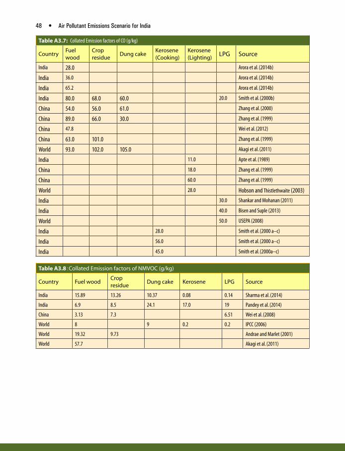
48 • Air Pollutant Emissions Scenario for India
Table A3.7: Collated Emission factors of CO (g/kg)
CountryFuel wood
Crop residue
Dung cakeKerosene (Cooking)
Kerosene (Lighting)
LPG Source
India 28.0 Arora et al. (2014b)
India 36.0 Arora et al. (2014b)
India 65.2 Arora et al. (2014b)
India 80.0 68.0 60.0 20.0 Smith et al. (2000b)
China 54.0 56.0 61.0 Zhang et al. (2000)
China 89.0 66.0 30.0 Zhang et al. (1999)
China 47.8 Wei et al. (2012)
China 63.0 101.0 Zhang et al. (1999)
World 93.0 102.0 105.0 Akagi et al. (2011)
India 11.0 Apte et al. (1989)
China 18.0 Zhang et al. (1999)
China 60.0 Zhang et al. (1999)
World 28.0 Hobson and Thistlethwaite (2003)
India 30.0 Shankar and Mohanan (2011)
India 40.0 Bisen and Suple (2013)
World 50.0 USEPA (2008)
India 28.0 Smith et al. (2000 a–c)
India 56.0 Smith et al. (2000 a–c)
India 45.0 Smith et al. (2000a–c)
Table A3.8 : Collated Emission factors of NMVOC (g/kg)
Country Fuel woodCrop residue
Dung cake Kerosene LPG Source
India 15.89 13.26 10.37 0.08 0.14 Sharma et al. (2014)
India 6.9 8.5 24.1 17.0 19 Pandey et al. (2014)
China 3.13 7.3 6.51 Wei et al. (2008)
World 8 9 0.2 0.2 IPCC (2006)
World 19.32 9.73 Andrae and Marlet (2001)
World 57.7 Akagi et al. (2011)
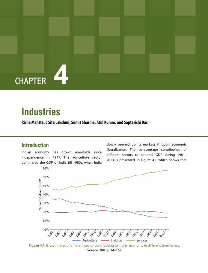
CHAPTER
IndustriesRicha Mahtta, C Sita Lakshmi, Sumit Sharma, Atul Kumar, and Saptarishi Das
4
Introduction Indian economy has grown manifolds since
independence in 1947. The agriculture sector
dominated the GDP of India till 1980s, when India
slowly opened up its markets through economic
liberalization. The perecentage contribution of
different sectors to national GDP during 1981–
2013 is presented in Figure 4.1 which shows that
Figure 4.1: Growth rates of different sector contributing to Indian economy in different timeframes.Source : RBI (2014–15)

50 • Air Pollutant Emissions Scenario for India
industry and services sectors have broadend
their shares in last two decades. Over all a healthy
growth rate of about 7.5% is achieved in post
2000 era, which is sufficient to double the average
income in a decade. There are certain states such
as Tamil Nadu (9.9%), Gujarat (9.6%), Haryana (9.1%),
or Delhi (8.9%) that have shown highest growth
rates during 1999–2008, while there are states
that have lagged behind. Now, India is the 10th
biggest economy in the world and the third
largest by purchasing power parity adjusted at
market exchange rates (World Bank 2015). Over the
years, the share of primary sector has gone down
and industrial manufacturing sector has shown
tremendous growth. While on one hand, it has
led to improved per capita incomes and quality
of life, it has also contributed to deterioration of
air quality. Inefficient combustion of fuels (with
high ash content), limited tail-pipe controls, and
fugitive process emissions have led to release
of huge quantities of air emissions, which lead
to deterioration of air quality. A Comprehensive
Environmental Pollution Index was formulated in
2009 that showed that 43 industrial areas/clusters
out of the 88 investigated were critically polluted,
with respect to one or more environmental
component (CPCB 2009). Air quality was one of the
important criteria that were evaluated.
Industrial PollutionAir pollution in industries in India is an important issue
that if not addressed can lead to severe deterioration
of air quality. Seventeen categories of highly polluting
industries have been identified in India. CPCB had
carried out an inventorization of the post-91 large and
medium scale industries under these 17 categories.
It was considered mandatory for these units to have
been allowed only if they had the requisite pollution
control facilities The state-wise status of 17 categories
of highly polluting industries in India (as on May 19,
2014) is presented in Table 4.1.
Manufacturing of products require energy, which
is produced in the industries through combustion
of fuels such as coal, fuel oil, biomass, and diesel.
Emissions from industries are function of quality of
fuel, combustion efficiency, and tail-pipe controls.
High sulphur fuels result in oxides of sulphur, while
high ash content in fuels leads to particulate matter
(PM) emissions. Inefficient combustion also leads to
PM, while high temperature combustion forms NOx
in the industrial stacks. In Indian scenario, tail-pipe
controls and their efficiencies play a very important
role in defining the emission, as the fuels combusted
are of high ash content. Other than due to combustion
of fuels, emissions also take place in manufacturing
processes of some products such as cement, lime, etc.
Other than large industrial units, there are 36
million micro, small, and medium enterprises. Their
contribution to GDP is about 8% besides 45% to
the total manufacturing output and 40% to the
exports from the country (MMSME 2015). Although
big industries are somewhat capable of controlling
emissions through installations of air pollutant
control devices, pollution from small scale industries
is an issue. Financial and technical capacities are
major constraints for control of pollution in small
scale industries.
Energy Consumption in Industries Based on the actual energy consumed in various
industries such as paper and pulp, iron & steel
production, chemical production, non-metallic
minerals and non-ferrous minerals, and other
industries, TERI-MARKAL model is used to derive
future projections of energy use in the industrial
sector. Estimated fuel-wise energy consumed in the
sector is shown in Figure 4.2, which clearly shows
around 51% of energy demand in industries is met
by coal, followed by petroleum products (16%), and
electricity (13%).
The sub-sector–wise distribution of energy
consumed in Industries is shown in Figure 4.3. Other
than cement, iron & steel, brick, aluminium, glass,
paper, and fertilizer industry, significant energy
consumption takes place in other small and medium
scale industries. In 2011, iron and steel sector has
the maximum share of 26%, followed by the brick,
fertilizers, and cement industries.

Industries • 51
Table 4.1: State-Wise Status of 17 Categories of Highly Polluting Industrial Units in India (as on May 19, 2014)
Sl No State Complying Non-Complying Closed Total
1 Andhra Pradesh 359 74 39 472
2 Arunachal Pradesh 2 0 0 2
3 Assam 36 12 1 49
4 Bihar 16 4 0 20
5 Chattisgarh 71 6 1 78
6 Chandigarh 0 0 0 0
7 Daman & Diu 1 1 1 3
8 Delhi 2 0 0 2
9 Goa 13 2 0 15
10 Gujarat 302 7 8 317
11 Haryana 119 6 16 141
12 H.P. 14 0 3 17
13 Jharkhand 103 48 22 173
14 Jammu & Kashmir 7 0 3 10
15 Karnataka 175 30 26 231
16 Kerala 21 11 19 51
17 Lakshadeep 0 0 0 0
18 Madhya Pradesh 65 16 2 83
19 Maharashtra 317 145 58 520
20 Meghalaya 4 12 1 17
21 Mizoram 1 0 0 1
22 Nagaland 0 0 0 0
23 Orissa 37 17 11 65
24 Puducherry 5 2 0 7
25 Punjab 57 12 18 87
26 Rajasthan 69 31 18 118
27 Sikkim 3 1 0 4
Total 1799 437 247 2483
Source: CPCB (2014)
Other than combustion of fuels, they are also used
in non-combustion activities. There are certain fuels
that are used in industry as feedstock and other non-
energy uses. Naphtha (part of GSL) and natural gas
are used as feedstock in fertilizers and petrochemical
industries. This non-combustion fuel usage also leads
to emissions. Data pertains to these uses is presented
in the Table 4.2.
Emission Inventorization of IndustriesEnergy estimates made in the previous section are
used to estimate emissions of various pollutants
Table 4.2: Fuel Used in Non-Energy Sector during Year 2009–10
Natural gas Million m³ (MCM)
Naphtha (000 tonnes)
Fertilizer 13168 13168
Petrochemical 1264 1264
Source: MoPNG (2010)
during different industrial processes. The calculations
are based on the following Equation 4.1.
Emissions = Activity level × Abated emission
factor × Percentage of capacity controlled .................4.1

52 • Air Pollutant Emissions Scenario for India
Figure 4.3: Past and projected energy consumption in the industrial sector (2001-2051)
Figure 4.2 Estimated energy consumption in industry sector (PJ) during 2001-2051Source: TERI (2015), TERI-MARKAL model results
where
Abated emission factor = Unabated emission factor
× (1 – Percentage removal efficiency of the control
system).
Other than fuel combustion, there are a number
of industries for which emissions are estimated
based on the processes followed rather than the
fuel consumed in the sector. In this study, emissions
are estimated separately for cement, iron and steel,
fertilizers, paper, brick, aluminium, and glass industries
and rest of the industries are clubbed in ‘others’
categories.
Cement IndustryWith growing economy, the demands for
construction material has grown multi-folds. The
cement production in India has grown from about
50 MT in 1993–94 to 169 MT in 2011. India is the
second largest producer of cement in the world after

Industries • 53
Figure 4.4: Variety-wise cement production in India
Source: Cement Manufacturers’ Association
OPC, Ordinary Portland Cement; PPC, Portland Pozzolana Cement; PBF, Portland Blast Furnace Slag
Cement; SR, Sulphate Resistant; IRS, Indian Railway Standard; Others
China (Planning Commission 2011). Major clusters of
cement industry in India are:
P 1. Satna in Madhya Pradesh
P 2. Chandrapur in Maharashtra
P 3. Gulbarga in Karnataka
P 4. Yerranguntla in Andhra Pradesh
P 5. Nalgonda in Andhra Pradesh
P 6. Bilaspur in Chattisgarh
P 7. Chandoria in Rajasthan
There are 183 large cement plants and more
than 360 mini cement plants. The Ordinary Portland
Cement (OPC) and Portland Pozzolana Cement
account for 93% of the total production (Figure 4.4).
In India, the housing sector is the biggest driver
of cement demand, accounting for about 67 per cent
of the total consumption. The other major consumers
of cement include infrastructure (17%), commercial
construction (13%), and industrial construction (9%)
(IBEF 2015).
TERI analysis (TERI 2015) on future projections of
the sector shows bright prospects for growth of the
sector. The cement production is expected to grow
about 6.5 times and will reach to about 1300 MT in
2051 (Figure 4.5).
Manufacturing of cement is a process which
leads to emissions of PM and gaseous pollutants.
The process flow diagram of cement manufacturing
is shown in Figure 4.6. There are a number of
stages which can lead to emissions in a cement
manufacturing process including
P handling and storage of raw, intermediate and
final materials,
P operation of kiln systems, clinker coolers, and mills.
The major release of emissions happens in the
kilns during the production through physical and
chemical reactions involving the raw materials and
combustion of fuels. The indigenous emission factors
per unit of cement production for this study are
adopted from ILFS, 2010 and CPCB (2007) (Table 4.3)
In a cement kiln, solid material moves counter
currently to the hot combusted gases. This counter
current flow affects the release of pollutants, since
it acts as a built-in circulating fluidized bed. Most
cement plants have made considerable efforts in
controlling the stack emissions using most efficient
control systems like bag filter and Electrostatic
Precipiators (ESPs) and these plants generally meet
the environmental regulations for stack emissions.

54 • Air Pollutant Emissions Scenario for India
Figure 4.5 Projected growth of cement production in India (TERI, analysis)
Figure 4.6: Process flow diagram for the cement manufacturing processSource: Adapted from Huntzinger, D.N. and Eatmon, T.D., 2008. A life-cycle assessment of Portland cement
manufacturing: comparing the traditional process with alternative technologies, J Clean Prod, doi:10.1016/j.jclepro.2008.04.007

Industries • 55
However, fugitive emissions from various sources in
cement plants still remain an area of concern (CPCB
2007). Based on the emission factors and controls,
the emissions coming out of the cement plant
are estimated and presented in Figure 4.7. These
emissions include pollutants emitted during captive
power generation activities.
The PM10
emissions are projected to go up from
354 Kt in 2011 to 2446 Kt in 2051. The ratio of PM2.5
emissions to the PM10
emissions is about 0.56. While,
the presence of air pollution control (APC) equipment
for PM leads to control of emissions, NOx emissions
are projected to go up uncontrolled by about 7 times
from the current levels of 450 Kt. This highlights the
need for emission control norms for NOx in industries.
The SO2 emissions are expected to increase from
about 1044 Kt in 2011 to about 7327 Kt in 2051. It
is to be noted that in last few years, many cement
industries have started co-processing of hazardous
and other high calorific value material like petcoke.
This leads to higher emissions of SO2 due to high
sulphur content of the fuel (petcoke) used in the
sector. Present estimates do not assume the influx
of FGD technology in the sector. However, with
Table 4.3: Emission Factors for Cement Sector
Emission factors (kg/t)
Dry process
PM NOX
SO2
CO
w/o APCD With APCD w/o APCD w/o APCD w/o APCD
Klin 94 0.98
Grinding 257 0.21
Others 7 0.01
Total 358 1.2 2.2 4.9 0.27
Fugitive 0.56*
Wet process
w/o APCD APCD w/o APCD w/o APCD w/o APCD
Klin 174 0.2
Grinding 123 0.02
Others 6 0.03
Total 303 0.25 4 3.75 0.27
Source: ILFS, 2010, CPCB (2007)APCD: Air pollution control devices * Ratios for PM
2.5, BC, OC are used from EEA 2009 and EPA 2012.
influx of FGDs in the sector, the SO2 emissions can
reduce considerably. The use of pet coke has resulted
in substantial reduction in conventional fuel and
present study has taken this into account for current
and future scenarios.
Iron and steel Industry The iron and steel industry in India caters to the
demands of key sectors like construction and
automobiles. The sector is mainly divided into
two types; the first one comprises of a few large
integrated steel providers producing primary
products billets, slabs and hot rolled coils, and
secondary smaller units producing value-added
products such as cold rolled coils, galvanised coils,
angles, columns, beams and other re-rollers, and
sponge iron units. The sector has seen enormous
growth in the recent past with India becoming
the fourth largest producer of crude steel and the
largest producer of soft iron in the world. The per
capita consumption is about 58 kg in 2013 which
is expected to rise with increased industrialization
throughout the country. The report of the Working
Group on Steel for the 12th Five Year Plan envisages

56 • Air Pollutant Emissions Scenario for India
Figure 4.7: Past and projected growth of emissions (Kt) from cement manufacturing in India
increase in the per capita steel consumption in
the country on the basis of high infrastructure
investment, high projected growth of manufacturing
sector, increasing urban population, and emergence
of the rural markets. The Working Group on Steel for
the 12th Five Year Plan made projections for domestic
crude steel capacity in the county to be about 140
MT by 2016–17 and has the potential to reach 149
MT. The MARKAL model estimates are close to the
projections. The model projected the finished steel
production to 388 MT in 2031 and 779 MT in 2051
(Figure 4.8).
Various processes involved in iron and steel
manufacturing are metallurgical coke production,
Figure 4.8: Past and projected finished steel production (MT) in India (2001-2051)
Source: TERI-MARKAL model
CO
SO2
PM2.5
NOx
PM10

Industries • 57
sinter production, pellet production, iron ore
processing, iron making, steel making, steel casting,
and sometimes combustion of blast furnace and
coke oven gases for other purposes. The raw steel is
produced using a basic oxygen furnace from pig iron
produced by the blast furnace and then processed
into finished steel products (Figure 4.9).
Emissions occur at all the stages of the production
and emission factors are chosen for different
Figure 4.9: Processes in iron and steel production industry
Adopted from EEA (2009)
processes followed in the iron and steel sector in
India (Table 4.4).
Basic oxygen furnaces use pig iron and electric
arc furnace is used for steel produced from scrap.
Based on emission factors, the emissions for different
pollutants from iron and steel plants are estimated
and presented in Figure 4.10.
The iron and steel plants are generally equipped
with high efficiency APC equipment and the PM10
Table 4.4: Emission Factors for Different Pollutants from Various Processes in Steel Making
Emission Factors Sintering Pig Iron Basic Oxygen Furnace with ESP Electric Arc Furnace with ESP
Kg/t Kg/t Kg/t Steel making
PM2.5 0.08 0.025 0.021 0.021
PM10 0.1 0.04 0.024 0.024
BC 0.00017 0.0024 0.00036 0.00036
OC – – 0.002484 0.003168
NOx 0.5 – 0.01 0.13
SO2 1 – – 0.06
CO 12 10 7 0.0017
NMVOC 0.138 – – 0.046
Source: EEA, 2.C.1 Iron and steel production , GAINS ASIA model

58 • Air Pollutant Emissions Scenario for India
emissions are projected to go up from 24.2 Kt in 2011
to 144 Kt in 2051. This is mainly due to the growth
expected in the sector. NOx emissions are projected to
grow from 86 Kt to 707 Kt during 2011- 2051.
Aluminium IndustryIn India, aluminium is mainly produced in large
integrated plants such as Hindalco and National
Aluminium Company, and Bharat Aluminium, etc.
The main energy inputs are in the form of electricity,
coal, and furnace oil and the standard Bayer–
Hall–Heroult technology is used for aluminium
production. The production process is described
in Figure 4.11. Captive power plants are installed
to provide uninterrupted power. Presently, India
accounts for 6% of the total deposits and 2.1 million
tons of aluminium production in 2011. Aluminium
production has grown steadily in India and is
projected to grow to about 9 MT in 2051 (Figure 4.12).
Aluminium production is expected to increase due to
demands from packaging, construction, automobiles,
and electrical sectors.
The emission factors used for estimating emissions
form aluminium production in India are shown in
Table 4.5. The emission factors are applied to the
Figure 4.10: Emissions (Kt) from iron and steel industry in India (2001–51)
activity data to estimate emissions during 2001–51
for different pollutants (Figure 4.13).
The emissions from aluminium industry are
comparatively less than cement and iron and steel
industries, except for CO. The CO emissions are
expected to grow from 194 Kt to 1,096 Kt during
2011–51.
Glass Industry Glass industry caters to the demands of key sector
such as construction, automotive, consumer
goods, and pharmaceuticals. Apart from few big
Table 4.5: Emission Factors for Aluminium Production
Pollutant Unabated Emission factor (kg/t)
PM10
2
PM2.5
1
BC 0.023
OC 0.0391
NOx 1
SO2
6
CO 120
NMVOC -
Source: EEA 2009, EPA 2012, GAINS

Industries • 59
Figure 4.11: Aluminium production process flow chart
Source: Adapted from Halvor and Per Arne (2014)
Figure 4.12: Aluminium production in India (2001-2051)
Source: TERI (2015)
manufacturers there are more than 1,000 small
and medium scale enterprises involved in glass
production in India. The glass consumption in India is
just 1.2 kg/c/yr in 2010–11 in comparison to 30–35 kg
in the US (TERI 2015).
Glass industry is highly energy intensive and the
melting and refining processes account for 60–70%
of the energy consumed in production. Furnace
oil and natural gas are mainly used in India as the
thermal energy source. The emission factors used to
estimate emissions from glass manufacturing in India
are shown in Table 4.6 and emissions are presented in
Figure 4.14. The PM10
emissions are expected to grow
from 1 Kt in 2011 to 5 Kt in 2051. NOx emissions will
grow from 34 Kt to 153 Kt during 2011–51.

60 • Air Pollutant Emissions Scenario for India
Figure 4.13: Emissions (kilotonnes) from aluminium industry in India (2001–51)
Paper and Pulp IndustryThe Indian paper industry accounts for about 2.6%
of the world’s paper production. The technologies
used in the paper mills show wide variations
ranging from oldest to the most modern. A variety
of raw material are used including wood, bamboo,
recycled fibre, bagasse, wheat straw, rice husk, etc.
Of the total paper production, 31% is based on
chemical pulp, 47% on recycled fibre, and 22% on
agro-residues (IPMA 2015). Paper industry is heavily
dependent on the industrial growth and literacy
rates in the country. Presently, the per capita paper
consumption is just 9.3 kg in India as against 42 kg
in China and 312 kg in US (TERI 2015). However, with
growing literacy and middle class, the consumption
is expected to grow. Production of paper is
projected to grown from 7.5 MT in 2011 to about 20
MT in 2051 (Figure 4.15).
There are about 720 paper mills in India of which
621 are in operation (Ministry of Commerce & Industry
2010–11). Gujarat has the maximum number of paper
mills followed by Uttar Pradesh. Majorly operating
mills in India falls under three categories (CPCB 2011;
Ministry of Commerce & Industry 2010–11):
P Large Integrated Wood Based: It includes
newsprint, rayon grade pulp, bleached and
unbleached varieties. Scale of operation for these
mills is 100–700 tpd.
P Medium Agricultural Residue Based: It includes
bleached varieties with and without recovery
system and unbleached varieties without recovery
system. Scale of operation for these mills is 50–100
tpd.
P Small Recycled Fibre and Market Pulp Based: It
includes unbleached craft, writing and printing
Table 4.6: Emissions Factors for Glass Manufacturing
Pollutant Unabated emission factor (kg/t)
PM10
0.27
PM2.5
0.24
BC 0.0038
NOx 8.12
SO2
1.74
CO 0.1
NMVOC –
Source: EEA 2009, GAINS
CO
SO2
PM2.5
NOx
PM10
OCBC

Industries • 61
Figure 4.14: Emissions (kilotonnes) from glass industry in India (2001–51)
Figure 4.15: Past and project growth of paper industry in India
Source: TERI Analysis
varieties with and without deinking, unbleached
crafts, and paper board. Scale of operation for
these mills is 5–50 tpd.
Kraft method is broadly used in India for paper
production. In this, the white liquor (water solution of
sodium sulphide and sodium hydroxide) is subjected
to high temperature and pressure. The lignin that
binds the cellulose fibres of the wood is chemically
dissolved. Thereafter, the pulp is washed, screened,
and dried or further delignified and bleached, if
required based upon the intended use of the product.

62 • Air Pollutant Emissions Scenario for India
The rest of the Kraft processes are there for chemicals
and heat recovery. The black liquor formed during the
process is concentrated through evaporation, which
is then combusted for recovery of heat and chemicals.
Broadly, the emissions produced from different
processes in paper and pulp industry are shown in
Figure 4.16.
The emission factors used to estimate emissions
of different pollutants from Kraft pulping process are
presented in Table 4.7. It is evident from the Figure
4.17 that emissions from the paper and pulp industry
will grow; PM10
will grow from 8 Kt to 17 Kt during
2011–51, while CO emissions from 42 Kt to 112 Kt in
the same period.
Fertilizer IndustryChemical fertilizers are important to improve or
sustain agricultural production in the country.
Government of India has consistently persuaded
policies conducive to increased availability and
consumption of fertilizers at affordable prices in the
country (MoCF 2012). The consumption of fertilizers,
in nutrient terms (N, P, & K ) has increased from 0.07
million MT in 1951–52 to more than 28 million MT in
Figure 4.16: Emissions produced from paper production process
Source: Reproduced from CPCB (2011)
2010–11 and per hectare consumption, has increased
from less than 1 Kg in 1951–52 to the level of 135 Kg
now. The overall production of fertilizers in India is
expected to grow to 56 MT/a by 2051 (Figure 4.18).
About 78 per cent of Urea production is through
natural gas used as feedstock. Fuel oil and naptha are
also used in the sector. Thakkar (2013) has found high
levels of pollutant emissions from industrial sector
in India. The emission factors used in this study for
emission estimation are presented in Table 4.8.
Table 4.7: Emission Factors for Paper Industry
Pollutant Unabated emission factor (kg/t)
PM10
0.8
PM2.5
0.6
BC 0.012
OC 0.0408
NOx 1
SO2
2
CO 5.5
NMVOC 2
Source: EEA 2009, EPA 2012

Industries • 63
Figure 4.17: Emissions from paper industry in India (2001–51)
The estimated emissions are shown in Figure 4.19
for the period 2001–51. The CO emissions from the
fertilizer industry are expected to go up from 1,020
Figure 4.18: Past and future projections of fertilizer production in India (2001-2051)
Source: TERI Analysis
Kt in 2011 to 3,462 Kt in 2051. SO2 emissions that are
coming from captive power generation using coal
will gradually diminish in the future.
CO
PM10
SO2
PM2.5
NMVOC
NOx

64 • Air Pollutant Emissions Scenario for India
Brick IndustryBrick industry is a small scale traditional and
unorganized industry in India (Maithel 2013; Pandey
et al. 2014; Rajarathnam et al. 2014). But over time, it
has become one of the largest consumers of coal in
the country. Around 17.14 tonnes of coal is required
to produce one lakh bricks. Incomplete combustion
of coal results in the release of several air pollutants
in atmosphere such as CO, SO2, NO
X, and PM. At local
level (in the vicinity of a brick kiln) some of these
Table 4.8: Emission Factors (kg/t) for Fertilizer Industry
Pollutant Emission factor (kg/t)
PM10
0.33
PM2.5
0.2145
BC –
OC –
NOX
2
SO2
0.04
CO 62.25
VOC –
Source: AP42, Section 6.10 phosphate fertilizers
pollutants are injurious to human health, animal, and
plant life. At global level, CO2 and BC contribute to
global warming and climate change.
There are about 300,000 brick kilns across the
world that produce around 1,350 billion bricks across
the year (MNRE 2013). Brick production is mainly
focused in four countries across the world. Among
these countries, China holds the maximum share
of brick production followed by India, Pakistan, and
Bangladesh (Figure 4.20). In India, total number of
brick kilns are estimated to be around 1.4 lakh with a
production of 280 billion brick annually (Rajarathnam
et al. 2014). It is reported that during 2000–01, about
80 billion bricks were produced in India (TERI 2002).
As a result of increasing demand for infrastructure,
commercial, and residential buildings, the demand for
bricks is also increasing at a high rate. Brick making in
India is concentrated in Indo-Gangetic plains and in
some scattered pockets in other states (Figure 4.21).
Maximum number of the brick kilns is located in the
rural areas lying adjacent to rapidly expanding cities.
Brick kiln industry in India started with the clamp
technology having non-fixed structures. The practice
was to take clay and mud from fields, moulding
them, and heating them in inefficient furnaces using
Figure 4.19: Emissions from fertilizer industry in India (2001-2051)
PM10
SO2
CO
PM2.5
NOx

Industries • 65
any fuel that is easily available. There was no control
technology involved in these temporary structures.
The brick manufacturing is known as one of the
major polluting sectors. Studies have pointed out
that around 9% of black carbon emissions in India
are from brick sector. Many technologies with varied
designs have been introduced from time to time
in order to reduce the huge environmental cost
associated with the sector.
Figure 4.20: Worldwide production of bricks in major producing industries
Source: MNRE (2013)
Figure 4.21: Brick production sites in India.
Source: Adapted from http://www.ecobrick.in/
brickmakinginindia.aspx
Brick production involves moulding, drying, and
firing processes. These bricks are heated between
600°C and 1,100°C to get the desired product (TERI
1999). Different types of kilns are used for firing bricks,
which are broadly divided into intermittent and
continuous categories (Figure 4.22).
Continuous kilns are generally more efficient as fire
is always burning and bricks are being warmed, fired,
and cooled simultaneously in different parts of the
kiln. Heat in the flue gas is utilized for heating green
bricks and the heat in fired bricks is used for heating
air for combustion. On the other hand, fire is allowed
to die out and the bricks to cool after they have been
fired in intermittent kilns. The kiln are emptied, refilled,
and a new fire is initiated for each load of bricks. In
intermittent kilns, most of the heat contained in the
hot flue gases and the fired bricks is lost.
Different types of Brick kiln technologies practiced
in India are Clamps (scove, scotch), Moving Chimney
Bull’s Trench kiln (MC-BTK), Fixed Chimney Bull’s
Trench kiln (FCBTK), Vertical Shaft Brick kiln (VSBK),
Zig-Zag, and Tunnel Kilns (Figure 4.23). Clamp and
downdraught kilns are examples of intermittent kilns,
while, rest are continuous in nature.
Figure 4.22: Brick production in India
Photo credit: R Suresh

66 • Air Pollutant Emissions Scenario for India
A transition has been observed in last two
decade with the introduction of new technologies
in the country, which are shown in Figure 4.24. These
different types of brick kilns differ in terms of specific
energy consumption (SEC). SEC is expressed in terms
of energy required for firing per Kg of bricks. A study
conducted by SDC (2008) has come up with SEC
values for few technologies, shown in Table 4.9.
In this study, bricks production has been estimated
by assuming growth in brick production same as
growth of construction sector, which is 6.6% for the
time period 2005–30 (MNRE 2013) in the country. For
further projections, growth rates have been taken
from TERI MARKAL model outputs. However, in the
past few decades, it has been observed that other
walling materials such as fly-ash bricks, fly-ash lime
gypsum blocks, autoclaved aerated concrete blocks
have entered the Indian market and replaced bricks
to some extent. In future, it is expected that these
Figure 4.23: Brick kilns categorization on basis of firing technology
Source: CSE (2015)
Figure 4.24: Technology transition in brick sector in India
Source: Maithel (2013)
alternate walling materials could decrease the share of
fired bricks to some extent in the construction sector.
For 2010, the share of other walling materials has
been estimated as 7.8%, which is expected to increase
to 14.1% in 2030 (Enzen & Greentech Knowledge
Solutions 2011). The current and expected brick
production in India is shown in Figure 4.25.
State-wise allocation is done on the basis of
reported number of brick kilns in the states in TERI
(2007). Based on consultation with experts, it is
Table 4.9: Comparison of SEC for Different Kilns
Type of Kiln SEC (MJ/kg of fired bricks)
Clamp and other batch kilns (Asia) 2.0-4.5
MC-BTK (India) 1.2-1.75
FCBTK (India) 1.1-1.5
VSBK (India, Nepal, Vietnam) 0.7-1.0
Tunnel Kiln (Vietnam) 1.4-1.6

Industries • 67
assumed that 32% of the bricks in the country are
manufactured using clamps, 61% are manufactured
using Bull’s trench kiln, 3% with moving chimney
BTK (BTK-MC), and 1% for Holfmann kiln for the
baseline year (2011). Vertical Shaft Brick Kilns (VSBKs)
contribute very little in the total share of kilns across
India (Table 4.10).
With the advent of advanced technologies such
as Zig-Zag firing and tunnel kilns, it is expected that
these cleaner technologies will penetrate into Indian
Brick industry and numbers of clamps will gradually
reduce (Figure 4.26). Thus, on consultation with
experts, it is assumed that for 2030, 12% of the bricks
will be produced from Clamps, 65% from FCBTKs,
19% from zig-zag kilns, and 3% through tunnel kilns.
Considering the field performance of VSBKs in India, it
is being assumed that their number will not increase
much with time. Further in 2050, it is assumed that
percentage of brick kilns with Zig-Zag technology
will increase to 45% and FCBTK to be 55%. Clamps
will diminish and tunnel kilns with economical
constraints will be negligible in number.
Emissions from brick manufacturing facilities
include PM (PM10
, PM 2.5
, SO2, nitrogen oxides (NOx),
Figure 4.25: Current and projected brick production in India (2001–51)
Table 4.10: Estimated Kiln Technology–Wise Distribution of Brick Production in India in 2011
Kiln Technology Number of Kilns (Approx.) 2010 Capacity Ratio (Thousand bricks/day) Total number of Bricks produced/day
DDK 300 3 900
MCBTK 2,000 20 40,000
FCBTK 32,000 30 9,60,000
Zig-Zag 2,000 30 60,000
Holfman Kiln 500 30 15,000
VSBK 100 7 700
Clamp 100,000 5 5,00,000
Tunnel Kiln (Coal) 0 45 0

68 • Air Pollutant Emissions Scenario for India
Figure 4.26: Projected kiln technology–wise distribution of brick production in India till 2051
Source: Expert consultations
Figure 4.27: Emissions from brick industry
Source: Reproduced from EPA (1997)
carbon monoxide (CO), carbon dioxide (CO2), metals,
organic compounds (including methane, ethane,
volatile organic compounds [VOC], hydrochloric acid
(HCl), and fluoride compounds) (EPA 1997) (Figure
4.27). Factors that may affect emissions from brick
industry include raw material composition, moisture
content, kiln fuel type, kiln operating parameters,
and plant design. Emissions of each gas depends on
different steps involved in the production of bricks in
kilns.
In a recent study conducted by Greentech
Knowledge solutions, nine brick kilns were monitored
in India and Vietnam in order to understand
energy consumption and emissions using different

Industries • 69
technologies. Table 4.11 presents emission factors for
different brick manufacturing technologies.
Based on the brick production rates and expected
influx of technologies, the emissions from Brick
kiln industry for India are estimated and are shown
in Table 4.12. In 2011, 294 Kt of PM10
and 226 Kt of
PM2.5 emissions are estimated. It is observed that
PM emissions will increase two folds by 2031 and
stabilize thereafter with marginal increase till 2051.
Similarly black carbon and organic carbon emissions
are expected to increase and will double by 2051.
These emission estimates take into account
the influx of improved technologies; however, in
absence of these, the emissions from the sector will
be much higher. Ministry of Environment, Forest, and
Climate Change in India has brought up PM emission
standards and stack height specifications based on
the kiln’s production capacity. Along with control
of emissions from brick industry, newer options for
alternative walling material should be explored which
are environmentally sustainable.
Other IndustriesOther than cement, iron & steel, brick, aluminium,
glass, paper, and fertilizer industry, significant energy
consumption takes place in small and medium scale
industries. The energy consumed in these ‘other
industries’ in comparison to the major sectors is
shown in Figure 4.3. The energy consumed in the
other industry sector is multiplied with emission
factors listed in Tables 4.13 and 4.14 to estimate
emissions. Table 4.13 shows the PM emission factors
for coal combustion in industries based on the ash
content and efficiency of tale pipe controls.
Table 4.11: Emission Factor for Different Type of Brick Kilns
Technology Unabated emission Factors (g/kg of fired brick)
PM10
PM2.5
SO2
CO CO2
Greentech energy solutions (2012)a
FCBTK 0.86 0.18 0.66 2.25 115
Zig-zag 0.26 0.13 0.32 1.47 103
VSBK 0.11 0.09 0.54 1.84 70
DDK 1.56 0.97 n.d 5.78 282
Tunnel 0.31 0.18 0.72 2.45 166
Rajarathnam et al. (2014)b FCBTK 0.89 0.52 3.63 179
NDZZ 0.22 0.06 0.35 119
FDZZ 0.24 0.24 2.04 96
VSBK 0.09 0.10 4.14 118
DDK 1.56 0 5.01 526aStudy was conducted on seven brick kilns in India and two (modified VSBK and Tunnel Kiln) in Vietnam in 2011.bStudy was performed on 15 brick kilns in India.Ratios of PM
2.5, BC, OC and EF of NO
X and NMVOC are adopted from GAINS Asia
Table 4.12: Emissions (Kt) from Brick Kiln Industry in India
2001 2011 2021 2031 2041 2051
PM10
164 294 430 588 678 691
PM2.5
126 226 331 453 522 531
BC 38 68 99 136 156 159
OC 44 79 116 158 183 186
NOx
0 0 0 0 0 0
SO2
38 68 99 136 156 159
CO 1263 2261 3307 4526 5216 5312
VOC 19 34 50 68 78 80

70 • Air Pollutant Emissions Scenario for India
Table 4.13: PM Emission Factor for Coal Combustion in Industrial Sector
PM10
PM2.5
Large Scale (High Controls e.g. ESP)
Medium (medium controls)
Small (low controls)
Large Scale (ESP)
Medium (medium controls)
Small (low controls)
Ash content 35% 35% 35% Ash content 35% 35% 35%
Fly/Bottom ash ratio 80:20 80:20 80:20 Fly/Bottom ash ratio 80:20 80:20 80:20
PM10
/PM 0.71 0.48 0.39 PM2.5/PM 0.35 0.29 0.21
Efficiency of control 99.90% 70% 40% Efficiency of control 99.90% 70% 40%
Emission factor (t/PJ)** 11 2314 3753 Emission factor (t/PJ)** 6 1379 2026
*PM10
/PM and PM2.5
/PM ratios are taken as an average of wet and dry bottom boilers BC and OC are assumed to be 0.1% and 0.2% of PM
10 fractions; adopted from emission factor ratios in GAINS
** Emission Factors = Ash content ×Fly/Bottom ash ratio × PM fraction ratio × (1–efficiency of control)
Table 4.14: Fuel- and Pollutant-Wise Emission Factors (Kt/PJ) for NOx, SO
2, CO, and HC
Fuel NOx
SO2
CO HC PM10
Coal 0.13 0.57 0.01 0.02
Natural Gas 0.07 0.02 0.04 -
Biomass 0.03 0.00 0.3 0.80 0.12
Fuel oil 0.15 1.73 0.01 0.09 0.11
Diesel 0.08 0.94 0.04 - 0.77
Light Diesel Oil 0.08 0.94 0.04 - 0.77
Naphtha 0.07 0.02 0.04 - 0.10
Source: CPCB 2011, GAINS Asia
Based on the energy consumption and respective
emission factors, the emissions for different years
are estimated (Figure 4.28). It is expected that
with industrial growth the emissions will grow
considerably. However, with improved enforcement
of existing standards for PM, there will be increased
penetration of APC technologies. Presently, only
large scale industries are assumed to be equipped
with high efficiency APC equipment such as ESPs
and Bag-filters. As per the consent to establish and
consent to operate requirements for industries, all
Figure 4.28: Emissions of different pollutants from other industrial fuel consumption (Kt)
PM10
SO2
PM2.5
NOx

Industries • 71
polluting industries need to install emission control
equipments. Although, the efficiency of controls vary
with the requirements and type of APCE installed.
Based on expert consultations, micro, small, and
medium industries are assumed to be equipped with
APCs with an efficiency of 40%. Based on the growth
of the current APCE industry, and growing concerns
over air pollution in Indian cities, penetration of high
efficiency APC equipments in industries is assumed
to increase to about 50% by 2051. However, there will
be variation in degree of control with the type of APC
technologies installed.
PM10
emissions from ‘other’ industries will grow
from 3,791 Kt in 2011 to 11,700 Kt in 2051, with an
increase of 209%. However with influx of control
technologies, the intensity of emission per unit of
production is expected to go down significantly. In
absence of suitable standards for NOx and SO
2, the
emissions will grow by eight to nine folds by 2051.
Mining Coal and iron scenario in IndiaCoal along with other fossil fuels continues to be
the primary source of energy in India, despite its
environmental impacts both at local as well as regional
level. Among all the ores and industrial minerals, iron
ore (along with bauxite and copper) is of the most
quantitative importance in terms of its mass flows in
the Indian economy (Singh et al. 2012). Mining of coal
along with other minerals is an important economic
activity though burdened by severe environmental
impact particularly on air and water quality, and forest
resources including biodiversity and green cover.
The growing demand for natural resources such as
coal and iron ore, from developed as well as rapidly
developing countries such as India and China, have led
to increasing shortages of these resources in the global
economy (Planning Commission 2013). In this scenario,
making a robust supply of domestic resources is all the
more necessary.
The geological coal reserves have been estimated
to be 301.56 billion tonnes (as on 1st April 2014)
in India according to the Ministry of Coal (MOC),
Government of India. Of the total reserves of coal
in India, the majority (88%) are comprised of non-
coking coal and about 11.5% are coking coal, while
a minimal share (0.5%) is of tertiary coal reserves
(Indian Chamber of Commerce & PwC 2012). Indian
coal is characterized by its high ash content (as high
as 45%), along with low sulphur content (0.2–0.7%),
and low calorific values (between 2,500–5,000 kcal/
kg) (IEA 2002). The total production of coal in India
in the year 2013–14 was 565.64 Million tonnes
(MoC 2013). The largest consumer of coal in India
is power sector, accounting for almost 70% of coal
consumption in 2011 (MOC 2014). Steel production
and cement industries are other significant coal
consumers in the country.
India is ranked third in coal, lignite, and bauxite
production and fourth in iron ore production in
the world in the year 2009–10 (Ministry of Mines,
Government of India). Public sector continues to play
a dominant role in mineral production, and accounts
for 74.5% of all minerals produced and a sizeable 91%
of the total coal produced. Data of major coal mines
along with their production capacities is presented in
Table 4.15 (MoC, 2014). The major coal field locations
are shown over the map of India in Figure 4.29.
Past trends and future growth of mining in India Mining and mineral extraction in India can be traced
back to the days of the ancient civilizations residing
in the region. The country is known to be endowed
with rich and widely available resources of many
metallic and non-metallic minerals; hence mining
sector plays a key role in the Indian economy. India
produces as many as 87 minerals, which include
four fuels among others (Ministry of Mines 2011).
Coal mining became an important part of the public
sector in India during the years 1971–73 with the
enactment of the Coal Mines (Nationalization) Act,
1973. In the same year, the Coal Mines Authority
Ltd. was set up and was made responsible for all the
operation and maintenance of the nationalized non-
coking coal mines in India (Dutt 2007).
Mainly there are two kinds of methods for
coal extraction: opencast (surface) mining and
underground mining. In India, the predominantly

72 • Air Pollutant Emissions Scenario for India
used method is opencast extraction; and mining in
the country has grown with a 4% annual average
growth rate over the past decade. Opencast
mining involves mining coal in an earth-moving
operation by excavating the overburden up to
the coal seams and then removing the coal using
draglines, shovels, and dump trucks. This method of
extraction is overall more advantageous due to the
following factors:
P greater extraction rate of coal
P higher productivity compared to the other
method of extraction
P lower in costs and labour intensity
P and better workplace conditions
However, opencast mining is infamous for
having greater impact on the local environment;
such as large-scale land use, overburden disposal,
disturbance of hydrology and run-off, increased
erosion, acid mine drainage, noise, and possible
damage to the ecosystems.
On the other hand, underground mining is
employed for extraction of very deep coal seams,
Table 4.15: Major Coal Mines along with their Production Capacities in India in 2012–13
Unit Production (in Million Tonnes)
Eastern Coal fields 33.9
Bharat Coking Coal Ltd. 31.2
Central Coalfields Ltd. 48.1
Northern Coalfields Ltd. 70.0
WCL western Coalfields Ltd. 42.3
SECL South Eastern Coalfields Ltd. 118.2
MCL Mahanadi Coalfields Ltd. 107.9
NEC North Eastern Coalfields. 0.6
Total CIL 452.2
SCCL Singareni Collieries Co. Ltd 53.2
Other Public 3.9
Total Public 509.2
Total Private 47.2
All India 556.4
Figure 4.29: Major coal fields in India
Source: CMPDI, Coal India
involves construction of a vertical shaft or slope
mine entry to the coal seam and then extracting the
coal using various standard techniques. About 9% of
India’s coal production was from underground mines
in the year 2012–13 (MoC, 2014).
In 2010, India produced the world’s third largest
volume (532 MT) of coal domestically, which was more
than double of the 1990 level of 205 MT; however,
the production has more or less plateaued in recent
years (Ahn and Graczyk 2012). The 12th Five-Year Plan
aims to further increase coal production to 715 MT
in FY 2016/17, a 33% increase from the level of 2010.
According to the World Energy Council, the demand
and supply gap of coal was around 85 million tons in
2011–12 and it is expected to gradually increase to as
much as 140 million tons by 2017.
On the consumption side, power sector in India
has been increasingly dependent on coal; in 2009,
73% of domestic coal was consumed by the power
sector, while in 1991, the figure was much lower at
61% (IEA 2012). Coal Vision 2025 estimates that the
power sector alone would require 916 MT of coal
in 2025. The Figure 4.30 illustrates the trend of coal

Industries • 73
consumption by different sectors in India from 2001
to 2010 (Qaisar and Ahmad 2014) showing a steady
and significant growth in the consumption by power/
electricity sector over the years.
The Planning Commission in 2006 put together
different projections from various agencies for coal
and other fossil fuel demands in future years in a
specific scenario, which estimates the coal demand
in 2031–32 to be 1,397 MT (for both power and non-
power use) in India. On the production side, TERI has
estimated the domestic coal production in India in
the same year 2031–32 to be in the tune of 868 MT,
again showing that the demand and supply gap
in coal is expected to increase in the future as well.
Under this likelihood of consistently increasing coal
demand, it becomes even more imperative to curb
the emissions from coal mining and production
activities to limit its environmental impact. Figure
4.31 shows the increasing trend in production of coal
in India and future projections (TERI 2015).
Among all the principal metallic ores mined in
India, iron ore has the major share. The total value
Figure 4.30: Consumption of raw coal (in million-tons) by different sectors from the period 2001–02 to 2009–10
of metallic minerals extracted in India in the year
2010 was 322.74 billion INR, of which iron ore’s
contribution was 268.65 billion INR (Ministry of
Mines 2011). Production of iron ore registered a
2.67% increase from the previous year, at 218.64
million tonnes in 2010. While in the year 2011 it
again decreased slightly and was recorded as 207
million tonnes by the Ministry of Mines, Government
of India. In contrast to the coal scenario, only 27%
of the total iron production was shared by public
sector companies like SAIL, NMDC, etc. While the
private sector owned the major share of 63%
including companies like Tata steel (8%) and Jindal
steel, etc. Almost 96% of the iron ore in India is
produced in Orissa, Karnataka, Chhattisgarh, Goa, and
Jharkhand during the year 2010. Iron ore mining is
also predominantly carried out by opencast mining
(both manual and mechanized) in India. The iron ore
industry in India is highly fragmented and prior to
the ban imposed by the Supreme Court in Karnataka
on iron ore mining, there were 336 operating mines
reporting production in 2011–12 (Firoz, 2014).

74 • Air Pollutant Emissions Scenario for India
Figure 4.31: Current and future trends of coal production in India (2001–51)
Source: TERI Analysis, 2015
Sources of emissions from mining The major causes of air pollution from mines are
fugitive emissions of PM and gases including CH4,
SO2, NO
X, and CO, although in lesser concentrations.
All major activities (overburden removal, drilling,
blasting, crushing, hauling, loading, transportation,
etc.) carried out in the mines produces a lot of dust.
As stated in the earlier sections of this chapter,
opencast mining has a more severe impact on air
quality compared to underground mining, with high
levels of suspended PM associated with opencast
mines. A number of studies have repeatedly reported
that as high as 50–80% of the total dust emitted in
open cast coal mines can be attributed to vehicular
movement on unpaved haul roads, followed by
loading and unloading of dumpers (Ghose and Majee
2001).
The dust not only affects the ambient air quality
in and around the mines but also pollutes the nearby
surface waters and stunts crop growth by shading
and clogging the pores of the plants (Singh 2006).
Despite such huge emissions of dusts from
opencast mining, there is no well-defined
methodology to calculate these emissions from
mining activities. Many independent studies have
been undertaken in different parts of the world
to calculate dust emissions from different mines
and have also developed relevant emission factors;
however, these are highly site-specific owing to the
highly variable conditions prevalent in different
mines in different regions and countries. Estimation
of the amount of dust actually generated in mining
is an important first step towards mitigating and
managing the emissions effectively.
A significant piece of work in this field was
carried out by Chakraborty et al. in 2002 in which
they developed empirical formulae to calculate the
emission rate of various opencast mining activities. In
this study, they selected seven coal and three iron ore
mining sites across India to generate emission data
for major mining activities by considering various
factors. We have adopted the empirical formula

Industries • 75
developed by Chakraborty et al. (2002), to quantify
the national emissions from opencast mining of coal
and iron ore in this study.
Methodology to estimate emissions from mining activities This study employed the empirical formulae derived
by Chakraborthy et al. (2002) to calculate the national
emissions of different pollutants from coal and iron
ore mining in India. The empirical formulae used for
calculating the emission rates of different pollutants
for the overall mines are listed below:
PM
E=[u0.4 a0.2 {9.7+0.01p+b/(4+0.3b)}]
SO2
E=a 0.14{u/(1.83+0.93u)}×[{p/(0.48+0.57p)}+{b/
(14.37+1.15b)}]
NOX
E=a0.25 {u/(4.3+32.5u)}[1.5p+{b/(0.06+0.08b)}]
Where, E = Emission rate for overall mine
u = wind speed (m/s)
a = area of pit (Km2)
p = mineral production (MT/year)
b = OB handling (Mm3/year)
The production and overburden removal and the
number of mines for each coal mining company for
the year 2011 were acquired from MoC, 2013. Since
the data on the mining area for each mine in India
is not available, the ratio of coal production to area
of production 0.039 MT/Km2 (calculated for the state
of Orissa; TERI 2013) is used to calculate area per
mine for the whole country. Wind speed datasets
were obtained from the nearest IMD stations using
Climatological Tables of India, published by the
IMD. Using this data and the empirical relationship
described above, the PM, SO2, and NO
X emissions for
each mine was calculated. Ratios of PM10
and PM2.5
in the total PM were adopted from GAINS database,
which were 0.5 and 0.1, respectively.
In order to validate the results obtained using
these formulae, the total emissions from open-
cast coal mining in India was also estimated using
emission factors developed by Ghose (2004). These
emission factors were developed by Ghose for
various open-cast mining activities (Table 4.16).
The PM emissions for India from open-cast coal
mining was also calculated by this method using
the average emission factor for OB removal and coal
mining along with emission factors for transportation
of OB and coal.
Emissions from mining sector in India The national emissions from coal and iron ore
mining are estimated using the methodology
described above for the years 2001 to 2051. The
national level emissions of different pollutants from
coal mining sector for India in the year 2011 are
shown in Table 4.17. For validating these emissions,
the overall emissions of PM were also calculated
Table 4.16: Emission Factors for Mining Operations (Ghose 2004)
Mining Activity Material Emission Factor for PM
Overburden (topsoil) removal
Overburden 0.029 kg/t
Dumper loading of overburden (by power shovel)
Overburden 0.018 Kt/t
Unloading Overburden 0.001 kg/t
Total emission factor for OB removal
Overburden 0.048 kg/t
Transportation in haul road Overburden 2.25 kg/vKt*
Loading Coal 0.014 kg/t
Unloading Coal 0.033 kg/t
Total emission factor for coal mining
Coal 0.047 kg/t
Transportation in haul road Coal 2.25 kg/vKt**
*For overburden, it is assumed that average length of haul road (h) is 0.5 km and the average capacity (c) of each dumper used to transport it is 85t**For coal, it is assumed that average length of haul road is 0.7 km and the average capacity of each dumper used to transport it is 58 t
So, VKT is calculated for both overburden and coal as:VKT= h ×c×total quantity of material transported in tonnes

76 • Air Pollutant Emissions Scenario for India
using the emission factors developed by Ghose
(2004) as mentioned in the methodology section.
PM10
and PM2.5
emissions calculated from both the
methodologies are almost the same hence proving
that the estimations in this study are reliable.
Due to lack of detailed data on mine-wise area
and location of each mine for iron ore mining, their
emissions were only calculated using the emission
factors developed by Ghose (2004). For open-cast iron
ore mining, the total emissions of different pollutants
across India are presented in Table 4.18.
The emissions from open-cast mining have
also been estimated for the past and future years.
Considering 2011 as the base year, estimates were
made for each 10-year interval from 2001 to 2051.
TERI 2015 has estimated the total coal production
and steel production in India for the future years,
till 2051. Using this data for total coal and steel
production in India from the recent TERI analysis
(TERI 2015) for future years and employing the same
emission factors mentioned in the methodology
section, the emissions were estimated for future years
(Figures 4.32 and 4.33). For estimating the amount of
iron ore mined from the projected steel production in
future years, the ratio of 1.93 (of iron ore to finished
Table 4.17: Emissions of PM from Open-Cast Coal Mining in India in 2011
Pollutant Total Emissions (kT/year)
Chakraborty (2002) Ghose (2004)
PM10 90.29 90.42
PM2.5 18.06 18.08
steel) was used. This ratio was based on the actual
2011 domestic iron ore consumption of 117 MT to
produce 60.51 MT of finished steel (12th Annual
Five Year Plan, Iron and Steel). However, for the past
years (2001, 2006) and the base year 2011, the actual
production numbers (from Ministry of mines for iron
ore and coal directory for coal) were used.
As evident from Figures 4.32 and 4.33, the total
emissions from open-cast mining of coal and iron ore
Table 4.18: Annual emissions from open-cast iron ore mining in India in 2011
Pollutant Total Emissions (kT/year)
PM10
49.92
PM2.5
9.98
SO2
9.54
NOX
3.08
Figure 4.32: Annual emission trends from 2001 to 2051 in India from open-cast coal mining sector

Industries • 77
in India have an increasing trend over the years. In
future also, they are expected to be growing further
considering the growing demand for coal and iron
ore as raw material for various industrial sectors as
well as for generating power.
Total Emissions from Industrial Sector in IndiaTotal emissions (process , combustion, and fugitive)
from the industrial sector are shown in Table 4.19.
While, there is some control of PM emissions envisaged
in the future scenario, the gaseous pollutants in
absence of control standards, are expected to grow
multi-folds in future. The majority of emissions are from
coal consumption in industries. Highest increase of
about six times is expected in NOx and SO
2 emissions,
while other pollutants will increase by 2.6–5.4 times
during 2011–51.
Spatial Allocation of EmissionsThe estimated emissions are spatially allocated to the
district levels using the industrial fuel consumption
Figure 4.33: Annual emission trends from 2001 to 2051 in India from iron ore open-cast mining
data from MoSPI, 2011. However, for some of the key
sectors such as Cement, Iron & Steel, the emission
are allocated at the grid locations using the actual
coordinates of the manufacturing plants. The
emissions maps for industrial emissions for PM10
and
SO2 emissions are shown in Figure 4.34.
The PM10
emissions from coal and iron ore mining
sectors in India where also allocated spatially using
the mining data of coal and iron ore in different
districts. The amount of coal or iron ore mined from
Table 4.19: Total Industrial Sector Emissions (kilotonnes) in India
Pollutant 2001 2011 2021 2031 2041 2051
PM10
3685 4562 10212 13953 15230 15093
PM2.5
1923 2351 5507 7816 8706 8546
BC 44 62 88 113 138 161
OC 63 90 143 198 248 290
NOx 520 950 1980 3405 4877 6038
SO2
1901 3160 6070 10118 14478 18147
CO 3196 5229 9921 16751 23370 28335
HC 74 115 194 305 425 532

78 • Air Pollutant Emissions Scenario for India
these districts was used to distribute emission loads
in these districts. The emission maps from mining
sector for PM10
emissions are shown in Figure 4.35.
Since mining is limited to few states in India, most
of the regions in the map show nil emissions and
only in the districts where coal or iron ore mining
was prevalent in 2010–11, the emissions have been
distributed based on activity level.
Emission from brick industry in India are spatially
distributed based on major regions of brick
manufacturing as shown in Figure 4.21. The main
regions for brick manufacturing are located in the
Indo-Gangetic plains, Gujarat, West Bengal, and some
regions of west and south of India (Figure 4.36).
Conclusions Industrial emissions are substantial and are of
important concern to India. Inefficient combustion
of fuels, high ash content, and limited control of
pollution are the major causes for high emissions
from the sector. The emissions are expected to
grow in future with rise in manufacturing activities.
However, it is also expected that in future there
will be better enforcement of the standards with
enhanced penetration of the APC technologies. For
this, there is an urgent need for capacity building
and strengthening of the pollution control boards
for better enforcement of standards. There is also
a need for development of standards for gaseous
pollutants such as NOx and SO
2, which are increasing
gradually with the growing industrial production.
Many of these gaseous pollutants such as NOx not
only just have their own health impacts, but they
also lead to secondary pollutant formation such as
Ozone and secondary particulates.
Figure 4.34: Spatial distribution of PM10 and SO2 emissions from industrial sector in India in 2011
Note: Brick and mining sector emissions not included

Industries • 79
Figure 4.35: Spatial distribution of PM10 emissions from coal and iron ore mining in India in 2011
Figure 4.36: Spatial distribution of PM10 emissions from brick industry in India in 2011
References AP-42, Background Report, Section 6.10 Phosphate Fertilizers Prepared for U.S. Environmental Protection Agency (EPA)
Central Electricity Authority (CEA). 2013. Growth of electricity sector in India from 1947-2013. New Delhi: Ministry of Power. Available at: <http://www.cea.nic.in/reports/planning/dmlf/growth.pdf>, last accessed on May 11, 2015.
Chakraborty, M. K., M. Ahmad, R. S. Singh, D. Pal, S. K. Bandhopadhyay, and S. K. Chaulya. 2002. Determination of the emission rate from various opencast mining operations. Environmental Modelling and Software 17: 467–80.
MoC, 2013, Coal Directory of India, 2011-12. Coal Statistics. Government of India, Ministry of Coal, New Delhi
CPCB. 2007. Assessment of fugitive emissions & development of environmental guidelines for control

80 • Air Pollutant Emissions Scenario for India
of fugitive emissions in cement manufacturing industries. New Delhi: Central Pollution Control Board.
CPCB. 2009. Comprehensive environmental assessment of industrial clusters. New Delhi: Central Pollution Control Board
CPCB. 2011. Paper and pulp industry: Regulatory overview. Available at: <http://www.igep.in/live/h r d p m p / h r d p m a s t e r / i g e p / c o n t e n t / e 4 8 7 4 5 /e49028/e51797/e52844/02_PulpPaperSector-RegulatoryOverview_BRNaidu_CPCB.pdf>.
CPCB. Paper and pulp industry standards. Available at: <http://www.cpcb.nic.in/Industry-Specific-Standards/Effluent/417.pdf>.
CPCB. 2011. Air quality monitoring, emission inventory and source apportionment study for six cities–National summary. Central Pollution Control Board, New Delhi.
CPCB. 2014. Rajya Sabha question no 940 answered on 17.07.2014. New Delhi: Central Pollution Control Board, Ministry of Environment, Forests and Climate Change, Government of India.
MoC, 2014. Coal Directory of India, 2012-13, Ministry of Coal, Government of India. Available at: http://www.coal.nic.in/sites/upload_files/coal/files/coalupload/coaldir12-13.pdf (accessed on May 11, 2015)
MoC, 2014. Annual Report, 2013-14. Ministry of Coal, Government of India, New Delhi. URL: http://coal.nic.in/content/annual-report-2013-14
Dutt K.L., 2007. Coal mining industry at the crossroads: Towards a Coal policy for liberalising India, ASARC Working Paper November 2007. Available at: https://cnnd.crawford.anu.edu.au/acde/asarc/pdf/papers/2007/WP2007_16.pdf (accessed on May 4, 2015)
EEA, 2009, EMEP/EEA emission inventory guidebook 2009, European environmental agency
EPA, 1997. Bricks and Structural Clay Product Manufacturing.
Enzen & Greentech Knowledge Solutions 2011, Strategies for cleaner walling material in India
Firoz A.S., 2014, Long Term Perspectives for Indian Steel Industry. Available at: http://steel.gov.in/Long%20Term%20Perspectives.pdf (accessed on May 15, 2015)
Ghose M.K., and Majee S.R., 2001, Air pollution due to opencast coal mining and its control in Indian context.
Journal of Scientific and Industrial Research. 60, 786-797.
Ghose M.K., 2004, Emission factors for the quantification of dust in Indian coal mines. Journal of Scientific & Industrial Research, 63, 763-768.
Greentech Knowledge Solutions, 2012, Brick Kilns Performance Assessment- A Roadmap of Cleaner Brick Production in India.
Halvor, k., and Per Arne, D., 2014. The aluminum smelting process and innovative alternative technologies. Journal of Occupational & Environmental Medicine, (56), p S23–S32. doi: 10.1097/JOM.0000000000000062
IBEF, 2015, Cement, Available at http://www.ibef.org/download/Cement-August-2015.pdf (last accessed on 4th Sep 2015)
IEA 2002, World Energy Outlook, International Energy Agency, URL: http://www.worldenergyoutlook.org/media/weowebsite/2008-1994/weo2002_part1.pdf
Ahn, S.J. & Graczyk, D. (2012). Understanding energy challenges in India; Policies, players and issues. OECD/IEA 2012. Indian Chamber of Commerce & PwC, 2012, The Indian coal sector: Challenges and future outlook. Available at: https://www.pwc.in/assets/pdfs/industries/power-mining/icc-coal-report.pdf (accessed on April 22, 2015)
International Energy Agency, 2012, Ahn S.J., and Graczyk, D., Understanding Energy Challenges in India; Policies, Players and Issues, OECD.
ILFS 2010, TGM for Cement Plants, Prepared for MoEF , Govt. of India, Infrastructure Leasing & Financial Services Limited (IL&FS) http://environmentclearance.nic.in/writereaddata/Form-1A/HomeLinks/TGM_Cement_010910_NK.pdf
IPMA, 2015, URL : http://www.ipma.co.in/paper_industry_overview.asp
Maithel, S., 2013, Towards Cleaner Brick Kilns in India: A win-win approach based on Zig-Zag Firing.
Ministry of Commerce and Industry. 2010–11. Annual Report 2010-11, Performance of Selected Industries.
MoCF 2012, REPORT OF THE WORKING GROUP ON FERTILIZER INDUSTRY FOR THE TWELFTH PLAN (2012▒13 TO 2016▒17), Government of India, Ministry of Chemicals

Industries • 81
& Fertilizers, url: http://planningcommission.gov.in/aboutus/committee/wrkgrp12/wg_fert0203.pdf
Ministry of Mines, Government of India 2011, Mineral and Metal Scenario, Annual Report 2010-11. Available at: http://mines.gov.in/annual201011/chap3.pdf (accessed on April 23, 2015)
MoPNG 2010, Petroleum and natural gas statistics-2009-10, Ministry of Petroleum and Natural Gas, GOI, New Delhi.
MNRE 2013, Verma S., Uppal J., Use of Biomass in Brick Kilns. RE Feature, Akshay Urja
MMSME, 2015, MSME AT A GLANCE, Ministry of Micro, Small and Medium Enterprises, Government of India, New Delhi.
MoSPI, 2011, Data base on district-wise fuel consumption in industries, Annual survey of industries Ministry of Statistics and Programme Implementation, Govt. of India, New Delhi
Pandey A., Sadavarte P., Rao AB., Venkataraman C., 2014, Trends in multi-pollutant emissions from a technology-linked inventory for India: II. Residential, agricultural and informal industry sectors, Atmos. Environ. 99, 341-352.
Planning Commission, 2011, Report of the Working Group on Cement Industry for XII Five Year Plan (2012-2017), Ministry of Commerce and Industry.
Planning Commission 2013, Government of India, Twelfth five year plan - Economic sectors, Volume II (2012-2017). SAGE Publications India Private Limited. New Delhi
Planning Commission 2006, Integrated Energy Book – Repot of the Expert Committee. Government of India.
Qaisar, S.H., and Ahmad, MA., 2014, Production, Consumption and Future Challenges of Coal in India. Int. J. Curr. Engg. Tech., 4 (5). URL: http://inpressco.com/category/ijcet
Rajarathnam U., Athalye V., Ragavan S., Maithel S., Lalchandani D., Kumar S., Baum E., Weyant C & Bond T., 2014, Assessment of air pollutant emissions from brick kilns, Atmos. Environ. 98, 549-553.
Reserve Bank of India (RBI) 2014-15, Handbook of Statistics on Indian Economy.
Singh, S.J., Krausmann F., Gingrich S., Haberl H., Erb K.H., Lanz P., Martinez-Alier J., and Temper L., 2012, India’s biophysical economy, 1961–2008, Sustainability in a national and global context. Ecological Economics, 76: 60–69. doi: 10.1016/j.ecolecon.2012.01.022.
Singh, G., 2006, Environmental Issues with Best Management Practice of Coal Mining in India, Indian School of Mines, Dhanbad, Available at: http://www.teriin.org/events/docs/gurdeep.pdf (accessed on April 23, 2015)
SDC, 2008, Brick by Brick: The Herculean task of cleaning up the Asian Brick Industry.
Thakkar A., 2013, Analysis of Air Pollution Parameters of Fertilizer Industries Specially Reference to G.S.F.C. Vadodara, Gujarat, International Journal of Theoretical & Applied Sci, 5(2): 109-113.
TERI, 1999. Maithel, S., Uma R, Kumar A., Vasudevan N. Energy Conservation and Pollution Control in Brick kilns.
TERI 2002, Study on Performance Evaluation of Air Pollution Control System, Modification thereon and Review of Emission Standards for Brick Kilns. The Energy and Resources Institute, New Delhi.
TERI 2007, Study on performance evaluation of air pollution control system, modification thereon and review of emission standards for brick kilns, The Energy and Resources Institute, New Delhi.
TERI 2013, Equitable sharing of benefits arising from coal mining and power generation among resource rich states. New Delhi: The Energy and Resources Institute. 204pp.
TERI 2015, Energy Security Outlook, The Energy and Resources Institute, New Delhi
World Bank 2015, GDP ranking, PPP based, URL: http://data.worldbank.org/data-catalog/GDP-PPP-based-table


CHAPTER
Power Richa Mahtta, Sumit Sharma, and Atul Kumar
5
IntroductionPower sector in India is undergoing a rapid
change not only in terms of installed capacity and
transmission and distribution, but also with the
introduction of advanced technologies such as
deployment of supercritical technology. The total
power generating capacities of utilities and non-
utilities in India have grown from 1,362 MW in 1947
to 243 GW in 2014. However, demand of power has
crossed the production levels leading to shortages in
the country. At consumer level in utilities, industries
are the largest consumer of electricity with a share of
45 per cent, followed by domestic (22 per cent), and
agriculture (18 per cent) sectors. Efforts are underway
to bridge the gap of demand–supply of electricity
by increasing the share of renewables, private sector
participation, and improved governance.
In India, more than 50 per cent of this electricity
production (utilities) is met through coal-
based thermal power plants (TPP) (Singh and
Siddique 2013; TERI 2015). To meet the electricity Photo Credit: R Suresh

84 • Air Pollutant Emissions Scenario for India
requirements, huge quantity of coal is burnt
annually. In 2010-11, around 360 MT of coal was
burnt that produced around 100 MT of fly ash and
25 MT of bottom ash annually (CEA 2012) which is
one of the major reasons for increasing air pollution
levels in India (Bhanarkar et al. 2008; Guttikunda and
Jawahar 2014; Ohara et al. 2007). Guttikunda and
Jawahar 2014, reported that TPP produced 1,200
kt of PM10
emissions in the year 2010–11. Also, SO2
emitted from TPP is a major source of environmental
pollution and has huge impact on health and
agriculture (Burney and Ramanathan 2014). Similarly
NOx emissions from power plants in India have
increased by 70 per cent during 1996–2010 (Lu and
Streets 2012), which is a prime precursor for Ozone
formation in India.
PM emissions from coal-based TPP are linked
to high ash content (30–50 per cent) in Indian coal
along with 7–20 per cent moisture content (Shail et
al. 1994). Ash, being a non-combustible part of the
coal, if present in large quantity, increases the coal
demand to produce the same amount of electricity.
This leads to increased specific coal consumption
in power plants in India. Specific coal consumption
(SCC) for TPP in India during 2011–12 was 0.72 Kg/
KWh and it varied from 0.60 (Ramagundam Thermal
Power Station in Andhra Pradesh) to 1.28 for
Bhusawal plant in Maharashtra (CEA 2012). However,
due to high calorific value of imported coal, SEC for
imported–coal based TPPs is comparatively quite
less. For example, Torangallu TPP has a SEC 0.33 Kg/
KWh. High SECs of Indian TPP leads to high emission
levels too. Although Electrostatic precipitators (ESPs)
are installed in all the TPP, but the efficiencies and
inspection and maintenance system for these units
is a major concern. Also, emission standards are
only available for PM in India for TPP. There are no
standards available for NOx, SO
2, CO, etc. pollutants
from TPP.
This chapter briefly present review on available
literature on methods used to compute emissions
from coal-based TPP, available emission factors from
existing studies, and emissions computed using unit-
based approach.
Power Generation in India Indian Power Sector, with an electricity generation
capacity of 243 GW as on March 2014, is the fourth
largest producer in the world. Despite a growth
of 11.75 per cent in the total installed generating
utilities in power sector during 2012–13 and 15
per cent in 2011–12, there are still gaps in demand
and supply (CEA 2013). In 2013–14, there was
4.2 per cent shortfall of energy as shown in Table 5.1.
Table 5.1: Energy Status in India (2013–14)
Energy (GWH) Peak (MW)
Requirement 1,002,257 135,918
Availability 959,829 129,815
Shortage 42,428 6,103
Shortfall 4.2% 4.5%
Of the total power produced in India, coal power
plants makes up for 57.42 per cent of the installed
capacity in India, followed by hydro (18.62 per cent),
renewable energy sources (12.2 per cent), natural
gas (8.92 per cent), nuclear plants (2.25 per cent), and
oil (0.56 per cent) (CEA 2013; Pryas 2011). Electricity
production from different energy sources in India in
past three decades is shown in Figure 5.1(a).
Power generation using coal has grown
significantly from 100 TWh in 1980 to around 670
TWh in 2012. The projections of future energy
demands and coal consumption for power
generation in India are made using the TERI-MARKAL
model. It is observed that coal consumption in power
plants will continue to grow in future (Figure 5.1(b) as
per the reference scenario (RES) (TERI 2015).
The share of natural gas and hydroelectric plants
has increased in electricity production in India after
1990. But as evident from the Figures 5.1(a) and (b),
despite growth of other sectors and renewables, coal
will remain to be the major fuel used for electricity
production in India. Thus, emissions from the sector
are expected to increase in future.

Power • 85
Figure 5.1(b): Present and future projections of coal consumption in power sector in India
Figure 5.1(a): Electricity production from all energy sources in India
Sources: The Shift project Data Portal; Baseline: CEA 2012, Future projections: TERI 2015 Markal Model
Methodology for Emission Estimation from Power Generation Sector in India Different approaches have been used across the
world to estimate emissions from power sector.
The approaches used for emission estimation are
conventionally classified as bottom-up and top-
down approaches. In the past two decades, a series
of studies have been carried out using top-down
method to compute emissions of PM, NOx, and SO
2
(Hao et al. 2002; Purohit et al. 2010; Streets et al. 2003;
Tian 2003; Wang 2001; Yi 2006; Zhang et al. 2007 a, b).
However, all of these studies focused on power
sector as a single source in the emission inventory
framework. Over time, it was felt that different
technologies and fuel characters among specific
power units can greatly affect emission levels from
power sector (Zhao 2008). Following this, unit-
based bottom-up approach came into practice.
In this approach, annual emission of each unit is
calculated based on emission factor and specific
fuel consumption of each unit. These emissions are
then aggregated at regional level. Zhao et al. (2008)
calculated SO2, NOx, and PM emissions over 31
provinces of China using this approach for the year
2005. It was based on detailed information on fuel,
control technology, and geographical location of
each unit types in China. Chen et al. (2014) calculated
emissions of SO2, NOx, and PM
10 and PM
2.5 for entire
China for the year 2011 to be 7,251 kt, 8,067 kt, 1,433
kt, and 622 kt, respectively, using unit-based approach.
Emission factors (kg/ton) for different pollutants
used in all these studies are summarized in Table 5.2a.
Table 5.2b provides emission factors for different
pollutants from gas-based power plants (GAINS Asia
database).
Unit-Based Methodology in this Study In this study, a unit-based approach is adopted to
compute emissions from power sector. All the TPP in
India are taken into account to calculate emissions
from the sector. Emissions from power plant are
dependent on the quality of fuel (ash and sulphur
content), type of boilers, the type of air pollution
control equipment, and their efficiencies.
The equations (5.1–5.3) used for emission
estimation are listed below
EPM
= ∑Pj × AC
j × (1–ar)× f ×(1–C
j) ........................... (5.1)
ENOx
= ∑Pj × EF × (1-C
j) ................................................... (5.2)
ESO2
= ∑Pj × EF × (1-Cj)..................................................... (5.3)
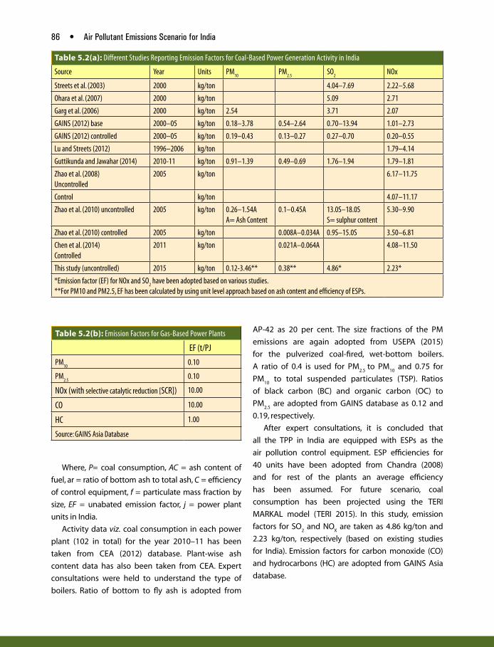
86 • Air Pollutant Emissions Scenario for India
Table 5.2(a): Different Studies Reporting Emission Factors for Coal-Based Power Generation Activity in India
Source Year Units PM10
PM2.5
SO2
NOx
Streets et al. (2003) 2000 kg/ton 4.04–7.69 2.22–5.68
Ohara et al. (2007) 2000 kg/ton 5.09 2.71
Garg et al. (2006) 2000 kg/ton 2.54 3.71 2.07
GAINS (2012) base 2000–05 kg/ton 0.18–3.78 0.54–2.64 0.70–13.94 1.01–2.73
GAINS (2012) controlled 2000–05 kg/ton 0.19–0.43 0.13–0.27 0.27–0.70 0.20–0.55
Lu and Streets (2012) 1996–2006 kg/ton 1.79–4.14
Guttikunda and Jawahar (2014) 2010-11 kg/ton 0.91–1.39 0.49–0.69 1.76–1.94 1.79–1.81
Zhao et al. (2008)Uncontrolled
2005 kg/ton 6.17–11.75
Control kg/ton 4.07–11.17
Zhao et al. (2010) uncontrolled 2005 kg/ton 0.26–1.54AA= Ash Content
0.1–0.45A 13.0S–18.0SS= sulphur content
5.30–9.90
Zhao et al. (2010) controlled 2005 kg/ton 0.008A–0.034A 0.9S–15.0S 3.50–6.81
Chen et al. (2014)Controlled
2011 kg/ton 0.021A–0.064A 4.08–11.50
This study (uncontrolled) 2015 kg/ton 0.12-3.46** 0.38** 4.86* 2.23*
*Emission factor (EF) for NOx and SO2 have been adopted based on various studies.
**For PM10 and PM2.5, EF has been calculated by using unit level approach based on ash content and efficiency of ESPs.
Table 5.2(b): Emission Factors for Gas-Based Power Plants
EF (t/PJ
PM10
0.10
PM2.5
0.10
NOx (with selective catalytic reduction [SCR]) 10.00
CO 10.00
HC 1.00
Source: GAINS Asia Database
Where, P= coal consumption, AC = ash content of
fuel, ar = ratio of bottom ash to total ash, C = efficiency
of control equipment, f = particulate mass fraction by
size, EF = unabated emission factor, j = power plant
units in India.
Activity data viz. coal consumption in each power
plant (102 in total) for the year 2010–11 has been
taken from CEA (2012) database. Plant-wise ash
content data has also been taken from CEA. Expert
consultations were held to understand the type of
boilers. Ratio of bottom to fly ash is adopted from
AP-42 as 20 per cent. The size fractions of the PM
emissions are again adopted from USEPA (2015)
for the pulverized coal-fired, wet-bottom boilers.
A ratio of 0.4 is used for PM2.5
to PM10
and 0.75 for
PM10
to total suspended particulates (TSP). Ratios
of black carbon (BC) and organic carbon (OC) to
PM2.5
are adopted from GAINS database as 0.12 and
0.19, respectively.
After expert consultations, it is concluded that
all the TPP in India are equipped with ESPs as the
air pollution control equipment. ESP efficiencies for
40 units have been adopted from Chandra (2008)
and for rest of the plants an average efficiency
has been assumed. For future scenario, coal
consumption has been projected using the TERI
MARKAL model (TERI 2015). In this study, emission
factors for SO2 and NO
X are taken as 4.86 kg/ton and
2.23 kg/ton, respectively (based on existing studies
for India). Emission factors for carbon monoxide (CO)
and hydrocarbons (HC) are adopted from GAINS Asia
database.

Power • 87
Control MeasuresSulphur emission–control system ranges from
limestone injection through control in furnaces, wet
scrubbing of flue gas, or high-efficiency regeneration
process (by capturing SO2 in the flue gas through
industrial processes). Limestone injection process
produces huge amount of waste material. On the
other hand, high-efficiency regeneration process is
very expensive. Wet flue gas desulphurization (FGD)
units are the most commonly used process with
sulphur removal rate of 90 per cent. There are only
four TPP in India that have FGD units in operation
(Guttikunda and Jawahar 2014; Prayas 2011). Among
those, three are in Maharashtra and one in Karnataka.
P Tata Power in Trombay (Maharashtra)
P BSES/Reliance at Dabanu (Maharashtra)
P Jindal TPP at Ratnagiri (Maharashtra)
P Udupi TPP (coastal Karnataka)
Till 2020, seven TPP which are just 3.2 per cent
of the total thermal power capacity in India have
been granted clearance for installation of FGD units.
However, this is to be noted that the coal used in
India is low in sulphur content (~0.5 per cent).
For NOx emissions, there are no existing norms
in India for coal-based power plants for control of
emissions. The formation of NOx emissions depends
on the temperature and residence time of the gases
in the combustion chamber. Formation of NOx can
be reduced by providing low nitrogen oxide burners.
Only a few newly installed TPP and extensions have
low NOx burners (Chikkatur et al. 2011; Guttikunda
2014). However, as per the new draft notification
issued by Ministry of Environment, Forest and Climate
Change (MOEF&CC), Government of India, new norms
for control of SO2 and NOx have been prescribed,
which will force the use of pollution control devices
for these pollutants in future years (Table 5.3).
Presently, PM is the only pollutant for which Indian
emission standards exist for coal-fired TPP in India.
Particulate emissions from a power plant can be
categorized into flue gas emissions and fugitive dust
emissions. ESPs are installed in all the TPP to remove
flue gas emissions. However, fugitive dust emissions
generated from coal handling units and ash ponds
still comprise around 20 per cent of the PM emissions
(UE and CAT 2015). For control of these emissions,
the government has notified certain guidelines.
To control fugitive emissions from coal handling,
MoEF&CC issued a notification in June 2001 that
specifies the TPP located beyond 1 km from pit heads
and the ones located in urban and sensitive areas are
required to use beneficiated coal containing ash not
more than 34 per cent. Further, to control fugitive
emissions from ash ponds, MoEF mandated through
a notification in 2003 that brick kiln units coming up
within 100-km radius of TPP have to use 25 per cent
of ash in brick kilns and any construction in the same
radius will use only fly ash bricks (Guttikunda and
Jawahar 2014).
Emissions from Thermal Power Generation in India Emissions from TPP are estimated and are presented
in Table 5.4. PM10
emissions are estimated to be about
453 kt from coal-based power plants in India for the
year 2011. Of which, around 181 kt are PM2.5
, 22 kt
black carbon, and 34 kt organic carbon emissions.
For the same year, SO2 and NO
x emissions are 1,842
kt and 1,015 kt, respectively. Due to lack of stringent
regulations on SO2 and NO
x emission in past, their
emissions are considerably high. As envisaged, a
minor capacity (3.2 per cent) will be installed with
FGD units for control of SO2 emissions, which is
accounted in projections of SO2 emissions till 2020.
However, MoEF&CC, Government of India has issued
Table 5.3: Emission Standards (mg/Nm3) for Coal-Based TPP
Capacity of TPP PM NOx SO2
Existing
<210 MW 350 No standards No standards
>210 MW 150 No standards No standards
Proposed standards in draft notification by MOEF&CC, 2015
Plants before 2003 100 600 600/200
Plants between 2003 and 2006
50 300 200
Plants after 2017 30 100 100Source: Guttikunda & Jawahar, 2014); MoEF & CC, 2015

88 • Air Pollutant Emissions Scenario for India
draft notification for revised emission standards for
coal-based TPP. Along with PM10
, standards for SO2,
NOx, and Hg have also been introduced. The new
emission limits are 83 per cent more stringent for
power plants envisaged after 2017 in comparison
to those established before 2003. Final guidelines
are expected to come in force in near future and
have been taken into account while estimation of
emissions for future years.
It is evident that under the RES scenario (TERI
2015) of future projections, despite an increase of
more than 7 times in the coal consumption, the PM
emissions from power sector will increase by about
three folds during 2011–51. The gaseous pollutants
show even lesser increase due to consideration of
stringent norms for NOx and SO
2 controls in future
from the power plants. Other than coal-based power
generation, emissions are also estimated for gas
power stations. Table 5.5 shows the emissions of
different pollutants from gas-based power stations.
This is to be noted that PM emissions are insignificant
in comparison to the emissions from coal-based
Table 5.5: Emissions from Gas-Based Power Plants in India (kt/yr) for 2001–51
2001 2011 2021 2031 2041 2051
PM10
0.04 0.10 0.07 0.09 0.13 0.40
PM2.5
0.04 0.10 0.07 0.09 0.13 0.40
NOx (with SCR) 3.72 9.61 6.95 8.69 12.60 40.30
CO 3.72 9.61 6.95 8.69 12.60 40.30
HC 0.37 0.96 0.69 0.87 1.26 4.03
Table 5.4: Emissions from Coal-Based Power Plants in India (kt/yr) for 2001–51
2001 2011 2021 2031 2041 2051
PM10
257 453 869 1016 1216 1353
PM2.5
103 181 348 406 486 541
BC 12 22 42 49 58 65
OC 20 34 66 77 92 103
SO2
1031 1842 3490 3981 4650 5108
NOx 570 1015 1928 3556 5773 7293
CO 19 34 65 120 194 246
NMVOC 4 7 13 24 39 49
power plants. The gas-based power plants are
required to maintain NOx standards and are generally
equipped with control equipment.
Spatial Distribution Emissions from power plants in India are spatially
put on the map of India using actual coordinates of
the power plant facilities (Figure 5.2). The emissions
are observed to be higher in the states of West
Bengal, Orissa and Chhattisgarh, and Maharashtra.
This can be due to higher coal consumption and
lower efficiencies of control equipments in the power
plants.
Comparison with Other Studies The emission estimated in this study is compared
with other studies for validation purpose (Table 5.6).
Particulate emissions calculated in this study are
Figure 5.2: Spatial distribution of PM2.5 emissions from power plants in India (2011)
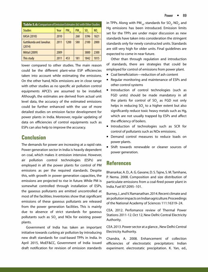
Power • 89
Table 5.6: Comparison of Emission Estimates (kt) with Other Studies
Studies Year PM10
PM2.5
SO2
NOx
IIASA (2010) 2010 268 3396 1821
Guttikunda and Jawahar. (2014)
2011 1200 580 2100 2000
Mittal (2009) 2009 3800 2300
This study 2011 453 181 1842 1015
lower compared to other studies. The main reason
could be the different plant-wise ESP efficiencies
taken into account while estimating the emissions.
On the other hand, NOx emissions are in close range
with other studies as no specific air pollution control
equipments APCE’s are assumed to be installed.
Although, the estimates are derived from actual unit
level data, the accuracy of the estimated emissions
could be further enhanced with the use of more
detailed studies on emission factor development for
power plants in India. Moreover, regular updating of
data on efficiencies of control equipments such as
ESPs can also help to improve the accuracy.
Conclusion The demands for power are increasing at a rapid rate.
Power generation sector in India is heavily dependent
on coal, which makes it emission intensive. However,
air pollution control technologies (ESPs) are
employed in all the power plants for control of PM
emissions as per the required standards. Despite
this, with growth in power generation capacities, the
emissions are projected to rise in future. While PM is
somewhat controlled through installation of ESPs,
the gaseous pollutants are emitted uncontrolled at
most of the facilities. Inventories show that significant
emissions of these gaseous pollutants are released
from the power generation facilities. This is mainly
due to absence of strict standards for gaseous
pollutants such as SO2 and NOx for existing power
plants.
Government of India has taken an important
initiative towards curbing air pollution by introducing
new draft standards for coal-based TPPs in India. In
April 2015, MoEF&CC, Government of India issued
draft notification for revision of emission standards
in TPPs. Along with PM10
, standards for SO2, NO
x, and
Hg emissions has been introduced. Emission limits
set for the TPPs are under major discussion as new
standards have taken into consideration the stringent
standards only for newly constructed units. Standards
are still very high for older units. Final guidelines are
expected to come in near future.
Other than through regulation and introduction
of standards, there are strategies that could be
employed for control of emissions from power plant.
P Coal beneficiation—reduction of ash content
P Regular monitoring and maintenance of ESPs and
other control systems
P Introduction of control technologies (such as
FGD units) should be made mandatory in all
the plants for control of SO2 as FGD not only
helps in reducing SO2 to a higher extent but also
significantly reduce toxic heavy metals such as Hg,
which are not usually trapped by ESPs and affect
the efficiency of boilers.
P Introduction of technologies such as SCR for
control of pollutants such as NOx emissions.
P Demand control measures to reduce loads on
power plants.
P Shift towards renewable or cleaner sources of
power generation.
ReferencesBhanarkar, A. D., A. G. Gavane, D. S. Tajne, S. M. Tamhane, P. Nema. 2008. Composition and size distribution of particulate emissions from a coal-fired power plant in India. Fuel 87:2095–101.
Burney, J., and V. Ramanathan. 2014. Recent climate and air pollution impacts on Indian agriculture. Proceedings of the National Academy of Sciences 111:16319–24.
CEA. 2012. Perfomance review of Thermal Power Stations 2011-12. Oct 12, New Delhi: Central Electricity Authority.
CEA. 2013 .Power sector at a glance. , New Delhi: Central Electricity Authority.
Chandra, A. 2008. Enhancement of collection efficiencies of electrostatic precipitators: Indian experiment. electrostatic precipitation. K. Yan, ed.,

90 • Air Pollutant Emissions Scenario for India
Proceedings of the Eleventh International Conference on Electrostatic Precipitation. Hangzhou, Zhejiang University Press, Springer.
Chandra, A., and H. Handra. 2004. Impact of Indian and imported coal on thermal power plants. Journal of Scientific & Industrial Research 63:156–62.
Chen, L., Y. Sun, X. Wu, Y. Zhang, C. Zeng, X. Gao, and K. Cen. 2014. Unit based emission inventory and uncertainty assessment of coal-fired thermal power plants. Atmospheric Environment 99:527–35.
Chikkatur, A. P., A. Chaudhary, and A. D. Sagar. 2011. Coal power impacts, technology and policy: Connecting the dots. Annual Review of Environment and Resources 36:101–38.
EPA,2012. Report to Congress on Black Carbon, USEPA Washington.
GAINS. 2012. Greenhouse gas and air pollution interactions and synergies South Asia Program. Laxenburg, Austria: International Institute of Applied Systems Analysis.
GAINS Database. Available at: <http://gains.iiasa.ac.at/gains/emissions.ASN/index.menu?page=609>,
last accessed on Jun 1, 2015
Garg, A., Shukla, P. R., Kapshe M., 2006. The sectoral trends of multigas emissions inventory of India. Atmospheric Environment 40(24), 4608-4620.
Guttikunda, S. K., and P. Jawahar. 2014. Atmospheric emissions and pollution from the coal-fired thermal power plants in India. Atmospheric Environment 92:449–60.
Hao, J.M., Tian, H.Z., Lu, Y.Q., 2002. Emission inventories of NOx from commercial energy consumption in China, 1995–1998. Environmental Science & Technology, 36(4): 552-560.
IIASA. 2010. Scenarios for cost-effective control of air pollution and greenhouse gases in India. Laxenburg, Austria: International Institute for Applied System Analysis.
Lu, Z., and D. G. Streets. 2012. Increase in NOx emissions from Indian thermal power plants during 1996-2010: Unit-based inventories and multiscale observations. Environmental Science & Technology 46:7463–70.
Mittal, M. L. 2009. Estimates of emissions from coal fired thermal power plants in India. Available at: <http://www.epa.gov/ttnchie1/conference/ei20/session5/mmittal.pdf>.
MoEF & CC, 2015. Draft Notification for emission standards http://envfor.nic.in/sites/default/files/draft%20Notification%20forinviting%20the%20public%20comments%20for%20the%20Coal%20BTPP.pdf
Ohara, T., H. Akimoto, K. Kurokawa, et al. 2007. An Asian emission inventory of anthropogenic emission sources for the period 1980–2020. Atmospheric Chemistry and Physics Disscussion 7:6843–902.
Prasad, A., R. Singh, and M. Kafatos. 2012. Influence of coal-based thermal power plants on the spatial temporal variability of tropospheric NO
2 column over
India. Environmental Monitoring and Assessment 184:1891–1907.
Prayas. 2011. Thermal power plants on the Anvil: Implications and need for rationalization. Pune, India: Prayas Energy Group.
Purohit, P., M. Amann, R. Mathur, et al. 2010. GAINS ASIA scenarios for cost-effective control of air pollution and greenhouse gases in India. Laxenburg, Austria: International Institute for Applied Systems Analysis.
Sengupta, I. 2007. Regulation of suspended particulate matter in India coal-based thermal power plants: A static approach. Energy Economics May; doi:10.1016/j.eneco.2006.01.004.
Shail, M., S. Sodha, R. Chandra, B. Pitchumani, and J. Sharma. 1994. Effect of coal properties on the specific coal consumption in a typical thermal power station in India. Energy Conversion and Management 35:597–603.
Singh, M., and R. Siddique. 2013. Effect of coal bottom ash as partial replacement of sand on properties of concrete. Resources, Conservation and Recycling 72:20-32.
Streets, D. G., T. C. Bond, G. R. Carmichael, et al. 2003. An inventory of gaseous and primary aerosol emissions in Asia in the year 2000. Journal of Geophysical Research 108(D21):Art. No. 8809.
TERI. 2015. Energy security outlook: Defining a secure and sustainable energy future for India. New Delhi: TERI.

Power • 91
The Shift Project data Portal, Electricity producton from different energy sources in India. Available at: <http://www.tsp-data-portal.org/Breakdown-of-Electricity-Generation-by-Energy-Source#tspQvChart>.Last Accessed on Jun 1, 2015
Tian, H. Z. 2003. Studies on present and future emissions of nitrogen oxides and its comprehensive control policies in China. Ph.D. thesis, Tsinghua University, Beijing.
Urban Emisisons (UE) and Conservation Action Trust (CAT). 2015. Coal kills: An assessment of death and disease caused by India’s dirtiest energy source. Goa: Urban Emisisons.info.
USEPA. 2015. AP-42 emission factor database. Washington, DC: United State Environment Protection Agency. Available at: <www.epa.gov/ttnchie1/ap42/>.
Wang, S. X. 2001. Technical options and planning on control of sulfur dioxide emitted from coal-fired power plants in China. Ph.D. thesis, Tsinghua University, Beijing.
Yi, H. H. 2006. Studies on emission characteristics of PM10 from power plants. Ph.D. thesis, Tsinghua University, Beijing
Zhang, Q., D. G. Streets, K. B. He, and Z. Klimont. 2007a. Major components of China’s anthropogenic primary particulate emissions. Environmental Research Letters 2(045027); doi:10.1088/1748-9326/2/4/045027.
Zhang, Q., D. G. Streets, K. B. He, et al. 2007b. NOx emission trends for China, 1995–2004: The view from the ground and the view from space. Journal of Geophysical Research 112(D22):Art. No. D22306.
Zhao, Y., S. Wang, L. Duan, Y. Lei, C. Pengfei, and J. Hao. 2008. Primary air pollutant emissions of coal-fired power plants in China: Current status and future prediction. Atmospheric Environment 42:8442–52.
Zhao, Y., S. Wang, C. P. Nielsen, X. Li, and J. Hao. 2010. Establishment of a database of emission factors for atmospheric pollutants from Chinese coal-fired power plants. Atmospheric Environment 44:1515–23.


CHAPTER
Transport Sumit Sharma, Atul Kumar, and Sarbojit Pal
6
Introduction Air pollution is a serious concern especially in the
urban areas of India. Source apportionment studies
have highlighted many sources of air pollution
in urban centres, and emissions from growing
number of motor vehicles play an important role
in the increasing pollutant loads in the cities. This
is particularly important in India, which has one of
the most critically polluted cities in the world. To
add to its woes, India has seen very rapid growth in
vehicles, especially across its urban centres that has
contributed to increase in particulate emissions
from vehicular sources; accounting for up to 50 per
cent in the particulate matter less than 2.5 microns
(PM2.5
) concentrations in a city like Bangalore (CPCB,
2010). These PM2.5
emissions from diesel vehicles
are critically important given that the World Health
Organization (WHO) has recently classified diesel
engine exhaust as carcinogenic to humans since
exposure to these emissions is associated with
increased risk of lung cancer.
Total registered vehicles in India has grown from
5.3 million in 1981 to 159 million by 2012 (MoRTH,
2013). However, not all registered vehicles are fit
to ply on road. Figure 6.1 shows the estimates of
on-road vehicles in India that have grown from
4.4 million in 1981 to about 96 million by 2011.
The numbers are projected to grow to 427 million
by 2031 and 933 million by 2051. Private vehicle
ownership in particular has grown from 6 per 1,000
people in 1981 to 75 in 2011. This is expected to grow
to up to 258 per 1,000 population by 2031, and 461
by 2051.
The distribution of vehicles in Figure 6.2 shows
that the share of two-wheelers has grown rapidly
during the period 1981–2011. However, in future with
growth in economy, the share of cars will grow and
will increase from 15 per cent in 2011 to about 18 per
cent by 2031 and 24 per cent by 2051.
Presently, the transport sector is the second largest
consumer of commercial energy in the country.
Growth of transport sector increases the dependence

94 • Air Pollutant Emissions Scenario for India
Figure 6.1: Year-wise on-road vehicular stock in India (TERI MARKAL model estimates)
Figure 6.2: Distribution of on-road vehicles by type in past and future years (TERI MARKAL model estimates)
on imported crude. The sector is expected to grow at
a steady rate for the next few decades. With further
growth projected in future, the energy consumption
is expected to increase considerably. In reference
scenario (RES) in TERI 2015, the energy consumption
in the sector is expected to grow from about 3.6
thousand PJ to more than 15 thousand PJ by 2031,
and further to about 37 thousand PJ by 2051 (Figure

Transport • 95
6.3). Currently, about 43 per cent of energy in road
transport sector is consumed by heavy and light
commercial vehicles (HCV and LCVs), followed by 23
per cent by buses. The share of private vehicles in
energy use is expected to increase from 11 per cent
in 2011 to about 19 per cent by 2051. The share of
buses in energy use will reduce from 21 per cent to
just 5 per cent in the same period of time. Increased
energy consumption may lead to higher emissions
of air pollutants in comparison to current levels, in a
stagnant emission control scenario.
Methodology for Emissions Estimation The transport sector emissions are estimated using
the basic approach of emission factors.
Emissions = Energy use (PJ) × No control emission
factor (kt/PJ) × (1 – Percentage of Bharat Stage
emission control)
The emission factors for this exercise have been
adopted from primarily three sources. CPCB (2000)
reported emissions factors for various categories of
vehicles with varying vintages. GAINS Asia database
provides a database of emission factors for different
categories of vehicles based on their classes under
various emission control categories, that is, Euro-I
to Euro-VI. ARAI (2008) also carried out a series of
measurements to ascertain indigenous emission
factors for different categories of vehicles in Indian
conditions. A vehicle-wise comparison of emission
factors from the three sources is shown in Figure 6.4.
It is evident that while the emission factors are more
or less in similar ranges, while there are considerable
differences in some categories. The most recent
measurements in Indian context is reported in ARAI
dataset, which shows higher emissions for heavy-
duty vehicles. However, lower emissions factors are
derived from ARAI in case of two-wheelers categories.
This is to be noted that ARAI (2008) reports emission
factors in gram per kilometre units, which have been
converted to gram per kilojoules based on typical
vehicle mileages. Energy consumption estimated for
the sector is compared and validated with actual fuel
consumption estimates reported by MoPNG.
PM emissions are also estimated for four different
fractions namely, PM10
, PM2.5
, Black Carbon (BC) and
organic carbon (OC). The shares of BC and OC in PM10
/
PM2.5
fractions are adopted from EPA (2012).
Figure 6.3: Growth in energy consumption (PJ) in transport sector in India
Source: MARKAL model results, TERI (2015)

96 • Air Pollutant Emissions Scenario for India
Figure 6.4: Comparison of PM emission factors from GAINS, ARAI (2008), and CPCB (2000)
Important Aspects Affecting Emissions from the Transport Sector Other than the emission factors, there are number
of aspects which affect energy consumptions and
emissions from the transport sector in India. Each of
these are discussed in subsequent sections.
Fuel Quality and New Vehicle Emission Standards The quality of fuel plays an important role in
determining the tail-pipe emissions of pollutants
from vehicles. The sulphur and benzene content
in fuels not only affect the emissions of SO2 and
hydrocarbons but also contribute to secondary
particulate formation. The Auto Fuel Policy of 2002
of Government of India (MoPNG 2002) laid down a
roadmap till 2010 for introduction of cleaner fuels
and vehicles in the country. Under this, 13 selected
cities were gradually moved to BS-IV norms by 2010,
while rest of the country reached BS-III norms. This
led to the establishment of one set of ambient air
quality standards to determine the quality of air, and
dual standards for vehicle emissions and fuel quality.
It was observed that the rate of increase in PM10
concentrations was much higher in cities where lower
quality fuel was provided (Sharma et al. 2014). More
importantly, the heavy-duty trucks (which are the
largest contributor to vehicular emissions) (Sharma
et al. 2014) need to move all across the country
and hence, remained on BS-III standards across the
country, despite BS-IV norms introduced in some
cities. Another Auto Fuel Vision Committee was set
up in 2013 to recommend the future roadmap on
advancement of fuel quality and vehicular emission
standards up to 2025. The committee recommended
that BS-IV and BS-V norms be introduced across the
country by 2017 and 2020, respectively (AFV 2014).
The road map suggested in Auto Fuel Policy 2002 and
the current recommendations of the Auto Fuel Vision
2025 Committee on the future road map of auto fuel
emissions are shown in Table 6.1.
However, it is to be noticed that the roadmap
recommended by the Auto Fuel Vision 2025
Committee would also keep India almost 10 years
behind the US and European countries. Although,
recently the BS-IV fuel quality norms have been
announced to be introduced in most regions of the
country by 2016, the automobile manufacturers have
shown their reluctance in moving to the BS-IV norms
for heavy-duty vehicles with the immediate effect.
The usefulness of BS-IV fuel can only be realised if the
manufacturers start supplying the BS-IV complaint
heavy-duty trucks and buses in the country. Moreover,
the lowest emission levels can only be achieved with

Transport • 97
Table 6.1: Road Map Suggested in Auto Fuel Policy 2002 and the Current Recommendations of the Expert Committee
Category Bharat Stage II Bharat Stage III Bharat Stage IV Bharat Stage V
Two and Three wheelers Entire country April 2005 Entire country April 2010 Entire country April 2016
Entire country April 2020
All other new vehicles Entire country April 200511 cities—April 2003
Entire country April 201011 cities—April 2005
Entire country 2017*11 cities—April 2010(20 cities ) No road map beyond 2010
Entire country 2020–2021*
*Suggested by the new Auto Fuel Vision 2025 Committee in 2014.
a move to BS-V quality of fuel (10 ppm sulphur) and
BS-VI vehicular emissions standards for vehicles. Till
date the Ministry of Road Transport and Highways,
(Government of India) has notified BS-IV and BS-V
emission norms. Based on the current scenario, the
business as usual scenario in this study assumes
adoption of BS-IV norms by 2016 and BS-V from 2021.
Growth of Private Vehicles vis-à-vis Enhancement of Public Transport One of the prime factors for emissions from the
transport sector is the rapid growth of private
vehicles. Ghate and Sundar (2013) showed that
the average level of private car ownership in India
could grow from 13 per 1,000 population to 35 by
2025. While, growing number of vehicles has serious
implications for energy security, road safety, and
equitable allocation of road space, it also adds to the
pool of air pollutants. Increasing private vehicles in
India is linked to growing income levels, aspirations,
and limited public transport. There is a lot to learn
from the experiences of some cities like Singapore,
Hong Kong, etc. to decouple vehicle ownership
with economic growth. The success of these cities
hinged on having efficient public transport systems
to cater to the growing demands of mobility. Indian
cities have however been moving in a different
and unsustainable direction as compared to these
international cities. The share of efficient mass
transport modes have continuously gone down
across most Indian urban centres.
Road transport now accounts for nearly 66–68
per cent of the total freight and 82–84 per cent of
the total passenger traffic shares. The share of the
energy efficient railways in freight movement have
reduced from over 80 per cent in 1950–51 to about
35 per cent in 2011–12, while the share of railways in
passenger traffic has reduced from over 50 per cent
to barely 14 per cent in the same period. The shares
of traffic on inland water ways and coastal shipping,
which are the most efficient forms of transport, have
almost declined to oblivion (Ramanathan et al. 2014).
Without a conscious effort to increase the share of
efficient transport modes, India is going to witness an
increase in energy intensity in the transport sector.
State of Public Transport in India The public transport scenario in India paints a grim
picture. Most Indian cities are not equipped with
effective public transport systems to meet their
demand for mobility. The share of buses in the overall
fleet of registered vehicles have declined from 11 per
cent in 1951 to just 1 per cent in 2011 (PC 2014). The
decline has been found to be rapid in the last decade
mainly due to enormous growth of private vehicles.
Government of India launched the National Urban
Transport Policy (NUTP) in 2006 to improve the health
of the urban transport systems across the country.
NUTP identifies a number of public transport options
such as metro-rail (Delhi, Hyderabad, Mumbai, etc.)
and bus rapid transit systems (Ahmedabad, Jaipur, etc.)
other than the existing suburban rail and bus systems

98 • Air Pollutant Emissions Scenario for India
for mass transport solutions in cities. The Ministry of
Urban Development also launched the Jawaharlal
Nehru National Urban Renewal Mission (JNNURM) to
provide financial assistance to cities for development
of projects for improving urban mobility. The NTDPC
report recommends a dense integrated system of
transport for Indian cities. While metro rail systems can
be considered for big cities with careful examination,
bus-based systems are absolutely essential for
small and medium cities. In addition to these, the
Government of India has recently launched the Smart
Cities Program and the AMRUT Scheme for India under
which urban transport finds special significance.
In-use Vehicle Management SystemWhile improvements have been made through
introduction of emission standards for new vehicles,
there are limited efforts being made in India to
control emissions from in-use vehicle fleet. This
requires an effective inspection and maintenance
system to check and tune the vehicles to comply
with the prescribed standards. Worldwide, it has been
reported that on-road vehicles emit much higher
levels of pollutants during their lifecycle as compared
to the limits set during their certification stage. This
could be mainly due to wear and tear, lack of proper
maintenance, engine faults, or misuse at the hands
of the driver, amongst other causes. This also points
to the fact that mere switching to advanced new
vehicle standards will not suffice and in-use vehicle
management should go hand in hand.
Presently, the only in-use vehicle testing
conducted in India is the Pollution-Under-Control
(PUC) programme, which is based on idle test
emission limits without any loaded mode tests.
These idle mode tests do not reflect the real-life
situation of a vehicle running on the road. Moreover,
despite a provision of heavy penalties, merely 21 per
cent of vehicles appear for PUC testing in Delhi (Sita
Lakshmi et al. 2014). The current situation is not so
effective in control of emissions and does not ensure
on-road compliance despite compliance during
manufacturing stage.
Congestion and Improving Driving Cycles Internationally, and now in 10 Indian cities, Sharma
et al. (2016) has observed that there are considerable
differences between driving cycles on which vehicles
are initially tested (for type approvals) and real-
Figure 6.5: Comparison of driving patterns observed in 10 Indian cities with the prescribed driving modified Indian driving cycle ((MIDC)) for emission testing for cars in India

Transport • 99
world driving conditions (Figure 6.5). The real world
driving patterns observed in 10 cities highlight
two issues. Firstly, there is a problem in the current
testing procedures, which may lead to higher on-
road emissions despite compliance with testing
procedures and limits. This means that the vehicles
may comply with emission regulations, but may
emit much more under real-world conditions, hence
making the policy ineffective. The second issue
highlighted in the TERI study of 10 cities is of very
high congestion levels, which could lead to loss
of time, fuel, and enhanced exposure to very high
emission levels (Sharma et al. 2013, 2016). The driving
patterns show very low driving speeds mainly on
account of congestion. City specific strategies will be
required to address and improve the traffic flows. This
will not only reduce exposure to emissions but also
could save fuel and time.
Baseline and Future Emission Inventory Based on the energy consumption (Figure 6.3), the
emission factors (Figure 6.4) and factors described in
section ‘Important Aspects Affecting Emissions from
the Transport Sector’ that affect vehicular emissions
in India, pollutant-wise emission estimates are
made and presented in subsequent sections . It is to
be noted that ARAI (2008) emission factors are used
to derive emission estimates; however, the variations
using other emission factor datasets is also presented
in subsequent section ‘Comparison of Emission
Estimates with Other Studies’. For future emission
norms, reduction factors are adopted from GAINS
Asia Database.
NOx Emissions
NOx emissions from vehicles grew by more than
two times during 2001–11 from 1164 kt to 2665 kt,
with heavy-duty vehicles having the biggest share.
The emissions are expected to grow further by 1.5
times till 2031 and 2.3 times by 2051 (Figure 6.6).
Figure 6.7 shows that introduction of BS norms have
arrested the growth of NOx emissions in India. BS-I/
II emission norms led to a reduction of 21 per cent
NOx emissions by 2051 in comparison to the no-
control scenario. Further, introduction of BS-III and IV
norms in 2011 and 2016 would lead to a reduction of
62 per cent NOx emissions by 2051. The RES scenario
assumed in this study takes into account the current
notification and assumes the introduction of BS-V in
2021. This leads to an overall reduction of 78 per cent
in comparison to the No control scenario.
Figure 6.6: Past and projected growth of NOx emissions (kilotonnes per year) in India (2001–51)

100 • Air Pollutant Emissions Scenario for India
Figure 6.7: Effect of introduction of vehicle emission norms (BS-I to BS-IV) on NOx emissions in India NOC refers to a scenario without any emission norms in the sector
PM Emissions Emission estimates are prepared for different fractions
of PM emitted from various vehicle categories.
The emission estimates of PM2.5, BC, and OC are
presented in Figures 6.8, 6.10, and 6.11. PM2.5
emissions grew from 191 in 2001 kt to 276 kt in
2011. Heavy-duty vehicles have the biggest share in
the current emissions. The emissions are expected
to increase till 2021 and are expected to reduce
thereafter with introduction of BS-V norms (Figure
6.8). Figure 6.9 shows that introduction of BS norms
have arrested the increase of PM emissions in India.
BS-I/II emission norms led to a reduction of 49 per
cent PM emissions by 2051 in comparison to the no-
control scenario. Further, introduction of BS-III and IV
norms in 2011 and 2016 would lead to a reduction of
83 per cent PM emissions by 2051. The BAU scenario
assumed in this study takes into account the current
recommendations of the expert committee and
assumes the introduction of BS-V in 2021. This leads
to an overall reduction of 97 per cent in comparison to
the no control scenario in 2051.
The PM2.5
emissions are speciated into BC and OC
components using factors from EPA (2012). The BC
emissions are dominated by diesel driven vehicles
with BC to PM2.5
ratios of 0.73–0.77. BC emissions from
the transport sector are first expected to grow till
2031 and then go down from 197 kt to 111 kt during
2011–51 (Figure 6.10 ).
Other than major contributions from diesel
driven vehicles, the organic carbon fraction receives
contributions from gasoline driven private vehicles.
The OC emissions from the transport sector are
expected to go down from 70 kt to 35 kt during
2011–51, due to introduction of BS-V norms (Figure
6.11).
Carbon MonoxideCarbon monoxide gas is released due to incomplete
combustion of fuel. Gasoline engines have higher
emission factors in comparison to diesel vehicles. The

Transport • 101
Figure 6.8: Past and projected growth of PM2.5 emissions (kilotonne per year) in India (2001–51)
Figure 6.9: Effect of introduction of vehicle emission norms (BS-I to BS-IV) on PM2.5 emissions in India

Figure 6.10: Past and projected growth of BC emissions in India (2001–51)
Figure 6.11 Past and projected growth of OC emissions in India (2001-2051)
emission estimates from 2001 to 2051 are presented
in Figure 6.12. CO emissions grew from 1,983 in 2001
kt to 2,777 kt in 2011. Private vehicles (two wheelers
and cars) have the biggest share in the current CO
emissions (38 per cent). Trucks with high energy
consumption also have a significant share of 33 per
cent in the overall inventory. With growing energy
demands, the emissions from the transport sector are
projected to grow by 2.2 and 5.1 times by 2031 and
2051, respectively. The emission is expected to grow

with the energy consumption mainly on account of
no further control of CO emissions in BS-V norms in
trucks. However, the emission could have been much
higher without the introduction of emission control
norms (BS-I to BS-IV) in India.
Hydrocarbons Hydrocarbons are released mostly from gasoline
engines that have higher emission factors in
Figure 6.12: Past and projected growth of CO emissions in India (2001–51)
Figure 6.13: Past and projected growth of HC emissions in India (2001–51)
comparison to diesel vehicles. The emission estimates
from 2001 to 2051 are presented in Figure 6.13. HC
emissions grew from 605 in 2001 kt to 802 kt in 2011.
Private gasoline driven vehicles have the biggest
share (46 per cent) in the overall inventory. On
account of introduction of BS-V norms, the emissions
are expected to grow only marginally till 2031 and
will increase to 980 kt. Despite introduction of BS-V
norms, the emission will grow to 1,103 kt by 2051,

104 • Air Pollutant Emissions Scenario for India
Table 6.2: Fuel Quality Improvement Program in India
Fuel Date Lead content Area covered
Gasoline 1994 Low leaded (0.15 g/l)
NCT, Delhi, Mumbai, Kolkata, and Chennai
Gasoline 1995 Unleaded (0.013 g/l) + low lead
NCT, Delhi, Mumbai, Kolkata, and Chennai
Gasoline 1998 Ban on leaded gasoline. Only unleaded
NCT
Gasoline 1999 Unleaded only NCR
Gasoline 2000 Unleaded only Entire country
Fuel Date Benzene Content Areas Covered
Gasoline Pre1996 No specification for Benzene
Entire country
Gasoline 2000 3 % Benzene Metro cities
Gasoline 2000 1% Benzene NCT and Mumbai
Gasoline 2005 1% Benzene Entire country
Fuel Date Sulphur Content Areas Covered
Diesel 1996 0.5% Four metros and Taj Trapezium
Diesel 1997 0.25% Delhi and Taj Trapezium
Diesel 1998 0.25% Delhi, Mumbai, Chennai, Kolkata
Diesel 2000 0.05% NCR-Private Vehicles
Diesel 2001 0.05% NCT-all diesel vehicles
Diesel 2001 0.05% NCR-all diesel vehicles
Diesel 2001 0.05% Chennai, Mumbai, and Kolkata
Diesel 2003 0.05% Ahmedabad, Bangalore, and Hyderabad
Diesel 2005 0.05% All over country
Diesel 2005 0.035% 11 cities
Diesel 2010 0.035% All over country
Diesel 2010 0.005% 11 cites
Diesel 2016 0.005% All over country*
Diesel 2021/2019 0.001%/ All over country*
*Planned as per AFV 2025; ** As per MoRTH notification
mainly due to growth in energy consumption. The
emission could have been much higher without the
introduction of emission control norms in India.
SO2 Emissions
Sulphur dioxide emissions are related to the sulphur
content in the automotive fuels. Fuel quality has
gradually improved in the country and sulphur
content has reduced considerably over the years
(Table 6.2).
With this the sulphur dioxide emissions have
come down significantly from 120 kt in 2001 to
53 kt in 2011 (Figure 6.14). It is expected to go
down further with introduction of BS-V (10 ppm
sulphur) fuels in 2021. However, no changes have
been assumed in high sulphur fuels used in non-
road sector (tractors, railways, and shipping). With
2,000 ppm sulphur assumed in non-road fuels, the
emissions are expected to reach 145 kt by 2051.
Comparison of Emission Estimates with Other Studies The emission estimates in the previous section are
based on emission factors from ARAI (2008) datasets.
The differences in emission esitmates using GAINS
and CPCB (2000) emission factors are shown in Table
6.3. The estimates in this study are also compared
with previous studies.
It is to be noted that when GAINS emission factors
are used, the emissions ranges between 115 kt to 147
kt between 2001 and 2051. However, in the current
study the emissions estimated using ARAI emission
factor leads to higher PM2.5 emissions of 261 kt in
2011. This is due to higher emission factors reported
in ARAI (2008) while testing of indigenous vehicles on
Indian driving cycles.
Emissions from Road Dust Re-Suspension When vehicles move on a road, the silt lying on the
road gets re-suspended. The rate of re-suspension
is dependent on the weight of the vehicles and
quantity of silt lying on the road. Road dust

Transport • 105
Figure 6.14: Past and projected growth of SO2 emissions in India (2001–51)
Table 6.3: Comparison of Different Studies Reporting Emissions (kilotonnes) for Different Pollutants from Transport Sector in India
Source Year PM2.5
NOx CO HC
ICCT, 2013 2011 220 2200
CPCB, 2010 2003–04 153 2298 5692 723
CAIA, 2008 2008 150 2200
Guttikunda and Mohan, 2014 2011 253 5000 5500 1850
Purohit et al., 2010 2010 319 2706 1798
This study (ARAI, 2008 efs) 2011 276 2665 2777 802
This study (GAINS efs) 2011 156 2820
This study (CPCB, 2000 efs) 2011 235 2376
suspension emissions in this study are estimated
using the USEPA procedure specified in AP-42.
Emission loads =VKT × EF where
EF = k (SL)0.91⋅(W)1.02
EF = particulate emission factor (having units
matching the units of k),
k = particle size multiplier for particle size range
and units of interest, for PM10
k = 0.62, PM2.5
k = 0.15
SL = road surface silt loading (grams per square
meter; g/m2),
W = average weight (tons) of the vehicles
travelling the road
Based on silt loadings experiments carried out
by TERI in the past in various cities of India (TERI
2007, 2011, Sharma et al, 2015) a conservative SL
of 0.1 g/m² is assumed in this study. Vehicle-wise
VKT estimates were taken from TERI (2015) (based
on TERI-MARKAL model estimates) for 2001–51. ‘W’
values were derived based on fleet distributions.
PM10 and PM2.5 emissions are estimated be
47.8 and 11.6 kt in 2011, respectively (Figure
6.15). The emission projections are made with an
assumption that road quality and maintenance
will improve at the rate of 10 per cent per annum
and silt loading will reduce to 0.043 g/m² by 2051.
The emissions will still grow by 12.5 times with the
growing mobility demands and weight of the overall
vehicular fleet.
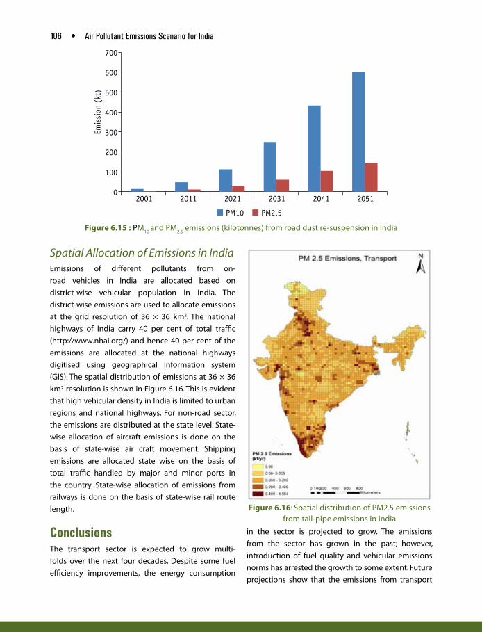
106 • Air Pollutant Emissions Scenario for India
Figure 6.15 : PM10
and PM2.5
emissions (kilotonnes) from road dust re-suspension in India
Spatial Allocation of Emissions in India Emissions of different pollutants from on-
road vehicles in India are allocated based on
district-wise vehicular population in India. The
district-wise emissions are used to allocate emissions
at the grid resolution of 36 × 36 km2. The national
highways of India carry 40 per cent of total traffic
(http://www.nhai.org/) and hence 40 per cent of the
emissions are allocated at the national highways
digitised using geographical information system
(GIS). The spatial distribution of emissions at 36 × 36
km² resolution is shown in Figure 6.16. This is evident
that high vehicular density in India is limited to urban
regions and national highways. For non-road sector,
the emissions are distributed at the state level. State-
wise allocation of aircraft emissions is done on the
basis of state-wise air craft movement. Shipping
emissions are allocated state wise on the basis of
total traffic handled by major and minor ports in
the country. State-wise allocation of emissions from
railways is done on the basis of state-wise rail route
length.
Conclusions The transport sector is expected to grow multi-
folds over the next four decades. Despite some fuel
efficiency improvements, the energy consumption
Figure 6.16: Spatial distribution of PM2.5 emissions from tail-pipe emissions in India
in the sector is projected to grow. The emissions
from the sector has grown in the past; however,
introduction of fuel quality and vehicular emissions
norms has arrested the growth to some extent. Future
projections show that the emissions from transport

Transport • 107
sector will stabilize over the years mainly due to
introduction of advanced vehicular emission norms
(BS-V) by 2021. The inventory of emissions from
transport sector is found to be comparatively lower
than other sectors such as residential and industries.
However, it is to be noted that transport emissions
are concentrated more in the urban regions and
that is why the sectoral contribution of transport
may not be prominent at the National scale but will
be significant at the urban scales. CPCB (2011) has
shown higher contributions of the transport sector
at the urban scales. Other than tail-pipe emissions,
fugitive emissions due to road dust re-suspensions
are also emitted from the sector. While there are
norms in place for control of tail-pipe emissions, the
road dust emissions are dependent on the quality of
roads and maintenance.
Evidently, there are a number of steps that are
required to be taken for control of vehicular pollution
in India.
Improve fuel quality and vehicular standards
Considering the current state of air quality, the
Government of India has notified earlier introduction
of BS-V fuels than those recommended in the AFV
(2014) by asking the Indian refineries to move to
BS-V fuels by 2019. The GOI has also announced
the possibility of leap frogging to BS-VI emissions
norms. GOI should also immediately set up an expert
group to prescribe BS-VI vehicle emission norms
by 2017 that can be adopted by the auto industry
by 2020. This would also facilitate the use of after
treatment devices (e.g., diesel particle filters) as
retrofits for vehicles already in use. Studies carried
out by TERI and ICCT have shown that the benefits
of the adoption of these advanced norms outweigh
the costs of implementation and the initial costs
of refinery upgradation can be met with a slight
increase in the fuel price (less than a rupee per litre)
(ICCT 2013; Sharma et al. 2014) .
Reduce private vehicles ownership in urban areas
Discouraging ownership of vehicles can be done
through higher taxation policies, high parking
fees, road usage fees, etc. However, this can only
be implemented once a public transport system is
in place that is attractive enough for the general
public. The bus-based public transport systems are
within reach of larger cities’ budgets as well as state
transport funding, but incentives from national
programs such as the forthcoming successor to the
JNNURM or the SMART cities program could motivate
greater attention to buses as an important part of
public transport systems. Bus-based systems are
particularly well suited for most Indian cities since
they are inherently more flexible than rail based ones
and can accommodate unforeseen growth.
Improved in-use vehicle management system
It could be better to set up adequate numbers of
well-equipped centralized inspection centres in
every city, in place of the existing decentralized PUC
centres. These limited number of inspection centres
should be closely monitored by the respective state
transport departments for quality assurance. Instead
of quarterly testing, annual testing of vehicles (such
as in US and China) across India can ensure higher
percentage of the vehicular fleet actually appearing
for inspections. For further improvement, annual I&M
checks can be linked with the vehicle insurance. The
total investment required for establishing inspection
centres for catering to all the vehicles is estimated
to be about INR 7,300 crores. Annual testing charges
of INR 100 to 400 per vehicle—for different category
of vehicles—should recover this cost within the next
2.3 years (Sitalakshami et al, 2014). Moreover, there is
a need of an in-use vehicle compliance programme
to check and ensure that vehicles actually comply
with their original emission standards (type approval
standards) throughout their useful life. Limited
testing can be initiated at the central level to assess
the compliance of in-use vehicles of different
manufacturers with the type approval norms.
Improving Driving cycles
This call for further investigations and change in the
current procedures and therefore improvement in
the prescribed driving cycles in the vehicle emission

108 • Air Pollutant Emissions Scenario for India
test procedures. In this respect, a move towards the
world harmonized test procedures could be explored,
which cover a variety of driving conditions and are
much more comprehensive than the current ones.
Other than these, encouraging fleet
modernization, promoting non-motorized means
of transport (walking and cycling), increasing
distribution of electric and hybrid vehicles, and
integrated land-use and transport planning should
also help. For control of road dust emissions, the
quality of roads and maintenance levels also need to
improve significantly.
ReferencesAFV. 2014. Auto Fuel Vision and Policy–2025. Report of the Expert Committee, Auto Fuel Vision and Policy–2025 Committee. New Delhi: Government of India
ARAI. 2008, Draft report on “Emission factor development for Indian vehicles “ as a part of ambient air quality monitoring and emission source apportionment studies. Pune Automotive Research Association Of India.
CAIA. 2008. Emissions from India’s Intercity and intracity road transport consultation draft –7 May 2009, Clean Air Initiative for Asian Cities (CAI-Asia). Available at < https://www.yumpu.com/en/document/view/22657705/emissions-from-indias-intercity-and-intracity-clean-air-initiative/5 (last accessed on September 4, 2015)>.
CPCB. 2000. Transport fuel quality for year 2005. PROBES/78/2000-01. New Delhi: Central Pollution Control Board, Ministry of Environment and Forests.
CPCB. 2010. Programme objective series PROBES/ 136 /2010 status of the vehicular pollution control programme in India. New Delhi: Central Pollution Control Board.
CPCB. 2011. Air quality monitoring, emission inventory, and source apportionment study for Indian cities. Control of Urban Pollution Series, CUPS/77/2010–11. New Delhi: CPCB.
EPA. 2012. BC report to Congress. Washington: United States Environmental Protection Agency. Available at <http://epa.gov/blackcarbon/2012report/Chapter4.pdf>, last accessed September 4, 2015.
ICCT. 2013. Overview of India’s vehicles emissions control programme. Washington: ICCT.
Ghate, A., and S. Sundar. 2013. Can we reduce the rate of growth of car ownership? Economic and Political Weekly XLVIII(23), June 8.
Guttikunda S.K. , Mohan D. 2014. Re-fueling road transport for better air quality in India, Energy Policy, 68, 556–561.
MoRTH. 2013. Road Transport Year Book (2011–12). Ministry of Road Transport and Highways, New Delhi
PC. 2014. India Transport Report, Moving India to 2032, National Transport development Policy Committee, Planning Commission, New Delhi.
Purohit, P., M. Amann, R. Mathur, et al. 2010. GAINS Asia
scenarios for cost-effective control of air pollution
and greenhouse gases in India. Laxenburg, Austria:
International Institute for Applied Systems Analysis.
Ramanathan V, Sundar S, Harnish R, Sharma S, Seddon J, Croes B, Lloyd A, Tripathi S N, Aggarwal A, Al Delaimy W, Bahadur R, Bandivadekar A, Beig G, Burney J, Davis S, Dutta A, Gandhi K K, Guttikunda S, Iyer N, Joshi T K, Kirchstetter T, Kubsh J, Ramanathan N, Rehman I H, Victor D G, Vijayan A, Waugh M, Yeh S. 2014: India California Air Pollution Mitigation Program: Options to reduce road transport pollution in India. Published by The Energy and Resources Institute in collaboration with the University of California at San Diego and the California Air Resources Board, California.
Sita Lakshmi, C., S. Sharma, S. Sundar, and B. Bhanot. 2014. Establishing a national inuse vehicle testing programme in India. New Delhi: The Energy and Resources Institute, New Delhi
Sharma, S., S. Jain, A. Goel, et al. 2014. Advancement
of fuel quality and vehicle emissions norms to improve
urban air quality in India (policy brief ). New Delhi: The
Energy and Resources Institute.
Sharma S, Goel A , Suresh R, Lakshami CS, Mhatta R,
Sundar S. 2013. Assessment of emission test driving cycles
in India: A case for improving compliance. New Delhi: The
Energy and Resources Institute.
MoPNG. 2002. Report of the expert committee on
auto fuel policy, August 2002, R.A. Mashelkar, 298 pp,
Ministry of Petroleum and Natural Gas, Government of
India, New Delhi

Transport • 109
TERI. 2007. Emission inventorisation for Faridabad town final report. New Delhi: The Energy and Resources Institute.
TERI. 2011. Air quality assessment, emission inventory and source apportionment study for Bangalore city, Final report. New Delhi: The Energy and Resources Institute.
Sharma S, Panandikar A, Gosh P, Mishra A. 2015. Directions, innovations, and strategies for harnessing action for sustainable development in Goa. New Delhi: The Energy and Resources Institute.
Annexure
Table A.6.1: Comparison of ARAI (2008), CPCB (2000) and GAINS Emission Factors (Tonnes/PJ)
Categories GAINS ARAI* CPCB (2000)*
Fuel Category Vintage CO HC NOx PM CO HC NOx PM CO HC NOx PM
Gasoline 2-W (2s) 1991–96 15000 200 1500 9449 5333 49 119 18022 10813 83 638
Gasoline 2-W (2s) 1996–2000 6719 4704 112 106 10922 9011 164 273
Gasoline 2-W (2s) Post 2000 7500 200 487.5 4069 3412 87 76 5189 5023 165 118
Gasoline 2-W (2s) Post 2005 1500 200 300 454 1470 60 84 2429 2290 139 87
Gasoline 2-W (4s) 1991–96 12000 108 10 7426 1856 547 24 8947 2386 924 209
Gasoline 2-W (4s) 1996–2000 9 3990 1869 758 38 7477 2013 863 173
Gasoline 2-W (4s) Post 2000 7200 108 6 3419 1384 798 60 4564 1452 622 104
Gasoline 2-W (4s) Post 2005 3000 96 1263 746 273 18 1739 870 373 62
Diesel Cars 1991–96 310 350 140 1088 607 743 249 3121 158 1184 359
Diesel Cars 1996–2000 1379 326 301 203 571 176 328 200
Diesel Cars Post 2000 257 350 60.9 450 116 387 95 346 50 192 27
Diesel Cars Post 2005 111 350 34.72 88 55 194 25 224 19 174 19
Gasoline Cars 1991–96 6900 860 2 3185 563 637 5 6850 1188 1258 42
Gasoline Cars 1996–2000 2765 403 458 5 2438 500 688 31
Gasoline Cars Post 2000 2760 249 1.1 1223 108 92 3 1048 132 106 16
Gasoline Cars Post 2005 828 112 1.1 341 49 37 1 537 58 46 8
Diesel LDV 1991–96 310 350 110 663 493 655 216 2991 1773 107 75
Diesel LDV 1996–2000 643 274 532 140 1804 1468 19 31
Diesel LDV Post 2000 257 350 47.8 652 241 378 85 749 357 19 14
Diesel Truck 1991–96 900 1300 70 795 167 857 143 459 149 793 125
Diesel Truck 1996–2000 52.7 577 94 1153 79 376 101 701 67
Diesel Truck Post 2000 855 904 28.3 685 130 1006 111 301 73 526 23
Diesel Truck Post 2005 23.1 327 23 682 33 267 73 459 10
Diesel Bus 1991–96 900 1300 70 1132 208 975 175 470 152 1625 257
Diesel Bus 1996–2000 352 115 1199 95 342 92 1276 121

110 • Air Pollutant Emissions Scenario for India
Table A.6.1: Comparison of ARAI (2008), CPCB (2000) and GAINS Emission Factors (Tonnes/PJ)
Categories GAINS ARAI* CPCB (2000)*
Diesel Bus Post 2000 855 904 52.7 371 188 607 52 326 79 1088 51
Diesel Bus Post 2005 756 958 19.6 472 19 787 36 372 101 1278 28
*Values are originally in gram per kilometre, converted using fuel efficiency values computed using CO2, HC, and CO concentrations.
Data source: ARAI (2008), GAINS, CPCB (2000)
Other than on-road vehicles, the emissions were
also calculated for non-road transport including
railways, airways, waterways transport, and tractors. The
emission factors (T/PJ) are provided in below in Table
A.6.2.
Table A.6.2:Emission Factors (T/PJ) for Railways, Airways, and
Waterways Transport
Controls Pollutant Air craft Diesel locomotives
Ship/coastal water transportation
NOC NOx 0.008 1.16 1.16
Euro-I 0.008 0.7656 0.7656
Euro-II 0.008 0.696 0.696
Euro-III 0.008 0.522 0.522
Euro-IV 0.008 0.348 0.348
Euro-V 0.008 0.2204 0.2204
Euro-VI 0.008 0.0522 0.0522
Euro-VII 0.008 0 0
NOC PM_2_5 0.35604 96.426 105.003
Euro-I 0.35604 64.31614 70.037
Euro-II 0.35604 48.213 52.5015
Euro-III 0.35604 14.4639 15.75045
Euro-IV 0.35604 2.89278 3.15009
Euro-V 0.35604 5.78556 6.30018
Euro-VI 0.35604 2.121372 2.310066
Euro-VII 0.35604 0 0
NOC CO — 0.25 0.25
Euro-I — 0.2375 0.2375
Euro-II — 0.21 0.21
Euro-III — 0.1125 0.1125
Euro-IV — 0.09 0.09
Euro-V — 0.09 0.09
Euro-VI — 0.09 0.09
Euro-VII — — —
NOC PM10 0 101.783 110.8365
Euro-I 0.387 67.88926 73.92795
Table A.6.3 Emission Factor for Tractors (g/kwh)
Pollutant Bharat Stage I
Bharat Stage II
Bharat Stage III
Bharat Stage III A
HC + NOx - 15 9.5 6.2
PM 2.43 1 0.8 0.51
PM2.5 2.06 0.85 0.68 0.44
BC 1.46 0.6 0.48 0.31
OC
NOx 18 12.6 8.0 5.2
SO2 0.24 0.060 0.060 0.042
CO 14 9 5.5 5
HC 3.5 2.44 1.55 1.01
Source: Based on prescribed emission norms
Table A.6.2:Emission Factors (T/PJ) for Railways, Airways, and
Waterways Transport
Controls Pollutant Air craft Diesel locomotives
Ship/coastal water transportation
Euro-II 0 50.8915 55.41825
Euro-III 0 15.26745 16.62548
Euro-IV 0 3.05349 3.325095
Euro-V 0 6.10698 6.65019
Euro-VI 0 2.239226 2.438403
Source: GAINS

CHAPTER
Diesel Generator Sets C. Sita Lakshmi and Sumit Sharma
7
IntroductionUnreliable power situation along with ever-increasing
gap between demand and supply has been a
major challenge in India for many years now. To
counter these issues, diesel generator (DG) sets have
become an imperative across various sectors such as
industries, infrastructure, housing, IT, and telecom. Not
only in India but all around the world diesel-powered
generator sets are the preferred choice for standby
and emergency power systems, perhaps owing to
the ease of installation and operation, limited space
requirement, and easy availability in the market
(Iverson 2007). The total energy availability in 2010–
11 in India increased by 5.6 per cent at 788,355 MU
over the previous year and the peak met increased by
6.0 per cent and was reported at 110,256 MW; still the
energy deficit (MU) was 8.5 per cent and peak deficit
(MW) was 9.8 per cent during 2010–11 (CEA 2012).
While the latest data indicates shortage situation to
have improved in the country with the energy deficit
(MU) reported as 3.6 per cent and the peak deficit
(MW) was 4.7 per cent during 2014–15. However, the
unreliability of supply necessitates the use of DG sets.
DG sets are used in number of residential
complexes, factories, and businesses in India, and
the estimated installed capacity in India during
2014 was about 60–90 GW, which was about 36 per
cent of India’s total installed generation capacity in
2014 (Pearson 2014; Sasi 2014). Despite the cost of
producing electricity from DG sets steadily rising,
owing to increasing prices of diesel fuel to as much
as INR 24–30 per kilowatt-hour in 2014 (Chatterjee
2014), its demand is still rising.
Of the total diesel sales in India, 82 per cent was
sold through retail outlets (petrol pumps) in the year
2011–12 while the remaining was directly sold by
the oil marketing companies to bulk consumers such
as industries, railways, and defence among others.
The retail sales data shows that maximum diesel
consumption is by the transport sector, with highest
by heavy and light duty vehicles (HCVs, LCVs) and

112 • Air Pollutant Emissions Scenario for India
buses followed by private cars and utility vehicles.
While in the non-transport sector, tractors consume
the maximum quantities of diesel followed by DG
sets (Petroleum Planning and Analysis Cell 2013).
One of the major sectors employing the use of
DG sets in India is the telecom industry. TRAI 2011
shows that there were 400,000 telecom towers across
India by end of the year 2010. With as high as 60 per
cent of the power requirement of telecom towers
being met through the use of DG sets and towers in
remote areas being powered 100 per cent by DG sets,
telecom sector has an important contribution in the
overall energy use and emissions from DG sets. It is
estimated that in 2010, the telecom sector consumed
about 2 billion litres of diesel (TRAI 2011).
The Indian DG set sector has both organized big
manufacturers, along with the unorganized and small
manufacturers, the latter constituting as high as 30–
40 per cent of the whole market size.
Compared to the transport sector, DG sets
consume a small amount of diesel; however it is
a key contributor in the non-transport segment
and is set to sustain in near future keeping in
mind the power situation in India. DG set is an
important source of emissions and many studies
including the source apportionment study
published by CPCB in 2011 has estimated a
significant share of DG sets in the prevailing air
pollution levels in the cities. In Bangalore, the share of
DG sets was about 14 per cent in the ambient PM2.5
concentrations (CPCB 2011). Other than particulate
matter (PM), these devices are known to emit
significant NOX emissions. Moreover, the pollutants
are emitted at low heights, and hence provide more
exposure to the receptors (Figure 7.1).
Agriculture contributes to as high as 15 per cent
of the overall GDP in India and employs a major
proportion of the county’s workforce (KPMG and
Shakti Foundation 2014). Almost all Indian states
heavily rely on diesel pump-sets for irrigating their
croplands. Currently, there are about 7 million
diesel-powered pump-sets in India (excluding
grid connected electric pump-sets) consuming
approximately 4 billion litres of diesel annually
(KPMG and Shakti Foundation 2014). The pump-
sets manufacturing market is predominantly
in the unorganized sector providing low cost
(less than INR 15,000) and low efficient pump-
sets with efficiency between 20 per cent and 35
per cent (BEE 2011). Owing to poor efficiency,
Figure 7.1: Small diesel generator set

Diesel Generator Sets • 113
these pump-sets consume a lot of diesel and
hence are an important source of PM emissions.
This chapter provides the estimates of energy
consumed by DG generator sets in India and the
corresponding emissions.
Past Trends and Future GrowthFaS 2010 showed results of a market research study
and states that the DG set market is estimated to
grow steadily at a compounded annual growth rate
of about 10.1 per cent in revenue terms between
2010 and 2015. Further, it reports a 7.2 per cent
annual growth in number of DG sets in India.
According to other industry estimates, the power
back-up market in India is growing at an annual
rate of 15–20 per cent (CWO 2010), varying within
the three different segments—generators, UPS, and
inverters. Annually it is estimated that roughly 2 lakh
DG sets are added to the domestic market, including
telecom sector. It is estimated that in the year 2000,
the number of DG sets sold in India was 37,569 units,
which grew to 186,531 units in 2010. Majority of the
DG sets sold in India are of the capacities 15–25 KVA
(56 per cent) and 62–125 (26 per cent) (Figure 7.2).
The agricultural pump-sets market is reported
to be growing at the rate of 6.3 per cent annually
in terms of number of units from 2009 to 2013
(KPMG and Shakti Foundation 2014). Farmers across
the country use pump-sets of varying capacities
depending on their specific requirement based on
ground water levels and affordability. Almost 50 per
cent of the market share is occupied by pump-sets in
the range of 5 to 7.5 HP (Figure 7.3).
Emission Control for DG Sets in IndiaThe Ministry of Environment and Forests set
regulations and emission norms (CPCB I) for the
diesel engines used in the DG sets in the year 2002
(Table 7.1), which also imposed type approval (TA)
testing and conformity of production (CoP) along
with labelling requirements on DG sets. These
emission norms were subsequently strengthened
with revised norms (CPCB II) in the year 2013; these
new norms are applicable to new DG sets being sold
from 1st July 2014 (Table 7.2).
The efficiency of a DG set is expressed as a
combined efficiency of its two subcomponents,
namely the engine and the alternator or the AC
converter; typically it varies between 30 per cent to
55 per cent depending on its design, size, capacity,
mechanism for fuel control, and operating speed,
among other factors (Shakti Sustainable Energy
Foundation and ICF International 2014). Efficiency
of the DG sets is also dependent on external factors
such as load conditions, ambient conditions, and
operation and maintenance (O&M) practices.
Small and medium-sized DG sets are designed
to meet the existing emission standards at
manufacturing stage itself, while the larger DG sets
Figure 7.2: Capacity wise sales of DG sets in India,
(2011)
Figure 7.3: Capacity wise market share of
agricultural pumps (by volume)
Source: KPMG and Shakti Foundation 2014

114 • Air Pollutant Emissions Scenario for India
Table 7.1: Emission Standards for Diesel Engines ≤800 kW for Generator Sets (2004–05) —CPCB I
Engine Power (P)
Date CO HC NOX PM Smoke
g/kWh l/m
P ≤ 19 kW 2004.01 5.0 1.3 9.2 0.6 0.7
2005.07 3.5 1.3 9.2 0.3 0.7
19 kW < P ≤ 50 kW
2004.01 5.0 1.3 9.2 0.5 0.7
2004.07 3.5 1.3 9.2 0.3 0.7
50 kW < P ≤ 176 kW
2004.01 3.5 1.3 9.2 0.3 0.7
176 kW < P ≤ 800 kW
2004.11 3.5 1.3 9.2 0.3 0.7
Table 7.2: Emission Standards for Diesel Engines ≤800 kW for Generator Sets (Gazette Notification of 2013, Applicable From 2014)—CPCB II
Power category
Emission limitsSmoke limit
NOX + HC CO PM
(g/kW-hr) Light absorption coefficient per m
Up to 19 KW ≤7.5 ≤3.5 ≤0.3 ≤0.7
19 kW < P ≤ 75 kW
≤4.7 ≤3.5 ≤0.3 ≤0.7
75 kW < P ≤ 800 kW
≤4.0 ≤3.5 ≤0.2 ≤0.7
need different interventions to reduce their emissions
(of NOX, PM, CO, and HC) and meet the emission
standards (Herzog 2002). Some of the most common
emission control technologies for DG sets are
P More efficient combustion engines
P Catalytic after treatment systems (DOCs/DPFs)
P Low sulphur fuels
P High-pressure direct injection gas technology
However, tail pipe controls are currently not
employed in India to control emissions from DG sets.
The PM and NOX emission conundrum, in controlling
diesel emissions, still poses a major challenge in
designing engines, since most engine technologies
increase NOX emissions to reduce PM inversely, and
vice versa. Both these pollutants are inherently linked
to the in-cylinder temperatures where combustion
takes place: with higher temperatures favouring
a reduction in PM emissions, but simultaneously
increasing NOX emissions. Lower temperatures lead
to a reduction in NOX emissions but increase in PM
emissions.
MethodologyEmissions from the DG set sector across India were
calculated using established emission factors (US
Environmental Protection Agency; USEPA) and
secondary data from various sources. The total daily
energy consumption by DG sets was estimated based
on the following equation.
E(kWh) = C × W (hrs)..........................................................(7.1)
Where, E = Energy
C = Installed capacity
W = Working/operating hours, (assumed as 2 hours/
day in this study)
The installed capacity (C) for DG sets was
calculated by:
C(kW) = P(kVA) × PE × Percentage of loading..........(7.2)
Where, P = Apparent power (kVA)
PE = Power factor, 0.8 in this case (i.e., 80 per cent of
apparent power is converted to working power) and,
85 per cent loading (percentage of DG set in use)
The energy consumption estimated using the
Equations 7.1 and 7.2 is used to estimate diesel
consumption in DG sets during 2011. The fuel
consumption of the DG sets varies according to
their capacity (Annexure 7.1). Thus, the average fuel
consumption (in Gal/hr) for the range of capacities
commonly used in India was correlated with their
respective sales data for the year 2010 (Figure 7.2), and
the weighted average fuel consumption for different
capacity ranges of DG sets was used to calculate the
total diesel fuel consumption across India (Table 7.3).
Table 7.3: Capacity-Wise Average Fuel Consumption in DG Sets
Range of capacities (in kVA) Average Fuel Consumption (Gal/hr)
7.5 and 10 0.6
15, 20 and 25 (Telecom series) 1.3
62–125 5.3
250–500 19.2
750–1500 58.6

Diesel Generator Sets • 115
To validate the estimates of fuel consumption, it
is compared with other similar studies that have
reported the diesel consumption by DG sets in India
(Section “Comparison with Other Fuel Consumption
Estimates”).
For calculating the emissions from the DG sets and
agricultural pump-sets, the total energy consumed
by these two sectors is taken from TERI MARKAL
model results (TERI 2015) and annual emissions are
calculated according to the formula and emission
factors given below:
EM = E(J) × EF (ng/J)......................................................... (7.3)
Where, EM = Emissions, in Nano gram
E = Energy, in Joules
EF = Emission factor (Table 7.4)
DG Set Emissions in IndiaEmissions from the DG set usage in India (including
agricultural pump-sets) are estimated for the years
2001, 2011, 2021, 2031, 2041, and 2051.
National Emissions Emissions for different pollutants from DG sets sector
were calculated using the methodology explained
in the previous section. The national level emissions
of different pollutants from DG sets (including
agricultural pump-sets) for India in the year 2011 are
shown in Table 7.5.
Table 7.4: Emission Factors for DG Sets
Pollutant Emission factor (ng/J*)
PM10
133.3
SO2
124.7
NOX
1896.3
TOC 154.8
CO 408.5
PM2.5
85% of PM10
BC 60% of PM10
* ng/J: Nano gram/JouleSource: AP-42, USEPA
Table 7.5: Emissions (in KT/year) from DG Sets and Agricultural Pump Sets Sector in 2011
2011 Total Emissions (KT/year)
PM10
81.9
SO2
76.6
NOX
1164.4
TOC 95.1
CO 250.8
PM2.5 70.0
BC 49.0
Spatial Distribution of Emissions Due to lack of data on installed DG set capacity
across different states or districts in India, the
state-wise diesel fuel consumption for DG sets
(including domestic, commercial, telecom DG sets,
and agricultural pump-sets) was used to distribute
the state-wise emissions from this sector. The fuel
consumption of DG sets in different states was
obtained from secondary sources (namely Petroleum
Planning and Analysis Cell and Ministry of Petroleum
and Natural Gas, refer to Annexure 7.2). This state-
wise diesel consumption data was used as a proxy to
distribute the overall emissions of PM10
and NOX from
DG sets sector across different states in India (Figures
7.4 and 7.5).
It is evident from the Figures 7.4 and 7.5 that some
states rely more heavily on DG sets, and hence have
higher emissions from this sector, such as Punjab,
Haryana, Delhi, and Uttar Pradesh in the north and
Tamil Nadu and Kerala in the south.
Comparison with Other Fuel Consumption EstimatesThere have been no previous estimates of national
emissions of various pollutants from DG sets sector
that can be used as comparative numbers to evaluate
our study. In order to validate the results of our
study, the total fuel (diesel) consumption by DG
sets in India was used as a proxy measure. This was
calculated for the baseline (2011) as 7,733 million
litres per year, which is satisfactorily close to the

116 • Air Pollutant Emissions Scenario for India
Figure 7.4: State-wise distribution of PM10
emissions from DG sets sector across India
Figure 7.5: State-wise distribution of NOx
emissions from DG sets sector across India
diesel consumption data reported by MoPNG for
the same year, that is, 7,426 million litres per year.
Industrial and miscellaneous diesel consumption
reported by MoPNG (2011) is assumed to be
consumed in running DG sets. A recent study by PPAC
also estimated the actual diesel fuel consumption
by DG sets (in all sectors) for the year 2012 through
primary surveys of retail outlets across India (Figure
7.6). Lately, another study on improving efficiency
and emission performance in DGs in India, by ICF
and Shakti foundation stated a lower figure of about
4,510 million litres of diesel consumption by the
DG sets in India in 2012–13. The closeness of diesel
consumption estimates with the reported numbers
in MoPNG statistics reflects the reliability of the
emission estimates in this study.
Figure 7.6: Comparative analysis with other
estimates of diesel consumption by the DG sets
sector

Diesel Generator Sets • 117
Past and Future Projections (2001–51)The emissions from DG sets sector has also been
estimated for the past and future years. Considering
2011 as the base year, estimates were made for
each five-year interval from 2001 to 2051. TERI has
estimated the total energy consumption by different
sectors in India from 2001 to 2051 using the MARKAL
model. The data for total energy consumed by DG
sets sector in India was derived from this model
for past and future years, and employing the same
emission factors mentioned in the ‘Methodology’
section, the emissions were estimated for different
years (Table 7.6). As evident from Figure 7.7, the
total emissions from the DG sets sector has been
decreasing over the years (from 2001 to 2011).
In the future also, the emissions are expected to
reduce, since it is expected that the power situation
will improve in India. Also, the new emission norms
(applicable from 2014) will further bring down the
emissions in the future (hence the marked drop
from 2016 to 2021 in the Figure 7.7). The estimated
emissions in 2051 of PM10
are 77.6 KT and that of
NOX are 893 KT as compared to 82 KT of PM
10 and
1164.4 KT of NOX in 2011. Beyond 2031, it is estimated
that DG sets will not be used in residential and
commercial sectors for power back-up and that there
will be continuous power supply.
ConclusionsIt is evident from assessing the past and future
growth trends for DG sets, that power back-up
sector will gradually diminish over the years, though
currently it contributes substantially to the PM10
and
other emissions. In India, there is still a significant
disparity between the demand and supply of power
both in the urban centres as well as the developing
rural set-up. Lack of alternative options for power
back-up and convenience of diesel-fired engines
has ensured that DG sets are the first choice for
consumers to meet their needs.
The contribution of this sector in overall emissions
of air pollutants is quite low compared to other
important sectors such as transport, industry, and
power, still it is likely to impact a large number of
the population since they are most often placed
in crowded and congested commercial areas that
already have potent levels of air pollutants in the
ambient air.
Along with manufacturing improvements,
inspection and maintenance of DG sets can not only
Table 7.6: Past and Future Annual Emissions of Different Pollutants from DG Sets Sector in India
PM10 SO2
NOX
TOC (BC + OC) CO
Past In KT/year
2001 103.66 96.97 1474.66 120.38 317.67
2006 91.59 85.68 1302.89 106.36 280.67
2011 81.85 76.57 1164.44 95.06 250.84
Future* In KT/year
2016 102.85 96.21 1463.11 119.44 315.18
2021 72.32 15.34 832.89 67.99 288.48
2026 73.49 15.59 846.33 69.09 293.14
2031 76.19 16.16 877.47 71.63 303.92
2036 76.30 16.19 878.74 71.73 304.36
2041 80.63 17.10 928.60 75.80 321.63
2046 84.38 17.90 971.78 79.33 336.59
2051 77.56 16.45 893.14 72.91 309.35
*in context of the base year taken for this study, which is 2011
Figure 7.7: Annual PM10 and NOx emission trends
from 2001 to 2051 in India from DG sets

118 • Air Pollutant Emissions Scenario for India
ensure that they do not emit more than they are
designed to over time but also that they function
efficiently.
ReferencesBureau of Energy Efficiency. 2011. Mitigation initiatives through agriculture demand side management. New Delhi: Ministry of Power, Government of India. Available at: < www.iitk.ac.in>, last accessed on May 20, 2015.
CEA. 2012. Load generation balance report, 2011-12. New Delhi: Ministry of Power, Central Electricity Authority, Government of India.
Chatterjee, V. 2014. Time to step on the gas for effective power generation. Business Standard Magazine. Available at: <http://www.business-standard.com/article/opinion/vinayak-chatterjee-time-to-step-on-the-gas-for-effective-power-generation-114111701669_1.html>, last accessed on March 14, 2015.
Construction Week Online. 2010. Generator business sees huge market potential. Available at: <http://www.constructionweekonline.in/article-6196-generator_business_sees_huge_market_potential/>, last accessed on February 10, 2015.
CPCB, 2011. Air quality assessment, emission inventory and source apportionment study for Indian cities, national summary report. New Delhi: Central Pollution Control Board. Available at: <http://cpcb.nic.in/FinalNationalSummary.pdf>, last accessed on May 5, 2015
Frost & Sullivan. 2010. Indian diesel generator set market. Available at: <http://www.frost.com/prod/servlet/press-release.pag?docid=209964140>, last accessed on January 9 2015.
Herzog, J. W. 2002. Current and near-term emission control strategies for diesel powered generator sets. Proceedings of the 24th Annual International Tele-communications Energy Conference, September 29–October 3, 2002. (INTELEC) Pg. no. 394-399 (2002).
Iverson, J. 2007. EPA emissions regulations: What they mean for standby, prime and distributed power systems. Available at: <https://www.cumminspower.com/www/literature/technicalpapers/F-1564-EPAEmissionsRegulations-en.pdf>, last accessed on February 17, 2015.
KPMG and Shakti Foundation. 2014. Feasibility analysis for solar agricultural water pumps in India. Available at: <http://shaktifoundation.in/wp-content/uploads/2014/02/feasibility-analysis-for-solar-High-Res-1.pdf>, last accessed on May 20, 2015.
MoPNG. 2011. Indian petroleum & natural gas statistics, 2010-11. New Delhi: Ministry of Petroleum & Natural Gas - Economic Division, Government of India.
Pearson, N. O. (2014). Jakson says solar to match diesel-generator sales by 2017. Bloomberg Business Magazine. Available at: <http://www.bloomberg.com/news/articles/2014-05-12/jakson-expects-solar-to-match-diesel-sales-by-2017>, last accessed on February 2, 2015.
Petroleum Planning and Analysis Cell. 2013. All India study on sectoral demand of diesel and petrol. Available at: <http://ppac.org.in/WriteReadData/Reports/201411110329450069740AllIndiaStudyonSectoralDemandofDiesel.pdf>, last accessed on February 3, 2015.
Sasi, A. 2014. Gensets add up to under half of installed power capacity. The Indian Express. August 18. Available at: <http://indianexpress.com/article/india/india-others/gensets-add-up-to-under-half-of-installed-power-capacity/>, last accessed on February 10, 2015.
Shakti Sustainable Energy Foundation and ICF International. 2014. Diesel generators: Improving efficiency and emission performance in India. Available at: <http://shaktifoundation.in/initiative/improving-efficiency-emission-performance-diesel-generators/>, last accessed on January 9, 2015.
The Energy and Resources Institute (TERI). 2015. Energy security outlook. New Delhi: The Energy and Resources Institute.
Telecom Regulatory Authority of India. 2011 Consultation paper on green telecommunications, 2011. Consultation paper no 3/2011. New Delhi: Telecom Regulatory Authority of India
U.S. Environmental Protection Agency (EPA). Chapter 3: Stationary internal combustion sources. In AP 42, 5h ed., Vol. I. Available at: <http://www.epa.gov/ttnchie1/ap42/ch03/>

Diesel Generator Sets • 119
Annexure – 7. 1Capacity-Wise Fuel Consumption for DG Sets
Generator Size (kW) 3/4 Load (gal/hr) Full Load (gal/hr)
20 1.3 1.6
30 2.4 2.9
40 3.2 4
60 3.8 4.8
75 4.6 6.1
100 5.8 7.4
125 7.1 9.1
135 7.6 9.8
150 8.4 10.9
175 9.7 12.7
200 11 14.4
230 12.5 16.6
250 13.6 18
300 16.1 21.5
350 18.7 25.1
400 21.3 28.6
500 26.4 35.7
600 31.5 42.8
750 39.3 53.4
1000 52.1 71.1
1250 65 88.8
1500 77.8 106.5
1750 90.7 124.2
2000 103.5 141.9
2250 116.4 159.6
Source: Diesel Service and Supply, available at: http://www.dieselserviceandsupply.com/Diesel_Fuel_Consumption.aspx )
Annexure – 7. 2States Diesel
consumption by DG sets (litre/year)*
Percentage distribution
Power deficit**
Andhra Pradesh 772.23 11% 3.44%
Arunachal Pradesh 11.79 0% 0.10%
Assam 81.59 1% 0.46%
Bihar 369.95 5% 2.20%
Chandigarh 9.66 0% 0.00%
Chhattisgarh 148.88 2% 0.24%
Delhi 180.85 2% 0.09%
Goa 38.80 1% 0.09%
Gujarat 281.61 4% 5.62%
Haryana 628.50 9% 2.63%
Himachal Pradesh 68.23 1% 0.36%
Jammu & Kashmir 75.52 1% 4.63%
Jharkhand 179.30 2% 0.29%
Karnataka 440.85 6% 5.26%
Kerala 312.09 4% 0.35%
Madhya Pradesh 297.48 4% 13.37%
Maharashtra 471.87 6% 29.05%
Manipur 9.47 0% 0.09%
Meghalaya 45.30 1% 0.26%
Mizoram 6.80 0% 0.07%
Nagaland 7.04 0% 0.09%
Orissa 231.70 3% 0.08%
Puducherry 42.77 1% 0.11%
Punjab 375.20 5% 3.67%
Rajasthan 222.98 3% 0.58%
Sikkim 6.79 0% 0.00%
Tamil Nadu 750.37 10% 7.12%
Tripura 10.38 0% 0.11%
Uttar Pradesh 969.94 13% 15.63%
Uttarakhand 86.91 1% 0.81%
West Bengal 196.71 3% 0.87%
* PPAC and MoPNG** From Central Electricity Authority


CHAPTER
Open Burning of Agricultural Residue Arindam Datta and Sumit Sharma
8
IntroductionOpen (in-situ) burning of crop residue in agricultural
lands is practiced in many part of the world for quick
preparation of the land for seeding of the next crop
and protection from the development of mould and
variety of crop diseases (Chen et al. 2005; Korontzi
et al. 2006; Sahai et al. 2007; Yan et al. 2006; Yang et
al. 2008; Yevich and Logan 2003; Zhang et al. 1996).
However, in-situ burning of crop residue has also
been identified as an important local and regional
contributor of particulate and trace gas emissions
that affect air quality and public health (Dennis et
al. 2002; Hays et al. 2005). Researchers all over the
globe have reported the effects of open burning
of biomass on local and regional climate (Krishna
Prasad et al. 2000; Seiler and Crutzen 1980; Yevich
and Logan 2003). Studies have also suggested
significant linkage of the crop residue burning event
with the severe asthmatic symptoms in child and
elderly (Boopathy et al. 2002, Mar et al. 2004). The
emissions characteristics are different from shielded
combustion of biofuel in small cook-stoves or
industrial boilers and in-situ burning of crop residue
or forest fires (Bond et al. 2004; Venkataraman et al.
2005).
Biomass burning is a major source of gaseous and
particulate pollution in the troposphere (Crutzen
and Andrae 1990; Venkataraman et al. 2005). Earlier

122 • Air Pollutant Emissions Scenario for India
studies have found a clear correlation between the
ambient concentrations of fine particulate matter
(PM10
and PM2.5
) and open burning of crop residue
(Long et al. 1998; Mar et al. 2004). Satellite observations
have revealed elevated levels of aerosols over wide
areas of Central Africa and South America, over the
tropical Atlantic, and the Indian Ocean due to long-
range transport of pollutants emitted from biomass
burning (Venkataraman et al. 2006). Global biomass
burning dataset from the satellites such as GLOBSCAR
(Hoelzemann et al. 2004; Simon et al. 2004), GBA-
2000 (Tansey et al. 2004), MODIS-Terra (Sharma et al.
2010), MODIS/UMD (Venkataraman et al. 2006) have
identified large scale open biomass burning in the
Northern America, South America, Central Africa, and
Tropical Asia (especially South Asia and South-East
Asia).
Indo-Gangetic Plains (IGP) is a very important
agro-economic zone in South-Asia, which occupies
substantial geographic area of four countries (Pakistan,
India, Nepal, and Bangladesh). Widespread adaptation
of the green revolution resulted in the inception of the
high-yielding varieties and increase in both crop and
residues. In the IGP region of India, rice and wheat are
the major crops that cover approximately 13.5 Mha of
crop land (DoES 2013). Harvesting crops with ‘combine
harvester’ (mechanical harvester) is very popular with
farmers of Punjab, Haryana, and western Uttar Pradesh
(Badarinath et al. 2009). These harvesters leave behind
large quantities of crop residue in the field. The crop
residues are subjected to in-situ burning on account
of high labour wages to collect them from the field
and their transportation to the market. Agricultural
crop residues, mainly of kharif (wet season) rice are
burnt during the months of October and November
each year in the IGP, which has significant impact on
pollutants and aerosol loading in the regional scale
(Badarinath et al. 2009). The small window between
harvest of rice crop and plantation of wheat crop
forces the farmers to burn the residue in field. The
wheat crops are harvested during March-April and
fraction of the wheat residues are burnt in the field
in the north western area of the IGP (Singh 2003).
However, apart from rice and wheat, a significant
fraction of the crop residues of cotton (lint), maize,
soyabean, jute also undergo in-situ burning in different
parts of India (Jain et al. 2014; Sharma et al. 2010). On
the other hand, ~350 Mt of sugarcanes are produced
in India from ~5.0 Mha of crop land area during 2013–
14 (INDIASTAT 2015). In India, Sugarcane is mainly
harvested manually (NAIP 2012). Before harvesting,
the dry above ground part of the sugarcane is burnt to
ensure the access of labours to harvest the crop (NAIP
2012). Large amount of sugarcane is harvested in the
southern part of India and the IGP during spring and
summer, respectively.
In different studies, researchers all over the globe
have established release of large amount of emission
of different atmospheric pollutants during the in-
situ burning of crop residues (He et al. 2010; Lai et
al. 2009; MacCarty et al. 2009; Yamaji et al. 2010). In
India, Mittal et al. (2009) have reported the ground
level study on the contribution of wheat and rice
crop stubble burning on SO2, NO
2, and aerosols
concentration levels in ambient air at five different
sites such as agricultural, commercial, and residential
areas of Patiala, Punjab. Singh et al. (2010a) analysed
the organic tarry matter (OTM) content in ambient air
of the north-western IGP during crop residue burning
months and non-crop residue burning months for
the period of 2006–07. OTM are the volatile and
non-volatile organic matter in the carbonaceous PM
(Lighty et al. 2000). Singh et al. (2010b) have reported
increase in the particulate concentration in the
ambient air of Patiala, Punjab, during two rice residue
burning seasons of 2006–08. Open field burning of
rice straw and other crop residues in the IGP emits
species such as CO, non-methane hydrocarbons,
NOx, SO2, PM, and few others species (Gadde et al.
2009). Recently, Jain et al. (2014) have reported the
state-level emissions of different pollutants due to
in-situ burning of different crop residues during
2008–09 using the state-level residue generation data
and reported emission factors of different pollutants.
However, burning pattern of crop residue is not
uniform in all districts in a state and crop residue
burning is not practiced in all states of India (Sharma
et al. 2015).

Open Burning of Agricultural Residue • 123
There are associated uncertainties in the
estimation of the emission of different pollutants
during burning of crop residues. It is required to
estimate the total residue burnt in each state (even
in districts) to reduce the uncertainty in estimation
of different pollutants emission from burning of
crop residue. Estimation of total crop residue burnt
with reduced uncertainty can help to develop
future projections of pollutants emission from crop
residue burning. It will support to develop mitigation
opportunities to reduce atmospheric emissions
from crop residue burning. In the present study, we
have used a bottom-up approach using the satellite
dataset to identify the district level in-situ burning of
crop residue in different states and union territories
of India. This district-level dataset was used to
estimate the emissions of different pollutants from
the in field burning of crop residue using respective
emission factors. An exhaustive literature survey was
conducted to generate emission factor of different
pollutants during the burning of different crop
residues.
Methodology
Estimation of base line Emissions of Different PollutantsEmission inventory of different pollutants from the
burning of different crop residues in the crop land
was prepared following the IPCC (2006) inventory
preparation guideline. The primary crops considered
for inventory preparation were sunflower, ragi,
soyabean, jute, maize, cotton (lint), wheat, rice,
and sugarcane. Data was collected based on the
discussion with agriculture experts from agriculture
research institutions spread across India. Emission
from the in-situ burning of crop residue was
calculated using eq. (i);
Epol
= ∑35
(S=1) ∑
n
(D=1) ∑
n
(C=a) P
a ×R
a ×fD
a ×fB
a ×EF
pol ..........................8.1
where, Epol
= Emission of a particular pollutant (pol)
(g); Pa is the total production of a particular crop (C
) in a particular district (D) of the state (S); Ra is the
fraction of residue generated for the production of
the particular crop (a); fDa is the fraction of dry matter
in the residue of the particular crop (a); fBa is the
fraction of the crop residue that is burnt, and EFpol
is
the emission factor of the particular pollutant. Epol
of
PM10
, PM2.5,
BC, OC, SOx, NO
x, and NMVOC are reported
in kilotonnes per annum.
District-wise different crop production (Pa) data
was collected from MoCIT (2012) for the year 2001 to
2011. Ra for different crop was adopted from available
literatures preferably from India (Table 8.1).
fD value of rice, wheat, maize, and sugarcane was
taken as 0.86, 0.88, 0.88, and 0.88, respectively (Jain
et al. 2014). For all other crops, the fD value was 0.80
(Jain et al. 2014). The burning fraction of different
crop residues (R) of different states of India is
different. We have estimated the burning fraction
of different crop residues for different states (to
the extent for the district) based on the available
literature and expert judgement from the local
agriculture institutes. The emission factor (EFpol
) of
different pollutants emission from the burning of
crop residues in the field was derived through the
literature survey of reported field level studies (Table
8.2).
The MODIS-terra platform dataset for the year
2006–10 was used to identify districts of India
where the in-situ burning of crop residues takes
place during different cropping seasons of the year
following the method of Sharma et al. (2010). A
mean value of this dataset was used in the present
study to identify the specific districts where in-situ
burning of crop residue takes place during different
cropping seasons. This derived mean dataset was
compared with values already published in literature
on open crop residue burning in India (Sharma et
al. 2010; Venkataraman et al. 2006) and opinion of
the agricultural expert groups from different states.
District-wise emission of different pollutants due
to open burning of the crop residue was estimated
following the Equation 8.1 for the year 2001 and 2011.
Future Projections of Pollutants Emission The contribution of different crops (e.g., sunflower,
ragi, soyabean, jute, maize, cotton, wheat, rice, and

124 • Air Pollutant Emissions Scenario for India
Table 8.1: Residue to Crop Ratio of Different Crops Included in the Present Study
Residue to crop ratio Source
Rice Wheat Sugarcane Maize Soyabean Cotton (lint) Jute Sunflower Ragi
1.75 Bhattacharya et al. 1993
1.87 Vimal 1979
1.50 1.50 Sidhu et al. 1995
1.25 Njie 2006
1.50 1.50 Singh and Ragnekar 1986
1.75 Koppman and Koppejan 1997
1.50 1.70 0.40 1.50 3.00 2.15 Jain et al. 2014
1.50 Gupta et al. 2004
1.70 Badarinath and Chand Kiran 2006
1.70 Brown 2003
2.30 0.60 1.85 Nelson 2002
0.60 Hemwong et al. 2009
3.00 3.50 2.00 Dubay and Chandra 2010
2.00 3.80 3.00 1.30 Hiloidharia et al. 2014
1.59 1.70 0.53 1.78 3.00 3.43 2.08 3.00 1.30 Mean (Present study)
sugarcane) to the total agricultural GDP during
the year 2001 and 2011 was calculated using the
crop production dataset of the year 2001 and 2011,
respectively. These values were used to project the
crop production in different years during 2021 to
2051 based on the agricultural GDP growth depicted
in Markal results (TERI 2015). The projected emissions
of different pollutants during the in-situ burning of
different crop residues were calculated using the
Equation 8.1.
Crop Residue Generation in IndiaThe amount of crop residue generated was estimated
as the product of crop production (Pa), residue to crop
ratio (Ra) and dry matter fraction of the crop biomass
(fDa). Total amount of dry residue generated during
2001 and 2011 was estimated as 489 Mt and 597 Mt,
respectively. Sahai et al. (2011) have estimated 253
Mt of crop residue generation in the year 2010 from
rice and wheat crop. On the other side, Jain et al.
(2014) have estimated 620 Mt of residue production
during 2008. The variation in the estimation with the
Figure 8.1: Projected production of different crops in India during 2021–51
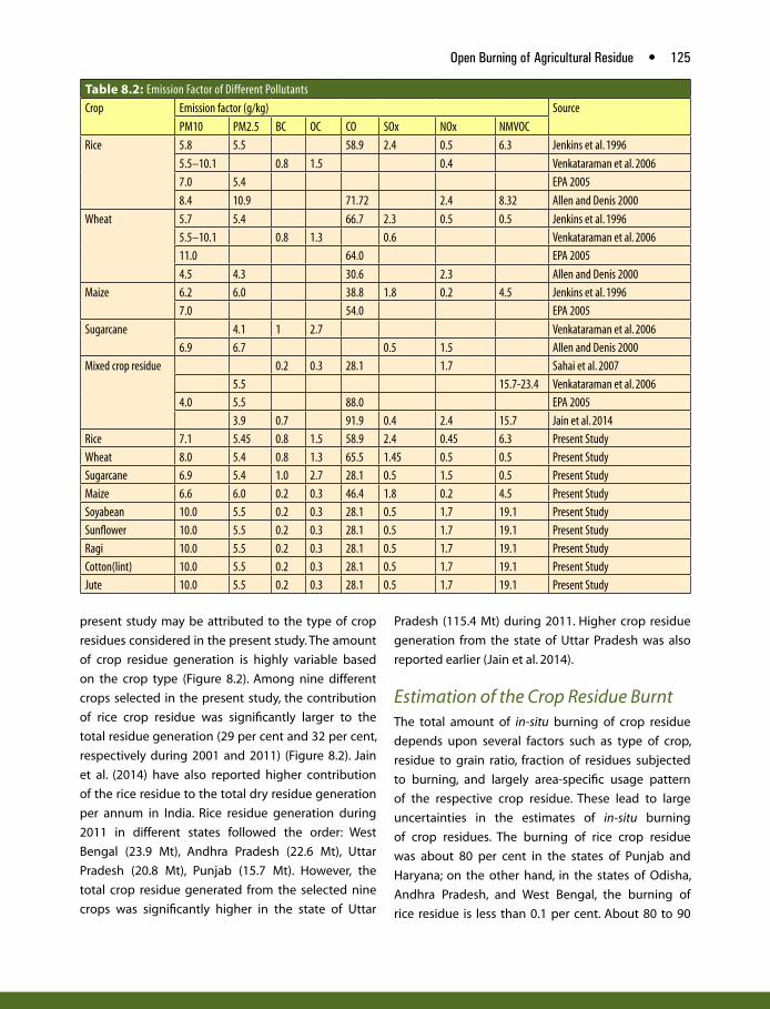
Open Burning of Agricultural Residue • 125
Table 8.2: Emission Factor of Different Pollutants
Crop Emission factor (g/kg) Source
PM10 PM2.5 BC OC CO SOx NOx NMVOC
Rice 5.8 5.5 58.9 2.4 0.5 6.3 Jenkins et al. 1996
5.5–10.1 0.8 1.5 0.4 Venkataraman et al. 2006
7.0 5.4 EPA 2005
8.4 10.9 71.72 2.4 8.32 Allen and Denis 2000
Wheat 5.7 5.4 66.7 2.3 0.5 0.5 Jenkins et al. 1996
5.5–10.1 0.8 1.3 0.6 Venkataraman et al. 2006
11.0 64.0 EPA 2005
4.5 4.3 30.6 2.3 Allen and Denis 2000
Maize 6.2 6.0 38.8 1.8 0.2 4.5 Jenkins et al. 1996
7.0 54.0 EPA 2005
Sugarcane 4.1 1 2.7 Venkataraman et al. 2006
6.9 6.7 0.5 1.5 Allen and Denis 2000
Mixed crop residue 0.2 0.3 28.1 1.7 Sahai et al. 2007
5.5 15.7-23.4 Venkataraman et al. 2006
4.0 5.5 88.0 EPA 2005
3.9 0.7 91.9 0.4 2.4 15.7 Jain et al. 2014
Rice 7.1 5.45 0.8 1.5 58.9 2.4 0.45 6.3 Present Study
Wheat 8.0 5.4 0.8 1.3 65.5 1.45 0.5 0.5 Present Study
Sugarcane 6.9 5.4 1.0 2.7 28.1 0.5 1.5 0.5 Present Study
Maize 6.6 6.0 0.2 0.3 46.4 1.8 0.2 4.5 Present Study
Soyabean 10.0 5.5 0.2 0.3 28.1 0.5 1.7 19.1 Present Study
Sunflower 10.0 5.5 0.2 0.3 28.1 0.5 1.7 19.1 Present Study
Ragi 10.0 5.5 0.2 0.3 28.1 0.5 1.7 19.1 Present Study
Cotton(lint) 10.0 5.5 0.2 0.3 28.1 0.5 1.7 19.1 Present Study
Jute 10.0 5.5 0.2 0.3 28.1 0.5 1.7 19.1 Present Study
present study may be attributed to the type of crop
residues considered in the present study. The amount
of crop residue generation is highly variable based
on the crop type (Figure 8.2). Among nine different
crops selected in the present study, the contribution
of rice crop residue was significantly larger to the
total residue generation (29 per cent and 32 per cent,
respectively during 2001 and 2011) (Figure 8.2). Jain
et al. (2014) have also reported higher contribution
of the rice residue to the total dry residue generation
per annum in India. Rice residue generation during
2011 in different states followed the order: West
Bengal (23.9 Mt), Andhra Pradesh (22.6 Mt), Uttar
Pradesh (20.8 Mt), Punjab (15.7 Mt). However, the
total crop residue generated from the selected nine
crops was significantly higher in the state of Uttar
Pradesh (115.4 Mt) during 2011. Higher crop residue
generation from the state of Uttar Pradesh was also
reported earlier (Jain et al. 2014).
Estimation of the Crop Residue BurntThe total amount of in-situ burning of crop residue
depends upon several factors such as type of crop,
residue to grain ratio, fraction of residues subjected
to burning, and largely area-specific usage pattern
of the respective crop residue. These lead to large
uncertainties in the estimates of in-situ burning
of crop residues. The burning of rice crop residue
was about 80 per cent in the states of Punjab and
Haryana; on the other hand, in the states of Odisha,
Andhra Pradesh, and West Bengal, the burning of
rice residue is less than 0.1 per cent. About 80 to 90

126 • Air Pollutant Emissions Scenario for India
per cent of the sugarcane residues are burnt in the
states of Bihar; whereas, sugarcane residue burning
in Punjab and Haryana is about 25 per cent. Lesser
amount of sugarcane residue burning in the states of
Punjab and Haryana may be attributed to the use of
mechanical harvesters (Gupta et al. 2003). However,
due to small window between the rice crop harvest
season and plantation of wheat, along with large
labour cost in handling the rice crop residues, large
amount of rice crop residues are burnt in situ in the
states of Punjab, Haryana, and western Uttar Pradesh
(Gupta 2014). The IPCC coefficient for the in-situ
burning of crop residue is 25 per cent of total amount
of residue produced (IPCC 2006). Following the IPCC
(2006) factor, the total amount of crop residue burnt
in India during 2011 was about 145 Mt. However
in the present study, we have estimated that about
56 Mt and 68 Mt of crop residues were burnt during
2001 and 2011 (Figure 8.2). Sahai et al. (2011) have
estimated 57 Mt and 63 Mt of crop residue burning,
respectively, during 2000 and 2010 in India. Street
et al. (2003) have estimated approximately 132 Mt
of crop residue burning in India annually, which was
about 18 per cent of total biomass burning from
anthropogenic and natural sources in Asia. However,
earlier studies have estimated 98.5 Mt of crop residue
burning in a year in India (Jain et al. 2014). Pathak
et al. (2010) have estimated 90 Mt of crop residue
Figure 8.2: Estimated total dry crop residue generated and amount of dry crop residue burnt in situ during
2001 and 2011 in India
burning during 2008 in India. During the present
study, we have identified the specific districts in
India with in-situ burning of crop residues using the
satellite data; however, most of the previous studies
have estimated the amount of crop residue burnt
based on the state level production data; this might
have led to higher estimation of total crop residue
burning in earlier studies.
Baseline Emission from Crop Residue Burning Based on the methodology described earlier, it is
estimated that the emission of all pollutants was
highest from the Muzaffarnagar district of the state
of Uttar Pradesh (Figure 8.3). It is estimated that
significantly higher (4.4 Mt) sugarcane residues
were burnt in the district. Total emission of PM10
was significantly higher (216 Kt) from the western
region of the state of Uttar Pradesh followed by the
state of Punjab (158 Kt). However, PM2.5
emission
was significantly higher from the state of Punjab
(110 Kt) followed by the western region of Uttar
Pradesh (100 Kt). Burning of rice crop residue (8.8
Mt) was significantly higher in the state of Punjab
after the harvest of the kharif crop. On the other
hand, burning of total crop residues was significantly
higher in Uttar Pradesh (21.5 Mt) with significantly
higher contribution of the sugarcane residue (17.5

Open Burning of Agricultural Residue • 127
Mt). However, the emission factor of PM2.5
was higher
with rice crop residue (7.8 g/Kg) compared to that
of sugarcane (4 g/Kg). Significantly higher burning
of the crop residue in the state of Uttar Pradesh
was attributed to higher PM10
emission; however,
large amount of rice crop residue burning which
has higher PM2.5
emission factor among nine crops
considered in the present study increases the PM2.5
emission from the state of Punjab. The total emissions
of PM10
and PM2.5
in India during 2001 were 619
Kt and 350 Kt, respectively; whereas during 2011,
emissions increased to 818 Kt and 419 Kt, respectively.
The emission of different gaseous and particulate
pollutants due to in-situ burning of crop biomass was
significantly higher in the northwestern region of the
IGP in India (Figure 8.3) during both 2001 and 2011.
Venkataraman et al. (2006) and Sharma et al. (2010)
have also reported higher emission of pollutants from
the crop residue burning in the northwester IGP.
In-situ burning of crop residues contributes
significantly to the atmospheric BC and OC. Total
atmospheric BC emissions from the crop residue
burning during 2001 and 2011 were estimated as
48 Kt and 57 Kt, respectively. During 2001, burning
of sugarcane crop residue (BC: 27 Kt) was the
largest contributor to total BC emission from the in-
situ burning of the crop residue. OC emission was
also significantly increased during 2011 (128 Kt)
compared to 2001 (108 Kt). Similar to BC, emissions
of OC was higher from the burning of the sugarcane
crop residues. Overall, BC emission from the in-situ
burning of crop residue was significantly higher from
the state of Uttar Pradesh (21 Kt) followed by Punjab
(10 Kt) and Haryana (6 Kt). OC emission also followed
the same pattern. Higher BC and OC emission
from the state of Uttar Pradesh was attributed to
significantly higher crop residue burning in the state.
State-wise emissions of different gaseous
pollutants from the in-situ burning of crop residues in
the field also followed the same pattern. Significantly
higher emissions of different gaseous pollutants
were recorded in the state of Uttar Pradesh during
2011. Total emissions of CO, SOx, NO
x, and NMVOC
during 2011 were 3244 Kt, 40 Kt, 137 Kt, and 511 Kt,
Figure 8.3: Estimation of the emission of particulate and gaseous pollutants (Kt/year) from the in-situ
burning of crop residues during 2011

128 • Air Pollutant Emissions Scenario for India
respectively. Among different crop residues, the
contribution of cotton (lint) crop residue burning
towards gaseous emission of different pollutants
was recorded higher during 2001 and 2011. A
comparative view of the reported emission of
different pollutants from the in-situ burning of crop
residue is India is given in Table 8.3.
Emission Projections Emissions of different pollutants were estimated
to increase during 2011–51 (Figure 8.4). By the
year 2051, the increase of emission of particulates
and gaseous pollutants would be significantly
higher from burning of soyabean crop residue
(approximately four times compared to 2011
emissions) (Figure 8.4). During 2051, emissions from
the in-situ burning of rice and wheat crop residues
would increase by 60 per cent and 82 per cent,
respectively, compared to their emissions during
2011.
Over all, PM10
, PM2.5
, NOX
, SO2, NMVOC, CO
will increase by ................................ by percentage,
respectively during 2011 to 2051.
However in the present estimates, we have
considered burning fraction of the crop constant till
2051. This may increase with increase in productivity
of an individual crop due to crunch of space to store
the excess crop residues. Oppositely, the burning
fraction may decrease if improved technology is
developed to effectively handle the excess crop
residues or develop crop varieties with lesser
amounts of residue generation.
ConclusionLarge amount of particulate and gaseous pollutants
are emitted during in-situ burning of crop residues
in the crop lands in different parts of the country.
Emissions of all pollutants were significantly higher in
the western part of the IGP of India. However, almost
all regions of the country contributed towards the
gaseous emission of the atmospheric pollutants.
The type of crop residue burnt varies across state.
However, this study has estimated that the residue
of the rice crop is mostly burnt all over the country.
Future prediction of emission of different pollutants
from in situ burning of crop residue suggests large
increase in the pollution emission by the year 2050,
if adequate measures to reduce the crop residue or
handling the crop residues are not developed.
The key measures that are required to be taken
for control of emissions from open burning of
agriculutural residue in India are:
P Imposition and strict enforcement of a ban on
open burning of agriculutural residue.
P Development of biomass gasification technologies
for waste to energy generation from agricultural
residue.
P Development of business model for collection
storage and processing of agriculutral waste for
waste to energy generation.
Table 8.3 Estimation of emission of different atmospheric pollutants from the in-situ burning of crop residues in India
Year of estimation
Kt annum-1 Reference
PM10 PM2.5 BC OC SOx NOx CO NMVOC
1994 78 2138 Gupta et al., 2004
2000 84 2305 Gupta et al., 2004
2000 3 6 33 541 Sahai et al., 2007
2001 572-2393 86-372 211-970 46-172 289-1290 10000-74000 1818-6767 Venkatraman et al., 2006
2006 8114 472 69 344 8114 633 Gadde et al., 2009
2010 658 Sharma et al., 2014
2011 384 68 246 7 9063 39 Jain et al., 2014
2011 818 462 49 57 40 137 3244 512 Present study

Open Burning of Agricultural Residue • 129
Figure 8.4: Emissions of different pollutants from the in-situ burning of crop residue in India
ReferencesAllen, D., and A. Denis A. 2000. Inventory of air pollutant emission associated with forest, grassland and agricultural burning in Texas. Austin, TX: Center for Environment and Energy Resources, The University of Texas, p 23.
Badarinath K. V. S., and T. R. Chand Kiran. 2006. Agriculture crop residue burning in the indo-Gangetic Plains—A study using IRSP6 WiFS satellite data. Current Science, 91(8):1085–89.
Badarinath, K. V. S., S. K. Kharol, A. R. Sharma, and V. Krishna Prasad. 2009. Analysis of aerosol and carbon monoxide characteristics over Arabian Sea during crop residue burning period in the Indo-Gangetic Plains using multi-satellite remote sensing datasets. Journal of Atmospheric and Solar-Terrestrial Physics 71:1267–76.
Bhattacharya, S. C., H. L. Pham, R. M. Shrestha, and Q. V. Vu. 1993. CO
2 emissions due to fossil and traditional
fuels, residues and wastes in Asia. In AIT Workshop on

Global Warming, Issues in Asia, September 8–10, 1993. Bangkok, Thailand: AIT.
Bond, T. C., D. G. Streets, K. F. Yarbar, S. M. Nelson, J.-H. Woo, and Z. Klimont. 2004. A technology-based global inventory of black and organic carbon emissions from combustion. Journal of Geophysical Research 109: D14203, doi:10.1029/2003JD003697.
Boopathy, R., B. R. Asrabadi, and T. G. Ferguson. 2002. Sugar cane burning and asthma in Southeast Louisiana, USA. Bulletin of Environmental Contamination and Toxicology 68:173–79.
Brown, R. C. 2003. Biorenewable resources—engineering new products from agriculture. Ames, IA: Iowa State Press.
Chen, Y., S. Tessier, C. Cavers, X. Xu, and E. Monero. 2005. A survey of crop residue burning practices in Manitoba. Applied Engineering in Agriculture 21:317–23.
Crutzen, P. J., and M. O. Andrae. 1990. Biomass burning in the tropics: Impact on atmospheric chemistry and biogeochemical cycles. Science 250(4988):1669–78.
Dennis, A., M. Fraser, S. Anderson, and D. Allen. 2002. Air pollutant emissions associated with forest, grassland, and agricultural burning in Texas. Atmospheric Environment 36:3779–92.
DoES. 2013. Homepage. New Delhi: Directorate of Economics and Statistics, Department of Agriculture and Cooperation, Ministry of Agriculture, Govt. of India. Available at <http://eands.dacnet.nic.in/>, last accessed April 20, 2015
Dubay, A. K., and P. Chandra. 2009. Energy from cotton stalk and other agro residue. Indian Cotton Advisory Committee. Available at <www.icac.org>, last accessed April 15, 2015
EPA. 2005. Open burning. AP42, Chapter 2.5. Washington, DC: Environmental Protection Agency. Available on <http://www.epa.gov/ttn/chief/ap42/index.html>, last accessed April 15, 2015.
Gadde, B., S. Bonneta, C. Menke, and S. Garivait S. 2009. Air pollutant emissions from rice straw open field burning in India, Thailand and the Philippines. Environmental Pollution 157(5):1554–58.
Gupta, R. 2014. The economic causes of crop residue burning in western Indo-Gangetic Plains. New Delhi:
Economic and Planning Unit, Indian Statistical Institute. Available at <www.isid.ac.in>, last accessed April 15, 2015
Gupta, R. K., R. K. Narsh, P. R. Hobbs, Z. Jiaguo, and J. K. Ladha. 2003. Sustainability of post-green revolution agriculture: The rice-wheat cropping systems of the Indo-Gangetic plains and China - Improving the productivity and sustainability of rice-wheat systems: Issues and impact. Madison, WI: ASA Special Publication, p. 65.
Gupta, P. K., S. Sahai, N. Singh, C. K. Dixit, D. P. Singh, and C. Sharma. 2004. Residue burning in rice-wheat cropping system: Causes and implications. Current Science 87(12):1713–15.
Hays, M. D., P. M. Fine, C. D. Geron, M. J. Kleemand, and B. K. Gullett. 2005. Open burning of agricultural biomass: Physical and chemical properties of particle-phase emissions. Atmospheric Environment 39:6747–64.
He, J., B. Zielinska, and R. Balasubramanian. 2010. Composition of semi-volatile organic compounds in the urban atmosphere of Singapore, influence of biomass burning. Atmospheric Chemistry and Physics 10:11401–13.
Hemwong, S., B. Toomsan, G. Cadisch, V. Limpinuntana, P. Vityakon, and A. Patanothai. 2009. Sugarcane residue management and grain legume crop effects on N dynamics, N losses and growth of sugarcane. Nutrient Cycling in Agroecosystems 83(2):135–51.
Hiloidharia, M., D. Dasb, and D. C. Baruaha. 2014. Bioenergy potential from crop residue biomass in India. Renewable & Sustainable Energy Reviews 32:504–12.
Hoelzemann, J. J., M. G. Schultz, G. Brassieur, C. Granier, and M. Simon. 2004. Global wildland fire emission model (GWEM): Evaluating the use of global area burned satellite data. Journal of Geophysical Research 109:D14S04, doi:10.1029/2003JD003666.
India’s Comprehensive Statistical Analysis (INDIASTAT). 2015. Crop: Sugarcane. Available at: <www.indiastat.com>, last accessed April 25, 2015.
Intergovernmental Panel on Climate Change (IPCC). 2006. Guidelines for national greenhouse gas inventories. Japan: IGES. Available at <www.ipcc.ch>, Last accessed January 15, 2015.

Jain, N., A. Bhatia, and H. Pathak. 2014. Emission of air pollutants from crop residue burning in India. Aerosol and Air Quality Research 14:422–30.
Korontzi, S., J. McCarty, T. Loboda, S. Kumar, and C. O. Justice. 2006. Global distribution of agricultural fires from three years of MODIS data. Global Biogeochemical Cycle 20:GB2021, 1–15.
Krishna Prasad, V., P. K. Gupta, C. Sharma, et al. 2000. NOx emissions from biomass burning of shifting cultivation areas from tropical deciduous forests of India – Estimates from ground-based measurements. Atmospheric Environment 34(20): 3271–80.
Lai, C. H., H. C. Li, and K. S. Chen. 2009. Source characterization and environment impact of open burning of rice straw residues on polycyclic aromatic hydrocarbons in agricultural county, Taiwan. Journal of Environmental Engineering & Management 19(2):79–88.
Lighty, J. S., J. M. Veranth, and A. F. Sarofim. 2000. Combustion SPM: Factors governing their size and composition and implications to human health. Journal of the Air and Waste Management Association 50:1565–618.
Long, W., R. B. Tate, M. Neuman, J. Manfreda, A. B. Becker, and N. R. Anthonisen. 1998. Respiratory symptoms in a susceptible population due to burning of agricultural residue. Chest 113:351–56.
MacCarty, J. L., S. Korontzi, C. O. Justice, and T. Loboda. 2009. The spatial and temporal distribution of crop residue burning in the contiguous United States. Science of the Total Environment 407:5701–12.
Mar, T. F., T. V. Larson, R. A. Stier, C. Claiborn, and J. Q. Koenig. 2004. An analysis of the association between respiratory symptoms in subjects with asthma and daily air pollution in Spokane, Washington. Inhalation Toxicology 16:809–15.
Mittal, S. K., K. Susheel, N. Singh, R. Agarwal, A. Awasthi, and P. K. Gupta. 2009. Ambient air quality during wheat and rice crop stubble burning episodes in Patiala. Atmospheric Environment 43:238–44.
MoCIT. 2012. Open government data (OGD). Crop production. New Delhi: Ministry of Communication and Information Technology, Govt. of India. Available at: <www.data.gov.in>, last accessed on April, 2015.
NAIP. 2012. Harvesting: Sugarcane. New Delhi: National Agriculture Initiative Project. Available at: www.agropedia.iitk.ac.in, last accessed on March, 2015.
Nelson, R. G. 2002. Resource assessment and removal analysis for corn stover and wheat straw in the Eastern and Midwestern United States—rainfall and wind-induced soil erosion methodology. Biomass & Bioenergy 22:349–63.
Njie, D. 2006. Energy generation from rice residues: A review of technological options, opportunities and challenges. Review articles. Rome, Italy: FAO. Available at: <ftp://ftp.fao.org/docrep/fao/010/a1410t/a1410t02.pdf>.
Pathak, H., A. Bhatia, N. Jain, and P. K. Aggarwal. 2010. Greenhouse gas emission and mitigation in Indian agriculture – A Review. In B. Singh, ed. ING bulletins on regional assessment of reactive nitrogen, bulletin no. 19, pp. i–iv, 1–34. New Delhi: SCON-ING.
Sahai, S., C. Sharma, S. K.Singh, and P. K. Gupta. 2011. Assessment of trace gases, carbon and nitrogen emissions from field burning of agricultural residues in India. Nutrient Cycling in Agroecosystems 89:143–57.
Sahai, S., C. Sharma, D. P. Singh, et al. 2007. A study for development of emission factor for trace gases and carbonaceous. Atmospheric Environment 41:9173–86.
Seiler, W., and P. Crutzen. 1980. Estimates of the gross and net flux of carbon between the biosphere and the atmosphere from biomass burning. Climatic Change 2:207–47.
Sharma, S., A. Goel, D. Gupta, et al. 2015. Emission inventory of non-methane volatile organic compounds from anthropogenic sources in India. Atmospheric Environment 102:202–19.
Sharma, A. R., S. K. Kharol, K. V. S. Badrinath, and D. Singh. 2010. Impact of agriculture crop residue burning on atmospheric aerosol loading – a study over Punjab State, India. Annals of Geophysics 28:367–79.
Sidhu, B. S., V. Beri, and S. K. Gosal. 1995. Soil microbial health as affected by crop residue management. In Proceedings of National Symposium on Developments in Soil Science, Ludhiana, India, November 2–5, 1995. New Delhi, India: Indian Society of Soil Science, pp. 45–46.

132 • Air Pollutant Emissions Scenario for India
Simon, M., S. Plummer, F. Fierens, J. J. Hoelzemann, and O. Arino. 2004. Burnt area detection at global scale using ATSR-2: The GLOBSCAR products and their qualification. Journal of Geophysical Research 109:D14S02, doi:10.1029/2003JD003622.
Singh, Y. 2003. Crop residue management in rice-wheat system. In: Addressing resource conservation issues in rice–wheat systems of South Asia: A resource book. Rice Wheat Consortium for Indo-Gangetic Plains (CIMMYT), Pusa, New Delhi, India.
Singh, K., and D. V. Rangnekar. 1986. Fibrous crop residues as animal feed in India. In M. N. M. Ibrahim and J. B. Schiere, eds., Rice straw and related feeds in ruminants’ ration, pp. 111–16. Kandy, Sri Lanka: Straw Utilization Project.
Singh, N., R. Agarwal, A. Awasthi, P. K. Gupta, and S. K. Mittal. 2010a. Characterization of atmospheric aerosols for organic tarry matter and combustible matter during crop residue burning and non-crop residue burning months in North-western region of India, Atmospheric Environment 44(10):1292–1300.
Singh, N., S. K. Mittal, R. Agarwal, A. Awasthi, and P. K. Gupta. 2010b. Impact of rice crop residue burning on levels of SPM, SO
2 and NO
2 in the ambient air of
Patiala (India). International Journal of Environmental Analytical Chemistry 90(10):829–43.
Tansey, K., J.-M. Gre´goire, D. Stroppiana, et al. 2004. Vegetation burning in the year 2000: Global burned area estimates from SPOT VEGETATION data. Journal of Geophysical Research 109:D14S03, doi:10.1029/2003JD003598.
Venkataraman, C., G. Habib, A. Eiguren-Fernandez, A. H. Miguel, and S. K. Friedlander. 2005. Residential biofuels in south Asia: Carbonaceous aerosol emissions and climate impacts. Science 307:1454–56.
Venkataraman, C., G. Habib, D. Kadamba, et al. 2006. Emissions from open biomass burning in India: Integrating the inventory approach with high-resolution Moderate Resolution Imaging Spectroradiometer (MODIS) active-fire and land cover data. Global Biogeochemical Cycles 20:GB2013, doi:10.1029/2005GB002547.
Vimal, O. P. 1979. Residue utilization, management of agricultural and agro-industrial residues of selected tropical crops (Indian experience). In Proceedings of UNEP/ESCAP/FAO, Workshop on Agricultural and Agro-industrial Residue Utilization in Asia and Pacific Region, Pattaya, Thailand: Industry & Environment Office, United Nations Environment Programme.
Yamaji, K., J. Li, I. Uno, et al. 2010. Impact of open crop residual burning on air quality over Central Eastern China during the Mount Tai Experiment 2006 (MTX2006). Atmospheric Chemistry and Physics 10:7353–68.
Yan, X. Y., T. Ohara, and H. Akimoto. 2006. Bottom-up estimate of biomass burning in mainland China. Atmospheric Environment 40: 5662−73.
Yang, S. J., H. P. He, S. L. Lu, D. Chen, J. X. Zhu. 2008. Quantification of crop residue burning in the field and its influence on ambient air quality in Suqian, China. Atmospheric Environment 42:1961–69
Yevich, R., and J. A. Logan. 2003. An assessment of biofuel use and burning of agricultural waste in the developing world. Global Biogeochemical Cycle 17(1095):1–21. doi:10.1029/2002GB001952,
Zhang, Y., M. Cao, X. Wang, and H. Yao. 1996. Spatial distribution of trace-gas emissions from burning crop residue in China. In J. S. Levine, ed., Biomass burning and global change, pp. 764–70. Cambridge, MA: MIT Press.

Introduction While there are pollutants emitted due to
combustion of fuels, there are activities that lead
to fugitive emissions, mainly due to volatility of
the compounds used in the process. Mostly these
are volatile hydrocarbons. These compounds
are grouped as non-methane volatile organic
compounds (NMVOCs) as the majority of them
display similar behaviour in the atmosphere (DEFRA
2003). While considerable attention has been paid
on control of pollutants such as particulate matter
(PM), non-methane hydrocarbons have steadily
grown unnoticed in India. NMVOCs not only have
direct health impacts over the exposed receptors,
but they also act as important precursor of ground
level Ozone formation and secondary particulates
known as secondary organic aerosols (SOAs). There
are multiple sources of these emissions including
use of paints, printing inks, personal products,
etc. The solvent use in these products is small but
cumulative assessment of the quantities of NMVOCs
released from the use of these products leads to
substantial emissions. Hence, there is a need for an
accurate emission inventory of these emissions for
their control.
Limited work has been carried out in past on
exhaustive estimation of emissions from these
sources. In this study, NMVOC emissions are estimated
for different years between 2001 and 2051 based on
the future growth trajectories. The ‘emission factor
approach’ is used in the current work for estimation
of NMVOCs from different sectors and sources. A list
of probable sources of NMVOC was compiled from
literature review exercise. These sources includes
paints, printing inks, dry cleaning, handling of oil and
solvent use in industries. Activity data for different
sectors was collected and compiled form reliable
sources. Emission factors are adopted from a recent
work of Sharma et al. (2015), where detailed review
was carried out to choose appropriate emission
factors for different sources. The source-wise emission
CHAPTER
Evaporative EmissionsSumit Sharma and Atul Kumar
9

134 • Air Pollutant Emissions Scenario for India
inventory is presented in subsequent sections using
folllowing equation:
E= Activity data × Emission factor × (1–% controls)
PaintsPaints are used in both residential and industrial
sectors. Due to increased urbanization, it is noticed
that there is a drastic shift from semi-permanent
to permanent housing structures, which has been
driving growth in decorative paints segment in the
domestic sector, which constitutes 77% of the 2.9
million tonne paint industry in India (Paint India 2011).
Per capita consumption of paint is about 1.6 Kg. The
industry has grown to about 10–15% annually in
last 5 years and is consistent with the growth of real
estate sector in India. There has been a recent shift
towards water-based coatings in the recent past, and
about 50% of the paints currently used for decorative
purposes are water based. About 65 per cent of
the demand for decorative paints is contributed to
repainting of houses, etc. Paints most commonly used
in bigger cities are premium decorative paints (acrylic
emulsions) while medium range paints consisting of
enamels are more popular in smaller cities and towns.
In India, nearly 11 per cent of all the decorative
paints are distempers, which are economical
products, mostly demanded in the suburban and
rural area. Considerable growth is observed in
the exterior coatings segment, under decorative
paint segment. Many superior quality paints with
high durability have been launched by many paint
manufacturers in India. Import of paints is about 4%
and export of paints is negligible. The total quantity
of decorative solvent based paints consumed in
India is 1.32 million tonnes (mt). Emission factor
(CITEPA 2003c) used for solvent-based paint is 400
kg/kt of paint used and for water-based paints is 102
kg/kt. Total emissions estimated from the sector is
582 kt/yr.
Industrial paints include powder coatings, high
performance coating, and automotive and marine
paints. The primary factors affecting emissions from
paint manufacture are care in handling dry pigments,
types of solvents used, and mixing temperature.
Industrial coatings in India are almost exclusively
solvent based. The only applications that are currently
employing water-borne technology are certain
automotive primers and high-end automotive
refinishes. The production of industrial paints is found
to be 0.67 mt in 2009 and about 0.9 mt in 2011(PI
2010), of which 44% accounts for paint used in auto
sector and coil coating, and rest is accounted for
industrial painting category. The distribution of paints
in plastic, general industry, continuous, and powders
is adopted from PI (2011).
During manufacture of automobiles, the
automobiles are painted and during this process
large amount of NMVOCs are emitted in one or
the other forms. The activity data in this case was
total number of vehicles manufactured in India,
which were about 10.4 million during 2011. Paints
used and emissions generated in the automobile
manufacturing and vehicle repair were estimated
from the size distribution of different vehicles
manufactured in India (IBEF 2008). The weighted
emission factor per unit vehicle manufactured is
derived as 3.18 kg per vehicle and total emissions
from the automobile manufacturing sector is
estimated to be 35 kt/year. The total paint consumed
in the sector is 160 kt. A total of 21% of paints used
in automobiles come out as NMVOC emissions.
Coil coating is another process that requires
paints, as it is a continuous and highly automated
process for coating metal before fabrication.
According to available data, the Indian domestic
market consumes colour-coated sheets in the
thickness range from 0.2 to 1.2 mm and widths
between 600 and 1,250 mm. Recently, the imported
galvalume colour-coated products and its plain sheet
(in small quantities) have gained popularity. In recent
years, colour-coated coils have gained importance
in the domestic market and, consequently, their
consumption has accelerated during the last two
years across the country. The total coil coating
capacity installed in the country is 9,85,000 T/yr
(Nagori and Ajemra 2006). Assuming an average
thickness of 0.7 mm, total coated surface area

Evaporative Emissions • 135
amounts to 128 million sq. m in 2011. The coil coating
capacity is projected using industrial GDP growth to
2,895 million sq. m in 2051.
The distribution of emissions from paints used in
industrial and residential sector in 2011 is shown in
Table 9.1.
Future projections of NMVOC emissions are made
using regression analysis of various activities with
appropriate variables. The past 15 years data of the
activity levels in different sectors were regressed
Table 9.1: Emission Inventory of NMVOC Emissions from Paint Usage in Different Sectors in India in 2011
Total Percentage of Distribution
EF (kt/kt) Emission Factor source
Paints (mt) Emissions (kt)
Plastic 18% 0.75 CITEPA (2004) 0.09 67.5
General industry 29% 0.69 0.144 99.4
Continuous 29% 0.74 0.144 106.6
Powders 25% 0 0.126 0.0
Total industrial paints 273.4
Coil coating Emission factor used is 0.04320 Kt/million m².
GAINSa Area of coils128 million m²
5.5
Automobile paints 3.18 kg/vehicles (weighted avg. for different vehicles)
Based on CITEPA (2003d), IBEF 2008
0.16 35
Decorative paints 50% solvent based 400 kg/kt GAINSa; CITEPA(2003c)
1.33 534
50% water based 102 kg/kt 1.33 137aEuropean version available from: http://gains.iiasa.ac.at.
Figure 9.1: Examples of regression analysis carried out for projection of industrial and decorative paints in
India
Table 9.2: Surrogate Variable Used for Projections of Different Non-Energy Sectors
S.No Sector Dependant Variable
1 Paints: Decorative Per capita income
2 Paints: Industrial Industrial GDP growth
3 Vehicle manufacturing and refinishing
Vehicular growth, number of road accidents
4 Coil coating Industrial GDP growth

136 • Air Pollutant Emissions Scenario for India
against the selected variables. In the case of paints,
regression equations were derived for projections
for future years after satisfactory correlations
are observed between the paint consumption
and dependant variables (Figure 9.1). The list of
dependant variable used for projections of emissions
from sectors using paints are shown in Table 9.2.
Based on the regression equations, the paint
consumption in residential and industrial sector
is estimated, as shown in Figure 9.2. With rise in
industrial GDP and per capita income levels, the
overall paint consumption will increase from 3.6
mt in 2011 to 71.6 mt in 2051. Based on the future
estimates of paint use in different sectors, the
Figure 9.2: Future projections of paint consumption (mt) in India
Figure 9.3: Future projections of NMVOC emissions in India
emissions are estimated. The future projections of
NMVOC emissions from paint used are shown in
Figure 9.3. The total emission will grow from 944 kt
in 2011 to 19301kt in 2051. The automotive paint
emissions will grow from 34.5 kt to 54.6 kt during
2011–51 and emission form coil coating will grow
from 5.5 kt to 125 kt in the same period.
Vehicular refinishing is another activity that
generates NMVOC emissions. Vehicles are repainted
or refinished due to different reasons. The NMVOC
emissions from this category are linked to application
of paint, drying operations, cleaning of equipment,
and cleaning operations before the coating and
between the applications of different layers. In India,

Evaporative Emissions • 137
Table 9.3 Total Use of Personal Products (kt) and NMVOC Emissions (kt) in India in 2011
Products Per Capita Consumption (g/yr) Volume (kt) Solvents (EF)* Emissions (kt) 2011
Facewash 7.2 8.0 65% 5.2
Perfumes 6.1 6.8 60% 4.1
Skin care 48.9 54.7 11% 6.0
Shoe polish 1.1 1.2 45% 0.6
Floor cleaning 14.0 15.6 5% 0.8
Glass cleaning 1.0 1.1 10% 0.1
Kitchen (liquid cleaners) 16.0 17.9 35% 6.3
Kitchen (solid cleaners) 304 339.6 3% 10.2
Detergents (liquid + powder) 2700.0 3015.9 3% 90.5
Shampoos 13.0 14.5 10% 1.5
Soap 460.0 513.8 5% 25.7
Hair oil 96.2 107.5 28% 30.1
Hair dyes/colour 9.5 10.6 44% 4.7
Colour cosmetics 0.1 0.1 44% 0.0
Shaving creams/toiletries 8.1 9.1 10% 0.9
Total 186
* Based on Umweltministerium Baden-Württemberg (1993)
the number of vehicles being refinished has been
estimated broadly using the data on accidents that
occurred in a year with an assumption of 50% of
those going for refinishing. Moreover, the paint used
per vehicle is also assumed to be half of the overall
paint used in manufacturing.
On this basis, the total emissions from this activity
are estimated to be 3.3 kt in 2011, which reduces to
almost negligible in future with anticipated reduction
in the rate of accidents. The weighted emission factor
used for all vehicles is 12 kg per vehicle (higher
emission factor due to higher percentage of heavy
vehicles going for refinishing).
Personal and Home Care Products The solvent-based products used in houses include
personal care and household care products. The
personal care products such as hair care, skin care,
oral care, personal wash (soaps), cosmetic and
toiletries, feminine hygiene, disinfectants, room
fresheners, furniture polishes are the potential
source of NMVOC emissions. Other household
products including detergents, floor cleaners, etc.
are although having lesser solvent content but
could be important source in the overall inventory.
Indian personal care industry is valued at USD 4
billion including different types of products. The
figures for the consumption of the personal care
products are derived using:
P per capita consumption values
P by converting the monetary units (market shares
of different products) to volumetric forms using
market prices (Rs/mL) of the major products in
each of the categories.
In abssence of readily availabel information on
Indian products, the solvent content of the different
types of personal and home care products is adopted
from Umweltministerium Baden-Württemberg (1993).
The overall estimates of different personal products

138 • Air Pollutant Emissions Scenario for India
used in India and the related emissions from the
solvent use in baseline year are presented in Table 9.3.
The total emissions from personal and home
care products consumption in India are estimated
to be 186 kt in 2011. Based on this an emission
factor of 0.16 kt of NMVOCs per million populations
can be derived. Use of personal products is
highly dependent on per capita income levels in
the region and the same is used as a variable to
project the consumption of personal products and
corresponding NMVOC emissions in future. With
growing economy and income levels, the NMVOC
emissions in future from the personal and home care
product use in India is expected to grow from 186 to
2,173 kt during 2011–51 (Figure 9.4). This is assuming
no interventions for control of solvent use in the
products.
Dry CleaningIt is the cleaning process for clothing and textiles
using a chemical solvent other than water. The
solvent typically used for this is tetrachloroethylene
(perchloroethylene). Other solvents used during
this process are Glycol ethers, hydrocarbons, liquid
silicone, liquid CO2, perchloroethylene, etc. In India,
Mineral Turpentine Oil is commonly used while the
use of perchloroethylene has also started.
The activity used to estimate emissions from this
exercise is the total weight of textiles dry cleaned
in India during 2011. It was estimated based on
percentage of households in rural and urban India
using laundry services. A total of 50% of it was
assumed to be dry cleaned. NSSO (2012) shows that
4% of rural households and 11% of urban households
are using dry cleaning facility. As per the per capita
expenditure estimates on dry cleaning, the net
weight of textile undergone for dry cleaning during
2011 was estimated to be 7.8 kt. Using average
emission factor of 0.177 kt/kt weight of textiles, the
NMVOC emissions are estimated to be 1.2 kt/yr. The
emissions from the activity are projected for future
years using per capita income as the influencing
variable. It is estimated that the emissions will grow
from 1.2 to 13.7 kt during 2011–51.
Extraction, Processing, and Distribution of Gaseous FuelsThe gaseous fuels are extracted directly from a gas
field or as part of the mixture from an oil and gas
field. During extraction by heating systems, lighting,
pumps and compressors, large amount of energy
(electrical energy supplied by gas turbine generators)
is being consumed. Other than energy consumed,
there are fugitive NMVOC emissions from not only
extracting, but transport, storage, and handling of
gaseous fuels. After extraction, minimal processing of
natural gas is carried out at the terminals prior to the
long distance transmission through pipeline network
Figure 9.4 Future projections of emissions from personal and home care products in India

Evaporative Emissions • 139
(distribution system). During processing, activities
mainly required are removal of hydrogen sulphide
from gas and drying—which results in sulphur
dioxide emission as the main ingredient. After
production and on-shore processing, natural gas is
fed directly into the distribution system.
The activity data in this case is total natural gas
production in the country, which is ~47,500 mmscm
in 2010/11, of which 18% is on-shore production.
The emission factors used to estimate the emissions
during extraction are 0.968 g/m³ for onshore and
0.1426 g/m³ for off-shore facilities (average of many
countries assumed from CORINAIR, 1990). Total
NMVOC emissions are estimated at 6.3 kt/yr for 2011.
NMVOC emissions are also estimated for activities
such as distribution of gas and the estimation
process is depicted in Table 9.4, which shows different
emission factors for losses in pipelines, compressors,
and others.
The emissions are projected for future years using
TERI analysis for energy modelling exercise (TERI
2015) for natural gas production and use in India
during 2001–51 (Figure 9.5).
Extraction, Processing, and Distribution of Liquid FuelsThe liquid fuels are mainly composed of crude oil (a
complex mixture of hydrocarbons with very different
chemical and physical properties). The extraction
Table 9.4: NMVOC Emissions from Gas Distribution in 2011
Activity Natural Gas Production (MMSCM) Emissions Factor ((g/m3)* Emissions (kt/yr)
Onshore Offshore Onshore Offshore Total
Production 8684 38826 Onshore :0.0968Offshore :0.142
0.8 5.5 6.3
Distribution**
General 1.38 16 74 90
Pipelines 0.01 0.1 0.6 0.7
Compressors 0.07 0.8 3.6 4.4
Network 0.78 9.4 41.9 51.3
Total 146.8
*Source : EEA,1999; ** including imports
Figure 9.5: Projections of NMVOC emissions from gas extraction and handling in India (2001–51)

140 • Air Pollutant Emissions Scenario for India
of crude is the first step. The route from extraction
to individual use (refined components) includes
storage, refining, transport, and filling of the fuel.
The processing of crude oil, aimed at separating the
mixture into groups of chemicals (identification of
them with similar properties for use in particular
applications). Refineries have many different
combinations of process units such as distillation
column. The last step is distribution of products
(could be through combination of pipeline, road,
rail, or even tanker) from the refinery to the point of
end use that could be either a single- or multi-stage
process.
Emissions have been estimated for each of these
steps:
P Extraction: Total crude extracted in India is 39 mt
in 2011 (MoPNG 2012). The emission factor used
to estimate NMVOC’s from extraction was taken
as 475 g/tonne of crude (Lewis 1997), and NMVOC
emissions from the activity is estimated to be 19
kt/yr.
P Storage of crude: Crude is stored in big tanks that
are an important source of NMVOC emissions.
These are called working and breathing losses. The
emissions from this activity are computed using
the TANKS model (http://www.epa.gov/ttnchie1/
software/tanks/). Typical tank capacity of 60,000
m³ is assumed with 75% filling to arrive at the
total number of tanks required. TANKS model takes
into account the tank geometry, meteorological
conditions (typical conditions given for Indian
conditions), and the type of fluid stored. The
emissions in this case are estimated for crude
stored at ports and refineries and the petroleum
products stored at refineries and bulk terminals.
The estimated emissions due to storage of crude
and other petroleum products are estimated to be
around 9 kt/yr.
P Transit losses: Transit losses occur when crude/
petroleum products move over road/rail. The
emissions factors used for estimation are shown in
Table 9.5. The transit losses are accounted for rail/
road travel and not for the pipelines. In India, 30%
of fuel is transported through pipelines and hence,
emissions are reduced by 30%. The total emissions
from transit of fuel are estimated to be 122 kt.
Table 9.5: Emission Factors for Loading and Transit Losses for Oil Handling
Transit Losses (Loading + Transit) EF (mg/L)
Crude 580
Gasoline 1430
Others 4
Naptha 430
Figure 9.6: NMVOC emissions from oil extraction, refining and handling

Evaporative Emissions • 141
P Refining: A total of 213 mt of crude is refined in
2011. An emission factor of 0.9 kt/mt of crude
is adopted and emissions are estimated.Total
NMVOC emissions from refining activities are 191
kt in 2011 and are projected to grow to 1696 kt in
2051.
P Emissions during fuel filling at the pumps:
Emissions at the fuel pumps are accounted using a
no-control emissions factor of 2.6 g/kg of gasoline
filled. After 2030, stage-II control norms have been
assumed that lowers the emission factor to 1.6 g/
kg. The emissions from this activity are estimated
to be about 30 kt in 2011, which is expected to go
up to 197 in 2051, despite introduction of stage-II
controls. Figure 9.6 shows the NMVOC emissions
from fuel extraction, working , transiting, refining
and filling operations in India.
P Evaporative emissions from vehicles: There are
significant evaporative emissions from different
categories of vehicles. Most volatile organic
compound (VOC) emissions generate from fuel
Table 9.6: Evaporative Emission Factors (kt/PJ) for Different Vehicles
No-control Euro-I Euro-II Euro-III Euro-IV Euro-V
2w/3w 0.60696 0.60696 0.60696 0.60696 0.17602 0.0789
Cars 0.60696 0.17602 0.0789 0.04856 0.02428 0.01821
Source: GAINS ASIA, 2015
systems (tanks, injection systems, and fuel lines)
of gasoline vehicles and emissions from diesel
vehicles are considered negligible (TRL 2009). In
this study, the evaporative emissions from these
sources are estimated using the energy consumed
in each of the vehicle category and emission
factors listed in Table 9.6.
It is to be noted that there is a Type IV standard
for evaporative emissions in BS III and IV four
wheeled vehicles while there is no standard for two
wheelers. However, two wheelers will be subjected
to evaporative emission test starting from BS IV in
2016 for the first time. Based on these controls, the
emissions for different years are estimated using the
energy consumption projected for different category
of vehicles using TERI-MARKAL model results (Figure
9.7). The evaporative emissions from vehicles are
projected to increase from 279 kt in 2011 to 257kt in
2051.
Figure 9.7: NMVOC evaporative emissions from vehicles in India during 2001–51

PrintingPrinting can be broadly categorized into four types:
offset, flexography and rotogravure in packaging,
rotogravure in publication, and screen printing.
Major printing ink components include clear and
colour concentrates (pigments or dyes), a solvent,
and pigment and, a binder resin. Organic solvents
are used almost exclusively with pigments. Emissions
from the printing activities depend on the total
amount of solvent used in inks. The sources of these
VOC emissions are the solvent components in the raw
inks, related coatings used at the printing presses, and
solvent added for dilution and press cleaning. The
data for printing ink produced in India as a whole was
collected from the Prowess database. The printing
ink produced during the year 2011 is estimated to
be 155 kt. Exports of ink is subtracted to derive the
consumption volumes in India. Based on ITALIA
(2010) and further discussion with industrial experts,
Table 9.7: Printing Ink Consumption for Different Uses and Corresponding NMVOC Emission Factors
Printing Type Ink Usage (Percentage of Total)
EF (kt/kt) No Control
Packaging 40% 2.2
Offset 35% 0.72
Publication 20% 2
Screen 5% 1
Figure 9.8: NMVOC evaporative emissions (kt) from printing activities in India during 2001-2051
the usage of ink in the four categories is broadly
distributed to 40% in packaging, 35% in offsetting,
20% in publications, and 5% in screen printing
activities. Finally, specific emission factors (CITEPA
2003a, b) for each of the categories of printing were
used to estimate NMVOC emissions as shown in Table
9.7.
The future projections of printing emissions are
made using the growth of per capita incomes as it is
found to be linked to the growth of printing industry.
The data on consumption of printing inks in India
is regressed with the per capita income levels to
forecast the future production of inks. Based on this,
the NMVOC emissions of 245 kt in 2011 are projected
to grow to 3,842 kt in 2051 (Figure 9.8).
Industrial Process Emissions There are number of industrial processes which
generate NMVOC emissions in different quantities.
Fat, Edible, and Non-Edible Oil ExtractionVegetable fats, edible oils, and non-edible oils are
extracted from various natural products. Examples

of inedible vegetable fats and oils include processed
linseed oil, tung oil, and castor oil. The estimation of
NMVOC emissions from edible and non-edible oils
production is made using the annual production of
these commodities. In India, about 30 mt of oil seeds
were produced in 2011 (MoFPI). However, only soya
bean oil is recovered through the solvent extraction
techniques and rest depend on crushing (with only
10% as crushed cake is processed through the use of
solvents). Hence, 14.4 mt of seeds are processed using
solvents. The emission factor used is 0.003 kt/kt (GAINS
Asia, 2015) and total emissions are estimated to be
43.1 kt/yr in 2011,which are projected to 264kt in 2051
based on growth expected in agricultural GDP.
Food and Drink Industry Food industry undergoes processing of food
and includes methods and techniques used to
transform raw ingredients into food for human
consumption. India’s food processing sector covers
fruit and vegetables; meat and poultry; milk and
milk products; alcoholic beverages; plantation; grain
processing; and other consumer product groups
such as confectionery, cocoa products, soya-based
products, mineral water, high protein foods, etc. The
processing involves use of many solvents in food
and drink industry. NMVOC emissions from this
sector is mainly expected from bread production
and distilleries. The data for the production of food
and drink was collected from the MoFPI (2012). The
bread production in India is about 2.52 mt in 2010.
The method used to estimate emissions from this
sector is adopted from AP-42 (Chapter 9).
VOC E.F. = 0.95Yi + 0.195ti – 0.51S – 0.86ts + 1.90
Where
VOC E.F. = pounds VOC per ton of baked bread
Yi = initial baker’s percentage of yeast (2%)
ti = total yeast action time in hours (12 hrs)
S = final (spike) baker’s percentage of yeast (1%)
ts = spiking time in hours (1 hr)
Based on this, the emissions factor for bread
production is estimated to be about 3.4 lb/ton of
bread produced. The total emissions from bread
production in India are projected using the per
capita income as a surrogate. The emissions will
grow from 3.6 kt in 2011 to 42.5 kt in 2051.
Beer production in India is estimated to be about
700 million litres in 2011. Emission factor is adopted
from AP-42 Emission Factor Database (www.epa.
gov/ttnchie1/ap42/ch09) as 0.035 kg/L. Total
emission from beer production turns out to be 25 kt
in 2011, which is projected to increase with growing
income levels to 454 kt in 2051.
Industrial Application of AdhesivesAn adhesive is a compound that adheres or bonds
two items together to form a single unit. Raw
materials required for adhesives are different
resins, solvents, preservatives. The global market
for adhesives and sealants is growing at about the
rate of GDP, with significant variations between the
regions. There are several commercial combinations
of multi-component adhesives in use in industry
such as polyester resin—polyurethane resin,
polyols—polyurethane resin, Acrylic polymers—
polyurethane resins. These solvents involved in
adhesives result in NMVOCs generation.
The production of adhesives was found to be
about 60 kt/yr in India (IP 2010). Emission factor
adopted is 0.78 kt/kt for no-control conditions.
Therefore, total emissions were estimated as
66 kt in 2011, which is projected to increase with the
industrial GDP growth to 1,481 kt in 2051.
Production of Paints, Inks, and AdhesivesOther than the usage, the production processes of
paints, inks, and adhesives also generate emissions.
A general emission factor used here is 0.00715 kt/kt
of production (GAINS ASIA, 2015). The emissions are
estimated as 27 kt in 2011, which is projected to grow
to 540 kt in 2051 with growth in production of paint,
inks, and adhesives (Figure 9.9).
Organic Chemical Industry, StorageThe organic chemicals are stored in tanks to avoid
hazardous effect on the environment. These tanks
then release VOCs emissions because most of the

144 • Air Pollutant Emissions Scenario for India
compounds are volatile and evaporate at normal
conditions.
Production of organic chemicals in India was 1,279
kt/yr (MoCF 2011). It was assumed that capacity of
tank is about 800 m3 and tanks are 75% filled. Based
on this, total number of tanks required for storage of
40 days was estimated. TANKS model software is used
to estimate the emissions during storage of organic
chemicals. The emissions for 2011 are estimated to be
10 kt/yr. The organic chemical production is regressed
with the industrial GDP for future projections. The
emissions are projected to grow 29 kt in 2031 and 38
kt in 2051.
Polystyrene, PVC, and Ethylene ProcessingProduction of Polystyrene (PS), PVC, and ethylene
also leads to generation of NMVOCs. PS, also called
thermocole, is an aromatic polymer made from
the monomer styrene, a liquid hydrocarbon that
is manufactured using petroleum in the chemical
industry. Foamed PS is used for packaging purposes
of chemicals, but it does not come into contact with
the actual solvents. The data on total PS, PVC, and
ethylene manufactured for different years is taken
from MoCF (2011). The emission factors used are
0.06 kt/kt, 0.03 kt/kt, and 0.0034 kt/kt for PS, PVC, and
ethylene production, respectively. The PS, PVC, and
Figure 9.10: NMVOC emissions (kt) from PS, PVC, and ethylene processing in India (2001–51)
Figure 9.9 NMVOC emissions from production of paints, inks, and adhesives

Evaporative Emissions • 145
ethylene production in 2011 is about 296 kt, 1,278 kt,
and 3,216 kt, respectively (MoCF 2011). Of the total
PVC production, 80% is through suspension process
that leads to NMVOC emissions (CPCB 2008). Seventy
per cent of ethylene production is through steam
cracking in India. The future estimates of production of
the three compounds were made using the regression
with industrial GDP. The emissions for different years
are presented in Figure 9.10. The emissions are
expected to grow from 59 kt in 2011 to 454 in 2051,
mainly due to higher growth in PVC production.
Synthetic Rubber Production
Synthetic rubber is produced through butadiene
(a by-product of petroleum refining) and styrene
(captured either in the coking process or as a
petroleum refining by-product). Two types of
polymerization reaction are used to produce styrene-
butadiene copolymers—the emulsion type and the
solution type. This activity addresses VOC emissions
from the manufacture of copolymers of styrene
and butadiene made by emulsion polymerization
processes. The amount of synthetic rubber produced
in kilotonnes for the different years is estimated
based on natural rubber production and its share
in total rubber production from George and
Chandrashekar (2014). The emission factor used is
0.021 kt/kt and total NMVOC emissions are estimated
to be 8.1 kt in 2011, which is expected to increase to
20 kt in 2051.
Tire ProductionThere are various activities that emit VOC at certain
stages of the manufacturing process of tyres and also
in offset natural drying sector. The tyre production for
the year 2010 was taken from the Prowess database,
which is about 1,781 lakh numbers (including cycle
tyres, passenger cars, etc.). Total weight of tyres
produced estimated based on standard sizes and
weights for different tyre categories. The total weight
of tyres produced was estimated to be 1,248.32
kt. The emission factor used is 0.01 kt/kt and total
NMVOC emissions are estimated to be 14 kt in 2011,
which is projected to increase to 23 kt in 2051. The
projections are made based on increased number of
vehicles and demands for tyres.
Winding Wire CoatingIn India, almost 88% of wires are in plain carbon steel
grades, 5% are in stainless steel, and remaining in
alloy steel wires. In the plain carbon wire category,
about 20–25% is in the Galvanized Wire sector or
copper-coated, bronze-coated, and others in coating
materials. A total of 75–80% of this is in the form of
black/uncoated wires only. During coating of wires,
large amount of solvents are used, thereby releasing
VOCs.
The emissions were calculated on the basis of
total quantities of wire coated in year 2011. The
production of wire was estimated to be around 2.68
million tonnes of which 25% is coated. The emission
Table 9.8: Sector-Wise Inventory of NMVOCs (kt/yr)
Source 2001 2011 2021 2031 2041 2051
Paints* 288 988 2484 5537 10857 19481
Personal & homecare 98 186 366 714 1287 2173
Dry cleaning 1 1 2 4 8 14
Gaseous fuel handling 43 153 181 289 424 695
Oil Handling 198 258 371 539 738 992
Printing 58 245 571 1201 2239 3842
Industrial processes 122 238 486 956 1749 2990
Total 808 2068 4460 9241 17301 30187
*Paints include decorative, industrial, coil coating and automobile paints.

146 • Air Pollutant Emissions Scenario for India
factor used is 0.0168 kt/kt and total VOC emissions
released amounts to 11.8 kt in 2011. The emissions
are projected to grow to 138 kt in 2051.
Total Evaporative Emissions The source-wise inventory of evaporative NMVOC
emissions in India is presented in Table 9.8 and
Figure 9.11. The evaporative NMVOC emissions
are expected to grow by almost 15 times during
2011–51. Sectoral distribution shows that emissions
from paints, printing, and personal products will
grow significantly with rise in per capita income
levels. Paint industry is expected to grow at the
fastest rate and corresponding emissions will grow
by 20 times during 2011–51, followed by 16 and 12
times growth in NMVOC emissions in printing and
personal products sectors. Most of these sources
of evaporative emissions are linked to the growth
of economy and income levels. With projected
economic growth and income levels, these sectors
Figure 9.11: Growth of NMVOC emissions in India (2001–51)
will grow and consumption of paints, printing inks,
and personal products will increase significantly.
While there are regulations in place for control of
PM and to some extent for gaseous pollutants such
as NOx and SO2, there are hardly any regulations
for control of NMVOC emissions. This is the primary
reason for steady growth of projected NMVOC
emissions in a business as usual scenario.
Conclusions Evaporative emissions of NMVOCs are gradually
increasing unnoticed. These emissions can have
serious implications over human health, ozone
formation, and SOA (Secondry Organic Aerosols)
formation. There are very limited regulations in place
for control of solvent use, manufacturing of low
VOC products, and control of fugitive/evaporative
emissions of VOCs. Some efforts are made by the
industry in this direction mainly due to market
demands for greener products. Projections for

Evaporative Emissions • 147
Table 9.9: NMVOC Control Strategies
Sector Control strategy
Paints Mandating low VOC paints for decorative and industrial use
Printing Solvent free inks and enclosure
Tyre Process optimization
Wire Low solvent content of enamel, and secondary measures (increased efficiency of the oven)
Dry cleaning Dry cleaning conventional closed circuit machine
Gasoline distribution - service stations Stage II vapour recovery systems at service stations
Fat oil Activated carbon adsorption
Adhesives Activated carbon adsorption
PS Expandable PS beads consumption-incineration
PVC Suspension process stripping and vent gas treatment
Manufacture of vehicles Adsorption, incineration, process modification, and substitution
Coil Incineration
Organic chemical storage Vapour recovery systems
Refinery Leak detection and repair programs
industrial sector show a strong competitive growth
that may lead to higher use of solvents and emissions
of NMVOCs. However, in attempt to keep the costs of
production down, the market competition may lead
to increased rate of recovery and reuse of solvents.
Despite this, there is an urgent need to have specific
strategies in place for control of NMVOC emissions
from various sources. Table 9.9 shows a list of
strategies that could be employed for their control.
References CITEPA. 2003a. Publication gravure, prepared in the framework of EGTEI. Paris: CITEPA. Available at: <http://ec.europa.eu/environment/archives/air/stationary/solvents/activities/pdf/d002_synopsis_sheet_publication_gravure.pdf>, last accessed on September 4, 2015.
CITEPA. 2003b. Heat set offset, prepared in the framework of EGTEI. Paris: CITEPA. Available at: <http://citepaax.alias.domicile.fr/forums/egtei/heat_set_offset.pdf>, last accessed on September 4, 2015.
CITEPA. 2003c. Architectural and domestic use of paints, prepared in the framework of EGTEI. Paris: CITEPA Available at: <http://www.citepa.org/old/
forums/egtei/17-Synopsis-sheet-decopaint-29-09-05.pdf>, last accessed on September 4, 2015.
CITEPA. 2003d. Final background document on the sector - Car coating. Paris: CITEPA.
CITEPA. 2004. Industrial applications of paints, prepared in the framework of EGTEI. Paris: CITEPA. Available at: <http://citepaax.alias.domicile.fr/forums/egtei/organic_chemical_industry_version2-280405.pdf>>, last accessed on September 4, 2015.
CITEPA. 2005. Processes in refineries and NMVOC emissions, prepared in the framework of EGTEI. Paris: CITEPA.
CORINAIR. 1990. Database. Copenhagen, Denmark: European Environmental Agency (EEA).
CPCB. 2008. Minimising release and environmental implications of chlorine and its compounds. New Delhi: Central Pollution Control Board.
DEFRA. 2003. UK emissions of air pollutants 1970 to 2001. Fifteenth Annual Report from the UK National Atmospheric Emissions Inventory (NAEI). London, UK: Department for Environment, Food and Rural Affairs.
GAINS ASIA. 2015. Austria: IIASA. Available at: <gains.iiasa.ac.at/gains>, last accessed September 4, 2015.

148 • Air Pollutant Emissions Scenario for India
George, J. G., and H. M. Chandrashekar. 2014. Growth and trends in production and marketing of natural rubber in Kerala, India. Indian Journal of Current Research and Academic Review 2(8):53–61.
IBEF. 2008. Automotive market & opportunities. Gurgaon, Haryana: Indian Brand Equity Foundation. Available at: <www.ibef.org/download/Automotive_250608.pdf>, last accessed on September 4, 2015.
IP. 2010. The power of adhesive. Indian purchase, industry review adhesives & sealants. Available at: <www.Indianpurchase.com>, last accessed September 4, 2015.
ITALIA. 2010. Indian printing industry profile 2010. Available at: <http://italiaindia.com/images/uploads/pdf/printing-industry.pdf>, last accessed September 4, 2015.
ITC. 2010. India Print Industry Profiel 2010. Italian Trade Commission.
Lewis, C. A. 1997. Fuel and energy production emission factors, project funded by the European commission under the transport RTD programme of the 4th framework programme. Harwell, UK: AEA Technology.
MoCF. 2011. Annual report for the Year 2010e2011. New Delhi: Ministry of Chemicals and Fertilizers, Government of India.
MoFPI. 2012. Ministry of Food Processing Industries, India. Available at: <mofpi.nic.in/ ContentPage.aspx? CategoryId¼687>.
MoPNG, 2012. Indian petroleum and natural gas statistics, 2010-11. New Delhi: Ministry of Petroleum & Natural Gas, Government of India, New Delhi.
Nagori, S. H., and S. Ajmera. 2006. The industry and the coil coating market in India. Steel Grips 4(3)
PI. 2010. Snapshot of Indian coatings industry –2010/11. D. Raghavan, ed. Mumbai: Paint India. Available at: <http://www.paintindia.in/PDFs/Paintindia_DR_Industry_Summary_2011.pdf>, last accessed September 4, 2015.
PI. 2011. Snapshot of Indian coatings industry e2010/11. D. Raghavan, ed. Mumbai: Paint India. Available at: http://www.paintindia.in/PDFs/Paintindia_DR_Industry_Summary_2011.pdf, last accessed September 4, 2015.
Sharma, S., A. Goel, D. Gupta, et al. 2015. Emission inventory of non-methane volatile organic compounds from anthropogenic sources in India. Atmospheric Environment 102:209–19.
TERI. 2015. Energy security outlook. New Delhi: The Energy and Resources Institute.
TRL. 2009. Emission factors 2009: Report 7 - a review of the NAEI methodology for modelling evaporative emissions. Wokingham, UK: TRL lmited.
Umweltministerium Baden-Württemberg. 1993. Konzeption zur Minderung der VOC Emissionen in Baden-Württemberg. Bericht der VOC Landeskommission. Luft-Boden, Abfall, Heft 21, Stuttgart, Germany.

CHAPTER
Other SectorsJai Malik and Sumit Sharma
10
Introduction The emissions from major pollutant sources have
already been covered in the earlier chapters.
However, there are certain sources of air pollution
that are not covered in these heads and seem too
insignificant as compared to other sources. This
chapter presents the emission inventory of other
unconventional and comparatively smaller sources
that also contribute in deterioration of air quality.
These emission are significant when considered
cumulatively. Also, understanding the unconventional
sources of pollution can be a cue towards filling the
knowledge gaps one comes across, especially, while
understanding the dynamics air pollution of a region
at a local level.
This chapter focuses on following ‘other sources’ in
terms of their contribution to air pollution:
P Handling and burning of waste;
P Storage, handling, and transportation of coal and
cement;
P Agricultural activities such as soil cultivation,
harvesting, cleaning, and drying;
P Waste gas flaring; and
P Crematorias.
These activities generate comparatively smaller
quantities of emissions at the National scale, but
could be significant at the local levels. The activity
data are collected and appropriate emission factors
(EFs) are applied to estimate the emissions of
different pollutants from these sources. Emissions
from all these sub-sectors are then cumulatively
compared to the emissions from conventionally
well-known sources such as transport, industries,
household cooking, etc. Each of these ‘other sectors’
emissions are presented in subsequent sections.
Waste Handling and BurningManagement of municipal solid waste (MSW) is a
major problem in India. Most of the waste produced
150 • Air Pollutant Emissions Scenario for India
goes uncollected. And, most of the collected
waste ends up in landfills that are not scientifically
designed for proper management and disposal.
Since collection efficiency is low in towns and almost
negligible in rural areas, some parts of waste is also
burnt in open for volume reduction and heating
purposes during winters. This adds to the emissions
loads in the regions. Moreover, the waste in landfills
is another source of pollution. These emissions are
directly linked with the quantity of waste produced.
Thus, the basic information required to estimate
emissions from the waste sector is the quantity of
waste produced and burnt in the country. It was
estimated that the per capita waste generation
rate increases by 1.33 per cent annually (Pappu et
al. 2007). Based on this and population projections,
Figure 10.1 shows the total generation of MSW for
2001 and 2011 and projections for 2021, 2031, 2041,
and 2051. The waste generation has increased from
almost 42 mt in 2011 to 160 mt in 2051.
Refuse BurningFor assessment of refuse burning in India, the data
on waste generated, collection effieciencies, and
fraction of waste burnt, were collected. It is found that
collection efficiency of MSW is about 68 per cent in
urban areas. It is assumed that waste is not collected
at all in rural areas. The per capita waste generation
in urban India is adopted as 0.45 kg/day. (Planning
Commission 2014). (Shah et al. 2012) has estimated a
corresponding value for rural areas as 0.29 Kg/day. As
per IPCC guidelines, it is assumed that in developing
Figure 10.1: Total municipal waste (kt) produced in urban areas in India
countries 60 per cent of the uncollected waste is
burnt (IPCC 2006). These numbers were used to
calculate the amount of MSW burnt in any given year
using the following Equation 10.1.
W = MSWP × Popl. × (1–F
coll.)
× B
frac .............................(10.1)
W = Waste burnt
MSWP = Per capita waste produced
Popl. = Population
Fcoll.
= Collection efficiency(0.68)
Bfrac
= Fraction of waste burnt (0.6)
Out of the total waste generated, Figure 10.2
shows the estimates of refuse burnt over the years in
India. The refuse burnt is expected to increase from
27 MT to 44 MT during 2011–51.
Table 10.1 shows the EFs for different pollutants,
which have been used to estimate the pollutant load
emitted from refuse burning activity.
These EFs were used to estimate the emission load
using Equation 10.2.
Emission from refuse burning = E.F × W..................(10.2)
LandfillsSince all kinds of waste are dumped in landfills in an
unplanned manner, they practically become a huge
store pile of wastes of various chemical and physical
compositions. Activities like movement of trucks on
unpaved roads, flaring, un-planned fires, etc. make
landfills a source of air pollution. The pollutants
released from landfills directly depend upon the
quantity of waste. According to a report on status of

Other Sectors • 151
MSW management by CPCB in 2012, 68 per cent of
the waste produced in urban areas is collected, out of
which, almost 28 per cent is processed (CPCB 2012).
It is assumed that the remaining unprocessed waste
ends up in landfills. Thus, yearly waste in landfills can
be calculated as per Equation 10.3.
Waste in landfills = Collected waste
– processed waste.....................(10.3)
The EFs in Table 10.2 were used to calculate
pollutant emissions from landfills using Equation 10.4:
Emissions = EF × Waste in landfills............................(10.4)
Figure 10.3 shows the combined emissions
from the waste sector in India. The most significant
pollutant emitted from the waste sector is CO, and
further increase in CO emissions is expected over
the years; an increase from almost 2,000 kT in 2001
to 5,600 kT in 2051. VOCs and particulate matters are
some other pollutants emitted from the waste sector
in relatively higher quantities.
Storage, Handling, and Transportation of Coal and CementIt is well known that pollutants such as particulate
matter are generated in extraction of coal
and production of cement. However, dust is
also generated during storage, handling, and
transportation of these products. These fugitive
emissions are directly dependent on the quantity of
Figure 10.2 Estimates of refuse burning (mt) in India during 2001–51
Table 10.1: EFs for Burning Waste
Pollutant Emission factor Unit
PM2.5
9.8 Kg/T
PM10
11.9 Kg/T
NOx
3.74 Kg/T
SO2
0.5 Kg/T
VOC 14.5 Kg/T
CO 38 Kg/T
BC 0.65 Kg/T
OC 5.27 Kg/T
SO2 – Sulphur Dioxide; VOC – Volatile Organic Carbon
BC – Black Carbon ; OC – Organic Carbon
Source: Woodall et al. (2012) & Pappu et al. (2007)
Table 10.2 EFs for landfills
Pollutant EF in Kg/MT
PM10 8
PM2.5 5.44
CO 42
SOx 0.5
NOx 3
VOC 21.5
Source: USEPA, AP42 EF database

152 • Air Pollutant Emissions Scenario for India
Figure 10.3: Emissions from waste (landfills and refuse burning) sector
Figure 10.4 Coal consumption and Cement production in India during 2001-2051
product produced or consumed. Figure 10.4 shows
TERI’s projections for coal consumption and cement
production in India.
The EFs used for estimation of fugitive emissions
are presented in Table 10.3.
Table 10.3 EFs for Fugitive Emissions from Coal and Cement
Product Pollutant EF Source
Coal PM10 0.042 kg/T EEA 2013
Coal PM2.5 0.005 k g/T EEA 2013
Cement PM10 0.46 kg/T CPCB 2007
Cement PM2.5 0.055 kg/T Derived from PM2.5/PM10 ratios from AP42
Equation 10.5 was used to estimate fugitive
emissions from coal and cement in the future as
shown in Figure 10.5. It can be seen that substantial
increase in the emissions of particulate matter is
expected.
Emissions = EF × production.......................................(10.5)
Waste Gas Flaring Oxidation of hydrocarbons in industrial waste gases
at high temperature is called flaring. Flaring is used
to dispose waste products from refineries and waste
gases emerging from:
P Chemical industries
P Oil wells
CO
VOCPM10PM2.5OCNOx

Other Sectors • 153
P Blast furnaces
P Coke ovens
Apart from apparent problem of heat and noise,
flares also produce pollutants such as un-burnt
hydrocarbons, carbon monoxide, particulate matter,
oxides of nitrogen, and sulphur dioxide, depending
upon the composition of the gas. Estimates of gas
flaring have been made using the outputs of the
TERI-MARKAL model exercise. Figure 10.6 shows the
quantity of gases (in terms of energy) that is expected
to be flared in future.
EFs, as shown in Table 10.4, have been used to
estimate the emissions using Equation 10.6.
Emission = E.F × gas flared (10.6)
The estimated emission loads of various
pollutants from the gas flaring activities are shown
in Figure 10.7. Of all the pollutants emitted from
waste gas flaring, the highest emissions are of CO,
which is about 23 Kt in 2011. It is projected that
emissions from this sector will be consistent in the
coming years.
Figure 10.5: Fugitive emissions from coal and cement storage and handling during 2001–51
Dust from Agricultural Operations Dust is generated during various agricultural
operations. A large portion of the emissions from this
sector can be on account of agricultural tilling, which
includes soil cultivation and crop harvesting. These
activities include movement of agricultural vehicles
on unpaved roads, wind-blown particles, application
of pesticides, etc. The settled particulate matter is also
re-suspended because of activities on agricultural
land. According to EEA emission inventory guidelines
2013, the emissions from this sector primarily
depends upon the climatic conditions, type of activity
undertaken, and the type of crop cultivated. To
calculate PM10
and PM2.5
emissions from this sector,
the EF are selected for different types of activities
on the agricultural field—soil cultivation, crop
harvesting, cleaning, and drying. These emissions
also depend on the types of crops cultivated. The EEA
guidelines suggest emission factors for various types
of crops—wheat, rye, barley, oat, grass, and others.
On this basis, the crops grown in India were further
divided into three broad categories—wheat, rye, and
others. Some of the crops such as cotton, sugarcane,

154 • Air Pollutant Emissions Scenario for India
groundnut, maize, etc. are covered in the ‘others’
categories. Table 10.5 shows the EFs for PM10
and
PM2.5
from this activity in agriculture sector.
The data on district-wise area of cultivation is
collected from MoA (2001). The estimated increase in
the areas of crops cultivated based on TERI’s analysis
for energy sector modelling is shown in Figure 10.8.
PM10
and PM2.5
emissions were calculated using the
following equation. The results are shown in Figure
10.9.
Emissions = E.F × Cultivated area ..............................(10.7)
The PM10
emissions are estimated to be 181 kT in
2011 and 214 kT in 2051.
Crematoria Significant quantities of wood is combusted
during creamation ceremony in the Hindu and
Sikh religions. The estimates of wood burnt and
Figure 10.6 Estimates of gas flaring (PJ) in India during 2001-2051Source: (TERI, 2015)
Table 10.4 EFs of Flaring Waste Gases
Pollutant EF in kg/PJ
Total HC 0.060
CO 0.159
NOx 0.029
Source: USEPA, AP42 EF database
corresponding emissions are made. The percentage
of Hindus and Sikhs in India is about 81.3 (GoI 2001).
Even though the electric crematoria have come up
over the years, but because of their unpopularity
and unavailability at most places, it is assumed that
a very insignificant number of bodies are cremated
there. On an average 350 kg of wood is burnt in each
cremation (NEERI 2010). Thus, total wood burnt every
year all over India was estimated using Equation 10.8,
based on the population projections in TERI analysis
till 2051 and death rates. Figure 10.10 shows the
projections.
TW = P × F × DR × 350 kg.............................................(10.8)
TW = Total wood burnt
P = Total population
F = Fraction of Hindus and Sikhs
DR = Death rate
The trends of crude death rate for India as reported
in WHO (2012) for the years 1950 to 2005 were used
to project death rate in future, as shown in Table 10.6.
The fraction of Hindu and Sikh population is assumed
to be constant.
The following EFs were used for calculating
emissions using Equation 10.9.
Emissions = EF × Total wood burnt ..........................(10.9)

Other Sectors • 155
Figure 10.7: Emissions from waste gas flaring
Table 10.5: EFs for PM10 and PM2.5 (kg/ha of Agricultural Land) from Agriculture Sector
Type of crop Soil cultivation Crop harvesting Cleaning Drying Total EFs
PM10 PM2.5 PM10 PM2.5 PM10 PM2.5 PM10 PM2.5 PM10 PM2.5
Wheat 0.25 0.015 0.49 0.02 0.19 0.009 0.56 0.168 1.49 0.212
Rye 0.25 0.015 0.37 0.015 0.16 0.008 0.37 0.111 1.17 0.221
Others 0.28 0.015 NA NA NA NA NA NA 0.25 0.015
Source: (EEA 2013)
Figure 10.8 : Projected increase in cultivated area in IndiaSource: TERI Analysis

156 • Air Pollutant Emissions Scenario for India
Figure 10.9: PM10 and PM2.5 emissions (kT) from agricultural sector
Figure 10.11 shows the emissions from crematoria all
over India. Crematoria contribute to some NMVOC
and PM emissions. Due to reduced death rate, the
emissions will show a decline of 43 per cent during
2011–51.
Total Emissions from all Sources in ‘Others’ Category This section summarizes the overall national
scenario of eight major pollutants—PM10, PM2.5,
BC, CO, VOC, NOx, SO2, and OC for the sources in
the ‘others’ category. The total estimated emissions
along with the contribution of various sectors, as
discussed in previous sections are summarized.
Figure 10.12 shows the PM10
emissions in India.
In 2001, the PM10 emissions from others sector
were about 900 kT, with major contribution from
refuse burning. However, in 2050 the emissions are
estimated to increase to about 2,600 kT. In 2050, the
contributions from coal and cement handling will
have higher contributions.
Figure 10.13 shows PM2.5
emission over the years.
Currently, the emissions from the ‘other’ category
sources are about 600 kT, which is estimated to
increase to 1500 kT in 2050. The major contribution
is again from refuse burning whereas emissions from
agriculture sector, crematoria, and waste gas flaring
are small.
Figure 10.10: Annual projected wood combustion (T/yr) in crematoria in 2001–51

Other Sectors • 157
Figure 10.12: Total PM10 emissions (kt) from other sectors in India
Table 10.6: Projected Crude Death Rates (Deaths per Thousand Population) in India
Year Crude death rate
2001 8.7
2011 7.9
2021 5.65
2031 4.63
2041 3.79
2051 3.1
Source: Based on data for 1951–2005 from (WHO 2012)
Table 10.7: EFs of Wood Burning
Pollutant EF in kg/T
SO2
0.4
NOx 2.55
PM2.5
9.1
PM10
18.5
NMVOC 51.9
BC 0.52
OC 4.71
Source: Akagi et al. (2011)
Figure 10.11: Current and projected emissions (kt) from crematoriums in India

Figure 10.14: Total BC emissions (kt) from other sectors in India
Figure 10.13: Total PM2.5 emissions (kt) from other sectors in India
The estimates of BC emissions are shown in
Figure 10.14. The other category sources contribute
in a small manner in case of black carbon emissions.
The total emissions were of 37 kT in 2001, which are
estimated to increase to above 100 kt by 2051. Refuse
burning and emissions from crematoria are the only
two major contributors. Comparatively, the emissions
from crematoria are less and also show a decreasing
trend over the years, with reduced death rates.
However, refuse burning emissions are projected
to grow with increasing population and waste
generation rates.
NOx emissions from these unconventional sources
were about 210 kT in 2001, which is estimated to
increase to 570 kT in 2050 (Figure 10.15). Like other
pollutants, the major source again is refuse burning
with contribution from crematoria and waste gas
flaring.
SO2 emissions show an increase of almost 40 kT
in next 5 decades, with refuse burning as the major
source. (Figure 10.16)
An increase of almost 1200 kT is estimated in VOC
emissions, as shown in Figure 10.17, with crematoria
and refuse burning are the major contributors.
Figure 10.18 depicts the increase of almost 175%
in the CO emission from the year 2001 to 2051. Refuse
burning and crematoria are the major contributors to
CO emissions.

Figure 10.15: Total NOx emissions (kt) from other sectors in India
Spatial allocationEmissions of different pollutants are spatially
allocated using various surrogate indicators, as
suggested in Table 10.8. Thereafter, the emissions are
gridded to a resolution of 36 × 36 km2.
Conclusions Other sectors for which emissions are estimated
in this chapter are important as they cumulatively
contribute significantly to the overall inventory of
emissions in India. The analysis shows that some of
the sectors such as refuse burning may contribute
significantly to the emission loads. The emission
projections also present an increase in emissions
from refuse burning in a population and waste
generation growth scenario. In case of all the
pollutants except PM10
, it is clear that refuse burning
is a dominant source among all sources in the ‘others‘
category. Over all, emissions from refuse burning,
and crematoria are also significant. However, the
emission may show a decline over the future mainly
on account of reducing death rates. Though, these
sectors have small contributions, these also need to
be controlled to reduce impacts over air quality.
Emissions from waste burning can be controlled
by improving the collection of waste at household
level. Creating awareness amongst the general
Figure 10.16: Total SO2 emissions (kt) from other sectors in India
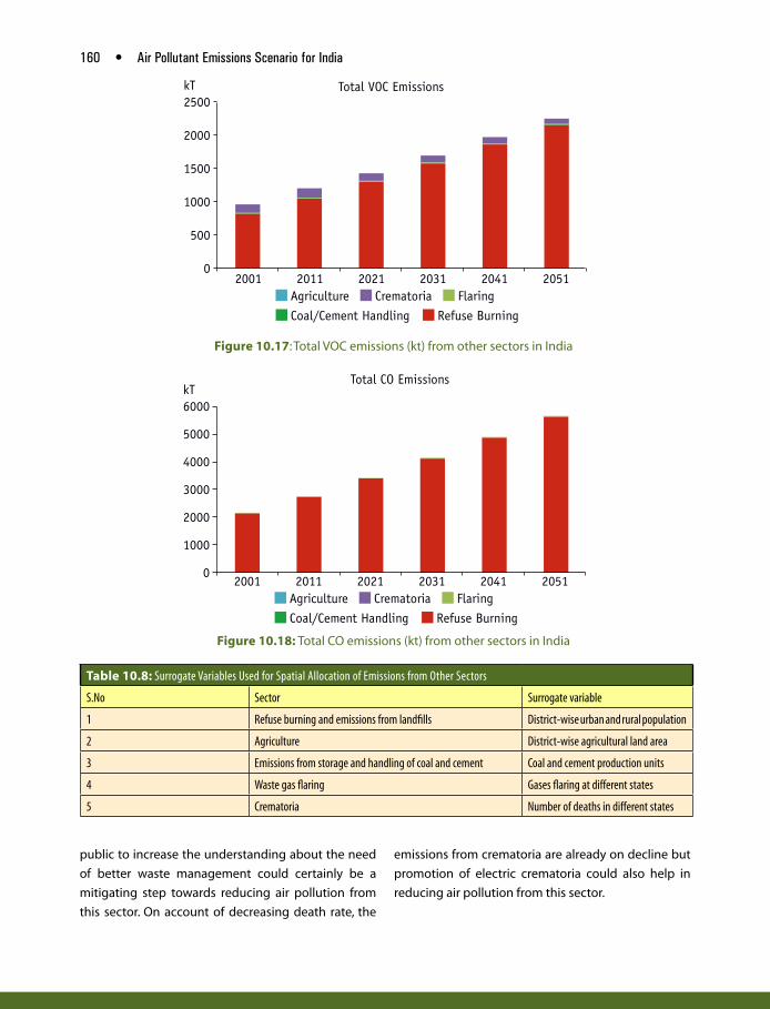
160 • Air Pollutant Emissions Scenario for India
public to increase the understanding about the need
of better waste management could certainly be a
mitigating step towards reducing air pollution from
this sector. On account of decreasing death rate, the
Figure 10.17: Total VOC emissions (kt) from other sectors in India
Figure 10.18: Total CO emissions (kt) from other sectors in India
emissions from crematoria are already on decline but
promotion of electric crematoria could also help in
reducing air pollution from this sector.
Table 10.8: Surrogate Variables Used for Spatial Allocation of Emissions from Other Sectors
S.No Sector Surrogate variable
1 Refuse burning and emissions from landfills District-wise urban and rural population
2 Agriculture District-wise agricultural land area
3 Emissions from storage and handling of coal and cement Coal and cement production units
4 Waste gas flaring Gases flaring at different states
5 Crematoria Number of deaths in different states

Other Sectors • 161
References Akagi, S. K., R. J. Yokelson, C. Wiedinmyer, et al. 2011. Emission factors for open and domestic biomass burning for use in atmospheric models. Atmospheric Chemistry and Physics 11(9): 4039–4072.
CPCB. 2007. Assessment of fugitive emissions and development of guideline for control of fugitive emissions from cement manufacturing industries . Delhi: CPCB.
CPCB. 2012. Status of municipal solid waste management. Delhi: CPCB.
European Environment Agency (EEA). 2013. EMEP/EEA air pollution inventory guidebook 2013. Luxembourg: European Environment Agency
Government of India (GoI). 2001. Census of India 2001. URL: http://www.jsk.gov.in/projection_report_december2006.pdf
IPCC. 2006. IPCC guidelines for national greenhouse gas inventories. Geneva, Switzerland: Intergovernmental Panel on Climate Change.
MoA. 2001. Agricultural statistics at a glance, 2000. New Delhi: Ministry of Agriculture.
National Environmental Engineering Research Institute (NEERI). 2010. Air quality monitoring, emission inventory & source apportionement studies for Delhi. New Delhi: Central Pollution Control Board.
Pappu, A., M. Saxena, and S. R. Asolekar. 2007. Solid wastes generation in India and their recycling potential in building materials. Building and Environment 42(6): 2311–2320.
Planning Commission. 2014. Report of the task force on waste to energy vol II. New Delhi: Government of India.
Shah, R., U. S. Sharma, and A. Tiwari. 2012. Sustainable solid waste management in rural areas. International Journal of Theoretical and Applied Sciences 4(2): 72–75.
TERI. 2015. Energy security outlook. New Delhi: The Energy and Resources Institute.
WHO. 2012. World population prospects: The 2012 revision. Geneva, Switzerland:World Health Organization
Woodall, B. D., D. P. Yamamoto, B. K. Gullett, and A. Touati. 2012, Emissions from small-scale burns of simulated deployed US military waste. Environmental science & technology 46(20): 10997–11003.


CHAPTER
Summary and ConclusionsSumit Sharma and Atul Kumar
11
Chapters 2 to 10 provided details of emissions of
different pollutants from different sectors in India.
The emissions are estimated for the years 2001 and
2011, and also projected for future years till 2051. It is
important to understand the relative contributions of
different sectors to the overall emission inventories.
This chapter focuses on summarization of results and
assessment of sectoral contributions to emissions of
various pollutants at the National scale. The pollutant-
wise results of emission inventories are presented in
subsequent sections.
Particulate Matter Growth of PM
10 emissions during 2001–51 is
presented in Figure 11.1. PM10
emissions in India
are presently (2011) estimated to be 10,641 kt,
dominated by industrial (43 per cent) and residential
combustion (29 per cent) sectors. Transport
contributes to just 3 per cent of PM10
emissions at
the National scale. However, these emissions are
concentrated at the urban centres where their
contribution to the prevailing air quality levels could
be much high. On the other hand, emissions from
domestic cooking are mainly from biomass burning
in rural households using traditional cook stoves.
Open burning of agricultural residue in rural areas
contributes 8 per cent to the total PM10
emissions.
Other sectors cumulatively contribute 11 per cent
of PM10
emissions. Power plant contribute 4 per cent
of PM10
emissions, however, these may contribute
significantly to pollution levels in specific zones of
influence of power plants.
The future projections of PM10
emissions show
that the emissions from industrial sector will grow
significantly till 2031. It is mainly due to anticipated
growth in the manufacturing sector in the next few
decades. Present environmental control scenario
in industries is limited considering absence of
continuous monitoring, limited vigilance capacity,
and limited installations of high efficiency air

164 • Air Pollutant Emissions Scenario for India
pollution control equipments. Enormous growth in
infrastructure development sector is expected to
fuel the demand for cement and brick in next few
decades. Cement industry despite being assumed
to be controlled with highly efficient electrostatic
precipitators (ESPs) for control of PM emissions,
is expected to emit 6.5 times more PM10
in 2051
than in 2011. In the brick sector, it is assumed that
penetration of Zig-Zag technologies will increase
from mere 4 per cent in 2011 to about 44 per cent
in 2051, despite which, the PM10
emissions will
be more than double in 2051 than in 2011. In the
medium and small industries, further penetration
of ESPs and other control technologies has been
assumed. Despite these considerations, the overall
emissions from industrial sector will be 3.3 times in
2051 in comparison to the 2011. However, the GDP
from industrial sector will grow by 17 times in the
same period. This point to tremendous reduction in
emission intensity in industrial sector.
Other than industries, the emissions from
combustion of fuels in residential sector will reduce
because of higher penetration of cleaner fuels for
cooking and lighting. On the other hand, emissions
from open agricultural biomass burning are expected
to go up by six times during 2011–51, with growth
in agricultural sector, in a no control scenario. Power
sector emissions are expected to grow despite
considerations of high-efficiency supercritical
technologies and installation of ESPs/flue gas
desulphurisation/selective catalytic reduction for tail-
pipe control. Transport sector emissions are expected
to go down further with considerations of advanced
(BS-V) emissions norms from 2020 onwards in India.
This could contribute to significant improvements in
air quality at the urban scales.
The distribution of energy-based sources have a
share of about 80 per cent in PM10
emissions, while
non-energy sources such as open burning, road
dust suspension, mining, and other fugitive sources
account for 20 per cent in 2011. Based on different
sectoral projections, the share of energy base sources
will remain to be about 80 per cent in 2051.
PM2.5
emissions also show similar trends as shown
by PM10
(Figure 11.2). The share of PM2.5
emissions
in PM10
emissions varies from 0.58 to 0.67 during all
years in considerations.
Black carbon (BC) and organic carbon (OC) are
the two main constituents of PM. BC emissions are
mainly a product of incomplete combustions. The
2011 inventories are dominated by residential sector
emissions (54 per cent), followed by 20 per cent
from transport sector (Figure 11.3a). It is to be noted
that while the share of transport was less in PM10
or
PM2.5
fractions, BC inventories show a very significant
contribution from the sector mainly form diesel
engines. Industries (8 per cent), open agricultural
burning (6 per cent), and diesel consumed in diesel
Figure 11.1: Year-wise growth of PM10 emissions (kilotonnes) during 2001–51

Summary and Conclusions • 165
generator (DG) sets (5 per cent) also contribute to
the BC inventories in 2011. The future projections
show that the emissions will stabilize over the years,
with decrease in contributions from residential
and transport sectors. However, emissions from
industrial combustion and open burning will increase.
Considering the stabilization of BC emission over the
years despite growing economy, there will be drastic
reduction in BC emission intensity in India.
OC emissions in India are dominated by residential
sector (Figure 11.3b), open burning and combustion
in other sector (crematoria and refuse burning).
However, with decline in biomass usage in future,
the emissions are expected to go down in future.
However, BC emissions could show higher reductions
mainly on account of reduced kerosene usage for
lighting, which is a very big source of BC emissions.
Gaseous Pollutants Figures 11.4 to 11.7 show emission inventories of
gaseous pollutants such as NOx, SO2, CO, and non-
methane volatile organic compounds (NMVOC).
While PM emissions are somewhat controlled
Figure 11.2: Year-wise growth of PM2.5 emissions (kilotonnes) during 2001–51
Figure 11.3a: Year-wise growth of BC emissions (kilotonnes) during 2001–51

166 • Air Pollutant Emissions Scenario for India
due to adoption of emission control standards,
gaseous pollutants are expected to grow gradually
mainly on account of high industrial growth, power
consumption, and mobility demands. The current
inventories of NOx emissions are dominated by
high-temperature combustion in transport sector
(38 per cent), power utilities (15 per cent), and DG
and agricultural pump sets (17 per cent). While it
is expected that with enhanced power generation
capacities, the use of small DG in residential and
commercial sector set will diminish over the years,
the demand for diesel will grow in transport sector.
However, introduction of BS-V emission norms will
reduce NOx emissions to some extent from the sector.
Overall, the NOx emissions are expected to grow 3.1
times between 2001 and 2051.
SO2 emissions are linked to sulphur content in
the fuels used in different sectors. The emissions are
presently and in future also will be dominated by coal
combustion activities in power and industrial sectors.
The sulphur content has already been considerably
reduced in the automotive fuels and is planned to
reduce it to 10 ppm levels by 2020. In power sector,
introduction of control norms for SO2 will somewhat
Figure 11.3b: Year-wise growth of OC emissions (kilotonnes) during 2001–51
Figure 11.4: Year-wise growth of NOx emissions (kilotonnes) during 2001–51

Summary and Conclusions • 167
arrest the growth of emissions. Despite this, with
limited SO2 controls in industrial sector, the emissions
are projected to increase by 4.3 times during 2011–51
(Figure 11.5).
Carbon monoxide is also a product of incomplete
combustion and is currently dominated by
biomass burning in residential sector. However,
with penetration of cleaner fuels in the sector, the
emission contribution will reduce. On the other hand,
the sectoral contribution from transport sector will
grow substantially with enormous growth expected
in private vehicle ownership. It is to be noted that CO
emissions are primarily emitted from gasoline-driven
vehicles. CO emissions form iron and steel sector are
expected to grow significantly in future. Increased
open crop-residue burning activities will add to CO
emissions with higher shares in future (Figure 11.6).
Currently NMVOC emissions are dominated by
residential biomass burning; however, its contribution
will reduce drastically in future. Evaporative emissions
from increased paints, printing activities, and use
of personal products will increase dramatically in a
Figure 11.5: Year-wise growth of SO2 emissions (kilotonnes) during 2001–51
Figure 11.6: Year-wise growth of CO emissions (kilotonnes) during 2001–51

168 • Air Pollutant Emissions Scenario for India
no-control business as usual (RES) scenario (Figure
11.7). The overall NMVOC emissions are projected to
increase by four folds by 2051.
Comparison with Other Studies A comparison of emissions estimated in this study
with others is shown in Table 11.1. There is variation
in emissions reported by different studies for various
pollutants. The emissions estimated in this study
show 34%,-23%, 20%, -10%, and 24% differences with
the mean of emissions estimated in other studies
for PM10
, SO2, NOx, NMVOC, and CO, respectively. The
standard deviation observed among all these studies
Table 11.1: Comparison of Emission Inventory (Million Tonnes) in This Study with Others
Study Year PM10 SO2 NOx NMVOC CO
This study 2011 10.6 5.6 7.0 11.4 46.4
Garg et al. (2006) 2005 4.6 4.4 41.7
Streets et al. (2003) 2000 5.5 4.0 8.6 51.1
Ohara et al. (2007) 2003 7.0 5.0 9.7 84.4
Zhang et al. (2009 2006 4.0 5.6 4.9 10.8 61.1
EDGAR 4.2a 2008 10.9 8.5 6.4 10.6 46.3
Kurokawa et al. (2013) 2008 4.7 10.0 9.7 15.9 61.8
Purohit et al (2010) 8.2 6.4 5.0 15.1
Lu et al. (2011) 2008 8.0
Klimont et al. (2009) 2005 6.4 5.0a http://edgar.jrc.ec.europa.eu/);
Figure 11.7: Year-wise growth of NMVOC emissions (kilotonnes) during 2001–51
is about 26–33 per cent of the emissions estimated in
this study for various pollutants.
The variations observed are due to a number of
reasons. Firstly, the estimates are for different years
and this study provides the latest estimates for
India-based local information. This study has used
Indian emission factors for most of the emission
sources and also accounts for latest information
on controls. For example, introduction of improved
vehicular emission norms, norms for DG sets
have been accounted in this study. There are also
methodological differences in estimation of energy
demand in some of the sectors such as residential,

Summary and Conclusions • 169
which is primarily dependent on poorly accounted
firewood combustion. Moreover, this study includes
many more sources such as evaporative, DG sets,
agricultural pumpsets, etc., which have not been
properly accounted in previous studies.
Spatial DistributionsEmissions of different pollutants for all the sectors are
spatially distributed using GIS into grids of 36 × 36
km². Figure 11.8(a–f ) shows the spatial distribution
of different pollutants in India. PM emissions are
geographically more in Indo-Gangetic plains (IGP)
mainly due to high population density, dependence
of biomass for cooking, vehicular density, and
presence of power plants. Other than IGP, PM10
intensities are higher in the states of Gujarat, Tamil
Nadu, and Maharashtra. NOx emissions are mainly
concentrated at urban centres and highways, mainly
(a) PM10 (b) PM2.5
(c) BC (d) OC

170 • Air Pollutant Emissions Scenario for India
due to vehicular activity. SO2 emissions are found
to be higher at locations of power plants, cement
plants, iron steel manufacturing units, and other
industries burning coal. CO emissions are primarily
driven by incomplete combustion in rural households
and hence show higher intensities in Bihar, West
Bengal, and Uttar Pradesh. NMVOC emissions are
also dominated by biomass burning in IGP, followed
by emissions in urban centres due to vehicles and
solvent use.
Figure 11.8(a–h): Spatial distribution of PM10
, PM2.5
, BC, OC, NOx, SO
2, CO, and NMVOC emissions in 2011
f
Economic Growth and Emissions While there is growth in emissions projected in future
for most of the pollutants, the emission intensities
are expected to reduce significantly with controls in
different sectors. These controls reduce the emissions
intensity (kilotonnes of pollutants per unit of GDP
produced) considerably over the years (Figure 11.9).
The emission intensities are also compared with
other regions in the world (Figure 11.10 and 11.11).
(e) NOx
(g) CO
(f ) SO2
(h) NMVOC
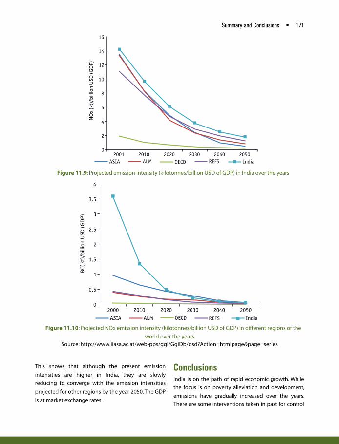
Summary and Conclusions • 171
Figure 11.8(a–h): Spatial distribution of PM10
, PM2.5
, BC, OC, NOx, SO
2, CO, and NMVOC emissions in 2011
f
Figure 11.9: Projected emission intensity (kilotonnes/billion USD of GDP) in India over the years
Figure 11.10: Projected NOx emission intensity (kilotonnes/billion USD of GDP) in different regions of the
world over the yearsSource: http://www.iiasa.ac.at/web-pps/ggi/GgiDb/dsd?Action=htmlpage&page=series
This shows that although the present emission
intensities are higher in India, they are slowly
reducing to converge with the emission intensities
projected for other regions by the year 2050. The GDP
is at market exchange rates.
Conclusions India is on the path of rapid economic growth. While
the focus is on poverty alleviation and development,
emissions have gradually increased over the years.
There are some interventions taken in past for control

172 • Air Pollutant Emissions Scenario for India
Figure 11.11: Projected BC emission intensity (kilotonnes/billion USD of GDP) in different regions of the
world over the yearsSource: http://www.iiasa.ac.at/web-apps/ggi/GgiDb/dsd?Action=htmlpage&page=series
OECD90 = Includes the OECD 90 countries, therefore encompassing the countries included in the regions Western Europe (Austria, Belgium, Denmark, Finland, France, Germany, Greece, Iceland, Ireland, Italy, Luxembourg, Netherlands, Norway, Portugal, Spain, Sweden, Switzerland, Turkey, United Kingdom), Northern America (Canada, United States of America), and Pacific OECD
(Australia, Fiji, French Polynesia, Guam, Japan, New Caledonia, New Zealand, Samoa, Solomon Islands, Vanuatu) .REF = Countries from the Reforming Economies region (Albania, Armenia, Azerbaijan, Belarus, Bosnia and Herzegovina, Bulgaria,
Croatia, Cyprus, Czech Republic, Estonia, Georgia, Hungary, Kazakhstan, Kyrgyzstan, Latvia, Lithuania, Malta, Poland, Republic of Moldova, Romania, Russian Federation, Slovakia, Slovenia, Tajikistan, TFYR Macedonia, Turkmenistan, Ukraine, Uzbekistan,
Yugoslavia).ASIA = The countries included in the regions China + (China, China Hong Kong SAR, China Macao SAR, Mongolia, Taiwan) , India + (Afghanistan, Bangladesh, Bhutan, India, Maldives, Nepal, Pakistan, Sri Lanka) and Rest of Asia (Brunei Darussalam, Cambodia,
Democratic People’s Republic of Korea, East Timor, Indonesia, Lao People’s Democratic Republic, Malaysia, Myanmar, Papua New Guinea, Philippines, Republic of Korea, Singapore, Thailand, Viet Nam) are aggregated into this region.
MAF = This region includes the Middle East (Bahrain, Iran (Islamic Republic of ), Iraq, Israel, Jordan, Kuwait, Lebanon, Oman, Qatar, Saudi Arabia, Syrian Arab Republic, United Arab Emirates, Yemen) and African (Algeria, Angola, Benin, Botswana, Burkina Faso, Burundi, Cote d’Ivoire, Cameroon, Cape Verde, Central African Republic, Chad, Comoros, Congo, Democratic Republic of
the Congo, Djibouti, Egypt, Equatorial Guinea, Eritrea, Ethiopia, Gabon, Gambia, Ghana, Guinea, Guinea-Bissau, Kenya, Lesotho, Liberia, Libyan Arab Jamahiriya, Madagascar, Malawi, Mali, Mauritania, Mauritius, Morocco, Mozambique, Namibia, Niger, Nigeria,
Reunion, Rwanda, Senegal, Sierra Leone, Somalia, South Africa, Sudan, Swaziland, Togo, Tunisia, Uganda, United Republic of Tanzania, Western Sahara, Zambia, Zimbabwe) countries.
LAM = This region includes the Latin American countries (Argentina, Bahamas, Barbados, Belize, Bolivia, Brazil, Chile, Colombia, Costa Rica, Cuba, Dominican Republic, Ecuador, El Salvador, Guadeloupe, Guatemala, Guyana, Haiti, Honduras, Jamaica,
Martinique, Mexico, Netherlands Antilles, Nicaragua, Panama, Paraguay, Peru, Puerto Rico, Suriname, Trinidad and Tobago, Uruguay, Venezuela).
where MAF and LAM are together, the former ALM region of the SRES scenarios
of air pollution mainly at the urban scales in India.
However, the recent studies have suggested that the
regional scale improvements are required to effectively
control pollution levels at urban and regional scales.
This calls for preparation of databases for emissions
inventories to carry out simulation studies for regional
scale improvement of air quality in India. This study
presents a multi-scale high-resolution emission
inventory for India for the baseline (2011) and future
years till 2051. The estimates are based on TERI’s

Summary and Conclusions • 173
earlier work in developing energy use scenarios for
the country. Established methodologies have been
used to estimate emissions from different sectors and
useful insights have been drawn. It is noted that while
residential sector biomass burning–based emissions
are significantly high currently, they are projected to
reduce considerably in next few decades. On the other
hand, rapid industrial growth will lead to significant
emissions and in a limited control scenario, the
emission are expected to increase in future. Transport
PM emissions may not be found significantly high at
the National scale but are significantly concentrated
at the urban levels, leading to higher contributions
there. Key sectoral recommendations that are made for
control of emissions are :
Power and industries P Development of standards for NOx and other
important gaseous pollutants
P Installation and maintenance of APC devices
P Continuous monitoring and reporting of stacks
P Development emission trading schemes and
other fiscal measures for performance beyond
compliance levels
P Ensuring 24×7 power supply to reduce DG Set
usage.
Transport P Adoption of stringent auto fuel policy and vehicle
emission norms
P On-road vehicle emission management : I&M
systems, fleet modernization, retrofitment
P Enhancement of public transportation systems
P Development of fuel efficiency standards
P Electric mobility
P Promotion of non-motorized transport options
Residential P Enhanced penetration of LPG
P Penetration of improved cook stoves, R&D
Open burning P Development of plans for more productive energy
use of the crop-residues currently burnt
Evaporative emissions P Development of standards for control of
evaporative/fugitive emissions from different
product use
P Installation of stage-I/II control at oil handling
units.
P Control of evaporative emissions from vehicles
References Garg, A., P. R. Shukla, and M. Kapshe. 2006. The sectoral trends of multigas emissions inventory of India. Atmospheric Environment 40:4608–20.
Klimont, Z., J. Cofala, J. Xing, et al. 2009. Projections of SO
2, NOx and carbonaceous aerosols emissions in Asia.
Tellus B 61(4):602–17.
Kurokawa, J., T. Ohara, T. Morikawa, S. Hanayama, J.-M. Greet, and T. Fukui. 2013. Emissions of air pollutants and greenhouse gases over Asian regions during 2000–2008: Regional Emission inventory in Asia (REAS) version 2; Discussion. Atmospheric Chemistry and Physics 13:11019–58; 10049–123.
Lu, Z., Q. Zhang, and D. G. Streets. 2011. Sulfur dioxide and primary carbonaceous aerosol emissions in China and India, 1996–2010. Atmospheric Chemistry and Physics 11:9839–64, doi:10.5194/acp-11-9839- 2011.
Ohara, T., H. Akimoto, J. Kurokawa, N. Horii, K. Yamaji, X. Yan, and T. Hayasaka. 2007. An Asian emission inventory of anthropogenic emission sources for the period 1980–2020. Atmospheric Chemistry and Physics 7:4419–44, doi:10.5194/acp-7-4419-2007.
Purohit, P., M. Amann, R. Mathur, et al. 2010. GAINS ASIA scenarios for cost-effective control of air pollution and greenhouse gases in India. Laxenburg, Austria: International Institute for Applied Systems Analysis.
Streets, D. G., T. C. Bond, G. R. Carmichael, et al. 2003. An inventory of gaseous and primary aerosol emissions in Asia in the year 2000. Journal of Geophysical Research 108(D21):8809
Zhang, Q., D. G. Streets, G. R. Carmichael, et al. 2009. Asian emissions in 2006 for the NASA INTEX-B mission. Atmospheric Chemistry and Physics 9:5131–53.

174 • Air Pollutant Emissions Scenario for India
Annexure 11.1: Sectoral emission estimates (kt/yr) of different pollutants 2001–51
PM10 Sectors 2001 2011 2021 2031 2041 2051
Residential 2944 3115 2913 2774 2502 2048
Industry 3685 4627 10212 13953 15230 15093
Power 257 453 869 1016 1216 1354
Transport 218 342 478 498 594 761
DG set 104 82 72 76 81 78
Open burning 620 818 1004 1190 1376 1562
Evaporative
Others 890 1204 1561 1976 2399 2773
Total 8717 10641 17110 21483 23398 23668
PM2.5 Sectors 2001 2011 2021 2031 2041 2051
Residential 2570 2660 2450 2333 2104 1723
Industry 1923 2451 5507 7816 8706 8546
Power 103 181 348 407 487 542
Transport 194 288 371 293 256 296
DG set 88 70 61 65 69 66
Open burning 350 462 567 672 777 882
Evaporative
Others 602 756 942 1149 1363 1574
Total 5830 6867 10246 12733 13760 13629
BC Sectors 2001 2011 2021 2031 2041 2051
Residential 835 521 260 247 223 183
Industry 44 77 88 113 138 161
Power 12 22 42 49 58 65
Transport 138 197 235 158 104 111
DG set 62 49 43 46 48 47
Open burning 48 57 66 75 83 92
Evaporative
Others 38 48 59 72 84 97
Total 1178 971 794 759 739 755
CO Sectors 2001 2011 2021 2031 2041 2051
Residential 25942 31385 31953 30560 27696 22827
Industry 3196 5728 9921 16751 23370 28335
Power 23 43 72 128 207 286
Annexure

Summary and Conclusions • 175
Transport 1983 2777 4149 6173 9488 14167
DG set 318 251 288 304 0 0
Open burning 2549 3244 3905 4565 5225 5885
Evaporative
Others 2389 3006 3621 4328 5059 5799
Total 36401 46435 53909 62809 71046 77299
NOx Sectors 2001 2011 2021 2031 2041 2051
Residential 633 766 789 762 699 585
Industry 520 950 1980 3405 4877 6038
Power 573 1015 1935 3565 5786 7334
Transport 1164 2665 3826 3904 4530 6162
DG set 1475 1164 833 877 929 893
Open burning 104 137 169 200 232 263
Evaporative
Others 220 280 344 415 488 562
Total 4689 6978 9876 13129 17540 21838
SO2 Sectors 2001 2011 2021 2031 2041 2051
Residential 303 330 314 299 270 221
Industry 1901 3175 6070 10118 14478 18147
Power 1031 1842 3490 3981 4650 5108
Transport 120 53 27 50 87 145
DG set 97 77 15 16 0 0
Open burning 30 40 50 59 68 77
Evaporative 0 0 0 0 0 0
Others 29 37 46 55 65 75
Total 3512 5553 10011 14577 19617 23773
NMVOC Sectors 2001 2011 2021 2031 2041 2051
Residential 5457 6637 6771 6471 5860 4824
Industry 74 123 194 305 425 532
Power 4 8 14 25 40 53
Transport 605 802 1026 980 926 1103
DG set 120 95 68 72 247 304
Open burning 274 512 732 952 1173 1393
Evaporative 797 2050 4431 9194 17233 30089
Others 952 1191 1418 1684 1960 2238
Total 8283 11418 14652 19683 27863 40536
OC Sectors 2001 2011 2021 2031 2041 2051
Residential 1222 1488 1513 1441 1300 1064

Industry 63 107 143 198 248 290
Power 20 34 66 77 92 103
Transport 47 70 96 66 42 35
DG set 19 15 13 14 15 14
Open burning 109 128 145 163 180 198
Evaporative
Others 309 392 482 581 684 788
Total 1787 2234 2459 2540 2561 2493
Annexure 11.2: State-wise emission estimates (kt/yr) of different pollutants in 2011
States PM10 PM2.5 NOx SO2 CO BC OC NMVOC
Andhra Pradesh 708 415 553 440 2956 54 126 736
Arunachal Pradesh 25 15 19 4 186 4 8 47
Assam 247 170 89 44 1594 30 72 364
Bihar 500 375 311 165 3834 65 224 891
Chhattisgarh 818 541 323 533 1222 36 34 145
Goa 22 10 19 14 42 1 2 16
Gujarat 1129 637 519 542 2509 48 99 804
Haryana 293 189 254 124 1355 30 49 322
Himachal Pradesh 92 51 65 39 392 7 16 98
Jammu & Kashmir 78 52 75 39 526 11 24 118
Jharkhand 238 153 194 210 1856 25 58 320
Karnataka 468 250 376 214 2401 42 105 657
Kerala 179 95 203 80 1250 24 54 350
Madhya Pradesh 568 384 366 246 2620 54 139 659
Maharashtra 748 469 589 528 3456 70 141 925
Manipur 12 10 14 1 93 2 4 23
Meghalaya 32 23 25 11 172 4 7 41
Mizoram 12 7 10 2 73 1 3 20
Nagaland 16 9 13 3 107 2 5 26
Orissa 963 630 307 392 2297 53 85 465
Punjab 461 280 267 149 2011 34 60 370
Rajasthan 617 421 439 354 2700 63 128 674
Sikkim 4 3 3 1 23 0 1 6
Tamil Nadu 414 246 553 418 1924 51 91 549
Tripura 27 16 13 3 218 4 9 50
Uttar Pradesh 1207 916 733 468 6985 159 391 1540
Uttaranchal 167 87 67 45 716 12 23 147
West Bengal 514 364 444 483 2858 62 138 664

The Energy and Resources Institute
EDITORS
Sumit SharmaAtul Kumar
Air pollutant emissions scenario for India