1

The effect of a tall tower on flow and dispersion through a model

urban neighborhood

Part 1. Flow characteristics

David K. Heist,a Jennifer Richmond-Bryant,b Laurie A. Brixey,c George E. Bowker,d Steven G.

Perrya and Russell W. Wienere

aAtmospheric Sciences Modeling Division, Air Resources Laboratory, National Oceanic and Atmospheric Administration, Research Triangle Park, NC 27711, USA bEnvironmental and Occupational Health Sciences, Hunter College, City University of New York, 425 East 25th Street, New York, NY 10010, USA cAlion Science and Technology, P.O. Box 12313, Research Triangle Park, NC 27709, USA dAtmospheric Modeling Division, National Exposure Research Laboratory, US Environmental Protection Agency, Research Triangle Park, NC 27711, USA eNational Homeland Security Research Center, US Environmental Protection Agency, Research Triangle Park, NC 27711, USA

Disclaimer The research presented here was performed under the Memorandum of Understanding between

the U.S. Environmental Protection Agency (EPA) and the U.S. Department of Commerce’s

National Oceanic and Atmospheric Administration (NOAA) and under agreement number

DW13921548. This work constitutes a contribution to the NOAA Air Quality Program.

Although it has been reviewed by EPA and NOAA and approved for publication, it does not

necessarily reflect their policies or views. Mention of trade names or commercial products does

not constitute endorsement or recommendation for use.

Abstract Wind tunnel and computational fluid dynamics (CFD) studies were performed to examine the

effect of a tall tower on the flow around an otherwise uniform array of buildings. The model used

in both the wind tunnel and CFD studies was designed to simulate an area of Brooklyn, NY,

where blocks of residential row houses form a neighborhood bordering a major urban highway.

2

This area was the site of a field study that, along with the work reported here, had the goal of

improving the understanding of airflow and dispersion patterns within urban micro-

environments. Results reveal that a tall tower has a dramatic effect on the flow in the street

canyons in the neighboring blocks, enhancing the exchange between the street canyon flow and

the free-stream flow aloft. In particular, vertical motion down the windward side and up the

leeward side of the tower resulted in strong flows in the lateral street canyons and increased

winds in the street canyons in the immediate vicinity of the tower. These phenomena were

visible in both the wind tunnel and CFD results, although some minor differences in the flow

fields were noted.

Introduction Urban and suburban neighborhoods present challenges for the prediction of pollutant dispersion

due to the heterogeneity of building configurations which sets up irregular, complex wind

patterns. There is a need to identify and quantify the relative importance of the dominant factors

that affect the dispersion. There have been many studies on regular arrays of buildings to develop

an understanding of the phenomena involved in urban dispersion, focusing on such factors as

street canyon width, building aspect ratio, traffic, and orientation of street canyons to prevailing

winds.1–5 These studies have produced a better understanding of the importance of near-field

effects on the initial dispersion of a plume arising from an urban source within the street canyon

(e.g., traffic). Several recent studies6–8 have highlighted the effect variations in building height

can have on the airflow patterns in urban areas. These variations enhance the transfer of

momentum from the winds aloft into the building canopy and provide for the rapid vertical

mixing of the pollutant from the street canyons. In this paper we examine the effect of a single

building that towers above a neighborhood of buildings of uniform height.

A combined wind tunnel and computational fluid dynamics (CFD) study was undertaken

to supplement a field study performed in Brooklyn, NY, USA, designed to study the dispersion

of pollutants from a line source in an urban neighborhood. This paper is the first of two papers

describing flow and pollutant dispersion for an idealized scale model of the site (see also Brixey

et al.9). The field study, the Brooklyn Traffic Real-Time Ambient Pollutant Penetration and

Environmental Dispersion (B-TRAPPED) Study, was performed in May 2005 with the goal of

improving the understanding of airflow patterns through a complex area to be able to predict the

3

dispersion patterns of pollution from traffic and hazardous releases along the roadway.10–14 The

section of the city chosen for the study has fairly regular city block shapes comprising row

houses with uniform heights and common backyards that form a courtyard. Adjacent to the

major thoroughfare passing through the study area was one tall building that dominated the area.

Standing 12 stories tall, it was significantly higher than the neighborhood row houses which

were typically three stories tall.

The experimental and numerical studies were performed to complement each other. The

wind tunnel study can provide insight into the flow patterns throughout the study area,

supplementing the information gathered from a limited number of field instruments deployed in

typical field studies and providing data to compare with the results of the numerical study. The

numerical study provides a more complete picture of the flow and concentration fields since the

velocity and concentration fields over the whole domain are computed. The goal of this study is

not, however, intended to be a comprehensive evaluation of the numerical simulation, but rather

to identify important flow phenomena in urban and suburban areas identified by both techniques.

Methods Meteorological wind tunnel experiment

Wind tunnel. The experiments were conducted in the EPA Fluid Modeling Facility’s single-

pass, draw-through meteorological wind tunnel (test section 3.7 m wide, 2.1 m high, and 18.3 m

long).15 The flow in the wind tunnel is conditioned to produce a deep boundary layer appropriate

for simulating neutral atmospheric conditions in an urban area by a series of screens,

honeycombs, and boundary-layer generation devices. These devices include three truncated

Irwin spires16 at the upwind limit of the test section that are tapered in height to remove

progressively more momentum from the flow approaching the floor of the tunnel. Roughness

blocks are positioned on the floor downwind of the spires to enhance the turbulence levels near

the floor and maintain the boundary layer in equilibrium. In addition, the tunnel ceiling is

adjustable to allow compensation for the blockage created by the model and the growth of the

wall boundary layers to produce a non-accelerating freestream flow. With a freestream flow

speed of 4.2 ms-1, the boundary layer that develops from this system has a friction velocity, u*, of

0.23 ms-1 and a roughness length, z0, of 0.7 mm (7 cm when scaled up to full scale).

4

Considering the smallest street width, D, of 12 cm, the street canyon Reynolds number

(ρUHD/μ) was approximately 24,000. The freestream velocity was chosen to ensure that the

Reynolds number of the flow through the model was substantially higher than 11,000, the critical

number for Reynolds number independence.17

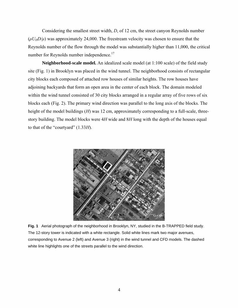
Neighborhood-scale model. An idealized scale model (at 1:100 scale) of the field study

site (Fig. 1) in Brooklyn was placed in the wind tunnel. The neighborhood consists of rectangular

city blocks each composed of attached row houses of similar heights. The row houses have

adjoining backyards that form an open area in the center of each block. The domain modeled

within the wind tunnel consisted of 30 city blocks arranged in a regular array of five rows of six

blocks each (Fig. 2). The primary wind direction was parallel to the long axis of the blocks. The

height of the model buildings (H) was 12 cm, approximately corresponding to a full-scale, three-

story building. The model blocks were 4H wide and 8H long with the depth of the houses equal

to that of the “courtyard” (1.33H).

Fig. 1 Aerial photograph of the neighborhood in Brooklyn, NY, studied in the B-TRAPPED field study.

The 12-story tower is indicated with a white rectangle. Solid white lines mark two major avenues,

corresponding to Avenue 2 (left) and Avenue 3 (right) in the wind tunnel and CFD models. The dashed

white line highlights one of the streets parallel to the wind direction.

5

Fig. 2 Wind tunnel model city block array. The model was built at a 1:100 scale relative to full scale.

Letters A through G and numbers 1 through 5 are used to indicate particular buildings in the array. Cross-

hatching indicates the location of the tower.

Throughout this paper, the streamwise streets (1H wide) are referred to as “streets,” while

the cross-stream streets (typically 2H wide) are called “avenues” (Fig. 2). One avenue was wider

than the others at 2.67H, simulating the width of a major urban multi-lane expressway (3rd

Avenue) in Brooklyn. The source for the concentration measurements9 is located in this wider

avenue downwind of the second row of blocks.

One block was constructed of Plexiglas and had 152 ports installed for concentration and

pressure measurements. This block was designed to be interchangeable with the other city blocks

for acquiring building surface data at a variety of locations.

A tall tower (representing a 12-story building in the field study) was positioned at the

downwind end of one of the blocks just upwind of the source (Fig. 2, block D2) to determine the

6

impact of this building on downwind concentrations. The tower is 1.33H long, 4H wide, and 4H

tall from ground level.

Laser Doppler velocimetry. The laser Doppler velocimetry (LDV) system used in these

experiments to measure velocities was a two-component, single-probe system that employed the

488- and 514.5-nm lines from a Coherent Innova 70C argon-ion laser. The beam splitting,

frequency shifting, and coupling of laser light to fiber-optic cables were all accomplished using a

TSI Colorburst multicolor beam separator (Model 9201, TSI Inc., St. Paul, MN, USA). The LDV

system was used in the real fringe mode with a frequency shift of 40 MHz to eliminate direction

ambiguity in the velocity measurements. The use of a portable fiber-optic probe (TSI Model

9832 with a 500 mm focal distance lens) facilitated movement of the LDV measurement volume,

an ellipsoid with a diameter of approximately 80 μm and a length of about 1 mm. The LDV

probe was installed on the wind tunnel carriage for computer-controlled positioning.

Theatrical smoke was used as seeding material for the LDV (Model 1600 fog machine,

Rosco Laboratories Inc., Stamford, CT) and was introduced near the inlet of the tunnel, far

upstream of the model. Data were processed with a digital burst correlator (Model IFA 755, TSI

Inc.) and acquired using FIND for Windows software (version 1.4, TSI Inc.).

Pressure. Mean surface pressure measurements were made at 152 locations on the model

building. These ports were constructed from brass tubing (0.16 cm inner diameter) mounted with

the tube opening flush with the surface of the building. Six capacitance manometers were used

during these measurements (five MKS Baratron, Model 270s with Model 698A01TRC heads and

one MKS Baratron Model 170M-6C with Model 398HD-001 head, Wilmington, MA). One

manometer was used to monitor the Pitot-static tube mounted at a height of 1.65 m above the

floor approximately 6 m upstream of the model building. The other five were connected to

building ports through a system that allowed automated switching between the 152 surface ports.

The coefficient of pressure (Cp = (Pbuilding – Pstatic)/(0.5ρUo2)) was calculated by incorporating the

measurement of static pressure from the Pitot-static tube, where Pbuilding is the surface

measurement, Pstatic is the Pitot-static tube measurement, ρ is the air density, and Uo is the

freestream flow velocity.

7

Computational fluid dynamics simulation

Geometry. The CFD model geometry shown in Fig. 3 was created using the GAMBIT v.2.1.0

(FLUENT, Inc., Lebanon, NH, USA) software. The model geometry was similar to that used in

the wind tunnel, but some differences accommodate memory constraints imposed by the

meshing process. The model geometry consisted of three rows of four blocks of the same

dimensions as used in the wind tunnel. The building height, H = 12 m, was used for scaling. The

source avenue width was slightly larger than for the wind tunnel experiments, with the first and

second rows separated by a distance of 3H. The tower, having a height of 4H (from the ground),

was centered at x = -2.3H and y = 2.5H, as shown in Fig. 3. x/H = 0 was designated 1.67H

downstream of the first row of buildings, y/H = 0 was positioned at the center of the domain

between the second and third building columns, and z/H = 0 was located at the ground. The

domain limits were -23.67 < x/H < 33.67, -19 < y/H < 19, 0 < z/H < 8.

Fig. 3 CFD model layout. Cross-hatching indicates location of tower. The domain limits noted in the

geometry section are not shown here.

Computational mesh. GAMBIT v.2.1.0 was also employed to create the initial mesh,

and refinement of the mesh was performed within the FLUENT v.6.2.16 software. A tetrahedral

mesh was employed. The mesh was graded so that mesh size was larger around the edges of the

domain and refined within the vicinity of the buildings. Grid independence testing was

performed according to Roache.18 Three successively finer meshes were created, and the

resultant average velocity was computed at 99 locations along y/H = 0. The error was calculated

8

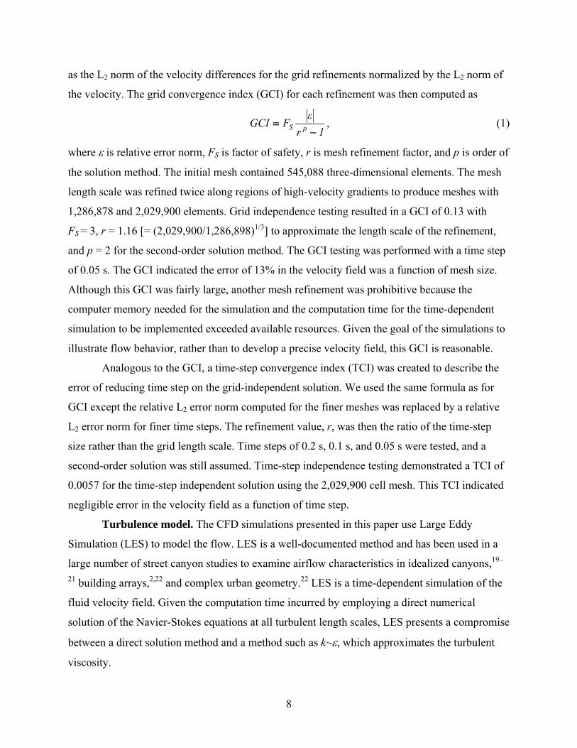
as the L2 norm of the velocity differences for the grid refinements normalized by the L2 norm of

the velocity. The grid convergence index (GCI) for each refinement was then computed as

1r

εFGCI pS −

= , (1)

where ε is relative error norm, FS is factor of safety, r is mesh refinement factor, and p is order of

the solution method. The initial mesh contained 545,088 three-dimensional elements. The mesh

length scale was refined twice along regions of high-velocity gradients to produce meshes with

1,286,878 and 2,029,900 elements. Grid independence testing resulted in a GCI of 0.13 with

FS = 3, r = 1.16 [= (2,029,900/1,286,898)1/3] to approximate the length scale of the refinement,

and p = 2 for the second-order solution method. The GCI testing was performed with a time step

of 0.05 s. The GCI indicated the error of 13% in the velocity field was a function of mesh size.

Although this GCI was fairly large, another mesh refinement was prohibitive because the

computer memory needed for the simulation and the computation time for the time-dependent

simulation to be implemented exceeded available resources. Given the goal of the simulations to

illustrate flow behavior, rather than to develop a precise velocity field, this GCI is reasonable.

Analogous to the GCI, a time-step convergence index (TCI) was created to describe the

error of reducing time step on the grid-independent solution. We used the same formula as for

GCI except the relative L2 error norm computed for the finer meshes was replaced by a relative

L2 error norm for finer time steps. The refinement value, r, was then the ratio of the time-step

size rather than the grid length scale. Time steps of 0.2 s, 0.1 s, and 0.05 s were tested, and a

second-order solution was still assumed. Time-step independence testing demonstrated a TCI of

0.0057 for the time-step independent solution using the 2,029,900 cell mesh. This TCI indicated

negligible error in the velocity field as a function of time step.

Turbulence model. The CFD simulations presented in this paper use Large Eddy

Simulation (LES) to model the flow. LES is a well-documented method and has been used in a

large number of street canyon studies to examine airflow characteristics in idealized canyons,19–

21 building arrays,2,22 and complex urban geometry.22 LES is a time-dependent simulation of the

fluid velocity field. Given the computation time incurred by employing a direct numerical

solution of the Navier-Stokes equations at all turbulent length scales, LES presents a compromise

between a direct solution method and a method such as k~ε, which approximates the turbulent

viscosity.

9

In FLUENT, the large-eddy scales were solved directly through a finite volume

formulation of the Navier-Stokes equations over the grid spacing. The small scales of turbulence

were approximated with a subgrid scale (SGS) model at length scales smaller than the grid

spacing. In the SGS model, the Navier-Stokes equations were closed by a formulation of the

subgrid-scale stress, τ 23–25:

jijiij uuuu ρρτ −= , (2)

where ρ is fluid density, u is velocity, and i and j denote velocity components. For low Reynolds

number flows, the SGS model may be dampened in the boundary layer. For relatively high

Reynolds number flows, such as the one modeled here, it was not possible to resolve the sharp

flow gradient near the boundary. For this reason, logarithmic wall model approximations were

used near the boundary. Initial and boundary conditions for the simulation consisted only of the

incoming velocity field and the geometry. LES does not require any approximation of upstream

turbulence conditions.

Boundary conditions. A logarithmic formulation of the upstream velocity profile was

designated to match that used in the wind tunnel:

⎟⎟⎠

⎞⎜⎜⎝

⎛ −=

0

ln1* z

dzuu

κ, (3)

where u* is friction velocity, κ = 0.4 is von Karman’s constant, z0 is roughness length scale, and

d is displacement length. These parameters were selected to match the wind tunnel experiments

at a 1:100 full scale equivalent (u* = 0.23 m s-1, z0 = 0.07 m, d = 0 m). All solid entities, including

the building surfaces and ground, had no-slip and no-flow designations to preserve mass balance.

Results and discussion Wind tunnel measurements and numerical simulations of the flow through the building array

present a picture of urban wind flow that exhibits significant channeling in the lateral avenues

and strong vertical flows surrounding the tall tower. The tower in the array substantially

influenced the patterns of flow throughout the building array. Vertical flow was found near the

faces of the tall building, toward the ground on the windward face and upward from the ground

on the leeward face. Vertical flow near the tower is important because of its ability to transport

high-momentum air from the upper boundary layer into the street canyons and air from ground

10

level, potentially polluted from a hazardous release, up over the roof lines of the neighboring

buildings. Fig. 4 shows the latter phenomenon with smoke from a pollutant source in the avenue

immediately downwind of the tower transported up the lee side of the tower. The source in the

photograph is a line segment source spanning an intersection and extending from the midpoint of

row C to the midpoint of row D (Fig. 2). The effect of the tower on pollutant dispersion is

discussed in more detail in Brixey et al.9

Fig. 4 Flow visualization of a line segment source in Avenue 2 demonstrating the vertical flow up the

leeward side of the building. Measurements show that there is an opposite effect on the windward face of

the building that produces a downdraft. Freestream flow is from left to right.

The velocity field responsible for the transport of pollutants, illustrated with flow

visualization, is revealed in both the wind tunnel measurements and in the CFD simulations.

Fig. 5 shows velocity vectors measured in the wind tunnel along a streamwise vertical plane

intersecting the tall tower at its spanwise center (i.e., at y/H = 2.5). As the flow approaches the

tower it splits into a portion traveling over the tower and a larger portion deflected downward.

This downward motion enhances the transport of momentum from the upper elevations into the

street canyons. This figure also shows the dramatic upwash in the lee of the tower which begins

at ground level and extends to the top of the tower. The magnitude of the vertical velocities in

this area reaches 25% of the freestream velocity.

11

Fig. 5 Mean velocity vectors measured with LDV at y/H = 2.5. Freestream flow is from left to right.

The CFD results present a more detailed picture of the flow field, filling in the gaps

between the velocity measurements from the wind tunnel. The CFD results show that flow

upwind and downwind of the tower comprises large recirculating eddies that are horizontally

centered roughly on the courtyards of the upwind and downwind city blocks as shown in Fig. 6.

The figure also shows the upwash on the lee side of the tower, with CFD also indicating vertical

velocities reaching 21-28% of the freestream velocity in this area, accounting for the GCI.

Fig. 6 Mean velocity vectors from CFD at y/H = 2.5. Freestream flow is from left to right.

An additional flow feature that in many cases may have significant effects on dispersion

is the lateral flow along the avenues toward the tower. This lateral flow supplies air to fill the

void created by the vertical flow up the lee side of the tower. This phenomenon can be seen

clearly in cross-sectional (or spanwise) views of the measured velocity field in planes

perpendicular to the downstream direction. Fig. 7a shows a spanwise view of the flow in the

avenue immediately downwind of the tower (at x/H = 0). The velocity vectors show lateral flow

toward the tower, especially in the lower half of the street canyon. The strength of the lateral

movement produces velocities that reach 50% of the freestream velocity in magnitude. The

ability of the tower to produce lateral flows in the avenues persists with downstream distance.

12

Even one block downwind (Fig. 7b, x/H = 10.3) the magnitude of the lateral flow reaches 30% of

the freestream velocity.

Fig. 7 a) Mean velocity vectors measured with LDV at x/H = 0. Note the flow toward the tower in the

avenue. The magnitude of the flow velocity is approximately half the freestream velocity. Flow is up the

lee side of the tall building. b) Mean velocity vectors measured with LDV at x/H = 10.3. One block

downstream of the tower strong lateral flow toward the tower persists.

CFD results also show the lateral flow in the avenues. Figs. 8a and 8b present the same

cross-sectional views of the flow for the CFD results that Figs. 7a and 7b presented for the wind

tunnel results. The CFD results show flow up the leeward side of the tower (Fig. 8a) with two

counter-rotating swirls downwind of the tower. The updraft draws air from near ground level,

creating a flow toward the tower in the avenue behind the tower. This lateral flow toward the

tower extends the full width of the building array. Also visible in Fig. 8a are large swirls of flow

behind the lower buildings (counterclockwise to the left of the tower, clockwise to the right) with

flow above the buildings in the opposite direction to the flow in the avenue. One block

13

downwind of the tower (Fig. 8b) the vertical flow has abated, but the flow toward the tower in

the avenue persists.

Fig. 8 Mean velocity vectors from CFD at a) x/H = 0 and b) x/H = 10.5.

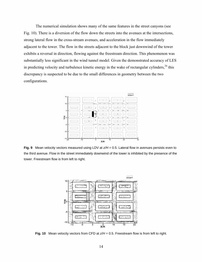
A horizontal slice through the street canyons at z/H = 0.5 illustrates the interactions

between the street and avenue flows (see Fig. 9). Flow proceeds in the downwind direction in the

streets (except immediately downwind of the tower) and is partially diverted into the avenues in

the intersections. Significant lateral flow toward the tower is seen in the avenue immediately

downstream of the tower, as well as in the two downwind avenues. The flows in the streets

immediately adjacent to the tower exhibit higher velocities due to the momentum transferred by

the downwash on the upstream side of the tower. The velocity near the end of the block in the

streets just upwind of Avenue 2 (at x/H = -2) is approximately 50–65% higher than at the

corresponding location just upwind of Avenue 4, two blocks from the tower. Flow in the streets

adjacent to the block just downwind of the tower is nearly stagnant on average.

14

The numerical simulation shows many of the same features in the street canyons (see

Fig. 10). There is a diversion of the flow down the streets into the avenues at the intersections,

strong lateral flow in the cross-stream avenues, and acceleration in the flow immediately

adjacent to the tower. The flow in the streets adjacent to the block just downwind of the tower

exhibits a reversal in direction, flowing against the freestream direction. This phenomenon was

substantially less significant in the wind tunnel model. Given the demonstrated accuracy of LES

in predicting velocity and turbulence kinetic energy in the wake of rectangular cylinders,26 this

discrepancy is suspected to be due to the small differences in geometry between the two

configurations.

Fig. 9 Mean velocity vectors measured using LDV at z/H = 0.5. Lateral flow in avenues persists even to

the third avenue. Flow in the street immediately downwind of the tower is inhibited by the presence of the

tower. Freestream flow is from left to right.

Fig. 10 Mean velocity vectors from CFD at z/H = 0.5. Freestream flow is from left to right.

15

Pressure fields predicted in the numerical simulations are useful in completing the picture

of the flow through the city array. Figs. 11a and 11b show the coefficient of pressure (Cp) for

two vertical planes, at y/H = 2.5 and at x/H = 0. In Fig. 11a, the high pressure on the windward

side of the building is clearly visible as the flow approaches the tower and decelerates. Pressures

at and below z/H = 1 were measured in the courtyard on the windward tower face and agree well

with the predicted values (measured Cp varied between 0.20 and 0.26 in that area). As seen in

Fig. 11b there is a low pressure region directly downstream of the tower that is widest near the

rooftop level. This negative pressure region is consistent with the flow in the cross-stream

avenues being driven from regions of higher to lower pressures (i.e., toward the tower).

Fig. 11 Coefficient of pressure from CFD in the a) y/H = 2.5 plane and b) x/H = 0 plane.

Several studies have examined the case of a street canyon with buildings of equal height

on the upstream and downstream sides of the street.27,28 In that case, turbulent transport was

found to be the dominant mechanism for ventilation of the street canyon. Liu and Barth28 note

that very little of the pollutant is removed by this mechanism. Others have found poor ventilation

of the street canyons for flow through regular arrays of buildings simulating an urban area.5 Xia

and Leung7 showed in a numerical study that an increase in the height of the buildings,

especially upwind of a street canyon, can improve the ventilation rates and reduce local pollutant

concentrations when sources are located at ground level in the street canyon. In their study of

16

two-dimensional buildings, the variation in height of buildings surrounding a street canyon had a

great impact on the flow fields in the street canyon, even when the tall building was not adjacent

to the street canyon. Our results suggest that the addition of one lone tower in an otherwise

uniform array of buildings can have a significant effect on the advection in a street canyon and

the resulting ventilation.

The presence of the tall building dramatically affects channeling of flow down the lateral

avenues in the building array. These lateral flows have been seen in other circumstances arising

from other causes. In some cases, traffic can cause a similar effect. Kastner-Klein et al.3 showed

that one-way traffic can act as a piston driving flow in the direction of the traffic with velocities

that approach half the wind velocity aloft (at a height of 4H). However, with two-way traffic the

lateral mean velocities remain nearly unchanged from the case with no traffic, although with

higher turbulence levels in the streets. Rafailidis5 observed lateral flows in street canyons formed

by two-dimensional buildings with winds perpendicular to the street, attributing them to minor

asymmetries in the physical domain. Leitl and Meroney,29 in a numerical simulation of the same

geometry, traced the source of the lateral flow to the corner vortices at the end plates of the

model street canyon. The magnitude of the lateral flow in the simulations, however, seemed to

have little effect on pollutant concentrations in the symmetry plane of the street canyon. The

lateral flow in the present study, in contrast, significantly affected the plume spread as discussed

in Brixey et al.9

Conclusions This study illustrates the dramatic effect that tall towers can have in an otherwise uniform array

of shorter buildings, enhancing the wind velocities in the street canyons and the ventilation of the

street canyon. In the case presented here, the horizontal flow in the street canyons perpendicular

to the prevailing winds aloft reached speeds equal to 50% of the freestream wind speed. In the

absence of the tower, these are expected to be negligible. In addition, the vertical flow on the

downwind side of the tower reached 25% of the freestream wind speed. A low-pressure region

was observed in the numerical simulation on the lee side of the tower. The lateral flow in the

street canyons is toward this region of low pressure.

The flow that develops as a result of the presence of a tall tower among an otherwise

uniform array of shorter buildings has important implications for dispersion of pollutants.

17

Future research is needed to explore the extent to which the vertical flow induced by a tower is

dependent on the existence or configuration of a network of street canyons from which to draw

air. A goal of this research would be to find scaling relationships that relate the height or frontal

area of the tower to flow velocities within street canyons and up the lee sides of tall buildings.

References 1. M. J. Davidson, K. R. Mylne, C. D. Jones, J. C. Phillips, R. J. Perkins, J. C. H. Fung and J. C.

R. Hunt, Atmos. Environ., 1995, 29, 3245–3256.

2. S. R. Hanna, S. Tehranian, B. Carissimo, R. W. MacDonald and R. Lohner, Atmos. Environ.,

2002, 36, 5067-5079.

3. P. Kastner-Klein, E. Fedorovich and M. W. Rotach, J. Wind Eng. Indus. Aerodyn., 2001, 89,

849–861.

4. R. W. MacDonald, R. F. Griffiths and D. J. Hall, Atmos. Environ., 1998, 32, 3845–3862.

5. S. Rafailidis, Boundary-Layer Meteorol., 1997, 85, 255–271.

6. S. G. Perry, D. K. Heist, R. S. Thompson, W. H. Snyder and R. E. Lawson, Environ.

Manager, February 2004, 31–34.

7. J. Xia and D. Y. C. Leung, Atmos. Environ., 2001, 35, 2033–2043.

8. H. Cheng and I. P. Castro, Boundary-Layer Meteorol., 2002, 104(2), 229–259.

9. L. A. Brixey, J. Richmond-Bryant, D. K. Heist, G. E. Bowker, S. G. Perry and R. W. Wiener,

The effect of a tall tower on flow and dispersion through a model urban neighborhood, Part 2.

pollutant dispersion, 2007, in review.

18

10. Z. E. Drake-Richman, L. A. Brixey, S. Lee, C. R. Fortune, A. D. Eisner, J. Richmond-

Bryant, I. Hahn, W. D. Ellenson and R. W. Wiener, Precision and accuracy tests of the TSI P-

Trak real-time ultrafine particle counter, 2007, in review.

11. J. Richmond-Bryant, I. Hahn, C. R. Fortune, C. E. Rodes, S. Lee, J. W. Portzer, R. Baldauf,

M. Wheeler, J. Seagraves, M. Stein, Z. E. Drake-Richman, L. A. Brixey, A. D. Eisner, W. D.

Ellenson and R. W. Wiener, The Brooklyn Traffic Real-Time Ambient Pollutant Penetration and

Environmental Dispersion (B-TRAPPED) Study, 2007, in review.

12. J. Richmond-Bryant, A. D. Eisner, I. Hahn, C. R. Fortune, Z. E. Drake-Richman, L. A.

Brixey, M. Talih, W. D. Ellenson and R. W. Wiener, Time-series analysis to study the impact of

an intersection on dispersion along a street canyon, 2007, in review.

13. A. D. Eisner, J. Richmond-Bryant, I. Hahn, Z. E. Drake-Richman, L. A. Brixey, W. D.

Ellenson and R. W. Wiener, Analysis of indoor air pollution trends and characterization of

infiltration delay time using a cross-correlation method, 2007, in review.

14. A. D. Eisner, J. Richmond-Bryant, I. Hahn, Z. E. Drake-Richman, W. D. Ellenson and R. W.

Wiener, Establishing a link between vehicular PM sources and PM measurements in urban street

canyons, 2007, in review.

15. W. H. Snyder, The EPA Meteorological Wind Tunnel: Its Design, Construction, and

Operating Characteristics, Report No. EPA-600/4-79-051, U. S. Environmental Protection

Agency, Research Triangle Park, NC, 1979.

16. H. P. A. H. Irwin, J. Wind Eng. Indus. Aerodyn., 1981, 7, 361–366.

17. W. H. Snyder, Guideline for Fluid Modeling of Atmospheric Diffusion, Report No. EPA-

600/8-81-009, U. S. Environmental Protection Agency, Research Triangle Park, NC, 1981.

19

18. P. J. Roache, Verification and Validation in Computational Science and Engineering,

Hermosa Publishers, Albuquerque, NM, 1998.

19. E. S. P. So, A.T. Y. Chan and A. Y. T. Wong, Atmos. Environ., 2005, 39, 3573–3582.

20. A. Walton, A. Y. S. Cheng and W. C. Yeung, Atmos. Environ., 2002, 36, 3601–3613.

21. C.-H. Liu, D. Y. C. Leung and M. C. Barth, Atmos. Environ., 2005, 39, 1567–1574.

22. Y.-H. Tseng, C. Meneveau and M. B. Parlange, Environ. Sci. Technol., 2006, 40, 2653–2662.

23. P. J. Mason, Quart. J. Royal Met. Soc., 1994, 120, 1–26.

24. J. Smagorinsky, Mon. Wea. Rev., 1963, 91, 99–164.

25. D. K. Lilly, On the application of the eddy viscosity concept in the inertial subrange of

turbulence, NCAR Manuscript 123, 1966.

26. H. Lübcke, St. Schmidt, T. Rung and F. Thiele, J. Wind Eng. Ind. Aerodyn, 2001, 89, 1471-

1485.

27. J.-J. Baik and J.-J. Kim, Atmos. Environ., 2002, 36, 527–536.

28. C.-H. Liu and M. C. Barth, J. Appl. Meteorol., 2002, 41, 660–673.

29. B. M. Leitl and R. N. Meroney, J. Wind Eng. Indus. Aerodyn., 1997, 67–68, 293–304.