Characteristics of wind forces acting on tall buildings
26
Journal of Wind Engineering and Industrial Aerodynamics 93 (2005) 217–242 Characteristics of wind forces acting on tall buildings Ning Lin a , Chris Letchford a, , Yukio Tamura b , Bo Liang c , Osamu Nakamura d a Civil Engineering, Texas Tech University, PO Box 41023, Lubbock 79409, Texas, USA b Tokyo Polytechnic University, Atsugi, Kanagawa, Japan c Huazhong University of Science and Technology, Wuhan, Hubei, PR China d Wind Engineering Institute, Tokyo, Japan Received 7 May 2004; received in revised form 23 November 2004; accepted 8 December 2004 Available online 7 January 2005 Abstract Nine models with different rectangular cross-sections were tested in a wind tunnel to study the characteristics of wind forces on tall buildings. The data was briefly reported (Local wind forces acting on rectangular prisms. Proceedings of 14th National Symposium on Wind Engineering, 4–6 December 1996, Japan Association for Wind Engineering, Tokyo, pp. 263–268.). In the present paper, local wind forces on tall buildings are investigated in terms of mean and RMS force coefficients, power spectral density, and spanwise correlation and coherence. The effects of three parameters, elevation, aspect ratio, and side ratio, on bluff- body flow and thereby on the local wind forces are discussed. The overall loads and base moments are obtained by integration of local wind forces. Comparisons are made with results obtained from high-frequency force balances in two wind tunnels. r 2004 Elsevier Ltd. All rights reserved. Keywords: Local wind forces; Wind force coefficients; Force spectra; Correlations; HFBB ARTICLE IN PRESS www.elsevier.com/locate/jweia 0167-6105/$ - see front matter r 2004 Elsevier Ltd. All rights reserved. doi:10.1016/j.jweia.2004.12.001 Corresponding author. Tel.: 1 806 742 3476; fax: 1 806 742 3446. E-mail address: [email protected] (C. Letchford).
-
Upload
independent -
Category
Documents
-
view
0 -
download
0
Transcript of Characteristics of wind forces acting on tall buildings

ARTICLE IN PRESS
Journal of Wind Engineering
and Industrial Aerodynamics 93 (2005) 217–242
0167-6105/$ -
doi:10.1016/j
�CorrespoE-mail ad
www.elsevier.com/locate/jweia
Characteristics of wind forces acting on tallbuildings
Ning Lina, Chris Letchforda,�, Yukio Tamurab, Bo Liangc,Osamu Nakamurad
aCivil Engineering, Texas Tech University, PO Box 41023, Lubbock 79409, Texas, USAbTokyo Polytechnic University, Atsugi, Kanagawa, Japan
cHuazhong University of Science and Technology, Wuhan, Hubei, PR ChinadWind Engineering Institute, Tokyo, Japan
Received 7 May 2004; received in revised form 23 November 2004; accepted 8 December 2004
Available online 7 January 2005
Abstract
Nine models with different rectangular cross-sections were tested in a wind tunnel to study
the characteristics of wind forces on tall buildings. The data was briefly reported (Local wind
forces acting on rectangular prisms. Proceedings of 14th National Symposium on Wind
Engineering, 4–6 December 1996, Japan Association for Wind Engineering, Tokyo, pp.
263–268.). In the present paper, local wind forces on tall buildings are investigated in terms of
mean and RMS force coefficients, power spectral density, and spanwise correlation and
coherence. The effects of three parameters, elevation, aspect ratio, and side ratio, on bluff-
body flow and thereby on the local wind forces are discussed. The overall loads and base
moments are obtained by integration of local wind forces. Comparisons are made with results
obtained from high-frequency force balances in two wind tunnels.
r 2004 Elsevier Ltd. All rights reserved.
Keywords: Local wind forces; Wind force coefficients; Force spectra; Correlations; HFBB
see front matter r 2004 Elsevier Ltd. All rights reserved.
.jweia.2004.12.001
nding author. Tel.: 1 806 742 3476; fax: 1 806 742 3446.
dress: [email protected] (C. Letchford).

ARTICLE IN PRESS
N. Lin et al. / J. Wind Eng. Ind. Aerodyn. 93 (2005) 217–242218
1. Introduction
Flexible structures are very sensitive to dynamic wind loads. For typical tallbuildings, oscillations have been observed in the alongwind and crosswinddirections, as well as in the torsional mode [1]. The alongwind motion primarilyresults from pressure fluctuations on windward and leeward faces and generallyfollows fluctuations in the approach flow. Therefore, most international codes andstandards utilize the ‘‘gust factor approach’’ based on the quasi-steady theory topredict the alongwind response. The crosswind motion is mainly caused byfluctuations in the separating shear layers. The torsional motion is due to imbalancein the instantaneous pressure distribution on each face of the building. It has beenrecognized that for many high-rise buildings, the crosswind and torsional responsesmay exceed the alongwind response in terms of both limit state and serviceabilitydesigns [2]. Nevertheless, most existing codes and standards (e.g. [3]) only provideprocedures for the alongwind response due to the complexity of the crosswind andtorsional responses.
Empirical expressions for crosswind and torsional dynamic loads would bevaluable additions to codes and standards to allow prediction of the dynamicresponse of tall buildings for preliminary design. The problem with this approach isthat such data are very much a function of building geometry, which is not so muchthe case for the alongwind response. Some empirical expressions for crosswind forcespectra as functions of building shapes have been developed (e.g. [4,5]). Some haveincluded the effects of both the building shape and flow conditions and some havealso examined building torque (e.g. [6]). Recently, the University of Notre Dame(UND) [7] has developed an interactive database that provides spectral dataobtained from high-frequency base balance (HFBB) experiments on 27 shapes in twokinds of simulated terrain. However, HFBB approaches must assume the spatialdistribution of wind loads because only base forces and moments are available.Although the equivalent static loading can be estimated by distributing the basemoment to each floor [8,9], using local wind force spectra is the accurate way toanalyze the dynamic response of a multi-degree-of-freedom system with non-linearor non-uniform mode shapes. Predicting the crosswind and torsional response ofbuildings using spectral functions, which describe the spectral variation along theheight of the structure, has been presented (e.g. [10]); however, the spatialdistribution and thus the spectral functions of local wind forces have not beengenerally available.
Moreover, sometimes a temporal response analysis rather than a frequencydomain analysis is required in order to study active and passive control of buildingvibration, or to examine the elasto-plastic process of building motion. A method ofsimulating fluctuating wind forces in the time domain which requires power spectraand spatial correlations has been developed [11,12]. The distribution of fluctuatingwind force along tall buildings is necessary to study structural response in the timedomain. However, few detailed experiments to determine the characteristics of localwind forces on structural shapes of varying dimensions are reported in the literature,although pressure fluctuations on a specific building have been studied (e.g. [13]).

ARTICLE IN PRESS
N. Lin et al. / J. Wind Eng. Ind. Aerodyn. 93 (2005) 217–242 219
In this paper, wind-tunnel experiments, with pressure measurements on ninerectangular cross-sectional models and base force measurement by HFBB on asquare cross-section model, are presented. First, the mean and RMS forcecoefficients at ten levels on each model were analyzed and, using FFT, the non-dimensional spectra, spanwise cross-correlations, and spanwise coherence wereobtained and are discussed in detail. These efforts focus on insights into physicalcharacteristics of the bluff-body flow and the wind forces at various levels on isolatedtall buildings. Then, overall loads are obtained from integration of time histories oflocal wind forces and validated by those obtained using base force balancemeasurements for a square model. Comparisons for eight square and rectangularmodels are also made using the corresponding HFBB measurement results in theUND database [7]. In addition, coherence and phase among the base forcecomponents are discussed. The dataset provided here can be used to developempirical expressions for force spectra and spatial correlations, considering theeffects of both the geometrical properties and elevations on the structure. Suchexpressions can be used in response prediction, cladding design, and vibrationcontrol.
2. Experiments
2.1. Features of experimental flow
The experiments were carried out in a boundary layer wind tunnel at the WindEngineering Institute (WEI) Co. Ltd (Japan). The wind tunnel has a test section 16mlong with a cross-section of 2� 3.1m. The power law index ðaÞ of the mean windspeed profile was estimated at 0.15. The experimental flow was similar to theconditions of an open country terrain. The variation of non-dimensional meanvelocity and turbulence intensity are plotted in Fig. 1 at a scale of 1:500, andcompared with AIJ Recommendations [4] for Category II and with the ASCE7-02 [3]specifications for exposure C.
zV / 10V
Hei
ght z
(m
)
Hei
ght z
(m
)
500
400
300
200
100
0
500
400
300
200
100
00 1 2 3 0 0.1 0.2 0.3
ExperimentASCE7-02AIJ(1996)
z/ zV�
Fig. 1. Vertical profile of mean speed and turbulence intensity at full scale.
ARTICLE IN PRESS
N. Lin et al. / J. Wind Eng. Ind. Aerodyn. 93 (2005) 217–242220
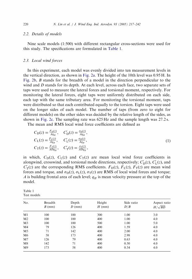
2.2. Details of models
Nine scale models (1:500) with different rectangular cross-sections were used forthis study. The specifications are formulated in Table 1.
2.3. Local wind forces
In this experiment, each model was evenly divided into ten measurement levels inthe vertical direction, as shown in Fig. 2a. The height of the 10th level was 0.95H. InFig. 2b, B stands for the breadth of a model in the direction perpendicular to thewind and D stands for its depth. At each level, across each face, two separate sets oftaps were used to measure the lateral forces and torsional moment, respectively. Formonitoring the lateral forces, eight taps were uniformly distributed on each side,each tap with the same tributary area. For monitoring the torsional moment, tapswere distributed so that each contributed equally to the torsion. Eight taps were usedon the longer sides of each model. The number of taps (from zero to eight fordifferent models) on the other sides was decided by the relative length of the sides, asshown in Fig. 2c. The sampling rate was 625Hz and the sample length was 27.2 s.
The mean and RMS local wind force coefficients are defined as
CDðzÞ ¼FDðzÞAqH
; C0DðzÞ ¼
sDðzÞAqH
;
CLðzÞ ¼FLðzÞAqH
; C0LðzÞ ¼
sDðzÞAqH
;
CTðzÞ ¼FTðzÞADqH
; C0TðzÞ ¼
sTðzÞADqH
;
(1)
in which, CDðzÞ; CLðzÞ and CTðzÞ are mean local wind force coefficients inalongwind, crosswind, and torsional mode directions, respectively; C0
DðzÞ; C0LðzÞ; and
C0TðzÞ are the corresponding RMS coefficients. FDðzÞ; FLðzÞ; FTðzÞ are mean wind
forces and torque, and sDðzÞ; sLðzÞ; sTðzÞ are RMS of local wind forces and torque;A is building frontal area of each level; qH is mean velocity pressure at the top of themodel.
Table 1
Test models
No. Breadth Depth Height Side ratio Aspect ratio
B (mm) D (mm) H (mm) D=B H=ffiffiffiffiffiffiffi
BDp
M1 100 100 300 1.00 3.0
M2 100 100 400 1.00 4.0
M3 100 100 500 1.00 5.0
M4 79 126 400 1.59 4.0
M5 71 142 400 2.00 4.0
M6 58 173 400 2.98 4.0
M7 126 79 400 0.63 4.0
M8 142 71 400 0.50 4.0
M9 173 58 400 0.34 4.0

ARTICLE IN PRESS
H
TF
(b)(a)
DF
LF
Wind
B
D
109 87654321 Level
(c)
0.5D0.207D0.134D 0.134D0.207D0.5D
D DD
D
0.18D 0.18D0.276D 0.276D0.333D 0.333D0.145D 0.145D
0.5D
0.20
7D0.
134D
0.13
4D0.
207D
0.5D
0.18
D0.
276D
0.33
3D0.
18D
0.27
6D0.
333D
0.14
5D0.
145D
0.15
9D0.
159D
0.159D0.159D
Fig. 2. Measurement configurations: (a) measurement levels, (b) local wind forces and (c) tapping
distribution for torsional moment.
N. Lin et al. / J. Wind Eng. Ind. Aerodyn. 93 (2005) 217–242 221
2.4. Base wind forces
A HFBB was employed to measure the base forces and moments on square modelM2. The sampling rate was 161Hz and the sample length was 62 s.
The mean and RMS base force and moment coefficients are defined by
CD ¼ FD
BHqH; C0
D ¼ sDBHqH
;
CL ¼ FL
BHqH; C0
L ¼ sLBHqH
;
CMD¼
FMD
BH2qH
; C0MD
¼sMD
BH2qH
;
CML¼
FML
BH2qH
C0ML
¼sML
BH2qH
;
CMT¼
FMT
B2HqH
; C0MT
¼sMT
B2HqH
;
(2)
in which, CD and CL are base force coefficients; CMD; CML
; and CMTare base
moment coefficients; C0D; C0
L; C0T; C0
MD; C0
ML; and C0
MTare the corresponding RMS
coefficients. FD and FL are base forces; FMD; FML
; and FMTare base moments; sD;
sL; sMD; sML
; and sMTare RMS of base forces and base moments.

ARTICLE IN PRESS
N. Lin et al. / J. Wind Eng. Ind. Aerodyn. 93 (2005) 217–242222
3. Results and discussions
3.1. Pressure measurements
3.1.1. Local wind force coefficients
Local wind forces on a stationary bluff cylinder are functions of the approachflow, the geometrical parameters, and the elevation level. The mean and RMScoefficients of local wind forces at each level of the seven models (M2, M4–M9) withthe same aspect ratio ðD=B ¼ 4Þ but different side ratios, are presented in Fig. 3, andthose of the three square models (M1–M3) with different aspect ratios are presentedin Fig. 4. Since the mean force coefficients for crosswind and torsional directions areclose to zero, only the RMS coefficients are presented here. The force coefficients can
0.05
0.15
0.25
0.35
0.45
0.55
0.65
0.75
0.85
0.95
0.4 0.7 1 1.3 1.6
z/H
D/B=0.34D/B=0.50D/B=0.63D/B=1.00D/B=1.59D/B=2.00D/B=2.98
0.05
0.15
0.25
0.35
0.45
0.55
0.65
0.75
0.85
0.95
0 0.1 0.2 0.3 0.4 0.5 0.6
z/H
0.05
0.15
0.25
0.35
0.45
0.55
0.65
0.75
0.85
0.95
0 0.1 0.2 0.3 0.4 0.5 0.6
z/H
0.05
0.15
0.25
0.35
0.45
0.55
0.65
0.75
0.85
0.95
0 0.1 0.2 0.3 0.4 0.5 0.6
z/H
(a) CD(z) C ′D (z)
C ′T (z)C ′L (z)
(b)
(c) (d)
D/B=0.34D/B=0.50D/B=0.63D/B=1.00D/B=1.59D/B=2.00D/B=2.98
D/B=0.34D/B=0.50D/B=0.63D/B=1.00D/B=1.59D/B=2.00D/B=2.98
Fig. 3. (a–d) Local wind force coefficients of rectangular models.

ARTICLE IN PRESS
0.05
0.15
0.25
0.35
0.45
0.55
0.65
0.75
0.85
0.95
0.4 0.7 1 1.3 1.6
z/H
0.05
0.15
0.25
0.35
0.45
0.55
0.65
0.75
0.85
0.95
0 0.1 0.2 0.3 0.4 0.5 0.6z/
H
0.05
0.15
0.25
0.35
0.45
0.55
0.65
0.75
0.85
0.95
0 0.1 0.2 0.3 0.4 0.5 0.6
z/H
0.05
0.15
0.25
0.35
0.45
0.55
0.65
0.75
0.85
0.95
0 0.1 0.2 0.3 0.4 0.5 0.6
z/H
5/
4/
3/
=
=
=
DBH
DBH
DBH
5/
4/
3/
=
=
=
DBH
DBH
DBH
5/
4/
3/
=
=
=
DBH
DBH
DBH
5/
4/
3/
=
=
=
H
H
H
DB
DB
DB
(a) CD(z) C ′D (z)
C ′T (z)C ′L (z)
(b)
(c) (d)
Fig. 4. (a–d) Local wind force coefficients of square models.
N. Lin et al. / J. Wind Eng. Ind. Aerodyn. 93 (2005) 217–242 223
be directly used in the wind-induced response analysis procedure [8], in which theRMS coefficient is important for both the background and the resonantcomponents. In addition, the variation of local wind force coefficients along theheight of different models indicates the physical flow structure around the isolatedbuildings.
3.1.1.1. Effects of side ratio. The side ratio D=B has a pronounced effect on themean drag force. Fig. 3a shows that the mean drag coefficients at each level increasedslightly with side ratio smaller than 0.63. Above 0.63, the local drag decreased withincreasing side ratio. This suggests that as the side ratio increases beyond a critical

ARTICLE IN PRESS
N. Lin et al. / J. Wind Eng. Ind. Aerodyn. 93 (2005) 217–242224
value, the downstream corners will interfere with the separated shear layers and leadto reduced suction on the rear wall. This critical value of side ratio will change due todifferent free-stream turbulence. Nakamura and Hirata [14] mentioned this influenceof the rear corner on the shear layer and referred to it as the shear-layer–edgeinteraction. This interaction yields a reattachment-type pressure distributioncharacterized by shortened separation bubbles near the front corners followed byrecovery to some higher pressure level near the rear corners. As the side ratioincreases, the interaction is intensified and finally results in steady reattachment.Nakamura [15] argued that this final steady reattachment would be postponed untilthe side ratio increases to about 3.0. On the other hand, from Fig. 3a, the coefficientsbecame constant again as the side ratio exceeds 2.0, indicating that when the depth isabout twice the breadth, the lower limit of wake width, which is approximately thefull width of the body, has been obtained. Side ratio, however, has little influence onthe variation in the vertical direction. All seven curves increase along the height withthe same pattern and attain peak values at the height of 0.85H. The work ofNakamura and Hirata [14] on stationary cylinders showed that the front-wallpressure distribution was almost independent of changing the model depth.Therefore, changes in local drag are caused by changes in rear-wall pressure.
The effect of side ratio on the RMS drag coefficients is relatively small. Thecoefficients at each level are near 0.2 (Fig. 3b). However, it is noted that the modelwith side ratio of 0.63 had the largest RMS local drag coefficients. Thus, both meanand fluctuating drag are expected to be large for a building with the critical sideratio.
Unlike the RMS in alongwind direction, the RMS lift coefficients vary with sideratio as well as with elevation. As the side ratio increases, relatively longer side facesare subjected to bigger imbalanced suctions due to separation, vortex shedding,shear-layer–edge interaction, and reattachment. Larger fluctuating forces occurredat middle and lower levels, especially for the models with side ratios greater than 0.63(Fig. 3c).
The RMS torque consistently increases with the side ratio. The coefficients are allless than 0.15 for all models and are almost constant along the height (Fig. 3d).
3.1.1.2. Effects of the aspect ratio. The mean drag coefficients of square modelsincreased with aspect ratio, while the variation with elevation remains the same (Fig.4a). In Fig. 4b, the RMS drag coefficients (0.2–0.25) changed little with elevation andwere insensitive to aspect ratio, except that the model with the smallest aspect ratio(H=
ffiffiffiffiffiffiffi
BDp
¼ 3) had slightly greater force coefficients at higher levels than the othertwo models. The RMS lift coefficients exceeded 0.4 at middle and lower levels anddecreased to 0.2 at the top (Fig. 4c). The RMS torque was small at 0.05 for squaremodels and was not dependent on aspect ratio (Fig. 4d).
3.1.2. Power spectra of local wind forces
Power spectra of local wind forces were obtained for ten levels on each of the ninemodels. Those at levels 2, 5, and 8 of each model are presented to discuss the effectsof elevation and building geometry. Figs. 5–7 present the alongwind (a), crosswind
ARTICLE IN PRESS
0.001
0.01
0.1
1
10
0.01
0.1
1
10
0.001 0.01 0.1 10.001 0.01 0.1 1
8
5
2
8
5
2
(b) (c)f B/VH f BD/VHf B/VH f
0.001
0.01
0.1
1
10
0.001 0.01 0.1 1
2 level
5 8
(a)
�2
f S (
f)
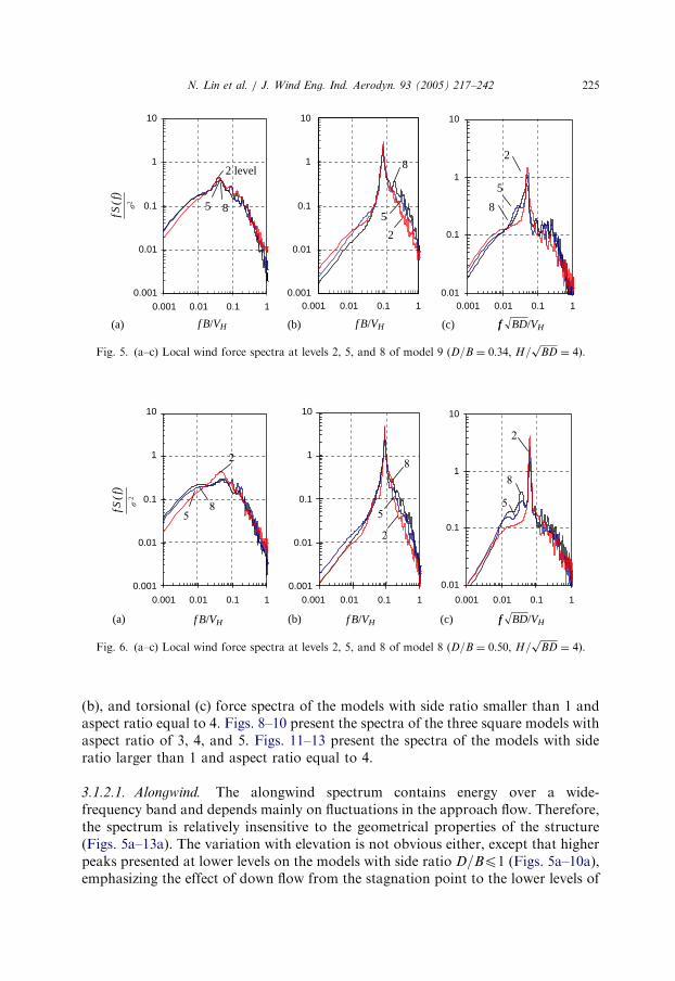
Fig. 5. (a–c) Local wind force spectra at levels 2, 5, and 8 of model 9 (D=B ¼ 0:34; H=ffiffiffiffiffiffiffi
BDp
¼ 4).
0.001 0.01 0.1 1
0.01
0.1
1
10
0.001 0.01 0.1 1
2
5 8
8
5
2
2
5
8
0.001
0.01
0.1
1
10
0.001
0.01
0.1
1
10
0.001 0.01 0.1 1
(b) (c)f B/VH f BD/VHf B/VH f(a)
� 2
f S (
f)
Fig. 6. (a–c) Local wind force spectra at levels 2, 5, and 8 of model 8 (D=B ¼ 0:50; H=ffiffiffiffiffiffiffi
BDp
¼ 4).
N. Lin et al. / J. Wind Eng. Ind. Aerodyn. 93 (2005) 217–242 225
(b), and torsional (c) force spectra of the models with side ratio smaller than 1 andaspect ratio equal to 4. Figs. 8–10 present the spectra of the three square models withaspect ratio of 3, 4, and 5. Figs. 11–13 present the spectra of the models with sideratio larger than 1 and aspect ratio equal to 4.
3.1.2.1. Alongwind. The alongwind spectrum contains energy over a wide-frequency band and depends mainly on fluctuations in the approach flow. Therefore,the spectrum is relatively insensitive to the geometrical properties of the structure(Figs. 5a–13a). The variation with elevation is not obvious either, except that higherpeaks presented at lower levels on the models with side ratio D=Bp1 (Figs. 5a–10a),emphasizing the effect of down flow from the stagnation point to the lower levels of

ARTICLE IN PRESS
0.001 0.01 0.1 1
2
5 8
8
5 2
2
5 8
(a) (b) (c)
1
0.001
0.01
0.1
10
0.001 0.01 0.1 1
1
0.01
0.1
10
1
0.001
0.01
0.1
10�
2
f S (
f )
0.001 0.01 0.1 1
crosswind torsional mode alongwind
Fig. 7. (a–c) Local wind force spectra at levels 2, 5, and 8 of model 7 (D=B ¼ 0:63;H=ffiffiffiffiffiffiffi
BDp
¼ 4).
0.01
0.1
1
10
0.001 0.01 0.1 1
2 5
8
2
5
82
5
8
0.001
0.01
0.1
1
10
0.001
0.01
0.1
1
10
0.001 0.01 0.1 10.001 0.01 0.1 1
(b) (c)f B/VH f BD/VHf B/VH f(a)
�2
f S (
f)
Fig. 8. (a–c) Local wind force spectra at levels 2, 5, and 8 of model 1 (D=B ¼ 1:0; H=ffiffiffiffiffiffiffi
BDp
¼ 3).
N. Lin et al. / J. Wind Eng. Ind. Aerodyn. 93 (2005) 217–242226
the windward wall. For D=B41; however, with relatively smaller width, the flowtends to move around to the sides and reduce the down flow effect, so the spectrumbecomes more insensitive to the elevation (Figs. 11a–13a).
3.1.2.2. Crosswind. Corresponding to a Strouhal number of about 0.1 for sharp-edged cylinders, the crosswind spectrum exhibited a distinct narrow-band peak dueto vortex shedding for models with side ratio D=Bo1: The peak increased with D=B
and attained the highest value at D=B ¼ 0:63 (Figs. 5b–7b). The energy of vortexshedding for the models with D=BX1 was reduced due to the shear-layer–edgeinteraction and the larger the side ratio, the lower and broader the peak of the

ARTICLE IN PRESS
25
8
10
0.1
1
0.01
0.001
0.001 0.01 0.1 1
85
2
10
0.1
1
0.010.001 0.01 0.1 1
2
5
10
0.1
1
0.01
0.0010.001 0.01 0.1 1
8
(a) (b) (c)
� 2
f S (
f )
crosswind torsional mode alongwind
Fig. 10. (a–c) Local wind force spectra at levels 2, 5, and 8 of model 3 (D=B ¼ 1:0; H=ffiffiffiffiffiffiffi
BDp
¼ 5).
10
0.1
0.01
0.001
10
0.1
0.01
0.001
10
1
0.1
0.01
1 1
0.001 0.01 0.1 1 0.001 0.01 0.1 1
1
28
258
8
5
2
0.001 0.01 0.1 1
5
(b) (c)f B/VH f BD/VHf B/VH(a)
�2
f S (
f)
Fig. 11. (a–c) Local wind force spectra at levels 2, 5, and 8 of model 4 (D=B ¼ 1:59; H=ffiffiffiffiffiffiffi
BDp
¼ 4).
2
5 8
0.001 0.01 0.1 1
10
1
0.1
0.01
10
1
0.1
0.01
0.001
25
8
0.001 0.01 0.1 1
10
0.1
0.01
0.001
1
0.001 0.01 0.1 1
25 8
(b) (c)f B/VH f BD/VHf B/VH(a)
�2
f S (
f)
Fig. 9. (a–c) Local wind force spectra at levels 2, 5, and 8 of model 2 (D=B ¼ 1:0; H=ffiffiffiffiffiffiffi
BDp
¼ 4).
N. Lin et al. / J. Wind Eng. Ind. Aerodyn. 93 (2005) 217–242 227
ARTICLE IN PRESS
0.001
0.01
0.1
1
10
0.001
0.01
0.1
1
10
0.001 0.01 0.1 1 0.001 0.01 0.1 1
0.01
0.1
1
10
0.001 0.01 0.1 1
2 85
2
5
8 2
5
8
(a) (b) (c)
� 2
f S (
f )
crosswind torsional mode alongwind
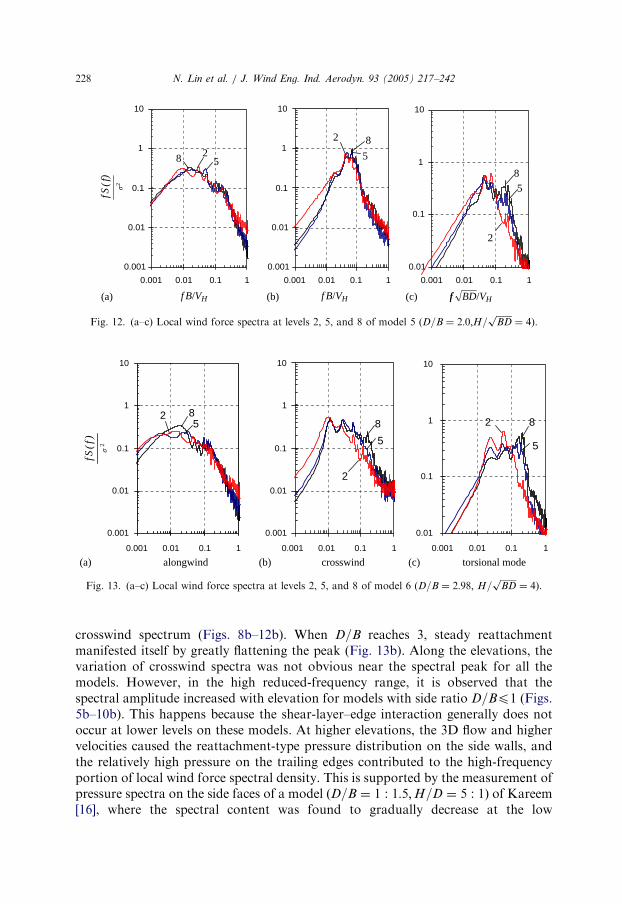
Fig. 13. (a–c) Local wind force spectra at levels 2, 5, and 8 of model 6 (D=B ¼ 2:98; H=ffiffiffiffiffiffiffi
BDp
¼ 4).
0.001
0.01
0.1
1
10
0.001
0.01
0.1
1
10
0.001 0.01 0.1 1
0.01
0.1
1
10
0.001 0.01 0.1 10.001 0.01 0.1 1
258 5
2 8
2
8
5
(b) (c)f B/VH f BD/VHf B/VH f(a)
�2
f S (
f)
Fig. 12. (a–c) Local wind force spectra at levels 2, 5, and 8 of model 5 (D=B ¼ 2:0;H=ffiffiffiffiffiffiffi
BDp
¼ 4).
N. Lin et al. / J. Wind Eng. Ind. Aerodyn. 93 (2005) 217–242228
crosswind spectrum (Figs. 8b–12b). When D=B reaches 3, steady reattachmentmanifested itself by greatly flattening the peak (Fig. 13b). Along the elevations, thevariation of crosswind spectra was not obvious near the spectral peak for all themodels. However, in the high reduced-frequency range, it is observed that thespectral amplitude increased with elevation for models with side ratio D=Bp1 (Figs.5b–10b). This happens because the shear-layer–edge interaction generally does notoccur at lower levels on these models. At higher elevations, the 3D flow and highervelocities caused the reattachment-type pressure distribution on the side walls, andthe relatively high pressure on the trailing edges contributed to the high-frequencyportion of local wind force spectral density. This is supported by the measurement ofpressure spectra on the side faces of a model ðD=B ¼ 1 : 1:5;H=D ¼ 5 : 1Þ of Kareem[16], where the spectral content was found to gradually decrease at the low

ARTICLE IN PRESS
N. Lin et al. / J. Wind Eng. Ind. Aerodyn. 93 (2005) 217–242 229
frequencies and increase at the high frequencies with the distance from theseparation edge.
3.1.2.3. Torsional mode. Fluctuating torque is produced by flow-induced asymme-tries in the lift force and pressure fluctuations on the leeward wall. Because of themultitude of influences, including separation, vortex shedding, reattachment andwake excitation, empirical models for torque spectra are even harder to develop thanmodels for crosswind spectra. Little data is available for the distribution of torquewith elevation. Isyumov and Poole [17] used weighted pneumatic averaging tomeasure mean and fluctuating torque contributions from particular portions of thebuilding perimeter. Although information for the vertical distribution of torque wasnot available, the torque spectra of the 7th level on three models with side ratio of0.5, 1, and 2, were presented [17]. They compare well with the spectra at the 8th levelof similar models in this paper.
Isyumov and Poole [17] concluded that vortex shedding induced pressurefluctuations on the leeward wall, making an important contribution to thefluctuating torque for sections with relatively short after bodies. When the sideratio D=Bo1 (Figs. 5c–7c), distinct peaks in the torque spectra emerged at reducedfrequencies lower than the Strouhal number, highlighting the fluctuation contribu-tion from leeward wall over that from the side faces, where the vortex shedding waspronounced right at the Strouhal number in Figs. 5b–7b. As the side ratio D=B
increases from 0.34 to 0.63, the reduced-frequency peak shifts towards 0.1, indicatingan increasing contribution from the side-wall fluctuation.
When D=B ¼ 1 (Figs. 8c–10c), two peaks appear in the torque spectra. The firstpeak is very close to the reduced frequency of 0.1, indicating the contribution tofluctuating torque from the vortex shedding induced asymmetries in the lift force forsquare models. However, this peak decreased with elevation, indicating that shear-layer–edge interaction on trailing edges at higher levels greatly reduced thecontribution from the sides to this peak. The second peak occurs at higher reducedfrequency, suggesting a more important role in the case of tall buildings. As the highreduced-frequency portion in the crosswind spectrum is mainly contributed from thedownstream zone on the side faces, the second peak in the torsional spectrum is dueto the shear-layer–edge interaction at the downstream edges. The higher theelevation, the larger is the second peak, due to this interaction. Isyumov and Poole[17] measured the torque components at particular portions on three models andnoted similar increased contribution from trailing-edge components to the totaltorque. In addition, the first peak increases with aspect ratio and when the side ratioreaches 5, the first peak at higher levels sharpens (Figs. 8c–10c). This implies that fortall buildings (large aspect ratio), the torque spectra will have large amplitude at thefirst peak over all levels.
When D=B41; the peak near the Strouhal number is further reduced andbroadened. For D=B ¼ 1:6 and 2.0, shear-layer–edge interaction developed at alllevels along the height, and this peak band changed little with elevation (Figs. 11cand 12c). For D=B ¼ 3; however, for the high levels, the first peak was furtherreduced and the second peak increased due to reattachment (Fig. 13c).

ARTICLE IN PRESS
N. Lin et al. / J. Wind Eng. Ind. Aerodyn. 93 (2005) 217–242230
3.1.3. Spanwise correlation of local wind forces
3.1.3.1. Cross-correlation coefficients. Spatial correlation of local wind forces interms of cross-correlation coefficients were analyzed along the elevation of eachmodel. Because of space limits, only the coefficients at zero time-lag with respect tothe top level (Fig. 14) as well as to the bottom level (Fig. 15) of the seven rectangularmodels and those of the three square models (Figs. 16 and 17) are presented.
For the alongwind force, the cross-correlation exponentially decreases withincreasing separation and changes little with elevation. The similarity between Fig.14a and 15a for the rectangular models with different side ratios and the similaritybetween Fig. 16a and 17a for the square models with different aspect ratios indicatethat, for each of the models, the alongwind force cross-coefficient at zero time-lagwith respect to the top level was almost the same as that to the bottom level.Alongwind force cross-correlation is also insensitive to the geometrical parameters,except that the correlation curves with side ratio D=BX2 were lower (Figs. 14a and
0
0.2
0.4
0.6
0.8
1
0 0.2 0.4 0.6 0.8 1
(Z1-Z2)/H
Cro
ss-c
orre
latio
n co
effic
ient D/B=0.34
D/B=0.50D/B=0.63D/B=1.00D/B=1.59D/B=2.00D/B=2.98
0
0.2
0.4
0.6
0.8
1
0 0.2 0.4 0.6 0.8 1
(Z1-Z2)/H
0
0.2
0.4
0.6
0.8
1
0 0.2 0.4 0.6 0.8 1
(Z1-Z2)/H(a) (c)(b)
Fig. 14. Spanwise cross-correlation of local wind forces on rectangular models (with respect to the top
level): (a) alongwind, (b) crosswind and (c) torsional mode.
0
1
0.2
0.4
0.6
0.8
0
1
0.2
0.4
0.6
0.8
0
1
0.2
0.4
0.6
0.8
0 0.2 0.4 0.6 0.8 1
Cro
ss-c
orre
latio
n co
effi
cien
t
(Z1-Z2)/H
Cro
ss-c
orre
latio
n co
effi
cien
t
0 0.2 0.4 0.6 0.8 1
(Z1-Z2)/H
Cro
ss-c
orre
latio
n co
effi
cien
t
0 0.2 0.4 0.6 0.8 1
(Z1-Z2)/H(a) (b) (c)
D/B=0.34D/B=0.50D/B=0.63D/B=1.00D/B=1.59D/B=2.00D/B=2.98
Fig. 15. Spanwise cross-correlation of local wind forces on rectangular models (with respect to the bottom
level): (a) alongwind, (b) crosswind and (c) torsional mode.

ARTICLE IN PRESS
0
0.2
0.4
0.6
0.8
1
0 0.2 0.4 0.6 0.8 1
0
0.2
0.4
0.6
0.8
1
0 0.2 0.4 0.6 0.8 1
0
0.2
0.4
0.6
0.8
1
0 0.2 0.4 0.6 0.8 1
(a)
5/
4/
3/
=
=
=
DBH
DBH
DBH
(b) (c)
Cro
ss-c
orre
latio
n co
effi
cien
t
Cro
ss-c
orre
latio
n co
effi
cien
t
Cro
ss-c
orre
latio
n co
effi
cien
t
(Z1-Z2)/H(Z1-Z2)/H(Z1-Z2)/H
Fig. 17. Spanwise cross-correlation of local wind forces on square models (with respect to the bottom
level): (a) alongwind, (b) crosswind, and (c) torsional mode.
0
0.2
0.4
0.6
0.8
1
0 0.2 0.4 0.6 0.8 1
(Z1-Z2)/H
0
0.2
0.4
0.6
0.8
1
0 0.2 0.4 0.6 0.8 1
(Z1-Z2)/H
0
0.2
0.4
0.6
0.8
1
0 0.2 0.4 0.6 0.8 1
(Z1-Z2)/H(a)
5/
4/
3/
=
=
=
DBH
DBH
DBH
Cro
ss-c
orre
latio
n co
effi
cien
t
Cro
ss-c
orre
latio
n co
effi
cien
t
Cro
ss-c
orre
latio
n co
effi
cien
t
(b) (c)
Fig. 16. Spanwise cross-correlation of local wind forces on square models (with respect to the top level):
(a) alongwind, (b) crosswind and (c) torsional mode.
N. Lin et al. / J. Wind Eng. Ind. Aerodyn. 93 (2005) 217–242 231
15a) and the correlation curve with aspect ratio H=ffiffiffiffiffiffiffi
BDp
¼ 3 was higher (Figs. 16aand 17a) than the correlation curves of the other models.
For the crosswind force, the cross-correlation not only varies with separation, butis also a function of elevation and the geometrical parameters. Comparing Fig. 14band 15b, the cross-correlation slightly increased with decreasing elevation for themodels with D=Bo1:0; while it decreased with elevation for models with D=BX1:0:It is noted, from both Fig. 14b and 15b that when D=Bo1:0 the crosswind forcecross-correlation increased with D=B and attained its highest amplitude when D=B ¼
0:63: From Figs. 16b and 17b, the crosswind force cross-correlation decreased withincreasing aspect ratio.
Compared with those in alongwind and crosswind directions, cross-correlation oftorque decreased faster with increasing separation and is more sensitive to thegeometrical parameters. As for crosswind, torque cross-correlation increased with
ARTICLE IN PRESS
N. Lin et al. / J. Wind Eng. Ind. Aerodyn. 93 (2005) 217–242232
decreasing elevation for the models with D=Bo1:0; while it decreased with elevationfor models with D=BX1:0 (Fig. 14c and Fig. 15c). However, the correlation curvesfor the models with D=BX1:0 presented great variability at low elevations and werevery sensitive to side ratio (Fig. 15c). The effect of aspect ratio shows the torquecross-correlation with respect to the top level decreased with increasing H=
ffiffiffiffiffiffiffi
BDp
(Fig. 16c), similar to the pattern of crosswind cross-correlation (Fig. 16b), while thetorque cross-correlations with respect to the bottom level for the models withH=
ffiffiffiffiffiffiffi
BDp
X2:0 changed little with H=ffiffiffiffiffiffiffi
BDp
(Fig. 17c), similar to the pattern presentedin alongwind direction (Fig. 17a).
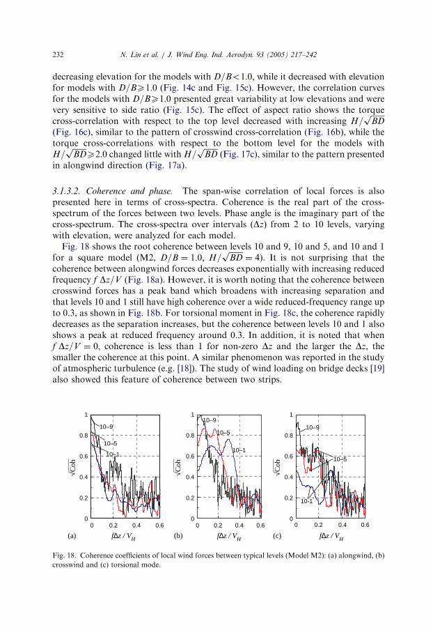
3.1.3.2. Coherence and phase. The span-wise correlation of local forces is alsopresented here in terms of cross-spectra. Coherence is the real part of the cross-spectrum of the forces between two levels. Phase angle is the imaginary part of thecross-spectrum. The cross-spectra over intervals ðDzÞ from 2 to 10 levels, varyingwith elevation, were analyzed for each model.
Fig. 18 shows the root coherence between levels 10 and 9, 10 and 5, and 10 and 1for a square model (M2, D=B ¼ 1:0; H=
ffiffiffiffiffiffiffi
BDp
¼ 4). It is not surprising that thecoherence between alongwind forces decreases exponentially with increasing reducedfrequency f Dz=V (Fig. 18a). However, it is worth noting that the coherence betweencrosswind forces has a peak band which broadens with increasing separation andthat levels 10 and 1 still have high coherence over a wide reduced-frequency range upto 0.3, as shown in Fig. 18b. For torsional moment in Fig. 18c, the coherence rapidlydecreases as the separation increases, but the coherence between levels 10 and 1 alsoshows a peak at reduced frequency around 0.3. In addition, it is noted that whenf Dz=V ¼ 0; coherence is less than 1 for non-zero Dz and the larger the Dz; thesmaller the coherence at this point. A similar phenomenon was reported in the studyof atmospheric turbulence (e.g. [18]). The study of wind loading on bridge decks [19]also showed this feature of coherence between two strips.
(a) (b) (c)
√Coh
√Coh
√Coh
0 0.2 0.4 0.6 0 0.2 0.4 0.6 0 0.2 0.4 0.6
10–9
10–5
10–1
10–9
10–5
10–1
10–9
10–5
10-1
f∆z / VH f∆z / VH f∆z / VH
1
0.8
0.6
0.4
0.2
0
1
0.8
0.6
0.4
0.2
0
1
0.8
0.6
0.4
0.2
0
Fig. 18. Coherence coefficients of local wind forces between typical levels (Model M2): (a) alongwind, (b)
crosswind and (c) torsional mode.
ARTICLE IN PRESS
0 0
(a) (b) (c)
Φ (d
eg)
Φ (d
eg)
Φ (d
eg)
f∆z / VH f∆z / VH f∆z / VH
10–1
10–9
10–5
10–1
10–9
10–510–1
10–9
10–5
0 0.2 0.4 0.6 0 0.2 0.4 0.6 0 0.2 0.4 0.6
180
90
0
−90
−180
180
90
0
−90
−180
180
90
0
−90
−180
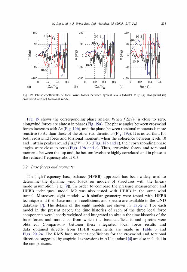
Fig. 19. Phase coefficients of local wind forces between typical levels (Model M2): (a) alongwind (b)
crosswind and (c) torsional mode.
N. Lin et al. / J. Wind Eng. Ind. Aerodyn. 93 (2005) 217–242 233
Fig. 19 shows the corresponding phase angles. When f Dz=V is close to zero,alongwind forces are almost in phase (Fig. 19a). The phase angles between crosswindforces increases with Dz (Fig. 19b), and the phase between torsional moments is moresensitive to Dz than those of the other two directions (Fig. 19c). It is noted that, forboth crosswind force and torsional moment, when the coherence between levels 10and 1 attain peaks around f Dz=V ¼ 0:3 (Figs. 18b and c), their corresponding phaseangles were close to zero (Figs. 19b and c). Thus, crosswind forces and torsionalmoments between the top and the bottom levels are highly correlated and in phase atthe reduced frequency about 0.3.
3.2. Base forces and moments
The high-frequency base balance (HFBB) approach has been widely used todetermine the dynamic wind loads on models of structures with the linear-mode assumption (e.g. [9]). In order to compare the pressure measurement andHFBB techniques, model M2 was also tested with HFBB in the same windtunnel. Moreover, eight models with similar geometry were tested with HFBBtechnique and their base moment coefficients and spectra are available in the UNDdatabase [7]. The details of the eight models are shown in Table 2. For eachmodel in the present paper, the time histories of each of the three local forcecomponents were linearly weighted and integrated to obtain the time histories of thebase forces and moments, from which the base coefficients and spectra wereobtained. Comparisons between these integrated local force results anddata obtained directly from HFBB experiments are made in Table 3 andFigs. 20–24. The RMS base moment coefficients for the crosswind and torsionaldirections suggested by empirical expressions in AIJ standard [4] are also included inthe comparisons.

ARTICLE IN PRESS
Table 3
Comparison between integrated local wind forces and base wind forces on square model M2
Wind force coefficients CD C0D CMD
C0MD
C0L C0
MLC0
MT
Average coefficients (WEI) 1.13 0.22 0.61 0.11 0.37 0.17 0.051
Integrated coefficients (WEI) 1.13 0.18 0.61 0.10 0.33 0.16 0.027
Coefficients by HFBB (WEI) 1.07 0.18 0.59 0.10 0.28 0.14 0.028
Coefficients by HFBB (UND) 0.068 0.12 0.022
Coefficients suggested by AIJ (1996) 0.16 0.054
0.5
0.4
0.3
0.2
0.1
0
0.5
0.4
0.3
0.2
0.1
0
1.2
1.5
0.9
0.6
0.3
0 0.6 1.2 1.8 2.4 3 0 0.6 1.2 1.8 2.4 3 0 0.6 1.2 1.8 2.4 30
Integrated
(a) (b)
IntegratedAverage
(c)
IntegratedAverage
C ′L vs. (D/B)C ′D vs. (D/B)CD vs. (D/B)
Fig. 20. (a–c) Variation of base force coefficients with side ratio.
Table 2
Models from UND database (BL1, a ¼ 0:16)
Shape Breadth Depth Height Side ratio Aspect ratio
B (mm) D (in) H (in) D=B H=ffiffiffiffiffiffiffi
BDp
1–16 6 2 16 0.33 4.62
2–16 6 3 16 0.50 3.77
3–20 6 4 20 0.67 4.08
4–16 4 4 16 1.00 4.00
5–20 4 6 20 1.50 4.08
6–16 3 6 16 2.00 3.77
7–16 2 6 16 3.00 4.62
4–20 4 4 20 1.00 5.00
N. Lin et al. / J. Wind Eng. Ind. Aerodyn. 93 (2005) 217–242234
3.2.1. Base force coefficients
There are two shear forces and three moment components acting on the base of amodel. Since the mean crosswind force and moment and mean torque are negligible,mean alongwind force and moment and all five RMS force components for each of

ARTICLE IN PRESS
0
0.1
0.2
0.3
0.4
0.5
0 0.6 1.2 1.8 2.4 3
Average UND (HFBB)
integrated
Average integrated UND (HFBB)
0
0.1
0.2
0.3
0.4
0.5
0 0.6 1.2 1.8 2.4 3
(b)
(d)
AIJ Eq. (6.6.24)
0
0.2
0.4
0.6
0.8
1
0 0.6 1.2 1.8 2.4 3
integrated
0
0.1
0.2
0.3
0.4
0.5
0 0.6 1.2 1.8 2.4 3
(a)
(c)
AIJ Eq. (6.6.12)
Average integrated UND (HFBB)
C′MD VS. (D/B)
C′ML VS. (D/B) C′MT
VS. (D/B)
CMD VS. (D/B)
Fig. 21. (a–d) Variation of base moment coefficients with side ratio.
N. Lin et al. / J. Wind Eng. Ind. Aerodyn. 93 (2005) 217–242 235
eight models (not including M1, which has no similar shape in the UND database)are presented and compared in Table 3 and Figs. 20 and 21. Also shown in thecomparison are the simple weighted average values of the local RMS forcecoefficients. These averaged coefficients would indicate fluctuating local forces andmoments that are fully correlated.
Table 3 compares the base force coefficients for the square model M2. Theintegrated local wind forces agree with the measurements by HFBB at WEI, exceptthat the mean drag force coefficient and RMS lift force coefficient from HFBB areslightly smaller. Therefore, integrated pressures and HFBB produce consistent baseforce coefficients for linear mode shape. The simple average results of RMScoefficients are larger than the integrated values, because of the assumed spanwisecorrelation of the local forces. This is especially the case for RMS torsional momentcoefficient, where the average coefficient (0.051) is almost twice the integrated value(0.027) and HFBB measurement (0.028). RMS base moment coefficients of shape4–16 from the UND database are smaller than those of the similar model M2,especially for the alongwind direction (0.068). The RMS lift moment coefficient

ARTICLE IN PRESS
0.001
0.01
0.1
1
10
0.001 0.01 0.1 1
integrated(D/B=0.34)
UND (D/B=0.33)
0.001
0.01
0.01 0.1
0.1
1
10
0.001 1
integrated(D/B=0.5)UND (D/B=0.5)
0.001
0.01
0.1
1
10
0.001 0.01 0.1 1
integrated(D/B=0.63)
H:D:B=4:1:1
0.001
0.01
0.1
1
10
0.001 0.01 0.1 1
H:D:B=5:1:1
0.001
0.01
0.1
1
10
0.001 0.01 0.1 1
IntegratedUND
0.001
0.01
0.1
1
10
0.001 0.01 0.1 1
integrated
UND (D/B=1.50)
0.001
0.01
0.1
1
10
0.001 0.01 0.1 1
integrated(D/B=2.0)UND (D/B=2.0)
0.001
0.01
0.1
1
10
0.001 0.01 0.1 1
UND
Integrated
WEI
(HFBB)
(a) (b) (c)
(d) (e)
(f ) (g) (h)
UND (D/B=0.67)
(D/B=1.59)
integrated(D/B=2.98)
UND (D/B=3.0)
Fig. 22. Comparison of derived alongwind base moment spectra and HFBB measurements (the X axis is
fB=V H and the Y axis is fSðf Þ=s2).
N. Lin et al. / J. Wind Eng. Ind. Aerodyn. 93 (2005) 217–242236
suggested by AIJ agrees with that of M2, but RMS torsional moment coefficient(0.054) from AIJ is even larger than the ‘‘fully correlated’’ average value for M2(0.051).

ARTICLE IN PRESS
0.001
0.01
0.1
1
10
0.001 0.01 0.1 1
integrated(D/B=0.34)
0.001
0.01
0.1
1
10
0.001 0.01 0.1 1
integrated
0.001
0.01
0.1
1
10
0.001 0.01 0.1 1
(D/B=0.63)
UND (D/B=0.67)
H:D:B=4:1:1
0.001
0.01
0.1
1
10
0.001 0.01 0.1 1
H:D:B=5:1:1
0.001
0.01
0.1
1
10
0.001 0.01 0.1 1
0.001
0.01
0.1
1
10
0.001 0.01 0.1 1
integrated(D/B=1.59)
UND (D/B=1.50)0.001
0.01
0.1
1
10
0.001 0.01 0.1 1
integrated
UND (D/B=2.0)0.001
0.01
0.1
1
10
0.001 0.01 0.1 1
integrated(D/B=2.98)
UND (D/B=3.0)
UND
WEI
(HFBB)
integrated
(a) (b) (c)
(d) (e)
(f) (g) (h)
(D/B=0.5)UND (D/B=0.5)UND (D/B=0.33)
integrated
UND
integrated
(D/B=2.0)
Fig. 23. Comparison of derived crosswind base moment spectra and HFBB measurements (the X axis is
fB=V H and the Y axis is fSðf Þ=s2).
N. Lin et al. / J. Wind Eng. Ind. Aerodyn. 93 (2005) 217–242 237
Fig. 20 presents the mean drag force, and comparisons of integrated and averagedRMS drag force and RMS lift force coefficients, for seven rectangular models. Meanand RMS drag forces both attained their largest values when the side ratio is 0.63. InFig. 20b, the integrated RMS drag force coefficients are lower than the averagevalues, but the difference is almost the same for each model, reflecting the fact that

ARTICLE IN PRESS
1
0.001
0.01
0.1
10
0.001 0.01 0.1 1
integrated(D/B=0.5)
UND (D/B=0.5)
1
1
0.001
0.01
0.
10
0.001 0.01 0.1 1
integrated(D/B=0.63)
UND (D/B=0.67)
(a) (b) (c)
H:D:B=4:1:1
10.00
0.01
0.1
1
10
0.001 0.01 0.1 1
H:D:B=5:1:1
0.001
0.01
0.1
1
10
0.001 0.01 0.1 1
integrated
UND
WEI
(HFBB)
Integrated
UND
(d) (e)
0.001
0.01
0.1
1
10
0.001 0.01 0.1 1
integrated(D/B=2.98)
UND (D/B=3.0)
(f) (g) (h)
1
1
0.001
0.01
0.
10
0.001 0.01 0.1 1
Intergrated(D/B=0.34)
UND (D/B=0.33)
10.00
0.01
0.1
1
10
0.001 0.01 0.1 1
integrated(D/B=1.59)
UND (D/B=1.50)
000. 1
0.01
0.1
1
10
0.001 0.01 0.1 1
integrated(D/B=2.0)
UND (D/B=2.0)
Fig. 24. Comparison of derived torsional base moment spectra and HFBB measurements (the X axis is
fffiffiffiffiffiffiffi
BDp
=V H and the Y axis is fSðf Þ=s2).
N. Lin et al. / J. Wind Eng. Ind. Aerodyn. 93 (2005) 217–242238
the spanwise correlation of local drag forces is relatively insensitive to the side ratio,as discussed earlier. For the RMS lift force (Fig. 20c), however, the coefficientsincrease as side ratios increase, as do the discrepancies between the integrated and

ARTICLE IN PRESS
N. Lin et al. / J. Wind Eng. Ind. Aerodyn. 93 (2005) 217–242 239
averaged values, which is due to the lower correlation of crosswind forces for themodels with D=BX1:0 compared with D=Bo1:0; as presented in Fig. 15b.
The base moment coefficients from integration are presented in Fig. 21 andcompared with HFBB results from the UND database and the AIJ suggestions.RMS base moments from HFBB are slightly smaller than the integrated local forcevalues for all three directions, while the variation of coefficients with side ratio isquite similar. In the case of RMS crosswind base moment coefficients (Fig. 21c), theintegrated coefficients agree with the AIJ suggestion (Eq. 6.6.12). Note that themodels in this paper were tested in a simulated open country terrain (Category II inAIJ [4]). For urban terrain, the increase of turbulence will cause earlier reattachmenton the sides of models with long afterbodies, resulting in larger fluctuating lift forces.Therefore, it is not unreasonable for AIJ to suggest higher RMS crosswindcoefficients for large side ratio models. However, for RMS torsional moment (Fig.21d), the coefficients suggested by AIJ (Eq. 6.6.24) for models with D=Bp1 areoverestimated. In addition, the average coefficients are close to the integrated valueswhen D=B is small, due to the relatively high spanwise correlation of local torque.When D=BX1; the shear-layer–edge interaction and reattachment on the sides varyalong the elevations and reduce the correlation of torques, as shown in Fig. 15c.Therefore, average torsional coefficients are much bigger than the integrated valuesfor models with D=BX1; and thereby cannot be used in design.
3.2.2. Base force spectra
Figs. 22–24 compare the alongwind, crosswind, and torsional base momentspectra, respectively, with those of the eight similar shapes from the UND database.
For the alongwind direction, the integrated local force spectrum agreeswith that obtained by HFBB at WEI for the square model (M2). However,UND spectrum obtained from HFBB has some discrepancies with theseresults (Fig. 22d). Even though the mean wind speed and turbulence intensityprofiles simulated in the two wind tunnels are comparable, the UND spectra shifttoward a higher reduced-frequency range and have higher magnitudes at the higherfrequency range in comparison with WEI results, for almost all the sectional shapes(Fig. 22). It can be concluded that the two techniques agree with each other in thesame experimental environment, while the alongwind spectrum is very sensitive totest conditions.
For the crosswind direction, results from the two techniques in different windtunnels agree with each other (Fig. 23), especially when D=Bp1: The validity of thedata in this paper and that in the UND database for crosswind base moment spectraare confirmed.
Kareem [16] compared the mode-generalized spectra of torsional loads obtainedfrom the two techniques for a model with D=B ¼ 1 : 1:5; and good agreement wasobtained. Relatively good agreement for the other models is also obtained (Fig. 24).Higher amplitude in the UND curves at higher reduced frequency when D=Bo1(Figs. 24a–e) correspond to the disagreement noted in Figs. 22a–e for alongwinddirection. This appears to confirm the contribution of vortex shedding effects on theleeward wall on the fluctuating torsional moment when D=Bo1: When D=B41;

ARTICLE IN PRESS
N. Lin et al. / J. Wind Eng. Ind. Aerodyn. 93 (2005) 217–242240
better agreement presented in Figs. 24f–h follows the agreement presented inFigs. 23a–e, confirming the significant contribution of the asymmetries in the liftforce to the fluctuating torsional moment. For square models, both HFBBmeasurements in the two wind tunnels are a little lower than the integrated valuesat the peaks (Figs. 24d and e).
3.2.3. Coherence and phase of base force components
The ten cross-spectra between the five force components at the base of the squaremodel M2 were analyzed. The alongwind force is almost fully correlated with thealongwind moment and the crosswind force is almost fully correlated with thecrosswind moment. The crosswind force and moment are highly correlated with thetorsional moment. The correlations of the other six pairs of force components are allnegligible. Fig. 25 shows the root coherence and phase between the alongwind forceand moment. Fig. 26 shows those between the alongwind and crosswind moments.And Fig. 27 shows these between crosswind and torsional moments. The coherence(Fig. 27a) reaches a peak near the Strouhal number (0.1) and shows an abrupt dip ata reduced frequency of about 0.12 where there is an 1801 phase shift (Fig. 27b). Asimilar finding was reported in [20].
Coh
(a) (b)0 0.1 0.2 0.3 0.4 0.5 0.60 0.1 0.2 0.3 0.4 0.5 0.6
1
0.8
0.6
0.4
0.2
0
180
90
0
-90
-180
fB / VH fB / VH
Φ (d
eg)
Fig. 25. (a, b) Coherence and phase between alongwind force and moment (Model M2).
Coh
0 0.2 0.4 0.6 0 0.2 0.4 0.6
1
0.8
0.6
0.4
0.2
0
180
90
0
−90
−180
fB / VH fB / VH(a) (b)
Φ (d
eg)
Fig. 26. (a, b) Coherence and phase between alongwind and crosswind moments (Model M2).

ARTICLE IN PRESS
Coh
(a) (b)
0 0.1 0.2 0.3 0.4 0.5 0.6 0 0.1 0.2 0.3 0.4 0.5 0.6
1
0.8
0.6
0.4
0.2
0
180
90
0
−90
−180
fB / VH fB / VH
Φ (d
eg)
Fig. 27. (a, b) Coherence and phase between crosswind and torsional moments (Model M2).
N. Lin et al. / J. Wind Eng. Ind. Aerodyn. 93 (2005) 217–242 241
4. Concluding remarks
This paper summarizes the findings of an extensive wind-tunnel study on localwind forces on isolated tall buildings. Based on experimental results on nine squareand rectangular models, comparing with information in the literature and anotherdatabase (UND), the following conclusions are made:
(1)
The effects of three parameters, side ratio, aspect ratio, and elevation werehighlighted in analyses of local wind force coefficients, spectra, and spanwisecross-correlation. Side ratio D=B; 0.63�3 in this study, greatly influences thebluff-body flow and the wind loads. Side ratio of stationary cylinders with certainfree-stream turbulence has a critical value (close to 0.63 here). At this critical sideratio, mean and RMS drag coefficients, peak of crosswind spectrum, and thecrosswind cross-correlation attain their maximum values. Above the critical sideratio, these values will be reduced due to the shear-layer–edge interaction andfurther reattachment. The variation of the shear-layer–edge interaction alongelevation levels is responsible for the variation of crosswind spectra, torsionalspectra, and the spanwise cross-correlation of these two force components.Torsional spectrum and torsional cross-correlation are very sensitive to all of thethree parameters.(2)
With the linear-mode shape assumption, the two measurement techniques,integrated simultaneous point pressures and HFBB, agree for base force andmoment spectra. The UND database effectively provides the base momentspectra for preliminary design and can be expanded on the Internet by thedataset here and by other experimental results in the future.(3)
For structures with non-linear sway mode shapes, however, HFBB approachmay be inaccurate, providing only base moment coefficients and spectra and nottheir variation with height. From the local wind force coefficients presented here,further work is intended to develop empirical expressions of local wind forcespectra, spatial correlation, and coherence, which can be used to simulate timehistories of fluctuating local and overall wind forces on tall buildings.
ARTICLE IN PRESS
N. Lin et al. / J. Wind Eng. Ind. Aerodyn. 93 (2005) 217–242242
Acknowledgments
Grateful acknowledgement is owed to Mr. A. Sasaki of Nishimatsu Corporationand Mr. A. Katsumura of Tokyo Polytechnic University. Without their support andinvaluable suggestions this experiment would not have been feasible. Dr. XinzhongChen of Texas Tech University is also greatly acknowledged for his comments andsuggestions.
References
[1] A. Sasaki, A. Katsumura, J. Katagiri, B. Liang, S. Suganuma, Y. Tamura, Local wind forces acting
on rectangular prisms, Proceedings of 14th National Symposium on Wind Engineering,
4–6 December 2003, Japan Association for Wind Engineering, Tokyo, pp. 263–268 (in Japanese).
[2] A. Kareem, Lateral-torsional motion of tall buildings to wind loads, J. Struct. Eng., ASCE 111 (11)
(1985) 2479–2496.
[3] American Society of Civil Engineers (ASCE), ASCE 7–02 Minimum Design Loads for Buildings and
Other Structures, Reston, Va, 2002.
[4] Architectural Institute of Japan (AIJ), Recommendations for loads on Buildings, 1996.
[5] Standards Australia AS/NZS 1170.2:2002, Structural Design Actions, Part 2, Wind Actions, Sydney,
2002.
[6] H. Choi, J. Kanda, Proposed formulae for the power spectral densities of fluctuating lift and torque
on rectangular 3-D cylinders, J. Wind Eng. Ind. Aerodyn. 46/47 (1993) 507–516.
[7] NatHaz Modeling Laboratory, University of Notre Dame, Aerodynamic loads database, http://
www.nd.edu/�nathaz/, 2003.
[8] Y. Zhou, T. Kijewski, A. Kareem, Aerodynamic loads on tall buildings: interactive database,
J. Struct. Eng., ASCE 129 (3) (2003) 394–404.
[9] T. Kijewski, A. Kareem, Dynamic wind effects: a comparative study of provisions in codes and
standards with wind tunnel data, Wind Struct. 1 (1) (1998) 77–109.
[10] A. Kareem, Model for prediction of the acrosswind response of buildings, Eng. Struct. 6 (2) (1984)
136–141.
[11] Y. Tamura, A. Wada, T. Ohkoshi, M. Kawamura, Simulation of wind-induced vibrations of tall
buildings. Summaries of Technical Papers of Annual Meeting, Architectural Institute of Japan,
Structures I, 1988 (in Japanese).
[12] H. Tsukagoshi, Y. Tamura, A. Sasaki, H. Kanai, Response analyses on along-wind and across-wind
vibrations of tall buildings in time domain, J. Wind Eng. Ind. Aerodyn. 46/47 (1993) 497–506.
[13] A. Kareem, J.E. Cermak, Pressure fluctuations on a square building model in boundary-layer flows,
J. Wind Eng. Ind. Aerodyn. 16 (1984) 17–41.
[14] Y. Nakamura, K. Hirata, Critical geometry of oscillating bluff bodies, J. Fluid Mech. 208 (1989)
375–393.
[15] Y. Nakamura, Bluff-body aerodynamics and turbulence, J. Wind Eng. Ind. Aerodyn. 49 (1993)
65–78.
[16] A. Kareem, Measurements of pressure and force fields on building models in simulated atmospheric
flows, J. Wind Eng. Ind. Aerodyn. 36 (1990) 589–599.
[17] N. Isyumov, M. Poole, Wind induced torque on square and rectangular building shapes, J. Wind
Eng. Ind. Aerodyn. 13 (1983) 183–196.
[18] N.O. Jensen, Atmospheric boundary layers and turbulence, in: A. Larsen, A. Larose, A. Livesey
(Eds.), Wind Engineering into the 21st Century, Balkema, Rotterdam, 1999, pp. 29–42.
[19] G.L. Larose, J. Mann, Gust loading on streamlined bridge decks, J. Fluids Struct. 12 (1998) 511–536.
[20] A. Tallin, B. Ellingwood, Wind induced lateral-torsional motion of buildings, J. Struct. Eng. 111 (10)
(1985).