This art icle was downloaded by: [ University of Essex] , [ Bowen Lu]On: 08 July 2011, At : 05: 06Publisher: Taylor & FrancisI nforma Ltd Registered in England and Wales Registered Number: 1072954 Registered office: Mort imer House,37-41 Mort imer St reet , London W1T 3JH, UK

International Journal of Systems SciencePublicat ion det ails, including inst ruct ions for aut hors and subscript ion informat ion:ht t p: / / www. t andfonl ine.com/ loi/ t sys20

Mobile sensor networks for modelling environmentalpollutant distributionBowen Lu a , John Oyekan a , Dongbing Gu a , Huosheng Hu a & Hossein Farid Ghassem Nia a

a School of Comput er Science and Elect ronic Engineering, Universit y of Essex, WivenhoePark, Colchest er, UK

Available onl ine: 1 January 2011

To cite this article: Bowen Lu, John Oyekan, Dongbing Gu, Huosheng Hu & Hossein Farid Ghassem Nia (2011): Mobilesensor net works for model l ing environment al pol lut ant dist ribut ion, Int ernat ional Journal of Syst ems Science,DOI:10.1080/ 00207721.2011.572198

To link to this article: ht t p: / / dx.doi.org/ 10.1080/ 00207721.2011.572198

PLEASE SCROLL DOWN FOR ARTI CLE

Full terms and condit ions of use: ht tp: / / www.tandfonline.com/ page/ terms-and-condit ions

This art icle may be used for research, teaching and private study purposes. Any substant ial or systemat icreproduct ion, re-dist r ibut ion, re-selling, loan, sub- licensing, systemat ic supply or dist r ibut ion in any form toanyone is expressly forbidden.

The publisher does not give any warranty express or implied or make any representat ion that the contentswill be complete or accurate or up to date. The accuracy of any inst ruct ions, form ulae and drug doses shouldbe independent ly verified with pr imary sources. The publisher shall not be liable for any loss, act ions, claims,proceedings, demand or costs or damages whatsoever or howsoever caused arising direct ly or indirect ly inconnect ion with or ar ising out of the use of this m aterial.

International Journal of Systems Science

2011, 1–15, iFirst

Mobile sensor networks for modelling environmental pollutant distribution

Bowen Lu*, John Oyekan, Dongbing Gu, Huosheng Hu and Hossein Farid Ghassem Nia

School of Computer Science and Electronic Engineering, University of Essex, Wivenhoe Park, Colchester, UK

(Received 2 September 2010; final version received 23 February 2011)

This article proposes to deploy a group of mobile sensor agents to cover a polluted region so that they are able toretrieve the pollutant distribution. The deployed mobile sensor agents are capable of making point observation inthe natural environment. There are two approaches to modelling the pollutant distribution proposed in thisarticle. One is a model-based approach where the sensor agents sample environmental pollutant, build up anenvironmental pollutant model and move towards the region where high density pollutant exists. The modellingtechnique used is a distributed support vector regression and the motion control technique used is a distributedlocational optimising algorithm (centroidal Voronoi tessellation). The other is a model-free approach where thesensor agents sample environmental pollutant and directly move towards the region where high density pollutantexists without building up a model. The motion control technique used is a bacteria chemotaxis behaviour.By combining this behaviour with a flocking behaviour, it is possible to form a spatial distribution matched to theunderlying pollutant distribution. Both approaches are simulated and tested with a group of real robots.

Keywords: mobile sensor network; model-based; model-free; pollutant monitoring

1. Introduction

Environmental pollutant distribution is a spatial

phenomenon. Modelling spatial phenomena requires

a distributed sensing capability of wireless mobile

sensor networks. There has been a number of research

projects in climatology, forestry and oceanography for

modelling environmental spatial phenomena (Merino,

Caballero, de Dios, and Ferruz 2006; Corrigan,

Roberts, Ramana, Kim, and Ramanathan 2007;

Leonard et al. 2007). The distribution nature of

mobile sensor agents in the natural environment

could be used to monitor pollutants more efficiently

and reliably, and could also be used to form a visual

representation of the pollutant. The importance of

forming a visual representation of the pollutant

becomes more obvious if the pollutant is invisible

and hazardous to human health. Such visual informa-

tion could enable emergency services strategically

evacuate populated areas in the event of a leak

especially if resources are scarce.

Recently, learning an environmental spatial func-

tion and optimising coverage control simultaneously

has attracted many researchers’ attention. Different

combinations between learning algorithms and cover-

age control algorithms have been researched. Lloyd’s

algorithm for optimising centroidal Voronoi tessella-

tion (CVT ) has been used as a locational optimising

algorithm in Cortes, Martinez, Karatas, and Bullo

(2004) and Pimenta, Kumar, Mesquita, and Pereira

(2008), where the environmental spatial function is

established as a prior knowledge. Using Lloyd’s

algorithm for coverage control with a radial basis

function (RBF ) neural network learning an environ-

mental spatial function has been implemented in

Schwager, Rus, and Slotine (2009). A consensus

algorithm is required to maintain the distributed

implementation.

With RBF neural networks, flocking algorithm is

another choice for coverage control, as has been

implemented in Lynch, Schwartz, Yang, and

Freeman (2008). Besides RBF neural networks, the

environmental spatio-temporal function can be learnt

by using a Kriging Kalman filter with a CVT coverage

control in Cortes (2009) and with a flocking coverage

control algorithm in Choi, Lee, and Oh (2008). A

Kalman filter and a weighting interpolation method

have been used to learn an environmental spatial

function in Martinez (2010). All these are model-based

approaches where a model needs to be built up first

based on sampled observations and then mobile agents

make their decisions to move based on the model. At

the early stage of the process, the model is not perfect

due to lack of information. Gradually, the perfor-

mance can be improved when mobile sensor agents

move closer to the source and the model is more

accurate.

*Corresponding author. Email: blv@essex.ac.uk

ISSN 0020–7721 print/ISSN 1464–5319 online

� 2011 Taylor & Francis

DOI: 10.1080/00207721.2011.572198

http://www.informaworld.com

Dow

nloa

ded

by [

Uni

vers

ity o

f E

ssex

], [

Bow

en L

u] a

t 05:

06 0

8 Ju

ly 2

011

There has also been an interest in the use of

model-free approaches to provide coverage control to

an environmental spatio-temporal function as in

Mesquita, Hespanha, and Astrom (2008) and

Oyekan, Hu, and Gu (2010). This involves the use of

a source seeking controller in combination with a

flocking controller. The source seeking controller is

used to drive the mobile agents towards the source of

environmental spatio-temporal function in the envir-

onment without the need to rely on models. As a result,

inaccuracies in controlling the agents in the early stage

of process are avoided. Many researchers have

investigated the use of bacteria chemotaxis behaviours

as a source seeking controller. The bacteria chemotaxis

behaviour is a stochastic optimisation approach to

seeking to find the extremum of a function. Dhariwal,

Sukhatme, and Requicha (2004) has used a bacteria

chemotaxis behaviour as a basis for developing the

controller. Marques, Nunes, and Almeida (2002) have

investigated the use of a silkworm moth algorithm and

a direct gradient following method on a robot.

Other approaches of source seeking behaviours

include Baronov and Baillieul’s work in Baronov and

Baillieul (2008) where a reactive controller can

navigate a single, sensor-enabled vehicle to ascend or

descend a scalar potential field. Mayhew, Sanfelice,

and Teel (2008) have used a hybrid controller that

combines a line minimisation-based algorithm and a

vehicle path planning algorithm to find the

extremum of a function. Their approach does not

need the agent’s position information or any knowl-

edge of the function to be mapped a prior. Lilienthal

and Duckett (2003) have used a Braitenberg vehicle

approach to find an ethanol source in their own

experiments.

In this article, we investigate the use of a

model-based approach and a model-free approach

and propose two novel algorithms for modelling

environmental pollutants using mobile sensor net-

works. The first one we used (SVR-CVT ) is based on

a distributed support vector regression (SVR) com-

bined with a CVT algorithm, which is a model-based

approach. Focusing on an instance of environmental

pollutant samples, our proposed SVR-CVT algorithm

can cover as much as the most polluted area and

produce an estimated pollutant spatial model. SVR is a

method for solving the function regression problem

(Smola and Scholkopf 2004). This method is able to

find a global minimum as it can be formulated in a

constrained quadratic optimisation problem. The

research of using kernel methods for function regres-

sion over sensor networks has been already conducted

in Predd, Kulkarni, and Poor (2006).

With the property of additive structure, the

minimisation problem has been solved using an

incremental sub-gradient method in Rabbat and

Nowak (2006). The incremental sub-gradient method

is proposed working in a sequential way with the need

of constructing a message passing path. Constructing a

message passing path is not scalable and robust in

wireless sensor networks. In our proposed SVR-CVT

algorithm, a distributed or parallel version is devel-

oped, which can directly be applied for wireless sensor

networks without the need for constructing a message

passing path. Our distributed algorithm is built on a

finite support kernel function in SVR. It only requires

local communication capability of wireless sensor

networks between neighbour sensor agents. In contrast

to the consensus algorithm used in RBF neural

networks, which requires multiple information

exchanges to achieve the consensus on interested

values among the neighbours at each time step, this

local algorithm requires one information exchange at

each time step and thus less intensive local commu-

nication. With the established model, the CVT algo-

rithm is able to control mobile sensor agents to move.

The second one we used (BCT-FLK ) is based on a

bacteria chemotaxis behaviour (BCT ) combined with

a flocking algorithm, which is a model-free approach.

Bacterial chemotaxis behaviour can make agents

swarm with a certain nutrition distribution, as in

Mesquita et al. (2008), that is consistent with the

environmental pollutant distribution so that even if the

pollutant distribution is invisible to the human eye, it is

possible to be observed by visible agent distribution.

The Berg and Brown model was chosen over other

complex models such as Yi, Huang, Simon, and Doyle

(2000) because of its ease of analysis and its ability to

find the source of a pollutant using a random walk

method. In addition, the parameters of this behaviour

model offers the user of the system a potential ability

to control mobile sensor agents to balance the

exploration and exploitation behaviours in order to

avoid local minima (Oyekan and Hu 2010) without the

need to model the environmental pollutant distribu-

tion. The mobile sensor agents obtain concentration

readings of the environmental spatio-temporal func-

tion such as pollution on the spot and use the readings

to calculate the gradient of the function. Also a

flocking behaviour is integrated with the bacteria

chemotaxis behaviour to keep the mobile sensor

agents moving as a group without collision.

Both approaches are simulated with multiple

mobile sensor agents. A testing platform has been set

up in our lab where six networked robots (wifibots) are

used to test two approaches. Due to the lack of real

pollutant data and realistic pollutant models, several

smooth mathematical functions are used as the

pollutant distribution in simulations and even in real

tests. In the following sections, Section 2 presents

2 B. Lu et al.

Dow

nloa

ded

by [

Uni

vers

ity o

f E

ssex

], [

Bow

en L

u] a

t 05:

06 0

8 Ju

ly 2

011

SVR-CVT algorithm and Section 3 presents BCT-FLK

algorithm. The simulation results are given in

Section 4. The experimental results are provided in

Section 5. Finally, our conclusion and future work are

given in Section 6.

2. The model-based approach

2.1. Distributed SVR

In an SVR algorithm, the problem is defined as

follows. Q�R2 is a 2D convex environment for a

sensor network with N agents. An arbitrary point in it

is denoted by q. The ith agent’s position in Q is denoted

by qi¼ [xi, yi]T, and zi denotes a sensory observation of

ith agent (i¼ 1, . . . ,N ). The sample set of sensory

observation is defined as S ¼ ðqiT, ziÞ

Ni¼1. Finding a

function f (q)¼wT�(q)þ b, which can give a regression

result to the sample set S with a limited error ", is the

goal of "-SVR (Vapnik 1999). �(q) is a feature space

function, which maps q from R2 to a higher-dimen-

sional space. b is a biased constant. Weight parameter

w can be found by solving the following constrained

convex optimising problem (Smola and Scholkopf

2004):

minw,�i,�

�i

1

2wTwþ C

�

X

N

i¼1

�i þX

N

i¼1

��i

�

( )

ð1Þ

subject to

zi � hw,�ðqiÞi � b � "þ �i

hw,�ðqiÞi þ b� zi � "þ ��i

�i, ��i � 0

8

>

<

>

:

where h�, �i denotes inner products. �i and ��i are slack

variables, and constant C4 0 is a scaler of slack

variables. These three parameters determine the trade-

off between the flatness of regression function f and the

error " tolerance. For solving this problem with the

inequality constraints, a dual optimisation problem

should be solved (Smola and Scholkopf 2004):

min�i,�

�i

J ¼1

2

X

N

i,j¼1

ð�i � ��i Þð�j � ��j ÞKðqi, qj Þ

þ "X

N

i¼1

ð�i þ ��i Þ �X

N

i¼1

zið�i � ��i Þ ð2Þ

subject to

X

N

i¼1

ð�i � ��i Þ ¼ 0

0 � �i,��i � C

8

>

<

>

:

where �i and ��i are non-negative Lagrange multipliers,

and weight parameter w can be obtained from the

equation below:

w ¼X

N

i¼1

ð�i � ��i Þ�ðqiÞ ð3Þ

With the above equations, the regression function

f (q)¼wT�(q)þ b can be reformulated as below:

f ðqÞ ¼X

N

i¼1

ð�i � ��i Þh�ðqiÞ,�ðqÞi þ b ð4Þ

In (4), h�(qi),�(q)i can be replaced with a kernel

function by using the kernel trick. A kernel function

K(qi, qj) for SVR needs to satisfy Mercer’s conditions:

(1) K(qi, qj) is continuous;

(2) K(qi, qj) is symmetrical K(qi, qj)¼K(qj, qi);

(3) K(qi, qj) is semi-positive definite.

Choosing a kernel function for SVR depends on the

underlying spatial property and the prior knowledge

about the underlying function. The following

modified cosine function (5) is selected for our SVR

algorithm.

Kðqi,qj Þ ¼

1

21þ cos

�kqi�qj k

B

� �� �

, kqi�qj k2 ½0,B�

0, otherwise

8

<

:

ð5Þ

This function has a finite support with radius equal to

B, and B’s value is related to the wireless communica-

tion range of each agent. In our simulations and

experiments, this kernel function provides a good

performance. With the selected kernel function, the

regression function is converted as below:

f ðqÞ ¼X

N

i¼1

ð�i � ��i ÞKðqi, qÞ þ b ð6Þ

A sequential method for solving �, ��i and b has been

given by Vijayakumar and Wu (1999). It is an

incremental sub-gradient algorithm. Basically the

gradient of each sample data, constrained by

the constraints on the parameters, is used to update

the parameters. It can be converted into a distributed

or parallel algorithm using the finite support kernel

function. The distributed algorithm maintains a

regression function f (q) in each node i.

f ðqÞ ¼X

j2Ni[i

ð�i � ��i ÞKðqj, qÞ þ b ð7Þ

International Journal of Systems Science 3

Dow

nloa

ded

by [

Uni

vers

ity o

f E

ssex

], [

Bow

en L

u] a

t 05:

06 0

8 Ju

ly 2

011

where Ni is the set of neighbour sensor agents of i. Our

distributed SVR learning algorithm is showed as in

Algorithm 1.

Algorithm 1: Distributed SVR algorithm

Initialise �i ¼ 0, ��i ¼ 0, t ¼ 0

Loops until the terminal condition is met:

Each sensor node obtains the distance kqi� qjk

from its neighbour set Ni

Each sensor node calculates the kernel function

K(qi, qj)

Ei ¼ zi �P

j2Ni[ið�i � ��i Þ½Kðqi, qj Þ þ �2�

��i¼min{max[�(Ei� "), ��i],C� �i}

���i ¼ minfmax½�ð�Ei � "Þ,���i �,C� ��i g

Update �i¼ �iþ ��iUpdate ��i ¼ ��i þ ���it tþ 1

end

2.2. Distributed CVT

In a CVT algorithm, the location is optimised based

on a Voronoi graph. A sensor agent position qi in a

convex space Q is termed as a generating point. An

arbitrary point in Q is denoted by q. The ith sensor’s

Voronoi cell Vi is defined as below:

Vi ¼ q 2 Qj q� qi�

�

�

� � q� qj�

�

�

�, 8i 6¼ j

ð8Þ

CVT is a special Voronoi tessellation, in which each

generating point moves forward to the mass centre of

each Voronoi cell. In our research, the mass is related

with pollutant distribution. The optimisation algo-

rithm of CVT is able to move the sensor agents

towards the high concentration region while still

located inside one of the Voronoi cells. Finally, all

the sensor agents are distributed in the monitoring

environment according to the pollutant distribution.

To develop a distributed CVT, the limited wireless

communication range of each agent is utilised to

redefine a range-limited Voronoi region Wi (Cortes

and Bullo 2005):

Wi ¼ fq 2 Qj�i \ Vig

where �i¼ {q2Qjkqi� qk�B} is a circle region of

radius B for agent i. The cost function of locational

optimisation problem is defined as Schwager et al.

(2009):

Hð p1, . . . , pnÞ ¼X

n

i¼1

Z

Wi

1

2q� pi

�

�

�

�

2f ðqÞdq ð9Þ

The following definitions are used:

MWi¼

Z

Wi

f ðqÞdq

LWi¼

Z

Wi

qf ðqÞdq

CWi¼

LWi

MWi

where MWi, LWi

and CWidenote the mass, first

moment and mass centre of the ith range-limited

Voronoi cell. The gradient of the cost function is used

as the controller for mobile sensor agents:

ui ¼ �@H

@qi

¼ MWiðCWi

� qiÞ ð10Þ

where ui is ith agent’s speed input and is a step length

of agent motion. The distributed CVT algorithm is

given in Algorithm 2:

Algorithm 2: Distributed CVT algorithm

Initialise MWi¼ 0,LWi

¼ 0

Agent qi is randomly located at a certain region

Loops until the terminal condition is met:

Sample environmental variable ziExecute the distributed SVR algorithm

Obtain the updated f (q) from SVR

MWi¼

R

Wif ðqÞdq

LWi¼

R

Wiqf ðqÞdq

Calculate the new mass centre CWi¼ LWi

=MWi

Move qi towards CWiwith a certain speed

end

3. The model-free approach

3.1. BCT behaviour

Based on the Berg and Brown model (Brown and Berg

1974), a bacterium motion is composed of a combina-

tion of tumble and run phases. The frequency of these

phases depends on the measured concentration gradi-

ent in the surrounding environment. The run phase is

generally a straight line while the tumble phase is a

random change in direction with a mean of about 68

in the E. Coli bacterium. If the bacterium is moving up

a favourable gradient, it tumbles less thereby increas-

ing the length of the run phase and vice versa if going

down an unfavourable gradient. This behaviour was

formulated by Berg and Brown by fitting the results

of their experimental observations with a best

4 B. Lu et al.

Dow

nloa

ded

by [

Uni

vers

ity o

f E

ssex

], [

Bow

en L

u] a

t 05:

06 0

8 Ju

ly 2

011

fit equation:

¼ 0 exp �d �Pb

dt

� �

d �Pb

dt¼

1

m

Z t

�1

dPb

dexp

� t

m

� �

d

dPb

dt¼

kD

ðkD þ C Þ2dz

dt

ð11Þ

where is the mean run time and 0 is the mean run

time in the absence of concentration gradients. � is a

constant of the system based on the chemotaxis

sensitivity factor of the bacteria. Pb is the fraction of

the chemical receptor bound at concentration z. z is the

present concentration reading taken by the sensor

agent. kD is the dissociation constant of the bacterial

chemoreceptor. d�Pb

dtis the weighted rate of change of Pb.

m is the time constant of the bacterial system.

The above equations determine the time between

tumbles and hence the length of runs between tumbles.

During the tumble phase, the agent can randomly

choose a range of angles in the set � 2 {0, . . . , 360}. The

range of the angle makes it possible for the mobile

sensor agents to backtrack if there is a favourable

gradient behind them. From above, it can

be summarised that the higher the pollutant level, the

smaller the length of runs between tumbles and the

smaller the pollutant level, the higher the length

of runs.

During the run phase, the speed function of BCT

behaviour is based upon the ideal gas law and the

Graham’s gas law of diffusion. The ideal gas law states

that by increasing the temperature of a gas system, a

larger volume is occupied by the gas. The Graham’s

gas law of diffusion states that the rate of diffusion of a

gas is inversely proportional to its density. Following

these laws, a speed function ubi of BCT behaviour as

below results:

ubi ¼u0T

zi

where u0 is the standard speed without any reading.

By using the BCT behaviour, each agent can be

viewed as a randomly vibrating gas molecule with bias

towards the source of the pollutant. By increasing T,

each agent vibrates more so that the distance covered

by each of the bacteria is increased per unit time and

the sensor agents spread more across the area of the

pollutant. As zi increases, the speed ubi of the bacteria

reduces making it dwell in areas of ‘rich food’ source.

A higher pollutant reading means smaller agent

vibration resulting in a small area covered whilst a

lower pollutant reading results in higher agent vibra-

tion resulting in a larger area being covered.

More detailed information on BCT behaviour can be

found in our previous publications (Oyekan et al. 2010;

Oyekan and Hu 2010).

3.2. Flocking behaviour

The flocking behaviour is used to keep the agents

together with a certain distance between each other

and to aid each individual ‘bacteria’ agent in finding

the source of the pollutant through group reinforce-

ment foraging. For the flocking behaviour, a general-

ised Morse potential given below is used.

ufi ¼ GG GR exp �

r

20

� �

� GA exp �r

20

� �� �

where the repulsion gain GR¼ 1 and the attractant gain

GA¼ 0.99 are used in our simulations and experiments,

and r is the Euclidean distance between two mobile

agents. It was discovered that it is possible to control

how closely the agents get to each other whilst not

colliding by adjusting the GG gain.

The outputs from the bacteria chemotaxis and

flocking behaviours are fused together to generate a

final speed control output ui for agent i:

ui ¼ GFufi þ GBu

bi

where the gains of GB¼ 0.8 and GF¼ 0.8 are used in

our simulations and experiments.

4. Simulation results

In the simulations, each agent knew its position in the

simulated arena. Only local communication between

neighbour sensor agents was allowed to exchange

information. For the SVR-CVT algorithm, the

exchanged information includes agent position and

model parameters. For the BCT-FLK algorithm, the

exchanged information includes agent position only.

4.1. SVR-CVT results

The simulation environment was constructed in a 1 1

area. The targeted pollutant distribution was a static

function with doughnut shape:

f ðqÞ ¼ 0:5 exp �ðx� 0:5Þ2 þ ð y� 0:5Þ2

�21

� �

� 0:5 exp �ðx� 0:5Þ2 þ ð y� 0:5Þ2

�22

� �

where �21 ¼ 0:07 and �2

2 ¼ 0:025. A mobile sensor

network with N¼ 25 agents was used, and the

communication range of each agent was set to 0.2.

The SVR algorithm with 10 loops was nested in each

iteration of the CVT algorithm.

International Journal of Systems Science 5

Dow

nloa

ded

by [

Uni

vers

ity o

f E

ssex

], [

Bow

en L

u] a

t 05:

06 0

8 Ju

ly 2

011

At the beginning of this simulation, 25 agents were

randomly deployed at a corner of the simulation

environment, as shown in the bottom right panel of

Figure 1. The initial result is in the top right panel of

Figure 1. When comparing it with the true pollutant

distribution in the top left panel of Figure 1, they are

quite different. This is because the agents did not have

enough knowledge about the environment and their

locations were not optimised. The error curve in the

bottom left panel of Figure 1 shows the modelling

error in the first CVT loop.

Figures 2, 3, and 4 show how the agents optimise

their locations and learn the pollutant model at 20, 40

and 60 CVT loops, respectively. The true distribution

(top left), the modelling distribution (top right), the

modelling error (bottom left) and the agent distribu-

tion (bottom right) clearly show the process of all the

agents simultaneously modelling the observation and

exploiting the model to cover as much of the area as

possible. The final modelling distribution is very close

to the true distribution after 60 loops.

4.2. BCT-FLK results

The BCT-FLK simulation was conducted with 50

mobile agents in a 100 100 area. The agents were able

to communicate with agents within a radius of

5 around them. In the simulations, the distribution

functions were not directly sampled, but the particles

sampled from the distribution functions using Monte

Carlo methods were used. The particles simulated the

pollutant particles and the sensors were able to sample

the particle concentration.

Figures 5 to 8 show how the mobile sensor agents

are distributed at the final stage in different pollutant

distributions within the same time step. Four distribu-

tions were used: skewed Gaussian distribution,

Gaussian distribution, double Gaussian distribution

and doughnut distribution. They were used to demon-

strate that the BCT-FLK algorithm was able to explore

the different environments and the agents were

distributed in the same way as the underlying true

distributions.

5. Experimental results

Six networked wifibots were used to test two

approaches. The testing environment was chosen in a

4000 4000mm rectangle area with a range from

�2000mm to 2000mm in x and y axis in our Robotic

Arena. The location of each robot was provided by

VICON motion capture system equipped in the arena.

As the testing environment was limited, the pollutant

Figure 1. Initial state of simulation.

6 B. Lu et al.

Dow

nloa

ded

by [

Uni

vers

ity o

f E

ssex

], [

Bow

en L

u] a

t 05:

06 0

8 Ju

ly 2

011

Figure 2. Simulation result after 20 loops.

Figure 3. Simulation result after 40 loops.

International Journal of Systems Science 7

Dow

nloa

ded

by [

Uni

vers

ity o

f E

ssex

], [

Bow

en L

u] a

t 05:

06 0

8 Ju

ly 2

011

Figure 4. Simulation result after 60 loops.

Figure 5. Skewed Gaussian distribution.

8 B. Lu et al.

Dow

nloa

ded

by [

Uni

vers

ity o

f E

ssex

], [

Bow

en L

u] a

t 05:

06 0

8 Ju

ly 2

011

Figure 6. Gaussian distribution.

Figure 7. Double Gaussian distribution.

International Journal of Systems Science 9

Dow

nloa

ded

by [

Uni

vers

ity o

f E

ssex

], [

Bow

en L

u] a

t 05:

06 0

8 Ju

ly 2

011

was only simulated by a Gaussian distribution in a

computer:

f ðqÞ ¼ Ae�ðx�aÞ2þð y�bÞ2

�2 ð12Þ

where A, a, b and � were defined individually in SVR-

CVT and BCT-FLK algorithms.

5.1. SVR-CVT results

The parameters of Equation (12) were defined as

follows: A¼ 0.5, a¼ 0.5, b¼ 0.5 and �2¼ 0.05. Figure 9

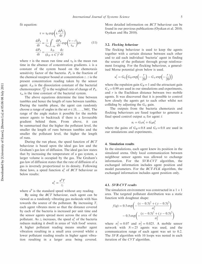
shows the trajectories of six wifibots, which were

recorded by VICON motion capture system. In

Figure 9, the blue circles show the initial positions of

agents and red squares show the optimised positions of

each of them. Curves are the trajectories travelled by

six wifibots with the SVR-CVT algorithm. The dotted

lines show the Voronoi tessellation cells at the end of

the test.

Figures 10 and 11 are two snap shots from a video

clip captured by a downward camera during the test.

Figure 10 shows the initial distribution of six wifibots,

which were randomly deployed. Figure 11 shows the

final optimised distribution of six wifibots. Their

locations were matched to the true distribution.

5.2. BCT-FLK results

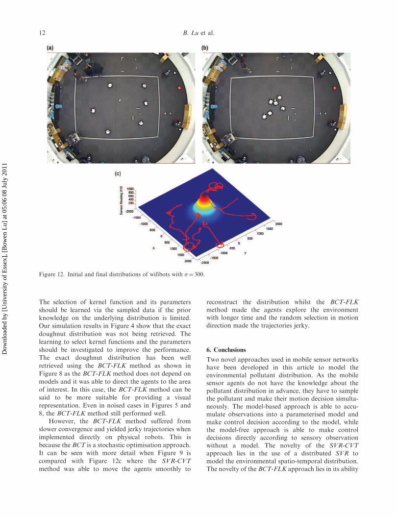
The test was conducted using two different Gaussian

distributions with the same values of A¼ 100, a¼ 0,

b¼ 0 and different standard deviations of �¼ 300 and

�¼ 1000. Figures 12a and 13 show how the six wifibots

formed the distribution. The initial locations are shown

in Figures 12a and 13a, the final locations are shown in

Figures 12b and 13b and the trajectories with the true

distribution are shown in Figures 12c and 13c. It can be

found that the trajectories were not very smooth and

there were some circles where the robots turned around

at the initial stage. This is due to the nature of the

bacteria chemotaxis behaviour, i.e. they are explora-

tory. However, the behaviour became more and more

stable when the agents got closer to the centre of the

pollutant source. In the end, the wifibots were able to

distribute themselves based upon the true Gaussian

distributions.

5.3. Discussions

In mobile sensor networks, collision avoidance is one

of the fundamental functions. The SVR-CVT method

deals with collision avoidance implicitly due to the fact

that each agent is controlled to move to the mass centre

of its Voronoi cell. The BCT-FLK method deals with

collision avoidance explicitly via the use of an artificial

separation potential functions. Our simulation and real

experimental results have demonstrated this point.

As it has been stated that the kernel function of the

SVR-CVT method is related to the underlying

distribution, the finite support kernel function we

used is just for implementing a distributed SVR.

Figure 8. Doughnut distribution.

10 B. Lu et al.

Dow

nloa

ded

by [

Uni

vers

ity o

f E

ssex

], [

Bow

en L

u] a

t 05:

06 0

8 Ju

ly 2

011

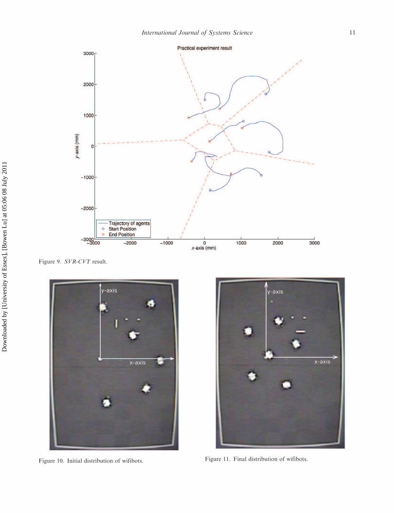
Figure 9. SVR-CVT result.

Figure 10. Initial distribution of wifibots. Figure 11. Final distribution of wifibots.

International Journal of Systems Science 11

Dow

nloa

ded

by [

Uni

vers

ity o

f E

ssex

], [

Bow

en L

u] a

t 05:

06 0

8 Ju

ly 2

011

The selection of kernel function and its parameters

should be learned via the sampled data if the prior

knowledge on the underlying distribution is limited.

Our simulation results in Figure 4 show that the exact

doughnut distribution was not being retrieved. The

learning to select kernel functions and the parameters

should be investigated to improve the performance.

The exact doughnut distribution has been well

retrieved using the BCT-FLK method as shown in

Figure 8 as the BCT-FLK method does not depend on

models and it was able to direct the agents to the area

of interest. In this case, the BCT-FLK method can be

said to be more suitable for providing a visual

representation. Even in noised cases in Figures 5 and

8, the BCT-FLK method still performed well.

However, the BCT-FLK method suffered from

slower convergence and yielded jerky trajectories when

implemented directly on physical robots. This is

because the BCT is a stochastic optimisation approach.

It can be seen with more detail when Figure 9 is

compared with Figure 12c where the SVR-CVT

method was able to move the agents smoothly to

reconstruct the distribution whilst the BCT-FLK

method made the agents explore the environment

with longer time and the random selection in motion

direction made the trajectories jerky.

6. Conclusions

Two novel approaches used in mobile sensor networks

have been developed in this article to model the

environmental pollutant distribution. As the mobile

sensor agents do not have the knowledge about the

pollutant distribution in advance, they have to sample

the pollutant and make their motion decision simulta-

neously. The model-based approach is able to accu-

mulate observations into a parameterised model and

make control decision according to the model, while

the model-free approach is able to make control

decisions directly according to sensory observation

without a model. The novelty of the SVR-CVT

approach lies in the use of a distributed SVR to

model the environmental spatio-temporal distribution.

The novelty of the BCT-FLK approach lies in its ability

Figure 12. Initial and final distributions of wifibots with �¼ 300.

12 B. Lu et al.

Dow

nloa

ded

by [

Uni

vers

ity o

f E

ssex

], [

Bow

en L

u] a

t 05:

06 0

8 Ju

ly 2

011

to reconstruct a distribution without relying on a

model. We have found that both of them can be used

to distribute mobile sensor agents in a pattern matched

to the underlying pollutant distribution. Our simula-

tion results and experimental results presented confirm

this point.

We plan to investigate an integrated approach

using the model-free approach at the early stage to

explore the environment while using the model-based

approach at the later stage to exploit the accumulated

knowledge.

The underlying distributions we used are simple

mathematical functions. As nature pollutants have

more complex property both in spatial and in temporal

domain, simulating realistic pollutant models is one of

the current research topics. With realistic pollutant

simulation, we are able to investigate more complex

modelling techniques and motion control techniques.

Acknowledgements

This research work was financially sponsored by EuropeanUnion FP7 program, no. ICT-231646, SHOAL.

Notes on contributors

Bowen Lu is a PhD candidate in theSchool of Computer Science andElectronic Engineering, University ofEssex, United Kingdom. He receivedhis BEng in Optical InformationScience and Technology fromShenzhen University (Guangdong,P.R. China) in 2008 and his MSc inEmbedded Systems from University

of Essex. Currently, he is researching on various distributedmethods for pollution monitoring. Specifically, it includescoverage control algorithms for wireless sensor network andpollutant distribution estimation. He has served as a reviewerof ICRA, IROS and other international conferences. Also, heis a student member of IEEE.

John Oyekan received his BEng(Hons) in Electronics Technologyfrom the University of Coventry in2006 and his MSc in EmbeddedSystems and Robotics fromUniversity of Essex in 2008. He iscurrently working toward a PhDdegree at the University of Essex.His research interests include using

Figure 13. Initial and final distributions of wifibots with �¼ 1000.

International Journal of Systems Science 13

Dow

nloa

ded

by [

Uni

vers

ity o

f E

ssex

], [

Bow

en L

u] a

t 05:

06 0

8 Ju

ly 2

011

bio inspired methods to solve engineering problems andsolving problems related to Unmanned Aerial Vehicles. Hehas published five conference papers, over two journals andco-authored two book chapters in these areas. He is also areviewer of various international conferences such asROBIO, ICRA and IROS among others.

Dongbing Gu is a Reader in School ofComputer Science and ElectronicEngineering at the University ofEssex, UK. His current research inter-ests include multi-agent systems, wire-less sensor networks, distributedcontrol algorithms, distributed infor-mation fusion, cooperative control,reinforcement learning, fuzzy logic

and neural network based motion control and modelpredictive control. He has published over 100 papers ininternational journals and conferences. He has also served asthe member of organising committees and programmecommittees for many IEEE conferences. Dr Gu is themember of several IEEE technical committees and a seniormember of IEEE.

Huosheng Hu is a Professor in theSchool of Computer Science andElectronic Engineering, University ofEssex, UK, leading the human-centred robotics research. His researchinterests include autonomous robots,human-robot interaction, rehabilita-tion robotics, embedded systems,multi-robot collaboration, pervasive

computing, sensor integration, intelligent control and net-worked robotics. He has published over 300 papers injournals, books and conferences, and received a number ofbest paper awards. Prof Hu is a founding member of IEEERobotics and Automation Society Technical committee onNetworked Robots, a Fellow of IET and InstMC and asenior member of IEEE and ACM. He has been a ProgramChair or a Committee member for many internationalconferences such as IEEE ICRA, IROS, ICMA, ROBIO,IASTED RA, CA and CI. He currently serves as Editor-in-Chief for International Journal of Automation and Computing.He is a reviewer for many international journals such asIEEE Transactions on Robotics, Automatic Control, NeuralNetworks and the International Journal of Robotics Research.Since 2000 he has been a Guest Professor at six universitiesin China: Central South University, Shanghai University,Xiamen University, Chongqing University of Post andTelecommunication, Kunming University of Science andTechnology and Northeast Normal University

References

Baronov, D., and Baillieul, J. (2008), ‘Autonomous Vehicle

Control for Ascending/Descending Along a Potential Field

with Two Applications’, in Proceedings of the American

Control Conference, pp. 678–683.

Brown, D.A., and Berg, H.C. (1974), ‘Temporal Stimulation

of Chemotaxis in Escherichia coli’, Proceedings of the

National Academy of Science USA, 71, 1388–1392.

Choi, J., Lee, J., and Oh, S. (2008), ‘Swarm Intelligence for

Achieving the Global Maximum using Spatio-temporal

Gaussian Processes’, in American Control Conference,

pp. 135–140.

Corrigan, C.E., Roberts, G.C., Ramana, M.V., Kim, D., and

Ramanathan, V. (2007), ‘Capturing Vertical Profiles of

Aerosols and Black Carbon Over the Indian Ocean using

Autonomous Unmanned Aerial Vehicles’, Atmospheric

Chemistry and Physics Discussions, 7, 11429–11463.

Cortes, J. (2009), ‘Distributed Kriged Kalman Filter for

Spatial Estimation’, IEEE Transactions on Automatic

Control, 54, 2816–2827.

Cortes, J., and Bullo, F. (2005), ‘Coordination and

Geometric Optimisation via Distributed Dynamical

Systems’, SIAM Journal of Control Optimization, 44,

1543–1574.

Cortes, J., Martinez, S., Karatas, T., and Bullo, F. (2004),

‘Coverage Control from Mobile Sensing Networks’, IEEE

Transactions on Robotics and Automation, 20, 243–255.

Dhariwal, A., Sukhatme, G.S., and Requicha, A.A.G.

(2004), ‘Bacterium-inspired Robots for Environmental

Monitoring’, in Proceedings of IEEE International

Conference on Robotics and Automation, New Orleans,

LA, April, pp. 1436–1443.

Leonard, N.E., Paley, D., Lekien, F., Sepulchre, R.,

Fratantoni, D.M., and Davis, R. (2007), ‘Collective

Motion, Sensor Networks and Ocean Sampling’,

Proceedings of the IEEE, 95, 48–74.

Lilienthal, A., and Duckett, T. (2003), ‘Experimental

Analysis of Smelling Braitenberg Vehicles’,

in Proceedings of the IEEE International Conference on

Advanced Robotics (ICAR), pp. 375–380.

Lynch, K.M., Schwartz, I.B., Yang, P., and Freeman, R.A.

(2008), ‘Decentralised Environmental Modelling by

Mobile Sensor Networks’, IEEE Transactions on

Robotics, 24, 710–724.

Marques, L., Nunes, U., and Almeida, T.D. (2002),

‘Olfaction-based Mobile Robot Navigation’, Thin Solid

Films, 418, 51–58.

Martinez, S. (2010), ‘Distributed Interpolation Schemes for

Field Estimation by Mobile Sensor Networks’, IEEE

Transactions on Control Systems Technology, 18, 491–500.

Mayhew, C.G., Sanfelice, R.G., and Teel, A.R. (2008),

‘Robust Source-seeking Hybrid Controllers for

Nonholonomic Vehicles’, in Proceedings of the American

Control Conference, pp. 2722–2727.

Merino, L.F., Caballero, J.R., de Dios, J.M., and Ferruz,

A.O. (2006), ‘A Cooperative Perception System for

Multiple UAVs: Application to Automatic Detection of

Forest Fires’, Journal of Field Robotics, 23, 165–184.

Mesquita, A., Hespanha, J., and Astrom, K. (2008),

‘Optimotaxis: A Stochastic Multi-agent Optimisation

Procedure with Point Measurements’, Hybrid Systems:

Computation and Control, 4981, 358–371.

Oyekan, J., and Hu, H. (2010), ‘Bacteria Controller

Implementation on a Physical Platform for Pollution

Monitoring’, In 2010 IEEE International Conference on

Robotics and Automation (ICRA), 3–7 May, Anchorage,

AK, pp. 3781–3786.

14 B. Lu et al.

Dow

nloa

ded

by [

Uni

vers

ity o

f E

ssex

], [

Bow

en L

u] a

t 05:

06 0

8 Ju

ly 2

011

Oyekan, J., Hu, H., and Gu, D. (2010), ‘Bio-inspired

Coverage of Invisible Hazardous Substances in

the Environment’, International Journal of Information

Acquisition, 7, 193–204.

Pimenta, L.C.A., Kumar, V., Mesquita, R.C., and Pereira,

G.A.S. (2008), ‘Sensing and Coverage for a Network of

Heterogeneous Robots’, in Proceedings of the IEEE

Conference on Decision and Control, pp. 3947–3952.

Predd, J.B., Kulkarni, S.R., and Poor, H.V. (2006),

‘Distributed Learning in Wireless Sensor Networks’,

IEEE Signal Processing Magazine, 23, 56–69.

Rabbat, M.G., and Nowak, R.D. (2006), ‘Quantized

Incremental Algorithms for Distributed Optimisation’,

IEEE Journal of Special Areas Comunication, 23, 798–808.

Schwager, M., Rus, D., and Slotine, J. (2009),

‘Decentralised, Adaptive Coverage Control for

Networked Robots’, International Journal of Robotics

Research, 28, 357–375.

Smola, A.J., and Scholkopf, B. (2004), ‘A Tutorial on

Support Vector Regression’, Statistics and Computing, 14,

199–222.

Vapnik, V.N. (1999), The Nature of Statistical Learning

Theory (Statistics for Engineering and Information Science)

(2nd ed.), eds. M. Jordan and S.L. Lauritzen, New York:

Springer Verlag.

Vijayakumar, S., and Wu, S. (1999), ‘Sequential Support

Vector Classifiers and Regression’, [Online]. Available at:

citeseer.ist.psu.edu/article/vijayakumar99sequential.html

Yi, T., Huang, Y., Simon, M., and Doyle, J. (2000), ‘Robust

Perfect Adaptation in Bacterial Chemotaxis Through

Integral Feedback Control’, Proceedings of the National

Academy of Science, 97, 4649–4653.

International Journal of Systems Science 15

Dow

nloa

ded

by [

Uni

vers

ity o

f E

ssex

], [

Bow

en L

u] a

t 05:

06 0

8 Ju

ly 2

011