Numerical and Experimental Study of Blockage Effect ...

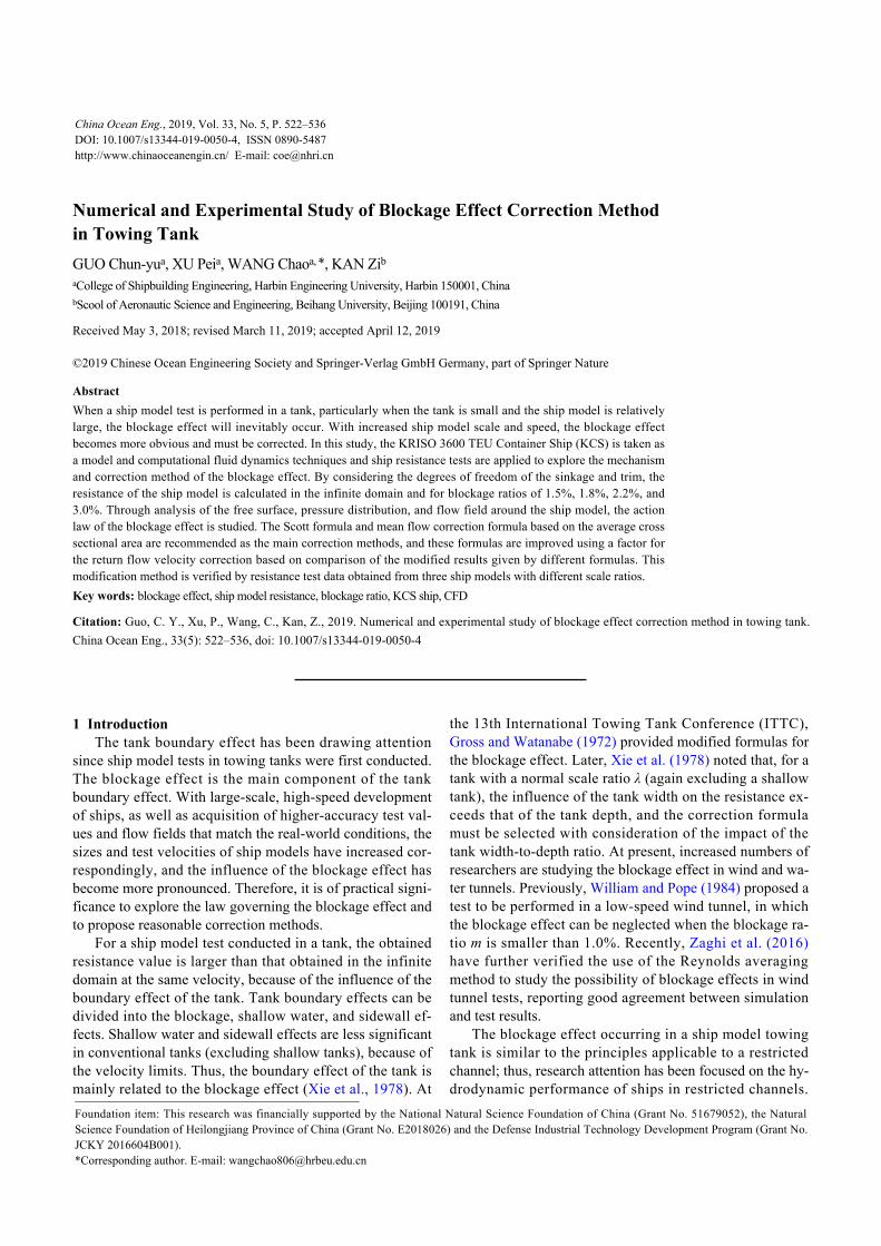
Numerical and Experimental Study of Blockage Effect Correction Methodin Towing TankGUO Chun-yua, XU Peia, WANG Chaoa, *, KAN ZibaCollege of Shipbuilding Engineering, Harbin Engineering University, Harbin 150001, ChinabScool of Aeronautic Science and Engineering, Beihang University, Beijing 100191, China

Received May 3, 2018; revised March 11, 2019; accepted April 12, 2019

©2019 Chinese Ocean Engineering Society and Springer-Verlag GmbH Germany, part of Springer Nature

AbstractWhen a ship model test is performed in a tank, particularly when the tank is small and the ship model is relativelylarge, the blockage effect will inevitably occur. With increased ship model scale and speed, the blockage effectbecomes more obvious and must be corrected. In this study, the KRISO 3600 TEU Container Ship (KCS) is taken asa model and computational fluid dynamics techniques and ship resistance tests are applied to explore the mechanismand correction method of the blockage effect. By considering the degrees of freedom of the sinkage and trim, theresistance of the ship model is calculated in the infinite domain and for blockage ratios of 1.5%, 1.8%, 2.2%, and3.0%. Through analysis of the free surface, pressure distribution, and flow field around the ship model, the actionlaw of the blockage effect is studied. The Scott formula and mean flow correction formula based on the average crosssectional area are recommended as the main correction methods, and these formulas are improved using a factor forthe return flow velocity correction based on comparison of the modified results given by different formulas. Thismodification method is verified by resistance test data obtained from three ship models with different scale ratios.Key words: blockage effect, ship model resistance, blockage ratio, KCS ship, CFD

Citation: Guo, C. Y., Xu, P., Wang, C., Kan, Z., 2019. Numerical and experimental study of blockage effect correction method in towing tank.China Ocean Eng., 33(5): 522–536, doi: 10.1007/s13344-019-0050-4

1 IntroductionThe tank boundary effect has been drawing attention

since ship model tests in towing tanks were first conducted.The blockage effect is the main component of the tankboundary effect. With large-scale, high-speed developmentof ships, as well as acquisition of higher-accuracy test val-ues and flow fields that match the real-world conditions, thesizes and test velocities of ship models have increased cor-respondingly, and the influence of the blockage effect hasbecome more pronounced. Therefore, it is of practical signi-ficance to explore the law governing the blockage effect andto propose reasonable correction methods.

For a ship model test conducted in a tank, the obtainedresistance value is larger than that obtained in the infinitedomain at the same velocity, because of the influence of theboundary effect of the tank. Tank boundary effects can bedivided into the blockage, shallow water, and sidewall ef-fects. Shallow water and sidewall effects are less significantin conventional tanks (excluding shallow tanks), because ofthe velocity limits. Thus, the boundary effect of the tank ismainly related to the blockage effect (Xie et al., 1978). At

the 13th International Towing Tank Conference (ITTC),Gross and Watanabe (1972) provided modified formulas forthe blockage effect. Later, Xie et al. (1978) noted that, for atank with a normal scale ratio λ (again excluding a shallowtank), the influence of the tank width on the resistance ex-ceeds that of the tank depth, and the correction formulamust be selected with consideration of the impact of thetank width-to-depth ratio. At present, increased numbers ofresearchers are studying the blockage effect in wind and wa-ter tunnels. Previously, William and Pope (1984) proposed atest to be performed in a low-speed wind tunnel, in whichthe blockage effect can be neglected when the blockage ra-tio m is smaller than 1.0%. Recently, Zaghi et al. (2016)have further verified the use of the Reynolds averagingmethod to study the possibility of blockage effects in windtunnel tests, reporting good agreement between simulationand test results.

The blockage effect occurring in a ship model towingtank is similar to the principles applicable to a restrictedchannel; thus, research attention has been focused on the hy-drodynamic performance of ships in restricted channels.

China Ocean Eng., 2019, Vol. 33, No. 5, P. 522–536DOI: 10.1007/s13344-019-0050-4, ISSN 0890-5487http://www.chinaoceanengin.cn/ E-mail: [email protected]

Foundation item: This research was financially supported by the National Natural Science Foundation of China (Grant No. 51679052), the NaturalScience Foundation of Heilongjiang Province of China (Grant No. E2018026) and the Defense Industrial Technology Development Program (Grant No.JCKY 2016604B001).*Corresponding author. E-mail: [email protected]

Various authors (Beck, 1981; Millward, 1996; Jachowski,2008; Zhou et al., 2013) have used computational fluid dy-namics (CFD) techniques to study the influence of the wa-ter depth, width, and ship velocity on the hull squat andwaveform. The CFD results were compared with empiric-ally obtained data. Theoretical methods have also been de-veloped to determine the squat and trim of ships sailing inrestricted water (Schijf, 1949; Gourlay, 2008; Alderf et al.,2010). Previously, Ma et al. (2013) used CFD techniques tostudy the influence of the sidewall effect in a restrictedchannel, and the force and moment of the hull were calcu-lated for different offshore distances in shallow water. In ad-dition, Zou and Larsson (2013a, 2013b) studied the possibil-ity of using different CFD methods to calculate the sidewalleffect in shallow water. The Korea Research Institute ofShips and Ocean Engineering (KRISO) Very Large Crude-oil Carrier (KVLCC2) ship model was used and the forceand squat changes on the hull were calculated at differentwater depths and offshore distances. Those researchers’ res-ults revealed that the Reynolds-averaged Navier–Stokesmethod has good computational accuracy, but the improvedaccuracy can be obtained with the shear stress transport(SST) k–ω turbulence model. Finally, Zhang et al. (2015)studied the hydrodynamic pressure field in the restricted wa-ter domain by calculating the hydrodynamic pressure andcomparing the results with experimentally obtained values.Hence, it was proposed that the effect of the watercoursecan be neglected when the width of the rectangular channelis three times larger than the ship length.

However, in comparison with theory-based researches,there are few experiment-based studies of the blockage ef-fect in a towing tank. Previously, Zhou (2002) and Wu(2007) analyzed the blockage effect when investigating theuncertainties of ship model resistance tests; however, theyused the ITTC formula to modify the speed and did not im-prove upon the revised formula. In addition, Lataire et al.(2012) studied the effects of the widths and depths of differ-ent tanks on the squat of the KVLCC2 ship model in a shal-low-water towing tank, and proposed a mathematical modelto solve the squat change of ship.

In this study, the SST k–ω turbulence model is used toanalyze the blockage effect mechanism and correctionmethod for the KCS. The volume of fluid (VOF) method isused to capture the free surface of the ship in order to calcu-late the hull heave, trim, and resistance for different widthsand depths, to explore the law governing the blockage ef-fect. In addition, three different λ values for the KCS modelare used in a ship model resistance test performed in theHarbin Engineering University towing tank, to propose theblockage effect correction method.

2 Numerical model

2.1 Control equationThe motion of an incompressible Newtonian fluid satis-

fies the continuity equation and momentum conservationequation (Wilcox, 1998):∂ρ∂t+∂(ρui)∂xi

= 0; (1)

∂(ρui)∂t+∂(ρuiu j)∂x j

= − ∂p∂x j+

∂∂x j

(μ∂ui

∂x j−ρu′iu

′j

)+Sj, (2)

ρu′iu′j

where ui and uj (i, j = 1, 2, 3) are the time-averaged velocitycomponents; p is the time-averaged pressure; μ is the dy-namic viscous coefficient; ρ is the fluid density; is theReynolds stress term; and Sj is the generalized source termof the momentum equation.

2.2 Turbulence model and treatment of the free surfaceThe SST k–ω model is used in the turbulence model

(Menter, 1994). The former model combines the advant-ages of the k–ω model and k–ε model and has good advant-ages as regards calculation of a viscous flow field. The ba-sic principle of the VOF method is to determine the free sur-face by investigating the volume ratio function of the fluidand grid in the mesh cell, and to track the changes in the flu-id rather than the movement of particles on the free surface(Hirt and Nichols, 1981; Wang et al., 2015). This methodcan trace the complex free surface phenomenon. In addition,the calculation requires less memory than other techniquesand is easy to implement and expand to three dimensions.The changes in the free surface are captured by the VOFmethod.

3 Computational model and grid

3.1 Calculation model and calculation conditionsIn this study, the KCS model is taken as the research ob-

ject; the geometric model is shown in Fig. 1 and the mainparameters of the ship model are listed in Table 1.

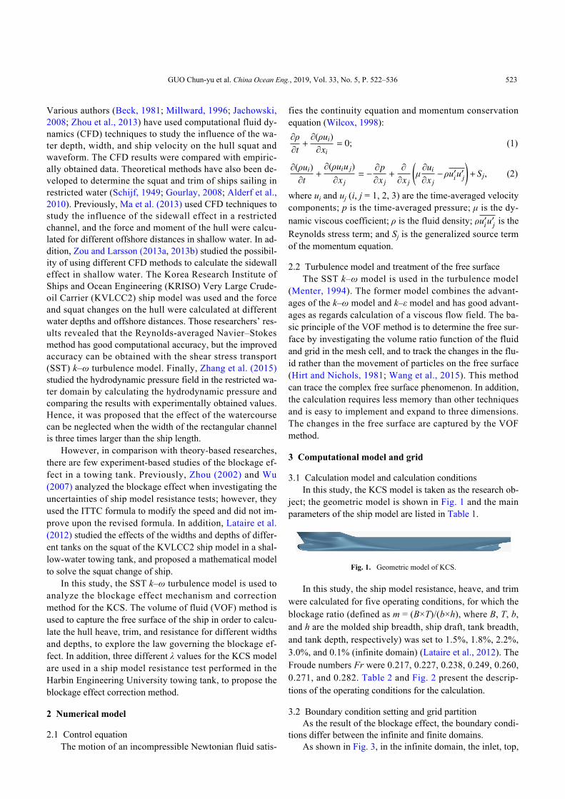
In this study, the ship model resistance, heave, and trimwere calculated for five operating conditions, for which theblockage ratio (defined as m = (B×T)/(b×h), where B, T, b,and h are the molded ship breadth, ship draft, tank breadth,and tank depth, respectively) was set to 1.5%, 1.8%, 2.2%,3.0%, and 0.1% (infinite domain) (Lataire et al., 2012). TheFroude numbers Fr were 0.217, 0.227, 0.238, 0.249, 0.260,0.271, and 0.282. Table 2 and Fig. 2 present the descrip-tions of the operating conditions for the calculation.

3.2 Boundary condition setting and grid partitionAs the result of the blockage effect, the boundary condi-

tions differ between the infinite and finite domains.As shown in Fig. 3, in the infinite domain, the inlet, top,

Fig. 1. Geometric model of KCS.

GUO Chun-yu et al. China Ocean Eng., 2019, Vol. 33, No. 5, P. 522–536 523

side, and bottom were set as the velocity inlet, and the out-let was set to the pressure outlet. In the finite domain, the ef-fect of the sidewall and bottom must be considered. There-fore, the sidewall and bottom in the finite domain were setas walls, unlike the infinite domain case.

Before the calculation, the grid independence was veri-fied, and the grid factor interference was eliminated by com-paring calculated values of the three different sets of

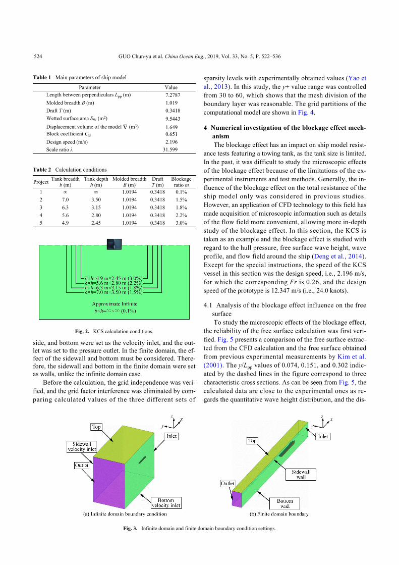
sparsity levels with experimentally obtained values (Yao etal., 2013). In this study, the y+ value range was controlledfrom 30 to 60, which shows that the mesh division of theboundary layer was reasonable. The grid partitions of thecomputational model are shown in Fig. 4.

4 Numerical investigation of the blockage effect mech-anismThe blockage effect has an impact on ship model resist-

ance tests featuring a towing tank, as the tank size is limited.In the past, it was difficult to study the microscopic effectsof the blockage effect because of the limitations of the ex-perimental instruments and test methods. Generally, the in-fluence of the blockage effect on the total resistance of theship model only was considered in previous studies.However, an application of CFD technology to this field hasmade acquisition of microscopic information such as detailsof the flow field more convenient, allowing more in-depthstudy of the blockage effect. In this section, the KCS istaken as an example and the blockage effect is studied withregard to the hull pressure, free surface wave height, waveprofile, and flow field around the ship (Deng et al., 2014).Except for the special instructions, the speed of the KCSvessel in this section was the design speed, i.e., 2.196 m/s,for which the corresponding Fr is 0.26, and the designspeed of the prototype is 12.347 m/s (i.e., 24.0 knots).

4.1 Analysis of the blockage effect influence on the freesurfaceTo study the microscopic effects of the blockage effect,

the reliability of the free surface calculation was first veri-fied. Fig. 5 presents a comparison of the free surface extrac-ted from the CFD calculation and the free surface obtainedfrom previous experimental measurements by Kim et al.(2001). The y/Lpp values of 0.074, 0.151, and 0.302 indic-ated by the dashed lines in the figure correspond to threecharacteristic cross sections. As can be seen from Fig. 5, thecalculated data are close to the experimental ones as re-gards the quantitative wave height distribution, and the dis-

Table 1 Main parameters of ship model

Parameter ValueLength between perpendiculars Lpp (m) 7.2787Molded breadth B (m) 1.019Draft T (m) 0.3418Wetted surface area SW (m2) 9.5443

∇Displacement volume of the model (m3) 1.649Block coefficient CB 0.651Design speed (m/s) 2.196Scale ratio λ 31.599

Table 2 Calculation conditions

Project Tank breadthb (m)Tank depth

h (m)Molded breadth

B (m)DraftT (m)

Blockageratio m

1 ∞ ∞ 1.0194 0.3418 0.1%2 7.0 3.50 1.0194 0.3418 1.5%3 6.3 3.15 1.0194 0.3418 1.8%4 5.6 2.80 1.0194 0.3418 2.2%5 4.9 2.45 1.0194 0.3418 3.0%

Fig. 2. KCS calculation conditions.

Fig. 3. Infinite domain and finite domain boundary condition settings.

524 GUO Chun-yu et al. China Ocean Eng., 2019, Vol. 33, No. 5, P. 522–536

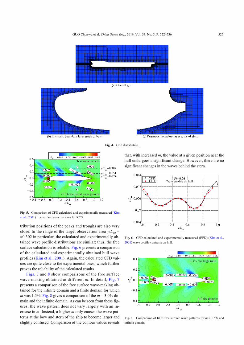
tribution positions of the peaks and troughs are also veryclose. In the range of the target observation area y/Lpp =±0.302 in particular, the calculated and experimentally ob-tained wave profile distributions are similar; thus, the freesurface calculation is reliable. Fig. 6 presents a comparisonof the calculated and experimentally obtained hull waveprofiles (Kim et al., 2001). Again, the calculated CFD val-ues are quite close to the experimental ones, which furtherproves the reliability of the calculated results.

Figs. 7 and 8 show comparisons of the free surfacewave-making obtained at different m. In detail, Fig. 7presents a comparison of the free surface wave-making ob-tained for the infinite domain and a finite domain for whichm was 1.5%. Fig. 8 gives a comparison of the m = 3.0% do-main and the infinite domain. As can be seen from these fig-ures, the wave pattern does not vary largely with an in-crease in m. Instead, a higher m only causes the wave pat-terns at the bow and stern of the ship to become larger andslightly confused. Comparison of the contour values reveals

that, with increased m, the value at a given position near thehull undergoes a significant change. However, there are nosignificant changes in the waves behind the stern.

Fig. 4. Grid distribution.

Fig. 5. Comparison of CFD calculated and experimentally measured (Kimet al., 2001) free surface wave patterns for KCS.

Fig. 6. CFD calculated and experimentally measured (EFD) (Kim et al.,2001) wave profile contrasts on hull.

Fig. 7. Comparison of KCS free surface wave patterns for m = 1.5% andinfinite domain.


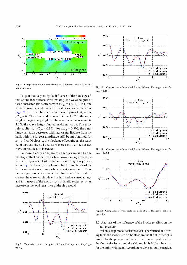
To quantitatively study the influence of the blockage ef-fect on the free surface wave-making, the wave heights ofthree characteristic sections with y/Lpp = 0.074, 0.151, and0.302 were compared under different m values, as shown inFigs. 9–11. It can be seen from these figures that, in they/Lpp = 0.074 section and for m = 1.5% and 2.2%, the waveheight changes very slightly. However, when m is equal to3.0%, the wave height fluctuates dramatically. The samerule applies for y/Lpp = 0.151. For y/Lpp = 0.302, the amp-litude variation decreases with increasing distance from thehull, with the largest amplitude still being obtained form = 3.0%. Obviously, the blockage effect affects the waveheight around the hull and, as m increases, the free surfacewave amplitude also increases.

To more clearly compare the changes caused by theblockage effect on the free surface wave-making around thehull, a comparison chart of the hull wave height is presen-ted in Fig. 12. Hence, it is obvious that the amplitude of thehull wave is at a maximum when m is at a maximum. Fromthe energy perspective, it is the blockage effect that in-creases the wave amplitude of the hull and its surroundings,and this aspect of the energy loss is finally reflected by anincrease in the total resistance of the ship model.

4.2 Analysis of the influence of the blockage effect on thehull pressureWhen a ship model resistance test is performed in a tow-

ing tank, the movement of the flow around the ship model islimited by the presence of the tank bottom and wall, so thatthe flow velocity around the ship model is higher than thatfor the infinite domain. According to the Bernoulli equation,

Fig. 8. Comparison of KCS free surface wave patterns for m = 3.0% andinfinite domain.

Fig. 9. Comparison of wave heights at different blockage ratios for y/Lpp =0.074.

Fig. 10. Comparison of wave heights at different blockage ratios fory/Lpp = 0.151.

Fig. 11. Comparison of wave heights at different blockage ratios fory/Lpp = 0.302.

Fig. 12. Comparison of wave profiles on hull obtained for different block-age ratios.


a change in flow velocity changes the hull pressure. In thisstudy, the hydrostatic pressure was subtracted from the cal-culated total pressure to obtain the pressure, and the pres-sure coefficient was defined as Cp = P/(1/2ρv2). Figs. 13 and14 show the distributions of the hull pressure coefficientsobtained at different m. In detail, Figs. 13 and 14 show thepressure distributions at the bottom of the ship and on thebow and stern of the ship, respectively, for m = 3.0% andthe infinite domain. From Fig. 13, it is obvious that the pres-sure at the bow of the ship’s bottom is larger than that at thestern of the ship’s bottom, such that a viscous resistance isproduced. The numerical results presented in Fig. 13 indic-ate that larger resistance is obtained for m = 3.0% than thatfor the infinite domain case. Comparison of the results forthese two cases presented in Fig. 13 reveals that the block-age effect yields a bottom flow velocity in the middle andstern of the ship that is slightly larger than that in the infin-ite domain, resulting in a decrease in pressure. As the bot-tom of the ship’s bow corresponds to a bulbous nose, thewetted surface is small and the pressure changes are not ob-vious.

As can be seen from the pressure distribution on theship’s side shown in Fig. 14, the low-pressure area is dis-tributed on both sides of the bulbous bow, and the pressurein this area at m = 3.0% is lower than that in the infinite do-main. This is because of the blockage effect at the bow ofthe ship. As a result, the flow near the bow is squeezed toboth sides of the ship hull, yielding a larger return flow ve-locity, which reduces the pressure at the bow. The numeric-ally calculated pressure distribution at the stern indicatesthat the pressure change is less obvious than that at the bow,but the pressure contour distribution is relatively confusedat m = 3.0%.

To more clearly observe the changes in the pressure at

the stern, the Q-criterion vortex structure distribution of theKCS hull was extracted, and the stern bilge vortex wasprimarily observed (Hunt et al., 1988). The calculation for-mula for Q is as follows:

Q =− 12

(∂u∂x

)2

+

(∂v∂y

)2

+

(∂w∂z

)2−(∂u∂y

∂v∂x+∂u∂z

∂w∂x+∂v∂z

∂w∂y

). (3)

Fig. 15 shows the vortex structure distributions with Q-criterion = 20 obtained for m = 3.0% and the infinite do-main. The areas shown in the figures correspond to the sternbilge vortices. In Fig. 15, because of the presence of theblockage effect, the stern bilge vortex structures are lesssmooth than those in the infinite domain, which means thatthe blockage induces chaotic behavior in the flow field be-hind the stern. In addition, in Fig. 15, the stern bilge vortexbecomes very small in the infinite domain, whereas that un-der the blockage condition remains obvious. The blockageemphasizes the whirlpool after the stern, which further de-

Fig. 13. Comparison of pressure distributions on ship bottom for m =3.0% and infinite domain.

Fig. 14. Comparison of pressure distributions at ship bow and stern for m = 3.0% and infinite domain.


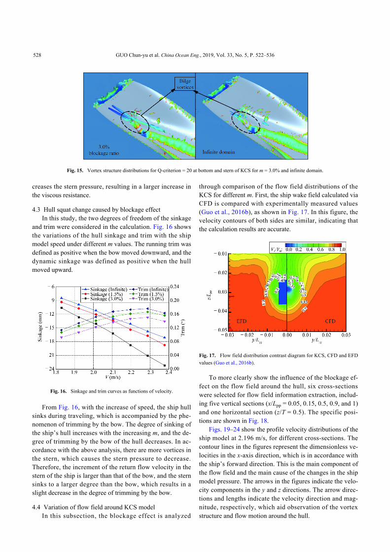
creases the stern pressure, resulting in a larger increase inthe viscous resistance.

4.3 Hull squat change caused by blockage effectIn this study, the two degrees of freedom of the sinkage

and trim were considered in the calculation. Fig. 16 showsthe variations of the hull sinkage and trim with the shipmodel speed under different m values. The running trim wasdefined as positive when the bow moved downward, and thedynamic sinkage was defined as positive when the hullmoved upward.

From Fig. 16, with the increase of speed, the ship hullsinks during traveling, which is accompanied by the phe-nomenon of trimming by the bow. The degree of sinking ofthe ship’s hull increases with the increasing m, and the de-gree of trimming by the bow of the hull decreases. In ac-cordance with the above analysis, there are more vortices inthe stern, which causes the stern pressure to decrease.Therefore, the increment of the return flow velocity in thestern of the ship is larger than that of the bow, and the sternsinks to a larger degree than the bow, which results in aslight decrease in the degree of trimming by the bow.

4.4 Variation of flow field around KCS modelIn this subsection, the blockage effect is analyzed

through comparison of the flow field distributions of theKCS for different m. First, the ship wake field calculated viaCFD is compared with experimentally measured values(Guo et al., 2016b), as shown in Fig. 17. In this figure, thevelocity contours of both sides are similar, indicating thatthe calculation results are accurate.

To more clearly show the influence of the blockage ef-fect on the flow field around the hull, six cross-sectionswere selected for flow field information extraction, includ-ing five vertical sections (x/Lpp = 0.05, 0.15, 0.5, 0.9, and 1)and one horizontal section (z/T = 0.5). The specific posi-tions are shown in Fig. 18.

Figs. 19–24 show the profile velocity distributions of theship model at 2.196 m/s, for different cross-sections. Thecontour lines in the figures represent the dimensionless ve-locities in the x-axis direction, which is in accordance withthe ship’s forward direction. This is the main component ofthe flow field and the main cause of the changes in the shipmodel pressure. The arrows in the figures indicate the velo-city components in the y and z directions. The arrow direc-tions and lengths indicate the velocity direction and mag-nitude, respectively, which aid observation of the vortexstructure and flow motion around the hull.

Fig. 15. Vortex structure distributions for Q-criterion = 20 at bottom and stern of KCS for m = 3.0% and infinite domain.

Fig. 16. Sinkage and trim curves as functions of velocity.

Fig. 17. Flow field distribution contrast diagram for KCS, CFD and EFDvalues (Guo et al., 2016b).


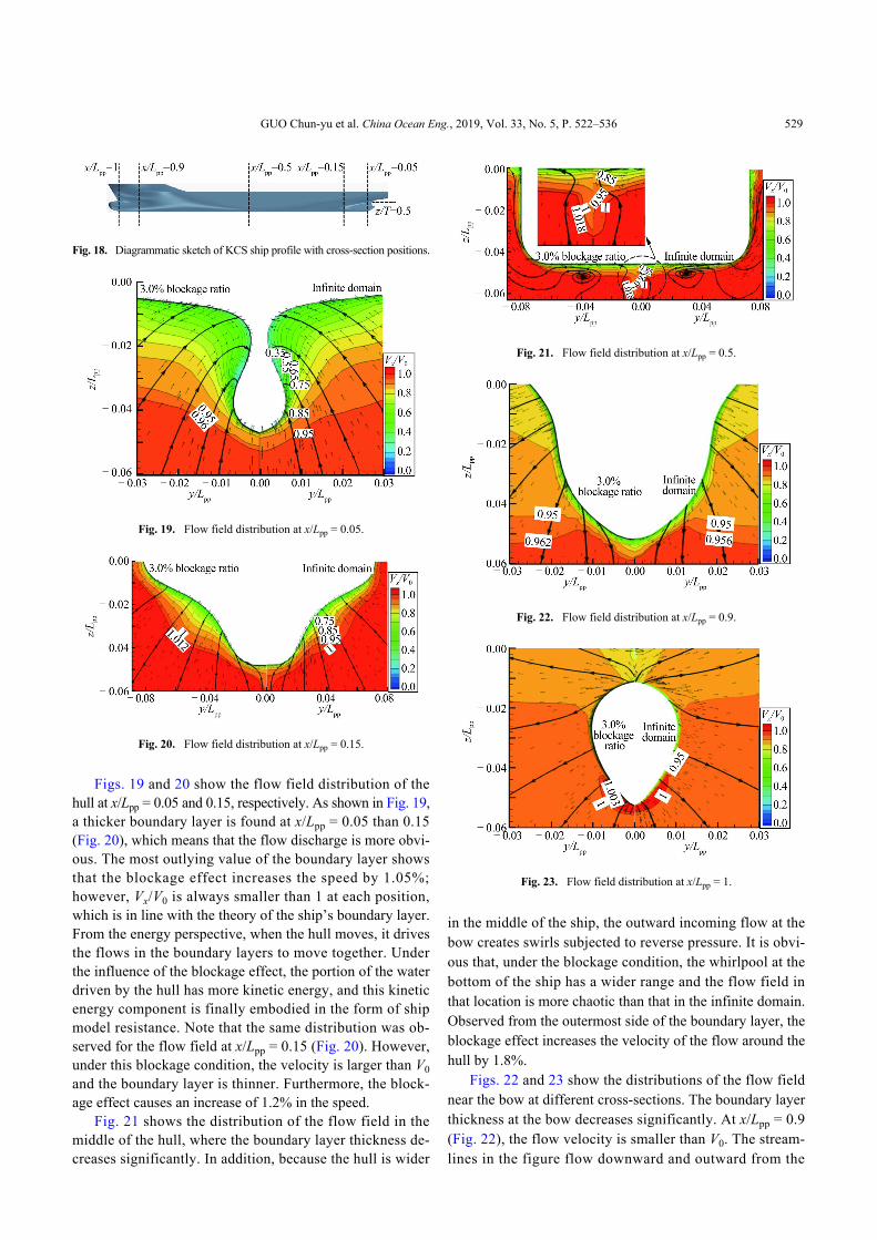
Figs. 19 and 20 show the flow field distribution of thehull at x/Lpp = 0.05 and 0.15, respectively. As shown in Fig. 19,a thicker boundary layer is found at x/Lpp = 0.05 than 0.15(Fig. 20), which means that the flow discharge is more obvi-ous. The most outlying value of the boundary layer showsthat the blockage effect increases the speed by 1.05%;however, Vx/V0 is always smaller than 1 at each position,which is in line with the theory of the ship’s boundary layer.From the energy perspective, when the hull moves, it drivesthe flows in the boundary layers to move together. Underthe influence of the blockage effect, the portion of the waterdriven by the hull has more kinetic energy, and this kineticenergy component is finally embodied in the form of shipmodel resistance. Note that the same distribution was ob-served for the flow field at x/Lpp = 0.15 (Fig. 20). However,under this blockage condition, the velocity is larger than V0and the boundary layer is thinner. Furthermore, the block-age effect causes an increase of 1.2% in the speed.

Fig. 21 shows the distribution of the flow field in themiddle of the hull, where the boundary layer thickness de-creases significantly. In addition, because the hull is wider

in the middle of the ship, the outward incoming flow at thebow creates swirls subjected to reverse pressure. It is obvi-ous that, under the blockage condition, the whirlpool at thebottom of the ship has a wider range and the flow field inthat location is more chaotic than that in the infinite domain.Observed from the outermost side of the boundary layer, theblockage effect increases the velocity of the flow around thehull by 1.8%.

Figs. 22 and 23 show the distributions of the flow fieldnear the bow at different cross-sections. The boundary layerthickness at the bow decreases significantly. At x/Lpp = 0.9(Fig. 22), the flow velocity is smaller than V0. The stream-lines in the figure flow downward and outward from the

Fig. 18. Diagrammatic sketch of KCS ship profile with cross-section positions.

Fig. 19. Flow field distribution at x/Lpp = 0.05.




Fig. 23. Flow field distribution at x/Lpp = 1.


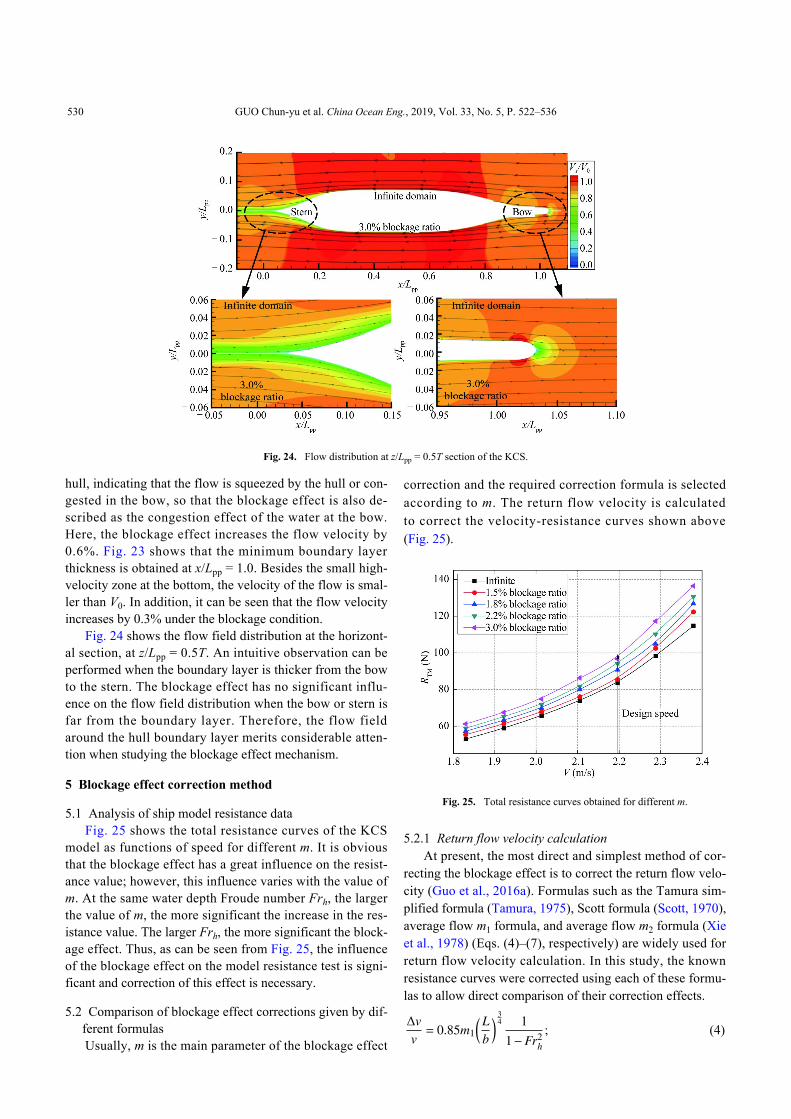
hull, indicating that the flow is squeezed by the hull or con-gested in the bow, so that the blockage effect is also de-scribed as the congestion effect of the water at the bow.Here, the blockage effect increases the flow velocity by0.6%. Fig. 23 shows that the minimum boundary layerthickness is obtained at x/Lpp = 1.0. Besides the small high-velocity zone at the bottom, the velocity of the flow is smal-ler than V0. In addition, it can be seen that the flow velocityincreases by 0.3% under the blockage condition.

Fig. 24 shows the flow field distribution at the horizont-al section, at z/Lpp = 0.5T. An intuitive observation can beperformed when the boundary layer is thicker from the bowto the stern. The blockage effect has no significant influ-ence on the flow field distribution when the bow or stern isfar from the boundary layer. Therefore, the flow fieldaround the hull boundary layer merits considerable atten-tion when studying the blockage effect mechanism.

5 Blockage effect correction method

5.1 Analysis of ship model resistance dataFig. 25 shows the total resistance curves of the KCS

model as functions of speed for different m. It is obviousthat the blockage effect has a great influence on the resist-ance value; however, this influence varies with the value ofm. At the same water depth Froude number Frh, the largerthe value of m, the more significant the increase in the res-istance value. The larger Frh, the more significant the block-age effect. Thus, as can be seen from Fig. 25, the influenceof the blockage effect on the model resistance test is signi-ficant and correction of this effect is necessary.

5.2 Comparison of blockage effect corrections given by dif-ferent formulasUsually, m is the main parameter of the blockage effect

correction and the required correction formula is selectedaccording to m. The return flow velocity is calculatedto correct the velocity-resistance curves shown above(Fig. 25).

5.2.1 Return flow velocity calculationAt present, the most direct and simplest method of cor-

recting the blockage effect is to correct the return flow velo-city (Guo et al., 2016a). Formulas such as the Tamura sim-plified formula (Tamura, 1975), Scott formula (Scott, 1970),average flow m1 formula, and average flow m2 formula (Xieet al., 1978) (Eqs. (4)–(7), respectively) are widely used forreturn flow velocity calculation. In this study, the knownresistance curves were corrected using each of these formu-las to allow direct comparison of their correction effects.

∆vv= 0.85m1

(Lb

) 34 1

1−Fr2h

; (4)

Fig. 24. Flow distribution at z/Lpp = 0.5T section of the KCS.

Fig. 25. Total resistance curves obtained for different m.


∆vv=(1.86−0.072×10−6Re

)· ∇A−

32+

BL2[2.4× (FrL −0.22)2

]A−

32 ; (5)

∆vv=

m1

1−m1−Fr2h

; (6)

∆vv=

m2

1−m2−Fr2h

, (7)

Frh = v/√

gh

FrL = v/√

gLWL

∇

where ∆υ is the calculated return flow velocity; υ representsthe ship model velocity in the finite domain; Frh is the wa-ter depth Froude number, ; Re is the Reynoldsnumber; A is the sectional area of the tank, A = b×h; FrL isthe ship length Froude number, ; m1 and m2are the blockage rat ios, m1 = am /A = BTCM / (b×h) ,m2=a/A= /LWL/(b×h); and the other parameters are definedpreviously.

5.2.2 Comparison of correction effectsTo intuitively compare the correction effects of each for-

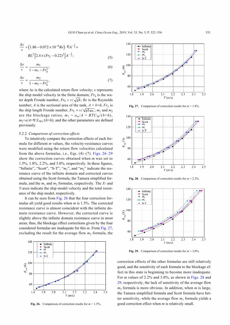
mula for different m values, the velocity-resistance curveswere modified using the return flow velocities calculatedfrom the above formulas, i.e., Eqs. (4)–(7). Figs. 26–29show the correction curves obtained when m was set to1.5%, 1.8%, 2.2%, and 3.0%, respectively. In these figures,“Infinite”, “Scott”, “S-T”, “m1”, and “m2” indicate the res-istance curve of the infinite domain and corrected curvesobtained using the Scott formula, the Tamura simplified for-mula, and the m1 and m2 formulas, respectively. The X- andY-axes indicate the ship model velocity and the total resist-ance of the ship model, respectively.

It can be seen from Fig. 26 that the four correction for-mulas all yield good results when m is 1.5%. The correctedresistance curve is almost coincident with the infinite do-main resistance curve. However, the corrected curve isslightly above the infinite domain resistance curve in mostareas; thus, the blockage effect corrections given by the fourconsidered formulas are inadequate for this m. From Fig. 27,excluding the result for the average flow m2 formula, the

correction effects of the other formulas are still relativelygood, and the sensitivity of each formula to the blockage ef-fect in this state is beginning to become more inadequate.For m values of 2.2% and 3.0%, as shown in Figs. 28 and29, respectively, the lack of sensitivity of the average flowm2 formula is more obvious. In addition, when m is large,the Tamura simplified formula and Scott formula have bet-ter sensitivity, while the average flow m1 formula yields agood correction effect when m is relatively small.

Fig. 26. Comparison of correction results for m = 1.5%.





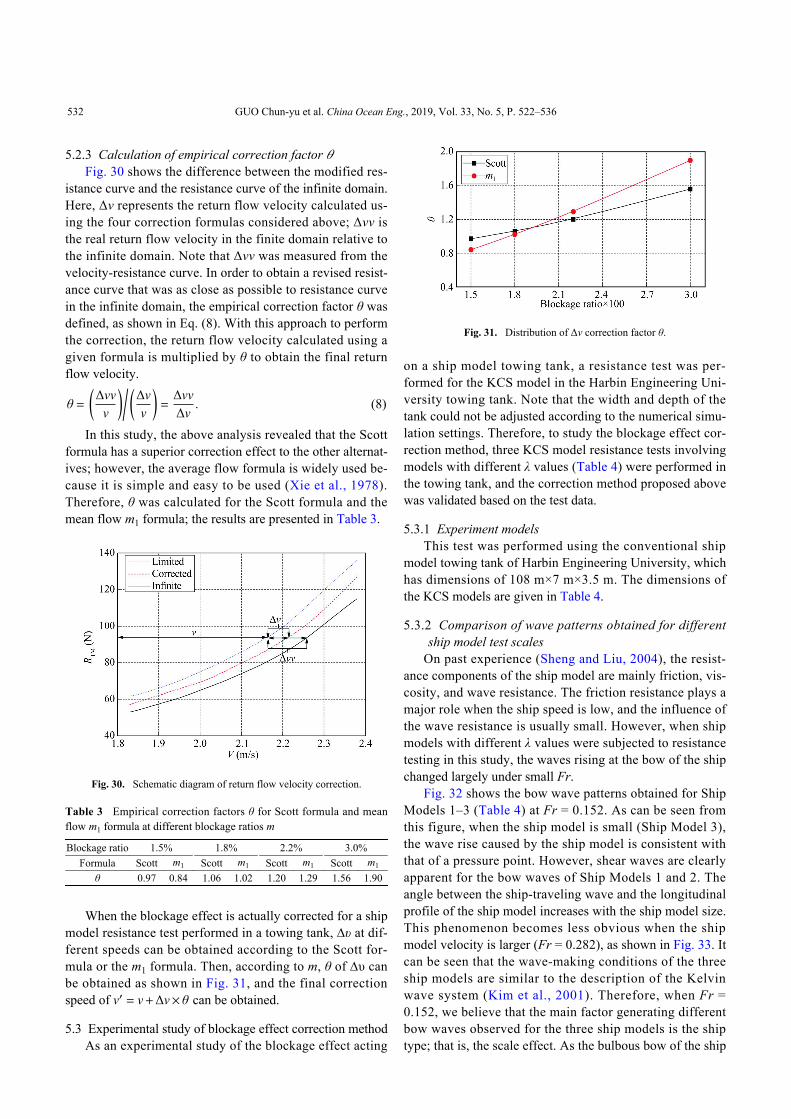
5.2.3 Calculation of empirical correction factor θFig. 30 shows the difference between the modified res-

istance curve and the resistance curve of the infinite domain.Here, Δv represents the return flow velocity calculated us-ing the four correction formulas considered above; Δvv isthe real return flow velocity in the finite domain relative tothe infinite domain. Note that Δvv was measured from thevelocity-resistance curve. In order to obtain a revised resist-ance curve that was as close as possible to resistance curvein the infinite domain, the empirical correction factor θ wasdefined, as shown in Eq. (8). With this approach to performthe correction, the return flow velocity calculated using agiven formula is multiplied by θ to obtain the final returnflow velocity.

θ =(∆vv

v

)/(∆vv

)=∆vv∆v. (8)

In this study, the above analysis revealed that the Scottformula has a superior correction effect to the other alternat-ives; however, the average flow formula is widely used be-cause it is simple and easy to be used (Xie et al., 1978).Therefore, θ was calculated for the Scott formula and themean flow m1 formula; the results are presented in Table 3.

v′ = v+∆v×θ

When the blockage effect is actually corrected for a shipmodel resistance test performed in a towing tank, ∆υ at dif-ferent speeds can be obtained according to the Scott for-mula or the m1 formula. Then, according to m, θ of ∆υ canbe obtained as shown in Fig. 31, and the final correctionspeed of can be obtained.

5.3 Experimental study of blockage effect correction methodAs an experimental study of the blockage effect acting

on a ship model towing tank, a resistance test was per-formed for the KCS model in the Harbin Engineering Uni-versity towing tank. Note that the width and depth of thetank could not be adjusted according to the numerical simu-lation settings. Therefore, to study the blockage effect cor-rection method, three KCS model resistance tests involvingmodels with different λ values (Table 4) were performed inthe towing tank, and the correction method proposed abovewas validated based on the test data.

5.3.1 Experiment modelsThis test was performed using the conventional ship

model towing tank of Harbin Engineering University, whichhas dimensions of 108 m×7 m×3.5 m. The dimensions ofthe KCS models are given in Table 4.

5.3.2 Comparison of wave patterns obtained for differentship model test scalesOn past experience (Sheng and Liu, 2004), the resist-

ance components of the ship model are mainly friction, vis-cosity, and wave resistance. The friction resistance plays amajor role when the ship speed is low, and the influence ofthe wave resistance is usually small. However, when shipmodels with different λ values were subjected to resistancetesting in this study, the waves rising at the bow of the shipchanged largely under small Fr.

Fig. 32 shows the bow wave patterns obtained for ShipModels 1–3 (Table 4) at Fr = 0.152. As can be seen fromthis figure, when the ship model is small (Ship Model 3),the wave rise caused by the ship model is consistent withthat of a pressure point. However, shear waves are clearlyapparent for the bow waves of Ship Models 1 and 2. Theangle between the ship-traveling wave and the longitudinalprofile of the ship model increases with the ship model size.This phenomenon becomes less obvious when the shipmodel velocity is larger (Fr = 0.282), as shown in Fig. 33. Itcan be seen that the wave-making conditions of the threeship models are similar to the description of the Kelvinwave system (Kim et al., 2001). Therefore, when Fr =0.152, we believe that the main factor generating differentbow waves observed for the three ship models is the shiptype; that is, the scale effect. As the bulbous bow of the ship

Table 3 Empirical correction factors θ for Scott formula and meanflow m1 formula at different blockage ratios m

Blockage ratio 1.5% 1.8% 2.2% 3.0%Formula Scott m1 Scott m1 Scott m1 Scott m1

θ 0.97 0.84 1.06 1.02 1.20 1.29 1.56 1.90

Fig. 30. Schematic diagram of return flow velocity correction.

Fig. 31. Distribution of Δv correction factor θ.


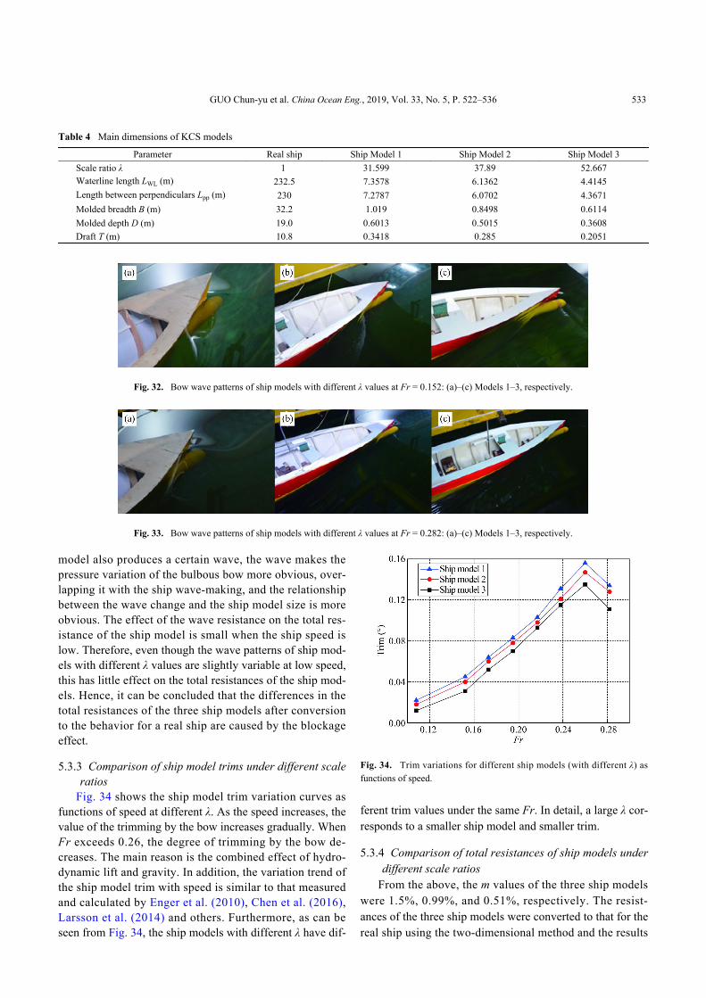
model also produces a certain wave, the wave makes thepressure variation of the bulbous bow more obvious, over-lapping it with the ship wave-making, and the relationshipbetween the wave change and the ship model size is moreobvious. The effect of the wave resistance on the total res-istance of the ship model is small when the ship speed islow. Therefore, even though the wave patterns of ship mod-els with different λ values are slightly variable at low speed,this has little effect on the total resistances of the ship mod-els. Hence, it can be concluded that the differences in thetotal resistances of the three ship models after conversionto the behavior for a real ship are caused by the blockageeffect.

5.3.3 Comparison of ship model trims under different scaleratiosFig. 34 shows the ship model trim variation curves as

functions of speed at different λ. As the speed increases, thevalue of the trimming by the bow increases gradually. WhenFr exceeds 0.26, the degree of trimming by the bow de-creases. The main reason is the combined effect of hydro-dynamic lift and gravity. In addition, the variation trend ofthe ship model trim with speed is similar to that measuredand calculated by Enger et al. (2010), Chen et al. (2016),Larsson et al. (2014) and others. Furthermore, as can beseen from Fig. 34, the ship models with different λ have dif-

ferent trim values under the same Fr. In detail, a large λ cor-responds to a smaller ship model and smaller trim.

5.3.4 Comparison of total resistances of ship models underdifferent scale ratiosFrom the above, the m values of the three ship models

were 1.5%, 0.99%, and 0.51%, respectively. The resist-ances of the three ship models were converted to that for thereal ship using the two-dimensional method and the results

Table 4 Main dimensions of KCS models

Parameter Real ship Ship Model 1 Ship Model 2 Ship Model 3Scale ratio λ 1 31.599 37.89 52.667Waterline length LWL (m) 232.5 7.3578 6.1362 4.4145Length between perpendiculars Lpp (m) 230 7.2787 6.0702 4.3671Molded breadth B (m) 32.2 1.019 0.8498 0.6114Molded depth D (m) 19.0 0.6013 0.5015 0.3608Draft T (m) 10.8 0.3418 0.285 0.2051

Fig. 32. Bow wave patterns of ship models with different λ values at Fr = 0.152: (a)–(c) Models 1–3, respectively.

Fig. 33. Bow wave patterns of ship models with different λ values at Fr = 0.282: (a)–(c) Models 1–3, respectively.

Fig. 34. Trim variations for different ship models (with different λ) asfunctions of speed.


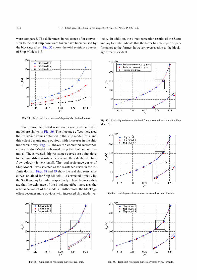
were compared. The differences in resistance after conver-sion to the real ship case were taken have been caused bythe blockage effect. Fig. 35 shows the total resistance curvesof Ship Models 1–3.

The unmodified total resistance curves of each shipmodel are shown in Fig. 36. The blockage effect increasedthe resistance values obtained in the ship model tests, andthis effect became more obvious with increases in the shipmodel velocity. Fig. 37 shows the corrected resistancecurves of Ship Model 3 obtained using the Scott and m1 for-mulas. The corrected ship resistance curves are quite closeto the unmodified resistance curve and the calculated returnflow velocity is very small. The total resistance curve ofShip Model 3 was selected as the resistance curve in the in-finite domain. Figs. 38 and 39 show the real ship resistancecurves obtained for Ship Models 1–3 corrected directly bythe Scott and m1 formulas, respectively. These figures indic-ate that the existence of the blockage effect increases theresistance values of the models. Furthermore, the blockageeffect becomes more obvious with increased ship model ve-

locity. In addition, the direct correction results of the Scottand m1 formula indicate that the latter has far superior per-formance to the former; however, overreaction to the block-age effect is evident.

Fig. 35. Total resistance curves of ship models obtained in test.

Fig. 36. Unmodified resistance curves of real ship.

Fig. 37. Real ship resistance obtained from corrected resistance for ShipModel 3.

Fig. 38. Real ship resistance curves corrected by Scott formula.

Fig. 39. Real ship resistance curves corrected by m1 formula.


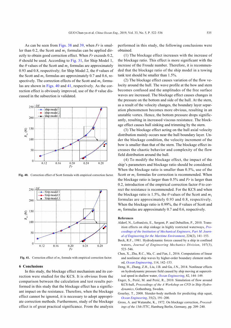
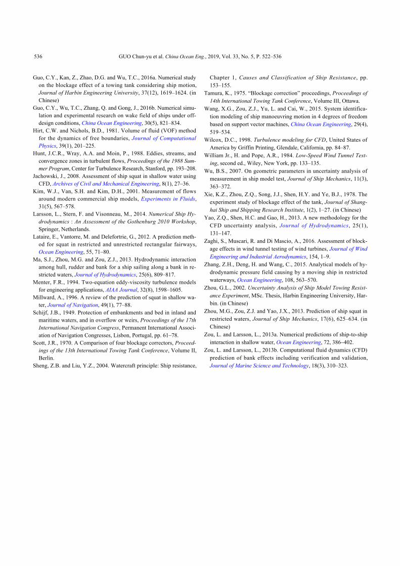
As can be seen from Figs. 38 and 39, when Fr is smal-ler than 0.2, the Scott and m1 formulas can be applied dir-ectly to obtain good correction effect. When Fr exceeds 0.2,θ should be used. According to Fig. 31, for Ship Model 1,the θ values of the Scott and m1 formulas are approximately0.93 and 0.8, respectively; for Ship Model 2, the θ values ofthe Scott and m1 formulas are approximately 0.7 and 0.6, re-spectively. The correction effects of the Scott and m1 formu-las are shown in Figs. 40 and 41, respectively. As the cor-rection effect is obviously improved, use of the θ value dis-cussed in the subsection is validated.

6 ConclusionsIn this study, the blockage effect mechanism and its cor-

rection were studied for the KCS. It is obvious from thecomparison between the calculation and test results per-formed in this study that the blockage effect has a signific-ant impact on the resistance. Therefore, when the blockageeffect cannot be ignored, it is necessary to adopt appropri-ate correction methods. Furthermore, study of the blockageeffect is of great practical significance. From the analysis

performed in this study, the following conclusions wereobtained.

(1) The blockage effect increases with the increase ofthe blockage ratio. This effect is more significant with theincrease of the Froude number. Therefore, it is recommen-ded that the blockage ratio of the ship model in a towingtank test should be smaller than 1.5%.

(2) The blockage effect causes variation of the flow ve-locity around the hull. The wave profile at the bow and sternbecomes confused and the amplitudes of the free surfacewaves are increased. The blockage effect causes changes inthe pressure on the bottom and side of the hull. At the stern,as a result of the velocity changes, the boundary layer separ-ation phenomenon becomes more obvious, resulting in anunstable vortex. Hence, the bottom pressure drops signific-antly, resulting in increased viscous resistance. The block-age effect causes hull sinking and trimming by the stern.

(3) The blockage effect acting on the hull axial velocitydistribution mainly occurs near the hull boundary layer. Un-der the blockage condition, the velocity increment of thebow is smaller than that of the stern. The blockage effect in-creases the chaotic behavior and complexity of the flowfield distribution around the hull.

(4) To modify the blockage effect, the impact of theship’s parameters and blockage ratio should be considered.When the blockage ratio is smaller than 0.5%, use of theScott or m1 formulas for correction is recommended. Whenthe blockage ratio is larger than 0.5% and Fr is larger than0.2, introduction of the empirical correction factor θ to cor-rect the resistance is recommended. For the KCS and whenthe blockage ratio is 1.5%, the θ values of the Scott and m1formulas are approximately 0.93 and 0.8, respectively.When the blockage ratio is 0.99%, the θ values of Scott andm1 formulas are approximately 0.7 and 0.6, respectively.

ReferencesAlderf, N., Lefranĉois, E., Sergent, P. and Debaillon, P., 2010. Trans-ition effects on ship sinkage in highly restricted waterways, Pro-ceedings of the Institution of Mechanical Engineers, Part M: Journ-al of Engineering for the Maritime Environment, 224(2), 141–153.

Beck, R.F., 1981. Hydrodynamic forces caused by a ship in confinedwaters, Journal of Engineering Mechanics Division, 107(3),523–546.

Chen, X., Zhu, R.C., Ma, C. and Fan, J., 2016. Computations of linearand nonlinear ship waves by higher-order boundary element meth-od, Ocean Engineering, 114, 142–153.

Deng, H., Zhang, Z.H., Liu, J.B. and Gu, J.N., 2014. Nonlinear effectson hydrodynamic pressure field caused by ship moving at supercrit-ical speed in shallow water, Ocean Engineering, 82, 144–149.

Enger, S., Perić, M. and Perić, R., 2010. Simulation of flow aroundKCS-hull, Proceedings of the A Workshop on CFD in Ship Hydro-dynamics, Gothenburg, Sweden.

Gourlay, T., 2008. Slender-body methods for predicting ship squat,Ocean Engineering, 35(2), 191–200.

Gross, A. and Watanabe, K., 1972. On blockage correction, Proceed-ings of the 13th ITTC, Hamburg Berlin, Germany, pp. 209–240.

Fig. 40. Correction effect of Scott formula with empirical correction factor.

Fig. 41. Correction effect of m1 formula with empirical correction factor.


http://dx.doi.org/10.1243/14750902JEME170




Guo, C.Y., Kan, Z., Zhao, D.G. and Wu, T.C., 2016a. Numerical studyon the blockage effect of a towing tank considering ship motion,Journal of Harbin Engineering University, 37(12), 1619–1624. (inChinese)

Guo, C.Y., Wu, T.C., Zhang, Q. and Gong, J., 2016b. Numerical simu-lation and experimental research on wake field of ships under off-design conditions, China Ocean Engineering, 30(5), 821–834.

Hirt, C.W. and Nichols, B.D., 1981. Volume of fluid (VOF) methodfor the dynamics of free boundaries, Journal of ComputationalPhysics, 39(1), 201–225.

Hunt, J.C.R., Wray, A.A. and Moin, P., 1988. Eddies, streams, andconvergence zones in turbulent flows, Proceedings of the 1988 Sum-mer Program, Center for Turbulence Research, Stanford, pp. 193–208.

Jachowski, J., 2008. Assessment of ship squat in shallow water usingCFD, Archives of Civil and Mechanical Engineering, 8(1), 27–36.

Kim, W.J., Van, S.H. and Kim, D.H., 2001. Measurement of flowsaround modern commercial ship models, Experiments in Fluids,31(5), 567–578.

Larsson, L., Stern, F. and Visonneau, M., 2014. Numerical Ship Hy-drodynamics : An Assessment of the Gothenburg 2010 Workshop,Springer, Netherlands.

Lataire, E., Vantorre, M. and Delefortrie, G., 2012. A prediction meth-od for squat in restricted and unrestricted rectangular fairways,Ocean Engineering, 55, 71–80.

Ma, S.J., Zhou, M.G. and Zou, Z.J., 2013. Hydrodynamic interactionamong hull, rudder and bank for a ship sailing along a bank in re-stricted waters, Journal of Hydrodynamics, 25(6), 809–817.

Menter, F.R., 1994. Two-equation eddy-viscosity turbulence modelsfor engineering applications, AIAA Journal, 32(8), 1598–1605.

Millward, A., 1996. A review of the prediction of squat in shallow wa-ter, Journal of Navigation, 49(1), 77–88.

Schijf, J.B., 1949. Protection of embankments and bed in inland andmaritime waters, and in overflow or weirs, Proceedings of the 17thInternational Navigation Congress, Permanent International Associ-ation of Navigation Congresses, Lisbon, Portugal, pp. 61–78.

Scott, J.R., 1970. A Comparison of four blockage correctors, Proceed-ings of the 13th International Towing Tank Conference, Volume II,Berlin.

Sheng, Z.B. and Liu, Y.Z., 2004. Watercraft principle: Ship resistance,

Chapter 1, Causes and Classification of Ship Resistance, pp.153–155.

Tamura, K., 1975. “Blockage correction” proceedings, Proceedings of14th International Towing Tank Conference, Volume III, Ottawa.

Wang, X.G., Zou, Z.J., Yu, L. and Cai, W., 2015. System identifica-tion modeling of ship manoeuvring motion in 4 degrees of freedombased on support vector machines, China Ocean Engineering, 29(4),519–534.

Wilcox, D.C., 1998. Turbulence modeling for CFD, United States ofAmerica by Griffin Printing, Glendale, California, pp. 84–87.

William Jr., H. and Pope, A.R., 1984. Low-Speed Wind Tunnel Test-ing, second ed., Wiley, New York, pp. 133–135.

Wu, B.S., 2007. On geometric parameters in uncertainty analysis ofmeasurement in ship model test, Journal of Ship Mechanics, 11(3),363–372.

Xie, K.Z., Zhou, Z.Q., Song, J.J., Shen, H.Y. and Ye, B.J., 1978. Theexperiment study of blockage effect of the tank, Journal of Shang-hai Ship and Shipping Research Institute, 1(2), 1–27. (in Chinese)

Yao, Z.Q., Shen, H.C. and Gao, H., 2013. A new methodology for theCFD uncertainty analysis, Journal of Hydrodynamics, 25(1),131–147.

Zaghi, S., Muscari, R. and Di Mascio, A., 2016. Assessment of block-age effects in wind tunnel testing of wind turbines, Journal of WindEngineering and Industrial Aerodynamics, 154, 1–9.

Zhang, Z.H., Deng, H. and Wang, C., 2015. Analytical models of hy-drodynamic pressure field causing by a moving ship in restrictedwaterways, Ocean Engineering, 108, 563–570.

Zhou, G.L., 2002. Uncertainty Analysis of Ship Model Towing Resist-ance Experiment, MSc. Thesis, Harbin Engineering University, Har-bin. (in Chinese)

Zhou, M.G., Zou, Z.J. and Yao, J.X., 2013. Prediction of ship squat inrestricted waters, Journal of Ship Mechanics, 17(6), 625–634. (inChinese)

Zou, L. and Larsson, L., 2013a. Numerical predictions of ship-to-shipinteraction in shallow water, Ocean Engineering, 72, 386–402.

Zou, L. and Larsson, L., 2013b. Computational fluid dynamics (CFD)prediction of bank effects including verification and validation,Journal of Marine Science and Technology, 18(3), 310–323.


Numerical and Experimental Study of Blockage Effect ...

Documents

Transcript of Numerical and Experimental Study of Blockage Effect ...