Experimental and numerical study of radial flow and itscontribution to wake development of a HAWT

Daniel Micallef1,2, Busra Akay1, Tonio Sant2, Carlos Simão Ferreira1, Gerard van Bussel1

1DUWIND, TUDelft, Faculty of Aerospace Engineering, Kluyverweg 1, 2629 HS, Delft, The Netherlands2University of Malta, Faculty of Engineering, Department of Mechanical Eng., Msida, MSD 2080 Malta.

Keywords: Horizontal axis wind-turbine, radial flow, wake expansion

Abstract:

The scope of this work was to investigate radial flowcomponent for a Horizontal Axis Wind Turbine in ax-ial flow conditions and to assess its impact on theturbine operation. This was done by means of Parti-cle Image Velocimetry and numerical simulation witha 3D unsteady potential-flow panel model. A directcomparison between the numerical and experimen-tal radial velocity results show differences in the tipand root regions. These differences have importantimplications on the wake development just at themoment of release of the tip vortex. Moreover, theimpact of the radial velocities on the blade loadinghas been studied using the numerical results. Thecontribution of the radial velocity to the normal loadon the blade is only slightly appreciable in the tip androot regions of the blade. However, as the numericalmodel does not account for viscous effects, furtheranalysis of impact on boundary layer development isnecessary.

Nomenclature

r = radial position [m]R = Rotor radius [m]θ = Twist [deg.]µ = Doublet strength [m3/s]∇ = Differential operatorΦ = Velocity potential [m2/s]S = Surface of integration [m2]σ = Source strength [m3/s]x = distance from a particular point in the flow field[m]∂/∂n = differential operator along the normaldirection [m−1]ε = error estimatorp = order of the numerical method used in thesimulationη = the ratio of the number of panels used for thesimulation against a reference simulationRhub = Rotor hub radius [m]D = Rotor diameter [m]

Cp = Pressure coefficientV = Absolute velocity [m/s]Vref = Reference velocity [m/s]t = Time [s]ρ = Air density [kg/m3]F = Force per unit length [N/m]

Subscripts:u = Upper surface of the airfoil (suction side)l = Lower surface of the airfoil (pressure side)w = WakeB = Body∞ = Free-streamref = Reference simulation (one having a finediscretization and a high number of revolutions)

Abbreviations:OJF - Open Jet FacilitySPIV - Stereo Particle Image VelocimetryNREL - National Renewable Energy LaboratoryUAE - Unsteady aerodynamics experimentMEXICO - Model experiment in controlled condi-tionsFOV - Field of viewGCI - Grid convergence index

1 Introduction and ResearchQuestions

The radial component of the flow perceived by therotor blade is a result of the apparent flow motionin the rotating reference frame and the radial induc-tion of the flow in the inertial reference frame. Inthis research paper, we experimentally and numeri-cally analyze the latter. A 2m diameter, two-bladedwind-turbine model was tested in the Open Jet Fa-cility (OJF) at Delft University of Technology. StereoParticle Image Velocimetry (SPIV) was used to de-termine the velocity field over the blades as well asin the wake. The experiment was simulated using apotential-flow panel method to investigate the radialflow and its contribution to the wake’s development.

The numerical simulations were validated with theexperimental data and used to analyze the sourceof the radial expansion.

Flow velocities were measured in past experi-ments using PIV as well as hot-wire anemome-try. An overview of wind-turbine wake research atTUDelft is given by Vermeer [1].For a wind-turbinein axial flow, the radial component of velocity is dueto the wake induction and the bound circulation andblockage of the blade. Much of the focus in literatureis placed on the effect that radial velocity has on thestability of the boundary layer in the root region of theblade resulting in stall delay. The NREL UnsteadyAerodynamics Experiment (UAE) [2] and the ModelExperiment in Controlled Conditions (MEXICO) [3]revealed the dramatic effects that radial flows havein the root region. Schreck et al. give an excellent re-view (especially of the findings from the NREL UAEphase VI experiments) in [4]. Moreover, some re-cent results have also been obtained for the MEX-ICO experiment by Schepers et al. [5] and Schrecket al. [6]. Various experimental studies have beenconducted which report radial velocities in the wakesuch as by Medici et al.[7] at locations 1D down-stream. At these distances from the rotor plane, ra-dial components are almost negligible. Ebert et al.[8, 9, 10] show the velocity components at around1.5 chord lengths downstream. The tip vortex wasfound to have a relatively high impact in the tip re-gion. A lifting-line numerical model was used bySant et al. [11, 12] and radial velocities on the bladelifting line were established for the NREL phase VIrotor. Sant found that radial components (due to thewake) are directed outwards at the tip region and in-wards towards the hub in the root region for the caseof attached flow. This was not found for the sepa-rated flow cases. The causes of this behaviour arenot discussed in detail and the effects of the nacellewere not included. In this work we address radialvelocities in the outer flow (external to the boundarylayer) since, as was shown in the referred literature,it has fundamental implications on the sectional air-foil behaviour. The aims of this study are thereforeas follows:

1. Shed light on the impact that radial velocity hason the wake development by means of compu-tational results

2. Build upon the current knowledge on the three-dimensionality of wind-turbine flow

3. Investigate the relevance of radial flows forwind-turbine blade design in particular how theradial flow impacts the loading

0

0.05

0.1

0.15

0.2

0.25

-2

0

2

4

6

8

10

12

14

16

18

0 0.2 0.4 0.6 0.8 1

c/Rθ

[deg

]

r/R

θ [deg]

c/R

Figure 1: Twist and chord distribution along theblade.

Yaw angle 0Wind speed 6 m/s

Pitch 0Tip speed ratio 7

Thrust coefficient 0.87Power coefficient 0.44

Table 1: Experimental wind-turbine specifications

2 Experimental Setup

In the SPIV experiment, the model wind-turbinemodel was tested in the OJF wind tunnel at TUDelft,which has an octagonal jet with equivalent diame-ter of 3 m. Figure 1 shows the chord and twistdistributions of the blade. The airfoil section usedwas a DU96-W180 throughout the entire span of theblade except at the connection point with the hub(nacelle). The tip radius was 1 m while the hub ra-dius was 0.147 m. The rotor had two blades androtated in a clock-wise direction when looking down-wind. The test conditions used in this experimentare summarised in table 1.

Spanwise measurements were performed toquantify the flow field.The laser sheet was on a hori-zontal plane with the cameras viewing from below.For this setup, a Field of View (FOV) of around265mm x 194mm was used. The angles betweenthe cameras was set to approximately 40°. Mea-surements were taken at five spanwise locations(covering the entire blade span) and for each loca-tion, images were taken for various azimuthal posi-tions. This ensured that the flow field was capturedfor the entire blade passage through the horizontalplane. In order to account for shadowing effects, im-ages were taken from an upwind and downwind di-rections. A single field-of-view result was composedof the several measurements at different spanwiseand azimuthal positions; these results are presentedin this paper. Figure 2 shows the camera-laser con-

Laser

Cameras

Experimental

turbine

Laser

sheet LaserLaser

Cameras

Experimental

turbine

Laser

sheet

Figure 2: Measurements in the spanwise direction.

figuration used to perform the measurements.

3 Potential Flow Solver

The experimental turbine was modelled using a 3Dunsteady potential-flow panel-method with a free-wake model as described in the work of Dixon [13].To model a 3D body, the surface is approximatedby a number of doublet and source panels. As theblades rotate, a wake of free-convecting doublets isreleased from the trailing edge. The panel modeluses a Dirichlet boundary condition. This can thenbe used to evaluate the velocities by means of dif-ferentiating the potential function given by [14]:

∇Φ = − 14π

∫SB

σ∇(

1x

)ds

+1

4π

∫SB+SW

µ∇[∂

∂n

(1x

)]dS +∇Φ∞ (1)

Figure 3 represents the body having doubletstrengths µu and µl on the suction and pressureside of the airfoil respectively. Source terms on theupper and lower surfaces should also be includedbut are not shown in the figure to keep it unclut-tered. According to the Kutta condition, the vorticityat the trailing edge should be zero. Thus, the wakedoublet strength is given by the difference in dou-blet strengths of the upper and lower surfaces of thebody. The model may be used to simulate the be-haviours of multiple bodies such as for instance theblades, nacelle and tower. The formulation used inthis model is an unsteady approach and thereforecan account for unsteady effects. More detail canbe found in [14]. Thorough validation of the modelwas carried out by Dixon [13] and Ferreira [15].

The simulated body includes both blades, huband nacelle. Solution convergence was checked

μu

μw = (μu - μl)t

μw = (μu - μl)t-Δt

μl

Trailing edgeAirfo

il low pressure side

Wake

Figure 3: Panel representation of the wing and therelease of panels representing the wake.

by studying the convergence of bound circulation aswell as velocities at various points in the flow field.The method proposed in [16] was used to obtain anestimate of the Grid Convergence index (GCI) whichis defined as follows:

GCI =|ε| ηp

ηp − 1(2)

Where p is the order of the numerical methodused (here taken as 1), η is the ratio of the totalnumber of panels used to the total number of pan-els used in a reference simulation (having a fine dis-cretization and a large number of rotor revolutions)and ε is an error estimator given by:

ε =f − fref

fref(3)

Where f is the value of a particular variable fromthe solution and fref is the same value but for thereference simulation.

Two types of checks were carried out:

1. Independence of blade and wake discretisationby having a coarse, moderate and fine discreti-sation of the blades (and hence of the shedwake): The GCI of the bound circulation andvelocities at various points converged to within4% with a fine mesh setting.

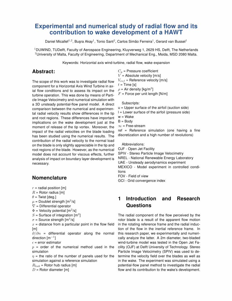
2. Independence from the number of rotor revo-lutions: The convergence errors are shown infigure 4. All quantities fall below 3% after 13wake revolutions.

The input parameters for the fine mesh simulationare summarised in table 2. The operating conditionsof wind speed and rotor speed of the experimentwere used as input.

0

5

10

15

20

25

30

35

40

45

50

0 1 2 3 4 5 6 7 8 9 10 11 12 13 14

ε(%

)

Number of rotor revolutions

Circulation

u (y/D = 0)

u (y/D = 0.2)

u (y/D = 0.4)

u (y/D = 0.6)

u (y/D = 0.8)

Figure 4: Convergence of bound circulation and ax-ial velocities for increasing number of revolutions.Velocity convergence is shown at 5 different down-stream positions (at x/D = 0.25).

Blade spanwise panels 46Blade chordwise panels 38

Nacelle spanwise panels 50Nacelle circumferential panels 50

Azimuthal step 10°No. of rotor revolutions 14

Vortex model Ramasamy-Leishman [17, 18]

Core growth model Ramasamy-Leishman [17, 18]

Table 2: - Input parameters for the panel code sim-ulation.

4 Results

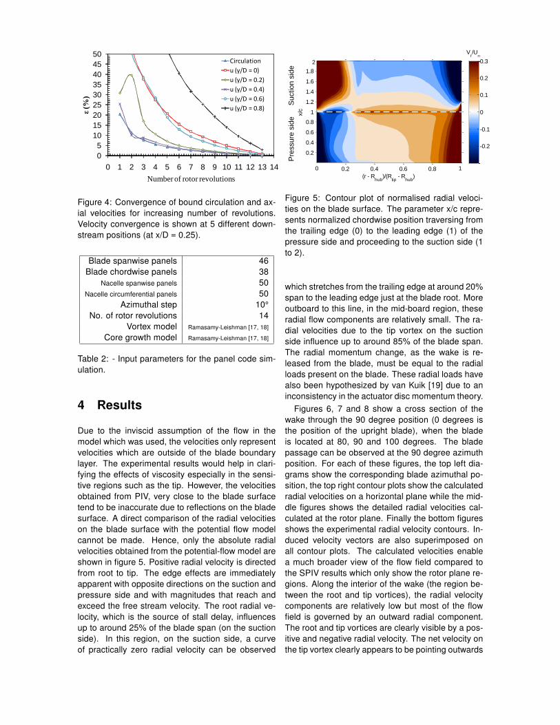
Due to the inviscid assumption of the flow in themodel which was used, the velocities only representvelocities which are outside of the blade boundarylayer. The experimental results would help in clari-fying the effects of viscosity especially in the sensi-tive regions such as the tip. However, the velocitiesobtained from PIV, very close to the blade surfacetend to be inaccurate due to reflections on the bladesurface. A direct comparison of the radial velocitieson the blade surface with the potential flow modelcannot be made. Hence, only the absolute radialvelocities obtained from the potential-flow model areshown in figure 5. Positive radial velocity is directedfrom root to tip. The edge effects are immediatelyapparent with opposite directions on the suction andpressure side and with magnitudes that reach andexceed the free stream velocity. The root radial ve-locity, which is the source of stall delay, influencesup to around 25% of the blade span (on the suctionside). In this region, on the suction side, a curveof practically zero radial velocity can be observed

(r - Rhub

)/(Rtip

- Rhub

)

x/c

0.2 0.4 0.6 0.8

0.2

0.4

0.6

0.8

1

1.2

1.4

1.6

1.8

Vr/U

-0.2

-0.1

0

0.1

0.2

0.3

Pre

ssu

re s

ide

Su

ctio

n s

ide

0 1

2

Figure 5: Contour plot of normalised radial veloci-ties on the blade surface. The parameter x/c repre-sents normalized chordwise position traversing fromthe trailing edge (0) to the leading edge (1) of thepressure side and proceeding to the suction side (1to 2).

which stretches from the trailing edge at around 20%span to the leading edge just at the blade root. Moreoutboard to this line, in the mid-board region, theseradial flow components are relatively small. The ra-dial velocities due to the tip vortex on the suctionside influence up to around 85% of the blade span.The radial momentum change, as the wake is re-leased from the blade, must be equal to the radialloads present on the blade. These radial loads havealso been hypothesized by van Kuik [19] due to aninconsistency in the actuator disc momentum theory.

Figures 6, 7 and 8 show a cross section of thewake through the 90 degree position (0 degrees isthe position of the upright blade), when the bladeis located at 80, 90 and 100 degrees. The bladepassage can be observed at the 90 degree azimuthposition. For each of these figures, the top left dia-grams show the corresponding blade azimuthal po-sition, the top right contour plots show the calculatedradial velocities on a horizontal plane while the mid-dle figures shows the detailed radial velocities cal-culated at the rotor plane. Finally the bottom figuresshows the experimental radial velocity contours. In-duced velocity vectors are also superimposed onall contour plots. The calculated velocities enablea much broader view of the flow field compared tothe SPIV results which only show the rotor plane re-gions. Along the interior of the wake (the region be-tween the root and tip vortices), the radial velocitycomponents are relatively low but most of the flowfield is governed by an outward radial component.The root and tip vortices are clearly visible by a pos-itive and negative radial velocity. The net velocity onthe tip vortex clearly appears to be pointing outwards

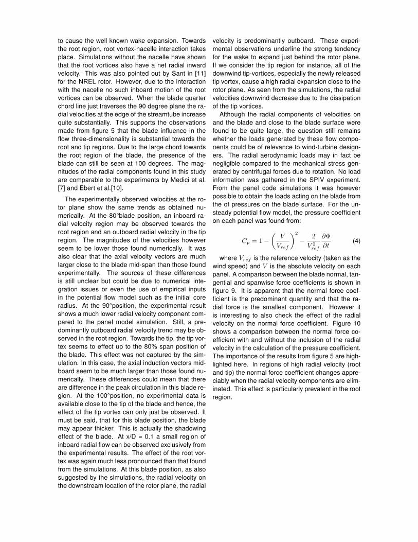
to cause the well known wake expansion. Towardsthe root region, root vortex-nacelle interaction takesplace. Simulations without the nacelle have shownthat the root vortices also have a net radial inwardvelocity. This was also pointed out by Sant in [11]for the NREL rotor. However, due to the interactionwith the nacelle no such inboard motion of the rootvortices can be observed. When the blade quarterchord line just traverses the 90 degree plane the ra-dial velocities at the edge of the streamtube increasequite substantially. This supports the observationsmade from figure 5 that the blade influence in theflow three-dimensionality is substantial towards theroot and tip regions. Due to the large chord towardsthe root region of the blade, the presence of theblade can still be seen at 100 degrees. The mag-nitudes of the radial components found in this studyare comparable to the experiments by Medici et al.[7] and Ebert et al.[10].

The experimentally observed velocities at the ro-tor plane show the same trends as obtained nu-merically. At the 80°blade position, an inboard ra-dial velocity region may be observed towards theroot region and an outboard radial velocity in the tipregion. The magnitudes of the velocities howeverseem to be lower those found numerically. It wasalso clear that the axial velocity vectors are muchlarger close to the blade mid-span than those foundexperimentally. The sources of these differencesis still unclear but could be due to numerical inte-gration issues or even the use of empirical inputsin the potential flow model such as the initial coreradius. At the 90°position, the experimental resultshows a much lower radial velocity component com-pared to the panel model simulation. Still, a pre-dominantly outboard radial velocity trend may be ob-served in the root region. Towards the tip, the tip vor-tex seems to effect up to the 80% span position ofthe blade. This effect was not captured by the sim-ulation. In this case, the axial induction vectors mid-board seem to be much larger than those found nu-merically. These differences could mean that thereare difference in the peak circulation in this blade re-gion. At the 100°position, no experimental data isavailable close to the tip of the blade and hence, theeffect of the tip vortex can only just be observed. Itmust be said, that for this blade position, the blademay appear thicker. This is actually the shadowingeffect of the blade. At x/D = 0.1 a small region ofinboard radial flow can be observed exclusively fromthe experimental results. The effect of the root vor-tex was again much less pronounced than that foundfrom the simulations. At this blade position, as alsosuggested by the simulations, the radial velocity onthe downstream location of the rotor plane, the radial

velocity is predominantly outboard. These experi-mental observations underline the strong tendencyfor the wake to expand just behind the rotor plane.If we consider the tip region for instance, all of thedownwind tip-vortices, especially the newly releasedtip vortex, cause a high radial expansion close to therotor plane. As seen from the simulations, the radialvelocities downwind decrease due to the dissipationof the tip vortices.

Although the radial components of velocities onand the blade and close to the blade surface werefound to be quite large, the question still remainswhether the loads generated by these flow compo-nents could be of relevance to wind-turbine design-ers. The radial aerodynamic loads may in fact benegligible compared to the mechanical stress gen-erated by centrifugal forces due to rotation. No loadinformation was gathered in the SPIV experiment.From the panel code simulations it was howeverpossible to obtain the loads acting on the blade fromthe of pressures on the blade surface. For the un-steady potential flow model, the pressure coefficienton each panel was found from:

Cp = 1−(

V

Vref

)2

− 2V 2

ref

∂Φ∂t

(4)

where Vref is the reference velocity (taken as thewind speed) and V is the absolute velocity on eachpanel. A comparison between the blade normal, tan-gential and spanwise force coefficients is shown infigure 9. It is apparent that the normal force coef-ficient is the predominant quantity and that the ra-dial force is the smallest component. However itis interesting to also check the effect of the radialvelocity on the normal force coefficient. Figure 10shows a comparison between the normal force co-efficient with and without the inclusion of the radialvelocity in the calculation of the pressure coefficient.The importance of the results from figure 5 are high-lighted here. In regions of high radial velocity (rootand tip) the normal force coefficient changes appre-ciably when the radial velocity components are elim-inated. This effect is particularly prevalent in the rootregion.

olid

Wor

ks S

tude

nt L

icen

seca

dem

ic U

se O

nly

(a)

00

.10

.20

.30

.40

.50

.6-0

.1

-0.0

50

0.0

5

0.1

0.1

5

0.2

0.2

5

0.3

x/D

y/D

Vr/U

-0.2

-0.1

00.1

0.2

0.3

(b)

0.0

50

.10

.15

0.2

0.2

50

.30

.35

0.4

0

0.0

2

0.0

4

0.0

6

0.0

8

x/D

y/D

Vr/U

-0.2

-0.1

00.1

0.2

0.3

Vr/U

∞

(c)

y/D

x/D

0

0.0

2

0.0

4

0.0

6

0.0

8

0.0

50

.10

.15

0.2

0.2

50

.30

.35

0.4

Vr/U

-0.2

-0.1

00.1

0.2

0.3

x/D

Vr/U

∞

(d)

Fig

ure

6:B

lade

posi

tion

at80

degr

ees.

Top-

left

figur

esh

ows

blad

epo

sitio

n,to

prig

htfig

ure

show

sco

mpu

ted

radi

alve

loci

ties

ona

horiz

onta

lpla

neas

obta

ined

from

the

pane

lmod

el,

cent

ralfi

gure

show

sco

mpu

ted

velo

citie

sat

the

roto

rpl

ane

only

and

botto

mfig

ure

show

sve

loci

ties

inth

ero

tor

plan

eas

obta

ined

from

the

expe

rimen

t.

00.0

5

0.1

0.1

5

0.2

0.2

5

-202468

10

12

14

16

18

00.2

0.4

0.6

0.8

1

c/R

θ[deg]

r/R

θ [

deg

]

c/R

olid

Wor

ks S

tude

nt L

icen

seca

dem

ic U

se O

nly

(a)

00

.10

.20

.30

.40

.50

.6-0

.1

-0.0

50

0.0

5

0.1

0.1

5

0.2

0.2

5

0.3

x/D

y/D

Vr/U

-0.2

-0.1

00.1

0.2

0.3

(b)

0.0

50

.10

.15

0.2

0.2

50

.30

.35

0.4

0.4

50

.50

.55

0

0.0

2

0.0

4

0.0

6

0.0

8

x/D

y/D

Vr/U

-0.2

-0.1

00.1

0.2

0.3

Vr/U

∞

(c)

y/D

x/D

0

0.0

2

0.0

4

0.0

6

0.0

8

0.0

50

.10

.15

0.2

0.2

50

.30

.35

0.4

0.4

50

.50

.55

Vr/U

-0.2

-0.1

00.1

0.2

0.3

x/D

Vr/U

∞

(d)

Fig

ure

7:B

lade

posi

tion

at90

degr

ees.

Top-

left

figur

esh

ows

blad

epo

sitio

n,to

prig

htfig

ure

show

sco

mpu

ted

radi

alve

loci

ties

ona

horiz

onta

lpla

neas

obta

ined

from

the

pane

lmod

el,

cent

ralfi

gure

show

sco

mpu

ted

velo

citie

sat

the

roto

rpl

ane

only

and

botto

mfig

ure

show

sve

loci

ties

inth

ero

tor

plan

eas

obta

ined

from

the

expe

rimen

t.

00.0

5

0.1

0.1

5

0.2

0.2

5

-202468

10

12

14

16

18

00.2

0.4

0.6

0.8

1

c/R

θ[deg]

r/R

θ [

deg

]

c/R

olid

Wor

ks S

tude

nt L

icen

seca

dem

ic U

se O

nly

(a)

00

.10

.20

.30

.40

.50

.6-0

.1

-0.0

50

0.0

5

0.1

0.1

5

0.2

0.2

5

0.3

x/D

y/D

Vr/U

-0.2

-0.1

00.1

0.2

0.3

(b)

Vr/U

∞

0.0

50

.10

.15

0.2

0.2

50

.30

.35

0.4

0

0.0

2

0.0

4

0.0

6

0.0

8

x/D

y/D

Vr/U

-0.2

-0.1

00.1

0.2

0.3

(c)

y/D

x/D

0

0.0

2

0.0

4

0.0

6

0.0

8

0.0

50

.10

.15

0.2

0.2

50

.30

.35

0.4

Vr/U

-0.2

-0.1

00.1

0.2

0.3

x/D

Vr/U

∞

(d)

Fig

ure

8:B

lade

posi

tion

at10

0de

gree

s.To

p-le

ftfig

ure

show

sbl

ade

posi

tion,

top

right

figur

esh

ows

com

pute

dra

dial

velo

citie

son

aho

rizon

talp

lane

asob

tain

edfr

omth

epa

nelm

odel

,ce

ntra

lfigu

resh

ows

com

pute

dve

loci

ties

atth

ero

tor

plan

eon

lyan

dbo

ttom

figur

esh

ows

velo

citie

sin

the

roto

rpl

ane

asob

tain

edfr

omth

eex

perim

ent.

00.0

5

0.1

0.1

5

0.2

0.2

5

-202468

10

12

14

16

18

00.2

0.4

0.6

0.8

1

c/R

θ[deg]

r/R

θ [

deg

]

c/R

-0.4

-0.2

0

0.2

0.4

0.6

0.8

1

1.2

0 0.1 0.2 0.3 0.4 0.5 0.6 0.7 0.8 0.9 1

Fo

rce

Co

effi

cien

t =

F/(

1/2ρ

Vre

l²c)

r/R

Normal

Tangential

Spanwise

Figure 9: Force coefficient against non-dimensionalised radius as obtained from thepotential flow simulations (effects of friction dragcannot be included). Normal, tangential andspanwise coefficients are shown.

-0.8

-0.6

-0.4

-0.2

0

0.2

0.4

0.6

0.8

1

1.2

0 0.1 0.2 0.3 0.4 0.5 0.6 0.7 0.8 0.9 1

Fo

rce

Co

effi

cien

t =

F/(

1/2ρ

Vre

l²c)

r/R

Normal

Normal (no effect of radial velocity)

Figure 10: Normal force coefficient against non-dimensionalised radius compared to the same quan-tity but without the effect of the radial velocity in thecalculation of the blade forces.

5 Conclusion

This work explores the behaviour of the radial flowvelocity, for an axial flow wind-turbine. To this end,SPIV experimental results have been used. To bet-ter understand the flow physics, a panel model hasbeen adopted. The evolution and expansion of thewake could hence be explained from the complexinteraction of the tip vortices. The description of theradial flow velocity on the blade leads to better un-derstanding of the relevance of blade radial loadswhich were investigated for the actuator disc caseby van Kuik et al. [19].

In conclusion it may be stated that radial flowspredominate in the root and tip regions of the bladewith directions corresponding to the orientations ofthe root and tip vortices. In the mid-board regionthe radial components are relatively small. Nacelle-

root vortex interaction was observed experimentallyas well as numerically. Moreover, the radial loadsfor axial flow conditions are small especially whencompared to the normal force component. It wasalso shown that if the radial velocity contribution tothe pressure distribution was ignored, only a slighteffect on the normal force coefficient results in theroot and tip regions. Nonetheless, it must be em-phasized that a viscous analysis is required to com-pletely understand the effects on the loading. In fu-ture work, chordwise measurements will be consid-ered. Also, for yawed flow, it can be hypothesizedthat radial flows play a much more important part.This will also be studied in later work.

References

[1] L. Vermeer, “A review of wind turbine wake re-search at TUdelft,” in A Collection of the 2001ASME Wind Energy Symposium Technical Pa-pers, pp. pp 103–113, 21-23 May 2001.

[2] M. Hand, D. Simms, L. Fingersh, D. Jager,J. Cotrell, S. Schreck, and S. Larwood, “Un-steady Aerodynamics Experiment Phase VI:Wind Tunnel Test Configurations and AvailableData Campaigns.” Technical Report NREL/TP-500-29955, National Renewable Energy Labo-ratory 1617 Cole Boulevard Golden, Colorado80401-3393, 2001.

[3] J. G. Schepers and H. Snel, “Model experi-ments in controlled conditions(MEXICO),” June2007. ECN-E-07-042.

[4] S. J. Schreck and M. C. Robinson, “Horizon-tal axis wind turbine blade aerodynamics in ex-periments and modeling,” Energy Conversion,IEEE Transactions on, vol. 22, pp. 61 –70, mar.2007.

[5] G. Schepers, K. Boorsma, and H. Snel, “Ieatask 29 mexnext: Analysis of wind tunnel mea-surements from the eu project mexico,” in 3rdTorque 2010 The Science of making Torquefrom Wind Conference, (FORTH, Heraklion,Crete, Greece), June 28-30 2010.

[6] S. Schreck, T.Sant, and D. Micallef, “Rotationalaugmentation disparities in the mexico and uaephase vi experiments,” in 3rd Torque 2010 TheScience of making Torque from Wind Con-ference, (FORTH, Heraklion, Crete, Greece),June 28-30 2010.

[7] D. Medici and P. Andersson, “Measurementson a wind turbine wake 3d effects and bluff

body vortex shedding,” Wind Energy Journal,vol. 9, pp. 219 – 236, 2006.

[8] P. Ebert and D. Wood, “The near wake of amodel horizontal-axis wind turbine - i experi-mental arrangements and initial results,” Re-newable Energy, vol. 12, pp. 225–243, 1997.

[9] P. Ebert and D. Wood, “The near wake of amodel horizontal-axis wind turbine - ii. generalfeatures of the three-dimensional flowfield,” Re-newable Energy, vol. 18, pp. 513–534, 1999.

[10] P. Ebert and D. Wood, “The near wake ofa model horizontal-axis wind turbine part 3:Properties of the tip and hub vortices,” Renew-able Energy, vol. 22, pp. 461–472, 2001.

[11] T. Sant, G. van Bussel, and G. van Kuik, “Es-timating the angle of attack from blade pres-sure measurements on the nrel phase vi rotorusing a free wake vortex model: Axial condi-tions,” Wind Energy Journal, vol. 9, pp. 549–577, 2006.

[12] T. Sant, Improving BEM based aerodynamicmodels in wind turbine design codes. PhD the-sis, Technische Universiteit Delft, 2007.

[13] K. Dixon, “The near wake structure of a verticalaxis wind turbine,” Master’s thesis, TechnischeUniversiteit Delft, 2008.

[14] J. Katz and A. Plotkin, Low-Speed Aerodynam-ics. Cambridge University Press, second ed.,2001.

[15] C. S. Ferreira, The Near Wake of the VAWT.PhD thesis, Technische Universiteit Delft,2009.

[16] P. J. Roache, Verification and Validationin Computational Science and Engineering,pp. 107–141. Hermosa Publishers, 1998.

[17] M. Ramasamy and J. G. Leishman, “A gen-eralized model for transitional blade tip vor-tices,” Journal of the American Helicopter So-ciety, vol. 51, no. 1, pp. 92–103, 2006.

[18] M. Ramasamy and J. G. Leishman, “A reynoldsnumber-based blade tip vortex model,” Jour-nal of the American Helicopter Society, vol. 52,no. 3, pp. 214–223, 2007.

[19] G. van Kuik and A. van Zuylen, “On actuatordisc force fields generating wake vorticity,” inProc. 508 Euromech Colloquium on wind tur-bine wakes, (Madrid, Spain), October 2009.

Acknowledgments

The research work disclosed in this publication ispartially funded by Malta Government ScholarshipScheme grant number MGSS PHD 2008-11, Ves-tas and TUDelft. The authors also acknowledge theassistance of B. Geurts during the experiment.

View publication statsView publication stats