Experimental and numerical FSI study of compliant hydrofoils
Upload
khangminh22Category
view
3download
0
HAL Id: tel-01587720https://tel.archives-ouvertes.fr/tel-01587720
Submitted on 14 Sep 2017
HAL is a multi-disciplinary open accessarchive for the deposit and dissemination of sci-entific research documents, whether they are pub-lished or not. The documents may come fromteaching and research institutions in France orabroad, or from public or private research centers.
L’archive ouverte pluridisciplinaire HAL, estdestinée au dépôt et à la diffusion de documentsscientifiques de niveau recherche, publiés ou non,émanant des établissements d’enseignement et derecherche français ou étrangers, des laboratoirespublics ou privés.
Multiscale experimental and numerical study of thestructure and the dynamics of water confined in clay
mineralsEmmanuel Guillaud
To cite this version:Emmanuel Guillaud. Multiscale experimental and numerical study of the structure and the dynamicsof water confined in clay minerals. Material chemistry. Université de Lyon, 2017. English. �NNT :2017LYSE1123�. �tel-01587720�

No d’ordre NNT : 2017LYSE1123
THÈSE DE DOCTORAT DE L’UNIVERSITÉ DE LYONopérée au sein de
l’Université Claude Bernard Lyon 1et de
l’Université Friedrich Alexander-Erlangen Nürnberg
École Doctorale ED34Matériaux
Spécialité de doctorat : Physique et science des matériauxDiscipline : Physico-chimie
Soutenue publiquement le 10/07/2017, par :Emmanuel Bertrand Guillaud
Multiscale experimental and numerical study of thestructure and the dynamics of water confined in clay
minerals(Étude multi-échelles expérimentale et numérique de la structure
et de la dynamique de l’eau confinée dans les argiles)
Devant le jury composé de :
Caupin Frédéric, Professeur, Université Claude Bernard Lyon 1 Président
Marry Virginie, Professeure, Université Pierre et Marie Curie Paris 6 RapporteureRoy Pascale, Directrice de Recherche, Université Paris-Sud et Synchrotron Soleil RapporteureGötz-Neunhoeffer Friedlinde, Professeure, Universität Erlangen Nürnberg ExaminatriceValeriani Chantal, Assistant-Professeure, Universidad Complutense de Madrid Examinatrice
De Ligny Dominique, Professeur, Universität Erlangen Nürnberg Directeur de thèse, rapporteurJoly Laurent, Maître de Conférences, Université Claude Bernard Lyon 1 Directeur de thèseMerabia Samy, Chargé de Recherche, Université Claude Bernard Lyon 1 Co-directeur de thèse, invitéPanczer Gérard, Professeur, Université Claude Bernard Lyon 1 Co-directeur de thèse, invité

ii ■■■
UNIVERSITE CLAUDE BERNARD - LYON 1
Président de l’Université M. le Professeur Frédéric FLEURYPrésident du Conseil Académique M. le Professeur Hamda BEN HADIDVice-président du Conseil d’Administration M. le Professeur Didier REVELVice-président du Conseil Formation et Vie Universitaire M. le Professeur Philippe CHEVALIERVice-président de la Commission Recherche M. Fabrice VALLÉEDirectrice Générale des Services Mme Dominique MARCHAND
COMPOSANTES SANTE
Faculté de Médecine Lyon Est - Claude Bernard Directeur : M. le Professeur G. RODEFaculté de Médecine et de Maïeutique Lyon Sud - Charles Mérieux Directeur : Mme la Professeure C. BURILLONFaculté d’Odontologie Directeur : M. le Professeur D. BOURGEOISInstitut des Sciences Pharmaceutiques et Biologiques Directeur : Mme la Professeure C. VINCIGUERRAInstitut des Sciences et Techniques de la Réadaptation Directeur : M. X. PERROTDépartement de formation et Centre de Recherche en Biologie Humaine Directeur : Mme la Professeure A-M. SCHOTT
COMPOSANTES ET DEPARTEMENTS DE SCIENCES ET TECHNOLOGIE
Faculté des Sciences et Technologies Directeur : M. F. DE MARCHIDépartement Biologie Directeur : M. le Professeur F. THEVENARDDépartement Chimie Biochimie Directeur : Mme C. FELIXDépartement GEP Directeur : M. Hassan HAMMOURIDépartement Informatique Directeur : M. le Professeur S. AKKOUCHEDépartement Mathématiques Directeur : M. le Professeur G. TOMANOVDépartement Mécanique Directeur : M. le Professeur H. BEN HADIDDépartement Physique Directeur : M. le Professeur J.C. PLENETUFR Sciences et Techniques des Activités Physiques et Sportives Directeur : M. Y. VANPOULLEObservatoire des Sciences de l’Univers de Lyon Directeur : M. B. GUIDERDONIPolytech Lyon Directeur : M. le Professeur E. PERRINEcole Supérieure de Chimie Physique Electronique Directeur : M. G. PIGNAULTInstitut Universitaire de Technologie de Lyon 1 Directeur : M. le Professeur C. VITONEcole Supérieure du Professorat et de l’Education Directeur : M. le Professeur A. MOUGNIOTTEInstitut de Science Financière et d’Assurances Directeur : M. N. LEBOISNE

Der Technischen Fakultät derUniversität Erlangen-Nürnberg
zur Erlangung des Grades
DOKTOR-INGENIEUR
vorgelegt vonHerr. M.Sc. Emmanuel Bertrand Guillaud
Multiscale experimental and numerical study of thestructure and the dynamics of water confined in clay
minerals(Multiskale experimentelle und numerische Untersuchung derStruktur und der Dynamik in Tonmineralien eingeschlossenen
Wasser)
Prüfungskollegium:
Prof. Caupin Frédéric, Université Claude Bernard Lyon 1 Vorsitzender
Prof. Marry Virginie, Université Pierre et Marie Curie Paris 6 GutachterinDr. Habil. Roy Pascale, Université Paris-Sud und Synchrotron Soleil GutachterinProf. Götz-Neunhoeffer Friedlinde, Universität Erlangen Nürnberg PrüferinDr. Valeriani Chantal, Universidad Complutense de Madrid Prüferin
Prof. De Ligny Dominique, Universität Erlangen Nürnberg Betreuer, GutachterDr. Habil. Joly Laurent, Université Claude Bernard Lyon 1 BetreuerDr. Habil. Merabia Samy, Université Claude Bernard Lyon 1 Co-Betreuer, GastProf. Panczer Gérard, Université Claude Bernard Lyon 1 Co-Betreuer, Gast

iv ■■■
Fundings
Technical support
Acknowledgements ■■■ v
Acknowledgements
This dissertation constitutes the end of three years of work (ok... much more actually ifone considers internships!) with wonderful people who I would like to warmly thank. Theirpresence in the following lines is at least as important as the six chapters of scientific contentthat come next! However, it is a difficult task to thank everybody. I hope I will not forgetanybody. I sincerely apologize if some people are missing.
First, I would like to thank my supervisors. Of course, there is no PhD if there is no supervi-sor! So, I thank Dominique de Ligny for introducing this very interesting topic about waterand clays, and Laurent Joly, Samy Merabia, Alain Mermet and Gérard Panczer for convert-ing what was initially just an internship subject into a full research project. Especially, thankyou Laurent and Samy for making me discover the world of simulations. Clearly, it was thedark side of science for me before.
Then, I would like to thank the members of my PhD defense evaluation committee, whokindly accepted to read and review the present dissertation, and gave me precious advicesto improve it or to go further about some topics.
During the three last years, I had the opportunity to work in two labs, in two different coun-tries, and I benefited from many large-scale facilities. I would like to thank the head ofthe Light and Matter Institute (iLM) and of the Institute for Glass and Ceramics (WW3), aswell as the different organisms which supported the project financially and / or technically:the French Ministry for Education and Research, the PALSE (Programme Avenir Lyon Saint-Etienne) program, the DFH/UFA (Université Franco-Allemande), the TGCC (Très Gros Cen-tre de Calculs), the PSMN (Pôle Scientifique de Modélisation Numérique) and the CeCoMO(Centre Commun de Microscopie Optique), and all people who helped to organize thesefundings. Especially, I would like to warmly thank Amel Nemili, Céline Fiordalisi, Jean-Claude Plenet and Jean-Yves Buffière.
I learned a lot during those last three years, about a huge variety of subjects and technicsthanks to fruitful discussions with many people who kindly accepted to give a little of theirtime to me. Especially, I would like to thank Bruno Issenmann for discussions about water,Pierre Mignon, Benjamin Rotenberg, Virginie Marry and Angelos Michaelides for discus-sions about classical and quantum simulations, Micheline Boudeulle for discussions aboutclays, François Gaillard for discussions about FTIR technics, Dominique Ectors, FriedlindeGötz-Neunhoeffer and Jürgen Neubauer for discussions about TD-NMR. This also includespeople who helped me performing some measurements, especially Dominique Ectors forTD-MNR, Eva Springer for SEM, Alfons Stiegelschmitt and Hana Strelec for porosimetry,Sabine Fiedler for thermogravimetry, and also engineers and technicians from the elec-tronic and mechanic workshops, Peter Reinhardt, Yann Guillin, Heiko Huber and PierreBeneteau, without whom no experiment would be possible.
I also would like to thank the staff of the AILES beamline for fruitful scientific discussionsand technical support during the two intense experimental journeys in Synchrotron SOLEIL,especially Pascale Roy, Jean-Blaise Brubach, Maxime Deutsch, Simona Dalla-Bernardina,Tania Tibiletti and Kelly Rader. I also thank Antoine Cornet for his night-time help duringthe second session of measurements.
I received also a lot of help, but also moral support, from my team mates and wonderfulroommates: Rita Cicconi, Nastya and Sasha Veber, Heike Reinfelder, Nahum Travitzky, To-bias Fey, Martin Brehl, Monika Holzner, Michael Schneider, Michael Bergler, Sana Rachidi,Hatim Laadoua, André Posch, Julie Pradas and Alexis Gonez, Nadia Tiabi, Abderrazak Mas-moudi, Franziska Eichhorn, Ruth Hammerbacher, Christoph Ebner, Simone Kellermann

vi ■■■ Acknowledgements
and Markus Rachinger in WW3, and Dominique Vouagner, Valérie Martinez, Jacques LeBrusq, Christine Martinet, Bernard Champagnon, Jérémie Margueritat, Gianpietro Cagnoli,Olivier Pierre-Louis, Thierry Biben, David Rodney, Tristan Albaret, Dome Tanguy, Pierre-Antoine Geslin, Thomas Niehaus, Elodie Coillet, Antoine Cornet, Adrien Girard, QuentinMartinet, Simon Degioanni, Hamed Bouchouicha, Hanan Belradhia, Mounira Amraoui,Marie Adier, Stéphane Tromp, Li Fu, Ali Alkurdi, Maxence Fombonne, Amira Saoudi, Ben-jamin Wodey, ... (sorry for people I missed...), in Villeurbanne. Thank you also to otherpeople in WW3: Jonas, Felix, Corinna, Azatuhi, Hannes, Martina, Philip, Bastian, Julia, Maja,Anh-Dai... I regret we did not have enough time to know each other better. I especially thankStefan Wolf and Martin Brehl for their help for German translations. I will miss Glass groupparties and excursions, as well as coffee breaks with some cakes of some piece of chocolatewith the SOpRaNO group. Concerning this last point, I thank also all cake tasters: people ofthe SOpRaNO team, Aline, Emilie...
Then, I would like to thank all the "Fête de la Science" team: Cécile Le Luyer, Bernard Moine,Amina Bensalah-Ledoux, Helainne Girão, Justine Baronnier... I hope the adventure will con-tinue during many years.
I must also thank my students and other teachers I have worked with. The few teachinghours I did during the last three years were a really rich experience. I hope I did not makeanybody disgusted with physics!...
Finally, this PhD would not have been possible without the moral support of my friends andfamily. I warmly thank them.
And I must conclude by a special dedication to Marky, Dee-Dee, Joey and their coworkersfor livening the second floor of the Lippmann building up.
Contents ■■■ vii
Contents
Acknowledgements . . . . . . . . . . . . . . . . . . . . . . . . . . . . . . . . . . . . . . . . . . . . . . . . . . . . . . . . . . . . . . . . . . . . . . . v
Contents . . . . . . . . . . . . . . . . . . . . . . . . . . . . . . . . . . . . . . . . . . . . . . . . . . . . . . . . . . . . . . . . . . . . . . . . . . . . . . . . . . . vii
Résumé . . . . . . . . . . . . . . . . . . . . . . . . . . . . . . . . . . . . . . . . . . . . . . . . . . . . . . . . . . . . . . . . . . . . . . . . . . . . . . . . . . . . xi
Zusammenfassung . . . . . . . . . . . . . . . . . . . . . . . . . . . . . . . . . . . . . . . . . . . . . . . . . . . . . . . . . . . . . . . . . . . . . . . . xv
Introduction . . . . . . . . . . . . . . . . . . . . . . . . . . . . . . . . . . . . . . . . . . . . . . . . . . . . . . . . . . . . . . . . . . . . . . . . . . . . . . 1
Chapter 1. Liquid water from bulk to confined media . . . . . . . . . . . . . . . . . . . . . . . . . . . . . . . . . . 51 Pure bulk water . . . . . . . . . . . . . . . . . . . . . . . . . . . . . . . . . . . . . 5
1.1 Liquid water and its anomalies . . . . . . . . . . . . . . . . . . . . . . . . 51.2 The water “liquid phase” diagram . . . . . . . . . . . . . . . . . . . . . . 61.3 Viscoelasticity of water . . . . . . . . . . . . . . . . . . . . . . . . . . . . . 8
2 Salt water . . . . . . . . . . . . . . . . . . . . . . . . . . . . . . . . . . . . . . . . . 102.1 Solvation and structure . . . . . . . . . . . . . . . . . . . . . . . . . . . . 102.2 Colligative properties . . . . . . . . . . . . . . . . . . . . . . . . . . . . . 112.3 Hydrodynamic transport . . . . . . . . . . . . . . . . . . . . . . . . . . . 12
3 Confined water . . . . . . . . . . . . . . . . . . . . . . . . . . . . . . . . . . . . . 143.1 Structure of confined water . . . . . . . . . . . . . . . . . . . . . . . . . . 143.2 Hydrodynamics in confined media: notions of nanofluidics . . . . . . . 16
4 Water confined in clays . . . . . . . . . . . . . . . . . . . . . . . . . . . . . . . . 184.1 Clay structure . . . . . . . . . . . . . . . . . . . . . . . . . . . . . . . . . . 184.2 Swelling processes . . . . . . . . . . . . . . . . . . . . . . . . . . . . . . . 204.3 Water structure and dynamics . . . . . . . . . . . . . . . . . . . . . . . . 21
5 Appendix: Table of effective ionic radii . . . . . . . . . . . . . . . . . . . . . . . 24
Chapter 2. Probing water from electrons to bulk: numerical and experimentalmethods . . . . . . . . . . . . . . . . . . . . . . . . . . . . . . . . . . . . . . . . . . . . . . . . . . . . . . . . . . . . . . . . . . . . . . . . . . . . . . . . . . . 25
1 Atoms and molecules . . . . . . . . . . . . . . . . . . . . . . . . . . . . . . . . . . 251.1 Atoms . . . . . . . . . . . . . . . . . . . . . . . . . . . . . . . . . . . . . . . 251.2 Molecules . . . . . . . . . . . . . . . . . . . . . . . . . . . . . . . . . . . . 261.3 Beyond the molecule: molecular interactions . . . . . . . . . . . . . . . 27
2 Infrared absorption spectroscopy . . . . . . . . . . . . . . . . . . . . . . . . . . 272.1 Theory (with applications to water) . . . . . . . . . . . . . . . . . . . . . 272.2 Instrumentation . . . . . . . . . . . . . . . . . . . . . . . . . . . . . . . . 30
3 Classical and ab initio molecular dynamics . . . . . . . . . . . . . . . . . . . . . 343.1 Molecular dynamics . . . . . . . . . . . . . . . . . . . . . . . . . . . . . . 343.2 Computing forces (I): density functional theory . . . . . . . . . . . . . . 393.3 Computing forces (II): point charge force fields . . . . . . . . . . . . . . 41
Chapter 3. Viscoelastic properties of pure liquid water . . . . . . . . . . . . . . . . . . . . . . . . . . . . . . . . . 451 Long time dynamics of water: water as a viscous liquid . . . . . . . . . . . . . . 45
1.1 Computational details . . . . . . . . . . . . . . . . . . . . . . . . . . . . . 461.2 Structural relaxation times . . . . . . . . . . . . . . . . . . . . . . . . . . 461.3 Shear viscosity . . . . . . . . . . . . . . . . . . . . . . . . . . . . . . . . . . 481.4 Stokes-Einstein relation . . . . . . . . . . . . . . . . . . . . . . . . . . . . 491.5 Summary . . . . . . . . . . . . . . . . . . . . . . . . . . . . . . . . . . . . . 52
2 Links with the short time dynamics: from viscous liquid to elastic solid . . . . 522.1 Numerical methods . . . . . . . . . . . . . . . . . . . . . . . . . . . . . . 52

viii ■■■ Contents
2.2 Slow dynamics vs elastic modulus . . . . . . . . . . . . . . . . . . . . . . 532.3 Hall-Wolynes equation . . . . . . . . . . . . . . . . . . . . . . . . . . . . . 542.4 Summary . . . . . . . . . . . . . . . . . . . . . . . . . . . . . . . . . . . . . 55
3 Towards a consideration of quantum effects: ab initio approach . . . . . . . . 553.1 Aim of the study and methods . . . . . . . . . . . . . . . . . . . . . . . . 553.2 Pulay stress correction . . . . . . . . . . . . . . . . . . . . . . . . . . . . . 563.3 Structural and dynamical predictions . . . . . . . . . . . . . . . . . . . . 57
4 Conclusion . . . . . . . . . . . . . . . . . . . . . . . . . . . . . . . . . . . . . . . . 60
Chapter 4. Water hydrodynamics near a hydrophobic surface . . . . . . . . . . . . . . . . . . . . . . . . . 671 Aim of the study . . . . . . . . . . . . . . . . . . . . . . . . . . . . . . . . . . . . . 672 Simulations details . . . . . . . . . . . . . . . . . . . . . . . . . . . . . . . . . . . 673 Temperature dependence of the friction coefficient and the slip length . . . . 684 Origin of the friction temperature dependence . . . . . . . . . . . . . . . . . . 71
4.1 Structure of the liquid near the interface . . . . . . . . . . . . . . . . . . 714.2 Corrugation of the solid surface . . . . . . . . . . . . . . . . . . . . . . . 734.3 Liquid and interface relaxation . . . . . . . . . . . . . . . . . . . . . . . . 73
5 Summary and conclusion . . . . . . . . . . . . . . . . . . . . . . . . . . . . . . . 75
Chapter 5. Influence of dissolved salts on the transport and structural propertiesof water . . . . . . . . . . . . . . . . . . . . . . . . . . . . . . . . . . . . . . . . . . . . . . . . . . . . . . . . . . . . . . . . . . . . . . . . . . . . . . . . . . . . 77
1 Molecular Dynamics in Electronic Continuum . . . . . . . . . . . . . . . . . . . 781.1 Principle . . . . . . . . . . . . . . . . . . . . . . . . . . . . . . . . . . . . . 781.2 Dielectric constant of TIP4P/2005f water . . . . . . . . . . . . . . . . . . 781.3 Application, pros and cons of the method . . . . . . . . . . . . . . . . . 79
2 Force field optimization . . . . . . . . . . . . . . . . . . . . . . . . . . . . . . . . 803 Molecular dynamics methods . . . . . . . . . . . . . . . . . . . . . . . . . . . . . 824 Application of the model . . . . . . . . . . . . . . . . . . . . . . . . . . . . . . . . 82
4.1 Crystal structures . . . . . . . . . . . . . . . . . . . . . . . . . . . . . . . . 824.2 Liquid structure . . . . . . . . . . . . . . . . . . . . . . . . . . . . . . . . . 824.3 Water self diffusion . . . . . . . . . . . . . . . . . . . . . . . . . . . . . . . 844.4 Shear viscosity . . . . . . . . . . . . . . . . . . . . . . . . . . . . . . . . . . 854.5 Mid-infrared absorption spectrum . . . . . . . . . . . . . . . . . . . . . . 87
5 Conclusion . . . . . . . . . . . . . . . . . . . . . . . . . . . . . . . . . . . . . . . . 88
Chapter 6. Structure and dynamics of water confined in clay minerals . . . . . . . . . . . . . . . . 911 Evolution of the structure and connectivity of water adsorbed in clay minerals
upon swelling . . . . . . . . . . . . . . . . . . . . . . . . . . . . . . . . . . . . . . 911.1 Experimental methods . . . . . . . . . . . . . . . . . . . . . . . . . . . . . 921.2 Results . . . . . . . . . . . . . . . . . . . . . . . . . . . . . . . . . . . . . . 931.3 Discussion . . . . . . . . . . . . . . . . . . . . . . . . . . . . . . . . . . . . 981.4 Summary and conclusion . . . . . . . . . . . . . . . . . . . . . . . . . . . 102
2 Mono- and bi-layer configurations of interlayer water . . . . . . . . . . . . . . 1032.1 Numerical methods . . . . . . . . . . . . . . . . . . . . . . . . . . . . . . 1032.2 Identification of the stable mono- and bi-layer hydration configura-
tions by molecular simulation . . . . . . . . . . . . . . . . . . . . . . . . 1042.3 Vibrational density of states of the mono- and bi-layer configurations . 105
3 Low temperature dynamics of confined water . . . . . . . . . . . . . . . . . . . 1063.1 Water thermally induced migration and dynamics singularities . . . . . 1063.2 Low temperature hydrodynamic properties of interlayer water . . . . . 110
4 Summary and conclusion . . . . . . . . . . . . . . . . . . . . . . . . . . . . . . . 1115 Appendix: Temperature dependance of the far-infrared absorption spectrum
for various hydration states . . . . . . . . . . . . . . . . . . . . . . . . . . . . . . 113
Conclusion . . . . . . . . . . . . . . . . . . . . . . . . . . . . . . . . . . . . . . . . . . . . . . . . . . . . . . . . . . . . . . . . . . . . . . . . . . . . . . . . 115
Bibliography . . . . . . . . . . . . . . . . . . . . . . . . . . . . . . . . . . . . . . . . . . . . . . . . . . . . . . . . . . . . . . . . . . . . . . . . . . . . . . 119

Table des matières ■■■ ix
Table des matières
Remerciements . . . . . . . . . . . . . . . . . . . . . . . . . . . . . . . . . . . . . . . . . . . . . . . . . . . . . . . . . . . . . . . . . . . . . . . . . . . v
Table des matières . . . . . . . . . . . . . . . . . . . . . . . . . . . . . . . . . . . . . . . . . . . . . . . . . . . . . . . . . . . . . . . . . . . . . . . . vii
Résumé . . . . . . . . . . . . . . . . . . . . . . . . . . . . . . . . . . . . . . . . . . . . . . . . . . . . . . . . . . . . . . . . . . . . . . . . . . . . . . . . . . . . xi
Zusammenfassung . . . . . . . . . . . . . . . . . . . . . . . . . . . . . . . . . . . . . . . . . . . . . . . . . . . . . . . . . . . . . . . . . . . . . . . . xv
Introduction . . . . . . . . . . . . . . . . . . . . . . . . . . . . . . . . . . . . . . . . . . . . . . . . . . . . . . . . . . . . . . . . . . . . . . . . . . . . . . 1
Chapitre 1. L’eau liquide : de l’eau en volume aux milieux confinés . . . . . . . . . . . . . . . . . . . . 51 L’eau pure en volume . . . . . . . . . . . . . . . . . . . . . . . . . . . . . . . . . . 5
1.1 L’eau liquide et ses anomalies . . . . . . . . . . . . . . . . . . . . . . . . . 51.2 Le diagramme des “phases liquides” de l’eau . . . . . . . . . . . . . . . 61.3 Viscoélasticité de l’eau . . . . . . . . . . . . . . . . . . . . . . . . . . . . . 8
2 L’eau salée . . . . . . . . . . . . . . . . . . . . . . . . . . . . . . . . . . . . . . . . 102.1 Solvatation et structure . . . . . . . . . . . . . . . . . . . . . . . . . . . . 102.2 Propriétés colligatives . . . . . . . . . . . . . . . . . . . . . . . . . . . . . 112.3 Transport hydrodynamique . . . . . . . . . . . . . . . . . . . . . . . . . . 12
3 L’eau confinée . . . . . . . . . . . . . . . . . . . . . . . . . . . . . . . . . . . . . . 143.1 Structure de l’eau confinée . . . . . . . . . . . . . . . . . . . . . . . . . . 143.2 Hydrodynamique en milieux confinés : éléments de nanofluidique . . 16
4 L’eau confinée dans les argiles . . . . . . . . . . . . . . . . . . . . . . . . . . . . 184.1 Structure des argiles . . . . . . . . . . . . . . . . . . . . . . . . . . . . . . 184.2 Mécanismes de gonflement . . . . . . . . . . . . . . . . . . . . . . . . . . 204.3 Structure et dynamique de l’eau . . . . . . . . . . . . . . . . . . . . . . . 21
5 Annexe : Table des rayons ioniques effectifs . . . . . . . . . . . . . . . . . . . . 24
Chapitre 2. Sonder l’eau de l’électron au liquide : méthodes numériques et expéri-mentales . . . . . . . . . . . . . . . . . . . . . . . . . . . . . . . . . . . . . . . . . . . . . . . . . . . . . . . . . . . . . . . . . . . . . . . . . . . . . . . . . . 25
1 Atomes et molécules . . . . . . . . . . . . . . . . . . . . . . . . . . . . . . . . . . 251.1 Atomes . . . . . . . . . . . . . . . . . . . . . . . . . . . . . . . . . . . . . . 251.2 Molécules . . . . . . . . . . . . . . . . . . . . . . . . . . . . . . . . . . . . 261.3 Au-dela des molécules : interactions moléculaires . . . . . . . . . . . . 27
2 Spectroscopie d’absorption infrarouge . . . . . . . . . . . . . . . . . . . . . . . 272.1 Théorie (avec des applications à l’eau) . . . . . . . . . . . . . . . . . . . 272.2 Instrumentation . . . . . . . . . . . . . . . . . . . . . . . . . . . . . . . . 30
3 Dynamique moléculaire classique et ab initio . . . . . . . . . . . . . . . . . . . 343.1 Dynamique moléculaire . . . . . . . . . . . . . . . . . . . . . . . . . . . . 343.2 Calcul des forces (I) : théorie de la fonctionnelle de la densité . . . . . . 393.3 Calcul des forces (II) : charges ponctuelles dans un champ de forces . . 41
Chapitre 3. Propriétés viscoélastiques de l’eau liquide pure . . . . . . . . . . . . . . . . . . . . . . . . . . . . 451 Dynamique de l’eau aux temps longs : l’eau vue comme un liquide visqueux . 45
1.1 Méthodes numériques . . . . . . . . . . . . . . . . . . . . . . . . . . . . . 461.2 Temps de relaxation structuraux . . . . . . . . . . . . . . . . . . . . . . . 461.3 Viscosité de cisaillement . . . . . . . . . . . . . . . . . . . . . . . . . . . . 481.4 Relation de Stokes-Einstein . . . . . . . . . . . . . . . . . . . . . . . . . . 491.5 Résumé . . . . . . . . . . . . . . . . . . . . . . . . . . . . . . . . . . . . . . 52
2 Liens avec la dynamique aux temps courts : du liquide visqueux au solide élas-tique . . . . . . . . . . . . . . . . . . . . . . . . . . . . . . . . . . . . . . . . . . . 52
x ■■■ Table des matières
2.1 Méthodes numériques . . . . . . . . . . . . . . . . . . . . . . . . . . . . . 522.2 Dynamique aux temps longs vs moldule élastique . . . . . . . . . . . . 532.3 Équation de Hall-Wolynes . . . . . . . . . . . . . . . . . . . . . . . . . . . 542.4 Résumé . . . . . . . . . . . . . . . . . . . . . . . . . . . . . . . . . . . . . . 55
3 Vers une prise en compte des effets quantiques : approche ab initio . . . . . . 553.1 Objectifs de l’étude et méthodes . . . . . . . . . . . . . . . . . . . . . . . 553.2 Correction de la contrainte de Pulay . . . . . . . . . . . . . . . . . . . . . 563.3 Prédictions structurales et dynamiques . . . . . . . . . . . . . . . . . . . 57
Conclusion . . . . . . . . . . . . . . . . . . . . . . . . . . . . . . . . . . . . . . . . . . . 60
Chapitre 4. Propriétés hydrodynamiques de l’eau près d’une surface hydrophobe . . . 671 Objectifs de l’étude . . . . . . . . . . . . . . . . . . . . . . . . . . . . . . . . . . . 672 Méthodes numériques . . . . . . . . . . . . . . . . . . . . . . . . . . . . . . . . . 673 Dépendance du coefficient de frottement et de la longueur de glissement à la
température . . . . . . . . . . . . . . . . . . . . . . . . . . . . . . . . . . . . . . . 684 Origine de la dépendance du frottement à la température . . . . . . . . . . . . 71
4.1 Structure du liquide près de l’interface . . . . . . . . . . . . . . . . . . . 714.2 Corrugation de la surface solide . . . . . . . . . . . . . . . . . . . . . . . 734.3 Relaxation du liquide et de l’interface . . . . . . . . . . . . . . . . . . . . 73
5 Résumé et conclusion . . . . . . . . . . . . . . . . . . . . . . . . . . . . . . . . . 75
Chapitre 5. Influence de sels dissouts sur les propriétés structurales et de transportde l’eau . . . . . . . . . . . . . . . . . . . . . . . . . . . . . . . . . . . . . . . . . . . . . . . . . . . . . . . . . . . . . . . . . . . . . . . . . . . . . . . . . . . . 77
1 Dynamique moléculaire en continuum électronique . . . . . . . . . . . . . . . 781.1 Principe . . . . . . . . . . . . . . . . . . . . . . . . . . . . . . . . . . . . . 781.2 Constante diélectrique de l’eau TIP4P/2005f . . . . . . . . . . . . . . . 781.3 Application, avantages et inconvénients de la méthode . . . . . . . . . 79
2 Optimisation du champ de force . . . . . . . . . . . . . . . . . . . . . . . . . . . 803 Dynamique moléculaire : méthodes . . . . . . . . . . . . . . . . . . . . . . . . . 824 Application du modèle . . . . . . . . . . . . . . . . . . . . . . . . . . . . . . . . . 82
4.1 Structures cristallines . . . . . . . . . . . . . . . . . . . . . . . . . . . . . 824.2 Structure du liquide . . . . . . . . . . . . . . . . . . . . . . . . . . . . . . 824.3 Auto-diffusion de l’eau . . . . . . . . . . . . . . . . . . . . . . . . . . . . . 844.4 Viscosité de cisaillement . . . . . . . . . . . . . . . . . . . . . . . . . . . . 854.5 Spectre d’absorption dans l’infrarouge moyen . . . . . . . . . . . . . . . 87
5 Conclusion . . . . . . . . . . . . . . . . . . . . . . . . . . . . . . . . . . . . . . . . 88
Chapitre 6. Structure et dynamique de l’eau confinée dans les minéraux argileux . . . . 911 Évolution de la structure et de la connectivité de l’eau adsorbée dans les mi-
néraux argileux lors du gonflement . . . . . . . . . . . . . . . . . . . . . . . . . 911.1 Méthodes expérimentales . . . . . . . . . . . . . . . . . . . . . . . . . . . 921.2 Résultats . . . . . . . . . . . . . . . . . . . . . . . . . . . . . . . . . . . . . 931.3 Discussion . . . . . . . . . . . . . . . . . . . . . . . . . . . . . . . . . . . . 981.4 Résumé et conclusion . . . . . . . . . . . . . . . . . . . . . . . . . . . . . 102
2 Configurations mono- et bi-couches de l’espace interfoliaire . . . . . . . . . . 1032.1 Méthodes numériques . . . . . . . . . . . . . . . . . . . . . . . . . . . . . 1032.2 Identification des configurations d’hydratation stables mono- et bi-couches
par simulation moléculaire . . . . . . . . . . . . . . . . . . . . . . . . . . 1042.3 Densité d’états vibrationnels des configurations mono- et bi-couches . 105
3 Dynamique à basse température de l’eau confinée . . . . . . . . . . . . . . . . 1063.1 Migration par activation thermique de l’eau et singularités dynamiques 1063.2 Propriétés hydrodynamiques de l’eau interfoliaire à basse température 110
4 Résumé et conclusion . . . . . . . . . . . . . . . . . . . . . . . . . . . . . . . . . 111
Conclusion . . . . . . . . . . . . . . . . . . . . . . . . . . . . . . . . . . . . . . . . . . . . . . . . . . . . . . . . . . . . . . . . . . . . . . . . . . . . . . . . 115

Résumé ■■■ xi
Résumé
Les argiles sont des matériaux complexes pouvant adsorber de l’eau. Ces matériaux jouentun rôle important dans des domaines aussi variés que l’habitat, la catalyse ou encore lestockage des déchets radioactifs. Pour autant, les propriétés de l’eau confinée dans lesargiles restent à ce jour mal comprises. L’objectif de ce travail est d’essayer de compren-dre l’évolution de la structure et de la dynamique de l’eau confinée à basse température, enmêlant simulations de dynamique moléculaire et spectrométrie infrarouge. En particulier,afin de valider les modèles utilisés pour l’étude numérique, nous étudions dans un premiertemps chacun des éléments qui constituent l’argile, à savoir l’eau pure, l’eau près d’une in-terface solide et l’eau salée, puis dans le dernier chapitre, nous essayons d’assembler cesdifférents éléments pour comprendre la dynamique de l’eau dans l’argile.
Chapitre 1. L’eau liquide : de l’eau en volume aux
milieux confinés.
Ce chapitre introduit les principaux concepts qui interviennent dans l’étude et décrit l’étatde l’art. L’eau est le liquide le plus abondant sur Terre, et intervient dans de nombreuxprocessus biologiques. Pour autant, sur le plan physico-chimique, c’est un liquide atypique,avec pas moins de 73 anomalies par rapport à un liquide simple. Un grand nombre deces anomalies sont dues aux liaisons hydrogènes, interactions directionnelles d’intensitéintermédiaire entre liaison covalente et interaction de Van der Waals, qui font de l’eau unliquide associé, avec un arrangement local tétraédrique des molécules.
Aux températures inférieures à sa température de cristallisation, il n’est pas rare de ren-contrer l’eau à l’état surfondu, c’est-à-dire liquide métastable, voire même à l’état vitreuxsi le liquide est refroidi suffisamment vite, suggérant l’existence d’une transition vitreuse.Mais la question fait débat, car cette transition, si elle existe, se trouverait dans une zonedu diagramme de phase inaccessible à l’expérience. Une façon de contourner le problèmeconsiste à extrapoler aux basses températures les propriétés viscoélastiques de l’eau dansle domaine surfondu au travers de modèles visqueux ou élastiques, fondés respectivementsur la dynamique aux temps longs ou aux temps courts de l’eau.
Lorsqu’un sel est ajouté dans l’eau, il se dissout et les ions ainsi formés sont solvatés pardes molécules d’eau, affectant ainsi l’organisation du liquide. En particulier, certains ions,dits kosmotropes, tendent à renforcer la structuration du liquide induite par les liaisons hy-drogène, tandis que d’autres ions, dits chaotropes, affaiblissent cette structure. Il en résultediverses conséquences sur la dynamique de l’eau, notamment les propriétés dites “colliga-tives”(abaissement du point de fusion, de la pression de vapeur saturante...), ou encore uneaugmentation ou une diminution du coefficient d’auto-diffusion de l’eau ou de sa viscosité.
Le confinement de l’eau par des parois solides peut également affecter la structure et la dy-namique de l’eau, en modifiant notamment les températures de changement d’état. Dansun nano-canal, on peut également observer des phénomènes de glissement de l’eau auniveau des parois solides, augmentant ainsi la perméabilité hydrodynamique du canal.
Les argiles constituent un exemple de milieu où l’eau peut être trouvée à l’état confiné. Ils’agit de minéraux en feuillets, généralement chargés et liés par des cations dits interfoli-aires, dont l’empilement irrégulier supporte une porosité multi-échelles. Sous atmosphère
xii ■■■ Résumé
humide, les argiles s’hydratent suivant un processus complexe contrôlé à la fois par la struc-ture des feuillets et la nature des cations interfoliaires. L’eau ainsi confinée présente uncomportement singulier vis-à-vis de la température, avec diverses transitions de phases àbasse température encore mal appréhendées à ce jour. L’étude des propriétés structuraleset dynamiques de l’eau dans différents environnements se rapprochant de plus en plus decelui des argiles fait l’objet des chapitres suivants.
Chapitre 2. Sonder l’eau de l’électron au liquide :
méthodes numériques et expérimentales.
Ce chapitre présente les méthodes numériques et expérimentales utilisées tout au long decette thèse. La matière est constituée d’atomes, eux-mêmes formés de noyaux et d’électrons.Ces atomes interagissent et peuvent se lier via une réorganisation de leur nuage électron-ique pour former des matériaux et/ou des molécules dont l’énergie est quantifiée. On dis-tingue des niveaux d’énergie électroniques, vibrationnels et rotationnels, tous caractéris-tiques des espèces en présence et de leur environnement.
La spectrométrie infrarouge est une méthode d’analyse des niveaux vibrationnels des édi-fices moléculaires. Elle s’appuie aujourd’hui sur des spectromètres à transformée de Fourier.Deux gammes spectrales sont utilisées : l’infrarouge moyen, domaine d’énergie correspon-dant aux transitions entre niveaux de vibrations intramoléculaires de l’eau, et l’infrarougelointain, domaine des vibrations intermoléculaires. Deux techniques sont présentées, l’unepermettant d’analyser la lumière absorbée en transmission, où l’échantillon est traversé parle faisceau, et l’autre, dite par réflexion totale atténuée, permettant d’analyser la lumière ab-sorbée après réflexion du faisceau à la surface de l’échantillon. Ces deux méthodes offrentla possibilité de contrôler la température et l’humidité autour de l’échantillon.
La dynamique moléculaire permet également de sonder la matière à l’échelle atomique,mais numériquement. La méthode est fondée sur le calcul des trajectoires des atomes enutilisant les lois de la mécanique classique. Cela implique d’estimer les forces qui s’exercententre les atomes, ce qui peut être réalisé directement à partir d’une évaluation de la distri-bution des électrons autour des atomes via la théorie de la fonctionnelle de la densité, oubien de manière empirique à l’aide de “champs de force”. On peut ensuite à partir des tra-jectoires atomiques calculer diverses observables structurales ou dynamiques.
Chapitre 3. Propriétés viscoélastiques de l’eau liquide
pure.
Dans ce chapitre, les deux approches introduites au premier chapitre (modèles visqueux etmodèles élastiques) sont testées à travers des simulations de dynamique moléculaire clas-sique pour évaluer les propriétés viscoélastiques de l’eau dans les domaines liquide stableet surfondu.
Nous commençons par utiliser le champ de force empirique TIP4P/2005f pour décrire l’eau.Nos calculs montrent que ce modèle est très précis pour reproduire les valeurs tabuléesde viscosité et de coefficient d’auto-diffusion de l’eau sur toute la plage de températureconsidérée. En extrapolant des calculs de viscosité et du temps de relaxation alpha du liq-uide jusqu’à la température de transition vitreuse au moyen de modèles tels que les lois deVogel-Tammann-Fulcher ou de Speedy-Angell, nous montrons notamment que, pour desconditions de simulation données, le choix de l’observable influe sur la prédiction de latempérature de transition vitreuse. En particulier, ces deux observables sont découplées àbasse température. En outre, la loi de Stokes-Einstein, qui traduit le couplage entre auto-diffusion et viscosité ou temps de relaxation alpha, est violée à partir de températures dif-férentes pour ces deux quantités. Aux températures plus basses, viscosité et temps de relax-ation alpha sont bien décrits par les modèles dits “élastiques”, qui relient la dynamique du

Résumé ■■■ xiii
liquide aux temps longs, à ses propriétés élastiques aux temps courts, notamment à traversson module de cisaillement à haute fréquence.
La dynamique moléculaire classique, aussi précise soit-elle pour décrire l’eau, ne permetnéanmoins pas d’évaluer le rôle des effets quantiques dans le comportement de l’eau. Dansun second temps, nous testons la théorie de la fonctionnelle de la densité (DFT) pour rendrecompte de la structure de l’eau liquide et de ses propriétés de transport hydrodynamique,en évaluant pour cela différentes fonctionnelles. En menant les calculs dans l’ensembleisotherme-isobare, et en corrigeant la pression vis-à-vis de la contrainte de Pulay – erreurqui est intrinsèque à l’approche DFT – nous montrons que la fonctionnelle VdW-DF2 per-met de rendre compte de manière presque quantitative de la structure et de la dynamiquede l’eau pure à température ambiante, ouvrant ainsi la voie à des systèmes complexes pourlesquels la dynamique moléculaire classique est mise en défaut, notamment lorsque l’eauest en contact avec des corps chargés (ions ou surfaces).
Chapitre 4. Propriétés hydrodynamiques de l’eau près
d’une surface hydrophobe.
Nous analysons ensuite le comportement particulier de l’eau au voisinage d’une surfacemodèle hydrophobe. En particulier, nous nous intéressons, par dynamique moléculaireclassique, au rôle de la température sur les propriétés de glissement de l’eau au voisinagede la surface. Deux méthodes sont mises en œuvre : la méthode de Green-Kubo, basée surles fluctuations du système à l’équilibre, et une méthode de cisaillement stationnaire. Cettedernière prédit une forte augmentation de la longueur de glissement de l’eau sur la surfacesolide à basse température, ce qui, appliqué à un écoulement dans un canal nanofluidique,pourrait conduire à des effets de perméabilité géante. Néanmoins, les calculs de longueurde glissement obtenus via la méthode de Green-Kubo sont en désaccord avec ces prédic-tions.
En essayant d’analyser les différents paramètres influençant le glissement, nous montronsque l’augmentation de la longueur de glissement à basse température pourrait être liéeà une transition d’un régime de frottement solide-liquide vers un régime de frottementsolide-solide à basse température. En revanche, la raison pour laquelle les deux méthodesde calculs diffèrent reste un problème ouvert.
Chapitre 5. Influence de sels dissouts sur les propriétés
structurales et de transport de l’eau.
Un dénominateur commun à tous les modèles numériques empiriques de sels est qu’ilsne rendent pas compte de l’augmentation du coefficient d’auto-diffusion de l’eau lors del’ajout d’un sel chaotrope en solution. Dans ce chapitre, en partant d’un modèle d’ion exis-tant proposé par Mao et Pappu des sels à l’état cristallin, nous proposons d’optimiser lesparamètres de Lennard-Jones du modèle pour reproduire les propriétés de diffusion dusolvant en traitant la charge portée par les ions comme un paramètre ajustable. L’idée estde pallier la mauvaise restitution des propriétés diélectriques du solvant par le champ deforce TIP4P/2005f. Les ions considérés sont les alcalins et les halogènes.
Nous évaluons ensuite la précision du nouveau modèle en comparant calculs et donnéestabulées pour la structure du cristal, la distribution de paires des atomes d’oxygène dans leliquide, l’évolution du coefficient d’auto-diffusion du solvant et de sa viscosité en fonctionde la concentration en sel dissout, et l’évolution du spectre d’absorption infrarouge. Uneétude expérimentale par spectrométrie infrarouge est également menée pour la compareraux calculs. Notre modèle reproduit précisément les propriétés des sels formés de petitsions, mais échoue à modéliser l’effet des ions plus gros sur les propriétés de l’eau. Uneré-optimisation des paramètres du modèle en suivant un autre protocole, basé sur les pro-
xiv ■■■ Résumé
priétés du liquide et non du solide comme c’est le cas ici, permettrait peut-être dans le futurd’obtenir de meilleurs résultats.
Chapitre 6. Structure et dynamique de l’eau confinée
dans les minéraux argileux.
En raison de leur caractère multi-échelles, les argiles sont délicates à étudier, autant surle plan expérimental que sur le plan numérique. Dans ce chapitre, nous montrons toutd’abord que la spectrométrie infrarouge peut être utilisée pour caractériser à elle seule lesdifférentes étapes d’hydratation et de déshydratation d’une argile. À cette occasion, nousproposons une attribution des bandes dans la gamme de connectivité du spectre, c’est-à-dire dans l’infrarouge lointain.
Pour autant, la seule étude infrarouge ne permet pas d’exploiter toutes les informationscontenues dans le spectre. Aussi, pour aller plus loin, nous montrons que la dynamiquemoléculaire reproduit bien les propriétés vibrationnelles de l’eau pour une argile hydratée,et permet d’isoler la contribution de l’eau interfoliaire, pour une unique couche d’eau ad-sorbée, ou deux couches d’eau adsorbées.
Ensuite, en appliquant les attributions précédemment établies des bandes dans l’infrarougelointain, nous analysons l’évolution du spectre de l’argile en fonction de la température.Nous montrons que cette évolution n’est pas linéaire et présente plusieurs singularités cor-respondant à un gel progressif de l’eau confinée dans chacun des pores. En outre, lorsquela température varie, nous observons une migration de l’eau adsorbée d’un pore à l’autre.Nous montrons également que l’eau ne cristallise pas.
Pour autant, pour l’eau, la spectrométrie infrarouge ne permet pas de distinguer la présencede liquide de celle de verre. Nous montrons alors que la dynamique moléculaire permetd’aller plus loin en sondant la dynamique de l’eau à travers sa viscosité. Elle permet parailleurs d’étudier la perméabilité de l’argile dans le contexte du stockage des déchets nu-cléaires.

Zusammenfassung ■■■ xv
Zusammenfassung
Tone sind komplexe Materialien, die Wasser adsorbieren können. Diese Materialien spie-len eine wichtige Rolle in Bereichen wie der Umwelt, der Katalyse oder der Lagerung vonradioaktiven Abfällen. Die Eigenschaft des Verbleibens des Wassers im Ton ist jedoch biszum heutigen Tag nicht gut verstanden. Das Ziel dieser Arbeit ist die Entwicklung der Struk-tur und der Dynamik des eingeschlossenen Wassers bei niedrigen Temperaturen durch dieKombination von Molekulardynamik-Simulationen und Infrarot-Spektroskopie zu verste-hen. Insbesondere um die Modelle für die numerische Untersuchung zu validieren un-tersuchen wir zunächst die einzelnen Wasserarten, die im Ton vorhanden sind machen,nämlich reines Wasser, Wasser in Oberflächennähe und das Salzwasser. Im letzten Kapi-tel versuchen wir diese Elemente zu kombinieren, um die Dynamik des Wassers im Ton zubeschreiben.
Kapitel 1. Flüssiges Wasser: Vom Volumenwasser bis
zum einschließenden Medium.
Dieses Kapitel stellt die wichtigsten Konzepte, die an der Studie beteiligt sind, dar undbeschreibt den Stand der Technik. Wasser ist die am häufigsten vorkommende Flüssigkeitauf der Erde und ist an vielen biologischen Prozessen beteiligt. Aus physikalisch-chemischerSicht ist es mit mehr als 73 Anomalien eine atypische Flüssigkeit. Eine große Anzahl dieserAnomalien sind durch Wasserstoffbrückenbindungen begründet. Aufgrund der Richtungs-abhängigkeit und der Bindungsstärke, welche zwischen der der kovalenten und der Van derWaals Bindungen liegt, ordnen sich die Wassermoleküle lokal tetraedrisch an.
Bei Temperaturen unterhalb der Kristallisationstemperatur ist es nicht ungewöhnlich, dassWasser in den unterkühlten Zustand (metastabile Flüssigkeit) oder sogar in den glasigen Zu-stand (Vorhandensein eines Glasübergang), wenn die Flüssigkeit schnell genug abgekühltwird, übergeht. Dieses Thema ist jedoch umstritten, weil dieser Übergang, wenn er dennvorhanden ist, in einem nicht experimentell beobachtbaren Bereich des Phasendiagramms.Eine Möglichkeit um dem Problem Abhilfe zu schaffen ist die Extrapolation der viskoe-lastischen Eigenschaften des Wassers im unterkühlten Bereich durch viskose oder elastis-che Modelle bei niedrigen Temperaturen, anhand von langen bzw. Relaxationszeiten.
Wenn Wasser ein Salz hinzugefügt wird, löst sich dieses auf und die Ionen werden von denWassermolekülen solvatisiert, wodurch die Organisation der Flüssigkeit modifiziert wird.Einige Ionen, wie beispielsweise kosmotrope, induzieren eine stärkere Strukturierung durchWasserstoffbindungen, während anderen Ionen, so genannte Chaotropen, die Struktur-ierung auflockern Daraus resultieren verschiedene Konsequenzen für die Dynamik desWassers, einschließlich der sogenannten „kolligativen“Eigenschaften (Schmelzpunkt De-pression, Dampfdruckabsenkung, ...), sowie Anstieg oder Rückgang des Selbstdiffusionsko-effizientes des Wassers oder der Viskosität.
Der Einschluss des Wassers durch undurchdringliche Wände, wechselnde Temperaturenund damit verbundene Zustandsänderungen können auch Auswirkungen auf die Strukturund Dynamik des Wassers haben. In einem Nano-Kanal kann man auch das Phänomendes Gleitens, das die hydrodynamische Durchlässigkeit des Kanals ändert, von Wasser aufOberflächen beobachten.

xvi ■■■ Zusammenfassung
Tone sind ein Beispiel für eine Umgebung an denen Wasser im eingeschlossenen Zustandgefunden werden kann. Der Ton ist ein Schichtmineral. Die Schichten sind negativ geladenund durch Zwischenschicht-Kationen miteinander verbunden, unregelmäßig gestapelt undmit einer multiskaligen Porosität durchzogen. In feuchter Atmosphäre hydratisieren dieTone nach einem komplexen Prozess, der durch die Struktur der Schichten und durch dieZwischenschicht-Kationen kontrolliert wird. Eingeschlossenes Wasser zeigt ein einzigar-tiges temperaturabhängiges Verhalten. Jedoch sind die Phasenübergänge bei niedrigenTemperaturen noch immer schlecht verstanden. Die Untersuchung der strukturellen- unddynamischen Eigenschaften des Wassers in verschiedenen Umgebungen, die sich mehr undmehr dem Ton annähert, werden in den folgenden Kapiteln untersucht.
Kapitel 2. Vom atomaren Aufbau zur Flüssigkeit: nu-
merische und experimentelle Methoden.
In diesem Kapitel werden experimentelle und numerische Methoden vorgestellt, die indieser Arbeit verwendet werden. Materie besteht aus Atomen, die aus Kernen und Elektro-nen zusammengesetzt sind. Diese Elektronen interagieren und können sich durch eine Re-organisation ihrer elektronischen Wolke miteinander verbinden, um Materialien und / oderMoleküle zu bilden, deren Energie quantifiziert werden kann. Man unterscheidet Elektro-nische-, Vibrations- und Rotationsniveaus, die alle charakteristisch für ihre Verbindungensind.
Infrarotspektroskopie (Fourier-Transformationsspektroskopie) ist ein Analyseverfahren derSchwingungsniveaus von molekularen Verbindungen. Es werden zwei Spektralbereicheverwendet: zum einen die mittlere Infrarotdomäne, die den Übergängen zwischen intra-molekularen Schwingungsenergien entspricht und Ferninfrarot, was intermolekularen Vi-brationen entspricht. Es existieren zwei verschiedene Messmethoden. Zum einen die Mes-sung und Analyse des transmutierten Strahls. Zum anderen die Detektion und Auswertungdes von der Probe reflektierten Strahls („Total Attenuated Reflection“) Beide Methoden er-möglichen es, die Temperatur und die Feuchtigkeit um die Probe zu kontrollieren.
Die Molekulardynamik kann numerisch auch im Atommaßstab angewendet werden. DieseMethode basiert auf der Berechnung von Atomtrajektorien nach den klassischen Mechanik-gesetzen. Dies erfordert die Auswertung der interatomaren Kräfte, die direkt aus der Elek-tronenverteilung um die Atome resultieren. Mit Hilfe der Dichtefunktionstheorie oder mitemotionalen Kraftfeldern (empirischer Ansatz) können verschiedene strukturelle oder dy-namische Observablen aus den atomaren Trajektorien berechnet werden.
Kapitel 3. Viskoelastische Eigenschaften des reinen
flüssigen Wassers.
In diesem Kapitel eingeführten Methoden (viskose Modelle und elastische Modelle) durchklassische molekulardynamische Simulationen getestet, um viskoelastische Eigenschaftenvon Wasser in stabilen und unterkühlten Bereichen zu bewerten.
Wir verwenden zuerst das TIP4P/2005f empirische Kraftfeld, um Wasser zu beschreiben.Unsere Berechnungen zeigen, dass dieses Modell sehr genau ist, um tabellierte Werte derViskosität und des Selbstdiffusionskoeffizienten von Wasser über den gesamten Bereich derbetrachteten Temperaturen zu reproduzieren. Durch die Extrapolation der berechnetenWerte der Viskosität und der Alpha-Relaxationszeit der Flüssigkeit bis hin zur Glasüber-gangstemperatur mit Modellen wie dem Vogel-Tammann-Fulcher-Gesetz oder dem Speedy-Angell-Gesetz können wir zeigen, dass bei gegebenen Simulationsbedingungen die Wahlder Parameter einen Einfluss auf die Vorhersage der Glasübergangstemperatur hat. Ins-besondere sind diese beiden Observablen bei niedrigen Temperaturen entkoppelt. Darüberhinaus wird das Stokes-Einstein-Gesetz, das die Kopplung zwischen dem Selbstdiffusion-skoeffizienten und der Viskosität oder der Alpha-Relaxationszeit ausdrückt, bei verschiede-

Zusammenfassung ■■■ xvii
nen Temperaturen für diese beiden Observablen verletzt. Bei niedrigeren Temperaturenwerden die Viskosität und die Alpha-Relaxationszeit durch sogenannte „Elastik“-Modellebeschrieben, die die Langzeitdynamik der Flüssigkeit mit ihren kurzzeitigen elastischenEigenschaften einschließlich ihres Hochfrequenz-Schermoduls verbinden.
Die klassische Molekulardynamik, ermöglicht es nicht, die Rolle der Quanteneffekte aufdas Verhalten von Wasser zu bewerten. Als zweite Möglichkeit wurde die Dichtefunktion-stheorie (DFT) getestet, ob die Struktur des flüssigen Wassers und seiner hydrodynamis-chen Eigenschaften mit verschiedenen Funktionalitäten zu verifizieren ist. Mit der Durch-führung von Berechnungen im isothermisch-isobaren Ensemble und durch die Korrekturdes Drucks in Bezug auf Pulay-Stress – ein Fehler, der dem DFT-Ansatz innewohnt – zeigenwir, dass das VdW-DF2-Funktionular die Möglichkeit bietet die Struktur und die Dynamikvon flüssigem Wasser bei Raumtemperatur nahezu quantitativ zu reproduzieren. Dadurcheröffnen sich Möglichkeiten zum Studium komplexer Systeme, für die die klassische Moleku-lardynamik fehlschlägt, beispielsweise. wenn Wasser mit geladenen Körpern (Ionen oderOberflächen) in Berührung kommt.
Kapitel 4. Hydrodynamische Eigenschaften von Wasser
in der Nähe einer hydrophoben Oberfläche.
Wir analysieren das besondere Verhalten von Wasser in der Nähe einer modellhaften hy-drophoben Oberfläche. Insbesondere unter Verwendung der klassischenMolekulardynamik betrachten wir die Rolle der Temperatur auf die gleitenden Eigen-schaften von Wasser in Oberflächennähe. Es werden zwei Methoden verwendet: erstensdie Green-Kubo-Methode, die auf den Fluktuationen des Systems im Gleichgewicht beruht,und zweitens eine stationäre Scherungsmethode. Letztere prognostiziert eine große Zu-nahme der Wasser-Schlupf-Länge auf der Oberfläche bei niedrigen Temperaturen, die,wenn sie auf eine Strömung innerhalb eines nanofluidischen Kanals angewendet werden,zu riesigen Permeabilitätseffekten führt. Allerdings stimmen die nach der Green-Kubo-Methode erhaltenen Schlupflängenberechnungen mit diesen Vorhersagen nicht überein.
Durch den Versuch, die verschiedenen Parameter zu analysieren, die den Schlupf beein-flussen, zeigen wir, dass die Zunahme der Schlupflänge bei niedrigen Temperaturen miteinem Übergang von einem Regime der Fest-Flüssig-Reibung zu einem Regime der Fest-Fest-Reibung zusammenhängen könnte. Allerdings ist der Grund, warum die beiden Meth-oden unterschiedliche Ergebnisse zeigen, immer noch eine offene Frage.
Kapitel 5. Einfluss von gelösten Salzen auf die Struktur-
und Transporteigenschaften von Wasser.
Ein gemeinsames Merkmal aller empirischen numerischen Salzmodelle ist, dass durch dieZugabe eines chaotropen Salzes keine Zunahme des Selbstdiffusionskoeffizienten vonWasser auftritt. Ausgehend von einem existierenden Ionenmodell, das von Mao und Pappufür kristalline Salze aufgestellt wurde, schlagen wir vor, die Lennard-Jones-Parameter desModells zu optimieren, um die Diffusionseigenschaften von Wasser zu reproduzieren, in-dem die Ladung von Ionen als abstimmbarer Parameter behandelt wird. Die Idee bestehtdarin, die schlechte Restitution der dielektrischen Eigenschaften von Wasser durch dasTIP4P/2005f Kraftfeld zu kompensieren. Die betrachteten Ionen sind Alkalien und Halo-genide.
Wir bewerten dann die Genauigkeit unseres neuen Modells durch Vergleich der berech-neten und tabellierten Daten der Kristallstruktur, der Paarverteilungsfunktion von Sauer-stoffatomen innerhalb der Flüssigkeit, der Entwicklung des Selbstdiffusionskoeffizientenund der Viskosität von Wasser in Bezug auf die Salzkonzentration sowie die Entwicklung desInfrarotabsorptionsspektrums. Eine experimentelle Studie mit Infrarotabsorptionsspektro-skopie wird ebenfalls durchgeführt, um Daten mit den Berechnungen zu vergleichen. Unser

xviii ■■■ Zusammenfassung
Modell reproduziert genau die Eigenschaften von Salzen mit kleinen Ionen, jedoch nicht dieWirkung von größeren Ionen auf die modelliierten Eigenschaften des Wassers. Eine weitereOptimierung der Parameter des Modells mittels eines alternativen Verfahrens, basierendauf flüssigen anstelle von festen Eigenschaften, könnte in Zukunft helfen bessere Ergeb-nisse zu erzielen.
Kapitel 6. Struktur und Dynamik des eingeschlossenen
Wassers in Tonmineralien.
Aufgrund ihrer multiskaligen Struktur sind Tone kompliziert zu studieren, sowohl aus ex-perimenteller wie auch aus numerischer Sicht. In diesem Kapitel zeigen wir zunächst, dassdie Infrarotabsorptionsspektroskopie verwendet werden kann, um die verschiedenenHydratations- und Dehydratationsschritte von Tonen zu charakterisieren. Zudem vermutenwir die Absorptionsbanden des Konnektivitätsbereiches im Ferninfrarot.
Die Infrarotstudie allein ermöglicht jedoch nicht den Zugriff auf sämtliche Informationen.Aus diesem Grund zeigen wir, dass die Molekulardynamik die Vibrationseigenschaften vonWasser in hydratisierten Tonen genau wiedergibt und dass adsorbiertes Zwischenschicht-wasser von einer bzw. zwei Schichten isoliert werden konnte. Durch die Anwendung derbisherigen Zuordnungen von fernen Infrarotbändern können wir die Entwicklung des Ton-spektrums in Bezug auf die Temperatur analysieren. Wir zeigen, dass diese Evolution nicht-linear ist und mehrere Singularitäten aufweist, die einem progressiven Einfrieren vonWasser entspricht, das in jeder Pore eingeschlossen ist. Zudem beobachten wir mit derVariation der Temperatur eine Migration von Wasser von einer Pore zur anderen. Wir zeigenauch, dass das Wasser nicht kristallisiert.
Im Falle von Wasser ermöglicht die Infrarotabsorptionsspektroskopie jedoch nicht, zwis-chen Flüssigkeit und Glas zu unterscheiden. Wir zeigen, dass die molekulare Dynamik es er-möglicht weiter zu gehen, indem wir die Wasserdynamik durch ihre Viskosität untersuchen.Darüber hinaus ermöglicht diese die Permeabilität von Tonen im Kontext der nuklearen Ab-fallwirtschaft zu untersuchen.

Introduction ■■■ 1
Introduction
From the dawn of humanity – and thus, far before knowing the structure of matter – humanstook advantage from the impermeability of clay minerals to cook and store food using pot-teries, and to insulate housing with bricks. And by an amusing twist of fate, this material isused again nowadays in construction industry as an eco-friendly insulator. It is however anegligible part of the millions of tons of clay used each year in industry. Among its numer-ous uses, this material is considered for nuclear waste and carbon dioxide storage, actingas a barrier for the diffusion of pollutant [Delage et al., 2010]. It is also a major catalyst. Ithelps the polymerization of RNA and DNA, and hydrocarbons cracking. Actually, it mighthave played a role in the synthesis of the first DNA molecules, enabling the apparition of lifeon Earth. People also think that it takes part in the oil and natural gas formation, catalyz-ing the maturation of kerogen [Heller-Kallai et al., 1996,Mignon et al., 2009,Yu and Schmidt,2011,Swadling et al., 2013]. Since clays largely constitutes soils at the surface of Earth, it alsoacts as a water reservoir that accumulate water during humid periods to restitute it duringdroughts. However, the same process also induces volume variations of soils that consti-tutes a major issue in civil engineering. Damages on housings and industrial plants costsbillions of dollars each year [Rinnert, 2004, Carrier et al., 2013, Rotenberg, 2014].
The main difficulties in the study of this material come from its multiscale porous structureand from water itself. Clays are layered materials [Mott, 1988, Cases et al., 1992]. Due tosubstitution defects inside the layers, these layers have a negative charge, called interlayercharge, balanced by the adsorption of cations at the surface of the layers. Cations also bondlayers together, forming aggregates called tactoids. The space between layers is called inter-layer space and is of nanometric size, whereas the spaces between tactoids are called meso-pores and their size ranges from hundreds of nanometers to a few microns. There are alsoother nanometric pores, called micropores, due to defects in the stacking of layers. Eachpore can be hydrated, inducing the macroscopic swelling of the clay. However, due to thevery different sizes of pores, and the presence or not of cations, the properties of adsorbedwater highly depend on the nature of the pore where it is confined.
Water, taken out of the context of clays, is also a curiosity for scientists, with more thanseventy three abnormal properties with respect to other liquids, including the well-knowndensity maximum at 277 K [Chaplin, 2017,Gonzalez et al., 2016,Pallares et al., 2016]. Most ofthese anomalies originate from the existence of hydrogen bonds between water molecules.Due to them, water is an associated liquid. Decreasing the temperature, water can remainliquid below the crystallization temperature, and is said supercooled. When it is cooledfast enough, a glassy state can be obtained, suggesting the existence of a glass transition ofwater. However, the topic is debated, since this transition should occur in a domain of thephase diagram that cannot be accessed experimentally. The study of supercooled water isof particular interest to understand water anomalies since hydrogen bonds are stronger atlow temperatures and thus anomalous properties are more visible.
Previous studies on clay minerals also revealed various thermal singularities of water ad-sorbed in clays at low temperatures, that could be explained on the one hand by a partialcrystallization of water molecules adsorbed at the surfaces of clay layers around 288 K [Ma-heshwari et al., 2013], and on the other hand by a glass transition of interlayer water around193 K [Gailhanou, 2005], with water staying in a metastable state at higher temperatures.
The aim of the present work is to provide an atomistic description of the structure andthe dynamics of water confined in clays at room and low temperatures, and moreover totry to understand the thermal singularities previously mentioned.

2 ■■■ Introduction
Various numerical and experimental methods will be coupled. At molecular scale, vibra-tional spectroscopy, such as infrared absorption spectroscopy,can probe inter- and intra-molecular interactions. Especially, it can be used to analyze molecules connectivity withneighboring molecules and with the mineral. To this extent, we will focus on low energyvibrational signatures, in the far-infrared domain, which are associated to hydrogen bonds.Molecular simulations will be also used to probe the dynamics of adsorbed water, usingboth empirical molecular dynamics and ab initio molecular dynamics. These methods fitwell to the scale of nano-channels, and thus are of particular interest to investigate the in-teractions between water and mineral layers. However, since clays are complex, modelingthem is not a simple task. Consequently, a large part of the present work will be devoted tothe analysis of the accuracy of molecular simulations to reproduce the properties of waterin simpler systems that constitute the key elements of the interlayer space. It includes purebulk water, interfacial water and salt water. This will help us to conclude about the benefitsand drawbacks of molecular simulations to model clay.
Thus, the present dissertation is organized as follows. In the first chapter, we introduce theconcepts that will be used in this manuscript, and review recent works about pure and ad-sorbed water. In the second chapter, we introduce the numerical and experimental meth-ods used in the following chapters. Then, chapters three to five are dedicated to a numeri-cal investigation of the three “building blocks” of clays previously mentioned and shown inFig. 0.1: the third chapter is about pure bulk water, the fourth chapter is about water neara model solid surface, and the fifth chapter is about salt water. Finally, in the sixth chapter,we confront experiments and simulations about water confined in clays, trying to use onemethod to complete the weaknesses of the other, in order to describe the dynamics of clayupon swelling at room temperature and upon cooling.
Figure 0.1
Organization of the presentmanuscript, dividing water confinedin clays in various “building blocks”.
Introduction ■■■ 3
Introduction
Dès l’aube de l’humanité – et donc bien avant de connaître la structure de la matière – leshommes ont su tirer profit des propriétés d’imperméabilité de l’argile pour cuisiner et sto-cker la nourriture à l’aide de poteries, ou encore isoler les habitations avec des briques. Etpar une ironie du sort, ce matériau est à nouveau utilisé aujourd’hui dans l’industrie du bâ-timent en tant qu’isolant écologique. Cela représente néanmoins qu’une part négligeabledes millions de tonnes d’argile utilisées chaque année dans l’industrie. Parmi ces nom-breuses applications, ce matériau est envisagé pour jouer le rôle de barrière à la diffusiondes polluants pour le stockage des déchets nucléaires [Delage et al., 2010]. C’est égalementun catalyseur majeur. Il favorise la polymérisation de l’ARN et de l’ADN, ainsi que le cra-quage des hydrocarbures. D’ailleurs, il pourrait avoir joué un rôle dans la synthèse des pre-mières molécules d’ADN, permettant ainsi l’apparition de la vie sur Terre. On pense aussiqu’il intervient dans la formation du pétrole et du gaz naturel, en catalysant le processusde maturation du kérogène [Heller-Kallai et al., 1996, Mignon et al., 2009, Yu and Schmidt,2011,Swadling et al., 2013]. Par ailleurs, comme l’argile constitue une grande partie des solsà la surface de la Terre, elle constitue un réservoir qui accumule l’eau pendant les périodeshumides et la restitue pendant les sècheresses. Cependant, ce même processus provoquedes variations de volume du sol qui posent de nombreux problèmes dans le génie civil.Les dégâts sur les habitations et les sites industriels coûtent plusieurs milliards de dollarschaque année [Rinnert, 2004, Carrier et al., 2013, Rotenberg, 2014].
Les principales difficultés dans l’étude de ce matériau proviennent de sa structure poreusemulti-échelles et de l’eau elle-même. Les argiles sont des matériaux en feuillets [Mott, 1988,Cases et al., 1992]. En raison de la présence de défauts de substitution dans les feuillets, cesderniers portent une charge négative, appelée charge interfoliaire, contrebalancée par l’ad-sorption de cations à la surface des feuillets. Ces cations lient également les feuillets entreeux, formant ainsi des agrégats appelés tactoïdes. L’espace entre les feuillets s’appelle l’es-pace interfoliaire et est de taille nanométrique, tandis que les espaces entre les tactoïdess’appellent les mésopores et leur taille varie d’une centaine de nanomètres à quelques mi-cromètres. Il existe aussi d’autres pores de taille nanométrique, appelés micropores, dusà des défauts d’empilement des feuillets. Chaque pore peut être hydraté, provoquant ungonflement macroscopique de l’argile. Cependant, en raison des tailles très différentes despores, et de la présence ou non de cations à l’intérieur, les propriétés de l’eau adsorbée dé-pendent fortement de la nature du pore où elle se trouve.
L’eau, sortie du contexte des argiles, constitue également une curiosité pour les scienti-fiques, avec pas moins de soixante-treize propriétés anormales au regard des autres liquides,dont l’existence du célèbre maximum de densité à 277 K [Chaplin, 2017, Gonzalez et al.,2016,Pallares et al., 2016]. La plupart de ces anomalies sont dues à l’existence de liaisons hy-drogène entre les molécules d’eau. A cause d’elles, l’eau est un liquide associé. Lorsque l’ondiminue la température, l’eau peut rester liquide au-dessous de la température de cristalli-sation, on dit alors qu’elle est surfondue. Par ailleurs, si le refroidissement est suffisammentrapide, on peut obtenir un état vitreux, ce qui suggère l’existence d’une transition vitreusede l’eau. Cependant, la question fait débat, puisque cette transition, si elle existe, devraitse trouver dans une partie du diagramme de phases inaccessible à l’expérience. L’étude duliquide surfondu est d’un intérêt tout particulier pour comprendre les anomalies de l’eau,puisque les liaisons hydrogène sont plus fortes à basse température, et donc les anomaliessont plus marquées.
De précédents travaux sur les minéraux argileux ont mis en évidence plusieurs singularités

4 ■■■ Introduction
de l’eau adsorbée dans les argiles à basse température, qui pourraient s’expliquer d’unepart par une cristallisation partielle des molécules d’eau adsorbées à la surface des feuilletsautour de 288 K [Maheshwari et al., 2013], et d’autre part par une transition vitreuse del’eau interfoliaire vers 193 K [Gailhanou, 2005], l’eau restant dans un étant métastable auxtempératures supérieures.
Le but de ce travail est de fournir une description atomistique de la structure et de ladynamique de l’eau confinée dans les argiles à température ambiante et à basse tempé-rature, et plus particulièrement de comprendre les singularités thermiques susmention-nées.
Diverses méthodes numériques et expérimentales seront couplées. À l’échelle moléculaire,les spectroscopies vibrationnelles, telles que la spectroscopie d’absorption infrarouge, per-mettent de sonder les interactions inter- et intra-moléculaires. En particulier, elles peuventêtre utilisées pour analyser la connectivité des molécules avec les molécules environnanteset avec le minéral. Dans ce but, nous nous intéresserons aux signatures vibrationnelles debasse énergie, dans l’infrarouge lointain, qui sont associées aux liaisons hydrogène. Les si-mulations moléculaires seront également utilisées pour sonder la dynamique de l’eau ad-sorbée. Cependant, comme les argiles sont des milieux complexes, leur modélisation n’estpas une tâche facile. Par conséquent, une grande partie de ce travail sera consacrée à l’ana-lyse de la précision des simulations moléculaires pour reproduire les propriétés de l’eaudans des systèmes plus simples qui constituent les éléments principaux de l’espace interfo-liaire, à savoir l’eau pure, l’eau interfaciale et l’eau salée. Cela nous aidera à conclure quantaux avantages et inconvénients des simulations moléculaires pour modéliser l’argile.
Ainsi, cette thèse s’organise de la manière suivante. Dans le premier chapitre, nous intro-duisons les concepts qui seront utilisés tout au long du manuscrit, et passons en revuequelques travaux récents sur l’eau pure et l’eau adsorbée. Dans le deuxième chapitre, onintroduit les méthodes numériques et expérimentales utilisées dans les chapitres suivants.Ensuite, les chapitres trois à cinq sont dédiés à l’étude numérique des « briques » consti-tutives de l’argile précédemment mentionnées et représentées sur la Fig. 0.1 : le troisièmechapitre traite de l’eau pure, le quatrième chapitre de l’eau près d’une surface solide, etle cinquième chapitre de l’eau salée. Enfin, dans le sixième chapitre, nous confronteronsexpériences et calculs sur l’eau confinée dans les argiles, en essayant avec chacune des mé-thodes de combler les lacunes de l’autre, afin de décrire la dynamique des argiles lors dugonflement à température ambiante et à basse température.
Figure 0.1
Organisation de ce manuscrit, endécomposant l’eau confinée dans lesargiles en plusieurs « briques ».

1 Pure bulk water ■■■ 5
Figure 1.1 �
The water molecule H2O.
See Chap. 2 for a microscopic de-scription of hydrogen bonds.
■■■ Chapter 1
Liquid water from bulk to confinedmedia
Outline
1 Pure bulk water . . . . . . . . . . . . . . . . . . . . . . . . . . . . . . 51.1 Liquid water and its anomalies . . . . . . . . . . . . . . . . . 51.2 The water “liquid phase” diagram . . . . . . . . . . . . . . . 61.3 Viscoelasticity of water . . . . . . . . . . . . . . . . . . . . . 8
2 Salt water . . . . . . . . . . . . . . . . . . . . . . . . . . . . . . . . . . 102.1 Solvation and structure . . . . . . . . . . . . . . . . . . . . . 102.2 Colligative properties . . . . . . . . . . . . . . . . . . . . . . . 112.3 Hydrodynamic transport . . . . . . . . . . . . . . . . . . . . . 12
3 Confined water . . . . . . . . . . . . . . . . . . . . . . . . . . . . . . . 143.1 Structure of confined water . . . . . . . . . . . . . . . . . . . 143.2 Hydrodynamics in confined media: notions of nanofluidics 16
4 Water confined in clays . . . . . . . . . . . . . . . . . . . . . . . . . . 184.1 Clay structure . . . . . . . . . . . . . . . . . . . . . . . . . . . 184.2 Swelling processes . . . . . . . . . . . . . . . . . . . . . . . . 204.3 Water structure and dynamics . . . . . . . . . . . . . . . . . 21
5 Appendix: Table of effective ionic radii . . . . . . . . . . . . . . . . . 24
1 Pure bulk water
1.1 Liquid water and its anomalies
Water is the most abundant chemical species on Earth, and is a key element of almost allbiological processes, with both acid and basic properties. This molecule is made of oneoxygen atom bound to two hydrogen atoms organized in a bent geometry (see Fig. 1.1). Itstands in a liquid state at ambient conditions, but can also easily be found in a crystalizedstate in daily life (snow) or gaseous state (water vapor in the atmosphere) due to the prox-imity of the triple point with respect to ambient conditions. More generally, water has avery rich phase diagram, with more than ten crystalline polymorphs [Chaplin, 2017]. Thecomplete diagram is shown in Fig. 1.2.
The most common crystalline structure is called “ordinary” or “hexagonal” ice, and is de-noted I h. It results from highly directional weak interactions between a hydroxyl groupfrom a water molecule, and a hydrogen atom from a neighboring molecule, called “hydro-gen bonds” [Maréchal, 2006]. In ordinary ice, each molecule is involved in four hydrogenbonds organized in a tetrahedral network (see Fig. 1.3). However, even if hydrogen bondsare weak interactions, their energy – around 20 kJ ·mol−1 – is higher than thermal agitationenergy at room temperature (R ·T ≈ 2.5 kJ ·mol−1) and the latent heat of fusion of water

6 ■■■ Chap. 1. Liquid water from bulk to confined media
Figure 1.2 �
The phase diagram of water(adapted from [Chaplin, 2017]).Only stable phases are represented.Roman numbers denote thedifferent crystalline polymorphs.
Figure 1.5 �
Phase transition and metastabil-ity. The phase transition temper-ature corresponds to a change ofminimum in the energy landscape(b), but the transition cannot oc-cur while the energy barrier is notcrossed. Below a critical tempera-ture near the homogeneous nucle-ation temperature, the liquid statebecomes unstable (d) and crystal-lization occurs.
(6 kJ ·mol−1). Consequently, this hydrogen bond induced tetrahedral structure subsists lo-cally in liquid water. About 63 % of hydrogen bonds still exists in liquid water at 273 K,and about 30 % at 373 K. However, rotation of water molecules due to thermal agitation inliquid state easily breaks this structure, which is consequently short-lived (typically a fewpicoseconds) [Teixeira, 1993].
Figure 1.3 �
The structure of ordinary ice. Afully developped hydrogen bondnetwork links each molecule to fourneighbors – two as hydrogen donorand two as hydrogen acceptor –giving a tetrahedral environment tooxygen atoms.
Due to the high orientational order induced by hydrogen bonds, at 273 K, ice is less densethan liquid water. Moreover, the destruction of this network in the liquid state when thetemperature is increased tends to increase the density. But this effect is counterbalanced byrepulsion induced by thermal agitation, resulting in the existence of a maximum of densityof liquid water around 277 K. This constitutes one of more than seventy-three anomalousproperties of water in comparison with other liquids (see Fig. 1.4). Understanding this pe-culiar behavior still constitutes a topical subject within the scientific community [Chaplin,2017, Pallares et al., 2016, Gonzalez et al., 2016]. As hydrogen bonds play an increasing rolein water structure and dynamics when the temperature is decreased below the maximum ofdensity, substantial interest has been devoted to supercooled water [Debenedetti, 2003,An-gell, 2002].
1.2 The water “liquid phase” diagram“Supercooled water” denotes water that remains in a liquid state below the temperature offusion. It is a metastable state, since it is not the state predicted by thermodynamics. Asevery phase transitions, liquid-solid transition needs an energy barrier to be overpassed tooccur (see Fig. 1.5). While this energy barrier is not reached, water remains liquid. However,the liquid state cannot theoretically exist below a limit temperature, called homogeneous

1 Pure bulk water ■■■ 7
Figure 1.4 �
Examples of abnormal propertiesof liquid water. Compared toother liquids, water shows numer-ous anomalies, including the exis-tence of a density maximum and theincrease of response functions (heatcapacity, isothermal compressibil-ity...) (adapted from [Debenedetti,2003]).
Figure 1.6 �
Liquid water polyamorphism.Schematic view of what couldbe LDL (a) and HDL (b) localstructures.
nucleation temperature, corresponding to the temperature at which energy fluctuationsbecomes higher than the energy barrier. On a molecular point of view, thermal fluctuationscreate solid nuclei inside the liquid. Below a critical radius, those germs are unstable anddisappear fast, but at higher radius, they grow up until the liquid is completely crystalized.The nucleation rate increases when the temperature is lowered, becoming very high at thehomogeneous nucleation temperature [Diu et al., 2007]. At normal pressure, the homo-geneous nucleation temperature of water is 231 K [Debenedetti, 2003]. However, if wateris cooled on a timescale short compared to the crystal growth timescale (about 10 ps for a3 μm liquid droplet), one gets a frozen phase, which is amorphous: it is the glassy state, andis denoted LDA (Low Density Amorphous) [Huang and Bartell, 1995, Sellberg et al., 2014].It suggests a glass transition can occur in water. However, due to very high cooling raterequired to reach this amorphous state, it is hard to perform any measurement to investi-gate such a transformation. Starting from the glassy state and increasing the temperature, amelted state has been observed at 136 K before the nucleation of (Ic) ice at 150 K. Thus, 136 Kis usually mentioned as the glass transition temperature of water [Debenedetti, 2003], butno transition from liquid to solid has been observed up to now and the existence of such atransition is still under debate [Pallares et al., 2016, Singh et al., 2016, Overduin and Patey,2015,Amann-Winkel et al., 2016]. Other authors predict a glass transition around 165 K [An-gell, 2002]. The domain between the two nucleation temperatures is called “no man’s land”since it cannot be studied experimentally. Note that researchers use sometimes confine-ment or mixtures to explore the “no man’s land”. We will give more details about this pointlater.
Various theories try to explain the transition from liquid to amorphous phases, i.e. whathappens in the “no man’s land”. Another amorphous solid state can be reached by cool-ing liquid water under high pressure, and is denoted HDA (High Density Amorphous). Byvarying the pressure, it is possible to go from one amorphous phase to the other through afirst order phase transition. Based on these observations, Poole et al. suggest the existenceof two liquid phases, denoted LDL and HDL (Low / High Density Liquid) associated to thetwo solid phases (see Fig. 1.6), and separated by a phase transition line which ends by acritical point in the “no man’s land” [Poole et al., 1992]. It is the polyamorphism of liquid
Figure 1.7 �
The “liquid phase” diagram of wa-ter, according to the second criticalpoint model [Tanaka, 1996]. Wa-ter is seen as a mixture of two liq-uids (LDL and HDL) separated bya phase transition line that ends bya critical point C’ in the “no man’sland”. At higher temperatures, thetwo liquid phases cannot be distin-guished anymore, like liquid and va-por above the usual critical point C.
water. For temperatures higher than this critical point – and thus for all temperatures that

8 ■■■ Chap. 1. Liquid water from bulk to confined media
Figure 1.8
The Maxwell relaxation time. Thefluid is modelled by a combinationof a spring and a dashpot. When astress is applied, the spring first sup-ports the whole deformation (elas-tic regime). Then, it relaxes andthe dashpot starts to move. Fi-nally, the spring recovers its originallength and the deformation is fullysupported by the dashpot (viscousregime).
See Chap. 2 for a discussion aboutintermolecular interactions.
can be explored experimentally – those two phases cannot be distinguished. The exact po-sition of the critical point (and its existence) vary from an author to another [Debenedetti,2003, Tanaka, 1996]. A schematic view of the metastable phase diagram according to thistheory is given on figure 1.7. Even if this model agrees with various numerical and spec-troscopic studies, it does not meet general approval [Smith et al., 2005]. One way to showthe existence of a glass transition and to characterize it is to compare the dynamics of waterwith other glass-formers. To do so, two approaches can be considered: see water as a liquid,or see it as a solid.
1.3 Viscoelasticity of waterMany materials display a viscoelastic behavior: they are elastic – i.e. they behave like solids– at short times, whereas they are viscous – i.e. they flow – at longer times. The distinctionbetween liquid and solid is only conditioned by the timescale considered, the temperatureand the level of stress applied to the material: under normal conditions, the Earth’s man-tle is solid at our timescale but flows on geological timescales, whereas water is liquid atour timescale and responds elastically at the picosecond scale [Oswald, 2009]. The char-acteristic time that separates elastic and viscous behavior is called the Maxwell relaxationtime and is usually denoted τM (see Fig. 1.8). Glass formers are well known examples ofsuch materials: at low temperature, they are glassy on typical experimental timescales, i.e.solids, whereas they are viscous liquids above the glass transition temperature Tg.
1.3.1 Viscous approachThe most common approach to study the dynamics of a glass former liquid is to look atits viscous behavior. One distinguishes strong liquids where interatomic interactions aremainly covalent, and fragile liquids where interatomic interactions are mainly ionic or Vander Waals [Barrat and Hansen, 2003]. Common dynamical observables such as shear viscos-ity or relaxation times, generically denoted X , follow an Arrhenius dependency with respectto temperature T for strong liquids,
X = X0 ·exp
(A
T
), ■ (1.1)
with A > 0, whereas fragile liquids are characterized by a faster increase. Several mod-els have been reported in the literature to describe this behavior. The most common arethe Vogel-Tammann-Fulcher (VTF) law (1.2a), the Speedy-Angell (SA) law (1.2b) and theBässler (B) law (1.2c) [Debenedetti and Stillinger, 2001, Angell, 2002, Bässler, 1987]:
X = X0 ·exp
(A
T −Tf
), ■ (1.2a)
X = X0 ·(
T
Tf−1
)−γ, ■ (1.2b)
X = X0 ·exp
((Tf
T
)2). ■ (1.2c)
Within some hypotheses, the VTF law can be interpreted in the scope of Adam-Gibbs theoryof liquid dynamics [Adam and Gibbs, 1965], whereas the SA law can be interpreted in thescope of stability limit conjecture at a thermodynamics level, or of mode-coupling theory ata dynamics level [Debenedetti, 2003, Dehaoui et al., 2015]. Those two laws are sometimescriticized because they introduce a singularity of X for a finite temperature Tf �= 0, which hasno physical basis. To this point of view, they should not be used to describe high values of X ,and the third law should be preferred [Gotze and Sjogren, 1992]. However, the agreementwith data is usually better with SA or VTF [Dehaoui et al., 2015, Gotze and Sjogren, 1992].Comparison of the accuracy of those two latter is still a very active topic of research, asdiscussed below.
In water, molecules are linked by hydrogen bonds, so that water may be considered as afragile liquid. Several experimental groups have focused on viscosity and diffusion to in-vestigate the dynamics of supercooled water. Smith et al. [Smith et al., 2000] fitted the self-diffusion coefficient of amorphous solid water (ASW) thin films between 150 and 160 K in

1 Pure bulk water ■■■ 9
The α-relataxion time will be de-fined in Chap. 3.
combination with supercooled water values between 238 and 273 K and found a very goodagreement with VTF law, whereas SA law failed to cover the whole range of temperature.Dehaoui et al. [Dehaoui et al., 2015] reported measurements of shear viscosity of water be-tween 239 and 293 K and found a better agreement with SA law, although deviations fromVTF law were small. Similar conclusions may be drawn from the study of structural re-laxation times, although their definition may be ambiguous. Using quasi-elastic neutronscattering between 253 and 293 K, Chen et al. [Chen et al., 1982, Teixeira et al., 1985] iden-tified two relaxation times: a rotational relaxation time, following an Arrhenius law, and atranslational relaxation time, with a non-Arrhenius behavior. According to NMR measure-ments, the latter followed the SA law for pressures lower than 1.5 kbar, whereas it followedthe VTF law for higher pressures [Lang et al., 1984]. Rønne et al. [Rønne and Keiding, 2002]showed that dielectric relaxation also splits into two relaxation times, whereas Bertolini etal. [Bertolini et al., 1982] and Torre et al. [Torre et al., 2004] found a unique relaxation time,with an Arrhenius behavior for the former and a SA behavior for the latter.
Molecular simulations studies led to similar discrepancies. Using TIP5P and ST2 watermodels, Kumar et al. [Kumar et al., 2007] found a unique relaxation time with non-Arrheniusbehavior, as well as Móron et al. with the SPC force field [Morón et al., 2016], whereas Galloet al. [Gallo et al., 1996], using the SPC/E water model, identified two relaxation times, onewith an Arrhenius behavior, and the other with a SA behavior.
Finally, at low temperatures, a fragile-to-strong dynamical crossover around 228 K has beenreported experimentally in confined water [Mallamace et al., 2006, Chen et al., 2006, Liuet al., 2006], i.e. the dynamics switches from a non-Arrhenius to an Arrhenius behaviorbelow 228 K. Nevertheless, the existence of such a crossover in bulk water is in contrast withthe experimental results of Smith et al. [Smith et al., 2000], showing a similar fragile behaviorin supercooled water and in amorphous solid water at lower temperatures. Moreover, the228 K crossover temperature reported experimentally is below homogeneous nucleationtemperature. Therefore, a fragile-to-strong transition is hard to observe in bulk water, atleast under atmospheric pressure.
This great variety of results could partly originate in the choice of different observables tocharacterize the dynamics of supercooled water. Most previous experimental and numer-ical studies focused on structural relaxation times, assuming that they provided an infor-mation equivalent to the viscosity, which is much more difficult to measure. However, re-cent work observed that viscosity and structural relaxation time were not equivalent in amodel glass former [Shi et al., 2013], raising doubts on the generality of previous studies ofsupercooled water dynamics focusing on relaxation times. This issue is of particular impor-tance if one aims to probe deviations from the Stokes-Einstein (SE) relation at low temper-atures [Hansen and McDonald, 2013]:
D ∝ kB ·T
η. ■ (1.3)
This equation links the self-diffusion D and the shear-viscosity η of simple liquids. Thedeviations are interpreted as a signature of the appearance of dynamical heterogeneitiesin supercooled liquids when approaching the glass transition [Ediger, 2000, Berthier, 2011].Most of the numerical works to date have considered the so called α-relaxation time τα as aproxy of the shear viscosity, but as already noticed in [Shi et al., 2013], this may lead to wrongestimates of the departure from the SE relation, departure which results from the differenttemperature dependence of the two observables η and τα. A numerical investigation onthis problem is proposed in Chap. 3.
1.3.2 Elastic models
Another approach is to look at the elastic properties of water, i.e. its short timescales dynam-ics. Very few works addressed the connection between the slow dynamics and short timeelastic properties of water. Recently, Klameth and Vogel discussed a connection betweenthe α-relaxation time and the high frequency shear modulus on the basis of Schweizer’selastic model [Klameth and Vogel, 2015]. We can also mention the study by Ciamarra et al.,

10 ■■■ Chap. 1. Liquid water from bulk to confined media
See Chap. 3 for a discussion aboutthe distinction between the plateaushear modulus and the shear mod-ulus at infinite frequency.
which does not concern specifically water, but a model glass former displaying a densitymaximum, as observed in water [Ciamarra and Sollich, 2015].
The common idea behind elastic models is the following [Dyre et al., 1996,Dyre, 2006,Puosiand Leporini, 2012a]. Collective relaxation processes such as flow events are infrequent inthe supercooled liquid and occur on long time-scales, consisting in local molecular rear-rangements characterized by an effective activation energy Ea(T ). Elastic models relate theactivation energy to the elastic properties of the supercooled liquid calculated on short –picosecond – time scales. In the shoving model for instance, the activation energy is pro-portional to the work W necessary to shove the surrounding of a given molecule, so thatflow can occur. The work W depends on the elastic properties of the supercooled liquid, asdescribed by the shear modulus, denoted G , and the bulk modulus, denoted K . If the localstructure around a rearranging region has a spherical symmetry, the rearrangement con-sists in a purely shear deformation [Dyre and Olsen, 2004]. Consequently, the observablescharacterizing the slow dynamics, including the shear viscosity η or the collective structuralrelaxation time τα – generally denoted X in the following, should be expressed as:⎧⎪⎨⎪⎩X = X0 ·exp
(Ea(T )
kB ·T
),
Ea(T ) =λ ·Gp(T ) ·a3■ (1.4)
where kB denotes Boltzmann’s constant, T is the temperature, a denotes a molecular length,Gp(T ) is the high frequency plateau shear modulus and λ is a dimensionless number whichtakes values close to one (see Ref. [Dyre, 2006] for a review of the various models leading tothis expression). Another popular version of the elastic models emphasizes correlations be-tween the slow dynamics and the mean square displacement (Hall-Wolynes equation) [Cia-marra and Sollich, 2015, Ottochian et al., 2009]:
X = X0 ·exp
(a2
2 · ⟨u2(T )⟩). ■ (1.5)
where ⟨u2(T )⟩ is the vibrational mean square displacement. Elastic models, in their two ver-sions, proved to provide a good description of various systems including metallic, polymerand colloid glasses [Wang, 2012, Mattsson et al., 2009, Puosi and Leporini, 2012a, Hecksherand Dyre, 2015], but showed also some limitations, as in the case of oxide glasses [Potuzaket al., 2013]. We will see in Chap. 3 to what extend those models apply to water.
If water can be easily found around us in a pure form, it is also largely present with solvatedspecies, like ions. We will see now to what extend those ions can influence the properties ofwater.
2 Salt water
2.1 Solvation and structure
When one puts a solid into liquid water, this solid can undergo no change, or can sometimesbe dispersed inside the liquid without necessary implying any chemical transformation ofthe liquid. In that case, one says the solid dissolves. This phenomenon is a consequence ofboth liquid and solid properties. For example, ionic solids (also called salts in the following)easily dissolve in water [Atkins and de Paula, 2010]. We will mainly focus on salts made ofmonoatomic ions in this section, although several considerations are more general.
Dissolution is generally described as a three steps process [Miomandre et al., 2011] (slightlydifferent mechanisms have be recently suggested, see e.g. [Liu et al., 2011]): (i) solid ion-ization, i.e. the formation of ion pairs inside the liquid, (ii) ion pair dissociation, and (iii)ion solvation. All these steps come from electrostatic interactions between the solvent andions. Under the attraction of the dipole of water molecules, ions located on the surface ofthe solid are dissociated from the crystal lattice. Then, water – which has a high dielectricconstant (εr = 78.5) – can go between ions and the solid or between the two ions of a pair,
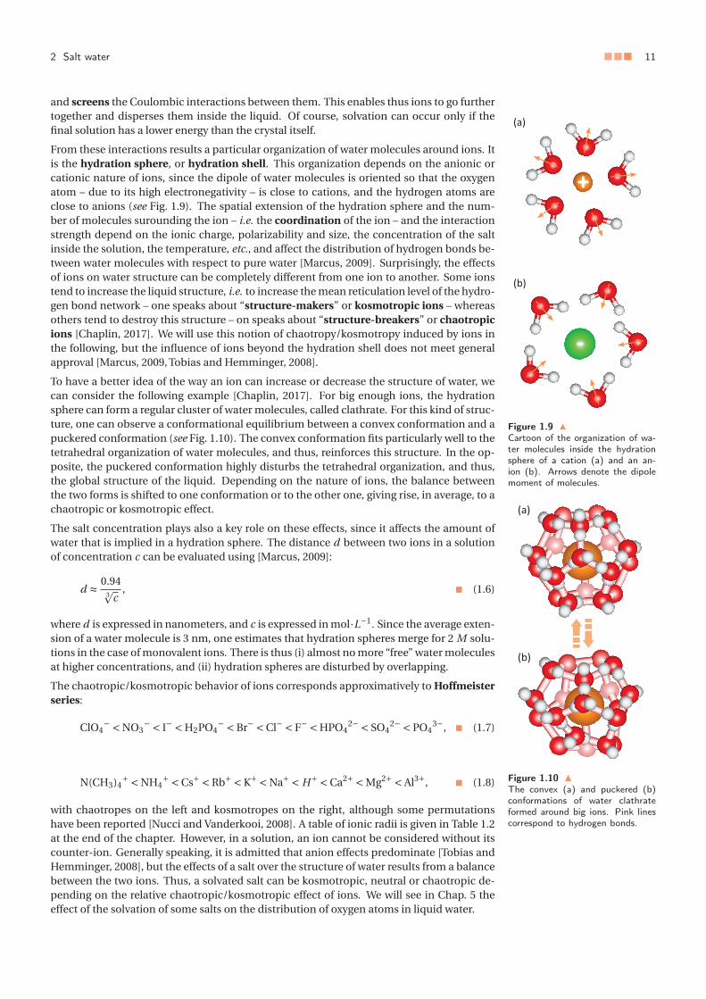
2 Salt water ■■■ 11
Figure 1.9 �
Cartoon of the organization of wa-ter molecules inside the hydrationsphere of a cation (a) and an an-ion (b). Arrows denote the dipolemoment of molecules.
Figure 1.10 �
The convex (a) and puckered (b)conformations of water clathrateformed around big ions. Pink linescorrespond to hydrogen bonds.
and screens the Coulombic interactions between them. This enables thus ions to go furthertogether and disperses them inside the liquid. Of course, solvation can occur only if thefinal solution has a lower energy than the crystal itself.
From these interactions results a particular organization of water molecules around ions. Itis the hydration sphere, or hydration shell. This organization depends on the anionic orcationic nature of ions, since the dipole of water molecules is oriented so that the oxygenatom – due to its high electronegativity – is close to cations, and the hydrogen atoms areclose to anions (see Fig. 1.9). The spatial extension of the hydration sphere and the num-ber of molecules surounding the ion – i.e. the coordination of the ion – and the interactionstrength depend on the ionic charge, polarizability and size, the concentration of the saltinside the solution, the temperature, etc., and affect the distribution of hydrogen bonds be-tween water molecules with respect to pure water [Marcus, 2009]. Surprisingly, the effectsof ions on water structure can be completely different from one ion to another. Some ionstend to increase the liquid structure, i.e. to increase the mean reticulation level of the hydro-gen bond network – one speaks about “structure-makers” or kosmotropic ions – whereasothers tend to destroy this structure – on speaks about “structure-breakers” or chaotropicions [Chaplin, 2017]. We will use this notion of chaotropy/kosmotropy induced by ions inthe following, but the influence of ions beyond the hydration shell does not meet generalapproval [Marcus, 2009, Tobias and Hemminger, 2008].
To have a better idea of the way an ion can increase or decrease the structure of water, wecan consider the following example [Chaplin, 2017]. For big enough ions, the hydrationsphere can form a regular cluster of water molecules, called clathrate. For this kind of struc-ture, one can observe a conformational equilibrium between a convex conformation and apuckered conformation (see Fig. 1.10). The convex conformation fits particularly well to thetetrahedral organization of water molecules, and thus, reinforces this structure. In the op-posite, the puckered conformation highly disturbs the tetrahedral organization, and thus,the global structure of the liquid. Depending on the nature of ions, the balance betweenthe two forms is shifted to one conformation or to the other one, giving rise, in average, to achaotropic or kosmotropic effect.
The salt concentration plays also a key role on these effects, since it affects the amount ofwater that is implied in a hydration sphere. The distance d between two ions in a solutionof concentration c can be evaluated using [Marcus, 2009]:
d ≈ 0.943�
c, ■ (1.6)
where d is expressed in nanometers, and c is expressed in mol·L−1. Since the average exten-sion of a water molecule is 3 nm, one estimates that hydration spheres merge for 2 M solu-tions in the case of monovalent ions. There is thus (i) almost no more “free” water moleculesat higher concentrations, and (ii) hydration spheres are disturbed by overlapping.
The chaotropic/kosmotropic behavior of ions corresponds approximatively to Hoffmeisterseries:
ClO4− < NO3
− < I− < H2PO4− < Br− < Cl− < F− < HPO4
2− < SO42− < PO4
3−, ■ (1.7)
N(CH3)4+ < NH4
+ < Cs+ < Rb+ < K+ < Na+ < H+ < Ca2+ < Mg2+ < Al3+, ■ (1.8)
with chaotropes on the left and kosmotropes on the right, although some permutationshave been reported [Nucci and Vanderkooi, 2008]. A table of ionic radii is given in Table 1.2at the end of the chapter. However, in a solution, an ion cannot be considered without itscounter-ion. Generally speaking, it is admitted that anion effects predominate [Tobias andHemminger, 2008], but the effects of a salt over the structure of water results from a balancebetween the two ions. Thus, a solvated salt can be kosmotropic, neutral or chaotropic de-pending on the relative chaotropic/kosmotropic effect of ions. We will see in Chap. 5 theeffect of the solvation of some salts on the distribution of oxygen atoms in liquid water.

12 ■■■ Chap. 1. Liquid water from bulk to confined media
Figure 1.11
Evolution of the relative humidity ofa gas phase in equilibrium with a liq-uid water-glycerol mixture at 298 Kwith respect to the glycerol massfraction (from [Forney and Brandl,1992]).
Figure 1.12
Cartoon of water displacement un-der a salt concentration gradient(osmosis).
Those structure modifications have, of course, some consequences on the dynamics of wa-ter. Among these effects, one can mention the so-called colligative properties of water (de-crease of the fusion temperature, decrease of the vapor pressure, osmosis...) or the modifi-cation of hydrodynamics transport properties (self-diffusion of water, shear viscosity...). Wewill study more precisely those effects in the remaining of this section.
2.2 Colligative properties
2.2.1 Decrease of the fusion temperature
It is a well-known effect: adding sodium chloride on roads in winter prevents water fromfreezing at 0 °C. In a water-salt mixture, the entropy of water is decreased with respect topure water, which decreases the chemical potential of water. This means more energy isneeded to transit from the liquid phase to the solid phase, which reduces the fusion tem-perature of water. Thus, the liquid phase remains stable at lower temperature than when itis pure [Chaplin, 2017]. Moreover, on a kinetic point of view, in some cases, the presence ofsolvated species can prevent the formation of big solid germs, and thus prevent the growingof the crystal phase [Kim and Yethiraj, 2008]. In that case, water is easier to supercool.
2.2.2 Decrease of the vapor pressure
One can also observe a decrease of the vapor pressure. The basic idea is close to the pre-vious case. The vapor pressure of water is the partial pressure of water vapor present inthe surrounding of liquid water when both phases are in equilibrium. The increase of theentropy of water due to ion mixing must be overcome to remove one molecule from the liq-uid phase and vaporize it, that lowers the vapor pressure. At low ionic concentrations, theincrease of entropy, and thus, the reduction of the vapor pressure, mainly depends on theionic fraction, independently of the nature of the salt. At higher concentrations, water-saltinteractions must be considered [Chaplin, 2017].
This property is used in practice to adjust the humidity rate in small volumes. The relativehumidity (RH), expressed in percent, is defined as the ratio between the water partial pres-sure pH2O and the equilibrium vapor pressure p∗
H2O of pure water at the same temperature:
RH = 100 · pH2O
p∗H2O
. ■ (1.9)
Since, for a given salt, the relative humidity depends on the concentration of the salt, itis more convenient to use saturated solutions. One can thus find tables with the relativehumidity associated to a saturated solution of various salts [Lide, 1997]. Another commonlyused method is to use water-glycerol mixtures with various mass fraction of glycerol (seeFig. 1.11) [Forney and Brandl, 1992]. We will use this method to control the hydration ofclay samples in next chapters.
2.2.3 Osmosis
One consider two reservoirs filled with salt water with different concentrations, and sep-arated by a membrane that enables only water molecules to go from one reservoir to theother. The membrane can be a “real” membrane, or the entrance of a nano-channel, as inthe case of the interlayer space of clays. It appears a flux of water across the membraneto homogenize the concentrations: this is the phenomenon of osmosis (see Fig. 1.12). Toavoid this displacement of water, one must apply a pressure, called osmotic pressure Π,on the low concentration liquid. This pressure is a thermodynamic quantity that dependsonly on the salt concentration c (in the limit of low concentrations) and the temperature T ,according to the Van’t Hoff’s law [Chaplin, 2017, Atkins and de Paula, 2010]:
Π= c ·R ·T, ■ (1.10)

2 Salt water ■■■ 13
where R denotes the perfect gas constant. In the case of high salt concentrations, a cor-rective factor must be added in this expression. The osmotic pressure is a colligative prop-erty. On the contrary, the intensity of the flux is a kinetic quantity that depends mainly onthe properties of the membrane and the concentration difference between the two reser-voirs [Alleva et al., 2012]. Osmotic flows play a key role in nanofluidic channels, as we willsee later.
2.3 Hydrodynamic transportWe already mentioned ions diffuse in a solution under a gradient of concentration. Theycan also migrate when an external electric field is applied. But ions also affect the solventdynamics. In this last paragraph about ions, we will focus on this last effect.
Due to their (dis)ordering effects on the structure of liquid water, ions can enhance or re-duce water molecule mobility in their vicinity, and thus modify the global viscoelastic prop-erties of the liquid with respect to pure water. The shear viscosity of electrolytes has beenextensively studied experimentally in the limit of low concentrations [Abdulagatov et al.,2006, Nakai et al., 1996, Goldsack and Franchetto, 1977], but not numerically. Within thelimit of low concentrations, experimental data can be well described using the Jones-Doleequation [Marcus, 2009]:
η= ηsolvent ·(1+ A ·�c +B · c
), ■ (1.11)
where ηsolvent is the shear-viscosity of pure water, and A and B are coefficients related to thesalt. A can be computed theoretically from solvent and ions properties and B is an empiricalcoefficient. A large amount of experiments have been devoted to the determination of B forvarious salts [Abdulagatov et al., 2006, Nakai et al., 1996, Goldsack and Franchetto, 1977]. Itis usually assumed that salts with a positive B are kosmotropic, while those with a negativeB are chaotropic [Marcus, 2009, Goldsack and Franchetto, 1977]. The evolution of the shearviscosity of water with respect to the concentration of various alkali metal halides is shownin Fig. 1.13. According to the Jones-Dole equation, A · �c should be negligeable at high
Figure 1.13 �
Evolution of the shear viscosity ofvarious alkali metal halide solutionswith respect to the concentration.Molarities were assimilated to mo-lalities when molarities were notavailable (from Refs. [Abdulagatovet al., 2006, Kestin et al., 1981b,Kestin et al., 1981a, Nakai et al.,1996, Zaytsev and Aseyev, 1992,Goldsack and Franchetto, 1977,Isono, 1984]).
concentrations. Indeed, for all salts considered here, experimental data are well describedby an affine relation. Consequently, the slope of the curves directly gives the sign of B ,and thus, the kosmotropic/chaotropic tendency of the salt. Using this assumption, lithiumand sodium halides are kosmotropic, whereas cesium iodide is chaotropic. The trend forpotassium halides and cesium chloride is not that clear and we can consider those saltshaving a neutral effect on the shear viscosity. Generally speaking, the kosmotropic effect ismore pronounced as the size of ions decreases, whereas large ions are rather chaotropic.
A similar behavior is observed for the self-diffusion coefficient of water. Its evolution withrespect to the concentration of various alkali metal halides is shown in Fig. 1.14.

14 ■■■ Chap. 1. Liquid water from bulk to confined media
Figure 1.14 �
Evolution of the self-diffusion co-efficient of water for various al-kali metal halide solutions with re-spect to the concentration (fromRef. [Müller and Hertz, 1996]).
According to experimental data, lithium and sodium based salts decrease the self diffu-sion of water (that should correspond to a more structured liquid, so a kosmotropic effect),whereas potassium, rubidium and iodine increase it (that should correspond to a less struc-tured liquid, so a chaotropic effect). Moreover, except for small cations, the evolution of theself diffusion coefficient with respect to the salt concentration only slightly depends on thenature of the cation: for a given anion, curves corresponding to potassium, rubidium andcesium are very close one to each other. Note that the structure making/breaking predic-tions are similar but not identical depending on the observable used (here the shear viscos-ity or the self diffusion coefficient). This is a general trend and it constitutes a major limitin the description of ions in terms of effects on the hydrogen bond network [Marcus, 2009].We will study the influence of salts on the viscoelastic properties of water in Chap. 5.
3 Confined water
Up to now, we considered water in the bulk without any constraint from its container. How-ever, in nature, there are many cases where water is confined, i.e. enclosed in a volumewhose at least one dimension is smaller than 100 nm [Sparreboom et al., 2009]. It is forexample the case inside some porous minerals, or inside biologic tissues. Those mate-rials can lie inside an aqueous medium or can be filled with water due to capillary con-densation under a humid atmosphere [Charlaix and Ciccotti, 2010]. Confinement impliesan increased role of surface phenomena on the properties of the liquid, that can be com-pletely modified with respect to bulk water [Sparreboom et al., 2009, Bocquet and Tabeling,2014, Bocquet and Charlaix, 2010]. The aim of this section is to introduce the formalismand the main effects of confinement on the structure of liquid water and its hydrodynam-ics properties [Sparreboom et al., 2009, Bocquet and Tabeling, 2014, Bocquet and Charlaix,2010, Chaplin, 2010].
3.1 Structure of confined water
3.1.1 Water-surface interactions: hydrophobicity, hydrophilicity
Interactions between water molecules and a solid surface can have two different nature:electrostatic (including Van der Waals interactions) and hydrogen bonds. We will explainthe molecular origin of those interactions in the next chapter. As water is a polar molecule,it interacts more with a polar surface than with a non-polar surface. For neutral solids, asurface is polar when it is made of a stack of atoms with very different electronegativity.Due to the presence of the surface that ends the periodicity of the solid structure, an elec-trostatic instability raises at the surface, that is stabilized by a reorganisation of the charge

3 Confined water ■■■ 15
Figure 1.15 �
Cartoon of a single wall carbon nan-otube filled with a single file of wa-ter molecules (adapted from [Maet al., 2017]).
distribution [Goniakowski et al., 2007]. Polar surfaces also include solids with a net charge,such as clay layers. However, as we will see, the nature of the surface is not the only factorthat controls the interactions. The geometry of the interface can also play a key role [Falket al., 2010, Chaplin, 2010].
Let us first consider a non-polar surface, neglecting all geometry-related issues. The inter-actions between water and the surface are mainly Van der Waals, and thus are weak withrespect to intermolecular hydrogen bonds. Consequently, the interactions with the surfacedo not directly drive the structure of interfacial water. One speaks about hydrophobic sur-face. However, as the presence of the wall removes water molecules from the neighboringof interfacial molecules, water near the surface undergoes molecular frustration: moleculescannot form as many hydrogen bonds than in the bulk. It results from this (i) a preferentialorientation of molecules near the surface, and (ii) the hydrogen bonds formed are stronger.Thus, water molecules are locally more structured. The main example of hydrophobic con-finement medium is carbon nanotube (see Fig. 1.15). It also constitutes a good example ofthe influence of the geometry. When the radius of the tube is decreased, the curvature ofthe water/solid interface is increased. Thus, the average distance between carbon atomsand water molecules decreases (the number of carbon atom in the first neighboor shell of agiven water molecule increases up to 36 atoms per molecule) and Van der Waals interactionsare stronger. So, for diameters smaller than 1.1 nm where a single molecule file is present,there are strong interactions between the tube and water molecules. We will mention latersome implications on the dynamics of water.
Let us consider now a polar surface. The influence of a polar surface on the structure ofthe liquid highly depends on the chemical composition of the surface. The latter can formbonds with water molecules that are weaker or stronger than inter-molecular hydrogenbonds. The existence of strong hydrogen bonds with the surface tends to weaken the energyof O–H bonds that lies near the surface. Moreover, as in the case of ions with their hydrationsphere, the solid surface orders molecules in a specific orientation. Then, due to coop-erative effects, the perturbation induced by the surface can extend over several molecularsizes (typically over 1 nm, i.e. three molecular sizes). In addition, the interactions with thesurface induce a layering of water molecules, with strong oscillations of the density profilewith respect to the distance to the wall. Such a surface is said to be hydrophilic. The mainexamples of hydrophilic confinement media are porous silicates and aluminosilicates suchas Vycor, MCM-41 or clays (see Fig. 1.16). However, the most striking effects happen whenelectrolytes are present inside pores, as we will see in the next section.
(a) Vycor glass (b) MCM-41
Figure 1.16 �
Cartoon of the structure of Vycorglass (a) and mesoporous MCM-41 silica (b). Red: O; blue: Si.Vycor glass is a silica matrix withrandomly distributed pores, whereasMCM-41 is made of regularly or-ganized parallel channels (adaptedfrom [Pellenq et al., 2001, Gusev,2017].
3.1.2 Charge distribution in salt water
When the confining medium has a charge surface and there are ions inside water, an elec-trical double layer (usually abbreviated EDL) of opposed charge is formed to screen thesurface charge. The charge surface can be intrinsic to the material, as in the case of clay lay-ers, or can be induced by the proximity of the electrolyte. Actually, when a solid is immersedinside an electrolyte, its surface acquires a surface charge due to various mechanisms suchas the dissociation of chemical groups on the surface in the case of hydrophobic surfaces, orthe adsorption of ionic species on hydrophobic surfaces [Israelachvili, 2011]. In the follow-ing, to simplify the discussion, we will consider a surface with a negative charge. Of course,

16 ■■■ Chap. 1. Liquid water from bulk to confined media
Figure 1.18
Definition of the contact angle φ fora droplet of liquid on top of a solidsurface.
the discussion holds in the case of positively charged surface but signs of charges must beinverted.
The EDL is divided into two parts: the Stern layer and the Gouy-Chapmann layer. Farfrom the interface, the solution is homogeneous, with an equal concentration of anionsand cations. The Stern layer is constituted by a layer of cations adsorbed on the solid sur-face, whereas the Gouy-Chapmann layer is a diffuse layer with a concentration gradient.The number of cations decreases progressively up to the bulk value with respect to the dis-tance to the interface, whereas the number of anions increases progressively (see Fig. 1.17).It plays an important role in the hydrodynamic transport properties, especially when the
Figure 1.17
Electrical double layer near a neg-atively charged surface. The qual-itative evolution of the concentra-tion of anions (green) and cations(orange) across the Stern and theGouy-Chapmann layers is shown onthe right graph.
confinement induces an overlap between the electrical double layers of the different sur-faces. We will give a few examples later.
Another important effect of confinement concerns phase transitions. That is what we aregoing to discuss in the upcoming paragraph.
3.1.3 Phases and phase transitionsConfinement influences the phase transitions of water in different manners [Chaplin, 2010,Lee et al., 2010b]. On a thermodynamics point of view – as in the case of a solvated salt– confinement affects the entropy of the liquid. Disordering induced by the interface in-creases the entropy, which decreases the heat of fusion and thus the melting temperature.The melting point depression becomes larger as the pore size decreases and the interfacialenergy (the surface tension) γ increases. For a spherical pore of diameter d , the meltingtemperature Tm of confined water is well evaluated by the Gibbs-Thompson equation:
Tm = T °m ·
(1− 4 ·γ ·cos(φ)
d ·ρc ·ΔH °m
), ■ (1.12)
where T °m denotes the bulk melting temperature, ΔH °
m is the bulk heat of fusion, ρc is theice density and φ is the liquid-solid contact angle (see Fig. 1.18). However, the oppositephenomenon is sometimes observed when the ice phase is particularly stabilized by watersurface interactions (i.e. the organization of water molecules induced by the surface corre-sponds to those of ice). Moreover, since φ usually shows a hysteretic behavior, the meltingtemperature can be different from the crystallization temperature.
To these thermodynamic effects, one must also add kinetic effects: confinement pertur-bates solid germs nucleation and their growth. Since the crystallites growth cannot occurbeyond the limits of pores, the global crystallisation of the confined liquid is mostly drivenby solid germs nucleation and can thus extend over a relatively large range of temperatures.Moreover, heterogeneous nucleation (i.e. from surfaces or foreign germs) dominates insmall pores, whereas homogeneous nucleation (i.e. from an ice germ) dominates in largepores.
Researchers used the melting temperature depression and the nucleation delay to exploreexperimentally a range of temperatures that includes the “no man’s land”. However, it isquestionable to consider the phase diagram of confined water as an extension of the phasediagram of bulk water due to surface effects. Using various confining media, a transitionfrom a fragile behavior to a strong behavior has been observed at low temperatures (below190 or 225 K depending on the considered medium). Other studies revealed a liquid-liquidtransition at 240 K and a glass transition at 165 K (see Ref. [Chaplin, 2010] for a review).

3 Confined water ■■■ 17
Figure 1.19
Velocity profile of a fluid shearedbetween two identical solid walls.Slippage is characterized by the sliplength b.
The structure of the ice formed during the crystallization process depends on the geometryof the confining medium. In this respect, in some cases, it is possible to observe directlycubic ice nucleation instead of hexagonal ice. In addition, for 1-d or 2-d confinements,one can observe structures that are not present in the phase diagram of bulk water, as, forexample, the so-called “zig-zag” 1-d structure of water inside carbon nanotubes.
As we have given the main implications of confinement on the structure of water, we willnow look at its consequences in terms of dynamics.
3.2 Hydrodynamics in confined media: notions of nanofluidics
3.2.1 Slippage
Generally speaking, the equations of hydrodynamics hold to describe the behavior of con-fined water, except at very short distances from the wall (typically distances lower than1 nm) [Sparreboom et al., 2009]. However, the traditional no-slip boundary condition –i.e. the continuity of the velocity at the solid-fluid interface – does not hold at small scales.Extrapolating the bulk fluid velocity profile up to the interface, a tangential velocity slipvslip is observed. To characterize this slippage phenomenon, two observables are usuallydefined [Bocquet and Barrat, 2007]. One defines the interfacial friction coefficient λ sothat:
σ=λ · vslip, ■ (1.13)
where σ is the shear stress applied by the liquid on the solid surface. One can also definethe slip length b as the distance to the wall beyond which the linear extrapolation of thevelocity profile satisfies the no-slip condition (see Fig. 1.19). This length can be expressedas:
b = η
λ, ■ (1.14)
where η denotes the shear viscosity of the bulk liquid. When the slip length is smallerthan the typical molecular size, one says there is no slip. It is the case for water frictionover a hydrophilic surface. On a hydrophobic surface, the slip length ranges from tens ofnanometers up to tens of micrometers inside carbon nanotubes [Sendner et al., 2009, Falket al., 2010,Falk et al., 2012] (although these latter orders of magnitude are strongly debated,with more recent work reporting slip lengths of hundreds of nanometers only [Secchi et al.,2016]). In this latter case, the curvature of the interface smooths at water molecule scalethe corrugation of the energy landscape created by the solid surface, that explains the lowfriction [Falk et al., 2010, Falk et al., 2012]. Recent studies also suggest that slippage is en-hanced by some coupling between the flow and surface phonons of the nanotube [Ma et al.,2015, Bocquet and Netz, 2015]. However, other factors can influence the dynamics near theinterface. A slight increase in the corrugation of the energy landscape of the surface due tothe presence of partial charges on atoms, for a given geometry, considerably decreases theslip length. This has been recently shown by comparing slippage on graphene and boronnitride sheets [Tocci et al., 2014].
High slippage enables fast flow of water. For a channel of typical size h, the flow rate isincreased by a factor 1+C ·b/h, where C is a dimensionless number close to 1 and dependingon the pore geometry [Sparreboom et al., 2009]. This fast transport property is of particularinterest when there is an electrolyte inside water, as explained below.
3.2.2 Electro-osmotic transport
Let us consider a nanometric channel with polar surfaces subject to an external electro-static potential parallel to the surfaces. Under this potential, the EDL undergoes an electricforce, that makes ions migrating inside the channel. The displacement of ions creates aglobal flow of the fluid due to its viscosity, that is called electro-osmotic flow (EOF). Thisflow is enhanced in case of slippage by a factor 1+ b/hedl where hedl denotes the thick-ness of the EDL [Sparreboom et al., 2009]. This kind of flow opens perspectives in terms
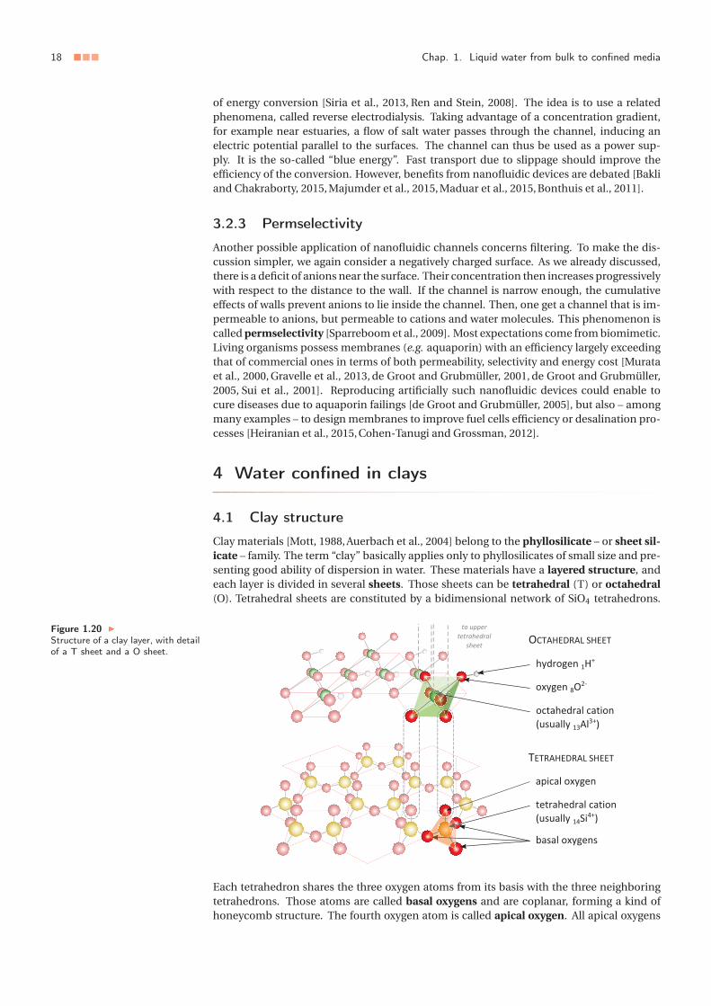
18 ■■■ Chap. 1. Liquid water from bulk to confined media
of energy conversion [Siria et al., 2013, Ren and Stein, 2008]. The idea is to use a relatedphenomena, called reverse electrodialysis. Taking advantage of a concentration gradient,for example near estuaries, a flow of salt water passes through the channel, inducing anelectric potential parallel to the surfaces. The channel can thus be used as a power sup-ply. It is the so-called “blue energy”. Fast transport due to slippage should improve theefficiency of the conversion. However, benefits from nanofluidic devices are debated [Bakliand Chakraborty, 2015, Majumder et al., 2015, Maduar et al., 2015, Bonthuis et al., 2011].
3.2.3 Permselectivity
Another possible application of nanofluidic channels concerns filtering. To make the dis-cussion simpler, we again consider a negatively charged surface. As we already discussed,there is a deficit of anions near the surface. Their concentration then increases progressivelywith respect to the distance to the wall. If the channel is narrow enough, the cumulativeeffects of walls prevent anions to lie inside the channel. Then, one get a channel that is im-permeable to anions, but permeable to cations and water molecules. This phenomenon iscalled permselectivity [Sparreboom et al., 2009]. Most expectations come from biomimetic.Living organisms possess membranes (e.g. aquaporin) with an efficiency largely exceedingthat of commercial ones in terms of both permeability, selectivity and energy cost [Murataet al., 2000, Gravelle et al., 2013, de Groot and Grubmüller, 2001, de Groot and Grubmüller,2005, Sui et al., 2001]. Reproducing artificially such nanofluidic devices could enable tocure diseases due to aquaporin failings [de Groot and Grubmüller, 2005], but also – amongmany examples – to design membranes to improve fuel cells efficiency or desalination pro-cesses [Heiranian et al., 2015, Cohen-Tanugi and Grossman, 2012].
4 Water confined in clays
4.1 Clay structure
Clay materials [Mott, 1988, Auerbach et al., 2004] belong to the phyllosilicate – or sheet sil-icate – family. The term “clay” basically applies only to phyllosilicates of small size and pre-senting good ability of dispersion in water. These materials have a layered structure, andeach layer is divided in several sheets. Those sheets can be tetrahedral (T) or octahedral(O). Tetrahedral sheets are constituted by a bidimensional network of SiO4 tetrahedrons.
Figure 1.20
Structure of a clay layer, with detailof a T sheet and a O sheet.
Each tetrahedron shares the three oxygen atoms from its basis with the three neighboringtetrahedrons. Those atoms are called basal oxygens and are coplanar, forming a kind ofhoneycomb structure. The fourth oxygen atom is called apical oxygen. All apical oxygens

4 Water confined in clays ■■■ 19
are also coplanar and have an hexagonal arrangement. Octahedral sheets are made of abidimensional network of octahedrons with oxygens on the vertex and a metallic cation inthe middle (or a vacancy).
A layer can be made whether by a T and a O sheet (TO layer), or by a O sheet surroundedby two T sheets (TOT layer). The O sheets share some of their oxygen atoms with apicaloxygens from T sheets (see Fig. 1.20). One distinguishes trioctahedral clays where thereis a metallic ion (generally Mg2+) in each octahedron, and dioctahedral clays where onlytwo thirds of the octahedrons are filled (generally by Al3+). Such a structure is neutral, butin practice, several metallic cations inside tetrahedrons or octahedrons are substituted bycations with lower valence. For example, Si4+ can be substituted by Al3+ or Fe3+. Due tothese defects, layers have a negative net charge, called interlayer charge. This charge isbalanced by absorbing cations – called interlayer cations – on the layer surface. The substi-tutions also slightly deform the layers. Interlayer cations behave as bridges that stick layerstogether, giving a 3-d structure to the material (see Fig. 1.21).
Figure 1.21 �
Layers staking in clay materials andinterlayer space. Water moleculesand interlayer cations do not oc-cupy their effective position on thecartoon.
Depending on the nature of the layers, the value of the interlayer charge and its localiza-tion inside the layers, phyllosilicates will adopt various behavior. Especially, some clays canadsorb water inside the interlayer space whereas micas cannot due to their higher inter-layer charge. A classification of the main families of phyllosilicates is given in Table 1.1. Inthis study, we will focus on Montmorillonite clays, that belong to the smectite family. Inthose clays, the interlayer space can adsorb water, implying a swelling of the structure. Forthis reason, one speaks about “swelling clays”. We will also study some Illite clays – whoseinterlayer space cannot adsorb water – as reference for non-hydrated interlayer space.
Successive layers have various size, so that the overall structure is irregular, with a coupleof holes between layers. Those holes are called micropores. Moreover, due to those ir-regularities, stacks of layers become unstable above a critical thickness. Thus, layers formaggregates, called tactoids. The space available between tactoids is called mesopores. Thetypical size of layers is 1 nm thick and 1 μm width. Micropores are nanometric size, whereasthe size of tactoids and mesopores range from tens of nanometers to micrometers [Caseset al., 1992]. A general view of the pore structure is shown in Fig. 1.22. All pores (inter-layer space, micropores and mesopores) can adsorb water, respectively called interlayer,interporal and mesoporal water in the following. Note that a slightly different descriptionof the structuration is sometimes considered: according to this description, tactoids arelocally ordered in micrometric aggregates. One then distinguishes mesopores that corre-spond to intertactoid space, whose size is typically tens of nanometers, and mesopores thatcorrespond to interaggregate space, whose size is micrometric [Carrier et al., 2013]. In thisdissertation, we will not do this distinction.
Depending on the pore type, water is more or less structured. Interlayer water could have adensity higher than bulk water, whereas microporal and mesoporal water could have a den-sity lower than bulk water [Tardy et al., 1999]. However, the structure of absorbed water is

20 ■■■ Chap. 1. Liquid water from bulk to confined media
Family Layer Interlayercharge
Interlayerspace/distance(pm)
Octahedral sheetcomposition
Examples
kaolinite-serpentine
TO x ≈ 0 empty720
dioctahedral kaolinitedickite
H2O720-1010
dioctahedral Halloysite
empty trioctahedral lizardite
talc-pyrophyllite
TOT x ≈ 0 empty930
dioctahedral pyrophyllite
trioctahedral talc
smectite TOT x ∈ [0.6;1.2] hydratedcations
dioctahedral montmorillonitebeidellite
960-1500 trioctahedral hectoritesaponite
vermiculite TOT x ∈ [1.2;1.8] hydratedcations
dioctahedral dioctahedralvermiculite
1200-1500 trioctahedral trioctahedralvermiculite
mica TOT x ≈ 2 dehydratedcations
dioctahedral muscoviteceladonite
1000 dioctahedral phlogopitebiotite
brittle mica TOT x ≈ 4 dehydratedcations
dioctahedral margarite
732 trioctahedral clintonite
illite TOT x ∈ [1.2;1.7] dehydratedcations1000
dioctahedral illite
chlorite TOT-O variable brucite-likelayer
di/dioctahedral donbassite
1400 di/trioctahedral sudoite
tri/trioctahedral chamosite
Table 1.1
Classifica(adaptedbach etorderedlayers (TOcharge,interlayerconventiointerlayercrystal uunit (instsometime
Figure 1.22
Multiscale porous structure ofsmectite-type clays. The SEMmicrograph was realized in WW3,Erlangen, Germany, using a Quanta200 microscope by FEI® on aNa-SAz-2 montmorillonite in the(001) (top) direction.
(a) Top scanning electron microscopy view (b) Transverse schematic view
not fully understood yet. One reason is that one cannot study only one kind of water insidea hydrated clay. However, varying the relative humidity of surrounding atmosphere enablesto modify the relative water population of pores, as we will see in the next paragraph.
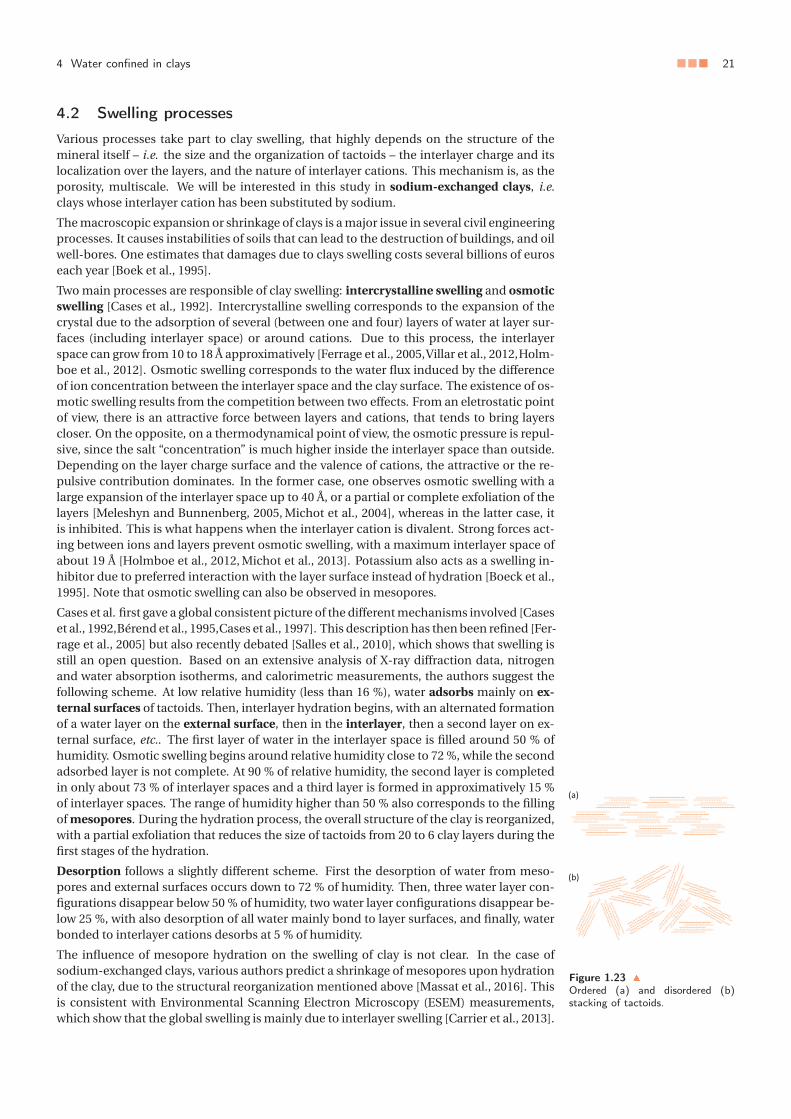
4 Water confined in clays ■■■ 21
Figure 1.23 �
Ordered (a) and disordered (b)stacking of tactoids.
4.2 Swelling processes
Various processes take part to clay swelling, that highly depends on the structure of themineral itself – i.e. the size and the organization of tactoids – the interlayer charge and itslocalization over the layers, and the nature of interlayer cations. This mechanism is, as theporosity, multiscale. We will be interested in this study in sodium-exchanged clays, i.e.clays whose interlayer cation has been substituted by sodium.
The macroscopic expansion or shrinkage of clays is a major issue in several civil engineeringprocesses. It causes instabilities of soils that can lead to the destruction of buildings, and oilwell-bores. One estimates that damages due to clays swelling costs several billions of euroseach year [Boek et al., 1995].
Two main processes are responsible of clay swelling: intercrystalline swelling and osmoticswelling [Cases et al., 1992]. Intercrystalline swelling corresponds to the expansion of thecrystal due to the adsorption of several (between one and four) layers of water at layer sur-faces (including interlayer space) or around cations. Due to this process, the interlayerspace can grow from 10 to 18 Å approximatively [Ferrage et al., 2005,Villar et al., 2012,Holm-boe et al., 2012]. Osmotic swelling corresponds to the water flux induced by the differenceof ion concentration between the interlayer space and the clay surface. The existence of os-motic swelling results from the competition between two effects. From an eletrostatic pointof view, there is an attractive force between layers and cations, that tends to bring layerscloser. On the opposite, on a thermodynamical point of view, the osmotic pressure is repul-sive, since the salt “concentration” is much higher inside the interlayer space than outside.Depending on the layer charge surface and the valence of cations, the attractive or the re-pulsive contribution dominates. In the former case, one observes osmotic swelling with alarge expansion of the interlayer space up to 40 Å, or a partial or complete exfoliation of thelayers [Meleshyn and Bunnenberg, 2005, Michot et al., 2004], whereas in the latter case, itis inhibited. This is what happens when the interlayer cation is divalent. Strong forces act-ing between ions and layers prevent osmotic swelling, with a maximum interlayer space ofabout 19 Å [Holmboe et al., 2012, Michot et al., 2013]. Potassium also acts as a swelling in-hibitor due to preferred interaction with the layer surface instead of hydration [Boeck et al.,1995]. Note that osmotic swelling can also be observed in mesopores.
Cases et al. first gave a global consistent picture of the different mechanisms involved [Caseset al., 1992,Bérend et al., 1995,Cases et al., 1997]. This description has then been refined [Fer-rage et al., 2005] but also recently debated [Salles et al., 2010], which shows that swelling isstill an open question. Based on an extensive analysis of X-ray diffraction data, nitrogenand water absorption isotherms, and calorimetric measurements, the authors suggest thefollowing scheme. At low relative humidity (less than 16 %), water adsorbs mainly on ex-ternal surfaces of tactoids. Then, interlayer hydration begins, with an alternated formationof a water layer on the external surface, then in the interlayer, then a second layer on ex-ternal surface, etc.. The first layer of water in the interlayer space is filled around 50 % ofhumidity. Osmotic swelling begins around relative humidity close to 72 %, while the secondadsorbed layer is not complete. At 90 % of relative humidity, the second layer is completedin only about 73 % of interlayer spaces and a third layer is formed in approximatively 15 %of interlayer spaces. The range of humidity higher than 50 % also corresponds to the fillingof mesopores. During the hydration process, the overall structure of the clay is reorganized,with a partial exfoliation that reduces the size of tactoids from 20 to 6 clay layers during thefirst stages of the hydration.
Desorption follows a slightly different scheme. First the desorption of water from meso-pores and external surfaces occurs down to 72 % of humidity. Then, three water layer con-figurations disappear below 50 % of humidity, two water layer configurations disappear be-low 25 %, with also desorption of all water mainly bond to layer surfaces, and finally, waterbonded to interlayer cations desorbs at 5 % of humidity.
The influence of mesopore hydration on the swelling of clay is not clear. In the case ofsodium-exchanged clays, various authors predict a shrinkage of mesopores upon hydrationof the clay, due to the structural reorganization mentioned above [Massat et al., 2016]. Thisis consistent with Environmental Scanning Electron Microscopy (ESEM) measurements,which show that the global swelling is mainly due to interlayer swelling [Carrier et al., 2013].

22 ■■■ Chap. 1. Liquid water from bulk to confined media
Figure 1.24 �
Cartoon of an inner-sphere surfacecomplex (a) and an outer-spheresurface complex (b) formed by theinterlayer cation on the layer (silox-ane) surface (adapted from [Spositoet al., 1999]).
On the contrary, other authors predict a swelling of mesopores [Salles et al., 2010]. A possi-ble explanation to resolve this discrepancy is a high dependence of mesopore hydration onthe ordering of tactoids. Randomly organized tactoids could imply a swelling of mesopores,whereas the latter shrink upon hydration when tactoids are regularly ordered (see Fig. 1.23).
Since adsorption and desorption do not occur in the same order for the different hydra-tion states, one can modify the relative amount of water in the various pores working atdifferent points of the adsorption/desorption isotherm. We will try to use this property todiscriminate the structure and dynamics corresponding to the different confinement areasin Chap. 6.
4.3 Water structure and dynamics
Structure. Numerous studies have been devoted to the analysis of the structure of wateradsorbed in clay minerals, both experimentally – using e.g. neutron scattering or infraredscattering – and numerically – using molecular dynamics or Monte-Carlo simulations. Inparticular, a lot of work focus on the arrangement of water molecules and cations inside theinterlayer space, in comparison with what happens in bulk water [Skipper et al., 2006, Skip-per et al., 1991, Skipper et al., 1995]. Here we discuss briefly the case of small alkali ions(lithium, sodium, potassium) exchanged clays (associated ionic radii are given in Table 1.2at the end of the chapter). We first focus on the arrangement of cations. The solvationenergy of lithium, sodium, and potassium increase with the size, and their solvation shellin bulk water is constituted respectively of 5, 6 and 6 water molecules. When no wateris adsorbed inside the interlayer space, cations are mainly trapped inside the hexagonalcavities of the layer siloxane surfaces. Interestingly, in the presence of two layers of wa-ter, the distribution of oxygen atoms around those ions remains almost unmodified withinthe first hydration shell, but some oxygen atoms from water molecules can be replaced bybasal oxygen atoms of the clay layers depending on the relative affinity of ions with the claysurface and water molecules. Indeed, as we mentioned in section 4.1, the coordination ofcations depends on the delocalization of the layer charge [Chang et al., 1997, Skipper et al.,2006,Skipper et al., 1995,Mignon et al., 2010]. One distinguishes three states of coordinationfor interlayer cations (see Fig. 1.24) [Sposito et al., 1999]:
• diffuse complex: the cation is solvated by water without significant effect of the layersurfaces;
• outer-sphere surface complex: the cation interacts weakly with the surfaces, and wa-ter molecules lie between the cation and the clay layer (see Fig. 1.24b);
• inner-sphere surface complex: the cation interacts strongly with the surface, withoutany water molecule between the cation and the clay layer (see Fig. 1.24a).
Lithium forms an outer-sphere surface complex, wherever the layer charge is localized.Sodium forms an outer-sphere complex near an octahedral substitution whereas it forms aninner-sphere surface complex near a tetrahedral substitution. Potassium only forms inner-sphere surface complexes [Chang et al., 1997,Skipper et al., 2006,Skipper et al., 1995,Mignonet al., 2010]. In the case of inner-sphere surface complexes, three water molecules are typ-ically substituted by basal oxygens within the first solvation shell. A similar trend has beenreported for sodium when only one water layer is adsorbed inside the interlayer space [Skip-per et al., 1995].
We focus now on the global arrangement of water molecules. When two (or more) wa-ter layers are adsorbed inside the interlayer space, the water structure is like those of saltwater we introduced previously [Sposito and Prost, 1982], but suffers from a slight weak-ening at longer distances [Skipper et al., 2006]. The clay surface is basically hydrophobic,but substitutions confer a hydrophilic behavior. Thus, a strong layering parallel to the lay-ers is observed, as we saw in the previous section near hydrophilic surfaces [Skipper et al.,2006,Rotenberg et al., 2010]. Molecules at the interface are oriented by the electric field cre-ated by the net charge of the crystal layers, and can form hydrogen bonds with both basaloxygens and other molecules. One hydrogen atom is directed to the surface, whereas the
4 Water confined in clays ■■■ 23
other one interacts with other molecules [Skipper et al., 2006]. When only one layer of wa-ter molecules is adsorbed, the structure is somehow more disordered, but oxygen atomsconcentrate in the mid-plane of the interlayer space whereas hydrogen atoms are directedto the layer surfaces [Boeck et al., 1995].
In a similar manner as the structure, we will see now that transport properties are not thatmuch affected by the confinement.
Hydrodynamics transport. The slip length of water over an uncharged clay layer is about4.1 Å, which is slightly above the molecular size (typically 3 Å), whereas it falls to 1.5 Å forMontmorillonites due to the net charge of the layers, conferring to the clay hydrophilicproperties [Botan et al., 2011, Botan et al., 2013]. Surprisingly, this hydrophilic behaviordoes not influence that much the hydrodynamics properties of confined water when morethan one water layer is adsorbed in the interlayer space. According to various experimentssuch as neutron scattering of conductimetry and various calculations, the self-diffusion co-efficients of cations and water molecules inside the interlayer space are typically reducedby a factor between 2 and 4 with respect to bulk water, but remain of the same order ofmagnitude [Salles et al., 2015, Ngouana W and Kalinichev, 2014, Malikova et al., 2005]. Asimilar trend is observed for the shear viscosity, with a slight increase inside the interlayerspace with respect to bulk water [Botan et al., 2011]. Cations forming inner-sphere surfacecomplexes, as Cs+ and K+, diffuse slightly slower than the one forming outer-sphere surfacecomplexes, as Li+ and Na+. For the two latter, the self-diffusion coefficient in the interlayerspace is almost equal to the one in bulk water. Logically, in mesopores where water is lessconfined, self-diffusion coefficients are almost identical to those in bulk water [Salles et al.,2015]. However, at macroscopic scale, the self-diffusion of water is lowered by about oneorder of magnitude with respect to interlayer water, due to the exchange dynamics betweenmesopores and interlayer space [Marry et al., 2002, Salles et al., 2015]. We will investigatenumerically those transport properties in the case of a sodium exchanged Montmorillonitein Chap. 6.
Low temperature dynamics. Several recent studies focus on the temperature behaviorof water confined in clay minerals. Gailhanou [Gailhanou, 2005], using Differential Scan-ning Calorimetry, reported between one and three phase transitions. At low water content,a unique phase transition is observed, extending from 150 and 250 K, associated to a glasstransition of confined water. At higher water contents, two additional phase transitions ap-pear: one between 240 and 273 K, and the other between 273 and 290 K. The first one isexplained by a second glass transition, or by the crystallization of water confined in the nar-rowest pores. For the second one, it is suggested it could correspond also to crystallizationof water in some pores. Maheshwari et al. [Maheshwari et al., 2013], using Positron Annihi-lation Spectroscopy, Dielectric Relaxation Spectroscopy, Differential Scanning Calorimetryand Nuclear Magnetic Resonance, reported two phase transitions for water confined in clayminerals: one between 274 and 286 K and the other between 240 and 245 K. The first oneis associated with an increase of free volume and an alteration of the hydrogen-bond net-work. It has been interpreted as a freezing of water molecules hydrogen-bonded to the layersurfaces. The other one is associated to a fragile-to-strong crossover and was explained bya partial freezing of remaining confined water. Between those two transitions, confined wa-ter behaves almost like a liquid. Fleury et al. [Fleury et al., 2013], using Low-Field NuclearMagnetic Resonance, reported two transitions: a water surface freezing between 263 and273 K and another transition around 243 K. Finally, Salles et al. [Salles et al., 2010], usingcalorimetry, reported solidification of water adsorbed in nanometric mesopores betweenaround 243 and 253 K, whereas water present in larger mesopores at high hydration statesfreezes around 269 K. In summary, all these studies agree to attribute two phase transitionsfor confined water, one around 273 K, and another one around 240 K. The interpretations ofthose transitions differ, but in each case, the transitions do not concern weakly-bound inter-layer water. According to Salles et al., those water molecules cannot freeze. Only Gailhanoureported a transition around 190 K, interpreting it as a glass transition of water molecules. Itis not inconsistent with other studies if one assumes this transition concerns weakly-boundinterlayer water. We will try to go further on this point in Chap. 6.
As we saw, even if water confined in clay minerals has been extensively studied during the

24 ■■■ Chap. 1. Liquid water from bulk to confined media
last decades, many open questions remain, especially in terms of dynamics. We will tryto give some elements to answer to these questions in Chap. 6. Before that, we will ana-lyze separately the various elements that constitutes water confined in clay minerals: water(Chap. 3), confinement (Chap. 4) and ions (Chap. 5).

5 Appendix: Table of effective ionic radii ■■■ 25
5 Appendix: Table of effective ionic radii
f severalon, 1976,
Ion Coordination Ionic radius (Å) Ion Coordination Ionic radius (Å)Al3+ 4 0.39 K+ 9 1.55Al3+ 5 0.48 K+ 10 1.59Al3+ 6 0.54 K+ 12 1.64Br− 6 1.96 Li+ 4 0.59Ca2+ 6 1 Li+ 6 0.76Ca2+ 7 1.06 Li+ 8 0.92Ca2+ 8 1.12 Mg2+ 4 0.57Ca2+ 9 1.18 Mg2+ 5 0.66Ca2+ 10 1.23 Mg2+ 6 0.72Ca2+ 12 1.34 Mg2+ 8 0.89Cl− 6 1.81 Na+ 4 0.99Cs+ 6 1.67 Na+ 5 1Cs+ 8 1.74 Na+ 6 1.02Cs+ 9 1.78 Na+ 7 1.12Cs+ 10 1.81 Na+ 8 1.18Cs+ 11 1.85 Na+ 9 1.24Cs+ 12 1.88 Na+ 12 1.39F− 2 1.29 Rb+ 6 1.52F− 3 1.3 Rb+ 7 1.56F− 4 1.31 Rb+ 8 1.61F− 6 1.33 Rb+ 9 1.63H+ 1 -0.38 Rb+ 10 1.66H+ 2 -0.18 Rb+ 11 1.69I− 6 2.2 Rb+ 12 1.72K+ 4 1.37 Rb+ 14 1.83K+ 6 1.38K+ 7 1.46K+ 8 1.51

26 ■■■ Chap. 1. Liquid water from bulk to confined media

1 Atoms and molecules ■■■ 27
■■■ Chapter 2
Probing water from electrons to bulk:numerical and experimental methods
Outline
1 Atoms and molecules . . . . . . . . . . . . . . . . . . . . . . . . . . . 251.1 Atoms . . . . . . . . . . . . . . . . . . . . . . . . . . . . . . . . 251.2 Molecules . . . . . . . . . . . . . . . . . . . . . . . . . . . . . 261.3 Beyond the molecule: molecular interactions . . . . . . . . . 27
2 Infrared absorption spectroscopy . . . . . . . . . . . . . . . . . . . . . 272.1 Theory (with applications to water) . . . . . . . . . . . . . . 272.2 Instrumentation . . . . . . . . . . . . . . . . . . . . . . . . . . 30
3 Classical and ab initio molecular dynamics . . . . . . . . . . . . . . . 343.1 Molecular dynamics . . . . . . . . . . . . . . . . . . . . . . . . 343.2 Computing forces (I): density functional theory . . . . . . . 393.3 Computing forces (II): point charge force fields . . . . . . . 41
1 Atoms and molecules
At the human scale, matter looks continuous, but at the nanometer scale, it is made of nu-merous atoms and molecules. From atoms and their interaction originate all phenomenaat macroscopic scale. Linking what occurs at one scale with what happens at another con-stitutes the main work of a great number of chemists and physicists. In this section, we willrecall some basics of atomic and molecular physics that will be useful to understand whatcomes next [Atkins and de Paula, 2010, Atkins and Friedman, 2011].
1.1 Atoms
An atom is constituted by electrons that gravitate around a nucleus. In all this dissertation,we will not consider the structure of the nucleus. The closest electrons to the nucleus aretightly bound with it and are called core electrons. Electrons from external shells are easierto pull off and are mostly responsible for the reactivity of the atom. They are called valenceelectrons.
Quantum mechanics teaches us two important properties of electrons: (i) one cannot knowprecisely at the same time their velocity and their position (it is also true for light nucleuslike hydrogen and helium, and, in a less extend, for others) – it is the Heisenberg’s uncer-tainty principle – and (ii) the energy of an electron is quantified. From (i), it results thatelectron cannot be described by its position, but rather by a field of probability of pres-ence, using its wavefunction ψ, with |ψ|2 ·dτ the probability for the electron to lie in the

28 ■■■ Chap. 2. Probing water from electrons to bulk: numerical and experimental methods
Figure 2.1
Approximate shape of the spatialdistribution of the probability ofpresence of the electron around thenucleus (in blue) for the first energylevels, represented by isodensity sur-faces.
volume dτ. From (ii), the wavefunction ψ cannot have a random form. A specific wave-function corresponds to each energy level. For hydrogenoid ions – i.e. ions with only oneelectron – these wavefunctions are called atomic orbitals, denoted 1s, 2s, 2p, 3s, 3p, 3d(see figure 2.1)... Energies Ei and wavefunctions ψi of each energy level i are solutions ofthe stationary Schrödinger equation:
H ψi = Ei ·ψi . ■ (2.1)
H is the Hamiltonian operator of the system, expressing the kinetic energy of both nucleusand electron and the Coulombic interaction between the electron and the nucleus:
H =− ħ2
2 ·mn·�∇2 − ħ2
2 ·me·�∇2 − Z ·e2
4 ·π ·ε0 · ‖�rn −�re‖, ■ (2.2)
where ħ is the reduced Planck constant, mn and �rn (resp. me and �re) are the mass and theposition of the nucleus (resp. the electron), Z is the atomic number of the atom, and ε0 isthe vacuum permittivity. For polyelectronic atoms and ions, since electrons dynamics arecoupled, one cannot anymore define atomic orbitals, i.e. monoelectronic wavefunctions(solutions of the Schrödinger equation depend of all degrees of freedom at the same time)and electronic levels are shifted. In practice, such wavefunction are nevertheless defined: itis the orbital approximation. We will see later some consequences of this approximation.However, a few rules must be respected to build the many-electron wavefunction, e.g. torespect the fact that electrons are indistinguishable. The repartition of electrons over thedifferent energy levels constitutes the electronic configuration of the atom and controls theenergy required to remove or to add an electron from / to the atom, and thus, it controls theability of the atom to form a molecule and the properties of resulting chemical bonds.
1.2 Molecules
Similarly to the coupling between electrons inside an atom, coupling between two atomsaffects the distribution of electronic energy levels of the pair. If the energy of the systemis lower than the sum of the energies of the two isolated atoms, then one says there is aconstructive overlap of atomic orbitals; a chemical bond is formed.
A nucleus/nucleus term must then be added in the Hamiltonian with respect to eq. (2.2).Due to this term, even for the simplest molecular structure, the analysis of the Schrödingerequation to evaluate the energy levels and associated wavefunctions becomes much harder.However, since nuclei are much heavier than electrons (mn ≈ 2000 ·me), they move veryslowly. A classical hypothesis consists in considering that nuclei are stationary at the elec-tron dynamics timescale. It is the Born-Oppenheimer approximation. Thus, one as toconsider (i) electronic energy levels that are solutions of the Schrödinger equation for agiven position of nuclei, and (ii) rotational and vibrational energy levels associated to thedynamics of nuclei. Under this hypothesis, the wavefunction can first be approximated asa linear combination of atomic orbitals in the Schrödinger equation. This enables to get anapproximation of the energy levels and the electron distribution, that can be used as ini-tial guess in molecular simulations. Once the electronic structure is known, the rotationaland vibrational energy levels can be computed using either classical or quantum mechan-ics. For example, in the case of ab initio molecular dynamics (see further), forces applied onnuclei are computed from the electronic structure, and then, the displacement of nuclei isdetermined using classical mechanics. Rotational and vibrational energy levels character-ize the molecular structure and its environment. They can be measured e.g. using infraredabsorption spectroscopy. We will go back on this point in the next section.
Depending on the electronic configuration of the atoms that constitute the molecular struc-ture and its geometry, the molecule can be polarized. The distribution of electrons can alsobe modified by an external electric field and induce a dipolar moment. In that case, one saysthe molecule is polarizable. From those polarity and polarizability properties originate lowenergy electrostatic interactions between molecules, which play a key role in the structureand dynamics of condensed phases, as detailed in the next section.

2 Infrared absorption spectroscopy ■■■ 29
In the specific case of linearmolecules, there are 3·N −5 internaldegrees of freedom since the rota-tion around the axis of the systemdoes not change the system.
Figure 2.2 �
Rotation around z-axis does notchange the dipole moment of themolecule and thus is infrared inac-tive.
1.3 Beyond the molecule: molecular interactionsInteractions between (induced or permanent) dipoles are called Van der Waals interac-tions. Among those interactions, those between two permanent dipoles are called Keesominteractions, those between a permanent dipole and an induced dipole are called Debyeinteractions, and those between two induced dipoles are called London, or dispersive, in-teractions. The latter require some comments. Due to quantum fluctuations, i.e. transientoccupation of excited energy levels by electrons, the electronic clouds of molecules can betemporary polarized. The resulting dipole direction is a priori random. However, sinceelectrons interact, the dipole moments of neighboring molecules are correlated and the re-sulting interaction leads to an attractive force between atoms. From this interaction, onecan explain the condensation of dihydrogen or argon at low temperature. Thus, the Londoninteraction is very important and is a purely quantum property resulting from electronicstructure fluctuations. Since only the ground-state wavefunction is considered within theBorn-Oppenheimer approximation, the existence of excited states, and thus of quantumfluctuations and London interaction, cannot be rendered by these approaches, constitut-ing a major limit to them. We will go back to this point at the end of this chapter.
All these interactions can be expressed in the following form:
V =− C
r 6 , ■ (2.3)
where C is a constant and r denotes the distance between the two molecules. Another im-portant interaction is the so called “hydrogen bond”. It is the interaction between a A–Hgroup of a molecule with a B atom from another molecule, where A and B denotes veryelectronegative atoms – mainly nitrogen, oxygen and fluor. From this interaction, it resultsa slightly constructive overlap between the orbitals of the three atoms A, B and H, which isthus directional. The associated energy lies between the energy of a covalent bond and aVan der Waals interaction. As we already saw in the previous chapter, this interaction playsa key role in water structure and dynamics.
2 Infrared absorption spectroscopy
2.1 Theory (with applications to water)As we mentioned in the previous section, energy levels can be associated to vibrations androtations of nuclei inside a molecule. For example, in the case of an isolated diatomicmolecule, the vibrational energy levels correspond in a rough approximation to the energylevels of the harmonic oscillator introduced in all quantum mechanics textbooks. The tran-sition energy between those levels usually fall inside the infrared domain. Thus, the study ofinfrared radiation absorption by molecular structures constitutes a precious analysis tool. Asystem constituted by N atoms has 3·N degrees of freedom in which 3·N−6 are vibrationaldegrees of freedom, and 3 are rotational degrees of freedom. These 3 ·N −6 vibrations arecoupled, but can be expressed in terms of 3 ·N −6 uncoupled collective vibrations, calledeigenmodes (or phonons) of the system [Atkins and de Paula, 2010, Atkins and Friedman,2011, Griffiths and De Haseth, 2007]. These collective vibrations affect notably the positionof only a small number of localized atoms. It can be for example a functional group of amolecule. Consequently, it is of common use to characterize and call those vibrations interms of the local rearrangement they make, even if all atoms move a little bit. For instance,in the case of water, one speaks about symmetric and antisymmetric stretching modes ofO–H bonds, or H–O–H stretching mode [Atkins and de Paula, 2010].
Each eigenmode is not necessary associated with a light absorption process. A system canabsorb or emit an electromagnetic wave of frequency ν0 only if it has – at least transiently –a dipole oscillating at a frequency ν close to ν0 (see the theory of oscillating dipoles in anyelectromagnetism textbook for details). Thus, in the specific case of infrared absorption,vibration modes must induce a variation of the dipole moment of the system. The mode isthen said “infrared active”. It is the same with rotational modes. Those conditions are the so-called selection rules [Atkins and de Paula, 2010, Atkins and Friedman, 2011, Griffiths and

30 ■■■ Chap. 2. Probing water from electrons to bulk: numerical and experimental methods
De Haseth, 2007]. Consider for example an isolated water molecule. It has three atoms thatare not aligned, so it has three rotational modes and three vibrational modes. The rotationaround the z-axis (see Fig. 2.2) does not affect the dipole moment of the molecule. Thus, thismode is not infrared active. All other modes are active, and are represented on figure 2.3.More generally, a systematic study of the symmetries and invariances of a molecular struc-ture enables to predict which modes are active or not [Atkins and de Paula, 2010,Atkins andFriedman, 2011]. In liquid water, all molecules are coupled. Vibration modes corresponding
Figure 2.3 �
Rotational and vibrational modes ofa single water molecule that are in-frared active.
mostly to molecular rotations are called libration modes. Moreover, the coupling betweenmolecules removes degeneracy of molecular energy levels. As the number of molecules ishuge (on the order of magnitude of 1023), the energy gap between successive levels goes tozero and one obtains a continuous spectrum [Atkins and de Paula, 2010, Atkins and Fried-man, 2011, Griffiths and De Haseth, 2007].
The absorption of infrared radiation by a sample can be expressed in terms of its absorbanceA, defined as:
A(ν) =− log
(I (ν)
I0(ν)
), ■ (2.4)
where I (ν) and I0(ν) denote respectively the intensity of the radiation at wave-number ν
after passing through the sample and after using the same path but without the sample.The absorbance is related to the number of absorbing species i via the Beer-Lambert’s law:
A(ν) =∑iαi (ν) · l · ci , ■ (2.5)
where l is the thickness of the sample, αi is the absorptivity of species i , and ci is its molarconcentration. The product l · ci (apart from a surface factor) give the amount of speciei . Thus, for a given set of experimental conditions (so at constant αi ), the absorbance isdirectly proportionnal to l ·ci and can thus be used to follow the evolution of the amount ofthe different species.
Figure 2.4 gives the infrared absorption spectrum of liquid water at ambient conditions.Libration, bending and stretching modes appear as three distinct large bands located inthe mid-infrared domain. Libration is located around 600 cm−1, bending around ν2 =1650 cm−1, and stretching around 3400 cm−1. The latter is usually deconvoluted in three (ormore) contributions using Gaussians, located approximatively at 3250 cm−1, ν1 = 3450 cm−1
and ν3 = 3600 cm−1 [Brubach et al., 2005]. Different hypotheses have been made to assignthese contributions. Based on the evolution of the spectrum with the temperature, someauthors suggest a link between the frequency and the connectivity of molecules. Per thishypothesis, the first peak corresponds to fully (or highly) H-bonded molecules, the sec-ond one to intermediately H-bonded molecules, and the third one to poorly H-bondedmolecules [Brubach et al., 2005, Mallamace et al., 2007]. Another explanation is to assignbands around ν1 and ν3 respectively to asymmetric and symmetric stretching of O–Hbonds, and the band at 3250 cm−1 ≈ 2 ·ν2 to an overtone of the bending band, enhanced
2 Infrared absorption spectroscopy ■■■ 31
Figure 2.4 �
Liquid water far- and mid-infraredabsorption spectrum at ambientconditions (from [Hasegawa andTanimura, 2011]). It is consti-tuted by three main components,corresponding to libration, bend-ing and stretching modes of watermolecules. A shoulder on the libra-tion band in the far-infrared regioncorresponds to inter-molecular vi-brations. Inset: the stretching bandcan be deconvoluted in three con-tributions, corresponding (from lowto high wavenumbers) to strongly,moderately and poorly H-bondedwater molecules.
by the proximity of the stretching bands (Fermi resonance) [Dalla Bernardina, 2015]. Theslight band around 2200 cm−1 is usually assigned to an overtone between stretching andlibration bands. Finally the shoulder at 200 cm−1 is assigned to inter-molecular vibrationsand are usually called connectivity bands. It corresponds to the longitudinal motion of thehydrogen atom between the two oxygens of a hydrogen bond. One also speaks about “H-bond stretching mode” [Brubach et al., 2005].
We also present briefly the spectra of ordinary ice and vapor on figures 2.5 and 2.6 respec-tively. The spectrum of ice is characterized by a narrowing of the different contributions
Figure 2.5 �
Ordinary (hexagonal) ice far- andmid-infrared absorption spectrumnear 0 ℃(from [Le Caër et al.,2014]). The mid-infrared absorp-tion spectrum is slightly shiftedat lower wavenumbers, with anincrease of the intensity of the3250 cm−1, due to the increaseof fully H-bonded water moleculeswith crystallization. The far-infrared absorption is made of twosharp contributions around 160 and230 cm−1 corresponding to H-bondstretching vibrations in two differentdirections of space.
of the liquid spectrum upon cooling. The stretching bands are slightly shifted to lowerwavenumbers, and the intensity of the 3250 cm−1 contribution increases with decreasingtemperature, due to the increase of the population of fully H-bonded water molecules be-tween liquid and ice structures. Two sharp peaks also appear on the far-infrared (FIR) ab-sorption spectrum, corresponding both to H-bond stretching modes in two different di-rections of space since water molecules have different orientations inside the ordinary icestructure [Le Caër et al., 2014].
The spectrum of vapor is easy to recognize since the three broad bands that appear onthe liquid spectrum are replaced by series of regularly spaced thin peaks, that character-ize gaseous phases [Atkins and de Paula, 2010, Atkins and Friedman, 2011, Griffiths andDe Haseth, 2007]. The series in the bending and stretching regions (cf. Fig. 2.6) correspondto rotational-vibrational modes, i.e. coupling between vibrational modes and low fre-

32 ■■■ Chap. 2. Probing water from electrons to bulk: numerical and experimental methods
Figure 2.6
Water vapor infrared absorptionspectrum (from [NIST, 2017]). Thespectrum is characterized by thepresence of two series of regu-larly spaced thin peaks correspond-ing to coupling between rotationaland bending or stretching modesof O-H bonds. The series approx-imatively lie in the bending andstretching regions of the liquid spec-trum. Another similar series ofpeaks corresponding to pure rota-tional modes lies in the libration re-gion (not shown here).
quency rotational modes, since in gaseous phase, water molecules can rotate freely (whichis not the case in the other phases due to neighboring molecules). The series at lower fre-quency corresponds to pure rotational modes. Even if we do not directly deal with watervapor in the present study, this spectrum is of importance since there is water vapor every-where in the atmosphere (especially when trying to hydrate a sample!) and thus this spec-trum contributes to the overall absorption and must be subtracted from the absorbance.
Now that we have the key theoretical elements of infrared absorption phenomena, we cansee how to record in practice an absorption spectrum.
2.2 Instrumentation
2.2.1 Description of Fourier Transform SpectrometersThe principle of a laboratory Fourier Transform spectrometer is illustrated on figure 2.7. An
Figure 2.7
Principle of a Fourier TransformSpectrometer (here a Spectrum GXby Perkin Elmer®). See maintext for details. On this model,a patented Dynascan interferome-ter is used instead of a conventionalMichelson interferometer. The prin-ciple is almost the same, except thatthe optical path is varied by tilt-ing a platform holding intermediatemirrors positioned along the opticalpath instead of translating one ofthe two limit mirrors.
infrared radiation with a wide spectrum is produced by heating a metallic wire. Then, usinga Michelson interferometer (or equivalent), a spectral component of the incident beam isisolated and directed to the sample area. Collimation of the beam is realized using parabolicmetallic mirrors, as standard glass lenses absorb most of infrared radiations. Changing
2 Infrared absorption spectroscopy ■■■ 33
the relative distance between the mirrors of the two arms of the interferometer enables toscan the complete spectrum of the source. Then, if the spectrometer is used in transmis-sion mode – which is the most common way to record an infrared spectrum – light passesthrough the sample, and the time evolution of the intensity of the light beam is recorded us-ing a detector sensitive to infrared radiations. The energy spectrum I (ν) of the light is thenobtained by calculating the Fourier Transform of the recorded signal. The Fourier trans-form operation requires many precautions in terms of sampling. A complete description ofthe signal processing procedure is beyond the scope of the present manuscript and can befound in textbooks [Griffiths and De Haseth, 2007]. Recording the energy spectrum with andwithout the sample, one can then calculate the absorption spectrum, using formula (2.4).The global intensity of the beam can be adjusted by changing the field stop diameter in or-der not to saturate the detector. The aperture stop controls the divergence of the beam, andthus, the spectral width of light after passing through the interferometer for a given positionof the mirrors. It consequently controls the resolution of the spectrum. The alignment ofthe mirrors of the interferometer is continuously controlled (and corrected if necessary) us-ing the interference pattern produced by a laser beam passing through the interferometer.
For the present study, three different standard commercial spectrometers were used: aSpectrum GX by Perkin-Elmer® at CeCoMO, Villeurbanne, France, a Nicolet iS10 by ThermoScientific® at WW3, Erlangen, Germany, and a IFS125HR by Bruker® at Synchrotron Soleil,Saint-Aubin, France (see Fig. 2.8). The first one was used for mid-infrared (MIR) measure-ments and some far-infrared (FIR) tests, the second one was used for MIR measurements,and the third one was used for FIR measurements.
(a) Bruker IFS125HR (b) Thermo Nicolet iS10
(c) Perkin Elmer Spectrum GX
Figure 2.8 �
Photographs of the different spec-trometers used in this study.
Thermal IR sources suffer from a lack of intensity and stability in the FIR domain [Griffithsand De Haseth, 2007]. Moreover, atmospheric water vapor highly absorbs in this domain,and standard laboratory deuterated triglycine sulfate (DTGS) detectors are not very sensi-tive. For all these reasons, it is a delicate task to perform FIR measurements using a standardlaboratory equipment. To avoid those troubles, we took benefits from synchrotron radia-tion and the associated high quality equipment to investigate FIR absorption. Measure-ments were performed on the AILES beamline of synchrotron Soleil, Saint-Aubin, France.In a synchrotron, a current of free electrons (500 mA in Soleil) circulates inside a storagering. The infrared radiation is produced by accelerating the electron beam using a bendingmagnet (see Fig. 2.9) [Dalla Bernardina, 2015,Synchrotron Soleil, 2017]. The produced radi-ation has a broad spectrum, extending from terahertz (THz) domain to X-rays. Most of thetime, only X-rays are used in synchrotrons. In that case, a monochromator is used to selectthe spectral range of interest. For the AILES beamline, the THz and IR components of theradiation are simply extracted using a mirror. The radiation has a high and very stable in-tensity that suits very well for measurements. This radiation is then directed inside a Bruker
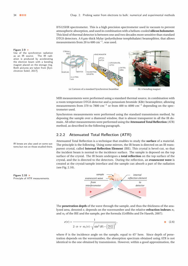
34 ■■■ Chap. 2. Probing water from electrons to bulk: numerical and experimental methods
IR lenses are also used on some sys-tems but not on those studied there.
IFS125HR spectrometer. This is a high precision spectrometer used in vacuum to preventatmospheric absorption, and used in combination with a helium-cooled silicon bolometer.This kind of thermal detector is between one and two decades more sensitive than standardDTGS detectors. A 6 μm-thick Mylar (polyethylene terephthalate) beamsplitter, that allowsmeasurements from 20 to 600 cm−1, was used.
Figure 2.9
Use of the synchrotron radiationas an IR source. The IR radi-ation is produced by acceleratingthe electron beam with a bendingmagnet placed on the storage ring.Both pictures are taken from [Syn-chrotron Soleil, 2017].
(a) Cartoon of a standard Synchrotron beamline (b) A bending magnet
MIR measurements were performed using a standard thermal source, in combination witha room temperature DTGS detector and a potassium bromide (KBr) beamsplitter, allowingmeasurements from 370 to 7800 cm−1 or from 400 to 4000 cm−1 depending on the spec-trometer used.
Synchrotron measurements were performed using the standard transmission method, bydeposing the sample over a diamond window, that is almost transparent in all the IR do-main. All other measurements were performed using the Attenuated Total Reflection (ATR)method, as described in the following paragraph.
2.2.2 Attenuated Total Reflection (ATR)
Attenuated Total Reflection is a technique that enables to study the surface of a material.The principle is the following. Using some mirrors, the IR beam is directed on an IR trans-parent crystal, called Internal Reflection Element (IRE). This crystal is bevel-cut, so thatthe incident beam is normal to the incidence surface. The sample is deposed on the topsurface of the crystal. The IR beam undergoes a total reflection on the top surface of thecrystal, and the is directed to the detectors. During the reflection, an evanescent wave iscreated at the crystal/sample interface and the sample can absorb a part of the radiation(see Fig. 2.10).
Figure 2.10
Principle of ATR measurements.
The penetration depth of the wave through the sample, and thus the thickness of the ana-lyzed area, denoted e, depends on the wavenumber and the relative refraction indexes n1
and n2 of the IRE and the sample, per the formula [Griffiths and De Haseth, 2007]:
e(ν) = 1
2 ·π ·ν ·n1(ν) ·√
sin2 (θ)−(
n2(ν)n1(ν)
)2, ■ (2.6)
where θ is the incidence angle on the sample, equal to 45° here. Since depth of pene-tration depends on the wavenumber, the absorption spectrum obtained using ATR is notidentical to the one obtained by transmission. However, within a good approximation, the
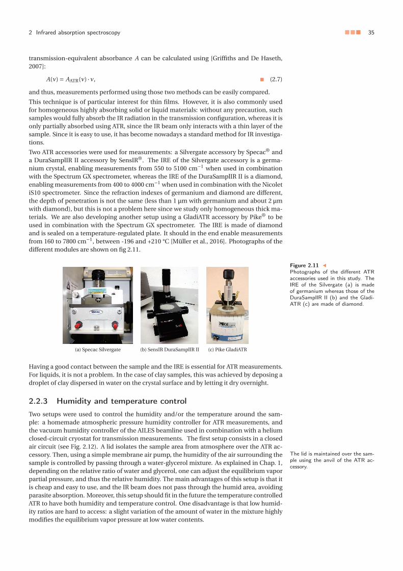
2 Infrared absorption spectroscopy ■■■ 35
The lid is maintained over the sam-ple using the anvil of the ATR ac-cessory.
transmission-equivalent absorbance A can be calculated using [Griffiths and De Haseth,2007]:
A(ν) = AATR(ν) ·ν, ■ (2.7)
and thus, measurements performed using those two methods can be easily compared.
This technique is of particular interest for thin films. However, it is also commonly usedfor homogeneous highly absorbing solid or liquid materials: without any precaution, suchsamples would fully absorb the IR radiation in the transmission configuration, whereas it isonly partially absorbed using ATR, since the IR beam only interacts with a thin layer of thesample. Since it is easy to use, it has become nowadays a standard method for IR investiga-tions.
Two ATR accessories were used for measurements: a Silvergate accessory by Specac® anda DuraSamplIR II accessory by SensIR®. The IRE of the Silvergate accessory is a germa-nium crystal, enabling measurements from 550 to 5100 cm−1 when used in combinationwith the Spectrum GX spectrometer, whereas the IRE of the DuraSamplIR II is a diamond,enabling measurements from 400 to 4000 cm−1 when used in combination with the NicoletiS10 spectrometer. Since the refraction indexes of germanium and diamond are different,the depth of penetration is not the same (less than 1 μm with germanium and about 2 μmwith diamond), but this is not a problem here since we study only homogeneous thick ma-terials. We are also developing another setup using a GladiATR accessory by Pike® to beused in combination with the Spectrum GX spectrometer. The IRE is made of diamondand is sealed on a temperature-regulated plate. It should in the end enable measurementsfrom 160 to 7800 cm−1, between -196 and +210 °C [Müller et al., 2016]. Photographs of thedifferent modules are shown on fig 2.11.
(a) Specac Silvergate (b) SensIR DuraSamplIR II (c) Pike GladiATR
Figure 2.11 �
Photographs of the different ATRaccessories used in this study. TheIRE of the Silvergate (a) is madeof germanium whereas those of theDuraSamplIR II (b) and the Gladi-ATR (c) are made of diamond.
Having a good contact between the sample and the IRE is essential for ATR measurements.For liquids, it is not a problem. In the case of clay samples, this was achieved by deposing adroplet of clay dispersed in water on the crystal surface and by letting it dry overnight.
2.2.3 Humidity and temperature controlTwo setups were used to control the humidity and/or the temperature around the sam-ple: a homemade atmospheric pressure humidity controller for ATR measurements, andthe vacuum humidity controller of the AILES beamline used in combination with a heliumclosed-circuit cryostat for transmission measurements. The first setup consists in a closedair circuit (see Fig. 2.12). A lid isolates the sample area from atmosphere over the ATR ac-cessory. Then, using a simple membrane air pump, the humidity of the air surrounding thesample is controlled by passing through a water-glycerol mixture. As explained in Chap. 1,depending on the relative ratio of water and glycerol, one can adjust the equilibrium vaporpartial pressure, and thus the relative humidity. The main advantages of this setup is that itis cheap and easy to use, and the IR beam does not pass through the humid area, avoidingparasite absorption. Moreover, this setup should fit in the future the temperature controlledATR to have both humidity and temperature control. One disadvantage is that low humid-ity ratios are hard to access: a slight variation of the amount of water in the mixture highlymodifies the equilibrium vapor pressure at low water contents.

36 ■■■ Chap. 2. Probing water from electrons to bulk: numerical and experimental methods
Figure 2
HomemaATR mea
Figure 2.13
Vacuum humidity (a) and temper-ature (b) controllers for transmis-sion measurements. Picture (b) wasfreely adapted from [Dalla Bernar-dina et al., 2014]
The second setup (see Fig. 2.13) is made of a vacuum chamber enclosed by polypropylene(IR transparent) windows positioned on the beam path [Dalla Bernardina et al., 2014]. Awater reservoir and a vacuum pump are plugged on the chamber, and isolated from the cellby valves. First the chamber is purged of all air and water until a high vaccuum of 10−4 mbaris obtained. Then, the humidity can be adjusted by opening one of the two valves to add orremove water vapor. The vapor pressure can be directly followed using precision manome-ters since water is the only gas present in the chamber. A vapor tank enables to increasethe volume of the setup to make the adjustment of the vapor pressure easier. The main ad-vantage of this setup is to enable to work at any water pressure with a high flexibility (in thefirst setup, the corresponding water-glycerol mixture must be prepared), and low humidityrates can be easily reached very quickly. The main disadvantage is that there is vapor onthe beam path, which implies post-corrections on spectra. Moreover, water can freeze onthe windows of the cell and thus on the beam path during low temperature measurements.On this setup, the temperature of the sample can be regulated down to 4 K using a heliumclosed-circuit cryostat coupled to a resistor and a PID controller.
Low temperature and humidity controlled measurements are reported in Chap. 6. The endof the chapter is devoted to molecular simulations.
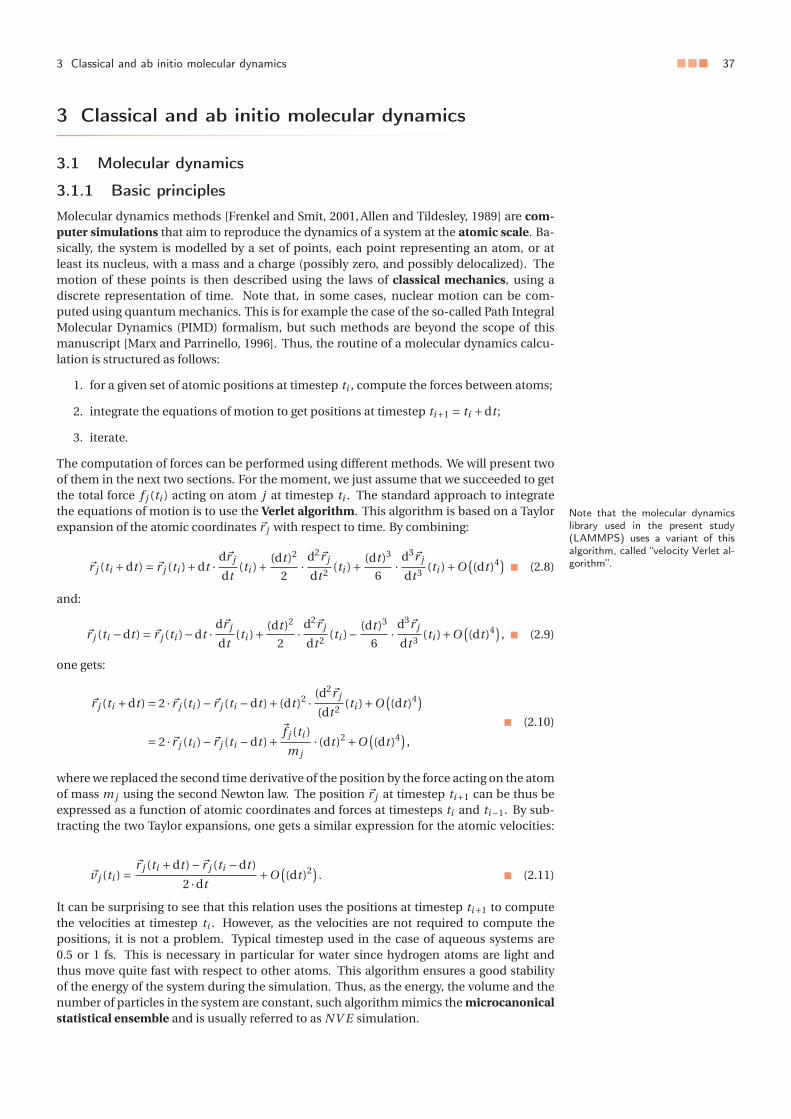
3 Classical and ab initio molecular dynamics ■■■ 37
Note that the molecular dynamicslibrary used in the present study(LAMMPS) uses a variant of thisalgorithm, called “velocity Verlet al-gorithm”.
3 Classical and ab initio molecular dynamics
3.1 Molecular dynamics
3.1.1 Basic principlesMolecular dynamics methods [Frenkel and Smit, 2001, Allen and Tildesley, 1989] are com-puter simulations that aim to reproduce the dynamics of a system at the atomic scale. Ba-sically, the system is modelled by a set of points, each point representing an atom, or atleast its nucleus, with a mass and a charge (possibly zero, and possibly delocalized). Themotion of these points is then described using the laws of classical mechanics, using adiscrete representation of time. Note that, in some cases, nuclear motion can be com-puted using quantum mechanics. This is for example the case of the so-called Path IntegralMolecular Dynamics (PIMD) formalism, but such methods are beyond the scope of thismanuscript [Marx and Parrinello, 1996]. Thus, the routine of a molecular dynamics calcu-lation is structured as follows:
1. for a given set of atomic positions at timestep ti , compute the forces between atoms;
2. integrate the equations of motion to get positions at timestep ti+1 = ti +dt ;
3. iterate.
The computation of forces can be performed using different methods. We will present twoof them in the next two sections. For the moment, we just assume that we succeeded to getthe total force f j (ti ) acting on atom j at timestep ti . The standard approach to integratethe equations of motion is to use the Verlet algorithm. This algorithm is based on a Taylorexpansion of the atomic coordinates �r j with respect to time. By combining:
�r j (ti +dt ) = �r j (ti )+dt · d�r j
dt(ti )+ (dt )2
2· d2�r j
dt 2 (ti )+ (dt )3
6· d3�r j
dt 3 (ti )+O((dt )4) ■ (2.8)
and:
�r j (ti −dt ) = �r j (ti )−dt · d�r j
dt(ti )+ (dt )2
2· d2�r j
dt 2 (ti )− (dt )3
6· d3�r j
dt 3 (ti )+O((dt )4) , ■ (2.9)
one gets:
�r j (ti +dt ) = 2 ·�r j (ti )−�r j (ti −dt )+ (dt )2 · (d2�r j
(dt 2 (ti )+O((dt )4)
= 2 ·�r j (ti )−�r j (ti −dt )+�f j (ti )
m j· (dt )2 +O
((dt )4) ,
■ (2.10)
where we replaced the second time derivative of the position by the force acting on the atomof mass m j using the second Newton law. The position �r j at timestep ti+1 can be thus beexpressed as a function of atomic coordinates and forces at timesteps ti and ti−1. By sub-tracting the two Taylor expansions, one gets a similar expression for the atomic velocities:
�v j (ti ) = �r j (ti +dt )−�r j (ti −dt )
2 ·dt+O
((dt )2) . ■ (2.11)
It can be surprising to see that this relation uses the positions at timestep ti+1 to computethe velocities at timestep ti . However, as the velocities are not required to compute thepositions, it is not a problem. Typical timestep used in the case of aqueous systems are0.5 or 1 fs. This is necessary in particular for water since hydrogen atoms are light andthus move quite fast with respect to other atoms. This algorithm ensures a good stabilityof the energy of the system during the simulation. Thus, as the energy, the volume and thenumber of particles in the system are constant, such algorithm mimics the microcanonicalstatistical ensemble and is usually referred to as NV E simulation.

38 ■■■ Chap. 2. Probing water from electrons to bulk: numerical and experimental methods
Figure 2.14
Cartoon of the construction of amolecular dynamics system. Tomimic a real system, one isolates asmall part of it and reproduces itperiodically at infinite.
The computational cost of molecular dynamics depends, of course, on the size of the sys-tem, i.e. the number of atoms, and it also depends on the complexity of the method used tocompute forces. In the simplest cases, the maximum number of atoms used in a simulationcan reach one million. Typical simple simulations will use about one hundred thousandatoms which corresponds to a typical system size below 100 nm. It rises two main prob-lems: first, it is far from a real macroscopic system, and one can expect finite size effects toinfluence the dynamics of the system, and secondly, one must find boundary conditionsthat do not add spurious effects. To limit those problems, the system is duplicated period-ically in all directions to mimic an infinite size system (see figure 2.14). It means that oneonly needs to compute the positions of the N atoms of the simulation box, but the interac-tions with atoms from all replicas are taken into account in the calculation. But consideringan infinite size system immediately introduces a new problem: interactions cannot be com-puted for an infinite number of atoms.
Two different strategies are used in practice to avoid that. In the case of short-ranged inter-actions (for example, Van der Waals interactions whose amplitude is proportional to 1/r 6
where r is the distance between atoms), one approach is to use a cutoff radius. This meansthat interactions are only computed between atoms separated by a distance lower than thecutoff, and the long-tail part of the interaction is neglected. In the case of long-rangedinteractions (for example, Coulombic interactions decrease like 1/r ), this approximationcannot stand. In that case, a common way to calculate long-ranged interactions is to usethe so-called Particle-Particle Particle-Mesh (PPPM) method, or the Ewald method. Thebasic idea is the same. Here we describe only the PPPM method that was mostly used inthe present work, in the case of Coulombic interactions. The distribution of charges is de-composed, using the superposition principle, in a “purely” short-ranged part and a “purely”long-ranged part. The short-ranged part can be then computed as explained before using acutoff. The long-ranged part, which is rather smooth at the simulation box length scale, issampled on a grid. Then the charge distribution is transposed in the Fourier space where in-teractions are short-ranged, and can be computed using a cutoff. The method is illustratedon figure 2.15.
Figure 2.15
PPPM method applied to Coulom-bic interactions. The distribution ofpunctual charges (the atomic par-tial charges, Dirac distributions) issuperimposed to a smooth distribu-tion with opposite charge. This dis-tribution creates a short-ranged po-tential so that interactions can becomputed using a cutoff. Then us-ing the superposition principle, anopposite term is added to the dis-tribution to get back the real distri-bution. This distribution creates along-ranged smooth potential. Tocalculate its effect, the distributionis sampled over a grid and trans-posed in Fourier space where it gen-erates a short-ranged potential thatis also evaluated using a cutoff.
For the moment, we did not assess the question of “experimental” conditions. In a realexperiment the system has an environment which controls its temperature and volume orpressure. It is the object of the next paragraph.
3.1.2 Reproducing experimental conditions with thermostats andbarostats
Various methods have been developed to mimic thermostats and/or barostat to reproducedifferent statistical ensembles and simulate real experimental conditions. The most popu-lar are the thermostat by Nose and Hoover and the barostat by Hoover and Andersen [Mar-tyna et al., 1994]. Those two algorithms were respectively used in calculations to reproducethe isothermal-isochoric ensemble (NV T ) or the isothermal-isobaric ensemble (N pT ).
First, we need to define the temperature and the pressure of the system from an atomicpoint of view. From the equipartition theorem, one knows that each degree of freedom has

3 Classical and ab initio molecular dynamics ■■■ 39
Figure 2.16 �
Evaluation of g(r) relative to the redatom.
an average energy equal to kB ·T /2, with kB the Boltzmann constant. Since a 3-d isolatedsystem made of N punctual atoms has 3 ·N −3 degrees of freedom, the temperature of thesystem can be evaluated from the total kinetic energy – and thus from the atomic velocities– of the system following the formula:
3 ·N −3
2·kB ·T = 1
2·
N∑j=1
m j · �v j2. ■ (2.12)
Pressure is usually evaluated using the virial equation, based on forces acting on atoms andtheir position:
p = N ·kB ·T
V+ 1
3 ·V ·N∑
j=1
j∑k=1
�f j k · �r j k , ■ (2.13)
where �f j k and �r j k denote respectively the force acting and the distance between atoms jand k (for pairwise interactions).
Now that we have a way to compute the temperature and the pressure using atomic coordi-nates and velocities, we can see how to fix them. The method by Nose and Hoover consistsin adding a fictitious degree of freedom to the system, with its own mass and momentum,that can exchange kinetic energy with other degrees of freedom – so other atoms – to adjustthe temperature of the system. The coupling is realized by adding a force acting on atoms,the momentum is adjusted on the fly at each timestep to get the correct temperature, andthe mass governs the inertia of the thermostat. This mass must be adjusted so that the typi-cal evolution timescale of the temperature of the system approaches molecular timescales.If this typical timescale is too long, the system will need a long time to equilibrate, and thesystem will not be thermostatted efficiently (for instance heat generated in flow conditionswill not be removed fast enough). On the contrary, if this time is too short, the dynamics ofthe system will be affected by the thermostat, and the dynamics may become unstable. Ina similar manner, the method by Hoover and Andersen adds a fictitious degree of freedomthat couples with the volume of the system, i.e. the simulation box size. In this case, themomentum associated to this degree of freedom is adjusted to get the right pressure.
In all calculations performed here, the implementation of these methods is achieved usingthe Martyna et al. formulation [Martyna et al., 1994], which is based on the Verlet algorithm.
3.1.3 Structural and dynamical measurements
Numerous structural and dynamical observables can be calculated from atomic coordi-nates, velocities and pair forces. We already met two examples in the previous paragraph:the temperature and the pressure of the system. In the following paragraph, we will see howto compute some other quantities that will be useful in the next chapters. Generally speak-ing, measurements are performed in the NV E ensemble after a sufficient equilibration timein the N pT ensemble to ensure the system reaches a steady state. However, they can changefrom one measurement to another, we will systematically precise in the upcoming chapterthe conditions used for the corresponding calculations.
Structural measurements The simplest structural observable is the mass density of thesystem. It is computed as the ratio between the global mass of particles lying inside thesimulation box over the volume of the box. This is of course an important information butit tells us nothing about the local structure of the system. The latter can be described us-ing the so-called radial distribution function, denoted g (r ) [Frenkel and Smit, 2001]. Thisobservable, which can be obtained using X-ray or neutron diffusion, gives the evolution ofthe local density of the system with respect to the distance to a given atom. This means, fora given tolerance dr , g (r ) is computed as the density of the volume enclosed between thespheres centered on the reference atom and of radius r and r +dr (see Fig. 2.16). Partialg (r ) can also be computed, for example to get the distribution of oxygen-oxygen distancesinside water.

40 ■■■ Chap. 2. Probing water from electrons to bulk: numerical and experimental methods
Figure 2.17
Evaluation of η and interfacial prop-erties under stationary flow.
Viscoelasticity. We will later focus on various other bulk observables, including the self-diffusion coefficient of water D , its shear viscosity η and high frequency elastic modu-lus G . The self-diffusion coefficient D can be computed at equilibrium from the slope ofthe atomic mean square displacement versus time curve at long times (i.e. in diffusiveregime) [Frenkel and Smit, 2001]:
D = 1
6· lim
t→∞d⟨
(�r (t )−�r (0))2⟩dt
. ■ (2.14)
Since D is highly influenced by long-ranged hydrodynamic interactions, it depends on thesimulation box size. To subtract these finite size effects, D can be extrapolated for an infinitebox size using the scaling relation [Yeh and Hummer, 2004, Tazi et al., 2012]:
D(L) = D∞+ ξ
L, ■ (2.15)
where L is the length of the simulation box and ξ is a constant that depends for exemple onthe viscosity and the temperature. No box size effects are observed for the other quantitiesconsidered here, as detailed for instance in Chap. 3.
The shear viscosity can be calculated – at equilibrium – within the Green-Kubo formal-ism [Frenkel and Smit, 2001]:
η= V
kB ·T·∫∞
0
⟨pi j (0) ·pi j (t )
⟩ ·dt , ■ (2.16)
where pi j is one of the five independent components of the traceless stress tensor: px y , pxz ,py z , (pxx −py y )/2 and (py y −pzz )/2 [Alfe and Gillan, 1998], V the volume of the simulationbox, kB the Boltzmann’s constant and ⟨·⟩ denotes an ensemble average over the differentreplicas. Of course, one cannot perform an infinite time measurement. That means theintegral must be computed over a finite time interval, that must be long enough so that theresult is converged, i.e. invariant when longer time domains are used.
The viscosity can also be computed within stationary shear flow conditions. Let us con-sider the fluid is enclosed between two rigid parallel walls moving with opposite tangentialvelocities. The viscosity can be computed from the shear rate γ of the fluid (obtained asthe slope of the fluid velocity versus distance to walls) and the shear stress σ applied onthe walls (i.e. the total force acting between water and wall atoms per unit of surface in thedirection of the flow) as (see Fig. 2.17):
η= σ
γ. ■ (2.17)
Finally, the Maxwell viscoelastic relaxation time τM and the infinite frequency shear mod-ulus can be extracted from the equilibrium autocorrelation function of the stress tensorcomponents by fitting it with a stretched exponential decay:
V
kB ·T·⟨pi j (0) ·pi j (t )
⟩=G∞ ·exp
((− t
τM
)γ). ■ (2.18)
We will also focus on surface hydrodynamics properties, such as the slip length b and theinterfacial friction coefficient λ. As in the case of the shear viscosity, those observables canbe computed at equilibrium or under stationary flow. Under flow, the friction coefficientλ is calculated from the slip velocity vslip, i.e. the tangential velocity jump at the liquid-solid interface, and the shear stress σ applied to the walls per σ= λ · vslip (see Fig. 2.17). Atequilibrium, the friction coefficient is calculated using the Green-Kubo formula by Bocquetand Barrat [Bocquet and Barrat, 1994]:
λ= 1
A ·kB ·T·∫∞
0(dt ·
⟨�F ∥
w(0) ·�F ∥w(t )
⟩, ■ (2.19)
where A denotes the surface of the wall and �F ∥w the total tangential force applied to the wall.
Then in both cases, the slip length is obtained using b = η/λ, with η the shear viscosity ofthe liquid, determined using one of the methods previously mentioned.

3 Classical and ab initio molecular dynamics ■■■ 41
Vibrational properties Vibrational properties computation can be of great interest tohelp identification of the components of experimental spectra. The IR absorption spec-trum can be approximated numerically using the molecular dipole moments �μ [Thomaset al., 2013]:
A(ν) ∝ m ·ν2 ·∫∞
0
⟨�μ(τ) ·�μ(t +τ)
⟩τ ·ei ·ν·t ·dt , ■ (2.20)
where A(ν) denotes the absorbance at the frequency ν, m the reduced mass of moleculesand ⟨·⟩τ denotes a time-average. Then, using the Wiener-Khintchine theorem, this formulacan be simplified in the following way:
A(ν) ∝ m ·ν2 ·{x,y,z}∑
α
∣∣F [μα(t )
]∣∣2, ■ (2.21)
where F [X ] is the time Fourier transform of X . As we will see at the end of this section,the charge of the oxygen atom is not localized at the same position as the atom when us-ing the TIP4P/2005f force field for calculations. In that case, the dipole moment of watermolecules is post-processed from atomic coordinates using the real position of the charges.Then the absorption spectra are calculated using a homemade routine based on the FFTW3library [Frigo and Johnson, 2005].
Another related quantity is the vibrational density of state (VDOS). It corresponds to thevibrational spectra of the system, without any selection rule. It can be obtained experimen-tally from neutron scattering experiments, and can be approximated numerically in a sim-ilar manner as the infrared spectrum, using the atomic velocities instead of the moleculardipole moments [Thomas et al., 2013].
We already mentioned several times the forces acting between atoms. We will now see howto compute them.
3.2 Computing forces (I): density functional theoryDensity functional theory consists in computing the potential energy surface of the atoms –and thus the forces – directly from the electronic structure. It means consequently that thisstructure must be computed for each set of atomic positions, so, at each iteration. We willfirst give the main ideas of this method, then say a few words about its implementation, andfinally review briefly its use with water. We refer the reader to textbooks such as Refs. [Sholland Steckel, 2011,Koch and Holthausen, 2015] for more details on density functional theory.
3.2.1 Density functional theory in a nutshellElectron density. We saw previously that electrons are described by wave-functions. Fora system of M atoms and a total of N electrons, an accurate determination of the electrondistribution would consist in solving a (N + M)-body problem. We said this is practicallyimpossible for a single molecule, thus, this is also impossible for a more complex system.This problem must consequently be simplified. Since we want to determine the electrondistribution for a given set of nucleus positions, we implicitly work within the frameworkof the Born-Oppenheimer approximation. Two other major approximations are that weconsider the system is in its ground-state and express the ground-state wavefunction asa product of monoelectronic wavefunctions (orbital approximation). We already showedthis means neglecting electronic structure fluctuations, that play a key role in molecularinteractions (dispersion interaction).
Within those approximations, the electron distribution is expressed in terms of its densityfunction:
n(�r ) = 2 ·N∑
i=1ψ∗
i (�r ) ·ψi (�r ), ■ (2.22)
where ψi is the monoelectronic wave-function associated to the i th electron. The densityfunctional theory relies on two theorems, by Kohn and Hohenberg:

42 ■■■ Chap. 2. Probing water from electrons to bulk: numerical and experimental methods
1. the ground-state energy from Schrödinger’s equation is a unique functional of theelectronic density;
2. the electronic density that minimizes the energy of the functional is the true electrondensity corresponding to the full solution of the Schrödinger equation.
This means one can express the energy of the system by a functional of n(�r ) and that, whenthis functional is known, the electron density can be determined by minimizing this func-tional. From this, density functional theory can be summarized in an unique question: whatis this functional? There is no answer and it must be postulated.
Energy functional. Re-expressing the Schrödinger equation in terms of mono-electronicwave-functions ψi , one gets the so-called Kohn and Sham equations:[
− ħ2
2 ·me·�∇2 +V (�r )+e2 ·
∫n(�r )
|�r −�r ′| ·d�r + δEXC (�r )
δn(�r )
]ψi (�r ) = Ei ·ψi (�r ). ■ (2.23)
The terms in brackets constitute the energy functional. From the Schrödinger equation, werecognize the kinetic energy within the first term, and the second term contains Coulom-bic interactions between the electron and the nucleus. The two other terms correspond toelectron-electron interactions. The first is called the Hartree potential and represents theCoulombic repulsion between electrons (including electron with itself), and the second iscalled exchange-correlation functional and contains all other information about electroninteractions, including the correction of the self-interaction term present in the Hartree po-tential. But as we already said, no one knows how to express this term. Defining efficientexchange-correlation functionals is a very active field of research. It exists many families ofsuch functionals corresponding to various approximations, called Local-Density Approx-imation (LDA), Generalized-Gradient Approximation (GGA), meta-GGA..., correspondingto various degrees of refinement. Of course, the most refinement are included inside thefunctional, the most precise it is expected to be, but also the most computational cost isrequired.
In various systems and especially in water, a major issue is to describe correctly disper-sion interactions. There are mainly two ways to do so: by refining the exchange-correlationfunctional with respect to electron correlation – this kind of functional is called dispersion-inclusive functional – or by applying corrections to the potential energy surface after theDFT calculation using a standard functional (by adding for example 1/r 6 terms) – one speaksin that case of dispersion-corrected functional.
For the moment, we said nothing about the way to calculate the electron density. We willgive some elements in the next paragraph.
3.2.2 ImplementationThe Kohn and Sham equations are resolved iteratively through a self-consistent field ap-proach:
1. define a trial electronic density n0(�r );
2. determine the corresponding mono-electronic wavefunctions using the Kohn andSham equations;
3. compute the new electronic density n1(�r );
4. if n0(�r ) and n1(�r ) are identical, then it is the ground-state electron density; otherwise,update n0(�r ) and iterate.
Various methods are used in practice to save computational time during this procedure.First, only the wavefunctions of valence electrons are directly computed. Core electronsare considered through a so-called pseudo-potential directly added to the electron density.Secondly, both wave-functions and electron density are projected on basis of trial func-tions. In the present study, we used the CP2K/Quickstep library for DFT calculations [Van-deVondele et al., 2005a]. This library uses the Gaussian and Plane-Wave method (GPW).

3 Classical and ab initio molecular dynamics ■■■ 43
The basis used for the electron density is made of a family of Gaussians, whereas the oneused for the wavefunctions is made of plane-waves. Bases have a finite size, that implieswavefunctions and electron density have a finite precision. The precision of the bases issetup in the calculation by specifying the spatial frequency kcut of the finest plane-wave. Inpractice, this frequency is given in terms of energy cutoff: Ecut = ħ2 ·k2
cut/(2 ·me). A highcutoff means a high computational cost, but a low cutoff can induce a non-negligible errorin the energy calculation. Thus, the energy cutoff value must be optimized for each calcu-lation so that it is the lowest value that gives converged results, i.e. results do not change ifa higher value is used.
3.2.3 DFT and water
We conclude this section by a brief review of the use of DFT to describe water. Since thepioneering work by Car and Parrinello [Car and Parrinello, 1985,Laasonen et al., 1993,Spriket al., 1996], DFT has been used to describe a great variety of phenomena implying aque-ous systems, such as reactivity [Tocci and Michaelides, 2014, Sulpizi et al., 2012, Mundy andKuo, 2006, Joly et al., 2016], friction [Tocci et al., 2014] or structure and dynamics [Lee et al.,2014, Ambrosetti et al., 2012, Cicero et al., 2008, Pedroza et al., 2015, Feibelman, 2013, De-montis et al., 2013, Rana and Chandra, 2013, Mignon et al., 2010] near a solid-liquid inter-face, liquid/vapor equilibrium [McGrath et al., 2006,Kuo et al., 2006,Baer et al., 2011,Choud-huri and Chandra, 2014, Kühne et al., 2010, Kuo and Mundy, 2004], water dissociation andionic transport [Tuckerman et al., 2002, Tuckerman et al., 2006, Chen et al., 2002b, Megyeset al., 2008, Chen et al., 2002a, Buch et al., 2007, Baer et al., 2014, Asthagiri et al., 2004, Baerand Mundy, 2011,Tuckerman et al., 1995,Baer and Mundy, 2013,Bankura et al., 2013]. Exten-sive work has also been performed to characterize the performance of exchange-correlationfunctionals to describe liquid water and clusters of molecules [Klimeš and Michaelides,2012,Gillan et al., 2016], using different static observables like the liquid density [Spura et al.,2015,Miceli et al., 2015,Gaiduk et al., 2015,Del Ben et al., 2013,McGrath et al., 2011], the paircorrelation function [Alfè et al., 2014, Wang et al., 2011, VandeVondele et al., 2005b, Todor-ova et al., 2006], the hydrogen bond angle distribution [DiStasio Jr et al., 2014, Møgelhøjet al., 2011], but also dynamical observables like the self diffusion coefficient [Corsetti et al.,2013, Ma et al., 2012, Jonchiere et al., 2011] or the infrared absorption spectrum [Lee andTuckerman, 2007, Grossman et al., 2004, Zhang et al., 2011]. It is well known that simpleGGA functionals like BLYP or PBE over-structure water and under-predict the density andself diffusion [Gaiduk et al., 2015, Wang et al., 2011, DiStasio Jr et al., 2014]. Various ap-proaches have been tested to improve those results, such as including dispersion terms inthe functional [Spura et al., 2015,Wang et al., 2011,Schmidt et al., 2009,McGrath et al., 2011],nuclear quantum effects (NQE) (through the use of the path integral formalism [Spura et al.,2015], or replacing H2O molecules by D2O for which nuclear quantum effects are muchlower [DiStasio Jr et al., 2014,Gaiduk et al., 2015,Todorova et al., 2006]), or a fraction of exactexchange through hybrid functionals [Zhang et al., 2011,DiStasio Jr et al., 2014,Gaiduk et al.,2015,Todorova et al., 2006]. In each case, an improvement is observed, but the self diffusioncoefficient remains too low. Moreover, cumulative inclusion of both NQE and dispersionimproves negligibly the accuracy of calculations with respect to calculations where only dis-persion is taken into account [Spura et al., 2015]. Another common approach is to increasethe temperature with respect to experiments to compensate the slow dynamics observed.The temperature is generally chosen to reproduce a particular property of water (eg. thecrystallization temperature [Yoo et al., 2009], the liquid density or diffusivity [Gaiduk et al.,2015,Joly et al., 2016] or the radial distribution function [Gaiduk et al., 2015,Jonchiere et al.,2011]) or to compensate NQE [DiStasio Jr et al., 2014], but highly depends on the functionaland system considered. Thus, one can question the validity of this approach for hetero-geneous systems. Moreover, for composite systems, the density is not necessarily equal tothe bulk density, so that constant volume calculations might not be suitable. In Chap. 3,we will investigate the accuracy of constant pressure methods to describe the structure anddynamics of water.

44 ■■■ Chap. 2. Probing water from electrons to bulk: numerical and experimental methods
Figure 2.18
The Lennard-Jones potential.
3.3 Computing forces (II): point charge force fieldsThe potential energy surface computation using DFT requires at each timestep to solveKohn and Sham equations using the iterative procedure previously described. That repre-sents a lot of computational time. Thus, DFT can be applied only to small systems (typicallya few hundred atoms) and very short times (typically a few tens of picoseconds). Even withsuch a small system, a simple molecular dynamics shear viscosity calculation typically lastsone month using 64 cores CPU. This considerably limits the possibilities of the method. Forthis reason, the use of classical force fields to compute the potential energy surface is verypopular and the development of new force fields is still an active field of research. In thissection, we will describe the key elements that constitutes force fields [Frenkel and Smit,2001, Allen and Tildesley, 1989, Plimpton et al., 2005] and mention a couple of popular wa-ter models.
The key point of force fields approaches is the interaction energy between a group (e.g. apair) of atoms has a fixed form that only depends on the relative positions of atoms withinthe group. There is thus no equation to solve to compute the potential energy surface. Thus,what is achieved within typically one minute using DFT requires only a fraction of secondusing force fields. For molecular systems, one distinguishes intermolecular interactionsand intramolecular interactions. Most of the time, molecules are considered as rigid bod-ies, and thus intra-molecular interactions are not considered.
3.3.1 Intermolecular interactionsIntermolecular interactions include Van der Waals interactions, hydrogen bonds, short-ranged electronic shell repulsion, and – if needed – Coulombic interactions.
Let us first consider non-Coulombic interactions. Generally speaking, interactions are usu-ally decomposed as a sum of 2-, 3-, 4-body... terms. Most of the time, the 2-body term is theonly term considered in the development. Thus, a common-use way to mimic interactionsis to apply a Lennard-Jones potential between pairs of atoms (see Fig. 2.18):
ULJ(ri j ) = 4 ·ε ·((
σ
ri j
)12
−(σ
ri j
)6), ■ (2.24)
where ri j is the distance between atoms i and j , and ε andσ are constants depending on thetype of atom considered. For an isolated pair of atoms, σ denotes the equilibrium distancebetween atoms and ε the binding energy. The second term corresponds to Van der Waalsinteractions, whereas the first term is empirical and mimics short range repulsion.
Instead of defining ε and σ for each pairs of atoms involved in the system, one usually de-fines atomic ε and σ values. Pair values are then computed using so-called mixing rules.Here we use Lorentz-Berthelot mixing rules:⎧⎨⎩
εi j =√
εi ·ε j
σi j =σi +σ j
2
, ■ (2.25)
where xi and x j denote atomic values and xi j denotes pair value. The determination of εand σ can be based on quantum mechanics calculations or can be empirical (for exampleadjusted to reproduce a specific property of the system).
The interaction potential can have a different form and include three-body (or more-body)terms, giving rise to an infinite variety of possible forcefields.
Coulombic interactions acts as two-body terms, using the standard formula:
Ucoul(ri j ) = qi ·q j
4 ·π ·ε · ri j. ■ (2.26)
For monoatomic entities, there is a priori no trouble in the definition of q values. But in thecase of polyatomic structures, one must attribute partial charges to atoms. As in the case ofthe Lennard-Jones parameters, this can be achieved using quantum mechanics calculationsor empirically.

3 Classical and ab initio molecular dynamics ■■■ 45
Figure 2.19
The harmonic and Morse potentials.
The potential energy surface is then computed as the sum of all contributions (Coulombicand non-Coulombic), eventually applying cutoffs as explained in section 3.1. The compu-tational cost depends on the complexity of non-Coulombic interaction terms that are used.Typical simulations include between 10000 and 100000 atoms, during 1 million timesteps(i.e. 1 ns).
3.3.2 Intramolecular interactions
As we mentioned, a common approach is to consider a molecule as a rigid body. In that case,a specific algorithm, as for example the SHAKE method [Ryckaert et al., 1977], is required tocompute the displacement of the molecule from the average atomic interactions. As we willconsider flexible molecules, we will not develop this point. Details can be found in manytextbooks [Frenkel and Smit, 2001, Allen and Tildesley, 1989].
Intramolecular interactions include, of course, all the terms previously mentioned. Thoseare treated exactly as in the case of intermolecular interactions. Here we only focus on termsthat are specific to molecules.
Chemical bonds can be described using various ways. The most popular way is to modelthe bond by a harmonic spring, i.e. a harmonic potential:
Uharm = k · (ri j − r0)2 , ■ (2.27)
with k the strength of the spring and r0 its equilibrium length. Another popular way includ-ing anharmonicity is to use a Morse potential (see Fig. 2.19):
Umorse = D · (1−e−α·(ri j −r0))2, ■ (2.28)
with α and D two constants. Again, k, r0, α and D can be computed or chosen empirically.
For molecules with more than two atoms, as bonds are strongly coupled, three- (angles) orfour-body (dihedral) terms can be added to the global interaction potential. For example, inwater molecules, three body terms can be considered adding a harmonic potential on theHOH angle.
In some cases, the polarizability of the electronic shell of atoms can be considered, to createso-called polarizable force fields. Those force fields require more computational resourcesand are not considered in the present study. As we saw, the different terms that constituteforce fields can be empirical, to reproduce a specific property of the system. For this rea-son, the geometry of molecules does not necessarily represent the real geometry. This isparticularly true concerning water models, as we will see now.
3.3.3 A few water force fields
Various geometries have been considered to model numerically a water molecule [Guillot,2002] (see Fig. 2.20). Of course, water can be modelled using three point charges for its threeatoms (see Fig. 2.20a). It is the case of the very popular SPC (Simple Point Charge) forcefield [Berendsen et al., 1981] and its derivatives (SPC/f [Teleman et al., 1987], SPC/E [Berend-sen et al., 1987]...), or the TIP3P [Jorgensen et al., 1983] (Transferable Intermolecular Poten-tial 3 Points) force field. But it is common to change this geometry to consider the twooxygen lone pairs of electrons. This is achieved by delocalizing the charge of the oxygenatom on one or two massless points located on the HOH bisector in the case of one point,or organized in a tetrahedral geometry with hydrogen atoms in the case of two points. Thegeometry with one massless point (see Fig. 2.20b) gave rise to the TIP4P force field fam-ily (TIP4P [Jorgensen and Madura, 1985], TIP4P/Ew [Horn et al., 2004], TIP4P/2005 [Abas-cal and Vega, 2005], TIP4P/2005f [González and Abascal, 2011], E3B [Kumar and Skinner,2008, Tainter et al., 2015] (Explicit Three Body)...), whereas the geometry with two mass-less sites (see Fig. 2.20d) is used in the TIP5P [Mahoney and Jorgensen, 2000] force field.Interestingly, although the TIP5P geometry seems to mimic more closely the real chargedistribution in water molecules, the best results are obtained with models from the TIP4Pfamily [Vega et al., 2009].
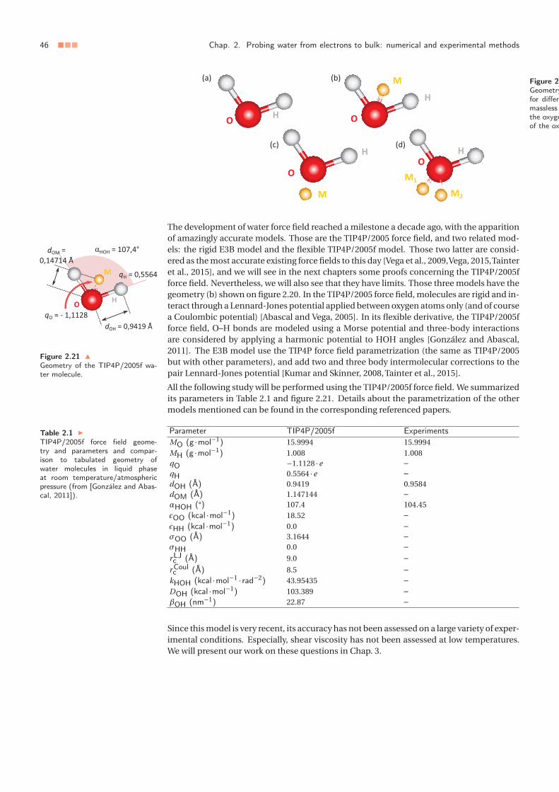
46 ■■■ Chap. 2. Probing water from electrons to bulk: numerical and experimental methods
Figure 2
Geometryfor differemasslessthe oxygeof the ox
Figure 2.21 �
Geometry of the TIP4P/2005f wa-ter molecule.
The development of water force field reached a milestone a decade ago, with the apparitionof amazingly accurate models. Those are the TIP4P/2005 force field, and two related mod-els: the rigid E3B model and the flexible TIP4P/2005f model. Those two latter are consid-ered as the most accurate existing force fields to this day [Vega et al., 2009,Vega, 2015,Tainteret al., 2015], and we will see in the next chapters some proofs concerning the TIP4P/2005fforce field. Nevertheless, we will also see that they have limits. Those three models have thegeometry (b) shown on figure 2.20. In the TIP4P/2005 force field, molecules are rigid and in-teract through a Lennard-Jones potential applied between oxygen atoms only (and of coursea Coulombic potential) [Abascal and Vega, 2005]. In its flexible derivative, the TIP4P/2005fforce field, O–H bonds are modeled using a Morse potential and three-body interactionsare considered by applying a harmonic potential to HOH angles [González and Abascal,2011]. The E3B model use the TIP4P force field parametrization (the same as TIP4P/2005but with other parameters), and add two and three body intermolecular corrections to thepair Lennard-Jones potential [Kumar and Skinner, 2008, Tainter et al., 2015].
All the following study will be performed using the TIP4P/2005f force field. We summarizedits parameters in Table 2.1 and figure 2.21. Details about the parametrization of the othermodels mentioned can be found in the corresponding referenced papers.
Table 2.1 �
TIP4P/2005f force field geome-try and parameters and compar-ison to tabulated geometry ofwater molecules in liquid phaseat room temperature/atmosphericpressure (from [González and Abas-cal, 2011]).
Parameter TIP4P/2005f ExperimentsMO (g ·mol−1) 15.9994 15.9994MH (g ·mol−1) 1.008 1.008qO −1.1128 ·e –qH 0.5564 ·e –dOH (Å) 0.9419 0.9584dOM (Å) 1.147144 –αHOH (°) 107.4 104.45εOO (kcal ·mol−1) 18.52 –εHH (kcal ·mol−1) 0.0 –σOO (Å) 3.1644 –σHH 0.0 –r LJc (Å) 9.0 –
r Coulc (Å) 8.5 –
kHOH (kcal ·mol−1 · rad−2) 43.95435 –DOH (kcal ·mol−1) 103.389 –βOH (nm−1) 22.87 –
Since this model is very recent, its accuracy has not been assessed on a large variety of exper-imental conditions. Especially, shear viscosity has not been assessed at low temperatures.We will present our work on these questions in Chap. 3.

1 Long time dynamics of water: water as a viscous liquid ■■■ 47
■■■ Chapter 3
Viscoelastic properties of pure liquidwater
Outline
1 Long time dynamics of water: water as a viscous liquid . . . . . . . 451.1 Computational details . . . . . . . . . . . . . . . . . . . . . . 461.2 Structural relaxation times . . . . . . . . . . . . . . . . . . . 461.3 Shear viscosity . . . . . . . . . . . . . . . . . . . . . . . . . . . 481.4 Stokes-Einstein relation . . . . . . . . . . . . . . . . . . . . . 491.5 Summary . . . . . . . . . . . . . . . . . . . . . . . . . . . . . . 52
2 Links with the short time dynamics: from viscous liquid to elasticsolid . . . . . . . . . . . . . . . . . . . . . . . . . . . . . . . . . . . . . 522.1 Numerical methods . . . . . . . . . . . . . . . . . . . . . . . . 522.2 Slow dynamics vs elastic modulus . . . . . . . . . . . . . . . 532.3 Hall-Wolynes equation . . . . . . . . . . . . . . . . . . . . . . 542.4 Summary . . . . . . . . . . . . . . . . . . . . . . . . . . . . . . 55
3 Towards a consideration of quantum effects: ab initio approach . . 553.1 Aim of the study and methods . . . . . . . . . . . . . . . . . 553.2 Pulay stress correction . . . . . . . . . . . . . . . . . . . . . . 563.3 Structural and dynamical predictions . . . . . . . . . . . . . 57
4 Conclusion . . . . . . . . . . . . . . . . . . . . . . . . . . . . . . . . . . 60
The aim of the following numerical study is first to assess the accuracy of empirical andab initio molecular simulations to describe the viscoelastic properties of pure liquid water,secondly to provide a reference for following studies on heterogeneous systems, and thirdlyto analyse the behaviour of various dynamical observables at low temperature, in order –for example – to investigate on the debated glass transition of water. The first part will bedevoted to a classical study of the long time dynamics of water, in the second part we dis-cuss the connection to the short time dynamics, and in the third part, we test the accuracyof ab initio methods in order to assess the role of quantum effects.
1 Long time dynamics of water: water as a viscous
liquid
Using molecular dynamics simulations, we propose here to analyze the temperature depen-dence of both the shear viscosity and the structural relaxation times on a range of temper-atures much larger than the one used in experiments and confront our results to empiricalmodels in order to get a consistent picture of the dynamics of water at low temperatures.

48 ■■■ Chap. 3. Viscoelastic properties of pure liquid water
α and β relaxations denote re-spectively collective and local relax-ations of the system.
1.1 Computational details
All calculations were performed using the LAMMPS simulation package [Plimpton, 1995].Water molecules interacted through the TIP4P/2005f force field [González and Abascal,2011] introduced in chapter 1. Two sets of calculations were performed: (i) equilibrium cal-culations and (ii) steady-state shear calculations. Due to the flexibility of molecular bond-ing, a small timestep was required; 1 fs was used for all calculations. For equilibrium cal-culations, eight different box sizes were used from 8×8×8 to 22×22×22 molecules, withperiodic boundary conditions. For each box size, four replicas of the system with differentinitial atomic coordinates and velocities were equilibrated in the isotherm-isobaric ensem-ble during a time that varied from 40 ps for the highest temperatures to 100 ps for the lowesttemperatures using a Langevin thermostat [Schneider and Stoll, 1978] and a Hoover andAndersen barostat [Martyna et al., 1994], making in total thirty-two replicas at each temper-ature. The temperature was varied from 360 K to 228 K by 3 K steps, using each time the finalconfiguration from the previous temperature as initial state to save computation time. Thepressure was fixed at 1 atm. For steady-state shear calculations, 8228 water molecules wereenclosed between two walls made of a face-centered cubic Lennard-Jones rigid crystal, withperiodic boundary conditions in the two directions parallel to the walls. Opposite tangentialvelocities of 40, 70 and 100 m/s were applied to the wall to shear the fluid, with a 1 ns prelim-inary run to reach the steady state. The temperature was controlled using a Nose-Hooverthermostat [Martyna et al., 1994] in the same range as for the equilibrium measurements,but was changed by 15 K steps, except two extra calculations at 230 and 235 K. The pressurewas set by applying normal forces on the walls. All data points reported in the followingdiscussion are averaged over the values obtained for each replica of the system, and errorbars are estimated as the standard error of those data sets.
1.2 Structural relaxation times
We introduce first the coherent intermediate scattering function, F (q, t ), defined by:
F (q, t ) =⟨ρ(�q , t ) ·ρ(−�q ,0)
⟩⟨ρ(�q ,0) ·ρ(−�q ,0)
⟩ , ■ (3.1)
where ρ(�q , t ) is the space Fourier transform of the density of the system at time t evaluatedfor each direction with �q the wave vector corresponding to the first maximum in the staticstructure factor [Kumar et al., 2007]. F (q, t ) was calculated during 10 ps and averaged over100 ps for each replica of the system. This function was fitted by a double exponential decayto extract the α- and β-relaxation times (see inset in Fig. 3.2):
F (q, t ) = (1−a) ·exp
(− t
τα
)+a ·exp
(− t
τβ
). ■ (3.2)
The coherent intermediate scattering function is usually fitted by stretched exponentials,and gives one or two relaxation times. In the present case, Fig. 3.1 reveals a two-timescalesprocess. As illustrated in the inset of Fig. 3.2, the best agreement with calculated values wasobtained using two simple exponential functions, Eq. (3.2), instead of stretched exponen-tials, with one decay time following a VTF / SA behavior and the other one an Arrheniusbehavior, as in the case of α- and β-relaxations of common glass-formers. Those two decaytimes were consequently identified with τα and τβ. α- and β-relaxation processes decou-ple at very high temperature, around 350 K, that is, near the boiling temperature, as shownon Fig. 3.2. Such α/β transition is usually observed in the supercooled regime of glass-formers [Debenedetti and Stillinger, 2001]. This implies that water may have a supercooled-like dynamics at much higher temperatures than its melting temperature, which is consis-tent with the fact that, as already mentioned, several water anomalies occur at quite hightemperature. Note also that the β-relaxation time follows an Arrhenius law with a nega-tive activation energy. Staib et al. [Staib and Hynes, 1993] reported that, contrary to othermolecular liquids, the relaxation time of O–H stretching modes from an excited state to thefundamental state increases with temperature in the case of water, due to the weakening ofthe hydrogen bonds. Assuming β-relaxation process is mainly related to bond stretching,

1 Long time dynamics of water: water as a viscous liquid ■■■ 49
Figure 3.1 �
Coherent intermediate scatteringfunctions for different tempera-tures. At low temperatures, thedecay process splits into a two-timescales decay.
this could explain this surprising behavior. Actually, O–H vibrational relaxation times mea-sured by Lock et al. [Lock et al., 2002] are in very good agreement with our calculated valuesof τβ, which confirms this hypothesis (see Fig. 3.2).
Figure 3.2 �
Water α- and β-relaxation timescomputed with the TIP4P/2005fforce field (points). For temper-atures lower than 350 K, the re-laxation function, observed throughthe coherent intermediate scatter-ing function decay, splits into aslow (α) and a fast (β) relax-ations (see inset), the former fol-lowing an inverted Arrhenius behav-ior, and the latter following a non-Arrhenius behavior. Both SA andVTF laws (lines) are in good agree-ment with the simulation data forthe α-relaxation time. Experimen-tal data by Lock et al. [Lock et al.,2002] of the O–H vibrational re-laxation time are also plotted forcomparison.
Regarding the evolution of the α-relaxation time with temperature, the calculated valuescan be fitted by both VTF and SA laws, without significant differences over the range oftemperature studied here. However, by defining the glass transition temperature Tg as thetemperature at which τα reaches 100 s [Debenedetti and Stillinger, 2001], and by assum-ing the fits using these laws can be extrapolated down to the glass transition, their predic-tions are very different: the VTF law predicts Tg = 119±10 K, whereas the SA law predictsTg = 178±13 K. The Tg predicted by VTF law is slightly lower than the lowest tabulated value,135 K [Debenedetti, 2003], whereas SA gives a much higher value. Another way to charac-terize a glass-forming liquid is to calculate its fragility index m. To give a good definition ofthis index is not trivial, as explained by Angell [Angell, 2002]. Here, we use:
m =− Tg
ln(10)·(∂ ln(X )
∂T
)Tg
, ■ (3.3)
where X can be the shear viscosity or the α-relaxation time. According to this definition,VTF law gives m ≈ 55, which is consistent with a highly fragile behavior, and SA law givesm ≈ 16650 which is much higher than usual fragility values. Assuming the definition (3.3) is

50 ■■■ Chap. 3. Viscoelastic properties of pure liquid water
valid whatever the model is used to extrapolate the values of τα at low temperatures [Mauroet al., 2009], that suggests that, for our study, the extrapolated data obtained with VTF laware more realistic than those using SA law. However, one must consider this result withcaution, since the definition of m has been initially derived for VTF law, and might be notsuitable for SA law. We will therefore consider only the fragility index provided by the VTFlaw in the following. To conclude, despite the same accuracy between the two laws to de-scribe computed values of α-relaxation time, their predictions in term of glass transitiontemperature are very different.
1.3 Shear viscosity
Figure 3.3 �
Variations of the Green-Kubo in-tegrals (Eq. (3.5)) with time at300 K. Dashed curves correspondto a small set of representative in-tegrals calculated for isolated repli-cas, whereas the plain curve cor-responds to the integral averagedover all 160 independent Green-Kubo curves. The value of viscosityis obtained by averaging the plateauvalue over the last 2 ps.
To go beyond this relaxation study, we also looked at the behavior of the shear viscosity withrespect to temperature and compared the picture of the glass transition given by both ap-proaches. This method is used by a few experimentalists to investigate supercooled liquids,but is almost not used by theoreticians, probably due to the poor convergence of viscositycalculations. As we already mentioned, two sets of calculations were performed: (i) equilib-rium calculations and (ii) steady-state shear calculations. We first briefly justify the validityof those two approaches, especially in terms of convergence.
For equilibrium calculations, the shear viscosity was computed using the Green-Kubo for-malism:
η= limt→∞η(t ), ■ (3.4)
with
η(t ) = V
kB ·T·∫t
0
⟨pαβ(0) ·pαβ(u)
⟩ ·du, ■ (3.5)
where ⟨. . .⟩ denotes an ensemble average, and αβ is one the five independant componentsof the traceless stress tensor (see Chap. 2). To get convergence, we averaged the values ob-tained for 160 independent Green-Kubo integrals (see previous paragraph) for each tem-perature, as illustrated in Fig. 3.3. Then, we estimated the error associated with the averagevalue by taking the standard deviation of this set of values, divided by the root mean squareof the number of values in the set (standard error). The time interval on which the integralsare calculated were adjusted to ensure that a plateau is reached for each temperature.
For steady-state shear calculations, the shear viscosity is then given by:
η= σ
γ, ■ (3.6)
where σ and γ denote the shear stress applied to the walls and the imposed shear rate,respectively. Both quantities were averaged over 1 ns. Three replica of the system were used

1 Long time dynamics of water: water as a viscous liquid ■■■ 51
at each temperature, applying shear velocities of ±40, 70 and 100 m · s−1 to the walls. Asshown in the Fig. 3.4, we checked the linearity of the shear stress with respect to the shearrate to control that the simulations remained in the linear response regime. The values ofviscosities reported are averages of the values obtained for each replica. The error is thencalculated as the standard error over those values.
The two sets of calculations (Green-Kubo and steady-state shear) are found to be consistentand show an excellent agreement with experimental data by Osipov et al. [Osipov et al.,1977], as shown in the inset of Fig. 3.5. The agreement is also very satisfactory with thedata by Dehaoui et al. [Dehaoui et al., 2015], and by Hallett et al. [Hallett, 1963] (whosedata are very close to those by Dehaoui et al.). This shows the accuracy of TIP4P/2005fforce field to describe the slow dynamics of supercooled water. Like for the α-relaxationtime, the calculated values of the shear viscosity were fitted over the range of temperature228 to 360 K since the α/β transition shows that a supercooled-like regime extends overthis full range of temperature. Again, both VTF and SA laws describe reasonably well ourvalues, with a slightly lower reduced χ2 for VTF law (see Fig. 3.5). We also tried to fit thedata with Bässler law [Bässler, 1987], but it clearly deviates from our simulation results. Inthe case of shear viscosity, the glass transition temperature is conventionally defined as thetemperature at which the viscosity reaches 1012 Pa · s. Again, extrapolated VTF and SA lawsgive different predictions for this temperature: Tg = 189±21 K for VTF, and Tg = 217±24 Kfor SA. Regarding the fragility index, the VTF law for the viscosity gives m ≈ 358, higherthan the value calculated from τα. All the values for Tg and m are summarized in Table 3.1.Overall, the relaxation time and the shear viscosity exhibit different behaviors with respectto temperature, providing different estimations of the glass transition temperature and ofthe fragility index. This is in contrast with a standard assumption in the community [Kumaret al., 2007], although previous work evidenced such a decoupling in a model glass former[Shi et al., 2013].
Shear viscosity α-relaxation timeVTF SA VTF SA
Tg 189±21 K 217±24 K 119±10 K 178±13 Km 358 – 55 –
Table 3.1 �
Values of the glass transition tem-perature Tg and the fragility indexm estimated from shear viscosityand α-relaxation time calculations,fitted by VTF and SA laws.
1.4 Stokes-Einstein relation
To compare the dynamics at low temperatures of both shear viscosity and α-relaxation timeand assess the reliability of the previous studies, we also looked at the coupling between onthe one hand viscosity and self-diffusion, and on the other hand α-relaxation time and self-
Figure 3.4 �
Evolution of the shear stress withrespect to the shear rate for differ-ent velocities applied to the walls.Points correspond to calculated val-ues at 300 K. The line shows thatall values are in the linear responseregime.

52 ■■■ Chap. 3. Viscoelastic properties of pure liquid water
Figure 3.5 �
Water shear viscosity computedwith the TIP4P/2005f force fieldusing the Green-Kubo formalism(+) and stationary shear calcula-tions (×). Both data sets are con-sistent and are in very good agree-ment with experimental values [Os-ipov et al., 1977, Dehaoui et al.,2015] (see inset). Fits by VTF,SA and Bässler laws (lines) are pre-sented on separate bottom figures.The two first are in overall goodagreement with the data, whereasthe third one does not match.
diffusion, through the Stokes-Einstein (SE) relation [Hansen and McDonald, 2013]:
D ·ηT
= Cst, ■ (3.7)
or its equivalent for α-relaxation time:
D ·ταT
= Cst’. ■ (3.8)
To the best of our knowledge previous numerical work on supercooled water only consid-ered the α-relaxation time, we would like to compare here the predictions obtained withboth observables, as it has been done previously for a model binary mixture [Shi et al., 2013].The self-diffusion coefficient of bulk water computed with the TIP4P/2005f force field is invery good agreement with NMR measurements over a wide range of temperatures [Priceet al., 1999], see Fig. 3.6, showing again the accuracy of this force field. The temperaturesT η
SE and T αSE below which violations of the SE relation for viscosity and α-relaxation time are
observed are very different: T η
SE is 265± 15 K, whereas T αSE is 320± 10 K, as shown in Fig.
3.7 (top). Note that we tested another suggested correlation between viscosity and struc-tural relaxation time, τα ∝ η/T [Yamamoto and Onuki, 1998], leading to an alternative SErelation for the α-relaxation time: D ·τα = cst. The temperature T α
SE, alt below which the al-ternative SE formula fails was well within the error bars of T α
SE. This confirms the fact thatshear viscosity and α-relaxation time behave differently at low temperatures in water.
However, even if those quantities are not equivalent, the glass transition is unique. Inde-pendently of the way the transition is approached, both quantities should predict similarglass transition temperatures. One needs consequently to go further. α-relaxation time and

1 Long time dynamics of water: water as a viscous liquid ■■■ 53
Figure 3.6 �
Water self-diffusion coefficient com-puted with TIP4P/2005f forcefield(+) using the slope of the atomicmean square displacement in thediffusive regime. Calculated valuesare in very good agreement withNMR measurements (•) by Price etal. [Price et al., 1999].
See Chap. 2 for the numerical deter-mination of τM. A discussion aboutthe validity of the approach will begiven in section 2.
shear viscosity refer to different physical quantities. To this point of view, it can be interest-ing to look at direct correlations between α-relaxation time and a macroscopic time relatedwith the viscosity: the Maxwell viscoelastic relaxation time τM, defined as the ratio betweenthe liquid shear viscosity η and the infinite frequency shear modulus G∞:
τM = η
G∞. ■ (3.9)
Those two timescales behave identically for temperatures higher than 285 K that is slightlylower than T α
SE, as shown in Fig. 3.7 (bottom), but are no more correlated for lower temper-atures. A possible explanation for this decoupling at low temperatures is related to the dif-ferent length scales probed by the two relaxation times [Berthier et al., 2004, Pastore et al.,2015]. Indeed, by definition the α relaxation time calculated here corresponds to densityfluctuations at the length scale 2 ·π/kmax, where kmax is the wavevector corresponding tothe first maximum of the static structure factor. This defines an almost temperature inde-pendent length scale which is comparable with the size of a water molecule. Conversely, thelength scale relevant to shear viscosity depends on temperature. At high temperatures, theshear viscosity has an Arrhenius-like behaviour, and stress relaxation should occur throughsingle molecule hopping. In this situation, the length scale probed by the shear viscosityis comparable with 2 ·π/kmax, and the two relaxation times τM and τα increase similarlyon cooling. At lower temperatures, the dynamics becomes heterogeneous and stress relax-ation should be cooperative and involves the relaxation of the cage formed by neighbouringmolecules. Hence, the length scale probed by the viscosity should be larger than 2 ·π/kmax.In conclusion, the heterogeneous dynamics, which is the hallmark of supercooled liquids,should explain the decoupling between τM and τα.
Another, yet not contradictory, recent interpretation for this decoupling is due to Iwashitaet al. who attribute the increase of shear viscosity at low temperatures in glass-formers interms of local configurational excitations, and introduced a timescale τLC for the evolutionof local atomic connectivity [Iwashita et al., 2013]. They found that τLC and τM coincidefor temperatures higher than TA that corresponds to a strong-to-fragile transition tempera-ture, i.e. a crossover between Arrhenius and non-Arrhenius behavior of the shear viscosity.This transition occurs at high temperatures and should not be confused with the fragile-to-strong transition observed in confined water at lower temperatures T < 228 K. In the presentcase, we found a similar behavior for τM and τα if we take TA = 285 K. Actually, the shearviscosity shows an Arrhenius behavior in Fig. 3.5 for temperatures higher than TA. Conse-quently, TA could indeed correspond to a strong-to-fragile crossover. As it is close to T α
SE,the decoupling between α-relaxation time and self-diffusion coefficient might be explainedby such a crossover. Reevaluation of the accuracy of VTF and SA laws by restricting data totemperatures lower than TA does not affect significantly the predictions of the glass transi-tion temperatures and fragility indexes: changes are within error bars. Thus, the existence

54 ■■■ Chap. 3. Viscoelastic properties of pure liquid water
Figure 3
Couplingscosity η,time τM,and the sTop figutween seshear viscare testeStokes-Eilation islower thacosity, aα-relaxature: micscopic (τpared. Trelaxationfor tempea constandiagram.
of a strong-to-fragile transition does not explain the differences observed between the twoobservables.
1.5 Summary
In this section, we have shown that the TIP4P/2005f force field is very accurate to model hy-drodynamic transport properties of supercooled water. It predicts two structural relaxationtimes, namely α- and β-relaxation times, with a α/β decoupling around 350 K, so that liquidwater behaves like a supercooled liquid almost up to its boiling temperature. It is importantto remark that in the present study, we are primarily concerned with the dynamics of super-cooled water above the homogeneous nucleation temperature around 232 K. Therefore, wedo not address any fragile-to-strong transition that may occur at lower temperatures, andwhich is observed under confinement [Mallamace et al., 2006, Liu et al., 2006, Chen et al.,2006]. Analyzing the α-relaxation time and shear viscosity temperature dependence, we in-vestigated the supercooled dynamics of water and compared with several empirical laws.VTF law gives glass transition temperatures that are closer to tabulated values than SA law,even if the two laws describe with a comparable accuracy the simulation data over the rangeof temperatures considered here. However, the viscosity and the α-relaxation time behavedifferently with temperature, with a decoupling around 309 K that could correspond to afragile-to-strong transition of water. This decoupling corresponds also to a violation of theStokes-Einstein relation for the α-relaxation time, whereas the Stokes-Einstein relation forshear viscosity is violated at a lower temperature (around 265 K).
2 Links with the short time dynamics: from viscous
liquid to elastic solid
We introduced two “elastic” models in the chapter 1 to connect the slow and fast dynamicsof glass-former liquids. In this section, we assess the validity of these models to describethe slow dynamics of supercooled water using molecular dynamics simulations. We con-sider the promising TIP4P/2005f force field as in the beginning of this chapter. We report astrong correlation between the α-relaxation time and the high frequency shear modulus orthe mean square displacement for the temperatures considered in this study. Conversely,elastic models perform well at low temperatures but, depending on the model and the ob-servable, they can fail above a temperature on the order of 260 K. Interestingly, this temper-ature is close to the temperature where the Stokes-Einstein relation begins to be violated.

2 Links with the short time dynamics: from viscous liquid to elastic solid ■■■ 55
2.1 Numerical methodsNumerical methods used in this study are the same as those introduced in the first sectionof this chapter (see section 1.1).
2.2 Slow dynamics vs elastic modulusWe first look at direct correlations between the shear viscosity or the α-relaxation time ofliquid water with the high frequency shear modulus using Eq. (1.4). As a reminder, thoseequations are:⎧⎪⎨⎪⎩X = X0 ·exp
(Ea(T )
kB ·T
),
Ea(T ) =λ ·Gp(T ) ·a3■ (3.10)
The plateau shear modulus Gp is traditionally defined as the value of the elastic moduluswhere the derivative of log(G(t )) is minimum [Puosi and Leporini, 2012a, Dyre and Wang,2012]. To estimate the position of the plateau, one can look at the vibrational density ofstate of water. We calculated the VDOS using the TIP4P/2005f force field for various tem-peratures, as shown on Fig. 3.8. The position of the different bands introduced in Chap. 2
Figure 3.8
Evolution of the vibrational densityof states (VDOS) of water with re-spect to the temperature. Left:the connectivity region, obtainedusing the VDOS of oxygen atoms.Right: the intramolecular stretchingregion, obtained using the VDOS ofhydrogen atoms.
is overall well reproduced. Especially, the connectivity band, at low wavenumbers, is as-sociated with the hydrogen bond bending mode around 50 cm−1 and the hydrogen bondstretching mode around 200 cm−1 [Brubach et al., 2005]. The latter shifts from approxma-tively 250 to 200 cm−1 when decreasing the temperature from 300 to 231 K. Note the pres-ence of isosbestic points, indicating an equilibrium between weakly and strongly H-bondedliquids [Walrafen et al., 1986]. Using 200 cm−1 band as a probe for the typical timescale de-scribing connectivity of molecules, the plateau should be located around 170 fs. However,due to zero wave vector optical phonon modes [Landry et al., 2008], the autocorrelationfunction of the stress tensor components strongly oscillates at short timescales, so that theplateau value Gp must be extrapolated. We fitted the stress autocorrelation function fort > 0.03 ps using a stretched exponential functional form,
⟨σαβ(t ) ·σαβ(0)⟩ = G0 ·kB ·T
V·exp
(−(
t
τM
)γ), ■ (3.11)
where V denotes the volume of the system and T the temperature, which was found to givegood results over long time scales for each temperature. In the following, we will thereforeuse the parameter G0 as a proxy to the high frequency plateau modulus Gp. Note that forthe highest temperatures, extraction of G0 becomes difficult as the oscillations of the stresstensor auto-correlation function extend over a time interval longer than the decay time τM .

56 ■■■ Chap. 3. Viscoelastic properties of pure liquid water
The stretching exponent γ as a function of temperature is shown in Fig. 3.9. At high tem-peratures T > 280 K, the exponent γ is close to 1 and the stress autocorrelation function canbe well described by a single exponential. Below 280 K, γ decreases with cooling, indicatingthat a single Maxwell relaxation time can not describe stress relaxation at low temperatures,as also observed in Refs Furukawa and Tanaka, 2011, Kawasaki and Kim, 2017.
Figure 3
Extractioshear mstress austretcheddata at lponent γ
nential ature. Mcorrelatioatures, Tsolid linesnential fiauto-corr240 K, toexponentexponentpared totimescaletively larglations offunction dtical pho2008].
As we showed in the first section, the TIP4P/2005f force field predicts a non-Arrhenius be-havior for the shear viscosity and the α-relaxation time, even if deviations to the Arrheniuslaw are smaller in the case of α-relaxation time. Both observables are displayed in Fig. 3.10.
The evolution of the high frequency shear modulus is also reported in the inset of this figure.Interestingly, the shear modulus G0 decreases monotonously with increasing temperature.Therefore, the temperature dependence of G0 follows that of the plateau modulus Gp, and
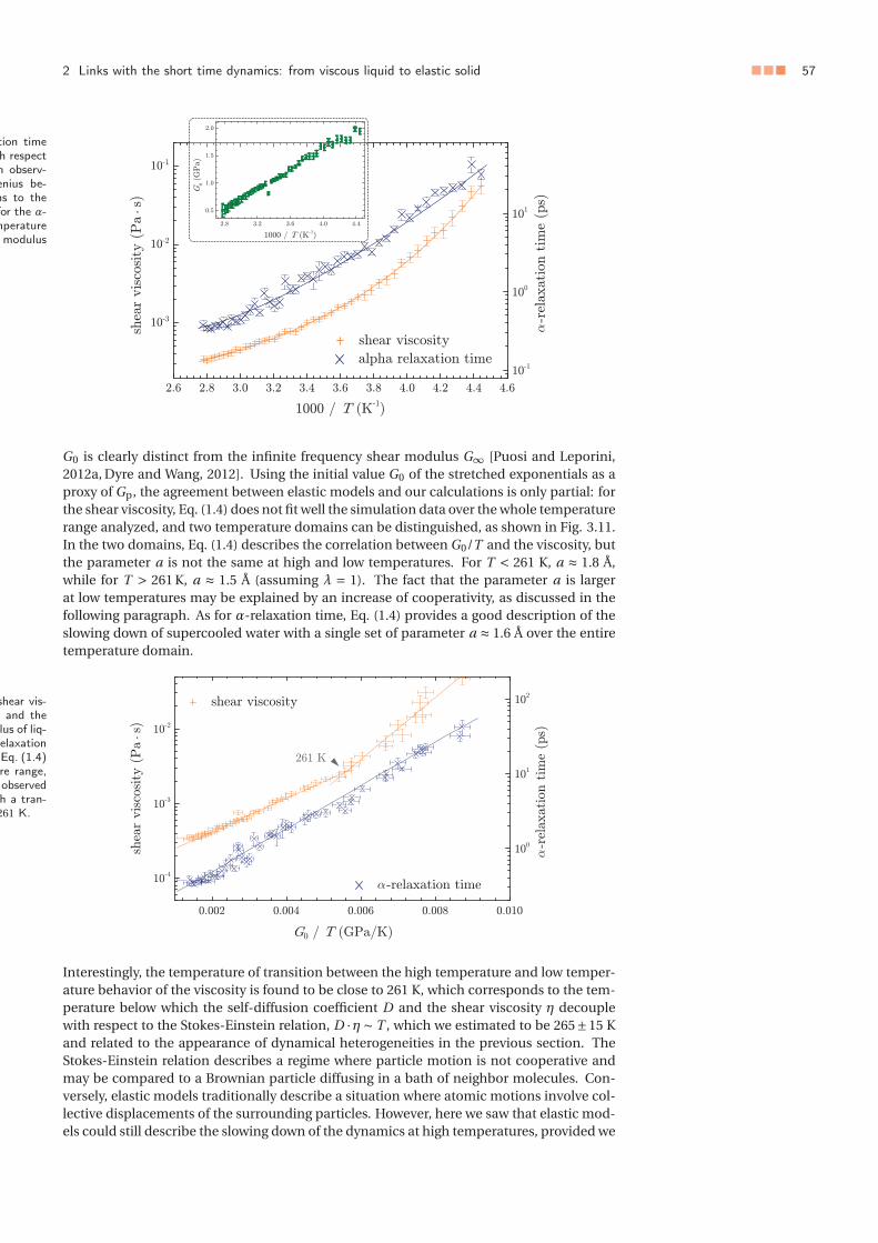
2 Links with the short time dynamics: from viscous liquid to elastic solid ■■■ 57
tion timeh respecth observ-enius be-ns to thefor the α-mperature
modulus
G0 is clearly distinct from the infinite frequency shear modulus G∞ [Puosi and Leporini,2012a, Dyre and Wang, 2012]. Using the initial value G0 of the stretched exponentials as aproxy of Gp, the agreement between elastic models and our calculations is only partial: forthe shear viscosity, Eq. (1.4) does not fit well the simulation data over the whole temperaturerange analyzed, and two temperature domains can be distinguished, as shown in Fig. 3.11.In the two domains, Eq. (1.4) describes the correlation between G0/T and the viscosity, butthe parameter a is not the same at high and low temperatures. For T < 261 K, a ≈ 1.8 Å,while for T > 261 K, a ≈ 1.5 Å (assuming λ = 1). The fact that the parameter a is largerat low temperatures may be explained by an increase of cooperativity, as discussed in thefollowing paragraph. As for α-relaxation time, Eq. (1.4) provides a good description of theslowing down of supercooled water with a single set of parameter a ≈ 1.6 Å over the entiretemperature domain.
shear vis-and the
lus of liq-elaxationEq. (1.4)re range,observedh a tran-
261 K.
Interestingly, the temperature of transition between the high temperature and low temper-ature behavior of the viscosity is found to be close to 261 K, which corresponds to the tem-perature below which the self-diffusion coefficient D and the shear viscosity η decouplewith respect to the Stokes-Einstein relation, D ·η ∼ T , which we estimated to be 265±15 Kand related to the appearance of dynamical heterogeneities in the previous section. TheStokes-Einstein relation describes a regime where particle motion is not cooperative andmay be compared to a Brownian particle diffusing in a bath of neighbor molecules. Con-versely, elastic models traditionally describe a situation where atomic motions involve col-lective displacements of the surrounding particles. However, here we saw that elastic mod-els could still describe the slowing down of the dynamics at high temperatures, provided we

58 ■■■ Chap. 3. Viscoelastic properties of pure liquid water
defined an effective length a which takes a smaller value as compared with the low temper-ature value. The fact that a is smaller at high temperatures could then be related to the lossof cooperativity. Therefore, two regimes emerge in the description of the dynamics in theframework of elastic models: a diffusive homogeneous regime at high temperature wheremolecule displacements are almost independent and the Stokes-Einstein relation is obeyed,and a low temperature regime where molecule motions are cooperative.
Figure 3.12
Correlations between the shear vis-cosity / α-relaxation time andthe vibrational mean squared dis-placement. The vibrational meansquared displacement is determinedas the value of the mean squareddisplacement of the center of massof a water molecule when the slopeis minimum (see top left inset).Similarly to the previous correla-tions with the elastic modulus, theα-relaxation time is described byEq. (3.12) over the whole tempera-ture range, while a transition is ob-served at ca. 258 K for the shearviscosity. The inset shows the corre-lation between the vibrational meansquared displacement and the highfrequency shear modulus.
2.3 Hall-Wolynes equationWe now assess the validity of the mean square displacement version of the elastic model, asdescribed in Eq. (3.12), reminded here:
X = X0 ·exp
(a2
2 · ⟨u2(T )⟩). ■ (3.12)
The quantity of interest here is the vibrational mean squared displacement, which can beaccessed through the mean square displacement ⟨r 2(t )⟩, as illustrated in the top inset ofFig. 3.12. In a dense system, molecules move ballistically at short times while they diffuseat long times: ⟨r 2(t )⟩ = 6 ·D · t where D is the diffusion coefficient. At intermediate timescales, the mean square displacement of a molecule is limited by the presence of neigh-bouring molecules. As seen in fig. 3.12, at these intermediate time scales the MSD has aminimum slope, which corresponds to the time tDW when the particle shoves its neighbors.The corresponding value of the MSD is called mean square vibrational amplitude or Debye-Waller (DW) factor [Puosi and Leporini, 2012a, Dyre and Olsen, 2004], and denoted ⟨u2⟩ inthe following.
Since the pioneering work of Buchenau and Zorn [Buchenau and Zorn, 1992], Eq. (3.12) hasbeen shown to hold in many systems [Larini et al., 2008,Puosi and Leporini, 2012b,Ciamarraand Sollich, 2015]. For supercooled water, Fig. 3.12 reports a good agreement betweenEq. (3.12) and our simulation data at low temperatures. As for the previous elastic model, wefind two different behaviors depending on the observable X . If X is the α-relaxation time,the agreement extends over the whole range of temperatures analyzed, with a molecularlength a = 1.62 Å. In the case of the shear viscosity, two regimes with different molecularlengths appear (a = 1.97 Å at low temperature and a = 1.48 Å at high temperature), with acrossover temperature close to 258 K. This crossover temperature is very close to the onedetermined in the previous approach. The equivalence between the two approaches dis-cussed is confirmed by the inset of Fig. 3.12, which demonstrates the good correlation be-tween G0/T and the MSD. The difference of behavior between the shear viscosity and theα-relaxation time is not surprising, and can be related to the decoupling between these twoobservables observed at low temperatures (see previous section and Ref. Shi et al., 2013).
3 Towards a consideration of quantum effects: ab initio approach ■■■ 59
The relevance of the vibrational MSD ⟨u2⟩ is supposed to hold while τα is lower than tDW
[Larini et al., 2008], which corresponds to a temperature much higher than the crossovertemperature T = 258 K. Actually, the activation energy associated with the two versions ofthe elastic models at this threshold temperature is close to the energy of a hydrogen bond(ca. 20 kJ/mol), which could explain the change of regime at high temperatures: the con-nectivity of water molecules is mainly due to hydrogen bonds. At high temperature, ther-mal motion breaks the hydrogen bond network, so that the local tetragonal structure isshort lived, and molecular displacements are no longer collective [Kawasaki and Kim, 2017].Again, an interesting point is that elastic models are valid when the Stokes-Einstein relationD ·η/T = Cst breaks down, i.e. below 265±15 K for the TIP4P/2005f force field (see previoussection). The breakdown of the Stokes-Einstein relation is usually associated with the riseof dynamical heterogeneities. Likewise, heterogeneous structural relaxation is connectedwith the experimental test of the Hall-Wolynes equation [Larini et al., 2008].
Before concluding, we should say a word about the role of quantum effects in the dynam-ics of supercooled water. Indeed, our simulations are fully classical and one may ask therelevance of quantum effects to describe the slow dynamics of water. These include thedescription of the nuclear degrees of motion, the hydrogen bond network but also the tem-perature dependence of the mean square displacement. We have already shown that theTIP4P/2005f potential reproduces accurately the shear viscosity of supercooled water (seeprevious section). It would be interesting to measure the elastic properties of supercooledwater at low temperatures, to see if the TIP4P/2005f potential can also describe the temper-ature dependence of the shear modulus, or the vibrational mean square displacement. Thiswould allow us to conclude whether quantum effects do play a signicant role in the slowdynamics of water, or if they play a negligible role due to compensation effects. If quantumeffects turn out to be important, demanding ab initio simulations could be unavoidable toinvestigate supercooled water dynamics [Ceriotti et al., 2016, Gillan et al., 2016, DiStasio Jret al., 2014].
2.4 SummaryWe show here that the long time dynamics of liquid water at low temperatures is highlycorrelated with its short time elastic properties, quantified by the shear modulus at highfrequency. In particular, it is surprising to see that in spite of the numerous anomalies ofwater, elastic models perform as well as for simple glass formers including metallic glassesor supercooled polymers. Moreover, for the viscosity, two different temperature regimeswith different effective molecular lengths a are observed, and the crossover temperature isclose to the one where the Stokes-Einstein relation starts to be violated. These results callfor experimental investigation of the high frequency shear modulus of supercooled waterusing e.g. inelastic X-ray scattering. Looking for correlations between the elastic modulusand the shear viscosity measured at low temperatures may also help in assessing the role ofquantum effects which are not considered in our classical approach.
3 Towards a consideration of quantum effects: ab initio
approach
3.1 Aim of the study and methodsWe reviewed in Chap. 2 some challenges of density functional theory (DFT) in the contextof aqueous systems. In this last section, the aim is to characterize the accuracy of DFT todescribe liquid water, to see in what extent this method could be used in the future to inves-tigate the role of quantum effects on the dynamics of water. We report density calculationsin the isothermal-isobaric ensemble (N pT ) of liquid water as a function of temperature forthree different functionals including or corrected with dispersion terms. We then look at dif-ferent commonly used observables to evaluate the accuracy of the different functionals: theradial distribution function, the hydrogen bond angles distribution, and the self diffusioncoefficient at room temperature. We also estimate the value of the shear viscosity, which to
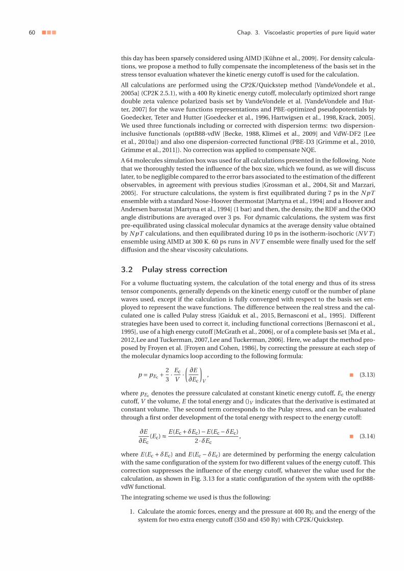
60 ■■■ Chap. 3. Viscoelastic properties of pure liquid water
this day has been sparsely considered using AIMD [Kühne et al., 2009]. For density calcula-tions, we propose a method to fully compensate the incompleteness of the basis set in thestress tensor evaluation whatever the kinetic energy cutoff is used for the calculation.
All calculations are performed using the CP2K/Quickstep method [VandeVondele et al.,2005a] (CP2K 2.5.1), with a 400 Ry kinetic energy cutoff, molecularly optimized short rangedouble zeta valence polarized basis set by VandeVondele et al. [VandeVondele and Hut-ter, 2007] for the wave functions representations and PBE-optimized pseudopotentials byGoedecker, Teter and Hutter [Goedecker et al., 1996, Hartwigsen et al., 1998, Krack, 2005].We used three functionals including or corrected with dispersion terms: two dispersion-inclusive functionals (optB88-vdW [Becke, 1988, Klimeš et al., 2009] and VdW-DF2 [Leeet al., 2010a]) and also one dispersion-corrected functional (PBE-D3 [Grimme et al., 2010,Grimme et al., 2011]). No correction was applied to compensate NQE.
A 64 molecules simulation box was used for all calculations presented in the following. Notethat we thoroughly tested the influence of the box size, which we found, as we will discusslater, to be negligible compared to the error bars associated to the estimation of the differentobservables, in agreement with previous studies [Grossman et al., 2004, Sit and Marzari,2005]. For structure calculations, the system is first equilibrated during 7 ps in the N pTensemble with a standard Nose-Hoover thermostat [Martyna et al., 1994] and a Hoover andAndersen barostat [Martyna et al., 1994] (1 bar) and then, the density, the RDF and the OOOangle distributions are averaged over 3 ps. For dynamic calculations, the system was firstpre-equilibrated using classical molecular dynamics at the average density value obtainedby N pT calculations, and then equilibrated during 10 ps in the isotherm-isochoric (NV T )ensemble using AIMD at 300 K. 60 ps runs in NV T ensemble were finally used for the selfdiffusion and the shear viscosity calculations.
3.2 Pulay stress correction
For a volume fluctuating system, the calculation of the total energy and thus of its stresstensor components, generally depends on the kinetic energy cutoff or the number of planewaves used, except if the calculation is fully converged with respect to the basis set em-ployed to represent the wave functions. The difference between the real stress and the cal-culated one is called Pulay stress [Gaiduk et al., 2015, Bernasconi et al., 1995]. Differentstrategies have been used to correct it, including functional corrections [Bernasconi et al.,1995], use of a high energy cutoff [McGrath et al., 2006], or of a complete basis set [Ma et al.,2012,Lee and Tuckerman, 2007,Lee and Tuckerman, 2006]. Here, we adapt the method pro-posed by Froyen et al. [Froyen and Cohen, 1986], by correcting the pressure at each step ofthe molecular dynamics loop according to the following formula:
p = pEc +2
3· Ec
V·(∂E
∂Ec
)V
, ■ (3.13)
where pEc denotes the pressure calculated at constant kinetic energy cutoff, Ec the energycutoff, V the volume, E the total energy and ()V indicates that the derivative is estimated atconstant volume. The second term corresponds to the Pulay stress, and can be evaluatedthrough a first order development of the total energy with respect to the energy cutoff:
∂E
∂Ec(Ec) ≈ E(Ec +δEc)−E(Ec −δEc)
2 ·δEc, ■ (3.14)
where E(Ec +δEc) and E(Ec −δEc) are determined by performing the energy calculationwith the same configuration of the system for two different values of the energy cutoff. Thiscorrection suppresses the influence of the energy cutoff, whatever the value used for thecalculation, as shown in Fig. 3.13 for a static configuration of the system with the optB88-vdW functional.
The integrating scheme we used is thus the following:
1. Calculate the atomic forces, energy and the pressure at 400 Ry, and the energy of thesystem for two extra energy cutoff (350 and 450 Ry) with CP2K/Quickstep.

3 Towards a consideration of quantum effects: ab initio approach ■■■ 61
Figure 3.13 �
Influence of the kinetic energy cut-off on the calculated pressure withand without Pulay stress correc-tion. Without correction, the abso-lute error varies between 1.2 kbarsfor the highest cutoff value allowedby CP2K (1200 Ry) and 5 kbars for200 Ry. No influence of the cut-off value is observed when the Pu-lay stress correction is applied, evenif the pressure fluctuates over an in-terval of ca. 1 kbar.
2. Calculate the corrected pressure at 400 Ry by expanding the derivative (∂E/∂Ec)V forthe three energy cutoff values.
3. Integrate the equation of motion in the N pT ensemble with the corrected pressureusing atomic forces calculated with 400 Ry energy cutoff.
4. Iterate.
This procedure is automated with a homemade software, using the standard algorithm byMartyna et al. [Martyna et al., 1994] for N pT integration.
3.3 Structural and dynamical predictions
3.3.1 Density
Compared to empirical molecular dynamics, simulation boxes and simulation times aremuch smaller in AIMD. It raises some questions about the accuracy of the approach. Wefirst discuss the influence of the simulation box size and the simulation time in the case ofdensity measurements.
The influence of the simulation box size on the density calculations is evaluated using em-pirical molecular dynamics. Calculations were performed using the LAMMPS simulationpackage [Plimpton, 1995], using the TIP4P/2005f force field [González and Abascal, 2011]for water, with the same parameters as in previous sections. Eight different box sizes wereused from 3×3×3 to 10×10×10 molecules, with periodic boundary conditions. For eachbox size, the system was equilibrated in the isotherm-isobaric ensemble during 500 ps us-ing a Nose and Hoover thermostat [Martyna et al., 1994] and a Hoover and Andersen baro-stat [Martyna et al., 1994], as in the case of AIMD calculations, then the density was averagedover 2 ns using the same thermostat/barostat. The temperature was fixed at 300 K and thepressure at 1 atm. The evolution of the equilibrium density with respect to the simulationbox size is given in Fig. 3.14.
The relative error due to finite box size effects is systematically lower than 0.4 %. Especially,in the case of a 4×4×4 = 64 molecules simulation box, which is the size considered in thepresent study, the error is about 0.3 %. This is, as we will see, completely negligible withrespect to the error bars associated to the present AIMD density calculations. Thus, finitesize effects do not affect the present density measurements.
Another striking point is the time used in the previous calculations to evaluate the den-sity. It is several orders of magnitude larger than the time used for AIMD calculations. Itraises questions about the convergence of the AIMD calculations. As explained previously,for each temperature, the system was equilibrated first during 7 ps. Then, the density was
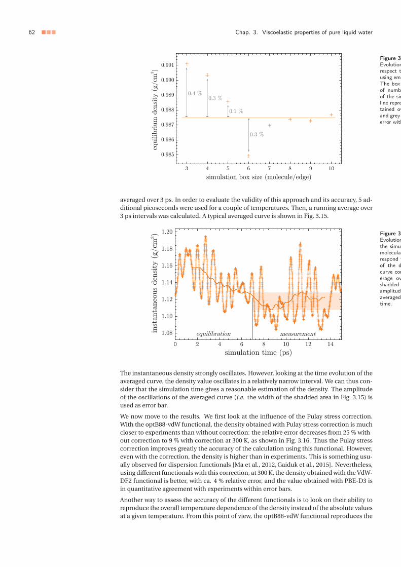
62 ■■■ Chap. 3. Viscoelastic properties of pure liquid water
Figure 3
Evolutionrespect tusing empThe boxof numbof the simline repretained ovand greyerror with
averaged over 3 ps. In order to evaluate the validity of this approach and its accuracy, 5 ad-ditional picoseconds were used for a couple of temperatures. Then, a running average over3 ps intervals was calculated. A typical averaged curve is shown in Fig. 3.15.
Figure 3
Evolutionthe simumolecularrespond tof the dcurve corerage ovshaddedamplitudeaveragedtime.
The instantaneous density strongly oscillates. However, looking at the time evolution of theaveraged curve, the density value oscillates in a relatively narrow interval. We can thus con-sider that the simulation time gives a reasonable estimation of the density. The amplitudeof the oscillations of the averaged curve (i.e. the width of the shadded area in Fig. 3.15) isused as error bar.
We now move to the results. We first look at the influence of the Pulay stress correction.With the optB88-vdW functional, the density obtained with Pulay stress correction is muchcloser to experiments than without correction: the relative error decreases from 25 % with-out correction to 9 % with correction at 300 K, as shown in Fig. 3.16. Thus the Pulay stresscorrection improves greatly the accuracy of the calculation using this functional. However,even with the correction, the density is higher than in experiments. This is something usu-ally observed for dispersion functionals [Ma et al., 2012, Gaiduk et al., 2015]. Nevertheless,using different functionals with this correction, at 300 K, the density obtained with the VdW-DF2 functional is better, with ca. 4 % relative error, and the value obtained with PBE-D3 isin quantitative agreement with experiments within error bars.
Another way to assess the accuracy of the different functionals is to look on their ability toreproduce the overall temperature dependence of the density instead of the absolute valuesat a given temperature. From this point of view, the optB88-vdW functional reproduces the
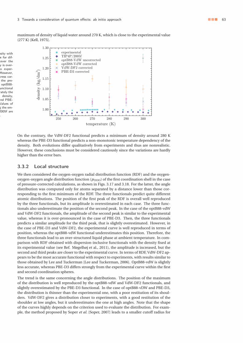
3 Towards a consideration of quantum effects: ab initio approach ■■■ 63
maximum of density of liquid water around 270 K, which is close to the experimental value(277 K) [Kell, 1975].
nsity withe for dif-tever they is over-to exper-However,tress cor-the pre-optB88-
unctionalrately the
m density,nd PBE-
Values ofg the em-2005f are.
On the contrary, the VdW-DF2 functional predicts a minimum of density around 280 Kwhereas the PBE-D3 functional predicts a non-monotonic temperature dependency of thedensity. Both evolutions differ qualitatively from experiments and thus are nonrealistic.However, these conclusions must be considered cautiously since the variations are hardlyhigher than the error bars.
3.3.2 Local structure
We then considered the oxygen-oxygen radial distribution function (RDF) and the oxygen-oxygen-oxygen angle distribution function (pOOO) of the first coordination shell in the caseof pressure-corrected calculations, as shown in Figs. 3.17 and 3.18. For the latter, the angledistribution was computed only for atoms separated by a distance lower than those cor-responding to the first minimum of the RDF. The three functionals predict quite differentatomic distributions. The position of the first peak of the RDF is overall well reproducedby the three functionals, but its amplitude is overestimated in each case. The three func-tionals also underestimate the position of the second peak. In the case of the optB88-vdWand VdW-DF2 functionals, the amplitude of the second peak is similar to the experimentalvalue, whereas it is over-pronounced in the case of PBE-D3. Then, the three functionalspredicts a similar amplitude for the third peak, that is slightly overestimated. However, inthe case of PBE-D3 and VdW-DF2, the experimental curve is well reproduced in terms ofposition, whereas the optB88-vdW functional underestimates this position. Therefore, thethree functionals lead to an over-structured liquid phase at ambient temperature. In com-parison with RDF obtained with dispersion-inclusive functionals with the density fixed atits experimental value (see Ref. Møgelhøj et al., 2011), the amplitude is increased, but thesecond and third peaks are closer to the experimental curve. In terms of RDF, VdW-DF2 ap-pears to be the most accurate functional with respect to experiments, with results similar tothose obtained by Lee and Tuckerman [Lee and Tuckerman, 2006]. OptB88-vdW is slightlyless accurate, whereas PBE-D3 differs strongly from the experimental curve within the firstand second coordination spheres.
The trend is the same concerning the angle distributions. The position of the maximumof the distribution is well reproduced by the optB88-vdW and VdW-DF2 functionals, andslightly overestimated by the PBE-D3 functional. In the case of optB88-vDW and PBE-D3,the distribution is thinner than the experimental one, with a poor restitution of its shoul-ders. VdW-DF2 gives a distribution closer to experiments, with a good restitution of theshoulder at low angles, but it underestimates the one at high angles. Note that the shapeof the curves highly depends on the criterion used to evaluate the distribution. For exam-ple, the method proposed by Soper et al. [Soper, 2007] leads to a smaller cutoff radius for

64 ■■■ Chap. 3. Viscoelastic properties of pure liquid water
Figure 3.17 �
Comparison of the experimentaloxygen-oxygen radial distributionfunction at 300 K [Soper, 2007]with the prediction of differentfunctionals. All functionals over-structurate the liquid, with a muchhigher first peak than experiments.The second peak is shifted up, butthe amplitude is similar to the ex-perimental curve.
O-O pairs selection, and the distribution obtained are much thinner, without any shoulder,whatever the functional is used.
The width of the distribution obtained with optB88-vdW and PBE-D3 is similar to thoseobtained working at the experimental density with various functionals including function-als without any correction of dispersion contributions and hybrid functionals [DiStasio Jret al., 2014], whereas VdW-DF2 leads to a much better agreement with the experimentalcurve. Moreover, the present distributions, obtained working at the equilibrium densitypredicted by the functional reproduce quite accurately the position of the maximum of thedistribution, whereas it is systematically largely shifted when the experimental density isused, even using hybrid functionals [DiStasio Jr et al., 2014]. According to Jonchiere etal. [Jonchiere et al., 2011], some dynamical properties such as the self diffusion of watermolecules is strongly dependent on interactions over several molecular sizes. One can thusexpect that the overall good restitution of the local structure of water observed through theRDF and the angle distribution, especially in the case of the VdW-DF2 functional, will leadsto accurate values of the self diffusion coefficient and the shear viscosity.
Figure 3.18 �
Comparison of the OOO angle dis-tributions in the first coordina-tion shell at 300 K for differentfunctionals and experiments [Soperand Benmore, 2008]. The func-tion pOOO (θ) · sin(θ) is normalizedto unit area over the [0°;180°]range. All functionals show anover-structuration of the liquid witha poor restitution of the shoulderat high angles observed experimen-tally. The shoulder around 60° isalso poorly reproduced by optB88-vDW and PBE-D3, but well repro-duced by VdW-DF2. Moreover, theposition of the maximum of the dis-tribution is overall well reproduced.
3.3.3 Hydrodynamics
In order to characterize the dynamical response of the models mentioned above, we calcu-lated the self diffusion coefficient and the shear viscosity of water. The diffusion coefficientwas computed from the slope of the mean squared displacement of the center of mass
⟨α2
⟩
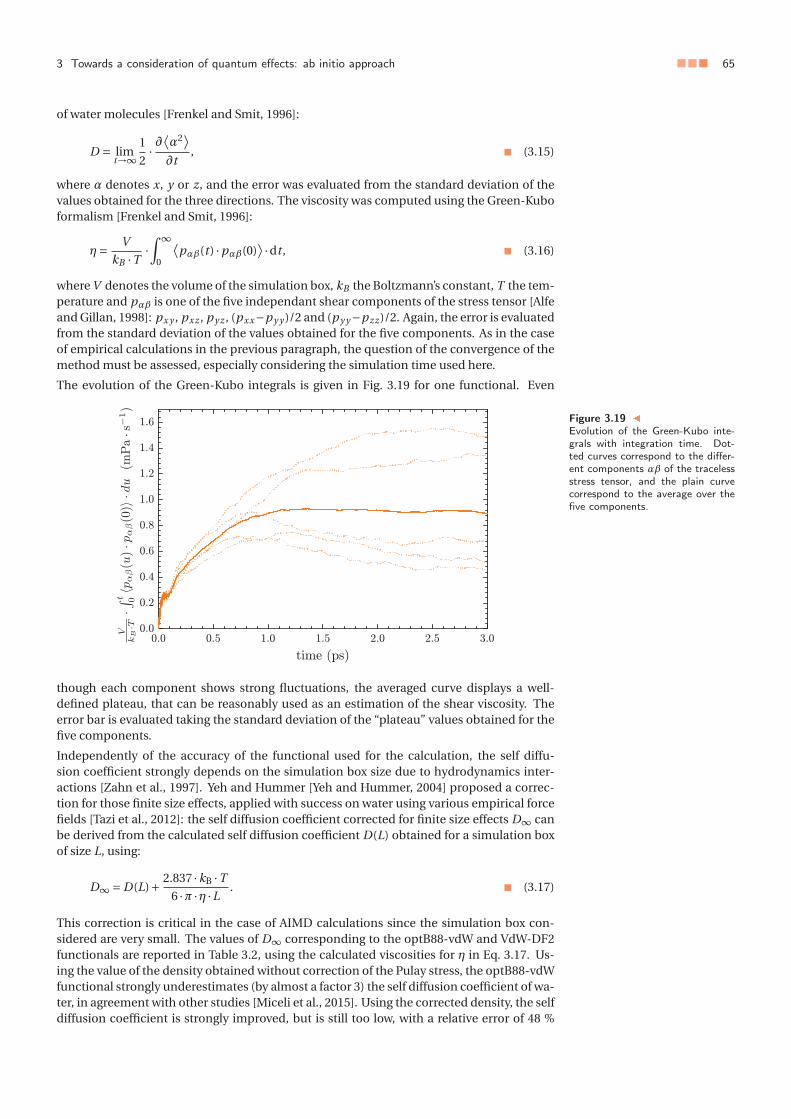
3 Towards a consideration of quantum effects: ab initio approach ■■■ 65
of water molecules [Frenkel and Smit, 1996]:
D = limt→∞
1
2· ∂
⟨α2
⟩∂t
, ■ (3.15)
where α denotes x, y or z, and the error was evaluated from the standard deviation of thevalues obtained for the three directions. The viscosity was computed using the Green-Kuboformalism [Frenkel and Smit, 1996]:
η= V
kB ·T·∫∞
0
⟨pαβ(t ) ·pαβ(0)
⟩ ·dt , ■ (3.16)
where V denotes the volume of the simulation box, kB the Boltzmann’s constant, T the tem-perature and pαβ is one of the five independant shear components of the stress tensor [Alfeand Gillan, 1998]: px y , pxz , py z , (pxx−py y )/2 and (py y−pzz )/2. Again, the error is evaluatedfrom the standard deviation of the values obtained for the five components. As in the caseof empirical calculations in the previous paragraph, the question of the convergence of themethod must be assessed, especially considering the simulation time used here.
The evolution of the Green-Kubo integrals is given in Fig. 3.19 for one functional. Even
Figure 3.19 �
Evolution of the Green-Kubo inte-grals with integration time. Dot-ted curves correspond to the differ-ent components αβ of the tracelessstress tensor, and the plain curvecorrespond to the average over thefive components.
though each component shows strong fluctuations, the averaged curve displays a well-defined plateau, that can be reasonably used as an estimation of the shear viscosity. Theerror bar is evaluated taking the standard deviation of the “plateau” values obtained for thefive components.
Independently of the accuracy of the functional used for the calculation, the self diffu-sion coefficient strongly depends on the simulation box size due to hydrodynamics inter-actions [Zahn et al., 1997]. Yeh and Hummer [Yeh and Hummer, 2004] proposed a correc-tion for those finite size effects, applied with success on water using various empirical forcefields [Tazi et al., 2012]: the self diffusion coefficient corrected for finite size effects D∞ canbe derived from the calculated self diffusion coefficient D(L) obtained for a simulation boxof size L, using:
D∞ = D(L)+ 2.837 ·kB ·T
6 ·π ·η ·L. ■ (3.17)
This correction is critical in the case of AIMD calculations since the simulation box con-sidered are very small. The values of D∞ corresponding to the optB88-vdW and VdW-DF2functionals are reported in Table 3.2, using the calculated viscosities for η in Eq. 3.17. Us-ing the value of the density obtained without correction of the Pulay stress, the optB88-vdWfunctional strongly underestimates (by almost a factor 3) the self diffusion coefficient of wa-ter, in agreement with other studies [Miceli et al., 2015]. Using the corrected density, the selfdiffusion coefficient is strongly improved, but is still too low, with a relative error of 48 %

66 ■■■ Chap. 3. Viscoelastic properties of pure liquid water
with respect to the tabulated value. The value obtained with PBE-D3 is much worse, whichis surprising since this functional is the most accurate in terms of room temperature density.In contrast, the value obtained using the VdW-DF2 functional is in quantitative agreementwith the tabulated value within the error bars, as in the case of the TIP4P/2005f force field,even if the error bar is much larger in the case of DFT.
Functional D (10−9 m · s−2) D∞ (10−9 m · s−2) η (mPa · s)optB88-vdW (uncorr.) 0.64±0.10 1.06±0.24 1.20±0.20optB88-vdW (corr.) 0.84±0.04 1.31±0.23 1.10±0.19VdW-DF2 (corr.) 1.43±0.20 1.99±0.38 0.91±0.12PBE-D3 (corr.) 0.27±0.06 0.29±0.10 3.6±1.1TIP4P/2005f – 2.30±0.01 0.76±0.05experimental – 2.3 0.896
Table 3.2
Comparisthe self dshear visfor differeiments [Tcalculatedcoefficiensimulatiocated in tlated valusimulatiothe calcuence, follin Ref. Ttext). VTIP4P/2given forsection).
As we already mentioned, the self diffusion coefficient was shown to be strongly influencedby long range interactions within the liquid [Jonchiere et al., 2011]. This includes disper-sion interactions, which decrease slowly with the distance. The VdW-DF2 reproduces moreaccurately the overall shape of the water RDF and angles distribution than the optB88-vdWand PBE-D3 functionals, and especially the position and the amplitude of the third peakof the RDF. This is consistent with the present observation that the VdW-DF2 reproducesmuch better the self-diffusion of water than the optB88-vdW functional.
A similar trend is observed concerning the shear viscosity. For this observable, as men-tionned in the first section of this chapter, no finite box size effect is expected. The optB88-vdW overestimates the shear viscosity of water when no correction is taken into accountfor the Pulay stress, with a relative error of 34 %, as shown in Table 3.2, whereas the erroris reduced to 23 % with the correction. Again, PBE-D3 leads to a value that is very far fromexperiments. In contrast, the VdW-DF2 functional is in agreement with the experimentalvalue, and gives a slightly better value than the TIP4P/2005f force field. The shear viscosityof water is mainly due to hydrogen bonding. So, it seems that using the density predictedby the functional improves the hydrogen bond structure and dynamics. The shear viscosityhas only be scarcely considered using AIMD. The only value for bulk water to our knowledge,obtained without taking into account dispersion effects, is much higher than the differentvalues obtained here [Kühne et al., 2009]. Thus, when used at their equilibrium density, thetwo dispersion functionals used here enable an accurate estimation of the shear viscosity.
3.3.4 Summary
We showed that accurate N pT -AIMD calculations are now feasible using moderate cut-off values. Correction for Pulay stress strongly improves the predictions of the calculationswith respect to standard N pT calculations. The VdW-DF2 functional reproduces almostquantitatively various observables such as the room temperature density, the RDF, the self-diffusion coefficient, and the shear-viscosity. However, it gives a wrong temperature depen-dence of the liquid density (although the variations of density are not large as compared touncertainties). Concerning this last point, the optB88-vdW functional gives better results,predicting a maximum of density close to its tabulated temperature, but the predictions forthe other observables considered here are less accurate. This opens new insight for com-plex aqueous system studies, where the density of water cannot be a priori figured out, andshould help to understand the role of quantum effects in the dynamics of liquid water.
4 Conclusion
In this chapter, we saw that the TIP4P/2005f force field describes accurately the long-timedynamics of water, and offers an interesting connection with short-time elastic propertiesof the liquid at low temperatures using the so-called elastic models. Ab initio approachesin the isothermal-isobaric ensemble, using the correction of the pressure introduced, alsopredicts accurately some properties of water, especially using the VdW-DF2 functional, and

4 Conclusion ■■■ 67
should be used with benefits in the future to investigate the role of quantum effects in thedynamics of water. However, regarding the numerical cost of the approach, and its limitedaccuracy with respect to classical molecular dynamics using the TIP4P/2005f force field,the latter approach will be preferred to the former in the next chapters, dedicated to waterbased complex systems.

68 ■■■ Chap. 3. Viscoelastic properties of pure liquid water

2 Simulations details ■■■ 69
Figure 4.1
Liquid-solid friction. Friction can becharacterized by the friction coeffi-cient λ = σ/vslip or the slip lengthb = η/λ, where η denotes the shearviscosity of the liquid.
■■■ Chapter 4
Water hydrodynamics near ahydrophobic surface
Outline
1 Aim of the study . . . . . . . . . . . . . . . . . . . . . . . . . . . . . . 672 Simulations details . . . . . . . . . . . . . . . . . . . . . . . . . . . . . 673 Temperature dependence of the friction coefficient and the slip
length . . . . . . . . . . . . . . . . . . . . . . . . . . . . . . . . . . . . 684 Origin of the friction temperature dependence . . . . . . . . . . . . 71
4.1 Structure of the liquid near the interface . . . . . . . . . . . 714.2 Corrugation of the solid surface . . . . . . . . . . . . . . . . 734.3 Liquid and interface relaxation . . . . . . . . . . . . . . . . . 73
5 Summary and conclusion . . . . . . . . . . . . . . . . . . . . . . . . . 75
1 Aim of the study
We characterized in the previous chapter the dynamics of bulk water. In various media,including clays, water is surrounded by solid surfaces. We pointed out in Chap. 1 the partic-ular properties of liquids near an interface, as for example friction/slippage, with its appli-cation to enhance the permeability of nano-channels. Fluid-solid friction is well known tobe highly dependent of the temperature in the tribology community, especially in the caseof complex fluids like polymers [Drda and Wang, 1995, Yoshizawa and Israelachvili, 1993].Moreover, as we saw in Chap. 1 and 3, water exhibits many anomalous properties at lowtemperatures. However, most of the current knowledge about interfacial water concernsproperties at room temperature. The aim of this chapter is – using classical molecular dy-namics simulations – to investigate the low temperature hydrodynamic properties of waterin the vicinity of a prototypical hydrophobic solid surface. We will first introduce the sys-tem used for the study, and then analyze the temperature dependence of both interfacialfriction coefficient and slip length (see Fig. 4.1).
2 Simulations details
All simulations were performed using the LAMMPS package. The simulations boxes are thesame as those used in the previous chapter for steady-state shear calculations, except theyare here used for both equilibrium (using the Green-Kubo formalism) and nonequilibrium(steady-state shear) calculations. The solid surface is a generic apolar surface, made of a setof atoms localized on the nodes of a face cubic centered (fcc) lattice, with lattice parameter

70 ■■■ Chap. 4. Water hydrodynamics near a hydrophobic surface
Figure 4.2
Partial screenshot of the simulationbox. A fcc unit cell is highlighted.
a = 5.34954 Å (see Fig. 4.2). The thickness of the solid is 5 atomic layers, i.e. about 10.7 Å, thatis higher than the cutoff radius value used to compute Lennard-Jones interactions (there isno Coulombic term since atoms are neutral), so the liquid sees a semi-infinite solid surface.
The walls are rigid, and interact with oxygen atoms through a Lennard-Jones potentialwith εC = 0.164 kcal ·mol−1 and σC = 3.37 Å. The thickness of the water layer is about 50 Å.Thus, since confinement water recovers its structure above 10 Åfrom the surface, no effectof confinement is expected here [Raviv et al., 2001, Li et al., 2007, Zhu et al., 2012, Zhanget al., 2013, Markesteijn et al., 2012]. The temperature is scanned from 225 to 360 K. Inthe case of steady-state shear calculations, for each wall velocity, the simulation was runduring 1 ns to reach the steady-state, and then measurements were performed during 1 ns.For Green-Kubo calculations, the system was first equilibrated during 0.5 ns and then, threemeasurements of 1 ns were performed. In each case, a Nose-Hoover thermostat was appliedto liquid atoms in the direction normal to the walls during the simulation. The pressurewas fixed by applying a force normal to the wall on the solid surfaces during the wholesimulation.
The shear-viscosity of the fluid, the friction coefficient and the slip length were computedusing both equilibrium Green-Kubo formalism and nonequilibrium steady-state shear flowmethods described in Chap. 2.
3 Temperature dependence of the friction coefficient
and the slip length
As in the case of shear viscosity calculations, one must check the validity and consistency ofboth Green-Kubo and steady-state shear flow approaches. The typical time evolution of theGreen-Kubo integral for the friction coefficient is shown in Fig. 4.3. Contrary to the Green-Kubo integral for the shear viscosity, the curve displays no plateau. The integral increasesto a maximum value and then decreases, due to the finite thickness of the water layer [Jolyet al., 2016]. We took the maximum value as the value of the friction coefficient, as it wasdone elsewhere [Joly et al., 2016]. This integral was evaluated in the two directions tan-gential to the walls, for each wall. It means 4 values of λ were obtained from each of the 3replicas used. The values reported in the following for each temperature are averaged overthose 12 values, and the error is computed as their statistical standard error.
Figure 4.3
Typical shape of the Green-Kubo in-tegral vs time curve (here at 240 K).
For steady-state shear flow calculations, we checked – using five different shear rates – thatthe friction coefficient did not depend on the shear rate. This was indeed the case, as shownon Fig. 4.4, except at high temperatures, at which friction values looked more dispersed.Consequently, for the highest temperatures, the friction coefficient was averaged only over

3 Temperature dependence of the friction coefficient and the slip length ■■■ 71
the two smallest shear rates, whereas it was averaged over the five shear rates for other tem-peratures. Again, the statistical standard error is used to estimate error bars.
Figure 4.4 �
Shear stress dependence of the fric-tion coefficient for various temper-atures. Dotted lines show averagevalues.
The temperature dependence of the water-wall friction coefficient is reported in Fig. 4.5 forGreen-Kubo and steady-state shear flow measurements. Both methods are in good agree-
Figure 4.5 �
Evolution of the water-wall fric-tion coefficient with respect to thetemperature for Green-Kubo (+)and steady-state shear flow (×)calculations.
ment for temperatures higher than 300 K and predict a slight decrease of the friction co-efficient when the temperature increases (the slight difference at high temperatures is dueto a misevaluation of the friction coefficient using the Green-Kubo method, since the limitof linear response regime is reached, as discussed previously). However, at lower tempera-tures, the two sets of measurements differ qualitatively: Green-Kubo calculations predict anincrease of the friction coefficient at low temperatures, in the continuation of high tempera-ture measurements, whereas steady-state shear flow calculations predict a non-monotonicevolution of the friction coefficient, with a slight decrease at low temperatures.
We also calculated the evolution of the slip length b = η/λ with the temperature using theshear viscosity measurements presented in Chap. 3 (see Fig. 4.6). Both methods predict anincrease of the slip length at low temperatures, but as in the case of the friction coefficient,the two sets of measurements differ below 300 K, with a faster increase in the case of steady-state shear flow measurements.
There are two interesting points. First, whatever the method used, the slip length, defined asthe ratio η/λ, increases at low temperatures. It means that, even for the Green-Kubo calcu-lations which predicts an increase of the friction coefficient at low temperatures, the shear

72 ■■■ Chap. 4. Water hydrodynamics near a hydrophobic surface
Figure 4.6
Evolution of the water-wall sliplength with respect to the tem-perature for Green-Kubo (+)and steady-state shear flow (×)calculations.
viscosity increases faster than the friction coefficient. Secondly, considering steady-stateshear flow calculations, we see that the slip length reaches high values in the supercooledregime. Especially, for moderately supercooled water, the slip length is found to be of thesame order of magnitude that in the case of water/graphene friction at room temperature(between 30 and 80 nm depending on the authors [Kotsalis, 2008,Thomas and McGaughey,2008, Falk et al., 2010]), and it reaches 1 μm before the nucleation limit. Generally speaking,superlubricity implies complex liquids or superhydrophobic surfaces. This is not the casehere, since we consider a simple liquid on a simple hydrophobic surface.
Such slip lengths may open new perspectives in the development of nanofluidic devices in alow temperature environment. Indeed, as explained in Chap. 1, slippage increases the waterflux through a nanochannel of width L by a factor 1+C ·b/L, where C is a constant close to1. Consequently, working at low temperatures would enable to considerably increase thehydrodynamic permeability of nanochannels.
However, since our two sets of measurements are in disagreement, we first need to solvethis discrepancy. Especially, we must determine if the difference means one of the two ap-proaches is not valid, or if it corresponds to two different regimes of friction (since one is atequilibrium and the other is not). This is the aim of the reminder of this chapter.
To check the role of the surface in this effect, we performed extra calculations (using Green-Kubo and steady-state shear flow methods) at 255 K replacing the model hydrophobic sur-face by two graphene sheets. The corresponding values of the friction coefficient and theslip length are given in Table 4.1. As in the case of the model hydrophobic surface, the val-
Table 4.1
Water-graphene friction coefficientλ and slip length b.
Green-Kubo Shear flowλ (Pa · s ·m−1) (41.7±2.6) ·103 (14.4±0.7) ·103
b (nm) 99±16 294±52
ues of the slip length predicted by steady-state shear flow calculations are much higher thanthose predicted by Green-Kubo calculations. Moreover, the value of the slip length is muchhigher than on the model surface, consistently with room temperature measurements.
The existence of two friction coefficients is a well-known property of solid-solid friction:the interface can sustain a higher tangential force when the solids are not sliding one overthe other than when they are sliding. This leads to the so called “stick-slip” motion whenone solid is dragged over the other with a fluctuating moderate force, that disappears abovesome critical force – one then gets a “smooth sliding” regime. Here, Green-Kubo calcula-tions would correspond to no effective sliding since the system is at equilibrium, whereassteady-state shear flow calculations would correspond to high velocity sliding. One canwonder thus to what extend a parallel can be made between the two friction coefficientsobserved here at low temperature and those traditionally observed in the case of solid-solidfriction. Actually, various cases of transitions between different friction regimes have been
4 Origin of the friction temperature dependence ■■■ 73
reported for fluid-solid friction. For example, for polymer melts, a transition from a “weak”slip regime – corresponding to desorption of molecules from the solid surface or partialdisentanglement of polymer molecules between adsorbed molecules and other molecules– to a “strong” slip regime – corresponding to complete disentanglement of molecules athigher flow velocities – can be observed [Drda and Wang, 1995, Hatzikiriakos, 2015]. An-other interesting example is molecularly thin films of a simple fluid. Stick-slip oscillationswith a transition to a “smooth” slip regime above a critical temperature or a critical slip ve-locity have been reported and studied extensively [Israelachvili et al., 1990, Yoshizawa andIsraelachvili, 1993, Gee et al., 1990]. In that case, the transition from a regime to another isexplained by transitions from a highly ordered “solid-like” liquid that tends to stick the twosolid surfaces together and a disordered “liquid-like” film that flows easily. At sufficientlyhigh temperature or slip velocity, the ordered phase cannot nucleate anymore and one getsa “smooth” slip regime [Yoshizawa and Israelachvili, 1993]. In the present case, similaritieswith those two examples can be found. On the one hand, since supercooled water is an as-sociated liquid, i.e. is highly reticulated by hydrogen bonds, it can behave to some extendlike a polymer melt. On the other hand, a strong organization of molecules can occur nearthe crystal surface at low temperatures and can modify the sliding dynamics. In the nextsection, we will analyze the evolution of the structure of water near the walls with the tem-perature and its relaxation dynamics to try to understand to what extent those hypothesescan apply to water.
4 Origin of the friction temperature dependence
From the equilibrium Green-Kubo formula for liquid-solid friction [Bocquet and Barrat,1994] (see Chap. 2),
λ= 1
A ·kB ·T·∫∞
0dt ·
⟨F ∥α
w (0) ·F ∥αw (t )
⟩, ■ (4.1)
where A denotes the surface of the wall and F ∥αw the total force applied to the wall in the
direction α tangential to the wall, one can decompose the friction coefficient as [Falk et al.,2010, Barrat et al., 1999]:
λ≈ τF
kB ·T·ρ1 · f 2
q∥ ·S(q∥), ■ (4.2)
where τF is the decorrelation time of the tangential force acting between the wall and water,ρ1 is the surface density of water near the interface, fq∥ is the roughness of the landscapecreated by the wall at a distance corresponding to the position of the first layer of watermolecules, and S(q∥) is the 2-dimensional structure factor of water for the wavenumbercorresponding to the transverse periodicity of the wall. Thus, this formula tells us that theinterfacial friction depends on:
• solid and liquid structures near the interface;
• the amount of water at the interface;
• the temperature;
• the relaxation time of water-wall interactions.
So, the friction is inversely proportional to the temperature and should consequently in-creases at low temperature, as it is observed for Green-Kubo calculations. Even if this for-mula is only valid for Green-Kubo calculations, it is interesting to analyze the different pa-rameters that influences friction involved in this formula.
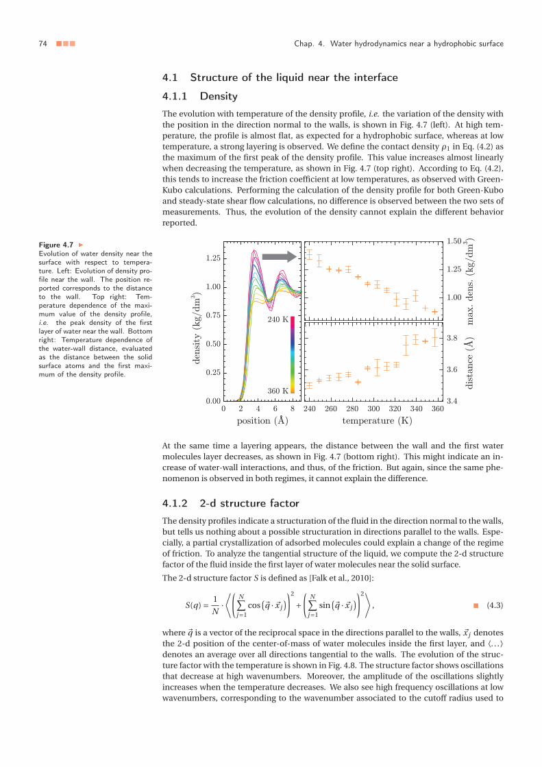
74 ■■■ Chap. 4. Water hydrodynamics near a hydrophobic surface
4.1 Structure of the liquid near the interface
4.1.1 DensityThe evolution with temperature of the density profile, i.e. the variation of the density withthe position in the direction normal to the walls, is shown in Fig. 4.7 (left). At high tem-perature, the profile is almost flat, as expected for a hydrophobic surface, whereas at lowtemperature, a strong layering is observed. We define the contact density ρ1 in Eq. (4.2) asthe maximum of the first peak of the density profile. This value increases almost linearlywhen decreasing the temperature, as shown in Fig. 4.7 (top right). According to Eq. (4.2),this tends to increase the friction coefficient at low temperatures, as observed with Green-Kubo calculations. Performing the calculation of the density profile for both Green-Kuboand steady-state shear flow calculations, no difference is observed between the two sets ofmeasurements. Thus, the evolution of the density cannot explain the different behaviorreported.
Figure 4.7 �
Evolution of water density near thesurface with respect to tempera-ture. Left: Evolution of density pro-file near the wall. The position re-ported corresponds to the distanceto the wall. Top right: Tem-perature dependence of the maxi-mum value of the density profile,i.e. the peak density of the firstlayer of water near the wall. Bottomright: Temperature dependence ofthe water-wall distance, evaluatedas the distance between the solidsurface atoms and the first maxi-mum of the density profile.
At the same time a layering appears, the distance between the wall and the first watermolecules layer decreases, as shown in Fig. 4.7 (bottom right). This might indicate an in-crease of water-wall interactions, and thus, of the friction. But again, since the same phe-nomenon is observed in both regimes, it cannot explain the difference.
4.1.2 2-d structure factorThe density profiles indicate a structuration of the fluid in the direction normal to the walls,but tells us nothing about a possible structuration in directions parallel to the walls. Espe-cially, a partial crystallization of adsorbed molecules could explain a change of the regimeof friction. To analyze the tangential structure of the liquid, we compute the 2-d structurefactor of the fluid inside the first layer of water molecules near the solid surface.
The 2-d structure factor S is defined as [Falk et al., 2010]:
S(q) = 1
N·⟨(
N∑j=1
cos(�q · �x j
))2
+(
N∑j=1
sin(�q · �x j
))2⟩, ■ (4.3)
where �q is a vector of the reciprocal space in the directions parallel to the walls, �x j denotesthe 2-d position of the center-of-mass of water molecules inside the first layer, and ⟨. . .⟩denotes an average over all directions tangential to the walls. The evolution of the struc-ture factor with the temperature is shown in Fig. 4.8. The structure factor shows oscillationsthat decrease at high wavenumbers. Moreover, the amplitude of the oscillations slightlyincreases when the temperature decreases. We also see high frequency oscillations at lowwavenumbers, corresponding to the wavenumber associated to the cutoff radius used to

4 Origin of the friction temperature dependence ■■■ 75
compute Lennard-Jones interactions, and which are consequently a purely numerical arti-fact.
Figure 4.8 �
Evolution of the 2-d structure fac-tor of water near the interface withrespect to the temperature in direc-tions parallel to the walls. Inset:Temperature dependence of the 2-dstructure factor for the wavevectorcorresponding to the periodicity ofthe lattice in the reciprocal space.
Since we are interested in the liquid structure commensurable to that of the wall (whichwill control friction), the structure factor is evaluated at q∥ = 2 ·π/a ≈ 1.17 Å−1 with a thelattice parameter of the wall (see inset in Fig. 4.8). Unfortunately, this wavevector corre-sponds to the part of the curve that is perturbated by the cutoff radius. However, since q∥corresponds to a minimum of the oscillations, the effect should be limited. The amplitudeof the structure factor at q∥ only slightly decreases at low temperatures, which contributesto a decrease of the friction coefficient according to Eq. (4.2). However, the decrease is verysmall, showing a negligible effect of temperature on the transverse structuration of the fluid.Moreover, as in the case of the density, the evolution is exactly the same for Green-Kubo andsteady-state shear flow measurements.
4.2 Corrugation of the solid surfaceWe mentioned previously that the distance between the first layer of water molecules andthe wall decreases at low temperatures. That might affect the friction coefficient. In thisparagraph, we compute the interfacial free energy to analyze the potential energy landscapecreated by the wall. The interfacial free energy is defined as:
F (x, y) =− 1
Δz·∫zwall+Δz
zwall
dz ·kB ·T · ln(pO(x, y, z)
), ■ (4.4)
where x and y denote the coordinates in the direction tangential to the wall, z the coor-dinate in the direction normal to the wall, pO is the oxygen atoms probability distributionfunction (pdf), and the integral is evaluated over the first water layers, by taking Δz = 10 Å.For each temperature, the oxygen atoms pdf is averaged over 200 ps. The typical evolutionof the free energy with the position over a quarter of unit cell of the wall is shown in Fig. 4.9(right). Then, the corrugation of this free energy landscape is computed as the differencebetween the minimum and maximum value, and reported in Fig. 4.9 (left). For more clarity,the energy corrugation is expressed in temperature unit.
The corrugation has a non-monotonous behavior, with a minimum around 300 K, show-ing a competition between (i) the decrease of the liquid-wall distance at low temperaturesand (ii) the flattering of the surface density profile at high temperatures. It means that thesurface is rougher at low and high temperatures than at intermediate temperatures, whichdisagrees with both Green-Kubo and steady-state shear flow calculations of the friction co-efficient. Indeed, both methods predict a decrease of the friction coefficient at high tem-peratures, that should indicate a smoother surface. However, whatever the temperature isconsidered, the corrugation is extremely low compared to the thermal energy of the system.Consequently, the surface appears very smooth in the range of temperatures considered in

76 ■■■ Chap. 4. Water hydrodynamics near a hydrophobic surface
Figure 4.9
Left: Evolution of the corrugationof the energy landscape created bythe wall with respect to the temper-ature. Right: Typical shape of theenergy landscape (here at 240 K).
the present study. Thus, the surface roughness does not explain the temperature depen-dence of the friction coefficient.
4.3 Liquid and interface relaxationWe finally probe directly the dynamics of the interface through the water-wall tangentialforce decorrelation time τF, defined as the plateau value of the time-integral:
τF =∫∞
0dt ·
⟨δF ∥α
w (0) ·δF ∥αw (t )
⟩⟨
F ∥αw (0) ·F ∥α
w (0)⟩ , ■ (4.5)
with δF ∥αw (t ) = F ∥α
w (t )−⟨
F ∥αw
⟩. The evolution of τF with the temperature for both Green-
Kubo and steady-state shear flow calculations is reported in Fig. 4.10.
Figure 4.10
Evolution of the friction force relax-ation time for both Green-Kubo (+)and steady-state shear flow (×) cal-culations. The curve correspondingto the α-relaxation time of bulk wa-ter (see Chap. 3) is also plotted forcomparison.
In both cases, τF increases at low temperature: for Green-Kubo calculations, it is approxi-matively multiplied by 10 with respect to the highest temperature considered here, whereasthe increase is lower in the case of steady-state shear flow calculations. However, in the caseof steady-state shear flow calculations, the decorrelation time is more than one order of

5 Summary and conclusion ■■■ 77
magnitude higher than in the case of Green-Kubo calculations, which, regarding Eq. (4.2),does not explain the lower values of the friction coefficient measured under steady-stateshear flow.
We compare then this interfacial relaxation time to a liquid relaxation time, the α-relaxationtime, assuming its value in the vicinity of the wall is close to its bulk value. In the caseof Green-Kubo calculations, τF is much lower than τα, whereas in the case of shear flowcalculations, both observables are of the same order of magnitude, with a crossover at lowtemperatures, as shown in Fig. 4.10. If the liquid relaxes more slowly than the interface,one can expect that the fluid appears frozen for the interface and the friction coefficientshould decrease. However, in the present case, comparing τF and τα at high temperatures,one would expect different friction regimes (τα is between the Green-Kubo and shear-flowvalues of τF) which is not consistent with the agreement observed between the two setsof friction coefficient measurements reported at high temperature. Nevertheless, lookingonly at steady-state shear flow calculations, the crossover between τF and τα may indicatethe system enters in a “solid friction” regime, that could explain the decrease of the frictioncoefficient.
5 Summary and conclusion
Using molecular dynamics, we computed the friction coefficient of water on a model hy-drophobic surface. At low temperatures, an increase of the friction coefficient is observedfor Green-Kubo calculations, whereas a decrease is observed for steady-state shear flow cal-culations. This decrease goes along with a rapid increase of the slip length, that opensnew perspectives to develop very high permeability nano-channels working at low tem-peratures. By probing then the structure and dynamics of the interface using various ob-servables, this surprising behavior might be due to a transition to a “solid friction” regimerelated to a crossover between the α-relaxation time and the friction force decorrelationtime at low temperature. However, we failed to explain the difference observed betweenGreen-Kubo and steady-state shear flow calculations.
Steady-state shear flow calculations are based on a direct application of the definition of thefriction coefficient. Moreover, we checked that calculations were performed within the lin-ear response domain. Consequently, the validity of this approach should not be question-able. In contrast, concerning Green-Kubo calculations, the formula is based on fluctuationsof the system at equilibrium. So, one can wonder if it is still valid in the supercooled regime,where the system is out of equilibrium in a thermodynamic point of view. The question isparticularly relevant since both methods give similar results in the “stable” liquid domain,whereas they differ in the “metastable” domain. One must mention also that the Green-Kubo formula for liquid-solid friction is controversed [Petravic and Harrowell, 2007]. Inaddition, further work should also check the influence of the thermostat, that can modifythe dynamics of the system. However, the reason why the two methods differ only at lowtemperature remains an open question. An experimental investigation of the evolution ofthe slip length with the temperature in the supercooled domain – for example using SurfaceForce Apparatus of Atomic Force Microscopy – should help to solve these discrepancies andhopefully confirm the giant slippage that can be obtained at low temperature. One shouldalso compute the friction coefficient at low temperatures for different interfacial energies(i.e. different water-wall ε parameters in the Lennard-Jones potential) to see if giant slip-page is also observed for wetting interfaces.

78 ■■■ Chap. 4. Water hydrodynamics near a hydrophobic surface

■■■ 79
■■■ Chapter 5
Influence of dissolved salts on thetransport and structural properties of
water
Outline
1 Molecular Dynamics in Electronic Continuum . . . . . . . . . . . . . 781.1 Principle . . . . . . . . . . . . . . . . . . . . . . . . . . . . . . 781.2 Dielectric constant of TIP4P/2005f water . . . . . . . . . . 781.3 Application, pros and cons of the method . . . . . . . . . . 79
2 Force field optimization . . . . . . . . . . . . . . . . . . . . . . . . . . 803 Molecular dynamics methods . . . . . . . . . . . . . . . . . . . . . . . 824 Application of the model . . . . . . . . . . . . . . . . . . . . . . . . . 82
4.1 Crystal structures . . . . . . . . . . . . . . . . . . . . . . . . . 824.2 Liquid structure . . . . . . . . . . . . . . . . . . . . . . . . . . 824.3 Water self diffusion . . . . . . . . . . . . . . . . . . . . . . . . 844.4 Shear viscosity . . . . . . . . . . . . . . . . . . . . . . . . . . . 854.5 Mid-infrared absorption spectrum . . . . . . . . . . . . . . . 87
5 Conclusion . . . . . . . . . . . . . . . . . . . . . . . . . . . . . . . . . . 88
In a recent paper, Kim et al. [Kim et al., 2012] pointed out a common flaw of salt models.They studied the evolution of the self diffusion coefficient of water with respect to the con-centration for nine alkali metal halides, using various ions and water force fields. Whateverthe combination they used for the two models, they always observed a decrease of the selfdiffusion coefficient of water when the salt concentration is increased, whereas the threebehavior – chaotrope, neutral and kosmotrope – were reported experimentally in terms ofself diffusion (see Chap. 1). A possible explanation of this flaw might be the poor restitu-tion of the dielectric properties of water by non-polarizable force fields, or the fact that ionpolarizability is not taken into account. However, as shown by Kim et al. [Kim et al., 2012]using the AMOEBA force field, taking into account polarizability improves the quantitativeagreement with experimental values of self diffusion but the evolution with respect to thesalt concentration still differs qualitatively from experiments.
Since the publication of their work, several solutions have been suggested or challengedto eliminate this deficiency. In a recent paper about water models, Vega [Vega, 2015] sug-gested a fair restitution of water properties requires to “leave the dogma”, i.e. to use differ-ent simulation parameters to describe potential energy and dielectric properties of water. Itmeans, for example, using charges different than ±1 for univalent ions. This approach wastested by Kann and Skinner [Kann and Skinner, 2014] by scaling the charge of ions in orderto compensate the difference between the calculated and tabulated dielectric constant ofpure water. Using the model by Mao and Pappu [Mao and Pappu, 2012] for ions and variouswater models, they obtained a slight increase of the self diffusion coefficient of water in CsIsolutions when the concentration is increased, in qualitative agreement with experiments,

80 ■■■ Chap. 5. Influence of dissolved salts on the transport and structural properties of water
but still far from a quantitative agreement. However, they did not adjust the Lennard-Jonesparameters of the model with respect to the new charges, that could have improved theirresults. Ding et al. [Ding et al., 2014] obtained similar results using ab initio molecular dy-namics. More recently two studies reached quantitative agreement between experimentsand calculations: Li et al. [Li and Wang, 2015] using a non-polarizable model with a muchmore complex parametrization than standard water force fields, and Yao et al. [Yao et al.,2015] using a polarizable force field. However, both studies were limited to a reduced set ofrelatively small ions without pronounced chaotropic effects on self diffusion. Further workis therefore needed to check the transferability of those approaches over a larger set of salts.
In this chapter, we try to go further with Kann and Skinner approach [Kann and Skinner,2014], using the promising TIP4P/2005f water force field [González and Abascal, 2011],since we showed in Chap. 3 that this force field reproduces accurately the self-diffusion co-efficient and shear viscosity of water over a wide range of temperatures.
1 Molecular Dynamics in Electronic Continuum
1.1 Principle
The Kann and Skinner approach [Kann and Skinner, 2014] is based on the so-called Molec-ular Dynamics in Electronic Continuum (MDEC) method. We first introduce the principleof this method.
For a system of N charged particles in vacuum, the electrostatic interaction energy can beexpressed as:
Uel =1
2·
N∑i=1
N∑j=1
qi ·q j
4 ·π ·ε0 · ri j, ■ (5.1)
where the sums stand over all particles and ri j denotes the distance between particles i andj .
The aim of MDEC is to model an homogeneous medium of relative dielectric constant εr.To do so, one adjusts the charges of particles so that:
qeffi = qi�
εr, ■ (5.2)
where qeffi denotes the new charge of the particle. The electrostatic interaction energy can
thus be rewritten:
Uel =1
2·
N∑i=1
N∑j=1
qeffi ·qeff
j
4 ·π ·ε0 · ri j= 1
2·
N∑i=1
N∑j=1
qi ·q j
4 ·π ·ε0 ·εr · ri j. ■ (5.3)
The system is formally equivalent to N particles lying in a medium of relative dielectricconstant εr.
The same method can be applied to compensate the underestimation of the dielectric con-stante of water using nonpolarizable force fields. In that case, denoting εff the relative di-electric constant predicted by the force field, and εr the tabulated “real” relativve dielectricconstant, one must define:
qeffi = qi ·
√εff
εr. ■ (5.4)
Thus, to apply this correction in the case of the TIP4P/2005f forcefield, one must first de-termine the associated dielectric constant.

1 Molecular Dynamics in Electronic Continuum ■■■ 81
Figure 5.1 �
The TIP4P/2005f water molecule.The partial charge of the oxygenatom is on a fictive massless site,denoted M, localized on the �HOHbissector.
1.2 Dielectric constant of TIP4P/2005f waterOne considers a cubic box filled by 16× 16× 16 water molecules, with periodic boundaryconditions. The relative dielectric constant of the system can be computed for the consid-ered force field εff using:
εff = 1+⟨�M 2
⟩3 ·ε0 ·V ·kB ·T
, ■ (5.5)
where �M denotes the total dipole moment of the system, V denotes the volume of the sim-ulation box, kB denotes the Boltzmann’s constant and T denotes the temperature.
The total dipole moment can be written as the sum of the molecular dipole moments �pi :
�M =∑�pi . ■ (5.6)
The dipole moment of a water molecule must be expressed considering the geometry of theTIP4P/2005f model (reminded in Fig. 5.1). Denoting H1 and H2 the two hydrogen atoms,one obtains :
�p = qH ·−−−→OH1 +qH ·−−−→OH2 +qO ·−−→OM ■ (5.7)
with:
−−→OM = d rel
OM ·(−−−→OH1 +−−−→
OH2
), ■ (5.8)
where d relOM = 0.13194 is a geometrical parameter of the force field. Considering thus that
qO =−2 ·qH, one obtains :
�p · �ex = qH ·(1−2 ·d rel
OM
)· (xH1 +xH2 −2 ·xO
), ■ (5.9)
so:
�M · �ex = qH ·(1−2 ·d rel
OM
)·(∑
{H}xH −2 ·∑
{O}xO
), ■ (5.10)
where the sums are respectively evaluated on all hydrogen atoms and all oxygen atoms.
By doing the simulations so, we found εff = 44.3± 2.8, and thus, qeffH = 0.7513. This value
of the relative dielectric constant is lower than those determined by Gonzales et al. (whofound εff = 55.3) but close to it.
1.3 Application, pros and cons of the methodUsing the value of the effective charge previously calculated, we determined the corre-sponding Lennard-Jones parameters for all alkali metal halide salts following the approachby Mao and Pappu [Mao and Pappu, 2012] (see next section). The coefficient are summa-rized in Table 5.1.
ε (kcal ·mol−1) σ (Å)Na 4.5145272 1.8147768Cl 4.2717176 3.3764782
Table 5.1 �
Optimized Lennard-Jones parame-ters obtained for zeff = 0.9292.
Those parameters lead to an overestimation of the self diffusion coefficient of water in a 4 Msodium chloride solution ((3.10±0.11) ·10−9 m2 ·s−1), and predicts – for the first time usinga Lennard-Joned force field – a strong chaotropic behavior for one salt. This shows that saltsthat enhance water self diffusion may be modeled using force fields. Unfortunately, in thecase of sodium chloride, this is in qualitative disagreement with experiments. To solve thisproblem, we propose in the present work to treat the charge of ions as an empirical param-eter, in the same manner as the Lennard-Jones parameters that describe non-Coulombicinteractions between atoms. The charge is optimized using directly the water self diffu-sion coefficient as target observable, whereas Lennard-Jones parameters are optimized for

82 ■■■ Chap. 5. Influence of dissolved salts on the transport and structural properties of water
each charge using the method previously mentioned. After a description of the optimiza-tion procedure, we test our new model for various structural and dynamical properties ofsalt solutions, including the water self diffusion, but also the shear viscosity and the infraredabsorption spectrum, that are usually not considered. For each properties, we analyze itsbenefits and drawbacks. Especially, in the case of the infrared absorption spectrum, we real-ize both an experimental and numerical investigation of the influence of salts on the shapeof the spectrum, and compare both results.
2 Force field optimization
The starting point of our approach is the method proposed by Mao and Pappu [Mao andPappu, 2012]. The authors introduce an elegant and fast way to calculate the Lennard-Jonesparameters of all alkali and halide ions based on the crystal structure of alkali metal halidesat 0 K. Here we first summarize their method, introducing along the way the slight mod-ifications needed for our model. All details can be found in their paper [Mao and Pappu,2012].
The main idea is to minimize an error function measuring the deviation of calculated in-terionic distances – i.e. the distance between closest anion and cation pair – and latticeenergies from their tabulated values for simple crystals with only one kind of anion andcation. The anion can be F−, Cl−, Br− or I−, whereas the cation can be Li+, Na+, K+, Rb+or Cs+. The interactions between ions in the crystal are modeled by a Coulombic potentialand a Lennard-Jones potential. The lattice energy U can thus be written:
U = 1
2·∑
j �=i
[zi · z j ·e2
4 ·π ·ε0 · ri j
+ 4 ·εi j ·((
σi j
ri j
)12
−(σi j
ri j
)6)], ■ (5.11)
where the sum stands over all pairs of ions {i , j } with i �= j and zi denotes the valence of ioni , e the electronic charge, ε0 the vacuum permittivity, ri j the distance between ions i andj , and εi j and σi j the Lennard-Jones pair parameters, obtained from single ion parametersusing the Lorentz-Berthelot mixing rules: σi j = (σi +σ j )/2 and εi j = �
εi ·ε j . By puttingtogether terms relative to the same ion and crossed terms, one gets:
U = −b1 · zeff ·e2
4 ·π ·ε0 ·d+ ∑
{α,β}2 ·εαβ ·
(b12,αβ ·
(σi j
ri j
)12
− b6,αβ ·(σi j
ri j
)6), ■ (5.12)
where {α,β} denotes one of the four cation (c) / anion (a) combinations {c,c}, {c, a}, {a,c}or {a, a}, b1, b6,αβ and b12,αβ are constants that depend on the lattice structure, zeff is theabsolute valence of ions (zeff = 1 in the present case), and d is the interionic distance, dtaken to minimize U . In practice, d is defined as the smallest positive root of the polynom:
Q(d) = −64 ·b1 · zeff ·e2
π ·ε0·d 11
− 96 · (b6,ca ·�εc ·εa · (σc +σa)6
+ 32 · (b6,cc ·εc ·σ6c +b6,aa ·εa ·σ6
a
)) ·d 6
+ 3 · (b12,ca ·�εc ·εa · (σc +σa)12
+ 2048 · (b12,cc ·εc ·σ12c +b12,aa ·εa ·σ12
a
)). ■ (5.13)
Among the twenty salts considered here, CsCl, CsBr, and CsI crystallize following the cesiumchloride structure whereas the others have a rock-salt structure. The associated values ofb6,αβ and b12,αβ can be easily computed since the sums converge fast. b1 is the Madelung

2 Force field optimization ■■■ 83
Cesium chloride structureαβ cc / aa ac / cab1 1.762674773b6,αβ 3.544561652 8.709106157b12,αβ 1.103849281 8.010339874Rock-salt structureαβ cc / aa ac / cab1 1.747564595b6,αβ 1.806740118 6.595183822b12,αβ 0.1895606281 6.012588417
Table 5.2 �
Values of b1, b6,αβ and b12,αβ forthe different structures.
constant and is thus tabulated (see e.g. Ref. [OEIS Foundation Inc., 2017]). All values aregathered in Table 5.2.
Having now a method to determine d and U for a given salt, one defines the error functionfor the whole set of salts:
F ({εi ,σi }, zeff) =√
1
40· ∑
salts%2
rel(U )+%2rel(d), ■ (5.14)
with:
%rel(X ) = X −Xtab
Xtab, ■ (5.15)
where Xtab denotes the tabulated value for X . Tabulated values of U and d will be givenin Table 5.4 of Results and Discussion section. For a given value of zeff, one needs to findthe set of Lennard-Jones parameters that minimize F , and satisfy moreover a set of addi-tional conditions, in order to respect the evolution of some properties of ions on a samecolumn/line of the periodic table [Mao and Pappu, 2012] as e.g. the evolution of ionic radii(see Appendix of Chap. 1): (i) σ j and ε j increase along a column of the periodic table, (ii) fora given line σc is smaller than σa , and (iii) for a given line, εc ·σ6
c is lower than εa ·σ6a . The
minimization procedure was implemented on Scilab 5.4.1 [Scilab Enterprises, 2012] usingthe integrated function for the determination of the roots of Q and the simple hill climbingalgorithm [Wikipedia, 2017] for the minimization of F .
Now come our contribution to the model. Up to now, the procedure is independent of thewater model used and thus should be universal. What comes next depends on the forcefield used to describe water. In order to optimize the force field with respect to water selfdiffusion properties, the effective valence of ions zeff is treated as an adjustable parame-ter. The idea is to build an error function in a similar manner than what was done before.Since we want to focus on the water self diffusion, it seems natural to make G being mini-mal when the deviation between D([X ]) – the self diffusion coefficient of water in a solutioncontaining a concentration [X ] of salt X – and tabulated values is minimum. However, itwould not be convenient since experimental reference data correspond to different sets ofconcentration depending on the salt. It would thus require to perform calculations withdifferent concentrations for each salt. A possible solution to avoid this issue is to look at thevariation of the self diffusion with respect to the concentration. Ignoring the point corre-sponding to pure water, the variation of the experimental water self diffusion with respectto the concentration is almost linear for each salt (see Fig. 5.3). It can thus be describedusing a model of the form D([X ]) = m · [X ]+p, where m and p depend on the salt. An im-portant issue when studying the influence of a salt on a given observable of water is thatthe water model can predict a value that differs from experiments for pure water. Thus, itnecessarly affects values for salt water and their deviation from tabulated values. To avoidthis problem, the quantity m/p is used to quantify the kosmotrope / chaotrope tendancy ofthe salt. A high negative value means a high kosmotropic behavior, whereas a high positivevalue means a high chaotropic behavior, independently of the accuracy of the model to re-produce pure water self diffusion coefficient. Using the observable m/p, the error functiontakes the form:
G (zeff) =√∑
salts%2
rel
(m
p
), ■ (5.16)
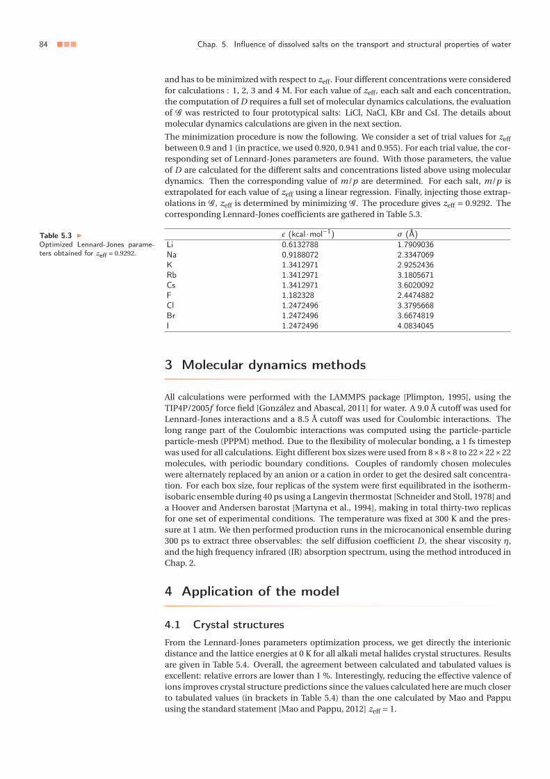
84 ■■■ Chap. 5. Influence of dissolved salts on the transport and structural properties of water
and has to be minimized with respect to zeff. Four different concentrations were consideredfor calculations : 1, 2, 3 and 4 M. For each value of zeff, each salt and each concentration,the computation of D requires a full set of molecular dynamics calculations, the evaluationof G was restricted to four prototypical salts: LiCl, NaCl, KBr and CsI. The details aboutmolecular dynamics calculations are given in the next section.
The minimization procedure is now the following. We consider a set of trial values for zeff
between 0.9 and 1 (in practice, we used 0.920, 0.941 and 0.955). For each trial value, the cor-responding set of Lennard-Jones parameters are found. With those parameters, the valueof D are calculated for the different salts and concentrations listed above using moleculardynamics. Then the corresponding value of m/p are determined. For each salt, m/p isextrapolated for each value of zeff using a linear regression. Finally, injecting those extrap-olations in G , zeff is determined by minimizing G . The procedure gives zeff = 0.9292. Thecorresponding Lennard-Jones coefficients are gathered in Table 5.3.
Table 5.3 �
Optimized Lennard-Jones parame-ters obtained for zeff = 0.9292.
ε (kcal ·mol−1) σ (Å)Li 0.6132788 1.7909036Na 0.9188072 2.3347069K 1.3412971 2.9252436Rb 1.3412971 3.1805671Cs 1.3412971 3.6020092F 1.182328 2.4474882Cl 1.2472496 3.3795668Br 1.2472496 3.6674819I 1.2472496 4.0834045
3 Molecular dynamics methods
All calculations were performed with the LAMMPS package [Plimpton, 1995], using theTIP4P/2005f force field [González and Abascal, 2011] for water. A 9.0 Å cutoff was used forLennard-Jones interactions and a 8.5 Å cutoff was used for Coulombic interactions. Thelong range part of the Coulombic interactions was computed using the particle-particleparticle-mesh (PPPM) method. Due to the flexibility of molecular bonding, a 1 fs timestepwas used for all calculations. Eight different box sizes were used from 8×8×8 to 22×22×22molecules, with periodic boundary conditions. Couples of randomly chosen moleculeswere alternately replaced by an anion or a cation in order to get the desired salt concentra-tion. For each box size, four replicas of the system were first equilibrated in the isotherm-isobaric ensemble during 40 ps using a Langevin thermostat [Schneider and Stoll, 1978] anda Hoover and Andersen barostat [Martyna et al., 1994], making in total thirty-two replicasfor one set of experimental conditions. The temperature was fixed at 300 K and the pres-sure at 1 atm. We then performed production runs in the microcanonical ensemble during300 ps to extract three observables: the self diffusion coefficient D , the shear viscosity η,and the high frequency infrared (IR) absorption spectrum, using the method introduced inChap. 2.
4 Application of the model
4.1 Crystal structuresFrom the Lennard-Jones parameters optimization process, we get directly the interionicdistance and the lattice energies at 0 K for all alkali metal halides crystal structures. Resultsare given in Table 5.4. Overall, the agreement between calculated and tabulated values isexcellent: relative errors are lower than 1 %. Interestingly, reducing the effective valence ofions improves crystal structure predictions since the values calculated here are much closerto tabulated values (in brackets in Table 5.4) than the one calculated by Mao and Pappuusing the standard statement [Mao and Pappu, 2012] zeff = 1.

4 Application of the model ■■■ 85
LiF LiCl LiBr LiI-U 251.7 (250.7) 207.7 (206.5) 196.1 (196.0) 180.9 (182.6)d 2.009 (1.996) 2.530 (2.539) 2.705 (2.713) 2.969 (2.951)
NaF NaCl NaBr NaI-U 221.1 (222.3) 188.5 (188.8) 180.5 (180.2) 169.9 (168.5)d 2.306 (2.295) 2.791 (2.789) 2.946 (2.954) 3.178 (3.194)
KF KCl KBr KI-U 199.1 (198.1) 170.8 (172.1) 164.2 (165.2) 155.9 (155.4)d 2.633 (2.648) 3.118 (3.116) 3.268 (3.262) 3.487 (3.489)
RbF RbCl RbBr RbI-U 191.2 (190.0) 164.3 (166.1) 158.1 (159.7) 150.2 (151.1)d 2.765 (2.789) 3.250 (3.259) 3.400 (3.410) 3.617 (3.628)
CsF CsCl CsBr CsI-U 179.7 (181.4) 161.2 (160.1) 155.5 (154.6) 147.7 (146.5)d 2.988 (2.982) 3.529 (3.523) 3.678 (3.668) 3.906 (3.898)
Table 5.4 �
Calculated and tabulated values oflattice energies U (kcal ·mol−1) andinterionic distances d (Å) of alkalimetal halides. The first value is thecalculated one using the Lennard-Jones parameters and the effec-tive valence determined previouslyzeff = 0.9292, and the value in brack-ets is the tabulated value, takenfrom [Mao and Pappu, 2012].
It could be interesting to analyze precisely other solid properties of alkali metal halides usingour model, but as our aim is to focus on aqueous state properties, we directly move to theanalysis of aqueous solutions with various concentrations.
4.2 Liquid structure
An important topic in the study of the effect of ion solvation on the associated structureof water is the oxygen-oxygen coordination. To this aim, we first analyze here the oxygen-oxygen (O–O) radial distribution function. To simplify the discussion, we will restrict our-selves to two limit case salts: lithium chloride (LiCl) will be treated as an example of kos-motrope, whereas potassium bromide (KBr) will be treated as an example of chaotrope.The curves corresponding to the different concentrations are gathered in Fig. 5.2.
The TIP4P/2005f force field is known to reproduce accurately the O–O radial distributionfunction [González and Abascal, 2011] at room temperature. Here, the first peak positionis found to be at 2.77± 0.17 Å. Interestingly, whatever the concentration used, the pres-ence of solvated species does not affect this position, in agreement with neutron and X-ray diffraction experiments on sodium and potassium chloride solutions [Bouazizi et al.,2006, Mancinelli et al., 2007]. Moreover, a decrease of the amplitude of the peak is observedwhen the salt concentration is increased. It corresponds to the decrease of the mean num-ber of oxygen atoms in their first coordination shell since a couple of them are replaced byions. However, this decrease is only qualitatively reproduced: the decrease is more pro-nounced on experimental curves, and is accompagned by a broadening of the peak, due tothe influence of ions hydration spheres [Mancinelli et al., 2007].
It is also interesting to look at other peaks, since the second peak of the O–O radial distribu-tion function describes the local order of water, and is sometimes said to be the signature ofthe tetrahedral hydrogen bond network [Bouazizi et al., 2006]. Moreover, the self diffusionof water is influenced by molecular interactions beyond several molecular sizes [Jonchiereet al., 2011], and thus by the O–O distribution in the second and third coordination shells.
A progressive shift of the second peak to lower distances is observed for KBr solutions,whereas the shift is observed in the other direction for LiCl solutions. Since non-hydrogenbonded water molecules should be closer than hydrogen bonded molecules, the trend ob-served here are consistent with a chaotropic and kosmotropic behaviour respectively. More-over, the trend observed for LiCl agrees with both X-ray and neutron diffraction data forNaCl [Bouazizi et al., 2006, Mancinelli et al., 2007], which is, like LiCl, a kosmotropic salt,whereas the trend observed for KBr agrees with neutron diffraction data [Mancinelli et al.,2007] for KCl which is, like KBr, a chaotropic salt.
In contrast with the second peak, using the present model, the third peak is found to shiftto lower distances for both salts when the concentration is increased. This is also consis-tent with neutron diffraction data [Mancinelli et al., 2007], as shown in Fig. 5.2. Moreover,experimental curves are overall close to our simulated results at long distances (around theposition of the third peak). Thus, the effect of ions, whether chaotropic or kosmotropic, on

86 ■■■ Chap. 5. Influence of dissolved salts on the transport and structural properties of water
Figure 5
Evolutiondial distrspect toand KBras an exsalt, anda chaotrbeen shifguides hasize the etions withtion. Neufrom Refhas beenson, withmotropicof chaotr
the local structure is accurately reproduced beyond the third coordination sphere or watermolecules, whereas the agreement is only qualitative in the first and second coordinationspheres.
An interesting point is that the third peak amplitude is not modified by the salts. This meansthus that the (de)structuring effect of salts is limited. However, it is clear that the structure ofwater is altered beyond the first hydration shell since the radial distribution function differsfrom that of pure water further than the second peak. To this point of view, the presentmodel reproduces well both the range and strength of the (de)structuration induced by ions.
4.3 Water self diffusion
The self diffusion coefficient of water has been computed for all alkali metal halides, ex-cept fluorides that suffered of numerical instabilities with the Morse potential used in theTIP4P/2005f force field to parametrize O–H bonds inside molecules. All calculations werecorrected for finite size effects, as described in Chap. 2. The results are shown in Fig. 5.3 andcompared to experimental data, when available. The self diffusion coefficient for pure wa-ter, computed in the same conditions than for salted solutions, but with twice more replicasof the system in order to reduce errors, is (2.30±0.01) ·10−9 m2 · s−1 which corresponds tothe tabulated value [Krynicki et al., 1978]. Thus, calculated and tabulated values for saltsolutions can be directly compared without any normalization.
According to experimental data, lithium and sodium based salts decrease the self diffusionof water (that should correspond to a more structured liquid), whereas potassium, rubid-ium and iodine increase it (that should correspond to a less structured liquid). Moreover,except for small cations, the evolution of the self diffusion coefficient with respect to thesalt concentration only slightly depends on the nature of the cation, in agreement with pre-vious studies: for a given anion, curves corresponding to potassium, rubidium and cesiumare very close one to each other. The trend is well reproduced by our model in the case oflithium and sodium. Except for LiBr solutions with concentration higher than 3 mol ·L−1,the differences between experimental and calculated values are within the error bars. How-ever, our model fails to reproduce the increase of the self diffusion coefficient of water in thepresence of chaotropic salts. In the case of chlorides whose influence on the self diffusionis small, calculated self diffusion coefficients slightly decrease with respect to the salt con-centration, whereas for more chaotropic salts, calculated values remains approximatively

4 Application of the model ■■■ 87
Figure 5.3
Evolution of the water self diffusioncoefficient with respect to the saltconcentration. Filled symbols rep-resent calculated values using ourmodel at 300 K, and empty sym-bols represent tabulated values at298 K (from Ref. [Müller and Hertz,1996]). For clarity, values have beenplotted on different graphs depend-ing on the anion. Globally, theagreement between calculated andtabulated values is good for lithiumand sodium based salts which arekosmotropic, whereas our modelfails to reproduce tabulated valuesfor others salts, that are mainlychaotropic.
constant with respect to the concentration. Despite of this strong failure of the model, therelative influence of the different salts is overall well restituted. Except for the chlorides, theset of points corresponding to the different cations are ordered in same way, and the dis-persion of values for potassium, rubidium and iodine for a given halide is almost the samefor tabulated and calculated values. Moreover, the overall accuracy of the present model toreproduce the self diffusion of salt water is similar to those of the model by Kann and Skin-ner [Kann and Skinner, 2014] or usual polarizable models [Kim et al., 2012], and is almostquantitative for salts involving small ions thanks to the accuracy of the TIP4P/2005f forcefield to reproduce the self diffusion of pure water.
88 ■■■ Chap. 5. Influence of dissolved salts on the transport and structural properties of water
4.4 Shear viscosityThe shear viscosity of electrolytes has been extensively studied experimentally in the limitof low concentrations [Abdulagatov et al., 2006, Nakai et al., 1996, Goldsack and Franchetto,1977], but not numerically. Within the limit of low concentrations, experimental data canbe well described using the Jones-Dole equation [Marcus, 2009] η/ηsolvent = 1+A ·�c+B ·c.A can be computed theoretically from solvent and ions properties and B is an empiricalcoefficient. A large amount of experiments have been devoted to the determination of B forvarious salts [Abdulagatov et al., 2006,Nakai et al., 1996,Goldsack and Franchetto, 1977]. It isusually assumed that salts with a positive B are kosmotropic, while those with a negative Bare chaotropic [Marcus, 2009, Goldsack and Franchetto, 1977]. According to the Jones-Doleequation, A ·�c should be negligible at high concentrations. Indeed, for all salts consideredhere, our calculations are well described by an affine relation within error bars, even if aslight convexity seems to appear on all sets of points, as shown in Fig. 5.4. Consequently,the slope of the curves directly gives the sign of B , and thus, the kosmotropic/chaotropictendency of the salt.
Using the TIP4P/2005f model, the shear viscosity of pure water at 300 K is 0.76±0.05 mPa·s,which is close to the tabulated value 0.896 mPa·s at 298.15 K [Harris and Woolf, 2004]. Thus,our values must be slightly underestimated with respect to experiments. We however applyno correction nor normalization on the graph of Fig. 5.4. Whatever the anion considered,the shear viscosity computed using the Green-Kubo method increases with respect to theconcentration for lithium and sodium based salts, which corresponds to a positive B value,and thus, a kosmotropic tendency. This is – as in the case of the self diffusion – in qual-itative agreement with experiments. The agreement is however better in the case of selfdiffusion: the increase of shear viscosity with respect to the concentration seems systemat-ically overestimated. Calculations also predict positive B values for other salts, which is inqualitative disagreement with experiments, but in agreement with another recent numer-cial study [Hartkamp and Coasne, 2014]. Again, the model fails to reproduce the chaotropicbehavior of salts. Note that the “saturation” of calculated values of the self diffusion coeffi-cient of water near the pure water value for bromide and iodide is not observed in the caseof shear viscosity. Even for the most chaotropic salts, the shear viscosity increases accordingto calculations. Recent models for salt water have not been employed to calculate the shearviscosity, so no comparison can be made between our model and other models.
4.5 Mid-infrared absorption spectrumThe infrared absorption spectrum of water represents the variations of dipole momentsof water molecules induced by molecular vibrations, and is thus a dynamical observable.However, in the stretching region, as we already mentionned, the spectrum is also highlycorrelated to the structure of water (see Chap. 2). Brubach et al. [Brubach et al., 2005] sug-gested to deconvolute the stretching band (see Fig. 5.5) into three main contributions lo-cated approximatively around 3200, 3400 and 3600 cm−1, and corresponding respectivelyto highly (four H-bonds per molecule), intermediately (between one and three) and poorlyhydrogen-bonded (no H-bond) water molecules [Brubach et al., 2005, Mallamace et al.,2007]. One or two additional Gaussians are sometimes used [Mallamace et al., 2007]. It isthus of particular interest to look at the influence of salts on the water spectrum. Rigid forcefields only restitute the permanent dipole moment of water molecules. Due to its flexibility,the TIP4P/2005f force field [González and Abascal, 2011] also takes into account induceddipole moments, even if the electronic degrees of freedom are not considered. As in theradial distribution function analysis, LiCl will be treated as an example of kosmotrope, andKBr as an example of chaotrope.
Experimental spectra were recorded using a Nicolet iS10 Fourier Transform InfraRed (FTIR)Spectrometer by Thermo Scientific in conjunction with a single diamond Attenuated To-tal Reflectance (ATR) DuraSamplIR II accessory by SensIR. The standard tungsten source,KBr beam-splitter and DGTS detector were used. 40 scans with a 4 cm−1 resolution wereaccumulated for each sample. The results are shown in Fig. 5.5.
The FTIR probe shows a large sensitivity to the salt concentration. In the case of KBr, the3200 cm−1 decreases when the concentration is increased, with only few modifications on

4 Application of the model ■■■ 89
viscosityconcen-
ls repre-sing ourpty sym-values atdulagatovin et al.,, 1981a],96], CsI,d Aseyev,Goldsack
Br [Isono,ssimilatedties werealts, theincreases
entration,th exper-
hium anddisagree-n text for
the other contributions, except a slight increase of the 3400 cm−1 contribution, as shownon the bottom graph of Fig. 5.5. That means the population of highly H-bonded watermolecules decreases when the concentration of KBr increases, with a partial transfer to in-termediately H-bonded molecules. This is consistent with the chaotropic behavior of KBr.In contrast, for LiCl, only the 3400 cm−1 band seems to be affected by adding salt, with aclear increase when the salt concentration is increased. That means the population of mod-erately H-bonded water molecules increases, without any change on the highly H-bondedwater molecules population, which is consistent with the kosmotropic behavior of LiCl.
The TIP4P/2005f force field reproduces the different components of the O–H stretchingspectrum of pure water, but each component is slightly shifted to higher frequencies. Tosimplify the discussion, we will speak about 3200, 3400 and 3600 cm−1 components for thethree highest bands (see deconvolution in Fig. 5.5) by reference to the experimental spec-trum, even if the first frequency is closer to 3300 cm−1. When adding LiCl, the 3200 cm−1
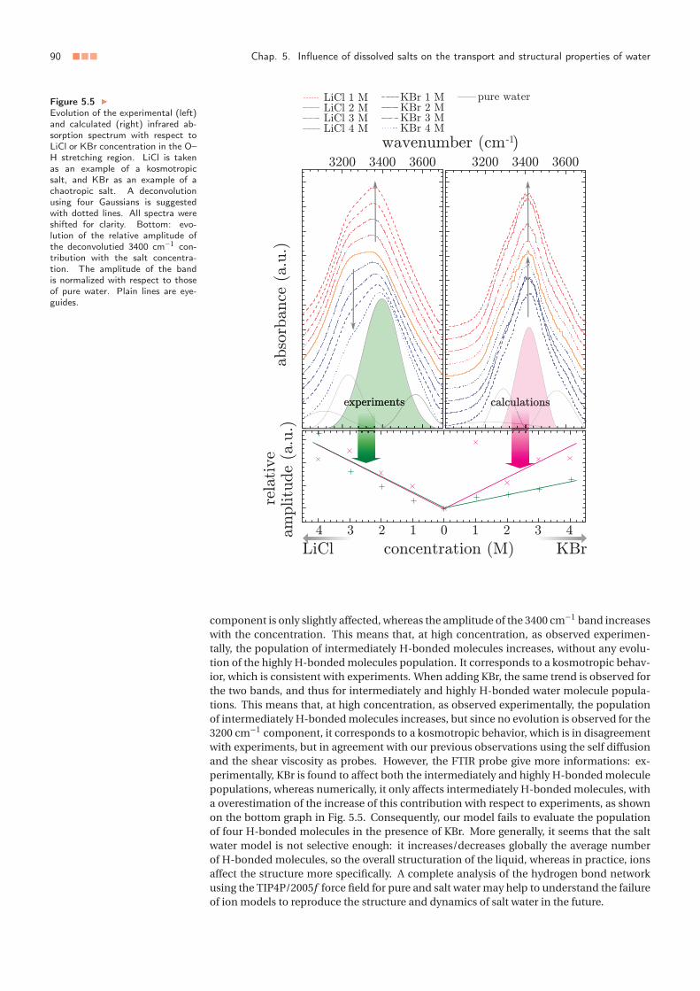
90 ■■■ Chap. 5. Influence of dissolved salts on the transport and structural properties of water
Figure 5.5
Evolution of the experimental (left)and calculated (right) infrared ab-sorption spectrum with respect toLiCl or KBr concentration in the O–H stretching region. LiCl is takenas an example of a kosmotropicsalt, and KBr as an example of achaotropic salt. A deconvolutionusing four Gaussians is suggestedwith dotted lines. All spectra wereshifted for clarity. Bottom: evo-lution of the relative amplitude ofthe deconvolutied 3400 cm−1 con-tribution with the salt concentra-tion. The amplitude of the bandis normalized with respect to thoseof pure water. Plain lines are eye-guides.
component is only slightly affected, whereas the amplitude of the 3400 cm−1 band increaseswith the concentration. This means that, at high concentration, as observed experimen-tally, the population of intermediately H-bonded molecules increases, without any evolu-tion of the highly H-bonded molecules population. It corresponds to a kosmotropic behav-ior, which is consistent with experiments. When adding KBr, the same trend is observed forthe two bands, and thus for intermediately and highly H-bonded water molecule popula-tions. This means that, at high concentration, as observed experimentally, the populationof intermediately H-bonded molecules increases, but since no evolution is observed for the3200 cm−1 component, it corresponds to a kosmotropic behavior, which is in disagreementwith experiments, but in agreement with our previous observations using the self diffusionand the shear viscosity as probes. However, the FTIR probe give more informations: ex-perimentally, KBr is found to affect both the intermediately and highly H-bonded moleculepopulations, whereas numerically, it only affects intermediately H-bonded molecules, witha overestimation of the increase of this contribution with respect to experiments, as shownon the bottom graph in Fig. 5.5. Consequently, our model fails to evaluate the populationof four H-bonded molecules in the presence of KBr. More generally, it seems that the saltwater model is not selective enough: it increases/decreases globally the average numberof H-bonded molecules, so the overall structuration of the liquid, whereas in practice, ionsaffect the structure more specifically. A complete analysis of the hydrogen bond networkusing the TIP4P/2005f force field for pure and salt water may help to understand the failureof ion models to reproduce the structure and dynamics of salt water in the future.
5 Conclusion ■■■ 91
5 Conclusion
Treating ionic charge as an adjustable parameter, we have developed a full set of parame-ters to model alkali metal halides in conjunction with the TIP4P/2005f force field. The localstructure of water, probed through the oxygen-oxygen radial distribution function, is wellrestituted by the model, but hydrodynamic properties such as the self diffusion coefficientof water and the shear viscosity are only reproduced for small ion salts, i.e. lithium andsodium salts, that are kosmotropic. Moreover, through the analysis of the infrared absorp-tion spectra of salt solutions, it appears that the point charge model fails to restitute the hy-drogen bond distribution in water. This reinforces the idea that empirical non-polarizableforce fields cannot reproduce fairly salt-water interactions. However, due to its flexibility,the TIP4P/2005f forcefield is slightly polarizable. Thus, considering our preliminary cal-culation of the self diffusion of water for sodium chloride solution with low charge ionsmentioned in the introduction, we think that choosing a different routine based on liquidproperties (see e.g. model by Horinek et al. [Horinek et al., 2009]) to optimize the modelcould improve the overall agreement between calculations and experiments. In spite of thelimitations of this model, the quantitative agreement with experiments for small ions due tothe combined accuracy of the TIP4P/2005f and salt force fields should increase the benefitsof molecular simulations to study heterogeneous systems such as for example nanofluidicdevices or clay minerals. In particlar, we will apply this model to describe interlayer cationsin clays in Chap. 6.

92 ■■■ Chap. 5. Influence of dissolved salts on the transport and structural properties of water

1 Evolution of the structure and connectivity of water adsorbed in clay minerals upon . . . ■■■ 93
■■■ Chapter 6
Structure and dynamics of waterconfined in clay minerals
Outline
1 Evolution of the structure and connectivity of water adsorbed inclay minerals upon swelling . . . . . . . . . . . . . . . . . . . . . . . . 911.1 Experimental methods . . . . . . . . . . . . . . . . . . . . . . 921.2 Results . . . . . . . . . . . . . . . . . . . . . . . . . . . . . . . 931.3 Discussion . . . . . . . . . . . . . . . . . . . . . . . . . . . . . 981.4 Summary and conclusion . . . . . . . . . . . . . . . . . . . . 102
2 Mono- and bi-layer configurations of interlayer water . . . . . . . . 1032.1 Numerical methods . . . . . . . . . . . . . . . . . . . . . . . . 1032.2 Identification of the stable mono- and bi-layer hydration
configurations by molecular simulation . . . . . . . . . . . . 1042.3 Vibrational density of states of the mono- and bi-layer con-
figurations . . . . . . . . . . . . . . . . . . . . . . . . . . . . . 1053 Low temperature dynamics of confined water . . . . . . . . . . . . . 106
3.1 Water thermally induced migration and dynamics singular-ities . . . . . . . . . . . . . . . . . . . . . . . . . . . . . . . . . 106
3.2 Low temperature hydrodynamic properties of interlayer water 1104 Summary and conclusion . . . . . . . . . . . . . . . . . . . . . . . . . 1115 Appendix: Temperature dependance of the far-infrared absorption
spectrum for various hydration states . . . . . . . . . . . . . . . . . . 113
This last chapter is dedicated to water adsorbed in clay minerals. As we explained in Chap. 1,the experimental investigation of the structural and dynamical properties of water adsorbedin clays is a delicate task due to the variety of scales implied. Performing for the first timeextensive infrared adsorption measurements in the connectivity region, and coupling themto standard mid-infrared measurements, we will show that the infrared probe can be usedas a standalone tool to characterize adsorbed water and the mechanisms of hydration anddehydration of clays. However, since the infrared spectrum of clay is complex, we will alsoshow the efficiency and accuracy of molecular dynamics to refine the interpretation of spec-tra. Finally, we will apply both infrared and molecular dynamics probes to characterize thelow temperature dynamics of confined water and propose a mechanism for water freezinginside clays.
1 Evolution of the structure and connectivity of water
adsorbed in clay minerals upon swelling
In the present study, we reinvestigate the hydration and dehydration processes of a sodium-exchanged montmorillonite clay using Fourier Transform infrared (FTIR) spectrometry in

94 ■■■ Chap. 6. Structure and dynamics of water confined in clay minerals
Figure 6.1
Scanning Electron Micrographs(Secondary Electrons) of sodium-exchanged montmorillonite SAz-2after particle size separation. Fromtop to bottom: (a) smaller than0.2 μm, (b) between 0.2 and 2 μmand (c) between 2 and 5 μm.
both far- and mid-infrared domains, and try to analyze the evolution of the structure andconnectivity of water molecules upon swelling. In Section 1.1, we will briefly present howsamples were prepared for both far- and mid-infrared measurements. Then, in Section 1.2,we will present the evolution of the main components of the absorption spectrum in thedifferent regions with respect to the relative humidity (RH), and discuss those evolutionsin Section 1.3 to provide an attribution of the vibrational bands of montmorillonite in thefar-infrared region and give a consistent picture of water adsorption and desorption mech-anisms. We will see that the far infrared probe is specific to the adsorption sites of water,and is able to monitor the hydration mechanism at the various scales of porosity of clayminerals.
1.1 Experimental methods
1.1.1 Sample preparation
The clay used in this study is a natural montmorillonite SAz-2 from the Clay Mineral Soci-ety [Costanzo and Guggenheim, 2001]. The chemical formula is given by:
(Ca0.39Na0.36K0.02)[
Al2.71Mg1.11Fe(III)0.12Mn0.03
][Si8]O20 (OH)4 . ■ (6.1)
The interlayer charge – i.e. the net charge deficit per unit cell induced by isomorphic sub-stitutions inside the clay layers – is 1.16 · e, with e the electronic charge, and is localizedexclusively inside the octahedral sites of the clay layers. The sample was purified with re-spect to carbonates, organic matter and iron oxides following the procedure by Kittrick andHope [Kittrick and Hope, 1963]. The interlayer cation was then exchanged with sodium us-ing successive cycles of dispersion in a 1 mol/L sodium chloride solution and dezionizedwater to remove excess ions. Finally, the clay was separated in four range of tactoids sizes –lower than 0.2 μm, between 0.2 and 2 μm, between 2 and 5 μm and higher than 5 μm – us-ing various centrifugation and decantation cycles, following the procedure by Kittrick andHope [Kittrick and Hope, 1963]. We qualitatively checked the result of particle-size sepa-ration using Scanning Electron Microscopy, as shown in Fig. 6.1. One can indeed observean increase of the average size of the aggregates visible on the micrographs between thedifferent pictures. In the following, all presented curves correspond to sample (a), i.e. claysparticles smaller than 0.2 μm. Curves corresponding to other samples displayed very similarbehavior and are thus not shown for the sake of simplicity.
1.1.2 Infrared absorption measurements
Infrared measurements were realized following the procedure described in Chap. 2. Far-infrared measurements were performed on the AILES beamline of Synchrotron Soleil, Saint-Aubin, France. Transmission spectra were recorded by averaging 200 scans from 100 to680 cm−1 with a resolution of 2 cm−1. The sample was dispersed in water, then a dropletof suspension was deposited over a diamond window, and let to evaporate. By doing so, aregular and a priori oriented (001) plans thin film was obtained. The sample was furtherdried from room conditions to RH = 0 in situ under vacuum during at least half an hour.Various RH values were used between 0 and 100 %. Before each measurement, we checkedthat the equilibrium was reached by following the evolution with time of the vapor pressurearound the sample after the water injection/removal stopped inside the experimental cell.
Mid-infrared measurements were performed on a Thermo Nicolet iS10 spectrometer. Eachspectrum was recorded by averaging 80 scans from 400 to 4000 cm−1 with a resolution of4 cm−1, using a single ATR accessory SensIR DuraSamplIR II. The sample was prepared ina similar manner than previously, except the droplet of clay suspension was deposited di-rectly on the top-surface of the internal reflection element to get a good contact betweenthe diamond and the clay thin film. All spectra were corrected following the formula A(ν) ≈AATR ·ν (see Chap. 2) to obtain transmission-equivalent spectra. The RH was varied from 0to 100 % by step of 5 %.

1 Evolution of the structure and connectivity of water adsorbed in clay minerals upon . . . ■■■ 95
1.2 Results
We present first the different results obtained in mid- and far-infrared domains, before dis-cussing them in the next section.
1.2.1 Far-infrared measurements: connectivity region
The absorption spectrum of the Na-substituted montmorillonite SAz-2 is shown in Fig. 6.2for various hydration states corresponding to different RH values among the adsorptionbranch of the water vapor adsorption isotherm (see Chap. 1). The absorbance was calcu-lated using the absorption spectrum of the empty experimental cell as background. The
Figure 6.2 �
(a) Evolution of the far-infrared ab-sorption spectrum with RH dur-ing adsorption. Spectra are domi-nated by five main components (ar-rows) around 180, 340, 470, 520and 630 cm−1. Dotted lines rep-resent the part of the spectrumcorresponding to “bulk-like” water.(b) Same spectra after subtractionof the “bulk-like” water component(dotted line of Fig. (a)).
spectrum appears complex, with many bands. However, five contributions predominate.They are located around 180, 340, 470, 520 and 630 cm−1 (marked with gray arrows inFig. 6.2). The two most intense contributions are localized at 470 and 520 cm−1. They areclearly identified in literature and corresponds to vibrations respectively associated withthe deformation of Si–O–Si and Si–O–Al units in the clay layers [Madejová and Komadel,2001, Boukili et al., 2003]. The other contributions have no clear assignement. We will sug-gest one in the discussion. Using a pumped bolometer working at 1.2 K, we also recordedthe absorption spectrum down to 50 cm−1 and saw no additional contribution. With in-creasing RH, one observes a strong evolution of the baseline, especially at high RH. Sinceit is generally assumed that water adsorbed in mesopores at high RH values behaves al-most like bulk water (see, e.g. [Tardy et al., 1999] for a discussion about the evolution of theproperties of water in mesopores with the water content), we tried to adjust the baselineusing the absorption spectrum of pure bulk water Abulk(ν) (courtesy of J.B. Brubach) as de-scribed in the following. Since there should not be water adsorbed at 0 % of RH (referred as

96 ■■■ Chap. 6. Structure and dynamics of water confined in clay minerals
the dry state in the following), the absorption spectrum corresponding to the dry state wassubtracted to the others. Then, we calculated a coefficient α(RH) so that α(RH) · Abulk(ν)fits to the lower and upper wavenumber values of each spectrum Aclay(ν,RH)− Aclay(ν,0).The adjusted bulk spectra are shown with dotted lines in Fig. 6.2a, and the clay spectra af-ter subtraction of this “bulk” component in Fig. 6.2b. It is noteworthy that the adjustedbulk spectra follow the shape of the clay spectra at low wavenumbers, i.e. between 130 and240 cm−1. The trend is the same for the desorption branch. We rewrite the Beer-Lambertlaw [Atkins and de Paula, 2010]:
A(ν) =∑i
ai (ν) · l · ci , ■ (6.2)
with ai (ν) and ci respectively the molar absorptivity and molar concentration of specie iand l the thickness of the sample, as a sum of “bulk-like” and other contributions:
A(ν) = abulk(ν) · l ·cbulk +∑
i �=bulkai (ν) · l · ci = abulk(ν) · nbulk
S+ ∑
i �=bulkai (ν) · l · ci , ■ (6.3)
where S is the surface of the sample (covered by the IR beam) and nbulk is the amount of“bulk-like” water. Then, considering Abulk(ν) as a proxy of the molar absorptivity of waterabulk(ν), α(RH) is proportional to the amount of “bulk-like” water inside the sample at thecorresponding RH.α(RH) is plotted for both adsorption and desorption branches in Fig. 6.3.The adsorption curve increases slowly at low RH, and more sharply at high RH. The desorp-
Figure 6.3 �
“Bulk-like” water adsorptionisotherm. According to the IUPACclassification, the adsorption curvecorresponds to a type II isotherm,whereas the desorption curvecorresponds to a type III isotherm.Dotted lines are guides for the eye.
tion curve match well with the adsorption curve at low and high RH values, but present anintermediate plateau between 80 and 60 % of RH. There is consequently a hysteresis on theadsorption isotherm. Using the classification of the IUPAC, the adsorption branch corre-sponds to an adsorption isotherm of type II, whereas the desorption branch corresponds totype III [Donohue and Aranovich, 1998]. We will discuss the implications of these particularshapes in the next section.
After subtraction of the “bulk-like” water contribution of all spectra (see Fig. 6.2b), the dif-ferent bands show only small dependency to the hydration state. However, the Si–O–Si andSi–O–Al bands at 470 and 520 cm−1 shift with the RH. It has been shown that the structureof the mineral, including those two bands, is highly sensitive to the presence of adsorbedwater [Sposito and Prost, 1982, Yan et al., 1996, Kuligiewicz et al., 2015]. To emphasize thechanges with respect to the dry state, the spectrum corresponding to the dry sample hasbeen subtracted to the others. The evolution of the position of the remaining Si–O–Si andSi–O–Al bands is plotted in Fig. 6.4. Let us first consider the Si–O–Si deformation around470 cm−1. The adsorption branch can be divided into three parts. Below 25 % of RH, theposition of the band slightly decreases from 476 to 474 cm−1. Then, between approxima-tively 25 % and 75 % of RH, the position remains constant, and finally, beyond 75 % of RH,it decreases from 474 to 472 cm−1. The desorption branch is somehow different since the

1 Evolution of the structure and connectivity of water adsorbed in clay minerals upon . . . ■■■ 97
Figure 6.4
Evolution of the Si–O–Si and Si–O–Al deformation bands positionsduring adsorption and desorption ofwater. Both vibrational signaturesbehave similarly. At low RH duringdesorption, one does not recover theinitial position of the bands, reveal-ing some troubles to desorb waterat low vapor pressures. Dotted linesare guides for the eye.
first step previously mentioned is not visible. The position increases slightly from 472 to473 cm−1 between 100 and 75 % of RH, and then remains constant. In addition, the plateauvalue is slightly shifted with respect to the adsorption branch. The same behavior is ob-served for the Si–O–Al deformation around 520 cm−1.
We now look at the band around 180 cm−1. Interestingly, this contribution is only visible atlow RH values. The evolution of the amplitude of the band is reported in Fig. 6.5 for bothadsorption and desorption branches. The position of the band and its half-height width donot change significantly with the RH. As in the previous case, the adsorption branch can be
Figure 6.5
Evolution of the amplitude of theband around 180 cm−1 with respectto the RH for both adsorption anddesorption processes. Dotted liesare guides for the eye.
divided into three parts. First, the amplitude remains almost constant up to 60 % of RH.Then it strongly decreases between 60 and 80 % of RH, and it stabilizes at a constant valueat higher RH. The desorption branch shows a bend between the low and high amplitudebetween 45 and 65 % of RH, revealing thus a strong hysteresis. Moreover, the plateau valueat low RH is much lower than on the adsorption curve, meaning that the initial amplitudeof the 180 cm−1 band and thus the initial state of the clay is not recovered.
The band at 630 cm−1 show a similar trend but the evolution of the amplitude of the peakis inverted: it increases instead of decreasing with respect to the RH. The curve reveals asimilar bend as the 180 cm−1 band, but the global evolution is less pronounced than thelatter. Finally, looking at the band around 340 cm−1, there is no change of the position northe amplitude with respect to the water content, but the half-height width slightly increaseswith RH in a similar manner to the amplitude of the 180 cm−1 band (bend approximativelyat the same position). However, since the evolution of the 340 and 630 cm−1 contributions

98 ■■■ Chap. 6. Structure and dynamics of water confined in clay minerals
are small, it is difficult to separate the evolution upon swelling from noise and thus we willnot use them in the following discussion.
1.2.2 Mid-infrared measurements (I): bending region
The “bending region” of the infrared absorption spectrum of Na-montmorillonite is givenin Fig. 6.6 for different RH values along the adsorption curve. The spectral range is closeto 1650 cm−1, which is the frequency of the bending motion of water molecules in bulk atambient conditions [Bergonzi et al., 2014]. In this region, the spectrum of confined wa-
Figure 6.6
Left: Evolution of the bendingmode of confined water with re-spect to the RH along the adsorp-tion curve. To emphasize the evo-lution with respect to the dry state,the latter was subtracted to eachspectrum. The grey curve corre-sponds to bulk water (courtesy ofJ.B. Brubach). Right: Deconvo-lution of the spectrum (at RH =100 %) in three main Gaussian con-tributions, shown with dotted lines.Small negative lines that appear onthe different spectra correspond toatmospheric water vapor.
ter is constituted, as in the case of bulk water, of a single well defined band. This band ishowever thinner than the one of bulk water and slightly shifted at lower frequencies. Theband is deconvoluted using three Gaussians, one similar to the bulk water spectrum around1655 cm−1, and two others of approximatively equal weight (in terms of band area) at lowerfrequencies around 1600 and 1620 cm−1. Following the evolution of those three bands dur-ing hydration and dehydration of the clay sample, the amplitude of the three Gaussiansevolves similarly. The evolution of the total area of the band (which should be proportionalto the amount of absorbing species) is given in Fig. 6.7. During adsorption, at very low and
Figure 6.7
Evolution of the total area of thebending band with respect to theRH along both adsorption and des-orption curves. The area of eachGaussian presented in Fig. 6.6 showa similar trend. Dotted lines areguides for the eye. ATR experi-mental data by Hatch et al. [Hatchet al., 2012] are reported forcomparison.
very high RH, the intensity of the band grows almost linearly. A plateau is observed around85 % of RH, before a second growth regime, faster than the first one, up to the vapor sat-uration pressure. Small steps are visible et 25 % and 40 % of RH, but the precision of themeasurements does not enable to be fully confident with their existence. The global shape
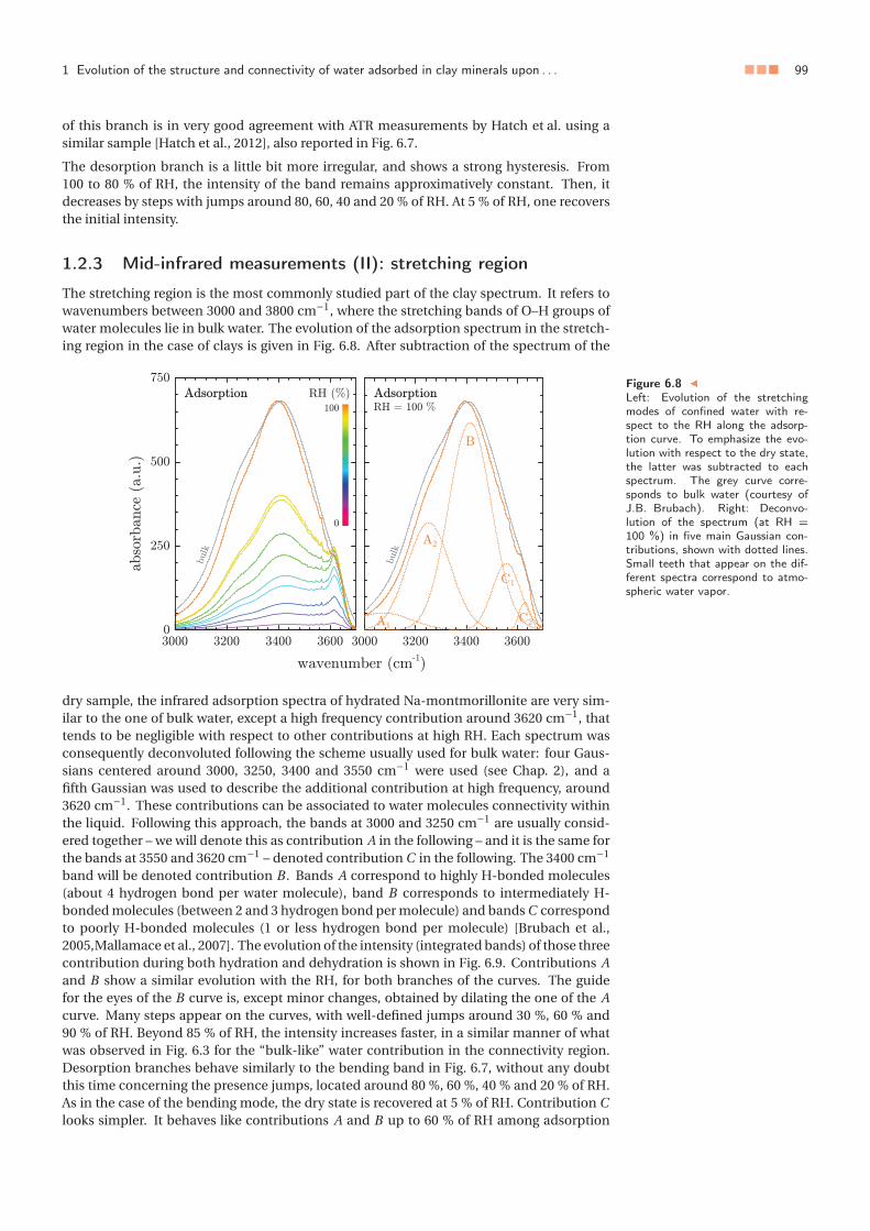
1 Evolution of the structure and connectivity of water adsorbed in clay minerals upon . . . ■■■ 99
of this branch is in very good agreement with ATR measurements by Hatch et al. using asimilar sample [Hatch et al., 2012], also reported in Fig. 6.7.
The desorption branch is a little bit more irregular, and shows a strong hysteresis. From100 to 80 % of RH, the intensity of the band remains approximatively constant. Then, itdecreases by steps with jumps around 80, 60, 40 and 20 % of RH. At 5 % of RH, one recoversthe initial intensity.
1.2.3 Mid-infrared measurements (II): stretching region
The stretching region is the most commonly studied part of the clay spectrum. It refers towavenumbers between 3000 and 3800 cm−1, where the stretching bands of O–H groups ofwater molecules lie in bulk water. The evolution of the adsorption spectrum in the stretch-ing region in the case of clays is given in Fig. 6.8. After subtraction of the spectrum of the
Figure 6.8
Left: Evolution of the stretchingmodes of confined water with re-spect to the RH along the adsorp-tion curve. To emphasize the evo-lution with respect to the dry state,the latter was subtracted to eachspectrum. The grey curve corre-sponds to bulk water (courtesy ofJ.B. Brubach). Right: Deconvo-lution of the spectrum (at RH =100 %) in five main Gaussian con-tributions, shown with dotted lines.Small teeth that appear on the dif-ferent spectra correspond to atmo-spheric water vapor.
dry sample, the infrared adsorption spectra of hydrated Na-montmorillonite are very sim-ilar to the one of bulk water, except a high frequency contribution around 3620 cm−1, thattends to be negligible with respect to other contributions at high RH. Each spectrum wasconsequently deconvoluted following the scheme usually used for bulk water: four Gaus-sians centered around 3000, 3250, 3400 and 3550 cm−1 were used (see Chap. 2), and afifth Gaussian was used to describe the additional contribution at high frequency, around3620 cm−1. These contributions can be associated to water molecules connectivity withinthe liquid. Following this approach, the bands at 3000 and 3250 cm−1 are usually consid-ered together – we will denote this as contribution A in the following – and it is the same forthe bands at 3550 and 3620 cm−1 – denoted contribution C in the following. The 3400 cm−1
band will be denoted contribution B . Bands A correspond to highly H-bonded molecules(about 4 hydrogen bond per water molecule), band B corresponds to intermediately H-bonded molecules (between 2 and 3 hydrogen bond per molecule) and bands C correspondto poorly H-bonded molecules (1 or less hydrogen bond per molecule) [Brubach et al.,2005,Mallamace et al., 2007]. The evolution of the intensity (integrated bands) of those threecontribution during both hydration and dehydration is shown in Fig. 6.9. Contributions Aand B show a similar evolution with the RH, for both branches of the curves. The guidefor the eyes of the B curve is, except minor changes, obtained by dilating the one of the Acurve. Many steps appear on the curves, with well-defined jumps around 30 %, 60 % and90 % of RH. Beyond 85 % of RH, the intensity increases faster, in a similar manner of whatwas observed in Fig. 6.3 for the “bulk-like” water contribution in the connectivity region.Desorption branches behave similarly to the bending band in Fig. 6.7, without any doubtthis time concerning the presence jumps, located around 80 %, 60 %, 40 % and 20 % of RH.As in the case of the bending mode, the dry state is recovered at 5 % of RH. Contribution Clooks simpler. It behaves like contributions A and B up to 60 % of RH among adsorption

100 ■■■ Chap. 6. Structure and dynamics of water confined in clay minerals
Figure 6.9
Evolution of the intensities of highly(A), intermediately (B) and poorly(C) H-bonded water molecule con-tributions in the stretching regionwith respect to the RH for both ad-sorption and desorption processes.Dotted lines are guides for theeye. Microgravimetry mesurementsof the water content, expressed ingrams of water per gram of dryclay, from Xu et al. were reported(dashed line) for comparison [Xuet al., 2000].
and then displays a large plateau from 60 to 90 % of RH and increases slightly at higher RH.The plateau is also visible and even larger on the desorption branch. It extends from 90 to25 % of RH. Then the intensity decreases to its initial value.
To understand this particular behavior with respect to contributions A and B , we looked atthe evolution of the intensity of the band at 3620 cm−1, that is specific to clays (whereas theothers also appear on the spectrum of bulk water). Adsorption and desorption curves areplotted in Fig. 6.10. This band evolves in a completely different manner compared to theothers. On the adsorption branch, the intensity increases almost linearly up to 55 % of RH,then it remains constant up to 85 % of RH and strongly decreases up to the vapor saturationpressure. The desorption branch evolves similarly, with a strong hysteresis. The intensityincreases from 100 to 80 % of RH, then remains almost constant down to 25 % of RH anddecreases to the initial value. We report the interpretation of this particular behavior in thediscussion.
Figure 6.10
Evolution of the area of the3620 cm−1 Gaussian contribution(see Fig. 6.8) with respect to theRH for both adsorption and des-orption processes. Dotted lines areguides for the eye.
1.3 Discussion
1.3.1 Band assignement in the connectivity region
As previously mentioned, among the five contributions that dominate the adsorption spec-trum in the far-infrared region (here from 130 to 640 cm−1), only two bands at 470 and520 cm−1 are clearly identified. They correspond respectively to the deformation of Si–O–Si

1 Evolution of the structure and connectivity of water adsorbed in clay minerals upon . . . ■■■ 101
Figure 6.11 �
Cartoon of the in-plane transla-tional mode of the Na inner-spheresurface complex.
and Si–O–Al units in the clay layers [Madejová and Komadel, 2001,Boukili et al., 2003]. Herewe propose an assignement for the other bands.
The band around 180 cm−1 disappears at high RH. During swelling, both mesopores andinterlayer space evolve, but however, the structure of mesopores should not change drasti-cally: one only expect change of volume. On the contrary, the structure and dynamics in-side the interlayer space strongly change [Sposito and Prost, 1982, Boek et al., 1995, Skipperet al., 2006]. Within the first stages of intercrystalline swelling, cations go out of the hexago-nal cavities formed by the siloxane surface and interactions between successive layers andbetween layers and cations are screened by water molecules. Moreover, at high RH val-ues, electric double layers are formed at each layer surface, inducing a repulsion betweenthe surfaces and giving rise to osmotic swelling. Various translational modes are usuallyassociated with the vibrations of the interlayer cation on the siloxane surface. It includesin-plane and out-of-plane modes. For example, in mica, out-of-plane vibrations of K+ werereported between 136 and 152 cm−1 depending on the layer structure, whereas in-plane vi-brations were reported between 124 and 190 cm−1 [Prost et al., 1990, Laperche and Prost,1991]. Both position and amplitude of these bands was shown to be affected by the natureof the interlayer cation, and the presence of substitutions in octahedral sites [Ishii et al.,1967, Laperche and Prost, 1991], probably due to the softening of interactions between lay-ers and cations. In Na-exchanged montmorillonite SAz-2, the cation/layer interaction areindeed softer than in micas. Thus, the band at 180 cm−1 could correspond to the in-planetranslational modes of Na+ on the layer surface. Nevertheless, a precision must be addedsince in the case of montmorillonite, the interlayer cation is hydrated. Since isomorphicsubstitutions are purely localized in octahedral sheets in the present samples, Na+ is sup-posed to form outer-sphere surface complexes when more than one layer of water is ad-sorbed inside the interlayer space [Skipper et al., 2006]. Those outer-sphere complexesmust reduce to inner-sphere complexes at lower water contents for steric reasons. Thus,we assign the band at 180 cm−1 to in-plane translational mode of Na+ inner-sphere sur-face complexes at the surface of clay layers. This band disappears at high water contents,due to the increasing in-plane mobility of the cation with the progressive transition frominner-sphere to outer-sphere surface complexes after completion of the first hydration layerinside the interlayer space. This band should probably be modified/shifted when the inner-sphere surface complex is formed, which is not consistent with our observations at low RH.However, maybe there is some water adsorbed in the initial state. In that case, the inner-sphere complexes are already partially formed in our “dry” state. A cartoon of this vibra-tion mode is given in Fig. 6.11. Interestingly, whatever the RH, no associated out-of-planetranslational mode is observed. Maybe the strength of the interactions in the case of Na-exchanged montmorillonite is too weak, resulting in a broad and low-intensity band thatdoes not appear clearly on the absorption spectrum.
The band around 340 cm−1 is almost not affected by hydration. The only modification isa slight enlarging at high RH, following a similar trend as the amplitude of the 180 cm−1
band. Thus, the enlargement is probably related to the intracrytalline swelling within theinterlayer space. In micas, a band at 375 cm−1 was assigned to Si–O–Mg deformations [Jenk-ins, 1989]. Since outer-sphere surface complexes of Na+ are preferentially localized closeto the siloxane hexagonal cavities on the top of substituted octahedral sites [Skipper et al.,2006,Mignon et al., 2010], it could correspond to the 340 cm−1 band observed in the presentwork. The enlarging of the band is then due to a coupling between outer-sphere surfacecomplexes and Mg atoms.
The band around 630 cm−1 slightly grows during hydration, and its amplitude follow thesame scheme as the 180 cm−1 band (plateau up to RH = 60 %, fast evolution between 60 %and 80 %, plateau). Many bands in this region are assigned to Si–O–Al and Si–O–Mg vibra-tions in micas [Beran, 2002]. Using similar arguments as in the case of the 340 cm−1 band,we may also assign this contribution to Si–O–Mg deformations. It is however difficult to saymore.
102 ■■■ Chap. 6. Structure and dynamics of water confined in clay minerals
1.3.2 Hydration of mesoporesAs we already mentioned, it is usually admitted that water adsorbed in mesopores behavesimilarly to bulk water at high RH. The adsorption isotherm of “bulk-like” water shown inFig. 6.3 corresponds indeed to type II and type III isotherms according to the classifica-tion of the IUPAC, which are prototypical isotherms for vapor adsorption in mesopores andmacropores [Donohue and Aranovich, 1998]. Thus, this isotherm must represent mainlythe contribution of mesopores within the global adsorption mechanism. The far-infraredadsorption spectrum of water is constituted by molecular libration as a very broad bandcentered around 600 cm−1, and connectivity as a shoulder of the previous band centeredaround 200 cm−1 [Brubach et al., 2005]. Connectivity bands designate inter-molecular vi-brations, and more precisely hydrogen bond stretching bands [Brubach et al., 2005]. In-terestingly, since the bulk-water spectrum follows very well the absorption spectrum of theclay sample around 200 cm−1, as shown in Fig. 6.3, it means the water molecules connec-tivity is almost not affected inside mesopores, and on the opposite completely destroyedelsewhere (other water molecules do not contribute to the adsorption spectrum in the con-nectivity region).
Assuming this assignement of the “bulk-like” water isotherm, we see that water adsorptionin mesopores begins at 0 % of RH, and the water content increases slowly and almost lin-early up to 50 % of RH. The change in the slope beyond 50 % might be associated to meso-pores swelling, which is consistent with the measurements by Salles et al., who found thatmesopore swelling starts at 54 % of RH for another Na-montmorillonite [Salles et al., 2008].Then, at high RH (beyond 85-90 %), the water content increases dramatically, that mightcorrespond to the beginning of osmotic swelling, in consistency with another study [Salleset al., 2010]. This is however a little bit higher than the prediction by Cases et al. [Cases et al.,1992]. The shape of the adsorption branch, of type II, indicates weak interactions betweenwater molecules and the surfaces. On the contrary, the shape of the desorption branch,of type III, indicates stronger interactions [Donohue and Aranovich, 1998]. It means thatmesopore shrinkage is somehow more difficult than swelling. Cases et al. shown that in-tercrystalline swelling is accompanied by a restructuration of tactoids, and more preciselya diminution of the average number of clay layers per tactoids [Cases et al., 1992]. Thus,the hysteresis behavior observed between the swelling and shrinkage of mesopores mightbe due to a reconstruction of tactoids upon shrinkage, or some delay in the desorption ofinterlayer water, preventing the global shrinkage of the clay, and thus the shrinkage of meso-pores. We will go back on this point later.
1.3.3 Hydration of interlayer cations and interlayer spaceInformation about the hydration of interlayer cations and interlayer space can be found inboth far- and mid-infrared domains. We first discuss the far-infrared contributions. As wealready mentioned, several bands in the connectivity region are sensitive to inner-spheresurface complexes. It includes the 180 cm−1 that we assigned to in-plane translationalmode of Na+ inner-sphere surface complex at the surface of clay layers. The evolution ofthis band consequently informs about the evolution of the population of such complexes,as explained in Section 1.3.1. Thus, at a RH of 60 %, inner-sphere surface complexes start toseparate to the layer surface to form outer-sphere complexes. This correspond to the com-pletion of the first hydration shell and the beginning of the formation of a second hydrationshell inside the interlayer space. At a RH of 80 %, the band does not appear anymore onthe spectrum, indicating the completion of the second hydration shell inside the interlayerspace. During dehydration, the second hydration shell subsists down to 65 % of RH, wherethe intensity of the 180 cm−1 starts to increase. The increase stops around 45 % of RH, butwithout recovering the initial value, meaning the desorption of the second hydration shell isincomplete. Hatch et al. argued that this non-reversibility can originate from traces of Ca2+interlayer cations after sodium exchange process, since calcium is much more difficult todehydrate than sodium [Hatch et al., 2012]. So, water molecules may stay bonded to Ca2+ions at low hydration rates.
Cations preferentially remain near isomorphic substitution sites [Skipper et al., 2006], i.e.near Si–O–Mg or Si–O–Fe groups instead of Si–O–Al groups. This is consistent with the

1 Evolution of the structure and connectivity of water adsorbed in clay minerals upon . . . ■■■ 103
presently observed behavior of the Si–O–Si and Si–O–Al bands at 470 and 520 cm−1, whichshow poor correlation with the 180 cm−1 contribution. Since those groups cover the wholesurface of the layers, they are of course correlated with intercrystalline swelling of the inter-layer space. The slight shift of the two bands observed in Fig. 6.4 up to 25 % of RH should berelated to the increase of the interlayer distance due to adsorption of first water moleculesinside the interlayer space and formation of inner-sphere surface complexes with cations.Then the positions of the two bands show no sensitivity to the evolution of the interlayerdistance during the adsorption of the first and second hydration shells. The final shift at RHhigher than 80-85 % can be explained by the high decrease of the strength of interactionsbetween layers when osmotic swelling starts, in consistency with our previous observationsbased on the evolution of the “bulk-like” water contribution. Moreover, as in the case ofthe “bulk-like” contribution, the desorption curve is really close to the absorption curve athigh RH values. The hysteretic behavior and the absence of any curvature at low RH is con-sistent with our previous observation with the 180 cm−1 band amplitude, and confirms thedifficulty to recover the dry-state interlayer distance.
The mid-infrared region is much more complex to analyze. There is no evident separationof the contributions of the different adsorption sites. Substituting standard water by heavywater, Kuligievicz et al. recently proved that the 3620 cm−1 contribution visible on the ab-sorption spectrum is related to both hydroxyl groups inside layers (also called constitutionwater) and hydration water, but the contribution of constitution water is only slightly af-fected by the hydration process [Kuligiewicz et al., 2015]. Consequently, since we subtractedthe spectrum corresponding to the dry state to all spectra on Fig. 6.8, the contribution ob-served at 3620 cm−1 should correspond only to hydration water. Therefore, the global areaof the spectrum in the stretching region should include more or less all water molecules ad-sorbed in the sample, and must be correlated to the global water content of the clay. A firstobservation is that there is no crystalline order among absorbed water. The spectrum is re-ally similar to that of liquid bulk water and does not show the characteristic contributions ofthe spectrum of ice (see e.g. [Le Caër et al., 2014]). It was the same in the far-infrared region.Water adsorbed in clays is thus, at room temperature, liquid-like or amorphous. Then, themulti-step shape of the intensity curves displayed in Fig. 6.9 can be assimilated to standardwater vapor adsorption isotherm plotted using, e.g. microgravimetry, even if our curves aremore structured than those obtained using microgravimetry [Cases et al., 1992, Xu et al.,2000] (see Fig. 6.9). The curve by itself however does not give an accurate description of theglobal hydration mechanism due to the lack of sensitivity with respect to the various adsorp-tion sites. The rapid increase of the global water content at high RH previously observed ishere confirmed. To this extent, the evolution of the 3620 cm−1 band is much more interest-ing. Kuligiewicz et al. assigned this band to interlayer water molecules bonded to the silox-ane surface [Kuligiewicz et al., 2015]. Using this assignement, the progressive increase of theintensity of the peak up to about 55 % of RH can be explained by the progressive filling of thefirst hydration shell inside the interlayer space, consistently with our conclusions based onthe 180 cm−1 band. After the saturation of the siloxane surface, this contribution does notevolve anymore up to 80 % of RH. The strong decrease of the intensity of the band at higherRH confirms the beginning of osmotic swelling. The stretching spectrum also indicates theevolution of the average connectivity of water molecules. As shown in Fig. 6.12, accordingto the deconvolution of the stretching spectrum previously mentioned in terms of hydrogenbonding, the stretching frequency of O-H bonds of water molecules decreases progressively,departing from C band to contribute then to A band. This has to be associated with theincrease of the interlayer distance, since water molecules become less constraint and canform hydrogen bonds with other molecules, acquiring a more “liquid-like” structure. TheH-bond distribution at the vapor saturation pressure is however slightly different to thosepredicted by the percolation model [Stanley and Teixeira, 1980] for bulk water, which de-scribes accurately the H-bond distibution from low to ambient temperature [Brubach et al.,2005]. The proportion of intermediately H-bonded molecules is much higher in confinedwater than in bulk water, whereas the population of highly H-bonded molecules is lower inconfined water. On the contrary, the poorly H-bonded molecules ratio is well reproduced.At the end of dehydration, the population of poorly H-bonded molecules is higher than be-fore hydration, which confirms that constrained interlayer water remains after at the end of

104 ■■■ Chap. 6. Structure and dynamics of water confined in clay minerals
Figure 6
Evolutionthe A,spondingtive popudiately ater molecspond toof the dmoleculesbulk watelation mo1980].
the desorption process.
The desorption branch shows, consistently with previous observations, that osmosis-drivenshrinkage stops around 80 % of RH, and then, dehydration of the first hydration shell of in-terlayer space starts around 25 % of RH whereas there is no more interlayer water at 5 %of RH, which is in very good agreement with the scheme proposed by Cases et al. (seeChap. 1) [Cases et al., 1992].
Surprisingly, atmospheric dehydration performed with ATR measurements enabled to re-cover the dry state, whereas we failed in the case of dehydration under vacuum performedduring transmission measurements. This might be explained by the fact that we waited forequilibration during a longer time in the case of ATR measurements, and that drying oc-cured under atmospheric pressure instead of vacuum (thus there was an external force ap-plied on the layers, making the departure of water molecules easier and leading to smallertactoids not so well oriented).
Figure 6.13 �
Correlation between the area of thedifferent contributions (A, B andC) of the stretching region and thearea of the bending band, for bothadsorption and desorption. Dottedlines are guides for the eye.
The absorption spectrum in the bending region is even harder to interpret, since all contri-butions behave similarly, as it can be observed in Fig. 6.7. It is however well correlated tothe evolution of the B band of the stretching region, as shown in Fig. 6.13, especially duringadsorption. The slight differences between the two spectral region might be due to the factthat water molecules strongly bonded to siloxane surfaces contribute less to the bendingregion, since bending is partially avoided by the constraints in the structure, as mentionedby Hatch et al. [Hatch et al., 2012]. It is however difficult to interpret more this curve.
2 Mono- and bi-layer configurations of interlayer water ■■■ 105
1.4 Summary and conclusion
Using infrared absorption spectrometry as a unique probe, we succeeded to recover andcomplete, e.g. by precising the hydration mechanism of mesopores and the dynamics ofcations, the hydration and dehydration schemes proposed by Cases et al. by combiningX-ray diffraction, thermogravimetry, N2 adsorption and calorimetry. During adsorption,mesopores are progressively filled up to 50 % of RH, and then starts to swell. In the mean-time, one observes the intercrystalline swelling of interlayer space. At 25 % of RH, there arewater molecules inside each interlayer space. Interlayer cations go out of siloxane cavitiesto form inner-sphere surface complexes. The first layer of interlayer water is completedaround 60 % of RH, and the second layer around 80 % of RH, with a progressive weakeningof interactions between interlayer cations and clay layers with the transition from inner-to outer-sphere surface complexes. At higher RH (80-85 %), intercrystalline swelling is re-placed by osmotic swelling. Desorption follow a slightly different scheme, with completedehydration of the second hydration shell of interlayer water around 25 % of RH, and ofthe first hydration shell around 5 % of RH. Dehydration of mesopores follow a similar paththat hydration, with however a slight hysteresis. Whatever how constrained they are, watermolecules never show any crystalline order at room temperature. Water structure insidemesopores was found to be very similar to those of bulk water in terms of connectivity ofmolecules, whereas this connectivity is almost destroyed for water adsorbed in other pores,indicating a more amorphous structure than liquid water.
The far-infrared spectrum turned out to be much easier to interpret than the mid-infraredspectrum, since its different contributions discriminate the different kinds of adsorptionsites. Thus, with the improvement of internal sources and detectors of commercial spec-trometers in the far-infrared domain, far-infrared absorption spectroscopy, using the presentband assignement, opens perspectives for easy monitoring of the hydration and dehydra-tion mechanisms in swelling clays, that could play an important role in the future in soilscience. We will apply this method to analyse the thermal behavior of absorbed water inSection 3.
2 Mono- and bi-layer configurations of interlayer water
Although we identified signatures associated to the different hydration states of a clay sam-ple, the study of the infrared absorption spectrum developed in the previous part is far fromcomplete. The aim of this section is to show how molecular simulations can help to go fur-ther in the previous discussion.
As mentioned in Chap. 1, the scale probed using molecular dynamics methods correspondsvery well to the interlayer space. Consequently, we will focus only on the properties of in-terlayer water in the following.
2.1 Numerical methods
Clay layers are modeled using the ClayFF forcefield by Cygan et al. [Cygan et al., 2004] and itsimprovement ClayFF/M [Greathouse et al., 2009]. With this model, the clay layers are fullyflexible. Atoms interact through a Lennard-Jones potential and Coulombic interactions.Moreover, a Morse potential is applied to O–H groups of layers (constitution water) and aharmonic potential is applied to angular displacement of M–O–H groups, with M the atomin octahedral sites connected to the hydroxyl group. To take into account the modificationsinduced by isomorphic substitutions, the charge of oxygen atoms depends on the nature oftheir surrounding atoms (see Fig. 6.14).
In order to reproduce experimental conditions, clay layers with the same chemical com-position as montmorillonite SAz-2 were generated using a homemade routine. Octahedralsubstitutions were randomly distributed, and interlayer cations were fully exchanged withsodium. All simulations are performed using two clay layers (repeated periodically) of 12×8crystal unit cells. The number of cations is adjusted to minimize the total charge of the sim-ulation box.
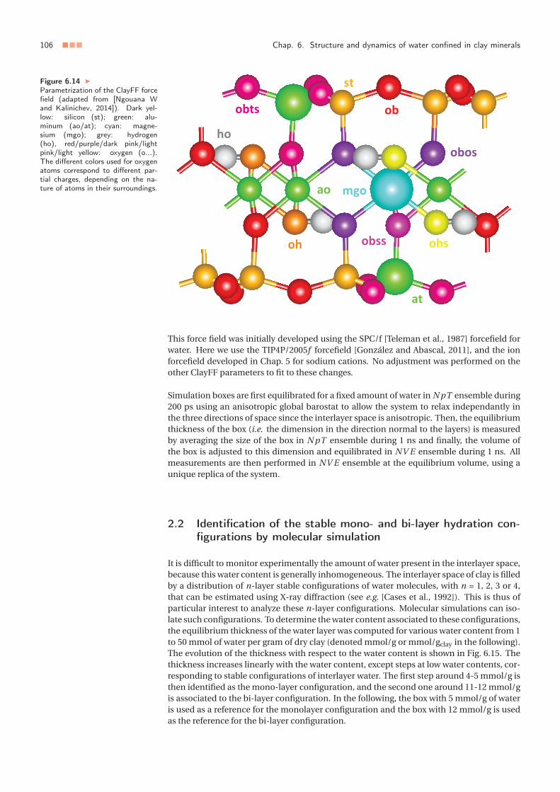
106 ■■■ Chap. 6. Structure and dynamics of water confined in clay minerals
Figure 6.14 �
Parametrization of the ClayFF forcefield (adapted from [Ngouana Wand Kalinichev, 2014]). Dark yel-low: silicon (st); green: alu-minum (ao/at); cyan: magne-sium (mgo); grey: hydrogen(ho), red/purple/dark pink/lightpink/light yellow: oxygen (o...).The different colors used for oxygenatoms correspond to different par-tial charges, depending on the na-ture of atoms in their surroundings.
This force field was initially developed using the SPC/f [Teleman et al., 1987] forcefield forwater. Here we use the TIP4P/2005f forcefield [González and Abascal, 2011], and the ionforcefield developed in Chap. 5 for sodium cations. No adjustment was performed on theother ClayFF parameters to fit to these changes.
Simulation boxes are first equilibrated for a fixed amount of water in N pT ensemble during200 ps using an anisotropic global barostat to allow the system to relax independantly inthe three directions of space since the interlayer space is anisotropic. Then, the equilibriumthickness of the box (i.e. the dimension in the direction normal to the layers) is measuredby averaging the size of the box in N pT ensemble during 1 ns and finally, the volume ofthe box is adjusted to this dimension and equilibrated in NV E ensemble during 1 ns. Allmeasurements are then performed in NV E ensemble at the equilibrium volume, using aunique replica of the system.
2.2 Identification of the stable mono- and bi-layer hydration con-figurations by molecular simulation
It is difficult to monitor experimentally the amount of water present in the interlayer space,because this water content is generally inhomogeneous. The interlayer space of clay is filledby a distribution of n-layer stable configurations of water molecules, with n = 1, 2, 3 or 4,that can be estimated using X-ray diffraction (see e.g. [Cases et al., 1992]). This is thus ofparticular interest to analyze these n-layer configurations. Molecular simulations can iso-late such configurations. To determine the water content associated to these configurations,the equilibrium thickness of the water layer was computed for various water content from 1to 50 mmol of water per gram of dry clay (denoted mmol/g or mmol/gclay in the following).The evolution of the thickness with respect to the water content is shown in Fig. 6.15. Thethickness increases linearly with the water content, except steps at low water contents, cor-responding to stable configurations of interlayer water. The first step around 4-5 mmol/g isthen identified as the mono-layer configuration, and the second one around 11-12 mmol/gis associated to the bi-layer configuration. In the following, the box with 5 mmol/g of wateris used as a reference for the monolayer configuration and the box with 12 mmol/g is usedas the reference for the bi-layer configuration.
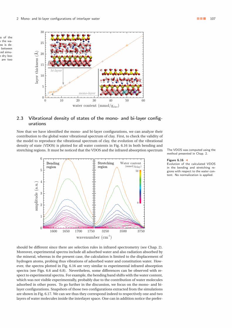
2 Mono- and bi-layer configurations of interlayer water ■■■ 107
ss of theo the wa-ess is de-e betweented simu-e dry boxare two
The VDOS was computed using themethod presented in Chap. 2.
2.3 Vibrational density of states of the mono- and bi-layer config-urations
Now that we have identified the mono- and bi-layer configurations, we can analyze theircontribution to the global water vibrational spectrum of clay. First, to check the validity ofthe model to reproduce the vibrational spectrum of clay, the evolution of the vibrationaldensity of state (VDOS) is plotted for all water contents in Fig. 6.16 in both bending andstretching regions. It must be noticed that the VDOS and the infrared absorption spectrum
Figure 6.16
Evolution of the calculated VDOSin the bending and stretching re-gions with respect to the water con-tent. No normalization is applied.
should be different since there are selection rules in infrared spectrometry (see Chap. 2).Moreover, experimental spectra include all adsorbed water and also radiation absorbed bythe mineral, whereas in the present case, the calculation is limited to the displacement ofhydrogen atoms, probing thus vibrations of adsorbed water and constitution water. How-ever, the spectra plotted in Fig. 6.16 are very similar to experimental infrared absorptionspectra (see Figs. 6.6 and 6.8). Nevertheless, some differences can be observed with re-spect to experimental spectra. For example, the bending band shifts with the water content,which was not visible experimentally, probably due to the contribution of water moleculesadsorbed in other pores. To go further in the discussion, we focus on the mono- and bi-layer configurations. Snapshots of those two configurations extracted from the simulationsare shown in Fig. 6.17. We can see thus they correspond indeed to respectively one and twolayers of water molecules inside the interlayer space. One can in addition notice the prefer-

108 ■■■ Chap. 6. Structure and dynamics of water confined in clay minerals
(a) Mono-layer configuration (b) Bi-layer configuration
Figure 6
Snapshotconfigurahydrogenicon, puiron.
ential orientation of water molecules near the solid surfaces with an O–H bond pointing tothe clay layer, as previously mentioned (see Chap. 1).
The VDOS of these two configurations are plotted in Fig. 6.18. As in the case of experimental
Figure 6.18 �
VDOS of the mono- and bi-layerconfigurations in the bending andstretching regions. A deconvolutionwith Gaussians is shown in dottedlines, using the same A/B/C clas-sification as in the previous sectionfor highly, intermediately and poorlyH-bonded species respectively.
spectra, the VDOS in the bending and stretching regions can be respectively deconvolutedusing three and five Gaussians. Looking first at the stretching region (6.18 (right)), the pres-ence of five Gaussians with a non negligible amplitude shows that the three populations –poorly, intermediately and highly H-bonded – of water molecules are present even in themono-layer configuration. Increasing the water content to form the bi-layer state, the am-plitude of the fourth Gaussian increases less than the others. It means that the averageconnectivity of water molecules inside the interlayer space increases in the bi-layer statewith respect to the mono-layer state.
In the bending region, the band is centered around the frequency of the second Gaussian inthe mono-layer configuration, which was not observed in our infrared experiments, prob-ably, as we already said, because of the contribution of water molecules in other pores. Onthe contrary, in the bi-layer configuration, the spectrum is largely dominated by the thirdcontribution, leading to a shift of the band to higher wavenumbers. Additional calculationsare necessary to interpret this shift, but should enable to learn much more about the dy-namics of confined water and water-clay interactions.

3 Low temperature dynamics of confined water ■■■ 109
Figure 6.19 �
Comparison of the temperature ofthe cold head of the cryostat andthose measured near the sample.
The other spectra are shown in ap-pendix at the end of this chapter.
3 Low temperature dynamics of confined water
3.1 Water thermally induced migration and dynamics singularitiesWe come back now on the experimental far-infrared absorption spectrum of clay and theattribution of its components proposed in Section 1. This aim of this section is to analyzethe low temperature global dynamics of water and try to understand the phases transitionsmentioned in Chap. 1.
3.1.1 Experimental methodsThe sample in the experimental setup used here are the same as those used in Section 1.The hydration cell is coupled to a helium cryostat to adjust the temperature, as explainedin Chap. 2. The sample is first cooled down to 130 K. Then, the temperature is increased bysteps of 5 K. Infrared spectra are recorded dynamically during the increase of the tempera-ture. The temperature is monitored using a thermocouple positioned close to the sample.Its variation during the time of the measurement is lower than 2 K. Due to the thermal iner-tia of the cryostat, the temperature recorded near the sample is slightly lower to that of thecold head. However, this difference remains almost constant during all the experiment, asshown in Fig. 6.19. Consequently, no spurious effect due to the inertia of the cooling systemis expected during the measurement.Six series of measurements were recorded with the same clay deposit, on different pointsof the water adsorption or desorption isotherm: at 0, 30, 75 and 90 % of RH upon hydra-tion, and at 75 and 30 % of RH upon dehydration. For each measurement, the sample wasfirst equilibrated at the corresponding vapor pressure at room temperature, and then, wasisolated from the hydration setup before cooling starts.
3.1.2 ResultsAll measurements show a similar evolution of the absorption spectrum with the tempera-ture. So, for the sake of simplicity, we only show curves corresponding to the sample equi-librated at RH = 30 % upon hydration. Moreover, for a given RH, except the contributionat 170 cm−1 associated to Na inner-sphere complexes, the different spectral contributionsmentioned in Section 1, i.e. bands at 340, 470, 520 and 630 cm−1, behave similarly whenthe temperature is increased. All these contributions were attributed to vibrations insidethe clay layers, but were shown to be highly sensitive to the water content (see Section 1).The curve corresponding to the evolution of the height of the band at 340 cm−1 is shown inFig. 6.20. The global variation of the height of the peak appears complex. It increases from130 to 250 K approximatively in a linear way. Three points corresponding to an increase ofthe slope are visible at 150, 210 and 235 K approximatively. Then, the curve decreases upto 275 K approximatively, and increases again at higher temperature, with a slope similar tothose corresponding to temperatures lower than 150 K. Moreover, the last segment looks inthe continuation of the first one, as underlined by the dotted line in Fig. 6.20. The evolutionof others layer bands are a little bit simpler, with no singularity between 150 and 250 K, butthe global shape is almost the same.
All these slope changes should correspond to sample singularities with respect to the tem-perature. This is confirmed by the similarity between our measurements and heat capac-ity measurements on a similar clay sample by Gailhanou (see Fig. 6.20) [Gailhanou, 2005].However, one must distinguish singularities associated to water and those associated to themineral itself. To this extent, it can be interesting to look at the temperature evolution of adehydrated sample. The evolution of the 340 cm−1 band at RH = 0 % is also given in Fig. 6.20.We also reported some typical spectra recorded at various temperatures between 130 and300 K at RH = 0 % in Fig. 6.21.
Various singularities are also present in the evolution of the height of the 340 cm−1 band,but not as much as for RH = 30 %, and the shape of the curve is slightly different. There isno more slope break at 210 and 235 K, and the slope between 150 and 210 K is lower at RH= 0 % than at RH = 30 %. The decrease between 250 and 275 K is also lower at RH = 0 %, but
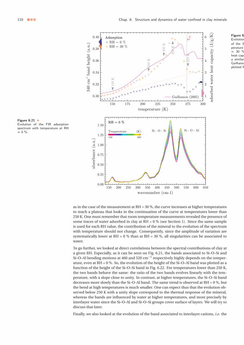
110 ■■■ Chap. 6. Structure and dynamics of water confined in clay minerals
Figure 6
Evolutionof the 34perature= 30 %heat capaa similarGailhanouplotted fo
Figure 6.21
Evolution of the FIR adsorptionspectrum with temperature at RH= 0 %.
as in the case of the measurement at RH = 30 %, the curve increases at higher temperaturesto reach a plateau that looks in the continuation of the curve at temperatures lower than250 K. One must remember that room temperature measurements revealed the presence ofsome traces of water adsorbed in clay at RH = 0 % (see Section 1). Since the same sampleis used for each RH value, the contribution of the mineral to the evolution of the spectrumwith temperature should not change. Consequently, since the amplitude of variation aresystematically lower at RH = 0 % than at RH = 30 %, all singularities can be associated towater.
To go further, we looked at direct correlations between the spectral contributions of clay ata given RH. Especially, as it can be seen on Fig. 6.21, the bands associated to Si–O–Si andSi–O–Al bending motions at 460 and 520 cm−1 respectively highly depends on the temper-ature, even at RH = 0 %. So, the evolution of the height of the Si–O–Al band was plotted as afunction of the height of the Si–O–Si band in Fig. 6.22. For temperatures lower than 250 K,the two bands behave the same: the ratio of the two bands evolves linearly with the tem-perature, with a slope close to unity. In contrast, at higher temperatures, the Si–O–Si banddecreases more slowly than the Si–O–Al band. The same trend is observed at RH = 0 %, butthe bend at high temperatures is much smaller. One can expect thus that the evolution ob-served below 250 K with a unity slope correspond to the thermal response of the mineral,whereas the bands are influenced by water at higher temperatures, and more precisely byinterlayer water since the Si–O–Al and Si–O–Si groups cover surface of layers. We will try todiscuss that later.
Finally, we also looked at the evolution of the band associated to interlayer cations, i.e. the
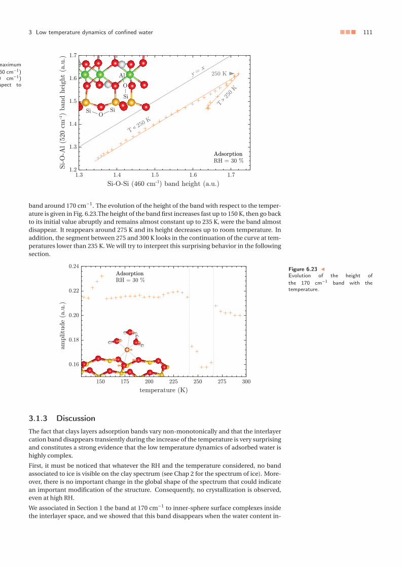
3 Low temperature dynamics of confined water ■■■ 111
maximum60 cm−1)0 cm−1)spect to
band around 170 cm−1. The evolution of the height of the band with respect to the temper-ature is given in Fig. 6.23.The height of the band first increases fast up to 150 K, then go backto its initial value abruptly and remains almost constant up to 235 K, were the band almostdisappear. It reappears around 275 K and its height decreases up to room temperature. Inaddition, the segment between 275 and 300 K looks in the continuation of the curve at tem-peratures lower than 235 K. We will try to interpret this surprising behavior in the followingsection.
Figure 6.23 �
Evolution of the height ofthe 170 cm−1 band with thetemperature.
3.1.3 DiscussionThe fact that clays layers adsorption bands vary non-monotonically and that the interlayercation band disappears transiently during the increase of the temperature is very surprisingand constitutes a strong evidence that the low temperature dynamics of adsorbed water ishighly complex.
First, it must be noticed that whatever the RH and the temperature considered, no bandassociated to ice is visible on the clay spectrum (see Chap 2 for the spectrum of ice). More-over, there is no important change in the global shape of the spectrum that could indicatean important modification of the structure. Consequently, no crystallization is observed,even at high RH.
We associated in Section 1 the band at 170 cm−1 to inner-sphere surface complexes insidethe interlayer space, and we showed that this band disappears when the water content in-

112 ■■■ Chap. 6. Structure and dynamics of water confined in clay minerals
side the interlayer space increases, due to the progressive transformation to outer-spheresurface complexes. Since the band is present at low temperatures (and looks in the contin-uation of the band at high temperatures), the transient disappearance of the band cannot beassociated to some freezing. It does not mean that there is no freezing, but that freezing, ifoccurs, do not affect the shape of the spectrum. Consequently, the transient disappearanceof the band should be associated to transient formation of outer-sphere surface complexes,and thus, a transient increase of the water content inside the interlayer space between 235and 275 K. Since the global water content inside the experimental cell is fixed during the ex-periment, it means water moves from one adsorption site to another when the temperatureincreases.
As we discussed in the previous paragraph looking at the correlation between the Si–O–Siand the Si–O–Al bands in Fig. 6.22, the structure and/or dynamics of water at the surfaceof clay layers undergo some change between 250 and 300 K, whereas no singular behav-ior is noticed at lower temperatures. It could mean thus that water at the surface of layersis frozen below 250 K. More specifically, the curve in Fig. 6.22 shows no more evolutionat temperatures higher than 275 K, so surface water melts between 250 and 275 K. This isconsistent with the experimental observations by Maheshwari et al. and Fleury et al. [Ma-heshwari et al., 2013, Fleury et al., 2013] who observed a partial freezing of water at layersurfaces around 273 K.
In addition, the similar evolution of the absorption spectrum below 150 K and above 275 K,as shown with the dotted line in Fig. 6.20, might indicate that water is completely frozenbelow 150 K, since glassy state dynamics is in the continuation of the liquid state dynamics.
We associated the band at 340 cm−1 to Si–O–Mg deformations inside the layers, and pointedout the fact that this band should be more sensitive to water close to interlayer cationssince cations stay preferentially near substituted sites of layers, so close to Mg atoms in thepresent case. Thus, it seems natural to associate the singularity observed at 235 K in Fig. 6.20to the disappearance of the 170 cm−1 band at the same temperature. The disappearance ofthe band at 170 cm−1 indicates an increase of the water content around ions and a swellingof the interlayer space below 235 K, but not above. This might be explained by a freezing ofwater around cations at lower temperatures, preventing thus clay swelling.
Then, between 150 and 235 K, the slow evolution of the band at 340 cm−1 might be explainedby the migration of some water molecules inside the interlayer space, and especially aroundcations, but this migration is limited because swelling is inhibited by the fact that cationsare frozen. The slope increase at 210 K indicates the migration is somehow easier between210 and 235 K, that can be explained by a partial melting of water bi-layer configurations ininterlayer space.
3.1.4 Summary and conclusion
Putting together all elements discussed in the previous paragraph, we suggest the followingmechanism. At temperatures lower than 150 K, water adsorbed in clay is completely frozen.Increasing the temperature, water in mesopores progressively melts from 150 to 210 K. Be-tween 210 and 240 K, water in interlayer space with several adsorbed water layers partiallymelts whereas surface water and water around cations remains frozen, allowing migrationof a few water molecules from mesopores to interlayer space. At 240 K, water found backmobility around interlayer cations, allowing larger expansion of interlayer space, and thus,migration of more water molecules from mesopores to interlayer space. This causes thedisappearance of inner-sphere surface complexes. Then, from 250 K to 275 K, water at layersurfaces melts, with a partial re-balancing of water contents between mesopores and inter-layer space, i.e. water migrates again from interlayer space to mesopores. Finally, at 275 K,there is no more frozen water and stable monolayer configurations inside interlayer spaceare recovered, with associated inner-sphere surface complexes.
We showed that temperature variations are associated with water migration between thedifferent porosities. Water in each pore freeze at a more or less low temperature, with-out crystallization. It means thus water is in a glassy state. It is consistent with observa-tions by Gailhanou, Maheshwari et al. and Fleury et al. [Gailhanou, 2005,Maheshwari et al.,

3 Low temperature dynamics of confined water ■■■ 113
2013, Fleury et al., 2013], but in disagreement with assumptions by Salles et al. [Salles et al.,2010] who predict no freezing of interlayer water. Further study, for example using X-raydiffraction to follow directly the evolution of the interlayer space with temperature, are nec-essary to confirm the migration mechanism proposed here. Moreover, advanced molecularsimulations could be used with interest to analyse the stability of a liquid-like phase insidethe interlayer space at low temperatures through a nucleation analysis (see e.g. [Sosso et al.,2016]), but this is beyond the scope of the present dissertation.
3.2 Low temperature hydrodynamic properties of interlayer waterWe showed in the previous part that there is no signature of crystallization of adsorbed wa-ter. However, the infrared probe fails to distinguish between “liquid-like” and “amorphous”(glassy) water. To this extent, simulations can give supplemental information. In this sec-tion, we come back on molecular dynamics simulations of interlayer water using the sameroutine as in Section 2, and perform steady-state shear flow calculations of the hydrody-namics properties of water and of the interface using the methods developed in Chaps. 3and 4, with however a slight modification. Since the clay layers are flexible, the thermostatis applied to the walls (layers) instead of water. This avoids spurious effects in the dynamicsdue to the thermostat. To validate the method, all calculations are performed for a watercontent equal to 50 mmol/g, which is very high compared to experiments and correspondsto almost no confinement. Further work would consist in applying the same procedure tothe bi-layer configuration to characterize the dynamics of interlayer water.
The evolution of the shear viscosity of interlayer water with the temperature is plotted inFig. 6.24. The curve is very similar to that of bulk water, but is slightly shifted up. This is not
Figure 6.24 �
Evolution of the shear viscosity ofinterlayer water, and of the clay-water friction coefficient and sliplength with respect to the temper-ature. The shear viscosity valuescalculated obtained numerically forbulk water in Chap. 3 are also plot-ted for comparison.
surprising since there are a lot of cations solvated inside interlayer water, and we showed inChap. 5 that numerical models predicts an increase of the shear viscosity when the salt con-centration is increased in the case of small ions. The shear viscosity can be extrapolated atlower temperatures to investigate about a possible glass transition. Consequently, repeatingthose calculations at low temperatures might help to identify the various phase transitionsobserved in the previous section.
We also looked at the evolution with the temperature of the properties of the water-clayinterface, through its friction coefficient and its slip length using nonequilibrium steady-state shear flow calculations. The corresponding curves are plotted in Fig. 6.24. Contrary towhat was observed in the case of the hydrophobic model surface (see Chap. 4), the frictioncoefficient calculated under shear-flow evolves monotonically over the range of tempera-tures considered here, with an increase at low temperatures. Interestingly, the slip lengthremains almost constant with the temperature, meaning the increase of the friction coeffi-cient follow that of the shear viscosity of interlayer water. The value, around 5 nm, is much
114 ■■■ Chap. 6. Structure and dynamics of water confined in clay minerals
higher than the molecular size (about 3 Å). This indicates a hydrophobic behavior, and thisis in strong disagreement with calculations by Botan et al. who found about 3 Å for the sliplength [Botan et al., 2011]. This might indicate a failure of the model used for clays, and thus,those results must be considered cautiously. Since we do not use the water force field thatwas used to develop ClayFF, water-clay interactions might be misevaluated. The slip lengthcould be thus used to calibrate interaction parameters, for example comparing experimen-tal and calculated slip length of water over mica surfaces. This is beyond the scope of thepresent dissertation, but it is of particular interest for future studies since the slip length in-fluences the permeability of the interlayer space. Especially, a fast increase of the slip lengthat low temperatures, similar to what we observed in Chap. 4 for a model surface, would en-able fast transport inside the interlayer space. This would be problematic for applicationsof clays for the storage of nuclear waste we mentioned in the Introduction.
4 Summary and conclusion
In this chapter, by investigating the now relatively well understood mechanisms of swellingand shrinkage of clays, we showed that the infrared probe can be used as a standalone probeto monitor water inside clay. The vibrational properties of adsorbed water are well resti-tuted by molecular dynamics simulations, that should be used with benefits in the future tomake the best from infrared spectra. We then applied infrared spectrometry to study the lowtemperature dynamics of water adsorbed in clays. We reported a complex mechanism of ex-change of water between the different kind of pores when the temperature is increased, andfreezing of water of all pores, including interlayer water, at various temperatures dependingon the pore type. Finally, we showed that molecular simulations could be used with interestin the future to analyze the low temperature dynamics of interlayer water, but the presentnumerical model must be first corrected to have a good restitution of the properties of thewater-clay interface.
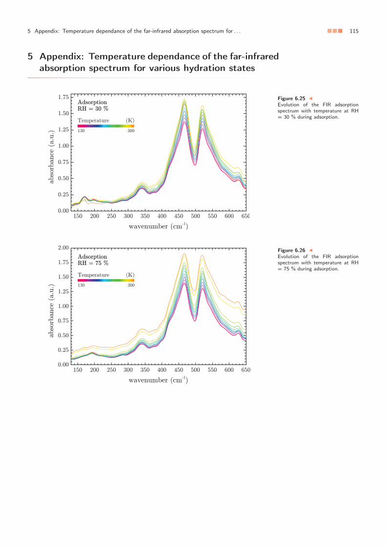
5 Appendix: Temperature dependance of the far-infrared absorption spectrum for . . . ■■■ 115
5 Appendix: Temperature dependance of the far-infrared
absorption spectrum for various hydration states
Figure 6.25 �
Evolution of the FIR adsorptionspectrum with temperature at RH= 30 % during adsorption.
Figure 6.26 �
Evolution of the FIR adsorptionspectrum with temperature at RH= 75 % during adsorption.

116 ■■■ Chap. 6. Structure and dynamics of water confined in clay minerals
Figure 6.27 �
Evolution of the FIR adsorptionspectrum with temperature at RH= 90 % during adsorption.
Figure 6.28 �
Evolution of the FIR adsorptionspectrum with temperature at RH= 75 % during desorption.
Figure 6.29 �
Evolution of the FIR adsorptionspectrum with temperature at RH= 30 % during desorption.

Conclusion ■■■ 117
Conclusion
Looking at the structural and dynamical properties of water in various environments – inpure bulk, near a hydrophobic wall or mixed with salts – we assessed the accuracy of clas-sical molecular dynamics to describe water over a wide range of temperatures, includingthe supercooled regime. Especially, we showed in Chap. 3 that the TIP4P/2005f force fieldreproduces the tabulated shear viscosity of bulk water over both stable and supercooleddomains at ambient pressure. Then, we used those viscosity calculations, combined withstructural relaxation time calculations, to investigate the debated glass transition of water,and pointed out the influence of the choice of the observable used to predict the glass tran-sition temperature. We also showed that the low temperature long-time dynamics of water(e.g. its viscosity and structural relaxation time) can be well described by the so called “elas-tic models”. Finally, we provided a method to perform accurate ab initio calculations inthe isothermal-isobaric ensemble, which, when applied with some dispersion functionalssuch as VdW-DF2, provided a quantitative agreement with several dynamical observablessuch as the liquid shear viscosity. In Chap. 4, we focused on the behavior of water near amodel hydrophobic surface when decreasing the temperature. We observed a very largeincrease of the water-wall slip length at low temperatures that might be due to a transitionfrom a liquid-solid to a solid-solid friction regime, and which could, if confirmed, improveconsiderably the hydrodynamic permeability of nano-channels. In Chap. 5, we developeda new force field to describe accurately water hydrodynamic transport when small ions,like lithium or sodium, are dissolved inside water. However, our model fails for larger ions.Nevertheless, putting everything together, one can expect a good modeling of the interlayerspace of sodium-exchanged montmorillonite clays, that can be seen as a layer of interfa-cial water with sodium cations inside. To this extent, we confronted infrared absorptionmeasurements and classical molecular dynamics calculations in the last chapter to studyboth room temperature and low temperature dynamics of water confined in clay miner-als. We showed that the infrared probe, and, in particular, the far-infrared probe, can beused as a standalone probe to discriminate the water molecules depending on the natureof the pore where they are confined. However, a large part of the infrared absorption spec-trum is hard to interpret without additional information. From this point of view, moleculardynamics constitutes an interesting complement, able to isolate molecular configurationscorresponding to specific hydration states of clays. Then, decreasing the temperature, wehighlighted a complex dynamic of water, with progressive freezing and transfer between thedifferent pores. However, since infrared spectroscopy cannot distinguish fluid water fromits glassy counterpart, molecular dynamics simulations are necessary to reach a completecharacterization of the dynamics of water at low temperatures. Along the way, this low tem-perature molecular study pointed out a weakness of our model, with a wrong restitution ofinterfacial friction, which needs to be adjusted in the future.
This work introduced the key elements to analyze water confined in clays, and more gener-ally various aqueous media, but is, of course, far from being complete. We just mentionedthe necessity to adjust the clay model to improve water-clay interactions. There is also aneed for a more general ion force field, compatible with the TIP4P/2005f force field. Then,using those elements, one could couple molecular dynamics and infrared spectrometry toreach a complete interpretation of the adsorption spectrum, and thus the structure andconnectivity of water adsorbed in clays. One should also look at the influence of the natureof substitutions inside the layers and the nature of the interlayer cation. Ab initio calcula-tions might help to understand these effects, for which dielectric properties of water are ex-pected to play an important role. Then, a precise understanding of the structure of confined

118 ■■■ Conclusion
water and of the interactions between clay layers and water should help to understand therole of clay as catalyst, and to assess the hydrodynamic permeability of clays in the contextof waste management and civil engineering.

Conclusion ■■■ 119
Conclusion
En étudiant les propriétés structurales et dynamiques de l’eau dans divers environnements– eau pure en volume, près d’une surface hydrophobe, ou en présence de sels – nous avonsévalué la précision de la dynamique moléculaire classique pour décrire l’eau sur une largegamme de températures, notamment dans le domaine surfondu. En particulier, nous avonsmontré au Chap. 3 que le champ de force TIP4P/2005f reproduit la viscosité tabulée pourl’eau pure en volume aussi bien dans le domaine stable que dans le domaine surfondu àpression atmosphérique. En combinant ensuite ces valeurs de viscosité à des calculs dutemps de relaxation structural, nous nous sommes intéressés à la transition vitreuse contro-versée de l’eau, et avons mis en avant l’influence du choix de l’observable utilisée pourprédire la température de transition vitreuse. Nous avons également montré que la dy-namique aux temps long de l’eau à basse température (sondée à travers sa viscosité et letemps de relaxation structural) est bien décrite par les modèles dits « élastiques ». Enfin,nous avons mis en place une méthode pour réaliser des calculs ab initio précis dans l’en-semble isotherme-isobare, qui, lorsqu’elle est mise en œuvre avec des fonctionnelles dis-persives telles que VdW-DF2, permettent d’évaluer de manière quantitative différentes ob-servables dynamiques telles que la viscosité du liquide. Dans le Chap. 4, nous nous sommesintéressés au comportement de l’eau près d’une surface hydrophobe modèle lorsque l’ondiminue la température. Nous avons observé une forte augmentation de la longueur deglissement de l’eau à l’interface qui pourrait être due à une transition entre un régime defrottement de type solide-liquide et un régime de frottement solide-solide, et qui pour-rait, si elle est confirmée, améliorer considérablement la perméabilité hydrodynamique desnano-canaux. Dans le Chap. 5, nous avons développé un nouveau champ de force pour dé-crire de façon précise les propriétés de transport hydrodynamique de l’eau en présence depetits ions tels que le lithium ou le sodium. Cependant, notre modèle est mis en défautpour les ions plus gros. Néanmoins, en regroupant tous les résultats, nous pouvons espérerune bonne modélisation de l’espace interfoliaire des montmorillonites sodiques, que l’onpeut voir comme un film d’eau interfaciale avec des cations sodium. Pour cette raison, nousavons confronté des mesures d’absorption infrarouge et des calculs de dynamique molécu-laire dans le dernier chapitre pour étudier la dynamique de l’eau confinée dans les argiles àla fois à température ambiante et à basse température. Nous avons montré que la spectro-scopie infrarouge, et plus particulièrement la spectroscopie dans l’infrarouge lointain, peutêtre utilisée comme un outil unique pour discriminer les molécules d’eau en fonction dela nature du pore dans lequel elles sont confinées. Cependant, une grande partie de l’in-formation contenue dans le spectre infrarouge est difficile à interpréter sans plus d’indica-tions. À ce titre, la dynamique moléculaire constitue un outil complémentaire intéressant,permettant d’isoler des configurations moléculaires correspondant à des états d’hydrata-tion particuliers de l’argile. Puis, en diminuant la température, nous avons mis en évidenceune dynamique complexe de l’eau, qui gèle progressivement et migre entre les différentstypes de pores. Cependant, comme la spectrométrie infrarouge ne permet pas de distinguerl’eau liquide de sa phase vitreuse, des simulations de dynamique moléculaire sont néces-saires pour caractériser complètement la dynamique de l’eau à basse température. Cetteétude moléculaire à basse température a révélé au passage une faiblesse de notre modèle,à travers une mauvaise restitution des propriétés de frottement interfacial, qui devra êtrecorrigée dans le futur.
Ce travail met en place les principaux éléments nécessaires pour analyser l’eau confinéedans les argiles, et plus généralement dans divers milieux aqueux, mais est, bien sûr, loind’être complète. Nous venons notamment d’évoquer la nécessité d’ajuster le modèle d’ar-

120 ■■■ Conclusion
gile pour améliorer la restitution des interactions eau-argile. Il est également nécessaire dedévelopper un champ de force plus général pour les ions, qui soit compatible avec le mo-dèle TIP4P/2005f. Une fois cela fait, il sera possible de coupler la dynamique moléculaire etla spectrométrie infrarouge pour essayer d’interpréter complètement le spectre d’absorp-tion, et dans le même temps la structure et la connectivité de l’eau adsorbée dans les argiles.Il serait également intéressant de regarder l’influence de la nature des substitutions à l’inté-rieur des feuillets et de la nature du cation interfoliaire. Les simulations ab initio devraientaider à appréhender ces effets, pour lesquelles les propriétés diélectriques de l’eau jouentcertainement un rôle important. Enfin, une compréhension précise de la structure de l’eauconfinée et des interactions entre les feuillets d’argile et l’eau devraient aider à comprendrele rôle de l’argile comme catalyseur, et mieux maîtriser la perméabilité hydrodynamiquedes argiles dans le contexte du stockage des déchets et du génie civil.

Bibliography ■■■ 121
Bibliography
[Abascal and Vega, 2005] Abascal, J. L. and Vega, C. (2005). A general purpose model for the condensed phases ofwater: Tip4p/2005. The Journal of chemical physics, 123(23):234505.
[Abdulagatov et al., 2006] Abdulagatov, I. M., Zeinalova, A. B., and Azizov, N. D. (2006). Experimental viscosityb-coefficients of aqueous licl solutions. Journal of molecular liquids, 126(1):75–88.
[Adam and Gibbs, 1965] Adam, G. and Gibbs, J. (1965). On the temperature dependence of cooperative relaxationproperties in glass-forming liquids. Journal of Chemical Physics, 43:139–146.
[Alfè et al., 2014] Alfè, D., Bartók, A., Csanyi, G., and Gillan, M. (2014). Analyzing the errors of dft approximationsfor compressed water systems. The Journal of chemical physics, 141(1):014104.
[Alfe and Gillan, 1998] Alfe, D. and Gillan, M. J. (1998). First-principles calculation of transport coefficients.Physical review letters, 81(23):5161.
[Allen and Tildesley, 1989] Allen, M. P. and Tildesley, D. J. (1989). Computer simulation of liquids. Oxford univer-sity press.
[Alleva et al., 2012] Alleva, K., Chara, O., and Amodeo, G. (2012). Aquaporins: another piece in the osmotic puzzle.FEBS letters, 586(19):2991–2999.
[Amann-Winkel et al., 2016] Amann-Winkel, K., Böhmer, R., Fujara, F., Gainaru, C., Geil, B., and Loerting, T. (2016).Colloquium: Water’s controversial glass transitions. Reviews of Modern Physics, 88(1):011002.
[Ambrosetti et al., 2012] Ambrosetti, A., Ancilotto, F., and Silvestrelli, P. L. (2012). van der waals-corrected ab initiostudy of water ice–graphite interaction. The Journal of Physical Chemistry C, 117(1):321–325.
[Angell, 2002] Angell, C. A. (2002). Liquid fragility and the glass transition in water and aqueous solutions.Chemical reviews, 102(8):2627–2650.
[Asthagiri et al., 2004] Asthagiri, D., Pratt, L. R., Kress, J. D., and Gomez, M. A. (2004). Hydration and mobility ofho-(aq). Proceedings of the National Academy of Sciences of the United States of America, 101(19):7229–7233.
[Atkins and de Paula, 2010] Atkins, P. and de Paula, J. (2010). Physical Chemistry. OUP Oxford.
[Atkins and Friedman, 2011] Atkins, P. and Friedman, R. (2011). Molecular Quantum Mechanics. OUP Oxford.
[Auerbach et al., 2004] Auerbach, S. M., Carrado, K. A., and Dutta, P. K. (2004). Handbook of layered materials.CRC Press.
[Baer et al., 2014] Baer, M. D., Kuo, I.-F. W., Tobias, D. J., and Mundy, C. J. (2014). Toward a unified picture ofthe water self-ions at the air–water interface: A density functional theory perspective. The Journal of PhysicalChemistry B, 118(28):8364–8372.
[Baer and Mundy, 2011] Baer, M. D. and Mundy, C. J. (2011). Toward an understanding of the specific ion effectusing density functional theory. The Journal of Physical Chemistry Letters, 2(9):1088–1093.
[Baer and Mundy, 2013] Baer, M. D. and Mundy, C. J. (2013). An ab initio approach to understanding the specificion effect. Faraday discussions, 160:89–101.
[Baer et al., 2011] Baer, M. D., Mundy, C. J., McGrath, M. J., Kuo, I.-F. W., Siepmann, J. I., and Tobias, D. J. (2011). Re-examining the properties of the aqueous vapor–liquid interface using dispersion corrected density functionaltheory. The Journal of chemical physics, 135(12):124712.
[Bakli and Chakraborty, 2015] Bakli, C. and Chakraborty, S. (2015). Electrokinetic energy conversion in nanoflu-idic channels: Addressing the loose ends in nanodevice efficiency. Electrophoresis, 36(5):675–681.
[Bankura et al., 2013] Bankura, A., Carnevale, V., and Klein, M. L. (2013). Hydration structure of salt solutions fromab initio molecular dynamics. The Journal of chemical physics, 138(1):014501.
[Barrat et al., 1999] Barrat, J.-L. et al. (1999). Influence of wetting properties on hydrodynamic boundary condi-tions at a fluid/solid interface. Faraday discussions, 112:119–128.
[Barrat and Hansen, 2003] Barrat, J.-L. and Hansen, J.-P. (2003). Basic concepts for simple and complex liquids.Cambridge University Press.
[Bässler, 1987] Bässler, H. (1987). Viscous flow in supercooled liquids analyzed in terms of transport theory forrandom media with energetic disorder. Physical review letters, 58(8):767.
[Becke, 1988] Becke, A. D. (1988). Density-functional exchange-energy approximation with correct asymptoticbehavior. Physical review A, 38(6):3098.
[Beran, 2002] Beran, A. (2002). Infrared spectroscopy of micas. Reviews in Mineralogy and Geochemistry,46(1):351–369.

122 ■■■ Bibliography
[Bérend et al., 1995] Bérend, I., Cases, J. M., François, M., Uriot, J. P., Michot, L., Masion, A., and Thomas, F. (1995).Mechanism of Adsorption and Desorption of Water Vapor by Homoionic Montmorillonites: 2. The Li+, Na+, K+,Rb+, and Cs+-exchanged Forms. Clays and Clay Minerals, 43(3):324–336.
[Berendsen et al., 1987] Berendsen, H., Grigera, J., Straatsma, T., et al. (1987). The missing term in effective pairpotentials. J. phys. Chem, 91(24):6269–6271.
[Berendsen et al., 1981] Berendsen, H., Postma, J., Van Gunsteren, W., and Hermans, J. (1981). Intermolecularforces, D. B. Pullman, Reidel, Dordrecht, page 331.
[Bergonzi et al., 2014] Bergonzi, I., Mercury, L., Brubach, J.-B., and Roy, P. (2014). Gibbs free energy of liquid waterderived from infrared measurements. Physical Chemistry Chemical Physics, 16(45):24830–24840.
[Bernasconi et al., 1995] Bernasconi, M., Chiarotti, G., Focher, P., Scandolo, S., Tosatti, E., and Parrinello, M.(1995). First-principle-constant pressure molecular dynamics. Journal of Physics and Chemistry of Solids,56(3):501–505.
[Berthier, 2011] Berthier, L. (2011). Dynamic heterogeneity in amorphous materials. Physics, 4:42.
[Berthier et al., 2004] Berthier, L., Chandler, D., and Garrahan, J. P. (2004). Length scale for the onset of fickiandiffusion in supercooled liquids. Europhysics Letters, 69:320.
[Bertolini et al., 1982] Bertolini, D., Cassettari, M., and Salvetti, G. (1982). The dielectric relaxation time of super-cooled water. The Journal of Chemical Physics, 76(6):3285–3290.
[Bocquet and Barrat, 1994] Bocquet, L. and Barrat, J.-L. (1994). Hydrodynamic boundary conditions, correlationfunctions, and Kubo relations for confined fluids. Physical review E, 49(4):3079.
[Bocquet and Barrat, 2007] Bocquet, L. and Barrat, J.-L. (2007). Flow boundary conditions from nano- to micro-scales. Soft matter, 3(6):685–693.
[Bocquet and Charlaix, 2010] Bocquet, L. and Charlaix, E. (2010). Nanofluidics, from bulk to interfaces. ChemicalSociety Reviews, 39(3):1073–1095.
[Bocquet and Netz, 2015] Bocquet, L. and Netz, R. R. (2015). Nanofluidics: Phonon modes for faster flow. Naturenanotechnology, 10(8):657–658.
[Bocquet and Tabeling, 2014] Bocquet, L. and Tabeling, P. (2014). Physics and technological aspects of nanoflu-idics. Lab on a Chip, 14(17):3143–3158.
[Boeck et al., 1995] Boeck, E., Coveney, J., and Skipper, N. (1995). Monte carlo molecular modeling studies ofhydrated li-, na-, and k-smectites: understanding the role of k as a clay swelling inhibitor. J. Am. Chem. Soc,117:12608–12617.
[Boek et al., 1995] Boek, E., Coveney, P., Skipper, N., et al. (1995). Monte-carlo molecular modeling studies ofhydrated li-smectites, na-smectites, and k-smectites-understanding the role of potassium as a clay swellinginhibitor. Journal of the American Chemical Society, 117(50):12608–12617.
[Bonthuis et al., 2011] Bonthuis, D. J., Rinne, K. F., Falk, K., Kaplan, C. N., Horinek, D., Berker, A. N., Bocquet, L.,and Netz, R. R. (2011). Theory and simulations of water flow through carbon nanotubes: prospects and pitfalls.Journal of Physics: Condensed Matter, 23(18):184110.
[Botan et al., 2013] Botan, A., Marry, V., Rotenberg, B., Turq, P., and Noetinger, B. (2013). How electrostatics in-fluences hydrodynamic boundary conditions: Poiseuille and electro-osmostic flows in clay nanopores. TheJournal of Physical Chemistry C, 117(2):978–985.
[Botan et al., 2011] Botan, A., Rotenberg, B., Marry, V., Turq, P., and Noetinger, B. (2011). Hydrodynamics in claynanopores. The Journal of Physical Chemistry C, 115:16109–16115.
[Bouazizi et al., 2006] Bouazizi, S., Nasr, S., Jaîdane, N., and Bellissent-Funel, M.-C. (2006). Local order in aqueousnacl solutions and pure water: X-ray scattering and molecular dynamics simulations study. The Journal ofPhysical Chemistry B, 110(46):23515–23523.
[Boukili et al., 2003] Boukili, B., Holtz, F., Bény, J.-M., Abdelouafi, A., and Niazi, S. (2003). Infrared spectra of annitein the interlayer and lattice vibrational range. Swiss Bulletin of Mineralogy and Petrology, 83(1):33–46.
[Brubach et al., 2005] Brubach, J.-B., Mermet, A., Filabozzi, A., Gerschel, A., and Roy, P. (2005). Signatures of thehydrogen bonding in the infrared bands of water. The Journal of chemical physics, 122(18):184509.
[Buch et al., 2007] Buch, V., Milet, A., Vácha, R., Jungwirth, P., and Devlin, J. P. (2007). Water surface is acidic.Proceedings of the National Academy of Sciences, 104(18):7342–7347.
[Buchenau and Zorn, 1992] Buchenau, U. and Zorn, R. (1992). A relation between fast and slow motions in glassyand liquid selenium. EPL (Europhysics Letters), 18(6):523.
[Car and Parrinello, 1985] Car, R. and Parrinello, M. (1985). Unified approach for molecular dynamics and density-functional theory. Physical review letters, 55(22):2471.
[Carrier et al., 2013] Carrier, B., Wang, L., Vandamme, M., Pellenq, R. J.-M., Bornert, M., Tanguy, A., andVan Damme, H. (2013). Esem study of the humidity-induced swelling of clay film. Langmuir, 29(41):12823–12833.
[Cases et al., 1997] Cases, J., Bérend, I., François, M., Uriot, J., Michot, L., and Thomas, F. (1997). Mechanism ofadsorption and desorption of water vapor by homoionic montmorillonite; 3, the mg (super 2+), ca (super 2+),and ba (super 3+) exchanged forms. Clays and Clay Minerals, 45(1):8–22.
[Cases et al., 1992] Cases, J. M., Berend, I., Besson, G., Francois, M., Uriot, J. P., Thomas, F., and Poirier, J. E.(1992). Mechanism of adsorption and desorption of water vapor by homoionic montmorillonite. 1. The sodium-exchanged form. Langmuir, 8(11):2730–2739.

Bibliography ■■■ 123
[Ceriotti et al., 2016] Ceriotti, M., Fang, W., Kusalik, P. G., McKenzie, R. H., Michaelides, A., Morales, M. A., andMarkland, T. E. (2016). Nuclear quantum effects in water and aqueous systems: Experiment, theory, and currentchallenges. Chemical reviews, 116(13):7529–7550.
[Chang et al., 1997] Chang, F.-R. C., Skipper, N., and Sposito, G. (1997). Monte carlo and molecular dynamicssimulations of interfacial structure in lithium-montmorillonite hydrates. Langmuir, 13(7):2074–2082.
[Chaplin, 2017] Chaplin, M. (2017). Water structure and science.
[Chaplin, 2010] Chaplin, M. F. (2010). Structuring and behaviour of water in nanochannels and confined spaces.In Adsorption and phase behaviour in nanochannels and nanotubes, pages 241–255. Springer.
[Charlaix and Ciccotti, 2010] Charlaix, E. and Ciccotti, M. (2010). Capillary condensation in confined media. InHandbook of Nanophysics: Principles and Methods, pages 1–17. CRC Press.
[Chen et al., 2002a] Chen, B., Ivanov, I., Park, J. M., Parrinello, M., and Klein, M. L. (2002a). Solvation structureand mobility mechanism of oh-: A car-parrinello molecular dynamics investigation of alkaline solutions. TheJournal of Physical Chemistry B, 106(46):12006–12016.
[Chen et al., 2002b] Chen, B., Park, J. M., Ivanov, I., Tabacchi, G., Klein, M. L., and Parrinello, M. (2002b). First-principles study of aqueous hydroxide solutions. Journal of the American Chemical Society, 124(29):8534–8535.
[Chen et al., 2006] Chen, S.-H., Mallamace, F., Mou, C.-Y., Broccio, M., Corsaro, C., Faraone, A., and Liu, L. (2006).The violation of the stokes–einstein relation in supercooled water. Proceedings of the National Academy ofSciences, 103(35):12974–12978.
[Chen et al., 1982] Chen, S.-H., Teixeira, J., and Nicklow, R. (1982). Incoherent quasielastic neutron scattering fromwater in supercooled regime. Physical Review A, 26(6):3477.
[Choudhuri and Chandra, 2014] Choudhuri, J. R. and Chandra, A. (2014). An ab initio molecular dynamics studyof the liquid-vapor interface of an aqueous nacl solution: Inhomogeneous density, polarity, hydrogen bonds,and frequency fluctuations of interfacial molecules. The Journal of chemical physics, 141(19):194705.
[Ciamarra and Sollich, 2015] Ciamarra, M. P. and Sollich, P. (2015). Elastic models of the glass transition appliedto a liquid with density anomalies. Journal of Non-Crystalline Solids, 407:23–28.
[Cicero et al., 2008] Cicero, G., Grossman, J. C., Schwegler, E., Gygi, F., and Galli, G. (2008). Water confined innanotubes and between graphene sheets: A first principle study. Journal of the American Chemical Society,130(6):1871–1878.
[Cohen-Tanugi and Grossman, 2012] Cohen-Tanugi, D. and Grossman, J. C. (2012). Water desalination acrossnanoporous graphene. Nano letters, 12(7):3602–3608.
[Corsetti et al., 2013] Corsetti, F., Artacho, E., Soler, J. M., Alexandre, S. S., and Fernández-Serra, M.-V. (2013).Room temperature compressibility and diffusivity of liquid water from first principles. The Journal of chemicalphysics, 139(19):194502.
[Costanzo and Guggenheim, 2001] Costanzo, P. and Guggenheim, S. (2001). Baseline studies of the clay mineralssociety source clays: preface. Clays and Clay Minerals, 49(5):371–371.
[Cygan et al., 2004] Cygan, R. T., Liang, J.-J., and Kalinichev, A. G. (2004). Molecular models of hydroxide, oxyhy-droxide, and clay phases and the development of a general force field. The Journal of Physical Chemistry B,108(4):1255–1266.
[Dalla Bernardina, 2015] Dalla Bernardina, S. (2015). Structure and connectivity of water molecules at theinterfaces of nanoconfined systems. PhD thesis, Université Paris-Saclay.
[Dalla Bernardina et al., 2014] Dalla Bernardina, S., Alabarse, F., Kalinko, A., Roy, P., Chapuis, M., Vita, N., Hiener-wadel, R., Berthomieu, C., Judeinstein, P., Zanotti, J.-M., et al. (2014). New experimental set-ups for studyingnanoconfined water on the ailes beamline at soleil. Vibrational Spectroscopy, 75:154–161.
[de Groot and Grubmüller, 2001] de Groot, B. L. and Grubmüller, H. (2001). Water permeation across biologicalmembranes: mechanism and dynamics of aquaporin-1 and glpf. Science, 294(5550):2353–2357.
[de Groot and Grubmüller, 2005] de Groot, B. L. and Grubmüller, H. (2005). The dynamics and energetics of waterpermeation and proton exclusion in aquaporins. Current opinion in structural biology, 15(2):176–183.
[Debenedetti, 2003] Debenedetti, P. G. (2003). Supercooled and glassy water. Journal of Physics: CondensedMatter, 15(45):R1669.
[Debenedetti and Stillinger, 2001] Debenedetti, P. G. and Stillinger, F. H. (2001). Supercooled liquids and the glasstransition. Nature, 410(6825):259–267.
[Dehaoui et al., 2015] Dehaoui, A., Issenmann, B., and Caupin, F. (2015). Viscosity of deeply supercooled waterand its coupling to molecular diffusion. Proceedings of the National Academy of Sciences, 112(39):12020–12025.
[Del Ben et al., 2013] Del Ben, M., Scho¨nherr, M., Hutter, J., and VandeVondele, J. (2013). Bulk liquid water atambient temperature and pressure from mp2 theory. The Journal of Physical Chemistry Letters, 4(21):3753–3759.
[Delage et al., 2010] Delage, P., Cui, Y.-J., and Tang, A. M. (2010). Clays in radioactive waste disposal. Journal ofRock Mechanics and Geotechnical Engineering, 2(2):111–123.
[Demontis et al., 2013] Demontis, P., Masia, M., and Suffritti, G. B. (2013). Water nanoconfined in clays: the struc-ture of na vermiculite revisited by ab initio simulations. The Journal of Physical Chemistry C, 117(30):15583–15592.
[Ding et al., 2014] Ding, Y., Hassanali, A. A., and Parrinello, M. (2014). Anomalous water diffusion in salt solutions.Proceedings of the National Academy of Sciences, 111(9):3310–3315.
124 ■■■ Bibliography
[DiStasio Jr et al., 2014] DiStasio Jr, R. A., Santra, B., Li, Z., Wu, X., and Car, R. (2014). The individual and collectiveeffects of exact exchange and dispersion interactions on the ab initio structure of liquid water. The Journal ofchemical physics, 141(8):084502.
[Diu et al., 2007] Diu, B., Guthmann, C., Lederer, D., and Roulet, B. (2007). Thermodynamique. Hermann.
[Donohue and Aranovich, 1998] Donohue, M. and Aranovich, G. (1998). Classification of gibbs adsorptionisotherms. Advances in colloid and interface science, 76:137–152.
[Drda and Wang, 1995] Drda, P. P. and Wang, S.-Q. (1995). Stick-slip transition at polymer melt/solid interfaces.Physical review letters, 75(14):2698.
[Dyre, 2006] Dyre, J. C. (2006). Colloquium: The glass transition and elastic models of glass-forming liquids.Reviews of modern physics, 78(3):953.
[Dyre and Olsen, 2004] Dyre, J. C. and Olsen, N. B. (2004). Landscape equivalent of the shoving model. PhysicalReview E, 69(4):042501.
[Dyre et al., 1996] Dyre, J. C., Olsen, N. B., and Christensen, T. (1996). Local elastic expansion model for viscous-flow activation energies of glass-forming molecular liquids. Physical Review B, 53(5):2171.
[Dyre and Wang, 2012] Dyre, J. C. and Wang, W. H. (2012). The instantaneous shear modulus in the shoving model.The Journal of chemical physics, 136(22):224108.
[Ediger, 2000] Ediger, M. (2000). Spatially heterogeneous dynamics in supercooled liquids. Annual Review ofPhysical Chemistry, 51:99–128.
[Falk et al., 2010] Falk, K., Sedlmeier, F., Joly, L., Netz, R. R., and Bocquet, L. (2010). Molecular origin of fast watertransport in carbon nanotube membranes: superlubricity versus curvature dependent friction. Nano letters,10(10):4067–4073.
[Falk et al., 2012] Falk, K., Sedlmeier, F., Joly, L., Netz, R. R., and Bocquet, L. (2012). Ultralow liquid/solid frictionin carbon nanotubes: comprehensive theory for alcohols, alkanes, omcts, and water. Langmuir, 28(40):14261–14272.
[Feibelman, 2013] Feibelman, P. J. (2013). Viscosity of ultrathin water films confined between aluminol surfacesof kaolinite: Ab initio simulations. The Journal of Physical Chemistry C, 117(12):6088–6095.
[Ferrage et al., 2005] Ferrage, E., Lanson, B., Sakharov, B. A., and Drits, V. A. (2005). Investigation of smectite hy-dration properties by modeling experimental x-ray diffraction patterns: Part i. montmorillonite hydration prop-erties. American Mineralogist, 90(8-9):1358–1374.
[Fleury et al., 2013] Fleury, M., Kohler, E., Norrant, F., Gautier, S., M’Hamdi, J., and Barré, L. (2013). Charac-terization and quantification of water in smectites with low-field nmr. The Journal of Physical Chemistry C,117(9):4551–4560.
[Forney and Brandl, 1992] Forney, C. F. and Brandl, D. G. (1992). Control of humidity in small controlled-environment chambers using glycerol-water solutions. HortTechnology, 2(1):52–54.
[Frenkel and Smit, 1996] Frenkel, D. and Smit, B. (1996). Understanding molecular simulations: from algorithmsto applications. Academic, San Diego.
[Frenkel and Smit, 2001] Frenkel, D. and Smit, B. (2001). Understanding molecular simulation: from algorithmsto applications, volume 1. Academic press.
[Frigo and Johnson, 2005] Frigo, M. and Johnson, S. G. (2005). The design and implementation of fftw3.Proceedings of the IEEE, 93(2):216–231.
[Froyen and Cohen, 1986] Froyen, S. and Cohen, M. L. (1986). Structural properties of nacl and kcl under pressure.Journal of Physics C: Solid State Physics, 19(15):2623.
[Furukawa and Tanaka, 2011] Furukawa, A. and Tanaka, H. (2011). Direct evidence of heterogeneous mechanicalrelaxation in supercooled liquids. Physical Review E, 84:061503.
[Gaiduk et al., 2015] Gaiduk, A. P., Gygi, F., and Galli, G. (2015). Density and compressibility of liquid water and icefrom first-principles simulations with hybrid functionals. The journal of physical chemistry letters, 6(15):2902–2908.
[Gailhanou, 2005] Gailhanou, H. (2005). Détermination expérimentale des propriétés thermodynamiques etétude des nanostructures de minéraux argileux. PhD thesis, Université Paul Cézanne Aix-Marseille 3.
[Gallo et al., 1996] Gallo, P., Sciortino, F., Tartaglia, P., and Chen, S.-H. (1996). Slow dynamics of water moleculesin supercooled states. Physical review letters, 76(15):2730.
[Gee et al., 1990] Gee, M. L., McGuiggan, P. M., Israelachvili, J. N., and Homola, A. M. (1990). Liquid to solidliketransitions of molecularly thin films under shear. The Journal of chemical physics, 93(3):1895–1906.
[Gillan et al., 2016] Gillan, M. J., Alfè, D., and Michaelides, A. (2016). Perspective: How good is dft for water? TheJournal of chemical physics, 144(13):130901.
[Goedecker et al., 1996] Goedecker, S., Teter, M., and Hutter, J. (1996). Separable dual-space gaussian pseudopo-tentials. Physical Review B, 54(3):1703.
[Goldsack and Franchetto, 1977] Goldsack, D. E. and Franchetto, R. (1977). The viscosity of concentrated elec-trolyte solutions. i. concentration dependence at fixed temperature. Canadian Journal of Chemistry, 55(6):1062–1072.
[Goniakowski et al., 2007] Goniakowski, J., Finocchi, F., and Noguera, C. (2007). Polarity of oxide surfaces andnanostructures. Reports on Progress in Physics, 71(1):016501.

Bibliography ■■■ 125
[González and Abascal, 2011] González, M. A. and Abascal, J. L. (2011). A flexible model for water based ontip4p/2005. The Journal of chemical physics, 135(22):224516.
[Gonzalez et al., 2016] Gonzalez, M. A., Valeriani, C., Caupin, F., and Abascal, J. L. (2016). A comprehensive sce-nario of the thermodynamic anomalies of water using the tip4p/2005 model. arXiv preprint arXiv:1605.05383.
[Gotze and Sjogren, 1992] Gotze, W. and Sjogren, L. (1992). Relaxation processes in supercooled liquids. Reportson progress in Physics, 55(3):241.
[Gravelle et al., 2013] Gravelle, S., Joly, L., Detcheverry, F., Ybert, C., Cottin-Bizonne, C., and Bocquet, L. (2013). Op-timizing water permeability through the hourglass shape of aquaporins. Proceedings of the National Academyof Sciences, 110(41):16367–16372.
[Greathouse et al., 2009] Greathouse, J. A., Durkin, J. S., Larentzos, J. P., and Cygan, R. T. (2009). Implemen-tation of a morse potential to model hydroxyl behavior in phyllosilicates. The Journal of chemical physics,130(13):134713.
[Griffiths and De Haseth, 2007] Griffiths, P. R. and De Haseth, J. A. (2007). Fourier transform infraredspectrometry, volume 171. John Wiley & Sons.
[Grimme et al., 2010] Grimme, S., Antony, J., Ehrlich, S., and Krieg, H. (2010). A consistent and accurate ab initioparametrization of density functional dispersion correction (dft-d) for the 94 elements h-pu. The Journal ofchemical physics, 132(15):154104.
[Grimme et al., 2011] Grimme, S., Ehrlich, S., and Goerigk, L. (2011). Effect of the damping function in dispersioncorrected density functional theory. Journal of computational chemistry, 32(7):1456–1465.
[Grossman et al., 2004] Grossman, J. C., Schwegler, E., Draeger, E. W., Gygi, F., and Galli, G. (2004). Towards anassessment of the accuracy of density functional theory for first principles simulations of water. The Journal ofchemical physics, 120(1):300–311.
[Guillot, 2002] Guillot, B. (2002). A reappraisal of what we have learnt during three decades of computer simula-tions on water. Journal of Molecular Liquids, 101(1-3):219–260.
[Gusev, 2017] Gusev, V. (2017). Mcm-41.
[Hallett, 1963] Hallett, J. (1963). The temperature dependence of the viscosity of supercooled water. Proceedingsof the Physical Society, 82(6):1046.
[Hansen and McDonald, 2013] Hansen, J.-P. and McDonald, I. R. (2013). Theory of Simple Liquids: WithApplications to Soft Matter. Academic Press.
[Harris and Woolf, 2004] Harris, K. R. and Woolf, L. A. (2004). Temperature and volume dependence of the viscos-ity of water and heavy water at low temperatures. Journal of Chemical & Engineering Data, 49(4):1064–1069.
[Hartkamp and Coasne, 2014] Hartkamp, R. and Coasne, B. (2014). Structure and transport of aqueous elec-trolytes: From simple halides to radionuclide ions. The Journal of chemical physics, 141(12):124508.
[Hartwigsen et al., 1998] Hartwigsen, C., Gœdecker, S., and Hutter, J. (1998). Relativistic separable dual-spacegaussian pseudopotentials from h to rn. Physical Review B, 58(7):3641.
[Hasegawa and Tanimura, 2011] Hasegawa, T. and Tanimura, Y. (2011). A polarizable water model for intramolec-ular and intermolecular vibrational spectroscopies. The Journal of Physical Chemistry B, 115(18):5545–5553.
[Hatch et al., 2012] Hatch, C. D., Wiese, J. S., Crane, C. C., Harris, K. J., Kloss, H. G., and Baltrusaitis, J. (2012). Wateradsorption on clay minerals as a function of relative humidity: application of bet and freundlich adsorptionmodels. Langmuir, 28(3):1790–1803.
[Hatzikiriakos, 2015] Hatzikiriakos, S. G. (2015). Slip mechanisms in complex fluid flows. Soft Matter, 11(40):7851–7856.
[Hecksher and Dyre, 2015] Hecksher, T. and Dyre, J. C. (2015). A review of experiments testing the shoving model.Journal of Non-Crystalline Solids, 407:14–22.
[Heiranian et al., 2015] Heiranian, M., Farimani, A. B., and Aluru, N. R. (2015). Water desalination with a single-layer mos2 nanopore. Nature communications, 6.
[Heller-Kallai et al., 1996] Heller-Kallai, L., Goldstein, T., and Navrotsky, A. (1996). Active components in clay con-densates and extracts as potential geocatalysts. Clays and clay minerals, 44(3):393–397.
[Holmboe et al., 2012] Holmboe, M., Wold, S., and Jonsson, M. (2012). Porosity investigation of compacted ben-tonite using xrd profile modeling. Journal of Contaminant Hydrology, 128(1):19–32.
[Horinek et al., 2009] Horinek, D., Mamatkulov, S. I., and Netz, R. R. (2009). Rational design of ion force fieldsbased on thermodynamic solvation properties. The Journal of chemical physics, 130(12):124507.
[Horn et al., 2004] Horn, H. W., Swope, W. C., Pitera, J. W., Madura, J. D., Dick, T. J., Hura, G. L., and Head-Gordon,T. (2004). Development of an improved four-site water model for biomolecular simulations: Tip4p-ew. TheJournal of chemical physics, 120(20):9665–9678.
[Huang and Bartell, 1995] Huang, J. and Bartell, L. S. (1995). Kinetics of homogeneous nucleation in the freezingof large water clusters. The Journal of Physical Chemistry, 99(12):3924–3931.
[Ishii et al., 1967] Ishii, M., Shimanouchi, T., and Nakahira, M. (1967). Far infra-red absorption spectra of layersilicates. Inorganica Chimica Acta, 1:387–392.
[Isono, 1984] Isono, T. (1984). Density, viscosity, and electrolytic conductivity of concentrated aqueous electrolytesolutions at several temperatures. alkaline-earth chlorides, lanthanum chloride, sodium chloride, sodium ni-trate, sodium bromide, potassium nitrate, potassium bromide, and cadmium nitrate. Journal of chemical andengineering data, 29(1):45–52.

126 ■■■ Bibliography
[Israelachvili et al., 1990] Israelachvili, J., McGuiggan, P., Gee, M., Homola, A., Robbins, M., and Thompson, P.(1990). Liquid dynamics in molecularly thin films. Journal of Physics: Condensed Matter, 2(S):SA89.
[Israelachvili, 2011] Israelachvili, J. N. (2011). Intermolecular and surface forces. Academic press.
[Iwashita et al., 2013] Iwashita, T., Nicholson, D. M., and Egami, T. (2013). Elementary excitations and crossoverphenomenon in liquids. Physical Review Letters, 110(20):205504.
[Jenkins, 1989] Jenkins, D. M. (1989). Empirical study of the infrared lattice vibrations (1100–350 cm- 1) of phlo-gopite. Physics and Chemistry of Minerals, 16(4):408–414.
[Joly et al., 2016] Joly, L., Tocci, G., Merabia, S., and Michaelides, A. (2016). Strong coupling between nanoflu-idic transport and interfacial chemistry: How defect reactivity controls liquid–solid friction through hydrogenbonding. The journal of physical chemistry letters, 7(7):1381–1386.
[Jonchiere et al., 2011] Jonchiere, R., Seitsonen, A. P., Ferlat, G., Saitta, A. M., and Vuilleumier, R. (2011). Vander waals effects in ab initio water at ambient and supercritical conditions. The Journal of chemical physics,135(15):154503.
[Jorgensen et al., 1983] Jorgensen, W. L., Chandrasekhar, J., Madura, J. D., Impey, R. W., and Klein, M. L. (1983).Comparison of simple potential functions for simulating liquid water. The Journal of chemical physics,79(2):926–935.
[Jorgensen and Madura, 1985] Jorgensen, W. L. and Madura, J. D. (1985). Temperature and size dependence formonte carlo simulations of tip4p water. Molecular Physics, 56(6):1381–1392.
[Kann and Skinner, 2014] Kann, Z. and Skinner, J. (2014). A scaled-ionic-charge simulation model that repro-duces enhanced and suppressed water diffusion in aqueous salt solutions. The Journal of chemical physics,141(10):104507.
[Kawasaki and Kim, 2017] Kawasaki, T. and Kim, K. (2017). Identification of time-scales that support violation orpreservation of stokes-einstein relation in supercooled water. arXiv preprint arXiv:1701.06028.
[Kell, 1975] Kell, G. S. (1975). Density, thermal expansivity, and compressibility of liquid water from 0. deg. to 150.deg.. correlations and tables for atmospheric pressure and saturation reviewed and expressed on 1968 temper-ature scale. Journal of Chemical and Engineering Data, 20(1):97–105.
[Kestin et al., 1981a] Kestin, J., Khalifa, H. E., and Correia, R. J. (1981a). Tables of the dynamic and kinematicviscosity of aqueous kcl solutions in the temperature range 25–150 c and the pressure range 0.1–35 mpa. Journalof Physical and Chemical Reference Data, 10(1):57–70.
[Kestin et al., 1981b] Kestin, J., Khalifa, H. E., and Correia, R. J. (1981b). Tables of the dynamic and kinematic vis-cosity of aqueous nacl solutions in the temperature range 20–150 c and the pressure range 0.1–35 mpa. Journalof physical and chemical reference data, 10(1):71–88.
[Kühne et al., 2010] Kühne, T. D., Pascal, T. A., Kaxiras, E., and Jung, Y. (2010). New insights into the structureof the vapor/water interface from large-scale first-principles simulations. The journal of physical chemistryletters, 2(2):105–113.
[Kim et al., 2012] Kim, J. S., Wu, Z., Morrow, A. R., Yethiraj, A., and Yethiraj, A. (2012). Self-diffusion and viscosityin electrolyte solutions. The Journal of Physical Chemistry B, 116(39):12007–12013.
[Kim and Yethiraj, 2008] Kim, J. S. and Yethiraj, A. (2008). The effect of salt on the melting of ice: A moleculardynamics simulation study. The Journal of chemical physics, 129(12):124504.
[Kittrick and Hope, 1963] Kittrick, J. and Hope, E. (1963). A procedure for the particle-size separation of soils forx-ray diffraction analysis. Soil Science, 96(5):319–325.
[Klameth and Vogel, 2015] Klameth, F. and Vogel, M. (2015). Slow water dynamics near a glass transition or a solidinterface: a common rationale. The journal of physical chemistry letters, 6(21):4385–4389.
[Klimeš et al., 2009] Klimeš, J., Bowler, D. R., and Michaelides, A. (2009). Chemical accuracy for the van der waalsdensity functional. Journal of Physics: Condensed Matter, 22(2):022201.
[Klimeš and Michaelides, 2012] Klimeš, J. and Michaelides, A. (2012). Perspective: Advances and challengesin treating van der waals dispersion forces in density functional theory. The Journal of chemical physics,137(12):120901.
[Koch and Holthausen, 2015] Koch, W. and Holthausen, M. C. (2015). A chemist’s guide to density functionaltheory. John Wiley & Sons.
[Kotsalis, 2008] Kotsalis, E. M. (2008). Multiscale modeling and simulation of fullerenes in liquids. PhD thesis,Swiss Federal Institute of Technology Zürich.
[Krack, 2005] Krack, M. (2005). Pseudopotentials for h to kr optimized for gradient-corrected exchange-correlation functionals. Theoretical Chemistry Accounts, 114(1-3):145–152.
[Krynicki et al., 1978] Krynicki, K., Green, C. D., and Sawyer, D. W. (1978). Pressure and temperature dependenceof self-diffusion in water. Faraday Discussions of the Chemical Society, 66:199–208.
[Kühne et al., 2009] Kühne, T. D., Krack, M., and Parrinello, M. (2009). Static and dynamical properties of liq-uid water from first principles by a novel car- parrinello-like approach. Journal of chemical theory andcomputation, 5(2):235–241.
[Kuligiewicz et al., 2015] Kuligiewicz, A., Derkowski, A., Szczerba, M., Gionis, V., and Chryssikos, G. D. (2015). Re-visiting the infrared spectrum of the water–smectite interface. Clays and Clay Minerals, 63(1):15–29.
Bibliography ■■■ 127
[Kumar et al., 2007] Kumar, P., Buldyrev, S. V., Becker, S. R., Poole, P. H., Starr, F. W., and Stanley, H. E. (2007). Break-down of the stokes-einstein relation in supercooled water. Proceedings of the National Academy of Sciences,103(35):12955–12956.
[Kumar and Skinner, 2008] Kumar, R. and Skinner, J. (2008). Water simulation model with explicit three-moleculeinteractions. The Journal of Physical Chemistry B, 112(28):8311–8318.
[Kuo and Mundy, 2004] Kuo, I.-F. W. and Mundy, C. J. (2004). An ab initio molecular dynamics study of the aqueousliquid-vapor interface. Science, 303(5658):658–660.
[Kuo et al., 2006] Kuo, I. W., Mundy, C. J., Eggimann, B. L., McGrath, M. J., Siepmann, J. I., Chen, B., Vieceli, J., andTobias, D. J. (2006). Structure and dynamics of the aqueous liquid-vapor interface: A comprehensive particle-based simulation study? The Journal of Physical Chemistry B, 110(8):3738–3746.
[Laasonen et al., 1993] Laasonen, K., Sprik, M., Parrinello, M., and Car, R. (1993). “abinitio” liquid water. TheJournal of chemical physics, 99(11):9080–9089.
[Landry et al., 2008] Landry, E., Hussein, M., and McGaughey, A. (2008). Complex superlattice unit cell designs forreduced thermal conductivity. Physical Review B, 77(18):184302.
[Lang et al., 1984] Lang, E., Lüdemann, H.-D., and Piculell, L. (1984). Nuclear magnetic relaxation rate dispersionin supercooled heavy water under high pressure. The Journal of chemical physics, 81(9):3820–3827.
[Laperche and Prost, 1991] Laperche, V. and Prost, R. (1991). Assignment of the far-infrared absorption bands of kin micas. Clays and Clay Minerals, 39(3):281–289.
[Larini et al., 2008] Larini, L., Ottochian, A., De Michele, C., and Leporini, D. (2008). Universal scaling betweenstructural relaxation and vibrational dynamics in glass-forming liquids and polymers. Nature Physics, 4(1):42–45.
[Le Caër et al., 2014] Le Caër, S., Klein, G., Ortiz, D., Lima, M., Devineau, S., Pin, S., Brubach, J.-B., Roy, P., Pom-meret, S., Leibl, W., et al. (2014). The effect of myoglobin crowding on the dynamics of water: an infrared study.Physical Chemistry Chemical Physics, 16(41):22841–22852.
[Lee et al., 2014] Lee, D., Schwegler, E., and Kanai, Y. (2014). Dependence of water dynamics on molecular adsor-bates near hydrophobic surfaces: First-principles molecular dynamics study. The Journal of Physical ChemistryC, 118(16):8508–8513.
[Lee and Tuckerman, 2006] Lee, H.-S. and Tuckerman, M. E. (2006). Structure of liquid water at ambient temper-ature from ab initio molecular dynamics performed in the complete basis set limit. The Journal of chemicalphysics, 125(15):154507.
[Lee and Tuckerman, 2007] Lee, H.-S. and Tuckerman, M. E. (2007). Dynamical properties of liquid water fromab initio molecular dynamics performed in the complete basis set limit. The Journal of chemical physics,126(16):164501.
[Lee et al., 2010a] Lee, K., Murray, É. D., Kong, L., Lundqvist, B. I., and Langreth, D. C. (2010a). Higher-accuracyvan der waals density functional. Physical Review B, 82(8):081101.
[Lee et al., 2010b] Lee, K., Yu, G., Woo, E., Hwang, S., and Shin, K. (2010b). Freezing and melting in nanopores. InAdsorption and Phase Behaviour in Nanochannels and Nanotubes, pages 257–272. Springer.
[Li and Wang, 2015] Li, J. and Wang, F. (2015). Pairwise-additive force fields for selected aqueous monovalent ionsfrom adaptive force matching. The Journal of chemical physics, 143(19):194505.
[Li et al., 2007] Li, T.-D., Gao, J., Szoszkiewicz, R., Landman, U., and Riedo, E. (2007). Structured and viscous waterin subnanometer gaps. Physical Review B, 75(11):115415.
[Lide, 1997] Lide, D. (1997). Handbook of chemistry and physics, 78th edition. CRC Press.
[Liu et al., 2006] Liu, L., Chen, S.-H., Faraone, A., Yen, C.-W., Mou, C.-Y., Kolesnikov, A. I., Mamontov, E., and Leao,J. (2006). Quasielastic and inelastic neutron scattering investigation of fragile-to-strong crossover in deeplysupercooled water confined in nanoporous silica matrices. Journal of Physics: Condensed Matter, 18(36):S2261.
[Liu et al., 2011] Liu, L.-M., Laio, A., and Michaelides, A. (2011). Initial stages of salt crystal dissolution determinedwith ab initio molecular dynamics. Physical Chemistry Chemical Physics, 13(29):13162–13166.
[Lock et al., 2002] Lock, A., Bakker, H., et al. (2002). Temperature dependence of vibrational relaxation in liquidh2o. Journal of Chemical Physics, 117(4):1708–1713.
[Ma et al., 2015] Ma, M., Grey, F., Shen, L., Urbakh, M., Wu, S., Liu, J. Z., Liu, Y., and Zheng, Q. (2015). Watertransport inside carbon nanotubes mediated by phonon-induced oscillating friction. Nature nanotechnology,10(8):692–695.
[Ma et al., 2017] Ma, X., Cambré, S., Wenseleers, W., Doorn, S. K., and Htoon, H. (2017). Quasiphase transition ina single file of water molecules encapsulated in (6, 5) carbon nanotubes observed by temperature-dependentphotoluminescence spectroscopy. Physical Review Letters, 118(2):027402.
[Ma et al., 2012] Ma, Z., Zhang, Y., and Tuckerman, M. E. (2012). Ab initio molecular dynamics study of water atconstant pressure using converged basis sets and empirical dispersion corrections. The Journal of chemicalphysics, 137(4):044506.
[Madejová and Komadel, 2001] Madejová, J. and Komadel, P. (2001). Baseline studies of the clay minerals societysource clays: infrared methods. Clays and clay minerals, 49(5):410–432.
[Maduar et al., 2015] Maduar, S., Belyaev, A., Lobaskin, V., and Vinogradova, O. (2015). Electrohydrodynamicsnear hydrophobic surfaces. Physical review letters, 114(11):118301.

128 ■■■ Bibliography
[Maheshwari et al., 2013] Maheshwari, P., Pujari, P. K., Sharma, S. K., Dutta, D., Sudarshan, K., Mithu, V., Madhu,P. K., Deshpande, S., Patil, P. N., and Raje, N. (2013). Phase transition of nanoconfined water in clay: Positronannihilation, nuclear magnetic resonance, and dielectric relaxation studies. The Journal of Physical ChemistryC, 117(27):14313–14324.
[Mahoney and Jorgensen, 2000] Mahoney, M. W. and Jorgensen, W. L. (2000). A five-site model for liquid water andthe reproduction of the density anomaly by rigid, nonpolarizable potential functions. The Journal of ChemicalPhysics, 112(20):8910–8922.
[Majumder et al., 2015] Majumder, S., Dhar, J., and Chakraborty, S. (2015). Resolving anomalies in predictingelectrokinetic energy conversion efficiencies of nanofluidic devices. Scientific reports, 5.
[Malikova et al., 2005] Malikova, N., Cadene, A., Marry, V., Dubois, E., Turq, P., Zanotti, J.-M., and Longeville,S. (2005). Diffusion of water in clays–microscopic simulation and neutron scattering. Chemical Physics,317(2):226–235.
[Mallamace et al., 2007] Mallamace, F., Branca, C., Broccio, M., Corsaro, C., Mou, C.-Y., and Chen, S.-H. (2007).The anomalous behavior of the density of water in the range 30 K < T < 373 K. Proceedings of the NationalAcademy of Sciences, 104(47):18387–18391.
[Mallamace et al., 2006] Mallamace, F., Broccio, M., Corsaro, C., Faraone, A., Wanderlingh, U., Liu, L., Mou, C.-Y.,and Chen, S. (2006). The fragile-to-strong dynamic crossover transition in confined water: nuclear magneticresonance results. The Journal of Chemical Physics, 124:161102.
[Mancinelli et al., 2007] Mancinelli, R., Botti, A., Bruni, F., Ricci, M., and Soper, A. (2007). Perturbation of waterstructure due to monovalent ions in solution. Physical Chemistry Chemical Physics, 9(23):2959–2967.
[Mao and Pappu, 2012] Mao, A. H. and Pappu, R. V. (2012). Crystal lattice properties fully determine short-rangeinteraction parameters for alkali and halide ions. The Journal of chemical physics, 137(6):064104.
[Marcus, 2009] Marcus, Y. (2009). Effect of ions on the structure of water: structure making and breaking.Chemical reviews, 109(3):1346–1370.
[Maréchal, 2006] Maréchal, Y. (2006). The hydrogen bond and the water molecule: The physics and chemistry ofwater, aqueous and bio-media. Elsevier.
[Markesteijn et al., 2012] Markesteijn, A., Hartkamp, R., Luding, S., and Westerweel, J. (2012). A comparison ofthe value of viscosity for several water models using poiseuille flow in a nano-channel. The Journal of chemicalphysics, 136(13):134104.
[Marry et al., 2002] Marry, V., Turq, P., Cartailler, T., and Levesque, D. (2002). Microscopic simulation of structureand dynamics of water and counterions in a monohydrated montmorillonite. The Journal of chemical physics,117(7):3454–3463.
[Martyna et al., 1994] Martyna, G. J., Tobias, D. J., and Klein, M. L. (1994). Constant pressure molecular dynamicsalgorithms. The Journal of Chemical Physics, 101(5):4177–4189.
[Marx and Parrinello, 1996] Marx, D. and Parrinello, M. (1996). Ab initio path integral molecular dynamics: Basicideas. The Journal of chemical physics, 104(11):4077–4082.
[Massat et al., 2016] Massat, L., Cuisinier, O., Bihannic, I., Claret, F., Pelletier, M., Masrouri, F., and Gaboreau, S.(2016). Swelling pressure development and inter-aggregate porosity evolution upon hydration of a compactedswelling clay. Applied Clay Science, 124:197–210.
[Mattsson et al., 2009] Mattsson, J., Wyss, H. M., Fernandez-Nieves, A., Miyazaki, K., Hu, Z., Reichman, D. R., andWeitz, D. A. (2009). Soft colloids make strong glasses. Nature, 462(7269):83–86.
[Mauro et al., 2009] Mauro, J. C., Yue, Y., Ellison, A. J., Gupta, P. K., and Allan, D. C. (2009). Viscosity of glass-forming liquids. Proceedings of the National Academy of Sciences, 106(47):19780–19784.
[McGrath et al., 2011] McGrath, M. J., Kuo, I.-F. W., and Siepmann, J. I. (2011). Liquid structures of water,methanol, and hydrogen fluoride at ambient conditions from first principles molecular dynamics simulationswith a dispersion corrected density functional. Physical Chemistry Chemical Physics, 13(44):19943–19950.
[McGrath et al., 2006] McGrath, M. J., Siepmann, J. I., Kuo, I.-F. W., Mundy, C. J., VandeVondele, J., Hutter, J., Mo-hamed, F., and Krack, M. (2006). Simulating fluid-phase equilibria of water from first principles. The Journal ofPhysical Chemistry A, 110(2):640–646.
[Megyes et al., 2008] Megyes, T., Bálint, S., Grósz, T., Radnai, T., Bakó, I., and Sipos, P. (2008). The structure ofaqueous sodium hydroxide solutions: A combined solution x-ray diffraction and simulation study. The Journalof chemical physics, 128(4):044501.
[Meleshyn and Bunnenberg, 2005] Meleshyn, A. and Bunnenberg, C. (2005). The gap between crystalline andosmotic swelling of na-montmorillonite: A monte carlo study. The Journal of chemical physics, 122(3):034705.
[Miceli et al., 2015] Miceli, G., de Gironcoli, S., and Pasquarello, A. (2015). Isobaric first-principles molecular dy-namics of liquid water with nonlocal van der waals interactions. The Journal of chemical physics, 142(3):034501.
[Michot et al., 2004] Michot, L. J., Bihannic, I., Porsch, K., Maddi, S., Baravian, C., Mougel, J., and Levitz, P. (2004).Phase diagrams of wyoming na-montmorillonite clay. influence of particle anisotropy. Langmuir, 20(25):10829–10837.
[Michot et al., 2013] Michot, L. J., Bihannic, I., Thomas, F., Lartiges, B. S., Waldvogel, Y., Caillet, C., Thieme, J., Fu-nari, S. S., and Levitz, P. (2013). Coagulation of na-montmorillonite by inorganic cations at neutral ph. a com-bined transmission x-ray microscopy, small angle and wide angle x-ray scattering study. Langmuir, 29(10):3500–3510.

Bibliography ■■■ 129
[Mignon et al., 2009] Mignon, P., Ugliengo, P., and Sodupe, M. (2009). Theoretical study of the adsorptionof rna/dna bases on the external surfaces of na+-montmorillonite. The Journal of Physical Chemistry C,113(31):13741–13749.
[Mignon et al., 2010] Mignon, P., Ugliengo, P., Sodupe, M., and Hernandez, E. R. (2010). Ab initio molecular dy-namics study of the hydration of li+, na+ and k+ in a montmorillonite model. influence of isomorphic substitu-tion. Physical Chemistry Chemical Physics, 12(3):688–697.
[Miomandre et al., 2011] Miomandre, F., Sadki, S., Audebert, P., and Méallet-Renault, R. (2011). Électrochimie-2eéd.: Des concepts aux applications. Dunod.
[Møgelhøj et al., 2011] Møgelhøj, A., Kelkkanen, A. K., Wikfeldt, K. T., Schiøtz, J., Mortensen, J. J., Pettersson, L. G.,Lundqvist, B. I., Jacobsen, K. W., Nilsson, A., and Nørskov, J. K. (2011). Ab initio van der waals interactionsin simulations of water alter structure from mainly tetrahedral to high-density-like. The Journal of PhysicalChemistry B, 115(48):14149–14160.
[Morón et al., 2016] Morón, M. C., Prada-Gracia, D., and Falo, F. (2016). Macro and nano scale modelling ofwater–water interactions at ambient and low temperature: relaxation and residence times. Physical ChemistryChemical Physics, 18(14):9377–9387.
[Mott, 1988] Mott, C. (1988). Clay minerals-an introduction. Catalysis today, 2(2-3):199–208.
[Müller et al., 2016] Müller, D., Knoll, C., Seifried, M., and Weinberger, P. (2016). Atr or transmission-a vari-able temperature study comparing both techniques using [fe (3ditz) 3](bf 4) 2 as model system. VibrationalSpectroscopy, 86:198–205.
[Müller and Hertz, 1996] Müller, K. and Hertz, H. (1996). A parameter as an indicator for water- water associationin solutions of strong electrolytes. The Journal of Physical Chemistry, 100(4):1256–1265.
[Mundy and Kuo, 2006] Mundy, C. J. and Kuo, I.-F. W. (2006). First-principles approaches to the structure andreactivity of atmospherically relevant aqueous interfaces. Chemical reviews, 106(4):1282–1304.
[Murata et al., 2000] Murata, K., Mitsuoka, K., Hirai, T., Walz, T., et al. (2000). Structural determinants of waterpermeation through aquaporin-1. Nature, 407(6804):599.
[Nakai et al., 1996] Nakai, T., Sawamura, S., Taniguchi, Y., and Yamaura, Y. (1996). Effect of pressure on theviscosity b coefficient of cesium chloride in water. Journal of the Society of Materials Science, Japan,45(9Appendix):143–147.
[Ngouana W and Kalinichev, 2014] Ngouana W, B. F. and Kalinichev, A. G. (2014). Structural arrangements of iso-morphic substitutions in smectites: Molecular simulation of the swelling properties, interlayer structure, anddynamics of hydrated cs–montmorillonite revisited with new clay models. The Journal of Physical ChemistryC, 118(24):12758–12773.
[NIST, 2017] NIST (2017). Nist standard reference data.
[Nucci and Vanderkooi, 2008] Nucci, N. V. and Vanderkooi, J. M. (2008). Effects of salts of the hofmeister series onthe hydrogen bond network of water. Journal of molecular liquids, 143(2):160–170.
[OEIS Foundation Inc., 2017] OEIS Foundation Inc. (2017). The On-Line Encyclopedia of Integer Sequences. OEISFoundation Inc.
[Osipov et al., 1977] Osipov, Y. A., Zheleznyy, B. V., and Bondarenko, N. F. (1977). The shear viscosity of watersupercooled to -35 °C. Russian Journal of Physical Chemistry, 51(5):748–749.
[Oswald, 2009] Oswald, P. (2009). Rheophysics: the deformation and flow of matter. Cambridge University Press.
[Ottochian et al., 2009] Ottochian, A., De Michele, C., and Leporini, D. (2009). Universal divergenceless scalingbetween structural relaxation and caged dynamics in glass-forming systems. The Journal of Chemical Physics,131(22):224517.
[Overduin and Patey, 2015] Overduin, S. and Patey, G. (2015). Fluctuations and local ice structure in model super-cooled water. The Journal of chemical physics, 143(9):094504.
[Pallares et al., 2016] Pallares, G., Gonzalez, M. A., Abascal, J. L. F., Valeriani, C., and Caupin, F. (2016). Equationof state for water and its line of density maxima down to -120 mpa. Physical Chemistry Chemical Physics,18(8):5896–5900.
[Pastore et al., 2015] Pastore, R., Coniglio, A., and Ciamarra, M. P. (2015). Dynamic phase coexistence in glass-forming liquids. Scientific Reports, 5:11770.
[Pedroza et al., 2015] Pedroza, L. S., Poissier, A., and Fernández-Serra, M.-V. (2015). Local order of liquid water atmetallic electrode surfaces. The Journal of chemical physics, 142(3):034706.
[Pellenq et al., 2001] Pellenq, R. J.-M., Rousseau, B., and Levitz, P. E. (2001). A grand canonical monte carlo study ofargon adsorption/condensation in mesoporous silica glasses. Physical Chemistry Chemical Physics, 3(7):1207–1212.
[Petravic and Harrowell, 2007] Petravic, J. and Harrowell, P. (2007). On the equilibrium calculation of the frictioncoefficient for liquid slip against a wall. The Journal of chemical physics, 127(17):174706.
[Plimpton, 1995] Plimpton, S. (1995). Fast parallel algorithms for short-range molecular dynamics. Journal ofcomputational physics, 117(1):1–19.
[Plimpton et al., 2005] Plimpton, S. et al. (2005). Lammps user’s manual. Sandia National Laboratory.
[Poole et al., 1992] Poole, P. H., Sciortino, F., Essmann, U., and Stanley, H. E. (1992). Phase behaviour of metastablewater. Nature, 360(6402):324–328.

130 ■■■ Bibliography
[Potuzak et al., 2013] Potuzak, M., Guo, X., Smedskjaer, M. M., and Mauro, J. C. (2013). Are the dynamics of a glassembedded in its elastic properties? The Journal of chemical physics, 138(12):12A501.
[Price et al., 1999] Price, W. S., Ide, H., and Arata, Y. (1999). Self-diffusion of supercooled water to 238 k using pgsenmr diffusion measurements. The Journal of Physical Chemistry A, 103(4):448–450.
[Prost et al., 1990] Prost, R., Laperche, V., et al. (1990). Far-infrared study of potassium in micas. Clays and ClayMinerals, 38(4):351–355.
[Puosi and Leporini, 2012a] Puosi, F. and Leporini, D. (2012a). Communication: Correlation of the instantaneousand the intermediate-time elasticity with the structural relaxation in glassforming systems. The Journal ofchemical physics, 136(4):041104.
[Puosi and Leporini, 2012b] Puosi, F. and Leporini, D. (2012b). Communication: Fast and local predictors of theviolation of the stokes-einstein law in polymers and supercooled liquids. The Journal of chemical physics,136(21):211101.
[Rana and Chandra, 2013] Rana, M. K. and Chandra, A. (2013). Ab initio and classical molecular dynamics studiesof the structural and dynamical behavior of water near a hydrophobic graphene sheet. The Journal of chemicalphysics, 138(20):204702.
[Raviv et al., 2001] Raviv, U., Laurat, P., and Klein, J. (2001). Fluidity of water confined to subnanometre films.Nature, 413(6851):51–54.
[Ren and Stein, 2008] Ren, Y. and Stein, D. (2008). Slip-enhanced electrokinetic energy conversion in nanofluidicchannels. Nanotechnology, 19(19):195707.
[Rinnert, 2004] Rinnert, E. (2004). Etats d’hydratation d’argiles suivis par analyses vibrationnelles de l’eau et deshydroxyles dans le proche infrarouge: Applications aux systèmes saponite et bentonite. PhD thesis, UniversitéHenri Poincaré-Nancy I.
[Rønne and Keiding, 2002] Rønne, C. and Keiding, S. R. (2002). Low frequency spectroscopy of liquid water usingthz-time domain spectroscopy. Journal of Molecular Liquids, 101(1-3):199–218.
[Rotenberg, 2014] Rotenberg, B. (2014). Water in clay nanopores. MRS Bulletin, 39(12):1074–1081.
[Rotenberg et al., 2010] Rotenberg, B., Marry, V., Malikova, N., and Turq, P. (2010). Molecular simulation of aque-ous solutions at clay surfaces. Journal of Physics: Condensed Matter, 22(28):284114.
[Ryckaert et al., 1977] Ryckaert, J.-P., Ciccotti, G., and Berendsen, H. J. (1977). Numerical integration of thecartesian equations of motion of a system with constraints: molecular dynamics of n-alkanes. Journal ofComputational Physics, 23(3):327–341.
[Salles et al., 2008] Salles, F., Beurroies, I., Bildstein, O., Jullien, M., Raynal, J., Denoyel, R., and Van Damme, H.(2008). A calorimetric study of mesoscopic swelling and hydration sequence in solid na-montmorillonite.Applied Clay Science, 39(3):186–201.
[Salles et al., 2010] Salles, F., Bildstein, O., Douillard, J., Jullien, M., Raynal, J., and Van Damme, H. (2010). Onthe cation dependence of interlamellar and interparticular water and swelling in smectite clays. Langmuir,26(7):5028–5037.
[Salles et al., 2015] Salles, F., Douillard, J.-M., Bildstein, O., El Ghazi, S., Pre´lot, B., Zajac, J., and Van Damme, H.(2015). Diffusion of interlayer cations in swelling clays as a function of water content: Case of montmorillonitessaturated with alkali cations. The Journal of Physical Chemistry C, 119(19):10370–10378.
[Schmidt et al., 2009] Schmidt, J., VandeVondele, J., Kuo, I.-F. W., Sebastiani, D., Siepmann, J. I., Hutter, J., andMundy, C. J. (2009). Isobaric- isothermal molecular dynamics simulations utilizing density functional the-ory: An assessment of the structure and density of water at near-ambient conditions. The Journal of PhysicalChemistry B, 113(35):11959–11964.
[Schneider and Stoll, 1978] Schneider, T. and Stoll, E. (1978). Molecular-dynamics study of a three-dimensionalone-component model for distortive phase transitions. Physical Review B, 17(3):1302.
[Scilab Enterprises, 2012] Scilab Enterprises (2012). Scilab: Le logiciel open source gratuit de calcul numérique.Scilab Enterprises, Orsay, France.
[Secchi et al., 2016] Secchi, E., Marbach, S., Niguès, A., Stein, D., Siria, A., and Bocquet, L. (2016). Massive radius-dependent flow slippage in carbon nanotubes. Nature, 537(7619):210–213.
[Sellberg et al., 2014] Sellberg, J. A., Huang, C., McQueen, T., Loh, N., Laksmono, H., Schlesinger, D., Sierra, R.,Nordlund, D., Hampton, C., Starodub, D., et al. (2014). Ultrafast x-ray probing of water structure below thehomogeneous ice nucleation temperature. Nature, 510(7505):381–384.
[Sendner et al., 2009] Sendner, C., Horinek, D., Bocquet, L., and Netz, R. R. (2009). Interfacial water at hydrophobicand hydrophilic surfaces: Slip, viscosity, and diffusion. Langmuir, 25(18):10768–10781.
[Shannon, 1976] Shannon, R. t. (1976). Revised effective ionic radii and systematic studies of interatomic dis-tances in halides and chalcogenides. Acta crystallographica section A: crystal physics, diffraction, theoreticaland general crystallography, 32(5):751–767.
[Shi et al., 2013] Shi, Z., Debenedetti, P. G., and Stillinger, F. H. (2013). Relaxation processes in liquids: Variationson a theme by stokes and einstein. Journal of Chemical Physics, 138:12A526.
[Sholl and Steckel, 2011] Sholl, D. and Steckel, J. A. (2011). Density functional theory: a practical introduction.John Wiley & Sons.
[Singh et al., 2016] Singh, R. S., Biddle, J. W., Debenedetti, P. G., and Anisimov, M. A. (2016). Two-state thermody-namics and the possibility of a liquid-liquid phase transition in supercooled tip4p/2005 water. The Journal ofchemical physics, 144(14):144504.

Bibliography ■■■ 131
[Siria et al., 2013] Siria, A., Poncharal, P., Biance, A.-L., Fulcrand, R., Blase, X., Purcell, S. T., and Bocquet, L.(2013). Giant osmotic energy conversion measured in a single transmembrane boron nitride nanotube. Nature,494(7438):455–458.
[Sit and Marzari, 2005] Sit, P.-L. and Marzari, N. (2005). Static and dynamical properties of heavy water at ambientconditions from first-principles molecular dynamics. The Journal of chemical physics, 122(20):204510.
[Skipper et al., 1995] Skipper, N., Chang, F.-R. C., and Sposito, G. (1995). Monte carlo simulation of interlayermolecular structure in swelling clay minerals. i: Methodology. Clays and Clay Minerals, 43(3):285–293.
[Skipper et al., 1991] Skipper, N., Soper, A., and McConnell, J. (1991). The structure of interlayer water in vermi-culite. The Journal of chemical physics, 94(8):5751–5760.
[Skipper et al., 2006] Skipper, N. T., Lock, P. A., Titiloye, J. O., Swenson, J., Mirza, Z. A., Howells, W. S., andFernandez-Alonso, F. (2006). The structure and dynamics of 2-dimensional fluids in swelling clays. Chemicalgeology, 230(3):182–196.
[Smith et al., 2005] Smith, J. D., Cappa, C. D., Wilson, K. R., Cohen, R. C., Geissler, P. L., and Saykally, R. J. (2005).Unified description of temperature-dependent hydrogen-bond rearrangements in liquid water. Proceedings ofthe National Academy of Sciences of the United States of America, 102(40):14171–14174.
[Smith et al., 2000] Smith, R. S., Dohnalek, Z., Kimmel, G. A., Stevenson, K. P., and Kay, B. D. (2000). The self-diffusivity of amorphous solid water near 150 k. Chemical Physics, 258(2):291–305.
[Soper, 2007] Soper, A. (2007). Joint structure refinement of x-ray and neutron diffraction data on disorderedmaterials: application to liquid water. Journal of Physics: Condensed Matter, 19(33):335206.
[Soper and Benmore, 2008] Soper, A. and Benmore, C. (2008). Quantum differences between heavy and light wa-ter. Physical review letters, 101(6):065502.
[Sosso et al., 2016] Sosso, G. C., Tribello, G. A., Zen, A., Pedevilla, P., and Michaelides, A. (2016). Ice formation onkaolinite: Insights from molecular dynamics simulations. The Journal of Chemical Physics, 145(21):211927.
[Sparreboom et al., 2009] Sparreboom, W. v., Van Den Berg, A., and Eijkel, J. (2009). Principles and applications ofnanofluidic transport. Nature nanotechnology, 4(11):713–720.
[Sposito and Prost, 1982] Sposito, G. and Prost, R. (1982). Structure of water adsorbed on smectites. ChemicalReviews, 82:553–573.
[Sposito et al., 1999] Sposito, G., Skipper, N. T., Sutton, R., Park, S.-h., Soper, A. K., and Greathouse, J. A. (1999).Surface geochemistry of the clay minerals. Proceedings of the National Academy of Sciences, 96(7):3358–3364.
[Sprik et al., 1996] Sprik, M., Hutter, J., and Parrinello, M. (1996). Abinitio molecular dynamics simulation ofliquid water: Comparison of three gradient-corrected density functionals. The Journal of chemical physics,105(3):1142–1152.
[Spura et al., 2015] Spura, T., John, C., Habershon, S., and Kühne, T. D. (2015). Nuclear quantum effects in liq-uid water from path-integral simulations using an ab initio force-matching approach. Molecular Physics,113(8):808–822.
[Staib and Hynes, 1993] Staib, A. and Hynes, J. T. (1993). Vibrational predissociation in hydrogen-bonded oh...ocomplexes via oh stretch-oo stretch energy transfer. Chemical physics letters, 204(1-2):197–205.
[Stanley and Teixeira, 1980] Stanley, H. E. and Teixeira, J. (1980). Interpretation of the unusual behavior of h2oand d2o at low temperatures: tests of a percolation model. The Journal of Chemical Physics, 73(7):3404–3422.
[Sui et al., 2001] Sui, H., Han, B.-G., Lee, J. K., Walian, P., and Jap, B. K. (2001). Structural basis of water-specifictransport through the aqp1 water channel. Nature, 414(6866):872–878.
[Sulpizi et al., 2012] Sulpizi, M., Gaigeot, M.-P., and Sprik, M. (2012). The silica–water interface: how the silanolsdetermine the surface acidity and modulate the water properties. Journal of chemical theory and computation,8(3):1037–1047.
[Swadling et al., 2013] Swadling, J. B., Suter, J. L., Greenwell, H. C., and Coveney, P. V. (2013). Influence of surfacechemistry and charge on mineral–rna interactions. Langmuir, 29(5):1573–1583.
[Synchrotron Soleil, 2017] Synchrotron Soleil (2017). About soleil.
[Tainter et al., 2015] Tainter, C. J., Shi, L., and Skinner, J. L. (2015). Reparametrized e3b (explicit three-body) watermodel using the tip4p/2005 model as a reference. Journal of chemical theory and computation, 11(5):2268–2277.
[Tanaka, 1996] Tanaka, H. (1996). A self-consistent phase diagram for supercooled water. Nature, 380:328–330.
[Tardy et al., 1999] Tardy, Y., Mercury, L., Roquin, C., and Vieillard, P. (1999). Le concept d’eau ice-like:hydratation-déshydratation des sels, hydroxydes, zeolites, argiles et matières organiques vivantes ou inertes.Comptes Rendus de l’Académie des Sciences-Series IIA-Earth and Planetary Science, 329(6):377–388.
[Tazi et al., 2012] Tazi, S., Botan, A., Salanne, M., Marry, V., Turq, P., and Rotenberg, B. (2012). Diffusion coefficientand shear viscosity of rigid water models. Journal of Physics: Condensed Matter, 24(28):284117.
[Teixeira, 1993] Teixeira, J. (1993). The physics of liquid water. Le Journal de Physique IV, 3(C1):C1–163.
[Teixeira et al., 1985] Teixeira, J., Bellissent-Funel, M.-C., Chen, S.-H., and Dianoux, A.-J. (1985). Experimentaldetermination of the nature of diffusive motions of water molecules at low temperatures. Physical Review A,31(3):1913.
[Teleman et al., 1987] Teleman, O., Jönsson, B., and Engström, S. (1987). A molecular dynamics simulation of awater model with intramolecular degrees of freedom. Molecular Physics, 60(1):193–203.

132 ■■■ Bibliography
[Thomas and McGaughey, 2008] Thomas, J. A. and McGaughey, A. J. (2008). Reassessing fast water transportthrough carbon nanotubes. Nano letters, 8(9):2788–2793.
[Thomas et al., 2013] Thomas, M., Brehm, M., Fligg, R., Vöhringer, P., and Kirchner, B. (2013). Computing vibra-tional spectra from ab initio molecular dynamics. Physical Chemistry Chemical Physics, 15(18):6608–6622.
[Tobias and Hemminger, 2008] Tobias, D. J. and Hemminger, J. C. (2008). Getting specific about specific ion ef-fects. Science, 319(5867):1197–1198.
[Tocci et al., 2014] Tocci, G., Joly, L., and Michaelides, A. (2014). Friction of water on graphene and hexagonalboron nitride from ab initio methods: very different slippage despite very similar interface structures. Nanoletters, 14(12):6872–6877.
[Tocci and Michaelides, 2014] Tocci, G. and Michaelides, A. (2014). Solvent-induced proton hopping at a water–oxide interface. The journal of physical chemistry letters, 5(3):474–480.
[Todorova et al., 2006] Todorova, T., Seitsonen, A. P., Hutter, J., Kuo, I.-F. W., and Mundy, C. J. (2006). Molecular dy-namics simulation of liquid water: hybrid density functionals. The Journal of Physical Chemistry B, 110(8):3685–3691.
[Torre et al., 2004] Torre, R., Bartolini, P., and Righini, R. (2004). Structural relaxation in supercooled water bytime-resolved spectroscopy. Nature, 428(6980):296–299.
[Tuckerman et al., 1995] Tuckerman, M., Laasonen, K., Sprik, M., and Parrinello, M. (1995). Ab initio molecu-lar dynamics simulation of the solvation and transport of h3o+ and oh-ions in water. The Journal of PhysicalChemistry, 99(16):5749–5752.
[Tuckerman et al., 2006] Tuckerman, M. E., Chandra, A., and Marx, D. (2006). Structure and dynamics of oh-(aq).Accounts of chemical research, 39(2):151–158.
[Tuckerman et al., 2002] Tuckerman, M. E., Marx, D., and Parrinello, M. (2002). The nature and transport mecha-nism of hydrated hydroxide ions in aqueous solution. Nature, 417(6892):925–929.
[Van Horn, 2001] Van Horn, J. D. (2001). Electronic table of shannon ionic radii.
[VandeVondele and Hutter, 2007] VandeVondele, J. and Hutter, J. (2007). Gaussian basis sets for accurate calcula-tions on molecular systems in gas and condensed phases. The Journal of chemical physics, 127(11):114105.
[VandeVondele et al., 2005a] VandeVondele, J., Krack, M., Mohamed, F., Parrinello, M., Chassaing, T., and Hutter,J. (2005a). Quickstep: Fast and accurate density functional calculations using a mixed gaussian and plane wavesapproach. Computer Physics Communications, 167(2):103–128.
[VandeVondele et al., 2005b] VandeVondele, J., Mohamed, F., Krack, M., Hutter, J., Sprik, M., and Parrinello, M.(2005b). The influence of temperature and density functional models in ab initio molecular dynamics simula-tion of liquid water. The Journal of chemical physics, 122(1):014515.
[Vega, 2015] Vega, C. (2015). Water: one molecule, two surfaces, one mistake. Molecular Physics, 113(9-10):1145–1163.
[Vega et al., 2009] Vega, C., Abascal, J. L., Conde, M., and Aragones, J. (2009). What ice can teach us about waterinteractions: a critical comparison of the performance of different water models. Faraday discussions, 141:251–276.
[Villar et al., 2012] Villar, M., Gómez-Espina, R., and Gutiérrez-Nebot, L. (2012). Basal spacings of smectite incompacted bentonite. Applied Clay Science, 65:95–105.
[Walrafen et al., 1986] Walrafen, G., Hokmabadi, M., and Yang, W.-H. (1986). Raman isosbestic points from liquidwater. The Journal of chemical physics, 85(12):6964–6969.
[Wang et al., 2011] Wang, J., Román-Pérez, G., Soler, J. M., Artacho, E., and Fernández-Serra, M.-V. (2011). Density,structure, and dynamics of water: The effect of van der waals interactions. The Journal of chemical physics,134(2):024516.
[Wang, 2012] Wang, W. H. (2012). The elastic properties, elastic models and elastic perspectives of metallic glasses.Progress in Materials Science, 57(3):487–656.
[Wikipedia, 2017] Wikipedia (2017). Hill climbing.
[Xu et al., 2000] Xu, W., Johnston, C. T., Parker, P., and Agnew, S. F. (2000). Infrared study of water sorption on na-,li-, ca-, and mg-exchanged (swy-1 and saz-1) montmorillonite. Clays and Clay Minerals, 48(1):120–131.
[Yamamoto and Onuki, 1998] Yamamoto, R. and Onuki, A. (1998). Heterogeneous diffusion in higly supercooledliquids. Physical Review Letters, 81:4915.
[Yan et al., 1996] Yan, L., Roth, C. B., and Low, P. F. (1996). Changes in the si-o vibrations of smectite layers accom-panying the sorption of interlayer water. Langmuir, 12(18):4421–4429.
[Yao et al., 2015] Yao, Y., Berkowitz, M. L., and Kanai, Y. (2015). Communication: Modeling of concentration de-pendent water diffusivity in ionic solutions: Role of intermolecular charge transfer. The Journal of chemicalphysics.
[Yeh and Hummer, 2004] Yeh, I.-C. and Hummer, G. (2004). System-size dependence of diffusion coefficients andviscosities from molecular dynamics simulations with periodic boundary conditions. The Journal of PhysicalChemistry B, 108(40):15873–15879.
[Yoo et al., 2009] Yoo, S., Zeng, X. C., and Xantheas, S. S. (2009). On the phase diagram of water with densityfunctional theory potentials: The melting temperature of ice ih with the perdew–burke–ernzerhof and becke–lee–yang–parr functionals. The Journal of chemical physics, 130(22):221102.

Bibliography ■■■ 133
[Yoshizawa and Israelachvili, 1993] Yoshizawa, H. and Israelachvili, J. (1993). Fundamental mechanisms of in-terfacial friction. 2. stick-slip friction of spherical and chain molecules. The Journal of Physical Chemistry,97(43):11300–11313.
[Yu and Schmidt, 2011] Yu, K. and Schmidt, J. (2011). Elucidating the crystal face-and hydration-dependent cat-alytic activity of hydrotalcites in biodiesel production. The Journal of Physical Chemistry C, 115(5):1887–1898.
[Zahn et al., 1997] Zahn, K., Méndez-Alcaraz, J. M., and Maret, G. (1997). Hydrodynamic interactions may en-hance the self-diffusion of colloidal particles. Physical review letters, 79(1):175.
[Zaytsev and Aseyev, 1992] Zaytsev, I. D. and Aseyev, G. G. (1992). Properties of aqueous solutions of electrolytes.CRC press.
[Zhang et al., 2011] Zhang, C., Donadio, D., Gygi, F., and Galli, G. (2011). First principles simulations of the in-frared spectrum of liquid water using hybrid density functionals. Journal of chemical theory and computation,7(5):1443–1449.
[Zhang et al., 2013] Zhang, C., Gygi, F., and Galli, G. (2013). Strongly anisotropic dielectric relaxation of water atthe nanoscale. The Journal of Physical Chemistry Letters, 4(15):2477–2481.
[Zhu et al., 2012] Zhu, H., Ghoufi, A., Szymczyk, A., Balannec, B., and Morineau, D. (2012). Anomalous dielectricbehavior of nanoconfined electrolytic solutions. Physical review letters, 109(10):107801.
Copyright © 2022 FDOKUMEN