Towards Object Oriented Software Tools for NumericalMultiscale Methods for P.D.E.s using WaveletsTitus Barsch Angela Kunoth Karsten UrbanAbstract. The enormous increase of computer power in the pastyears has lead to the possibility of solving more and more complexpartial di�erential and integral equations numerically. All the moreone is faced with the problem of developing e�cient software routinesthat can be handled and overlooked by the users. A correspondinglist of basic requirements including a uni�ed disciplined and modularstructure lead to object oriented programming that, in particular,can handle operator equations in higher spatial dimensions.One of the characteristics of multiscale basis{oriented schemesfor solving operator equations numerically featuring wavelets is thatthey do not rely on geometric decompositions of the underlying do-main. During the past few years, we have developed such a softwarepackage for a class of p.d.e.s. We describe some of our software toolsand provide examples for the use of the package.Keywords: Multiscale methods, wavelets, object oriented softwaretools.AMS subject classi�cation: 65N30, 68N99, 68P05, 65Y20.x1 IntroductionDuring the past years, multiscale methods have been proven to be asymp-totically optimal e�cient numerical schemes for elliptic partial di�erentialequations. This means that the resulting linear systems of equations can besolved with an overall amount of work which is of the order of the numberof unknowns. In particular, this implies that the number of iterations for aniterative scheme is independent of the scale. Discretizations allowing suchMultiresolution Analysis and Wavelets for the Numerical Solution of Partial Differential Equations 1W. Dahmen, A. Kurdila, P. Oswald (eds.), pp. 1{30.Copyright c 1996 by Academic Press, Inc.All rights of reproduction in any form reserved.ISBN XXX

2 T. Barsch, A. Kunoth, K. Urbana multilevel structure include uniformly re�ned �nite elements and bases ofmultiresolution spaces. The latter one may be used as a nested sequence oftrial spaces where also bases, called wavelets, of the complement betweentwo succeeding spaces are available. This availability together with addi-tional analytic properties provide a powerful tool to prove the e�ciency ofthe resulting numerical schemes for a whole range of operator equationsincluding elliptic partial di�erential and singular integral equations.Therefore, we aimed at designing a software package that realizes allpromising features of wavelet based multiscale methods for this class ofproblems. In this paper we describe some modules that we have imple-mented during the last years and which might be helpful as a �rst step toa library for this kind of schemes.Naturally, at the beginning we had to limit the scope of problems wewanted to solve and decided to restrict ourselves to stationary problemswhich are Galerkin formulations of(I) scalar elliptic problems with variable coe�cients and(II) systems of elliptic problems with variable coe�cients.As already mentioned, also a class of elliptic operators stemming from(III) boundary integral equationscan be e�ciently treated by wavelet based multiscale methods. Here theadditional problem of compressing the corresponding matrices which arein general not sparse arises. This can be done by using wavelet expan-sions, [20]. We mention (III) here since it is intended that the work juststarted in [6] based on [21] is adjusted according to the common featuresof the problems (I){(III) like data structures, preconditioning and iterativemethods.The Galerkin discretization of (I), (II) leads to the problem of solvinglinear systems of equations involving(i) positive de�nite matrices and(ii) inde�nite matrices stemming from saddle point formulations.Both systems may arise in single- and vector{valued form. For example,for a scalar elliptic partial di�erential equation, including the boundaryconditions into the approximation spaces leads to a single{valued problemof type (i) whereas appending them by Lagrange multipliers as proposed in[26] gives a single{valued system of type (ii). Furthermore, the divergencefree formulation of the Stokes problem (see for example [22]) results in asystem (i) for vector{valued equations whereas the mixed formulation ofthe Stokes problem leads to a vector{valued system (ii). As a last example,

Object oriented software tools for multiscale methods 3from the mixed formulation of a second order problem one obtains a single{valued system of type (ii), [3, 5].It is important to implement these linear systems in such a way thatthe solution method has optimal complexity as predicted by the theoreticalresults and also to use appropriate data structures in order to be able tohandle realistic problems in three and more dimensions.The promising features of wavelet based multiscale methods may besummarized in the following list:(a) no geometric decomposition of the underlying domain,(b) independence of the spatial dimension,(c) easy realization of discretizations of higher order,(d) high e�ciency for multivariate problems by using tensor products,(e) adaptation of the bases to the underlying problem.Some comments on these topics are in order. Although a geometric decom-position of the domain like in the �nite element case allows to handle morecomplex geometries, this may lead to di�culties in three and more dimen-sions. The realization of a multivariate discretization using wavelet typemethods need not to be done by tensor products. However, this approachincreases e�ciency enormously. This fact is also exploited in spectral el-ement methods, [7]. Sometimes the discretization has to ful�ll additionalrequirements due to the structure of the underlying problem. As an exam-ple, consider the Stokes problem, [22]. For the divergence free formulationone needs trial spaces of divergence free vector �elds while for the mixedformulation the trial spaces for velocity and pressure have to satisfy theLady�senskaja-Babu�ska-Brezzi (LBB) condition. The realization of theseconditions in terms of wavelets can be found in [18, 27, 33].We feel that these advantages deserve to draw attention and make itworthwile for an attempt for implementation. However, we are well awareof a so far essential drawback of wavelet based multilevel schemes, namely,the adaptation to domains di�erent from rectangular ones. The investi-gations in [8] where multiscale decompositions for Lipschitz domains wereintroduced may lead to e�cient software also for wavelet type methods ongeneral domains. In view of subsequent investigations in this direction,we have designed our data structures such that they also ful�ll the re-quirements of the construction in [8]. However, for the present we restrictourselves to the case of the domain being the d-dimensional cube [0; 1]d.

4 T. Barsch, A. Kunoth, K. Urban1.1 Requirements on software caused by the scope of problemsThe above described scope of problems requires the following routines fora wavelet based multilevel scheme:� construction of trial functions of arbitrary regularity,� construction of trial spaces that satisfy additional conditions like be-ing divergence-free or ful�lling the LBB condition,� procedures for setting up the corresponding sti�ness matrices andright hand sides,� iterative schemes for solving linear systems of equations and saddlepoint problems,� interfaces for graphic tools to visualize the solution data.These tools must be built in a way such that� data structures do not destroy the optimal complexity,� they are independent of the spatial dimension and the single- orvector{valuedness of the problem,� two{dimensional single{valued problems should run on a personalcomputer and three{dimensional problems on a workstation.1.2 General requirements on softwareIn addition to the items collected in the past section, there are generalrequirements that modern software packages should satisfy. These include� modularity, i.e. , the package consists of independent modules,� use of multi{purpose tools like data structures independent of theproblem,� clearly de�ned interfaces between the di�erent tools,� easy extension of the existing collection of subroutines,� type safe programming,� independence with respect to the underlying hardware and compiler.

Object oriented software tools for multiscale methods 5A prominent well{known possibility to guarantee the satisfaction of thesefeatures is provided by object{oriented programming. In particular, thepossible independence of the spatial dimension and the single- or vector{valuedness are in favour of an object{oriented language like C++. In addi-tion, the more and more complex algorithms and software can be arrangedand validated more clearly. Finally, these codes are more readable for theuser. Many users may prefer packages in FORTRAN with the justi�cationof being wide{spread and a perhaps easier parallelization of the correspond-ing codes. But the above mentioned arguments lead us to use C++.The remainder of this paper is structured as follows. In the next section2 we brie y describe the basic linear algebra structures and tools that areindependent of any multilevel background. Section 3 collects the neces-sary theoretic multiscale concepts and introduces the corresponding datastructures that are frequently used in the sequel. Here Section 3.1 dealswith the masks of generators and wavelets and Section 3.2 with the setupof the sti�ness matrix and the right hand side and the fast computation oftheir entries. The fast multiscale transformations described in Section 3.3provide an e�cient tool which is the main ingredient of the fast multilevelpreconditioners in Section 3.4. In Section 4 we point out future problemsthat we would like to include in the software package. Finally, the two- andthree{dimensional examples in Section 5 illustrate the range of problemswe are able to solve numerically up to now.It should be understood that this paper is more a rough description ofthe present stage of the developed scienti�c software tool box than an easy-to-use manual of a commercial and well{documented package. However, adetailed description of these software tools is in preparation, [2].1.3 Access to softwareTo receive this software package with the corresponding commenting re-ports, the interested reader may write e-mail tourban@igpm.rwth-aachen.deand look at the homepage http://www.igpm.rwth-aachen.de/�urban.x2 Basic linear algebra toolsThe scope of problems as described in Section 1 requires in particular thesolution of linear systems of equations and saddle point problems. Hencewe need some tools handling the algebraic structures, which will be brie ydescribed in this section. Although there is a whole variety of softwarepackages also in C++ available for vector{matrix{operations, we found it

6 T. Barsch, A. Kunoth, K. Urbanadvantageous to develop an own package that allows us to adapt the datastructures to the special requirements of multiscale methods.The classes designed for the handling of vectors are called vector andivector, where the latter one represents multiindices, i.e. , vectors withinteger entries. The memory needed to store the vectors is allocated dy-namically with respect to the length of the particular vector. Naturally, allthe standard manipulations like arithmetic operations, norms and scalarproducts are provided.To handle di�erent kinds of matrices, we constructed the classes matrix,sparse, symspa and blband. The purpose of the class matrix is to handleall kinds of operations in connection with non sparse matrices. Moreover,for the problems described in Section 1 we usually have sparse matrices sothat routines are required that make use of this fact in order to optimizememory. This is done by the class sparse which stores the entries of asparse matrix in the frequently used compressed row format. In addition,many of the matrices arising from the above described problems are sym-metric. Consequently, we have introduced a corresponding class symspathat reduces the amount of memory to store a symmetric sparse matrix bya factor of two.It turns out that many of the system matrices have a block band struc-ture. In spatial dimensions higher than one these matrices become blockbanded with a `depth' equal to the dimension. Our implementation of suchblock band matrices allow an arbitrary depth and are thus automaticallyindependent of the spatial dimension.The basic idea for the class blband that handles such block band ma-trices is a contol ag that checks whether the elements of the matrix arenumbers or banded matrices themselves. Additionally, blband containstwo pointers called LittleBlocks and GreatBlocks. Both pointers sharethe same memory, because only one is used. In C++ this is realized with aunion. During the construction of an object of blband the user speci�es thenumber of elements and if the elements are numbers or matrices. In the �rstcase the control ag is set true and memory is allocated for LittleBlocks,while in the latter case memory is allocated for GreatBlocks and the agis set false. This makes sure that no memory is wasted for storing un-needed objects. If the elements are banded matrices, the same questionrecursively arises for these ones. We emphasize that there is no theoreticallimit concerning the depth of this structure. Since the allocation and theassembly of such a matrix is completely dynamical, this means that thedepth may even be arbitrary at compilation time.For every line in the matrix we store the borders of the horizontal band.The same recursive strategy can therefore also be used for the implementa-tion of multilevel preconditioners or multiscale transformations, see Section3 below.

Object oriented software tools for multiscale methods 7A special feature which drastically reduces the amount of necessarymemory is linked to the observation that in the above described applicationsmany of the involved blocks may be equal. And again, in every blockmany of the entries which can be blocks or numbers may coincide. Thus,the entries of these blocks need only be stored once, while the individualinformation on their position within the matrix is stored individually.Using these data structures we implemented solvers for di�erent kindof algebraic problems. In addition to the usual direct methods for solvinglinear problems like QR decomposition and backward substitution, we im-plemented several iterative routines at �rst for symmetric positive de�nitematrices. These include the conjugate gradient method to solve a lin-ear system of equations and the power iteration for computing the largesteigenvalue of a matrix. The preconditioners that guarantee asymptoticallyoptimal e�ciency of the cg{method are based on multilevel theory and aredescribed in Section 3.4. Moreover, several versions of the Uzawa algorithmfor solving the symmetric saddle point problems (ii) mentioned in Section1 are implemented, including also the modi�ed ones described in [30].All the iterative routines make essential use of matrix{vector multipli-cations. Nevertheless they are independant of the special structure of thematrix. As long as the matrix{vector multiplication is programmend withspecial respect to the structure the iterative routines may be written with-out knowledge of the type of matrix. Here the program language C++reveals its full power: with the use of templates or generic functions all thealgorithms are implemented only once with the type of the matrix as anargument. The compiler automatically generates di�erent routines for thedi�erent types of matrices. It should be mentioned that this program{stylepreserves the main advantage of C++ over C: it is still a type{safe way ofprogramming, i.e. , the compiler checks all arguments.x3 Multiscale methodsIn this section we review the basic concepts of multiscale methods andprovide examples of the structures as they are implemented in the code.Contrary to the setup for multilevel schemes based on �nite elements,wavelet oriented methods do not make use of a decomposition of the un-derlying geometric domain. The advantage of this approach is apparent asin higher dimensions subdivision of a domain into e.g. tetrahedrons may becostly and di�cult. In fact, here �ner discretization levels are introducedautomatically in terms of re�nement equations like (3.1.6) and (3.1.7) be-low.

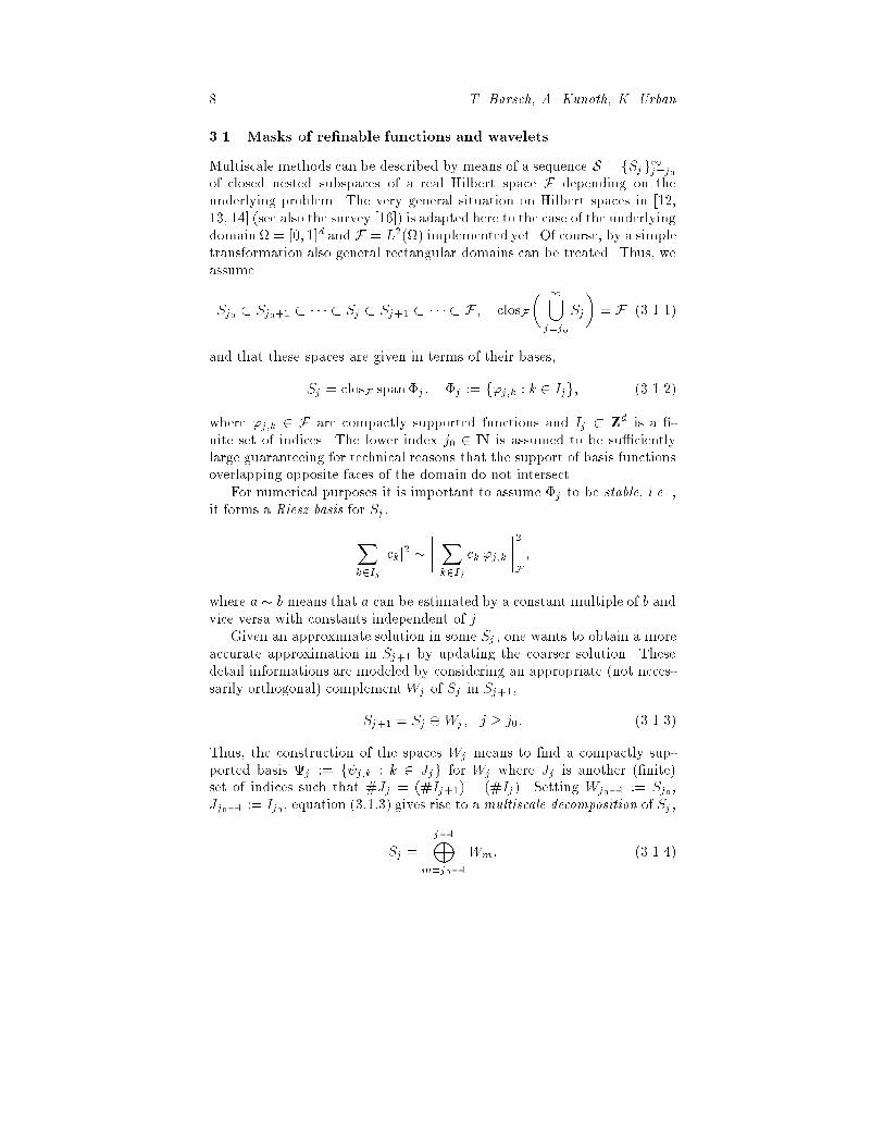
8 T. Barsch, A. Kunoth, K. Urban3.1 Masks of re�nable functions and waveletsMultiscale methods can be described by means of a sequence S = fSjg1j=j0of closed nested subspaces of a real Hilbert space F depending on theunderlying problem. The very general situation on Hilbert spaces in [12,13, 14] (see also the survey [16]) is adapted here to the case of the underlyingdomain = [0; 1]d and F = L2() implemented yet. Of course, by a simpletransformation also general rectangular domains can be treated. Thus, weassumeSj0 � Sj0+1 � � � � � Sj � Sj+1 � � � � � F ; closF� 1[j=j0 Sj� = F (3.1.1)and that these spaces are given in terms of their bases,Sj = closF span�j; �j := f'j;k : k 2 Ijg; (3.1.2)where 'j;k 2 F are compactly supported functions and Ij � ZZd is a �-nite set of indices. The lower index j0 2 IN is assumed to be su�cientlylarge guaranteeing for technical reasons that the support of basis functionsoverlapping opposite faces of the domain do not intersect.For numerical purposes it is important to assume �j to be stable, i.e. ,it forms a Riesz basis for Sj ,Xk2Ij jckj2 � Xk2Ij ck 'j;k 2F ;where a � b means that a can be estimated by a constant multiple of b andvice versa with constants independent of j.Given an approximate solution in some Sj , one wants to obtain a moreaccurate approximation in Sj+1 by updating the coarser solution. Thesedetail informations are modeled by considering an appropriate (not neces-sarily orthogonal) complementWj of Sj in Sj+1,Sj+1 = Sj �Wj; j � j0: (3.1.3)Thus, the construction of the spaces Wj means to �nd a compactly sup-ported basis j := f j;k : k 2 Jjg for Wj where Jj is another (�nite)set of indices such that #Jj = (#Ij+1) � (#Ij). Setting Wj0�1 := Sj0 ,Jj0�1 := Ij0 , equation (3:1:3) gives rise to a multiscale decomposition of Sj ,Sj = j�1Mm=j0�1Wm: (3.1.4)

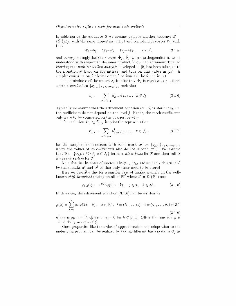
Object oriented software tools for multiscale methods 9In addition to the sequence S we assume to have another sequence ~S =f~Sjg1j=j0 with the same properties (3:1:1) and complement spaces ~Wj suchthat ~Wj?Sj; Wj?~Sj; Wj? ~Wj0; j 6= j0; (3.1.5)and correspondingly for their bases ~�j , ~j where orthogonality is to beunderstood with respect to the inner product (�; �)F . This framework calledbiorthogonal multiresolution analysis developed in [9] has been adapted tothe situation at hand on the interval and thus on unit cubes in [17]. Asimpler construction for lower order functions can be found in [21].The nestedness of the spaces Sj implies that �j is re�nable, i.e. , thereexists a mask aj := fajk;mgk2Ij;m2Ij+1 such that'j;k = Xm2Ij+1 ajk;m'j+1;m; k 2 Ij : (3.1.6)Typically we assume that the re�nement equation (3:1:6) is stationary, i.e.the coe�cients do not depend on the level j. Hence, the mask coe�cientsonly have to be computed on the coarsest level j0.The inclusion Wj � Sj+1 implies the representation j;k = Xm2Ij+1 bjk;m 'j+1;m; k 2 Jj; (3.1.7)for the complement functions with some mask bj := fbjk;mgk2Jj;m2Ij+1where the values of its coe�cients also do not depend on j. We assumethat := f j;k : j � j0; k 2 Jjg forms a Riesz basis for F and then call a wavelet system for F .Note that in the cases of interest the 'j;k; j;k are uniquely determinedby their masks aj and bj so that only these need to be stored.Here we describe this for a simpler case of masks, namely, in the well-known shift-invariant setting on all of lRd where F = L2(lRd) and'j;k(�) := 2dj=2'(2j � �k); j 2 ZZ; k 2 ZZd: (3.1.8)In this case, the re�nement equation (3:1:6) can be written as'(x) = uXk=l ak '(2x� k); x 2 lRd; l = (l1; : : : ; ld); u = (u1; : : : ; ud) 2 ZZd;(3.1.9)where supp a = [l; u], i.e. , ak = 0 for k 62 [l; u]. Often the function ' iscalled the generator of S.Since properties like the order of approximation and adaptation to theunderlying problem can be realized by taking di�erent basis systems �j as

10 T. Barsch, A. Kunoth, K. Urbantrial functions, the software should be independent of the particular choiceof 'j;k. To this end, we designed three classes, namely, MaskBorder, Maskand Basis as follows.Observe that we can writeIj � d�i = 1 fli; : : : ; uig =: Ij; li � ui; li; ui 2 ZZ; 1 � i � d: (3.1.10)The class MaskBorder contains the two vectors l and u of lower and upperborder of the mask indices, respectively. Since the implementation shouldnot depend on the spatial dimension d, the allocation of the integer vectorsrepresenting l (LowBorder) and u (UpBorder) is done dynamically withrespect to d.The class MaskBorder is used to declare an object of the class Maskwhich contains the mask coe�cients ak, l � k � u. Using an object ofMaskBorder as argument for the constructor of an object of Mask, a vectorof length MaskDim := dYi=1(ui � li + 1)is allocated. Now one can de�ne the mask coe�cients as in the followingsimple example for the cardinal B{spline of order 2 for d = 1 where a0 =a2 = 12 , a1 = 1:MaskBorder N2Bord(1); // constructor of MaskBorder// de�nes object N2Bord in 1DN2Bord.putLowBorder(1) = 0; // sets the bordersN2Bord.putUpBorder(1) = 2;Mask N2(N2Bord); // constructor for MaskN2.put(0) = 0.5; // sets mask coe�cientsN2.put(1) = 1;N2.put(2) = 0.5;For multivariate masks we have to index the multiindices in Ij which havethe form of integer vectors. This is done in the canonical way, i.e. , fork = (k1; : : : ; kd) 2 Ij we de�ne for some object MB of the class MaskBorderIndex(k; MB) := dXi=1(ki � li + 1) dYj=i+1(uj � lj + 1):

Object oriented software tools for multiscale methods 11The function Inc increases the multiindex within the borders of MB by one.The multiindices are ordered lexicographically such that k < l is equivalenttok1 < l1 or k1 = l1; k2 < l2; or k1 = l1; k2 = l2; k3 < l3 and so on:By this, we obtain k < l if and only if Index(k; MB) < Index(l; MB). Sinceone often has to realize a loop of the form "k 2 Ij", this can now be doneas follows:ivector k(d);k = MB.getLowBords();for (int i=0; i<MB.getMaskDim(); i++){ // ...Inc(k,MB);}To illustrate its usefulness in dimension independent programming, com-pare the following two equivalent examples, where in the right column thespace dimension only plays the role of a parameter.int SpaceDim = 2;MaskBorder TestBord(SpaceDim);TestBord.putLowBorder(1) = 0; TestBord.putUpBorder(1) = 2;TestBord.putLowBorder(2) = 1; TestBord.putUpBorder(2) = 3;Mask Test(TestBord);Test.put(0,1) = 1; int i, index;Test.put(0,2) = 2; ivector k(2);Test.put(0,3) = 3; k = TestBord.getLowBords();Test.put(1,1) = 4;Test.put(1,2) = 5; for (i=1; i<=TestBord.getMaskDim(); i++)Test.put(1,3) = 6; f index = Index(k,TestBord);Test.put(2,1) = 7; Test.putI(index) = i;Test.put(2,2) = 8; Inc(k,TestBord);Test.put(2,3) = 9; gIn order to collect a �nite number of re�nable functions and to handlelinear combinations of re�nable functions as in (3:1:7), we designed theclass Basis which is an array of Mask with some additional information ags, see [2, 32]. This class is also important for handling wavelet systems

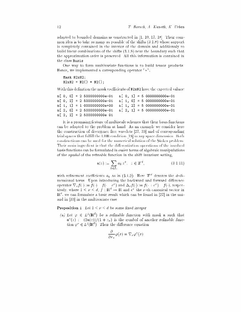
12 T. Barsch, A. Kunoth, K. Urbanadapted to bounded domains as constructed in [1, 10, 17, 18]. Their com-mon idea is to take as many as possible of the shifts (3:1:8) whose supportis completely contained in the interior of the domain and additionaly tobuild linear combinations of the shifts (3:1:8) near the boundary such thatthe approximation order is preserved. All this information is contained inthe class Basis.One way to form multivariate functions is to build tensor products.Hence, we implemented a corresponding operator "�":Mask N2xN2;N2xN2 = N2() * N2();With this de�nition the mask coe�cients of N2xN2 have the expected values:a[ 0, 0] = 2.5000000000e-01 a[ 0, 1] = 5.0000000000e-01a[ 0, 2] = 2.5000000000e-01 a[ 1, 0] = 5.0000000000e-01a[ 1, 1] = 1.0000000000e+00 a[ 1, 2] = 5.0000000000e-01a[ 2, 0] = 2.5000000000e-01 a[ 2, 1] = 5.0000000000e-01a[ 2, 2] = 2.5000000000e-01It is a promising feature of multiscale schemes that their basis functionscan be adapted to the problem at hand. As an example we consider herethe construction of divergence free wavelets [27, 33] and of correspondingtrial spaces that ful�ll the LBB condition [18] in any space dimension. Bothconstructions can be used for the numerical solution of the Stokes problem.Their main ingredient is that the di�erentiation operations of the involvedbasis functions can be formulated in easier terms of algebraic manipulationsof the symbol of the re�nable function in the shift invariant setting,a(z) := Xk2Ij ak zk; z 2 TT d; (3.1.11)with re�nement coe�cients ak as in (3:1:9). Here TT d denotes the d{di-mensional torus. Upon introducing the backward and forward di�erenceoperator r�f(�) := f(�) � f(� � e�) and ��f(�) := f(�+ e�)� f(�), respec-tively, where 1 � � � d, f : lRd ! lR and e� the �-th canonical vector inlRd, we can formulate a basic result which can be found in [27] in the uni-and in [33] in the multivariate case.Proposition 1. Let 1 � � � d be some �xed integer.(a) Let ' 2 L2(lRd) be a re�nable function with mask a such thata�(z) := (2a(z))=(1 + z�) is the symbol of another re�nable func-tion '� 2 L2(lRd). Then the di�erence equation@@x�'(x) = r�'�(x)

Object oriented software tools for multiscale methods 13holds.(b) De�ne ~a�(z) := (1=2) (1 + �z�)a(z). Then there exists a re�nablefunction �� with mask ~a� such that@@x� ��(x) = ��'(x)is valid.The above described modi�cations are realized by the functionsMask MaskDivision(int nu, Mask a);Mask MaskMultiplication(int nu, Mask a);Mask MaskBackwardDifference(Mask c, int nu, int alpha);Mask MaskForwardDifference(Mask c, int nu, int alpha);The �rst two generate 2a(z)1 + z� and 1 + z�2 a(z) and the last two �r�c and���c, respectively.3.2 Re�nable integrals and sti�ness matricesThe Galerkin formulation of problems like (I), (II) in Section 1 and itsdiscretization in terms of the basis �j leads to the linear system of equationsA�jcj = fj ; (3.2.1)where A�j = (a('j;k; 'j;l))k;l2Ij denotes the single scale sti�ness matrixaccording to the bilinear form a(�; �), fj = ((f; 'j;k))k2Ij is the right handside and cj = (cj;k)k2Ij is the vector of unknown (single scale) coe�cients.In the solution process, the �rst task is to set up the linear system(3:2:1), i.e. , to compute the entries of the sti�ness matrix and right handside. Here the entries of the sti�ness matrix are integrals of re�nable func-tions over all of the domain. Note that this is di�erent from the setup in�nite element codes where �rst an element sti�ness matrix on a referenceelement is computed and then the global sti�ness matrix is assembled byusing geometric transformations.Here the energy inner products can be reduced to integrals likeZlRd '0(x) sYi=1D�i'i(x� ki) dx; �i; ki 2 ZZd: (3.2.2)Note that the domain can be treated in terms of the indicator function '0which is also re�nable. We call the terms (3:2:2) re�nable integrals becausethey are re�nable as a function of (k1; : : : ; ks) if all 'i are, [19]. It is provedthere that the evaluation of terms like (3:2:2) reduces to the solution of an

14 T. Barsch, A. Kunoth, K. Urbaneigenvector problem which is uniquely solvable provided that certain mul-tivariate discrete moment conditions are added. A �rst implementation forthe evaluation of (3:2:2) is documented in [25]. This was used to implementan extended version using the above described data structures. To handlethe factors in the integral, we designed the class IntegralFactor.Let us consider the following example of evaluatingZlR2(N1N1)(x)D(1;0)(N3N2)(x�k1)D(0;1)(N2N3)(x�k2) dx (3.2.3)where Di := @jij@xi , i 2 ZZd, which is handled as follows:int SpaceDim = 2;Mask F1, F2, F3;Mask IntegralValues;F1 = N1() * N1();F2 = N3() * N2();F3 = N2() * N3();// For the construction only the space dimension// is needed. The particular factors are put into// this object of the class.IntegralFactor Functions(SpaceDim);Functions.AddFactor(F1);Functions.AddFactor(F2);Functions.AddFactor(F3);// Now the user determines the derivatives: the// first parameter is the number of the function,// the second one the index of the partial derivative,// default value is zero.Functions.putDer(2,1) = 1;Functions.putDer(3,2) = 1;integrals(Functions, IntegralValues);The class IntegralFactor is written as a data structure for the factors inthe integral. The spatial dimension is the parameter used in the constructorso that this function is independent of the dimension. The masks of the

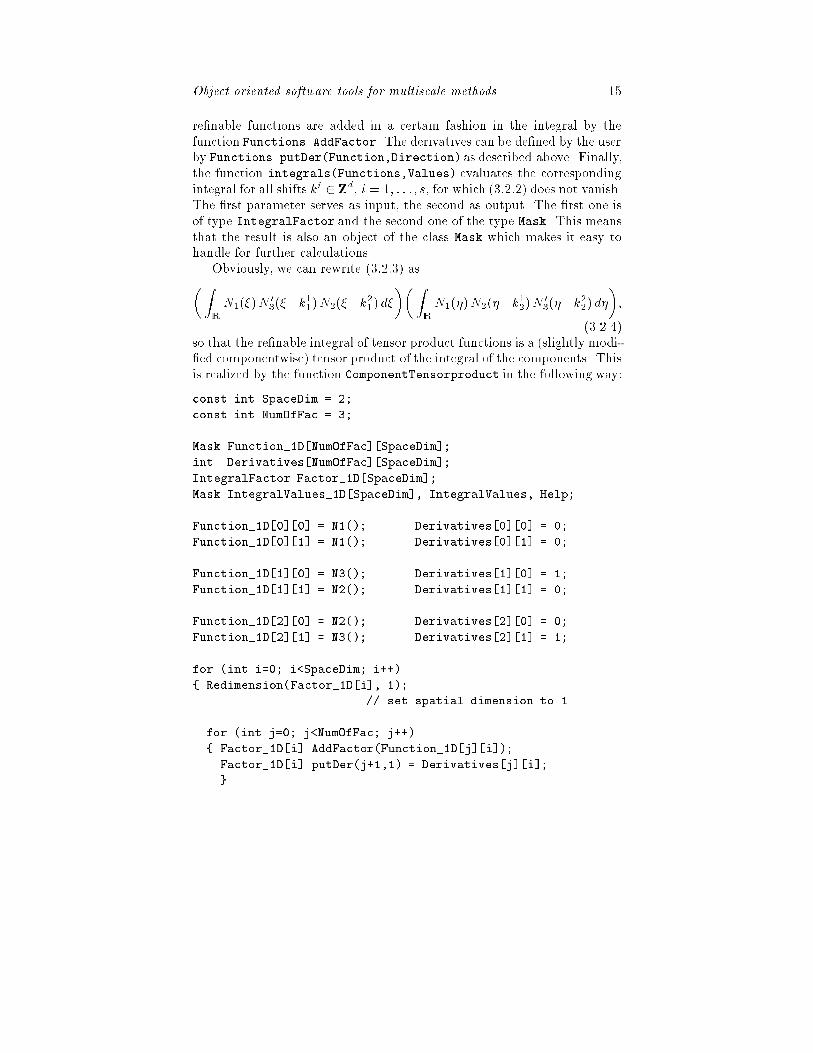
Object oriented software tools for multiscale methods 15re�nable functions are added in a certain fashion in the integral by thefunction Functions.AddFactor. The derivatives can be de�ned by the userby Functions.putDer(Function,Direction) as described above. Finally,the function integrals(Functions,Values) evaluates the correspondingintegral for all shifts ki 2 ZZd, i = 1; : : : ; s, for which (3:2:2) does not vanish.The �rst parameter serves as input, the second as output. The �rst one isof type IntegralFactor and the second one of the type Mask. This meansthat the result is also an object of the class Mask which makes it easy tohandle for further calculations.Obviously, we can rewrite (3:2:3) as�ZlR N1(�)N 03(��k11)N2(��k21) d���ZlRN1(�)N2(��k12)N 03(��k22) d��;(3.2.4)so that the re�nable integral of tensor product functions is a (slightly modi-�ed componentwise) tensor product of the integral of the components. Thisis realized by the function ComponentTensorproduct in the following way:const int SpaceDim = 2;const int NumOfFac = 3;Mask Function_1D[NumOfFac][SpaceDim];int Derivatives[NumOfFac][SpaceDim];IntegralFactor Factor_1D[SpaceDim];Mask IntegralValues_1D[SpaceDim], IntegralValues, Help;Function_1D[0][0] = N1(); Derivatives[0][0] = 0;Function_1D[0][1] = N1(); Derivatives[0][1] = 0;Function_1D[1][0] = N3(); Derivatives[1][0] = 1;Function_1D[1][1] = N2(); Derivatives[1][1] = 0;Function_1D[2][0] = N2(); Derivatives[2][0] = 0;Function_1D[2][1] = N3(); Derivatives[2][1] = 1;for (int i=0; i<SpaceDim; i++){ Redimension(Factor_1D[i], 1);// set spatial dimension to 1for (int j=0; j<NumOfFac; j++){ Factor_1D[i].AddFactor(Function_1D[j][i]);Factor_1D[i].putDer(j+1,1) = Derivatives[j][i];}

16 T. Barsch, A. Kunoth, K. Urbanintegrals(Factor_1D[i], IntegralValues_1D[i]);if (i==0) IntegralValues = IntegralValues_1D[0];else{ Help = ComponentTensorproduct(IntegralValues,IntegralValues_1D[i]);IntegralValues = Help;}}It turns out that the second, tensor product version is much faster thanthe �rst one which computes (3:2:3). For the above example, the �rstalgorithm took 36.122 seconds on a SiliconGraphics R4400 workstationwhile only 0.063 seconds were needed for the second one. This di�erencegets even bigger when dealing with more factors in the integral or higherspatial dimensions. As already mentioned, the same behaviour has alsobeen observed in spectral methods, [7].Since the values of such an integral is also an object of the class mask,we have a straightforward way for the setup of the sti�ness matrix A�j in(3:2:1). As a simple example, let �j be a basis such thata('j;k; 'j;l) = �j a('0;0; '0;l�k) (3.2.5)is valid where �j is some constant depending on j. This assumption isalways satis�ed in the shift{invariant case with bases consisting of re�n-able functions satisfying (3:1:8) and (3:1:9) and constant coe�cients inthe energy inner product. Assume that the values (3:2:5) are stored inBilinearValues and the borders for multiindices according to the entriesof the sti�ness matrix in MatrixBorders. Then the following procedurerealizes the setup:int d; // spatial dimensionMaskBorder MatrixBorders;int MatrixDim = MatrixBorders.getMaskDim();matrix A(MatrixDim,MatrixDim);double alphaj;ivector k(d), l(d), difference(d);int RowIndex, ColIndex, ValueIndex;k = MatrixBorders.getLowBords();

Object oriented software tools for multiscale methods 17for (int i=0; i<MatrixBorders.getMaskDim(); i++){ RowIndex = Index(k,MatrixBorders);l = MatrixBorders.getLowBords();for (int j=0; j<MatrixBorders.getMaskDim(); j++){ difference = l - k;ColIndex = Index(l,MatrixBorders);ValueIndex = Index(difference,BilinearValues);A(RowIndex,ColIndex) = alphaj* BilinearValues.getI(ValueIndex);Inc(l,MatrixBorders);}Inc(k,MatrixBorders);}For the computation of the solution at a given point we have to evaluatere�nable functions, which is done as a special case of integrals for thecase of only one factor.3.3 Multiscale transformationsOne of the most important advantages of multiscale methods is the fastrealization of asymptotically optimal preconditioners [4, 15, 20] which isbased on the e�ciency of multiscale transformations also called the FastWavelet Transforms. Let us brie y recall the main ingredient for the abovedescribed classes of problems. In view of (3:1:4), any vj 2 Sj can either bewritten in single scale representation asvj = Xk2Ij ck 'j;kor in multiscale form asvj = j�1Xm=j0�1 Xk2Jm dm;k m;k:The transformation Tj : (dm;k)m=j0�1;:::;j�1;k2Jm 7! (ck)k2Ij , which takesthe multilevel coe�cients to the single scale ones is known as multiscaletransformation, see [12, 13, 14]. Although the matrix associated with Tj is

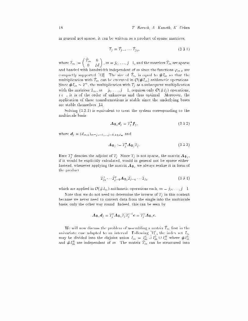
18 T. Barsch, A. Kunoth, K. Urbanin general not sparse, it can be written as a product of sparse matrices,Tj = T̂j�1 � � � T̂j0 ; (3.3.1)where T̂m := � ~Tm 00 Id� ; m = j0; : : : ; j�1, and the matrices ~Tm are sparseand banded with bandwidth independent of m since the functions 'm;k arecompactly supported [12]. The size of ~Tm is equal to #Im so that themultiplication with ~Tm can be executed in O(#Im) arithmetic operations.Since #Im � 2m, the multiplication with Tj as a subsequent multiplicationwith the matrices T̂m, m = j0; : : : ; j � 1, requires only O(#Ij) operations,i.e. , it is of the order of unknowns and thus optimal. Moreover, theapplication of these transformations is stable since the underlying basesare stable themselves [13].Solving (3:2:1) is equivalent to treat the system corresponding to themultiscale basis Ajdj = T �j fj; (3.3.2)where dj = (dm;k)m=j0�1;:::;j�1;k2Jm andAj := T �j A�jTj: (3.3.3)Here T �j denotes the adjoint of Tj . Since Tj is not sparse, the matrix Aj ,if it would be explicitly calculated, would in general not be sparse either.Instead, whenever applying the matrix Aj we always realize it in form ofthe product T̂ �j0 � � � T̂ �j�1A�j T̂j�1 � � � T̂j0 (3.3.4)which are applied in O(#Im) arithmetic operations each, m = j0; : : : ; j�1.Note that we do not need to determine the inverse of Tj in this contextbecause we never need to convert data from the single into the multiscalebasis, only the other way round. Indeed, this can be seen byAjdj = T �j A�jTjT�1j c = T �j A�jc:We will now discuss the problem of assembling a matrix ~Tm �rst in theunivariate case adapted to an interval. Following [17], the index set Immay be divided into the disjoint union Im = ILm [ Iom [ IRm where #ILmand #IRm are independent of m. The matrix ~Tm can be structured into

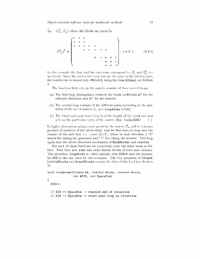
Object oriented software tools for multiscale methods 19~Tm = ( ~T 0m; ~T 1m) where the blocks are given by( ~T im)T = 0BBBBBBBBB@ � � �� � �� � � � �� � � � �� � �� � � � �� � �� � �1CCCCCCCCCA ; i = 0; 1: (3.3.5)In this example the �rst and last two rows correspond to ILm and IRm, re-spectively. Since the entries for every row are the same in the interior part,the matrix can be stored very e�ciently using the class blband, see Section2. The function that sets up the matrix consists of three nested loops:(a) The �rst loop distinguishes between the mask coe�cients am for there�nable functions and bm for the wavelet.(b) The second loop consists of the di�erent parts according to the par-tition of the set of indices Im (see loop4rows below).(c) The third and most inner loop is of the length of the mask size andsets up the particular entry of the matrix (for (cols(DIR) ...) ).In higher dimensions using tensor products the matrix ~Tm will be a tensorproduct of matrices of the above kind: now we �rst have to loop over thecorners of the unit box, i.e. , over f0; 1gd, where in each direction a "0"stands for taking the generator and "1" for taking the wavelet. This loopagain uses the above described mechanism of MaskBorder and ivector.For each of these functions we recursively start the other loops as fol-lows. Note that now rows and cols denote blocks of rows and columns.The procedure loop4rows is called initially with DIR=0 and the parame-ter DIR is the one used for the recursion. The two members of blband,LittleBlocks and GreatBlocks contain the data of this level (see Section2):void loop4rows(blband &A, ivector &rows, ivector &cols,int &DIR, int SpaceDim){ DIR++;// DIR == SpaceDim -> reached end of recursion// DIR != SpaceDim -> start next loop in recursion

20 T. Barsch, A. Kunoth, K. Urbanif (DIR==SpaceDim)// ... allocate memory for double-entries in Aelse // ... allocate memory for blband-entries in Aint Counter; // represents here different countersint masklength; // contains different values,// depending on rows(DIR)// first we treat I_m^L :for (/* rows(DIR) \in I_m^L */){ if (DIR==SpaceDim){ // setup information about masklength, location within// the matrix A etc.; then start the inner loop over// the length of the mask:for (cols(DIR)=0; cols(DIR)<masklength; cols(DIR)++)A.LittleBlocks[Counter][cols(DIR)] = ...// store entries in A (doubles)}else{ // setup information about size and position of the// blocks in A; then start the inner loop with the// next blocklevel of A:for (cols(DIR)=0; cols(DIR)<masklength; cols(DIR)++)loop4rows(A.GreatBlocks[Counter], rows, cols, DIR,SpaceDim);}}// Now the same for the other two parts of I_m:for (/* rows(DIR) \in I_m^0 */) // ...for (/* rows(DIR) \in I_m^R */) // ...DIR--; //end of recursion} In summary, the application of multiscale transformations | when ap-plicable | is a fast process. Its e�ectivity depends to a large extent on the

Object oriented software tools for multiscale methods 21fact that the underlying structures are de�ned on a uniform grid.However, there are situations when a non{uniform grid may be pre-ferred. For instance, wavelet based adaptive schemes are designed to reducethe overall complexity by not considering the basis functions that are notnecessary for a good resolution, [11]. This makes it necessary to work withthe wavelet bases themself and to set up and apply the system of equationscorresponding to the multiscale representation which are in general notO(#Ij) processes. Also the optimal compression results for elliptic singu-lar integral equations in a sequel of [20, 21] are based on carefully weightedadaptive quadrature rules in terms of wavelets which cannot make use ofthe fast multiscale transformations.Moreover, when dealing with divergence free wavelets it could be moree�cient to set up and apply the sti�ness matrix with respect to the di-vergence free wavelets. In this case one starts by multiresolution spaces ofvector �elds with components in H1(). The corresponding complementspaces are decomposed into the divergence free part and a stable comple-ment. That means that the single scale basis does not consist of divergencefree functions. Solving the system according to a compressed multiscaledivergence free basis might overcome this di�culty.3.4 Multilevel preconditionersThe relevance of multiscale transformations in numerical analysis is thattogether with a diagonal matrix they lead to asymptotically optimal condi-tion numbers and thus to a fast iterative solution of linear systems (3:2:1)independent of the re�nement depth j.To recall the basic results, let Hs = Hs(), s 2 lR, be a scale of Sobolevspaces on the domain underlying the problem, where here Hs for s < 0 isto be understood as (H�s)0 and H0 = L2. The operators in questionA : Hs+r ! Hs for which our software is developed is typically boundedlyinvertible, kAvkHs � kvkHs+r ; v 2 Hs: (3.4.1)This together with the norm equivalences 1Xj=0 2(s+r)j Xk2Jj(v; ~ j;k) j;k L2 � kvkHs+r ; s + r 2 (�~ ; ); (3.4.2)which are assumed to hold for some ~ ; > 0 and which are valid formany known biorthogonal wavelet systems [12, 13], proves the following[15, 20, 24]Theorem 1. Let the operator A satisfy (3:4:1) with some r 2 lR and let(3:4:2) hold for s + r 2 (�~ ; ). If Ds denotes the diagonal matrix with

22 T. Barsch, A. Kunoth, K. Urbanentries2sm �(m;k);(m0;k0); m;m0 = j0 � 1; : : : ; j � 1; k 2 Jm; k0 2 Jm0 ;then one has cond(D�r=2AD�r=2) = O(1); j !1; (3.4.3)where condB := kBk kB�1k and k � k is the spectral norm.This shows the crucial role of multiscale transformations for precondition-ing: on the one hand, one wants to store A� because of its sparsity whileon the other hand A together with a diagonal matrix gives rise to anoptimal preconditioned linear system. Note that Theorem 1 is also validfor nonsymmetric operators A.If A has positive order and is symmetric it should be mentioned thatclosely related alternative preconditioners often referred to as BPX{pre-conditioners or multilevel Schwarz schemes are available [4, 15, 28, 29] thatdo not need to use the wavelet bases explicitly. In this case, the operatorCju = A�1j0 Xk2Ij0(u; 'j0;k)L2 'j0;k + j�1Xm=j0 2�2mr Xk2Im(u; 'm;k)L2 'm;k(3.4.4)also gives rise to optimal condition numbers, i.e. , cond(C1=2j A�jC1=2j ) =O(1), j ! 1. However, the application of this preconditioner requiressome restriction and prolongation operators because information concern-ing all levels is to be summed up. In numerical experiments with di�erentimplementations for the restriction and prolongation operators we achievedthe best results when using block{banded matrices which were set up atthe beginning of the program and applied as matrix{vector multiplicationsin every step. The use of the class blband makes the preconditioner veryfast since expensive index{calculations can be avoided completely duringthe algorithm. Moreover, it also needs only little memory (less than 100KByte in two and three dimensions) due to its speci�c structure.The structure of the matrices is almost the same as above. The onlydi�erence is that e.g. the restriction matrices look like the upper half of thematrix in (3.3.5). Therefore, the �rst loop over the generators and waveletsis obsolete and the rest is essentially the same as above.x4 OutlookWe view the software described in this paper as a �rst step of the imple-mentation of multiscale methods for "realistic" problems. Here we outlinesome of the future projects which are already in preparation.

Object oriented software tools for multiscale methods 23The Stokes problem can be seen as the linear kernel of the incompress-ible (stationary) Navier{Stokes equations which is a system of nonlinearpartial di�erential equations. One way to solve these equations is to con-sider a sequence of Oseen problems [31] which are nonsymmetric problems.Since multilevel preconditioners as described in the last Section 3.4 are alsoavailable for nonsymmetric problems it is a natural goal to develop softwarefor these kind of problems as a preliminary step towards a Navier{Stokessolver. On the other hand, this requires to solve a convection{dominantproblem which is also aimed to be considered in further research.The next natural application are the full Navier{Stokes equations in-cluding the non{stationary terms which requires a solver for time dependentproblems.Another important class of problems arising in uid dynamics are hy-perbolic conservation laws. There is already ongoing work concerning theimplementation of multiscale methods for the numerical solution of thesesystems using the above described software tools [23].In many applications one has to deal with partial di�erential equationswith non{constant coe�cients. Approximating these variable coe�cients interms of a re�nable function on a certain level as in [19] which can be doneeven for non{smooth coe�cients, the solution of these problems in terms ofa multiscale method then requires the evaluation of re�nable integrals withat least four factors. The present implementation already covers this caseso that the development of a code for non{constant coe�cients should notbe too complicated.One of the perhaps most promising features of multiscale methods is theavailability of error estimators and adaptive schemes that already ful�ll thesaturation property [11]. Since adaptivity is crucial for the e�ciency of asolver, the development of corresponding software is an important project.The implementation of these methods requires a very careful look at thedata structure because the adaptivity can only be performed in the waveletbasis. As pointed out in Section 3, the corresponding sti�ness matrix isnot as sparse as in the single scale basis. Since adaptive procedures mustreduce the size of the problem dramatically, the overall cost should still beof the order of unknowns.We are also interested in other kinds of problems arising in engineer-ing. For example, the application of multiscale methods to the solution ofseparation processes in chemical engineering requires to solve a large DAEsystem, [34]. Controlling chemical processes lead to optimization problemson which our group also works on.Finally, the combination of solvers with visualization tools is essentialto make the solution visible. Up to now there is an interface to the code

24 T. Barsch, A. Kunoth, K. UrbanTecplot1. Since there is a whole variety of codes available for visualizationwe plan to further develop corresponding interfaces.x5 ExamplesIn this �nal section, we describe an application of the above describedsoftware tools, namely, the numerical solution of the Stokes problem inboth the divergence free and mixed weak formulation. As a test problemwe treat the driven cavity problem which models the ow of a viscous uidover a unit box. A detailed description of the numerical results concerningthis example can be found in [32].5.1 Mixed formulation of the Stokes problem in 2DThe �rst example is the two dimensional driven cavity problem in the mixedformulation � Aj BTjBj 0 ��vjpj� = �f j0 �; (5.1.1)where the matrices and vectors are given byAj := �Z grad'j;k(x) grad'j;m(x) dx�k;m2IXj ;Bj := �Z �j;k(x) div'j;m(x) dx�k2IMj ;m2IXj ;fj := �Z f(x)'j;k(x) dx�k2IXjand the trial spaces Mj := span(f�j;k : k 2 IMj g) and Xj := span(f'j;k :k 2 IXj g) are build in such a way that the LBB condition is ful�lled.As generator for the velocity trial space Xj we have used a tensor prod-uct cardinal B{spline of order three. The trial space Mj for approximatingthe pressure pj is spanned by the biorthogonal functions ~'2;4 from [9]. Theconstruction of the corresponding trial spaces can be found in [18].The results are obtained on a PC, Intel Pentium 90 with 16 MBytememory using Linux and the gcc{compiler2.In Table 1 we display the level j and the corresponding number of un-knowns. The columns A and B contain the size of the needed memoryin KByte for the corresponding sti�ness matrices A, B. Uz. shows the1Copyright by Amtec Engineering, Inc., Bellevue, Washington, USA.2Copyright by Gnu software foundation.

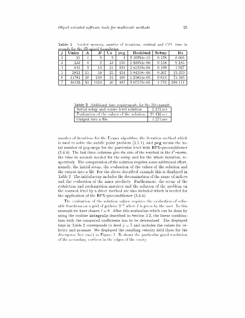
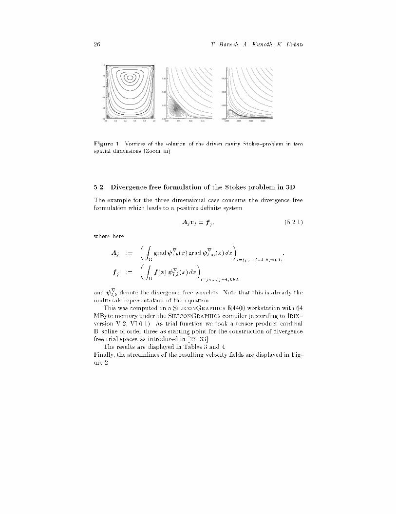
Object oriented software tools for multiscale methods 25Table 1. Needed memory, number of iterations, residual and CPU{time inseconds for the 2D-mixed formulation.j Unkn. A B Uz. pcg Residual Setup Its.2 21 1 0 3 4 3.16354e-15 0.138 0.0053 133 6 2 13 156 1.93954e-06 0.158 0.1854 645 9 13 21 331 2.81319e-06 0.198 1.9275 2821 15 59 25 454 5.84368e-06 0.307 15.3306 11781 28 249 24 496 1.25834e-05 0.644 73.5667 48133 55 1024 20 487 3.07779e-05 1.776 288.111Table 2. Additional time requirements for the 2D-example.Initial setup and coarse level solution 2.272 sec.Evaluation of the values of the solution 21.430 sec.Output into a �le 1.271 sec.number of iterations for the Uzawa algorithm, the iteration method whichis used to solve the saddle point problem (5:1:1), and pcg means the to-tal number of pcg{steps for the particular level with BPX{preconditioner(3:4:4). The last three columns give the size of the residual in the `2{norm,the time in seconds needed for the setup and for the whole iteration, re-spectively. The computation of the solution requires some additional e�ort,namely, the initial setup, the evaluation of the values of the solution andthe output into a �le. For the above described example this is displayed inTable 2. The initial setup includes the determination of the range of indicesand the evaluation of the inner products. Furthermore, the setup of therestriction and prolongation matrices and the solution of the problem onthe coarsest level by a direct method are also included which is needed forthe application of the BPX{preconditioner (3:4:4).The evaluation of the solution values requires the evaluation of re�n-able functions on a grid of gridsize 2�l where l is given by the user. In thisexample we have chosen l = 6. After this evaluation which can be done byusing the routine integrals described in Section 3.2, the linear combina-tion with the computed coe�cients has to be determined. The displayedtime in Table 2 corresponds to level j = 7 and includes the values for ve-locity and pressure. We displayed the resulting velocity �eld (here for thedivergence free case) in Figure 1. It shows the particular good resolutionof the secondary vortices in the edges of the cavity.

26 T. Barsch, A. Kunoth, K. Urban0.0 0.2 0.4 0.6 0.8 1.0 1.2

0.0

0.2

0.4

0.6

0.8

1.0

0.00 0.05 0.10 0.150.00

0.05

0.10

0.15

0.000 0.005 0.010 0.0150.000

0.005

0.010

0.015Figure 1. Vortices of the solution of the driven cavity Stokes{problem in twospatial dimensions (Zoom{in).5.2 Divergence free formulation of the Stokes problem in 3DThe example for the three dimensional case concerns the divergence freeformulation which leads to a positive de�nite systemAjvj = fj ; (5.2.1)where hereAj := �Z grad rl;k(x) grad rl;m(x) dx�l=j0 ;:::;j�1;k;m2Il;fj := �Z f(x) rl;k(x) dx�l=j0 ;:::;j�1;k2Iland rl;k denote the divergence free wavelets. Note that this is already themultiscale representation of the equation.This was computed on a SiliconGraphics R4400 workstation with 64MByte memory under the SiliconGraphics compiler (according to Irix{version V.2, VI.0.1). As trial function we took a tensor product cardinalB{spline of order three as starting point for the construction of divergencefree trial spaces as introduced in [27, 33].The results are displayed in Tables 3 and 4.Finally, the streamlines of the resulting velocity �elds are displayed in Fig-ure 2.

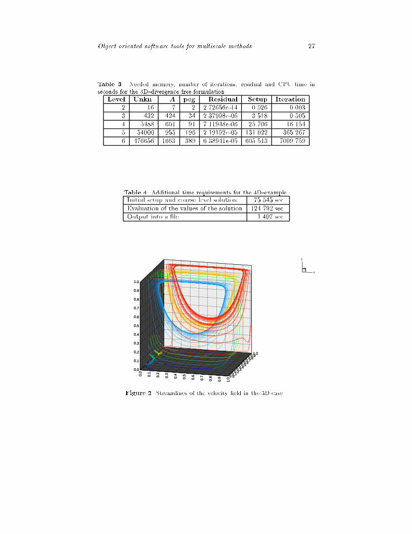
Object oriented software tools for multiscale methods 27Table 3. Needed memory, number of iterations, residual and CPU{time inseconds for the 3D{divergence free formulation.Level Unkn. A pcg Residual Setup Iteration2 16 7 2 2.72656e-14 0.026 0.0033 432 424 34 2.37998e-06 3.518 0.5054 5488 601 91 7.11948e-06 25.706 16.1545 54000 955 196 2.19192e-05 131.022 365.2676 476656 1663 389 6.38941e-05 605.513 7009.759Table 4. Additional time requirements for the 3D{example.Initial setup and coarse level solution 75.545 sec.Evaluation of the values of the solution 124.792 sec.Output into a �le 1.407 sec.0.0

0.1

0.2

0.3

0.4

0.5

0.6

0.7

0.8

0.9

1.0

0.0

0.1

0.2

0.3

0.4

0.5

0.6

0.7

0.8

0.9

1.00.0

0.10.2

0.30.4

0.50.6

0.70.8

0.91.0

0.00.1

0.20.3

0.40.5

0.60.7

0.80.9

1.0

0.0

0.1

0.2

0.3

0.4

0.5

0.6

0.7

0.8

0.9

1.0

0.0

0.1

0.2

0.3

0.4

0.5

0.6

0.7

0.8

0.9

1.0

Y

X

Z

Figure 2. Streamlines of the velocity �eld in the 3D case.

28 T. Barsch, A. Kunoth, K. UrbanAcknowledgments. The authors are grateful to Frank Knoben for manyvaluable hints concerning the implementation. The second author is sup-ported by the Deutsche Forschungsgemeinschaft.References[1] L. Andersson, N. Hall, B. Jawerth, and G. Peters. Wavelets on closedsubsets of the real line. In Topics in the Theory and Applicationsof Wavelets, L.L. Schumaker and G. Webb (eds.), Academic Press,Boston, 1994, 1{61.[2] T. Barsch and K. Urban. MSLib { software tools for multilevel meth-ods, in preparation.[3] D. Braess and W. Dahmen. Wavelet methods for mixed formulationsof second order elliptic problems, in preparation.[4] J.H. Bramble, J.E. Pasciak, and J. Xu. Parallel multilevel precondi-tioners. Math. Comp., 55 (1990), 1{22.[5] F. Brezzi and M. Fortin. Mixed and Hybrid Finite Element Methods.Springer{Verlag, Berlin, 1991.[6] M. B�ucker and M. Sauren. Private communication.[7] C. Canuto, M.Y. Hussaini, A. Quarteroni, and T.A. Zang. SpectralMethods in Fluid Dynamics. Springer{Verlag, 1988.[8] A. Cohen, W. Dahmen, and R.A. DeVore. Multiscale decompositionson bounded domains. IGPM{Report 113, RWTH Aachen, 1995.[9] A. Cohen, I. Daubechies, and J. Feauveau. Bi{orthogonal bases ofcompactly supported wavelets. Comm. Pure Appl. Math., 45 (1992),485{560.[10] A. Cohen, I. Daubechies, and P. Vial. Wavelets on the interval and fastwavelet transforms. Appl. Comput. Harmon. Anal., 1, No. 1 (1993),54{81.[11] S. Dahlke, W. Dahmen, R. Hochmuth, and R. Schneider. Stable mul-tiscale bases and local error estimation for elliptic problems. IGPM{Report 124, RWTH Aachen, 1996.[12] W. Dahmen. Some remarks on multiscale transformations, stabilityand biorthogonality. In Wavelets, Images and Surface Fitting, P.J.Laurent, A. Le M�ehaut�e, and L.L. Schumaker (eds.), A K Peters,Wellesley, 1994, 157{188.

Object oriented software tools for multiscale methods 29[13] W. Dahmen. Stability of multiscale transformations. IGPM{Report109, RWTH Aachen, 1994. To appear in J. Fourier Anal. Appl. 4,1996.[14] W. Dahmen. Multiscale analysis, approximation, and interpolationspaces. In Approximation Theory VIII, C.K. Chui and L.L. Schumaker(eds.), World Scienti�c Publishing Co., 1995, 47{88.[15] W. Dahmen and A. Kunoth. Multilevel preconditioning. Numer.Math., 63, No. 2 (1992), 315{344.[16] W. Dahmen, A. Kunoth, and R. Schneider. Operator equations, mul-tiscale concepts and complexity. WIAS-Report 206, 1995. To appearin: Lectures in Applied Mathematics, J. Renegar, M. Shub and S.Smale (eds.), American Mathematical Society.[17] W. Dahmen, A. Kunoth, and K. Urban. Biorthogonal spline-waveletson the interval { stability and moment conditions, in preparation.[18] W. Dahmen, A. Kunoth, and K. Urban. A Wavelet{Galerkin methodfor the Stokes{equations. Computing, 56, No. 3 (1996), 259{302.[19] W. Dahmen and C.A. Micchelli. Using the re�nement equation forevaluating integrals of wavelets. SIAM J. Numer. Anal., 30, No. 2(1993), 507{537.[20] W. Dahmen, S. Pr�ossdorf, and R. Schneider. Multiscale methods forpseudodi�erential equations. In Recent Advances in Wavelet Analysis,L.L. Schumaker and G.Webb (eds.), Academic Press, San Diego, 1994,191{235.[21] W. Dahmen and R. Schneider. Multiscale methods for boundary in-tegral equations I: Biorthogonal wavelets on 2D manifolds in lR3, inpreparation.[22] V. Girault and P.-A. Raviart. Finite Element Methods for Navier{Stokes{Equations. Springer, Berlin, 2nd edition, 1986.[23] B. Gottschlich-M�uller. A multiresolution scheme based on biorthog-onal wavelets for scalar conservation laws in one space dimension, inpreparation.[24] S. Ja�ard. Wavelet methods for fast resolution of elliptic problems.SIAM J. Numer. Anal., 29 (1992), 965{986.[25] A. Kunoth. Computing re�nable integrals | Documentation of theprogram | Version 1.1. Texas A&M-University, preprint ISC-95-02-Math, 1995.

30 T. Barsch, A. Kunoth, K. Urban[26] A. Kunoth. Multilevel preconditioning { Appending boundary con-ditions by Lagrange multipliers. Advances in Computational Mathe-matics, 4, No. 1,2 (1995), 145{170.[27] P.G. Lemari�e{Rieusset. Analyses multi-r�esolutions non orthogonales,commutation entre projecteurs et derivation et ondelettes vecteurs �adivergence nulle. Revista Mat. Iberoamericana, 8 (1992), 221{236.[28] P. Oswald. On discrete norm estimates related to multilevel precon-ditioners in the �nite element method. In Constructive Theory ofFunctions, Proc. Int. Conf. Varna 1991, K.G. Ivanov, P. Petrushev,and B. Sendov (eds.), Bulg. Acad. Sci., So�a, 1992, 203{214.[29] P. Oswald. Multilevel Finite Element Approximation. TeubnerSkripten zur Numerik, Stuttgart, 1994.[30] M.P. Robichaud, P.A. Tanguy, and M. Fortin. An iterative implemen-tation of the Uzawa algorithm for 3{D uid ow problems. Interna-tional Journal for Numerical Methods in Fluids, 10 (1990), 429{442.[31] S. Turek. Ein robustes und e�zientes Mehrgitterverfahren zur L�osungder instation�aren, inkompressiblen 2{D Navier{Stokes{Gleichungenmit diskret divergenzfreien �niten Elementen, dissertation, Univer-sit�at Heidelberg, 1991.[32] K. Urban. Multiskalenverfahren f�ur das Stokes{Problem undangepa�te Wavelet{Basen, dissertation, RWTH Aachen, 1995.[33] K. Urban. On divergence{free wavelets. Advances in ComputationalMathematics, 4, No. 1,2 (1995), 51{82.[34] R. v. Watzdorf, K. Urban, W. Dahmen, and W. Marquardt. AWavelet{Galerkin method applied to separation processes. In Sci-enti�c Computing in Cemical Engineering, S. Keil, W. Mackens, H.Vo�, and J. Werther (eds.), Springer{Verlag Berlin, 1996, 246{252.Titus BarschInstitut f�ur Geometrie und Praktische MathematikRWTH AachenTemplergraben 5552056 AachenGermanybarsch@igpm.rwth-aachen.de

Object oriented software tools for multiscale methods 31Angela KunothWeierstrass{Institut f�ur Angewandte Analysis und Stochastik (WIAS)Mohrenstr. 3910117 BerlinGermanykunoth@wias-berlin.deKarsten UrbanInstitut f�ur Geometrie und Praktische MathematikRWTH AachenTemplergraben 5552056 AachenGermanyurban@igpm.rwth-aachen.de