Stochastic PDEs with heavy-tailed noise - mediaTUM

Stochastic PDEs with heavy-tailed noise

Carsten Chong∗

Abstract

We analyze the nonlinear stochastic heat equation driven by heavy-tailed noise on un-bounded domains and in arbitrary dimension. The existence of a solution is proved even ifthe noise only has moments up to an order strictly smaller than its Blumenthal-Getoor index.In particular, this includes all stable noises with index α < 1 + 2/d. Although we cannotshow uniqueness, the constructed solution is natural in the sense that it is the limit of thesolutions to approximative equations obtained by truncating the big jumps of the noise or byrestricting its support to a compact set in space. Under growth conditions on the nonlinearterm we can further derive moment estimates of the solution, uniformly in space. Finally,the techniques are shown to apply to Volterra equations with kernels bounded by generalizedGaussian densities. This includes, for instance, a large class of uniformly parabolic stochasticPDEs.

AMS 2010 Subject Classifications: primary: 60H15, 60H20, 60G60secondary: 60G52, 60G48, 60G51, 60G57

Keywords: generalized Gaussian densities; heavy-tailed noise; Itô basis; Lévy basis; parabolicstochastic PDE; stable noise; stochastic heat equation; stochastic partial differential equation;stochastic Volterra equation

∗Center for Mathematical Sciences, Technical University of Munich, Boltzmannstraße 3, 85748 Garching, Ger-many, e-mail: [email protected], url: www.statistics.ma.tum.de

1

Stochastic PDEs with heavy-tailed noise 2

1 IntroductionIn this paper we investigate the nonlinear stochastic heat equation

∂tY (t, x) = ∆Y (t, x) + σ(Y (t, x))M(t, x), (t, x) ∈ R+ × Rd,Y (0, x) = ψ(x), (1.1)

where M is some random noise, the function σ is globally Lipschitz and ψ is some given initialcondition. In the theory of stochastic partial differential equations (stochastic PDEs) there arevarious ways to make sense of the formal equation (1.1). We refer to Peszat and Zabczyk (2007),Liu and Röckner (2015) and Holden et al. (2010) for detailed accounts within the semigroup,the variational and the white noise approach, respectively. Our analysis is based on the randomfield approach going back to Walsh (1986) where the differential equation (1.1) is interpreted asthe integral equation

Y (t, x) = Y0(t, x) +∫ t

0

∫Rdg(t− s, x− y)σ(Y (s, y))M(ds,dy), (t, x) ∈ R+ × Rd, (1.2)

where g is the heat kernel

g(t, x) = 1(4πt)d/2

exp(−|x|

2

4t

)1(0,∞)(t), (t, x) ∈ R+ × Rd, (1.3)

Y0 is related to the initial condition ψ via

Y0(t, x) =∫Rdg(t, x− y)ψ(y) dy, (t, x) ∈ R+ × Rd,

and the integral with respect to M is understood in Itô’s sense, see e.g. Bichteler and Jacod(1983), Walsh (1986) and Chong and Klüppelberg (2015).

There are multiple reasons for the broad interest in studying the stochastic heat equation(1.1): on the one hand, it is of great significance within mathematics because, for example,it has strong connections to branching interacting particles (see e.g. Carmona and Molchanov(1994), Dawson (1993) and Mueller (2015)) and it arises from the famous Kardar-Parisi-Zhangequation via the Cole-Hopf transformation (Corwin, 2012; Hairer, 2013). On the other hand, thestochastic heat equation has found applications in various disciplines like turbulence modeling(Davies et al., 2004; Barndorff-Nielsen et al., 2011), astrophysics (Jones, 1999), phytoplanktonmodeling (Saadi and Benbaziz, 2015) and neurophysiology (Walsh, 1981; Tuckwell and Walsh,1983).

If M is a Gaussian noise, the initial theory developed by Walsh (1986) has been comprehen-sively extended and many properties of the solution to the stochastic heat equation or variantshereof have been established, see Khoshnevisan (2014), for example. When it comes to non-Gaussian noise, the available literature on stochastic PDEs within the random field approach ismuch less. While the papers by Albeverio et al. (1998) and Applebaum and Wu (2000) remainin the L2-framework of Walsh (1986), Saint Loubert Bié (1998) is one of the first to treat Lévy-driven stochastic PDEs in Lp-spaces with p < 2. The results are extended in Chong (2016) toVolterra equations with Lévy noise, on finite as well as on infinite time domains. In both SaintLoubert Bié (1998) and Chong (2016), one crucial assumption the Lévy noise has to meet isthat its Lévy measure, say λ, must satisfy∫

R|z|p λ(dz) <∞ (1.4)


for some p < 1 + 2/d. This a priori excludes stable noises, or more generally, any noise with lessmoments than its Blumenthal-Getoor index. Of course, if the noise intensity decreases sufficientlyfast in space, for example, if it only acts on a bounded domain instead of the whole Rd, thisproblem can be solved by localization, see Balan (2014) and Chong (2016). Also on a boundedspace domain, Mueller (1998) considers the stochastic heat equation with spectrally positivestable noise of index smaller than one and the non-Lipschitz function σ(x) = xγ (γ < 1). Toour best knowledge, the paper by Mytnik (2002), where the same function σ is considered withspectrally positive stable noises of index bigger than one, is the only work that investigates thestochastic heat equation on the whole Rd with noises violating (1.4) for all p ≥ 0. The purpose ofthis article is to present results for Lipschitz σ and more general heavy-tailed noisesM , includingfor all dimensions d stable noises of index α < 1 + 2/d (with no drift in the case α < 1).

More specifically, if M is a homogeneous pure-jump Lévy basis with Lévy measure λ andψ is, say, a bounded deterministic function, we will prove in Theorem 3.1 the existence of asolution to (1.2) under the assumption that∫

|z|≤1|z|p λ(dz) +

∫|z|>1

|z|q λ(dz) <∞

for some p < 1+2/d and q > p/(1+(1+2/d−p)). Although the proof does not yield uniquenessin a suitable Lp-space, we can show in Theorem 3.7 that our solution is the limit in probabilityof the solutions to (1.2) when either the jumps of M are truncated at increasing levels or whenM is restricted to increasing compact subsets of Rd. Furthermore, if |σ(x)| ≤ C(1 + |x|γ) withan exponent γ < 1 ∧ q/p, the constructed solution has q-th order moments that are uniformlybounded in space, see Theorem 3.8. Finally, in Theorem 3.10, we extend the previous resultsto Volterra equations with kernels bounded by generalized Gaussian densities, which includesuniformly parabolic stochastic PDEs as particular examples.

2 PreliminariesUnderlying the whole paper is a stochastic basis (Ω,F ,F = (Ft)t∈R+ ,P) satisfying the usualhypotheses of right-continuity and completeness that is large enough to support all consideredrandom elements. For d ∈ N we equip Ω := Ω × R+ × Rd with the tempo-spatial predictableσ-field P := P ⊗ B(Rd) where P is the usual predictable σ-field and B(Rd) is the Borel σ-field on Rd. With a slight abuse of notation, P also denotes the space of predictable, thatis, P-measurable processes Ω → R. Moreover, Pb is the collection of all A ∈ P satisfyingA ⊆ Ω× [0, k]× [−k, k]d for some k ∈ N. Next, writing p∗ := p∨ 1 and p∗ := p∧ 1 for p ∈ [0,∞),we equip the space Lp = Lp(Ω,F ,P) with the usual topology induced by ‖X‖Lp := E[|X|p]1/p∗

for p > 0 and ‖X‖L0 := E[|X| ∧ 1] for p = 0. Further notations and abbreviations includeJR,SK := (ω, t) ∈ Ω × R+ : R(ω) ≤ t ≤ S(ω) for two F-stopping times R and S (otherstochastic intervals are defined analogously), |µ| for the total variation measure of a signedBorel measure µ, x(i) for the i-th coordinate of a point x ∈ Rd and x+ := x ∨ 0 for x ∈ R. Lastbut not least, the value of all constants C and CT may vary from line to line without furthernotice.

In this paper the noise M that drives the equations (1.1) and (1.2) will be assumed to havethe form

M(dt,dx) = b(t, x) d(t, x) + ρ(t, x)W (dt,dx) +∫Eδ(t, x, z) (p− q)(dt,dx,dz)

+∫Eδ(t, x, z) p(dt,dx, dz) (2.1)


with the following specifications:

• (E, E) is an arbitrary Polish space equipped with its Borel σ-field,

• b, ρ ∈ P,

• δ := δ + δ := δ1|δ|≤1 + δ1|δ|>1 is a P ⊗ E-measurable function,

• W is a Gaussian space–time white noise relative to F (see Walsh (1986)),

• p is a homogeneous Poisson random measure on R+ × Rd × E relative to F (see Def-inition II.1.20 in Jacod and Shiryaev (2003)), whose intensity measure disintegrates asq(dt,dx,dz) = dtdxλ(dz) with some σ-finite measure λ on (E, E).

Moreover, all coefficients are assumed to be “locally integrable” in the sense that the randomvariable

M(A) =∫R+×Rd

1A(t, x)b(t, x) d(t, x) +∫R+×Rd

1A(t, x)ρ(t, x)W (dt,dx)

+∫R+×Rd×E

1A(t, x)δ(t, x, z) (p− q)(dt,dx,dz)

+∫R+×Rd×E

1A(t, x)δ(t, x, z) p(dt,dx,dz)

is well defined for all A ∈ Pb. In analogy to the notion of Itô semimartingales in the purelytemporal case, we call the measure M in (2.1) an Itô basis. We make the following structuralassumptions on M : there exist exponents p, q ∈ (0, 2] (without loss of generality we assume thatq ≤ p), numbers βN ∈ R+, F-stopping times τN , and deterministic positive measurable functionsjN (z) such that

M1. τN > 0 for all N ∈ N and τN ↑ ∞ a.s.,

M2.∫E jN (z)λ(dz) <∞,

M3. |b(ω, t, x)|, |ρ2(ω, t, x)| ≤ βN and |δ(ω, t, x, z)|p + |δ(ω, t, x, z)|q ≤ jN (z) for all (ω, t, x) ∈ Ωwith t ≤ τN (ω) and z ∈ E.

If p ≤ 1 (resp. q ≥ 1), we can a.s. define b0(t, x) := b(t, x) −∫E δ(t, x, z)λ(dz) (resp. b1(t, x) :=

b(t, x)+∫E δ(t, x, z)λ(dz)) for (t, x) ∈ R+×Rd. In this case, we assume without loss of generality

that |b0(ω, t, x)| (resp. |b1(ω, t, x)|) is bounded by βN as well when t ≤ τN (ω).

Example 2.1 IfM is an Itô basis with E = R, deterministic coefficients b(t, x) = b, ρ(t, x) = ρand δ(t, x, z) = z, and λ satisfies λ(0) = 0 and

∫R(1∧z2)λ(dz) <∞, thenM is a homogeneous

Lévy basis (and M a space–time white noise) with Lévy measure λ. In this case, conditions M1–M3 reduce to the requirement that∫

|z|≤1|z|p λ(dz) +

∫|z|>1

|z|q λ(dz) <∞, (2.2)

with τN := +∞ and jN (z) := |z|p1[−1,1](z) + |z|q1R\[−1,1](z). If p ≤ 1 (resp. q ≥ 1), b0 (resp. b1)is the drift (resp. the mean) of M . 2


Regarding integration with respect to Itô bases, essentially, as all integrals are taken on finitetime intervals, the reader only has to be acquainted with the integration theory with respectto Gaussian white noise (see Walsh (1986)) and (compensated) Poisson random measures (seeChapter II of Jacod and Shiryaev (2003)). But at one point in the proof of Theorem 3.1 below, weneed the more abstract theory behind. So we briefly recall this, all omitted details can be foundin e.g. Bichteler and Jacod (1983) or Chong and Klüppelberg (2015). The stochastic integral ofa simple function is defined in the canonical way: if S(t, x) =

∑ri=1 ai1Ai with r ∈ N, ai ∈ R and

Ai ∈ Pb, then ∫S dM :=

∫S(t, x)M(dt,dx) :=

r∑i=1

aiM(Ai).

In order to extend this integral from the class of simple functions S to general predictableprocesses, it is customary to introduce the Daniell mean

‖H‖M,p := supS∈S,|S|≤|H|

∥∥∥∥∫ S dM∥∥∥∥Lp

for H ∈ P and p ∈ R+. A predictable function H is called Lp-integrable (or simply integrableif p = 0) if there exists a sequence (Sn)n∈N of simple functions in S with ‖Sn −H‖M,p → 0 asn→∞. In this case, the stochastic integral∫

H dM :=∫H(t, x)M(dt,dx) := lim

n→∞

∫Sn(t, x)M(dt,dx)

exists as a limit in Lp and does not depend on the choice of Sn. It is convenient to indicate thedomain of integration by

∫A or

∫ t0∫Rd =

∫(0,t)×Rd , for example. In the latter case, contrary to

usual practice, the endpoint t is excluded.Although the Daniell mean seems to be an awkward expression, it can be computed or

estimated effectively in two important situations: if M is a strict random measure, that is,if it can be identified with a measure-valued random variable M(ω, ·), then we simply have‖H‖M,p = ‖

∫|H|d|M |‖Lp ; if M is a local martingale measure, that is, for every A ∈ Pb the

process t 7→ M(A ∩ (Ω × [0, t] × Rd)) has a version that is an F-local martingale, then by theBurkholder-Davis-Gundy inequalities (in conjunction with Theorem VII.104 of Dellacherie andMeyer (1982)) there exists, for every p ∈ [1,∞), a constant Cp ∈ R+ such that

‖H‖M,p ≤ Cp

∥∥∥∥∥(∫

H2 d[M ])1/2

∥∥∥∥∥Lp

for all H ∈ P. Here [M ](dt,dx) := ρ2(t, x) d(t, x) +∫E δ

2(t, x, z) p(dt,dx,dz) is the quadraticvariation measure of M .

Finally, for p ∈ (0,∞), we define the space Bp (resp. Bploc) as the collection of all φ ∈ P for

which we have

‖φ‖p,T := sup(t,x)∈[0,T ]×Rd

‖φ(t, x)‖Lp <∞(resp. ‖φ‖p,T,R := sup

(t,x)∈[0,T ]×[−R,R]d‖φ(t, x)‖Lp <∞

)

for all T ∈ R+ (resp. for all T,R ∈ R+). Moreover, if τ is an F-stopping time, we write φ ∈ Bp(τ)(resp. φ ∈ Bp

loc(τ)) if φ1J0,τK belongs to Bp (resp. Bploc).


3 Main resultsIn Saint Loubert Bié (1998) and Chong (2016), Equation (1.2) driven by a Lévy basis is provedto possess a solution in some space Bp under quite general assumptions. The most restrictivecondition, however, is that the Lévy measure λ has to satisfy∫

R|z|p λ(dz) <∞. (3.1)

Although there is freedom in choosing the value of p ∈ (0, 1+2/d], there is no possibility to choosethis exponent for the small jumps (i.e., |z| ≤ 1) and the big jumps (i.e., |z| > 1) separately. Sofor instance, stable Lévy bases are always excluded. The main goal of this paper is to describea way of how one can, to a certain extent, choose different exponents p in (3.1) for the smalland the large jumps, respectively. In fact, we can consider a slightly more general equation than(1.2), namely the stochastic Volterra equation

Y (t, x) = Y0(t, x) +∫ t

0

∫RdG(t, x; s, y)σ(Y (s, y))M(ds,dy), (t, x) ∈ R+ × Rd, (3.2)

under the following list of assumptions.

A1. For every N ∈ N we have that Y0 ∈ Bp(τN ).

A2. There exists C ∈ R+ such that |σ(x)− σ(y)| ≤ C|x− y| for all x, y ∈ R.

A3. The function G : (R+ × Rd)2 → R is measurable and for all T ∈ R+ there exists CT ∈ R+with |G(t, x; s, y)| ≤ CT g(t − s, x − y) for all (t, x), (s, y) ∈ [0, T ] × Rd, where g is the heatkernel (1.3).

A4. The exponents p and q in M3 satisfy 0 < p < 1 + 2/d and p/(1 + (1 + 2/d− p)) < q ≤ p.

A5. If p < 2, we assume ρ ≡ 0; if p < 1, we also require that b0 ≡ 0.

As it is usual in the context of stochastic PDEs, we call Y ∈ P a solution to (3.2) if for all(t, x) ∈ R+ × Rd the stochastic integral on the right-hand side of (3.2) is well defined and theequation itself holds a.s. Two solutions Y1 and Y2 are identified if they are versions of each other.

Theorem 3.1. Let M be an Itô basis satisfying M1–M3. Then under A1–A5 there exists asequence (τ(N))N∈N of F-stopping times increasing to infinity a.s. such that Equation (3.2) hasa solution Y belonging to Bp

loc(τ(N)) for every N ∈ N. One possible choice of (τ(N))N∈N isgiven in (3.4) below.

Figure 1 illustrates the possible choices for the exponents p and q such that Theorem 3.1 isapplicable. For each dimension d ∈ N, the exponent p must be smaller than (1 + 2/d) ∧ 2 andthe exponent q larger than p/(1 + (1 + 2/d− p)), which corresponds to the area above the boldlines in Figure 1. If q ≥ p, the result is well known from Saint Loubert Bié (1998) and Chong(2016). So the new contribution of Theorem 3.1 pertains to the area above the bold lines andbelow the diagonal q = p. As we can see, all stable noises with index α < 1 + 2/d (and zerodrift if α < 1) are covered: they are “located” infinitesimally below the line q = p in the figure.Moreover, we observe that there exists a non-empty region below the diagonal that constitutesvalid parameter choices for all dimensions d ∈ N: namely when p ≤ 1 and p/(2− p) < q ≤ p.


321.671

q

p

q=p

d = ∞

d = 3

d = 2

d = 1

Figure 1: Constraints for p and q in Theorem 3.1 dependent on the dimension d

Put in a nutshell, the method of Saint Loubert Bié (1998) and Chong (2016) to construct asolution to (3.2) is this: first, one defines the integral operator J that maps φ ∈ P to

J(φ)(t, x) := Y0(t, x) +∫ t

0

∫RdG(t, x; s, y)σ(φ(s, y))M(ds,dy), (t, x) ∈ R+ × Rd, (3.3)

when the right-hand side is well defined, and to +∞ otherwise. Then one establishes momentestimates in such a way that J becomes, at least locally in time, a contractive self-map on someBp-space. Then the Banach fixed point theorem yields existence and uniqueness of solutions.However, if q < p, the problematic point is that the p-th order moment of J(φ) is typicallyinfinite, while taking the q-th order moment, which would be finite, produces a non-contractiveiteration. The idea in this article to circumvent this is therefore to consider a modified Picarditeration: we still take p-th moment estimates (in order to keep contractivity) but stop theprocesses under consideration before they become too large (in order to keep the p-th momentsfinite). The following lemma makes our stopping strategy precise.

Lemma 3.2. Let h(x) := 1 + |x|η with some η ∈ R+ and define for N ∈ N the stopping times

τ(N) := infT ∈ R+ :

∫ T

0

∫Rd

∫E1|δ(t,x,z)|>Nh(x) p(dt,dx,dz) 6= 0

∧ τN , (3.4)

where (τN )N∈N are the stopping times in M1. If q is the number in M3 and η > d/q, then a.s.τ(N) > 0 for all N ∈ N and τ(N) ↑ ∞ a.s. for N ↑ ∞.

Proof. Define U0 := ∅ and

Un :=x ∈ Rd : |x| ≤ π−1/2Γ(1 + d/2)1/dn1/d \ Un−1, n ∈ N.

In other words, (Un)n∈N forms a partition of Rd into concentric spherical shells of Lebesguemeasure 1. Then there exists a constant C ∈ R+ which is independent of x and n such that


h(x) ≥ C(n− 1)η/d for all x ∈ Un and n ∈ N. Next, observe that for all T ∈ R+ we a.s. have∫ T

0

∫Rd

∫E1|δ(t,x,z)|>Nh(x)1J0,τN K(t) p(dt,dx,dz)

≤∫ T

0

∫Rd

∫E1jN (z)1/q>Nh(x) p(dt,dx,dz)

≤∞∑n=1

∫ T

0

∫Rd

∫E1Un(x)1jN (z)1/q>NC(n−1)η/d p(dt,dx,dz).

If we show that the last expression is finite a.s., we can conclude, on the one hand, that τ(N) > 0a.s. for all N ∈ N. On the other hand, it also implies that τ(N) ↑ ∞ for N ↑ ∞ because then, forany T ∈ R+, the left-hand side of the previous display would be 0 as soon as N is large enough.So with an := NC(n− 1)η/d and using the Borel-Cantelli lemma, it remains to verify that

∞∑n=1

P[p([0, T ]× Un × jN (z) > aqn) 6= 0] <∞. (3.5)

Indeed,

P[p([0, T ]× Un × jN (z) > aqn) 6= 0] = 1− e−q([0,T ]×Un×jN (z)>aqn)

≤ q([0, T ]× Un × jN (z) > aqn)

= Tλ(jN (z) > aqn) ≤ T∫EjN (z)λ(dz)a−qn .

The last term is of order n−ηq/d. Since η > d/q, it is summable and leads to (3.5). 2

The stopping times in the previous lemma are reminiscent of a well established technique ofsolving stochastic differential equations driven by semimartingales (Protter, 2005). Here, if thejumps of the driving semimartingale lack good integrability properties, one can still solve theequation until the first big jump occurs, then continue until the next big jump occurs and soon, thereby obtaining a solution for all times. In principle, this is exactly the idea we employin the proof of Theorem 3.1. However, in our tempo-spatial setting, the law of M is typicallynot equivalent to the law of its truncation at a fixed level on any set [0, T ] × Rd: Infinitelymany big jumps usually occur already immediately after time zero. This is the reason why inLemma 3.2 above we have to take a truncation level h that increases sufficiently fast in thespatial coordinate.

As a next step we introduce for each N ∈ N a truncation of M by

MN (dt,dx) := 1J0,τN K(t)(b(t, x) d(t, x) + ρ(t, x)W (dt,dx) +

∫Eδ(t, x, z) (p− q)(dt,dx,dz)

+∫Eδ(t, x, z)1|δ(t,x,z)|≤Nh(x) p(dt,dx,dz)

). (3.6)

An important step in the proof of Theorem 3.1 is to prove that (3.2) has a solution when M issubstituted by MN . To this end, we establish several moment estimates.

Lemma 3.3. Let N ∈ N be arbitrary but fixed and JN the integral operator defined in the sameway as J in (3.3) but with MN instead of M . Under M1–M3 and A1–A5 the following estimateshold.


(1) For all T ∈ R+ there exists a constant CT ∈ R+ such that for all φ ∈ P and (t, x) ∈ [0, T ]×Rdwe have

‖JN (φ)(t, x)‖Lp ≤ ‖Y0(t, x)1J0,τN K(t)‖Lp

+ CT

(∫ t

0

∫Rdgp(t− s, x− y)(1 + ‖φ(s, y)‖p

∗

Lp)h(y)p−q d(s, y)) 1p∗

+ CT

(∫ t

0

∫Rdg(t− s, x− y)(1 + ‖φ(s, y)‖pLp)h(y)p−q d(s, y)

) 1p

1p≥1. (3.7)

(2) For all T ∈ R+ there exists a constant CT ∈ R+ such that for all (t, x) ∈ [0, T ] × Rd andφ1, φ2 ∈ P with JN (φ1)(t, x), JN (φ2)(t, x) <∞ we have

‖JN (φ1)(t, x)− JN (φ2)(t, x))‖Lp

≤ CT(∫ t

0

∫Rdgp(t− s, x− y)‖φ1(s, y)− φ2(s, y)‖p

∗

Lph(y)p−q d(s, y)) 1p∗

+ CT

(∫ t

0

∫Rdg(t− s, x− y)‖φ1(s, y)− φ2(s, y)‖pLph(y)p−q d(s, y)

) 1p

1p≥1.

Proof. Both parts can be treated in a similar fashion. We only prove (1). Starting with the casep ≥ 1, we use the fact that δ = δ1|δ|>1, δ = δ1|δ|≤1 and h ≥ 1 to decompose MN (dt,dx) =LN (dt,dx) +BN

1 (dt,dx) where

LN (dt,dx) := 1J0,τN K(t)(ρ(t, x)W (dt,dx) +

∫Eδ(t, x, z)1|δ(t,x,z)|≤Nh(x) (p− q)(dt,dx, dz)

),

BN1 (dt,dx) := 1J0,τN K(t)

(b(t, x) d(t, x) +

∫Eδ(t, x, z)1|δ(t,x,z)|≤Nh(x) q(dt,dx, dz)

). (3.8)

In the following CT denotes a positive constant independent of φ (but possibly dependent on p,q, d and N). Recalling that ρ = 0 unless p = 2, using the Burkholder-Davis-Gundy inequalitiesand applying the inequality (x+y)r ≤ xr+yr for x, y ∈ R+ and r ∈ [0, 1] to the Poisson integral,we deduce for all (t, x) ∈ [0, T ]× Rd that∥∥∥∥∫ t

0

∫RdG(t, x; s, y)σ(φ(s, y))LN (ds,dy)

∥∥∥∥Lp

≤ CTE[ ∫ t

0

∫Rd|g(t− s, x− y)σ(φ(s, y))ρ(s, y)|21J0,τN K(s) d(s, y)

+(∫ t

0

∫Rd

∫E|g(t− s, x− y)σ(φ(s, y))δ(s, y, z)|21|δ(s,y,z)|≤Nh(y)1J0,τN K(s) p(ds,dy,dz)

) p2] 1p

≤ CTE[ ∫ t

0

∫Rdg2(t− s, x− y)(1 + |φ(s, y)|2)1p=2 d(s, y)

+∫ t

0

∫Rd

∫E|g(t− s, x− y)δ(s, y, z)|p(1 + |φ(s, y)|p)1|δ(s,y,z)|≤Nh(y)1J0,τN K(s) p(ds,dy,dz)

] 1p

≤ CT

(∫ t

0

∫Rdg2(t− s, x− y)(1 + ‖φ(s, y)‖2L2)1p=2 d(s, y)


+∫EjN (z)λ(dz)

∫ t

0

∫Rdgp(t− s, x− y)(1 + ‖φ(s, y)‖pLp)h(y)p−q d(s, y)

) 1p

≤ CT

(∫ t

0

∫Rdgp(t− s, x− y)(1 + ‖φ(s, y)‖pLp)h(y)p−q d(s, y)

) 1p

Next, by Hölder’s inequality, we obtain∥∥∥∥∫ t

0

∫RdG(t, x; s, y)σ(φ(s, y))BN

1 (ds,dy)∥∥∥∥Lp

≤ CT

(∫ T

0

∫Rdg(t, x) d(t, x)

)1− 1p

E[ ∫ t

0

∫Rdg(t− s, x− y)(1 + |φ(s, y)|p)

×(|b(s, y)|+

∫E|δ(s, y, z)|1|δ(s,y,z)|≤Nh(y) λ(dz)

)p1J0,τN K(s) d(s, y)

] 1p

≤ CT

(∫ t

0

∫Rdg(t− s, x− y)(1 + ‖φ(s, y)‖pLp)

(βN +

∫EjN (z)λ(dz)(Nh(y))(1−q)+

)pd(s, y)

) 1p

≤ CT

(∫ t

0

∫Rdg(t− s, x− y)(1 + ‖φ(s, y)‖pLp)h(y)p−q d(s, y)

) 1p

,

which completes the proof for the case p ≥ 1.For p < 1 we have by hypothesis b0, c ≡ 0. Therefore,∥∥∥∥∫ t

0

∫RdG(t, x; s, y)σ(φ(s, y))MN (ds,dy)

∥∥∥∥Lp

≤ CTE[∫ t

0

∫Rd

∫E|g(t− s, x− y)σ(φ(s, y))δ(s, y, z)|p1|δ(s,y,z)|≤Nh(y)1J0,τN K(s) p(ds,dy,dz)

]≤ CT

∫ t

0

∫Rdgp(t− s, x− y)(1 + ‖φ(s, y)‖Lp)h(y)p−q d(s, y).

2

We need two further preparatory results. The first one is classic. Henceforth, we denote byNd(µ,Σ) the d-dimensional normal distribution with mean vector µ and covariance matrix Σ.

Lemma 3.4. If X is an N1(0, σ2)-distributed random variable, then for every p ∈ (−1,∞) wehave

E[|X|p] = (2σ2)p/2π−1/2Γ(

1+p2

).

The second lemma determines the size of certain iterated integrals. It is proved by a straight-forward induction argument, which is omitted.

Lemma 3.5. Let t ∈ R+ and a ∈ (−1,∞). Then we have for every n ∈ N that (t0 := t)∫ t

0

∫ t1

0. . .

∫ tn−1

0

n∏j=1

(tj−1 − tj)a dtn . . . dt2 dt1 = Γ(1 + a)n

Γ(1 + (1 + a)n) tn(1+a).

We are now in the position to prove the existence of a solution to (3.2) under the conditionsof Theorem 3.1.


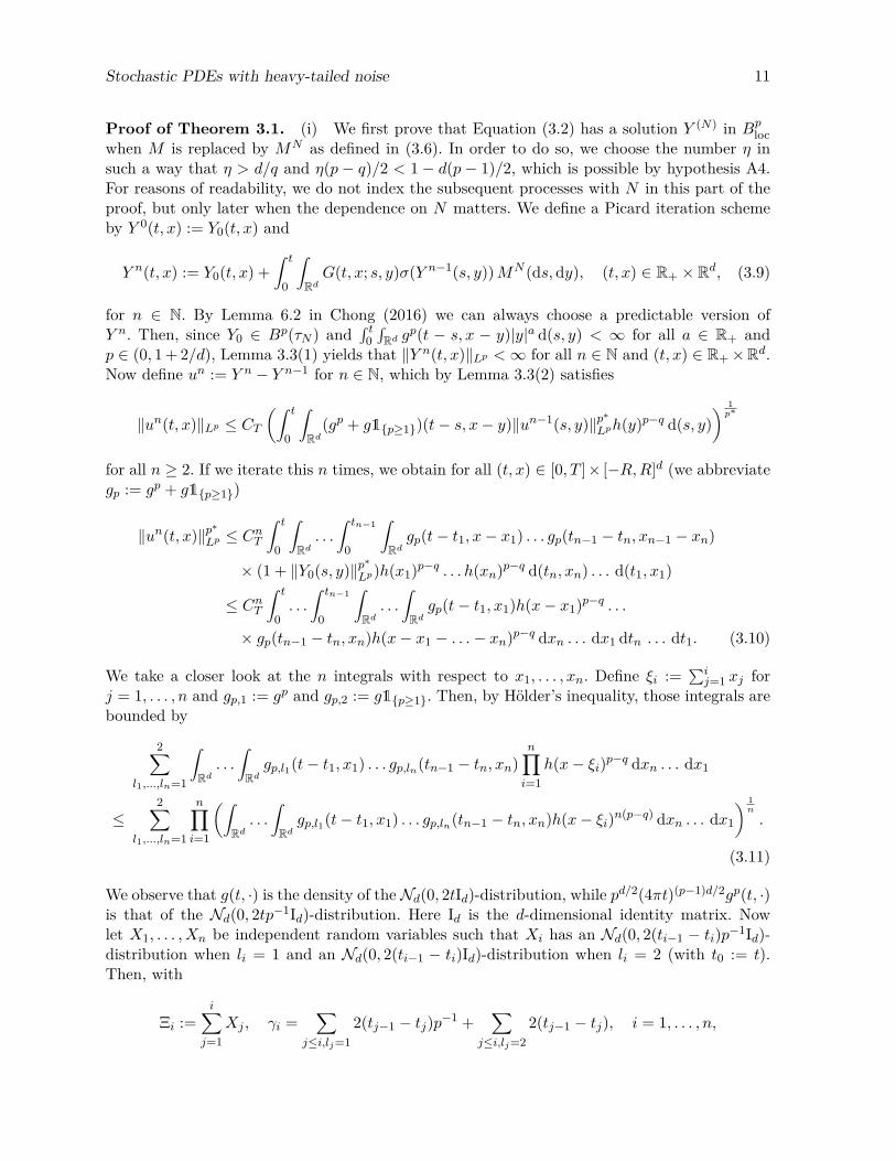
Proof of Theorem 3.1. (i) We first prove that Equation (3.2) has a solution Y (N) in Bploc

when M is replaced by MN as defined in (3.6). In order to do so, we choose the number η insuch a way that η > d/q and η(p − q)/2 < 1 − d(p − 1)/2, which is possible by hypothesis A4.For reasons of readability, we do not index the subsequent processes with N in this part of theproof, but only later when the dependence on N matters. We define a Picard iteration schemeby Y 0(t, x) := Y0(t, x) and

Y n(t, x) := Y0(t, x) +∫ t

0

∫RdG(t, x; s, y)σ(Y n−1(s, y))MN (ds,dy), (t, x) ∈ R+ × Rd, (3.9)

for n ∈ N. By Lemma 6.2 in Chong (2016) we can always choose a predictable version ofY n. Then, since Y0 ∈ Bp(τN ) and

∫ t0∫Rd g

p(t − s, x − y)|y|a d(s, y) < ∞ for all a ∈ R+ andp ∈ (0, 1 + 2/d), Lemma 3.3(1) yields that ‖Y n(t, x)‖Lp <∞ for all n ∈ N and (t, x) ∈ R+×Rd.Now define un := Y n − Y n−1 for n ∈ N, which by Lemma 3.3(2) satisfies

‖un(t, x)‖Lp ≤ CT(∫ t

0

∫Rd

(gp + g1p≥1)(t− s, x− y)‖un−1(s, y)‖p∗

Lph(y)p−q d(s, y)) 1p∗

for all n ≥ 2. If we iterate this n times, we obtain for all (t, x) ∈ [0, T ]× [−R,R]d (we abbreviategp := gp + g1p≥1)

‖un(t, x)‖p∗

Lp ≤ CnT

∫ t

0

∫Rd. . .

∫ tn−1

0

∫Rdgp(t− t1, x− x1) . . . gp(tn−1 − tn, xn−1 − xn)

× (1 + ‖Y0(s, y)‖p∗

Lp)h(x1)p−q . . . h(xn)p−q d(tn, xn) . . . d(t1, x1)

≤ CnT∫ t

0. . .

∫ tn−1

0

∫Rd. . .

∫Rdgp(t− t1, x1)h(x− x1)p−q . . .

× gp(tn−1 − tn, xn)h(x− x1 − . . .− xn)p−q dxn . . . dx1 dtn . . . dt1. (3.10)

We take a closer look at the n integrals with respect to x1, . . . , xn. Define ξi :=∑ij=1 xj for

j = 1, . . . , n and gp,1 := gp and gp,2 := g1p≥1. Then, by Hölder’s inequality, those integrals arebounded by

2∑l1,...,ln=1

∫Rd. . .

∫Rdgp,l1(t− t1, x1) . . . gp,ln(tn−1 − tn, xn)

n∏i=1

h(x− ξi)p−q dxn . . . dx1

≤2∑

l1,...,ln=1

n∏i=1

(∫Rd. . .

∫Rdgp,l1(t− t1, x1) . . . gp,ln(tn−1 − tn, xn)h(x− ξi)n(p−q) dxn . . . dx1

) 1n

.

(3.11)

We observe that g(t, ·) is the density of the Nd(0, 2tId)-distribution, while pd/2(4πt)(p−1)d/2gp(t, ·)is that of the Nd(0, 2tp−1Id)-distribution. Here Id is the d-dimensional identity matrix. Nowlet X1, . . . , Xn be independent random variables such that Xi has an Nd(0, 2(ti−1 − ti)p−1Id)-distribution when li = 1 and an Nd(0, 2(ti−1 − ti)Id)-distribution when li = 2 (with t0 := t).Then, with

Ξi :=i∑

j=1Xj , γi =

∑j≤i,lj=1

2(tj−1 − tj)p−1 +∑

j≤i,lj=22(tj−1 − tj), i = 1, . . . , n,


we use Lemma 3.4 and the fact that |x(k)| ≤ R and γi ≤ 2(t− ti)/(p ∧ 1) ≤ 2T/(p ∧ 1) in orderto derive∫

Rd. . .

∫Rdgp,l1(t− t1, x1) . . . gp,ln(tn−1 − tn, xn)h(x− ξi)n(p−q) dxn . . . dx1

=

∏j : lj=1

p−d2 (4π(tj−1 − tj))−

d2 (p−1)

E[h(x− Ξi)n(p−q)]

≤ CnT

n∏j=1

(tj−1 − tj)−d2 (p−1)

(1 + E[|x− Ξi|nη(p−q)])

≤ CnT

n∏j=1

(tj−1 − tj)−d2 (p−1)

(1 + CnT supk=1,...,d

(|x(k)|nη(p−q) + E[|Ξ(k)

i |nη(p−q)]

))

≤ CnT

n∏j=1

(tj−1 − tj)−d2 (p−1)

(1 + CnT

(Rnη(p−q) + (2γi)

nη(p−q)2 π−

12 Γ(

1+nη(p−q)2

)))

≤ CnT

n∏j=1

(tj−1 − tj)−d2 (p−1)

Γ(

1+nη(p−q)2

).

The last term no longer depends on l1, . . . , ln and i. Thus the last expression in (3.11) is boundedby

2nCnT

n∏j=1

(tj−1 − tj)−d2 (p−1)

Γ(

1+nη(p−q)2

). (3.12)

We insert this result back into (3.10) and apply Lemma 3.5 to obtain

‖un(t, x)‖p∗

Lp ≤ CnTΓ(

1+nη(p−q)2

) ∫ t

0. . .

∫ tn−1

0

n∏j=1

(tj−1 − tj)−d2 (p−1) dtn . . . dt1,

≤ CnTΓ(

1+nη(p−q)2

) Γ(1− d

2(p− 1))n

Γ(1 + (1− d

2(p− 1))n) , (3.13)

valid for all (t, x) ∈ [0, T ] × [−R,R]d. Together with our choice of η (see the beginning of theproof), it follows that

∞∑n=1

sup(t,x)∈[0,T ]×[−R,R]d

‖un(t, x)‖Lp <∞,

implying that there exists some Y ∈ Bploc such that ‖Y n − Y ‖p,T,R → 0 for every T,R ∈ R+ as

n → ∞. This Y solves (3.2) with MN instead of M . Indeed, the previous calculations actuallyshow that for every (t, x) ∈ R+×Rd, G(t, x; ·, ·)σ(Y n) forms a Cauchy sequence with respect tothe Daniell mean ‖ · ‖MN ,p. Therefore, it must converge to its limit G(t, x; ·, ·)σ(Y ) with respectto the Daniell mean, pointwise for (t, x). In particular, the stochastic integrals with respect toMN converge to each other, showing that Y is a solution.

(ii) As a next step we define for n ∈ N the operators

J (1)(φ) = J(φ), J (n)(φ) := J(J (n−1)(φ)), (3.14)

J(1)N (φ) = JN (φ), J

(n)N (φ) := JN (J (n−1)

N (φ)), N ∈ N, n ≥ 2, (3.15)


hereby setting J (n)(φ), J (n)N (φ) := +∞ as soon as J (n−1)(φ), J (n−1)

N (φ) = +∞. Then apart fromthe solution Y = Y (N) we found in (i) there exists no Y ∈ Bp

loc which also satisfies JN (Y ) = Y

and for which there exists some Y0 ∈ Bp(τN ) such that Y n := J(n)N (Y0) converges to Y in

Bploc(τN ) as n→∞. Indeed, by the same arguments as above one can show that ‖Y n− Y n‖p,T,R

is bounded by the right-hand side of (3.13) to the power of 1/p∗, possibly with another constantCT . So taking the limit n→∞ proves Y = Y .

(iii) A solution to the original equation (3.2) is now given by

Y := Y (1)1J0,τ(1)K +∞∑N=2

Y (N)1Kτ(N−1),τ(N)K,

where Y (N) is the solution constructed in (i). By (ii), we have Y (N)1J0,τ(K)K = Y (K)1J0,τ(K)K forall N ∈ N and K = 1, . . . , N . Thus, as in the proof of Theorem 3.5 of Chong (2016), one canverify that Y indeed solves (3.2). 2

The uniqueness statement in part (ii) of the proof above can also be formulated for (3.2).

Theorem 3.6. The process Y constructed in Theorem 3.1 is the unique solution to (3.2) in thespace of processes φ ∈ P for which there exist a sequence of F-stopping times (TN )N∈N increasingto +∞ a.s. and a process φ0 such that for arbitrary T,R ∈ R+ and N ∈ N we have φ0 ∈ Bp(TN )and

‖(φ− J (n)(φ0))1J0,TN K‖p,T,R → 0, n→∞,

where J (n) is defined via (3.14).

Of course, this uniqueness result is quite weak: it does not say much about how other potentialsolutions to (3.2) compare with the one we have constructed. Let us explain why we are notable to derive uniqueness in, say, Bp

loc(τ(N)) although the Picard iteration technique — via theBanach fixed point theorem — usually yields existence and uniqueness at the same time. Thereason is simply the following: on the one hand, the stopping times from Lemma 3.2 allow us toobtain locally finite Lp-estimates. On the other hand, as one can see from Lemma 3.3, an extrafactor h(y)p−q appears in these estimates. So for any φ ∈ P with JN (φ) < ∞ the right-handside of (3.7) increases faster in x than the input ‖φ(t, x)‖Lp . Consequently, we cannot find acomplete subspace of Bp

loc(τ(N)) containing Y 0 on which the operator JN is a self-map, whichis a crucial assumption for the Banach fixed point theorem.

Nevertheless, the next result demonstrates that the solution constructed in Theorem 3.1 isthe “natural” one in terms of approximations.

Theorem 3.7. Let Y be the solution process to (3.2) as constructed in Theorem 3.1 wherethe stopping times τ(N) are given by (3.4). Furthermore, consider the following two ways oftruncating the noise M :

(1) ML(dt,dx) := b(t, x) d(t, x) + ρ(t, x)W (dt,dx) +∫Eδ(t, x, z) (p− q)(dt,dx,dz)

+∫Eδ(t, x, z)1|δ(t,x,z)|≤L p(dt,dx, dz), L ∈ N,

(2) ML(dt,dx) := b(t, x) d(t, x) + ρ(t, x)W (dt,dx) +∫Eδ(t, x, z) (p− q)(dt,dx,dz)

+∫Eδ(t, x, z)1[−L,L]d(x) p(dt,dx,dz), L ∈ N.


In both cases, if YL denotes the unique solution to (3.2) with M replaced by ML that belongsto Bp(τ(N)) for all N ∈ N (see Theorems 3.1 and 3.5 in Chong (2016)), then we have for allN ∈ N and T,R ∈ R+

limL→∞

‖(YL − Y )1J0,τ(N)K‖p,T,R = 0.

From another point of view, Theorem 3.7 paves the way for simulating from the solution of(3.2). In fact, in Chen et al. (2016) different methods are suggested for the simulation of (3.2)with the noiseML as given in the first part of the previous theorem. The approximations in thatpaper were shown to be convergent in an Lp-sense. Thus, letting L increase in parallel, theseapproximations will then converge to the solution of (3.2) with the untruncated noise M , atleast in Bp

loc(τ(N)).

Proof of Theorem 3.7. (i) We first prove the case (1). Let N , T and R be fixed. Then thearguments in the proof of Theorem 3.1 reveal that

limn→∞

‖(Y − Y n)1J0,τ(N)K‖p,T,R = limn→∞

supL∈N‖(YL − Y n

L )1J0,τ(N)K‖p,T,R = 0,

where Y n is given by (3.9) and Y nL is defined in the same way but with MN

L instead of MN ,and MN

L is the measure specified through (3.6) with Nh(x) replaced by Nh(x) ∧ L. Therefore,it suffices to prove that for every n ∈ N we have ‖(Y n − Y n

L )‖p,T,R → 0 as L→∞. To this end,we observe that

Y n(t, x)− Y nL (t, x) =

∫ t

0

∫RdG(t, x; s, y)

(σ(Y n−1(s, y))− σ(Y n−1

L (s, y)))MNL (ds,dy)

+∫ t

0

∫RdG(t, x; s, y)σ(Y n−1(s, y)) (MN −MN

L )(ds,dy)

=: vn(t, x) + wn(t, x). (3.16)

Furthermore, since n is fixed and the function |x| 7→∫ T

0∫Rd |g(s, x − y)|p|y|a d(s, y) grows at

most polynomially in |x| for any a ∈ R+, it follows that ‖Y n−1(t, x)‖pLp ≤ CT (1 + |x|)m/2 for all(t, x) ∈ [0, T ]×Rd when m ∈ R+ is chosen large enough (we may assume that m/2 ≥ η(p− q)).Therefore, recalling the notation gp = gp + g1p≥1, we obtain for p ≥ 1

‖wn(t, x)‖pLp ≤∥∥∥∥∥∫ t

0

∫Rd

∫EG(t, x; s, y)σ(Y n−1(s, y))δ(s, y, z)1L<|δ(s,y,z)|≤Nh(y)

× 1J0,τ(N)K(s) (p− q)(ds,dy,dz)∥∥∥∥∥p

Lp

+∥∥∥∥∥∫ t

0

∫Rd

∫EG(t, x; s, y)σ(Y n−1(s, y))δ(s, y, z)1L<|δ(s,y,z)|≤Nh(y)

× 1J0,τ(N)K(s) q(ds,dy,dz)∥∥∥∥∥p

Lp

≤ CT

(∫ t

0

∫Rdgp(t− s, x− y)‖σ(Y n−1(s, y))‖pLp(Nh(y))p−q1Nh(y)>L d(s, y)

+∫ t

0

∫Rdg(t− s, x− y)‖σ(Y n−1(s, y))‖pLp(Nh(y))p−q1Nh(y)>L d(s, y)


×(∫ t

0

∫Rdgp(s, y) d(s, y)

)p−1)

≤ CT∫ t

0

∫Rdgp(s, x− y)(1 + |y|)m1

|y|>( LN−1)1/η d(s, y).

Using slightly modified calculations, one can derive the final bound also for p < 1 and show that

‖vn(t, x)‖p∗

Lp ≤ CT∫ t

0

∫Rdgp(t− s, x− y)‖Y n−1(s, y)− Y n−1

L (s, y)‖p∗

Lph(y)p−q d(s, y)

with a constant CT independent of L. Plugging these estimates into (3.16), we obtain by iterationfor all (t, x) ∈ [0, T ]× [−R,R]d (θi :=

∑ij=1 ti and ξi :=

∑ij=1 xi)

‖Y n(t, x)− Y nL (t, x)‖p

∗

Lp

≤ CT∫ t

0

∫Rdgp(t− s, x− y)‖Y n−1(s, y)− Y n−1

L (s, y)‖p∗

Lp(1 + |y|)m d(s, y)

+ CT

∫ t

0

∫Rdgp(t− s, x− y)(1 + |y|)m1

|y|>( LN−1)1/η d(s, y)

≤n∑j=1

CjT

∫ t

0

∫Rd. . .

∫ tj−1

0

∫Rdgp(t− t1, x− x1) . . . gp(tj−1 − tj , xj−1 − xj)

× (1 + |x1|)m . . . (1 + |xj |)m1|xj |>( LN−1)1/η d(tj , xj) . . . d(t1, x1)

=n∑j=1

CjT

∫ t

0

∫Rd. . .

∫ t−θj−1

0

∫Rdgp(t1, x1) . . . gp(tj , xj)

× (1 + |x− ξ1|)m . . . (1 + |x− ξj |)m1|x−ξj |>( LN−1)1/η d(tj , xj) . . . d(t1, x1)

≤n∑j=1

CjT

∫ T

0

∫Rd. . .

∫ T

0

∫Rdgp(t1, x1) . . . gp(tj , xj)(1 + d1/2R+ |ξ1|)m

× . . .× (1 + d1/2R+ |ξj |)m1|ξj |>( LN−1)1/η−d1/2R d(tj , xj) . . . d(t1, x1).

The integrals in the last line do not depend on (t, x) and would be defined even without theindicator function. Hence they converge to 0 as L→∞ by dominated convergence.

(ii) If ML is defined as in (2), we first notice that for every L,N ∈ N there exists N ′ ∈ Nsuch that τ(N) ≤ τ(N ′, L) a.s. where

τ(N,L) := infT ∈ R+ :

∫ T

0

∫[−L,L]d

∫E1|δ(t,x,z)>N | p(dt,dx,dz) 6= 0

, N, L ∈ N.

Therefore, Theorem 3.5 in Chong (2016) which states that there exists a unique solution to(3.2) with noise ML that belongs to Bp(τ(N,L)) for all N ∈ N automatically implies that thissolution is also the unique one that belongs to Bp(τ(N)) for all N ∈ N. The actual claim isproved in basically the same way as in (1), except that in the moment estimate of wn(t, x) onehas to replace the indicator 1Nh(y)>L by 1Rd\[−L,L]d(y), which obviously does not effect thefinal convergence result. 2

Until now, the solution Y to (3.2) that we have constructed in Theorem 3.1 only has finitep-th moments, locally uniformly in space and locally uniformly in time until T ∧ τ(N) for any


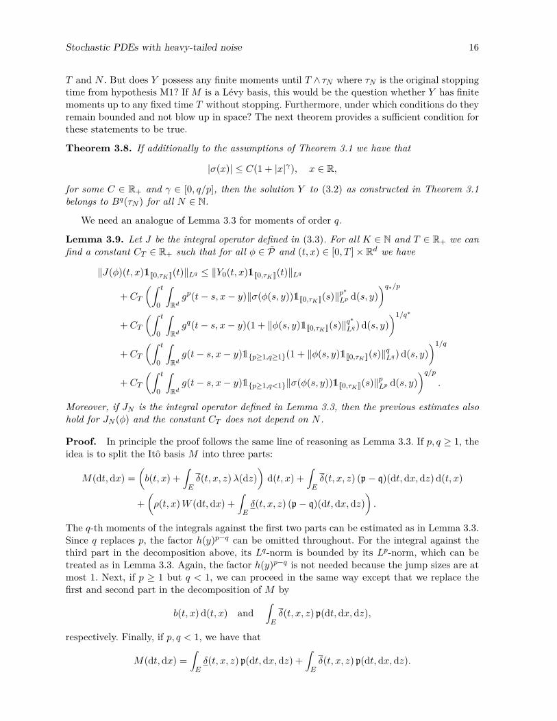
T and N . But does Y possess any finite moments until T ∧ τN where τN is the original stoppingtime from hypothesis M1? If M is a Lévy basis, this would be the question whether Y has finitemoments up to any fixed time T without stopping. Furthermore, under which conditions do theyremain bounded and not blow up in space? The next theorem provides a sufficient condition forthese statements to be true.

Theorem 3.8. If additionally to the assumptions of Theorem 3.1 we have that

|σ(x)| ≤ C(1 + |x|γ), x ∈ R,

for some C ∈ R+ and γ ∈ [0, q/p], then the solution Y to (3.2) as constructed in Theorem 3.1belongs to Bq(τN ) for all N ∈ N.

We need an analogue of Lemma 3.3 for moments of order q.

Lemma 3.9. Let J be the integral operator defined in (3.3). For all K ∈ N and T ∈ R+ we canfind a constant CT ∈ R+ such that for all φ ∈ P and (t, x) ∈ [0, T ]× Rd we have

‖J(φ)(t, x)1J0,τKK(t)‖Lq ≤ ‖Y0(t, x)1J0,τKK(t)‖Lq

+ CT

(∫ t

0

∫Rdgp(t− s, x− y)‖σ(φ(s, y))1J0,τKK(s)‖

p∗

Lp d(s, y))q∗/p

+ CT

(∫ t

0

∫Rdgq(t− s, x− y)(1 + ‖φ(s, y)1J0,τKK(s)‖

q∗

Lq) d(s, y))1/q∗

+ CT

(∫ t

0

∫Rdg(t− s, x− y)1p≥1,q≥1(1 + ‖φ(s, y)1J0,τKK(s)‖

qLq) d(s, y)

)1/q

+ CT

(∫ t

0

∫Rdg(t− s, x− y)1p≥1,q<1‖σ(φ(s, y))1J0,τKK(s)‖

pLp d(s, y)

)q/p.

Moreover, if JN is the integral operator defined in Lemma 3.3, then the previous estimates alsohold for JN (φ) and the constant CT does not depend on N .

Proof. In principle the proof follows the same line of reasoning as Lemma 3.3. If p, q ≥ 1, theidea is to split the Itô basis M into three parts:

M(dt,dx) =(b(t, x) +

∫Eδ(t, x, z)λ(dz)

)d(t, x) +

∫Eδ(t, x, z) (p− q)(dt,dx,dz) d(t, x)

+(ρ(t, x)W (dt,dx) +

∫Eδ(t, x, z) (p− q)(dt,dx,dz)

).

The q-th moments of the integrals against the first two parts can be estimated as in Lemma 3.3.Since q replaces p, the factor h(y)p−q can be omitted throughout. For the integral against thethird part in the decomposition above, its Lq-norm is bounded by its Lp-norm, which can betreated as in Lemma 3.3. Again, the factor h(y)p−q is not needed because the jump sizes are atmost 1. Next, if p ≥ 1 but q < 1, we can proceed in the same way except that we replace thefirst and second part in the decomposition of M by

b(t, x) d(t, x) and∫Eδ(t, x, z) p(dt,dx,dz),

respectively. Finally, if p, q < 1, we have that

M(dt,dx) =∫Eδ(t, x, z) p(dt,dx,dz) +

∫Eδ(t, x, z) p(dt,dx,dz).


The result then follows in a similar way if we switch to the p-th moment for the first term. Thestatement regarding JN is evident because the estimates above hold for all measures with onlya subset of jumps of M . 2

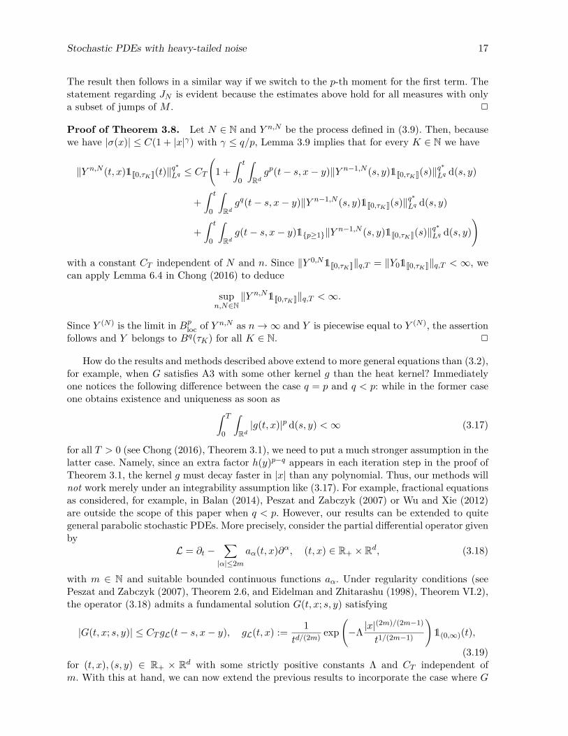
Proof of Theorem 3.8. Let N ∈ N and Y n,N be the process defined in (3.9). Then, becausewe have |σ(x)| ≤ C(1 + |x|γ) with γ ≤ q/p, Lemma 3.9 implies that for every K ∈ N we have

‖Y n,N (t, x)1J0,τKK(t)‖q∗

Lq ≤ CT

(1 +

∫ t

0

∫Rdgp(t− s, x− y)‖Y n−1,N (s, y)1J0,τKK(s)‖

q∗

Lq d(s, y)

+∫ t

0

∫Rdgq(t− s, x− y)‖Y n−1,N (s, y)1J0,τKK(s)‖

q∗

Lq d(s, y)

+∫ t

0

∫Rdg(t− s, x− y)1p≥1‖Y n−1,N (s, y)1J0,τKK(s)‖

q∗

Lq d(s, y))

with a constant CT independent of N and n. Since ‖Y 0,N1J0,τKK‖q,T = ‖Y01J0,τKK‖q,T < ∞, wecan apply Lemma 6.4 in Chong (2016) to deduce

supn,N∈N

‖Y n,N1J0,τKK‖q,T <∞.

Since Y (N) is the limit in Bploc of Y n,N as n→∞ and Y is piecewise equal to Y (N), the assertion

follows and Y belongs to Bq(τK) for all K ∈ N. 2

How do the results and methods described above extend to more general equations than (3.2),for example, when G satisfies A3 with some other kernel g than the heat kernel? Immediatelyone notices the following difference between the case q = p and q < p: while in the former caseone obtains existence and uniqueness as soon as∫ T

0

∫Rd|g(t, x)|p d(s, y) <∞ (3.17)

for all T > 0 (see Chong (2016), Theorem 3.1), we need to put a much stronger assumption in thelatter case. Namely, since an extra factor h(y)p−q appears in each iteration step in the proof ofTheorem 3.1, the kernel g must decay faster in |x| than any polynomial. Thus, our methods willnot work merely under an integrability assumption like (3.17). For example, fractional equationsas considered, for example, in Balan (2014), Peszat and Zabczyk (2007) or Wu and Xie (2012)are outside the scope of this paper when q < p. However, our results can be extended to quitegeneral parabolic stochastic PDEs. More precisely, consider the partial differential operator givenby

L = ∂t −∑|α|≤2m

aα(t, x)∂α, (t, x) ∈ R+ × Rd, (3.18)

with m ∈ N and suitable bounded continuous functions aα. Under regularity conditions (seePeszat and Zabczyk (2007), Theorem 2.6, and Eidelman and Zhitarashu (1998), Theorem VI.2),the operator (3.18) admits a fundamental solution G(t, x; s, y) satisfying

|G(t, x; s, y)| ≤ CT gL(t− s, x− y), gL(t, x) := 1td/(2m) exp

(−Λ |x|

(2m)/(2m−1)

t1/(2m−1)

)1(0,∞)(t),

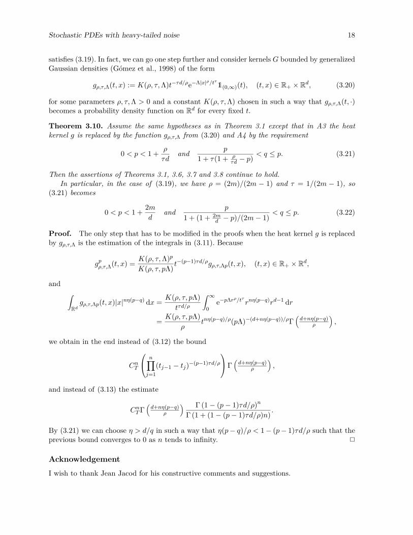
(3.19)for (t, x), (s, y) ∈ R+ × Rd with some strictly positive constants Λ and CT independent ofm. With this at hand, we can now extend the previous results to incorporate the case where G


satisfies (3.19). In fact, we can go one step further and consider kernels G bounded by generalizedGaussian densities (Gómez et al., 1998) of the form

gρ,τ,Λ(t, x) := K(ρ, τ,Λ)t−τd/ρe−Λ|x|ρ/tτ1(0,∞)(t), (t, x) ∈ R+ × Rd, (3.20)

for some parameters ρ, τ,Λ > 0 and a constant K(ρ, τ,Λ) chosen in such a way that gρ,τ,Λ(t, ·)becomes a probability density function on Rd for every fixed t.

Theorem 3.10. Assume the same hypotheses as in Theorem 3.1 except that in A3 the heatkernel g is replaced by the function gρ,τ,Λ from (3.20) and A4 by the requirement

0 < p < 1 + ρ

τdand p

1 + τ(1 + ρτd − p)

< q ≤ p. (3.21)

Then the assertions of Theorems 3.1, 3.6, 3.7 and 3.8 continue to hold.In particular, in the case of (3.19), we have ρ = (2m)/(2m − 1) and τ = 1/(2m − 1), so

(3.21) becomes

0 < p < 1 + 2md

and p

1 + (1 + 2md − p)/(2m− 1)

< q ≤ p. (3.22)

Proof. The only step that has to be modified in the proofs when the heat kernel g is replacedby gρ,τ,Λ is the estimation of the integrals in (3.11). Because

gpρ,τ,Λ(t, x) = K(ρ, τ,Λ)p

K(ρ, τ, pΛ) t−(p−1)τd/ρgρ,τ,Λp(t, x), (t, x) ∈ R+ × Rd,

and ∫Rdgρ,τ,Λp(t, x)|x|nη(p−q) dx = K(ρ, τ, pΛ)

tτd/ρ

∫ ∞0

e−pΛrρ/tτ rnη(p−q)rd−1 dr

= K(ρ, τ, pΛ)ρ

tnη(p−q)/ρ(pΛ)−(d+nη(p−q))/ρΓ(d+nη(p−q)

ρ

),

we obtain in the end instead of (3.12) the bound

CnT

n∏j=1

(tj−1 − tj)−(p−1)τd/ρ

Γ(d+nη(p−q)

ρ

),

and instead of (3.13) the estimate

CnTΓ(d+nη(p−q)

ρ

) Γ (1− (p− 1)τd/ρ)n

Γ (1 + (1− (p− 1)τd/ρ)n) .

By (3.21) we can choose η > d/q in such a way that η(p− q)/ρ < 1− (p− 1)τd/ρ such that theprevious bound converges to 0 as n tends to infinity. 2

Acknowledgement

I wish to thank Jean Jacod for his constructive comments and suggestions.


ReferencesS. Albeverio, J.-L. Wu, and T.-S. Zhang. Parabolic SPDEs driven by Poisson white noise. Stoch.Process. Appl., 74(1):21–36, 1998.

D. Applebaum and J.-L. Wu. Stochastic partial differential equations driven by Lévy space–timewhite noise. Random Oper. Stoch. Equ., 8(3):245–259, 2000.

R.M. Balan. SPDEs with α-stable Lévy noise: A random field approach. Int. J. Stoch. Anal.,2014. Article ID 793275, 22 pages.

O.E. Barndorff-Nielsen, F.E. Benth, and A.E.D. Veraart. Ambit processes and stochastic partialdifferential equations. In G. Di Nunno and B. Øksendal, editors, Advanced MathematicalMethods for Finance, pages 35–74. Springer, Berlin, 2011.

K. Bichteler and J. Jacod. Random measures and stochastic integration. In G. Kallianpur,editor, Theory and Application of Random Fields, pages 1–18. Springer, Berlin, 1983.

R.A. Carmona and S.A. Molchanov. Parabolic Anderson Model and Intermittency. AmericanMathematical Society, Providence, RI, 1994.

B. Chen, C. Chong, and C. Klüppelberg. Simulation of stochastic Volterra equations drivenby space–time Lévy noise. In M. Podolskij, R. Stelzer, S. Thorbjørnsen, and A.E.D. Ver-aart, editors, The Fascination of Probability, Statistics and their Applications, pages 209–229.Springer, Cham, Switzerland, 2016.

C. Chong. Lévy-driven Volterra equations in space and time. J. Theor. Probab., 2016. In press.

C. Chong and C. Klüppelberg. Integrability conditions for space–time stochastic integrals:Theory and applications. Bernoulli, 21(4):2190–2216, 2015.

I. Corwin. The Kardar-Parisi-Zhang equation and universality class. Random Matrices: TheoryAppl., 1(1):76 pages, 2012.

I.M. Davies, A. Truman, and H. Zhao. Stochastic heat and Burgers equations and the intermit-tence of turbulence. In R.C. Dalang, M. Dozzi, and F. Russo, editors, Seminar on StochasticAnalysis, Random Fields and Applications IV, pages 95–110. Birkhäuser, Basel, 2004.

D. Dawson. Measure-valued Markov processes. In P.L. Hennequin, editor, École d’Été de Prob-abilités de Saint Flour XXI - 1991, pages 1–260. Springer, Berlin, 1993.

C. Dellacherie and P.-A. Meyer. Probabilities and Potential B. North-Holland, Amsterdam,1982.

S.D. Eidelman and N.V. Zhitarashu. Parabolic Boundary Value Problems. Birkhäuser, Basel,1998.

E. Gómez, M.A. Gómez-Villegas, and J.M. Marín. A multivariate generalization of the powerexponential family of distributions. Commun. Stat. Theory Methods, 27(3):589–600, 1998.

M. Hairer. Solving the KPZ equation. Ann. Math., 178(2):559–664, 2013.

H. Holden, B. Øksendal, J. Ubøe, and T. Zhang. Stochastic Partial Differential Equations.Springer, New York, 2nd edition, 2010.


J. Jacod and A.N. Shiryaev. Limit Theorems for Stochastic Processes. Springer, Berlin, 2ndedition, 2003.

B.J.T. Jones. The origin of scaling in the galaxy distribution. Mon. Not. R. Astron. Soc., 307(2):376–386, 1999.

D. Khoshnevisan. Analysis of Stochastic Partial Differential Equations. American MathematicalSociety, Providence, RI, 2014.

W. Liu and M. Röckner. Stochastic Partial Differential Equations: An Introduction. Springer,Cham, Switzerland, 2015.

C. Mueller. The heat equation with Lévy noise. Stoch. Process. Appl., 74(1):67–82, 1998.

C. Mueller. Stochastic PDE from the point of view of particle systems and duality. In R.C.Dalang, M. Dozzi, F. Flandoli, and F. Russo, editors, Stochastic Analysis: A Series of Lectures,pages 271–295. Birkhäuser, Basel, 2015.

L. Mytnik. Stochastic partial differential equation driven by stable noise. Probab. Theory Relat.Fields, 123(2):157–201, 2002.

S. Peszat and J. Zabczyk. Stochastic Partial Differential Equations with Lévy Noise. CambridgeUniversity Press, Cambridge, 2007.

P.E. Protter. Stochastic Integration and Differential Equations. Springer, Berlin, 2nd edition,2005.

N. El Saadi and Z. Benbaziz. On the existence of solutions for a nonlinear stochastic partialdifferential equation arising as a model of phytoplankton aggregation. Preprint available underarXiv:1507.06784 [math.AP], 2015.

E. Saint Loubert Bié. Étude d’une EDPS conduite par un bruit poissonnien. Probab. TheoryRelat. Fields, 111(2):287–321, 1998.

H.C. Tuckwell and J.B. Walsh. Random currents through nerve membranes. Biol. Cybern., 49(2):99–110, 1983.

J.B. Walsh. A stochastic model of neural response. Adv. Appl. Probab., 13(2):231–281, 1981.

J.B. Walsh. An introduction to stochastic partial differential equations. In P.L. Hennequin,editor, École d’Été de Probabilités de Saint Flour XIV - 1984, pages 265–439. Springer, Berlin,1986.

J.-L. Wu and B. Xie. On a Burgers type nonlinear equation perturbed by a pure jump Lévynoise in Rd. Bull. Sci. Math., 136(5):484–506, 2012.

Stochastic PDEs with heavy-tailed noise - mediaTUM

Documents

Transcript of Stochastic PDEs with heavy-tailed noise - mediaTUM