The Geometry of Brackets and the Area Principle - mediaTUM
254
The Geometry of Brackets and the Area Principle Susanne Apel Fakultät für Mathematik Technische Universität München D-85747 Garching 2013
-
Upload
khangminh22 -
Category
Documents
-
view
0 -
download
0
Transcript of The Geometry of Brackets and the Area Principle - mediaTUM

The Geometry of Bracketsand the Area Principle
Susanne Apel
Fakultät für Mathematik
Technische Universität München
D-85747 Garching
2013


Technische Universität MünchenFakultät für Mathematik
The Geometry of Bracketsand the Area Principle
Susanne Jasmin Apel
Vollständiger Abdruck der von der Fakultät für Mathematik der Technischen Uni-versität München zur Erlangung des akademischen Grades eines
Doktors der Naturwissenschaften (Dr. rer. nat.)
genehmigten Dissertation.
Vorsitzende: Univ.-Prof. Dr. Caroline LasserPrüfer der Dissertation: 1. Univ.-Prof. Dr.Dr. Jürgen Richter-Gebert
2. Univ.-Prof. Dr. Eva Maria FeichtnerUniversität Bremen
3. Prof.Walter Whiteley, Ph.D.York University, Kanada
Die Dissertation wurde am 17. Oktober 2013 bei der Technischen Universität Müncheneingereicht und durch die Fakultät für Mathematik am 3. März 2014 angenommen.


Zusammenfassung
Diese Arbeit beschäftigt sich mit dem Zusammenspiel von Geometrie und Algebra.Als Geometrie behandeln wir projektive Geometrie sowie euklidische Spezialisierun-gen. Die Algebra, um die es hier gehen soll, baut auf Determinanten auf derensymbolische Darstellung im Englischen “Brackets” heißen. Das von Grünbaum undShephard wiederentdeckte “Flächenprizip” macht es möglich, Brüche von Bracketsals orientierte Längenverhältnisse zu interpretieren. Diese Interpretation wird inzwei Teilen der Arbeit verwendet:Zunächst werden sogenannte Γ-Kreise untersucht. Diese ergeben sich auf natür-
liche Weise bei der Interpretation von binomischen oder biquadratischen Beweisenvon Schließungssätzen mittels des Flächenprinzips. Diese kann angewendet wer-den, da solche Beweise, wie von Richter-Gebert eingeführt, in der Sprache derBrackets formuliert sind. Γ-Kreise können als grundlegende Bausteine in dieserTheorie betrachtet werden. Man kann die Γ-Kreise zusammen mit biquadratischenBrüchen, die den biquadratischen Beweisen entspringen, auch nutzen, um darausselbst Schließungssätze zu konstruieren. Dabei ermöglicht die Interpretation durchdas Flächenprinzip geometrische Kontrolle über die Kürzungsmuster. Die formaleBehandlung der Bausteine orientiert sich an der Sprache von Dress und Wenzel. Diein unserer Behandlung nicht vollständig vorhandene Information über Kollinear-itäten impliziert, dass sich nicht automatisch alle Γ-Kreise auf einige wenige ihrerArt zurückführen lassen. Daher werden sogenannte irreduzible Γ-Kreise genaueruntersucht, was es zudem ermöglicht sie zu zählen. Wendet man das Flächenprinzipauf (Kombinationen von) Γ-Kreisen an, so erhält man Resultate, die die von Grün-baum und Shephard verallgemeinern.Anschließend wird das Problem der Cayley-Faktorisierung behandelt. Hierbei
möchte man mit einer Linealkonstruktion überprüfen, ob sich endlich viele Punkteder projektiven Ebene in spezieller Lage befinden. Die spezielle Lage der Punktewird durch das Verschwinden eines Polynoms in Brackets beschrieben, das wir mit Bbezeichnen wollen. Es ist durch Sturmfels und Whiteley bekannt, dass dies nicht im-mer möglich ist – stattdessen kann man immerM ·B durch eine Linealkonstruktioncharakterisieren, wobei M ein Monom in Brackets ist. Wir stellen einen neuen Al-gorithmus für das gleiche Resultat vor, der einen geringeren Grad von M aufweist.Der konstante Faktor in der Gradschranke wird von 105 auf 9 reduziert. Dieswird durch das implizite Einführen von lokalen Koordinatensystemen mittels desFlächenprinzips erreicht. Die gefundenen orientierten Längenverhältnisse könnendann mit den Konstruktionen von Ceva und Menelaus sowie der von-Staudt’schenprojektiven Arithmetik kombiniert werden. Der Algorithmus kann den Satz vonPascal erklären und ist prägnant genug, um auf dem Computer implementiert zuwerden. Zwei beispielhafte Ausgaben werden angegeben.
i

Abstract
The present thesis is on the interplay of geometry and algebra. As geometry weconsider projective geometry as well as Euclidean specializations. The algebra inquestion is based on determinants whose symbolic representation is called bracket.The area principle, which was rediscovered by Grünbaum and Shephard, allows forinterpreting ratios of brackets as oriented length ratios. This interpretation is madeuse of in two parts of the thesis:At first, so-called Γ-cycles are investigated. They emerge in a natural way when
interpreting binomial or biquadratic proofs of incidence theorems via the area prin-ciple. It can be applied, since such proofs, as introduced by Richter-Gebert, areformulated in the language of brackets. Γ-cycles can be understood as basic buildingblocks within this theory. One can use Γ-cycles together with biquadratic fractions,which arise from biquadratic proofs, also in order to construct incidence theorems.In doing so, the interpretation via the area principle provides geometric control overthe cancellation patterns. The formal treatment of these building blocks follows thelanguage of Dress and Wenzel. Since the information about collinearities is not com-plete in our setup, we cannot automatically reduce the number of relevant Γ-cyclesto only a few. Therefore, so-called irreducible Γ-cycles are analyzed in more detail,which allows for also counting them. Applying the area principle to (a combinationof) Γ-cycles results in statements that generalize those of Grünbaum and Shephard.Afterwards, the problem of Cayley factorization is treated. Here one wishes to
check with a ruler construction whether finitely many points in the projective planeare located in special position. The special position of the points is described bythe vanishing of a polynomial in brackets which is denoted by B. It is known dueto a result of Sturmfels and Whiteley that this is not always possible—instead onecan characterize always M · B by a ruler construction, where M is a monomial inbrackets. We present a new algorithm for the same result and show that it impliesa smaller degree of M . The constant factor in the bound on the degree is reducedfrom 105 to 9. This is achieved by implicitly introducing local coordinate systemsvia the area principle. The obtained oriented length ratios can be combined with theconstructions of Ceva and Menelaus as well as with the projective arithmetic givenby von Staudt. The algorithm is able to explain Pascal’s theorem and is conciseenough to be implemented on a computer. Two exemplary outputs are given.
iii


Acknowledgment
First of all, I wish to thank my advisor Jürgen Richter-Gebert for giving me theopportunity to do this thesis at his chair and within the program of TopMath. Hisstyle of supervision includes an amount of freedom that made it possible to findtopics that suited me well. He taught me many things including of course mathe-matics, reasoning, didactics, programming, using Cinderella and enjoying what oneis doing. I also learned my geometry from him and he showed me many tools thatare used within this thesis. Through him, I got to know problems and results whichwere the starting points for all parts of the present text. Together, we got interestedand started to analyze Γ-cycles which are one of the central topics treated here. Healways encouraged me to go on with this topic.Next, I want to thank Walter Whiteley for examining this thesis. Furthermore I
am thankful for the discussions I had with him during my stay at the Fields Institutein Toronto. The thematic program there was a great opportunity for a stay abroadand meeting many interesting people. Especially the discussions with him aboutbracket polynomials and weights as well as about his results obtained together withBernd Sturmfels on Cayley factorization enabled me to come up with and pursuingthe ideas for improving their result.Moreover, I am very grateful to Eva Maria Feichtner for kindly agreeing to act as
examiner of this thesis.The graduate program “TopMath” within the Elite Network of Bavaria allowed
me to start doing research at a very early level. I am thankful for covering expensesof my scientific travels and for the opportunity to participate in the program of theElite Network of Bavaria.Not only travel funds were also provided by Evangelisches Studienwerk Villigst.
Its scholarship and the resulting independence gave me room to develop personally.Furthermore, I enjoyed the atmosphere and the exchange with other fellows in thelocal Munich group and at the graduates’ conventions.I am also grateful to the Powell family for letting me stay at their place during
my time in Toronto. It was a pleasure meeting them.Likewise, I want to thank all members of the Chair M10 of Geometry and Vi-
sualization for the great time I had there. During this time, I had different officecolleagues. Each of them was different and by the time, we got to know each otherbetter and learned different aspects from each other. My last office colleagues Mar-tin von Gagern and Stefan Kranich where very helpful with technical issues andhelped completing many details of this thesis. Florian Quiring also helped me tosee that a rational version of the first fundamental theorem of invariant theory holds.Finally, I am most thankful to Eike for being who he is and for loving me and
being there for me. In addition, I would like to express my gratitude for the supportI got from my family.
v


Contents
1. Introduction 1
I. Basics, Language and Fundamental Ideas 9
2. Fundamental Definitions in Projective Geometry 112.1. Homogenous Coordinates of Points . . . . . . . . . . . . . . . . . . . 112.2. Homogenous Coordinates of Lines . . . . . . . . . . . . . . . . . . . . 122.3. Join, Meet and Collinearity in Homogenous Coordinates . . . . . . . 132.4. The Intersection of Two Lines Given as Spans of Points via Plücker’s µ 142.5. Points in Projective Space of Rank n . . . . . . . . . . . . . . . . . . 14
3. Geometric Tools and Constructions 173.1. The Area Principle . . . . . . . . . . . . . . . . . . . . . . . . . . . . 173.2. The Theorems of Ceva and Menelaus . . . . . . . . . . . . . . . . . . 193.3. Projective Transformations and Invariants . . . . . . . . . . . . . . . 203.4. The Cross-Ratio . . . . . . . . . . . . . . . . . . . . . . . . . . . . . 223.5. Projective Number Lines . . . . . . . . . . . . . . . . . . . . . . . . . 243.6. Quadrilateral Sets . . . . . . . . . . . . . . . . . . . . . . . . . . . . 253.7. Von Staudt’s Constructions: Arithmetic on Projective Number Lines 273.8. Harmonic Sets . . . . . . . . . . . . . . . . . . . . . . . . . . . . . . 283.9. Configurations of Ceva and Menelaus Revisited . . . . . . . . . . . . 283.10. Conics and Pascal’s Theorem . . . . . . . . . . . . . . . . . . . . . . 31
4. The Bracket Ring and the Fundamental Theorems of Invariant Theory 334.1. Grassmann-Plücker Relations in Rank 3 . . . . . . . . . . . . . . . . 354.2. The Bracket Ring BP in Rank 3 . . . . . . . . . . . . . . . . . . . . . 354.3. Grassmann-Plücker Relations in Rank n . . . . . . . . . . . . . . . . 37
4.3.1. Interpreting Grassmann-Plücker Relations: Intersection of Sub-spaces . . . . . . . . . . . . . . . . . . . . . . . . . . . . . . . 38
4.4. The Bracket Ring BP in Rank n . . . . . . . . . . . . . . . . . . . . 384.5. Fundamental Theorems of Invariant Theory . . . . . . . . . . . . . . 394.6. Applications to Projective Geometry . . . . . . . . . . . . . . . . . . 394.7. Comparing Expressions in BP and the Straightening Algorithm . . . 41
vii
Contents
5. A Symbolic Version of the Grassmann-Cayley Algebra 435.1. The Elements . . . . . . . . . . . . . . . . . . . . . . . . . . . . . . . 465.2. The Join ∨ . . . . . . . . . . . . . . . . . . . . . . . . . . . . . . . . 485.3. The Meet ∧ . . . . . . . . . . . . . . . . . . . . . . . . . . . . . . . . 495.4. Interpretations and Relations . . . . . . . . . . . . . . . . . . . . . . 515.5. Grassmann-Cayley Algebra Expressions . . . . . . . . . . . . . . . . 59
6. Evaluations 616.1. Evaluations of Pascal’s Construction . . . . . . . . . . . . . . . . . . 62
6.1.1. First Evaluation . . . . . . . . . . . . . . . . . . . . . . . . . 636.1.2. Symmetric (Classical) Evaluation . . . . . . . . . . . . . . . . 636.1.3. Evaluation by Rerooting the Expression . . . . . . . . . . . . 646.1.4. Diagram Representations . . . . . . . . . . . . . . . . . . . . 65
6.2. Rerooting in Diagrams . . . . . . . . . . . . . . . . . . . . . . . . . . 666.3. Splitting Diagrams along Inner Edges and Notation . . . . . . . . . . 666.4. Exemplary Evaluation of an Expression of Part III . . . . . . . . . . 71
7. Incidence Theorems 777.1. General Structure of Incidence Theorems . . . . . . . . . . . . . . . . 777.2. Pascal’s Theorem Revisited . . . . . . . . . . . . . . . . . . . . . . . 777.3. Incidence Theorems of Points and Lines . . . . . . . . . . . . . . . . 797.4. (General) Automated Theorem Proving . . . . . . . . . . . . . . . . 807.5. Modeling Incidence Theorems of Points and Lines . . . . . . . . . . . 82
II. Γ-Cycles 85
8. Introduction to Γ-Cycles 87
9. Motivation: Example on How to Transform a Binomial Proof to Γ-Cycles 899.1. Formal Language for Stating Biquadratic Proofs . . . . . . . . . . . 909.2. A Biquadratic Proof for the Given Example . . . . . . . . . . . . . . 919.3. Interpreting a Biquadratic Proof . . . . . . . . . . . . . . . . . . . . 939.4. On the Power of Biquadratic Proofs . . . . . . . . . . . . . . . . . . 101
10.The Base Graph Γ, Irreducible Γ-Cycles and Morphisms 10310.1. Weak Irreducibility . . . . . . . . . . . . . . . . . . . . . . . . . . . . 10410.2. Oriented Γ-Cycles and Strong Irreducibility . . . . . . . . . . . . . . 10510.3. Decomposing Large Γ-cycles within Biquadratic Proofs . . . . . . . . 10610.4. Some Subgroups Vanishing under Morphisms . . . . . . . . . . . . . 107
10.4.1. A Euclidean Interpretation of Oriented Γ-Cycles . . . . . . . 10810.4.2. Including Collinearities . . . . . . . . . . . . . . . . . . . . . . 109
viii

Contents
11.Counting (Weakly) Irreducible Γ-Cycles 11311.1. Assumptions on the Irreducible Γ-Cycles . . . . . . . . . . . . . . . . 11311.2. Table Representations of Irreducible Γ-Cycles . . . . . . . . . . . . . 11411.3. Counting Irreducible Γ-Cycles . . . . . . . . . . . . . . . . . . . . . . 117
12.Glueing Γ-Cycles along Their Orbits 12512.1. An Example . . . . . . . . . . . . . . . . . . . . . . . . . . . . . . . . 12512.2. Edges of Γ-Cycles and Informations about Orbits . . . . . . . . . . 130
13.Relations between Γ-Cycles and Results of Grünbaum and Shephard 135
III. Cayley Factorization 143
14.Statement of the Problem and Progress so Far 14514.1. Conventions about Notions and Evaluations . . . . . . . . . . . . . . 150
15.Instructive Binomial Example 153
16. Algorithm for Binomials with Coefficients in −1,+1 15916.1. Matching the Brackets of Both Summands . . . . . . . . . . . . . . . 15916.2. Geometric Interpretation of the Pairs of Brackets in P . . . . . . . . 16316.3. Detecting Cycles . . . . . . . . . . . . . . . . . . . . . . . . . . . . . 16516.4. Triangulating Cycles . . . . . . . . . . . . . . . . . . . . . . . . . . . 16616.5. Combining 2-Cycles or Cross-Ratios . . . . . . . . . . . . . . . . . . 16916.6. Final Coincidence . . . . . . . . . . . . . . . . . . . . . . . . . . . . . 17616.7. Example: A Derivation of Pascal’s Theorem . . . . . . . . . . . . . . 177
17.Generalization for Polynomials with Arbitrary Number of Summands 18117.1. Constructing the Coefficients . . . . . . . . . . . . . . . . . . . . . . 18317.2. Adding up Two 2-Cycles or Cross-Ratios . . . . . . . . . . . . . . . 18517.3. Adding up All 2-Cycles or Cross-Ratios . . . . . . . . . . . . . . . . 19317.4. Final Coincidence . . . . . . . . . . . . . . . . . . . . . . . . . . . . . 19617.5. The Multiplier of the Factorization . . . . . . . . . . . . . . . . . . . 199
18.Examples 20118.1. Example 1 . . . . . . . . . . . . . . . . . . . . . . . . . . . . . . . . . 20118.2. Example 2: Ten Points on a Cubic . . . . . . . . . . . . . . . . . . . 213
Bibliography 231
ix


1. Introduction
“ Ich bemerke nur noch, dass ich das [...] Verfahren, nach welchemder positive oder negative Werth einer Linie durch die verschiedeneNebeneinanderstellung der die Endpuncte der Linie bezeichnendenBuchstaben ausgedrückt wird, durchgehends angewendet und auchauf die Bezeichnung des Inhaltes von Dreiecken [...] und dreiseitigenPyramiden erweitert habe. Es wird hierdurch, so wie auch zumTheil durch den barycentrischen Calcul selbst, die Anschaulichkeitder synthetischen Methode mit der Allgemeinheit der analytischenin möglichst nahe Verbindung gebracht, indem man mit Anwendungrein geometrischer Zeichen, dergleichen die für die Puncte einerFigur gewählten Buchstaben sind, die arithmetischen Beziehungenzwischen den Theilen der Figur durch Formeln darstellt, welche füralle möglichen Lagen der Theile Gültigkeit haben.”
August Ferdinand Möbius, Der barycentrische Calcul, 1827
The topic of this thesis in its most general sense is the interplay of geometry andalgebra which both have a very long history. In the following it shall become clearwhy we feel connected to the above statement made by Möbius which in a loosetranslation and with a language adjusted to the present thesis can be summarizedas follows: The method of considering oriented lengths and volumes, indicated bythe order of points naming them, is able to connect the imagination of the syntheticmethod and the generality of the analytic one by naming geometric points withletters and representing geometric relations with formulas such that they are validin all possible concrete geometric situations. The so-called area principle is a specialcase of considering ratios of oriented lengths and volumes. It is used within thisthesis to address several problems. However, as we will show in Section 3.9, it canoften be translated into considerations regarding weights as it was Möbius’s startingpoint for introducing barycentric coordinates. To begin with, we now describe thesynthetic and algebraic methods and language used in the present text.
1

1. Introduction
Our setup is projective geometry (for a very brief introduction see Chapter 2).Here, three points are collinear if and only if the matrix whose columns are the3-vectors of the homogenous coordinates of the points has a vanishing determinant.Naming the homogenous coordinates of the three points p, q and r, this can bewritten as
|p, q, r| := det(p, q, r) = 0.
This notion does not refer to the concrete coordinates of the points but only to itsnames. This motivates the notion of a symbolized version of a determinant usingonly names of points:
[p,q, r]
which is called a bracket. The names p, q and r themselves have a symbolic natureand can be considered to be taken from an alphabet P describing a point set. Thislanguage emphasizes the symbolic and combinatoric way points will be treated. Thenotion of brackets is useful since many geometric properties can be represented bycombinations of brackets, more precisely with bracket polynomials. E.g. three linesspanned by the pairs of points a, b, c, d and e, f are concurrent if and only if
|a, b, c||d, e, f | − |a, b, d||c, e, f | (1.1)
vanishes. Expressing the same property on the level of concrete homogenous coor-dinates yields much longer expressions (see Section 4.6). This is one reason whygeometers since Cayley have been interested in brackets.Another approach to brackets is invariant theory (see Section 3.3 for more details).
According to Klein’s Erlangen program, geometry can always be considered as beinginvariant theory. This seems reasonable when recalling that in Euclidean geometrythe property of a triangle being equilateral does not depend on its position relativeto the origin. Therefore this property is at least invariant under translations. Itturns out that all Euclidean properties are invariant under the group of Euclideanmoves.In projective geometry one considers those transformations that maintain collin-
earity of points. It is the first fundamental theorem of (real) projective geometrythat each such transformation is induced by multiplying the homogenous coordi-nates of a point with an invertible matrix. Now (1.1) vanishing is a projectivelyinvariant property, since
|M · a,M · b,M · c||M · d,M · e,M · f | − |M · a,M · b,M · d||M · c,M · e,M · f |= det(M)2
(|a, b, c||d, e, f | − |a, b, d||c, e, f |
)
for a real invertible 3 × 3 matrix M and due to the multiplicativity of the deter-minant. For technical reasons we restrict ourselves to polynomial invariants with
2
respect to the multiplication of matrices M with determinant equal to 1. Theseinvariants can be classified by the bracket polynomials and the corresponding fun-damental theorems of invariant theory (which is described in Section 4.5 in moredetail). Projectively invariant properties can be easily constructed by their means.They are considered to be elements of the bracket ring as introduced by White in[120]. Here the names of the points are treated as symbols, not as vectors, whichallows for generalizing the concept to more general combinatorial geometries.
The usage of bracket polynomial and invariant language turned out to be usefulfor many geometers. There are also applications that use the algebra of brackets todetermine special positions of points. These applications include robotics, statics,rigidity of frameworks and scene analysis (see e.g. [125, 127, 33, 129, 28, 27, 81, 32]).
Until now this introduction was very algebraic. In the following we will presenta more geometric point of view: there are natural geometric constructions in theprojective plane. The most fundamental ones are the operations join and meetwhose existence is guaranteed by the axioms of projective planes: two points can bejoined to a unique line and two lines meet in a unique point. We will focus on thesetwo constructions. An exemplary computation in the more general Grassmann-Cayley algebra shows that the intersection of the lines spanned by the pairs ofpoints c, d and a, b can be given by
x := |a, b, d| · c− |a, b, c| · d. (1.2)
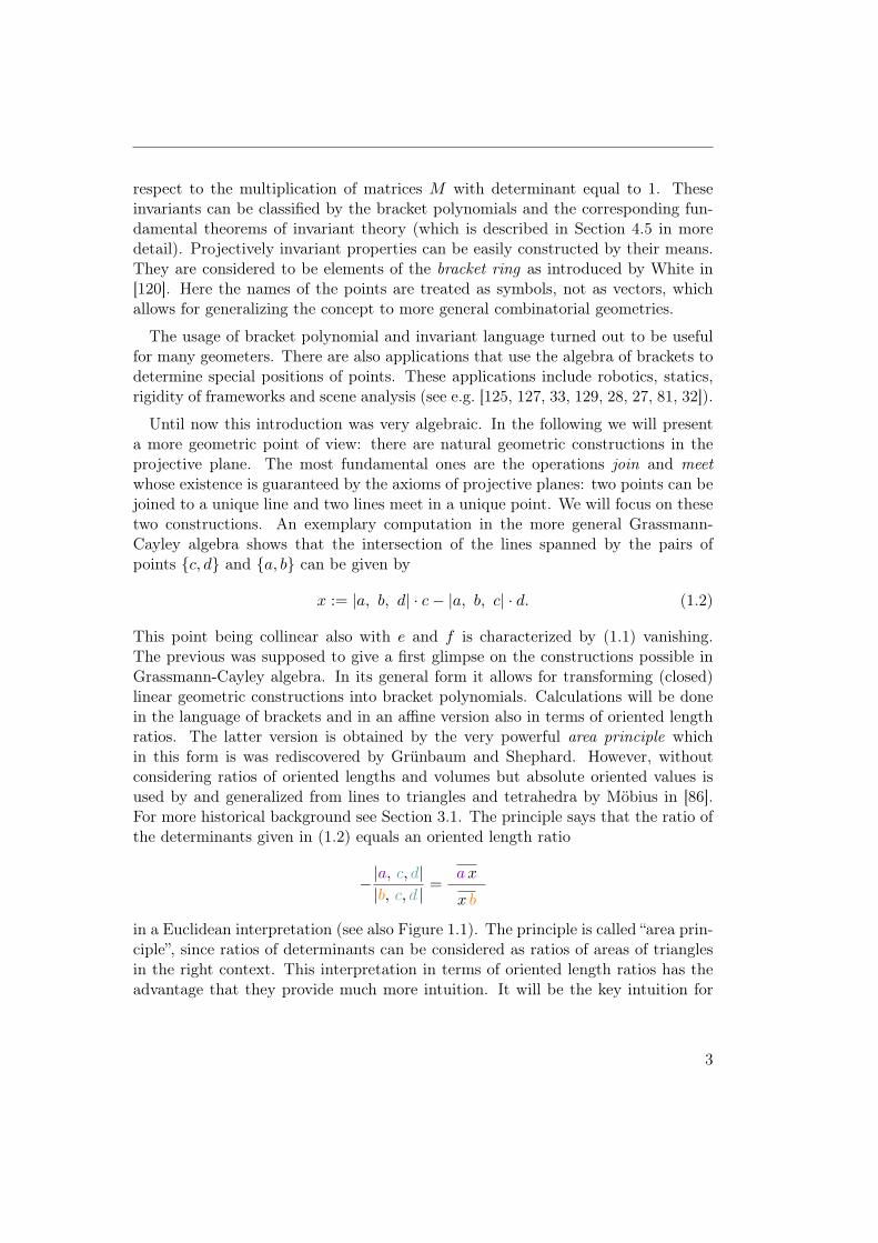
This point being collinear also with e and f is characterized by (1.1) vanishing.The previous was supposed to give a first glimpse on the constructions possible inGrassmann-Cayley algebra. In its general form it allows for transforming (closed)linear geometric constructions into bracket polynomials. Calculations will be donein the language of brackets and in an affine version also in terms of oriented lengthratios. The latter version is obtained by the very powerful area principle whichin this form is was rediscovered by Grünbaum and Shephard. However, withoutconsidering ratios of oriented lengths and volumes but absolute oriented values isused by and generalized from lines to triangles and tetrahedra by Möbius in [86].For more historical background see Section 3.1. The principle says that the ratio ofthe determinants given in (1.2) equals an oriented length ratio
−|a, c, d||b, c, d | =a x
x b
in a Euclidean interpretation (see also Figure 1.1). The principle is called “area prin-ciple”, since ratios of determinants can be considered as ratios of areas of trianglesin the right context. This interpretation in terms of oriented length ratios has theadvantage that they provide much more intuition. It will be the key intuition for
3

1. Introduction
the considerations done in Part II and in Part III. Furthermore, as it is pointed outin Section 3.9, it is closely related with the theory of weights and centers of massreferred to by Möbius in the introductory quotation.
Figure 1.1.: The length ratio a x/ x b equals |a, d,c||b, c,d | , a ratio of determinants.
Part I: BasicsPart I introduces many of the previously mentioned concepts in more detail. Itsummarizes the basic definition and computing techniques (projective geometry,bracket algebra, Grassmann-Cayley algebra, tensor diagrams and evaluation) aswell as some tools or basic building blocks (the area principle, the theorems of Cevaand Menelaus and von Staudt constructions) used in both Parts II and III. First,this part will focus on the plane case. For most of the results in Parts II and III, thisis sufficient. Since the theory also extends to arbitrary dimensions results in Parts IIand III can sometimes also be applied to general dimensions. This will not be treatedexplicitly but should be mentioned. We remark that we give a symbolic version ofthe definitions for the Grassmann-Cayley algebra which is not the standard one (seeChapter 5). The symbolic definition is very close to the formulation of Möbius whois amazed by the possibility to calculate only with the names of the points. Thisalgebra can be thought of a tool for computing with subspaces both of Rn and alsowith projective subspaces. We choose the symbolic version for the following reasons:as before when introducing brackets, it is natural to work only with abstract namesof points not with vectors representing homogenous coordinates as it is done inclassical introductions which mostly go back to [37] by Doubilet, Rota and Steinin which the ideas go back to Grassmann’s “Ausdehnungslehre” (see [48, 49]). Thisapproach fits better with the symbolic treatment in the bracket ring. This wasalready done by the school of Rota and is called the “White module” there. It islocated at the transition to a more general, supersymmetric theory and the verydetailed geometric ideas presented in [37] are less present. We want to connect bothin the introductive treatment of Grassmann-Cayley algebra.
4

It is an important basic fact that in Grassmann-Cayley algebra, any “closed”construction done by the means of join and meet with respect to some (abstract)base points a, b, . . . , e can be evaluated to a (multihomogenous) bracket polynomialB in the points a, b, . . . , e which has integer coefficients. This serves as motivationfor the problem treated in Part III. A closed construction can be thought of aconstruction that asks for the collinearity of three points that are constructed by themeans of join and meet depending on the points a, b, . . . , e. The resulting bracketpolynomial is unique in the previously mentioned bracket ring. Nevertheless, thebracket ring is a factor ring, say R/I with a non-trivial modulo I. Therefore, itmakes sense to consider several methods for evaluation since their output mightlook quite different and be identical only modulo I (see Chapter 6). We also give anintroduction to the background of incidence theorems (see Chapter 7). Theoremsof this kind are the starting point for the considerations in Part II. The techniquesused in this part are in turn used to attack the problems in Part III. Incidencetheorems are theorems using only incidences in their formulation of hypothesesand conclusions. The most famous examples are the theorems of Pappos and ofDesargues.
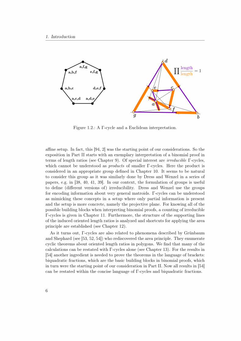
Part II: Γ-CyclesPart II is about so-called Γ-cycles, which is a new concept developed together withJürgen Richter-Gebert and describing a special class of binomial identities in thebracket algebra. In general, binomial identities in the bracket algebra are obvious.However, in the case of Γ-cycles its only at first sight and without knowing anycontext that they could be considered being trivial. At second sight, any Γ-cyclecan be interpreted as a theorem about oriented length ratios in affine geometry.Regarding them on their own, these Euclidean theorems are surprising and do notlook trivial any longer. An example seems to be appropriate: In Figure 1.2 on theleft-hand side, a Γ-cycle in its graphical version is shown. It induces the identity
[a, f , g]
[a,b, f ]· [a,b, f ]
[a,b, c]· [a,b, c]
[a, c,d]· [a, c,d]
[a,d, e]· [a,d, e]
[d, e, f ]· [d, e, f ]
[e, f , g]· [e, f , g]
[a, f ,g]= 1,
which can also be written as a vanishing binomial in the bracket ring, since allbrackets occurring somewhere in a numerator also occur somewhere in a denomi-nator. In the concrete form given, every fraction can be interpreted via the areaprinciple yielding that the product of oriented length ratios in the right-hand sideof Figure 1.2 equals 1 (for more details see Chapter 10).
Γ-cycles are exactly those binomial identities, for which such an interpretationin terms of oriented lengths is possible. This is due to the fact that they can beinterpreted as cycles in a Γ-graph known from matroid theory (see [84]).Furthermore, Γ-cycles do appear naturally when one tries to interpret so-called
binomial or biquadratic proofs (see [92, 93, 9, 30]) in terms of length ratios in an
5
1. Introduction
∏ lengthlength
= 1
Figure 1.2.: A Γ-cycle and a Euclidean interpretation.
affine setup. In fact, this [94, 2] was the starting point of our considerations. So theexposition in Part II starts with an exemplary interpretation of a binomial proof interms of length ratios (see Chapter 9). Of special interest are irreducible Γ-cycles,which cannot be understood as products of smaller Γ-cycles. Here the product isconsidered in an appropriate group defined in Chapter 10. It seems to be naturalto consider this group as it was similarly done by Dress and Wenzel in a series ofpapers, e.g. in [38, 40, 41, 39]. In our context, the formulation of groups is usefulto define (different versions of) irreducibility. Dress and Wenzel use the groupsfor encoding information about very general matroids. Γ-cycles can be understoodas mimicking these concepts in a setup where only partial information is presentand the setup is more concrete, namely the projective plane. For knowing all of thepossible building blocks when interpreting binomial proofs, a counting of irreducibleΓ-cycles is given in Chapter 11. Furthermore, the structure of the supporting linesof the induced oriented length ratios is analyzed and shortcuts for applying the areaprinciple are established (see Chapter 12).As it turns out, Γ-cycles are also related to phenomena described by Grünbaum
and Shephard (see [53, 52, 54]) who rediscovered the area principle. They enumeratecyclic theorems about oriented length ratios in polygons. We find that many of thecalculations can be restated with Γ-cycles alone (see Chapter 13). For the results in[54] another ingredient is needed to prove the theorems in the language of brackets:biquadratic fractions, which are the basic building blocks in binomial proofs, whichin turn were the starting point of our consideration in Part II. Now all results in [54]can be restated within the concise language of Γ-cycles and biquadratic fractions.
6
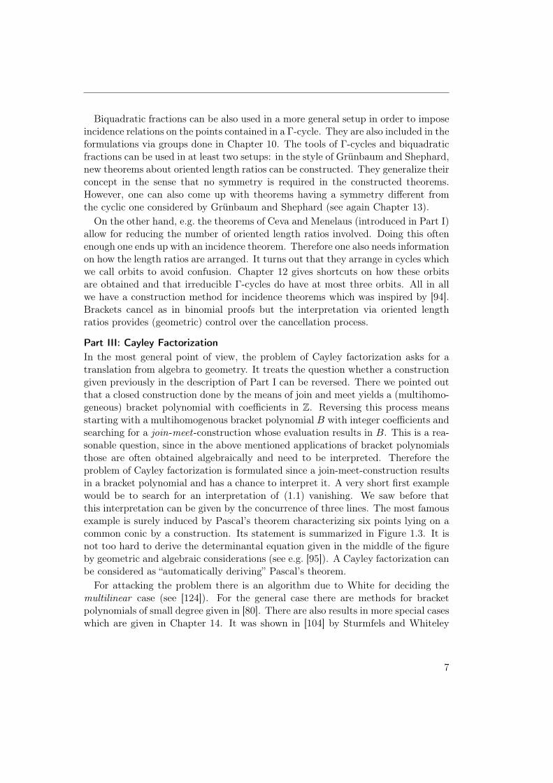
Biquadratic fractions can be also used in a more general setup in order to imposeincidence relations on the points contained in a Γ-cycle. They are also included in theformulations via groups done in Chapter 10. The tools of Γ-cycles and biquadraticfractions can be used in at least two setups: in the style of Grünbaum and Shephard,new theorems about oriented length ratios can be constructed. They generalize theirconcept in the sense that no symmetry is required in the constructed theorems.However, one can also come up with theorems having a symmetry different fromthe cyclic one considered by Grünbaum and Shephard (see again Chapter 13).On the other hand, e.g. the theorems of Ceva and Menelaus (introduced in Part I)
allow for reducing the number of oriented length ratios involved. Doing this oftenenough one ends up with an incidence theorem. Therefore one also needs informationon how the length ratios are arranged. It turns out that they arrange in cycles whichwe call orbits to avoid confusion. Chapter 12 gives shortcuts on how these orbitsare obtained and that irreducible Γ-cycles do have at most three orbits. All in allwe have a construction method for incidence theorems which was inspired by [94].Brackets cancel as in binomial proofs but the interpretation via oriented lengthratios provides (geometric) control over the cancellation process.
Part III: Cayley FactorizationIn the most general point of view, the problem of Cayley factorization asks for atranslation from algebra to geometry. It treats the question whether a constructiongiven previously in the description of Part I can be reversed. There we pointed outthat a closed construction done by the means of join and meet yields a (multihomo-geneous) bracket polynomial with coefficients in Z. Reversing this process meansstarting with a multihomogenous bracket polynomial B with integer coefficients andsearching for a join-meet-construction whose evaluation results in B. This is a rea-sonable question, since in the above mentioned applications of bracket polynomialsthose are often obtained algebraically and need to be interpreted. Therefore theproblem of Cayley factorization is formulated since a join-meet-construction resultsin a bracket polynomial and has a chance to interpret it. A very short first examplewould be to search for an interpretation of (1.1) vanishing. We saw before thatthis interpretation can be given by the concurrence of three lines. The most famousexample is surely induced by Pascal’s theorem characterizing six points lying on acommon conic by a construction. Its statement is summarized in Figure 1.3. It isnot too hard to derive the determinantal equation given in the middle of the figureby geometric and algebraic considerations (see e.g. [95]). A Cayley factorization canbe considered as “automatically deriving” Pascal’s theorem.For attacking the problem there is an algorithm due to White for deciding the
multilinear case (see [124]). For the general case there are methods for bracketpolynomials of small degree given in [80]. There are also results in more special caseswhich are given in Chapter 14. It was shown in [104] by Sturmfels and Whiteley
7

1. Introduction
⇔ |a, c, e| · |a, d, f | · |b, c, f | · |b, d, e|−|a, c, f | · |a, d, e| · |b, c, e| · |b, d, f | = 0
⇔
Figure 1.3.: Pascal’s theorem: six points a, b, c, d, e and f lie on a common conicif and only if the depending points x, y, z lie on a common line.
that a factorization is not always possible. However, they also show that for anybracket polynomial B (homogenous, with integer coefficients), there always exists abracket monomial M such that M ·B can be factored. This is the reformulation ofthe problem which we focus on. In the present thesis, the degree of the monomialMand therefore also the complexity of the construction can be reduced to an extentthat makes an implementation possible. The constant factor in the bound on thedegree of M can be reduced from 105 (in the algorithm used in [104]) to 9.The algorithm presented here relies on the (intuition of the) area principle and in
its first version interprets only bracket binomials. The configurations of Ceva andMenelaus as well as von Staudt constructions are used to perform multiplication onoriented length ratios and cross-ratios. In a next step, the approach is generalizedto the case of an arbitrary number of summands. Von Staudt’s construction forprojective addition is used to combine several summands. Some optimizations aredone in order to keep the degree of the leading monomialM low. The most relevantoptimizations done are factoring out common factors and reusing existing points inthe constructions.The algorithm is able to explain Pascal’s theorem: The algorithm has some free-
dom of choice during its execution. We will show in Section 16.7 that local opti-mizations within the algorithm yield Pascal’s theorem. In a more general and lesssymmetric setup this cannot be expected. However we think that this derivation ofPascal’s theorem shows that our algorithm is very close to geometry. In addition, aspreviously mentioned, a concrete implementation in Mathematica ([136]) togetherwith the Combinatorica package was possible. With its help we include two exam-ples of the output of the implementation (see Chapter 18). One of its examples canbe considered to be a generalization of Pascal’s theorem since it factors a polyno-mial describing the property of ten points lying on a common cubic. The concreterepresentation of the bracket polynomial that is factored has 20 summands. It isdue to Richter-Gebert and it is the shortest representation known to our group.
8
Part I.
Basics, Language andFundamental Ideas
9


2. Fundamental Definitions inProjective Geometry
This and the following chapter give a very short reference for basic concepts inprojective geometry which are used later on in this text. We will mostly focus onthe real projective plane. The exposition given here is by no means exhaustive.For a more extensive treatise, there are a lot of monographs on the topic, e.g.[24, 25, 43, 110, 65] to mention only a few of them. They provide most of theconcepts used here. We follow closely the exposition in [95]. E.g. [24, 95] alsoprovide comments on the historical development.
2.1. Homogenous Coordinates of Points
In the real projective plane RP2, a point is a one-dimensional subspace of R3. Thismotivates why the two-dimensional real projective plane is also called projectivegeometry of rank 3. We define an equivalence relation on the vectors spanning theone-dimensional subspaces. For v ∈ R3 \ (0, 0, 0) let
[v] :=v′ ∈ R3 | v′ = λ · v for λ ∈ R \ 0
.
The points P of RP2 are all of these equivalence classes:
P :=R3 \ (0, 0, 0)
R \ 0 :=
[v] | v ∈ R3 \ (0, 0, 0).
Topologically, P is in fact a two-dimensional structure. The usual affine plane R2
can be embedded in RP2. One possible embedding is shown in Figure 2.1. Thisembedding, where the last coordinate equals 1, is called the standard embedding. Itprovides an intuition for most of the points in RP2 except for points of the shape(x, y, 0), where x, y ∈ R. Those can be thought as being points infinitely far awaypointing in direction (x, y) in the corresponding affine picture in R2. All lines withdirection (x, y) have this point in common. This brings us to the next ingredient ofthe projective plane: lines.
11

2. Fundamental Definitions in Projective Geometry50 3 Homogeneous Coordinates
y
x
z
p
l
R2 ! (x, y, z) " R3 | z = 1
Fig. 3.1 Embedding the Euclidean plane in R3.
coordinate representation of the Euclidean plane E. As usual, we identify theEuclidean plane with R2. Each point in the Euclidean plane can be repre-sented by a two-dimensional vector of the form (x, y) ! R2. A line can be con-sidered as the set of all points (x, y) satisfying the equation a·x+ b·y + c = 0.However, since we will treat lines as individual objects rather than sets ofpoints, we will consider the parameters (a, b, c) themselves as a representationof the line. Observe that for nonzero ! the vector (!·a, !·b, !·c) represents thesame line as (a, b, c). Furthermore, the vector (0, 0, 1) does not represent areal line at all, since then the above equation would read 1 = 0.
Now we make the step to homogeneous coordinates. For this we considerour Euclidean plane embedded a!nely in the three-dimensional space R3. Itis convenient to consider the plane to be the z = 1 plane. Each point (x, y)of the Euclidean plane will now be represented by the point (x, y, 1). Howshould we interpret all other points in R3? In fact, for any point that doesnot have a zero z-component we can easily assign a corresponding Euclideanpoint. For (x, y, z) ! R3 we consider the one-dimensional subspace spannedby this point. If z "= 0 this subspace intersects the embedded Euclidean planeat a unique single point. We can calculate this point simply by dividing by thez-coordinate. Thus for z "= 0 the vector p = (x, y, z) represents the Euclideanpoint (x/z, y/z, 1). Note that all vectors in the equivalence class [p] representthe same Euclidean point. So if we are interested only in Euclidean points,we do not have to care about nonzero scalar factors.
How about the remaining points of R3, those with z-coordinate equal to 0?These points will correspond to the points at infinity of the projective com-pletion of the Euclidean plane. To see this, we consider a limit process that
Figure 2.1.: Embedding the Euclidean plane in R3. The figure is due to Richter-Gebert and e.g. used in [95].
2.2. Homogenous Coordinates of Lines
Lines in RP2 should be defined in such a way that points, that lie on a commonline in R2, should be collinear in their embedding in RP2. The embedded pointsof a line in R2 form planes that pass through the (three-dimensional) origin. Theplane can be identified by its normal vector, which is unique up to non-zero scalarmultiples. L shall denote the set of lines. We can set
P =R3 \ (0, 0, 0)
R \ 0 = L (2.1)
and for [p] ∈ P and [l] ∈ L
[p] incident to [l] :⇐⇒ 〈p, l〉 = 0, (2.2)
where 〈∗, ∗〉 denotes the usual scalar product in R3. One can check that the resultingplane RP2 characterized by P, L and the incidence relation just described, fulfillsthe axioms for (general) projective planes given e.g. in [24]. These axioms as wellas the equations (2.1) and (2.2) indicate that there is a dual relationship betweenpoints and lines in this geometry.
12

2.3. Join, Meet and Collinearity in Homogenous Coordinates
2.3. Join, Meet and Collinearity in HomogenousCoordinates
Even though non-zero scalar-multiples of a vector in R3 represent the same pointor line, when doing concrete calculations, the actual vector does matter. This willbe the case in large parts of the present thesis. We will refer to the concrete vectorby referring to the homogeneous coordinates of a point. The approach of takinginto account the concrete homogeneous coordinates can be considered to be thestructural geometry described in [131, p. 16, p. 136].
Suppose we are given the homogeneous coordinates p and q of two distinct pointsin RP2. From (2.2) one can conclude how to compute homogeneous coordinates l ofthe line joining the points [p] and [q]. The line [l] is orthogonal to p and q. Therefore
l = p× q
where × denotes the usual cross product or vector product from linear algebra.Furthermore we have l 6= 0, since p and q are linearly independent. By duality wecan summarize
join(p, q) := p× q and meet(l,m) := l ×m (2.3)
for homogeneous coordinates of the line joining the two points [p] and [q] as well ashomogeneous coordinates of the point of intersection of the lines [l] and [m]. Thedefinition of join and meet can be extended to the case where p, q, l or m arearbitrary elements in R3. We have
join(p, q) = 0
if and only if p = (0, 0, 0) or q = (0, 0, 0) or [p] = [q] which describes degeneratecases. With the help of (2.3) (or with the intuition provided by Figure 2.1) one candeduce a condition for three points [p], [q] and [r] being collinear:
[p], [q], [r] collinear ⇐⇒ 〈join(p, q), r〉 = 0
⇐⇒ 〈p× q, r〉 = 0 ⇐⇒ |p, q, r| = 0 (2.4)
where |p, q, r| shall be a shortcut for det(p, q, r). Furthermore, in the case that p, qand r are induced by the standard embedding, we have
|p, q, r| =
∣∣∣∣∣∣
p1 q1 r1
p2 q2 r2
1 1 1
∣∣∣∣∣∣= 2 · 4(p, q, r) (2.5)
13

2. Fundamental Definitions in Projective Geometry
where 4(p, q, r) denotes the oriented area of the triangle that corresponds to p, qand r in the Euclidean plane. 4(p, q, r) is positive if and only if a counterclockwisetriangle is induced.
2.4. The Intersection of Two Lines Given as Spans ofPoints via Plücker’s µ
Let a, b, c and d be the homogeneous coordinates of points in RP2. We seek foran easy representation of meet(join(a, b), join(c, d)). We assume non-degeneratesituations for the moment. By (2.4) we search homogeneous coordinates x with|x, a, b| = 0 as well as |x, c, d| = 0. For any (λ, µ) ∈ R2 \ (0, 0), we have
|µ · b+ λ · a, a, b| = 0 (2.6)
and therefore [µ · b + λ · a] lies on the line spanned by [a] and [b]. Testing thecollinearity with [ join(c, d)] is testing
|µ · b+ λ · a, c, d| = µ · |b, c, d|+ λ · |a, c, d| = 0.
Therefore, the choice µ = |a, c, d| and λ = −|b, c, d| are valid parameters fordescribing x and it holds:
[meet(join(a, b), join(c, d))
]=[|a, c, d| · b− |b, c, d| · a
]. (2.7)
Furthermore, one can convince oneself that this formula also holds on the level ofhomogeneous coordinates and due to the commutation rules for the vector productit holds:
meet(join(a, b), join(c, d)) = −|a, b, c| · d + |a, b, d| · c= |c, d, a| · b − |c, d, b| · a. (2.8)
Though this equation was not too hard to find, in rank 3 it motivates definitions inthe bracket ring and in the Grassmann-Cayley algebra (see Chapter 4 and Chap-ter 5). Grassmann-Cayley algebra in general rank can be considered as the symboliccomputation of spans and intersections. Assigning concrete homogeneous coordi-nates to the symbols results in exact calculations with coordinates.
2.5. Points in Projective Space of Rank n
Analogously to Section 2.1, one can define a real projective geometry RPn−1 of rankn. Its points are given by imposing an equivalence relation on non-zero vectors in
14
2.5. Points in Projective Space of Rank n
Rn: For v ∈ Rn \ 0 let
[v] := v′ ∈ Rn | v′ = λ · v for λ ∈ R \ 0.
The points P(n−1) of RPn−1 are all of these equivalence classes:
P(n−1) :=Rn \ (0, . . . , 0)
R \ 0 :=
[v] | v ∈ Rn \ 0.
In rank 3 we proceeded by giving coordinates of lines and incidence relations betweenpoints and lines (see Section 2.2). In general rank n, it does make sense not onlyto talk about lines but also about planes, hyperplanes and subspaces of a rankbetween 0 and n. A detailed treatment of these properties very soon leads to theintroduction of Grassmann coordinates (see e.g. [95, 65] also for more informationabout projective spaces). In principle, the Grassmann-Cayley algebra introducedin Chapter 5 is a symbolic version of these coordinates. For future reference, weobserve: The (n−1)-dimensional Euclidean space Rn−1 can be embedded in RPn−1
by the same standard embedding as before, i.e. by homogeneous coordinates whoselast coordinate equals 1. As before, the homogeneous coordinates of points spanningsubspaces in RPn−1 span linear subspaces in Rn. Therefore, the foundations of analgebraic treatment of projective (n − 1)-space is linear algebra. Some generalrelations between vectors in Rn will be given in Section 4.4. They are used toformulate (symbolic versions of) incidence relations of points in Rn and in RPn−1
in Chapter 5.
15


3. Geometric Tools and Constructions
This chapter is to be understood as loose collection of geometric tools and techniquesused throughout the thesis.
3.1. The Area Principle
Assuming the standard embedding and using triangle areas leads to an interpre-tation of ratios of determinants: let a, b, c and d be homogeneous coordinates ofpoints in RP2 with last coordinates equal to 1 and located in such a way that
x = meet(join(a, b), join(c, d)) = |a, c, d| b− |b, c, d| a (3.1)
is a well defined point in the embedded version of R2 (i.e. the last coordinate of xis not 0) and [x] is distinct from [a] and [b]. Due to (2.5) it holds:
|a, d, c||b, c, d | =
4(a, d, c)
4(b, c, d)=
a x
x b, (3.2)
where and the notation ∗ ∗∗ ∗
denotes an oriented length ratio in the correspondingEuclidean setup (see also Figure 3.1). This identity can easily be checked by meansof elementary geometry. We will use this principle very often. It is able to give
Figure 3.1.: The area principle: |a,d,c||b,c,d| = a x/ x b .
a geometric interpretation of determinantal expressions. The area principle willbe the key ingredient and starting point for Γ-cycles in Part II as well as the key
17

3. Geometric Tools and Constructions
intuition for Cayley factorization in Part III. Observe that formula for x given in(3.1) uses the same determinants as the area principle in (3.2). One can say, thatstarting with the determinants, one can generate them as coefficients in a linearcombination expressing x. This observation will be used later on as well. It is notnew and was recovered e.g. by Grünbaum and Shephard in [53]. On page 182 ina subsequent publication [54] the same authors give some historical remarks. Theoldest emergence of the principle given there is [34] from 1816. They also give thereference [21] which is closely related to incidence theorems. They are the originfrom which Part II emerged. As mentioned earlier, the principle is closely relatedwith the theory of weights and centers of mass used by Möbius in [86]. Generatingthe determinants in linear combinations by the above construction was also used in[104] which will get more important in Part III.
When doing calculations with oriented length ratios, there is always a formulationvia brackets nearby and no explicit specialization to Euclidean space is needed forformal calculations. First demonstrations of this fact will be done in Section 3.2and Section 3.6.
In general, the area principle can be used in two directions: the first one is toexpress oriented length ratios via determinants. This will be used e.g. in the nextsection and allows for simple proofs of theorems about oriented length ratios as wellas incidence theorems (see Part II).
When we take the opposite direction and we use the words “applying the areaprinciple”: assume that we have two determinants (or entities closely related todeterminants, see Chapter 4 and Chapter 10) which differ by exactly one entry. Thisfits with the combinatorics of (3.2) and the ratio of determinants can be interpretedas oriented length ratio. The combinatorics of (3.2) are highlighted in a coloredversion below:
|a, d, c||b, c, d |
In fact, for applying the area principle to generalized determinants, it will sufficethat they differ by exactly one element for permutations of the entries can by ac-counted by sign changes of the result. We emphasize the combinatorics, since wewant to show how they are interpreted when “applying the area principle” and tointroduce some terminology. The blue-grey entries are the common elements of thedeterminants, the blue-violet entry only occurs in the numerator, the orange entryonly in the denominator. The blue-grey entries span the transversal , the blue-violetand the orange entry span the reference line. x is the intersection of the transversaland the reference line. The length ratio is taken along the reference line with respectto x. Sometimes a and b are called endpoints and x is called intermediate point.The complete picture including the newly introduced terms is shown in Figure 3.2.
18
3.2. The Theorems of Ceva and Menelaus
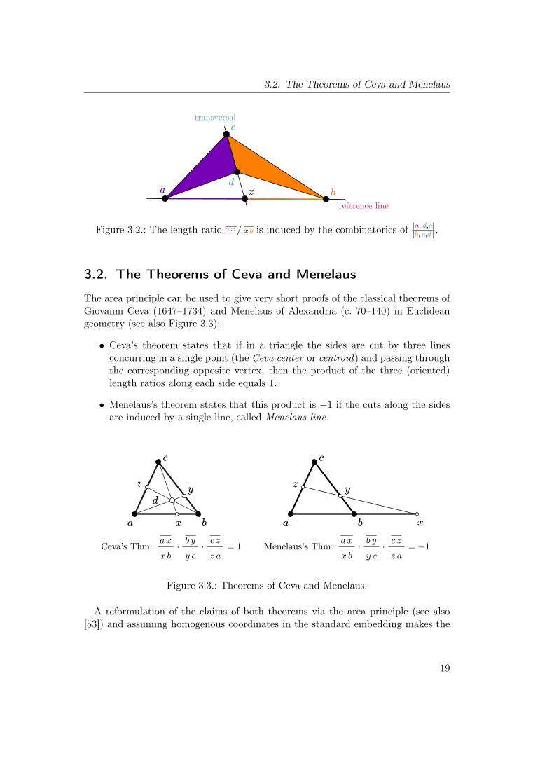
Figure 3.2.: The length ratio a x/ x b is induced by the combinatorics of |a, d,c||b, c,d | .
3.2. The Theorems of Ceva and Menelaus
The area principle can be used to give very short proofs of the classical theorems ofGiovanni Ceva (1647–1734) and Menelaus of Alexandria (c. 70–140) in Euclideangeometry (see also Figure 3.3):
• Ceva’s theorem states that if in a triangle the sides are cut by three linesconcurring in a single point (the Ceva center or centroid) and passing throughthe corresponding opposite vertex, then the product of the three (oriented)length ratios along each side equals 1.
• Menelaus’s theorem states that this product is −1 if the cuts along the sidesare induced by a single line, called Menelaus line.
Ceva’s Thm:a x
x b· b yy c· c zz a
= 1 Menelaus’s Thm:a x
x b· b yy c· c zz a
= −1
Figure 3.3.: Theorems of Ceva and Menelaus.
A reformulation of the claims of both theorems via the area principle (see also[53]) and assuming homogenous coordinates in the standard embedding makes the
19

3. Geometric Tools and Constructions
statement of the theorems almost trivial: in the Ceva case we have
a x
x b· b y
y c· c z
z a=|a, c, d||b, d, c | ·
|b, a, d||c, d, a| ·
|c, b, d ||a, d, b| = 1 (3.3)
and in the Menelaus case we have
a x
x b· b y
y c· c z
z a=|a, x, y||b, y, x | ·
|b, x, y||c, y, x| ·
|c, x, y ||a, y, x| = −1. (3.4)
Observe that for each α ∈ R \ 0, there is exactly one vector w of homogeneouscoordinates (with last coordinate 1) such that cw / w a = α. This implies that alsothe converse of the above formulation is true: from a x/ x b · b y / y c · cw / w a = 1 ora x/ x b ·b y / y c ·cw / w a = −1 we can deduce the existence of a centroid or a Menelausline, resp. This can be seen by the fact that x and y already determine the centroidof the Menelaus line. Therefore there is a point z′ fulfilling the adapted versions of(3.3) and (3.4). It has to coincide with z since c z / z a = c z′ / z′ a. In the following,we will consider the theorems of Ceva and Menelaus as containing both directionsof implication.
3.3. Projective Transformations and Invariants
This section will be formulated for general rank n in order to establish the necessaryconcepts needed in Section 4 which treats the bracket ring. Consider an invertiblen × n matrix M . The left multiplication of M with the homogeneous coordinatesof a point x in RPn−1 induces a map P(n−1) → P(n−1). Any such map is calleda projective transformation. The class of projective transformations also coversthe better known (embedded versions of) affine transformations such as rotations,scaling and shearing. A projective transformation is intrinsic to projective geometryin the sense that a projective transformation preserves collinearity, i.e.
[a], [b], [c] ∈ Pn−1 are collinear =⇒ [M · a], [M · b], [M · c] are collinear.
In rank 3 this can be easily seen by assuming that l provides the coordinates of theline incident with [a], [b] and [c]. Now, the line with coordinates M−T l is incidentwith [M · a], [M · b] and [M · c]. It is a classical result traditionally formulated forthe plane that in the real projective plane, also the converse is true.
Theorem 3.1 (Fundamental Theorem of Projective Geometry). If Φ : P → P isany bijective map on the points of the real projective plane RP2 that preserves thecollinearity of points, then Φ can be expressed as multiplication by a invertible 3× 3matrix.
20

3.3. Projective Transformations and Invariants
This classical result is known as fundamental theorem of projective geometry. Onecan find proofs in many textbooks on projective geometry. A detailed descriptionof the history of the theorem is given in [111]. Its origins are attributed to Möbius,Chasles and Steiner whereas the real treatment of the questions starts with vonStaudt [112]. The constructions he uses will be restated in Section 3.7. Under ageneral projective transformation, lengths and ratios of lengths are not preserved.This leads to the question, which properties are preserved and to the definition ofa projective invariant. This kind of question can be regarded as being fundamentalto all kind of geometries and is closely related to Klein’s Erlangen program.Note that the proof of Theorem 3.1 actually works with properties on projective
lines and incorporates each additional dimension by introducing a new projectiveline as reference system. Therefore Theorem 3.1 also holds in all higher dimensions(see e.g. [3] for a verification of this fact). Observe that each element of Rn·k canbe interpreted as giving a point configuration: we can consider it as a matrix whosecolumns are coordinates of points.
Definition 3.2. Let S be an arbitrary set. A projective invariant of rank n on kpoints in the real projective space RPn−1 is a map f from a dense subset of Rn·k toS such that for all invertible real n×n matrices M ∈ GL(R, n) and k× k invertiblereal diagonal matrices D ∈ diag(R \ 0, k) and for any configuration P , the map fis defined on M · P ·D and we have
f(P ) = f(M · P ·D).
In the case that S is a binary set, f is called a projectively invariant property.
Each projective invariant is also an SL-invariant as defined below. We considerSL-invariants since the polynomial SL-invariants have a nice structure as we will seein Chapter 4. Therefore all objects built on this structure, as the Grassmann-Cayleyalgebra introduced in Chapter 5, are closely related with SL-invariants.
Definition 3.3. Let S be an arbitrary set. A SL-invariant of rank n on k pointsin Rn is a map f from a dense subset of Rn·k to S such that for all real n × nunimodular matrices M , i.e. M ∈ SL(R, n), and for any configuration P , the mapf is defined on M · P and we have
f(P ) = f(M · P ).
When no rank is explicitly specified we assume rank 3. In Section 3.4, we will getto know the prototype of a projective invariant, whereas Chapter 4 will provide acomplete description of (polynomial) SL-invariant functions. It turns out that someof them induce projectively invariant properties. In fact, in the context of projective
21

3. Geometric Tools and Constructions
geometry, there is a whole zoo of different definitions of invariants. There is alsoa definition of a relative invariant or semi-invariant. In [37] (used as foundationof Chapter 5) the relative invariant is called an invariant. So the reader shouldbe careful in this context. In the present text, we decided to chose the projectiveinvariants and the SL-invariants in order to have a clear setup. We are guided by[95, 102].
3.4. The Cross-Ratio
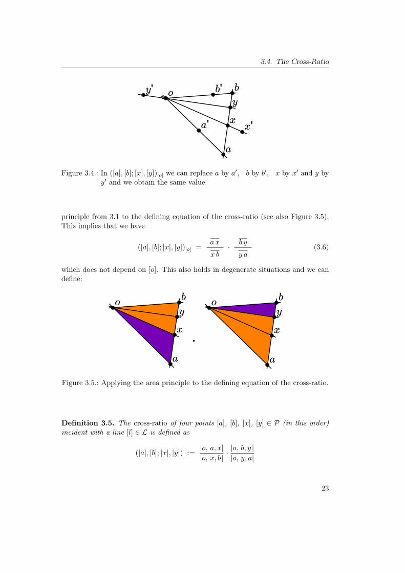
Another fundamental ingredient to projective geometry used extensively in Part IIIis the cross-ratio. It forms the smallest projective invariant and is in fact an invariantinvolving four points on a projective line. The origins of the concept even dates backto the ancient greeks. In order to keep the exposition short, we embed the definitionin RP2.
Definition 3.4. The cross-ratio of the points [a], [b], [x], [y] ∈ P (in this order)seen from [o] ∈ P is defined as the magnitude
([a], [b]; [x], [y])[o] :=|o, a, x||o, x, b | ·
|o, b, y ||o, y, a| (3.5)
whenever the magnitude can be considered as a value in R∪∞, i.e. whenever [o],[a], [b], [x], [y] are such that the right-hand side of (3.5) is in R or they are suchthat the denominator vanishes but the numerator does not vanish.
Due to the linearity of the determinant, the cross-ratio is well defined for pointsin P. The multiplicativity and multilinearity of the determinant imply that thecross-ratio seen form [o] is a projective invariant. Furthermore, in non-degeneratesituations, replacing e.g. a by o + λa (for λ ∈ R \ 0) results in the same valuefor the cross-ratio seen from [o]. So the cross-ratio seen from [o] in fact dependson the lines through [o] and [a], [b], [x], [y], resp. (see also Figure 3.4 where thesquare brackets indicating equivalence classes are omitted in order to obtain a cleararrangement).On the other hand, assuming that [a], [b], [x] and [y] are on a common line not
incident to [o], the expression does not depend on the specific choice of the point [o]:Since ([a], [b]; [x], [y])[o] is invariant under projective transformations and rescaling,we can assume that a, b, x, y and o are coordinates of the standard embedding:if the last coordinate of a, b, x, y or o equals 0, one can find an invertible matrixsuch that the transformed coordinates can be rescaled to coordinates of points inthe standard embedding. We will not give such a matrix explicitly. However almostall matrices are appropriate. In a non-degenerate situation, we can apply the area
22
3.4. The Cross-Ratio
Figure 3.4.: In ([a], [b]; [x], [y])[o] we can replace a by a′, b by b′, x by x′ and y byy′ and we obtain the same value.
principle from 3.1 to the defining equation of the cross-ratio (see also Figure 3.5).This implies that we have
([a], [b]; [x], [y])[o] =a x
x b· b y
y a(3.6)
which does not depend on [o]. This also holds in degenerate situations and we candefine:
·
Figure 3.5.: Applying the area principle to the defining equation of the cross-ratio.
Definition 3.5. The cross-ratio of four points [a], [b], [x], [y] ∈ P (in this order)incident with a line [l] ∈ L is defined as
([a], [b]; [x], [y]) :=|o, a, x||o, x, b | ·
|o, b, y ||o, y, a|
23

3. Geometric Tools and Constructions
with arbitrary [o] ∈ P not on the line [l].
Due to the possible replacement of e.g. a by o+ λa in ([a], [b]; [x], [y])[o] we have:
Proposition 3.6 (Invariance of Cross-Ratios under Projections). Let [o] be a pointand let [l] and [l′] be two lines not passing through [o]. If four points [a], [b], [c], [d]on [l] are projected by the viewpoint [o] to four points [a′], [b′], [c′], [d′] on [l′], thenthe cross-ratios satisfy ([a], [b]; [c], [d]) = ([a′], [b′]; [c′], [d′]).
3.5. Projective Number Lines
Figure a line in RP2 and three distinct points [p0], [p1] and [p∞] on this line. W.l.o.g.we can assume that they are scaled in such a way that p1 = p0 + p∞. This fixes therelative scaling between the three given points. Any other point [px] on this line,that different from [p0], is identical to [p0 + x · p∞] for some x ∈ R. One can easilycheck that it holds
([p0] , [p∞] ; [px] , [p1]) = x
for any such x and also
([p0] , [p∞] ; [p∞] , [p1]) =∞,([p0] , [p∞] ; [p0] , [p1]) = 0,
([p0] , [p∞] ; [p1] , [p1]) = 1.
Thus by its projective invariance, the cross-ratio can be interpreted as a numberobtained by rescaling three of the points and expressing a fourth point with respectto the other three ones.Furthermore, for any point [p] on the line spanned by distinct points [p0] and
[p∞], there is the tuple of real numbers (µp, λp) different from (0, 0) such that[p] = [µp p0 + λp p∞]. Any rescaling of the pair (λp, µp) gives the same point.This induces homogenous coordinates of the line with respect to the concrete ho-mogeneous coordinates p0 and p∞. In a situation analogue to Section 2.1 thesecoordinates have the structure of R2\(0,0)
R\0 . So if p0 and p∞ are scaled in such away that p1 = p0 + p∞ and [q] is a point on the line with q = µq p0 +λq p∞ we havethat
([p0] , [p∞] ; [q] , [p1]) =λqµq.
Alltogether, the cross-ratio can be considered as line coordinates of any point on a
24

3.6. Quadrilateral Sets
line with respect to three given base points [p0], [p∞] and [p1]. Since the propertiesdescribing a basis do not depend on the concrete homogeneous coordinates of thepoints, it is possible to talk about three points in P being a basis.
3.6. Quadrilateral Sets
Quadrilateral sets are the foundation for doing constructive calculations on projec-tive number lines in the next section. In the (old) literature they are often called“points of an involution”. Consider the situation in Figure 3.6: there it is given acomplete quadrilateral [z], [z1], [z2], [z3] which sides are cut with another line result-ing in points [a1], [a2], [a3], [b1], [b2] and [b3]. Again, we omit the square bracketsindicating equivalence classes in order to obtain a clear arrangement.
Figure 3.6.: The incidence configuration shows that (3.7) holds and that[a1], [b2], [a2], [b3], [a3], [b1]
is a quadrilateral set.
We will show that in this case for any point [o] it holds that
|o, a1, b1| · |o, a2, b2| · |o, a3, b3| = |o, a1, b3| · |o, a2, b1| · |o, a3, b2|. (3.7)
In order to show this and assuming a non-degenerate situation, where all the deter-minants do not vanish, we can rewrite the identity as
|o, a1, b1||o, a2, b1|
· |o, a2, b2||o, a3, b2|
· |o, a3, b3||o, a1, b3|
= 1. (3.8)
Since the left-hand side of (3.8) is again invariant under projective transformationsand rescaling of the points, we can w.l.o.g. assume homogeneous coordinates withlast coordinate equaling 1. This allows for an reformulation of (3.8) equation via
25
3. Geometric Tools and Constructions
the area principle:a1 b1
b1 a2
· a2 b2
b2 a3
· a3 b3
b3 a1
= −1.
This identity can be proved by applying Menelaus’s theorem to the three triangles(a1, a2, z), (a2, a3, z) and (a3, a1, z). This allows us to rewrite all parts of the aboveequation in a way such that their overall product equals −1:
a1 b1
b1 a2
=− a1 z1
z1 z· z z2
z2 a2
,
a2 b2
b2 a3
=− a2 z2
z2 z· z z3
z3 a3
,
a3 b3
b3 a1
=− a3 z3
z3 z· z z1
z1 a1
.
As announced in Section 3.1, the advantage of the area method is that it comeswith a less Euclidean and more projective formulation of this derivation, which is alittle harder to read but does not make assumptions on the shape of homogeneouscoordinates of the points involved:
|o, a1, b1||o, a2, b1|
=|z1, z2, a1||z1, z2, a2|
=|z1, z2, a1||z1, z2, z |
· |z1, z2, z ||z1, z2, a2|
=|z1, z2, a1||z1, z2, z |
· |z2, z3, z ||z2, z3, a2|
,
|o, a2, b2||o, a3, b2|
=|z2, z3, a2||z2, z3, a3|
=|z2, z3, a2||z2, z3, z |
· |z2, z3, z ||z2, z3, a3|
=|z2, z3, a2||z2, z3, z |
· |z1, z3, z ||z1, z3, a3|
,
|o, a3, b3||o, a1, b3|
=|z1, z3, a3||z1, z3, a1|
=|z1, z3, a3||z1, z3, z |
· |z1, z3, z ||z1, z3, a1|
=|z1, z3, a3||z1, z3, z |
· |z1, z2, z ||z1, z2, a1|
.
In a Euclidean setup, the identities can be considered to be true since they can bederived by applying the area principle to the Menelaus identities given above.By a more careful investigation one can find two basic kind of operations in the
detailed calculation:
• In each row, the first and the last equality can be considered as changing thepoints involved in the area principle. Therefore one needs the existence ofsome collinearities.
• The second equality explains itself by canceling on the right-hand side.
Both tools will be introduced more formally in Chapter 10 and are called biquadraticfractions and Γ-cycles. These calculations have the advantage that they are more
26

3.7. Von Staudt’s Constructions: Arithmetic on Projective Number Lines
projective in nature. However, they are less intuitive and more algebraic and non-geometric in nature, unless the area principle can be applied.In fact, (3.7) has some symmetries which can be captured by saying that
[a1], [b2], [a2], [b3], [a3], [b1]
(3.9)
forms a quadrilateral set whenever (3.7) is fulfilled. We use the notation of sets whichshall be allowed to be multisets. Furthermore, this condition does not depend on theorder of elements of the sets in (3.9). So the construction in Figure 3.6 witnesses thefact, that [a1], [b2], [a2], [b3], [a3], [b1] forms a quadrilateral set. However,due to the symmetry just described it is not the only construction for witnessing(3.9). For our purposes we conclude that the combinatorics of a quadrilateral setgiven by the construction in Figure 3.6 can be identified by following pairs of linesthat do not share a common point in the construction.
3.7. Von Staudt’s Constructions: Arithmetic onProjective Number Lines
In this section, no explicit reference to the concrete homogeneous coordinates isneeded and we can do our considerations without square brackets denoting equiv-alence classes. Let p0, p1 and p∞ be in P such that they form a projective ba-sis of a number line in RP2. Let px and py two other points on this line with(p0 , p∞ ; px , p1) = x and (p0 , p∞ ; py , p1) = y. We are interested in points px+y
with (p0 , p∞ ; pz , p1) = x + y and px·y with (p0 , p∞ ; pz , p1) = x · y. One caneasily check by hand calculation thatp0 , px+y ; px , py ; p∞ , p∞
and
p0 , p∞ ; px , py ; p1 , px·y
form quadrilateral sets. Figure 3.7 induces a construction of the points px+y andpx·y. Observe that the symmetry of quadrilateral sets implies the commutativity ofprojective addition and multiplication.The tools of projective addition and multiplication where originally introduced
by von Staudt in [112]. He introduces the language of Würfe (which is translatedto throws e.g. in [110]). This concept makes it possible to avoid the assignment ofcoordinates. Von Staudt uses throws for his version of the fundamental theorem ofprojective geometry (see Theorem 3.1 in Section 3.3). Those constructions are notcontained in every textbook on projective geometry. E.g. in [25] as well as in [110]they are introduced. The latter has the advantage that it gives a translation fromthe old notions of von Staudt into more modern terms of language.
27

3. Geometric Tools and Constructions
Figure 3.7.: Von Staudt constructions for projective addition and multiplication.
3.8. Harmonic Sets
In Section 16.4, we will once use the classical construction for a harmonic set. Infact, this concept is much more fundamental than the arithmetic constructions justseen. However it can be easily explained with their help: We say that
a , b ; c , d
(3.10)
(a, b, c, d ∈ P) is a harmonic set whenever
(a, b; c, d) = −1.
Observe that after canceling this is equivalent toa, a, b, b, c, d
being a quadrilateral set. This implies that the order of the elements in the sets inin (3.10) does not affect the property of being a harmonic set. In particular, theconsiderations done in Section 3.6 imply that the
a , b ; c , d
is a harmonic
set if the construction shown in Figure 3.8 is possible.
3.9. Configurations of Ceva and Menelaus Revisited
Most of the considerations involving oriented length ratios can be restated in termsof weights. Therefore we will use physical properties and intuition which we will notprove. If one wishes, one can translate large parts of the thesis into terms of weightratios. A overall illustration of the phenomena described is shown in Figure 3.9.Consider homogeneous coordinates a, b and c of three non-collinear points in thestandard embedding, i.e. the last coordinate a, b and c equals 1. Assume wa, xb in
28
3.9. Configurations of Ceva and Menelaus Revisited
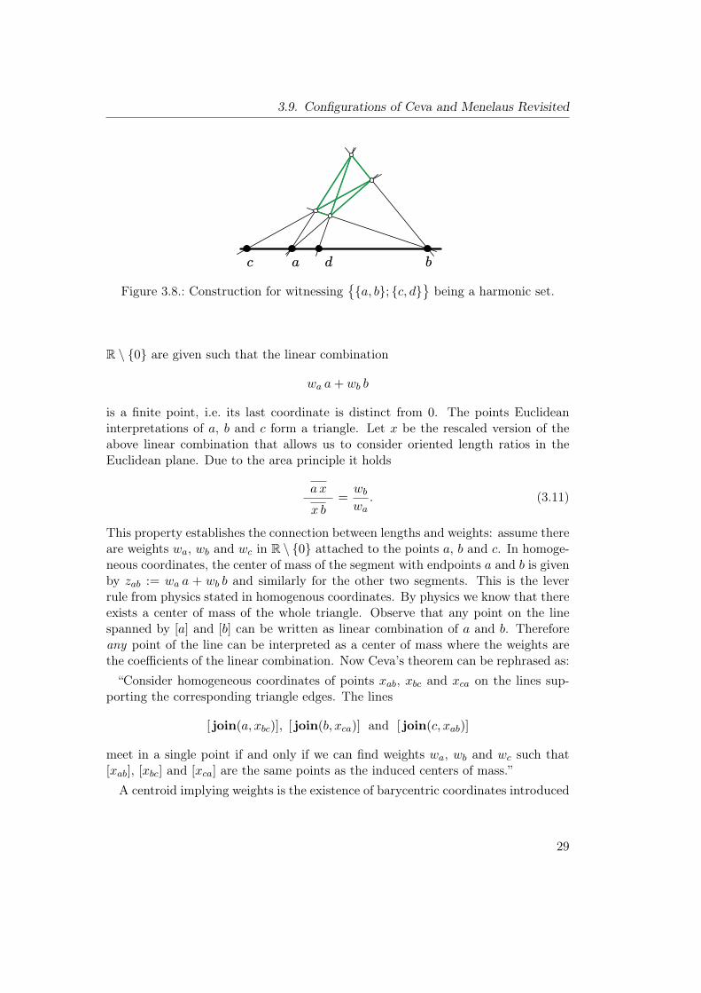
Figure 3.8.: Construction for witnessinga, b; c, d
being a harmonic set.
R \ 0 are given such that the linear combination
wa a+ wb b
is a finite point, i.e. its last coordinate is distinct from 0. The points Euclideaninterpretations of a, b and c form a triangle. Let x be the rescaled version of theabove linear combination that allows us to consider oriented length ratios in theEuclidean plane. Due to the area principle it holds
a x
x b=wbwa. (3.11)
This property establishes the connection between lengths and weights: assume thereare weights wa, wb and wc in R \ 0 attached to the points a, b and c. In homoge-neous coordinates, the center of mass of the segment with endpoints a and b is givenby zab := wa a + wb b and similarly for the other two segments. This is the leverrule from physics stated in homogenous coordinates. By physics we know that thereexists a center of mass of the whole triangle. Observe that any point on the linespanned by [a] and [b] can be written as linear combination of a and b. Thereforeany point of the line can be interpreted as a center of mass where the weights arethe coefficients of the linear combination. Now Ceva’s theorem can be rephrased as:“Consider homogeneous coordinates of points xab, xbc and xca on the lines sup-
porting the corresponding triangle edges. The lines
[ join(a, xbc)], [ join(b, xca)] and [ join(c, xab)]
meet in a single point if and only if we can find weights wa, wb and wc such that[xab], [xbc] and [xca] are the same points as the induced centers of mass.”A centroid implying weights is the existence of barycentric coordinates introduced
29

3. Geometric Tools and Constructions
by Möbius who starts his investigations by studying the center of mass (see [86]).He also relates length ratios together with an orientation to the ratio of masses.Barycentric coordinates can be understood as homogenous coordinates of an em-bedding of the Euclidean plane into projective space which is different from thestandard embedding introduced in Section 2.1. This shows the deep connectionbetween Ceva’s theorem and weights.
Figure 3.9.: Weights are given for the vertices of the triangle. They are indicatedby the size of the vertices. Its inverses are indicated by green arrowswhich are considered to be forces located at the vertices. The centroidand the Menelaus lines are given. The latter contains the centers ofmotions of the edges which are induced by the green forces.
Also for the theorem of Menelaus it can be given an interpretation which dependson the same weights wa, wb and wc: consider again the segment with endpointsa and b and forces induced by 1/wa and 1/wb at the corresponding vertices of thesegment. Due to (3.11), the ratio of these values is the same as a x
x b. There is an
associated rotation of the segment with center
yab := wa a− wb b.
Observe that yab is related to zab by[a], [b]; [zab], [yab]
being a harmonic
point set. Assume ybc and yca are defined analogously. Now yab and ybc suffice to
30

3.10. Conics and Pascal’s Theorem
induce a rotation of the whole triangle. This motion has an axis which is spannedby yab and ybc. The point yca has to lie on this axis as well. This fact can beunderstood as Menelaus’s theorem. It can be paraphrased as: “Given instantaneousmotions on the three vertices of a triangle, the induces centers of motion on theedges lie on a common line.”A generalization of this fact, which uses weights on the vertices of a tetrahedron
in 3-space and its the inverses of the weights as instantaneous motions, induces thewell known incidence theorem of Desargues. For more information about incidencetheorems see Chapter 7. A generalization to 4-space should be possible as well.A related reasoning, which uses three vertices of a triangle as a basis for furtherconstructions, is given in [139]. The three base points remain fixed during thecalculations. The method can be interpreted as using barycentric coordinates withrespect to the three base points chosen.
3.10. Conics and Pascal’s Theorem
For future reference, we also state another classical theorem about conics. It is dueto Pascal who proved it in 1640 (see [22] for an english translation). A conic Cconsists of those points [(x, y, z)] in RP2 that fulfill
α · x2 + β · y2 + γ · xy + δ · xz + ε · yz + ζ · z2 = 0
for some real α, β, γ, δ, ε and ζ depending on C. By counting degrees of freedom onefinds that five points in general position supply enough equations to determine thesevalues. Therefore, six points, that lie on the same conic, are in a special position. Itis not hard to derive (see [95, p. 169]) that the six points [a], [b], [c], [d], [e] and [f ]lie on a common conic if and only if
|a, c, e| · |a, d, f | · |b, c, f | · |b, d, e| − |a, c, f | · |a, d, e| · |b, c, e| · |b, d, f | = 0. (3.12)
It is the statement of Pascal’s theorem that both is also equivalent to the fact thatthe points [x], [y] and [z], whose construction is shown in Figure 3.10 on the right,are collinear. We will prove the equivalence of (3.12) and the collinearity of [x], [y]and [z] in Chapter 6. Observe that a and b never occur in the same determinant.The defining equation can be rewritten in terms of cross-ratios of line bundles:
|a, c, e| · |a, d, f ||a, c, f | · |a, d, e| =
|b, c, e| · |b, d, f ||b, c, f | · |b, d, e|
which is equivalent to
([c], [d]; [e], [f ])[a] = ([c], [d]; [e], [f ])[b].
31

3. Geometric Tools and Constructions
⇔ |a, c, e| · |a, d, f | · |b, c, f | · |b, d, e|−|a, c, f | · |a, d, e| · |b, c, e| · |b, d, f | = 0
⇔
Figure 3.10.: Pascal’s theorem: six points a, b, c, d, e and f ∈ P lie on a commonconic if and only if the depending points x, y, z lie on a common line.
32

4. The Bracket Ring and theFundamental Theorems of InvariantTheory
A lot of properties in projective geometry can be stated with the help of deter-minants. The cross-ratio (Section 3.4) and the condition for six points lying on acommon conic (Section 3.10) are only a few examples. Theorem 4.9 will show thatin a certain sense, any projectively invariant (polynomial) property can be statedwith the help of determinants. To formulate this result, we introduce some nota-tion in the current chapter. In the literature (see below), there are many slightlydifferent versions of these results. We follow the approach given by Sturmfels in[102]. The concept, that all geometry is in fact invariant theory, motivates manyof the considerations in the following Chapters and is subject of Klein’s Erlangenprogram.In the present chapter, we give an algebraic structure that describes determinants
symbolically. We dissociate the determinants from their definition via vector coor-dinates and instead view them as formal symbols only depending on the names ofthe points without referring to concrete coordinates. Therefore the notion of de-terminants is simplified and square brackets, e.g. [∗, ∗, ∗] in rank 3, are used. Thisexplains the name “bracket ring”. We briefly describe the main ideas in the exampleof rank 3 and then give some additional informations about the origin of the bracketring. Let P be a finite set of names of points and let ∆(P) = [i, j,k] | i, j,k ∈ P be the set of formal determinants. The points in P are thought to be points in RP2
or non-zero points in R3. R[∆(P)] is the ring over R which is generated by thesesymbols. We aim to model the behavior of true determinants as well as possible.This is in fact achieved quite well as, we will see in Section 4.5. We will ensure thate.g. [a,b,a] = 0 and [a,b, c] = −[a, c,b]. Apart from that, there are other phenom-ena which we have to take into account. There are relations between determinantswhich are called Grassmann-Plücker relations. We will provide an interpretation ofthem. In Section 4.4, we will generalize the concept of the bracket ring to rank n,i.e. for RPn−1 or Rn.Another approach to the bracket ring is to consider SL-invariants. The deter-
minant is an SL-invariant. The first fundamental theorem of invariant theory canbe summarized as stating that combinations of determinants—or bracket polynomi-
33

4. The Bracket Ring and the Fundamental Theorems of Invariant Theory
als, which are their symbolic counterparts—are enough to describe all (polynomial)SL-invariants. The second fundamental theorem describes the relations holding be-tween different bracket polynomials. These relations will match the ones given inthe definition of the bracket ring. They also imply that a representation of a bracketpolynomial is not unique. Therefore we will briefly describe the straightening algo-rithm which is able to compute a normal form of bracket polynomials.
The definitions given here are taken from [95] and [102]. First, a definition forrank 3 is given. In the context of Grassmann coordinates, a symbolic treatmentof determinants is already used in [65] whereas a systematic symbolic treatment isdone by White in [120] in the more general setup of combinatorial geometries (seee.g. [31]). This point of view is fundamental for the definitions as they are done inthe present chapter. Great insight of the subject is also shown in [109] and [107].However, the treatment there is not symbolic in nature. This branch of invarianttheory is (in this context) often referred to as “classical invariant theory”. A linkagebetween new and old invariant theory is given in [16] by Carrell and Dieudonné. Itis based on Weyl’s classical groups [119]. Also classical invariant theory considersits computations as “symbolic method”. However the terms and definitions usedrely on coordinates. A formal language, which uses names of points, is also givenby Whiteley in [135, 130, 134]. Here first order logic is considered. This meansthat relations under investigation include quantifiers. There, there are also givenfundamental theorems of invariant theory. In particular, an invariant first orderformula in coordinates can be translated into a first order formula in brackets.Within these notions it is natural to talk about models which are distinct fromthe language. In [51, 68, 99] Rota and his collaborators use a symbolic methodwhich is generalized to model symmetric and antisymmetric tensors. This is doneby generalizing the straightening algorithm for comparing bracket polynomials (seeSection 4.7). In the case that the signed alphabet used contains only negativeletters, classical invariant theory is obtained. This case is treated in more detailin [68, Chap. 8]. It is pointed out that the bracket ring is a special case of thesupersymmetric bracket algebra introduced there. A point configuration assigningconcrete homogeneous coordinates to the point names is considered being a model.Again the word model is borrowed from logic. This distinction will also be done inthe present and the next chapter. More comments on this development, which isalso related to the following chapter, can be found in [50].
Proofs for (versions of) the crucial results given in Section 4.5 can be found e.g.in [102, 37, 68, 65, 71, 119, 16]. A detailed summary of related topics including thedefinitions and relations given in the next chapters is given in the recent book [77]by Li. Again observe that the following treatment is symbolic in nature and thatwe never have to refer to concrete coordinates.
34

4.1. Grassmann-Plücker Relations in Rank 3
4.1. Grassmann-Plücker Relations in Rank 3
We start with a definition of the bracket ring in rank 3. In this case, we canshow some connections to geometric and algebraic facts derived in Chapters 2 andChapter 3. On the level of true determinants, (2.8) implies that for any homogeneouscoordinates a, b, c, d, e and f of points in RP2, there are two ways of expressing∣∣a, b, meet(join(c, d), join(e, f))
∣∣ and it holds
− |c, d, e| · |a, b, f | + |c, d, f | · |a, b, e| = |e, f, c| · |a, b, d|− |e, f, d| · |a, b, c|. (4.1)
This motivates the 4-term Grassmann-Plücker relation
[a, b, c][d, e, f ]− [a, b, d][c, e, f ] + [a, b, e][c, d, f ]− [a, b, f ][c, d, e] = 0
for a, b, c, d, e, f ∈ P (4.2)
for the symbolized versions of determinants. The equation will be required to holdin the following definition of the bracket ring.
Remark 4.1. Assuming f = a and the rules for permutations of the point namesgiven in the next definition (and in particular implying that [a, b, a] = 0) we candeduce the 3-term Grassmann-Plücker relation for a, b, c, d, e ∈ P:
[a, b, c][a, d, e]− [a, b, d][a, c, e] + [a, b, e][a, c, d] = 0. (4.3)
In fact, [77, Prop. 2.16] tells us, that in a specific sense, the 3-term Grassmann-Plücker relations can also generate 4-termed Grassmann-Plücker relations. This isalso true in higher rank.
4.2. The Bracket Ring BP in Rank 3
The previous considerations give rise to the following definition:
Definition 4.2 (Bracket Ring of Rank 3). Let P be a finite set of point names.∆(P) := [i, j,k] | i, j,k ∈ P defines a set of indeterminantes in the ring R[∆(P)].With S3 the symmetric group on three elements, R[∆(P)] contains the ideals
Irepeat :=⟨
[i, j,k] ∈ ∆(P)∣∣ i = j or i = k or j = k
⟩
35

4. The Bracket Ring and the Fundamental Theorems of Invariant Theory
Ialtern :=⟨
[p1,p2,p3] + sgn(σ) [pσ(1),pσ(2),pσ(3)]∣∣p1,p2,p3 ∈ P, σ ∈ S3
⟩
IGP :=⟨
[a, b, c][d, e, f ]− [a, b, d][c, e, f ] + [a, b, e][c, d, f ]
− [a, b, f ][c, d, e]∣∣a, b, c, d, e, f ∈ P
⟩.
The bracket ring is defined as
BP := R[∆(P)]/⟨
Irepeat ∪ Ialtern ∪ IGP⟩.
Remark 4.3. Observe that for Q and P disjoint we have
BP ⊂ BP∪Q .
Following [102], consider an abstract point configuration X consisting of |P| ho-mogeneous coordinates in RP2: let X = (xij) be an 3 × |P|-matrix whose entriesare indeterminates and whose columns correspond to elements of P. R[xij ] is thecorresponding ring in 3 · |P| variables. To make the connection between the abstractbracket ring and the projective geometry introduced in Chapter 2, we define an al-gebra homomorphism from the bracket ring BP to R[xij ]. Therefore, fix an orderon P and let i be the element of P at position i. We allow ourselves to write xi−instead of x
− i.
Definition 4.4. The map
φ :
R[∆(P)] → R[xij ]
[i, j,k] 7→ det
xi1 xj1 xk1
xi2 xj2 xk2
xi3 xj3 xk3
vanishes on Irepeat, Ialtern and IGP, φ. Therefore it induces a map
Φ : BP → R[xij ]
which is called the generic coordinatization.
Where identities induces by Φ hold for all point configurations, the followingdefinition of ΦP can check for relations between concrete homogeneous coordinatesof points:
36

4.3. Grassmann-Plücker Relations in Rank n
Definition 4.5. Let P be a (concrete) point configuration associated to |P| manypoints in RP2: let P = (pij) be an 3× |P|-matrix, whose columns are homogeneouscoordinates. The coordinatization map
ΦP : R[∆(P)]→ R
is the composition of Φ and the substitution homomorphism given by the values ofP .
4.3. Grassmann-Plücker Relations in Rank n
The bracket ring can be defined not only for rank 3. The Grassmann-Plücker rela-tions are induced essentially by Cramer’s rule from linear algebra. It can be restatedas follows: Searching for solutions of the linear equation (b1, . . . , bn)x = bn+1 in Rngives an identity on the level of vectors: assuming the solvability of the equationimplies
bn+1 = (b1, . . . , bn)x =
n∑
i=1
xi bi
with xi being the entries of a solution x (for 1 ≤ i ≤ n). Furthermore, the multilin-earity of the determinant gives
|b1, . . . , bi−1, bn+1, bi+1, . . . , bn| = xi |b1, . . . , bn| for 1 ≤ j ≤ n
and thereforen∑
i=1
|b1, . . . , bi−1, bn+1, bi+1, . . . , bn| bi = |b1, . . . , bn|n∑
i=1
xi bi
which implies
n∑
i=1
|b1, . . . , bi−1, bn+1, bi+1, . . . , bn| bi = |b1, . . . , bn| bn+1. (4.4)
In the case that (b1, . . . , bn)x = bn+1 is not solvable in Rn, assume there is anothern-element subset of b1, . . . , bn+1, such that the corresponding determinant does notvanish (otherwise, (4.4) already holds true). Letting play these vector the rolesof the b1, . . . , bn gives the same result. Thus (4.4) holds in general. Plugging itin the last column of det(a1, . . . , an−1, ∗) gives the coordinate version of a generalGrassmann-Plücker relation holding for all vectors in Rn and for all homogeneouscoordinates of points in RPn−1 and motivates Definition 4.6.
37

4. The Bracket Ring and the Fundamental Theorems of Invariant Theory
4.3.1. Interpreting Grassmann-Plücker Relations: Intersection ofSubspaces
(4.4) has a similar interpretation as (4.1): for any 2 ≤ k ≤ n − 1 (4.4), can berewritten as
k∑
i=1
(−1)i |b1, . . . , bi−1, bi+1, . . . , bn+1| bi
=n+1∑
i=k+1
(−1)i+1 |b1, . . . , bi−1, bi+1, . . . , bn+1| bi. (4.5)
Both sides of the equation give homogeneous coordinates of points in RPn−1. Theleft-hand side of the equation indicates that the point lies in the subspace spannedby the points b1, . . . , bk and the right-hand side of the equation indicates that italso lies in the space spanned by the points bk+1, . . . , bn+1. Thus, (4.5) allows forexpressing the intersection of two subspaces of suitable dimensions in two differentways. This phenomenon will be generalized in Chapter 5.
4.4. The Bracket Ring BP in Rank n
Definition 4.6 (Bracket Ring of Rank n). Let P be a finite set of point names andlet n be a natural number. ∆(P) := [p1,p2, . . . ,pn] |p1,p2, . . . ,pn ∈ P definesa set of indeterminantes for the ring R[∆(P)]. With Sn the symmetric group on nelements, it contains the ideals
Ialtern :=⟨
[p1,p2, . . . ,pn] + sgn(σ) [pσ(1),pσ(2), . . . ,pσ(n)]∣∣p1,p2, . . . ,pn ∈ P, σ ∈ Sn⟩,
Irepeat :=⟨
[p1,p2, . . . ,pn]∣∣p1 = p2, p1,p2, . . . ,pn ∈ P
⟩,
IGP :=⟨ n+1∑
i=1
(−1)i[a1, . . . ,an−1,bi][b1, . . . ,bi−1,bi+1, . . . ,bn+1]
∣∣a1, . . . ,an−1, b1, . . . ,bn+1 ∈ P⟩.
The bracket ring of rank n is defined as
B(n)P := BP := R[∆(P)]
/⟨Irepeat ∪ Ialtern ∪ IGP
⟩.
φ, Φ and ΦP can be defined in analogy to the rank 3 case in Definitions 4.4 and 4.5.
38

4.5. Fundamental Theorems of Invariant Theory
4.5. Fundamental Theorems of Invariant Theory
φ and Φ make it easier to formulate the fundamental theorems of invariant theorywhich emphasize the fundamental role of the bracket ring. Again, all statementsinvolving Φ are statements which hold for all possible point configurations (in con-trast to ΦP ). No proofs will be given. Proofs can be found e.g. in [102] or otherreferences given in the beginning of the chapter.As it turns out, the ideals Irepeat, Ialtern and IGP generate all dependencies along
determinants and the bracket polynomials in R[∆(P)] vanishing in any coordinati-zation and for arbitrary rank:
Theorem 4.7 (Second Fundamental Theorem of Invariant Theory). The homomor-phism Φ is injective. In other words, kerφ (which is a subset of R[∆(P)]) equals⟨Irepeat ∪ Ialtern ∪ IGP
⟩.
Any element of ker ΦP =⟨Irepeat ∪ Ialtern ∪ IGP
⟩is called a syzygy. The following
first fundamental theorem of invariant theory states in essence that all (polynomial)invariants are induced by bracket polynomials. For the correct formulation we define
Definition 4.8. Let R[xij ]SL be the ring of polynomials in R[xij ] that are SL-
invariants when considered as functions.
Theorem 4.9 (First Fundamental Theorem of Invariant Theory). Φ is surjective,i.e. it holds
im(φ) = φ(R[∆(P)] ) = R[xij ]SL.
A concrete algorithm for finding a bracket representation of an element in R[xij ]SL
is provided by [102, Alg. 3.2.8]. First and second fundamental theorem togetherimply:
Corollary 4.10. The Bracket ring is isomorphic to the invariant ring:
BP ∼= R[xij ]SL.
One can also derive a “first fundamental theorem” for rational functions. However,it is needed precisely once in this thesis so it is implicitly given in the last part ofthe proof of Theorem 5.15.
4.6. Applications to Projective Geometry
So for any SL-invariant, we can chose whether we want to give it as an elementof BP or as an element of R[xij ]
SL. It is a deep believe of many geometers, thatthe representation within the bracket ring is “better”. We give two reasons for
39

4. The Bracket Ring and the Fundamental Theorems of Invariant Theory
that: First of all, this formulation is independent on the choice of coordinates.This is a basic property of properties in geometry. Consider e.g. the statementof Pascal’s theorem (see Section 3.10): the fact that six points lie on a commonconic should not depend on the position of the six points relative to the origin.Secondly, the representation of the invariants of interest is usually much shorterin the language of brackets than in the language of homogeneous coordinates. Weborrow an example from [102] to demonstrate this: with P = 1, . . . ,6 we havethat Φ
([1,2,3][4,5,6]− [1,2,4][3,5,6]
)equals
−x1,3x2,2x3,3x4,1x5,2x6,1 +x1,2x2,3x3,3x4,1x5,2x6,1 +x1,3x2,1x3,3x4,2x5,2x6,1−x1,1x2,3x3,3x4,2x5,2x6,1 +x1,3x2,2x3,1x4,3x5,2x6,1 −x1,2x2,3x3,1x4,3x5,2x6,1−x1,3x2,1x3,2x4,3x5,2x6,1 +x1,1x2,3x3,2x4,3x5,2x6,1 +x1,3x2,2x3,2x4,1x5,3x6,1−x1,2x2,3x3,2x4,1x5,3x6,1 −x1,3x2,2x3,1x4,2x5,3x6,1 +x1,2x2,3x3,1x4,2x5,3x6,1−x1,2x2,1x3,3x4,2x5,3x6,1 +x1,1x2,2x3,3x4,2x5,3x6,1 +x1,2x2,1x3,2x4,3x5,3x6,1−x1,1x2,2x3,2x4,3x5,3x6,1 +x1,3x2,2x3,3x4,1x5,1x6,2 −x1,2x2,3x3,3x4,1x5,1x6,2−x1,3x2,1x3,3x4,2x5,1x6,2 +x1,1x2,3x3,3x4,2x5,1x6,2 −x1,3x2,2x3,1x4,3x5,1x6,2+x1,2x2,3x3,1x4,3x5,1x6,2 +x1,3x2,1x3,2x4,3x5,1x6,2 −x1,1x2,3x3,2x4,3x5,1x6,2−x1,3x2,1x3,2x4,1x5,3x6,2 +x1,1x2,3x3,2x4,1x5,3x6,2 +x1,2x2,1x3,3x4,1x5,3x6,2−x1,1x2,2x3,3x4,1x5,3x6,2 +x1,3x2,1x3,1x4,2x5,3x6,2 −x1,1x2,3x3,1x4,2x5,3x6,2−x1,2x2,1x3,1x4,3x5,3x6,2 +x1,1x2,2x3,1x4,3x5,3x6,2 −x1,3x2,2x3,2x4,1x5,1x6,3+x1,2x2,3x3,2x4,1x5,1x6,3 +x1,3x2,2x3,1x4,2x5,1x6,3 −x1,2x2,3x3,1x4,2x5,1x6,3+x1,2x2,1x3,3x4,2x5,1x6,3 −x1,1x2,2x3,3x4,2x5,1x6,3 −x1,2x2,1x3,2x4,3x5,1x6,3+x1,1x2,2x3,2x4,3x5,1x6,3 +x1,3x2,1x3,2x4,1x5,2x6,3 −x1,1x2,3x3,2x4,1x5,2x6,3−x1,2x2,1x3,3x4,1x5,2x6,3 +x1,1x2,2x3,3x4,1x5,2x6,3 −x1,3x2,1x3,1x4,2x5,2x6,3+x1,1x2,3x3,1x4,2x5,2x6,3 +x1,2x2,1x3,1x4,3x5,2x6,3 −x1,1x2,2x3,1x4,3x5,2x6,3.
Now, one could ask whether the SL-invariants are of any interest for a geometerwho is expected to be interested in projective invariants. In fact, for any pointconfiguration P , the vanishing of ΦP
([1,2,3][4,5,6] − [1,2,4][3,5,6]
)expresses
the fact that the lines with coordinates join(ΦP (1),ΦP (2)
), join
(ΦP (3),ΦP (4)
)
and join(ΦP (5),ΦP (6)
)meet in a single point. Here ΦP (p) is to be understood as
the point in P corresponding to p ∈ P and the geometric interpretation follows fromSection 2.4. The following Definition 4.11 is needed in order to see which of the SL-invariants also lead to more general invariants, e.g. projectively invariant properties(see Section 3.3). Before that, we observe that giving SL-invariants as elements ofthe bracket ring BP has the disadvantage that there are many representations ofthe same invariant. Section 4.7 will deal with this problem in more detail.
Definition 4.11. Let P be a finite set. For a bracket monomial m in R[∆(P)] andfor p ∈ P we define the relative degree deg(m,p) as the total number of occurrencesof p in m. Let m1 + · · · + mk be a polynomial in R[∆(P)] given as a sum of
40

4.7. Comparing Expressions in BP and the Straightening Algorithm
monomials. We say that m1 + · · ·+mk is multihomogenous if
deg(m1,p) = . . . = deg(mk,p) for all p ∈ P.
If m1 + · · · + mk is also in Z[∆(P)] then m1 + · · · + mk is said to have integercoefficients. For k = 1, 2, 3, . . . , the expression m1 + · · · + mk is called monomial,binomial, trinomial, . . . , resp. as long as m1, . . . ,mk /∈ 〈Irepeat〉.A bracket polynomial B in BP has a subset of the properties just defined whenever
it has a representation in R[∆(P)] satisfying all properties in the subset at once.
By the multiplicativity of the determinant, every multihomogenous bracket poly-nomial induces a projectively invariant property: Interpreting Φ as function andfollowing that up with applying a function that decides whether the result equalszero, induces the desired invariant. To see that the resulting functions are projec-tively invariant property, observe that is holds since e.g. in rank 3:
|M · λa · a,M · λb · b,M · λc · c| = det(M) · λa λb λc · |a, b, c|
for λa, λb, λc ∈ R \ 0, M ∈ GL(R, 3) and a, b, c ∈ R3. Thus in a (representation ofa) multihomogeneous bracket polynomial, each summand induces the same non-zeroscalar factors when testing the function being a projectively invariant property. Wesummarize:
Proposition 4.12. Multihomogeneous bracket polynomials induce projectively in-variant properties.
4.7. Comparing Expressions in BP and the StraighteningAlgorithm
The advantage of short expressions for geometric properties comes with a big dis-advantage: especially IGP makes it hard to tell whether two bracket polynomialequal each other or not (or equivalently to tell whether a bracket polynomial is infact the zero polynomial). The standard answer for this problem is the classicalstraightening algorithm which goes back to Young (see [138]). It is also treated in[37]. [103, 102] show the connection to Gröbner bases as introduced by Buchbergerin [14, 15] and by Hironaka in [64]. Another introduction on Gröbner bases canbe found e.g. in [113]. More precisely, [103, 102] show that the straightening algo-rithm is as a Gröbner bases algorithm where in addition the shape of the Gröbnerbasis is known beforehand. It is able to transform any bracket polynomial into anormal form. After reducing two bracket polynomials to normal form, they canbe compared. Nevertheless, in practice, the normal forms tend to have much more
41
4. The Bracket Ring and the Fundamental Theorems of Invariant Theory
summands than the polynomials one started with. Due to [93], the straighteningalgorithm requires overexponential CPU time which is not surprising, since it is aGröbner bases algorithm.We will give a very rough sketch of the algorithm in order to get an impression
on how it works. The normal form is characterized by the fact that all monomi-als of the polynomial are standard. A monomial is standard, whenever all of itssorted brackets (sorted with respect to the some fixed order imposed on P) canbe arranged as rows of a matrix in such a way that the columns of the matrix arenon-decreasing. The ordering of P also induces a monomial order which ordersthe set of monomials.1 Whenever there is a biggest monomial of the current rep-resentation of the bracket polynomial that is non-standard, it can be replaced by abracket polynomial (taken from the Göbner bases) whose summands are all smallerin the monomial order. Monomial orders have the property that they cannot haveinfinite decreasing chains. Therefore, this process has to terminate. This is therequired normal form. It can be shown that the set of so-called van der Waerdensyzygies is a Gröbner basis for
⟨Irepeat ∪ Ialtern ∪ IGP
⟩(see again [103, 102]). One
can use not only van der Waerden syzygies but also other additional syzygies inorder to eliminate non-standard monomials as long as the monomial order is de-creased. One can hope for better running times of the straightening algorithm.This is done in [122] by White including a comparison of the performance of the fivevariations given. Furthermore, if the bracket polynomial is antisymmetric in somepoints of P, an optimized version of the algorithm is given in [85], called the dottedstraightening algorithm. According to [102, p. 117] it can be understood as a specialcase of the straightening law in the superalgebra [51]. Considering antisymmetryis closely related with Grassmann-Cayley algebra treated in the next chapter andwith multilinear Cayley factorization mentioned in Part III. Here in this context,the straightening algorithm is treated in sake of completeness. It will not be usedwithin this thesis.
1In rank 3, it suffices to order the indeterminantes [i, j,k] | i, j,k ∈ P and i < j < k . One chosesthe lexicographical order on these variables and the induced degree reverse lexicographic orderis the monomial order in question.
42

5. A Symbolic Version of theGrassmann-Cayley Algebra
Grassmann-Cayley algebra is used to calculate with subspaces of Rn and thereforealso with subspaces of RPn−1 (see also Section 2.5). In the classical literature, this isdone by referring to the concrete coordinates of points in Rn. We will again use thenames of points to introduce the elements of a symbolic version of Grassmann-Cayleyalgebra. We are interested in those elements of the algebra that can be interpretedas being subspaces of Rn. The join operation allows for spanning a subspace withsome points. The meet operation can be interpreted as an intersection of subspaces.We give formal definitions and afterwards interpretations in order to show that thedefinitions meet the intuition of join and meet just described. To do so on a symboliclevel, relations are established in Theorem 5.13. Theorem 5.15 is a symbolic versionof the fact that in classical Grassmann-Cayley algebra “identical subspaces are scalarmultiples of each other”. This will be used as a motivation for different evaluationsin Chapter 6.Classical introductions can be found e.g. in [126, 127, 4, 102] and also in [77,
Chap. 2.3]. In [77] and in [73] many additional references can be found. [4, 36]provide many historical comments and give many credits to Grassmann for his Aus-dehnungslehre (see [48, 49]). There are also many articles honoring Grassmann in[90] celebrating the bicentennial birthday of Grassmann. Within this communityit is also provided a software package for Grassmann algebra calculations. It isdistributed with an introductory book (see [13]). Forder [44] can be understoodas giving an early restatement of Grassmann’s original ideas in modern language.Furthermore, many examples are given within this book. In [77], in addition tothe conventional meet, also a total meet product is given by Li which is inspired bythe coproduct given in [51]. It is also given a more recent development to connectGrassmann-Cayley algebra with Clifford algebra or geometric algebra. For an intro-duction to the latter we refer to [89]. On page 49 it is stated that “Grassmann-Cayleyalgebra and Clifford algebra are equivalent in the sense that anything expressed inone of them can also be expressed in the other. Which one you prefer is probablya matter of taste.” The foundations of geometric algebra are given by Hestenesin [59] and first applications to projective geometry are given in [61]. Anotheroverview over related algebras is given in [60]. As one investigates literature usingGrassmann-Cayley algebra, one finds that one often calculates symbolically.
43

5. A Symbolic Version of the Grassmann-Cayley Algebra
Therefore we will use a symbolized version of this algebra and refer to it as“Grassmann-Cayley algebra” as well when no confusion can arise. We saw anothersymbolic treatment before in the case of bracket polynomials: here in every expres-sion, the names of points in P are unbreakable symbols in the sense that it is neverreferred to coordinates of the points. In the context of Grassmann-Cayley algebra,this has the advantage that no coordinates for subspaces have to be defined. Thisdefinition is a little cumbersome and needs an interpretation as determinants ofpoints given by coordinates with respect to a specific basis. This does not providegeometric interpretation in the first place. The symbolic version captures geometricmeaning and emphasizes the nature of the computations done in this thesis. Fur-thermore, we do not need to specify a certain basis. Of course, when interpreting aformula, some points can be considered constituting a basis. However, interpretinganother formula, other points can be considered yielding a basis.Another motivation for the symbolic treatment is that in the literature, the
bracket ring is considered to be a substructure of Grassmann-Cayley algebra. How-ever, in a formal way of thinking, i.e. without using isomorphisms, this is not thecase when we use the symbolic version of the bracket ring given by White in [120]and the classical definition of the Grassmann-Cayley algebra based on coordinates.The symbolic version Λ(P) of the Grassmann-Caylay algebra given below allows
for this and is completely coordinate-free. It is called White module in [18]. Theelements of P play again the role of generic points in Rn. In order to see the beautyand structure of the algebra, we will introduce it for general geometric rank n. Inrank 3, a lot of phenomena cannot be seen. The definition of Λ(P) depends on thegeometric rank n as well as on (the cardinality of) the set P. It uses the definitionof the bracket ring in rank n on P. It is used to ensure that any n + 1 points aredependent. Furthermore, we will also give an interpretation of the elements of Λ(P)for a concrete instance of points. This is done by inserting concrete homogenouscoordinates in brackets. In principle, this interpretation can be slightly extendedin order to achieve the classical version of Grassmann-Cayley algebra includingGrassmann coordinates as defined e.g. in [65]. In essence, this follows from lettingP be a n-elements set which is considered to be a basis of the vector space. Thisapproach is taken in [28].The exposition given in the current chapter follows [37] by Doubilet, Rota and
Stein. The following references can be considered to emerge from a school whichgoes back to Rota. The definitions in [37] are closely related to concrete coordinates.However, almost every definition given there can be literally translated to namesof points instead of points in Rn. This makes the presentation symbolic in nature.With their vocabulary, it is in essence (a symbolized version of) a non-standardCayley or Peano space (see also [4, 28]). This is a vector space together with aso-called bracket, which is in fact a determinant there. The Peano space is callednon-standard, if the length of the bracket is not the same as the dimension of the
44

vector space. This case is neglected in the exposition in [37]. In our case, the vectorspace is replaced by a module with coefficients in BP. As it was mentioned in theprevious chapter, this symbolic approach using only point names or an alphabet wasalready taken in [51, 68, 99] in order to treat generalizations of the bracket ring. In[37], it is pointed out that it is the first time since the period between Grassmannand Bourbaki that the so-called meet product is defined without referring to dualityof vector spaces. This feature is essential for the symbolized treatment given heresince dualizing refers explicitly to single coordinates of points (or to a fixed basis).This makes it hard to treat points in a whole. [4] treats classical Grassmann-Cayley algebra which is called double algebra there. It also provides much historicalbackground.As mentioned before, the symbolic version of Grassmann-Cayley algebra given
here is in essence the White module considered in [18, 12] and also [11]. [18] in-troduces the White module as a motivation for the more general superalgebras.In [12] the White module is called G−n (P) on a negative alphabet P. Based ona prejoin and a premeet a join and a meet are defined. The fact that the pre-meet is well defined follows from the existence of a Hopf algebra structure. Thisapproach, which is inspired by the connection of the exterior product and Hopf al-gebras, is also mentioned in [4]. We think that the White module can be consideredas an intermediate step in the passage from the classical version of Grassmann-Cayley algebra and superalgebras. Another introduction in this context is givenin [57, 29]. We consider the passage to the White module as being a naturalconcept in the same way as the symbolic treatment of the bracket ring is nat-ural. It is less general than the supersymmetric theory but it is more in tra-dition with the very geometric ideas given in [37]. Furthermore, in our defini-tion we will not need to refer to a Hopf algebra. Instead we refer to the bracketring.Observe that while trying to restate known properties of Grassmann-Cayley al-
gebra in a purely symbolic manner, one can also see the limitations of symboliccomputing in general. Or to state it differently, one sees in which parts of the the-ory coordinates are involved. For example, as mentioned before, the definition ofthe Hodge star operator for dualization and therefore presumably the concept ofduality relies on coordinates. Furthermore, in the symbolic formulation, one canalways see which parts of a formula (may) depend on which points in P. Whenin classical theory it is easy to argue that entities representing the same subspacein Rn differ only by a scalar factor, this gets more difficult in a symbolic version(see Theorem 5.15). However, one gains information about this scalar factor andsees that it can be given as (the quotient of) two SL-invariants on the points inP.Doing this, it turns out that in Grassmann-Cayley algebra calculations with pro-
jective objects are done exactly, i.e. taking scalar factors into account. Thus these
45

5. A Symbolic Version of the Grassmann-Cayley Algebra
calculations can be regarded as being also valid for points in Rn. Nevertheless, theinterpretation of the elements as subspaces of Rn (or RPn−1) does not take scalarmultiples into account.
5.1. The Elements
The Grassmann-Cayley algebra has two operations: the join ∨ and the meet ∧. Wewill first define the elements of the algebra as elements of a quotient space and treatthe two (compatible) operations later on.
Definition 5.1 (Elements of the Grassmann-Cayley Algebra of Rank n). Let P bea finite set of names of points and let n be a natural number. The set of all stringsover P of length j is denoted Pj with P0 := 1. Let BP = B(n)
P be the bracket ringof rank n on P. For 1 ≤ k ≤ n let Λk(P) be the quotient of the free BP-module onPk and the submodule which contains all elements
∑p1···pk∈Pk
αp1···pk p1 · · ·pk withαp1···pk ∈ BP such that
∑
p1···pk∈Pkαp1···pk [p1, . . . ,pk, z1, . . . , zn−k] ∈ BP∪z1, ...,zn−k (5.1)
is a representation of 0 in BP∪z1, ...,zn−k (for symbols z1, . . . , zn−k not in P). Λ(P)is the graded direct sum
Λ(P) :=n⊕
k=0
Λk(P).
Elements of Λ1(P) are called points.
The elements of Λk(P) can be regarded as incomplete brackets. Due to (5.1), itselements equal each other, whenever the completed brackets equal each other forany choice of completion. Thus, z1, . . . , zn−k are regarded as generic points withrespect to the elements in P.
Remark 5.2. Observe that whenever (5.1) equals 0, it equals 0 as well for lettingz1, . . . , zn−k be arbitrary names of points in P ∪ z1, . . . , zn−k due to the secondfundamental theorem of invariant theory.
The points, i.e. the elements of Λ1(P), can be easily interpreted, since they arelinear combination of the points in P: let P be a point configuration describing Pin Rn. We write ΦP (p) for the column in P that corresponds to p ∈ P. There is a
46

5.1. The Elements
natural extension of the coordinatization ΦP defined on BP:∑
p∈Pαp p ∈ Λ1(P) is mapped to
∑
p∈PΦP(αp) ΦP (p)
which is the same linear combination with coordinates substituted in the coefficients(which are determinants) as well as in the points themselves. ΦP is well defined:from
∑p∈Pk αp p = 0 it follows that∣∣∣∣∣∣∑
p∈PΦP(αp) ΦP (p), z1, . . . , zn−1
∣∣∣∣∣∣= 0 for all z1, . . . , zn−1 ∈ Rn.
This implies that∑
p∈P ΦP(αp) ΦP (p) = 0 and ΦP is well defined. For futurereference, we remark that the same construction can be also done for the genericcoordinatization Φ.The interpretation of Λ0(P) is easy, since it is the bracket ring BP. Further-
more, Λn(P) can also be identified with the bracket ring (see also [102, p. 96]): forp1, . . . ,pn ∈ P we map p1 · · ·pn to [p1, . . . ,pn]. The multilinear extension of thismap is a well-defined injective map. Parts of ΦP can be generalized to more generalΛk(P):
Definition 5.3. For P, P and n as before, and for∑
p1···pk∈Pk αp1···pk p1 · · ·pk ∈Λk(P) we say that
ΦP
∑
p1···pk∈Pkαp1···pk p1 · · ·pk
= 0
if and only if∑
p1···pk∈PkΦP (αp1···pk) ·
∣∣∣ΦP (p1), . . . ,ΦP (pk), z1, . . . , zn−k∣∣∣ = 0
holds for all z1, . . . , zn−k ∈ Rn.
The fact that Definition 5.3 is well-defined follows from the following remark:
Remark 5.4. Observe that with this terminology and e ∈ Λk(P) we have:
e = 0 in Λk(P) ⇐⇒ ΦP (e) = 0 for all P
due to Definition 5.1 and the second fundamental theorem of invariant theory (The-orem 4.7).
47
5. A Symbolic Version of the Grassmann-Cayley Algebra
For an interpretation of ΦP (e) = 0, for the time being we analyze
ΦP (p1 · · ·pk) = 0 with p1, . . . ,pk ∈ P. (5.2)
This equation must hold true also in the case that the coordinates of z1, . . . , zn−k arechosen in such a way that they are linearly independent among themselves and notin the space spanned by ΦP (p1), . . . ,ΦP (pk). Thus ΦP (p1 · · ·pk) = 0 if and only ifΦP (p1), . . . ,ΦP (pk) are linearly dependent. In particular, if ΦP (p1), . . . ,ΦP (pk−1)are linearly independent, it describes the subspace spanned by them. The conditionin (5.2) checks for ΦP (pk) lying in this subspace. Therefore, p1 · · ·pk−1 is meantto describe the space spanned by the points p1, . . . ,pk−1 on a symbolic level. Thefollowing definition of the join allows for extending this spanning property also topoints in Λ1(P). It is the linear extension of the juxtaposition as defined in thefollowing section.
5.2. The Join ∨The join ∨ is a symbolic version of the exterior product. In any coordinatization, itwill be the exterior product. Though the traditional symbol for the exterior productis ∧, most authors in the context of Grassmann-Cayley algebra use the symbol ∨.This is due to geometric reasons, since it resembles more the symbol ∪.
Definition 5.5 (Join). For A = a1 · · ·ak and B = b1 · · ·bl in⋃nj=1 Pj the join ∨
is defined as the juxtaposition
AB := A ∨B :=
a1 · · ·akb1 · · ·bl if k + l ≤ n.0 otherwise.
Furthermore,1A := 1 ∨A := A =: A ∨ 1 =: A 1.
The general join ∨ is this associative map extended linearly to a binary operationon Λ(P) and can also be written as juxtaposition.
The join is well defined since it vanishes on the defining submodules due to Re-mark 5.2. By multilinearity of the join and the determinant, the following holdsalso for general points a1, . . . ,ak ∈ Λ1(P):
ΦP (a1 · · ·ak) = 0⇐⇒∣∣∣ΦP (a1), . . . ,ΦP (ak), z1, . . . , zn−k
∣∣∣ = 0
for all z1, . . . , zn−k ∈ Rn (5.3)
48

5.3. The Meet ∧
and similarly for k = n it holds
ΦP (a1 · · ·an) =∣∣∣ΦP (a1), . . . ,ΦP (an)
∣∣∣.
Remark 5.6 (The join is antisymmetric). Due to Definition 5.1 of the elements ofΛ(P) and due to Ialtern and Irepeat, the juxtaposition of elements, i.e. the join, isantisymmetric.
5.3. The Meet ∧Definition 5.7. For A = a1 · · ·ak and B = b1 · · ·bl in
⋃nj=0 Pj with k+ l ≥ n the
meet ∧ is defined as
A ∧B =∑
σ
sgn(σ)[aσ(1), . . . ,aσ(n−l),b1, . . . ,bl] aσ(n−l+1) · · ·aσ(k) (5.4)
where the sum is taken over all permutations σ of 1, . . . , k such that σ(1) < σ(2) <· · · < σ(n − l) and σ(n − l + 1) < σ(n − l + 2) < · · · < σ(k). Such permutationsare called shuffles of the (n − l, k − (n − l)) split of A. For k + l < n we defineA∧B := 0. The general meet ∧ is this map extended linearly to a binary operationon Λ(P). The join has higher precedence than the meet.
The fact, that the meet is well-defined, follows from Theorem 5.9 and Remark 5.2.Before stating it, we remark
Remark 5.8. There is a natural notion for brackets also for a1, . . . ,an ∈ Λ1(P).It is the multilinear extension of the bracket. This is consistent with identifyingΛ0(P) with Λn(P). With this notion and by multilinearity, (5.4) is also valid fora1, . . . ,ak, b1, . . . ,bl ∈ Λ1(P) and
ΦP([a1, . . . ,an]
)=∣∣∣ΦP (a1), . . . ,ΦP (an)
∣∣∣
for any configuration P and for a1, . . . ,an ∈ Λ1(P). For future reference we alsostate that due to the second fundamental theorem of invariant theory, we have
n+1∑
i=1
(−1)i[a1, . . . ,an−1,bi][b1, . . . ,bi−1,bi+1, . . . ,bn+1] = 0
in B(n)P also for a1, . . . ,an−1, b1, . . . ,bn+1 ∈ Λ1(P) (compare Definition 4.6).
49

5. A Symbolic Version of the Grassmann-Cayley Algebra
Theorem 5.9 (Anticommutativity of the Meet). For A = a1 · · ·ak and B =b1 · · ·bl in
⋃nj=0 Pj it holds
A ∧B = (−1)(n−k)(n−l) B ∧A.
Proof (sketch). Just as it is done in [102, Thm. 3.2.2.], one can show by inductionon k + l that for z1, . . . , z2n−k−l not in P
∑
σ
sgn(σ)[aσ(1), . . . ,aσ(n−l),b1, . . . ,bl][aσ(n−l+1), . . . ,aσ(k), z1, . . . , z2n−k−l]
− (−1)(n−k)(n−l)∑
τ
sgn(τ)[bτ(1), . . . ,bτ(n−k),a1, . . . ,ak]
[bτ(n−k+1), . . . ,bτ(l), z1, . . . , z2n−k−l]
is a syzygy.
Remark 5.10. Due to the linearity of all operations involved, Theorem 5.9 holds alsofor a1, . . . ,ak, b1, . . . ,bl ∈ Λ1(P).
Corollary 5.11. The meet is associative.
Proof. We follow the proof in [102, Thm. 3.2.2.]. Due to the linearity of the joinwe consider A = a1, . . . ,ak, B = b1, . . . ,bl and C = c1, . . . , cm which are joins ofpoints in P with 1 ≤ k, l, m ≤ n. By Theorem 5.9, we have
A ∧ (B ∧ C ) = (−1)(n−k)(2n−l−m) (B ∧ C) ∧ A and(A ∧ B) ∧ C = (−1)(n−k)(n−l) (B ∧ A) ∧ C. (5.5)
By the iterated application of Definition 5.7, one finds that both expressions areidentical: in the non-trivial case that k+ l+m ≥ 2n the expressions A ∧ (B ∧ C)and (A ∧ B) ∧ C result both in
∑
τ
sgn(τ)[bτ(1), . . . ,bτ(n−m), c1, . . . , cm]
[bτ(n−m+1), . . . ,bτ(2n−m−k), a1, . . . ,ak] bτ(2n−m−k+1) · · ·bτ(l)
and the sum is taken over the generalized splits τ , i.e. such that the indices of the bsare ordered inside each bracket and outside. A ∧ (B ∧ C) and (A ∧ B) ∧ C differ inthe value for sgn(τ): the value for the former is induced by sorting τ(1), . . . , τ(n−m), τ(n−m+1), . . . , τ(2n−m−k), τ(2n−m−k+1), . . . , τ(l) whereas the latteris induced by sorting τ(n−m+ 1), . . . , τ(2n−m− k), τ(1), . . . , τ(n−m), τ(2n−m − k + 1), . . . , τ(l). Therefore both values differ by (−1)(n−k)(n−m) which showsthe claim.
50

5.4. Interpretations and Relations
Remark 5.12. Identifying the elements in Λ0(P) with the ones in Λn(P) as indicatedbefore, one finds that for A ∈ Λk(P) and B ∈ Λl(P) holds
A ∧ B = A ∨ B when k + l = n. (5.6)
In what follows, we want to interpret the meet A∧B in the case for A = a1 · · ·akand B = b1 · · ·bl being joins of points in Λ1(P). For k + l = n + 1, the meeta1, . . . ,ak, b1, . . . ,bl is a point. By Definition 5.7 and Theorem 5.9, these pointsare linear combinations of the points a1, . . . ,ak as well as of the points b1, . . . ,bl.Thus their meet can be regarded as lying in the intersection of both objects (comparealso Section 4.3.1). For the more general situation of k + l ≥ n + 1, intuition isprovided by the following theorem. Points c1, . . . , ck+l−n are defined that lie inthe intersection of both subspaces represented by A and B. Taking enough of themresults in spanning the subspace. Therefore A∧B can be considered as representingthe intersection of A and B. The exact formulation of this reads as:
5.4. Interpretations and Relations
Theorem 5.13. For A = a1 · · ·ak and B = b1 · · ·bl with a1, . . . ,ak, b1, . . . ,bl ∈Λ1(P) and k + l ≥ n+ 1 let
c1 := a1 · · ·an−l an−l+1 ∧ Bc2 := a1 · · ·an−l an−l+2 ∧ B
...ck+l−n := a1 · · ·an−l ak ∧ B.
It holds
[a1, . . . ,an−l, b1, . . . ,bl]k+l−n−1 A ∧ B = c1 c2 . . . ck+l−n. (5.7)
Proof. We will proceed by induction on the number l− (n−k) of joins on the right-hand side of (5.7), which is also the rank of the resulting space. The base step isthe case k + l = n + 1 which was treated before. We give a short overview of the(quite lengthy) inductive step: the right-hand side will be expanded which can beshown to be identical with the left-hand side. Therefore the inductive hypothesiswill be applied to the first part of the right-hand side of (5.7). Performing the lastjoin will result in a linear combination of elements ai1 · · ·aik+l−n (i1, . . . , ik+l−n ∈1, . . . , k). The coefficients of this linear combination can be reduced to the onesemerging from applying Definition 5.7 to the left-hand side of (5.7).We apply the inductive hypothesis to a1 · · ·ak−1 and B in order to give an ex-
pression for c1 c2 . . . ck+l−n−1 and use Remark 5.8 on the validity of (5.4). This
51
5. A Symbolic Version of the Grassmann-Cayley Algebra
reduces the right-hand side of (5.7) to
[a1, . . . ,an−l, B]k+l−n−2 (a1 · · ·ak−1 ∧ B) ∨ (a1 · · ·an−l ak ∧ B)
= [a1, . . . ,an−l, B]k+l−n−2
∑
σ∈R1, ...,k−1τ∈R1, ...,n−l,k
(sgn(σ) sgn(τ)[aσ(1), . . . ,aσ(n−l), B][aτ(1), . . . ,aτ(n−l), B]
aσ(n−l+1) · · ·aσ(k−1) aτ(k)
)
if we use [∗, . . . , ∗, B] as a shortcut for [∗, . . . , ∗,b1, . . . ,bl] and Ri1,, ...,it denotesall permutations of i1, , . . . , it that indicate (n− l, t− (n− l)) splits of ai1 · · ·ait .Since the join is antisymmetric, there are coefficients απ such that we can rewritethe summation part of the above equation:
∑
σ∈R1, ...,k−1τ∈R1, ...,n−l,k
(sgn(σ) sgn(τ)[aσ(1), . . . ,aσ(n−l), B][aτ(1), . . . ,aτ(n−l), B]
aσ(n−l+1) · · ·aσ(k−1) aτ(k)
)
=∑
π∈R1, ...,kαπ aπ(n−l+1) · · · aπ(k).
(5.8)
We fix a π ∈ R1, ...,k and determine απ. In order to do so, we have to identify allpairs (σ, τ) with σ ∈ R1, ...,k−1 and τ ∈ R1, ...,n−l,k such that the sets
Sσ,τ :=σ(n− l + 1), . . . , σ(k − 1), τ(k)
and Pπ :=
π(n− l + 1), . . . , π(k)
are identical. From now on let σ, τ and π always denote elements in R1, ...,k−1,R1, ...,n−l,k and R1, ...,k, resp. Let sσ,τ be the signature of the permutation thatsorts (
σ(n− l + 1), . . . , σ(k − 1), τ(k)). (5.9)
This sorting results in the order of (π(n− l+ 1), . . . , π(k)) which is already sorted,since π is a split (see Definition 5.7). With
βσ := sgn(σ) [aσ(1), . . . ,aσ(n−l), B] and
γτ := sgn(τ) [aτ(1) , . . . ,aτ(n−l), B](5.10)
we haveαπ =
∑
Sσ,τ =Pπsσ,τ · βσ · γτ . (5.11)
52

5.4. Interpretations and Relations
In order to determine απ, we assume that σ and τ are given such that
Sσ,τ = Pπ. (5.12)
We distinguish two cases:Case 1: Assume k ∈ Pπ. Since π is ordered within the parts of the split, we haveπ(k) = k. Furthermore, k cannot be in the range of σ and due to (5.12) we haveτ(k) = k and τ = id. Again (5.12) implies
σ(n− l + 1), . . . , σ(k − 1) = π(n− l + 1), . . . , π(k − 1)
and
σ(1), . . . , σ(n− l) = π(1), . . . , π(n− l)
.
Since π and σ are ordered within the parts of the splits, they coincide on 1, . . . , k−1. Therefore we have
απ = 1 · sgn(π) · 1 [aπ(1), . . . ,aπ(n−l), B] [a1, . . . ,an−l, B]
due to (5.11) and (5.10).Case 2: Assume k /∈ Pπ. Since π is a split, its range can be divided in four parts asgiven by
π(1), . . . , π(J)︸ ︷︷ ︸∈1, ...,n−l
, π(J + 1), . . . ,
=k︷ ︸︸ ︷π(n− l)︸ ︷︷ ︸
∈n−l+1, ...,k
, π(n− l + 1), . . . , π(j)︸ ︷︷ ︸∈1, ...,n−l
, π(j + 1), . . . , π(k)︸ ︷︷ ︸∈n−l+1, ...,k−1
with some 0 ≤ J ≤ n− l − 1 and n− l + 1 ≤ j ≤ k. Let
I :=π(n− l + 1), . . . , π(j)
.
Observe that I cannot be the empty set since k /∈ Pπ and π(n− l + 1), . . . , π(j)alone does not contain enough elements to constitute Pπ. Due to (5.12) and due tothe range of τ there has to be a
x ∈ I such that τ(k) = x.
The range of σ and the fact that σ is ordered within the parts split this imply thatthe following identities on sets completely determine σ and τ :
π(j + 1), . . . , π(k)
=
σ(j), . . . , σ(k − 1)
,
I \ x =σ(n− l + 1), . . . , σ(j − 1)
,
σ(1), . . . , σ(n− l)
=
π(1), . . . , π(n− l − 1)
∪ x,
τ(1), . . . , τ(n− l)
=
1, . . . , n− l
\ x ∪ x.
53

5. A Symbolic Version of the Grassmann-Cayley Algebra
Let y ∈ n − l + 1, . . . , j be the preimage of x under π: π(y) = x. This easesthe description of I \ x. In order to determine sσ,τ one has to sort the followingsequence (see (5.9)):
(σ(n− l + 1), . . . , σ(k − 1), τ(k)
)
=(π(n− l + 1), . . . , π(y − 1), π(y + 1), . . . , π(k), τ(k) = x = π(y)
).
This impliessσ,τ = (−1)k+y.
Comparing the sorting of complete sequences given by σ and π yields
βσ = sgn(π) · (−1)y+k [aπ(1), . . . ,aπ(J), aπ(J+1), . . . ,aπ(n−l−1), ax=π(y), B].
To determine γτ one has to sort the sequence
π(1), . . . , π(J), π(n−l+1), . . . , π(y−1), π(y+1), . . . , π(j), k, x = π(y) = τ(k).
It can be ordered with a permutation of signature (−1)y+j ·ε. Here ε is the signatureobtained by sorting
π(1), . . . , π(J), π(n− l + 1), . . . , π(j).
Therefore, we obtain
γτ = (−1)y+j · ε[aπ(1), . . . ,aπ(J), aπ(n−l+1), . . . ,aπ(y−1), aπ(y+1), . . . ,aπ(j), ak, B].
Due to (5.11), we can give the complete coefficient:
απ = sgn(π) · (−1)j · ε∑
n−l+1 ≤ y ≤j(−1)y
[aπ(1), . . . ,aπ(J), aπ(J+1) , . . . , aπ(n−l−1), aπ(y), B]
[aπ(1), . . . ,aπ(J), aπ(n−l+1),aπ(y−1), aπ(y+1), . . . ,aπ(j), ak, B]
= sgn(π) · (−1)j · ε · (−1)j
[aπ(1), . . . ,aπ(J), aπ(J+1) , . . . , aπ(n−l−1), ak=π(n−l), B]
[aπ(1), . . . ,aπ(J), aπ(n−l+1), . . . , aπ(j−1), aπ(j), B]
= sgn(π)
[aπ(1), . . . , aπ(n−l), B]
[a1, . . . , an−l, B]
54

5.4. Interpretations and Relations
where the first identity is due to IGP in Definition 4.6 and the second identity isdue to the definition of ε.In both cases and due to (5.8), we have that the right-hand side of (5.7) now equals
=[a1, . . . ,an−l, B]k+l−n−1
∑
π∈T1, ...,k1
sgn(π)[aπ(1), . . . ,aπ(n−l), B] aπ(n−l+1) · · ·aπ(k−1)
=[a1, . . . ,an−l, B]k+l−n−1 A ∧ B
due to the definition of A ∧ B.
Remark 5.14. Suppose A = a1 · · ·ak and B = b1 · · ·bl with a1 · · ·ak, b1 · · ·bl ∈Λ1(P). Definition 5.7 and Theorem 5.9 together with Remark 5.8 give representa-tions for A ∧ B that are linear combinations of either a’s or b’s. In [77, p. 68 f.]there are given representations where a’s and b’s can be mixed. This gives newrepresentations starting with rank 4.
In classical Grassmann-Cayley algebra there exists a statement which can besummarized informally as “identical subspaces are scalar multiples of each other”.The following theorem gives a symbolic version of this statement.
Theorem 5.15. Suppose there are given A,B ∈ Λ(P) such that a multiple of themcan be given as joins of points: suppose that αA = a1 · · · ak 6= 0 and β B =b1 · · ·bk 6= 0 with α, β ∈ BP \ 0 and a1, . . . ,ak, b1, . . . ,bk ∈ Λ1(P) as well as0 ≤ k ≤ n. For 1 ≤ k ≤ n− 1 assume furthermore that
a1 · · ·ak bi = 0 for all 1 ≤ i ≤ k and
b1 · · ·bk ai = 0 for all 1 ≤ i ≤ k.
There are λ, µ ∈ BP \ 0 such that
λ A = µ B.
Remark 5.16. The above theorem should be read as: Whenever A and B representthe same subspace, they are related be multiplicative λ and µ in BP. Furthermore,λ and µ are indeed elements of BP, i.e. they SL-invariant on a coordinate level. Inaddition, it must be possible to obtain µ B from λ A by essentially only applyingGrassmann-Plücker relations.
Proof of Theorem 5.15. The statement is trivial for k ∈ 0, n and we can assume1 ≤ k ≤ n− 1 from now on. The overall strategy for the proof can be described asshowing that some suitable λ and µ are SL-invariant polynomials (in the sense of
55

5. A Symbolic Version of the Grassmann-Cayley Algebra
Definition 4.8) and then to use a fundamental theorem of invariant theory. There-fore, it is necessary to have control over λ and µ. However, the λ′ and µ′ we are ableto give directly are not SL-invariant, but their ratio λ′
µ′ is. So the first part of theproof is dedicated to giving polynomials in coordinats and showing that their ratiois SL-invariant. The second part of the proof can be considered as giving a rationalversion of the first fundamental theorem. It provides the existence of λ, µ ∈ BP\0.Finding λ′ and µ′ if α = 1 = β: for now, we are looking for polynomials λ′ and µ′
only depending on the generic coordinates of a1, . . . ,ak, b1, . . . ,bk such that
λ′ · Φ ( A ∨ z1 · · · zn−k) = µ′ · Φ ( B ∨ z1 · · · zn−k) (5.13)
(for z1 · · · zn−k not in P, compare Definition 5.1) and λ′
µ′ is SL-invariant. It triviallyholds in BP ∪ z1, ..., zn−k that
[b1, . . . ,bk, z1, . . . , zn−k][a1, . . . ,ak, z1, . . . , zn−k]
= [a1, . . . ,ak, z1, . . . , zn−k][b1, . . . ,bk, z1, . . . , zn−k].
Our strategy is to show that there are polynomial functions λ′ and µ′ only dependingon the generic coordinates of a1, . . . ,ak, b1, . . . ,bk such that
λ′
µ′=
Φ([b1, . . . ,bk, z1, . . . , zn−k]
)
Φ([a1, . . . ,ak, z1, . . . , zn−k ]
) . (5.14)
In particular, λ′
µ′ is SL-invariant since the right-hand side of (5.14) is. Now forthe concrete values of λ′ and µ′: Since a1 · · · ak 6= 0, there exist row indices s =s1, . . . , sk ⊂ 1, . . . , n such that the subdeterminant Φ(a1, . . . , ak | s) consistingof the rows s of
(Φ(a1), . . . ,Φ(ak)
)is a non-zero polynomial. The notation is
borrowed from [51]. We let
λ′ := Φ(b1, . . . , bk | s) and µ′ := Φ(a1, . . . , ak | s).
We show that
λ′ · Φ([a1, . . . ,ak, z1, . . . , zn−k]
)= µ′ · Φ
([b1, . . . ,bk, z1, . . . , zn−k]
). (5.15)
It is a task of linear algebra to show that this equation holds for all values, i.e. toshow for any configuration P and for any z1, . . . , zn−k ∈ Rn that
∣∣∣ΦP (b1), . . . , ΦP (bk) | s∣∣∣ ·∣∣∣ΦP (a1), . . . ,ΦP (ak), z1, . . . , zn−k
∣∣∣
=∣∣∣ΦP (a1), . . . , ΦP (ak) | s
∣∣∣ ·∣∣∣ΦP (b1), . . . ,ΦP (bk), z1, . . . , zn−k
∣∣∣ (5.16)
56

5.4. Interpretations and Relations
where∣∣ΦP (∗), . . . , ΦP (∗) | s
∣∣ denotes the corresponding subdeterminant. We fixa point configuration P . We can assume that the set ΦP (a1), . . . , ΦP (ak) islinearly independent (otherwise (5.16) holds trivially). So due to a1 · · ·ak bi = 0(for all 1 ≤ i ≤ k) there are scalars γi,j ∈ R (1 ≤ i, j ≤ k) such that
ΦP (bi) =k∑
j=1
γi,j ΦP (aj)
and we have
∣∣∣ΦP (b1), . . . , ΦP (bk) | s∣∣∣ =
∣∣∣∣∣∣∣
γ1,1 . . . γ1,k...
...γk,1 . . . γk,k
∣∣∣∣∣∣∣·∣∣∣ΦP (a1), . . . , ΦP (ak) | s
∣∣∣
and therefore also∣∣∣ΦP (b1), . . . ,ΦP (bk), z1, . . . , zn−k
∣∣∣
=
∣∣∣∣∣∣∣
γ1,1 . . . γ1,k...
...γk,1 . . . γk,k
∣∣∣∣∣∣∣·∣∣∣ΦP (a1), . . . ,ΦP (ak), z1, . . . , zn−k
∣∣∣
for all z1, . . . , zn−k ∈ Rn Substituting both identities in (5.16) and using (5.14)implies (5.13).
Finding λ′ and µ′ in the general case: in the case that α 6= 1 or β 6= 1 it is not hardto see that
Φ(a1, . . . , ak | s) = Φ(α) · Φ(A | s) and
Φ(b1, . . . , bk | s) = Φ(β) · Φ(B | s)where the definition of Φ(∗ | s) is linearly extended and s is determined by theprevious case in which we had α = 1 = β. Substituting this and αA = a1 · · · akand β B = b1 · · ·bk into (5.15) gives
Φ(β) · Φ(B | s
)· Φ(α) · Φ
(A ∨ z1, . . . , zn−k
)
= Φ(α) · Φ(A | s
)· Φ(β) · Φ
(B ∨ z1, . . . , zn−k
)
which due to α 6= 0 6= β implies (5.13) for
λ′ := Φ(B | s) and µ′ := Φ(A | s).
57

5. A Symbolic Version of the Grassmann-Cayley Algebra
Furthermore, λ′
µ′ is SL-invariant since we can rewrite the SL-invariant
Φ(b1, . . . , bk | s)Φ(a1, . . . , ak | s)
=Φ(β)
Φ(α)· Φ(B | s)
Φ(A | s) .
Since the first factor on the right-hand side is SL-invariant, the second one has tobe as well.
Finding λ and µ via a rational version of the first fundamental theorem: we use thefact, that any SL-invariant ratio of polynomials (e.g. λ
′
µ′ ) can be written as the ratioof two SL-invariant polynomials. To see this we follow [16, Chap. 1, Prop. 1]. Afirst verification of this statement was found in [91, Thm. 3.3]. Here the setup ismuch more general. In the situation given, a short proof can be obtained as follows:since R[xij ] is factorial, there are λ′′ and µ′′ in R[xij ] that are relative prime and
λ′′
µ′′=λ′
µ′.
In the following, we introduce a notion and employ that it denotes a group action.Therefore, let M ∈ SL(R, n) and let λ ∈ R[xij ] and consider the xijs as entries ofa matrix X. Now insert the entry at position (i, j) of M · X in λ instead of xij .The resulting polynomial is denoted by M ∗ λ. With this notion and due to theSL-invariance of λ
′
µ′ , we have also SL-invariance for the fully canceled ratio:
λ′′
µ′′=M ∗ λ′′M ∗ µ′′ which implies (M ∗ µ′′) · λ′′ = (M ∗ λ′′) · µ′′
for every M ∈ SL(R, n). Since λ′′ does not divide µ′′, it divides M ∗ λ′′. Due to thefact that M ∗ λ′′ and λ′′ have the same degree, d(M) := M∗λ′′
λ′′ does only depend onM . We know from linear algebra that M · (M ′ ·X) = (M ·M ′) ·X for X as beforeand M, M ′ ∈ SL(R, n). We obtain
(M ·M ′) ∗ λ′′ = M ∗ (M ′ ∗ λ′′) which implies d(M ·M ′) = d(M) · d(M ′). (5.17)
This is the defining equation for d being a character (since λ′′ 6= 0 due to thedefinition of λ′ 6= 0). d(M) := M∗λ′′
λ′′ can be read as giving a rational definition ofd in terms of the entries of M . This definition can be also applied to elements ofGL(R, n). Obviously (5.17) is still valid as an identity of polynomials and d(M)can be understood as an character of GL(R, n). Now the sole theorem in [16,Chap. 2, Sec. 4] tells us that every rational abelian character of GL(R, n) is aninteger exponent of the determinant. Therefore we have d(M) = det(M)g for some
58
5.5. Grassmann-Cayley Algebra Expressions
g ∈ Z whenever M ∈ GL(R, n) and
d(M) = 1 if M ∈ SL(R, n).
Due to the definition of d, the polynomial λ′′ is an SL-invariant. Due to symmetry,the same applies for µ′′.Now the (regular) first fundamental theorem of invariant theory applied to λ′′
and µ′′ implies that there are λ and µ ∈ BP such that
Φ(λ) = λ′′ and Φ(µ) = µ′′.
The existence of these λ and µ together with (5.13) completes the proof.
5.5. Grassmann-Cayley Algebra Expressions
The following definition is taken from [102, p. 98].
Definition 5.17. Any element of Λ(P) that can be written as an expression onlycontaining the symbols ∨, ∧ and points in P is called a (simple) Grassmann-Cayleyalgebra expression. Whenever this expression is an element of Λ0(P) or Λn(P), it iscalled closed (simple) Grassmann-Cayley algebra expression or (closed) syntheticconstruction. A formula for a (simple) Grassmann-Cayley algebra expression inΛ1(P) can also be called construction.
Observe that the simple Grassmann-Cayley algebra expressions are consideredto represent subspaces. Theorem 5.13 and Theorem 5.15 imply that whenever Aand B are simple Grassmann-Cayley algebra expressions that represent the samesubspace, there are λ, µ ∈ BP such that
λA = µB.
Furthermore, observe that in each step of the evaluation, any summand has thesame number of occurrences of any element in P. In addition, this evaluation canonly produce coefficients in Z. We summarize:
Theorem 5.18. Each closed simple Grassmann-Cayley algebra expression is a mul-tihomogenous bracket polynomial with integer coefficients.
Remark 5.19. The classical version of the Grassmann-Cayley algebra is the onewhere |P| = n, say P = e1, . . . , en, and the coefficients for linear combinations areallowed to be in the ground field R. In this case, any expression in the resultingalgebra can be uniquely written as linear combinations of the ordered words on P.This is the way of coordinating objects in the classical Grassmann-Cayley algebra.
59

5. A Symbolic Version of the Grassmann-Cayley Algebra
The join can easily be performed in the framework of coordinates. For the meet,dualization allows for deriving a formula that is well-structured on the level ofcoordinates see e.g. [95].
60

6. Evaluations
In the present chapter we want to emphasize the role of different evaluations ofGrassmann-Cayley algebra expressions. We will demonstrate the effects of differentstrategies for evaluation with the help of the example given by the constructionunderlying Pascal’s theorem. We will promote a graphical evaluation techniquewhich can be considered as the technique of tensor diagrams due to Blinn. Inaddition, we will introduce a notation which, in the cases considered within thisthesis, can encode the choices, which done in the evaluation, in a single graphic.This notation is illustrated with an example taken from Part III.From now on, we will work in rank 3, we assume P to be a finite set of names
of points and we will identify Λ0(P) with Λ3(P). In principle, in rank 3, a closedsynthetic construction can always be evaluated by essentially knowing that
ab ∧ cd = [a, c,d]b− [b, c,d]a = [a,b,d]c− [a,b, c]d (6.1)
for a,b, c,d ∈ Λ1(P) (compare also (2.8)). However, we know from Chapter 5on Grassmann-Cayley algebra that the elements of Λ(P) may have many differentrepresentations. When doing calculations in the Grassmann-Cayley algebra, somerepresentations are more useful than others. For example, let p,q, r be any (possiblydependent) points in Λ1(P). In the case that [p,q, r] = (p∨q)∧r = 0, verifying thisidentity may be nontrivial and can be done e.g. by using the straightening algorithm.The use of different representations can be illustrated as follows: Theorem 5.15 tellsus that if [p,q, r] = 0, there are λ, µ ∈ BP \ 0 such that
λpq = µpr.
So if those λ and µ were known beforehand, [p,q, r] = 0 could be seen much moreeasily since it would hold
λ [p,q, r] = µ [p, r, r] = 0
which would imply [p,q, r] = 0, since λ 6= 0 and BP has no zero divisors. In generalit is not at all obvious how to find suitable representations. However, whenever p,qand r are simple Grassmann-Cayley algebra expressions, we have some freedom inevaluating them. The different evaluations give many different representations ofthe same object. It is obvious that the anticommutativity of the meet allows for
61

6. Evaluations
(at least) two different evaluations of the meet given in (6.1). Choosing a suitableone will sometimes ease the whole calculation. And there is even more freedom inchoosing a concrete evaluation. We will illustrate different phenomena with the helpof three different evaluations of the construction underlying Pascal’s theorem (seealso Section 3.10 and the non-gray part of Figure 6.1). This will establish a symbolicversion of the already diagrammatically notion of tensor diagrams introduced byBlinn in [7, 8, 6] incorporated in [96]. These references follow in their definitionsmore the lines of non-symbolic tensors as given in [55, 82]. The capacity of tensordiagram evaluations is in principal the same as the basic expansions in [77] given byLi. We will argue that the diagrammatically notion of tensor diagrams is intuitiveand symmetric in the sense that no root of the calculation tree has to be specified.This is an advantage of the diagram notion which is not present in this clear mannerin the formalism of basic expansions given in [77]. There it is also brought up theproblem of binomial evaluations: The author states that in all of his experiments, hisevaluation algorithm achieves binomial evaluations whenever the result is binomial.I.e. in all steps of the algorithm, the expressions stays binomial. In [77, 80] a wholeCayley expansion theory is given. The notion of Cayley bracket evaluations seemsto be similar to the exposition in terms of tensor diagrams given here. However,without a graphical representation, the computations can be considered being lessobvious. In the present chapter, we give a notion to indicate evaluations in termsof tensor diagrams. This notion is appropriate especially when the expansions arebinomial (or trinomial, in the case that the result is trinomial). It is used in Part IIIof the thesis in order to give concise certificates for the evaluations stated there. Theinduced calculations have the same property as the executions of Li’s algorithm: theintermediate steps do not have more summands than the result (perhaps except forthe computation in Section 17.1 which is a special case since integers are constructedand projective addition is used).
6.1. Evaluations of Pascal’s Construction
In Grassmann-Cayley algebra, the collinearity of the three constructed points x, yand z in Pascal’s construction (see Section 3.10) in a given point configuration isexpressed by
[ab ∧ de, cd ∧ fa, ef ∧ bc] = (ab ∧ de)(cd ∧ fa)(ef ∧ bc) (6.2)
vanishing in the coordinatization. Due to (3.12) we expect (6.2) to be (a scalarmultiple of)
[a, c, e] [a,d, f ] [b, c, f ] [b,d, e]− [a, c, f ] [a,d, e] [b, c, e] [b,d, f ]. (6.3)
62

6.1. Evaluations of Pascal’s Construction
Figure 6.1.: Two Pascal lines for a conic.
6.1.1. First Evaluation
In order to reduce the number of summands after expanding the first two parts of(6.2) it seems to be a good idea to evaluate it like
([a,d, e]b− [b,d, e]a) ([c,d,a]f − [c,d, f ]a) (ef ∧ bc).
This way, some summands will vanish. By evaluating ef ∧bc to [e,b, c]f− [f ,b, c]e,(6.2) expands to
− [b, f , e][a,d, e][c,d,a][f ,b, c]− [b,a, f ][a,d, e][c,d, f ][e,b, c]
+ [b,a, e][a,d, e][c,d, f ][f ,b, c] + [a, f , e][b,d, e][c,d,a][f ,b, c]. (6.4)
This is not a representation we expected. We could straighten (6.3) as well (6.4)and compare both expressions. We will not do this and try another evaluation.
6.1.2. Symmetric (Classical) Evaluation
We chose to evaluate (6.2) as
([a,d, e]b− [b,d, e]a) ([c, f ,a]d− [d, f ,a]c) ([e,b, c]f − [f ,b, c]e).
Here no summand vanishes by repeated points a, b, c, d, e, f in the expansion ofthe above joins. This evaluation is symmetric in the sense that any point appears
63

6. Evaluations
exactly once outside the brackets. Expanding this evaluation gives
[b,d, f ][a,d, e][c, f ,a][e,b, c]− [b,d, e][a,d, e][c, f ,a][f ,b, c]
− [b, c, f ][a,d, e][d, f ,a][e,b, c] + [b, c, e][a,d, e][d, f ,a][f ,b, c]
− [a,d, f ][b,d, e][c, f ,a][e,b, c] + [a,d, e][b,d, e][c, f ,a][f ,b, c]
+ [a, c, f ][b,d, e][d, f ,a][e,b, c]− [a, c, e][b,d, e][d, f ,a][f ,b, c]
which directly simplifies to
= [a, c, f ][a,d, e][b, c, e][b,d, f ]− [a, c, e][a,d, f ][b, c, f ][b,d, e], (6.5)
since a lot of identical summands are produced. This is exactly (6.3) with anadditional factor of −1. In particular, we know that (6.4) is identical to (6.5) inBP, i.e. one can be transferred to the other one by adding some Grassmann-Plückerrelations. With the evaluation just seen a short representation can be obtained butin between the expression grows exponentially.
6.1.3. Evaluation by Rerooting the Expression
Another possibility to evaluate (6.2) is applying Remark 5.12 which states that forelements A ∨ B ∈ Λn(P), the join can be replaced by the meet. Furthermore, themeet is associative. This implies:
(ab ∧ de)(cd ∧ fa)(ef ∧ bc) (6.6)=((ab ∧ de)(cd ∧ fa)
)∧(ef ∧ bc
)(6.7)
=((
(ab ∧ de)(cd ∧ fa))∧ ef
)∧ bc (6.8)
=([
(ab ∧ de), e, f](cd ∧ fa)−
[(cd ∧ fa), e, f
](ab ∧ de)
)∧ bc
=[(ab ∧ de), e, f
][(cd ∧ fa),b, c
]−[(cd ∧ fa), e, f
][(ab ∧ de),b, c
]
= [a,b, e][d, e, f ][c, f ,a][d,b, c]− [c,d, f ][a, e, f ][b,d, e][a,b, c]. (6.9)
A remarkable property of this evaluation is that it stays binomial during all of thecalculation. Furthermore, in contrast to many evaluations in the classical literature,the evaluation starts not in the first part of the underlying construction (which ise.g. evaluating (ab∧de)) but leaves points unevaluated. This allows for evaluatingit in two different ways in the last step. The resulting bracket polynomial differs inits representation from the one in (6.5). However, exchanging the points b and dlets them coincide. This implies that
(ab ∧ de)(cd ∧ fa)(ef ∧ bc) = (ad ∧ be)(cb ∧ fa)(ef ∧ dc)
64

6.1. Evaluations of Pascal’s Construction
and in any coordinatization, the three gray points are collinear as well (see Fig-ure 6.1). In fact, there is much more underlying symmetry, since the condition forsix points lying on a common conic is symmetrical. In each instance, the lines ob-tained by permuting the points (6.2) are called Pascal lines. In fact it is a classicalresult that there are 60 of them. They are again related an meet in bundles inSteiner points (see [58, 100] and more recently [23]).
6.1.4. Diagram Representations
We illustrate the above calculations by giving expression trees. This helps to alsoaccess general evaluations more easily. (6.6) and (6.2) are read as
af
⋁
dc
⋁
⋀
ed
⋁
ba
⋁
⋀
⋁
cb
⋁
fe
⋁
⋀
(6.7) and (6.8) can be read as
fe
⋁
af
⋁
dc
⋁
⋀
ed
⋁
ba
⋁
⋀
⋁
⋀
cb
⋁
65

6. Evaluations
6.2. Rerooting in Diagrams
We see, that the expression tree as a topological structure is not changed. However,at each vertex, the order of the neighboring vertices has a meaning and does matter.One can argue inductively and traveling along edges, that the expression tree canbe rerooted at any inner vertex ⋁ or ⋀ . If the order around inner vertices ismaintained, this will result in an equivalent Grassmann-Cayley expression: since weare in rank 3 and 3 is an odd number, we have that
p ∨ q ∨ r = q ∨ r ∨ p and P ∧Q ∧R = Q ∧R ∧P
for all p, q, r ∈ Λ1(P) and P, Q, R ∈ Λ2(P). This implies that the rooting can becompletely omitted. What matters, is the topological structure of the evaluationtree including the cyclic order around the inner vertices. Therefore, the previousdiagram can by symmetrized as
c d
⋁
e
f
⋁
bc
⋁
⋀
a
b ⋁
d
e
⋁
⋀ ⋁
⋀
f
a⋁
It encodes the same Grassmann-Cayley expression as the diagrams given before.The representation of Grassmann-Cayley expressions as expression trees has theadvantage that it is invariant under rerooting in contrast to the underlying geometricconstruction.
6.3. Splitting Diagrams along Inner Edges and Notation
We call an edge an inner edge, whenever it is an edge between inner nodes. Anyinner edge has the shape
66
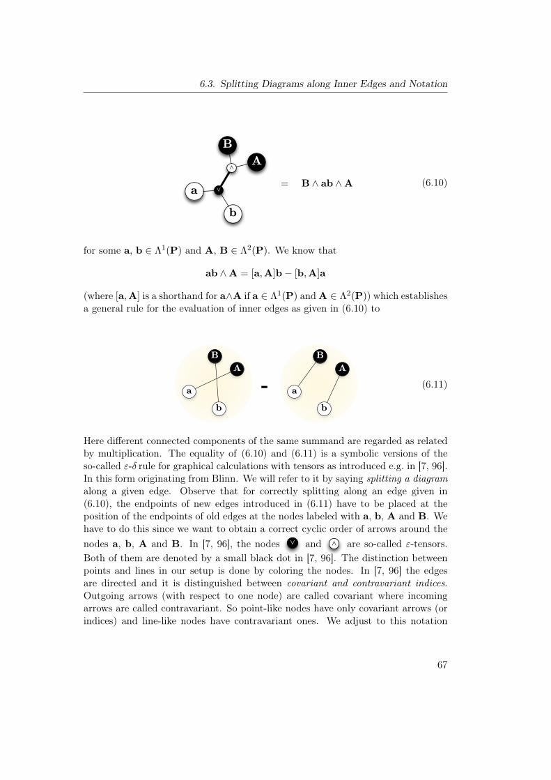
6.3. Splitting Diagrams along Inner Edges and Notation
A
B
b
a
⋀
⋁ = B ∧ ab ∧A (6.10)
for some a, b ∈ Λ1(P) and A, B ∈ Λ2(P). We know that
ab ∧A = [a,A]b− [b,A]a
(where [a,A] is a shorthand for a∧A if a ∈ Λ1(P) and A ∈ Λ2(P)) which establishesa general rule for the evaluation of inner edges as given in (6.10) to
A
B
b
a
A
B
b
a- (6.11)
Here different connected components of the same summand are regarded as relatedby multiplication. The equality of (6.10) and (6.11) is a symbolic versions of theso-called ε-δ rule for graphical calculations with tensors as introduced e.g. in [7, 96].In this form originating from Blinn. We will refer to it by saying splitting a diagramalong a given edge. Observe that for correctly splitting along an edge given in(6.10), the endpoints of new edges introduced in (6.11) have to be placed at theposition of the endpoints of old edges at the nodes labeled with a, b, A and B. Wehave to do this since we want to obtain a correct cyclic order of arrows around thenodes a, b, A and B. In [7, 96], the nodes ⋁ and ⋀ are so-called ε-tensors.Both of them are denoted by a small black dot in [7, 96]. The distinction betweenpoints and lines in our setup is done by coloring the nodes. In [7, 96] the edgesare directed and it is distinguished between covariant and contravariant indices.Outgoing arrows (with respect to one node) are called covariant where incomingarrows are called contravariant. So point-like nodes have only covariant arrows (orindices) and line-like nodes have contravariant ones. We adjust to this notation
67

6. Evaluations
by directing the edges pointing from white nodes to black nodes. This might beconvenient for readers familiar with this notion. Nevertheless, we can drop thesymbols inside the inner nodes and use and instead of ⋁ and ⋀ .
With these notions, the three evaluations of Pascals construction can be summa-rized in
c d
e
f
bc
a
b
d
ef
a
Splitting along the red edges correspond to the first evaluation, splitting along greenedges to the second and splitting along the blue edges is the first step of the thirdevaluation. The next step in the third evaluation is now splitting along the blueedges in the result:
c d
e
f
bc
a
b
d
ef
a
c d
e
f
bc
a
b
d
ef
a
- (6.12)
68

6.3. Splitting Diagrams along Inner Edges and Notation
We say that Classical evaluations, like the first and the second evaluations ofPascal’s construction, distinguish a single inner node as root and then evaluate thediagram from outside to inside. More precisely, after the specification of a root, itis split only along edges that enter a white node . Here entering is understoodas being contained in a directed path from the leave to the distinguished root.Therefore, any classical evaluation can be summarized in a single diagram withhighlighted edges. The highlights correspond to the splits and the order of splittingsdoes not really matter. More general, i.e. non-classical evaluations may not besummarized that easily. However, the additional degree of freedom in evaluatingmay lead to binomial evaluations.With the help of some conventions we can also summarize both steps of the third
evaluation in a single diagram:
c d
e
f
bc
a
b
d
ef
a
a1!b
a3
a2
b1
b2
It should be read as follows: start splitting along the edge a1. In a generic generalcase this will result in two summands. This is also true for the actual edge a1 givenhere. Therefore it is labeled with an arrow → and a letter b. This means thatin the first summand, one should continue splitting edges whose labels start withan a. In the second summand one should start with the newly introduced letterb and split along the edge b1. So in the case of splitting edge a1→b in the firststep one splits along a2 in the first induced summand and along b1 in the secondinduced summand. The edges, where the label does not contain an arrow →, havethe property that after splitting along them one of the induced summands triviallyvanishes. After splitting along the edge a1 the diagram essentially looks like (6.12).After all steps it looks like
69

6. Evaluations
c d
e
fbc
ab
de
f
a
c d
e
fbc
ab
de
f
a-
a3: +1
a2: +1
b3: !1
b2: !1
The blue label a2: +1 indicates that after splitting along the edge labeled a2, onlythe first summand survives. It induces a factor +1 for the first summand. Nowthe result of the evaluation can be easily read of: The small black dots with threeadjacent points correspond to joins. In order to read of an expression in Λ(P), werecall that they also represent expression trees. Therefore e.g.
c
f
a
can be read as c ∨ f ∨ a = [c, f ,a].
So after splitting any inner edges, the summands consist of products of small dia-grams that can be interpreted as brackets when the letters are read in counterclock-wise order. Therefore the above evaluation can be read as
(+1) ·(+1) · [a,b, e][d, e, f ][c, f ,a][d,b, c]−(−1) ·(−1) · [c,d, f ][a, e, f ][b,d, e][a,b, c]
which is the same as (6.9). This notion is appropriate for evaluations with fewsummands. In this case, one does not have to introduce to many new letters.Observe that now the order of splittings might be crucial for the property to havefew summands during the evaluation. Furthermore, the notion is (not yet) adjustedto the case that in some step of the evaluation one wants to split along an edge thatwas not present in the very first diagram. We think, in principle, this problem canbe resolved. However, we do not need this kind of notion in this exposition andtherefore we use the description of calculations as introduced.
70

6.4. Exemplary Evaluation of an Expression of Part III
6.4. Exemplary Evaluation of an Expression of Part III
In the following, we extend the notion of expansion in order to use not only pointsin P as arguments of simple Grassmann-Cayley algebra expressions of diagrams.We also use points that are given by a linear combination. We demonstrate thisand some additional phenomena arising in this treatment with an example used inSection 16.5. There it is labeled with Case 2 (ii) and it is given by the diagram
∞=0'0=∞'b'
0=∞'a'x
∞=0'b'x' a'
b1
b4
b3
b2
a2
a3
a5
a4
a1!b
(6.13)
with 0 =∞′, ∞ = 0′, a′ and b′ ∈ P. x and x′ are given as
x = Mx (µx0− λx∞) and x′ = Mx′ (µx′0′ − λx′∞′) (6.14)
with µx, λx, µx′ and λx′ ∈ BP. Furthermore the shape of µ1′ and λ1′ is known.
µ1′ = [a′,b′,0′] and λ1′ = [a′,b′,∞′].
We split along the edge a1 and consider the first summand. It looks like
71
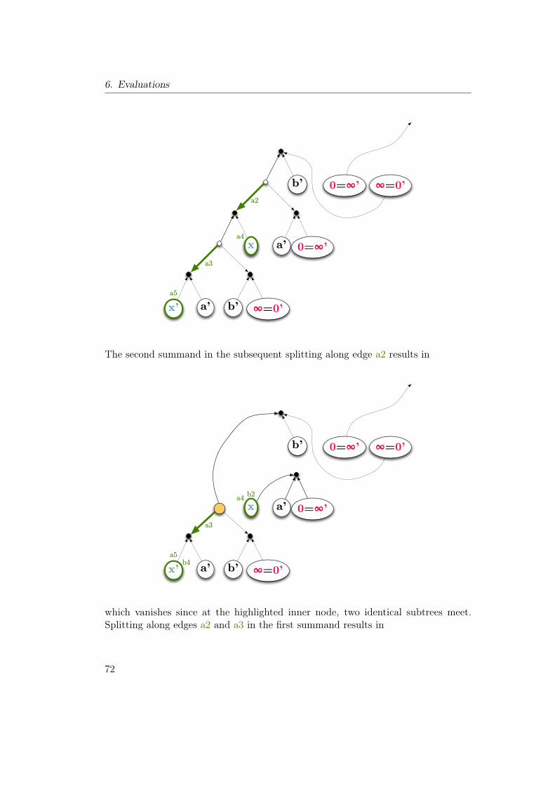
6. Evaluations
∞=0'0=∞'b'
0=∞'a'x
∞=0'b'x' a'
a2
a3
a5
a4
The second summand in the subsequent splitting along edge a2 results in
∞=0'0=∞'b'
∞=0'b'x' a'b4
a3
a5
0=∞'a'xb2a4
which vanishes since at the highlighted inner node, two identical subtrees meet.Splitting along edges a2 and a3 in the first summand results in
72

6.4. Exemplary Evaluation of an Expression of Part III
∞=0'0=∞'b'
0=∞'a'x
∞=0'b'x' a'
a5
a4
a3: !1a2: +1
The label a4 indicates that now, we should plug in the value of x given in (6.14).This means that we evaluate
∞=0'b'
xa4
=
Mx·µx· ∞=0'b'
0=∞'
−Mx·λx· ∞=0'b'
∞=0'
where the second summand vanishes. Plugging in also the value of x′ implies thatthe first summand after splitting (6.13) along the edge a1 can be written as
73

6. Evaluations
a'
∞=0'0=∞'b'
0=∞'a'0=∞'
∞=0'b'∞=0'
a4: a3: !1a2: +1
a5: Mx · µx
Mx′ · µx′
(6.15)
where all values in the top left are considered as factors of the diagram. Now forthe second summand. After splitting along the edge b1 the diagram looks like
∞=0'0=∞'b'
0=∞'a'x
∞=0'b'x' a'b4
b3
b2
b1: +1
74
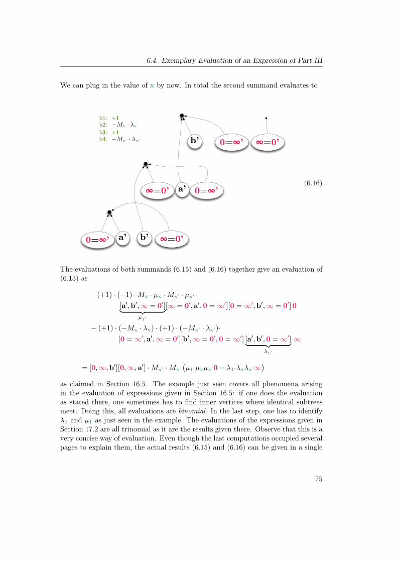
6.4. Exemplary Evaluation of an Expression of Part III
We can plug in the value of x by now. In total the second summand evaluates to
∞=0'0=∞'b'
0=∞'a'∞=0'
∞=0'b'0=∞' a'
b1: +1
b4: b3: +1b2: −Mx · λx
−Mx′ · λx′
(6.16)
The evaluations of both summands (6.15) and (6.16) together give an evaluation of(6.13) as
(+1) · (−1) ·Mx · µx ·Mx′ · µx′ ·[a′,b′,∞ = 0′]︸ ︷︷ ︸
µ1′
[∞ = 0′,a′,0 =∞′][0 =∞′,b′,∞ = 0′] 0
− (+1) · (−Mx · λx) · (+1) · (−Mx′ · λx′)·[0 =∞′,a′,∞ = 0′][b′,∞ = 0′,0 =∞′] [a′,b′,0 =∞′]︸ ︷︷ ︸
λ1′
∞
= [0,∞,b′][0,∞,a′] ·Mx′ ·Mx
(µ1′µxµx′0− λ1′λxλx′∞
)
as claimed in Section 16.5. The example just seen covers all phenomena arisingin the evaluation of expressions given in Section 16.5: if one does the evaluationas stated there, one sometimes has to find inner vertices where identical subtreesmeet. Doing this, all evaluations are binomial. In the last step, one has to identifyλ1 and µ1 as just seen in the example. The evaluations of the expressions given inSection 17.2 are all trinomial as it are the results given there. Observe that this is avery concise way of evaluation. Even though the last computations occupied severalpages to explain them, the actual results (6.15) and (6.16) can be given in a single
75

6. Evaluations
diagram. One can do the calculations easily by printing (6.13) twice, consideringeach copy as a summand, deleting edges and keeping track of factors.
76

7. Incidence Theorems
There are some reasons to have a separate chapter on incidence theorems. One isthat it is a classical part of projective geometry. The defining axioms of projectivegeometry are essentially about incidence and therefore it is interesting, which kindof theorems can be deduced. Some of the incidence theorems date back to theancient Greeks. Another reason is that it is closely related to everything presentedin this thesis. Although most of the time, this connection is not explicit, it is there.Furthermore, incidence theorems are the starting point for the considerations inPart II. We will only treat incidence theorems in RP2. We start with describing thegeneral structure of incidence theorems. We will give background information onautomated proving of (incidence) theorems. Sometimes incidence theorems can alsobe detected automatically. We will argue that it is important to consider so-callednon-degeneracy conditions. Many approaches use construction sequences to provethe theorem. This might restrict the classes of theorems as well as the generalityof the statements that are considered. For both, stating and proving incidencerelations, it plays a role how theorems are actually given. We will restate ourpoint of view on this subject. It was formalized in [2]. It captures theorems thatdo not have a construction sequence. Furthermore it can automatically take mildnon-degeneracy conditions into account.
7.1. General Structure of Incidence Theorems
In its most general form an incidence theorem may roughly be stated as “Givensome objects in the projective plane and some prescribed incidence relations holdbetween them. Then an additional incidence relation holds.”
7.2. Pascal’s Theorem Revisited
We already encountered a statement matching this description: Pascal’s theorem(see Section 3.10) can be read as:
• Given a conic C, points a, b, c, d, e, f , x, y and z points in the projectiveplane RP2 and lines l1, l2, l3, l4, l5 and l6
77

7. Incidence Theorems
• such that a, b, c, d, e and f are incident with C and
a, b and x are incident with l1,e, d and x are incident with l2,a, f and y are incident with l3,c , d and y are incident with l4,e, f and z are incident with l5 andb, c and z are incident with l6.
• Then the points x, y and z are incident with some line l.
A different formulation with the incidence constraints more implicitly would be:
• Given points a, b, c, d, e, f , x, y and z in the projective plane
• such that a, b, c, d, e and f are on a common conic and the triples of points(a, b, x), (e, d, x), (a, f, y), (c, d, y), (e, f, z) and (b, c, z) are collinear.
• Then the points x, y and z are collinear as well.
In fact, often in the literature, incidence theorems are stated in this fashion butthey are not completely correct in this way. Figure 7.1 gives a configuration inRP2 fulfilling all requirements of the above formulation of Pascal’s theorem wherethe conclusion does not hold. In fact, Figure 7.1 is a degenerate configuration. So
Figure 7.1.: A degenerate configuration where the conic consists of the two red lines.Here a naive formulation of Pascal’s theorem does not hold.
78

7.3. Incidence Theorems of Points and Lines
in the above formulation of Pascal’s theorem, it is not taken care of degenerateconfigurations. A correct formulation of the theorem that matches the presentexhibition could be:Whenever points a, b, c, d, e and f lie on a common conic it holds that the
determinant∣∣∣meet
(join(a, b), join(d, e)
),meet
(join(c, d), join(f, a)
),
meet(join(e, f), join(b, c)
)∣∣∣ (7.1)
vanishes. In the case that meet(join(a, b), join(d, e)
), meet
(join(c, d), join(f, a)
)
and meet(join(e, f), join(b, c)
)can be interpreted as homogenous coordinates, this
fact implies the collinearity of the three points. However, it may happen, that oneof the three vectors is zero. This can only happen, if the underlying construction de-generates. In this case, (7.1) holds trivially and one cannot conclude a “collinearity”of three points.This example is supposed to illustrate the fact, that depending on the formu-
lation of an incidence theorem, non-degenerate conditions have to be formulated.Supposing a correct formulation, Pascal’s theorem is surely an incidence theorem.However, in the present text, we will focus mostly on incidence relations and in-cidence theorems involving only points and lines. So unless mentioned differently,from now on, an incidence theorem will be formulated in terms of points and lines.
7.3. Incidence Theorems of Points and Lines
A first example of a theorem on points and lines is in fact another degeneratesituation of Pascal’s theorem: consider the case where the conic C degenerates totwo lines which are incident to the points a, c and e resp. b, d and f (see Figure 7.2).
In fact, Pappos’s theorem is very special in a lot of senses. For example, it isthe smallest of all incidence theorems and also the only one on nine points. In theliterature you can find many other special properties and also a variety of differentproofs. See [95] for nine proofs and more relations. It is also treated in almostevery textbook on projective geometry. We referred to some of them already inChapter 2. We will present two ideas for proofs. The first one is just the fact that(7.1) holds since points a, . . . , f lie on a common conic. Furthermore, in general,within this specialization, the construction does not degenerate. So this proves,that whenever the construction indicated in Figure 7.2 does not degenerate, theconstructed points are collinear. One can see this also without the knowledge thata pair of lines constitutes a degenerate conic: reconsider from Chapter 6 that in
79

7. Incidence Theorems
Figure 7.2.: A degenerate configuration of Pascal’s theorem gives Pappos’s theorem.
Grassmann-Cayley algebra it holds
(ab ∧ de)(cd ∧ fa)(ef ∧ bc)
= [a, c, f ][a,d, e][b, c, e][b,d, f ]− [a, c, e][a,d, f ][b, c, f ][b,d, e].
Plugging in e = ac ∧ uv = [a,u,v]c − [c,u,v]a and f = bd ∧ xy = [b,x,y]d −[d,x,y]b gives zero (for some u, v, x and y). This can be also read as a proof fora pair of lines being a conic. The above formulation in Grassmann-Cayley algebraimplies the existence of an underlying construction. All incidence theorems that areformulated with the help of an underlying construction by the ruler alone can inprinciple be proved with the help of Grassmann-Cayley algebra and a method forshowing the vanishing of a resulting bracket polynomial. This method might be thestraightening algorithm or substituting symbolic coordinates with the help of Φ.
7.4. (General) Automated Theorem Proving
The method last described can be considered a an automated version of theoremproving. Actually, there is a whole branch of mathematics and computer sciencededicated to automated geometric reasoning. Overviews of the development (upto the point of publication) are given in [93, 114] by Richter-Gebert and Wang.The latter contains many references for the development of automated reasoning.The first steps date back to [46]. First theoretical results are given by the factthat arbitrary algebraic equations can be encoded as projective incidence theorems([83, 10, 121]). Furthermore, realizability is theoretically decidable ([105]).It was Wu who gave a systematic translation routine from geometry to algebra (see
e.g. [137]). He uses Euclidean geometry and translates constructions to polynomialsin coordinates. Therefore, he gives a complete restatement of Hilbert’s “Foundations
80

7.4. (General) Automated Theorem Proving
of Geometry” (see [62]). He uses a constructive treatment of algebraic geometryintroduced previously by Ritt (see e.g. [98]). The method encodes the hypothesesof a theorems in the vanishing of a polynomial (in the coordinates of points). Theconclusion is encoded in a polynomial as well. It aims to show that a multiple of thispolynomial vanishes in behalf of the hypotheses. The theorem is true in a concreteinstance, whenever the multiplier monomial not yields zero. The multiplier is saidto be a non-degeneracy condition. Wu’s method tries also to interpret the non-degeneracy conditions derived. To show the vanishing of a multiple of the conclusionpolynomial, a construction sequence of the theorem is assumed and used in orderto eliminate variables. Using the translation from geometry to algebra done by Wu,in [72], Kutzler and Stifter use a different approach to do the algebraic calculations:they use Buchberger’s algorithm using Gröbner bases. Both methods are introducedand compared in [20]. A variant of using Gröbner bases was introduced by Kutzler(see e.g. [70]). For another overview regarding Gröbner bases in geometric theoremproving see also [117]. Here one finds also a section on discovering theorems.A view words on theorems with a construction sequence (or theorems of con-
structive type) are appropriate: As stated in [20, p. 19], the choice of a constructionsequence is intimately related not only with the selection of parameters and depen-dent variables but also to the validity of the theorem as well as the non-degeneracyconditions given by an algorithm. Recalling the re-rooting process from the pre-vious chapter, one sees that this approach may not cover the spirit that (some)points have same rights. For example, there might be constructions where one canconstruct a point a depending on b as well as the point b depending on a.There are also coordinate-free methods. One of its is the so-called area method
summarized in [21]. An external overview over the method is given in [69]. It is coor-dinate free and expresses relations via areas and length ratios and is therefore closelyrelated with the content of this thesis. The area method also uses a constructionsequence in order to make symbolic manipulations. Another coordinate-free methodis bracket algebra together with Grassmann-Cayley algebra (see e.g. [30, 74, 78]).A final polynomial exists whenever an (oriented) matroid is non-realizable. There-fore an incidence theorem is proved whenever a counterexample is non-realizable.Final polynomials trace back to Bokowski and Sturmfels ([10]), and independentlyto Whiteley ([135, 130, 132, 133]). The connection between both theories is empha-sized in [134]. The latter also addresses the problem of interpreting non-degeneratemultipliers appearing in the methods described above. This is done by consideringinvariant properties and translating them into invariant language. The special caseof biquadratic final polynomials due to Bokowski and Richter-Gebert is easier tocompute and works in many cases (see [92, 93, 9, 30]). We will give an example ofthis method in Section 9. In [101], Sturmfels points out that incidence theorems arespecial cases of configurations and that also [63] gives comments about the greatsignificance of configurations in former times. In the concrete computations he uses
81

7. Incidence Theorems
(partial) construction sequences in order to get algebraic expressions. Results ofMnëv and Shor are cited in order to obtain the result that the real realizabilityproblem is NP-hard. Due to [10, p. 5] the existence of a construction sequence isthe question of rational realizability.Closely related to bracket algebra and Grassmann-Cayley algebra is also the
method of Clifford algebra (which is closely related with Grassmann-Cayley al-gebra). This approach is due to Li and Cheng (see e.g. [67, 73, 116]). In theseapproaches the borders are not sharp and also variants of the previously mentionedapproaches are used. See also the work of Li e.g. in [75, 74, 79, 80, 76]. The detailedbook [77] can be seen as a summary of the above mentioned. [42] can be read asgeneralizing the elimination methods seen e.g. in Wu’s method to Clifford Algebra.More developments on the subject are given in several collections e.g. [26] and
the proceedings on the workshops of automated deduction in geometry starting with[115, 45, 97]. More literature can be found under http://www-calfor.lip6.fr/~wang/GRBib/.Applications of mechanical theorem proving are due to [93] given in computer-
aided geometric reasoning, robotics and robot motion planning, computer visionand scene analysis, rigidity of frameworks, molecular conformation, computer-aideddesign and computer-aided manufacturing and many other related topics.
7.5. Modeling Incidence Theorems of Points and Lines
The starting point for the investigation of Γ-cycles in Part II is the binomial orbiquadratic proving method given in [92, 93, 9, 30]. It provides a construction-free formulation and treatment. Pappos’s theorem in this kind of formulation canbe stated as: if (a, e, c), (b, d, f), (a, b, x), (e, d, x), (a, f, y), (c, d, y), (e, f, z) and(b, c, z) are triples of collinear points then x, y and z are collinear as well. Alsothis formulation needs non-degeneracy conditions: the theorem is false in the verydegenerate situation where we identify the points a, . . . , f and put x, y and zanywhere in a non-collinear situation in the projective plane. A more general formof a construction-free formulation including non-degeneracy conditions is restatedfrom [2]:
Definition 7.1. A real projective incidence assertion T on a finite point set P isa triple (H,B, C) such that:
• H,B ⊂i, j,k | i, j,k ∈ P pairwise distinct
• C = a,b, c with a,b, c ∈ P pairwise distinct and C /∈ H.
A point configuration P in RP2 is called an instance of T if [i, j,k]P := ΦP ([i, j,k])= 0 for all i, j,k ∈ H and [i, j,k]P 6= 0 for all i, j,k ∈ B. If in addition for
82

7.5. Modeling Incidence Theorems of Points and Lines
every instance P of T also [a,b, c]P = 0 holds, then T is called a valid assertion ora theorem.
Observe that although the formulation in Definition 7.1 is similar to the one of theGrassmann-Cayley algebra, the indices in P play a different role. In Grassmann-Cayley algebra, they are considered to play the role of free generic points. Dependingon points in P, new points can be constructed. In contrast to this, Definition 7.1uses a more symmetric formulation that does not need the distinction between freeand dependent points. So it might allow for changing the underlying constructionwithout changing the validity of the theorem.Non-degeneracy conditions are cumbersome to deal with. The proposed formula-
tion as triples of points that are considered to be non-collinear has the advantagethat they can be easily formulated and interpreted. It turns out, that there is anatural choice of B depending on H and C. This natural choice ensures essentiallythat points on the same line may not coincide, as long as this line is relevant to theformulation of the theorem. Furthermore, the dual shall also hold: two (distinct)lines sharing a point in P may not coincide.For some considerations in Part II we restate some definitions from [2]. Let
A := H ∪ C. Assume w.l.o.g. that A is saturated, i.e. for
a, b, c ∈ A and b, c, d ∈ A =⇒ a, b, d ∈ A.
We definef(a, b, c) := i | a, b, i ∈ A
which can be thought as the line supported by a, b and c. f is well defined due tothe saturation of A. The set of all derived lines is collected in a set
G :=f(a, b, c) | a, b, c ∈ A
.
These notions allow us to define the natural choice for B mentioned above:
B(A) :=a, b, c
∣∣∃G,H ∈ G with |G ∩H| = 1
and a ∈ G \H, b ∈ H \G, c ∈ H ∪G.
B(A) is meant to be a default value for non-degeneracy conditions and dependsonly on the collinearities and the conclusion of a (generic drawing of) an incidencetheorem. As an example, we consider Theorem 9.1 which is treated in more detaillater. It is illustrated in Figure 9.1. We have h,g,p ∈ B(A) since 0,g,h,kand ∞,k,m,p are in G and intersect in the single element k. On the other hand,h,m, c is not an element of B(A). It also turns out in [2] that this natural choiceof B is well-suited for the purposes of binomial proofs and Ceva-Menelaus proofs
83

7. Incidence Theorems
investigated there: the equivalence of both proving methods. The idea is alreadypresented in [94]. In Chapter 9, we will exemplify the implication which starts withbinomial proofs and ends up with Ceva-Menelaus proofs. This implication is themore interesting one.The definition of B(A) is crucial for this translation process. Since we want to
derive a geometric reasoning working in any instance, we have to restrict to elementsin B(A). We will see in Section 10.3 that the shape of B(A) influences the way somecycles can be decomposed. So a few comments on why we believe the definitionmakes sense are appropriate. First of all, the fact that collinear points shall notcoincide (and its dual version) seems natural to us. The non-degeneracy conditionsmay be in some cases a little too restrictive. However, they do not fix all pointsin the construction and some degeneracies are still allowed. Having in mind thatB(A) can be stated automatically, this seems to be a good tradeoff. Furthermore,as mentioned before, the conditions are strong enough to do the translation processfrom biquadratic proofs to Ceva-Menelaus proofs.There is an additional advantage of the construction-free approach for formulating
incidence theorems: one can also require to have relations between points that arenot ruler-constructible. This happens e.g. if one implicitly needs to have (irrational)roots of real numbers. Von Staudt constructions (see Section 3.7) allow for checkingwhether we have a root but not to construct one. This happens e.g. in the projectiveversion of a regular pentagon. It can be summarized as follows: consider five pointsdetermining a pentagon. Construct all intersections of an edge and the diagonalopposite to it. Whenever four of these intersections lie on a common line, the fifthdoes lie on the same line (see Figure 7.3). This statement can be made a rigorous onein the sense of Definition 7.1 but no construction sequence can be given. However,there exists a binomial proof for it ([93, Ex. 14] and [47] for another occurrenceof the configuration). For other non-rational incidence types, e.g. configurationswithout construction sequence see [10, Chap. 5].
Figure 7.3.: A non-constructible incidence theorem: as soon as 4 of the black pointsare on a line l, the last black point is on l, too.
84

Part II.
Γ-Cycles
85


8. Introduction to Γ-Cycles
The present part of the thesis is dedicated to so-called Γ-cycles. They emerged inthe investigation of binomial proofs (see [92, 93, 9, 30]). This kind of investigationcan be found in [94, 2]. An example of it will be given in Chapter 9. There,the area principle is used to translate an algebraic proof of an incidence theoreminto an argument working with oriented length ratios. These oriented length ratiosare structured in such a way that they can be interpreted as being induced byconfigurations of Ceva and Menelaus. The overall result is a collection of Ceva andMenelaus triangles which are glued together. This resultis in the structure of atriangulated oriented combinatorial 2-manifold. The existence of all but one Cevaor Menelaus triangles implies the existence of the last one. This gives another prooffor the incidence theorem in question. It is formulated in the language of lengthratios. At some point during the translation process, one is left with a collectionof (possibly long) cycles in a base graph Γ (defined in detail in Chapter 10). In[2] the cycles can be decomposed into triangles by adding new points to the overallsetup. These triangles indicate the configurations of Ceva and Menelaus. However,the number of additional triangles needed might be big. Therefore it makes sense toconsider the cycles on its own. This motivates the treatment of Γ-cycles. All cyclesobtained in the translation process are in fact Γ-cycles.All edges in the overall base graph Γ can be interpreted via the area principle
(see Section 3.1). The edges can be considered as unbreakable ratios of determinantsand as elements of a group RGB defined in Chapter 10. The group is related toa group BGB encoding all products of bracket (and its inverses). This relation isalso used in the translation process of a binomial proof. It is based on theory anddefinitions due to Dress and Wenzel (see [38, 40, 41, 39]). Their theory is developedfor very general setups of finite or infinite matroids with coefficients. Our morespecific setup is the projective plane. However, we are in a situation, where notthe full information about triples of points being collinear or not being collinear ispresent.As the edges of Γ, each edge of a Γ-cycle can be interpreted as a length ratio in
Euclidean geometry (with some additional assumptions on the coordinates). Thefact, that the length ratios are induced by cycles yields that the overall product of alllength ratios induced by the cycle equals +1 or −1. This is an identity in Euclideangeometry called a Γ-cycle theorem and is introduced in Section 10.4.1. Γ-cycletheorems can be understood as generalization of Ceva’s and Menelaus’s theorem.
87

8. Introduction to Γ-Cycles
Similar theorems are also considered by Grünbaum and Shephard (see [53, 52, 54]).The connections of Γ-cycle theorems and their results is given in Chapter 13.The investigation of Γ-cycles themselves first focuses on irreducibility. The con-
cept emerges from the translation process described before and is also considered byDress and Wenzel. A Γ-cycle is said to be weakly irreducible whenever it cannot beobtained by combining two shorter Γ-cycles which use only vertices of the first Γ-cycle. For the definition of strongly irreducibility one includes additional informationabout non-degeneracy conditions as it is possible when treating incidence theorems.Since this information is very specific we focus on weakly irreducibility and omitthe word “weakly”. These restrictions allow for structuring the irreducible Γ-cycles.We give a table representation which provides a good visualization and allows forcounting irreducible Γ-cycles of fixed length (see Chapter 11). The table repre-sentation and the suggestion of an underlying structure is due to Richter-Gebert.Furthermore, this coding of Γ-cycles allows for extracting additional informationabout Γ-cycles. This information (see Section 12.2) is helpful when further usingthe Γ-cycle (see Section 12.1). By using Γ-cycles we mean imposing additional in-cidence relations. This allows for more complicated theorems about oriented lengthratios (see Chapter 13) and also for constructing new projective incidence theorems.This construction is possible since one has good geometric control of the cancellationprocess by glueing length ratios. This gluing process is the reason why Chapter 10also includes definitions of groups capturing informations about triples of pointsbeing collinear. These identities are also present in the expositions of Dress andWenzel.
88

9. Motivation: Example on How toTransform a Binomial Proof toΓ-Cycles
The topic of Γ-cycles treated in this part of the thesis emerged from the investigationof the relations between biquadratic proofs (introduced by Richter-Gebert in [92, 93,9, 30]) and Ceva-Menelaus proofs (see [95, 94, 2]). Since this emergence is essentialto the understanding of the relevance and concrete treatment of Γ-cycles, we willgive another brief introduction with the help of a concrete example. Other examplescan be found in [94, 2]. In this introduction, all considerations are exemplary. Theygeneralize as it was shown in [2].The example considered here is not the smallest one possible. However, its size
may give an impression on how the general case behaves. Furthermore, the con-struction considered fits quite well into the topics of this thesis and can be extendedto show the limitations of the proofing method (see Section 9.4).Now for the example. Consider Figure 9.1. Assuming all incidences except the
one indicated by the red line implies the existence of the red line. This is due tothe fact that addition is associative. To see this, recall Section 3.7 and observe:
Figure 9.1.: (a+b)+c = a+(b+c) encoded in geometry via von Staudt constructions.
89

9. Motivation: Example on How to Transform a Binomial Proof to Γ-Cycles
the quadrilateral with vertices d, k, m and h induces a quadrilateral set such thatthe small gray point on the line spanned by m and d represents the sum of aand b. The quadrilateral set induced by d, m, n and p adds c to it. This meansthat meet(join(d, p), join(0,∞)) represents the sum (a + b) + c. Similarly, thequadrilateral sets induced by f , g, h and l and the one induced by d, e, f and ltogether compute a+ (b+ c). The fact that both values are identical is encoded inthe fact that the lines join(d, p) and join(d, l) meet join(0,∞) in the same point.In other words (and in a non-degenerate situation): d, l and p are collinear. Allgray points do not play a crucial role in the construction and can be omitted. Thisresults in the following formulation of our toy example:
Theorem 9.1. Let P = 0, c,d, e, f ,g,h,∞,k, l,m,n,p, let H consist of all 3-element subsets of the sets
∞,0, c, 0, e, f, 0,m,n, c, f ,g, c,n,p, d, e,k, h, l,m,0,g,h,k, ∞, e,g, l, ∞,k,m,p, ∞,d, f ,h,n.
Let C = d, l,p. In the sense of Definition 7.1, A := (H,B = B(A), C) is anincidence theorem.
9.1. Formal Language for Stating Biquadratic Proofs
The formalization of biquadratic or binomial proofs done in [2] points out that thedomain of its calculations is a multiplicative group generated by formal determinantsof (free and dependent) points together with a symbol ε that plays the role of aformal −1. We will need the following definition as a setup for symbolic calculations,e.g. for binomial proofs:
Definition 9.2. Let (H,B, C) be a real projective incidence theorem on P. LetBGB be the quotient of the free multiplicatively written abelian group generated by
[a,b, c]
∣∣ a,b, c ∈ B∪ε
and the group generated by
[a,b, c]
[b, c,a]
∣∣∣∣ a,b, c ∈ B
∪ε · [a,b, c]
[b,a, c]
∣∣∣∣ a,b, c ∈ B
∪ε2.
This definition allows for formal multiplicative calculations with determinantsthat are supposed to be non-zero. The permutational properties of the determi-nants are implemented. We define a subgroup of BGB encoding properties of thecollinearities encoded in H:
90

9.2. A Biquadratic Proof for the Given Example
Definition 9.3. Let (H,B, C) be a real incidence projective theorem on P. LetHGB,H be the subgroup of BGB generated by
[a,b,x][a, c,y]
[a,b,y][a, c,x]∈ BGB
∣∣∣∣ a,b, c ∈ H, x,y ∈ P
.
The generating elements of HGB,H are called biquadratic fractions.
Proposition 9.4. Let P be a point configuration in RP2 that is an instance of a realprojective incidence theorem (H,B, C). There is a well-defined homomorphism ΦP :BGB → (R \ 0, ·) which is the extension of the map ΦP defined in Definition 4.5and which maps ε to −1. Furthermore we have
ΦP(HGB,H
)= 1 .
Proof. It suffices to show the last statement. Let [a,b,x][a,c,y][a,b,y][a,c,x] ∈ BGB with a,b, c ∈
H, x,y ∈ P. By writing a, b, c, x and y for the points in P corresponding to a, b,c, x and y we have that
ΦP
([a,b,x][a, c,y]
[a,b,y][a, c,x]
)=
[a,b,x]P [a, c,y]P[a,b,y]P [a, c,x]P
=|a, b, x| · |a, c, y||a, b, y| · |a, c, x|
and it suffices to show that
|a, b, x| · |a, c, y| − |a, b, y| · |a, c, x| = 0.
This is an easy consequence of the 3-term Grassmann-Plücker relation (4.3) implyingthat
|a, b, x| · |a, c, y| − |a, b, y| · |a, c, x|+ |a, b, c| · |a, y, x| = 0.
Since a,b, c is in H and P is an instance, we have |a, b, c| = 0 which proofs theclaim.
9.2. A Biquadratic Proof for the Given Example
A binomial proof for A is formulated within this language is given by:
[0,∞,g] · [∞, c,n]
[∞, c,g] · [0,∞,n]0,∞, c [∞,d,g] · [0,∞, e]
[∞,d, e] · [0,∞,g]∞, e,g, l
[0,∞,m] · [0, c,k]
[0, c,m] · [0,∞,k]0,∞, c [∞,n,p] · [0, c,n]
[∞, c,n] · [0,n,p]c,n,p
91

9. Motivation: Example on How to Transform a Binomial Proof to Γ-Cycles
[0,∞, f ] · [0, c, e]
[0,∞, e] · [0, c, f ]0,∞, c [0,d,k] · [∞, e,k]
[∞,d,k] · [0, e,k]d, e,k
[∞,d,k] · [d,h,m]
[d,h,k] · [∞,d,m]∞,d, f ,h,n ε· [0,∞,k] · [k, l,m]
[∞,k, l] · [0,k,m]∞,k,m,p
[0,∞,n] · [∞,d,p]
[∞,n,p] · [0,∞,d]∞,d, f ,h,n ε· [0,m,p] · [∞,d,m]
[0,∞,m] · [d,m,p]∞,k,m,p
[0,∞,d] · [∞, f ,g]
[∞,d,g] · [0,∞, f ]∞,d, f ,h,n [0,n,p] · [0, c,m]
[0, c,n] · [0,m,p]0,m,n
ε· [d,h,k] · [0,k,m]
[0,d,k] · [h,k,m]0,g,h,k ε· [d, l,m] · [h,k,m]
[d,h,m] · [k, l,m]h, l,m
[0, c,h] · [0, e,k]
[0, e,h] · [0, c,k]0,g,h,k [0, e,h] · [0, c, f ]
[0, f ,h] · [0, c, e]0, e, f
[0, f ,h] · [0, c,g]
[0, c,h] · [0, f ,g]0,g,h,k [0, f ,g] · [∞, c,g]
[0, c,g] · [∞, f ,g]c, f ,g
ε· [∞,k, l] · [∞,d, e]
[∞, e,k] · [∞,d, l] ∞, e,g, l
This is a list of elements of HGB,H together with a certificate for the membership.This certificate are sets of collinear points in the way they are given in Theorem 9.1.The product of all these biquadratic fractions is an element of HGB,H. After can-celing it is
ε · [d, l,m] · [∞,d,p]
[d,m,p] · [∞,d, l] .
For an instance P and using non-bold letters as point names for the correspondingbold letters in P and due to Proposition 9.4 we have
|d, l,m| · |∞, d, p|+ |d,m, p| · |∞, d, l| = 0.
Again, by a 3-termed Grassmann-Plücker relation it holds that
|d, l,m| · |d,∞, p| − |d, l,∞| · |d,m, p|+ |d, l, p| · |d,m,∞| = 0.
Adding up both equations yields
|d, l, p| · |d,m,∞| = 0.
Since we have that d,m,∞ ∈ B = B(A) and since P is an instance, we knowthat |d,m,∞| 6= 0 and therefore it must hold that |d, l, p| = 0 which proofs A.
92

9.3. Interpreting a Biquadratic Proof
Generally and roughly speaking, a binomial proof is a collection of biquadraticfractions whose product also has the structure of a biquadratic fraction. This way,an additional collinearity can be concluded. It should be remarked that this proofwas obtained by an automatic prover given in [108]. It is based on the theory givenin [93] and uses a substitution method for solving the resulting linear equationsystem. This procedure happens to be good for producing short proofs.
9.3. Interpreting a Biquadratic Proof
Biquadratic proofs are concise and human checkable. However, in the form justpresented, there is less geometric intuition attached to them. One could draw aEuclidean picture and interpret bracket as (scaled) oriented triangle areas. However,we think that this is not very intuitive. A concept that is easier to deal with areoriented length ratios. When applicable, the area principle (see Section 3.1) providesan translation from ratios of brackets to oriented length ratios. An analysis of ageneric biquadratic fraction
[a,b,x][a, c,y]
[a,b,y][a, c,x]
shows that the area principle can be applied. Furthermore, it can be applied in twodifferent ways induced by two different splittings of the fraction:
[a,b,x]
[a,b,y]· [a, c,y]
[a, c,x]and
[a,b,x]
[a, c,x]· [a, c,y]
[a,b,y].
We choose to split the biquadratic fractions in the binomial proof of A in the firstway indicated. This results in considering the products of ratios
1.[0,∞,g]
[∞, c, g]· [∞, c, n]
[0,∞,n]11.
[∞,d,g]
[∞,d, e]· [0,∞, e]
[0,∞,g]
2.[0,∞,m]
[0, c, m]· [0, c, k]
[0,∞,k]12.
[∞,n,p]
[∞, c, n]· [0, c, n]
[0,n,p]
3.[0,∞, f ]
[0,∞, e]· [0, c, e]
[0, c, f ]13.
[0,d, k]
[∞,d,k]· [∞, e,k]
[0, e, k]
4.[∞,d,k]
[d,h, k]· [d,h, m]
[∞,d,m]14. ε· [0,∞,k]
[∞,k, l]· [k, l, m]
[0,k,m]
5.[0,∞, n]
[∞,n,p]· [∞,d,p]
[0,∞, d]15. ε· [0,m, p]
[0,∞,m]· [∞,d,m]
[d,m, p]
93
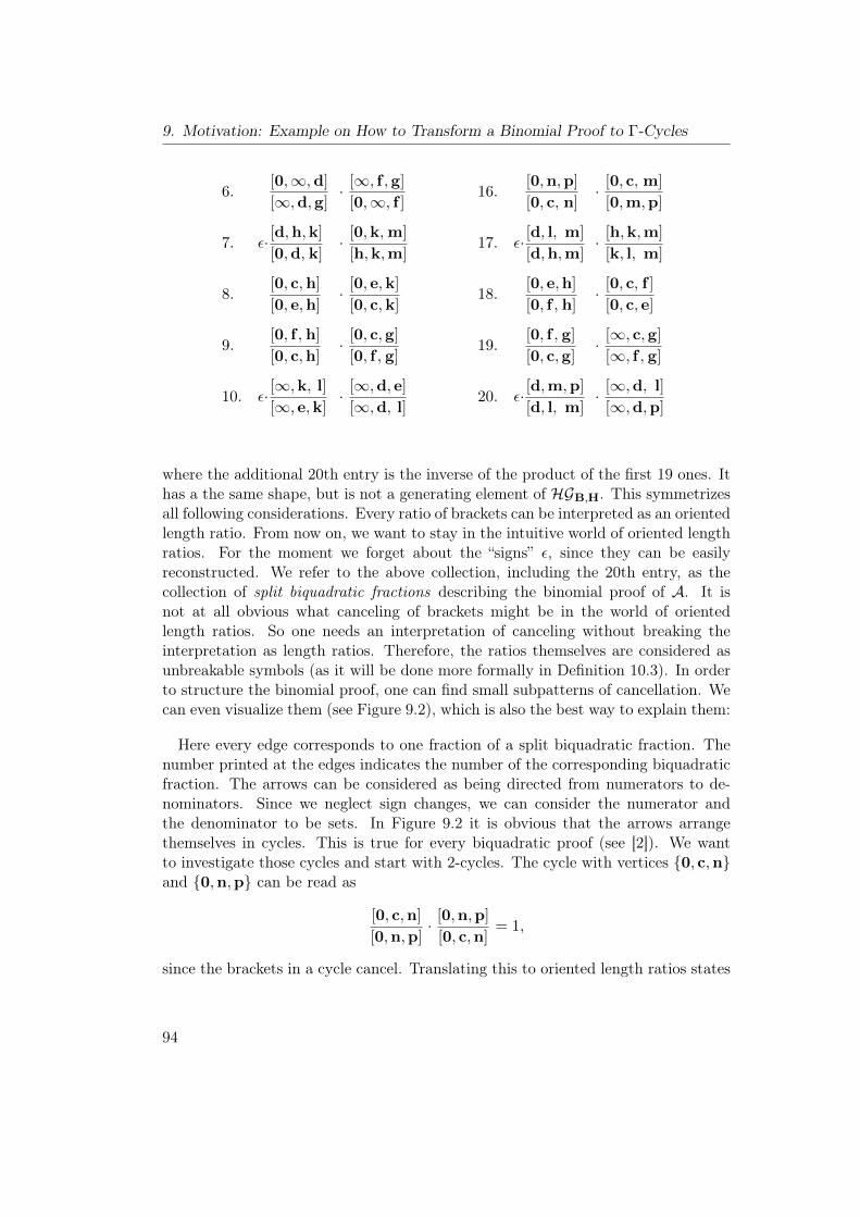
9. Motivation: Example on How to Transform a Binomial Proof to Γ-Cycles
6.[0,∞,d]
[∞,d,g]· [∞, f ,g]
[0,∞, f ]16.
[0,n,p]
[0, c, n]· [0, c, m]
[0,m,p]
7. ε· [d,h,k]
[0,d, k]· [0,k,m]
[h,k,m]17. ε· [d, l, m]
[d,h,m]· [h,k,m]
[k, l, m]
8.[0, c,h]
[0, e,h]· [0, e,k]
[0, c, k]18.
[0, e,h]
[0, f , h]· [0, c, f ]
[0, c, e]
9.[0, f , h]
[0, c,h]· [0, c,g]
[0, f , g]19.
[0, f , g]
[0, c,g]· [∞, c,g]
[∞, f , g]
10. ε· [∞,k, l]
[∞, e,k]· [∞,d, e]
[∞,d, l]20. ε· [d,m,p]
[d, l, m]· [∞,d, l]
[∞,d,p]
where the additional 20th entry is the inverse of the product of the first 19 ones. Ithas a the same shape, but is not a generating element of HGB,H. This symmetrizesall following considerations. Every ratio of brackets can be interpreted as an orientedlength ratio. From now on, we want to stay in the intuitive world of oriented lengthratios. For the moment we forget about the “signs” ε, since they can be easilyreconstructed. We refer to the above collection, including the 20th entry, as thecollection of split biquadratic fractions describing the binomial proof of A. It isnot at all obvious what canceling of brackets might be in the world of orientedlength ratios. So one needs an interpretation of canceling without breaking theinterpretation as length ratios. Therefore, the ratios themselves are considered asunbreakable symbols (as it will be done more formally in Definition 10.3). In orderto structure the binomial proof, one can find small subpatterns of cancellation. Wecan even visualize them (see Figure 9.2), which is also the best way to explain them:
Here every edge corresponds to one fraction of a split biquadratic fraction. Thenumber printed at the edges indicates the number of the corresponding biquadraticfraction. The arrows can be considered as being directed from numerators to de-nominators. Since we neglect sign changes, we can consider the numerator andthe denominator to be sets. In Figure 9.2 it is obvious that the arrows arrangethemselves in cycles. This is true for every biquadratic proof (see [2]). We wantto investigate those cycles and start with 2-cycles. The cycle with vertices 0, c,nand 0,n,p can be read as
[0, c,n]
[0,n,p]· [0,n,p]
[0, c,n]= 1,
since the brackets in a cycle cancel. Translating this to oriented length ratios states
94

9.3. Interpreting a Biquadratic Proof
0, f ,g
0, c,g
0, c, f
0, c, e
0, c,n
0,n,p
0, f ,h 0, c,h
0, e,h
∞,n,p ∞, c,n
0,∞,n
0,m,p 0,∞,m
0, c,m
h,k,m k, l,m
0,k,m
∞,d,k d,h,k
0,d,k
d, l,m d,h,m
∞,d,md,m,p
∞,d, e ∞,d, l
∞,d,p
0,∞,d
∞,d,g
0,∞,k ∞,k, l
∞, e,k
0, e,k
0, c,k
0,∞,g ∞, c,g
∞, f ,g
0,∞, f
0,∞, e
5
12
1
16
15
2
13
4
7
7
17
14
18
9
8
56
1110
20
138
214
1063
111
19
17
4
15
20
19 9
18 312 16
Figure 9.2.: The combinatorics of the edges induced by the split biquadratic frac-tions describing the binomial proof of A.
95
9. Motivation: Example on How to Transform a Binomial Proof to Γ-Cycles
that an oriented length ratio multiplied with its inverse equals one. This is intuitivealso on the level of oriented length ratios as well as on the level of brackets. There-fore, two edges with the same endpoints but pointing in opposite directions can beomitted or added as one likes.
In the following, we will argue that the 3-cycles induce exactly the same structuresas either Ceva’s or Menelaus’s theorem in Section 3.2. Here, in this biquadraticproof of A, there is no need to consider cycles of length greater than three in moredetail. This is due to the fact, that additional pairs of arrows pointing in oppositedirections can be inserted at the dashed lines in Figure 9.2. These arrows can beintroduced since they can be interpreted via the area principle. However, this isthe point where the interest in Γ-cycles comes form. Before describing Γ-cyclesin more detail, we complete the interpretation of the biquadratic proof via lengthratios.
For that purpose, observe that we are left with 2-cycles and 3-cycles in Figure 9.2.Each 3-cycle is associated with a Ceva or Menelaus triangle in an instance: let P bean instance which admits Euclidean interpretations of the points. Since incidencerelations are projectively invariant, we can furthermore assume that all additional(finitely many) points introduced in the following also admit a Euclidean interpreta-tion. In the instance, we use non-bold letters as point names for the correspondingbold letters in P. Now consider e.g. the two triangles that contain arrows from thebiquadratic fraction number six. These triangles are
41 := (f ,g,∞, 0, f ,∞, 0,g,∞) and 42 := (0,d,∞, d,g,∞, d, e,∞).
The vertices of 41 do have one letter in P in common and the combinatorics of thearea principle (see Section 3.1) applied to the three edges of 41 tell us that in aninstance, this is an identity in a Ceva triangle with vertices 0, f and g and centroid∞ . Similarly, 42 has the combinatorics of a triangle with vertices 0, g and e anda Menelaus line spanned by d and ∞.
Now, the biquadratic fractions tell us, that some length ratios are identical andcorresponding triangles can be glued : in the case of 41 and 42, both triangles sharean edge. The existence of the biquadratic fraction number six
[0,∞,d]
[∞,d,g]· [∞, f ,g]
[0,∞, f ]
can be interpreted via the area principle and the combinatorics of the constructiongiven in Figure 9.1 or Theorem 9.1:
0h
h g· g h
h 0
96

9.3. Interpreting a Biquadratic Proof
This has to yield 1 by Proposition 9.4. In the present formulation, this is quiteobvious. One can easily convince oneself that there can be only two kinds of triangles
Figure 9.3.: When interpreting the triangles in Figure 9.2 as Ceva and Menelaustriangles (in an instance), the triangles can be considered being gluedtogether via the biquadratic fractions. The numbers indicate whichbiquadratic fractions induce the glueings of edges.
in Figure 9.2 since these triangle have the property that their edges indicate orientedlength ratios. They can be distinguished by the number of point names the verticeshave in common.Translating all triangles in Figure 9.2 to Ceva and Menelaus triangles yields a
collection of triangles which are glued together by the interpretation of biquadraticfractions. The combinatorics are shown in Figures 9.3 and 9.4. The arrows aredirected in such a way, that in the induced length ratios, the letters at the end ofthe arrow are located in the numerator and the letters at the arrow tips are locatedin the denominator of the original biquadratic fraction. Figure 9.3 describes whichbiquadratic fractions induce the glueings. Two gray letters in a triangle indicate
97

9. Motivation: Example on How to Transform a Binomial Proof to Γ-Cycles
that the triangle is considered to be a Menelaus triangle with vertices given byblack labelings. The gray points indicate the points spanning the Menelaus line.A single letter inside a circle indicates the centroid of a Ceva triangle. Edges onthe boundary equipped with the same symbols are considered to be glued as well.Therefore, the structure is a topological sphere. The glueings without labelingcorrespond to dashed lines in Figure 9.2. Edges with two numbers correspond toplaces where two 2-cycles were glued. E.g. the biquadratic fractions number 12 and16 are
[∞,n,p]
[∞, c, n]· [0, c, n]
[0,n,p]and
[0,n,p]
[0, c, n]· [0, c, m]
[0,m,p]
and they both express an equality of length ratios with same endpoints and in theproduct one ratio cancels as a whole. The product implies
|∞, n, p||∞, c, n| ·
|0, c, m||0,m, p| = 1 (9.1)
in an instance. This identity can easily be checked by means of the area principle:[∞,n,p][∞,c,n] and
[0,c,m][0,m,p] are edges of triangles in Figure 9.2 that express mutually inverse
length ratiosp n
n cand
c n
n p.
Since in any biquadratic fraction, both of its ratios always share a common point,an equation corresponding to (9.1) needs to be stated with the help of two bi-quadratic fractions. For a Euclidean interpretation, the point n of intersection isalso important for the combinatorics of Ceva and Menelaus triangles. All points ofintersection for all edges are given in Figure 9.3. Therefore seven new points haveto be introduced and can be defined as follows:
t = meet(join(d,∞)join(e, p)), u = meet(join(c, e), join(0, k)),
v = meet(join(e, 0), join(∞, k)), w = meet(join(0, l), join(∞, k)),
x = meet(join(p, h), join(d,m)), y = meet(join(p, 0), join(d,∞)),
a = meet(join(e, k), join(0,∞)).
These intersections exists and do not degenerate since e.g.
t = meet(join(d,∞)join(e, p)) = |d, ∞, p| · e − |d, ∞, e| · p
and d,∞,p and d,∞, e are elements of B.
Based on Figure 9.4, we state either Menelaus’s or Ceva’s theorem multiply allresulting equations. The arrows pointing in opposite directions along the same edges
98

9.3. Interpreting a Biquadratic Proof
Figure 9.4.: When interpreting the triangles in Figure 9.2 as Ceva and Menelaustriangles (in an instance), the triangles can be considered being gluedtogether via the biquadratic fractions. Interpreting the fractions viathe area principle shows that glued edges share the same intermediatepoint.
99

9. Motivation: Example on How to Transform a Binomial Proof to Γ-Cycles
imply that in the overall product, length ratios cancel:
0 k
k h
hm
m l
l w
w 0· 0w
w l
l∞∞ e
e v
v 0· 0 v
v e
e g
g∞∞ a
a 0· 0 a
a∞∞ d
d h
h k
k 0· h d
d∞∞m
mp
px
xh· hx
x p
p d
d l
l m
mh· l d
d p
p t
t e
e∞∞ l
·
e t
t p
p y
y 0
0 f
f e· 0 y
y p
p n
n c
c∞∞ 0
· c n
n p
pm
m∞∞ 0
0 c· c 0
0∞
∞ g
g e
e u
u c· c u
u e
e 0
0 f
f g
g c· c g
g f
f e
e 0
0∞∞ c
· f 0
0 e
e∞∞ g
g c
c f· f c
c g
g h
h 0
0 e
e g· 0h
h g
g∞∞ e
e f
f 0= (−1)14 = 1. (9.2)
This also yields a proof for theorem A called Ceva-Menelaus proof : The require-ments of A ensure that (9.2) can be stated everywhere except for the places in-dicated with highlighted letters d. Define d′ = meet(join(l, p), join(d,m)) andd′′ = meet(join(l, p), join(d,∞)). With those points induced by the triangles de-rived in Figure 9.4, we can state (9.2) with d′ and d′′ instead of d. This implies
p d′
d′ l· l d′′
d′′ p= 1
which implies d′ = d′′. By the definition of d′ and d′′, this also implies d′ = d′′ = dand hence yields the desired conclusion that d, l and p are collinear.So the interpretation of a biquadratic proof via the area principle yields another
independent proof consisting of Ceva and Menelaus triangles, a glueing pattern andinverse oriented length ratios along the glueings. Observe that the right-hand sideof (9.2) have to yield 1, i.e. the overall number of Menelaus configurations has tobe an even number. So in order to get a complete cancellation pattern, one has totake sign changes into account.
The Translation Process in the General CaseAs discussed in [94, 2], this translation is in principle possible for every biquadraticproof. In order to formulate this statement one needs to specify what is an admissibleresult of such a translation. The first idea was to require sets of Ceva and Menelaustriangles together with a glueing pattern. In our example, this was possible since wecould decompose every cycle in Figure 9.2 into triangles. In an arbitrary translation
100

9.4. On the Power of Biquadratic Proofs
process, this might not be the case. Starting at this point, there are at least twodifferent options to deal with this problem. In order to formulate these options weintroduce some notions in the next section.
9.4. On the Power of Biquadratic Proofs
We remarked earlier that A is a good example to also show the limitations ofthe biquadratic proving method. Therefore see Figure 9.5 which is only a slightmodification of Figure 9.1. Now the quadrilateral sets induced by d2, k, m, h andd2, m, n and p compute (a + b) + c and the quadrilateral sets induced by f , g, hand l and d1, e, f and l compute a+ (b+ c). With the help of an computer algebra
Figure 9.5.: Another version of (a + b) + c = a + (b + c) encoded in geometry viavon Staudt constructions.
system one can see that the incidence theorem induced has no biquadratic proofeven assuming B to be as general as possible. However, there are biquadratic proofsfor the fact, that constructive projective addition is well defined and independentof the points responsible for constructing the quadrilateral set. Therefore, usingseveral binomial proofs and inserting additional points still can proof the theorembinomially. To do so, one can insert all gray points from Figure 9.1 and one canshow that they coincide with the corresponding ones in Figure 9.5 (which have tobe inserted there). Then we can use the binomial proof of A. It was conjecturedby Richter-Gebert that this approach might be universal. One does not know howmany binomial proof have to be applied and therefore the algorithm has no longer
101

9. Motivation: Example on How to Transform a Binomial Proof to Γ-Cycles
polynomial running time. One cannot expect a better time bound since it wasmentioned in Section 7.4 that the realization problem is proven to be NP-hard overthe reals.
102
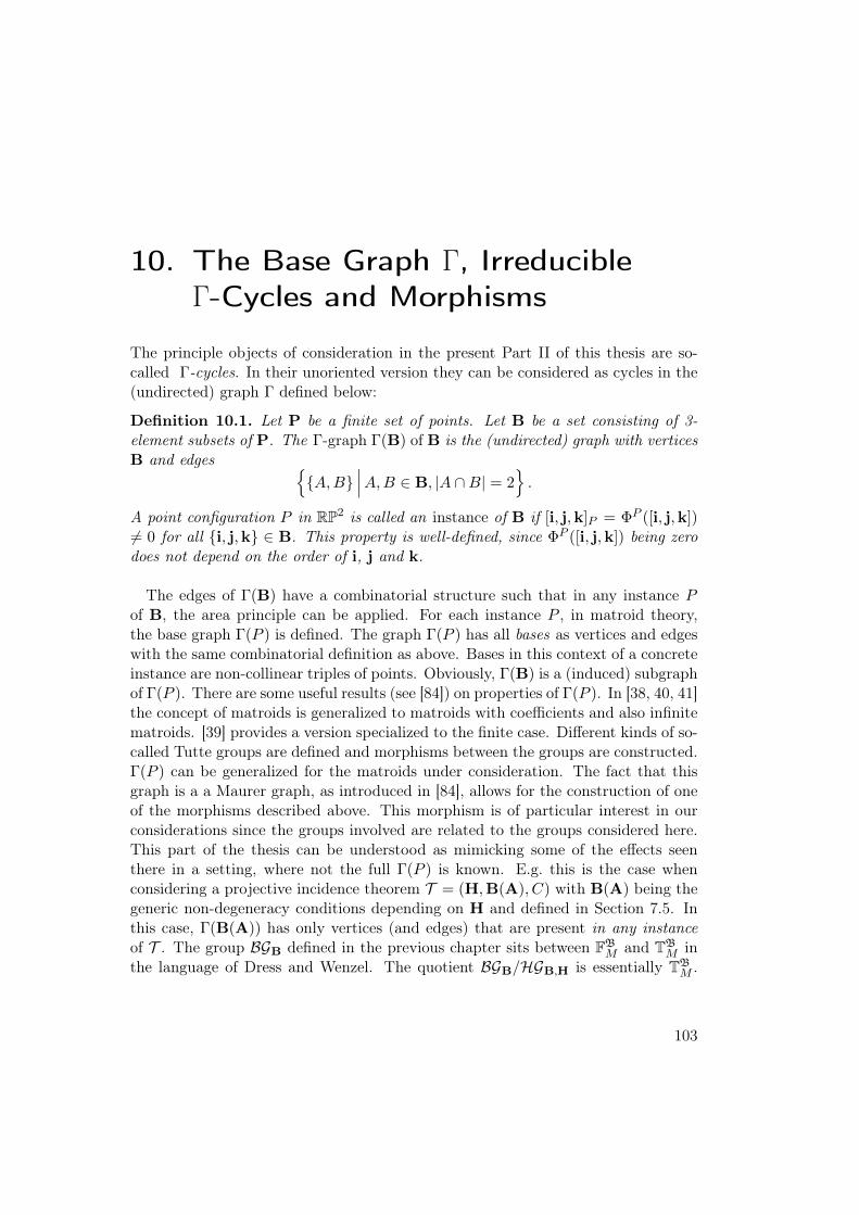
10. The Base Graph Γ, IrreducibleΓ-Cycles and Morphisms
The principle objects of consideration in the present Part II of this thesis are so-called Γ-cycles. In their unoriented version they can be considered as cycles in the(undirected) graph Γ defined below:
Definition 10.1. Let P be a finite set of points. Let B be a set consisting of 3-element subsets of P. The Γ-graph Γ(B) of B is the (undirected) graph with verticesB and edges
A,B∣∣∣A,B ∈ B, |A ∩B| = 2
.
A point configuration P in RP2 is called an instance of B if [i, j,k]P = ΦP ([i, j,k])6= 0 for all i, j,k ∈ B. This property is well-defined, since ΦP ([i, j,k]) being zerodoes not depend on the order of i, j and k.
The edges of Γ(B) have a combinatorial structure such that in any instance Pof B, the area principle can be applied. For each instance P , in matroid theory,the base graph Γ(P ) is defined. The graph Γ(P ) has all bases as vertices and edgeswith the same combinatorial definition as above. Bases in this context of a concreteinstance are non-collinear triples of points. Obviously, Γ(B) is a (induced) subgraphof Γ(P ). There are some useful results (see [84]) on properties of Γ(P ). In [38, 40, 41]the concept of matroids is generalized to matroids with coefficients and also infinitematroids. [39] provides a version specialized to the finite case. Different kinds of so-called Tutte groups are defined and morphisms between the groups are constructed.Γ(P ) can be generalized for the matroids under consideration. The fact that thisgraph is a a Maurer graph, as introduced in [84], allows for the construction of oneof the morphisms described above. This morphism is of particular interest in ourconsiderations since the groups involved are related to the groups considered here.This part of the thesis can be understood as mimicking some of the effects seenthere in a setting, where not the full Γ(P ) is known. E.g. this is the case whenconsidering a projective incidence theorem T = (H,B(A), C) with B(A) being thegeneric non-degeneracy conditions depending on H and defined in Section 7.5. Inthis case, Γ(B(A)) has only vertices (and edges) that are present in any instanceof T . The group BGB defined in the previous chapter sits between FB
M and TBM in
the language of Dress and Wenzel. The quotient BGB/HGB,H is essentially TBM .
103
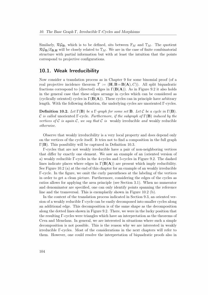
10. The Base Graph Γ, Irreducible Γ-Cycles and Morphisms
Similarly, RGB, which is to be defined, sits between FM and TM . The quotientRGB/EB,H will be closely related to TM . We are in the case of finite combinatorialstructure with partial information but with at least the intuition that the pointscorrespond to projective configurations.
10.1. Weak Irreducibility
Now consider a translation process as in Chapter 9 for some binomial proof (of areal projective incidence theorem T := (H,B=B(A), C)). All split biquadraticfractions correspond to (directed) edges in Γ(B(A)). As in Figure 9.2 it also holdsin the general case that these edges arrange in cycles which can be considered as(cyclically oriented) cycles in Γ(B(A)). These cycles can in principle have arbitrarylength. With the following definition, the underlying cycles are unoriented Γ-cycles.
Definition 10.2. Let Γ(B) be a Γ-graph for some set B. Let C be a cycle in Γ(B).C is called unoriented Γ-cycle. Furthermore, if the subgraph of Γ(B) induced by thevertices of C is again C, we say that C is weakly irreducible and weakly reducibleotherwise.
Observe that weakly irreducibility is a very local property and does depend onlyon the vertices of the cycle itself. It tries not to find a composition in the full graphΓ(B). This possibility will be captured in Definition 10.3.
Γ-cycles that are not weakly irreducible have a pair of non-neighboring verticesthat differ by exactly one element. We saw an example of an (oriented version ofa) weakly reducible Γ-cycles in the 4-cycles and 5-cycles in Figure 9.2. The dashedlines indicate places where edges in Γ(B(A)) are present which imply reducibility.See Figure 10.2 (a) at the end of this chapter for an example of an weakly irreducibleΓ-cycle. In the figure, we omit the curly parentheses at the labeling of the verticesin order to get a clean picture. Furthermore, considering the edges of the cycles asratios allows for applying the area principle (see Section 3.1). When no numeratorand denominator are specified, one can only identify points spanning the referenceline and the transversal. This is exemplarily shown in Figure 10.2 (b).In the context of the translation process indicated in Section 9.3, an oriented ver-
sion of a weakly reducible Γ-cycle can be easily decomposed into smaller cycles alongan additional edge. This decomposition is of the same shape as the decompositionalong the dotted lines shown in Figure 9.2. There, we were in the lucky position thatthe resulting Γ-cycles were triangles which have an interpretation as the theorems ofCeva and Menelaus. In general, we are interested in situations where such a simpledecomposition is not possible. This is the reason why we are interested in weaklyirreducible Γ-cycles. Most of the considerations in the next chapters will refer tothem. However, one could resolve the interpretation of biquadratic proofs also in
104

10.2. Oriented Γ-Cycles and Strong Irreducibility
different ways. These ways should be depicted now. Furthermore, a language fororiented Γ-cycle is developed.
10.2. Oriented Γ-Cycles and Strong Irreducibility
To model the considerations about split biquadratic fractions (as they were donein Section 9.3) in terms of directed edges in Γ(B), we define an algebraic structureRGB which has the directed edges of Γ(B) as elements. Furthermore, they vanishwhen they are traversed in opposite directions (see Definition 10.3). Clearly eachset of split biquadratic fractions can be considered to be an element of RGB. In thesame way, any cycle emerging from the translation process is an element of RGB.
Definition 10.3. Let P be a finite set of points. Let B be a set consisting of 3-element subsets of P. The group of bracket ratios compatible with the area principleRGB is defined to be the quotient of the multiplicatively written free abelian groupgenerated by the formal (unbreakable) symbols
A
B
∣∣∣ A,B is an edge in Γ(B)
∪
ε
and the subgroup generated byA
B· BA
∣∣∣ A,B is an edge in Γ(B)
∪ε2
.
Furthermore, any element−→C ∈ RGB that as an representation as
−→C =A1
A2· A2
A3· · · Ak−1
Ak· AkA1
is a called a k-cycle in RGB (for some k ∈ N) whenever(A1, A2, A2, A3, . . . ,
Ak, A1)is a Γ-cycle. It is weakly irreducible whenever
(A1, A2, A2, A3, . . . ,
Ak, A1)is weakly irreducible. It is also called (oriented) Γ-cycle of length k. It
is strongly irreducible whenever it is not contained in the subgroup of RGB that isgenerated by all k′-cycles where k′ < k. A point configuration P is called an instanceof−→C whenever it is an instance of B.
Clearly, whenever an oriented Γ-cycle is strongly irreducible, it is weakly irre-ducible. Within this setting, one could argue that one should focus on the stronglyirreducible k-cycles in RGB.
105

10. The Base Graph Γ, Irreducible Γ-Cycles and Morphisms
Remark 10.4. Observe that any element ofRGB can be given a representation whicheither contains ε once or does not contain ε. Ignoring ε, the rest of the element as the
shapeA1
A2· · · Ak−1
Akwhich can be drawn as a directed version of a subgraph of Γ(B)
where we also allow multiple edges. This yields a graphical representation of many
objects in RGB which is often quite helpful. The objectsA1
A2directly correspond
to edges and are sometimes called edges as well.
10.3. Decomposing Large Γ-cycles within BiquadraticProofs
Due to [84, 39], when the same definitions are done with underlying graph Γ(P )for an instance P instead of Γ(B), one can cut down the maximal k for which ak-cycle can be strongly irreducible to 3. For a general projective incidence theoremT = (H,B, C) specific informations about the shape of Γ(B) are out of reach,especially in the case that B has very few elements. Those cases can be easilyachieved by redefining B after a (binomial) proof and letting it consist of thoseelements that are needed for the proof. This may induce big strongly irreduciblecycles. The big ambiguity about the shape of B is another reason, different from theones given in Chapter 7.5, to restrict ourselves to the cases where B equals B(A).Even in the case that B = B(A), one does not have the property of Γ(B(A))
being a Maurer graph. So one cannot apply the same techniques as in the matroidalrealizable case in order to control the length of the cycles. It remains an open prob-lem whether for any incidence theorem T = (H,B(A), C), any biquadratic proofcan be transferred to a collection of 3-cycles in RGB(A). Observe that therefore,it would be allowed that not every splitting of biquadratic fractions may lead tooriented Γ-cycles that can be written as a product of 3-cycles. There has to beonly one splitting which allows for this. It remains also open the stronger problemwhether any k-cycle in RGB(A) can be written as a product of 3-cycles.We do know cycles where this is possible but this decomposition is not at all
easy. More precisely, there is a theorem (H,B(A), C) with a 4-cycle such that thedecomposition into 3-cycles that was obtained by solving a linear equation systemwith Mathematica ([136]) uses 54 triangles. Having this in mind, it could be muchmore convenient to have a better understanding of the underlying Γ-cycle than toactually carry out the decomposition into 54 triangles.There is also another way to deal with large cycles as introduced in [2]. Here
one adds two new generic points, say g and h, to the whole theorem. This allowsfor a decomposition of large cycles but also generates at least 3k − 2 new triangleswhen decomposing a k-cycle. Within a biquadratic proof, Γ-cycles do look not very
106

10.4. Some Subgroups Vanishing under Morphisms
complicated. In fact, this is also a benefit of the modeling of an incidence theorem by(H,B, C). It has the advantage that we do not have to distinguish between free anddependent points. For dependent points expressed in Grassmann-Cayley algebra, abracket may look much more complicated and will have more than one evaluation.Therefore, in a setup of Grassmann-Cayley algebra, the canceling of brackets used inbiquadratic proofs is less trivial. This cancellation process corresponds to Γ-cycles.
10.4. Some Subgroups Vanishing under Morphisms
In order to describe the relations between RGB and BGB, we consider the grouphomomorphism Φ : RGB → BGB induced by
ε 7→ ε andb,a, cd, c,a 7→
[b,a, c]
[d, c,a]
where colors only highlight the combinatorics of a given unbreakable symbol inRGB. Observe that the result indeed only depends on the combinatorics of theargument. The combinatorics are induced by the considerations done in Section 3.1.Furthermore, Φ is well-defined since it vanishes on the defining subgroup. Let
−→C =A1
A2· A2
A3· · · Ak−1
Ak· AkA1∈ RGB
be an oriented Γ-cycle. Apparently it holds that
Φ(−→C ) =
k∏
i=1
Φ
(Ai
Ai+1
)∈ ε, 1.
We define Φ(−→C ) to be the signature of
−→C . In order to determine the signature,one has to compare the orientations of canceling brackets in Φ(
−→C ). We will give aneasier way to read of the signature of weakly irreducible Γ-cycles later on. We willuse the structure introduced when counting them (see Section 12.2). By abuse ofnotation, we can assume Φ(
−→C ) to lie in RGB as well. This allows for defining ©B
to be the group generated by
Φ(−→C ) · −→C
∣∣∣−→C is oriented Γ-cycle
which impliesΦ(©B
)=
1.
107

10. The Base Graph Γ, Irreducible Γ-Cycles and Morphisms
Figure 10.2 (c) highlights the combinatorics which are given in the definition of Φfor each edge in the given example.
10.4.1. A Euclidean Interpretation of Oriented Γ-Cycles
Consider an instance P . We assume that all points have Euclidean interpretationsand all intersections defined in the following fit in Euclidean space given by thestandard embedding. We write non-bold letters for points in P corresponding tobold indices in P. For a, b, c and d ∈ P it holds:
ΦP
(b,a, cd, c,a
)=|b, a, c ||d, c, a|
where we use ΦP also to denote ΦP Φ since no confusion can arise. We apply thearea principle and it holds:
|b, a, c ||d, c, a| =
b p
p d(10.1)
where p := meet(join(b, d), join(a, c)).
Definition 10.5. Let−→C =
A1
A2· A2
A3· · · Ak−1
Ak· AkA1
be an oriented Γ-cycle. Let P
be an instance of−→C . Assume the last entries of the points in P equal 1 and applying
the area principle gives
ΦP
(Ai
Ai+1
)=
bi pi
pi di
for finite points pi (for 1 ≤ i ≤ k and indices considered modulo k). Due to (10.1),there is a induced Euclidean theorem stating that
k∏
i=1
bi pi
pi di= ΦP (
−→C ) ∈ −1,+1.
This Euclidean theorem is called a Γ-cycle theorem induced by−→C .
Figure 10.2 (d) gives an example of a Γ-cycle theorem. In fact, a Γ-cycle theoremis not trivial in Euclidean space.
Remark 10.6. There are two Γ-cycles of length 3. The Γ-cycle theorems induced bythem are exactly the theorems of Ceva and Menelaus.
108

10.4. Some Subgroups Vanishing under Morphisms
10.4.2. Including Collinearities
Let H a set of 3-element subsets of P such that B and H are disjoint. The groupof biquadratic fractions in area form ↑- - -
- - -↓B,H is the subgroup of RGB generated bya,b,xa,b,y ·
a, c,ya, c,x
∣∣∣∣∣ a,b, c ∈ H or a,x,y ∈ H
(10.2)
which impliesΦ(↑- - -
- - -↓B,H)⊂ HGB,H.
LetEB,H := 〈©B ∪ ↑- - -
- - -↓B,H〉.We say that P is an instance of of B and H if [i, j,k]P 6= 0 for all i, j,k ∈ B and[i, j,k]P = 0 for all i, j,k ∈ H. This implies together with Proposition 9.4 thatfor all instances P it holds that
ΦP (EB,H) = 1.
Remark 10.7. Observe that the graphical version of the elements generating ↑- - -- - -↓B,H
(see (10.2)) looks like Figure 10.1. The dashed lines indicate places where there isan edge in Γ(B). This explains the name of the group ↑- - -
- - -↓B,H. Observe thatmultiplying an oriented 4-cycle yields the other splitting of the biquadratic fraction.Observe furthermore that in the left edge, the transversal is given by a and b and in
Figure 10.1.: Graphical version of a biquadratic fraction in area form.
the right edge it is given by a and c. It might be the case, that H implies that thetransversal can be also spanned by some other points. If one wants to express thisfact in EB,H, one can alter the points spanning the transversal step by step givinga graphical picture as ↑- - -
- - -↓↑- - -- - -↓ ··· ↑- - -
- - -↓ (see also Figure 12.3 for an example).
109

10. The Base Graph Γ, Irreducible Γ-Cycles and Morphisms
Slight modifications of [39] as well as [2] imply that each biquadratic proof hasa preimage under Φ that lies in EB,H. The formulation in terms of EB,H can beconsidered easier since one has better (geometric) control of the cancellation process.This control is gained via the interpretation as oriented length ratios and the Γ-cycle theorems. In particular, it is easier to construct new theorems within thistheory because cancellation can be easily achieved. These theorems can be theoremsabout oriented length ratios or incidence theorems (along with a biquadratic proof).We will present examples for both cases in Chapter 12 and Chapter 13. Bothcases can be regarded as giving a specific representation of an element of EB,H byits defining elements. The overall product can again be interpreted geometricallyresulting in a derived geometric fact. The approach can be understood as startingwith cancellation patterns (or with Γ-cycles) and imposing incidence constraints(requiring H to contain some elements such that some elements in ↑- - -
- - -↓B,H arepresent). The geometric control that one achieves is also a reason for the Cayleyfactorization to work (see Part III).
110

10.4. Some Subgroups Vanishing under Morphisms
(a) (b)
(c) (d)
∏ lengthlength
= 1
Figure 10.2.: A weakly irreducible Γ-cycle in an unoriented and in an oriented ver-sion together with the corresponding Γ-cycle theorem.
111


11. Counting (Weakly) IrreducibleΓ-Cycles
Suppose C = (A1, A2, A2, A3, . . . , Ak, A1) is a weakly irreducible unorientedΓ-cycle. From now on, we will drop the word “weakly”, since we will not considerstrong irreducibility any longer. The following is joint work with Jürgen Richter-Gebert who invented the table representation of (irreducible) Γ-cycles as shown e.g.in Figure 11.1 (e) and in many other diagrams. In order to structure and enumeratethem he made the assumptions given in the following section. By enumeratingand investigating all irreducible cycles of fixed length up to 9 he suggested thesubscheme depicted in Figure 11.3. The formulation in his enumeration was via thepermutation σ which will be used in Section 12.2.
11.1. Assumptions on the Irreducible Γ-Cycles
We will w.l.o.g. require that P =⋃ki=1 Ai and that C has connected entries, i.e.
that for each p ∈ P, the subgraph of C induced by the vertices Vp containing p
Vp =Ai∣∣p ∈ A, i ∈ 1, . . . , k
is connected. For a Γ-cycle not meeting this requirement for some p, the entry p canbe given a new name in each connected component. This maintains the property ofbeing a Γ-cycle as well as the irreducibility.The aim of this Chapter is to give a reasonable counting of irreducible Γ-cycles of
fixed length k. Figure 11.5 and 11.6 at the end of the chapter show a resulting listingof irreducible Γ-cycles of length 7 and 8. They use a table representation which isto be defined in the following section. In order to avoid case distinctions, from nowon, we will assume that k ≥ 4. Furthermore, some Γ-cycles have to be consideredidentical, e.g. Γ-cycles that differ only by labeling the entries of the vertices. Theseassumptions also imply that there is exactly one irreducible Γ-cycle where Va coversall vertices of C for some a ∈ P:
(a,b1,b2, a,b2,b3, a,b3,b4, . . . , a,bk−1,bk, a,bk,b1
). (11.1)
In order to count the remaining irreducible Γ-cycles we temporally exclude this cyclefrom the following considerations and each Vp induces a path in C.
113

11. Counting (Weakly) Irreducible Γ-Cycles
11.2. Table Representations of Irreducible Γ-Cycles
We chose an orientation−→C for C: Let
−→C =A1
A2· A2
A3· · · Ak−1
Ak· AkA1
.
As in the definition of Φ we identify blue-grey, blue-violet and orange entries foreach edge (see Figure 11.1 (c) whithin is a continuation and partial restatement ofFigure 10.2 ). Each end of a path induced by Vp corresponds to a blue-violet orto a orange coloring of p. Since this is true for any p in P, each element of P iscolored in orange exactly once. This implies that P has exactly k different entries.Furthermore, we can identify the vertices A1, A2, . . . , Ak with its orange labeling(highlighted with grey circles in Figure 11.1(c)). With this identification, the con-secutive sequence of vertices vertices A1, A2, . . . , Ak of
−→C induces a linear order onthe elements of P. We will use the notion ±l to indicate steps of size l (l ∈ N) inthe cyclically closed linear order of P. It is used to produce a table representation ofthe oriented Γ-cycle
−→C . This representation is in essence an incidence matrix (seealso Figure 11.1 (e): we label both rows and columns by the elements of P in thegiven order. The labels of the columns are considered as vertex labels. We drawa dot at position (p,q) whenever p is contained in the defining set of the vertexwhich is labeled with q. The black lines indicate the paths induced by the Vps.
(c) (e)[3, 1, 1, 2]
position
entr
y
Figure 11.1.: Continuation of Figure 10.2 giving a table representation of the Γ-cycleunder consideration.
114

11.2. Table Representations of Irreducible Γ-Cycles
One can read of the oriented Γ-cycle from the diagram: each column is a vertexand its entries are indicated by dots. Clearly any oriented Γ-cycle can be given atable representation. In Figure 11.1 (e), there is an additional coloring of some dots.The coloring indicates for each column, which entries are colored in blue-violet ororange at the corresponding vertex in the diagram (c). The sequence of numbersgiven there is detailedly explained below. A rough description is as follows: in thefirst line, there are 2+3 dots in the second line there are 2+0 dots, and so on. Thisinduces a sequence [3, 0, 0, 1, 1, 2, 0]. Omitting the 0s gives the sequence depicted inFigure 11.1 (e). The omission is possible since we will see in Figure 11.3 that e.g.the second and the third line are induced by the first one. On the other hand, therestrictions for a table to represent a (not necessarily irreducible) oriented Γ-cycleof length k can be easily expressed (compare Definition 10.2 and 10.1):
• Each column has to contain three dots and therefore the table has to contain3 k dots.
• For two neighboring columns, there have to be precisely two rows in which bothcolumns contain a dot. Here neighboring also includes a cyclic neighboring,i.e. the first and the last column are considered as neighbors as well.
Taking into account also the specific labeling of the vertices we chose for our re-stricted class of irreducible oriented Γ-cycles, we need to require also:
• In diagonal of the table, dots are drawn, but not in the positions (p,p − 1)for all p ∈ P.
We will argue:
• For all p ∈ P there is a dot at position (p,p + 1).
In order to see this, suppose the contrary: suppose there is a p ∈ P such that thereis no dot in position (p,p− 1) and (p,p + 1). Since column p has to have two dotsin common with both vertices p− 1 and p + 1 and non of these entries can be p byassumption, vertices p − 1 and p + 1 must have the same entries, say a and b incommon with vertex p. Therefore, vertices p− 1 and p + 1 both consist of a and bplus another entry and they differ by exactly one element. This is a contradictionto the assumption that
−→C is irreducible.All previous assumptions imply that 2 k of the 3 k dots of a Γ-cycle of length k are
already fixed. Therefore, each table representation corresponding to an irreducibleoriented Γ-cycle contains the dots indicated in Figure 11.2. Since the Vps induceconnected components, the entries of row p have to be given by the column indices
p, p + 1, p + 2, . . . , p + l + 1
115

11. Counting (Weakly) Irreducible Γ-Cycles
Figure 11.2.: Common subscheme of all table representations of irreducible Γ-cycles.
for some l depending on p and with 0 ≤ l ≤ k − 3. Visually speaking, this meansthat in Figure 11.2 the black lines have to be extended to the right.Since we have only fixed 2 k positions of dots, there has to be a row p in which
the corresponding l is strictly positive. Since−→C is a cycle, we can w.l.o.g. assume
that p is the first element in P with respect to its induced order. Therefore, thethe first row of the table corresponds to the first row in Figure 11.3.Now consider some q within the range of p + 1 to p + l− 1. Due to our previous
considerations, there have to be dots at positions (q,q) and (q,q+1). There cannotbe more dots in this row since this would imply a dot at position (q,q + 2). Thisin not possible since in column q + 2 there are already three dots in rows p, q + 1and q + 2.Furthermore, there has to be a dot at position (p + l,p + l+ 2): column p + l+ 1
as to have two entries in common with column p + l + 2. Since there is no dot atposition (p,p + l + 2) and at position (p + l + 1,p + l) it has to be at position(p + l,p + l + 2). Now one can restart the game with entry p + l in the place ofp. This implies that the whole table is composed of building blocks as given inFigure 11.3 and there is a sequence [l1, l2, . . . , lt] of positive numbers that uniquelydetermines
−→C . Since Figure 11.2 fixes 2 k of the overall 3 k dots, we have
t∑
i=1
li = k.
Therefore, [l1, . . . , lt] is a composition of n. Any cyclic shift, e.g. [l2, . . . , lt, l1], ofthe ls will also represent
−→C . So in fact,−→C corresponds to a cyclic composition of
k.
116

11.3. Counting Irreducible Γ-Cycles
Figure 11.3.: l dots added to Figure 11.2 in row p determine all other black dots inrows p + 1 up to p + l+ 1 as well as a dot at position (p + l,p + l+ 2).
We summarize:Each irreducible (oriented) Γ-cycle of length k (with the restrictions done in Sec-tion 11.1 ) corresponds to a cyclic composition of k.
11.3. Counting Irreducible Γ-Cycles
A first step in the direction of counting irreducible Γ-cycles of length k is to givethe number of cyclic compositions of k. It is included in the On-Line Encyclopediaof Integer Sequences (OEIS) (as sequence number A008965, see [87]) and a formulais given by
number of cyclic compositions of k =1
k
∑
d|kϕ(d)2
kd − 1
where ϕ is Euler’s phi function and d|k means that d divides k. In the OEIS there isgiven another suitable interpretation of this number: it is the number of necklaceswhere the beads themselves are sets of beads with total number of beads being k.Turning over of the necklace is not allowed. This fits with the action of adding dots
117

11. Counting (Weakly) Irreducible Γ-Cycles
to a table as in Figure 11.2 in the allowed way, i.e. locally generating patterns as inFigure 11.3. For future reference we illustrate the connection to number sequencenumber A000031 (see [88]) in the OEIS: It gives the number of k-bead necklaceswith 2 colors when turning over is not allowed. Sequence A008965 is essentiallysequence A000031 with an offset of −1. The connection between 2-colored neck-laces and cyclic compositions is just an extension of the standard bijection between(ordinary) compositions of the number k and the k − 1 bit binary numbers to thecyclic case.
In order to count irreducible oriented Γ-cycles we analyze which cyclic composi-tions encode irreducible oriented Γ-cycles. There are exactly four cyclic composi-tions that obviously cannot encode irreducible Γ-cycles since their entries are biggerthan k − 3. They are:
[k], [k − 1], [k − 2, 2], [k − 2, 1, 1].
All remaining cyclic compositions do encode (not necessarily irreducible) Γ-cycles:a table representation of a given cyclic composition can be derived by transferringthe first entry of the composition to the first part of the table representation asshown in Figure 11.3. Afterwards, one can do a cyclic shift of the table and of thecomposition a fill the whole table with dots. Now each column contains three dotsand neighboring columns share exactly two dots: due to the translation procedure,it suffices to check this property locally in Figure 11.3. Since it holds true there,each of the remaining cyclic compositions does encode a Γ-cycle. Due to our pre-vious considerations, it remains to identify those cyclic compositions that do notcorrespond to irreducible Γ-cycles in order to find all irreducible Γ-cycles (fulfillingthe requirements stated in Section 11.1).
Assume that there is a cyclic composition such that the induced Γ-cycle has twovertices V andW that are not neighbored in the cycle but nevertheless have exactlytwo elements p and q in common. Since V and W have at least distance 2 (in thecycle) and since p and q are in both columns belonging to V and W and since pand q are connected entries, both p and q have to belong to at least three vertices.Therefore, p and q locally look like the first row in Figure 11.3 and the number ofvertices containing p and q determined by adding 2 to an entry of the composition.Let l be the entry corresponding to p in the composition and consider the localsituation shown in Figure 11.3. The columns indexed by p + 2 up to p + l − 1already contain three dots and none of them can be q since q has to be containedin at least three vertices. Therefore, w.l.o.g. V is the vertex belonging to column por p + 1 and W belongs to column p + l or p + l + 1. In any case, q has to be incolumn p + l or p + l + 1 which by our labeling convention of the columns implies
118
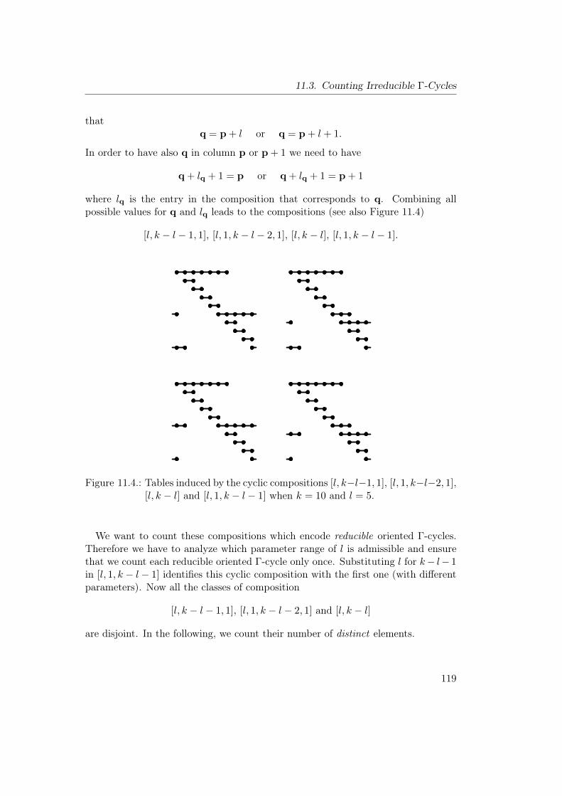
11.3. Counting Irreducible Γ-Cycles
thatq = p + l or q = p + l + 1.
In order to have also q in column p or p + 1 we need to have
q + lq + 1 = p or q + lq + 1 = p + 1
where lq is the entry in the composition that corresponds to q. Combining allpossible values for q and lq leads to the compositions (see also Figure 11.4)
[l, k − l − 1, 1], [l, 1, k − l − 2, 1], [l, k − l], [l, 1, k − l − 1].
Figure 11.4.: Tables induced by the cyclic compositions [l, k−l−1, 1], [l, 1, k−l−2, 1],[l, k − l] and [l, 1, k − l − 1] when k = 10 and l = 5.
We want to count these compositions which encode reducible oriented Γ-cycles.Therefore we have to analyze which parameter range of l is admissible and ensurethat we count each reducible oriented Γ-cycle only once. Substituting l for k− l− 1in [l, 1, k − l − 1] identifies this cyclic composition with the first one (with differentparameters). Now all the classes of composition
[l, k − l − 1, 1], [l, 1, k − l − 2, 1] and [l, k − l]
are disjoint. In the following, we count their number of distinct elements.
119

11. Counting (Weakly) Irreducible Γ-Cycles
Number of [ l, k − l − 1, 1 ]-Type Cyclic CompositionsWe have to ensure that 1 ≤ l ≤ k− 3 and 1 ≤ k− l− 1 ≤ k− 3. This equivalent to2 ≤ l ≤ k − 3. In these case we neither have l = 1 nor k − l − 1 = 1. So each l inthe given range gives a different cyclic composition. Their number is
k − 4.
Number of [ l, k − l ]-Type Cyclic CompositionsWe have to ensure that 1 ≤ l ≤ k − 3 and 1 ≤ k − l ≤ n − 3. This equivalent to3 ≤ l ≤ k − 3. We count the lexicographically maximal representatives, which arethe ones with l ≥ k − l. In total there are
k − 3−⌈k
2
⌉+ 1 =
⌊k
2
⌋− 2
different cyclic compositions of this type.
Number of [ l, 1, k − l − 2, 1 ]-Type Cyclic CompositionsWe have to ensure that 1 ≤ l ≤ k−3 and 1 ≤ k− l−2 ≤ k−3. The second equationis redundant. We count the lexicographically maximal representatives, which arethe ones with l ≥ k − l − 2. In total there are
k − 3−⌈k − 2
2
⌉+ 1 =
⌊k
2
⌋− 1
different cyclic compositions of this type.
Theorem 11.1. Up to relabeling, the total number of weakly irreducible orientedΓ-cycles with connected entries of length k (with k ≥ 3) is
1
k
∑
d|kϕ(d)2
kd − k − 2
⌊k
2
⌋+ 3.
Proof. The proof for k = 3 can be done by hand. For k ≥ 4 we have:
1
k
∑
d|kϕ(d)2
kd − k − 2
⌊k
2
⌋+ 3 =
1
︸︷︷︸cycle as in (11.1)
+1
k
∑
d|kϕ(d)2
kd − 1
︸ ︷︷ ︸cyclic comp.s
− 4
︸︷︷︸[k], [k−1], [k−2,2], [k−2,1,1]
120

11.3. Counting Irreducible Γ-Cycles
− (k − 4)︸ ︷︷ ︸
[ l, k−l−1, 1 ]-type cyclic comp.s
− (
⌊k
2
⌋− 2)
︸ ︷︷ ︸[ l, k−l ]-type cyclic comp.s
− (
⌊k
2
⌋− 1)
︸ ︷︷ ︸[ l, 1, k−l−2, 1 ]-type cyclic comp.s
Corollary 11.2. Up to relabeling, the total number of unoriented irreducible Γ-cycles of length k (with k ≥ 3) with connected entries is
1
2k
∑
d|kϕ(d)2
kd − k − 2
⌊k
2
⌋+ 3 +
2k−1
2 if k is odd3 · 2 k2−2 if k is even.
Proof. The case for k = 3 can be checked by hand. Now assume k ≥ 4. Anyunoriented Γ-cycle can be oriented arbitrarily and in the case that there is no p ∈ Psuch that Vp = P, this induces a cyclic composition [l1, . . . , lt]. It is not hard tosee that the other orientation of the same cycle results in the cyclic composition[lt, . . . , l1]. Furthermore, the number of 2-colored necklaces where turning over isallowed, is A000029 in the OEIS. Its formula is given by
1
2k
∑
d|kϕ(d)2
kd +
2k−1
2 if k is odd3 · 2 k2−2 if k is even.
By another extension of the standard bijection between (ordinary) compositionsof the number k and the k − 1 bit binary numbers we see that, with an offset of−1, sequence A000029 corresponds to the cyclic compositions where reversing theorientation is allowed. One can also check by hand, that all cyclic compositions thathad to be excluded in the oriented case give distinct compositions also in the casethat turning over is allowed.
121

11. Counting (Weakly) Irreducible Γ-Cycles
Figure 11.5.: Table representations of the nine irreducible oriented Γ-cycle of length7 that are not induced by (11.1).
122

11.3. Counting Irreducible Γ-Cycles
Figure 11.6.: Table representations of the 21 irreducible oriented Γ-cycle of length8 that are not induced by (11.1).
123


12. Glueing Γ-Cycles along TheirOrbits
12.1. An Example
As already mentioned at the end of Section 10.4.2, Γ-cycles might be more interest-ing if the entries are considered as dependent points instead of free points. In orderto do concrete constructions using a given (oriented) Γ-cycle
−→C one wants to haveinformation about the length ratios, i.e. about the shape of the Γ-cycle theoremassociated with
−→C . In the context of binomial proofs, this can be easily seen: Hereedges of Γ-cycles can be glued together only if they can be interpreted as a lengthratio along the same edge. One can also go the other way round: one can start witha Γ-cycle and impose further incidence relations on the points. This may simplifythe statement of the corresponding Γ-cycle theorem in such a way, that an addi-tional incidence relation can be concluded. In this case, one has generated a newincidence theorem. We show the procedure in more detail in an example. Considerthe irreducible oriented Γ-cycle associated with the cyclic composition [3, 1, 1, 2]which is illustrated in Figure 10.2 (c) and in Figure 11.1 (c). In the Γ-cycle theoremassociated to it and illustrated in Figure 10.2 (d), the length ratios are arrangedin two disjoint cycles called orbits (see also Section 12.2). We use this terminologysince the word “cycle” is already in use. In fact, in Part III, a similar structure willbe called “cycle” since no confusion can arise and since there, it is closely relatedwith cycles in a graph theoretic sense.
In an instance as in Figure 10.2 (d), the corresponding Γ-cycle theorem can beread as
g p1
p1 b· b p2
p2 d· d p3
p3 g· f q1
q1 c· c q2
q2 e· e q3
q3 a· a q4
q4 f= 1,
where the labeling of Figure 12.2 gives definitions for the newly introduced points.Imposing a Ceva configuration on the orbit of length three as shown in Figure 12.2
125

12. Glueing Γ-Cycles along Their Orbits
ensures that
g p1
p1 b· b p2
p2 d· d p3
p3 g·
︸ ︷︷ ︸=1
f q1
q1 c· c q2
q2 e· e q3
q3 a· a q4
q4 f= 1. (12.1)
Therefore, the other orbit on its own yields 1 in the product. A multi-ratio is aproduct
∏
i
ai xi
xi ai+1
(12.2)
where the indices are considered cyclically and ai, xi can be considered to be Eu-clidean and such that xi is on the line spanned by and distinct from ai and ai+1.A multi-ratio equaling 1 is in non-degenerate situations equivalent to the factthat a triangulation with Ceva and Menelaus triangles (such that the number ofMenelaus triangles is even) is possible. For the triangulation we assume that itis compatible with all points of intersection, i.e. when multiplying all theoremscorresponding to the Ceva and Menelaus triangles, all ratios except for the onesin (12.2) cancel. For an example, see Figure 12.1. We proceed by demonstrat-
Figure 12.1.: The possibility of triangulating with Ceva and Menelaus configurationsis a necessary and sufficient condition for the multi-ratio being 1 (in anon-degenerate instance).
126

12.1. An Example
ing this equivalence in the example of the remaining 4-orbit in (12.1). We definez := meet(join(a, c), join(q2, q3)). This imposes a Menelaus configuration on thetriangle with vertices a, e and c. Multiplying the resulting identity
a q3
q3 e· e q2
q2 c· c z
z a= −1
with (12.1) yieldsf q1
q1 c· a q4
q4 f· c z
z a= −1.
This equation implies the existence of a Menelaus line and therefore z, q1 and q4
have to be collinear. With this construction, we were able to derive an incidencetheorem on 16 points very easily (see Figure 12.2).
What we just saw was a Euclidean reasoning for an incidence theorem also holdingin projective geometry. Via the area principle, this reasoning can be done via(formal) determinants yielding a more projective reasoning. It can be summarizedwith Figure 12.3 (where we again omit the curly parentheses at the labeling of thevertices in order to get a clean picture). Black arrows indicate elements of ↑- - -
- - -↓B,Hand each set of non-black arrows, which have the same color, corresponds to anelement in ©B. The Γ-cycle we started with is highlighted in blue. The orbits ofthis cycle can be associated with the length ratio colored in green and in shades ofred. However, the graphical version is not enough to see the membership in EB,Hsince one has to also reason about the signature. Multiplying all indicated elementsof ↑- - -
- - -↓B,H and all cycles together with their signatures yields an element in EB,H.In fact, in this example, only the cycles colored in shades of red have signature ε.Due to the signatures determined, the overall product
a,q1,q4c,q1,q4
· c,q2,q3a,q2,q3
is proven to be an element of EB,H. Therefore, for any instance P (and non-boldletters for the corresponding points in the instance) we have
ΦP
(a,q1,q4c,q1,q4
· c,q2,q3a,q2,q3
)=|a, q1, q4||c, q4, q1|
· |c, q2, q3||a, q3, q2|
= 1
which implies the concurrence of the lines join(a, c), join(q1, q4) and join(q2, q3).
This procedure can be generalized to other oriented Γ-cycles−→C . First assume
that all orbits have length ≥ 3. Here one has to impose incidence relations suchthat all but one orbit are triangulated with Ceva and Menelaus triangles. Then the
127

12. Glueing Γ-Cycles along Their Orbits
Figure 12.2.: Imposing incidence constraints to the Γ-cycle theorem given in Fig-ure 10.2 results in the incidence theorem stating that the three redlines are concurrent.
128

12.1. An Example
Figure 12.3.: The graphical version of an element of EB,H. The corresponding el-ement of EB,H yields a proof for the incidence theorem given in Fig-ure 12.2.
129

12. Glueing Γ-Cycles along Their Orbits
last orbit can be triangulated with Ceva and Menelaus triangles as well as long asthe parity of the total number of Menelaus triangles matches the signature of
−→C .For orbits of length two, the condition, that there exists a triangulation, should bereplaced by the fact that the length ratios along both edges of the orbit are identical.Certainly, this construction may not be possible in any case, since degenerate
situations may occur when imposing incidence relations. However, it works in manycases. During this process, there are two steps that are independent of the degen-erate situations.
• One needs to know the signature of−→C .
• One needs to know the number, length and shape of the orbits of−→C .
We will show how these informations can be easily obtained from encodings of theΓ-cycle in question. Observe that in [2], it is pointed out that glueing the threeorbits of length two of the cycle given by the cyclic composition [1, 1, 1, 1, 1, 1],yields Pappos’s theorem.
Remark 12.1. Observe that this construction can be generalized in different direc-tions: first, one can close the orbits not only by triangulating them but also by usingagain more general Γ-cycles. We are not restricted to irreducible Γ-cycle. We canuse reducible cycles for closing the orbits and also as a starting point. Of course,we can obtain all reducible Γ-cycles by combining irreducible ones. The larger theorbits of the original cycle, the larger are the straightforward possibilities to closethe cycles using irreducible and reducible Γ-cycles. In any cases, informations aboutsignature and orbits are needed.
12.2. Edges of Γ-Cycles and Informations about Orbits
In order to address the problems of signature and orbits, we consider edges in agiven irreducible oriented Γ-cycle
−→C together with its table representation. Assumethat for all p ∈ P we have Vp 6= P. For an example see Figure 12.4 which isa continuation of Figure 10.2 and Figure 11.1. To identify the endpoints of thelength ratio of an edge (p,p + 1) (where p and p + 1 are considered to be vertexnames), one takes the blue-violet dot from the column labeled p and the orangedot from the column labeled p + 1. Due to the labeling conventions, the orange dotis in position (p + 1,p + 1). For each p ∈ P we define σ(p) such that the dot inposition
(p, σ(p)
)is colored in blue-violet. For considerations similar to the ones
done in Section 11.2, σ is a permutation. For each p ∈ P, the edge (σ(p), σ(p) + 1)induces an length ratio whose blue-violet endpoint is p and whose orange endpointis σ(p) + 1. Therefore, the endpoints of all length ratios are given by the pairs
(p, σ(p) + 1).
130

12.2. Edges of Γ-Cycles and Informations about Orbits
The length ratios arrange in orbits. The structure of these orbits can now be definedon a combinatorial level as the cycles of the permutation σ(p) + 1. They can bevisualized quite well also in the table representation of an irreducible oriented Γ-cycleas it is done in Figure 12.4. For glueing Γ-cycles Theorem 12.2 and Theorem 12.3might be interesting.
(f)
f
a
g
b
d
c
e
(g)
Figure 12.4.: Continuation of Figure 10.2 and Figure 11.1: illustration of the com-binatorics of the orbits.
Figure 12.5.: Figure 11.5 with additional information about orbits and its lengths.
131
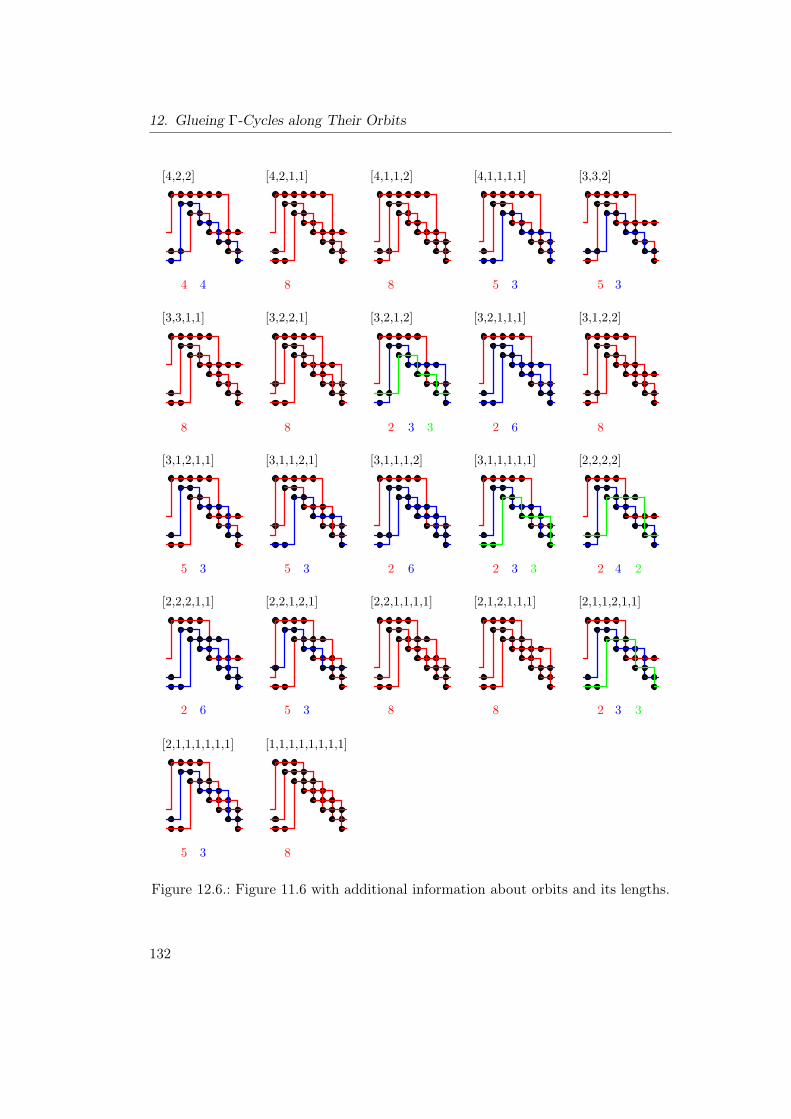
12. Glueing Γ-Cycles along Their Orbits
Figure 12.6.: Figure 11.6 with additional information about orbits and its lengths.
132
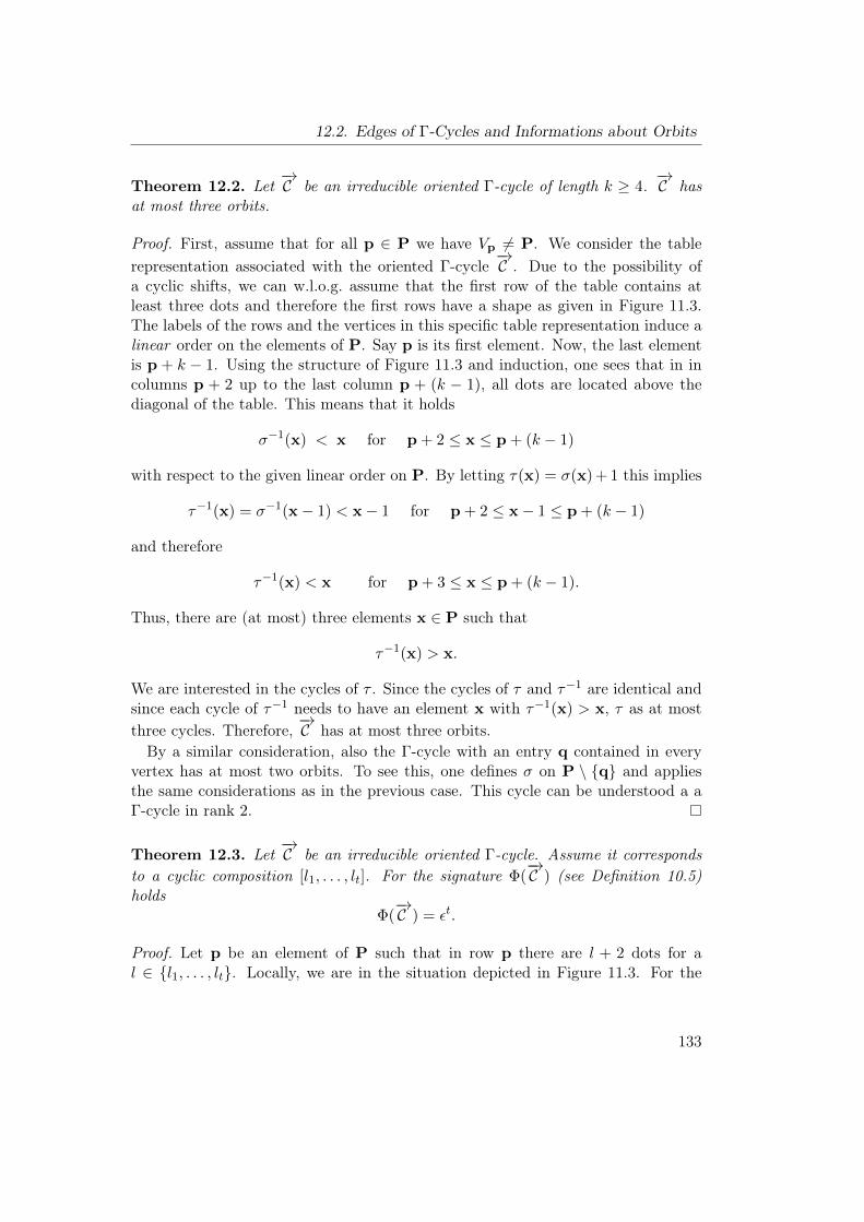
12.2. Edges of Γ-Cycles and Informations about Orbits
Theorem 12.2. Let−→C be an irreducible oriented Γ-cycle of length k ≥ 4.
−→C hasat most three orbits.
Proof. First, assume that for all p ∈ P we have Vp 6= P. We consider the tablerepresentation associated with the oriented Γ-cycle
−→C . Due to the possibility ofa cyclic shifts, we can w.l.o.g. assume that the first row of the table contains atleast three dots and therefore the first rows have a shape as given in Figure 11.3.The labels of the rows and the vertices in this specific table representation induce alinear order on the elements of P. Say p is its first element. Now, the last elementis p + k − 1. Using the structure of Figure 11.3 and induction, one sees that in incolumns p + 2 up to the last column p + (k − 1), all dots are located above thediagonal of the table. This means that it holds
σ−1(x) < x for p + 2 ≤ x ≤ p + (k − 1)
with respect to the given linear order on P. By letting τ(x) = σ(x) + 1 this implies
τ−1(x) = σ−1(x− 1) < x− 1 for p + 2 ≤ x− 1 ≤ p + (k − 1)
and therefore
τ−1(x) < x for p + 3 ≤ x ≤ p + (k − 1).
Thus, there are (at most) three elements x ∈ P such that
τ−1(x) > x.
We are interested in the cycles of τ . Since the cycles of τ and τ−1 are identical andsince each cycle of τ−1 needs to have an element x with τ−1(x) > x, τ as at mostthree cycles. Therefore,
−→C has at most three orbits.By a similar consideration, also the Γ-cycle with an entry q contained in every
vertex has at most two orbits. To see this, one defines σ on P \ q and appliesthe same considerations as in the previous case. This cycle can be understood a aΓ-cycle in rank 2.
Theorem 12.3. Let−→C be an irreducible oriented Γ-cycle. Assume it corresponds
to a cyclic composition [l1, . . . , lt]. For the signature Φ(−→C ) (see Definition 10.5)
holdsΦ(−→C ) = εt.
Proof. Let p be an element of P such that in row p there are l + 2 dots for al ∈ l1, . . . , lt. Locally, we are in the situation depicted in Figure 11.3. For the
133

12. Glueing Γ-Cycles along Their Orbits
edge (p + 1,p + 2) we have
Φ
(p + 1
p + 2
)= Φ
(x,p,p + 1p + 2,p,p + 1
)= ε · [p,p+1, x]
[p,p+1,p+2]
for some x ∈ P. For the edges (p + i,p + i+ 1) (2 ≤ i ≤ l) we have:
Φ
(p + i
p + i+ 1
)= Φ
(p + i− 1,p,p + ip + i+ 1,p,p + i
)=
[p,p+i− 1, p+i]
[p,p+i,p + i+ 1].
Since the edge (p + l,p + l + 1) is edge (q,q + 1) for q = p + l, we can restate thewhole game with q in the role of p. We obtain:
k−1∏
j=0
Φ
(p + j
p + j + 1
)=
t∏
r=1
ε · [pr,pr+1, xr]
[pr,pr+1,pr+2]·∏
2≤i≤lr
[pr,pr+i− 1, pr+i]
[pr,pr+i,pr + i+ 1]
where each pr corresponds to lr (1 ≤ r ≤ t). Since all determinants are positivelyoriented with respect to the given cyclic order of P they cancel and
k−1∏
j=0
Φ
(p + j
p + j + 1
)= εt
proves the statement.
134

13. Relations between Γ-Cycles andResults of Grünbaum andShephard
As previously mentioned in Section 3.1, the usage of the area method as used hereis taken from Grünbaum and Shephard [53, 52, 54]. Earlier use of the area andthe volume principle was also treated in Section 3.1. In [53] a special kind oftheorems about oriented length ratios is investigated: the cyclically ordered vertices(v1, . . . , vk) of a k-gon in the affine plane are considered. The authors want toassign (oriented) length ratios to edges or diagonals in a cyclic way and in sucha fashion that the product of the ratios equals +1 or −1. This means cyclicallyputting Figure 3.2 on the edges or diagonals of the polygon. The transversal issupposed to be spanned by vertices of the k-gon. The formulation of Theorem 3 in[53] summarizes this. It investigates when one can define and assure that
k∏
i=1
viwi
wi vi+j= (−1)k (13.1)
(indices considered modulo k) for suitable values of j, r and s and with wi beingthe intersection of the line spanned by vi and vi+j and the line spanned by vi+r andvi+s. Hence, all points of Figure 3.2 are shifted cyclically in the k-gon. In orderto get a better impression, we give an examples in Figure 13.1). In the proof ofthe theorem, it is shown, that there is always an underlying [1, . . . , 1]-cycle (or astatement involving trivially pairwise canceling length ratios). The different casesin the original formulation of the theorem correspond to different cyclic labelingsof the points in the same given Γ-cycle. We think that this restriction to perfectlycyclic products of k factors is very strict. At this point, we want to compare thiswith Γ-cycle theorems in Definition 10.5. They also give theorems about productsof k oriented length ratios. In principle, they can be quite asymmetric as the oneshown in Figure 10.2. However, there are Γ-cycle theorems that are cyclic butwith period bigger than 1. See Figure 13.2 for Γ-cycle theorems corresponding tothe cyclic compositions [3, 3, 3, 3] (one orbit) and [3, 1, 3, 1, 3, 1] (three symmetricorbits). The vertices are arranged in a regular manner in order to emphasize thesymmetry. Clearly, the theorems are valid for all positions of the vertices except for
135

13. Relations between Γ-Cycles and Results of Grünbaum and Shephard
Figure 13.1.: With k = 5, j = 4, r = 1 and s = 3, (13.1) holds. By applying thepermutation that is given by the cycle (5, 3, 2, 4) to the indices, this isidentical to a figure given in [53]. There, the case k = 5, j = 2, r = 3and s = 4 is considered.
degenerate situations. Figure 13.2 should be read as follows: blue-violet and orangeline segments supported by the same line form oriented length ratios. The product
∏ lengthlength
(13.2)
equals +1 or −1 depending on the signature of the underlying Γ-cycle. Due toTheorem 12.3, the product of length ratios given in (13.2) equals 1 in both cases ofFigure 13.2.
Including Reasonable Dependent PointsBased on the structure of [3, 1, 3, 1, 3, 1], one can also construct theorems aboutoriented length ratios including depending points as shown in Figure 13.3. It wasachieved by a procedure which can also be described more generality: we replaceeach edge
a,x,yb,x,y
of an irreducible oriented Γ-cycle−→C , which corresponds to a cyclic composition, by
the product of two edgesa,x,yw,x,y ·
w,x,yb,x,y (13.3)
136

Figure 13.2.: Instances of Γ-cycle theorems corresponding to the cyclic compositions[3, 3, 3, 3] and [3, 1, 3, 1, 3, 1].
for a newly introduced w. This gives a new (reducible) oriented Γ-cycle. In principle,this induces a Γ-cycle theorem with 2 k length ratios. However, we can also encodeadditional collinearities in a set H: for each edge, we choose a,w,x, w,y,b ∈ Hor a,y,w, w,x,b ∈ H. Assume the latter option is used for some edge. Foran instance P , applying ΦP to (13.3) yields
a y
y w· w xx b
, (13.4)
if we are using non-bold letters to identify the corresponding bold letters. Since theunderlying cycle
−→C is irreducible, there is a first vertex following b,x,y in thecyclic order of the vertices, that does not contain both elements b and x. Therefore,there are some u and v such that either
x,b,uv,b,u or
b,x,uv,x,u
137

13. Relations between Γ-Cycles and Results of Grünbaum and Shephard
is an edge in the original cycle−→C . In the general approach given in (13.3), this edge
is transferred to
x,b,uw′,b,u ·
w′,b,uv,b,u or
b,x,uw′,x,u ·
w′,x,uv,x,u (13.5)
for some newly introduced w′. Requiring w′,x,b, w′,u,v ∈ H and applyingΦP to (13.5) yields
x b
bw′· ∗ ∗∗ ∗
orb x
xw′· ∗ ∗∗ ∗
. (13.6)
Hence, in the product of all induced length ratios, two line segments in (13.4) and(13.6) cancel and a theorem on directed length ratios of less than the assumed 2 kratios is derived. In order to state it correctly, one has to generalize the notion oforiented length ratios along the same supporting line. Therefore we consider numer-ator and denominator as directed line segments and compare their or orientations.Line segments with the same orientation have positive ratios while line segmentswith different orientations have negative ratios. In Figure 13.3, the ws are indicatedby black dots and they are defined in a way that many ratios cancel. The whitedots are points associated to the entries of the original irreducible Γ-cycle
−→C . Thedirections are such that the blue-violet segments point from white points to blackpoints and the orange segments the other way round. For the underlying cyclecorresponding to the cyclic composition [1, . . . , 1] it is possible to achieve cancella-tion everywhere giving theorems involving k length ratios. This results in Hoehn’s(first) theorem for k-gons (see [66, 53]). Observe that the Hoehn’s second theorem(as given in [53]) can be obtained in essence by a substitution form the first one.
The SelftransversalityThe results in [52] can be understood as a generalization of the cyclic products in-vestigated in [53] to higher dimensions. In [54], the general approach is amplifiedsuch that the (cyclic) transversal (see Figure 3.1) is spanned by points that are in-tersections of lines spanned by diagonals of the polygon. Two setups are considered.The first transversality property holds whenever
k∏
i=1
vi−mwi
wi vi+m= 1,
where indices considered modulo k. Now, wi is the intersection of the referenceline spanned by vi−m and vi+m and the line spanned by vi and zi. Here zi is theintersection of the line spanned by vi−r and vi−s and the line spanned by vi+r andvi+s for suitable parameters k, m, r and s. The structures for which this property
138

Figure 13.3.: Introducing dependent points in the Γ-cycle associated with[3, 1, 3, 1, 3, 1] yields a statement about 15 oriented length ratios.
holds can be determined and can be stated concisely in [54, Thm. 1]. Figure 13.4gives examples for the previous and the following transversality property. A furthergeneralization of this property leads to the second transversality property statingthat
k∏
i=1
viwi
wi vi+m= 1
(indices considered modulo k) where again wi is the intersection of the reference linespanned by vi and vi+m and the line spanned by some yi and zi. yi is intersection ofvi−tvi−u and vi+m+tvi+m+u and zi is intersection of vi−rvi−s and vi+m+rvi+m+s forsuitable parameters k, m, r, s, t and u. There are several parameter sets for whichthis property holds. They are listed and proven in [54, Thm. 2–5]. Unfortunately,the systematics of the admissible parameters is not very concise. It is proven tobe exhaustive up to k = 20. It should be said, that all proofs can be paraphrasedin terms of EB,H by hand calculation. To do so, one needs in essence three toolswhich we will describe in the following: first consider a fraction of two determinantsgiven in the proof. As long as they do not differ by exactly one element, theratio can be written as a product of at most three ratios of determinants differing
139

13. Relations between Γ-Cycles and Results of Grünbaum and Shephard
Figure 13.4.: Examples for the 1st and the 2nd transversality property taken form[54] and adjusted to the notation. On the left-hand side, e.g. the valuesk = 5, m = 2, r = 1 and s = −1 correspond to the above description.On the right-hand side k = 5, m = 1, r = 1, s = −1, t = 0 and u = 2can be taken as parameters.
by exactly one element. E.g. the producta,b, cb, c,d ·
b, c,dc,d, e can be used to
model a fraction where the determinants differ by two elements (and assuminga non-degenerate situation, i.e. b, c,d ∈ B). This technique is also used inPart III (see Section 16.1) in order to have a geometric interpretation of bracketratios which cannot be directly interpreted via the area principle. Furthermore,similar to Remark 10.7, the rearrangement of numerators and denominators intoother ratios can be done by multiplying a suitable Γ-cycle. The last technique usedin the proofs of [54] is the elimination lemma. It states for a being the intersection ofthe line spanned by d and e and the line spanned by f and g, and for two additionalpoints b and c, it holds in non-degenerate situations that
|d, a, b||f, a, c| =
|d, e, b||f, g, c| ·
|f, g, d||e, d, f | .
This can be modeled as the
d,a,bd, f ,a ·
d, f ,af ,a, c · e,d, f
d, e,b ·f ,g, cf ,g,d
140

being in EB,H. These three tools can be used to transfer any proof given in [54]into a statement in BGB. The fact that this translation is possible is not surprisingand fits with the results [39, 38, 40, 41, 118] of Dress and Wenzel, which treat therelations between different types of Tutte groups. Typically, during the translationprocess, there will be very symmetric underlying Γ-cycles. Parts of the structure ofthe proof of the first transversality property can be applied to our standard example(see Figure 10.2, Figure 11.1 and Figure 12.4) giving an identity on oriented lengthratios shown in Figure 13.5.
Figure 13.5.: An identity on oriented length ratios inspired by the proof of the firsttransversality property in [54]. The underlying cycle can be identifiedwith [3, 1, 1, 2] and is also shown in Figure 10.2.
141


Part III.
Cayley Factorization
143


14. Statement of the Problem andProgress so Far
This part of the thesis gives a new solution for (a variant of) the Cayley factoriza-tion problem: we start by describing the problem. We work in rank 3 as it is donein [104] by Sturmfels and Whiteley. In principle, the ideas can also be generalizedto arbitrary rank by in essence adjusting the definitions in Section 16.1. Cayleyfactorization can be understood as translating algebra to geometry. For anotherintroduction to this more general topic located in the context of Grassmann-Cayleyalgebra, see again [37, p. 213 ff.]. Remember from Theorem 5.18 that any syntheticconstruction s (see Definition 5.17) is a bracket polynomial B in Λ(P). In order tosee this, one has to evaluate or expand the synthetic construction (see e.g. Chap-ter 6). Since s is a construction it has a geometric meaning. Say s can be read as thejoin of three (dependent) points. In this case, s describes the construction of threepoints by means of join and meet. They are collinear if and only if B evaluates tozero (for a given instance). Theorem 5.18 also states that this bracket polynomial ismultihomogenous and has integer coefficients. In the situation just described, onetranslates the collinearity of points into the vanishing of a polynomial. One can alsogo a step further: we can also interpret the equality for any resulting number: sinduces a construction of three points by join and meet based on the coordinatesgiven in P . Computing the determinant of these resulting points will be equivalentto applying ΦP to B. Interpreting the vanishing of a bracket polynomial is muchmore projective then the interpretation of resulting numbers, since the vanishing ofa multihomogeneous bracket polynomial is a projectively invariant property. There-fore, the vanishing usually gains more attention. In total, we have that s provides ageometric interpretation for the resulting evaluation B. B in turn is multihomoge-neous and has integer coefficients. This, and the knowledge of Pascal’s theorem (seeSection 3.10 and Chapter 6) motivates a first version of the Cayley factorizationproblem. It is the reversal of the process just described
Problem 14.1 (Cayley factorization). Given a multihomogeneous bracket polynomialB with integer coefficients. Is there a synthetic construction which equals B in thebracket ring? If yes, give one, otherwise output “not Cayley factorable”
There are situations, in which a bracket polynomial is derived in an algebraicmanner and a geometric interpretation of it is missing. As mentioned before, one
145

14. Statement of the Problem and Progress so Far
often wants to describe the conditions under which a point configuration P yields
ΦP (B) = 0. (14.1)
Again, due to Section 4.6, this condition describes a projectively invariant propertyand the first fundamental theorem of invariant theory (Theorem 4.9) is valid. Soa geometric interpretation of a multihomogeneous bracket polynomial is in fact ageometric interpretation of a very general concept.
The previously mentioned situations providing B include robotics, statics, rigid-ity of frameworks and scene analysis (see e.g. [125, 127, 33, 129, 28, 81, 32]). [27,p. 528] has the intention to “make clear why Cayley factorization of invariant poly-nomial forms is both a crucial and rather difficult problem.” In order to underlinethis intention it provides many examples of possible applications of Cayley factor-ization within scene analysis and structural mechanics. It is pointed out that theapproach of the special case of multilinear Cayley factorization (see below) has itslimitations and it is suggested to look “for a alternative approach to the factoriza-tion problem, one which will hopefully respect the advice of geometric intuition.”We think that our algorithm can go another step in this direction, especially theinterpretation of bracket binomials is very close to geometry. For an example of thequality of interpretation we refer to Section 16.7. Furthermore, using methods givenby Whiteley in [134] and also outlined by Sturmfels in [102], it can be embedded in abigger procedure starting with expressions in coordinates and resulting in syntheticconstruction. This may help to interpret non-degeneracy conditions in automatedgeometric theorem proving. Furthermore, most references given elsewhere in thepresent chapter, as well as [123], also contain introductions and overviews of thedevelopment. The problem is also mentioned in the overview [50, Note 10] overRota’s work in invariant theory.
On the concrete problem on Cayley factorization, there exists an algorithm dueto White that decides the special case of the multilinear problem (see [128, 124]).It is uses the straightening algorithm several times in order to identify possible joinsand meets and in order to factor. A concise exposition of this algorithm is alsogiven in [102]. In [80] by Li and Wu one can find algorithms for factoring bracketpolynomials up to a specific degree in the brackets. There are also some cases ofaddressing very special shapes of bracket polynomials, e.g. [106]. The latter appearsto be a generalization of phenomena in [27].
We will now focus on the approach considered in [104] by Sturmfels and Whiteley.They give an explicit non-factorable example in order to motivate a variant of theCayley factorization problem. We choose a different example which also qualifiesfor this purpose. Consider the bracket polynomial which is inspired by Menelaus’s
146

theorem depicted in Figure 3.3:
[x1,x2,a][y1,y2,b][z1, z2, c]− [x1,x2,b][y1,y2, c][z1, z2,a] ∈ BP, (14.2)
for some set P containing the distinct points a, b, c, x1, x2, y1, y2, z1 and z2.This polynomial is multilinear and an execution of White’s algorithm (see [124]) fordeciding the multilinear Cayley factorization problem shows that it is not Cayleyfactorable. Alternatively, one can achieve this insight also by an exhaustive testing ofall possible synthetic constructions using each letter of the polynomial exactly once.However, there is an interpretation of the vanishing of (14.2) in a (non-degenerate)instance P :
[x1,x2,a]P[x1,x2,b]P
· [y1,y2,b]P[y1,y2, c]P
· [z1, z2, c]P[z1, z2,a]P
= 1.
Due to the area principle (see Section 3.1), in the instance (assuming finite positionsof the points), this translates into an identity where a product of length ratiosalong the sides of a triangle equals −1. This is exactly the situation of Menelaus’stheorem and the identity can be tested by checking for the existence of a Menelausline. We state the corresponding construction directly on the symbolic level in theGrassmann-Cayley algebra yielding a synthetic construction:
(x1x2 ∧ ab
)(y1y2 ∧ bc
)(z1z2 ∧ ca
)
=(
[x1,x2,b] a− [x1,x2,a] b)(
[y1,y2, c] b− [y1,y2,b] c)
([z1, z2,a] c− [z1, z2, c] a
)
= [a, c,b](
[x1,x2,a][y1,y2,b][z1, z2, c]− [x1,x2,b][y1,y2, c][z1, z2,a]).
This is a bracket monomial multiple of (14.2). In [104] it is shown, that this phe-nomenon can be generalized to arbitrary bracket polynomials qualified for Cayleyfactorization.
Theorem 14.2 (Sturmfels, Whiteley). Given a multihomogeneous bracket polyno-mial B with integer coefficients. Then there exists a bracket monomial M such thatthe product M ·B can be factored yielding a synthetic construction.
This theorem has consequences for testing (14.1) for an instance P : the equationΦP (B) = 0 now is known to be equivalent to a ruler construction, which testswhether three (dependent) points are collinear (or three lines meet in a point), aslong as the point-triples corresponding to the brackets of the monomial M of arenot collinear. Theorem 14.2 motivates the generalized Cayley factorization problem(see also [102]):
147

14. Statement of the Problem and Progress so Far
Problem 14.3 (Generalized Cayley Factorization Problem). Given a multihomoge-nous bracket polynomial B with integer coefficients. Find a synthetic constructionsuch that it equals M · B in the bracket ring with a bracket monomial M and thedegree of M in the brackets being minimal among all candidates.
We remark that this version of Cayley factorization is called rational Cayley fac-torization in [77] by Li. There, it is considered to be of great importance for actualcomputations with bracket polynomials. The book also contains a rational Cayleyfactorization algorithm for conic geometry. It treats only configurations where sev-eral points lie on a common conic. For the generalized Cayley factorization problemone could argue that it is very restrictive to allow only bracket monomial multipliersand not arbitrary non-zero bracket polynomials. However, bracket monomial havesome advantages: the first one is that the vanishing of a bracket monomial can beeasily interpreted geometrically. Now one could wish to also allow Cayley factorablemultipliers. This could be done but this is less convenient for concrete calculations.It is much easier to deal with bracket monomials. Furthermore it is non-trivial toensure that that a general multiplier monomial does not vanish in BP. These mightbe the reasons why the literature states the problem as it does. We follow thisapproach as well.
We chose a motivating example different from the one given in [104] and [102]since it provides a small example where the multiplier monomial consists of only asingle bracket (see also [102, p. 117: Exer. (2)∗ ]). The bound for the monomial Mgiven in analysis of the original proof of Theorem 14.2 and for the common specialcase, that the coefficients of the bracket polynomial are in −1, 1, is (see [104,p. 449])
105 · (# summands in B) · (# brackets per summand of B)
referring to the specific representation of the input bracket polynomial B. Thealgorithm given in this thesis will be able to reduce this bound to
9 · (# summands in B − 1) · (# brackets per summand of B).
The size of the synthetic construction is directly reflected in the degree of the mul-tiplier monomial. Therefore, we obtain a much less complicated construction. Theapproach is able to explain the introducing example of Pascal’s theorem by factor-ing the corresponding bracket polynomial (see Section 16.7). Furthermore, whenlocally optimizing the choices in the execution of the algorithm, Pascal’s construc-tion can be obtained automatically. In [104], the size of the construction is dueto essentially introducing a global coordinate system. The bracket polynomial isbroken up into elementary arithmetic operations which in turn are mimicked by
148

von Staudt constructions. In order to use this coordinate system, every calculationhas to be represented on a single geometric line, along which it is geometricallycalculated afterwards. This reduction needs a lot of join and meet operations. In[102, p. 112] it is commented to by one of the authors as being “far too general tobe of practical use”. This statement goes with the fact that not a single exampleof the algorithm is worked out in [104]. Using the letter P for what is called B inthe present text, White comments in [126]: “However, M may be of high degreeand may be non-multilinear (even if P is multilinear) and the resulting geometriccondition equivalent toM P = 0 may be as uninteresting as the geometric construc-tion corresponding to the complete expansion of P as a determinantal expressionin the coordinates of its points. The monomial M may also be thought of as anon-degeneracy condition: M must be non-zero in order for P = 0 to imply thedesired geometric condition”. And in [104] it is commented by the authors: “Let usremark that our factorization theorem is by no means competitive to the White al-gorithm because it is too general to be useful for geometrically interpreting concretealgebraic expressions. White’s results, however, suggest that Cayley factorization isnot only an elegant mathematical tool but that it might play a substantial role infuture "Geometric Algebra" computer systems (cf. Section 3). Our theorem showsthat there is no theoretical block to factoring all expressions.”It is the purpose of this part of the present thesis to reprove Theorem 14.2 giving
a better upper bound for the degree of the multiplier monomial. Furthermore, thealgorithm given in the proof is concise enough to be implemented in Mathematicausing the Combinatorica package ([136], see Chapter 18 for samples of the output).The approach can be considered as introducing ad-hoc local 1-dimensional coordi-nate systems whenever the area principle is applied and length ratios are combined.Chapter 15 demonstrates the main ideas with the help of an instructive example.The implementation is able to compute Cayley factorizations of even “medium sized”bracket polynomials. The three following chapters aim to prove the following twostatements:
Theorem 14.4 (Binomial (Generalized) Cayley Factorization). Let P be a finiteset and let B ∈ R[∆(P)] be a multihomogenous bi-nomial of rank 3 with coefficientsin −1,+1. Assume B’s summands do not have a common bracket factor andthat they are not in 〈Irepeat〉. Let k ≥ 2 be the degree of B in its brackets. Thereis an algorithm running in time O(k3) that outputs two simple Grassmann-Cayleyexpressions
1 = a b ∧ 0∞with a, b, 0, ∞ ∈ P
andx = A ∧ ∞0
with A ∈ Λ2(P) representing a line
such thata b ∧ x equals M ·B
149

14. Statement of the Problem and Progress so Far
in BP for a bracket monomial M ∈ R[∆(P)] yielding a Cayley factorization of B(considering M and B as element of BP). Furthermore, me have
deg(M) ≤ 5 k.
Theorem 14.5 ((Generalized) Cayley Factorization). Let P be a finite set and letB ∈ R[∆(P)] be multihomogenous, with integer coefficients and of rank 3. AssumeB’s summands do not have a common bracket factor. Let k ≥ 2 be the degree of Bin its brackets and l + 1 its number of summands (which are supposed to be not in〈Irepeat〉). There is an algorithm running in time O(l · k3) that outputs a syntheticconstruction identical to M ·B for a bracket monomial M ∈ R[∆(P)]. Furthermore,the degree of M is bounded by
10 k l + 3α
in the general case (where α is the sum of the absolute values of the coefficients ofB) and by
9 k l
in the case that the coefficients of B lie in −1,+1.
Restricting k to be bigger than 1 is no big restriction since multihomogenousbracket polynomials of degree 1 in its brackets are rather boring: they are justZ-multiples of a single bracket.
14.1. Conventions about Notions and Evaluations
In Theorem 14.4 and everywhere else in the following, the color in which some let-ters are printed is not part of the name of the point. It is just used to highlightthe role, a point plays in the current setup. We will use boldface letters for pointsin Λ1(P). Whenever the letters 0, ∞, 0′, ∞′, a, b, a′ and b′ are used, they areelements of P. Furthermore, we will use schematic diagrams that illustrate con-structions in Λ(P) (see e.g. Section 16.4). These constructions are labeled withelements of Λ1(P). They are not thought as depicting an instance but to illustratethe combinatorics of the construction. Instead of only giving a formula in Λ(P) forconstructed points,s we also give the corresponding tensor diagram together withsome rules of evaluation explained in Section 6.3. This evaluation yields the re-sult stated there and no intermediate step contains more summands than the result(except for the evaluation in Section 17.1 which can be considered to lie on theborderline of two and three summands, since integers are constructed). In principleone can also perform classical evaluations. The formulas are stated in such a waythat evaluating ab ∧ cd as [a,b,d]c − [a,b, c]d (where a, b, c, d ∈ Λ1(P)) alsoyields the result stated. With this information at hand, one can also use software
150

14.1. Conventions about Notions and Evaluations
as the GrassmannAlgebra package for Mathematica (see [136]), which is availableunder www.grassmannalgebra.info together with the accompanying book [13], toverify the computations. Observe that in classical evaluations it will happen thatthe result consists of few (e.g. two) summands but in the steps in between, a lot ofsummands are produced.
151


15. Instructive Binomial Example
In this chapter, we introduce the main ideas of the binomial Cayley factorizationwith the help of an instructive example. The general algorithm will be given inChapter 16. We follow [1], which was given earlier. Consider the (representationof) the multihomogenous bracket binomial (and let P = a,b, c,d, e, f ,g,h)
B=[a,b,g][a, c, e][b, c, f ][e,d, f ][a, f ,h]−[a, e,g][a,b, c][f ,b,h][f , c, e][a,d, f ]∈BP.
Interpretation as Cycles of Length Ratios In a (non-degenerate) instance P , thevanishing of the coordinatization of B can be written as
[a,b,g]P[a, e, g]P
· [a, c, e]P[a,b, c]P
· [b, c, f ]P[f ,b,h]P
· [e,d, f ]P[f , c, e]P
· [a, f ,h]P[a,d, f ]P
= 1. (15.1)
The combinatorics of the given ratios allow us to apply the area principle. Thesecombinatorics are highlighted by rearranging and coloring the letters:
[b,a,g]P[e,g, a]P
· [e, c, a]P[b,a, c]P
· [c,b, f ]P[h, f ,b]P
· [d, e, f ]P[c, f , e]P
· [h,a, f ]P[d, f ,a]P
= 1. (15.2)
In order to apply it in the instance P , one needs to consider the points that aresymbolically (i.e. in Λ(P)) given by
k = ag ∧ be
l = ac ∧ eb
m = bf ∧ ch
n = ef ∧ dc
o = af ∧ hd.
(15.3)
With this setting, (15.2) reduces to a product of oriented length ratios in the instanceP . The combinatorics of the length ratios can be already seen on a symbolic levelwhich is shown below.
b
e
c
h
dkl
m
o
n
(15.4)
153

15. Instructive Binomial Example
One can directly read of the product of oriented length ratios for the instance P(see (15.5)). Without referring to the instance, one can see the cycles in which thelength ratios arrange. This situation is similar to the case of length ratios arrangingthemselves in orbits in Chapter 12. Again, we use non-bold letters for points of theinstance P and also for points depending on them by a construction. Therefore,(15.1) reads as
b k
k e· e l
l b· cm
mh· dn
n c· h o
o d= 1, (15.5)
since the transition from (15.1) to (15.2) was possible without any global signchanges. Furthermore, by grouping the fractions, we highlight the cyclic arrange-ment of the length ratios.
Shrinking the Length of the Cycles With the help of a Ceva configuration, it ispossible to “shrink” the triangle of length ratios. Therefore we define
z := (n h ∧ o c) d ∧ c h
and Ceva’s theorem (see Section 3.2) implies
dn
n c· h o
o d=
h z
z c.
This reduces (15.5) to
b k
k e· e l
l b· cm
mh· h z
z c= 1 (15.6)
which also reduces the combinatorics:
b
e
c
h
dkl
m
o
n
z →b
e
c
h
kl
mz
We record for the general case that plugging in Ceva configurations enables us tocombine two length-ratios into one single length-ratio, as long as they have exactlyone endpoint in common. Depending on the original distribution of signs induced byapplying the area principle, one might want plug in also Menelaus configurations (seeagain Section 3.2). So by letting z = n o ∧ c h we can obtain dn
n c· h o
o d= − h z
z c.
Observe that the construction for a Menelaus configuration is less complicated and
154

should be preferred in the general case. However, one has to pay attention to theoverall sign and some Ceva configurations may be needed. Since Ceva configurationsdo not need outer intersections on the edges of a triangles and are therefore easierto draw, we use an example with a Ceva configuration.
Combining 2-Cycles or Cross-Ratios We are left with two 2-cycles of length-ratios. If we look closer at them, we see that in fact, any 2-cycle encodes a cross-ratio(see also (3.6)). Therefore, (15.6) can be rewritten as
(b, e; k, l) · (c, h;m, z) = 1.
In principle, one can test this property by considering both cross-ratios as numberson projective number lines. In order to calculate with such points, one can usevon Staudt’s projective multiplication and addition (see Section 3.7). For thatpurpose one first has to express both numbers as cross-ratios with respect to thesame number line. This approach will be used in Section 17.2 in order to add twocross-ratios.However, for multiplying two cross-ratios, there is a shortcut described as follows:
There are well-known ruler-constructions that transfer a cross-ratio to another line.This can be easily seen by the iterative application of the fact that projections of linesdo not alter the cross-ratio of points on the line (see Proposition 3.6). Figure 15.1shows such a construction which concatenates two projections. I.e. there are ruler
b
q
l
e
h
m
z
c
k
Figure 15.1.: Construction of a point q such that (c, h;m, z) = (e, b; q, l).
constructions for determining a point q such that
(c, h;m, z) = (e, b; q, l).
155

15. Instructive Binomial Example
This can be read as
e q
q b=
e l
l b· cm
mh· h z
z c. (15.7)
Observe that (15.6) contains the right-hand side of this equation. Therefore it canbe reduced to
1 =b k
k e· e q
q b. (15.8)
This equation holds as soon as k = q. Since k is defined to be the intersectionof the line spanned by a and g and the line spanned by b and e (see (15.3)), theabove equation (15.8) reduces to the collinearity of a, g and q. Altogether, we de-rived a ruler-construction that is able to test whether (15.1) holds. The completeconstruction (considered as an element of Λ(P)) is shown in Figure 15.2.
Figure 15.2.: A schematic figure for a generalized Cayley factorization of B.
The fact that this construction has an evaluation as a bracket monomial multipleof B is not trivial. All constructions used in this example are (variants of the)building blocks of a more general algorithm stated in Chapter 16. The actual con-structions used there are a little bit different since they use already existing points toconstruct the projections. This keeps the degree of the multiplier monomial smalland leads to a case distinction done in Section 16.5. There, each building block
156

comes with an associated evaluation. They are used to express some (intermedi-ate) points as linear combinations of the points spanning the reference line. Thecoefficients correspond to numerators and denominators indicating length ratios.Furthermore, the constructions in Λ(P) meet all requirements for Cayley factoriza-tion. I.e. we will prove in the general case that the construction is equal to a multipleof the input polynomial and that this multiple is a (non-zero) bracket monomial.In the present example it holds:
a g ∧(((
(a f ∧ h d) (b h ∧ e d) ∧ e h) (
a c ∧ e b)∧ b h
)
∨((
((b f ∧ c h) d ∧ (e f ∧ d c) h) c ∧ d h) (
b h ∧ ed)∧ e h
)∧ b e
)
= M · [a,b,g][a, c, e][b, c, f ][e,d, f ][a, f ,h]− [a, e,g][a,b, c][f ,b,h][f , c, e][a,d, f ]
for a bracket monomial M of degree 8.
157

16. Algorithm for Binomials withCoefficients in −1,+1
We generalize the ideas presented in the previous chapter and provide the necessarycomputations. The previous chapter will serve as a guideline. An abstract graphicalpicture of all the steps of the binomial algorithm is given in Figure 16.1. Let P be afinite set and let B ∈ R[∆(P)] be a multihomogenous binomial with coefficients +1or −1. By switching the positions of two elements in some brackets, we can w.l.o.g.assume that it looks like
[∗, ∗, ∗][∗, ∗, ∗] · · · [∗, ∗, ∗]− [∗, ∗, ∗][∗, ∗, ∗] · · · [∗, ∗, ∗].
Let k ≥ 2 be the degree of B in its brackets. Assume that in each bracket of Bthe entries are pairwise distinct elements of P. In Chapter 15 it was crucial thatthe area principle could be applied. More precisely, in (15.1), each fraction consistsof a numerator taken from the first summand and a denominator taken from thesecond summand. This can be reformulated: each bracket of the first summand ofB is matched with a bracket of the second summand such that the area principlecan be applied. In the example we were lucky, since such a matching was existent.In the general case, this might not be the case. In this general case, we introducesome slack variables. In order to bound the number of slack variables and the sizeof the construction afterwards, we show the existence of a special matching in thenext section.
16.1. Matching the Brackets of Both Summands
Therefore, let LB be a set which, in the most general case, has to be a multiset. Itshall contain all brackets of the first summand of B: if there are brackets, whichappear more than once in the summand, then add a copy of the bracket for eachadditional exponent. Analogously, letMB be the multiset of brackets of the secondsummand:
B = [∗, ∗, ∗][∗, ∗, ∗] · · · [∗, ∗, ∗]︸ ︷︷ ︸constitute LB
− [∗, ∗, ∗][∗, ∗, ∗] · · · [∗, ∗, ∗]︸ ︷︷ ︸constitute MB
. (16.1)
159

16. Algorithm for Binomials with Coefficients in −1,+1
[ , , ] [ , , ] [ , , ]
[ , , ] [ , , ] [ , , ]
p1 p2 . . . p∗
LB
MB
P:
B = [∗, ∗, ∗][∗, ∗, ∗] · · · [∗, ∗, ∗]︸ ︷︷ ︸→LB
− [∗, ∗, ∗][∗, ∗, ∗] · · · [∗, ∗, ∗]︸ ︷︷ ︸→MB
Pε =∏
p ∈Psgn(p)
p(1)1
p(1)2
i(1)1
p(1)3i
(1)2
p(1)4
i(1)3
p(1)
`(1)
i(1)
`(1)
. . .
p(2)1
p(2)2
i(2)1
p(2)3
i(2)2
p(2)
`(2)
i(2)
`(2)
. ..
. ..
p(k)1
p(k)2
i(k)1
p(k)
`(k)i(k)
`(k)
.... . .
0
∞
xa
b 1
a b ∧ x
(p)
Menelaus,1× Ceva iffε = −1
Combiningpairs of2-cycles
Figure 16.1.: Schematic figure illustrating the general approach.
160

16.1. Matching the Brackets of Both Summands
We define a bipartite directed graph G = (LB,MB, E). The set of edges E containsedges of two types and is the union of
E1 :=
(l ,m)∣∣ l ∈ LB,m ∈MB : the brackets l and m have exactly
two entries in common
and
E2 :=
(l ,m)∣∣ l ∈ LB,m ∈MB : the brackets l and m have exactly
one entry in common.
For the example considered in Chapter 15 the graph G is shown below. Straightarrows indicate edges in E1, dashed ones edges in E2. The thick edges indicatethe selection of fractions in (15.1). They form a perfect matching in G.
[a,b,g] [a, c, e] [b, c, f ] [e,d, f ] [a, f ,h]
[a, e,g] [a,b, c] [f ,b,h] [f , c, e] [a,d, f ]
In the general case we claim:
Lemma 16.1. G has a perfect matching, i.e. there is a P ⊂ E such that no twoedges in P share a vertex and each vertex is contained in an edge in P.
In order to prove this lemma we restate a classical result from graph theoryoriginally given in [56]. There are many textbooks including it, e.g. [35]. As a matterof fact, also [31, p. 212] gives a sketch of the proof using vector configurations aftertranslating the problem to linear algebra.
Theorem 16.2 (Hall’s Marriage Theorem). Let G = (U, V,E) be a bipartite graph.For a subset W of U we denote by NG(W ) the neighborhood of W in G, i.e. theset of all vertices adjacent to some element of W . G has a perfect matching if andonly if
|NG(W )| ≥ |W | for all W ⊂ U.
Obviously, the existence of a perfect matching ofG is not affected by passing to theunderlying undirected graph G′ (which is also good for concrete implementations).We use the directed version of the graph because it fits with the interpretation viathe area principle where the ratios indicate a direction along an edge.
161

16. Algorithm for Binomials with Coefficients in −1,+1
Proof of Lemma 16.1. Let G′ be the graph obtained from G by forgetting the ori-entation of the edges. Let W be a subset of LB. Contained in NG′(W ) are allelements ofMB that have at least one entry in common with any bracket containedin W . Let vW be the entries in W :
vW :=⋃
[p,q,r]∈Wp,q, r.
Since B is multihomogenous, the elements of vW occur in brackets ofMB as well,namely ∑
p∈ vWdeg(B,p) ≥ 3 · |W |
times. Since only three of them can share a bracket, at least
1
3
∑
p∈ vWdeg(B,p) ≥ |W |
elements ofMB contain elements of vW . Since all of them are in NG′(W ), we have|NG′(W )| ≥ |W |.
Let P denote a perfect matching in G. The edges in P ∩E1 are compatible withthe (combinatorics of the) area principle. Consider an edge (l ,m) ∈ P ∩ E2. Herel and m have exactly one entry in common. Therefore, there is a bracket b ∈ BPsuch that both ordered pairs (l , b) and (b,m) have exactly two elements in common(for an example see Figure 16.2). Let P be the set of ordered pairs P ∩E1 togetherwith pairs (l , b) and (b,m) for each (l ,m) ∈ P ∩ E2.
[a,b, c]
[c,d, e]
[a,b, c] [a, c,d]
[a, c,d] [c,d, e]
Figure 16.2.: An example on how to resolve an edge in E2.
Now any pair of brackets in P can be interpreted via the area principle. P is thefoundation of all following steps of the algorithm. Obviously we have
∣∣P∣∣ ≤ 2 k, (16.2)
since k was the degree of B in the brackets and therefore k is also the size of the
162

16.2. Geometric Interpretation of the Pairs of Brackets in P
sets LB andMB. P’s connection with B can be summarized as follows:
∏
(l ,m)∈Pl −
∏
(l ,m)∈Pm = N ·
∏
l ∈LBl −
∏
m ∈MB
m
= N ·B (16.3)
where N is the bracket monomial consisting of all brackets b introduced in theresolution of P ∩ E2. Therefore we have
deg(N) ≤ k. (16.4)
(16.3) holds due to the definition of P and due to (16.1).
Remark 16.3. For the theoretical result, any perfect matching P in G is good for thealgorithm. However, in a concrete implementation one should prefer edges in E1 overthose in E2, since this reduces the size of the following constructions considerably.
Remark 16.4. If someone, for some reasons, wants to also factor binomials with com-mon bracket factors, say [a,b, c], he or she can add the two pairs ([a,b, c], [a,b,d])and ([a,b,d], [a,b, c]) to P (for some d ∈ P) and this will do it.
16.2. Geometric Interpretation of the Pairs of Bracketsin P
In order to state the next definitions and to interpret the bracket pairs P, weintroduce another notation: For σ being a permutation in the symmetric groupSa,b,c, we abbreviate [σ(a), σ(b), σ(c)] by the notion [σ(a,b, c)]. With this notionthere are σ and τ such that every element p of P can be written as
p =(
l ,m)
=(
[σ(a,b, c)], [τ(b, c,d)]).
Remember that the colors shall only indicate the role of the points and are not partof the names of the points. As in (15.3), we define for each pair p ∈ P its edgeinformation
(p) := (a, bc ∧ ad, d).
It contains all information about the induced length ratios in an instance (compare(15.5)). Motivated by the expansion [b, c,d] a− [b, c,a] d of bc ∧ ad we define:
µp := [b, c,d] and λp := [b, c,a]
such that(p) = (a, µp a− λp d, d).
163

16. Algorithm for Binomials with Coefficients in −1,+1
Observe that µp differs from m only by sgn(τ) and a similar statement holds for λp.Note also that there is an ambiguity in the definition of (p), λp and µp sincethe order of b and c is not determined. In fact, everything what follows in this textworks with either one of the orders chosen. The result just differs by a factor of −1.For better readability, we use the notation above which can be thought of choosingan arbitrary order. The notion of any (more general and later modified) 3-tuples
(a, x, b)
as also used in the definition of , shall indicate that x lies on the line spannedby a and b where a 6= b and a, b ∈ P. In particular, x has a definition of theshape ∗ ∗ ∧a b and an evaluation as linear combination of the two (distinct!) pointsa and b: x evaluates generically to
Mx (µx a− λx b), (16.5)
for some bracket monomials Mx, µx and λx. Observe that the area principle canbe applied by considering
[a,x,q]
[b,q,x]=Mx[a, (µx a− λx b),q]
Mx[b,q, (µx a− λx b)]= −λx
µx(16.6)
for some q ∈ P \ a,b evaluated in an instance. Thus, in any representation ofthe same shape as in (16.5), the ratio of the coefficients of a and b in the expansionof x can be considered as a negated oriented length ratio. This length ratio canbe considered as pointing from a to b. This is the reason why we call 3-tuples inthe shape of (16.5) edges. The calculations following later, in essence keep track ofthe exact shape of a specific linear combination describing x. This is done induc-tively. These conventions on the notation of edges make it easier to keep track ofall calculations.We proceed with the interpretation of a p ∈ P. We learned before that when
dealing with the area principle, one has to pay attention to the sign. We define forp given as above
sgn(p) := sgn(τ) · sgn(σ).
The overall sign is given byε :=
∏
p ∈Psgn(p).
This allows us to alter (16.3) in order to obtain
∏
p ∈Pµp − ε ·
∏
p ∈Pλp = ±1 ·
∏
(l ,m)∈Pl −
∏
(l ,m)∈Pm
= N ·B (16.7)
with another bracket monomial N whose degree is not bigger than k.
164

16.3. Detecting Cycles
16.3. Detecting Cycles
We saw in (15.4) that the edges corresponding to the length ratios form cycles. Inwhat follows we will argue that the same holds in the general case: All informationabout all length ratios is encoded in
(P)
=
(p)∣∣ p ∈ P
which might be a multiset. We state:
Lemma 16.5. Forgetting the middle entry in the elements of(P)indicates
the edges of a graph that can be decomposed into edge-disjoint (simple) cycles. Thedecomposition can be done in linear time with respect to the size of
(P).
Proof. In order to see this, choose any (l ,m) ∈ P. Assume((l ,m)
)= (∗, ∗,a).
Therefore a is an entry in m . Since B is multihomogenous and due to the definitionof P, there must be a bracket
l ′ ∈⋃
(r ,s)∈Pr
that contains a and that is paired with another bracket m ′ not containing a. I.e.there is a
(l ′,m ′) ∈ P with((l ′,m ′)
)= (a, ∗, ∗).
One can proceed this way until one meets a vertex which was formerly visited. Inthis case, a cycle is detected and one can delete all corresponding paired bracketsfrom P. Also in the new P corresponds to a multihomogenous bracket polynomialand one can restart the same game with a new (l ,m) ∈ P.
From now on, we will work on the elements of (P) that are organized incycles C1, . . . , Ct (see the box on the bottom right in Figure 16.1). By the definitionof , they contain incidence information as described in Section 16.2. Inparticular, any edge is of the shape
(a, Mx (µx a− λx b), b).
165
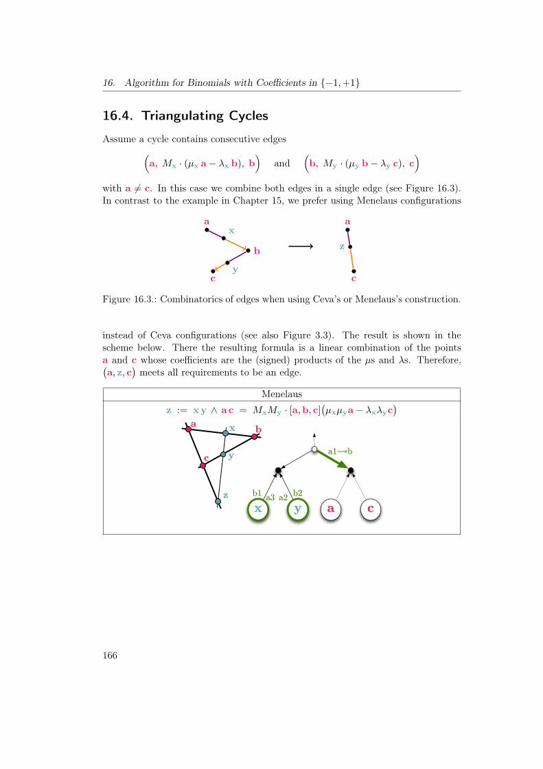
16. Algorithm for Binomials with Coefficients in −1,+1
16.4. Triangulating Cycles
Assume a cycle contains consecutive edges(a, Mx · (µx a− λx b), b
)and
(b, My · (µy b− λy c), c
)
with a 6= c. In this case we combine both edges in a single edge (see Figure 16.3).In contrast to the example in Chapter 15, we prefer using Menelaus configurations
a
b
c
x
y
a
c
z
Figure 16.3.: Combinatorics of edges when using Ceva’s or Menelaus’s construction.
instead of Ceva configurations (see also Figure 3.3). The result is shown in thescheme below. There the resulting formula is a linear combination of the pointsa and c whose coefficients are the (signed) products of the µs and λs. Therefore,(a, z, c
)meets all requirements to be an edge.
Menelaus
z := x y ∧ a c = MxMy · [a,b, c](µxµya− λxλyc
)
cayxb1 b2
a1!b
a2a3
166

16.4. Triangulating Cycles
Using a Ceva configuration instead results in a sign change in the linear combination:
Ceva
z := (y a ∧ c x) b ∧ a c = MxMy · [a,b, c]2(µxµya + λxλyc
)
cab
c xay
b1 a2
b2a3 b3
a4
a1!b
A sign change can also be obtained on a single edge. Suppose the edge is given by(
p)
= (c, x = ab ∧ cd = [a,b,d]︸ ︷︷ ︸µp
c− [a,b, c]︸ ︷︷ ︸λp
d, d)
for some p ∈ P. The harmonic point construction (see Section 3.8) gives
Harmonic Point
z := (b c ∧ a d) (b d ∧ c a) ∧ c d = [b, c,d][a, c,d](µpc + λpd
)
dc
acdba dcb
b1
b2
a2
a3
a1!b
167

16. Algorithm for Binomials with Coefficients in −1,+1
The processing of the cycles C1, . . . , Ct detected in Section 16.3 is composed of thebuilding blocks just given and is described as follows:
In the case that ε = −1 we do a case distinction. If there is no cycle of lengthbigger than 2 then replace any edge by the edge obtained in the harmonic point con-struction. Else there is a cycle with length bigger than 2. Replace two consecutiveedges by the edge obtained in the Ceva construction. If ε = 1 we do nothing.
Now, if there are left any cycles of length bigger than 2 we triangulate them byplugging in Menelaus configurations. This means successively replacing consecutiveedges by the edge obtained in the Menelaus construction. This results in a collectionof 2-cycles. The triangulation can be done in such a way that one edge of the 2-cycleis in its original state, i.e. there is a p ∈ P such that this edge equals (p).
In any case, we give an evaluation of the points in any resulting 2-cycle: considere.g. Ct ⊂ (P). For using (16.7) later on, let Ct be the (algorithmic) preimageof Ct under . After triangulation, Ct is transferred to a 2-cycle, say
((∞, 1, 0) , (0, x, ∞)
)with (∞, 1, 0) = (p1) for a p1 ∈ P (16.8)
and with ∞, 0 ∈ P. 1, x are simple Grassmann-Cayley algebra expressions inΛ1(P). By induction, x has an evaluation as
Mx ·
∏
p ∈ Ct\p1
µp
︸ ︷︷ ︸=:µx
0 −(± 1) ∏
p ∈ Ct\p1
λp
︸ ︷︷ ︸=:λx
∞
(16.9)
for a bracket monomial Mx. The sign in the above equation equals −1 if the cyclewas altered by a construction resulting from ε = −1. Otherwise the sign is +1.Observe that Mx is really a bracket monomial in BP, since the monomials in theconstruction above contain distinct elements of P. This is due to the assumptiona 6= c and the definition of . Furthermore, the cycles detected in Section 16.3are simple. Observe that we have
deg(Mx) ≤ length(Ct)− 2 (16.10)
if Ct was not altered by a construction resulting from ε = −1. Otherwise we have
deg(Mx) ≤(
length(Ct)− 2)
+ 2. (16.11)
168

16.5. Combining 2-Cycles or Cross-Ratios
16.5. Combining 2-Cycles or Cross-Ratios
In this section, we give tools to combine two 2-cycles (see Figure 16.4). Inductively,this allows for combining all 2-cycles. Due to the intuition of 2-cycles alreadyprovided in Chapter 15 and by abusing the notion, we call the 2-cycles cross-ratiosas well. All of the following constructions will result in similar evaluations. Sincewe want to keep the degree of the multiplier monomial small, we give a lot ofdifferent constructions which shall be used depending on the current setup. Thesetup common to all situations is given as:((∞, 1 = (µ1∞ − λ1 0 ), 0
),(0, x = Mx (µx 0 − λx∞ ), ∞
))and
((∞′, 1′ = (µ1′∞′ − λ1′0′), 0′
),(0′, x′ = Mx′ (µx′0
′ − λx′∞′), ∞′))
(16.12)being two 2-cycles. Furthermore, due to (16.8) we can assume that there are a, b,a′ and b′ in P such that
1 = a b ∧ ∞0 and 1′ = a′ b′ ∧ ∞′ 0′ (16.13)
as well as µ1′ = [a′,b′,0′] and λ1′ = [a′,b′,∞′], 0′ 6=∞′ and in addition a′,b′,0′and a′,b′,∞′ are pairwise distinct (due to the definition of P). Similar propertieshold for the points in the first cycle.
∞
0
1 x
∞′
0′
1′x′
∞
0
1z
Figure 16.4.: Combinatorics of combining two 2-cycles.
The following tables summarize the constructions for a point z. In this step ofthe algorithm, both cross-ratios in (16.12) are combined in the single cross-ratio
((∞, 1, 0) , (0, z, ∞)
).
Observe that also in the case of the resulting 2-cycle, there is a p1 ∈ P such that(∞, 1, 0) = (p1). The evaluations of z given below all are a bracketmonomial
169

16. Algorithm for Binomials with Coefficients in −1,+1
multiple ofE∗ := Mx′ ·Mx
(µ1′µxµx′0− λ1′λxλx′∞
). (16.14)
The degree of the multiplier monomial in all cases is
≤ 4.
By (16.6), the multiplier E∗ can be viewed to be a version of (15.7) in Grassmann-Cayley algebra. Observe that the assumptions on the points used in (16.13) implythat the bracket monomial multiplies in the evaluations of the constructions belowall do not vanish in BP. If one would not need a monomial multiplier we could saveourselves the case distinction in the case
∣∣0,∞,0′,∞′∣∣ = 4. We could construct z
by using the fact that in any instance, the six lines induced by 0∞,∞′ 0′, 0 0′,∞∞′,x 1′ and x′ z are tangent to the same conic. Together with Brianchon’s theorem(which is the dual of Pascal’s theorem in Section 3.10) this gives a construction forz. However, the resulting multiplier of degree 4 is not a monomial. The four casesfor
∣∣0,∞,0′,∞′∣∣ = 3 are very similar and therefore only one case is illustrated
detailedly. Furthermore, by possibly exchanging the roles of the points a′ and b′ orof the two 2-cycles in question, one of the cases given below is applicable. A remarkon the evaluation of the formula given in Case 2 (i): Observe that by 0 = ∞′ and∞ = 0′ it now holds µ1′ = [a′,b′,∞] and λ1′ = [a′,b′,0]. Similar comments arealso appropriate in the other cases.
170

16.5. Combining 2-Cycles or Cross-Ratios
Case 2 (i):∣∣0,∞,0′,∞′
∣∣ = 2: 0 = 0′ and ∞ =∞′
z :=(a′ 0 ∧ x b′
) (b′∞ ∧ x′ a′
)∧ 0∞ = [0,∞,a′][0,∞,b′]E∗
∞=∞'0=0'
a'∞=∞'b'b'xa' 0=0' x'
b1
b4b3
b2
a1
a2
a3
a4a5
Case 2 (ii):∣∣0,∞,0′,∞′
∣∣ = 2: 0 =∞′ and ∞ = 0′
z :=((
x′ a′ ∧ b′∞)x ∧ a′ 0
)b′ ∧ 0∞ = [0,∞,b′][0,∞,a′]E∗
∞=0'0=∞'b'
0=∞'a'x
∞=0'b'x' a'
b1
b4
b3
b2
a2
a3
a5
a4
a1!b
171
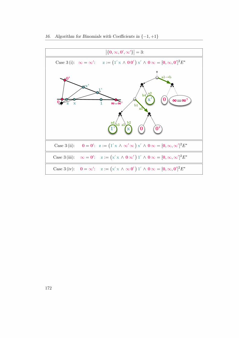
16. Algorithm for Binomials with Coefficients in −1,+1
∣∣0,∞,0′,∞′∣∣ = 3:
Case 3 (i): ∞ =∞′: z :=(1′ x ∧ 0 0′
)x′ ∧ 0∞ = [0,∞,0′]2E∗
∞=∞'0x'
0'0x1'
a1!b
b1
a2
b2
a3
b3a4
a5
b4
Case 3 (ii): 0 = 0′: z :=(1′ x ∧ ∞′∞
)x′ ∧ 0∞ = [0,∞,∞′]2E∗
Case 3 (iii): ∞ = 0′: z :=(x′ x ∧ 0∞′
)1′ ∧ 0∞ = [0,∞,∞′]2E∗
Case 3 (iv): 0 =∞′: z :=(x′ x ∧ ∞0′
)1′ ∧ 0∞ = [0,∞,0′]2E∗
172

16.5. Combining 2-Cycles or Cross-Ratios
Case 4 (i):∣∣0,∞,0′,∞′
∣∣ = 4: |a′,b′,0| = 3
z :=((
a′ b′ ∧ 0∞′)x ∧ ∞∞′
)(x′(a′ b′ ∧ 0 0′
)∧ 0∞′
)∧ 0∞
= [0,∞,∞′]2[0,0′,∞′][0,a′,b′]E∗
∞0
∞'0
0'0b'a'
x'∞'∞x
∞'0b'a'
b1
b6b5
b4
b3
b2
a2a3
a4
a5
a6
a7
a1!b
173
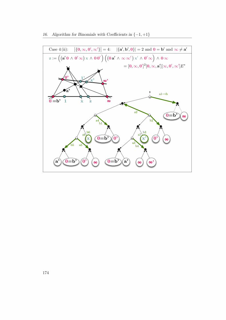
16. Algorithm for Binomials with Coefficients in −1,+1
Case 4 (ii):∣∣0,∞,0′,∞′
∣∣ = 4: |a′,b′,0| = 2 and 0 = b′ and ∞ 6= a′
z :=((
a′ 0 ∧ 0′∞)x ∧ 0 0′
)((0 a′ ∧ ∞∞′
)x′ ∧ 0′∞
)∧ 0∞
= [0,∞,0′]2[0,∞,a′][∞,0′,∞′]E∗
∞0=b'
∞0'x'
∞'∞a'0=b'
0'0=b'x
∞0'0=b'a'
b1
b6
b5 b4
b3
b2
a2
a3
a4
a5
a6 a7
a1!b
174

16.5. Combining 2-Cycles or Cross-Ratios
Case 4 (iii):∣∣0,∞,0′,∞′
∣∣ = 4: |a′,b′,0| = 2 and 0 = b′ and ∞ = a′
z :=(x∞′ ∧ 0 0′
)((x′(0 0′ ∧ ∞∞′
)∧ ∞0
)0′ ∧ ∞∞′
)∧ 0∞
= [0,∞,0′][0,∞,∞′][0,0′,∞′][∞,0′,∞′]E∗
∞=a'0=b'
∞'∞=a'0'
∞=a' 0=b'
∞'∞=a'0'0=b'
x'
0'0=b'∞'x
b1
b6
b5
b4
b3
b2
a2
a3
a4
a5
a6
a7
a1!b
175

16. Algorithm for Binomials with Coefficients in −1,+1
In total Obviously, one can combine all cross-ratios resulting from Section 16.4(by triangulating C1, . . . , Ct) in a single cross-ratio or 2-cycle
((∞, 1, 0) , (0, x, ∞)
). (16.15)
By induction and by using (16.14) as well as (16.9) for the shape of the cross-ratiosresulting from Section 16.4, there is a bracket monomial Mx and a p1 ∈ P with(∞, 1, 0) = (p1) such that
Mx ·
∏
p ∈P\p1µp 0 − ε ·
∏
p ∈P\p1λp ∞
. (16.16)
For a degree bound on Mx we observe that we need to sum up the costs for trian-gulating the cycles C1, . . . , Ct (see (16.10) and (16.11)) and for t − 1 many timescombining pairs of 2-cycles. This implies
deg(Mx) ≤t∑
i=1
(length(Ci)− 2
)+ 2 + 4 (t− 1)
=∣∣P∣∣+ 2 t− 2
≤ 2 k + 2 k − 2
≤ 4 k
(16.17)
since∑t
i=1 length(Ci) =∣∣P∣∣ and t ≤
⌊ |P|2
⌋as well as (16.2) which states
∣∣P∣∣ ≤ 2 k.
16.6. Final Coincidence
Consider the resulting 2-cycle given in (16.15). Due to (∞, 1, 0) = (p1) wehave
1 = a b ∧ ∞0
for some a, b in P and
µp1 = [a,b,0] and λp1 = [a,b,∞].
By (16.16) and due to (16.7) it holds
176

16.7. Example: A Derivation of Pascal’s Theorem
a b ∧ x
=Mx ·
∏
p ∈P\p1µp [a,b,0]︸ ︷︷ ︸
µp1
− ε ·∏
p ∈P\p1λp [a,b,∞]︸ ︷︷ ︸
λp1
=Mx ·N ·B
and with a bracket monomialN with deg(N) ≤ k. Therefore, a b∧x is a generalizedCayley factorization with multiplier Mx ·N with
deg(Mx ·N) ≤ 5 k.
The algorithm described is linear in k except for the step where it has to find aperfect matching. The construction of G and finding the matching is possible intime O(k3) (e.g. the classical algorithm using augmented path which is due to [5]runs in the given time). This proves Theorem 14.4.
Remark 16.6. Observe that one can also achieve a linear running time with a weakerupper bound on the degree of the multiplier: Therefore one omits the step in whicha perfect matching is obtained. Instead, one pairs a bracket in LB with any bracketinMB. In order to apply the area principle, an additional slack variable might hasto be introduced for pairs that have no common letter.
Remark 16.7. It should be remarked that the algorithm is not completely deter-ministic in the sense that there are various options of choice: in the concrete shapeof the pairing P, in the concrete triangulation of the cycles and in the order andpattern in which the 2-cycles are combined. This freedom is partially used for localoptimizations in the actual implementation presented in Chapter 18.
16.7. Example: A Derivation of Pascal’s Theorem
One of the smallest non-trivial example only consisting of two 2-cycles is given bythe bracket monomial
B := [a, c, e][a,d, f ][b, c, f ][b,d, e]− [a, c, f ][a,d, e][b, c, e][b,d, f ]. (16.18)
Actually, any pairing P using only edges in E1 (i.e. only edges joining bracketswith exactly two common entries) of B corresponds to two 2-cycles. B belongsto Pascal’s theorem (see Section 3.10 and also Section 6.1) and the existence of asynthetic construction describing the bracket polynomial was one of the motivations
177

16. Algorithm for Binomials with Coefficients in −1,+1
for Cayley factorization. This example is also used in [104, p. 449 ff.] in orderto motivate the use of Cayley factorization. There it is assumed that that theyalready possess an efficient subroutine for Cayley factoring non-multilinear bracketpolynomials. Afterwards, they use this routine in order to “detect” Pascal’s theorem.We will demonstrate in the following that with suitable choices done, our algorithmcan in principle do this. The diagram below indicates all edges in E1. There arethree pairings using only edges in E1 such that the combination of resulting 2-cycles can be expressed as Case 2 (i) or Case 2 (ii). The other matchings correspondto a case with
∣∣0,∞,0′,∞′∣∣ = 4 which yields a multiplier monomial of bigger
degree than the cases indicated by∣∣0,∞,0′,∞′
∣∣ = 2. One of these matchingscorresponding to Case 2 (i) or Case 2 (ii) is highlighted by thick edges, the two otherones have a symmetric structure. The highlighted matching shall be called P.
16. Algorithm for Binomials with Coefficients in −1, +1
for Cayley factorization. This example is also used in [105, p. 449 ff.] in orderto motivate the use of Cayley factorization. There it is assumed that that theyalready possess an efficient subroutine for Cayley factoring non-multilinear bracketpolynomial. Afterwards they use this routine in order to “detect” Pascal’s theorem.We will demonstrate that with suitable choices done, our algorithm can in princi-ple do this: the diagram below indicates all edges in E1. There are three pairingsusing only edges in E1 such that the combination of resulting 2-cycles can be ex-pressed as Case 2 (i) or Case 2 (ii). The other matchings correspond to a case with0,∞,0,∞
= 4 which yields a multiplier monomial of bigger degree. One ofthese matchings corresponding to Case 2 (i) or Case 2 (ii) is highlighted by thickedges, the two other ones have a symmetric structure. The highlighted matchingshall be called P.
[a, c, e] [a,d, f ] [b,d, e] [b, c, f ]
[a, c, f ] [a,d, e] [b,d, f ] [b, c, e]
16. Algorithm for Binomials with Coefficients in −1, +1
for Cayley factorization. This example is also used in [105, p. 449 ff.] in orderto motivate the use of Cayley factorization. There it is assumed that that theyalready possess an efficient subroutine for Cayley factoring non-multilinear bracketpolynomial. Afterwards they use this routine in order to “detect” Pascal’s theorem.We will demonstrate that our algorithm can in principle do this: P can be taken tobe the pairs indicated by
[a, c, e] [a,d, f ] [b,d, e] [b, c, f ]
[a, c, f ] [a,d, e] [b,d, f ] [b, c, e]
which induces ε = +1. The pairing induces the two 2-cycle
e
f
ac ∧ efad ∧ fe
f
e
bd ∧ efbc ∧ fe
This resembles the Case 2 (i) labeled with0,∞,0,∞
= 2: 0 = 0 and ∞ = ∞.We define
z :=eb ∧ (ad ∧ f e)d
d f ∧ (bc ∧ f e)b
∧ e f (16.18)
By the results of the previous sections we have
ac ∧ z = [f , e,b][f , e,d] · B
where the multiplier monomial from the combination of 2-cycles. Furthermore, wehave
(ad ∧ f e)d = −[f , e,d]ad and (bc ∧ f e)b = [f , e, c] cb. (16.19)
176
which induces ε = +1. The pairing induces the two 2-cycle
e
f
ac ∧ efad ∧ fe
f
e
bd ∧ efbc ∧ fe
176
which induces ε = +1. The pairing induces the two 2-cycle
176
P induces ε = +1 and the two 2-cycles
e
f
ac ∧ efad ∧ fe
e
f
bd ∧ efbc ∧ fe
We choose to use Case 2 (i) labeled with∣∣0,∞,0′,∞′
∣∣ = 2: 0 = 0′ and ∞ =∞′.We define
z :=(b f ∧ (a d ∧ f e) d
) (d e ∧ (b c ∧ f e) b
)∧ f e. (16.19)
By the results of the previous sections we have
ac ∧ z = [f , e,b][f , e,d] ·B
178
16.7. Example: A Derivation of Pascal’s Theorem
where the multiplier monomial comes from the combination of 2-cycles. Further-more, we have
(a d ∧ f e) d = −[f , e,d] a d and (b c ∧ f e) b = [f , e,b] c b. (16.20)
Therefore, we can substitute (16.20) in (16.19), cancel and conclude
−B = ac∧((
b f ∧ a d) (
d e ∧ c b)∧ f e
)= −
(a c ∧ f e
)∧(b f ∧ a d
) (d e ∧ c b
).
This is a synthetic construction differing from the one given in Section 3.10 only bya permutation of indices. We have seen similar phenomena also in Section 6.1. Wewill argue that the given factorization can be considered as an automatic derivationof Pascal’s theorem when the algorithm for Cayley factorization is optimized locally.We already did a local optimization when choosing the matching. After choosingCase 2 (i) for the combination of 2-cycles, we had to decide which points shouldbe considered as a′ and b′. Here the given choice should be preferred since it canbe locally simplified using (16.20). Now when choosing Case 2 (ii), adjusting theroles of points a′ and b′, allows again for local simplifications of the construction andyields a version of Pascal’s construction. We think that this is due to the beauty andsymmetry of the conic condition. However, the algorithm for Cayley factorizationis close enough to geometry to benefit from this beauty. For further comments onalso automatically deriving (16.18) see [104].
179


17. Generalization for Polynomialswith Arbitrary Number ofSummands
An intuition for the general algorithm in terms of length ratios (compare Section 15)can be provided as follows: Consider a general bracket polynomial
α1[∗, ∗, ∗][∗, ∗, ∗] · · · [∗, ∗, ∗] + · · ·+ αl[∗, ∗, ∗][∗, ∗, ∗] · · · [∗, ∗, ∗]− αΩ[∗, ∗, ∗][∗, ∗, ∗] · · · [∗, ∗, ∗].
For an instance P , we have
α1[∗, ∗, ∗]P · · · [∗, ∗, ∗]P + · · ·+ αl[∗, ∗, ∗]P · · · [∗, ∗, ∗]P − αΩ[∗, ∗, ∗]P · · · [∗, ∗, ∗]P = 0
⇐⇒α1[∗, ∗, ∗]P · · · [∗, ∗, ∗]P + · · ·+ αl[∗, ∗, ∗]P · · · [∗, ∗, ∗]P
[∗, ∗, ∗]P · · · [∗, ∗, ∗]P= αΩ
⇐⇒
α1[∗, ∗, ∗]P · · · [∗, ∗, ∗]P[∗, ∗, ∗]P · · · [∗, ∗, ∗]P
+ · · ·+ αl[∗, ∗, ∗]P · · · [∗, ∗, ∗]P[∗, ∗, ∗]P · · · [∗, ∗, ∗]P
= αΩ .(17.1)
In principle, the algorithm for the binomial case given in Section 16 can interpreteach of the summands (without the coefficient) as a product of length ratios. Itcan output a cross-ratio that contains the same information. They can be combinedusing the tool of projective addition (see Section 3.7). In order to combine them, wehave to consider them as numbers on the same projective number line with respectto the same basis. This is the very general outline of the present chapter.To work out the details and to achieve a low total upper bound on the multiplier
monomial, we need more than the brief description above. In particular, practicalexperiments with large bracket polynomials in an implementation of the algorithmin Mathematica ([136]) by the author (see Chapter 18 for more information aboutthe implementation) has shown that it is worth to explicitly factor out some commonfactors when appropriate (see below). Unfortunately, this makes the exposition a
181

17. Generalization for Polynomials with Arbitrary Number of Summands
little tedious. Let P be a finite set and let B ∈ R[∆(P)] be multihomogenous withcoefficients in Z. Let k ≥ 2 be the degree of B in its brackets and l+ 1 the numberof summands, such that no summand has repeating indices in its brackets and suchthat no difference of two summands lies in
⟨Irepeat∪Ialtern
⟩. (Observe that this does
not affect the bounds given in Theorem 14.5.) Furthermore, the summands shall nothave a overall bracket monomial factor. By switching the positions of two elementsin some brackets we can w.l.o.g. assume that all the coefficients αj (1 ≤ j ≤ l + 1)are in N \ 0 such that B has the following sign pattern:
α1 [∗, ∗, ∗][∗, ∗, ∗] · · · [∗, ∗, ∗]︸ ︷︷ ︸=:Π1
+ · · ·+ αl [∗, ∗, ∗][∗, ∗, ∗] · · · [∗, ∗, ∗]︸ ︷︷ ︸=:Πl
− αΩ [∗, ∗, ∗][∗, ∗, ∗] · · · [∗, ∗, ∗]︸ ︷︷ ︸=:Ω
. (17.2)
Consider the l binomials given below. The right-hand sides are versions where thecommon factors F (∗)s are factored out explicitly:
Π1 − Ω = F (1) (L(1) −M(1))︸ ︷︷ ︸=:B1
,
...
Πl − Ω = F (l) (L(l) −M(l))︸ ︷︷ ︸=:Bl
.
(17.3)
This impliesF (i) L(i) = Πi and F (i) M(i) = Ω. (17.4)
Let ki denote the degree of Bi (1 ≤ i ≤ l). Since the summands of B are distinct,all kis are bigger than 1. Due to Theorem 14.4 and Chapter 16, the Bis can beCayley factored. In particular, for each (1 ≤ i ≤ l) there is a 2-cycle
Ci :=((∞i, 1i = [ai,bi,0i]︸ ︷︷ ︸
=: µ1i
∞i − [ai,bi,∞i]︸ ︷︷ ︸=: λ1i
0i , 0i),
(0i, xi = Mxi ( µxi 0i − λxi∞i), ∞i)).
for some ai and bi in P with the following properties:
µxiµ1i = Ni · M(i) and λxiλ1i = Ni · L(i). (17.5)
182

17.1. Constructing the Coefficients
which impliesMxi ·
(µxiµ1i − λxiλ1i
)= Mxi ·Ni ·Bi
for suitable bracket monomials Ni such that
deg(Mxi ·Ni) ≤ 5 ki.
Similarly to the situation in Chapter 16, we now are left with l highly preprocessed2-cycles. In a next step, if necessary, we establish the summands with coefficientsαi 6= 1.
17.1. Constructing the Coefficients
Due to classical literature, the integers can be constructed on projective numberlines. This is often referred to as a harmonic sequence. We also give an (inductive)evaluation in order to ensure that the multiplier is a bracket monomial. Consider ai ∈ 1, . . . , l with αi ≥ 2. We can recursively construct the natural numbers withrespect to the base 0i,∞i,1i.
183

17. Generalization for Polynomials with Arbitrary Number of Summands
Constructing the natural numbers m ∈ N \ 0.
ni(m) :=
1i = µ1i∞i − λ1i 0i = [ai,bi,0i]∞i − [ai,bi,∞i] 0i for m = 1((
ai 0i ∧ bi ∞i
)ni(m− 1) ∧ ai ∞i
)bi ∧ 0i ∞i for m ≥ 2
= (λ1i [0i,∞i,ai][0i,∞i,bi])m−1
(mµ1i∞i−λ1i 0i
)
∞i0ibi
∞iaini(m-1)
∞ibi0iai
b2
a2
a3
b3
a1!b
a4!c
b1
Now, ni(αi) and xi can be considered to represent numbers on the same projectivenumber line. A multiplication of both numbers can be achieved by a von Staudtconstruction (see Section 3.7). We define
zi :=(0i ai ∧ xi bi
) (bi∞i ∧ ni(αi) ai
)∧ 0i∞i.
By a pattern matching (substitute 1i for 1′, xi for x and ni for x′) with the casedescribed in Case 2 (i) in Section 16.5, we obtain after simplification:
zi = Mxi (λ1i [bi,0i,∞i][ai,0i,∞i])αi µ1i
(µxi 0i − αi λxi∞i
)
184

17.2. Adding up Two 2-Cycles or Cross-Ratios
By replacing each xi by zi in Ci whenever the corresponding αi is bigger than 1, wecan w.l.o.g. assume xi = Mxi
(µxi 0i − λxi∞i
)such that we have (compare (17.5))
µxiµ1i = Ni · M(i) and λxiλ1i = Ni · αi · L(i) (17.6)
which induces
Mxi ·(µxiµ1i − λxiλ1i
)= Mxi ·Ni · (αi L(i) −M(i))
with
deg(Mxi ·Ni) ≤
5 ki if αi = 1
5 ki + 3αi + 1 if αi > 1.(17.7)
Remark 17.1. There are various possibilities to construct the coefficients αi. Wechose the present one because the degree bound only depends on the αi and is not toocomplicated. Of course, there are more efficient methods for constructing the naturalnumbers than just adding 1s. E.g. we could also use the binary representationtogether with Horner’s method in order to constructm ∈ N with a leading monomialof degree not bigger than 8 · dlog2(m)e. We will not give any details in order to savespace.
17.2. Adding up Two 2-Cycles or Cross-Ratios
We are left with a lot of 2-cycles or cross-ratios C1, . . . , Cl. At this points, literallyall comments from the first part of Section 16.5 apply. With the same settingsas given there we give constructions for combining two 2-cycles. We do the samecase distinction as before. Now the evaluations of z given below all are a bracketmonomial multiple of
E+ = Mx′ ·Mx
(λ1µ1′µx′µx 0− (λ1′λx′µ1µx + λ1λxµ1′µx′)∞
). (17.8)
We put on record that the degree of the multiplier monomial is
≤ 5. (17.9)
The idea behind all of the constructions is just the one given in the beginning of thechapter: We first express both cross-ratios with respect to the same basis. Then weperform a projective addition. Furthermore, we want to keep the construction small(in order to keep the degree of the multiplier small). Therefore, for the addition wereuse points introduced for changing the projective basis. The points marked witha circle in the following diagrams give vertices of a quadrilaterals witnessing theprojective addition (compare Section 3.7). In the corresponding quadrilateral a line
185
17. Generalization for Polynomials with Arbitrary Number of Summands
is missing. Including this line and intersecting it with the line 0∞, one can see bothparts of the construction: the adjustment of the basis and the projective addition.In order to interpret the construction for Case 2 (ii), one should observe that one canexchange the role of the points 0′ and ∞′ when simultaneously exchanging points1′ and x′. Therefore the same picture is drawn as in the case where 0 = 0′ and∞ =∞′. However, one has to take into account that the points a′ and b′ determine1′ (not x′) and therefore both constructions differ. By the same arguments as inSection 16.5, the multipliers do not vanish in BP. Again, by possibly exchangingthe roles of the points a′ and b′ or of the two 2-cycles in question, one of the casesgiven below is applicable. The possibility of being forced to exchange the rolesof the two 2-cycles will make the things more complicated in Section 17.3. Sucha situation arises e.g. if
∣∣0,∞,0′,∞′∣∣ = 4, |a′,b′,0| = 2, 0 = b′, ∞ = a′,
a,b 6= 0′,∞′. Clearly, there are constructions that do not need to exchangethe cycles also in this situation. However, those that we know of, all result in abigger degree of the multiplier monomial of E+. A remark on the evaluation of thelast formula: the result is identical to −λ1µ1′ E+ which might be confusing whenidentifying λs and µs.
186

17.2. Adding up Two 2-Cycles or Cross-Ratios
Case 2 (i):∣∣0,∞,0′,∞′
∣∣ = 2: 0 = 0′ and ∞ =∞′
z :=(∞ (b′ 0 ∧ a′ 1) ∧ x (b′ 0 ∧ a′∞)
)(b′ x′ ∧ a′∞
)∧ 0∞
= [0,∞,a′]2[0,∞,b′]2E+
∞=∞'0=0'
∞=∞'a'x'b'
∞=∞'a'0=0'b'
x
a' 10=0'b'
∞=∞'
b2
a2
b6
a3
b3a4
a1!b
a5
a6
a8
a7b1!c
b5
b7b4
c2
c1
c4
c3 c6c5
187
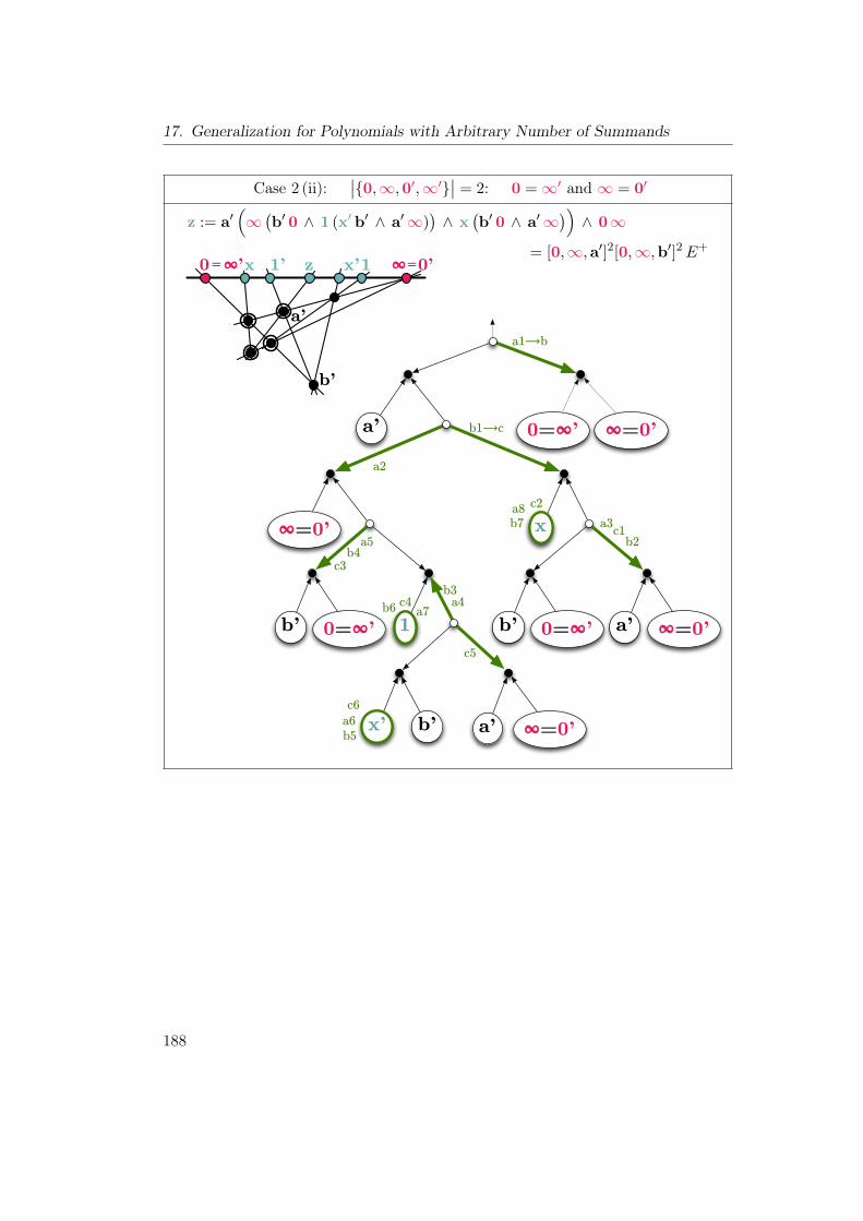
17. Generalization for Polynomials with Arbitrary Number of Summands
Case 2 (ii):∣∣0,∞,0′,∞′
∣∣ = 2: 0 =∞′ and ∞ = 0′
z := a′(∞(b′ 0 ∧ 1 (x′ b′ ∧ a′∞)
)∧ x
(b′ 0 ∧ a′∞
))∧ 0∞
= [0,∞,a′]2[0,∞,b′]2E+
∞=0'0=∞'
∞=0'a'0=∞'b'
x
a' ∞=0'b'x'
10=∞'b'
∞=0'
a'
b2
a2
b6
a3
b3a4
a1!b
a5
a6
a8
a7
b1!c
b5
b7
b4
c2
c1
c4
c3
c6
c5
188

17.2. Adding up Two 2-Cycles or Cross-Ratios
∣∣0,∞,0′,∞′∣∣ = 3:
Case 3(i): ∞ =∞′: z :=((
1 1′ ∧ 0 0′)∞ ∧ x 0′
)x′ ∧ 0∞=[0,∞,0′]3E+
∞=∞'0x'
0'x∞=∞'
0'01'1
b2
a2
b6a3
b3
a4
a1!b
a5a6
a7
b1!c
b5
b4
c2
c1
c4c3
c5
Case 3(ii): 0 = 0′: z :=(1′ 1 ∧ ∞′∞
) (x′∞ ∧ ∞′ x
)∧ 0∞=[0,∞,∞′]3E+
Case 3(iii): ∞ = 0′: z :=((
1 x′ ∧ 0∞′)∞ ∧ x∞′
)1′ ∧ 0∞=[0,∞,∞′]3E+
Case 3(iv): 0 =∞′: z :=(1 x′ ∧ 0′∞
) (1′∞ ∧ 0′ x
)∧ 0∞=[0,∞,0′]3E+
189

17. Generalization for Polynomials with Arbitrary Number of Summands
Case 4 (i):∣∣0,∞,0′,∞′
∣∣ = 4: |a′,b′,0| = 3
z :=
(∞(x′(a′ b′ ∧ 0 0′
)∧ 0∞′
)∧ x∞′
)((a′ b′ ∧ 0∞′
)1 ∧ ∞∞′
)∧ 0∞
= [0,∞,∞′]3[0,0′,∞′][0,a′,b′]E+
∞0
∞'∞1
∞'0b'a'
∞'x
∞'0
0'0b'a'
x'
∞
b2a2
b6
a3b3
a4
a1!b
a5
a6
a9
a7
b1!c
b5
b7
b4
c2
c1
c4
c3
c6
c5
a8
b8c7
190

17.2. Adding up Two 2-Cycles or Cross-Ratios
Case 4 (ii):∣∣0,∞,0′,∞′
∣∣ = 4: |a′,b′,0| = 2 and 0 = b′ and ∞ 6= a′
z :=(x′(a′ 0 ∧ ∞∞′
)∧ 0′∞
)((1(a′ 0 ∧ 0′∞
)∧ 0 0′
)∞ ∧ 0′ x
)∧ 0∞
= [0,∞,0′]3[0,∞,a′][∞,0′,∞′]E+
∞0=b'
x0'∞
0'0=b'
∞0'0=b'a'
1
∞0'
∞'∞0=b'a'
x'b2
a2
b6a3
b3
a4
a1!b
a5
a6
a8
a7
b1!c
b5
b7
b4
c2
c1
c4
c3
c6
c5a9
b8c7
191
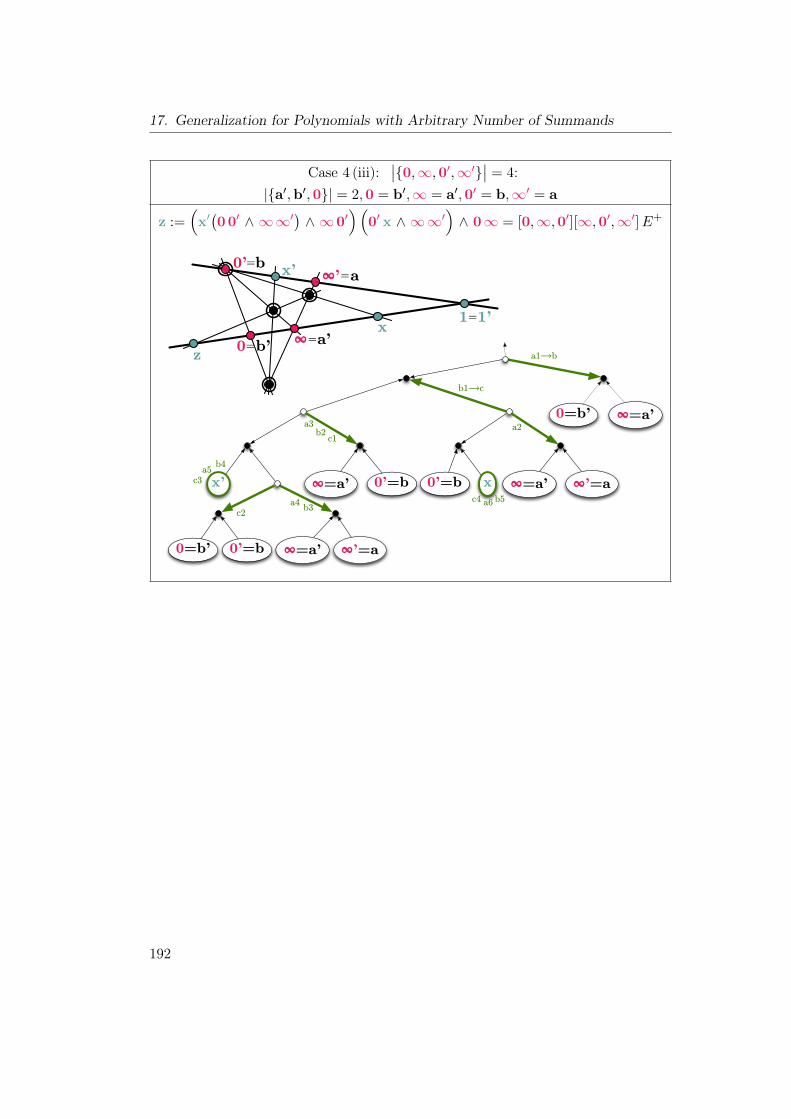
17. Generalization for Polynomials with Arbitrary Number of Summands
Case 4 (iii):∣∣0,∞,0′,∞′
∣∣ = 4:|a′,b′,0| = 2,0 = b′,∞ = a′,0′ = b,∞′ = a
z :=(x′(0 0′ ∧ ∞∞′
)∧ ∞0′
)(0′ x ∧ ∞∞′
)∧ 0∞ = [0,∞,0′][∞,0′,∞′]E+
∞=a'0=b'
∞'=a∞=a'0'=b x0'=b∞=a'
∞'=a∞=a'0'=b0=b'
x'
b2 a2a3
b3a4
a1!b
a5
a6
b1!c
b5
b4
c2
c1
c4
c3
192

17.3. Adding up All 2-Cycles or Cross-Ratios
17.3. Adding up All 2-Cycles or Cross-Ratios
Unfortunately, in the case of adding up 2-cycles, the result differs much more fromthe shape of the xi in the original Cis. Therefore, the iterative addition is formulateddifferently (see Lemma 17.2 below). As mentioned before, the case distinction donein Section 17.2 for combining two 2-cycles implies that in some cases, one has toexchange the roles of both cycles. This implies that one looses the control of which2-cycles plays which role in the combination. Therefore, the statement and proof ofthe following lemma have to be formulated without the knowledge of the role thecycles play in the combination.
Lemma 17.2. Suppose that the cross-ratios C1, . . . , Cl are combined linearly, i.e.w.l.o.g. we start by adding the 2-cycles C1 and C2. Then we add C3, C4, . . . by the con-structions of Section 17.2. Let Aj be the bracket monomial of degree not bigger than5 that is produced during the addition of Cj as multiplier of E+. The 2-cycle obtainedafter adding Cj (2 ≤ j ≤ l) can be written as
((∞i∗ , 1i∗ , 0i∗
),(0i∗ , x(j), ∞i∗
))
with some i∗ ∈ 1, . . . , j. For j ≥ 2 there is an evaluation of x(j) as:
x(j) = Mx(j) ·
µxi∗λ1i∗
j∏
i=1i6=i∗
M(i) 0i∗ −
j∑
s=1
αs L(s)j∏
i=1i 6=s
M(i)
Ni∗∞i∗
such that there is a bracket monomial Qj of degree j − 2 with
Mx(j) = Qj ·j∏
i=1i 6=i∗
Ni
j∏
i=1
Mxi
j∏
i=2
Ai.
Proof. We proceed by induction on j. Let j = 2. We can w.l.o.g. assume thati∗ = 1. Due to (17.8), x(2) is given as
x(2) = A2 ·Mx1 ·Mx2
·(λ11 µ12µx2︸ ︷︷ ︸M(2)N2
µx1 01 −(λ12 λx2︸ ︷︷ ︸α2L(2)N2
µ11µx1︸ ︷︷ ︸M(1)N1
+ λ11 λx1︸ ︷︷ ︸α1L(1)N1
µ12µx2︸ ︷︷ ︸M(2)N2
)∞1
)
= A2 ·Mx1 ·Mx2 ·N2
(µx1λ11M(2) 01 − (α2 L(2)M(1) + α1 L(1)M(2))N1 ∞1
).
The underbraces are due to (17.6). This is of the required form. Now let j ≥ 3. Thelemma is considered to be true for j − 1. Therefore there is a i∗ ∈ 1, . . . , j − 1
193

17. Generalization for Polynomials with Arbitrary Number of Summands
such that in step j the to 2-cycles((∞i∗ , 1i∗ , 0i∗
),(0i∗ , x
(j−1),∞i∗))
and
Cj =((∞j , 1j , 0j
),(0j , xj , ∞j
))
are added. With
µx(j−1) =µxi∗ λ1i∗
j−1∏
i=1i6=i∗
M(i) and λx(j−1) =Ni∗
j−1∑
s=1
αs L(s)j−1∏
i=1i 6=s
M(i)
we havex(j−1) = Mx(j−1) ·
(µx(j−1) 0i∗ − λx(j−1)∞i∗
).
We distinguish two cases: Case 1: Cj plays the role of((∞′ , 1′ , 0′
),(0′ , x′, ∞′
))
in the addition when using the notions of Section 17.2. Using (17.8) and (17.6) weobtain
x(j) = Aj ·Mx(j−1) ·Mxj ·(λ1i∗µ1jµxjµx(j−1) 0i∗
−(λ1jλxjµ1i∗µx(j−1) +λ1i∗λx(j−1)µ1jµxj )∞i∗
)
= Aj ·Mx(j−1) ·Mxj · λ1i∗ µ1j µxj µxi∗λ1i∗
j−1∏
i=1i 6=i∗
M(i) 0i∗
−λ1j λxj µ1i∗ µxi∗λ1i∗
j−1∏
i=1i 6=i∗
M(i) ∞i∗
−λ1i∗ Ni∗
j−1∑
s=1
αs L(s)j−1∏
i=1i 6=s
M(i)
µ1j µxj ∞i∗
194

17.3. Adding up All 2-Cycles or Cross-Ratios
= Aj · Qj−1 ·j−1∏
i=1i 6=i∗
Ni
j−1∏
i=1
Mxi
j−1∏
i=2
Ai ·Mxj · λ1i∗ ·
NjM(j) µxi∗λ1i∗
j−1∏
i=1i6=i∗
M(i) 0i∗
−Nj αj L(j) Ni∗M(i∗)j−1∏
i=1i6=i∗
M(i) ∞i∗
−Ni∗
(j−1∑
s=1
αs L(s)j−1∏
i=1i6=s
M(s)
Nj M(j) ∞i∗
= Qj ·j∏
i=1i6=i∗
Ni
j∏
i=1
Mxi
j∏
i=2
Ai ·
µxi∗λ1i∗
j∏
i=1i 6=i∗
M(i) 0i∗
− Ni∗ αj L(j)j−1∏
i=1
M(i) ∞i∗
− Ni∗
(j−1∑
s=1
αs L(s)j∏
i=1i6=s
M(i)
∞i∗
withQj := Qj−1·λ1i∗ which by induction has degree j−3+1 = j−2. This proves theclaim in the first case. In Case 2, where Cj plays the role of
((∞, 1, 0
),(0, x, ∞
)),
one analogously computes
Aj ·Mxj ·Mx(j−1)
(λ1jµ1i∗µx(j−1)µxj 0j−(λ1i∗λx(j−1)µ1jµxj+λ1jλxjµ1i∗µx(j−1))∞j
).
195

17. Generalization for Polynomials with Arbitrary Number of Summands
This results in
Qj ·j∏
i=1i 6=j
Ni
j∏
i=1
Mxi
j∏
i=2
Ai ·
µxjλ1j
j∏
i=1i6=j
M(i) 0j −
j∑
s=1
αs L(s)j∏
i=1i 6=s
M(i)
Nj∞j
with Qj := Qj−1 · λ1i∗ which is the desired statement in this case.
Remark 17.3. It is also possible to use other patterns for combining the 2-cycles(e.g. tree-like structures). One can show that Lemma 17.2 can be adjusted in itsformulation and remains still valid. This needs more of bookkeeping of the indicesand the multiplier monomial has higher degree. However, in a concrete implemen-tation of the algorithm there might be a potential for optimizing the degree of themultiplier monomial.
17.4. Final Coincidence
Assume that all 2-cycles C1, . . . , Cl have been combined in a single 2-cycle given by((∞i∗ , 1i∗ , 0i∗), (0i∗ , x(l), ∞i∗)
).
As already declared in (17.1), in an instance testing B = 0 can be read as
α1Π1
Ω+ · · ·+ αl
Πl
Ω= αΩ
in the corresponding coordination. This equation holds in an instance if and onlyif the coordinatization of
ni∗(αΩ) and x(l)
are identical points in the projective plane in an instance. We will define c suchthat
ni∗(αΩ) = c bi∗ ∧ 0i∗ ∞i∗
by letting
c :=
ai∗ if αΩ = 1(ai∗ 0i∗ ∧ bi∗ ∞i∗
)ni∗(αΩ − 1) ∧ ai∗ ∞i∗ otherwise.
196

17.4. Final Coincidence
We havec = Mc
((αΩ − 1)µ1i∗ ∞i∗ − λc ai∗
)
with
λc =
−[0i∗ ,∞i∗ ,bi∗ ] for αΩ ≥ 2
1 otherwise
Mc =
(λ1i∗ [0i∗ ,∞i∗ ,ai∗ ])
αΩ−1[0i∗ ,∞i∗ ,bi∗ ]αΩ−2 for αΩ ≥ 2
1 otherwise.
(17.10)
For an evaluation of c observe that the construction is contained in the constructionof ni∗(αΩ). Splitting the edges in the tensor diagram representation in the same wayas before in the bigger diagram (see Section 17.1) gives the desired representation.With this setting it holds due to Lemma 17.2 and due to the above identities that
c bi∗ ∧ x(l)
=Mc ·Mx(l) ·((αΩ − 1)µ1i∗ ∞i∗ bi∗ − λcai∗ bi∗
)
∧
µxi∗λ1i∗
l∏
i=1i 6=i∗
M(i) 0i∗ −
l∑
s=1
αs L(s)l∏
i=1i6=s
M(i)
Ni∗∞i∗
=Mc ·Mx(l) ·
(αΩ − 1) µ1i∗ µxi∗︸ ︷︷ ︸
=Ni∗ ·M(i∗) by (17.6)
λ1i∗
l∏
i=1i 6=i∗
M(i) [∞i∗ ,bi∗ ,0i∗ ]
− λc λ1i∗l∏
i=1i 6=i∗
M(i) µxi∗ [ai∗ ,bi∗ ,0i∗ ]︸ ︷︷ ︸=Ni∗ ·M(i∗) by (17.6)
+ λc
l∑
s=1
αs L(s)l∏
i=1i 6=s
M(i)
Ni∗ [ai∗ ,bi∗ ,∞i∗ ]︸ ︷︷ ︸
=λ1i∗
197

17. Generalization for Polynomials with Arbitrary Number of Summands
=Mc ·Mx(l) ·Ni∗ · λ1i∗ ·
(αΩ − 1)
l∏
i=1
M(i) [∞i∗ ,bi∗ ,0i∗ ]︸ ︷︷ ︸=−λc if αΩ≥2
− λcl∏
i=1
M(i)
+ λc
l∑
s=1
αs L(s)l∏
i=1i 6=s
M(i)
=Mc ·Mx(l) ·Ni∗ · λ1i∗ · λc ·(−αΩ
l∏
i=1
M(i) +
l∑
s=1
αs L(s)l∏
i=1i6=s
M(i)
.
This bracket polynomial can be further factored. In order to see this, for 1 ≤ s ≤ lconsider
l∏
i=1i6=s
M(i).
Observe, that F (s) (see (17.3)) is a bracket monomial factor of the above. If it wasnot, there would be a overall bracket monomial factor of B due to the definition ofF (s) as maximal common factor of Πs−Ω. But a bracket monomial factor of B wasexcluded in the beginning. On the other hand, we have F (s) = Ω
M(s) and therefore
∏li=1, i 6=sM(i)
F (s)=
∏li=1M(i)
Ω
which is independent of the particular s chosen. Therefore we can rewrite
c bi∗ ∧ x(l) = Mc ·Mx(l) ·Ni∗ · λ1i∗ · λc ·∏li=1M(i)
Ω·
l∑
s=1
αs L(s)F (s)︸ ︷︷ ︸
=Πs
−αΩ Ω
(17.11)
and therefore we obtained a generalized Cayley factorization of B.
198
17.5. The Multiplier of the Factorization
17.5. The Multiplier of the Factorization
The overall multiplier is due (17.11) and due to Lemma 17.2 given by
M :=Mc ·Mx(l) ·Ni∗ · λ1i∗ · λc ·∏li=i∗M(i)
Ω
=Mc ·Ql ·l∏
i=1
(Ni ·Mxi)
l∏
i=2
Ai. · λ1i∗ · λc ·∏li=1M(i)
Ω.
(17.12)
We want to give upper bounds on the degree of M . It remains to plug in theestimates given in (17.7). We distinguish two cases:
Common Special CaseAssume
α1 = · · · = αl = αΩ = 1.
Observe that by switching elements inside of the brackets, this case covers alsoα1, . . . , αl, αΩ ∈ −1,+1. In this case, M simplifies to
M = Qj ·l∏
i=1
(Ni ·Mxi)l∏
i=2
Ai. · λ1i∗ ·∏li=1M(i)
Ω.
Due to (17.7) and due to the degree of Qj given in Lemma 17.2 we have
deg(M) ≤(l − 2) + 5l∑
i=1
ki +l∑
i=2
deg(Ai) + 1 +l∑
i=1
ki − k
≤(l − 2) + 5 l k + (l − 1) 5 + 1 + l k − k
=6 k l + 6 l − k − 6
≤9 k l
where the estimate on the Ais is due to (17.9) and we use k ≥ 2.
199
17. Generalization for Polynomials with Arbitrary Number of Summands
General CaseIn the general case, we can use the representations of Mc and λc given in (17.10)to bound the overall degree of M as given in (17.12). We get
deg(M) ≤
≤ 3αΩ − 4 + (l − 2) +
l∑
i=1
(5 ki + 3αi + 1) + 5 (l − 1) + 2 +
l∑
i=1
ki − k
≤ 6l∑
i=1
ki + 3
(l∑
i=1
αi + αΩ
)+ 7 l − k − 9
≤ 10 k l + 3
(l∑
i=1
αi + αΩ
)
where we again used k ≥ 2. Also observe that after using the subroutine for thebinomial case l times, the algorithm is linear in l. The subroutine runs in O(k3).Therefore, the overall running time is in O(l · k3). This proves Theorem 14.5.
200

18. Examples
In this Chapter we give two examples illustrating the execution of the Cayley fac-torization algorithm. The output was obtained automatically by an implementationin Mathematica ([136]) and using the Combinatorica package for finding a bipartitematching and for producing graph representations. The algorithm works exactly asdescribed earlier. Within this description there is some freedom of choice. Withinthe algorithm, some of this freedom is used in order to construct an optimized match-ing. Furthermore when factoring binomials, the resulting cycles are triangulated insuch a way that the costs of combining the resulting 2-cycles are optimized.We will give two examples. Both of them have their coefficients in −1,+1 since
this is often the case when describing geometric properties. The first example is anextension of the introductive example given in Chapter 15. The second one is givenin Section 18.2 and treats the condition for ten points lying on a common cubic.Unfortunately, we do not have enough space to show the complete output.
18.1. Example 1
B := [a,b,g][a, c,k][b,a, c][e, f ,h][f ,d, e]
+[a,b,g][a, c, e][a, f , e][b, c,k][h,d, f ]
−[a,b, f ][a,d, f ][a, e,g][c,b,h][k, c, e]
Formatting and pre-processing input:
The bracket polynomial is processed such that it is composed of summands with allbut the last coefficient equal to +1. The last coefficient is -1. Cayley factorizationyields a ∨-∧-sequence to interpret it. Intuition is provided by interpreting thevanishing of the bracket polynomial:
B = 0
⇐⇒
201

18. Examples
[a,c,k][b,a,c][f ,d,e][a,b,g][e,f ,h][a,e,g][a,b,f ][c,b,h][k,c,e][a,d,f ] + [a,f ,e][h,d,f ][b,c,k][a,c,e][a,b,g]
[a,e,g][a,b,f ][c,b,h][k,c,e][a,d,f ] = 1
Start of the Main Part of the Algorithm:
Factor all induced fractional equations [∗,∗,∗]...[∗,∗,∗][∗,∗,∗]...[∗,∗,∗] = 1
—–Factorize the fractional equation [a,f ,e][h,d,f ][b,c,k][a,c,e][a,b,g][a,e,g][a,b,f ][c,b,h][k,c,e][a,d,f ]
= 1
Brackets occurring in the numerator as well as in the denominator can be canceled.The common elements are: ∅This reduces the bracket identity in question to:
[a, f , e][h,d, f ][b, c,k][a, c, e][a,b,g]
[a, e,g][a,b, f ][c,b,h][k, c, e][a,d, f ]= 1
Find a Matching in order to apply the area principle:
Split the big fraction into fractions of the form [∗,∗,∗]...[∗,∗,∗][∗,∗,∗]...[∗,∗,∗] . This matches each
bracket of the numerator with a bracket of the denominator. The aim will be toapply the area principle to each factor [∗,∗,∗]...[∗,∗,∗]
[∗,∗,∗]...[∗,∗,∗] . This is possible as soon as bothbrackets differ by exactly one element. In the graph below, we have one vertex perbracket, but brackets are replaced by corresponding sets of indices. The situationswhere the area principle can be applied directly are indicated by green edges. Thered edges indicate situations where the corresponding fraction can by multiplied byan additional factor [∗,∗,∗]...[∗,∗,∗]
[∗,∗,∗]...[∗,∗,∗] = 1 such that the area principle can be applied
to the product. E.g. [a,b,c][c,d,e] ·
[a,c,d][a,c,d] can be rearranged to [a,b,c]
[a,c,d] ·[a,c,d][c,d,e] . Due to
Hall’s Marriage Theorem, there exists a perfect matching in the graph below. Thegreen edges are given weights 2 and the red edges weight 1 and a perfect maximummatching with maximal total weight is highlighted by the thick edges.
202

18.1. Example 1
!a, f, e"!h, d, f"!b, c, k"
!a, c, e"!a, b, g"!a, e, g"
!a, b, f" !c, b, h"!k, c, e"!a, d, f"
Apply the area principle to fractions corresponding to the matching just found:
Below, reddish letters indicate the end points of the length ratio. The completeformula indicates the intermediate point of the length ratio. E.g. ab∧cd) indicatesa length ratio c x
x din the corresponding instance. x is the point corresponding to
ab ∧ cd) in the instance.[a,f ,e][a,e,g]
→ (ae ∧ fg)
[h,d,f ][a,d,f ]
→ (df ∧ ha)
[b,c,k][c,b,h]
→ (bc ∧ kh)
[a,c,e][k,c,e]
→ (ce ∧ ak)
[a,b,g][a,b,f ]
→ (ab ∧ gf)
Product of sign-errors occurring when applying the area principle: ε = 1
The length ratios induced by applying the area principle to the edges of the matchingarrange in cycles. In the following, the corresponding formulas in Grassmann-Cayleyalgebra are called edges or length ratios (which overloads the notation). The con-structions of Ceva and Menelaus are used to combine two edges that share exactlyone endpoint into a single edge. Therefore, any cycle of the length ratios can bereduced to a 2-cycle by triangulating the cycle. The combinatorics of the lengthratios is depicted in the first diagram appearing below. Also in general the firstdiagram in the row shows the combinatorics of the length ratios left over. Thesecond diagram shows the triangulation used, and if applicable the edge in which asign-error-correction ε was included is highlighted in blue. In the last diagram the2-cycle resulting from the triangulation is highlighted.
203

18. Examples
Find and triangulate Cycles
Length-ratios left over to be processed: (ae ∧ fg) (df ∧ ha) (bc ∧ kh) (ce ∧ak) (ab ∧ gf)Cycle found:(ce ∧ ak) (bc ∧ kh) (df ∧ ha)Intermediate steps in the triangulation with Menelaus triangles:
((bc ∧ kh)(df ∧ ha) ∧ ka)
a
bc
d
e
f gh
k
a
bc
d
e
f gh
k
a
bc
d
e
f gh
k
Length-ratios left over to be processed: (ae ∧ fg) (ab ∧ gf)Cycle found:(ae ∧ fg) (ab ∧ gf)
a
bc
d
e
f gh
k
a
bc
d
e
f gh
k
a
bc
d
e
f gh
k
Combination of 2-cycles resulting from triangulation
Two 2-cycles can be reduced to a single 2-cycle whose endpoint are the same as theones of the starting 2-cycles. In the following, if a 2-cycle is drawn thickly, thenanother 2-cycle has been reduced to it in the step before. This other 2-cycle hasvanished from the drawing in this step before. The case distinction is emphasized bygiving the values of 0,∞,0′,∞′ (and also the value of a′,b′,0 if appropriate)in the corresponding situation (with the specified order of elements within the sets).The first complete first formula given the 2-cycles corresponds to the value of 1, thesecond one to x.
Current 2-cycles:
(ce ∧ ak) ((bc ∧ kh)(df ∧ ha) ∧ ka)(ae ∧ fg) (ab ∧ gf)
204

18.1. Example 1
abc
d
e
f gh
k
The following 2-cycles are to be combined:
(ce ∧ ak) ((bc ∧ kh)(df ∧ ha) ∧ ka)(ae ∧ fg) (ab ∧ gf)
We have |k,a,g, f| = 4 and |a, e,k| = 3 which indicates Case 4 (i) and resultsin:
(ce ∧ ak) (((ae∧kf)((bc∧kh)(df ∧ha)∧ka)∧af)((ab∧gf)(ae∧kg)∧kf) ∧ ka)
Current 2-cycles:
(ce ∧ ak) (((ae∧kf)((bc∧kh)(df ∧ha)∧ka)∧af)((ab∧gf)(ae∧kg)∧kf) ∧ ka)
abc
d
e
f gh
k
[a,f ,e][h,d,f ][b,c,k][a,c,e][a,b,g][a,e,g][a,b,f ][c,b,h][k,c,e][a,d,f ] = 1 whenever the both intermediate points areidentical:
205

18. Examples
(ce ∧ ak) (((ae∧kf)((bc∧kh)(df ∧ha)∧ka)∧af)((ab∧gf)(ae∧kg)∧kf) ∧ ka)
In order to factor the complete bracket polynomial, one has to projectively add
(ce ∧ ak) (((ae∧kf)((bc∧kh)(df ∧ha)∧ka)∧ af)((ab∧gf)(ae∧kg)∧kf) ∧ ka)
abc
d
e
f gh
k
AND the cross-ratios resulting from factorization of the remaining summandsrewritten as
[a,c,k][b,a,c][f ,d,e][a,b,g][e,f ,h][a,e,g][a,b,f ][c,b,h][k,c,e][a,d,f ] = 1
—–Factorize the fractional equation [a,c,k][b,a,c][f ,d,e][a,b,g][e,f ,h][a,e,g][a,b,f ][c,b,h][k,c,e][a,d,f ]
= 1
Brackets occurring in the numerator as well as in the denominator can be canceled.The common elements are: ∅This reduces the bracket identity in question to:
[a, c,k][b,a, c][f ,d, e][a,b,g][e, f ,h]
[a, e,g][a,b, f ][c,b,h][k, c, e][a,d, f ]= 1
Find a Matching in order to apply the area principle:
Split the big fraction into fractions of the form [∗,∗,∗]...[∗,∗,∗][∗,∗,∗]...[∗,∗,∗] . This matches each
bracket of the numerator with a bracket of the denominator. The aim will be toapply the area principle to each factor [∗,∗,∗]...[∗,∗,∗]
[∗,∗,∗]...[∗,∗,∗] . This is possible as soon as bothbrackets differ by exactly one element. In the graph below, we have one vertex perbracket, but brackets are replaced by corresponding sets of indices. The situationswhere the area principle can be applied directly are indicated by green edges. The
206

18.1. Example 1
red edges indicate situations where the corresponding fraction can by multiplied byan additional factor [∗,∗,∗]...[∗,∗,∗]
[∗,∗,∗]...[∗,∗,∗] = 1 such that the area principle can be applied
to the product. E.g. [a,b,c][c,d,e] ·
[a,c,d][a,c,d] can be rearranged to [a,b,c]
[a,c,d] ·[a,c,d][c,d,e] . Due to
Hall’s Marriage Theorem, there exists a perfect matching in the graph below. Thegreen edges are given weights 2 and the red edges weight 1 and a perfect maximummatching with maximal total weight is highlighted by the thick edges.
!a, c, k"!b, a, c"!f, d, e"
!a, b, g"!e, f, h"!a, e, g"
!a, b, f" !c, b, h"!k, c, e"!a, d, f"
Apply the area principle to fractions corresponding to the matching just found:
Below, reddish letters indicate the end points of the length ratio. The completeformula indicates the intermediate point of the length ratio. E.g. ab∧cd) indicatesa length ratio c x
x din the corresponding instance. x is the point corresponding to
ab ∧ cd) in the instance.[a,c,k][k,c,e]
→ (ck ∧ ae)
[b,a,c][a,b,f ]
→ (ba ∧ cf)
[f ,d,e][a,d,f ]
→ (fd ∧ ea)
[a,b,g][a,e,g]
→ (ag ∧ be)[e,f ,h][e,h,b] ·
[e,h,b][c,b,h]
→ (eh ∧ fb), (hb ∧ ec)
Product of sign-errors occurring when applying the area principle: ε = −1
The length ratios induced by applying the area principle to the edges of the matchingarrange in cycles. In the following, the corresponding formulas in Grassmann-Cayleyalgebra are called edges or length ratios (which overloads the notation). The con-structions of Ceva and Menelaus are used to combine two edges that share exactlyone endpoint into a single edge. Therefore, any cycle of the length ratios can be
207

18. Examples
reduced to a 2-cycle by triangulating the cycle. The combinatorics of the lengthratios is depicted in the first diagram appearing below. Also in general the firstdiagram in the row shows the combinatorics of the length ratios left over. Thesecond diagram shows the triangulation used, and if applicable the edge in which asign-error-correction ε was included is highlighted in blue. In the last diagram the2-cycle resulting from the triangulation is highlighted.
Find and triangulate Cycles
Length-ratios left over to be processed: (ck ∧ ae) (ba ∧ cf) (fd ∧ ea) (ag ∧be) (eh ∧ fb) (hb ∧ ec)Cycle found:(ag ∧ be) (hb ∧ ec) (ba ∧ cf) (eh ∧ fb)Due to ε = −1 a Ceva configuration is used once in the triangulation. The blueedge reads as (((eh ∧ fb)c ∧ b(ba ∧ cf))f ∧ cb)Intermediate steps in the triangulation with Menelaus triangles:
((hb ∧ ec)(((eh ∧ fb)c ∧ b(ba ∧ cf))f ∧ cb) ∧ eb)
a
bc
d
e
f gh
k
a
bc
d
e
f gh
k
a
bc
d
e
f gh
k
Length-ratios left over to be processed: (ck ∧ ae) (fd ∧ ea)Cycle found:(ck ∧ ae) (fd ∧ ea)
a
bc
d
e
f gh
k
a
bc
d
e
f gh
k
a
bc
d
e
f gh
k
Combination of 2-cycles resulting from triangulation
Two 2-cycles can be reduced to a single 2-cycle whose endpoint are the same as theones of the starting 2-cycles. In the following, if a 2-cycle is drawn thickly, thenanother 2-cycle has been reduced to it in the step before. This other 2-cycle has
208

18.1. Example 1
vanished from the drawing in this step before. The case distinction is emphasized bygiving the values of 0,∞,0′,∞′ (and also the value of a′,b′,0 if appropriate)in the corresponding situation (with the specified order of elements within the sets).The first complete first formula given the 2-cycles corresponds to the value of 1, thesecond one to x.
Current 2-cycles:
(ag ∧ be) ((hb ∧ ec)(((eh ∧ fb)c ∧ b(ba ∧ cf))f ∧ cb) ∧ eb)(ck ∧ ae) (fd ∧ ea)
abc
d
e
f gh
k
The following 2-cycles are to be combined:
(ag ∧ be) ((hb ∧ ec)(((eh ∧ fb)c ∧ b(ba ∧ cf))f ∧ cb) ∧ eb)(ck ∧ ae) (fd ∧ ea)
We have |e,b, e,a| = 3 and e = e which indicates Case 3 (ii) and results in:
(ag ∧ be) (((ck∧ ae)((hb∧ ec)(((eh∧ fb)c∧b(ba∧ cf))f ∧ cb)∧ eb)∧ab)(fd ∧ ea) ∧ eb)
Current 2-cycles:
(ag ∧ be) (((ck∧ ae)((hb∧ ec)(((eh∧ fb)c∧b(ba∧ cf))f ∧ cb)∧ eb)∧ab)(fd ∧ ea) ∧ eb)
209

18. Examples
abc
d
e
f gh
k
[a,c,k][b,a,c][f ,d,e][a,b,g][e,f ,h][a,e,g][a,b,f ][c,b,h][k,c,e][a,d,f ] = 1 whenever the both intermediate points areidentical:
(ag ∧ be) (((ck∧ ae)((hb∧ ec)(((eh∧ fb)c∧b(ba∧ cf))f ∧ cb)∧ eb)∧ab)(fd ∧ ea) ∧ eb)
In order to factor the complete bracket polynomial, one has to projectively add
(ce ∧ ak) (((ae∧kf)((bc∧kh)(df ∧ha)∧ka)∧ af)((ab∧gf)(ae∧kg)∧kf) ∧ ka)
(ag ∧ be) (((ck ∧ ae)((hb ∧ ec)(((eh ∧ fb)c ∧ b(ba ∧ cf))f ∧ cb) ∧ eb) ∧ab)(fd ∧ ea) ∧ eb)
abc
d
e
f gh
k
Adding up all cross-ratios
Similar to the situation before, two 2-cycles can be reduced to a single 2-cycle byprojective addition.In the following, if a 2-cycle is drawn thickly, then another 2-cycle has been reduced to it in the step before.This other 2-cycle has vanished fromthe drawing in this step before.
210

18.1. Example 1
The following 2-cycles are to be combined:(ce ∧ ak) (((ae∧kf)((bc∧kh)(df ∧ha)∧ka)∧af)((ab∧gf)(ae∧kg)∧
kf) ∧ ka)(ag ∧ be) (((ck∧ ae)((hb∧ ec)(((eh∧ fb)c∧b(ba∧ cf))f ∧ cb)∧ eb)∧
ab)(fd ∧ ea) ∧ eb)
We have |k,a, e,b| = 4 and |a,g,k| = 3 which indicates Case 4 (i) and resultsin:
Resulting 2-cycles:
(ce ∧ ak) ((a((((ck ∧ ae)((hb ∧ ec)(((eh ∧ fb)c ∧ b(ba ∧ cf))f ∧ cb) ∧eb) ∧ ab)(fd ∧ ea) ∧ eb)(ag ∧ ke) ∧ kb) ∧ (((ae ∧ kf)((bc ∧kh)(df ∧ha)∧ka)∧af)((ab∧gf)(ae∧kg)∧kf)∧ka)b)((ag∧kb)(ce ∧ ak) ∧ ab) ∧ ka)
abc
d
e
f gh
k
Asking for the final 2-cycle to equal 1 is to ask for the coincidence of both inter-mediate points of the last remaining length-ratios. Or equivalently:
Result:
ce((a((((ck∧ ae)((hb∧ ec)(((eh∧ fb)c∧b(ba∧ cf))f ∧ cb)∧ eb)∧ ab)(fd∧ ea)∧eb)(ag ∧ ke) ∧ kb) ∧ (((ae ∧ kf)((bc ∧ kh)(df ∧ ha) ∧ ka) ∧ af)((ab ∧ gf)(ae ∧kg) ∧ kf) ∧ ka)b)((ag ∧ kb)(ce ∧ ak) ∧ ab) ∧ ka)
Degree of multiplier monomial: 22
211
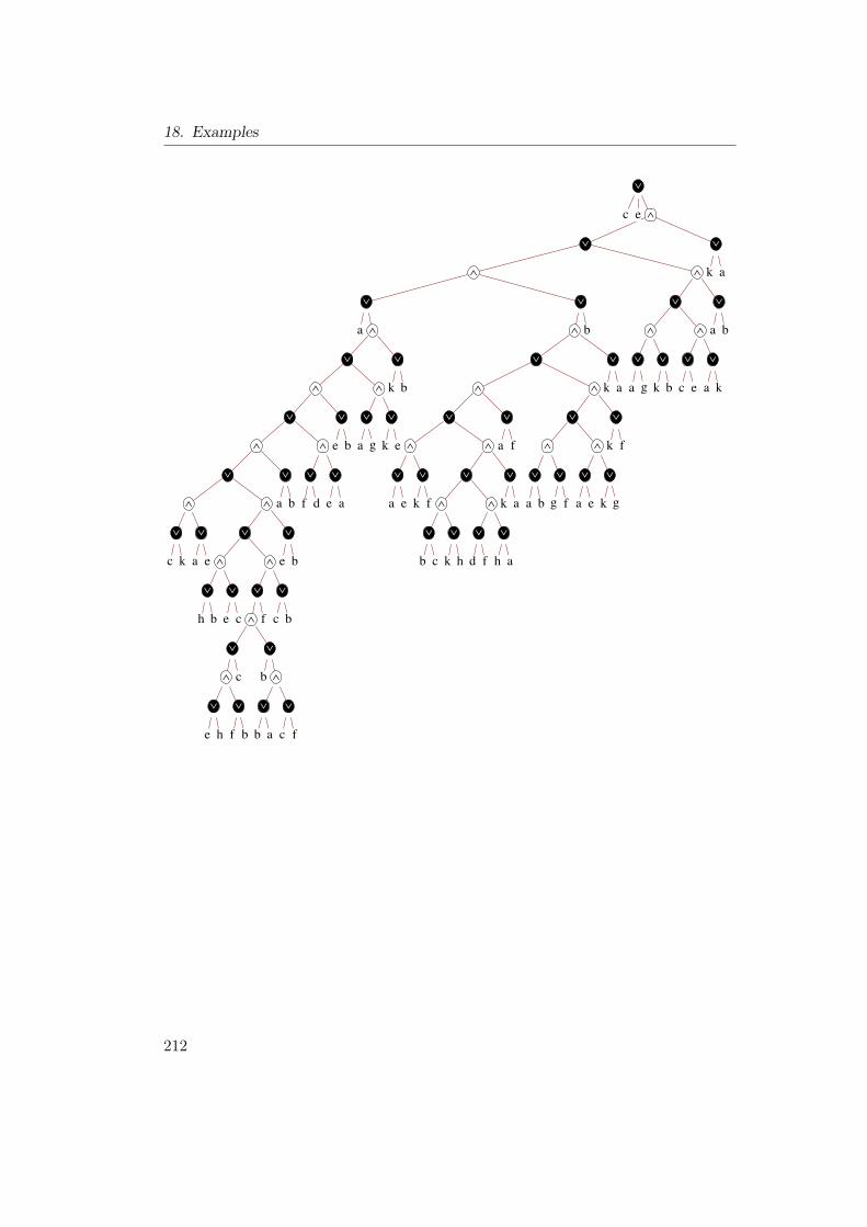
18. Examples
!! !
!! !
! !! !
! !!
! !
!! !
! !! !
! !
! !
"c e
""a
""
""c k
"a e
""h b
"e c
""
"e h
"f b
c
"b
"b a
"c f
f
"c b
"e b
"a b
"f d
"e a
"e b
"a g
"k e
"k b
""
""a e
"k f
""b c
"k h
"d f
"h a
"k a
"a f
""a b
"g f
"a e
"k g
"k f
"k a
b
""a g
"k b
"c e
"a k
"a b
"k a
212
18.2. Example 2: Ten Points on a Cubic
18.2. Example 2: Ten Points on a Cubic
Inspired by Pascal’s theorem, it is natural to ask for a condition for ten pointslying on a common cubic. We will factor a bracket polynomial with 20 summandsdescribing this situation. This representation is due to Richter-Gebert and to theknowledge of our research group, it is the shortest known representation of thepolynomial. In particular, this bracket polynomial is far from being multilinear andwe ask for a ruler construction to interpret it. The conic condition is interestingand of degree two. For cubics, the Cayley factorization might be interesting, sincethere can arise more coincidences in the execution of the algorithm.We know of two different synthetic constructions characterizing the situation: the
first one is due to [17] and [19]. The construction needs some intermediate steps notcarried out in detail in the original references. A straightforward construction, whichalso fills the gaps and which was obtained by the author, yields a construction wherethe degree of the multiplier polynomial is 626. However, the computation cannotbe carried out in detail and it is unlikely that the multiplier is in fact a monomial.The second construction is given in [61] and the degree of the multiplier is 113. Thesame comments on the shape of the multiplier apply. The following factorizationyields a multiplier monomial of degree 342. This shows, that in concrete instances,the actual result is much better than the bound given in Theorem 14.5. However,the optimizations done in the concrete implementation turn out to be useful in thepresent example: a first execution of the algorithm lead to a multiplier monomialof degree 603, a more advanced triangulation of the cycles in the binomial stepof the algorithm yielded 544. Here, common factors in the monomial step werenot factored out. Instead, they were altered such that they could be treated asto be distinct. The actual factoring out lead to the present degree of 342. Theexample is given in order to show that polynomials of this can be treated andthat the degree of the multiplier is not as big as expected. However, we do nothave enough space to give the complete output and large parts are omitted. Afterhanding in this thesis, the complete output will be made available under http://www-m10.ma.tum.de/CayleyFactorizationExtras.
213

18. Examples
B := [0,1,9][0,5,2][6,1,2][6,5,9][1,7,8][2,3,7][4,3,9][4,5,7][4,6,8][0,3,8]
−[6,5,2][0,5,9][0,1,2][9,6,1][1,7,8][2,3,7][4,3,9][4,5,7][4,6,8][0,3,8]
−[0,1,8][3,8,7][0,5,9][1,2,7][1,6,9][3,2,0][4,3,9][4,5,7][4,6,8][5,2,6]
+[0,1,9][0,3,5][0,7,8][1,2,7][1,6,8][2,3,9][4,3,8][4,5,7][4,6,9][5,2,6]
−[0,1,9][0,3,8][0,5,7][1,2,7][1,6,8][2,3,5][4,3,9][4,5,6][4,7,8][2,6,9]
+[1,2,9][0,3,9][0,5,8][1,0,6][1,7,8][2,3,7][4,3,8][4,5,7][4,6,9][5,2,6]
+[0,1,8][0,3,9][0,5,7][1,2,7][1,6,9][2,3,8][4,3,6][4,5,9][4,7,8][5,2,6]
+[0,1,9][0,3,8][0,5,6][1,2,6][1,7,8][2,3,9][4,3,7][4,6,9][4,5,8][5,2,7]
+[0,1,9][0,3,2][0,5,8][1,2,6][1,7,8][9,3,6][4,3,8][4,5,6][4,7,9][5,2,7]
+[0,3,8][0,5,9][1,0,7][1,6,9][1,2,8][2,3,6][4,3,9][4,5,6][4,7,8][5,2,7]
−[0,1,8][0,3,5][0,9,6][1,2,6][1,7,9][2,3,8][4,3,9][4,5,6][4,7,8][5,2,7]
−[0,1,8][0,3,9][0,5,6][1,2,6][1,7,9][2,3,5][4,3,8][4,5,7][4,6,9][8,2,7]
+[0,1,8][0,3,9][0,5,2][1,2,7][1,6,9][2,3,6][4,3,8][4,5,6][4,7,9][5,8,7]
−[0,1,9][0,3,8][0,5,7][1,2,7][1,6,8][2,3,9][4,3,5][4,6,9][4,7,8][5,2,6]
−[0,1,8][0,3,9][0,5,2][1,2,7][1,6,9][8,3,7][4,3,8][4,5,7][4,6,9][5,2,6]
+[0,1,8][0,3,9][0,5,3][1,2,7][1,6,9][2,7,8][4,3,8][4,5,7][4,6,9][5,2,6]
−[0,3,9][0,5,8][1,0,2][1,6,9][1,7,8][2,3,6][4,3,8][4,5,6][4,7,9][5,2,7]
+[0,1,9][0,3,8][0,5,2][1,2,6][1,7,8][6,3,9][4,3,9][4,5,6][4,7,8][5,2,7]
−[0,1,9][0,3,8][0,5,3][1,2,6][1,7,8][2,9,6][4,3,9][4,5,6][4,7,8][5,2,7]
−[0,1,8][0,3,9][0,5,6][1,2,6][1,7,9][2,3,8][4,3,5][4,6,9][4,7,8][5,2,7]
Formatting and pre-processing input:
The bracket polynomial is processed such that it is composed of summands with allbut the last coefficient equal to +1. The last coefficient is -1. Cayley factorizationyields a ∨-∧-sequence to interpret it. Intuition is provided by interpreting thevanishing of the bracket polynomial:
B = 0
⇐⇒
[0,1,9][0,5,2][6,1,2][6,5,9][1,7,8][2,3,7][4,3,9][4,5,7][4,6,8][0,3,8][0,1,9][0,3,8][0,5,7][1,2,7][1,6,8][2,3,9][4,3,5][4,6,9][4,7,8][5,2,6] +
214

18.2. Example 2: Ten Points on a Cubic
[5,6,2][0,5,9][0,1,2][9,6,1][1,7,8][2,3,7][4,3,9][4,5,7][4,6,8][0,3,8][0,1,9][0,3,8][0,5,7][1,2,7][1,6,8][2,3,9][4,3,5][4,6,9][4,7,8][5,2,6] +
[1,0,8][3,8,7][0,5,9][1,2,7][1,6,9][3,2,0][4,3,9][4,5,7][4,6,8][5,2,6][0,1,9][0,3,8][0,5,7][1,2,7][1,6,8][2,3,9][4,3,5][4,6,9][4,7,8][5,2,6] +
[0,1,9][0,3,5][0,7,8][1,2,7][1,6,8][2,3,9][4,3,8][4,5,7][4,6,9][5,2,6][0,1,9][0,3,8][0,5,7][1,2,7][1,6,8][2,3,9][4,3,5][4,6,9][4,7,8][5,2,6] +
[1,0,9][0,3,8][0,5,7][1,2,7][1,6,8][2,3,5][4,3,9][4,5,6][4,7,8][2,6,9][0,1,9][0,3,8][0,5,7][1,2,7][1,6,8][2,3,9][4,3,5][4,6,9][4,7,8][5,2,6] +
[1,2,9][0,3,9][0,5,8][1,0,6][1,7,8][2,3,7][4,3,8][4,5,7][4,6,9][5,2,6][0,1,9][0,3,8][0,5,7][1,2,7][1,6,8][2,3,9][4,3,5][4,6,9][4,7,8][5,2,6] +
[0,1,8][0,3,9][0,5,7][1,2,7][1,6,9][2,3,8][4,3,6][4,5,9][4,7,8][5,2,6][0,1,9][0,3,8][0,5,7][1,2,7][1,6,8][2,3,9][4,3,5][4,6,9][4,7,8][5,2,6] +
[0,1,9][0,3,8][0,5,6][1,2,6][1,7,8][2,3,9][4,3,7][4,6,9][4,5,8][5,2,7][0,1,9][0,3,8][0,5,7][1,2,7][1,6,8][2,3,9][4,3,5][4,6,9][4,7,8][5,2,6] +
[0,1,9][0,3,2][0,5,8][1,2,6][1,7,8][9,3,6][4,3,8][4,5,6][4,7,9][5,2,7][0,1,9][0,3,8][0,5,7][1,2,7][1,6,8][2,3,9][4,3,5][4,6,9][4,7,8][5,2,6] +
[0,3,8][0,5,9][1,0,7][1,6,9][1,2,8][2,3,6][4,3,9][4,5,6][4,7,8][5,2,7][0,1,9][0,3,8][0,5,7][1,2,7][1,6,8][2,3,9][4,3,5][4,6,9][4,7,8][5,2,6] +
[1,0,8][0,3,5][0,9,6][1,2,6][1,7,9][2,3,8][4,3,9][4,5,6][4,7,8][5,2,7][0,1,9][0,3,8][0,5,7][1,2,7][1,6,8][2,3,9][4,3,5][4,6,9][4,7,8][5,2,6] +
[1,0,8][0,3,9][0,5,6][1,2,6][1,7,9][2,3,5][4,3,8][4,5,7][4,6,9][8,2,7][0,1,9][0,3,8][0,5,7][1,2,7][1,6,8][2,3,9][4,3,5][4,6,9][4,7,8][5,2,6] +
[0,1,8][0,3,9][0,5,2][1,2,7][1,6,9][2,3,6][4,3,8][4,5,6][4,7,9][5,8,7][0,1,9][0,3,8][0,5,7][1,2,7][1,6,8][2,3,9][4,3,5][4,6,9][4,7,8][5,2,6] +
[1,0,8][0,3,9][0,5,2][1,2,7][1,6,9][8,3,7][4,3,8][4,5,7][4,6,9][5,2,6][0,1,9][0,3,8][0,5,7][1,2,7][1,6,8][2,3,9][4,3,5][4,6,9][4,7,8][5,2,6] +
[0,1,8][0,3,9][0,5,3][1,2,7][1,6,9][2,7,8][4,3,8][4,5,7][4,6,9][5,2,6][0,1,9][0,3,8][0,5,7][1,2,7][1,6,8][2,3,9][4,3,5][4,6,9][4,7,8][5,2,6] +
[3,0,9][0,5,8][1,0,2][1,6,9][1,7,8][2,3,6][4,3,8][4,5,6][4,7,9][5,2,7][0,1,9][0,3,8][0,5,7][1,2,7][1,6,8][2,3,9][4,3,5][4,6,9][4,7,8][5,2,6] +
[0,1,9][0,3,8][0,5,2][1,2,6][1,7,8][6,3,9][4,3,9][4,5,6][4,7,8][5,2,7][0,1,9][0,3,8][0,5,7][1,2,7][1,6,8][2,3,9][4,3,5][4,6,9][4,7,8][5,2,6] +
[1,0,9][0,3,8][0,5,3][1,2,6][1,7,8][2,9,6][4,3,9][4,5,6][4,7,8][5,2,7][0,1,9][0,3,8][0,5,7][1,2,7][1,6,8][2,3,9][4,3,5][4,6,9][4,7,8][5,2,6] +
[1,0,8][0,3,9][0,5,6][1,2,6][1,7,9][2,3,8][4,3,5][4,6,9][4,7,8][5,2,7][0,1,9][0,3,8][0,5,7][1,2,7][1,6,8][2,3,9][4,3,5][4,6,9][4,7,8][5,2,6] = 1
Start of the Main Part of the Algorithm:
Factor all induced fractional equations [∗,∗,∗]...[∗,∗,∗][∗,∗,∗]...[∗,∗,∗] = 1
215

18. Examples
—–Factorize the fractional equation[1,0,8][0,3,9][0,5,6][1,2,6][1,7,9][2,3,8][4,3,5][4,6,9][4,7,8][5,2,7][0,1,9][0,3,8][0,5,7][1,2,7][1,6,8][2,3,9][4,3,5][4,6,9][4,7,8][5,2,6]
= 1
Brackets occurring in the numerator as well as in the denominator can be canceled.The common elements are: [3,4,5], [4,6,9], [4,7,8]
This reduces the bracket identity in question to:
[1,0,8][0,3,9][0,5,6][1,2,6][1,7,9][2,3,8][5,2,7]
[0,1,9][0,3,8][0,5,7][1,2,7][1,6,8][2,3,9][5,2,6]= 1
Find a Matching in order to apply the area principle:
!1, 0, 8"!0, 3, 9"!0, 5, 6"!1, 2, 6"!1, 7, 9"
!2, 3, 8"!5, 2, 7"!0, 1, 9"!0, 3, 8"!0, 5, 7"!1, 2, 7"!1, 6, 8"
!2, 3, 9"!5, 2, 6"
Apply the area principle to fractions corresponding to the matching just found:
[1,0,8][1,6,8]
→ (18 ∧ 06)
[0,3,9][0,3,8]
→ (03 ∧ 98)
[0,5,6][0,5,7]
→ (05 ∧ 67)
[1,2,6][1,2,7]
→ (12 ∧ 67)
[1,7,9][0,1,9]
→ (19 ∧ 70)
[2,3,8][2,3,9]
→ (23 ∧ 89)[5,2,7][5,2,6]
→ (52 ∧ 76)
Product of sign-errors occurring when applying the area principle: ε = −1
Find and triangulate Cycles
Length-ratios left over to be processed: (18 ∧ 06) (03 ∧ 98) (05 ∧ 67) (12 ∧67) (19 ∧ 70) (23 ∧ 89) (52 ∧ 76)
Cycle found:(18 ∧ 06) (12 ∧ 67) (19 ∧ 70)
216
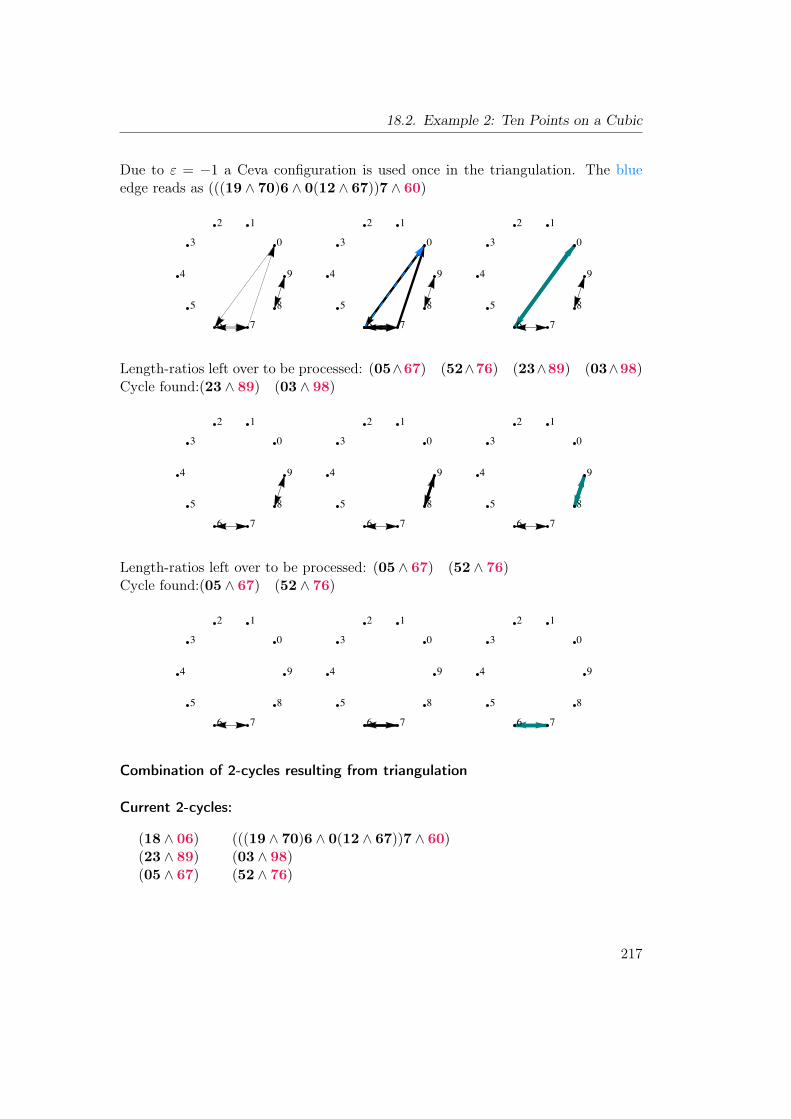
18.2. Example 2: Ten Points on a Cubic
Due to ε = −1 a Ceva configuration is used once in the triangulation. The blueedge reads as (((19 ∧ 70)6 ∧ 0(12 ∧ 67))7 ∧ 60)
0
12
3
4
5
6 7
8
9
0
12
3
4
5
6 7
8
9
0
12
3
4
5
6 7
8
9
Length-ratios left over to be processed: (05∧67) (52∧76) (23∧89) (03∧98)Cycle found:(23 ∧ 89) (03 ∧ 98)
0
12
3
4
5
6 7
8
9
0
12
3
4
5
6 7
8
9
0
12
3
4
5
6 7
8
9
Length-ratios left over to be processed: (05 ∧ 67) (52 ∧ 76)Cycle found:(05 ∧ 67) (52 ∧ 76)
0
12
3
4
5
6 7
8
9
0
12
3
4
5
6 7
8
9
0
12
3
4
5
6 7
8
9
Combination of 2-cycles resulting from triangulation
Current 2-cycles:
(18 ∧ 06) (((19 ∧ 70)6 ∧ 0(12 ∧ 67))7 ∧ 60)(23 ∧ 89) (03 ∧ 98)(05 ∧ 67) (52 ∧ 76)
217

18. Examples
0
12
3
4
5
6 7
8
9
The following 2-cycles are to be combined:
(05 ∧ 67) (52 ∧ 76)(18 ∧ 06) (((19 ∧ 70)6 ∧ 0(12 ∧ 67))7 ∧ 60)
We have |7,6,6,0| = 3 and 6 = 6 which indicates Case 3 (iii) and results in:
(05 ∧ 67) (((((19∧70)6∧0(12∧67))7∧60)(52∧76)∧70)(18∧06)∧76)
Current 2-cycles:
(05 ∧ 67) (((((19∧70)6∧0(12∧67))7∧60)(52∧76)∧70)(18∧06)∧76)(23 ∧ 89) (03 ∧ 98)
0
12
3
4
5
6 7
8
9
The following 2-cycles are to be combined:
(05 ∧ 67) (((((19∧70)6∧0(12∧67))7∧60)(52∧76)∧70)(18∧06)∧76)(23 ∧ 89) (03 ∧ 98)
218

18.2. Example 2: Ten Points on a Cubic
We have |7,6,9,8| = 4 and |2,3,7| = 3 which indicates Case 4 (i) and resultsin:
(05 ∧ 67) (((23 ∧ 78)(((((19 ∧ 70)6 ∧ 0(12 ∧ 67))7 ∧ 60)(52 ∧ 76) ∧70)(18 ∧ 06) ∧ 76) ∧ 68)((03 ∧ 98)(23 ∧ 79) ∧ 78) ∧ 76)
Current 2-cycles:
(05 ∧ 67) (((23 ∧ 78)(((((19 ∧ 70)6 ∧ 0(12 ∧ 67))7 ∧ 60)(52 ∧ 76) ∧70)(18 ∧ 06) ∧ 76) ∧ 68)((03 ∧ 98)(23 ∧ 79) ∧ 78) ∧ 76)
0
12
3
4
5
6 7
8
9
[1,0,8][0,3,9][0,5,6][1,2,6][1,7,9][2,3,8][4,3,5][4,6,9][4,7,8][5,2,7][0,1,9][0,3,8][0,5,7][1,2,7][1,6,8][2,3,9][4,3,5][4,6,9][4,7,8][5,2,6] = 1 whenever the bothintermediate points are identical:
(05 ∧ 67) (((23 ∧ 78)(((((19 ∧ 70)6 ∧ 0(12 ∧ 67))7 ∧ 60)(52 ∧ 76) ∧70)(18 ∧ 06) ∧ 76) ∧ 68)((03 ∧ 98)(23 ∧ 79) ∧ 78) ∧ 76)
—–Factorize the fractional equation[1,0,9][0,3,8][0,5,3][1,2,6][1,7,8][2,9,6][4,3,9][4,5,6][4,7,8][5,2,7][0,1,9][0,3,8][0,5,7][1,2,7][1,6,8][2,3,9][4,3,5][4,6,9][4,7,8][5,2,6]
= 1
Brackets occurring in the numerator as well as in the denominator can be canceled.The common elements are: [0,1,9], [0,3,8], [4,7,8]
This reduces the bracket identity in question to:
[5,0,3][1,2,6][1,7,8][2,9,6][4,3,9][4,5,6][5,2,7]
[0,5,7][1,2,7][1,6,8][2,3,9][4,3,5][4,6,9][5,2,6]= 1
219

18. Examples
Find a Matching in order to apply the area principle:
!5, 0, 3"!1, 2, 6"!1, 7, 8"!2, 9, 6"!4, 3, 9"
!4, 5, 6"!5, 2, 7"!0, 5, 7"!1, 2, 7"!1, 6, 8"!2, 3, 9"!4, 3, 5"
!4, 6, 9"!5, 2, 6"
Apply the area principle to fractions corresponding to the matching just found:[5,0,3][0,5,7]
→ (50 ∧ 37)
[1,2,6][1,2,7]
→ (12 ∧ 67)
[1,7,8][1,6,8]
→ (18 ∧ 76)
[2,9,6][2,3,9]
→ (29 ∧ 63)
[4,3,9][4,3,5]
→ (43 ∧ 95)
[4,5,6][4,6,9]
→ (46 ∧ 59)[5,2,7][5,2,6]
→ (52 ∧ 76)
Product of sign-errors occurring when applying the area principle: ε = −1
Find and triangulate Cycles
Length-ratios left over to be processed: (50 ∧ 37) (12 ∧ 67) (18 ∧ 76) (29 ∧63) (43 ∧ 95) (46 ∧ 59) (52 ∧ 76)
Cycle found:(50 ∧ 37) (18 ∧ 76) (29 ∧ 63)
Due to ε = −1 a Ceva configuration is used once in the triangulation. The blueedge reads as (((29 ∧ 63)7 ∧ 3(18 ∧ 76))6 ∧ 73)
0
12
3
4
5
6 7
8
9
0
12
3
4
5
6 7
8
9
0
12
3
4
5
6 7
8
9
220

18.2. Example 2: Ten Points on a Cubic
Length-ratios left over to be processed: (12∧67) (52∧76) (46∧59) (43∧95)Cycle found:(46 ∧ 59) (43 ∧ 95)
0
12
3
4
5
6 7
8
9
0
12
3
4
5
6 7
8
9
0
12
3
4
5
6 7
8
9
Length-ratios left over to be processed: (12 ∧ 67) (52 ∧ 76)Cycle found:(12 ∧ 67) (52 ∧ 76)
0
12
3
4
5
6 7
8
9
0
12
3
4
5
6 7
8
9
0
12
3
4
5
6 7
8
9
Combination of 2-cycles resulting from triangulation
Current 2-cycles:
(50 ∧ 37) (((29 ∧ 63)7 ∧ 3(18 ∧ 76))6 ∧ 73)(46 ∧ 59) (43 ∧ 95)(12 ∧ 67) (52 ∧ 76)
0
12
3
4
5
6 7
8
9
221

18. Examples
The following 2-cycles are to be combined:
(12 ∧ 67) (52 ∧ 76)(50 ∧ 37) (((29 ∧ 63)7 ∧ 3(18 ∧ 76))6 ∧ 73)
We have |7,6,7,3| = 3 and 7 = 7 which indicates Case 3 (ii) and results in:
(12 ∧ 67) (((50∧37)(52∧76)∧36)(((29∧63)7∧3(18∧76))6∧73)∧76)
Current 2-cycles:
(46 ∧ 59) (43 ∧ 95)(12 ∧ 67) (((50∧37)(52∧76)∧36)(((29∧63)7∧3(18∧76))6∧73)∧76)
0
12
3
4
5
6 7
8
9
The following 2-cycles are to be combined:
(12 ∧ 67) (((50∧37)(52∧76)∧36)(((29∧63)7∧3(18∧76))6∧73)∧76)(46 ∧ 59) (43 ∧ 95)
We have |7,6,9,5| = 4 and |4,6,7| = 3 which indicates Case 4 (i) and resultsin:
(12 ∧ 67) (((46 ∧ 75)(((50 ∧ 37)(52 ∧ 76) ∧ 36)(((29 ∧ 63)7 ∧ 3(18 ∧76))6 ∧ 73) ∧ 76) ∧ 65)((43 ∧ 95)(46 ∧ 79) ∧ 75) ∧ 76)
Current 2-cycles:
(12 ∧ 67) (((46 ∧ 75)(((50 ∧ 37)(52 ∧ 76) ∧ 36)(((29 ∧ 63)7 ∧ 3(18 ∧76))6 ∧ 73) ∧ 76) ∧ 65)((43 ∧ 95)(46 ∧ 79) ∧ 75) ∧ 76)
222

18.2. Example 2: Ten Points on a Cubic
0
12
3
4
5
6 7
8
9
[1,0,9][0,3,8][0,5,3][1,2,6][1,7,8][2,9,6][4,3,9][4,5,6][4,7,8][5,2,7][0,1,9][0,3,8][0,5,7][1,2,7][1,6,8][2,3,9][4,3,5][4,6,9][4,7,8][5,2,6] = 1 whenever the bothintermediate points are identical:
(12 ∧ 67) (((46 ∧ 75)(((50 ∧ 37)(52 ∧ 76) ∧ 36)(((29 ∧ 63)7 ∧ 3(18 ∧76))6 ∧ 73) ∧ 76) ∧ 65)((43 ∧ 95)(46 ∧ 79) ∧ 75) ∧ 76)
—–Factorize the fractional equation[0,1,9][0,3,8][0,5,2][1,2,6][1,7,8][6,3,9][4,3,9][4,5,6][4,7,8][5,2,7][0,1,9][0,3,8][0,5,7][1,2,7][1,6,8][2,3,9][4,3,5][4,6,9][4,7,8][5,2,6]
= 1
Brackets occurring in the numerator as well as in the denominator can be canceled.The common elements are: [0,1,9], [0,3,8], [4,7,8]
[omitted output]
In order to factor the complete bracket polynomial, one has to projectively add
(05 ∧ 67) (((23∧78)(((((19∧70)6∧0(12∧67))7∧60)(52∧76)∧70)(18∧06) ∧ 76) ∧ 68)((03 ∧ 98)(23 ∧ 79) ∧ 78) ∧ 76)
(12 ∧ 67) (((46∧75)(((50∧37)(52∧76)∧36)(((29∧63)7∧3(18∧76))6∧73) ∧ 76) ∧ 65)((43 ∧ 95)(46 ∧ 79) ∧ 75) ∧ 76)
223

18. Examples
(12 ∧ 67) (((46∧75)(((05∧27)(52∧76)∧26)(((39∧62)7∧2(18∧76))6∧72) ∧ 76) ∧ 65)((43 ∧ 95)(46 ∧ 79) ∧ 75) ∧ 76)
(12 ∧ 07) ((49∧76)((23∧69)((16∧98)((43∧85)((08∧53)((09∧31)((78∧14)((56∧42)(57∧20)∧40)∧10)∧30)∧50)∧80)∧90)∧60)∧70)
(39 ∧ 02) (((01∧28)(((57∧40)2∧0(78∧24))4∧20)∧08)((((43∧85)(16∧98) ∧ 95)(03 ∧ 58) ∧ 98)(01 ∧ 29) ∧ 28) ∧ 20)
(39 ∧ 02) (((10∧28)((05∧27)((45∧73)((87∧34)(38∧40)∧30)∧70)∧20) ∧ 08)((16 ∧ 98)(10 ∧ 29) ∧ 28) ∧ 20)
(01 ∧ 89) (((23∧69)(47∧98)∧68)(((46∧59)((03∧98)((57∧80)(52∧06) ∧ 86) ∧ 96) ∧ 56)((16 ∧ 98)(43 ∧ 85) ∧ 95) ∧ 96) ∧ 98)
(18 ∧ 06) (((23 ∧ 65)((05 ∧ 67)(19 ∧ 70) ∧ 60) ∧ 05)(((((47 ∧ 58)(27 ∧81) ∧ 51)((03 ∧ 98)(43 ∧ 85) ∧ 95) ∧ 91)(26 ∧ 15) ∧ 95)(23 ∧69) ∧ 65) ∧ 60)
(18 ∧ 06) (((03 ∧ 65)(((96 ∧ 04)((12 ∧ 67)(19 ∧ 70) ∧ 60) ∧ 64)((56 ∧42)(57 ∧ 20) ∧ 40) ∧ 60) ∧ 05)(((23 ∧ 89)(43 ∧ 95) ∧ 85)(03 ∧68) ∧ 65) ∧ 60)
(23 ∧ 69) (((46∧59)((16∧98)((12∧87)(52∧76)∧86)∧96)∧56)(((09∧51)(43 ∧ 95) ∧ 91)(07 ∧ 15) ∧ 95) ∧ 96)
(47 ∧ 98) (((((12∧67)((18∧76)((93∧62)(03∧28)∧68)∧78)∧68)(52∧76) ∧ 78)((43 ∧ 85)(46 ∧ 59) ∧ 89) ∧ 97)(05 ∧ 87) ∧ 89)
(12 ∧ 67) (((48∧57)((07∧ (18∧76)5)(56∧ (52∧76)0)∧76)∧56)(43∧75) ∧ 76)
(49 ∧ 56) (((23∧68)(43∧65)∧58)(((09∧ (03∧98)1)(18∧ (16∧98)0)∧98)(23 ∧ 69) ∧ 68) ∧ 65)
(03 ∧ 98) (((47∧58)((05∧87)(23∧79)∧89)∧59)(((16∧08)(43∧85)∧05)((17 ∧ 82)(19 ∧ 20) ∧ 80) ∧ 85) ∧ 89)
(46 ∧ 59) ((39 ∧ (43 ∧ 95)2)(25 ∧ (26 ∧ 95)3) ∧ 95)(47 ∧ 58) ((08 ∧ (07 ∧ 85)3)(35 ∧ (43 ∧ 85)0) ∧ 85)(46 ∧ 89) (((((43∧95)8∧5(10∧89))9∧85)(((32∧09)(16∧98)∧08)((05∧
97)(38 ∧ 70) ∧ 90) ∧ 98) ∧ 95)(47 ∧ 58) ∧ 98)(46 ∧ 89) (((23∧79)(61∧98)∧78)((43∧95)((09∧51)((78∧14)((57∧
40)(12 ∧ 07) ∧ 47) ∧ 17) ∧ 57) ∧ 97) ∧ 98)(46 ∧ 89) (((23∧79)(((47∧58)9∧8(43∧95))5∧98)∧78)(((18∧76)((65∧
92)(05 ∧ 27) ∧ 97) ∧ 96)(12 ∧ 67) ∧ 97) ∧ 98)
224

18.2. Example 2: Ten Points on a Cubic
0
12
3
4
5
6 7
8
9
Adding up all cross-ratios
Similar to the situation before, two 2-cycles can be reduced to a single 2-cycle byprojective addition. In the following, in each step, the last two 2-cycles in the listare combined.We have |9,8,9,8| = 2 and 9 = 9 and 8 = 8 which indicates Case 2 (i).
Resulting 2-cycles:
(05 ∧ 67) (((23 ∧ 78)(((((19 ∧ 70)6 ∧ 0(12 ∧ 67))7 ∧ 60)(52 ∧ 76) ∧70)(18 ∧ 06) ∧ 76) ∧ 68)((03 ∧ 98)(23 ∧ 79) ∧ 78) ∧ 76)
(12 ∧ 67) (((46 ∧ 75)(((50 ∧ 37)(52 ∧ 76) ∧ 36)(((29 ∧ 63)7 ∧ 3(18 ∧76))6 ∧ 73) ∧ 76) ∧ 65)((43 ∧ 95)(46 ∧ 79) ∧ 75) ∧ 76)
(12 ∧ 67) (((46 ∧ 75)(((05 ∧ 27)(52 ∧ 76) ∧ 26)(((39 ∧ 62)7 ∧ 2(18 ∧76))6 ∧ 72) ∧ 76) ∧ 65)((43 ∧ 95)(46 ∧ 79) ∧ 75) ∧ 76)
(12 ∧ 07) ((49 ∧ 76)((23 ∧ 69)((16 ∧ 98)((43 ∧ 85)((08 ∧ 53)((09 ∧31)((78 ∧ 14)((56 ∧ 42)(57 ∧ 20) ∧ 40) ∧ 10) ∧ 30) ∧ 50) ∧80) ∧ 90) ∧ 60) ∧ 70)
(39 ∧ 02) (((01 ∧ 28)(((57 ∧ 40)2 ∧ 0(78 ∧ 24))4 ∧ 20) ∧ 08)((((43 ∧85)(16 ∧ 98) ∧ 95)(03 ∧ 58) ∧ 98)(01 ∧ 29) ∧ 28) ∧ 20)
(39 ∧ 02) (((10 ∧ 28)((05 ∧ 27)((45 ∧ 73)((87 ∧ 34)(38 ∧ 40) ∧ 30) ∧70) ∧ 20) ∧ 08)((16 ∧ 98)(10 ∧ 29) ∧ 28) ∧ 20)
(01 ∧ 89) (((23∧69)(47∧98)∧68)(((46∧59)((03∧98)((57∧80)(52∧06) ∧ 86) ∧ 96) ∧ 56)((16 ∧ 98)(43 ∧ 85) ∧ 95) ∧ 96) ∧ 98)
(18 ∧ 06) (((23 ∧ 65)((05 ∧ 67)(19 ∧ 70) ∧ 60) ∧ 05)(((((47 ∧ 58)(27 ∧81)∧ 51)((03∧ 98)(43∧ 85)∧ 95)∧ 91)(26∧ 15)∧ 95)(23∧69) ∧ 65) ∧ 60)
(18 ∧ 06) (((03 ∧ 65)(((96 ∧ 04)((12 ∧ 67)(19 ∧ 70) ∧ 60) ∧ 64)((56 ∧42)(57∧20)∧40)∧60)∧05)(((23∧89)(43∧95)∧85)(03∧68) ∧ 65) ∧ 60)
(23 ∧ 69) (((46∧59)((16∧98)((12∧87)(52∧76)∧86)∧96)∧56)(((09∧51)(43 ∧ 95) ∧ 91)(07 ∧ 15) ∧ 95) ∧ 96)
(47 ∧ 98) (((((12∧67)((18∧76)((93∧62)(03∧28)∧68)∧78)∧68)(52∧76) ∧ 78)((43 ∧ 85)(46 ∧ 59) ∧ 89) ∧ 97)(05 ∧ 87) ∧ 89)
225

18. Examples
(12 ∧ 67) (((48∧57)((07∧(18∧76)5)(56∧(52∧76)0)∧76)∧56)(43∧75) ∧ 76)
(49 ∧ 56) (((23∧68)(43∧65)∧58)(((09∧(03∧98)1)(18∧(16∧98)0)∧98)(23 ∧ 69) ∧ 68) ∧ 65)
(03 ∧ 98) (((47 ∧ 58)((05 ∧ 87)(23 ∧ 79) ∧ 89) ∧ 59)(((16 ∧ 08)(43 ∧85) ∧ 05)((17 ∧ 82)(19 ∧ 20) ∧ 80) ∧ 85) ∧ 89)
(46 ∧ 59) ((39 ∧ (43 ∧ 95)2)(25 ∧ (26 ∧ 95)3) ∧ 95)(47 ∧ 58) ((08 ∧ (07 ∧ 85)3)(35 ∧ (43 ∧ 85)0) ∧ 85)(46 ∧ 89) (((((43 ∧ 95)8 ∧ 5(10 ∧ 89))9 ∧ 85)(((32 ∧ 09)(16 ∧ 98) ∧
08)((05 ∧ 97)(38 ∧ 70) ∧ 90) ∧ 98) ∧ 95)(47 ∧ 58) ∧ 98)(46 ∧ 89) ((8(69∧4(46∧89))∧(((23∧79)(61∧98)∧78)((43∧95)((09∧
51)((78∧14)((57∧40)(12∧07)∧47)∧17)∧57)∧97)∧98)(69∧48))(6(((23∧79)(((47∧58)9∧8(43∧95))5∧98)∧78)(((18∧76)((65∧92)(05∧27)∧97)∧96)(12∧67)∧97)∧98)∧48)∧98)
0
12
3
4
5
6 7
8
9
We have |9,8,9,8| = 2 and 9 = 9 and 8 = 8 which indicates Case 2 (i).
Resulting 2-cycles:
(05 ∧ 67) (((23 ∧ 78)(((((19 ∧ 70)6 ∧ 0(12 ∧ 67))7 ∧ 60)(52 ∧ 76) ∧70)(18 ∧ 06) ∧ 76) ∧ 68)((03 ∧ 98)(23 ∧ 79) ∧ 78) ∧ 76)
(12 ∧ 67) (((46 ∧ 75)(((50 ∧ 37)(52 ∧ 76) ∧ 36)(((29 ∧ 63)7 ∧ 3(18 ∧76))6 ∧ 73) ∧ 76) ∧ 65)((43 ∧ 95)(46 ∧ 79) ∧ 75) ∧ 76)
(12 ∧ 67) (((46 ∧ 75)(((05 ∧ 27)(52 ∧ 76) ∧ 26)(((39 ∧ 62)7 ∧ 2(18 ∧76))6 ∧ 72) ∧ 76) ∧ 65)((43 ∧ 95)(46 ∧ 79) ∧ 75) ∧ 76)
(12 ∧ 07) ((49 ∧ 76)((23 ∧ 69)((16 ∧ 98)((43 ∧ 85)((08 ∧ 53)((09 ∧31)((78 ∧ 14)((56 ∧ 42)(57 ∧ 20) ∧ 40) ∧ 10) ∧ 30) ∧ 50) ∧80) ∧ 90) ∧ 60) ∧ 70)
(39 ∧ 02) (((01 ∧ 28)(((57 ∧ 40)2 ∧ 0(78 ∧ 24))4 ∧ 20) ∧ 08)((((43 ∧85)(16 ∧ 98) ∧ 95)(03 ∧ 58) ∧ 98)(01 ∧ 29) ∧ 28) ∧ 20)
226

18.2. Example 2: Ten Points on a Cubic
(39 ∧ 02) (((10 ∧ 28)((05 ∧ 27)((45 ∧ 73)((87 ∧ 34)(38 ∧ 40) ∧ 30) ∧70) ∧ 20) ∧ 08)((16 ∧ 98)(10 ∧ 29) ∧ 28) ∧ 20)
(01 ∧ 89) (((23∧69)(47∧98)∧68)(((46∧59)((03∧98)((57∧80)(52∧06) ∧ 86) ∧ 96) ∧ 56)((16 ∧ 98)(43 ∧ 85) ∧ 95) ∧ 96) ∧ 98)
(18 ∧ 06) (((23 ∧ 65)((05 ∧ 67)(19 ∧ 70) ∧ 60) ∧ 05)(((((47 ∧ 58)(27 ∧81)∧ 51)((03∧ 98)(43∧ 85)∧ 95)∧ 91)(26∧ 15)∧ 95)(23∧69) ∧ 65) ∧ 60)
(18 ∧ 06) (((03 ∧ 65)(((96 ∧ 04)((12 ∧ 67)(19 ∧ 70) ∧ 60) ∧ 64)((56 ∧42)(57∧20)∧40)∧60)∧05)(((23∧89)(43∧95)∧85)(03∧68) ∧ 65) ∧ 60)
(23 ∧ 69) (((46∧59)((16∧98)((12∧87)(52∧76)∧86)∧96)∧56)(((09∧51)(43 ∧ 95) ∧ 91)(07 ∧ 15) ∧ 95) ∧ 96)
(47 ∧ 98) (((((12∧67)((18∧76)((93∧62)(03∧28)∧68)∧78)∧68)(52∧76) ∧ 78)((43 ∧ 85)(46 ∧ 59) ∧ 89) ∧ 97)(05 ∧ 87) ∧ 89)
(12 ∧ 67) (((48∧57)((07∧(18∧76)5)(56∧(52∧76)0)∧76)∧56)(43∧75) ∧ 76)
(49 ∧ 56) (((23∧68)(43∧65)∧58)(((09∧(03∧98)1)(18∧(16∧98)0)∧98)(23 ∧ 69) ∧ 68) ∧ 65)
(03 ∧ 98) (((47 ∧ 58)((05 ∧ 87)(23 ∧ 79) ∧ 89) ∧ 59)(((16 ∧ 08)(43 ∧85) ∧ 05)((17 ∧ 82)(19 ∧ 20) ∧ 80) ∧ 85) ∧ 89)
(46 ∧ 59) ((39 ∧ (43 ∧ 95)2)(25 ∧ (26 ∧ 95)3) ∧ 95)(47 ∧ 58) ((08 ∧ (07 ∧ 85)3)(35 ∧ (43 ∧ 85)0) ∧ 85)(46 ∧ 89) ((8(69∧4(46∧89))∧(((((43∧95)8∧5(10∧89))9∧85)(((32∧
09)(16∧ 98)∧ 08)((05∧ 97)(38∧ 70)∧ 90)∧ 98)∧ 95)(47∧58)∧ 98)(69∧ 48))(6((8(69∧ 4(46∧ 89))∧ (((23∧ 79)(61∧98)∧ 78)((43∧ 95)((09∧ 51)((78∧ 14)((57∧ 40)(12∧ 07)∧47)∧17)∧57)∧97)∧98)(69∧48))(6(((23∧79)(((47∧58)9∧8(43∧95))5∧98)∧78)(((18∧76)((65∧92)(05∧27)∧97)∧96)(12 ∧ 67) ∧ 97) ∧ 98) ∧ 48) ∧ 98) ∧ 48) ∧ 98)
0
12
3
4
5
6 7
8
9
227

18. Examples
We have |8,5,9,8| = 3 and 8 = 8 which indicates Case 3 (iv).
[omitted output]
Asking for the final 2-cycle to equal 1 is to ask for the coincidence of both interme-diate points of the last remaining length-ratios. Or equivalently:
Result:
05((6(27∧1(05∧67))∧ (((23∧78)(((((19∧70)6∧0(12∧67))7∧60)(52∧76)∧70)(18∧06)∧76)∧68)((03∧98)(23∧79)∧78)∧76)(27∧16))(2((6(27∧1(12∧67))∧(((46∧75)(((50∧37)(52∧76)∧36)(((29∧63)7∧3(18∧76))6∧73)∧76)∧65)((43∧95)(46∧79)∧75)∧76)(27∧16))(2(((12∧07)(12∧67)∧06)(((((12∧07)(39∧02)∧72)0∧((49∧76)((23∧69)((16∧98)((43∧85)((08∧53)((09∧31)((78∧14)((56∧42)(57∧20)∧40)∧10)∧30)∧50)∧80)∧90)∧60)∧70)2)((0(92∧3(39∧02))∧(((01∧28)(((57∧40)2∧0(78∧24))4∧20)∧08)((((43∧85)(16∧98)∧95)(03∧58)∧98)(01∧29)∧28)∧20)(92∧30))(9((0(((8(((0(86∧1(18∧06))∧(((23∧65)((05∧67)(19 ∧ 70) ∧ 60) ∧ 05)(((((47 ∧ 58)(27 ∧ 81) ∧ 51)((03 ∧ 98)(43 ∧ 85) ∧ 95) ∧91)(26∧15)∧95)(23∧69)∧65)∧60)(86∧10))(8(((18∧06)(((23∧69)((9(((((12∧67)((5(((((03 ∧ 98)((((46 ∧ 59)(47 ∧ 58) ∧ 98)5 ∧ ((39 ∧ (43 ∧ 95)2)(25 ∧ (26 ∧95)3) ∧ 95)8)(((47 ∧ 58)((8(69 ∧ 4(46 ∧ 89)) ∧ (((((43 ∧ 95)8 ∧ 5(10 ∧ 89))9 ∧85)(((32∧09)(16∧98)∧08)((05∧97)(38∧70)∧90)∧98)∧95)(47∧58)∧98)(69∧48))(6((8(69∧4(46∧89))∧ (((23∧79)(61∧98)∧78)((43∧95)((09∧51)((78∧14)((57∧40)(12∧07)∧47)∧17)∧57)∧97)∧98)(69∧48))(6(((23∧79)(((47∧58)9∧8(43∧95))5∧98)∧78)(((18∧76)((65∧92)(05∧27)∧97)∧96)(12∧67)∧97)∧98)∧48)∧98)∧48)∧98)∧95)((46∧89)5∧9((08∧ (07∧85)3)(35∧ (43∧85)0)∧85))∧85)∧95)∧85)9∧ (((47∧58)((05∧87)(23∧79)∧89)∧59)(((16∧08)(43∧85)∧05)((17∧82)(19∧20)∧80)∧85)∧89)5)(46∧59)∧89)(03∧68)∧69)∧(((23∧68)(43∧65)∧58)(((09∧(03∧98)1)(18∧(16∧98)0)∧98)(23∧69)∧68)∧65)9)((03∧69)(49∧56)∧59)∧65)∧75)6∧(((48∧57)((07∧(18∧76)5)(56∧(52∧ 76)0)∧ 76)∧ 56)(43∧ 75)∧ 76)5)(49∧ 56)∧ 76)(12∧ 87)∧ 86)∧ (((((12∧67)((18∧76)((93∧62)(03∧28)∧68)∧78)∧68)(52∧76)∧78)((43∧85)(46∧59)∧89)∧97)(05∧87)∧89)6)((12∧86)(47∧98)∧96)∧89)∧86)((47∧98)6∧8(((46∧59)((16∧98)((12∧87)(52∧76)∧86)∧96)∧56)(((09∧51)(43∧95)∧91)(07∧15)∧95)∧96))∧96)∧90)((23∧69)0∧9(((03∧65)(((96∧04)((12∧67)(19∧70)∧
228

18.2. Example 2: Ten Points on a Cubic
60)∧64)((56∧42)(57∧20)∧40)∧60)∧05)(((23∧89)(43∧95)∧85)(03∧68)∧65)∧60))∧60)∧10)∧60)(18∧96)∧90)∧(((23∧69)(47∧98)∧68)(((46∧59)((03∧98)((57∧80)(52∧06)∧86)∧96)∧56)((16∧98)(43∧85)∧95)∧96)∧98)0)((18∧90)(01∧89)∧80)∧98)(01∧29)∧28)∧(((10∧28)((05∧27)((45∧73)((87∧34)(38∧40)∧30)∧70)∧20)∧08)((16∧98)(10∧29)∧28)∧20)8)((01∧28)(39∧02)∧08)∧20)∧30)∧20)∧70)6∧0(((46∧75)(((05∧27)(52∧76)∧26)(((39∧62)7∧2(18∧76))6∧72)∧76)∧65)((43∧95)(46∧79)∧75)∧76))∧76)∧16)∧76)∧16)∧76)
Degree of multiplier monomial: 342
!! !!! ! !! !! !!!!!!!!!!
!! !!! ! !! !! !! !!!!!!!!
!! !!! !! !!!! !! !! !! !! !! !! !! !!!
! !!! ! !! !!!!!!! !!!!!
!! !!! !! !!! !! !!! ! !! !! !!! ! !! !! !!!!!
!! !! !! !! !! !!! !! !!! !! !!! !! !!! !! !!!! !!!!!! !! !! !!! ! !! !! !!!! ! !!!!!
!! !!! ! !! !!!! !! !! !!!
!! !!!!!!! !! !!!
! !!!!!
!! !! !!! ! !!!!!
!! !!! !!!!!!!!
!! !! !!!!!
!! !! !! !! !! !!!!!
!!! !! !! !! !!!
!!!!
! !! !! !! !! !!!!!!!!!
!! !!! ! !! !! !!!!!!!
!! !! !! !! !!!!!!!
!! !! !! !!!!!!!!
"05""
6"27"1"05"67
""""23"78"""""
19"70
6"0"12"67
7"60"52"76
"70"18"06
"76
"68""
03"98"23"79
"78
"76"27"16
"2""
6"27"1"12"67
""""46"75"""
50"37"52"76
"36"""
29"63
7"3"18"76
6"73
"76
"65""
43"95"46"79
"75
"76"27"16
"2"""
12"07"12"67
"06
"""""12"07"39"02
"72
0"""
49"76""
23"69""
16"98""
43"85""
08"53""
09"31""
78"14""
56"42"57"20
"40
"10
"30
"50
"80
"90
"60
"70
2""
0"92"3"39"02
""""01"28"""
57"40
2"0"78"24
4"20
"08
""""43"85"16"98
"95"03"58
"98"01"29
"28
"20"92"30
"9""
0"""8"""
0"86"1"18"06
""""23"65""
05"67"19"70
"60
"05
"""""47"58"27"81
"51""
03"98"43"85
"95
"91"26"15
"95"23"69
"65
"60"86"10
"8"""
18"06
"""23"69""
9"""""12"67""
5"""""03"98
""""46"59"47"58
"98
5"""
39""43"95
2"25""26"95
3
"95
8"""
47"58
""8"69"4"46"89
""""""43"95
8"5"10"89
9"85"""
32"09"16"98
"08""
05"97"38"70
"90
"98
"95"47"58
"98"69"48
"6""
8"69"4"46"89
""""23"79"61"98
"78""
43"95""
09"51""
78"14""
57"40"12"07
"47
"17
"57
"97
"98"69"48
"6"""
23"79"""
47"58
9"8"43"95
5"98
"78"""
18"76""
65"92"05"27
"97
"96"12"67
"97
"98
"48
"98
"48
"98
"95
""46"89
5"9""
08""07"85
3"35""43"85
0
"85
"85
"95
"85
9""""
47"58""
05"87"23"79
"89
"59"""
16"08"43"85
"05""
17"82"19"20
"80
"85
"89
5"46"59
"89"03"68
"69
""""23"68"43"65
"58"""
09""03"98
1"18""16"98
0
"98"23"69
"68
"65
9""
03"69"49"56
"59
"65
"75
6""""
48"57""
07""18"76
5"56""52"76
0
"76
"56"43"75
"76
5"49"56
"76"12"87
"86
""""""12"67""
18"76""
93"62"03"28
"68
"78
"68"52"76
"78""
43"85"46"59
"89
"97"05"87
"89
6""
12"86"47"98
"96
"89
"86""47"98
6"8"""
46"59""
16"98""
12"87"52"76
"86
"96
"56"""
09"51"43"95
"91"07"15
"95
"96
"96
"90
""23"69
0"9"""
03"65"""
96"04""
12"67"19"70
"60
"64""
56"42"57"20
"40
"60
"05"""
23"89"43"95
"85"03"68
"65
"60
"60
"10
"60"18"96
"90
""""23"69"47"98
"68
"""46"59""
03"98""
57"80"52"06
"86
"96
"56""
16"98"43"85
"95
"96
"98
0""
18"90"01"89
"80
"98"01"29
"28
""""10"28""
05"27""
45"73""
87"34"38"40
"30
"70
"20
"08""
16"98"10"29
"28
"20
8""
01"28"39"02
"08
"20
"30
"20
"70
6"0"""
46"75"""
05"27"52"76
"26"""
39"62
7"2"18"76
6"72
"76
"65""
43"95"46"79
"75
"76
"76
"16
"76
"16
"76
229


Bibliography
[1] S. Apel. Cayley factorization and the area principle. In Papers presentedat ADG 2012: The 9th International Workshop on Automated Deduction inGeometry, held on September 17–19, 2012 at the University of Edinburgh,pages 33–41, 2012.
[2] S. Apel and J. Richter-Gebert. Cancellation patterns in automatic geometrictheorem proving. In Automated Deduction in Geometry, pages 1–33. Springer,2011.
[3] E. Artin. Geometric Algebra. Interscience, 1957.
[4] M. Barnabei, A. Brini, and G.-C. Rota. On the exterior calculus of invarianttheory. Journal of Algebra, 96(1):120–160, 1985.
[5] C. Berge. Two theorems in graph theory. Proceedings of the National Academyof Sciences of the United States of America, 43(9):842—-844, 1957.
[6] J. Blinn. Using tensor diagrams to represent and solve geometric problems.Siggraph 2002, Course, 25, 2002.
[7] J. F. Blinn. Jim Blinn’s corner-uppers and downers. 2. [graphics]. ComputerGraphics and Applications, IEEE, 12(3):80–85, 1992.
[8] J. F. Blinn. Polynomial discriminants. 2. Tensor diagrams. Computer Graphicsand Applications, IEEE, 21(1):86–92, 2001.
[9] J. Bokowski and J. Richter. On the finding of final polynomials. EuropeanJournal of Combinatorics, 11:21–34, 1990.
[10] J. Bokowski and B. Sturmfels. Computational Synthetic Geometry. Springer,1989.
[11] A. Brini, F. Regonati, and A. G. B. Teolis. Grassmann geometric calculus,invariant theory and superalgebras. In Algebraic Combinatorics and ComputerScience, pages 151–196. Springer, 2001.
[12] A. Brini and A. G. B. Teolis. Capelli’s method of variabili ausiliarie, su-peralgebras and geometric calculus. In Invariant Methods in Discrete andComputational Geometry, pages 59–75. Springer, 1995.
231

BIBLIOGRAPHY
[13] J. Browne. Grassmann Algebra: Foundations: Exploring Extended VectorAlgebra With Mathematica. CreateSpace Independent Publishing Platform,2012.
[14] B. Buchberger. Ein algorithmisches Kriterium für die Lösbarkeit eines alge-braischen Gleichungssystems. Aequationes mathematicae, 4(3):374–383, 1970.
[15] B. Buchberger. Grobner bases: An algorithmic method in polynomial idealtheory. Multidimensional Systems Theory, pages 184–232, 1985.
[16] J. B. Carrell and J. A. Dieudonné. Invariant Theory, Old and New. AcademicPress, 1971.
[17] A. Cayley. On the construction of the ninth point of intersection of the cubicswhich pass through eight given points. In The Collected Mathematical Papers.Cambridge University Press, 2009.
[18] W. Chan, G.-C. Rota, and J. A. Stein. The power of positive thinking.In Invariant Methods in Discrete and Computational Geometry, pages 1–36.Springer, 1995.
[19] M. Chasles. Construction de la courbe du troisième ordre déterminée par neufpoints. Comptes Rendus des Séances de l’Académie des Sciences, 36:943–952,1853.
[20] S.-C. Chou. Mechanical Geometry Theorem Proving, volume 41. Springer,1988.
[21] S.-C. Chou, X.-S. Gao, and J.-Z. Zhang. Machine Proofs in Geometry: Au-tomated Production of Readable Proofs for Geometry Theorems, volume 6.World Scientific, 1994.
[22] F. M. Clarke and D. E. Smith. “Essay pour les Coniques” of Blaise Pascal.Isis, 10(1):16–20, 1928.
[23] J. Conway and A. Ryba. The Pascal mysticum demystified. The MathematicalIntelligencer, pages 1–5, 2012.
[24] H. S. M. Coxeter. Projective Geometry. Springer, 2nd edition, 1974.
[25] H. S. M. Coxeter. The Real Projective Plane. Springer, 3rd edition, 1993.
[26] H. Crapo. Computer-Aided Geometric Reasoning: Workshop, 22-26 June1987, INRIA Sophia-Antipolis (France). INRIA, 1987.
232

BIBLIOGRAPHY
[27] H. Crapo. Invariant-theoretic methods in scene analysis and structural me-chanics. Journal of Symbolic Computation, 11(5):523–548, 1991.
[28] H. Crapo. Projective configurations: Their invariants and homology. Pro-ceedings of the Royal Irish Academy. Section A: Mathematical and PhysicalSciences, 95A, Supplement:35–58, 1995.
[29] H. Crapo. On Grassmann’s regressive product. In From Past to Future:Graßmann’s Work in Context, pages 261–274. Springer, 2011.
[30] H. Crapo and J. Richter-Gebert. Automatic proving of geometric theorems. InInvariant Methods in Discrete and Computational Geometry, pages 167–196.Springer, 1995.
[31] H. Crapo and G.-C. Rota. On the Foundations of Combinatorial Theory:Combinatorial Geometries. MIT Press, Cambridge, 1970.
[32] H. Crapo and G.-C. Rota. The resolving bracket. In Invariant Methods inDiscrete and Computational Geometry, pages 197–222. Springer, 1995.
[33] H. Crapo and W. Whiteley. Statics of frameworks and motions of panel struc-tures: A projective geometric introduction. Structural Topology, 6, 1982.
[34] A. L. Crelle. Ueber einige Eigenschaften des ebenen geradlinigen Dreiecksrücksichtlich dreier durch die Winkel-Spitzen gezogenen geraden Linien. 1816.
[35] R. Diestel. Graph Theory. Springer, 2nd edition, 2000.
[36] J. Dieudonné. The tragedy of Grassmann. Linear and Multilinear Algebra,8(1):1–14, 1979.
[37] P. Doubilet, G.-C. Rota, and J. Stein. On the foundations of combinatorialtheory IX. Combinatorial methods in invariant theory. Studies in AppliedMathematics, 53(3):185–216, 1974.
[38] A. W. M. Dress. Duality theory for finite and infinite matroids with coeffi-cients. Advances in Mathematics, 59(2):97–123, 1986.
[39] A. W. M. Dress and W. Wenzel. Endliche Matroide mit Koeffizienten.Bayreuther Mathematische Schriften, 26:37–98, 1988.
[40] A. W. M. Dress and W. Wenzel. Geometric algebra for combinatorial geome-tries. Advances in Mathematics, 77(1):1–36, 1989.
[41] A. W. M. Dress and W. Wenzel. Grassmann-Plücker relations and matroidswith coefficients. Advances in Mathematics, 86(1):68–110, 1991.
233

BIBLIOGRAPHY
[42] S. Fèvre and D. Wang. Proving geometric theorems using Clifford algebra andrewrite rules. In Automated Deduction – CADE-15, pages 17–32. Springer,1998.
[43] W. T. Fishback. Projective and Euclidean Geometry. John Wiley, 2nd edition,1969.
[44] H. G. Forder and R. W. Genese. The Calculus of Extension. CUP Archive,1941.
[45] X.-S. Gao, D. Wang, and L. Yang, editors. Automated Deduction in Geometry:Second International Workshop, ADG’98, Beijing, China, August 1-3, 1998,Proceedings. Springer, 1999.
[46] H. Gelernter. Realization of a geometry theorem proving machine. In IFIPCongress, pages 273–281, 1959.
[47] J. E. Goodman and R. Pollack. On the combinatorial classification of nonde-generate configurations in the plane. Journal of Combinatorial Theory, SeriesA, 29(2):220–235, 1980.
[48] H. Graßmann. Die Wissenschaft der extensiven Größe oder die Aus-dehnungslehre, eine neue mathematische Disciplin: Die lineale Aus-dehnungslehre, eine neuer Zweig der Mathematik. Wigand, 1844.
[49] H. Graßmann. Die Ausdehnungslehre. Vollständig und in strenger Form bear-beitet. Verlag von Th. Chr. Fr. Enslin, 1862.
[50] F. D. Grosshans. The work of Gian-Carlo Rota on invariant theory. AlgebraUniversalis, 49(3):213–258, 2003.
[51] F. D. Grosshans, G.-C. Rota, and J. A. Stein. Invariant Theory and Superal-gebras. American Mathematical Society, 1987.
[52] B. Grünbaum and G. C. Shepard. Ceva, Menelaus, and selftransversality.Geometriae Dedicata, 65(2):179–192, 1997.
[53] B. Grünbaum and G. C. Shephard. Ceva, Menelaus, and the area principle.Mathematics Magazine, 68(4):254–268, 1995.
[54] B. Grünbaum and G. C. Shephard. Some new transversality properties. Ge-ometriae Dedicata, 71(2):179–208, 1998.
[55] G. B. Gurevich. Foundations of the Theory of Algebraic Invariants. P. No-ordhoff, 1964.
234
BIBLIOGRAPHY
[56] P. Hall. On representatives of subsets. Journal of the London MathematicalSociety, 10(1):26–30, 1935.
[57] M. J. Hawrylycz. Geometric Identities in Invariant Theory. PhD thesis,Massachusetts Institute of Technology, 1995.
[58] O. Hesse. Ueber die Reciprocität der Pascal-Steinerschen und der Kirkman-Cayley-Salmonschen Sätze von dem Hexagrammum mysticum. Journal fürdie reine und angewandte Mathematik, 68:193–207, 1868.
[59] D. Hestenes. New Foundations for Classical Mechanics. Springer, 1999.
[60] D. Hestenes. Grassmann’s legacy. In From Past to Future: Graßmann’s Workin Context, pages 243–260. Springer, 2011.
[61] D. Hestenes and R. Ziegler. Projective geometry with Clifford algebra. ActaApplicandae Mathematica, 23(1):25–63, 1991.
[62] D. Hilbert. Grundlagen der Geometrie. Teubner, 14th edition, 1999.
[63] D. Hilbert and S. Cohn-Vossen. Geometry and the Imagination. ChelseaPublishing Company, 1952.
[64] H. Hironaka. Resolution of singularities of an algebraic variety over a field ofcharacteristic zero. The Annals of Mathematics, 79(1):109–326, 1964.
[65] W. V. D. Hodge and D. Pedoe. Methods of Algebraic Geometry, volume 1.Cambridge University Press, 1994.
[66] L. Hoehn. A Menelaus-type theorem for the pentagram. Mathematics Maga-zine, 66(2):121–123, 1993.
[67] L. Hongbo and C. Minteh. Proving theorems in elementary geometry withClifford algebraic method. Chinese Advances in Mathematics, 26(4):357–371,1997.
[68] R. Q. Huang, G.-C. Rota, and J. A. Stein. Supersymmetric bracket algebraand invariant theory. In Topics in Computational Algebra, pages 193–246.Springer, 1990.
[69] P. Janičić, J. Narboux, and P. Quaresma. The area method. Journal ofAutomated Reasoning, 48(4):489–532, 2012.
[70] D. Kapur. Automated geometric reasoning: Dixon resultants, Gröbner bases,and characteristic sets. In Automated Deduction in Geometry, pages 1–36.Springer, 1997.
235

BIBLIOGRAPHY
[71] H. Kraft and C. Procesi. Classical invariant theory, a primer. Lecture Notes,2000.
[72] B. Kutzler and S. Stifter. On the application of Buchberger’s algorithm toautomated geometry theorem proving. Journal of Symbolic Computation,2(4):389–397, 1986.
[73] H. Li. Automated theorem proving in the homogeneous model with Cliffordbracket algebra. In Applications of Geometric Algebra in Computer Scienceand Engineering, pages 69–78. Springer, 2002.
[74] H. Li. Algebraic representation, elimination and expansion in automated geo-metric theorem proving. In Automated Deduction in Geometry, pages 106–123.Springer, 2004.
[75] H. Li. Automated geometric theorem proving, Clifford bracket algebra andClifford expansions. In Advances in Analysis and Geometry, pages 345–363.Springer, 2004.
[76] H. Li. A recipe for symbolic geometric computing: long geometric product,BREEFS and Clifford factorization. In Proceedings of the 2007 InternationalSymposium on Symbolic and Algebraic Computation, pages 261–268. ACM,2007.
[77] H. Li. Invariant Algebras and Geometric Reasoning. World Scientific, 2008.
[78] H. Li. Projective geometric theorem proving with Grassmann-Cayley alge-bra. In From Past to Future: Graßmann’s Work in Context, pages 275–285.Springer, 2011.
[79] H. Li and Y. Wu. Automated theorem proving in incidence geometry–—abracket algebra based elimination method. In Automated Deduction in Ge-ometry, pages 199–227. Springer, 2001.
[80] H. Li and Y. Wu. Automated short proof generation for projective geometrictheorems with Cayley and bracket algebras: I. Incidence geometry. Journalof Symbolic Computation, 36(5):717–762, 2003.
[81] H. Li, L. Zhao, and Y. Chen. Polyhedral scene analysis combining paramet-ric propagation with calotte analysis. In Computer Algebra and GeometricAlgebra with Applications, pages 383–402. Springer, 2005.
[82] D. E. Littlewood. Invariant theory, tensors and group characters. PhilosophicalTransactions of the Royal Society of London. Series A. Mathematical andPhysical Sciences, pages 305–365, 1944.
236
BIBLIOGRAPHY
[83] S. MacLane. Some interpretations of abstract linear dependence in terms ofprojective geometry. American Journal of Mathematics, 58(1):236–240, 1936.
[84] S. B. Maurer. Matroid basis graphs. I. Journal of Combinatorial Theory,Series B, 14(3):216–240, 1973.
[85] T. McMillan and N. L. White. The dotted straightening algorithm. Journalof Symbolic Computation, 11(5):471–482, 1991.
[86] A. F. Möbius. Der barycentrische Calcul. Johann Ambrosius Barth, 1827.
[87] OEIS Foundation Inc. The On-Line Encyclopedia of Integer Sequences. http://oeis.org/A008965. Number of necklaces of sets of beads containing a totalof n beads.
[88] OEIS Foundation Inc. The On-Line Encyclopedia of Integer Sequences. http://oeis.org/A000031. Number of n-bead necklaces with 2 colors when turningover is not allowed.
[89] C. B. U. Perwass and D. Hildenbrand. Aspects of geometric algebra in Eu-clidean, projective and conformal space, 2004.
[90] H.-J. Petsche, A. C. Lewis, J. Liesen, and S. Russ, editors. From Past toFuture: Graßmann’s Work in Context: Graßmann Bicentennial Conference,September 2009. Springer, 2011.
[91] V. L. Popov and E. B. Vinberg. Invariant theory. In Algebraic Geometry IV,pages 123–278. Springer, 1994.
[92] J. Richter-Gebert. On the Realizability Problem of CombinatorialGeometries—Decision Methods. Dissertation, Technische Hochschule Darm-stadt, Fachbereich Mathematik, 1992.
[93] J. Richter-Gebert. Mechanical theorem proving in projective geometry. Annalsof Mathematics and Artificial Intelligence, 13(1-2):139–172, 1995.
[94] J. Richter-Gebert. Meditations on Ceva’s theorem. The Coxeter Legacy:Reflections and Projections, 14:227–254, 2006.
[95] J. Richter-Gebert. Perspectives on Projective Geometry. Springer, 2011.
[96] J. Richter-Gebert and P. Lebmeir. Diagrams, tensors and geometric reasoning.Discrete & Computational Geometry, 42(2):305–334, 2009.
[97] J. Richter-Gebert and D. Wang, editors. Automated Deduction in Geometry:Third International Workshop, ADG 2000, Zurich, Switzerland, September25-27, 2000, Revised Papers. Springer, 2001.
237

BIBLIOGRAPHY
[98] J. F. Ritt. Differential Algebra. AMS Bookstore, 1966.
[99] G.-C. Rota and J. A. Stein. Symbolic method in invariant theory. Proceedingsof the National Academy of Sciences, 83(4):844–847, 1986.
[100] J. Steiner. Jacob Steiners gesammelte Werke, volume 1. American Mathe-matical Society, 1971.
[101] B. Sturmfels. Computational algebraic geometry of projective configurations.Journal of Symbolic Computation, 11(5):595–618, 1991.
[102] B. Sturmfels. Algorithms in Invariant Theory. Springer, 1993.
[103] B. Sturmfels and N. L. White. Gröbner bases and invariant theory. Advancesin Mathematics, 76(2):245–259, 1989.
[104] B. Sturmfels and W. Whiteley. On the synthetic factorization of projectivelyinvariant polynomials. Journal of Symbolic Computation, 11(5):439–453, 1991.
[105] A. Tarski. A decision method for elementary algebra and geometry. In B. F.Caviness and J. R. Johnson, editors, Quantifier Elimination and CylindricalAlgebraic Decomposition, pages 24–84. Springer, 1998.
[106] T.-S. Tay. On the Cayley factorization of calotte conditions. Discrete &Computational Geometry, 11(1):97–109, 1994.
[107] H. W. Turnbull. The Theory of Determinants, Matrices, and Invariants. DoverPublications, 3rd edition, 1960.
[108] A. Umbach. Automatisches Erzeugen geometrischer Beweise. Diplomarbeit,Eidgenössische Technische Hochschule Zürich, Institut für Theoretische Infor-matik, 2000.
[109] B. L. Van der Waerden. Über die fundamentalen Identitäten der Invarianten-theorie. Mathematische Annalen, 95(1):706–735, 1926.
[110] O. Veblen and J. W. Young. Projective Geometry. Blaisdell, 1938.
[111] J.-D. Voelke. Le théorème fondamental de la géométrie projective: évolu-tion de sa preuve entre 1847 et 1900. Archive for History of Exact Sciences,62(3):243–296, 2008.
[112] K. G. C. von Staudt. Beiträge zur Geometrie der Lage. F. Korn, 1856.
[113] J. Von Zur Gathen and J. Gerhard. Modern Computer Algebra. CambridgeUniversity Press, 2013.
238

BIBLIOGRAPHY
[114] D. Wang. Geometry machines: From AI to SMC. In Artificial Intelligenceand Symbolic Mathematical Computation, pages 213–239. Springer, 1996.
[115] D. Wang, editor. Automated Deduction in Geometry: International Workshopon Automated Deduction in Geometry, Toulouse, France, September 27-29,1996: Selected Papers. Springer, 1997.
[116] D. Wang. Clifford algebraic calculus for geometric reasoning. In AutomatedDeduction in Geometry, pages 115–140. Springer, 1997.
[117] D. Wang. Gröbner bases applied to geometric theorem proving and discover-ing. In Gröbner Bases and Applications, pages 281–304. Cambridge UniversityPress, 1998.
[118] W. Wenzel. Über die Struktur der Tutte-Gruppe von Matroiden. Dissertation,Universität Bielefeld, Fakultät für Mathematik, 1986.
[119] H. Weyl. The Classical Groups: Their Invariants and Representations, vol-ume 1. Princeton University Press, 1997.
[120] N. L. White. The bracket ring of a combinatorial geometry. I. Transactionsof the American Mathematical Society, 202:79–95, 1975.
[121] N. L. White. Combinatorial Geometries. Cambridge University Press, 1987.
[122] N. L. White. Implementation of the straightening algorithm of classical in-variant theory. Proceedings, Invariant Theory and Tableaux. Minneapolis, MN,Institute for Mathematics and its Applications, 1988.
[123] N. L. White. Cayley factorization and a straightening algorithm. In Topicsin Computational Algebra, pages 163–184. Springer, 1990.
[124] N. L. White. Multilinear Cayley factorization. Journal of Symbolic Compu-tation, 11(5):421–438, 1991.
[125] N. L. White. Grassmann-Cayley algebra and robotics. Journal of Intelligentand Robotic Systems, 11(1-2):91–107, 1994.
[126] N. L. White. A tutorial on Grassmann-Cayley algebra. In Invariant Methodsin Discrete and Computational Geometry, pages 93–106. Springer, 1995.
[127] N. L. White. Grassmann-Cayley algebra and robotics applications. In Hand-book of Geometric Computing, pages 629–656. Springer, 2005.
[128] N. L. White and T. McMillan. Cayley factorization. In P. Gianni, editor,Symbolic and Algebraic Computation, pages 521–533. Springer, 1989.
239

BIBLIOGRAPHY
[129] N. L. White and W. Whiteley. The algebraic geometry of stresses in frame-works. SIAM Journal on Algebraic Discrete Methods, 4(4):481–511, 1983.
[130] W. Whiteley. Logic and invariant theory. I. Invariant theory of projectiveproperties. Transactions of the American Mathematical Society, 177:121–139,1973.
[131] W. Whiteley. Introduction to structural geometry I: Infinitesimal motions andinfinitesimal rigidity. Preprint. Champlain Regional College, 1977.
[132] W. Whiteley. Logic and invariant theory III: Axiom systems and syzygies.Journal of the London Mathematical Society (2), 15:1–15, 1977.
[133] W. Whiteley. Logic and invariant theory IV. Invariants and syzygies in combi-natorial geometry. Journal of Combinatorial Theory, Series B, 26(2):251–267,1979.
[134] W.Whiteley. Invariant computations for analytic projective geometry. Journalof Symbolic Computation, 11(5):549–578, 1991.
[135] W. J. Whiteley. Logic and Invariant Theory. PhD thesis, MassachusettsInstitute of Technology, Department of Mathematics, 1971.
[136] Wolfram Research, Inc. Mathematica Edition: Version 9.0, 2012.
[137] W.-t. Wu. Mechanical Theorem Proving in Geometrics. Basic Principles.Springer, 1994.
[138] A. Young. On quantitative substitutional analysis (third paper). Proceedingsof the London Mathematical Society, s2-28(1):255–292, 1928.
[139] Y. Zou and J. Zhang. Automated generation of readable proofs for con-structive geometry statements with the mass point method. In AutomatedDeduction in Geometry, pages 221–258. Springer, 2011.
240


![[square brackets] - Convention on Biological Diversity](https://static.fdokumen.com/doc/165x107/631db8745ff22fc745065d61/square-brackets-convention-on-biological-diversity.jpg)