Water: Structure, Dynamics and Solvation - mediaTUM
145
Technische Universität München Physik Department Theoretische Physik T37 Dissertation Water: Structure, Dynamics and Solvation Felix Sedlmeier
-
Upload
khangminh22 -
Category
Documents
-
view
3 -
download
0
Transcript of Water: Structure, Dynamics and Solvation - mediaTUM

Technische Universität München
Physik Department
Theoretische Physik T37
Dissertation
Water: Structure, Dynamics and Solvation
Felix Sedlmeier


Technische Universität München
Physik Department
Theoretische Physik T37
Water: Structure, Dynamics and Solvation
Dipl.-Phys. (Univ.)
Felix Sedlmeier
Vollständiger Abdruck der von der Fakultät für Physik der Technischen Universität Münchenzur Erlangung des akademischen Grades eines
Doktors der Naturwissenschaften (Dr. rer. nat.)
genehmigten Dissertation.
Vorsitzender: Univ.-Prof. Dr. Thorsten Hugel
Prüfer der Dissertation: 1. Univ.-Prof. Dr. Roland Netz, Freie Universität Berlin2. Univ.-Prof. Dr. Martin Zacharias
Die Dissertation wurde am 22.11.2011 bei der Technischen Universität München eingereichtund durch die Fakultät für Physik am 15.12.2011 angenommen.


The most incomprehensible thing about the world is that itis comprehensible.
Albert Einstein (1879 – 1955)
i

ABSTRACT
In recent years it has become clear that water has a much more significant function inbiological processes on the nano scale than it was assumed previously. Especially hy-drophobic effects play an important role in aggregation processes and protein folding.It is the goal of this work to gain a thorough understanding of the behavior of waternear curved interfaces by the use of molecular dynamics simulation methods. As aprerequisite, in a first step, structural correlations in bulk water are investigated. Bystudying solvation processes and fluctuations of air/water interfaces we succeed in fur-ther clarifying the role of the hydrophobic effect in protein folding and develop a con-sistent description of hydrophobic solvation over several length scales. Furthermore,we describe the dynamics of water molecules near interfaces by means of stochasticmethods.
In den letzten Jahren hat sich die Erkenntnis durchgesetzt, dass Wasser eine sehr vielbedeutendere Funktion in biologischen Prozessen auf der Nanoskala hat, als bisherangenommen. Vor allem hydrophobe Effekte spielen eine entscheidende Rolle für Ag-gregationsvorgänge und die Proteinfaltung. Das Ziel dieser Arbeit ist es, durch den Ein-satz von Molekulardynamik Simulationen, ein umfassendes Verständnis des Verhaltensvon Wasser an gekrümmten Grenzflächen zu erlangen. Als Grundlage dafür werden ineinem ersten Schritt strukturelle Korrelationen in purem Wasser untersucht. Durchdas Studium von Solvationsprozessen und der Fluktuationen an Luft/Wasser Grenz-flächen, gelingt es die Rolle des hydrophoben Effekts für die Proteinfaltung weiter zuklären und eine skalenübergreifende Beschreibung hydrophober Solvation zu entwi-ckeln. Des weiteren wird die Dynamik von Wassermolekülen an Grenzflächen mittelsstochastischer Methoden beschrieben.
ii

CONTENTS
1. Introduction and Outline 11.1. Water at interfaces: Hydrophobicity and curvature effects . . . . . . . . . 31.2. Water dynamics: The hydrogen bond dance . . . . . . . . . . . . . . . . . . 61.3. Outline of this work . . . . . . . . . . . . . . . . . . . . . . . . . . . . . . . . 7
2. Computational Methods and Modeling 112.1. Molecular dynamics simulations . . . . . . . . . . . . . . . . . . . . . . . . . 112.2. Force fields and modeling . . . . . . . . . . . . . . . . . . . . . . . . . . . . . 13
2.2.1. Water models . . . . . . . . . . . . . . . . . . . . . . . . . . . . . . . . 132.2.2. Solutes . . . . . . . . . . . . . . . . . . . . . . . . . . . . . . . . . . . . 152.2.3. Planar interfaces . . . . . . . . . . . . . . . . . . . . . . . . . . . . . . 17
2.3. Free energy simulations . . . . . . . . . . . . . . . . . . . . . . . . . . . . . . 182.3.1. Particle insertion method . . . . . . . . . . . . . . . . . . . . . . . . . 192.3.2. Thermodynamic integration method . . . . . . . . . . . . . . . . . . 19
3. Correlations of Density and Structural Fluctuations in Bulk Water 233.1. Introduction . . . . . . . . . . . . . . . . . . . . . . . . . . . . . . . . . . . . . 23
3.1.1. Motivation . . . . . . . . . . . . . . . . . . . . . . . . . . . . . . . . . . 233.1.2. Outline . . . . . . . . . . . . . . . . . . . . . . . . . . . . . . . . . . . . 25
3.2. Structure factor and orientational order parameters . . . . . . . . . . . . . 263.3. Results and discussion . . . . . . . . . . . . . . . . . . . . . . . . . . . . . . . 29
3.3.1. Structure factor . . . . . . . . . . . . . . . . . . . . . . . . . . . . . . . 293.3.2. Order parameters . . . . . . . . . . . . . . . . . . . . . . . . . . . . . 323.3.3. Correlation functions . . . . . . . . . . . . . . . . . . . . . . . . . . . 35
3.4. Conclusion . . . . . . . . . . . . . . . . . . . . . . . . . . . . . . . . . . . . . . 36
4. Entropy and Enthalpy Convergence beyond the Hard Sphere Model 414.1. Introduction . . . . . . . . . . . . . . . . . . . . . . . . . . . . . . . . . . . . . 41
4.1.1. Motivation . . . . . . . . . . . . . . . . . . . . . . . . . . . . . . . . . . 41
iii

4.1.2. Outline . . . . . . . . . . . . . . . . . . . . . . . . . . . . . . . . . . . . 424.2. Thermodynamics of convergence . . . . . . . . . . . . . . . . . . . . . . . . 434.3. Hard-core solutes . . . . . . . . . . . . . . . . . . . . . . . . . . . . . . . . . . 484.4. Influence of the solute-water interaction . . . . . . . . . . . . . . . . . . . . 50
4.4.1. Stiffness of the repulsion . . . . . . . . . . . . . . . . . . . . . . . . . 504.4.2. Water models . . . . . . . . . . . . . . . . . . . . . . . . . . . . . . . . 524.4.3. Attractive interactions . . . . . . . . . . . . . . . . . . . . . . . . . . . 56
4.5. Conclusion . . . . . . . . . . . . . . . . . . . . . . . . . . . . . . . . . . . . . . 61
5. Surface Functional Description of Hydrophobic Hydration 655.1. Introduction . . . . . . . . . . . . . . . . . . . . . . . . . . . . . . . . . . . . . 65
5.1.1. Motivation . . . . . . . . . . . . . . . . . . . . . . . . . . . . . . . . . . 655.1.2. Outline . . . . . . . . . . . . . . . . . . . . . . . . . . . . . . . . . . . . 68
5.2. Capillary waves at the air/water interface . . . . . . . . . . . . . . . . . . . 695.2.1. Capillary wave theory . . . . . . . . . . . . . . . . . . . . . . . . . . . 695.2.2. Interface extraction . . . . . . . . . . . . . . . . . . . . . . . . . . . . 715.2.3. Interfacial broadening . . . . . . . . . . . . . . . . . . . . . . . . . . . 725.2.4. Lateral correlations . . . . . . . . . . . . . . . . . . . . . . . . . . . . 76
5.3. Solvation of spheres and cylinders . . . . . . . . . . . . . . . . . . . . . . . . 795.3.1. Curvature expansion of free energies . . . . . . . . . . . . . . . . . 795.3.2. Small scale solvation regime and crossover . . . . . . . . . . . . . . 805.3.3. Large scale solvation regime . . . . . . . . . . . . . . . . . . . . . . . 82
5.4. Conclusion . . . . . . . . . . . . . . . . . . . . . . . . . . . . . . . . . . . . . . 87
6. Water Dynamics near Solutes and Interfaces 896.1. Introduction . . . . . . . . . . . . . . . . . . . . . . . . . . . . . . . . . . . . . 89
6.1.1. Motivation . . . . . . . . . . . . . . . . . . . . . . . . . . . . . . . . . . 896.1.2. Outline . . . . . . . . . . . . . . . . . . . . . . . . . . . . . . . . . . . . 89
6.2. Diffusional dynamics and analysis . . . . . . . . . . . . . . . . . . . . . . . . 906.2.1. Variance method . . . . . . . . . . . . . . . . . . . . . . . . . . . . . . 916.2.2. Mean first-passage time method . . . . . . . . . . . . . . . . . . . . 91
6.3. Water dynamics at interfaces . . . . . . . . . . . . . . . . . . . . . . . . . . . 926.3.1. Diffusivity perpendicular to the interface . . . . . . . . . . . . . . . 926.3.2. Diffusivity parallel to the interface . . . . . . . . . . . . . . . . . . . 936.3.3. Water orientation relative to the interface . . . . . . . . . . . . . . 95
6.4. Water dynamics near solutes . . . . . . . . . . . . . . . . . . . . . . . . . . . 996.5. Conclusion . . . . . . . . . . . . . . . . . . . . . . . . . . . . . . . . . . . . . . 101
7. Summary and Outlook 103
8. Danksagung 105
9. List of Publications 107
iv

A. Appendix - Lateral Structure Factor 109A.1. Equivalence of the local GDS power spectrum and the lateral structure
factor . . . . . . . . . . . . . . . . . . . . . . . . . . . . . . . . . . . . . . . . . 109A.2. Relation between lateral and bulk structure factor . . . . . . . . . . . . . . 110
B. Appendix - Accuracy Checks for Solvation Free Energy Calculations 113B.1. Integration error . . . . . . . . . . . . . . . . . . . . . . . . . . . . . . . . . . . 113B.2. Finite size effects . . . . . . . . . . . . . . . . . . . . . . . . . . . . . . . . . . 115B.3. Cutoff effects . . . . . . . . . . . . . . . . . . . . . . . . . . . . . . . . . . . . . 116
Bibliography 117
v


CHAPTER 1
INTRODUCTION AND OUTLINE
Water was the matrix of the world and of all itscreatures ... Just as the noblest and most del-icate colors arise from this black, foul earth,so various creatures sprang forth from the pri-mordial substance that was only formless filthin the beginning. Behold the element of waterin its undifferentiated state! And then see howall the metals, all the stones, all the glitteringrubies, shining carbuncles, crystals, gold, andsilver are derived from it; who could have re-cognized all these things in water ?
Paracelsus (1493 – 1541)
Water is without doubt the most essential liquid on earth. More than 70% of ourplanet’s surface is covered by oceans. Deep sea currents and water vapour in theathmosphere determine our climate. The hydrological cycle provides the land withrain. Rivers and glaciers shape the surface of the earth.
But most importantly, water is the "matrix" of life [10, 11]. Although it is debatedif water is unique in its function as the "universal solvent of life" or if it is just one ofmany possible candidates, happening to be abundant on earth, it is doubtless essentialfor life as we know it. On average 60% of the body weight of a human are dueto water [12], and most life sustaining processes require its presence. Water is notonly the solvent, in which most biochemical processes take place, but also plays animportant role in many metabolic reactions in the body [10].
The importance of water for all aspects of our life has also had its impact on ourculture and society. Aristotle named water one of his four elements beside earth,fire and air and in all major religions water plays a key role in ceremonial rituals,symbolizing purification and rebirth. Not surprisingly, water is also one of the most
1

1. Introduction and Outline
Figure 1.1.: Illustration of the geometry of (a) the water molecule and (b) the hydrogen bond.
studied liquids, the web of science lists more than 300 000 publications containing thekey word water only in 2010. Still, many of its properties are not yet well understood.
Although the necessity of the presence of water for biological life has been recog-nized a long time ago, our understanding of its role has changed drastically in the lastdecades. While water was long considered merely as the background in front of whichthe biomolecular machinery worked, even computer simulations of biomolecules usedto be performed in vacuum rather than in water, it becomes more and more clear thatwater has a more significant and active part in these processes [13]. Understanding ofthe role that water plays in biomolecular processes is therefore one of the prerequisitesto understanding these processes themselves.
Water is not only the most important, but also one of the most extraordinary liquidsknown. Water is the only inorganic substance that appears naturally in its liquid formand also the only substance on earth that is naturally found in its solid, liquid andgaseous state. Furthermore, water shows anomalies in almost all of its thermodynamicand transport properties, most prominent among these the anomaly in the density,showing a maximum at a temperature of 4◦ C [14] in contrast to the monotonousincrease of density with decreasing temperature that most liquids exhibit.
All these extraordinary properties of water can be traced back to its molecular struc-ture and with it its ability to form hydrogen bonds (see Fig. 1.1). The water moleculeis formed by two hydrogen atoms that are both bound to one oxygen atom formingan angle of about ∠(HOH) ≈ 104◦, close to the tetrahedral angle, while the OH bondlength is roughly 1 Å [15]. Since the oxygen atom has a much higher electronegativitythan the hydrogen atoms, it tends to draw their electron density towards itself, leav-ing the hydrogen atoms with a positive and the oxygen atom with a negative partialcharge. Together with the small size of the water molecule, this allows for a very stronginteraction between the hydrogen atom of one water molecule and the oxygen atomof an adjacent molecule, which is commonly referred to as a hydrogen bond (HB).The binding energy of a HB is roughly 25 kJ/mol which equals ≈ 10 kBT at ambienttemperatures [16], much stronger than other intermolecular interactions, but it is alsohighly directional, losing much of its strength if the angle between the OH bond of thedonor molecule with the line connecting the oxygen atoms becomes larger than ≈ 30◦.It is these two properties, that largely account for the structural properties of water.
2
1.1. Water at interfaces: Hydrophobicity and curvature effects
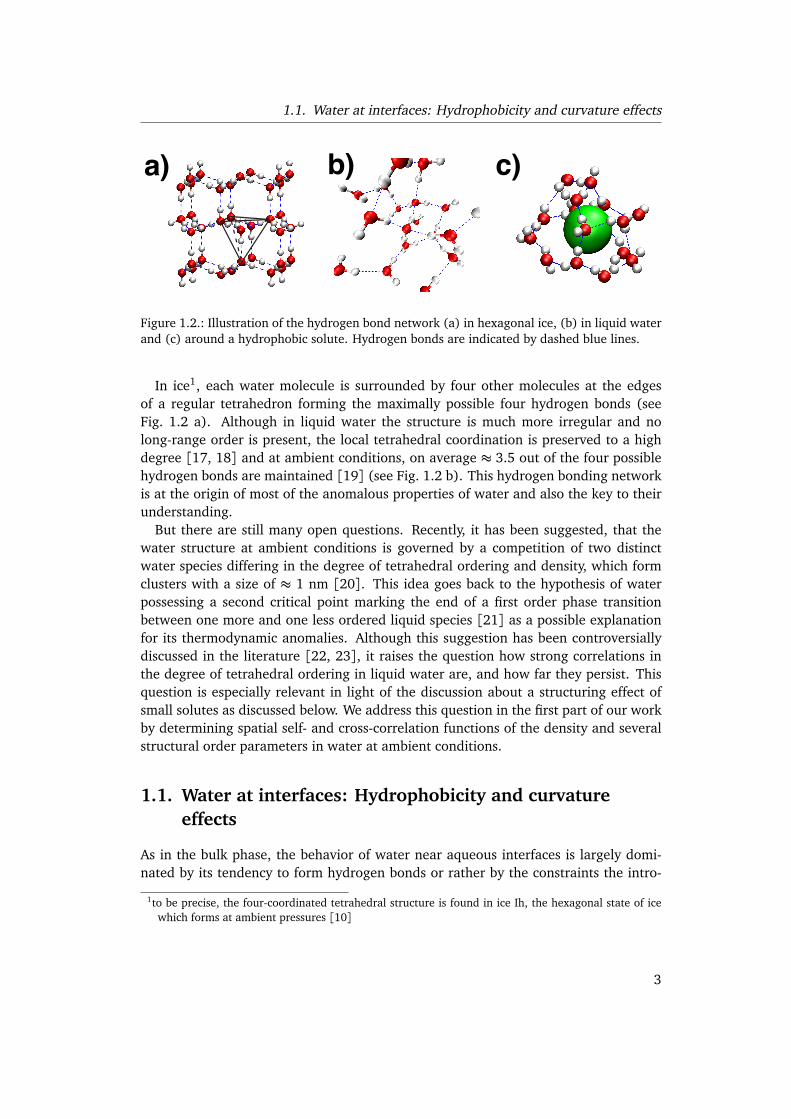
Figure 1.2.: Illustration of the hydrogen bond network (a) in hexagonal ice, (b) in liquid waterand (c) around a hydrophobic solute. Hydrogen bonds are indicated by dashed blue lines.
In ice1, each water molecule is surrounded by four other molecules at the edgesof a regular tetrahedron forming the maximally possible four hydrogen bonds (seeFig. 1.2 a). Although in liquid water the structure is much more irregular and nolong-range order is present, the local tetrahedral coordination is preserved to a highdegree [17, 18] and at ambient conditions, on average ≈ 3.5 out of the four possiblehydrogen bonds are maintained [19] (see Fig. 1.2 b). This hydrogen bonding networkis at the origin of most of the anomalous properties of water and also the key to theirunderstanding.
But there are still many open questions. Recently, it has been suggested, that thewater structure at ambient conditions is governed by a competition of two distinctwater species differing in the degree of tetrahedral ordering and density, which formclusters with a size of ≈ 1 nm [20]. This idea goes back to the hypothesis of waterpossessing a second critical point marking the end of a first order phase transitionbetween one more and one less ordered liquid species [21] as a possible explanationfor its thermodynamic anomalies. Although this suggestion has been controversiallydiscussed in the literature [22, 23], it raises the question how strong correlations inthe degree of tetrahedral ordering in liquid water are, and how far they persist. Thisquestion is especially relevant in light of the discussion about a structuring effect ofsmall solutes as discussed below. We address this question in the first part of our workby determining spatial self- and cross-correlation functions of the density and severalstructural order parameters in water at ambient conditions.
1.1. Water at interfaces: Hydrophobicity and curvatureeffects
As in the bulk phase, the behavior of water near aqueous interfaces is largely domi-nated by its tendency to form hydrogen bonds or rather by the constraints the intro-
1to be precise, the four-coordinated tetrahedral structure is found in ice Ih, the hexagonal state of icewhich forms at ambient pressures [10]
3

1. Introduction and Outline
duction of a surface puts on the formation of a hydrogen bond network. This dependsof course on the chemical nature of the substrate.
The interactions between a hydrophobic surface and water are non-specific andmuch weaker than the water-water interaction, so that the water attempts to min-imize the contact area by forming a large contact angle [24–26]. Also, the watermolecules in the layers adjacent to the surface orient themselves in a way reminiscentof the orientational structure in hexagonal ice in order to minimize the number of hy-drogen bonds that are broken [9, 27]. This effect should, however, not be taken asevidence for the formation of an ’ice-like’ layer near the surface, since the total entropyincreases when a hydrophobic interface is created, which is evident from the decreaseof the interfacial tension with increasing temperature [15]. Further characteristics ofa hydrophobic surface are the formation of a depletion layer [6, 28–32] and the oc-currence of slip in hydrodynamic flows [33, 34] as will be discussed in more detailbelow. It shall be noted, that in this sense an air/water interface should be viewedas a perfectly hydrophobic interface, i. e., the limiting case for completely vanishingsurface water interaction.
At hydrophilic surfaces, that possess polar groups with which the water can formhydrogen bonds, the water structure is still perturbed by the presence of the interfacebut wholly different phenomena occur. For instance, two hydrophilic surfaces repeleach other [35–37], the so called phenomenon of hydration repulsion, while two hy-drophobic surfaces are drawn together [38, 39].
The situation changes completely if we go from extended surfaces to the solvationof small solutes, that confront the aqueous phase with a highly curved interface. Whilethe hydrogen bond network has to be broken at an extended hydrophobic interface,small hydrophobic molecules can be accommodated without breaking hydrogen bondsat the cost of a slight rearrangement of the network (see Fig. 1.2 c). This manifestsitself in a crossover from a large scale solvation or extended interface regime to asmall scale solvation regime that can be seen in many characteristic properties[40, 41].While the cost of the creation of an extended interface or the solvation of a large solutescales with its surface area, the solvation free energy for smaller solutes scales with thesolute’s volume [42]. At ambient temperatures the solvation entropy of small solutes isnegative, while for large solutes and extended surfaces it is positive [43, 44]. In short,on the nano scale most interfacial properties attain a distinctive curvature dependence.Furthermore, hydrophobic solutes tend to aggregate in water, the mechanism of whichis still debated but supposedly also depends on the involved length scales [40, 45].
All these phenomena taken together make up the famous "hydrophobic effect" [46],which is at the bottom of many aggregation and solvation processes spanning a widerange of length scales from the solubility of rare gas solutes [47–49], over molecu-lar recognition [50, 51] and amphiphilic aggregation processes [52] to protein fold-ing [53] and misfolding [54, 55]. Since Kauzmann [56] first suggested that the burialof hydrophobic residues in the protein interior away from the water could be a driv-ing force for protein folding, the hydrophobic effect is believed to play a dominantrole in protein structure and stability, for reviews see e. g. [45, 53]. On the other
4

1.1. Water at interfaces: Hydrophobicity and curvature effects
hand misfolding and the subsequent aggregation of globular proteins to form amyloidstructures is at the origin of many diseases such as Alzheimer’s and Parkinson’s [54].
Despite the importance of the hydrophobic effect its mechanism is still debated anda consistent description over the different regimes is missing. Frank and Evans [57]explained the negative entropy and enthalpy of solvation of small hydrophobes in their’ice-berg’ model by the formation of a layer of structured water with enhanced hydro-gen bonds around the solute, reminiscent of the crystalline clathrate hydrates that canform under high pressures [58]. Building on this, Kauzmann [56] suggested, that theaggregation of two hydrophobes is facilitated by the release of the structured waterin between the solutes which is accompanied by an increase of entropy. Stillinger onthe other hand attributed the hydrophobic aggregation to the clumping tendency ofordered structures and draws an analogy to the thermodynamic anomalies in super-cooled water [16, 59]. Although the ’ice-berg’ view has been adopted by many authors,the character of the water in the solvation shell is a matter of debate. Blokzijl and Eng-berts [45] argue, that the assumption of a crystalline-like structure with enhanced hy-drogen bonding is not necessary to explain the favorable enthalpy of solvation, whichthey attribute to van der Waals interaction between water and solutes. The structureof the hydrogen bonding network around the solutes is merely maintained toleratingthe orientational constrains put up by the solute, while the aggregation of solutes is aconsequence of the limited capacity to accommodate hydrophobic solutes.
It has been argued, that the hydrophobic effect should rather be defined by its un-usual temperature dependence [46, 60] and any explanation of its mechanism mustaccount for it instead of the solvation entropy at ambient temperature. Indeed, thesolvation entropy of hydrophobic solutes increases rapidly with increasing tempera-ture and even changes its sign due to the large and positive heat capacity changeupon solvation. Extrapolating the solvation entropies and enthalpies for several smallhydrophobic solutes, it has been noted that they converge at a universal tempera-tures [61], which seems to indicate that hydrophobic solvation is dominated by uni-versal water features and not so much by solute specifics [62, 63]. The reported con-vergence of the denaturing entropy of a group of different proteins at roughly the sametemperature as hydrophobic solutes [64, 65] was consequently argued to indicate thatthe denaturing entropy of proteins is dominated by the hydrophobic effect and usedto estimate the hydrophobic contribution to protein stability [66–68]. However, thisappealing picture was subsequently questioned since the initially claimed universalconvergence of denaturing entropies holds only for a small subset of proteins, for alarger data collection no convergence is seen [69], which can still not be satisfactorilyexplained. We argue, based on the study of solvation of small hydrophobic soluteswith varying solute water interactions, that the differences induced by variations inthe residue-water interactions are sufficient to explain these effects.
Besides its temperature dependence, the size dependence is maybe the most strikingcharacteristic of hydrophobic solvation. The crossover between the small scale and thelarge scale solvation regime, happens on a length scale on the order of ≈ 0.5 nm [41],which makes it especially relevant for protein folding and molecular aggregation [70].
5

1. Introduction and Outline
Theoretical descriptions based on the assumption of Gaussian density fluctuations onsmall length scales give a reasonable description of the small solute regime [71–75],while interfacial thermodynamics are employed to account for large solutes [76]. Buteven for solutes smaller than 0.5 nm, proportionality of the solvation free energy andthe solvent accessible surface of the solute with varying effective proportionality con-stants is often reported, see e. g. Ref. [77], a common misconception which has itsorigin in the fact that for molecules made up from similar building blocks, like alkanechains, due to additivity the solutes surface area as well as its volume are proportionalto the chain length [41, 78].
A description spanning both regimes might be obtained by the introduction of acurvature dependent surface tension, a concept which has been first proposed by Tol-man [79] in 1949 in the context of liquid droplets. However, not even for simpleliquids a consensus has been reached about the sign of the coefficient to the first ordercurvature correction, usually termed the Tolman length, see e. g. [80, 81] and refer-ences therein. Scaled particle theories try to bridge the gap between the two regimesby constructing a sophisticated interpolation function including curvature correctionterms [43, 82–85]. While most of the studies mentioned so far deal with sphericalsolutes, there is evidence that hydrophobic hydration is not only sensitive to the sizebut to the shape of a solute as well [86–88].
This could be taken into account by a more general description of the surface freeenergetics in terms of a curvature based free energy functional like the one proposedby Helfrich [89]. Such a description involves additional parameters, whose determina-tion provides a formidable challenge, see [90–92] and references therein. We demon-strate that progress can be made by studying simultaneously the solvation of sphericaland cylindrical solutes, which allows for the extraction of the elastic properties of theaqueous interface.
Instead of studying water interfaces curved due to the presence of a solute, onecan also take a complementary approach and study the shape fluctuations of a free liq-uid/vapor interface, where curvature corrections manifest themselves in a wave vectordependent effective surface tension [92–94]. Experimentally interfacial fluctuationscan be studied by small angle X-ray scattering techniques [95–97]. Restrictions in theaccessible wave vector range and accuracy and the entanglement of interfacial andbulk fluctuations make the interpretation of such experiments difficult [91, 98–100].The complete configurational knowledge in a computer simulation, on the other hand,allows for the disentanglement of these effects and leads to a consistent description ofthe surface energetics, as we demonstrate in this work.
1.2. Water dynamics: The hydrogen bond dance
As well as the static properties, also the dynamic properties of many processes inaqueous solution are closely related to the dynamics of the water itself. Examplesinclude the kinetics of protein folding [101, 102], ion pair dissociation [103] or the
6

1.3. Outline of this work
water permeation through membrane channels [104]. Also the boundary conditionsof hydrodynamic flows are determined by the dynamics of the interfacial water [105,106] with important implications for microfluidic devices [107].
The water dynamics in turn is governed by the fluctuations and rearrangementsof the hydrogen bonding network through the breakage and formation of individualhydrogen bonds. Stillinger [16] suggested, that the dominant process is what he calledswitching-of-allegiance, that is the substitution of one hydrogen bond acceptor withanother near at hand, a view which is supported by the work of Csajka and Chandler[108]. Laage and Hynes [109, 110] note that this switching occurs in a rather abruptmanner including angular jumps of the hydrogen bond donor. The non-exponentialkinetics of the hydrogen bond relaxation [111, 112] is attributed to a coupling withdiffusion by Luzar and Chandler [113].
Near interfaces, the dynamics of the water are influenced by the chemical charac-ter of the surface. At hydrophobic surfaces the lateral motion of the water is not sostrongly perturbed by the weak substrate water interactions, which leads to the phe-nomenon of surface slip [105, 106], that is in hydrodynamic flows the water keeps afinite velocity relative to the substrate, an effect which is closely linked to the occur-rence of a depletion layer [33, 34]. Near hydrophilic surfaces on the other hand thewell known no-slip boundary condition holds, that is the water layers adjacent to thesurface do not show a relative velocity.
Simulation studies report a slowing down of water diffusion both at hydropho-bic [34, 114, 115] and hydrophilic surfaces [34, 114, 116], which is much stronger athydrophilic surfaces. Some studies of water in thin films on hydrophilic surfaces [117,118] and in confinement by hydrophilic walls at nanometer separation [119–121]even report the formation of ’ice-like’ layers in conjunction with a viscosity increaseof several orders of magnitude, while others find a moderate increase of the viscosityby a factor on the order of 4 [34]. A quantitative comparison is difficult, however,since most of the methods used to determine the dynamics involve an averaging overa certain distance from the surface that might obscure fast variations [34, 117]. Alsothe entanglement of effects due to the free energy profile imposed by the substrate andthe diffusivity require a more careful analysis, as has been recently demonstrated for asystem of hard spheres in confinement [122]. In this work we apply a similar methodto the dynamics of water near hydrophobic and hydrophilic walls and solutes.
1.3. Outline of this work
It is the goal of this work to gain a thorough understanding and a consistent descriptionof the thermodynamics and dynamics of water near curved and planar interfaces bythe use of molecular dynamics simulation methods.
In chapter 2 we describe the computational and analysis methods used in this workas far as relevant for the overall work. More specific analysis tools are described in
7
1. Introduction and Outline
the individual chapters if it is necessary. We also discuss the general properties of thewater models employed and the modeling of surfaces and solutes.
In chapter 3 we investigate several structural properties of bulk water. As a stringenttest of the quality of the water models used, we determine the low wave vector regionof the static structure factor and compare the results with experimental data. It turnsout, that all investigated water models can reproduce the experimental data reason-ably well, including subtle features such as the slight minimum observed around wavevectors of q ≈ 4nm−1 [23, 123, 124] and are consequently well suited to investigatewater structure. Subsequently, we calculate spatial self- and cross correlation functionsof the density and structural order parameters such as the hydrogen bond number andthe tetrahedrality parameter introduced by Errington and Debenedetti [125] and showthat there is no strong coupling between density and structural fluctuations.
In chapters 4 and 5 we turn to the description of hydrophobic solvation effects.While chapter 4 is mainly concerned with the solvation of small scale solutes andits dependence on the solute water interaction, chapter 5 deals with the crossoverbetween the small scale and large scale solvation regime and a consistent descriptionbased on a local surface free energy functional.
By determining the thermodynamic solvation properties for idealized hydrophobicsolutes with varying solute water interactions over a wide range of temperatures, weshow in chapter 4 that the temperature at which entropy and enthalpy converge de-pends sensitively on the specific features of the interaction potentials. We furtherexplain the differences in the solvation thermodynamics for different water modelsand the discrepancies with previous studies [72] using hard sphere models. Finally,we discuss the implications for the interpretation of the hydrophobic contribution toprotein stability.
In chapter 5 we investigate, how the Helfrich [89] free energy functional can givea consistent description of the free energy of a curved water interface. In the firstpart (Sec. 5.2) we extract the bending rigidity by analyzing fluctuation spectra of thefree air/water interface. For this purpose we introduce a method to separate bulkand interfacial fluctuations without any fitting parameters. We also determine theintrinsic density profile and discuss implications for the interpretation of scattering ex-periments. In the second part (Sec. 5.3) we study the solvation of hydrophobic spheresand cylinders with radii up to 2 nm. We determine solvation free energies, entropiesand enthalpies which enables us to identify the relevant crossover length scales anddiscuss implications for hydrophobic aggregation. Applying the Helfrich functionalsimultaneously to the solvation free energies of solutes with different geometries al-lows us to extract the surface elastic constants, including the coefficient of the firstorder correction, i. e., the Tolman length, which is not accessible by analyzing surfacefluctuations.
In chapter 6 we apply a Fokker-Planck based stochastic formalism to describe thedynamics of single water molecules near hydrophobic and hydrophilic solutes and in-terfaces. This formalism allows us to disentangle the free energy and diffusivity profilesof the dynamic processes. We find that the diffusivity profiles show strong variations
8

1.3. Outline of this work
including a dramatic drop near the hydrophilic surface as well as near another watermolecule, whereas the drop near hydrophobic surface and solute is rather moderate.
Finally, we give a summary of our results and discuss implications and possiblestarting points for future work.
9

10
CHAPTER 2
COMPUTATIONAL METHODS AND MODELING
Since the relevant length scales we are interested in are in the nanometer regime, anaive application of the concepts from continuum theories is bound to fail at somepoint. Rather, modeling on the molecular scale is necessary. On the one hand thisgives direct access to structural properties on the atomistic scale, on the other hand itis the basis for a description on a meso- or macroscopic scale, e. g. by the introductionof suitable corrections to continuum theories.
In principle, statistical mechanics provides the framework to derive physical observ-ables from the microscopic properties of a system, that is its Hamiltonian. In practice,however, exact solutions exist only for few special cases and in general approximationshave to be made. Density functional and integral equation theories yield good resultsfor simple liquids, that is atomic liquids with pairwise additive interactions. The com-plex structure of the water molecule and the coexistence of long and short rangedinteractions make an analytical treatment of liquid water very difficult.
That is where numerical simulations techniques like Monte Carlo and MolecularDynamics can step in. Based on the interaction model put in, a simulation yields ex-act results, their statistical accuracy, however, limited by the computational resourcesavailable. Simulations therefore serve a twofold purpose. On the one hand they canbe used to verify theoretical results, on the other hand, they can tackle problems elud-ing theoretical treatment altogether, provided the underlying models have been thor-oughly tested. In that way, simulations can also give input to higher level theories,whose parameters are hard to derive from a more fundamental treatment.
2.1. Molecular dynamics simulations
For the present study, we chose to employ the molecular dynamics (MD) method,since, in contrast to Monte Carlo simulations, it is suitable for the investigation ofdynamic as well as static properties [126, 127]. In MD simulations one numericallyintegrates Newton’s equations of motion for a system of interest in order to obtain a
11

2. Computational Methods and Modeling
trajectory of the system. Such a trajectory does not follow the exact time evolutionof the system for the given starting conditions over the time scales of the simulationbut there is much evidence that the generated trajectory is always close to a truetrajectory for a time scale that is much longer than the time the Lyapunov instabilitytakes to develop [128, 129]. Since one is usually only interested in statistical averagesover an ensemble of trajectories, or equivalently a time average over a long trajectory,the results obtained from an MD simulation are representative of a true trajectory inphase space.
At the center of any molecular dynamics technique is of course the question of howto describe the interatomic interactions that enter into the equations of motion. Sincewe are dealing with molecular systems, these interactions are of quantum mechanicalnature. However, even approximate quantum mechanical treatments [130] as e. g.in the Car-Parinello MD method [131] are computationally expensive and the systemsizes and time scales that can be reached with reasonable effort are still to small formany applications. In classical MD simulations, as we will employ throughout thiswork, one therefore uses effective pairwise interaction potentials, whose parametersand functional forms are either derived from first principles methods or are optimizedto reproduce experimental observables. Bonded interactions are typically modeledby harmonic bond and angle potentials and empirical torsion potentials to yield thecorrect molecular geometry, while non-bonded interactions include electrostatic forcesdue to partial charges on polar molecules and dispersion interactions described byLennard-Jones potentials. Since these are only effective interaction potentials muchcare has to be taken to validate their performance in each specific situation. A detaileddescription of the force fields used in this work is given below.
All MD simulations throughout this work are performed using the Gromacs sim-ulation package [132, 133], which is well tested and optimized for computationalefficiency. The equations of motion are integrated via a leap frog integrator with atime step of ∆t = 2 fs.
While the integration of Newton’s equation produces trajectories with constant to-tal energy and therefore corresponds to a micro-canonical ensemble (NVE), it is oftenmore suitable to use a canonical (NVT) or isobaric-isothermal ensemble (NPT) in or-der to compare to experimental situations or theoretical calculations. This can beaccomplished by using a thermostat or barostat algorithm to keep the temperatureor the pressure constant during a simulation [126]. Unless noted otherwise, we use aBerendsen weak coupling thermostat and barostat [134] for temperature and pressurecontrol. The relaxation times are usually set to τ= 1.0ps in production runs.
Simulation systems are contained in cubic or rectangular boxes. To avoid finite sizeand undesired surface effects at the box edges periodic boundary conditions are ap-plied in all three dimensions. To reduce the computational cost, short-ranged, e. g.Lennard-Jones, interactions are truncated at a cutoff radius rc = 0.9 nm, unless notedotherwise. Since the interaction potential decays ∝ r−6 such a simple cutoff sufficesand its effects on the systems dynamics are negligible, except for very rare cases asdemonstrated in [135]. The effects on the pressure tensor can be significant, how-
12

2.2. Force fields and modeling
ever, which can lead to errors in NPT simulations. In homogeneous systems one cancorrect for these cutoff effects by an analytical correction applied to both energy andpressure [127]. The treatment of electrostatic forces requires more elaborate meth-ods, since the Coulomb potential decays only as ∝ r−1 and a simple cutoff schemewould lead to severe artifacts. We use a variant of the Ewald summation technique,where the interaction is split up into a quickly varying short-ranged part and a slowlyvarying long-ranged part. While the short-ranged part can be calculated in real spaceby using a simple cutoff as for the Lennard-Jones interaction with a cutoff radius ofrc = 0.9 nm, the contribution of the long-ranged part is calculated by a Fourier sum-mation in reciprocal space. In the so-called particle mesh Ewald variant [136, 137],that we use in our simulations, the partial charges are spread on a grid in order tobe able to use the fast Fourier transform method for the summation. We apply tinfoilboundary conditions in all simulations.
Furthermore, all bonds involving hydrogen atoms are constrained using the LINCS[138] algorithm (in the substrates) or the analytic SETTLE algorithm [139] (in thewater molecules). Due to these constraints high frequency modes are removed and alonger integration time step can be used.
2.2. Force fields and modeling
As discussed above the force fields, that define the interatomic interactions in a MDsimulation, are of utmost importance and have to be chosen carefully. In the followingsection we describe in detail the interaction potentials and the solvent, solute andsubstrate models that are used in this work.
2.2.1. Water models
Since the first computer simulations of liquid water by Barker and Watts [140] andRahman and Stillinger [141] a great number of water models has been proposed (fora review see e.g. [142, 143]). The majority of these models treats the interactionsbetween two molecules by electrostatic and dispersion interactions and an electronicrepulsion. The charge distribution of the molecule is usually modeled by point chargeslocated at the positions of the oxygen and hydrogen atoms or on additional virtualsites. The electronic repulsion is typically modeled by an r−12-term which is combinedwith the r−6-dispersion term in a Lennard-Jones potential centered on the oxygenatom. In most cases the interaction parameters, that is the partial charges and theLennard-Jones interaction parameters, are optimized in such a way that a certain setof experimental observables, e. g. the heat of vaporization, density, etc. at ambientconditions is reproduced. The geometry of the molecule is either rigid or flexible, inwhich case the intramolecular forces are treated by harmonic bond and angle poten-tials. Further refinements include the introduction of atomic polarizability to describemulti-body interactions [144].
13

2. Computational Methods and Modeling
However, with increasing complexity of the models also the computational cost in-creases and a thorough optimization in the high-dimensional parameter space is of-ten not possible any more. Therefore, in this work we restrict ourselves to severalsimple rigid water models, that nonetheless haven proven to perform well in varioussituations. A detailed discussion of the relevant model properties and correspondingreferences is given in the individual chapters.
The SPC [145], SPC/E [146], TIP4P/2005 [147] and TIP5P [148] water models allhave a rigid geometry with fixed point charges and a varying number of interactionsites. All of them have two positively charged hydrogen atoms and an oxygen atom onwhich the Lennard-Jones interaction is centered. They differ mainly in the placementof the negative charge. In the SPC and SPC/E water model the negative charge isplaced on the oxygen atom, while in the TIP4P/2005 water model the negative chargeis placed on an additional virtual site on the bisector of the HOH angle. In the TIP5Pmodel the negative charge is placed on two virtual sites located on the edges of aslightly distorted tetrahedron, formed by the hydrogen atoms and two virtual sites.
While the geometry of the SPC water model was set to an OH bond length ofOH = 0.1 nm and a bond angle equal to the tetrahedral angle ∠(HOH) = 109.47◦,the partial charge of the hydrogen atom qH = 0.41 e and the coefficient of the repul-sive Lennard-Jones term were optimized to reproduce the heat of vaporization andthe density of water at T = 300 K. Here, e denotes the unit charge. The SPC/E watermodel is a reparameterization of the SPC model with the same objectives but includ-ing a correction for the polarization self-energy of the water dipole which leads to adifferent hydrogen partial charge of qH = 0.4238 e. Despite its simplicity, the SPC/Ewater models yields good results and has become one of the most widely used watermodels [142, 143]. It represents a good compromise between accuracy and computa-tional efficiency and due to its widespread use it allows easy comparison of our resultswith the literature. We therefore use it in most parts of this work. Simulations withthe SPC water model are only included for comparison with previous works.
As two examples of more refined water models we also use the TIP4P/2005 and theTIP5P models. In addition to the density and heat of vaporization at ambient condi-tions, the TIP4P/2005 parameters were fit to reproduce the temperature of the densitymaximum at ambient pressure, the density of ice II at 123 K and 0 MPa and of ice V at223 K and 530 MPa, and the range of stability temperatures of ice III at 300 MPa [147].The TIP4P/2005 model gives a very good description of the temperature dependenceof several thermodynamic properties of water, including the density, isothermal com-pressibilty and isobaric heat capacity [149]. The TIP5P model was developed with thegoal of reproducing the water density over a wide range of temperatures and pres-sures while simultaneously recovering the water structure at ambient conditions byintroducing an additional interactions site with respect to the TIP4P model [148].
14
2.2. Force fields and modeling
2.2.2. Solutes
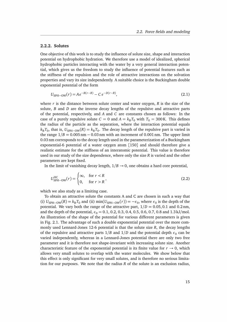
One objective of this work is to study the influence of solute size, shape and interactionpotential on hydrophobic hydration. We therefore use a model of idealized, sphericalhydrophobic particles interacting with the water by a very general interaction poten-tial, which gives us the freedom to study the influence of potential features such asthe stiffness of the repulsion and the role of attractive interactions on the solvationproperties and vary its size independently. A suitable choice is the Buckingham doubleexponential potential of the form
USPH−OW(r) = Ae−B(r−R)− C e−D(r−R), (2.1)
where r is the distance between solute center and water oxygen, R is the size of thesolute, B and D are the inverse decay lengths of the repulsive and attractive partsof the potential, respectively, and A and C are constants chosen as follows: In thecase of a purely repulsive solute C = 0 and A = kBT0 with T0 = 300K. This definesthe radius of the particle as the separation, where the interaction potential equalskBT0, that is, USPH−OW(R) = kBT0. The decay length of the repulsive part is varied inthe range 1/B = 0.005nm− 0.03nm with an increment of 0.001 nm. The upper limit0.03 nm corresponds to the decay length used in the parameterization of a Buckinghamexponential-6 potential of a water oxygen atom [150] and should therefore give arealistic estimate for the stiffness of an interatomic potential. This value is thereforeused in our study of the size dependence, where only the size R is varied and the otherparameters are kept fixed.
In the limit of vanishing decay length, 1/B→ 0, one obtains a hard core potential,
UHCSPH−OW(r) =
(
∞, for r < R
0, for r > R, (2.2)
which we also study as a limiting case.To obtain an attractive solute the constants A and C are chosen in such a way that
(i) USPH−OW(R) = kBT0 and (ii) min(USPH−OW(r)) = −ε0, where ε0 is the depth of thepotential. We vary both the range of the attractive part, 1/D = 0.05, 0.1 and 0.2nm,and the depth of the potential, ε0 = 0.1, 0.2, 0.3, 0.4, 0.5, 0.6, 0.7, 0.8 and 1.3 kJ/mol.An illustration of the shape of the potential for various different parameters is givenin Fig. 2.1. The advantage of such a double exponential potential over the more com-monly used Lennard-Jones 12-6 potential is that the solute size R, the decay lengthsof the repulsive and attractive parts 1/B and 1/D and the potential depth ε0 can bevaried independently, whereas in a Lennard-Jones potential there are only two freeparameter and it is therefore not shape-invariant with increasing solute size. Anothercharacteristic feature of the exponential potential is its finite value for r → 0, whichallows very small solutes to overlap with the water molecules. We show below thatthis effect is only significant for very small solutes, and is therefore no serious limita-tion for our purposes. We note that the radius R of the solute is an exclusion radius,
15

2. Computational Methods and Modeling
Figure 2.1.: Illustration of thesolute-water interaction poten-tial USPH−OW(r) (see Eq. 2.1)for a spherical solute of radiusR = 0.28nm and various po-tential shapes. (a) Purely re-pulsive potential with varyingdecay lengths 1/B = 0.005,0.01, 0.015, 0.02, 0.025 and0.03 nm. (b) Attractive poten-tials with 1/B = 0.02nm, at-traction decay length 1/D =0.05 nm and varying potentialdepth ε0 = 0.1, 0.2, 0.3, 0.4,0.5, 0.6, 0.7 and 0.8kJ/mol. (c)Attractive potentials with 1/B =0.02 nm, ε0 = 0.8 kJ/mol andvarying range 1/D = 0.05, 0.1and 0.2nm. Vertical lines indi-cate the radius R of the solute,defined by USPH−OW(R) = kBT0with T0 = 300K. The insets in(a) and (b) show enlarged viewsof the potential.
that is, it is the radius around the center of the solute from which the center of thewater oxygen atom is effectively excluded by the repulsion. We neglect all interactionsbetween the solute and the water hydrogens.
Cylindrical solutes are modeled as a string of spheres aligned along the z-axis, withan axial separation of ∆z. The cylinder has the same length as the box size in z-direction, so that by the use of periodic boundary conditions, it has an infinite lengthand edge effects are excluded. The interaction potential of the cylindrical solutes withthe water oxygen is therefore given by
VCYL−OW(r||, z) = AN∑
i=1
e−BÆ
r2||+(z−zi)2 , (2.3)
where N is the number of spheres, r|| =p
x2+ y2 is the distance from the cylinderaxis and zi = i∆z, i = 1, . . . , N , are the z-positions of the spheres that form the cylin-der. Note that in Eq. 2.3 we have absorbed the term exp(−BR) into the prefactor A.
16

2.2. Force fields and modeling
Figure 2.2.: Side view of the simulation box in the interfacial geometry and top views of thedifferent hydrophobic and hydrophilic substrates.
To obtain a rather smooth cylinder, we choose the spacing between the spheres as∆z = 0.025 nm, which ensures that the corrugation of the potential along the z-axis isnegligible and we have
VCYL−OW(r||) ≈ A
∫ ∞
−∞
dz
∆ze−B
Æ
r2||+z2
=2Ar||∆z
K1(Br||), (2.4)
where K1 is the first order modified Bessel function of the second kind. Analogouslyto the spherical solutes we choose 1/B = 0.03 nm and determine the constant Aby the condition VCYL−OW(R) = kBT0. From that definition it follows, that A(R) =∆zkBT0/ fCYL(B, R), with fCYL(B, R) = 2RK1(BR).
For comparison we also calculate solvation free energies for solutes interacting viathe repulsive part of a Lennard-Jones potential,
V LJSPH−SOL(r) =
E
r12 . (2.5)
The solute radii R are defined analogously to the Buckingham potential by V LJSPH−SOL(R) =
kBT0, yielding E = kBT0R12.As an example of a hydrophobic solute with optimized force field parameters we
also study a methane molecule modeled in a united atom representation as a singleLennard-Jones sphere using the OPLS [151] force field parameters.
2.2.3. Planar interfaces
For the study of water near planar interfaces, we use a slab geometry, where a simula-tion box is only partially filled by water in the z-direction, the remaining part is eitherempty, thereby forming a setup with two planar air/water interfaces parallel to thex y-plane (see Fig. 5.1 and Fig. 5.3), or filled by a solid substrate (see Fig. 2.2). Dueto the periodic boundary conditions, this setup corresponds to a water slab confinedbetween two solid surfaces.
17

2. Computational Methods and Modeling
As a model for a nonpolar surface we use hydrogen-terminated diamond, to ob-tain polar surfaces a certain fraction of the terminal hydrogen atoms is replaced byhydroxyl groups. The diamond surface is modeled by the well known double face-centered-cubic lattice (lattice constant a = 3.567 Å) of carbon atoms with the ⟨100⟩direction parallel to the z-axis. A slab of finite thickness is cut out of the lattice withits two surfaces perpendicular to the z-axis, and the surface layer is reconstructed andterminated by hydrogen atoms. The atoms of the diamond interact with each othervia harmonic bond and angle potentials as well as a torsion potential. The interac-tion between a surface atom and a water oxygen atom is given by a Lennard-Jonespotential.
For the hydrophilic diamond, a variable fraction (12% or 25%) of the terminalhydrogen atoms is replaced by hydroxyl groups with partial charges qC = 0.266 e,qO = −0.674 e and qH = 0.408 e (see Fig. 2.2). The force constants and Lennard-Jones interaction parameters are taken from the GROMOS96 force field [152].
The contact angle of SPC/E water on the hydrophobic diamond was found to beΘ= 101◦ [9], while the hydrophilic substrates exhibit complete wetting.
2.3. Free energy simulations
The key quantity characterizing the solvation of a solute is its solvation free energy∆F , that is, the free energy necessary to bring the solute from the pure ideal gas phaseinto aqueous solution. The solvation free energy per solute is equal to the solutesexcess chemical potential ∆F = µex in the solution. From the temperature derivativeof the solvation free energy one obtains the solvation entropy ∆S per solute,
∆S =−∂∆F
∂ T. (2.6)
and the solvation enthalpy,
∆H =∆F + T∆S. (2.7)
We use different methods to determine the solvation free energy, based mainly on thesize of the solute. While the Widom particle insertion method [153] is very efficient, itis only applicable for small solutes. We use it to determine the solvation free energiesof small solutes with varying interaction parameters, where a wide range of differentparameters is scanned. The thermodynamic integration method [126], on the otherhand, can be used for arbitrary solute sizes, but demands much more computationaleffort. It is therefore used to determine solvation free energies for the large sphericaland cylindrical solutes.
18

2.3. Free energy simulations
Figure 2.3.: Running average of the excess chemical potential calculated by the particle in-sertion method according to Eq. 2.8 for a purely repulsive solute of radius R = 0.345 nm witha potential stiffness of 1/B = 0.03nm (black curve) and for a hard core solute of the samesize (red line), where the average ⟨.⟩t0
is taken over all saved configurations with t < t0. Theinsertions are done in a box containing 895 SPC/E water molecules simulated at T = 300K.In each configuration of the trajectory nins = 107 insertions are performed for the finite poten-tial stiffness and nins = 2 ·106 for the hard core solutes. It is seen, that the excess chemicalpotential is well converged after 10ns.
2.3.1. Particle insertion method
We determine the excess chemical potential of small solutes with varying interactionparameters by the Widom particle insertion method [153]. In the case of an isobaric-isothermal ensemble it is given by [154]
µex =−kBT ln
�
< Ve−β∆U >
< V >
�
, (2.8)
where∆U is the potential energy of the interaction between the solute and the solvent,V is the volume of the system, β = 1/(kBT ) and the angle brackets denote an isobaric-isothermal average over configurations of the system without the solute.
For each saved configuration nins = 107 insertions are performed in the case of afinite potential stiffness and nins = 2 ·106 in the case of hard sphere solutes. Figure 2.3shows the running average, that is an average including only configurations up to acertain time t0, of the excess potential (Eq. 2.8) for a purely repulsive solute of radiusR = 0.345nm with a potential stiffness of 1/B = 0.03nm (black curve) and a hardcore solute of the same size (red curve) in SPC/E water at T = 300K. It is seen thatthe excess potential is well converged after 10ns.
2.3.2. Thermodynamic integration method
To determine the solvation free energies of large spherical and cylindrical solutes ∆F ,the method of thermodynamic integration is used, which relates the free energy dif-
19

2. Computational Methods and Modeling
ference ∆F between two states I and II of a thermodynamic system, characterized bytwo potential energy functions U I and U II, to the averaged derivative ⟨∂ U(λ)/∂ λ⟩ ofan intermediate potential energy U(λ), that connects the two states by a virtual path,i. e., U(λ = 0) = U I and U(λ = 1) = U II, where λ = 0 . . . 1 is a path variable. The freeenergy difference F between the two states is then given by the integral
∆F =
∫ 1
0
dλ⟨∂ U(λ)∂ λ
⟩λ, (2.9)
where the average ⟨.⟩λ has to be taken for a system interacting via U(λ). To obtainthe solvation free energy of a solute, the initial state I is chosen such that the so-lute does not interact with the solvent, while in the final state II, the full interactionwith the solvent is switched on. That is, the potential energy function U I contains nosolute-solvent interactions, while U II contains the full interaction. For simulations inan isobaric-isothermal ensemble the solvation free energy contains an additional termdue to the volume change [155],
∆F =∆F + kBT ln(V II
V I ), (2.10)
where V I and V I I are the system volumes in state I and state II, respectively. Thisterm accounts for the difference in the ideal gas entropy in the initial and final stateof the thermodynamic integration. For the solvation of a nonpolar solute, this volumechange is mainly due to the solute’s volume ∆V , since the water can be consideredincompressible to a good approximation. If the volume of the simulation box V ismuch larger than the volume of the solute, the correction term is small.
For large solutes it is convenient to break the thermodynamic integration into severalsteps with varying system sizes, going from an initial size RI to a final size RII in eachstep, where RI = 0 for the first step and RII equals the desired solute size in the laststep. In this way, smaller simulation boxes can be used for small solutes, reducing thecomputational cost.
We perform linear scaling between the states, that is the potential energy functionof the intermediate states is defined by
URI→RII(λ) = (1−λ)URI
+λURII. (2.11)
Since the repulsive Buckingham potential has no divergence at small distances, linearscaling is possible even for the first step, where the solute is completely decoupled inthe initial state, without getting a diverging ⟨∂ URI→RII
(λ)/∂ λ⟩, as for a Lennard-Jonespotential [156].
Since the radius of the solute depends only on the prefactor of the interaction po-tential, the potential URI→RII
(λ) at each intermediate λ-value corresponds to a soluteof intermediate radius R(λ). Conversely, the λ-values can be chosen in such a way,that they correspond to equidistant values of the solute radius. For the integration
20
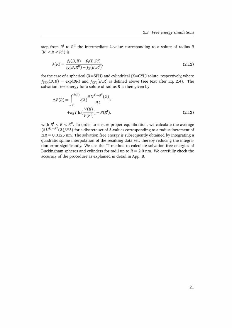
2.3. Free energy simulations
step from RI to RII the intermediate λ-value corresponding to a solute of radius R(RI < R< RII) is
λ(R) =fX(B, R)− fX(B, RI)fX(B, RII)− fX(B, RI)
, (2.12)
for the case of a spherical (X=SPH) and cylindrical (X=CYL) solute, respectively, wherefSPH(B, R) = exp(BR) and fCYL(B, R) is defined above (see text after Eq. 2.4). Thesolvation free energy for a solute of radius R is then given by
∆F(R) =
∫ λ(R)
0
dλ⟨∂ URI→RII
(λ)∂ λ
⟩
+kBT ln(V (R)V (RI)
) + F(RI), (2.13)
with RI < R < RII. In order to ensure proper equilibration, we calculate the average⟨∂ URI→RII
(λ)/∂ λ⟩ for a discrete set of λ-values corresponding to a radius increment of∆R = 0.0125 nm. The solvation free energy is subsequently obtained by integrating aquadratic spline interpolation of the resulting data set, thereby reducing the integra-tion error significantly. We use the TI method to calculate solvation free energies ofBuckingham spheres and cylinders for radii up to R = 2.0 nm. We carefully check theaccuracy of the procedure as explained in detail in App. B.
21

22

CHAPTER 3
CORRELATIONS OF DENSITY AND STRUCTURAL
FLUCTUATIONS IN BULK WATER
3.1. Introduction
3.1.1. Motivation
Understanding the water structure in the pure bulk liquid is the prerequisite for un-derstanding its behaviour in more complex situations. But even the bulk behaviourof water is surprisingly difficult to understand, partly due to anomalous behaviour inalmost all thermodynamic observables [15]. The best-known example is certainly theanomaly in the water density, which shows a maximum at 4◦ C, at which temperaturethe thermal expansion coefficient αP = 1/V (∂ V/∂ T )P changes sign. But also otherthermodynamic properties like the isothermal compressibility κT = −1/V (∂ V/∂ P)Tand the isobaric heat capacity CP = (∂ H/∂ T )P exhibit anomalies: At atmosphericpressure κT has a minimum at 46◦C and CP has a minimum at 35◦C [14, 157–159].This stands in marked contrast to the behaviour of simple liquids, whose thermody-namic properties vary monotonously with temperature.
Despite intense efforts for many years, there is still no complete and simple explana-tion for these anomalies. Several hypotheses have been proposed [160–162], amongwhich the liquid-liquid critical point (LLCP) scenario has received much support in therecent literature. According to the LLCP scenario, water possesses a metastable criticalpoint at very low temperatures which marks the endpoint of a first order phase tran-sition between a high density (HDL) and a low density (LDL) liquid phase. The LDLphase is associated with tetrahedral-like local structure, while the HDL phase corre-sponds to a local structure with distorted hydrogen bonds [21, 163]. The anomaloustemperature dependence of the thermodynamic response functions then follows nat-urally, since they are expected to diverge at the transition line or exhibit maxima orminima at the continuation of the transition line into the one phase region [163].However, conclusive experimental evidence for this scenario is still missing and the
23

3. Correlations of Density and Structural Fluctuations in Bulk Water
connection between anomalous water properties and the existence of low-temperaturesingularities is controversially discussed [163, 164].
Recently, it has been suggested that remnants of these phases persist even at highertemperatures and that extended clusters of HDL and LDL are present at ambient con-ditions [20]. These conclusions were partly based on the well-known experimentalobservation that the structure factor S(q), obtained from SAXS or neutron scattering,shows an enhancement at very low wave vectors q [23, 123, 124, 165]. In conjunc-tion with X-ray adsorption, Rahman and Emission spectroscopy it was argued that thedensity fluctuations manifest in S(q) originate from concentration fluctuations of twostructurally distinct liquid species differing in density [20]. From an Ornstein-Zernike(OZ) analysis of the scattering data the typical size of these clusters was estimated tobe on the order of ≈ 1 nm. It was also stated that standard three-point water modelssuch as SPC/E are not able to reproduce the minimum in the structure factor [20],from which it was concluded that the local water structure is ill-reproduced by currentclassical simulation models for water.
The relationship between the density and structure of water has been much dis-cussed in recent literature [23, 166–168], partly because this relation is crucial forunderstanding the water density anomaly. Using an analysis of structural water clus-ters in SPC/E water simulations, Errington et al. [166] have found a decrease in thedensity of water clusters both with increasing tetrahedrality and increasing clustersize at temperatures of T = 220 K and T = 240 K. This suggests that the formationof tetrahedrally ordered low-density water is cooperative. Moore and Molinero [167]used the monatomic mW [169] water model for an extensive study of the water struc-ture in the temperature range from 100 K to 350 K. They found an increase in theaverage tetrahedrality and the fraction and cluster size of four-coordinated moleculesupon cooling. However, they did not observe a low-q enhancement of the structurefactor, which they attributed to the lack of density difference between differently co-ordinated water molecules in the mW model [167]. Only when they restricted thecalculation of the structure factor to four-coordinated water molecules, they saw anincrease for low q from which they infer correlation lengths that grow with decreas-ing temperature, using an OZ analysis. Matsumoto [168] showed that the change inthe average composition of differently coordinated water molecules upon cooling isnot correlated with the mean density of the liquid. He could accurately explain thetemperature dependence of the density by taking into account the interplay of the av-erage bond length, which decreases upon cooling and therefore tends to increase thedensity, and the distortion of the tetrahedral bonding network, which decreases uponcooling and thereby decreases the density. Very recently, Soper et al. [22] and Clarket al. [23] argued that an enhancement in the low-q region of the structure factor isconsistent with normal particle number fluctuations and not necessarily indicates thepresence of two structural water species with different densities. Furthermore, it wasshown that the OZ analysis applied in Ref. 20 used to infer a spatial scale of regionswith correlated densities is not very meaningful far away from a critical point. Clarket al. [23] very convincingly demonstrated the absence of pronounced density inho-
24

3.1. Introduction
mogeneities on lengthscales ranging from 0.6 nm to 6 nm based on the unimodalityof density histograms obtained by simulations of TIP4P-Ew water [23], thus castingadditional doubt on the interpretation of S(q) data as a sign of the coexistence of twodifferent local structural motifs in liquid water [20].
While the relation between spatially averaged structural properties and the meandensity of water seems well understood, the question of the existence and spatialsize of structurally correlated regions in liquid water is less clear. In particular, thediscussion in Ref. 20 raised the question to what degree the spatial extent of densitycorrelations (as directly inferred from SAXS experiments via the structure factor) isrelated to the size of structurally correlated water patches (which can only indirectlybe inferred from experiments).
3.1.2. Outline
Instead of using clustering algorithms to define the size of regions with high structuralorder [166–168], we determine spatial two-point correlation functions involving thelocal density and different local structural order parameters, namely the tetrahedral-ity order parameter [125, 170, 171], ψ, and the number of hydrogen bonds a watermolecule forms with its neighbours, nHB. By using the exact same mathematical formfor assessing the presence of spatial correlations of density and structural fluctuations,we are able to make a simple and meaningful comparison between density-densitycorrelations (expressed in terms of the well-known radial distribution function) anddensity-structure and structure-structure correlations. Except for the density-densitycorrelation function, we find only weak correlations that decay to zero within a few Å.This means that although water is a highly structured fluid, the structure shows onlyweak spatial correlation and that the coupling between density and structural fluctu-ations is also quite weak when compared with the degree to which density-densitycorrelations are present.
In order to check how robust the simulated structure factor is with respect to forcefield modifications, we compare the SPC/E [146], the TIP4P/2005 [147] and theTIP5P [148] water models. The SPC/E water model has a density maximum atT = 235 K [172] and a minimum in κT around T = 270 K [149] and thus differsconsiderably from the experimental values. It exhibits the LDA and HDA phases inthe amorphous state [173, 174] and it has been suggested, that it has a LLCP [175].The TIP5P water model has been parameterized to yield the correct position of thedensity maximum at T = 277 K [148] using a reaction field method to account forelectrostatic periodic boundary conditions. Note that in combination with the ParticleMesh Ewald summation method [136, 137], as used in this work, the density maxi-mum is shifted slightly to T = 284 K [176]. It has been shown, that the TIP5P watermodel shows a LLCP [174, 177] and that its isobaric heat capacity shows a sharp in-crease for decreasing temperature [174], in accordance with the experimental data.The isothermal compressibility of the TIP5P water model does not show a minimumwithin the range studied so far [149]. The TIP4P/2005 model is a recent reparam-
25

3. Correlations of Density and Structural Fluctuations in Bulk Water
eterization of the widely used TIP4P [178] water model. It excellently reproducesthe temperature dependence of the density as well as the isothermal compressibilityat atmospheric pressure, exhibiting a density maximum at T = 278 K [147] and aminimum in κT at T = 310 K [149]. The TIP4P model has a LLCP [174], so it islikely that the TIP4P/2005 model has a LLCP, too. We find that all three water modelsexhibit an enhancement of the structure factor for low q, which is pronounced for theTIP5P and TIP4P/2005 water models, and still perceptible for the SPC/E water model.The TIP4P/2005 model almost quantitatively accounts for the experimental structurefactor in the low-q region, while the TIP5P and SPC/E models show various degreesof deviation. Together with the results of Clark et al. [23], who found a minimum ofS(q) using the TIP4P-Ew water model in very good agreement with experiment, thisshows that the scattering enhancement at low q is a quite robust feature of simpleclassical water models and does not point to any subtle structural property of waterthat is missed by these models. Clearly, the accurate determination of the low-q re-gion of the structure factor is a challenging task in simulations, since in a finite systemthe minimal accessible wave vector as well as the resolution in reciprocal space areinversely proportional to the system size. Therefore, large systems are necessary lead-ing to high computational costs. Furthermore, the method to extract the structurefactor from simulation trajectories has to be chosen with care, since finite size arti-facts can otherwise obscure the results [179]. Clark et al. [23] managed to reduceFourier truncation ripples by performing simulations in the grand canonical ensemble.We compare several methods to extract the structure factor from simulations in thecanonical ensemble that yield a consistent picture of the low-q region of the structurefactor.
3.2. Structure factor and orientational order parameters
From Molecular Dynamics (MD) simulations we can obtain information about densityand structural correlations of water in the liquid temperature range.Structure factor. On the two-point level the density correlations of a fluid are charac-terized by the pair distribution function,
g(~r,~r ′) =⟨ρ(2)(~r,~r ′)⟩⟨ρ(~r)⟩⟨ρ(~r ′)⟩
, (3.1)
where ρ(2)(~r,~r ′) =∑N
i, j=1;i 6= j δ(~r − ~ri)δ(~r ′ − ~r j) and ρ(~r) =∑N
i=1δ(~r − ~ri) are thetwo and one particle density operators, N is the number of particles and ~ri is theposition of the i-th particle. For a homogenous and isotropic system g(r) = g(~r,~r ′)is a function of the distance r = |~r − ~r ′| only and called radial distribution function(RDF). The RDF can be extracted straightforwardly from a MD simulation by generat-
26

3.2. Structure factor and orientational order parameters
ing a histogram of inter particle distances and appropriate normalization. Scatteringexperiments measure the structure factor S(~q), defined as
S(~q) = ⟨1
N
N∑
i, j=1
e−i~q · (~ri−~r j)⟩. (3.2)
For a homogeneous and isotropic system it is a function of q = |~q| only and related tothe RDF by a Fourier transformation [180],
S(q) = 1+ 4πρ
∫ ∞
0
drrsin(qr)
q(g(r)− 1), (3.3)
where ρ = ⟨ρ(~r)⟩ = N/V is the number density of the fluid. Eq. 3.3 constitutes thefirst of the two methods used to calculate the structure factor in this work (FT method)and is based on the RDFs obtained from MD simulations. Note, that we take only theoxygen atoms of the water molecules into account, thereby assuming that the electrondensity of the water molecule is approximately spherical and centered around theoxygen atom [181]. Due to the periodic boundary conditions and the minimum imageconvention used in the MD simulation the RDF can only be obtained up to a radiusrmax = L/2, where L is the length of the periodic box. Therefore, the upper boundaryin the integral in Eq. 3.3 has to be replaced by rmax, which leads to pronounced "cutoffripples" especially for low wave vectors q [179] and effectively restricts the use ofEq. 3.3 to the range q > qFT
min = 2π/rmax. The cubic simulation box we use in this studyhas a size of L ≈ 10 nm and thus qFT
min ≈ 1.2 nm−1. Due to the r factor in the integrandof Eq. 3.3 these cutoff artifacts are increased even by minute numerical errors in theRDF at larger radii, which might be introduced for example by round-off errors. Toenforce that the RDFs correctly converge to 1 for large r, we calculate the averageof the RDF over the interval 3 nm < r < 5 nm and divide the RDF by that average.Typically, the deviations of the average from 1 before the normalization are on theorder of 10−5.
Since the aforementioned subtleties in the application of Eq. 3.3 to calculate thestructure factor prohibit a clear interpretation of S(q), especially in the low-q limitwe are interested in, we also calculate the structure factor directly from the simulationtrajectories by applying the definition, Eq. 3.2. One can rewrite Eq. 3.2 in the followingway,
S(~q) = ⟨1
N�
N∑
i=1
sin(~q ·~ri)�2⟩+ ⟨
1
N�
N∑
i=1
cos(~q ·~ri)�2⟩], (3.4)
which is more convenient for evaluation from a simulation trajectory, since it containsonly single sums. Eq. 3.4 constitutes the second method used to calculate the structurefactor in this work (D method). Due to the finite size of our simulation system, S(~q)can only be evaluated for wave vectors ~q = (nx , ny , nz)2π/L, where the ni are integers
27

3. Correlations of Density and Structural Fluctuations in Bulk Water
and L is the length of the simulation box, which in our simulations is cubic. Theminimum wave vector that can be sampled is therefore given by qD
min = 2π/L and thussmaller by a factor of two compared to the FT method, leading to qD
min ≈ 0.6 nm−1 forthe box size used in this study.
Additional information on the low q behaviour of the structure factor is availablefrom thermodynamics. The limiting value S(0) for q→ 0 is connected to the isother-mal compressibility κT =−1/V (∂ V/∂ P)T by the relation [180],
S(0) = ρkBTκT, (3.5)
which will be used as a stringent test of the data for S(q) at small but finite q.Isothermal compressibility. The isothermal compressibility is determined by a finitedifference method [182],
κT =1
ρ
�
∂ ρ
∂ P
�
T≈
ln(ρ2/ρ1)P2− P1
. (3.6)
To evaluate this expression the system is simulated in a NVT ensemble with the densi-ties ρ1,2 = ρ ± 0.04 kg/l and the resulting pressures P1,2 are sampled. Here ρ is theequilibrium density at a pressure of P = 1 bar, as obtained from separate MD simula-tions (see Tab. 3.1). The resulting compressibilities (see Tab. 3.1) agree very well withthose from previous studies, see e. g. Ref. 149, where κT was calculated from volumefluctuations in an isobaric-isothermal ensemble.Order parameters. To quantify the degree of water structuring we use two differentorder parameters. The first one is the tetrahedrality order parameter ψ [170] with thenormalization used by Errington and Debenedetti [125],
ψ= 1−3
8
3∑
i=1
4∑
j=i+1
�
cos(φi j) +1
3
�2
, (3.7)
where φi j is the angle formed by the lines connecting the oxygen atom of a givenwater molecule to the oxygen atoms of its i-th and j-th nearest neighbor. Only the fournearest neighbors are taken into account. In order to investigate spatial correlations,we define the spatially resolved tetrahedrality density,
ψ(~r) =N∑
i=1
ψiδ(~r −~ri), (3.8)
where ψi and ~ri are the tetrahedrality and the position of the i-th water molecule.As a second measure for the water ordering we use the number of hydrogen bonds
(HB), nHB, a water molecule forms with its neighbors. Two water molecules areconsidered to form an HB if the distance between their oxygen atoms is less thanrHB = 0.35 nm and the angle formed by the OH vector of one molecule and the lineconnecting the oxygen atoms of both molecules is less than θHB = 30◦. Analogously to
28

3.3. Results and discussion
Figure 3.1.: (a) Structure factor S(q) obtained by the FT method (see Eq. 3.3) at T = 298 Kand p = 1 bar for the SPC/E (full line), TIP4P/2005 (dotted line) and TIP5P (dashed dottedline) water models in comparison with the experimental S(q) (dashed line). The experimentaldata for the scattering cross-section is taken from an X-Ray scattering experiment [183], andwe calculate the structure factor using the isotropic form factor from quantum chemical cal-culations [184]. (b) Low-q region of the structure factor for SPC/E water at T = 298 K andp = 1 bar obtained by the FT method (dashed line, see Eq. 3.3) and by the direct method (filledcircles, see Eq. 3.4). The S(q = 0) value obtained by Eq. 3.5 (cross) is also shown. The full lineis obtained by smoothing the data from the direct method including the S(q = 0) value. Notethat in the smoothing we did not enforce the slope of S(q) to vanish at q = 0. The minimumwave vector of the FT method, qFT
min ≈ 1.2 nm−1, is indicated by an arrow.
the tetrahedrality order parameter we define the spatially resolved HB number density,
nHB(~r) =N∑
i=1
nHB,iδ(~r −~ri), (3.9)
where nHB,i is the number of HBs the i-th water molecule forms with its neighbours.Note, that with the above definitions ⟨nHB(~r)⟩= ⟨nHB⟩ρ and ⟨ψ(~r)⟩= ⟨ψ⟩ρ.
3.3. Results and discussion
3.3.1. Structure factor
It is a subtle task to extract the low wave vector region of the structure factor S(q) fromcomputer simulations, since the minimal accessible wave vector and the resolution inreciprocal space are restricted by the size of the simulated system. To determine S(q)unambiguously we use two different methods. The first method, to which we will re-fer in the following as Fourier transform (FT) method, makes use of Eq. 3.3 to obtainthe structure factor from the radial distribution function. The second method (di-rect method) is to directly calculate S(q) from the simulation trajectories by Eq. 3.4.Additionally we determine the isothermal compressibility κT to calculate the q → 0
29

3. Correlations of Density and Structural Fluctuations in Bulk Water
Figure 3.2.: Running integral of the (a) zero order and (b) normalized second order coefficientof the Taylor expansion of the structure factor of the SPC/E water model (Eq. 3.11) for differenttemperatures T = 278, 298, 320 and 340 K, where σ = 3.17 Å is the Lennard-Jones length ofSPC/E water. Dashed lines in (a) indicate the S(q = 0) values obtained from the compressibilitydata (see Tab. 3.1) by Eq. 3.5.
Figure 3.3.: Small wave vector region of the structure factor S(q) obtained from MD simula-tions of the SPC/E, TIP5P and TIP4P/2005 water models and from experimental SAXS data(taken from Ref. 20). Filled circles are the result of the direct evaluation of Eq. 3.4. TheS(q = 0) values obtained from the compressibility data by Eq. 3.5 are marked by crosses. Fulllines are obtained by smoothing of the data from the direct method including the S(q = 0) val-ues obtained from the compressibility (not enforcing a vanishing slope at the origin). Differentcolors indicate different temperatures as indicated in the graphs. Experimental compressibili-ties are taken from Ref. 14.
30
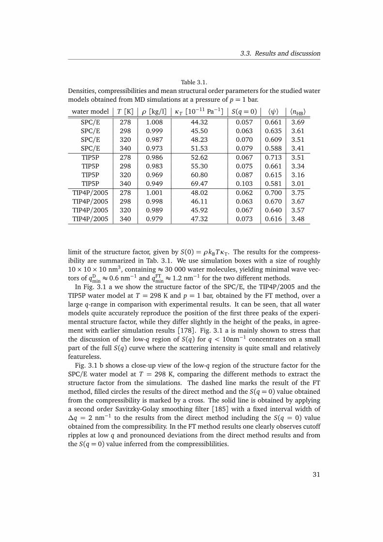
3.3. Results and discussion
Table 3.1.Densities, compressibilities and mean structural order parameters for the studied watermodels obtained from MD simulations at a pressure of p = 1 bar.
water model T [K] ρ [kg/l] κT [10−11 Pa−1] S(q = 0) ⟨ψ⟩ ⟨nHB⟩SPC/E 278 1.008 44.32 0.057 0.661 3.69SPC/E 298 0.999 45.50 0.063 0.635 3.61SPC/E 320 0.987 48.23 0.070 0.609 3.51SPC/E 340 0.973 51.53 0.079 0.588 3.41TIP5P 278 0.986 52.62 0.067 0.713 3.51TIP5P 298 0.983 55.30 0.075 0.661 3.34TIP5P 320 0.969 60.80 0.087 0.615 3.16TIP5P 340 0.949 69.47 0.103 0.581 3.01
TIP4P/2005 278 1.001 48.02 0.062 0.700 3.75TIP4P/2005 298 0.998 46.11 0.063 0.670 3.67TIP4P/2005 320 0.989 45.92 0.067 0.640 3.57TIP4P/2005 340 0.979 47.32 0.073 0.616 3.48
limit of the structure factor, given by S(0) = ρkBTκT. The results for the compress-ibility are summarized in Tab. 3.1. We use simulation boxes with a size of roughly10× 10× 10 nm3, containing ≈ 30 000 water molecules, yielding minimal wave vec-tors of qD
min ≈ 0.6 nm−1 and qFTmin ≈ 1.2 nm−1 for the two different methods.
In Fig. 3.1 a we show the structure factor of the SPC/E, the TIP4P/2005 and theTIP5P water model at T = 298 K and p = 1 bar, obtained by the FT method, over alarge q-range in comparison with experimental results. It can be seen, that all watermodels quite accurately reproduce the position of the first three peaks of the experi-mental structure factor, while they differ slightly in the height of the peaks, in agree-ment with earlier simulation results [178]. Fig. 3.1 a is mainly shown to stress thatthe discussion of the low-q region of S(q) for q < 10nm−1 concentrates on a smallpart of the full S(q) curve where the scattering intensity is quite small and relativelyfeatureless.
Fig. 3.1 b shows a close-up view of the low-q region of the structure factor for theSPC/E water model at T = 298 K, comparing the different methods to extract thestructure factor from the simulations. The dashed line marks the result of the FTmethod, filled circles the results of the direct method and the S(q = 0) value obtainedfrom the compressibility is marked by a cross. The solid line is obtained by applyinga second order Savitzky-Golay smoothing filter [185] with a fixed interval width of∆q = 2 nm−1 to the results from the direct method including the S(q = 0) valueobtained from the compressibility. In the FT method results one clearly observes cutoffripples at low q and pronounced deviations from the direct method results and fromthe S(q = 0) value inferred from the compressiblilities.
31

3. Correlations of Density and Structural Fluctuations in Bulk Water
The reason is the high sensitivity of the FT method in the low-q region to statisticalfluctuations in the RDF. This becomes apparent if we look at a Taylor expansion ofS(q),
S(q) =∞∑
i=0
s2i q2i , (3.10)
s2i = δi,0+(−1)i4πρ(2i+ 1)!
∫ ∞
0
drr2i+2[g(r)− 1]. (3.11)
The function value and the curvature at q = 0 of S(q) are determined by the first twoterms in the expansion and thus by the coefficients s0 and s2. Obviously, the slope ofS(q) at q = 0 vanishes. In Fig. 3.2, we plot the running integrals corresponding to s0(Fig. 3.2 a) and s2 (Fig. 3.2 b) obtained from the RDF of the SPC/E water model atdifferent temperatures of T = 278, 298, 320 and 340 K. Also included in Fig. 3.2 aare the results for S(q = 0) estimated from Eq. 3.5 (dashed lines). It is obvious fromFig. 3.2 a, that the statistical fluctuations, amplified by the r2 factor in the integral,make an accurate determination of s0 impossible. The actual s0 value obtained fromEq. 3.11 and therefore also the S(q = 0) value calculated by the FT method is a resultof these random fluctuations. The situation is even worse for s2, since there is a factorof r4 in the integral. This shows, that a meaningful determination of the curvatureof S(q) for q = 0 from the FT method alone is not possible. It also demonstrates thateven very slight numerical inaccuracies in the RDF can result in significant changes ofthe low-q behaviour of the structure factor.
Fig. 3.3 shows the low-q region of the structure factor of the SPC/E, the TIP5P andthe TIP4P/2005 water models at different temperatures using the direct method. Alsoincluded for comparison are the experimental curves of Ref. 20 (SAXS). It is seen,that for the TIP5P and TIP4P/2005 water models there is a pronounced minimumin the structure factor at wave vectors between q ≈ 3 nm−1 and q ≈ 5 nm−1, inagreement with previous results for the TIP4P-Ew water model [23]. For the SPC/Emodel the minimum is less pronounced but still perceptible. Quantitatively, the resultsfor the SPC/E and TIP5P water models deviate somewhat from the experimental S(q),while the TIP4P/2005 model compares excellently with the experiment. So rather thanstressing the differences between different water models, we take as the main messageof this figure that all water models studied by us and also the TIP4P-Ew model [23],exhibit an S(q) minimum at small q, which means that this is a quite robust feature ofclassical water models.
3.3.2. Order parameters
In the following we investigate to what extent the enhancement seen in the low-qregion of the structure factor is related to spatial correlations of the water struc-ture. To that end we examine two structural order parameters and their self and
32

3.3. Results and discussion
Figure 3.4.: (a) Probability distribution p(nHB) of the number of hydrogen bonds nHB and (b)probability distribution p(ψ) of the tetrahedrality order parameter ψ for TIP5P, TIP4P/2005and SPC/E water at temperatures of T = 278 K (black), 298 K (red), 320 K (green) and 340 K(blue) and at a pressure of p = 1 bar. Arrows indicate the effect of increasing temperature.
cross-correlations with the local density. The geometric aspects of the local water or-dering can be accurately described by the tetrahedrality order parameter ψ, definedin Eq. 3.7. For a perfect tetrahedral network ψ = 1, while for randomly orientedmolecules ψ = 0. As a measure for the strength of the hydrogen bonding networkwe take the number of hydrogen bonds nHB a water molecule forms with its neigh-bors. Here, we adopt the commonly used HOO-angle and OO-distance criterium forthe hydrogen bond formation [19]. Fig. 3.4 and Fig. 3.5 show the single and jointprobability distribution of the two order parameters for the studied water models andvarying temperatures. In agreement with previous studies [125], the tetrahedralityparameter displays a bimodal structure and for increasing temperature the probabilityof the high-ψ peak decreases while the probability of the low-ψ peak increases. Sim-ilarly, the number of water molecules forming four hydrogen bonds decreases, whilethe number of water molecules forming three or less hydrogen bonds increases withincreasing temperature. From the joint probability distribution (Fig. 3.5) it transpiresthat the high-ψ peak corresponds to water molecules forming four hydrogen bonds,while the low-ψ peak corresponds to water molecules forming three or less hydrogenbonds. The distinctly different ψ distributions of the sub populations for nHB = 3 andnHB = 4 explains the bimodality of the ψ distributions in Fig. 3.4.
33

3. Correlations of Density and Structural Fluctuations in Bulk Water
Figure 3.5.: Joint probability distribution p(ψ, nHB) of the number of hydrogen bonds nHB andthe tetrahedrality order parameter ψ for (a) SPC/E, (b) TIP4P/2005 and (c) TIP5P water attemperatures of T = 278 K (black), 298 K (red), 320 K (green) and 340 K (blue) and at apressure of p = 1 bar.
34

3.3. Results and discussion
3.3.3. Correlation functions
To gain information about spatial correlations of the different local water configura-tions, we define two-point correlation functions of the various local order parameters.In Fig. 3.6 a we show the normalized self-correlation function for the density
Cρρ(r) = g(r) =⟨ρ(0)ρ(r)⟩
ρ2 , (3.12)
and the normalized self-correlation functions
Cψψ(r) =⟨ψ(0)ψ(r)⟩⟨ψ⟩2⟨ρ(0)ρ(r)⟩
, (3.13)
and
Cnn(r) =⟨nHB(0)nHB(r)⟩⟨nHB⟩2⟨ρ(0)ρ(r)⟩
, (3.14)
of the tetrahedrality order parameter and the hydrogen bond numbers for the SPC/Ewater model at temperatures of T = 278, 298, 320 and 340 K. All correlation functionsare normalized to unity at large separations. In addition, we normalize the functionsCψψ(r) and Cnn(r) by the density density correlation function Cρρ(r) such that in theabsence of variations in the tetrahedrality parameter ψ or hydrogen bond number nHBthe functions would be constant. In contrast to the density density correlation functionCρρ(r), the self-correlation functions Cψψ(r) and Cnn(r) are quite featureless and thusshow that there are only weak correlations between structural fluctuations. The weakcorrelations that one can discern decay to zero after ≈ 6 Å. Note that the small jumpseen in the correlation function Cnn (indicated by a vertical arrow) is due to the HBcutoff radius rHB = 0.35 nm of the hydrogen bond criterium.
In Fig. 3.6 b the self-correlation functions Cψψ(r) and Cnn(r) are compared with thecross-correlation functions
Cψn(r) =⟨ψ(0)nHB(r)⟩
⟨ψ⟩⟨nHB⟩⟨ρ(0)ρ(r)⟩, (3.15)
Cρψ(r) =⟨ρ(0)ψ(r)⟩⟨ψ⟩⟨ρ(0)ρ(r)⟩
(3.16)
and
Cρn(r) =⟨ρ(0)nHB(r)⟩⟨nHB⟩⟨ρ(0)ρ(r)⟩
. (3.17)
Not surprisingly, the self- and cross-correlation functions of the tetrahedrality param-eter and the hydrogen bond number show similar behaviour, in line with the results
35

3. Correlations of Density and Structural Fluctuations in Bulk Water
from Fig. 3.5 which point to a close correspondence between the two order param-eters. We see that there are only weak spatial correlations between these two mea-sures of the local water structure, in other words the degree to which a given watermolecule is tetrahedrally ordered or hydrogen-bonded is only very weakly correlatedto the structural ordering of a neighboring water molecule. Note that Fig. 3.5 tells usthat the structural distribution functions are quite broad, so we learn that while struc-tural fluctuations are pronounced, their spatial correlation is weak. Interestingly, thecross-correlation functions Cρψ and Cρn between the density and the two structural or-der parameters exhibit even weaker correlations than the other correlation functions.In disagreement with the arguments brought forward in Ref. 20, we see that there isvery little correlation between density and structural fluctuations, meaning in specificthat features in S(q) data unfortunately tell us very little about the spatial correlationsof water structure. In Fig. 3.7 we show the normalized self- and cross-correlation func-tions of the density and the structural order parameters for the SPC/E, the TIP4P/2005and the TIP5P water models for different temperatures. The qualitative behaviour doesnot differ much between the different water models. In agreement with previous find-ings [181], the TIP5P water model is slightly overstructured in comparison with theTIP4P/2005 and SPC/E water models.
3.4. Conclusion
In this chapter we showed that for several commonly used water models at tempera-tures above melting, there exist only weak spatial correlations between different struc-tural order parameters. The typical range of structural correlations in Fig. 3.6 is con-sistent with a decay length on the order of 1 Å as observed in Ref. 167 for a coarsegrained water model. The relation of such a decay length with a correlation length asinferred from an Ornstein-Zernike analysis of the structure factor is however far fromclear [23]. We furthermore do not observe a pronounced spatial correlation betweenstructural and density fluctuations, implying that features in the structure factor cannot be interpreted in terms of or associated with structural properties, in contradictionto the assumptions made in Ref. 20 and in line with the results in Ref. 23. Erringtonet al. [166] report a reciprocal coupling between the tetrahedrality and the density intetrahedrally ordered clusters in SPC/E water at low temperatures of T = 220 K andT = 240 K. That we find very weak spatial coupling between the density and the tetra-hedral ordering in two-point correlation functions suggests that the clustering resultof Errington et al. [166] involves multi-point correlations. At this point it is impor-tant to stress that the correlations we find between local density and structure are nottotally absent, but they are rather much smaller than the density-density correlations(see Fig. 3.6). So whether one calls the density-structure correlation small or large de-pends on which reference one is using for comparison. Our results are consistent withthe findings of Matsumoto [168], who observed no direct relation between the densityanomaly and structural heterogeneities, but rather an interplay of monotonic hydro-
36

3.4. Conclusion
Figure 3.6.: (a) Self-correlationfunctions of density, Cρρ, tetra-hedrality order parameter, Cψψ,and the number of hydrogenbonds, Cnn. The inset showsan enlarged view of the longrange region of the density self-correlation function. (b) Com-parison of the self- and cross-correlation functions of the den-sity and the structural order pa-rameters. For clarity some curvesare shifted as indicated in the fig-ure. All data is obtained by MDsimulations of the SPC/E watermodel at temperatures of T =278 K (black), 298 K (red), 320 K(green) and 340 K (blue) and ata pressure of p = 1 bar.
37

3. Correlations of Density and Structural Fluctuations in Bulk Water
Figure 3.7.: Correlation functions of the density and the structural order parameters for theTIP5P, TIP4P/2005 and SPC/E water models at temperatures of T = 278 K (black), 298 K(red), 320 K (green) and 340 K (blue) and at a pressure of p = 1 bar. (a) Density densitycorrelation function Cρρ, (b) correlation function of the tetrahedrality order parameter Cψψ,(c) correlation function of the number of hydrogen bonds Cnn, (d) cross correlation of thetetrahedrality order parameter and the hydrogen bond number Cψn, (e) cross correlation of thetetrahedrality order parameter and the density Cρψ and (f) cross correlation of the hydrogenbond number and the density Cρn. Arrows in graphs (c), (d) and (f) indicate the cutoff radiusrHB = 0.35 nm of the hydrogen bond criterium. For clarity some curves are shifted as indicatedin the graph.
38

3.4. Conclusion
gen bond extension and angular distortion in the network (see Fig. 3.4) upon cooling.While the spatially averaged values of the density and the hydrogen bonding networkdistortion are of course related, we show that their fluctuations are not strongly cor-related in space. The picture of coexisting domains of differently structured water isnot supported by an analysis of the respective two-point correlation functions. Suchcorrelations might grow as temperature is lowered into the metastable liquid regimebelow melting and one approaches the liquid-liquid critical point, which, however, isnot focus of the present work.
We also show that the experimentally well documented minimum in the structurefactor at small wave vector q, which has very recently been seen in simulations ofTIP4P-Ew water [23], is obtained with different simple water models, suggesting thatthis is a quite robust feature, which in fact is related to the interplay of attractiveand repulsive forces [22, 186]. Finally, let us stress that we are not claiming thatclassical water models can accurately describe all aspects of water structure, however,the low-q behavior of S(q) does not constitute a serious hurdle for current classicalwater models.
39

40

CHAPTER 4
ENTROPY AND ENTHALPY CONVERGENCE BEYOND
THE HARD SPHERE MODEL
4.1. Introduction
4.1.1. Motivation
The question of protein folding and stability is one of the fundamental problems inbiology [187]. Despite intense scientific efforts since Anfinsens pioneering work [188]it is not yet completely clear what the dominant forces are, that govern protein sta-bility [53, 189]. The hydrophobic effect has long been suspected to play a majorrole [56]. It was therefore seen as a major breakthrough, when the observation ofconvergence of the denaturation entropy per residue of a whole class of proteins at auniversal temperature allowed to draw a close analogy with the solvation propertiesof simple hydrophobic compounds [66, 67].
It was first observed by Privalov and Khechinashvili [64, 65], that the entropies andenthalpies of denaturation per residue for a number of proteins, if extrapolated to hightemperatures, converge to a common value at a temperature near T ∗S ≈ T ∗H ≈ 110◦C.Baldwin [61] noticed, that at roughly the same temperature the entropy of dissolu-tion of several liquid hydrocarbons [190] extrapolates to zero (while the convergencetemperature of the solvation enthalpy is much lower). A similar convergence hasbeen observed [66, 67] for the dissolution of saturated hydrocarbon gases [47, 191–194], noble gases [47–49], cyclic dipeptides [62, 195] and gaseous alcohols [196].These observations stirred an intense discussion about the interpretation and im-plications of these findings for the role of the hydrophobic effect in protein fold-ing [62, 63, 67, 68, 196–198], which we will summarize briefly further below.
Theoretically, the temperature dependence of hydrophobic hydration has been stud-ied by various methods [43, 71–73, 75, 199–208], mostly focussing on the solvation ofsimple model solutes such as hard spheres [43, 72, 73, 75, 200–202, 204] or Lennard-Jones particles [71, 199, 203, 206, 208]. Using a Gaussian model for particle number
41

4. Entropy and Enthalpy Convergence beyond the Hard Sphere Model
fluctuations in atomic-scale cavities in conjunction with simulated water radial distri-bution functions, convergence temperatures of about T ∗S ≈ 400 K for small hard-spheresolutes of different radii, close to the experimental results, were obtained [72, 73, 75].The model allowed a simple interpretation of this phenomenon in terms of particlenumber fluctuations, water density variation, and to a limited extent the isothermalcompressibility of water [72, 73]. Results from the revised scaled-particle theory [43]show, that the convergence temperature T ∗S for larger sphere radii starts to depend onthe size of the solutes, but for typical solute radii around 3 Å convergence temperaturesin the range ≈ 370− 400 K are observed.
Despite this seemingly good agreement of the entropy convergence temperatures ob-tained from theoretical models for hard-sphere solvation with the experimental resultsfor both proteins and simple hydrophobic compounds, a few open questions remain:
i) For simple hydrophobic compounds, the convergence temperatures of solvationentropy and enthalpy widely differ, the latter being lower by typically 100◦, whilethe putative entropy and enthalpy convergence temperatures for proteins are thesame [61, 67]. To account for this, it is assumed that the solvation of hydrophilicgroups contributes to the enthalpy but not to the entropy, so that the solvation en-tropies of proteins and hydrophobic compounds are similar but not the enthalpies [68].In contradiction to this assumption and not surprisingly, we find a continuous changeof the solvation entropy as one goes from hydrophobic to hydrophilic solutes and inall cases the solvation entropy does not strictly vanish.
ii) The theoretically predicted convergence of hard-sphere solvation entropies atabout 400 K was obtained based on simulation results for SPC water simulated atthe experimental liquid-vapor coexistence density [72]. As we show in this work,at ambient pressure of 1 bar, which seems the relevant condition when comparingto protein data, the entropy convergence temperature for hard-sphere solvation goesdown to 340 K, in disagreement with both protein and simple hydrocarbon data.
iii) Perhaps most strikingly, Robertson and Murphy [69] showed, that for a largerset of proteins neither entropy nor enthalpy convergence is observed (see Fig. 4.1,circles), although the polar and non-polar surface areas per residue, that are buriedupon folding, show the same trends as for the smaller set of proteins originally studied(denoted by triangles) [67].
4.1.2. Outline
In this chapter we do not directly consider protein denaturation thermodynamics, butrather investigate the solvation of a more general class of spherical solutes. It has beenshown, that attractive solute-water interactions have a pronounced influence on thesolvation thermodynamics [71, 75, 202, 203, 207]. We therefore systematically studythe dependence of the entropy and enthalpy convergence temperature for sphericalsolutes on the solute-water interaction potential. We use a Buckingham double expo-nential potential with four free parameters to vary the stiffness of the repulsive part,the range and strength of the attractive part of the interaction as well as the solute
42

4.2. Thermodynamics of convergence
radius independently. Solvation free energies are obtained from molecular dynamics(MD) simulations by the particle insertion method. We mainly use the popular ex-tended simple point charge (SPC/E) water model, but also compare our results withthe simple point charge (SPC) and the TIP5P parameters to check the influence of thewater model [206, 208] on the solvation properties.
In Sec. 4.2, we review basic notions of thermodynamic convergence of solvation andprotein denaturation, in Sec. 4.3, we introduce the main concepts using the exampleof hard-sphere solutes. In Sec. 4.4, we discuss the dependence of the entropy andenthalpy convergence on the solute-water interaction details and the water modelemployed. In Sec. 4.5, we summarize and conclude.
4.2. Thermodynamics of convergence
Assuming a temperature independent heat capacity change ∆CP upon solvation of asolute or denaturation of a protein, from T∂∆S/∂ T =∆Cp and ∂∆H/∂ T =∆Cp, theentropy and enthalpy changes follow as [209]
∆S(T ) = ∆S(T0) +∆Cp ln�
T
T0
�
, (4.1)
and
∆H(T ) = ∆H(T0) +∆Cp�
T − T0�
, (4.2)
where T0 is an arbitrary reference temperature. We will show, that this assumption isapproximately true for the systems studied by us. If entropy convergence occurs at atemperature denoted by T ∗S for a group of species, then a plot of∆S(T ) versus∆Cp at afixed temperature T yields a straight line, whose slope ln(T/T ∗S ) is determined by theconvergence temperature T ∗S and whose intercept ∆S(T ∗S ) gives the entropy changeat the convergence temperature [67]. Similarly, a plot of ∆H versus ∆Cp yields astraight line with the slope T − T ∗H and intercept ∆H∗, if enthalpy convergence isobserved. Note that such a plot allows to extract the convergence temperature and theconvergence entropy or enthalpy based on the assumption of a constant heat capacityin a straightforward manner (but it does not allow to check wether the heat capacity isactually constant). In Fig. 4.1 we show such a plot for the original set of proteins [66]used in the analysis of Murphy et al. [67] (open triangles) including a linear fit to thedata. The data indicated by the filled triangle, corresponding to the denaturing of theprotein parvalbumin, was listed in Ref. 66 (see Table I of Ref. 66) but neither includedin the data fitting nor in the graph of Ref. 67. Note that the data in this plot has beenextrapolated from the denaturing temperature by assuming the relations Eqs. 4.1 and4.2 to hold, an assumption which for proteins is in general difficult to validate sincethe denaturing temperature can only be varied by adding denaturant or pH change(and thus possibly causing side effects) in a restricted range.
43

4. Entropy and Enthalpy Convergence beyond the Hard Sphere Model
Figure 4.1.: (a) Entropy change ∆S plotted against the change in isobaric heat capacity ∆Cpupon denaturation per residue extrapolated to 25◦ C for different sets of proteins. The small set(triangles) is taken from Ref. 66. Open triangles denote the proteins, that have been used in theanalysis of Ref. 67 to argue for the occurrence of entropy convergence in protein denaturation.The data point for parvalbumin (filled triangle) was included in the data set of Ref. 66 (seeTable I of Ref. 66) but not shown in the graph and not considered in the data fitting of Ref. 67.The data for the larger set of proteins (circles) is taken from Ref. 69. This set is separated intoproteins with denaturation temperatures Tm in the interval 55◦C < Tm < 65◦C (open circles)and Tm outside this interval (filled circles). The black line is a linear fit to the data set ofRef. 69, the dashed line to the open triangles. (b) Deviation ∆∆S of the unfolding entropy perresidue from the linear fit for the small set (dashed line in (a)) as a function of the number ofresidues Nres of the proteins. No systematic trend as a function of the protein size is seen. Also,there is no qualitative difference between the set of proteins with a denaturation temperatureclose to 60◦ C (open circles) and far away from 60◦ C (filled circles).
44

4.2. Thermodynamics of convergence
Murphy and Gill [62, 63] and Lee [68] showed that convergence of some ther-modynamic observable, e. g. the entropy of denaturation of a set of proteins or theentropy of dissolution ∆S within a homologous series of compounds, can generally beexpected if that observable is linearly dependent on the variable X (e.g. the number ofhydrophobic groups in a homologous series of hydrocarbons) which distinguishes theelements of the series,
∆S(T ) = ∆SR(T ) + X∆SX (T ), (4.3)
where ∆SX (T ) is the entropy change associated with the variable X and ∆SR is theresidual entropy change due to the molecular parts that are common within the series.From the relation Cp = T∂ S/∂ T we obtain a linear dependence of the heat capacitychange on X ,
∆Cp =∆CR+ X∆CX (4.4)
where we assume all heat capacity contributions to be independent of temperature.Then, by eliminating X from Eqs. 4.3 and 4.4, we obtain
∆S(T ) = ∆SR(T ) + (∆Cp −∆CR)∆SX (T )∆CX
, (4.5)
i. e., a linear dependence of ∆S(T ) on ∆Cp. A sufficient condition for both Eqs. 4.3and 4.4 is the linear dependence of the free energy change ∆F on X [68]. The ar-gument presented above is equivalent to the earlier observation of Sturtevant [210],that the ratio of entropy change and heat capacity change upon dissolution of sev-eral hydrophobic compounds is constant. Comparison with Eq. 4.1 shows, that theconvergence temperature, given by the slope,
ln
�
T
T ∗S
�
=∆SX (T )∆CX
, (4.6)
depends solely on quantities associated with the variable X . Equation 4.5 furtherimplies, that the entropy at convergence is equal to the residual entropy, ∆S(T ∗S ) =∆SR(T ∗S ). Therein lies the importance of convergence phenomena, since they enableone to separate different contributions to the observable under study.
In the case of protein denaturation it is not a priori clear, what the distinguishingvariable X is and therefore how the observed convergence should be interpreted [62,63, 67, 68, 196]. Murphy et al. [63, 67, 211] argue, that for globular proteins thepolar surface area per residue that is exposed to water upon unfolding is constant,while the non-polar surface area per residue varies and thus is taken proportional toX [211, 212]. This implies, that the contribution of the non-polar protein surfacevanishes at T ∗S , while the residual entropy is due to solvation of polar groups andconfigurational entropy, and corroborates the analogy with the dissolution of otherhydrophobic compounds [61, 67]. Accordingly, the similar convergence temperature
45

4. Entropy and Enthalpy Convergence beyond the Hard Sphere Model
for the different compounds is taken as an universal feature of hydrophobic hydra-tion [63, 67, 196]. Lee [68] originally suggested a slightly different assignment, nor-malizing the unfolding entropy by the buried surface area instead of the number ofresidues and taking the fraction of non-polar surface area exposed upon unfolding asthe variable X . In that case the convergence is observed at the temperature, at whichthe polar and non-polar contributions to the entropy are equal. Both approaches es-sentially can be viewed as different definitions of the hydrophobic contribution todenaturation [211].
One notes that the mechanism for entropy convergence discussed in Eqs. 4.3 - 4.6obviously rests on the assumption of additivity of the contributions of individual chem-ical groups to the total solvation entropy and enthalpy, an assumption which has beenindependently verified [191, 213, 214]. The other, more serious, assumption is thatit is sufficient to sort the solvation contributions of all chemical groups into just twogroups, hydrophilic and hydrophobic, characterized by the variable X , an assump-tion which we show not to be entirely true in this work. In fact, the concept of en-tropy convergence treated theoretically by the information theory approach and re-vised scaled particle theory in some sense goes beyond the additivity concept outlinedabove [62, 63, 68], since here it is shown that the entropy of solvation of hard spheresconverges to a universal value at one temperature for a whole range of different sphereradii. The importance of this observation lies in the fact that the hydrophobic groupsthat are solvated when a protein denatures in general have different radii. However,the convergence entropy is non-zero for hard-sphere solvation, so that according tothe assignment of Lee [68] one will in general not find a unique temperature wherethe hydrophobic contributions to the solvation entropy cancel the polar contributionsfor different proteins. Even more importantly, individual amino acids differ in moreproperties than just their radii, since details of the solute-water potential are expectedto vary between different species, which adds additional variation to the expectedconvergence temperatures. Again, all these reservations serve to explain that entropyconvergence for protein denaturation is not really expected, in accord with actual ex-perimental observations (see the complete set of protein data in Fig. 4.1) [69].
The convergence of solvation entropies and enthalpies of liquid hydrocarbons (e.g.alkanes) simply reflects the additivity of solvation of individual linked methyl groupsand thus is not really related to the main point of this work. An additional complica-tion comes in because transfer studies from liquid hydrocarbons to aqueous solution(as well as protein denaturation studies) involve the liquid (or protein core) referencestate, which is difficult to treat theoretically. Such complications are obviously absentfor solvation studies with noble or hydrocarbon gases, which are more closely relatedto our calculations. In this respect it is important to realize that the entropy conver-gence of noble gases is far from perfect [43], a fact that is very much in line with ourfindings.
46

4.2. Thermodynamics of convergence
Figure 4.2.: (a) Excess chemicalpotential µex, (b) entropy ∆S,(c) enthalpy ∆H and (d) iso-baric heat capacity ∆Cp of dif-ferently sized hard core solutesin SPC/E water as a function ofthe temperature. The soluteshave radii of 0.28nm (circles,black lines), 0.31 nm (squares,red lines), 0.33nm (diamonds,green lines) and 0.345nm (tri-angles, blue lines), correspond-ing roughly to the size of neon,argon, methane and xenon. Ex-cess chemical potentials are de-termined by test particle inser-tion (symbols). Solid lines areobtained by full fits of µex accord-ing to Eq. 4.7 and using Eqs. 4.8-4.10. Dotted lines are fits of µexunder the constraint of constant∆Cp, that is c = 0. Dashedlines are obtained by extrapola-tion, using Eqs. 4.1 and 4.2, fromthe reference temperature T0 =300 K with ∆S(T0), ∆H(T0) and∆Cp(T0) taken from the full fit.The trajectories for the particleinsertion are obtained from MDsimulations of 895 SPC/E watermolecules at constant pressurep = 1bar.
47
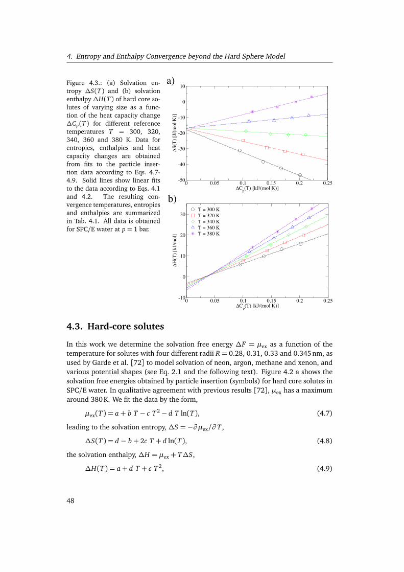
4. Entropy and Enthalpy Convergence beyond the Hard Sphere Model
Figure 4.3.: (a) Solvation en-tropy ∆S(T ) and (b) solvationenthalpy ∆H(T ) of hard core so-lutes of varying size as a func-tion of the heat capacity change∆Cp(T ) for different referencetemperatures T = 300, 320,340, 360 and 380 K. Data forentropies, enthalpies and heatcapacity changes are obtainedfrom fits to the particle inser-tion data according to Eqs. 4.7-4.9. Solid lines show linear fitsto the data according to Eqs. 4.1and 4.2. The resulting con-vergence temperatures, entropiesand enthalpies are summarizedin Tab. 4.1. All data is obtainedfor SPC/E water at p = 1 bar.
4.3. Hard-core solutes
In this work we determine the solvation free energy ∆F = µex as a function of thetemperature for solutes with four different radii R= 0.28, 0.31, 0.33 and 0.345 nm, asused by Garde et al. [72] to model solvation of neon, argon, methane and xenon, andvarious potential shapes (see Eq. 2.1 and the following text). Figure 4.2 a shows thesolvation free energies obtained by particle insertion (symbols) for hard core solutes inSPC/E water. In qualitative agreement with previous results [72], µex has a maximumaround 380 K. We fit the data by the form,
µex(T ) = a+ b T − c T 2− d T ln(T ), (4.7)
leading to the solvation entropy, ∆S =−∂ µex/∂ T ,
∆S(T ) = d − b+ 2c T + d ln(T ), (4.8)
the solvation enthalpy, ∆H = µex+ T∆S,
∆H(T ) = a+ d T + c T2, (4.9)
48

4.3. Hard-core solutes
Table 4.1.: Convergence temperatures T ∗S and T ∗H , entropies∆S∗ and enthalpies∆H∗ obtainedfrom the plots shown in Fig. 4.3 for different reference temperatures T .
T [K] T ∗S [K] ∆S∗ [J/(mol K)] T ∗H [K] ∆H∗ [kJ/mol]
300 347.2 -17.8 205.0 -3.1320 347.4 -17.1 204.7 -3.8340 347.5 -16.8 204.5 -4.5360 347.5 -16.8 204.2 -5.4380 347.5 -17.1 204.0 -6.4
and a linearly varying heat capacity increment
∆Cp = d + 2c T, (4.10)
see Fig. 4.2. To estimate how relevant the temperature dependence of the heat capacityis, we compare in Fig. 4.2 fit results using the full expression (shown by solid lines)with constrained fits where the heat capacity is forced to be constant and thus c = 0(dotted lines in Fig. 4.2). We find the fits with c = 0 to be of acceptable quality,which is in line with the fact that the actual heat capacity variation with temperatureis small. This is quite important in light of the common assumption of a constant heatcapacity used for extrapolating experimental solvation data. To check this procedureexplicitly, we extrapolate µex(T ), ∆S(T ) and ∆H(T ), using Eqs. 4.1 and 4.2 with areference temperature T0 = 300 K, where we extract values for ∆S(T0), ∆H(T0) and∆Cp(T0) from the full fit. The resulting extrapolated curves (dashed lines) differ fromthe full fits for high temperatures, but otherwise the accuracy seems acceptable. Theentropy shows convergence at a temperature around T ∗S ≈ 350 K, regardless of themethod used to fit the data, which is gratifying as most experimental convergencetemperatures are obtained via extrapolation. The value for T ∗S is significantly lowerthan the convergence temperature of about T ∗S ≈ 400 K found previously for hard-spheres in SPC water [72]. We will discuss the origin of this discrepancy in detailfurther below but briefly mention here that it has to do with the different densitiesat which the simulations in [72] have been performed. The enthalpy convergencetemperature lies outside the studied temperature range and occurs at roughly T ∗H ≈205 K. The difference in convergence temperature of about T ∗S − T ∗H ≈ 140 K is inrough agreement with experiments for simple liquid hydrocarbons, which give T ∗S ≈380 K and T ∗H ≈ 290 K, but there is a significant shift and we note that convergencein hydrocarbons occurs at vanishing entropy and enthalpy [61]. This is due to thefact that for homologous alkanes, convergence is mostly a consequence of additivity.For noble gases the entropy converges also around T ∗S ≈ 380K , but the convergenceentropy is non-zero. We will come back to this issue further below.
49

4. Entropy and Enthalpy Convergence beyond the Hard Sphere Model
In Fig. 4.3 we plot the solvation entropy ∆S(T ) and the solvation enthalpy ∆H(T )as a function of the heat capacity change ∆Cp(T ) for several different reference tem-peratures T = 300, 320, 340, 360 and 380 K. The convergence temperatures T ∗S andT ∗H and the entropies ∆S∗ and enthalpies ∆H∗ at convergence are summarized inTab. 4.1. For the entropy, the resultant numbers do not depend significantly on thereference temperature T and agree very well with what one directly reads off fromFig. 4.2. For the enthalpy, the individual linear fits in Fig. 4.3 are excellent, but theresulting convergence temperatures T ∗H and convergence enthalpies ∆H(T ) dependquite a bit on the reference temperature chosen. This is in line with the fact that theenthalpy data show less pronounced convergence when compared to the entropy, seeFig. 4.2. This shows clearly that a plot of ∆S(T ) or ∆H(T ) versus ∆Cp(T ) can bequite misleading, since if the heat capacity change is not independent of the temper-ature the values for the convergence temperature and convergence thermodynamicquantity depend considerably on the reference temperature chosen.
In all what follows we use the full expression Eq. 4.7 with a temperature dependentheat capacity change to fit the particle insertion data. As a simple definition for theconvergence temperature T ∗S we take the temperature at which the entropies of soluteswith radii R= 0.28nm and R= 0.345nm intersect, that is
∆SR=0.28nm(T ∗S ) = ∆SR=0.345nm(T ∗S ). (4.11)
The enthalpy convergence temperature T ∗H is defined analogously. We note that theconvergence temperature depends systematically on the solute sizes that are com-pared [43], so our definition only makes sense for the restricted range of radii actuallyconsidered by us.
4.4. Influence of the solute-water interaction
4.4.1. Stiffness of the repulsion
We first investigate the effect of the stiffness of the repulsive part of the potential,which is determined by the decay length 1/B. For this purpose, we study purely re-pulsive solutes (i.e. C = 0 in Eq. 2.1) with repulsion decay lengths in the range of1/B = 0.005− 0.03 nm and compare with hard core solutes. Figure 4.4 a shows theexcess chemical potential of a solute of radius R = 0.33nm for different values of thedecay length 1/B (circles, full lines) and for a hard core potential (squares, dashedline). This radius roughly corresponds to a methane molecule and is - because of theadditivity of solvation properties - also relevant for alkane chains. It is seen that thesolvation free energy curves are systematically shifted downwards for increasing po-tential stiffness, the stiffer the potential the less unfavorable the solvation process. Thiseffect is more pronounced at small temperatures, leading to a shift of the free energymaxima to higher temperatures as indicated by the dashed-dotted line. The corre-sponding solvation entropies are shown in Fig. 4.4 b. For increasing potential stiffness
50

4.4. Influence of the solute-water interaction
Figure 4.4.: (a) Excess chemicalpotential, (b) solvation entropyand (c) heat capacity changeupon solvation of purely repul-sive spherical solutes of radiusR = 0.33nm for varying repul-sion decay length 1/B = 0.005,0.01, 0.015, 0.02, 0.025 and0.03 nm (circles, full lines) and ahard core solute of the same ra-dius (squares, dashed lines) as afunction of the temperature. Thesymbols are results from parti-cle insertion. Lines are fits tothe data according to Eqs. 4.7 -4.10. The crosses in (a) markthe positions of the maxima ofthe chemical potentials and thedashed-dotted line is a quadraticfit. The trajectories for the parti-cle insertion are obtained by MDsimulations of the SPC/E watermodel at a constant pressure ofp = 1bar.
they are shifted towards higher temperatures, while the temperature dependence ofthe heat capacity in Fig. 4.4 c becomes more pronounced with increasing potentialstiffness. One notes, that there is no crossing of the curves, i. e., for solutes character-ized by same radii but different stiffness one does not find entropy convergence. Theentropy shifts have a pronounced influence on the convergence temperature, as shownin Fig. 4.5. For increasing stiffness the convergence is shifted to higher temperatures,reaching a value of T ∗S = 347K for the limiting case of a hard core solute alreadyshown in Fig. 4.2. Actual interaction potentials between solutes and water are farfrom the hard-core limit. For a realistic value of 1/B = 0.03nm the convergence tem-perature is T ∗S = 314 K. This temperature is even farther away from the experimentallyobserved value of T ∗S ≈ 385 K for noble gases and proteins [67]. In essence, we seethat a certain softness of the repulsive part of the solute-water interaction is relevantas it significantly shifts the convergence temperature to lower temperatures, but this
51

4. Entropy and Enthalpy Convergence beyond the Hard Sphere Model
Figure 4.5.: Solvation entropies for purely repulsive solutes of varying size R = 0.28nm(black), 0.31nm (red), 0.33nm (green) and 0.345nm (blue) and varying potential stiffness1/B = 0.03 nm (solid lines), 0.015nm (dashed lines), 0.005nm (dashed-dotted lines) andhard core (dotted lines) in SPC/E water at constant pressure p = 1 bar. Circles indicate theintersection of the entropies of solutes with radii R = 0.28 nm and R = 0.345 nm for the samevalues of the potential stiffness as shown in Fig. 4.4 (not all entropy curves are shown). In theinset the convergence temperature defined by Eq. 4.11 is shown as a function of the repulsiondecay length 1/B.
realistic feature does not improve the comparison with the experimental convergencetemperature. We will later see that an attractive component to the interaction willbring the convergence temperature up again.
4.4.2. Water models
Here, we investigate the origin of the discrepancies of our particle insertion simulationresults, obtained with SPC/E water so far, with previous theoretical results, based oninformation theory in conjunction with simulations for SPC water [72]. Figures 4.6 aand b show the solvation free energies and entropies for hard core solutes of varyingsize in SPC/E, SPC and TIP5P water including the information theory results of Ref. 72.Our data for the three different water models indicated by solid lines are all obtainedby particle insertion simulations at ambient pressure of p = 1 bar. While the excesschemical potentials agree rather well for temperatures around 300 K, they differ sig-nificantly at higher temperatures, which leads to a considerable spread in the resultingentropy convergence temperatures by about 30 K in Fig. 4.6 b. The data from Ref. 72,shown by the orange dashed lines, was obtained by the information theory approachbased on SPC simulations at densities corresponding to the experimental vapor-liquidcoexistence curve of water. The deviations from all the other data at p = 1 bar issignificant. To understand the reason for this deviation, we resimulated SPC waterat densities that match the experimental liquid-vapour coexistence densities and used
52

4.4. Influence of the solute-water interaction
Figure 4.6.: (a) Excess chemical potentials µex and (b) solvation entropies of hard core solutesof varying size R = 0.28, 0.31, 0.33 and 0.345nm for different water models. Symbols showthe data obtained from particle insertion for the SPC/E (circles, black), the SPC (squares,magenta) and the TIP5P (triangles, cyan) water model, solid lines are obtained by fits to theparticle insertion data according to Eq. 4.7 and 4.8. All simulations are performed at a constantpressure of p = 1bar. For comparison the information theory (IT) results of Garde et al.[72] (orange dashed lines) and our own IT results for SPC water simulated at the densitiesof the experimental saturation curve (purple stars and double-dotted dashed lines) are alsoincluded. (c) Comparison of the chemical potential obtained by the information theory model(see Eq. 4.12) including (circles and full lines) and neglecting (squares and dashed lines) thelogarithmic term, the compressibility approximation (Eq. 4.15) (diamonds and dashed-dottedlines) and the results from the particle insertion (triangles and dotted lines) for SPC/E waterat a constant pressure of p = 1 bar. Lines are fits to the data points. The inset in (d) showsthe fits to µex on a larger scale. (d) Comparison of the solvation entropies obtained by thetemperature derivative of the fits to the chemical potentials shown in (c). Line styles have thesame meaning as in (c).
53

4. Entropy and Enthalpy Convergence beyond the Hard Sphere Model
Table 4.2.: Isothermal compressibility κT of the SPC/E water model at a pressure of p =1 bar for varying temperature. The compressibilities are obtained from MD simulations by anumerical derivative according to Eq. 3.6. Error estimates are obtained by a block averagingalgorithm.
T [K] κT [10−11 Pa−1]
278 44.32 ± 0.17298 45.50 ± 0.17320 48.23 ± 0.19340 51.53 ± 0.20360 55.91 ± 0.25380 61.61 ± 0.28400 69.10 ± 0.44420 78.66 ± 0.96
the same information theory approach, the results are shown by purple stars and lines.The agreement with the previous IT approach is perfect, yet, the disagreement withthe other simulations still needs to be explained.
To that end, let us briefly reconsider the information theory model for the solvationof hard core solutes [72–74]. It relates the excess chemical potential µex of a hard-coresolute to the solvent particle number fluctuations inside a cavity of the size and shapeof the solute, assuming Gaussian fluctuations. Using a continuous Gaussian approxi-mation for the particle number distribution, the excess chemical potential follows as
µI Tex = kBTρ2v2/2⟨δn2⟩+ kBT ln(2π⟨δn2⟩)/2, (4.12)
where ρ is the number density of the solvent, v is the volume of the cavity, δn= n−⟨n⟩,and n is the number of solvent particles inside the randomly placed cavity. The secondmoment of the particle number fluctuations, ⟨δn2⟩, is related to a double integral overthe oxygen-oxygen radial distribution function gOO(r) by
⟨n(n− 1)⟩= ρ2
∫
v
d3r
∫
v
d3r ′gOO�
|~r −~r ′|�
, (4.13)
which thus yields a straightforward way to evaluate the expression Eq. 4.12 based onsimulation results for the distribution function gOO(r). In the thermodynamic limit,i.e. for infinite cavity volume v, the relation
⟨δn2⟩⟨n⟩
= ρkBTκT (4.14)
54
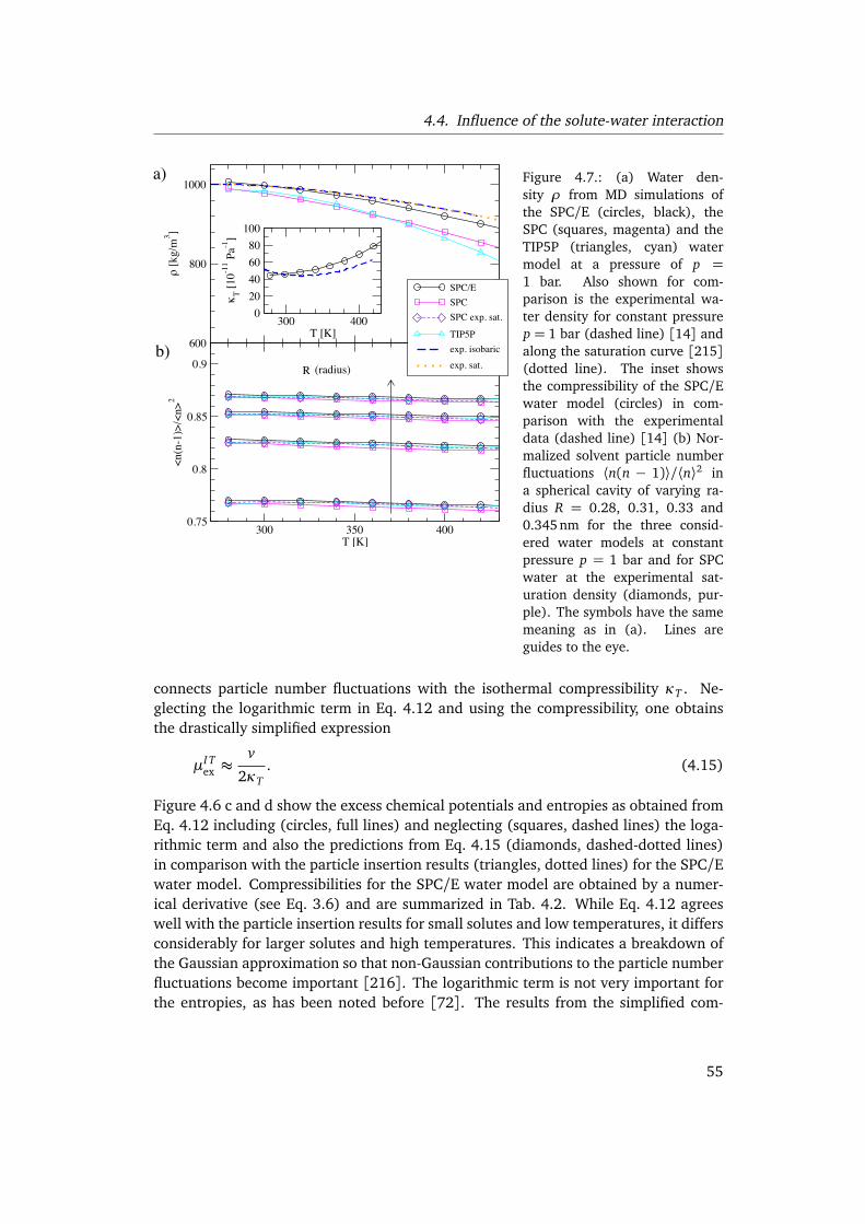
4.4. Influence of the solute-water interaction
Figure 4.7.: (a) Water den-sity ρ from MD simulations ofthe SPC/E (circles, black), theSPC (squares, magenta) and theTIP5P (triangles, cyan) watermodel at a pressure of p =1 bar. Also shown for com-parison is the experimental wa-ter density for constant pressurep = 1 bar (dashed line) [14] andalong the saturation curve [215](dotted line). The inset showsthe compressibility of the SPC/Ewater model (circles) in com-parison with the experimentaldata (dashed line) [14] (b) Nor-malized solvent particle numberfluctuations ⟨n(n − 1)⟩/⟨n⟩2 ina spherical cavity of varying ra-dius R = 0.28, 0.31, 0.33 and0.345 nm for the three consid-ered water models at constantpressure p = 1 bar and for SPCwater at the experimental sat-uration density (diamonds, pur-ple). The symbols have the samemeaning as in (a). Lines areguides to the eye.
connects particle number fluctuations with the isothermal compressibility κT . Ne-glecting the logarithmic term in Eq. 4.12 and using the compressibility, one obtainsthe drastically simplified expression
µI Tex ≈
v
2κT. (4.15)
Figure 4.6 c and d show the excess chemical potentials and entropies as obtained fromEq. 4.12 including (circles, full lines) and neglecting (squares, dashed lines) the loga-rithmic term and also the predictions from Eq. 4.15 (diamonds, dashed-dotted lines)in comparison with the particle insertion results (triangles, dotted lines) for the SPC/Ewater model. Compressibilities for the SPC/E water model are obtained by a numer-ical derivative (see Eq. 3.6) and are summarized in Tab. 4.2. While Eq. 4.12 agreeswell with the particle insertion results for small solutes and low temperatures, it differsconsiderably for larger solutes and high temperatures. This indicates a breakdown ofthe Gaussian approximation so that non-Gaussian contributions to the particle numberfluctuations become important [216]. The logarithmic term is not very important forthe entropies, as has been noted before [72]. The results from the simplified com-
55

4. Entropy and Enthalpy Convergence beyond the Hard Sphere Model
pressibility expression in Eq. 4.15 are completely off the particle insertion results (seeinset of Fig. 4.6), showing that Eq. 4.14 is not valid on the nano scale.
To explain the different results for the different water models and the discrepancywith the data of Ref. 72 we rearrange Eq. 4.12 without the logarithmic term in thefollowing way,
µI Tex ≈
kBT
2
�⟨n(n− 1)⟩⟨n⟩2
− 1+1
vρ
�−1
, (4.16)
where we used the relation ⟨n⟩= vρ. We show ρ and ⟨n(n−1)⟩/⟨n⟩2 for the differentwater models and pressures as obtained from simulations in Fig. 4.7. As noted be-fore [72], ⟨n(n− 1)⟩/⟨n⟩2 shows only a weak dependence on temperature or pressureand does not differ much between the different water models (see Fig. 4.7 b). Thedensity ρ on the other hand shows a pronounced temperature dependence, differsappreciably between the water models and also shows deviations from the experi-mental data. Comparing with Eq. 4.16 and noting that the neglect of the logarithmicterm in Eq. 4.12 is not very serious, as shown in Figure 4.6 c and d, one concludesthat it is mostly the variation in ρ that causes the differences in the solvation freeenergy [72, 206, 208], as seen in Fig. 4.6 a and b. Note that the compressibility κTobtained for SPC/E, shown in the inset of Fig. 4.7 a, shows considerable dependenceon temperature and agrees overall quite well with experimental data. But, as shownabove, its temperature dependence cannot be used as a simple explanation of the en-tropy convergence phenomena since Eq. 4.14 is too inaccurate to describe solvation ofsmall solutes.
In summary, two different factors contribute to the shift of the entropy convergencetemperature between our simulated particle insertion data and the published informa-tion theory results: Firstly, the temperature dependence of the experimental coexis-tence density is quite different from the simulated density at ambient pressure (andas a side remark, this deviation is more pronounced with SPC than with SPC/E), seeFig. 4.7 a, while the experimental densities at ambient and saturation pressures arevery close. Secondly, there is a systematic shift of the entropy convergence to highertemperatures for the information theory results as compared to straight particle inser-tion results, see Figure 4.6 c and d. Finally, we note that the coexistence densities ofthe SPC water model are significantly lower than the experimental ones [217], sim-ulating the SPC water model at experimental saturation densities therefore leads tounrealistically high pressures, e.g. 880 bar at T = 500 K compared to the experimen-tal saturation pressure of 26.4 bar [215]. It is not clear what the significance of suchhigh pressure is, but it might significantly change the water properties and thereforelead to unrealistic results.
4.4.3. Attractive interactions
We next investigate the solvation of non-polar solutes whose interaction with wateralso has an attractive part, according to Eq. 2.1. For a fixed decay length 1/B =
56

4.4. Influence of the solute-water interaction
Figure 4.8.: Excess chemical potential for a spherical solute with radius R = 0.33 nm (a) for1/B = 0.02nm, 1/D = 0.05 nm and varying potential depth ε0 = 0.0, 0.1, 0.2, 0.3, 0.4, 0.5,0.6, 0.7 and 0.8 kJ/mol and (e) for 1/B = 0.02 nm, ε0 = 0.7 kJ/mol and varying range of theattractive part of the potential 1/D = 0.05, 0.1 and 0.2 nm. Circles show the data obtainedby test particle insertion, lines are fits to the particle insertion data. The dashed line marksa purely repulsive solute (ε0 = 0), while the solid lines correspond to the attractive solutes.Crosses indicate the position of the maxima of the free energy curves and the dashed-dottedline is a fit to the maxima. [(b), (f)] Solvation entropies, [(c), (g)] enthalpies and [(d), (h)]heat capacity changes obtained from derivatives of the fits to the free energies shown in (a)and (e). The trajectories for particle insertion are obtained by MD simulation of the SPC/Ewater model at p = 1bar.
57

4. Entropy and Enthalpy Convergence beyond the Hard Sphere Model
Figure 4.9.: (a) Solvation entropies for solutes with radii R = 0.28 nm (black), 0.31 nm (red),0.33 nm (green) and 0.345 nm (blue) for 1/B = 0.02 nm, 1/D = 0.05 nm and varying po-tential depth ε0 = 0 (solid lines), 0.3 kJ/mol (dashed lines) and 0.8kJ/mol (dashed-dottedlines). The symbols show the intersection of the curves for solutes of size R = 0.28 nmand R = 0.345 nm for an attraction range 1/D = 0.05nm (circles), 1/D = 0.1 nm (squares,entropy curves not shown) and 1/D = 0.2nm (triangles, entropy curves not shown) and1/B = 0.02 nm. The dashed curves are linear fits to the intersection points. The inset showsthe convergence temperature defined by Eq. 4.11 for 1/D = 0.05 nm (circles), 1/D = 0.1 nm(squares) and 1/D = 0.2 nm (triangles) and 1/B = 0.02 nm. Solid curves show linear fits tothe data. (b) Analogous results for the solvation enthalpy. [(c), (d)] Solvation entropy andenthalpy for the stiffer repulsive potential characterized by 1/B = 0.005nm for varying poten-tial depth ε0 = 0 (solid lines), 0.3 kJ/mol (dashed lines), 0.8 kJ/mol (dashed-dotted lines) and1.3 kJ/mol (dotted lines) and for only one attractive range 1/D = 0.05nm.
58

4.4. Influence of the solute-water interaction
Figure 4.10.: (a) Convergence temperature for spherical solutes with 1/B = 0.02 nm, 1/D =0.05 nm (circles), 0.1 nm (squares) and 0.2 nm (triangles) and varying depth (ε0 = 0.0 - 0.8kJ/mol) as a function of the effective stiffness (1/B)eff, defined in Eq. 4.17. Lines are quadraticfits to the data. Also shown for reference is the convergence temperature for purely repulsivesolutes (crosses) including a linear fit to the data. (b) Convergence temperature T ∗S , correctedfor the varying effective stiffness as a function of the potential depth ε0. The inset shows theeffective stiffness of the attractive potentials as a function of the potential depth. Symbols havethe same meaning as in (a). All data is obtained by particle insertion in SPC/E water at p = 1bar.
0.02 nm of the repulsive part of the potential, we vary the range of the attractiveinteraction (1/D = 0.05,0.1 and 0.2 nm) as well as the potential depth (ε0 = 0.0,0.1, 0.2, 0.3, 0.4, 0.5, 0.6, 0.7 and 0.8 kJ/mol). In Fig. 4.8 a and b we show theresulting solvation free energies and entropies for a solute of radius R = 0.33 nm andfor 1/B = 0.02 nm and 1/D = 0.05nm for different values of the potential depth ε0;in Fig. 4.8 e and f we show solvation free energies and entropies for 1/B = 0.02nmand ε0 = 0.7 kJ/mol for varying potential range 1/D. It can be seen from Fig. 4.8 aand e, that for increasing potential depth and range the solvation free energies areshifted downwards, as expected due to the more favorable enthalpic contribution ofthe attraction (see Fig. 4.8 c and g). For the largest range studied, 1/D = 0.2 nm, thesolvation free energy energy approaches zero, meaning that we are almost describinghydrophilic (yet non-polar) solutes. At the same time the position of the maximumof the free energy curve is shifted towards higher temperatures. Accordingly, alsothe solvation entropy curves are shifted towards higher temperatures with increasingpotential depth and range (see Fig. 4.8 b and f). Interestingly, for increasing attraction,that is as one goes from very hydrophobic solutes to less hydrophobic solutes, thesolvation entropies become more negative while the heat capacities in Figs. 4.8 d and hstay roughly the same. This stands in contrast to the common view according to whichthe solvation of hydrophilic solutes is purely enthalpic and characterized by vanishingheat capacity [63, 68]. We note, that the solvation free energies for a Lennard-Jonesparameterization of methane [208] are well within the spread observed in Fig. 4.8
59

4. Entropy and Enthalpy Convergence beyond the Hard Sphere Model
e. For example at T = 300 K Ashbaugh et al. [208] find a solvation free energy of9.3 kJ/mol for OPLS-methane in SPC/E water, while for a methane size solute withε0 = 0.7 kJ/mol and 1/B = 0.02 nm we obtain 15.2 kJ/mol for 1/D = 0.1 nm and3.2 kJ/mol for 1/D = 0.2 nm.
The effect of increasing potential depth and range on the convergence tempera-ture is shown in Fig. 4.9, where we plot the solvation entropies and enthalpies forsolutes of varying radii and different values of the potential depth ε0 and range 1/Das a function of the temperature. For the less stiff repulsive potential characterizedby 1/B = 0.02 nm we show in Figs. 4.9 a and b the intersection points of the en-tropy and enthalpy curves for solutes with radii R = 0.28nm and R = 0.345nm forattractive potential ranges of 1/D = 0.05 nm (circles), 1/D = 0.1nm (squares) and1/D = 0.2nm (triangles). For the latter two the entropy curves are not shown. InFigs. 4.9 c and d we show data for 1/D = 0.05 nm and the stiffer repulsive potential1/B = 0.005 nm. It can be seen, that the convergence for increasing potential depthis shifted to higher temperatures, while the convergence entropies and enthalpies be-come more negative. This effect is more pronounced for more long-ranged attraction.In the insets of Fig. 4.9 we plot the convergence temperatures, defined by Eq. 4.11,as a function of the potential depth for varying potential ranges. Surprisingly, theconvergence temperatures show very little dependence on the range of the attractivepotential. It is apparent from Fig. 2.1 b, that a changing attractive potential depthalso modifies the repulsive flank of the potential and thereby increases the apparentstiffness of the potential slightly. To understand the reason for the insensitivity of theentropy convergence temperature on the attractive range, we first have to disentanglethe effects due to the repulsive and attractive parts of the potential. As a measureof the actual stiffness of the repulsive flank of the potential we define the effectivestiffness 1/Beff of the potential (Eq. 2.1) as
1
Beff=−
kBT0
∂ USPH−OW(r)/∂ r|r=R. (4.17)
For a purely repulsive solute (C = 0), this reduces to the usual decay length of thepotential, 1/Beff = 1/B. The effective stiffness for attractive potentials with varyingrange 1/D = 0.05, 0.1 and 0.2 nm is plotted in the inset of Fig. 4.10 b as a functionof the potential depth ε0. The increase in the effective stiffness with potential depthis smaller for the longer ranged potentials in accordance with Fig. 2.1. We assume,that the convergence temperature is an analytic function of the effective stiffness Beff,the potential depth ε0 and range D, that is T ∗S = T ∗S (Beff,ε0, D). Since with increasingthe potential depth ε0 also the effective stiffness Beff increases, it is a priori not clearwhich of the two causes the change in the convergence temperature. In Fig. 4.10 a, weplot the convergence temperature for the attractive solutes as a function of 1/Beff andcompare it to the results for the purely repulsive solutes. It is seen, that the conver-gence temperature for the attractive solutes rises much faster with increasing effectivestiffness than for the purely repulsive solutes, so the change in effective stiffness alonecannot explain the shift in the convergence temperature; it is rather a combined effect
60

4.5. Conclusion
of both factors. In order to disentangle the effects of the attractive interactions andthe effective stiffness of the repulsive part of the potential, we expand T ∗S (Beff,ε0, D)for fixed D in a Taylor series with respect to ε0 and Beff,
T ∗S (Beff,ε0, D) ≈ T ∗S (B0eff,ε
00, D)
+∂ T ∗S (B
0eff,ε
00, D)
∂ Beff(Beff− B0
eff) (4.18)
+∂ T ∗S (B
0eff,ε
00, D)
∂ ε0(ε0− ε0
0).
Adding and subtracting T ∗S (B0eff,ε
00, D) one can rearrange Eq. 4.18 to yield
T ∗S (Beff,ε0, D) ≈ T ∗S (Beff,ε00, D) + T ∗S (B
0eff,ε0, D)
− T ∗S (B0eff,ε
00, D). (4.19)
If we choose 1/B0eff = 0.02 nm and ε0
0 = 0, then T ∗S (Beff,ε00, D) and T ∗S (B
0eff,ε
00, D) are
given by the results for purely repulsive solutes and we can calculate T ∗S (B0eff,ε0, D)
by solving Eq. 4.19. We plot T ∗S (B0eff,ε0, D) for 1/B0
eff = 0.02 nm in Fig. 4.10 b asa function of the potential depth ε0 for the three different ranges studied. Still astrong dependence on ε0 can be observed, while there is almost no change with therange of the attractive part of the potential. We conclude that the entropy convergencetemperature shows no dependence on the range of the attractive part of the potentialand only depends on the attractive strength and repulsive stiffness. This suggests,that the main contribution to the temperature dependence of the solvation free energycomes from the first solvation shell around the solute and is therefore determined bythe short range structure of the hydrogen bonding network.
4.5. Conclusion
We performed an analysis of the solvation properties of small spherical solutes for abroad class of solute-water potentials. In all cases the free energies show a maximumat a temperature that depends quite sensitively on details of the potential, below thattemperature the solvation entropy is negative (i.e. the solute orders the water), abovethat temperature the entropy is positive (i.e. the solute increases the water disor-der). The heat capacity is invariably positive. These are the common signatures of hy-drophobic solvation of small solutes. No convergence is found for solutes of the samesize characterized by different 1/B and ε0, but restricted convergence is observed forthe same 1/B and ε0 and different radii of the solutes. The entropy convergence tem-perature, at which the solvation entropies of solutes of different radii are the same,depends also on potential details in the following fashion: The less stiff the short-ranged repulsive part of the potential, the lower the convergence temperature, thedeeper the attractive part, the higher the convergence temperature. The range of the
61

4. Entropy and Enthalpy Convergence beyond the Hard Sphere Model
attractive part does not influence the convergence properties, which suggests that it isonly the first water shell that plays a role for convergence. Nevertheless, these resultsmean for the case of protein denaturation, where different amino acids plausibly arecharacterized by different effective water-amino acid potentials, entropy or enthalpyconvergence cannot be expected in the general case. This is in agreement with a re-cent analysis of a large unbiased set of protein data [69]. It has been suggested thatthe spread in the protein convergence properties in Fig. 4.1 can be related to the sizeof the proteins [200]. However, when we plot the deviation from a straight-line fitas a function of the number of residues (see Fig. 4.1 b) we seem not to obtain anysystematic trend. Likewise, although we show that the extrapolation procedure whichis used to obtain thermodynamic data at one temperature, which basically rests on theassumption of a constant heat capacity, is fine for the solvation of non-polar solutes(see our analysis in Figs. 4.2 and 4.3), there could be extrapolation artifacts in theprotein denaturation data. However, when we separate data from proteins that dena-ture around 60◦ C (shown by open circles) from proteins that denature further awayfrom 60◦ C (filled circles) we do not see a systematic difference in the two data sets,ruling out problems with the extrapolation method as a possible cause of the absenceof entropy convergence. Taken together all evidence, entropy convergence of proteindenaturation does not seem to be evidenced by the experimental data.
Although strictly speaking we cannot conclude that the breakdown of convergencein protein denaturation data is caused by the variations of the interactions of indi-vidual amino acids with water as we have studied in this work, we note that thesevariations are sufficient to give rise to a breakdown of convergence. Other factors thatwould work in the same direction are specificities in the folded state, which we didnot address.
Most directly our results are applicable to the solvation of gaseous particles in water,since here specifics of the reference state (which is the liquid state for liquid hydro-carbons or the protein core for folded proteins) are absent. We stress again a subtlepoint mentioned already in the previous sections: For liquid hydrocarbons which forma homologous series, entropy convergence is foremost a consequence of the additivityof solvation properties of individual methyl and methylene groups and yields a van-ishing entropy at the convergence temperature. In contrast, convergence for differentnoble gases is not connected to the additivity hypothesis but rather to an insensitivityof solvation thermodynamics to variations in the solute-water interaction and leads ingeneral to a non-vanishing entropy at convergence.
We see that the entropy convergence of noble gases, which experimentally occursaround 380 K, is quite well reproduced for sensible values of the attractive strengthand range around 1/B = 0.005 nm and ε0 = 1.3 kJ/mol. Experimentally, the conver-gence is far from perfect, since e. g. the entropies of Ne, Ar and Xe do not cross at onetemperature. The actual value of the entropy at convergence comes also out quite wellfrom our simulation results. As seen in Fig. 2 of Ref. 43, Ar and Xe cross at an entropyof ∆S ≈ −4 cal/mol K ≈ −17 J/molK, which is in line with typical convergence en-
62

4.5. Conclusion
tropies we obtain for a wide range of values of the attractive depth between ε0 = 0.3and 1.3 kJ/mol, see Fig. 4.9 c.
Note that the model potential considered by us should be viewed as realistic for thesolvation of hydrophobic particles which cannot form hydrogen bonds with the water.In the future, it will be interesting to study polar solutes as well and to check whetherrobust and significant differences to the solvation of unpolar solutes are obtained.
As a word of caution, we note that convergence properties depend sensitively onthe water parameters used, which simply reflects the fact that one is dealing withhigher-order derivatives of the free energy. Thus, they are very sensitive to small force-field variations and imperfections. The actual numbers quoted by us should thus beconsidered with care. Likewise, we only study small radii, for which more complicatedeffects associated with the crossover to the solvation of planar interfaces is not yetreached [42].
63

64

CHAPTER 5
SURFACE FUNCTIONAL DESCRIPTION OF
HYDROPHOBIC HYDRATION
5.1. Introduction
5.1.1. Motivation
As noted above, the hydrophobic effect is the dominant driving force for self-assemblyin the aqueous environment and spans many length scales, ranging from proteinfolding over macromolecular aggregation and membrane formation to macroscopicphase separation [52]. The solvation of hydrophobic objects displays a characteris-tic crossover at a length scale of R∗ ≈ 0.5 nm [40, 41, 43] which can be associatedwith the discreteness of water: While small hydrophobic solutes can be readily ac-commodated within the water hydrogen bonding network, mostly reducing the waterconfigurational freedom, large solutes lead to a reduction of hydrogen bonds and theformation of a liquid-vapour like interface. It has been a long standing question howhydrophobic solvation on the nanoscale can be described by an interface model interms of suitably defined geometrical measures.
In 1949, Tolman [79] proposed an asymptotic curvature correction for the surfacetension of a spherical cavity, obtained from purely thermodynamic considerations,
γSPH = γ0
�
1−2δ
R
�
, (5.1)
where γ0 is the surface tension of a planar interface, R is the cavity radius and δ isthe Tolman length, which corresponds to the shift between the Gibbs dividing surface(GDS) RGDS and the surface of tension RS in the planar limit [218],
δ = limR→∞
RGDS− RS. (5.2)
With the convention that the radius of a cavity (or bubble) is taken as positive (notethat all cited results are adapted to this sign convention), a negative Tolman length
65

5. Surface Functional Description of Hydrophobic Hydration
Figure 5.1.: a) Simulation snap-shot of a simulation system con-taining two air/water interfacesfor a lateral box size of L =3.0 nm, containing 1807 watermolecules. The enlarged sliceto the right exhibits pronouncedsurface roughness. b) Aver-age density profile (circles, L =3.0 nm) compared with a hyper-bolic tangent fit (solid line). Ver-tical dashed lines show the posi-tions of the global GDS. c) Den-sity profiles centered around theGDS for varying L; lines areguides to the eye.
means that a droplet is preferred over a cavity, i.e. the surface of tension is shiftedtowards the liquid water side of the GDS.
A more general description of the free energy of an interface is given by Helfrich’sphenomenological curvature expansion [89],
∆F =
∫
dA�
γ+ 2κ(J − c0)2+ κK
�
, (5.3)
where J = (1/R1 + 1/R2)/2, K = 1/(R1R2) and c0 are the mean, Gaussian and spon-taneous curvatures, R1,2 are the local principal radii of curvature and κ and κ are thenormal and Gaussian bending rigidities. The planar surface tension is given by theconstant term in Eq. 5.3, γ0 ≡ γ+2κc2
0 . Expressions like Eqs. 5.1 and 5.3 give a simpledescription of hydrophobic solvation and are at the core of advanced implicit solvationmodels [219].
However, the determination of the coefficients is for several reasons not straight-forward: i) While the magnitude of δ is generally agreed to be on the order of themolecular size, not even for simple Lennard-Jones (LJ) liquids a consensus is reachedabout its sign, see [80, 81] and references therein. ii) The aforementioned crossoverbetween small-scale and large-scale solvation, caused by the water discreteness, occursat roughly the same scale as the Tolman length, i.e. R∗ ∼ δ, and it is not straightfor-ward to disentangle these two lengths. iii) Furthermore, it is not clear how the Tolmanlength for water in contact with a hard solute compares with that of a liquid dropletor a bubble, where one has a liquid-vapor interface [220–224]. Using a combinationof simulations and scaled particle theory, a Tolman length of the order of 1 Å waspredicted for water at ambient temperature [83, 85]. Ashbaugh and Pratt [43] find
66

5.1. Introduction
δ ≈ 0.6 Å at T = 300 K which decreases with increasing temperature and changessign at T ≈ 350 K. Huang et al. [42] deduce δ = 0.9 Å at T = 298 K for SPC/Ewater from simulated solvation free energies of hydrophobic spheres. Yamamoto andOhnishi [225] on the other hand find a maximum in the surface tension of heliumbubbles in water as a function of bubble radius, corresponding to a negative Tolmanlength.
Not surprisingly, the sign and magnitude of the second order curvature correctionis much debated as well. Square-gradient theory yields a negative bending rigidity forthe "equilibrium route" [90], that is by considering an interface that is curved due toan external potential, while van Giessen and Blokhuis [226] obtained a positive κ andnegative κ by applying a virial expression to computer simulations of a Lennard-Jonesliquid forming spherical and cylindrical droplets.
Instead of bending the water surface by external forces, represented by a solute, onecan also obtain information on the interfacial elastic properties by studying the equi-librium fluctuations of a free liquid/vapour interface, i. e. thermally induced capillarywaves, which has been termed "fluctuation route" [90]. Standard capillary wave (CW)theory can be extended to incorporate the effects of higher order curvature correctionsas described by Eq. 5.3, which results in a wave vector dependent effective surface ten-sion γeff(q) = γ0 + κq2 [93]. Note, that odd curvature terms vanish due to symmetryreasons.
Since a few years grazing-incidence X-ray scattering from liquid surfaces yields in-formation on lateral density correlations in the interfacial region. The obtained scat-tering signal combines effects due to bulk-like density fluctuations close to the in-terface, dominant at large wavevectors [97], and effects due to shape fluctuationsof the interface, dominant at small wavevectors [95, 96]. Disentangling these twocontributions in the experimentally accessible intermediate range of wavevectors andextracting the capillary wave spectrum of the liquid-vapor surface is by no meansstraightforward [91, 98–100]. Experimental scattering spectra span the wave vectorrange of q−1 ' 0.1− 10 nm, posing a dilemma: for q values small enough that CWtheory is valid, the deviations from the trivial limit γeff(q) = γ are small and accuracybecomes the limiting factor.
In theoretical work, the extended capillary wave theory has been applied to the liq-uid vapor interface in a Lennard-Jones fluid by Stecki [93, 94], who found evidencefor a negative bending rigidity. Chacón and Tarazona [92] on the other hand found apositive bending rigidity, using a different definition of the surface, where a minimumarea surface is pinned to a set of pivot atoms. To complicate matters, it has been sug-gested by Blokhuis et al. [90], that the bending rigidities obtained by this "fluctuationroute" might differ from those obtained by the "equilibrium route". Furthermore it hasbeen argued, that for interaction potentials decaying ∝ r−6 a curvature expansion ofthe surface tension fails beyond the linear term [91, 227, 228], a problem which canbe circumvented if the retardation to a r−7 dependence is taken into account.
67

5. Surface Functional Description of Hydrophobic Hydration
Figure 5.2.: Simulation snapshots of [(a),(b)] spherical and [(d),(e)] cylindrical hydrophobicsolutes in water with different radii. Dashed lines indicate water hydrogen bonds. [(c),(f)]Radial distribution functions gSPH−OW(r) and gCYL−OW(r) between solutes and water oxygenatoms for solute radii in the range R = 0.05− 2.0nm. Vertical dotted lines indicate the soluteradii for R≥ 0.75 nm. All simulation data for SPC/E water at T = 300 K and p = 1 bar.
Capillary waves also have a broadening effect on liquid surfaces, adding to the in-trinsic width of the interface with important consequences for scattering experimentsprobing the structure normal to the interface. Recent scattering experiments [229]suggest that the contribution of the intrinsic roughness is greater and consequentlythe length scale at which capillary wave theory breaks down is larger than it was pre-viously assumed [230–233].
5.1.2. Outline
In this work we use large scale MD simulations to gain a thorough understanding ofthe curvature dependence of the interfacial free energy of water.
In Sec. 5.2 we follow the "fluctuation route", that is we investigate interfacial shapefluctuations present in large-scale atomistic simulations of the water-vapor interface(see Fig. 5.1). Simulating up to N = 115000 molecules in a rectangular box suchthat a water slab with two planar interfaces spontaneously forms, we can probe laterallength scales up to 24 nm and thus are in a similar wave vector range as scattering ex-periments; however, complete configurational knowledge allows us to gain structuralinsight beyond the pair correlation level. We introduce a method to separate bulk-likeand interfacial shape fluctuations without any fitting parameters, which allows us toextract an estimate for the bending rigidity κ by comparison with capillary wave the-
68

5.2. Capillary waves at the air/water interface
ory. We further reconstruct the intrinsic density profile at the air/water interface bydeconvolution and discuss the contribution of capillary waves to the total interfacialwidth.
In Sec. 5.3 we use a complementary approach. We determine solvation free ener-gies of hydrophobic spherical and cylindrical solutes of radii up to R = 2 nm in water(see Fig. 5.2). By considering the full radius range from zero to R = 2 nm, we coverthe crossover between the regimes where the solvation free energy scales as the cavityvolume (for R < R∗) and where it scales as the surface area (for R > R∗). Simultane-ously considering spherical and cylindrical geometries allows us to reliably extract theTolman length, which is shown to be negative, and to obtain estimates for the otherelastic constants of the Helfrich formula (Eq. 5.3). By comparing the solvation freeenergies of spheres and cylinders, we also estimate the free energy for aggregation ofspheres into cylindrical objects.
5.2. Capillary waves at the air/water interface
5.2.1. Capillary wave theory
We have come a long way since the pioneering work of van der Waals (VDW) [218],who described the density profile across the interface on the mean field level (neglect-ing fluctuations of the interface shape) in the form
ρ(z) =ρl+ρv
2+∆ρ2
tanh(2z
w), (5.4)
where ρl,v are the bulk liquid and vapour densities, ∆ρ = ρl−ρv and w is a measureof the interfacial width. On the other hand, in capillary wave theory [234], the densityprofile is assumed to be kink-like while the interface position h(~r||) is a smooth functionof the lateral coordinate ~r|| = (x , y). For Gaussian fluctuations, the CW spectrum is
< |h(q)|2 >=kBT L2
q2γeff(q), (5.5)
where L is the lateral system size,
h(~q) =
∫
h(~r||)ei~q ·~r||d2r|| (5.6)
is the Fourier transform of h(~r||), and γeff(q) is the wave vector dependent effective sur-face tension. In the original CW theory [234] γeff(q) = γ0 where γ0 is the macroscopicsurface tension of the planar interface. Including the coupling between the intrinsicdensity profile and interface shape fluctuations [90, 235], additional terms in the CWspectrum appear and in a low-momentum expansion one finds γeff(q) = γ0 + κq2 inaccordance with Helfrich’s formula (Eq. 5.3).
69
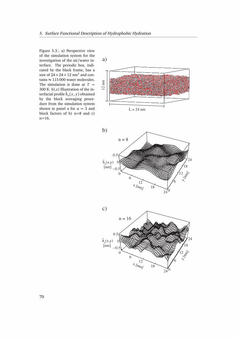
5. Surface Functional Description of Hydrophobic Hydration
Figure 5.3.: a) Perspective viewof the simulation system for theinvestigation of the air/water in-terface. The periodic box, indi-cated by the black frame, has asize of 24×24×12 nm3 and con-tains ≈ 115000 water molecules.The simulation is done at T =300 K. b),c) Illustration of the in-terfacial profile hn(x , y) obtainedby the block averaging proce-dure from the simulation systemshown in panel a for α = 3 andblock factors of b) n=8 and c)n=16.
70

5.2. Capillary waves at the air/water interface
Figure 5.4.: a) Schematic illustration of the definition of the Gibbs-dividing-surface. The posi-tion zG is defined in such a way, that the shaded regions A and B have equal area. b) Illustrationof the prisms used in the local GDS method to extract the interface profile.
5.2.2. Interface extraction
Figure 5.3 a shows a perspective view of the simulation system. From the atomic coor-dinates, the interface profile is determined by the local Gibbs-dividing-surface (GDS)method [236] (see Fig. 5.4). The GDS is a measure for the interface position definedas the boundary zG, for which the surface excess of the water vanishes,
∫ zG
−∞
�
ρ(z)−ρl�
dz+
∫ ∞
zG
�
ρ(z)−ρv�
dz = 0. (5.7)
Here, ρl,v are the bulk liquid and vapour densities. In Fig. 5.4 a this is schematicallyshown. Equation 5.7 enforces that the two shaded regions denoted by A and B haveequal area.
To determine the interface profile the simulation box is divided into n× n prismswith quadratic base area of edge length ∆L = L/n, as shown in Fig. 5.4 b. Theinterface height hn(~r||) at the lateral coordinates ~r|| is then defined as the position ofthe local GDS within the prism centered around ~r||, that is by Eq. 5.7 with zG replacedby hn(~r||) and ρ(z) replaced by the density profile ρr||(z) within the corresponding
prism. Thus, hn(~r||) is defined only on the grid formed by the prisms footprints. Toseparate the two interfaces present in the simulation box and to control the influenceof the bulk fluctuations the prisms are further restricted to an interval [z−, z+] in zdirection, where z± = zG ± αw, zG is the global GDS, w is the interfacial width and αis an adjustable parameter. With these substitutions Eq. 5.7 reads
∫ hn(~r||)
z−
h
ρr||(z)−ρl
i
dz+
∫ z+
hn(~r||)
h
ρr||(z)−ρv
i
dz = 0. (5.8)
71

5. Surface Functional Description of Hydrophobic Hydration
Multiplying both sides with (∆L)2 and rearranging Eq. 5.8 we find
hn(~r||) =Mr||
(∆L)2∆ρ−ρlz−+ρvz+∆ρ
, (5.9)
where ∆ρ = ρl −ρv and Mr|| = (∆L)2∫ z+
z−ρr||(z)dz is the number of molecules in the
prism centered around ~r||. The advantage of this method is, that it does not involvefitting of the density profile in a single prism and is therefore still applicable for largen, where the average number of molecules in a prism is very small. The height pro-file obtained by this method is denoted by hn(~r||), in contrast to the height functionh(~r||) that appears in capillary wave theory, since it depends on the block factor n,which specifies the lateral resolution ∆L = L/n, α, the prism height, and also containscontributions from bulk-like density fluctuations. Figure 5.3 b and c show the heightprofile obtained from the same configuration for different values of the block factor n.
The coarse-grained profile hn(~r||) is related to the infinite-resolution limit h(~r||) ≡limn→∞ hn(~r||) by the convolution
hn(~r||) =
∫
d2r ′||gn(~r||−~r ′||)h(~r′||), (5.10)
with the coarse-graining function gn(~r||) = 1/(∆L)2 for −∆L/2 < x , y < ∆L/2 andgn(~r||) = 0 otherwise. The connection with the height function h(~r||) that appears inthe CW theory in Eq. (5.5) will be discussed below.
5.2.3. Interfacial broadening
The total width of the interfacial density profile is due to the width of the intrinsicdensity profile, which is the density profile in absence of capillary waves, and thebroadening due to fluctuations of the surface shape. Having determined the profileof the surface shape, the intrinsic density profile can be reconstructed by shifting themolecular positions by the position of the local GDS,
ρint,n(z) = ⟨N∑
i=1
δ(z− zi + hn(~r||,i))⟩/L2, (5.11)
where ~r||,i and zi are the coordinates of the water molecules. In Fig. 5.5 we showρint,n(z) for n = 1 and n = 30. The inset shows that for a given α a value of thelateral resolution ∆L = L/n exists for which the width w of ρint,n(z) is minimal. Forα= 3 we find a minimal w for∆L∗ = L/30= 0.8nm, which agrees with the roughnesslength scale found by visual inspection of the snapshots (see Fig. 5.1). It also coincidesmore or less with the cross-over radius R∗ in the solvation of hydrophobic spheres [41](as discussed below), supporting the view that this is the length scale of the intrinsicroughness due to the restructuring of the H-bonding network in water. For smaller ncapillary waves broaden the interface, for larger n nano-scale roughness increases the
72

5.2. Capillary waves at the air/water interface
-0.4 -0.2 0.0 0.2 0.4z [nm]
0.0
0.5
1.0
1.5
ρin
t,n [
kg/l]
n = 1n = 30
0 10 20 30 40 50 60 70n
3.0
3.5
4.0
4.5
5.0
5.5
w [
Å]
α = 2α = 3α = 4
Figure 5.5.: Intrinsic density profiles ρint,n(z) for α = 3 and block factor n = 30 (circles)and n = 1 (squares, corresponding to the global laterally averaged density profile) with fitsρint,n(z) = (ρl + ρv)/2+ (∆ρ/2) tanh(2z/w) (solid lines). The inset shows the width w as afunction of n for α= 2, 3,4. Here L = 24 nm.
1 10 100L [nm]
0.00
0.02
0.04
0.06
0.08
∆2 [
nm
2]
Tanh fitErf fit
Figure 5.6.: Squared total interfacial width ∆2 as a function of the lateral system size L ob-tained either from a hyperbolic tangent (circles) or an error function (squares) fit to the aver-aged density profile across the air/water interface. The lines are linear fits to the data. Notethe logarithmic scale of the abscissa.
73

5. Surface Functional Description of Hydrophobic Hydration
width of the intrinsic density profile. The slight α dependence of the minimum is dueto bulk-like density fluctuations as discussed below.
Similarly, for increasing system size L, the density profiles in Fig. 5.1 c exhibit in-creasing widths due to the increasing effects of capillary waves. In the convolutionapproximation [237] the interfacial width is given by
∆2 =∆20+
kBT
2πγ0ln�
L
b
�
, (5.12)
where∆0 is the intrinsic width and the second term describes the contribution of capil-lary waves. It depends logarithmically on the lateral system size L and the length scaleb associated with the short-wavelength cut-off of the capillary wave modes. We extractthe total width from the simulation trajectory by fitting the averaged density profilenormal to the interface either with the mean field hyperbolic tangent (see Eq. 5.4) oran error function,
ρ(z) =ρl+ρv
2+∆ρ2
erf
�pπz
w
�
. (5.13)
The squared width ∆2, which is defined as the variance of the derivative ρ′(z), is thengiven by ∆2 = (πw)2/48 for the hyperbolic tangent and by ∆2 = w2/(2π) for theerror function [237]. In Fig. 5.6 we plot the squared total width ∆2 as a function ofthe lateral system size L for both the hyperbolic tangent and the error function fit. Itis seen that the total width indeed scales with the logarithm of the lateral system size,as predicted by capillary wave theory. From the slope of a linear fit to the data, wecalculate the planar surface tension γ0 yielding γ0 = 45.6 mN/m for the hyperbolictangent fit and γ0 = 51.3 mN/m for the error function fit. The result from the errorfunction fit agrees very well with the surface tension obtained independently from theanisotropy of the pressure tensor (γlv,0 = 52.9 mN/m) in agreement with the findingsof Ismail et al. [237]. Note, that the simulations in this section are done with a slightlysmaller Lennard-Jones cutoff rc = 0.8 nm, leading to a slightly smaller surface tensionin comparison with the results presented in Sec. 5.3.
The intrinsic width ∆0 can be inferred from the width of the intrinsic density profile(see Fig. 5.5). Since the intrinsic width depends on the block factor n but only slightlyon the parameter α with which the height profile is determined, we take the minimalwidth for α = 3 as an estimate of the intrinsic width, yielding ∆0 = 1.6 Å. UsingEq. 5.12 we can obtain the short-wavelength cut-off b from the fit to the simulationdata. We find b = 4.8 nm for the hyperbolic tangent fit and b = 6.1 nm for the errorfunction fit, in agreement with recent X-ray reflectivity experiments [229]. Thesefindings support the view that capillary wave theory breaks down at length scaleslarger than the molecular size of the liquid, in considerable contrast to the assumptionin previous works [231].
74

5.2. Capillary waves at the air/water interface
Figure 5.7.: a) Capillary wavespectra ⟨|hn(q)|2⟩ for n = 1024and α ranging from 1 to 5(from bottom to top, full lines).For comparison Sb
|| (~q), the lateralbulk structure factor for a slabthickness 5w, scaled by an ar-bitrary factor, (dashed line) andthe CWT result with γ0 = γlv,0(dash-dotted line) are included.b) Bare capillary wave spectra(σq)2⟨|hn(q)|2⟩ (upper data set,left scale) and (σq)2⟨|hn(q)|2⟩ ac-cording to Eq. 5.20 (lower dataset, right scale) for n = 64and varying α. The dashedstraight lines show the surfacetension contribution determinedindependently. c) Rescaled effec-tive surface tension γeff,n/γlv,0 forα= 3 and varying n. Full squaresfor n= 30 correspond to a LJ cut-off rc = 1.6 nm, all other data arefor rc = 0.8nm. Dashed lines arefits of the form γeff,n/γlv,0 = 1+κn/γlv,0q2. In all plots L = 24nmand q is rescaled by the water LJdiameter σ = 3.166 Å.
75

5. Surface Functional Description of Hydrophobic Hydration
5.2.4. Lateral correlations
The lateral structure factor is defined as
S||(q) =
∫
d3rd3r ′
N||f (z) f (z′)ei~q · (~r||−~r ′||)⟨ρ(~r)ρ(~r ′)⟩c, (5.14)
with the microscopic density ρ(~r) =∑N
i=1δ(~r −~ri), the weight function f (z) and thenormalization factor
N|| =
∫
d3r f 2(z)⟨ρ(~r)⟩. (5.15)
S||(~q) is obtained from grazing angle X-ray diffraction below the critical angle for totalreflection, in which case the weight function is f (z) = exp(−|z|/(2l)) and l is thepenetration depth, which depends on the wave vector transfer normal to the surfaceqz. We write the microscopic density as
ρ(~r) = ρlθ(h(~r||)− z) +ρvθ(z− h(~r||)) +δρ(~r), (5.16)
where δρ accounts for all density fluctuations not captured by the sharp-kink approx-imation and θ(z) = 1 for z > 0 and zero otherwise. Equation (5.14) leads to
S||(q)≡ (∆ρ)2⟨|h(q)|2⟩/N||+∆S||(q), (5.17)
where the contribution due to density fluctuations is
∆S||(q) =
∫
d3rd3r ′ f (z) f (z′)ei~q · (~r||−~r ′||)⟨δρ(~r)δρ(~r ′)⟩. (5.18)
In the limit n→∞, the relation
limn→∞⟨|hn(q)|2⟩ ≡ ⟨|h(q)|2⟩= N||S||(q)/(∆ρ)
2 (5.19)
between the power spectrum of the local GDS and the lateral structure factor with arectangular weight function f (z) = θ(z+ − z)θ(z − z−) holds, where N|| = ρlαwL2,which is formally proven in App. A. Figure 5.7 a shows ⟨|hn(q)|2⟩ obtained by Fourier-transforming simulation data for hn(~r||) for different values of α and n = 1024. Com-parison with the bulk structure factor for a slab (broken line) shows that bulk-like den-sity fluctuations dominate at high wave vectors and are proportional to α. To extractthe bare height spectrum ⟨|h(q)|2⟩ one has to subtract ∆S||, ideally in an experimen-tally reproducible fashion. A meaningful subtraction is possible by using the structurefactor Sb
|| (q) calculated analogously to Eq. (5.14) in a slab located in the bulk of the
liquid. Note that Sb||(q) can be calculated for an arbitrary weight function f (z) from the
experimentally accessible 3D bulk structure factor, as shown in App. A. In our simula-tions we calculate Sb
||(q)with the same block factor n for an interval of size αw centered
76

5.2. Capillary waves at the air/water interface
around the middle of a water slab. We furthermore use S||(q) = (∆ρ)2⟨|hn(q)|2⟩/N||even for finite n and make the association ∆S||(q) = Sb
|| (q). These simplifications canbe viewed as a definition of the interface profile h(~r||). Using Eq. (5.17) we thus obtain
⟨|hn(q)|2⟩= ⟨|hn(q)|2)⟩ − N||Sb|| (q)/(∆ρ)
2. (5.20)
Writing the effective surface tension for the spectrum ⟨|hn(q)|2⟩ in analogy to Eq. 5.5as
γeff,n(q) = γ0+ κnq2+O(q4) (5.21)
and defining the isothermal compressibility κT,|| of a slab,
Sb|| (q) = kBTρlκT,||+O(q2), (5.22)
we obtain in the low-q limit the relation
κn = κn+ γ20αwκT,||. (5.23)
This shows that correct subtraction of the bulk-like fluctuations is the key to extractingthe correct interfacial bending rigidity κn.
In Fig. 5.7 b we show the spectra q2⟨|hn(q)|2⟩ ∼ γ−1eff,n(q) (upper data points) and
q2⟨|hn(q)|2⟩ ∼ γ−1eff,n(q) (lower data points) for fixed n= 64 and different α. In contrast
to a similar data analysis of colloid-polymer interfaces [99], we subtract the bulk struc-ture factor Sb
|| of a corresponding slab of thickness αw without any fitting parameter.
This is an important detail, since the functional form of Sb|| (q) strongly depends on α
(see App. A). As seen in Fig. 5.7 b, all data for q2⟨|hn(q)|2⟩ collapse onto a single curve,which shows that i) the parameter α does not influence the final result for κn, and ii)our method for subtracting bulk-like density fluctuations is consistent. Not surpris-ingly, for α = 1 (circles) the data slightly deviate, indicating that this prism size is toosmall to entirely capture the interface fluctuations. The dashed lines in Fig. 5.7 b showthe limiting behavior γeff,n(q→ 0) = γeff,n(q→ 0) = γ0 with γ0 = γlv,0 = 52.91 mN/mdetermined independently from the anisotropy of the pressure tensor [237]. In Fig. 5.7c we plot γeff,n(q)/γlv,0 as a function of q2 for fixed α = 3 and various n and comparewith straight line fits of the form γeff,n(q)/γlv,0 = 1+κnq2/γlv,0.
The resulting n-dependence of the κn values is introduced by the coarse-graining ofthe local GDS method. From Eq. (5.10) we obtain
⟨|hn(~q)|2⟩= |gn(~q)|2⟨|h(~q)|2⟩, (5.24)
where
gn(~q) =4
(∆L)2qxqysin(∆Lqx
2) sin(
∆Lqy
2) (5.25)
77

5. Surface Functional Description of Hydrophobic Hydration
300 350 400 450T [K]
0
1
2
3
κ [
10
-22J]
0
20
40
60
γ [
mN
/m]
0 0.0002 0.0004 0.0006
1/n2
0
0.1
0.2
0.3
κn [
kBT
]
α = 1
α = 2
α = 3
α = 4
α = 5
Figure 5.8.: Bending rigidity κn from fits in Fig. 5.7 c as a function of the inverse squaredblock factor 1/n2 for different α. The line denotes a fit of Eq. (5.26) to the data for α = 2− 5yielding a value of κ = 0.04 kBT as n → ∞. The inset shows the temperature dependenceof κ (circles), the simulated surface tension (squares, including a tail correction) and theexperimental surface tension (triangles, [237]).
is the Fourier transform of the rectangular coarse-graining function gn(~r||). For smallq we have gn(~q) ' 1− (∆L)2q2/24. Combining this with Eq. 5.5 we obtain γeff,n =γ0 + κq2 + γ0 L2q2/(12n2), where we have used that ∆L = L/n. The asymptoticbending rigidity κ is thus related to κn as
κn = κ+ γ0 L2/(12n2). (5.26)
In Fig. 5.8 we show κn for different α as a function of 1/n2. Except for α= 1, the datafor different slabthickness αw collapse, reinforcing our earlier statement that we haveseparated density and interface fluctuations in a consistent way. From Eq. (5.26),shown by the solid line, the bending rigidity follows by extrapolation to n → ∞ asκ = (0.04± 0.02) kBT at T = 300 K for a Lennard-Jones cut-off rc = 0.8 nm. Thetemperature dependence of κ (inset in Fig. 5.8, circles) is similar to that of the surfacetension from simulations (squares) or experiments (triangles). As a consequence, thecross-over length scale between bending and tension,
p
κ/γ0, is of the order of about0.5 Å and rather independent of temperature.
Our results, yielding a monotonously increasing effective surface tension, i.e., apositive bending rigidity, on first glance conflict with previous calculations includingthe long-ranged VDW tail that predict a negative slope of γeff(q) for small q [91]. InMD simulations, however, the VDW interaction is truncated at a finite cutoff length
78

5.3. Solvation of spheres and cylinders
rc. The contribution of an attractive intermolecular interaction w(r) to the bendingrigidity is given in the sharp-kink approximation by [91]
κattr =π
32(∆ρ)2
∫ rc
σ
drr5w(r). (5.27)
For the attractive part of the Lennard-Jones potential in the simulations, w(r) =−4ε(σ/r)6 with ε = 0.65 kJ/mol and σ = 0.317 nm, we obtain for the upper cut-offs rc = 0.8nm and 1.6 nm the contributions κattr = −0.11 kBT and −0.19 kBT atT = 300K, yielding a difference of −0.08 kBT . In the limit rc =∞ Eq. 5.27 predicts adivergent contribution. In reality, retardation effects change the VDW distance depen-dence from 1/r6 to 1/r7 at a cross-over length on the order of rret = 100nm [238].Using w(r) = −4ε(σ/r)6 for r < rret and matching continuously a function w(r) ∼−1/r7 for r > rret, we obtain κattr = −0.67 kBT . Assuming simple additivity of thelong-ranged contribution κattr to the simulation result would result in a negative valueκ= (−0.63±0.02) kBT . In fact, the same analysis as in Fig. 5.8 for simulations with acut-off rc = 1.6 nm yields a slightly smaller bending rigidity of κ= (0.03± 0.02) kBT ,so it seems plausible that in the infinite cut-off limit κ becomes negative.
5.3. Solvation of spheres and cylinders
5.3.1. Curvature expansion of free energies
In this section we determine the elastic constants of the water surface by consideringthe solvation of spherical and cylindrical hydrophobic solutes. For a sphere with radiusR one obtains from Eq. 5.3
∆FSPH/A= γ0−4κc0
R+ (2κ+ κ)
1
R2 , (5.28)
with γ0 ≡ γ + 2κc20 . Comparison of the leading terms in Eqs. 5.1 and 5.28 shows
that the Tolman length is given by δ = 2κc0/γ0. For a cylinder of radius R Helfrich’scurvature expansion yields
∆FCYL/A= γ0−2κc0
R+κ
2
1
R2 , (5.29)
and therefore the equivalent of Eq. 5.1 is
γCYL = γ0
�
1−δ
R
�
. (5.30)
By considering the full radius range from zero to R = 2 nm, we cover the crossoverbetween the regimes where the solvation free energy scales as the cavity volume (forR< R∗) and where it scales as the surface area (for R> R∗). Simultaneously consider-ing spherical and cylindrical geometries allows an additional consistency check on Eqs.
79

5. Surface Functional Description of Hydrophobic Hydration
5.1 and 5.30 (which is essential in light of the pronounced crossover effects present,as will be shown below) and to reliably extract the Tolman length.
The range of applicability of Eqs. 5.28 and 5.29 can be extended by including higherorder terms. If we include terms up to third order in the curvature, the Helfrich freeenergy is given by
∆F =∫
dAh
γ+ 2κ�
1
2
�
1
R1+
1
R2
�
− c0
�2
+ κ1
R1R2
+ η
�
1
R31
+1
R32
�
+ η
�
1
R1R22
+1
R21R2
�
i
, (5.31)
where we have introduced the moduli η and η. For a spherical solute Eq. 5.31 yields,
∆FSPH/A= γ0−4κc0
R+ (2κ+ κ)
1
R2 + 2(η+ η)1
R3 , (5.32)
for a cylindrical solute,
∆FCYL/A= γ0−2κc0
R+κ
2
1
R2 +η1
R3 . (5.33)
Unless specified otherwise, the radius of the solutes, R, is defined as the distance wherethe interaction is kB T0, VSOL−OW(R) = kBT0, where kB is the Boltzmann constant andT0 = 300 K, alternative radius definitions lead to minor modifications, as is discussedbelow.
5.3.2. Small scale solvation regime and crossover
The radial distribution functions in Fig. 5.2 c and f and the solvation entropy ∆S inFig. 5.9 clearly display the gradual crossover from small-scale solvation (negative sol-vation entropy, strong density peak in the first solvation shell) to large-scale solvationcharacterized by a monotonic density distribution around the solute, positive ∆S andconstant free energy per area ∆F/A. Depending on the observable one looks at, thiscrossover occurs around R∗ ' 0.5− 1.0 nm and at a significantly smaller radius for acylinder compared to a sphere (which makes cylinders particularly suited for determin-ing the Tolman length, as shown later on). Note that ∆F/A does not quite reach theindependently determined planar liquid vapour surface tension γlv,0, dotted horizontalline in Fig. 5.9 a, as will be discussed below.
For small radii the solvation free energy of hard-sphere solutes scales proportionalto the volume [40, 41], whereas our Buckingham solutes exhibit for very small R adivergence in ∆F/V . This is due to the finite r → 0 limit of the Buckingham potential.It vanishes for a potential shape, that diverges with r → 0, as is seen in Fig. 5.10,where we plot the solvation free energy for spherical solutes that interact with thewater oxygen atoms via a purely repulsive Lennard-Jones (LJ) potential of the form
V LJSPH−SOL(r) =
E
r12 . (5.34)
80
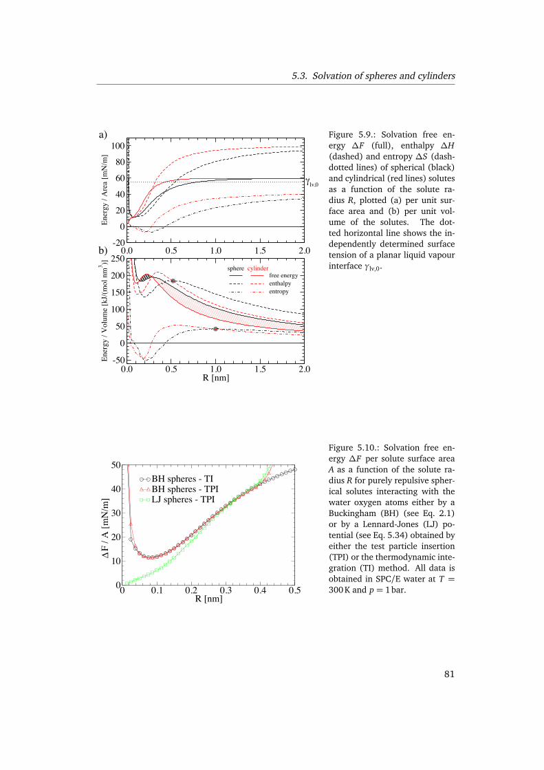
5.3. Solvation of spheres and cylinders
Figure 5.9.: Solvation free en-ergy ∆F (full), enthalpy ∆H(dashed) and entropy ∆S (dash-dotted lines) of spherical (black)and cylindrical (red lines) solutesas a function of the solute ra-dius R, plotted (a) per unit sur-face area and (b) per unit vol-ume of the solutes. The dot-ted horizontal line shows the in-dependently determined surfacetension of a planar liquid vapourinterface γlv,0.
0 0.1 0.2 0.3 0.4 0.5R [nm]
0
10
20
30
40
50
F /
A [
mN
/m]
BH spheres - TIBH spheres - TPILJ spheres - TPI
Figure 5.10.: Solvation free en-ergy ∆F per solute surface areaA as a function of the solute ra-dius R for purely repulsive spher-ical solutes interacting with thewater oxygen atoms either by aBuckingham (BH) (see Eq. 2.1)or by a Lennard-Jones (LJ) po-tential (see Eq. 5.34) obtained byeither the test particle insertion(TPI) or the thermodynamic inte-gration (TI) method. All data isobtained in SPC/E water at T =300 K and p = 1bar.
81

5. Surface Functional Description of Hydrophobic Hydration
Solute radii R are defined analogously to the Buckingham potential by V LJSPH−SOL(R) =
kBT0. The solvation free energy of the LJ-spheres are obtained by the test particleinsertion method. They are shown in Fig. 5.10 together with solvation free energiesfor Buckingham spheres obtained by both TI and TPI. The solvation free energy perunit area of the LJ-spheres smoothly goes to 0 for R→ 0, while it converges with thesolvation free energy of the Buckingham-spheres for radii R> 0.2nm. The TPI data forthe Buckingham-spheres agree perfectly with the Buckingham TI data for small radii.Deviations from the TI data for R > 0.4 nm are due to insufficient sampling, whichshows that the TPI method is not applicable for solutes of too large size. We note thatthe solvation free energy ∆F of the Buckingham solutes of course goes to zero forR→ 0, only slower than the area A.
The difference between ∆F/V for spheres and cylinders in Fig. 5.9 b gives the freeenergy change per volume upon an aggregation of spheres into a cylinder with thesame radius, which is an idealized model for linear hydrophobic aggregation. Surpris-ingly, only for R > 0.3 nm is this aggregation favored (red shaded region), for smallerR the cylindrical free energy per volume is higher than the spherical one (black shadedregion). This transition is driven by complex crossovers in the enthalpic and entropicdifferences [44], which change sign at R ' 0.5 nm and R ' 1.0 nm, respectively, asindicated by filled circles: For R > 1.0 nm cylinders are enthalpically favored (andentropically disfavored), while for R < 0.5 nm cylinders are entropically favored (andenthalpically disfavored).
5.3.3. Large scale solvation regime
To extract the Tolman length, in Fig. 5.11 a we plot ∆F/A for T = 300 K as a functionof the inverse radius 1/R as solid lines. The data are strongly curved and fits accordingto Eqs. 5.1 and 5.30 are obviously impossible: The slopes for cylinders and spheresat 1/R = 0.5 nm−1 have opposite signs, so extrapolation to the limit 1/R → 0 andextraction of the Tolman length (which is the slope in this plot) is not obvious. Thesituation for higher temperature T = 360 K in Fig. 5.11 b is more favorable, since herecrossovers are shifted to smaller radii [44]. Indeed, now a maximum in∆F/A is clearlyresolved in both data sets, although a linear fit according to Eqs. 5.1 and 5.30 is still notfeasible. The dashed-dotted lines in Fig. 5.11 a and b show a simultaneous fit to bothspherical and cylindrical data according to Eqs. 5.32 and 5.33 with γ0, δ, κ, κ, η andη as free parameters (fits are performed on the interval 0.5 nm−1 < 1/R< 1.4 nm−1).The influence of the cubic term and the dependence on the fitting range is discussedbelow.
The fit parameters are summarized in Tab. 5.1. The resulting Tolman length isnegative, on the order of δ ≈−1 Å and decreasing with temperature, implying that thespontaneous curvature is such that water favors droplets over cavities. The maximumof ∆F/A for spheres occurs at 1/Rmax ' 0.7 nm−1 for T = 360 K and extrapolatedat 1/Rmax ' 0.5 nm−1 for T = 300 K, consistent with previous simulations [42] forspheres and for 1/R > 1 nm−1 that were interpreted in terms of a positive Tolman
82

5.3. Solvation of spheres and cylinders
Figure 5.11.: Solvation free energies∆F (full lines) per unit area of spherical (black) and cylin-drical (red lines) solutes as a function of the inverse radius 1/R at temperatures (a) T = 300 Kand (b) T = 360 K. Dashed-dotted lines are cubic fits in the range 0.5 nm−1 < 1/R< 1.4 nm−1,where Eqs. 5.32 and 5.33 are fit simultaneously to the data for spherical and cylindrical so-lutes. The resulting best-fit parameters are listed in Tab. 5.1. [(c),(d)] Same data as in (a)and (b) but for a larger range of 1/R. Linear fits in the region 1.5 nm−1 < 1/R < 3 nm−1 forspheres and 3 nm−1 < 1/R< 5 nm−1 for cylinders (dashed-dotted lines) with the constraint ofan equal surface tension are included.
83

5. Surface Functional Description of Hydrophobic Hydration
Table 5.1.: Best fit parameters γ0, κ, κ, c0, δ, η and η obtained from fitting Eqs. 5.32 and5.33 to the spherical and cylindrical data in Fig. 5.11 a and b. The independently determinedplanar surface tension of the free water/vapour interface, γlv,0, is included for comparison.
T [K] γlv,0 [mN/m] γ0 [mN/m] c0 [nm−1] δ [nm]
280 58.1 59.7 0.41 -0.092300 54.7 56.8 0.50 -0.10320 52.0 53.8 0.53 -0.12360 45.5 47.4 0.69 -0.16
T [K] κ [10−21 J] κ [10−21 J] η [10−32Jm] η [10−32Jm]
280 -6.7 -2.4 0.018 3.2300 -5.8 -2.8 -0.23 3.0320 -6.2 -2.3 -0.23 3.2360 -5.4 -2.5 -0.35 3.3
length. The increased radius range up to R = 2 nm in conjunction with the cylindricaldata, that show the crossover at considerably smaller radii, allows to clearly resolvethe maximum in ∆F/A and thus to reliably extract the Tolman length. The best-fitvalues for γ0 are slightly larger than the surface tension γlv,0 of the planar liquid/vapour interface. Similar behaviour for a Lennard-Jones liquid [80] was rationalizedby suppressed interfacial fluctuations near a hard wall [239], as we will show in thefollowing this can also be interpreted as a finite-size crossover.
Figure 5.12 shows fits according to Eqs. 5.32 and 5.33 including (dashed-dottedlines) and neglecting (dotted lines) the cubic term. The fitting is performed over theinterval 0.5 nm−1 < 1/R < (1/R)upper, where (1/R)upper = 0.6 and 1.4 nm−1. Thedependence of the fitted surface tension and Tolman length on the fitting range isshown in Fig. 5.13.
As can be seen from Fig. 5.12, for small curvature 1/R the deviations between thequadratic and cubic fit are quite small. For larger curvature the cubic function fitsthe data better than the quadratic one, since higher order corrections become moreimportant in this region. The planar surface tension and the Tolman length obtainedfrom the fits show only a slight dependence on the fitting range (see Fig. 5.13). Theplanar surface tension γ0 decreases with decreasing (1/R)upper, suggesting that thediscrepancy between the γ0 obtained from the fit and the surface tension obtainedfrom simulations of a planar air/water interface γlv,0 can be explained by the finiteminimal curvature that is accessible by these simulations. Indeed, if we extrapolate γ0to (1/R)upper = 0 it agrees within the statistical errors with γlv,0 which is indicated bya dotted horizontal line.
For the bending rigidities we find negative values on the order of κ, κ ≈ −1 to−10 kBT with only small dependencies on the LJ cutoff length (see App. B), consistent
84

5.3. Solvation of spheres and cylinders
0 0.5 1 1.5 21/R [1/nm]
46
48
50
52
54
F /
A [
mN
/m]
spherescylinders
(1/R)upper
= 0.6 nm-1
a)
0 0.5 1 1.5 21/R [1/nm]
46
48
50
52
54
F /
A [
mN
/m]
cubic fitquadratic fit
(1/R)upper
= 1.4 nm-1
b)
Figure 5.12.: Solvation free en-ergies per area for spherical andcylindrical solutes at T = 360 Kand p = 1 bar, simultaneouslyfit by Eqs. 5.32 and 5.33 ei-ther neglecting (dashed lines) orincluding (dashed-dotted lines)the cubic term. The fit is re-stricted to the range 0.5 nm−1 <1/R < (1/R)upper, where (a)(1/R)upper = 0.6 nm−1 and (b)(1/R)upper = 1.4 nm−1.
44
46
48
γ 0 [
mN
/m]
0 0.2 0.4 0.6 0.8 1 1.2 1.4 1.6(1/R)
upper [1/nm]
-0.3
-0.2
-0.1
δ [
nm
]
quadratic fitcubic fit
γlv,0
Figure 5.13.: Dependence of thebest fit parameters of the fits tothe solvation free energies perarea of spherical and cylindricalsolutes at T = 360 K and p =1 bar for a quadratic (black cir-cles) or cubic (red squares) fit-ting function (see Fig. 5.12) onthe fitting range 0.5 nm−1 <1/R < (1/R)upper. Solid linesare quadratic fits to the data,the dotted line indicates γlv,0 =45.5 mN/m.
85

5. Surface Functional Description of Hydrophobic Hydration
Figure 5.14.: Comparison of var-ious definitions for the radius of(a) spherical and (b) cylindricalsolutes in SPC/E water at T =300 K. Shown are the radii R1/2,defined by gX−OW(R1/2) = 1/2,RGDS, the radius of the Gibbs di-viding surface (GDS) and RMAX,the radius of the maximum ofthe radial distribution functiongX−OW(r), as a function of thereference radius R, defined byVX−OW(R) = kBT0, with X = SPHor CYL. Solid lines are linear fitsto the data. The dashed linemarks the identity. In the in-set the radial distribution func-tion gSPH−OW(r) for a sphericalsolute with R= 0.75 nm is shownand the different definitions ofthe radius are indicated by ver-tical lines.
0.0
0.5
1.0
1.5
2.0
2.5
radiu
s [n
m]
R1/2
RGDS
RMAX
0.0 0.5 1.0 1.5 2.0R [nm]
0
0.5
1
1.5
2
radiu
s [n
m]
0.7 0.8 0.9r [nm]
0
0.5
1
1.5
gS
PH
-OW
(r)
a)
b)
with the estimates from the capillary wave fluctuations, that included a long-range LJcorrection.
The elastic coefficients in Eqs. 5.3 and 5.31 depend on the definition of the ra-dius R, for which there are several common choices: (i) the radius R1/2, defined bygX−OW(R1/2) = 1/2, (ii) the radius RGDS, defined by the Gibbs dividing surface (GDS),that is defined by
∫
d3r�
gX−OW(r)− θ(r − RGDS)�
= 0, (5.35)
where θ(x) = 1 if x ≥ 0 and θ(x) = 0 if x < 0, in accordance with the interfacedefinition in Sec. 5.2, and (iii) the radius RMAX, defined as the first maximum of theradial distribution function gX−OW(r). In Fig. 5.14 we compare alternative definitions.It is seen that, except for RMAX, all other radii differ only slightly from R. For radiiR> 0.2 nm the curves are well fit by a linear function, if we allow for a non-zero offset.For small radii R< 0.2 nm, there are deviations from the linear dependence, which arecaused by the finite r → 0 limit of the Buckingham potential as discussed above. Notethat the GDS based radius definition is thermodynamically the most sound definition,but requires extensive additional simulations for accurate determination. The heuristicradius definition we use in most parts of Sec. 5.3 is the most practical one, since it doesnot require additional simulations; this is the reason why we used it.
86

5.4. Conclusion
If we generally assume a linear relationship between an alternative definition of thesolute radius, R′, and R, R = R′(1+ ε) +∆, then we obtain to linear order in 1/R′ fora sphere,
∆F = 4πR2γ0
�
1−2δ
R+O(
1
R2 )�
= (5.36)
= 4πR′2γ0(1+ ε)2�
1−2(δ−∆)R′(1+ ε)
+O(1
R′2)�
.
The Tolman length associated with R′ is therefore given by
δ′ =δ−∆1+ ε
. (5.37)
For RGDS and R1/2 we obtain ε=−0.049 and−0.042 and∆= 0.040 nm and 0.025 nm,leading to δ′ = −0.14 nm and -0.12 nm at T = 300 K. From a direct fit usingthe same fitting procedure as described in the main paper, but taking RGDS as di-viding surface, we obtain γ0 = 52.6 mN/m, c0 = 2.73 nm−1, κ=−0.98× 10⁻²¹ J,κ = −6.49× 10⁻²¹ J and δ = −0.10 nm at T = 300 K. While the Tolman length doesnot change significantly, the bending rigidities, which constitute higher-order curva-ture corrections, not surprisingly do. So our results for the bending rigidities shouldonly be regarded as indicative. The Tolman lengths obtained from the direct fit andfrom Eq. 5.37 differ slightly, since the fit range is restricted by the finite minimumcurvature.
Finally, we stress that the expressions in Eqs. 5.1 and 5.30 strictly only apply to theasymptotic small-curvature regime, i.e. to radii R > Rmax, because otherwise higher-order curvature terms take over. Curiously, as can be seen in Fig. 5.11 c and d, there isan intermediate range where ∆F/A scales linear in 1/R with effective Tolman lengthsδSPH,CYL that are positive and on the order of 1 Å (see Tab. 5.2), in rough agreementwith previous estimates [42, 43, 83, 85]. It is clear that such a fit at intermediate radiiis incompatible with a surface free energy functional in terms of local curvatures andrather illustrates the subtleties of analyzing simulation data.
5.4. Conclusion
We have presented a thorough analysis of the curvature dependence of the free en-ergy of a water surface, taking into account both, fluctuations of an planar air/waterinterface and surfaces forced to curve due to the presence of a solute.
Considering the free air/water interface, we have introduced a method to consis-tently separate surface and bulk contributions to the interfacial structure factor oflarge scale water simulations. It is found that in the limit of small q the effective sur-face tension is well described by a small but positive bending rigidity on the orderof κ = (0.04± 0.02) kBT at T = 300 K. Considering the long-ranged and retarded
87
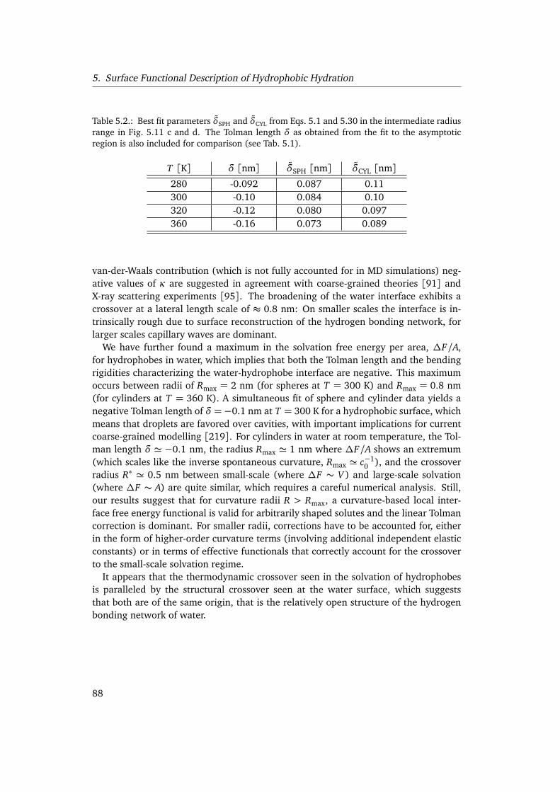
5. Surface Functional Description of Hydrophobic Hydration
Table 5.2.: Best fit parameters δSPH and δCYL from Eqs. 5.1 and 5.30 in the intermediate radiusrange in Fig. 5.11 c and d. The Tolman length δ as obtained from the fit to the asymptoticregion is also included for comparison (see Tab. 5.1).
T [K] δ [nm] δSPH [nm] δCYL [nm]
280 -0.092 0.087 0.11300 -0.10 0.084 0.10320 -0.12 0.080 0.097360 -0.16 0.073 0.089
van-der-Waals contribution (which is not fully accounted for in MD simulations) neg-ative values of κ are suggested in agreement with coarse-grained theories [91] andX-ray scattering experiments [95]. The broadening of the water interface exhibits acrossover at a lateral length scale of ≈ 0.8 nm: On smaller scales the interface is in-trinsically rough due to surface reconstruction of the hydrogen bonding network, forlarger scales capillary waves are dominant.
We have further found a maximum in the solvation free energy per area, ∆F/A,for hydrophobes in water, which implies that both the Tolman length and the bendingrigidities characterizing the water-hydrophobe interface are negative. This maximumoccurs between radii of Rmax = 2 nm (for spheres at T = 300 K) and Rmax = 0.8 nm(for cylinders at T = 360 K). A simultaneous fit of sphere and cylinder data yields anegative Tolman length of δ =−0.1 nm at T = 300 K for a hydrophobic surface, whichmeans that droplets are favored over cavities, with important implications for currentcoarse-grained modelling [219]. For cylinders in water at room temperature, the Tol-man length δ ' −0.1 nm, the radius Rmax ' 1 nm where ∆F/A shows an extremum(which scales like the inverse spontaneous curvature, Rmax ' c−1
0 ), and the crossoverradius R∗ ' 0.5 nm between small-scale (where ∆F ∼ V ) and large-scale solvation(where ∆F ∼ A) are quite similar, which requires a careful numerical analysis. Still,our results suggest that for curvature radii R > Rmax, a curvature-based local inter-face free energy functional is valid for arbitrarily shaped solutes and the linear Tolmancorrection is dominant. For smaller radii, corrections have to be accounted for, eitherin the form of higher-order curvature terms (involving additional independent elasticconstants) or in terms of effective functionals that correctly account for the crossoverto the small-scale solvation regime.
It appears that the thermodynamic crossover seen in the solvation of hydrophobesis paralleled by the structural crossover seen at the water surface, which suggeststhat both are of the same origin, that is the relatively open structure of the hydrogenbonding network of water.
88

CHAPTER 6
WATER DYNAMICS NEAR HYDROPHOBIC AND
HYDROPHILIC SOLUTES AND INTERFACES
6.1. Introduction
6.1.1. Motivation
In this final chapter we turn to the investigation of the dynamics of single watermolecules near interfaces. Water dynamics is important not only in its own right butalso because it influences the kinetics of many other processes that take place in anaqueous environment, for example protein folding [102]. The modeling of water dy-namics in bulk and at surfaces steadily progressed over the least years. A prominentgoal in recent water research has been to relate macroscopic dynamic properties, suchas the viscosity, to microscopic kinetic events and thus to the hydrogen bonding dy-namics between individual water molecules [16]. Yet, even for the most elementarykinetic process of breaking a single hydrogen bond between two water molecules thatare embedded in the bulk liquid matrix, no clear picture exists. One particular prob-lem is to disentangle the influence of the free energy profile and the local friction onthe kinetics of processes that involve water.
6.1.2. Outline
In this chapter we study the dynamics of single water molecules at interfaces and so-lutes using molecular dynamics simulations. Special attention is paid to differences be-tween hydrophobic and hydrophilic solutes and interfaces. We report recent progresson the interpretation of simulation data using a Fokker-Planck based formalism thatallows to extract and disentangle the free energy and diffusivity profiles of various dy-namic processes, an important distinction previously drawn using a similar approachfor systems of hard-spheres [122].
89

6. Water Dynamics near Solutes and Interfaces
We first study the water dynamics at planar boundaries and derive water diffusiv-ity profiles at hydrophilic and hydrophobic surfaces. Here we see a dramatic slowingdown of water diffusion close to a hydrophilic surface that is distinct from the strongbinding of water to such surfaces. We next study the water dynamics in bulk betweentwo water molecules and close to a non-polar solute which is taken as a methanemolecule. Similar to the surface case, we see substantial slowing down of water diffu-sion in the first solvation shell of a water-water hydrogen bond, the effect close to themethane molecule is less pronounced.
This chapter is organized as follows: The diffusional analysis is introduced in Sec. 6.2.Results for the dynamics of single water molecules at interfaces and close to solutesare presented and discussed in Sec. 6.3 and Sec. 6.4, respectively. Finally, based onour results, conclusions are drawn in Sec. 6.5.
6.2. Diffusional dynamics and analysis
In our analysis we assume that the dynamics of water molecules is accurately capturedby an overdamped Fokker-Planck (FP) or Smoluchowski equation
∂
∂ tψ(q, t) =
∂
∂ q
�
D(q)e−βF(q) ∂
∂ q
�
ψ(q, t)eβF(q)�
�
, (6.1)
which describes diffusive motion along a general coordinate q. In the FP Eq. 6.1,where the inverse thermal energy is denoted by β ≡ 1/
�
kBT�
, the time evolutionof the probability density ψ of observing a value q at time t is subject to the freeenergy landscape F and the q-dependent diffusivity D. While the free energy F(q) ≡−kBT logψeq.(q), the Boltzmann inverse of the equilibrium probability ψeq.(q), is apurely static quantity, dynamic time scales are set by the diffusivity profile D(q).
In the following, free energies and diffusivity profiles are resolved for water dynam-ics in various contexts: water dynamics parallel (q = x , y) and perpendicular (q = z)to a planar interface as well as relative dynamics of pairs of water molecules and pairsof water and methane molecules, where q = r denotes the radial separation betweenboth molecules. While translation invariance parallel to an (unstructured) confiningsurface ensures a constant free energy F(x) = F(y) = const., the free energy profile indirection perpendicular to the interface is given (up to arbitrary constant shifts) by
F(z) =−kBT log�
ρ(z)/ρbulk�
, (6.2)
where ρ denotes the density profile perpendicular to the interface. For the radial caseof relative diffusion of molecule pairs the free energy is
F(r) =−2kBT log r − kBT log g(r), (6.3)
i.e., the ideal entropic free energy is modified by the radial pair correlation functiong(r).
90

6.2. Diffusional dynamics and analysis
In the past, different approaches have been taken for determining (spatially vary-ing) diffusion coefficients in various contexts ranging from simple liquids in confine-ment [122], dynamics of nano-confined water [115, 116], water dynamics at the air-water interface [240, 241] and the protein-water interface [242, 243] to protein dy-namics [244–247]. While the Bayesian approach of Ref. [122] optimizes the diffusivityprofile to maximize the likelihood of the series of transitions at fixed lag time observedin the simulation, we choose a complementary route which allows to extract the dif-fusivity based on two dynamic observables: mean square displacements and MFPTs.The methods used hereafter for characterizing water dynamics in bulk and at solidinterfaces are described in the following.
6.2.1. Variance method
In cases, where both free energy F(q) = const. and diffusivity D(q) = const. are q-independent, the FP Eq. 6.1 reduces to the simple equation for free diffusion
∂
∂ tψ(q, t) = D
∂ 2
∂ q2ψ(q, t), (6.4)
which is readily solved in terms of the Green’s function
ψ(q, t) =1
p4πDt
exp−(q− q0)2
4Dt, (6.5)
specifying the probability of observing q a time t after a given start in q0. In thesecases either the direct comparison of histograms from trajectory data with Eq. 6.5 orthe evaluation of the second central moment or variance
¬
(q− q0)2
= 2Dt, (6.6)
allows to determine the value of the diffusion coefficient D. Note, that because of non-Markovian (ballistic) effects at short time scales, the diffusive description of Eq. 6.1and thus also the linear temporal scaling of the variance in Eq. 6.6 generally onlyapplies in the long time limit. This approach, hereafter named “variance method“, isused for resolving the distance dependence of the water molecule diffusion coefficientsparallel to planar interfaces in Sec. 6.3.2.
6.2.2. Mean first-passage time method
In cases where the Green’s function solution to the FP Eq. 6.1 is not known analytically,an alternative approach [246] based on the evaluation of mean first-passage times(MFPTs) proves to be useful. For a diffusive process described by the FP Eq. 6.1, theMFPT τfp of first reaching a target value qt when starting off from q [248] is given by
τfp(q, qt) =
∫ qt
q
dq′eβF(q′)
D(q′)
∫ q′
qmin
dq′′e−βF(q′′), (6.7)
91

6. Water Dynamics near Solutes and Interfaces
where qmin denotes the position of a reflective (zero-flux) boundary. DifferentiatingEq. 6.7, one readily obtains [246]
D(q) =−eβF(q)
∂ τfp(q, qt)/∂ q
∫ q
qmin
dq′e−βF(q′). (6.8)
Extracting MFPT curves τfp from simulation trajectories thus allows to determine theq-dependent diffusivity D(q) governing the dynamics in an arbitrary free energy land-scape F(q). This approach, named “MFPT method“ below, is used for determining vari-ous q-dependent diffusivity profiles: results for the dynamics of single water moleculesperpendicular to planar interfaces are presented in Sec. 6.3.1 and relative diffusivityprofiles in bulk are resolved in Sec. 6.4.
6.3. Water dynamics at interfaces
6.3.1. Diffusivity perpendicular to the interface
Diffusivity profiles perpendicular to the wall are resolved by the MFPT method de-scribed in Sec. 6.2.2. Using a spatial resolution ∆z = 0.01 nm, all trajectories startingat a separation within ∆z/2 from z and crossing zt −∆z/2 for the first time a timetfp later contribute to the MFPT τfp =
¬
tfp
. The derivative ∂ τfp(z, zt)/∂ z neededin Eq. 6.8 is determined by fitting a linear function to the MFPT values τfp within asmall region of magnitude δz around z, where δz = 0.07 nm; this approach allows tosmooth out the statistical noise in the MFPT curves without hiding the relevant fea-tures of the diffusivity profiles. For the evaluation of the integral in Eq. 6.8, the equi-librium distributionψeq.(z) = exp
�
−βF(z)�
is linearly interpolated; results are showntogether with the corresponding free energy profiles and MFPT curves in Fig. 6.1. Theorigin of the z axis is set to the Gibbs dividing surface, that is the dividing surface forwhich the excess density of the water vanishes.
Near the hydrophobic substrate the diffusivity shows several oscillations and thenconverges towards the bulk diffusivity, indicated by a horizontal broken line, for sepa-rations of z ≈ 0.7 nm. Next to the surface the diffusivity drops to about 40% of the bulkvalue. Diffusivity minima and maxima are located in between maxima and minima ofthe free energy profile. Similar behaviour has been observed for a hard-sphere liquidin confinement [122], implying that layering effects are the cause for the oscillations.Note, that the water diffusivity in the "bulk" region of the slab, DH2O ≈ 2.7 nm2/ns,is slightly larger than the diffusivity obtained from the bulk simulations (see below),since due to the lack of a long-range correction for the Lennard-Jones interaction inthe interfacial geometry the water density is slightly smaller than in the bulk case.
The diffusivity near the hydrophilic walls (Fig. 6.1 b and c) shows a dramatic dropto roughly 4% and 1% of the bulk value for 12% and 25% OH coverage, respectively.This drop can be attributed to water molecules forming relatively long-lived hydrogenbonds with the surface OH groups and is in qualitative agreement with previous results
92
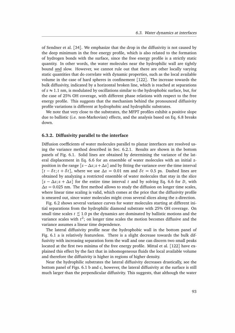
6.3. Water dynamics at interfaces
of Sendner et al. [34]. We emphasize that the drop in the diffusivity is not caused bythe deep minimum in the free energy profile, which is also related to the formationof hydrogen bonds with the surface, since the free energy profile is a strictly staticquantity. In other words, the water molecules near the hydrophilic wall are tightlybound and slow. However, we cannot rule out that there are other locally varyingstatic quantities that do correlate with dynamic properties, such as the local availablevolume in the case of hard spheres in confinement [122]. The increase towards thebulk diffusivity, indicated by a horizontal broken line, which is reached at separationsof z ≈ 1.1 nm, is modulated by oscillations similar to the hydrophobic surface, but, forthe case of 25% OH coverage, with different phase relations with respect to the freeenergy profile. This suggests that the mechanism behind the pronounced diffusivityprofile variations is different at hydrophobic and hydrophilic substrates.
We note that very close to the substrates, the MFPT profiles exhibit a positive slopedue to ballistic (i.e. non-Markovian) effects, and the analysis based on Eq. 6.8 breaksdown.
6.3.2. Diffusivity parallel to the interface
Diffusion coefficients of water molecules parallel to planar interfaces are resolved us-ing the variance method described in Sec. 6.2.1. Results are shown in the bottompanels of Fig. 6.1. Solid lines are obtained by determining the variance of the lat-eral displacement in Eq. 6.6 for an ensemble of water molecules with an initial z-position in the range [z−∆z; z+∆z] and by fitting the variance over the time interval[t − δt; t + δt], where we use ∆z = 0.01 nm and δt = 0.5 ps. Dashed lines areobtained by analyzing a restricted ensemble of water molecules that stay in the slice[z − ∆z; z + ∆z] for the entire time interval t and by solving Eq. 6.6 for D, with∆z = 0.025 nm. The first method allows to study the diffusion on longer time scales,where linear time scaling is valid, which comes at the price that the diffusivity profileis smeared out, since water molecules might cross several slices along the z-direction.
Fig. 6.2 shows several variance curves for water molecules starting at different ini-tial separations from the hydrophilic diamond substrate with 25% OH coverage. Onsmall time scales t ® 1.0 ps the dynamics are dominated by ballistic motions and thevariance scales with t2; on longer time scales the motion becomes diffusive and thevariance assumes a linear time dependence.
The lateral diffusivity profile near the hydrophobic wall in the bottom panel ofFig. 6.1 a is relatively featureless. There is a slight decrease towards the bulk dif-fusivity with increasing separation form the wall and one can discern two small peakslocated at the first two minima of the free energy profile. Mittal et al. [122] have ex-plained this effect by the fact that in inhomogeneous fluids the local available volumeand therefore the diffusivity is higher in regions of higher density.
Near the hydrophilic substrates the lateral diffusivity decreases drastically, see thebottom panel of Figs. 6.1 b and c, however, the lateral diffusivity at the surface is stillmuch larger than the perpendicular diffusivity. This suggests, that although the water
93

6. Water Dynamics near Solutes and Interfaces
Figure 6.1.: From top to bottom: Free en-ergy profiles, MFPT curves for several tar-get separations zt, diffusivity profiles for themotion of water molecules perpendicular tothe surface obtained by the MFPT method(Eq. 6.8) and distance dependent diffusioncoefficients of single water molecules paral-lel to the surface obtained by the variancemethod (Eq. 6.6) with (solid lines) or with-out (dashed lines) taking into account watermolecules that cross slices in z-direction dur-ing the observation time for various kinds ofsurfaces: a) hydrophobic wall, b) hydrophilicwall (12% OH), c) hydrophilic wall (25%OH). Dashed horizontal lines show the bulkdiffusivity, vertical dotted lines indicate localextrema of the free energy profile.
-1
0
1
F [k
BT]
0100200300400
τ fp [p
s]
0
1
2
3
Dz [n
m2 /n
s]
0 0.5 1 1.5z [nm]
01234
Dx,
y [nm
2 /ns]
a)
-1
0
1
F [k
BT]
0100200300400500
τ fp [p
s]
0
1
2
3
Dz [n
m2 /n
s]
0 0.5 1 1.5z [nm]
012345
Dx,
y [nm
2 /ns]
b)
-1
0
1
F [k
BT]
0
200
400
600
τ fp [p
s]
0
1
2
3
Dz [n
m2 /n
s]
0 0.5 1 1.5z [nm]
012345
Dx,
y [nm
2 /ns]
t = 10 pst = 2.0 pst = 1.0 pst = 0.8 pst = 0.6 ps
c)
94

6.3. Water dynamics at interfaces
0 1 2 3 4 5t [ps]
0
0.01
0.02
0.03
<(q-
q 0)2 > [n
m2 ]
z = 0.1 nmz = 0.3 nmz = 0.5 nmz = 1.5 nm
Figure 6.2.: Mean variance of thelateral diffusion (q=x,y) for wa-ter molecules starting at variousseparations z = 0.1,0.3, 0.5 and1.5 nm from a hydrophilic di-amond substrate with 25% OHcoverage (solid lines) and for wa-ter molecules staying in the inter-val [z − ∆z; z + ∆z] with δz =0.025 nm (dashed lines).
mobility perpendicular to the substrate is strongly reduced, water molecules can stillmove laterally to some extent. The fact, that the diffusivity profiles for all but thesmallest analysis duration times t more or less coincide near the surface, shows againthat the residence time of the water molecules is quite long [34], that is on average thewater molecules do not cross the boundary of their initial bin during the observationinterval t.
In a previous study Feng et al. [249] used the variance method to determine theparallel and perpendicular water diffusivity profiles at a substrate made of acetylatedaminosilane linkers grafted on a silica surface. They also found a strongly oscillatingperpendicular diffusivity with a decrease towards the surface but whose oscillationsare in antiphase with the density profile. The shift in the phase relation might becaused by the use of the variance method in a situation with a non-uniform free energyprofile, where the entanglement of free energetic and diffusivity effects requires astochastic approach as used in this work; in fact, we observe a similar shift whenemploying the variance method instead of the MFPT method (data not shown). Theparallel diffusivity profiles found by Feng et al. [249] are in qualitative agreement withour results.
6.3.3. Water orientation relative to the interface
As is illustrated in Fig. 6.3, the projections of the (unit) dipole vector µ and of the unitvector along a water OH-bond ηOH define two angles
cos(α)≡ µ · z, cos(β)≡ ηOH · z. (6.9)
where z denotes the unit vector in z-direction pointing into the water (see Fig. 6.3).Free energy landscapes in the (z, cosα)- and in the (z, cosβ)-plane are shown in the leftcolumn of the Figs. 6.4 and 6.5, taken from Ref. [2]. Near the hydrophobic surface thewater molecules dipole is preferentially oriented parallel to the surface (cos(α) ≈ 0),while one of its OH vectors either points directly towards the surface (cos(β) ≈ −1,
95

6. Water Dynamics near Solutes and Interfaces
Figure 6.3.: Definition of anglesα and β specifying the orienta-tion of the water dipole vectorand of the OH-bond with respectto the z-axis.
around z ≈ 0.10 nm) or away from the surface (cos(β) ≈ 1, around z ≈ 0.16 nm).Correspondingly, the other OH vector points either slightly away from (cos(β) ¦ 0)or slightly towards (cos(β) ® 0) the surface. With such an orientation, which emu-lates the configuration in hexagonal ice, the water minimizes the number of brokenhydrogen bonds at the surface [9, 27].
Near the hydrophilic substrates the orientational distribution is dominated by thetendency of the water molecules to form hydrogen bonds with the surface OH groups.The water molecules can either act as hydrogen bond donors and therefore point oneof their OH bonds towards the surface (cos(β) ≈ −0.75), the other OH bond pointingconsequently away from the surface (cos(β)≈ 1.0), or as hydrogen bond acceptors inwhich case both OH bonds are oriented more or less parallel to the surface (cos(β) ≈0.0).
Whether however orientations towards the wall are relevant for the separation dy-namics of the binding partners, can not be inferred from these free energy landscapesalone. Average first-passage times to cross a given separation zt are therefore evalu-ated in the (z, cosα)- and the (z, cosβ)-plane; results are shown in the right columnsof the Figs. 6.4 and 6.5. The water dynamics perpendicular to the hydrophobic wall israther insensitive to the initial orientation of the water relative to the interface, whilea strong dependence on the initial orientation is observed for the hydrophilic walls.Note, that the above-mentioned non-monotonicity of the MFPT curves in Fig. 6.1 isreflected in the two-dimensional MFPT landscapes, but more detail is contained in theMFPT data in the angle-distance plane. Especially on the hydrophilic surfaces, verylong-lived configurational states close to the wall are discerned, which do not seemto be simply correlated with the free-energy landscape. These long-lived states arepresumably related to the kinetics of hydrogen bonding to polar surface groups andpossibly also collective water hydrogen-bonding effects.
96

6.3. Water dynamics at interfaces
Figure 6.4.: From top to bottom: hydrophobic wall, hydrophilic wall (12% OH), and hydrophilicwall (25% OH). Left column: Free energy landscape in the (z, cosα)-plane for water moleculesnear planar interfaces. Right column: Average first-passage times to reach the right boundary ofthe plots (zt ≈ 0.3 nm) for water molecules starting from a distance r and an initial orientationof the water dipole moment cosα. Colors display average first-passage times, the black linesdenote contour lines of constant free-energy (0.5 kBT per line) as shown in the left column.
97
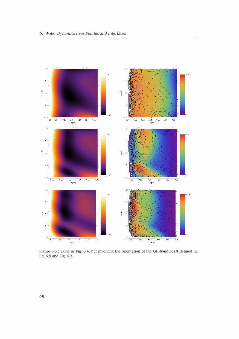
6. Water Dynamics near Solutes and Interfaces
Figure 6.5.: Same as Fig. 6.4, but involving the orientation of the OH-bond cosβ defined inEq. 6.9 and Fig. 6.3.
98

6.4. Water dynamics near solutes
0.0
0.5
1.0
1.5
2.0
2.5
3.0
3.5
4.0F
[kBT
]
0
10
20
30
40
50
τ fp
[ps]
rt = 1.2 nm
rt = 1.0 nm
rt = 0.8 nm
rt = 0.6 nm
rt = 0.4 nm
0.4 0.6 0.8 1.0 1.2
r [nm]
0
1
2
3
4
5
6
7
8
D[n
m2/ns
](a)
(b)
(c)
Figure 6.6.: (a) Radial free en-ergy profile for pairs of watermolecules (solid blue line) andideal free energy (broken blackline). (b) MFPT curves for wa-ter pair dynamics for several tar-get separations rt. (c) Relativediffusivity profiles resulting fromthe curves in panel b) (same colorcoding) using the MFPT method(see Eq. 6.8). The dashed hori-zontal line denotes the value ofthe diffusivity at large separa-tions 2DH2O ≈ 5.1 nm2/ns. Verti-cal lines indicate the positions ofthe first local minimum and max-imum in the free energy profile.
6.4. Water dynamics near solutes
Based on MD simulation trajectories of pure SPC/E bulk water and of a single methanemolecule in SPC/E bulk water, relative separation trajectories between pairs of wa-ter molecules and water methane pairs are generated. Using a spatial resolution∆r = 0.005 nm, all paths starting within a distance∆r/2 from r and crossing rt−∆r/2for the first time a time tfp later contribute to the MFPT τfp =
¬
tfp
. Due to the pe-riodicity of the system we only consider target distances rt < L/2, where L ≈ 3 nmdenotes the edge length of the simulation box. The fitting range used to determine∂ τfp(r, rt)/∂ r is δr = 0.06 nm for the water pairs and δr = 0.1 nm for the watermethane dynamics. For the evaluation of the integral in Eq. 6.8, the equilibrium distri-butionψeq. = exp
�
−βF�
is linearly interpolated; the integral is calculated numerically
99

6. Water Dynamics near Solutes and Interfaces
Figure 6.7.: Same as Fig. 6.6, butfor water methane pair dynam-ics. In the limit r → ∞ the rel-ative diffusivity reaches DH2O +DCH4
≈ 4.85 nm2/ns (dashed hor-izontal line in panel c).
0.0
0.5
1.0
1.5
2.0
2.5
3.0
3.5
4.0
F[k
BT
]
0
10
20
30
40
50
τ fp
[ps]
rt = 1.2 nm
rt = 1.0 nm
rt = 0.8 nm
rt = 0.6 nm
0.4 0.6 0.8 1.0 1.2
r [nm]
0
1
2
3
4
5
6
7
8
D[n
m2/ns
]
(a)
(b)
(c)
using reflective boundaries rmin = 0.235 nm for water pairs and to rmin = 0.28 nm forwater methane pairs.
Free energy profiles for water-water and for water methane pairs are shown in thepanels a of Figs. 6.6 and 6.7, taken from Ref. [2]: While the free energy barrier forwater pairs is ≈ 1 kBT , water methane pairs only encounter a barrier ® 0.5 kBT .
MFPT curves τfp are shown in the central panels b of the corresponding figures.Diffusivity profiles obtained by the MFPT method (see Sec. 6.2.2) are shown in thepanels c of the Figs. 6.6 and 6.7: profiles obtained from MFPT curves belonging todistinct target separations rt mainly fall on top of each other, clearly demonstratingthe validity of our approach (see Sec. 6.2). Deviations between the profiles obtainedfrom distinct MFPT curves occur for transitions covering separations rt − r ® 0.2 nmand taking place on time scales on the order of 1 ps: they are caused by ballistic
100

6.5. Conclusion
(non-Markovian) contributions to the dynamics which can not be captured by ouroverdamped description.
For large separations where molecules move independently from each other, thediffusivity profiles tend towards the values 2DH2O and DH2O+DCH4
(dashed horizontallines in the Figs. 6.6 c and 6.7 c, where these diffusion coefficients obtained from thelong time mean square displacement of single molecules are DH2O ≈ 2.55 nm2/ns andDCH4
≈ 2.3 nm2/ns.Note that the diffusivities in the first coordination shells show pronounced differ-
ences: while the relative diffusivity for water pairs exhibits a clear drop down to≈ 15 % of the values at large separations, the diffusivity profile for water methanepair dynamics is rather characterized by smooth oscillations and does not drop be-low ≈ 40%, similar to the empiric results obtained for simple two dimensional flu-ids [250, 251] and to the diffusivity near the hydrophobic wall. Also the diffusivity pro-files of methane-water dissociation and of water at the hydrophobic wall both exhibita very pronounced second minimum at a separation of r ≈ 0.6 nm and z ≈ 0.4 nm.
Note, that differences in the dissociation times between the water-water and thewater-methane cases are caused both by differences in the F and D profiles. To bespecific, the dissociation time for the water-water case is distinctly higher, most pro-nounced for the curve reaching a target separation of rt = 0.6 nm. This is due tothe higher free energy barrier for water-water in Fig. 6.6 a but also due to the lowdiffusivity below distances r < 0.3 nm, seen in Fig. 6.6 c. The higher diffusivity ofthe methane-water separation coordinate at small separation presumably is related tothe absence of hydrogen bonds between methane and water. The pronounced dip inD at r = 0.6 nm in Fig. 6.7 c must have to do with water restructuring of the secondsolvation shell. Interestingly, while the methane-water diffusion is faster than water-water at small separation, it becomes slower at large separations. This explains thatthe MFPTs with rt = 1.2 nm are rather similar for the two systems. The smaller CH4-H2O diffusivity at large separations is caused by the larger hydrodynamic radius of theCH4 molecule. This behavior reflects that the diffusivity of objects is influenced bothby their bare size but also by their ability to form hydrogen bonds with water.
6.5. Conclusion
Based on the Fokker-Planck description of the diffusion of individual water moleculessubject to a free energy landscape and a spatially dependent diffusivity profile, wehave determined diffusivity profiles at solid surfaces of varying hydrophilicity. Wehave also determined diffusivity profiles governing the diffusion of the distance coor-dinate between two water molecules and between a methane and a water molecule.The variation in the diffusivity profiles are pronounced, especially at the hydrophilicsurface and for water-water diffusion. We conclude that the neglect of diffusivity pro-files for predicting water kinetics in these situations can lead to gross inaccuracies.Our protocol for extracting D profiles is based on mean first passage time profiles, by
101

6. Water Dynamics near Solutes and Interfaces
construction our approach thus gets the long-time dynamics right. We note that thesame procedure can in principle be applied to experimental time series data.
In summary, there is no simple or direct relation between the free energy and diffu-sivity profiles, but both are needed for predicting the kinetics of single water molecules.On hydrophilic surfaces the water molecules are strongly bound, but in addition theyare also slow, which presumably is due to a coupling between translational and rota-tional degrees of freedom. The layer where the diffusivity is reduced has a width ofroughly 0.5 to 1 nm and thus matches the width over which the viscosity was found tobe reduced in MD Couette shearing simulations [34].
The same difference is seen when comparing the water dynamics at a non-polar so-lute (methane in the present case) and a polar "solute" (taken to be a water molecule).These results point to pronounced and quite universal differences of the dynamics ofindividual water molecules close to hydrophobic and hydrophilic objects.
102

CHAPTER 7
SUMMARY AND OUTLOOK
In this work the structure and dynamics of water and the solvation of hydrophobicsolutes has been studied by means of extensive molecular dynamics simulations. Wehave shown that molecular dynamics simulations in conjunction with current watermodels are capable to give an accurate description of water’s properties in varioussituations.
In chapter 3 we have presented evidence, that the water models we use in thiswork can reproduce the water structure quite well. Even subtle features, such asthe experimentally observed enhancement of the static structure factor at low wavevectors are not missed. We have further shown that at ambient conditions spatialcorrelations between order parameters describing the tetrahedral ordering of waterare rather weak and decay after a few Å. That means, that no extended clusters ofhighly ordered water exist under these conditions [20]. It also adds to the doubts ontheories that build on the idea of the propagation of structural order in water, likethe structure-making/structure-breaking explanations of Hofmeister [252–254] andosmolyte [255, 256] effects. We have also seen that correlations between density andstructural fluctuations are rather weak, which tells us that one has to be very carefulto interpret scattering experiments, that probe density fluctuations, in terms of waterorder.
In chapter 4 we determined the dependence of the solvation thermodynamics ofsmall non-polar solutes on the solute water interaction potential and its implicationsfor the interpretation of entropy convergence. We found that for solutes with similarinteractions but varying size, entropy and enthalpy convergence exists, but that theconvergence temperature changes with changing interaction parameters: For increas-ing stiffness as well as for increasing depth of the interaction potential the convergencetemperature increases, while it does not change for increasing range of the interaction.The meaning of this finding is, that there is no universality in the temperature depen-dence of hydrophobic solvation. As a consequence, for a set of solutes with similarinteractions but differing size, which with restrictions might apply for the rare gases,as well as for homologous series of solutes, entropy convergence is expected, while for
103

7. Summary and Outlook
proteins in general it is not in accordance with recent experimental findings [69]. Itmight be interesting to extend the study of the temperature dependence to the solva-tion of polar solutes, which could further clarify the denaturation thermodynamics ofproteins. Unfortunately, this comes at the cost of a drastic increase in the computa-tional effort, since the particle insertion method cannot be used efficiently any more ifthe solute carries partial charges.
In chapter 5 we investigated the fluctuations of a free air/water interface on theone hand and the solvation of spherical and cylindrical hydrophobic solutes on theother hand and described both phenomena based on a Helfrich type local surface freeenergy functional. It could be shown, that after successfully separating bulk-like andinterfacial contributions, the fluctuation spectrum of the air/water interface is welldescribed by an effective surface tension including a bending term. Using the width ofthe intrinsic density profile to disentangle the capillary wave contribution to the totalinterfacial width, we find cutoff lengths in agreement with recent experiments [229].
From the comparison of the solvation free energies of spherical and cylindrical so-lutes we inferred the free energy of the isochoric aggregation of spheres to form acylinder, which is unfavourable below a threshold radius of ≈ 0.3 nm. It is furtherfound that the solvation free energies for spheres and cylinders exhibit a maximumas a function of the inverse radius, which is equivalent with a negative Tolman lengthon the order of −0.1 nm at room temperature, meaning that water prefers to formdroplets over cavities. From fitting the solvation free energies of spheres and cylinderssimultaneously we obtain estimates for the elastic constants of the water surface, thebending rigidity beeing in qualitative agreement with the result form the air/waterinterface, if the latter is corrected for the effect of a finite Lennard-Jones cutoff. Al-though we extended the solute size to radii of 2 nm there is still a dependence of thefit parameters on the fitting range seen, which means that the asymptotic regime is notyet sufficiently reached. Increased computational capacities in the future will permit toreach even larger length scales and to yield more accurate results. Also, the extensionof this study to other solute shapes might give another stringent test on the validity ofthe Helfrich description of the water surface. It is notable, that the cross-over lengthscale R∗ ≈ 0.5 nm seen in the size dependence of solvation free energies is found to besimilar to the characteristic length of the intrinsic roughness of the air/water interface.It transpires, that this is the relevant length scale separating a change in the behaviourof an aqueous interface. Below that scale the discreteness of the hydrogen bondingnetwork is dominant, while on larger scales the overall shape of the surface prevails.
Finally, in chapter 6 we applied a Fokker-Planck based formalism to the dynam-ics of single water molecules near hydrophobic and hydrophilic surfaces and solutes.We found a strongly varying diffusivity profile with a pronounced slow-down of thedynamics near the hydrophilic surface and near another water molecule. Near the hy-drophobic surface and a methane solute the drop in the diffusivity is less pronounced.Nonetheless it should be emphasized, that in order to model the dynamics of waternear a surface or solute, both the diffusivity and the free energy profile needs to betaken into account.
104
CHAPTER 8
DANKSAGUNG
An dieser Stelle möchte ich mich bei allen bedanken, die mich bei der Entstehungdieser Arbeit unterstützt haben. Besonderer Dank gebührt meinem Betreuer HerrnProf. Roland Netz für interessante Forschungsprojekte, stete Unterstützung und nichtzuletzt die Ermöglichung vieler Konferenzbesuche und Forschungsaufenthalte in al-ler Welt. Insbesondere die Trips nach Boston, Istanbul und die Zeit in Santa Barbarawerden mir immer in guter Erinnerung bleiben. Nie zu kurz kamen auch die vielengemeinsamen Lehrstuhlaktivitäten: Winterschulen, Wandertage, Oktoberfestbesuche,Weihnachtsfeiern und Grillfeste. Auch dafür herzlichsten Dank.
Des weiteren bedanke ich mich bei Herrn Prof. Dominik Horinek, dafür dass er michin die Kunst der MD Simulation eingeführt hat und dass er für alle wissenschaftlichen,technischen und sonstigen Fragen stets zur Verfügung stand.
Nicht unerwähnt bleiben darf auch unsere Sektretärin Frau Sonja Ortner, ohne dieam Lehrstuhl gar nichts funktionieren würde. Für stete Hilfe und Unterstützung inallen organisatorischen Dingen ein herzliches Dankeschön.
Und schließlich möchte ich mich auch bei allen übrigen T37’lern bedanken, für diehervorragende Arbeitsathmosphäre, viele wissenschaftliche und nichtwissenschaftli-che Diskussionen und auch die ein oder andere BZFlag und Kickerrunde. Besondershervorheben möchte ich meinen Bürokollegen Herrn Aykut Erbas. Für unzählige Dis-kussionen, eine schöne Zeit in Istanbul trotz Vulkanausbruchs und viel Spaß bei dertäglichen Arbeit, tesekkürler.
Für gute und erfolgreiche Zusammenarbeit in vielen Projekten während meiner Dok-torarbeit danke ich Herrn Prof. Thorsten Hugel, Herrn Prof. Lydéric Bocquet, FrauKerstin Falk, Herrn Prof. Laurent Joly und Herrn Dr. Markus Mezger.
Bei Herrn Dr. Joseph Homolka und Herrn Dr. Stefan Recksiegel bedanke ich michfür die Zurverfügungstellung von Speicherplatz auf dem NAS System der Fakultät undfür die Hilfe beim Umzug unseres Rechenclusters.
Für die großzügige Förderung im Rahmen des Graduiertenkollegs "Materials Scienceof Complex Interfaces" bedanke ich mich beim Elitenetzwerk Bayern und für die Re-chenzeit auf dem Höchstleistungrechner HLRB-II beim Leibnitz-Rechenzentrum Mün-chen.
Ganz besonders bedanken möchte ich mich bei meiner Freundin Emö und bei mei-ner Familie, meinen Eltern und Geschwistern. Ihre bedingungslose Unterstützung istmir stets ein großer Rückhalt.
105

106
CHAPTER 9
LIST OF PUBLICATIONS
This thesis is mainly based on the following articles, that have been published in orsubmitted to peer-reviewed journals:
F. Sedlmeier and R. R. Netz: The Tolman length of water. under review by PhysicalReview Letters, submitted August 24, 2011
F. Sedlmeier, Y. von Hansen, L. Mengyu, D. Horinek and R. R. Netz: Water Dy-namics at Interfaces and Solutes: Disentangling Free Energy and Diffusivity Contri-butions. J. Stat. Phys. 145 (2), 240 (2011)
F. Sedlmeier, D. Horinek and R. R. Netz: Entropy and enthalpy convergence ofhydrophobic solvation beyond the hard-sphere limit. J. Chem. Phys. 134 (5),055105 (2011)
F. Sedlmeier, D. Horinek and R. R. Netz: Spatial Correlations of Density andStructural Fluctuations in Liquid Water: A Comparative Simulation Study. J. Am.Chem. Soc. 133 (5), 1391 (2011)
F. Sedlmeier, D. Horinek and R. R. Netz: Nanoroughness, Intrinsic Density Profile,and Rigidity of the Air-Water Interface. Phys. Rev. Lett. 103 (13), 136102 (2009)
Further publications, which are not directly related to this thesis:
Y. von Hansen, F. Sedlmeier, M. Hinczewski and R. R. Netz: Friction contributionto water-bond breakage kinetics. Phys. Rev. E 84 (5), 051501 (2011)
K. Falk, F. Sedlmeier, L. Joly, R. R. Netz and L. Bocquet: Molecular Origin of FastWater Transport in Carbon Nanotube Membranes: Superlubricity versus CurvatureDependent Friction. Nano Lett. 10 (10), 4067 (2010)
M. Mezger, F. Sedlmeier, D. Horinek, H. Reichert, D. Pontoni and H. Dosch: Onthe Origin of the Hydrophobic Water Gap: An X-ray Reflectivity and MD SimulationStudy. J. Am. Chem. Soc. 132 (19), 6735 (2010)
107

9. List of Publications
D. Horinek, A. Herz, L. Vrbka, F. Sedlmeier, S. Mamatkulov and R. R. Netz: Spe-cific ion adsorption at the air/water interface: The role of hydrophobic solvation.Chem. Phys. Lett. 479 (4-6), 173 (2009)
F. Sedlmeier, J. Janecek, C. Sendner, L. Bocquet, R. R. Netz and D. Horinek:Water at polar and nonpolar solid walls. Biointerphases 3 (3), FC23-FC39 (2008)
108

APPENDIX A
APPENDIX - LATERAL STRUCTURE FACTOR
In this appendix we derive the relation between the lateral structure factor, defined by(see Eq. 5.14)
S||(~q) =1
N||
∫
d3rd3r ′ f (z) f (z′)ei~q(~r||−~r ′||)⟨ρ(~r)ρ(~r ′)⟩c, (A.1)
and the 3D structure factor given by
S(~Q) =
∫
d3rd3r ′ei~Q(~r−~r ′)⟨ρ(~r)ρ(~r ′)⟩c, (A.2)
where ~q = (qx , qy) and ~Q = (Q x ,Q y ,Qz) are lateral and 3D wave vectors and
N|| =
∫
d3r f 2(z)⟨ρ(~r)⟩. (A.3)
We also show that the power spectrum of the local GDS profile in the limit of an infiniteblock factor, n→∞, is proportional to the lateral structure factor with a rectangularweight function f (z) = θ(z+− z)θ(z− z−).
A.1. Equivalence of the local GDS power spectrum and thelateral structure factor
To prove the equivalence of the GDS power spectrum and the lateral structure factor,we start from the definition of the height profile using the local GDS method, givenin Eq. 5.9. The number of molecules in a prism Mr|| can be written in terms of themicroscopic density ρ(~r) as
Mr|| =
∫ z+
z−
dz′∫
d2r ′||θ(x′− (x −∆L/2))θ((x +∆L/2)− x ′)
×θ(y ′− (y −∆L/2)θ((y +∆L/2)− y ′)ρ(~r ′), (A.4)
109
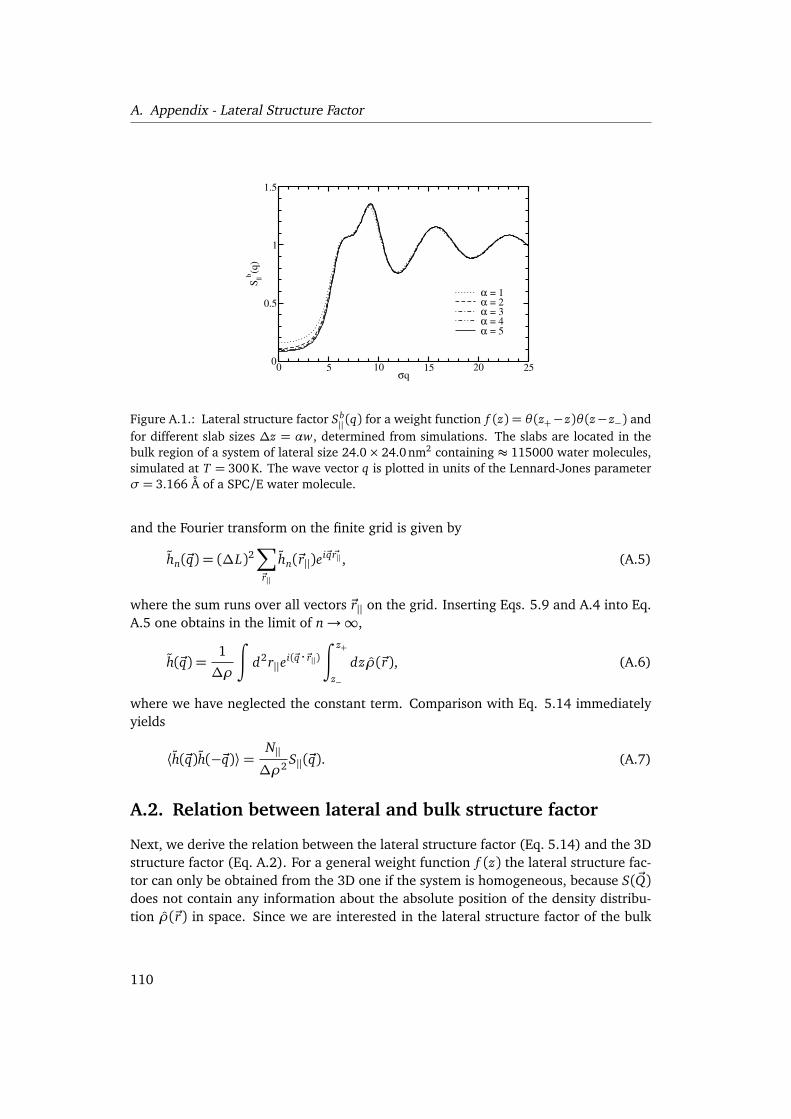
A. Appendix - Lateral Structure Factor
0 5 10 15 20 25σq
0
0.5
1
1.5
S||b
(q)
α = 1α = 2α = 3α = 4α = 5
Figure A.1.: Lateral structure factor Sb|| (q) for a weight function f (z) = θ(z+−z)θ(z−z−) and
for different slab sizes ∆z = αw, determined from simulations. The slabs are located in thebulk region of a system of lateral size 24.0× 24.0 nm2 containing ≈ 115000 water molecules,simulated at T = 300K. The wave vector q is plotted in units of the Lennard-Jones parameterσ = 3.166 Å of a SPC/E water molecule.
and the Fourier transform on the finite grid is given by
hn(~q) = (∆L)2∑
~r||
hn(~r||)ei~q ~r|| , (A.5)
where the sum runs over all vectors ~r|| on the grid. Inserting Eqs. 5.9 and A.4 into Eq.A.5 one obtains in the limit of n→∞,
h(~q) =1
∆ρ
∫
d2r||ei(~q ·~r||)
∫ z+
z−
dzρ(~r), (A.6)
where we have neglected the constant term. Comparison with Eq. 5.14 immediatelyyields
⟨h(~q)h(−~q)⟩=N||∆ρ2 S||(~q). (A.7)
A.2. Relation between lateral and bulk structure factor
Next, we derive the relation between the lateral structure factor (Eq. 5.14) and the 3Dstructure factor (Eq. A.2). For a general weight function f (z) the lateral structure fac-tor can only be obtained from the 3D one if the system is homogeneous, because S(~Q)does not contain any information about the absolute position of the density distribu-tion ρ(~r) in space. Since we are interested in the lateral structure factor of the bulk
110

A.2. Relation between lateral and bulk structure factor
region of the simulation, we can safely assume homogeneity. In that case the correla-tion function depends only on the relative distance, ⟨ρ(~r)ρ(~r ′)⟩c = ⟨ρ(~0)ρ(~r ′ −~r)⟩c,and we can write it as the inverse Fourier transform of the structure factor
⟨ρ(~0)ρ(~r ′−~r)⟩c = ρ∫
d3Q
(2π)3e−i~Q(~r ′−~r)S(~Q), (A.8)
where ρ = N/V is the mean density. Inserting this into Eq. 5.14 and carrying out theintegration over the lateral coordinates yields
S||(~q) =1
Lf
∫
dQz
2πf (Qz) f (−Qz)S(~q,Qz), (A.9)
where f (Qz) =∫
dzeiQzz f (z) is the Fourier transform of the weight function and we
have defined Lf =∫
dz f 2(z). We evaluate this first for the special choice of f (z) =θ(z+ − z)θ(z − z−), we used in our simulations. The Fourier transform is then givenby
f (Qz) f (−Qz) =�
sin(Qz∆z/2)Qz/2
�2
, (A.10)
and Lf =∆z, with ∆z = z+− z−. Inserting this into Eq. A.9 yields
S||(~q) =1
∆z
∫
dQz
2π
�
sin(Qz∆z/2)Qz/2
�2
S(~q,Qz) (A.11)
In the limit of an infinite slab thickness, ∆z→∞, we have
lim∆z→∞
2sin2(Qz∆z/2)π∆zQ2
z= δ(Qz), (A.12)
and the lateral structure factor reduces to S||(~q) = S(~q, 0) as expected. For a finite slabthickness ∆z, however, the lateral structure factor differs from the three dimensionalone. This is illustrated in Fig. A.1, where we plot the lateral structure factor Sb
|| (q)for slabs of different thickness ∆z = αw located in the bulk region of the simulationsystem. Especially in the low q limit there is a pronounced dependence on the slabthickness. The corresponding compressibilities, defined by Sb
||(0) = ρkBTκT,||, aregiven in Tab. A.1.
Next, we evaluate Eq. A.9 for the experimentally relevant case of an exponentialweight function f (z) = exp(−|z|/(2l)), for z < 0, and f (z) = 0 for z > 0, with apenetration depth l. The Fourier transform is then found to be
f (Qz) f (−Qz) =4l2
1+ (2lQz)2, (A.13)
111

A. Appendix - Lateral Structure Factor
Table A.1.: Isothermal compressibility κT,|| defined by the limit of the lateral bulk structurefactor Sb
||(q) for q→ 0, Sb||(0) = ρkBTκT,||, for varying slab size ∆z = αw. The compressibilities
are derived from the data presented in Fig. A.1.
α κT,||[10−11Pa−1]
1 115.72 78.83 69.34 64.15 60.4∞ 45.51
1 bulk compressibility of SPC/E water at T = 298 K (see Tab. 3.1), in good agreement with theexperimental value of 45.8× 10⁻¹¹Pa−1 [257].
and Lf = l. With Eq. A.9 we obtain
S||(~q) =
∫
dQz
π
2l
1+ (2lQz)2S(~q,Qz). (A.14)
Again, in the limit of an infinite penetration depth, l →∞, we can use the relation
liml→∞
1
π
2l
1+ (2lQz)2= δ(Qz), (A.15)
and the lateral structure factor reduces to S||(~q) = S(~q, 0).
112

APPENDIX B
APPENDIX - ACCURACY CHECKS FOR SOLVATION
FREE ENERGY CALCULATIONS
In this appendix we present several checks concerning the accuracy of the solvationfree energy calculations with the thermodynamic integration method. We first show,that the employed integration procedure and the number of λ-points used is sufficientto yield accurate results. Next, we demonstrate that finite size effects are negligibleand finally we investigate the dependence of the solvation free energy on the Lennard-Jones cutoff length rc .
B.1. Integration error
We first evaluate the integration error, i. e., the error made due to the usage of a fi-nite number of λ-values at which the derivative ⟨∂ URI→RII
/∂ λ⟩ is evaluated. For thatpurpose, we double the number of λ-values, corresponding to a radius increment of∆R= 0.00625 nm, for the integration step RI = 1.75 nm→ RII = 2.0 nm for the spher-ical solute at T = 300 K. Figure B.1 a shows a plot of the derivative ⟨∂ URI→RII
/∂ λ⟩ asa function of λ for the different step sizes including the interpolating function. Theinterpolation for the coarser resolution coincides very well with the additional datapoints at finer resolution. In Fig. B.1 b we plot the free energy difference obtainedeither by simple trapezoidal integration of ⟨∂ URI→RII
(λ)/∂ λ⟩ (symbols and full lines)or by using the spline interpolation (dashed lines) for both data sets. It can be seenthat for the trapezoidal integration there is a systematically increasing difference be-tween the two data sets. This difference is caused by the systematic integration errordue to the concave shape of the integrand. The two curves obtained by integratingthe spline interpolation lie almost perfectly on top of each other indicating that us-ing the spline interpolation the smaller resolution of ∆R = 0.0125 nm is sufficient forobtaining accurate results.
113

B. Appendix - Accuracy Checks for Solvation Free Energy Calculations
Figure B.1.: (a) Average of thederivative ⟨∂ URI→RII
/∂ λ⟩ as afunction of λ for the integra-tion step from RI = 1.75 nmto RI = 2.0 nm for a spheri-cal solute at T = 300K. Redsquares and black circles indi-cate λ-values corresponding toequidistant radii with an incre-ment of ∆R = 0.0125nm and∆R = 0.00625 nm, respectively.The black full and red dashedlines are spline interpolations tothe data sets. (b) Free energy dif-ference with respect to the initialstate RI = 1.75nm obtained bysimple trapezoidal integration of⟨∂ URI→RII
/∂ λ⟩ for an incrementof ∆R = 0.0125 nm (red cirlces/full line) and ∆R = 0.00625nm(black squares / full line) and byintegrating the spline interpola-tion of both data sets (red andblack dashed lines).
0.0001 0.001 0.01 0.1 1λ
1×10²
1×10³
1×10⁴
1×10⁵
<∂U
r th
I → r
th
II
/∂λ
> [
kJ/
mo
l]
∆rth
= 0.00625 nm
Spline Interpolation
∆rth
= 0.0125 nm
Spline Interpolation
a)
1.75 1.8 1.85 1.9 1.95 2R [nm]
0
100
200
300
400
∆F
r th
I → r
th
II
[k
J/m
ol]
trapezoidal integration, ∆rth
= 0.00625 nm
trapezoidal integration, ∆rth
= 0.0125 nm
spline integration, ∆rth
= 0.00625 nm
spline integration, ∆rth
= 0.0125 nm
b)
114

B.2. Finite size effects
0.25 0.3 0.35 0.4 0.45 0.5R [nm]
-0.004
-0.002
0
0.002
0.004
Rela
tiv
e d
ev
iati
on
L = 3.0 nmL = 3.5 nmL = 4.0 nmL = 4.5 nm
a)
0.75 0.8 0.85 0.9 0.95 1R [nm]
-0.004
-0.002
0
0.002
0.004
Rel
ativ
e d
evia
tio
n
Lz = L
x,y = 3.5 nm
Lz = L
x,y = 4.0 nm
Lz = L
x,y = 4.5 nm
b)
Figure B.2.: Relative differencesof the free energies of solvation(a) for the integration step fromRI = 0.25 nm to RII = 0.5 nmfor a spherical solute for differentbox sizes L = 3.0, 3.5, 4.0 and4.5 nm and (b) for the integra-tion step from RI = 0.75 nm toRII = 1.0 nm for a cylindrical so-lute for box sizes of Lz = Lx ,y =3.5, 4.0 and 4.5 nm. The differ-ences are taken with respect tothe smallest box. For the caseof the cylinders the free energyper unit length is considered. Nosystematic deviation is observedwith increasing box size. All sim-ulations are done at T = 300 Kand p = 1 bar.
B.2. Finite size effects
We further check the sensitivity of the free energy calculation to finite size effects bycomparing the solvation free energies for the integration step from RI = 0.25 nm toRII = 0.5 nm for a spherical solute for different box sizes of L ≈ 3.0, 3.5, 4.0 and 4.5 nmand for the integration step from RI = 0.75 nm to RII = 1.0 nm for cylindrical solutesfor box sizes of Lz ≈ Lx ,y ≈ 3.5, 4.0 and 4.5 nm. Figure B.2 shows the relative freeenergy differences with respect to the smallest box size in each case. No significanttrend is seen with the system size and the relative deviations for all cases are quitesmall, which again evidences the high accuracy of the method. Since the simulationsare done at fixed pressure, the box size L (spheres) and Lx ,y (cylinders) vary slightlyduring each simulation. The actual box sizes at the final integration step are LII = 2.98,3.54, 4.06 and 4.54 nm for the spherical solute and LII
x ,y = 3.48, 4.02 and 4.48 nm forthe cylindrical solute, while Lz = 3.5, 4.0 and 4.5 nm is fixed.
115

B. Appendix - Accuracy Checks for Solvation Free Energy Calculations
Figure B.3.: (a) Solvation free en-ergy ∆F per area A of a cylindri-cal solute obtained using a cut-off radius of rc = 0.9 nm (redcurves) and rc = 1.8 nm (greencurves) for the nonbonded wa-ter water interactions as a func-tion of the inverse radius R. Thesolvation free energies per areaare rescaled by the planar surfacetension γlv,0 of the free air/wa-ter interface obtained with therespective cutoff radii. Simula-tions are done at a temperatureof T = 360 K and a pressure ofp = 1 bar.
B.3. Cutoff effects
Finally, we discuss the dependence of the solvation free energy on the cutoff length ofthe Lennard-Jones interactions, which is set to rc = 0.9 nm in most of our simulations.Since we only study solutes up to a radius of 2.0 nm, which is on the same order asrc, no strong influence of the finite cutoff length would be expected. We check thisexplicitly by determining the solvation free energy of a cylindrical solute at T = 360 Kusing a Lennard-Jones cutoff length of rc = 1.8 nm. In Fig. B.3 we show the solvationfree energies for both cutoff lengths rescaled by the planar air/water surface tension,which is γlv,0 = 50.9 mN/m for rc = 1.8 nm and γlv,0 = 45.5 mN/m for rc = 0.9 nm.The slight shift, that is seen in Fig. B.3, can be attributed to the statistical uncertaintyof the planar surface tension, which is on the order of 2%. Apart from this smalldeviation the shape of both curves is very similar, which in particular means that theTolman length extracted from the data does not depend significantly on the LennardJones cutoff length.
116

BIBLIOGRAPHY
[1] Y. von Hansen, F. Sedlmeier, M. Hinczewski, et al. Friction contribution towater-bond breakage kinetics. Phys. Rev. E 84 (5), 051501 (2011)
[2] F. Sedlmeier, Y. von Hansen, L. Mengyu, et al. Water Dynamics at Interfaces andSolutes: Disentangling Free Energy and Diffusivity Contributions. J. Stat. Phys.145 (2), 240 (2011)
[3] F. Sedlmeier, D. Horinek, R. R. Netz. Entropy and enthalpy convergence ofhydrophobic solvation beyond the hard-sphere limit. J. Chem. Phys. 134 (5),055105 (2011)
[4] F. Sedlmeier, D. Horinek, R. R. Netz. Spatial Correlations of Density and Struc-tural Fluctuations in Liquid Water: A Comparative Simulation Study. J. Am.Chem. Soc. 133 (5), 1391 (2011)
[5] K. Falk, F. Sedlmeier, L. Joly, et al. Molecular Origin of Fast Water Transportin Carbon Nanotube Membranes: Superlubricity versus Curvature DependentFriction. Nano Lett. 10 (10), 4067 (2010)
[6] M. Mezger, F. Sedlmeier, D. Horinek, et al. On the Origin of the HydrophobicWater Gap: An X-ray Reflectivity and MD Simulation Study. J. Am. Chem. Soc.132 (19), 6735 (2010)
[7] F. Sedlmeier, D. Horinek, R. R. Netz. Nanoroughness, Intrinsic Density Profile,and Rigidity of the Air-Water Interface. Phys. Rev. Lett. 103 (13), 136102(2009)
[8] D. Horinek, A. Herz, L. Vrbka, et al. Specific ion adsorption at the air/waterinterface: The role of hydrophobic solvation. Chem. Phys. Lett. 479 (4-6), 173(2009)
117

Bibliography
[9] F. Sedlmeier, J. Janecek, C. Sendner, et al. Water at polar and nonpolar solidwalls. Biointerphases 3 (3), FC23 (2008)
[10] F. Franks. Water: a matrix of life. 2nd edition (Royal Society of Chemistry,Cambridge, 2000)
[11] P. Ball. Life’s matrix: a biography of water. 1st edition (University of CaliforniaPress, Berkeley, 2001)
[12] S. Jackson. Anatomy & Physiology for Nurses. Nurses’ Aids Series. 9th edition(Bailliere Tindall, London, 1985)
[13] P. Ball. Water as an Active Constituent in Cell Biology. Chem. Rev. 107 (1), 74(2008)
[14] G. S. Kell. Density, thermal expansivity, and compressibility of liquid water from0◦ to 150◦: Correlations and tables for atmospheric pressure and saturationreviewed and expressed on 1968 temperature scale. J. Chem. Eng. Data 20 (1),97 (1975)
[15] F. Franks. Water. A Comprehensive Treatise. 1st edition (Ed. Plenum, New York,1973)
[16] F. Stillinger. Water revisited. Science 209 (4455), 451 (1980)
[17] A. K. Soper, M. G. Phillips. A new determination of the structure of water at25◦ C. Chem. Phys. 107 (1), 47 (1986)
[18] T. Head-Gordon, G. Hura. Water Structure from Scattering Experiments andSimulation. Chem. Rev. 102 (8), 2651 (2002)
[19] R. Kumar, J. R. Schmidt, J. L. Skinner. Hydrogen bonding definitions and dy-namics in liquid water. J. Chem. Phys. 126 (20), 204107 (2007)
[20] C. Huang, K. T. Wikfeldt, T. Tokushima, et al. The inhomogeneous structureof water at ambient conditions. Proc. Natl. Acad. Sci. U.S.A. 106 (36), 15214(2009)
[21] O. Mishima, H. E. Stanley. The relationship between liquid, supercooled andglassy water. Nature 396 (6709), 329 (1998)
[22] A. K. Soper, J. Teixeira, T. Head-Gordon. Is ambient water inhomogeneous onthe nanometer-length scale? Proc. Natl. Acad. Sci. U.S.A. 107 (12), E44 (2010)
[23] G. N. I. Clark, G. Hura, J. Teixeira, et al. Small-angle scattering and the struc-ture of ambient liquid water. Proc. Natl. Acad. Sci. U.S.A. 107 (32), 14003(2010)
118

Bibliography
[24] P. G. de Gennes, F. Brochard-Wyart. Capillarity and wetting phenomena: drops,bubbles, pearls, waves. 1st edition (Springer Science+Business Media, Inc., NewYork, 2004)
[25] X. Li, J. Li, M. Eleftheriou, et al. Hydration and dewetting near fluorinatedsuperhydrophobic plates. J. Am. Chem. Soc 128 (38), 12439 (2006)
[26] J. Janecek, R. R. Netz. Interfacial Water at Hydrophobic and Hydrophilic Sur-faces: Depletion versus Adsorption. Langmuir 23 (16), 8417 (2007)
[27] C. Y. Lee, J. A. McCammon, P. J. Rossky. The structure of liquid water at anextended hydrophobic surface. J. Chem. Phys. 80 (9), 4448 (1984)
[28] D. A. Doshi, E. B. Watkins, J. N. Israelachvili, et al. Reduced water density athydrophobic surfaces: Effect of dissolved gases. Proc. Natl. Acad. Sci. U.S.A.102 (27), 9458 (2005)
[29] M. Maccarini, R. Steitz, M. Himmelhaus, et al. Density depletion at solid-liquidinterfaces: A neutron reflectivity study. Langmuir 23 (2), 598 (2007)
[30] R. Steitz, T. Gutberlet, T. Hauss, et al. Nanobubbles and Their Precursor Layerat the Interface of Water Against a Hydrophobic Substrate. Langmuir 19 (6),2409 (2003)
[31] D. Schwendel, T. Hayashi, R. Dahint, et al. Interaction of Water with Self-Assembled Monolayers: Neutron Reflectivity Measurements of the Water Den-sity in the Interface Region. Langmuir 19 (6), 2284 (2003)
[32] M. Mezger, H. Reichert, S. Schöder, et al. High-resolution in situ x-ray studyof the hydrophobic gap at the water-octadecyl-trichlorosilane interface. Proc.Natl. Acad. Sci. U.S.A. 103 (49), 18401 (2006)
[33] D. M. Huang, C. Sendner, D. Horinek, et al. Water Slippage versus ContactAngle: A Quasiuniversal Relationship. Phys. Rev. Lett. 101 (22), 226101 (2008)
[34] C. Sendner, D. Horinek, L. Bocquet, et al. Interfacial Water at Hydrophobic andHydrophilic Surfaces: Slip, Viscosity, and Diffusion. Langmuir 25 (18), 10768(2009)
[35] S. Leikin, V. Parsegian, D. Rau, et al. Hydration forces. Annu. Rev. Phys. Chem.44 (1), 369 (1993)
[36] R. Rand, V. Parsegian. Hydration forces between phospholipid bilayers.Biochim. Biophys. Acta 988 (3), 351 (1989)
[37] D. Leneveu, R. Rand, V. Parsegian. Measurement of forces between lecithinbilayers. Nature 259 (5544), 601 (1976)
119

Bibliography
[38] J. N. Israelachvili, R. Pashley. The hydrophobic interaction is long-range, dea-cying exponentially with distance. Nature 300 (5890), 341 (1982)
[39] R. Pashley, J. N. Israelachvili. A comparison of surface forces and interfacialproperties of mica in purified surfactant solutions. Colloid Surface 2 (2), 169(1981)
[40] K. Lum, D. Chandler, J. D. Weeks. Hydrophobicity at small and large lengthscales. J. Phys. Chem. B 103 (22), 4570 (1999)
[41] D. Chandler. Interfaces and the driving force of hydrophobic assembly. Nature437 (7059), 640 (2005)
[42] D. M. Huang, P. L. Geissler, D. Chandler. Scaling of hydrophobic solvation freeenergies. J. Phys. Chem. B 105 (28), 6704 (2001)
[43] H. S. Ashbaugh, L. R. Pratt. Colloquium: Scaled particle theory and the lengthscales of hydrophobicity. Rev. Mod. Phys. 78 (1), 159 (2006)
[44] H. S. Ashbaugh. Entropy crossover from molecular to macroscopic cavity hy-dration. Chem. Phys. Lett. 477 (1-3), 109 (2009)
[45] W. Blokzijl, J. B. F. N. Engberts. Hydrophibic effects - opinion and facts. Angew.Chem. Int. Ed. 32 (11), 1545 (1993)
[46] K. Dill. The meaning of hydrophobicity. Science 250 (4978), 297 (1990)
[47] E. Wilhelm, R. Battino, R. Wilcock. Low-pressure solubility of gases in liquidwater. Chem. Rev. 77 (2), 219 (1977)
[48] S. Dec, S. J. Gill. Enthalpies of aqueous solutions of noble gases at 25◦ C. J.Solution Chem. 14 (6), 417 (1985)
[49] G. Olofson, A. Oshodj, E. Qvarnström, et al. Calorimetric measurements onslightly soluble gases in water. Enthalpies of solution of helium, neon, argon,krypton, xenon, methane, ethane, propane, n-butane, and oxygen at 288.15,298.15, and 308.15 K. J. Chem. Thermodyn. 16 (11), 1041 (1984)
[50] F. Diederich. Complexation of neutral molecules by cyclophane hosts. Angew.Chem. Int. Ed. 27 (3), 362 (1988)
[51] H. Schneider. Mechanisms of molecular recognition: investigations of organichost–guest complexes. Angew. Chem. Int. Ed. 30 (11), 1417 (1991)
[52] C. Tanford. The Hydrophobic Effect: Formation of Micelles and Biological Mem-branes. 1st edition (Wiley-Interscience, New York, 1973)
[53] K. A. Dill. Dominant forces in protein folding. Biochemistry 29 (31), 7133(1990)
120

Bibliography
[54] F. Chiti, C. M. Dobson. Amyloid formation by globular proteins under nativeconditions. Nat. Chem. Biol. 5 (1), 15 (2009)
[55] G. Reddy, J. Straub, D. Thirumalai. Dry amyloid fibril assembly in a yeast prionpeptide is mediated by long-lived structures containing water wires. Proc. Natl.Acad. Sci. U.S.A. 107 (50), 21459 (2010)
[56] W. Kauzmann. Some factors in the interpretation of protein denaturation. Adv.Protein Chem. 14, 1 (1959)
[57] H. Frank, M. Evans. Free volume and entropy in condensed systems III. Entropyin binary liquid mixtures; partial molal entropy in dilute solutions; structureand thermodynamics in aqueous electrolytes. J. Chem. Phys. 13, 507 (1945)
[58] E. Sloan. Clathrate Hydrates of Natural Gases. 2nd edition (Marcel Dekker, NewYork, 1998)
[59] F. H. Stillinger. Water in Polymers. 1st edition (ACS Symposium Series, Wash-ington DC, 1980)
[60] N. Southall, K. A. Dill, A. D. J. Haymet. A view of the hydrophobic effect. J.Phys. Chem. B 106 (3), 521 (2002)
[61] R. L. Baldwin. Temperature dependence of the hydrophobic interaction in pro-tein folding. Proc. Natl. Acad. Sci. U.S.A. 83 (21), 8069 (1986)
[62] K. P. Murphy, S. J. Gill. Group additivity thermodynamics for dissolution of solidcyclic dipeptides. Thermochim. Acta 172, 11 (1990)
[63] K. P. Murphy, S. J. Gill. Solid model compounds and the thermodynamics ofprotein unfolding. J. Mol. Biol. 222 (3), 699 (1991)
[64] P. L. Privalov, N. N. Khechinashvili. Thermodynamic approach to the problemof stabilization of globular protein structure: A calorimetric study. J. Mol. Biol.86 (3), 665 (1974)
[65] P. L. Privalov. Stability of Proteins - Small Globular Proteins. Adv. Protein Chem.33, 167 (1979)
[66] P. L. Privalov, S. J. Gill. Stability of protein structure and hydrophobic interac-tion. Adv. Protein Chem. 39, 191 (1988)
[67] K. P. Murphy, P. L. Privalov, S. J. Gill. Common features of protein unfolding anddissolution of hydrophobic compounds. Science 247 (4942), 559 (1990)
[68] B. Lee. Isoenthalpic and isoentropic temperatures and the thermodynamics ofprotein denaturation. Proc. Natl. Acad. Sci. U.S.A. 88 (12), 5154 (1991)
121

Bibliography
[69] A. D. Robertson, K. P. Murphy. Protein structure and the energetics of proteinstability. Chem. Rev. 97 (5), 1251 (1997)
[70] D. Chandler. Two faces of water. Nature 417 (6888), 491 (2002)
[71] S. Garde, A. E. Garcia, L. R. Pratt, et al. Temperature dependence of the solu-bility of non-polar gases in water. Biophys. Chem. 78 (1-2), 21 (1999)
[72] S. Garde, G. Hummer, A. E. Garcia, et al. Origin of entropy convergence inhydrophobic hydration and protein folding. Phys. Rev. Lett. 77 (24), 4966(1996)
[73] G. Hummer, S. Garde, A. E. Garcia, et al. Hydrophobic effects on a molecularscale. J. Phys. Chem. B 102 (51), 10469 (1998)
[74] G. Hummer, S. Garde, A. E. Garcia, et al. An information theory model ofhydrophobic interactions. Proc. Natl. Acad. Sci. U.S.A. 93 (17), 8951 (1996)
[75] G. Hummer, S. Garde, A. E. Garcia, et al. New perspectives on hydrophobiceffects. Chem. Phys. 258 (2-3), 349 (2000)
[76] G. Hummer, S. Garde. Cavity expulsion and weak dewetting of hydrophobicsolutes in water. Phys. Rev. Lett. 80 (19), 4193 (1998)
[77] W. Still, A. Tempczyk, R. Hawley, et al. Semianalytical treatment of solvationfor molecular mechanics and dynamics. J. Am. Chem. Soc. 112 (16), 6127(1990)
[78] C. Tanford. Interfacial free energy and the hydrophobic effect. Proc. Natl. Acad.Sci. U.S.A. 76 (9), 4175 (1979)
[79] R. C. Tolman. The Effect of Droplet Size on Surface Tension. J. Chem. Phys.17 (3), 333 (1949)
[80] H. S. Ashbaugh. Blowing bubbles in Lennard-Jonesium along the saturationcurve. J. Chem. Phys. 130 (20), 204517 (2009)
[81] A. van Giessen, E. Blokhuis. Direct determination of the Tolman length fromthe bulk pressures of liquid drops via molecular dynamics simulations. J. Chem.Phys. 131 (16), 164705 (2009)
[82] F. H. Stillinger. Structure in Aqueous Solutions of Nonpolar Solutes from theStandpoint of Scaled-Particle Theory. J. Solution Chem. 2 (2-3), 141 (1973)
[83] F. Floris. Modeling the cavitation free energy. J. Phys. Chem. B 109 (50), 24061(2005)
122

Bibliography
[84] F. Floris, M. Selmi, A. Tani, et al. Free energy and entropy for inserting cavitiesin water: Comparison of Monte Carlo simulation and scaled particle theoryresults. J. Chem. Phys. 107, 6353 (1997)
[85] H. S. Ashbaugh, M. E. Paulaitis. Effect of solute size and solute-water attractiveinteractions on hydration water structure around hydrophobic solutes. J. Am.Chem. Soc. 123 (43), 10721 (2001)
[86] A. Wallqvist, B. Berne. Molecular dynamics study of the dependence of watersolvation free energy on solute curvature and surface area. J. Phys. Chem.99 (9), 2885 (1995)
[87] F. Grigoriev, M. Basilevsky, S. Gabin, et al. Cavitation free energy for organicmolecules having various sizes and shapes. J. Phys. Chem. B 111 (49), 13748(2007)
[88] C. Fennell, C. Kehoe, K. Dill. Oil/Water Transfer Is Partly Driven by MolecularShape, Not Just Size. J. Am. Chem. Soc. 132 (1), 234 (2009)
[89] W. Helfrich. Elastic properties of lipid bilayers - theory and possible experi-ments. Z. Naturforsch., C: Biosci. 28 (11-1), 693 (1973)
[90] E. M. Blokhuis, J. Groenewold, D. H. Bedeaux. Fluctuation route to the bendingrigidity. Mol. Phys. 96 (3), 397 (1999)
[91] K. R. Mecke, S. Dietrich. Effective Hamiltonian for liquid-vapor interfaces. Phys.Rev. E 59 (6), 6766 (1999)
[92] E. Chacón, P. Tarazona. Characterization of the intrinsic density profiles forliquid surfaces. J. Phys. Condens. Matter 17 (45), S3493 (2005)
[93] J. Stecki. Extended capillary wave theory and the ellipsometric coefficient. J.Chem. Phys. 109 (12), 5002 (1998)
[94] J. Stecki. An effective Hamiltonian for correlations in interfaces. J. Chem. Phys.114 (17), 7574 (2001)
[95] C. Fradin, A. Braslau, D. Luzet, et al. Reduction in the surface energy of liquidinterfaces at short length scales. Nature 403 (6772), 871 (2000)
[96] D. X. Li, B. Yang, B. H. Lin, et al. Wavelength dependence of liquid-vaporinterfacial tension of Ga. Phys. Rev. Lett. 92 (13), 136102 (2004)
[97] D. Vaknin, W. Bu, A. Travesset. Extracting the pair distribution function ofliquids and liquid-vapor surfaces by grazing incidence x-ray diffraction mode.J. Chem. Phys. 129 (4), 044504 (2008)
123

Bibliography
[98] P. Tarazona, R. Checa, E. Chacón. Critical analysis of the density functionaltheory prediction of enhanced capillary waves. Phys. Rev. Lett. 99 (19), 196101(2007)
[99] E. M. Blokhuis, J. Kuipers, R. L. C. Vink. Description of the fluctuating colloid-polymer interface. Phys. Rev. Lett. 101 (8), 086101 (2008)
[100] M. Paulus, C. Gutt, M. Tolan. Static structure factor of capillary waves at largemomentum transfer. Phys. Rev. B 78 (23), 235419 (2008)
[101] Y. Rhee, E. Sorin, G. Jayachandran, et al. Simulations of the role of water inthe protein-folding mechanism. Proc. Natl. Acad. Sci. U.S.A. 101 (17), 6456(2004)
[102] P. Fenimore, H. Frauenfelder, B. McMahon, et al. Slaving: solvent fluctuationsdominate protein dynamics and functions. Proc. Natl. Acad. Sci. U.S.A. 99 (25),16047 (2002)
[103] P. Geissler, C. Dellago, D. Chandler. Kinetic pathways of ion pair dissociation inwater. J. Phys. Chem. B 103 (18), 3706 (1999)
[104] B. de Groot, H. Grubmuller. Water permeation across biological membranes:Mechanism and dynamics of aquaporin-1 and GlpF. Science 294 (5550), 2353(2001)
[105] L. Bocquet, J.-L. Barrat. Flow boundary conditions from nano- to micro-scales.Soft Matter 3 (6), 685 (2007)
[106] P. Thompson, M. Robbins. Shear flow near solids: Epitaxial order and flowboundary conditions. Phys. Rev. A 41 (12), 6830 (1990)
[107] H. Stone, A. Stroock, A. Ajdari. Engineering flows in small devices: Microflu-idics toward a lab-on-a-chip. Annu. Rev. Fluid. Mech. 36, 381 (2004)
[108] F. Csajka, D. Chandler. Transition pathways in a many-body system: Applicationto hydrogen-bond breaking in water. J. Chem. Phys. 109 (3), 1125 (1998)
[109] D. Laage, J. T. Hynes. On the molecular mechanism of water reorientation. J.Phys. Chem. B 112 (45), 14230 (2008)
[110] D. Laage, J. T. Hynes. A molecular jump mechanism of water reorientation.Science 311 (5762), 832 (2006)
[111] D. Zichi, P. J. Rossky. Solvent molecular dynamics in regions of hydrophobichydration. J. Chem. Phys. 84 (5), 2814 (1986)
[112] F. Sciortino, P. Poole, H. Stanley, et al. Lifetime of the bond network and gel-likeanomalies in supercooled water. Phys. Rev. Lett. 64 (14), 1686 (1990)
124

Bibliography
[113] A. Luzar, D. Chandler. Hydrogen-bond kinetics in liquid water. Nature379 (6560), 55 (1996)
[114] M. O. Jensen, O. G. Mouritsen, G. H. Peters. The hydrophobic effect: Moleculardynamics simulations of water confined between extended hydrophobic andhydrophilic surfaces. J. Chem. Phys. 120 (20), 9729 (2004)
[115] S. Han, P. Kumar, H. E. Stanley. Absence of a diffusion anomaly of water inthe direction perpendicular to hydrophobic nanoconfining walls. Phys. Rev. E77 (3), 030201 (2008)
[116] S. R.-V. Castrillon, N. Giovambattista, I. A. Aksay, et al. Evolution from Surface-Influenced to Bulk-Like Dynamics in Nanoscopically Confined Water. J. Phys.Chem. B 113 (23), 7973 (2009)
[117] M. Odelius, M. Bernasconi, M. Parrinello. Two dimensional ice adsorbed onmica surface. Phys. Rev. Lett. 78 (14), 2855 (1997)
[118] W. Cantrell, G. Ewing. Thin film water on muscovite mica. J. Phys. Chem. B105 (23), 5434 (2001)
[119] T.-D. Li, J. Gao, R. Szoszkiewicz, et al. Structured and viscous water in sub-nanometer gaps. Phys. Rev. B: Condens. Matter 75 (11), 115415 (2007)
[120] T.-D. Li, E. Riedo. Nonlinear Viscoelastic Dynamics of Nanoconfined WettingLiquids. Phys. Rev. Lett. 100 (10), 106102 (2008)
[121] R. Zangi, A. Mark. Monolayer ice. Phys. Rev. Lett. 91 (2), 025502 (2003)
[122] J. Mittal, T. M. Truskett, J. R. Errington, et al. Layering and position-dependentdiffusive dynamics of confined fluids. Phys. Rev. Lett. 100 (14), 145901 (2008)
[123] L. Bosio, J. Teixeira, M.-C. Bellissent-Funel. Enhanced density fluctuations inwater analyzed by neutron scattering. Phys. Rev. A 39 (12), 6612 (1989)
[124] Y. Xie, K. F. L. Jr, G. Morales, et al. Noncritical behavior of density fluctuationsin supercooled water. Phys. Rev. Lett. 71 (13), 2050 (1993)
[125] J. R. Errington, P. G. Debenedetti. Relationship between structural order andthe anomalies of liquid water. Nature 409 (6818), 318 (2001)
[126] D. Frenkel, B. Smit. Understanding Molecular Simulation. 2nd edition (Aca-demic Press, Amsterdam, 2002)
[127] M. P. Allen, D. J. Tildesley. Computer Simulation of Liquids. 1st edition (OxfordUniversity Press, Oxford, 1987)
[128] R. Gillilan, K. Wilson. Shadowing, rare events, and rubber bands. A variationalVerlet algorithm for molecular dynamics. J. Chem. Phys. 97, 1757 (1992)
125

Bibliography
[129] D. G. Quinlan, S. Tremaine. On the reliability of gravitational N-body integra-tions. Mon. Not. R. Astron. Soc. 259, 505 (1992)
[130] D. Marx, J. Hutter. In Modern methods and algorithms of quantum chemistry.1st edition (NIC Series, Jülich, 2000)
[131] R. Car, M. Parrinello. Unified approach for molecular dynamics and density-functional theory. Phys. Rev. Lett. 55 (22), 2471 (1985)
[132] B. Hess, C. Kutzner, D. van der Spoel, et al. GROMACS 4: Algorithms for highlyefficient, load-balanced, and scalable molecular simulation. J. Chem. TheoryComput. 4 (3), 435 (2008)
[133] D. van der Spoel, E. Lindahl, B. Hess, et al. GROMACS: Fast, flexible, and free.J. Comput. Chem. 26 (16), 1701 (2005)
[134] H. J. C. Berendsen, J. Postma, W. F. van Gunsteren, et al. Molecular dynamicswith coupling to an external bath. J. Chem. Phys. 81 (8), 3684 (1984)
[135] D. Bonthuis, K. Falk, C. Kaplan, et al. Comment on “Pumping of ConfinedWater in Carbon Nanotubes by Rotation-Translation Coupling”. Phys. Rev. Lett.105 (20), 209401 (2010)
[136] U. Essmann, L. Perera, M. L. Berkowitz, et al. A smooth particle mesh ewaldmethod. J. Chem. Phys. 103 (19), 8577 (1995)
[137] T. Darden, D. York, L. Pedersen. Particle mesh ewald - an N log(N) method forewald sums in large systems. J. Chem. Phys. 98 (12), 10089 (1993)
[138] B. Hess, H. Bekker, H. J. C. Berendsen, et al. LINCS: A linear constraint solverfor molecular simulations. J. Comput. Chem. 18 (12), 1463 (1997)
[139] S. Miyamoto, P. A. Kollmann. SETTLE: An analytical version of the SHAKE andRATTLE algorithm for rigid water molecules. J. Comput. Chem. 13 (8), 952(1992)
[140] J. A. Barker, R. O. Watts. Structure of water; A Monte Carlo calculation. Chem.Phys. Lett. 3 (3), 144 (1969)
[141] A. Rahman, F. H. Stillinger. Molecular dynamics study of liquid water. J. Chem.Phys. 55 (7), 3336 (1971)
[142] B. Guillot. A reappraisal of what we have learnt during three decades of com-puter simulations on water. J. Mol. Liq. 101 (1-3), 219 (2002)
[143] W. L. Jorgensen, J. Tirado-Rives. Potential energy functions for atomic-levelsimulations of water and organic and biomolecular systems. Proc. Natl. Acad.Sci. U.S.A. 102 (19), 6665 (2005)
126

Bibliography
[144] J. Gregory, D. Clary, K. Liu, et al. The water dipole moment in water clusters.Science 275 (5301), 814 (1997)
[145] H. J. C. Berendsen, J. Postma, W. F. van Gunsteren, et al. in IntermolecularForces (Reidel, Dordrecht, 1981)
[146] H. J. C. Berendsen, J. R. Grigera, T. P. Straatsma. The missing term in effectivepair potentials. J. Phys. Chem. 91 (24), 6269 (1987)
[147] J. Abascal, C. Vega. A general purpose model for the condensed phases ofwater: TIP4P/2005. J. Chem. Phys. 123 (23), 234505 (2005)
[148] M. Mahoney, W. L. Jorgensen. A five-site model for liquid water and the repro-duction of the density anomaly by rigid, nonpolarizable potential functions. J.Chem. Phys. 112 (20), 8910 (2000)
[149] H. L. Pi, J. L. Aragones, C. Vega, et al. Anomalies in water as obtained fromcomputer simulations of the TIP4P/2005 model: density maxima, and density,isothermal compressibility and heat capacity minima. Mol. Phys. 107 (4-6),365 (2009)
[150] J. R. Errington, A. Z. Panagiotopoulos. A fixed point charge model for water op-timized to the vapor-liquid coexistence properties. J. Phys. Chem. B 102 (38),7470 (1998)
[151] W. L. Jorgensen, J. D. Madura, C. J. Swenson. Optimized intermolecular po-tential functions for liquid hydropcarbons. J. Am. Chem. Soc. 106 (22), 6638(1984)
[152] W. R. P. Scott, P. H. Hünenberger, I. G. Tironi, et al. The GROMOS BiomolecularSimulation Program Package. J. Phys. Chem. A 103 (19), 3596 (1999)
[153] B. Widom. Some topics in the theory of fluids. J. Chem. Phys. 39 (11), 2808(1963)
[154] P. Sindzingre, G. Ciccotti, C. Massobrio, et al. Partial enthalpies and relatedquantities in mixtures from computer simulations. Chem. Phys. Lett. 136 (1),35 (1987)
[155] M. R. Shirts, J. W. Pitera, W. C. Swope, et al. Extremely precise free energy cal-culations of amino acid side chain analogs: Comparison of common molecularmechanics force fields for proteins. J. Chem. Phys. 119 (11), 5740 (2003)
[156] T. C. Beutler, A. E. Mark, R. C. Vanschaik, et al. Avoiding singularities and nu-merical instabilities in free energy calculations based on molecular simulations.Chem. Phys. Lett. 222 (6), 529 (1994)
127

Bibliography
[157] C. Angell, J. Shuppert, J. Tucker. Anomalous properties of supercooled water.Heat capacity, expansivity, and proton magnetic resonance chemical shift from0◦ to -38◦. J. Phys. Chem. 77 (26), 3092 (1973)
[158] A. Saul, W. Wagner. A Fundamental Equation for Water Covering the Rangefrom the Melting Line to 1273 K at Pressures up to 25 000 MPa. J. Phys. Chem.Ref. Data 18 (4), 1537 (1989)
[159] R. Speedy, C. Angell. Isothermal compressibility of supercooled water and ev-idence for a thermodynamic singularity at -45◦ C. J. Chem. Phys. 65 (3), 851(1976)
[160] P. Poole, F. Sciortino, U. Essmann, et al. Phase behaviour of metastable water.Nature 360 (6402), 324 (1992)
[161] R. Speedy. Stability-limit conjecture. An interpretation of the properties of wa-ter. J. Phys. Chem. 86 (6), 982 (1982)
[162] H. E. Stanley, J. Teixeira. Interpretation of the unusual behaviour of H20 andD20 at low temperatures: Tests of a percolation model. J. Chem. Phys. 73 (7),3404 (1980)
[163] P. G. Debenedetti. Supercooled and glassy water. J. Phys. Condens. Matter15 (45), 1669 (2003)
[164] S. Sastry, P. G. Debenedetti, F. Sciortino, et al. Singularity-free interpretation ofthe thermodynamics of supercooled water. Phys. Rev. E 53 (6), 6144 (1996)
[165] L. Bosio, J. Teixeira, H. E. Stanley. Enhanced Density Fluctuations in Super-cooled H2O, D2O, and Ethanol-Water Solutions: Evidence from Small-AngleX-Ray Scattering. Phys. Rev. Lett. 46 (9), 597 (1981)
[166] J. R. Errington, P. G. Debenedetti, S. Torquato. Cooperative origin of low-densitydomains in liquid water. Phys. Rev. Lett. 89 (21), 215503 (2002)
[167] E. B. Moore, V. Molinero. Growing correlation length in supercooled water. J.Chem. Phys. 130 (24), 244505 (2009)
[168] M. Matsumoto. Why Does Water Expand When It Cools? Phys. Rev. Lett.103 (1), 017801 (2009)
[169] V. Molinero, E. Moore. Water Modeled As an Intermediate Element betweenCarbon and Silicon. J. Phys. Chem. B 113 (13), 4008 (2009)
[170] P. Chau, A. Hardwick. A new order parameter for tetrahedral configurations.Mol. Phys. 93 (3), 511 (1998)
128

Bibliography
[171] P. Kumar, S. Buldyrev, H. Stanley. A tetrahedral entropy for water. Proc. Natl.Acad. Sci. U.S.A. 106 (52), 22130 (2009)
[172] L. Baez, P. Clancy. Existence of a density maximum in extended simple pointcharge water. J. Chem. Phys. 101 (11), 9837 (1994)
[173] N. Giovambattista, H. E. Stanley, F. Sciortino. Phase diagram of amorphoussolid water: Low-density, high-density, and very-high-density amorphous ices.Phys. Rev. E 72 (3), 031510 (2005)
[174] I. Brovchenko, A. Geiger, A. Oleinikova. Liquid-liquid phase transitions in su-percooled water studied by computer simulations of various water models. J.Chem. Phys. 123 (4), 044515 (2005)
[175] S. Harrington, P. H. Poole, F. Sciortino, et al. Equation of state of supercooledwater simulated using the extended simple point charge intermolecular poten-tial. J. Chem. Phys. 107 (18), 7443 (1997)
[176] M. Lísal, J. Kolafa, I. Nezbeda. An examination of the five-site potential (TIP5P)for water. J. Chem. Phys. 117 (19), 8892 (2002)
[177] L. Xu, P. Kumar, S. V. Buldyrev, et al. Relation between the Widom line and thedynamic crossover in systems with a liquid–liquid phase transition. Proc. Natl.Acad. Sci. U.S.A. 102 (46), 16558 (2005)
[178] W. L. Jorgensen, J. Chandrasekhar, J. D. Madura, et al. Comparison of simplepotential functions for simulating liquid water. J. Chem. Phys. 79 (2), 926(1983)
[179] J. Waser, V. Schomaker. The Fourier inversion of diffraction data. Rev. Mod.Phys. 25 (3), 671 (1953)
[180] J. P. Hansen, I. R. McDonald. Theory of simple liquids. 3rd edition (AcademicPress, Amsterdam, 2006)
[181] J. M. Sorenson, G. Hura, R. M. Glaeser, et al. What can x-ray scattering tellus about the radial distribution functions of water? J. Chem. Phys. 113 (20),9149 (2000)
[182] K. A. Motakabbir, M. L. Berkowitz. Isothermal compressibility of SPC/E water.J. Phys. Chem. 94 (21), 8359 (1990)
[183] G. Hura, J. M. Sorenson, R. M. Glaeser, et al. A high-quality x-ray scatteringexperiment on liquid water at ambient conditions. J. Chem. Phys. 113 (20),9140 (2000)
129
Bibliography
[184] J. Wang, A. N. Tripathi, V. H. Smith. Chemical binding and electron correlationeffects in x-ray and high energy electron scattering. J. Chem. Phys. 101 (6),4842 (1994)
[185] A. Savitzky, M. Golay. Smoothing and differentiation of data by simplified leastsquares procedures. Anal. Chem. 36 (8), 1627 (1964)
[186] J. D. Weeks, D. Chandler, H. Andersen. Role of repulsive forces in determin-ing the equilibrium structure of simple liquids. J. Chem. Phys. 54 (12), 5237(1971)
[187] J. Buchner, T. Kiefhaber. Protein Folding Handbook. 1st edition (Wiley-VCH,Weinheim, 2005)
[188] C. Anfinsen. Principles that govern folding of protein chains. Science181 (4096), 223 (1973)
[189] W. Kauzmann. Protein stabilization - thermodynamics of unfolding. Nature325 (6107), 763 (1987)
[190] S. J. Gill, N. Nichols, I. Wadsö. Calorimetric determination of enthalpies of so-lution of slightly soluble liquids. II. Enthalpy of solution of some hydrocarbonsin water and their use in establishing the temperature dependence of their sol-ubilities. J. Chem. Thermodyn. 8 (5), 445 (1976)
[191] S. Dec, S. J. Gill. Heats of solution of gaseous hydrocarbons in water at 25◦ C.J. Solution Chem. 13 (1), 27 (1984)
[192] H. Naghibi, S. Dec, S. J. Gill. Heat of solution of methane in water from 0 to50◦ C. J. Phys. Chem. 90 (19), 4621 (1986)
[193] H. Naghibi, S. Dec, S. J. Gill. Heats of solution of ethane and propane in waterfrom 0 to 50◦ C. J. Phys. Chem. 91 (1), 245 (1987)
[194] H. Naghibi, D. Ownby, S. J. Gill. Enthalpies of solution of butanes in water from5 to 45◦ C. J. Chem. Eng. Data 32 (4), 422 (1987)
[195] K. P. Murphy, S. J. Gill. Thermodynamics of dissolution of solid cyclic dipeptidescontaining hydrophobic side groups. J. Chem. Thermodyn. 21 (9), 903 (1989)
[196] K. P. Murphy. Hydration and convergence temoeratures - on the use and inter-pretation of correlation plots. Biophys. Chem. 51 (2-3), 311 (1994)
[197] A. Yang, K. A. Sharp, B. Honig. Analysis of the heat capacity dependence ofprotein folding. J. Mol. Biol. 227 (3), 889 (1992)
[198] L. Fu, E. Freire. On the origin of the enthalpy and entropy convergence temper-atures in protein folding. Proc. Natl. Acad. Sci. U.S.A. 89 (19), 9335 (1992)
130

Bibliography
[199] B. Guillot, Y. Guissani. A computer simulation study of the temperature depen-dence of hydrophobic hydration. J. Chem. Phys. 99 (10), 8075 (1993)
[200] D. M. Huang, D. Chandler. Temperature and length scale dependence of hy-drophobic effects and their possible implications for protein folding. Proc. Natl.Acad. Sci. U.S.A. 97 (15), 8324 (2000)
[201] S. Garde, H. S. Ashbaugh. Temperature dependence of hydrophobic hydra-tion and entropy convergence in an isotropic model of water. J. Chem. Phys.115 (2), 977 (2001)
[202] H. S. Ashbaugh, T. M. Truskett, P. G. Debenedetti. A simple molecular ther-modynamic theory of hydrophobic hydration. J. Chem. Phys. 116 (7), 2907(2002)
[203] D. M. Huang, D. Chandler. The Hydrophobic Effect and the Influence of Solute-Solvent Attractions. J. Phys. Chem. B 106 (8), 2047 (2002)
[204] G. Graziano, B. Lee. Entropy convergence in hydrophobic hydration: A scaledparticle theory analysis. Biophys. Chem. 105 (2-3), 241 (2003)
[205] B. Widom, P. Bhimalapuram, K. Koga. The hydrophobic effect. Phys. Chem.Chem. Phys. 5 (15), 3085 (2003)
[206] D. Paschek. Temperature dependence of the hydrophobic hydration and in-teraction of simple solutes: An examination of five popular water models. J.Chem. Phys. 120 (14), 6674 (2004)
[207] G. Graziano. Entropy convergence in the hydration thermodynamics of n-alcohols. J. Phys. Chem. B 109 (24), 12160 (2005)
[208] H. S. Ashbaugh, N. J. Collett, H. W. Hatch, et al. Assessing the thermody-namic signatures of hydrophobic hydration for several common water models.J. Chem. Phys. 132 (12), 124504 (2010)
[209] W. Becktel, J. A. Schellman. Protein stability curves. Biopolymers 26 (11), 1859(1987)
[210] J. Sturtevant. Heat capacity and entropy changes in processes involving pro-teins. Proc. Natl. Acad. Sci. U.S.A. 74 (6), 2236 (1977)
[211] K. P. Murphy, V. Bhakuni, D. Xie, et al. Molecular basis of co-operativity inprotein folding. III. Structural identification of cooperative folding units andfolding intermediates. J. Mol. Biol. 227 (1), 293 (1992)
[212] C. Chothia. Nature of accessible and buried surfaces in proteins. J. Mol. Biol.105 (1), 1 (1976)
131

Bibliography
[213] S. J. Gill, I. Wadsö. Equation of state describing hydrophobic interactions. Proc.Natl. Acad. Sci. U.S.A. 73 (9), 2955 (1976)
[214] C. Hu, H. Kokubo, G. Lynch, et al. Backbone additivity in the transfer model ofprotein solvation. Protein Sci. 19 (5), 1011 (2010)
[215] E. Lemmon, M. McLinden, D. Friend. NIST Chemistry WebBook, NIST Stan-dard Reference Database Number 69 (Eds. P.J. Linstrom and W.G. Mallard,National Institute of Standards and Technology, Gaithersburg MD, 20899,http://webbook.nist.gov, 2010)
[216] A. J. Patel, P. Varilly, D. Chandler. Fluctuations of Water near Extended Hy-drophobic and Hydrophilic Surfaces. J. Phys. Chem. B 114 (4), 1632 (2010)
[217] J. de Pablo, J. Prausnitz, H. Strauch, et al. Molecular simulation of water alongthe liquid–vapor coexistence curve from 25◦ C to the critical point. J. Chem.Phys. 93 (10), 7355 (1990)
[218] J. S. Rowlinson, B. Widom. Molecular Theory of Capillarity. 1st edition (Claren-don Press, Oxford, 1982)
[219] J. Dzubiella, J. Swanson, J. McCammon. Coupling hydrophobicity, dispersion,and electrostatics in continuum solvent models. Phys. Rev. Lett. 96 (8), 087802(2006)
[220] J. Henderson. Statistical mechanics of fluids at spherical structureless walls.Mol. Phys. 50 (4), 741 (1983)
[221] A. Poniewierski, J. Stecki. Statistical mechanics of a fluid in contact with acurved wall. J. Chem. Phys. 106 (8), 3358 (1997)
[222] G. Graziano. Significance of the Tolman length at a molecular level. Chem.Phys. Lett. 497 (1-3), 33 (2010)
[223] M. Moody, P. Attard. Curvature dependent surface tension from a simulation ofa cavity in a Lennard-Jones liquid close to coexistence. J. Chem. Phys. 115 (19),8967 (2001)
[224] E. M. Blokhuis, J. Kuipers. On the determination of the structure and tension ofthe interface between a fluid and a curved hard wall. J. Chem. Phys. 126 (5),054702 (2007)
[225] T. Yamamoto, S. Ohnishi. Molecular dynamics study on helium nanobubbles inwater. Phys. Chem. Chem. Phys. 13 (36), 16142 (2011)
[226] A. E. van Giessen, E. M. Blokhuis. Determination of curvature corrections to thesurface tension of a liquid-vapor interface through molecular dynamics simula-tions. J. Chem. Phys. 116 (1), 302 (2002)
132

Bibliography
[227] E. M. Blokhuis, D. H. Bedeaux. Derivation of microscopic expressions for therigidity constants of a simple liquid-vapor interface. Physica A 184 (1-2), 42(1992)
[228] M. Napiórkowski, S. Dietrich. Structure of the effective Hamiltonian for liquid-vapor interfaces. Phys. Rev. E 47 (3), 1836 (1993)
[229] D. Vaknin, W. Bu, J. Sung, et al. Thermally excited capillary waves at vapor/liq-uid interfaces of water-alcohol mixtures. J. Phys. Condens. Matter 21 (11),115105 (2009)
[230] A. Braslau, M. Deutsch, P. Pershan, et al. Surface roughness of water measuredby x-ray reflectivity. Phys. Rev. Lett. 54 (2), 114 (1985)
[231] A. Braslau, P. S. Pershan, G. Swislow, et al. Capillary waves on the surface ofsimple liquids measured by x-ray reflectivity. Phys. Rev. A 38 (5), 2457 (1988)
[232] D. K. Schwartz, M. L. Schlossman, E. H. Kawamoto, et al. Thermal diffuse x-ray-scattering studies of the water-vapor interface. Phys. Rev. A 41 (10), 5687(1990)
[233] O. Shpyrko, M. Fukuto, P. S. Pershan, et al. Surface layering of liquids: The roleof surface tension. Phys. Rev. B 69 (24), 245423 (2004)
[234] F. P. Buff, R. A. Lovett, F. H. Stillinger. Interfacial density profile for fluids in thecritical region. Phys. Rev. Lett. 15 (15), 621 (1965)
[235] A. O. Parry, C. J. Boulter. Fluctuation theory for the wavevector expansion of theexcess grand potential of a liquid-vapour interface and the theory of interfacialfluctuations. J. Phys. Condens. Matter 6 (36), 7199 (1994)
[236] R. L. C. Vink, J. Horbach, K. Binder. Capillary waves in a colloid-polymer inter-face. J. Chem. Phys. 122 (13), 134905 (2005)
[237] A. E. Ismail, G. S. Grest, M. J. Stevens. Capillary waves at the liquid-vaporinterface and the surface tension of water. J. Chem. Phys. 125 (1), 014702(2006)
[238] J. N. Israelachvili. Intermolecular and Surface Forces. 3rd edition (AcademicPress, Oxford, 2011)
[239] H. Reiss, H. Frisch, E. Helfand, et al. Aspects of the statistical thermodynamicsof real fluids. J. Chem. Phys. 32 (1), 119 (1960)
[240] P. Liu, E. Harder, B. Berne. On the calculation of diffusion coefficients in con-fined fluids and interfaces with an application to the liquid-vapor interface ofwater. J. Phys. Chem. B 108 (21), 6595 (2004)
133

Bibliography
[241] C. Wick, L. Dang. Diffusion at the liquid-vapor interface of an aqueous ionicsolution utilizing a dual simulation technique. J. Phys. Chem. B 109 (32),15574 (2005)
[242] I. Muegge, E. W. Knapp. Residence times and lateral diffusion of water at pro-tein surfaces: application to BPTI. J. Phys. Chem. 99 (5), 1371 (1995)
[243] E. W. Knapp, I. Muegge. Heterogeneous diffusion of water at protein surfaces:application to BPTI. J. Phys. Chem. 97 (43), 11339 (1993)
[244] S. Yang, J. N. Onuchic, A. E. Garcia, et al. Folding time predictions from all-atom replica exchange simulations. J. Mol. Biol. 372 (3), 756 (2007)
[245] R. B. Best, G. Hummer. Coordinate-dependent diffusion in protein folding.Proc. Natl. Acad. Sci. U.S.A. 107 (3), 1088 (2010)
[246] M. Hinczewski, Y. von Hansen, J. Dzubiella, et al. How the diffusivity pro-file reduces the arbitrariness of protein folding free energies. J. Chem. Phys.132 (24), 245103 (2010)
[247] Y. von Hansen, I. Kalcher, J. Dzubiella. Ion Specificity in α-Helical FoldingKinetics. J. Phys. Chem. B 114 (43), 13815 (2010)
[248] G. Weiss. First passage time problems in chemical physics. Adv. Chem. Phys.13, 1 (1967)
[249] J. Feng, K.-Y. Wong, K. Dyer, et al. Transport properties of water at functional-ized molecular interfaces. J. Chem. Phys. 131 (12), 125102 (2009)
[250] P. Fehder, C. Emeis, R. Futrelle. Microscopic mechanism for self-diffusion andrelative diffusion in simple liquids. J. Chem. Phys. 54 (11), 4921 (1971)
[251] C. Emeis, P. Fehder. The microscopic mechanism for diffusion and the ratesof diffusion-controlled reactions in simple liquid solvents. J. Am. Chem. Soc.92 (8), 2246 (1970)
[252] M. Cacace, E. Landau, J. Ramsden. The Hofmeister series: salt and solventeffects on interfacial phenomena. Q. Rev. Biophys. 30 (3), 241 (1997)
[253] A. Omta, M. Kropman, S. Woutersen, et al. Negligible effect of ions on thehydrogen-bond structure in liquid water. Science 301 (5631), 347 (2003)
[254] K. Collins. Ions from the Hofmeister series and osmolytes: effects on proteinsin solution and in the crystallization process. Methods 34 (3), 300 (2004)
[255] H. Frank, F. Franks. Structural approach to the solvent power of water forhydrocarbons; urea as a structure breaker. J. Chem. Phys. 48 (10), 4746 (1968)
134

Bibliography
[256] D. Horinek, R. R. Netz. Can Simulations Quantitatively Predict Peptide TransferFree Energies to Urea Solutions? Thermodynamic Concepts and Force FieldLimitations. J. Phys. Chem. A 115, 6125 (2011)
[257] Y. Wu, H. L. Tepper, G. A. Voth. Flexible simple point-charge water model withimproved liquid-state properties. J. Chem. Phys. 124 (2), 024503 (2006)
135