A new genus and new species of Staphylinidae (Coleoptera) from Baltic amber
Upload
independentCategory
view
0download
0
Three-dimensional molecular theory of solvation coupled withmolecular dynamics in Amber
Tyler Luchko†,‡,Δ, Sergey Gusarov†, Daniel R. Roe¶, Carlos Simmerling§,‖, David A.Case⊥,#, Jack Tuszynski@, and Andriy Kovalenko*,†,‡Andriy Kovalenko: [email protected]†National Institute for Nanotechnology, 11421 Saskatchewan Drive, Edmonton, Alberta, T6G 2M9,Canada‡Department of Mechanical Engineering, University of Alberta, Edmonton, Alberta, T6G 2G8,Canada¶National Institute of Standards and Technology, 100 Bureau Drive, Gaithersburg, MD 20899-8443§Department of Chemistry, Graduate Program in Biochemistry and Structural Biology, and Centerfor Structural Biology, Stony Brook University, Stony Brook, New York 11794-3400‖Computational Science Center, Brookhaven National Laboratory, Upton, New York 11973⊥BioMaPS Institute, Rutgers University, Piscataway, NJ#Department of Chemistry & Chemical Biology, Rutgers University, Piscataway, NJ@Department of Oncology, University of Alberta, Edmonton, Alberta, Canada
AbstractWe present the three-dimensional molecular theory of solvation (also known as 3D-RISM) coupledwith molecular dynamics (MD) simulation by contracting solvent degrees of freedom, acceleratedby extrapolating solvent-induced forces and applying them in large multi-time steps (up to 20 fs) toenable simulation of large biomolecules. The method has been implemented in the Amber molecularmodeling package, and is illustrated here on alanine dipeptide and protein G.
1 IntroductionMolecular dynamics (MD) simulation with explicit solvent, in particular, available in theAmber molecular dynamics package,1 yields accurate and detailed modeling of biomolecules(e.g. proteins and DNA) in solution, provided the processes to be described are withinaccessible time scales, typically up to tens of nanoseconds. A major computational burdencomes from the treatment of solvent molecules (usually water, sometimes cosolvent, andcounterions/buffer or salt for electrolyte solutions) which typically constitute a large part ofthe system. Moreover, solvent enters pockets and inner cavities of the proteins through theirconformational changes, which is a very slow process and nearly as difficult to model as proteinfolding.
Of no surprise, then, is the considerable interest in MD simulation with solvent degrees offreedom contracted by using implicit solvation approaches. In particular, the generalized Born
*To whom correspondence should be addressed.ΔPresent affiliation: Department of Chemistry & Chemical Biology, and BioMaPS Institute, Rutgers University
NIH Public AccessAuthor ManuscriptJ Chem Theory Comput. Author manuscript; available in PMC 2011 March 9.
Published in final edited form as:J Chem Theory Comput. 2010 March 9; 6(3): 607–624. doi:10.1021/ct900460m.
NIH
-PA Author Manuscript
NIH
-PA Author Manuscript
NIH
-PA Author Manuscript

(GB) model,2 in which the solvent polarization effects are represented by a cavity in dielectriccontinuum (optionally, with Debye screening by the charge distribution of structureless ionsin the form of the Yukawa screened potential), whereas the non-electrostatic contributions arephenomenologically parameterized against the solvent accessible area and excluded volumeof the biomolecule. The cavity shape is formed by rolling a spherical probe, of a size to beparameterized for each solvent, over the surface of the biomolecule. The polarization energyfollows from the solution to the Poisson equation, which is computationally expensive, and isapproximated in the GB model for fast calculation by algebraic expressions interpolatingbetween the simple cases of two point charges in a spherical cavity. Conceptually transparentand computationally simple, the GB model has long been popular, including itsimplementations in the Amber molecular dynamics package.1 However, it bears thefundamental drawbacks of implicit solvation methods: the energy contribution from solvationshell features such as hydrogen bonding can be parameterized but not represented in atransferable manner; the three-dimensional variations of the solvation structure, in particular,the second solvation shell are lost; the volumetric properties of the solute are not well defined;the non-electrostatic solvation energy terms are empirically parameterized, and therefore,effective interactions like hydrophobic interaction and hydrophobic attraction are not describedfrom the first principles and thus are not transferable to new systems with complexcompositions (e.g. with cosolvent and/or different buffer ions); the entropic term is absent incontinuum solvation, thus excluding from consideration the whole range of effects, such as theenergy-entropy balance for the temperature control over supramolecular self-assembly insolution. To this end, the notion of a surface accessible surface, defined as that delineated bythe center of the probe “rolled” over the surface becomes meaningless for inner cavities ofbiomolecules hosting just a few solvent molecules.
An attractive alternative to continuum solvation is the three-dimensional molecular theory ofsolvation, also known as the 3D reference interaction site model (3D-RISM).3–10 Starting froman explicit solvent model, it operates with solvent distributions rather than individualmolecules, but yields the solvation structure and thermodynamics from the first principles ofstatistical mechanics. It properly accounts for chemical specificities of both solute and solventmolecules, such as hydrogen bonding or other association and hydrophobic forces, by yieldingthe 3D site density distributions of solvent, similar to explicit solvent simulations. Moreover,it readily provides via analytical expressions all the solvation thermodynamics, including thesolvation free energy potential, its energetic and entropic decomposition, and partial molarvolume and compressibility. The expression for the solvation free energy (and its derivatives)in terms of integrals of the correlation functions follows from a particular approximation forthe so-called closure relation used to complete the integral equation for the direct and totalcorrelation functions.11 The 3D-RISM theory in the so-called hypernetted chain (HNC) closureapproximation was sketched by Chandler and co-workers in their derivation of densityfunctional theory for classical site distributions of molecular liquids.3,4 Beglov and Roux forthe first time used the 3D-HNC closure to calculate the distribution of a monoatomic Lennard-Jones (LJ) solvent in the neighborhood of solid substrates of arbitrary shape constructed fromLJ centers12 and introduced the 3D-RISM-HNC theory in the above way for polar moleculesin liquid water.5 Kovalenko and Hirata derived the 3D-RISM integral equation from the six-dimensional, molecular Ornstein-Zernike integral equation11 for the solute-solvent correlationfunctions by averaging out the orientation degrees of freedom of solvent molecules whilekeeping the orientation of the solute macromolecule described at the three-dimensional level.6,7,10 They also developed an analytical treatment of the electrostatic long-range asymptoticsof both the 3D site direct correlation functions (Coulomb tales) and total correlation functions(screened Coulomb tales and constant shifts), including analytical corrections to the 3D sitecorrelation functions for the periodicity of the supercell used in solving the 3D-RISM integralequation.8–10 This enabled 3D-RISM calculation of the solvation structure andthermodynamics of different ionic and polar macromolecules/supramolecules, for which
Luchko et al. Page 2
J Chem Theory Comput. Author manuscript; available in PMC 2011 March 9.
NIH
-PA Author Manuscript
NIH
-PA Author Manuscript
NIH
-PA Author Manuscript

distortion or loss of the long-range asymptotics of either of the correlation functions leads tohuge errors in the 3D-RISM results for the solvation free energy (even for simple ions and ionpairs in water) while the analytical corrections/treatment of the asymptotics restores it to anaccuracy of a small fraction of kcal/mol. Furthermore, Kovalenko and Hirata proposed theclosure approximation (3D-KH closure) that couples the 3D-HNC treatment automaticallyapplied to repulsive cores and other regions of density depletion due to repulsive interactionand steric constraints, and the 3D mean-spherical approximation (3D-MSA) applied todistribution peaks due to associative forces and other density enhancements, including long-range distribution tales for structural and phase transitions in fluids and mixtures.7,10 The 3D-KH approximation yields solutions to the 3D-RISM equations for polyionic macromolecules,solid-liquid interfaces, and fluid systems near structural and phase transitions, for which the3D-HNC approximation is divergent and the 3D-MSA produces non-physical areas of negativedensity distributions. (For the site-site OZ, or conventional RISM theory,11 the correspondingradial 1D-KH version is available and capable of predicting phase and structural transitions inboth simple and complex associating liquids and mixtures.10) The 3D-RISM-KH theory hasbeen successful in analyzing a number of chemical and biological systems in solution,10
including structure of solid-liquid interfaces,7 structural transitions and thermodynamics ofmicromicelles in alcohol-water mixtures,13,14 structure and thermochemistry of variousinorganic and (bio)organic molecules in different solvents,15,16 conformational equilibria,tautomerization energies, and activation barriers of chemical reactions in solution,16 solvationof carbon nanotubes,15 structure and thermodynamics of self-assembly, stability andconformational transitions of synthetic organic supramolecules (e.g. organic rosette nanotubesin different solvents)17–20 as well as peptides and proteins in aqueous solution,21–23 andmolecular recognition and ligand-protein docking in solution.23,24 It constitutes a promisingmethod to contract solvent degrees of freedom in MD simulation.
Miyata and Hirata25 have introduced a coupling of 3D-RISM with MD in a multiple time step(MTS) algorithm which can be formulated in terms of the RESPA26,27 method. It convergesthe 3D-RISM equations for the solvent correlations at the current snapshot of the soluteconformation by using the accelerated iterative MDIIS solver, then performs several MD steps,and solves the 3D-RISM equations over again. The MDIIS (modified direct inversion in theiterative subspace) procedure10 is a Krylov subspace type iterative solver for integral equationsof liquid state theory, closely related to the DIIS approach of Pulay28 for quantum chemistryequations and other similar algorithms, in particular, the GMRES solver.29 The MTS approachwas necessary to bring down the relatively large computational expenses of solving the 3D-RISM equations. Their implementation achieved stable simulation with the 3D-RISMequations solved at each 5th step of MD at most, which is not sufficient for realistic simulationof macromolecules and biomolecular structures of interest.
In this work, we couple the 3D-RISM solvation theory with MD in the AMBER moleculardynamics package in an efficient way that includes a number of accelerating schemes. Thisincludes several cutoffs for the interaction potentials and correlation functions, an iterativeguess for the 3D-RISM solutions, and an MTS procedure with solvation forces at each MDstep which are extrapolated from the previous 3D-RISM evaluations. This coupled methodmakes modeling of biomolecular structures of practical interest, e.g. proteins with water ininner pockets feasible. As a preliminary illustration, we apply the method to Alanine-dipeptideand protein G in ambient water.
2 Theory and Implementation2.1 Molecular Solvation
Solvation free energies, and their associated forces, are obtained for the solute from the 3Dreference interaction site model (3D-RISM) for molecular solvation, coupled with the 3D
Luchko et al. Page 3
J Chem Theory Comput. Author manuscript; available in PMC 2011 March 9.
NIH
-PA Author Manuscript
NIH
-PA Author Manuscript
NIH
-PA Author Manuscript

version of the Kovalenko-Hirata (3D-KH) closure.10 3D-RISM provides the solvent structurein the form of a 3D site distribution function, , for each solvent site, γ. With gγ (r) → 1,the solvent density distribution ργ (r) = ργgγ (r) approaches the solvent bulk density ργ. The3D-RISM integral equation has the form
(1)
where superscripts ‘U’ and ‘V’ denote the solute and solvent species respectively; h (r) = g(r) − 1 is the site-site total correlation function; is the 3D direct correlation function forsolvent site α having asymptotics of the interaction potential between the solute and solventsite: ; and is the site-site susceptibility of the solvent, given by
(2)
Here, is the intramolecular correlation function, representing the internal geometry ofthe solvent molecules while is the site-site radial total correlation function of the puresolvent calculated from the dielectrically consistent version of the 1D-RISM theory (DRISM).30,31 eq 1 is complemented with the 3D-KH closure
(3)
where
and is the 3D interaction potential of the solute acting on solvent site γ, given by thesum of the pairwise site-site potentials from all the solute interaction sites i located at frozenpositions Ri,
(4)
As with the 3D-HNC closure approximation, the 3D-RISM eq 1 with 3D-KH closure (3)possesses an exact differential of the free energy, and thus has a closed analytical expressionfor the excess chemical potential of solvation10
Luchko et al. Page 4
J Chem Theory Comput. Author manuscript; available in PMC 2011 March 9.
NIH
-PA Author Manuscript
NIH
-PA Author Manuscript
NIH
-PA Author Manuscript

(5)
where Θ(x) is the Heaviside function, which results in (hα(r))2 being applied only in areas ofsite density depletion.
2.2 Analytical Solvent Forces for 3D-RISMThe solvation free energy Δμ is generally determined by the Kirkwood “charging” formulawith thermodynamic integration over the parameter λ gradually “switching on” the solute-solvent interaction potential ũ(r;λ) along some path from no interaction at λ = 0 to the fullinteraction potential u(r) at λ = 1. In the case of the interaction site model, it has the form
(6)
The solvation free energy Δμ({Ri}) dependent on protein conformation {Ri}, determined by(6) and obtained as (5) is actually the potential of mean force. The expression for the meansolvent force acting on each atom i of the solute is defined as a derivative of the solvation freeenergy with respect to the atom coordinates Ri. The mean solvent force can by obtained in thegeneral form by differentiating the expression (6) modified in such a way that thethermodynamic integration is extended over the endpoint λ = 1 to the full interaction potentialfurther changed by due to infinitesimal shift dRi of solute atom i,
For the 3D site interaction potential (4), differentiation of this expression with respect to Riimmediately gives the mean solvent force acting on solute site i as
(7)
where is the pairwise interaction potential between solute site i located at Ri andsolvent site γ at r. It is obvious that the form (7) is valid for any closure approximation thatyields the solvation free energy (at a frozen solute conformation {Ri}) independent on athermodynamic integration path, that is, possesses an exact free energy differential. These are,in particular, the 3D-HNC and 3D-KH closures.10 The expression (7) has also been obtained,by directly differentiating a closure to the 3D-RISM equation, for the 3D-KH closure15 andfor the 3D-HNC closure.15,25 The mean solvent force in the general form (7) still holds for anyclosure, subject to performing the thermodynamic integration along the path described above.
2.3 Computational Methods for Accelerating DynamicsModifications to the SANDER molecular dynamics module of Amber were minor. Other thancalling the RISM3D subroutine, the only modifications were to add in calls for memory
Luchko et al. Page 5
J Chem Theory Comput. Author manuscript; available in PMC 2011 March 9.
NIH
-PA Author Manuscript
NIH
-PA Author Manuscript
NIH
-PA Author Manuscript

allocation and file input/output. A single 3D-RISM calculation is roughly three orders ofmagnitude slower than a single time step for a system solvated with the same solvent modelat the same volume and density. This is not unexpected as 3D-RISM calculates the completeequilibrium distribution of solvent about the solute. To obtain meaningful sampling of soluteconformations it is necessary to reduce the computational expense of 3D-RISM calculations.To achieve this goal three different optimization strategies were employed: (1) high qualityinitial guesses to the direct correlation function were created from multiple previous solutions;(2) the pre- and post-processing of the solute-solvent potentials, long-range asymptotics andforces was accelerated using a cut-off scheme and minimal solvation box; and (3) directcalculation of the 3D-RISM solvation forces was avoided altogether by interpolating currentforce based off of atom positions from previous time steps.
2.3.1 Solution Propagation—Rapid convergence of an individual 3D-RISM calculationis facilitated by a high quality initial guess. Given the nature of molecular dynamicssimulations, it is possible to use solutions from previous time steps as the initial guess forcurrent time step tk. The simplest case is to use the solution from the previous time step. It ispossible to improve on this by including numerically calculated derivatives
(8)
Derivatives may be calculated for each point on the grid using finite difference techniques. Inthis paper we have used up to the fourth order derivative to calculate initial guess:
(9)
(10)
(11)
(12)
(13)
The order at which the propagation is terminated can be indicated by the number of previoussolutions used, .
2.3.2 Adaptive Solvation Box—The number of floating point entries that must be storedin memory for a 3D-RISM calculation is approximately
Luchko et al. Page 6
J Chem Theory Comput. Author manuscript; available in PMC 2011 March 9.
NIH
-PA Author Manuscript
NIH
-PA Author Manuscript
NIH
-PA Author Manuscript

(14)
where NFP is the total number of floating point entries, Nbox = Nx × Ny × Nz is the total numberof grid points, Nsolv is the number of solvent atom species and NMDIIS is the number of MDIISvectors used to accelerate convergence. A full grid for g and h is required for each solventspecies and four grids are required to compute the long range asymptotics. Memory, therefore,scales linearly with Nbox while computation time scales as O(Nbox log(Nbox)) due to therequirements of calculating the 3D fast Fourier transform (3D-FFT).
For independent 3D-RISM calculations solvation box dimensions can be selected toaccommodate the particular shape of the solute. For MD, however, a solvation box of fixedsize through out the simulation must be cubic to accommodate rotations and large enough tohandle changes in size and shape of the solute. Alternatively, the solvation box may bedetermined dynamically throughout the simulation. In this case, a linear grid spacing andminimal buffer distance between any atom of the solute and the edge of the solvent box isspecified. The actual dimensions of the solvent box must satisfy the constraints of maintainingspecified buffer distance and linear grid spacing. In order to calculate the required 3D-FFT andlong range asymptotics each grid dimension must also be divisible by two and have factors ofonly two, three or five. Previous solutions may still be propagated by transferring the pastsolutions to the new grid. Past solutions are truncated or padded with zeroes as required bylarger or small grid dimension.
2.3.3 Potential and Force Cut-offs—Both solute-solvent potential interactions and forcecalculations require interactions of every solute atom with every grid point for each solventatom species. These calculations then scale as O(NboxMUMV) where MU and MV are the numberof solute atoms and solvent species respectively. As each grid point must still be assigned avalues, the use of cutoffs will not change how these calculations scale. However,computationally expensive distance-based potential calculations can be replaced with cheapercalculations outside the cut-off, reducing the computational cost by a constant factor.
As Lennard-Jones and coulomb potentials have different long-range asymptotic behavior, thetwo potentials are treated differently outside the cut-off radius. Lennard-Jones calculations usea hard cut-off for each solute atom. For both potential and force calculations, each solute atomonly interacts with grid points within the cut-off distance, as is depicted in Figure 1(a). Incontrast, the long tail of the coulomb interaction does not allow hard cut-offs to be used. Rather,within the union of the entire volume within the cut-off distance of all atoms the entireinteraction for all solute atoms is calculated at each grid point (see Figure 1(b)). Outside of thisvolume, where the interaction varies smoothly, only even grid points have the full potentialcalculated. I.e., only one eighth of the grid is visited. Values are then interpolated for grid pointsthat have not been visited using a fast interpolation scheme.32
Contributions to atomic forces from grid points outside the cut-off volume are calculated in ananalogous treatment for both Lennard-Jones and coulomb interactions. For Lennard-Jonesforces on each solute atom, only the volume within the cut-off distance from that atom isincluded in the integration. Coulomb forces achieve the same low density sampling used in thepotential calculation by doubling the integration step size outside of the cut-off volume,effectively visiting only one eighth of the points in this region. However, for simplicity, thecut-off volume is taken as a rectangular prism rather than a sphere for coulomb forces alone.
Luchko et al. Page 7
J Chem Theory Comput. Author manuscript; available in PMC 2011 March 9.
NIH
-PA Author Manuscript
NIH
-PA Author Manuscript
NIH
-PA Author Manuscript

An alternate method for the electrostatic potential is Ewald summation,33 which scales as O(Nbox ln(Nbox)MV). This scaling is generally better than the cut-off method with interpolationdescribed as ln(Nbox) < MU for most systems. However, the scaling coefficients for the twomethods are not equal and the cutoff method significantly outperformed Ewald summation forsystems in this study. Furthermore, Ewald summation necessarily provides a periodic potentialand a correction to this must be computed to maintain the assumption of infinite dilution,34
adding to the overhead of the Ewald method. Of course, for a large enough solute the Ewaldmethod with periodic correction will be more efficient than the cutoff method.
2.3.4 Force Extrapolation—A variety of multiple time step (MTS) method have beendeveloped to limit the number of expensive force calculations required for MD. Specificallyfor 3D-RISM-HNC calculations, Miyata and Hirata25 used RESPA MTS26,27 where slowlyvarying forces are only applied at an integer multiple of the base time step, effectivelyintroducing large, periodic impulses to the dynamics. RESPA MTS has desirable properties,such as energy conservation, however, it is well known that resonance artifacts limit the MTSstep size to 5 fs for atomistic biomolecular simulations, after which the method becomescatastrophically unstable.35–37 An alternate approach, extrapolative MTS, applies a constantforce over all intermediate time steps. There are no impulses in this method to cause resonanceartifacts but it does not conserve energy as the forces at intermediate time steps do notcorrespond to a conservative potential. LN MTS couples extrapolative MTS with Langevindynamics to produce stable trajectories for MTS time steps up to 10s or 100s of femtoseconds,provided the forces being extrapolated are slow varying on these time scales.37–39
Unfortunately, the microscopic detail present in 3D-RISM calculations give rise to forces varyon too short a timescale to make use of LN MTS.
Inspired by LN MTS, we introduce force-coordinate extrapolation (FCE) MTS. Rather thanapplying a constant force, based on the last force calculations, we use previous atomconfigurations and forces to extrapolate what the forces should be at intermediate time steps.In this method, the forces on each of the MU solute atoms for a current intermediate time steptk given by the 3 × MU matrix of forces {F}(k) are approximated as a linear combination offorces {F}(l) at N previous time steps obtained in 3D-RISM calculations,
(15)
The weight coefficients akl are obtained as the best representation of the arrangement of soluteatoms at the current time step k in terms of its projections onto the “basis” of N previous solutearrangements obtained from 3D-RISM, by minimizing the norm of the difference between thecurrent 3 × MU matrix of coordinates {R}(k) and the corresponding linear combination of theprevious ones {R}(l),
(16)
This is achieved by calculating the scalar products of the current coordinates matrix {R}(k) andeach basis coordinates matrix {R}(l) and between all the basis matrices,
Luchko et al. Page 8
J Chem Theory Comput. Author manuscript; available in PMC 2011 March 9.
NIH
-PA Author Manuscript
NIH
-PA Author Manuscript
NIH
-PA Author Manuscript

(17)
where i is the solute atom index, and then solving the set of N linear equations for the weightcoefficients akl,
(18)
Coefficients akl′ are then used in eq 15 to extrapolate forces at the current intermediate timestep. Similarly, the known coordinates for the current time step can be approximated fromprevious time steps as
(19)
These forces are approximate and do not correspond to a conservative potential; thus, MDsimulations using these forces will not conserve energy. However, they provide ‘smooth’transition between explicitly calculated forces. As in the LN MTS method, the resulting energygains can be damped out with the use of Langevin dynamics to provide stable, constanttemperature trajectories and enhance conformational sampling through increased efficiency.38,39
With this method one chooses a base time step, δt, and then calculates 3D-RISM at an integernumber of base time steps, giving Δt between 3D-RISM calculations. Furthermore, RESPAMTS can also be applied to the intermediate, extrapolated forces, reducing the number ofextrapolations required. As a concrete example, one can choose δt = 2 fs; after the specifiednumber of previous coordinate sets with 3D-RISM forces has been calculated, extrapolatedforces can be applied every 5 fs with new 3D-RISM solutions calculated every Δt = 20 fs.
Since the solvation forces on any particular solute atom typically correlate only with nearestneighbors, it is possible to use a cut-off for {R} and {F}. Given the size of the systems in thispaper, this was not used though this capability is in our implementation.
2.3.5 Distributed Memory Parallelization—3D-RISM calculations typically requirelarge amounts of both computer time and memory. A distributed memory parallelimplementation allows computation time to be decreased but also allows the aggregate memoryof a distributed cluster to be utilized. The role of 3D-FFTs in calculation 3D-RISM solutionsdictates that the memory model of the 3D-FFT library must be adopted by 3D-RISM. As weuse the FFTW 2.1.5 library,40 memory decomposition is performed along the Z-axis for all 3Darrays (uUV, gUV, hUV, cUV etc.). Communication between processes only occurs in the MDIIS,3D-FFT routines and for the final summation of forces.
The force extrapolation method may also be parallelized. In anticipation of the use of cut-offs,coefficients for each solute atom in eq 19 are found independently. This is trivially distributedbetween processes.
Luchko et al. Page 9
J Chem Theory Comput. Author manuscript; available in PMC 2011 March 9.
NIH
-PA Author Manuscript
NIH
-PA Author Manuscript
NIH
-PA Author Manuscript

2.4 Solvent Model1D- and 3D-RISM calculate the equilibrium distribution of an explicit solvent model. Two ofthe most popular models for water, SPC/E41 and TIP3P,42 do not include van der Waals termsfor the hydrogens. The incomplete intramolecular correlation in RISM theory allows acatastrophic overlap between oxygen and hydrogen sties, preventing 1D-RISM fromconverging on a solution. The standard approach to this problem has been to apply a smallLennard-Jones potential to the hydrogen atoms
(20)
Common parameters used in the literature include those of Pettitt and Rossky, σ = 0.4 Å andε = 0.046 kcal/mol,43 which we will refer to as PR-SPC/E and PR-TIP3P, and those often usedby Hirata and co-workers, σ = 1.0 Å and ε = 0.05455 kcal/mol.44 As noted by Sato and Hirata,45 van der Waals parameters are required to solve the RISM equations but also perturb thethermodynamics of the solution.
Alternative approaches to this problem do exist and involve corrective bridge functions46–48
or new formalisms that go beyond RISM theory to include orientational correlations and useproper diagrams.49–52 The major drawback of the corrective bridge function approach is thata new expression for the excess chemical potential must be derived, a non-trivial task. Byincluding our correction in the potential, the standard closures and related thermodynamicexpressions still hold. Including orientational correlations obviates the need for any“protective” Lennard-Jones potential and holds considerable promise. However, thecomputational complexity of these methods is even greater than that of RISM. Applying themto relatively simple systems presented here will require considerable further development ofthese methods.
To overcome shortcomings in previous Lennard-Jones parameters while maintaining ananalytic expression for the excess chemical potential and mean solvation force, we introducea general and transferable rule that can be applied to any model with embedded sites.Specifically, we choose
(21)
(22)
where σe is the radius of the embedded site, σh is the radius of the host site and bhe is the bondlength between the two. As the embedded radius is now coincident with the host radius alongthe bond vector, unphysical overlap between sites is prevented. The size of εe relative to εhbalances deforming the potential of the host while proving a “stiff” enough potential to theembedded site to prevent overlaps. When applied to SPC/E and TIP3P we refer to these modelsas coincident SPC/E (cSPC/E) and coincident TIP3P (cTIP3P). This is illustrated for SPC/Ewater in Figure 2(a) and parameters for SPC/E and TIP3P water are given in Table 1.
Unlike the Pettitt and Rossky parameters, the large hydrogen site suggested here does slightlyperturb the Lennard-Jones potential of the explicit model (Figure 2(b) and (c)). In particular,
Luchko et al. Page 10
J Chem Theory Comput. Author manuscript; available in PMC 2011 March 9.
NIH
-PA Author Manuscript
NIH
-PA Author Manuscript
NIH
-PA Author Manuscript

the well depth is increased in an orientationally dependent manner with hydrogen-hydrogen(solid line Figure 2(b)) and hydrogen bond (long dashed line) orientations becoming morefavorable by 0.1 kcal/mol and 0.05 kcal/mol respectively. Given the improvement inthermodynamics, this small perturbation is justified.
3 Computational DetailsAll simulations were carried out in a modified version of Amber 101 with the Langevinintegrator53 and SHAKE54 on all bonds involving hydrogen. All 3D-RISM-KH, GB and GBSA(GBNeck,55 igb=7, parameters in Amber 10) simulations for alanine-dipeptide and protein-Gused free boundary conditions, no cut-off for for long-range interactions and a δt = 2 fs basetime step. Explicit solvent calculations used periodic boundary conditions (PBC) with particle-mesh Ewald (PME) summation.56
For all alanine-dipeptide simulations, the Amber03 force field57 was used with neutral acetyland N-methal caps. Protein-G simulations used the Amber99SB force field58 with an initialconformation from PDB ID:1P7E.59
3.1 Alanine Dipeptide - Single PointGrid resolution and residual tolerance effects on numerical artifacts and integration of forces,including net force, were characterized with single point SPC/E 3D-RISM-KH calculations onalanine-dipeptide. A fixed solvation box of 32 Å ×32 Å ×32 Å with grid spacings of 0.5, 0.25,0.125 and 0.0625 Å was used to perform calculations with residual error tolerances of 10−2,10−3, 10−4, 10−5 and 10−6. Since equilibration does not have an impact on these calculations,the default structure for alanine-dipeptide from TLEAP was used. For technical reasons weused the Numerical Recipes FFT60 rather than FFTW for these calculations only.
3.2 Alanine Dipeptide - Constant EnergyConstant energy simulations were performed on alanine-dipeptide using 3D-RISM-KH andGB solvation models with the standard leapfrog-Verlet integrator. Four 3D-RISM parameterspaces were explored with 8 ns MD simulations.
1. Impulse MTS 3D-RISM for a fixed box size (32 Å ×32 Å ×32 Å), using three previoussolutions, with variable grid spacing (0.5 Å, 0.25 Å) and residual tolerance (10−3,10−4, 10−5).
2. Impulse MTS 3D-RISM for a fixed box size (32 Å ×32 Å ×32 Å), 0.5 Å grid spacingand variable tolerance (10−3, 10−4, 10−5) and zero to five previous solutions
.
3. Dynamic solvation box impulse MTS 3D-RISM calculations with buffers and cut-offs of 4, 6, 8, 10, 12, 14, 16 and 18 Å .
4. Force extrapolation impulse MTS 3D-RISM for a fixed box size (32 Å ×32 Å ×32Å), 0.5 Å grid spacing, 10−5 tolerance and full 3D-RISM solutions every Δt =2, 4, 6,10 and 20 fs.
3.3 Alanine Dipeptide - Constant TemperatureLong sampling runs were carried out on alanine dipetide at constant temperature (300 K) withexplicit (SPC/E and TIP3P), implicit (GBNeck) and cSPC/E 3D-RISM-KH solvents. TheLangevin integrator53 was used in all cases with γ = 1 ps−1 for explicit solvents, γ = 5 ps−1 forimplicit solvents and γ = 5, 10, 20 ps−1 for 3D-RISM-KH. 3D-RISM-KH simulations wereperformed with and without extrapolated forces. Simulations without extrapolated forces hadtolerances of 10−5 and 10−3 with , and one run with a tolerance of 10−3 and .
Luchko et al. Page 11
J Chem Theory Comput. Author manuscript; available in PMC 2011 March 9.
NIH
-PA Author Manuscript
NIH
-PA Author Manuscript
NIH
-PA Author Manuscript

Simulations with force extrapolation were performed with 1 fs and 2 fs time steps. δt = 1 fstime step runs were performed at γ = 5,10,20 ps−1, used 10 previous force/coordinate pairs andΔt =10 or 20 fs. δt = 2 fs time step runs were performed at γ = 5,10,20 ps−1, used 10 previousforce/coordinate pairs and performed full 3D-RISM calculations every Δt =4, 6, 8 or 10 fs.
For all 3D-RISM simulations, a 14 Å cut-off was used for solvent-solute potential and forcecalculations. Explicit solvent simulations were carried out with both 8 and a 14 Å cut-offs fordirect non-bond calculations. There was a negligible difference in the results and only the 14Å results are presented here.
All simulations were at least 3 ns. Explicit solvent simulations were extended 21 ns to obtainbetter sampling. Several other simulations were extended to test convergence of samplingquality. This included GBNeck, 3D-RISM-KH with a tolerance of 10−3, and Δt = 0,and 3D-RISM-KH with δt = 1 fs, Δt = 20 fs and γ = 20 ps−1.
3.4 Sodium-ChlorideA Na+Cl− pair in a SPC/E solvent was simulated with 3D-RISM-KH-MD and the distributioncompared to that expected from the potential of mean force (PMF). To prevent completedissociation of the ion pair, a distance based restraint was used
(23)
where k = 1 kcal/mol and r0 = 4 Å. Simulations were carried out with both RESPA and FCEMTS. RESPA MTS simulations used Δt = 5 ps and γ = 5 ps−1. FCE MTS simulations usedΔt = 10 ps and γ = 5, 10 or 20 ps−1. An integration time step of δt = 1 fs was used in all casesfor a total of 500 ps simulation time.
The PMF was calculated using single point calculations of a Na+Cl− pair with radial separationsfrom 2 Å to 8 Å in 0.02 Å steps. The expected Boltzmann probability distribution is calculatedas
(24)
where ω(r) is the PMF as a function of r.
3.5 Protein-GExplicit solvent (SPC/E and TIP3P), GBSA and cSPC/E 3D-RISM-KH simulations werecarried out on protein-G (PDB ID: 1P7E).59 SPC/E and TIP3P simulations were both solvatedwith 16895 water molecules and used a 8 Å cut-off for direct, non-bonded interactions. MBondiradii were applied for the GBSA (GBNeck) system. All systems were minimized for 1000steps. Explicit solvent systems were heated to 300 K over 10 ps before production runs.Equilibrium NPT dynamics for the explicit solvent systems was run for 3 ns. GBSA and 3D-RISM-KH were each run for 600 ps. γ = 1 ps−1 was used for the explicit simulations while γ= 5 ps−1 was used for GBSA. 3D-RISM-KH simulations used time steps of δt = 1 fs and Δt=10 fs. A 10 Å cut-off for solute-solvent calculations.
Luchko et al. Page 12
J Chem Theory Comput. Author manuscript; available in PMC 2011 March 9.
NIH
-PA Author Manuscript
NIH
-PA Author Manuscript
NIH
-PA Author Manuscript

3.6 Deca-AlanineMD, thermodynamic integration (TI) and implicit solvent free energy calculations for deca-alanine are described in Roe et al.61 As with the implicit solvent calculations, cTIP3P 3D-RISM-KH calculations were performed on each of 1000 frames for each conformation of the5 ns TI calculation. To accelerate the convergence of 3D-RISM solutions for each frame, thestructures in each individual frame were rotated such that the first principal axis was on the z-axis using PTRAJ. A 36 Å × 36 Å × 60 Å solvation box with a 0.5 Å grid spacing was used forall calculations.
4 Results and Discussion4.1 Decoy Analysis
Comparison of 3D-RISM-KH MD simulations to explicit and implicit solvent calculationsnecessarily includes the quality of the pair potential used in the 3D-RISM-KH calculation.Thus, we begin by determining our ability to reproduce the SPC/E and TIP3P model with 1D-and 3D-RISM-KH.
As all thermodynamic properties of the solvent are ultimately calculated from the 1D radialdistribution function (RDF), the RDFs of our cTIP3P model with PR-TIP3P, TIP3P MD andexperimental values62 are compared in Figure 3 (analogous SPC/E calculations show similarresults). The cTIP3P parameters do not improve gOO(r) relative to PR-TIP3P (Figure 3(a)).Rather, we see that first peak has moved to a slightly larger radius while the second peak, theso-called fingerprint of the tetrahedral hydrogen bonding of water,43,45 is qualitatively presentin PR-TIP3P but completely lost for cTIP3P. gOH(r) and gHH(r), on the other hand, arenoticeably improved. The first peak of gOH(r) (Figure 3(b)) is now at the correct separation(though the magnitude is slightly too low) while the second peak is relatively unchanged. ForgHH(r) (Figure 3(c)) the first peak has moved to a slightly larger separation but the magnitude,both absolute and relative to the second peak, is much improved.
The improved structure of liquid water seen in Figure 3 should also provide improvedthermodynamics as the ultimate goal of 3D-RISM (the accurate prediction of experimentalsolvation free energies) is achieved through accurately reproducing the results of the explicitpair potential used as input. For the purposes of such a comparison, it is useful to decomposethe total solvation free energy into polar and non-polar parts, following the standard definitionsof the corresponding components in the literature63–65
(25)
where Gcav, GvdW and Gpol are the free energies of cavity formation, van der Waals dispersionand solvent polarization respectively and are all path dependent quantities. 3D-RISM calculatesGsol directly so obtaining each component for comparison with TI of explicit solvent it isnecessary to follow the same path as used in the benchmark calculation. The free energy ofsolvent polarization with 3D-RISM-KH is then
(26)
where is the solvation free energy of the solute with all partial charges removed.Using this method we can compare values for deca-alanine calculated by Roe et al.61 (Table
Luchko et al. Page 13
J Chem Theory Comput. Author manuscript; available in PMC 2011 March 9.
NIH
-PA Author Manuscript
NIH
-PA Author Manuscript
NIH
-PA Author Manuscript

2). Absolute values of solvent polarization free energy are qualitatively correct for PR-TIP3P,with alpha > left > hairpin > PP2. Both absolute values for and relative difference between thedifferent conformations are quantitatively poor. cTIP3P greatly improves on this with relativeerrors of 3% or less for each conformation and less than 1 kcal/mol RMSD in relative differencebetween conformations. Though this does not include non-polar contributions it does show agood agreement with the input model.
4.2 Net Force Drift ErrorA necessary property of mean solvation forces, such as those calculated by 3D-RISM, is thelack of a net force on the solute. As 3D-RISM is a grid base method with an iterative solution,a zero net force is not guaranteed and is a function of the quality of the solution; in particular,the density of the grid and the residual tolerance of the solution. To quantify the net force errorwe calculate the absolute force and root-mean-squared error (RMSE) in the force for a singlepoint alanine dipeptide 3D-RISM-KH solution (see Table 3).
The absolute force drift is the total force in each direction applied to the solute, and should bezero for the mean solvation force. For convenience, we report the magnitude of this vector
(27)
Ideally, all components should be zero though in numerical force calculations this is often notthe case, (for example, particle-mesh Ewald summation56). In practice, artifacts associatedwith a non-zero net force can be minimized by subtracting the mass weighted average forcefrom each atom
(28)
where mi is the mass of the ith solute particle and M is the total mass of the solute. However,the error in the net force is also an indicator of inaccuracies in other components not as easilycorrected, such as the net torque. Table 3(a) suggests that the residual tolerance used for thecalculation should be no higher than 10−3. Values lower than this have little impact unless thegrid spacing is sufficiently small.
Another method to quantify the numerical error in the forces is the root mean squared error(RMSE).56 For a set of ‘correct’ forces, f ̃, we have
(29)
Since there is no analytic calculation of the forces available for comparison, we use the solutionwith the smallest grid spacing (0.0625 Å) and lowest tolerance (10−6) as our benchmark. Aswith the net force calculations, the maximum tolerance permissible is dependent on the gridspacing used. While results do improve as finer grid spacings and smaller tolerances are used,results similar to other methods, e.g. particle mesh Ewald,56 are obtained for a residualtolerance of 10−4 and grid spacings of 0.5 Å or 0.25 Å.
Luchko et al. Page 14
J Chem Theory Comput. Author manuscript; available in PMC 2011 March 9.
NIH
-PA Author Manuscript
NIH
-PA Author Manuscript
NIH
-PA Author Manuscript

This observation is also evident in the solvation free energies calculated. A minimum resolutionof 0.5 Å provides agreement with high grid densities within 1%. Decreasing the spacing to0.25 Å improves this to four significant digits but little is gained beyond this. In particular, aresidual tolerance of 10−4 appears to be sufficient, though 10−3 can also be consideredacceptable.
4.3 Energy ConservationNumerical artifacts, such as those seen in the net force, typically have a large impact on energyconservation during simulation. Even after removal of the net force, all NVE simulationsdisplayed small amplitude oscillations in the total energy about a linear decay. To quantify thelinear decay, the equation
(30)
was fit to each data set with t representing the time in ps and a corresponding to the rate ofdecay in kcal/mol/ps (Table 4). All calculations employed RESPA MTS as the method is knownto conserve energy for 3D-RISM time steps <= 5 fs. A comparable calculation using GBNeckyields a decay rate of −6.37 ± 6 × 10⁻³ kcal/mol/ps.
The impact of grid density and residual tolerance on energy conservation is shown in Table 4(a) for practical grid densities. Despite differences in the net force and force RMSE producedby these two different spacings, there is negligible difference in the conservation of energy forthe same residual tolerance. Considering Table 3 and Table 4(a) suggests that the net force onthe solute is primarily an artifact of the grid. The grid is part of the potential and the tolerancedetermines the accuracy of the solution for this potential.
The issue is complicated by the fact that the 3D-RISM solution at each time step is notindependent but is influenced by the previous solution(s) calculated and retained to seed theinitial guess. Table 4(b) shows the effect on both energy conservation and the number ofiterations required to converge on a solution for various truncations of eq 8 and residualtolerances of the 3D-RISM solution. Using zero previous solutions means that the solution ateach time step is independent, cUV = 0. A strong memory effect is observed when only one ortwo previous solutions are used. Increasing the number of solutions or decreasing the toleranceeffectively erases this effect. Increasing the number of terms used from eq 8 increases thememory required and the number of iterations required to converge.
Two other time saving methods introduced were cut-offs and a dynamic solvation box. Intesting these methods, the cut-off was set equal to the buffer distance, effectively cutting offthe corners of the solvation box. Table 4(c) shows that once a minimal distance of 8 Å is used,energy conservation is not effected by these methods. It should be noted that the solvation freeenergy calculated will vary with buffer size.
In contrast to the methods already discussed, FCE RESPA MTS (Table 4(d)) is not expectedto conserve energy. The ability of Langevin dynamics to compensate for this depends on therate of energy gain. For example, if the time steps between 3D-RISM solutions is limited to20 fs, energy drifts comparable to 10−3 tolerance are obtained. Given that dynamics arenecessarily perturbed by mean-field methods like 3D-RISM and by Langevin dynamics, someenergy drift may be permissible as long as a the temperature and sampling are not adverselyeffected. Figure 4 shows the average temperature for several solvent models and parameters.Note that the values for SCP/E and TIP3P include the solute and solvent. The combination ofaveraging over a larger system and longer simulation time results in smaller standard errors in
Luchko et al. Page 15
J Chem Theory Comput. Author manuscript; available in PMC 2011 March 9.
NIH
-PA Author Manuscript
NIH
-PA Author Manuscript
NIH
-PA Author Manuscript

the mean. Combined with a sufficiently large friction coefficient, γ, a number of differentparameters for FCE RESPA MTS provide stable simulations at the target temperature.
The numerical quality of the 3D-RISM solution is controlled by two parameters; (a) the residualerror tolerance in the 3D-RISM calculation and (b) the linear grid spacing of the grid that thesolution is found on. To large extent, these two parameters independently control theconservation of energy and the net force error, respectively.
The 3D-RISM parameters used for MD/3D-RISM-KH depend on the objective of thesimulation. If rigorous, constant energy simulations are desired a residual tolerance of 10−5 orlower should be used with and a buffer and cut-off of 8 Å or more. A larger bufferand cut-off, together with a finer grid spacing, provide better solvation accuracy. However, ifthe objective is efficient conformational sampling with solvation effects, FCE RESPA MTScan be introduced with Δt =20 fs and a Langevin friction coefficient of γ = 20 ps−1.
4.4 Sodium-ChlorideMD sampling of a Na+Cl− pair in solution with a weak restraint provides a simple test of theability of FCE MTS to correctly sample a known distribution. The small size of the system(the smallest for which solvation effects will perturb the distribution) and the distance restraintnear the largest potential barrier in the PMF (Figure 5(a)) ensures that the solvation forces playthe largest possible role in the dynamics.
As expected for such a system, the FCE MTS method does cause heating that is effectivelycontrolled by the Langevin damping coefficient. In particular, the distribution for γ = 20 ps−1
(Figure 5(b)) is only slightly skewed from the expected distribution. Here the distribution isshifted towards larger separations, though this is only clear by the small under sampling aroundglobal minimum.
4.5 Conformational SamplingAs 3D-RISM-KH uses an explicit solvent model as input, the conformational sampling should,ideally, be comparable to the underlying explicit solvent model used, in this case, SPC/E.Figure 6 shows free energy differences calculated from sampling distribution between SPC/Eand TIP3P, GB, 3D-RISM-KH and no model (vacuo). Figure 6(a)-(c) shows differencesbetween other solvent models and SPC/E, providing context for comparisons with 3D-RISM-KH. Clearly, solvation effects are important, as demonstrated by 6c. Even between very similarexplicit models (Figure 6(a)) the impact can be observed with the TIP3P simulation samplingrelatively more in regions of extended (−150°, 155°) and polyproline II conformations (−70°,150°) than SPC/E. 3D-RISM-KH does see some minor deviations from the SPC/E model, withslightly more sampling of extended regions and slightly less α-helical (−58°, −47°) (Figure 6(d)-(f)). Overall, differences between 3D-RISM-KH with the cSPC/E water model and SPC/E are similar to, if slightly less, than differences between TIP3P and SPC/E. Using FCE RESPAMTS with 3D-RISM-KH also provides good results, though some softening of the potentialbarriers appears to occur (Figure 6(f) and (g)). This is evidenced by slightly increased samplingparticularly between α-helical and polyproline II regions.
Both the quality of the sampling used for Figure 6 and the rate of convergence is shown inFigure 7. Following Lui et al.,66 convergence of the Ramachandran sampling was calculatedby dividing each trajectory into thirds and computing for each pair of trajectories, A and B,
Luchko et al. Page 16
J Chem Theory Comput. Author manuscript; available in PMC 2011 March 9.
NIH
-PA Author Manuscript
NIH
-PA Author Manuscript
NIH
-PA Author Manuscript

(31)
where the Ramachandran plot at time t is discretized into an m × n grid. The average χ2(t) ofthe three trajectory combinations for each solvent model is then shown in Figure 7. Asmentioned in the methods section, some trajectories were extended to obtain better sampling(explicit SPC/E and TIP3P) or to confirm that convergence was not artificial or coincidental(3D-RISM-KH with 10−3 tolerance and Δt = 20 fs). As expected, the convergence rate of GBSAand 3D-RISM-KH calculations was faster than explicit solvent as friction from the solvent isremoved. By this measure, 3D-RISM and GBSA sample three to four times more efficientlyper simulation time than explicit solvent.
Electrostatic properties of the solute are strongly coupled to conformational sampling andinfluenced by the solvent. In particular, dielectric properties of the solvent can modify thedipole moment distribution of the solvent. The dipole moment distribution of various solventmodels is shown in Figure 8 and tends to echo the results of the Ramachandran distributions.As Kwac et al.67 have noted, peaks at 2.5 D, 4.5 D and 7 D for alanine-dipeptide tend tocorrespond to extended, polyproline II and α-helical conformations. Compared to SPC/E, allother solvent models show enhancement in extended regions and reductions in α-helicalregions. Only TIP3P shows enhancement in polyproline II.
4.6 SpeedupAs 3D-RISM computes the complete equilibrium solvent distribution for each solute structureit is applied to, its cost is relatively high per time step compared to explicit solvent. To offsetthis we have introduced a number of methods to reduce the number of computations requiredand distribute the work over multiple processors.
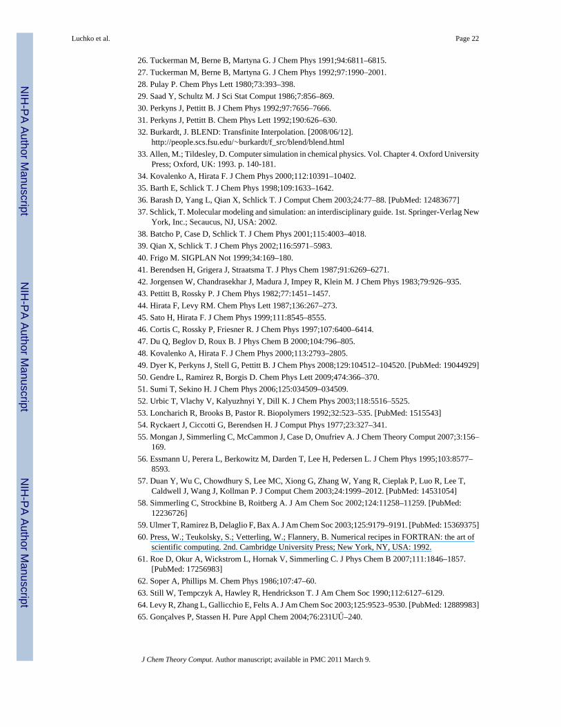
Serial optimizations for MD/3D-RISM-KH consist of multiple time step methods, solutionpropagation, cut-offs and a dynamic solvation box. Two of these methods, MTS and solutionpropagation have been previously introduced by Miyata and Hirata25 but have been furtherextended here. By extending our solution propagation (eq 8) to higher derivatives, usingadditional previous time steps, computational efficiency has actually been slightly reducedfrom using only a single previous solution (Figure 9(a): RESPA and RESPA
). However, as shown in Table 4(b), this additional work greatly enhances energyconservation by eliminating memory effects. A moderate speedup is still achieved over nosolution propagation (Figure 9(a): SHAKE and SHAKE ).
Additional computational savings can be achieved for grid-based solute-solvent potential andforce calculations. While similar to the use of cut-offs for explicit simulations, cut-offs herecan take advantage of the fixed grid spacing (no need for cut-off lists) and points outside ofthe cutoff can still be accounted for through simple interpolation. However, cut-off methodsonly offer computational reductions by a constant factor as all grid points must still be visited.The computational savings are due to the number of grid points requiring expensivecalculations, involving all of the solute atoms, being considerably reduced. As the grid densityand number of solute atoms increases, the cutoff optimizations become more valuable.
A natural extension to cut-offs is the dynamic resizing of the solvation box. For globular solutesthis has little cost saving effect and is mostly useful as a convenience; the user only needs toinput the buffer distance from the solute and the grid spacing. As solutes become less sphericalor undergo large conformational changes, the benefits of the adaptive box size grow by ensuring
Luchko et al. Page 17
J Chem Theory Comput. Author manuscript; available in PMC 2011 March 9.
NIH
-PA Author Manuscript
NIH
-PA Author Manuscript
NIH
-PA Author Manuscript

only the minimum number of grids points is used. Together adaptive box sizes and cut-offsoffer a small overall improvement for alanine-dipeptide (Figure 9(a) RESPA and cut-off=12 Å).
The greatest computational savings can be achieved by avoiding 3D-RISM calculationsaltogether by using MTS methods. The nature of biomolecular systems does not allow RESPAMTS time steps to be larger than 5 fs as resonance artifacts are introduced.37 It is possible toovercome this resonance barrier, however, by introducing a non-conservative forceapproximation at intermediate time steps and using Langevin dynamics to compensate. In thecase of FCE RESPA MTS, 3D-RISM-KH solutions can be calculated once every 20 fs (Figure4). Combined with the other cost saving measures, a speed up over a basic implementation of3D-RISM-KH of approximately 10-times is achieved (Figure 9(a) SHAKE and Δt = 10,20 fs).While it is true that increasing the friction coefficient has a negative impact on the accuracyof dynamics, the use of a mean-field method, 3D-RISM, means that the observed dynamicsare not true dynamics in any case. Our goal is to increase sampling efficiency and using a largefriction coefficient is justified in this context.
While parallelization does not decrease the computational workload, it does decrease the walltime for calculations. Furthermore, the spatial decomposition, distributed memory model usedhere allows the calculation to be run on a network of computers and make use of the totalaggregate memory available. Relative speedups compared to single CPU are shown in Figure9(b). Parallel speedups used protein-G simulations with a total of 50 timesteps. Of these, therewere eight full 3D-RISM-KH calculations and three were interpolated 3D-RISM-KH forces.Calculations were performed on a four CPU AMD Opteron machine with four cores per CPU.Grid-based potential and force calculations that were already accelerated with cut-offs and adynamic solvation box show linear speedups with the number of cores. The force extrapolationmethod has increasing efficiencies comparable to the overall speedup of 3D-RISM. Overallparallel performance is heavily influenced by the scaling of the 3D-FFT and MDIIS routineswhich also dominate the overall computation time. As we use FFTW 2.1.5 library for our 3D-FFT calculations our speedup for the 3D-FFT part of the calculation is limited to scaling of thelibrary.
4.7 Protein-GEven with our decreased calculation costs, exhaustive conformational sampling of smallproteins is still not accessible with 3D-RISM-KH-MD at this time. It is possible to comparedifferent solvation models on the sub-nanosecond time scale for errors that may be introduced.In particular, differences in secondary and tertiary structure that are indicative of errors maybe apparent in sub-nanosecond trajectories in 3D-RISM-KH due to the enhanced sampling thatthe method provides.
Figure 10 gives the root mean squared deviation (RMSD) of the Cα atoms from the crystalstructure of protein G as a function of simulation time. Both 3D-RISM-KH and GBSA quicklyapproach RMSD values of 1 Å or greater, with 3D-RISM-KH generally being higher. Whilethese values are higher than those observed with either of the explicit models, they arecomparable to previous works.68–70 Furthermore, the RMSD of longer explicit simulationscontinues to grow throughout, suggesting that the equilibrium value may be close to that of3D-RISM-KH.
Radius of gyration (Figure 11) also shows quickly equilibrating, stable trajectories for 3D-RISM-KH and GBSA with similar values and distributions. Explicit solvent simulations showa smaller and steadily increasing radius of gyration. While it is not clear if the radius of gyrationhas equilibrated by the end of the simulation (3 ns), it has approached values comparable toboth 3D-RISM-KH and GBSA.
Luchko et al. Page 18
J Chem Theory Comput. Author manuscript; available in PMC 2011 March 9.
NIH
-PA Author Manuscript
NIH
-PA Author Manuscript
NIH
-PA Author Manuscript

As well as providing stable dynamics, solvation methods should preserve both the secondaryand tertiary structure of the solute. Hydrogen bond calculations were performed with PTRAJusing the default criteria: a distance cut-off of 3.5 Å and an angle cut-off of 120°. Secondarystructure involves hydrogen bonding within the backbone of the protein. Figure 12(a) showsbackbone NH groups occupied by hydrogen bonds from backbone CO groups over the entiretrajectory. While all solvent models are generally in good agreement, five residues showdifferences in the occupancies between models (Figure 12(b)): LYS4, GLY9, LEU12, ALA20,THR25, GLU56. We examine these case by case.
Hydrogen bonding between residues LYS4 and LYS50 is primarily an issue for GBSA. Asthis is at the end of a β-sheet, it may indicate some additional flexibility, even unzipping, ofthe sheet. If the hydrogen bond cut-off criteria is extended to 4.0 Å from 3.5 Å, the occupancyexceeds 80%. Enhanced flexibility also appears to be the cause for reduced hydrogen bondingbetween THR25 (NH) and ASP22 (CO) for non-explicit models with 14% and 28% occupancyfor GBSA and 3D-RISM-KH compared to 40% and 50% for SPC/E and TIP3P.
The loop consisting of residues 9 through 12 is a site of qualitative difference in structure(Figure 12(b)) and behavior (Figure 13) of the 3D-RISM-KH simulation from other solvationmodels. While a stable hydrogen bond is seen for GBSA (81%), SPC/E (80%) and TIP3P(94%) 3D-RISM-KH shows an occupancy of only 12% for a GLY9 (NH) to LEU12 (CO). Incontrast, 3D-RISM-KH also shows an occupancy of 17% for a LEU12 (NH) to GLY9 (CO)while the three other methods only show a 1-2% occupancy. This suggests that there is aoscillation between two weak hydrogen bonds. Indeed, in Figure 13(b) and (c) the GLY9 (NH)to LEU12 (CO) hydrogen bond is disrupted by solvent. The overall effect is to bend this loopout from the protein core into the solvent (12b).
Residue ALA20 is another site where it would appear that GBSA has failed to capture thecorrect hydrogen bonding; however, the situation is somewhat more complex. The ALA20(NH) site is 60% occupied in hydrogen bonding but this bonding is strictly with THR18 (CO).For SPC/E and TIP3P ALA20 (NH) has no hydrogen bonding with THR18 but 99% and 100%respectively with MET1. 3D-RISM-KH, however, has ALA20 (NH) binding to both THR18and MET1, 54% and 33% respectively. The correct behavior in this case is not clear. Cloreand Gronenborn,73 on the basis of nuclear magnetic resonance (NMR) data, proposed a threesite bifurcated hydrogen bond between ALA20 (NH), MET1 (CO) and a bound water moleculewith residence time > 1 ns. In an explicit solvent MD simulation Sheinerman and Brooks68
observed a long residence time water in this location but, in this case, there was no directhydrogen bond between ALA20 (NH) and MET1 (CO) and the water served as an intermediarybetween the two residues. No such long residence time water is observed in our explicit solventsimulations, though the residues are highly solvated (Figure 14(a)). For our 3D-RISM-KHsimulation, however, the hydrogen bond is broken by the solvent (Figure 14(c)), re-formed(Figure 14(b)) and broken again in the course of the 600 ps simulation.
As well, Clore and Gronenborn also proposed that a similar long residence time water wouldstabilize a hydrogen bond between TYR33 (NH) and ALA29 (CO). Neither the explicitsimulations nor the 3D-RISM-KH simulation showed any water situated to do this, though thesite was well hydrated. This is in agreement with the observations of Sheinerman and Brooks.
Both GBSA and 3D-RISM-KH have 50% occupancy for the hydrogen bond between GLU56(NH) and ASN8 (CO) compared to 75% and 79% for SPC/E and TIP3P. However, the reasonfor the low occupancy for 3D-RISM-KH is due to a larger systematic problem. As shown inFigure 15, a large, solvated cleft opens into the hydrophobic interior of the protein in the 3D-RISM-KH simulation. This allows the GLU56 (NH) and ASN8 (CO) pair to be solvated suchthat the hydrogen bond is disrupted. As pointed out by Kovalenko and Hirata,48 this is likely
Luchko et al. Page 19
J Chem Theory Comput. Author manuscript; available in PMC 2011 March 9.
NIH
-PA Author Manuscript
NIH
-PA Author Manuscript
NIH
-PA Author Manuscript

due to the overestimation of solvent ordering around the hydrophobic sidechains at the core ofthe protein. This is a shortcoming of the KH closure, though the same deficiency was originallyidentified in the HNC closure equation. As such, it is not a shortcoming of 3D-RISM and canbe overcome with an improved closure, though sure a development is not a trivial task.
5 ConclusionsWe have presented an efficient coupling of molecular dynamics simulation with the three-dimensional molecular theory of solvation (3D-RISM-KH), contracting the solvent degrees offreedom, and have implemented this multiscale method in the Amber molecular dynamicspackage.
The 3D-RISM-KH theory uses the first principles of statistical mechanics to provide properaccount of molecular specificity of both the solute biomolecule and solvent. This includes sucheffects as hydrogen bonding both between solvent molecules and between the solute andsolvent, hydrophobic hydration and hydrophobic interaction. The 3D-RISM-KH theory readilyaddresses electrolyte solutions and mixtures of liquids of given composition andthermodynamic conditions. As the solvation theory works in a full statistical-mechanicalensemble, the coupled method yields solvent distributions without statistical noise, and further,gives access to slow processes like hydration of inner spaces and pockets of biomolecules.
The use of 3D-RISM, a mean-field method contracting the solvent degrees of freedom in astatistical-mechanical average means that the solvent dynamics are lost and the observedtrajectories in any case are not true dynamics of MD simulation with explicit solvent. They aredriven largely by a solvent-mediated potential of mean force, that is, by the probability offinding the biomolecule in a particular conformation, sampled over an ensemble of solvationshell arrangements which frequently require extremely long time to get realized (e.g. openingof protein parts to let solvent molecules or ions in to the inner spaces or pockets, multiplyrepeated to reach proper statistics). However, such trajectories in a solvent potential of meanforce preserve the thermodynamic properties such as conformational distribution of thebiomolecule and efficiently sample the conformational space regions of interest in a numberof molecular biology problems such as functioning of biomolecular structures (e.g. biologicalchannels and chaperons), protein folding, aggregation, and ligand binding.
Arrangements of solution species in the solvation shells of the biomolecule, sampled by the3D-RISM-KH theory can include structural solvent and/or cosolvent molecules and otherassociating structures like salt bridges, buffer ions, and associated ligand molecules. In thelatter case, ligand molecules (or their relatively small fragments) at a given concentration insolution are described as a component of solvent at the level of site-site RISM theory and thenmapped onto the biomolecule surface by the 3D-RISM method identifying the most probablebinding modes of ligand molecules.24 Together with MD sampling of biomolecularconformations, this opens up a new computational method for fragment-based drug designwhich provides proper, statistical-mechanical account of solvation forces with self-consistentcoupling of both non-polar and polar components and which gives access to binding eventsaccompanied with rearrangements of the biomolecule and solvent on a long-time scale.
The implementation includes several procedures to maximally speed up the calculation: (i) cut-off procedures for the Lennard-Jones and electrostatic potentials and the forces acting on thesolute, (ii) cut-offs and approximations for the asymptotics of the 3D site correlation functionsof solvent, (iii) an iterative guess for the solution to the 3D-RISM-KH equations byextrapolating the past solutions, (iv) multiple time step (MTS) interpolation of solvation forcesbetween the successive 3D-RISM-KH evaluations of the forces, which are then extrapolatedforward at the MD steps until the next 3D-RISM evaluation.
Luchko et al. Page 20
J Chem Theory Comput. Author manuscript; available in PMC 2011 March 9.
NIH
-PA Author Manuscript
NIH
-PA Author Manuscript
NIH
-PA Author Manuscript

As a preliminary validation, we have applied the method to alanine-dipeptide and protein G inambient water. Analysis of the accuracy of forces, energy and temperature, including suchknown artifacts as net force drift, has been performed; factors affecting the accuracy have beenquantified and the range of grid resolution and tolerance parameters ensuring reliable resultshas been outlined. The performance of the coupled method has been characterized, comparedto MD with explicit and implicit solvent. This work is a preliminary but significant step towardthe full-scale characterization and analysis of the new method, and further improvement of itsperformance to address slow processes of large biomolecules in solution.
AcknowledgmentsThis work was supported by the Natural Sciences and Engineering Research Council (NSERC) of Canada and theNational Research Council (NRC) of Canada. All calculations were performed on the HPC cluster of the Center ofExcellence in Integrated Nanotools (CEIN) at the University of Alberta. T.L. acknowledges financial support fromNSERC, NRC, and the University of Alberta.
References1. Case D, Cheatham T, Darden T, Gohlke H, Luo R, Merz K, Onufriev A, Simmerling C, Wang B,
Woods R. J Comput Chem 2005;26:1668–1688. [PubMed: 16200636]2. Still W, Tempczyk A, Hawley R, Hendrickson T. J Am Chem Soc 1990;112:6127–6129.3. Chandler D, McCoy J, Singer S. J Chem Phys 1986;85:5971–5976.4. Chandler D, McCoy J, Singer S. J Chem Phys 1986;85:5977–5982.5. Beglov D, Roux B. J Phys Chem B 1997;101:7821–7826.6. Kovalenko A, Hirata F. Chem Phys Lett 1998;290:237–244.7. Kovalenko A, Hirata F. J Chem Phys 1999;110:10095–10112.8. Kovalenko A, Hirata F. J Chem Phys 2000;112:10391–10402.9. Kovalenko A, Hirata F. J Chem Phys 2000;112:10403–10417.10. Kovalenko, A. Molecular Theory of Solvation. Hirata, F., editor. Vol. 24. Kluwer Academic
Publishers; Norwell, MA, USA: 2003. p. 169-276.11. Hansen, JP.; McDonald, I. Theory of Simple Liquids. 3rd ed. Elsevier; Amsterdam, the Netherlands:
2006.12. Beglov D, Roux B. J Chem Phys 1995;103:360–364.13. Yoshida K, Yamaguchi T, Kovalenko A, Hirata F. J Phys Chem B 2002;106:5042–5049.14. Omelyan I, Kovalenko A, Hirata F. J Theor Comput Chem 2003;2:193–203.15. Gusarov S, Ziegler T, Kovalenko A. J Phys Chem A 2006;110:6083–6090. [PubMed: 16671679]16. Casanova D, Gusarov S, Kovalenko A, Ziegler T. J Chem Theory Comput 2007;3:458–476.17. Moralez J, Raez J, Yamazaki T, Motkuri R, Kovalenko A, Fenniri H. J Am Chem Soc
Communications 2005;127:8307–8309.18. Johnson R, Yamazaki T, Kovalenko A, Fenniri H. J Am Chem Soc 2007;129:5735–5743. [PubMed:
17417852]19. Tikhomirov G, Yamazaki T, Kovalenko A, Fenniri H. Langmuir 2008;24:4447–4450. [PubMed:
18351794]20. Yamazaki T, Fenniri H, Kovalenko A. Chem Phys Chem. 2010 accepted.21. Drabik P, Gusarov S, Kovalenko A. Biophys J 2007;92:394–403. [PubMed: 17056728]22. Yamazaki T, Imai T, Hirata F, Kovalenko A. J Phys Chem B 2007;111:1206–1212. [PubMed:
17266276]23. Yoshida N, Imai T, Phongphanphanee S, Kovalenko A, Hirata F. J Phys Chem B Feature Article
2009;113:873–886. and references therein.24. Imai T, Oda K, Kovalenko A, Hirata F, Kidera A. J Am Chem Soc 2009;131:12430–12440. [PubMed:
19655800]25. Miyata T, Hirata F. J Comput Chem 2008;29:871–882. [PubMed: 17963231]
Luchko et al. Page 21
J Chem Theory Comput. Author manuscript; available in PMC 2011 March 9.
NIH
-PA Author Manuscript
NIH
-PA Author Manuscript
NIH
-PA Author Manuscript
26. Tuckerman M, Berne B, Martyna G. J Chem Phys 1991;94:6811–6815.27. Tuckerman M, Berne B, Martyna G. J Chem Phys 1992;97:1990–2001.28. Pulay P. Chem Phys Lett 1980;73:393–398.29. Saad Y, Schultz M. J Sci Stat Comput 1986;7:856–869.30. Perkyns J, Pettitt B. J Chem Phys 1992;97:7656–7666.31. Perkyns J, Pettitt B. Chem Phys Lett 1992;190:626–630.32. Burkardt, J. BLEND: Transfinite Interpolation. [2008/06/12].
http://people.scs.fsu.edu/∼burkardt/f_src/blend/blend.html33. Allen, M.; Tildesley, D. Computer simulation in chemical physics. Vol. Chapter 4. Oxford University
Press; Oxford, UK: 1993. p. 140-181.34. Kovalenko A, Hirata F. J Chem Phys 2000;112:10391–10402.35. Barth E, Schlick T. J Chem Phys 1998;109:1633–1642.36. Barash D, Yang L, Qian X, Schlick T. J Comput Chem 2003;24:77–88. [PubMed: 12483677]37. Schlick, T. Molecular modeling and simulation: an interdisciplinary guide. 1st. Springer-Verlag New
York, Inc.; Secaucus, NJ, USA: 2002.38. Batcho P, Case D, Schlick T. J Chem Phys 2001;115:4003–4018.39. Qian X, Schlick T. J Chem Phys 2002;116:5971–5983.40. Frigo M. SIGPLAN Not 1999;34:169–180.41. Berendsen H, Grigera J, Straatsma T. J Phys Chem 1987;91:6269–6271.42. Jorgensen W, Chandrasekhar J, Madura J, Impey R, Klein M. J Chem Phys 1983;79:926–935.43. Pettitt B, Rossky P. J Chem Phys 1982;77:1451–1457.44. Hirata F, Levy RM. Chem Phys Lett 1987;136:267–273.45. Sato H, Hirata F. J Chem Phys 1999;111:8545–8555.46. Cortis C, Rossky P, Friesner R. J Chem Phys 1997;107:6400–6414.47. Du Q, Beglov D, Roux B. J Phys Chem B 2000;104:796–805.48. Kovalenko A, Hirata F. J Chem Phys 2000;113:2793–2805.49. Dyer K, Perkyns J, Stell G, Pettitt B. J Chem Phys 2008;129:104512–104520. [PubMed: 19044929]50. Gendre L, Ramirez R, Borgis D. Chem Phys Lett 2009;474:366–370.51. Sumi T, Sekino H. J Chem Phys 2006;125:034509–034509.52. Urbic T, Vlachy V, Kalyuzhnyi Y, Dill K. J Chem Phys 2003;118:5516–5525.53. Loncharich R, Brooks B, Pastor R. Biopolymers 1992;32:523–535. [PubMed: 1515543]54. Ryckaert J, Ciccotti G, Berendsen H. J Comput Phys 1977;23:327–341.55. Mongan J, Simmerling C, McCammon J, Case D, Onufriev A. J Chem Theory Comput 2007;3:156–
169.56. Essmann U, Perera L, Berkowitz M, Darden T, Lee H, Pedersen L. J Chem Phys 1995;103:8577–
8593.57. Duan Y, Wu C, Chowdhury S, Lee MC, Xiong G, Zhang W, Yang R, Cieplak P, Luo R, Lee T,
Caldwell J, Wang J, Kollman P. J Comput Chem 2003;24:1999–2012. [PubMed: 14531054]58. Simmerling C, Strockbine B, Roitberg A. J Am Chem Soc 2002;124:11258–11259. [PubMed:
12236726]59. Ulmer T, Ramirez B, Delaglio F, Bax A. J Am Chem Soc 2003;125:9179–9191. [PubMed: 15369375]60. Press, W.; Teukolsky, S.; Vetterling, W.; Flannery, B. Numerical recipes in FORTRAN: the art of
scientific computing. 2nd. Cambridge University Press; New York, NY, USA: 1992.61. Roe D, Okur A, Wickstrom L, Hornak V, Simmerling C. J Phys Chem B 2007;111:1846–1857.
[PubMed: 17256983]62. Soper A, Phillips M. Chem Phys 1986;107:47–60.63. Still W, Tempczyk A, Hawley R, Hendrickson T. J Am Chem Soc 1990;112:6127–6129.64. Levy R, Zhang L, Gallicchio E, Felts A. J Am Chem Soc 2003;125:9523–9530. [PubMed: 12889983]65. Gonçalves P, Stassen H. Pure Appl Chem 2004;76:231UŰ–240.
Luchko et al. Page 22
J Chem Theory Comput. Author manuscript; available in PMC 2011 March 9.
NIH
-PA Author Manuscript
NIH
-PA Author Manuscript
NIH
-PA Author Manuscript

66. Liu P, Kim B, Friesner R, Berne B. Proc Natl Acad Sci USA 2005;102:13749–13754. [PubMed:16172406]
67. Kwac K, Lee KK, Han JB, Oh KI, Cho M. J Chem Phys 2008;128:105106. [PubMed: 18345930]68. Sheinerman F, C B III. Proteins: Struct Func Genet 1997;29:193–202.69. Patel S Jr, A M, C B III. J Comput Chem 2004;25:1504–1514. [PubMed: 15224394]70. Calimet N, Schaefer M, Simonson T. Proteins: Struct Func Genet 2001;45:144–158.71. Humphrey W, Dalke A, Schulten K. Journal of Molecular Graphics 1996;14:33–38. [PubMed:
8744570]72. Stone, J. MSc thesis. Computer Science Department, University of Missouri-Rolla; 1998.73. Clore G, Gronenborn A. J Mol Biol 1992;223:853–856. [PubMed: 1538400]74. Sanner, M.; Olsen, A.; Spehner, JC. Fast and Robust Computation of Molecular Surfaces. Proceedings
of the 11th ACM Symposium on Computational Geometry; New York. 1995. p. C6-C7.
Luchko et al. Page 23
J Chem Theory Comput. Author manuscript; available in PMC 2011 March 9.
NIH
-PA Author Manuscript
NIH
-PA Author Manuscript
NIH
-PA Author Manuscript

Figure 1.Cut-off schemes for grid based (a) Lennard-Jones and (b) coulomb potential and forcecalculations. Lennard-Jones calculations are performed for each solute atom only at grid siteswithin the cut-off distance of that atom. Grid sites within the cut-off distance of multiple solutesites take on the sum of these interactions. Coulomb interactions are calculated for every soluteatom at grid sites in the union of all cut-off volumes. Grid sites outside the cut-off use explicitcalculations or interpolation from surrounding values.
Luchko et al. Page 24
J Chem Theory Comput. Author manuscript; available in PMC 2011 March 9.
NIH
-PA Author Manuscript
NIH
-PA Author Manuscript
NIH
-PA Author Manuscript

Figure 2.Modified water potential. (a) Schematic illustration of Lennard-Jones parameters for SPC/Ewater. Lennard-Jones radii, σ/2, are illustrated by white circles. The radius on the right handhydrogen corresponds to that of Pettitt and Rossky43 while the left hand hydrogen radius isfrom eqs 21 and 22. (b) Perturbation of water-water Lennard-Jones potential due to thehydrogen potential. The maximum perturbation (solid line) is for two waters with hydrogensaligned. The case of hydrogen bonding is given by the long-dashed line while the originalpotential is given by the short dashed line. HH (dot-dashed line) and OH (dotted line)interactions are a result of the new parameters. (c) Angle dependent water-water interaction.The second water is oriented such that a hydrogen is always pointing towards the central water.The solid and long dashed arrows correspond to the solid and long-dashed lines in (b). Contourlines are spaced 0.02 kcal/mol apart.
Luchko et al. Page 25
J Chem Theory Comput. Author manuscript; available in PMC 2011 March 9.
NIH
-PA Author Manuscript
NIH
-PA Author Manuscript
NIH
-PA Author Manuscript

Figure 3.Water radial distribution functions from experiment, MD simulation and 1D-RISM for (a)oxygen-oxygen, (b) oxygen-hydrogen and (c) hydrogen-hydrogen.
Luchko et al. Page 26
J Chem Theory Comput. Author manuscript; available in PMC 2011 March 9.
NIH
-PA Author Manuscript
NIH
-PA Author Manuscript
NIH
-PA Author Manuscript

Figure 4.Average temperature for Langevin dynamics simulations of alanine-dipeptide. Error barsrepresent the standard error in the mean.
Luchko et al. Page 27
J Chem Theory Comput. Author manuscript; available in PMC 2011 March 9.
NIH
-PA Author Manuscript
NIH
-PA Author Manuscript
NIH
-PA Author Manuscript

Figure 5.Na+Cl− pair in a SPC/E with a weak distance restraint. (a) PMF for the unrestrained pair (dashline) and restrained pair (solid line). (b) site-site distance distribution for Na+Cl− with a weakharmonic restraint. The expected distribution from the potential of mean force is the thick blackline; RESPA MTS is the thin black line; FCE MTS with Langevin damping coefficients of γ=5, 10 and 20 ps−1 are colored gray, blue and red respectively.
Luchko et al. Page 28
J Chem Theory Comput. Author manuscript; available in PMC 2011 March 9.
NIH
-PA Author Manuscript
NIH
-PA Author Manuscript
NIH
-PA Author Manuscript

Figure 6.Ramachandran free energy differences of (a)-(f) of select solvation methods from explicit SPC/E water for alanine-dipeptide. (g) Difference of 3D-RISM-KH with a residual tolerance of10−5 and 3D-RISM-KH with a FCE RESPA MTS time step of Δt=20 fs. Energy units are inkcal/mol.
Luchko et al. Page 29
J Chem Theory Comput. Author manuscript; available in PMC 2011 March 9.
NIH
-PA Author Manuscript
NIH
-PA Author Manuscript
NIH
-PA Author Manuscript

Figure 7.Convergence (χ2) of Ramachandran plots over simulation time for select solvation methods.
Luchko et al. Page 30
J Chem Theory Comput. Author manuscript; available in PMC 2011 March 9.
NIH
-PA Author Manuscript
NIH
-PA Author Manuscript
NIH
-PA Author Manuscript

Figure 8.Dipole moment magnitude distributions of alanine-dipeptide for select solvation methods.
Luchko et al. Page 31
J Chem Theory Comput. Author manuscript; available in PMC 2011 March 9.
NIH
-PA Author Manuscript
NIH
-PA Author Manuscript
NIH
-PA Author Manuscript
Figure 9.3D-RISM execution speedup. (a) Serial calculations are shown with optimizationsincrementally added. ‘SHAKE’ refers to calculations where δt = Δt. ‘NCUV’ indicates thenumber of previous solutions used for the initial guess. A cut-off of 12 Å was used for all othercalculations. (b) The total parallel speedup is indicated by ‘3D-RISM’ while the relativespeedups of critical subroutines are indicated by the colored lines.
Luchko et al. Page 32
J Chem Theory Comput. Author manuscript; available in PMC 2011 March 9.
NIH
-PA Author Manuscript
NIH
-PA Author Manuscript
NIH
-PA Author Manuscript

Figure 10.Cα RMSD of protein-G for explicit, implicit and 3D-RISM-KH solvent models.
Luchko et al. Page 33
J Chem Theory Comput. Author manuscript; available in PMC 2011 March 9.
NIH
-PA Author Manuscript
NIH
-PA Author Manuscript
NIH
-PA Author Manuscript

Figure 11.Radius of gyration of protein-G for explicit, implicit and 3D-RISM-KH solvent models.
Luchko et al. Page 34
J Chem Theory Comput. Author manuscript; available in PMC 2011 March 9.
NIH
-PA Author Manuscript
NIH
-PA Author Manuscript
NIH
-PA Author Manuscript

Figure 12.(a) Occupancies for internal backbone hydrogen bonding of protein-G for explicit, implicit and3D-RISM-KH solvent models. Occupancies >100% indicate bifurcated hydrogen bonds. (b)3D trace of Cα atoms for NMR structure (PDB ID: 1P7E) in white and final 3D-RISM-KHstructure in cyan. Backbone atoms are shown for residues with hydrogen bonding that differsfrom explicit solvent simulation. Images are made with VMD.71,72
Luchko et al. Page 35
J Chem Theory Comput. Author manuscript; available in PMC 2011 March 9.
NIH
-PA Author Manuscript
NIH
-PA Author Manuscript
NIH
-PA Author Manuscript

Figure 13.Backbone hydrogen bonding between residues 9 and 12 for representative structures of (a)explicit SPC/E, (b) 3D-RISM-KH with hydrogen bonding and (c) 3D-RISM-KH withouthydrogen bonding. Protein backbone drawn as a white tube, backbone atoms for residues 9and 12 as spheres and side chains as sticks. Carbons are cyan, oxygens red, hydrogens blackand nitrogens blue. Solvent density isosurfaces are shown at for both oxygen (red)and hydrogen (gray). Images made with VMD.71,72
Luchko et al. Page 36
J Chem Theory Comput. Author manuscript; available in PMC 2011 March 9.
NIH
-PA Author Manuscript
NIH
-PA Author Manuscript
NIH
-PA Author Manuscript

Figure 14.Backbone hydrogen bonding between residues 1 and 20 for representative structures of (a)explicit SPC/E, (b) 3D-RISM-KH with hydrogen bonding and (c) 3D-RISM-KH withouthydrogen bonding. Coloring as in Figure 13. Images made with VMD.71,72
Luchko et al. Page 37
J Chem Theory Comput. Author manuscript; available in PMC 2011 March 9.
NIH
-PA Author Manuscript
NIH
-PA Author Manuscript
NIH
-PA Author Manuscript

Figure 15.Solvent accessible surface area for protein G simulated with (a) explicit SPC/E and (b) 3D-RISM-KH. Surface is colored by residue type: acid (red), base (blue), polar (green) and non-polar (white). Images made with VMD71,72,74
Luchko et al. Page 38
J Chem Theory Comput. Author manuscript; available in PMC 2011 March 9.
NIH
-PA Author Manuscript
NIH
-PA Author Manuscript
NIH
-PA Author Manuscript

NIH
-PA Author Manuscript
NIH
-PA Author Manuscript
NIH
-PA Author Manuscript
Luchko et al. Page 39
Tabl
e 1
Para
met
ers f
or st
anda
rd a
nd m
odifi
ed S
PC/E
and
TIP
3P w
ater
mod
els.
Mod
el N
ame
σ Oε O
σ Hε H
q Oq H
r(O
H)
Åkc
al/m
olÅ
kcal
/mol
eÅ
SPC
/E3.
1658
0.15
530
--
-0.8
476
0.42
381.
0000
cSPC
/E3.
1658
0.15
530
1.16
580.
0155
3-0
.847
60.
4238
1.00
00
PR-S
PC/E
3.16
580.
1553
00.
4000
0.04
600
-0.8
476
0.42
381.
0000
TIP3
P3.
1507
0.15
200
--
-0.8
340
0.41
700.
9572
cTIP
3P3.
1507
0.15
200
1.23
630.
0152
0-0
.834
00.
4170
0.95
72
PR-T
IP3P
3.15
070.
1520
00.
4000
0.04
600
-0.8
340
0.41
700.
9572
J Chem Theory Comput. Author manuscript; available in PMC 2011 March 9.
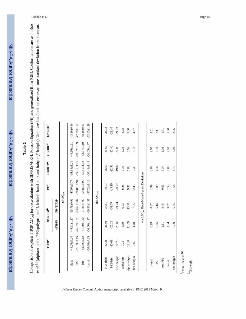
NIH
-PA Author Manuscript
NIH
-PA Author Manuscript
NIH
-PA Author Manuscript
Luchko et al. Page 40
Tabl
e 2
Com
paris
on o
f exp
licit
TIP3
P ΔG
pol f
or d
eca-
alan
ine
with
3D
-RIS
M-K
H, P
oiss
on E
quat
ion
(PE)
and
gen
eral
ized
Bor
n (G
B).
Con
form
atio
ns a
re a
s in
Roe
et a
l.61 (a
lpha
:α-h
elix
, PP2
:pol
ypro
line I
I, le
ft:le
ft-ha
nd h
elix
and
hairp
in:β
-hai
rpin
). U
nits
are k
cal/m
ol an
d er
rors
are o
ne st
anda
rd d
evia
tion
from
the m
ean.
TIP
3Pa
3D-R
ISM
bPE
aG
BH
CT
aG
BO
BC
aG
BN
ecka
cTIP
3PPR
-TIP
3P (a) Δ
Gpo
l
alph
a-4
4.08
±0.0
4-4
4.91
±1.2
7-5
5.79
±0.9
3-4
7.97
±0.7
7-5
1.69
±1.2
1-4
9.38
±1.2
1-4
3.26
±0.9
0
PP2
-76.
39±0
.15
-76.
82±1
.31
-93.
60±1
.07
-78.
05±0
.91
-77.
35±1
.05
-78.
07±1
.09
-77.
59±1
.02
left
-51.
30±0
.12
-51.
60±1
.22
-61.
81±1
.03
-54.
85±0
.90
-55.
05±1
.08
-52.
67±1
.10
-48.
19±0
.91
hairp
in-5
4.16
±0.2
5-5
6.00
±1.1
7-6
9.36
±1.3
1-5
7.28
±1.1
3-5
7.48
±1.4
5-5
6.03
±1.4
7-5
2.85
±1.2
9
(b) Δ
ΔGpo
l
PP2-
alph
a-3
2.31
-31.
91-3
7.81
-30.
07-2
5.67
-28.
69-3
4.33
PP2-
left
-25.
09-2
5.22
-31.
79-2
3.19
-22.
31-2
5.40
-29.
40
PP2-
hairp
in-2
2.23
-20.
82-2
4.24
-20.
77-1
9.87
-22.
03-2
4.73
alph
a-le
ft7.
226.
696.
026.
883.
363.
294.
93
alph
a-ha
irpin
10.0
811
.09
13.5
79.
315.
806.
669.
60
left-
hairp
in2.
864.
407.
552.
432.
433.
374.
67
(c) Δ
ΔGpo
l Roo
t-Mea
n-Sq
uare
Dev
iatio
ns
over
all
0.99
4.37
1.39
3.89
2.60
2.51
PP2
0.85
5.14
1.89
4.37
2.10
3.11
non-
PP2
1.11
3.45
0.55
3.34
3.02
1.71
hairp
in1.
343.
571.
532.
832.
001.
80
non-
hairp
in0.
395.
051.
584.
723.
093.
05
a From
Roe
et a
l.61
b This
wor
k.
J Chem Theory Comput. Author manuscript; available in PMC 2011 March 9.

NIH
-PA Author Manuscript
NIH
-PA Author Manuscript
NIH
-PA Author Manuscript
Luchko et al. Page 41
Table 3
(a) Net force (kcal/mol/Å), (b) root-mean squared error in the force and (c) solvation free energy (kcal/mol) forsingle point 3D-RISM-KH calculations of alanine-dipeptide.
Tolerance Grid Spacing
0.5 Å 0.25 Å 0.125 Å 0.0625 Å
(a) Net Force
10−2 3.2 2.4 2.7 3.3
10−3 1.6 0.35 0.093 0.30
10−4 1.5 0.36 0.061 0.044
10−5 1.5 0.37 0.041 0.0047
10−6 1.5 0.37 0.042 0.0016
(b) Force RMS Error
10−2 7.1 × 10+0 6.3 × 10+0 6.3 × 10+0 8.3 × 10+0
10−3 3.4 × 10⁻¹ 1.0 × 10⁻¹ 1.2 × 10⁻¹ 6.2 × 10⁻²
10−4 1.8 × 10⁻¹ 7.5 × 10⁻³ 7.6 × 10⁻⁴ 8.7 × 10⁻⁴
10−5 1.8 × 10⁻¹ 7.4 × 10⁻³ 5.1 × 10⁻⁵ 9.2 × 10⁻⁶
10−6 1.8 × 10⁻¹ 7.6 × 10⁻³ 5.0 × 10⁻⁵ -
(c) Solvation Free Energy
10−2 7.5794 7.3873 7.4024 8.4253
10−3 14.5614 14.4441 14.4574 14.3924
10−4 14.6366 14.5097 14.5090 14.5092
10−5 14.6382 14.5123 14.5121 14.5117
10−6 14.6382 14.5125 14.5120 14.5116
J Chem Theory Comput. Author manuscript; available in PMC 2011 March 9.

NIH
-PA Author Manuscript
NIH
-PA Author Manuscript
NIH
-PA Author Manuscript
Luchko et al. Page 42
Tabl
e 4
Rat
e of
dec
ay (k
cal/m
ol/p
s) o
f con
stan
t ene
rgy
sim
ulat
ions
of a
lani
ne d
ipep
tide
for (
a) v
aria
ble
grid
spac
ing
and
solu
tion
tole
ranc
e, (b
) var
iabl
e so
lutio
npr
opag
atio
n an
d so
lutio
n to
lera
nce,
(c) v
aria
ble
cut-o
ff a
nd so
lven
t box
buf
fer a
nd (d
) var
iabl
e tim
e st
ep fo
r FC
E R
ESPA
MTS
. Err
or in
the
leas
t-squ
ares
fit fo
r the
last
sign
ifica
nt d
igit
is g
iven
in b
rack
ets.
(a)
Tol
eran
ceG
rid
Spac
ing
0.5
Å0.
25 Å
10−4
-0.4
372(
9)-0
.220
7(6)
10−5
-0.0
828(
6)-0
.082
4(6)
10−6
-0.0
234(
6)-0
.012
2(5)
(b)
Tole
ranc
e
NcU
V
01
23
45
Ener
gy C
onse
rvat
ion
1e-3
0.29
2(3)
22.6
2(6)
38.6
(1)
9.89
(1)
0.06
86(4
)0.
1127
(9)
1e-4
0.00
63(1
)0.
651(
1)0.
992(
4)0.
0684
(2)
-0.0
0321
(6)
0.00
282(
9)
1e-5
-0.0
0196
(7)
0.01
918(
6)0.
0152
6(7)
0.00
306(
7)-0
.005
90(6
)-0
.000
89(6
)
Ave
rage
Num
ber o
f 3D
-RIS
M It
erat
ions
per
Sol
utio
n
1e-3
47.5
18.3
21.4
28.9
29.4
35.3
1e-4
73.2
27.5
30.5
28.0
32.6
35.8
1e-5
95.7
47.1
42.8
40.4
40.1
44.1
(c)
(d)
Cut
-off
& B
uffe
rEn
ergy
Con
serv
atio
nΔt
δt
4Å0.
623(
4)1
fs2
fs
6Å0.
0706
(4)
4 fs
--0
.048
(2)
8Å-0
.002
18(9
)8
fs-
0.13
2(1)
10 Å
-0.0
0188
(6)
10 fs
0.13
9(4)
-
12 Å
-0.0
0033
(5)
12 fs
-1.
15(1
)
J Chem Theory Comput. Author manuscript; available in PMC 2011 March 9.

NIH
-PA Author Manuscript
NIH
-PA Author Manuscript
NIH
-PA Author Manuscript
Luchko et al. Page 43
(a)
Tol
eran
ceG
rid
Spac
ing
0.5
Å0.
25 Å
14 Å
-0.0
0198
(6)
15 fs
1.50
(1)
-
16 Å
-0.0
0112
(6)
20 fs
2.26
(4)
2.37
(3)
18 Å
-0.0
0139
(7)
40 fs
-75
(3)
J Chem Theory Comput. Author manuscript; available in PMC 2011 March 9.
Copyright © 2022 FDOKUMEN