Supporting information for:

Accurate Calculation of Solvation Free Energies in

Supercritical Fluids by Fully Atomistic Simulations:

Probing the Theory of Solutions in Energy

Representation

Andrey I. Frolov

Institute of Solution Chemistry, Russian Academy of Sciences, Akademicheskaya St. 1,

153045 Ivanovo, Russia

Studied compounds

Table S1: Set of solutes.

Solute Class Structure

n-hexane alkane

3-hexene alkene

3-hexyne alkyne

1-pentanol alcohol

ethyl-propyl-ether ether

diethyl-ketone ketone

pentanal aldehyde

Continuation on the next page

37

butyric acid carboxylic acid

ethyl-acetate ester

1-chloropentane chloroalkane

1-fluoropentane fluoroalkane

methylcyclohexane cycloalkane

methylbenzene arene

phenol phenol

chlorobenzene chloroarene

fluorobenzene fluoroarene

38

Dipole moments and average number of hydrogen bonds.

Table S2: Dipole moments (D) of the solute molecules in the infinite diluted solution in puresc-CO2. The average number of hydrogen bonds n̄HB formed between cosolvent moleculesand solutes in sc-CO2. Here the 66.7% confidence intervals are shown. The data taken fromRef.23

solute D [Debye] n̄HB with ethanol n̄HB with acetonehexane 0.128±0.003 - -3-hexene 0.129±0.004 - -3-hexyne 0.123±0.003 - -ethyl-propyl-ether 1.486±0.007 0.07 -butyric-acid 1.601±0.014 1.24 0.811-fluoropentane 1.853±0.005 - -ethyl-acetate 2.080±0.008 0.11 -1-chloropentane 2.171±0.005 - -1-pentanol 2.351±0.009 0.73 0.20pentanal 2.850±0.004 0.13 -diethyl-ketone 3.127±0.004 0.19 -methylcyclohexane 0.130±0.003 - -toluene 0.598±0.005 - -phenol 1.992±0.010 0.92 0.50fluorobenzene 2.021±0.004 - -chlorobenzene 2.083±0.004 - -

39

Comparison of SFE in sc-CO2 with acetone and hexane

for BAR and ER methods.

Figure S1: First row: SFE of studied organic compounds calculated with ER (red circles)and BAR (blue squares) methods in sc-CO2 with 6 molar % of acetone (first column) andhexane (second column). Here and after the lines are drawn to guide the eye. The moleculesare split into two groups: solutes with linear backbone and solutes with cyclic backbone,to facilitate comparison. In each group the solutes are sorted in the order of increase ofthe molecule dipole moment (see Table S2). Second row: the difference between the SFEcalculated with ER and BAR methods. The errorbars represent the 99% confidence intervals.One can see that in the case of sc-CO2 with acetone the difference between ER and BARpredictions resembles the trend of sc-CO2 with ethanol system (see Figure 2). However, thedeviation for butyric acid becomes smaller, which can be explained by the smaller numberof hydrogen bonds formed by solute and acetone compared to ethanol (see Table S2). In thecase of sc-CO2 with hexane the ER method has a tendency to systematically overestimatethe absolute value of SFE: the entire plot is shifted downward compared to other solvents.However, for the most of the solute the confidence intervals of ER and BAR calculationsoverlap.

40

Difference between ∆GvdWsolv calculated by ER and BAR

methods for the case of pure sc-CO2 and sc-CO2 with

ethanol.

Figure S2: The difference between ∆GvdWsolv calculated with ER and BAR methods. The

errorbars represent the 99% confidence intervals. In contrast to the total SFE the differenceis negligible for butyric acid. However, the difference for methylcyclohexane is still nonzero,which illustrates a non-electrostatic origin of the theoretical error in ER method in thiscase. For the rest of the solutes the confidence intervals of ER and BAR method predictionsoverlap.

41

Comparison of statistical uncertainties of the BAR and

ER calculations.

Figure S3: Calculated 99% confidence intervals (3 standard deviations) for the SFE estimatedwith ER and BAR methods in different solvents. In most cases the statistical uncertaintiesof the two methods are comparable. When solute molecules form a significant number ofhydrogen bonds with cosolvent molecules, there is a considerable increase of the confidenceinterval. This increase correlates with the average number of hydrogen bonds formed bythese solutes (see Table S2), especially for the case of BAR calculations. Analysis showsthat this error arises due to a non-optimal choice of the λLJ and λC sets for the case ofcompounds with OH groups. Indeed, for all these cases there is a big free energy differencebetween the stages with λC equal to 0.5 and 1.0 at λLJ = 1.0 with large confidence intervals.For instance, for butyric acid in sc-CO2 with ethanol system this free energy difference is-2.83 +/- 0.21 kcal/mol, where the 99% confidence interval is comparable with that of thetotal SFE estimate. The mean of the 99% confidence intervals for the rest of intermediatefree energy changes is 0.03 kcal/mol. For errorbar calculations we used 10 ns simulations,the data from extended simulations for selected systems are not shown here.

42

Benchmarking SFE calculations of ER and BAR meth-

ods.

43

Figure S4: Deviation from the reference value of the SFE calculated with the different numberof MD trajectory configurations per λ-stage used in calculations. The reference values arethe SFE calculated with the largest number of configurations. For each method there isits own reference value. The 99% confidence intervals are shown. The distributions at fullsolute coupling ρesw(ǫ) were constructed from trajectories of different length. The trajectorieswith the reduced number of configurations were obtained by collecting configurations witha certain interval from the initial long trajectory. The distribution functions at zero solutecoupling (ρesw,0(ǫ) and χe

sww,0(ǫ, ǫ′)) were calculated from the longest pure solvent trajectory

and 1000 solute insertions for each configuration. (first row) the case of butyric acid in sc-CO2

with ethanol, (second row) the case of hexane in pure sc-CO2. There are three importantobservations: 1) One can see that ∼ 2.5−5.0 ·103 configurations from the solution trajectoryare sufficient to get a prediction with the ER method fairly close to the reference value. Thesame number of configurations is required for the BAR method to reach the plateau for theconfidence interval. 2) The predictions of the ER method with low statistics are sufficientlybiased, however, the confidence interval does not increase with the reduction of statistics.BAR predictions are not biased, however, the confidence interval increases more significantlycompared to the ER method calculations. 3) For both methods the confidence interval hasa tendency to decrease with the increase of the number of data points. However, after somethreshold value (∼ 2.5−5.0 ·103 ) the confidence interval does not change for both methods.This illustrates that we stored the configurations too frequently, such that the subsequentdata points became correlated and their account in the averaging does not influence theoutcome. This shows that we can safely increase our trajectory sampling interval by oneorder.

44

Benchmarking SFE calculations of ER method: case of

zero solute coupling

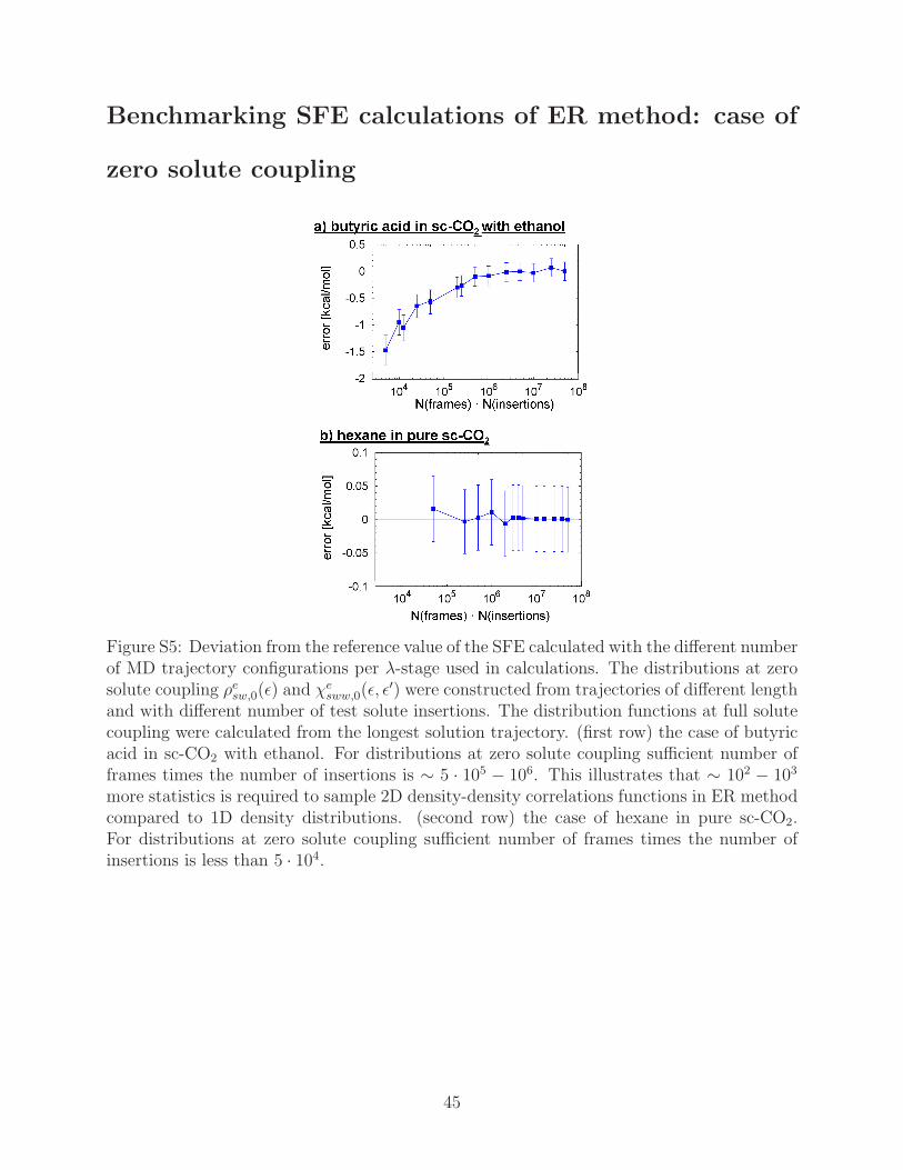
Figure S5: Deviation from the reference value of the SFE calculated with the different numberof MD trajectory configurations per λ-stage used in calculations. The distributions at zerosolute coupling ρesw,0(ǫ) and χe

sww,0(ǫ, ǫ′) were constructed from trajectories of different length

and with different number of test solute insertions. The distribution functions at full solutecoupling were calculated from the longest solution trajectory. (first row) the case of butyricacid in sc-CO2 with ethanol. For distributions at zero solute coupling sufficient number offrames times the number of insertions is ∼ 5 · 105 − 106. This illustrates that ∼ 102 − 103

more statistics is required to sample 2D density-density correlations functions in ER methodcompared to 1D density distributions. (second row) the case of hexane in pure sc-CO2.For distributions at zero solute coupling sufficient number of frames times the number ofinsertions is less than 5 · 104.

45

Density distributions for different potentials.

Figure S6: Solvent density distributions ρesw in energy representation for butyric-acid in sc-CO2 with addition of 6 molar % of ethanol for different types of potential functions: (total)potential at full solute coupling, (vdW) all but Coulombic interactions and (WCA) repulsivepart of the WCA potential.

46

Details on derivation of the ER method.

We provide details on the derivation of the theory of solutions in energy representation (ER

method) developed by Matubayasi et al.24–26,33,51 This derivation is adopted from Ref.29

This method provides with an approximate way of calculating solvation free energies (or,

identically, the excess chemical potentials) from atomistic simulations. The method can

be seen as bridge between the molecular simulations and the classical density functional

theory (DFT). We provide details on some important relations of ER method for the case

of NPT-ensemble.

Some definitions

We consider a system with Ns = 1 solute and Nw solvent molecules at isothermo-isobaric

ensemble (NPT-ensemble). We describe the interactions between the molecules in the force

field approximation at the level of classical mechanics. Each molecule is represented as a set

of atoms, which interact with each other via bonded and nonbonded potentials present in the

given force field (e.g. OPLS, CHARMM, AMBER, etc). Each interaction site is considered

as a separate object, which has its own translational degrees of freedom and translational

partition function. Therefore, when we talk about a set of coordinates which define the

position of a molecule xi we mean the positions of all atoms which belong to this molecule,

where index α runs over all atoms (nt) of the molecule of type t:

xi = {ri,α}nt

α=1 (19)

where t is the molecule type, e.g. s denotes solute, w denotes solvent, and the coordinates

of atom α of ith molecule:

ri,α = {xi,α, yi,α, zi,α}

Each atom has its own momentum: pi,α

47

Parametrized Hamiltonian

Here and after we mostly adopt the notations used in the Appendix of the Shirts et al.

publication.14 The excess chemical potential can be calculated in the process of gradual

switching on the intermolecular interactions between a solute molecule and the solvent. We

introduce λ parameter which controls the degree of coupling between the solute and solvent

molecules, such that when λ=0 the interactions are absent and when λ=1 interactions are

at full coupling. Since, only solute-solvent interaction potential usw,λ(xs,xw,i) depends on λ,

the potential energy function of the system can be written as follows:

Uλ(xs,xNw

w ) = Ψ(xs) +Nw∑

i=1

usw,λ(xs,xw,i) + Uww(xNw) (20)

where subscript s denotes solute, subscript w denotes solvent, Ψ(xs) is the potential energy

of the solute molecule, xw,i is the position of ith solvent molecule, Nw is the number of

solvent molecules, usw,λ is the λ-dependent solute-solvent interaction potential, Uww is the

potential energy of the solvent molecules, xNw is the short notation of positions of all solvent

molecules.

The total Hamiltonian can be written as:

Hλ = K(ps,pNw

w ) + Uλ(xs,xNw

w ) (21)

where the kinetic energy is written as:

K(ps,pNw

w ) =ns∑

α=1

p2s,α2ms,α

+Nw∑

i=1

nw∑

α=1

p2w,i,α

2mw,α

(22)

where ms,α and mw,α are the masses of αth atoms of solute and solvent molecules, corre-

spondingly.

48

Partition functions with non-parameterized Hamiltonian

The partition function in NPT ensemble can be written as:

∆(Ns, Nw, P, T ) =

∫ ∞

0

d

(

V

V ′

)

e−βPVQ(Ns, Nw, V, T ) (23)

where V ′ is an arbitrary constant which makes the partition function dimensionless, β is

(kBT )−1, kB is the Boltzmann constant, Q(Ns, Nw, V, T ) is the canonical partition function,

which has the following form:

Q(Ns, Nw, V, T ) =1

h3NwnwNw!h3NsnsNs!

∫ +∞

−∞dpNs

s dpNw

w

∫

V

dxNs

s dxNw

w exp[

−βH(pNs

s ,pNw

w ,xNs

s ,xNw

w )]

where h is the Planck’s constant. Multiplication by h−1 serves as a quantum correction

for purely classical partition function.1 The factorials of number of atoms in the system

appear due to indistinguishably of atoms belonging to the molecules of the same type. Each

integration symbol denotes integration over multiple coordinates. Differential dxNww is the

short notation for dxw,1...dxw,Nw. Symbol V at the integration sign -

∫

V- reflects that

integration limits are bound by the system’s volume.

In the case of classical statistical mechanics the momenta degrees of freedom are inde-

pendent and can be analytically integrated:34

h−3

∫ +∞

−∞dpx,αe

−β(p2x,α

2mx,α)=

[

h2

2πmx,αkBT

]−1.5

= Λ−3x,α

where Λx,α is the thermal de Broglie wavelength for atom α in molecule of type x.

Therefore we get:

Q(Ns, Nw, V, T ) =ns∏

α=1

Λ−3Nss,α

Ns!

nw∏

α=1

Λ−3Nww,α

Nw!· Z(Ns, Nw, V, T ) (24)

49

where Z is the configuration integral of the system:

Z(Ns, Nw, V, T ) =

∫

V

dxNs

s dxNw

s exp[

−βU(xNs

s ,xNw

w )]

(25)

between a

Solvation free energy

The solvation free energy (SFE) can be defined as a reversible work required to switch on the

interactions between a solute molecule and the rest.1 In NPT ensemble this can be written

as:

∆Gsolv = −kBT ln∆(Ns, Nw, P, T, λ = 1)

∆(Ns, Nw, P, T, λ = 0)(26)

where the λ in the brackets indicate that the partition functions are written with the λ-

parameterized Hamiltonian (Eq. 21).

following:

One can show that SFE is always equal to the excess (over ideal) chemical potential:

∆Gsolv ≡ µex (see Ref.29).

only

Kirkwood charging formula

In order to make the forthcoming derivations simpler, from now we explicitly consider the

case of infinite diluted solution: Ns = 1. The point here is that we will express the excess

chemical potential of solute via the particle density distributions. Therefore, considering

many solute molecules in the system will require to introduce the solute-solute density dis-

tribution, which will unnecessarily complicate the derivations. Note, that all the forthcom-

ing derivation can be straightforwardly extended to the case of multicomponent solvent (see

Ref.35).

50

Let us define the excess chemical potential for the system with parameterized Hamiltonian

(Eq. 21) at a certain λ value. Using Eq. 26 we get:

∆Gsolv,λ = −kBT ln∆(Ns, Nw, P, T, λ)

∆(Ns, Nw, P, T, λ = 0)

Since the denominator does not depend on λ one can write:

∂∆Gsolv,λ

∂λ= −kBT

∫∞0

d(

VV ′

)

e−βPV∫

Vdxsdx

Nww

∂Uλ

∂λexp

[

−βUλ(xs,xNww )]

∆(Ns, Nw, P, T, λ)=

⟨

∂Uλ

∂λ

⟩

λ

With the explicit form of the potential function (Eq. 20) we have:

∂∆Gsolv,λ

∂λ=

⟨

Nw∑

i=1

∂usw,λ(xs,xw,i)

∂λ

⟩

λ

=

⟨

∫ +∞

−∞dx′

sdx′w

∂usw,λ(x′s,x

′w)

∂λ

Nw∑

i=1

δ(xs − x′s)δ(xw,i − x′

w)

⟩

λ

where 〈·〉λ denotes ensemble average in isothermo-isobaric condition at given λ. We can

change order of integration and take out the derivative from the ensemble average:

∂∆Gsolv,λ

∂λ=

∫ +∞

−∞dx′

sdx′w

∂usw,λ(x′s,x

′w)

∂λ

⟨

Nw∑

i=1

δ(xs − x′s)δ(xw,i − x′

w)

⟩

λ

(27)

In the right hand side there is the pair solute-solvent density distribution in NPT-

ensemble by definition (see e.g. Eq. (2.5.13) of Ref.,34 but mind that for density distributions

of non-identical particles the sum should include terms with i = j):

∂∆Gsolv,λ

∂λ=

∫ +∞

−∞dx′

sdx′w

∂usw,λ(x′s,x

′w)

∂λρsw,λ(x

′s,x

′w)

Finally, SFE can be written as an integral over lambda:

∆Gsolv =

∫ 1

0

dλ∂∆Gsolv,λ

∂λ=

∫ 1

0

dλ

∫ +∞

−∞dx′

sdx′w

∂usw,λ(x′s,x

′w)

∂λρsw,λ(x

′s,x

′w) (28)

51

Energy representation (ER)

Basic definitions in ER

Collective coordinate. We define a new collective coordinate which is the interaction

energy between a solute molecule and a solvent molecule: ǫ. We make this coordinate

λ-independent, such that this coordinate is calculated with the solute-solvent potential at

full coupling vsw(xs,xw), irrespective of the ensemble and Hamiltonian which were used to

generate this configuration:

vsw(xs,xw) ≡ usw,λ=1(xs,xw) (29)

Microscopic density. For a single configuration of the system the microscopic density in

energy representation can be written as:

ρ̂esw(ǫ) =Nw∑

i=1

δ (vsw(xs,xw)− ǫ) = (30)

=

∫ +∞

−∞dx′

sdx′wδ(vsw(x

′s,x

′w)− ǫ)

Nw∑

i=1

δ(x′s − xs)δ(x

′w − xw,i) = (31)

=

∫ +∞

−∞dxsdxwδ(vsw(xs,xw)− ǫ)ρ̂sw(xs,xw) (32)

Potential in ER. The potential in energy representation can be written as:

uesw,λ(ǫ) =

∫ +∞

−∞dxsdxwδ (vsw(xs,xw)− ǫ) usw,λ(xs,xw) (33)

It is important for the following derivation that we choose the lambda path in such a

way that usw,λ(xs,xw) is constant on each equi-energy surface of vsw(xs,xw). This can be

achieved, for instance, when usw,λ(xs,xw) = λvsw(xs,xw). With this restriction of the usw,λ

52

potential we can write the following identity:

usw,λ(xs,xw) =

∫ +∞

−∞dǫ · δ (vsw(xs,xw)− ǫ) ue

sw,λ(ǫ) (34)

Taking the partial derivative of the both sides of equation we obtain the formula, which

will be used later on:

∂usw,λ(xs,xw)

∂λ=

∫ +∞

−∞dǫ · δ (vsw(xs,xw)− ǫ)

∂uesw,λ(ǫ)

∂λ(35)

Solute-solvent density distribution in ER. Solute-solvent density distribution in NPT

ensemble is written as:

ρesw,λ(ǫ) = 〈ρ̂(ǫ)〉λ

Using the definition of microscopic density in ER (Eq. 32) and writing explicitly its

ensemble average we get:

ρesw,λ(ǫ) =

∫∞0

d(

VV ′

)

e−βPV∫

Vdxsdx

Nww

[

∫ +∞−∞ dx′

sdx′wδ(vsw(x

′s,x

′w)− ǫ)ρ̂sw(x

′s,x

′w)]

exp[

−βUλ(xs,xNww )]

∫∞0

d(

VV ′

)

e−βPV∫

VdxsdxNw

w exp [−βUλ(xs,xNww )]

(36)

Change of the integration order:

ρesw,λ(ǫ) =

∫ +∞

−∞dx′

sdx′wδ(vsw(x

′s,x

′w)−ǫ)

∫∞0

d(

VV ′

)

e−βPV∫

Vdxsdx

Nww [ρ̂sw(x

′s,x

′w)] exp

[

−βUλ(xs,xNww )]

∫∞0

d(

VV ′

)

e−βPV∫

VdxsdxNw

w exp [−βUλ(xs,xNww )]

The ratio gives us the definition of the solute-solvent density distribution (see Comment

after Eq. 27):

ρesw,λ(ǫ) =

∫ +∞

−∞dx′

sdx′wδ(vsw(x

′s,x

′w)− ǫ)ρsw,λ(x

′s,x

′w) (37)

53

Kirkwood charging formula in energy representation

Kirkwood charging formula via density distribution

Let us obtain the charging formula in energy representation. We start from coordinate

representation (Eq. 28):

∆Gsolv =

∫ 1

0

dλ

∫ +∞

−∞dx′

sdx′w

∂usw,λ(x′s,x

′w)

∂λρsw,λ(x

′s,x

′w) =

Using Eq. 35 we obtain:

∆Gsolv =

∫ 1

0

dλ

∫ +∞

−∞dx′

sdx′w

[∫ +∞

−∞dǫδ (vsw(x

′s,x

′w)− ǫ)

∂uesw,λ(ǫ)

∂λ

]

ρsw,λ(x′s,x

′w)

We change the integration order:

∆Gsolv =

∫ 1

0

dλ

∫ +∞

−∞dǫ

∂uesw,λ(ǫ)

∂λ

[∫ +∞

−∞dx′

sdx′wδ (vsw(x

′s,x

′w)− ǫ) ρsw,λ(x

′s,x

′w)

]

We use the relation Eq. 37 to obtain:

∆Gsolv =

∫ 1

0

dλ

∫ +∞

−∞dǫ

∂uesw,λ(ǫ)

∂λρesw,λ(ǫ) (38)

Eq. 38 is the Kirkwood’s charging formula in ER.

Indirect part of potential of mean force (IPMF)

We can introduce an auxiliary function wesw,λ(ǫ), which is an analogue of the indirect part of

potential of mean force in coordinate representation:

ρesw,λ(ǫ) = ρesw,λ=0(ǫ) · exp[

−β(

uesw,λ(ǫ) + we

sw,λ(ǫ))]

(39)

54

The potential then can be rewritten as:

uesw,λ(ǫ) = −kBT ln

ρesw,λ(ǫ)

ρesw,λ=0(ǫ)− we

sw,λ(ǫ) (40)

Kirkwood charging formula via IPMF

Let us rewrite the Kirkwood’s charging formula (Eq. 38) via wesw,λ:

∆Gsolv =

∫ 1

0

dλ

∫ +∞

−∞dǫ

∂uesw,λ(ǫ)

∂λρesw,λ(ǫ)

Change of the integration order:

∆Gsolv =

∫ +∞

−∞dǫ

∫ 1

0

dλ∂ue

sw,λ(ǫ)

∂λρesw,λ(ǫ)

Integration by parts for the inner integral:

∆Gsolv =

∫ +∞

−∞dǫ

[

ρesw,λ=1(ǫ)uesw,λ=1(ǫ)−

∫ 1

0

dλ∂ρesw,λ(ǫ)

∂λuesw,λ(ǫ)

]

Change of the integration order back. Mind that uesw,λ=1(ǫ) = vesw(ǫ) = ǫ according to

the definition (Eq. 29 and Eq. 33):

∆Gsolv =

∫ +∞

−∞dǫρesw,λ=1(ǫ)ǫ−

∫ 1

0

dλ

∫ +∞

−∞dǫ

∂ρesw,λ(ǫ)

∂λuesw,λ(ǫ) (41)

Let us denote the last term as a functional of the potential and the solute-solvent density

distribution:

F [ρesw,λ(ǫ), uesw,λ(ǫ)] =

∫ 1

0

dλ

∫ +∞

−∞dǫ

∂ρesw,λ(ǫ)

∂λuesw,λ(ǫ) (42)

The functional can be written via IPMF. Here and after, we use the following simplified

notations:

ρesw,0 ≡ ρesw,λ=0

55

ρesw ≡ ρesw,λ=1

Similar notations are adopted for other functions.

Using Eq. 40 and changing the integration order we obtain from Eq. 42:

F [ρesw,λ(ǫ), uesw,λ(ǫ)] =

∫ +∞

−∞dǫ

∫ 1

0

dλ∂ρesw,λ(ǫ)

∂λ

(

−kBT lnρesw,λ(ǫ)

ρesw,0(ǫ)− we

sw,λ(ǫ)

)

(43)

The first integral in Eq. 43 can be taken analytically by parts:

∫ 1

0

dλ∂ρesw,λ(ǫ)

∂λln

ρesw,λ(ǫ)

ρesw,0(ǫ)= ρesw,λ(ǫ) ln

ρesw,λ(ǫ)

ρesw,0(ǫ)

∣

∣

∣

∣

1

0

−

∫ 1

0

dλρesw,λ(ǫ)

ρesw,λ(ǫ)

∂ρesw,λ(ǫ)

∂λ=

= ρesw(ǫ) lnρesw(ǫ)

ρesw,0(ǫ)−(

ρesw(ǫ)− ρesw,0(ǫ))

(44)

Therefore, we rewrite Eq. 43 using Eq. 44 as:

F [ρesw,λ(ǫ), uesw,λ(ǫ)] =

=

∫ +∞

−∞dǫ

[

−kBT

(

ρesw(ǫ) lnρesw(ǫ)

ρesw,0(ǫ)−(

ρesw(ǫ)− ρesw,0(ǫ))

)

+

∫ 1

0

dλ∂ρesw,λ(ǫ)

∂λ

(

−wesw,λ(ǫ)

)

]

Regrouping the terms we get:

F [ρesw,λ(ǫ), uesw,λ(ǫ)] = kBT

∫ +∞

−∞dǫ

[

(

ρesw(ǫ)− ρesw,0(ǫ))

− ρesw(ǫ) lnρesw(ǫ)

ρesw,0(ǫ)− β

∫ 1

0

dλ∂ρesw,λ(ǫ)

∂λwe

sw,λ(ǫ)

]

(45)

This expression can be further simplified if we choose the λ-dependence of the potential

such that the density distribution is a linear function of λ:

ρesw,λ(ǫ) = λρesw(ǫ) + (1− λ)ρesw,0(ǫ) (46)

56

With this restriction (Eq. 46) the λ-derivative is:

∂ρesw,λ(ǫ)

∂λ= (ρesw(ǫ)− ρesw,0(ǫ))

and the functional (Eq. 45) becomes:

F [ρesw,λ(ǫ), uesw,λ(ǫ)] =

= kBT

∫ +∞

−∞dǫ

[

(

ρesw(ǫ)− ρesw,0(ǫ))

− ρesw(ǫ) lnρesw(ǫ)

ρesw,0(ǫ)− β(ρesw(ǫ)− ρesw,0(ǫ))

∫ 1

0

dλwesw,λ(ǫ)

]

(47)

Finally, SFE (Eq. 38) reads:

∆Gsolv[ρesw,λ(ǫ), u

esw,λ(ǫ)] =

∫ +∞

−∞dǫρesw(ǫ)ǫ−F [ρesw,λ(ǫ), u

esw,λ(ǫ)] (48)

Density functional

For further derivations we would like to consider the functional F as a unique functional

of ρesw,λ(ǫ). This can be the case if the solute-solvent interaction potential is a unique

functional of ρesw,λ(ǫ). This implies that there should be only one uesw,λ(ǫ) to which a given

ρesw,λ(ǫ) corresponds. Both in coordinate and energy representation it is not the case if one

considers ensembles where the number of particles is fixed.26,35–37 This can be easily seen

from the definition of ρesw,λ(ǫ) (Eq. 36 and Eq. 20): if one adds a constant to the solute-solvent

interaction potential usw,λ the resulting ρe function does not change (Mind, that there is a

one-to-one correspondence between the potential in energy and coordinate representations

(Eqs. 34 and 33)). The lack of the one-to-one correspondence between ρ and u results

to the fact that the density-density correlation matrix is not invertible and has a singular

eigenvalue.26,35,36

Matubayasi proposed a way how to retain the one-to-one ρ - u correspondence by intro-

ducing additional condition based on the physical sense. Firstly, he proved that the potentials

57

giving different density profiles can differ from each other only by an additive constant (see

Appendix of Ref.35 and Ref.26). Secondly, he sets the additive constant to ensure that the

chemical potential is an intensive property of the system. This can be achieved by ensuring

that the solute-solvent pair potential reaches zero when particle separation tends to infinity.

With this approach a one-to-one correspondence between usw,λ(ǫ) and ρsw,λ(ǫ) achieved

both in coordinate and energy representation. This allows us to consider the potential

uesw,λ(ǫ) as a functional of ρesw,λ(ǫ) in a fixed-N ensemble and use the functional calculus to

obtain approximate free energy functionals.

Therefore, SFE (Eq. 48) can be written as a density functional of the solute-solvent

density distribution:

∆Gsolv[ρesw,λ(ǫ)] =

∫ +∞

−∞dǫρesw(ǫ)ǫ−F [ρesw,λ(ǫ)] (49)

Approximate free energy functional.

The exact free energy functional (Eq. 47) contains the term which depends on λ. To elim-

inate the λ-dependence we apply the Percus’s method of functional expansion to obtain

approximate functionals.

HNC-like approximation.

Following Percus38 we obtain the HNC-like approximation by expanding the following func-

tional in powers of density fluctuation ρesw(ǫ′)− ρesw,0(ǫ

′):

ln ρesw(ǫ)+βusw(ǫ) ≈ ln ρesw,0(ǫ)+

∫ +∞

−∞dǫ′·(

ρesw(ǫ′)− ρesw,0(ǫ

′))

·δ [ln ρesw(ǫ) + βusw(ǫ)]

δρesw(ǫ′)

∣

∣

∣

∣

ρesw(ǫ′)=ρesw,0(ǫ′)

(50)

With the help of Eq. 40 we rewrite the left hand side of Eq. 50 via IPMF. Therefore,

58

IPMF in HNC-like approximation can be written as:

we,HNCsw (ǫ) = −kBT

∫ +∞

−∞dǫ′ ·

(

ρesw(ǫ′)− ρesw,0(ǫ

′))

·

[

δ(ǫ− ǫ′)

ρesw,0(ǫ)+ β

δuesw(ǫ)

δρesw(ǫ′)

∣

∣

∣

∣

ρesw(ǫ′)=ρesw,0(ǫ′)

]

(51)

Let us show that the functional derivative in Eq. 51 is a functional inverse of the density-

density correlation function. For that we start from the definition of solute-solvent distribu-

tion function at full solute coupling:

ρesw(ǫ) = 〈ρ̂(ǫ)〉λ=1 =

=

∫∞0

d(

VV ′

)

e−βPV∫

Vdxsdx

Nww ρ̂e(ǫ)e−βU(xs,x

Nww )

∫∞0

d(

VV ′

)

e−βPV∫

VdxsdxNw

w e−βU(xs,xNww )

(52)

Let us denote nominator of Eq. 52 as f and denominator as g. Then, find the functional

derivative of distribution function with respect to solute-solvent potential:

δρesw(ǫ)

δuesw(ǫ

′′)=

δf

δuesw

g−

δg

δuesw

g·f

g(53)

Both in f and g only potential energy U depends on uesw. To write its explicit dependence

on uesw we use the relation between the solute-solvent interaction potentials in coordinate

and energy representations (Eq. 34).

U(xs,xNw

w ) = Ψ(xs) +Nw∑

i=1

usw(xs,xw,i) + Uww(xNw

w ) =

= Ψ(xs) +Nw∑

i=1

∫ +∞

−∞dǫ′′ · δ(vsw(xs,xw,i)− ǫ′′)ue

sw(ǫ′′) + Uww(x

Nw

w ) (54)

59

Therefore, we find the following derivative which will be used in later derivations:

δ[

e−βU]

δuesw(ǫ

′)= −βe−βU

Nw∑

i=1

∫ +∞

−∞dǫ′′ · δ(vsw(xs,xw,i)− ǫ′′)δ(ǫ′′ − ǫ′) =

= −βe−βU

Nw∑

i=1

δ(vsw(xs,xw,i)− ǫ′) = −βe−βU ρ̂esw(ǫ′) (55)

where we used Eq. 33.

With this relation (Eq. 55) the first term in Eq. 53 then can be written as:

δf

δuesw

g= −β 〈ρ̂esw(ǫ)ρ̂

esw(ǫ

′)〉usw(56)

Also, with relation Eq. 55 we see that g′ = −βf . With this Eq. 55 is written as:

δρesw(ǫ)

δuesw(ǫ

′)= −β

[

〈ρ̂esw(ǫ)ρ̂esw(ǫ

′)〉usw− 〈ρ̂esw(ǫ)〉usw

〈ρ̂esw(ǫ′)〉usw

]

(57)

Which equivalently can be written as:

δρesw(ǫ)

δuesw(ǫ

′)= −β [ρesww(ǫ, ǫ

′) + ρesw(ǫ)δ(ǫ− ǫ′)− ρesw(ǫ)ρesw(ǫ

′)] = −βχesww(ǫ, ǫ

′) (58)

where χesww(ǫ, ǫ

′) is the density-density correlation function, and ρesww(ǫ, ǫ′) is the three

molecule density distribution defined by analogy to the two molecule density distribution

in coordinate representation (see Eq. (2.5.13) of Ref.34) as:

ρesww(ǫ, ǫ′) =

⟨

Nw∑

i=1

∑

j 6=i

δ(v(xs,xw,i)− ǫ)δ(v(xs,xw,j)− ǫ′)

⟩

(59)

From Eqs. 57 and 58 we obtain:

δuesw(ǫ)

δρesw(ǫ′)=

(

δρesw(ǫ)

δuesw(ǫ

′)

)−1

= −kBT (χesww)

−1 (ǫ, ǫ′) (60)

60

where (χesww)

−1 is the functional inverse of the density-density correlation function defined

as (see Eq. (3.5.8) of Ref.34):

∫ +∞

−∞dǫ′′ · χe

sww(ǫ, ǫ′′) (χe

sww)−1 (ǫ′′, ǫ′) = δ(ǫ− ǫ′) (61)

With Eq. 60 we can rewrite the HNC-like approximation of the indirect part of potential

of mean force (Eq. 51) as:

we,HNCsw (ǫ) = −kBT

[

ρesw(ǫ)− ρesw,0(ǫ)

ρesw,0(ǫ)−

∫ +∞

−∞dǫ′ ·

[

ρesw(ǫ′)− ρesw,0(ǫ

′)]

·(

χesww,0

)−1(ǫ, ǫ′)

]

(62)

PY-like approximation.

Again, following Percus38 we obtain the Percus-Yevick-like (PY-like) approximation by ex-

panding the following functional:

ρesw(ǫ)eβusw(ǫ) ≈ ρesw,0(ǫ) +

∫ +∞

−∞dǫ′ ·

(

ρesw(ǫ′)− ρesw,0(ǫ

′))

·δ[

ρesw(ǫ)eβusw(ǫ)

]

δρesw(ǫ′)

∣

∣

∣

∣

∣

ρesw=ρesw,0

(63)

We rewrite Eq. 63 via IPMF (Eq. 39):

we,PYsw (ǫ) = −kBT ln

(

1 +

∫ +∞

−∞dǫ′ ·

[

δ(ǫ− ǫ′)

ρesw,0(ǫ)+ β

δuesw(ǫ)

δρesw(ǫ′)

∣

∣

∣

∣

ρesw=ρesw,0

])

= (64)

With the help of Eq. 51 we can rewrite the PY-like approximation via the HNC-like w:

we,PYsw (ǫ) = −kBT ln

(

1− βwe,HNCsw (ǫ)

)

(65)

61

Lambda-integral in HNC-like approximation.

When uλ is the solute-solvent interaction potential the corresponding IPMF is written as:

we,HNCsw,λ (ǫ) = −kBT

[

ρesw,λ(ǫ)− ρesw,0(ǫ)

ρesw,0(ǫ)−

∫ +∞

−∞dǫ′ ·

[

ρesw,λ(ǫ′)− ρesw,0(ǫ

′)]

·(

χesww,0

)−1(ǫ, ǫ′)

]

(66)

With the linear dependence of ρesw,λ on λ (Eq. 46) Eq. 66 can be written via we,HNCsw at

full solute coupling:

we,HNCsw,λ (ǫ) = λ · we,HNC

sw (ǫ) (67)

The λ-integral in Eq. 47 can be written in HNC-like approximation as:

β

∫ 1

0

dλwe,HNCsw,λ (ǫ) = we,HNC

sw (ǫ) · β

∫ 1

0

dλ · λ =1

2βwe,HNC

sw (ǫ) (68)

Lambda-integral in PY-like approximation.

When uλ is the solute-solvent interaction potential the corresponding IPMF in PY-like ap-

proximation is written as (see Eq. 65):

we,PYsw,λ (ǫ) = −kBT ln

(

1− βwe,HNCsw,λ (ǫ)

)

= −kBT ln(

1− λ · βwe,HNCsw (ǫ)

)

(69)

Now, we use the following known tabulated relation:

∫

dx · ln(ax+ b) =(ax+ b) · ln(ax+ b)− ax

a

to find the λ-integral:

β

∫ 1

0

dλwe,PYsw,λ (ǫ) = −

[

−βwe,HNCsw (ǫ) + 1

]

· ln[

−βwe,HNCsw (ǫ) + 1

]

+ βwe,HNCsw (ǫ)

−βwe,HNCsw (ǫ)

(70)

Next, we use the relation between w in PY and HNC-like approximations at full solute

coupling λ = 1 (see Eq. 69):

62

we,PYsw (ǫ) = −kBT ln

(

1− βwe,HNCsw (ǫ)

)

=> −βwe,HNCsw (ǫ) = e−βw

e,PYsw (ǫ) − 1 (71)

Using Eq. 71 we rewrite Eq. 70 as:

β

∫ 1

0

dλwe,PYsw,λ (ǫ) = − ln

[

1− βwe,PYsw (ǫ)

]

+ 1 +ln[

1− βwe,PYsw (ǫ)

]

βwe,PYsw (ǫ)

(72)

Constructing hybrid functional.

The approximate functional is developed by Matubayasi et al.25 based on the following

considerations. To make an end-point expression of ∆Gsolv we need to approximate the

λ-integral in Eq. 47. Beforehand, we would like to note that the approximate expression of

the λ-integral will have four parts.

Firstly, the λ-integration can be analytically performed both in PY-like and HNC-like

approximations (see Eqs. 72 and 68). There is a general knowledge in the field that in

the case of simple liquids the PY approximation works better for short range repulsive

potentials, while HNC approximation performs better for long-range attractive potentials.34

Matubayasi25 decided to use the PY-like expression for the λ-integral in the unfavorable

region of solvation (wesw ≥ 0) and HNC-like expression for the λ-integral in the favorable

region of solvation (wesw < 0).

Secondly, the indirect part of potential of mean force wesw can be determined from un-

biased molecular simulations (regular MD or Monte-Carlo) only outside of the solute-core

region (region of very large solute-solvent interaction energies: ǫ). Matubayasi33 proposed

to use HNC-approximation of the potential of mean force when wesw is not resolved from

molecular simulations. In HNC-like approximation we,HNCsw is determined by the solute-

solvent density distribution ρesw,0 and the inverse of the density-density correlation function(

χesww,0

)−1in the case of the zero solute-solvent coupling (this can bee seen from Eq. 62,

where the difference ρesw − ρesw,0 can be safely approximated by −ρesw,0 since in the core

region ρesw << ρesw,0). Therefore, we,HNCsw in the core-region can be calculated with high

63

resolution in the ensemble, where solute and solvent are fully decoupled and the probability

to find solvent molecule in the core region is high. The later can be in the most conve-

nient way realized by the insertion of the solute molecule configurations into the ensemble

of precalculated pure solvent configurations.

Combination of two different expression for λ-integral and two different input w functions

results into functional consisting of four parts. The final expression for SFE (Eq. 49).

∆Gsolv[ρesw,λ(ǫ)] =

∫ +∞

−∞dǫρesw(ǫ)ǫ−F [ρesw,λ(ǫ)] (73)

where

F [ρesw,λ(ǫ)] = kBT

∫ +∞

−∞dǫ

[

(

ρesw(ǫ)− ρesw,0(ǫ))

− ρesw(ǫ) lnρesw(ǫ)

ρesw,0(ǫ)− (ρesw(ǫ)− ρesw,0(ǫ)) · β

∫ 1

0

dλwesw,λ(ǫ)

]

(74)

where the λ-integral is approximated by the following expression:

β

∫ 1

0

dλwesw,λ(ǫ) = α(ǫ) · Fw(ǫ) + [1− α(ǫ)] · FwHNC(ǫ) (75)

where the functions Fw and FwHNC are in turn written as the combination of PY and

HNC-like expressions for the λ-integral:

Fw(ǫ) =

βwesw(ǫ)

2, when we

sw(ǫ) ≥ 0

βwesw(ǫ) + 1 +

βwesw(ǫ)

e−βwesw(ǫ) − 1

, when wesw(ǫ) < 0

(76)

and

FwHNC(ǫ) =

βwe,HNCsw (ǫ)

2, when we,HNC

sw (ǫ) ≥ 0

− ln[

1− βwe,HNCsw (ǫ)

]

+ 1 +ln[

1− βwe,HNCsw (ǫ)

]

βwe,HNCsw (ǫ)

, when we,HNCsw (ǫ) < 0

(77)

64

The parameter α(ǫ), which is responsible for merging parts with different w functions, is

set heuristically33 as:25

α(ǫ) =

1, when ρesw(ǫ) ≥ ρesw,0(ǫ)

1−

(

ρesw(ǫ)− ρesw,0(ǫ)

ρesw(ǫ) + ρesw,0(ǫ)

)2

, when ρesw(ǫ) < ρesw,0(ǫ)

(78)

65