Numerical simulation and decomposition of kinetic energies

OSD8, 1161–1214, 2011

Numerical simulationand decompositionof kinetic energies

R. Sorgente et al.

Title Page

Abstract Introduction

Conclusions References

Tables Figures

J I

J I

Back Close

Full Screen / Esc

Printer-friendly Version

Interactive Discussion

Discussion

Paper

|D

iscussionP

aper|

Discussion

Paper

|D

iscussionP

aper|

Ocean Sci. Discuss., 8, 1161–1214, 2011www.ocean-sci-discuss.net/8/1161/2011/doi:10.5194/osd-8-1161-2011© Author(s) 2011. CC Attribution 3.0 License.

Ocean ScienceDiscussions

This discussion paper is/has been under review for the journal Ocean Science (OS).Please refer to the corresponding final paper in OS if available.

Numerical simulation and decompositionof kinetic energies in the CentralMediterranean Sea: insight on mesoscalecirculation and energy conversion

R. Sorgente1, A. Olita1, P. Oddo2, L. Fazioli1, and A. Ribotti1

1IAMC, Consiglio Nazionale delle Ricerche, Oristano, Italy2INGV, Istituto Nazionale di Geofisica e Vulcanologia, Bologna, Italy

Received: 30 March 2011 – Accepted: 11 May 2011 – Published: 24 May 2011

Correspondence to: R. Sorgente ([email protected])

Published by Copernicus Publications on behalf of the European Geosciences Union.

1161

http://www.ocean-sci-discuss.net

http://www.ocean-sci-discuss.net/8/1161/2011/osd-8-1161-2011-print.pdf

http://www.ocean-sci-discuss.net/8/1161/2011/osd-8-1161-2011-discussion.html

http://creativecommons.org/licenses/by/3.0/

OSD8, 1161–1214, 2011


R. Sorgente et al.

Title Page



Tables Figures

J I

J I

Back Close

Full Screen / Esc



Discussion

Paper

|D

iscussionP

aper|

Discussion

Paper

|D

iscussionP

aper|

Abstract

The spatial and temporal variability of eddy and mean kinetic energy of the CentralMediterranean Sea has been investigated, from January 2008 to December 2010, bymean of a numerical simulation mainly to quantify the mesoscale dynamics and theirrelationships with physical forcing. In order to understand the energy redistribution5

processes, the baroclinic energy conversion has been analysed, suggesting hypothe-ses about the drivers of the mesoscale activity in this area. The ocean model usedis based on the Princeton Ocean Model implemented at 1/32◦ horizontal resolution.Surface momentum and buoyancy fluxes are interactively computed by mean of stan-dard bulk formulae using predicted model Sea Surface Temperature and atmospheric10

variables provided by the European Centre for Medium Range Weather Forecast op-erational analyses. At its lateral boundaries the model is one-way nested within theMediterranean Forecasting System operational products.

The model domain has been subdivided in four sub-regions: Sardinia channel andsouthern Tyrrhenian Sea, Sicily channel, eastern Tunisian shelf and Libyan Sea. Tem-15

poral evolution of eddy and mean kinetic energy has been analysed, on each of thefour sub-regions composing the model domain, showing different behaviours. On an-nual scales and within the first 5 m depth, the eddy kinetic energy represents approxi-mately the 60 % of the total kinetic energy over the whole domain, confirming the strongmesoscale nature of the surface current flows in this area. The analyses show that the20

model well reproduces the path and the temporal behaviour of the main known sub-basin circulation features. New mesoscale structures have been also identified, fromnumerical results and direct observations, for the first time as the Pantelleria Vortexand the Medina Gyre.

The classical the kinetic energy decomposition (eddy and mean) allowed to depict25

and to quantify the stable and fluctuating parts of the circulation in the region, andto differentiate the four sub-regions as function of relative and absolute strength ofthe mesoscale activity. Furthermore the Baroclinic Energy Conversion term shows

1162





OSD8, 1161–1214, 2011


R. Sorgente et al.

Title Page



Tables Figures

J I

J I

Back Close

Full Screen / Esc



Discussion

Paper

|D

iscussionP

aper|

Discussion

Paper

|D

iscussionP

aper|

that in the Sardinia Channel the mesoscale activity, due to baroclinic instabilities, issignificantly larger than in the other sub-regions, while a negative sign of the energyconversion, meaning a transfer of energy from the Eddy Kinetic Energy to the EddyAvailable Potential Energy, has been recorded only for the surface layers of the SicilyChannel during summer.5

1 Introduction

The Central Mediterranean Sea (CMED, hereafter) is a large area connecting the east-ern and the western Mediterranean sub-basins delimited by the eastern Sardinia Chan-nel, the southern Tyrrhenian Sea and, mainly, the shallow (∼400 m) Sicily Channel(Fig. 1), an intermediate basin with an average depth of 500 m. It plays a crucial role10

in modulating the passage of the surface and intermediate water masses between thetwo Mediterranean sub-basins.

The highly irregular bottom topography of the Sicily Channel, in the form of a sub-marine ridge characterised by shallow banks along the Tunisian (Galite and Skerkibanks) and Sicilian (Adventure Bank and Malta Channel area) coasts, further limits the15

water flow particularly at deeper levels. Flat-bottomed deep trenches are situated inthe central part of the Sicily Channel, west of Malta, reaching depths of 1100–1200 moff Pantelleria, 1300 m off Linosa and 1650 m in the Malta Graben. The Tunisian andLibyan continental shelves are very wide and cover more than one-third of the aerialextent of the Sicily Channel. In the Gulf of Gabes, the bathymetry is shallower than20

30 m for large stretches away from the coast.The circulation in the CMED is characterized by a number of significant dynami-

cal processes covering the full spectrum of temporal and spatial scales (Millot, 1999;Pinardi et al., 1997). The surface and subsurface flows are mainly driven by the largescale of the Mediterranean thermohaline circulation, and clearly by the momentum and25

buoyancy fluxes at the air-sea interface. In addition there are wind-driven currents onthe shelf due to remote storms; upwelling events off Sicily; sub-basin scale cyclonic

1163





OSD8, 1161–1214, 2011


R. Sorgente et al.

Title Page



Tables Figures

J I

J I

Back Close

Full Screen / Esc



Discussion

Paper

|D

iscussionP

aper|

Discussion

Paper

|D

iscussionP

aper|

and anticyclonic permanent gyres and small energetic mesoscale eddies with timescale shorter than 10 days (Manzella et al., 1988). The mesoscale structures underthe influence of wind stress, topography and internal dynamical processes generateboundary currents and jets which can bifurcate, meander and grow then forming ringvortices and filament patterns interacting with the large scale flow fields (Lermusiaux,5

1999; Lermusiaux and Robinson, 2001).The high variability of the water masses properties and circulation characteristics

has been largely investigated in the past years through hydrographical observations(Manzella and La Violette, 1990; Sammari et al., 1999), sub-surface currentmetersdata (Astraldi et al., 1999; Vetrano et al., 2004; Gasparini et al., 2005), Lagrangian10

drifters (Poulain and Zambianchi, 2007) and high resolution numerical simulations(Onken et al., 2003; Sorgente et al., 2003; Beranger et al., 2005). However, avail-able observations are often characterized by poor spatial and temporal coverages, andare usually confined to the Italian seas lacking over the Tunisian and Libyan continentalshelves. Only few datasets have adequate temporal and spatial resolution to capture15

the mesoscale in local areas (Lermusiaux and Robinson, 2001).Thus, numerical model simulations constitute an important tool to fill the observa-

tional gaps and to study the spatial and temporal ocean circulation variability. Highresolution models, below 5 km, have been poorly used in the past mainly due to com-putational constraints. The computational issue poses the need to nest a hierarchy of20

successively embedded model domains, to downscale the large scale features to thecoastal areas (Pinardi et al., 2003; Sorgente et al., 2003; Oddo et al., 2005). Thismethodology is found to be computationally efficient and sufficiently accurate to trans-mit information across the connecting lateral open boundaries without excessive dis-tortion (Oddo and Pinardi, 2008).25

The aim of this study is to investigate the mesoscale and the sub-basin scale dy-namics in the CMED region, by mean of decomposition of the simulated flow fieldsinto a mean and eddy components, then giving an overall assessment of the spa-tial and temporal mesoscale variability in relation with atmospheric forcing and energy

1164





OSD8, 1161–1214, 2011


R. Sorgente et al.

Title Page



Tables Figures

J I

J I

Back Close

Full Screen / Esc



Discussion

Paper

|D

iscussionP

aper|

Discussion

Paper

|D

iscussionP

aper|

redistribution processes. The interest on mesoscale dynamic derives from the fact thateddies can potentially interact with the mean current and the bottom topography pro-ducing long term responses in the ocean circulation (Fernandez et al., 2005). Thework has been done in the framework of the European COastal sea OPerational ob-serving and forecasting system integrated project (ECOOP) funded by the European5

Commision’s Sixth Framework Programme, whom main aim was the construction of anEuropean network of sea-forecasting systems, through the improvement (resolution,physics, data assimilation, distribution, etc.) of existing operational models.

In order to improve the investigation of the dynamics in the area, the model domainhas been subdivided in four sub-regions, each one supposedly characterized by an10

homogeneous dynamics, as visible in Fig. 1: the Sardinia-Tyrrhenian area (area A);the Sicily Channel (area B); the wide and shallow shelf area off Tunisia and Libya (areaC); the wide slope area in front of Libya (area D).

This paper is structured as follows: in the Sect. 2 the main spatial and temporalscale variability of the surface circulation is briefly reviewed. Section 3 describes the15

characteristics of the model used, including the nesting method and the atmosphericcoupling. In Sect. 4 the mean and eddy near surface kinetic energies, their seasonalcycle and structures are discussed, conclusions are presented in Sect. 5.

2 The physical regimes

Three main spatial and temporal scales characterize the CMED: the large Mediter-20

ranean basin scale, including the thermohaline circulation; the sub-basin scale and themesoscale. Each interacts with the others giving complex circulation patterns whicharise from the multiple driving forces, strong topographic and coastal influences, andfrom internal dynamical processes (Robinson et al., 2001).

1165





OSD8, 1161–1214, 2011


R. Sorgente et al.

Title Page



Tables Figures

J I

J I

Back Close

Full Screen / Esc



Discussion

Paper

|D

iscussionP

aper|

Discussion

Paper

|D

iscussionP

aper|

2.1 The large scale circulation

The main engine of the surface and subsurface large scale circulation is the remoteforcing induced by the basin scale Mediterranean dynamics. The basin-scale ther-mohaline circulation in the Mediterranean Sea has been extensively studied in thepast years by several authors through observational programs and numerical mod-5

elling studies (Zavatarelli and Mellor, 1995; Pinardi et al., 1997; Pinardi and Masetti,2000; Beranger et al., 2005). The thermohaline circulation is anti-estuarine (lagoonal)and it is driven mainly by the balance between the relatively fresh waters enteringat the Gibraltar Strait and the negative fresh-water budgets over the whole Mediter-ranean basin. This is usually described as a zonal cell which involves the exchanges10

of water masses between the eastern and the western Mediterranean basins with thetransformation of the surface Atlantic Water (AW, hereafter) in the Levantine Interme-diate Water. Thus, the vertical structure consists of a two-layers flow with the surfaceAW moving eastward from the Gibraltar Strait and spreading from the Sicily Channelthroughout the eastern Mediterranean sub-basin as modified AW (Astraldi et al., 2002),15

and a salty Levantine Outflow moving westward at intermediate depth. The zonal cellis connected with the “meridional” cells that are driven by the dense water mass forma-tion processes occurring in the Gulf of Lions and Adriatic Sea (Schlitzer et al., 1991).In the Sicily Channel, the sill depth strongly modulates the exchange of these deep andintermediate waters between the two Mediterranean sub-basins.20

In the western Mediterranean basin the amplitude of the seasonal variability is largeand involves intensity currents and mesoscale variability while, in the eastern basin,the inter-annual and seasonal variabilities have the same order of magnitude involvingthe characteristics of the deep and intermediate water masses and high mesoscale ac-tivities (Korres et al., 2000). Then, the CMED is a key area to monitor the thermohaline25

circulation and the corresponding hydrological trends (Astraldi et al., 1999; 2002) ofthe entire Mediterranean Sea.

1166





OSD8, 1161–1214, 2011


R. Sorgente et al.

Title Page



Tables Figures

J I

J I

Back Close

Full Screen / Esc



Discussion

Paper

|D

iscussionP

aper|

Discussion

Paper

|D

iscussionP

aper|

2.2 The sub-basin scale

A schematic description of the seasonal variability of the sub-basin scale surface cir-culation is represented in Fig. 2, as derived from Lermusiaux and Robinson (2001);Beranger et al. (2004) and Hamad et al. (2005). In the CMED the sub-basin scalefeatures (jets, gyres and meanders) are part of the basin-wide circulation. The up-5

per layer is occupied by the AW moving eastward as Algerian Current (AC), a coastalboundary current whose instability origins meanders few kilometres long and coastaleddies (Robinson et al., 2001). The cyclonic eddies are relatively superficial and short-lived, while the anticyclones last for weeks or months (Sammari et al., 1999; Astraldi etal., 2002). These mesoscale phenomena are disturbed by the South Eastern Sardinia10

Gyre (SESG, hereafter), a sub-basin scale wind curl driven cyclonic gyre centred ap-proximately at 10◦ E–38.5◦ N (Artale et al., 1994) with a diameter that varies between200 and 300 km.

Part of AC, after having crossed the Sardinia Channel, west of Sicily splits in twobranches as a consequence of a topographic effect (Pierini and Rubino, 2001; Onken15

and Sellschopp, 2001; Onken et al., 2003; Beranger et al, 2004). The first branchdirectly flows into the Tyrrhenian Sea along the northern coast of Sicily (Astraldi etal., 1996), as Bifurcation Tyrrhenian Current (BTC), while the second turns southwardinto the Sicily Channel as a strong and narrow jet. Here it flows eastward in a two-jetstructure covering the upper 100 m with an associated salinity minimum: the Atlantic20

Tunisian Current (ATC) moving over the Tunisian continental slope, and the Atlantic Io-nian Stream (AIS) along the southern coast of Sicily (Astraldi et al., 1996; Lermusiaux,1999; Robinson et al., 1999; Lermusiaux and Robinson, 2001). It is worth to mentionthat the described bifurcation pattern is lightly different from what estimated by Astraldiet al. (1999, 2002), Gasparini et al. (2004) and by Gerin et al. (2009) from in situ data.25

They found that AW directly splits in three veins at the entrance of the Sicily Channelfollowing separate tracks with the minimum of salinity along Tunisia. Vice versa, duringthe 1994–1996 AIS investigation by Robinson et al. (1999), the ATC/AIS bifurcation

1167





OSD8, 1161–1214, 2011


R. Sorgente et al.

Title Page



Tables Figures

J I

J I

Back Close

Full Screen / Esc



Discussion

Paper

|D

iscussionP

aper|

Discussion

Paper

|D

iscussionP

aper|

has not been observed but only the AIS was present with southerly branches in theSicily Channel and Ionian Sea in a complicated meandering path. These changes incurrents and water mass properties confirm the strong temporal variability of the area,where the mesoscale activity can be considered as an important source of interannualvariability (Fernandez et al., 2005).5

The main stream associated to the ATC flows eastward along the Tunisian andLibyan continental shelf break just south of Lampedusa or confined into the centralpart of the Sicily Channel (Manzella et al., 1988, 1990). The AIS constitutes a freejet energetic current mainly flowing eastward, along the southern coast of Sicily, as atypical waveform forcing upwelling on the Adventure Bank (western Sicilian shelf), es-10

pecially during the summer when the current is strong. An important spatial variabilityexists and includes: shape, position and strength of permanent or quasi-permanentsub-basin gyres and their unstable lobes, meanders patterns, bifurcation structuresand strength of permanent jets, transient eddies and filaments (Robinson et al., 1999).

The sub-basin scale structures have seasonal amplitudes associated with the large15

wind stress variability (Pinardi and Navarra, 1993; Molcard et al., 2002). Recently,numerical studies (Onken et al., 2003; Sorgente et al, 2003; Beranger et al., 2004)and direct observations (Astraldi et al., 1996; 1999; Sammari et al., 1999; Poulainand Zambianchi, 2007) have been devoted to assess the seasonal characteristics ofthe surface circulation. Superimposed to such seasonal (sub-basin) variability there20

is also a signal of interannual variability mainly due to the mesoscale and, in somemeasures, to lower frequencies signals related to climate change (Olita et al., 2007).

2.3 The mesoscale

Mesoscale variability can be defined as the ensemble of flow fluctuations whose pe-riods range from a few days to a few tenths of days. Many events are included in25

this broad definition, among which we are mostly interested in mesoscale variabil-ity associated to small vortices (i.e. mesoscale eddies). Its forcing mechanisms aremainly instabilities from the large-scale circulation, interactions between currents and

1168





OSD8, 1161–1214, 2011


R. Sorgente et al.

Title Page



Tables Figures

J I

J I

Back Close

Full Screen / Esc



Discussion

Paper

|D

iscussionP

aper|

Discussion

Paper

|D

iscussionP

aper|

bathymetry and the direct surface forcing. The interest in the CMED mesoscale dy-namics comes from the hypothesis that fronts, jets, meanders and eddies can play animportant role in the ocean as response to buoyancy forcing, winds and topographicgradients.

The horizontal scale of mesoscale eddies is related to the first baroclinic Rossby ra-5

dius of deformation which, in the Sicily Channel, varies seasonally ranging from a min-imum of about 8 km in January, to about 11 km during period of stratification (Borzelliand Ligi, 1998). The radius almost vanishes in winter, over the Tunisian and Libyanshelf shallow area, due to a complete mixing of the water column.

In the CMED the mesoscale variability has been only marginally investigated. This10

is due to very high horizontal resolution required by numerical ocean models (com-puter resources) and/or a huge amount of in-situ data needed. An observationalstudy was recently carried out by Poulain and Zambianchi (2007) analyzing morethan 150 surface-drifters in the period 1990–1999 to assess the spatial and sea-sonal variability of eddy and mean surface kinetic energy. Previously, a similar study15

was realized by Lermusiaux (1999) and Lermusiaux and Robinson (2001) using afour-dimensional numerical primitive equation model and intensive in-situ data dur-ing August–September 1996, but limited to northern Sicily Channel. All of them foundthat the main features of dominant mesoscale variability are associated with five fea-tures: the Adventure Bank Vortex, Maltese Channel Crest, Ionian Shelf break Vortex,20

Messina Rise Vortex and temperature and salinity fronts of the Ionian slope with theirmeanders and topographic wave patterns.

3 Methods

3.1 Model design

In order to reach an adequate resolution to model the mesoscale dynamics in the25

central Mediterranean Sea, a nesting approach has been adopted. The Sicily Channel

1169





OSD8, 1161–1214, 2011


R. Sorgente et al.

Title Page



Tables Figures

J I

J I

Back Close

Full Screen / Esc



Discussion

Paper

|D

iscussionP

aper|

Discussion

Paper

|D

iscussionP

aper|

Regional Model (SCRM, hereafter) has been embedded into the coarse basin model ofthe Mediterranean Forecasting System (MFS1671, hereafter, Tonani et al., 2008). Thispermits to produce a more detailed description of the circulation in the region, includingsome mesoscale components that cannot be resolved by the coarse model. SCRMis a free surface three-dimensional primitive equation finite difference hydrodynamic5

model based on the Princeton Ocean Model (Blumberg and Mellor, 1987). It solvesthe equations of continuity, motion, conservation of temperature, salinity and assumesthat the fluid is hydrostatic and the Boussinesq approximation is valid. The density iscalculated by an adaptation of the UNESCO equation of state revised by Mellor (1991).The vertical mixing coefficients for momentum and tracers are calculated using the10

Mellor and Yamada (1982) turbulence closure scheme, while the horizontal viscosityterms are provided by the Smagorinsky parameterization (Smagorinsky, 1993).

SCRM is implemented between 9◦ E and 17.10◦ E and from 31.50◦ N to 39.50◦ N witha horizontal resolution of 1/32◦ (∼3.5 km). In the vertical it uses 30 sigma levels, densernear the surface following a logarithmic distribution. The external time step is set to 4 s,15

with an internal every 120 s. The model bathymetry has been obtained from the USNavy Digital Bathymetric Data Base-DBDB1 at 1/60◦ by bilinear interpolation into themodel grid. The minimum depth is set to 5 m. Additional smoothing is applied to reducethe sigma coordinate pressure gradient error (Mellor et al., 1994). The resulting modelbathymetry is shown in Fig. 1.20

The numerical system was run in free mode (i.e. without any data assimilationscheme) from January 2008 to December 2010.

The model has been initialized at 00:00 on 1 January 2008 using dynamically bal-anced analyses fields from MFS1671 through an innovative tool based on the Varia-tional Initialization and Forcing Platform (Auclair et al., 2000). This method is largely25

used in meteorological activities as drastically reduces the amplitude of the numericaltransient processes, generally following the initialization phases for several days afterthe initialization. This method has been proven to drastically reduce the spin up timeof the SCRM slave 5-days forecasts by Gabersek et al. (2007) to some few hours. On

1170





OSD8, 1161–1214, 2011


R. Sorgente et al.

Title Page



Tables Figures

J I

J I

Back Close

Full Screen / Esc



Discussion

Paper

|D

iscussionP

aper|

Discussion

Paper

|D

iscussionP

aper|

the light of such a result it has been used in the present experimental setup, permittingto negligee the spin up time problem.

Surface momentum and buoyancy fluxes are interactively computed by mean of ded-icated bulk formulae developed and tested for the Mediterranean Sea in previous nu-merical exercises (Castellari et al., 1998; Tonani et al., 2008; Pinardi et al., 2003, Oddo5

et al., 2009). Fluxes computation takes into account model predicted sea surface tem-perature and the 6-h (00:00, 06:00, 12:00, 18:00 UTC) atmospheric parameters fromEuropean Centre for Medium range Weather Forecast operational analysis. The pa-rameters are wind at 10 m a.s.l., air temperature at 2 m a.s.l., cloud cover, dew-pointtemperature and atmospheric pressure. These data have a horizontal resolution of10

0.25◦ and, successively, are mapped on the SCRM grid through bilinear interpolationand linearly interpolated in time at each model time step.

The surface boundary condition for momentum is:

KM∂u∂z

∣∣∣∣z=η

=τ

ρ0, (1)

where τ is the wind stress vector, KM is the vertical kinematic viscosity,15

ρ0 =1025 Kg m−3 is a reference density and η is the free surface elevation. The windstress components use a drag coefficient Cd =Cd(Ta, T , W ) as function of the windamplitude (W ), the air temperature (Ta) and the sea surface temperature predicted bythe model (T ) following the polynomial approximation given by Hellerman and Rosen-stein (1983). The surface boundary conditions for potential temperature take the clas-20

sic form:

KH∂T∂z

∣∣∣∣z=η

=QT

ρ0Cp, (2)

where QT is the net heat flux, Cp (4186 J Kg−1 K−1) is the specific heat capacity ofpure water at constant pressure and KH is the vertical heat diffusivity. The net heat flux(Eq. 2) involves the balance between surface solar radiation (QS ), the net long-wave25

1171





OSD8, 1161–1214, 2011


R. Sorgente et al.

Title Page



Tables Figures

J I

J I

Back Close

Full Screen / Esc



Discussion

Paper

|D

iscussionP

aper|

Discussion

Paper

|D

iscussionP

aper|

radiation (QB), the latent (QE ) and sensible (QH ) heat fluxes. The heat flux componentsare calculated using the formula by Reed (1977) for the short wave radiation flux andthat by Bignami et al. (1995) for long wave radiation. The turbulent components (latentand sensible heat fluxes) are computed by mean of the bulk aerodynamic formulaeproposed by Kondo (1975).5

For the salinity flux we consider the water balance:

KH∂S∂z

∣∣∣∣z=η

= (E −P −R) ·S+C2(S∗−S) (3)

C2 =∆σ(1)Hα

where E =QE /LE is the evaporation rate interactively calculated, LE the latent heatof evaporation, P the monthly precipitation rate obtained from Legates and Will-10

mott (1990), R is the river runoff and S∗ is the surface model salinity. In our simulationsthe runoff R is set to 0 because of the absence of rivers with significant discharge. Thelast term of Eq. (3) is the salinity flux correction, where S∗ is the monthly mean sea cli-matology surface salinity from Med6, while C2 is the thickness of the surface layer andalpha is the relaxation time. This correction term accounts for the imperfect knowledge15

of E -P (P especially).Lateral open boundary conditions are defined through a simple off-line one way nest-

ing technique that represents an efficient way to downscale the model solutions fromthe basin-scale (∼7 km) to the regional scale (∼3.5 km). It has been largely used innumerical weather predictions and recently in numerical oceanography to simulate the20

hydrodynamics of limited coastal areas (Drago et al., 2003; Sorgente et al., 2003;Zavatarelli and Pinardi, 2003; Oddo and Pinardi 2008). The SCRM is nested at thelateral open boundaries with MFS1671 covering the whole Mediterranean Sea with ahorizontal resolution of 1/16◦ (Tonani et al., 2008; Oddo et al., 2009). The daily meanvalues of temperature, salinity, total velocity and elevation were transferred from the25

1172





OSD8, 1161–1214, 2011


R. Sorgente et al.

Title Page



Tables Figures

J I

J I

Back Close

Full Screen / Esc



Discussion

Paper

|D

iscussionP

aper|

Discussion

Paper

|D

iscussionP

aper|

coarse spaced grid of MFS1671 to the finely spaced grid of the SCRM open bound-aries through an off-line, one-way asynchronous nesting. The definition of the nestedopen boundary conditions is based on Sorgente et al. (2003).

3.2 Energy analysis

By taking in account previous experiences, and in order to quantify the energy levels5

involved in the simulated circulation, in our work the flow field is divided into mean andeddy components. Generally, any velocity field (u,v,w) can be divided into a time inde-pendent component (U,V,W ) and an eddy fluctuating part (time dependent, u′,v ′,w ′):

u=U+u′ v = V +v ′ w =W +w ′ (4)

where the time independent part is obtained averaging temporally the full field over a10

given interval, m. For the three velocity components:

U =1m

m∑j=1

uj , V =1m

m∑j=1

vj W =1m

m∑j=1

wj . (5)

The m term indicates the temporal scale (annual or monthly, as defined into theSects. 4.1 and 4.2), j-th is the daily mean field and u, v and w are the zonal, meridionaland vertical components of the total velocity respectively (as defined in Eq. 4).15

The Total Kinetic Energy (TKE) per unit mass can be expressed as:

TKE=12

(u2+v2),

substituting in the above equation the decomposition of the total velocity as defined inthe Eq. (4), we obtain:

TKE=12

(U2+V 2)+12

(u′2+v ′2)+ (Uu′+V v ′), (6)20

1173





OSD8, 1161–1214, 2011


R. Sorgente et al.

Title Page



Tables Figures

J I

J I

Back Close

Full Screen / Esc



Discussion

Paper

|D

iscussionP

aper|

Discussion

Paper

|D

iscussionP

aper|

where the first term on the right hand side is the kinetic energy of mean flow per unitmass (MKE):

MKE=12

(U2+V 2), (7)

while the second term is the kinetic energy per unit mass of the fluctuating flow, alsocalled Eddy Kinetic Energy (EKE):5

EKE=12

(u′2+v ′2). (8)

The last term in the r.h.s of Eq. (6) is the first-order correlation term (Orlansky andKatzfey, 1991). The time average of TKE (Eq. 6) will contain only the first two terms(Eq. 7 and 8), since the time mean of the third term vanishes. The logarithm of the ratiobetween the EKE (Eq. 8) and MKE (Eq. 7) defines the following parameter:10

Φ= log(EKEMKE

) (9)

which provides information on the energy distribution between the mean constant andfluctuating currents in the study area. In general, if Φ < 0 then MKE prevails on EKE, ifΦ=0 then EKE and MKE are of the same order, otherwise if Φ>0 then EKE is largerthan MKE. This last condition suggests that the energy of currents is dominated by the15

velocity fluctuating component.In order to evaluate part of the sources of energy for the mesoscale in the study

area, the Baroclinic Energy Conversion (BEC) has been evaluated. BEC (Orlanskyand Katzfey, 1991) is defined as:

BEC=−ρ′gw ′ (10)20

where g is the gravitational acceleration, w ′ is the vertical component of the fluctuat-ing velocity obtained applying Eq. (1), while ρ′ arises from the decomposition of the

1174





OSD8, 1161–1214, 2011


R. Sorgente et al.

Title Page



Tables Figures

J I

J I

Back Close

Full Screen / Esc



Discussion

Paper

|D

iscussionP

aper|

Discussion

Paper

|D

iscussionP

aper|

instantaneous density ρ(x,y,z,t) into a motion less part, a time independent compo-nent and a spatial and temporal varying component following the below equation:

ρ(x,y,z,t)=ρ(z)+ρ(x,y,z)+ρ′(x,y,z,t).

BEC is the buoyancy work, which defines the conversion between the two form ofeddy energies: Eddy Available Potential Energy (EAPE) and EKE (Lorenz, 1955; Ped-5

losky, 1987).We use the wind stress work W s to evaluate the relationship between TKE and the

wind forcing. It is defined as:

Ws=u ·τ (11)

where u is the surface current vector and τ the wind stress vector (Pedlosky, 1987).10

MKE and EKE have been vertically integrated and horizontally averaged over thefour sub-regions previously defined and visible in Fig. 1 as follows:

ϑ(t)=1V

∫ h2

h1

∫ y2

y1

∫ x2

x1ϑ(x,y,z,t)dxdydz. (12)

The integration limits are the coordinates delimiting the horizontal sub-domain (x andy) and the vertical layers (z), while the temporal scale (t) is defined into the Sects. 4.115

and 4.2. Moreover the grid point, whose depth of the first sigma layer exceeds 1 m,has been excluded (the deepest part of the Tyrrhenian Sea and of the east Ionianescarpment).

3.3 Data

In order to support results obtained by analyzing modelled fields, different sets of satel-20

lite measurements have been used.Sea Level Anomaly data, used to support the observations of relatively large and

offshore mesoscale eddies, are AVISO SSALTO/DUACS mapped and gridded weeklyproducts with a spatial resolution of 1/4◦ (http://www.aviso.oceanobs.com/).

1175





http://www.aviso.oceanobs.com/

OSD8, 1161–1214, 2011


R. Sorgente et al.

Title Page



Tables Figures

J I

J I

Back Close

Full Screen / Esc



Discussion

Paper

|D

iscussionP

aper|

Discussion

Paper

|D

iscussionP

aper|

Ocean-Color 1 km data are Level-2 (single swaths) acquired from MODerate resolu-tion Imaging Spectro-radiometer (MODIS) sensor on board of the AQUA mission anddownloaded from the oceancolor web portal (http://oceancolor.gsfc.nasa.gov/). TheLevel-2 MODIS data have been post-processed and re-projected through SEADAS™software.5

4 Results and discussion

The spatial variability of MKE, EKE and the ratio of EKE over MKE (Φ) simulated bySCRM on the period 2008–2010 are described on annual (Sect. 4.1) and monthly scale(Sect. 4.2), also comparing the simulated circulation with literature. In Sect. 4.3, thetemporal variability of BEC has been analyzed, giving information about the source of10

energy for mesoscale induced by baroclinic instabilities.The MKE field has been computed as defined in the Eq. (7), while EKE was obtained

according to Eq. (8). Successively, MKE and EKE have been vertically integrated overthe firsts 5 m depth and horizontally averaged over the whole area and in the foursub-regions as previously defined (Eq. 12). The choice to integrate over the upper 5 m15

depth was done to allow the comparison of the model based kinetic energy estimationswith the results of Lagrangian observations obtained by Poulain and Zambianchi (2007)through drifter trajectories collected during the period 1990–1999.

4.1 Mean circulation

The annual mean field of the simulated surface circulation is obtained by averaging20

the daily mean velocity fields of SCRM as described in Eq. (5) where m denotes thenumber of days over the simulated period (2008–2010). The model results are shownin Fig. 3, drawing the main characteristics of the basin and sub-basin mean surfacecirculation and confirming the results obtained from observations and previous studiesdescribed by Zavatarelli and Mellor, 1995; Robinson et al., 2001; Astraldi et al., 2001,25

2002; Onken et al., 2003; Beranger et al., 2004.1176





http://oceancolor.gsfc.nasa.gov/

OSD8, 1161–1214, 2011


R. Sorgente et al.

Title Page



Tables Figures

J I

J I

Back Close

Full Screen / Esc



Discussion

Paper

|D

iscussionP

aper|

Discussion

Paper

|D

iscussionP

aper|

The analysis of the mean circulation (Fig. 3a) shows the AC flowing eastward alongthe northern Tunisian shelf with MKE over 400 cm2 s−2 (Fig. 3b) on the northernTunisian shelf break and the Skerki Bank. AC splits in the AIS and the ATC, while BTCdoesn’t clearly appear in the mean flow. The AIS flows between Pantelleria and thesouthern Sicilian coast, then north of Malta and intrudes into the deep Ionian Sea after5

the overshooting along the eastern Sicilian coast, as described by Lermusiaux (1999)and Sorgente et al. (2003). High values of MKE (Fig. 3b) above 500 cm2 s−2 are foundover the Adventure Bank, along the southern Sicilian coast and along the Ionian shelfbreak. Apart the MKE patches over the Adventure Bank that could be overestimatedbecause of an approximate bathymetry, the simulated MKE distribution is generally in10

agreement with the paths detected by Poulain and Zambianchi (2007).In the central part of the Sicily Channel the MKE appears rather weak. The ATC flows

southward along the Tunisian coast as a relatively strong current decreasing progres-sively its velocity south-eastward. It flows approximately following the 200 m isobathsuntil Libya with MKE below 50 cm2 s−2 between 12◦ E and 14◦ E. This limited feature is15

also visible in Fig. 3a and in full agreement with drifter observations. We call this nar-row current as Atlantic Libyan Current (hereafter ALC), which can be considered as theeastward extension of ATC along the Libyan coast (Gasparini et al., 2008; Poulain andZambianchi, 2007). A further dominant feature is the Sidra Gyre, previously mentionedby several authors (Korres et al., 2000; Sorgente et al., 2003; Fernandez et al., 2005;20

Tonani et al., 2008), a sub-basin permanent anti-cyclonic structure centred at about33.5◦ N and 16◦ E and detected also by drifter trajectories (Poulain and Zambianchi,2007). It strongly interacts with the ALC, pushing the modified AW toward the Libyancoast in a narrow stream. The Sidra Gyre appears as the main dynamical mechanismthat influences the outflow of AW outside the Sicily Channel, having a seasonal and25

interannual variability, as stated by Gerin et al. (2009) and Ciappa (2009). It also con-trols the inflow of warm and salty Ionian Surface Water from the eastern side of theLibyan shelf through its southern arm. This feature is represented by a westward flowcharacterized by values of MKE of about 100 cm2 s−2 (Fig. 3b).

1177





OSD8, 1161–1214, 2011


R. Sorgente et al.

Title Page



Tables Figures

J I

J I

Back Close

Full Screen / Esc



Discussion

Paper

|D

iscussionP

aper|

Discussion

Paper

|D

iscussionP

aper|

The EKE map (Fig. 3c), which includes the variability due to small scale eddies, tosporadic wind-driven current events and also to the seasonal modulation of the surfacecirculation with internal energy redistribution processes, shows almost the same spatialpatterns observed for MKE, suggesting a strong variability associated to the intensityof the currents with larger values of TKE. Values of EKE less than 50 cm2 s−2 are found5

at the deepest part of the Sicily Channel, below Malta. Vice-versa, large fluctuationsover 100 cm2 s−2 are found in regions with strong currents, such as along the northernTunisian shelf break (the AC), with the highest values (>350 cm2 s−2) over the SkerkiBank, westward and along the northern Sicilian coast. This succession identifies thepath of BTC, which doesn’t clearly appear in the mean flow. Downstream the Sicily10

Channel, high values are found between Malta and Sicily and at significant topographicgradients of the Ionian escarpment. Isolated structures appear also along the Libyancoast between 12◦ E and 14◦ E. Most of these features have been also confirmed bythe above mentioned drifter observations, even if the model underestimates the energycontent of these structures. This underestimate for MKE and EKE could be due to the15

different sampling periods, 1990–1999 for the drifter-based study and 2008–2010 forthe model, or to the unevenly sampling accomplished through the drifters. Obviously,this disagreement in term of values could also be due to the other different factors likethe low resolution atmospheric forcing, an inadequate modelled viscosity-diffusivity, oran insufficient vertical resolution of the model. In any case, our model results indicate20

that the mean EKE, averaged over the whole domain, is about 90 cm2 s−2, 3 timesMKE.

The energy ratio between the mean constant and fluctuating currents is representedby the parameter Φ (Eq. 9), which compares the levels of MKE and EKE (Fig. 3d).The values with Φ < 0 identify the main stream currents where the mean flow kinetic25

energy is larger than EKE, as for AC and AIS. The areas where MKE and EKE areroughly similar (Φ= 0) are identified by the paths of ATC with its bifurcations, ALCand the Sidra Gyre. Vice versa the EKE can be up about 3 times larger in logarithmicterm than MKE (Φ>1) into the deepest part of the Sardinia Channel and Tyrrhenian

1178





OSD8, 1161–1214, 2011


R. Sorgente et al.

Title Page



Tables Figures

J I

J I

Back Close

Full Screen / Esc



Discussion

Paper

|D

iscussionP

aper|

Discussion

Paper

|D

iscussionP

aper|

Sea, over the major part of the Tunisian shelf, as isolated features in the Sicily Channel,between ATC and AIS, and between Malta and Libya westward of the Sidra Gyre wherethe mean flow is really weak.

4.2 Seasonal variability of kinetic energy and surface circulation

In order to analyze the MKE and EKE components of the kinetic energy budgets, the5

simulated daily mean velocity fields of SCRM have been averaged on monthly basisover the period 2008–2010, computed as in Eq. (4) where m denotes the number ofdays for each month.

The monthly averaged time series of TKE, MKE, EKE and the wind stress work(Eq. 11) are shown in Figs. 4. The TKE (Fig. 4a), sum of MKE and EKE, has a sea-10

sonal cycle with values larger than 150 cm2 s−2 between November and March. TheEKE, always larger than MKE (Fig. 4b), dominates such a TKE seasonality drawinga similar path while MKE shows smaller seasonal variability with a relative MKE max-ima in July (∼60 cm2 s−2), end of a noteworthy phase opposition period between MKE(slight increase) and EKE (decrease) started in May. The winter peaks of MKE and15

EKE appear to be related to the wind stress work (Fig. 4c), which has values overabout 0.5 N m−1 s−1 from November to March. From April to October the wind stresswork is weak and remains approximately constant, not exceeding 0.2 N m−1 s−1. Onthe contrary, the summer peak (in July) of MKE is not directly related to the wind stresswork, but is probable due to the internal dynamics associated with the presence and20

action of intense summer current systems as AIS and the Westward Northern SicilianCurrent. The latter feature will be introduced into the Sect. 4.2.1.

The same analyses has been applied in each of the four sub-regions in which thewhole domain has been divided (Fig. 1) in order to quantify possible differences in thespatial energy distribution and ratio (MKE, EKE and Φ).25

1179





OSD8, 1161–1214, 2011


R. Sorgente et al.

Title Page



Tables Figures

J I

J I

Back Close

Full Screen / Esc



Discussion

Paper

|D

iscussionP

aper|

Discussion

Paper

|D

iscussionP

aper|

4.2.1 The Sardinia-Tyrrhenian sub-region

The Sardinia-Tyrrhenian sub-region (A in Fig. 1) appears as the most energetic of thefour. EKE is always larger than MKE (Fig. 5a) apart in November and December. Onannual mean the contribution of EKE to TKE is about 57 %. The EKE shows a sea-sonal cycle with a maximum value in February (∼170 cm2 s−2) and minimum in October5

(∼85 cm2 s−2), while MKE shows values over 100 cm2 s−2 from November to Januarythen decreasing progressively towards its minimum values in April and September(∼60 cm2 s−2) and a relative maximum in July (∼80 cm2 s−2). The wind stress work(Fig. 5b) is characterized by two forcing regimes. From November to March the windstress work is always over 0.7 N m−1 s−1, reaching its absolute maximum in December10

(1.1 N m−1 s−1), while from April to October it doesn’t overpass 0.25 N m−1 s−1. Thenthe small MKE summer peak in July appears not directly related to the wind stresswork. The comparison between EKE and MKE (Fig. 5c), represented by the param-eter Φ (see Eq. 9), shows a positive signal (Φ>0) apart November and December.This means that the surface dynamics is usually dominated by the velocity fluctuating15

component with its maximum in April (Φ∼1), while in November the mean flow on thevelocity fluctuating component prevails (Φ<0). We would underline the significanceof such a ratio: the Φ parameter informs when/where EKE is larger than MKE or, inother words, when mesoscale activity is stronger than the mean flow then neglectingthe absolute value of EKE.20

The horizontal distribution of Φ in November (Fig. 6a) shows MKE prevailing onEKE (Φ<0) in correspondence of AC and BTC paths. The mean flow of such featuresappear as coastal boundary currents flowing, respectively, along the northern Tunisiancoast (AC) and along the northern Sicilian shelf break (BTC), in agreement with theliterature (Astraldi et al., 1996; Molcard et al., 2002). Such a spatial feature is mainly25

due to the MKE field (not shown) reaching values over 800 cm2 s−2 along the AC paththat are compatible with speed currents of about 40 cm s−1 then decreasing eastward.Lower values (<200 cm2 s−2) occur along the BTC path. The EKE is largely higher than

1180





OSD8, 1161–1214, 2011


R. Sorgente et al.

Title Page



Tables Figures

J I

J I

Back Close

Full Screen / Esc



Discussion

Paper

|D

iscussionP

aper|

Discussion

Paper

|D

iscussionP

aper|

MKE (Φ>1), especially in deep areas of the Sardinia Channel where the energy of thecurrents is dominated by the fluctuating component, whose monthly mean reaches itsmaximum in February (Fig. 5a). The EKE field, with the current mean flow overlapped,is represented in Fig. 6b. Values over 300 cm2 s−2 are found along AC and BTC paths,increasing to the same order than MKE (not shown). Isolated patches of EKE show5

very high values (>400 cm2 s−2) on the northern Tunisian shelf and along the northernSicilian coast. Then, in general, the EKE maxima is always associated with the highenergetic flows as the AC and, less, to the BTC whose strength, in term of mean flowand fluctuating velocity currents, appears mainly related to the eastward flow at theSardinia-Tunisia section (Fig. 7) and, secondly, to the atmospheric forcing (Fig. 5b).10

Vice-versa, the EKE prevails where there is not a clear mean flow, suggesting that theEKE signal would be due to instabilities generated along the currents boundaries.

Toward the summer months AC and BTC progressively decrease, in agreement withAstraldi et al. (2002) and Sorgente et al. (2003), but the temporal evolution of MKE(Fig. 5a) show a small increase on July. Here, the model results shows the mean15

surface circulation dominated by the meandering of a weaker AC, some split currents,cyclonic and anti-cyclonic eddies, the SESG and by a westward current flowing alongthe northern Sicilian coast (not shown). SESG replaces in summer part of the BTC pathand appears particularly active in term of MKE from June to September (not shown).It seems to be part of a large anti-cyclonic gyre located on the southern side of the20

Tyrrhenian Sea. Actually there are no bibliographic indications on the existence of thisfeature which would deserve a more detailed study. We refer to this as WestwardNorthern Sicilian Current (WNSC, hereafter). It appears more stable and stronger thanAC justifying the July increase of MKE described above.

4.2.2 The Sicily sub-region25

The Sicily sub-region (B in Fig. 1) appears less energetic than the previous one, witha contribution of EKE to TKE of about 55 %. The monthly time series of MKE andEKE (Fig. 8a) have almost comparable values, except in October, and do not show a

1181





OSD8, 1161–1214, 2011


R. Sorgente et al.

Title Page



Tables Figures

J I

J I

Back Close

Full Screen / Esc



Discussion

Paper

|D

iscussionP

aper|

Discussion

Paper

|D

iscussionP

aper|

clear seasonal cycle. EKE levels are always larger than MKE, apart in June, July andDecember, ranging approximately between 50 and 80 cm2 s−2. The MKE series show atemporal evolution characterized by a relative maximum in June and July (∼60 cm2 s−2)and an absolute maximum in December (∼65 cm2 s−2). The wind stress work (Fig. 8b)is characterized by lower values than in the Sardinia – Tyrrhenian sub-region, but with5

a similar temporal evolution. The comparison between EKE and MKE (Fig. 8c) showsthe former prevailing (Φ>0) especially in October, slightly negative in June and July,while in August, November and December the two kinetic components are almost equal(Φ∼0).

The horizontal distribution of Φ in December (Fig. 9a) shows MKE prevailing on EKE10

(Φ<0) in correspondence of ATC and AIS. On the contrary the EKE exceeds the MKE(Φ>0) up to three times (in logarithmic term) into the deepest part of the channelbetween the two currents systems ATC and AIS.

The horizontal distribution of EKE, with the mean current flow superimposed, is pre-sented in (Fig. 9b). This figure shows the ATC as an offshore boundary current rather15

variable (EKE>150 cm2 s−2) and intense, which progressively decreases southeast-ward along Tunisia. It is visible from October to May and reaches its maximum inten-sity in December (not shown). Here the AIS is represented as a coastal current, lessvariable (EKE<100 cm2 s−2) than ATC, flowing eastward confined along the southernSicilian coast in agreement with literature, e.g. Ciappa (2009). In Fig. 9c high values of20

MKE (>800 cm2 s−2) are isolated patches on the Adventure Bank, in correspondenceof the Malta Channel Crest and along the ATC path downstream Cape Bon. A contribu-tion to the increase of the MKE along the ATC path is given by a small cyclonic vortexdownstream the island of Pantelleria (Fig. 9d), which constrains the core of the AW to-wards the Tunisian slope increasing its velocity. This mesoscale feature appears to be25

connected to ATC path and is located approximately at 11.75◦ E – 36.6◦ N. We namedthis feature Pantelleria Vortex (PV, hereafter). If particularly energetic, PV can inducea recirculation of AW into the Sicily Channel (not shown). Actually there are no biblio-graphic references on the existence of this feature from oceanographic surveys, but PV

1182





OSD8, 1161–1214, 2011


R. Sorgente et al.

Title Page



Tables Figures

J I

J I

Back Close

Full Screen / Esc



Discussion

Paper

|D

iscussionP

aper|

Discussion

Paper

|D

iscussionP

aper|

is clearly identified by Ocean Color images (MODIS AQUA level 2 data). Figures 10aand b show respectively MODIS K490 level 2 (reflectance at 490 nm wavelength, whichis used in this case as passive tracer for dynamical features), and the simulated freesurface elevation field at 11 May 2010 in the PV area. The PV is well identified anddefined both in the simulated and observational satellite fields.5

The monthly mean flow prevails on the velocity fluctuating component in July (Fig. 8c)due to an increase of MKE, with a slight decrease of EKE (Fig. 8a), induced mainly bythe AIS. Here the surface circulation (not shown) is represented by intense AIS, whichappear rather variable (EKE ∼100 cm2 s−2) reaching the largest values in the westernside of the Adventure Bank Vortex (MKE >800 cm2 s−2) and decreasing progressively10

south-eastward. Along its path the mean flow prevails on the fluctuating component(Φ<0) up twice, while the south-western side of the domain shows large portions ofthe area dominated by the fluctuating component (not shown). The ATC appears weakor not present at all, in agreement with observations (Manzella et al., 1988; 1990) andnumerical simulations (Sorgente et al., 2003; Beranger et al., 2004).15

4.2.3 The Tunisian – Libyan sub-region

The Tunisian Libyan sub-region (C in Fig. 1) is a very shallow area with maximumdepths of about 250 m at its easternmost limit. Here the MKE is quite low, while themonthly EKE values are till four times higher than MKE (Fig. 11a) in logarithmic scale.The EKE contribution to TKE is therefore dominant, reaching about 83 % on annual20

basis. This means that this area is almost completely controlled by the fluctuatingcurrents. The wind stress (Fig. 11b) is very weak and does not seem to be the primarysource of energy in this region. The EKE –MKE ratio (Fig. 11c) shows an absolutemaximum in May and a relative maximum in October, while the absolute minimum is inJuly.25

The horizontal distribution of Φ for May (Fig. 12a) shows the whole domain roughlydominated by the fluctuating component, with the highest ratio (Φ > 3) between Libyaand the 100 m isobath. This signal propagates northwesterly, gradually decreasing.

1183





OSD8, 1161–1214, 2011


R. Sorgente et al.

Title Page



Tables Figures

J I

J I

Back Close

Full Screen / Esc



Discussion

Paper

|D

iscussionP

aper|

Discussion

Paper

|D

iscussionP

aper|

EKE and MKE are almost of the same order (Φ ∼ 0) along the Libyan shelf break,where the mean flow is represented by a weak current bounded by a cyclonic vortexapproximately located at 12.8◦ E – 33.4◦ N (Fig. 12b). This vortex appears as a perma-nent feature of the surface circulation from May to October whose position and strengthcontribute, together with the atmospheric forcing, to frequent reversals of the coastal5

currents along the Libyan coast. This is shown by the high EKE values (>200 cm2 s−2)between the southern side of the cyclonic vortex and the Libyan coast. Another inter-esting feature is represented by the western current coming from the center of the SicilyChannel towards the Gulf of Gabes. It appears weak (MKE <10 cm2 s−2) and particu-larly evident in the model results from April to July under the forcing of easterly winds10

(not shown). This feature has been also observed by Poulain and Zambianchi (2007).

4.2.4 The Libyan sub-region

The Libyan sub-region (D in Fig. 1) has an important role in the thermohaline circulationof the Mediterranean Sea, as underlined by Gasparini et al. (2008). In this sub-regionthe contribution of EKE to TKE is about 65 % on annual basis. The MKE and EKE15

signals are in phase without a clear seasonal cycle. Highest kinetics are found throughthe whole year, but especially from May to September (Fig. 13a). It is difficult, even vi-sually, to find any relation with the wind stress work (Fig. 13b), which seems uncoupledfrom EKE. The wind stress work is more intense than in the Tunisia – Libya sub-regionand weaker than in the Sicily Channel and in the Sardinia – Tyrrhenian sub-region. The20

EKE-MKE ratio (Fig. 13c) is always positive (Φ>0) with maximum values from Augustto October and minima from March to June (Φ∼0.5).

The horizontal distribution of Φ in October (Fig. 14a) shows EKE prevailing on MKE(Φ>0) over bathymetries shallower than 200 m depth. Here EKE reaches and over-passes 200 cm2 s−2 (Fig. 14b). This obviously indicates a highly variable zone with25

current reversals induced by the temporal variability of the atmospheric forcing and theALC, whose existence is supported by CTD observations (Gasparini et al., 2008) anddrifting measurements (Poulain and Zambianchi, 2007). Its width and flow advection

1184





OSD8, 1161–1214, 2011


R. Sorgente et al.

Title Page



Tables Figures

J I

J I

Back Close

Full Screen / Esc



Discussion

Paper

|D

iscussionP

aper|

Discussion

Paper

|D

iscussionP

aper|

along the Libyan shelf seems to be connected to the strength of the ATC and to theposition and horizontal extension of the Sidra Gyre. Our results indicate the existenceof ALC especially from November to April (not shown). EKE and MKE are almost ofthe same order (see Fig. 14a, Φ= 0.0) offshore Libya where the mean flow is repre-sented by the western side of the Sidra Gyre, approximately centered at about 15.9◦ E5

– 33.5◦ N (see in Fig. 14b). This feature, observed also by satellite image (Ciappa,2009), appears as a permanent structure of the surface circulation and its temporaland spatial variability would deserve a deeper study. Its main impact on the surfacecirculation is the advection of warm and salty Ionian surface water, coming from theeastern side of the Libyan shelf, through a wide and weaker (MKE<120 cm2s−2) sur-10

face current flowing northwestward offshore Libya (not shown). The presence of thisdense vein along the Libyan continental margin has been also detected by Gaspariniet al. (2008) during a cruise in 2006. The contrast between the Ionian surface waterand the modified AW, advected by the ALC, can induce the formation of strong densitygradients along the Libyan shelf break, as shown in the next section.15

In this sub-region model results also show some unfamiliar features like the split-ting of ATC, approximately at 34◦ N and 14◦ E, that bifurcates in an eastward and asouthward component (Fig. 15). The eastward current mainly flows into the IonianSea supported by the anti-cyclonic circulation (the Sidra Gyre) and we named thisbranch as the Bifurcation Atlantic Tunisian Current (BATC) represented by a wide, weak20

(MKE<150 cm2 s−2) and stable surface current (EKE∼50 cm2 s−2) particularly evidentfrom November to April. Unfortunately the knowledge of the circulation in this area israther poor due to a lack of observational data, as also recently underlined by Gas-parini et al. (2008). Future investigations will be addressed to evaluate the favorableconditions for the splitting of the ATC and on what influences on its spatial and temporal25

variability.

1185





OSD8, 1161–1214, 2011


R. Sorgente et al.

Title Page



Tables Figures

J I

J I

Back Close

Full Screen / Esc



Discussion

Paper

|D

iscussionP

aper|

Discussion

Paper

|D

iscussionP

aper|

4.3 Baroclinic Energy Conversion

The variability of the EKE of the circulation in the CMED has been depicted in theprevious sections. In order to evaluate and identify the part of the mesoscale activitydue to baroclinic instabilities, the spatial and temporal variability of the BEC (Eq. 10)has been analyzed in the model domain and in each sub-region. The maps of BEC5

permit to represent the spatial distribution of the baroclinic instabilities at monthly scale.The monthly time series of the BEC for the four sub-regions, vertically integrated

from surface to 5 m depth, (Fig. 16a) show that all curves have a marked seasonalvariability characterized by an energy transfer from EAPE to EKE, mainly occurringfrom autumn to spring. Only in the Sicily Channel sub-region an inversion of the energy10

conversion, from EKE to EAPE, is well evident and occurs from June to August. A weaksignal is observed also into the Sardinia – Tyrrhenian sub-region, but with really smallvalues. The Tunisian and Libyan sub-regions show the BEC always positive. Thismeans that the energy conversion is in the direction from EAPE to EKE throughout theyear. Highest levels of BEC (>0.5 e−5 J s−1 m−3) in the Tunisian sub-region are found15

from October to March, while from December to February the maxima are locatedin the Libyan sub-region, (lower than 0.5e−5 J s−1 m−3). Furthermore in the Tunisian-Libyan sub-region the temporal evolution of BEC is in phase with the correspondingEKE and with the wind forcing (see Figs. 13a and b). The other sub-region showsa more complicated relationship probably due to the fact the core of AW along its20

circulation paths is characterized by a seasonal variability, especially with respect tothe core depth and thickness (Sorgente et al., 2003). For this reason it is interesting toinvestigate the temporal trend of the BEC integrated below the superficial layers (5 to80 m depth).

The monthly time series of the BEC, integrated below the superficial layer for each25

sub-region, is shown in Fig. 16b. Their signals are characterized by large positivevalues from November to March, with higher values than those obtained for the surfacelayer.

1186





OSD8, 1161–1214, 2011


R. Sorgente et al.

Title Page



Tables Figures

J I

J I

Back Close

Full Screen / Esc



Discussion

Paper

|D

iscussionP

aper|

Discussion

Paper

|D

iscussionP

aper|

In the Sardinia – Tyrrhenian sub-region the BEC (Fig. 16b, solid line and circle) is al-most two-three times larger than in the other sub-regions. Its temporal behavior showsa large energy transfer from EAPE to EKE from November to March (>2e−5 J s−1 m−3),located over the fast flowing currents AC and BTC (Fig. 17). This would be reasonablydue to the density gradient generated between the inflow of modified AW through the5

Sardinia Channel (see Fig. 7) and resident water masses. From April to June the BECis slightly positive, while the inverse energy transfer mainly occurs in summer reachingits maximum in October. The BEC appears related to the correspondent EKE timeseries (Fig. 5a, solid line and empty square) and the inflow of modified AW throughthe Sardinia Channel (Fig. 7). In this area, part of the mesoscale dynamics seems10

to be due to the energy conversion from EAPE to EKE, typical of baroclinic instabilityprocesses connected to the inflow of modified AW.

The Sicily Channel sub-region shows a slightly different trend in terms of energyconversion processes. The BEC signal (see Fig. 16b, solid line and empty square) ischaracterized by smaller values than those observed in the Sardinia Channel and by15

a positive seasonal cycle nearly throughout the year. The maximum energy transferfrom EAPE to EKE occurs in February while we observe the inverse process in June.The BEC does not appear directly related to the EKE behaviour (see Fig. 8a, solid lineand empty square). This is clearly evident if we consider the summer period when theEKE reaches its minimum in July and October. This weaker or null relation between the20

BEC and EKE suggests that, in the Sicily Channel sub-region, the BEC is not the onlysource/loss of energy. In this area an important role would be played by the advectiveflows associated to the AIS, ATC and BATC, as well by the atmospheric forcing and thetopographic constrain.

Contributes to the domain averaged BEC in the Tunisian and Libyan sub-regions are25

always positive. This means that the energy conversion from EAPE to EKE occursthroughout the year at this layer. Highest levels of contribution to the baroclinic insta-bility in the Tunisian sub-region mainly occur from October to February (see Fig. 16b,dashed line and squares), well related to the EKE (see Fig. 11a, dashed line and

1187





OSD8, 1161–1214, 2011


R. Sorgente et al.

Title Page



Tables Figures

J I

J I

Back Close

Full Screen / Esc



Discussion

Paper

|D

iscussionP

aper|

Discussion

Paper

|D

iscussionP

aper|

square). Differently the Libyan sub-region is the only sub-region where the energyconversion reaches its maximum value in late summer (see Fig. 16b, dashed line andtriangle), well related to the EKE time series (see Fig. 13a, dashed line and triangles).Thus the internal energy redistribution processes reach their maximum in Septemberwhen the external forcing is almost at its lowest intensity (see Fig. 13b). This is as-5

sociated with the inverse baroclinic energy conversion processes, where the EKE fieldmotion restores the vertical and horizontal shears. In fact this region can accumulateEAPE during the winter then released to EKE during summer. Patchy distributed max-ima of BEC are found also in the Sicily Channel and along eastern Sicily due to thestrong density gradient between the modified AW, coming from the Sicily Channel, and10

the Ionian surface water (Fig. 17b).The last figure shows BEC patches dislocated also along the AC and ATC paths.

Weak BEC signals also occur along the Libyan shelf break, approximately betweenthe ALC and southern arm of the Sidra Gyre (not shown), probably generated by thecontrast between the advection of modified AW by the ALC and the salty and warm15

water masses coming from the southern part of the Ionian Sea.

5 Summary and conclusions

The circulation in the Central Mediterranean Sea has been simulated from January2008 to December 2010 using a high resolution primitive equations numerical model.The aim was to assess the spatial and temporal mesoscale variability and evaluate its20

relationships with the atmospheric forcing (winds) and the energy redistribution pro-cesses. So the simulated flow field has been decomposed into a mean and eddy(fluctuating) component that have been used to compute, respectively, the MKE (thekinetic energy of the mean flow) and the EKE (the kinetic energy of the fluctuating com-ponent); the latter assumed as a good indicator for mesoscale activity. Moreover, the25

spatial and temporal variability of the BEC has been analysed in order to identify partof mesoscale activity due to baroclinic instabilities.

1188





OSD8, 1161–1214, 2011


R. Sorgente et al.

Title Page



Tables Figures

J I

J I

Back Close

Full Screen / Esc



Discussion

Paper

|D

iscussionP

aper|

Discussion

Paper

|D

iscussionP

aper|

On the base of known oceanographic characteristics the model domain has beendivided into 4 different sub-regions (Fig. 1): the Sardinia-Tyrrhenian; the Sicily; Tunisianshelf and the Libyan area.

The Sardinia-Tyrrhenian appears as the most energetic sub-region. It is dominatedby the seasonal modulation of the AC, seasonal reversal of the BTC, the presence5

and action of the quasi-permanent SESG and by a significant mesoscale activity in theform of mesoscale eddies (<100 km) in agreement with Sammari et al. (1999). Theseeddies are mainly induced by baroclinic instabilities of the AC and our results show thatthis process is seasonal, more evident in fall-winter than in summer. This is confirmedby the energy transfer from EAPE to EKE occurring from September to February while10

a weak inverse energy transfer is clear from April to June.The Sicily sub-region appears less energetic than the Sardinia – Tyrrhenian one.

MKE and EKE have almost comparable values without a clear seasonal cycle. Thesurface circulation is dominated by the seasonal modulation between ATC (maximumin winter and fall) and AIS (in summer), by intermittent eddies features, meanders and15

fronts which define the horizontal distribution of the surface waters. The footprints ofthe ATC in the MKE and the EKE fields indicate the ATC as a coastal boundary cur-rent, rather variable, flowing along the eastern Tunisian slope mainly from Novemberto June in agreement with Sorgente et al. (2003) and Beranger et al. (2004). The ATCis often accompanied by the Pantelleria Vortex, a small and intermittent mesoscale20

feature, induced by the potential vorticity stretching which can be involved on the recir-culation of the AW into the Sicily Channel toward the Tunisian – Sicily section. Duringthe summer months the ATC tends to vanish and it is replaced by a counter-currentclose to Cape Bon that is accompanied by a complex system of small cyclonic andanti-cyclonic eddies induced by baroclinic instabilities. In the same months the MKE is25

sustained by the AIS which moves eastward with the typical waveform around perma-nent mesoscale features such as the Adventure Bank Vortex, Maltese Channel Crest,Ionian Shelf break Vortex (Robinson et al., 1999; Lermusiaux, 2001). In winter, the AISappear as a less intense coastal boundary current confined along the southern Sicilian

1189





OSD8, 1161–1214, 2011


R. Sorgente et al.

Title Page



Tables Figures

J I

J I

Back Close

Full Screen / Esc



Discussion

Paper

|D

iscussionP

aper|

Discussion

Paper

|D

iscussionP

aper|

coast, in agreement with satellite observations (Ciappa, 2009).The Tunisian shelf sub-region appears characterized by strong mesoscale variability,

with an EKE two-three times larger than in the previous areas. Here, the contribution ofthe fluctuating component of the velocity to the total kinetic energy reaches about 90 %on annual basis. The analysis of BEC indicates that this sub-region is characterized5

by a permanent energy conversion from EAPE to EKE. This can be explained takingin mind that this zone is interested by sudden current reversals whose effect, in termsof enhancement of the variability, is increased by a flat and shallow bathymetry, by aweak wind regime and by the unsettled advection of ATC over the wide shelf.

The Libyan sub-region is fairly unknown in terms of dynamics and water masses10

due to a strong lack of observational data, although recent observations are beginningto fill this gap (Gasparini et al., 2008; Ciappa, 2009). The surface circulation appearscomplex and characterized by the seasonal modulation of the ALC and by the presenceof gyres, eddies and current bifurcations. The EKE is about two times higher than theMKE with a weak seasonal signal. The model shows some unfamiliar features as the15

BATC and ALC. The former appears as a weak and stable current flowing toward theopen Ionian Sea and has been recently identified by Gerin (2009) and Ciappa (2009).This current is particularly evident from November to April and constitutes the mainmechanism for the advection of AW outside the Sicily Channel. The ALC follows alongthe Libyan coast, south of the Sidra Gyre, from November to April. It is rather energetic20

and highly variable. The existence of the ALC is supported by Gasparini et al. (2008)and Poulain and Zambianchi (2007). Ciappa (2009) as well, by means of satellitechlorophyll images, observed the ALC, although he stated that this current cannot beconsidered a branch of the ATC. The presence, strength and horizontal extension ofthe ALC and BATC are influenced by a complex system of cyclonic and anti-cyclonic25

mesoscale eddies. The largest is the Sidra Gyre that blocks or reduces the advectionof AW along Libya deviating it offshore towards the open Ionian Sea.

In conclusion, the decomposition and analysis of the kinetic energies proved its utilityin identifying areas and periods where mesoscale phenomena are more evident, and to

1190





OSD8, 1161–1214, 2011


R. Sorgente et al.

Title Page



Tables Figures

J I

J I

Back Close

Full Screen / Esc



Discussion

Paper

|D

iscussionP

aper|

Discussion

Paper

|D

iscussionP

aper|

weight their relevance to the mean flow. The model results indicate that the mesoscalecirculation (described through the EKE) represents an important component of the flowover the entire study area, but having important differences between the various sub-regions. The BEC analysis allowed to partially understand the mechanisms driving thepresence-absence of a mesoscale activity, underlying further differences between the5

four sub-regions. The baroclinic instabilities that can contribute to the EKE signal aremainly located on the boundaries of the large-scale current systems, still retaining aseasonal signal. High values of EKE can be connected to the baroclinic instabilitiesespecially on AC and BTC in winter and on AC and ATC in fall. The model also revealsits ability in reproducing the surface and sub-surface circulation features known by10

literature as well in the identification of some new structures and streams, often verifiedthrough satellite data, and contributing to further explain circulation mechanisms inthe region. A direct verification would be needed for the Westward Northern SicilianCurrent, a westward current identified on model results (not shown) as a stream flowingalong the northern Sicilian coast particularly strong in summer. Finally the results of15

this work will be helpful to improve the sampling design (space and time frequency ofcasts) in oceanographic cruises addressed to the study of the mesoscale dynamics inthe Central Mediterranean.

Acknowledgements. This work is part of the project European COastal sea OPerational ob-serving and forecasting system integrated project funded by the European Commision’s Sixth20

Framework Programme, under the priority Sustainable Development, Global Change andEcosystems. Contract No. 36355. This work is part also of the project SOS-BONIFACIO (con-tract DEC/DPN 2291 of 19/12/2008) funded by the Directorate General for Nature Protection ofthe Italian Ministry for Environment, Land and Sea.

References25

Artale, V., Astraldi, M., Buffoni, G., and Gasparini, G. P.: Seasonal variability of gyre-scalecirculation in the Northern Tyrrhenian Sea, J. Geophys. Res. Oceans, 99 (C7), 14127–14137,1994.

1191





OSD8, 1161–1214, 2011


R. Sorgente et al.

Title Page



Tables Figures

J I

J I

Back Close

Full Screen / Esc



Discussion

Paper

|D

iscussionP

aper|

Discussion

Paper

|D

iscussionP

aper|

Astraldi, M., Gasparini, G. P., Sparnocchia, S., Moretti, S., and Sansone, E.: The characteristicsof the Mediterranean water masses and the water transport in the Sicily Channel at longtimescale, edited by: Briand, F., Dynamics of the Straits and Channels, 2, CIESM Science Series,Monaco, 95–118, 1996.

Astraldi, M., Balopoulos, S., Candela, J., Font, J., Gacic, M., Gasparini, G. P., Manca, B.,5

Theocharis, A., and Tintore, J.: The role of straits and channels in understanding the char-acteristics of Mediterranean circulation, Prog. Oceanogr., 44, 65–108, 1999.

Astraldi, M., Gasparini, G. P., Vetrano, A., and Vignudelli, S.: Hydrographic characteristics andinterannual variability of water masses in the central Mediterranean: a sensitivity test forlong-term changes in the Mediterranean Sea, Deep-Sea Res. Pt. I, 49, 661–680, 2002.10

Auclair, F., Casitas, S., and Marsaleix, P.: Application of an Inverse Method to Coastal Modeling,J. Atmos. Ocean Technol., 17, 1368–1391, 2000.

Beranger, K., Astraldi, M., Crepon, M., Mortier, L., Gasparini, G. P., and Gervaso, L.: Thedynamics of the Sicily Strait: a comprehensive study from observations and models, Deep-Sea Res. Pt. II., 411–440, 2004.15

Beranger, K., Mortier, L., and Crepon, M.: Seasonal variability of water transport through theStraits of Gibraltar, Sicily and Corsica, derived from a high-resolution model of the Mediter-ranean circulation, Prog. Oceanogr., 66, 341–364, 2005.

Bignami, F., Marullo, S., Santoleri, L., and Schiano, M. E.: Long-wave radiation budget in theMediterranean Sea, J. Geophys. Res., 100, 2501–2514, 1995.20

Blumberg, A. F. and Mellor, G. L.: A description of a three-dimensional coastal ocean circu-lation model, edited by: Heaps, N. S., Three-dimensional coastal ocean models, AmericanGeophysical Union, Washington D.C., 208, 1–16, 1987.

Borzelli, G. and Ligi, R.: Autocorrelation Scales of the SST Distribution and Water MassesStratification in the Channel of Sicily, J. Atmos. Ocean. Technol., 16, 776–782, 1998.25

Castellari, S., Pinardi, N., and Leaman, K.: A model study of air-sea interaction in the Mediter-ranean Sea, J. Mar. Syst., 18, 89–114, 1998.

Ciappa, A. C.: Surface circulation pattern in the Sicily Channel and Ionian Sea as revealed byMODIS chlorophyll images from 2003 to 2007, Cont. Shelf Res., 29, 17, 2099–2109, 2009.

Drago, A. F., Sorgente, R., and Ribotti, A.: A high resolution hydrodynamic 3-D model simula-30

tion of the malta shelf area, Ann. Geophys., 21, 323–344, doi:10.5194/angeo-21-323-2003,2003.

Fernandez, V., Dietrich, D.E., Haney, R. L., and Tintore, R. L.: Mesoscale, seasonal and inter-

1192





http://dx.doi.org/10.5194/angeo-21-323-2003

OSD8, 1161–1214, 2011


R. Sorgente et al.

Title Page



Tables Figures

J I

J I

Back Close

Full Screen / Esc



Discussion

Paper

|D

iscussionP

aper|

Discussion

Paper

|D

iscussionP

aper|

annual variability in the Mediterranean Sea using a numerical ocean model. Prog. Oceanogr.,66, 321–340, 2005.

Gabersek, S., Sorgente, R., Natale, S., Ribotti, A., Olita, A., Astraldi, M., and Borghini, M.: TheSicily Channel Regional Model forecasting system: initial boundary conditions sensitivity andcase study evaluation, Ocean Sci., 3, 31–41, doi:10.5194/os-3-31-2007, 2007.5

Gasparini, G. P., Smeed, D. A., Alderson, S., Sparnocchia, S., Vetrano, A., and Mazzola,S.: Tidal and subtidal currents in the Strait of Sicily, J. Geophys. Res., 109, C02011,doi:10.1029/2003JC002011, 2004.

Gasparini, G. P., Ortona, A., Budillon, G., Astraldi, M., and Sansone, E.: The effect of theEastern Mediterranean transient on the hydrographyc characteristics in the Straits of Sicily10

and in the Tyrrhenian Sea, Deep-Sea Res. Pt. I, 52, 915–935, 2005.Gasparini, G. P., Bonanno, A., Zgozi, S., Basilone, G., Borghini, M., Buscaino, G., Cuttitta, A.,

Essarbout, N., Mazzola, S., Patti, B., Ramadan, A. B., Schroeder, K., Bahri, T., and Massa,F.: Evidence of a dense water vein along the Libyan continental margin, Ann. Geophys., 26,1–6, doi:10.5194/angeo-26-1-2008, 2008.15

Gerin, R., Poulain, P.-M., Taupier-Letage, I., Millot, C., Ben Ismail, S., and Sammari, C.: Surfacecirculation in the Eastern Mediterranean using drifters (20052007), Ocean Sci., 5, 559–574,doi:10.5194/os-5-559-2009, 2009.

Hamad, N., Millot, C., and Taupier-Letage, I.: A new hypothesis about the surface circulation inthe eastern basin of the Mediterranean Sea, Prog. Oceanogr., 66 (2–4), 287–298, 2005.20

Hellerman, S. and Rosenstein, M.: Normal monthly wind stress oce the world ocean with errorestimates, J. Phys. Oceanogr., 13, 1093–1104, 1983.

Kondo, J.: Air Sea bulk transfer coefficients in adiabatic conditions, Bound.-Layer Meteorol.,9(1), 91–112, doi:10.1007/BF00232256, 1975.

Korres, G., Pinardi, N., and Lascaratos, A.: The ocean response to low-frequency interannual25

atmospheric variability in the Mediterranean Sea. Part 1: Sensitivity experiments and energyanalyses, J. Climate, 13 (4), 705–731, 2000.

Legates, D. R. and Willmott, J.: Mean seasonal and spatial variability in a gauge correctedglobal precipitation, Int. J. Climatol., 10, 121–127, 1990.

Lermusiaux, P. F. J.: Estimation and study of mesoscale variability in the Strait of Sicily, Dynam.30

Atmos. Oceans, 29, 255–303, 1999.Lermusiaux, P. F. J. and Robinson, A. R.: Features of dominant mesoscale variability, circulation

patterns and dynamics in the Strait of Sicily, Deep-Sea Res. Pt. I, 48, 1953–1997, 2001.

1193





http://dx.doi.org/10.5194/os-3-31-2007

http://dx.doi.org/10.1029/2003JC002011


http://dx.doi.org/10.5194/os-5-559-2009

http://dx.doi.org/10.1007/BF00232256

OSD8, 1161–1214, 2011


R. Sorgente et al.

Title Page



Tables Figures

J I

J I

Back Close

Full Screen / Esc



Discussion

Paper

|D

iscussionP

aper|

Discussion

Paper

|D

iscussionP

aper|

Lorenz E. N.: Available potential energy and the maintenance of the general circulation, Tellus,7, 157–167, 1955.

Manzella, G. M. R., Gasparini, G. P., and Astraldi, M.: Water Exchange between the easternand western Mediterranean through the Strait of Sicily, Deep-Sea Res. Pt. I, 35 (6), 1021–1035, 1988.5

Manzella, G. M. R. and La Violette, P.: The seasonal variation of water mass content in thewestern Mediterranean and its relationship with the inflow through the Strait of Gibraltar andSicily, J. Geophys. Res., 95 (C2), 1623–1626, 1990.

Manzella, G. M. R., Hopkins, T. S., Minnet, P. J., and Nancini, E.: Atlantic water in the Strait ofSicily, J. Geophys. Res., 95 (C7), 1569–1575, 1990.10

Mellor, G. L. and Yamada, T.: Development of a turbulent closure model for geophysical fluidproblems, Rev. Geophys. Space Phys., 20, 851–875, 1982.

Mellor, G. L.: An equation of state for numerical models of oceans and estuaries, J. Atmos.Ocean. Tech., 8, 609–611, 1991.

Mellor, G. L., Ezer, T., and Oey, L. Y.: The pressure gradient conundrum of sigma coordinate15

ocean models, J. Atmos. Ocean. Tech., 11 (4), 1126–1134, 1994.Millot, C.: Circulation in the Western Mediterranean Sea, J. Mari. Syst., 20 (1–4), 423–442,

1999.Molcard, A., Gervasio, L., Griffa, A., Gasparini, G. P., Mortier, L., and Ozgokmen, T. M.: Numer-

ical investigation of the Sicily Channel dynamics: density currents and water mass advection,20

J. Mar. Syst., 36, 219–238, 2002.Oddo, P., Pinardi, N., and Zavatarelli, M.: A numerical study of the interannual variability of the

Adriatic Sea (2000–2002), Sci. Total Environ., 353, 39–56, 2005.Oddo, P. and Pinardi, N.: Lateral open boundary conditions for nested limited area models: A

scale selective approach, Ocean Modell., 20, 134–156, 2008.25

Oddo, P., Adani, M., Pinardi, N., Fratianni, C., Tonani, M., and Pettenuzzo, D.: A nested Atlantic-Mediterranean Sea general circulation model for operational forecasting, Ocean Sci., 5, 461–473, doi:10.5194/os-5-461-2009, 2009.

Olita, A., Sorgente, R., Ribotti, A., Natale, S., and Gabersek, S.: Effects of the 2003 Europeanheatwave on the Central Mediterranean sea surface layer: a numerical simulation. Ocean30

Sci., 3, 273–289, 2007,http://www.ocean-sci.net/3/273/2007/.

Onken, R. and Sellschopp, J.: Water masses and circulation between the eastern Algerian

1194





http://dx.doi.org/10.5194/os-5-461-2009

http://www.ocean-sci.net/3/273/2007/

OSD8, 1161–1214, 2011


R. Sorgente et al.

Title Page



Tables Figures

J I

J I

Back Close

Full Screen / Esc



Discussion

Paper

|D

iscussionP

aper|

Discussion

Paper

|D

iscussionP

aper|

basin and the Strait of Sicily in October 1996, Oceanol. Acta, 24, 151–166, 2001.Onken, R., Robinson, A. R., Lermusiaux, P. F. J., Haley, P. J., and Aanderson, A. L.: Data-driven

simulations of synoptic circulation and transports in the Tunisian-Sardinia-Sicily region, J.Geophys. Res., 108, C9, 8123–8136, 2003.

Orlansky, I. and Katzfey, J.: The life Cycle of a cyclone Wave in the southern Hemisphere, Part5

I: Eddy Energy Budget, J. Atmos. Sci., 48 (17), 1972–1998, 1991.Pedlosky, J.: Geophysical Fluid Dynamics, 2nd Edition, Springer, 710 pp., Berlin, 1987.Pierini, S. and Rubino, A.: Modeling the Ocean Circulation in the Area of the Sicily Strait: the

Remotely Forced Dynamics, J. Phys. Oceanogr., 31, 1297–1412, 2001.Pinardi, N. and Navarra, A.: Baroclinic wind adjustment processes in the Mediterranean Sea,10

Deep-Sea Res. Pt. II, 40, 1299–1326, 1993.Pinardi, N., Korres, G., Lascaratos, A., Roussenov, V., and Stanev, E.: Numerical simulation of

the interannual variability of the Mediterranean Sea upper ocean circulation, Geophys. Res.Lett., 24 (4), 425–428, 1997.

Pinardi, N. and Masetti, E.: Variability of the large scale general circulation of the Mediter-15

ranean Sea from observations and modeling: a review, Paleogeography, Palaeoclimatology,Palaeoecology, 158, 153–173, 2000.

Pinardi, N., Allen, I., Demirov, E., De Mey, P., Korres, G., Lascaratos, A., Le Traon, P.-Y.,Maillard, C., Manzella, G., and Tziavos, C.: The Mediterranean ocean forecasting system:first phase of implementation (1998–2001), Ann. Geophys., 21, 3–20, doi:10.5194/angeo-20

21-3-2003, 2003.Poulain, P. M. and Zambianchi, E.: Surface circulation in the central Mediterranean Sea as

deduced from Lagrangian drifters in the 1990s, Cont. Shelf Res., 27, 981–1001, 2007.Reed, R. K.: On estimating insolation over the ocean, J. Phys. Oceanography, 17, 482–485,

197725

Robinson, A. R., Sellschopp, J., Warn-Varnas, A., Leslie, W. G., Lozano, C. J., Haley Jr., P.J., Anderson, L. A., and Lermusiaux, P. F. J.: The Atlantic Ionian Stram, J. Mar. Syst., 20,129–156, 1999.

Robinson, A. R., Wayne, G., Thecharis, A., and Lascaratos, A.: Mediterranean Sea circulation,in: Encyclopedia of Ocean Sciences, edited by: Steele, J., Turekian, K., and Thorpe, S.,30

Academic Press, 2001.Sammari, C., Millot, C., Taupier-Letage, I., Stefani, A., and Brahim, M.: Hydrological charac-

teristics in the Tunisian-Sardinia-Sicily area during spring 1995, Deep-Sea Res. Pt. I, 46,

1195








OSD8, 1161–1214, 2011


R. Sorgente et al.

Title Page



Tables Figures

J I

J I

Back Close

Full Screen / Esc



Discussion

Paper

|D

iscussionP

aper|

Discussion

Paper

|D

iscussionP

aper|

1671–1703, 1999.Schlitzer R., Roether, W., Oster, H., Junghans, H., Hausmann, M., Johannsen, H., and

Michelato, A.: Chlorofluoromenthane and Oxygen in the Eastern Mediterranean, Deep-SeaRes. Pt. I, 38 (12), 1531–1551, 1991.

Smagorinsky, J.: Some historical remarks on the use of nonlinear viscosities, in: Large eddy5

simulations of complex engineering and geophysical flows, edited by: Galperin, B. andOrszag, S., Cambrige Univ. Press, 1–34, 1993.

Sorgente, R., Drago, A. F., and Ribotti, A.: Seasonal variability in the Central MediterraneanSea circulation, Ann. Geophys., 21, 299–322, doi:10.5194/angeo-21-299-2003, 2003.

Tonani, M., Pinardi, N., Dobricic, S., Pujol, I., and Fratianni, C.: A high-resolution free-surface10

model of the Mediterranean Sea, Ocean Sci., 4, 1–14, doi:10.5194/os-4-1-2008, 2008.Vetrano, A., Gasparini, G. P., Molcard, R., and Astraldi, M.: Water flux estimates in the central

Mediterranean Sea from an inverse box model, J. Geophys. Res., 109, C01019, 1–24, 2004.Zavatarelli, M. and Mellor, G. L.: A numerical study of the Mediterranean Sea circulation, J.

Phys. Oceanogr., 1384–1414, 1995.15

Zavatarelli, M. and Pinardi, N.: The Adriatic Sea modelling system: a nested approach, Ann.Geophys., 21, 345–364, doi:10.5194/angeo-21-345-2003, 2003.

1196






http://dx.doi.org/10.5194/os-4-1-2008


OSD8, 1161–1214, 2011


R. Sorgente et al.

Title Page



Tables Figures

J I

J I

Back Close

Full Screen / Esc



Discussion

Paper

|D

iscussionP

aper|

Discussion

Paper

|D

iscussionP

aper|

Table 1. Acronyms and abbreviations.

AC: Algerian CurrentAIS: Atlantic Ionian StreamALC: Atlantic Lybian CurrentATC: Atlantic Tunisian CurrentAW: Atlantic WaterBATC: Bifurcation Atlantic Tunisian CurrentBEC: Baroclinic Energy ConversionBTC: Bifurcation Tyrrhenian CurrentCMED: Central Mediterranean SeaEAPE: Eddy Available Potential EnergyECOOP: European COastal sea OPerational observing and forecasting systemEKE: Eddie Kinetic EnergyMKE: Mean Kinetic EnergyMODIS: MODerate resolution Imaging SpectroradiometerPOM: Princeton Ocean ModelPV: Pantelleria VortexSCRM: Sicily Channel Regional ModelSESG: South Eastern Sardinia GyreTKE: Total Kinetic EnergyWNSC: Westward Northern Sicilian Current

1197





OSD8, 1161–1214, 2011


R. Sorgente et al.

Title Page



Tables Figures

J I

J I

Back Close

Full Screen / Esc



Discussion

Paper

|D

iscussionP

aper|

Discussion

Paper

|D

iscussionP

aper|

Fig. 1. The Central Mediterranean model bathymetry from US Navy DBDB1 (1/60◦). Theboxes define the sub-domains where diagnostics are calculated: Sardinia Channel and south-ern Tyrrhenian Sea (box A), Sicily Channel (box B), Tunisian shelf area (box C) and Libyan area(box D). The contour interval is 100 m.

1198





OSD8, 1161–1214, 2011


R. Sorgente et al.

Title Page



Tables Figures

J I

J I

Back Close

Full Screen / Esc



Discussion

Paper

|D

iscussionP

aper|

Discussion

Paper

|D

iscussionP

aper|

Fig. 2. Schematic surface circulation (modified from Lermusiaux and Robinson, 2001;Beranger et al., 2004 and Hamad et al., 2005). AC: Algerian Current; AIS: Atlantic IonianStream; ALC: Atlantic Lybian Current; ATC: Atlantic Tunisian Current; BTC: Bifurcation Thyrre-nian Current; SESG: South Eastern Sardinian Gyre.

1199





OSD8, 1161–1214, 2011


R. Sorgente et al.

Title Page



Tables Figures

J I

J I

Back Close

Full Screen / Esc



Discussion

Paper

|D

iscussionP

aper|

Discussion

Paper

|D

iscussionP

aper|

1

Figure 3. Spatial variability of kinetic energy of mean flow (panel A, [m s-1]), mean 2

kinetic energy MKE (panel B, [cm2 s-2]), mean eddy kinetic energy EKE (panel C, [cm2 3

s-2]) and the logarithmic ratio EKE over MKE (panel D, [cm2 s-2]) averaged on the 4

period 2008-2010 and vertically integrated from 0 to 5 m depth. In panel A the 5

minimum velocity current represented is 5 cm s-1. In panels B and C areas with MKE 6

and EKE larger than 100 cm2 s-2 are shaded while the contour interval is 50 cm2 s-2. In 7

panel D the contour interval is 1. 8

9

10

Fig. 3. Spatial variability of kinetic energy of mean flow (panel A, [m s−1]), mean kinetic en-ergy MKE (panel B, [cm2s−2]), mean eddy kinetic energy EKE (panel C, [cm2s−2]) and thelogarithmic ratio EKE over MKE (panel D, [cm2s−2]) averaged on the period 2008–2010 andvertically integrated from 0 to 5 m depth. In panel A the minimum velocity current representedis 5 cm s−1. In panels B and C areas with MKE and EKE larger than 100 cm2 s−2 are shadedwhile the contour interval is 50 cm2 s−2. In panel D the contour interval is 1.

1200





OSD8, 1161–1214, 2011


R. Sorgente et al.

Title Page



Tables Figures

J I

J I

Back Close

Full Screen / Esc



Discussion

Paper

|D

iscussionP

aper|

Discussion

Paper

|D

iscussionP

aper|

48

1

Figure 4. Time series of: monthly mean TKE (panel A, [cm2 s-2]); MKE -solid line- and 2

EKE – dashed line - (panel B, [cm2 s-2]); wind stress work (panel C, [N m-1 s-1]). All 3

time series has been averaged overall the model domain, vertically integrated from 4

surface to 5 m depth and on the period 2008 – 2010. 5

6

Fig. 4. Time series of: monthly mean TKE (panel A, [cm2s−2]); MKE – solid line – and EKE –dashed line – (panel B, [cm2s−2]); wind stress work (panel C, [N m−1s−1]). All time series hasbeen averaged overall the model domain, vertically integrated from surface to 5 m depth andon the period 2008–2010.

1201





OSD8, 1161–1214, 2011


R. Sorgente et al.

Title Page



Tables Figures

J I

J I

Back Close

Full Screen / Esc



Discussion

Paper

|D

iscussionP

aper|

Discussion

Paper

|D

iscussionP

aper|

49

1

Figure 5. Time series of: monthly mean time series of kinetic energy of mean flow 2

MKE -solid line- and mean eddy kinetic energy EKE -dashed line- (panel A, [cm2 s-2]); 3

wind stress work (panel B, [N m-1 s-1]). All time series has been averaged for the 4

Sardinia – Tyrrhenian sub-region, vertically integrated from surface to 15 m depth and 5

on the period 2008-2010. 6

Fig. 5. Time series of: monthly mean time series of kinetic energy of mean flow MKE –solidline– and mean eddy kinetic energy EKE –dashed line– (panel A, [cm2s−2]); wind stress work(panel B, [N m−1 s−1]). All time series has been averaged for the Sardinia – Tyrrhenian sub-region, vertically integrated from surface to 15 m depth and on the period 2008–2010.

1202





OSD8, 1161–1214, 2011


R. Sorgente et al.

Title Page



Tables Figures

J I

J I

Back Close

Full Screen / Esc



Discussion

Paper

|D

iscussionP

aper|

Discussion

Paper

|D

iscussionP

aper|

50

1

Figure 6. Monthly mean map of Sardinia – Tyrrhenian sub-region for Ф (panel A, [m s-2

1]) and mean flow overlapped the mean eddy kinetic energy - EKE (panel B, [cm2 s-2]). 3

The monthly mean field has been computing averaging the daily data from January 4

50

1

Figure 6. Monthly mean map of Sardinia – Tyrrhenian sub-region for Ф (panel A, [m s-2

1]) and mean flow overlapped the mean eddy kinetic energy - EKE (panel B, [cm2 s-2]). 3

The monthly mean field has been computing averaging the daily data from January 4

Fig. 6. Monthly mean map of Sardinia – Tyrrhenian sub-region for Φ (panel A, [m s−1]) andmean flow overlapped the mean eddy kinetic energy – EKE (panel B, [cm2s−2]). The monthlymean field has been computing averaging the daily data from January 2008 to December2010 and vertically integrated from surface to 5 m depth. Area with MKE and EKE higherthan 80 cm2 s−2 are shaded.

1203





OSD8, 1161–1214, 2011


R. Sorgente et al.

Title Page



Tables Figures

J I

J I

Back Close

Full Screen / Esc



Discussion

Paper

|D

iscussionP

aper|

Discussion

Paper

|D

iscussionP

aper|

51

2008 to December 2010 and vertically integrated from surface to 5 m depth. Area with 1

MKE and EKE higher than 80 cm2 sec-2 are shaded. 2

3

Figure 7. Monthly mean time series of eastward flow [Sv] at the section Sardinia-4

Tunisia computed averaging the daily data from January 2008 to December 2010. 5

6

Figure 8. Monthly mean time series, vertically integrated from surface to 5 m depth, of 7

kinetic energy of mean flow (MKE, solid line) and mean eddy kinetic energy (EKE, 8

Fig. 7. Monthly mean time series of eastward flow [Sv] at the section Sardinia-Tunisia computedaveraging the daily data from January 2008 to December 2010.

1204





OSD8, 1161–1214, 2011


R. Sorgente et al.

Title Page



Tables Figures

J I

J I

Back Close

Full Screen / Esc



Discussion

Paper

|D

iscussionP

aper|

Discussion

Paper

|D

iscussionP

aper|

51


MKE and EKE higher than 80 cm2 sec-2 are shaded. 2

3

Figure 7. Monthly mean time series of eastward flow [Sv] at the section Sardinia-4

Tunisia computed averaging the daily data from January 2008 to December 2010. 5

6


kinetic energy of mean flow (MKE, solid line) and mean eddy kinetic energy (EKE, 8

Fig. 8. Monthly mean time series, vertically integrated from surface to 5 m depth, of kineticenergy of mean flow (MKE, solid line) and mean eddy kinetic energy (EKE, dashed line) onpanel A in [cm2 s−2], wind stress work (panel B, [N m−1 s−1]) and Φ (panel C, [ms−1]) for theSicily sub-region averaged on the period 2008–2010

1205





OSD8, 1161–1214, 2011


R. Sorgente et al.

Title Page



Tables Figures

J I

J I

Back Close

Full Screen / Esc



Discussion

Paper

|D

iscussionP

aper|

Discussion

Paper

|D

iscussionP

aper|

Fig. 9. Monthly mean map into the Sicily Channel sub-region for Φ (panel A, [m s−1]), meanflow overlapped the eddy kinetic energy – EKE (panel B, [cm2s−2]) and mean kinetic energy forthe mean flow – MKE (panels C and D, [cm2s−2]). The monthly mean field has been computedby averaging the daily data from January 2008 to December 2010 and vertically integrated fromsurface to 5 m depth. Area with MKE and EKE higher than 80 cm2 s−2 are shaded.

1206





OSD8, 1161–1214, 2011


R. Sorgente et al.

Title Page



Tables Figures

J I

J I

Back Close

Full Screen / Esc



Discussion

Paper

|D

iscussionP

aper|

Discussion

Paper

|D

iscussionP

aper|

1

2

3

(A) (B)

(C) (D)

4

Figure 10. Panel A: MODIS level-2 K490 image for 11 May 2009 [cm] where the 5

Pantelleria Vortex is clearly defined south west of the Pantelleria island; panel B: 6

simulated surface elevation field [cm] for the same day where the depression 7

corresponding to the vortex is clearly shown in the same position of the observation; 8

panel C: Sea Level Anomaly [cm] map on 30 January 2009 where the Medina Gyre is 9

evident as a wide depression (cyclonic) south of Malta; panel D: the Medina Gyre for 1 10

February 2009 well identified in the simulated surface elevation. 11

12

Fig. 10. Panel A: MODIS level-2 K490 image for 11 May 2009 [cm] where the Pantelleria Vortexis clearly defined south west of the Pantelleria island; panel B: simulated surface elevation field[cm] for the same day where the depression corresponding to the vortex is clearly shown in thesame position of the observation; panel C: Sea Level Anomaly [cm] map on 30 January 2009where the Medina Gyre is evident as a wide depression (cyclonic) south of Malta; panel D: theMedina Gyre for 1 February 2009 well identified in the simulated surface elevation.

1207





OSD8, 1161–1214, 2011


R. Sorgente et al.

Title Page



Tables Figures

J I

J I

Back Close

Full Screen / Esc



Discussion

Paper

|D

iscussionP

aper|

Discussion

Paper

|D

iscussionP

aper|

56

1

2

3


kinetic energy of mean flow (MKE, solid line in [cm2 s-2]) and mean eddy kinetic 5

energy (EKE, dashed line in [cm2 s-2]) on panel A, wind stress work (panel B, [N m-1 s-6

1]) and Ф (panel C, [m s-1]) for the Tunisian sub - region averaged on the period 2008-7

2010. 8

9

10

Fig. 11. Monthly mean time series, vertically integrated from surface to 5 m depth, of kineticenergy of mean flow (MKE, solid line in [cm2s−2]) and mean eddy kinetic energy (EKE, dashedline in [cm2s−2]) on panel A, wind stress work (panel B, [N m−1 s−1]) and Φ (panel C, [m s−1])for the Tunisian sub – region averaged on the period 2008–2010.

1208





OSD8, 1161–1214, 2011


R. Sorgente et al.

Title Page



Tables Figures

J I

J I

Back Close

Full Screen / Esc



Discussion

Paper

|D

iscussionP

aper|

Discussion

Paper

|D

iscussionP

aper|

57

1

Figure 12. Monthly mean map, in the Tunisian sub-region, for Ф (panel A, [m s-1]) and 2

mean eddy kinetic energy - EKE (panel B, [cm2 s-2], with currents velocity [m s-1] over 3

imposed). The monthly mean field has been computed averaging the daily data from 4

57

1

Figure 12. Monthly mean map, in the Tunisian sub-region, for Ф (panel A, [m s-1]) and 2

mean eddy kinetic energy - EKE (panel B, [cm2 s-2], with currents velocity [m s-1] over 3

imposed). The monthly mean field has been computed averaging the daily data from 4

Fig. 12. Monthly mean map, in the Tunisian sub-region, for Φ (panel A, [m s−1]) and meaneddy kinetic energy – EKE (panel B, [cm2s−2], with currents velocity [m s−1] over imposed).The monthly mean field has been computed averaging the daily data from January 2008 toDecember 2010 and vertically integrated from the surface to 5 m depth. Area with EKE largerthan 80 cm2 s−2 are shaded.

1209





OSD8, 1161–1214, 2011


R. Sorgente et al.

Title Page



Tables Figures

J I

J I

Back Close

Full Screen / Esc



Discussion

Paper

|D

iscussionP

aper|

Discussion

Paper

|D

iscussionP

aper|

58

January 2008 to December2010 and vertically integrated from the surface to 5 m depth. 1

Area with EKE larger than 80 cm2 sec-2 are shaded. 2

3

4

5

6


kinetic energy of mean flow (MKE, solid line in [cm2 s-2]) and mean eddy kinetic 8

energy (EKE, dashed line in [cm2 s-2]) on panel A, wind stress work (panel B, [N m-1 s-9

1]) and Ф (panel C, [m s-1]) for the Libyan sub. 10

11

12

Fig. 13. Monthly mean time series, vertically integrated from surface to 5 m depth, of kineticenergy of mean flow (MKE, solid line in [cm2s−2]) and mean eddy kinetic energy (EKE, dashedline in [cm2s−2]) on panel A, wind stress work (panel B, [N m−1 s−1]) and Φ (panel C, [m s−1])for the Libyan sub.

1210





OSD8, 1161–1214, 2011


R. Sorgente et al.

Title Page



Tables Figures

J I

J I

Back Close

Full Screen / Esc



Discussion

Paper

|D

iscussionP

aper|

Discussion

Paper

|D

iscussionP

aper|

59

Figure 14. Monthly mean map into the Libyan sub-region for Ф (panel A) and mean 1

eddy kinetic energy - EKE (panel B, [cm2 s-2]) over imposed on the velocity current [m 2

s-1]. The monthly mean field has been computing averaging the daily data from January 3


EKE larger than 80 cm2 sec-2 are shaded. 5

6

Figure 15. Monthly mean map of eddy kinetic energy over imposed on the velocity 7

current (units are m s-1) on December including the Tunisian and Libyan areas. 8

Fig. 14. Monthly mean map into the Libyan sub-region for Φ (panel A) and mean eddy kineticenergy – EKE (panel B, [cm2s−2]) over imposed on the velocity current [m s−1]. The monthlymean field has been computing averaging the daily data from January 2008 to December 2010and vertically integrated from surface to 5 m depth. Area with EKE larger than 80 cm2 s−2 areshaded.

1211





OSD8, 1161–1214, 2011


R. Sorgente et al.

Title Page



Tables Figures

J I

J I

Back Close

Full Screen / Esc



Discussion

Paper

|D

iscussionP

aper|

Discussion

Paper

|D

iscussionP

aper|

59

Figure 14. Monthly mean map into the Libyan sub-region for Ф (panel A) and mean 1

eddy kinetic energy - EKE (panel B, [cm2 s-2]) over imposed on the velocity current [m 2

s-1]. The monthly mean field has been computing averaging the daily data from January 3


EKE larger than 80 cm2 sec-2 are shaded. 5

6

Figure 15. Monthly mean map of eddy kinetic energy over imposed on the velocity 7

current (units are m s-1) on December including the Tunisian and Libyan areas. 8

Fig. 15. Monthly mean map of eddy kinetic energy over imposed on the velocity current (unitsare m s−1) on December including the Tunisian and Libyan areas.

1212





OSD8, 1161–1214, 2011


R. Sorgente et al.

Title Page



Tables Figures

J I

J I

Back Close

Full Screen / Esc



Discussion

Paper

|D

iscussionP

aper|

Discussion

Paper

|D

iscussionP

aper|

60

1

Figure 16. Monthly mean time series of BEC for the Sardinia – Tyrrhenian (solid line 2

and circle), Sicily Channel (solid line and empty square), Tunisian (dash-dot line and 3

full square) and Libyan (dashed line and triangle) sub-regions, as reported in Fig. 1, 4

vertically integrated from the surface to 5 m depth (panel A) and from 5 to 80 m depth 5

(panel B). Unit area J s-1 m-3. 6

7

Fig. 16. Monthly mean time series of BEC for the Sardinia – Tyrrhenian (solid line and circle),Sicily Channel (solid line and empty square), Tunisian (dash-dot line and full square) and Libyan(dashed line and triangle) sub-regions, as reported in Fig. 1, vertically integrated from thesurface to 5 m depth (panel A) and from 5 to 80 m depth (panel B). Unit area J s−1 m−3.

1213





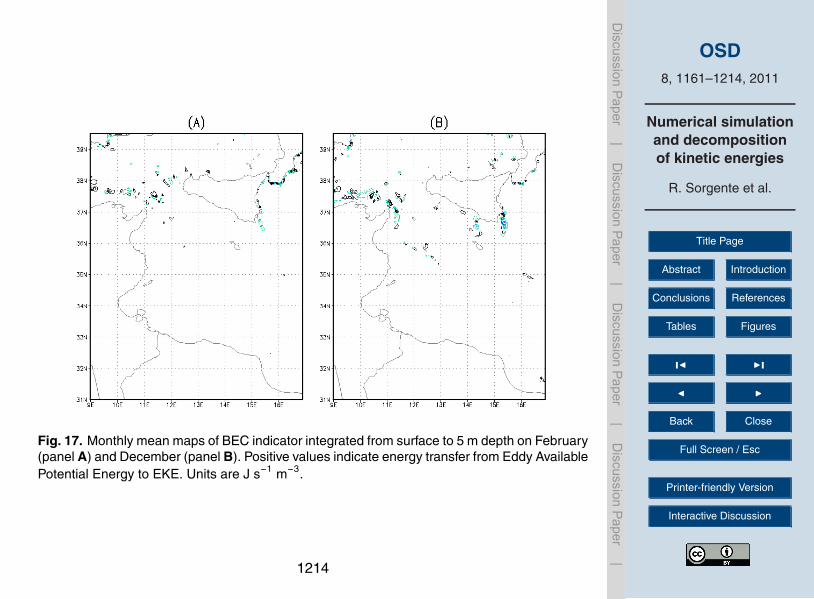
OSD8, 1161–1214, 2011


R. Sorgente et al.

Title Page



Tables Figures

J I

J I

Back Close

Full Screen / Esc



Discussion

Paper

|D

iscussionP

aper|

Discussion

Paper

|D

iscussionP

aper|

61

1

Figure 17. Monthly mean maps of BEC indicator integrated from surface to 5 m depth 2

on February (panel A) and December (panel B). Positive values indicate energy transfer 3

from Eddy Available Potential Energy to EKE. Units are J s-1 m-3. 4

Fig. 17. Monthly mean maps of BEC indicator integrated from surface to 5 m depth on February(panel A) and December (panel B). Positive values indicate energy transfer from Eddy AvailablePotential Energy to EKE. Units are J s−1 m−3.

1214





Numerical simulation and decomposition of kinetic energies

Documents

Transcript of Numerical simulation and decomposition of kinetic energies