Citation: Kamperidis, T.;

Tremouli, A.; Peppas, A.;

Lyberatos, G. A 2D Modelling

Approach for Predicting the

Response of a Two-Chamber

Microbial Fuel Cell to Substrate

Concentration and Electrolyte

Conductivity Changes. Energies 2022,

15, 1412. https://doi.org/10.3390/

en15041412

Academic Editors:

Constantinos Noutsopoulos,

Panagiotis G. Kougias and

Attilio Converti

Received: 30 December 2021

Accepted: 12 February 2022

Published: 15 February 2022

Publisher’s Note: MDPI stays neutral

with regard to jurisdictional claims in

published maps and institutional affil-

iations.

Copyright: © 2022 by the authors.

Licensee MDPI, Basel, Switzerland.

This article is an open access article

distributed under the terms and

conditions of the Creative Commons

Attribution (CC BY) license (https://

creativecommons.org/licenses/by/

4.0/).

energies

Article

A 2D Modelling Approach for Predicting the Response of aTwo-Chamber Microbial Fuel Cell to Substrate Concentrationand Electrolyte Conductivity ChangesTheofilos Kamperidis 1, Asimina Tremouli 1,*, Antonis Peppas 1 and Gerasimos Lyberatos 1,2

1 School of Chemical Engineering, National Technical University of Athens, 15780 Athens, Greece;kamp.theo@gmail.com (T.K.); antonis93@windowslive.com (A.P.); lyberatos@chemeng.ntua.gr (G.L.)

2 Institute of Chemical Engineering Sciences (ICE-HT), Stadiou Str., Platani, 26504 Patras, Greece* Correspondence: atremouli@chemeng.ntua.gr

Abstract: Bioelectrochemical systems have been the focus of extensive research due to their uniqueadvantages of converting the chemical energy stored in waste to electricity. To acquire a betterunderstanding and optimize these systems, modelling has been employed. A 2D microbial fuelcell (MFC) model was developed using the finite element software Comsol Multiphysics® (version5.2), simulating a two-chamber MFC operating in batch mode. By solving mass and charge balanceequations along with Monod–Butler–Volmer kinetics, the operation of the MFC was simulated. Themodel accurately describes voltage output and substrate consumption in the MFC. The computationalresults were compared with experimental data, thus validating the model. The voltage output andsubstrate consumption originating from the model were in agreement with the experimental datafor two different cases (100 Ω, 1000 Ω external resistances). A polarization curve was extractedfrom the model by shifting the external resistance gradually, calculating a similar maximum power(47 mW/m2) to the observed experimental one (49 mW/m2). The validated model was used to predictthe MFC response to varying initial substrate concentrations (0.125–4 g COD/L) and electrolyteconductivity (0.04–100 S/m) in order to determine the optimum operating conditions.

Keywords: MFC; modelling; BES; bioelectricity; conductivity; concentration

1. Introduction

Bioelectrochemical systems (BES) have been the focus of research due to their abilityto convert the chemical energy contained in various wastewaters to electricity [1,2]. Theoperation of these systems is based on the oxidation of an electron donor followed by thereduction of an electron acceptor. The oxidation reaction takes place in the anode chamberand is catalyzed by electrogenic bacteria, which have the ability to transfer the electronsto their exterior [3]. Similarly, the reduction reaction occurs in the cathode chamber andmay be catalyzed by microorganisms (biocathode) or catalysts such as platinum, activatedcarbon, etc. (abiotic cathodes) [4]. Different types of BES have been developed, suchas microbial fuel cells (MFCs), microbial electrolysis cells (MECs), microbial solar cells(MSCs) [5], microbial electrosynthesis cells [6], microbial desalination cells (MDCs) [7],and enzymatic fuel cells (EFCs) [8]. These electrochemical cells have been developedfor simultaneous wastewater treatment, current generation, and in the case of MECsproduction of other substances such as hydrogen [9]. The most studied BES systems areMicrobial Electrolysis Cells (MECs) and Microbial Fuel Cells (MFCs). In the case of MECsystems, an external voltage is applied in order for electrolysis to take place. [10]. Onthe other hand, the redox reactions that take place in a microbial fuel cell (MFC) occurspontaneously, generating electricity by oxidizing an organic substrate [11]. The plethoraof bioelectrochemical processes which are catalyzed by microorganisms are exhibited inthe multiple BESs that have been developed.

Energies 2022, 15, 1412. https://doi.org/10.3390/en15041412 https://www.mdpi.com/journal/energies

Energies 2022, 15, 1412 2 of 15

The phenomena that take place in BESs are varied and complex. The most im-portant phenomena that take place in BESs have been presented and summarized byRabaey et al. [12]. The different processes that occur within BESs, such as MFCs, can bebroken down into the following phenomena: (i) microbial metabolism on the anode elec-trode; (ii) diffusion of the organic substrate from the bulk into the biofilm of the anodechamber initiating the oxidation reaction of the electron donor; (iii) transport of the organicsubstrate by diffusion and by stirring (convection) in the bulk of the anolyte; (iv) oxidationreaction and production of protons and electrons; and (v) transfer of electrons through thewiring connection (external resistance) from the anodic electrode to the cathodic electrode.In the case of an MEC, instead of the external resistance a voltage is applied between theanode and the cathode. The protons are diffused into the anode and then transportedvia convection and diffusion through the separator to the cathode chamber (vi), to eitherparticipate in the reduction reaction or to balance the concentration gradient between theanode and the cathode. Other substances produced by oxidation are diffused into thebulk of the anolyte. In the cathode chamber, the electron acceptor comes into contactwith the cathodic electrode and, combined with the electrons, starts the reduction reaction(vii). The products of the reduction are deposited on the cathode electrode, settled in thecathode chamber, or mixed with the bulk of the catholyte (viii). Moreover, in the caseof a bio-cathode, microbial metabolism can be studied in the cathode. Overall, chargetransfer and balance are examined in the BES, along with losses regarding the developedvoltage [12].

Modelling is a powerful tool in seeking to understand the complex processes occurringwithin BES systems. Several models have been proposed in this direction. Because of thevarious MFC setups (single chamber, dual chamber) and the variety of materials usedfor the electrodes and the catalysts, in combination with the different phenomena duringthe MFC operation, many models have been developed [13,14]. One of the first modelsdescribing MFC operation was created by Zhang and Halme in 1995 [15]. Zhang andHalme [15] simulated the operation of a dual-chamber MFC using Monod kinetics todescribe the bacterial growth and substrate consumption, coupling this with Faraday’slaw to calculate the current generation. Their model was based on the assumption thatmass transport and the cathodic reaction are faster than the biochemical and oxidationreactions, and thus focused on the latter. As one of the first attempts at MFC modelling, theyhighlighted the importance of maintaining control over the process through simulation [15].An example of a model combining bioelectrochemical kinetics along with mass and chargebalances in a dual-chamber MFC was developed by Zeng et al. in 2009 [16]. The developedmodel aimed to describe an acetate-fed dual chamber MFC with the ability to adapt to otherorganic substrates. In order to describe the electrochemical phenomena, a combination ofthe Butler–Volmer expression and Monod kinetics was utilized. Several of the parametervalues were extracted from experimental data, while others were estimated by the model.Zeng et al. concluded that the cathodic reaction is the liming factor for current generationin an MFC. Furthermore, their results indicated that an increase in the electron donorconcentration was effective in boosting MFC performance [16].

Various approaches have been presented in the literature, with different focus points. Astudy on the biofilm of electrochemically active bacteria during the operation of an MFC wasconducted by Belleville et al., 2019 [17]. A 2D model was developed, examining at a cellularlevel the microorganisms on the anodic electrode. Taking into account microbial growthand segregation, their model aimed to predict the different types of bacteria (methanogens,electrogens) that grow, perish or detach from the electrode during the operation of a glucose-fed MFC [17]. Serra et al., 2019 focused on the power output of MFCs through polarizationcurves and created a steady-state electrical model to simulate them [18]. The polarizationexperiments were conducted by varying the external resistance on six different MFCs from1000 Ω to 20 Ω, with simultaneous refreshment of the synthetic wastewater. The model haddifferent kinetics for the different power losses (activation, ohmic, concentration) whichmay be present during MFC operation [18].

Energies 2022, 15, 1412 3 of 15

Furthermore, the various operation modes of MFCs have been examined. A 2D modelfor simulating the operation of a continuously fed, single-chamber MFC was developed byDay et al., 2021 [19]. Different parameters such as the variation of the hydraulic retentiontime (HRT) and the alteration of MFC geometry were examined in order to determinethe optimal conditions for simultaneous maximum current generation and substrate con-sumption. Matsena et al., 2021 created a model simulating the operation of an MFC withhexavalent chromium as the electron acceptor [20]. Monod kinetics were used to describethe growth of the biofilm taking into account inhibition by the substrate and the intracellu-lar mediator. Moreover, two types of microorganisms were considered: one that contributesto electricity generation and one that consumes the substrate without releasing electrons. Todescribe the electrochemistry, the Butler–Volmer expression was utilized, while Faraday’slaw was used to couple the electrochemistry with the microbial activity. In order to simulatethe reduction of hexavalent chromium, they combined Faraday’s law with Butler–Volmer,and the mass balance equation was derived from the reaction of dichromate (Cr2O−7 ) toCr(III) [20].

Apart from simulations describing MFC operation, models have been developed tosupport experiments. Thus, Sindhuja et al., 2016 conducted electrochemical impedancespectroscopy (EIS) experiments in a dual chamber MFC and developed a model to extractthe equivalent circuit [21]. The model was developed for an MFC with charcoal electrodes,and was used along with a fitting model of a Nyquist plot for graphite electrodes. Their aimwas the determination of internal resistances in both experimental configurations (charcoal,graphite based electrodes respectively) and the estimation of the rate determining stepin their MFC operation with glucose as the organic substrate [21]. Oliveira et al., 2013published a study presenting a 1D MFC model [22]. This particular model incorporatedheat, charge, and mass transfer phenomena at a steady state across an MFC configurationconsisting of an anodic electrode, a biofilm, the anolyte solution, the separator (proton ex-change membrane), the catholyte, and the cathodic electrode. They successfully comparedtheir computational data to the respective results presented by Zeng et al., 2009 [16,22]. Bybriefly presenting these models, it is easy to deduce that MFC modelling is applied overdifferent focus points (i.e., cellular level, spatial and time dependent, or dimensionless),resulting in a plethora of publications describing different aspects of this technology.

The aim of this work was to develop a time-dependent 2D MFC model containing massand charge conservation and transfer phenomena along with combined Butler–Volmer–Monod kinetics. The model was developed with minimal computational requirementsin order to extract quick and accurate results taking into account the geometry of the celland the materials that comprise it. This model examines glucose consumption in an H-type MFC, calculating the voltage output, substrate consumption and polarization curves.The model proposed an approach to quickly predict and validate optimal conditions forMFC operation. This was accomplished by the use of electrochemical kinetics along withparameters determined by experimental data fitting. The focus of this work was thecreation of an improved model to quickly predict accurate conditions, in order to improvethe performance of the particular MFC setup.

2. Materials and Methods2.1. Experimental Setup

The model was based upon a dual-chamber MFC in order to validate the compu-tational results with experimental data. Specifically, an H-type MFC was operated inbatch mode, consisting of an anode (0.3 L) and a cathode (0.3 L). The solutions in bothchambers were continuously stirred. Plain graphite paper (3.8 cm × 2.5 cm) and graphitecloth (3.8 cm × 2.5 cm) coated with Pt as the oxygen reduction catalyst were used as theanodic electrode and the cathodic electrode, respectively. Titanium wire and a silver con-ductive epoxy (Conductive Epoxy, Circuit Works) were used for the electrode connection.A proton exchange membrane (Nafion® 117, DuPont–PEM) was placed between the twochambers. Both chambers were under continuous stirring and operated in a temperature

Energies 2022, 15, 1412 4 of 15

control environment set at 30 C. A resistance box set at 100 Ω was connected to thecell. The cell was operated with synthetic glucose wastewater (1 g COD/L) in the anode,containing a phosphate buffer (3.67 g/L NaH2PO4 and 3.45 g/L Na2HPO4), potassiumchloride (0.16 g/L KCl), sodium bicarbonate (5 g/L NaHCO3), and solutions containingelements necessary for the microbia (1% v/v, presented in Table 1, based on [23]). Duringthe acclimation period, anaerobic sludge (10% v/v) was added to the synthetic glucosewastewater (10 g COD/l). For the cathode phosphate buffer, (3.67 g/L NaH2PO4 and3.45 g/L Na2HPO4) and potassium chloride (0.16 g/L KCl) were used. The cathode cham-ber was continuously sparged with air, supplying the electron acceptor (O2).

Table 1. Composition of trace elements solutions used in the synthetic glucose feed.

Component Concentration (mg/L)

Solution A

CaCl2·2H2O 22,500NH4Cl 35,900

MgCl2·2H2O 16,200KCl 117,000

MnCl2·4H2O 1800CoCl2·6H2O 2700

H3BO3 513CuCl2·2H2O 243

Na2MoO4·2H2O 230ZnCl2 189

NiCl2·6H2O 200H2WO4 10

Solution B

FeSO4 700

Solution C

(NH4)2PO4 7210

The cell’s potential was recorded at set intervals (2 min) using an Agilent Keysight34972A LXI Data Acquisition/Switch Unit. The pH and conductivity were measured bydigital instruments, (WTW INOLAB PH720) and (WTW INOLAB), respectively. SolubleCOD was measured according to standard methods [24]. Polarization experiments wereconducted by altering the resistance on the resistance box. Initially, the system achievedopen circuit voltage (OCV) by removing the external resistance for 3 h, thus resulting ininfinite resistance between the two electrodes. Then, the resistance box was connectedto the cell and different consecutive resistances were applied (1 MΩ–0 Ω). Each externalresistance was applied for 6 min, recording the voltage and the current every 2 min. Thecurrent was measured using a multimeter.

2.2. Model Description

The model was developed in the finite element software (FEM) Comsol Multiphysics®

Version 5.2. The model focused on the description of the voltage output, the organicsubstrate (glucose) consumption, and the estimation of the maximum power throughpolarization curves. Experimentally, the glucose concentration was measured in g COD/L;however, in the model, the corresponding glucose concentration (mol/m3) was determined.For this reason, the organic substrate results were normalized with the initial value (C/C0).

The geometry was a vertical section (2D) of the MFC, depicted in Figure 1a. It con-sisted of an anode, a cathode, the separator (PEM membrane [25]), and the two electrodes(2.5 cm × 3.8 cm). The third dimension (z-axis) was considered equal to the width of theelectrodes (2.5 cm). The distance between the two electrodes was 15 cm. The cell wasconsidered to operate in batch mode and at a set temperature (32 C). As the electron donor

Energies 2022, 15, 1412 5 of 15

to be oxidized by the electrogen biofilm, glucose was chosen. The reaction assumed to takeplace in the biofilm was [26]:

C6H12O6 + 6 H2O→ 6 CO2 + 24 H+ + 24 e− (1)

Energies 2022, 15, x FOR PEER REVIEW 5 of 16

however, in the model, the corresponding glucose concentration (mol/m3) was deter-mined. For this reason, the organic substrate results were normalized with the initial value (C/C0).

The geometry was a vertical section (2D) of the MFC, depicted in Figure 1a. It con-sisted of an anode, a cathode, the separator (PEM membrane [25]), and the two electrodes (2.5 cm × 3.8 cm). The third dimension (z-axis) was considered equal to the width of the electrodes (2.5 cm). The distance between the two electrodes was 15 cm. The cell was con-sidered to operate in batch mode and at a set temperature (32 °C). As the electron donor to be oxidized by the electrogen biofilm, glucose was chosen. The reaction assumed to take place in the biofilm was [26]:

C6H12O6 + 6 H2O → 6 CO2 + 24 H+ + 24 e− (1)

Figure 1. (a) Schematic of the MFC domain in the model and (b) concise algorithm of the model.

The biofilm was considered to be on the surface of the anodic electrode such that glucose reacted as it came into contact with it. Despite the porosity of graphite paper and the presence of microorganisms, the reaction was assumed to take place homogeneously on the electrode. In the anode chamber, the carbon dioxide was considered dissolved in the liquid, thus taking into account only the liquid phase. Furthermore, due to the pres-ence of a phosphate buffer, the changes in the anodic pH were considered negligible. The concentration of microorganisms was considered constant, as the assumption was made

Figure 1. (a) Schematic of the MFC domain in the model and (b) concise algorithm of the model.

The biofilm was considered to be on the surface of the anodic electrode such thatglucose reacted as it came into contact with it. Despite the porosity of graphite paper andthe presence of microorganisms, the reaction was assumed to take place homogeneouslyon the electrode. In the anode chamber, the carbon dioxide was considered dissolvedin the liquid, thus taking into account only the liquid phase. Furthermore, due to thepresence of a phosphate buffer, the changes in the anodic pH were considered negligible.The concentration of microorganisms was considered constant, as the assumption wasmade that the growth rate was equal to the decline rate. This assumption led to a constantbiofilm present on the anodic electrode. Moreover, the biofilm was assumed to consistonly of electrogenic bacteria and no competing biomass was considered to be present. Thedescription of the electrochemical reaction rate (mol/m2/s) taking place in the biofilm

Energies 2022, 15, 1412 6 of 15

used the Monod–Butler–Volmer expression. This equation combines the organic substrateconsumption rate and the effect of electrochemical phenomena on it, taking into accountthe overpotential:

R1 = k1CGlucose

KGlucose + CGlucoseexp

(aaFRT

ηa

)(2)

where k1 (mol/(m2·h)) is the maximum specific growth rate multiplied by the biomassconcentration (k1 = k0

1·Xbio), CGlucose (mol/m3) is the concentration of glucose in the anodechamber, KGlucose (mol/m3) is the half velocity rate constant for glucose, aa is the anodictransfer coefficient, F (C/mol) is Faraday’s constant, R (J/(mol·K)) is the gas constant, T(K) is the temperature, and ηa (V) is the anode overpotential. No inhibition of microbialactivity by the organic substrate was considered.

Through the separator, only protons were transferred. The cathodic chamber wasconsidered to be operating with a phosphate buffer as the catholyte, resulting in negligiblevariations of pH. The electrons were transferred to the cathode electrode through externalresistance, which was set at 100 Ω during batch cycles and varied accordingly duringpolarization experiments. The dissolved oxygen was assumed to react when in contactwith the cathode electrode. The concentration of dissolved oxygen was considered constantbecause of the continuous supply of air in the cathode chamber. The reduction reaction(proton consuming [12]) taking place on the cathodic electrode was

O2 + 4 H+ + 4 e− → 2 H2O (3)

It was assumed that no diffusion of oxygen from the cathode to the anode wouldtake place. To describe the rate of the reaction in Equation (3), a Monod–Butler–Volmerkinetic was employed, assuming a Monod-type dependence on dissolved oxygen concen-tration [27]:

R2 = k2COxygen

KOxygen + COxygenexp

(aCFRT

ηc

)(4)

where k2 (m12/(m4·h)) is the forward rate constant of cathode reaction, COxygen (mol/m3)is the concentration of dissolved oxygen in the cathode chamber, KOxygen (mol/m3) is thehalf velocity rate constant for oxygen, aC is the cathode transfer coefficient, and ηc (V) isthe cathode overpotential.

The correlation between reaction and rate and current development was carried outusing Faraday’s law:

Ri =νiiA/C

niF(5)

where νi is the stoichiometric coefficient (i = glucose or oxygen), iA (A/m2) is the currentdensity (anode or cathode), and ni the number of electrons that take part in the reaction.

The algorithm of the model is presented in Figure 1b. After selection of an initial glu-cose concentration, the simulation is initiated and the reaction rate on the anode electrodesurface is calculated by Monod–Butler–Volmer kinetics. The initial value for the voltagebetween the two electrodes is 0 V. Using Faraday’s law, the current density on the anodeis calculated based on the reaction rate. Through external resistance, the current bringselectrons to the cathode electrode, where oxygen reduction takes place. The respectivecurrent density is calculated by Faraday’s law based on the oxygen reduction reaction rate.The charge balance equations calculate the total transfer of charge throughout the cell andthe voltage developed between the two electrodes. The overpotential is determined basedon the voltage and the standard potentials of the reactions. Simultaneously, the decreasein the glucose concentration and the respective glucose distribution is determined. As anew glucose concentration on the electrode surface is calculated, a new reaction rate isdetermined, taking into account the new overpotential value.

Energies 2022, 15, 1412 7 of 15

2.3. Mass and Charge Transfer Equations

The anode and the cathode chambers were considered to be full of the aforementionedsynthetic solutions. For the transfer of mass through the anode and the cathode the Nernst–Planck equation was used. This equation takes into account the change of concentration intime and the transport of chemical species by diffusion, convection, and migration. Thisequation takes into account the transport of species due to the concentration gradient(diffusion), by the movement of the bulk of the fluid (convection), and due to the presenceof an electric field (migration).

∂c∂t−∇·

[D∇c− uc +

zFRT

c(∇ϕ)

]=

0, in the bulk

R, on the electrode sur f ace(6)

where D (m2/s) is the diffusion coefficient of the species, u (m/s) is the velocity vector ofthe liquid, z is the valence of the ionic species, ϕ (V) is the potential, and R (mol/(m2·h))is the reaction rate. A no flux condition was applied on the walls; similarly, no flux wasapplied on the separator. Inside the cell, an incompressible Newtonian fluid was assumed.

For the charge transfer in the cell, Ohm’s law was used along with charge balanceequations. More specifically, a uniform electrolyte medium was assumed for the transfer ofcharged ions, and activation overpotentials were taken into account as well:

∇·ii = Qi (7)

ii = σi∇ϕi (8)

where ii (A/m2) is the current density (i = electrode/electrolyte), Q (C) is the total charge, σ(S/m) is the conductivity, and ϕ (V) is the potential. Ohmic changes in the electricalconnections were considered negligible. For the calculation of the cell’s voltage, thestandard reaction potential, the anode and cathode overpotential, and the ohmic losses inthe electrolyte were considered using the following equation:

Vcell = E0 + ηanode + ηcathode + Rcell icell (9)

where E0 (V) is the standard redox potentials and Rcell (Ω) is the internal resistance of thecell, consisting of the separator and the electrolyte resistances. Furthermore, Ohm’s lawwas used to calculate the voltage between the anode and cathode electrodes:

Vcell = IRext (10)

where I (A) is the current of the closed circuit and Rext (Ω) is the external resistanceconnected in the MFC. After the initial simulation runs, the capacitance of the electrodeswas incorporated into the model in order to further examine its effect. The followingequation was added to take into account the changes in the potential in the electrodeelectrolyte interface, as well as the capacitance:

i =(

∂(ϕelectrode)

∂t

)Celectrode (11)

where Celectrode (F/m) is the capacitance of the electrode. In the anode, the capacitance takesinto account the biofilm’s existence and is different for every acclimation, namely everybiofilm. The capacitance depends on the type of the electrode as well.

The parameters of the aforementioned equations were extracted by a fitting modeldeveloped using Aquasim 2.0 software [28]. This model was a modified version of the oneused by Zeng et al., 2009 [16]. The model contained altered mass balance equations in orderto simulate a batch reactor instead of a CSTR. Glucose was assumed as the electron donor,

Energies 2022, 15, 1412 8 of 15

and Andrews kinetics were used instead of Monod. The resulting Andrews–Butler–Volmerequation is as follows:

Ri = kiCGlucose

KGlucose + CGlucose +CGlucose

2

Ki

exp(

aaFRT

ηa

)(12)

where Ki (mol/m3) is the inhibition of the glucose concentration. Experimental data on theoperation of the previously-described dual chamber MFC were used as input values forthe estimation of the parameters. The results and additional details of the Aquasim modelare presented elsewhere [28]. The values of the parameters used are presented in Table 2.

3. Results3.1. Model Results and Validation

The model presented fast convergence in under one minute, simulating the consump-tion of glucose in the MFC and the simultaneous voltage output. Initially, the results fromthe model were compared with the operation of the two-chamber MFC, with the external re-sistance set at 100 Ω. Figure 2a presents the concentration of the organic substrate calculatedduring one batch cycle as extracted by the model, as well as the concentration obtained fromthe experiments. Figure 2b shows the voltage output of the cells as calculated by the modelalong with the respective values originating from the experiment. Specifically, the concen-tration was normalized to the initial substrate concentration (1 g COD/L), while voltagerecording started as soon as the MFC was fed with fresh glucose synthetic wastewater.

Energies 2022, 15, x FOR PEER REVIEW 8 of 16

donor, and Andrews kinetics were used instead of Monod. The resulting Andrews–But-ler–Volmer equation is as follows: 𝑅 = 𝑘 𝐶𝐾 + 𝐶 + 𝐶 𝐾 exp (𝑎 𝐹𝑅𝑇 𝜂 ) (12)

where Ki (mol/m3) is the inhibition of the glucose concentration. Experimental data on the operation of the previously-described dual chamber MFC were used as input values for the estimation of the parameters. The results and additional details of the Aquasim model are presented elsewhere [28]. The values of the parameters used are presented in Table 2.

3. Results 3.1. Model Results and Validation

The model presented fast convergence in under one minute, simulating the con-sumption of glucose in the MFC and the simultaneous voltage output. Initially, the results from the model were compared with the operation of the two-chamber MFC, with the external resistance set at 100 Ω. Figure 2a presents the concentration of the organic sub-strate calculated during one batch cycle as extracted by the model, as well as the concen-tration obtained from the experiments. Figure 2b shows the voltage output of the cells as calculated by the model along with the respective values originating from the experiment. Specifically, the concentration was normalized to the initial substrate concentration (1 g COD/L), while voltage recording started as soon as the MFC was fed with fresh glucose synthetic wastewater.

Figure 2. Comparison of simulated results (blue line) with experimental data (red circles and red dashed line) for the MFC with the external resistance set at 100 Ω. Glucose concentration versus time (a) and voltage output (b). The black arrows in both figures indicate the point when the voltage plateau drops.

As shown in Figure 2a, the concentration initially presents a linear drop, then tends asymptotically to zero (blue line Figure 2a). The COD removal achieved by the cell was 91% (Figure 2a). The simulation continued until the substrate concentration inside the cell reached 0 mol/m3. The operation cycle lasted for 75 h, while the simulated time for the model was 100 h (Figure 2a). The model predicted a 98% substrate consumption at the 75 h mark. The experimental measurements of substrate concentration (red circles) were in agreement with the simulation data.

The voltage output originating from the model at 100 Ω was close to the experimental data (Figure 2b). In particular, the maximum voltage was 29 mV, while the respective voltage peak during the experiment was 31 mV. The voltage plateau was close, and with the same duration for both experimental and computational results (~40 h). The difference between the experiment and the model was that the plateau formed immediately in the model (0 h), while in the experiment the maximum voltage was achieved after 10 h of cell

Figure 2. Comparison of simulated results (blue line) with experimental data (red circles and reddashed line) for the MFC with the external resistance set at 100 Ω. Glucose concentration versustime (a) and voltage output (b). The black arrows in both figures indicate the point when the voltageplateau drops.

As shown in Figure 2a, the concentration initially presents a linear drop, then tendsasymptotically to zero (blue line Figure 2a). The COD removal achieved by the cell was91% (Figure 2a). The simulation continued until the substrate concentration inside the cellreached 0 mol/m3. The operation cycle lasted for 75 h, while the simulated time for themodel was 100 h (Figure 2a). The model predicted a 98% substrate consumption at the75 h mark. The experimental measurements of substrate concentration (red circles) were inagreement with the simulation data.

The voltage output originating from the model at 100 Ω was close to the experimentaldata (Figure 2b). In particular, the maximum voltage was 29 mV, while the respectivevoltage peak during the experiment was 31 mV. The voltage plateau was close, and withthe same duration for both experimental and computational results (~40 h). The differencebetween the experiment and the model was that the plateau formed immediately in themodel (0 h), while in the experiment the maximum voltage was achieved after 10 h of

Energies 2022, 15, 1412 9 of 15

cell operation. This was attributed to glucose diffusion in the biofilm and the activationenergy required to initiate glucose oxidation. On the other hand, in the model the reactiontakes place on the electrode surface and comes immediately into contact with the organicsubstrate, thus achieving the maximum value at the beginning of the cycle. The seconddifference between the results of the experimental data and the model prediction is observedafter the plateau and the voltage decrease trend. The experimental data show that it takes19 h for the voltage to be reduced to 0 V; however, the model requires 59 h to decrease thisvalue to 0 V. This deviation is attributed to the ohmic losses which are present during theexperiment because of the electrical connections. In the case of the model (100 Ω), a slowerand smoother voltage decline takes place. Overall, the model fitting regarding the voltageoutput of the units at 100 Ω external load is considered to be satisfactory. The experimentaldata used in the modified Zang model Formatting Citation were extracted from theoperation of the cell with 100 Ω external resistance. The voltage output and the substrateconsumption were in good agreement with the experimental measurements in the MFCoperated with 100 Ω, as these experimental data were used for the parameter calculation.

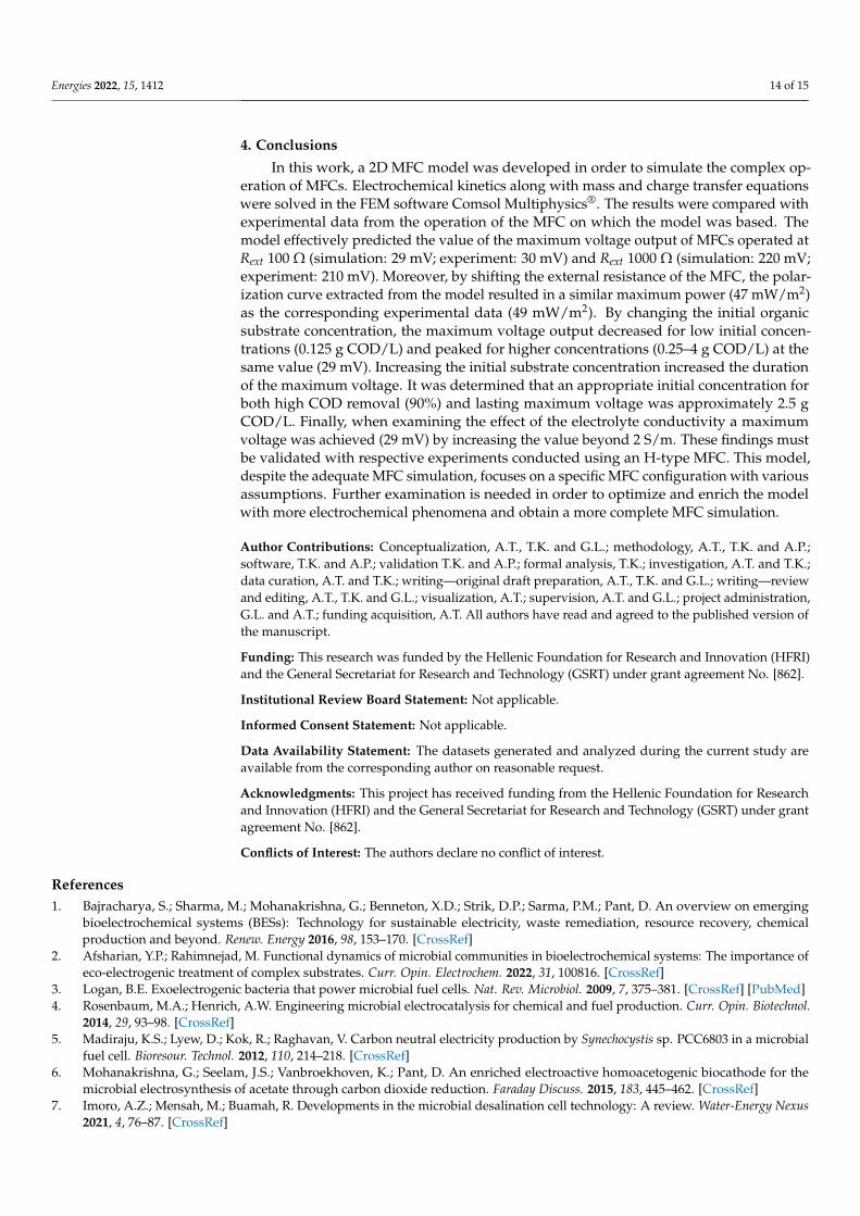
For better understanding of the organic substrate distribution, four different imagesare presented in Figure 3. The concentration of glucose was normalized to the initialvalue (C0).

Energies 2022, 15, x FOR PEER REVIEW 9 of 16

operation. This was attributed to glucose diffusion in the biofilm and the activation energy required to initiate glucose oxidation. On the other hand, in the model the reaction takes place on the electrode surface and comes immediately into contact with the organic sub-strate, thus achieving the maximum value at the beginning of the cycle. The second dif-ference between the results of the experimental data and the model prediction is observed after the plateau and the voltage decrease trend. The experimental data show that it takes 19 h for the voltage to be reduced to 0 V; however, the model requires 59 h to decrease this value to 0 V. This deviation is attributed to the ohmic losses which are present during the experiment because of the electrical connections. In the case of the model (100 Ω), a slower and smoother voltage decline takes place. Overall, the model fitting regarding the voltage output of the units at 100 Ω external load is considered to be satisfactory. The experimental data used in the modified Zang model Formatting Citation were extracted from the operation of the cell with 100 Ω external resistance. The voltage output and the substrate consumption were in good agreement with the experimental measurements in the MFC operated with 100 Ω, as these experimental data were used for the parameter calculation.

For better understanding of the organic substrate distribution, four different images are presented in Figure 3. The concentration of glucose was normalized to the initial value (C0).

Figure 3. Organic substrate distribution (normalized concentration C/C0) for 0, 25, 50 and 75 h, with 100 Ω external resistance.

The distribution of the substrate is presented in Figure 3a, at a point when the oxida-tion had not started yet. At 25 h (Figure 3b) the substrate consumption was 45%, at 50 h (Figure 3c) it was 87%, and at 75 h it was 98% (Figure 3d). The distribution of the substrate in the anodic chamber is uniform, with the exception of a gradient present at 25 h and 50 h. This was observed around the anodic electrode, as expected, as the reaction takes place on its surface. Moreover, in all four cases (Figure 3 a–d) the effect of the separator was seen to inhibit the transfer of glucose from the anode to the cathode (Ccathode = 0, dark blue color).

In order to validate the model and test its ability to predict MFC performance with Rext 1000 Ω, more data were compared. Figure 4 presents the results of the simulation of glucose concentration and the voltage output during cell operation (at Rext 1000 Ω) in com-parison with the respective experimental data.

Figure 3. Organic substrate distribution (normalized concentration C/C0) for 0, 25, 50 and 75 h, with100 Ω external resistance.

The distribution of the substrate is presented in Figure 3a, at a point when the oxidationhad not started yet. At 25 h (Figure 3b) the substrate consumption was 45%, at 50 h(Figure 3c) it was 87%, and at 75 h it was 98% (Figure 3d). The distribution of the substratein the anodic chamber is uniform, with the exception of a gradient present at 25 h and 50 h.This was observed around the anodic electrode, as expected, as the reaction takes place onits surface. Moreover, in all four cases (Figure 3a–d) the effect of the separator was seen toinhibit the transfer of glucose from the anode to the cathode (Ccathode = 0, dark blue color).

In order to validate the model and test its ability to predict MFC performance withRext 1000 Ω, more data were compared. Figure 4 presents the results of the simulationof glucose concentration and the voltage output during cell operation (at Rext 1000 Ω) incomparison with the respective experimental data.

Energies 2022, 15, 1412 10 of 15Energies 2022, 15, x FOR PEER REVIEW 10 of 16

Figure 4. Comparison of simulated results (blue line) with experimental data (red circles and red dashed line) for the MFC with external resistance set at 1000 Ω. Glucose concentration (a) and volt-age output (b) versus time. The black arrows in both figures indicate the point when the voltage plateau drops.

By shifting the external resistance in the model to 1000 Ω, similar results were ob-tained with the respective experimental data (Figure 4). The experimental COD removal was 89% at the end of the batch cycle. The cycle duration for the 1000 Ω experiment was 92 h, close to the simulated time (110 h) for the full depletion of substrate in the anode chamber. At 92 h, the model calculated 98% substrate consumption (Figure 4a). A similar pattern is observed from the results originating from the system set at 100 Ω, as expected, as the consumption of glucose primarily depends on the Monod kinetics and not on the external resistance. The substrate concentration decreased similarly in the model and the experiment. The voltage output peak was 220 mV for the model and 210 mV for the ex-periment (Figure 4b). The voltage plateau was maintained for 63 h in the simulation and 72 h in the experiment. The voltage output reached its maximum value (210 mV) after 10 h of cell operation, while the model predicted the voltage to reach its maximum value (220 mV) at 0 h. The voltage decrease lasted for 52 h simulated time, while this decrease in the experiment was faster (7 h). Similar to Figure 2b, the time difference between the model and the experiment is attributed to glucose diffusion within the biofilm, and to the voltage losses on account of the electrical connections and cell geometry (H-type). Moreover, when the simulated voltage plateau ceased in both cases, at 40 h and 63 h, respectively (see black arrows in Figures 2b and 4b), the organic substrate was reduced by 75% and 81%, respectively (see black arrows in Figures 2a and 4a). The prediction of the MFC op-eration with an external resistance set at 1000 Ω was considered successful, validating the developed model.

After simulating the MFC operation with two different external resistances (100 Ω, 1000 Ω) and comparing the results with experimental data, the next step was the extrac-tion of the polarization curve. A parametric study was carried out on the external re-sistance variable, testing a range of values (0.5 MΩ–0 Ω).

The polarization curve calculated by the model (blue line Figure 5) was in agreement with the respective curve resulting from the experiment. Both power and current values were normalized to the surface of the anodic electrode (Table 2) in order for the results to be easily comparable with other cases. The model’s maximum power density (47 mW/m2) was obtained at an external resistance equal to 5000 Ω and current density equal to 63 mA/m2. The corresponding experimental power density (49 mW/m2) was achieved at 1900 Ω and 80 mA/m2. Despite the apparent consistency of these results, the same maximum power was achieved for different external resistances (Simulation: 5000 Ω, Experiment: 1900 Ω) and consequently different current densities (see blue and red arrows in Figure 5). On the other hand, the model was able to predict the range of the current densities 2.6–154 mA/m2 produced by the MFC (0–149 mA/m2). The difference between the experi-mental and the computational polarization curves was observed in the 20–140 mA/m2

Figure 4. Comparison of simulated results (blue line) with experimental data (red circles and reddashed line) for the MFC with external resistance set at 1000 Ω. Glucose concentration (a) andvoltage output (b) versus time. The black arrows in both figures indicate the point when the voltageplateau drops.

By shifting the external resistance in the model to 1000 Ω, similar results were obtainedwith the respective experimental data (Figure 4). The experimental COD removal was 89%at the end of the batch cycle. The cycle duration for the 1000 Ω experiment was 92 h, close tothe simulated time (110 h) for the full depletion of substrate in the anode chamber. At 92 h,the model calculated 98% substrate consumption (Figure 4a). A similar pattern is observedfrom the results originating from the system set at 100 Ω, as expected, as the consumptionof glucose primarily depends on the Monod kinetics and not on the external resistance. Thesubstrate concentration decreased similarly in the model and the experiment. The voltageoutput peak was 220 mV for the model and 210 mV for the experiment (Figure 4b). Thevoltage plateau was maintained for 63 h in the simulation and 72 h in the experiment. Thevoltage output reached its maximum value (210 mV) after 10 h of cell operation, whilethe model predicted the voltage to reach its maximum value (220 mV) at 0 h. The voltagedecrease lasted for 52 h simulated time, while this decrease in the experiment was faster(7 h). Similar to Figure 2b, the time difference between the model and the experiment isattributed to glucose diffusion within the biofilm, and to the voltage losses on accountof the electrical connections and cell geometry (H-type). Moreover, when the simulatedvoltage plateau ceased in both cases, at 40 h and 63 h, respectively (see black arrows inFigures 2b and 4b), the organic substrate was reduced by 75% and 81%, respectively (seeblack arrows in Figures 2a and 4a). The prediction of the MFC operation with an externalresistance set at 1000 Ω was considered successful, validating the developed model.

After simulating the MFC operation with two different external resistances (100 Ω,1000 Ω) and comparing the results with experimental data, the next step was the extractionof the polarization curve. A parametric study was carried out on the external resistancevariable, testing a range of values (0.5 MΩ–0 Ω).

The polarization curve calculated by the model (blue line Figure 5) was in agreementwith the respective curve resulting from the experiment. Both power and current valueswere normalized to the surface of the anodic electrode (Table 2) in order for the results to beeasily comparable with other cases. The model’s maximum power density (47 mW/m2) wasobtained at an external resistance equal to 5000 Ω and current density equal to 63 mA/m2.The corresponding experimental power density (49 mW/m2) was achieved at 1900 Ω and80 mA/m2. Despite the apparent consistency of these results, the same maximum powerwas achieved for different external resistances (Simulation: 5000 Ω, Experiment: 1900 Ω)and consequently different current densities (see blue and red arrows in Figure 5). On theother hand, the model was able to predict the range of the current densities 2.6–154 mA/m2

produced by the MFC (0–149 mA/m2). The difference between the experimental and thecomputational polarization curves was observed in the 20–140 mA/m2 range. In Figure 5,

Energies 2022, 15, 1412 11 of 15

the I–V curves for both the experiment (red line) and the simulation (blue line) are presented.The slope of the lines indicates in both cases the ohmic resistance as the main cause ofelectrochemical losses. The OCV of the model was 0.75 V, while the respective valuemeasured in the experiment was 0.7. In the simulated I–V curve, apart from the ohmiclosses the effect of substrate diffusion is visible for high current densities and low voltages.The experimental I–V line does not indicate other electrochemical losses apart from ohmic.

Energies 2022, 15, x FOR PEER REVIEW 11 of 16

range. In Figure 5, the I–V curves for both the experiment (red line) and the simulation (blue line) are presented. The slope of the lines indicates in both cases the ohmic resistance as the main cause of electrochemical losses. The OCV of the model was 0.75 V, while the respective value measured in the experiment was 0.7. In the simulated I–V curve, apart from the ohmic losses the effect of substrate diffusion is visible for high current densities and low voltages. The experimental I–V line does not indicate other electrochemical losses apart from ohmic.

Table 2. List of model parameters presented in the order their equations were presented (1–12).

Symbol Description Unit Value Source 𝑘 Maximum specific growth rate mol m−2 h−1 6 × 10−3

Calculated by Aquasim model [28]

𝐾 Half–velocity rate constant for glucose mol m−3 3 × 10−4 𝑎 Anode transfer coefficient – 0.05 𝑘 Forward rate constant of

cathode reaction m12 mol−4 h−1 9.19 × 10−5 𝐾 Half–velocity rate constant

for oxygen mol m−3 4 × 10−3 𝑎 Cathode transfer coefficient – 0.7 ∁ Anode Capacitance F m−2 13,721 ∁ Cathode Capacitance F m−2 500 𝐾 Glucose inhibition constant mol m−3 37 × 10−3

F Faraday’s constant Coulombs mol−1 96,485 [29]

R Gas constant J mol−1 K−1 8.31 𝐶 Dissolved oxygen

concentration in the cathode chamber

mol m−3 0.3125 [30] 𝐷 Glucose diffusion

coefficient m2 s−1 0.5 × 10−9 𝜎 Electrolyte conductivity S m−1 1.2

Experimental values

𝜎 Electrode conductivity S m−1 10 𝐸 Open Circuit Voltage V 0.75 𝑆 Electrode surface cm2 19 𝑆 Separator surface cm2 1 𝑑 Electrode distance cm 17

Figure 5. Comparison of polarization curves extracted by the model and experiments for 1 g COD/Linitial glucose concentration. The blue arrow indicates the maximum simulated power density whilethe red arrow indicates the maximum power density measured in experiments.

Table 2. List of model parameters presented in the order their equations were presented (1–12).

Symbol Description Unit Value Source

k1 Maximum specific growth rate mol m−2 h−1 6 × 10−3

Calculated byAquasim model

[28]

KGlucose Half–velocity rate constant for glucose mol m−3 3 × 10−4

aa Anode transfer coefficient – 0.05

k2Forward rate constant of cathode

reaction m12 mol−4 h−1 9.19 × 10−5

KOxygen Half–velocity rate constant for oxygen mol m−3 4 × 10−3

aC Cathode transfer coefficient – 0.7

Canode Anode Capacitance F m−2 13,721

Ccathode Cathode Capacitance F m−2 500

KS Glucose inhibition constant mol m−3 37 × 10−3

F Faraday’s constant Coulombs mol−1 96,485[29]

R Gas constant J mol−1 K−1 8.31

COxygenDissolved oxygen concentration in the

cathode chamber mol m−3 0.3125[30]

D Glucose diffusion coefficient m2 s−1 0.5 × 10−9

σi Electrolyte conductivity S m−1 1.2

Experimentalvalues

σi Electrode conductivity S m−1 10

E0 Open Circuit Voltage V 0.75

Selectrode Electrode surface cm2 19

Sseparator Separator surface cm2 1

delectrode Electrode distance cm 17

Energies 2022, 15, 1412 12 of 15

3.2. Different Initial Substrate Concentrations

The model was further validated in terms of its ability to predict MFC performancewhen the initial glucose concentration is changed. The initial glucose concentration rangedbetween 0.125–4 g COD/L. In terms of Chemical Oxygen Demand removal (COD), 90%COD removal was considered adequate in a well-performing MFC. The time required forthe 90% COD removal was defined as the time required for the MFC model to achieve asatisfying substrate treatment. Furthermore, the duration of the maximum voltage outputwas maintained for the different initial substrate concentrations. The results are presentedin Figure 6.

Energies 2022, 15, x FOR PEER REVIEW 12 of 16

Figure 5. Comparison of polarization curves extracted by the model and experiments for 1 g COD/L initial glucose concentration. The blue arrow indicates the maximum simulated power density while the red arrow indicates the maximum power density measured in experiments.

3.2. Different Initial Substrate Concentrations The model was further validated in terms of its ability to predict MFC performance

when the initial glucose concentration is changed. The initial glucose concentration ranged between 0.125–4 g COD/L. In terms of Chemical Oxygen Demand removal (COD), 90% COD removal was considered adequate in a well-performing MFC. The time required for the 90% COD removal was defined as the time required for the MFC model to achieve a satisfying substrate treatment. Furthermore, the duration of the maximum voltage out-put was maintained for the different initial substrate concentrations. The results are pre-sented in Figure 6.

Figure 6. Duration of maximum voltage output (Vmax) plateau (black line) and duration until 90% COD removal (red line) versus the initial glucose concentration (g COD/L).

The duration of the plateau during which maximum voltage output was maintained increased with increasing glucose concentration (Figure 6, black line). A similar increase was observed for the time to 90% COD removal, corresponding to a glucose increase (Fig-ure 6, red line). In the case with the glucose concentration at 0.125 g COD/L the maximum voltage value was 15 mV, which was lower than that achieved for the other concentrations (29 mV), and was maintained for less than 1 h. For 0.25, 0.3 g COD/L the maximum voltage (29 mV) was maintained for 1 h as well. As the initial glucose concentration increased, the duration of the maximum voltage increased as well, presenting a linear correlation be-tween the two. For the 90% COD removal duration, a similar pattern was extracted from the model. The time required for 90% COD consumption was higher than the respective duration of the maximum voltage required for lower initial concentrations (0.125–2 g COD/L). On the other hand, for values higher than 2 g COD/L the two lines intersected at approximately 2.5 g COD/L and the duration of the maximum voltage was higher than the corresponding time required for 90% COD removal. This result indicates that there may be an initial concentration which, when fed to an MFC will achieve a more intensive and effective operation in successive batch cycles. Moreover, for lower initial concentra-tions the MFC underperforms in terms of voltage output, as it did not achieve the maxi-mum voltage value. The maximum voltage (29 mV) achieved did not depend on the in-creasing initial glucose concentration for the larger part of the range examined (0.4–4 g COD/L).

Figure 6. Duration of maximum voltage output (Vmax) plateau (black line) and duration until 90%COD removal (red line) versus the initial glucose concentration (g COD/L).

The duration of the plateau during which maximum voltage output was maintainedincreased with increasing glucose concentration (Figure 6, black line). A similar increasewas observed for the time to 90% COD removal, corresponding to a glucose increase(Figure 6, red line). In the case with the glucose concentration at 0.125 g COD/L themaximum voltage value was 15 mV, which was lower than that achieved for the otherconcentrations (29 mV), and was maintained for less than 1 h. For 0.25, 0.3 g COD/Lthe maximum voltage (29 mV) was maintained for 1 h as well. As the initial glucoseconcentration increased, the duration of the maximum voltage increased as well, presentinga linear correlation between the two. For the 90% COD removal duration, a similarpattern was extracted from the model. The time required for 90% COD consumption washigher than the respective duration of the maximum voltage required for lower initialconcentrations (0.125–2 g COD/L). On the other hand, for values higher than 2 g COD/Lthe two lines intersected at approximately 2.5 g COD/L and the duration of the maximumvoltage was higher than the corresponding time required for 90% COD removal. Thisresult indicates that there may be an initial concentration which, when fed to an MFC willachieve a more intensive and effective operation in successive batch cycles. Moreover, forlower initial concentrations the MFC underperforms in terms of voltage output, as it didnot achieve the maximum voltage value. The maximum voltage (29 mV) achieved didnot depend on the increasing initial glucose concentration for the larger part of the rangeexamined (0.4–4 g COD/L).

Energies 2022, 15, 1412 13 of 15

3.3. Different Initial Electrolyte Conductivities

In order to examine the model’s capabilities, a parametric study was conducted onthe effect of electrolyte conductivity, maintaining all other parameters at their respectiveinitial values (Table 2) and the external resistance at 100 Ω. The electrolyte conductivitywas adjusted in the experiments by the addition of potassium chloride, sodium hydroxide,and trace elements, which altogether increased the conductivity of the synthetic glucosesolution to 1.2 S/m. The range of the electrolyte values tested was 0.036 S/m–100 S/m.The initial glucose concentration corresponded to 1 g COD/L.

Figure 7 presents the results of the electrolyte conductivity parametric study. Themaximum voltage output was 30 mV, and the lowest voltage was 2.1 mV. For a betterpresentation of the computational results, a logarithmic scale was used for the x-axis,aiming to indicate the effect of the electrolyte conductivity on the voltage output. The pointof the electrolyte value (1.2 S/m) used in the experiments and the initial runs (100 Ω, 1000 Ω)is highlighted in Figure 7 (black arrow). An increase in the maximum voltage outputwas observed as electrolyte conductivity increased. Furthermore, at higher conductivityvalues (>2 S/m) the maximum voltage from each simulation converged to the same value(30 mV). The initially-selected value of the electrolyte conductivity (1.2 S/m) achieved asimilar maximum voltage (29 mV). These results indicate that by increasing the electrolyteconductivity up to 2 S/m, the maximum voltage output of the MFC increased as well.Further increasing the electrolyte conductivity (>2 S/m) did not have a similar effect onvoltage, and the maximum value remained the same. Based on this conclusion, it wasdeduced that in order to increase the performance of an MFC the addition of electrolytesalts was effective up to a critical value, beyond which adding extra conductivity boostershad no effect on the maximum voltage.

Energies 2022, 15, x FOR PEER REVIEW 13 of 16

3.3. Different Initial Electrolyte Conductivities In order to examine the model’s capabilities, a parametric study was conducted on

the effect of electrolyte conductivity, maintaining all other parameters at their respective initial values (Table 2) and the external resistance at 100 Ω. The electrolyte conductivity was adjusted in the experiments by the addition of potassium chloride, sodium hydrox-ide, and trace elements, which altogether increased the conductivity of the synthetic glu-cose solution to 1.2 S/m. The range of the electrolyte values tested was 0.036 S/m–100 S/m. The initial glucose concentration corresponded to 1 g COD/L.

Figure 7 presents the results of the electrolyte conductivity parametric study. The maximum voltage output was 30 mV, and the lowest voltage was 2.1 mV. For a better presentation of the computational results, a logarithmic scale was used for the x-axis, aim-ing to indicate the effect of the electrolyte conductivity on the voltage output. The point of the electrolyte value (1.2 S/m) used in the experiments and the initial runs (100 Ω, 1000 Ω) is highlighted in Figure 7 (black arrow). An increase in the maximum voltage output was observed as electrolyte conductivity increased. Furthermore, at higher conductivity values (>2 S/m) the maximum voltage from each simulation converged to the same value (30 mV). The initially-selected value of the electrolyte conductivity (1.2 S/m) achieved a similar maximum voltage (29 mV). These results indicate that by increasing the electrolyte conductivity up to 2 S/m, the maximum voltage output of the MFC increased as well. Further increasing the electrolyte conductivity (>2 S/m) did not have a similar effect on voltage, and the maximum value remained the same. Based on this conclusion, it was deduced that in order to increase the performance of an MFC the addition of electrolyte salts was effective up to a critical value, beyond which adding extra conductivity boosters had no effect on the maximum voltage.

Figure 7. Maximum voltage output versus the corresponding electrolyte conductivity. The black arrow indicates the electrolyte conductivity value used in the experiments and in the initial model simulation.

The different electrolyte conductivities did not have an effect on COD removal. This observation was expected as well, as conductivity does not directly affect the substrate consumption, rather affecting the voltage which, through the overpotential, is imple-mented in Monod–Butler–Volmer. The voltage was not high enough to have an impact on glucose consumption, nor did it affect the transport of species due to migration, as the electric field was weak.

Figure 7. Maximum voltage output versus the corresponding electrolyte conductivity. The blackarrow indicates the electrolyte conductivity value used in the experiments and in the initialmodel simulation.

The different electrolyte conductivities did not have an effect on COD removal. Thisobservation was expected as well, as conductivity does not directly affect the substrateconsumption, rather affecting the voltage which, through the overpotential, is implementedin Monod–Butler–Volmer. The voltage was not high enough to have an impact on glucoseconsumption, nor did it affect the transport of species due to migration, as the electric fieldwas weak.

Energies 2022, 15, 1412 14 of 15

4. Conclusions

In this work, a 2D MFC model was developed in order to simulate the complex op-eration of MFCs. Electrochemical kinetics along with mass and charge transfer equationswere solved in the FEM software Comsol Multiphysics®. The results were compared withexperimental data from the operation of the MFC on which the model was based. Themodel effectively predicted the value of the maximum voltage output of MFCs operated atRext 100 Ω (simulation: 29 mV; experiment: 30 mV) and Rext 1000 Ω (simulation: 220 mV;experiment: 210 mV). Moreover, by shifting the external resistance of the MFC, the polar-ization curve extracted from the model resulted in a similar maximum power (47 mW/m2)as the corresponding experimental data (49 mW/m2). By changing the initial organicsubstrate concentration, the maximum voltage output decreased for low initial concen-trations (0.125 g COD/L) and peaked for higher concentrations (0.25–4 g COD/L) at thesame value (29 mV). Increasing the initial substrate concentration increased the durationof the maximum voltage. It was determined that an appropriate initial concentration forboth high COD removal (90%) and lasting maximum voltage was approximately 2.5 gCOD/L. Finally, when examining the effect of the electrolyte conductivity a maximumvoltage was achieved (29 mV) by increasing the value beyond 2 S/m. These findings mustbe validated with respective experiments conducted using an H-type MFC. This model,despite the adequate MFC simulation, focuses on a specific MFC configuration with variousassumptions. Further examination is needed in order to optimize and enrich the modelwith more electrochemical phenomena and obtain a more complete MFC simulation.

Author Contributions: Conceptualization, A.T., T.K. and G.L.; methodology, A.T., T.K. and A.P.;software, T.K. and A.P.; validation T.K. and A.P.; formal analysis, T.K.; investigation, A.T. and T.K.;data curation, A.T. and T.K.; writing—original draft preparation, A.T., T.K. and G.L.; writing—reviewand editing, A.T., T.K. and G.L.; visualization, A.T.; supervision, A.T. and G.L.; project administration,G.L. and A.T.; funding acquisition, A.T. All authors have read and agreed to the published version ofthe manuscript.

Funding: This research was funded by the Hellenic Foundation for Research and Innovation (HFRI)and the General Secretariat for Research and Technology (GSRT) under grant agreement No. [862].

Institutional Review Board Statement: Not applicable.

Informed Consent Statement: Not applicable.

Data Availability Statement: The datasets generated and analyzed during the current study areavailable from the corresponding author on reasonable request.

Acknowledgments: This project has received funding from the Hellenic Foundation for Researchand Innovation (HFRI) and the General Secretariat for Research and Technology (GSRT) under grantagreement No. [862].

Conflicts of Interest: The authors declare no conflict of interest.

References1. Bajracharya, S.; Sharma, M.; Mohanakrishna, G.; Benneton, X.D.; Strik, D.P.; Sarma, P.M.; Pant, D. An overview on emerging

bioelectrochemical systems (BESs): Technology for sustainable electricity, waste remediation, resource recovery, chemicalproduction and beyond. Renew. Energy 2016, 98, 153–170. [CrossRef]

2. Afsharian, Y.P.; Rahimnejad, M. Functional dynamics of microbial communities in bioelectrochemical systems: The importance ofeco-electrogenic treatment of complex substrates. Curr. Opin. Electrochem. 2022, 31, 100816. [CrossRef]

3. Logan, B.E. Exoelectrogenic bacteria that power microbial fuel cells. Nat. Rev. Microbiol. 2009, 7, 375–381. [CrossRef] [PubMed]4. Rosenbaum, M.A.; Henrich, A.W. Engineering microbial electrocatalysis for chemical and fuel production. Curr. Opin. Biotechnol.

2014, 29, 93–98. [CrossRef]5. Madiraju, K.S.; Lyew, D.; Kok, R.; Raghavan, V. Carbon neutral electricity production by Synechocystis sp. PCC6803 in a microbial

fuel cell. Bioresour. Technol. 2012, 110, 214–218. [CrossRef]6. Mohanakrishna, G.; Seelam, J.S.; Vanbroekhoven, K.; Pant, D. An enriched electroactive homoacetogenic biocathode for the

microbial electrosynthesis of acetate through carbon dioxide reduction. Faraday Discuss. 2015, 183, 445–462. [CrossRef]7. Imoro, A.Z.; Mensah, M.; Buamah, R. Developments in the microbial desalination cell technology: A review. Water-Energy Nexus

2021, 4, 76–87. [CrossRef]

Energies 2022, 15, 1412 15 of 15

8. Minteer, S.D.; Liaw, B.Y.; Cooney, M.J. Enzyme-based biofuel cells. Curr. Opin. Biotechnol. 2007, 18, 228–234. [CrossRef]9. Kadier, A.; Simayi, Y.; Abdeshahian, P.; Azman, N.F.; Chandrasekhar, K.; Kalil, M.S. A comprehensive review of microbial

electrolysis cells (MEC) reactor designs and configurations for sustainable hydrogen gas production. Alex. Eng. J. 2016, 55, 427–443.[CrossRef]

10. Kundu, A.; Sahu, J.N.; Redzwan, G.; Hashim, M.A. An overview of cathode material and catalysts suitable for generatinghydrogen in microbial electrolysis cell. Int. J. Hydrogen Energy 2013, 38, 1745–1757. [CrossRef]

11. Mohan, S.V.; Mohanakrishna, G.; Velvizhi, G.; Babu, V.L.; Sarma, P. Bio-catalyzed electrochemical treatment of real field dairywastewater with simultaneous power generation. Biochem. Eng. J. 2010, 51, 32–39. [CrossRef]

12. Rabaey, K.; Angenent, L.; Schröder, U.; Keller, J. Bioelectrochemical Systems: From Extracellular Electron Transfer to BiotechnologicalApplication, 1st ed.; IWA Publishing: London, UK, 2010; pp. 401–430. ISBN 9781843392330. [CrossRef]

13. Jadhav, D.A.; Carmona-Martínez, A.A.; Chendake, A.D.; Pandit, S.; Pant, D. Modeling and optimization strategies towardsperformance enhancement of microbial fuel cells. Bioresour. Technol. 2021, 320, 124256. [CrossRef] [PubMed]

14. Recio-Garrido, D.; Perrier, M.; Tartakovsky, B. Modeling, optimization and control of bioelectrochemical systems. Chem. Eng. J.2016, 289, 180–190. [CrossRef]

15. Zhang, X.; Halme, A. Modelling of a Microbial Fuel Cell Process Xia-Chang Zhang and Aarne Halme Automation Technology Laboratory;Helsinki University of Technology: Espoo, Finland, 1995; Volume 17, pp. 809–814.

16. Zeng, Y.; Choo, Y.F.; Kim, B.-H.; Wu, P. Modelling and simulation of two-chamber microbial fuel cell. J. Power Sources 2010, 195,79–89. [CrossRef]

17. Belleville, P.; Merlin, G.; Ramousse, J.; Deseure, J. Two-dimensional modelling of syntrophic glucose conversion in bioanodes forcoulombic efficiency optimization. Bioresour. Technol. Rep. 2019, 6, 15–25. [CrossRef]

18. Serra, P.; Espírito-Santo, A.; Magrinho, M. A steady-state electrical model of a microbial fuel cell through multiple-cyclepolarization curves. Renew. Sustain. Energy Rev. 2020, 117, 109439. [CrossRef]

19. Day, J.R.; Heidrich, E.S.; Wood, T.S. A scalable model of fluid flow, substrate removal and current production in microbial fuelcells. Chemosphere 2021, 291, 132686. [CrossRef]

20. Matsena, M.T.; Chirwa, E.M. Hexavalent chromium-reducing microbial fuel cell modeling using integrated Monod kinetics andButler-Volmer equation. Fuel 2022, 312, 122834. [CrossRef]

21. Sindhuja, M.; Kumar, N.S.; Sudha, V.; Harinipriya, S. Equivalent circuit modeling of microbial fuel cells using impedancespectroscopy. J. Energy Storage 2016, 7, 136–146. [CrossRef]

22. Oliveira, V.; Simões, M.; Melo, L.; Pinto, A. A 1D mathematical model for a microbial fuel cell. Energy 2013, 61, 463–471. [CrossRef]23. Skiadas, I.V.; Lyberatos, G. The periodic anaerobic baffled reactor. Water Sci. Technol. 1998, 38, 401–408. [CrossRef]24. APHA; AWWA; WEF. Standard Methods for Examination of Water and Wastewateri, 22nd ed.; American Public Health Association:

Washington, DC, USA, 2012; ISBN 978-0875532356.25. Al-Baghdadi, M.A.S. Modelling of proton exchange membrane fuel cell performance based on semi-empirical equations. Renew.

Energy 2005, 30, 1587–1599. [CrossRef]26. Logan, B.E. Microbial Fuel Cells; John Wiley & Sons, Inc.: Hoboken, NJ, USA, 2008.27. Logan, B.E.; Murano, C.; Scott, K.; Gray, N.; Head, I. Electricity generation from cysteine in a microbial fuel cell. Water Res. 2005,

39, 942–952. [CrossRef] [PubMed]28. Tremouli, A. Development of an Innovative Single Chamber Microbial Fuel Cell for Wastewater Treatment. Ph.D. Thesis,

University of Patras, School of Chemical Engineering, Patras, Greece, 2013.29. Lide, D.R. CRC Handbook of Chemistry and Physics: A Read-Reference Book of Chemical and Physical Data, 82; CRC Press: Boca Raton,

FL, USA, 2001.30. Batstone, D.J.; Keller, J.; Angelidaki, I.; Kalyuzhnyi, S.V.; Pavlostathis, S.G.; Rozzi, A.; Sanders, W.T.; Siegrist, H.A.; Vavilin, V.A.

The IWA Anaerobic Digestion Model No 1 (ADM1). Water Sci. Technol. 2002, 45, 65–73. [CrossRef] [PubMed]