energies

Article

Development of a Multiphysics Real-Time Simulatorfor Model-Based Design of a DCShipboard Microgrid

Fabio D’Agostino 1 , Daniele Kaza 1, Michele Martelli 1 , Giacomo-Piero Schiapparelli 1 ,Federico Silvestro 1,* and Carlo Soldano 2

1 Department of Electrical, Electronic, Telecommunication Engineering and Naval Architecture (DITEN),University of Genoa, Via All’Opera Pia 11a, 16145 Genoa, Italy; fabio.dagostino@unige.it (F.D.);danielekaza@gmail.com (D.K.); michele.martelli@unige.it (M.M.);giacomo-piero.schiapparelli@edu.unige.it (G.-P.S.)

2 ABB Marine and Ports S.p.a., Via Molo Giano, 16128 Genoa, Italy; carlo.soldano@it.abb.com* Correspondence: federico.silvestro@unige.it

Received: 20 May 2020; Accepted: 5 July 2020; Published: 11 July 2020

Abstract: Recent and strict regulations in the maritime sector regarding exhaust gas emissionshas led to an evolution of shipboard systems with a progressive increase of complexity, from theearly utilization of electric propulsion to the realization of an integrated shipboard power systemorganized as a microgrid. Therefore, novel approaches, such as the model-based design, start tobe experimented by industries to obtain multiphysics models able to study the impact of differentdesigning solutions. In this context, this paper illustrates in detail the development of a multiphysicssimulation framework, able to mimic the behaviour of a DC electric ship equipped with electricpropulsion, rotating generators and battery energy storage systems. The simulation platform has beenrealized within the retrofitting project of a Ro-Ro Pax vessel, to size components and to validate controlstrategies before the system commissioning. It has been implemented on the Opal-RT simulator, as thecore component of the future research infrastructure of the University of Genoa, which will includepower converters, storage systems, and a ship bridge simulator. The proposed model includes thepropulsion plant, characterized by propellers and ship dynamics, and the entire shipboard powersystem. Each component has been detailed together with its own regulators, such as the automaticvoltage regulator of synchronous generators, the torque control of permanent magnet synchronousmotors and the current control loop of power converters. The paper illustrates also details concerningthe practical deployment of the proposed models within the real-time simulator, in order to share thecomputational effort among the available processor cores.

Keywords: model-based design; HIL; multi physics simulation; marine propulsion; ship dynamic;DC microgrid; shipboard power systems

1. Introduction

In recent years, complexity and interoperability requirements of industrial products and systems,have seen a significant increase. This has led to new challenges in both design and development ofinnovative and competitive solutions. High-tech, automotive, and aerospace industries, have beenamong the firsts to apply a model-based design (MBD) approach, exploiting information technologiesand CAD models [1] to assist designers in every stage of the development process [2]. The main ideabehind the MBD is the development of a complete system in a virtual environment, to reproduce theexpected behaviour of the real system, and to predict its performances before the building. Someexamples of MBD application are experienced for propulsion plant control purposes [3,4]. Figure 1a

Energies 2020, 13, 3580; doi:10.3390/en13143580 www.mdpi.com/journal/energies

Energies 2020, 13, 3580 2 of 18

summarizes the main aspects of the MBD philosophy. More specifically, the workflow can be describedin four points: (I) requirements collection; (II) physical system and control definition; (III) verificationand validation; (IV) test, performed with hardware-in-the-loop (HIL) setups. As depicted in Figure 1b,these main points are not necessarily sequential, since the continuous verification after each step is thekey aspect of the MBD design procedure. Several variations of this general structure are available inliterature, e.g., the V-model approach is often used. It consists of an iterative process, typically used forsoftware development and now also for microgrid design, which associates at each development stepa specific test phase for validation [5,6]. IEES laboratory

28

Model-Based

Design

Implementation with automatic

code generation

Continuous test and verification

Executable

specification from models

Design

Physical system and controllers

Requirements

Verification

& ValidationDesign with

simulation

Design

verification

Code

verification

Integration

testing

Implementation

Codes, simulation softwares

Test

HIL, PHIL, co-simulation

START

END

(a)

IEES laboratory

28

Model-Based

Design

Implementationwith aoutomaticcode generation

Continuous test and verification

Executable

specification from models

Design

Physical systemand controllers

Requirements

Verification

& ValidationDesign with

simulation

Design

verification

Code

verification

Integration

testing

Implementation

Codes, simulationsoftwares

Test

HIL, PHIL, co-simulation

START

END

(b)

Figure 1. (a) Model-based design philosophy [1]. (b) Model-based design workflow scheme [2].

In general, the application of the MBD for power system and microgrid studies regards controland protection design and testing [7–9], generation sizing [5] and on-board power systems [10].In this context the adoption of MBD can support the microgrid design phases [11], which typically are:(1) definition of the system layout and voltage levels, (2) load analysis, (3) generators and storage sizing,(4) distribution system and cables sizing, (5) fault current analysis and protection schemes selection.The availability of a model allows to validate each step in a simulated environment, especially whena microgrid is characterized by heterogeneous generation resources and technologies that increaseconsiderably the system complexity. Finally, HIL configurations introduce additional improvementsto the MBD procedure, by allowing the possibility to test real components, such as controllers orprotection devices [12,13].

The installation of innovative energy sources [14–17], to reduce harmful emissions as imposed byrecent regulations [18–20], has considerably increased on-board system complexity among all the assetsof the marine industry. Shipboard power systems have become modern microgrids where complextechnologies need to be integrated with high performance requirements. Such a complexity increasehas led shipboard power systems designers to consider the use of model-based design techniques toachieve the goals of an efficient and more cost-effective product development in a simple manner [21].

In this paper, a DC microgrid multi-physics real-time model is presented. This work has beendeveloped in the context of an industry project consisting in the retrofit of a roll-on roll-of (RORO)ferry; starting from a conventional diesel propulsion plant a new diesel–electric hybrid system hasbeen designed and successfully tested. The aim of work is the development of a real-time simulationsetup in order to support the design of a new microgrid. The ship model, studied and developedfor a specific application, considering both electrical and ship dynamics, has been implemented inMatlab/Simulink environment and deployed on Opal–RT simulator [22]. Such a HIL setup , as afuture development, will be integrated in a co-simulation environment provided by the ShIL researchinfrastructure, of the University of Genoa. The ship-in-the-loop (ShIL) research infrastructure is aproject developed by DITEN, DIME and DIBRIS departments of the University of Genoa to buildup a co-simulation environment power-hardware-in-the-loop (PHIL) in which shipboard microgrid,

Energies 2020, 13, 3580 3 of 18

cyber range and ship dynamic behaviour tests can be driven simultaneously [23]. The project, startedin 2020 is co-founded by Regione Liguria.

As it is clearly depicted in Figure 2 the laboratory is equipped with different simulators andfacilities. In particular the Opal–RT simulator is connected to a power converter sized 15 kW at canprovide an active front-end and a DC bus where it is possible to connect Lithium-ion battery andother DC sources. The ShIL infrastructure is composed of: four-quadrant power converters connectedto Opal–RT simulator, storage systems, 5 kW fuel-cell, ship bridge simulator which replicates shipdynamics and human interaction, 5G and telecommunication simulators.

Figure 2. Co-simulation enviroment for HIL simulation.

The contributions of the paper are: (I) description of the model-based design methodology inthe context of a revamping project of a ferry; (II) presentation of the detailed models of shipboardpower system controls and components; (III) description and detailed modeling main propulsionplant machinery and ship dynamics, not usually considered coupled with power system studies [24];(IV) critical discussion of a real-time HIL setup, developed to allow components testing; (V) integrationof multi-level hierarchical controls including automation system and management of differentoperating modes. The latter, is essential for the integration of the ship bridge simulator in theco-simulation environment and it represents an improvement beyond the state-of-the-art.

The paper is organised as follows: Section 2 presents the main characteristics of the RORO ferrycase study, highlighting design choices and requirements for the electrical and the ship components.Sections 3 and 4 describe the system models and control loops adopted. In Section 5, the modeldeployment in Opal-RT is presented, and results obtained by the real-time simulations are describedin Section 6. Finally, conclusions and future developments are discussed in Section 7.

2. Revamping Project Overview

The case study used to test the proposed methodology refers to a ferry, designed for the navigationin Lago Maggiore (Italy). It is a bi-directional ship with the hull that presents a bow-stern symmetry;two propellers, located at bow and stern region, provide the thrust in both ahead and astern run.This solution is quite common for RORO ships that connects ports close each other, since it reducesthe berthing time [25]. The main characteristics of the ship are summarized in Table 1.

Energies 2020, 13, 3580 4 of 18

Table 1. Ro-Ro ferry main dimensions.

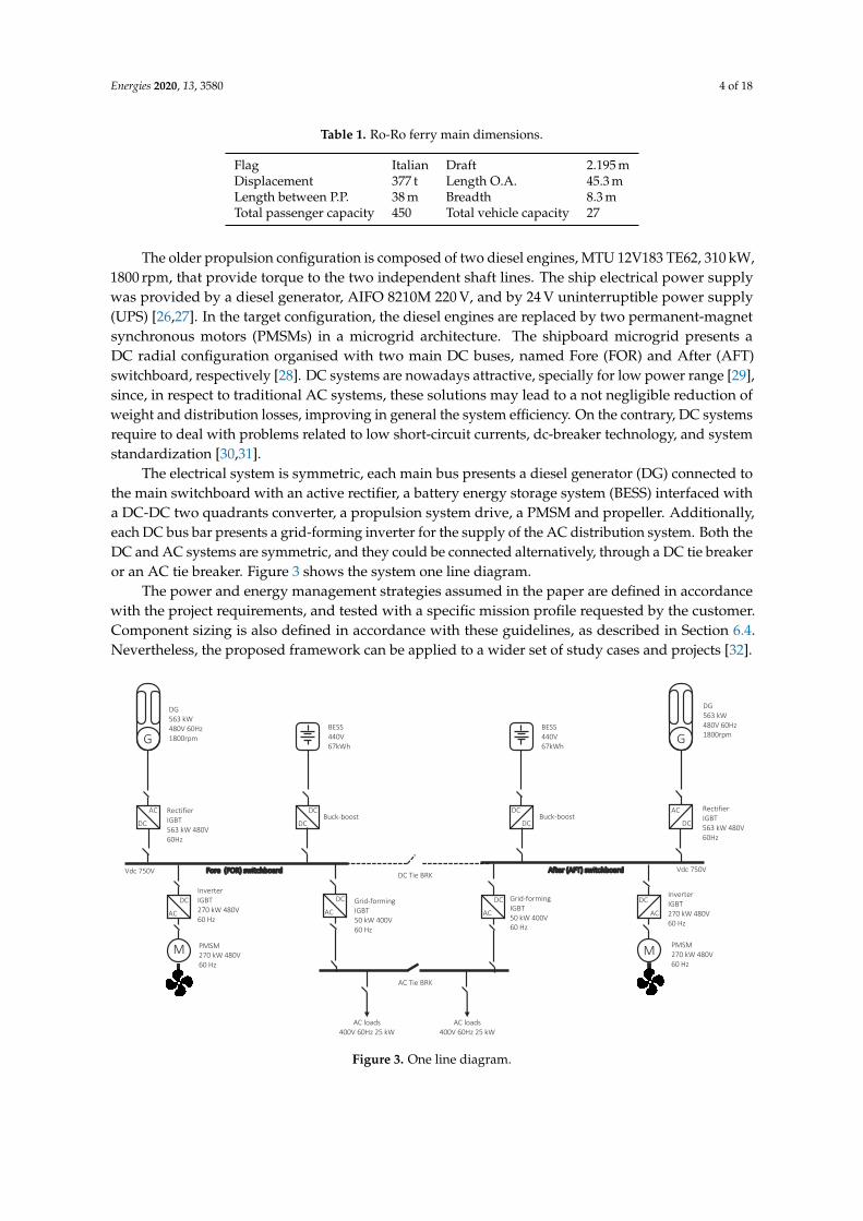
Flag Italian Draft 2.195 mDisplacement 377 t Length O.A. 45.3 mLength between P.P. 38 m Breadth 8.3 mTotal passenger capacity 450 Total vehicle capacity 27

The older propulsion configuration is composed of two diesel engines, MTU 12V183 TE62, 310 kW,1800 rpm, that provide torque to the two independent shaft lines. The ship electrical power supplywas provided by a diesel generator, AIFO 8210M 220 V, and by 24 V uninterruptible power supply(UPS) [26,27]. In the target configuration, the diesel engines are replaced by two permanent-magnetsynchronous motors (PMSMs) in a microgrid architecture. The shipboard microgrid presents aDC radial configuration organised with two main DC buses, named Fore (FOR) and After (AFT)switchboard, respectively [28]. DC systems are nowadays attractive, specially for low power range [29],since, in respect to traditional AC systems, these solutions may lead to a not negligible reduction ofweight and distribution losses, improving in general the system efficiency. On the contrary, DC systemsrequire to deal with problems related to low short-circuit currents, dc-breaker technology, and systemstandardization [30,31].

The electrical system is symmetric, each main bus presents a diesel generator (DG) connected tothe main switchboard with an active rectifier, a battery energy storage system (BESS) interfaced witha DC-DC two quadrants converter, a propulsion system drive, a PMSM and propeller. Additionally,each DC bus bar presents a grid-forming inverter for the supply of the AC distribution system. Both theDC and AC systems are symmetric, and they could be connected alternatively, through a DC tie breakeror an AC tie breaker. Figure 3 shows the system one line diagram.

The power and energy management strategies assumed in the paper are defined in accordancewith the project requirements, and tested with a specific mission profile requested by the customer.Component sizing is also defined in accordance with these guidelines, as described in Section 6.4.Nevertheless, the proposed framework can be applied to a wider set of study cases and projects [32].

IEES laboratoryOne line diagram

3

DC

DC

DC

AC

AC

DC

G

M

Vdc 750V

DC

DC

DC

AC

AC

DC

G

M

AC loads

400V 60Hz 25 kW

PMSM

270 kW 480V

60 Hz

Inverter

IGBT

270 kW 480V

60 Hz

Rectifier

IGBT

563 kW 480V

60Hz

Buck-boost

DG

563 kW

480V 60Hz

1800rpm

BESS

440V

67kWh

DG

563 kW

480V 60Hz

1800rpm BESS

440V

67kWh

Buck-boost

Vdc 750V

DC

AC

DC

AC

DC Tie BRK

PMSM

270 kW 480V

60 Hz

Inverter

IGBT

270 kW 480V

60 Hz

AC loads

400V 60Hz 25 kW

Grid-forming

IGBT

50 kW 400V

60 Hz

Grid-forming

IGBT

50 kW 400V

60 Hz

Rectifier

IGBT

563 kW 480V

60Hz

AC Tie BRK

Fore (FOR) switchboard After (AFT) switchboard

Figure 3. One line diagram.

Energies 2020, 13, 3580 5 of 18

3. Components Modeling and Control Strategies

The ferry with the new power configuration, should operates in three different operational modes:full-electric, hybrid and diesel mode. In the first case, the DGs are off and the energy to the propulsionmotor is provided by BESSs. In the second case DGs and BESSs cooperates for the power supplywhile in the third case the BESSs are disconnected and the necessary power is provided by the DGs.In order to fulfill requirements imposed by the different navigation modes, several solutions have beendeveloped. In this work, a DC voltage droop control scheme is considered and adopted when theoperation mode requires the coordination of multiple resources (DGs and/or BESSs) [33–35]. Instead,a single DC voltage forming control scheme is used when the operative mode requires only one systemproviding the DC bus regulation.

Figure 4 shows a synthesis of the higher level control loops of the system. Starting from the DG,the AC voltage is controlled by an automatic voltage regulator (AVR) (IEEE-AC1A) while the speed isregulated by a governor (modelled as a standard Woodward Diesel Governor DEGOV1). The DG isconnected to the DC bus through an active rectifier which implements a proportional-integral (PI) DCvoltage regulator and a PI dq-axis current control, described in the following. Such a system is capableto operate in stand alone DC forming mode or in multiple resources droop control mode.

The BESS are connected to the DC bus via a DC-DC buck-boost converter. According to thedifferent operating mode, the BESS can be controlled in order to regulate the injected current or theDC bus voltage, both in stand alone or droop scheme.

The propulsion system implemented consists of a PMSM supplied by a variable speed drive.The motor should provide the propeller required torque. The motor speed, and consequently thepropeller rotational regime, is controlled by an upper level closed loop control cruise control, basedon the error between the desired and the actual ship speed, evaluated using a one degree of freedommotion equation [36].

The AC power system is supplied by two grid-forming converters, which can be operated aloneor in parallel both in grid-supporting mode [37].

Details on the adopted control strategies for the single devices are reported in the following.IEES laboratoryOne line diagram

4

DC

DC

DC

AC

AC

DC

G

M

Vdc 750V

DC

DC

DC

AC

AC

DC

G

M

AC loads

400V 60Hz 25 kW

Vdc 750V

DC

AC

DC

AC

AC loads

400V 60Hz 25 kW

AC Tie BRK

Fore (FOR) switchboard After (AFT) switchboard

Speed

AC voltage

DEGOV1

AVR

Pm

Vf

Rec. ctrl.

DC voltage

PWM

AC voltage & current

Buck-boost

Voltage ctrl.

DC voltage

duty

Buck-boost

Current ctrl.

DC current

duty

DC-DC Volt.

droop ctrl.

DC voltage

Buck-boost

Voltage ctrl.

DC voltage

duty

Buck-boost

Current ctrl.

DC current

duty

DC-DC Volt.

droop ctrl.

DC voltage

Speed

AC voltage

DEGOV1

AVR

Pm

Vf

Rec. ctrl.

DC voltage

PWM

AC voltage & current

Speed &

Torque ctrl.

Ship Speed

ctrl.

Ship speed (kn)

Rot. speed

PWM

Speed &

Torque ctrl.

Ship Speed

ctrl.

Ship speed (kn)

Rot. speed

PWMGrid. forming

PWM

AC voltage & current

Grid. forming

PWM

AC voltage & current

Figure 4. Shipboard microgrid main control loops.

Energies 2020, 13, 3580 6 of 18

3.1. Battery Energy Storage Systems and DC-DC Converters

The BESS model is realised using a standard Simulink SimPowerSystem (SPS) Li-ion batterymodel connected to the DC bus thought a DC-DC buck-boost converter, Figure 5a.

Three different control strategies can be selected. The first one, Figure 5b, consists of a PI currentcontrol with voltage droop. Specifically, the current reference signal given to the PI current controlis calculated as the sum of the current set point I∗B and the voltage droop error signal, Kdr(V∗

dc − Vdc).Where Kdr is the droop coefficient and V∗

dc, Vdc are the voltage DC bus reference and measured signal,respectively. The duty cycle δ, for the pulse width modulation (PWM) is the sum of the PI outputsignal and the measured battery voltage VB. This control mode allows to participate in the DC busvoltage regulation and to implement state of charge (SOC) management strategies. When multipledevices are involved in the DC bus droop regulation, the power sharing, and thus the contribution ofeach resources, can be controlled by changing the reference current I∗B [34,38].

The second control strategy, Figure 5c, is a DC voltage forming control. The DC-DC converter iscontrolled alternatively either as a boost or buck converter. When the bus voltage Vdc is lower than itsreference value, V∗

dc, the converter is controlled as a boost, when the previous condition is not respectedit is controlled as a buck. The duty cycles, one for each control channel, are defined by a PI regulator.

The third control strategy, Figure 5d, consists of a battery current control. This regulation strategyallows to control precisely the battery output current and it can be used for SOC management strategies.

IEES laboratory

16

buck

boost !!""!""#$

##$ $#$

!# %#

(a)

IEES laboratory

20

)*,

!#$

!#$∗ *"

"&

"&∗

−−

!&

− *+,1−1

buck

boost

*"

$*+

$*+∗− *+,1

−1

boost

buck

*"

$*+

$*+∗− *+,1

−1

buck

boost

0

0

$*+

$*+∗>

boost

buck

"#

"'

"'∗ −"$%1

−1

boost

buck

"#

"'

"'∗− "$%1

−1

buck

boost

0

0

0

"'∗>

boost

buck

#

#

#

#

#

(b)

IEES laboratory

20

)*,

!#$

!#$∗ *"

"&

"&∗

−−

!'())

− *+,1−1

buck

boost

*"

$*+

$*+∗− *+,1

−1

boost

buck

*"

$*+

$*+∗− *+,1

−1

buck

boost

0

0

$*+

$*+∗>

boost

buck

"#

"'

"'∗ −"$%1

−1

boost

buck

"#

"'

"'∗− "$%1

−1

buck

boost

0

0

0

"'∗>

boost

buck

#

#

#

#

#

(c)

IEES laboratory

20

)*,

!#$

!#$∗ *"

"&

"&∗

−−

!'())

− *+,1−1

buck

boost

*"

$*+

$*+∗− *+,1

−1

boost

buck

*"

$*+

$*+∗− *+,1

−1

buck

boost

0

0

$*+

$*+∗>

boost

buck

"#

"'

"'∗ −"$%1

−1

boost

buck

"#

"'

"'∗− "$%1

−1

buck

boost

0

0

0

"'∗>

boost

buck

#

#

#

#

#

(d)

Figure 5. (a) Battery DC-DC circuit diagram. (b) DC voltage droop control, (c) DC voltage formingcontrol, (d) battery current control.

3.2. AC-DC and DC-AC Three Phase Converters

The DG model consists of a standard SPS synchronous machine per unit model. The implementedcontrols are the governor, Woodward Diesel Governor DEGOV1, and the AVR IEEE-AC1A [39].The DGs are coupled with the DC bus thought an active rectifier. The rectifier model consists of athree phase converter and a LCL filter in which the output L is realised with a transformer, Figure 6.The rectifier controls consist of a PI feed-forward current control and an outer DC voltage PI controlwhich defines the dq-axis current references. Similarly the two DC-AC converters which provides thepower supply to the AC subsystem have been implemented with the same scheme but implement agrid-forming with supporting mode control strategy [40].

The LCL filters for both cases have been designed following criteria detailed in theliterature [41,42].

Energies 2020, 13, 3580 7 of 18

3.2.1. Converter Control Loops

The convert control loops implement a hierarchical control system organization. In this contextwe call device level controls the PI dq- current and voltage feed-forward controls, and system levelcontrols, all the other loops which define the reference for the device level loops according to specificsystem requirements [43]. In this second group we consider the DC bus voltage regulation in case ofthe AC-DC active rectifier, and grid-forming control in case of the DC-AC converter.

The device level controls considered in this paper are dq PI current and voltage feed-forwardcontrols, Figure 6. The control system design is out of the purpose of the paper. As detailed in literature,the current and voltage control loop can be modelled, considering the system of equation of the LCLfilter [44–46]. Thus, control parameters can be defined according to the system eigen values anddesired control performance [44,47].

The reference frame for the dq-transformation, can be provided by a phase locked loop (PLL) orcan be generated internally by the controller according to the regulation strategy implemented by thesystem level controls. More specifically, power converters can be in general divided into grid followingand grid forming units [43,48]. The grid following unit, can operate only with an already energisedgrid, since it controls active and reactive power by regulating the current output according to thevoltage magnitude and phase. The active rectifier, Figure 6a, is a grid following unit. It controls activeand reactive powers by properly changing the current dq reference in a synchronized way with thevoltage phase measured by the PLL. On the other hand, the grid forming unit can be considered asvoltage generators. It can control voltage magnitude ad frequency, and thus it can energize an AC grid.The DC-AC converter in Figure 6b is a grid forming unit [37].

&! &!"

#$-$#1-1

.1 '!

(!

1:1, 3(234

5-6 .*.

7!//28!//

+29!//

50Δ.(22

/*$∗

/*.∗

8$&

:

1/!234

−1/!35 −

−

.*$

)$&∗

>*∗

-.0

012

-.0

012.*$

28&

28&−

.*$

.*.

−

−

/*.

/*$?*$

?*.

5+&5+&

-.0

012

!#$

DC voltage and Power control loopCurrent control loop

Dro

op C

ontr

olle

rSRF

-PL

L

System level controls

Device level controls

28434

28564

−)$&

−

5!//

G2/,* + A:/,*

)#

*$"#$

(a)

&! &!"

#$-$#1-1

.1 '!

(! 1:1, 3(

234

/,$∗

/,.∗

-.0

012

28&

28&−

.*$

.*.

−

−

/,.

/,$<*$

<*.

5+&5+&

-.0

012

!#$

.*$∗

.*.∗

-.0

012

28"

28"−

/*$

−

−

.*.

.*$

5*'5*'

/*$

.*$

.*. −4!" 55 + 7!"

8#$%&

.*$.7∗

−8'$( + 8'%(

9:#")#∞

0 −<*

× 8'$

8'%×

×

−9:#")$

×

>+/! 4-?./

9:#")#$

:#$%&∗∗

-.0

012

/*.

.∗

.82

3%"&

4%!9:∗

−6

6∗

.;2 + .;

8< 2 + 18=2 + 1

−@.

"∗@!

".*/*

(%

Virtual impedance controlVoltage control loopCurrent control loop

Act

ive

and

reac

tive

pow

er d

roop

System level controls

Device level controls

−

.%"& Δ.

AC grid

(b)

Figure 6. AC-DC converters single line diagrams: (a) rectifier control scheme (b) grid-forming scheme.

The diesel genset is connected to the DC bus by an active rectifier, Figure 6a. The AC section isenergised by the generator and the converter has to control the active and reactive power in order toregulate the DC and AC voltage, respectively. In this specific application two droop control schemeshave been adopted. The d-axis current reference is given by the DC current PI controller with DCvoltage droop [49,50]. The q-axis current reference is given by a reactive power PI controller whosereference is given by AC voltage error multiplied by the AC voltage droop coefficients.

The grid forming converter, Figure 6b, is used to supply the AC distribution system. The adoptedcontrol structure is a grid forming with supporting scheme [37,40,48]. The supporting scheme isrequired if the converter operates in parallel with other units. More specifically, the implementedstrategy corresponds to the one presented in [37]. It implements two separate control channelsin order to regulate the active and reactive power sharing. The voltage phase, and the frequency,are controlled by the active power channel, which implements the so called reverse droop controlapplied to the active power error. While the voltage magnitude is controlled by the reactive powerchannel, which implements the reverse droop on the reactive power error [43]. Additionally, to improve

Energies 2020, 13, 3580 8 of 18

the performance, the active power channel presents a low-pass filter which is used to avoid fastfrequency variations and allows an inertial response, while the reactive power channel implementsa virtual inertia control [37]. The adopted control strategy allows the systems to operate in both,AC radial or meshed grid configuration [51]. Notice that the same capability could be obtained evenwith virtual synchronous machines (VSM) control strategies [43,52].

3.3. Propulsion Plant Dynamic

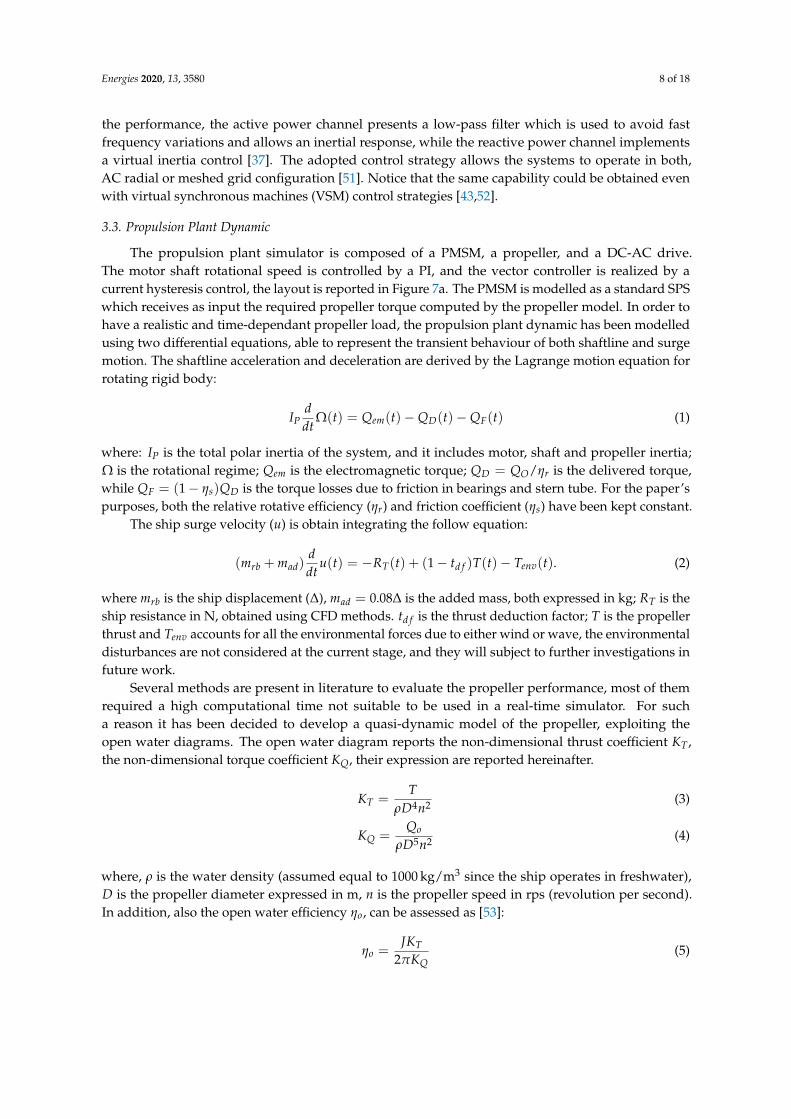
The propulsion plant simulator is composed of a PMSM, a propeller, and a DC-AC drive.The motor shaft rotational speed is controlled by a PI, and the vector controller is realized by acurrent hysteresis control, the layout is reported in Figure 7a. The PMSM is modelled as a standard SPSwhich receives as input the required propeller torque computed by the propeller model. In order tohave a realistic and time-dependant propeller load, the propulsion plant dynamic has been modelledusing two differential equations, able to represent the transient behaviour of both shaftline and surgemotion. The shaftline acceleration and deceleration are derived by the Lagrange motion equation forrotating rigid body:

IPddt

Ω(t) = Qem(t)− QD(t)− QF(t) (1)

where: IP is the total polar inertia of the system, and it includes motor, shaft and propeller inertia;Ω is the rotational regime; Qem is the electromagnetic torque; QD = QO/ηr is the delivered torque,while QF = (1 − ηs)QD is the torque losses due to friction in bearings and stern tube. For the paper’spurposes, both the relative rotative efficiency (ηr) and friction coefficient (ηs) have been kept constant.

The ship surge velocity (u) is obtain integrating the follow equation:

(mrb + mad)ddt

u(t) = −RT(t) + (1 − td f )T(t)− Tenv(t). (2)

where mrb is the ship displacement (∆), mad = 0.08∆ is the added mass, both expressed in kg; RT is theship resistance in N, obtained using CFD methods. td f is the thrust deduction factor; T is the propellerthrust and Tenv accounts for all the environmental forces due to either wind or wave, the environmentaldisturbances are not considered at the current stage, and they will subject to further investigations infuture work.

Several methods are present in literature to evaluate the propeller performance, most of themrequired a high computational time not suitable to be used in a real-time simulator. For sucha reason it has been decided to develop a quasi-dynamic model of the propeller, exploiting theopen water diagrams. The open water diagram reports the non-dimensional thrust coefficient KT ,the non-dimensional torque coefficient KQ, their expression are reported hereinafter.

KT =T

ρD4n2 (3)

KQ =Qo

ρD5n2 (4)

where, ρ is the water density (assumed equal to 1000 kg/m3 since the ship operates in freshwater),D is the propeller diameter expressed in m, n is the propeller speed in rps (revolution per second).In addition, also the open water efficiency ηo, can be assessed as [53]:

ηo =JKT

2πKQ(5)

Energies 2020, 13, 3580 9 of 18IEES laboratory

g

PMSM

rps

, = !,- ⋅ /

- ⋅ /2 ⋅ 03

- ⋅ /4 ⋅ 03

15

16

Ω

0(1 − :) 3

3<

4

4167

8

9

1 ⋅ 23

−;−

=#$%

1.! /

9&−

(1 − 2)

Ω9>?

3

!012

< 4"#$

3"3"%&'(

Ω

Ω∗−

−3AB∗

3

(a)

IEES laboratory

g

PMSM

rps

, = !,- ⋅ /

8 ⋅ :> ⋅ ;=

8 ⋅ :? ⋅ ;=

<@

<A

Ω

;

(1 − E)>

?G

@

@1

(H%& +H'()JA

B:

−D@

−K)*+

1<- 5

BL−

1 − 3!"

ΩBMN

>

!012

E 8456

3"3"7893

Ω

Ω∗−

−

?OP∗

?

1G"BQ

(1 − R,)

−

(b)

0 0.2 0.4 0.6 0.8 1

J

0

0.2

0.4

0.6

0.8

1

KQ

, K

T a

nd

0

Open water diagram

10 KQ

KT 0

(c)

0 5 10 15

u (kn)

0

10

20

30

40

50

RT (

kN

)

Total resistance curve

RT = u

2 ( = 0.216)

CFD data

fit

(d)

Figure 7. (a) Propulsion system layout; (b) propulsion plant model; (c) propeller open water diagramand (d) ship hull total resistance curve.

The open water diagram is shown in Figure 7c. The numerical values of these coefficients,stationary for definition, have been obtained from a 5-bladed Wageningen B series [54] and given infunction of the advance coefficient J, computed as:

J(t) =Va(t)n(t)D

(6)

Va(t) = (1 − w)u(t) (7)

where: Va is the advance speed at propeller plane in m s−1, and w is the wake fraction. As it canbe seen, the advance coefficient is a time-dependant variable so the propeller transient behaviour ispartially catch. Using the previous steps, it is possible to evaluate the last two terms not yet definedin (2) and (1) ,T(t) and Qo(t). For reader’s clarity, the schematic representation of the whole propulsionmodel is reported in Figure 7b.

4. Ship Automation

The ship automation consists of the highest level control of the microgrid. At this level usuallyoperates the algorithm which performs the energy management strategy, mission control and thehuman–machine interface (HMI). The development of these types of control is out of the purpose ofthe paper, therefore, in this study, only the minimum possible control loops have been implemented inthe system. Nevertheless, the benchmark proposed will be used in the next steps of the retrofit projectfor testing new control algorithms and interfaces. Thus, the automation system received as commandthe devices on/off signals and some user-defined setpoints such as ship speed and batteries chargedischarge controls. The main inputs and outputs of the implemented automation system are reportedin Figure 8.

Energies 2020, 13, 3580 10 of 18IEES laboratoryOne line diagram

5

DC

DC

DC

AC

AC

DC

G

M

Vdc 750V

DC

DC

DC

AC

AC

DC

G

M

Vdc 750V

DC

AC

DC

AC

Fore (FOR) switchboard After (AFT) switchboard

DEGOV1

AVR

Rec. ctrl. Buck-boost

Voltage ctrl.

Buck-boost

Current ctrl.

DC-DC Volt.

droop ctrl.Buck-boost

Voltage ctrl.

Buck-boost

Current ctrl.

DC-DC Volt.

droop ctrl.

DEGOV1

AVR

Rec. ctrl.

Speed &

Torque ctrl.

Ship Speed

ctrl.

Speed &

Torque ctrl.

Ship Speed

ctrl.

Grid. formingGrid. forming

on/off

DG Wref

DG Vref

DC Vref

DC Iref

on/off

DC Vref

DC Iref

on/off

on/off

DG Wref

DG Vref

Ship SPEEDref

on/off

Ship SPEEDref

on/off

on/off on/off

on/off

on/off

Figure 8. Automation controls.

5. Implementation on Real-Time Simulation Platform

The practical implementation of the model in Opal-RT is described in Figure 9. The simulationuses the computational power of three cores, the base model is coded in Simulink environmentusing the SimPowerSystems blockset and the add-on advanced real-time electro-magnetic solvers(ARTEMiS) [55]. The solver is the the state-space nodal (SSN) algorithm, a delay-free solver providedwith ARTEMiS [56].

ARTEMiS precomputes and discretizes all the state-space matrix which represents the networkand store them into cache memory,in order to simulate the system in real-time. The most switchesare in the network the most typologies are possible and therefore the most state-space matrixesneed to be stored in cache memory, causing overflows. To overcome this problem, the network isdecoupled, into many sub circuits reducing the total size of the state-space matrices in memory [56].The decoupling is realized in two different ways, the first solution exploits the fact that the transmissionlines introduce a natural delay to the propagation of the waves, thus when we deal with longtransmission lines, the delay naturally introduced is usually larger than the simulation step size,while in the case of short lines, which provides a delay shorter than the time steps, an additionalexternal delay is introduced, since at the end we get at least one time step delay. The decouplingin the case of short lines is realized with the ARTEMiS StubLines, which are used in the system todivide the network in order to be simulated in parallel on different cores, Figure 9. When there are notransmission lines, a second decoupling method is provided by the state-space nodal (SSN) approach.Specifically, ARTEMiS provides the SSN solver, which combines the state-space approach with theNodal approach which is able to divide the electrical network into smaller electrical systems withoutintroducing any delay. This second solution for the decoupling is realised by the ARTEMiS SSN blockswhich divides the system into sub circuits which can be characterised as inductive group (V-typeport) considered as a voltage source connected to an inductive element, or as capacitive group (I-typeport) considered a a current source connected to a capacitive element. The system decoupling strategyfor the real-time (RT) simulations is shown in Figure 9.

Energies 2020, 13, 3580 11 of 18

DC

DC

DC

AC

G

M

Vdc 750V

PM motor

270 kW 480V

60 Hz

Inverter

IGBT

270 kW 480V

Rectifier

IGBT

Buck-boost

DG

599 kW

480V 60Hz

1800rpm

BESS

440V

67kWh

DG local load

480V 60Hz 0.08puSSN3ϕ V-V

SSN3ϕ V-I

LCL

SSN

SSN

Stub Line

Stub Line

DC

AC

AC load

400V 60Hz

DC

DC

DC

AC

G

M

Vdc 750V

Rectifier

IGBT

Buck-boost

DG

599 kW

480V 60Hz

1800rpm

BESS

440V

67kWh

DG local load

480V 60Hz 0.08puSSN 3ϕ V-V

SSN 3ϕ V-I

LCL

SSN

SSN

Stub Line

Stub Line

DC

AC

AC load

400V 60Hz

Stub Line

Stub Line

DC

AC

DC

AC

Console & system

monitoring

Core 1 Core 2Core 3

SSN 3ϕ I-V-VSSN3ϕ I-V-V

PM motor

270 kW 480V

60 Hz

Inverter

IGBT

270 kW 480V

LCL

SSN3ϕ I-V-V

LCL

SSN 3ϕ I-V-V

Local host

Figure 9. Opal-RT implementation.

The simulation step-size has been set to 30 µs and therefore with such a time step we are not ableto simulate PWM with high switching frequency. In order to overcome this limitation, PWM signalsare generated using the RT-EVENTS toolbox, which is capable to represent the logical state of staticswitches, whose value can change inside a single simulation time-step. Ten RT-EVENTS have beenset for each time step, allowing the correct evaluation of PWM high frequency modulation signals.Nevertheless, in a planned upgrade of the RT simulator an FPGA board will be available for thesimulation of power converters at high switching frequency.

In the described configuration the real-time model can be simulated without any overrun, meaningthat at each time step the computation time of each step is less than the simulation time-step definedby the user. Numerical results are shown in the following section.

6. Simulation Results

The performances of the described real-time simulation setup are demonstrated with threedifferent simulations. The first and the second ones aim to test the controls of the DC and AC systemrespectively. The third one, proposes a simulation of the ship in realistic design condition reproducingthe the mission profile that the ship will be facing with. The main parameters of systems and controllersare reported in the Appendix A, Table A1.

6.1. DC Bus Regulation

All the devices in the microgrid operate to the system regulation which different strategies.Figure 10a shows the results of a simulation in which the different DC bus control strategies areexchanged. In the top graph of Figure 10a, the timeline of the different events is described. The initialconfiguration considers the two batteries, cooperating in droop control scheme to the regulation of thetwo DC switchboard connected by the DC tie breaker. Then, the two buses are disconnected, the shipsaccelerate to a speed of 6 kn and the two DGs are connected to the DC buses. At 180 s the two DCbuses are connected again and BESS control test starts. Firstly, some set points are driven to the BESSswhich operates in droop control scheme. Then, at 350 s the battery control strategy is changed tocurrent control mode. In this configuration the BESS current is controlled directly and the voltageregulation is left to the DGs. With this control mode some set points are sent to the BESS controllers

Energies 2020, 13, 3580 12 of 18

and finally at 500 s the BESS droop control strategy is restored. For the last tests, the two DGs and theFOR BESS are disconnected. In this configuration, the AFT BESS is the only resources left to feed thepropulsion system in voltage forming control mode. Below of the time line plot in Figure 10a, somemeasurements are shown, such as, DC voltage at the two main busbars, batteries current and state ofcharge, generators speed and voltages and finally, generator powers.

720

740

760

780

Voltage (

V)

DC bus

VdcFOR

VdcAFT

100 200 300 400 500

Time (s)

Events time line

DCtie (on)

PRPFOR

(6kn)

DGFOR

(on)

DGAFT

(on)

DCtie (off)

BESS (D;100A,50A)

BESSFOR

(D;-20A)

BESSAFT

(D;40A)

BESS (I;0A,0A)

BESSFOR

(I;-20A)

BESSAFT

(I;40A)

BESS (D;-20A,40A)

DGs (off)

BESSAFT

(V)

BESSFOR

(off)

-200

-100

0

100

200

Curr

ent (A

)

48

49

50

51

SO

C (

%)

Battery current

Ib,FOR

Ib,AFT

SOCFOR

SOCAFT

0.98

1

1.02

Speed (

pu)

1

1.05

1.1

1.15

Voltage (

pu)

Diesel Genset

wFOR

wAFT

VFOR

VAFT

50 100 150 200 250 300 350 400 450 500 550

Time (s)

0

0.05

0.1

0.15

0.2

Pow

er

(pu)

Diesel Genset

PFOR

PAFT

(a)

710

720

730

740

750

760

Vo

lta

ge

(V

)

DC bus

VdcFOR

VdcPRT

0.6

0.8

1

1.2

Vo

lta

ge

(p

u)

AC system

VacFOR

B0 VacPRT

B1 VacPRT

B0 VacPRT

B1

0 50 100 150 200 250 300 350 400 450

Time (s)

59.4

59.6

59.8

60

Fre

qu

en

cy (

Hz)

AC system

fFOR

fPRT

50 100 150 200 250 300 350 400 450

Time (s)

Events time line

DCtie (off)

PRPPRT

(6kn)

ACFOR

(on)

ACPRT

(on)

ACtie (on)

DCtie (on)

ACtie (off)

ACPRT

(off)

ACtie (on)

(b)

Figure 10. (a) DC and (b) AC control system tests.

6.2. AC Bus Regulation

The performance of the AC regulation system are shown in Figure 10b. The timeline in the topgraph, summarize the commands sequence. Initially, the DC tie breaker is in state off, then, the twoDC-AC grid forming converters are activated and the AC grid is energised. At this stage the grid isoperated completely separated from starboard to port side, both AC and DC tie breakers are open.At 160 s the AC tie breaker is closed, and the two side of the grid are connected. At 160 s the DC tiebreaker is also closed and the grid pass from a radial to a meshed configuration. Finally, the AC tiebreaker is operated in order to disconnect the two AC grid, the port side converter is turned of and theDC tie breaker is closed again in order to reach the configuration in which all the AC supply is givenby the only starboard side converter. Below of the time line plot in Figure 10b, DC voltage, AC voltageand AC frequency are shown.

6.3. Ship Mission

The whole system performance has been finally evaluated by simulating a realistic navigation ofapproximately 5 nautical miles between the port of Intra and the port of Laveno on Lago Maggiore,Italy. The mission considers a round trip of almost 1 h and it is described in the top graph of Figure 11.Specifically, mission starts in port of Intra, the ship is moored and the power system is supplied onlyby the two batteries with a SOC equal to 50%. After few seconds, the navigation starts; the engine setpoint is set to obtain 6 kn, and this speed is kept constant for almost 300 s, the time needed to reach asufficient distance from the coast and to switch to hybrid mode. Thus, one diesel generator is turned on,the battery set-points are set 128 A (recharge), and the ship speed is increased up to 10 kn. After almost23 min of navigation, with the DG running smoothly at half load, the ferry is close to the arrival port

Energies 2020, 13, 3580 13 of 18

of Laveno, thus the battery recharge is stopped with a SOC about of 60% (suggested value by themanufactures to extend the life cycle), the diesel genset is turned off, and the ship starts the manoeuvreto enter the port in full electric mode with a speed of 6 kn. Once the port is reached, the ship is mooredand after a while the way back trip starts, following the same procedure described before. For sake ofcompleteness, in the lower sub-plot the ship speed and the propeller thrust are reported, pointing outa symmetric behavior, without any peak. Some simulation results for the shipboard power system areshown in the plots of Figure 11.

Figure 11. Simulation of a navigation mission between port of Intra and port of Laveno, LagoMaggiore, Italy.

Figure 12 shows the real-time simulator core monitoring outputs provided by the OpMonitorblock [55]. The yellow line refers to the time step size, the time set by the user in which the simulatorhas to complete a cycle of measurements–computation–commands [55]. The blue line represents thenumber of overruns, meaning the number of times in which the time of computation exceeded thedefined time step. The red line corresponds to the effective computation time, and the purple timecorresponds to the time idle, meaning the difference between the step size and the computation time.As it can be seen, the simulation results to be stable, the systems is able to keep the real-time for all themission duration. The overall loading is 49.65% of the total computation power, divided as 35.30% forcore 1, 34.77% for core 2 and 78.88% for core 3.

Energies 2020, 13, 3580 14 of 18

0 500 1000 1500 2000 2500 3000

Simulation time (s)

0

5

10

15

20

25

30

Co

mp

uta

tio

n t

ime

(s)

Core 1, FOR (Master)

0 500 1000 1500 2000 2500 3000

Simulation time (s)

0

5

10

15

20

25

30

Core 2 - PTR (Slave)

Ovrn. Comp. Step Idle

0 500 1000 1500 2000 2500 3000

Simulation time (s)

0

5

10

15

20

25

30

Core 3 - AC grid (Slave)

Figure 12. Real-time setup performance monitoring during the mission simulation.

6.4. Observations on the Ship Management Strategies

The mission simulation proposed in the previous section refers to the operating mode requestedby the customer. Specifically, the project requirements impose (I) to be able to operate in full electricmode below 6 kn, (II) to operate the batteries between a minimum and maximum SOC in order toextend their expected life, (III) to operate in hybrid mode, with one diesel genset as main supply atcruise speed of 10 kn. Moreover, (IV) no shore connection capability is considered, thus, batteriesshould be kept within the limits during all the operating time and even during the time at berth.Nevertheless, other control strategies could be applied in order to improve the system efficiency [32].

7. Conclusions

The paper presents the development of a real-time simulation framework of a DC shipboardmicrogrid, realized to support the retrofitting project of a RORO Pax vessel with a model-baseddesign approach. The shipboard microgrid model shows its capability to reproduce real operatingconditions including ship dynamics within the electrical power system study. Models includepropellers, prime movers, electrical machines, battery energy storage systems, power converters andregulators. The proposed architecture has been realized to allow hardware-in-the-loop configurations.

Results show that several control schemes can be implemented, to test system performancesunder different conditions, and to verify operational constraints during the expected ship missions.Moreover, since the simulator has been developed following a modular and parametric approach,it can be continuously tuned with experimental data to improve results fidelity, and to realize thedigital twin of the ship during its entire life cycle.

Future works will regard the experimental validation of simulation results, the implementation ofthe shore connection, and the inclusion of protection devices for short-circuits studies .

Author Contributions: Conceptualization F.D., D.K., M.M., G.-P.S., F.S. and C.S.; methodology F.D., D.K., M.M.,G.-P.S., F.S. and C.S., investigation G.-P.S., D.K., C.S.; supervision F.D, M.M., F.S. All authors have read and agreedto the published version of the manuscript.

Funding: This research received no external funding.

Conflicts of Interest: The authors declare no conflict of interest.

Appendix A

The main parameters of the implemented real-time model are listed in Table A1.

Energies 2020, 13, 3580 15 of 18

Table A1. Main parameters.

Variable Description Value Variable Description Value

Diesel Genset

Nominal power 596 kW Inertia time constant 0.17 sNominal voltage 480 V AVR (gain Ka, time const. Ta) 600 pu, 0.05 sNominal speed, freq. 1800 rpm, 60 Hz DEGOV1 (gain K, droop Kd) 8 pu, 0.05 pu

Propulsion motor PMSM

Nominal power 270 kW Nominal, maximum torque 5.73 kN, 7.2 kNNominal voltage 480 V Nominal speed 450 rpmNominal speed 22.5 Hz Nominal stator current 347 ASpeed PI regulator (Kp, Ki) 10 pu, 15 pu

AC-DC Active rectifier

Nominal power 596 kW Current PI regulator (Kp, Ki) 1 pu, 7 puNominal AC voltage 480 V DC voltage PI reg. (Kp, Ki) 0.2 pu, 0.5 puNominal DC voltage 750 V Reactive power PI reg. (Kp, Ki) 0.02 pu, 0.05 puSwitching frequency ( fs) 1620 Hz DC, AC volt. droop (KVdc , KEg ) 0.05 pu, 0.05 puLCL Filter (L1, L2, C) 1.29 pu, 0.09 pu, 0.07 pu

Battery Energy Storage System

Nominal capacity 128 A h Switching frequency 5000 HzNominal voltage 440 V DC voltage droop (Kdr) 1/0.05 puDC-DC stage param. (R, L, C) 0.25 Ω, 0.8 mH, 12 µF

DC-AC grid–forming converter

Nominal power 50 kVA TVR ‡ gain (kRV) 0.09Transformer (Vt1/Vt2) 390 V/400 V TVR ‡ HPF ∗ cut-off (ωRV) 16.66 rad s−1

LCL Filter (L1, Lt, C) 1.54 pu, 0.10 pu, 0.06 pu LPF ∗∗ cut-off freq. (ωc) 31.41 rad s−1

P and Q droop (mp, mq) 0.02 pu Virtual resistance (Rvi) 0.6716 puVI † ratio Xvi/Rvi (σX/R) 5 Lead-lag filter (T1, T2) 0.033 s, 0.011 s

Ship model

Displacement (∆) 377 t Propeller diameter (D) 1.25 mAdded mass (madd) 30.16 t Density (ρ) 1000 kg/m3

Nominal speed (V) 10 kn Resistance at 10 kn (RT) 18.06 kNTotal polar inertia (Itot) 383.4 kgm2 Relative rotative efficiency (ηr) 1.026 puThrust deduction factor (td f ) 0.205 pu Shaft efficiency (ηsha f t) 0.98 puWake fraction (w) 0.235 pu Ship speed PI ctrl. (Kp, Ki) 3 pu, 1 pu

† Virtual impedance (VI); ‡ Transient Virtual Resistor (TVR); ∗ High-Pass Filter (HPF); ∗∗ Low-Pass Filter (LPF).

Energies 2020, 13, 3580 16 of 18

References

1. Smith, P.F.; Prabhu, S.M.; Friedman, J. Best Practices for Establishing a Model-Based Design Culture.Technical Report, SAE Technical Paper. 2007. Available online: https://www.sae.org/publications/technical-papers/content/2007-01-0777/ (accessed on 2 March 2020).

2. Kelemenová, T.; Kelemen, M.; Miková, L.; Maxim, V.; Prada, E.; Lipták, T.; Menda, F. Model based designand HIL simulations. Am. J. Mech. Eng. 2013, 1, 276–281.

3. Martelli, M.; Figari, M. Real-Time model-based design for CODLAG propulsion control strategies. Ocean Eng.2017, 141, 265–276. [CrossRef]

4. Vrijdag, A.; Stapersma, D.; van Terwisga, T. Systematic modelling, verification, calibration and validation ofa ship propulsion simulation model. J. Mar. Eng. Technol. 2009, 8, 3–20. [CrossRef]

5. Sonnenberg, M.; Pritchard, E.; Zhu, D. Microgrid Development Using Model-Based Design. In Proceedingsof the 2018 IEEE Green Technologies Conference (GreenTech), Austin, TX, USA, 4–6 April 2018; pp. 57–60.

6. Kirby, B.; Zou, L.; Cao, J.; Kamwa, I.; Heniche, A.; Dobrescu, M. Development of a predictive out of steprelay using model based design. In Proceedings of the IET Conference on Reliability of Transmission andDistribution Networks (RTDN 2011) , London, UK, 22–24 November 2011.

7. Panova, E.A.; Nasibullin, A.T. Development and Testing of the Adequacy of the 220/110 kV DistributionSubstation Matlab Simulink Mathematical Model for Relay Protection Calculations. In Proceedings of the2019 IEEE Russian Workshop on Power Engineering and Automation of Metallurgy Industry: Research &Practice (PEAMI), Magnitogorsk, Russia, 4–5 October 2019; pp. 134–138.

8. Zhu, W.; Shi, J.; Liu, S.; Abdelwahed, S. Development and application of a model-based collaborativeanalysis and design framework for microgrid power systems. IET Gener. Transm. Distrib. 2016, 10, 3201–3210.[CrossRef]

9. Zhang, Y.; Bastos, J.L.; Schulz, N.N. Model-based design of a protection scheme for shipboard power systems.In Proceedings of the 2008 IEEE Power and Energy Society General Meeting-Conversion and Delivery ofElectrical Energy in the 21st Century, Pittsburgh, PA, USA, 20–24 July 2008; pp. 1–9.

10. Dufour, C.; Soghomonian, Z.; Li, W. Hardware-in-the-loop testing of modern on-board power systems usingdigital twins. In Proceedings of the 2018 International Symposium on Power Electronics, Electrical Drives,Automation and Motion (SPEEDAM), Amalfi, Italy, 20–22 June 2018; pp. 118–123.

11. Patel, M.R. Shipboard Electrical Power Systems; CRC Press: Boca Raton, FL, USA, 2011.12. Kotsampopoulos, P.; Lagos, D.; Hatziargyriou, N.; Faruque, M.O.; Lauss, G.; Nzimako, O.; Forsyth, P.;

Steurer, M.; Ponci, F.; Monti, A.; et al. A Benchmark System for Hardware-in-the-Loop Testing of DistributedEnergy Resources. IEEE Power Energy Technol. Syst. J. 2018, 5, 94–103. [CrossRef]

13. Edrington, C.S.; Steurer, M.; Langston, J.; El-Mezyani, T.; Schoder, K. Role of Power Hardware in theLoop in Modeling and Simulation for Experimentation in Power and Energy Systems. Proc. IEEE 2015,103, 2401–2409. [CrossRef]

14. Capasso, C.; Veneri, O.; Notti, E.; Sala, A.; Figari, M.; Martelli, M. Preliminary design of the hybrid propulsionarchitecture for the research vessel “G. Dallaporta”. In Proceedings of the 2016 International Conference onElectrical Systems for Aircraft, Railway, Ship Propulsion and Road Vehicles International TransportationElectrification Conference (ESARS-ITEC), Toulouse, France, 2–4 November 2016; pp. 1–6.

15. Manouchehrinia, B.; Molloy, S.; Dong, Z.; Gulliver, A.; Gough, C. Emission and life-cycle cost analysis ofhybrid and pure electric propulsion systems for fishing boats. J. Ocean Technol. 2018, 13, 66–87.

16. Martelli, M.; Figari, M. Maritime Transportation and Harvesting of Sea Resources; CRC Press: Boca Raton, FL,USA, 2018; Volume 1, pp. 87–93.

17. Barelli, L.; Bidini, G.; Gallorini, F.; Iantorno, F.; Pane, N.; Ottaviano, P.A.; Trombetti, L. Dynamic Modeling ofa Hybrid Propulsion System for Tourist Boat. Energies 2018, 11, 2592. [CrossRef]

18. Abadie, L.M.; Goicoechea, N. Powering newly constructed vessels to comply with ECA regulations underfuel market prices uncertainty: Diesel or dual fuel engine? Transp. Res. Part D Transp. Environ. 2019,67, 433–448. [CrossRef]

19. Halff, A.; Younes, L.; Boersma, T. The likely implications of the new IMO standards on the shipping industry.Energy Policy 2019, 126, 277–286. [CrossRef]

Energies 2020, 13, 3580 17 of 18

20. Vieira, G.; Peralta, C.; Salles, M.B.d.C.; Carmo, B.S. Reduction of CO2 emissions in ships with advancedEnergy Storage Systems. In Proceedings of the 2017 6th International Conference on Clean Electrical Power(ICCEP), Santa Margherita Ligure, Italy, 27–29 June 2017, pp. 564–571.

21. Hosagrahara, A.S. Measuring Productivity and Quality in Model-Based Design. U.S. Patent 7,613,589,3 November 2009.

22. Satpathi, K.; Balijepalli, V.M.; Ukil, A. Modeling and Real-Time Scheduling of DC Platform Supply Vessel forFuel Efficient Operation. IEEE Trans. Transp. Electrif. 2017, 3, 762–778. [CrossRef]

23. Silvestro, F.; D’Agostino, F.; Schiapparelli, G.P.; Boveri, A.; Patuelli, D.; Ragaini, E. A Collaborative Laboratoryfor Shipboard Microgrid: Research and Training. In Proceedings of the 2018 AEIT International AnnualConference, Bari, Italy, 3–5 October 2018; pp. 1–6.

24. Boveri, A.; D’Agostino, F.; Fidigatti, A.; Ragaini, E.; Silvestro, F. Dynamic modeling of a supply vessel powersystem for DP3 protection system. IEEE Trans. Transp. Electrif. 2016, 2, 570–579. [CrossRef]

25. Campora, U.; Laviola, M.; Zaccone, R. An Overall Comparison Between Natural Gas Spark Ignition andCompression Ignition Engines for a Ro-Pax Propulsion Plant. In Proceedings of the 3th InternationalConference on Maritime Technology and Engineering, MARTECH, Lisbon, Portugal, 4–6 July 2016;pp. 735–743.

26. Motonave Traghetto San Cristoforo. Available online: https://www.navigazionelaghi.it/doc/pdf/flotta/S.%20CRISTOFORO_Ita.pdf (accessed on 2 March 2020).

27. Italy-Milan: Conversion services of ships. Supplies—Contract notice—Restricted procedure 247237-2018,Ministero delle Infrastrutture e dei Trasporti—Gestione Governativa dei Servizi Pubblici di Navigazione suiLaghi Maggiore di Garda e di Como, 2018.

28. Ghimire, P.; Park, D.; Zadeh, M.K.; Thorstensen, J.; Pedersen, E. Shipboard Electric Power Conversion:System Architecture, Applications, Control, and Challenges [Technology Leaders]. IEEE Electrif. Mag. 2019,7, 6–20. [CrossRef]

29. Skjong, E.; Volden, R.; Rødskar, E.; Molinas, M.; Johansen, T.A.; Cunningham, J. Past, present, and futurechallenges of the marine vessel’s electrical power system. IEEE Trans. Transp. Electrif. 2016, 2, 522–537.[CrossRef]

30. Staudt, V.; Bartelt, R.; Heising, C. Fault Scenarios in DC Ship Grids: The advantages and disadvantages ofmodular multilevel converters. IEEE Electrif. Mag. 2015, 3, 40–48. [CrossRef]

31. Satpathi, K.; Ukil, A.; Nag, S.S.; Pou, J.; Zagrodnik, M.A. DC Marine Power System: Transient Behavior andFault Management Aspects. IEEE Trans. Ind. Inform. 2019, 15, 1911–1925. [CrossRef]

32. Boveri, A.; Silvestro, F.; Molinas, M.; Skjong, E. Optimal sizing of energy storage systems for shipboardapplications. IEEE Trans. Energy Convers. 2018, 34, 801–811. [CrossRef]

33. D’Agostino, F.; Grillo, S.; Schiapparelli, G.; Silvestro, F. DC Shipboard Microgrid Modeling for Fuel CellIntegration Study. In Proceedings of the IEEE PES General Meeting, Atlanta, GA, USA, 4–8 August 2019;pp. 4–8.

34. D’Agostino, F.; Massucco, S.; Schiapparelli, G.P.; Silvestro, F. Modeling and Real-Time Simulation of a DCShipboard Microgrid. In Proceedings of the 2019 21st European Conference on Power Electronics andApplications (EPE’19 ECCE Europe), Genova, Italy, 3–5 September 2019; pp. 1–8.

35. Satpathi, K.; Ukil, A.; Thukral, N.; Zagrodnik, M.A. Modelling of DC shipboard power system.In Proceedings of the 2016 IEEE International Conference on Power Electronics, Drives and Energy Systems(PEDES), Trivandrum, India, 14–17 December 2016; pp. 1–6.

36. Alessandri, A.; Donnarumma, S.; Vignolo, S.; Figari, M.; Martelli, M.; Chiti, R.; Sebastiani, L. System controldesign of autopilot and speed pilot for a patrol vessel by using LMIs. Towards Green Marine Technologyand Transport. In Proceedings of the 16th International Congress of the International Maritime Associationof the Mediterranean, Pula, Croatia, 21–24 September 2015; pp. 577–583.

37. Qoria, T.; Cossart, Q.; Li, C.; Guillaud, X.; Colas, F.; Gruson, F.; Kestelyn, X. Deliverable 3.2: Local Control andSimulation Tools for Large Transmission Systems. MIGRATE Project. 2018; Volume 2, p. 81. Available online:https://www.h2020-migrate.eu/_Resources/Persistent/5c5beff0d5bef78799253aae9b19f50a9cb6eb9f/D3.2%20-%20Local%20control%20and%20simulation%20tools%20for%20large%20transmission%20systems.pdf (accessed on 11 July 2020).

38. Fei, G.; Ren, K.; Jun, C.; Tao, Y. Primary and secondary control in DC microgrids: A review. J. Mod. PowerSyst. Clean Energy 2019, 7, 227–242.

Energies 2020, 13, 3580 18 of 18

39. Madan, M.; Meena, R. Adapting IEEE 1992 AC1A excitation system model for industrial application.In Proceedings of the 2018 International Conference on Computing, Power and Communication Technologies,GUCON 2018, Uttar Pradesh, India, 28–29 September 2019; pp. 28–31.

40. Qoria, T.; Prevost, T.; Denis, G.; Gruson, F.; Colas, F.; Guillaud, X. Power Converters Classification andCharacterization in Power Transmission Systems. In Proceedings of the EPE’19 ICCE EUROPE, Genova,Italy, 3–5 September 2019.

41. Reznik, A.; Simões, M.G.; Al-Durra, A.; Muyeen, S. LCL filter design and performance analysis forgrid-interconnected systems. IEEE Trans. Ind. Appl. 2013, 50, 1225–1232. [CrossRef]

42. Prodanovic, M.; Green, T.C. Control and filter design of three-phase inverters for high power quality gridconnection. IEEE Trans. Power Electron. 2003, 18, 373–380. [CrossRef]

43. D’Agostino, F.; Massucco, S.; Schiapparelli, G.P.; Silvestro, F.; Paolone, M. Performance ComparativeAssessment of Grid Connected Power Converters Control Strategies. In Proceedings of the 2020 IEEEInternational Conference on Industrial Electronics for Sustainable Energy Systems (IESES), Cagliari, Sardinia,1–3 September 2020.

44. Timbus, A.; Liserre, M.; Teodorescu, R.; Rodriguez, P.; Blaabjerg, F. Evaluation of current controllers fordistributed power generation systems. IEEE Trans. Power Electron. 2009, 24, 654–664. [CrossRef]

45. Dong, N.; Yang, H.; Han, J.; Zhao, R. Modeling and Parameter Design of Voltage-Controlled Inverters Basedon Discrete Control. Energies 2018, 11, 2154. [CrossRef]

46. Bajracharya, C.; Molinas, M.; Suul, J.A.; Undeland, T.M. Understanding of tuning techniques of convertercontrollers for VSC-HVDC. In Proceedings of theNordic Workshop on Power and Industrial Electronics(NORPIE/2008), Espoo, Finland, 9–11 June 2008.

47. Aydin, O.; Akdag, A.; Stefanutti, P.; Hugo, N. Optimum controller design for a multilevel AC-DC convertersystem. In Proceedings of the Twentieth Annual IEEE Applied Power Electronics Conference and Exposition,APEC 2005, Austin, TX, USA, 6–10 March 2005; Volume 3, pp. 1660–1666.

48. Rocabert, J.; Luna, A.; Blaabjerg, F.; Rodriguez, P. Control of power converters in AC microgrids. IEEE Trans.Power Electron. 2012, 27, 4734–4749. [CrossRef]

49. Jin, Z.; Meng, L.; Vasquez, J.C.; Guerrero, J.M. Specialized Hierarchical Control Strategy for DC Distributionbased Shipboard Microgrids: A combination of emerging DC shipboard power systems and microgridtechnologies. In Proceedings of the IECON 2017—43rd Annual Conference of the IEEE Industrial ElectronicsSociety, Beijing, China, 29 October–1 November 2017; pp. 6820–6825.

50. Guerrero, J.M.; Chandorkar, M.; Lee, T.L.; Loh, P.C. Advanced control architectures for intelligentmicrogrids—Part I: Decentralized and hierarchical control. IEEE Trans. Ind. Electron. 2012, 60, 1254–1262.[CrossRef]

51. Kumar, D.; Zare, F.; Ghosh, A. DC microgrid technology: System architectures, AC grid interfaces, groundingschemes, power quality, communication networks, applications, and standardizations aspects. IEEE Access2017, 5, 12230–12256. [CrossRef]

52. D’Arco, S.; Suul, J.A.; Fosso, O.B. A Virtual Synchronous Machine implementation for distributed control ofpower converters in SmartGrids. Electr. Power Syst. Res. 2015, 122, 180–197. [CrossRef]

53. Carlton, J. Marine Propellers and Propulsion; Butterworth-Heinemann: Cambridge, MA, USA, 2018.54. Kuiper, G. The Wageningen Propeller Series; Technical Report; Marin: Wageningen, The Netherlands, 1992.55. RT-LAB Powering Real-Time Simulation. Available online: https://www.opal-rt.com (accessed on 2 March

2020).56. Dufour, C.; Mahseredjian, J.; Bélanger, J.; Naredo, J.L. An advanced real-time electro-magnetic simulator

for power systems with a simultaneous state-space nodal solver. In Proceedings of the 2010 IEEE/PESTransmission and Distribution Conference and Exposition: Latin America (T&D-LA), Sao Paulo, Brazil,8–10 November 2010; pp. 349–358.

c© 2020 by the authors. Licensee MDPI, Basel, Switzerland. This article is an open accessarticle distributed under the terms and conditions of the Creative Commons Attribution(CC BY) license (http://creativecommons.org/licenses/by/4.0/).