Dynamics and Control of Redundant Robots - mediaTUM
227
Fakultt für Maschinenwesen Lehrstuhl für Angewandte Mechanik Dynamics and Control of Redundant Robots Efficient Simulation, Biped Walking, Redundancy Resolution and Collision Avoidance Dr.-Ing. Thomas Buschmann Geboren 27.06.1978 in Bobingen, Bundesrepublik Deutschland Vollstndiger Abdruck der zur Erlangung der Lehrbefhigung an der Fakultt für Maschi- nenwesen der Technischen Universitt München für das Fachgebiet Angewandte Mechanik eingereichten Habilitationsschrift. Mentorat: 1. Prof. Dr.-Ing. habil. Heinz Ulbrich (Vorsitz) 2. Prof. Dr.-Ing. habil. Boris Lohmann 3. Prof. Dr.-Ing. Prof. E.h. Peter Eberhard (Universitt Stuttgart) Die Habilitation wurde am 21.03.2014 eingereicht.
-
Upload
khangminh22 -
Category
Documents
-
view
2 -
download
0
Transcript of Dynamics and Control of Redundant Robots - mediaTUM

Fakultät für MaschinenwesenLehrstuhl für Angewandte Mechanik
Dynamics and Control of Redundant Robots
Efficient Simulation, Biped Walking, Redundancy Resolution andCollision Avoidance
Dr.-Ing. Thomas Buschmann
Geboren 27.06.1978 in Bobingen, Bundesrepublik Deutschland
Vollständiger Abdruck der zur Erlangung der Lehrbefähigung an der Fakultät für Maschi-nenwesen der Technischen Universität München für das
Fachgebiet „Angewandte Mechanik“
eingereichten Habilitationsschrift.
Mentorat:
1. Prof. Dr.-Ing. habil. Heinz Ulbrich (Vorsitz)2. Prof. Dr.-Ing. habil. Boris Lohmann3. Prof. Dr.-Ing. Prof. E.h. Peter Eberhard (Universität Stuttgart)
Die Habilitation wurde am 21.03.2014 eingereicht.


Acknowledgment
First, I would like to thank Prof. Heinz Ulbrich, Prof. Boris Lohmann and Prof. PeterEberhard for supporting me and serving as mentors during my habilitation period andProf. Rixen for giving me the opportunity to continue my research at the Institute ofApplied Mechanics.
Most of all, I want to thank my colleges and students and acknowledge their contri-bution to the results presented in this manuscript. Markus Schwienbacher contributeda large part of the work on recursive forward dynamics, efficient collision geometriesand distance calculations. The application of these methods to the redundant agri-cultural manipulator was implemented and analyzed by Jörg Baur. The manipulatoritself was developed by Julian Pfaff. Christoph Schütz implemented the predictiveapproach to inverse kinematics and analyzed the approach for different manipulatormodels. The chapter on walking control owes much to the collaboration with AlexanderEwald, Arndt von Twickel and Ansgar Büschges on a comprehensive review of walkingcontrol in animals and robots. The section on task-space trajectory modifications forbipedal walking is the outcome of joint work with Arne-Christoph Hildebrandt, whoimplemented and experimentally evaluated the ideas presented here. Robert Wittmannimplemented and analyzed the “Inverse Kineto-Dynamics” method, as well as the errorcompensation methods and contributed ideas to the stabilization of the walking patterngeneration method base on “Inverse Kineto-Dynamics.” Finally, the work described herewould not have been possible without the excellent biped robot prototype developed bySebastian Lohmeier and the work on electronics and low-level control by Valerio Favotand Georg Mayr. I am also indebted to Wilhelm Miller, Walter Wöß, Simon Gerer, PhilipSchneider, Tobias Schmidt and Georg König for their excellent work in manufacturingand maintaining the bipedal and agricultural robots.
I would also like to thank Jörg Baur, Alexander Ewald, Arne-Christoph Hildebrandt,Christoph Schütz, Markus Schwienbacher and Robert Wittmann and Kathrin Buschmannfor proofreading the manuscript.


Contents
1 Introduction 1
2 Kinematics 32.1 Single Rigid Body Kinematics 3
2.1.1 Conditions for Rigid Body Motion 32.1.2 Rigid Body Positions 62.1.3 Velocities 72.1.4 Accelerations 9
2.2 Rotation Matrices 102.2.1 Axis-Angle Representation 102.2.2 Elementary Rotations 132.2.3 Successive Rotations 142.2.4 Discussion 16
2.3 Multibody Kinematics 172.3.1 Coordinate Systems, Constraints and Coordinate Sets 172.3.2 Topology 19
2.4 Efficient Forward Kinematics Calculation 292.5 Chapter Summary 34
3 Rigid Body Dynamics 353.1 Principles of Mechanics 363.2 Global EoM-based Dynamics 40
3.2.1 Equations of Motion 403.2.2 Inverse Dynamics Simulation 423.2.3 Forward Dynamics Simulation 42
3.3 Recursive Linear-Complexity Dynamics for Trees 473.3.1 Linear-Complexity Inverse Dynamics 483.3.2 Linear-Complexity Forward Dynamics 50
3.4 Kinematic Constraints 573.4.1 Lagrangian Multiplier-based Methods 603.4.2 Minimal Coordinate Linear-Complexity Forward Dynamics with Loops 63
3.5 Outlook – Parallel Algorithms 693.6 Chapter Summary and Discussion 74
4 Biped Walking Control 754.1 Neural Control of Posture and Balance 754.2 Hardware Design 78

6 Contents
4.3 Basic Dynamics of Legged Locomotion 804.4 Model-Based Control of Underactuated Robots 814.5 Model-Based Control of Fully-Actuated Robots 83
4.5.1 Planning Reference Trajectories 844.5.2 Stabilizing Control 86
4.6 Biologically-Based Pattern Generation 884.7 Gait Cycle-Centered Control 90
4.7.1 Limit Cycle Walkers 904.7.2 Step-Phase Control 91
4.8 Chapter Summary and Discussion 92
5 Optimal Redundancy Resolution and Collision Avoidance 955.1 Local Inverse Kinematics 95
5.1.1 Position-Level Inverse Kinematics 965.1.2 Velocity-Level Inverse Kinematics 985.1.3 Acceleration-Level Inverse Kinematics 1015.1.4 A Note on Singularities 1015.1.5 Hierarchical Methods and Inequality Constraints 103
5.2 Efficient Collision Geometries and Distance Calculations 1035.2.1 Background and Related Work 1045.2.2 Geometry Models Based on Swept Sphere Volumes 1055.2.3 Distance Calculation 107
5.3 Local Nullspace Optimization for Walking and Manipulation 1115.4 Collision Avoidance in Task-Space 118
5.4.1 Introduction and Related Work 1185.4.2 Proposed Method 1205.4.3 Experimental Evaluation 1275.4.4 Summary 129
5.5 Inverse Kineto-Dynamics 1295.5.1 Introduction and Related Work 1325.5.2 The Concept of Inverse Kineto-Dynamics 1345.5.3 Walking Pattern Generation Based on Inverse Kineto-Dynamics 1375.5.4 Experimental Results 146
5.6 Predictive Inverse Kinematics 1465.6.1 Introduction and Related Work 1485.6.2 Motivational Example 1505.6.3 Predictive Approach to Redundancy Resolution 1515.6.4 Application to 9-DoF Manipulator 1565.6.5 Conclusion 157
5.7 Chapter Summary 158
6 Conclusion and Directions for Future Work 161
A Kinematics 165A.1 Useful Identities 165

Contents 7
A.2 Angular Velocity for Axis-Angle Representation 165A.3 The Denavit-Hartenberg Convention 166A.4 Recursive Kinematics Calculations 168
A.4.1 Recursive Equations 168A.4.2 Relative Quantities 169
A.5 Gradients for Predictive Inverse Kinematics 171A.5.1 Gradients for Optimization on Velocity Level 171A.5.2 Gradients for Optimization on Acceleration Level 171
B Gauss’ Principle for a Rigid Body 173
C Alternative Derivations of O(nb) Method 177C.1 Derivation of O(nb) Method Using Constraint Forces 177C.2 Derivation of O(nb) Method Using Projective EoM 178
Bibliography 181
Acronyms 209
Symbols 211
Indices and Accents 215
Index 217


1 Introduction
This monograph summarizes research on the dynamics and control of robots carried outat the Institute of Applied Mechanics at the Technische Universität München, Germany.The problem of fast, robust, flexible and stable bipedal walking has served as a constantsource of challenges and has motivated most of the work described here.
Humanoid walking robots are among the most complex robotic systems. The largenumber of Degrees of Freedom (DoFs) requires efficient methods for computing thekinematics and dynamics. These algorithms are both essential components of manyplanning and control methods and important tools for the design and evaluation ofcontrol systems in closed-loop simulations. Chapters 2 and 3 address these topics. Theyare meant to provide the theoretical background, including specialized algorithmssuitable for most robotic systems. The first novel contribution in these chapters isan efficient recursive implementation of forward dynamics for systems with kinemat-ics loops described in minimal coordinates. As a second contribution, the recursiveapproach is compared to efficient, structure exploiting methods that explicitly use asystem mass matrix, which enables a realistic assessment of the relative merit of thetwo approaches.
Chapter 4 reviews current approaches to controlling bipedal robots, as well as theneural control of human posture and balance. It is intended to provide the contextof this motivating application, describe what is possible with current technology anddiscuss some of the remaining open questions. Current state-of-the-art bipedal robotsare capable of quite fast and robust locomotion, but the gap between the capabilitiesof humans and machines remains considerable. A large portion of current researchis still at the level of generating and stabilizing basic walking patterns and successfulapproaches to this problem use strong simplifications and impose severe restrictionson possible motions.
Promising approaches towards improving the capabilities of bipedal robots are there-fore to be found in basic research on improved methods for generating, modeling andcontrolling bipedal walking. This is the subject of ongoing research in the robotics groupat the institute, which is aimed at improved event-based walking control (Buschmannet al. 2012a; Ewald et al. 2012; Ewald and Buschmann 2013) and better modeling andprediction of walking dynamics to enable reactive stepping control (Wittmann et al.2014). This line of research, however, is not the subject of this monograph.
The second promising line of research is to improve the capability of generatingmotions that use all the robot’s DoFs to achieve this task. This in turn requires efficientmethods that enable real-time modification of the generated motion to account for self-

2 1 Introduction
collision, obstacle avoidance and the minimization of appropriately defined objectivefunctions. Suitable methods for this problem are discussed in chapter 5 and applicationsboth to biped walking and to a redundant agricultural manipulator are discussed.Solving general planning and optimal control problems for systems with many DoFsstill is too computationally demanding for real-time use. Real-time control systemstherefore usually take a hierarchical approach, in which higher layers use coarsersystem descriptions, enabling longer planning horizons. For complex robots with manyDoFs, any given task is likely described by fewer equations than could be satisfiedwith the system’s number of DoFs. In such redundant configurations it is naturalto plan in a suitably defined task-space of lower dimension than the configurationspace. This reduces the planning effort and allows lower layers to choose a solutionwhich is optimal with respect to some additional criteria. This approach is explored inchapter 5. Classical inverse kinematics methods for redundant manipulators form thebackground for the presented methods. An important contribution is a very efficientapproach to avoiding obstacles and self-collisions. Redundancy resolution is extendedto task-space modifications to enable walking over arbitrarily shaped obstacles. Thepresented method exploits all of the robot’s DoFs and is therefore more general thanprevious approaches. Another contribution is the extension of the inverse kinematicsapproach to hybrid tasks including desired generalized force trajectories. This enablesa novel walking pattern generation scheme for biped robots, but is not restricted tothis application. The final contribution discussed in this monograph is a predictiveapproach to redundancy resolution, which promises to reduce many of the drawbacksof local potential field methods while remaining fast enough for real-time use.
Most work was conducted together with students or PhD candidates at the Instituteof Applied Mechanics, whose contribution is acknowledged in the individual chapters.

2 Kinematics
As the “geometry of motion,” kinematics is concerned with the description of the motionof mechanical systems without taking forces or inertia into account. In many practicalcases, robots can be viewed as systems of interconnected rigid bodies. Elastic defor-mations do play an important role in some cases. Typical examples are small bendingor torsional deformations in light-weight robot links (see Bremer 2008; Siciliano andKhatib 2008, ch. 13.2.2). In the overwhelming majority of robotic applications, however,elastic deformations are small relative to the gross motion of the (deformable) body. Insuch cases, the overall motion of the body is equivalent to that of a rigid body withadditional small elastic deformations relative to the rigid-body motion (Bremer 2008,ch. 5). This is why the description of rigid body motion is central to the kinematics,dynamics and control of robotic systems. In most cases, robots are explicitly designedto avoid significant link deformations. We will therefore limit the discussion to rigidbody systems in the following. Treatments of elastic multibody dynamics may be foundin (e.g., Shabana 2005; Bremer 2008; Gattringer 2011). Note that elastic deformationsin components such as gears and bearings, which are the most relevant in the majorityof applications, are not excluded. Such components are typically modeled by forceelements describing the effect of elasticity (and damping) as a function of generalizedcoordinates and velocities. Such a model assumes that elasticity is relevant, but internalvibrations of the elastic structure itself are negligible.
This chapter derives the kinematics of a single rigid body (section 2.1), varioususeful coordinate transformations (section 2.2) and the kinematics of systems ofinterconnected rigid bodies (section 2.3). In section 2.4 different methods for improvingthe efficiency of kinematics calculations in computer programs are described.
2.1 Single Rigid Body Kinematics
This section develops equations governing the motion of a single rigid body, which arean important foundation for the kinematics and dynamics of multibody systems.
2.1.1 Conditions for Rigid Body Motion
A mathematical description of rigid body motion can be derived directly from the factthat the shape of a rigid body remains constant at all times, which implies a constant

4 2 Kinematics
dr 0
reference
dr current
Figure 2.1: The current and the reference positions of a rigid body with a line segmentin its current configuration (dr) and in the reference configuration (dr 0). The linesegment is rotated and shifted, but the length is unchanged.
distance between any two body-fixed points r i and r k: r i − r k
= constant, r i, r k ∈ IR3. (2.1)
More specifically, the current length of an infinitesimal line segment dr is equal to thelength dr 0 in a reference position of the body (see figure 2.1) and therefore
dr 2 − dr 20 = 0. (2.2)
Since the current configuration of the line segment dr depends only on the point inthe rigid body it emanates from, it is a function of r 0. We can therefore express it as
dr = ∂ r (r 0)∂ r 0︸ ︷︷ ︸
F
dr 0, (2.3)
where F is the deformation gradient tensor. With (2.3), we can re-formulate (2.2) as:
dr 2 − dr 20 = dr T
0
F T F − I3
︸ ︷︷ ︸
G
dr 0. (2.4)
The matrix I3 is the 3× 3 identity matrix. A vanishing Green-Lagrangian strain tensorG therefore is a necessary and sufficient condition for rigid-body motion (Altenbachand Altenbach 1994, p. 56, Shabana 2005, ch. 4.4):
G = 0 ⇔ F T F = I3. (2.5)

2.1 Single Rigid Body Kinematics 5
This directly yields the useful relationship
F−1 = F T . (2.6)
With F =f 1 f 2 f 3
, (2.5) can be expanded into six equations for the nine compo-
nents of F :
f Ti f k = 0 for i = x , y, z, k = x , y, z, i 6= k (2.7)
f Ti f i = 1 for i = x , y, z (2.8)
That is, the f i form an orthonormal basis of IR3 whose configuration may be uniquelydescribed by three independent parameters.
In the reference configuration we have r = r 0, and therefore F = (e x e y ez),where the e i are the basis of the inertial reference frame from which the currentconfiguration r is measured.1 Adopting an orthonormal, right-handed2 frame as theinertial reference, this simplifies to f i = e i, F = I3 in the reference configuration.By continuity this implies that the f i also define a right-handed frame with unitdeterminant.3 Mathematically, F can then be identified as a member of the specialorthogonal group SO(3) of matrices with orthonormal column vectors and a determinantequal to one.4
Since F is derived for the motion of an infinitesimal line segment without referenceto an absolute position, it describes the rotation of the body relative to the inertialframe. An equivalent view is that F transforms a vector represented in the body-fixedframe given by f i into a representation in the global frame.
When used as a rotation matrix describing such a transformation from a frame K toa second frame L, F will be denoted by ALK in the following.5 Since we will use severalcoordinate frames, the frame in which a vector is represented will be indicated by apreceding subscript in the following. That is, the vector r written in the K-frame (FK)and L-frame (FL) is denoted by K r and L r . The representations can be converted intoeach other via
L r = ALK K r . (2.9)
In the following, we will denote the inertial reference frame by the index I (FI), and a
1. An “inertial” frame is a global, non-accelerated frame.2. That is, ez = e x × e y with the usual definition of the cross product ×.3. This follows from det
f 1 f 2 f 3
= f T
1 ( f 2 × f 3) = f T1 f 1 = 1. The first identity follows from
the scalar triple product representation of the determinant and the second and third identities from theuse of an orthonormal and right-handed frame.
4. The set of matrices with F T F = I3 (elements of the orthogonal group O(3)) with det(F) = −1 arereflections and not relevant for representing rigid-body motion. For a presentation of mechanics basedon concepts from differential geometry see (e.g., Holm 2008a, 2008b).
5. The naming of rotation matrices follows Shabana (2005) and Bremer (2008)

6 2 Kinematics
P
FIreference
P
FB
current r B
r BP
r BP
r OP
AIB
Figure 2.2: A point P of a rigid body in the current configuration (dark color) and thereference configurations (light color) of the body, together with the inertial frame FIand body-fixed frame FB.
body-fixed frame by B (FB). We can then write (2.3) as
dI r = AIB dB r . (2.10)
2.1.2 Rigid Body Positions
The current position of a point in the rigid body can be calculated by integrating (2.10):
I r = AIB B r + I r T . (2.11)
The “integration constant” r T ∈ IR3 adds three more free parameters to the three inAIB, giving the rigid body six independent parameters, or DoFs. Mathematically, thepose (position and orientation) of a rigid body is a member of the special Euclideangroup SE(3) = IR3 × SO(3) (see, e.g., Holm 2008a). Geometrically, (2.11) implies thatthe position of the point r in FI is obtained from the position in FB by transformingthe vector in the body-fixed frame B r via AIB about r T (rotation) and adding r T
(translation).6
Eq. (2.11) is useful not only for rigid bodies, but also for the more general case ofdetermining the absolute position of a point given in a moving frame, relative to theorigin OB of FB (see section 2.3). To emphasize this, we can re-write it as:
I r P = I r B + AIB B r BP . (2.12)
6. This is also referred to as Chasles’ theorem: rigid body motion consists of three translations andthree rotations (Shabana 2005).

2.1 Single Rigid Body Kinematics 7
Here, r B is the origin of FB and r BP the vector from OB to P (see figure 2.2)
2.1.3 Velocities
The absolute velocity of a point given by the vector B r BP relative to the moving FB issimply determined by differentiating with respect to time in FI :
I r P =ddt
I r B + AIB B r BP
= I r B + AIB B r BP + AIB Br BP .
(2.13)
Here, the circle (x ) indicates the differentiation of the component representation of a
vector in the current frame, while the dot (x ) denotes the absolute differentiation ofthe vector. The two differ by the velocity induced by the rate of change of the basisvectors of FB relative to FI . The absolute velocity in FB is finally obtained from (2.13)by writing the result in FB:
B r P = ABI I r P
= B r B + ABI AIB B r BP + Br BP .
(2.14)
Eqs. (2.13) and (2.14) could be used to calculate the absolute velocity. This, however,would require calculating the derivative of the transformation matrix with respectto time, which would be tedious and inefficient as the parametrizations of ABI givenin section 2.2 show. Fortunately, there is a simpler formulation based on the angularvelocity.
Angular VelocityTo determine the time derivative of the rotation matrix, it is useful to study the con-sequences of the rigidity conditions with respect to the time evolution of the columnvectors ai of AIB, which are the basis-vectors of FB. Differentiating (2.8) yields:
d(aTi ai)
dt = 2aTi ai = 0, (2.15)
Since the dot product vanishes, ai and ai are orthogonal and we can parametrize ai
by a vector u i ∈ IR3:
ai = u i × ai = eu iai. (2.16)

8 2 Kinematics
The tilde operator f( ) maps a vector in IR3 to a skew-symmetric matrix,7 and is anequivalent way of denoting the cross product:
à
xyz
:=
0 −z yz 0 −x−y x 0
. (2.17)
Differentiating the orthogonality relationship (2.7) and substituting (2.16) into theresult we obtain:
0= ddt (a
Ti ak) = aT
i ak + aTi ak,
⇒ 0= (eu iai)T ak + aT
i (eukak) = aTi
euTi + euk
ak.
(2.18)
Since the tilde operator is skew-symmetric (euTi = −eu i), this implies that all u i, uk are
identical:
u i = uk =ω i, k ∈ x , y, z. (2.19)
The unique vector ω describing the rate of change of the basis vectors of FB relativeto FI is the angular velocity of the rigid body. From (2.16) we directly get:
ai = I eωIB ai, (2.20)
⇒ AIB = I eωIB AIB, (2.21)
⇔ I eωIB = AIBATIB. (2.22)
The angular velocity in FB is obtained via:
I eωIB I r = I eωIB (AIB B r )!= AIB(B eωIB B r ) (2.23)
⇒ B eωIB = ABI AIB = ABI I eωIB AIB. (2.24)
That is, eω satisfies the transformation rules of a second order tensor.
Linear VelocityWith the angular velocity ω, the linear velocity equation (2.13) may be re-written as:
I r P = I r B + AIB B r BP + AIB Br BP
= I r B + I eωIB AIB B r BP + AIB Br BP .
(2.25)
7. Since eω is skew-symmetric, it is an element of so(3), the tangent space to O(3) at the identitymatrix.

2.1 Single Rigid Body Kinematics 9
FBP
r B
r BPr BP
ωω× r BP
r BP +ω× r BP
r B r P
Figure 2.3: Illustration of the components contributing to the absolute velocity r P ofa point in a rigid body. FB is a body-fixed frame, ω the angular velocity of the bodyand r B the absolute velocity of the origin of FB.
The absolute velocity in the body-fixed frame is then given by:
B r P = ABI I r BP
= B r B + ABI AIB B r BP + B r BP
= B r B + B eωIB B r BP + Br BP .
(2.26)
That is, the translational velocity is the sum of the velocity of FB, the speed inducedby the rotation of FB with ω and the velocity B
r BP relative to FB (see figure 2.3).
Note that B r B still denotes the absolute rate of change of the vector r B relative to theinertial frame and cannot be calculated by differentiating the component representationB r B, since this would ignore the velocity induced by the moving basis vectors of thebody-fixed frame.
2.1.4 Accelerations
As with velocities, the absolute acceleration with respect to an inertial frame is easilycalculated by differentiation in the inertial frame:
I r P =ddt
I r P
= I r B + I eωIB AIB B r BP + I eωIB AIB B r BP + I eωIB AIB Br BP + AIB B
r BP + AIB B
r BP
= I r B +
I eωIB + I eωIB I eωIB
AIB B r BP + 2 I eωIB AIB B
r BP + AIB B
r BP . (2.27)

10 2 Kinematics
The body-fixed representation is again obtained by back-transformation:
B r P = ABI I r P
= B r B + ABI
I eωIB + I eωIB I eωIB
AIB B r BP + 2ABI I eωIB AIB B
r BP + B
r BP
= B r B +
B eωIB + B eωIB B eωIB
B r BP + 2 B eωIB B
r BP + B
r BP .
(2.28)
2.2 Rotation Matrices
What is missing in the preceding section for a complete description of rigid body motionis a parametrization of the rotation matrix AIB, that is, a concrete representation of AIB
as a function of some free parameters representing the spacial rotation.
2.2.1 Axis-Angle Representation
Rotations can be parametrized in a number of ways. One possible parametrization maybe derived directly from (2.21) by considering constant angular velocities.8 With thereference configuration as initial condition, the Initial Value Problem (IVP) becomes:
AIB = I eωIB AIB, (2.29)
AIB(t = 0) = I3, (2.30)
which has the closed-form solution:
AIB = eeωt = I3 + eωt +12!eω2 t2 +
13!eω3 t3 +
14!eω4 t4 + · · · (2.31)
Considering only the current and a final configuration at time T with a rotation angleof ϕ =ωT = ϕu, the rotation matrix may be written as
AIB = I3 + euϕ + 12!eu2ϕ2 +
13!eu3ϕ3 +
14!eu4ϕ4 + · · · ,
ϕ =pϕTϕ,
u =ϕ
ϕTϕ.
(2.32)
Since the final rotation depends only on the magnitude and direction of rotation andnot the intermediate configurations, this result is not restricted to constant angular
8. The derivation is inspired by that given by Bremer (2008, pp. 30). However, Bremer begins byparametrizing AIB with uϕ,‖u‖ = 1 and studying the derivative of the squared length a vector r T rwith respect to ϕ.

2.2 Rotation Matrices 11
velocities. Using the identities eu3 = −eu, eu4 = −eueu, . . . (cf. appendix A.1) we obtain
AIB = I3 + euϕ − 1
3!ϕ3 + · · ·
+ eu2
12!ϕ2 − 1
4!ϕ4 + · · ·
= I3 + eu sin(ϕ) + eu2(1− cosϕ)
=
1+ aϕu2x − sϕuz + aϕuyux sϕuy + aϕuzux
sϕuz + aϕuyux 1+ aϕu2y − sϕux + aϕuzuy
− sϕuy + aϕuzux sϕux + aϕuzuy 1+ aϕu2z
,
aϕ := (1− cϕ).
(2.33)
Here, s x = sin(x) and c x = cos(x) are used for conciseness. The four parametersϕ, ux , uy , uz must satisfy the constraint ‖u‖ = 1, leaving three free parameters asexpected from (2.7). Eq. (2.33) is called the axis-angle representation of spacial rotations,since it produces a rotation by ϕ about the fixed rotation axis u. Figure 2.4 gives ageometric illustration of (2.33).
Eq. (2.33) may be rearranged into an alternative representation, the so-called Ro-driguez formula (e.g., Shabana 2005):
AIB = I3 + eu sin(ϕ) + 2eu2(sin2 ϕ
2). (2.34)
A minimal representation with three independent parameters and no constraints maybe obtained from the axis-angle formulation by directly using u = ϕ/
ϕ in (2.33):
AIB = I3 +1ϕeϕ sin(ϕ) +
1ϕ2eϕ2(1− cosϕ), ϕ =
pϕTϕ. (2.35)
A more widely used geometrical derivation of the axis-angle parametrization maybe found in (e.g., Siciliano et al. 2008; Gattringer 2011; Shabana 2005).
Angular VelocityWe assumed a constant angular velocity and axis of rotation for deriving the axis-anglerepresentation. The angular velocity for a constant axis of rotation u = constant isobviously given by uϕ. In the general case, however, a non-constant axis of rotationcontributes to the angular velocity, which must then be calculated from (2.21), that is,AT
IB AIB = B eωIB, yielding:
BωIB = uϕ +sin(ϕ)I3 − (1− cos(ϕ))eu u. (2.36)
A detailed derivation of this result is given in appendix A.2.

12 2 Kinematics
x
y
z
u
uT r u
r Ar
v
∆r v
w∆r w
ϕ
∆r v = cos(ϕ)(I3 − uuT )r
∆r w = sin(ϕ)eur
Figure 2.4: Geometric illustration of the axis-angle parametrization of spatial ro-tations. Rearranging the axis angle parametrization of A (2.33) using the iden-tity (A.5) the rotated vector may be written as the sum of three components:Ar = (u)uT r + cos(ϕ)(I3 − uuT )r + sin(ϕ)eur . The first term contains the componentin the direction of u, which is not changed by the rotation. The second summandcontains the component in direction of v = r − uuT r , which is a natural basis vec-tor for an orthogonal frame in the plane formed by r and u. The third term containsthe contribution in the direction of w = u × r , which together with u and v formsa right-handed frame. The magnitude of the contributions in x and y direction aregiven by the dashed and dotted lines, whose length is directly obtained from ϕ via thegeometric definition of the sine and cosine functions.
Inverse Calculation: Axis and Angle from Rotation MatrixIn case a rotation matrix is known, the corresponding axis and angle of rotation canbe computed from (2.33). Following the procedure in (Gattringer 2011), the rotationangle is obtained by calculating the trace of AIB:
tr(AIB) = 1+ 2cos(ϕ)
⇔ cos(ϕ) =12
AIB,11 + AIB,22 + AIB,33 − 1
.
(2.37)
With cos(ϕ), the rotation axis may be calculated from AIB (2.34) by observing thateu is anti-symmetric, while eu2 and I3 are symmetric, so the axis vector u is easilycalculated by subtracting the corresponding non-diagonal elements of AIB, leaving only

2.2 Rotation Matrices 13
the contribution due to eu sin(ϕ):
u =1
2sin(ϕ)
AIB,32 − AIB,23
AIB,13 − AIB,31
AIB,21 − AIB,12
. (2.38)
Apparently, the angle of rotation can always be calculated, while the axis is ill definedfor all ϕ = kπ, k ∈ ZZ. For ϕ = 0 this is geometrically plausible, since any rotation axisgives the same rotation matrix AIB = I3. For ϕ = ±π the result is ambiguous, becausethe parameters ϕ = π and u yield the same rotation matrix AIB = I3 + u2 as ϕ = −πand −u.
2.2.2 Elementary Rotations
An important special case are rotations about the coordinate axes e i: with the properchoice of reference frames, transformations between the body-fixed frames of segmentsconnected by revolute joints can always be described using such elementary rotations.
Evaluating the axis-angle formulation (2.33) for a rotation about the x-axis e x byan angle of α directly yields:
AIB(α) = ATx (α) = I3 +ee x sin(α) +ee2
x(1− cos(α))
=
1 0 00 1 00 0 1
+
0 0 00 0 −10 1 0
sin(α) +
0 0 10 0 0−1 0 0
(1− cos(α))
=
1 0 00 cos(α) − sin(α)0 sin(α) cos(α)
.
(2.39)
Here the “elementary rotation” Ax(α) is defined for a positive angle and a transforma-tion from FI to FB, following the sign convention in (Gattringer 2011; Bremer 2008;Pfeiffer 1989).
The results for rotations by β about e y and by γ about ez are:
AIB(β) = ATy (β) =
cos(β) 0 sin(β)0 1 0
− sin(β) 0 cos(β)
, (2.40)

14 2 Kinematics
AIB(γ) = ATz (γ) =
cos(γ) − sin(γ) 0sin(γ) cos(γ) 0
0 0 1
. (2.41)
2.2.3 Successive Rotations
Other widely used descriptions of spatial rotations are constructed by three successiveelementary rotations. Many choices for the rotation axes are possible, but successiverotations should be performed about different axes in order to maintain three rotaryDoFs. This leaves twelve admissible choices out of the total of 27 (3× 3× 3).9 Twoof the most widely used sequences are x yz (Tait-Bryan or Cardan angles) and zxz(Eulerian angles).
Cardan Angles
For Cardan angles (x yz) the resulting rotation matrix is:
ABI = Az(γ)Ay(β)Ax(α)
=
cγ cβ sγ cα+ cγ sβ sα sγ sα− cγ sβ cα
− sγ cβ cγ cα− sγ sβ sα cγ sα+ sγ sβ cα
sβ − cβ sα cβ cα
.
(2.42)
The Cardan angles α,β ,γ can be calculated for a given rotation matrix by solving thetrancendental equation (2.42). Elements ABI ,1,1, ABI ,2,1 directly yield γ:
sγcγ=−ABI ,2,1
ABI ,1,1,
⇒ γ= atan2−ABI ,2,1, ABI ,1,1
.
(2.43)
Here the function atan2(y, x) is a variant of atan(y/x) that returns the correct anglebetween the positive x-axis and the point (x , y) for all values of x , y other thanx = y = 0. The angle β follows from ABI ,3,1, ABI ,1,1 and ABI ,2,1:
ABI ,3,1
cγABI ,1,1 − sγABI ,2,1=
sβ(cγ)2 cβ + (sγ)2 cβ
⇒ β = atan2ABI ,3,1, cγABI ,1,1 − sγABI ,2,1
.
(2.44)
9. For the first axis there are no restrictions (3 choices), the second must differ from the first (2choices) and the third from the second (2 choices), resulting in 3× 2× 2= 12 parametrizations.

2.2 Rotation Matrices 15
Finally, α is given by:
ABI ,3,2
ABI ,3,3=− cβ sαcβ cα
,
⇒α= atan2(−ABI ,3,2, ABI ,3,3).(2.45)
For successive rotations the angular velocity of the rotating body (or frame) can becalculated from the rotation matrix and its time derivative via (2.21), that is, AT
IBAIB =B eωIB. Alternatively the angular velocities induced by the elementary rotations maysimply be added, since angular velocity is a vector quantity. However, the contributionsα, β , γ must be transformed into a common reference frame first:
Bω IB = Bα+ Bβ + Bγ (2.46)
= Az(γ)Ay(β)e x α+ Az(γ)e y β + ezγ (2.47)
=
cos(γ) cos(β) sin(γ) 0− sin(γ) cos(β) cos(γ) 0
sin(β) 0 1
ϕ, ϕ :=
αβγ
. (2.48)
The inverse mapping is easily obtained by matrix inversion:
ϕ =1
cos(β)
cos(γ) − sin(γ) 0sin(γ) cos(β) cos(γ) cos(β) 0− cos(γ) sin(β) sin(γ) sin(β) cos(β)
BωIB . (2.49)
The result clearly indicates a singular configuration at β = π2 + kπ, k ∈ ZZ: evaluating
(2.49) requires a division by zero and evaluation of (2.45) and (2.43) evaluation ofatan2(0,0). The geometrical explanation is that the third rotation about the z-axis isparallel or anti-parallel to the first about the x-axis, yielding one rotation by a totalangle of α± γ.
Eulerian Angles
The rotation matrix for Eulerian angles is also obtained from three elementary rotations:by ψ about ez, by ϑ about the new e x and finally by φ about the new ez:
ABI = Az(φ)Ax(ϑ)Az(ψ)
=
cφ cψ− sφ cϑ sψ cφ sψ+ sφ cϑ cψ sφ sϑ− sφ cψ− cφ cϑ sψ − sφ sψ+ cφ cϑ cψ cφ sϑ
sϑ sψ − sϑ cψ cϑ
.
(2.50)

16 2 Kinematics
The Eulerian angles can again be calculated from a given rotation matrix by solving(2.50), yielding:
ψ= atan2(−ABI ,3,1, ABI ,3,2), (2.51)
ϑ = atan2(ABI ,3,1 sψ− ABI ,3,2 cψ, ABI ,3,3), (2.52)
φ = atan2(ABI ,1,3, ABI ,2,3). (2.53)
Note that there are several expressions for the solution to the inverse problem, sincethe system of equations is overdetermined, for example, ϑ could also be calculatedfrom ABI ,1,3 and ABI ,2,3 instead of ABI ,3,1 and ABI ,3,2.
The angular velocity is again obtained from the vector sum of the individual contri-butions and the inverse mapping by matrix inversion:
Bω IB = Bψ+ Bϑ+ Bφ , (2.54)
= Az(φ)Ax(ϑ)ezφ + Az(φ)e x ϑ+ ezψ, (2.55)
=
sin(φ) sin(ϑ) cos(φ) 0cos(φ) sin(ϑ) − sin(φ) 0
cos(ϑ) 0 1
ϕ, ϕ :=
ψ
ϑ
φ
, (2.56)
⇒ ϕ =1
sin(ϑ)
sin(φ) cos(φ) 0cos(φ) sin(ϑ) − sin(φ) sin(ϑ) 0− sin(φ) cos(ϑ) − cos(ϑ) cos(φ) sin(ϑ)
Bω IB. (2.57)
For Eulerian angles the singular case obviously occurs for ϑ = kπ, k ∈ ZZ, when thefirst and last rotation are about parallel or anti-parallel axes. This is again clear bothfrom the inverse solution for ϕ ((2.57): division by zero) and ϕ ((2.53) and (2.51):atan2(0,0)).
2.2.4 Discussion
In this section we developed a number of different parametrizations of spacial rota-tions using either three or four parameters. The minimal representations using threeparameters are simpler to use in most calculations, since for redundant representationsadditional constraints, such as the unit length of the axis of rotation, must be taken intoaccount, for example, during the time integration of Equations of Motion (EoMs). Onthe other hand, minimal representations always have singular configurations. In manytechnological applications, however, the motion of the individual bodies is limited. Insuch cases, a proper sequence of elementary rotations can put the singularities outsidethe physical range of motion.
Besides the parametrizations shown in this section, there is a range of other, more

2.3 Multibody Kinematics 17
or less widely used parametrizations, such as Euler parameters10 (Shabana 2005),Rodriguez parameters11 (Shabana 2005) and Quaternions12 (Siciliano et al. 2009). Anextreme case of a redundant parametrization is the direct use of the rotation matrix(or basis vectors of the body fixed frame) together with the constraints (2.7) ensuringthat the matrix remains orthonormal (see e.g., Betsch and Leyendecker 2006).
2.3 Multibody Kinematics
This section develops the kinematic equations of rigid multibody systems that are usedin subsequent chapters.
2.3.1 Coordinate Systems, Constraints and Coordinate Sets
To simplify the following discussion, we will number the bodies in the MultibodySystem (MBS) from 1 . . . nb and introduce one body-fixed frame Fi for each body iin the system and denote the inertial frame by I = F0. The pose of the i-th body isthen given by the origin r i = r Oi
of Fi and the orientation Ai0 of Fi, which may beparametrized by ϕ iIR
3. The configuration of the whole MBS is then simply given bythe system coordinates:13
zT =r 1 r 2 . . . r nb
ϕ1 ϕ2 . . . ϕnb
∈ IR6nb . (2.58)
For robotic systems, the individual bodies are generally connected by joints, limitingthe physically feasible set of system coordinates. Figure 2.5 shows a simple example ofa robotic manipulator with one rotary and one prismatic joint. This type of holonomic(or geometric) constraint only depends on position variables and may be written as
Φ(z, t) = 0 ∈ IRm. (2.59)
10. The Euler parameters ϑ are a redundant parametrization related to axis-angle parameters via
ϑ0 = cos(ϕ
2), ϑ1 = u1 sin(
ϕ
2), ϑ2 = u2 sin(
ϕ
2), ϑ3 = u3 sin(
ϕ
2), ‖ϑ‖= 1
11. The Rodriguez parameters γ are a minimal representation related to Euler parameters ϑ via
γ1 =θ1
θ2, γ2 =
θ2
θ0, γ3 =
θ3
θ0
12. Quaternions are a redundant parametrization q1,q related to axis-angle parameters via
q1 = cos(ϕ
2), q = sin(
ϕ
2)u
13. For planar systems the number of system coordinates becomes dim(z) = 3nb

18 2 Kinematics
x
ybody 1
body 2
q1
q2
Figure 2.5: Example of a robotic manipulator as MBS with constraints. The two bodiesand the environment are connected by one rotary and one prismatic joint. There aretwelve system coordinates, position and orientation of body 1 and body 2. Due to theconstraints (three position and two orientation constraints at joint 1, two position andthree orientation constraints at joint 2) only the two DoFs q1 and q2 remain.
If time appears explicitly in the constraint equation, it is called rheonomic, otherwisescleronomic. Systems with constraints including velocities are called nonholonomic andmay be written as:
Φ(z, z, t) = 0 ∈ IRm. (2.60)
Holonomic and scleronomic constraints are by far the most prevalent for robotic systems.A notable exception, however, are nonholonomic constraints introduced by wheels inmobile robots. Here the velocity of the vehicle is constrained to move in the directionthe wheels are steering towards, while there is no such constraint for the position ofthe vehicle. In other words, there are additional restrictions for the feasible velocitiesbeyond those imposed by geometric constraints.
When the system’s configuration is described by the 6nb variables z, the constraintequation (2.59) must be explicitly taken into account to ensure feasible configurations(cf. section 3.4). In many cases it is possible to identify a set of minimal coordinates,that is, a minimal set of position parameters that (together with fixed parameters)is sufficient for describing the configuration of a system (i.e., the system coordinatesz). For minimal coordinates the constraints are automatically fulfilled: Φ(z(q)) ≡ 0.The term generalized coordinates is also used for minimal coordinates, even though itshould be understood to include non-minimal sets of coordinates.

2.3 Multibody Kinematics 19
2.3.2 Topology
Kinematic TreesThe topology of many robotic systems resembles a tree. For such tree structured sys-tems every body has exactly one predecessor (or parent) and an arbitrary number ofsuccessors (or children). The only exception is the root of the tree, which does nothave a predecessor. Obviously, the kinematics of the i-th body only depend on themotion of the predecessor and the relative motion between parent and child body, asdescribed by the relative DoF q i. The topology of a tree is uniquely defined by the listof bodies with their corresponding parents. This list is easily converted into a moreuseful representation of the kinematic tree based on references to parent and childbodies for each body in the system. Pseudocode for building a graph representation foran implementation in a C++-like language is given in algorithm 1, figure 2.6 shows anexample of a kinematic tree listing parent and child bodies and figure 2.7 illustrates thelocal description of a tree using references to neighboring bodies. Other approachesusing matrix representations of the graph may be found in (Bremer 2008, pp. 50) andreferences therein.
Algorithm 1: Building the kinematic tree from a list of bodies and parents. Forthis algorithm, each body should contain references (pointers) to parent and childnodes. The MBS object contains a reference to the root of the tree (cf. Yamane2004; Buschmann et al. 2006; Buschmann 2010).
input : list of bodies with parents as pair (body, parent)output : Reference-based graph representation of kinematic treeforall the pairs (body, parent) in list do
b= get_node(body) ; // get reference from body nameif parent not empty then
p= get_node(parent) ; // get reference from parent nameb.set_parent(p) ; // set parent of bodyp.add_child(b) ; // add body as child of parent
elseroot=b ; // no parent ⇒ this is the root node
A special case of a tree is a kinematic chain, where each body has one successorand one predecessor. Systems that cannot be described by a tree have kinematic loops,their structure is described by a general graph. Figure 2.8 illustrates these topologicalclasses.
Systems with LoopsBecause a tree structure enables many optimizations of kinematics and dynamicscalculations, it is common to treat even general systems with loops as trees. This is

20 2 Kinematics
B1
B2
B3
B4
q1
q2
q3
q4
Body i B1 B2 B3 B4
parent p(i) ; B1 B1 B3children (NCi) B2, B3 ; B4 ;predec. (Pi) ; B1 B1 B3, B1DoF q1 q2 q3 q4
Figure 2.6: Example of a kinematic tree. The table on the right lists the parent/childrelationships and DoFs, when B1 is chosen as the root node. The set NCi contains allchildren of Bi.
morenodes
morenodes
towardsroot
reference body
parent body
child body
brother body
c
p
b
Figure 2.7: Local description of a kinematic tree using references to neighboring nodes(p: parent, c: child, b: brother; cf. Yamane (2004), Buschmann et al. (2006), andBuschmann (2010); figure redrawn from Buschmann 2010).

2.3 Multibody Kinematics 21
Figure 2.8: Topological classes: chain (left), tree (center) and graph (right).
B1 B3
B2
A B
C D
B1
B3
B2
A B
C
D
E
Figure 2.9: Illustration of how systems with loops can be treated as tree structuredsystems by cutting all loops open and adding algebraic constraints. The original sys-tem (left) consists of three bodies (B1, B2, B3), forming the kinematic loop A-C-D-B-A.The system may be cut at B, generating an open kinematic chain A-C-D-E (thespanning tree). The removed joint at B is modeled by a holonomic constraintΦ(z) =
r T
E − r TB ,αEB,βEB
= 0, where αEB,βEB are the relative out-of-plane angles
between B3 and the environment.

22 2 Kinematics
Symbol Definition
p(i) or p parent of the i-th nodec(i) or c child of the i-th nodeb(i) or n brother of the i-th nodePi list of all predecessors of the i-th nodeNB set of all body nodes in the MBSNS set of all subsystem nodes in the MBSNCi set of all children of the i-th node: NCi = n ∈ NB| p(n) = iNCSi set of all subsystems, that are children of i:
NCSi = n ∈ NS| p(n) = iNSi set of all bodies in the i-th subsystemCSi child nodes of nodes in NSi, that are not themselves in NSi:
CSi = n ∈ NB \ NSi| p(n) ∈ NSiNPSi parents of nodes in CSi: NPSi = n ∈ NSi| c(n) ∈ CSiNS set of all bodies that are part of a subsystem (union of all NSi)
Table 2.1: Notation for describing the topology of MBSs with and without loops (forthe definition of parent/child/brother references see figure 2.7 and 2.11.). When it isclear from the context, the index in parentheses for p(i), b(i) and c(i) is omitted.
done by cutting the loops, thereby formally generating a tree structure, the spanningtree. Joints within the spanning tree are called primary joints. The joints that have beencut (secondary joints) are replaced by kinematic constraints Φ(q) = 0 (cf. section 3.4).Figure 2.9 illustrates the procedure.
For robots, it is often possible to describe the configuration of all bodies in a loopas a function of the parent body’s configuration and a set of minimal coordinates qSi(Si denotes the i-th subsystem containing the loop, cf. section 3.4.2). In that case, thekinematics of all bodies within the subsystem depend on qSi and the kinematics of theparent body (see figure 2.10 for an example and figure 2.11 for the local description ofthe kinematic structure). We can divide the loop into a primary branch and a secondarybranch, and choose the relative DoFs q i of the primary branch as subsystem DoFs qSi.The configuration of the bodies in the secondary branch of the loop are then computedusing problem-specific equations.14 This is often simplified by using results from thecomputations in the primary branch. The procedure is illustrated in figure 2.10.
Coordinate Frames and Minimal CoordinatesFor robotic systems it is common to choose the body-fixed frames such that the z-axisof the i-th body is aligned with the axis of the joint connecting it to its parent (cf.Denavit-Hartenberg Convention in appendix A.3). For a kinematic tree with nb bodies
14. The inverse kinematics for the loop could also be solved numerically, but this is not discussed here(also see section 3.4).

2.3 Multibody Kinematics 23
B1
B2
B3B4
B5
q1
q2
q3
q4
J1
J2
J3
J4
J5 Body i B1 B2 B3 B4 B5
parent p(i) ; B1 B1 B3 B3children (NCi) B2, B3 ; B4 ; ;predec. (Pi) ; B1 B1 B3, B1subsystem ; ; ; S1 S1DoF q1 q2 q3 q4 q4
Figure 2.10: The system from figure 2.6 with an additional body that introduces aclosed loop. The kinematics are described by the spanning tree, which is generatedby cutting the loop at the yellow link. The relative DoFs in the primary branch arechosen as subsystem DoFs qSi. In the example, the primary branch in the loop con-sists of only B4, while the secondary branch consists of B5. The kinematics of thesecond branch (here: B5) are computed as a function of qSi, possibly using results ofthe forward kinematics of the primary branch (here: B4). There is only one subsystemconsisting of the coupled bodies B4 and B5.
and nq DoFs, a set of minimal coordinates q can be constructed from the variables q idescribing the relative motion between the i-th body and its predecessor:
q T =q T
1 ,q T2 , . . . ,q T
nb
∈ IRnq . (2.61)
To enable subsequent optimizations, the bodies in the tree should be numbered suchthat the index of a body closer to the root will always have a lower index. For systemswith loops, the minimal coordinates may be constructed from the spanning tree, usingonly the primary branches. The motion of the bodies in the secondary branch dependon all relative DoFs in the primary branch (see figure 2.6 for trees and figure 2.10 forsystems with loops).
Recursive Kinematics Calculations
An essential characteristic of a kinematic tree is the fact that the motion of the i-th bodyonly depends on that of its parent and the relative DoFs q i. The kinematic quantities

24 2 Kinematics
subsystem node NSi
subsystem member nodes ∈ NSi
towardsroot
morenodes
morenodes
child nodes outsidesubsystem CSi
rootp
c
p
p
p
Figure 2.11: Local description of a system with loops using references to neighboringnodes and subsystems encapsulating loops (p: parent, c: child, b: brother, adaptedfrom Schwienbacher (2013)). At the level of a full MBS, a subsystem is treated as abody, just as, e.g., bodies with one, two or three DoFs. At the same time, a subsys-tem is a small MBS, inheriting methods from full MBSs for calculating kinematics anddynamics. Programmatically, this is done in C++ via multiple inheritance.
of the system may therefore be calculated recursively starting at the root node, asillustrated in algorithm 2. This forward recursion requires recursive equations for thekinematic quantities. For the transform matrix this equation becomes:
A0i = A0pApi, i = 2 . . . nb. (2.62)
The relative rotation Api from parent to child is a function of the relative coordinatesq i. In robotic systems it is usually composed of a constant transformation aligning thez-axis with the axis of rotation, followed by an additional elementary rotation aboutthe z-axis in the case of rotary joints.
According to figure 2.12 and (2.12), the origin of the i-th body-fixed frame r i is

2.3 Multibody Kinematics 25
parent (p)
body (i)
F0
Fp
Fir p
r pi
Figure 2.12: Coordinate systems and relative kinematics for body i in a tree structuredMBS.
Algorithm 2: Calculate kinematic quantities by forward recursion.input : Minimal coordinates q (and derivatives for velocities and accelerations)output : Kinematic quantities for all bodiesfor i = 1 to nb do
Calculate kinematics for i-th body from that of its parent body p(i) and relativeDoFs q i.
given by
i r i = Aip
pr p + pr pi
, (2.63)
where p = p(i) denotes the parent of the i-th body and r pi is the vector from Op to Oi.For the root body (i = 1) this equation is simply replaced by
0r 0 = 0r 01 (q1), (2.64)
where r 01(q1) is a function depending on the coupling with the environment. For afree floating reference, r 01 is simply a subset of the DoFs q1 of the root body, if thebody is connected via a rotary joint, r 01 is constant.

26 2 Kinematics
The angular velocity of the i-th body is calculated from (2.62) and (2.22):
i eω i =A0pApi
T ddt
A0pApi
= ATpiA
T0pA0pApi + AT
piAT0pA0pApi
= i eω0p + i eω pi,
⇒ iω i = Aip
pω0p + pω pi
= Aip
pω0p + pJ Jωiq i
.
(2.65)
Here the final equation defines the recursive calculation of angular velocities. Therelative angular velocity iω pi and the corresponding joint Jacobian15 J Jω is easily cal-culated: For free floating bodies, the required equations depend on the parametrizationof the rotation matrix (see section 2.2), for prismatic joints iω pi = 0, J Jω = 0 and forrotary joints iω pi = iu qi, J Jω = u, where u is the joint axis and qi the correspondingDoF. For u = ez we simply have iω pi
T = (0 0 qi) , i J Jωi = ez.The linear velocity of the i-th body is directly obtained from (2.63):
i r i = Aip
p r p + p eω 0p pr pi + p
r pi
= Aip
p r p + p eω 0p pr pi + pJ J vi q i
.
(2.66)
Here J J vi is the translational joint Jacobian. The p-frame is chosen for r pi, since thisoften simplifies the description (for rotary joints: pr pi is constant; for prismatic joints:
pr pi = uqi, with u the direction of motion and qi the displacement). The equation forthe root body again depends on the connection to the environment.
The accelerations are obtained by differentiation (or from (2.28)):
iω i = Aip
pω0p + p eω pi pω 0p + pωpi
= Aip
pω0p + p eω pi pω 0p + p J Jωiq i + pJ Jωiq i
,
(2.67)
i r i = Aip
p r p +
p eω0p + p eω0p p eω0p
pr pi + 2 p eω0p p
r pi + p
r pi
= Aip
p r p +
p eω0p + p eω0p p eω0p
pr pi + 2 p eω0p p J J viq i + pJ J viq i
.
(2.68)
Recursive equations for other kinematic quantities are easily derived from these basicequations. For example, the gradient of ω with respect to q (the rotational Jacobian)
15. Note: joint Jacobians denote Jacobians for the relative motion in joints, their dimension dependson the dimension of the joint DoFs q i .

2.3 Multibody Kinematics 27
is given by
i JR,i := ∂ iωi∂ q = Aip
∂ pω0p
∂ q +∂ iωpi
∂ q
= Aip pJR,p + i JR,rel,i ,(2.69)
where JR,rel,i is obtained by expanding J Jωi with zero entries, depending on the locationof q i in q . A comprehensive listing of formulas for recursively calculating kinematicquantities for tree structured systems is given in appendix A.4. The appendix alsoincludes explicit equations for all relative kinematic quantities for rotational joints,prismatic joints and free floating bodies. Examples for more complex, nonlinear jointkinematics found in the robot Lola are given in (Buschmann et al. 2006; Buschmann2010; Schwienbacher 2013).
Compact Representation Using 6D-Vectors
For rigid-body kinematics and dynamics it is useful to combine rotational and trans-lational components of velocities and accelerations into 6D-vectors.16 Note that the6D-representation is used only for writing equations in a compact fashion. For computerimplementations the multiplications with zeros introduced by this notation should beavoided, essentially leading to the original 3D-representation. The compact representa-tion for the recursive kinematics calculation of velocities is (cf. (2.66), (2.65)):
v i = C ipv p + J J iq i. (2.70)
with : (2.71)
v i =
iω i
i r i
, (2.72)
C ip =
Aip 0
Aip per Tpi Aip
, (2.73)
J J i =
J Jωi
J J vi
. (2.74)
The equations for accelerations are (cf. (2.68), (2.67)):
iai = i v i = C ip p ap + J J iq i + bi, (2.75)
with : (2.76)
16. Such a notation is also used in the theory of screws (going back to, e.g., Ball (1876)). Morerecently, the closely related concept of “spacial vector algebra” has been popularized by Featherstone(e.g., Featherstone 1983, 2008). Note, however, that we make no use of screw theory or spacial vectoralgebra, but instead simply stack two 3D vectors to obtain a more compact notation, similar to (Brandlet al. 1987).

28 2 Kinematics
iai =
ωi
r i
, (2.77)
bi =
Aip p eω pi p eω 0p + J Jωiq i,
Aip
p eω0p p eω0p pr pi + 2 p eω0p p
r pi
+ J J viq i
. (2.78)
Note that the rate of change of the joint Jacobian J J is often assumed to be zero (seee.g., Gattringer 2011; Bremer 2008; Hippmann 2008). This is in fact true for prismaticand revolute joints, the most important cases for robots, but not for more complexmechanisms. The nonlinear drive mechanisms used for the ankle and knee joints inthe robot Lola are an example (see figure 2.13; kinematics equations may be found inBuschmann et al. (2006), Buschmann (2010), and Schwienbacher (2013)).
For the important cases of prismatic joints and hinge joints, the joint Jacobians havethe form of simple Boolean matrices:
hinge: J J =∂∂ q i
ezq i
0
=0 0 0 0 0 1
T, (2.79)
prismatic: J J =∂∂ q i
0
ezq i
=0 0 1 0 0 0
T. (2.80)
Similar to the joint Jacobian, we can define a global Jacobian for the 6D-motion ofthe i-th body according to (2.66) and (2.65):
i J i =∂∂ q
i
ωi
r i
=
Aip pJR,p + i JR,rel,i
Aip
pJ T,p + per T
pi pJR,p
+ i J T,rel,i
!,
= C ipJ p + J J i.
(2.81)
The Jacobian J J i ∈ IR6×nq consists of the columns of the joint Jacobian J J i (cf. (2.74),(2.65), (2.66)) at the corresponding position of q i in q and zeros everywhere else. Therelative Jacobians JR,rel,i, J T,rel,i may be constructed from J Jωi, J J vi in the same fashion.With this the global Jacobian J i can be written as:
J i = C ip(i)C p(i)p(p(i)) . . .C X1︸ ︷︷ ︸=:C i1
J J1 +C i2 J J2 + · · ·+C ip(i) J p(i) + J J i
=C i1J J1 C i2J J2 . . . J J i 0 . . .
,
(2.82)
where X in C X1 denotes the child of body 1 on the branch towards body i.

2.4 Efficient Forward Kinematics Calculation 29
2.4 Efficient Forward Kinematics Calculation
Forward kinematics are a basic ingredient for many algorithms in robot dynamicsand control, making efficient implementations very useful. The recursive calculationscheme outlined above is efficient when a kinematic quantity should be calculatedfor all bodies in the MBS, since results for one body are reused for its successors. Thebasic recursive approach is due to Vukobratovic and Potkonjak (1979). In this section,achievable efficiency improvements are illustrated using the example of calculatingthe rotational Jacobian. The special case when the Jacobian is needed only for theend-effector of a serial manipulator with prismatic and rotational joints is analyzed indetail by Orin and Schrader (1984). In such a case, methods that do not calculate theJacobians for all bodies are more efficient, reaching linear complexity in the number ofbodies and roughly halving the calculation time for a 7-DoF manipulator (Orin andSchrader 1984, table 2). In the following, we will only the case where the Jacobian (oranother kinematic quantity) is needed for all bodies.17
There are a number of possible efficiency improvements to the basic recursivescheme. Here we will only discuss exploiting the tree structure to reduce the requirednumber of additions and multiplications. Further reductions in the calculation times arepossible through programming techniques exploiting the Single Instruction MultipleData (SIMD) instruction sets available on modern Central Processing Units (CPUs)18
and general methods for efficient numerical programming such as loop unrolling andreordering.19
The speedups achieved by exploiting the tree structure when calculating the rota-tional Jacobian (2.69) will be illustrated using three types of mechanisms. The first twoare the synthetic Coil(nb) and Dill(L) systems proposed as benchmark mechanismsby Featherstone (1999b). The third is a rigid-body model of the humanoid robot Lola(Buschmann et al. 2012b). The synthetic mechanisms can be generated for differentintegers nb, L, enabling an experimental investigation of the scaling properties of thealgorithms applied to them, while the model of Lola chosen here always has 30 DoFs(see figure 2.13).
The Coil(nb) mechanism is an unbranched kinematic chain with nb identical bodiesconnected by revolute joints. It is defined by the Denavit-Hartenberg parameters20
di = 0, ai = 1/nb,αi =5πnb
for the i-th body (Featherstone 1999b).The Dill(L) mechanism is a self-similar kinematic tree consisting of nb = 2L bodies
connected by revolute joints. Dill(0) is a single cylindrical 0.1 m long body. Dill(L)
17. This is motivated by the fact that advanced motion generation and control methods often requireJacobians for all bodies in the system, e.g., for collision avoidance (see chapter 5).
18. Such as Streaming SIMD Extensions (SSE), Streaming SIMD Extensions 2 (SSE2), Advanced VectorExtensions (AVX), Advanced Vector Extensions 2 (AVX2) on Intel® CPUs (see Intel Corporation 2011).
19. For an overview of optimization strategies for numerical programs see (Goedecker and Hoisie2001)
20. For a definition of the Denavit-Hartenberg parameters, see appendix A.3.

30 2 Kinematics
Total number of bodies 49Number of drives 24Number of drive-bodies 24Active leg joints 2× 7Active arm joints 2× 3Active pelvis joints 2Active head joints 2Total height ≈1.8 mTotal weight ≈60 kg
Figure 2.13: Model of the humanoid robot Lola as an example of a system with moder-ate branching factor. Computer rendering of the robot model with joints additionallyshown as cylinders (left). Red, green and blue lines show body-fixed x , y and z axes.Basic parameters of the model are listed in the table (right). An overview of the de-sign is given in (Buschmann et al. 2012b), details in (Lohmeier 2010). A descriptionof different MBS models of the machine may be found in (Buschmann 2010).
consists of nb subtrees, all attached to a Dill(0) and scaled by L. The i-th subtreeis a Dill(i − 1), shifted along and rotated about the x-axis by 0.1nb and iπ
3 , respec-tively (Featherstone 1999b). Figure 2.14 shows examples of different Coil and Dillmechanisms.
The two synthetic mechanisms are extreme examples of unbranched and highlybranched systems, while the humanoid robot is an example of an actual technicalsystem with a moderate branching factor.
We have already observed that the kinematics of any body in the system only dependson the predecessor and the relative DoFs. For the recursive equation of the rotationalJacobian
i JR,i = Aip pJR,p + i JR,rel,i (2.83)
this implies that the result i JR,i will only contain non-zero entries for columns corre-sponding to the DoFs of predecessors of the i-th body. Since the bodies are ordered suchthat the indices for the DoFs of successors are always larger than those of predecessors,the simplest optimization scheme is to evaluate the matrix-vector operations in (2.83)only for columns smaller than the index of the DoF occupied by the i-th body. For aserial mechanism with only 1-DoF joints, the evaluation of (2.83) then requires a total

2.4 Efficient Forward Kinematics Calculation 31
8= 23 Bodies 32= 25 Bodies 256= 28 Bodies
Coil
Dill
Figure 2.14: Examples of synthetic Coil (above) and Dill mechanisms (below).
of 9(i − 1) multiplications and additions.21 For all nb bodies we then have
nb∑i=1
9(i − 1) =92
nb(nb − 1) (2.84)
multiplications and additions. Without any optimizations, we have 9nb additions andmultiplications for every body,22 leading to a total number of
nb∑i=1
9nb = 9nb2 (2.85)
additions and multiplications. For nb = 6 the speedup is 125 and decreases to 2 in the
limit nb→∞.In the more general case of branched systems the optimization potential is even
21. From the matrix-matrix multiplication Aip pJR,p. The addition of the relative Jacobian requires onlya copy operation for simple joints, which is not accounted for here. In practical terms, however, memoryaccess is very important, but difficult to include in a theoretical, operations-count oriented analysis (seechapter 3, figure 3.8).
22. Since we are evaluating Aip pJR,p for all nb columns of pJR,p

32 2 Kinematics
100 101 102 103
100
102
104
106
Bodies nb
Ope
ratio
nsNaive (Coil and Dill)Dill (sparse)Coil (sparse)
Figure 2.15: Theoretical operations for calculating the rotational Jacobians of Coil(nb)and Dill(L) systems with and without exploiting the tree structure. The naive imple-mentation gives the same operations count for Coil and Dill mechanisms, while usingsparse linear algebra greatly reduces the necessary number of operations (cf. (2.84),(2.88)).
larger, since there are additional “holes” in the Jacobian because the motion of a bodyonly depends on the DoFs corresponding to its predecessors. The rotational Jacobianof the third body of the mechanism in figure 2.6 may serve as an example. It has thefollowing structure
3JR,3 =
? 0 ? 0? 0 ? 0? 0 ? 0
, (2.86)
which can be directly deduced from the predecessor list P3 = B1. The sparsity can beexploited by re-writing (2.83) in index notation and making use of the predecessor listof the i-the body Pi:
iJR,i,[k,l] =∑m∈Pi
Aip,[k,m] pJR,p,[m,l] + iJR,rel,i,[k,l] . (2.87)
The efficiency improvements depend how sparse the Jacobian is, that is, how long thepredecessor lists Pi are, which in turn depends on the topology of the mechanism. Thatis, the speedup is different for every system. The worst-case speedup is achieved fora serial mechanism, since this mechanism maximizes the length of Pi (speedup: 2nb
nb−1 ,see above). The best-case speedup is obviously achieved for a mechanism with emptyPi, which corresponds to nb bodies directly connected to the environment.
An analysis of the Dill(L) mechanism shows that its bodies have between 0 and L

2.4 Efficient Forward Kinematics Calculation 33
101 102 103
10−7
10−5
10−3
Bodies nb
Run
-Tim
e[s]
Dill (base)Dill (sparse)Coil (base)Coil (sparse)
Figure 2.16: Measured run-times for calculating the rotational Jacobians of all bodiesin the Coil(nb) and Dill(L) systems with and without exploiting the tree structure.The basic implementation gives the same run-times for Coil and Dill mechanisms(see (2.85)), while using sparse linear algebra greatly reduces the computational cost,especially for the branched Dill mechanism, which translates into a reduced inclinationof the corresponding graph (cf. (2.84), (2.88)).
predecessors. The number of bodies with i predecessors isL
i
because of the recursive
definition of the mechanism. The number of multiplications and additions requiredfor evaluating Aip pJR,p for a body with l predecessors is 9(l − 1), since pJR,p has l − 1non-zero columns. The total number of operations for all Jacobians is then given by:
Nops = 9L∑
i=1
Li
(i − 1)
= 91− 2L + 2L−1 L
= 9
1− nb +12
nb log2 nb
.
(2.88)
The last equality uses the relationship between the number of bodies nb and the recur-sion level of the mechanism L, nb = 2L. Apparently, the complexity is no longer O(nb
2),but O(nb log(nb)) for this branched mechanism. The theoretical operations count foroptimized and naive implementations for Coil and Dill mechanisms is illustrated infigure 2.15.
The reduced computational cost is also evident in the computation times for the Dilland Coil mechanisms determined in numerical experiments (see figure 2.16). Notethat the measured run-times do not exactly follow this simplified analysis, due to theoverhead in sparse matrix multiplications and the complexities of modern CPUs andmemory hierarchies (see also “Note on Run-Time Performance,” page 54). The trend

34 2 Kinematics
for large nb is captured by the operations count, but there is a large difference forsmall nb. Apparently, there are additional constant and linear terms not captured bythe analysis (see page 54).
2.5 Chapter Summary
This chapter coveres the kinematics of rigid bodies and rigid multibody systems. Stan-dard approaches to parametrize the configuration, as well as methods for computingpositions, velocities, accelerations and Jacobian matrices are presented. Different kine-matic topologies are discussed, as well as methods for exploiting the kinematic structureto reduce the cost of kinematics calculations. The equations and algorithms discussed inthis chapter form the basis for dynamics and redundancy resolution methods presentedin the following chapters.

3 Rigid Body Dynamics
This chapter covers methods from classical mechanics, which studies the motion ofbodies caused by forces (forward dynamics) – and vice versa (inverse dynamics). Thefield is based on Newton’s laws of motion for particles (Newton 1687; Eberhard andSchiehlen 2005) and Euler’s laws of motion for the dynamics of rigid bodies (Euler1776; Eberhard and Schiehlen 2005). Today Euler’s laws of motion are known as theNewton-Euler equations, or, alternatively, the linear and angular momentum theorem.Fundamental contributions to the dynamics of constrained systems were presentedD’Alembert (1743), who separated forces and motion into constrained and free com-ponents (impressed forces and constraint/lost forces). The mathematically consistentformulation in use today, based on constraint forces and the principle of virtual workwas developed by Lagrange (1788). Alternative formulations for constrained systemswere subsequently formulated on the velocity level by Jourdain (1909) and at theacceleration level by Gauss (1829; see below). Today, research is mainly targeted atdeveloping and improving methods for efficiently formulating and solving the EoMsfor systems of bodies. For a review of the history, current challenges, an overview ofalgorithms and a literature survey see (Schiehlen 1997; Eberhard and Schiehlen 2005;Bremer 1988, 1982). For methods for elastic multibody dynamics see (Ritz/modalapproaches: Sorge (1993) and Bremer (2008); Finite Element Method (FEM)-based:Shabana (1990, 2005)).
Both simulation and control of robots require fast numerical codes for calculatingforward and inverse dynamics of multibody systems. Together with the regular topologyof most robots, this has led to the development of some of the most efficient dynamicsalgorithms. The 1980s saw a peak in this development, when the most well-knownlinear-complexity algorithms were developed (cf. section 3.3; Featherstone 1983; Brandlet al. 1986; Bae and Haug 1987a). The first algorithm following this approach, however,was published earlier by Vereshchagin (1974). Current research on efficient MBSalgorithms is aimed at achieving sub-linear complexity by parallelizing the computation(cf. section 3.5; Featherstone 1999a; Yamane and Nakamura 2009). For a review ofefficient algorithms for MBSs see (Featherstone and Orin 2000; Featherstone 2008).
The wide range of methods may be classified into purely numerical algorithms andmethods using some symbolic processing prior to numerically solving the EoMs. Themethods discussed in this chapter are examples of numerical algorithms (see sections3.2, 3.3 and 3.4). Symbolic methods are used, for example, in the NEWEUL system,1
1. http://www.itm.uni-stuttgart.de/research/neweul/neweulm2_en.php, accessed2013-11-12

36 3 Rigid Body Dynamics
MapleSim2 and Modelica/Dymola.3 A very large number of free and commercial soft-ware packages for multibody dynamics are available. Lists of programs are maintained,for example, by John McPhee4 and Jeff Trinkle.5 Both lists are extensive, but cannotinclude all relevant projects.
The remainder of this chapter is organized as follows: section 3.1 reviews basicprinciples of mechanics, section 3.2 develops methods for simulating multibody dy-namics based on the EoM of the system and section 3.3 presents methods that scalelinearly with the number of DoFs. The treatment of kinematic constraints is discussed insection 3.4, including a novel method with linear complexity that can handle kinematicloops in a minimal coordinate representation.
3.1 Principles of Mechanics
Classical mechanics can be built on several principles. If one of them is accepted asaxiomatic, the remaining directly follow from it. Which one is chosen as a startingpoint is therefore a matter of taste and convenience. This section briefly reviews threeprinciples from analytical mechanics that will be useful for the results in this chapter.In describing the different principles, we will study variations of the motion that arecompatible with the constraints. The constraints are written as a set of equations,6 whichdepend on the full set of system variables7 z and time t
Φ(z, t) = 0 (3.1)
and possibly also on their time derivatives z (non-holonomic constraints)
Φ(z, z, t) = 0. (3.2)
We will make use of three types of variation of the motion of a mass particle dm,which must all be compatible with the constraints Φ= 0 (see Bremer 1993; Jourdain1909):
• δr : a variation of the position r , for which time is held constant (Lagrange’svariation).
2. http://www.maplesoft.com/products/maplesim/, accessed 2013-11-123. http://www.modelica.org/ and http://www.dymola.com, accessed 2013-11-124. http://real.uwaterloo.ca/~mbody/, accessed 2013-11-125. http://www.cs.rpi.edu/~trink/sim_packages.html, accessed 2013-11-12, for systems
with unilateral contacts6. Inequality constraints are beyond the scope of this monograph, but the extension is straightforward,
even if more sophisticated mathematical treatments are more recent (cf. footnote 13 on page 38).7. That is, parameters that directly describe the configuration of every body without referring to the
interconnections, i.e., six parameters for rigid bodies.

3.1 Principles of Mechanics 37
• δ r : a variation of the velocity r , for which time and r are held constant (Jourdain’svariation).
• δ r : a variation of the acceleration r , for which time, r and r are held constant(Gauss’ variation).
Jourdain (1909) uses the symbols δ1,δ2,δ3 to distinguish variations at the position,velocity and acceleration level. To simplify notation, we use δ to denote all variationsand assume that the variation applies only to accelerations for δ r , only velocities toδ r and only positions to δr .
For the variation of the constraints we have:8
δΦ= ∂ Φ∂ r δr = 0. (3.3)
Therefore, δr is orthogonal to the gradient of Φ at r , that is, tangential to the manifoldΦ = 0. For Jourdain’s and Gauss’ variation we get equivalent results by studyingvariations of the time derivatives of Φ and “canceling the dots:”9
δΦ= ∂ Φ∂ r δ r = ∂ Φ
∂ r δ r = 0, (3.4)
δΦ= ∂ Φ∂ r δ r = ∂ Φ
∂ r δ r = 0. (3.5)
That is, all three variations can be identified as elements of the tangent plane of Φ at r .
Principles of d’Alembert and JourdainD’Alembert’s principle in the form given by Lagrange10 is given by:
∫
S
r m dm− dF i
Tδr m =
∫
S
(dF c)T δr m = 0. (3.6)
Here, r m is the vector to the mass element dm, F c denotes the constraint forces due toΦ and F i the impressed forces, that is, forces doing work. The integration is performedover the whole system S.
Jourdain’s principle is similar, but formulated with variations at the velocity level
8. This may be obtained from the total differential dΦ = ∂ Φ∂ r dr + ∂ Φ
∂ t dt by setting dt = 0 (time isheld constant).
9. That is, using ∂ Φ∂ r =
∂ Φ∂ r =
∂ Φ∂ r = . . . . Proof: Φ = ∂ Φ
∂ r r + ∂ Φ∂ r r + ∂ Φ
∂ t ⇒ ∂ Φ∂ r =
∂ Φ∂ r , etc. (e.g., Hamel
1949; Bremer and Glocker 2000).10. This principle is also called Lagrange’s principle or the Lagrange-d’Alembert principle, since the
form used today involving the principle of virtual work was developed by Lagrange (e.g., Hamel 1949,chapter 2).

38 3 Rigid Body Dynamics
instead of the position level (Jourdain 1909; Bremer 1993):∫
S
r m dm− dF i
Tδ r m =
∫
S
(dF c)T δ r m = 0. (3.7)
Since δr m and δ r m are simply elements of the tangent space to Φ (see above andBremer 1993), both Jourdain’s and d’Alembert’s principle have the same geometricalinterpretation: constraint forces are orthogonal to the constraint manifold and thereforetheir virtual work/power vanishes.11
Gauss’ PrincipleGauss (1829) introduced a further fundamental principle of mechanics. Gauss’ Principlestates that the accelerations of the mass particles in a system will minimize the distanceto the acceleration that would occur in the absence of any constraints.12 Since theeffect of the constraints is minimized, the principle is also known as the Principle ofLeast Constraint. As noted in the original article, this principle is equivalent to thed’Alembert/Lagrange principle and does not lead to any new results. Formulatingdynamics in terms of a constrained minimization problem can, however, be benefi-cial from a computational point of view and can lead to new (numerical) dynamicsalgorithms.13 In modern mathematical notation Gauss’ principle reads:
G =12
∫
S
(r m − dF i
dm )2 dm→min! with: Φ(z, z, t) = 0. (3.8)
Note that only the impressed forces F i enter the function G, since dF i
dm is the accelerationthat dm would undergo in the absence of any constraints. The first order optimality
11. Jourdain himself provided a proof that the variations (and therefore the principles) are equivalent(see Jourdain 1909, eq. (4), (5) and (6)).
12. The exact wording is: “Die Bewegung eines Systems materieller, auf was immer für eine Artunter sich verknüpfter Punkte, deren Bewegungen zugleich an was immer für äußere Beschränkungengebunden sind, geschieht in jedem Augenblick in möglichst größter Übereinstimmung mit der freienBewegung, oder unter möglich kleinstem Zwange, in dem man als Maaß des Zwanges, den das ganzeSystem in jedem Zeitteilchen erleidet, die Summe der Produkte aus dem Quadrate der Ablenkung jedesPunkts von seiner freien Bewegung in seine Maße betrachtet” (Gauss 1829; spelling changed in somepoints).
13. The footnote in (Gauss 1829, p. 234) is especially interesting in this respect. Gauss remarksthat inequality constraints can be taken into account. That is, the original paper is directly connectedto modern formulations for systems with unilateral constraints via optimization methods for convexproblems (cf. e.g., Glocker 1998; Förg et al. 2006; Rockafellar 1976; Anitescu 2006). Gauss, however,does not treat impacts and obviously does not make use of modern mathematical constructs such asmeasure differential inclusions to treat them. The connection, however, is very strong. Anitescu (2006),for example, derives an optimization-based time stepping scheme at the velocity level. The same result,however, directly follows from Gauss’ principle when applying a Euler discretization of the states togetherwith the additional assumptions in (Anitescu 2006, figure 5.1).

3.1 Principles of Mechanics 39
condition for (3.8) is that the variation δG vanishes for any admissible variation of theaccelerations, that is,
δG =
∫
S
(r m dm− F i)Tδ r m = 0, (3.9)
which demonstrates the equivalence to Jourdain’s and d’Alembert’s principles (seeabove). Nevertheless, it can be beneficial to evaluate the integral for G before derivingoptimality conditions, opening the path to new simulation algorithms. For a rigid bodyB this is done by substituting (2.28) for the acceleration of the mass element dm:
G =12
∫
B
(r m − dF i
dm )2 dm (3.10)
=12
∫
B
(r c + ( eω+ eωeω)r cm − dF i
dm )2 dm (3.11)
=12
mr 2c +
12ωTΘcω+ ω
TeωΘcω
− r Tc F i − ωT T i
c + irrel. terms. (3.12)
T ic impressed moment about Center of Mass (CoM)
Θc mass moment of inertia about CoM
r m position of mass element dmr c position of CoM
r cm position of mass element relative to CoM
Here, “irrelevant terms” are all those that do not change the solution, that is, areindependent of the linear accelerations of the CoM r c and the angular acceleration ω.A detailed derivation is given in appendix B. A more compact notation for the results is
G =12
a+M−1h?
TMa+M−1h?
, (3.13)
where M is the mass matrix, h? is a force vector and a the vector of accelerations.When choosing the CoM as reference point for the body, these quantities are
M =
Θc 00 mI
, (3.14)
h? =
eωΘcω− T ic−F i
, (3.15)
a =
ωr c
. (3.16)

40 3 Rigid Body Dynamics
For an arbitrary reference point O they become (cf. appendix B)
M =
Θo mer oc
mer Toc mI3
, (3.17)
h? =
eωΘoω− T io
meωeωr oc − F i
, (3.18)
a =
ωr o
. (3.19)
Note that the alternative formulation G = 12
Ma+ h?
TM−1
Ma+ h?
, which is often
found in the literature, is equivalent. We prefer the definition used above, since it iscloser the original proposal by Gauss (1829). Both formulations directly lead to theNewton-Euler equations of a rigid body via the necessary optimality conditions:
Ma+ h? = 0. (3.20)
3.2 Global EoM-based Dynamics
The straightforward approach towards dynamics simulation for MBSs is to calculatethe EoM explicitly and to then solve it for either accelerations (forward dynamics) orforces (inverse dynamics). This section presents approaches for generating and solvingthe EoMs, as well as possibilities for reducing the run-time of the resulting computerprograms.
3.2.1 Equations of Motion
Minimal Coordinate FormulationThe equations of motion for a MBS can be derived from any of the principles presentedabove. In the following, we use Gauss’ Principle to derive the EoM in a minimalcoordinate formulation, that is, in an Ordinary Differential Equation (ODE)-formulationwithout explicit algebraic (kinematic) constraints.
For a system of rigid bodies, the function G to be minimized is the sum of thecontributions of the nb bodies in the system, cf. (3.13):
G =12
nb∑i=1
ai +M−1
i h?iT
M i
ai +M−1
i h?i → min! (3.21)
Assuming we have a set of minimal coordinates q , the kinematic constraints areimplicitly given by the forward kinematics for ai(q , q , q), cf. (2.75). Gauss’ Principlecan then be written as an unconstrained minimization problem in q by substituting the

3.2 Global EoM-based Dynamics 41
constraints ai = ai(q , q , q) into G. The first order optimality conditions are obtainedby differentiating with respect to q :14
dGdq
T=
nb∑i=1
∂ ai∂ q
T M iai + hi − u i
(3.22)
=nb∑
i=1
J Ti
M iai + hi − u i
= 0. (3.23)
Here, the vector h? = h− u was separated into forces h attributed to the physical MBSitself and applied actuator forces u influenced by a controller. This (or an equivalent)form of the EoM can be derived in a number of ways. Accordingly, different authorshave given different derivations and names. Essentially, these variants are equivalent,but there are some differences in the formalisms related to them (e.g., Bremer 2008;Shabana 2005, p.117; Schwertassek and Roberson 1984; Kane and Levinson 1983;Kane 1961; for discussion see Bremer 1987; Piedboeuf 1993; Bremer and Pfeiffer 1988,p.413). In the following, the algorithms based on (3.23) will be called the Newton-EulerMethod (NE).
Standard Form of the EoMThe most common approach to forward dynamics based on the global EoM is to solve forq and use a suitable time integration scheme to obtain the system trajectory q(t), q(t).A form of the EoM suitable for this task is obtained by substituting the accelerationsai as a function of q , q , q into the optimality conditions given above. A non-recursiveequation for the accelerations is obtained by calculating the absolute accelerationsfrom (2.66) and (2.65), yielding:15
ωi
r i
=
∂ ωi∂ q
q + d
dt
∂ ωi∂ q
q
∂ r i∂ q
q + d
dt
∂ r i∂ q
q + eωi r i
, (3.24)
⇒ ai = J iq + J iq + c i, cTi =
0eωi r i
T
. (3.25)
Substituting this into (3.23) gives the standard form of the EoM (3.28):
0=nb∑
i=1
J Ti
M i(J iq + J iq + c i) + hi − u i
(3.26)
14. Note that G is strictly convex, since the mass matrices M i are positive definite. Solving the firstorder optimality conditions therefore always yields the uniquely defined global minimum.
15. In a computer implementation, it might be better not to use the time derivatives of the Jacobians,but to use ∂ r
∂ q q = ddt
∂ r∂ q
q instead. Note that while the previous equality holds,
∂ r∂ q
6= d
dt
∂ r∂ q
!

42 3 Rigid Body Dynamics
=nb∑
i=1
J Ti M i J iq +
nb∑i=1
J Ti
M i
J iq + c i
+ hi − u i
, (3.27)
⇒M(q)q + h(q , q) = u. (3.28)
3.2.2 Inverse Dynamics Simulation
Inverse dynamics, that is, calculating the generalized forces u for a given state ofmotion q , q , q is a simple algebraic problem.16 In many cases, the simplest approach isto use the explicit form of the EoM (3.25), if it is available, and to calculate actuatorforces by evaluating u = Mq + h. If efficiency is important, however, this is not thebest choice, since calculating M is generally an O(n2
b) operation (but see section 3.2.3,“Efficiently Calculating M and h”). A more efficient approach is to use (3.23) directly:after calculating ai recursively for given q , q , q , the corresponding generalized actuatorforces u =
∑nb
i=1 J Ti u i are given by (3.23). The most efficient known inverse dynamics
algorithms avoid calculating the Jacobians, since calculating all Jacobians is generallyan O(n2
b) operation (cf. section 2.4). This can be avoided by using a recursive approachwhich has O(nb) complexity, as described in section 3.3.1.
3.2.3 Forward Dynamics Simulation
All terms for M(q) and h(q , q) are easily calculated by forward recursion (cf. sec-tion 2.3). The simplest method to simulate the forward dynamics is: (1) calculate Mand h using (3.28), (2) solve for q using, for example, a Cholesky Factorization (e.g.,Quarteroni et al. 2007) and (3) integrate q using a suitable ODE integration scheme.There are a number of possible optimizations to this basic forward scheme. They maybe classified into (1) speedups in calculating M and h and (2) efficiency improvementsin solving for q . Additionally, (3) efficient programming is essential for speeding uprun-times.
Efficiently Calculating M and hAn analysis of the EoMs (3.28) and (3.23) shows, that the most costly operation is cal-culating the global Jacobians and using them to map forces to generalized coordinatesand calculate the mass matrix. Calculating the Jacobians can be made much moreefficient by exploiting the sparsity introduced by branches in the kinematic tree (cf.section 2.4). Using sparse linear algebra for evaluating the products J T
i hi and J Ti M i J i
can greatly reduce the computational cost. Similar to the Jacobians (cf. (2.87)), M canbe determined more efficiently by only calculating non-zero elements. The matrix M is
16. This is true for most robotic systems. More complex cases, for example, overactuated systems withno unique solution for the inverse dynamics problem, are not considered here.

3.2 Global EoM-based Dynamics 43
the sum of the contributions by all bodies:
Mi j =nb∑
n=1
∆Mn,i j, ∆Mn,i j =6∑
k=1
6∑l=1
Jn,k,i Mn,k,l Jn,l, j. (3.29)
Programmatically, the sum is calculated in a triple loop over all bodies, all rows andcolumns of the matrix. Here, we can exploit the fact that ∆Mn,i j is non-zero onlyif i and j are indices of a DoF of one of the parents of n (i.e., i ∈ Pn ∧ j ∈ Pn).Further optimizations are possible in the calculation of ∆Mn,i j itself by decomposingthe matrices M i and J i into rotational and translational components, according totheir definitions (3.17) and (2.74). Then, the cross product can be used instead of thetilde operator for terms involving er ic and multiplications with the 3×3 matrix mI3 arereplaced with scalar multiplications.17
Also, h may be calculated recursively based on an inverse dynamics routine withoutcalculating the Jacobians (see section 3.3.1; Luh et al. 1980a). The basic procedure,described by Walker and Orin (1982), is as follows: (1) Calculate the inverse dynamicsfor the mechanism, setting q = 0. Since the impressed forces u are equal to the biasforce h according to (3.28), this procedure is O(nb), if an O(nb) inverse dynamicsalgorithm is used (cf. section 3.3.1). A slightly less efficient, but simpler variant is touse the inverse dynamics algorithm based on (3.23) (cf. section 3.2.2). (2) Calculatethe mass matrix recursively without using the Jacobians. This may be achieved either bycalculating the inverse dynamics for q = e i, with q = 0 and without gravity. Accordingto (3.28) the resulting u is equal to the i-th column of M . An even more efficientmethod is based on the comparison of (3.28) for unit accelerations q = e i with theNE equations for the subtree of the MBS rooted at the joint corresponding to q i.
18
Obviously, the corresponding mass matrix entries are related to the effective inertiasof the subtree with respect to the joint currently studied via the joint Jacobians. Theeffective inertias for the subtree may be calculated recursively via the Huygens-Steiner(or parallel axis) theorem (e.g., Ginsberg 1998, p.176). This algorithm was proposed byWalker and Orin (1982) as method 3 and has subsequently been called the CompositeRigid Body Algorithm (CRBA) (term introduced in Featherstone 1983; see originalpaper Walker and Orin 1982 or Siciliano and Khatib 2008, section 2.5.3 for a detaileddescription of the algorithm).
Exploiting Sparsity in Solving for qThe computational cost of forward dynamics methods based on the explicit equationof motion19 (3.28) have a worst-case computational complexity of O(n3
q), since thisis the complexity of solving a linear equation using a direct method such as the
17. The implementation of many of these optimization for the results described here was done byMarkus Schwienbacher (see also Schwienbacher 2013).
18. That is, the tree is cut at the joint for q i and only this body and its successors are considered.19. Also called mass matrix methods (Featherstone 2008).

44 3 Rigid Body Dynamics
Humanoid Lola with elasticgears (46 DoFs).
Dill(5) mechanism with25 = 32 DoFs.
Coil(32) mechanism with25 = 32 DoFs.
Figure 3.1: Examples of the sparsity patterns in mass matrices, non-zero elementsmarked by . The only tree-structured system with no systematic sparsity is a kine-matic chain, for example, the Coil(nb) shown on the right (Coil and Dill mechanismsare shown in figure 2.14).
Cholesky Factorization. If the sparsity introduced by branches is exploited, however,solving the linear equation has a lower complexity than O(n3
q). How the sparsityarises mathematically is evident from the equation for the mass matrix (3.29) and thesparsity of J i resulting from the connectivity of the kinematic tree (see section 2.4;for an example see (2.86) and figure 2.6). Figure 3.1 shows the structure of the massmatrices of a biped robot model (Lola, see figure 2.13), a Dill mechanism and a Coilmechanism (see section 2.4 for a description of Dill and Coil).
The number of non-zero mass matrix elements can be determined from the equationfor the mass matrix (3.29). The j-th column in the Jacobian Ji for the i-th body isnon-zero, if the body for the j-th DoF is a predecessor of the i-the body (see section 2.4,p. 32). Therefore, the number of non-zero elements in the j-th column above thediagonal is equal to the number of predecessors of the corresponding body. For amatrix factorization procedure, only the number of non-zero elements Nnz in the uppertriangular matrix are relevant, which depends on the number of predecessors Np(i) ofthe i-the body:
Nnz = nb +nb∑
i=1
Np(i). (3.30)
For the Dill mechanism this sum may be re-written using binomial coefficients and theDill level (cf. section 2.4, p. 32):
Nnz = nb +L∑
i=k
Lk
k (3.31)

3.2 Global EoM-based Dynamics 45
2 4 6 8 1010−2
10−1
100
101
103
105
Dill level
Spar
sityα
Num
ber
ofEl
emen
ts
Sparsity αNo. of elementsNon-zero elements
Figure 3.2: Total number of elements, non-zero elements and sparsity of the massmatrix of Dill mechanisms (i.e., the sparsity value, cf. (3.33); for examples of themechanism, see figure 2.14). The log scale shows the exponential increase in sparsityfor large systems.
= nb +Lnb
2. (3.32)
The resulting sparsity factor α, that is, the ratio of non-zero elements to all elements ofthe upper triangular matrix, decreases exponentially with increasing L:
α=Nnz
nb(nb + 1)/2=
2+ L1+ 2L
. (3.33)
Figure 3.2 illustrates the resulting sparsity pattern for the Dill mechanism.The standard Cholesky Factorization of a sparse matrix does not preserve the sparsity
pattern, therefore it cannot take advantage of the sparsity and accordingly also hasthe complexity O(n3
q). The sparsity may be exploited, however, by a Reversed SparseCholesky (RSC) decomposition. The algorithm is known from standard sparse matrixalgebra, but was described and analyzed in detail for branched MBS by Featherstone(2005).20 The resulting complexity depends on the topology of the tree, not only theoverall sparsity α. The worst case complexity is O(nbd2), where d is the depth21 of thetree (Featherstone 2008, p. 116).
Figure 3.3 illustrates the run-time improvements achievable for Coil-chains andfigure 3.4 those for Dill-trees. For chains, the CRBA22 algorithm is significantly faster
20. The implementation used for the work presented here is described by Schwienbacher (2013,previously unpublished), who independently discovered the applicability of RSC to branched systemsafter Featherstone (2005).
21. The depth is the largest number of predecessors for any body, e.g., the level L for a Dill(L) system.22. Maximilian Grill implemented the CRBA algorithm as part of a semester project (Grill 2013).

46 3 Rigid Body Dynamics
101 102 103
10−6
10−4
10−2
100
Bodies nb
Run
-Tim
e[s]
Coil, NE, baseCoil, NE, optCoil, CRBA, baseCoil, CRBA, opt
Figure 3.3: Run-times for calculating q for Coil mechanisms using the NE and CRBAmethods. Trends are similar for basic (base) and optimized (opt) code, but optimiza-tion reduces absolute run-time significantly.
101 102 103
10−6
10−4
10−2
100
Bodies nb
Run
-Tim
e[s]
Dill, NE, baseDill, NE, optDill, NE, opt,RSCDill, CRBA, baseDill, CRBA, optDill, CRBA, opt, RSC
Figure 3.4: Run-times for calculating q for Dill mechanisms using the NE and CRBAmethods. Both methods shown in basic (base), optimized (opt) and optimized ver-sions with RSC decomposition.

3.3 Recursive Linear-Complexity Dynamics for Trees 47
than NE, especially for very large systems. Note that pure chains with more thanten bodies are very uncommon. For a small number of DoFs, however, the quality ofthe implementation (optimizations, used programming language, etc.) will be moreimportant than the choice of the algorithm (cf. figure 3.3). The performance of thenaive implementations of CRBA and NE without RSC are identical for Coil and Dill,since sparsity is not exploited (i.e., CRBA is superior for large systems). For optimized23
versions of NE and CRBA-based algorithms, however, the performance for the Dillmechanism is comparable. For very small systems NE is faster, for fairly large systemsCRBA is faster.24 It is important to note that the actual run-time varies depending on thecomputer that is used (CPU, compiler, etc.; cf. run-time comparisons in section 3.3.2).
3.3 Recursive Linear-Complexity Dynamics for Trees
As detailed above, most methods based on the global EoM (3.28) have a computationalcomplexity of O(n3
q), which can be reduced to linear complexity in the number ofDoFs (O(nqd2), see above) if sparsity of the mass matrix is exploited. Over the pastdecades, a number of methods have been developed with a linear complexity in thenumber of bodies (O(nb)). Many derivations and variants of these algorithms havebeen given. All require a tree structure to function and exploit two basic recursiveproperties introduced by it: (1) The kinematic state of any body is related to that of itspredecessor via the relative DoF. Since the state of the first body is fixed or directlyrelated to q , this leads to a forward recursion for kinematic quantities; (2) Constraintforces acting on a body depend on the impressed forces (e.g., actuator torques) andthe constraint forces acting on its neighboring bodies. Since leaf bodies25 only have
23. If not explicitly stated otherwise, all calculations were performed on a computer with In-tel® Core™ i5 CPU 660 (4 cores at 3.33 GHz), 7.7 GB Random Access Memory (RAM) in 64 bitmode, running Linux 3.12.6, programs compiled with GCC 4.8.2 (the GNU Compiler Collection,http://gcc.gnu.org/).
Most optimizations were implemented by Markus Schwienbacher (partially published in Schwien-bacher 2013). The optimizations include exploiting the sparsity patterns, as described above, manualloop-unrolling and reordering of operations, as well as the usage of SSE-intrinsics (Intel Corporation2011). Using SSE provides average run-time improvements of approximately 20-50%. The “base” or“naive” implementation is a straightforward application of the equations of the methods described in thischapter without further optimization. All programs were written in the C++ programming languageusing an in-house linear algebra library. The library uses operator overloading for basic linear algebra,some simple optimizations for the most frequent operations encountered in kinematics calculationsand a pool-allocator for efficient memory management (allocating and freeing memory accounts fora significant portion of the run-time for small linear algebra operations encountered in rigid bodykinematics and dynamics).
24. Note, however, that for very large systems details of the CPU cache hierarchy and aspects of thememory management and memory usage of the programs become more and more important relative tothe number of floating point operations, see “Note of Run-Time Performance,” page 54.
25. That is, bodies with no children.

48 3 Rigid Body Dynamics
constraint forces from the connection to their parent, this leads to a backward recursionfor forces. The linear complexity methods avoid calculating the explicit form of the EoM(3.28) and instead directly operate on a form of dynamics equation prior to projectioninto the constraint free directions.
The first known presentation of an O(nb) method is given by Vereshchagin (1974).The method is derived based on Gauss’ principle and dynamic programming (Bellman1954). The derivation is limited to serial chains, makes some simplifying assumptionsregarding inertia matrices and the choice of coordinate frames is not optimal from acomputational point of view. Nevertheless, this concisely written paper preceded thepublication of the essentially equivalent Articulated Body Algorithm (ABA) by nineyears and the paper by Walker and Orin (1982), previously widely believed to be themost efficient method, by eight years. A further variation of the O(nb) algorithm waspresented by Bae and Haug (1987a). The most efficient general formulation currentlyknown was developed by Brandl et al. (1986). Basically, the O(nb) algorithms constitutea symbolic Gaussian elimination process for the EoM (cf. Saha 1997; Mohan and Saha2007). A different approach towards a dynamics algorithm with linear complexity istaken by Baraff (1996), based on a non-minimal coordinate set. The author notes thatminimal coordinate methods are generally faster, but more complex to implement. Afurther drawback of this approach is the need for constraint stabilization, which canincrease the cost for numerical time integration (Baraff 1996).
Improvements and specialization of the O(nb) method are still an active researcharea. In a recent publication, a method for treating systems with very small mass andinertia parameters based on singular perturbation theory was presented by Arnold(2013). For applications of the recursive approach to elastic MBSs see (e.g., Sorge1993; Shabana 1991; Bremer 2008; Bremer and Pfeiffer 1988).
3.3.1 Linear-Complexity Inverse Dynamics
Luh et al. (1980b) proposed an algorithm with linear complexity in the number ofbodies for calculating the inverse dynamics of kinematic trees. The algorithm hassubsequently been called Recursive Newton Euler Algorithm (RNEA), a term introducedby Featherstone (see Featherstone and Orin 2000).
With reference to (3.23) and (3.28), the task of inverse dynamics is to calculate theimpressed forces u (usually actuator torques). Here, we give a derivation based on theprojective form of the EoM (3.23) and the recursive kinematics equations, which arerepeated here for convenience:
0=nb∑
i=1
J Ti
M iai + hi − u i
, (3.34)
J i =C i1J J1 C i2J J2 . . . J J i 0 . . .
. (3.35)

3.3 Recursive Linear-Complexity Dynamics for Trees 49
The original paper by Luh et al. (1980b) studies rigid bodies in IR3, connected bytranslational and rotational joints and derives the recursive equations based on theNewton-Euler equations and the free body diagram of the system. We choose thederivation given in the following for consistency with the other material presented inthis chapter, and because it appears more straightforward to extend it to more complexjoint and body types. Combining both equations given above, we can write the i-thline of the EoM as:
J TJ i
hM iai + hi − u i
+∑
k∈NCi
C Tki
M kak + hk − uk
i= 0, (3.36)
where NCi denotes the set of child bodies of i (cf. table 2.1). In this equation, the onlyunknowns are the impressed forces for the body i (u i) and its children (uk). All otherterms may be calculated by forward recursion with O(nb) operations (cf. section 2.4).The key observation is that for leaf nodes, NCi = ; by definition.26 Since the columns ofJ J i are the unconstrained directions for the i-th joint, u i = J J i u i, where the dimensionof u i corresponds to the DoFs of i. With this, (3.36) for a leaf node becomes:
0= J TJ i
M iai + hi − J J i u i
, (3.37)
⇒ u i = J J i
J T
J i J J i
−1J T
J i
M iai + hi
. (3.38)
The matrix J TJ i J J i is always invertible, constant for standard joint types and scalar in
the case of one-DoF joints. Substituting (3.38) into the equation (3.36) for the parentnode yields:
J TJ i
M iai + hi − u i
= 0, (3.39)
with: hi = hi −∑
k∈NCi
C Tki
hI − J Jk
J T
JkJ Jk
−1J T
Jk
i︸ ︷︷ ︸
NJk
M kak + hk
. (3.40)
The matrix N Jk is the nullspace projection matrix for the joint Jacobian J Jk, whichprojects any vector into the nullspace of J J i (see also section 5.1.2). This indicates thatforces in the directions blocked by joint k are propagated from the child nodes back tothe parents. Solving the above equation for u i yields
u i = J J i
J T
J i J J i
−1J T
J i
M iai + hi
. (3.41)
The same procedure may be applied recursively back to the root body (proof byinduction). The algorithm is summarized in algorithm 3. It is also used as a componentin forward dynamics algorithms (cf. section 3.2.3).
26. This corresponds to the “backward recursion property” of forces in trees (see above).
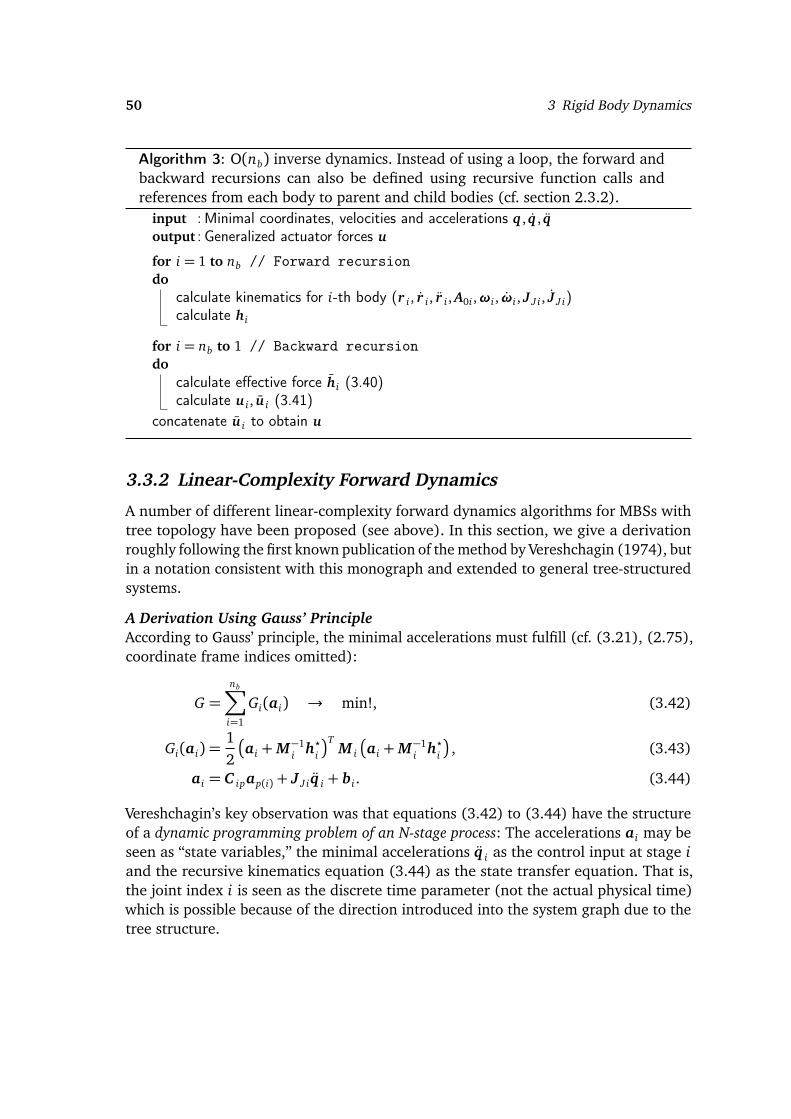
50 3 Rigid Body Dynamics
Algorithm 3: O(nb) inverse dynamics. Instead of using a loop, the forward andbackward recursions can also be defined using recursive function calls andreferences from each body to parent and child bodies (cf. section 2.3.2).
input : Minimal coordinates, velocities and accelerations q , q , qoutput : Generalized actuator forces u
for i = 1 to nb // Forward recursiondo
calculate kinematics for i-th body (r i , r i , r i , A0i ,ωi , ωi , J J i , J J i)calculate hi
for i = nb to 1 // Backward recursiondo
calculate effective force hi (3.40)calculate u i , u i (3.41)
concatenate u i to obtain u
3.3.2 Linear-Complexity Forward Dynamics
A number of different linear-complexity forward dynamics algorithms for MBSs withtree topology have been proposed (see above). In this section, we give a derivationroughly following the first known publication of the method by Vereshchagin (1974), butin a notation consistent with this monograph and extended to general tree-structuredsystems.
A Derivation Using Gauss’ PrincipleAccording to Gauss’ principle, the minimal accelerations must fulfill (cf. (3.21), (2.75),coordinate frame indices omitted):
G =nb∑
i=1
Gi(ai) → min!, (3.42)
Gi(ai) =12
ai +M−1
i h?iT
M i
ai +M−1
i h?i
, (3.43)
ai = C ipap(i) + J J iq i + bi. (3.44)
Vereshchagin’s key observation was that equations (3.42) to (3.44) have the structureof a dynamic programming problem of an N-stage process: The accelerations ai may beseen as “state variables,” the minimal accelerations q i as the control input at stage iand the recursive kinematics equation (3.44) as the state transfer equation. That is,the joint index i is seen as the discrete time parameter (not the actual physical time)which is possible because of the direction introduced into the system graph due to thetree structure.

3.3 Recursive Linear-Complexity Dynamics for Trees 51
An efficient solution procedure for such problems is based on the Principle of Optimal-ity, which states that: “An optimal policy has the property that whatever the initial stateand the initial decision may be, the remaining decisions must constitute an optimalpolicy with regard to the state resulting from the first decision” (Bellman 1954, p. 47).Using this for applying Gauss’ Principle to a kinematic chain, we get:
G?k(ak−1) =minq k
Gk(ak−1, q k) + G?k+1(ak(ak−1, q k))
, k = nb, . . . , 1. (3.45)
The solution strategy is to determine the minimal accelerations at the last stage asa function of the predecessor accelerations. With this, the optimal choice for thepredecessor minimal accelerations follow from (3.45). This procedure is then repeatedrecursively until the root body is encountered. In dynamic programming, there is nobranching of the time parameter. This corresponds to the unbranched mechanismsstudied by Vereshchagin (1974). Here, we extend the approach to branched systems,where “all remaining decisions” at the k-th stage are not encapsulated in Gk+1, but inall contributions by children of k:
G?k(ap(k)) =minq k
hGk(ap(k), q k) +
∑n∈NCk
G?n(ak(ap(k), q k))i, k = nb, . . . , 1. (3.46)
Note that the backward-recursion following from the Principle of Optimality does nothave to follow the bodies from nb to 1 for branched systems, but can use any sequenceensuring that children are treated before parents.
For a terminal body i the condition for a minimum of Gi is:
∂ Gi∂ q i=∂ ai∂ q i
T M iai + h?i
, (3.47)
= J TJ i
M i
C ipap(i) + J J iq i + bi
+ h?i
= 0. (3.48)
Solving for q i gives:
⇒ q i = P iap(i) + p i,
with:
P i = −J T
J i M i J J i
−1J T
J i M iC ip,
p i = −J T
J i M i J J i
−1J T
J i
M i bi + h?i
.
(3.49)
According to (3.46), we must minimize the sum Gk +∑
n∈NCkG?n in the next step:
0= ∂∂ q k
Gk +
∑n∈NCk
G?n
(3.50)

52 3 Rigid Body Dynamics
=∂ ak∂ q k
T M kak + h?k
+∂ ak∂ q k
T ∑n∈NCk
∂ an∂ ak
T hMn
C nkak + J Jn
Pnak + pn
+ bn
+ h?n
i (3.51)
=J TJk
M kak + h?k
+ J TJk
∑n∈NCk
C Tnk
hMn
C nk + J JnPn
︸ ︷︷ ︸
K n
ak +Mn
J Jnpn + bn
+ h?n︸ ︷︷ ︸
kn
i(3.52)
Regrouping the final equation leads to an identical structure to that found for theterminal body:
0= J TJk
M kak + h?k
,
with:
M k = M k +∑
n∈NCk
C Tnk K n,
h?k = h?k +∑
n∈NCk
C Tnkkn.
(3.53)
Accordingly, the solution is given by (3.49) and (3.53), if M , h? are replaced by M , h?:
q i = P iap(i) + p i,
with:
P i = −J T
J i M i J J i
−1J T
J i M iC ip,
p i = −J T
J i M i J J i
−1J T
J i
M i bi + h?i
,
K i = M i
C ip + J J iP i
,
k i = M i
J J i p i + bi
+ h?i ,
M i = M i +∑
n∈NCk
C Tni K i,
h? i = h?i +∑
n∈NCi
C Tnik i.
(3.54)
The resulting computational scheme is outlined in algorithm 4. For completeness,alternative derivations of the O(nb)-method using the same notation are listed in theappendix (free body approach: appendix C.1; projective EoM approach: appendix C.2).

3.3 Recursive Linear-Complexity Dynamics for Trees 53
Algorithm 4: O(nb) forward dynamics for trees. Instead of using a loop, theforward and backward recursions can also be defined using recursive functioncalls and references from each body to parent and child bodies (cf. section 2.3.2).The vector h?i includes impressed forces and moments F i
i, T io due to gravity,
actuation, etc., which are either provided externally (by a control algorithm) orcomputed from force laws as a function of q , q . Note that force laws are oftenmost naturally described in generalized coordinates, for example, for joint frictionor joint drives. In such cases, equivalent impressed forces must be calculated andapplied to all bodies which contributing to the relevant DoFs. In the exampleof joint actuators, the forces must be applied both to the driven body and itspredecessor.
input : Minimal coordinates, minimal velocities and impressed forcesoutput : Minimal accelerations
for i = 1 to nb // First forward recursiondo
calculate kinematics for i-th body (r i , r i , A0i ,ωi , J J i , J J i ,C ip, bi)
for i = nb to i // Backward recursiondo
calculate h?i
h? i ←h?i +∑
k∈NCi
C Tkikk
M i ←M i +∑
k∈NCi
C Tki K k
p i ←−J T
J i M i J J i
−1J T
J i
M i bi + h?i
P i ←−J T
J i M i J J i
−1J T
J i M iC ip
k i ←M i
J J i p i + bi
+ h?i
K i ←M i
C ip + J J iP i
for i = 1 to nb // Second forward recursiondo
q i ← P iap(i) + p i
ai = C ipap(i) + J J iq i + bi
Run-Time MeasurementsCalculation times for the Dill and Coil systems are given in figure 3.5 and figure 3.6.As expected, the O(nb) methods are vastly superior for very large nb, especially forunbranched systems. For unbranched robots, the number of bodies will typically be

54 3 Rigid Body Dynamics
101 102 103
10−6
10−4
10−2
100
Bodies nb
Run
-Tim
e[s]
Coil, NE, optCoil, CRBA, optCoil, O(N), baseCoil, O(N), opt
Figure 3.5: Run-times for calculating q for Coil mechanisms using the optimized NEand CRBA methods (best versions from figure 3.3), as well as naive and optimizedimplementations of the O(nb) method.
closer to 10 than 100 and more than 100 bodies are very unusual even for branchedrobots. The run-time measurements show that optimized NE and CRBA-based softwareis more efficient than a naive implementation of the O(nb) method for fairly largesystems (up to 10. . . 100 bodies for chains and up to 100. . . 400 bodies in branchedsystems, cf. figure 3.5, figure 3.6; see footnote 23 on page 47).
The results are in line with those by Featherstone, who found that for 30-DoFs systems“The O(n) algorithm beats the O(n3) algorithm by a factor of 2.6 on the unbranchedchain, but is only about 15% faster on the humanoid. This is mainly due to the O(n3)algorithm running approximately 2.2 times faster on the humanoid [with 30 DoFs]than on the unbranched chain” (Featherstone 2005). We obtained similar results fornaive implementations with RSC decomposition, where the CRBA algorithm is 2.41times slower than the O(nb) method for a Coil(32) mechanism and 1.31 times slowerfor a Dill(5) mechanism. Optimized versions of CRBA and NE are almost always fasterthan the naive O(nb) algorithm, but optimized O(nb) are always superior (see table 3.1for numerical values).
Note on Run-Time PerformanceIt should be noted that Featherstone’s cost analysis is based on counting the numberof additions and multiplications, while the results given here are experimentally de-termined run-time measurements. Counting operations might appear to be a morerigorous method of determining the computational complexity of different algorithmsand certainly does show the asymptotic behavior of the number of arithmetic operationsfor large nb (cf. run-time for Jacobian calculations, figures 2.15 and figure 2.16). How-ever, as noted by Baraff (1996), “It used to be that one could attempt to discuss therunning times of algorithms based on the number of multiplications and additions;

3.3 Recursive Linear-Complexity Dynamics for Trees 55
101 102 103
10−6
10−5
10−4
10−3
10−2
Bodies nb
Run
-Tim
e[s]
Dill, NE, opt, RSCDill, CRBA, opt, RSCDill, O(N), baseDill, O(N), opt
Figure 3.6: Run-times for calculating q for Dill mechanisms using the optimized NEand CRBA methods (best versions from figure 3.4), as well as naive and optimizedimplementations of the O(nb) method.
today, when a memory access may be as costly as a multiplication, such analysis nolonger holds true.” This remark is even more relevant today, since cache hierarchiesin CPUs have become more complex, main memory access has become even moreexpensive in terms of CPU clock cycles and special instruction sets such as SSE arerequired to use the full potential of modern processors. In conclusion, the degree ofcode optimization is far more important for almost all moderately sized systems thanthe question if NE, CRBA or O(nb) algorithms are used.
A close analysis of figure 3.5 and figure 3.6 shows that the scaling of the O(nb)algorithm is in fact not exactly linear, but piecewise linear with a clear increase ofthe inclination at approximately 256 and 512 bodies.27 That this is not an artifact ofour implementation can be seen from figure 3.7, where run-times of the optimizedalgorithm are shown for two different CPUs, as well as for the commercial MBS codeSIMPACK.28
The largest change in inclination occurs for 512 bodies on CPU A and for 256 bodieson CPU B. The kink is more pronounced in the curves showing run-times of our researchcode, but also clearly visible in the timings obtained from SIMPACK simulations.29 This
27. This is more evident in a linearly scaled plot, see figure 3.7.28. SIMPACK is a commercial MBS simulation program which implements the O(nb) algorithm de-
scribed by Brandl et al. (1986, 1987). For information regarding the program, see Rulka and Eichberger(1993) and http://www.simpack.com. The computational kernel is written in FORTRAN.
29. The simulations were performed using input files generated by Python scripts (http://www.python.org), which were written by Maximilian Grill as part of his semester project. A fixed step-sizeintegrator was chosen and all output was deactivated, leading to a fixed number of 30000 solver stepsper model. The average “wall clock time” reported by the solver was taken as run-time.
The fact that the kink in our code is more pronounced is probably because no attempt was made toeliminate unnecessary data structures in the research code. Instead, the classes contain various methods

56 3 Rigid Body Dynamics
Run-time [s]Run-timerel. to base O(nb)
Run-timerel. to opt O(nb)
Coil(32), O(nb), base 1.55× 10⁻⁴ (1.00) 7.00Coil(32), CRBA, base 3.73× 10⁻⁴ 2.41 16.90Coil(32), NE, base 5.42× 10⁻⁴ 3.50 24.53Coil(32), O(nb), opt 2.21× 10⁻⁵ 0.14 (1.00)Coil(32), CRBA, opt 8.62× 10⁻⁵ 0.56 3.90Coil(32), NE, opt 1.98× 10⁻⁴ 1.28 8.95
Dill(5), O(nb), base 1.54× 10⁻⁴ (1.00) 7.01Dill(5), CRBA, base, sparse 2.01× 10⁻⁴ 1.31 9.17Dill(5), NE, base, sparse 5.41× 10⁻⁴ 3.52 24.64Dill(5), O(nb), opt 2.20× 10⁻⁵ 0.14 (1.00)Dill(5), CRBA, opt, sparse 6.85× 10⁻⁵ 0.45 3.12Dill(5), NE, opt, sparse 4.95× 10⁻⁵ 0.32 2.26
Table 3.1: Run-times for branched and unbranched mechanisms with 32 bodies(Coil(32) and Dill(5)), using naive implementations of CRBA, NE and O(nb) meth-ods, together with RSC decomposition for the Dill examples, compared to optimizedimplementations (cf. figure 3.3, figure 3.4, figure 3.5 and figure 3.6).
is due to the memory architecture used in most current computers: multiple levelsof cache with different speeds and sizes are used to reduce the latency of read andwrite access to main memory. For very small systems, all data will fit in the fastestcache. With increasing nb, the storage requirements increase, requiring access first tohigher level caches and finally to main memory. Figure 3.8 shows the large differencein memory bandwidth for level one cache (L1), level two cache (L2), level three cache(L3) and main memory for the two CPUs. Since CPU A (green and blue lines) has4096 kB of cache at the highest level CPU B (orange and red lines) only 2048 kB, thedrop in bandwidth for the latter one appears at half the number of bodies (figure 3.7).The reduced speed of main memory increases the change of run-time per body forlarge systems by almost an order of magnitude. Counting operations is therefore notvery meaningful, since for very large systems the actual performance is dominatedby memory speed even for such a numerically intensive application as multibodysimulation.
and data structures required for different algorithms. This leads to a larger memory footprint and a lessoptimal memory layout (i.e., distribution of data used for a specific algorithm in memory). Also, manualoptimizations of our code were carried out for medium sized systems (nb < 100).

3.4 Kinematic Constraints 57
0 500 1,000 1,500 2,000
0
2
4
6
8
·10−3
Bodies nb
run-
time[s]
4× 10⁻⁷nb
4× 10⁻⁶nbO(nb), opt, CPU AO(nb), opt, CPU BSIMPACK (O(nb), CPU A)
Figure 3.7: Run-times for kinematic chains (Coil mechanism) for research code runon two different CPUs (red: 4096 kB cache, orange: 2048 kB cache). The green lineshows run-times using SIMPACK for the same models. Due to different implementa-tions the memory requirements and therefore the position of the kinks are different,but also present. As a reference for comparison, the blue lines show perfectly linearbehavior. The run-time per body increases by approximately one order of magnitudefor large nb, even though the algorithm is O(nb). This is due to the speed differencebetween cache and main memory (see figure 3.8).
3.4 Kinematic Constraints
Kinematic constraints are present in any non-trivial system. If a minimal parametriza-tion of the configuration is known, they can be eliminated by projection into theconstraint-free directions, see (3.2), (3.1), (3.26). In case no minimal parametrizationis known, a kinematically independent subset q I of the redundant parametrizationq T = (q I q D) can often be found. Together with the kinematic constraints, the EoMcan then be projected into the constraint free directions after numerically determiningthe dependent parameters q D (for the basic technique, see Shabana 2005; Bayazitogluand Chace 1973, p. 416; for an application to a Hardware in the Loop (HiL) simulation,where q D is determined using a velocity-level Inverse Kinematics (IK) algorithm, seeRulka and Pankiewicz 2005). Systematic methods for analyzing the kinematics ofcomplex mechanisms and finding analytical solutions for the global kinematics as afunction of a set of minimal coordinates were presented by Kecskemethy and Hiller(1993). The problem is related to IK in robotics (Hiller and Woernle 1988; Hiller et al.1986), but extended and applied to the problem of automatically setting up the explicitEoM (3.26) by Kecskemethy and Hiller (1993). A less general variant of the method is

58 3 Rigid Body Dynamics
102 103 104 105 106 107 108
0
2
4
6
·104
16kB
32kB
256
kB51
2kB
2048
kB40
96kB
size [B]
band
wid
th M
B /s
Read CPU ACopy CPU ARead CPU BCopy CPU B
Figure 3.8: Memory bandwidth for sequentially reading and copying data using 128-bit transfers for two different CPUs.c The distinct drops in bandwidth are due tothe memory architecture: CPU A has 32 kB L1 cache, 512 kB L2 cache, 4096 kB L3cache; CPU B has 32 kB L1 cache and 2048 kB L2 cache; both CPUs have a 4 kBpage size). The largest drop in read bandwidth occurs when the highest level cacheis exhausted, since main memory access is much slower than all cached reads. Forcopying, the drops occur at half the cache sizes.d CPU A is the one used for otherrun-time measurements in this chapter, see footnote 23 on page 47.
c. Results obtained with the synthetic “Bandwidth” benchmarking program (available athttp://zsmith.co/bandwidth.html)
d. The oscillations visible for small data sizes are due to the intricacies of the memory architec-ture, which are beyond the scope of this monograph.
implemented in the Modelica simulation system.30 While these and related techniquesare important for general MBSs, complex interconnected kinematic loops are lesscommon in robotics.
For tree-structured systems, efficient recursive forward dynamics procedures areavailable (see above), but their basic form cannot treat kinematic loops. Even thoughthe O(nb) methods were developed with robots in mind, many robotic systems havekinematic loops. For serial robots with rigid gears, every drive introduces a kinematicloop (see figure 3.9). Modeling the gears as elastic eliminates the loops, but increasesthe number of DoFs and leads to a stiffer EoM, due to the high gear stiffness and lowmotor shaft inertia. The classical solution is based on a Lagrangian multiplier approach.
The following section reviews methods based on Lagrangian multipliers and sec-tion 3.4.2 describes a novel recursive linear-time algorithm for systems with kinematic
30. See https://www.modelica.org/ for information about Modelica; for a description ofthe treatment of loops, see https://build.openmodelica.org/Documentation/Modelica.Mechanics.MultiBody.Joints.Assemblies.html; sites accessed 2013-11-12.

3.4 Kinematic Constraints 59
segment A segment B
motorshaft
circularspline
flexspline
wavegenerator
CAD drawing of joint drive withpermanent magnet synchronousmotor and Harmonic Drive gear.
segment A segment B
motorshaft
circularspline
flexspline
wavegenerator
Schematic diagram of joint module(left).
Figure 3.9: Computer Aided Design (CAD) drawing (top left) and schematic diagram(top right) of a typical robot joint with electric motor and reduction gear.c If segmentB is closest to the root node, it is the parent of both segment A and the motor shaft.If all components are assumed to be rigid, the relative motion between segment A andthe motor shaft is fully determined by the kinematic loop formed by wave generator,flex spline and circular spline.d Depending on the sizing of the gear relative to theloads during operation, deformations can be non-negligible. In that case, at leastthe deformation in the flex splinee must be taken into account. This removes thekinematic loop, leading to a tree structure.
c. Joint designed for Lola by Lohmeier (2010).d. For details of the operational principle of Harmonic Drive gears, refer to the company website
http://www.harmonicdrive.come. The flex spline is the pot-shaped component connecting segment A and segment B to the
motor shaft.

60 3 Rigid Body Dynamics
loops.
3.4.1 Lagrangian Multiplier-based Methods
Basic ApproachFor a system with constraints in a non-minimal parametrization, Gauss’ principle ofleast constraint (see section 3.1) can be written as:
G =12
q +M−1h?
Mq +M−1h?
→min!
Φ(q) = 0.(3.55)
Here, the free motion is obtained from the EoM without the constraints.31 A standardquadratic optimization problem is obtained by differentiating the constraints untilaccelerations appear32
G =12
q +M−1h?
Mq +M−1h?
→min!,
Φ(q) =∂ Φ∂ q
q + d
dt
∂ Φ∂ q
q = 0.
(3.56)
Following the method of Lagrangian multipliers, the solution is given by the stationarypoint of the Lagrangian L = G −λT Φ:33
∂ L∂ q∂ L∂ λ
= 0, (3.57)
⇒
M − ∂ Φ∂ q
T
− ∂ Φ∂ q
T0
!qλ
=
−h?ddt
∂ Φ∂ q
q
. (3.58)
There are a number of methods for solving (3.58). Standard procedures can be found intextbooks on advanced engineering dynamics, multibody dynamics and robot dynamics(see, e.g., Ginsberg 1998; Shabana 2005; Featherstone 2008). The most straightforwardapproach is to solve (3.58) directly, preferably using a sparsity exploiting decomposition.Another approach is to solve for λ, substitute the solution and then solve for q .
31. Here we have assumed holonomic constraints. However, non-holonomic constraints can be treatedwithout any difficulty.
32. This is equivalent to a reduction of the corresponding Differential Algebraic Equation (DAE) fromindex 3 to index 1. The index is the number of differentiations required in order to obtain an equivalentode in all unknowns (here: in q ,λ, cf. (3.58)).
33. A minus sign is used in front of the Lagrangian multiplier λ in order to have the usual directconnection to constraint forces.

3.4 Kinematic Constraints 61
Constraint StabilizationWhile the EoM (3.58) with constraints at the acceleration level is mathematically exact,it is numerically unstable and leads to unbounded numerical drift since it contains an“open-loop” integration of Φ. A simple solution to obtain a numerically stable system isto close the loop artificially by introducing a PD-type feedback to stabilize the systemaround Φ= 0 (Baumgarte 1972):
Φ+ 2αΦ+ β2Φ= 0. (3.59)
Typically, the feedback parameters are chosen such that:
Φ+ 2αΦ+α2Φ= 0. (3.60)
Substituting (3.60) into (3.58) yields the stabilized form of the EoM:
M − ∂ Φ∂ q
T
− ∂ Φ∂ q
T0
!qλ
=
−h?ddt
∂ Φ∂ q
q + 2αΦ+α2Φ
. (3.61)
The method has the appeal of being easy to understand and to implement: a spring-damper system introduces fast dynamics that keep the system within a neighborhoodof the constraint manifold Φ = 0. A criticism of this method is the need for tuning thestabilization parameter(s) (α,β) and that the numerical solution based on (3.61) nolonger satisfies the “exact” constraints Φ= 0. However, the “exact” constraint Φ= 0is itself an idealization of real constraints, often imposed by joints with imperfectgeometries and finite stiffness. In practical applications, this error can therefore usuallybe neglected (cf., e.g., Bremer 2008). A further point of criticism is the fact that largestabilization parameters can lead to stiff ODEs, requiring small integrator time stepsand leading to an inefficient solution procedure. Constraint violation due to numericaldrift and the effect of Baumgarte’s stabilization method are illustrated in figure 3.10and figure 3.11.
An alternative approach to stabilization is to re-project the solution obtained byintegration onto the manifold Φ = 0 (see e.g., Ascher et al. (1995, 1994) and Schiehlen(1997); see also Schoeder et al. (2013) for a discussion of the non-smooth case).According to Arnold, “. . . the practical use of Baumgarte’s approach is restricted tosmall scale models . . . . In off-line simulation, it is today state-of-the-art to avoid thedrift-of effect by projection techniques” (Arnold 2009, p. 31). Since robot models areusually “small” in terms of multibody systems, the first point is less relevant in thiscontext. However, the fact that there is always a finite loop-closure error and reducingit increases the numerical cost remains (see Arnold 2009).

62 3 Rigid Body Dynamics
10−1 100 101 10210−12
10−9
10−6
10−3
Time [s]
‖Φ‖
α= 0α= 1
Figure 3.10: Illustration of the influence of the stabilization parameter α for simulatinga constrained system based on (3.61). The example system is a simple planar pendu-lum with unit mass and rod length and a gravitational acceleration of 9.81 m/s2. Thesystem was integrated for 100 s using Matlab’s ode45 with absolute and relative toler-ances of 1× 10⁻⁶ starting in a horizontal position. The plot shows the constraint vio-lation for α= 0 and α= 1. Without stabilization, numerical drift leads to a quadraticincrease of the constraint violation error (inclination two in log-log graph), while α > 0leads to a bounded error with a magnitude dependent on α (as well as system andintegrator parameters).
104
105
106
107
Num
ber
offu
nctio
nev
alua
tions
10−3 10−2 10−1 100 101 102 10310−10
10−7
10−4
10−1
Stabilization factor α
Max
imum
of‖Φ‖
Figure 3.11: Maximum constraint violation and required number of function calls de-pending on the stabilization parameter α for a fixed integrator error bound (samesystem as in figure 3.10). In this example, the constraint violation error is approxi-mately equal to the error bounds for numerical integration. The required number offunction evaluations is almost constant for a small value of α. For the large values ofα required for very high accuracy, however, the resulting stiffness of the ODE stronglyincreases the required number of time steps.

3.4 Kinematic Constraints 63
3.4.2 Minimal Coordinate Linear-Complexity Forward Dynamicswith Loops
Introduction and Related WorkAs discussed in the previous section, arbitrary kinematic constraints can be treated bythe Lagrangian multiplier method. Lagrangian multipliers can also be used to extendthe recursive O(nb) algorithms discussed in section 3.3.2 to general systems withloops. The special case of serial manipulators with endpoint constraints was studiedby Lathrop (1986). To treat arbitrary constraints, a spanning tree must be defined bycutting all kinematic loops and introducing corresponding kinematic constraints andLagrangian multipliers for the eliminated joints. The Lagrangian multipliers can becalculated within the recursive procedure at the point where the last body in a loop (orconnected system of loops) is encountered. This operation is cubic in the number ofconstraint forces, which can increase the cost beyond that of a non-recursive methodin the worst case (see Brandl et al. 1987; Bae and Haug 1987b; Sorge 1993).
The Lagrangian multipliers can also be computed in a global approach. Ratherthan computing λ during the recursive procedure, the method proposed by Gattringer(2011) and Gattringer and Bremer (2005) is based on the constrained EoM (3.58),(3.61). Instead of explicitly solving the equation for λ, the multipliers can be solvedby running the O(nb) algorithm m + 2 times for m constraints. Gattringer (2011)also uses the approach for recursively solving a system with a single impact withoutinversion of the mass matrix. In his PhD-thesis, Förg also applied the O(nb) methodto constrained systems (Förg 2007). The approach assumes that the multipliers arecalculated iteratively in an outer loop. This simplifies the O(nb) algorithm, since λ istreated as a known impressed force, but it requires multiple runs of the algorithm,increasing the numerical cost.
Lagrangian multiplier-based methods have the merit of being able to treat arbitrarykinematic loops. The disadvantage is the use of a non-minimal coordinate represen-tation, increasing the number of equations and requiring the use of either constraintstabilization methods (see section 3.4.1) or DAE solvers.
In the case of robotic systems, geared drives are a common cause for kinematic loops(see figure 3.9). For the simplest case of a tree with only revolute joints and one motorand gear per joint, the DoFs are doubled and, additionally, nb Lagrangian multipliersare introduced.34 This motivates the search for methods to efficiently calculate thegeneralized accelerations in O(nb) time, while still using a minimal parametrization ofthe system to decrease numerical cost, eliminate the need for parameter tuning andavoid any constraint violation.
Schwienbacher (2013) developed a method for recursively calculating the forwarddynamics in linear time using minimal coordinates for systems with kinematic loops.The method uses the original graph representation of the system and automatically
34. The number of multipliers depends on details of the formulation.

64 3 Rigid Body Dynamics
identifies bodies that are part of at least one kinematic loop. All bodies within a loop(or multiple connected loops) are added to a subsystem. The O(nb) algorithm can thenbe run on the system consisting of individual bodies and subsystems.
The concept of subsystems was previously proposed as a tool for simplifying themodeling of complex MBS (Bremer 1987; Bremer and Pfeiffer 1988). An applicationof the subsystem concept to the recursive solution of forward dynamics was presentedby Bremer (2008), Bremer and Pfeiffer (1988), Gattringer (2011), and Gattringer andBremer (2005). The subsystems are manually defined during the modeling procedure.The process enables the treatment of loops, but subsystems and the EoM of eachsubsystem must be defined manually. The procedure uses an extended state vector foreach subsystem with > 6 DoFs to allow an explicit calculation of the full subsystemstate without referring to the state of the parent, which incurs additional overhead.35
The method presented here is different, because it is based on an automatic analysisof the unmodified graph of the MBS and only introduces subsystems where this isrequired by the presence of loops. The MBS still explicitly contains the individualbodies, which are used, for example, for various kinematics calculations. Essentially,the “subsystems” used here introduce a hierarchical definition of a MBS as a set ofabstract “bodies”, which in turn can themselves be small MBSs (cf. figure 2.11). Also,the minimal coordinates of the subsystem only include the relative DoFs with respectto the predecessor, which reduces the size of the vectors and matrices used within thealgorithm.
The automatic generation of subsystems is based on first automatically building agraph of the system and assigning DoFs by traversing the graph. Bodies within a loopor group of connected loops will use the same indices into the vector of generalizedcoordinates for describing relative kinematics. This is in turn used to move all of thesebodies into a subsystem according to figure 2.11 (for details of the graph restructuringalgorithm, refer to Schwienbacher 2013).
Recursive O(nb) Algorithm with SubsystemsThe recursive procedure for systems with loops follows the basic approach for treestructured systems (see section 3.3.2). If there are kinematic loops, however, we mayencounter a group of m kinematically coupled bodies during the backward recursion. Inthat case, all minimal accelerations for these bodies are coupled and cannot be resolvedwith the standard recursive procedure. In such a case, the coupled bodies are combinedto a subsystem, whose relative motion with respect to the common predecessor isdescribed by the subsystem DoFs qSi (cf. section 2.3.2, figure 2.11).
In order to apply the procedure used for tree structures in section 3.3.2, we canre-write (3.42) by grouping bodies into those that are part of one of the subsystems
35. The overhead will depend on the amount of symbolic pre-processing and the exploitation of sparsitypatterns for specific subsystems. A certain amount of overhead is present due to the use of redundant“describing velocities” y i for the i-th body, with y i ∈ IR6+ fi ( fi: no. of DoFs of the i-th body relative to itspredecessor). The advantage is that one set of equations can be used for all subsystems.

3.4 Kinematic Constraints 65
and the remaining ones (see node sets defined in table 2.1):
G =∑i∈nb
Gi(ai) =∑
i∈NB\NS
Gi(ai) +∑i∈NS
GSi, (3.62)
GSi =∑k∈NSi
Gk(ak). (3.63)
When minimizing this function using the dynamic programming principle, we encountertwo different cases: (1) the next contribution to G is from an individual body and (2)the next contribution is from a subsystem. The first case has already been treated insection 3.3.2. We can therefore assume that we are encountering a subsystem duringthe backward recursion process. In this case, (3.46) becomes:
G?Si(ap(si)) =minqSi
GSi(ap(si), qSi) +
∑k∈NCSi
G?k(ak(ap(sk), qSi))
. (3.64)
The index p(si) denotes the predecessor of the subsystem the i-th body belongs to, thatis, ap(si) is the predecessor’s acceleration (or, equivalently, that of the subsystem node,cf. figure 2.11 and figure 2.7). Following the derivation in section 3.3.2, we first studythe case of a terminal subsystem, that is, NCSi = ;. In that case:
G?Si(ap(si)) =minqSi
GSi(ap(si), qSi)
,
⇒ 0=∑k∈NSi
∂ Gk(ak)∂ qSi
=∑k∈NSi
∂ ak∂ qSi
T M kak + h?k
.
(3.65)
This is obviously similar to the projective form of the EoM (3.26) used for the entireMBS. The difference lies in the fact that here we have an additional dependency onthe acceleration of the subsystem’s parent body. The acceleration of each body in thesubsystem can be written as a function of the parent’s acceleration and the minimalsubsystem accelerations qSi using the known subsystem kinematics:36
ak = bC kap(si) + bJ kqSi + bbk. (3.66)
The newly introduced quantities are obtained by recursively applying the relativekinematics equations (2.75) and (2.81) until we arrive at the subsystem’s root node:
bC k = C kp(k)bC p(k) for subsystem root: bC k = I6 (3.67)
bJ k =∂ ak∂ q si= C kp(k)bJ p(k) + bJ Jk for subsystem root: bJ k = 0 (3.68)
36. This is straightforward for many robotic systems. In cases without a closed-form solution, directlyresorting to Lagrangian-multiplier methods might be more efficient.

66 3 Rigid Body Dynamics
bbk = C kp(k)bbp(k) + bk for subsystem root: bbk = 0 (3.69)
Here (and in what follows), the hat c(·) marks variables used for describing a bodywithin its subsystem. Equation (3.68) is analogous to (2.81) for the entire MBS: bJ k isa block matrix consisting of zero entries and the joint Jacobian J Jk, similar to J k forthe entire MBS (cf. (2.82)), and bJ k is similar to the corresponding global Jacobian J k
for the entire MBS. That is, quantities related to the subsystem are defined in analogyto those for the whole MBS, but retain an additional dependency on the predecessorbody. After substituting the kinematic relationships, (3.65) becomes:
∑k∈NSi
bJ T
k
hM k
bC kap(si) + bJ k + bbk
+ h?k
i= 0 (3.70)
⇔ MSiqSi + BSiap(si) + h?Si = 0. (3.71)
With:
MSi :=∑k∈NSi
bJ T
k M kbJ k,
BSi :=∑k∈NSi
bJ T
k M kbC k,
h?Si :=∑k∈NSi
bJ T
k
M kbbk + h?k
.
(3.72)
Solving (3.71) for qSi gives:
qSi = −M−1Si BSi
=:PSi
ap(si),−M−1Si h?Si
=:pSi
(3.73)
⇒ qSi = PSiap(si) + pSi. (3.74)
Similar to the O(nb)-method for systems without loops, we can substitute qSi intothe corresponding equation for the parent node i = p(si) of the terminal subsystem si.Child nodes of i that are not part of a subsystem can be eliminated using equationsfrom the standard O(nb)-method.37 As for the case without loops, the next step consistsof minimizing the sum of the contributions for the terminal subsystem and its parentbody k, taking the solution (3.74) for the terminal node into account. Since all childrenare assumed to be members of a subsystem,38 we can split the sum in (3.50) into sumsover the individual subsystems:
0= ∂∂ q k
Gk +
∑l∈NCSk
∑n∈l
G?n
(3.75)
37. In that case, M k, h?k is replaced by M k, h?
k, see section 3.3.2.38. This is possible, since single bodies have already been eliminated by the standard O(nb) method.

3.4 Kinematic Constraints 67
=∂ ak∂ q k
T¨
M kak + h?k
+∑
l∈NCSk
∑n∈l
∂ an∂ ak
T hMn
bC nkak + bJ n
PSnak + pSn
+ bbn
+ h?n
i« (3.76)
=J Tk
M kak + h?k +
∑l∈NCSk
h∑n∈l
bC T
nkMnbC nk
︸ ︷︷ ︸=:MSl
+∑n∈l
bC T
nkMnbJ nPSn
iak
+∑
l∈NCSk
h∑n∈l
bC T
nkMnbJ npSn +
∑n∈l
bC T
nkMnbbn + h?n
i(3.77)
(3.71)= J T
k
M kak + h?k +
∑l∈NCSk
hMSl + BT
SlPSl
i︸ ︷︷ ︸
KSl
ak
+∑
l∈NCSk
hBT
Sl p l +∑n∈l
bC T
nk(Mnbbn + h?n)
i
︸ ︷︷ ︸kSl
(3.78)
= J Tk
M k +
∑l∈NCSk
K Sl
=:MSk
ai +
h?k +∑
l∈NCSk
kSl
=:h?
Sk
= 0. (3.79)
The last equation again has the same structure encountered for a single terminal bodyor subsystem (cf. (3.47)), allowing us (via induction) to continue with the recursiveelimination of nodes until we encounter the root node. For the final algorithm, allinertia and force variables in the previous derivation must be replaced by the “effective”quantities including the contributions from bodies farther down the tree.
Comparing the result for systems with and without loops (3.53) suggests definingC Sl =: I6, conceptually treating the entire subsystem as a complex “meta-body” withinthe MBS, whose reference frame moves with the parent node. The full procedure forsystems containing loops is summarized in algorithm 5, with detailed equations shownin algorithm 6, 7 and 8. An alternative derivation of the method based on a minimalexample is given by Schwienbacher (2013).
Run-Time MeasurementsWe have analyzed the run-time performance of the algorithm using modified Coil andDill mechanisms (cf. section 2.4): an additional body representing motor and gearcomponents was added for every body in the Coil or Dill system. Figure 3.12 showsrun-times for the driven Coil mechanism together with the unmodified Coil mechanism(i.e., without kinematic loops) with the same number of bodies. Since the overhead
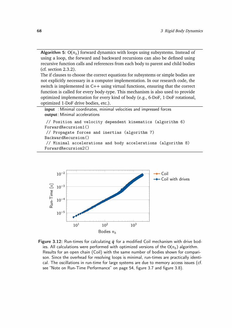
68 3 Rigid Body Dynamics
Algorithm 5: O(nb) forward dynamics with loops using subsystems. Instead ofusing a loop, the forward and backward recursions can also be defined usingrecursive function calls and references from each body to parent and child bodies(cf. section 2.3.2).The if clauses to choose the correct equations for subsystems or simple bodies arenot explicitly necessary in a computer implementation. In our research code, theswitch is implemented in C++ using virtual functions, ensuring that the correctfunction is called for every body-type. This mechanism is also used to provideoptimized implementation for every kind of body (e.g., 6-DoF, 1-DoF rotational,optimized 1-DoF drive bodies, etc.).
input : Minimal coordinates, minimal velocities and impressed forcesoutput : Minimal accelerations
// Position and velocity dependent kinematics (algorithm 6)ForwardRecursion1()// Propagate forces and inertias (algorithm 7)BackwardRecursion()// Minimal accelerations and body accelerations (algorithm 8)ForwardRecursion2()
101 102 103
10−5
10−4
10−3
10−2
Bodies nb
Run
-Tim
e[s]
CoilCoil with drives
Figure 3.12: Run-times for calculating q for a modified Coil mechanism with drive bod-ies. All calculations were performed with optimized versions of the O(nb) algorithm.Results for an open chain (Coil) with the same number of bodies shown for compari-son. Since the overhead for resolving loops is minimal, run-times are practically identi-cal. The oscillations in run-time for large systems are due to memory access issues (cf.see “Note on Run-Time Performance” on page 54, figure 3.7 and figure 3.8).
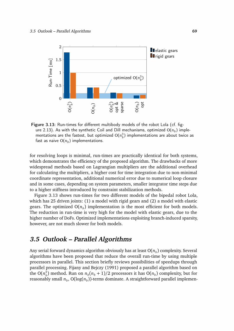
3.5 Outlook – Parallel Algorithms 69
O(n
3 b)
O(n
b)
O(n
3 b)op
t&
spar
se
O(n
b) opt
0
0.5
1
1.5
2
optimized O(n3b)
Run
-Tim
e[m
s]elastic gearsrigid gears
Figure 3.13: Run-times for different multibody models of the robot Lola (cf. fig-ure 2.13). As with the synthetic Coil and Dill mechanisms, optimized O(nb) imple-mentations are the fastest, but optimized O(n3
b) implementations are about twice asfast as naive O(nb) implementations.
for resolving loops is minimal, run-times are practically identical for both systems,which demonstrates the efficiency of the proposed algorithm. The drawbacks of morewidespread methods based on Lagrangian multipliers are the additional overheadfor calculating the multipliers, a higher cost for time integration due to non-minimalcoordinate representation, additional numerical error due to numerical loop closureand in some cases, depending on system parameters, smaller integrator time steps dueto a higher stiffness introduced by constraint stabilization methods.
Figure 3.13 shows run-times for two different models of the bipedal robot Lola,which has 25 driven joints: (1) a model with rigid gears and (2) a model with elasticgears. The optimized O(nb) implementation is the most efficient for both models.The reduction in run-time is very high for the model with elastic gears, due to thehigher number of DoFs. Optimized implementations exploiting branch-induced sparsity,however, are not much slower for both models.
3.5 Outlook – Parallel Algorithms
Any serial forward dynamics algorithm obviously has at least O(nb) complexity. Severalalgorithms have been proposed that reduce the overall run-time by using multipleprocessors in parallel. This section briefly reviews possibilities of speedups throughparallel processing. Fijany and Bejczy (1991) proposed a parallel algorithm based onthe O(n3
b) method. Run on nb(nb + 1)/2 processors it has O(nb) complexity, but forreasonably small nb, O(log(nb))-terms dominate. A straightforward parallel implemen-

70 3 Rigid Body Dynamics
Algorithm 6: First forward recursion for O(nb) forward dynamics with loops (seealgorithm 5).
input : Minimal coordinates, minimal velocitiesoutput : Velocity and position dependent kinematics
for i = 1 to nb // Forward recursiondo
if i is a subsystem // Check if node is a subsystem or a simple bodythen
// Initialize variablesbbi ← 0
bC i ← I6
bJ J i ← 0forall the k ∈ NSi // Iteration over subsystem member bodiesdo
calculate kinematics for body k (r k, r k, A0k,ωk, J Jk, J Jk,C kp, bk)// Calculate quantities w.r.t. the subsystembbk← C kp(k)
bbp(k) + bk
bC k← C kp(k)bC p(k)
bJ k← C kp(k)bJ p(k) + bJ Jk
else// Single bodycalculate kinematics for body i (r i , r i , A0i ,ωi , J J i , J J i ,C ip, bi)calculate h?i

3.5 Outlook – Parallel Algorithms 71
Algorithm 7: Backward recursion for O(nb) forward dynamics with loops (seealgorithm 5).
input : Kinematics from algorithm 7 and impressed forcesoutput : Intermediate variables for backward recursion algorithm 8
for i = nb to 1 // Backward recursiondo
if i is a subsystem thenforall the k ∈ NSi // iteration over subsystem member bodiesdo
calculate h?k// Effect of child nodes that are not in the subsystembh?k← h?k +
∑j∈(CSi∩NCk)
C Tjpk j
cMk← Mk +∑
j∈(CSi∩NCk)
C Tjp K j
// Calculate subsystem quantitiesMSi ←
∑k∈NSi
bJ TkcMkbJ k
MSi ←∑
k∈NSi
bC TkicMkbC ki
BSi ←∑
k∈NSi
bJ TkcMkbC k
h?Si ←∑
k∈NSi
bJ Tk
cMkbbk + bh
?
k
PSi ← M−1Si BSi
pSi ←−M−1Si h?Si
KSi ← MSi + BTSiPSi
kSi ← BTSi p i +
∑k∈NSi
bC Tki(Mk
bbk + h?k)
else// single bodycalculate h?ih? i ←h?i +
∑k∈NCi
C Tkikk
M i ←M i +∑
k∈NCi
C Tki K k
p i ←−J T
J i M i J J i
−1J T
J i
M i bi + h? i
P i ←−J T
J i M i J J i
−1J T
J i M iC pi
k i ←M i
J J i p i + bi
+ h? i
K i ←M i
C ip + J J i
P i

72 3 Rigid Body Dynamics
Algorithm 8: Second forward recursion for O(nb) forward dynamics with loops(see algorithm 5).
input : Output from algorithm 6 and algorithm 7output : Minimal accelerations q , linear and angular accelerations for all bodies
for i = 1 to nb // Forward recursiondo
// Calculate minimal accelerationsq i ← P iap(i) + p i
if i is a subsystem then
ai = ap(i) // Subsystem node moves with parentforall the k ∈ NPSi // Nodes with children outside the subsystemdo
ak = bC kiai + bJ kq i + bbk
else// Single body
ai = C ipap(i) + J J iq i + bi
tation of recursive O(nb) schemes is to process each branch (or groups of branches)in parallel on a separate processor. Such a parallel implementation of forward andbackward recursion steps was proposed by Bae et al. (1988), along with parallel matrixfactorization methods.
A different class of algorithms for kinematic trees works by recursively disassem-bling and assembling sub-trees in order to enable parallel processing. The Divide andConqueror Algorithm (DCA) proposed by Featherstone (1999a) achieves O(log(nb))complexity when run on nb processors. An extension to (almost) arbitrary topologiesbased on loop-cutting and Baumgarte-stabilization (Baumgarte 1972) is described byFeatherstone (1999b). The asymptotic complexity is preserved for many systems, butworst-case complexity can be O(n3
b). Featherstone (1999b) also analyzes the compu-tational cost of different parallel algorithms and the ABA by counting the number ofadditions and multiplications. If the parallel algorithm is run on nb processors, theoperations count is lower than for the O(nb) ABA for as few as 14 bodies. Operationscounts for the DCA and ABA algorithms are shown in figure 3.14. It is important tonote that for current processors, a similar speedup of the run-time is unlikely, since thelocking and communication costs induced by such a massive parallelization are verylarge compared to the number of operations between synchronizations.
Yamane and Nakamura (2009) analyzed and compared the serial ABA-Algorithmwith two parallel O(log(nb)) methods, Assembly Dissasembly Algorithm (ADA) byYamane and Nakamura (2009), a method similar to Featherstone’s DCA, and the

3.5 Outlook – Parallel Algorithms 73
0 10 20 30 40 50
0
1
2
3·104
Number of Bodies (nB)
Num
ber
ofO
pera
tions
DCA (nB cores, m= 1, a = 1)DCA (nB cores, m= 1, a = 0)ABA (m= 1, a = 1)ABA (m= 1, a = 0)
Figure 3.14: Number of operations for the ABA and DCA (on nb processors). The ar-eas show upper and lower limits of the number of operations, when multiplications(m) are given a weight of one and additions (a) a weight between zero and one (oper-ations count equations from Featherstone 1999b).
Constraint Force Algorithm (CFA) proposed by Fijany et al. (1995). Differences in theparallel algorithms are mainly due to the formulation of the EoM for the subtree (or“articulated body”) and the constraints.
Critchley et al. presented an alternative DCA, which is more efficient for a smallernumber of processors and provides approximately 40% reduction of run-time for a128-body chain on a four processor system.39 (Critchley et al. 2007, figure 8)
In his PhD-thesis, Clauberg describes work on parallelizing MBS code. Speedupsof a factor of 2.3. . . 2.4 are achieved on an eight processor machine (Clauberg 2013,figure 4.3 and figure 4.4). The implementation is based on work by Förg (2007), whichuses a redundant coordinate formulation in combination with bilateral and unilateralconstraints. The mass matrix is always block diagonal, so its decomposition can becalculated efficiently. Lagrangian multipliers are calculated with a fixed-point iterationscheme, requiring the inversion of a matrix with the dimension of the Lagrangianmultipliers (for details see Förg 2007).
For very large systems, parallelization can potentially provide significant speedups.For kinematic trees, special O(log(nb)) algorithms have been developed. For typicalsystem sizes in robotics, however, the gains are smaller than those of code-optimizations(see above). It is likely, however, that the importance of parallel algorithms will onlybecome greater with the wider availability of “Many-Core” processors and more efficient,hardware-supported communication and locking mechanisms.
39. System specification: 3.2 GHz quad-processor Intel® Xeon® shared memory system running Linux.Programs compiled with GCC, POSIX threads and semaphores used for parallelization (Critchley et al.2007).

74 3 Rigid Body Dynamics
3.6 Chapter Summary and Discussion
This chapter presents principles and methods from classical mechanics that form thebasis of computational algorithms for forward and inverse dynamics of multibodysystems. We presented both global EoM-based methods and recursive approaches in auniform mathematical notation.
It is widely recognized that linear-time algorithms are the most efficient for treestructured systems. They provide a dramatic improvement of run-times over naiveimplementations of the NE method for very large kinematic chains. Efficient implemen-tations of the NE method exploiting sparsity induced by the topology of the mechanism,however, are quite competitive for reasonably sized and/or branched systems.
While the classical linear-time algorithm uses Lagrangian multipliers and redundantcoordinates to enable the simulation of systems with kinematic loops, a new formulationof a subsystem-based approach described in this chapter enables the simulation ofmechanisms with loops using minimal coordinates.
The detailed run-time analyses in this chapter support the basic trends in run-timeperformance expected from counting the number of operations required per DoF. Theactual run-times, however, vary strongly and depend on details of the implementation,the computer and memory architecture.
The algorithms outlined above can be used to provide the core of an efficient simula-tion program for robotic systems, as well as dynamics and kinematics routines requiredas building blocks for model-based controllers.
Realistic simulations must incorporate models for actuators (including friction, motordynamics, possibly gear elasticity) and contact dynamics. Effectively, this adds addi-tional ODEs for the actuator dynamics and algebraic force laws. For possible models formotor dynamics and gear friction see (Buschmann et al. 2006; Buschmann 2010; Bauret al. 2014) and references therein. In many cases, robot-environment interaction canbe modeled as visco-elastic. For unilateral, visco-elastic contacts the resulting force lawis non-smooth and requires the detection of contacts and the integration of a first-orderODE. A possible implementation for biped robots with visco-elastic soles walking on arigid polygonal mesh is given in (Buschmann 2010).
Unilateral contacts between rigid bodies require special treatment. They are notconsidered here, since the contact elasticity is non-negligible in most robotic appli-cations. For a treatment of non-smooth mechanical systems the reader is referred toGlocker (2006, 2000), Acary and Brogliato (2008), and Leine and Nijmeijer (2004)and references therein.

4 Biped Walking Control
This chapter reviews widely-used control strategies for biped walking robots. It ismostly based on a previous paper co-authored by me (Buschmann et al. 2014). Thischapter, however, focuses on walking control for biped robots, as well as the postureand balance control of humans. It also adds references to other parts of the monographand a discussion motivating the following chapter.
For a comprehensive review of the neural and robotic control of walking of two, fourand six-legged systems with cross-references between the fields, see (Buschmann et al.2014).
Section 4.1 briefly reviews posture and balance control of humans to provide thecontext for the following sections covering walking robots. Section 4.2 reviews typicalhardware designs, since they determine the dynamics, the sensing capabilities and ap-plicable forces. Section 4.3 covers basic concepts in the mechanics of legged locomotion,while the remaining sections review widely-used walking control approaches, whichwe have classified into model-based control of underactuated robots (section 4.4),model-based control of fully-actuated robots (section 4.5), biologically-based control(section 4.6) and gait cycle-centered control (section 4.7).
There are some parallels in the design and control of legged robots and animals, sincethey share the same basic principle of locomotion and are governed by the same physicallaws. However, there are significant differences, mainly due to three reasons. (1) Thephysical properties of robots and animals differ with respect to sensing, actuation andmass distribution, mainly as a consequence of the currently available technology. (2)Since any robot must function as a whole, the focus in robot walking control is mostlyon global coordination, postural control and balance, since these are the predominantproblems for bipedal robots. In neuroscience, on the other hand, the complexities ofthe organisms and available experimental techniques often lead to a focus on low-levelaspects of neural control. (3) Because there is no thorough understanding of the neuralcontrol of posture and balance in the Central Nervous System (CNS) (see section 4.1),robotic controllers are mostly based on first principles and control theory. Nevertheless,a brief review on the neural control of walking is given in the following, since it hasand continues to influence research on robotic walking controllers (and vice versa).
4.1 Neural Control of Posture and Balance
Posture and balance control in walking animals is a complex neural task. Posturecontrol concerns the generation of motor activity to produce and maintain an adequate

76 4 Biped Walking Control
position and orientation of the animal relative to the vector of gravity and the footlocations. The actions of the skeleton-muscle system undertaken to prevent the bodyfrom falling out of any position taken during (quasi-) static motion and the actionstaken to prevent falling during dynamic locomotion are called balance control (e.g.,Winter 1995; Orlovsky et al. 1999; Deliagina et al. 2012). Legged animals differ in thecontrol of posture and balance depending on the number of legs. For a review of thecontrol of multilegged animals, see (Buschmann et al. 2014).
There are two central systems that play an important role in the balance and posturecontrol of humans (for review see Orlovsky et al. 1999; Deliagina et al. 2012). Thefirst is located in the spinal cord at the level of the legs. It receives input from limbmechanoreceptors about force, load and position.1 It counteracts disturbances bygenerating corrective motor responses. The second is located in the motor cortex andthe brain stem. It receives signals from limb mechanoreceptors, vestibular and visualsignals (figure 4.1). These three sensory qualities contribute to balance control in aredundant fashion. This second system mediates its influence on the muscle-skeletonsystem by acting on those local networks in the spinal cord that generate motor activitycontrolling posture and movements. Which of the two systems contributes how muchto the control of posture and balance is not clear yet (Buschmann et al. 2014).
The details of neural control of human balance are not well-understood, but basicpostural reflexes and some fundamentals of the dynamics of locomotion are knownfrom biomechanical studies. In stance, humans respond to external disturbances with alimited set of motor primitives (Horak and Nashner 1986). The dominant reaction is theankle-strategy, when anterior and posterior disturbances are effectively counteractedby reflex activation of ankle plantarflexors and dorsiflexors to maintain balance. Analternative response is the hip-strategy, that is, flexion or extension of the hip. Therealso are mixed reactions containing ankle and hip activation, suggesting that thesestrategies are really muscle synergies underlying the neural control of balance (Torres-Oviedo and Ting 2007; Horak and Nashner 1986). Larger disturbances are compensatedby a stepping-strategy, that is, by modifying the Base of Support (BoS), or even byhopping or stumbling motions (Horak 1987). It has been suggested that ankle-, hip- andstepping-strategy constitute a hierarchy of possible responses (Horak 1987), but morerecent work indicates that all strategies are activated in parallel and that the steppingstrategy is aborted if deemed unnecessary (Maki and McIlroy 1997). It has also beenshown that prior knowledge of and repeated exposure to perturbations significantly
1. Vertebrates have different sensory organs that provide force, position and velocity information to theCNS (see Buschmann et al. 2014, and citations therein). The golgi-tendon organs (GTOs) are responsiblefor force information and are located in the tendons of all skeletal muscles. The Muscle Spindles (MSs)report information concerning muscle stretch and velocity. There are two types of MSs: static anddynamic, whose sensitivity is actively and separately modified by γ-motoneurons. Type Ia afferent fibersinnervate both types of MSs, reporting velocity and position information to the CNS, while type IIafibers only innervate static MSs and therefore mostly report length changes. The relative contribution ofboth types of MSs depends both on the specific muscle and the activation by γ-motoneurons.

4.1 Neural Control of Posture and Balance 77
Supraspinal Commands
Visual Signals Vestibular Signals
Spinal Postural Circuits
Muscle Skeleton System: Limbs
Posture
RS VS CS RbSexcitatory drive
load feedbackmovement feedback
Brain
SpinalCord
Figure 4.1: Main components of the postural system in quadrupeds. Two closed loopsystems contribute to postural control. Spinal networks generate postural reflexes andtheir action is added to the influence of supraspinal commands, which originate fromsensory information from visual and vestibular sensors and which are transmitted tothe spinal networks via reticulaspinal (RS), vestibulospinal (VS), corticospinal (CS)and rubrospinal (RbS) tracts (modified from Deliagina et al. 2012).
changes the response (Marigold and Patla 2002; Horak and Nashner 1986). Thesethree basic control strategies are also applied in many biped walking control algorithms(see section 4.5.2).
There have been some attempts to model and reproduce the overall behavior ofhuman balance control during stance using methods from control theory. Fujisawa et al.(2005) analyzed the hip and ankle strategies in humans by studying responses to smalldisturbances during stance.2 Using system identification techniques and modeling thehuman as a double pendulum, linear transfer functions from upper and lower bodyinclination to ankle and hip moment were determined. The study found proportionaland derivative contributions in the response, but distinguishing the contributions ofneural control and the muscle-skeleton system is not possible. A different model ofstance control based on sensor fusion, disturbance estimation and linear control theoryis discussed in (Tahboub and Mergner 2007; Mergner et al. 2009).
In biomechanical studies, balance in humans is mostly studied based on simplemodels such as the Inverted Pendulum Model (IPM) or Linear Inverted PendulumModel (LIPM) and the concept of balance is usually not clearly connected to themathematical theory of the stability of dynamical systems. In this field, balance is
2. Knee bending was prevented by wooden splints.

78 4 Biped Walking Control
classically equated with keeping the CoM over the BoS (Winter 1995). Hof et al.(2005) proposed an extended stability measure based on an IPM, requiring that theeXtrapolated center of Mass (XcoM) remain within the BoS (cf. section 4.5.2) andproposed hypothetical walking control laws based on this concept (Hof 2008). Notethat this analysis is based on a transformation of the pendulum equations previouslyproposed in the context of biped robots (see section 4.5). Aftab et al. (2012) proposedanother hypothetical control law for stepping based on an optimal predictive controllerfor the LIPM and found similar responses to perturbations during stance also found inhumans.
It should be noted that current state-of-the-art robots are not only capable of maintain-ing balance during stance, but also during dynamic locomotion and even in somewhatuneven terrain (see following sections). Neural control of posture and balance in hu-mans is not well understood in such cases, partly because they are difficult to analyzeexperimentally with humans.
4.2 Hardware Design
Robot StructureA wide range of different walking robots have been built, with quite different mechanicaldesigns. The leg mechanisms are often designed as rigid links connected by rotary joints.The rigidity of the links is especially important for model-based control approaches:Measuring link deformations is difficult even with additional sensors such as straingauges on structural components. Also, structural elasticity can lead to undesirablevibrations and link deformations can cause early or late ground contact, disturbingthe gait. Some robots, however, intentionally include elasticity in the drives or in thetelescopic legs of running robots (see below).
For fully-actuated bipeds, the most common design features six actuated joints per legand feet enabling surface contact (Hirose and Ogawa 2006; Pfeiffer 2006; Nelson et al.2012; Pratt et al. 2009; Ogura et al. 2006). Planar bipeds and some three dimensionalsystems use point feet and as few as two DoFs (Chevallereau et al. 2003; Miura andShimoyama 1984).
ActuationDifferences in robot hardware in comparison to biology are to a large extent due toavailable actuator technologies (cf. Buschmann et al. 2014; Pons 2005). For many years,the prevalent choice of actuators for bipedal robots were geared brushed DC motors(Hirai et al. 1998; Nishiwaki et al. 2000; Pfeiffer et al. 2002). More recently, permanentmagnet synchronous motors have been used for highly loaded joints (Lohmeier et al.2009; Hirose and Ogawa 2006; Tsagarakis et al. 2011). Hydraulics (Nelson et al. 2012;G. Cheng et al. 2006; Raibert et al. 2008) and pneumatics (Vanderborght et al. 2005a,2005b) are also used, but less often.

4.2 Hardware Design 79
One motivation for using pneumatic actuators is their inherent compliance, which isalso apparent in biological muscle-tendon systems where it has a significant impacton the dynamics of walking. An early attempt towards designing a human-like actu-ation system is described by Yamaguchi and Takanishi 1997. The humanoid Wabianhas antagonistically driven joints incorporating nonlinear spring mechanisms, whichenables the robot to control both the effective torque and stiffness of the joint, similarto animals and humans.
In a different approach to actuation involving compliance, a position controlled,geared electrical motor is connected to the output side by mechanical springs, a conceptknown as series elastic actuation (Pratt and Williamson 1995). The goal is to providehigh-fidelity force control by measuring and controlling the spring deflection, whichis proportional to the applied force, but also adds an unactuated DoF to the systemand lowers the position control bandwidth. Robots using these devices include the2D-biped Spring Flamingo (Pratt and Pratt 1998b) and the 3D-bipeds M23 and itsmore recent redesign M2V2 (Pratt and Krupp 2008). Similar to Robinson et al. (1999)and Pratt and Williamson (1995), more recent studies also cite high fidelity torquecontrol as an advantage of series elastic actuation (Remy et al. 2012; Hutter et al.2012). Several humanoid robots with compliant, antagonistic and bi-articular actuationwere developed at the University of Tokyo4(e.g., Shirai et al. 2011).
Elasticity is widely used in the actuation systems of one-legged and multi-leggedhopping robots, but less so in bipeds. Hyon and Mita (2002) and others use mechanicalsprings, M. H. Raibert (1986) uses pneumatic cylinders and Brown and Zeglin (1998)bow-shaped legs. For an overview of the hardware design (and control principles) ofone-legged hopping machines, see (Sayyad et al. 2007). Most notably, M. H. Raibert(1986) built a one-legged hopping machine to conduct experiments on balancing inthree dimensions during continuous hopping. The leg is a pneumatic cylinder that isconnected to the body by a gimbal joint. The lateral DoFs of the leg are actuated byhydraulic actuators. For details on the hardware design, refer to (M. H. Raibert 1986;Raibert et al. 1984).
SensingIn contrast to biological walking systems, walking machines generally have a muchlower number of sensors which are, on the other hand, often more precise than theirbiological counterparts. Most robots are equipped with motor encoders for positionsensing, a smaller percentage also has torque sensing in the joints and/or link sideencoders. Due to the importance of contact forces for balance, Force/Torque Sensors(FTSs) in the feet are a standard component in biped robots. FTSs are sometimescombined with or substituted by contact switches for detecting ground contact. Mostrobots also have Inertial Measurement Units (IMUs) in the upper body or pelvis whichare used for balance control (Lohmeier et al. 2009; Tajima et al. 2009; Hirose and
3. http://www.ai.mit.edu/projects/leglab/robots/m2/m2.html, accessed 2013/18/104. http://www.jsk.t.u-tokyo.ac.jp/research.html, accessed 2013/18/10

80 4 Biped Walking Control
Ogawa 2006; Kaneko et al. 2004; Nelson et al. 2012).
4.3 Basic Dynamics of Legged Locomotion
Machine locomotion can be categorized either as statically or as dynamically stable (cf.Berns et al. 1999; Bekey 2005; Full et al. 2002). The first formulation of a conditionfor static stability of a walking system is given by McGhee and Frank (1968), wherethe authors define static stability for walking on a horizontal plane as a configurationwhere the projected CoM lies within the current BoS. This criterion, however, is onlysuitable in the idealized quasi-static case, when inertial forces are negligible. In caseswith significant accelerations, dynamic stability has to be investigated. See M. Raibert(1983) and Full et al. (2002) for a discussion of dynamic stability. Note that stability isnot to be confused with feasibility, which is related to the set of possible contact forcescompatible with the unilateral foot ground contact. See also section 4.5 and (Wieber2002).
Walking machines are hybrid systems, since the foot-ground contact is unilateral:The contact states of the feet take on discrete values such as opened, closed, slipping orsticking, while at the same time the pose of the robot varies continuously. This hybridnature is also found in the dynamics of walking systems: Trajectories of joint angles orjoint torques are continuous functions of time, but landing positions of feet and stridelengths have discrete values for each step.
As with any controlled system, the resulting motion of the robot will depend both onthe dynamics of the uncontrolled system, composed of the robot and its environment,and the walking controller. In the large body of work on walking control, the emphasisput on the design of either (passive) mechanics or control varies greatly, as does theemphasis put on either the discrete (step-to-step) or continuous aspects of walking. Infigure 4.2 we give a rough overview of which aspects are emphasized in the predominantapproaches to walking control described below. Figure 4.3 and 4.4 illustrate twodifferent approaches towards stable bipedal walking described in more detail below:stabilization through contact force control (figure 4.4) and (almost) passively stablewalking, augmented by some control and energy supply (figure 4.3).
Strictly speaking, every legged robot is underactuated, since the foot-ground contactalways has finite stiffness and there is no input corresponding to the elastic deforma-tion of the contact. Nevertheless, robots with one actuator per joint will be termedfully actuated in this monograph, if the remaining underactuation is only due to thedeformation in the ground contact. This is to distinguish them from robots with pointfeet, with unactuated joints or additional elastic DoFs.

4.4 Model-Based Control of Underactuated Robots 81
Continuous
Phase-Dependent
Fully ActuatedPassive Walkers
Limit Cycle Walkers
CPG-BasedOptimal Predictive Feedback Control
Figure 4.2: Schematic diagram of different walking control methods. The approachesare categorized according to the emphasis put on continuous feedback control andphase dependent or step-to-step control. In our view, an ideal walking controller wouldbe situated in the central area of the diagram with equal emphasis on the discrete andcontinuous aspects of both dynamics and control. A possible implementation could beachieved by optimal control methods with properly chosen cost functions (figure fromBuschmann et al. 2014).
4.4 Model-Based Control of Underactuated Robots
In this section, we give an overview of model-based control methods for underactuatedhopping machines and biped robots.
Raibert’s experiments with one-legged hopping machines (cf. section 4.2) and thegeneral control strategy developed for them is a milestone in legged robot research.The control system is model-based and the control task is decomposed into the threeparts forward running velocity, body attitude and hopping height (M. Raibert 1983).The employed control principle is sometimes referred to as Raibert’s three-part control(Semini 2010). By introducing the virtual leg concept originally introduced by Suther-land and Ullner (1984), where multiple legs are considered to behave as one virtualleg, the three part control principle can be used to control walking machines with morethan one leg (M. H. Raibert 1986).
An interesting theoretical framework for walking control that emphasizes the problemof underactuation was developed for the five-link planar robot Rabbit (Chevallereauet al. 2003; Westervelt et al. 2003). This robot uses four electric motors for actuation.The actuated joints, as well as the passive joints connecting the robot to the centralboom enforcing the planar motion, are equipped with position sensors and the feet withcontact force sensors. The robot has point feet, leaving one degree of underactuationat the foot-ground contact.
The controller enforces the same number of position-dependent virtual constraints

82 4 Biped Walking Control
Balance Control
Inertial Data
Joint Angles
Force Control
Force
Force Setpoint
Joint Setpoints
Figure 4.3: Structure of model-based biped balance control system based on force andinertial measurements following the approach found in (e.g., Buschmann et al. 2009;Takenaka et al. 2009c). The inertial data is used to calculate modified contact forcesetpoints, which are tracked via a low-level joint position control loop. Note that thisis a simplified drawing emphasizing a basic principle. An actual implementation mustat least add load distribution during double support, as well as account for swing-stance and stance-swing transitions (figure modified from Buschmann et al. 2014).
as can be directly controlled via the actuators, for example, four in this case. Theconstraints are not given as a function of time, but parameterized by some monotonicstate variable, for example, the stance leg inclination. Since the chosen outputs (orvirtual constraints) can easily be tracked by a position controller, stability is determinedby the remaining internal dynamics of the system (the zero dynamics) that are not visiblein the outputs. Since the robot is a hybrid dynamical system, the internal dynamics arecalled hybrid zero dynamics. A stable control system is designed by calculating virtualconstraints using offline optimization methods that can enforce stable zero dynamicsvia inequality constraints in the optimization problem. The essence of the approach isto control only as many outputs as can be directly controlled and to choose these insuch a way as to assure stability of the uncontrolled DoFs.
This approach has more recently been applied to the planar five-link biped Mabel(Sreenath et al. 2011). The basic structure is similar to Rabbit’s, but forces are appliedby compliant, antagonistic actuators, increasing the degree of underactuation andadding a mechanical energy storage and shock absorption mechanisms. Very recently,Park et al. (2013) expanded the system to include a component based on a FiniteState Machine (FSM) for reacting to large changes in ground height. According to thedetected system state (step-down, step-up, tripping, . . . ), modified virtual constraintsare controlled. Additionally, active force control is added to stabilize the system andattenuate shocks when stepping off high platforms.

4.5 Model-Based Control of Fully-Actuated Robots 83
Round Feet
KneesFinite State Machine
ener
gysu
pply
cont
act
stat
e
Figure 4.4: Semi-passive limit cycle walker with typical design elements. Round feetwith a (passive or active) knee-locking mechanism enable a passive rocking motionduring stance. Limited actuation is included to compensate for energy losses andcontrol is performed by a simple finite state machine. The degree of actuation andcontrol may vary from fully passive (McGeer 1990) to some actuation (Collins andRuina 2005) or even almost full actuation with step position control (see Hobbelenand Wisse 2009; figure modified from Buschmann et al. 2014).
While a number of robots with elastic actuation mechanisms have been developed(see section 4.2), the question of how to utilize the compliance in walking machinesremains an open problem. In the controller proposed by Vanderborght et al. (2005a)for the pneumatically actuated robot Lucy (cf. section 4.2), joint position referencesare tracked at a lower control level, compensating joint elasticity.
Robots with series elastic actuators are also underactuated (see section 4.2). However,since a low-level controller tracks the desired joint torque, the upper control levels canview the system as a torque controlled robot. Pratt et al. (2001) proposed using VirtualModel Control for such robots. In this approach, virtual forces acting on the robot aregenerated using intuitive, heuristic rules and then mapped to actuator forces via thecorresponding Jacobians.
4.5 Model-Based Control of Fully-Actuated Robots
Many successful approaches to walking controller design for fully-actuated robots arebased on physical models and classical control system design. This section reviewsmodel-based control of fully-actuated bipeds.
From a control systems perspective, the major differences between the control of a(rigid) manipulator and walking control are the hybrid nature of the walking system, theunderactuation and the inequality constraints imposed by the unilateral ground contact.

84 4 Biped Walking Control
While questions such as low-level control of the joints can be efficiently handled withwell-known methods from manipulator control, the additional tasks of (1) satisfyingall constraints and (2) stabilizing the unactuated DoFs, while (3) exhibiting the desiredwalking behavior remain challenging.
Due to the highly nonlinear dynamics and the inequality constraints, a straightfor-ward solution of the control problem, using, for example, optimal control methods,is currently impossible due to the computational costs. Nevertheless, a number ofpromising results from simulation studies using detailed models and optimization havebeen reported: Azevedo used nonlinear Model Predictive Control (MPC)5 for a planarbipedal robot (Azevedo et al. 2002), Schultz presented optimal trajectories for a 3Dmodel of a human (Schultz and Mombaur 2010) and Tassa reported a fast but non yetreal-time MPC method for generating and stabilizing various motions of a humanoidrobot (cf. Tassa et al. 2012 and section 5.6.1). Therefore, most control systems use ahierarchical design with higher levels responsible for overall behavior, intermediatelevels for the discrete gait sequences and lower levels for task-space and joint-spacemotion (see Buschmann et al. 2009; Nishiwaki et al. 2002 and figure 4.5), therebyexpressing organizational similarities to walking animals (see Buschmann et al. 2014).The control problem is often separated into planning ideal reference trajectories andmodifying the references using feedback control. However, more recently there hasbeen a trend towards incorporating sensor feedback into planning to improve longterm stability, blurring the distinction between planning and feedback control (Tajimaet al. 2009; Nishiwaki and Kagami 2006).
4.5.1 Planning Reference Trajectories
Since real-time planning using complex multibody robot models is currently compu-tationally intractable, there are two dominating approaches to planning referencetrajectories: (1) off-line planning using comprehensive models and (2) online planningusing simplified models. Due to the importance of real-time gait generation for adapt-ing to changes in the environment or the desired behavior, most systems today usereal-time methods. For examples of offline planning methods see (Denk and Schmidt2003; Buschmann et al. 2005; Bessonnet et al. 2004; Cho and Oh 2008). Most work ononline planning is based on simplified lumped mass models, usually the LIPM (Kajitaand Tani 1995). This model describes the linear dynamics of the CoM in the lateraland sagittal planes when the CoM height remains constant (see Buschmann 2010, fora discussion). Occasionally, additional terms for approximating the influence of legmotion and torso rotation are added (Pratt et al. 2006; Takenaka 2004b; Park and Kim1998; Buschmann et al. 2007).
The simplified robot model is given as an ODE relating the CoM to the contact moment
5. That is, solving an optimal control problem, using the result for the next time step and thenrepeating the procedure at every time step.

4.5 Model-Based Control of Fully-Actuated Robots 85
Planning
Stabilizing Control
Inverse Kinematics
Robot(with low-level control)
Desired Behavior
Ideal Force & Movement
Adapted Force &Movement
Joint Space Commands
Sensor Data
Figure 4.5: Example of a hierarchical control architecture with real-time planning andbalance control for fully-actuated robots, as it is used in many state-of-the-art walkingmachines (e.g., Buschmann et al. 2009). Each level can have multiple sub-levels, forexample, step-cycle and trajectory planning within the “Planning” level. Planning andcontrol are typically formulated in terms of foot and CoG positions and contact forces.Joint space variables for low-level control are then obtained from inverse kinematics.Most early and some current implementations use offline planning, but online methodsnow dominate since they facilitate more reactive behavior. (figure from Buschmannet al. 2014).
at the foot. The planning system must determine contact force and CoM trajectoriesthat satisfy the ODE and for which the forces satisfy the inequality constraints imposedby the unilateral ground contact. In biped walking control the Zero Moment Point(ZMP)6 is often used instead of the contact moment, since it leads to a simple criterionfor feasible contact forces when walking on flat ground: the ZMP must remain withinthe convex hull of the BoS (Vukobratovic and Borovac 2004). This feasibility criterionis often mistakenly used as a stability criterion, even though satisfying it does not assurethat the robot will not fall.7 General feasibility criteria are discussed in (Hirukawa et al.
6. This is the point where the resulting contact force acts.7. The relationship between ZMP and stability is controversial (Vukobratovic et al. 2006; Sardain
and Bessonnet 2004). We will only try to briefly describe the controversy. A central issue is the fact thatVukobratovic distinguishes between the case when the ZMP is strictly within the BoS and the case whenit is on the edge (Vukobratovic et al. 2006), a fine point that is often overlooked. Vukobratovic onlyrefers to the first case as stable, since the ZMP may be moved towards the edge to stabilize the system.If the resulting contact force lies on the edge of the BoS, this point is no longer called the ZMP. Thisdistinction separates the Center of Pressure (CoP) from the ZMP according to Vukobratovic. Nevertheless,it is easy to design cases when the ZMP is at the center of the BoS and no feasible control can preventthe robot from falling. This is possible, since the state of the system is not uniquely defined by the

86 4 Biped Walking Control
2006; Takao et al. 2003). Most planners first calculate an admissible force trajectorythat can then be used to determine a CoM trajectory by solving the ODE. To assurea stable solution to the planning problem, this approach requires either a deviationfrom the ideal force trajectory by actively modifying the reference (Takenaka et al.2009a; Buschmann et al. 2007), by only approximately satisfying it (Kajita et al. 2003b;Diedam et al. 2008), or by violating the desired boundary values for the CoM-trajectory(Sugihara and Nakamura 2005).
Proposed planning algorithms using this approach include analytical solutions(Harada et al. 2004; Morisawa et al. 2006; Löffler et al. 2004), numerical solutionsby finite difference approximation (Kagami et al. 2002), a kind of shooting method(Takenaka 2004b; Takenaka et al. 2009a), methods based on model predictive control(Kajita et al. 2003b) and a method based on spline collocation (Buschmann et al. 2007).Diedam et al. (2008) proposed using linear MPC for solving the planning problem. Theimplementation is based on quadratic programming, enabling a simple extension ofCoM-planning to footstep adaptation.
4.5.2 Stabilizing Control
General Walking ControlA large and growing number of control methods for stabilizing fully-actuated bipeds hasbeen proposed and successfully implemented. The task of balance control (also calledstabilizing control) is to assure a given reference motion while simultaneously prevent-ing the robot from falling. Most methods build on the basic stabilizing mechanisms of(1) modifying the contact forces, (2) horizontally accelerating the CoM and (3) foot-step control. These mechanisms are roughly equivalent with the (1) ankle-strategy, (2)hip-strategy and (3) stepping-strategy observed in animals (see section 4.1). Figure 4.3illustrates the basic idea of balance control through contact force modification.
If the robot becomes unstable, it will diverge from the ideal, stable reference motion.A deviation of individual joint angles from the reference gait pattern is not critical, butthe robot must avoid falling. Since a computationally tractable, practical and correctstability criterion for walking systems remains to be found (cf. Wieber 2002), thedivergence of the total linear and angular momentum of the system may be taken as apractical measure of instability. The total linear and angular momentum of a systemcan only be changed by external forces acting on the system boundary. Modifyingcontact forces therefore is the only possible way of stabilizing the system. In fact, thehip-strategy changes contact forces by accelerating the CoM (or vice versa) and thestepping-strategy modifies the whole range of feasible forces by changing the BoS.
ZMP. The simplest examples are statically stable configurations for which a very high CoM velocity ischosen (Buschmann 2010). Regardless of the relationship of the ZMP to stability, the concept has beeninstrumental in the development of biped walking controllers.

4.5 Model-Based Control of Fully-Actuated Robots 87
The dominant method of stabilization via contact force control consists of modi-fying the contact moment in order to stabilize the upper body orientation or CoMposition (Kajita et al. 2005; Löffler et al. 2004; Takenaka 2004a; Takenaka et al. 2009c;Buschmann et al. 2009). Usually, the contact moment is measured by the FTS in thefoot and controlled via an underlying joint position controller. The landing impact maybe reduced by an additional vertical impedance or force control (Löffler et al. 2004;Kajita et al. 2005; Nishiwaki and Kagami 2009; Buschmann et al. 2009), or an indirectforce control via reduced joint position control gains (Tajima et al. 2009; Nishiwaki2001; Hashimoto et al. 2009).
Accelerating the upper body or CoM for balance control is also widespread (Tajimaet al. 2009; Nishiwaki and Kagami 2006). Takenaka et al. propose activating thisstrategy when the maximum admissible contact moment is reached (Takenaka et al.2009c).
An interesting approach addressing the issue of underactuation was proposed byChevallereau et al. (2008). Instead of tracking trajectories, only a reference path istracked. This adds the path parameter as an additional control input, making planarbipeds fully actuated. This method is related to ideas from path-following control ofrobot manipulators (Pfeiffer and Johanni 1986).
Modifying the next foothold leads to a strong deviation from the originally intendedmotion, but at the same time is the most powerful method of stabilization. For thestepping-strategy the range for modifying the forces is limited by the maximum steplength and stepping speed, while contact force control and upper body accelerationare limited by the size of the feet and the friction coefficient between the feet and theground.
The stepping-strategy is also used by the one-, two- and four-legged hopping machinesdeveloped by M. H. Raibert (1986) and Hodgins and Raibert (1991). In this work thecontrol of speed and balance is achieved by modifying the stepping position relative to aneutral point defined by the foothold corresponding to a periodic hopping motion (M. H.Raibert 1986; Raibert and Brown 1984). This strategy can be used very effectively forthe hopping machines due to the very low leg mass and inertia.
Takenaka et al. (2009c) propose modifying the step positions in case modificationsof the upper body trajectory induced by the hip-strategy cannot be compensated duringthe next step without changing the step length. Urata et al. (2011) propose calculatingfootstep positions using singular preview control and online parameter optimization.The strategy requires fast stepping, which is enabled by high-speed actuation and highstructural stiffness (Urata et al. 2010). Tajima et al. (2009) propose a controller for arunning biped based on frequently replanning the CoM trajectories, as proposed byNishiwaki and Kagami (2006). The system uses the initial velocity of a periodic gaitpattern as final velocity for calculating the CoM trajectory of the current step. Theresulting final CoM position for the current step and the initial distance of the CoMfrom the stance leg for the periodic gait are then used to determine the next stance legposition.

88 4 Biped Walking Control
Pratt et al. (2006) coined the term Capture Point for positions where the robot canstep in order to come to a complete stop. The set of all Capture Points is called theCapture Region. To facilitate the calculation of Capture Points, the robot is described bythe LIPM, augmented by a fly wheel. Based on this concept, strategies for push-recoveryand walking control are formulated. Nelson et al. (2012) propose positioning the footrelative to the Capture Point according both to the desired gait and the balancingrequirements in the walking control of the Petman robot.
For the LIPM, the Capture Point is equivalent to the XcoM introduced by Hof et al.(2005, also see section 4.1). It is also equivalent to the divergent component introducedeven earlier in a patent by Honda Motor Co. Ltd. (Takenaka 2004b). The essenceof Honda’s method is a diagonalization of a first-order representation of the LIPMODE, which leads to two decoupled systems, of which one is stable (the convergentcomponent) and one is unstable (the divergent component). The divergent componentis then used to assure convergence of the CoM-trajectory to a desired periodic gait.8
The concept has since been extended to running gaits with non-constant CoM-heights(Takenaka et al. 2009d).
Walking in Uneven TerrainWalking in unknown and uneven terrain is especially challenging for biped robotsand has been addressed both by control and by hardware design. Kang et al. (2010)developed a special foot mechanism for the robot Wabian-IIR with distance sensorsthat can mechanically adapt to uneven terrain. Similar mechanisms were previouslydeveloped at the same institute for biped walking chairs (Yamaguchi et al. 1995,1994). Impedance or force control have been proposed for reducing the landing impactduring walking (Buschmann et al. 2009; Nishiwaki and Kagami 2010; Lim et al. 2001).Other researchers have proposed implicit force control for reducing landing impacts,implemented by reducing joint position control gains during the expected impact phase(Tajima et al. 2009; Nishiwaki 2001; Hashimoto et al. 2009). Very recently, the robotATLAS developed by Boston Dynamics for the DARPA Robotics Challenge9 based onPetman, was shown to walk over loose rocks held in a wooden frame. To our knowledge,the only publication is a video10 released on the internet and details on the controllerdesign are unknown.
4.6 Biologically-Based Pattern Generation
BackgroundMost robot control systems are model-based and adopt the basic architecture of planningideal reference trajectories and modifying them based on sensor feedback (cf. figure 4.5).
8. Note that coming to a complete stop is a special case of a periodic orbit.9. http://www.theroboticschallenge.org
10. http://youtu.be/SD6Okylclb8, accessed 2013/18/10.

4.6 Biologically-Based Pattern Generation 89
In contrast to this, many biologically inspired concepts use Central Pattern Generator(CPG) models for creating walking trajectories. The goal of these concepts is to replicatethe generation of rhythmic patterns for walking generation as observed in animals andhumans in the walking machine control systems. As a CPG model, a neural oscillatorproposed by Matsuoka (1985) is often used (e.g., Endo et al. 2008; Fukuoka and Kimura2009). Matsuoka’s CPG is a model of two mutually inhibiting neurons described bycoupled differential equations. This model represents the half-center oscillator conceptwhich is the most important element of neural networks for creating alternatingleft-right locomotion activity in vertebrates. One feature of CPGs is their ability tosynchronize their intrinsic oscillations with input signals,11 thus allowing adaptabilityto changing environments. This integration of internal and reflex loops is seen as oneof the key features of biological walking control (see Buschmann et al. 2014).
However, CPG models often require costly parameter tuning to realize even basicwalking in bipeds. Many optimization methods have been proposed for creating aset of suitable parameters, such as a gradient method with reinforcement learning in(Matsubara et al. 2006; Sugimoto and Morimoto 2011).
One important approach in CPG-based control is the concept of resetting the phaseof a neural oscillator as soon as ground contact of the swing leg is detected. It has beenshown in theory (e.g., Aoi and Tsuchiya 2006) and in experiments (e.g., Nakanishiet al. 2004) that this phase reset can improve the stability of a CPG-controlled walkingmachine. Fukuoka and Kimura (2003) propose a CPG-based control system for aquadruped robot in which the walking pattern for each leg is generated by definingdesired joint positions depending on the current state of the leg. The criteria for statetransition initiation depend on CPG model variables and position feedback.
Application to Biped RobotsSugihara (2009) proposes a CPG based on a controlled LIPM. While the pendulum isinherently unstable when generating the pendulum position by integrating the equationof motion based on a given ZMP trajectory, a stable limit cycle can be generated bycalculating the input ZMP using a nonlinear feedback law.
Geng et al. (2006) proposed a biologically inspired control method for the smallbiped robot RunBot with four active joints, based on previous work with the similarWalkBot robot. Walking is based solely on reflexive control implemented in a networkof non-spiking neurons consisting of one extensor and one flexor neuron per joint(see Buschmann et al. 2014; Büschges et al. 2011). The motoneuron output is directlyconverted to an armature voltage for the driving DC motors. The mechanical design ofWalkBot has typical features of passive walkers such as mechanical end-stops in theknees and round feet. Sensory feedback is provided by potentiometers in the joints andcontact sensors in the feet. The authors have also used online learning based on policysearching to tune controller parameters (Geng et al. 2006).
11. This is known as entrainment. A famous example is the adaptation of the stepping rate of decerebratecats walking on a motor-driven treadmill (Pearson 2008).

90 4 Biped Walking Control
Applicability and PotentialFor high-performance walking robots the dominant control methods are based onphysical models and classical control theory. We can hypothesize that biologically-based pattern generation approaches have been less successful so far because theyhave mostly focused on low-level aspects, such as the structure of the neural oscillatorsinstead of the performance of the system as a whole. However, it is known fromneurobiology that the relevant aspect of the pattern generators is not necessarily theperiodic output they are capable of generating, since this will always be modifiedby task-dependent intra-joint-, intra-leg- and inter-leg- sensor feedback and couplinginfluences of other CPGs as well as by higher brain areas. The more important aspectis the structure of possible feedback paths they define, for example, positive forcefeedback during stance or position feedback during swing. The biological backgroundis reviewed in (Buschmann et al. 2014). An example of biologically inspired walkingcontrol within a model-based framework is given in (Buschmann et al. 2012a).
4.7 Gait Cycle-Centered Control
4.7.1 Limit Cycle Walkers
It is known from biomechanics that the physical properties of the musculosceletalsystem are important for human and animal walking. In fact, simple mechanicalmodels of walking and running have been developed that show similar force patternsin simulations to those observed in experiments with humans. The simplest models arethe inverted pendulum model and the SLIP model (Blickhan 1989). Interestingly, ithas been observed that such very simple spring-mass models are stable without activecontrol, a property often called self stability or open-loop stability.
This has motivated the design of a number of mechanisms and robots that emphasizethe natural dynamics of walking over active control. At the extreme end are passivedynamic walkers with no active control pioneered by McGeer (1990), which go back tosimple mechanical toys that can walk down an inclined slope by rocking from one footto the other. The gait is fully determined by the kinematics and mass distribution of themechanism and the incline of the slope. In a sense, the walking control is embedded intothe mechanical design of these machines. The passively swinging legs are stabilizedby mechanical stops during stance, the landing impact acts as a physical resettingmechanism and the inclined ground provides energy. While mostly explored in thecontext of bipedal robots, the underlying principles of passive dynamic walking havealso been applied to multi-legged mechanisms (Sugimoto et al. 2011).
More recent work has focused on exploiting passive dynamics while adding someactuation and control (cf. figure 4.4). Collins and Ruina (2005) presented a mechanismincorporating actuators and springs connected in series to the ankle joints. This mecha-nism provides energy via a push-off motion after initial contact of the contralateral leg.
4.7 Gait Cycle-Centered Control 91
The actuator is controlled by a simple FSM. Sensing is provided by ground contact andfoot extension switches.
In general, limit cycle walkers emphasize step-to-step control, not continuous stabi-lization or tracking control (Hobbelen et al. 2008). An example of a more recent limitcycle walker is the robot Flame. It combines some classical design elements seen inpassive dynamic walkers, such as hyperextension stops in the knees, but still is capableof level ground walking thanks to the addition of joint actuation (Hobbelen et al. 2008).The robot uses lateral foot placement for stabilization. The heuristic linear control lawis based on the CoM position and velocity in combination with foot contact switchesfor step-phase control (Hobbelen and Wisse 2009).
4.7.2 Step-Phase Control
In the majority of robot walking control systems there is no real step-phase controlin the sense of a feedback control system, since timing and duration of stance andswing phases are predetermined by a planning module. Note that this is not the casefor CPG-based controllers, which often include step-phase control via a phase-resettingmechanism for the neural oscillators (see section 4.6). This section focuses on step-phase control for non-CPG-based systems.
Event-based phase switching mechanisms that incorporate sensory feedback intostep-phase control have been developed for a variety of walking systems such as ahopping robot (Sato 2007), quadruped robots (Fukuoka and Kimura 2003; Hawkerand Buehler 2000), planar biped robots (Pratt and Pratt 1998a, 1998b; Pratt et al.2001; Sreenath et al. 2011) and 3D biped robots (Furusho and Sano 1990; Pratt andPratt 1999; Morisawa et al. 2011; Buschmann et al. 2012a). Sato (2007) presents aswitching controller for a hopping robot where the same controller is used during theflight and the ground contact phases. Phase change events cause a switching of desiredvariables and gains.
The control framework for biped robots developed by Pratt et al. incorporates a statemachine for each leg. The rules for state transitions are formulated intuitively based onthe position of the body relative to the feet and ground contact force information (Prattand Pratt 1998a, 1999, 1998b; Pratt et al. 2001). In simulation, the contact forcesacting on the feet are used to realize a phase reset mechanism for the transition tothe double support phase. The transition to the single support phase is initiated oncethe ground contact force on the designated swing leg falls below a given threshold(Pratt and Pratt 1998b, 1999). In experiments with a planar robot, these contact forceconditions are replaced with geometric conditions (Pratt and Pratt 1998a). The phasereset mechanism is also used by Furusho and Sano (1990), who developed a walkingcontrol system for a 3D robot and realized stable walking at a speed of 0.18 m/s. Thecondition for the transition to the single support phase is that the CoM passes abovethe toe. A phase reset mechanism is also used in the walking control of the planar robot

92 4 Biped Walking Control
MABLE (Sreenath et al. 2011) and in a simulation of the robot HRP-2 (Morisawa et al.2011).
Currently, many realizations of event-based walking control systems incorporateintuitive rules for phase transition, especially for the transition to the single supportphase (Furusho and Sano 1990; Pratt and Pratt 1998a, 1998b; Pratt et al. 2001;Sreenath et al. 2011). Most of the event-based control strategies mentioned above aretested in simulation (Pratt et al. 2001; Pratt and Pratt 1998a, 1999) or experiments withplanar robots with few degrees-of-freedom (Pratt and Pratt 1998a, 1998b; Sreenathet al. 2011) and not in experiments with 3D robots. The author has proposed step-phasecontrol laws for biped walking based on stability considerations, which has enabledthe robot Lola to walk over unexpected and unmodelled obstacles (Buschmann et al.2012a).
4.8 Chapter Summary and Discussion
This chapter reviews common approaches to hardware and control design for bipedrobots, as well as current knowledge of human balance and postural control. A largenumber of different approaches have been taken in this field and no review can dofull justice to all of them. Nevertheless, some distinct approaches can be distinguished.Currently, robots with stiff structures and hierarchical controllers with an inner high-gain control loop and outer loops handling contact force/impedance control andbalance clearly show the best performance.
Theoretically, MPC methods should be the tool of choice for walking control sincethey provide a systematic approach towards optimally exploiting the known dynamics infeedback controllers for complex systems. With increasing computational power, theseapproaches will become more widespread. At the same time, the direct implementationof walking control using real-time MPC for realistic robot models is still many yearsaway due to the prohibitive computational cost. More importantly, no control methodcan tell us how to choose the inputs, the outputs and the control objectives.
This is where neurobiological findings can help us identify which physical quantitiesare controlled during a certain task in animals (positions, velocities, forces, etc.) andwhich coordinates are chosen for the control (joint velocities, foot velocities, etc.),which can help to identify promising control approaches for walking machines.
While state-of-the-art bipedal robots are capable of quite fast and robust locomotion,the gap between the capabilities of humans and machines still is considerable. Muchresearch is still at the level of generating and stabilizing a basic walking pattern andsuccessful approaches use strong simplifications and impose severe restrictions onpossible motions.
Promising approaches towards improving the capabilities of bipedal robots are there-fore to be found in basic research on improved methods for generating, modelingand controlling bipedal walking. One approach currently being pursued is to move

4.8 Chapter Summary and Discussion 93
from time-based trajectories that are modified by feedback for stabilization to a funda-mentally feedback-based coordination of the gait cycle, as it is found in animals andhumans (see Buschmann et al. 2012a, 2014). The second promising line of research isto improve the capability of generating motions in real-time that efficiently make useof all DoFs. This second line of research is addressed in the following chapter.


5 Optimal Redundancy Resolution andCollision Avoidance
Algorithms for generating and controlling the motion of complex robots must take manyconstraints into account while trying to satisfy multiple goals. This chapter reviewssome classical methods for robot motion generation that are suitable for real-time useand presents methods and application examples for humanoid robots and redundantagricultural manipulators. Classical methods for choosing locally optimal motions arereviewed in section 5.1. An efficient approach to modeling complex robot geometriesfor the purpose of collision detection and avoidance is presented in section 5.2. Applica-tion examples of local methods for nullspace optimization and collision avoidance aredescribed in section 5.3, an approach to task-space collision avoidance for humanoidrobots in section 5.4. An extension of the classical local methods to hybrid task descrip-tions composed of force and position variables is described in section 5.5. A predictiveapproach to redundancy resolution with an application to redundant manipulators ispresented in section 5.6. Section 5.7 concludes the chapter.
5.1 Local Inverse Kinematics
Often motion generation can be simplified by not planning a trajectory of generalizedcoordinates q(t) ∈ IRn (typically joint angles), but rather a set of suitably definedtask-space trajectories w (t) ∈ IRm. For robot manipulators, w typically consists of theposition and orientation of the end-effector, but can be an arbitrary function w (q) ofthe generalized coordinates. In the case of bipedal robots, w might contain the CoM aswell as the foot positions and orientations.1 The following review of local IK methodsis in part based on (Buschmann et al. 2012c, section 1).
One approach to controlling a robot along a task-space trajectory w d is to track anequivalent joint-space trajectory qd satisfying
w (qd) = w d. (5.1)
Here (and in what follows) the index d indicates a desired quantity. Solving the IKproblem (5.1) is more complex than direct kinematics calculations (see section 2.3),since there generally is no function mapping w to q , even in the non-redundant
1. See (Buschmann et al. 2009; Buschmann 2010) for examples of task-space definitions for bipedalrobots.

96 5 Optimal Redundancy Resolution and Collision Avoidance
case where dim(w ) = dim(q) (or: m = n). In general, there are four characteristicconfigurations (see figure 5.1): (1) there is exactly one solution, (2) there are multiplesolutions, (3) there is no solution and (4) there are an infinite number of solutions.
The IK problem (5.1) can be solved using several approaches. In simple cases geo-metrical reasoning or analytical manipulations might lead to a solution. Much efforthas been put into the analysis of serial manipulators with four, five and six DoFs. Inspecial cases, such as when three consecutive axes of rotation of a six-axis manipulatorintersect, or when three consecutive rotational joints are parallel, there are closed-formsolutions (see Pieper 1968; for a recent review see Siciliano and Khatib 2008, chapter 2).Tsai and Morgan (1985) reduced the IK problem for general six-axis manipulators tothe solution of a system of eight second order equations in eight unknowns. In specialcases the solutions of this system can again be computed in closed form. In the generalcase all solutions can be calculated using continuation methods (a numerical technique,see Tsai and Morgan 1985).
The advantage of analytical approaches is the ability to obtain all solutions. Theyare, however, restricted to special cases. General choices of w and arbitrary branchedsystems can only be handled numerically. The direct solution of (5.1) (position-levelIK) is described in the next section, more widespread methods at the velocity andacceleration levels are discussed in the following ones.
5.1.1 Position-Level Inverse Kinematics
The simplest numerical IK method consists of iteratively solving the nonlinear equationw d = w (q) starting from an initial guess q0. In the non-redundant case the classicalNewton-Raphson method (dim(q) = dim(w )) is well suited. In this approach, a linearapproximation of (5.1)
w (q0 +∆q)≈ w (q0) +∂ w∂ q |q0
∆q , (5.2)
is repeatedly solved for ∆q , until some error bound is deemed small enough. With theJacobian Jw =
∂ w∂ q , applying the Newton-Raphson method yields the basic algorithm 9
(see Pieper 1968, for an early use of this method). This approach inherits characteristicproperties of Newton’s method: (1) the solution depends on the initial guess, (2)only one solution is generated, (3) rapid convergence for good initial guess, (4) rapiddivergence for bad initial guess and (5) no solution for singular Jw.
Better convergence properties are achievable by standard globalization strategiessuch as damping methods or steepest descent methods (for details see, for example,Deuflhard (2011, chapter 3)). A straightforward generalization for the redundant caseis to use the pseudoinverse instead of the inverse of the Jacobian, which is closelyrelated to velocity-level approaches for redundant systems (cf. section 5.1.2). TheIK problem can also be formulated as a nonlinear optimization problem (for a goodoverview see Bonnans et al. 1997). The advantage is the straightforward inclusion

5.1 Local Inverse Kinematics 97
w d
w d
Case 1: Two solutions. w d in the interiorof W .
Case 2: Exactly one solution. w d on theboundary of W .
w d
w d
Case 3: No solution. w d outside of W . Case 4: An infinite number of solutions(the second body exactly covers the first).w d in the interior of W .
Figure 5.1: Illustration of some configurations encountered during in the solution of IKproblems. The desired end-effector position w T
d = (x y) is given (green dot) the jointangles q T = (q1 q2) are unknown. Depending on the position of w d in the domain Wof reachable task-space positions w and the parameters of the system there may beno solutions, one solution, multiple solutions or an infinite number of solutions. HereW the disc centered on the first joint with a radius given by the stretched length ofboth bodies.

98 5 Optimal Redundancy Resolution and Collision Avoidance
Algorithm 9: Position-level IK based on the Newton-Raphson method.input : Initial guess q0, desired output w d, error bound εoutput : Approximate solution q to w d = w (q)
repeat∆w ← w d − w (q k)Solve Jw∆q =∆wq k← q k−1 +∆qk← k+ 1
until ‖∆w‖< ε
of additional objectives and constraints, the disadvantage the larger numerical cost.An early example is the method published by Goldenberg et al. (1985) based oncoordinate partitioning and numerical optimization. More recent optimization-basedwork including a comparison of different descent algorithms2 is reported by Ayusawaand Nakamura (2012).
5.1.2 Velocity-Level Inverse Kinematics
The direct kinematics function w (q) is nonlinear, such that (5.1) has no closed formsolution in the general case. A standard method of obtaining an approximate solutionis to differentiate (5.1) once with respect to time, which leads to an implicit first-orderODE in the unknown q :
w = Jwq = w d. (5.3)
For non-redundant robots (dim(q) = dim(w )) in non-singular configurations, we candirectly solve for q to obtain an explicit ODE:
q = J−1w w d. (5.4)
If a solution w (q(t0)) = w d(t0) is known at a time t0, calculating q(t) from a givenw d(t) amounts to solving an IVP for (5.4). Similar to integrating differentiated kine-matic constraints in a mechanical system, directly integrating (5.4) leads to unboundeddrift (cf. section 3.4.1). As for constrained mechanical systems, drift can be limited bya Baumgarte-like control term (Baumgarte 1972), replacing w d in (5.3), (5.4) by
w d,eff = w d + K(w d − w (q)). (5.5)
This Closed Loop Inverse Kinematics (CLIK) algorithm is illustrated in figure 5.2.Using the measured instead of the current desired generalized coordinates q in (5.5)
2. Steepest descent, conjugate gradient Levenberg-Marquardt and Quasi-Newton

5.1 Local Inverse Kinematics 99
K J−1w
∫(·)dt
DK
w d ∆w w d,eff q q
w−
w d
+
Figure 5.2: Velocity-level inverse kinematics using the inverse Jacobian and drift com-pensation (CLIK, closed loop inverse kinematics).
leads to a task-space feedback control law, where the actual task-space tracking erroris controlled instead of the numerical drift. In this scheme, the calculated referencevelocity q can also be directly input to a joint velocity controller.
For position controlled robots, q(t) is calculated by numerically integrating q(t),usually using a simple forward Euler scheme. A significant difference between standardIVPs and the differential IK problem is the fact that the integration error ∆w =w d − w (q) can be computed directly. This has led to the development of problem-specific step-size control methods (e.g., Gupta and Kazerounian 1985). An investigationof different integration and error control algorithms that achieve better accuracy thanEuler’s algorithm at the same cost may be found in (Featherstone 1994). For largestep-sizes or very high accuracy requirements, advanced algorithms should be used,but the basic algorithms are sufficient for most real-time applications. For a stabilityproof of CLIK algorithms in the discrete domain, see (Falco and Natale 2011).
For redundant systems with dim (q)> dim (w ), one of the infinite number of possiblesolutions to (5.3) may be chosen by adding a cost function to be minimized at everytime step. The use of a quadratic penalty on joint velocities was proposed by Whitney(1969) as Resolved Motion Rate Control (RMC):
Φ=12
q T Wq →min!
g = w d,eff − Jwq = 0.(5.6)
The positive definite, and usually diagonal, matrix W defines the norm for penalizingq and usually reflect the motion range and/or maximum speeds of different joints.An extension to more general cost functions was proposed by Liégeois (1977). ThisAutomatic Supervisory Control method minimizes the weighted sum of the original cost12 q T Wq and the change ∆H of an additional cost function H(q) during the next timestep ∆t:
Φ=12
q T Wq +α ∂ H∂ q q →min!
g = w d,eff − Jwq = 0(5.7)

100 5 Optimal Redundancy Resolution and Collision Avoidance
The first equation uses the linear approximation ∆H = ∂ H∂ q q∆t which is added to Φ
with an appropriately chosen weighting factor α.A straightforward solution to this Quadratic Program (QP) is obtained with the
method of Lagrange multipliers. The Lagrangian
L =12
q T Wq +α ∂ H∂ q q +λT (w d,eff − Jwq) (5.8)
yields the optimality conditions
∂ L∂ q
T= 0= Wq +α
∂ H∂ q
T − J Twλ, (5.9)
∂ L∂ λ
T= 0= w d,eff − Jwq . (5.10)
Since W is positive definite, (5.9) can always be solved for q :
q = W−1J Twλ+W−1α ∂ H
∂ qT, (5.11)
(5.10)⇒ w d,eff = JwW−1J Twλ+ JwW−1α ∂ H
∂ qT, (5.12)
⇒ λ= JwW−1J Tw
−1w d,eff −
JwW−1J T
w
−1JwW−1α ∂ H
∂ qT. (5.13)
Substituting λ into (5.11) yields the closed-form solution:
q = J#w ,W w d,eff −αNw ,W W−1
∂ H∂ q
T, (5.14)
J#w ,W = W−1J T
w
JwW−1J T
w
−1, (5.15)
Nw ,W = (I − J#w ,W J w ). (5.16)
Here, J#w ,W is the (W -) weighted (Moore-Penrose) pseudoinverse and Nw ,W the cor-
responding nullspace projection matrix, which maps any vector x ∈ IRnq into J w ’snullspace, that is:
J w (Nw ,W x ) = J w x − J w J#w ,W︸ ︷︷ ︸
I
J w x = 0 ∀ x ∈ IRnq . (5.17)
A numerically more efficient method is the direct solution of the original optimizationproblem, without explicit calculation of the pseudoinverse,3 see algorithm 10.
3. This is due to Klein and Huang (1983).

5.1 Local Inverse Kinematics 101
Algorithm 10: Velocity-level IK for redundant robots without explicit calculationof the pseudoinverse.
input : Task w d, nullspace vector zB← JwW−1J T
wp ← w d − JW zSolve Bλ= p for λq ← W−1
J T
Wλ− z
5.1.3 Acceleration-Level Inverse Kinematics
Differentiating the velocity-level forward kinematics function (5.3) once more yields
Jwq + Jwq = w d, (5.18)
which can be solved for the generalized accelerations q and integrated to obtain q andq . Luh et al. (1980b) proposed a Resolved Acceleration Rate Control law for a six-axismanipulator which is similar to (5.5), but defined at the acceleration level:
w d,eff = w d + K D(w d − w (q)) + K P(w d − w (q)). (5.19)
Luh et al. (1980b) closes the feedback loop via an inverse model control, that is, therequired input forces are computed from an inverse model of the robot and then appliedto it. An alternative for position-controlled robots is to integrate q and send q to a jointposition controller.
Hollerbach and Suh (1985) proposed resolving kinematic redundancy by locallyminimizing joint torques. Since both the equations of motion and (5.18) are linearin q , this corresponds to solving a QP. The linearity in q is also exploited in theoperational space control framework proposed by Khatib (1983). This approach hasbeen generalized to hybrid position/force control based on the operational spaceformulation of the EoM4 (Khatib 1987).
A generalized algorithm with collision avoidance and joint limits is applied to ahumanoid by Dariush et al. (2010). The methods from first order redundancy resolution(see (5.1.2)) are modified in this work for second order kinematics.
5.1.4 A Note on Singularities
IK methods that rely on solving a linear equation involving J w fail when the Jacobianbecomes singular. Geometrically, the rank deficiency of Jw corresponds to a loss of
4. The “operational space formulation” uses an EoM in task space Mww + hw = uw, calculated fromthe original EoM and the acceleration-level differential kinematics (5.18).

102 5 Optimal Redundancy Resolution and Collision Avoidance
DoFs. task-space velocities are related to the Jacobian via
w = ∂ w (q)∂ q q = Jwq , (5.20)
that is, w is a linear combination of Jw’s columns. Rank deficiency therefore correspondsto a reduction of the dimension of the space of achievable task-space velocities.5 Singularconfigurations can appear at the outer edge of the reachable workspace (e.g., for fullystretched manipulators) or inside the workspace (often when multiple axes becomeparallel).
A classical approach to handle singular (or nearly singular) configurations at thevelocity-level is due to Nakamura and Hanafusa (1984, 1986). It is based on a leastsquares approach to solving (5.3), where an additional term penalizing velocities isadded:
Φ=12(w d,eff − J w q)2 + kq2→min!, (5.21)
⇒ q =J T
w J w + kI−1
J Tw w d,eff. (5.22)
For a weighting factor k > 0 the inverse exists. The main drawback is an inexactsolution outside of singularities. This, however, may be counteracted by an adaptive,configuration-dependent choice of k.
A further classical method is related to minimizing the task-space tracking errorew = w d − w (q). The steepest descent method for minimizing 1
2e2w gives the update
rule:
q k+1 = q k − ∂ ew∂ q
T= q k + J T
w (w d − w (q)). (5.23)
By analogy, the corresponding transposed Jacobian CLIK algorithm is defined by:
q = J Tw w d,eff. (5.24)
This IK scheme does not suffer from singularities and is very cheap computationally,but also significantly less accurate since task space velocities are only tracked due tothe feedback law: in almost all cases
w = J w J Tw w d,eff 6= w d, (5.25)
since J w J Tw 6= I . The method is obviously stable in the sense of Lyapunov in the static
case (e.g., Lyapunov 1992; Khalil 2000).6 For w d 6= 0 stability is not guaranteed, but
5. The same argument applies to Newton’s method at the position-level or acceleration-level ap-proaches, when “task-space velocity” is replaced by “task-space position increment” or “task-spaceacceleration” and q is replaced by ∆q (during the Newton iteration) or q .
6. This is easily proven using the Lyapunov function candidate V (q) = 12 eT
w Kew , where K is the

5.2 Efficient Collision Geometries and Distance Calculations 103
maintained in most applications.
5.1.5 Hierarchical Methods and Inequality Constraints
The idea proposed by Liégeois (1977) of actively exploiting kinematic redundancyhas been applied to tracking multiple tasks with a given priority (Nakamura et al.1987). Effectively, the tracking error of a less important task is tracked in the nullspaceof a more important task by appropriate application of pseudoinverses. The methodhas been extended to an arbitrary number of priority levels (Baerlocher and Boulic1998; Siciliano 1990). More recently, extensions to incorporate inequality constraintshave been proposed (F. Cheng et al. 1994; Kanoun 2011; Escande et al. 2010). Whenlower-priority tasks are not feasible within the nullspace of high-priority tasks, theprojected matrices become rank-deficient, a phenomenon known as an algorithmicsingularity. A possible solution is to use truncated singular value decomposition tocalculate inverses, or to use smooth regularization methods similar to the dampedpseudoinverse (cf. (5.22); Chiaverini 1997; Kanoun 2011). Inequality constraintstypically arise due to physical limits of the robot such as joint ranges, maximum jointspeeds and accelerations or collision avoidance (e.g., Stasse et al. 2008). A numberof groups have worked on this approach extensively, adding more capabilities andapplication examples and developing software frameworks. Notable examples are the“iTaSC” software (see Decre et al. 2013; De Schutter et al. 2007; Decre et al. 2009) andthe “Stack of Tasks” (see Mansard et al. 2009b, 2009a).
5.2 Efficient Collision Geometries and DistanceCalculations
Since robots usually have a large workspace and wide range of motion, they can easilycollide with the environment or with themselves. This problem is especially acute forbranched systems with many DoFs such as humanoid robots. For such systems, mostchoices of generalized coordinates are unfeasible, since they lead to self-collision orviolate joint limits. This section reviews some approaches to collision detection andcollision avoidance, with a focus on humanoid robots. It also presents an efficientsystem for real-time detection and avoidance of potential collisions, which has beensuccessfully applied to an agricultural manipulator and a humanoid robot. This sectionis based on joint work with Markus Schwienbacher (Schwienbacher et al. 2011).
closed-loop feedback matrix. Alternatively, this can be viewed as a property that is inherited from thestability of the steepest descent method for convex objective functions.

104 5 Optimal Redundancy Resolution and Collision Avoidance
5.2.1 Background and Related Work
Distance calculations are not only essential for real-time control of complex robots, butalso central to other fields such as computer graphics, CAD or dynamics simulation.Much research has therefore gone into developing efficient algorithms for this task (forreview see, e.g., Lin and Gottschalk 1998; Jiménez et al. 2001). In motion planning andcomputer graphics polygonal models are dominant, since they enable the approximationof arbitrarily complex geometries and hardware-accelerated rendering is enabled byGraphics Processing Units (GPUs). The major drawback is the high computational costof distance queries between complex objects. Also, the edges of the polyhedra lead tokinks in the distance function between objects, with is not ideal for optimization-basedmethods and real-time control (see below).
The importance of proper collision avoidance for complex robots has motivatedseveral research efforts on (real-time) self-collision avoidance for humanoid robots(e.g., Kuffner et al. 2002; Okada et al. 2005; Sugiura et al. 2007; Toussaint et al. 2007;Gienger et al. 2008a; Stasse et al. 2008; Kanehiro et al. 2009). To enable real-timecontrol, the robot geometry is always simplified and the number of possible collisionpairs is often (manually) pruned.
To ensure real-time performance, early work was more focused on collision detectionthan avoidance. Kuffner et al. (2002) developed a collision detection system for thehumanoid H7 (Nishiwaki et al. 2002) which uses the V-clip algorithm (Mirtich 1998)to compute the distance between conservative convex polyhedral approximations ofthe robot’s segments. If a potential collision is detected in the planned motion, apre-determined safe stopping trajectory is executed.
Okada et al. (2005) experimentally evaluated the performance of several librariesin a real-time self-collision detection program for the robot HRP-2. The authors usedas many collision pairs as possible with detailed geometric models of the robot. Theauthors suggest the use of Axis-Aligned Bounding Box (ABB)-based methods which arefaster than conventional Oriented Bounding Box (OBB)-based methods. The methodwas tested on HRP2 in an experiment where the commanded arm motion would leadto a self-collision.
The work on upper-body control of the robot Asimo at the Honda Research InstituteEurope is also notable (Sugiura et al. 2007; Toussaint et al. 2007; Gienger et al. 2008a).The authors use simplified robot geometry models composed of Swept Sphere Volumes(SSVs) (e.g., Larsen et al. 1999), enabling fast distance calculations between robotlinks. The collision model is used with gradient-based approaches for online collisionavoidance during reaching and grasping. The same collision avoidance scheme is usedfor off-line optimization of a sequence of attractors to generate collision free trajectoriesof the arms for reaching objects (Toussaint et al. 2007; Gienger et al. 2008a).
Many approaches involving collision avoidance rely on off-line computations, dueto the computational complexity of performing many distance queries over the fullduration of a trajectory. An example of such an approach is the work on whole-body

5.2 Efficient Collision Geometries and Distance Calculations 105
Figure 5.3: The complex CAD-geometry is manually approximated by SSVs. The figureshows the lower and upper leg segments on the left and the corresponding collisiongeometries on the right (figure redrawn from Schwienbacher et al. 2011).
motion generation for humanoids presented by Kanehiro et al. (2009).Many collision avoidance schemes use the gradients of distance functions to incre-
mentally modify the robot’s motion, either in velocity-level CLIK schemes, or duringtrajectory optimization.7 This makes C1-continuity of the distance function desirable,since discontinuous gradients pose problems for standard optimization algorithms andlead to non-smooth velocity references, which is not ideal for the widely used high-gain joint controllers. Escande et al. proposed using strictly convex bounding volumesconstructed of patches of spheres and tori (Sphere Torus Patch Bounding Volumes,STP-BV), which ensures C1 continuity of the distance function with other convex objects(Escande et al. 2007, 2014, 2010). It must be noted, however, that smooth gradientsare only possible between strictly convex shapes. Approximating every shape by astrictly convex hull can, in some cases, introduce unacceptable modeling errors.
A further approach based on “Sphere Swept Convex Hulls” (SSCH) was developedby Taubig et al. (2011): a polygonal convex bounding volume is enlarged by a bufferradius and used for collision avoidance in a torque-level control system.
5.2.2 Geometry Models Based on Swept Sphere Volumes
In the following, a collision avoidance and detection scheme based on SSVs is pre-sented.8 The system includes three shapes, which are defined by the volume generatedwhen a sphere is moved along a generating geometric primitive: (1) the Point SweptSphere (PSS), (2) the Line Swept Sphere (LSS) and (3) the Triangle Swept Sphere(TSS). CAD geometries are manually approximated using a graphical user interface.An example is given in figure 5.3, for details see (Schwienbacher 2013). The TSS
7. This is in contrast to classical sampling-based path planners, that only need to know if a poseis collision free, not which modification would improve the motion (for an overview of path planingalgorithms see, e.g., LaValle 2006)
8. A prototypical implementation of the library this work is based was developed by Träger (2010).The current system was developed and optimized by Markus Schwienbacher (Schwienbacher et al. 2011;Schwienbacher 2013).

106 5 Optimal Redundancy Resolution and Collision Avoidance
vR
v1
v2
R
R
Rv1
v2
v3
R
R
R
Figure 5.4: Basic SSVs Point-Swept-Sphere (PSS), Line-Swept-Sphere (LSS) andTriangle-Swept-Sphere (TSS). The generating geometric primitives point, line andtriangle are defined by the vertices v i, the SSV additionally by the radius R.
developed for this system enables more accurate modeling of general 3D shapes thanthe rectangle-SSV proposed by Larsen et al. (2000).
With reference to figure 5.4, the generating primitives are defined by the vertices v i
and any point r ∈ IR3 on them is given by:
PSS r = v , (5.26)
LSS r = v1 + (v2 − v1)s, s ∈ ΩL,
ΩL = s ∈ IR|0≤ s ≤ 1, (5.27)
TSS r = v1 +(v2 − v1) (v3 − v1)
s , s ∈ ΩT ,
ΩT = s ∈ IR2| (0≤ s1 ≤ 1) ∧ (0≤ s2 ≤ 1) ∧ (s1 + s2 ≤ 1). (5.28)
Geometrically relevant parts of the robot R are modeled by nS segments Si, eachconsisting of nSV i of SSV volumes Vik. Similarly, the environment E is modeled by nO
segments (i.e., obstacles) Ol , each built from nOV l SSV volumes Vlm:
R = Si|0≤ i < nS, (5.29)
Si = Vik|0≤ k < nSV i, (5.30)
E = Ol |0≤ l < nO, (5.31)
Ol = Vlm|0≤ m< nOV l. (5.32)
The collision environment C is defined as a set of nC collision pairs Pk, which in turnconsist of two different segments SF ,ST (from/to):
C =Pl |0≤ l < nC, (5.33)
Pl =(SF ,ST )|SF ∈ R ,ST ∈ R \SF ∪E. (5.34)

5.2 Efficient Collision Geometries and Distance Calculations 107
pF
pT
FI
FF
FT
SFST
r c
r T
r F
r PTr PF
segment
closest SSV
Figure 5.5: A collision pair with the definition of the shortest distance vector r c fromsegment F to segment T (redrawn from Schwienbacher et al. 2011).
Figure 5.6 shows the simplified collision model for the bipedal robot Lola. For collisiondetection, the minimum distance for each collision pair Pk must be calculated. Forcollision avoidance, we additionally require the determination of the locations on thesegments that have this minimum distance. The situation is illustrated in figure 5.5.
Computing the minimum distance between two segments in turn requires calcu-lating the distance between all SSV primitives the segments are composed of. Theminimum distance between two SSVs is obviously given by the minimimum betweenthe generating primitives, minus the radii of the corresponding spheres.
For complex geometries, the procedure can be sped-up by adding bounding boxesto the segments (for details see Schwienbacher 2013). Alternatively, a hierarchy ofbounding SSVs can be constructed. We have used this procedure for speeding upcollision detection between a walking robot and obstacles in the environment (seesection 5.4, figure 5.13).
5.2.3 Distance Calculation
Finding the minimum distance between two segments Si is equivalent to minimizingthe square of the distance:
12(S1 −S2)
2→min! (5.35)

108 5 Optimal Redundancy Resolution and Collision Avoidance
Figure 5.6: Visualization of the collision geometry of the robot Lola during walking,together with the underlying CAD-geometry. In the left image, the closest SSVs in asegment is drawn opaquely, with the color indicating the minimum distance to othersegments. Objects with sufficient distance to others are transparent. In the rightimage, all SSVs are rendered in a uniform, opaque gray.
Since the segments Si are composed of PSSs, LSSs and TSSs, the problem is solved bycalculating the minimum between all SSV primitives Ok in both segments. The basictask therefore is to minimize the distance between two SSVs:
12(O1 −O2)
2→min! (5.36)
In the following, the basic procedure is outlined. A detailed description of an efficientnumerical implementation is given in (Schwienbacher 2013, section 6.4).
PSS to PSSThe PSS is defined by its center v i and its radius Ri (see figure 5.4). The squareddistance function d between two (generating volumes of) PSSs (index 1, 2) is obviouslygiven by the constant
dPP =12(v1 − v2)
2 (5.37)
and the corresponding points on the generating volumes are the vertices v i themselves.

5.2 Efficient Collision Geometries and Distance Calculations 109
PSS to LSSAn equivalent optimization problem for determining the minimum distance between aPSS (v3) and an LSS (v1, v2) is
dP L =12(v1 + (v2 − v1)s− v3)
2
=12((v1 − v3)︸ ︷︷ ︸
w
+(v2 − v1)︸ ︷︷ ︸d
s)2→ min!, s ∈ ΩL.(5.38)
Since the problem is strictly convex, we can determine the solution by calculatingthe minima in the unconstrained case and along the edges of ΩL. The global minimumis then obtained by choosing among these. If the solution to the unconstrained problemis in ΩL, it is the global solution. Otherwise, the candidate solutions along the edgesmust be compared. The unconstrained minimum is obtained from:
∂ dP L∂ s = (ds1 + w )T d = 0, (5.39)
⇒ s1 =−w T d
d2 . (5.40)
The function values at the edges of ΩL (s = 0, 1) are given by:
dP L(0) =12(w ), (5.41)
dP L(1) =12(w + d)2. (5.42)
Apparently, the global solution depends only on the value of s1 (5.40):
s? =
s1 for s1 ∈ [0,1],0 for s1 < 0
1 for s1 > 1.
(5.43)
The corresponding point on the LSS’s line segment is obtained by substituting s? into(5.27).

110 5 Optimal Redundancy Resolution and Collision Avoidance
LSS to LSSThe minimum-distance problem for two LSSs L1 (vertices v1,1, v1,2) and L2 (verticesv2,1, v2,2) is equivalent to:
dLL =12
v1,1 + (v1,2 − v1,1)s1 −
v2,1 + (v2,2 − v2,1)s2
2
=12
(v1,1 − v2,1)︸ ︷︷ ︸
w
+ d1︷ ︸︸ ︷
v1,2 − v1,1
d2︷ ︸︸ ︷v2,1 − v2,2
︸ ︷︷ ︸
D
s
2
→ min!, s ∈ ΩL ×ΩL.(5.44)
The unconstrained minimum at s1 is calculated from:
∂ dLL∂ s = w T D + s T
1 DT D = 0, (5.45)
⇒ s1 = −(DT D)−1DT r (5.46)
The global minimum d?LL can be determined by comparing the unconstrained min-imum distances with the minimum distances obtained from all possible point-linecalculation for the vertex/line-segment pairs in L1, L2
d?LL =mindLL(s1), dP L(v1,1, L2), dP L(v1,2, L2), dP L(v2,1, L1), dP L(v2,2, L1). (5.47)
The procedure failes when DT D is singular, which is the case for parallel line segments.In that case, the unconstrained minimum is the same for all points along the lines,including the vertices. The global solution can then be computed by omitting the firstterm in (5.47):
d?LL =mindP L(v1,1, L2), dP L(v1,2, L2), dP L(v2,1, L1), dP L(v2,2, L1) (5.48)
If the parallel lines overlap, there is a continuous region along the lines with equaldistance. In that case it can be more convenient to return the middle of this minimizingregion, instead of one of the vertices. Some edges of the admissible region ΩL ×ΩL canbe omitted from the distance query after calculating the unconstrained minimum andanalyzing its location relative to ΩL×ΩL. For details of such an efficient implementationsee (Schwienbacher 2013, section 6.4).
Queries Involving TSSsThe procedure for distance queries involving TSSs is similar to that outlined above. First,the unconstrained minimum is calculated by solving the associated quadratic problem.Then, the minima along the edges of the admissible region are calculated. Similar tothe LSS-LSS query, this is solved by calling minimum-distance routines associated withsimpler geometric primitives. The minimum distance is then obtained by choosingamong the candidate solutions. Due to the large number of configurations that mustbe tested, distance queries involving TSSs are quite complex. For two TSSs, there are a

5.3 Local Nullspace Optimization for Walking and Manipulation 111
Distancefunction
absoluterun-time (tabs)
stdev(tabs)relativerun-time (trel)
stdev(trel)
[µs] [ns] [−] [−]PSS-PSS 0.0538 0.422 1.00 0.000PSS-LSS 0.0555 0.527 1.03 0.016LSS-LSS 0.0773 0.483 1.44 0.012PSS-TSS 0.0909 0.738 1.69 0.023LSS-TSS 0.3351 0.568 6.23 0.054TSS-TSS 0.9007 0.919 16.74 0.140
Table 5.1: Run-time comparison for SSV distance computations on Lola’s on-boardcomputera for a set of test cases that include all possible geometrical configurationsof SSV objects (from Schwienbacher et al. 2011).
a. Intel Core2 Duo at 2.33 GHz, running the 32-bit real-time OS QNX 6.4.1. More recent CPUsand 64-bit code perform significantly better.
total of 15 different configurations that must be considered: 9 edge/edge queries and6 vertex/plane queries.9 For details, the reader is again referred to (Schwienbacher2013, section 6.4).
Run-time measurements from Lola’s real-time computer are shown in table 5.1. Sincequeries involving the complex TSSs are about one-order of magnitude more expensivethan simple PSSs, modeling accuracy and computational efficiency must be carefullyweighed when constructing the collision model.
5.3 Local Nullspace Optimization for Walking andManipulation
In this section, two application examples for real-time redundancy resolution arepresented: a redundant manipulator for harvesting single crops and a bipedal walkingrobot. In both projects a velocity-level CLIK method based on Liégeois’ approach is used(cf. section 5.1.2). The original implementation for the bipedal robot Lola is describedin (Buschmann et al. 2009). It was subsequently extended to include self-collisionavoidance in the nullspace of the task description, see (Schwienbacher et al. 2011;Schwienbacher 2013). The implementation for the agricultural robot was performedby Baur et al. (2012).10
9. The vertex/edge queries are implicitly included in edge/edge queries.10. Markus Schwienbacher helped port the collision avoidance software to the agricultural robot.

112 5 Optimal Redundancy Resolution and Collision Avoidance
Collision AvoidanceCollision avoidance in nullspace can be implemented using the potential-field approachdescribed in section 5.1.2. The total collision potential is given by the sum over thecontributions from all collision pairs:
Hc =∑i∈C
Hc,i(di). (5.49)
The scalar di denotes the distance of the i-th collision pair. In principle, any potentialHc,i that increases with the proximity of robot segments is admissible. From a practicalpoint of view, it is desirable to have a zero potential field for safe distances and arapidly increasing potential for smaller distances. Typical choices are quadratic andcubic functions, such as (e.g., Schwienbacher et al. 2011; Sugiura et al. 2007):
Hc2(d) =
(s0(d − da)2 for d < da,
0, otherwise.(5.50)
Hc3(d) =
(s0(d − da)3 for d < da,
0, otherwise.(5.51)
Here, da > 0 is an activation threshold and s0 > 0 a gain factor. Better performancefor a wider range of velocities is obtained for a piecewise function constructed from aquadratic term for low distances and a cubic term for larger distances (cf. Schwienbacher2013):
Hc23 =
H2(d) for d < tda,
H3(d) for tda ≤ d ≤ 0,
0 for d > da.
(5.52)
The functions H2(d), H3(d) are general polynomials of 2nd and 3rd degree:
H2(d) =2∑
i=0
aidi, (5.53)
H3(d) =3∑
i=0
bidi. (5.54)
The seven unknown parameters ai, bi are calculated from C2-continuity conditionsat the switching point d = tda, the given slope s0 for zero distance and the choice of azero potential, zero gradient and zero curvature at the activating distance:
H ′2(0) = s0, (5.55)

5.3 Local Nullspace Optimization for Walking and Manipulation 113
0
0
da
s0
Distance d
Hc2
3(d)
Hc23Hc2Hc3
H ′c23H ′c2H ′c3
Figure 5.7: Piecewise definition of the repulsive collision avoidance potential and thecorresponding gradient (cf. (5.58), (5.59)).
H2(tda)−H3(tda) = H ′2(tda)−H ′3(tda) = H ′′2 (tda)−H ′′3 (tda) = 0, (5.56)
H3(da) = H ′3(da) = H ′′3 (da) = 0. (5.57)
The solution is obtained by straightforward calculations:
Hc23 =
−s0d2
(da(t+1) + s0d − s0da(t2+t+1)3(t+1) for d < tda,
s0(da−d)3
3d2a (t2−1) for tda ≤ d ≤ 0,
0 for d > da.
(5.58)
The corresponding gradient is given by:
H ′c23 =
−2s0da(t+1)d + s0 for d < tda,−s0(da−d)2
d2a (t2−1) for tda ≤ d ≤ 0,
0 for d > da.
(5.59)
The function is illustrated in figure 5.7.Collision avoidance in nullspace according to (5.7) requires computing the gradient
∂ Hc23∂ q :
∂ Hc23∂ q = ∂ Hc23
∂ d∂ d∂ q . (5.60)
With reference to figure 5.5, the distance is given by d =Æ
r 2c , with the gradient
∂ d∂ q =
1d
r Tc∂ (pT−pF )
∂ q =1d
T r T
c T J T,T − F r Tc F J T,F
. (5.61)

114 5 Optimal Redundancy Resolution and Collision Avoidance
Figure 5.8: Photographs of the CROPS manipulator in a greenhouse for bell peppers(left, with gripper) and in the lab (center, no gripper). The collision model is shownshown on the right (from Baur et al. 2013). Experiments in the greenhouse, green-house platform design and system integration realized by Wageningen University andResearch Center (WUR), gripper designed and built by FESTO.
The matrices J T,T , J T,F are the translational Jacobians for the closest points on thecorresponding robot segments, which are calculated via the methods described insection 2.3.2. It is worth noting that the rotational and translational Jacobians of allbodies are readily available as intermediate results, since the task-space Jacobians arecomputed by the recursive approach.
This collision-avoidance scheme must be combined with a joint-limit avoidancepotential, since the collision geometry generally does not account for collisions ofneighboring segments. This is easily achieved by potentials similar to the one describedabove, when d is taken as the distance to a joint limit.
The same approach was also implemented for a redundant, nine-DoF agriculturalmanipulator, including SSV-based collision avoidance and joint-limit avoidance innullspace in combination with joint velocity minimization (see Baur et al. 2012). Themanipulator and collision model are shown in figure 5.8, the kinematic structure infigure 5.9. The effect of collision avoidance is illustrated in figure 5.10.
Angular Momentum MinimizationA straightforward extension to this scheme, which is relevant for walking robots, isthe integration of angular-momentum into the IK-scheme by either tracking referencesor minimizing the angular momentum in the nullspace. The relevance of angularmomentum for biped walking has been recognized previously (see, e.g., Goswami andKallem 2004; Orin and Goswami 2008). A well-known method in humanoid roboticsinvolving angular and linear momentum is the “resolved momentum control” proposed

5.3 Local Nullspace Optimization for Walking and Manipulation 115
q1
q6
q7
q3
q4
q8
q9
q5
q2
Figure 5.9: Kinematics of the modular 9-DoF agricultural manipulator (adapted fromSchuetz et al. 2014; Baur et al. 2012).
1 2 3 4
Off
1 2 3 4
On
1 2 3 4
On(SSV
s)
Figure 5.10: Example of the effect of nullspace collision avoidance for a point-to-pointtrajectory of the agricultural manipulator. The top row shows an animation withoutcollision avoidance, which leads to self-collision for snapshot 3 and 4. Active collisionavoidance (middle row: CAD geometry, bottom row: SSV collision geometry) preventsthis (adapted from Baur et al. 2013).

116 5 Optimal Redundancy Resolution and Collision Avoidance
by Kajita et al. (2003a). This method allows tracking a prescribed angular and linearmomentum trajectories. The cited approach, however, does not directly implement thisin the general framework of velocity-level IK, but instead directly makes use of thespecific structure of a humanoid robot.
Within the general scheme described in section 5.1.2, exact tracking of linear andangular momentum is trivial. In fact, linear momentum (or, equivalently the CoM), havebeen used in the task-space coordinates of bipedal robots for many years (Buschmannet al. 2005, 2007; Löffler et al. 2002). The difficulty in tracking angular momentumlies in the prescription of adequate reference trajectories (which is not the subjectof Kajita et al. 2003a). This difficulty is caused by the fact that the exact limits offeasible angular momentum depends on the details of the MBS model and is not easilypredictable. That is, planning the angular momentum within the feasible limits requirestaking the full kinematic complexity into account. This, however, would run contrary tothe intention of the hierarchical approach aimed at reducing the planning complexityto enable real-time planning. A further complication is due to the fact that angularmomentum is non-integrable, which makes the compensation of numerical drift lessstraight-forward than for linear momentum/CoM trajectories.
This motivated the development of the angular momentum minimization approach(see also Schwienbacher et al. 2012). Since the angular momentum for the wholesystem depends linearly on the generalized velocities (L = J Lq), it is easily integratedinto the primary nullspace objective function 1
2 q Wq . In biped walking, minimizing thevertical angular momentum Lz = J Lzq is especially important to avoid slipping at highvelocities. This can be taken into account by the cost function
β
2(γq T q + L2
z ) =β
2q T (γI + J T
Lz J Lz)︸ ︷︷ ︸W
q . (5.62)
Including the squared joint velocities with a weight of γ avoids a singular optimizationproblem. The scalar β is used to scale (5.62) relative to other nullspace potentialfunctions and to choose the step size for the descent along the direction of the pro-jected gradient. The drawback of this method is a non-constant and non-diagonal Wmatrix, which makes solving the IK more expensive.11 The method enables a significantreduction of the resulting angular momentum and also of the vertical contact moments(see figure 5.11). For small step-lengths an effective reduction to zero is possible. Forlarger step length the mass distribution of the robot makes this physically impossible,but L2
z is still reduced significantly.Figure 5.12 shows snapshots from a walking experiment with the robot Lola with
active angular momentum minimization and collision avoidance.
11. An efficient inversion is possible using the Sherman-Morris-Woodbury identity.

5.3 Local Nullspace Optimization for Walking and Manipulation 117
0 2 4 6 8 10 12 14 16
−2
0
2
Time [s]
Ver
tical
Ang
ular
Mom
entu
m[N
ms]
W = Eβ = 10β = 50β = 100
Figure 5.11: Vertical angular momentum for a reference walking pattern with a unitnullspace weighting matrix (no angular momentum minimization) compared to solu-tions with nullspace angular momentum minimization based on (5.62). For angularmomentum minimization, γ= 0.008 and β is given in the key. In both cases the robotis walking with a maximum step length of 60 cm and a step duration of 0.8 s (resultsfrom MBS simulation).
1 2 3 4
Figure 5.12: Snapshots from an experiment of the robot Lola walking at 3.5 km/h. Avelocity-level CLIK-algorithm with nullspace optimization is used. Optimization cri-teria are collision avoidance, angular momentum minimization, joint limit avoidanceand a preference posture. The arm and pelvis motion is not set by task-space refer-ences, leading to frequent collisions without active collision avoidance. Arm swingingcounteracting the leg motion is the result of nullspace optimization (see text).

118 5 Optimal Redundancy Resolution and Collision Avoidance
obstacle
outer bounding volume
inner collision geometry
Figure 5.13: Collision geometry for the robot Lola during an obstacle avoidance exper-iment. Calculation times are reduced by using a simple bounding volume hierarchywith one LSS bounding the entire robot. Distance computations between the obstacleand the complex robot SSV-geometry are only necessary when the obstacle is withinthe bounding LSS.
5.4 Collision Avoidance in Task-Space
5.4.1 Introduction and Related Work
As described in the preceding sections, collision avoidance is important for any complex,branched robotic system. Bipedal robots must also avoid obstacles during locomotion incluttered environments. This is a very challenging task due to the complex 3D geometryand large number of DoFs. One of the primary advantages of legged robots over trackedor wheeled vehicles is their potential for locomotion in rough terrain, including steppingover or onto large and complex-shaped obstacles. Solving the problem of walking incluttered, dynamically changing environments by real-time planning and control istherefore essential.
The objective of this section is to present a method suitable for generating collision-free and stable trajectories in 3D for bipeds walking among arbitrary obstacles whileexploiting all the system’s DoFs. The emphasis is on locally modifying the walkingpattern. It is assumed that the general direction of motion is given by the user or ahigher-level path planner. The method is the outcome of joint work with Arne-ChristophHildebrandt and others and was previously published in (Hildebrandt et al. 2014).
The self-collision avoidance algorithm discussed in section 5.3 can be extended toinclude collisions with the environment. Since it operates in the nullspace of the primarytask, however, the algorithm requires the existence of a collision-free solution to theprimary task, which cannot be guaranteed by simple real-time task-space planners.
This section presents a real-time approach to collision avoidance based on modifyingthe task-space trajectories. The method generates locally optimized trajectories online

5.4 Collision Avoidance in Task-Space 119
during locomotion in order to avoid complex 3D obstacles. The proposed method com-bines a heuristic trajectory and footstep re-planning algorithm based on the obstacle’sbounding box with a local potential-field method for obstacle avoidance in task-space.The system was integrated into Lola’s walking control system and self-collision avoid-ance framework (cf. section 5.3).
There is a large body of work on navigation of mobile robots in known and unknownenvironments, including specializations for legged robots. Most approaches to navigat-ing humanoids in cluttered environments are hierarchical, with higher layers planningdiscrete footstep sequences based on global mapping data (Seara et al. 2002; Chestnuttet al. 2003, 2010; Baudouin et al. 2011). Footstep locations are planned and rated basedon heuristics of which locations are feasible and desirable, approximations of whichobstacles can be traversed and (mostly) fixed action sets. We previously presentedwork on autonomous locomotion of bipeds in unknown environments (Buschmannet al. 2010).
There is a smaller body of work dedicated to the narrower task of stepping overobstacles. Guan et al. investigated the feasibility of stepping over obstacles for bipedalrobots and have proposed a quasi-static trajectory planner for this task (Guan et al.2004, 2005, 2006). Dynamically stepping over obstacles has also been studied (Stasse etal. 2009; Verrelst et al. 2006b, 2006a; Arbulú et al. 2010). From a planning perspective,the main difference to quasi-static planning is the necessity of taking the feasibility ofgenerated contact forces into account. Fundamentally, this can be enforced by usingadequate planning methods for the overall CoM motion (e.g., Buschmann et al. 2007),or the method for exactly tracking force references (see section 5.5). Many systemstrack the torso position instead of the CoM. This, in turn, leads to strong perturbationsfor fast swing leg trajectories, which are not such a significant issue for Lola’s walkingcontrol system thanks to exact CoM tracking and angular momentum minimization.
Arbulú et al. (2010) modeled obstacles and the lower part of the swing leg as boxes.Based on this representation, the algorithm checks collisions of the robot with theobstacle for several key configurations via distance calculations between the boxesbefore the step is executed. Based on the key frames, smooth swing foot trajectoriesare interpolated using clamped splines. The robot’s motion is finally generated usingthe preview control and resolved momentum control algorithms for planning (Kajitaet al. 2003b, 2003a), and verified for feasibility by calculating the inverse dynamics ofthe multibody model.
A similar approach is proposed by Verrelst et al. (2006a, 2006b) and Stasse et al.(2009). During a step planning process the authors determine the required step lengthand the appropriate waist height for a collision-free double support phase. Based onthis, foot trajectories are calculated. One important feature in comparison to Arbulúet al. (2010) is the horizontal online adaptation of the swing foot trajectory for collisionavoidance. Unlike Arbulú et al. (2010), the collision detection used by Verrelst et al.relies on a 2D line segment model of the robot’s legs and the obstacle.
Although the approaches mentioned above allowed humanoids to step over large

120 5 Optimal Redundancy Resolution and Collision Avoidance
obstacles, they also have several disadvantages: (1) only collisions between the obstacleand the legs are considered, (2) very simplified geometric models are used, (3) potentialself-collisions and the complex 3D parts of the robot and the environment are not takeninto account. (4) Most importantly, the methods are limited to foot movements in aplane and do not allow for more general movements which make use of all of therobot’s DoFs. Finally, the methods are probably not all suitable for real-time use.12
Many promising approaches that address several of the problems mentioned abovehave been proposed for generating reaching and grasping motions. El Khoury et al.(2013) proposed a quite general strategy based on generating an initial path usingRapidly-Exploring Random Trees (RRTs) (see LaValle 1998) and calculating a finalsolution using a multiple shooting optimal control approach. Although general enoughfor complex walking tasks, the approach is not suitable for real-time use in the controllerof a complex humanoid during locomotion, due to the computational cost.
The work by Michael Gienger et al. is especially relevant, since it enables real-timemotion planning for complex, branched systems with collision and obstacle avoid-ance. In this system, geometries are approximated using SSVs and self-collision isimplemented using a projected gradient approach at the velocity level. The group haspresented different hierarchical real-time planning methods. The basic layer consistsof velocity-level redundancy resolution, whose references are generated by task-spaceattractors. The low number of parameters for the attractors enable online optimiza-tion for reaching and grasping motions (Toussaint et al. 2007; Gienger et al. 2008b).Behnisch et al. (2010) combined the approach with task-space randomized path plan-ning using the RRT algorithm. A subsequent paper introduces a gradient-projectionapproach to obstacle avoidance. In this approach, modifications are projected intotask-space (Behnisch et al. 2011; Behnisch 2012). From a kinematic point of view theseapproaches are suitable for generating stepping trajectories in cluttered environments.However, due to their origin in grasping, dynamic constraints and exact timing are notconsidered. We therefore cannot directly apply these methods to biped walking control.The idea of task-space gradient projection, however, is suitable for biped locomotionand was adopted for the system presented in this section.
The rest of the section is organized as follows: section 5.4.2 presents the proposedmethod, section 5.4.3 results from walking experiments and section 5.4.4 concludesthe section with an outlook an future directions for research.
5.4.2 Proposed Method
As mentioned above, the framework for obstacle avoidance consists of two separatealgorithms: (1) The Step Sequence and Heuristic Trajectory Adaption (SSTA) thatmodifies foot placement and reference trajectories during the planning phase to ap-
12. This is conjecture, since most papers do not mention computation times and the exact integrationinto the real-time control systems is not discussed.

5.4 Collision Avoidance in Task-Space 121
proximately avoid obstacles and (2) the Reactive 3D Collision Avoidance (RCA), whichtakes the 3D geometries and kinematics into account. Figure 5.14 shows the integrationof both algorithms into the overall planning process. For further information about thewalking controller, see (Buschmann et al. 2007, 2009, 2011).
The robot and environment geometry are represented by SSV objects and distancesare calculated by the framework described in section 5.2. Figures 5.15 and 5.18 showtwo walking experiments with obstacles, together with the corresponding collisiongeometries. As discussed in section 5.2.1, page 105, the distance functions betweenSSVs are not strictly convex, leading to discontinuities in the Jacobians (see Escandeet al. 2007). Discontinuous references are undesirable and discontinuous gradientscan pose a significant problem for optimization-based approaches. In this application,however, the exact value of the gradient is not relevant. Also, for a local method,convexifying the volumes by adding additional curvature, for example, in the form ofSphere Torus Bounding Volumess (STP-BVs), will simply smooth the transition from thediscrete values observed at the discontinuity for the SSV geometry. In the interest ofsimplicity and run-time efficiency, we therefore simply temporally filter the Jacobiansto obtain a smooth map for gradient projection. This approach allows us to use ourhighly optimized SSV library, enabling a control cycle of 2 ms including all planning,collision avoidance, redundancy resolution, force and position control tasks.13
Step Sequence and Heuristic Trajectory Adaption
The first part of the proposed system, the SSTA, is integrated into the hierarchicalmotion generation process. Based on simple, high level commands such as walkingdirection and velocity, the step sequence planner determines required parameters suchas step lengths, step heights and CoM height. From these parameters, the walkingpattern generator calculates ideal reference trajectories in task-space w 0(t) ∈ IRm. Thebasic motion pattern is re-computed once per step.
The SSTA is an extension of the step-sequence-planner presented in (Buschmannet al. 2008; Buschmann 2010). It modifies the stance foot positions and swing foottrajectories to obtain an initial solution according to the size of the obstacle’s boundingbox, which is calculated from the SSV geometry. In the first processing step, the situationis categorized according to the size and location of the obstacle:
1. The robot can set one foot next to the obstacle,
2. The robot has to step over the obstacle with both feet or
3. The obstacle is too large.
13. The real-time system for these experiments had an Intel® Xeon™ Quad [email protected] GHz runningthe 32-bit Operating System (OS) QNX 6.50. The cycle time includes sampling sensor data and settingnew motor commands, that is, there is no additional delay.

122 5 Optimal Redundancy Resolution and Collision Avoidance
Obstacle
Finite State Machine
Step Sequence Planner &Heuristic Step and
Trajectory Adaptation
Trajectory Planning
Reactive 3DCollision Avoidance
Inertial Stabilization
Position/Force Control
Inverse Kinematics DirectKinematics
Position Controlled Robot
GUI, Joystick,Computer Vision
Gait Paramters
Step Sequence
Ideal Trajectoriesλd0 and w d0
Modified Trajectoriesλd0 and w d1
Modified Trajectoriesλd1 and w d2
Modified Trajectoriesλd1 and w d3
q J ,d and q J ,d
q J ,λ,ϕ
Walking
State
SSVmod
el
λ contact forcesϕ IMU measurementsw task-space coordinatesq J joint angles
Figure 5.14: Integration of obstacle avoidance modules into Lola’s real-time walk-ing control system (additions shown in bold; figure adapted from Hildebrandt et al.(2014)). Reference values are indicated by an index dn, where n identifies modifiedvalues after different algorithms have been applied.

5.4 Collision Avoidance in Task-Space 123
Based on this classification, the footstep locations are calculated using basic geometricreasoning.14 The algorithm determines footstep parameters that minimize the requiredstep lengths while maintaining pre-defined security margins from the obstacle’s bound-ing box.
The task-space of the robot includes the position and spacial orientation of theswing leg, which is planned kinematically and represented by piecewise-defined 5thorder polynomials (see Buschmann 2010). In the second processing step of the SSTA,the control points of the ideal swing foot trajectories are modified according to theobstacle’s bounding box. The modification, again, depends on a geometric classificationof the situation:
1. The robot must step over the obstacle (see first experiment with beam-shapedobstacle, figure 5.15). In that case, the height of the control points for the verticalposition of the swing foot zF are set to the height of the obstacle’s bounding box.
2. The robot can swing the foot around the obstacle sideways (see second experimentwith triangular obstacle, figure 5.18). In that case, the position of the controlpoints for the lateral swing foot position yF are shifted sideways, approximatelyby the overlap of swing foot and obstacle.
Providing approximate foot trajectories during planning has two major benefits. First,larger obstacles can be handled, since there are limits to the possible modifications ofthe reactive layer, especially for fast movements. Second, we use a three mass model forplanning the CoM trajectory to improve the planning accuracy (see Buschmann et al.2007). While local, reactive swing leg modifications act as a disturbance for the balancecontroller, the dynamic effect of swing leg trajectories set during the planning stageare taken into account. Note that the collocation method proposed by us (Buschmannet al. 2007) would also enable modifications of the vertical CoM trajectory, whichmight be valuable for very large obstacles. This has, however, not been necessary so far.Since we track the CoM, not the torso position, stretched leg configurations are not akinematic singularity and CoM positions can be controlled via arm joint angles. That is,the leg segments can be repelled by the potential field, which is then compensated bythe motion of other body parts (e.g., the arms). Note also that the heuristic trajectorymodifications (generally) do not lead to collision-free motions. Their purpose is toreduce the modification that the reactive layer must perform and to increase the qualityof the dynamic CoM trajectory planning.
Reactive 3D Collision Avoidance
The second part of the proposed system, the RCA, is integrated into the main feedbackcontrol loop responsible for stabilizing control and redundancy resolution (see fig-
14. Obviously, a further alternative would be to walk around the obstacle. Since we assume that theglobal planning has already been performed, however, this option is not considered here.

124 5 Optimal Redundancy Resolution and Collision Avoidance
ure 5.14; Buschmann et al. (2011)). In the IK module, generalized velocities q areobtained from task-space velocities w via15
q = J#w ,W w −αW−1Nw ,W
∂ Hnull∂ q
T. (5.63)
Since collision avoidance is handled by the nullspace potential Hnull and its gradient isprojected into the nullspace of J w via Nw ,W , some collisions cannot be avoided by thismethod. Behnisch et al. (2011) proposes an additional task-space modification w col
that changes the original task-space trajectories w d0:
w d1 = w d0 + w col (5.64)
To implement collision avoidance in task-space, we construct a potential function Hw,col
based on the same distance potential used for nullspace collision avoidance (5.58).The locally optimal choice for the task-space modification minimizes the value of thepotential function at the next time step. For the velocity-level CLIK algorithm, thegeneralized coordinates at the next time step are given by
q k+1 = q k +∆tq k (5.65)
and the first-order change of the potential function during the next time step by
∆Hw,col =∂ Hw,col
∂ q∂ q k+1
∂ w w col∆t =∂ Hw,col
∂ q J#w ,W
w col∆t. (5.66)
The direction for which w col locally minimizes the potential function (for a given lengthof w col) obviously is minus the bracketed term in (5.66):
w col = −J#
w ,W
T ∂ Hw,col
∂ q
T. (5.67)
This is the task-space modification proposed in (Behnisch et al. 2011; Behnisch 2012).The same result is obtained by solving the local optimization problem
Φ=12
w 2col +∆H →min!
q = J#w,W w col
(5.68)
with the optimality conditions
∂ Φ∂ w col
= w col +∂ H∂ q J#
w,W = 0, (5.69)
⇒ w col = −J#
w ,W
T ∂ Hw,col
∂ q
T. (5.70)
15. Note that this must be understood symbolically. The real-time system uses algorithm 10, page 101and does not explicitly calculate pseudoinverses and nullspace projection matrices.

5.4 Collision Avoidance in Task-Space 125
The time step ∆t was omitted, since only the direction is relevant. Apparently thistrajectory modification law minimizes the sum of the collision potential and squaredtask-space velocity.
We can derive a number of different task-space modification laws by changing thelocal optimization problem (5.68). One obvious choice is to replace w 2 by q2 in orderto penalize joint velocities instead of task-space velocities:
Φ=12
q2 +∆H →min!
q = J#w,W w col.
(5.71)
The solution is obtained as (omitting the weighting matrix W for clarity):
∂ Φ∂ w col
= ∂∂ w col
w T
col
J#
w
TJ#
ww col
+ ∂ H∂ q J#
ww col (5.72)
= w Tcol
JwJ T
w
−1JwJ T
w
JwJ T
w
−1Jw +
∂ H∂ q J T
w
JwJ T
w
−1= 0 (5.73)
⇒ w col = Jw∂ H∂ q . (5.74)
The obvious merit of this version is the decreased numerical cost in calculatingw col, the disadvantage the smaller decrease in the potential ∆H for a given task-spacemodification.
For biped walking, we cannot use any of the above approaches, since we mustassure proper tracking of the dynamically planned CoM trajectory and the positionand orientation of feet during ground contact. Also, the timing and location of groundcontact must be maintained. The exact trajectory of the foot and leg during swing,however, are not essential. So simply modifying the whole task-space is not acceptable.
We therefore limit the modification to the subspace of our task-space occupied bythe Cartesian swing foot coordinates w F ∈ IR6. The subset w F and the remaining coor-dinates w R ∈ IRm−6 can be defined by a binary selection matrix SF and its complimentSF :
w F = SF w , (5.75)
w R = SF w , (5.76)
w = STF w F + ST
F w R. (5.77)
The modification law directly corresponding to that proposed by Behnisch et al. (2011)is obtained by applying the chain rule
∆Hw,col =∂ Hw,col
∂ q∂
∂ w F,col
hJ#
w ,W
ST
F (w F,0 + w F,col) + STF w R,0
iw F,col∆t,
⇒ w F,col = −SF
J#
w ,W
T ∂ Hw,col
∂ q
T.
(5.78)

126 5 Optimal Redundancy Resolution and Collision Avoidance
This is a viable approach, but it has the drawback that we must first calculate thewhole task-space modification before selecting the swing-foot components. An alter-native is to use a modified local optimization problem in which we minimize themodification w F,col and the potential function under the condition that the correspond-ing q is obtained from the least squares solution of w F,col = SF Jww .
Φ=12
w 2F,col +∆H →min!
q =SF Jw,W
#w col,
(5.79)
leading to the task-space modification
w F,col = −(SF J w ,W )
#T ∂ Hw,col
∂ q
T(5.80)
w d1 = w d0 + STF w F,col. (5.81)
The modified task-space velocity w d1 is sent to the lower feedback control layers(see figure 5.14). Note that the pseudoinverse in (5.80) does not have to be calculatedexplicitly, since the algorithm 10 can be applied for calculating w F,col directly.
As with nullspace collision avoidance, an additional nullspace potential for avoidingjoint limits is required (see section 5.3).
Ideal Reference Trajectory Attractor and Re-planningAs explained above, it is crucial that the exact timing and location of foot contacts aremaintained. This is equivalent to convergence of the modified trajectory w d1 to theoriginal trajectory w d0 at the end of the step. We propose a two-layer approach to solvethis problem. First, an additional potential function is introduced, which penalizes thedivergence from the original trajectory
Hw,att =satt
2(w d1 − w d0)
2. (5.82)
The scalar satt is a gain determining the relative weighing of this quadratic attractor. Aswith most potential-field approaches, Hatt reduces the effect of the collision avoidanceand joint limit avoidance potentials. Choosing the relative weights of parameters isquite important for the correct operation and the performance of the algorithms. Thetuning is done manually, but the same set of parameters is used for all experiments.
While the attractor can reduce the distance to the original trajectory, the differencewill never be reduced to zero. We therefore deactivate the task-space potentials beforethe end of the step and plan back to the original trajectory using a smooth, overshoot-free function. Planning C2-smooth, overshoot free trajectories for arbitrary initialvalues back to zero is a surprisingly difficult problem. Here, we use the same approachused for planning fast stopping trajectories for event-triggered phase transitions inbipedal walking (see Ewald et al. 2012; Buschmann et al. 2012a). In summary, the

5.4 Collision Avoidance in Task-Space 127
total task-space potential Hw is denoted by
Hw = Hw,coll +Hw,limit +Hw,att. (5.83)
5.4.3 Experimental Evaluation
The proposed method has been analyzed both in closed loop dynamics simulationsusing our in-house simulation system (see Buschmann et al. 2006; Buschmann 2010)and in experiments with Lola. Both, simulations and experiments showed the efficiencyand flexibility of the method in trials with obstacles of various shapes and sizes. Inthis section, two experiments are discussed. A step duration of TS = 1 s and a maincontrol cycle of ∆t =2 ms was used. Obstacle geometries and positions were manuallydetermined prior to the experiments. All calculations were performed in real-timewithin one control cycle. Both experiments used the identical controllers and parametersets.
First Experiment – Rectangular ObstacleIn the first experiment a 16.1 cm high, 8 cm deep and 35 cm wide rectangular obstacleis used. It is modeled as an LSS with a radius of 10 cm and a center 7 cm beneath thefloor. The scene is shown in figure 5.15. The obstacle is placed in a position wherethe normal step sequence would make both the robot’s feet collide with it. The SSTAalgorithm modifies the footstep locations to avoid the obstacle, positioning them asclosely in front and behind the obstacle as possible. The right swing leg trajectory ismodified according to the height of the obstacle (16.1 cm), allowing the robot to stepover it. The left foot is swung around the obstacle (modification 3.8 cm), since this is theless severe modification in this situation. A top view of the modified footstep locationsand foot trajectories is shown on the left of figure 5.17. The normal, regular walkingpattern resumes after the obstacle, before the robot comes to a stop at approximately4 m. The lateral and vertical components of the swing foot trajectories are shown infigure 5.16. Note that all six foot coordinates are modified, but only two are shownhere for conciseness.
Second Experiment – Triangular ObstacleIn the second experiment a 30 cm high and 9 cm deep triangular obstacle is used thatis 13 cm wide at the base. It is modeled by one TSS. The scene is shown in figure 5.18.
As with the first experiment, both the robot’s feet would collide with the obstacle,if no evasive action would be taken. Since the obstacle is very high but not too wide,the SSTA algorithm choose to swing both feet around the obstacle, by approximately4.1 cm for the left and 10 cm for the right foot. A top view of the modified footsteplocations and foot trajectories is shown on the right of figure 5.17. The normal, regularwalking pattern resumes after passing the obstacle. The lateral and vertical componentsof the swing foot trajectories are shown in figure 5.19, with other components omittedfor conciseness.
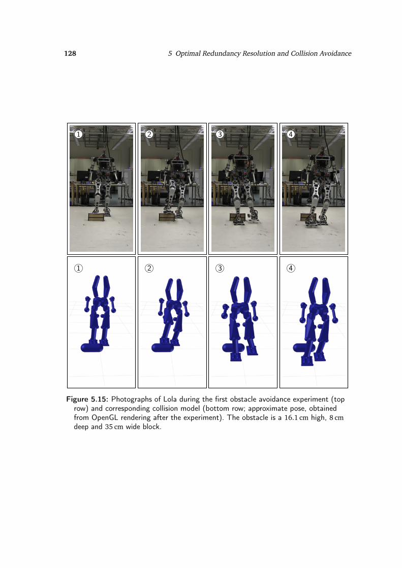
128 5 Optimal Redundancy Resolution and Collision Avoidance
1 2 3 4
1 2 3 4
Figure 5.15: Photographs of Lola during the first obstacle avoidance experiment (toprow) and corresponding collision model (bottom row; approximate pose, obtainedfrom OpenGL rendering after the experiment). The obstacle is a 16.1 cm high, 8 cmdeep and 35 cm wide block.

5.5 Inverse Kineto-Dynamics 129
5 6 7 8 9 100
2
4
6
·10−2
Time [s]
y F[m]
Right (ideal) Right (mod)Left (ideal) Left (mod)
5 6 7 8 9 10
0
0.1
0.2
Time [s]
z F[m]
Right (ideal) Right (mod)Left (ideal) Left (mod)
Figure 5.16: Foot trajectories for the first obstacle avoidance experiment (see fig-ure 5.15). Both initial, heuristically modified (ideal) and final (mod) foot trajectoriesin the lateral (yF) and vertical (zF) directions are shown. Note that the sagittal po-sition, as well as the spatial orientation of the foot are also modified, but not shownhere (redrawn from Hildebrandt et al. 2014).
5.4.4 Summary
We developed a new method which enables a bipedal robot to walk over and aroundobstacles in a cluttered environment while avoiding collisions. This method extendsthe framework designed for self-collision avoidance presented in the previous section,enabling the robot to dynamically integrate obstacles into its collision model. Based onthis, a local potential field method is combined with a heuristic modification of swingleg trajectories based on the height and width of an obstacle. This enables the robot toflexibly overcome obstacles of arbitrary shapes using locally optimized 3D trajectories.The efficiency of the proposed method is demonstrated in experiments with the robotLola.
5.5 Inverse Kineto-Dynamics
This section describes an extension to the IK algorithms described in the previoussections to hybrid task descriptions consisting of both task-space trajectories andgeneralized forces. The approach was reported in a paper previously published bythe author, upon which this section is strongly based (Buschmann et al. 2012c). Themethod presented here is motivated by the problem of biped walking control for whicha natural task description consists of contact forces and task-space trajectories. Wepresent both a general method based on the full EoM of the MBS, and a more efficientapproach tailored to the problem of biped walking control. We analyze the method and

130 5 Optimal Redundancy Resolution and Collision Avoidance
−0.4−0.200.20.4
−0.5
0
0.5
1
1.5
2
2.5
3
3.5
4
4.5
y [m]
x[m]
−0.4−0.200.20.4
−0.5
0
0.5
1
1.5
2
2.5
3
3.5
4
4.5
y [m]
x[m]
wal
king
dire
ctio
n
First Experiment(Rectangular Obstacle)
Second Experiment(Triangular Obstacle)
Figure 5.17: Modified step sequences for two obstacle avoidance experiments. Leftstance foot positions shown in red, right stance foot positions in green and corre-sponding heuristically adapted TCP trajectories as red and green lines. Obstaclebounding box shown in orange (note that footprints are distorted; redrawn from Hilde-brandt et al. (2014)).

5.5 Inverse Kineto-Dynamics 131
1 2 3 4
1 2 3 4
Figure 5.18: Photographs of Lola during the second obstacle avoidance experiment(top row) and corresponding collision model (bottom row; approximate pose, obtainedfrom OpenGL rendering after the experiment). The obstacle is a triangle that is 30 cmhigh, 9 cm deep and 13 cm wide at the base.

132 5 Optimal Redundancy Resolution and Collision Avoidance
5 6 7 8 9 10
−0.1
0
0.1
Time [s]
y F[m]
Right (ideal) Right (mod)Left (ideal) Left (mod)
5 6 7 8 9 10
0
2
4
6
8·10−2
Time [s]
y F[m]
Right (ideal) Right (mod)Left (ideal) Left (mod)
Figure 5.19: Foot trajectories for the second obstacle avoidance experiment (see fig-ure 5.18). Both initial, heuristically modified (ideal) and final (mod) foot trajectoriesin the lateral (yF) and vertical (zF) directions are shown. Note that the sagittal po-sition, as well as the spatial orientation of the foot are also modified, but not shownhere (redrawn from Hildebrandt et al. 2014).
compare it to the dynamics error compensation method proposed by Takenaka et al.(2009b, figure 4), which can reduce the planning error resulting from simplified robotmodels. The controller is evaluated in walking experiments and compared to a differentwalking controller using an inverse kinematics algorithm. The method enables exacttracking of desired contact forces in real-time, since they are directly included in thetask-description.
5.5.1 Introduction and Related Work
Generating and controlling stepping in humanoid walking robots is a complex task:The unilateral ground contact limits the set of feasible contact forces, the dynamics arenon-linear and the system has a large number of DoFs (cf. chapter 4). The computa-tional complexity of full MBS models has led to the development of planning methodsbased on simplified point-mass models (see section 4.5.1). While these methods enablereal-time planning, they do not generate dynamically consistent force and motionreferences that respect the dynamic constraints. That is, if the inverse dynamics for acomprehensive model are solved along the trajectory generated with the simplifiedmodel, the calculated forces will differ from the targets used during trajectory genera-tion. We have proposed a method based on spline collocation for the three point massmodel which reduces the modeling error, but cannot fully remove it (see Buschmannet al. 2007).
Even though the widely used lumped-mass models are vast simplifications, they have

5.5 Inverse Kineto-Dynamics 133
proven to be well-suited for walking pattern generation up to moderate walking speeds.At higher speeds, however, the influence of modeling errors becomes more severe.The difference between the desired contact forces or, equivalently, CoP trajectoriesfor which the planning problem is solved and the values calculated by solving theinverse dynamics for a comprehensive model becomes unacceptably large. For thisreason, approximate methods for reducing the effects of the modeling error have beenproposed. All methods exploit the fact that the simplified linear model of the CoMdynamics also approximates the modeling error. The simplified model can therefore bereused to reduce the planning error without having to solve a planning problem for thefull MBS model. Kajita et al. (2003b) used the preview control method for reducing themodeling error by feeding the difference between desired ZMP and that determined byinverse dynamics into the preview control method. Takenaka et al. proposed feedingthe moment error into an inverted pendulum model and adding the output to theoriginal CoM trajectory (Takenaka 2005; Takenaka et al. 2009b). These methods arecapable of reducing the modeling error significantly. However, perfect tracking of thereference force is not possible and the size of the contact force tracking error dependson the specific robot motion and is not easily controllable.
This section describes a method that enables exact tracking of desired contact forcesand task-space trajectories by directly including them into the task specification andusing a full MBS model of the robot for generating joint-space trajectories.
The method tries to solve the same problem other researchers have addressed byincorporating angular momentum into walking pattern generation methods (see also:“Angular Momentum Minimization” in section 5.3, page 114). The “resolved momentumcontrol” approach is notable, but suffers from the problem of prescribing adequateangular momentum trajectories (see discussion on page 114). Also, the method isused for offline generation of reference trajectories according to Kajita et al. (2005).Goswami and Kallem (2004) introduced a new criterion for stable states of the robotbased on rate of change of angular momentum about the robot’s CoM. Three differentstrategies are proposed to obtain a vanishing rate of change of angular momentumabout the CoM. The angular momentum minimization method described in section 5.3enables local minimization of the difference to a zero (or non-zero) angular momentumreference. Due to complex kinematic limits, however, the reference can usually not beperfectly tracked.
The method introduced in this section, by contrast, uses the correlation betweenground reaction forces and the rate of change of angular momentum about the CoMLc. With this, the full MBS model is taken into account, the contact forces which muststrictly satisfy the conditions of unilateral ground contact are accurately tracked anda zero-reference for LC or LC is avoided, which is usually unfeasible and leads tounnaturally looking movements.

134 5 Optimal Redundancy Resolution and Collision Avoidance
5.5.2 The Concept of Inverse Kineto-Dynamics
As outlined above, motion generation can be simplified by choosing task-space coor-dinates that naturally matches the control task. Especially in the case of interactioncontrol, a natural task description might contain both position and force variables.This has led to the development of hybrid position/force control, which was originallyproposed for torque-controlled manipulators (Craig and Raibert 1979; Khatib 1987).The wider availability of position controlled devices has led to the development ofhybrid position/force control methods based on an inner position or velocity controlloop (Siciliano and Khatib 2008, chapter 7). We have previously proposed a methodfor hybrid position/force control of biped robots based on an inner velocity or positioncontrol loop (Buschmann et al. 2009).
While hybrid position/force control addresses the situation of a task descriptionbased on both position and force variables, it does not solve the problem of generating areference trajectory for the generalized coordinates that satisfy a hybrid task description.This task is similar to differential IK algorithms, but includes both kinematic and kineticquantities. We will therefore call this approach Inverse Kineto-Dynamics (IKD).
Vukobratovic et al. (1990, chapter 1) described the “prescribed synergy method” forgenerating biped walking patterns. The method is related to the general IKD methodpresented in section 5.5.2 and motivated by similar observations, but is different inthe following aspects. First, the “prescribed synergy method” works in joint space,calculating some joint angles from given contact forces and assuming that the otherjoint angles are given. This makes it more difficult to take geometrical boundaryconditions such as early ground impact into account. Also, only contact forces are takeninto account, not the general case of any generalized force studied in section 5.5.2.Additionally, the important aspect of stabilizing the system discussed in section 5.5.3 isnot addressed. Finally, Vukobratovic proposes numerically solving the Boundary ValueProblem (BVP) using periodicity conditions, which makes this approach an offlinemethod due to the high computational cost.
Inverse Kineto-Dynamics for Biped Walking
A dominant approach to walking pattern generation for biped robots consists of first de-termining feasible contact forces or (equivalently) CoP trajectories and then calculatingthe horizontal components of the CoM trajectory by solving the planning problem fora simplified model (see section 4.5.1 and 5.5.1). In this section we describe a methodfor directly generating joint trajectories from given contact moment and task-spacetrajectories.
The global dynamics of an arbitrarily complex MBS can be described by the angularand linear momentum theorems evaluated for the entire system:
p = mr C = mg + F (5.84)

5.5 Inverse Kineto-Dynamics 135
LC =nb∑
i=1
LC ,i = T + r C F × F (5.85)
Here, m denotes the total mass, p the linear momentum, LC ,i the angular momentum ofthe i-th body about the system’s CoM, g the gravitational acceleration, nb the numberof bodies in the MBS, F the contact force, T the contact moment, r C the accelerationof the CoM and r C F the vector from the CoM to the point where the contact force Facts. In the preceding equations, all quantities are evaluated in an inertial coordinateframe. Note that the terms for a moving reference point in the angular momentumtheorem (5.85) cancel, since the robot’s CoM is used as a reference point.
The absolve rate of change of angular momentum can be rewritten as:
LC = J Lq + J Lq . (5.86)
The matrix J L =∂ LC∂ q is the Jacobian of the system’s angular momentum. Substituting
(5.86) and (5.84) into (5.85) and choosing the foot reference point as the origin, thatis, r F = 0⇒ r C F = −r C , we obtain:
J Lq + J Lq −mr C × g +mr C × r C − T = 0. (5.87)
Taking the x and y components16 of (5.87), factoring out the unknown horizontalcomponents of the CoM-acceleration xC and yC , assuming that g acts in the negativez-direction and rearranging, we obtain:
J L,x
J L,y
q +
0 −mzC
mzC 0
xC
yC
+
J L,x
J L,y
q +
myC(g + zC)− Tx
−mxC(zC + g)− Ty
= 0.
(5.88)
Here, J L,x and J L,y are the first and second row of J L, respectively. This can be writtenmore compactly as
Aq + Bw u + c = 0, (5.89)
where the unknown CoM accelerations are denoted by w Tu =
xC yC
.
In order to determine the generalized accelerations, we split the full set of task-space trajectories into known (w k) and unknown components (w u) using appropriatematrices:
w = T wkw k + T wuw u. (5.90)
16. The x-axis as assumed to point forward, the z-axis upward and the y-axis to the left.

136 5 Optimal Redundancy Resolution and Collision Avoidance
Note that T wk and T wu are not restricted to binary selection matrices. Combining (5.18),(5.89) and (5.90) yields:
Rq + r = 0.
With: R = Jw + T wuB−1A,
r = Jwq − T wkw k + T wuB−1c.
(5.91)
In the non-redundant case, q can be determined directly by solving (5.91). In theredundant case, the typical methods of nullspace optimization can be applied tominimize accelerations, avoid joint angle limits and collisions. Note that terms in Roriginating from the angular momentum Jacobian and from the task-space Jacobianare automatically scaled to similar values by premultiplication with B−1.
The General Case
The same basic approach applied to walking pattern generation above can be general-ized to arbitrary tasks with a hybrid task description consisting of both position andforce variables. The method is not restricted to humanoids and may be applied to anysystem governed by the MBS equations
Mq + h = Wλλ, (5.92)
where λ denotes the impressed actuator and contact forces and Wλ the corresponding(transposed) Jacobians used for projecting λ into the space of generalized coordinates.In the case of a fully actuated manipulator, λ is equal to the joint torques. For humanoidrobots, λ contains both actuator torques and the total contact wrench.17
We assume that the task is specified using sub-vectors of λ and w and that λ ispartitioned into known (index k) and unknown (index u) components:
λ= Tλkλk + Tλuλu. (5.93)
As with the partitioning of the task variables w in (5.90), the Tλ j are suitably definedmatrices for assembling the known and unknown sub-vectors of λ.
Substituting (5.93) into (5.92) and (5.90) into (5.18) yields:
Mq + h = Wλ
Tλkλk + Tλuλu
, (5.94)
Jwq + Jwq =T wkw k + T wuw u
. (5.95)
Solving (5.94) for q , substituting the result into (5.95) and rearranging yields a linear
17. In the overactuated case, or when both legs of a biped are in contact, a force distribution must bechosen to obtain a unique solution.

5.5 Inverse Kineto-Dynamics 137
equation in the unknown variables λu, w u:
G
λu
w u
+ f =0,
G =JwM−1WλTλu , −T wu
,
f =JwM−1WλTλkλk − JwM−1h+ Jwq − T wkw k.
(5.96)
The joint accelerations are determined by solving the above equation and q(t) is thencalculated by numerical integration. In the case of redundant systems, well-knownredundancy resolution methods may be applied (see previous sections). Appropriateweighting matrices should be chosen to take the different physical meaning of λu andw u into account.
The approach proposed above is equivalent to determining the trajectory resultingfrom the impressed forces λk by simulating the forward dynamics of the MBS (5.92)with rheonomic constraints according to the kinematic part of the task (see alsosection 3.4). Therefore, the proposed approach consists of designing a constrainedmechanical system, simulating it online and then forcing the physical system to trackthe simulated one using an adequate controller.
5.5.3 Walking Pattern Generation Based on InverseKineto-Dynamics
This section presents an application of the ideas outlined above to the walking patterngeneration problem. The method was implemented in the walking control systemused for the robot Lola. Figure 5.20 shows an overview of the walking control system.Without activated IKD, the block “Trajectory Planning” outputs a full set of task-spaceand contact force trajectories, including a CoM reference calculated with the collocationmethod (Buschmann et al. 2007). With the IKD method, only a subset w k of the originaltask-space without the horizontal CoM coordinates is used (see section 5.5.2).
Figure 5.21 shows CoM trajectories in the lateral plane calculated using the IKDmethod. The contact moments were taken from the solution for the simplified modelusing the collocation method (Buschmann et al. 2007) and are exactly tracked bythe generated joint trajectories. The original CoM planning method is therefore stillrequired for generating a suitable contact moment reference. The results in figure 5.21show that for a good choice of the relative leg mass ml
m in the three point model (fordetails see Buschmann et al. 2007; Buschmann 2010) the solution is close to thereference trajectory obtained from the collocation method. For poor choices of ml
m thetrajectory quickly diverges. Even for an optimal choice the CoM will eventually diverge,making the approach unusable in its simplest implementation.

138 5 Optimal Redundancy Resolution and Collision Avoidance
Finite State Machine
Step Sequence Planner
Trajectory Planning
Inertial Stabilization
Force/Position Control
Inverse Kinematics DirectKinematics
Position Controlled Robot
GUI, Joystick,Computer Vision
Gait Paramters
Step Sequence
λd0 and w d0
λd1 and w d1
λd1 and w d2
q J ,d and q J ,d
q J ,λ,ϕ
Wal
king
Stat
e
λ contact forcesϕ IMU measurementsw task-space coordinatesq J joint angles
Figure 5.20: Overview of Lola’s basic walking control system. Reference values are in-dicated by an index dn, where n identifies modified values. The “inertial stabilization”modifies contact force trajectories to stabilize the robot, as well as foot trajectoriesto assure proper landing of the swing foot. task-space trajectories are modified bythe “position/force” control algorithm, in order to track a subset of contract forcesand moments. The modified task space trajectories are then mapped to joint spaceby the inverse kinematics algorithm. For details, refer to (Buschmann et al. 2009;Buschmann 2010; Buschmann et al. 2011).

5.5 Inverse Kineto-Dynamics 139
0 1 2 3 4 5 6 7
0
0.2
Time [s]
y C[m]
referencemlm = 0.00mlm = 0.05mlm = 0.10mlm = 0.15mlm = 0.20
Figure 5.21: CoM trajectories calculated with the IKD method without stabilization.The plot shows results for contact forces corresponding to the solutions for the threepoint mass model using the collocation method (Buschmann et al. 2007) with differ-ent ratios of leg mass ml to total mass m. The reference trajectory is the solution forthe simplified model.
Stabilization via Planning
A closer analysis shows that the divergence of the CoM can be approximately modeledusing the simplified robot model, a fact used by the “error compensation” methods men-tioned above (Takenaka et al. 2009a; Kajita et al. 2003b). This motivates a stabilizationmethod based on the planning algorithms for the simplified model.
The collocation method generates a CoM trajectory by solving a BVP starting atthe current position and velocity of the CoM. In the original publication (Buschmannet al. 2007) we chose the position and velocity given by a periodic reference step asfurther boundary conditions. Here, the “divergent component” of the CoM proposedby Takenaka et al. (2009a) is used instead. In order to be able to satisfy more thantwo boundary conditions, the method modifies the contact force trajectory using shapefunctions. These shape functions are designed to only allow contact force modificationsduring periods when the reference is far from the maximum and minimum admissibleforce, for example, during double support.
We can therefore stabilize the CoM planning system simply by taking the outputof the IKD method as initial value for the planning system based on the simplifiedmodel.18 This is equivalent to a predictive control of the final CoM position and velocity.Figure 5.22 shows a resulting trajectory in the lateral plane obtained by this methodtogether with the corresponding CoP trajectory and the maximum and minimum
18. The stabilizing effect follows directly from the fact that the “divergent component” at the endof the step is equal to that of the next periodic (and therefore stable) reference. Obviously stability isconditioned on a sufficiently small difference between the three mass model and the MBS model.

140 5 Optimal Redundancy Resolution and Collision Avoidance
0 1 2 3 4 5 6 7
−0.2
0
0.2
Time [s]
y[m]
Feasible CoPCoGCoP
Figure 5.22: Lateral CoM position with stabilization via feedback to the planning sys-tem.
admissible CoP values. The CoP stays within the permissible bounds and is trackedexactly by the generated joint trajectories.
Stabilization via planning enables exact tracking of the modified reference forcesand allows us to choose the time when the forces should be modified. The ability tochoose when to modify contact forces is a major strength of the method — we can usethe large contact area during double support and are not forced to move the CoP closeto the edge of the foot during single support. In addition, stabilization via planningexplicitly takes long term stability into account, since the contact moment trajectory ismodified in such a way as to ensure that the divergent component of the CoM becomesequal to that of the ideal and stable reference generated by the collocation method.
The drawback is that feedback from the IKD output to the planner is only providedat the step frequency of the current walking pattern and that numerical drift is notcompensated. For slow steps this can lead to strong divergence of the CoM from theperiodic reference, which in turn requires large modifications of the contact momentfor stabilization. Also, the predictive stabilization is based on the reduced order model,which introduces a modeling error in the control loop.
Stabilization via the Contact Moment
An alternative for stabilization is to locally modify the desired contact moment by asmall amount ∆T cont in order to avoid large differences between the CoM generatedby the IKD and the CoM output by the collocation method. This can be achieved bya PD control law, augmented by a saturation function sat(·) for avoiding unfeasible

5.5 Inverse Kineto-Dynamics 141
contact forces:
∆T cont = satB[Kp,CoG(w u,plan − w u,IKD)
+ Kd,CoG(w u,plan − w u,IKD)].
(5.97)
Small values are chosen for the gain matrices K p,CoG, K d,CoG in order to avoid largemodifications of the contact moments. The matrix B scales the control output, see(5.91). For large gains, it is possible to closely track the reference CoM trajectory,essentially turning the IKD into an acceleration level IK algorithm. The difference isthat we prescribe the contact force and can guarantee that it will remain within thefeasible set.19
Figure 5.23 shows the ideal contact moment Tx and the resulting contact momentscalculated by inverse dynamics when the system is stabilized by modifying the contactmoments. The original reference moment is perfectly tracked without feedback (k = 0),but the CoM eventually becomes unstable. For a low but non-zero gain of k = 10−3 thesystem is stabilized, but the resulting moment shows small oscillations about the idealreference. As k is increased, the deviations from the ideal reference increase and theresulting CoM trajectory approaches the one calculated by the collocation method.
Hybrid Stabilization
The differences between the ideal reference moment and the resulting contact momentfor the calculated trajectory can be further minimized by combining stabilization via thecontact moment and the trajectory planner. Figure 5.24 shows the ideal contact momentTx and the trajectories obtained for different values of k. The system is stable for allvalues of k. For k = 0, the reference is perfectly tracked and the planner modifies thereference using a trapezoidal shape function during double support. The modificationsare clearly visible during the double support phases, which are approximately indicatedby yellow rectangles. Larger values of k reduce the modifications during double supportat the cost of larger tracking errors. For the walking experiments shown here, we usedk = 2×10⁻⁴, which leads to very small tracking errors and equally small modificationsduring double support.
Summing up, the hybrid method combines two components to ensure a stableCoM reference: (1) fast feedback by locally modifying the contact moment and (2)slow feedback via the CoM-planner. The first component compensates small errors
19. Stability of the IKD with PD control is not guaranteed. This is due to the nonlinear coupling betweenw k and w u in LC — it should even be possible to construct mass distributions and task-spaces where thecontrol law is destabilizing. However, if we make the reasonable assumption that (5.88) is dominatedby the CoM-dynamics (|LC | is sufficiently small), (5.97) is reduced to a PD-type control of the invertedpendulum in the limiting case. For perfect position tracking (zC = zC ,d) and LC = 0, the error dynamics
are reduced to ∆w u + Kd,CoG∆w u +K p,CoG − (g+z)
z
∆w u = 0. In this simplified case we can expect
stability for Kd,CoG > 0, K p,CoG >(g+z)
z . This is confirmed by the numerical results (see figure 5.23).

142 5 Optimal Redundancy Resolution and Collision Avoidance
2 3 4 5 6
−100
0
100
Time [s]
T x[N
m]
idealIKk = 10−2
k = 10−3
k = 0
Figure 5.23: Total resulting contact moment Tx summed up at the stance leg (calcu-lated by inverse dynamics), when the CoM is stabilized via local feedback to the refer-ence contact moment. The parameter k represents the overall feedback gain. It is mul-tiplied with the drift compensation gains (see section 5.5.3) to obtain Kp,cog, Kd,cog.The effective gains are: Kp,cog = 26.7, Kd,cog = 8.8 for k = 10−3 and Kp,cog = 266.7,Kd,cog = 27.8 for k = 10−2. The configuration with k = 0 is unstable. Note that in-stability occurs at a different time than in figure 5.21, since the walking sequence isdifferent. The divergence of Tx for k = 0 is due to joint limit avoidance triggered by adiverging CoM.
2 3 4 5 6
−100
0
100
Time [s]
T x[N
m]
idealIKk = 0k = 10−4
k = 10−3
k = 10−2
Figure 5.24: The total resulting contact moment Tx summed up at the stance leg(calculated by inverse dynamics), when the CoM is stabilized via local feedback andpredictive control (cf. figure 5.23 for only local feedback; parametrization same as Fig-ure 5.23). Double support periods with CoP modifications via planning approximatelyindicated by yellow rectangles.

5.5 Inverse Kineto-Dynamics 143
TrajectoryPlanner
Inverse Kineto-Dynamics
StabilizingControl
PositionControlled
Robot
GaitParameters
λd0, wd0
qd
w kλd0
w u
q ,λ
Figure 5.25: Integration of Inverse Kineto-Dynamics into the walking control system.
such as drift due to numerical integration. The second component ensures long termstability by predicting the CoM trajectory for the next step and modifying the contactforce reference accordingly. While stability can be ensured by both basic stabilizationmethods, the hybrid approach minimizes the difference between ideal and modifiedforce reference and moves most of the modification into the double support phase.
Comparison With Dynamics Error Compensation
We have compared the proposed approach with a combination of our collocation-basedplanner with additional dynamics error compensation. We have implemented thefeed-forward compensation method described by Takenaka et al. (2009b, figure 4).The method works by first calculating the contact moment resulting from the currentCoM-trajectory by inverse dynamics for a full MBS model. The difference from theoriginal reference is used as input for an inverted pendulum model. The output is thenadded to the CoM trajectory. To prevent the pendulum from diverging a controller isadded that stabilizes the pendulum by modifying the contact moment. Figure 5.26illustrates the method. We use a real PD controller with the continuous-time transferfunction
KRTRs+ 1Tds+ 1
(5.98)
to stabilize the pendulum. Here, s denotes the Laplace variable. We chose the controlparameters Td = 0.02, TR = 0.2, KR = 3200. The results shown here were obtainedwith a discrete time implementation of (5.98) with a sampling period of 1.5 ms.
Figure 5.27 shows the contact moments Tx and Ty calculated by inverse dynamicsfor three different planning methods: (1) the three point mass model, (2) the three

144 5 Optimal Redundancy Resolution and Collision Avoidance
Simplifiedmodel
Detailedmodel
IPM
pendulumcontrol
xbody,cmd
θbody,cmdTfull −
Tmdfd
Tmdfd
+
Ffull +
Fpend
+
Fmdfd
+
xpend
+
xbody,mdfd
Figure 5.26: Dynamics error compensation method proposed by Takenaka et al. Real-time trajectory planning is based on simplified dynamics such as the three point massmodel. Takenaka also adds a reaction wheel (angle Θ) to model torso rotation dy-namics. The error between intended contact moment and that obtained by inversedynamics from a full model (Tfull) is approximately compensated by a feedback sys-tem based on an inverted pendulum model (IPM). The modified quantities used asreference for walking control are indicated by the index mdfd. Figure modified from(Takenaka et al. 2009b, figure 4).
point mass model with error compensation and (3) IKD with hybrid stabilization. Theoverall deviation is the smallest for the proposed IKD-method. For Tx , a trapezoidalmodification during the double support phase (approximately 6.1 s. . . 6.3 s) can be seen.This illustrates an advantage of the IKD-based trajectory generation. The dynamics errorcompensation approach is local, so we cannot choose when to perform the modificationof the contact forces that are necessary for stabilizing the CoM. The IKD-based approach,on the other hand, allows us to perform most of the modification at a time during thegait cycle when the CoP is far from the edges of the support polygon. Accordingly, thedifference during the single support phase can be reduced significantly.
Also, we can guarantee that the resulting CoP calculated by inverse dynamics willstrictly stay within the support polygon. Stabilization via local feedback modifies thecontact force, but we can saturate it according to the current support polygon. Sincethe modified contact moment is used as input to the IKD, the resulting contact momentis exactly equal to the input. We can also saturate the output from the dynamics errorcompensation. However, since the compensation works with an approximate model,the resulting contact moments cannot be guaranteed to stay strictly within a prescribedrange. Finally, since we can exactly track a chosen contact moment, we know the

5.5 Inverse Kineto-Dynamics 145
6.2 6.4 6.6 6.8
50
100
150
Time [s]
T x[N
m]
ideal IKerrcomp IKD
6.2 6.4 6.6 6.8
0
100
200
300
Time [s]
Ty[N
m]
ideal IKerrcomp IKD
Figure 5.27: Comparison of the ideal contact moments and the moment from inversedynamics using the collocation method with the three point mass model (orange),using additional model error compensation (green) and using the IKD method withhybrid stabilization (blue, k = 10−4).
moment and the resulting CoP without calculating the inverse dynamics.
Implementation Issues
In the practical implementation a drift compensation law similar to (5.19) must beadded to the IKD equation (5.91) to stabilize tracking of the task-space trajectories. Driftcompensation is only applied to the planned task-space components w k, however, sinceapplying it to w u would prevent perfect tracking of the desired forces λk. For the resultsshown here the drift compensation gains were chosen as KP = 40/∆t, Kd = 2
pKp0.85
(i.e., a slightly underdamped configuration). For a sampling period of ∆t = 1.5ms thenumerical values are Kp = 2.7× 10⁴ and Kd = 2.8× 10².
All kinematic and kinetic quantities are calculated using the recursive analyticapproach described in section 2.3.2. To reduce the computational cost, we use thegradient ∂ w
∂ q instead of the time derivative of the Jacobian Jw. This is admissible, since
Jwq = ∂ w∂ q q . Similarly, J L is replaced by ∂ LC
∂ q .On Lola’s onboard PC with an Intel® Core2Duo™ Mobile CPU running at 2.33 GHz,
all calculations for the IKD-based walking controller require an average of 823µs. Awalking controller based on velocity-level CLIK requires only 548µs. However, the IKD-based program still is sufficiently fast for a control cycle of 1.5 ms from the samplingof new sensor data to the application of new motor commands.

146 5 Optimal Redundancy Resolution and Collision Avoidance
5.5.4 Experimental Results
We have evaluated the method in walking experiments with the robot Lola (see fig-ure 2.13). In the first set of experiments we used a walking controller based on onlineplanning using the collocation method and balancing control based on hybrid po-sition/force control (Buschmann et al. 2009). In the second set of experiments wereplace the IK with redundancy resolution (Schwienbacher et al. 2011) with the IKDwith hybrid stabilization and k = 2× 10⁻⁴.
In all experiments, Lola walked with a step cycle of 0.8 s, starting with a step lengthof 40 cm and accelerating to 55 cm steps. The step length and walking speed waslimited since angular momentum minimization via nullspace optimization was not yetimplemented for the IKD-based controller.
For the moderate walking speed of approximately 2.5 km/h, both the original IK-based control and the proposed IKD-based control showed very similar performance.Figure 5.28 shows the upper body inclination error in the sagittal and lateral planes.Both IK and IKD work in a reference frame that rotates with the upper body and theresulting joint angles are tracked with high gain controllers. Accordingly, the upper bodyerror ∆ϕx is roughly proportional to the CoM-tracking error in an inertial referenceframe. The reference CoP, planned CoM and CoM from IKD for the same experimentare shown in figure 5.29. On the position level, the CoM-trajectories are quite similar,but the amplitude for the planned CoM is larger.
For walking speeds above 3 km/h nullspace optimization methods (see section 5.3)significantly improve walking performance and stability. It is to be expected that theadvantages of the IKD method will become more apparent during fast walking withadditional nullspace optimization.
5.6 Predictive Inverse Kinematics
The algorithms discussed in the previous sections of this chapter take a local approach tosolving the IK for redundant manipulators. Optimization-based approaches were usedin the previous sections, but the optimization was only applied to the current time step.This section presents a predictive approach to redundancy resolution that optimizesthe motion for a given task-space reference w d over a finite horizon tb . . . te. A directformulation as a constrained optimal control problem in the unknown generalizedvelocities q is
Φ=
te∫
tb
ϕq , q , t
dt →min!
Jwq − w d = 0.
(5.99)

5.6 Predictive Inverse Kinematics 147
0 5 10 15
−6
−4
−2
0
2·10−2
Time [s]
∆ϕ
x[r
ad]
IK IKD
0 5 10 15
−4
−2
0
2
4·10−2
Time [s]
∆ϕ
y[r
ad]
IK IKD
Figure 5.28: Measured upper body inclination ∆ϕx in sagittal (walking) direction (left)and ∆ϕy in lateral direction (right) with IKD (hybrid stabilization, k = 2 × 10⁻⁴)compared to the collocation method with inverse kinematics in a walking experimentwith Lola.
0 1 2 3 4 5−0.3
−0.2
−0.1
0
x [m]
y[m]
CoG (planned)CoG (IKD)CoP
Figure 5.29: Planned CoM, CoM from IKD (hybrid stabilization, k = 2 × 10⁻⁴) anddesired CoP for a walking experiment with Lola.

148 5 Optimal Redundancy Resolution and Collision Avoidance
The equation assures that the task-space trajectories are followed and Φ describes thecost of a solution as the integral over a suitably chosen function ϕ(q , q , t). Typicalchoices for ϕ are the squared joint velocities and collision avoidance potentials.
This section describes an efficient method for solving this problem based on Pontrya-gin’s Minimum Principle (PMP) and the (conjugate) gradient method. The results inthis section are the outcome of joint work with Christoph Schütz, who implemented thealgorithms. The results were previously published in a joint paper (Schuetz et al. 2014).The next section briefly discusses the background and related work and is followed bya presentation of the proposed method. A number of different minimal examples, aswell as an application to the 9-DoF agricultural robot are also discussed.
5.6.1 Introduction and Related Work
The preceding sections reviewed classical methods for redundancy resolution, whichoften operate at the velocity level (see section 5.1), as well as an extension to hybrid taskdescriptions composed of force and position variables (section 5.5). These approacheshave the major advantage of being very efficient computationally, enabling the on-linegeneration of reactive behaviors for robots with complex kinematics and 3D geometry(see section 5.3). Since the motion is only optimized individually for every time step atthe level of joint velocities, however, the steepest descent within the nullspace resultingfrom the current configuration is taken. The effect this local change will have on thefuture configuration cannot be taken into account. This is the main drawback of thelocal approach, since a locally slightly better choice can lead to significantly greatercosts in the future. At the same time, many of the future constraints are known at thecurrent time, even for reactive systems. The constraints can still be satisfied in manycases, but at the cost of severe peaks in the joint velocities that are not necessary if alonger horizon is taken into account when controlling the given task (see section 5.6.2).
There are two major approaches to generating optimal trajectories: (1) Pontryagin’sapproach, which leads to a set of ODEs and an open-loop optimal trajectory and (2)dynamic programming (and variants), which lead to optimal feedback laws (see, e.g.,Pontryagin 1962; Tolle 1971; Bellman 1954). A large number of different approachesand numerical algorithms have been proposed for solving the optimal control problem.
One possible solution is to directly use the PMP, which leads to necessary optimalityconditions in the form of a BVP that can be solved using a number of different methods(e.g., collocation, finite differences, etc.; for some standard numerical methods, see,e.g., Quarteroni et al. 2007). In cases without terminal constraints, the BVP is decoupledand can easily be solved using the gradient method (see below; review, e.g., Polak1973).
The direct application of dynamic programming is not possible for systems with morethan a few DoFs since both the computational cost and memory requirements increaserapidly with the number of states (this is the “curse of dimensionality,” see, e.g., Bellmanand Lee 1984). However, a number of methods based on the principle of dynamic

5.6 Predictive Inverse Kinematics 149
programming have been developed that use local approximations of the value function20
and the dynamic equations. The best-known method may be Differential DynamicProgramming (DDP), which uses a quadratic approximation of the value function anddynamics to derive a set of ODEs to be solved for iteratively improving the solution(Mayne 1966; Jacobson 1968c, 1968a; Jacobson and Mayne 1970). The methodhas quadratic convergence and maintains the forward and backward integrationscharacteristic for dynamic programming methods (cf. section 3.3), but does not requirethe solution of Bellman’s partial differential equation. Other methods based on linearand quadratic approximations were developed by Jacobson (1968b).
Todorov and Li (2005) proposed a variant of DDP which they term iterative LinearQuadratic Regulator (iLQR) that uses a linear approximation of the dynamics and asimplified quadratic approximation of the value function.21 The authors report signif-icantly better performance than DDP for some problems (Li and Todorov 2004). Arecent article describes an implementation that almost achieves real-time capabilityfor moderately complex systems through the use of multiple processors for calculatingfinite difference approximations (Tassa et al. 2012).
One major advantage of DDP and iLQR over the gradient method is the fasterrate of convergence. The gradient method can be significantly improved, however, bycomputing better directions of descent via the conjugate gradient method. An extensionof this method to optimal control was given by Lasdon et al. (1967). The paper reportssignificantly better performance of conjugate gradient methods compared to the simplegradient method. Second order algorithms are reported to converge more rapidly thanthe conjugate gradient method at the cost of more complex calculations for everyiteration. One reason for reducing the order in iLQR compared to DDP is that it isapplied in an MPC or receding horizon approach. That is, the optimal trajectory iscomputed over a finite horizon, but the resulting control is only applied for the nexttime step. The procedure is then repeated frequently, using the current state as initialcondition (for review, see Diehl et al. 2009). The current estimate should thereforealways be close to the optimal trajectory, making a simplified approximation of thedynamics and value function sufficient. The same reasoning let us adopt the (conjugate)gradient method. Since we intend to use it in a receding horizon approach, we havechosen it over dynamic programming approaches, since we only require the optimalcontrol, not the feedback law. Feedback is provided via the repeated calculation of theoptimal open-loop trajectory. The gradient method, the linear method proposed byJacobson (1968b) and iLQR (Todorov and Li 2005) are related, but distinct. All threemethods have one ODE in common which is integrated backward in time, correspondingto the co-state or, equivalently, the gradient of the value function (for a discussion ofthe equivalence of value function gradient and co-state, see Vinter 1986).
20. The “value function” is a term widely used for the cost-to-go, i.e., the remainder of the integralcost starting at the current time step, and any terminal costs.
21. Essentially, the Hessian of the value function is not taken into account.

150 5 Optimal Redundancy Resolution and Collision Avoidance
1 2 3
Figure 5.30: Collision avoidance in the nullspace of the robot. Black robot: Local Opti-mization. Blue robot: Global Optimization (adapted from Schuetz et al. 2014).
5.6.2 Motivational Example
A motivational example for the predictive approach to IK is given in figure 5.30. Theplanar 4-DoF robot performs a predefined Tool Center Point (TCP) movement on astraight line from top to bottom. The reference trajectory of the TCP does not collidewith the obstacle (orange sphere). To demonstrate the effect of a longer control horizon,the sum of squared joint velocities (pseudoenergy) is chosen as a cost function forlocal redundancy optimization and the integral of the pseudoenergy as cost functionalfor global optimization. In both cases, collision avoidance is implemented using thepenalty approach.
Without active collision avoidance, the robot would collide with the obstacle. Thelocal nullspace collision avoidance scheme can prevent collisions, but it is only activatedafter the obstacle is close to the robot (see section 5.3). By this time, however, thelocal optimization has led to an unfavorable configuration relative to the obstacle,requiring very high joint velocities to avoid a collision. The globally optimal solution(blue robot) uses slightly higher velocities during the initial period to obtain a betterconfiguration relative to the obstacle when passing it, significantly reducing peak jointspeeds. This behavior can be seen in the the pseudoenergy shown in figure 5.31. Thepredictive approach with a planning horizon of 1 s performs slightly worse than theglobal solution, but much better than the local approach.

5.6 Predictive Inverse Kinematics 151
0 1 2 3 4 5
0
2
4
Time [s]
qTq ra
d2 /s2
localMPCGlobal
Figure 5.31: Pseudoenergy of the global, local and predictive (MPC) redundancy op-timization methods. The relative weights for the optimization are: 1.0 velocity min-imization, 1.0 for collision avoidance and 0.6 for joint limit avoidance (predictionhorizon 1 s; redrawn from Schuetz et al. 2014).
5.6.3 Predictive Approach to Redundancy Resolution
Formulation of the Optimal Control ProblemNakamura proposed a formulation of globally optimal redundancy resolution based onthe general solution
q = J#ww d + Nwu (5.100)
of the underdetermined linear constraints imposed by the desired task space trajectory(Nakamura and Hanafusa 1987; Nakamura 1991). The newly introduced variable uparameterizes the nullspace velocity and is chosen as input for the optimal controlproblem:
Φ(u,q) =
te∫
tb
ϕq , u, t
dt →min! (5.101)
q = fq , u, t
= J#w d + Nwu (5.102)
w (tb) = w d,b (5.103)
t ∈ tb, te
The optimality conditions following from the PMP are
H(q , u,λ, t) = ϕq , u, t
+λT f
q , u, t
(5.104)

152 5 Optimal Redundancy Resolution and Collision Avoidance
∂ H∂ λ
T= q (5.105)
−∂ H∂ q
T= λ= −
∂ ϕ
∂ q
T −∂ f∂ q
Tλ (5.106)
w (q(tb)) = w d,b (5.107)
λ(te) = 0 (5.108)
Nλ(0) = 0 (5.109)
u? = argminu
H(q?,λ?, u, t), (5.110)
where starred versions of the variables denote the optimal solution. The boundaryconditions on w (5.107) are self-explanatory and those on λ (5.108) follow from thefree final state and the fact that the problem has Lagrange form. The transversalitycondition (5.109) ensures that the adjoint variables lie within the normal cone to thetangent cone of the constraint set defined by w (q(tb)) = w d,b. Requiring that theprescribed task w d,b be satisfied at the beginning enables the calculation of a globallyoptimal solution, but also leads to a coupled two-point BVP due to the transversalitycondition.
If we intend to solve the problem continuously in the spirit of MPC as proposedabove, we must ensure that q(t) is continuous, that is, q(tb) = q b. This modifiedoptimal control problem leads to optimality criteria with decoupled boundary conditionsfor λ and q :
H(q , u,λ, t) = ϕq , u, t
+λT f
q , u, t
(5.111)
∂ H∂ λ
T= q (5.112)
−∂ H∂ q
T= λ= −
∂ ϕ
∂ q
T −∂ f∂ q
Tλ (5.113)
q(tb) = q b (5.114)
λ(te) = 0 (5.115)
u? = argminu
H(q?,λ?, u, t) (5.116)
Conditions (5.112)-(5.115) allow us to calculate λ(t),q(t) for any given u(t) bysimply integrating (5.112) forward in time and (5.113) backward in time. We cantherefore think of (5.101) as an unconstrained problem that only depends on the inputu:
bΦ(u) =te∫
tb
ϕq(u), u, t
dt →min! (5.117)

5.6 Predictive Inverse Kinematics 153
Such problems are easily solved using the gradient method,22 which is characterizedby an iterative calculation of the unknowns according to the basic rule
uk+1 = uk −α ∂ bΦ∂ u
T, (5.118)
where α is calculated from some step-size rule. The gradient of the reduced optimalcontrol problem (5.117) happens to be the gradient of the Hamiltonian, leading to theupdate rule
uk+1 = uk −α ∂ H∂ u
T. (5.119)
A derivation of this result is given by Gerdts (2011, chapter 8). The text also includes acomparison of the function space gradient method used here and the gradient methodapplied to a discretized optimal control problem. While the two methods are closelyrelated, the function space approach often converges much more rapidly (Gerdts 2011,p. 410). A review of the mathematical and historical background of the method is givenby Polak (1973).
Efficient Numerical SolutionWhile simple, the gradient method is also known for its relatively slow convergence.We therefore use the conjugate gradient method as described by Lasdon et al. (1967) tosolve the optimal control problem (5.111)-(5.116), since it enables a computationallyefficient solution of the nonlinear problem in real-time. Applying the basic algorithmleads to sequential forward integration of the system ODE (5.112) and backwardintegration of the adjoint variable ODE (5.113) to update the system for a new inputu. The computational scheme is shown in algorithm 11. Direct kinematics of the robotare calculated by the recursive approach described in section 2.4. The step size α caneither be chosen as a sufficiently small constant or computed for every iteration using astep-size control algorithm, for example, the backtracking method (see, e.g., Bonnanset al. 1997). We could confirm the superior convergence of the conjugate gradientmethod compared to the steepest descent method in our applications (see above andLasdon et al. 1967). Results for the motivational example given above are shown infigure 5.32.
Predictive ApproachDepending on the number of DoFs and the length of the trajectory, the global approachmay not be solvable in real time. We therefore propose an approach which follows theidea of MPC. We solve the optimal control problem for the nullspace vector u at everytime step tk with a prediction horizon of [tk, tk + Thorizon]. The basic scheme is shownin algorithm 12.
The straightforward formulation of predictive inverse kinematics as an optimal
22. If u is constrained (u ∈ U ), the projected gradient method can be used.

154 5 Optimal Redundancy Resolution and Collision Avoidance
Algorithm 11: Conjugate Gradient Method for optimal control.input : Initial guess for control: u0, interval [tb, te]output : Optimal control: u?
j← 0q0(t) =
∫ ttb
q(u0,τ)dτ // q for u0 by forward integration
Φ0← ∫ te
tbϕ(q0, u0,τ)dτ // Cost for initial trajectory
repeatλ j(t) =
∫ te
t λ(qj , q j , u j ,τ)dτ // λ for u j by backward integration
g j ← ∂ H∂ u // gradient for u j
if j 6= 0 then
β j ←g j , g j
g ( j−1), g ( j−1)
whereg j , g j
=
te∫
tb
(g j(τ))T g (τ) j dτ // dot product
s j ←−g j + β j s( j−1)
elses j ←−g j
u( j+1)← u j +α j s j // improved control inputj← j + 1 // next iterationq j(t) =
∫ ttb
q(u j ,τ)dτ // q for u j by forward integration
Φ j ← ∫ te
tbϕ(q j , u j ,τ)dτ // Cost for updated trajectory
until
j > jmax
∨Φ j−Φ j−1
Φ j−1 < ε∨ Φ j > Φ j−1
return u j
Algorithm 12: Model Predictive Controltstart = tb, te = tn, ∆tmpc = tk+1 − tkfor k = 0 to n // for every control cycledo
tb← tk +∆tmpc // lower bound for prediction intervalte← tk + Thorizon // upper bound for prediction intervalu0← u∗,k−1 // last result as initial guesssolve optimal control problem for u∗ // e.g., using algorithm 11apply u∗(tstart) // Use result for next time step

5.6 Predictive Inverse Kinematics 155
0 20 40 60 80 100
220
240
260
Iteration
Cos
tConjugate GradientSteepest Descent
Figure 5.32: Comparison between the conjugate gradient and the steepest descentmethod for the planar 4-DoF manipulator (cf. figure 5.30; redrawn from Schuetz et al.2014).
control problem (5.102) imposes constraints for the joint positions q k at the start of theperiod, but not for the joint velocities q k. Since the constraints and the time intervalchange at every time step, the resulting joint velocities at the first time step can changediscontinuously from one sampling period to the next. This leads to a non-smooth jointtrajectory for the predictive solution, as shown in figure 5.33.
One possible solution to this problem would be to formulate the task-space constraintsat the acceleration level, which would shift the discontinuity to the joint accelerations.This, however, would require the computation of additional gradients (e.g., of J , J#),unacceptably increasing the computational cost. A less expensive approach is to use anaugmented state space consisting of q and u and to use the derivative of u as the newinput vector. The modified cost functional and augmented system dynamics are
Φ=
te∫
tb
ϕq , u, t
dt →min!, (5.120)
f acc
q , u, t
=
f 1
f 2
=
qu
=
J#w d +
I − J#J
u
u
. (5.121)
The modified optimality conditions are:
λTacc =
λT
1 λT2
, (5.122)
H(q , u,λacc, t) = ϕq , u, t
+λT
1 f 1
q , u, t
+λT
2 f 2 (u) , (5.123)∂ H∂ λacc
T=
qu
, (5.124)

156 5 Optimal Redundancy Resolution and Collision Avoidance
0 1 2 3 4 5−1
−0.5
0
Time [s]
q 2 ra
d /s
Local solutionglobalPredicted TrajectoriesMPC
Figure 5.33: Solutions for the motivational example for different velocity-level ap-proaches (cf. figure 5.30). The curves show the nonsmooth trajectory (second joint)for velocity-level MPC, the individual solutions of the optimal control problem (predic-tion horizon 1 s) for different time steps, the local solution and the global solution (cf.figure 5.30; for weights see figure 5.31; redrawn from Schuetz et al. 2014).
−∂ H∂ q
T= λ1 = −
∂ ϕ
∂ q
T −∂ f 1∂ q
Tλ1, (5.125)
−∂ H∂ u
T= λ2 = −
∂ ϕ
∂ u
T −∂ f 1∂ u
Tλ1, (5.126)
q(tb) = q b, u(tb) = u b, (5.127)
λacc(te) = 0, (5.128)
u? = argminu
H(q?,λ?acc, u, t). (5.129)
The augmented state space allows the introduction of the additional constraint u(tb) = u b,which assures continuous velocities, since the task-space component is continuous ifw d is. The numerical solution is analogous to the optimization on velocity level (seeabove). Required gradients are listed appendix A.5. The smooth trajectories computedusing this approach are shown in figure 5.34 for the motivational example.
5.6.4 Application to 9-DoF Manipulator
The approach has been evaluated for the 9-DoF agricultural manipulator (see figure 5.8;Baur et al. 2012). A similar setup to that described in section 5.3 is evaluated. In thegeneral case, the cost functional is defined as the sum of nc terms:
Φ(q , u, t) =
te∫
tb
nc∑i=1
ϕi(q , u, t)dt (5.130)

5.6 Predictive Inverse Kinematics 157
0 1 2 3 4 5−1
−0.5
0
Time [s]
q 2 ra
d /s
global (vel. level)Local solutionPredicted TrajectoriesMPC solution
Figure 5.34: Smooth trajectory (second joint) for MPC solution with augmented statespace (prediction horizon 1 s), individual trajectories of the MPC-solution and localsolution. Global solution of velocity-level approach shown for comparisson (Schuetzet al. 2014, redrawn from).
For the example given below, three terms were used: (1) joint velocity minimization ϕv,(2) joint limit avoidance ϕ jl and (3) collision avoidance ϕca. The term ϕv is defined by
ϕv = q T q . (5.131)
For ϕ jl , the piece-wise function given in (5.58) is used and a simple cubic repulsivepotential is used for ϕca.
Results for the local solution, as well as the predictive approach with different lengthsof the moving horizon Thorizon are shown in figure 5.35. The smaller horizon couldbe realized in the MATLAB/SIMULINK-based real-time control unit at a sampling rateof 10 ms and one MPC iteration per time step, while a larger horizon of 2 s currentlyrequires up to seven sampling periods to solve. A small horizon of 0.15 s already slightlyreduces velocity peaks, but a longer horizon leads to significant better results.
5.6.5 Conclusion
This section presents a novel approach to real-time predictive inverse kinematics forredundant manipulators. The optimal control problem is solved based on Pontryagin’sMinimum Principle and the conjugate gradient method. A similar approach to globaloptimization was previously proposed by Nakamura and Hanafusa (1987). The con-tribution of the method proposed here is the receding horizon approach, which leadsto a decoupled BVP, which enables an efficient solution in real-time. The potential ofthe approach is demonstrated both with a minimal 4-DoF example and a redundant9-DoF agricultural manipulator. Currently, the implementation does not yet enable long

158 5 Optimal Redundancy Resolution and Collision Avoidance
prediction horizons on the 9-DoF manipulator, but this should become possible withmore efficient programming, the use of multiple CPUs and a larger sampling period forthe predicted trajectory and more sophisticated time integration methods.
5.7 Chapter Summary
This chapter reviews classical approaches to solving the inverse kinematics problemfor redundant and non-redundant robots. The framework first proposed by Liégeois(1977) is used to develop a system for reducing joint velocities, avoiding joint limitsand potential self-collisions. An application of the approach to angular momentumminimization for bipedal robots shows the flexibility of the method.
While the nullspace approach is very powerful, there are situations in which theprimary task-space trajectory must be modified to avoid collisions. A real-time task-space modification method is developed, which combines approximate heuristic re-planning with local potential field-based obstacle avoidance. The method is used inexperiments with the biped Lola, allowing it to avoid different obstacles by modifyingfootstep locations and task-space trajectories in real-time.
An extension of differential inverse kinematics to force references (Inverse Kineto-Dynamics) enables real-time tracking of desired generalized forces, taking the fullmultibody model into account. The method is successfully applied to biped walkingcontrol.
Local potential field-based redundancy resolution methods are very powerful andcomputationally efficient techniques for real-time and reactive motion generation.Since they are local, however, changing configurations and obstacles can sometimeslead to large peaks in joint velocities. The methods are also theoretically prone to localminima. The predictive approach to inverse kinematics presented in this chapter solvessome of these drawbacks. The integral cost is significantly reduced and local peaks canoften be avoided by predictively modifying the robot’s motion. The second drawback oflocal approaches, local minima, have not been an issue for the applications discussedin this chapter. For general manipulation tasks, however, local minima can quicklybecome a significant problem. Possible solutions are the combination with samplingbased methods, which, however, are much more demanding computationally.

5.7 Chapter Summary 159
0 1 2 3 4 5
0
0.5
1
Time [s]
qTq ra
d2 /s2
LocalMPC (2 s)MPC (0.15 s)
Figure 5.35: Pseudoenergy of revolute joints of the 9-DoF manipulator in a self-collision scenario. Results shown for local IK and MPC-approach with a movinghorizon of 0.15 s and 2 s. The relative weights for the optimization are: 1.0 veloc-ity minimization, 2.0 for collision avoidance and 0.6 for joint limit avoidance for localversion; 1.0 velocity minimization, 5000.0 for collision avoidance and 80 for joint limitavoidance for MPC version (redrawn from Schuetz et al. 2014).

6 Conclusion and Directions for Future Work
This monograph summarizes recent research on efficient algorithms for redundantrobots the author is involved in. Most of the work has been motivated by the problemsposed by designing and controlling bipedal walking machines. The results, however,are applicable to a much wider range of systems. One of the core challenges is to designand implement efficient algorithms that are applicable to complex, redundant systemsin dynamic environments.
The first chapters treat basic aspects of multibody kinematics and dynamics andpresent efficient algorithms suitable for robotic systems. A special emphasis is put ontree structures and structure exploiting methods. Detailed comparisons of standard andstructure-exploiting versions of both EoM-oriented and recursive dynamics algorithmsare presented. The extreme improvements provided by linear-time recursive algorithmsover naive EoM-based implementations are confirmed by run-time measurements.Efficient, structure-exploiting implementations, however, often give comparable resultsfor realistic system topologies. To apply the efficient recursive approach to generalmultibody systems, closed kinematic loops are usually cut and then handled by addi-tional algebraic constraints. The chapter on dynamics introduces a new method forefficiently calculating the forward dynamics of systems with closed loops in minimalcoordinates, without the introduction of algebraic constraints.
A detailed review of biped walking control is given, spanning different approachesto hardware and controller design, as well as current knowledge on human control ofposture and balance. One area in which current systems are still lacking is generatingcomplex movements of systems with many DoFs in 3D environments.
Since holistic optimal-control approaches are not suitable for real-time use due tothe computational cost, a layered approach must be taken. Mapping a coarse high-leveldescription to joint level motion is a core building block of such a system and addressedin detail in the chapter on optimal redundancy resolution and collision avoidance. Nextto a review of standard methods, an extension of inverse kinematics problem to hybridtasks involving generalized force trajectories is presented (“Inverse Kineto-Dynamics”).This extension is motivated by and well suited for generating dynamically consistentwalking trajectories, but is not limited to this application. Other potential applicationscan be found in many robotic tasks, especially such involving contacts.
The tasks described above require efficient collision modeling and distance computa-tion methods. An approach to this problem is presented, together with applicationsto a biped robot and a redundant manipulator. Collision avoidance in the nullspaceof a given task, as well as collision avoidance by task-space trajectory modifications

162 6 Conclusion and Directions for Future Work
are discussed. The methods are based on a local potential-field approach and workvery well both for bipedal walking tasks and reaching tasks for redundant agriculturalmanipulators. A well-known drawback of this approach are local minima. This has notbeen a problem in the presented applications, but certainly is a potential source ofsystem failure for manipulation in very cluttered environments. A second drawbackis more relevant to the presented applications: the motion locally optimized for thecurrent time step is generally not optimal for the entire trajectory. A potential solutionis to solve the optimization problem over a receding horizon. An implementation of thisidea based on the conjugate gradient method is presented, which shows very promisingresults both for a minimal planar model and a spatial 9-DoF manipulator.
The presented algorithms can serve as building blocks enabling efficient modeling,simulation and real-time control of redundant and high-dimensional systems. Theyhave been proven in many experiments with the walking robot Lola and the redundantCROPS manipulator. For the agricultural robot, the algorithms are successfully used bymany partners working with the manipulator.
While the presented methods have all proven to work well, many open questionsremain. An additional line of research necessary for realizing the vision of robots per-forming human-like tasks reactively in complex, 3D environments is aimed at improvingthe basic mechanisms for generating and stabilizing the motion using feedback. For thetask of biped walking, this is the objective of ongoing research in the robotics groupat Institute of Applied Mechanics (Buschmann et al. 2012a; Ewald et al. 2012; Ewaldand Buschmann 2013; Wittmann et al. 2014).
As mentioned above, the real-time capability is one of the major challenges in thecontrol of complex robots. An open question is how to use some off-line computationfor reducing run-time costs without excessive memory requirements or reducing thespace of potential movements. Also, the technological road-map for processors showsthat any algorithm aiming at fully utilizing the available computing power will have tobe parallelized. This is a major challenge in robotics, where many standard algorithmsare currently inherently serial.
The section on predictive redundancy resolution shows one possible path towardsusing optimal control methods in real-time for complex systems by reducing the searchspace. A detailed comparison of the proposed conjugate gradient method with otherlinear and quadratic approaches from dynamic programming (e.g., DDP, iLQR) are thesubject of ongoing work. An open question is how far this approach can be extended byincluding dynamic models without loosing real-time capability and how such a moduleshould be integrated into a layered control system. This is related to the constantquestion of how to adequately model the system for a given module in the controller,so as to include sufficient detail, but still retain the real-time capability essential forrobust and flexible performance.
A further open question is the integration of continuous and state-dependent com-ponents, including continuous task switching without excessive cost (cf. Mansard andKhatib 2008). This is an important aspect for integrating the work described in this

163
monograph with the second, ongoing line of research mentioned above.Finally, learning from motor control research in neuroscience remains an ongoing
challenge. While classically designed controllers currently offer superior performancefor most robotic tasks, the interaction with neuroscience can help us reason aboutpossible approaches to generating a desired behavior (cf. Buschmann et al. 2014,2012a).


Appendix A
Kinematics
This appendix summarizes some useful equations for kinematics calculations of kinematictrees.
A.1 Useful Identities
Cross Product and Spin Tensor
ex y = x × y (A.1)
ex y = ey T x = −eyx (A.2)
I ex = AIB Bex ABI (A.3)
ex x = x × x = 0 (A.4)
ex ey = yx T − x T y I3 (A.5)
Ýex y = yx T − x y T = ex ey − eyex (A.6)
ex ex ex = −ex‖x‖2 (A.7)
ex eyeyx = eyex T ex y (A.8)
A.2 Angular Velocity for Axis-Angle Representation
The following is a detailed derivation of the angular velocity for the axis-angle representationof spatial rotations:
B eωIB1=AT
IB AIB (A.9)2=I3 − eu sϕ + eu2(1− cϕ)
eu sϕ + eu cϕϕ + (eueu + eueu)(1− cϕ) + eu2 sϕϕ
(A.10)
3=eu sϕ + eu cϕϕ + (eueu + eueu)(1− cϕ) + eu2 sϕϕ (A.11)
− eueu s2ϕ − eu2 sϕ cϕϕ − (eueueu + eu2eu)(sϕ − sϕ cϕ)− eu3 s2ϕϕ (A.12)
+ eu2eu(sϕ − sϕ cϕ) + eu3(cϕ − c2ϕ)ϕ + (eu2eueu + eu3eu)(1− cϕ)2 (A.13)
+ eu4(sϕ − sϕ cϕ)ϕ (A.14)4=euϕ + eu sϕ − (1− cϕ)(eueu − eueu)− eueueu sϕ(1− cϕ) + eu2eueu(1− cϕ)2 (A.15)

166 Appendix A Kinematics
5=euϕ + eu sϕ − (1− cϕ)Ýeuu. (A.16)
The first equality follows from (2.22), the second one from (2.33) and the third one simplyby multiplication. Equality four uses (A.7), as well as trigonometric simplifications, and thelast one (A.6). For all transformations the fact that‖u‖= 1 is exploited. Eliminating the spintensor from the final result gives the vector representation of ω:
BωIB = uϕ + u sinϕ − (1− cosϕ)euu (A.17)
A.3 The Denavit-Hartenberg Convention
The Denavit-Hartenberg convention (DH convention) is a widely used parametrization of therelative location of two rigid bodies connected by a rotary or prismatic joint. It describes boththe location of the body-fixed frame and the relative location of the bodies to each other. Itis repeated here for convenience. Note that different variants of the DH convention can befound in the literature (for review see Lipkin 2005). In the following, the proximal variantpresented in (Craig 1989) is used. The DH convention is usually applied to serial kinematicchains and will be described for this case in the following. However, it can easily be adapted totree structures by replacing the indices i−1 with p(i) in the following equations and associatingthe parameters with p(i) not with the parent but the i-th body itself.
The DH parameters are defined as:
• ai: distance between the zi axis and zi+1 axis along the x i axis.
• αi: twist angle between zi axis and zi+1 axis about the x i axis.
• di: distance between x i−1 axis and x i axis along the zi axis.
• θi: rotation angle about x i−1 axis and x i axis about zi axis.
For a given mechanism, the body-fixed frames are then chosen according to the followingrecipe:
1. Assign numbers 1 to N to the bodies. The environment is denoted by 0.
2. Label the axes of motion from 1 to N .The following statements refer to the axes i and i + 1
3. The origin of Fi is defined by:
• The intersection of the i-th axis of motion with the orthogonal connection to thei + 1-st axis, or
• The intersection of the i-th and i + 1-st axis
4. The zi axis is identical to the i-th axis of motion with the positive axis direction definedby the positive direction of the corresponding DoF.

A.3 The Denavit-Hartenberg Convention 167
5. The x i axis is chosen as follows:
• Along the orthogonal connection of zi and zi+1 with x i pointing from Fi towardsFi+1.
• If the axes intersect, x i is chosen orthogonally to zi and zi+1
6. The yi axis is chosen such that x i , yi , zi form a right-handed coordinate frame.
7. Choosing F0 and FN :
• F0: Aligns with F1 for q1 = 0 (θ1 or d1, depending on the type of joint).
• FN : Origin and xN axis are chosen in such a way, that as many DH parameters aspossible vanish.
In cases in which there is more than one possible choice of parameters, the general rule is toset as many as possible to zero.
The Denavit-Hartenberg TransformationThe position of a point P relative to frame Fi is given by the vector i r iP . The same physicalpoint may also be described relative another frameFk by the vector kr kP . A conversion betweenboth representation is achieved via the vector chain Fk,Fi , P and a coordinate transformation:
kr kP = kr ki + Aki i r iP . (A.18)
The same equation may be written more compactly using the homogeneous transformation T ki:
kr kP1
︸ ︷︷ ︸k zp
=
Aki kr ki0 1
︸ ︷︷ ︸T ki
i r iP
1
︸ ︷︷ ︸i zp
. (A.19)
The coordinate vector r p extended by 1 (zp) is called the vector of homogeneous coordinates.The homogeneous transformation T i−1,i from Fi to Fi−1 is uniquely defined by the DH
parameters. The full DH transformation is obtained by four consecutive elementary homogeneoustransformations (translations or rotations along/about the coordinate axes):
1. Rotation by −θiabout zi: T1 =
Az(−θi) 0
0 1
2. Translation by −di along zi: T2 =
I3 ezdi0 1
3. Translation by −ai−1 along x i−1: T3 =
I3 e x ai−10 1
4. Rotation by −αi−1 along x i−1: T4 =
Ax(−αi−1) 0
0 1

168 Appendix A Kinematics
The full DH transformation is then given by:
T i−1,i = T4T3T2T1
=
cθi −sθi 0 ai−1sθicαi−1 cθicαi−1 −sαi−1 −sαi−1disθisαi−1 cθisαi−1 cαi−1 cαi−1di
0 0 0 1
.
(A.20)
A.4 Recursive Kinematics Calculations
This section lists equations for recursively calculating kinematic quantities of tree structuredMBSs. Note: gradients with respect to the generalized coordinates q are written in indexnotation using the Einstein summation convention. In that case, vector and matrix indicesare written in square brackets, that is, M[i, j] denotes the i-th row and j-th column of M anda[i] = M[i,k]b[k] is equivalent to a = Mb.
A.4.1 Recursive Equations
Positions, Velocities and AccelerationsThese equations are valid for all bodies except the for the root, i.e. i > 1. For the root body,the equations depend on the coupling with the environment and are a function of the relativeDoFs q1 (see section 2.3.2). The index p refers to the parent of the i-th body, i.e. p = p(i).
A0i = A0pApi (A.21)
i r i = Aip
pr p + pr pi
(A.22)
iω 0i = Aip pω0p + iω pi (A.23)
i r i = Aip
p r p + p eω 0p pr pi + p
r pi
(A.24)
iω 0i = Aip
pω0p + p eω pi p eω 0p
+ iω pi (A.25)
i r i = Aip
p r p +
0 eω0p + 0 eω0p 0 eω0p
A0p pr pi + 2 0 eω0p A0p p
r pi + A0p p
r pi
(A.26)
Jacobian Matrices
i J R,i := ∂ iωi∂ q =Aip pJ R,p +
∂ iωpi
∂ q︸︷︷︸=:i JR,rel,i
(A.27)
i J T,i := ∂ i r i∂ q =Aip pJ T,p + Aip per T
pi pJ T,p +∂ ir pi
∂ q︸︷︷︸=:i J T,rel,i
(A.28)
iJ Rq,i,[k,l] :=∂ iωi,[k]∂ q[l]
=Aip,[k,m] pJ Rq,p,[m,l]

A.4 Recursive Kinematics Calculations 169
+∂ Aip,[k,m]∂ q[l] pω p,[m] +
∂ iωpi,[k]∂ q[l]︸ ︷︷ ︸
=:i JRq,rel,i,[k,l]
(A.29)
iJ Tq,i,[k,l] :=∂ i r i,[k]∂ q[l]
=Aip,[k,m] pJ Tq,p,[m,l] +
Aip per Tpi pJRq,p
[k,l]
+∂ Aip,[k,m]∂ q[l] p r p,[m] +
∂ irpi,[k]∂ q[l]︸ ︷︷ ︸
=:i J Tq,rel,i,[k,l]
(A.30)
A.4.2 Relative Quantities
In the following, relative quantities are given for rotary and prismatic joints described by theDenavit-Hartenberg convention (see appendix A.3). However, the procedure is not limited tothese simple joints and can easily be extended to more complex coupling mechanisms (forexample, equations for nonlinear joint kinematics of Lola are given in Buschmann 2010).
Note that it might be desirable to deviate from the DH convention in order to be able tochoose the orientation of the body-fixed frames more freely. In that case, the relative locationand orientation may be described by a fixed rotation matrix H and offset vector r pi,0, such thatfor a rotary joint
pr pi = pr pi,0 (A.31)
Aip = Az(qi)H (A.32)
and for a prismatic joint
pr pi = pr pi,0 +Hezqi (A.33)
Aip = H . (A.34)
The additional flexibility in choosing the frames, however, comes at the cost of slightly morefloating point operations.
In the following, the equations are given based on the DH-Transformation (A.20).
Rotary JointsFor rotary joints, the parameter di is fixed and θi = qi is the joint DoF. Relative rotation andtranslation are directly given by (A.20):
pr pi = ATx (α)(ezd + e x a) =
a− sin(α)dcos(α)d
= constant (A.35)
Aip = Az(qi)Ax(α) (A.36)
The remaining quantities are obtained by differentiation:
p r pi = pω p × pr pi (A.37)
iω pi = ez qi (A.38)

170 Appendix A Kinematics
iJ R,rel,i,[k,l] =
(1 for l = i ∧ k = 3
0 else(A.39)
i J T,rel,i = 0 (A.40)
iJ Rq,rel,i,[k,l] =∂ Aip,[k,m]∂ q[l] pω p,[m] (Note: 0 for l 6= i) (A.41)
iJ Tq,rel,i,[k,l] =∂ Aip,[k,m]∂ q[l]
p r i
[m]
(A.42)
Prismatic JointsFor prismatic joints di = qi is the DoF and θi is a fixed parameter. Rotation and translation areagain given by (A.20):
pr pi = ATx (α)(ezd + e x a) =
a00
︸︷︷︸=:p r pi,0=constant!
+
0− sin(α)+ cos(α)
qi
︸ ︷︷ ︸=:p∆r pi(qi)
(A.43)
Api = Az(θ )Ax(α) = constant! (A.44)
The remaining quantities are again obtained by differentiation:
p r pi = ATx (α)ez qi + pω p × pr pi (A.45)
iω pi = 0 (A.46)
i J R,rel,i = 0 (A.47)
iJ T,rel,i,[k,l] =
((AipAT
x (α)ez)[k] for l=i
0 else(A.48)
iJ Rq,rel,i,[k,l] = 0 (A.49)
iJ Tq,rel,i,[k,l] =
Aip
pω p × (AT
x (α)ez)[k]
for l=i
0 else(A.50)
Free Bodies (6-DoF Joints)For freely floating bodies, the position is simply given by the absolute position relative to theinertial frame
I r I i =
qx i ,qyiqzi
, (A.51)
i r I i = Ai I I r I i , (A.52)
where qx i , qyi , qzi are corresponding entries of the generalized coordinate vector q . For theorientation, any of the parametrizations of spatial rotations can be chosen (see section 2.2).

A.5 Gradients for Predictive Inverse Kinematics 171
Jacobians, velocities and accelerations are trivially obtained by differentiation.
A.5 Gradients for Predictive Inverse Kinematics
A.5.1 Gradients for Optimization on Velocity Level
∂ f∂ q =
∂ q∂ q = J#
q w − J#q Ju − J#Jqu (A.53)
∂ f∂ u = I − J#J (A.54)∂ H∂ u =
∂ ϕ∂ u +λ
T ∂ f∂ u (A.55)
∂ ϕv∂ q =
∂
∂ q
q T q
= 2
∂ f∂ q
T
q (A.56)
∂ ϕv∂ u = 2
∂ f∂ u
T
q (A.57)
∂ ϕl∂ q =
n∑i=1
2 (qi−qM ,i)(qM ,i−qM ,i)2
if qi > qM ,i
n∑i=1
2 (qi−qm,i)(qm,i−qm,i)2
if qi < qm,i
0 else
(A.58)
J#qi= ∂ J#
∂ qi= ∂qi
J TJ J T
−1+ J T
h− J J T
−1 (∂qi
J)J T + J(∂qiJ T )
J J T
−1i
(A.59)
A.5.2 Gradients for Optimization on Acceleration Level
∂ f1∂ q =
∂ f∂ q , ∂ f1
∂ u = I − J#J (A.60)∂ f2∂ q =
∂ f2∂ u = 0 (A.61)
∂ ϕna∂ u = 2u, ∂ f2
∂ u = I (A.62)∂ H∂ u =
∂ ϕ∂ u +λ
T2 (A.63)


Appendix B
Gauss’ Principle for a Rigid Body
In this section we derive Gauss’ principle for rigid bodies. We start with (3.8), which is repro-duced here for convenience:
G =12
∫
S
(r m − dF i
dm )2 dm→min! with Φ(z) = 0. (B.1)
Substituting (2.28) for r m yields:
G =12
∫
S
r m − dF i
dm
2(B.2)
=12
∫
S
r c + ( eω+ eωeω)r cm − dF i
dm
2(B.3)
=12
∫
S
r 2c dm
︸ ︷︷ ︸(1)
−∫
S
r Tc dF i
︸ ︷︷ ︸(2)
+12
∫
S
dF i
dm
2dm
︸ ︷︷ ︸(3)
−∫
S
r Tcm( eωT + eωeω)
dF i
dm
dm
︸ ︷︷ ︸(4)
+
∫
S
r Tc ( eωT + eωeω)r cm dm
︸ ︷︷ ︸(5)
+12
∫
S
r Tcm( eωT + eωeω)( eωT + eωeω)r cm dm
︸ ︷︷ ︸(6)
.
(B.4)
In the general case, we must know the force-field dF i(r m), if we want to evaluate the integral.For rigid bodies, however, any force-field that yields the same overall wrench is equivalent.Assuming the impressed wrench (F i , T i
c) at the CoM is known, an equivalent force field dF i(r m)can be calculated using the ansatz dF i(r m) = (a+er T
mb)dm, where a, b are unknown constants.The conditions for determining the unknowns are
F i =
∫
s
(a+ er Tmb)dm= ma and (B.5)
T ic =
∫
s
er m(a+ er Tmb)dm= Θc b. (B.6)

174 Appendix B Gauss’ Principle for a Rigid Body
The last equations make use of the definition of the CoM mr c =∫
s r m dm and the mass momentof inertia Θc =
∫s er cmer T
cm dm. Solving for a, b yields:
a = m−1F i , (B.7)
b = Θ−1c T i
c , (B.8)
⇒ dF i =m−1F i + er T
cmΘ−1c T i
c
dm. (B.9)
Evaluating the integrals yields (equations labeled according to (B.4), using identities for thecross product from appendix A.1):
12
∫
S
r 2c dm=
12
mr 2c , (1)
∫
S
r Tc dF i = r T
c F i , (2)
12
∫
S
dF i
dm
2dm=
12
∫
S
m−2(F i)2 +m−1(F i)Ter TcmΘ
−1c T i dm
+12
∫
S
(T i)TΘ−1c er cmF im−1T i + (T i)TΘ−1
c r cmer TcmΘ
−1c T i dm
=1
2m(F i)2 +
12(T i)TΘ−1
c T i ,
(3)
∫
S
r Tcm( eωT + eωeω)
dF i
dm
dm=
∫
S
r Tcm( eωT + eωeω)m−1F i
︸ ︷︷ ︸=0
+
∫
S
r Tcm( eωT + eωeω)er T
cmΘ−1c T i
c
=
∫
S
r Tcm eωTer T
cmΘ−1c T i
c +
∫
S
r Tcm eωeωer T
cmΘ−1c T i
c
=ωT T i −ωTΘc eωΘ−1c T i ,
(4)
∫
S
r Tc ( eωT + eωeω)r cm dm= 0, (5)

175
12
∫
S
r Tcm( eωT + eωeω)( eωT + eωeω)r cm dm
=12
∫
S
r Tcm eωT eωr cm dm+
12
∫
S
r Tcm eωT eωeωdm
+12
∫
S
r Tcm eωeω eωdm+
12
∫
S
r Tcm eωeωeωeωr cm dm
=12ωT
∫
S
er cmer Tcm dmω+
12ωT eω
∫
S
er cmer Tcm dmω
− 12ωT
∫
S
er cmer Tcm dmeω eω+ 1
2ω2ωT
∫
S
er cmer Tcm dmω
=12ωTΘcω+ ω
TeωΘcω
+
12ω2ωTΘcω.
(6)
With this, we have:
G =12
mr 2c +
12ωTΘcω+ ω
TeωΘcω
− r Tc F i − ωT T i
+ωTΘc eωΘ−1
c T i +12ω2ωTΘcω+
12m(F i)2 +
12(T i)TΘ−1
c T i
︸ ︷︷ ︸irrelevant
. (B.10)
Since only terms involving the accelerations ω, r c influence the minimum, the bracketed termsare irrelevant and may be omitted.
A more compact notation, which is equivalent except for irrelevant terms, uses the massmatrix M of the rigid body and the vector of impressed and inertial forces h?:
G =12
a+M−1h?
TMa+M−1h?
, (B.11)
M =
Θc 00 mI
, (B.12)
h? =
eωΘcω− T ic
−F i
, (B.13)
a =
ωr c
. (B.14)
The equation for G for a reference point o 6= c is easily calculated by substituting r c =r o + ( eω+ eωeω)r oc into the above equation, yielding:
G =12
a+M−1h?
TMa+M−1h?
, (B.15)

176 Appendix B Gauss’ Principle for a Rigid Body
M =
Θo mer oc
mer Toc mI
, (B.16)
h? =
eωΘoω− T io
meωeωr oc − F i
, (B.17)
a =
ωr o
. (B.18)

Appendix C
Alternative Derivations of O(nb) Method
C.1 Derivation of O(nb) Method Using ConstraintForces
This section contains an alternative derivation of the O(nb) method based on the free-bodymethod, d’Alembert’s Principle and the constraint forces acting at the joints. The Newton-Eulerequations for the i-th body may be written as (cf. (3.20)):
M iai + hi = f J i −∑
k∈NCi
C Tki f Jk. (C.1)
Here, f J i is the total force (constraint force and impressed force) acting on the i-th body at theconnection to its parent. Substituting the joint kinematics equation (2.75) into the EoM (C.1)and pre-multiplying with the transposed joint Jacobian yields:
J TJ i M i J J iq i + J T
J i M iC ipap + J TJ i
M i bi + hi +
∑k∈NCi
C Tki f Jk − f J i
= 0. (C.2)
According to d’Alembert’s principle the constraint forces are canceled by the multiplicationwith the joint Jacobian and we may substitute the (known) impressed forces u i for the sum ofimpressed and constraint forces f J i , which are included in h?i . For leaf nodes we have NCi = ;and can therefore directly solve (C.2) for q i:
q i = −J T
J i M i J J i
−1J T
J i M iC ip︸ ︷︷ ︸Pi
ap−J T
J i M i J J i
−1J T
J i
M i bi + h?i
︸ ︷︷ ︸
pi
(C.3)
= P iap + p i . (C.4)
Substituting the result for q i into the EoM (C.1) gives us the joint force f J i as a function of the(unknown) predecessor acceleration ap(i):
f J i = M i
C ip + J J iP i
︸ ︷︷ ︸
K i
ap +M i
J J i p i + bi
+ h?i︸ ︷︷ ︸
k i
(C.5)
= K iap + k i . (C.6)

178 Appendix C Alternative Derivations of O(nb) Method
Substituting the joint forces f J i of the leaf nodes into the EoM of the i-th predecessor body weobtain:
M iai + h?i +∑
k∈NCi
C Tki
K k ap(k)︸︷︷︸
!=ai
+kk
= 0, (C.7)
⇔M i +
∑k∈NCi
C Tki K k
︸ ︷︷ ︸M i
ai +
h?i +
∑k∈NCi
C Tkikk
︸ ︷︷ ︸h?
i
= 0. (C.8)
Since this equation has the same structure as (C.1) for a leaf node with NCi = ;, we canrecursively apply the above equations until we arrive at the root node. Since we apply theprocedure to the modified EoM (C.7), we must use the modified quantities M i , h? i . At the rootnode we can directly solve (C.4) for q1, since there is no unknown predecessor acceleration.
C.2 Derivation of O(nb) Method Using Projective EoM
This section contains an alternative derivation of the O(nb) method based on the projectiveform or the EoM and the recursive kinematics equations. The i-th line of the EoM is (cf. (3.36)):
J TJ i
M iai + h?i
+∑
k∈NCi
C Tki
Mkak + h?k
= 0. (C.9)
For any terminal body in the tree, the sum over the child nodes NCi vanishes. We can thereforedirectly solve (3.36) for the unknown q i after substituting the equation for ai (2.75):
J TJ i
M i
C ipap(i) + J J iq i + bi
+ h?i
= 0, (C.10)
⇒ q i = −J T
J i M i J J i
−1J T
J i M iC ip
=:P i
ap(i)−J T
J i M i J J i
−1J T
J i
M i bi + h?i
=:p i
, (C.11)
⇒ q i = P iap(i) + p i . (C.12)
From this we can write ai as a function of the parent acceleration ap(i), which we can substituteinto (3.36) for bodies which have only leaf nodes as children:
J TJ i
M iai + h?i
+∑
k∈NCi
C Tki
Mk
C kp(k)ap(k) + J Jkq k + bk
+ h?k
= 0
(C.13)

C.2 Derivation of O(nb) Method Using Projective EoM 179
With ap(k) = ai , rearranging yields:
J TJ i
M i +
∑k∈NCi
C Tki K k
=:M i
ai +
h?i +
∑k∈NCi
C Tkikk
=:h? i
= 0, (C.14)
K k =: Mk
C kp(k) + J JkPk
, (C.15)
kk =: Mk
J JkPk + bk
+ h?k. (C.16)
The key observation for the recursive calculation of q is the fact that the previous equations havethe same structure as (3.36) for a leaf node. We can therefore recursively apply the previoussteps, if we use the modified mass matrix M i and force vector h? i (cf. algorithm 4).


Bibliography
Acary, V., and B. Brogliato. 2008. Numerical Methods for Nonsmooth Dynamical Systems.Edited by F. Pfeiffer and P. Wriggers. Lecture Notes in Applied and ComputationalMechanics. Springer. doi:10.1007/978-3-540-75392-6.
Aftab, Z., T. Robert, and P.-B. Wieber. 2012. “Predicting multiple step placements forhuman balance recovery tasks.” Journal of Biomechanics 45 (16): 2804–2809.doi:10.1016/j.jbiomech.2012.08.038.
Altenbach, J., and H. Altenbach. 1994. Einführung in die Kontinuumsmechanik.Teubner-Studienbücher. Teubner B.G. GmbH. ISBN: 9783519030966.
Anitescu, M. 2006. “Optimization-based simulation of nonsmooth rigid multibodydynamics.” Mathematical Programming 105 (1): 113–143.doi:10.1007/s10107-005-0590-7.
Aoi, Shinya, and K. Tsuchiya. 2006. “Stability analysis of a simple walking modeldriven by an oscillator with a phase reset using sensory feedback.” Robotics, IEEETransactions on 22 (2): 391–397. doi:10.1109/TRO.2006.870671.
Arbulú, M., A. Kheddar, and E. Yoshida. 2010. “An approach of generic solution forhumanoid stepping over motion.” In Proc IEEE-RAS Intl Conf on HumanoidRobotics (Humanoids). doi:10.1109/ICHR.2010.5686345.
Arnold, M. 2009. “Numerical methods for simulation in applied dynamics.” InSimulation Techniques for Applied Dynamics, edited by M. Arnold and W. Schiehlen,507:191–246. CISM International Centre for Mechanical Sciences. SpringerVienna. ISBN: 978-3-211-89547-4. doi:10.1007/978-3-211-89548-1_5.
. 2013. “A recursive multibody formalism for systems with small mass andinertia terms.” Mechanical Sciences 4 (1): 221–231.doi:10.5194/ms-4-221-2013.
Ascher, U. M., H. Chin, L. R. Petzold, and S. Reich. 1995. “Stabilization of ConstrainedMechanical Systems with DAEs and Invariant Manifolds.” Mechanics of Structuresand Machines 23 (2): 135–157. doi:10.1080/08905459508905232.
Ascher, U. M., H. Chin, and S. Reich. 1994. “Stabilization of DAEs and invariantmanifolds.” Numerische Mathematik 67 (2): 131–149.doi:10.1007/s002110050020.

182 Bibliography
Ayusawa, K., and Y. Nakamura. 2012. “Fast inverse kinematics algorithm for large DOFsystem with decomposed gradient computation based on recursive formulation ofequilibrium.” In Proc IEEE/RSJ Intl Conf Intelligent Robots and Systems (IROS).doi:10.1109/IROS.2012.6385780.
Azevedo, C., P. Poignet, and B. Espiau. 2002. “Moving horizon control for biped robotswithout reference trajectory.” In Proc IEEE Intl Conf Robotics and Automation(ICRA), 3:2762–2767. doi:10.1109/ROBOT.2002.1013650.
Bae, D.-S., and E. J. Haug. 1987a. “A Recursive Formulation for ConstrainedMechanical System Dynamics: Part I. Open Loop Systems.” Mechanics of Structuresand Machines 15 (3): 359–382. doi:10.1080/08905458708905124.
. 1987b. “A Recursive Formulation for Constrained Mechanical SystemDynamics: Part II. Closed Loop Systems.” Mechanics of Structures and Machines 15(4): 481–506. doi:10.1080/08905458708905130.
Bae, D.-S., J. G. Kuhl, and E. J. Haug. 1988. “A Recursive Formulation for ConstrainedMechanical System Dynamics: Part III. Parallel Processor Implementation.”Mechanics of Structures and Machines 16 (2): 249–269.doi:10.1080/08905458808960263.
Baerlocher, P., and R. Boulic. 1998. “Task-priority formulations for the kinematiccontrol of highly redundant articulated structures.” In Proc IEEE/RSJ Intl ConfIntelligent Robots and Systems (IROS). doi:10.1109/IROS.1998.724639.
Ball, R.S. 1876. “The theory of screws: A study in the dynamics of a rigid body.”Mathematische Annalen 9 (4): 541–553. doi:10.1007/BF01442479.
Baraff, D. 1996. “Linear-time dynamics using Lagrange multipliers.” In Proceedings ofthe 23rd annual conference on Computer graphics and interactive techniques.SIGGRAPH ’96. New York, NY, USA: ACM. doi:10.1145/237170.237226.
Baudouin, L., N. Perrin, T. Moulard, F. Lamiraux, O. Stasse, and E. Yoshida. 2011.“Real-time replanning using 3D environment for humanoid robot.” In ProcIEEE-RAS Intl Conf on Humanoid Robotics (Humanoids), 584–589.doi:10.1109/Humanoids.2011.6100844.
Baumgarte, J. 1972. “Stabilization of constraints and integrals of motion in dynamicalsystems.” Computer Methods in Applied Mechanics and Engineering 1 (1): 1–16.doi:10.1016/0045-7825(72)90018-7.
Baur, J., S. Dendorfer, J. Pfaff, C. Schütz, T. Buschmann, and H. Ulbrich. 2014.“Experimental Friction Identification in Robot Drives.” In Proc IEEE Intl ConfRobotics and Automation (ICRA). (to appear).

Bibliography 183
Baur, J., J. Pfaff, C. Schuetz, and H. Ulbrich. 2013. “Dynamic modeling and realizationof an agricultural manipulator.” In Proceedings of XV International Symposium onDynamic Problems of Mechanics, DINAME.
Baur, J., J. Pfaff, H. Ulbrich, and T. Villgrattner. 2012. “Design and development of aredundant modular multipurpose agricultural manipulator.” In AdvancedIntelligent Mechatronics (AIM), 2012 IEEE/ASME International Conference on,823–830. doi:10.1109/AIM.2012.6265928.
Bayazitoglu, Y. O., and M. A. Chace. 1973. “Methods for Automated Dynamic Analysisof Discrete Mechanical Systems.” J. Appl. Mech. 40:809–811.doi:10.1115/1.3423095.
Behnisch, M. 2012. “Task Level Motion Planning – Integrating Local Robot Control andGlobal Sampling.” PhD diss., Universität Bielefeld.http://pub.uni-bielefeld.de/publication/2532359.
Behnisch, M., R. Haschke, and M. Gienger. 2010. “Task space motion planning usingreactive control.” In Proc IEEE/RSJ Intl Conf Intelligent Robots and Systems (IROS).doi:10.1109/IROS.2010.5651285.
Behnisch, M., R. Haschke, H. Ritter, and M. Gienger. 2011. “Deformable trees -exploiting local obstacle avoidance.” In 2011 11th IEEE-RAS InternationalConference on Humanoid Robots. doi:10.1109/Humanoids.2011.6100876.
Bekey, G. A. 2005. Autonomous robots: from biological inspiration to implementationand control. The MIT Press.
Bellman, R. 1954. “Some Problems in the Theory of Dynamic Programming.”Econometrica 22 (1): 37–48. ISSN: 00129682.
Bellman, R., and E. Lee. 1984. “History and development of dynamic programming.”Control Systems Magazine, IEEE. doi:10.1109/MCS.1984.1104824.
Berns, K., W. Ilg, M. Deck, J. Albiez, and R. Dillmann. 1999. “Mechanical Constructionand Computer Architecture of the Four-Legged Walking Machine BISAM.”IEEE/ASME Trans. Mechatron. 4 (1): 32–38.
Bessonnet, G., S. Chessé, and P. Sardain. 2004. “Optimal Gait Synthesis of aSeven-Link Planar Biped.” The Intl Journal of Robotics Research 23 (10-11):1059–1073. doi:10.1177/0278364904047393.
Betsch, P., and S. Leyendecker. 2006. “The discrete null space method for the energyconsistent integration of constrained mechanical systems. Part II: multibodydynamics.” International Journal for Numerical Methods in Engineering 67 (4):499–552. doi:10.1002/nme.1639.

184 Bibliography
Blickhan, R. 1989. “The Spring Mass Model for Running And Hopping.” J. ofBiomechanics 22:1217–1227.
Bonnans, J.F., J.C. Gilbert, C. Lemaréchal, and C.A. Sagastizábal. 1997. NumericalOptimization: Theoretical and Practical Aspects. Springer.
Brandl, H., R. Johanni, and M. Otter. 1986. “A very efficient algorithm for thesimulation of robots and similar multibody systems without inversion of the massmatrix.” In IFAC/IFIP/IMACS Symposium on Theory of Robots, 95–100.
. 1987. “An algorithm for the simulation of multibody systems with kinematicloops.” In Theory of Robots. Selected Papers from the IFAC/IFIP/IMACS Symposium,Vienna/Austria. Pergamon Press.
Bremer, H. 1982. “Kinetik Starr-elastischer Mehrkörpersysteme.” (German).Habilitation diss., Technische Universität München.
. 1987. “Subsystem computation of large mechanical systems.” In Proceedings ofthe 7th World Congress on Theory of Machines and Mechanisms, 1:413–416.
. 1988. Dynamik und Regelung mechanischer Systeme. Wiesbaden: B.G. TeubnerVerlag.
. 1993. “Das Jourdainsche Prinzip.” ZAMM - Journal of Applied Mathematics andMechanics / Zeitschrift für Angewandte Mathematik und Mechanik 73 (3):184–187. doi:10.1002/zamm.19930730317.
. 2008. Elastic Multibody Dynamics. 35:29–58. Intelligent Systems, Control, AndAutomation: Science And Engineering. Springer Netherlands.doi:10.1007/978-1-4020-8680-9.
Bremer, H., and Ch. Glocker. 2000. “Contact in Multibody Systems.” ZAMM - Journalof Applied Mathematics and Mechanics / Zeitschrift für Angewandte Mathematikund Mechanik 80 (S1): 33–36. doi:10.1002/zamm.20000801309.
Bremer, H., and F. Pfeiffer. 1988. Elastische Mehrkörpersysteme. (German). Wiesbaden:B.G. Teubner Verlag.
Brown, B., and G. Zeglin. 1998. “The bow leg hopping robot.” In Proc IEEE Intl ConfRobotics and Automation (ICRA). doi:10.1109/ROBOT.1998.677072.
Büschges, A., H. Scholz, and A. El Manira. 2011. “New Moves in Motor Control.”Current Biology 21 (13): R513–R524. doi:10.1016/j.cub.2011.05.029.
Buschmann, T. 2010. “Simulation and Control of Biped Walking Robots.” PhD diss.,Technische Universität München.http://nbn-resolving.de/urn/resolver.pl?urn:nbn:de:bvb:91-diss-20101201-997204-1-6.

Bibliography 185
Buschmann, T., A. Ewald, A. von Twickel, and A. Büschges. 2014. “Controlling Legs forLocomotion — Insights from Robotics and Neurobiology.” (to appear), Journal ofBioinspiration and Biomimetics.
Buschmann, T., A. Ewald, H. Ulbrich, and A. Buschges. 2012a. “Event-based walkingcontrol – From neurobiology to biped robots.” In Proc IEEE/RSJ Intl ConfIntelligent Robots and Systems (IROS). doi:10.1109/IROS.2012.6385783.
Buschmann, T., V. Favot, S. Lohmeier, M. Schwienbacher, and H. Ulbrich. 2011.“Experiments in fast biped walking.” In Proc IEEE Intl Conf on Mechatronics (ICM).doi:10.1109/ICMECH.2011.5971235.
Buschmann, T., S. Lohmeier, M. Bachmayer, H. Ulbrich, and F. Pfeiffer. 2007. “ACollocation Method for Real-Time Walking Pattern Generation.” In Proc IEEE-RASIntl Conf on Humanoid Robotics (Humanoids).doi:10.1109/ICHR.2007.4813841.
Buschmann, T., S. Lohmeier, M. Schwienbacher, V. Favot, H. Ulbrich,F. Von Hundelshausen, G. Rohe, and H. -J Wuensche. 2010. “Walking in unknownenvironments – A step towards more autonomy.” In Proc IEEE-RAS Intl Conf onHumanoid Robotics (Humanoids), 237–244. doi:10.1109/ICHR.2010.5686338.
Buschmann, T., S. Lohmeier, and H. Ulbrich. 2009. “Biped walking control based onhybrid position/force control.” In Proc IEEE/RSJ Intl Conf Intelligent Robots andSystems (IROS). doi:10.1109/IROS.2009.5354643.
Buschmann, T., S. Lohmeier, H. Ulbrich, and F. Pfeiffer. 2005. “Optimization based gaitpattern generation for a biped robot.” In Humanoid Robots, 2005 5th IEEE-RASIntl Conf on, 98–103. doi:10.1109/ICHR.2005.1573552.
. 2006. “Dynamics simulation for a biped robot: modeling and experimentalverification.” In Proc IEEE Intl Conf Robotics and Automation (ICRA).doi:10.1109/ROBOT.2006.1642105.
. 2008. “Regelung des humanoiden Laufroboters LOLA,” in TagungsbandROBOTIK 2008. (German).
Buschmann, T., M. Schwienbacher, V. Favot, A. Ewald, and H. Ulbrich. 2012b. “TheBiped Walking Robot Lola – Hardware Design and Walking Control –.” Journal ofthe Robotics Society of Japan 30 (4): 363–366.
Buschmann, T., R. Wittmann, M. Schwienbacher, and H. Ulbrich. 2012c. “A methodfor real-time Kineto-Dynamic trajectory generation.” In Proc IEEE-RAS Intl Conf onHumanoid Robotics (Humanoids). doi:10.1109/HUMANOIDS.2012.6651519.

186 Bibliography
Cheng, F.T., T.H. Chen, and Y.Y. Sun. 1994. “Resolving manipulator redundancy underinequality constraints.” Robotics and Automation, IEEE Transactions on 10 (1):65–71. doi:10.1109/70.285587.
Cheng, G., S.-H. Hyon, J. Morimoto, A. Ude, G. Colvin, W. Scroggin, and S.C. Jacobsen.2006. “CB: A Humanoid Research Platform for Exploring NeuroScience.” In ProcIEEE-RAS Intl Conf on Humanoid Robotics (Humanoids).doi:10.1109/ICHR.2006.321382.
Chestnutt, J., J. Kuffner, K. Nishiwaki, and S. Kagami. 2003. “Planning BipedNavigation Strategies in Complex Environments.” In Proc IEEE-RAS Intl Conf onHumanoid Robotics (Humanoids).
Chestnutt, J., Y. Takaoka, M. Doi, K. Suga, and S. Kagami. 2010. “Safe adjustmentregions for legged locomotion paths.” In Proc IEEE-RAS Intl Conf on HumanoidRobotics (Humanoids). doi:10.1109/ICHR.2010.5686829.
Chevallereau, C., G. Abba, Y. Aoustin, F. Plestan, E.R. Westervelt, C. Canudas-De-Wit,and J.W. Grizzle. 2003. “RABBIT: a testbed for advanced control theory.” ControlSystems, IEEE 23 (5): 57–79. doi:10.1109/MCS.2003.1234651.
Chevallereau, C., D. Djoudi, and J. Grizzle. 2008. “Stable Bipedal Walking With FootRotation Through Direct Regulation of the Zero Moment Point.” IEEE Trans. Robot.Automat. 24:390–401. doi:10.1109/TRO.2007.913563.
Chiaverini, S. 1997. “Singularity-robust task-priority redundancy resolution forreal-time kinematic control of robot manipulators.” Robotics and Automation, IEEETransactions on 13 (3): 398–410. doi:10.1109/70.585902.
Cho, K.-B., and J.-H. Oh. 2008. “Running pattern generation of humanoid biped with afixed point and its realization.” In Proc IEEE-RAS Intl Conf on Humanoid Robotics(Humanoids). doi:10.1109/ICHR.2008.4755968.
Clauberg, J. P. 2013. “Methoden zur parallelen Berechnung von nicht-glattendynamischen Systemen.” (German). PhD diss., Technische Universität München.http://nbn-resolving.de/urn/resolver.pl?urn:nbn:de:bvb:91-diss-20130122-1111045-0-3.
Collins, S.H., and A. Ruina. 2005. “A Bipedal Walking Robot with Efficient andHuman-Like Gait.” In Proc IEEE Intl Conf Robotics and Automation (ICRA),1983–1988. doi:10.1109/ROBOT.2005.1570404.
Craig, J.J. 1989. Introduction to Robotics, Mechanics & Control. Addison-WesleyPublishing Company, Inc.

Bibliography 187
Craig, J.J., and M.H. Raibert. 1979. “A systematic method of hybrid position/forcecontrol of a manipulator.” In Computer Software and Applications Conference,1979. Proceedings. COMPSAC 79. The IEEE Computer Society’s Third International,446–451. doi:10.1109/CMPSAC.1979.762539.
Critchley, J. H., K. Anderson, and A. Binani. 2007. “An Efficient Multibody Divide AndConquer Algorithm.” In Proc of the ASME Intl Design Engineering TechnicalConferences & Computers and Information in Engineering Conference (IDETC/CIE).
D’Alembert, J. 1743. Traité de Dynamique. Paris.
Dariush, B., G. Bin Hammam, and D. Orin. 2010. “Constrained resolved accelerationcontrol for humanoids.” In Proc IEEE/RSJ Intl Conf Intelligent Robots and Systems(IROS). doi:10.1109/IROS.2010.5653673.
De Schutter, J., T. De Laet, J. Rutgeerts, W. Decré, R. Smits, E. Aertbeliën, K. Claes, andH. Bruyninckx. 2007. “Constraint-based Task Specification and Estimation forSensor-Based Robot Systems in the Presence of Geometric Uncertainty.” TheInternational Journal of Robotics Research 26 (5): 433–455.doi:10.1177/027836490707809107.
Decre, W., H. Bruyninckx, and J. De Schutter. 2013. “Extending the iTaSCConstraint-based Robot Task Specification Framework to Time-IndependentTrajectories and User-Configurable Task Horizons.” In Proc IEEE Intl Conf Roboticsand Automation (ICRA). doi:10.1109/ICRA.2013.6630835.
Decre, W., R. Smits, H. Bruyninckx, and J. De Schutter. 2009. “Extending iTaSC tosupport inequality constraints and non-instantaneous task specification.” In ProcIEEE Intl Conf Robotics and Automation (ICRA), 964–971.doi:10.1109/ROBOT.2009.5152477.
Deliagina, T.G., P.V. Zelenin, and G.N. Orlovsky. 2012. “Physiological and circuitmechanisms of postural control.” Current Opinion in Neurobiology 22 (4):646–652. doi:http://dx.doi.org/10.1016/j.conb.2012.03.002.
Denk, J., and G. Schmidt. 2003. “Synthesis of walking primitive databases for bipedrobots in 3D-environments.” In Proc IEEE Intl Conf Robotics and Automation(ICRA). doi:10.1109/ROBOT.2003.1241778.
Deuflhard, P. 2011. Newton Methods for Nonlinear Problems: Affine Invariance andAdaptive Algorithms. Springer.
Diedam, H., D. Dimitrov, P. -B Wieber, K. Mombaur, and M. Diehl. 2008. “Onlinewalking gait generation with adaptive foot positioning through Linear ModelPredictive control.” In Proc IEEE/RSJ Intl Conf Intelligent Robots and Systems(IROS). doi:10.1109/IROS.2008.4651055.

188 Bibliography
Diehl, M., H.-J. Ferreau, and N. Haverbeke. 2009. “Efficient Numerical Methods forNonlinear MPC and Moving Horizon Estimation.” In Nonlinear Model PredictiveControl SE - 32, edited by L. Magni, D.M. Raimondo, and F. Allgöwer,384:391–417. Lecture Notes in Control and Information Sciences. Springer BerlinHeidelberg. doi:10.1007/978-3-642-01094-1\_32.
Eberhard, P., and W. Schiehlen. 2005. “Computational Dynamics of Multibody Systems:History, Formalisms, and Applications.” Journal of Computational and NonlinearDynamics 1 (1): 3–12. doi:10.1115/1.1961875.
El Khoury, A., F. Lamiraux, and M. Taix. 2013. “Optimal motion planning forhumanoid robots.” In Proc IEEE Intl Conf Robotics and Automation (ICRA). IEEE.doi:10.1109/ICRA.2013.6631013.
Endo, G., J. Morimoto, T. Matsubara, J. Nakanishi, and G. Cheng. 2008. “LearningCPG-based biped locomotion with a policy gradient method: Application to ahumanoid robot.” The International Journal of Robotics Research 27:213–228.
Escande, A., N. Mansard, and P. -B Wieber. 2010. “Fast resolution of hierarchizedinverse kinematics with inequality constraints.” In Proc IEEE Intl Conf Robotics andAutomation (ICRA). doi:10.1109/ROBOT.2010.5509953.
Escande, A., S. Miossec, M. Benallegue, and A. Kheddar. 2014. “A Strictly Convex Hullfor Computing Proximity Distances With Continuous Gradients.” Robotics, IEEETransactions on PP (99): 1–13. doi:10.1109/TRO.2013.2296332.
Escande, A., S. Miossec, and A. Kheddar. 2007. “Continuous gradient proximitydistance for humanoids free-collision optimized-postures.” In Proc IEEE-RAS IntlConf on Humanoid Robotics (Humanoids). doi:10.1109/ICHR.2007.4813867.
Euler, L. 1776. “Nova methods motum corporum rigidarum determinandi.” NoviCommentarii Academiae Scientiarum Petropolitanae 20:208–238.
Ewald, A., and T. Buschmann. 2013. “Online Trajectory Replanning for Biped RobotsBased on Foot Step Position Modification.” In Advances in Nano, Biomechanics,Robotics, and Energy Research, 1:155–163. Seoul, Korea.
Ewald, A., J. Mayet, T. Buschmann, and H. Ulbrich. 2012. “Generating SmoothTrajectories Free from Overshoot for Humanoid Robot Walking PatternReplanning,” in Autonomous Mobile Systems (AMS).
Falco, P., and C. Natale. 2011. “On the Stability of Closed-Loop Inverse KinematicsAlgorithms for Redundant Robots.” Robotics, IEEE Transactions on 27 (4):780–784. doi:10.1109/TRO.2011.2135210.

Bibliography 189
Featherstone, R. 1983. “The Calculation of Robot Dynamics Using Articulated-BodyInertias.” The International Journal of Robotics Research 2 (1): 13–30.doi:10.1177/027836498300200102.
. 1994. “Accurate trajectory transformations for redundant and nonredundantrobots.” In Proc IEEE Intl Conf Robotics and Automation (ICRA).doi:10.1109/ROBOT.1994.351189.
. 1999a. “A Divide-and-Conquer Articulated-Body Algorithm for ParallelO(log(n)) Calculation of Rigid-Body Dynamics. Part 1: Basic Algorithm.” TheInternational Journal of Robotics Research 18 (9): 867–875.doi:10.1177/02783649922066619.
. 1999b. “A Divide-and-Conquer Articulated-Body Algorithm for ParallelO(log(n)) Calculation of Rigid-Body Dynamics. Part 2: Trees, Loops, andAccuracy.” The International Journal of Robotics Research 18 (9): 876–892.doi:10.1177/02783649922066628.
. 2005. “Efficient Factorization of the Joint-Space Inertia Matrix for BranchedKinematic Trees.” The Intl Journal of Robotics Research 24 (6): 487–500.doi:10.1177/0278364905054928.
. 2008. Rigid Body Dynamics Algorithms. Kluwer international series inengineering and computer science: Robotics. Springer. ISBN: 9780387743158.
Featherstone, R., and D. Orin. 2000. “Robot dynamics: equations and algorithms.” InProc IEEE Intl Conf Robotics and Automation (ICRA).doi:10.1109/ROBOT.2000.844153.
Fijany, A., and A. K. Bejczy. 1991. “Parallel algorithms and architecture forcomputation of manipulator forward dynamics.” In Proc IEEE Intl Conf Roboticsand Automation (ICRA), 1156–1162 vol.2. doi:10.1109/ROBOT.1991.131765.
Fijany, A., I. Sharf, and G. M. T. D’Eleuterio. 1995. “Parallel O(log N) algorithms forcomputation of manipulator forward dynamics.” Robotics and Automation, IEEETransactions on 11 (3): 389–400. doi:10.1109/70.388780.
Förg, M. 2007. Mehrkörpersysteme mit mengenwertigen Kraftgesetzten – Theorie undNumerik. Fortschrittberichte VDI, Reihe 20 411. (German). Düsseldorf: VDI-Verlag.ISBN: 978-3-18-341120-7.
Förg, M., T. Geier, L. Neumann, and H. Ulbrich. 2006. “R-Factor Strategies for theAugmented Lagrangian Approach in Multi-Body Contact Mechanics.” In IIIEuropean Conf on Computational Mechanics, Solids, Structures and CoupledProblems in Engineering.

190 Bibliography
Fujisawa, N., T. Masuda, H. Inaoka, Y. Fukuoka, A. Ishida, and H. Minamitani. 2005.“Human standing posture control system depending on adopted strategies.”Medical and Biological Engineering and Computing 43 (1): 107–114.doi:10.1007/BF02345130.
Fukuoka, Y., and H. Kimura. 2003. “Adaptive Dynamic Walking of a Quadruped Roboton Irregular Terrain Based on Biological Concepts.” The International Journal ofRobotics Research 22 (3-4): 187–202.
. 2009. “Dynamic locomotion of a biomorphic quadruped Tekken robot usingvarious gaits: walk, trot, free-gait and bound.” Journal of Applied Physiology 6 (1):1–9.
Full, R. J., T. Kubow, J. Schmitt, P. Holmes, and D. Koditschek. 2002. “QuantifyingDynamic Stability and Maneuverability in Legged Locomotion.” Integrative andComparative Biology 42 (1): 149–157.
Furusho, J., and A. Sano. 1990. “Sensor-based Control of a Nine-link Biped.” The IntlJournal of Robotics Research 9 (2): 83–98.
Gattringer, H. 2011. Starr-elastische Robotersysteme – Theorie und Anwendungen.(German). Springer Berlin / Heidelberg. doi:10.1007/978-3-642-22828-5.
Gattringer, H., and H. Bremer. 2005. “Ein O(n) Verfahren mit Kontaktbedingungen zurModellierung einer zweibeinigen Laufmaschine.” (German), PAMM 5 (1):199–200. doi:10.1002/pamm.200510077.
Gauss, C. F. 1829. “Über ein neues allgemeines Grundgesetz der Mechanik.” (German),Journal für die reine und angewandte Mathematik 4:232–235.
Geng, T., B. Porr, and F. Wörgötter. 2006. “Fast Biped Walking with a Sensor-drivenNeuronal Controller and Real-time Online Learning.” The International Journal ofRobotics Research 25 (3): 243–259. doi:10.1177/0278364906063822.
Gerdts, M. 2011. Optimal Control of ODEs and DAEs. De Gruyter.
Gienger, M., M. Toussaint, and C. Goerick. 2008a. “Task maps in humanoid robotmanipulation.” In Proc IEEE/RSJ Intl Conf Intelligent Robots and Systems (IROS).doi:10.1109/IROS.2008.4651027.
Gienger, M., M. Toussaint, N. Jetchev, A. Bendig, and C. Goerick. 2008b.“Optimization of fluent approach and grasp motions.” Proc IEEE-RAS Intl Conf onHumanoid Robotics (Humanoids). doi:10.1109/ICHR.2008.4755940.
Ginsberg, J. H. 1998. Advanced Engineering Dynamics. Cambridge University Press.

Bibliography 191
Glocker, Ch. 1998. “The Principles of d’Alembert, Jourdain, and Gauss in NonsmoothDynamics Part I: Scleronomic Multibody Systems.” ZAMM - Journal of AppliedMathematics and Mechanics / Zeitschrift für Angewandte Mathematik und Mechanik78 (1): 21–37. doi:10.1002/(SICI)1521-4001(199801)78:1<21::AID-ZAMM21>3.0.CO;2-W.
. 2000. “Set-Valued Force Laws in Rigid Body Dynamics.” Habilitation diss.,Technische Universität München.
. 2006. “An Introduction to Impacts.” Nonsmooth Mechanics of Solids. CISMCourses and Lectures 485:45–102.
Goedecker, S., and A. Hoisie. 2001. Performance Optimization of Numerically IntensiveCodes. Society for Industrial / Applied Mathematics.doi:10.1137/1.9780898718218.
Goldenberg, A.A., B. Benhabib, and R.G. Fenton. 1985. “A complete generalizedsolution to the inverse kinematics of robots.” Robotics and Automation, IEEEJournal of 1 (1): 14–20. doi:10.1109/JRA.1985.1086995.
Goswami, A., and V. Kallem. 2004. “Rate of change of angular momentum and balancemaintenance of biped robots.” In Proc IEEE Intl Conf Robotics and Automation(ICRA). doi:10.1109/ROBOT.2004.1308858.
Grill, M. 2013. “Comparison of Forward Dynamics Algorithms for Rigid MultibodySystems.” Term paper (Semesterarbeit), Lehrstuhl für Angewandte Mechanik,Technische Universität München.
Guan, Y., E.S. Neo, K. Yokoi, and K. Tanie. 2006. “Stepping over obstacles withhumanoid robots.” IEEE Transactions on Robotics 22 (5): 958–973.doi:10.1109/TRO.2006.878962.
Guan, Y., K Yokoi, and K. Tanie. 2004. “Feasibility of humanoid robots stepping overobstacles.” In Proc IEEE/RSJ Intl Conf Intelligent Robots and Systems (IROS).doi:10.1109/IROS.2004.1389341.
Guan, Y., K. Yokoi, and K. Tanie. 2005. “Feasibility: Can Humanoid Robots OvercomeGiven Obstacles?” In Proc IEEE Intl Conf Robotics and Automation (ICRA).doi:10.1109/ROBOT.2005.1570255.
Gupta, K., and K. Kazerounian. 1985. “Improved numerical solutions of inversekinematics of robots.” In Proc IEEE Intl Conf Robotics and Automation (ICRA).doi:10.1109/ROBOT.1985.1087237.
Hamel, G. 1949. Theoretische Mechanik. (German). Springer, Berlin/Heidelberg/NewYork.

192 Bibliography
Harada, K., S. Kajita, K. Kaneko, and H. Hirukawa. 2004. “An Analytical Method onReal-time Gait Planning for a Humanoid Robot.” In Proc IEEE-RAS Intl Conf onHumanoid Robotics (Humanoids).
Hashimoto, K., A. Hayashi, T. Sawato, Y. Yoshimura, T. Asano, K. Hattori, Y. Sugahara,Hun-ok Lim, and A. Takanishi. 2009. “Terrain-adaptive control to reduce landingimpact force for human-carrying biped robot.” In Advanced IntelligentMechatronics, 2009. AIM 2009. IEEE/ASME International Conference on, 174–179.doi:10.1109/AIM.2009.5230020.
Hawker, G., and M. Buehler. 2000. “Quadruped trotting with passive knees: design,control, and experiments.” In Proc IEEE Intl Conf Robotics and Automation (ICRA),3:3046–3051.
Hildebrandt, A.-C., R. Wittmann, D. Wahrmann, A. Ewald, and T. Buschmann. 2014.“Real-Time 3D Collision Avoidance for Biped Robots.” In Proc IEEE/RSJ Intl ConfIntelligent Robots and Systems (IROS). (submitted).
Hiller, M., A. Kecskemethy, and C. Woernle. 1986. “A loop-based kinematical analysisof complex mechanisms.” In Proc of the ASME Design Engineering TechnicalConference, 184.
Hiller, M., and C. Woernle. 1988. “The characteristic pair of joints – an effectiveapproach for the inverse kinematic problem of robots.” In Proc IEEE Intl ConfRobotics and Automation (ICRA). doi:10.1109/ROBOT.1988.12166.
Hippmann, G. 2008. Introduction to SIMPACK’s MBS-Formalism. Technical report.SIMPACK AG.
Hirai, K., M. Hirose, Y. Haikawa, and T. Takenaka. 1998. “The development of Hondahumanoid robot.” In Proc IEEE Intl Conf Robotics and Automation (ICRA).doi:10.1109/ROBOT.1998.677288.
Hirose, M., and K. Ogawa. 2006. “Honda humanoid robots development.” Phil. Trans.R. Soc. A 365:11–19.
Hirukawa, H., S. Hattori, K. Harada, S. Kajita, K. Kaneko, F. Kanehiro, K. Fujiwara, andM. Morisawa. 2006. “A universal stability criterion of the foot contact of leggedrobots - adios ZMP.” In Proc IEEE Intl Conf Robotics and Automation (ICRA).doi:10.1109/ROBOT.2006.1641995.
Hobbelen, D. G. E., and M. Wisse. 2009. “Active Lateral Foot Placement For 3DStabilization Of A Limit Cycle Walker Prototype.” International Journal ofHumanoid Robotics 06 (01): 93–116. doi:10.1142/S0219843609001632.

Bibliography 193
Hobbelen, D., T. de Boer, and M. Wisse. 2008. “System overview of bipedal robotsFlame and TUlip: Tailor-made for Limit Cycle Walking.” In Proc IEEE/RSJ Intl ConfIntelligent Robots and Systems (IROS). doi:10.1109/IROS.2008.4650728.
Hodgins, J.K., and M.H. Raibert. 1991. “Adjusting step length for rough terrainlocomotion.” Robotics and Automation, IEEE Transactions on 7 (3): 289–298.doi:10.1109/70.88138.
Hof, A.L., M.G.J. Gazendam, and Sinke W.E. 2005. “The condition for dynamicstability.” Journal of Biomechanics 38:1–8.doi:10.1016/j.jbiomech.2004.03.025.
Hof, At L. 2008. “The ‘extrapolated center of mass’ concept suggests a simple controlof balance in walking.” Human Movement Science 27 (1): 112–125.doi:10.1016/j.humov.2007.08.003.
Hollerbach, J., and Ki Suh. 1985. “Redundancy resolution of manipulators throughtorque optimization.” In Proc IEEE Intl Conf Robotics and Automation (ICRA).doi:10.1109/ROBOT.1985.1087285.
Holm, D. D. 2008a. Geometric Mechanics, Part I: Dynamics and Symmetry. ImperialCollege Press, London.
. 2008b. Geometric MeRolling, Part II: Rotating, Translating and Rolling. ImperialCollege Press, London.
Horak, Fay B. 1987. “Clinical Measurement of Postural Control in Adults.” PhysicalTherapy 67 (12): 1881–1885.
Horak, F.B., and L.M. Nashner. 1986. “Central programming of postural movements:adaptation to altered support-surface configurations.” Journal of Neurophysiology55 (6): 1369–1381.
Hutter, M., C. Gehring, M. Bloesch, M.A. Hoepflinger, C.D. Remy, and R. Siegwart.2012. “StarlETH: A compliant quadrupedal robot for fast, efficient, and versatilelocomotion.” In Proc Intl Conf Climbing and Walking Robots (CLAWAR), 1–8.
Hyon, S.H., and T. Mita. 2002. “Development of a biologically inspired hopping robot —“Kenken”.” In Proc IEEE Intl Conf Robotics and Automation (ICRA), 4:3984–3991.
Intel Corporation. 2011. Intel®64 and IA-32 Architectures Software Developer’s ManualVolume 1: Basic Architecture.
Jacobson, D. H. 1968a. “Differential dynamic programming methods for solvingbang-bang control problems.” Automatic Control, IEEE Transactions on 13 (6):661–675. doi:10.1109/TAC.1968.1099026.

194 Bibliography
Jacobson, D. H. 1968b. “New second-order and first-order algorithms for determiningoptimal control: A differential dynamic programming approach.” Journal ofOptimization Theory and Applications 2 (6): 411–440.doi:10.1007/BF00925746.
. 1968c. “Second-order and Second-variation Methods for Determining OptimalControl: A Comparative Study using Differential Dynamic Programming.”International Journal of Control 7 (2): 175–196.doi:10.1080/00207176808905594.
Jacobson, D. H., and D. Q. Mayne. 1970. Differential Dynamic Programming. New York,New York, USA: American Elsevier Publishing Company, Inc.
Jiménez, P., F. Thomas, and C. Torras. 2001. “3D collision detection: a survey.”Computers & Graphics 25:269–285.
Jourdain, P.E.B. 1909. “Note on an analogue of Gauss’ principle of least constraints.”Quarterly Journal of Pure and Applied Mathematics 40:153–197.
Kagami, S., T. Kitagawa, K. Nishiwaki, T. Sugihara, M. Inaba, and H. Inoue. 2002. “AFast Dynamically Equilibrated Walking Trajectory Generation Method ofHumanoid Robot.” Autonomous Robots 12:71–82.doi:10.1023/A:1013210909840.
Kajita, S., F. Kanehiro, F. Kaneko, K. Fujiwara, K. Harada, K. Yokoi, and H. Hirukawa.2003a. “Resolved Momentum Control: Humanoid Motion Planning based on theLinear and Angular Momentum.” In Proc IEEE/RSJ Intl Conf Intelligent Robots andSystems (IROS).
Kajita, S., F. Kanehiro, K. Kaneko, K. Fujiwara, K. Harada, K. Yokoi, and H. Hirukawa.2003b. “Biped walking pattern generation by using preview control ofzero-moment point.” In Proc IEEE Intl Conf Robotics and Automation (ICRA), vol. 2,1620–1626 vol.2.
Kajita, S., T. Nagasaki, K. Kaneko, K. Yokoi, and K. Tanie. 2005. “A Running Controllerof Humanoid Biped HRP-2LR.” In Proc IEEE Intl Conf Robotics and Automation(ICRA), 616–622.
Kajita, S., and K. Tani. 1995. “Experimental study of biped dynamic walking in thelinear inverted pendulum mode.” In Proc IEEE Intl Conf Robotics and Automation(ICRA). doi:10.1109/ROBOT.1995.525693.
Kane, T. R. 1961. “Dynamics of Nonholonomic Systems.” Journal of Applied Mechanics28 (4): 574–578. doi:10.1115/1.3641786.
Kane, T.R., and D.A. Levinson. 1983. “Multibody Dynamics.” Transactions of the ASMEJournal of Applied Mechanics 50:1071–1078.

Bibliography 195
Kanehiro, F., W. Suleiman, K. Miura, M. Morisawa, and E. Yoshida. 2009. “Feasiblepattern generation method for humanoid robots.” In Proc IEEE-RAS Intl Conf onHumanoid Robotics (Humanoids), 542–548. doi:10.1109/ICHR.2009.5379520.
Kaneko, K., F. Kanehiro, S. Kajita, H. Hirukawa, T. Kawasaki, M. Hirata, K. Akachi, andT. Isozumi. 2004. “Humanoid robot HRP-2.” In Proc IEEE Intl Conf Robotics andAutomation (ICRA). doi:10.1109/ROBOT.2004.1307969.
Kang, H.J., K. Hashimoto, H. Kondo, K. Hattori, K. Nishikawa, Y. Hama, Hun-ok Lim,A. Takanishi, K. Suga, and K. Kato. 2010. “Realization of biped walking on uneventerrain by new foot mechanism capable of detecting ground surface.” In Proc IEEEIntl Conf Robotics and Automation (ICRA). doi:10.1109/ROBOT.2010.5509348.
Kanoun, O. 2011. “Real-time prioritized kinematic control under inequality constraintsfor redundant manipulators.” In Proc Robotics Science and Systems (RSS). LosAngeles, CA, USA.
Kecskemethy, A., and M. Hiller. 1993. “Modellierung der Dynamik komplexerMehrkörpersysteme mit Hilfe von kinematischen Übertragungselementen.”(German), Archive of Applied Mechanics 63 (6): 386–401.doi:10.1007/BF00805739.
Khalil, H. K. 2000. Nonlinear Systems. 3rd ed. Pearson Education.
Khatib, O. 1983. “Dynamic Control of Manipulators in Operational Space.” In Proc. ofthe Sixth CISM-IFToMM Symposium on Theory and Practice of Robots andManipulators, 1128–1131. New Delhi, India.
. 1987. “A unified approach for motion and force control of robot manipulators:The operational space formulation.” Robotics and Automation, IEEE Journal of 3(1): 43–53. doi:10.1109/JRA.1987.1087068.
Klein, C.A., and C.-H. Huang. 1983. “Review of pseudoinverse control for use withkinematically redundant manipulators.” Systems, Man and Cybernetics, IEEETransactions on SMC-13 (2): 245–250. doi:10.1109/TSMC.1983.6313123.
Kuffner, J., K. Nishiwaki, S. Kagami, Y. Kuniyoshi, M. Inaba, and H. Inoue. 2002.“Self-collision detection and prevention for humanoid robots.” In Proc IEEE IntlConf Robotics and Automation (ICRA). doi:10.1109/ROBOT.2002.1013569.
Lagrange, J.-L. 1788. Méchanique Analytique. L’Académie Royal des Sciences, Paris.
Larsen, E., S. Gottschalk, M. C. Lin, and D. Manocha. 1999. Fast Proximity Queries withSwept Sphere Volumes (TR99-018). Technical report. Department of ComputerScience, UNC Chapel Hill.

196 Bibliography
Larsen, E., S. Gottschalk, M.C. Lin, and D. Manocha. 2000. “Fast distance queries withrectangular swept sphere volumes.” In Proc IEEE Intl Conf Robotics andAutomation (ICRA). doi:10.1109/ROBOT.2000.845311.
Lasdon, L., S. Mitter, and A. Waren. 1967. “The conjugate gradient method for optimalcontrol problems.” IEEE Transactions on Automatic Control 12 (2): 132–138.doi:10.1109/TAC.1967.1098538.
Lathrop, R.H. 1986. “Constrained (closed-loop) robot simulation by local constraintpropagation.” In Proc IEEE Intl Conf Robotics and Automation (ICRA), 3:689–694.doi:10.1109/ROBOT.1986.1087601.
LaValle, S.M. 1998. Rapidly-Exploring Random Trees – A New Tool for Path Planning.Technical report. Iowa State University.
. 2006. Planning Algorithms. Cambridge University Press.
Leine, R. I., and H. Nijmeijer. 2004. Dynamics and Bifurcations of Non-smoothMechanical Systems. Springer.
Li, W., and E. Todorov. 2004. “Iterative Linear Quadratic Regulator Design forNonlinear Biological Movement Systems.” In ICINCO, 222–229.
Liégeois, A. 1977. “Automatic Supervisory Control of the Configuration and Behaviorof Multibody Mechanisms.” Systems, Man and Cybernetics, IEEE Transactions on 7(12): 868–871. doi:10.1109/TSMC.1977.4309644.
Lim, H.O., S. A. Setiawan, and A. Takanishi. 2001. “Balance and Impedance Controlfor Biped Humanoid Robot Locomotion.” In Proc IEEE/RSJ Intl Conf IntelligentRobots and Systems (IROS).
Lin, M. C., and S. Gottschalk. 1998. “Collision detection between geometric models: asurvey.” In In Proc. of IMA Conf on Mathematics of Surfaces, 37–56.
Lipkin, H. 2005. “A note on Denavit-Hartenberg notation in robotics.” In Proceedings ofthe ASME International Design Engineering Technical Conferences and Computersand Information in Engineering Conference, Vol 7, Pts A and B, 921–926.
Löffler, K., M. Gienger, and F. Pfeiffer. 2002. “Model Based Control of a Biped Robot.”In Proc. Int. Workshop on Advanced Motion Control (AMC), 443–448. Maribor,Slovenia.
Löffler, K., M. Gienger, F. Pfeiffer, and H. Ulbrich. 2004. “Sensors and control conceptof a biped robot.” Industrial Electronics, IEEE Transactions on 51 (5): 972–980.doi:10.1109/TIE.2004.834948.

Bibliography 197
Lohmeier, S. 2010. “Design and Realization of a Performance Enhanced HumanoidRobot.” PhD diss., Technische Universität München.http://nbn-resolving.de/urn/resolver.pl?urn:nbn:de:bvb:91-diss-20101126-980754-1-4.
Lohmeier, S., T. Buschmann, and H. Ulbrich. 2009. “System Design and Control ofAnthropomorphic Walking Robot LOLA.” IEEE/ASME Trans. Mechatron. 14 (6):658–666. doi:10.1109/TMECH.2009.2032079.
Luh, J.S., M. W. Walker, and R. C. Paul. 1980a. “On-Line Computational Scheme forMechanical Manipulators.” J. Dyn. Sys., Meas., Control. 102 (2): 69–76.doi:10.1115/1.3149599.
Luh, J.S., M.W. Walker, and R.C. Paul. 1980b. “Resolved-acceleration control ofmechanical manipulators.” Automatic Control, IEEE Transactions on 25 (3):468–474. doi:10.1109/TAC.1980.1102367.
Lyapunov, A. M. 1992. The General Problem of the Stability of Motion. Taylor & Francis.
Maki, B. E., and W. E McIlroy. 1997. “The Role of Limb Movements in MaintainingUpright Stance: The “Change-in-Support” Strategy.” Physical Therapy 77 (5):488–507.
Mansard, N., and O. Khatib. 2008. “Continuous control law from unilateralconstraints.” In Proc IEEE Intl Conf Robotics and Automation (ICRA).doi:10.1109/ROBOT.2008.4543723.
Mansard, N., O. Khatib, and A. Kheddar. 2009a. “A Unified Approach to IntegrateUnilateral Constraints in the Stack of Tasks.” IEEE Transactions on Robotics 25 (3):670–685. doi:10.1109/TRO.2009.2020345.
Mansard, N., O. Stasse, P. Evrard, and A. Kheddar. 2009b. “A versatile GeneralizedInverted Kinematics implementation for collaborative working humanoid robots:The Stack Of Tasks.” In Advanced Robotics, 2009. ICAR 2009. InternationalConference on, 1–6. Munich.
Marigold, Daniel S., and Aftab E. Patla. 2002. “Strategies for Dynamic Stability DuringLocomotion on a Slippery Surface: Effects of Prior Experience and Knowledge.”Journal of Neurophysiology 88 (1): 339–353. doi:10.1152/jn.00691.2001.
Matsubara, T., J. Morimoto, J. Nakanishi, M. Sato, and K. Doya. 2006. “LearningCPG-based biped locomotion with a policy gradient method.” Robotics andAutonomous Systems 54:911–920.
Matsuoka, K. 1985. “Sustained oscillations generated by mutually inhibiting neuronswith adaptation.” Biological Cybernetics 52 (52): 367–376.

198 Bibliography
Mayne, D. 1966. “A Second-order Gradient Method for Determining OptimalTrajectories of Non-linear Discrete-time Systems.” International Journal of Control3 (1): 85–95. doi:10.1080/00207176608921369.
McGeer, Tad. 1990. “Passive Dynamic Walking.” The Intl Journal of Robotics Research 9(2): 62–82. doi:10.1177/027836499000900206.
McGhee, R.B., and A.A. Frank. 1968. “On the stability properties of quadrupedcreeping gaits.” Mathematical Biosciences 3 (1–2): 331–351.
Mergner, T., G. Schweigart, and L. Fennell. 2009. “Vestibular humanoid posturalcontrol.” Journal of Physiology-Paris 103 (3–5): 178–194.doi:10.1016/j.jphysparis.2009.08.002.
Mirtich, B. 1998. “V-Clip: Fast and robust polyhedral collision detection.” ACMTransactions on Graphics (TOG) 17 (3): 177–208.
Miura, H., and I. Shimoyama. 1984. “Dynamic Walk of a Biped.” The Intl Journal ofRobotics Research 3:60–74. doi:10.1177/027836498400300206.
Mohan, Ashish, and S. Saha. 2007. “A recursive, numerically stable, and efficientsimulation algorithm for serial robots.” Multibody System Dynamics 17 (4):291–319. doi:10.1007/s11044-007-9044-8.
Morisawa, M., K. Harada, S. Kajita, K. Kaneko, F. Kanehiro, K. Fujiwara, S. Nakaoka,and H. Hirukawa. 2006. “A Biped Pattern Generation Allowing ImmediateModification of Foot Placement in Real-time.” In Proc IEEE-RAS Intl Conf onHumanoid Robotics (Humanoids), 581–586. doi:10.1109/ICHR.2006.321332.
Morisawa, M., F. Kanehiro, K. Kaneko, S. Kajita, and K. Yokoi. 2011. “Reactive BipedWalking Control for a Collision of a Swinging Foot on Uneven Terrain.” In Proc.IEEE-RAS Int. Conf. on Humanoid Robots (Humanoids), 768–773.
Nakamura, Y. 1991. Advanced Robotics: Redundancy and Optimization. Addison-Wesley.
Nakamura, Y., and H. Hanafusa. 1984. “Singularity Low-Sensitive Motion Resolutionof Articulated Robot Arms.” (Japanese), Transactions of the Society of Instrumentand Control Engineers 20:453–459.
. 1986. “Inverse Kinematic Solutions With Singularity Robustness for RobotManipulator Control.” Journal of Dynamic Systems, Measurement, and Control108:0022–0434. doi:10.1115/1.3143764.
. 1987. “Optimal Redundancy Control of Robot Manipulators.” The Intl Journalof Robotics Research 6 (1): 32–42. doi:10.1177/027836498700600103.

Bibliography 199
Nakamura, Yoshihiko, Hideo Hanafusa, and Tsuneo Yoshikawa. 1987. “Task-PriorityBased Redundancy Control of Robot Manipulators.” The Intl Journal of RoboticsResearch 6 (2): 3–15. doi:10.1177/027836498700600201.
Nakanishi, J., J. Morimoto, G. Endo, G. Cheng, S. Schaal, and M. Kawato. 2004. “AnEmpirical Exploration of Phase Resetting for Robust Biped Locomotion withDynamical Movement Primitives.” In Proc IEEE/RSJ Intl Conf Intelligent Robotsand Systems (IROS). Sendai, Japan.
Nelson, G., A. Saunders, B. Swilling, J. Bondaryk, D. Billings, C. Lee, R. Playter, andM.H. Raibert. 2012. “PETMAN: A Humanoid Robot for Testing ChemicalProtective Clothing.” Journal of the Robotics Society of Japan 30:372–377.
Newton, I. 1687. Philosophiae Naturalis Principia Mathematica. Royal Society.
Nishiwaki, K. 2001. “Design of walking system and online control of a humanoidrobot.” (Japanese). PhD diss., University of Tokyo.
Nishiwaki, K., and S. Kagami. 2006. “High frequency walking pattern generationbased on preview control of ZMP.” In Proc IEEE Intl Conf Robotics and Automation(ICRA). doi:10.1109/ROBOT.2006.1642104.
. 2009. “Frequent walking pattern generation that uses estimated actualposture for robust walking control.” In Proc IEEE-RAS Intl Conf on HumanoidRobotics (Humanoids). doi:10.1109/ICHR.2009.5379519.
. 2010. “Strategies for adjusting the ZMP reference trajectory for maintainingbalance in humanoid walking.” In Proc IEEE Intl Conf Robotics and Automation(ICRA). doi:10.1109/ROBOT.2010.5510002.
Nishiwaki, K., S. Kagami, J. Kuffner, M. Inaba, and H. Inoue. 2002. “Humanoid“JSK-H7”: Research Platform for Autonomous Behavior and Whole Body Motion.”In Proc Intl Workshop Humanoid and human friendly Robotics (IARP), 2–9.Tsukuba, Japan.
Nishiwaki, K., T. Sugihara, S. Kagami, F. Kanehiro, M. Inaba, and H. Inoue. 2000.“Design and development of research platform for perception-action integration inhumanoid robot: H6.” In Proc IEEE/RSJ Intl Conf Intelligent Robots and Systems(IROS). doi:10.1109/IROS.2000.895195.
Ogura, Y., H. Aikawa, K. Shimomura, A. Morishima, Hun-ok Lim, and A. Takanishi.2006. “Development of a new humanoid robot WABIAN-2.” In Proc IEEE Intl ConfRobotics and Automation (ICRA). doi:10.1109/ROBOT.2006.1641164.
Okada, K., M. Inaba, and H. Inoue. 2005. “Real-time and Precise Self CollisionDetection System for Humanoid Robots.” In Proc IEEE Intl Conf Robotics andAutomation (ICRA). doi:10.1109/ROBOT.2005.1570256.

200 Bibliography
Orin, D.E., and A. Goswami. 2008. “Centroidal Momentum Matrix of a humanoidrobot: Structure and properties.” In Proc IEEE/RSJ Intl Conf Intelligent Robots andSystems (IROS), 653–659. doi:10.1109/IROS.2008.4650772.
Orin, D.E., and W.W. Schrader. 1984. “Efficient Computation of the Jacobian for RobotManipulators.” The Intl Journal of Robotics Research 3 (4): 66–75.doi:10.1177/027836498400300404.
Orlovsky, G.N., T.G. Deliagina, and S. Grillner. 1999. Neuronal Control of Locomotion.Oxford University Press.
Park, H.-W., A. Ramezani, and J.W. Grizzle. 2013. “A Finite-state Machine forAccommodating Unexpected Large Ground Height Variations in Bipedal RobotWalking.” IEEE Transactions on Robotics.
Park, Jong H., and Kyoung D. Kim. 1998. “Biped Robot Walking UsingGravity-Compensated Inverted Pendulum Mode and Computed Torque Control.”In Proc IEEE Intl Conf Robotics and Automation (ICRA).
Pearson, K.G. 2008. “Role of sensory feedback in the control of stance duration inwalking cats.” Brain Research Reviews 57 (1): 222–227.
Pfeiffer, F. 1989. Einführung in die Dynamik. (German). B.G. Teubner Verlag.
. 2006. “The TUM walking machines.” Phil. Trans. R. Soc. A 365:109–131.doi:10.1098/rsta.2006.1922.
Pfeiffer, F., and R. Johanni. 1986. “A Concept for Manipulator Trajectory Planning.” InProc IEEE Intl Conf Robotics and Automation (ICRA).doi:10.1109/JRA.1987.1087090.
Pfeiffer, F., K. Löffler, and M. Gienger. 2002. “The Concept of Jogging Johnnie.” In ProcIEEE Intl Conf Robotics and Automation (ICRA), 3129–3135. Washington, USA.
Piedboeuf, J.-C. 1993. “Kane’s equations or Jourdain’s principle?” In Circuits andSystems, 1993., Proceedings of the 36th Midwest Symposium on.doi:10.1109/MWSCAS.1993.343389.
Pieper, D.L. 1968. “The Kinematics Of Manipulators Under Computer Control.”PhD diss., Stanford University California Dept Of Computer Science.
Polak, E. 1973. “An Historical Survey of Computational Methods in Optimal Control.”SIAM Review 15 (2): pages. ISSN: 00361445.
Pons, J.L. 2005. Emerging Actuator Technologies: A Micromechatronic Approach. JohnWiley & Sons, Ltd.
Pontryagin, L. S. 1962. The mathematical theory of optimal processes. Interscience /John Wiley & Sons Inc.

Bibliography 201
Pratt, G.A., and M.M. Williamson. 1995. “Series elastic actuators.” In Proc IEEE/RSJIntl Conf Intelligent Robots and Systems (IROS).doi:10.1109/IROS.1995.525827.
Pratt, J., J. Carff, S. Drakunov, and A. Goswami. 2006. “Capture Point: A Step towardHumanoid Push Recovery.” In Proc IEEE-RAS Intl Conf on Humanoid Robotics(Humanoids). doi:10.1109/ICHR.2006.321385.
Pratt, J., C.M. Chew, A. Torres, P. Dilworth, and G.A. Pratt. 2001. “Virtual ModelControl: An Intuitive Approach for Bipedal Locomotion.” The Intl Journal ofRobotics Research 20:129–143.
Pratt, J., and B. Krupp. 2008. “Design of a bipedal walking robot.” In UnmannedSystems Technology X. doi:10.1117/12.777973.
Pratt, J., B. Krupp, V. Ragusila, J. Rebula, T. Koolen, N. van Nieuwenhuizen, C. Shake,et al. 2009. “The Yobotics-IHMC Lower Body Humanoid Robot.” In Proc IEEE/RSJIntl Conf Intelligent Robots and Systems (IROS).doi:10.1109/IROS.2009.5354430.
Pratt, J., and G.A. Pratt. 1998a. “Exploiting Natural Dynamics in the Control of aPlanar Bipedal Walking Robot.” In Proceedings of the Thirty-Sixth Annual AllertonConference on Communication, Control, and Computing.
. 1998b. “Intuitive control of a planar bipedal walking robot.” In Proc IEEE IntlConf Robotics and Automation (ICRA). doi:10.1109/ROBOT.1998.680611.
. 1999. “Exploiting Natural Dynamics in the Control of a 3D Bipedal WalkingSimulation.” In Proceedings of the International Conference on Climbing andWalking Robots.
Quarteroni, A., R. Sacco, and F. Saleri. 2007. Numerical Mathematics. Vol. 37. Texts inApplied Mathematics Series. Springer. ISBN: 978-3-540-49809-4.
Raibert, M. H. 1986. Legged Robots that Balance (Artificial Intelligence). Cambridge:MIT Press.
Raibert, M.H. 1983. Dynamically stable legged locomotion: progress report: October1982 – October 1983.
Raibert, M.H., K. Blankespoor, G. Nelson, and R. Playter. 2008. “BigDog, theRough-Terrain Quadruped Robot.” In Proc. of the 17th World Congress The IntlFederation of Automatic Control.
Raibert, M.H., and H.B. Jr. Brown. 1984. “Experiments in Balance With a 2DOne-Legged Hopping Machine.” Journal of Dynamic Systems, Measurement, andControl 106:75–81.

202 Bibliography
Raibert, M.H., H.B. Brown, and M. Chepponis. 1984. “Experiments in Balance with a3D One-Legged Hopping Machine.” The Intl Journal of Robotics Research 3 (2):75–92. doi:10.1177/027836498400300207.
Remy, C.D., M. Hutter, M. Hoepflinger, M. Bloesch, C. Gehring, and R. Siegwart. 2012.“Quadrupedal Robots with Stiff and Compliant Actuation.” at –Automatisierungstechnik 60:682–691.
Robinson, D., J. Pratt, D. Paluska, and G.A. Pratt. 1999. “Series Elastic ActuatorDevelopment for a Biomimetic Walking Robot.” In Proc. of the ASME Intl Conf onAdvanced Intelligent Mechatronics, 561–568. Atlanta, Georgia, USA.
Rockafellar, R. T. 1976. “Augmented Lagrangians and Applications of the ProximalPoint Algorithm in Convex Programming.” Mathematics Of Operations Research 1(2): 97–116. doi:10.1287/moor.1.2.97.
Rulka, W., and A. Eichberger. 1993. “SIMPACK An Analysis and Design Tool forMechanical Systems.” Vehicle System Dynamics 22 (sup1): 122–126.doi:10.1080/00423119308969483.
Rulka, W., and E. Pankiewicz. 2005. “MBS Approach to Generate Equations of Motionsfor HiL-Simulations in Vehicle Dynamics.” Multibody System Dynamics 14 (3-4):367–386. doi:10.1007/s11044-005-1144-8.
Saha, S.K. 1997. “A decomposition of the manipulator inertia matrix.” Robotics andAutomation, IEEE Transactions on 13 (2): 301–304. doi:10.1109/70.563652.
Sardain, P., and G. Bessonnet. 2004. “Forces acting on a biped robot. Center ofpressure-zero moment point.” Systems, Man and Cybernetics, Part A: Systems andHumans, IEEE Transactions on 34 (5): 630–637.doi:10.1109/TSMCA.2004.832811.
Sato, A. 2007. “Simple switching control for hybrid dynamics of a planar hoppingrobot.” In Ninth IASTED International Conference on Control and Applications.
Sayyad, A., B. Seth, and P. Seshu. 2007. “Single-legged hopping robotics research — Areview.” Robotica 25 (5): 587–613.
Schiehlen, W. 1997. “Multibody System Dynamics: Roots and Perspectives.” MultibodySystem Dynamics 1 (2): 149–188. doi:10.1023/A:1009745432698.
Schoeder, S., H. Ulbrich, and T. Schindler. 2013. “Discussion of theGear–Gupta–Leimkuhler method for impacting mechanical systems.” MultibodySystem Dynamics:1–19. doi:10.1007/s11044-013-9370-y.
Schuetz, C., T. Buschmann, J. Baur, J. Pfaff, and H. Ulbrich. 2014. “Predictive OnlineInverse Kinematics for Redundant Manipulators.” In Proc IEEE Intl Conf Roboticsand Automation (ICRA). (to appear).

Bibliography 203
Schultz, G., and K. Mombaur. 2010. “Modeling and Optimal Control of Human-LikeRunning.” Mechatronics, IEEE/ASME Transactions on 15 (5): 783–792.doi:10.1109/TMECH.2009.2035112.
Schwertassek, R., and R.E. Roberson. 1984. “A state-space dynamical representationfor multibody mechanical systems part I: Systems with tree configuration.” ActaMechanica 50 (3-4): 141–161. doi:10.1007/BF01170956.
Schwienbacher, M. 2013. “Efficient Algorithms for Biped Robots – Simulation,Collision Avoidance and Angular Momentum Tracking.” (submitted). PhD diss.,Technische Universität München.
Schwienbacher, M., T. Buschmann, S. Lohmeier, V. Favot, and H. Ulbrich. 2011.“Self-collision avoidance and angular momentum compensation for a bipedhumanoid robot.” In Proc IEEE Intl Conf Robotics and Automation (ICRA).doi:10.1109/ICRA.2011.5980350.
Schwienbacher, M., T. Buschmann, and H. Ulbrich. 2012. “Vertical AngularMomemtum Minimization For Biped Robots With Kinematically RedundantJoints.” In 23rd Intl Conf on Theoretical and Applied Mechanics (ICTAM).
Seara, J.F., K.H. Strobl, and G. Schmidt. 2002. “Information management for gazecontrol in vision guided biped walking.” In Proc IEEE/RSJ Intl Conf IntelligentRobots and Systems (IROS). doi:10.1109/IRDS.2002.1041357.
Semini, C. 2010. “HyQ — Design and Development of a Hydraulically ActuatedQuadruped Robot.” PHD thesis, University of Genoa.
Shabana, A. A. 1990. “On the use of the finite element method and classicalapproximation techniques in the non-linear dynamics of multibody systems.”International Journal of Non-Linear Mechanics 25 (23): 153–162.doi:10.1016/0020-7462(90)90047-D.
. 1991. “Constrained motion of deformable bodies.” International Journal forNumerical Methods in Engineering 32 (8): 1813–1831.doi:10.1002/nme.1620320817.
. 2005. Dynamics of Multibody Systems. Cambridge University Press. ISBN:9780521850117.
Shirai, T., J. Urata, Y. Nakanishi, K. Okada, and M. Inaba. 2011. “Whole body adaptingbehavior with muscle level stiffness control of tendon-driven multijoint robot.” InRobotics and Biomimetics (ROBIO), 2011 IEEE International Conference on,2229–2234. doi:10.1109/ROBIO.2011.6181623.
Siciliano, B. 1990. “Kinematic Control of Redundant Robot Manipulators: A Tutorial.”Journal of lntelligent and Robotic Systems 3:201–212. doi:10.1007/BF00126069.

204 Bibliography
Siciliano, B., and O. Khatib, eds. 2008. Springer Handbook of Robotics. Springer-VerlagBerlin Heidelberg. doi:10.1007/978-3-540-30301-5.
Siciliano, B., L. Sciavicco, L. Villani, and G. Oriolo. 2008. Robotics: Modelling, Planningand Control. Advanced Textbooks in Control and Signal Processing Series.Springer. ISBN: 9781849966344.
. 2009. Robotics. Edited by J. Grimble and A. M. Johnson. Springer VerlagLondon Ltd. doi:10.1007/978-1-84628-642-1.
Sorge, K. 1993. “Mehrkörpersysteme mit starr-elastischen Subsystemen.” PhD diss.,Technische Universität München.
Sreenath, K., H.-W. Park, I. Poulakakis, and J. Grizzle. 2011. “A compliant hybrid zerodynamics controller for stable, efficient and fast bipedal walking on MABEL.” TheIntl Journal of Robotics Research 30 (9): 1170–1193.
Stasse, O., A. Escande, N. Mansard, S. Miossec, P. Evrard, and A. Kheddar. 2008.“Real-time (self)-collision avoidance task on a HRP-2 humanoid robot.” In ProcIEEE Intl Conf Robotics and Automation (ICRA).doi:10.1109/ROBOT.2008.4543698.
Stasse, O., B. Verrelst, B. Vanderborght, and K. Yokoi. 2009. “Strategies for HumanoidRobots to Dynamically Walk Over Large Obstacles.” IEEE Transactions on Robotics25 (4): 960–967. doi:10.1109/TRO.2009.2020354.
Sugihara, T. 2009. “Dynamics morphing from regulator to oscillator on bipedalcontrol.” In Proc IEEE/RSJ Intl Conf Intelligent Robots and Systems (IROS).doi:10.1109/IROS.2009.5354582.
Sugihara, T., and Y. Nakamura. 2005. “A Fast Online Gait Planning with BoundaryCondition Relaxation for Humanoid Robots.” In Robotics and Automation, 2005.ICRA 2005. Proceedings of the 2005 IEEE International Conference on, 305–310.doi:10.1109/ROBOT.2005.1570136.
Sugimoto, N., and J. Morimoto. 2011. “Phase-dependent Trajectory Optimization forCPG-based Biped Walking Using Path Integral Reinforcement Learning.” In ProcIEEE-RAS Intl Conf on Humanoid Robotics (Humanoids), 255–260.
Sugimoto, Y., H. Yoshioka, and K. Osuka. 2011. “Development of Super-multi-leggedPassive Dynamic Walking robot “Jenkka-III”.” In SICE Annual Conference (SICE),2011 Proceedings of, 576–579.
Sugiura, H., M. Gienger, H. Janssen, and C. Goerick. 2007. “Real-Time CollisionAvoidance with Whole Body Motion Control for Humanoid Robots.” In ProcIEEE/RSJ Intl Conf Intelligent Robots and Systems (IROS).

Bibliography 205
Sutherland, I.E., and M.K. Ullner. 1984. “Footprints in the Asphalt.” The Intl Journal ofRobotics Research 3 (2): 29–36.
Tahboub, K., and T. Mergner. 2007. “Biological and engineering approaches to humanpostural control.” Integr. Comput.-Aided Eng. 14 (1): 15–31. ISSN: 1069-2509.
Tajima, R., D. Honda, and K. Suga. 2009. “Fast running experiments involving ahumanoid robot.” In Proc IEEE Intl Conf Robotics and Automation (ICRA).doi:10.1109/ROBOT.2009.5152404.
Takao, S., Y. Yokokohji, and T. Yoshikawa. 2003. “FSW (feasible solution of wrench)for multi-legged robots.” In Proc IEEE Intl Conf Robotics and Automation (ICRA).doi:10.1109/ROBOT.2003.1242182.
Takenaka, T. 2004a. Controller of Legged Mobile Robot. European Patent Application no.EP1475198A1.
. 2004b. Gait generation system of legged mobile robot. european patentapplication no. EP1671754A2.
. 2005. Gait Generating Device For Moving Robot. european patent applicationno. EP1738879A1.
Takenaka, T., T. Matsumoto, and T. Yoshiike. 2009a. “Real time motion generation andcontrol for biped robot –1st report: Walking gait pattern generation–.” In ProcIEEE/RSJ Intl Conf Intelligent Robots and Systems (IROS).doi:10.1109/IROS.2009.5354662.
. 2009b. “Real time motion generation and control for biped robot –3rd report:Dynamics error compensation–.” In Proc IEEE/RSJ Intl Conf Intelligent Robots andSystems (IROS). doi:10.1109/IROS.2009.5354542.
Takenaka, T., T. Matsumoto, T. Yoshiike, T. Hasegawa, S. Shirokura, H. Kaneko, andA. Orita. 2009c. “Real time motion generation and control for biped robot –4threport: Integrated balance control–.” In Proc IEEE/RSJ Intl Conf Intelligent Robotsand Systems (IROS). doi:10.1109/IROS.2009.5354522.
Takenaka, T., T. Matsumoto, T. Yoshiike, and S. Shirokura. 2009d. “Real time motiongeneration and control for biped robot – 2nd report: Running gait patterngeneration –.” In Proc IEEE/RSJ Intl Conf Intelligent Robots and Systems (IROS),1092–1099. doi:10.1109/IROS.2009.5354654.
Tassa, Y., T. Erez, and E. Todorov. 2012. “Synthesis and stabilization of complexbehaviors through online trajectory optimization.” In Proc IEEE/RSJ Intl ConfIntelligent Robots and Systems (IROS). doi:10.1109/IROS.2012.6386025.

206 Bibliography
Taubig, H., B. Bauml, and U. Frese. 2011. “Real-time swept volume and distancecomputation for self collision detection.” In Proc IEEE/RSJ Intl Conf IntelligentRobots and Systems (IROS), 1585–1592. doi:10.1109/IROS.2011.6094611.
Todorov, E., and Weiwei Li. 2005. “A generalized iterative LQG method forlocally-optimal feedback control of constrained nonlinear stochastic systems.” InAmerican Control Conference, 2005. Proceedings of the 2005.doi:10.1109/ACC.2005.1469949.
Tolle, H. 1971. Optimierungsverfahren für Variationsaufgaben mit gewöhnlichenDifferentialgleichungen als Nebenbedingungen. IngenieurwissenschaftlicheBibliothek. (German). Springer. ISBN: 9780387051628.
Torres-Oviedo, G., and L. H. Ting. 2007. “Muscle Synergies Characterizing HumanPostural Responses.” Journal of Neurophysiology 98 (4): 2144–2156.doi:10.1152/jn.01360.2006.
Toussaint, M., M. Gienger, and C. Goerick. 2007. “Optimization of sequentialattractor-based movement for compact behaviour generation.” In Proc IEEE-RASIntl Conf on Humanoid Robotics (Humanoids).
Träger, M. 2010. “Echtzeitfähige Kollisionserkennung mit Swept-Sphere-Volumes ineiner Robotikanwendung.” (German). Term paper (Semesterarbeit), Lehrstuhl fürAngewandte Mechanik, Technische Universität München.
Tsagarakis, N.G., Zhibin Li, J. Saglia, and D.G. Caldwell. 2011. “The design of thelower body of the compliant humanoid robot.” In Robotics and Automation (ICRA),2011 IEEE International Conference on, 2035–2040.doi:10.1109/ICRA.2011.5980130.
Tsai, L.W., and A. P. Morgan. 1985. “Solving the Kinematics of the Most General Six-and Five-Degree-of-Freedom Manipulators by Continuation Methods.” J. of Mech.,Trans, and Automation. 107(2):189–200. doi:10.1115/1.3258708..
Urata, J., Y. Nakanishi, K. Okada, and M. Inaba. 2010. “Design of High Torque andHigh Speed Leg Module for High Power Humanoid.” In Proc IEEE/RSJ Intl ConfIntelligent Robots and Systems (IROS). doi:10.1109/IROS.2010.5649683.
Urata, J., K. Nshiwaki, Y. Nakanishi, K. Okada, S. Kagami, and M. Inaba. 2011. “Onlinedecision of foot placement using singular LQ preview regulation.” In ProcIEEE-RAS Intl Conf on Humanoid Robotics (Humanoids).doi:10.1109/Humanoids.2011.6100894.
Vanderborght, B., B. Verrelst, R. van Ham, J. Vermeulen, and D. Lefeber. 2005a.“Dynamic Control of a Bipedal Walking Robot actuated with Pneumatic ArtificialMuscles.” In Proc IEEE Intl Conf Robotics and Automation (ICRA), 1–6.

Bibliography 207
Vanderborght, B., B. Verrelst, R. Van Ham, M. Van Damme, and D. Lefeber. 2005b. “Apneumatic biped: experimental walking results and compliance adaptationexperiments.” In Proc IEEE-RAS Intl Conf on Humanoid Robotics (Humanoids),44–49.
Vereshchagin, A. F. 1974. “Computer Simulation of the Dynamics of ComplicatedMechanisms of Robot Manipulators.” Engineering Cybernetics 6:65–70.
Verrelst, B., O. Stasse, K. Yokoi, and B. Vanderborght. 2006a. “Dynamically SteppingOver Obstacles by the Humanoid Robot HRP-2.” In Proc IEEE-RAS Intl Conf onHumanoid Robotics (Humanoids). Proc IEEE-RAS Intl Conf on Humanoid Robotics(Humanoids). ISBN: 1-4244-0199-2. doi:10.1109/ICHR.2006.321372.
Verrelst, B., K. Yokoi, O. Stasse, H. Arisumi, and B. Vanderborght. 2006b. “Mobility ofHumanoid Robots: Stepping over Large Obstacles Dynamically.” In Proc IEEE IntlConf Mechatronics and Automation. doi:10.1109/ICMA.2006.257774.
Vinter, R.B. 1986. “Is the costate variable the state derivative of the value function?” InDecision and Control, 1986 25th IEEE Conference on, 25:1988–1989.doi:10.1109/CDC.1986.267362.
Vukobratovic, M., and B. Borovac. 2004. “Zero-Moment Point - Thirty Five Years of itsLife.” Intl Journal of Humanoid Robotics (IJHR) 1 (1): 157–173.doi:10.1142/S0219843604000083.
Vukobratovic, M., B. Borovac, and V. Potkonjak. 2006. “Zmp: A Review Of Some BasicMisunderstandings.” Intl Journal of Humanoid Robotics (IJHR) 3:153–175.doi:10.1142/S0219843606000710.
Vukobratovic, M., B. Borovac, D. Surla, and D. Stokic. 1990. Biped Locomotion:Dynamics, Stability, Control and Applications. Berlin, Heidelberg, New York:Springer.
Vukobratovic, M., and V. Potkonjak. 1979. “Contribution of the forming of computermethods for automatic modelling of spatial mechanisms motions.” Mechanism andMachine Theory 14 (3): 179–188. doi:10.1016/0094-114X(79)90051-X.
Walker, M. W., and D. E. Orin. 1982. “Efficient Dynamic Computer Simulation ofRobotic Mechanisms.” Journal of Dynamic Systems, Measurement, and Control104:205–211.
Westervelt, E.R., J.W. Grizzle, and D.E. Koditschek. 2003. “Hybrid zero dynamics ofplanar biped walkers.” Automatic Control, IEEE Transactions on 48 (1): 42–56.doi:10.1109/TAC.2002.806653.

208 Bibliography
Whitney, D. E. 1969. “Resolved Motion Rate Control of Manipulators and HumanProstheses.” IEEE Transactions on Man Machine Systems 10 (2): 47–53.doi:10.1109/TMMS.1969.299896.
Wieber, P. B. 2002. “On the stability of walking systems.” In Proceedings of the IntlWorkshop on Humanoid and Human Friendly Robotics.
Winter, D. A. 1995. “Human balance and posture control during standing and walking.”Gait & Posture 3 (4): 193–214. doi:10.1016/0966-6362(96)82849-9.
Wittmann, R., A. Hildebrandt, A. Ewald, and T. Buschmann. 2014. “An EstimationModel for Footstep Modifications of Biped Robots.” In Proc IEEE/RSJ Intl ConfIntelligent Robots and Systems (IROS). (submitted).
Yamaguchi, J., and A. Takanishi. 1997. “Development of a biped walking robot havingantagonistic driven joints using nonlinear spring mechanism.” In Proc IEEE IntlConf Robotics and Automation (ICRA), vol. 1, 185–192 vol.1.doi:10.1109/ROBOT.1997.620036.
Yamaguchi, J., A. Takanishi, and I. Kato. 1994. “Development of a Biped WalkingRobot Adapting to a Horizontally Uneven Surface.” In Proc IEEE/RSJ Intl ConfIntelligent Robots and Systems (IROS), 1156–1163. Munich, Germany.
. 1995. “Experimental Development of a Foot Mechanism with Shock AbsorbingMaterial for Acquisition of Landing Surface Position Information and Stabilizationof Dynamic Biped Walking.” In Proc IEEE Intl Conf Robotics and Automation(ICRA), 2892–2899. Nagoya, Japan.
Yamane, K. 2004. Simulating and Generating Motions of Human Figures. SpringerTracts in Advanced Robotics. Springer-Verlag Berlin Heidelberg. ISBN:978-3-540-20317-9.
Yamane, K., and Y. Nakamura. 2009. “Comparative Study on Serial and ParallelForward Dynamics Algorithms for Kinematic Chains.” The Intl Journal of RoboticsResearch 28:622–629. doi:10.1177/0278364909102350.

Acronyms
ABA Articulated Body Algorithm.ABB Axis-Aligned Bounding Box.ADA Assembly Dissasembly Algorithm.AVX Advanced Vector Extensions.AVX2 Advanced Vector Extensions 2.
BoS Base of Support.BVP Boundary Value Problem.
CAD Computer Aided Design.CFA Constraint Force Algorithm.CLIK Closed Loop Inverse Kinematics.CNS Central Nervous System.CoM Center of Mass.CoP Center of Pressure.CPG Central Pattern Generator.CPU Central Processing Unit.CRBA Composite Rigid Body Algorithm.
DAE Differential Algebraic Equation.DCA Divide and Conqueror Algorithm.DDP Differential Dynamic Programming.DK Direct Kinematics.DoF Degree of Freedom.
EoM Equation of Motion.
FEM Finite Element Method.FSM Finite State Machine.FTS Force/Torque Sensor.
GCC GNU Compiler Collection.GPU Graphics Processing Unit.
HiL Hardware in the Loop.
IK Inverse Kinematics.

210 Acronyms
IKD Inverse Kineto-Dynamics.iLQR iterative Linear Quadratic Regulator.IMU Inertial Measurement Unit.IPM Inverted Pendulum Model.IVP Initial Value Problem.
LIPM Linear Inverted Pendulum Model.LSS Line Swept Sphere.
MBS Multibody System.MPC Model Predictive Control.MS Muscle Spindles.
NE Newton-Euler Method.
OBB Oriented Bounding Box.ODE Ordinary Differential Equation.OS Operating System.
PMP Pontryagin’s Minimum Principle.PSS Point Swept Sphere.
QP Quadratic Program.
RAM Random Access Memory.RCA Reactive 3D Collision Avoidance.RMC Resolved Motion Rate Control.RNEA Recursive Newton Euler Algorithm.RRT Rapidly-Exploring Random Tree.RSC Reversed Sparse Cholesky.
SIMD Single Instruction Multiple Data.SSE Streaming SIMD Extensions.SSE2 Streaming SIMD Extensions 2.SSTA Step Sequence and Heuristic Trajectory Adaption.SSV Swept Sphere Volumes.STP-BV Sphere Torus Bounding Volumes.
TCP Tool Center Point.TSS Triangle Swept Sphere.
XcoM eXtrapolated center of Mass.
ZMP Zero Moment Point.

Symbols
Aik transformation matrix performing the mapping from a vectordescribed in the frame Fk to a description in the frame Fi ,∈ IR3×3.
a spacial acceleration ∈ IR6.Ax elementary rotation about x-axis, ∈ IR3×3.Ay elementary rotation about y-axis, ∈ IR3×3.Az elementary rotation about z-axis, ∈ IR3×3.
b velocity-dependent terms in spatial acceleration ∈ IR6.bb velocity-dependent terms in spatial acceleration, relative to
subsystem.
c x abbreviation for cos(x).C Collision pair for SSV distance computation.bC ip spacial transform matrix relative to the subsystem, ∈ IR6×6.C ip spacial transform matrix from p to i ∈ IR6×6.
δr virtual displacement (Lagrange’s variation).δ r virtual velocity (Jourdain’s variation).δ r virtual acceleration (Gauss’ variation).
E SSV model of environment.e i i-th unit vector, i = x , y, z or i = 1,2, 3, . . . .
F Strain Tensor.F c constraint force.F i impressed force.f i i-th column vector of the strain tensor.
G Green-Lagrange strain tensor.G Gibbs-Appell function / “acceleration energy”.
H nullspace potential function (scalar).h force vector without actuator forces, ∈ IR6 for rigid body,
∈ IRnq for MBS.H Hamiltonian (scalar).h? force vector, ∈ IR6 for rigid body, ∈ IRnq for MBS.

212 Symbols
i imaginary numberp−1.
In Identity matrix, ∈ IRn×n.
J global Jacobian ∈ IR6×nq .bJ Jacobian relative to the subsystem.J J joint Jacobian ∈ IR6×nq .J Jω rotational joint Jacobian ∈ IR3×nq .J J v translational joint Jacobian ∈ IR3×nq .JR rotational Jacobian ∈ IR3×nq .JR,rel relative rotational Jacobian ∈ IR3×nq .J T translational Jacobian ∈ IR3×nq .J T,rel relative translational Jacobian ∈ IR3×nq .Jw task coordinate Jacobian, ∈ IRm×nq .J#
w,W pseudo inverse for Jw, with weighting matrix W , ∈ IRnq×m.
K backward propagation matrix for recursive forward dynam-ics.
k backward propagation vector for recursive forward dynam-ics.
L Lagrangian (scalar).λ Lagrangian multiplier or adjoint variable.Lo angular momentum w.r.t. point O, ∈ IR3.
M mass matrix, ∈ IRnq×nq for MBS, ∈ IR6×6 for rigid body.m mass (scalar).
nb number of bodies in MBS.nq Dimension of q .Nw,W nullspace projection matrix for Jw, with weighing matrix
W , ∈ IRnq×nq .
OB origin of frame B.OBi
origin of Bi (the i-th body-fixed frame).O SSV segment (for E).ω angular velocity.ω angular acceleration.
p linear momentum, ∈ IR3.Φ cost function (scalar).Φ(z, t) holonomic constraints for MBS.Φ(z, z, t) nonholonomic constraints for MBS.P forward propagation matrix for recursive forward dynamics.

Symbols 213
p forward propagation vector for recursive forward dynamics.
q minimal coordinates / generalized coordinates, ∈ IRnq .
IR3 Euclidean space of dimension 3.R SSV model of robot.r p vector to point P, ∈ IR3.r p absolute rate of change of r p.r p absolute rate of change of r p.r p time derivative of components of r p.r p time derivative of components of r p.
s x abbreviation for sin(x).S SSV segment (for R).
T c constraint moment.ΘP mass moment of inertia w.r.t. point P, ∈ IR3×3.T i impressed moment.tr(M) trace of matrix M .
u actuator forces or control input.
v spacial velocity ∈ IR6.V SSV element.
w task space coordinates, ∈ IRm.
z system coordinates, ∈ IR6nb .


Indices and Accents
(·)d desired quantity.( ) derivative with respect to time (relative to inertial frame).( ) derivative with respect to time (relative to current frame).
(·)# (Moore Penrose) pseudo inverse.
ex ∈ IR3×3 spin tensor.


Index
Articulated Body Algorithm, 48, 72, 73Axis-Aligned Bounding Box, 104Assembly Dissasembly Algorithm, 72Advanced Vector Extensions 2, 29Advanced Vector Extensions, 29Base of Support, 76, 78, 80, 85, 86Boundary Value Problem, 134, 139, 148,
152, 157Computer Aided Design, 59, 104, 105, 108Constraint Force Algorithm, 73Closed Loop Inverse Kinematics, 98, 99,
102, 105, 111, 117, 124, 145Central Nervous System, 75, 76Center of Mass, 39, 78, 80, 84–88, 91, 95,
116, 119, 121, 123, 125, 133–135,137, 139–144, 146, 147, 173, 174
Center of Pressure, 85, 133, 134, 139, 140,142, 144–147
Central Pattern Generator, 89–91Central Processing Unit, 29, 33, 47, 55–58,
111, 145, 158Composite Rigid Body Algorithm, 43, 45,
47, 54–56Differential Algebraic Equation, 60, 63Divide and Conqueror Algorithm, 72, 73Differential Dynamic Programming, 149,
162Degree of Freedom, 1, 2, 6, 14, 18–20,
22–26, 29, 30, 32, 36, 43, 44, 47,49, 53, 54, 58, 63, 64, 68, 69, 74,78, 80, 93, 96, 102, 103, 114, 115,118, 120, 132, 148, 150, 153,155–159, 161, 162, 166, 168–170
Equation of Motion, 16, 35, 36, 40–42,47–49, 52, 57, 58, 60, 61, 63–65,73, 74, 101, 129, 161, 177, 178
Finite Element Method, 35
Finite State Machine, 82, 91Force/Torque Sensor, 79Graphics Processing Unit, 104Hardware in the Loop, 57Inverse Kineto-Dynamics, 134, 137,
139–141, 144–147Inverse Kinematics, 57, 95–97, 99, 101,
102, 114, 116, 124, 129, 134, 141,146, 150, 159
iterative Linear Quadratic Regulator, 149,162
Inertial Measurement Unit, 79Inverted Pendulum Model, 77, 78Initial Value Problem, 10, 98, 99Linear Inverted Pendulum Model, 77, 78,
84, 88, 89Line Swept Sphere, 105, 108–111, 118,
127Multibody System, 17–19, 22, 24, 25, 29,
30, 35, 40, 41, 43, 45, 48, 50, 55,58, 64–67, 73, 116, 117, 129,132–137, 139, 143, 168
Model Predictive Control, 84, 86, 92, 149,152, 153, 156, 157, 159
Muscle Spindles, 76Newton-Euler Method, 41, 43, 47, 54–56,
74Oriented Bounding Box, 104Ordinary Differential Equation, 40, 42, 61,
62, 74, 84–86, 88, 98, 148, 149,153
Operating System, 121Pontryagin’s Minimum Principle, 148, 151Point Swept Sphere, 105, 108, 109, 111Quadratic Program, 100, 101Random Access Memory, 47Reactive 3D Collision Avoidance, 121, 123

218 INDEX
Resolved Motion Rate Control, 99Recursive Newton Euler Algorithm, 48Rapidly-Exploring Random Tree, 120Reversed Sparse Cholesky, 45–47, 54, 56Single Instruction Multiple Data, 29Streaming SIMD Extensions 2, 29Streaming SIMD Extensions, 29, 47, 55Step Sequence and Heuristic Trajectory
Adaption, 120, 121, 123, 127Swept Sphere Volumes, 104–108, 111, 114,
115, 118, 120, 121Sphere Torus Bounding Volumes, 121Tool Center Point, 150Triangle Swept Sphere, 105, 108, 110, 111,
127eXtrapolated center of Mass, 78Zero Moment Point, 85, 86, 89, 133
accelerationlinear, 9
Articulated Body Algorithm, 48
Bellman, 48
collision avoidance, 103geometry, 103nullspace, 111swept sphere volumes, see swept
sphere volumestask-space, 118
conjugate gradient method, 153Constraints
nonholonomic, 18constraints, 17
holonomic, 17rheonomic, 17scleronomic, 17
Coordinatessystem, 17
coordinatesgeneralized, 18minimal, 18
dynamics, 35efficient EoM-based, 42EoM-based, 40
history, 35recursive linear-complexity algorithm
for trees, 47
equation of motionminimal coordinate formulation, 40standard form, 41
forward dynamicsconstraint stabilization, 61constraints, 57EoM-based, 42Lagrangian multipliers, 60parallel algorithms, 69recursive linear-complexity algorithm,
50recursive linear-complexity algorithm
with loops, 63run-time measurements, 53, 67run-time performance, 54sparsity exploiting, 43
gradient method, 153
inverse dynamicsEoM-based, 42recursive linear-complexity algorithm,
48inverse kinematics, 95
acceleration-level, 101angular momentum minimization, 114hierarchical, 103hybrid tasks, see Inverse
Kineto-Dynamicsinequalities, 103local methods, 95nullspace optimization, 111position-level, 96predictive, 146velocity-level, 98
Inverse Kineto-Dynamics, 129biped walking, 134general case, 136walking pattern generation, 137
kinematics

INDEX 219
6D-notation, 27efficient calculation, 29recursive calculation, 23singularities, see singularity
minimal coordinates, 22
Principled’Alembert’s, 37Gauss’, 173Jourdain’s, 38
principled’Alembert, 37Gauss’, 38, 50Jourdain, 37
principles of mechanics, 36
rigid body, 5motion, 6
rigid body dynamics, 35rotation matrix, 10
axis angle representation, 10Cardan, 14elementary, 13Euler Angles, 15Eulerian Angles, 15Tait-Bryan, 14
singularity, 101swept sphere volumes, 105
distance calculation, 107
topologycoordinate frames, 22loops, 19tree, 19
tree-structured, 19
Vareshchagin, 48variation, 36velocity
angular, 7, 11linear, 8
virtual velocity, 36virtual acceleration, 36virtual displacement, 36
walking robotbiologically-based control, 88control, 75design, 78dynamics, 80gait cycle-centered control, 90limit cycle walker, 90model-based control, 83neural control, 75stabilizing control, 86step-phase control, 91trajectory planning, 84