PROC. WIOPT 2010 1

Delay Efficient Scheduling via RedundantConstraints in Multihop Networks

Longbo Huang, Michael J. Neely

Abstract—We consider the problem of delay-efficient schedul-ing in general multihop networks. While the class of max-weighttype algorithms are known to be throughput optimal for thisproblem, they typically incur undesired delay performance. Inthis paper, we propose the Delay-Efficient SCheduling algorithm(DESC). DESC is built upon the idea of accelerating queues (AQ),which are virtual queues that quickly propagate the traffic arrivalinformation along the routing paths. DESC is motivated by theuse of redundant constraints to accelerate convergence in theclassic optimization context. We show that DESC is throughput-optimal. The delay bound of DESC can be better than previousbounds of the max-weight type algorithms which did not use suchtraffic information. We also show that under DESC, the servicerates allocated to the flows converge quickly to their target valuesand the average total “network service lag” is small. In particular,when there are O(1) flows and the rate vector is of Θ(1) distanceaway from the boundary of the capacity region, the average total“service lag” only grows linearly in the network size.

Index Terms—Queueing, Scheduling, Dynamic Power Alloca-tion, Redundant Constraints, Lyapunov analysis

I. INTRODUCTION

We consider the problem of routing a set of flows overa general multihop network, which operates in slotted timet = 0, 1, 2, .... At every time slot, there are random packetarrivals entering the network. These packets eventually needto be routed to their destination. Therefore, at every time slot,the network operator needs to allocate power to the networklinks and transmit data over the links with the correspondingrates. Depending on the physical configuration of the network,there will be constraints on how the power and rates can beallocated. The goal of the operator is to find a joint powerallocation, routing and scheduling policy that stabilizes thenetwork and preferably, ensures a low delay of the data.

This is a classic routing problem that has been studied inprevious work, e.g., [1], [2]. It is known that the class of max-weight type scheduling algorithms are able to stabilize thenetwork whenever the arrival rate vector is within the networkcapacity region, hence are throughput optimal. For instance,the “Longest Connected Queue” (LCQ) algorithm [3] and the“Longest Connected Group” (LCG) algorithm [4] for downlinkscheduling problems, and the “Dynamic Routing and PowerControl” (DRPC) and Ehanced-DRPC (EDRPC) algorithms[1] [2] for general multihop networks are examples of the

Longbo Huang (web: http://www-scf.usc.edu/∼longbohu) and Michael J.Neely (web: http://www-rcf.usc.edu/∼mjneely) are with the Department ofElectrical Engineering, University of Southern California, Los Angeles, CA90089, USA.

This material is supported in part by one or more of the following: theDARPA IT-MANET program grant W911NF-07-0028, the NSF grant OCE0520324, the NSF Career grant CCF-0747525.

max-weight type algorithms. However, though being optimalin throughput performance, the max-weight type algorithmsare not guaranteed to yield good delay performance. Indeed,the known delay-efficient results of the max-weight typealgorithms are mainly for single-hop networks. In downlinksystems with binary arrival and service variables, LCQ andLCG are shown to be delay-order-optimal, i.e., delay in thenetwork does not grow with the number of users [4] [5]. Ina single hop network with arrival rate in a reduced capacityregion, the simpler maximal-weight scheduling algorithm isshown to be delay-order-optimal for both i.i.d. and burstytraffic [6]. For general multihop networks, a delay bound thatis polynomial in the number of nodes is computed in [2] forthe DRPC algorithm, although the bound is not order-optimal,and [7] derives a lower bound of the network delay.

In fact, it has been argued that the max-weight type algo-rithms perform poorly in delay for multihop networks mainlydue to the following two disadvantages [8]: (1) They maintaina separate queue for each commodity flow at each node,and (2) They may route packets via a long route even ifshorter routes are available. Many algorithms have thus beenproposed trying to improve the delay performance of themax-weight type algorithms by alleviating the effect of thesetwo disadvantages. [9] proposes a cluster-based max-weightalgorithm to reduce the number of queues maintained at eachnode. [10] combines the shortest path routing with the max-weight scheduling algorithm. The scheme is able to reducepacket hop counts to the destination but can suffer from largequeueing delay. [8] proposes using shadow queues to makescheduling decisions and using a single FIFO queue insteadof one queue for each flow commodity. Simulation resultsshow that the scheme is able to dramatically reduce delay.[11] combines max-weight and dynamic programming andproposes the scheme “Opportunistic Routing with CongestionDiversity” (ORCD) where packets are routed to the node withthe “minimum-delay-to-go.” In [12], the authors also provethat ORCD is throughput optimal. Outside the max-weightcontext, there has also been work designing and studyingdelay-efficient algorithms. [13] develops a delay-order-optimalscheduling algorithm for traffic in a reduced capacity region.[14] uses a dynamic programming approach to derive delay-efficient algorithms for the downlink scheduling problem. [15]and [16] instead use the large deviation approach to studyand design algorithms that maximize the queue length decayexponent. However, though the proposed schemes are intu-itively delay efficient, it is usually difficult to obtain explicitdelay bounds for the non-max-weight type algorithms, andthe analytical bounds for the max-weight type schemes are

PROC. WIOPT 2010 2

usually not better than those of DRPC [2], which will serveas the benchmark algorithm for comparison in this paper.

In this paper, we focus on designing throughput-optimaldelay-efficient algorithms using max-weight type approaches.However, we do not try to solve the two disadvantagesmentioned above. We instead note that in all the above max-weight type algorithms, only the actual queue sizes are usedto build the algorithms. We thus construct the Delay-EfficientSCheduling algorithm (DESC), a max-weight type algorithm,based on the actual network queues and a set of virtualaccelerating queues (AQs), which quickly propagate the trafficarrival information down the routing path.

Our approach is motivated by the convergence acceleratingtechniques in the classic optimization context, where by addingredundant constraints to the original problem, one usuallyobtain a faster convergence of gradient-type algorithms [17].As shown in [18], many of the max-weight type algorithmsare closely related to solving a discrete version of somerate allocation optimization problem with a dual subgradientmethod. Thus one major role of the backlogs is to propagatethe traffic information down the routing path. However, ifonly the actual queue sizes are used to do so, the queueshave to build up to create “gradients” towards the destination,leading to large network delay. In fact, such undesired delayperformance can happen even in the simple case of routinga single flow over a fixed route using a max-weight typealgorithm [8]. DESC instead uses virtual queues to providetraffic information to intermediate nodes. Under DESC, theconvergence of the allocated service rates to their target valuesis faster than that under the DRPC algorithm. The delaybound we obtain can also be potentially better than those ofDRPC. Finally, we note that DESC can be combined withsome of the above approaches to also deal with the twoaforementioned disadvantages and to further reduce networkdelay. Interestingly, we note that the order-optimality proof ofthe max-weight algorithm for downlink systems in [5] can beviewed as considering all the redundant constraints in someassociated optimization problem for the delay analysis.

This paper is organized as follows. In Section II we state ourmodel. We then introduce the notion of an accelerating queue(AQ) and present the DESC algorithm in Section III. SectionIV summarizes the performance results of DESC. The resultsare then proved in Section V. Section VI considers the casewhen there is delay in propagating the arrival information.Simulation results are in Section VII. For convenience, wesummarize all the notations in this paper in Table I.

II. NETWORK MODEL

We consider a network operator that operates a generalmultihop network as shown in Fig. 1. The network is modeledas a graph G = (N ,L), where N = 1, 2, ..., N denotes theset of N nodes and L denotes the set of L directed links in thenetwork. Here a link [m,n] where m,n ∈ N is in L if there isa communication link from node m to node n. The network isassumed to operate in slotted time, i.e., t ∈ 0, 1, 2, .... Thegoal of the operator is to support a set of flows going throughthe network and to achieve good delay performance.

TABLE ITABLE OF NOTATIONS

Notation Definitionsf , df source and destination nodes of flow fAf (t) number of arrivals for flow f at time tPf , Kf the routing path of flow f and its lengthkf (n) the order of node n in path Pf

uf (n), lf (n) the upstream and downstream nodes of n in Pf

S(t) the aggregate network channel stateP (t) the network power allocation vector

µf[m,n]

(t) the rate allocated to flow f over link [m,n] at t

Qfn(t) the queue size of flow f at node n at t

Hfn(t) the accelerating queue size of flow f at node n at t

W ∗[m,n]

(t) the weight of link [m,n] at time t

Dfn(t) the messaging passing delay of Af (t) for node n at tD upper bound of Df

n(t) for all f, n, tLag(t) the approximate network service lag

!

"

#

$

%

&!

&#

&"

'%$()*

&!

&#

&"

Fig. 1. Flows traversing a multihop network.

A. The Flow and Routing Model

We assume there are a total of M flows going through thenetwork. We denote the set of flows as F = 1, 2, ...,M.Each flow f ∈ F enters the network from its source nodesf and needs to be routed to its destination node df . LetAf (t) denote the number of packets of flow f arriving at itssource node at time t. We assume Af (t) is i.i.d. every slotand let λf = E

Af (t)

. The operator can observe the value

of Af (t) at every slot. However, the statistics of Af (t) may beunknown. We assume there exists some constant Amax <∞such that Af (t) ≤ Amax for all f and t.

For each pair of nodes s, d, we define an acyclic path P be-tween them to be a sequence of nodes P = (n1, n2, ..., nK+1)such that [ni, ni+1] ∈ L for all i = 1, ...,K, n1 = s, nK+1 =d and ni 6= nj if i 6= j. In a general multihop network, flowscan usually be routed to their destination via multiple paths.In this paper, in order to highlight the scheduling component,we assume that every flow f is routed via a single fixed pathPf to its destination. The results in this paper can easily beextended to the case where every flow is routed over multipleacyclic fixed paths to their destinations. We define the lengthof the path Pf = sf = n1, ..., nKf +1 = df for flow f to beKf . We use kf (n) to denote node n’s order in the path Pf forall n ∈ Pf , e.g., kf (sf ) = 1 and kf (df ) = Kf + 1. For anynode n with kf (n) ≥ 2, we use uf (n) to denote its upstreamnode in the path Pf ; for any node n with kf (n) ≤ Kf , weuse lf (n) to denote its downstream node in the path Pf .

Note that this routing model is different from the multihop

PROC. WIOPT 2010 3

network considered in [2], [11], where no route informationis needed. However, this assumption is not very restrictive.In many cases, e.g., the internet, such route information caneasily be obtained.

B. The Transmission Model

We assume the channel states of the links are potentiallytime varying. We use S(t) = (Smn(t),m, n ∈ N ), whereSmn(t) is the channel condition between nodes m and n,to denote the aggregate channel state vector of the network.Note that S(t) contains information of channels between allpairs of nodes in the network, even pairs that do not have acommunication link in between. This is to capture the factthat in some cases, though one node can not communicatewith another node, their transmissions can still interfere witheach other. We assume S(t) takes values in a finite statespace S. For simplicity, we also assume that S(t) is i.i.d. overslots, but the components of S(t) are allowed to be correlated.The network operator can observe the aggregate channel stateinformation S(t) at every time slot, but the distribution ofS(t) is not necessarily known.

At every time t, after observing the channel state vectorS(t), the network operator allocates power to each link fordata transmission. It does so by choosing a power allocationvector P (t) = (P[m,n](t), [m,n] ∈ L), where P[m,n](t)denotes the power allocated to link [m,n]. We assume thatif S(t) = S ∈ S, then P (t) is chosen from a feasiblepower allocation set associated with S, denoted by P(S).We assume for any S ∈ S, P(S) is compact and timeinvariant. Given the channel state S(t) and the power vec-tor P (t), the rate over link [m,n] at time t is given byµ[m,n](t) = Φ[m,n](S(t),P (t)), for some general rate-powerfunction Φ[m,n](·, ·). Now let µf[m,n](t) be the rate allocatedto flow f over link [m,n] at time t, chosen subject to thefollowing constraint:

∑f µ

f[m,n](t) ≤ µ[m,n](t). It is evident

that if m 6= uf (n), i.e., m is not the upstream node of n in thepath Pf , then µf[m,n](t) = 0 ∀ t. In the following, we assumethat there exists some µmax <∞ such that µ[m,n](t) ≤ µmaxfor all [m,n] ∈ L, S ∈ S and P ∈ P(S).

C. Queueing Dynamics and Network Capacity Region

Let Q(t) = (Qfn(t)), f ∈ F , n ∈ Pf and t = 0, 1, 2, ... bethe queue backlog vector of the network, in units of packets.1 We assume the following queueing dynamics for all noden ∈ Pf with kf (n) ≤ Kf :

Qfn(t+ 1) ≤ max[Qfn(t)− µf[n,lf (n)]

(t), 0] + µf[uf (n),n]

(t) (1)

In the above equation we assume that when kf (n) = 1, i.e.,when node n is the source node of flow f , µf

[uf (n),n](t) =

Af (t) for all t. The inequality is due to the fact that theupstream node may not have enough packets to send. Whenkf (n) = Kf + 1, i.e., n = df , we always assume that:Qfn(t) = µf

[n,lf (n)](t) = 0 for all t. Throughout this paper,

1Nodes that are not used by any flow are assumed to always have zerobacklog for all flows.

we assume the following notion of queue stability:

Q , lim supt→∞

1t

t−1∑τ=0

∑f,n

EQfn(τ)

<∞. (2)

Define Λ ⊂ RM to be the network capacity region, whichis the closure of all arrival rate vectors λ = (λ1, ..., λM )T

for which under the routing and transmission configurationsthere exists a stabilizing control algorithm that ensures (2). Thefollowing theorem from [19] gives a useful characterizationof the capacity region in our setting and will be useful in thefollowing analysis.

Theorem 1: The capacity region Λ is the set of arrivalvectors λ = (λ1, ..., λM )T ∈ RM such that there exists astationary randomized power allocation and scheduling algo-rithm that allocates power and flow rates purely as a functionof S(t) and achieves:

Eµf

[n,lf (n)](t)

= λf , ∀ f ∈ F , n ∈ Pf : kf (n) ≤ Kf , (3)

where the expectation is taken with respect to the randomchannel states and the (possibly) random power allocation andscheduling actions.

In the following, we use S-only policies to refer to sta-tionary randomized policies that allocate power and flow ratespurely as functions of the aggregate channel state S(t).

D. The Delay Efficient Scheduling ProblemOur goal is to find a joint power allocation and scheduling

algorithm that, at every time slot, chooses the right powerallocation vector and transmits the right amount of packetsfor each flow, so as to maintain queue stability of the networkand to yield good delay performance. We will refer to thisproblem as the Delay Efficient Scheduling Problem (DESP).

This framework has been studied by many previous works,e.g., [1], [2]. It is also well known that the max-weight typealgorithms in e.g., [2], [19], can be used to stabilize thenetwork whenever the arrival rate vector is in the networkcapacity region. However, the best known delay bounds ofthe max-weight algorithms are not order optimal. Indeed, thedelay performance of the max-weight type algorithms can bepoor except for scheduling problems in downlink systems andsome single hop networks, [5], [6].

III. TOWARDS BETTER DELAY PERFORMANCE

In this section, we present the Delay-Efficient SChedulingalgorithm (DESC). In the following, we first introduce the ideaof an “Accelerating Queue” (AQ). We then use these AQs todevelop the DESC algorithm.

A. Accelerating Queues and Redundant ConstraintsIn this subsection, we first define the notion of an acceler-

ating queue (AQ). We then provide an example relating theAQs to redundant constraints in the optimization context.

For each flow f traversing a path Pf = (nf1 , nf2 , ..., n

fKf +1),

we create Kf accelerating queues (AQ) Hfn(t) for n ∈

nf1 , nf2 , ..., n

fKf that evolve as follows:

Hfn(t+ 1) = max

[Hfn(t)− µf

[n,lf (n)](t), 0

](4)

+θAf (t) + (1− θ)µf[uf (n),n]

(t),

PROC. WIOPT 2010 4

where θ ∈ (0, 1] is a parameter that is chosen independentof the network size and routing configurations. The choiceof θ will be discussed in Section IV-B. Here we similarlydefine µf

[uf (n),n](t) = Af (t) if kf (n) = 1, i.e., n = sf ,

and Hfn(t) = µf

[n,lf (n)](t) = 0 if kf (n) = Kf + 1, i.e.,

n = df , for all f and t. These AQs are used to ensure thatthe instantaneous traffic arrival information is quickly sent toall the downstream nodes. We emphasize that these AQs arevirtual queues and can easily be implemented in software.The actual queues in the system will still obey the queueingdynamic in (1). Note that (4) requires that the Af (t) values besent to all intermediate nodes instantly, which can easily bedone when centralized control is available. We will considerthe case when this information propagation requires nonzerotime in Section VI.

We now relate the AQs to redundant constraints in theoptimization context. Consider the example shown in Fig.1, where we try to support the three flows f1, f2, f3. Forsimplicity assume all channels are static, i.e., no channelvariation, and the arrivals are constant. At each time, rate needsto be allocated to each link [m,n] ∈ L for data transmissionvia power allocation. Assume that due to physical constraints,e.g., interference, the obtained rates are restricted to be withinsome feasible rate allocation set X . Our goal is to find analgorithm to stabilize the network whenever possible.

Now let µfi

[m,n] be the rate allocated to flow fi over link[m,n]. It has been shown in [18] that a max-weight typealgorithm applied to the above routing problem is closelyrelated to solving the following optimization problem by adual subgradient method.

(P1) min 1s.t. λ1 ≤ µf1[1,3], µf1[1,3] ≤ µ

f1[3,5],

λ2 ≤ µf2[2,3], µf2[2,3] ≤ µf2[3,5],

λ3 ≤ µf3[2,4],

(µfi

[m,n], i = 1, 2, 3, ∀[m,n])T ∈ X .

Now consider modifying (P1) by adding two redundantconstraints as follows:

(P2) min 1s.t. λ1 ≤ µf1[1,3], µf1[1,3] ≤ µ

f1[3,5],

θλ1 + (1− θ)µf1[1,3] ≤ µf1[3,5], (5)

λ2 ≤ µf2[2,3], µf2[2,3] ≤ µf2[3,5],

θλ2 + (1− θ)µf2[2,3] ≤ µf2[3,5], (6)

λ3 ≤ µf3[2,4],

(µfi

[m,n], i = 1, 2, 3, ∀[m,n])T ∈ X .

It is easy to see that the set of optimal solutions (possiblyempty) of (P1) and (P2) are always the same. Also, it hasbeen observed in the optimization context, e.g., Page 585 in[17], that adding these redundant constraints usually leadsto faster convergence of the variables µfi

[m,n] to their targetvalues under gradient type methods, due to the fact that these

additional constraints effectively “reduce” the search space ofthe optimal solution for the optimization methods.

Now suppose we try to solve (P2) with a dual subgradientmethod and we assign to the redundant constraints (5) and (6)Lagrange multipliers Hf1

3 and Hf23 . Then Hf1

3 and Hf23 will

be updated according to:

Hf13 (t+ 1) =

[Hf1

3 (t)− µf1[3,5](t)]+ + θλ1 + (1− θ)µf1[1,3](t),

Hf23 (t+ 1) =

[Hf2

3 (t)− µf2[3,5](t)]+ + θλ2 + (1− θ)µf2[2,3](t),

where [x]+ = max[x, 0] and µf[m,n](t) is obtained by solvingsome optimization problem. Compare these update rules with(4), we see that the Accelerating Queues correspond exactlyto the Lagrange multipliers of the redundant constraints, andhence can be viewed as mimicking the functionality of theredundant constraints. Therefore, we expect that with the aidof the AQs, the µf

[n,lf (n)]values will converge quickly to their

target values under DESC, and hence the network delay willlikely be small.

B. The DESC algorithm

In this section, we develop the Delay Efficient SChedulingalgorithm (DESC) that will be applied to the DESP problem.

Delay Efficient SCheduling Algorithm (DESC): Choose aparameter θ ∈ (0, 1] independent of the network size androuting configurations. At every time slot t, observe all queuevalues Qfn(t) and Hf

n(t), and do:(1) Link Weight Computing: For all [m,n] ∈ L such that

there exists a flow f with m = uf (n), find the flow f∗[m,n]

such that (ties broken arbitrarily):

f∗[m,n] = arg maxf∈F :m=uf (n)

Qfm(t)−Qfn(t) (7)

+Hfm(t)− (1− θ)Hf

n(t).

Then define the weight of the link [m,n] to be:

W ∗[m,n](t) = max[Qf∗[m,n]m (t)−Qf

∗[m,n]n (t) (8)

+Hf∗[m,n]m (t)− (1− θ)Hf∗[m,n]

n (t), 0].

If no such f exists, i.e., [m,n] is not used by any flow, defineW ∗[m,n](t) = 0 ∀ t.

(2) Power Allocation: Observe the aggregate channel stateS(t), if S(t) = S, choose P (t) ∈ P(S) such that:

P (t) = arg maxP∈P(S)

∑[m,n]∈L

µ[m,n](t)W ∗[m,n](t), (9)

where µ[m,n](t) = Φ[m,n](S,P (t)).(3) Scheduling: For each link [m,n] ∈ L, allocate the

transmission rate as follows:

µf[m,n](t) =µ[m,n](t) if f = f∗[m,n] and W ∗[m,n](t) > 0

0 else.

That is, the full transmission rate over each link [m,n] at time tis allocated to the flow f∗[m,n] that achieves the maximum pos-

itive weight W ∗[m,n](t) of the link. If µf∗[m,n]

[m,n] (t) > Qf∗[m,n]m (t),

null bits are transmitted if needed.

PROC. WIOPT 2010 5

(4) Queue Update: Update Qfn(t) and Hfn(t), ∀ f, n ∈ Pf ,

according to (1) and (4), respectively.We note that DESC inherits almost all properties of the

previous max-weight type algorithms: it does not requirestatistical knowledge of the arrival or channels, and it guaran-tees network stability whenever the arrival rate is inside thenetwork capacity region. DESC is also not very difficult toimplement. The link weights can easily be computed locally.The scheduling part can be done node-by-node. The AQs arevirtual queues implemented in software and can easily beupdated by message passing the information of Af (t) to allthe nodes in its path, similar to the assumptions of the internetflow models in [20], [21]. Although DESC requires routinginformation, such information is usually not difficult to obtainin many contexts, e.g., the internet. The most complex part isthe power allocation computation, which in general can be NP-hard. However, it can easily be solved in some special cases,e.g., when transmissions over different links do not interferewith each other, e.g., internet, or it can be easily approximatedat the cost of some network capacity loss [19].

We finally note that DESC is similar to the DRPC algorithmin [2], in terms of power allocation and scheduling. Indeed,the major difference is the use of AQs in DESC. However,we will see that this simple distinction can lead to significantdifference in algorithm performance.

IV. DESC: STABILITY AND DELAY PERFORMANCE

Now we present the performance results of DESC anddiscuss their implications, using the DRPC algorithm in [2]as the benchmark algorithm for comparison. The proofs willbe presented in Section V. Our first result characterizes theperformance of DESC in terms of queue stability. In particular,we show that whenever the arrival rate vector is within thecapacity region, both the actual queues and the AQs are stable.This result shows that the DESC algorithm is throughputoptimal. Our second result concerns the difference betweenthe aggregate packet arrival rates and the aggregate servicerates allocated to the flows. This result, as we will see, statesthat under DESC, the service rates allocated to each flow overits path converge quickly to their desired rate values. We nowhave our first performance result of DESC.

Theorem 2: Suppose there exists an ε > 0 such that λ +1ε ∈ Λ, then under the DESC algorithm, we have:∑f

∑n∈Pf

Qfn(t)Kf

≤2∑f KfB

2

ε(10)

−∑f

∑n∈Pf

Hfn(t)[θkf (n) + (1− θ)]

Kf,

∑f

∑n∈Pf

Hfn(t) ≤

2∑f KfB

2

θε−∑f

Qfsf (t)θ

, (11)

where 1 is the M -dimensional column vector with every entryequal to 1, B = max[Amax, µmax] and the notation x(t) isdefined:

x(t) = lim supT→∞

1T

T−1∑t=0

Ex(t)

, (12)

which denotes the expected time average of a sequencex(t), t = 0, 1, 2, .... Here the expectation is taken over therandomness of the arrivals and link states.

Note here λ+ 1ε ∈ Λ means that (λ1 + ε, λ2 + ε, ..., λM +ε)T ∈ Λ. In other words, we can increase the arrival ratesof all flows by the same amount ε and the rate vector isstill supportable. Thus ε can be viewed as measuring howfar is the current rate vector away from the boundary of thecapacity region Λ. Also note that the bound (10) containsthe parameters Kf on the left-hand side, which are the pathlengths of the flows. This is due to the following: Whenanalyzing the average total backlog size, one has to comparethe drift under DESC with the drift under an S-only strategy.To obtain bounds on the total network backlog, the S-onlystrategy has to simultaneously ensure that for each flow f , itsaverage output rate at every node n ∈ Pf (n 6= df ) is largerthan its average input rate into that node by some δfn > 0. Toguarantee such a stationary randomized policy exists, we need∑n∈Pf

δfn ≤ ε. In our case, all δfn are equal, hence δfn = ε/Kf

and Kf appears on the left-hand side.We note that the bound (10) has the potential to be strictly

better than the bounds of the DRPC and EDRPC algorithms in[2]. Indeed, the corresponding congestion bound under DRPCcan be shown to be:∑

f

∑n∈Pf

Qfn(t)Kf

≤∑f KfB

2

ε. (13)

Hence if the second term in (10) is large, then (10) can bestrictly better than (13). As we will see in the simulationsection, the second term is indeed large and thus the bound in(10) can actually be better than (13) for DRPC.

We also note that the bound for the AQs in (11) is smallerthan the bound (13) for the actual queues under DRPCroughly by a factor θKf/2. Since the AQ sizes measure theconvergence speed of the allocated rates under DESC andthe actual queue sizes measure the convergence speed ofthe allocated rates under DRPC, we see from (11) and (13)that the allocated rates under DESC converge faster to theirtarget values than under DRPC. To see this better, we definethe following total approximate network service lag functionLag(t) at time t as:

Lag(t) =∑f

[KfAf [0, t− 1]−

∑n∈Pf

µf[n,lf (n)]

[0, t− 1]]

=∑f

[Kf

t−1∑τ=0

Af (τ)−∑n∈Pf

t−1∑τ=0

µf[n,lf (n)]

(τ)], (14)

where Af [0, t − 1] =∑t−1τ=0Af (τ) and µf

[n,lf (n)][0, t − 1] =∑t−1

τ=0 µf[n,lf (n)]

(τ) are the total number of arrivals of flowf and the total amount of rate allocated to flow f overlink [n, lf (n)] in the time period [0, t − 1]. Since everyarrival from Af (t) needs to be transmitted Kf times beforereaching the destination, the quantity Lag(t) can be viewed asapproximating the total amount of “effective unserved data”that is currently in the network. Hence any delay efficientalgorithm is expected to have a small time average value of

PROC. WIOPT 2010 6

Lag(t). The following theorem characterizes the performanceof DESC with respect to the Lag(t) metric.

Theorem 3: Suppose there exists an ε > 0 such that λ +1ε ∈ Λ, then under the DESC algorithm, we have:

Lag(t) ≤2∑f KfB

2

θ2ε−∑f

Qfsf (t)θ2

, (15)

where the notion x(t) is defined in (12).Note that if

∑f Kf = O(N), e.g., M = O(1), and ε =

Θ(1), then (15) implies that the average total service lag inthe network grows only linearly in the network size.

A. Demonstrating Example

As a concrete demonstration of Theorems 2 and 3, we lookat a simple example shown in Fig. 2, where a flow is goingthrough an N + 1 node tandem wireless network, with thesource being node 1 and the destination being node N + 1.

1 2 3 4 N-1 NΑ(t)

μ_[1,2] μ_[N, N+1]

N+1

f

μ_[2,3]

Fig. 2. A flow traversing a tandem.

In this case we see that Kf = N . Suppose we choose θ = 1in the DESC algorithm, then Theorems 2 and 3 state that underDESC, we have:

N∑i=1

Qn(t) ≤ 2N2B2

ε−

N∑n=1

nHn(t), (16)

N∑n=1

Hn(t) ≤ 2NB2

ε−Q1(t), (17)

Lag(t) = N

t−1∑τ=0

A(τ)−N∑n=1

t−1∑τ=0

µ[n,n+1](τ) ≤ 2NB2

ε. (18)

Suppose the network parameters are such that λ = Θ(1) andε = Θ(1). Then it is easy to see that the term

∑Nn=1 nHn(t) =

Ω(N2). By subtracting out this term, the bound in (16) canlikely be small. (17) shows that the time average value ofthe AQs is O(N), which implies that the rates allocated to thelinks converge in O(N) time to their target values. (18) showsthat the average total network service lag at all the nodes is nomore than some Θ(N) constant, whereas the average servicelag under DRPC will be Ω(N2) in this case.

We will see in the simulation section that under the DESCalgorithm, the time average actual queue backlog can indeedbe Θ(N) when λ = Θ(1) and ε = Θ(1).

B. Discussion on the Choice of θ

We note that the results in Theorems 2 and 3 hold for anyθ ∈ (0, 1]. Hence the bounds may be optimized by choosingthe best θ. Intuitively, using a larger θ, e.g., θ = 1 will leadto a faster convergence of the allocated rates. However, usinga θ 6= 1 may also be beneficial in some cases when we wantto reduce the impact of the arrival information, for example,when the propagated traffic information may become noisy.

V. PERFORMANCE ANALYSIS

In this section we analyze the DESC algorithm by usingthe Lyapunov techniques developed in works [1] [2] [19]. Tostart, we first have the following lemma, which shows that ifthe current rate vector is strictly inside Λ, then we can findan S-only policy that offers “perturbed” rates to all the nodesalong the paths for all flows.

Lemma 1: Suppose there exists an ε > 0 such that λ+1ε ∈Λ, then there exists an S-only policy under which:

Eµf

[n,lf (n)](t)

= λf + δfn, ∀n ∈ Pf : kf (n) ≤ Kf (19)

for any −λn ≤ δfn ≤ ε and for all f ∈ F .Proof: By Theorem 1, we see that if λ + 1ε ∈ Λ, then

there exists an S-only policy Π that achieves:

Eµf

[n,lf (n)](t)

= λf + ε, ∀ f, n ∈ Pf : kf (n) ≤ Kf .

Now we create a new S-only policy Π′ by modifying Π asfollows. In every time slot, allocate rates to nodes using thepolicy Π. However, for each n ∈ Pf , in every time slot,transmit packets for flow f with the corresponding rate withprobability (λf +δfn)/(λf +ε) (this is a valid probability since−λn ≤ δfn ≤ ε). It is easy to see that Π′ is an S-only policy,and that (19) is satisfied under Π′.

We now prove the performance of DESC. To start, we firstdefine the following Lyapunov function:

L(Q(t),H(t)) =12

∑f

∑n∈Pf

([Qfn(t)]2 + [Hf

n(t)]2). (20)

Denote Z(t) = (Q(t),H(t)), and define the one-slot condi-tional Lyapunov drift to be:

∆(t) = EL(t+ 1)− L(t) | Z(t)

, (21)

where we use L(t) as a short-hand notation for L(Q(t),H(t)).We have the following lemma:

Lemma 2: The drift ∆(t) defined in (21) satisfies:

∆(t) ≤ C −∑f

∑n∈Pf

Hfn(t)E

µf

[n,lf (n)](t) (22)

−(1− θ)µf[uf (n),n]

(t)− θAf (t) | Z(t)

−∑f

∑n∈Pf

Qfn(t)Eµf

[n,lf (n)](t)− µf

[uf (n),n](t) | Z(t)

.

where C = 2∑f KfB

2.Proof: See Appendix A.

We are now ready to prove Theorem 2. We will use thefollowing theorem in [19].

Theorem 4: Let Q(t) be a vector process of queue back-logs that evolves according to some probability law, and letL(Q(t)) be a non-negative function of Q(t). If there existsprocesses f(t) and g(t) and positive constants a, b > 0 suchthat at all time t, we have:

∆(t) ≤ ag(t)− bf(t),

then:

b lim supt→∞

1t

t−1∑τ=0

Ef(τ)

≤ a lim sup

t→∞

1t

t−1∑τ=0

Eg(τ)

.

PROC. WIOPT 2010 7

Proof: (Theorem 2) Rearranging the terms in (22), weobtain:

∆(t) ≤ C +∑f

∑n∈Pf

Hfn(t)E

θAf (t) | Z(t)

(23)

+∑f

[Qfsf

(t) + (1− θ)Hfsf

(t)]EAf (t) | Z(t)

,

−∑f

∑n∈Pf :kf (n)≤Kf

Eµf

[n,lf (n)](t)[Qfn(t)−Qf

lf (n)(t)

+Hfn(t)− (1− θ)Hf

lf (n)(t)]| Z(t)

.

Now compare (23) and the DESC algorithm and recall thatµ[m,n](t) = Φ[m,n](S(t),P (t)), we see that the DESC al-gorithm chooses the power allocation vector and allocatestransmission rates to flows every time slot to minimize theright-hand side (RHS) of the drift expression (23). Because theRHS of (22) and (23) are equivalent, the drift value satisfiesthe following:

∆(t) ≤ C −∑f

∑n∈Pf

Hfn(t)E

µ∗f

[n,lf (n)](t) (24)

−(1− θ)µ∗f[uf (n),n]

(t)− θAf (t) | Z(t)

−∑f

∑n∈Pf

Qfn(t)Eµ∗f

[n,lf (n)](t)− µ∗f

[uf (n),n](t) | Z(t)

,

where µ∗f[n,lf (n)]

(t) corresponds to the rate allocated to Flow f

on link [n, lf (n)] at time t by any other alternative algorithms.Now since λ+ε ∈ Λ, by Lemma 1, we see that there exists

an S-only policy that chooses the power allocation vectorP (t) and allocates transmission rates µf

[n,lf (n)](t) purely as

a function of the aggregate channel state S(t), and yields:

Eµ∗f

[n,lf (n)](t) | Z(t)

= λf +

kf (n)εKf

, (25)

for all f ∈ F and n ∈ Pf : kf (n) ≤ Kf . Thus:

Eµ∗f

[n,lf (n)](t)

= λf +kf (n)εKf

. (26)

Now plug this alternative algorithm into (24), we have:

∆(t) ≤ C −∑f

∑n∈Pf

Qfn(t)ε

Kf(27)

−∑f

∑n∈Pf

Hfn(t)

[θkf (n) + (1− θ)]εKf

,

which by Theorem 4 implies:∑f

∑n∈Pf

[Qfn(t)Kf

+Hfn(t)[θkf (n) + (1− θ)]

Kf

](28)

≤ C

ε=

2∑f KfB

2

ε.

Rearranging terms, we have:∑f

∑n∈Pf

Qfn(t)Kf

≤2∑f KfB

2

ε(29)

−∑f

∑n∈Pf

Hfn(t)[θkf (n) + (1− θ)]

Kf.

This proves (10). Now similar as above, but plug in (24)another alternative S-only policy that yields for all f ∈ F :

Eµ∗f

[n,lf (n)](t) | Z(t)

= λf + ε, n ∈ Pf : kf (n) ≤ Kf . (30)

Such an algorithm exists by Lemma 1. We then obtain:

∆(t) ≤ C −∑f

Qfsf(t)ε−

∑f

∑n∈Pf

Hfn(t)θε (31)

−∑f

Hfsf

(t)(1− θ)ε.

Using the fact that Hfsf

(t)(1− θ)ε ≥ 0, this implies that:

∑f

Qfsf (t)θ

+∑f

∑n∈Pf

Hfn(t) ≤

2∑f KfB

2

θε(32)

Proving the theorem.Now we prove Theorem 3:

Proof: (Theorem 3) For a flow f ∈ F , let its path bePf = n1, n2, ..., nKf +1. From (4), it is easy to show thatfor all t, we have [19]:

Hfn1

(t) ≥t−1∑τ=0

Af (τ)−t−1∑τ=0

µf[n1,n2](τ),

which implies:t−1∑τ=0

µf[n1,n2](τ) ≥

t−1∑τ=0

Af (τ)−Hfn1

(t). (33)

Repeating the above for n2, we have:

Hfn2

(t)

≥t−1∑τ=0

[θAf (τ) + (1− θ)µf[n1,n2](τ)]−

t−1∑τ=0

µf[n2,n3](τ)

≥t−1∑τ=0

Af (τ)−t−1∑τ=0

µf[n2,n3](τ)− (1− θ)Hf

n1(t),

where the second inequality follows from (33). Hence:

Hfn2

(t) + (1− θ)Hfn1

(t) ≥t−1∑τ=0

Af (τ)−t−1∑τ=0

µf[n2,n3](τ).

More generally, we have for all i = 1, ...,Kf that:i∑

j=1

(1− θ)i−jHfnj

(t) ≥t−1∑τ=0

Af (τ)−t−1∑τ=0

µf[ni,ni+1](τ).

Summing up all i = 1, 2, ...,Kf , we have:Kf∑i=1

i∑j=1

(1− θ)i−jHfnj

(t)

≥Kf∑i=1

[ t−1∑τ=0

Af (τ)−t−1∑τ=0

µf[ni,ni+1](τ)].

However:Kf∑i=1

i∑j=1

(1− θ)i−jHfnj

(t) =Kf∑i=1

Hfni

(t) ·[Kf−i∑j=0

(1− θ)j]

≤ 1θ

Kf∑i=1

Hfni

(t),

PROC. WIOPT 2010 8

which implies:Kf∑i=1

[ t−1∑τ=0

Af (τ)−t−1∑τ=0

µf[ni,ni+1](τ)]≤ 1

θ

Kf∑i=1

Hfni

(t).

Summing this over all f ∈ F and using (11) in Theorem 2proves Theorem 3.

VI. DESC UNDER DELAYED ARRIVAL INFORMATION

Here we consider the case when the time required topropagate the arrival information Af (t) is nonzero. Sucha case can happen, for instance, when there is no centralcontroller and thus message passing is required to propagatethe Af (t) values. Let Df

n(t) be the delay (number of slots)to propagate the Af (t) information from sf to node n ∈ Pfat time t. We assume there exists a constant D < ∞ suchthat Df

n(t) ≤ D for all f, n, t. Note that in this case, wecan no longer use (4) to update the AQs due to the messagepassing delay. Instead, we modify the DESC algorithm to usethe “delayed” traffic information. Specifically, we create a setof AQs using the “delayed” traffic information Af (t−D) asfollows: For all 0 ≤ t < D, let Hf

n(t) = 0 and for all t ≥ D,we update the AQs according to:

Hfn(t+ 1) = max

[Hfn(t)− µf

[n,lf (n)](t), 0

](34)

+θAf (t−D) + (1− θ)µf[uf (n),n]

(t).

We then define the following Delayed-DESC algorithm toperform power allocation and scheduling.

Delayed-DESC: Choose a parameter θ ∈ (0, 1] independentof the network size and routing configurations. At every timeslot, observe all queue values Qfn(t−D) and Hf

n(t), and do:1) Link Weight Computing: For all [m,n] ∈ L such that

there exists a flow f with m = uf (n), find the flowf∗[m,n] such that (ties broken arbitrarily):

f∗[m,n] = arg maxf∈F :m=uf (n)

Qfm(t−D)−Qfn(t−D) (35)

+Hfm(t)− (1− θ)Hf

n(t).

Then define the weight of the link [m,n] to be:

W ∗[m,n](t) = max[Qf∗[m,n]m (t−D)−Qf

∗[m,n]n (t−D) (36)

+Hf∗[m,n]m (t)− (1− θ)Hf∗[m,n]

n (t), 0].

If no such f exists, i.e., [m,n] is not used by any flow,define W ∗[m,n](t) = 0 ∀ t.

2) Power Allocation and Scheduling are the same as DESCexcept that the weights are now given by (36).

3) Queue Update: Update Qfn(t) and Hfn(t) for all n, f

according to (1) and (34), respectively.Specifically, Delayed-DESC is the same as DESC except

that at every time slot t, it uses (Q(t − D),H(t)) as thequeue backlog vector to perform power and rate allocation, andthe AQ values are updated according (34) instead of (4). Theperformance of Delayed-DESC is summarized in the followingtheorem.

Theorem 5: Suppose there exists an ε > 0 such that λ +1ε ∈ Λ, then under the Delayed-DESC algorithm with theparameter D, we have:∑f

∑n∈Pf

Qfn(t)Kf

≤2∑f Kf (1 +D)B2

ε

−∑f

∑n∈Pf

Hfn(t)[θkf (n) + (1− θ)ε]

Kf,

∑f

∑n∈Pf

Hfn(t) ≤

2∑f Kf (1 +D)B2

θε−∑f

Qfsf (t)θ

,

Lag(t) ≤2∑f Kf (1 +D)B2

θ2ε−∑f

Qfsf (t)θ2

,

where x(t) represents the expected time average of the se-quence x(t)∞t=0 and is defined in (12).

Note that since we typically only need a few bits to representthe Af (t) values, and we can pass these AQ information at amuch faster time scale, i.e., not necessarily once per slot, theD value will typically be very small. In this case, Theorem 5states that Delayed-DESC performs nearly as well as DESC.

Proof: (Theorem 5) Let Z(t) = (Q(t−D),H(t)) be thedelayed queue state and define the drift to be:

∆(t) , EL(t+ 1)− L(t) | Z(t)

,

where if t − D < 0 we define Qfn(t − D) = 0. Now usingLemma 2, we see that:

∆(t) ≤ C −∑f

∑n∈Pf

Hfn(t)E

µf

[n,lf (n)](t) (37)

−(1− θ)µf[uf (n),n]

(t)− θAf (t−D) | Z(t)

−∑f

∑n∈Pf

EQfn(t)

[µf

[n,lf (n)](t)− µf

[uf (n),n](t)]| Z(t)

,

where C = 2∑f KfB

2. Denote the RHS of (37) as ∆R(t).Using the fact that for all f and n ∈ Pf :

Qfn(t−D)−DB ≤ Qfn(t) ≤ Qfn(t−D) +DB,

we have:∑f

∑n∈Pf

Qfn(t)[µf

[n,lf (n)](t)− µf

[uf (n),n](t)]

≥ −∑f

∑n∈Pf

2DB2

+∑f

∑n∈Pf

Qfn(t−D)[µf

[n,lf (n)](t)− µf

[uf (n),n](t)],

where B = max[Amax, µmax]. Plug this into (37), we get:

∆R(t) ≤ C + 2∑f

KfDB2 (38)

−∑f

∑n∈Pf

Qfn(t−D)Eµf

[n,lf (n)](t)− µf

[uf (n),n](t) | Z(t)

−∑f

∑n∈Pf

Hfn(t)E

µf

[n,lf (n)](t)

−(1− θ)µf[uf (n),n]

(t)− θAf (t−D) | Z(t).

PROC. WIOPT 2010 9

We can similarly see that the power and rate allocation ofDelayed-DESC minimizes the RHS of (38). Hence the aboveinequality holds if we plug in any alternative power and rateallocation policy. Thus under Delayed-DESC, we have:

∆(t) ≤ C + 2∑f

KfDB2 (39)

−∑f

∑n∈Pf

Qfn(t−D)Eµ∗f

[n,lf (n)](t)− µ∗f

[uf (n),n](t) | Z(t)

−∑f

∑n∈Pf

Hfn(t)E

µ∗f

[n,lf (n)](t)

−(1− θ)µ∗f[uf (n),n]

(t)− θAf (t−D) | Z(t),

where µ∗f[n,lf (n)]

(t) is the rate allocated to flow f over link[n, lf (n)] by any alternative policy. We can now carry out asimilar argument as in the proof of Theorem 2 and prove thetheorem. The details are omitted for brevity.

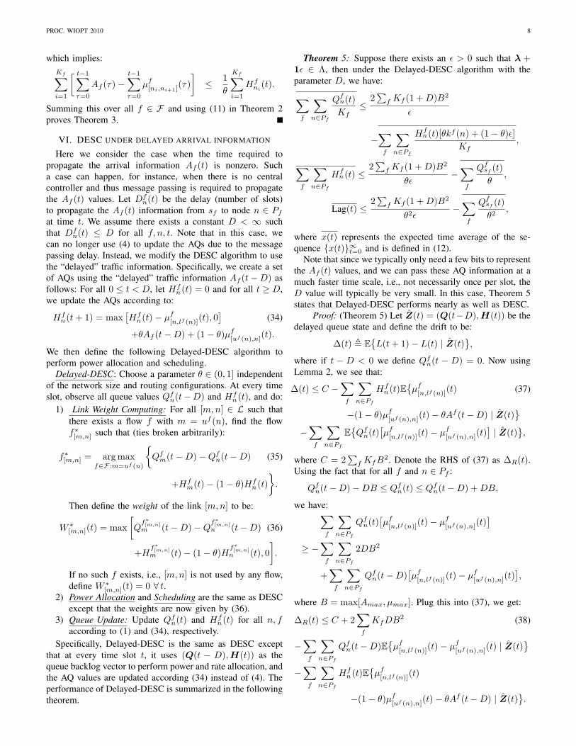
VII. SIMULATION

Here we provide simulation results of DESC. The networktopology and flow configuration are shown in Fig. 3. Weassume the channel conditions are independent and each link[m,n] is i.i.d. every slot being ON with probability 0.8 andOFF with probability 0.2. When the channel is “ON ,” wecan allocate one unit of power and transmit two packets;otherwise we can send zero packets. We further assume thatall links can be activated without affecting others. However,a node can only transmit over one link at a time, though itcan simultaneously receive packets from multiple nodes. Eachflow fi is an independent Bernoulli process with Afi

(t) = 2with probability λi/2 and Afi(t) = 0 else. The rate vectoris given by λ = (λ1, λ2, λ3, λ4)T = (0.8, 0.4, 0.2, 0.6)T . Wesimulate the system with (h = η

2 , υ = η2 ), where η, h and υ

are parameters in Fig. 3. Note that in this case, N = 3η2 + 7.

The η value is chosen to be 10, 50, 100, 200, 500. We useθ = 0.5.

s1 3 η-12 η-k

s2

1d3

η

f1

ν

3+h

s3

f2

f3 s4

d1

d2

d4f4

Fig. 3. A Network with 4 Flows. η is f1’s path length, h measures the pathoverlap length of f1 and f2, and υ is the vertical path length of f2.

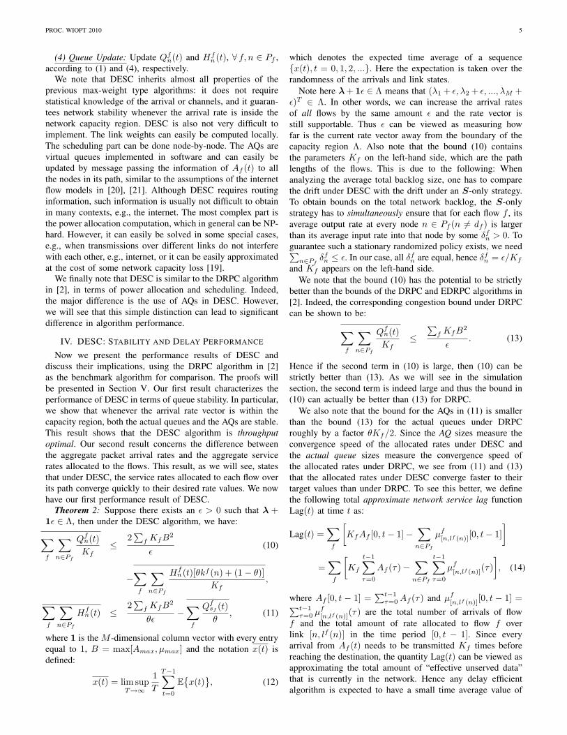
Fig. 4 and Fig. 5 show the simulation results. Fig. 4 showsthat under DESC, the average total backlogs of Flow 1 and2 scale only linearly in N . This is in contrast to the exampleprovided in [8], which shows that the average backlog growsquadratically with N under the usual max-weight schedulingpolicy. We also see that the average total backlog of Flow3 and 4 remains roughly the same. This is intuitive, as theirpath lengths do not grow with N . Interestingly, we observe

that∑n∈Pf

Hfn(t) ≥

∑n∈Pf

Qfn(t), ∀ f . By equation (11) ofTheorem 2, this implies that :∑

f

∑n∈Pf

Qfn(t) ≤∑f

∑n∈Pf

Hfn(t) ≤

2∑f KfB

2

θε.

Since we also have∑f Kf = O(N) and ε = Θ(1)

in this example, we see that indeed∑f

∑n∈Pf

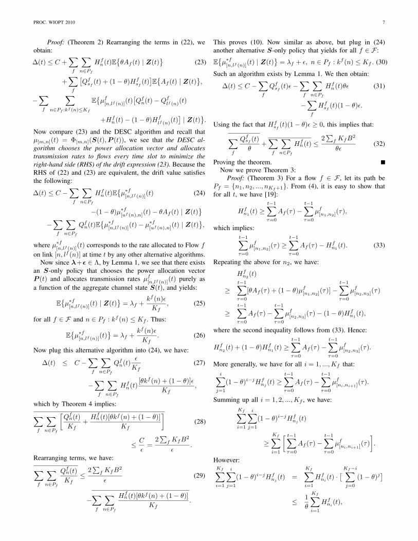
Qfn(t) =O(N) in this case. This suggests that DESC can poten-tially be a way to achieve delay-order-optimal schedul-ing in general multihop networks. Fig. 5 shows thatthe total average rates allocated to Flow 1 and 2 overtheir paths, i.e., 1

tKf1

∑ni∈Pf1

µf1[ni,lf1 (ni)]

[0, t − 1] and1

tKf2

∑nj∈Pf2

µf2[nj ,lf2 (nj)]

[0, t−1] with µfk

[ni,lfk (ni)]

[0, t−1] =∑t−1τ=0 µ

fk

[ni,lfk (ni)]

(τ), converge quickly to above the actualaverage arrival rates i.e., 1

tAf [0, t − 1]. Whereas the corre-sponding rates under DRPC converge very slowly from belowto the actual average arrival rate. These plots suggest that thepoor delay performance of many max-weight type algorithmsin multihop networks can be due to slow convergence of thecorresponding service rates.

0 100 200 300 400 5000

500

1000

1500

!

0 100 200 300 400 5002

3

4

5

6

7

8

9

!

H4

Q1

Q2

Q4

Q3

H3

H2

H1

"=0.5

Fig. 4. Qi and Hi, i = 1, 2, 3, 4, are the average total actual and AQbacklog sizes of flow i, respectively.

0 0.5 1 1.5 2 2.5 3 3.5 4 4.5 5

x 104

0

0.2

0.4

0.6

0.8

1

Time

Av

g.

Ra

te

0 0.5 1 1.5 2 2.5 3 3.5 4 4.5 5

x 104

0

0.2

0.4

0.6

0.8

1

1.2

1.4

Time

Av

g.

Ra

te

Avg. Rate to Flow 1 by DPRC

Flow 1 Avg. Arrival Rate

Avg. Rate to Flow 1 by DESC

Avg. Rate to Flow 2 by DRPC

Flow 2 Avg. Arrival Rate

Avg. Rate to Flow 2 by DESC

Fig. 5. UP: the average rate allocated to Flow 1 (η = 100); DOWN: theaverage rate allocated to Flow 2 (η = 100).

VIII. CONCLUSION

In this paper, we consider the problem of delay-efficientscheduling in general multihop networks. We develop a max-weight type Delay Efficient SCheduling Algorithm (DESC).

PROC. WIOPT 2010 10

We show that DESC is throughput optimal and derive aqueueing bound which can potentially be better than previouscongestion bounds on max-weight type algorithms. We alsoshow that under DESC, the time required for the allocatedrates to converge to their target values scales only linearly inthe network size. This contrasts with the usual max-weightalgorithms, which typically require a time that is at leastquadratic in the network size.

APPENDIX A – PROOF OF LEMMA 2

Proof: Define B = max[Amax, µmax] and denote [x]+ =max[x, 0]. From the queueing dynamic (1) we have for allnode n ∈ Pf with kf (n) ≤ Kf that:

[Qfn(t+ 1)]2

=([Qfn(t)− µf

[n,lf (n)](t)]+ + µf

[uf (n),n](t))2

=([Qfn(t)− µf

[n,lf (n)](t)]+

)2 + [µf[uf (n),n]

(t)]2

+2([Qfn(t)− µf[n,lf (n)]

(t)]+)µf[uf (n),n]

(t)

≤ [Qfn(t)− µf[n,lf (n)]

(t)]2 +B2 + 2Qfn(t)µf[uf (n),n]

(t).

The inequality holds since for any x ∈ R, we have([x]+)2 ≤ x2, and ([Qfn(t) − µf

[n,lf (n)](t)]+)µf

[uf (n),n](t) ≤

Qfn(t)µf[uf (n),n]

(t). We also use in the above equation thatif kf (n) = 1, i.e., node n is the source node of flow f ,then µf

[uf (n),n](t) = Af (t) for all t. Thus by expanding the

term [Qfn(t) − µf[n,lf (n)]

(t)]2, we have for all n ∈ Pf withkf (n) ≤ Kf that:

[Qfn(t+ 1)]2 ≤ [Qfn(t)]2 + 2B2

−2Qfn(t)[µf

[n,lf (n)](t)− µf

[uf (n),n](t)].

Note that if kf (n) = Kf +1, i.e., n = df , we have Qfn(t) = 0for all t, and so [Qfn(t + 1)]2 − [Qfn(t)]2 = 0, ∀t. Summingthe above over all n, f , and multiply by 1

2 , we have:

12

∑f

∑n∈Pf

[Qfn(t+ 1)]2 − 12

∑f

∑n∈Pf

[Qfn(t)]2 (40)

≤ Y1B2 −

∑f

∑n∈Pf

Qfn(t)[µf

[n,lf (n)](t)− µf

[uf (n),n](t)],

where Y1 =∑f Kf . Repeat the above argument on the term∑

f

∑n∈Pf

[Hfn(t+ 1)]2 −

∑f

∑n∈Pf

[Hfn(t)]2, we obtain:

12

∑f

∑n∈Pf

[Hfn(t+ 1)]2 − 1

2

∑f

∑n∈Pf

[Hfn(t)]2 (41)

≤ Y1B2 −

∑f

∑n∈Pf

Hfn(t)[µf

[n,lf (n)](t)− (1− θ)µf

[uf (n),n](t)

−θAf (t)].

Now adding (40) to (41), taking expectations conditioning onZ(t) = (Q(t),H(t)), and letting C = 2Y1B

2 = 2∑f KfB

2

proves the lemma.

REFERENCES

[1] L. Tassiulas and A. Ephremides. Stability properties of constrainedqueueing systems and scheduling policies for maximum throughput inmultihop radio networks. IEEE Trans. on Automatic Control, vol. 37,no. 12, pp. 1936-1949, Dec. 1992.

[2] M. J. Neely, E. Modiano, and C. E. Rohrs. Dynamic power allocationand routing for time-varying wireless networks. IEEE Journal onSelected Areas in Communications, Vol 23, NO.1, January 2005.

[3] L. Tassiulas and A. Ephremides. Dynamic server allocation to parallelqueues with randomly varying connectivity. IEEE Transactions onInformation Theory, Vol. 39, No. 2, pp. 466-478, March1993.

[4] M. J. Neely. Order optimal delay for opportunistic scheduling inmulti-user wireless uplinks and downlinks. IEEE/ACM Transactionson Networking, vol. 16, no. 5, pp. 1188-1199,, October 2008.

[5] M. J. Neely. Delay analysis for max weight opportunistic schedulingin wireless systems. IEEE Transactions on Automatic Control, Vol. 54,No. 9, pp. 2137-2150, Sept. 2009.

[6] M. J. Neely. Delay analysis for maximal scheduling with flow control inwireless networks with bursty traffic. IEEE Transactions on Networking,August 2009.

[7] G. R. Gupta and N. B. Shroff. Delay analysis for multi-hop wirelessnetworks. Proceedings of IEEE INFOCOM, April 2009.

[8] L. Bui, R. Srikant, and A. Stolyar. Novel architectures and algorithms fordelay reduction in back-pressure scheduling and routing. Proceedingsof IEEE INFOCOM 2009 Mini-Conference, April 2009.

[9] L. Ying, R. Srikant, and D. Towsley. Cluster-based back-pressure routingalgorithm. Proc. of IEEE INFOCOM, April 2008.

[10] L. Ying, S. Shakkottai, and A. Reddy. On combining shortest-path andback-pressure routing over multihop wireless networks. Proc. of IEEEINFOCOM, April 2009.

[11] P. Gupta and T. Javidi. Towards throughput and delay-optimal routingfor wireless ad-hoc networks. Asilomar Conference on Signals, Systemsand Computers, Nov 2007.

[12] M. Naghshvar, H. Zhuang, and T. Javidi. A general class ofthroughput optimal routing policies in multi-hop wireless networks.arXiv:0908.1273v1.

[13] S. Jagabathula and D. Shah. Optimal delay scheduling in networks witharbitrary constraints. In Proceedings of ACM SIGMETRIC/Performance,,2008.

[14] B. Sadiq and S. Baekand G. de Veciana. Delay-optimal opportunisticscheduling and approximations: The log rule. Proceedings of IEEEINFOCOM, April 2009.

[15] S. Shakkottai, R. Srikant, and A. Stolyar. Pathwise optimality of theexponential scheduling rule for wireless channels. Advances in AppliedProbability,, December 2004.

[16] V. J. Venkataramanan and X. Lin. Structural properties of ldp for queue-length based wireless scheduling algorithms. 45th Annual AllertonConference on Communication, Control, and Computing, Monticello,Illinois,, September 2007.

[17] D. P. Bertsekas. Nonlinear Programming, 2nd Edition. Athena Scientific,2003.

[18] L. Huang and M. J. Neely. Delay reduction via lagrange multipliers instochastic network optimization. Proc. of WiOpt, Seoul, June 2009.

[19] L. Georgiadis, M. J. Neely, and L. Tassiulas. Resource Allocation andCross-Layer Control in Wireless Networks. Foundations and Trends inNetworking Vol. 1, no. 1, pp. 1-144, 2006.

[20] Y. Li, A. Papachristodoulou, and M. Chiang. Stability of congestioncontrol schemes with delay sensitive traffic. Proc. IEEE ACC, Seattle,WA, June 2008.

[21] S. H. Low and D. E. Lapsley. Optimization flow control, i: Basicalgorithm and convergence. IEEE/ACM Transactions on Networking,vol. 7(6): 861-75, Dec. 1999.