Navigation System Integrity Monitoring Using Redundant Measurements

NAVIGNION: Joud afThe htitute ofNaG@ion Vol. 35, No. 4, Winter 1988-89 Prinhd ia USA.

Navigation System Integrity Monitoring Using Redundant Measurements

MARK A. STURZA Litton Systems, Inc., Woodland Hills, California Received Jammy 1988 Revised October 1988

ABSTRACT

The advantages of a navigation system that can monitor its own integrity are obvious. Integrity monitoring requires that the navigation system detect faulty measurement sources before they corrupt the outputs. This paper describes a parity approach to measurement error detection when redundant measurements are available. The general form of the detector operating characteristic (DO0 is developed. This equation relates the probability of missed detection to the probability of false alarm, the measurement observation matrix, and the ratio of the detectable bias shift to the standard deviation of tbe measurement noise.

Rvo applications are presented: skewed axis strapdown inertial navigation systems, where DOCs are used to compare the integrity monitoring capabilities of various redundant sensor strapdown system configurations; and GPS navigation sets, where DOCs are used to discuss GPS integrity monitoring for meeting nonprecision approach requirements. A fault identification algorithm is also presented.

INTRODUCTION

The Federal Padionavigation Plan [ll defines navigation system integrity monitoring as “the ability of a system to provide timely warnings to users when the system should not be used for navigation.” To implement integrity monitoring, the navigation system must detect faulty measurement sources hefore they result in out-of-specification performance. This in turn requires measurement redundancy. One redundant measurement is necessary for detecting a faulty measurement source. If additional redundant measurements are available, it is possible to isolate the faulty measurement source.

Integrity monitoring can be applied to any navigation system that provides redundant measurements. Potential applications include skewed axis strapdown inertial navigation systems (INS& GPS, Omega, and Loran-C. The INS and GPS applications will be used as examples to illustrate the theory.

Conventional INSs are configured with three gyro/accelerometer pairs mounted on orthogonal axes. Integrity monitoring can be achieved externally only by comparing the outputs of two or more such systems. A single redundant sensor INS incorporating four or more sensor pairs can provide internal integrity monitoring. The benefits of one redundant sensor INS versus two or more

69

70 Global Positioning System

conventional INSs are significant. Typical redundant sensor INSs incorporate four, five, or six pairs of inertial sensors [2,3,4,5,6,7,&3].

Conventional GPS navigation requires measurements from 4 satellites to resolve three spatial dimensions and time. With the baseline l&satellite constellation, 5 or more satellites will be available 99.3 percent of the time. By using the redundant measurement(s), it is possible to provide integrity monitoring. This is a requirement if GPS is to be certified as a sole means navigation system [ll. If measurements from 6 or more satellites are available, it is possible to isolate the faulty satellite and continue operating with the remaining ones. Considerable interest in GPS self-integrity monitoring has been sparked by the activities of the Radio Technical Commission for Aeronautics Special Com- mittee-159 Integrity Working Group 19,101.

The theory for both inertial navigation and radionavigation integrity monitoring is the same. This theory will be developed in the next three sections.

MEASUREMENT MODEL

The general case of M measurements in an N dimensional state space, M 2 N + 1, is addressed. The measurement equation is:

z=Hx+n+b 01

where z is the M x 1 vector of measurements compensated with all a priori information; H is the M x N measurement matrix which transforms from the state space to the measurement space, rank [HI = N; x is the N x 1 state vector; n is the M x 1 vector of Gaussian measurement noise, E[nl = 0 and COV[n] = un21M, where IM is the identity matrix of order M; and b is the M x 1 vector of uncompensated measurement biases (faults).

The fault model is a single measurement source failure resulting in a step bias shift. A failure of measurement source i is modeled by b = bi, where bi is an M x 1 vector with ith element B and zeros elsewhere. If there are no faults, then b = 0.

In the INS application, the gyro and accelerometer measurements are considered separately. In both cases, N = 3 and M 2 4. The measurement vector, z, contains the A& (gyro measurements) or AVs (accelerometer measurements) compensated for scale factor and biases. The state vector, x, consists of the three orthogonal body A& or AVs. The measurement matrix, H, consists of the unit projection vectors from the sensor axis to the orthogonal body axis. It is assumed that H is known perfectly (there are no uncompensated misalign- ments).

In the GPS application, the pseudorange residual (PI?) and delta-range residual (AR) measurements are considered separately. For both types of measurements, N = 4 and-M zz 5. The measurement vector, z, contains the PRmea- surements or the ARmeasurements compensated for atmospheric effects and clock biases. The state vector, x, consists of three orthogonal positions and clock bias for the PR measurements, or three orthogonal velocities and clock bias rate for the ARmeasurements. The PRmeasurement matrix consists of the line- of-sight (LOS) vectors to the satelliJes, with 1s in the fourth column corresponding to the clock bias state. The ARmeasurement matrix consists of the LOS vectors to the satellites, with ATs in the fourth column corresponding to the

Sturza: Navigation Sys tern Integrity Monitoring 71

clock bias rate state, where AT is the delta-range interval. It is again assumed that H is known perfectly.

PARITY VECTOR

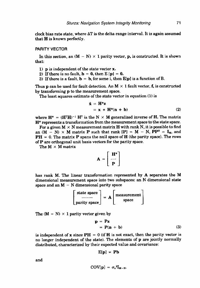
In this section, an (M - N) x 1 parity vector, p, is constructed. It is shown that:

1) p is independent of the state vector x. 2) If there is no fault, b = 0, then E [pl = 0. 3) If there is a fault, b = bi for some i, then E[p] is a function of B.

Thus p can be used for fault detection. An M x 1 fault vector, f, is constructed by transforming p to the measurement space.

The least squares estimate of the state vector in equation (1) is

g = H% = x + H*(II + b) (2)

where H* = @I%)-l I-P is the N x M generalized inverse of H. The matrix H* represents a transformation from the measurement space to the state space.

For a given M x N measurement matrix H with rank N, it is possible to find an (M - N) x M matrix P such that rank [PI = M - N, PPT = IM, and PH = 0. The matrix P spans the null space of H (the parity space). The rows of P are orthogonal unit basis vectors for the parity space.

The M x M matrix

A=

has rank M. The linear transformation represented by A separates the M dimensional measurement space into two subspaces: an N dimensional state space and an M - N dimensional parity space

[;;;;;;j = A [mea;Eyt]

The (M - N) x 1 parity vector given by

p = Pz = P(n + bl (3)

is independent of x since PH = 0 (if H is not exact, then the parity vector is no longer independent of the state). The elements of p are jointly normally distributed, characterized by their expected value and covariance:

E[pl = Pb

and

COV[pl = u”zIM-t+


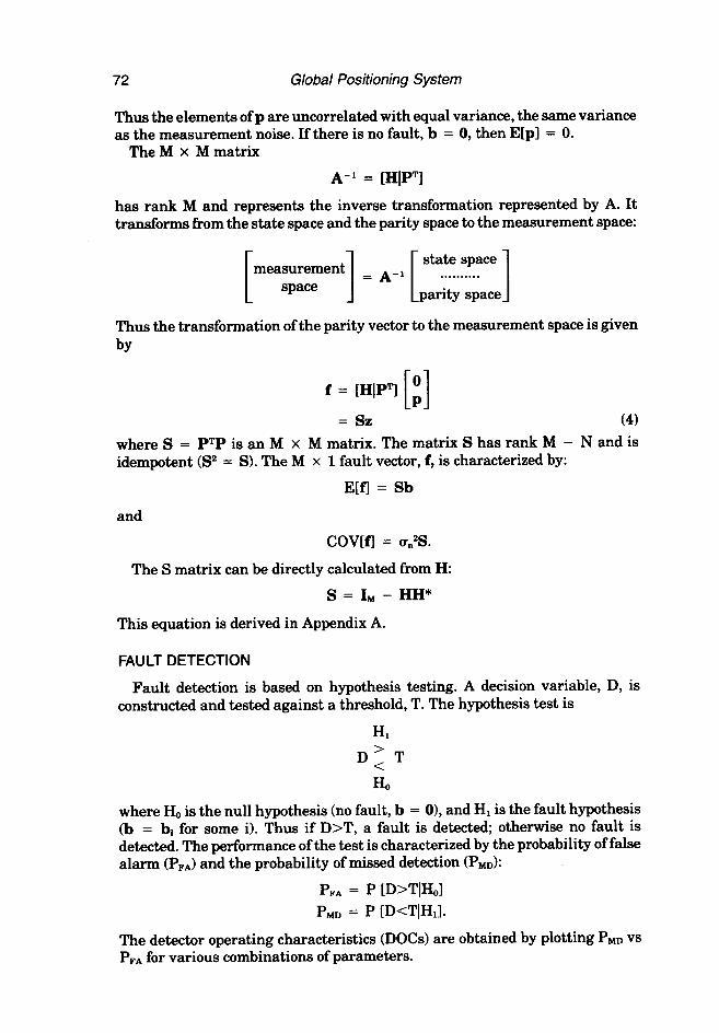
Thus the elements of p are uncorrelated with equal variance, the same variance as the measurement noise. If there is no fault, b = 0, then E[p] = 0.

The M x M matrix

A-l = [HiPTl

has rank M and represents the inverse transformation represented by A. It transforms from the state space and the parity space to the measurement space:

Thus the transformation of the parity vector to the measurement space is given by

f = [HiPTl ; [I = sz (41

where S = PT is an M x M matrix. The matrix S has rank M - N and is idempotent W = S). The M x 1 fault vector, f, is characterized by:

EKI = Sb

and

COV[fl = un2s.

The S matrix can be directly calculated from H:

s=I~--HH*

This equation is derived in Appendix A.

FAULT DETECTION

Fault detection is based on hypothesis testing. A decision variable, D, is constructed and tested against a threshold, T. The hypothesis test is

where H,, is the null hypothesis (no fault, b = O), and HI is the fault hypothesis (b = bi for some i). Thus if D>T, a fault is detected; otherwise no fault is detected. The performance of the test is characterized by the probability of false alarm (Pi& and the probability of missed detection (PM&

PFA = P [D>T[HJ Pj,,D = P [DcT[HJ.

The detector operating characteristics (DOCs) are obtained by plotting PMD vs PFA for various combinations of parameters.

Stwza: Navigation System htegrity Monitoring 73

The decision variable considered is the square of the magnitude of the parity vector, which is equivalent to the quadratic form D = pTp. It is equal to the square of the magnitude of the fault vector, D = Ff. This decision variable is popular in the literature 17,111.

The hypothesis test is characterized by

PFA = P ID=-Tib = 01

and, assuming that measurement faults are equally likely,

If b = 0, then E [p] = 0, and D/u,,~ has chi-square distribution with M - N degrees of freedom. Thus

PFA = Q CTW]M - N) (51

where Q (x2/r) = 1 - P (xzlr), and P (xzlr) is the chi-square probability function

PFA depends on M - N, the number of redundant measurements, and is otherwise independent of H. For given Pr+*, M - N, and un2, the required threshold is given by

T (PFA, M - N, un2) = un2 Q-l (I%~]M - Nl (7)

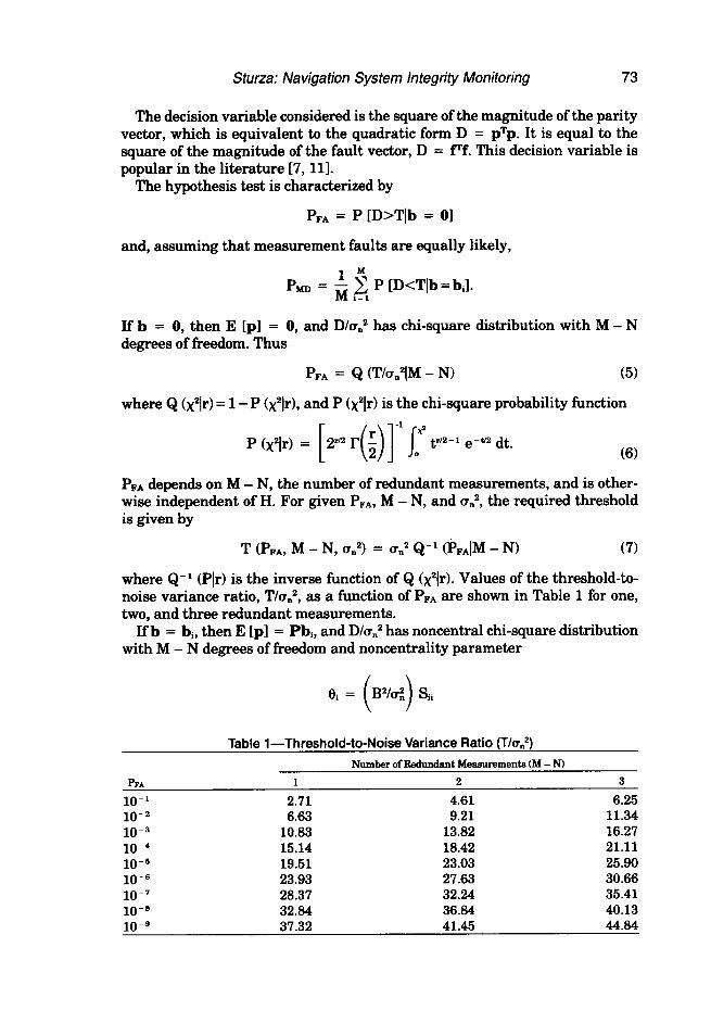
where Q-l (Plr) is the inverse function of Q (x?jr). Values of the threshold-to- noise variance ratio, T/u,,~, as a function of PFA are shown in Table 1 for one, two, and three redundant measurements.

If b = hip then E [P] = Pbiy and D/u,,~ has noncentral chi-square distribution with M - N degrees of freedom and noncentrality parameter

h

10-l lo-2 10-3 10-4 10-s lo+ lo-7 lo-a 10-g

Table l-Threshold-to-Noise Variance Ratio (T/u”*) Number of Redundant Meaawementa CM - N)

1 2

2.71 4.61 6.63 9.21

10.83 13.82 15.14 18.42 19.51 23.03 23.93 27.63 28.37 32.24 32.84 36.84 37.32 41.45

3

6.25 11.34 16.27 21.11 25.90 30.66 35.41 40.13 44.84

74 Global Positioning Sy.s tern

where Sii is the ith diagonal element of S. Thus

where P (x2]r, 0) is the noncentral chi-square probability function

P (x2[r, f3) = j$0e-W2 y P (x2ir+2jJ.

The DOC is given by

PMn depends on the ratio B/U,, and not on the individual values. Calculation of the DOC is discussed in Appendix B.

To summarize, the fault detection algorithm is as follows:

1) Based on the required P FA, the number of redundant measurements, M - N, and the measurement noise variance, u,,~, calculate the threshold

T = un2 Q-l (PFAIM - N).

2) Calculate the fault vector, f = Sz. 3) Calculate the decision variable, D = pf. 4) If D > T, then declare that a fault has occurred. 5) Repeat steps 2,3, and 4 for each new measurement vector.

INTEGRITY MONITORING PERFORMANCE

hertial Navigation System

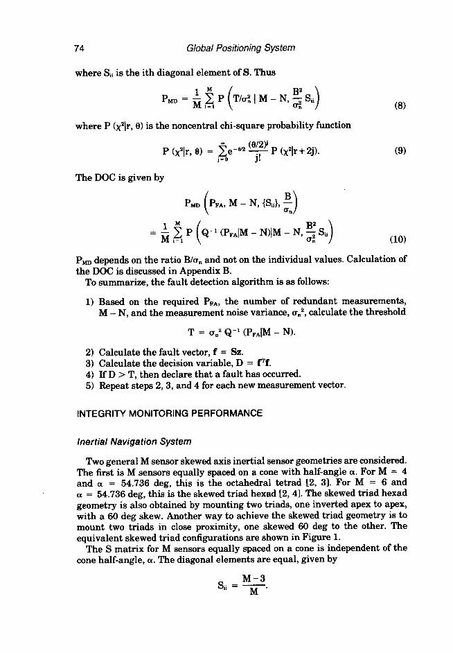
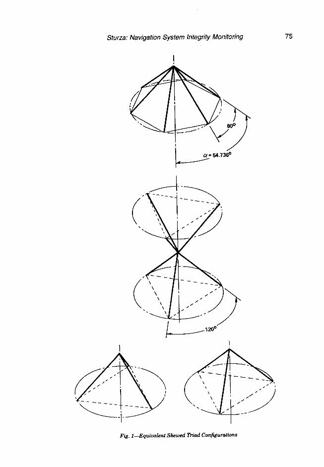
Two general M sensor skewed axis inertial sensor geometries are considered. The first is M sensors equally spaced on a cone with half-angle a. For M = 4 and a = 54.736 deg, this is the octahedral tetrad [2, 31. For M = 6 and a = 54.736 deg, this is the skewed triad hexad [2,4]. The skewed triad hexad geometry is also obtained by mounting two triads, one inverted apex to apex, with a 60 deg skew. Another way to achieve the skewed triad geometry is to mount two triads in close proximity, one skewed 60 deg to the other. The equivalent skewed triad configurations are shown in Figure 1.

The S matrix for M sensors equally spaced on a cone is independent of the cone half-angle, a. The diagonal elements are equal, given by

s.. = M-3 1, M ’

Sturza: Navigation Sys tern /n tegrity Monitoring

I I

75

Fig. 1 -Equivalent Skewed !hzd Configumtions


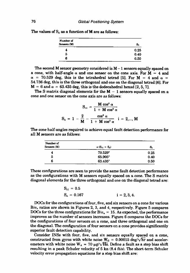
The values of Si as a function of M are as follows:

4 0.25 5 0.40 6 0.50

The second M sensor geometry considered is M - 1 sensors equally spaced on a cone, with half-angle a and one sensor on the cone axis. For M = 4 and a = 70.529 deg, this is the tetrahedral tetrad [5]. For M = 4 and a = 54.736 deg, this is the three orthogonal and one on the diagonal tetrad [6]. For M = 6 and a = 63.435 deg, this is the dodecahedral hexad [2,5,7].

The S matrix diagonal elements for the M - 1 sensors equally spaced on a cone and one sensor on the cone axis are as follows:

f&l = M cosz a

1 + M co9 a

i = 2,..., M

The cone half-angles required to achieve equal fault detection performance for all M sensors are as follows:

4 70.529O 0.25 5 65.905O 0.40 6 63.435' 0.50

These configurations are seen to provide the same fault detection performance as the configurations with M sensors equally spaced on a cone. The S matrix diagonal elements for the three orthogonal and one on the diagonal tetrad are:

Sll = 0.5

Sii = 0.167 i = 2,3,4.

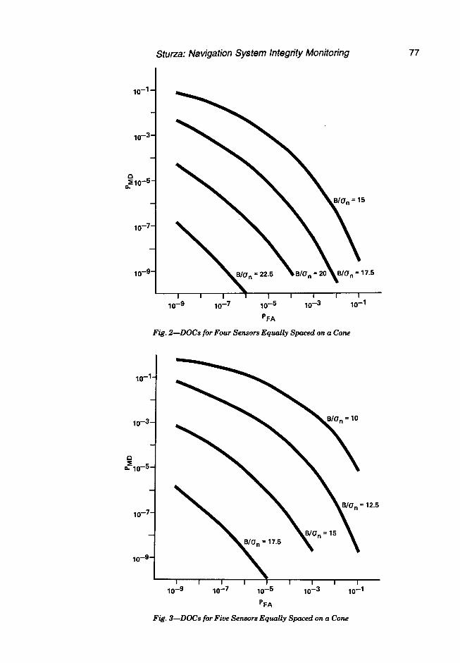
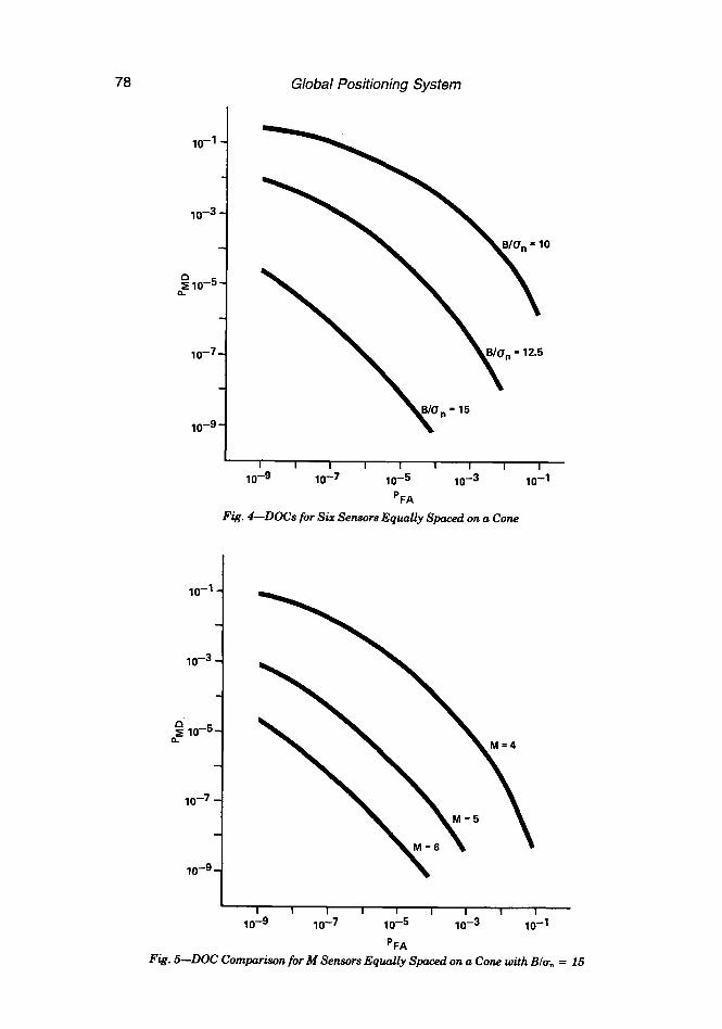
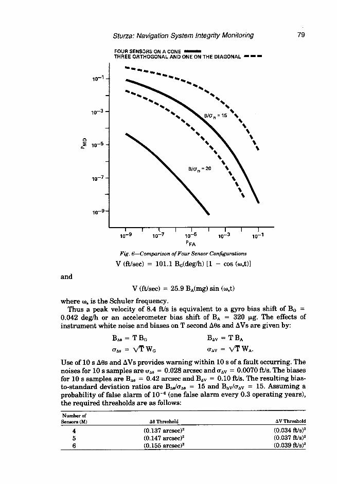
DOCs for the configurations of four, five, and six sensors on a cone for various B/u” ratios are shown in Figures 2, 3, and 4, respectively. Figure 5 compares DOCs for the three configurations for B/u,, = 15. As expected, the performance improves as the number of sensors increases. Figure 6 compares the DOCs for the configurations of four sensors on a cone, and three orthogonal and one on the diagonal. The configuration of four sensors on a cone provides significantly superior fault detection capability.

Consider INSs with four, five, and six sensors equally spaced on a cone, constructed from gyros with white noise Wo = 0.00015 deg/VE and acceler- ometers with white noise W,, = 70 pg/G. Define a fault as a step bias shift resulting in a peak Schuler velocity of 5 kn (8.4 ft/s). The short-term Schuler velocity error propagation equations for a step bias shifi are:

Stutza: Navigation System Integrity Monitoring 77

10-9-

10-g 10-g 10-7 10-7 10-5 10-5 10-3 10-3 10-l 10-l

'FA 'FA

Fig. Z-DOG for Four Sensors Equally Spaced on a Cone . Z-DOG for Four Sensors Equally Spaced on a Cone

10-l-

10-3-

n z

n 10-5-

10-7-

10-g-

10-9 10-7 .5 lo- ,0-3 .l lo-

'FA

Fig. 3-DO&for Five Sensors Equally Spaced on a Cone

12.5

7a Global Positioning System

10-l -

10-S -

j 10-S -

lo-‘-

10-g-

I I I I I I I I I I

10-g 10-7 10-S 10-3 10-l

‘FA

Fig, 4-DOCs far Six Sensors Equally Spaced on a Cone

10-l -

10-s -

; 10-s-

10-7 -

10-g-

I I I I I I I I I

10-g 10-7 10-S 10-S 10-l

‘FA Fig. 5-DOC Comparison for kl Sensors Equally Spaced on a Cone with BIu~ = ki

10-l -

10-s -

; 10-S -

10-T -

10-g-

Sturza: Navigation System Integrity Monitoring 79

FOUR SEN%XXi ON A CDNE - THREE ORTHOGONAL AND ONE ON THE DIAGONAL - - -

I I 1 I I I I I I 10-g 10-T 10-S 10-3 10-l

‘FA

Fig. 6-Comparison of Four Sensor Configurations

V (ft/secI = 101.1 BJdegW [l - cos Co&l and

V (ft/sec) = 25.9 B*(mgI sin (co&l

where mS is the Schuler frequency. Thus a peak velocity of 8.4 ft/s is equivalent to a gyro bias shift of BG =

0.042 deg/h or an accelerometer bias shift of B* = 320 Fg. The effects of instrument white noise and biases on T second A& and AVs are given by:

BA,j = TBo Bdv = TBA

uA8 = fl WG UAV = fl WA.

Use of 10 s A&J and AVs provides warning within 10 s of a fault occurring. The noises for 10 s samples are oA@ = 0.028 arcsec and oAv = 0.00’70 ft./s. The biases for 10 s samples are B&e = 0.42 arcsec and BAv = 0.10 R/s. The resulting bias- to-standard deviation ratios are B&A@ = 15 and BAV/UAV = 15. Assuming a probability of false alarm of lo-‘j (one false alarm every 0.3 operating years), the required thresholds are as follows:

Nmnher of Smsms CM)

4 5 6

A0 Threshold

(0.137 arcsec)’ (0.147 arcsecJ* (0.155 arcsecY

AV Threshold

(0.034 f?,w (0.037 ftw (0.039 ft./SF


The probabilities of missed detection for both gyro and accelerometer faults are equal:

ho Number of Mid Detections

per Million Faulta

4 5 x lo-: 5000 5 8 x lo-6 8 6 1 x lo-7 Cl

GPS Navigation Set

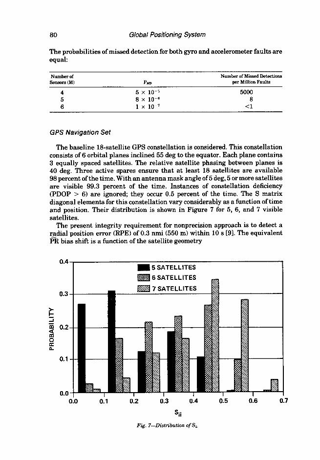
The baseline 18~satellite GPS constellation is considered. This constellation consists of 6 orbital planes inclined 55 deg to the equator. Each plane contains 3 equally spaced satellites. The relative satellite phasing between planes is 40 deg. Three active spares ensure that at least 18 satellites are available 98 percent of the time. With an antenna mask angle of 5 deg, 5 or more satellites are visible 99.3 percent of the time. Instances of constellation deficiency (PDOP > 6) are ignored; they occur 0.5 percent of the time. The S matrix diagonal elements for this constellation vary considerably as a function of time and position. Their distribution is shown in Figure 7 for 5, 6, and 7 visible satellites.

The present integrity requirement for nonprecision approach is to detect a r-adial position error (RPE) of 0.3 nmi (550 m) within 10 s 191. The equivalent

bias shift is a function of the satellite geometry

0.4

0.3

0.2

0.1

0.0 0.0 0.1 0.2 0.3 0.4 0.5 0.6 0.7

sii

Fig. 7-Distribution of&

Sturza: Navigation Sys tern /n tegrity Monitoring 81

where H*li and H*zi are the elements of H* that transform a bias in satellite i’s PR measurement into the horizontal components of x.

The noncentrality parameter in the DOC equation, equation GO), can be rewritten to group the geometry-dependent factors

K sii z Sii RPE2 U” H*,iz + H*a2 U” 2 *

(12)

Then equation (10) becomes

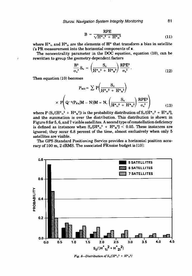
where P (SJ[H*lF + H*2T]) is the probability distribution of Sii/[H*lF + H*&, and the summation is over the distribution. This distribution is shown in Figure 8 for 5,6, and 7 visible satellites. A second type of constellation deficiency is defined as instances when SJ[H*li’ + H*2i2] < 0.05. These instances are ignored; they occur 6.8 percent of the time, almost exclusively when only 5 satellites are visible.

The GPS Standard Positioning ServiE provides a horizontal position accu- racy of 100 m, 2 dRMS. The associated PRnoise budget is [lo]:

6.8

0.8

c i $ 0.4

! a

0.2

0.0

m 5 SATELLITES

I 8 SATELLITES

m 7 SATELLITES

D 0:5 1:O 115 2:O 2:5 3:0

Sii/[H*li’+ H*2i21

Fig. 8-Distribution of Siii[H*Iiz + He=?1

3:5 4:0 5


Noise Source Standard Deviation Noise Type

Satellite Clock and Ephemeris 5m Colored Propagation Uncertainties 10 m Colored Receiver Noise 15 m White Selective Availability 30 m Colored

The correlation times ofJhe colored noise sources are modeled as significantly greater than 10 s. The PRstandard deviation for a single measurement is the RSS of the individual noise sources. For a T second PRformed by averaging PRmeasurements made every 1 s over a T second interval, the contjbution of the white noise sources is reduced by l/n. Thus the 10 s average PRstandard deviation is 32.4 m.

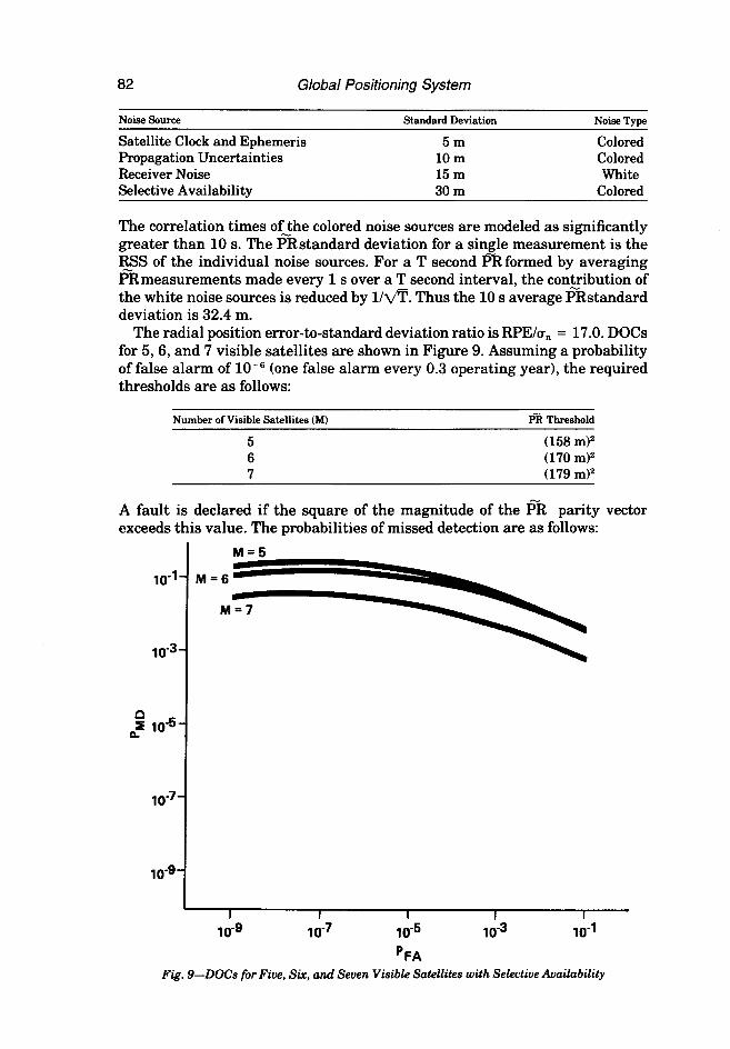
The radial position error-to-standard deviation ratio is RPE/cr,, = 17.0. DOCs for 5,6, and 7 visible satellites are shown in Figure 9. Assuming a probability of false alarm of 10e6 (one false alarm every 0.3 operating year), the required thresholds are as follows:

Number of Visible Satellites CM) P% Thrashold

5 (158 mY 6 (170 ml2 7 (179 ml2

A fault is declared if the square of the magnitude of the PR parity vector exceeds this value. The probabilities of missed detection are as follows:

10-l

10-3

; 10-5

10-7,

10-g

M=5

M=iEEF

I

‘7 I 1

10-g lo- 10-5 ‘3 lo- 10-l

‘FA Fig. 9-DOCs for Five, S~JG, and Seven Visible Satellites with Selective Availability


Number of Missed Detections Number of Visible Satellites CM) PMD per Million Faults

5 2 x 10-l 200,ooo 6 1 x 10-l 100,000 7 2 x 10-Z 20,000

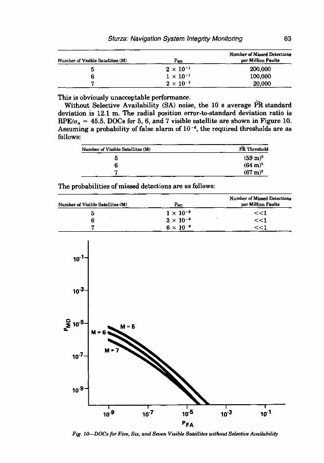
This is obviously unacceptable performance. Without Selective Availability @A) noise, the 10 s average PR standard

deviation is 12.1 m. The radial position error-to-standard deviation ratio is RPE/u~ = 45.5. DOCs for 5, 6, and 7 visible satellite are shown in Figure 10. Assuming a probability of false alarm of lo+, the required thresholds are as follows:

Number of Visible Satellites CM) P% Threshold

5 (59 ml2 6 (64 mY 7 (67 ml2

The probabilities of missed detections are as follows:

Number of Missed Detections Number of Visible Satellitea CM) PMD per Million Faults

5 1 x 10-8 c-4 6 3 x 10-8 <Cl 7 6 x lo-’ <Cl

10-l.

10-3.

j 10-5.

VI-'-

10-9.

I I I I I

10-g 10-7 10-6 10-3 10-l

'FA Fig. lo-DO& for Five, S&q and Seuen Visibh Satellites without Selective Availability

a4 Global Positioning System

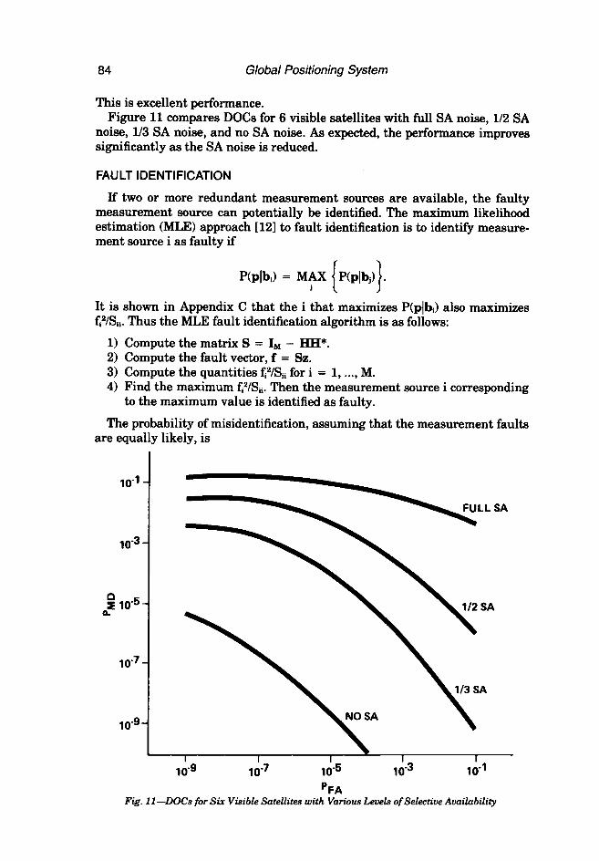
This is excellent performance. Figure 11 compares DOCs for 6 visible satellites with full SA noise, l/2 SA

noise, l/3 SA noise, and no SA noise. As expected, the performance improves significantly as the SA noise is reduced.

FAULT IDENTIFICATION

If two or more redundant measurement sources are available, the faulty measurement source can potentially be identified. The maximum likelihood estimation (MIX) approach 1121 to fault identification is to identify measurement source i as faulty if

P(pibJ = MAX P(pibj) j 1 I

.

It is shown in Appendix C that the i that maximizes P(p/bJ also maximixes <‘/Elii. Thus the Mm fault identification algorithm is as follows:

1) Compute the matrix S = IM - HH*. 2) Compute the fault vector, f = Sz. 3) Compute the quantities foe& for i = 1, . . . . M. 4) Find the maximum &‘/Sii. Then the measurement source i corresponding

to the maximum value is identified as faulty.

The probability of misidentification, assuming that the measurement faults are equally likely, is

10-l

10-3

2 lo-5 a

10-7

lO+

pFA Fig. 11-DOCs for Six Visibk Satellites with V&us L-evels of Selective Availubility

Sturza: Navigation Sys tern /n tegrity Monitoring 85

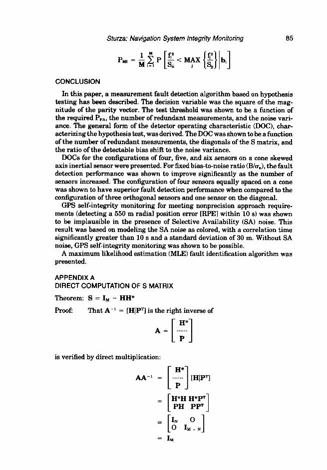
CONCLUSION

In this paper, a measurement fault detection algorithm based on hypothesis testing has been described. The decision variable was the square of the magnitude of the parity vector. The test threshold was shown to be a function of the required P FA, the number of redundant measurements, and the noise variance. The general form of the detector operating characteristic (DOC!), char- acterizing the hypothesis test, was derived. The DOC was shown to be a function of the number of redundant measurements, the diagonals of the S matrix, and the ratio of the detectable bias shift to the noise variance.

DOCs for the configurations of four, five, and six sensors on a cone skewed axis inertial sensor were presented. For fixed bias-to-noise ratio (B/u,,), the fault detection performance was shown to improve significantly as the number of sensors increased. The configuration of four sensors equally spaced on a cone was shown to have superior fault detection performance when compared to the configuration of three orthogonal sensors and one sensor on the diagonal.

GPS self-integrity monitoring for meeting nonprecision approach requirements (detecting a 550 m radial position error LRF’EI within 10 s) was shown to be implausible in the presence of Selective Availability @Al noise. This result was based on modeling the SA noise as colored, with a correlation time significantly greater than 10 s and a standard deviation of 30 m. Without SA noise, GPS self-integrity monitoring was shown to be possible.

A maximum likelihood estimation (MLE) fault identification algorithm was presented.

APPENDIX A DIRECT COMPUTATION OF S MATRIX

Theorem: S = IM - HH*

ProofI That A-l = [HiPTl is the right inverse of

A=

is verified by direct multiplication:

86 Global Positioning Sys tern

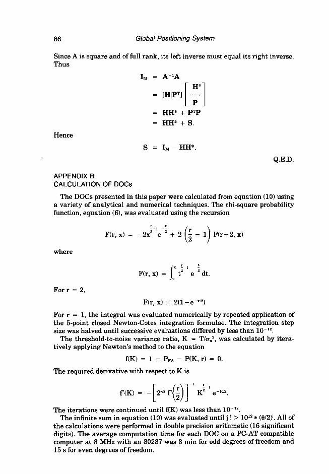
Since A is square and of full rank, its left inverse must equal its right inverse. Thus

IM = A-lA

F

H* = [H/PTl . . . . . .

P

Hence

= HH* + PTP = HH* + S.

S = IM - HH*.

Q.E.D.

APPENDIX 6 CALCULATION OF DOCs

The DOCs presented in this paper were calculated from equation (10) using a variety of analytical and numerical techniques. The chi-square probability function, equation (6), was evaluated using the recursion

L-1 -;

F(r, x) = -2x’ e + 2

where

F(r, x) =

For r = 2,

F(r, x) = 2(1 -emd2)

For r = 1, the integral was evaluated numerically by repeated application of the 5-point closed Newton-Cotes integration formulae. The integration step size was halved until successive evaluations differed by less than 10-12.

The threshold-to-noise variance ratio, K = T/u,,~, was calculated by itera- tively applying Newton’s method to the equation

f(K) = 1 - PFA - P(K, r) = 0.

The required derivative with respect to K is

The iterations were continued until f(K) was less than 10-12. The infinite sum in equation (10) was evaluated until j ! > 1012 * (W2Y. All of

the calculations were performed in double precision arithmetic (16 significant digits). The average computation time for each DOC on a PC-AT compatible computer at 8 MHz with an 80287 was 3 min for odd degrees of freedom and 15 s for even degrees of freedom.


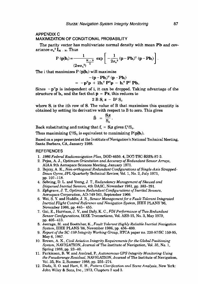
APPENDIX C MAXIMIZATION OF CONDITIONAL PROBABILITY

The parity vector has multivariate normal density with mean Pb and covariance un2 IM - N. Thus

The i that maximizes P (p[bi) will maximize - (p - Pbi)T (p - Phi)

= -pTp + 2biT PTp - biT PT Pbie

Since -pTp is independent of i, it can be dropped. Taking advantage of the structure of bi, and the fact that p = Pz, this reduces to

2 B Si z - B2 Sii where Si is the ith row of S. The value of B that maximizes this quantity is obtained by setting its derivative with respect to B to zero. This gives

Back substituting and noting that fi = Siz gives f2&. Thus maximizing fF/Sii is equivalent to maximizing P(p[bJ.

Based on a paper presented at the Institute of Navigation’s National Technical Meeting, Santa Barbara, CA, January 1988.

REFERENCES 1. 1986 Federul &xf~o~uu&~r~orr P&n, DOD-4650.4, DOT-TSC-RSPA-87-3. 2. Pejsa, A. J., Optimum Orientation und Accurucy of Redundunt Sensor Arrays,

AIAA 9th Aerospace Sciences Meeting, January 1971. 3. Bejczy, A. K., Non-orthogonal Redundunt Configurutions of Single-Axis Strupped-

Down Gyros, JPL Quarterly ‘Ibchnical Review, Vol. 1, No. 2, July 1971, pp. 107-118.

4. Sebring, D. L. and Young, J. T., Redunduncy Management of Skewed and Dispersed Znertiul Sensors, 4th DASC, November 1981, pp. 383-391.

5. Ephgrave, J. ‘I!, Optimum Redundant Configurations of ZnertiuZ Sensors, Aerospace Corporation, AD-749 561, September 1966.

6. Wei, S. Y. and Huddle, J. R., Sensor Management for u Fault Tolerunt Zntegruted Znertial Flight Control Reference und Nuwgution System, IEEE PLANS ‘86, November 1986, pp. 445- 455.

7. Gai, E., Harrison, J. V., and Daly, K. C., FDZ Pe$orm.ance of Two Redundunt Sensor Configurutions, IEEE Transactions, Vol. AES-15, No. 3, May 1979, pp. 405-413.

8. Jeerage, M. and Boettcher, K., Fault Tolerunt HighZy ReZiuble Znertial Navigation System, IEEE PLANS ‘86, November 1986, pp. 456-460.

9. Report of the SC-159 Zntegrity Working Group, RTCA paper no. 220-87lSC 159-95, May 6,1987.

10. Brown, A. K., Civil Aoiution Zntegrity Requirements for the GZobul Positioning System, NAVlGATION, Journal of The Institute of Navigation, Vol. 35, No. 1, Spring 1988, pp. 23-40.

11. Parkinson, B. W. and Axelrad, F?, Autonomous GPS Zntegrity Monitoring Using the Pseudorunge ResiduuZ, NAVIGATION, Journal of The Institute of Navigation, Vol. 35, No. 2, Summer 1988, pp. 255-274.

12. Duda, R. 0. and Hart, E. H., Pattern CZurification und Scene Analysis, New York: John Wiley 8z Sons, Inc., 1973, Chapters 2 and 3.

Navigation System Integrity Monitoring Using Redundant Measurements

Documents

Transcript of Navigation System Integrity Monitoring Using Redundant Measurements