The fusion of redundant SEVA measurements
12
IEEE TRANSACTIONS ON CONTROL SYSTEMS TECHNOLOGY, VOL. XX, NO. Y, MONTH 2000 100 The fusion of redundant SEVA measurements Mihaela Duta, Manus Henry Abstract— The self-validating (SEVA) sensor carries out an internal qual- ity assessment, and generates, for each measurement, standard metrics for its quality, including on-line uncertainty. This pa- per discusses consistency checking and data fusion between sev- eral SEVA sensors observing the same measurand. Consistency checking is shown to be equivalent to the maximum clique prob- lem, which is NP-hard, but a linear approximation is described. A technique called uncertainty extension is proposed which causes a smooth reduction in the influence of outliers as they become in- creasingly inconsistent with the majority. Index Terms— Sensor fusion, SEVA sensors, Maximum clique problem I. I NTRODUCTION This paper proposes a simple method for fusing measurement data from a set of independent self-validating (SEVA) sensors monitoring the same real-time measurand in order to provide the combined best estimate for the value, uncertainty and mea- surement status of the measurand. The method also provides consistency checking between the measurements. After a brief description of the concept of the SEVA sensor, the basic issues in sensor fusion will be discussed. A method of fusing a set of measurement values and uncertainties will then be presented, based on the analogy with the maximum clique problem from graph theory. A linear search method for find- ing the maximum clique, tuned to the specific problem at hand, is then proposed, and the results obtained after applying this method on simulated data are contrasted with those obtained by finding the maximum clique using exhaustive search. These are followed by simulation results demonstrating how, in a three-sensor system, a variety of sensor faults are dealt with. II. THE CONCEPT OF THE SEVA SENSOR For the purpose of this paper a sensor is a device consisting of one or more transducers and a transmitter which converts transducer signals into a form recognizable by the control or monitoring system. Increasingly, the availability of local computing power has been exploited to carry out internal diagnostics within so-called ’intelligent’ sensors. A SEVA sensor, [1], performs additional processing to generate generic validity metrics for each mea- surement, as follows (Figure 1): • The validated measurement value (VMV) is the best es- timate of the true measurand value, taking all diagnostic information into account. If a fault occurs, then the VMV is corrected to the best ability of the sensor. In the most The authors are with the Invensys University Technology Centre, Depart- ment of Engineering Science, University of Oxford, Oxford, UK, E-mail: mi- [email protected]. Raw data Transducer Device status Detailed diagnostic Transmitter VMV VU MV status Fig. 1. The SEVA sensor severe cases (where the raw data is judged to have no cor- relation with the measurand), the current VMV is extrapo- lated from past measurement behaviour. • The validated uncertainty (VU) is the uncertainty asso- ciated with the VMV. The metrological definition is used here, [2], [3]: the VU gives a confidence interval for the true value of the measurand. For example, if VMV is 2.51 units, and the VU is 0.08, then there is a 95% chance that the true measurement lies within the interval 2.51 ± 0.08 units. The VU takes into account all likely sources of error, including noise, measurement technology and any fault- correction strategy currently being used. • The measurement value status (MV status) is a discrete- valued flag indicating how the VMV has been calculated. The basic categories defined are shown in Table I. The MV status assists users (whether human or automated) to determine whether the measurement is acceptable in the particular application - e.g. BLIND data should never be used for feedback control. The SEVA sensor concept has become the basis of a British Standard for the reporting of measurement quality in industrial control systems, [4]. In the absence of localised validation, measurement redun- dancy has frequently been used to ensure that a verified and reliable measurement is provided with high availability. Such redundancy may be implemented through the use of several in- dependent sensors monitoring the same measurand (hardware redundancy), or through a plant model to provide an indepen- dent estimate of the measurand (analytical redundancy), [5]. The SEVA model assumes that the designer builds into the sen- sor techniques to detect the most important fault modes of the device. However, there remains a non-zero probability that a fault may go undetected for a not insignificant period of time. It thus may be desirable in certain applications to use higher level validation to perform consistency checking and data fu- sion between redundant SEVA measurements. In this paper a correct SEVA measurement x with uncer- tainty u means one that is truly representative of the measurand, i.e. the true value of the measurand lies within x ± u with a prob- ability of 95%. An incorrect SEVA measurement falsely rep-
Transcript of The fusion of redundant SEVA measurements
IEEE TRANSACTIONS ON CONTROL SYSTEMS TECHNOLOGY, VOL. XX, NO. Y, MONTH 2000 100
The fusion of redundant SEVA measurementsMihaela Duta, Manus Henry
Abstract—The self-validating (SEVA) sensor carries out an internal qual-
ity assessment, and generates, for each measurement, standardmetrics for its quality, including on-line uncertainty. This pa-per discusses consistency checking and data fusion between sev-eral SEVA sensors observing the same measurand. Consistencychecking is shown to be equivalent to the maximum clique prob-lem, which is NP-hard, but a linear approximation is described.A technique called uncertainty extension is proposed which causesa smooth reduction in the influence of outliers as they become in-creasingly inconsistent with the majority.
Index Terms— Sensor fusion, SEVA sensors, Maximum cliqueproblem
I. INTRODUCTION
This paper proposes a simple method for fusing measurementdata from a set of independent self-validating (SEVA) sensorsmonitoring the same real-time measurand in order to providethe combined best estimate for the value, uncertainty and mea-surement status of the measurand. The method also providesconsistency checking between the measurements.
After a brief description of the concept of the SEVA sensor,the basic issues in sensor fusion will be discussed. A method offusing a set of measurement values and uncertainties will thenbe presented, based on the analogy with the maximum cliqueproblem from graph theory. A linear search method for find-ing the maximum clique, tuned to the specific problem at hand,is then proposed, and the results obtained after applying thismethod on simulated data are contrasted with those obtained byfinding the maximum clique using exhaustive search.
These are followed by simulation results demonstrating how,in a three-sensor system, a variety of sensor faults are dealtwith.
II. THE CONCEPT OF THE SEVA SENSOR
For the purpose of this paper a sensor is a device consistingof one or more transducers and a transmitter which convertstransducer signals into a form recognizable by the control ormonitoring system.
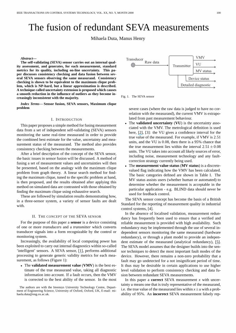
Increasingly, the availability of local computing power hasbeen exploited to carry out internal diagnostics within so-called’intelligent’ sensors. A SEVA sensor, [1], performs additionalprocessing to generate generic validity metrics for each mea-surement, as follows (Figure 1):
• The validated measurement value (VMV) is the best es-timate of the true measurand value, taking all diagnosticinformation into account. If a fault occurs, then the VMVis corrected to the best ability of the sensor. In the most
The authors are with the Invensys University Technology Centre, Depart-ment of Engineering Science, University of Oxford, Oxford, UK, E-mail: [email protected].
Raw dataTransducer
Device status
Detailed diagnostic
Transmitter
VMV
VU
MV status
Fig. 1. The SEVA sensor
severe cases (where the raw data is judged to have no cor-relation with the measurand), the current VMV is extrapo-lated from past measurement behaviour.
• The validated uncertainty (VU) is the uncertainty asso-ciated with the VMV. The metrological definition is usedhere, [2], [3]: the VU gives a confidence interval for thetrue value of the measurand. For example, if VMV is 2.51units, and the VU is 0.08, then there is a 95% chance thatthe true measurement lies within the interval 2.51± 0.08units. The VU takes into account all likely sources of error,including noise, measurement technology and any fault-correction strategy currently being used.
• The measurement value status (MV status) is a discrete-valued flag indicating how the VMV has been calculated.The basic categories defined are shown in Table I. TheMV status assists users (whether human or automated) todetermine whether the measurement is acceptable in theparticular application - e.g. BLIND data should never beused for feedback control.
The SEVA sensor concept has become the basis of a BritishStandard for the reporting of measurement quality in industrialcontrol systems, [4].
In the absence of localised validation, measurement redun-dancy has frequently been used to ensure that a verified andreliable measurement is provided with high availability. Suchredundancy may be implemented through the use of several in-dependent sensors monitoring the same measurand (hardwareredundancy), or through a plant model to provide an indepen-dent estimate of the measurand (analytical redundancy), [5].The SEVA model assumes that the designer builds into the sen-sor techniques to detect the most important fault modes of thedevice. However, there remains a non-zero probability that afault may go undetected for a not insignificant period of time.It thus may be desirable in certain applications to use higherlevel validation to perform consistency checking and data fu-sion between redundant SEVA measurements.
In this paper a correct SEVA measurement x with uncer-tainty u means one that is truly representative of the measurand,i.e. the true value of the measurand lies within x±u with a prob-ability of 95%. An incorrect SEVA measurement falsely rep-

IEEE TRANSACTIONS ON CONTROL SYSTEMS TECHNOLOGY, VOL. XX, NO. Y, MONTH 2000 101
SEVA category DefinitionSECURE DIVERSE The VMV is derived from multiple
values of the same measurementat least two of which are CLEARor better and which are notsusceptible to common mode faults
SECURE COMMON The VMV is derived from multiplevalues of the same measurement atleast two of which are CLEAR orbetter, but which are susceptibleto common mode faults
CLEAR The VMV is calculated normally
BLURRED The VMV is based on live data,but is being corrected for a fault
DAZZLED A transient state: the VMV is basedon historical data while thefault is assessed
BLIND No credible live data is available.The VMV is being projectedfrom past behaviour
REPLACED The VMV comes from an externalagent (operator or higher levelmodelling program)
OFFLINE the instrument is off-lineThe VMV and VU are typically zero
UNVALIDATED Validation not in operation
TABLE I
resents the true value of the measurand, that is, there is higherthan 5% probability that the true value of the measurand liesoutside x± u. A correct measurement should not be confusedwith a measurement that has been ‘corrected’ as part of the di-agnostic process within a SEVA sensor.
An incorrect measurement does not mean a SEVA measure-ment with a status other than CLEAR or SECURE. Indeed sucha measurement is likely to be correct: whatever condition iscausing the non-ideal status value has been identified by thesensor, which implies that the measurement and uncertaintyhave been corrected accordingly, so they are likely to still berepresentative of the measurand. As stated above, an incorrectmeasurement is likely to be generated if the sensor fails to no-tice a fault within itself, or if a phenomenon such as availablemeasurement drift, discussed later, occurs. In either case thestatus is likely to be CLEAR or even SECURE. Of course if thecorrection algorithms are inadequate then a BLURRED, DAZ-ZLED or BLIND measurement may also be incorrect.
III. SENSOR FUSION: MAIN ISSUES
In the broadest sense, the process of sensor fusion is the syn-ergistic use of a set of not necessarily consistent measurementsfrom different sources to achieve a specific task. There is aconsiderable wealth of academic literature devoted to this is-sue. The applications range from simple problems (e.g. robot
Combination Block
1. Check for consistency2. Deal with outliers3. Calculate CBE
Mea
sura
nd
Tx1
VMV , VU
MV status1 1
1
VMV , VU
MV status
* *
*
Tx2
VMV , VU
MV status2 2
2
Tx3
VMV , VU
MV status3 3
3
Fig. 2. The combination block for redundant SEVA measurements.
self-location) to 3-D tracking of multiple targets and decoys byfusing data from different sensor systems (e.g. radar, range-finders) in air defence systems. There also exists a wide varietyof methods for performing the actual fusion of the measure-ments, among which the most important are the Bayesian meth-ods ([6] and [7]), Dempster-Shafer methods ([7]) and methodsbased on robust statistics (see [8]). The reader is directed tothese references for further details.
The basic questions posed by sensor fusion are:
• What is the model of the measurand to be tracked?• What is the model of measurement uncertainty (here used
in the broadest sense)?• How are measurements judged to be consistent?• What happens to measurements inconsistent with the rest
(typically they are discarded)?• How are consistent measurements fused to provide a com-
bined best estimate of the measurand?
Clearly, the measurand and uncertainty models dictate boththe consistency checking and fusion methods. In the literature arange of uncertainty models have been used, based normally onprobabilistic or fuzzy models, but no examples of sensor fusionbased upon metrological uncertainty have been found.
Consider now the case of n SEVA measurements xi, i =1, ..,n, with their associated uncertainties ui, all estimating thesame single valued measurand. This is a relatively simple prob-lem compared with e.g. target tracking. What is to be deter-mined is whether any of the measurements is inconsistent withthe rest and, having dealt with any such outliers, what is thecombined best estimate of the measurand and its uncertainty.The MV status for the combined measurement is also to bedetermined, based upon the consistency of the input measure-ments as well as their individual MV status values. These cal-culations can take place within a generic Combination Block(CB).
Figure 2 illustrates the scenario. Each measurement may bethe product of a different sensor, as shown. Alternatively, allcalculations can take place within a single transmitter handlingmultiple transducers. In either case the calculation of the com-bined estimate will be largely identical.
The core functions of the CB are:
• checking for consistency for a set of measurements usingtheir uncertainties
• combining the consistent measurements and uncertaintiesto obtain a best estimate
These issues will be studied in detail in the following sec-tions.

IEEE TRANSACTIONS ON CONTROL SYSTEMS TECHNOLOGY, VOL. XX, NO. Y, MONTH 2000 102
IV. COMBINATION OF A SET OF MEASUREMENTS
Given n measurements xi and their associated uncertaintiesui, and assuming that they are all consistent, a combined bestestimate (CBE) x∗ of the measurand is given by, [3]:
x∗ =n
∑1
wixi where wi =( 1
ui)2
∑n1(
1ui
)2(1)
It follows that the uncertainty u∗ of CBE is:
u∗ =
√(
n
∑1
w2i u2
i ) =1√
∑n1 ( 1
ui)2
(2)
The following example illustrates the use of these formulae.Table II lists five measurements, their uncertainties and corre-sponding weights. The measurement values were randomly se-lected from normal distributions N (0,ui/1.96). The CBE isx∗ = 0.0328, and its uncertainty u∗ = 0.0876. Notice the veryhigh weighting given to the measurement with the smallest un-certainty. Note also that the overall uncertainty is smaller thanthe smallest individual uncertainty. This is to be expected, asadditional information about the measurand is being accumu-lated, so that the result should have a reduced uncertainty.
xi 0.0192 0.1154 0.1868 −1.2192 −0.2808ui 0.1 0.2 0.5 1.0 2.0
wi(%) 76.8 19.2 3.07 0.768 0.192
TABLE II
Let the combination operation be denoted by:
x∗ = Λni=1xi ≡ Λ{x1,x2, ...,xn}
An important property of Λ is that it is associative. For example,given variables x1, x2 and x3 and defining
x∗1,2 ≡ Λ{x1,x2} and x∗2,3 ≡ Λ{x2,x3}it is trivial to show that
Λ{x∗1,2,x3} ≡ Λ{x1,x∗2.3} ≡ Λ{x1,x2,x3}
This implies that the order in which measurements are com-bined is not important.
V. CONSISTENCY CHECKING
A. Consistent vs. inconsistent measurements
Consistent measurements agree with each other, accordingto a criterion to be defined later. Inconsistencies can arise forany of the following three reasons.
Firstly, even when all of the redundant measurements are in-dividually representative of the measurand, random fluctuationsmay result in mutual inconsistencies occurring from sample tosample.
The other two reasons are more serious, in that they entail amisrepresentation of the measurand by one or more measure-ments:
Sensor BSensor A Average temperature
TA TB
Fig. 3. Sensors A and B both measure the same nominal temperature, but dueto local temperature fluctuations, their output TA and TB may drift apart.
• Each measurement is generated by a SEVA sensor, whichshould provide detailed and device-specific fault detection.It might reasonably be assumed that a commercial SEVAsensor should be able to detect (say) between 90% and99.9% of all occurrences of faults within itself, allowingfor faults which are inherently difficult to detect and com-mercial design limitations due to cost/benefit trade-offs.Thus there exists the possibility that a sensor may fail todetect a fault within itself, and so generate an unrepresen-tative or incorrect measurement. Within a single trans-mitter handling multiple transducers, consistency check-ing may be the primary form of validating the raw data,and so inconsistencies may arise more frequently.
• A sensor is only able to measure the available value of aprocess parameter, rather than its ideal or true value [9].For example (Figure 3), the ‘average’ temperature withina pressure vessel may be the parameter of interest, but inpractice only localised temperatures (such as A and B)near the vessel wall are available. A better estimate ofthe average temperature may be obtained by combiningthe two measurements. Irrespective of any sensor faults,it is possible for the two measurements to become incon-sistent if, for example, a significant temperature gradientdevelops across the vessel, a phenomenon called availablemeasurement drift.
Of course consistency does not necessarily imply that themeasurements are correct, only that they agree with each other.However in practice, just as the true value of the measurand isnever known the correctness of a measurement is never known.The fundamental principle of consistency checking, the purposeof which is to identify incorrect measurements to assume that:
• Incorrect measurements are relatively rare.• Correct measurements are likely to be consistent with one
another.
It follows that if one measurement is inconsistent with therest, it is likely that it is incorrect, as the alternative, that it iscorrect and all the other measurements are incorrect, is muchless probable. Generalising, the principle of majority voting isderived: if a majority of measurements are consistent they areassumed to be correct; any minority of measurements inconsis-tent with the majority are judged to be incorrect. If there is nomajority consensus, then special action will have to be taken.To summarize, the guiding principle is that inconsistency im-plies incorrectness.

IEEE TRANSACTIONS ON CONTROL SYSTEMS TECHNOLOGY, VOL. XX, NO. Y, MONTH 2000 103
B. The case of two measurements
The detection of inconsistencies between redundant mea-surements is a well-established academic field of study. Typ-ically, however, the measurements are treated as time series ofpoint values. It is less common for consideration to be given tothe uncertainty interval surrounding each measurement, as itsmagnitude is not usually available.
According to the classical techniques of analytical redun-dancy [5], given a set of redundant measurements, one or moreresidual functions are created, each of which is designed toremain ‘close’ to zero as long as the measurements are con-sistent. When a fault occurs, a variety of techniques may beapplied to determine which sensor (or other plant component)is responsible for the inconsistency. Normally such techniquesentail modelling of plant dynamic behaviour and/or sensor faultmodes, which can be difficult and/or expensive. Choices mustalso be made about each decision-making threshold, i.e. thevalue which, if exceeded by a residual, indicates a significantinconsistency.
The availability of the uncertainty of each measurement pro-vides a richer set of information to work with; on the other handit adds to the complexity and dimensionality of the problem.
The aim of this paper is not to extend the techniques of ana-lytical redundancy to exploit uncertainty information, but ratherto develop an algorithm which does not require any modellingof the measurand M beyond the simplest possible assumptionthat the expected value of each measurement is equal to themeasurand:
E(x1) = E(x2) = ... = E(xn) = E(M) (3)
It is assumed that such an algorithm will be less able thana more elaborate scheme to detect subtle inconsistencies, butcould be more widely and readily used in applications whichdo not justify the expense of detailed modelling. Nor is itproposed here to detect all undiagnosed faults in a SEVA sen-sor, for example through pattern recognition of time-frequencyproperties which may be characteristic of specific fault modes,[10]. Rather, the intention is simply to be able to detect faultswhich cause measurements to be inconsistent with their redun-dant peers.
Moffat, [11], suggests a method of testing consistency be-tween two measurements x1 and x2, given their uncertainties u1
and u2. Under the hypothesis that the measurements are cor-rect, i.e. they are representative of the same measurand, thenthe function
φ = x1 − x2 with uncertainty uφ =√
u21 +u2
2
should be close to zero. In other words, it is expected that
dM12 =
x1 − x2√u2
1 +u22
(4)
where dM12 is the Moffat distance, satisfies the following crite-
rion (called here the Moffat criterion):
|dM12| < 1 (5)
0 0.5 1.5 3.5-0.5-1.5-3.5
x ±u1 1
x ±u2 2
True value
Fig. 4. An example of uncertainty intervals which, though overlapping, arenot Moffat consistent.
at the usual, say, 95% probability. The Moffat consistency testcan thus be seen as a simple static form of residual function.This definition of consistency is somewhat counter-intuitive, inthat uncertainty intervals may overlap and yet still be declaredinconsistent, as illustrated in the following example.
Suppose that the true measurand is 0, and that the two sensorsgenerate measurements x1 and x2 with a distribution N (0,1).Then it follows that u1 = u2 = 1.96. Suppose that at a partic-ular instant x1 = −1.5 and x2 = +1.5. Figure 4 illustrates thesituation.
It can be seen that the uncertainty intervals overlap the truevalue and each other, and yet the consistency test fails, forφ = −3 and uφ =
√2×1.96 = 2.77. In other words, both mea-
surements are correct, and yet they are not consistent. This isdue to the probabilistic nature of the test - the chance of a TypeI error is 5%. As the distributions are normal, this can be con-firmed analytically: x1 and x2 are N (0,1), so φ = x1 − x2 hasdistribution N (0,2). Thus there is a 5% probability that a ran-dom sample from this distribution will fall outside the uncer-tainty interval uφ =
√2×1.96.
The degree of overlap required for Moffat consistency ismaximum when u1 = u2. Suppose u1 is kept constant and u2 isincreased, then the degree of overlap required for consistency,as a proportion of u1, decreases asymptotically to zero. Indeed,as shown in Appendix 1, Moffat consistency ensures that theCBE of the two measurements falls within the uncertainty in-tervals of each. A logical corollary is that there must be anoverlap between the two uncertainty intervals and that the CBEfalls within the overlap. A further useful (and intuitively nec-essary) result is proved in Appendix 2: if x1 and x2 are Moffatconsistent, then the CBE (n.b. with its reduced uncertainty) isalso Moffat consistent with x1 and x2.
The Type I threshold of 5% is presumably acceptable for theanalysis of experimental data, the context in which Moffat con-ceived the test, and of course all the uncertainties themselvesare expressed at the 95% probability level. However, for thepurposes of on-line monitoring of redundant measurements inan industrial context, this probability is too high, leading to asteady stream of trivial alarms. The alarm frequency could bereduced by modifying the test as follows: use the test crite-rion kuφ <= φ <= kuφ to demonstrate consistency, where k isa fixed but arbitrary value which controls the probability of aType I error. The value k =
√2 has intuitive appeal, because
then two uncertainty intervals of equal magnitude are declared
IEEE TRANSACTIONS ON CONTROL SYSTEMS TECHNOLOGY, VOL. XX, NO. Y, MONTH 2000 104
0 1.0 2.0-1.0-2.0
x ±u1 1
x ±u2 2
x ±u3 3
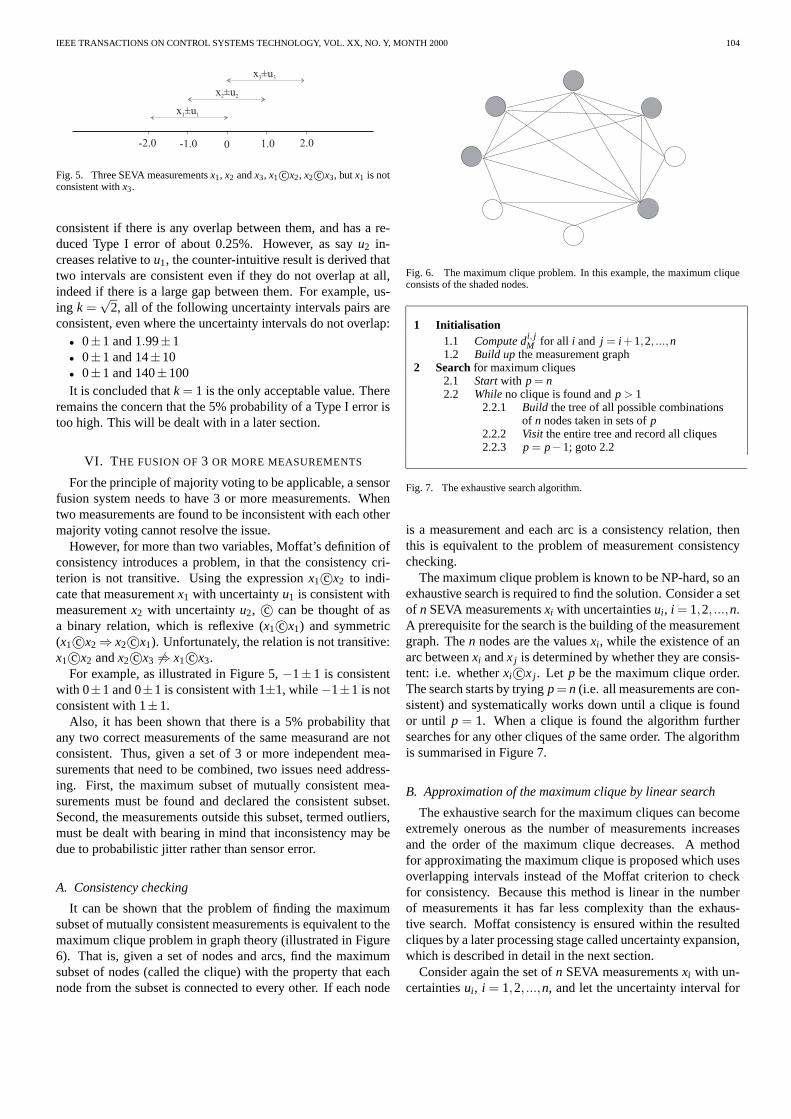
Fig. 5. Three SEVA measurements x1, x2 and x3, x1 c©x2, x2 c©x3, but x1 is notconsistent with x3.
consistent if there is any overlap between them, and has a re-duced Type I error of about 0.25%. However, as say u2 in-creases relative to u1, the counter-intuitive result is derived thattwo intervals are consistent even if they do not overlap at all,indeed if there is a large gap between them. For example, us-ing k =
√2, all of the following uncertainty intervals pairs are
consistent, even where the uncertainty intervals do not overlap:• 0±1 and 1.99±1• 0±1 and 14±10• 0±1 and 140±100It is concluded that k = 1 is the only acceptable value. There
remains the concern that the 5% probability of a Type I error istoo high. This will be dealt with in a later section.
VI. THE FUSION OF 3 OR MORE MEASUREMENTS
For the principle of majority voting to be applicable, a sensorfusion system needs to have 3 or more measurements. Whentwo measurements are found to be inconsistent with each othermajority voting cannot resolve the issue.
However, for more than two variables, Moffat’s definition ofconsistency introduces a problem, in that the consistency cri-terion is not transitive. Using the expression x1 c©x2 to indi-cate that measurement x1 with uncertainty u1 is consistent withmeasurement x2 with uncertainty u2, c© can be thought of asa binary relation, which is reflexive (x1 c©x1) and symmetric(x1 c©x2 ⇒ x2 c©x1). Unfortunately, the relation is not transitive:x1 c©x2 and x2 c©x3 �⇒ x1 c©x3.
For example, as illustrated in Figure 5, −1± 1 is consistentwith 0±1 and 0±1 is consistent with 1±1, while −1±1 is notconsistent with 1±1.
Also, it has been shown that there is a 5% probability thatany two correct measurements of the same measurand are notconsistent. Thus, given a set of 3 or more independent mea-surements that need to be combined, two issues need address-ing. First, the maximum subset of mutually consistent mea-surements must be found and declared the consistent subset.Second, the measurements outside this subset, termed outliers,must be dealt with bearing in mind that inconsistency may bedue to probabilistic jitter rather than sensor error.
A. Consistency checking
It can be shown that the problem of finding the maximumsubset of mutually consistent measurements is equivalent to themaximum clique problem in graph theory (illustrated in Figure6). That is, given a set of nodes and arcs, find the maximumsubset of nodes (called the clique) with the property that eachnode from the subset is connected to every other. If each node
Fig. 6. The maximum clique problem. In this example, the maximum cliqueconsists of the shaded nodes.
1 Initialisation1.1 Compute di, j
M for all i and j = i+1,2, ...,n1.2 Build up the measurement graph
2 Search for maximum cliques2.1 Start with p = n2.2 While no clique is found and p > 1
2.2.1 Build the tree of all possible combinationsof n nodes taken in sets of p
2.2.2 Visit the entire tree and record all cliques2.2.3 p = p−1; goto 2.2
Fig. 7. The exhaustive search algorithm.
is a measurement and each arc is a consistency relation, thenthis is equivalent to the problem of measurement consistencychecking.
The maximum clique problem is known to be NP-hard, so anexhaustive search is required to find the solution. Consider a setof n SEVA measurements xi with uncertainties ui, i = 1,2, ...,n.A prerequisite for the search is the building of the measurementgraph. The n nodes are the values xi, while the existence of anarc between xi and x j is determined by whether they are consis-tent: i.e. whether xi c©x j. Let p be the maximum clique order.The search starts by trying p = n (i.e. all measurements are con-sistent) and systematically works down until a clique is foundor until p = 1. When a clique is found the algorithm furthersearches for any other cliques of the same order. The algorithmis summarised in Figure 7.
B. Approximation of the maximum clique by linear search
The exhaustive search for the maximum cliques can becomeextremely onerous as the number of measurements increasesand the order of the maximum clique decreases. A methodfor approximating the maximum clique is proposed which usesoverlapping intervals instead of the Moffat criterion to checkfor consistency. Because this method is linear in the numberof measurements it has far less complexity than the exhaus-tive search. Moffat consistency is ensured within the resultedcliques by a later processing stage called uncertainty expansion,which is described in detail in the next section.
Consider again the set of n SEVA measurements xi with un-certainties ui, i = 1,2, ...,n, and let the uncertainty interval for

IEEE TRANSACTIONS ON CONTROL SYSTEMS TECHNOLOGY, VOL. XX, NO. Y, MONTH 2000 105
Bounds
Clique order p
l1 l2h1 l3 l4
l5 h4h3
h5 h2
0 1 2 1 2 3 4 3 2 1 0
Direction of search algorithm
Fig. 8. Illustrative example of overlapping intervals.
the ith measurement, i = 1,2, ...,n, be (li,hi),, where l = xi −ui
and hi = xi + ui, the lower and upper bound, respectively. Theset of n measurements can then be described by an orderedbound list containing all li and hi. Without loss of general-ity the xi can be assumed ordered so that l1 < l2 < ... < ln.Of course the hi may occur in any order interleaved throughthe li, subject only to the constraint that hi > li (and hencehi > lk,k = 1..i). The overlapping intervals are readily iden-tified by stepping through the ordered list of bounds. The ap-proximation of the maximum clique(s) is given by the measure-ments whose uncertainty intervals define the area(s) of maxi-mum overlap.
Figure 8 illustrates the method. The bound list is in this casegiven by l1l2h1l3l4l5h4h3h5h2. The point of maximum overlapinvolves measurements 2, 3, 4 and 5, which are therefore con-sidered as an approximation of the maximum clique.
The algorithm walks through the bound list in increasing or-der. When a lower boundary is encountered the correspondingmeasurement is added to the set of active measurements, whoseorder p is thus incremented. When an upper bound is encoun-tered, the corresponding measurement is removed from the setof active measurements whose order is thus decremented. Ateach stage, if the order of the active measurement set exceedsall previous values, then the active set becomes the new max-imum clique. If its order equals that of the current maximumclique then the set is stored as an additional maximum clique.The algorithm is summarised in Figure 9.
C. Dealing with outliers
Having found or approximated a maximum clique, the ob-vious next step would be to use it to calculate the CBE usingEquations 1 and 2 and to ignore all outliers. This approach hasa number of difficulties:
1) Given the probabilistic nature of the uncertainty, even ifall measurements are correct representations of the mea-surand, there is only a 95% chance of each pair beingconsistent. As the number of inputs increases, the proba-bility of all measurements being consistent reduces. Forexample, with 10 normally distributed measurements ofequal variance and mean, there is only a 37.3% chanceof all 10 sensors being mutually consistent at any giventime.
2) If, on average, one measurement is only marginally con-sistency with the rest, then sample by sample it may reg-
1 Initialisation1.1 Compute li and hi, i = 1,2, ...,n1.2 Build up boundlist Z of triplets:
z j = {bound j, index j, type j}where z2i = {li, i, lower}and z2i+1 = {hi, i,upper}
1.3 Sort the bound list by bound value z j.bound2 Search the bound list for maximum areas of overlap
2.1 Start: p = 0, maxp = 0,active meas = Φ and clique list = Φ
2.2 For j = 1 : 2n do2.2.1 If z j.type = lower
then add z j.index to active measand p = p+1
2.2.2 If z j.type = upperthen remove z j.index from active measand p = p−1
2.2.3 If p = maxpthen append active meas to clique list
2.2.4 If p > maxpthen clique list = {active meas}and maxp = p
Fig. 9. The approximation of the maximum clique(s) by linear search.
ularly switch between being judged consistent and incon-sistent. This will generate undesirable jitter on the CBE.
3) It is possible that at any given time there may be morethan one maximum clique. For example, with three mea-surements x1, x2 and x3 such that x1 c©x2 and x2 c©x3,while x1 c©x3 is not true, then there are two maximumcliques, (x1,x2) and (x2,x3). It is not obvious which ofthe maximum cliques to use for calculating the CBE.
A simple strategy can be implemented to tackle these issues.The underlying idea is that any inconsistent measurement canbe ‘made consistent’ by a sufficient increase in its own uncer-tainty, and that such an increase will cause a reduction in theweight of that measurement in the CBE. This approach is notbased on uncertainty theory, but rather is a heuristic approachwhich has the desirable characteristics of smoothing over prob-abilistic inconsistency jitter, and providing a smooth reductionof weighting for inconsistent measurements.
In the most general case when there is more that one clique,the measurements are partitioned into two sets:
• the core set - the intersection of all the maximum cliques• the peripheral set - the rest of the measurements i.e. those
being either in at least one of the maximum cliques, but notin the core set, or those outside any maximum clique
If the maximum cliques were found using exhaustive search,then the mutual Moffat consistency of the measurements insideit is ensured. However, this is not guaranteed to be the case withthe linear search, thus, for the core and peripheral sets resultedfrom the linear search algorithm, additional consistency check-ing need to done before the CBE is computed. The maximumMoffat distance dM
max between pairs of measurements from thecore set is computed. If this value is greater than one, then atleast one of the measurements pairs is inconsistent. The uncer-tainty ui of all measurements from the core set is then increasedto u′i = dM
max ×ui, values which will ensure mutual consistency.

IEEE TRANSACTIONS ON CONTROL SYSTEMS TECHNOLOGY, VOL. XX, NO. Y, MONTH 2000 106
Each measurement from the peripheral set is then consideredin turn and the maximum Moffat distance to the measurementsin the core set is found. If this value is greater than a specifiedthreshold (for example 3.0), then the measurement is judged tobe a true outlier and is ignored. If, however, this distance isless than the specified threshold, then its uncertainty interval isexpanded as described to make it consistent with the measure-ments in the core set. The measurements from the peripheral setthus processed are then merged with those in the core set to ob-tain the CBE. This technique of uncertainty expansion reduces,but does not eliminate, the influence of the involved measure-ments on the CBE. In particular, if a measurement slowly driftsinto inconsistency with the rest, uncertainty expansion ensuresa smooth reduction of influence on the CBE before it is finallylabelled as an outlier. This is illustrated in the simulations at theend of the paper.
One circumstance not covered by the above procedure iswhere there are multiple maximum cliques with no intersectionbetween them. Here the ”middle clique” is found as being themaximum clique closest to the mean of the merged values foreach maximum clique. The middle clique is then considered tobe the core set while the peripheral set contains the remainingmeasurements.
D. The Combination Block
Given a set of n SEVA measurements (xi,ui,statusi), the taskof the Combination Block is as follows.
• calculate the CBE and its uncertainty using the techniquesdescribed above. Normally, the VMV output is set equalto the CBE and the VU to its uncertainty - see below.
• assign the MV status of the output block. As a configu-ration option, the user can assign the minimum acceptablesize of the maximum clique (for example 2 out of 3 or 6out of 10). If this size is not reached, then the CBE isnot used but instead the VMV and VU are projected frompast history in the usual way, [1], and the MV status isset to DAZZLED or, if the condition persists, BLIND. Ifthe minimum acceptable size of clique is reached, then theMV status is set to SECURE; COMMON if the sensors areof identical type, otherwise DIVERSE. A further configu-ration option is the minimum number of CLEAR (or bet-ter) consistent measurements required to declare the CBEto be SECURE. It this target is not met, then the CBE is as-signed the best status of the consistent measurements (i.e.CLEAR, BLURRED, DAZZLED or BLIND).
• each SEVA measurement is also assigned a consistencyflag.
The takes the value 1 if the measurement was found to be inthe core or was made consistent with the core by uncertaintyexpansion, and 0 otherwise. This flag may be used (possiblyafter further filtering to avoid jitter) to trigger additional diag-nostic testing within any SEVA sensors whose measurementswere found inconsistent with the majority.
E. Exhaustive search vs. linear search approximation
Simulations have been carried out to compare the perfor-mance of the two methods for finding the set of mutually con-sistent SEVA measurements i.e. the exhaustive search for the
Exhaustive Linear Theoreticalsearch search value
3 sensors:Mean of CBE 0.002 0.002 0.0Std of CBE 0.581 0.579 0.577Mean of unc. 1.136 1.129 1.131Sets with k < n 0 06 sensors:Mean of CBE 0.002 0.002 0.0Std of CBE 0.411 0.410 0.408Mean of unc. 0.806 0.804 0.800Sets with k < n 0 010 sensors:Mean of CBE 0.0 0.0 0.0Std of CBE 0.320 0.320 0.316Mean of unc. 0.626 0.624 0.619Sets with k < n 0 0
TABLE IIINOTE: k IS THE NUMBER OF CONSISTENT MEASUREMENTS AFTER
UNCERTAINTY EXPANSION AND n IS THE TOTAL NUMBER OF
MEASUREMENTS IN THE SET
maximum clique and the approximation of the maximum cliqueby linear search. In these first studies, fault-free behaviour isconsidered. It is desirable to have a match between theoreticaland simulation results for the following statistics:
• mean of the CBE• variance in mean of the CBE• reported uncertainty of the CBEIn addition, it is desirable for the reported uncertainty to be
reasonably constant, and for the incidence of reported incon-sistencies to be low (as there are no true faults, just randomvariations).
100000 random sets of 3, 6 and 10 SEVA measurements weregenerated as follows:
• the true measurand value is 0• the measurements were randomly generated from a normal
distribution with a mean of zero and unit variance. Thiscorresponds to an uncertainty of 1.96.
The theoretical value of the standard deviation of the CBEis then 1√
n . This gives an uncertainty of 1.96 1√n . The means
and standard deviations of the reported values of the CBE andits uncertainty has been computed over the 100000 simulations,and they are contrasted with the corresponding expected valuesin Table III.
In this fault-free simulation, all sensor values were includedin the calculation of all the CBEs through the use of the ex-panded uncertainty weighting technique. By contrast, withoutthis technique, a significant percentage of sets are found to beinconsistent (e.g. in the case of 10 sensors, only 37.3% of thesets were found fully consistent).
At this point it can be concluded that the exhaustive searchfor the maximum clique and the approximation of the maxi-mum clique with the linear search give very similar results.Given the simplicity and computational efficiency of the lin-

IEEE TRANSACTIONS ON CONTROL SYSTEMS TECHNOLOGY, VOL. XX, NO. Y, MONTH 2000 107
ear search, it may be preferred, certainly for larger numbers ofsensors (say > 5). Also, the results show a reasonable matchbetween the expected value of the CBE uncertainty, its actualvariation, and its reported uncertainty.
VII. SIMULATION RESULTS
Experiments have been carried out to study the behaviour ofthe Combination Block when one of the SEVA sensors eithersignals a fault or gives a incorrect description of the measurand.In view of the results in the previous section, the linear searchmethod was used to generate the following results.
The experiments consisted of simulating the on-line be-haviour of 3 SEVA sensors. Two of the SEVA sensors give acorrect description of the measurand (as in the previous sec-tion), while the third SEVA sensor either signals a fault or gen-erates an incorrect description of the measurand.
In each case, a constant true measurement value of 2 wasconsidered. The simulated faults were as follows:
• Example 1: a spike fault - saturation at upper limit occursat 125s; the fault is permanent; the SEVA sensor detectsthe fault and first changes the MV status to DAZZLEDand then to BLIND.
• Example 2: a spike fault - a faulty ramping value is addedto the true measurement with the slope of 0.001 units persecond; the fault begins at 125s and is permanent; theSEVA sensor detect the fault and changes the MV statusto BLURRED.
• Exanple 3: a drift fault - a faulty ramping value is added tothe true measurement with the slope of 0.001 units per sec-ond; the fault begins at 125s and is permanent; the SEVAsensor does not detect the fault and reports the measuredvalue along with an MV status of CLEAR.
For the cases when the third SEVA sensor gives an incorrectdescription of the measurand, this was accomplished by ensur-ing that the VU was of the usual magnitude and the MV Statuswas CLEAR, while the VMV in fact suffers a drift starting at125s, with a slope of 0.001 units per second.
The time series of the VMV, the VU and the MV status fora typical sensor (as used in this study) exhibiting fault-free be-haviour and generating a correct description of the measurandis given in Figure 10.
Figures 11, 12 and 13 show the outputs of the faulty sensorand the Combination Block for examples 1, 2 and 3 respec-tively.
In example 1 the third sensor exhibits a permanent saturationfault. Its output is characterised by the usual SEVA responsei.e.
• The VMV is projected from past history. In this case theVMV remains reasonably accurate as the process is sta-tionary.
• The MV status changes to DAZZLED and then BLINDwhen it is deemed that the saturation is permanent.
• The uncertainty increases at a rate learned from past his-tory using conventional SEVA algorithms.
The response of the Combination Block is as follows:1) The MV status of the Combination Block can only re-
main SECURE COMMON if a configured number of in-put sensors are CLEAR. In this case the number is three,
0 50 100 150 200 250 300 350 400 450
1.75
1.8
1.85
1.9
1.95
2
2.05
2.1
2.15
2.2
2.25
[ o C ]
true valueVMV RMV
0 50 100 150 200 250 300 350 400 450
0.06
0.08
0.1
0.12
0.14
Unc
erta
inty
[ o C
]
0 50 100 150 200 250 300 350 400 450
UnvOff
RepBld
DazBluClr
S−CS−D
Sta
tus
Time [s]
Fig. 10. A typical fault-free sensor with a constant true value.
so as soon as sensor 3 changes MV status the Combina-tion Block output reverts to CLEAR. Note that hystere-sis is used to prevent excessive jitter on the combinationblock MV status.
2) The measurements are combined according to their con-sistency and uncertainty weightings. In both cases themeasurement from the faulty sensor remains consistent,but its influence declines rapidly, weighted by the inversesquare of its increasing uncertainty. This also results inthe rapid increase in the uncertainty of the combined mea-surement from about 0.06 to 0.075 after the fault.
In example 2 a drift fault occurs in sensor 3, but the sen-sor detects the fault and attempts to compensate. Thus the rawmeasurement value (RMV) is seen to drift off quickly, but theSEVA sensor reduces the effect of the fault by internal cor-rection (which still leaves some marginal drift). The sensordeclares the measurement BLURRED and increases its uncer-tainty. In these cases, the slow increase in the VU of the faultysensor is reflected in a very marginal increase in the uncertaintyof the Combination Block. Again, the change in the MV statusis also accounted for in the change of MV for the CombinationBlock.
In examples 1 and 2, since the fault is compensated for insidethe SEVA sensor, the repored VMV is a correct representationof the true measurand. Therefore the combination block findsall 3 measurements to be consistent and uses them all to calcu-late the CBE. The occurrence of the fault is then reflected in thevalue of the VU for the combination block and in the MV statusof the Combination Block output (determined by the change inMV status of the faulty sensor).
Example 3 shows the most important case: when one SEVAsensor does not give a correct representation of the measurand.

IEEE TRANSACTIONS ON CONTROL SYSTEMS TECHNOLOGY, VOL. XX, NO. Y, MONTH 2000 108
0 50 100 150 200 250 300 350 400 450
−10
−5
0
5
10
15[ o C
]
Example 1: sensor 3
true valueVMV RMV
0 50 100 150 200 250 300 350 400 450
1
2
3
4
5
6
Unc
erta
inty
[ o C
]
0 50 100 150 200 250 300 350 400 450
UnvOff
RepBld
DazBluClr
S−CS−D
Sta
tus
Time [s]
0 50 100 150 200 250 300 350 400 450
1.8
1.85
1.9
1.95
2
2.05
2.1
2.15
2.2
2.25
[ o C ]
Example 1: Combination Block
true valueVMV
0 50 100 150 200 250 300 350 400 450
0.06
0.08
0.1
0.12
0.14
Unc
erta
inty
[ o C
]
0 50 100 150 200 250 300 350 400 450
UnvOff
RepBld
DazBluClr
S−CS−D
Sta
tus
Time [s]
Fig. 11. The faulty sensor and the Combination Block for example 1.
0 50 100 150 200 250 300 350 400 4501.6
1.7
1.8
1.9
2
2.1
2.2
2.3
2.4
2.5
2.6
[ o C ]
Example 2: sensor 3
true valueVMV RMV
0 50 100 150 200 250 300 350 400 450
0.06
0.08
0.1
0.12
0.14
Unc
erta
inty
[ o C
]
0 50 100 150 200 250 300 350 400 450
UnvOff
RepBld
DazBluClr
S−CS−D
Sta
tus
Time [s]
0 50 100 150 200 250 300 350 400 450
1.85
1.9
1.95
2
2.05
2.1
2.15
[ o C ]
Example 3: combination block
true valueVMV
0 50 100 150 200 250 300 350 400 450
0.06
0.08
0.1
0.12
0.14
Unc
erta
inty
[ o C
]
0 50 100 150 200 250 300 350 400 450
UnvOff
RepBld
DazBluClr
S−CS−D
Sta
tus
Time [s]
Fig. 12. The faulty sensor and the Combination Block for example 2.

IEEE TRANSACTIONS ON CONTROL SYSTEMS TECHNOLOGY, VOL. XX, NO. Y, MONTH 2000 109
0 50 100 150 200 250 300 350 400 4501.4
1.6
1.8
2
2.2
2.4
2.6
2.8
3
3.2
3.4
[ o C ]
Example 3: sensor 3
true valueVMV RMV
0 50 100 150 200 250 300 350 400 450
0.06
0.08
0.1
0.12
0.14
Unc
erta
inty
[ o C
]
0 50 100 150 200 250 300 350 400 450
UnvOff
RepBld
DazBluClr
S−CS−D
Sta
tus
Time [s]
0 50 100 150 200 250 300 350 400 450
1.8
1.85
1.9
1.95
2
2.05
2.1
2.15
2.2
2.25
2.3
[ o C ]
Example 3: Combination Block
true valueVMV
0 50 100 150 200 250 300 350 400 450
0.06
0.08
0.1
0.12
0.14
Unc
erta
inty
[ o C
]0 50 100 150 200 250 300 350 400 450
UnvOff
RepBld
DazBluClr
S−CS−D
Sta
tus
Time [s]
Fig. 13. The faulty sensor and the Combination Block for example 3.
The chain of events is as follows:1) An undetected drift fault begins in sensor 3 at t = 125s.2) The CBE begins to rise as long as the faulty value remains
consistent with the rest.3) From t=200s to t=275s sensor 3 becomes increasingly
inconsistent with the other two (i.e. its Moffat distancefrom their combination is between 1 and 3). Accordingly,its influence diminishes, the CBE returns towards the truevalue and the uncertainty increases as reliance is placedon only two instead of three measurements.
4) Finally, at t=275s sensor 3 is deemed to be persistentlyinconsistent (Moffat distance > 3) and the MV status ofthe output drops to CLEAR.
The results shown illustrate that the combination block is ca-pable of detecting and compensating for both detected and un-detected faults in one of a set of SEVA sensors. The VU of theCBE is increased accordingly to account for faults and, whenthis is necessary, the faulty sensor is excluded from the calcula-tion of the CBE. The CBE provided by the combination blockin these examples remains a correct representation of the mea-surand, and is smooth, while the MV status is free from jitter.
VIII. CONCLUSIONS
APPENDIX 1
Theorem 1: For any two measurements x1,x2 ∈ ℜ with un-certainties u1,u2 ∈ ℜ+, the Combined best estimate (CBE) ofthe measurand Λ(x1,x2) defined as
Λ(x1,x2) =x1u2
1 + x2u22
u21 +u2
2
satisfies
Λ(x1,x2) ∈ [x1 −u1,x1 +u1] (6)
Λ(x1,x2) ∈ [x2 −u2,x2 +u2] (7)
if the Moffat consistency criterion is satisfied
|x1 − x2| <√
u21 +u2
2
Proof:With no loss of generality and by applying suitable linear
transformations (e.g. x′i = xi − x1, u
′i = ui
u1), it can be assumed
that
x1 = 0 and u1 = 1
The definition of Λ then becomes
Λ(x1,x2) =x2
u22 +1
while the Moffat consistency criterion can be rewritten as
|x2| <√
u22 +1 (8)
and condition (6) becomes
|Λ| < 1 (9)
Define q =√
1+u22 and note that q > 1, ∀u2 ∈ ℜ+.
The required proof then becomes: (8) ⇒ (9) and (7).1) (8) ⇒ (9):
If |x2| <√
u22 +1 = q, this implies |x2|
q < 1. Then Λ be-comes:

IEEE TRANSACTIONS ON CONTROL SYSTEMS TECHNOLOGY, VOL. XX, NO. Y, MONTH 2000 110
|Λ| = |x2|u2
2 +1=
|x2|q2 =
|x2|q
1q
But |x2|q < 1 and q > 1. Thus, it follows that
Λ < 1
2) (8) ⇒ (7):The condition (7) can be rewritten as
x2 −u2 <x2
1+u22
< x2 +u2 (10)
Multiplying through the above by 1 + u22 and manipulat-
ing the result
x2 +u22x2 −u2 −u3
2 < x2
Subtracting x2 and dividing through by u2
u2(x2 −u2) < 1 ⇒ x2 < u2 +1u2
(11)
But from Moffat consistency criterion x2 <√
1+u22. So,
if√
1+u22 < u2 + 1
u22, then 1+u2
2 < u22 +2+ 1
u22, true for
u2 ∈ ℜ+. So (11) is proven.Now take the second inequality of (10). This is trivial ifx2 ∈ ℜ+, but this cannot be assumed. Let this inequalitybe multiplied through by 1+u2
2:
x2 < x2 +u22x2 +u2 +u3
2
Subtract x2 and divide through by u2
x2u2 +1+u22 > 0
Which leads to x2 < 1u2
+ u2, which is the same as 11,thus proving 10.
Corollary 1: If the Moffat consistency criterion is satisfied,then there exists an overlap between x1 ± u1 and x2 ± u2, andΛ(x1,x2) falls within this overlap.
APPENDIX 2
Theorem 2: If x1 c©x2, then Λ(x1,x2) c© x1 andΛ(x1,x2) c© x2.
ProofAs before, let x1 = 0, u1 = 1.1) Λ(x1,x2) c© x1 can then be rewritten as
x2√u2
2 +1± u2
2√u1
2 +1c© 0±1
which is equivalent with∣∣∣∣∣∣x2√
u22 +1
∣∣∣∣∣∣ <
√11 +
u22
u22 +1
(12)
The right-hand side of the inequality can be written√2u2
2 +1
u22 +1
> 1 for u > 0
while the left-hand side is equal to Λ(x1,x2) and is lessthen 1. These prove the inequality 12
2) Λ(x1,x2) c© x2 can be rewritten as:
x2
q± u2
qc© x2 ±u2
where q =√
1+u22. As before, this is equivalent to
|x2|(1− 1q) <
√u2
2(1+1q2 )
But u22 = q2 −1, thus
|x2| <√
(q2 −1)(q2 +1)1− 1
q
Multiply the right-hand side of the inequality with q andsquare both sides and obtain:
x22 <
(q1 +1)(q2 −1)q−1
Thi leads to
x22
q2 +1<
q+1q−1
But for q > 1, ∀u2 ∈ ℜ2, the right-hand side is greater
than 1, while from 8 |x2| < q. Thenx22
q2+1< 1. These
prove the desired inequality.
ACKNOWLEDGMENTS
The authors wish to acknowledge the financial support of In-vensys PLC. The second author is an EPSRC Advanced Re-search Fellow.
REFERENCES
[1] M. P. Henry and D.W. Clarke, “The self-validating sensor: rationale,definitions and examples,” Control Eng. Practice, vol. 1, no. 4, pp. 585–610, 1993.
[2] S.J. Kline and F.A. McClintock, “Describing uncertainties in single sam-ple experiments,” Mech. Eng., pp. 3–8, 1853.
[3] The Quality Management and Statistics Standards Policy Commit-tee(QMS/24), “Vocabulary of metrology part3. guide to the expressionof uncertainty in measurement,” PD 6461, 1995.
[4] BSI, “Specification for data quality metrics for intelligent fieldbus instru-ments,” AMT/7, 2000.
[5] P.M. Frank, “Fault diagnosis in dynamic systems using analytical andknowledge-based redundancy - a survey and some new results,” Auto-matica, vol. 26, no. 3, pp. 459–474, 1990.
[6] J.K Hackett and M. Shah, “Multi-sensor fusion: A perspective,” Proc.1990 IEEE Int. Conf. Rob. Autom., pp. 1324–30, 1990.
[7] R. C. Luo and M. G. Kay, “A tutorial on multisensor fusion,” 16th AnnualConf. of IEEE Industrial Electronics Soc. IECON 90, pp. 707–722, 1990.
[8] R. McKendall and M. Mintz, “Using robust statistics for sensor fusion,”SPIE Vol 1198 Sensor Fusion II: Human and Machine Strategies, pp.178–191, 1990.

IEEE TRANSACTIONS ON CONTROL SYSTEMS TECHNOLOGY, VOL. XX, NO. Y, MONTH 2000 111
[9] J.C.-Y. Yang, Self-Validating Sensors, Ph.D. thesis, University of Oxford,1993.
[10] S. K. Yung, Signal Processing in Local Sensor validation, Ph.D. thesis,University of Oxford, 1993.
[11] R. J. Moffat, “Contributions to the theory of single sample uncertaintyanalysis,” ASME Journal of Fluid Engineering,, vol. 104, pp. 250–260,1982.
[12] Sira Test & Certification Ltd, “The impact of fieldbus and sensor fusionon flow measurements,” Tech. Rep., Department of Trade and Industry,NMS Programme for Flow Measurement, 1998.
PLACEPHOTOHERE
Authors biographies