SPARSE AND REDUNDANT MODELS FOR DATA MINING AND CONSUMER VIDEO

SUMMARIZATION

By

Chinh Trung Dang

A DISSERTATION

Submitted

to Michigan State University

in partial fulfillment of the requirements

for the degree of

Electrical Engineering – Doctor of Philosophy

2015

ABSTRACT

SPARSE AND REDUNDANT MODELS FOR DATA MINING AND CONSUMER VIDEO

SUMMARIZATION

By

Chinh Trung Dang

This dissertation develops new data mining and representative selection techniques for consumer

video data using sparse and redundant models. Extracting key frames and key excerpts from video

has important roles in many applications, such as to facilitate browsing a large video collection,

to support automatic video retrieval, video search, video compression, etc. In addition, a set of

key frames or video summarization in general helps users to quickly access important sections (in

semantic meaning) in a video sequence, and hence enable rapid viewing.

The current literature on video summarization has focused mainly on certain types of videos

that conform to well-defined structures and characteristics that facilitates key frame extraction.

Some of these typical types of videos include sports, news, TV drama, movie dialog, documentary

videos, and medical video. The prior techniques on well-defined structured/professional videos

cannot be applied into consumer (or personal generated) videos acquired from digital cameras.

Meanwhile, consumer video is increasing rapidly due to the popularity of handheld consumer

devices, on-line social networks and multimedia sharing websites.

Consumer video has no particular structure or well-defined theme. The mixed sound track

coming from multiple sound sources, along with severe noise make it difficult to identify semanti-

cally meaningful audio segments for key frames. In addition, consumer videos typically have one

long shot with low quality visuals due to various factors such as camera shake and poor lighting

along with no fixed features (subtitles, text captions) that could be exploited for further informa-

tion to evaluate the importance of frames or segments. For many of these reasons, consumer-video

summarization is still a very challenging problem area.

In this dissertation, we present 3 different new frameworks based on sparse and redundant

models of image and video dataset toward solving the consumer video summarization problem.

1. Sparse representation of video frames

We exploit the self-expressiveness property to create �1 norm sparse graph, which is appli-

cable for huge high dimensional dataset. A spectral clustering algorithm has been applied

into the sparse graph for the selection of a set of clusters. Our work analyzes each cluster as

one point in a Grassmann manifold and then selects an optimal set of clusters. The final rep-

resentative is evaluated using a graph centrality technique for the sub-graph corresponding

with each selected cluster. Related publication is Ref. [17]

2. Sparse and low rank model for video frames

A novel key frame extraction framework based on Robust Principal Component Analysis is

proposed to automatically select a set of maximally informative frames from an input video.

A set of key frames are identified by solving an �1 norm based non-convex optimization

problem where the solution minimizes the reconstruction errors of the whole dataset for a

given set of selected key frames and maximizes the sum of distinct information. Moreover,

the algorithm provides a mechanism for adapting new observations, and consequently, up-

dating new set of key frames. Related publication is Ref.[5]

3. Sparse/redundant representation for a single video frame

We propose a new patch-based image/video analysis approach. Using the new model, we

create a new feature that we refer to as the heterogeneity image patch (HIP) index of an image

or a video frame. The HIP index, which is evaluated using patch-based image/video analysis,

provides a measure for the level of heterogeneity (and hence the amount of redundancy) that

exists among patches of an image/video frame. We apply the proposed HIP framework

to solve both of the video summarization problem areas: key frame extraction and video

skimming. Related publications are Ref. [1][15]

Committee members: Prof. Hayder Radha (chairman), Prof. Jonathan I Hall, Prof. Selin

Aviyente, and Prof. Percy A. Pierre.

Copyright by

CHINH TRUNG DANG

2015

To my grandfather, and my loving family.

v

ACKNOWLEDGEMENTS

For the five years of my PhD program, I would like to express my special thanks to my research

advisor, Professor Hayder Radha for the countless help and support throughout my PhD studies.

The period of five years working at Michigan State University has been one of the most important

parts of my life, and I am so delighted that I had the opportunity to learn many precious lessons

from him.

I am very grateful to Professor Percy A. Pierre, who is an honorary member of my committee

and as always been very supportive. It was very fortunate to meet Professor Pierre in Hanoi,

Vietnam in 2010, just before my journey toward the doctoral degree. I would also like to thank

Professor Jonathan I Hall, Professor Selin Aviyente, and Professor John R. (Jack) Deller, Jr. as my

other committee members from whom I received their guidance and advice. I would also like to

thank Professor Nikolai V. Ivanov for teaching me geometric topology.

I would also like to thank my old friends who still keep in touch with me over a huge spatial-

temporal distance and friends whom I am so lucky to get to know during the very special five years

that I spent at Michigan State University.

Finally, my special gratitude and thanks to my parents for their unconditional love and support

throughout my life. All of my successes are greatly contributed by my parents.

Chinh Trung Dang

vi

TABLE OF CONTENTS

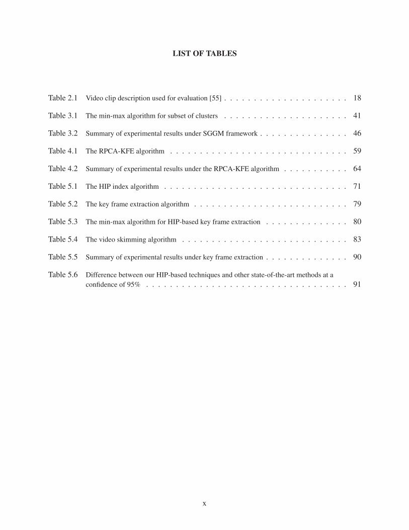
LIST OF TABLES . . . . . . . . . . . . . . . . . . . . . . . . . . . . . . . . . . . . . . . x

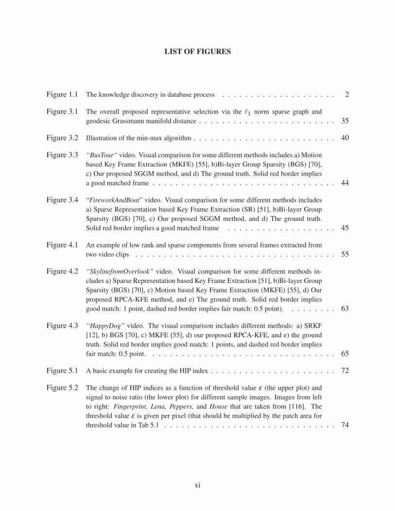
LIST OF FIGURES . . . . . . . . . . . . . . . . . . . . . . . . . . . . . . . . . . . . . . . xi

CHAPTER 1 INTRODUCTION . . . . . . . . . . . . . . . . . . . . . . . . . . . . . . . 1

1.1 Video Summarization from “Knowledge Discovery in Database” Point of View . . 1

1.2 Sparse Models for Data Mining . . . . . . . . . . . . . . . . . . . . . . . . . . . . 5

1.2.1 Sparse Models in Signal Processing . . . . . . . . . . . . . . . . . . . . . 5

1.2.2 Current Models for Data Mining . . . . . . . . . . . . . . . . . . . . . . . 6

1.2.3 Contributions: The Proposed Sparse Models for Data Mining Summa-

rization Task . . . . . . . . . . . . . . . . . . . . . . . . . . . . . . . . . 7

1.3 Representative Selection . . . . . . . . . . . . . . . . . . . . . . . . . . . . . . . 9

1.4 Video Summarization . . . . . . . . . . . . . . . . . . . . . . . . . . . . . . . . . 10

1.4.1 Current Video Summarization Challenges . . . . . . . . . . . . . . . . . . 11

1.5 Dissertation Organization . . . . . . . . . . . . . . . . . . . . . . . . . . . . . . . 13

CHAPTER 2 CONSUMER VIDEO SUMMARIZATION OVERVIEW . . . . . . . . . . 15

2.1 Introduction . . . . . . . . . . . . . . . . . . . . . . . . . . . . . . . . . . . . . . 15

2.1.1 Consumer Video Summarization Challenges . . . . . . . . . . . . . . . . . 16

2.1.2 Dataset and The Ground Truth . . . . . . . . . . . . . . . . . . . . . . . . 17

2.1.3 Evaluation . . . . . . . . . . . . . . . . . . . . . . . . . . . . . . . . . . . 18

2.2 Related Methods on Consumer Video Summarization . . . . . . . . . . . . . . . . 21

2.2.1 Motion-based Key Frame Extraction . . . . . . . . . . . . . . . . . . . . 21

2.2.2 Bi-layer Group Sparsity based Key Frame Extraction . . . . . . . . . . . . 23

2.2.3 Dictionary Selection based Video Summarization . . . . . . . . . . . . . . 24

2.2.4 Sparse Representation based Video Summarization . . . . . . . . . . . . . 25

2.2.5 Image Epitome based Key Frame Extraction . . . . . . . . . . . . . . . . . 25

2.3 Conclusions . . . . . . . . . . . . . . . . . . . . . . . . . . . . . . . . . . . . . . 28

CHAPTER 3 REPRESENTATIVE SELECTION FOR CONSUMER VIDEOS VIA SPARSE

GRAPH AND GEODESIC GRASSMANN MANIFOLD DISTANCE . . . 30

3.1 Motivation . . . . . . . . . . . . . . . . . . . . . . . . . . . . . . . . . . . . . . . 30

3.2 Related Works and Contributions . . . . . . . . . . . . . . . . . . . . . . . . . . . 31

3.2.1 Normalized Cut Method . . . . . . . . . . . . . . . . . . . . . . . . . . . 31

3.2.2 Clustering-based Key Frame Extraction Techniques . . . . . . . . . . . . . 32

3.2.3 Contributions . . . . . . . . . . . . . . . . . . . . . . . . . . . . . . . . . 33

3.3 Representative Selection via Sparse Graph and Geodesic Grassmann Manifold

Distance . . . . . . . . . . . . . . . . . . . . . . . . . . . . . . . . . . . . . . . . 34

3.3.1 The �1 Sparse Graph for Data Clustering . . . . . . . . . . . . . . . . . . . 35

3.3.2 The Selection of an Optimal Subset of Clusters . . . . . . . . . . . . . . . 38

3.3.2.1 Geodesic Grassmann Manifold Distance . . . . . . . . . . . . . 38

vii

3.3.2.2 The Min-max Algorithm . . . . . . . . . . . . . . . . . . . . . . 40

3.3.3 Principal Component Centrality for Representative Selection . . . . . . . . 41

3.4 Experimental Results on Video Summarization . . . . . . . . . . . . . . . . . . . 43

3.5 Conclusions . . . . . . . . . . . . . . . . . . . . . . . . . . . . . . . . . . . . . . 47

CHAPTER 4 ROBUST PRINCIPAL COMPONENT ANALYSIS BASED VIDEO SUM-

MARIZATION . . . . . . . . . . . . . . . . . . . . . . . . . . . . . . . . . 48

4.1 Robust Principal Component Analysis . . . . . . . . . . . . . . . . . . . . . . . . 48

4.2 Related Works and Contributions . . . . . . . . . . . . . . . . . . . . . . . . . . . 51

4.2.1 Related Works . . . . . . . . . . . . . . . . . . . . . . . . . . . . . . . . . 51

4.2.2 Contributions . . . . . . . . . . . . . . . . . . . . . . . . . . . . . . . . . 52

4.2.3 Notations . . . . . . . . . . . . . . . . . . . . . . . . . . . . . . . . . . . 53

4.3 Robust Principal Component Analysis based Key Frame Extraction . . . . . . . . . 54

4.3.1 Problem Formulation . . . . . . . . . . . . . . . . . . . . . . . . . . . . . 54

4.3.2 Proposed Solution . . . . . . . . . . . . . . . . . . . . . . . . . . . . . . . 57

4.3.2.1 Iterative Algorithm for Non-convex Optimization Problem . . . . 57

4.3.2.2 RPCA-KFE with New Observations . . . . . . . . . . . . . . . 60

4.4 Experimental Results . . . . . . . . . . . . . . . . . . . . . . . . . . . . . . . . . 61

4.4.1 Parameter Selection . . . . . . . . . . . . . . . . . . . . . . . . . . . . . . 61

4.4.2 Evaluation . . . . . . . . . . . . . . . . . . . . . . . . . . . . . . . . . . . 62

4.4.3 Computational Complexity . . . . . . . . . . . . . . . . . . . . . . . . . . 66

4.5 Conclusions . . . . . . . . . . . . . . . . . . . . . . . . . . . . . . . . . . . . . . 66

CHAPTER 5 HETEROGENEITY IMAGE PATCH INDEX AND ITS APPLICATION

TO CONSUMER VIDEO SUMMARIZATION . . . . . . . . . . . . . . . . 67

5.1 Motivation . . . . . . . . . . . . . . . . . . . . . . . . . . . . . . . . . . . . . . . 67

5.2 Related Works and Contributions . . . . . . . . . . . . . . . . . . . . . . . . . . . 68

5.2.1 Related Works . . . . . . . . . . . . . . . . . . . . . . . . . . . . . . . . . 68

5.2.2 Contributions . . . . . . . . . . . . . . . . . . . . . . . . . . . . . . . . . 69

5.3 The Proposed Heterogeneity Image Patch Index . . . . . . . . . . . . . . . . . . . 70

5.3.1 Heterogeneity Image Patch Index . . . . . . . . . . . . . . . . . . . . . . . 73

5.3.2 Accumulative Patch Matching Image Dissimilarity . . . . . . . . . . . . . 76

5.4 Extracting Key Frame from Video Using Heterogeneity Image Patch Index . . . . . 78

5.4.1 Candidate Key Frame Extraction . . . . . . . . . . . . . . . . . . . . . . . 78

5.4.2 Selection of The Final Set of Key Frames . . . . . . . . . . . . . . . . . . 81

5.5 Dynamic Video Skimming Using Heterogeneity Image Patch Index . . . . . . . . . 82

5.5.1 Video Skimming Problem Statement . . . . . . . . . . . . . . . . . . . . . 82

5.5.2 HIP-based Video Distance . . . . . . . . . . . . . . . . . . . . . . . . . . 83

5.5.3 Optimal Solution . . . . . . . . . . . . . . . . . . . . . . . . . . . . . . . 86

5.6 Experimental Results . . . . . . . . . . . . . . . . . . . . . . . . . . . . . . . . . 87

5.6.1 Key Frame Extraction . . . . . . . . . . . . . . . . . . . . . . . . . . . . . 87

5.6.1.1 Parameter Selection . . . . . . . . . . . . . . . . . . . . . . . . 87

5.6.1.2 Quantitative Comparison . . . . . . . . . . . . . . . . . . . . . . 89

5.6.1.3 Statistical Test . . . . . . . . . . . . . . . . . . . . . . . . . . . 90

5.6.1.4 Visual Comparison . . . . . . . . . . . . . . . . . . . . . . . . . 90

viii

5.6.1.5 Computational Complexity . . . . . . . . . . . . . . . . . . . . 94

5.6.2 Video Skimming . . . . . . . . . . . . . . . . . . . . . . . . . . . . . . . 94

5.6.2.1 Parameter Selection . . . . . . . . . . . . . . . . . . . . . . . . 94

5.6.2.2 Evaluation . . . . . . . . . . . . . . . . . . . . . . . . . . . . . 95

5.7 Conclusions . . . . . . . . . . . . . . . . . . . . . . . . . . . . . . . . . . . . . . 98

CHAPTER 6 CONCLUSIONS . . . . . . . . . . . . . . . . . . . . . . . . . . . . . . . . 99

APPENDICES . . . . . . . . . . . . . . . . . . . . . . . . . . . . . . . . . . . . . . . . . 101

Appendix A Proof of Lemma 1 and 2 . . . . . . . . . . . . . . . . . . . . . . . . . 102

Appendix B Proof of Theorem 5.1. . . . . . . . . . . . . . . . . . . . . . . . . . . 104

Appendix C Publications . . . . . . . . . . . . . . . . . . . . . . . . . . . . . . . 106

BIBLIOGRAPHY . . . . . . . . . . . . . . . . . . . . . . . . . . . . . . . . . . . . . . . . 108

ix

LIST OF TABLES

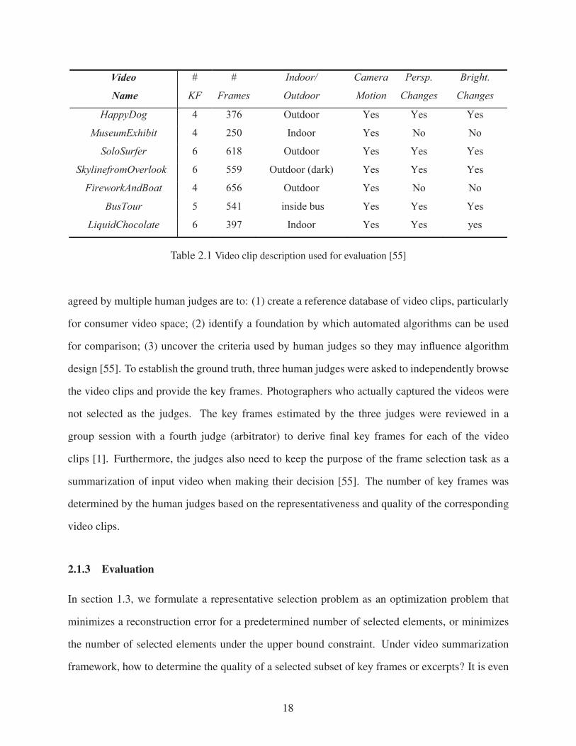
Table 2.1 Video clip description used for evaluation [55] . . . . . . . . . . . . . . . . . . . . . 18

Table 3.1 The min-max algorithm for subset of clusters . . . . . . . . . . . . . . . . . . . . . 41

Table 3.2 Summary of experimental results under SGGM framework . . . . . . . . . . . . . . . 46

Table 4.1 The RPCA-KFE algorithm . . . . . . . . . . . . . . . . . . . . . . . . . . . . . . 59

Table 4.2 Summary of experimental results under the RPCA-KFE algorithm . . . . . . . . . . . 64

Table 5.1 The HIP index algorithm . . . . . . . . . . . . . . . . . . . . . . . . . . . . . . . 71

Table 5.2 The key frame extraction algorithm . . . . . . . . . . . . . . . . . . . . . . . . . . 79

Table 5.3 The min-max algorithm for HIP-based key frame extraction . . . . . . . . . . . . . . 80

Table 5.4 The video skimming algorithm . . . . . . . . . . . . . . . . . . . . . . . . . . . . 83

Table 5.5 Summary of experimental results under key frame extraction . . . . . . . . . . . . . . 90

Table 5.6 Difference between our HIP-based techniques and other state-of-the-art methods at a

confidence of 95% . . . . . . . . . . . . . . . . . . . . . . . . . . . . . . . . . . 91

x

LIST OF FIGURES

Figure 1.1 The knowledge discovery in database process . . . . . . . . . . . . . . . . . . . . 2

Figure 3.1 The overall proposed representative selection via the �1 norm sparse graph and

geodesic Grassmann manifold distance . . . . . . . . . . . . . . . . . . . . . . . . 35

Figure 3.2 Illustration of the min-max algorithm . . . . . . . . . . . . . . . . . . . . . . . . . 40

Figure 3.3 “BusTour“ video. Visual comparison for some different methods includes a) Motion

based Key Frame Extraction (MKFE) [55], b)Bi-layer Group Sparsity (BGS) [70],

c) Our proposed SGGM method, and d) The ground truth. Solid red border implies

a good matched frame . . . . . . . . . . . . . . . . . . . . . . . . . . . . . . . . 44

Figure 3.4 “FireworkAndBoat” video. Visual comparison for some different methods includes

a) Sparse Representation based Key Frame Extraction (SR) [51], b)Bi-layer Group

Sparsity (BGS) [70], c) Our proposed SGGM method, and d) The ground truth.

Solid red border implies a good matched frame . . . . . . . . . . . . . . . . . . . 45

Figure 4.1 An example of low rank and sparse components from several frames extracted from

two video clips . . . . . . . . . . . . . . . . . . . . . . . . . . . . . . . . . . . 55

Figure 4.2 “SkylinefromOverlook” video. Visual comparison for some different methods in-

cludes a) Sparse Representation based Key Frame Extraction [51], b)Bi-layer Group

Sparsity (BGS) [70], c) Motion based Key Frame Extraction (MKFE) [55], d) Our

proposed RPCA-KFE method, and e) The ground truth. Solid red border implies

good match: 1 point, dashed red border implies fair match: 0.5 point). . . . . . . . . 63

Figure 4.3 “HappyDog” video. The visual comparison includes different methods: a) SRKF

[12], b) BGS [70], c) MKFE [55], d) our proposed RPCA-KFE, and e) the ground

truth. Solid red border implies good match: 1 points, and dashed red border implies

fair match: 0.5 point. . . . . . . . . . . . . . . . . . . . . . . . . . . . . . . . . 65

Figure 5.1 A basic example for creating the HIP index . . . . . . . . . . . . . . . . . . . . . . 72

Figure 5.2 The change of HIP indices as a function of threshold value ε (the upper plot) and

signal to noise ratio (the lower plot) for different sample images. Images from left

to right: Fingerprint, Lena, Peppers, and House that are taken from [116]. The

threshold value ε is given per pixel (that should be multiplied by the patch area for

threshold value in Tab 5.1 . . . . . . . . . . . . . . . . . . . . . . . . . . . . . . 74

xi

Figure 5.3 “LiquidChocolate”video. An example for selecting a set of candidate key frames.

The ground truth contains 6 key frames that are shown on the HIP curve with the red

stars (the first key frame is hidden by the third candidate key frame). The algorithm

selects 10 candidate key frames that are shown with the green circles, frame indices

4 11 51 106 181 214 269 312 375 390. The visual display of candidate key frames

and key frames from the ground truth are shown in Figure 5.6 . . . . . . . . . . . . . 79

Figure 5.4 Illustration of the set αr from Theorem 1. ht1−1 and h1+t2(points in red color) are

the ending of the previous selected segment and the beginning of the next selected

segment from a skimmed video S. The algorithm scans every possible option of

mapping HIP indices from the remaining segment into that two points (based on

parameter r). . . . . . . . . . . . . . . . . . . . . . . . . . . . . . . . . . . . . 85

Figure 5.5 “HappyDog” video HIP curve for different patch sizes from four to eight. The HIP

index of a single frame tends to increase. However, the overall HIP curve does not

change much in the shape form (at least in subjective evaluation). . . . . . . . . . . 89

Figure 5.6 “LiquidChocolate” video. The set of candidate key frames. Frames in red border

are selected as final key frames. . . . . . . . . . . . . . . . . . . . . . . . . . . . 91

Figure 5.7 “LiquidChocolate” video. The visual comparison includes different methods: a)

SRKF [12], b) BGS [70], c) MKFE [55], d) our proposed RPCA-KFE, and e) the

ground truth. Solid red border implies good match: 1 points, and dashed red border

implies fair match: 0.5 point. . . . . . . . . . . . . . . . . . . . . . . . . . . . . 92

Figure 5.8 “MuseumExhibit” video. The visual comparison includes different methods: a)

BGS [70], b) MKFE [55], c) HIP-based approach - 8 candidate key frames and

the selected ones in solid border, and d) the ground truth. Solid border implies good

match: 1 points. . . . . . . . . . . . . . . . . . . . . . . . . . . . . . . . . . . 93

Figure 5.9 An example of Turkey-style boxplot (Notched boxplot) . . . . . . . . . . . . . . . . 96

Figure 5.10 Comparison of video summary using different methods . . . . . . . . . . . . . . . . 97

xii

CHAPTER 1

INTRODUCTION

Developing new approaches for video summarization1 has been the primary motivation for this

dissertation. The application area of video summarization is becoming increasingly critical due

to the massive amount of video data been generated and communicated over the global Internet.

Video summarization is a process for creating an abstract of an input video so that users can

quickly review the abstract video, without the need of viewing the original full video content.

More importantly, video summarization can be considered as a data-mining problem with video

being the data and extracting a video summarization as the process of mining. In particular, it

belongs to the general problem of extracting valuable knowledge or desired information from a

massive amount of data. This area is commonly known as Knowledge Discovery in Database

(KDD). Consequently, in this chapter, we briefly introduce video summarization from the point of

view of the general KDD problem area.

This chapter also outlines current challenges in video summarization and our contributions in

solving these challenges. The final section provides a summary of the overall dissertation outline.

1.1 Video Summarization from “Knowledge Discovery in Database” Pointof View

KDD is an attempt to solve the problem of information overload. It is well-known that the digital

age has generated fast-growing, tremendous amount of data that is far beyond the human ability

to extract desired information or knowledge without powerful tools. For example, it is estimated

that the global digital content will reach 40 Zettabytes (trillion gigabytes) of data by 2020, which

is about 57 times the number of all the grains of sand on all the beaches on earth, according to

1Video summarization can also be viewed as a representative selection process. Under representative

selection, a small number of data points are selected to represent the whole (usually massive) data set. We

will use both terms, video summarization and representative selection, throughout this dissertation.

1

Data Transformed Data (a) (b) Patterns (c) Knowledge

- Selection of data - Preprocessing - Transformation of

data into appropriate forms

(a)

Data Mining

- Model representation - Model evaluation - Search

(b)

- Interpretation - Evaluation - Presentation

(c)

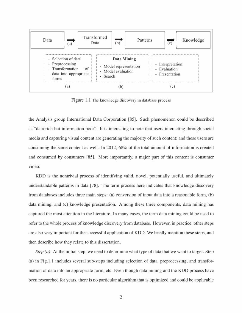
Figure 1.1 The knowledge discovery in database process

the Analysis group International Data Corporation [85]. Such phenomenon could be described

as “data rich but information poor”. It is interesting to note that users interacting through social

media and capturing visual content are generating the majority of such content; and these users are

consuming the same content as well. In 2012, 68% of the total amount of information is created

and consumed by consumers [85]. More importantly, a major part of this content is consumer

video.

KDD is the nontrivial process of identifying valid, novel, potentially useful, and ultimately

understandable patterns in data [78]. The term process here indicates that knowledge discovery

from databases includes three main steps: (a) conversion of input data into a reasonable form, (b)

data mining, and (c) knowledge presentation. Among these three components, data mining has

captured the most attention in the literature. In many cases, the term data mining could be used to

refer to the whole process of knowledge discovery from database. However, in practice, other steps

are also very important for the successful application of KDD. We briefly mention these steps, and

then describe how they relate to this dissertation.

Step (a): At the initial step, we need to determine what type of data that we want to target. Step

(a) in Fig.1.1 includes several sub-steps including selection of data, preprocessing, and transfor-

mation of data into an appropriate form, etc. Even though data mining and the KDD process have

been researched for years, there is no particular algorithm that is optimized and could be applicable

2

broadly to every type of data for the best result. Many types of data have been considered in the

past, which includes generic database data (a set of interrelated data and a collection of software

programs to manage and access the data), transactional data, graph or networked data, text data,

multimedia data, etc. In our work, we focus on video dataset, particularly consumer video, which

is generated unprofessionally by individuals. We will discuss in more detail consumer video and

related video summarization techniques in chapter 2. The preprocessing step may include cleaning

data (removing noise and inconsistent data, deciding appropriate model for the data, handling miss-

ing data points, etc.). The data transformation sub-step converts the raw data into appropriate form

for the mining algorithm. For example, it may only preserve essential or important information

related to the output desired knowledge that the system prefer to extract.

Step (b): Data mining could be considered as the heart of the KDD process in which an auto-

mated method is applied to extract desired patterns. These patterns must be essential to obtain the

desired knowledge. Data mining includes mainly two high-level primary goals: prediction (using

given data to predict unknown other variables of interest) and description (finding patterns that

describe the data in a human interpretable way). These goals are usually obtained via one of six

common classes of data mining tasks [78]:

• Summarization 2

• Clustering

• Dependency modeling

• Classification

• Regression

• Change and deviation detection

Summarization is one of the key data mining tasks that attempt to find a compact represen-

tation of dataset. Different dataset may require using different techniques for summarization, for

2We highlight these three tasks: summarization, clustering, and dependency modeling since our work

will focus more about them.

3

example text summarization, summarization of multiple documents, summarization of large col-

lection of photographs [80-81]. Our work focus on summarization techniques for video datasets,

and hence are commonly known as video summarization or video abstraction, which refers to an

automatic technique to select the most informative sequences of still or moving pictures that help

users quickly review the whole video content in a constrained amount of time.

Beside summarization techniques, clustering and dependency modeling are other data mining

tasks that are often used. These tasks are related and inter-dependent to each other. Clustering

techniques target to find groups of objects such that the objects in a group are similar (or related)

to one another and different from (or unrelated to) the objects in other groups. Centroids from

data’s clusters could be further exploited to summarize the whole dataset such as text document,

multimedia dataset, etc. That explains why clustering techniques are widely used for summariza-

tion. On the other hand, dependency modeling consists of finding a model that describes significant

dependencies among variables/data points [79]. Successful modeling of dependency among vari-

ables or data points is a crucial step to create a graph dependency among data points, and hence

leads to better clustering results. Nowadays, graph and network data play a very important role

in data mining. Before moving to sparse model representation for data mining, we note that even

though clustering based techniques represent an important research direction in creating a summa-

rization result, they are only effective in domains where the features are continuous or asymmetric

binary, and hence cluster centroids are a meaningful description of clusters [82]. The result may

not be good for summarization of a given data that has a more complicated or undefined structure.

Step (c): The evaluation of extracted pattern/feature interestingness is important for the dis-

covery of desired knowledge. The methods for evaluation depend on what kind of patterns being

extracted, and what kind of knowledge is desired to be extracted from the data-mining process. Un-

der the video summarization framework, the target is to find a compact representation of dataset

that summarizes the whole video content. We would discuss about the ground truth for video sum-

marization, and evaluation of experimental result latter. In the next section, we formulate the rep-

resentative selection technique, and consider the overall current video summarization challenges,

4

some of our main contributions in this topic.

Since data mining is the most important part of the KDD process, and since our contributions

are currently focused on sparse models for solving summarization tasks of data mining, we spend

the next section discussing these models.

1.2 Sparse Models for Data Mining

Various traditional models have been considered for data mining algorithms, which include deci-

sion trees, probabilistic graphical dependency models, Bayesian classifiers, rule-based classifiers,

relational attribute models, neural networks, etc. A decision tree model is a tree-like graph struc-

ture, which is commonly used in decision analysis and classification tasks. The model has been

extensively researched and developed over decades due to its ability to break a global complex

decision region into a union of simpler local regions. One of the main issues associated with

such models is that errors could be accumulated from level to level in a large tree. Moreover, a

decision tree model has a tendency to be biased in favor of variables with more attributes [86].

Probabilistic graphical dependency models combine basic tools from graph theory and probability

theory. The models possess many useful properties: visualize the structure of the probabilistic

model, transfer complex computations during inference and learning processes into graphical ma-

nipulations. However, modeling a huge amount of data using probabilistic graphical dependency

models is quite challenging. Overall, most of these traditional data mining models being exploited

extensively for one or several particular data mining tasks (mostly focus on pattern recognition,

classification, and regression).

1.2.1 Sparse Models in Signal Processing

The recent explosion of massive amounts of high dimensional data in various fields of studies,

such as science, engineering, and society, has demanded better models for data mining. Working

directly in the high dimensional space generally involves much more complex algorithms. The

5

signal processing community alleviates the curve of dimension and scale based on a reasonable

assumption that such data has intrinsically low dimensionality. For example, a set of high di-

mensional data points could be modeled as a low dimensional subspace, or more generally as a

union of multiple low dimensional subspaces. This modeling leads to the challenging problem of

subspace clustering [16] [41-42], which aims at clustering data points into multiple linear/affine

subspaces. Considering a different low dimensional model, manifolds with a few degrees of free-

dom have been used successfully for the class of non-parametric signals, e.g. image of human

faces and handwritten digits [2]. Numerous methods aiming at dimensionality reduction (em-

bedding) have been developed that could be classified into two main categories. On one hand,

several well-known (linear and non-linear dimensionality reduction) methods, for example Prin-

cipal Component Analysis (PCA), multidimensional scaling, Isomap, classical multidimensional

scaling, multilayer auto-encoders [3][43], belong to the first category that mainly focus on preserv-

ing some particular desired properties. The algorithms in the other category aim at reconstructing

the original dataset from the lower dimensional space measurement, such as compressive sensing,

sparse representation and related random linear projections on a low dimensional manifold [4].

1.2.2 Current Models for Data Mining

Although sparse/low dimensional models have been exploited widely in signal processing, the

applications of sparse models for solving data mining problems are limited. As pointed out in a

recent data mining review [87], traditional models (decision tree, neural network, support vector

machine, etc.) are still the main data mining techniques. Recently, some works using sparsity

as a constraint have been pursued (mostly on classification task, e.g. texture, hand written digits,

face/hyperspectral image classification [88-91], and some few works on regression, clustering,

summarization [7][16][51]). The general idea is to use sparse representation coefficients of an

input signal as extracted feature vector for further processing (in other words, y = Ax, in which y

is the input signal, A and x are the dictionary and sparse representation coefficients, respectively).

This includes the development of a variety of techniques aimed at building a good dictionary A for

6

a better feature extraction method or handling well the obtained sparse representation coefficients

for a better result.

Even though several works [92] claimed that sparsity is helpful for some data mining tasks (es-

pecially on classification), the claims are only supported by few experiments in a supervised/semi-

supervised context. It leads to a concern that whether sparsity constrain is really helpful? A recent

work [93] evaluated the importance of sparsity in image classification by performing an extensive

empirical evaluation and adopting the recognition rate as a criterion. The experiments indicated

that enforcing sparsity constraints actually does not improve recognition performance.

Our work is focused on summarization task for video. We also see that even sparse representa-

tion based summarization has been exploited recently in some few works [7][51][67], the obtained

results are still not as good as we expected. There are two main problems with using sparse models

based on these recent efforts:

• All these works [7][51][67] were developed based on considering the input dataset, or fea-

tures extracted from it, as the dictionary itself (named as the self-expressiveness property

[16]). Consequently, for such techniques, the quality of summarization depends on how a

proposed algorithm could handle well the sparse representation coefficients. However, it

requires a deeper analysis than simply relying on the sparse coefficients to create a viable

video summarization.

• The sparse model for summarization until now is quite simple and straightforward. For a

better result, we need better sparse models.

1.2.3 Contributions: The Proposed Sparse Models for Data Mining Summarization Task

In our work, we are pursuing three different sparse models for video summarization:

1. Sparse representation of video frames

We exploit the self-expressiveness property to create �1 norm sparse graph, which is appli-

cable for huge high dimensional dataset. A spectral clustering algorithm has been applied

7

into the sparse graph for the selection of a set of clusters. Our work analyzes each cluster as

one point in a Grassmann manifold and then selects an optimal set of clusters. The final rep-

resentative is evaluated using a graph centrality technique for the sub-graph corresponding

with each selected cluster. Related publication is Ref. [17]

2. Sparse and low rank model for video frames

A novel key frame extraction framework based on Robust Principal Component Analysis is

proposed to automatically select a set of maximally informative frames from an input video.

The framework is developed from a novel perspective of low rank and sparse components,

in which the low rank component of a video frame reveals the relationship of that frame

to the whole video sequence, and the sparse component indicates the distinct information

of particular frames. A set of key frames are identified by solving an �1 norm based non-

convex optimization problem where the solution minimizes the reconstruction errors of the

whole dataset for a given set of selected key frames and maximizes the sum of distinct

information. Moreover, the algorithm provides a mechanism for adapting new observations,

and consequently, updating new set of key frames. Related publication is Ref.[5]

3. Sparse/redundant representation for a single video frame

We propose a new patch-based image/video analysis approach. Using the new model, we

create a new feature that we refer to as the heterogeneity image patch (HIP) index of an image

or a video frame. The HIP index, which is evaluated using patch-based image/video analysis,

provides a measure for the level of heterogeneity (and hence the amount of redundancy) that

exists among patches of an image/video frame. We apply the proposed HIP framework

to solve both of the video summarization problem areas: key frame extraction and video

skimming. Related publications are Ref. [1][15]

8

1.3 Representative Selection

A more general problem than key frame extraction is representative selection. We briefly review

this problem area before moving back to the video summarization topic. The problem of finding

a subset of important data points, also known as representatives or exemplars, which have the

ability to efficiently describe the whole input dataset (at least to some extent) is emerging as a

key approach for dealing with the massive growth of data. The problem has an important role in

scientific data analysis with many applications in machine learning, computer vision, information

retrieval and clustering [5-19][94].

Given a set of data points X = {x1,x2, . . . ,xn}, we want to find a subset of k < n data points

from X , denoted by Xs ={

xi1 ,xi2 , . . . ,xik

}⊆ X , which minimizes (or provides a suitably small

value for) the ‘difference’ of the reconstruction error D(Xs,X) between the two sets Xs and X .

Depending on a particular objective for the selected subset, the reconstruction error function could

be formulated differently. In general, the optimization problem could be organized in two different

forms:

1. For a predetermined number of selected elements k, searching for a subset Xs ⊂ X that does

not contain more than k elements and minimize D(Xs,X):

Xs = arg minXs⊂X ,|Xs|≤k

D(Xs,X) (1.1)

2. Minimizing the number of selected elements under the upper bound constraint of D(Xs,X):

Xs = arg minXs⊆X ,D(Xs,X)≤δ

|Xs| (1.2)

Most of the techniques on representative selection belong to one of these two categories. Some

others [45-46] produce the set of representative points progressively. Under such scenario, the al-

gorithm stops if the number of selected elements reaches a predetermined value or if the difference

reaches the upper bound value. The representative selection problem can be considered from sev-

eral different perspectives or applications, under some other names: column subset selection [8]

9

[10], feature subset selection [9][14][11], video summarization [15-46]. Column subset selection

considers the problem of selecting a subset of few columns from a huge matrix with particular

constrains such as minimizing the reconstruction error or achieving favorable spectral properties

(rank revealing QR, non-negative matrix, etc.) [8][47][49]. Feature subset selection considers se-

lecting a subset of (m) features from a much larger set of (n) features or measurements to optimize

the value of criterion over all subsets of the size (m) [9]. The criterion may vary depending on the

application. Under the classification problem, the optimal subset of features is the one that maxi-

mizes the accuracy of the classifier while minimizing the number of selected features [14]. Besides

quantitative evaluation for the subset of selected elements, video summarization, on the other hand,

provides a tool for selecting the most informative sequences of still or moving pictures/frames that

help users quickly glance through the whole video clip in a constrained amount of time.

1.4 Video Summarization

Under video circumstance, representative selection problem is also known as video summariza-

tion/abstraction. Video summarization provides tools for selecting the most informative sequences

of still or moving pictures that help users quickly glance through the whole video clip within a con-

strained amount of time. These video summarization methods are getting more important due to

the fast growing of digital video dataset, the popularity of personal digital equivalents, and sharing

channels via social network. Generally speaking, there are two categories of video summarization

[15]:

• Key frames or static story board: a collection of salient images or key frames extracted from

video.

• Dynamic video skimming or a preview sequence: a collection of essential video segments

or excerpts (key video excerpts) and the corresponding audio, which are joined together to

become a much shorter version of the original video content.

10

A set of key frames has many important roles in intelligent video management systems such as

video retrieval and browsing, navigation, indexing, and prints from video. It helps to reduce com-

putational complexity since the system could process a smaller set of representative frames or

excerpts instead of the whole video sequence. Key frames capture both the temporal and spatial

information of the video sequence, and hence, they also enable rapid viewing functionality [5][15]

[21]. Conventional key frame extraction approaches can be loosely divided into two groups: (i)

shot-based and (ii) segment-based. In shot-based key frame extraction, the shots of the original

video are first detected, and then one or more key frames are extracted from each shot [18-19]

[50]. In segment-based key frame extraction approaches, a video is segmented into higher-level

video components, where each segment or component could be a scene, an event, a set of one or

more shots, or even the entire video sequence. Representative frame(s) from each segment are then

selected as the key frames [1][51].

The second type of video summarization, dynamic video skimming, contains both audio and

visual motion elements. Therefore, it is typically more appealing for users than viewing a series

of still key frames only. Video skimming, however, is a relatively new research area and normally

requires high-level semantic analysis [15]. Several approaches for skimming range from basic

extension of key frame extraction (as an initial step and then considering each frame as the middle

frame of a fixed-length excerpt) to more advanced methods such as integrating motion metadata

to reconstruct an excerpt [22]. Various features have been extensively used for video skimming

generation; these features include text, audio, camera motion, and other visual features such as

color histogram, edge, and texture [32-33]–[52].

1.4.1 Current Video Summarization Challenges

There are some challenging problems associated with prior representative selection techniques in

video:

(i) A majority of the proposed video summarization techniques is domain-dependent. They ex-

ploit specific properties of the input dataset to select a subset of representative data points.

11

For example, prior efforts exploit specific properties of a video clip in a specific domain (e.g.

news, sport, documentaries, and entertainment videos) to generate a video summarization

[25-29][39]. These types of videos are structured videos, which are normally of good qual-

ity, relatively high resolution, taken by stable cameras and with low background noise [24].

However, until now, there is a very little focus on solving the challenges associated with

consumer (or personal generated) videos. Consumer videos have no predefined structure,

contain diverse content, and may suffer from low quality due to factors such as poor lighting

and camera shake. Not to mention that the amount of consumer videos has been increased

dramatically due to the rapid development of personal smart devices as well as the popularity

of social networks and sharing channels.

(ii) Most of the prior video summarization approaches [18-19][21-23] work directly with the

input high dimensional dataset, without considering the underlying low rank structure of the

original video dataset. Some other approaches [23] focus on the low rank component only,

ignoring the essential information from the other components.

(iii) Prior efforts focused on the first form of video summarization, the key frame extraction prob-

lem. Video skimming is relatively new research area and normally requires high-level se-

mantic analysis [21]. Several approaches for skimming range from basic extension of key

frame extraction (as an initial step and then considering each frame as the middle frame of a

fixed-length excerpt) to more advanced methods using various features (such as text, audio,

camera motion, and other visual image features) to reconstruct an excerpt [22]. There is a

lacking of an overall feature dealing with video skimming, especially for consumer videos.

(iv) Although some video summarization techniques produce acceptable quality, they endure very

high computational complexity. Various pre-sampling techniques have been proposed to re-

duce the computational cost of these algorithms. However, using pre-sampling techniques

cannot guarantee selecting the best set of key frames or video-skimming summarization.

(v) Clustering-based techniques have an important role in dealing with summarization tasks

12

where similar frames (based on particular type of features, such as color histogram, lumi-

nance, etc.) are clustered into groups, and then one/several frames are selected from each

group. However, as we mentioned in section 1.1, clustering-based results depend heavily on

data structures, which are not typical for various types of videos.

1.5 Dissertation Organization

In this dissertation, we develop advanced video-summarization frameworks that address the chal-

lenges outlined above. In particular, we pursue three different frameworks that exploit different

aspects of signal sparsification/redundancy.

Chapter 2 reviews some related consumer video summarization methods. These methods will

be used for comparison in our simulation-result section. The main challenges that are specific to

consumer videos, along with the evaluation process and the ground truth are also presented in this

chapter.

Chapter 3 develops video summarization based on a sparse model of video frames. We propose

a novel representative selection framework via creating �1 norm sparse graph for a given dataset.

A given big dataset is partitioned recursively into clusters using spectral clustering algorithm on

the sparse graph. We consider each cluster as one point in a Grassmann manifold, and measure

the geodesic distance among these points. The distances are further analyzed using a min-max

algorithm to extract an optimal set of clusters. We have developed this min-max algorithm in [1].

Finally, by considering a sparse sub-graph of each selected cluster, we detect a representative using

principal component centrality.

Chapter 4 introduces a sparse and low rank model for video frames. Under the proposed

model, input video frames are grouped into a matrix that could be decomposed into sum of low

rank and sparse components using Robust Principal Component Analysis (Robust PCA). Under

the proposed framework, a different perspective of low rank and sparse components decomposed

using Robust PCA has been developed. Furthermore, we present a novel iterative algorithm to

solve the non-convex optimization problem obtained from the combination of low rank and sparse

13

components. The algorithm adapts to new observations, and it updates the selected set of key

frames.

Chapter 5 proposes a novel image/video frame index, named as Heterogeneity Image Patch

(HIP) index, which provides a measure for the level of heterogeneity (and hence the amount of

redundancy) among patches of an image/video frame. We exploit the HIP index in solving two

categories of video summarization applications: key frame extraction and dynamic video skim-

ming.

Finally, Chapter 6 outlines concluding remarks, future works, and the Appendix contains proofs

for several lemmas and theorem from Chapter 4 and 5.

14

CHAPTER 2

CONSUMER VIDEO SUMMARIZATION OVERVIEW

2.1 Introduction

Extracting key frames or key excerpts from video has important roles in many applications, such

as to facilitate browsing a large video collection, to support automatic video retrieval, video search,

video compression, etc. [44][53]. In addition, a set of key frames and video skimming in general

help users to quickly access important sections (in semantic meaning) in a video sequence, and

hence enable rapid viewing. As a result, the topic has been researched for long time. However,

current literature on video summarization has focused mainly upon certain types of videos that

conform to well-defined structures and characteristics, and hence facilitate key frame extraction

problem for such videos [55]. Some of these typical types of videos include sports [60-62], news

[63-65], TV drama, movie dialog [39][56-59], documentary videos, or medical video etc. Sev-

eral typical characteristics in each type of videos will be exploited to solve video summarization

problem. For example, in news video summarization, some techniques [65] focus on analyzing the

audio channel to filter out commercial advertisings that are normally appeared in between news

program. In case of sport video summarization, some methods exploit score caption techniques

[60], [66] due to the significance of an event is related to the score. The environment for sport

video is also quite clear, since there is normally two opposing teams plus the reference(s) in dis-

tinct colorful uniforms. In movie and drama summarization, two factors (actions and dialogues)

are considered as the most important parts of a video. Several techniques based on analyzing av-

erage pitch frequency and temporal variation of speech signal intensity levels to detect emotional

dialogues. On the other hand, detection of rapid movements could be based on estimating spatio-

temporal dynamic visual activities. In some cases, an action event is simply defined by the lack of

repletion of similar shots.

15

2.1.1 Consumer Video Summarization Challenges

The prior techniques on well-defined structured/professional videos cannot be applied directly into

consumer (or personal generated) videos which are acquired from personal digital cameras. On the

other hand, that type of videos is increasing rapidly due to the popularity of equipment and sharing

channels. So far, there is a little work that targets on consumer-quality videos for the following

reasons:

(i) There is no particular information from background, themes, etc. that could be assumed in

personal-generated videos. Even on the themed consumer videos such as wedding, birthday

and party, there is no similar level of structure or content. Lacking specific domain knowledge

is one of the main challenges on consumer video summarization.

(ii) The mixed sound track coming from multiple sound sources, along with severe noise. As

a result, the techniques based on pitch frequency and temporal variation of speech signal

intensity cannot be employed. There is no sense to identify semantically meaningful audio

segments, for instance nouns, exited or normal speech, etc., and based on that to determine

key frames.

(iii) There are no fixed features (such as subtitles, text captions, or score captions) that could be

exploited for further information to evaluate the importance of frames or segments.

(iv) Consumer videos typically have one long shot under possibly low quality due to various

factors such as camera shake, poor lighting/uneven illumination, clutter, and combination of

motions from both objects and the camera. As a result, the traditional shot-based or segment-

based approaches do not perform well under that circumstance.

(v) Finally, it is also challenging to assess the quality of selected key frames in terms of user’s

satisfaction. How to evaluate a good set of selected key frames? Is there any criteria that

human used for selecting key frames? In addition, there is a lack of reference database of

video clips that is reasonably representative of consumer video space.

16

For many of these reasons, consumer-video summarization is still being a very challenging

topic. One of the very first efforts dealing with consumer videos has been proposed by Lue et al.

[55]. Under the proposed framework, the camera operator’s general intents (e.g. pan, zoom, etc.)

have been considered as main factors to segment input videos into homogeneous parts. More im-

portantly, the authors target to solve the last problem of consumer videos (as we mentioned above)

by conduct ground truth collection of key frames from video clips taken by digital cameras. Then,

several other methods [5][15-17][24][51][67] have been proposed after [55] in solving consumer

video summarizations. Here, we first discuss about dataset, the ground truth for consumer videos,

and evaluation of consumer video summarization algorithm. Then, we will discuss further these

above methods.

2.1.2 Dataset and The Ground Truth

Dataset: In a recent effort, Luo et al. [55] has been focused on study the ground truth for con-

sumer videos taken by digital cameras. In particular, they considered short clips captured using

KodakEasyShare C360 and V550 zoom digital cameras, with a VGA resolution (frame size of

640×480). Our experiments are performed on a set of seven clips for evaluation and comparison

with other methods. The detail description of these clips is provided in Table 2.1. They vary in

duration from 250 frames to 656 frames, approximately 450 frames per clip on average. The av-

erage number of key frames is five per clip, depends on the number of key frames in the ground

truth. We do not perform any pre-sampling technique as in previous approaches, such as at a pre-

determine rate [32] or by selecting only I-frames [33]. Therefore, it is rather straightforward to

extend our work for longer structured video clips (not consumer videos) in conjunction with sim-

ple sub-sampling (e.g. 15 minutes if a pre-sampling rate at one frame/sec is employed). However,

we focus on short consumer videos in our works.

The ground truth: Human selection process arguably produces the best evaluation of video

summarization problem. Having a subjective ground truth for consumer video summarization is

one of the most important steps in solving the problem. The goal of creating the ground truth

17

Video

Name

#

KF

#

Frames

Indoor/

Outdoor

Camera

Motion

Persp.

Changes

Bright.

Changes

HappyDog 4 376 Outdoor Yes Yes Yes

MuseumExhibit 4 250 Indoor Yes No No

SoloSurfer 6 618 Outdoor Yes Yes Yes

SkylinefromOverlook 6 559 Outdoor (dark) Yes Yes Yes

FireworkAndBoat 4 656 Outdoor Yes No No

BusTour 5 541 inside bus Yes Yes Yes

LiquidChocolate 6 397 Indoor Yes Yes yes

Table 2.1 Video clip description used for evaluation [55]

agreed by multiple human judges are to: (1) create a reference database of video clips, particularly

for consumer video space; (2) identify a foundation by which automated algorithms can be used

for comparison; (3) uncover the criteria used by human judges so they may influence algorithm

design [55]. To establish the ground truth, three human judges were asked to independently browse

the video clips and provide the key frames. Photographers who actually captured the videos were

not selected as the judges. The key frames estimated by the three judges were reviewed in a

group session with a fourth judge (arbitrator) to derive final key frames for each of the video

clips [1]. Furthermore, the judges also need to keep the purpose of the frame selection task as a

summarization of input video when making their decision [55]. The number of key frames was

determined by the human judges based on the representativeness and quality of the corresponding

video clips.

2.1.3 Evaluation

In section 1.3, we formulate a representative selection problem as an optimization problem that

minimizes a reconstruction error for a predetermined number of selected elements, or minimizes

the number of selected elements under the upper bound constraint. Under video summarization

framework, how to determine the quality of a selected subset of key frames or excerpts? It is even

18

difficult for humans to decide if one video abstract is better than another, for example two people

under different backgrounds and perspectives may evaluate one video abstract differently, not to

mention a video abstract could be evaluated from application-dependent point of view. Hence,

building a consistent evaluation framework for a general video summarization topic is still chal-

lenging problem. Since the TRECVID workshop on video summarization [18-19], the evaluation

criteria from various methods have been getting more consistent.

Types of Evaluation: In general, prior works on video summarization evaluation can be clas-

sified into three different groups: (i) result description, (ii) objective metrics, and (iii) subjective

metrics or user studies. Some works may prefer combine some of these methods to provide addi-

tional information on the summarization results.

(i) Result description: This method can be considered as one of the simplest form of evaluation.

It neither includes any comparison with prior other techniques or quantitative result. The

proposed technique will be tested with several videos and then the generated video summa-

rization (a set of frames) will be displayed, and the general video also is described to indicate

how well the proposed method adequately generates the video summarization.

(ii) Objective metrics: The method refers back to our original formulation in section 1.3, in

which the reconstruction error (or the fidelity function) between the selected subset of repre-

sentatives (frames or excerpts) and the original video has been defined mathematically. The

method allows comparing results from different methods quantitatively. However, there are

some main problems with using objective metrics. First, the so-called objective metrics have

a tendency to be biased toward the proposed method. As a result, the method solving an op-

timization with the objective metric leads to a better result in comparison with other methods

(if using the same that objective metric). More importantly, there is no guarantee that the

selected key frames or key excerpts will map well to human perception, which is actually the

final objective of video summarization.

(iii) Subjective metrics (User studies): The method is the most useful and realistic form of eval-

19

uation. It requires the participation of several independent users to evaluate the quality of

video summarization algorithm. In particular, some methods classify selected frames into

three groups as “good”, “fair/acceptable”, “poor”; or could give them quantitative score cor-

respondingly like 1, 0.5, 0. The comparison between different methods could be evaluated

based on counting the number of corrected key frames and the performance of the proposed

techniques have been evaluated on many types of structured videos, such as sports, home

video, news, entertainment videos [18-19][21][68-69]. Moreover, subjective metrics also al-

low evaluating the overall performance using statistical analysis, comparing different meth-

ods using confidence interval.

Evaluation Score: In order to quantitatively evaluate the performance of an automated algo-

rithm in selecting key frames relative to the key frames in the ground truth, we examine both image

content and time differences as has been done in prior efforts [55][67][70]. In particular, if the se-

lected key frame by an automated algorithm has (a) similar content and (b) is within 30 frames

(approximately one second) of the corresponding key frame in the ground truth, then the algorithm

receives one full point. Otherwise, if the predicted key frame is only similar to the frame in the

ground truth, but the time difference is larger than the one-second threshold (30 frames), then the

algorithm gets 0.5 point. In the latter case, if the selected key frame does not have similar content

to the frame in the ground truth, then the algorithm receives no points. Since similar content is a

subjective term, we evaluate the similar content between the obtained results and the ground truth

to be such that it is consistent with a human observer, and with previous results using different

methods. For example, if one frame (a) in our method that looks similar to another frame (b) from

a different method. Then, if frame (b) received zero point in a previous evaluation, then frame (a)

also receives the same point.

The score here could be understood as the number of good key frames selected by each method.

The difference between the number of key frames in the ground truth and the obtained score could

be considered as the missing frames. Since in all of algorithms being compared, the number of

desired key frames selected by the automatic algorithms are set to equal the number of frames from

20

the ground truth, the two factors of precision and recall (and F measure [34]) are not used in our

works (since in this case precision = recall).

2.2 Related Methods on Consumer Video Summarization

Several consumer video summarization methods [15-17][24][51][55][67][70] have been proposed

using the same database and evaluation criterion. Most of them focused on the first form of video

summarization, the key frame extraction problem. Here, we review briefly overall approaches on

consumer video summarization approaches.

2.2.1 Motion-based Key Frame Extraction

The Motion-based Key Frame Extraction (MKFE) [55] approach was developed based on the

camera operator’s general intents, e.g. camera and object motion descriptors. Based on several

major types of camera motion, (such as pan, zoom in/out, pause, steady, etc.) an input video clip

is segmented into homogeneous parts.

Motion descriptors: The approach finds the mappings between the dominant camera motions

with the camera operator’s intent. For example, a “zoom in” corresponds to the interest of the

camera operator in a specific area, while a camera “pan” could be a scanning of an environment

or tracking a moving object of interest. A “rapid pan”, on the other hand, shows the lacking of

interest or moving toward a new interest.

Camera motion-based video segmentation: The algorithm considers four camera motion-based

classes: “pan”, “zoom in”, “zoom out”, and “fixed”. Adaptive thresholds for “pan”, and “zoom”

(denoted by thpan, thzoom) have been computed, along with the scaling and translation over time,

to perform video segmentation. thpan, thzoom is defined as the unit amount of camera translation

needed to scan a distance equal to the frame width ω multiplied by a normalized coefficient γ

(a value beyond which the image content is considered different enough) [55]. thpan should be

smaller for a longer pan. To reduce the computation time, the temporal sampling rate ts has been

21

exploited. Hence, we have adaptive threshold as follows:

thpan = γ.ωl′.ts (2.1)

in which ω is the frame width, and l′ is the duration after sampling. The adaptive zoom threshold-

ing factor thzoom has been computed in a similar method for segmenting the scaling curve.

Candidate Key Frame Extraction: For a zoom segment, a key frame should be at the end of

the segment. In terms of region of interest, it is reasonable since the camera operator will keep

zooming until reach the desired frame. As a result, the last frame at the end of the zoom segment

has a higher importance score compared with other prior frames in the segment. A confidence

function considers translation parameters, scaling factors, etc. has been computed. On the other

hand, for pan segment, candidate key frames are extracted based on the local motion descriptor

and the global translation parameters. Some other candidate key frames are selected as frames

with large object motion. In a more detail, a global confidence value will be computed combining

both the cumulative camera displacements and the camera operator’s subtler actions. Finally, for

a steady or fixed camera segment, a single frame located at the middle of the segment is simply

selected.

Final Key Frame Selection from the Set of Candidate Key Frames: Two factors will be consid-

ered for the final set of key frames. At least one representative frame is selected per segment if its

confidence value is not too small. After that, other frames with higher confidence values will be

selected to fill up the desired number of key frames. For two close frames in time, only one with

higher confidence value is selected.

The MKFE method assumes a connection between the dominant camera motions with the cam-

era operator’s intent. This approach performs well only for a particular group of consumer videos,

in which there are numerous camera motions. it is clearly does not work if there is no camera oper-

ations from input videos. In addition, it demands a good algorithm to determine correctly camera

motions. More importantly, the objects of interest here are coming from the camera operator’s

perspective, while key frame extraction targets to summarize input videos for general users.

22

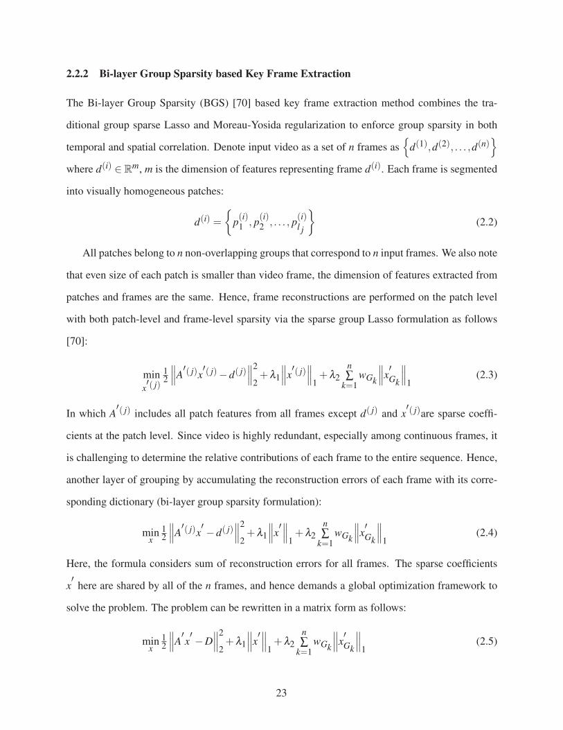
2.2.2 Bi-layer Group Sparsity based Key Frame Extraction

The Bi-layer Group Sparsity (BGS) [70] based key frame extraction method combines the tra-

ditional group sparse Lasso and Moreau-Yosida regularization to enforce group sparsity in both

temporal and spatial correlation. Denote input video as a set of n frames as{

d(1),d(2), . . . ,d(n)}

where d(i) ∈ Rm, m is the dimension of features representing frame d(i). Each frame is segmented

into visually homogeneous patches:

d(i) ={

p(i)1 , p(i)2 , . . . , p(i)l j

}(2.2)

All patches belong to n non-overlapping groups that correspond to n input frames. We also note

that even size of each patch is smaller than video frame, the dimension of features extracted from

patches and frames are the same. Hence, frame reconstructions are performed on the patch level

with both patch-level and frame-level sparsity via the sparse group Lasso formulation as follows

[70]:

minx′( j)

12

∥∥∥A′( j)x

′( j)−d( j)∥∥∥2

2+λ1

∥∥∥x′( j)∥∥∥

1+λ2

n∑

k=1wGk

∥∥∥x′Gk

∥∥∥1

(2.3)

In which A′( j) includes all patch features from all frames except d( j) and x

′( j)are sparse coeffi-

cients at the patch level. Since video is highly redundant, especially among continuous frames, it

is challenging to determine the relative contributions of each frame to the entire sequence. Hence,

another layer of grouping by accumulating the reconstruction errors of each frame with its corre-

sponding dictionary (bi-layer group sparsity formulation):

minx

12

∥∥∥A′( j)x

′ −d( j)∥∥∥2

2+λ1

∥∥∥x′∥∥∥

1+λ2

n∑

k=1wGk

∥∥∥x′Gk

∥∥∥1

(2.4)

Here, the formula considers sum of reconstruction errors for all frames. The sparse coefficients

x′

here are shared by all of the n frames, and hence demands a global optimization framework to

solve the problem. The problem can be rewritten in a matrix form as follows:

minx

12

∥∥∥A′x′ −D

∥∥∥2

2+λ1

∥∥∥x′∥∥∥

1+λ2

n∑

k=1wGk

∥∥∥x′Gk

∥∥∥1

(2.5)

23

in which A′=[A′(1),A′(2), . . . ,A′(n)

]Tand D =

[d(1), . . . ,d(n)

]. The problem can be solved via

the regular group sparse solver [71] that converts multi-task group sparse representation problem

into single-task group sparse representation with dimension concatenated target signals and dictio-

naries.

On the final step, low-level features obtained from sparse coefficients are combined with high-

level semantics evaluated via three different scores (image quality score, color histogram change

score, and scene complexity score) to select key frames.

2.2.3 Dictionary Selection based Video Summarization

Dictionary Selection based Video Summarization (DSVS) approach has been proposed by Yang

Cong et al. [67]. Under the DSVS framework, the key frame extraction problem is evaluated from

dictionary selection problem, in particular how to select an optimal subset from the set of entire

video frames such that the original set can be accurately recovered from the optimal subset while

using as small as possible the size of the subset.

Denote D= [d1,d2, . . . ,dN ]∈Rd×N as the initial candidate pool, each column vector represents

a feature vector of one frame. The DSVS problem can be formulated as:

minX

: f (X) = λ2 ‖D−DX‖2

F + 1−λ2 ‖X‖2,1 (2.6)

Here, ‖X‖2,1 := ∑i

∥∥Xi,:∥∥

2and Xi,: denotes the ith row of X . The �2,1 norm of a matrix generalizes

�1 of a vector since it would be come �1 norm if X has only one column. In the formula (2.6),

the first term measures the quality of reconstruction, and the second one controls the sparsity level

of the dictionary selection. The tuning parameter λ helps to balances the reconstruction error and

the group sparsity level. The obtained coefficient matrix X refers to as a feature matrix, in which

each row corresponds to a feature. If the weight ‖Xi.‖2 is close to zero, then the corresponding ith

feature will not be selected. The selected features will be used to create the dictionary for video

summarization. An efficient algorithm has been proposed [72] to solve the type of convex but non-

24

smooth optimization problem with the guarantee of convergence rate of O( 1

k2 ), k is the number of

iterations.

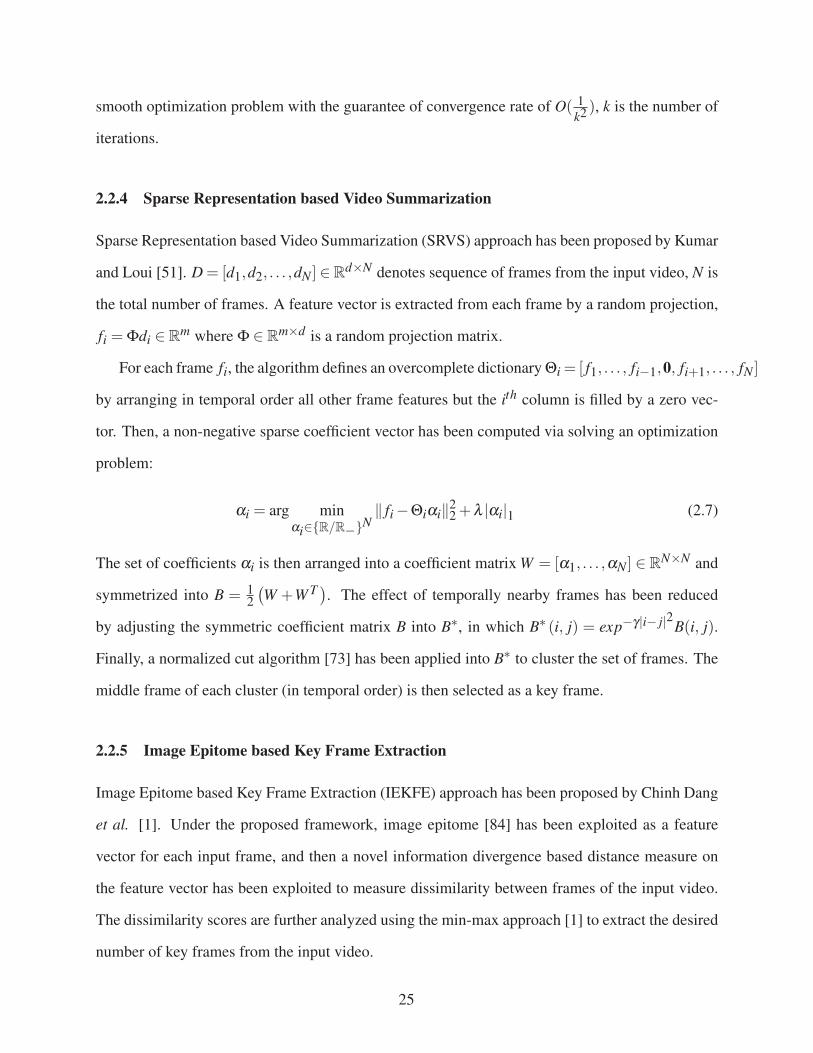
2.2.4 Sparse Representation based Video Summarization

Sparse Representation based Video Summarization (SRVS) approach has been proposed by Kumar

and Loui [51]. D = [d1,d2, . . . ,dN ] ∈Rd×N denotes sequence of frames from the input video, N is

the total number of frames. A feature vector is extracted from each frame by a random projection,

fi = Φdi ∈ Rm where Φ ∈ R

m×d is a random projection matrix.

For each frame fi, the algorithm defines an overcomplete dictionary Θi = [ f1, . . . , fi−1,0, fi+1, . . . , fN ]

by arranging in temporal order all other frame features but the ith column is filled by a zero vec-

tor. Then, a non-negative sparse coefficient vector has been computed via solving an optimization

problem:

αi = arg minαi∈{R/R−}N

‖ fi −Θiαi‖22 +λ |αi|1 (2.7)

The set of coefficients αi is then arranged into a coefficient matrix W = [α1, . . . ,αN ] ∈ RN×N and

symmetrized into B = 12

(W +W T ). The effect of temporally nearby frames has been reduced

by adjusting the symmetric coefficient matrix B into B∗, in which B∗ (i, j) = exp−γ|i− j|2B(i, j).

Finally, a normalized cut algorithm [73] has been applied into B∗ to cluster the set of frames. The

middle frame of each cluster (in temporal order) is then selected as a key frame.

2.2.5 Image Epitome based Key Frame Extraction

Image Epitome based Key Frame Extraction (IEKFE) approach has been proposed by Chinh Dang

et al. [1]. Under the proposed framework, image epitome [84] has been exploited as a feature

vector for each input frame, and then a novel information divergence based distance measure on

the feature vector has been exploited to measure dissimilarity between frames of the input video.

The dissimilarity scores are further analyzed using the min-max approach [1] to extract the desired

number of key frames from the input video.

25

Image epitome review: An image epitome E of size p×q is a condensed version of the corre-

sponding input image X of size M×N where p M, q N[84][111]. Let Z = {Zk}P1 be the patch

level representation of X , i.e., is the set of all possible patches from X . The epitome (E) corre-

sponding to X is estimated using Z and represents the salient visual contents of X effectively. More

specifically, epitome E is derived by searching for a set of patches in E that corresponds to the set

Z based on Gaussian probability distribution. The patches in E are defined by a set of mapping,

T = {Tk}P1 , which shows a displacement between two patches X and E respectively. Assuming dis-

tribution at each epitome location to be Gaussian, the conditional probability for mapping patches

in epitome to set of patches in an image is defined as:

p(Zk|Tk,E) = ∏i∈Sk

N(zi,k; μTk(i),φTk(i)

) (2.8)

p({Zk}P

1 |{Tk}P1 ,E)=

p∏

k=1p(Zk|Tk,E) (2.9)

in which{

μTk(i),φTk(i)

}, mean and variance of a Gaussian distribution, are parameters stored in

one epitome coordinate that is mapped to pixel i in Zk. Solving the maximum likelihood problem

leads to expectation maximization algorithm. In the expectation-step, given the current epitome E

and Z = {Zk}P1 , the set of mappings is specified by optimizing (2.9), searching for every allowed

correspondences. The multiple patch mappings allow one pixel in epitome to be mapped onto nu-

merous pixels in the larger image. In the maximization-step, given the new set of mappings, mean

and variance at each location, e.g. location u, are calculated [84]:

μu =∑i ∑k[u=Tk(i)]zi,k

∑i ∑k[u=Tk(i)](2.10)

φu =∑i ∑k[u=Tk(i)](zi,k−μu)2

∑i ∑k[u=Tk(i)](2.11)

[P] =

⎧⎪⎨⎪⎩

1 i f Pistrue

0 otherwise(2.12)

26

Image epitome dissimilarity measurement: Measuring perceptual or visual dissimilarity be-

tween images is an important research area and finds its applications in many image processing

and computer vision problems including key frame extraction. Selecting feature(s) or descriptor(s)

that describe visual content of images effectively is crucial for image dissimilarity measurement.

Motivated by this, we use epitome representation of an image as feature to compute image dissim-

ilarity since epitome is significantly smaller as compared to the original image and yet preserves

important visual information (texture, edge, color, etc.) of the input image. Furthermore, epit-

ome has been shown to be shift and scale invariant and effective in terms of modeling the spatial

structure [107].

Let Ei be the lexicographical representation of the epitome (for example, Ei ∈ Rm×1) corre-

sponding to the ith image Ii. Therefore, the distribution function (represented as fi) of Ei can be

expressed as a linear combination of m Gaussians as given bellows:

fi = 1m

m∑

k=1N(μ i

k,φik) (2.13)

Where N(μ i

k,φik)

is the distribution of the kth element of Ei. The proposed dissimilarity of two

images, denoted as Ii and I j, respectively, is computed as follows:

D(Ii/I j) = D(I j/Ii) = 12

(∫fi log

fif j+ f j log

f jfi

)(2.14)

Note that the proposed dissimilarity measure in eq. (2.14) exploits well-known Kullback-Leibler

divergence [108]. In case of two Gaussian mixtures, there is no closed form solution for eq. (2.14);

hence approximate solution based on unscented transform or Gaussian elements matching is typ-

ically employed in practice to solve eq. (2.14)[20]. In the proposed approach, we use unscented

transform-based approach to solve eq. (2.14) because of the potential overlap between epitomes

caused due to temporal correlation present between video frames. The unscented transformation

attempts to calculate the statistics of a random variable which undergoes a non-linear transforma-

tion. Given a d-dimensional normal random variable x, distribution function f (x) ∼ N(μ,Σ) and

an arbitrary non-linear function h(x) :Rd →R, the approximated expectation of function h(x) over

f (x) is given by:

27

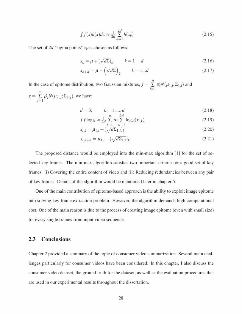
∫f (x)h(x)dx ≈ 1

2d

2d∑

k=1h(xk) (2.15)

The set of 2d "sigma points" xk is chosen as follows:

xk = μ +(√

dΣ)k k = 1 . . .d (2.16)

xk+d = μ −(√

dΣ)

kk = 1...d (2.17)

In the case of epitome distribution, two Gaussian mixtures, f =n∑

i=1αiN(μ1,i;Σ1,i) and

g =m∑

j=1β jN(μ2, j;Σ2, j), we have:

d = 3; k = 1, ...,d (2.18)

∫ f logg ≈ 12d

n∑

i=1αi

2d∑

k=1logg(xi,k) (2.19)

xi,k = μ1,i +(√

dΣ1,i)k (2.20)

xi,k+d = μ1,i − (√

dΣ1,i)k (2.21)

The proposed distance would be employed into the min-max algorithm [1] for the set of se-

lected key frames. The min-max algorithm satisfies two important criteria for a good set of key

frames: (i) Covering the entire content of video and (ii) Reducing redundancies between any pair

of key frames. Details of the algorithm would be mentioned later in chapter 5.

One of the main contribution of epitome-based approach is the ability to exploit image epitome

into solving key frame extraction problem. However, the algorithm demands high computational

cost. One of the main reason is due to the process of creating image epitome (even with small size)

for every single frames from input video sequence.

2.3 Conclusions

Chapter 2 provided a summary of the topic of consumer video summarization. Several main chal-

lenges particularly for consumer videos have been considered. In this chapter, I also discuss the

consumer video dataset, the ground truth for the dataset, as well as the evaluation procedures that

are used in our experimental results throughout the dissertation.

28

A quick summary of recent works on consumer video summarization has been provided, which

includes: Motion-based Key Frame Extraction (MKFE) [55], Bi-layer Group Sparsity based Key

Frame Extraction (BGS) [70], Dictionary Selection based Video Summarization (DSVS) [67],

Sparse Representation based Video Summarization (SRVS) [51], and Image Epitome based Key

Frame Extraction (IEKFE) [1].

Section 2.2.5, in full, is reproduced from the material as it appears in: Chinh Dang, M. Ku-

mar, and Hayder Radha, "Key Frame Extraction From Consumer Video using Epitome" - in IEEE

Proceedings of International Conference on Image Processing (ICIP12), pp.93-96, Oct. 2012.

29

CHAPTER 3

REPRESENTATIVE SELECTION FOR CONSUMER VIDEOS VIA SPARSE GRAPHAND GEODESIC GRASSMANN MANIFOLD DISTANCE

3.1 Motivation

Capturing, storing, and extracting valuable information from massive collections of data (Big Data)

raise a number of technical challenges. Issues related to Big Data are normally classified based on

three typical characteristics: volume, velocity, and variety. Volume is the greatest challenge, and it

refers to the fact that the massive amount of data is (could be) in a high dimensional space. Beside

the high volume, users and many applications also demand high speed (velocity) data stream that

could be higher than the capacity of the underlying network. Additional challenges are related to a

variety of data sources, going from traditional type of data, e.g. documents, financial transactions

to audio/video, set of images, location data, etc.

Multimedia data, such as consumer and surveillance videos, medical images, etc. has become

increasingly important. Challenging problems related to high volume amount of digital dataset

has been raised in many areas of machine learning, computer vision, image/video processing, and

information retrieval, to name a few. The traditional multimedia processing and analysis systems

cannot handle effectively the rapid increase in the amount of data. As a result, many systems decide

to ignore a large amount of potentially valuable information without being processed. Video sum-

marization is one of the main directions dealing with extracting a condensed visual summary of a

full length input video. The general area of video summarization has been research for a long time

due to its important role in many video-related applications. However, prior video summarization

techniques endure some limitations that cannot be generalized to the representative selection from

a Big Data point of view. First, as we mentioned in chapter 2, most proposed video summarization

techniques are domain-dependent [25-29][39], in which they exploit specific properties of video

clips or particular domains (soccer videos, documental videos, news, etc.) for the set of represen-

30

tatives. More importantly, although some of these techniques produce summaries of acceptable

quality, the summarization process endure a high computational complexity [32]. The required

time of creating a summary may be up to ten times the video length [99]. Some recent efforts [6]

target to solve the representative selection problem for a general type of data points. However,

the method requires creating a dense similarity matrix among every pair of data points, and that

restricts the range of applications that can employ this method.

3.2 Related Works and Contributions

We discuss some related works on representative selection techniques, which basically provide a

review of the normalized cut algorithm, and clustering-based key frame extraction techniques.

3.2.1 Normalized Cut Method

Normalized cut algorithm has been proposed by Jianbo Shi and Jitendra Malik [73]. Different from

prior works, normalized cut is a global method, which considers all links in the affinity graph and

finds the weakest set of links for the partitioning.

In this method [73], a graph G= (V,E) can be partitioned into two disjoint sets, A,B, A∪B=V ,

and A∩B = φ . A cut, which is the degree of dissimilarity between two sets A,B, can be computed

as the total weight of the edges connecting A and B:

cut(A,B) = ∑u∈A,v∈B

ω(u,v) (3.1)

Clustering algorithms based on minimizing the cut have a tendency to be unnatural bias for par-

titioning out small sets of points. This is not suprising since the cut value in (3.1) increases with

the number of edges going across the two partitioned parts [73]. A new measurement, called

normalized cut, has been considered to solve the biased clustering problem:

Ncut(A,B) = cut(A,B)assoc(A,V )

+cut(A,B)

assoc(B,V )(3.2)

31

In this equation, assoc(A,V ) = ∑u∈A,v∈V

ω(u, t) denotes the total edges connecting from nodes in A

to all nodes in the graph. In stead of minimizing the cut value, the algorithm looks for a partition

that minimize the normalized cut value defined in (3.2).

Given a partition of nodes in a graph V into two sets A and B, the partition can be represent as

an indicator vector x = [x1,x2, ...,xN ], N = |V | in which xi = 1 if node i is in A and −1, otherwise.

Next, we denote d(i) = ∑j

ω(i, j) as the total weights from node i to all other nodes. Then, the

normalized cut value in (3.2) has a new expression form in terms of x and d as:

Ncut(A,B) =∑xi>0,x j<0−ωi jxix j

∑xi>0 di+

∑xi<0,x j>0−ωi jxix j∑xi<0 di

(3.3)

The goal now is to estimate the indicator vector x that minimizes the normalized cut value, we

denoted by Ncut(x) instead of Ncut(A,B). By defining some other terms: D be an N ×N diagonal

matrix with d on its diagonal, W be an N ×N matrix of elements ω(i, j), k =∑xi>0 di

∑i di, b = k

1−k ,

and y = (1+ x)−b(1− x), the indicator vector solution can be found in the following form:

minxNcut(x) = minyyT (D−W )y

yT Dy(3.4)

with the condition y(i) ∈ {1,−b} and yT D1 = 0. Instead of solving for indicator vector x, we

look for y solution. if we relax y to take on real values, then the minimization of (3.4) can be

transformed into solving for the generalized eigenvalue system:

(D−W )y = λDy (3.5)

It turns out that the second smallest eigenvector of the generalized eigensystem (3.5) is the real

valued solution to the normalized cut problem. The final step transforms this real valued solution

into a discrete form.

3.2.2 Clustering-based Key Frame Extraction Techniques

There is an inherent connection between key frame extraction and clustering methods. As a re-

sult, numerous key frame extraction approaches have been developed from clustering perspectives

[7][32][51][68][74-75]. De Avila et al. [32] employed color histogram for Hue component and

32

k-means algorithm to extract key frames. In a similar approach, Zhuang et al. [74] measured the

similarity of two frames using color histogram, and then performed unsupervised clustering algo-

rithm to extract key frames. Hadi et al. [75] exploited local motion estimation and fast full search

block matching algorithm to measure distance of two frames. The most representative frames

are obtained by a similarity-based clustering. Clustering-based methods are also used widely in

“Rush video summarization” tasks for shots instead of frames [18-19]. Most proposed methods

are based on shot boundary detection and then evaluating the importance score and the similarity

among these shots to compose the final summarization. Despite their effectiveness in some cases,

clustering-based approaches cannot guarantee optimal selection of representative content due to

their largely heuristic nature. In particular, heuristic algorithms refer to a class of experience-

based techniques that provide solution, which is not guaranteed to be optimal. For example, k-

mean clustering that is widely used in the literature is heuristic. The problem is computational

challenging (NP-hard). However, heuristic algorithms are commonly employed (e.g. Expectation-

Maximization algorithm for a mixture of Gaussians) in order to archive rapid convergence to a local

optimum. Consequently, such algorithm depends heavily of initial set of k-means, and therefore

the final results could vary significantly for different initial sets. In addition, clustering approaches

have an inherent problem of choosing appropriate threshold values for various video types. T. Liu

and J. Kender [76] proposed an optimization-based approach for video key frame extraction. A set

of key frames is extracted based on optimizing an energy function using dynamic programming.

3.2.3 Contributions

Prior clustering-based representative selection methods requires to create a similarity matrix using

traditional techniques such as k-nearest neighbors, ε-ball approaches, or even using dense graph.

Instead of working with a full graph of similarity, the �1 norm sparse graph has been proposed

recently, in which the vertices represent all the samples and the edge-weights represent �1-norm

driven reconstruction using the remaining samples and the noise [96]. The �1-norm sparse graph is

originated from the self-expressiveness property, which has been proposed by Elhamifar and Vidal

33

[16] to solve the subspace clustering problem. The sparse graph is then generalized to solve many

image/video related problems in data clustering, semi-supervised learning, classification. A brief

introduction of the �1-norm sparse graph will be introduced later.

Prior clustering–based key frame extraction efforts mainly target a particular type of video

using dense (or even full) graph, which require high computational cost and depend heavily on

data structure. Our main contributions in this chapter include:

(i) A novel representative selection algorithm for a general type of dataset.

(ii) A practical representative selection algorithm using the �1-norm sparse graph, that is appli-

cable to massive high-dimensional datasets in a constrained amount of time.

(iii) Prior clustering-based approaches select each frame from one cluster. Normally the number

of clusters is set to be equal the number of desired key frames. The selected frame could

be at the beginning, the middle, or the end in terms of the time sequence for each cluster.

This approach ignores important information of sub-graph structure in each cluster. More

importantly, the number of key frames is a parameter that is defined by users. Hence, this

parameter does not reveals the number of clusters, an underlying factor from the input dataset.

Our work analyzes each cluster as one point in a Grassmann manifold, and then selects an

optimal set of clusters. The final representative will be evaluated using a graph centrality

technique for the sub-graph corresponding to each selected cluster.

3.3 Representative Selection via Sparse Graph and Geodesic GrassmannManifold Distance

Under the proposed framework, we exploit a spectral clustering technique for the set of data points

using the �1 norm sparse graph, which outperforms traditional methods of creating graphs. Then

each cluster is considered as one point in a Grassmann manifold that allows measuring geodesic

distances among these clusters. We employ the min-max algorithm developed in [1] in conjunction

with the geodesic distance to detect a subset of representative clusters. Each selected cluster is

34

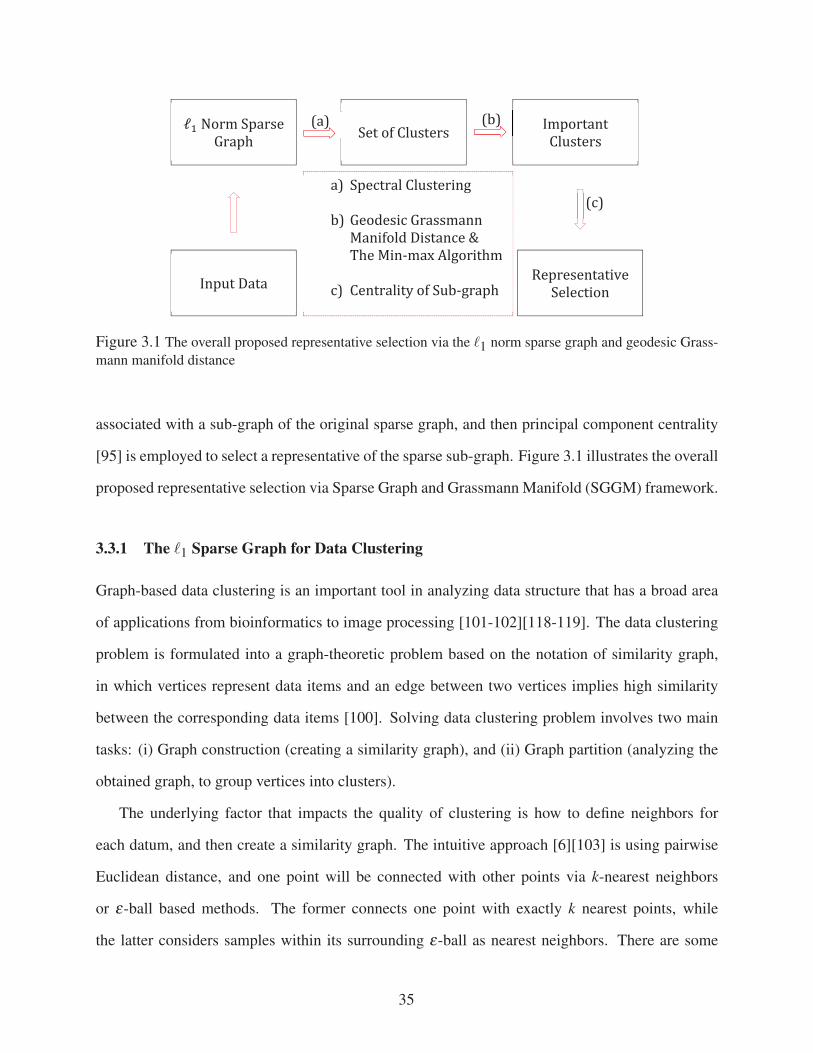
Input Data

Norm Sparse Graph Set of Clusters Important

Clusters

Representative Selection

(a) (b)

(c) a) Spectral Clustering

b) Geodesic Grassmann

Manifold Distance & The Min-max Algorithm

c) Centrality of Sub-graph

Figure 3.1 The overall proposed representative selection via the �1 norm sparse graph and geodesic Grass-

mann manifold distance

associated with a sub-graph of the original sparse graph, and then principal component centrality

[95] is employed to select a representative of the sparse sub-graph. Figure 3.1 illustrates the overall

proposed representative selection via Sparse Graph and Grassmann Manifold (SGGM) framework.

3.3.1 The �1 Sparse Graph for Data Clustering

Graph-based data clustering is an important tool in analyzing data structure that has a broad area

of applications from bioinformatics to image processing [101-102][118-119]. The data clustering

problem is formulated into a graph-theoretic problem based on the notation of similarity graph,

in which vertices represent data items and an edge between two vertices implies high similarity

between the corresponding data items [100]. Solving data clustering problem involves two main

tasks: (i) Graph construction (creating a similarity graph), and (ii) Graph partition (analyzing the

obtained graph, to group vertices into clusters).

The underlying factor that impacts the quality of clustering is how to define neighbors for

each datum, and then create a similarity graph. The intuitive approach [6][103] is using pairwise

Euclidean distance, and one point will be connected with other points via k-nearest neighbors

or ε-ball based methods. The former connects one point with exactly k nearest points, while

the latter considers samples within its surrounding ε-ball as nearest neighbors. There are some

35

minus points for the traditional graph construction. First, such approaches suffer from using a

predetermined number of neighbors or a fixed radius for each ball. Hence, they do not fit well

with a general dataset in which each data point may have diverse connections to other points. Not

to mention that the algorithm performance depends heavily on the selection of k or ε as a global

parameters. Second, the graph constructed by k-nearest neighbor or ε-ball method (that could

be Euclidean distance or others) is highly sensitive to data noise [6][104]. For example, noised

features may lead to erroneous similarities among data points, and hence deteriorate the overall

algorithm performance. Third, traditional graph construction endures a fundamental problem of

storage in large scale data. Meanwhile, recent works on subspace clustering, face recognition

[16][105] have shown a trend toward using sparse graph for classification purpose due to its locality

characteristics of each data point in making connections with its neighbors. Here, we briefly review

the method to create a sparse graph.

Denote H ={

h j ∈ RD}N

j=1is the set of data points, where D is the dimension of the ambient

Euclidean space, which is smaller than the total number of elements in the dataset (N � D).

The underlying idea of defining a neighborhood for each point is to consider the data itself as

a dictionary for sparse representation. The set of data points can be written in a matrix form

H = [h1,h2, . . . ,hN ] ∈ RD×N . Let Hi ∈ R

D×(N−1) = H/{hi} be the matrix obtained from H

by removing its ith column. The algorithm looks for the sparsest representation of hi from its

corresponding dictionary Hi:

min‖ci‖0 subject to hi = Hici (3.6)

Here, ‖.‖0 is the �0 norm that counts the number of non-zero elements. Although the problem is

NP hard, recent results from compressed sensing [40] has concluded that the sparest solution could

be found approximately via �1 norm minimization:

min‖ci‖1 subject to hi = Hici (3.7)

Minimizing �1 norm with an equality constrain could be transformed into a relaxed form of a

convex optimization problem, for a fixed dictionary Hi of the form:

36

ci = arg minci∈RN−1

∥∥hi −Hici∥∥

2+λ‖ci‖1 (3.8)

There exists a globally optimal solution to the optimization problem using an available efficient

�1-norm optimization toolbox. We summarize the process of creating a sparse graph for a dataset:

1. Input the set of data points in the matrix form H = [h1,h2, . . . ,hN ] ∈ RD×N .

2. For each data point hi, solve (3.8) for its corresponding coefficient ci ∈ RN−1, which is

arranged accordingly into the ith column of the coefficient matrix C ∈ RN×N by inserting a

zero entry at ith position of ci (i.e. C has zero diagonal).

3. Graph construction in the form of G = {H,C} in which each point in H is mapped to one

vertex, and C =[Ci j]N×N denotes the graph weight matrix, Ci j =

∣∣Ci j∣∣+ ∣∣Cji

∣∣.An clustering algorithm from spectral graph theory has been exploited for data segmentation. We

briefly discuss how clustering algorithm has been exploited in this case. The number of desired

representatives is an input parameter, which is determined by users. If an automated representative

selection algorithm selects the number of clusters to be equal the number of desired representatives,

there are two main problems:

• Since the number of desired representatives is determined by users, it does not imply the

structure of input data (and hence there is no relation to the number of clusters).

• If we change the number of desired representatives, then the whole clustering results may

change dramatically. As a result, the set of representatives also change, possibly completely

different to the prior ones. It is not a good property because a smaller set of representatives

(for example 3 points) should be contained in a larger one (for example 5 points).

For those reasons, in our work, we do not select the number of clusters to be equal the number of

representatives. In particular, normalized cut algorithm [73] iteratively segments the input dataset

into two clusters, and check for the maximum rank of linear spaces spanned by elements in these

37

clusters. If a cluster has a rank which is greater than a predetermined threshold, it will be re-

cursively partitioned into smaller clusters. This produce serves to avoid the problem of having

too many data points in one cluster. The next part introduces an algorithm for selecting a set of

important clusters, and then to select representatives from these clusters.

3.3.2 The Selection of an Optimal Subset of Clusters

In the next step, we consider each cluster as one point in the Grassmann manifold. Since the

number of obtained clusters could be larger than the number of desired representatives, some

clusters contain outliers or no important/redundant information. We exploit geodesic Grassmann

manifold distance to measure the dissimilarity between two clusters (as two points in the manifold).

Then, the min-max algorithm [1] has been exploited for the final optimal subset of clusters.

3.3.2.1 Geodesic Grassmann Manifold Distance

Grassmann manifold: given n, p (p≤ n) are positive integers, denote Grass(p,n) and Rn×p∗ are the

set of all p-dimensional subspaces of Rn, and the set of all n× p matrices whose columns are linear

independent, respectively. Rn×p∗ is an open subset of Rn×p. The subset admits a structure of an

open sub-manifold of Rn×p where its differential structure is created using the chart Φ : Rn×p∗ →

Rnp : X → vec(X). Therefore, this manifold is referred to as non-compact Stiefel manifold of full

rank n× p matrices. The manifold Rn×p∗ is equipped with an equivalence relation ∼ that is defined

as follows:

X ∼ Y if and only if span(X) = span(Y ) (3.9)

Here, X ,Y ∈ Rn×p∗ and span(X) denotes the subspaces spanned by the columns of matrix

X . The quotient manifold defined on the non-compact Stiefel manifold Rn×p∗ with the above

equivalence relation [X ] :={

Y ∈ Rn×p∗ : Y ∼ X

}is the equivalence class that contains element X ,

and the set Rn×p∗ /∼:=

{[X ] : X ∈ R

n×p∗}

is a quotient space that has one-to-one correspondence

to Grass(p,n), where each point in Grass(p,n) is one p-dimensional subspace. The distance

38

between two subspaces is now mapped to geodesic distance between two points in the manifold,

which is mainly computed using the concept of principal angles.

Denote H1 and H2 be two subspaces (assuming that dim(H1) = d1 ≥ dim(H2) = d2), the princi-

pal angles between two subspaces, 0≤ θ1 ≤ . . .≤ θt ≤ π/2, are defined recursively for t = 1, . . . ,d2

as follows [97]:

cosθt = maxut∈H1

maxvt∈H2

utT vt (3.10)

s.t. ‖ut‖2 = 1, ‖vt‖2 = 1

uTj ut = 0, vT

j vt = 0 for j = 1,2, ..., t −1

These vectors(

u1, . . . ,ud2

)and(

v1, . . . ,vd2

)are called principal vectors of these two subspaces

H1 and H2. The principal angle θk is the angle between two principal vectors uk and vk. There

are several methods of computing the principal angles and principal vectors; one efficient stable

method has been developed using singular value decomposition on the product of two basis ma-

trices H1T H2 (the subspace H1 and its basis matrix are used interchangeably in this context). In

particular,

H1T H2 =USV T (3.11)

where U =[u1, . . . ,ud2

], V =

[v1, . . . ,vd2

]are matrices of these principal vectors and

S = diag(

cosθ1, . . . ,cosθd2

). There are several methods of computing Grassmann manifold dis-

tance based on these obtained principal angles, for example projection distance, Binet-Cauchy

distance, etc. Some additional properties and applications of these distances could be found at [9].

In this work, we exploit the geodesic Grassmann manifold distance (arc length) in the form:

G(H1,H2) =

√√√√ d2∑

j=1θ j

2 (3.12)

The distance has been also exploited successfully in prior work on image search problem to ma-

nipulate leaf nodes in the data partition tree [98]. It has some desired properties of a metric, such

as symmetric, triangular properties. In addition, it is derived from the intrinsic geometry of Grass-

mann manifold, which is the length of geodesic curve connection two points on the manifold.

39

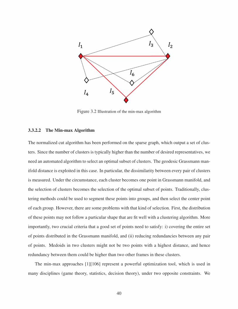
Figure 3.2 Illustration of the min-max algorithm

3.3.2.2 The Min-max Algorithm

The normalized cut algorithm has been performed on the sparse graph, which output a set of clus-

ters. Since the number of clusters is typically higher than the number of desired representatives, we

need an automated algorithm to select an optimal subset of clusters. The geodesic Grassmann man-

ifold distance is exploited in this case. In particular, the dissimilarity between every pair of clusters

is measured. Under the circumstance, each cluster becomes one point in Grassmann manifold, and

the selection of clusters becomes the selection of the optimal subset of points. Traditionally, clus-

tering methods could be used to segment these points into groups, and then select the center point

of each group. However, there are some problems with that kind of selection. First, the distribution

of these points may not follow a particular shape that are fit well with a clustering algorithm. More

importantly, two crucial criteria that a good set of points need to satisfy: i) covering the entire set

of points distributed in the Grassmann manifold, and (ii) reducing redundancies between any pair

of points. Medoids in two clusters might not be two points with a highest distance, and hence

redundancy between them could be higher than two other frames in these clusters.

The min-max approaches [1][106] represent a powerful optimization tool, which is used in

many disciplines (game theory, statistics, decision theory), under two opposite constraints. We

40

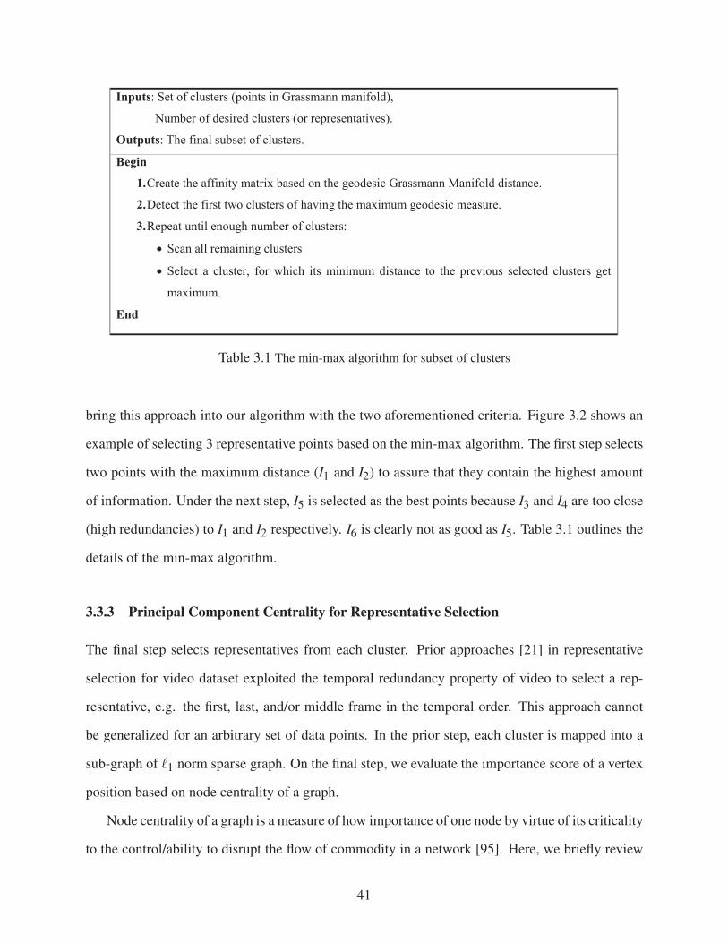
Inputs: Set of clusters (points in Grassmann manifold),

Number of desired clusters (or representatives).

Outputs: The final subset of clusters. Begin

1. Create the affinity matrix based on the geodesic Grassmann Manifold distance.

2. Detect the first two clusters of having the maximum geodesic measure.

3. Repeat until enough number of clusters:

Scan all remaining clusters

Select a cluster, for which its minimum distance to the previous selected clusters get

maximum.

End

Table 3.1 The min-max algorithm for subset of clusters

bring this approach into our algorithm with the two aforementioned criteria. Figure 3.2 shows an

example of selecting 3 representative points based on the min-max algorithm. The first step selects

two points with the maximum distance (I1 and I2) to assure that they contain the highest amount

of information. Under the next step, I5 is selected as the best points because I3 and I4 are too close

(high redundancies) to I1 and I2 respectively. I6 is clearly not as good as I5. Table 3.1 outlines the

details of the min-max algorithm.

3.3.3 Principal Component Centrality for Representative Selection

The final step selects representatives from each cluster. Prior approaches [21] in representative

selection for video dataset exploited the temporal redundancy property of video to select a rep-

resentative, e.g. the first, last, and/or middle frame in the temporal order. This approach cannot

be generalized for an arbitrary set of data points. In the prior step, each cluster is mapped into a

sub-graph of �1 norm sparse graph. On the final step, we evaluate the importance score of a vertex

position based on node centrality of a graph.

Node centrality of a graph is a measure of how importance of one node by virtue of its criticality

to the control/ability to disrupt the flow of commodity in a network [95]. Here, we briefly review

41

Principal Component Centrality (PCC) [95], which has been proposed recently to overcome the

limitation of the traditional eigenvalue centrality in dealing with a large spatial graph.

Eigenvalue centrality is one of centrality tools that is widely used to detect the most influential

nodes(s). Denote A ∈ Rm×m be the adjacency matrix of a graph consisting a set of nodes V =

{v1,v2, . . . ,vN}. Let xi be the eigenvalue centrality score of a node vi, then the vector of these

scores x = [x1,x2, ...,xN ]T satisfies:

αx = Ax (3.13)

Here, α is a constant. This is the well-known eigenvector equation and eigenvalue centrality

vector x is the principal eigenvector corresponding with the largest of all eigenvalues of A (the

Perron eigenvalue). The main problem of eigenvalue centrality raises when applied to large spatial

graphs of randomly deployed nodes. In our work, we plan to dealing with a huge amount of high-

dimensional data points, distributed kind of randomly. Therefore, we exploit principal component

centrality [95] in the final step of selecting representative from each selected cluster.

In the adjacency matrix, the magnitude of an entry implies the “relationship” between two

nodes. A high value indicates a strong connection, while zero entry means no connection. PCC

makes a connection between graph adjacency matrix and covariance matrix. That allows tak-

ing additional features into consideration instead of using only one principal eigenvector. In

particular, PCC of a node in a graph is defined as the Euclidean distance of a node from the

origin in the P-dimensional eigenspace formed by the P most significant eigenvectors [95]. De-

note X = [x1x2 . . .xm] ∈ Rm×m be the matrix of concatenated eigenvectors, and Λ = [λ1λ2 . . .λm]

′

(|λ1| ≥ |λ2| ≥ . . . |λm|) be the vector of corresponding eigenvalues of A. Xm×q is the sub-matrix

consisting of the first q columns of X . Then, PCC can be expressed in a matrix form as:

Cq =√((

AXm×q)• (AXm×q

))1q×1 (3.14)

In which • denotes the Hadamard (or Schur product) operator.

42

3.4 Experimental Results on Video Summarization

In this section, we select consumer videos as a dataset for testing. Under video dataset, represen-

tatives are considered as key frames extracted from a video sequence. As we mentioned in chapter

2, consumer video summarization is more challenging to select a few key frames than structured

professionally-generated videos (e.g. news, documentary, sports). The detail descriptions of these

clips and the ground truth are provided in chapter 2. They vary in duration from 250 frames to

656 frames, approximately 485 frames per clip on average. The average number of key frames is

five per clip, depends on the number of key frames in the ground truth. The proposed algorithm

does not perform any pre-sampling as in previous approaches, such as at a predetermined rate [32].

Therefore, it is rather straightforward to extend the proposed algorithm for longer video clips in

conjunction with simple sub-sampling (e.g. 15 minutes if a pre-sampling rate at one frame/sec is

employed).

Experiment setup: Given input video sequence, a feature vector is extracted from each frame

to reduce the high dimension in the pixel domain. In particular, we choose color histogram as a

popular feature vector, using 16 bins for each RGB components. After this step, each frame is

mapped to a vector point in the R48 Euclidean space. Since in video dataset, a frame has a very

close feature to its neighbor frames in temporal domain. Therefore, for each frame, its neighbor-

hood of a predetermined number of frames will be removed from the corresponding dictionary for

a sparse representation. These coefficients will be assigned to be one after solving (3.8). In our

experiment, for each frame, its neighborhood containing maximum 15 consecutive frames (before

and after) will be removed from the dictionary. In addition, each sparse coefficient is scaled by

the difference of time index [51]. In particular, Ci j := eβ |i− j|2Ci j where β = 0.02 is chosen as a

constant in our work.

Under the spectral clustering step, we exploited the normalized cut algorithm iteratively with

the upper bound rank threshold is chosen to be 10. The upper bound rank controls the maximum

element in each cluster, and therefore helps to automatically determine the number of clusters in

the end. We also evaluate the impact of selecting a predetermined number of clusters via iteratively

43

a) #67 #265 #289 #343 #511

b) #66 #116 #371 #471 #511

c) #26 #103 #161 #382 #493

d) #7 #186 #276 #389 #508

Figure 3.3 “BusTour“ video. Visual comparison for some different methods includes a) Motion based Key

Frame Extraction (MKFE) [55], b)Bi-layer Group Sparsity (BGS) [70], c) Our proposed SGGM method,

and d) The ground truth. Solid red border implies a good matched frame

clustering the data with the upper bound rank. We conclude that using a predetermined number of

clusters does not lead to as good result as iterative partition input video sequence.

Baseline algorithms: we compare our work with some state-of-the-art algorithms, including

motion based key frame extraction (MKFE) [55], sparse modeling finding representatives (SMFR)

[7] (the code is provided online), sparse representation based method (SR) [51], and bi-layer group

sparsity (BGS) [70]. Chapter 2 provides a brief summary of these compared methods.

Visual Comparison: Figure 3.3 shows the results of “BusTour” video, including two compared

methods from the baseline algorithms (MKFE [55] and BGS [70]), our proposed SGGM method,

44

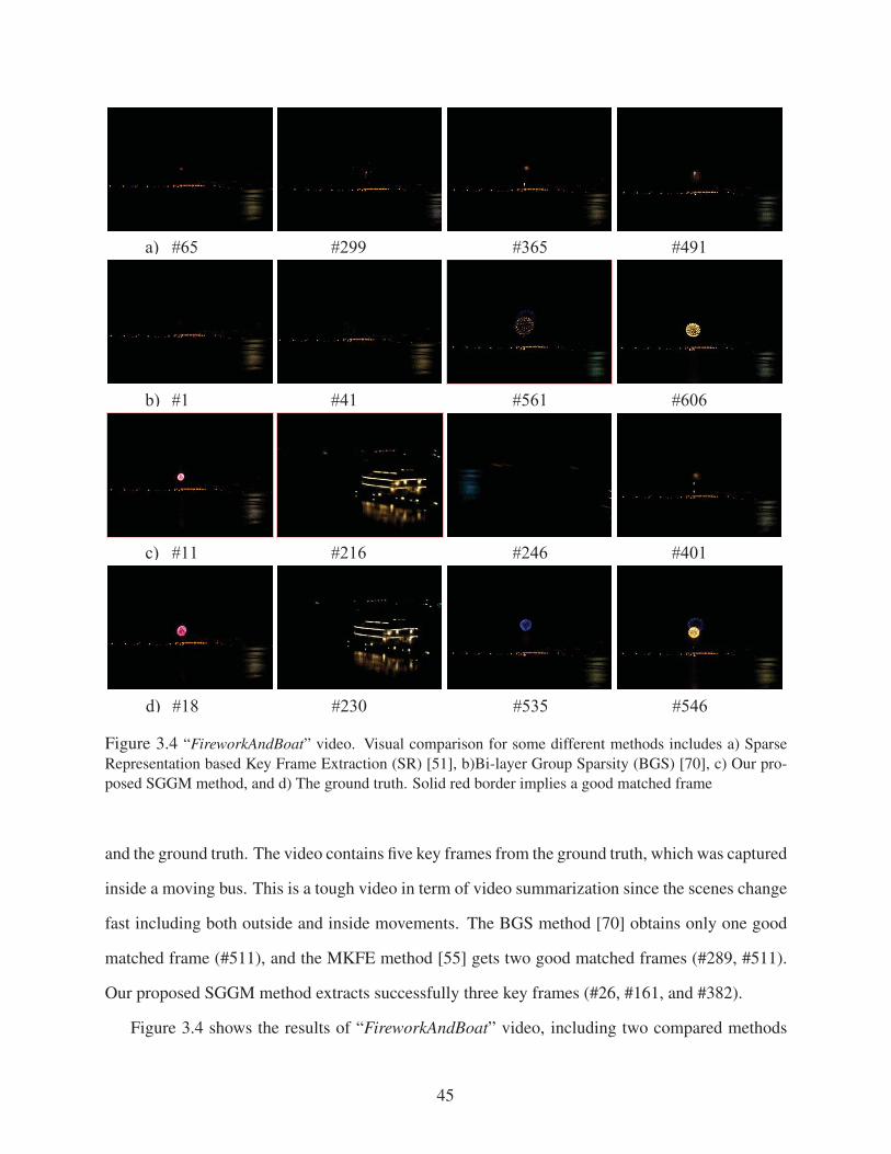
a) #65 #299 #365 #491

b) #1 #41 #561 #606

c) #11 #216 #246 #401

d) #18 #230 #535 #546

Figure 3.4 “FireworkAndBoat” video. Visual comparison for some different methods includes a) Sparse

Representation based Key Frame Extraction (SR) [51], b)Bi-layer Group Sparsity (BGS) [70], c) Our pro-

posed SGGM method, and d) The ground truth. Solid red border implies a good matched frame

and the ground truth. The video contains five key frames from the ground truth, which was captured

inside a moving bus. This is a tough video in term of video summarization since the scenes change

fast including both outside and inside movements. The BGS method [70] obtains only one good

matched frame (#511), and the MKFE method [55] gets two good matched frames (#289, #511).

Our proposed SGGM method extracts successfully three key frames (#26, #161, and #382).

Figure 3.4 shows the results of “FireworkAndBoat” video, including two compared methods

45

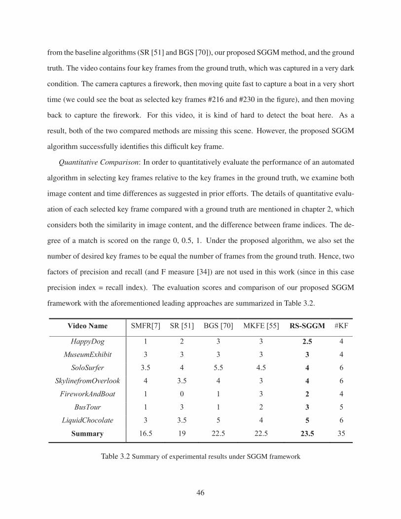
from the baseline algorithms (SR [51] and BGS [70]), our proposed SGGM method, and the ground

truth. The video contains four key frames from the ground truth, which was captured in a very dark

condition. The camera captures a firework, then moving quite fast to capture a boat in a very short

time (we could see the boat as selected key frames #216 and #230 in the figure), and then moving

back to capture the firework. For this video, it is kind of hard to detect the boat here. As a

result, both of the two compared methods are missing this scene. However, the proposed SGGM

algorithm successfully identifies this difficult key frame.

Quantitative Comparison: In order to quantitatively evaluate the performance of an automated

algorithm in selecting key frames relative to the key frames in the ground truth, we examine both

image content and time differences as suggested in prior efforts. The details of quantitative evalu-

ation of each selected key frame compared with a ground truth are mentioned in chapter 2, which

considers both the similarity in image content, and the difference between frame indices. The de-

gree of a match is scored on the range 0, 0.5, 1. Under the proposed algorithm, we also set the

number of desired key frames to be equal the number of frames from the ground truth. Hence, two

factors of precision and recall (and F measure [34]) are not used in this work (since in this case

precision index = recall index). The evaluation scores and comparison of our proposed SGGM

framework with the aforementioned leading approaches are summarized in Table 3.2.

Video Name SMFR[7] SR [51] BGS [70] MKFE [55] RS-SGGM #KF

HappyDog 1 2 3 3 2.5 4

MuseumExhibit 3 3 3 3 3 4

SoloSurfer 3.5 4 5.5 4.5 4 6

SkylinefromOverlook 4 3.5 4 3 4 6

FireworkAndBoat 1 0 1 3 2 4

BusTour 1 3 1 2 3 5

LiquidChocolate 3 3.5 5 4 5 6

Summary 16.5 19 22.5 22.5 23.5 35

Table 3.2 Summary of experimental results under SGGM framework

46

Computational Complexity: Since the time required for producing a set of key frames depends

on a particular hardware, it is almost impossible to produce a fair comparison in term of com-

plexity among these methods. In this work, we evaluate the average processing time per frame to

evaluate the complexity. According to those experiments, our SGGM method takes 0.0140 second

on average to process a single frame. This particular number depends on the computational power

of the employed hardware. In our work, we used an Intel Core E7500 @2.93GHz platform. The

average processing time per frame could be reduced further by a factor of pre-sampling rate.

3.5 Conclusions

The chapter considered a novel SGGM framework dealing with representative selection for a huge

amount of data. The self-expressiveness property has been exploited to create a sparse graph

for a dataset. The sparse graph allows working more efficiently than traditional dense graph for

this particular problem. We exploited geodesic Grassmann manifold distance and the min-max

algorithm [1] to recursively cluster a sparse graph into set of clusters, and then select a subset of

important clusters. The principal component centrality technique [95] has been used to select a

final representative for each selected cluster. We showed the application on video summarization,

in a very challenging type of consumer videos.

Chapter 3, in full, is reproduced from the material as it appears in: Chinh Dang, Mohammed

Al-Qizwini, and Hayder Radha, "Representative Selection for Big Data via Sparse Graph and

Geodesic Grassmann Manifold Distance" - in Proceedings of 48th IEEE Asilomar Conference on

Signal, Systems, and Computers, 2014.

47

CHAPTER 4

ROBUST PRINCIPAL COMPONENT ANALYSIS BASED VIDEO SUMMARIZATION

4.1 Robust Principal Component Analysis

One of the main directions dealing with high dimensional data is based on the assumption that

data points belong to an underlying low dimensional subspace. Principal Component Analysis

(PCA), one of the most well-known techniques in dimension reduction, searches for the best low

dimensional linear subspace to approximate a given dataset in an �2-sense. Denote the set of data

by D, PCA can be formulated as:

L = arg minrank(L)≤k

‖D−L‖2 (4.1)

Here, k is a predetermined dimension of the approximated linear subspace. The method performs

well under the assumption of Gaussian noise. However, the performance of PCA-based approaches

can degrade significantly for non-Gaussian noise, and especially for grossly corrupted observations

or in the present of outliers [30][37].

Matrix decomposition into low rank and sparse components: To combat the shortcomings of

traditional PCA, the data-reduction problem can be formulated by invoking the assumption that

the observed data consists of two components, a low rank component L0 and a sparse component

S0. Consequently, the problem can be reduced to the recovery of the low rank component L0 from

highly corrupted measurements D = L0 + S0, in which S0 can have arbitrary large elements, but

must be a sparse matrix. Furthermore, to make such modeling approach viable and meaningful,

we must assume that the low rank component L0 is not sparse.

As eluded above, the sparse component S0 can capture the effect of arbitrary noisy measure-

ments (due to sensor failures, occlusions, etc.). On the other hand, from an application perspective,

S0 may contain important information that could be used to distinguish different elements with the

same underlying property (contained in L0). For example, on latent sematic indexing, the input

48

matrix D contains entries that encode the relevance of a word to a document. If we could decom-

pose D into two components, low rank and sparse components, then L0 could capture common

words, and S0 captures some key words that could be used to distinguish each document from

others.

The general form of the problem described above has been considered in the literature over

several decades with limited promising results. Recently, Candes et al. [30] introduced a novel al-

gorithm based on tractable convex optimization to solve the problem within a polynomial time and

a strong performance guarantee. It transforms the sparsity condition into the principal component

pursuit problem:

{L0,S0

}= arg min

L+S = D

‖L‖∗+λ |S|1 (4.2)

Here, ‖L‖∗ := ∑i

σi (L) denote the nuclear norm of the matrix L and |S|1 = ∑i j

∣∣Si j∣∣ denote the

�1 norm of a matrix. Under rather a weak assumption, the principal component pursuit estimates

exactly the underlying low rank and sparse components {L0,S0}. Here, we state some main results.

Details of the proofs could be found in [30].

The incoherent condition: Consider the matrix L0 ∈ Rn1×n2. Denote the singular value de-

composition L0 = UΣV ∗ =r∑

i=1σiuivi

∗, r is the rank of the matrix and U = [u1,u2, . . . ,ur] and

V = [v1,v2, . . . ,vr] are the matrices of left- and right-singular vectors. The incoherent condition

with parameters μ states that:

maxi

‖U∗ei‖2 ≤ μrn1

and maxi

‖V ∗ei‖2 ≤ μrn2

(4.3)

‖UV ∗‖∞ ≤√

μrn1n2

(4.4)

Here, (ei) is the standard basis, and ‖.‖∞ denotes maximum of absolute values of entries. The in-

herent condition controls the spread-out property of a singular vector. A small value of μ generally

leads to a non-sparse singular value vector.

Main result: Suppose that L0 ∈ Rn1×n2 (denote n(1) = max(n1,n2), and n(2) = min(n1,n2)

satisfies the incoherent condition and the support of S0 is uniformly distributed among all sets of

49

cardinality m. Then, there is a numerical constant c such that with probability at least 1−cn(1)−10

(over the choice of support of S0), solving the principal component pursuit problem (4.2) with

λ = 1/√n(1) could recover the sparse and low rank components exactly, i.e.

{L0,S0

}= {L0,S0},

provided that:

rank(L0)≤ ρrn(2)μ−1(

logn(1))2

and m ≤ ρsn(1)n(2) (4.5)

where ρr,ρs are positive numerical constants.

Analysis: The first point is about the deterministic property of the result. Only a small assump-

tion about the randomness property of the locations of nonzero entries of S0 has been made. It even

does not require the turning parameter to balance between the sparse and low rank component. The

scalar parameter depends only on the size of the input dataset λ = 1/√n(1).

The second point is the connection with the prior matrix completion problem. Matrix comple-

tion aims to recover the full matrix, which is assumed to be low rank, based on a small number of

observed samples. The problem assumes a prior knowledge of measured points, while the Robust

PCA problem does not require prior knowledge of the positions of corrupted samples. Moreover,

Robust PCA also considers the given measured points containing errors while matrix completion

assumes them as corrected measurements. Denote Ω ⊂ [n1]× [n2] be the set of measured locations,

and the measured matrix M ∈ Rn1×n2 satisfying Mi j = 0 if (i, j) /∈ Ω. These two problems can be

stated as follows:

• Matrix completion: Recover the low rank matrix X such that Xi j = Mi j if (i, j) ∈ Ω

• Robust PCA problem: (when combined with matrix completion problem) Recover the low

rank and sparse component (L0,S0) such that (L0 +S0)i j = Mi j if (i, j) ∈ Ω

Candes et al. [30] guarantees that using similar Principal Component Pursuit technique could per-

fectly recover the low rank and sparse components from these incomplete and corrupted entries. In

the next section, we propose a novel framework for how to exploit Robust PCA into representative

selection for video.

50

4.2 Related Works and Contributions

4.2.1 Related Works

We discuss some related works on key frame extraction, which mostly focus on pre-sampling

techniques in key frame extraction, and hybrid linear modeling.

Pre-sampling techniques: A variety of pre-sampling techniques have been considered in prior

works for other types of videos [32-34]. Such approach is naturally of low-complexity and effective

strategy due to the inherent redundancy in video. However, sampling at a pre-determined rate [32]

cannot guarantee the extraction of the best representative frames, especially in the case of consumer

video where the content tends to change abruptly and unpredictably. Subsampling by selecting

only I-frames [33] cannot ensure a viable set of representative frames either. This is due to the fact

that, in general, no particular human perception rules or video-summarization driven strategy are

followed when coding video pictures as I-frame or B/P-frames. The video summarization based

on compressed domain has a strong point of producing a video summarization in a short time,

which is potential for on-line applications [34]. However, creating a set of key frames, while only

a part of video available (for on-line application), cannot summarize the whole video content with

a minimum number of key frames.

Hybrid linear modeling: Zhang et al. [35] considered the problem of Hybrid Linear Modeling

(HLM), approximating a dataset with outliers by a mixture of d-dimensional linear subspaces. The

paper concludes that replacing the �2-norm by the �1-norm improves significantly the robustness

against outliers and noise. Yang et al. [36] considers the problem of sequential HLM that is of

sequential recovery of multiple subspaces hidden in outliers. It leads to the problem of searching

for the best �0 subspace (i.e. the subspace with largest number of data points) among multiple

subspaces. G. Lerman and T. Zhang [37] studied the problem by minimizing the �p-averaged

distance of data points from d-dimensional subspaces in high ambient dimensional space. The

paper has an important conclusion that if 0 < p ≤ 1, then with overwhelming probability (i.e. the

probability is at least 1−u×e−Nu ,N is the size of dataset and u is a constant independent of N) the

51

best �0 subspace can be recovered tractably. Even if some typical types of noise are added around

the underlying subspaces, still the space can be recovered with overwhelming probability and the

error will be proportional to the noise level. However, if p > 1, then the best �0 subspace cannot

be recovered with overwhelming probability. The problem and results have been generalized into

simultaneous recovery of multiple subspaces. In summary, the geometric properties of �p norm for

0< p≤ 1 lead to the ability of recovering the underlying subspaces with overwhelming probability,

while the result is negative if p > 1.

4.2.2 Contributions

We adapt a dimensionality reduction technique for the problem of key frame extraction. The

proposed approach has been originated from Robust PCA [30], which provides a stable tool for

data analysis and dimensionality reduction. Under the Robust PCA framework, the input dataset is

decomposed into a sum of low rank and sparse components. A majority of prior approaches work

directly with the input high dimensional dataset, without considering the underlying low rank

structure of input videos [21-22]. Other approaches focus on the low rank component only [23],

ignoring the essential information from the other components. In this dissertation, we exploit both

low-rank and sparse components into the problem of key frame extraction. Our main contributions

in this chapter include:

(i) A novel key frame extraction framework based on Robust PCA is proposed to automati-

cally select a set of maximally informative frames from an input video. The framework is

developed from a novel perspective of low rank and sparse components, in which the low

rank component of a video frame reveals the relationship of that frame to the whole video se-

quence, referred to as systematic information, and the sparse component indicates the distinct

information of particular frames.

(ii) A set of key frames are identified by solving an �1-norm based non-convex optimization

problem where the solution minimizes the reconstruction error of the whole dataset for a

52

given set of selected key frames and maximizes the sum of distinct information.

(iii) We propose a novel iterative algorithm to solve the aforementioned non-convex optimization

problem. The algorithm provides a mechanism for adapting new observations, and conse-

quently, updating new set of key frames.

(iv) For our evaluation and simulation effort, we target consumer videos, which is the most chal-

lenging video type due to its unstructed nature and for being very diverse in content and

quality. Our results are compared with state-of-the-art methods to validate the effectiveness

of the proposed framework.

4.2.3 Notations

The rest of the chapter is organized as follows. In the next section, we formalize the proposed

RPCA-KFE method, and then introduce a novel iterative algorithm to solve an optimization prob-

lem, dealing with new observations. Experiments, results, and comparison of the proposed RPCA-

KFE methods with other state-of-the-art methods are presented in the last section. For easy refer-

ence, the following is a list of key notations used in this section; a capital notation will be used for

a matrix.

D = [d1,d2, . . . ,dN ] ∈ Rm×N Data points in matrix form

L = [l1, l2, . . . , lN ] ∈ Rm×N Low rank component of D

S = [s1,s2, ...,sN ] ∈ Rm×N Sparse component of D

Dr =[dt1 ,dt2 , ...,dtk

]The set of selected key frames

Lr =[lt1 , lt2 , ..., ltk

]Low rank component of Dr

Sr =[st1 , . . . ,stk

]Sparse component of Dr

C = [c1,c2, . . . ,cN ] ∈ Rk×N Coefficient matrix

[C]i j (ith row, jthcolumn) element of C

Ci,: ith row of a matrix C

C/Ci,: Matrix C without its ith row

53

C:,i ith column of a matrix C

C/C:,i Matrix C without its ith column

||L||1 =N∑

i=1||li||1 = ∑

i j

∣∣Li j∣∣1

The �1-norm of a matrix

||L||∗ := ∑i

σi(L) The nuclear norm of matrix L

#Lr Number of elements in the set Lr

4.3 Robust Principal Component Analysis based Key Frame Extraction

4.3.1 Problem Formulation

A given input video could be represented by a data matrix D, where each video frame is a column

vector of that matrix in a high dimensional ambient space. Then, D is decomposed into a low rank

component L and a sparse component S via a Robust PCA framework. Using the notations that we

mentioned earlier in Section I, we have D = L+S and Dr = Lr +Sr, where Dr is the data matrix

of the selected key frames, Lr and Sr are the corresponding low rank and sparse components from

Dr. Figure 4.1 shows an example of these two components for some videos.

Under the proposed RPCA-KFE framework, Dr will be analyzed jointly with systematic and

distinct information corresponding to Lr and Sr, respectively. First, Lr will be evaluated quantita-

tively by considering accumulatively the reconstruction error of each data point li ∈ L, in a general

form of ||li − f (Lr)||q, where f (.) is chosen as a linear function in this work.

We discuss a little about choosing f as a linear function of selected low rank components.

The key frame extraction problem has inherently a strong connection with clustering techniques,

where a key frame can be considered as a medoid of each cluster [21]. k-means clustering is one

of the most popular clustering techniques, in which each data point will be assigned uniquely to

one and only one of the clusters. We consider that type of assignment as hard assignment. The

performance of clustering algorithm has been improved by adopting a probabilistic approach with

soft assignment of each data point to these clusters. It means that each data point may belong to

54

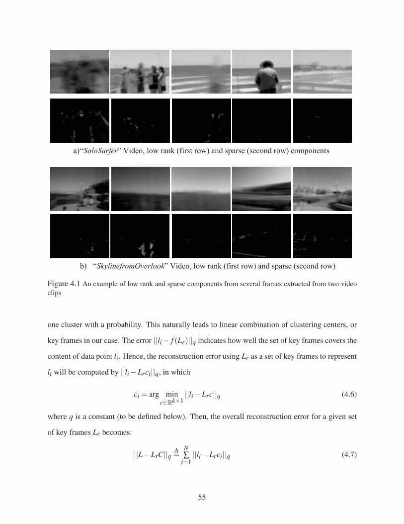
a)“SoloSurfer” Video, low rank (first row) and sparse (second row) components

b) “SkylinefromOverlook” Video, low rank (first row) and sparse (second row)

Figure 4.1 An example of low rank and sparse components from several frames extracted from two video

clips

one cluster with a probability. This naturally leads to linear combination of clustering centers, or

key frames in our case. The error ||li− f (Lr)||q indicates how well the set of key frames covers the

content of data point li. Hence, the reconstruction error using Lr as a set of key frames to represent

li will be computed by ||li −Lrci||q, in which

ci = arg minc∈Rk×1

||li −Lrc||q (4.6)

where q is a constant (to be defined below). Then, the overall reconstruction error for a given set

of key frames Lr becomes:

||L−LrC||q Δ=

N∑

i=1||li −Lrci||q (4.7)

55

Second, the distinct information associated with each video frame, si ∈ Sr, can be by measured

using its �1 norm:‖si‖1. Hence, the total distinct information of the set of key frames isk∑

j=1

∥∥∥st j

∥∥∥1,

which should be maximum for a good selection of key frames (with a fixed cardinality). Combining

these two terms leads to an overall non-convex optimization problem:

{lt1 , lt2 , . . . , ltk

}= argmin

Lr||L−LrC||q − γ

k∑

j=1

∥∥∥st j

∥∥∥1

(4.8)

s.t. Lr ⊆ L and #Lr = k

Here, γ>0 is a regularization constant parameter that indicates the relative importance of two

components. In the experiment, these two components are considered equally important, so we

select γ=1.

As we mentioned earlier in related works, we expect to search for a subspace that contains the

largest number of data points. Hence, 0 < q ≤ 1 leads to the ability of recovering the underlying

subspaces with an overwhelming probability. Therefore, in our work, we select q = 1, and the

problem (3.8) can be considered as a specific case of recovering the best �0 subspace with an

additional condition that the subspace must be spanned by elements from the input dataset (key

frames).

{lt1 , lt2 , . . . , ltk

}= argmin

Lr||L−LrC||1 − γ

k∑

j=1

∥∥∥st j

∥∥∥1

(4.9)

s.t. Lr ⊆ L and #Lr = k

This selection distinguishes our �1-norm based optimization from other �2-norm based optimiza-

tion methods in image collection/video summarization [12][38]. More interestingly, our result is

also consistent with other results from the compressive sensing theory area [39]. In particular, let

us denote X Δ=[∥∥l1 −LrC1,:

∥∥1, . . . ,

∥∥lN −LrCN,:

∥∥1

]T ∈ RN×1. Then ‖X‖1 = ||L−LrC||1. In this

case, X is a vector of distances from a data point to the linear subspace spanned by the selected

key frames Lr. Since the �1 norm-based minimization problem tends to encourage solutions to be

sparse [39], the linear space spanned by Lr contains the maximum number of elements from the

input dataset (or the best �0 subspace). Despite the merits of using �1-norm, the solution obtained

56

from �1 norm based problem might not be unique. However, under this circumstance, the addi-

tional constraint of maximizing the total distinct information leads to the unique solution for (3.9).

In addition, we take advantages of using �2 norm by considering the least square solution as an ini-

tial solution in an iterative process when solving (3.9). The detailed algorithm and corresponding

solution is presented in the next subsection.

4.3.2 Proposed Solution

4.3.2.1 Iterative Algorithm for Non-convex Optimization Problem

The optimization problem (3.9) has a form that is close to dictionary learning for sparse repre-

sentation [40]. However, there are some key differences between these two problems. Dictionary

learning aims at finding good bases/frames for a given set of input data for sparse representation

(minimizing �0 norm of coefficients). Hence, the number of learned elements in that basis is huge.

Moreover, these learned bases may not contain exact elements in the dataset but sparse combina-

tion of atoms in the basis/frame, so they cannot be used as representatives of input dataset. As a

result, most existing algorithms in dictionary learning and sparse coding cannot be directly applied

into our optimization problem. In this work, we propose a novel iterative algorithm to solve the

problem (3.9) with some distinguished properties. Conventional iterative algorithms update all

elements simultaneously at each step that leads to some main drawbacks of slow convergence and

difficulty of solving sub-optimization problem inside a single step. We propose an algorithm that

divides each main update step into smaller sub-steps, so that elements will be updated sequentially

in a single sub-step. In addition, the updated formula guarantees to decrease the objective function

in (3.9) after a single step.

Recall that the objective function is to find a set of indices {t1, t2, . . . , tk}, for a given number

of k, that minimize the objective function:

||L−LrC||1 − γk∑

j=1

∥∥∥st j

∥∥∥1

(4.10)

57

Here, Lr = [lt1 , . . . , ltk ] is the corresponding low rank data matrix for the set of indices. Define

Lri,ξ as a matrix for the current set of key frames of ith sub-step in the ξ th main step: Lr

i,ξ =[lt1(ξ ) , lt2(ξ )

, . . . , lti(ξ ) , lti+1

(ξ−1) , . . . , ltk(ξ−1)

]where the algorithm already update i elements{

lt1(ξ ) , lt2(ξ )

, . . . , lti(ξ )

}. In the initial set of indices

{t1(0), t2(0), . . . , tk(0)

}, the algorithm fixes

Lr0,1 =

[lt1(0) , lt2(0)

, . . . , ltk(0)

]and computes the coefficient matrix:

C0,1 = arg minC∈Rk×N

||L−Lr0,1C||1 (4.11)

Since the solution of (4.11) becomes the input of the iterative process in the RPCA-KFE algorithm,

the exact solution is not strictly demanded. Therefore, we convert the problem into the least square

problem for fast and easy computation of the unique solution:

C0,1 = arg minC∈Rk×N

||L−Lr0,1C||2 (4.12)

Therefore,

C0,1 =((Lr

0;1)T

Lr0;1)−1

(Lr0;1)T L (4.13)

Let us consider the low rank component matrix of the current set of key frames Lri,ξ and the

corresponding coefficient matrix Ci,ξ =[C(ξ )

1 ,C(ξ )2 , . . . ,C(ξ )

i ,C(ξ−1)i+1 , . . . ,C(ξ−1)

k

]Tat the ith sub-

step of the ξ th main step of the algorithm. In this sub-step, to update lti+1

(ξ−1) into lti+1

(ξ ) , the

RPCA-KFE algorithm assumes that Lri,ξ/

{łti+1

(ξ−1)

}and Ci,ξ/

{C(ξ−1)

i+1

}Tare constants, and

then the optimization problem focuses only on lti+1

(ξ−1) and its corresponding coefficient row.

Using the property of decomposition of a matrix product as a sum of rank one matrices,

Lri,ξCi,ξ will be decomposed into the sum of two matrices:

Lri,ξCi,ξ = Lr

i,ξ/

{lti+1

(ξ−1)

}Ci,ξ/

{C(ξ−1)

i+1

}T

+ lti+1

(ξ−1)

{C(ξ−1)

i+1

}T (4.14)

58

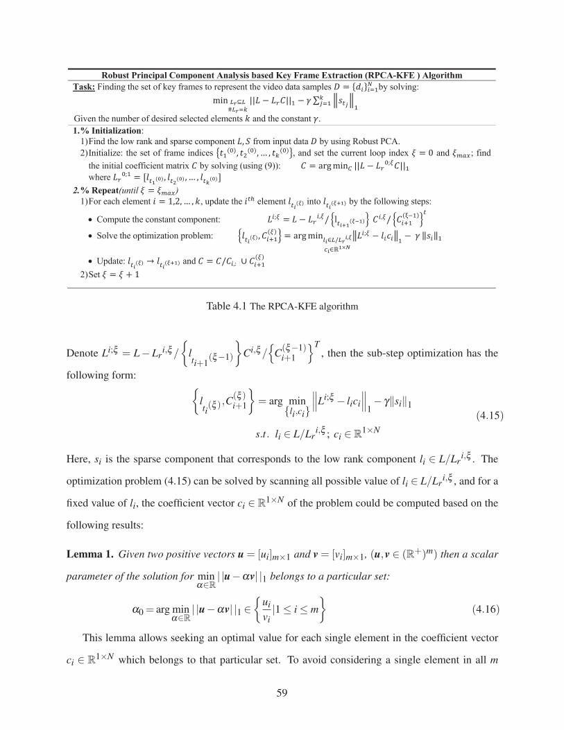
Robust Principal Component Analysis based Key Frame Extraction (RPCA-KFE ) Algorithm Task: Finding the set of key frames to represent the video data samples by solving:

Given the number of desired selected elements and the constant . 1. % Initialization:

1) Find the low rank and sparse component from input data by using Robust PCA. 2) Initialize: the set of frame indices , and set the current loop index and ; find

the initial coefficient matrix by solving (using (9)): where

2. % Repeat(until ) 1) For each element , update the element into by the following steps:

Compute the constant component:

Solve the optimization problem:

Update: and 2) Set

Table 4.1 The RPCA-KFE algorithm

Denote Li;ξ = L−Lri,ξ/

{lti+1

(ξ−1)

}Ci,ξ/

{C(ξ−1)

i+1

}T, then the sub-step optimization has the

following form: {lti(ξ ) ,C

(ξ )i+1

}= arg min

{li,ci}∥∥∥Li;ξ − lici

∥∥∥1− γ‖si‖1

s.t. li ∈ L/Lri,ξ ; ci ∈ R

1×N

(4.15)

Here, si is the sparse component that corresponds to the low rank component li ∈ L/Lri,ξ . The

optimization problem (4.15) can be solved by scanning all possible value of li ∈ L/Lri,ξ , and for a

fixed value of li, the coefficient vector ci ∈ R1×N of the problem could be computed based on the

following results:

Lemma 1. Given two positive vectors u = [ui]m×1 and v = [vi]m×1, (u,v ∈ (R+)m) then a scalar

parameter of the solution for minα∈R

| |u−αv| |1 belongs to a particular set:

α0 = arg minα∈R

| |u−αv| |1 ∈{

uivi|1 ≤ i ≤ m

}(4.16)

This lemma allows seeking an optimal value for each single element in the coefficient vector

ci ∈ R1×N which belongs to that particular set. To avoid considering a single element in all m

59

possible values of the set{

uivi|1 ≤ i ≤ m

}, the following simple result helps to determine the exact

solution:

Lemma 2. Without loss of generality, assuming that the sequence{

uivi|1 ≤ i ≤ m

}is a non-

decreasing sequence. Then, the unique solution for (12) is in the form ofut0vt0

where:

t0 = min1≤t≤m

t s.t.t

∑i=1

vi ≥m

∑i=t+1

vi (4.17)

The detail proof for Lemma 1 and 2 are given in the APPENDIX. Lemma 2 helps to determine

the exact solution without scanning all m possible solutions. In the experiment, m is the dimension

of high dimensional data points that is the number of image pixels in a visual dataset. There-

fore, not scanning all m possible solutions significantly improves the speed of convergence of the

algorithm.

4.3.2.2 RPCA-KFE with New Observations

In this section, we show how the proposed RPCA-KFE algorithm could be adapted to deal with

new observations. Matrices D(0),L(0),S(0) are respectively the current set of data points, low rank,

and sparse components as before. D(0)r = L(0)r + S(0)r is the set of selected key frames for the

current dataset. Let us use D(0) to denote the set of new observations and D(1)r = L(1)r +S(1)r where

L(1) and S(1) for the low rank and sparse components, founding using Robust PCA. The overall

problem (4.10) could be rewritten as:

argminLr

∥∥∥[L(0)L(1)]−Lr

[C(0)C(1)

]∥∥∥1− γ

k

∑j=1

∥∥∥st j

∥∥∥1

s.t. Lr ⊆[L(0)L(1)

]and #Lr = k (4.18)

Here,{

st j

}k

j=1are sparse components corresponding to Lr. Instead of starting solve the problem

from the beginning as in Section III.B, the algorithm will be adapted as follows. Since L(0)r is

the set of selected key frames for L(0) (the low rank component), it becomes the initial set of key

60

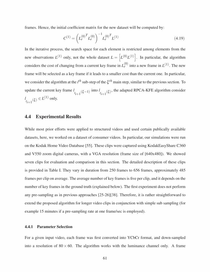
frames. Hence, the initial coefficient matrix for the new dataset will be computed by:

C(1) =

(L(0)r

TL(0)r

)−1

L(0)rT

L(1) (4.19)

In the iterative process, the search space for each element is restricted among elements from the

new observations L(1) only, not the whole dataset L =[L(0)L(1)

]. In particular, the algorithm

considers the cost of changing from a current key frame in L(0)r into a new frame in L(1). The new

frame will be selected as a key frame if it leads to a smaller cost than the current one. In particular,

we consider the algorithm at the ith sub-step of the ξ th main step, similar to the previous section. To

update the current key frame lti+1

(ξ−1) into lti+1

(ξ ) , the adapted RPCA-KFE algorithm consider

lti+1

(ξ ) ∈ L(1) only.

4.4 Experimental Results

While most prior efforts were applied to structured videos and used certain publically available

datasets, here, we worked on a dataset of consumer videos. In particular, our simulations were run

on the Kodak Home Video Database [55]. These clips were captured using KodakEasyShare C360

and V550 zoom digital cameras, with a VGA resolution (frame size of [640x480]). We showed

seven clips for evaluation and comparison in this section. The detailed description of these clips

is provided in Table I. They vary in duration from 250 frames to 656 frames, approximately 485

frames per clip on average. The average number of key frames is five per clip, and it depends on the

number of key frames in the ground truth (explained below). The first experiment does not perform

any pre-sampling as in previous approaches [25-26][38]. Therefore, it is rather straightforward to

extend the proposed algorithm for longer video clips in conjunction with simple sub sampling (for

example 15 minutes if a pre-sampling rate at one frame/sec is employed).

4.4.1 Parameter Selection

For a given input video, each frame was first converted into YCbCr format, and down-sampled

into a resolution of 80× 60. The algorithm works with the luminance channel only. A frame

61

of size 80 × 60 is converted to a column vector of dimension 4800 × 1. The input video be-

comes a dataset of high (normally full) rank matrix, dimension of [4800, number of frames]. Ro-

bust PCA method has been exploited to decompose the input data matrix into the low rank and

sparse components. We use the augmented Lagrange multiplier method for this kind of decom-

position because of its high accuracy in a small number of iterations. Some other parameters for

this decomposition include: the maximum number of iterations is set to 100, and the tolerance

of stopping criterion equals to 1e− 5, and the constant parameter balancing two components is

λ0 = 1/√

max(4800,number f rames) as suggested by Candes et al. [30]. Algorithm 1 has been

performed for the two obtained components. In the experiment, the initial set of key frames is

sampled uniformly from the video sequence. The parameter γ is selected as a rule of thumb, γ=1.

That means we consider these two types of information (distinct and systematic) to be equally

important. We test the obtained result with some different values of maximum iteration (stopping

rule), ξmax, and see that the algorithm converges quickly to the stable results in many cases. There

is only two videos (“SoloSurfer” and “SkylinefromOverlook”), where the obtained set of selected

key frames in second iteration (ξmax=3) is slightly different from the set of selected key frames

from the first iteration (ξmax=2). Therefore, in our experiments, we select the maximum number

of iterations ξmax=2 to minimize the computation burden. This implies that the algorithm requires

only one iteration with k sub-steps to stop.

4.4.2 Evaluation

In the proposed RPCA-KFE framework, we exploit the result description (visual comparison) and

subjective metric (quantitative comparison) approach. In particular, our results are compared with

the ground truth agreed by multiple human judges.

Visual Comparison: Figure 4.2 shows the result of “SkylinefromOverlook” video. The video

contains six key frames in the ground truth (the last row on the right figure), which was captured

outdoors with a significant amount of change in perspective and brightness. In this video, the

SR-based method [51] obtains 3.5 points. There are three frames (#28, 329, and 532) that get full

62

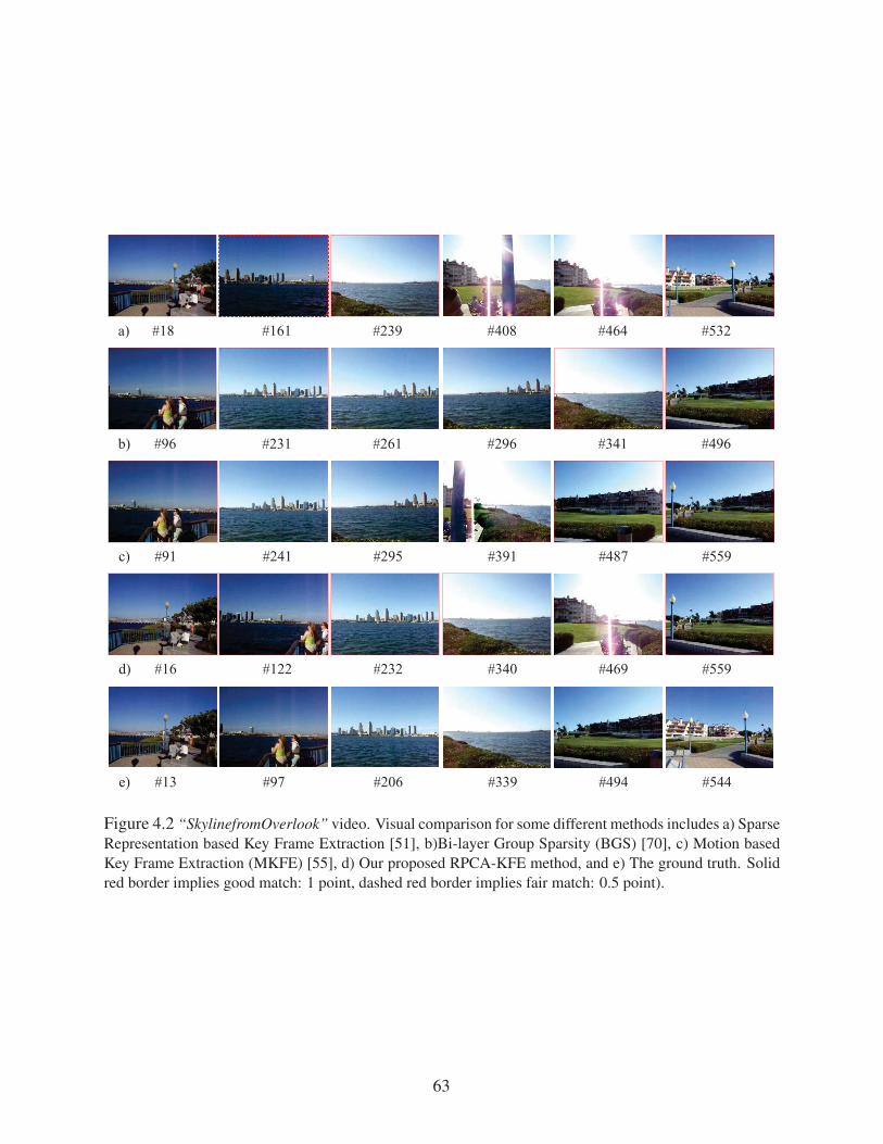
a) #18 #161 #239 #408 #464 #532

b) #96 #231 #261 #296 #341 #496

c) #91 #241 #295 #391 #487 #559

d) #16 #122 #232 #340 #469 #559

e) #13 #97 #206 #339 #494 #544

Figure 4.2 “SkylinefromOverlook” video. Visual comparison for some different methods includes a) Sparse

Representation based Key Frame Extraction [51], b)Bi-layer Group Sparsity (BGS) [70], c) Motion based

Key Frame Extraction (MKFE) [55], d) Our proposed RPCA-KFE method, and e) The ground truth. Solid

red border implies good match: 1 point, dashed red border implies fair match: 0.5 point).

63

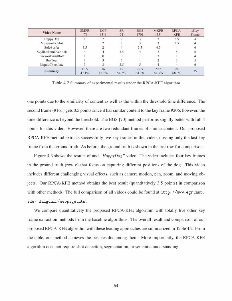
Video Name SMFR [7]

UCF [31]

SR [51]

BGS [70]

MKFE [55]

RPCA-KFE

#Key Frame

HappyDog 1 2 2 3 3 3.5 4 MuseumExhibit 3 2 3 3 3 3.5 4

SoloSurfer 3.5 2 4 5.5 4.5 4 6 SkylinefromOverlook 4 4 3.5 4 3 5 6

FireworkAndBoat 1 0 0 1 3 1 4 BusTour 1 3 3 1 2 3 5

LiquidChocolate 3 3 3.5 5 4 4 6

Summary 16.5 47.1%

16 45.7%

19 54.2%

22.5 64.3%

22.5 64.3%

24 68.6% 35

Table 4.2 Summary of experimental results under the RPCA-KFE algorithm

one points due to the similarity of content as well as the within the threshold time difference. The

second frame (#161) gets 0.5 points since it has similar content to the key frame #206; however, the

time difference is beyond the threshold. The BGS [70] method performs slightly better with full 4

points for this video. However, there are two redundant frames of similar content. Our proposed

RPCA-KFE method extracts successfully five key frames in this video, missing only the last key

frame from the ground truth. As before, the ground truth is shown in the last row for comparison.

Figure 4.3 shows the results of and “HappyDog” video. The video includes four key frames

in the ground truth (row e) that focus on capturing different positions of the dog. This video

includes different challenging visual effects, such as camera motion, pan, zoom, and moving ob-

jects. Our RPCA-KFE method obtains the best result (quantitatively 3.5 points) in comparison

with other methods. The full comparison of all videos could be found at ��������������� �

�� ��������������������.

We compare quantitatively the proposed RPCA-KFE algorithm with totally five other key

frame extraction methods from the baseline algorithms. The overall result and comparison of our

proposed RPCA-KFE algorithm with these leading approaches are summarized in Table 4.2. From

the table, our method achieves the best results among them. More importantly, the RPCA-KFE

algorithm does not require shot detection, segmentation, or semantic understanding.

64

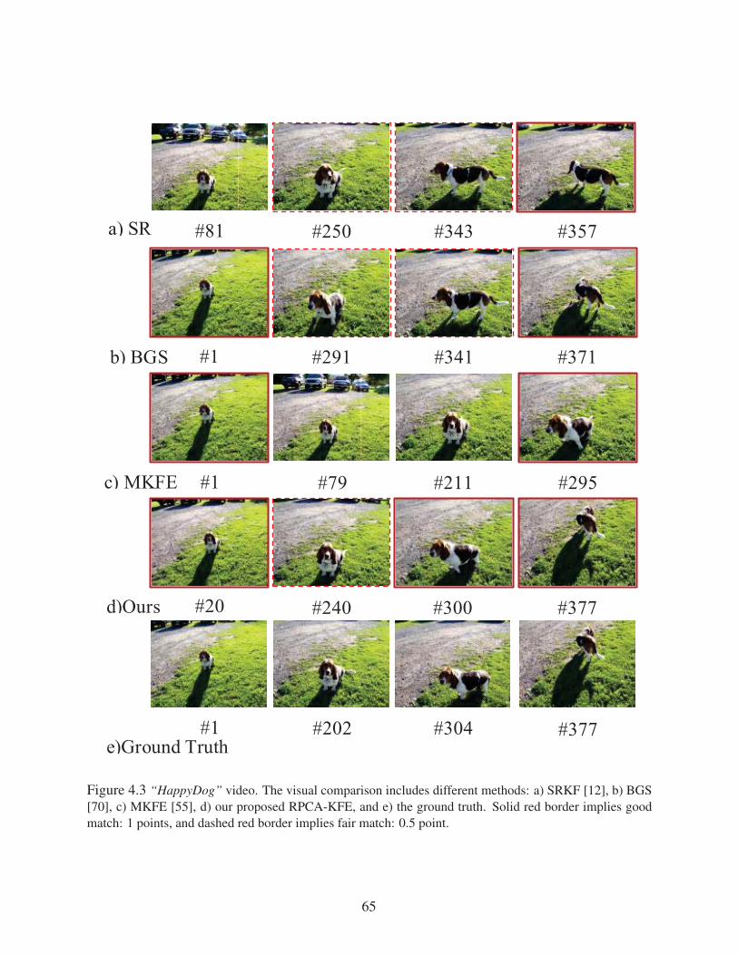
#81 #250 #343 #357

#1 #291 #341 #371

a) SR

b) BGS

#1 #79 #211 #295 c) MKFE

#20 #240 #300 #377 d)Ours

#1 #202 #304 #377 e)Ground Truth

Figure 4.3 “HappyDog” video. The visual comparison includes different methods: a) SRKF [12], b) BGS

[70], c) MKFE [55], d) our proposed RPCA-KFE, and e) the ground truth. Solid red border implies good

match: 1 points, and dashed red border implies fair match: 0.5 point.

65

4.4.3 Computational Complexity

Since the source codes of the other methods being compared here are not available, and the time

required for producing a set of key frames depends on a particular hardware, it is almost impossible

to produce a fair comparison in term of complexity among these methods. In this work, we evaluate

the average processing time per frame, as appeared in [33] to evaluate the complexity. According

to those experiments, our RPCA-KFE algorithm takes 1.469 second on average to process a single

frame, including 0.233 second per frame for Robust PCA decomposition input signal into low rank

and sparse components, and then solving an optimization problem (on average 1.236 second per

frame). This particular number depends on the computational power of the underlying hardware.

In our work, we used an Intel Core E7500 2.93Ghz platform. The average processing time per

frame could be reduced by a factor depending on a pre-sampling rate (if used), and the image size

ration in comparison with the size of 80x60, which we used in our experiments. For example,

using a pre-sampling rate of 1frame/sec, the average time per a single frame could be reduced into

0.0612 sec/frame.

4.5 Conclusions

An effective algorithm for key frame extraction from a consumer video has been proposed using

Robust Principal Component Analysis. Our work was based on the assumption that the low rank

component contains systematic information along with distinct information that is captured by the

sparse component of Robust PCA. We formulate the problem of key frame extraction from a video

as an optimization problem and analyzed the advantages of using �1 norm based optimization. A

greedy algorithm has been proposed to solve the non-convex optimization problem.

Chapter 4, in full, is reproduced from the material as it appears in: Chinh Dang and Hayder

Radha, "RPCA-KFE: Key Frame Extraction for Consumer Video based Robust Principal Compo-

nent Analysis" - arXiv:1405.1678

66

CHAPTER 5

HETEROGENEITY IMAGE PATCH INDEX AND ITS APPLICATION TO CONSUMERVIDEO SUMMARIZATION

5.1 Motivation

Natural images contain repetitive visual content. Small image patches in a given natural image have

a tendency to recur many times within the same image [15][118]. Patch-based analysis methods

have played a critical role in both analyzing and synthesizing visual data. Existing approaches

work based on the observation that a natural image usually contains abundance of short/long-range

correlation among patches. The observation of patch redundancy has been used successfully in

image denoising, image restoration [109-110].

In a different approach, Jojic et al. [84] introduced image epitome, and then further developed

by V. Cheung et al. [111] into video epitome. Epitome is created by exploiting the local and non-

local correlation among patches using a generative model. It is a condensed version of image/video

data that contains essential texture and shape information of the original image. Furthermore, we

have recently extended the utility of image epitome for key frame extraction [1]. Due to the nature

of applications, (e.g. denoising, inpainting, restoration, encoding, super-resolution), prior patch-

based techniques exploited the redundancy property of image patches to create or reconstruct high

quality image output. For example, example-based image super-resolution [101-102][120-121]

typically require the processing of a very large number of overlapped patches for the best output

high resolution image. Under the video summarization framework, we aim to two main problems:

• How to evaluate the level of non-redundancies (or uniqueness) that exists among image

patches in a video frame or an image.

• How is the level of non-redundancies correlated to the interest of people? If there is a con-

nection between the level of non-redundancies and the way people used to select a set of key

67

frames, that could be a foundation to solve the key frame extraction problem.

5.2 Related Works and Contributions

5.2.1 Related Works

The general area of video summarization has been researched for years due to its important role in

many video-related applications. Comprehensive reviews of previous approaches could be found

in [18-19], [21] and [28]. Here, we briefly outline some prior related efforts in two categories of

video summarization that directly relate to our proposed approaches.

DeMenthon et al. [112] represented a video sequence as a trajectory curve in a high dimen-

sional space. Using the classic binary curve splitting algorithm, the video curve can be recursively

split into binary structure. A video can then be represented as a tree structure, and key frames are

defined as functions between curve segments at different levels of the tree. Luo et al. [55] built

a ground truth for a set of typical consumer videos. By estimating the camera motion types, e.g.

pan, zoom, pause, and steady, a video clip is segmented into homogeneous parts, and then a set of

key frames from these parts is extracted. Kumar and Loui [51] projected video frames onto a low

dimensional random feature space, and then exploited the theory of sparse signal representation in

the projected space to generate key frames. The problem of key frame extraction could be seen as

a specific case of selecting a few representatives from a dataset that could be a video, or a set of

images/data points [7], [12].

In an effort to characterize viewer attention, user attention model, which is the fusion of visual

and aural attentions, has been proposed [113]. The attention curve is then generated for a video,

and a set of key frames are selected by considering crests on the curve. For a given skimming ratio,

skim segments are selected around each key frame of a shot. This method requires going through

the key frame extraction step to get a video skim. In addition, it makes an underlying assumption

that a key frame should be at the center (in time index) of an extracted segment within the target

video skim. On a different effort of soccer video abstraction, an excited commentary is anticipated

68

to correspond to an interesting moment of a soccer game [62]. A detector of excited speech seg-

ments has been proposed based on an increase of the pitch (or fundamental frequency) and energy

within voiced segments. Two different features using dominant color and camera motion analysis

are then performed to distinguish between speech sequences of the game and in commercials.

5.2.2 Contributions

The main contributions of this chapter include:

(i) We propose a new patch-based image/video analysis approach. Using the new model, we

create a new feature that we refer to as the heterogeneity image patch (HIP) index of an image

or a video frame. The HIP index, which is evaluated using patch-based image/video analysis,

provides a measure for the level of heterogeneity (and hence the amount of redundancy) that

exists among patches of an image/video frame.

(ii) By measuring the HIP index for each video frame, we generate a HIP curve that becomes a

characteristic curve of a video sequence. Based on the proposed HIP framework, we apply

the HIP index and HIP curve function to solve both of the video summarization problem

areas: key frame extraction and video skimming.

(iii) We propose a novel Accumulative Patch Matching Image Dissimilarity (APMID) measure.

Under the key frame extraction framework, a set of candidate key frames is selected from

abundant video frames based on the HIP curve. Then, the APMID measure is exploited to

create the affinity matrix of these candidate key frames. The final set of key frames has been

detected using the min-max algorithm [1].

(iv) We propose a new method for measuring the distance between an input video and its skimmed

version based on the HIP curve and Fréchet distance [114-115], called HIP-based video dis-

tance. The distance, if seen generally, can be applicable to any measurement of 1D-based

summarization methods. Then, we develop an automated algorithm to directly extract a set

of essential video excerpts by solving an optimization problem that minimizes the HIP-based

69

video distance between an input video and its skimming for given constrains. We conclude

our analysis by formulating the main result of the HIP optimization problem as a theorem.

We also show the viability of the proposed HIP framework through extensive simulations.

5.3 The Proposed Heterogeneity Image Patch Index

Denote [a,b] := {t|a ≤ t ≤ b; t ∈ N}. Under the proposed patch-based image/video analysis, we

represent a frame using two sets (U and LU ). The first one, U , is the set of all non-overlapping

patches; and where each of these patches is represented by the vector form ui ∈ Rm(i ∈ [1,r] ,r

is the total number of patches obtained from an image, and each patch contains m pixel values).

These values are usually natural numbers, however, we are using the real set mainly to cover

the most general case of possible values and to be consistent with obtained averaged values. The

second set, LU , represents the set of positions (or locations) of these patches over the image domain

lui ∈N2(i ∈ [1,r]) in which lui is a two dimensional vector defined by the upper left pixel of patch

ui in the image. Thus, the two sets U and LU can be expressed as follows:

U = {ui|ui ∈ Rm, i ∈ [1,r]} (5.1)

LU = {lui ∈ N2|ui ∈U, i ∈ [1,r]} (5.2)

Our framework exploits the short/long range correlation properties of image patches by using two

parameters: a threshold ε , and a metric to measure distance between two patches, ui,u j,1≤ i, j ≤ r

denoted by∥∥ui −u j

∥∥. In our experiments, we exploited the sum absolute difference metric that

has been used successfully in some video applications, such as block-based motion estimation.

A patch, e.g. u j, is considered as a distorted version of a different patch ui, which is assumed

as a sample vector drawn according to an underlying distribution, if∥∥ui −u j

∥∥ < ε; or (ui,u j)

are considered two distinct sample vectors if∥∥ui −u j

∥∥ ≥ ε . This strategy allows creating an

underlying probability model PU (ε) of an image U for a given threshold ε in the form:

PU (ε) = {(uk, pk)|uk ∈U,k ∈ [1,nr]} (5.3)

70

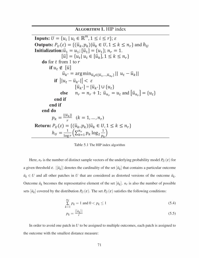
ALGORITHM 1. HIP index

Inputs: ; Outputs: and Initialization: ; .

do for from 1 to

if

if = [ else and end if end if

end do ( )

Return:

Table 5.1 The HIP index algorithm

Here, nr is the number of distinct sample vectors of the underlying probability model PU (ε) for

a given threshold ε . |[uk]| denotes the cardinality of the set [uk] that contains a particular outcome

uk ∈ U and all other patches in U that are considered as distorted versions of the outcome uk.

Outcome uk becomes the representative element of the set [uk]. nr is also the number of possible

sets [uk] covered by the distribution PU (ε). The set PU (ε) satisfies the following conditions:

nr∑

k=1pk = 1 and 0 < pk ≤ 1 (5.4)

pk =|[uk]|

r (5.5)

In order to avoid one patch in U to be assigned to multiple outcomes, each patch is assigned to

the outcome with the smallest distance measure:

71

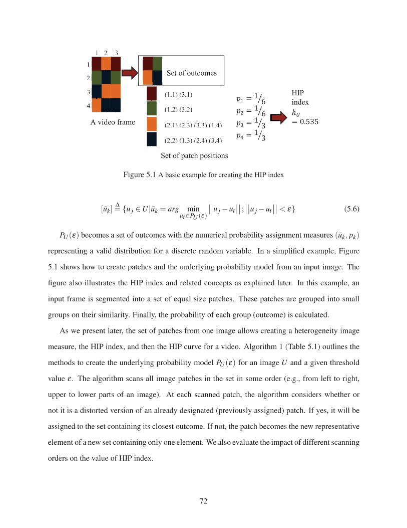
A video frame

(1,1) (3,1)

(1,2) (3,2) (2,1) (2,3) (3,3) (1,4) (2,2) (1,3) (2,4) (3,4)

Set of outcomes

Set of patch positions

HIP index

1

2 3 4

1 1 2 3

Figure 5.1 A basic example for creating the HIP index

[uk]Δ= {u j ∈U |uk = arg min

ut∈PU (ε)

∣∣∣∣u j −ut∣∣∣∣ ; ∣∣∣∣u j −ut

∣∣∣∣< ε} (5.6)

PU (ε) becomes a set of outcomes with the numerical probability assignment measures (uk, pk)

representing a valid distribution for a discrete random variable. In a simplified example, Figure

5.1 shows how to create patches and the underlying probability model from an input image. The

figure also illustrates the HIP index and related concepts as explained later. In this example, an

input frame is segmented into a set of equal size patches. These patches are grouped into small

groups on their similarity. Finally, the probability of each group (outcome) is calculated.

As we present later, the set of patches from one image allows creating a heterogeneity image

measure, the HIP index, and then the HIP curve for a video. Algorithm 1 (Table 5.1) outlines the

methods to create the underlying probability model PU (ε) for an image U and a given threshold

value ε . The algorithm scans all image patches in the set in some order (e.g., from left to right,

upper to lower parts of an image). At each scanned patch, the algorithm considers whether or

not it is a distorted version of an already designated (previously assigned) patch. If yes, it will be

assigned to the set containing its closest outcome. If not, the patch becomes the new representative

element of a new set containing only one element. We also evaluate the impact of different scanning

orders on the value of HIP index.

72

5.3.1 Heterogeneity Image Patch Index

Using the underlying patch probability model PU (ε) obtained from a set of patches U , we define

the HIP index for an image U as the normalized entropy of PU (ε). Therefore, the HIP index of an

image U , denoted by hU , is given by:

hU = 1logr

( nr∑

k=1pklog2

1pk

)(5.7)

Where r is the total number of patches in the input image U , and nr ≤ r is the number of

outcomes in the underlying probability model PU (ε). Note that if nr = r, then this implies that the

minimum distance among every pair of patches is beyond the threshold value ε; hence, PU (ε) ={(ui,

1r

)|ui ∈U,1 ≤ i ≤ r

}. Therefore, logr becomes the normalized parameter as the maximum

possible entropy for a given image U . As a result, the HIP parameter is normalized within the

range 0 ≤ hU ≤ 1. The HIP index intuitively reveals the amount of detail information through the

entropy of the underlying probability model of image patches. In video summarization, key frames

are the most informative frames that capture salient and new events in a video [55]. As a result,

we expect a connection between an informative frame and the diversity among the set of image

patches under consideration. In addition, a key frame should be evaluated within the context of the

whole video sequence. Therefore, our algorithm considers both the HIP index, and subsequently

the HIP curve of a video to select a final set of key frames. Before proceeding, we briefly address

three important questions regarding the proposed HIP index: (1) the impact of the threshold value

ε on the HIP index value, and (2) the impact of noise on the stability of the HIP index, and (3) the

impact of scanning order of image patches on the HIP index value.

The threshold value ε has a salient impact on the value of HIP index for a given image. In

general, the HIP index hU (ε) is a non-increasing function of ε . Figure 5.2 shows the HIP index as

a function of threshold value ε (per pixel) for different images (the upper plot). In such evaluation,

the patch size can be selected relative to the size of the input image. In particular, Fingerprint

and Lena are of size 512× 512 and their patches are of size 16× 16, while Peppers and House

are of size 256× 256 and their patches are of size 8× 8. As we can see from this set of images,

73

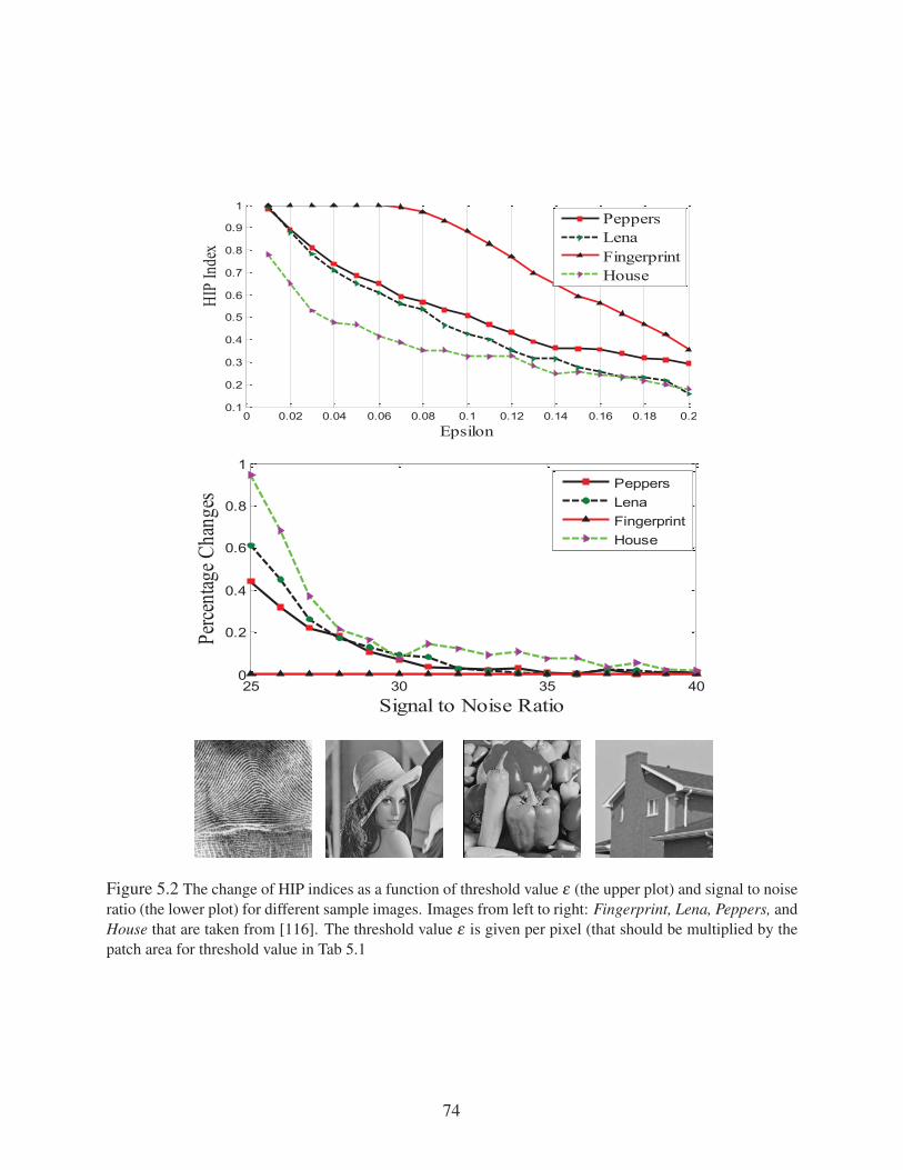
25 30 35 400

0.2

0.4

0.6

0.8

1

Signal to Noise Ratio

Perce

ntag

e Cha

nges

PeppersLenaFingerprintHouse

0 0.02 0.04 0.06 0.08 0.1 0.12 0.14 0.16 0.18 0.20.1

0.2

0.3

0.4

0.5

0.6

0.7

0.8

0.9

1

Epsilon

HIP

Inde

x

PeppersLenaFingerprintHouse

Figure 5.2 The change of HIP indices as a function of threshold value ε (the upper plot) and signal to noise

ratio (the lower plot) for different sample images. Images from left to right: Fingerprint, Lena, Peppers, and

House that are taken from [116]. The threshold value ε is given per pixel (that should be multiplied by the

patch area for threshold value in Tab 5.1

74

Fingerprint has the highest HIP index. This is expected since the image contains a high level of

detail information. Such picture can arguably form a benchmark for the selection of a patch size

and the threshold value. In particular, pictures that are similar to the Fingerprint image tend to have

quite high values for the HIP index. Subsequently, in our simulations, ε = 0.06 is selected as the

maximum threshold that leads to a HIP index of one (as is the case for the Fingerprint image). The

patch size is calculated according to the image size as we eluded above. For example, an image of

size 120×160 may use a patch of size 4×4. We follow these rules for the selection of parameters

that are used in our simulations. In addition, we also evaluate the impact of different patch sizes

on the algorithm performance.

Another important aspect is the impact of noise on the stability of the HIP index values. In

Figure 5.2 (the lower plot), we evaluate the changes of the HIP index value as a function of signal

to noise ratio (SNR) for the same above set of images. In this evaluation, the threshold value is

fixed (ε = 0.06). Percentages of changes are computed as the relative difference between the HIP

index of a noisy image and that of the original image (|HIPnoise −HIP|/HIP). The results show

that the HIP index is quite stable if the SNR is above a certain value, which is around 28db in

these examples of tested images. The HIP index of Fingerprint does not change for different SNR

values. This is expected since the parameter (ε = 0.06) is selected as the maximum threshold that

leads to a HIP index of 1. Adding noise to the image does not change the maximum value of the

HIP index (the distance between two patches after adding noise is still greater than the threshold

value).

Finally, we evaluate the impact of different scanning orders on the value of HIP index. We

select the threshold value ε = 0.06 and patch size accordingly as we mentioned above. The HIP

values are computed with four different scanning orders: (a) the default scanning order (from left

to right, upper to lower), (b) scanning from upper to lower, left to right (c) scanning from lower to

upper, right to left, and (d) scanning from right to left, lower to upper. The percentage of changes

are computed as the relative difference between the HIP indices of different scanning methods ((b),

(c), (d)), and the default scanning method (a)). The maximum percentage of changes for these four

75

testing images is 5.14%, which is relatively small when compared to the amount of changes caused

by a small amount of noise. In our experiment, we fix the default scanning order to be consistent

in the computation of the HIP curve.

5.3.2 Accumulative Patch Matching Image Dissimilarity

Using the representation of an image as two sets, one set of patch values, and the other of patch

locations, we propose a method in measuring image dissimilarity. Similar to image U of the form

in (1), image V is defined as follows:

V = {vi|vi ∈ Rm, i ∈ [1,r]} (5.8)

LV = {lvi ∈ N2|vi ∈V, i ∈ [1,r]} (5.9)

lvi is a two dimensional vector defined by the upper left pixel of patch vi in the image V . For

consistency, we consider same size images, and use an equal patch size. By judging two images,

the human visual system has a tendency to match each patch/object in one image to the most

identical patch/object in the other image. Furthermore, the difference in the positions of similar

objects/patches within the two images should also be taken into consideration. Based on these

arguments, we propose the Accumulative Patch Matching Image Dissimilarity (APMID) measure

between images U and V , denoted by D(U,V ), which is computed by considering the accumulative

difference between patch values and patch locations.

D(U,V ) =

⎧⎪⎪⎪⎪⎪⎨⎪⎪⎪⎪⎪⎩

r∑

i=1||ui − vi∗||E

(lui , lvi∗

)+

r∑

j=1||v j −u j∗||E(lv j , lu j∗)

⎫⎪⎪⎪⎪⎪⎬⎪⎪⎪⎪⎪⎭

(5.10)

where

vi∗ = arg minv j∈V

||ui − v j|| for i, j ∈ [1,r] (5.11)

u j∗ = arg minui∈U

||v j −ui|| for i, j ∈ [1,r] (5.12)

76

E(., .) is the Euclidean norm of two vector positions. This is a symmetric distance D(U,V ) =

D(V,U) in which each patch in U searches for the most identical patch in V and vice versa. The dif-

ference between two patches is scaled by the relative difference in the patch locations. In general,

the computation is intensive if it is performed for every single pair of frames from a video sequence.

However, in our method, the proposed APMID has been used only for computing the dissimilarity

among a small subset of candidate key frames, hence, decreasing the computational burden signifi-

cantly. The computation aspects will be discussed further in the experimental section. The APMID

measure increases in general if: i) the distance between two closest patches increases and/or ii) the

relative difference of two closest patch positions increases. Some other important properties of the

proposed APMID distance includes translation invariant, D(U +a,V +a) = D(V,U), and homo-

geneity, D(aU,aV ) = a×D(V,U) for a > 0. In addition, D(U,V )≥ 0 and D(U,V ) = 0 if and only

if (vi∗ = ui or lui = lvi∗) and (ui∗ = vi or lv j = lu j∗) for every 1 ≤ i, j ≤ r. We note that equations

(11) and (12) always have solutions for a given patch. It means that for a given image patch, its

closest patch in the other image exists. In a particular case, for some patches of U that are exactly

matched in V , these patches are simply discarded in the APMID measure, since ‖ui − vi∗‖= 0 (or

conversely) in this case.

The underlying probability model of images, PU and PV , could be used for measuring the

image dissimilarity. However, this kind of measurement ignores the important information of

patch locations, since an outcome uk is mapped to multiple positions in an image. We have tested

a statistical based measurement (the well-known Kullback-Leibler Divergence-based image dis-

similarity). However, the obtained results were not as good as the results of using the proposed

APMID method; consequently, we do not show the results for these aforementioned statistical

distance-measures in this work.

77

5.4 Extracting Key Frame from Video Using Heterogeneity Image Patch In-dex

5.4.1 Candidate Key Frame Extraction

Key frame selection focuses on identifying the minimal number of frames that can provide

users the highest amount of information about the overall video content and its scene(s). To sum-

marize the video content, the human-driven selection process arguably produces the best possible

set of key frames (at least subjectively). Under such assumption, the set of key frames selected by

an algorithm should be “close to”the set of key frames resulting from the subjective evaluation of

users. We observe that considering how people select key frames is the best approach in solving

key frame extraction problem, to make the result close to the human selection. By considering

positions of key frames on the HIP curve, one can make some general observations:

• Frames that are close to the beginning or toward the end (not necessarily the first or last

frame) can play a critical role in the selection of key frames in a video sequence. This is

consistent with the observation from [55], where the judges usually selected frames that are

in the proximity of the beginning and end of the video sequence.

• A key frame is within the vicinity of a local maximum value of the HIP index.

Based on these observations, we propose an algorithm to extract a set of candidate key frames,

which refer to a larger set of frames with high probability of containing key frames. First, the

algorithm divides a video sequence into segments of equal length (e.g. 50 frames), then the frame

with the maximum HIP index in each segment is selected as a candidate key frame. As we eluded

above, the beginning- and end-parts of a video sequence tend to have higher importance in term of

summarizing a video sequence; hence, we consider smaller segments at the beginning- and end-

regions.(e.g. 10 frames). The frames having maximum HIP indices in these two segments are

selected as candidate key frames as well.

78

0 50 100 150 200 250 300 350 400

0.35

0.4

0.45

0.5

0.55

0.6

0.65

Frame Index

HIP

inde

x

Figure 5.3 “LiquidChocolate”video. An example for selecting a set of candidate key frames. The ground

truth contains 6 key frames that are shown on the HIP curve with the red stars (the first key frame is hidden

by the third candidate key frame). The algorithm selects 10 candidate key frames that are shown with the

green circles, frame indices 4 11 51 106 181 214 269 312 375 390. The visual display of candidate key

frames and key frames from the ground truth are shown in Figure 5.6

ALGORITHM 2. Key frame extraction Task: Find the set of key frames to summarize a video content

Given input video and length of segments for local optimum point

Algorithm 1. Generate the HIP curve using Algorithm 1. 2. Generate set of candidate key frames:

The frames of maximum HIP indices in the beginning/ending segments are selected.

Input video is divided into segments of predetermined length ( frames).

The frames of maximum HIP indices in each segment will be selected.

3. Generate affinity matrix using the APMID. 4. Generate set of key frames using Algorithm 3.

Table 5.2 The key frame extraction algorithm

79

ALGORITHM 3. The min-max algorithm (summary) Inputs: Set of candidate key frames, number of key frames. Outputs: The final set of key frames. Begin

1. Create the affinity matrix based on the APMID measure. 2. Detect the first two key frames of having the maximum

APMID measure. 3. Repeat until enough key frames are acquired:

Scan all remaining frames Select a key frame, for which its minimum distance to

the previous selected key frames get maximum. End

Table 5.3 The min-max algorithm for HIP-based key frame extraction

Our technique of extracting candidate key frames from a video sequence is purely based on its

HIP curve. Therefore, it is more suitable than relying on camera motions [55] such as zoom in,

pan, zoom segment or other information that is not always available in every video. In addition,

the proposed algorithm demands a single parameter, the length of the segment, for extracting

a candidate key frame that coincides with a local maximum HIP index in the segment. More

importantly, the proposed HIP approach provides an improvement over the performance of the

uniform pre-sampling approach as used in many other approaches where the sampling rate is fixed

(e.g. one frame per second [32]). Figure 5.6 shows one example of sampling candidate key frames

based on HIP index for “LiquidChocolate” video [55]. The visual displays of these candidate

key frames are displayed in Figure 5.6 in the experiment section. Since the retrieval of candidate

key frames is based solely on the HIP curve without considering the spatio-temporal information

[117], the set of candidate frames may include a set of redundant key frames that have similar

visual content. However, the retrieval of the final key frames is not only based on the HIP curve,

where the set of candidate key frames is extracted. An additional step, which is based on the

APMID for the affinity matrix and the min-max algorithm [1] is also used. This additional step,

which is presented in the next section, allows detecting a good set of key frames, while minimizing

80

the number of redundant frames. On the other hand, the method of video summarization based on

spatio-temporal derivatives [117] also requires the final step of redundancy reduction. Hence, the

spatio-temporal feature based approach does not guarantee a redundancy-free key frame selection.

5.4.2 Selection of The Final Set of Key Frames

The next step of our approach makes use of the APMID distance to select key frames among

the small set of candidate key frames. Since the retrieval of the candidate key frames is absolutely

based on the HIP curve, the obtained set of candidate key frames may contain redundant frames.

The affinity matrix that contains pairwise distance of every pair of candidate key frames is com-

puted using the proposed distance. The traditional clustering based approach, e.g. normalized

cut algorithm [73], could be used to select the final set of key frames. Previous clustering-based

methods usually select the center frame (in term of time index within a video sequence) of each

cluster as a key frame for that cluster. On a different approach, the min-max algorithm has been

used successfully in the problem of key frame extraction from consumer videos [1]. There are key

differences between the HIP -based approach and the one used in [1]. The only common point

between the HIP-based method and the previous epitome-based approach is the use of the min-

max algorithm in the final stage of key frame extraction. First, the min-max algorithm has been

used here only for the set of candidate key frames, which are extracted based on the HIP curve

as explained above. The number of HIP-based candidate key frames is significantly smaller than

the total number of frames in a whole input video sequence, over which the min-max algorithm is

applied to in [1]. Second, we exploit the novel APMID measure to create an affinity matrix. On

the last step, the min-max algorithm [1] has been used on the affinity matrix for the final set of

key frames. Details and an example of the min-max algorithm could be found in [1]. Algorithm

3 (Tab.5.4) outlines the min-max algorithm. In this case, the benefit of the min-max algorithm

is twofold. First, it is optimum in each step. The algorithm would select the next frame as the

best frame given the previous selected key frames. Second, it is consistent and synergetic with

the problem of key frame extraction in the following sense. It preserves previously selected key

81

frames when the number of desired key frames increases. For example, initially we might prefer to

select four key frames from a given video; then, we might wish to increase the number of selected

key frames to five (or any number larger than the original four). In this case, the four previously

selected key frames will be a subset of the set of five key frames selected afterward (for the same

given video). Experimental results confirm that the min-max algorithm [1] based selection leads

to a better set of key frames compared to the clustering based approaches in almost all of the

tested videos; however, we do not focus on this comparison in the paper. Algorithm 2 (Tab.5.2)

summarizes the key frame extraction algorithm.

5.5 Dynamic Video Skimming Using Heterogeneity Image Patch Index

5.5.1 Video Skimming Problem Statement

The video skimming problem can be stated as searching for an optimal set of excerpts that min-

imizes the distance between the original video and its skimming, given a skimming ratio (or a

length of a skimmed video) and the input video V . The set needs to satisfy two main constraints:

• The total length of all excerpts in the set (length of video skimming) equals a given input

parameter l.

• The length (number of frames) of an excerpt ≥ lmin.

Denote A as the set of all possible skimmed videos satisfying the two above constraints [21] as

follows:

A =

{V1 ◦V2 ◦ . . .◦Vk|

k∑

i=1|Vi|= l,Vi ⊂V, |Vi| ≥ lmin

}(5.13)

where Vi(1 ≤ i ≤ k) is an extracted excerpt from the input video V , and |Vi| is the number of

frames in that excerpt. The optimum solution for the skimming video can be formulated as follows:

S∗ = argminS∈A

D(S,V ) (5.14)

82

Task: Create a skimmed video for a given input video , minimum length of an excerpt

and skimming ratio (or length of the desired skimmed video).

Algorithm

Initialization:

Generate the HIP indices for ;

Consider as a big remaining segment, and select one excerpt (of length computed

based on skimming ratio) (*)

o Scan all possible excerpt of length

o Select the excerpt of the minimum distance to the remaining segment

o Update the set of new remaining segments

Select the next remaining segment among set of remaining segments ,…, (**)

o For each remaining segment , compute (as in theorem 1)

o The remaining segment with maximum will be selected as the next remaining

segment.

Repeat until converge (stopping rule):

Select one excerpt from the next remaining segment (same procedure as (*))

Update the set of new remaining segments

Select the next remaining segment (same procedure as (**))

Table 5.4 The video skimming algorithm

Here, D(S,V ) measures the dissimilarity between the skimmed video S and its original video V .

Designing a good measurement D(S,V ) as well as solving the optimization problem (5.14) are key

contributions in our proposed framework. Below, we consider a HIP-based method in formalizing

a distance D(S,V ), and propose an optimal algorithm for solving (5.14).

5.5.2 HIP-based Video Distance

Let HV be the set of HIP indices for a given video V :

HV = {ht |t ∈ [1,n]} (5.15)

83

here, ht is the HIP index of the tth frame of the input video sequence V containing n frames. For a

given video skimming S ∈ A, the set of HIP indices is given by:

HS = {ht |t ∈ [Bi,Ei] ; i ∈ [1,k]} (5.16)

where Bi and Ei are indices of the beginning and ending frames of the ith excerpt among k excerpts

of S. |HS|= |S|= l is the number of elements in each set and Ei−Bi ≥ lmin−1 is the requirement

of minimum length for an excerpt.

Based on the idea of coupling between two polygonal curves, and the discrete Fréchet dis-

tance [114-115], which is a distance measure between polygonal curves, we construct a HIP-based

coupling, with one additional constraint to make it more suitable for the skimming problem. In

particular, we define the HIP coupling C between two polygonal curves HV and HS as follows:

C ={(

h1,ha1

),(

h2,ha2

), . . . ,(hn,han)

}(5.17)

In which ha j ∈ HS for j ∈ [1,n] is a HIP index that is taken from the set HS to match with the jth

HIP index (h j) from the video. A coupling satisfies two boundary conditions: a1 = B1, an = Ek;

and we have a j ≤ a1+ j and a j ∈ {t|t ∈ [Bi,Ei]&i ∈ [1,k]} which is the set of frame indices from

the given video skimming S. In case a j = a1+ j, the two HIP indices (h j,h1+ j) in the original video

are mapped to one HIP index (ha j) of the video skimming. Since a frame in a skimmed video also

belongs to the original video sequence, so two HIP indices extracted from a single frame should

be matched with each other. Therefore, we require one additional constraint:(

ha j ,ha j

)∈ C for

j ∈ [1,n]. The constraint not only makes more sense for the video skimming problem, but also

restricts the range of search for an optimal skimmed video solution. The distance between a video

and its skimming D(S,V ) is now defined as the discrete Fréchet distance between their two HIP

curves:

D(S,V ) = minC

{maxj∈[1,r]

d(

h j,ha j

)∣∣∣∣∣(

h j,ha j

)∈C

}(5.18)

84

….

….

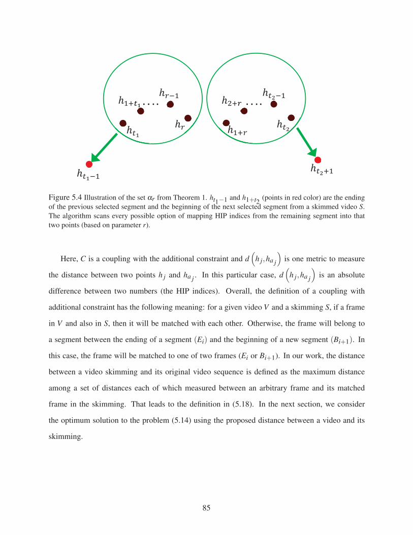
Figure 5.4 Illustration of the set αr from Theorem 1. ht1−1 and h1+t2(points in red color) are the ending

of the previous selected segment and the beginning of the next selected segment from a skimmed video S.

The algorithm scans every possible option of mapping HIP indices from the remaining segment into that

two points (based on parameter r).

Here, C is a coupling with the additional constraint and d(

h j,ha j

)is one metric to measure

the distance between two points h j and ha j . In this particular case, d(

h j,ha j

)is an absolute

difference between two numbers (the HIP indices). Overall, the definition of a coupling with

additional constraint has the following meaning: for a given video V and a skimming S, if a frame

in V and also in S, then it will be matched with each other. Otherwise, the frame will belong to

a segment between the ending of a segment (Ei) and the beginning of a new segment (Bi+1). In

this case, the frame will be matched to one of two frames (Ei or Bi+1). In our work, the distance

between a video skimming and its original video sequence is defined as the maximum distance

among a set of distances each of which measured between an arbitrary frame and its matched

frame in the skimming. That leads to the definition in (5.18). In the next section, we consider

the optimum solution to the problem (5.14) using the proposed distance between a video and its

skimming.

85

5.5.3 Optimal Solution

We mention the general idea of our proposed algorithm in solving the optimization problem (5.14)

with the HIP-based video distance. First, we state the following key result about the proposed

HIP-based Fréchet distance.

Theorem 5.1. Given a video V , and a skimmed video S. The remaining segments (the separated

parts of V , which are not included in S) are denoted by R1, . . . ,RT for which Rt = {ht1 ,ht1+1, . . . ,ht2}for t ∈ [1,T ] are the HIP indices of the tth segment. Let

αr =

⎧⎪⎨⎪⎩d(

hi,ht1−1

),d(h j,h1+t2

)

∣∣∣∣∣∣∣i ∈ [t1 −1,r]

j ∈ [r+1, t2 +1]

⎫⎪⎬⎪⎭ (5.19)

Dt = minr∈[t1−1,t2+1]

maxαr (5.20)

Then, we have D(S,V ) = maxt∈[1,T ]Dt .

We note that [t1, t2] ⊆ [a1,an] from (5.17), which denotes indices of tth segment. The proof

is given in the APPENDIX. Theorem 1 intuitively explains how a coupling matches one frame hr

from a remaining segment Rt to a selected segment in a video skimming. In particular, a frame

hr will be matched with the end of previously selected segment ht1−1 or the beginning of the

next selected segment ht2+1 in the skimming, and all other frames in that remaining segment wil

be assigned accordingly to satisfy the temporal constraint a j ≤ a1+ j. We illustrate the mapping

in Figure 5.4.The theorem considers every possible matching, and selects the one with minimum

value for each remaining segment, which is indicated in (5.20). Finally, the maximum of these

values considering every remaining segment equals the discrete Fréchet distance between there

two HIP curves appeared in (5.18). Based on the result of theorem 5.1, we could see that to

minimize the distance D(S,V ), an algorithm needs to minimize maxt∈[1,T ]Dt . This leads to the

skimming algorithm that is shown in Algorithm 5.4. Overall, this is a greedy algorithm with roots

that originated from the matching pursuit algorithm [54]. At first, an input video is considered

as one remaining segment. The algorithm scans for all possible excerpts and the one that has the

86

smallest distance (based on the Fréchet form in (5.18)) to this remaining segment is selected. A

video skimming now includes one selected excerpt. There are two (or possibly one if the selected

excerpt is at the beginning or end of the input video) remaining segments. The algorithm considers

how to select the next segment to extract an excerpt. The process is repeated until the algorithm

reaches the desired length of video skimming. For a given set of previous selected excerpts, the

selection based on our algorithm is optimal in minimizing the distance D(S,V ).

5.6 Experimental Results

In this section, we evaluate the proposed HIP-based video summarization framework for both key

frame extraction and video skimming. The algorithm is performed on consumer video, which is

more challenging to summarize than structured professionally-generated videos. Details of the

dataset, the ground truth and evaluation produce were introduced in chapter 2.

5.6.1 Key Frame Extraction

5.6.1.1 Parameter Selection

To be consistent, we employ the same technique in creating the HIP index/curve for these video

clips. In particular, each frame was first down-sampled into a resolution of 160× 120 The other

parameters include: patch size = 4×4 and ε = 0.06. We have covered the rationale for the selection

of these parameters in the previous section. The impact of different patch size selection onto the

overall algorithm performance will be discussed latter. In addition, the input frame of RGB channel

is converted into YCbCr, and the HIP index is computed for the luminance channel only. To extract

the initial candidate key frame set, we partition the video into segments, each of which consists

of 50 frames, and the frame of maximum HIP index for each segment is selected. In a more

sophisticated framework of video segmentation, automatic shot boundary detection algorithms

could be exploited to divide an input video into segments, and then candidate key frames could

be selected for each segment. However, these techniques require the selection of a good threshold

87

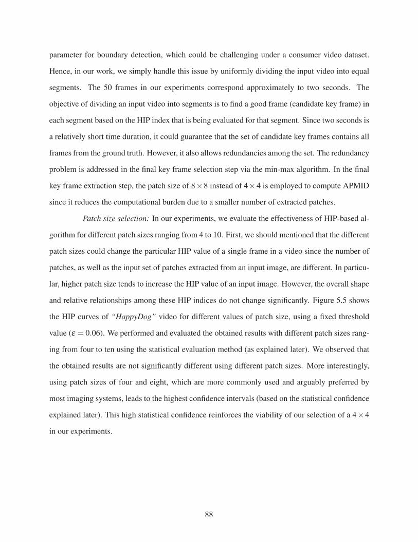
parameter for boundary detection, which could be challenging under a consumer video dataset.

Hence, in our work, we simply handle this issue by uniformly dividing the input video into equal

segments. The 50 frames in our experiments correspond approximately to two seconds. The

objective of dividing an input video into segments is to find a good frame (candidate key frame) in

each segment based on the HIP index that is being evaluated for that segment. Since two seconds is

a relatively short time duration, it could guarantee that the set of candidate key frames contains all

frames from the ground truth. However, it also allows redundancies among the set. The redundancy

problem is addressed in the final key frame selection step via the min-max algorithm. In the final

key frame extraction step, the patch size of 8×8 instead of 4×4 is employed to compute APMID

since it reduces the computational burden due to a smaller number of extracted patches.

Patch size selection: In our experiments, we evaluate the effectiveness of HIP-based al-

gorithm for different patch sizes ranging from 4 to 10. First, we should mentioned that the different

patch sizes could change the particular HIP value of a single frame in a video since the number of

patches, as well as the input set of patches extracted from an input image, are different. In particu-

lar, higher patch size tends to increase the HIP value of an input image. However, the overall shape

and relative relationships among these HIP indices do not change significantly. Figure 5.5 shows

the HIP curves of “HappyDog” video for different values of patch size, using a fixed threshold

value (ε = 0.06). We performed and evaluated the obtained results with different patch sizes rang-

ing from four to ten using the statistical evaluation method (as explained later). We observed that

the obtained results are not significantly different using different patch sizes. More interestingly,

using patch sizes of four and eight, which are more commonly used and arguably preferred by

most imaging systems, leads to the highest confidence intervals (based on the statistical confidence

explained later). This high statistical confidence reinforces the viability of our selection of a 4×4

in our experiments.

88

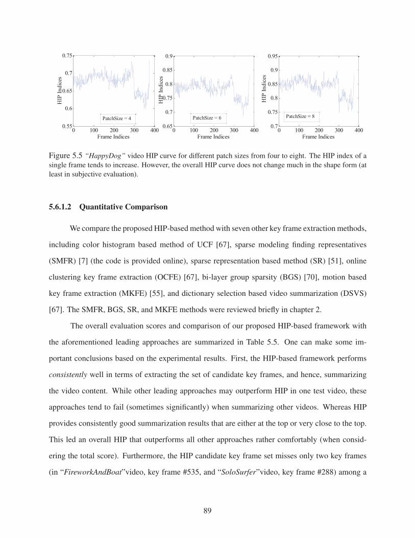
0 100 200 300 4000.55

0.6

0.65

0.7

0.75H

IP In

dice

s

Frame Indices0 100 200 300 400

0.65

0.7

0.75

0.8

0.85

0.9

Frame Indices

HIP

Indi

ces

0 100 200 300 4000.7

0.75

0.8

0.85

0.9

0.95

Frame Indices

HIP

Indi

ces

PatchSize = 4 PatchSize = 6 PatchSize = 8

Figure 5.5 “HappyDog” video HIP curve for different patch sizes from four to eight. The HIP index of a

single frame tends to increase. However, the overall HIP curve does not change much in the shape form (at

least in subjective evaluation).

5.6.1.2 Quantitative Comparison

We compare the proposed HIP-based method with seven other key frame extraction methods,

including color histogram based method of UCF [67], sparse modeling finding representatives

(SMFR) [7] (the code is provided online), sparse representation based method (SR) [51], online

clustering key frame extraction (OCFE) [67], bi-layer group sparsity (BGS) [70], motion based

key frame extraction (MKFE) [55], and dictionary selection based video summarization (DSVS)

[67]. The SMFR, BGS, SR, and MKFE methods were reviewed briefly in chapter 2.

The overall evaluation scores and comparison of our proposed HIP-based framework with

the aforementioned leading approaches are summarized in Table 5.5. One can make some im-

portant conclusions based on the experimental results. First, the HIP-based framework performs

consistently well in terms of extracting the set of candidate key frames, and hence, summarizing

the video content. While other leading approaches may outperform HIP in one test video, these

approaches tend to fail (sometimes significantly) when summarizing other videos. Whereas HIP

provides consistently good summarization results that are either at the top or very close to the top.

This led an overall HIP that outperforms all other approaches rather comfortably (when consid-

ering the total score). Furthermore, the HIP candidate key frame set misses only two key frames

(in “FireworkAndBoat”video, key frame #535, and “SoloSurfer”video, key frame #288) among a

89

Video Name SMFR UCF SR OCFE BGS MKFE DSVS HIP #KF (GroundTruth)

HappyDog 1 2 2 3 3 3 2.5 2.5 4 MuseumExhibit 3 2 3 2 3 3 2 4 4

SoloSurfer 3.5 2 4 3.5 5.5 4.5 4.5 4 6 SkylinefromOverlook 4 4 3.5 4.5 4 3 5 4.5 6

FireworkAndBoat 1 0 0 2 1 3 3 2 4 BusTour 1 3 3 2 1 2 3 3 5

LiquidChocolate 3 3 3.5 3.5 5 4 4.5 6 6 OrnateChurch 2 3 4 2.5 4 4 3 4 4

Summary 18.5 19 23 23 26.5 26.5 27.5 30 39

Table 5.5 Summary of experimental results under key frame extraction

total of 39 key frames in the ground truth. Second, the experimental results indicate that the HIP-

based algorithm performs quite well, achieving the highest quantitative score (total score of 30 out

of 39), with almost perfect results in “LiquidChocolate”and “MuseumExhibit”videos. The visual

comparison of “LiquidChocolate” video will be presented later.

5.6.1.3 Statistical Test

We employed the technique that has been used in [33] to verify the statistical significance

results of our method with different methods being compared. Table 5.6 shows the comparison

of our HIP-based method with other state-of-the-art methods using confidence interval of 95% in

which, if the confidence interval includes zero, the difference is not significant at that confidence

level; otherwise, the sign of the difference indicates which alternative is better [33, 48]. The min.

(max.) values in the table indicate the difference between the minimum (maximum) values between

two compared methods.The statistical analysis shows that the HIP-based approach leads to a set of

key frames with superior quality compared to other state-of-the-art consumer video summarization

methods, DSVS [67], MKFE [55], BGS [70], and SR [51].

5.6.1.4 Visual Comparison

Figure 5.6 shows the set of candidate key frames for LiquidChocolate video, and Figure

5.7. shows the visual comparison among several different methods: SRKF[51], BGS [70], MKFE

90

Measure HIP – DSVS HIP - MKFE HIP - BGS HIP - SR

min. max. min. max. min. max. min. max. Score 0.0068 0.1390 0.0561 0.0877 0.1592 0.0346 0.2359 0.1287

Table 5.6 Difference between our HIP-based techniques and other state-of-the-art methods at a confidence

of 95%

#4 #11 #51 #106 #181

#214 #269 #312 #375 #390

Figure 5.6 “LiquidChocolate” video. The set of candidate key frames. Frames in red border are selected

as final key frames.

[55], HIP-based approach, and the ground truth. The video contains six key frames in the ground

truth, which was captured inside a store. The HIP curve of this video is shown in Figure 5.3. The

initial set of candidate key frames includes ten frames including six key frames in the ground truth,

and four redundant frames. In this video, the SR method [51] obtains 3.5 points quantitatively

including 3 matched frames of full points (#179, #178) (#344, #334), (#380, #396). The first

frame #82 looks identical to #51 in the ground truth, however the time difference is above the

predetermined threshold (one second), so it gets 0.5 point. On the other case, #253 is very close

to #265 in the ground truth (only 11 frames in between), but the content is not similar. Therefore,

this frame gets zero point. The MKFE in this video detected four good frames (#43, 175, 343, and

391). The HIP-based algorithm extracts successfully all six key frames in this video among ten

candidate key frames, in both visual content as well as time difference.

Figure 5.8. shows the results for MuseumExhibit video and the visual comparison among

91

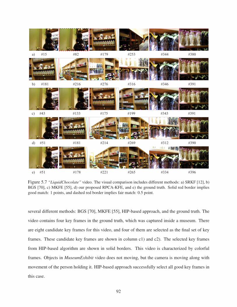
a) #15 #82 #179 #253 #344 #380

b) #181 #216 #276 #316 #346 #391

c) #43 #133 #175 #199 #343 #391

d) #51 #181 #214 #269 #312 #390

e) #51 #178 #221 #265 #334 #396

Figure 5.7 “LiquidChocolate” video. The visual comparison includes different methods: a) SRKF [12], b)

BGS [70], c) MKFE [55], d) our proposed RPCA-KFE, and e) the ground truth. Solid red border implies

good match: 1 points, and dashed red border implies fair match: 0.5 point.

several different methods: BGS [70], MKFE [55], HIP-based approach, and the ground truth. The

video contains four key frames in the ground truth, which was captured inside a museum. There

are eight candidate key frames for this video, and four of them are selected as the final set of key

frames. These candidate key frames are shown in column c1) and c2). The selected key frames

from HIP-based algorithm are shown in solid borders. This video is characterized by colorful

frames. Objects in MuseumExhibit video does not moving, but the camera is moving along with

movement of the person holding it. HIP-based approach successfully select all good key frames in

this case.

92

#10 #35 #93 #111

#192 #240 #242 #251

c1)

c2)

#1 #97 #223 #249

b)

#1 #51 #126 #231

#1 #120 #178 #244

d)

a)

Figure 5.8 “MuseumExhibit” video. The visual comparison includes different methods: a) BGS [70], b)

MKFE [55], c) HIP-based approach - 8 candidate key frames and the selected ones in solid border, and d)

the ground truth. Solid border implies good match: 1 points.

93

5.6.1.5 Computational Complexity

Since the source codes of the other methods being compared here are not available, and the

time required for producing a set of key frames or a video skimming excerpt depends on a partic-

ular hardware, it is almost impossible to produce a fair comparison in term of complexity among

these methods. In this paper, we evaluate the average processing time per frame, as appeared in

[33] to evaluate the complexity. According to those experiments, our HIP-based technique takes

0.3848 second on average to process a single frame, including the generation of a HIP curve, com-

puting the affinity matrix among candidate key frame using the APMID distance, and the min-max

algorithm. Among these steps, computing a single feature HIP index takes the longest time, on

average 0.2461 sec per frame. This particular number depends on the computational power of the

underlying hardware. In our work, we used an Intel Core E7500 2.93Ghz platform. The average

processing time per frame could be reduced by a factor depending on a pre-sampling rate, and the

image resize ratio in comparison with the size of 160× 120, which we used in our experiments.

For example, using a pre-sampling rate of 1frame/sec, the average time per a single frame could

be reduced into 0.016 sec/frame.

5.6.2 Video Skimming

5.6.2.1 Parameter Selection

In video skimming application, one needs to consider the minimum length of extracted excerpts.

For a fixed skimming ratio (or skimming length), a smaller length of an excerpt leads to a larger

number of excerpts, which could lead to a better ability of capturing the input video content.

However, very short excerpts annoy viewers since it is quite challenging for an average viewer to

gain much information from a very short one. Consequently, when generating a video skimming

summary, one needs to balance between the minimum length of these excerpt and the total number

of excerpts for a given skimming ratio. In this work, we selected the minimum length of an excerpt,

lmin, to be one second and the skimming ratio to be 20% of the total length of the original video.

94

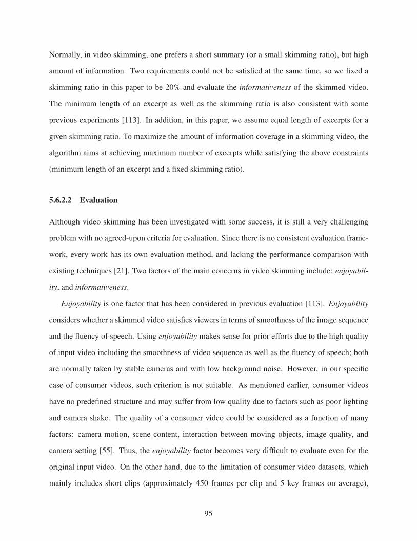
Normally, in video skimming, one prefers a short summary (or a small skimming ratio), but high

amount of information. Two requirements could not be satisfied at the same time, so we fixed a

skimming ratio in this paper to be 20% and evaluate the informativeness of the skimmed video.

The minimum length of an excerpt as well as the skimming ratio is also consistent with some

previous experiments [113]. In addition, in this paper, we assume equal length of excerpts for a

given skimming ratio. To maximize the amount of information coverage in a skimming video, the

algorithm aims at achieving maximum number of excerpts while satisfying the above constraints

(minimum length of an excerpt and a fixed skimming ratio).

5.6.2.2 Evaluation

Although video skimming has been investigated with some success, it is still a very challenging

problem with no agreed-upon criteria for evaluation. Since there is no consistent evaluation frame-

work, every work has its own evaluation method, and lacking the performance comparison with

existing techniques [21]. Two factors of the main concerns in video skimming include: enjoyabil-

ity, and informativeness.

Enjoyability is one factor that has been considered in previous evaluation [113]. Enjoyability

considers whether a skimmed video satisfies viewers in terms of smoothness of the image sequence

and the fluency of speech. Using enjoyability makes sense for prior efforts due to the high quality

of input video including the smoothness of video sequence as well as the fluency of speech; both

are normally taken by stable cameras and with low background noise. However, in our specific

case of consumer videos, such criterion is not suitable. As mentioned earlier, consumer videos

have no predefined structure and may suffer from low quality due to factors such as poor lighting

and camera shake. The quality of a consumer video could be considered as a function of many

factors: camera motion, scene content, interaction between moving objects, image quality, and

camera setting [55]. Thus, the enjoyability factor becomes very difficult to evaluate even for the

original input video. On the other hand, due to the limitation of consumer video datasets, which

mainly includes short clips (approximately 450 frames per clip and 5 key frames on average),

95

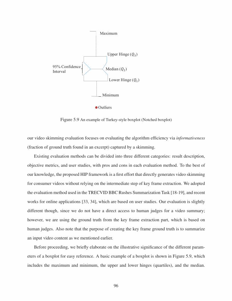
Maximum

Upper Hinge ( )

Median ( )

Lower Hinge ( )

Minimum

Outliers

95% Confidence Interval

Figure 5.9 An example of Turkey-style boxplot (Notched boxplot)

our video skimming evaluation focuses on evaluating the algorithm efficiency via informativeness

(fraction of ground truth found in an excerpt) captured by a skimming.

Existing evaluation methods can be divided into three different categories: result description,

objective metrics, and user studies, with pros and cons in each evaluation method. To the best of

our knowledge, the proposed HIP framework is a first effort that directly generates video skimming

for consumer videos without relying on the intermediate step of key frame extraction. We adopted

the evaluation method used in the TRECVID BBC Rushes Summarization Task [18-19], and recent

works for online applications [33, 34], which are based on user studies. Our evaluation is slightly

different though, since we do not have a direct access to human judges for a video summary;

however, we are using the ground truth from the key frame extraction part, which is based on

human judges. Also note that the purpose of creating the key frame ground truth is to summarize

an input video content as we mentioned earlier.

Before proceeding, we briefly elaborate on the illustrative significance of the different param-

eters of a boxplot for easy reference. A basic example of a boxplot is shown in Figure 5.9, which

includes the maximum and minimum, the upper and lower hinges (quartiles), and the median.

96

0

0.2

0.4

0.6

0.8

1

1 2 3 4 5Comparison Methods (1.SR, 2.BGS, 3.MKFE, 4.DSVS, 5.HIP-based Approach)

Frac

tion

of G

roun

d Tr

uth

Foun

d

Figure 5.10 Comparison of video summary using different methods

Some outliers may appear below the lower extreme or above the upper extreme. Quartiles are

three points that divide a data set into four equal parts. Lower hinge (Q1) is the first quartile that

splits off the lowest 25% of data. Median (Q2) is the second quartile that cuts the data set in half,

and the upper hinge (Q3) splits off the highest 25% of data from the lowest 75%.

In order to quantitatively evaluate the performance of the HIP-based video skimming, we clas-

sified an extracted excerpt as a good excerpt (received one point) if it contains a key frame from

the ground truth. Otherwise, if an extracted excerpt contains no key frame from the ground truth,

it will receive no point (not a good excerpt). We compare the quality of the HIP-based video skim-

ming with other key frame based video skimming approaches including DSVS [67], MKFE [55],

BGS [70], and SR [51], in which the overall results of these algorithms are presented as boxplots

[18][19][33] in Figure 5.10. Those graphs are sorted by the median of obtained scores for each

method for easier comparison. In some boxplots, several notches protrude beyond the hinges. That

is because medians lie very near to the hinges. The figure is plotted based on the boxplot function

in MATLAB. The results indicate that our HIP-based approach is among the best with respect to

the fraction of ground truth included in the video summary. We note that the proposed method

directly generate a video skimming without going through the key frame extraction step. In terms

of computation complexity, the algorithm needs to compute HIP indices of the video sequence

97

(0.2461 sec per frame as we mentioned previously) and on average 0.0331 sec per frame for the

video skimming algorithm.

5.7 Conclusions

We introduced the HIP index as a new feature of natural images and video sequences. Using

the HIP indices of a series of frames, a HIP curve can then be created for video analysis. We

demonstrated the effectiveness of the new feature in the problem areas of video summarization.

In key frame extraction, a set of candidate key frames is automatically extracted from the input

video. Then, we introduce a novel distance measure, which we refer to as APMID to measure

image dissimilarity. The final set of key frames is extracted from the candidate key frame set

using APMID and the min-max algorithm [1]. In dynamic video skimming, the HIP-curve is used

for measuring the dissimilarity between an input video and its skimmed version. We mapped the

skimming problem into an optimization problem that minimizes the HIP-based Fréchet distance.

The proposed algorithm was validated on consumer video datasets. The obtained results were

then compared with the ground truth, selected by human judges, as well as leading state-of-the-art

methods using the same datasets. Experimental results show that, among the evaluated approaches,

the HIP-based framework is the best method in terms of accuracy. In term of complexity, the HIP

index is naturally extracted from a video without any prior processing. Using only one dimensional

feature reduces the computational complexity relative to the other previous techniques that consider

an image as a feature point in a high dimensional space. We intend to extend the usage of the HIP

index into other applications.

Chapter 5, in full, is reproduced from the material as it appears in: Chinh Dang and Hayder

Radha, "Heterogeneity Image Patch Index and Its Application to Consumer Video Summarization"

- the IEEE Transactions on Image Processing , vol.23, no.6, pp.2704-2718, June 2014.

98

CHAPTER 6

CONCLUSIONS

In this dissertation, we developed and analyzed the performance of signal processing-based tech-

niques to solve the video summarization problem. In particular, three different models have been

proposed for key frame extraction and video summarization:

1. Sparse representation of video frames

2. Sparse and low rank model for video frames

3. Sparse/redundant representation for a single video frame

There are several areas in which our work can be extended. This includes:

(i) Human Visual System (HVS) Driven Video Summarization

Signal processing-based approaches exploited low-level features (such as color, texture, or

shape features) to solve the video summarization problem. On the other hand, high-level

features (concepts) are being used by human. Even though many sophisticated algorithms

have been designed to match these two levels, there are still many challenges to bridge a gap

between them. The video summarization problem is directly related to a subjective human

evaluation. As a result, we plan to tackle the problem from a different angle, starting with

high-level features of image and video.

(ii) High-Level Semantic Based Key-Frame Extraction and Video Skimming

Two types of video summarization, key frame extraction and dynamic video skimming, have

been considered in our work. Dynamic video skimming contains both audio and visual mo-

tion elements. As a result, it is more attractive for users than a set of static key frames.

However, there have been still only very few papers published on this challenging problem.

To address this challenging problem, we must resort to high-level semantic analysis.

99

(iii) A General HIP-Based Video Skimming Framework

So far, most of the proposed works for video skimming is based on the key-frame extraction

step and then considering each key frame as a middle frame of a fixed length excerpt. In

chapter 5, we have proposed the HIP-based approach for video skimming, which directly

generates a set of excerpts without going through key frame extraction step. Our HIP-based

approach, on the other hand, generated a video skim without the need to perform the key-

frame extraction step. One important reason why we were able to do that is that our HIP-

based skimming approach was designed and tailored for consumer video specifically (due

to the fact that this thesis addressed the area of consumer video datasets). Hence, the HIP

approach for video skimming worked well on consumer video since a typical consumer video

represents, in general, a single continuous shot; and hence, it does not normally include

different distinct segments or video shots. Consequently, it is not clear how well a HIP-

based approach would work on more general videos, and in particular, on professionally

generated structured video content. Therefore, a more general HIP-based approach needs to

be developed to handle any form of video.

100

APPENDICES

101

APPENDIX A

PROOF OF LEMMA 1 AND 2

.

Denote f (α) = | |u−α × v| |1 =m∑

i=1|ui −α × vi|. Without loss of generality, we assume that:

u0v0

=−∞ <u0v0

≤ u1v1

≤ . . .≤ umvm <

um+1vm+1

=+∞

Then, denote St =( ut−1

vt−1, ut

vt

]for 1 ≤ t ≤ m+1, we have the following properties:

⎧⎪⎨⎪⎩

Si ∩S j = /0(∀1 ≤ i �= j ≤ m+1)

R =m+1∪t=1

St

Assuming that α ∈ St , then

f (α) =t−1∑

i=1|ui −α × vi|+

m∑

i=t|ui −α × vi|

= α ×(

t−1∑

i=1vi −

m∑

i=tvi

)+

(m∑

i=tui −

t−1∑

i=1ui

)

Take the derivative of f (α) with α ∈(ut−1

vt−1, ut

vt

), we obtain the following result:

⎧⎪⎪⎨⎪⎪⎩

f (x)≤ f (y)∀utvt

≥ x ≥ y >ut−1vt−1

if

(t−1∑

i=1vi −

m∑

i=tvi

)≤ 0

f (x)≥ f (y)∀utvt

≥ x ≥ y >ut−1vt−1

if

(t−1∑

i=1vi −

m∑

i=tvi

)> 0

Denote t0 = min1≤t≤m

t s.t.t∑

i=1vi ≥

m∑

i=t+1vi. Since f (α) is a continuous function of α , the prop-

erty holds for R. In particular, we have:

102

⎧⎪⎨⎪⎩

f (x)≤ f (y) ∀ ut0vt0

≥ x ≥ y > u0v0

f (x)≥ f (y) ∀ um+1vm+1

> x ≥ y ≥ ut0vt0

Since

⎧⎪⎪⎪⎪⎨⎪⎪⎪⎪⎩

(t0−1

∑i=1

vi −m∑

i=tvi

)≤ 0(

t0∑

i=1vi −

m∑

i=t0+1vi

)> 0

As a result, f(

u0v0

)= min

α∈Rf (α).

103

APPENDIX B

PROOF OF THEOREM 5.1.

Let C be an arbitrary coupling with the additional constraint(

ha j ,ha j

)∈C for j ∈ [1,n] between

V and S. Let us consider the range [t1, t2] that corresponds to a remaining segment Rt , in which

the coupling has elements of d(

h j,ha j

)for j ∈ [t1 −1, t2 +1]. The additional constraint leads to(

ht1−1,ht1−1

)= d(

h1+t2 ,h1+t2

)= 0. Since

{d(

h j,ha j

)|t1 −1 ≤ j ≤ 1+ t2

}∈ {αr|t1 −1 ≤ r ≤ 1+ t2}

→ maxt1−1≤ j≤1+t2

d(

h j,ha j

)≥ Dt

Dt is defined from Theorem 1. Therefore, max1≤ j≤n

d(

h j,ha j

)≥ max

1≤t≤TDt . This conclusion

holds for an arbitrary coupling, so

minC

{max

1≤ j≤nd(

h j,ha j

)∣∣∣∣(h j,ha j

)∈C}≥ max

1≤t≤TDt

→ D(S,V )≥ max1≤t≤T

Dt (*)

On the other hand, one can construct a coupling C∗. For each 1 ≤ t ≤ T , one can employ the

following steps:

r∗ = argminr

maxαr

Then the coupling C∗ is constructed by:

ha j = ht1−1 if t1 −1 ≤ j ≤ r∗

ha j = ht2+1 if r∗ < j ≤ t2 +1

&ha j = h j for other values of j not in the range

[t1 −1, t2 +1] (1 ≤ t ≤ T ).

104

The coupling C∗ satisfies the additional constraint (h(a j),h(a j)

)∈Y ∗ for 1≤ j ≤ n. In addition,

max1≤ j≤n

d(

h j,ha j

)= max

1≤t≤TDt

≥ minC

{max

1≤ j≤nd(

h j,ha j

)∣∣∣∣(h j,ha j

)∈C}

(**)

(*)(**) lead to our result: D(S,V ) = max1≤t≤T Dt

105

APPENDIX C

PUBLICATIONS

C.1 Peer Reviewed Journal Papers

1. Chinh Dang and Hayder Radha, “Heterogeneity Image Patch Index and Its Application to

Consumer Video Summarization,” Image Processing, IEEE Transactions on, vol.23, no.6,

pp.2704-2718, June 2014. (IF: 3.111) (pdf)

2. Chinh Dang, M. Aghagolzadeh, and Hayder Radha, “Image Super-resolution via Local Self-

learning Manifold Approximation,” IEEE Signal Process. Letters, Vol. 21, No. 10, October

2014. (IF: 1.639) (pdf)

3. Chinh Dang and Hayder Radha, “RPCA-KFE: Key Frame Extraction for Consumer Video

based on Robust Principal Component Analysis,” submitted to Image Processing, IEEETransactions on, 2015. (pdf)

4. Chinh Dang and Hayder Radha, “Single Image Super Resolution via Manifold Approxima-

tion,”arXiv 2014. (To be submitted) (pdf)

5. Phong Pham, Chinh Dang and Yem Vu, “A novel Spectrum Sensing without Channel State

Information using Estimated Parameters,” Research, Development and Application on Infor-mation & Communication Technology Journal, Vol. E-1, No. 3 (7), Dec. 2010.

C.2 Peer Reviewed Conference Proceedings

1. Chinh Dang and Hayder Radha, “Fast Image Super Resolution via Selective Manifold Learn-

ing of High Resolution Patches,”-in Proceedings of 22th IEEE International Conference onImage Processing (ICIP’15), 2015. (accepted)

2. Chinh Dang, A. Safaie, M. Phanikumar, and Hayder Radha, “Poster Abstract: Wind Speed

and Direction Estimation Using Manifold Approximation,”- in Proceedings of the 14th ACMInternational Conference on Information Processing in Sensor Networks, (IPSN) 2015. (In

the finalist for best poster award) (Presentation)

3. Chinh Dang, Mohammed Al-Qizwini, and Hayder Radha, “Representative Selection for Big

Data via Sparse Graph and Geodesic Grassmann Manifold Distance,”- in Proceedings of48th IEEE Asilomar Conference on Signal, Systems, and Computers, 2014. (pdf)

4. Chinh Dang, M. Aghagolzadeh, A.A. Moghadam, and Hayder Radha, “Single Image Super

Resolution via Manifold Approximation using Sparse Subspace Clustering,”- in Proceedings

106

of 1st IEEE Global Conference on Signal and Information Processing (GlobalSIP) 2013.

(pdf) (Presentation)

5. Chinh Dang, M. Kumar, and Hayder Radha, “Key Frame Extraction From Consumer Video

using Epitome,”-in Proceedings of 19th IEEE International Conference on Image Processing(ICIP’12), Oct. 2012. (pdf) (Presentation)

6. Phong Pham, Chinh Dang and Yem Vu, “Or Rule and Parallel Processing Technique in Mul-

tiple Antennas for Spectrum Sensing,”- in Proceedings of 3rd IEEE International Conferenceon Communications and Electronics (ICCE), Aug. 2010. (pdf)

7. Phong Pham, Chinh Dang, Yem Vu, and Khang Nguyen “More Practical Spectrum Sensing

Technique in Cognitive Radio Networks,”- in Proceedings of IEEE International Conferenceon Advanced Technologies for Communications (ATC), Oct. 2010. (pdf)

107

BIBLIOGRAPHY

108

BIBLIOGRAPHY

[1] Chinh Dang, M. Kumar, and Hayder Radha, “Key frame extraction from consumer videos

using epitome,” in Proceedings of the IEEE International Conference on Image Processing(ICIP), pp. 93-96, 2012.

[2] Hinton, Geoffrey E., Peter Dayan, and Michael Revow, “Modeling the manifolds of images of

handwritten digits,”IEEE Transactions on Neural Networks, no. 1 (1997): 65-74.

[3] Frey, Brendan J., and Delbert Dueck, “Clustering by passing messages between data points,”

Science 315.5814 (2007): 972-976.

[4] Baraniuk, Richard G., and Michael B. Wakin, “Random projections of smooth manifolds,”

Foundations of Computational Mathematics 9.1 (2009): 51-77.

[5] Chinh Dang and Hayder Radha, “RPCA-KFE: Key Frame Extraction for Consumer Video

based Robust Principal Component Analysis,”arXiv:1405.1678 (2014).

[6] Elhamifar, Ehsan, Guillermo Sapiro, and René Vidal. “Finding Exemplars from Pairwise Dis-

similarities via Simultaneous Sparse Recovery.” Advances in Neural Information ProcessingSystems, pp. 19-27. 2012.

[7] Elhamifar, Ehsan, Guillermo Sapiro, and Rene Vidal, “See all by looking at a few: Sparse

modeling for finding representative objects,” in IEEE Conference on Computer Vision andPattern Recognition (CVPR), 2012, pp. 1600-1607.

[8] Boutsidis, Christos, Michael W. Mahoney, and Petros Drineas, “An improved approximation

algorithm for the column subset selection problem,”in Proceedings of the twentieth AnnualACM-SIAM Symposium on Discrete Algorithms, pp. 968-977. Society for Industrial and Ap-

plied Mathematics, 2009.

[9] Narendra, Patrenahalli M., and Keinosuke Fukunaga, “A branch and bound algorithm for fea-

ture subset selection,” IEEE Transactions on Computers 100, no. 9 (1977): 917-922.

[10] Balzano, Laura, Robert Nowak, and Waheed Bajwa, “Column subset selection with missing

data,”in NIPS Workshop on Low-Rank Methods for Large-Scale Machine Learning, vol. 1.

2010.

[11] Alan Miller, “Subset selection in regression,” CRC Press, 2012.

[12] Yang, Chunlei, Jialie Shen, Jinye Peng, and Jianping Fan, “Image collection summarization

via dictionary learning for sparse representation,”Pattern Recognition 46, no. 3 (2013): 948-

961.

[13] Wang, Yu, Sheng Tang, Yong-Dong Zhang, Jin-Tao Li, and Dong Wang. “Representative

selection based on sparse modeling.”Neurocomputing 139 (2014): 423-431.

109

[14] Kohavi, Ron, and George H. John, “Wrappers for feature subset selection,”Artificial intelli-gence 97, no. 1 (1997): 273-324.

[15] Chinh Dang, and Hayder Radha, “Heterogeneity Image Patch Index and its Application to

Consumer Video Summarization,”IEEE Trans. Image Processing 23(6): 2704-2718

[16] Elhamifar, Ehsan, and Rene Vidal, “Sparse subspace clustering: Algorithm, theory, and ap-

plications.”IEEE Transactions on Pattern Analysis and Machine Intelligence, no. 11 (2013):

2765-2781.

[17] Chinh Dang and Hayder Radha, “Representative Selection for Big Data via Sparse Graph

and Geodesic Grassmann Manifold Distance,”in Asilomar Conference on Signals, Systems,and Computers, November 2014

[18] P. Over, A. F. Smeaton, and P. Kelly, “The TRECVID 2007 BBC rushes summarization

evaluation pilot,” in Proc. Int. Workshop TRECVID Video Summarization, 2007, pp. 1–15.

[19] P. Over, A. F. Smeaton, and G. Awad, “The TRECVID 2008 BBC rushes summarization

evaluation,” in Proc. 2nd ACM TRECVID Summarization Workshop, 2008, pp. 1–20.

[20] Goldberger, Jacob, Shiri Gordon, and Hayit Greenspan. “An efficient image similarity mea-

sure based on approximations of KL-divergence between two Gaussian mixtures.”in IEEEInternational Conference on Computer Vision, 2003.

[21] Truong, Ba Tu, and Svetha Venkatesh, “Video abstraction: A systematic review and clas-

sification,”ACM Transactions on Multimedia Computing, Communications, and Applications(TOMCCAP) 3, no. 1 (2007): 3.

[22] Tang, Lin-Xie, Tao Mei, and Xian-Sheng Hua. “Near-lossless video summarization.”in Pro-ceedings of the 17th ACM international conference on Multimedia, pp. 351-360. ACM, 2009.

[23] Gong, Yihong, and Xin Liu, “Video summarization using singular value decomposition,”in

Computer Vision and Pattern Recognition, 2000. Proceedings. IEEE Conference on, vol. 2, pp.

174-180. IEEE, 2000.

[24] Jiang, Wei, Courtenay Cotton, and Alexander C. Loui. “Automatic consumer video summa-

rization by audio and visual analysis,”in Multimedia and Expo (ICME), 2011 IEEE Interna-tional Conference on, pp. 1-6. IEEE, 2011.

[25] A. Ekin, A. M. Tekalp, and R. Mehrotra, “Automatic soccer video analysis and summariza-

tion,” IEEE Trans. Image Process., vol. 12, no. 7, pp. 796–807, Jul. 2003.

[26] W.-T. Peng et al., “Editing by viewing: Automatic home video summarization by viewing

behavior analysis,” IEEE Trans. Multimedia, vol. 13, no. 3, pp. 539–550, Jun. 2011.

[27] L. Li, K. Zhou, G.-R. Xue, H. Zha, and Y. Yu, “Video summarization via transferrable struc-

tured learning,” in Proc. 20th Int. Conf. World Wide Web, 2011, pp. 287–296.

110

[28] Y. Li, S.-H. Lee, C.-H. Yeh, and C.-C. J. Kuo, “Techniques for movie content analysis and

skimming: Tutorial and overview on video abstraction techniques,” IEEE Signal Process.Mag., vol. 23, no. 2, pp. 79–89, Mar. 2006.

[29] W. Meng, R. Hong, G. Li, Z.-J. Zha, S. Yan, and T.-S. Chua, “Event driven web video sum-

marization by tag localization and key-shot identification,” IEEE Trans. Multimedia, vol. 14,

no. 4, pp. 975–985, Aug. 2012.

[30] Candès, Emmanuel J., Xiaodong Li, Yi Ma, and John Wright. “Robust principal component

analysis?,”Journal of the ACM (JACM) 58, no. 3 (2011): 11.

[31] Rasheed, Zeeshan, and Mubarak Shah. “Detection and representation of scenes in

videos,”Multimedia, IEEE Transactions on 7, no. 6 (2005): 1097-1105.

[32] De Avila, Sandra Eliza Fontes, and Ana Paula Brandão Lopes. “VSUMM: A mechanism de-

signed to produce static video summaries and a novel evaluation method,”Pattern RecognitionLetters 32.1 (2011): 56-68.

[33] Almeida, Jurandy, Neucimar J. Leite, and Ricardo da S. Torres. “Online video summarization

on compressed domain,” Journal of Visual Communication and Image Representation 24, no.

6 (2013): 729-738.

[34] Almeida, Jurandy, Neucimar J. Leite, and Ricardo da S. Torres. “Vison: Video summarization

for online applications,” Pattern Recognition Letters 33.4 (2012): 397-409.

[35] Zhang, T., Szlam, A., & Lerman, G. (2009, September). “Median k-flats for hybrid linear

modeling with many outliers,” in Proceedings of IEEE 12th International Conference on Com-puter Vision Workshops, 2009 (pp. 234-241).

[36] Yang, Allen Y., Shankar R. Rao, and Yi Ma. “Robust statistical estimation and segmenta-

tion of multiple subspaces,” IEEE Conference on Computer Vision and Pattern RecognitionWorkshop, 2006.

[37] Lerman, Gilad, and Teng Zhang. “�p-Recovery of the Most Significant Subspace among

Multiple Subspaces with Outliers,” arXiv preprint:1012.4116 (2010).

[38] H. Ji, C. Liu, Z. Shen, Y. Xu. “Robust video denoising using low rank matrix completion,”

Proceedings of IEEE Conference on Computer Vision and Pattern Recognition, 2010.

[39] Niu, Jianwei, Da Huo, Xiao Zeng, and Jonathan Mugan. “Interactive and real-time generation

of home video summaries on mobile devices,” In Proceedings of the 2011 international ACMworkshop on Interactive multimedia on mobile and portable devices, pp. 27-32. ACM, 2011.

[40] Donoho, David L. “For most large underdetermined systems of linear equations the minimal

�1-norm solution is also the sparsest solution,” Communications on pure and applied mathe-matics 59.6 (2006): 797-829.

[41] Agrawal, Rakesh, Johannes Gehrke, Dimitrios Gunopulos, and Prabhakar Raghavan, “Auto-

matic subspace clustering of high dimensional data for data mining applications,” Vol. 27, no.

2. ACM, 1998.

111

[42] Parsons, Lance, Ehtesham Haque, and Huan Liu. “Subspace clustering for high dimensional

data: a review,” ACM SIGKDD Explorations Newsletter 6, no. 1 (2004): 90-105.

[43] Roweis, Sam T., and Lawrence K. Saul. “Nonlinear dimensionality reduction by locally linear

embedding,” Science 290, no. 5500 (2000): 2323-2326.

[44] Hung, Edson Mintsu, Ricardo L. de Queiroz, Fernanda Brandi, Karen França de Oliveira,

and Debargha Mukherjee. “Video super-resolution using codebooks derived from key-frames,”

Circuits and Systems for Video Technology, IEEE Transactions on 22, no. 9 (2012): 1321-1331.

[45] Divakaran, Ajay, Regunathan Radhakrishnan, and Kadir A. Peker. “Motion activity-based

extraction of key-frames from video shots,” In Image Processing. Proceedings. 2002 Interna-tional Conference on, vol. 1, pp. I-932. IEEE, 2002.

[46] Liu, Tieyan, Xudong Zhang, Jian Feng, and Kwok-Tung Lo. “Shot reconstruction degree: a

novel criterion for key frame selection,” Pattern recognition letters 25, no. 12 (2004): 1451-

1457.

[47] Tropp, Joel A. “Column subset selection, matrix factorization, and eigenvalue optimization,”

In Proceedings of the Twentieth Annual ACM-SIAM Symposium on Discrete Algorithms, pp.

978-986. Society for Industrial and Applied Mathematics, 2009.

[48] R. Jain, “The Art of Computer Systems Performance Analysis: Techniques for Experimental

Design, Measurement, Simulation, and Modeling,” New York, NY, USA: Wiley, 1991.

[49] Lee, Daniel D., and H. Sebastian Seung. “Algorithms for non-negative matrix factorization,”

In Advances in neural information processing systems, pp. 556-562. 2001.

[50] S. Uchihashi and J. Foote, “Summarizing video using a shot importance measure and a frame-

packing algorithm,” in Proc. IEEE ICASSP, vol. 6. Mar. 1999, pp. 3041–3044.

[51] M. Kumar and A. C. Loui, “Key frame extraction from consumer videos using sparse repre-

sentation,” in Proc. 18th IEEE ICIP, Sep. 2011, pp. 2437–2440.

[52] G. Evangelopoulos, K. Rapantzikos, A. Potamianos, P. Maragos, A. Zlatintsi, and Y. Avrithis,

“Movie summarization based on audiovisual saliency detection,” in Proc. 15th IEEE ICIP, Oct.

2008, pp. 2528–2531.

[53] Bevilacqua, Marco, Aline Roumy, Christine Guillemot, and Marie-Line Alberi Morel. “Video

super-resolution via sparse combinations of key-frame patches in a compression context.” In

30th Picture Coding Symposium (PCS). 2013.

[54] S. G. Mallat and Z. Zhang, “Matching pursuits with timefrequency dictionaries,” IEEE Trans.Signal Process., vol. 41, no. 12, pp. 3397–3415, Dec. 1993.

[55] Luo, Jiebo, Christophe Papin, and Kathleen Costello. “Towards extracting semantically

meaningful key frames from personal video clips: from humans to computers,” Circuits andSystems for Video Technology, IEEE Transactions on19, no. 2 (2009): 289-301.

112

[56] Chen, Bo-Wei, Jia-Ching Wang, and Jhing-Fa Wang. “A novel video summarization based on

mining the story-structure and semantic relations among concept entities,” IEEE Transactionson Multimedia 11, no. 2 (2009): 295-312.

[57] Moriyama, Tsuyoshi, and Masao Sakauchi. “Video summarisation based on the psychologi-

cal content in the track structure,” In Proceedings of the 2000 ACM workshops on Multimedia,

pp. 191-194. ACM, 2000.

[58] Nam, Jeho, and Ahmed H. Tewfik. “Dynamic video summarization and visualization,” In

Proceedings of the seventh ACM international conference on Multimedia (Part 2), pp. 53-56.

ACM, 1999.

[59] Pfeiffer, Silvia, Rainer Lienhart, Stephan Fischer, and Wolfgang Effelsberg, “Abstracting

digital movies automatically,” Journal of Visual Communication and Image Representation 7,

no. 4 (1996): 345-353.

[60] Babaguchi, Noboru, Yoshihiko Kawai, Takehiro Ogura, and Tadahiro Kitahashi, “Personal-

ized abstraction of broadcasted American football video by highlight selection,” IEEE Trans-actions on Multimedia 6, no. 4 (2004): 575-586.

[61] Chang, Peng, Mei Han, and Yihong Gong. “Extract highlights from baseball game video with

hidden Markov models,” In Proceedings International Conference on Image Processing, vol.

1, pp. I-609. IEEE, 2002.

[62] Coldefy, François, and Patrick Bouthemy, “Unsupervised soccer video abstraction based on

pitch, dominant color and camera motion analysis,” In Proceedings of the 12th annual ACMInternational Conference on Multimedia, pp. 268-271. ACM, 2004.

[63] Bagga, Amit, Jianying Hu, Jialin Zhong, and Ganesh Ramesh, “Multi-source combined-

media video tracking for summarization,” In Proceedings of IEEE International Conferenceon Pattern Recognition, vol. 2, pp. 20818-20818, 2002.

[64] Oh, JungHwan, and Kien A. Hua, “An efficient technique for summarizing videos using

visual contents,” In Proceedings of IEEE International Conference on Multimedia and Expo,

vol. 2, pp. 1167-1170. IEEE, 2000.

[65] Huang, Qian, Zhu Liu, Aaron Rosenberg, David Gibbon, and Behzad Shahraray, “Automated

generation of news content hierarchy by integrating audio, video, and text information,” In

Proceedings of IEEE International Conference on Acoustics, Speech, and Signal Processing,

vol. 6, pp. 3025-3028, 1999.

[66] Pan, Hao, P. Van Beek, and M. Ibrahim Sezan, “Detection of slow-motion replay segments

in sports video for highlights generation,” In Acoustics, Speech, and Signal Processing, IEEEInternational Conference on, vol. 3, pp. 1649-1652. IEEE, 2001.

[67] Cong, Yang, Junsong Yuan, and Jiebo Luo, “Towards scalable summarization of consumer

videos via sparse dictionary selection,” IEEE Transactions on Multimedia 14, no. 1 (2012):

66-75.

113

[68] Drew, Mark S., and James Au, “Video keyframe production by efficient clustering of com-

pressed chromaticity signatures (poster session),” In Proceedings of 18th ACM InternationalConference on Multimedia, pp. 365-367. ACM, 2000.

[69] Dirfaux, F. “Key frame selection to represent a video.” In IEEE International Conference onImage Processing, vol. 2, pp. 275-278, 2000.

[70] Wang, Zheshen, Mrityunjay Kumar, Jiebo Luo, and Baoxin Li, “Extracting key frames from

consumer videos using bi-layer group sparsity,” In Proceedings of 19th ACM InternationalConference on Multimedia, pp. 1505-1508. ACM, 2011.

[71] Liu, Jun, and Jieping Ye, “Moreau-Yosida regularization for grouped tree structure learning,”

In Advances in Neural Information Processing Systems, pp. 1459-1467. 2010.

[72] Nesterov, Yu. “Gradient methods for minimizing composite objective function,” No.

2007076. Université catholique de Louvain, Center for Operations Research and Econometrics

(CORE), 2007.

[73] Shi, Jianbo, and Jitendra Malik, “Normalized cuts and image segmentation,” IEEE Transac-tions on Pattern Analysis and Machine Intelligence, 22, no. 8 (2000): 888-905.

[74] Y. Zhuang, Y. Rui, T. S. Huang, and S. Mehrotra, “Adaptive key frame extraction using unsu-

pervised clustering,” in Proceedings of IEEE International Conference on Image Processing,

vol. 1. Oct. 1998, pp. 866-870.

[75] Y. Hadi, F. Essannouni, and R. O. H. Thami, “Video summarization by k-medoid clustering,”

in Proceedings of ACM symposium on Applied Computing, pp.1400-1401, 2006.

[76] T. Liu and J. R. Kender, “Optimization algorithms for the selection of key frame sequences of

variable length,” in Proceedings of the 7th European Conference on Computer Vision (ECCV),

pp. 403-417, 2002.

[77] Pal, Sankar K., Alfredo Petrosino, and Lucia Maddalena, “Handbook on Soft Computing for

Video Surveillance,” Boca Raton, FL: CRC Press, 2012.

[78] Fayyad, Usama, Gregory Piatetsky-Shapiro, and Padhraic Smyth, “The KDD process for

extracting useful knowledge from volumes of data,” Communications of the ACM 39, no. 11

(1996): pp.27-34.

[79] Fayyad, Usama, Gregory Piatetsky-Shapiro, and Padhraic Smyth, “From data mining to

knowledge discovery in databases,” AI magazine 17.3 (1996): 37.

[80] Mani, Inderjeet, and Mark T. Maybury, eds, “Advances in automatic text summarization,”

Vol. 293. Cambridge: MIT press, 1999.

[81] Jaffe, Alexandar, Mor Naaman, Tamir Tassa, and Marc Davis, “Generating summaries and

visualization for large collections of geo-referenced photographs,” In Proceedings of the 8th

ACM international workshop on Multimedia information retrieval, pp. 89-98. ACM, 2006.

114

[82] Chandola, Varun, and Vipin Kumar, “Summarization–compressing data into an informative

representation,” Knowledge and Information Systems 12, no. 3 (2007): 355-378.

[83] Furini, Marco, Filippo Geraci, Manuela Montangero, and Marco Pellegrini, “STIMO: STIll

and MOving video storyboard for the web scenario,” Multimedia Tools and Applications 46,

no. 1 (2010): 47-69.

[84] N. Jojic, B. Frey, and A. Kannan, “Epitomic analysis of appearance and shape,” In Proceed-ings of International Conference on Computer Vision (ICCV), 2003.

[85] Gantz, John, and David Reinsel, “The digital universe in 2020: Big data, bigger digital shad-

ows, and biggest growth in the far east,” IDC iView: IDC Analyze the Future (2012).

[86] Deng, Houtao, George Runger, and Eugene Tuv, “Bias of importance measures for multi-

valued attributes and solutions,” In Artificial Neural Networks and Machine Learning, pp.

293-300, Springer Berlin Heidelberg, 2011.

[87] Liao, Shu-Hsien, Pei-Hui Chu, and Pei-Yuan Hsiao, “Data mining techniques and appli-

cations–A decade review from 2000 to 2011,” Expert Systems with Applications 39, no. 12

(2012): 11303-11311.

[88] Ramirez, Ignacio, Pablo Sprechmann, and Guillermo Sapiro, “Classification and clustering

via dictionary learning with structured incoherence and shared features,” in Proceedings ofIEEE Conference on Computer Vision and Pattern Recognition(CVPR), pp. 3501-3508, 2010.

[89] Mairal, Julien, Jean Ponce, Guillermo Sapiro, Andrew Zisserman, and Francis R. Bach, “Su-

pervised dictionary learning,” In Advances in Neural Information Processing Systems, pp.

1033-1040. 2009.

[90] Chen, Yi, Nasser M. Nasrabadi, and Trac D. Tran, “Hyperspectral image classification us-

ing dictionary-based sparse representation,” IEEE Transactions on Geoscience and RemoteSensing 49, no. 10 (2011): 3973-3985.

[91] Huang, Ke, and Selin Aviyente, “Sparse representation for signal classification,” In Advancesin Neural Information Processing Systems, pp. 609-616. 2006.

[92] Wright, John, Yi Ma, Julien Mairal, Guillermo Sapiro, Thomas S. Huang, and Shuicheng

Yan, “Sparse representation for computer vision and pattern recognition,” Proceedings of theIEEE 98, no. 6 (2010): 1031-1044.

[93] Rigamonti, Roberto, Matthew A. Brown, and Vincent Lepetit, “Are sparse representations

really relevant for image classification?,” In Proceedings of IEEE Computer Vision and PatternRecognition (CVPR), pp. 1545-1552, 2011.

[94] Huang, Ke, and Selin Aviyente, “Wavelet feature selection for image classification,” IEEETransactions on Image Processing 17, no. 9 (2008): 1709-1720.

[95] Ilyas, Muhammad Usman, and Hayder Radha, “A KLT-inspired node centrality for iden-

tifying influential neighborhoods in graphs,” In Proceedings of the 44th IEEE InformationSciences and Systems (CISS), pp. 1-7. IEEE, 2010.

115

[96] B. Cheng, J. Yang, S. Yan, and T. Huang, “Learning with �1-graph for image analysis,” IEEETransactions on Image Processing, 2010.

[97] J. Hamm, “Subspace-Based learning with Grassmann kernels,” Ph.D. dissertation, 2008.

[98] Wang, X., Li, Z., & Tao, D., “Subspaces indexing model on Grassmann manifold for image

search,” IEEE Transactions on Image Processing, 20(9), pp.2627-2635, 2011.

[99] Mundur, Padmavathi, Yong Rao, and Yelena Yesha, “Keyframe-based video summarization

using Delaunay clustering,” International Journal on Digital Libraries 6, no. 2 (2006): 219-23.

[100] Fellows, Michael R., Jiong Guo, Christian Komusiewicz, Rolf Niedermeier, and Johannes

Uhlmann, “Graph-based data clustering with overlaps,” Discrete Optimization 8, no. 1 (2011):

2-17.

[101] Dang, C. T., Aghagolzadeh, M., Moghadam, A. A., & Radha, H., “Single image super

resolution via manifold linear approximation using sparse subspace clustering,” in Proceedingsof IEEE Global Conference on Signal and Information Processing (GlobalSIP), pp. 949-952,

2013.

[102] Chinh Dang, M. Aghagolzadeh, and Hayder Radha, “Image Super-resolution via Local Self-

learning Manifold Approximation,” IEEE Signal Process. Letters, Vol. 21, No. 10, October

2014.

[103] Allard, William K., Guangliang Chen, and Mauro Maggioni, “Multi-scale geometric meth-

ods for data sets II: Geometric multi-resolution analysis,”Applied and Computational Har-monic Analysis 32.3 (2012): 435-462.

[104] SáEz, José A., JuliáN Luengo, and Francisco Herrera, “Predicting noise filtering efficacy

with data complexity measures for nearest neighbor classification,” Pattern Recognition 46,

no. 1 (2013): 355-364.

[105] Gui, Jie, Zhenan Sun, Wei Jia, Rongxiang Hu, Yingke Lei, and Shuiwang Ji, “Discriminant

sparse neighborhood preserving embedding for face recognition,”Pattern Recognition 45, no.

8 (2012): 2884-2893.

[106] Jafarpour S, Cevher V, Schapire R.E, “A game theoretic approach to expander-based com-

pressive sensing,” in Proceedings of the IEEE International Symposium on Information TheoryProceedings (ISIT), August 2011, page(s):464-468.

[107] Ni, Kai, Anitha Kannan, Antonio Criminisi, and John Winn, “Epitomic location recog-

nition,” in Proceedings of IEEE Conference on Computer Vision and Pattern Recognition(CVPR), 2008.

[108] Kullback, Solomon, “Information theory and statistics,” Courier Corporation, 1997.

[109] C. Kervrann and J. Boulanger, “Optimal spatial adaptation for patch based image denoising,”

IEEE Transactions on Image Processing, vol. 15, no. 10, pp. 2866–2878, Oct. 2006.

116

[110] J. Boulanger, C. Kervrann, and P. Bouthemy, “Space-time adaptation for patch-based image

sequence restoration,” IEEE Transactions on Pattern Analysis and Machine Intelligence, vol.

29, no. 6, pp. 1096–1102, Jun. 2007.

[111] Cheung, Vincent, Brendan J. Frey, and Nebojsa Jojic, “Video epitomes,” International Jour-nal of Computer Vision 76, no. 2, pp.141-152, 2008.

[112] D. DeMenthon, V. Kobla, and D. Doermann, “Video summarization by curve simplifica-

tion,” in Proc. 6th ACM Multimedia Conf., pp. 211–218, 1998.

[113] Y. F. Ma, L. Lu, H. J. Zhang, and M. J. Li, “A user attention model for video summarization,”

in Proceedings of the 10th ACM International Conference on Multimedia, pp. 533–542, 2002.

[114] A. Mosig and M. Clausen, “Approximately matching polygonal curves with respect to the

Fréchet distance,” Computational Geometry, vol. 30, no. 2, pp. 113–127, Feb. 2005.

[115] H. Alt and M. Godau, “Computing the Frechet distance between two polygonal curves,”

International Journal of Computational Geometry & Applications, vol. 5, nos. 1–2, pp. 75–91,

1995.

[116] J. Portilla, V. Strela, M. J. Wainwright, and E. P. Simoncelli, “Image denoising using scale

mixtures of Gaussians in the wavelet domain,” IEEE Transactions on Image Processing, vol.

12, no. 11, pp. 1338–1351, Nov. 2003.

[117] R. Laganiere, R. Bacco, A. Hocevar, P. Lambert, G. Païs, and B. E. Ionescu, “Video sum-

marization from spatio-temporal features,” in Proceedings of the 2nd ACM TRECVid VideoSummarization Workshop, Oct. 2008, pp. 144–148.

[118] R. Sharan, A. Maron-Katz, and R. Shamir, “CLICK and EXPANDER: a system for cluster-

ing and visualizing gene expression data,” Bioinformatics, 19(14):1787–1799, 2003.

[119] Z. Wu and R. Leahy, “An optimal graph theoretic approach to data clustering: theory and

its application to image segmentation,” IEEE Transactions on Pattern Analysis and MachineIntelligence, 15(11):1101–1113, 1993.

[120] Glasner, Daniel, Shai Bagon, and Michal Irani, “Super-resolution from a single image,”

in Proceedings of the 12th IEEE International Conference on Computer Vision (CVPR), pp.

349-356. IEEE, 2009.

[121] Chinh Dang and Hayder Radha, “Single Image Super Resolution via Manifold Approxima-

tion,” preprint arXiv:1410.3349 (2014).

117