PDEs

March 3, 2017

Chapter 1

Partial Di�erential Equations

Partial di�erential equations arise in connection with various physical and geometrical problems

when the functions involved depend on two or more independent variables. These variables may be

the time and one or more co-ordinates in space. We will consider some of the most important partial

di�erential equations occurring in engineering applications. Only the simplest physical systems can

be modelled by ordinary di�erential equations, whereas most problems in �uid mechanics,

elasticity, heat transfer, chemical reactions, electromagnetic theory and other areas of study lead to

partial di�erential equations.

We shall derive these equations from physical principles and consider methods for solving initial and

boundary value problems, that is, methods for obtaining solutions of those equations corresponding

to the physical situations.

1.1 Basic Concepts

An equation involving one or more partial derivatives of an (unknown) function of two or more

independent variable is called a partial di�erential equation. The order of the highest derivative

is called the order of the equation. The unknown function is often termed the dependent variable.

Just as in the case of an ordinary di�erential equation, we say that a partial di�erential equation is

linear if it is of the �rst degree in the dependent variable and its partial derivatives. If each term

of such an equation contains either the dependent variable or one of its derivatives, the equation is

said to be homogeneous, otherwise it is said to be inhomogeneous.

Some Important linear partial di�erential equations of the second order are:

1.∂2u

∂t2= c2

∂2u

∂x2(one dimensional wave equation)

2.∂u

∂t= c2

∂2u

∂x2(one dimensional heat equation)

1

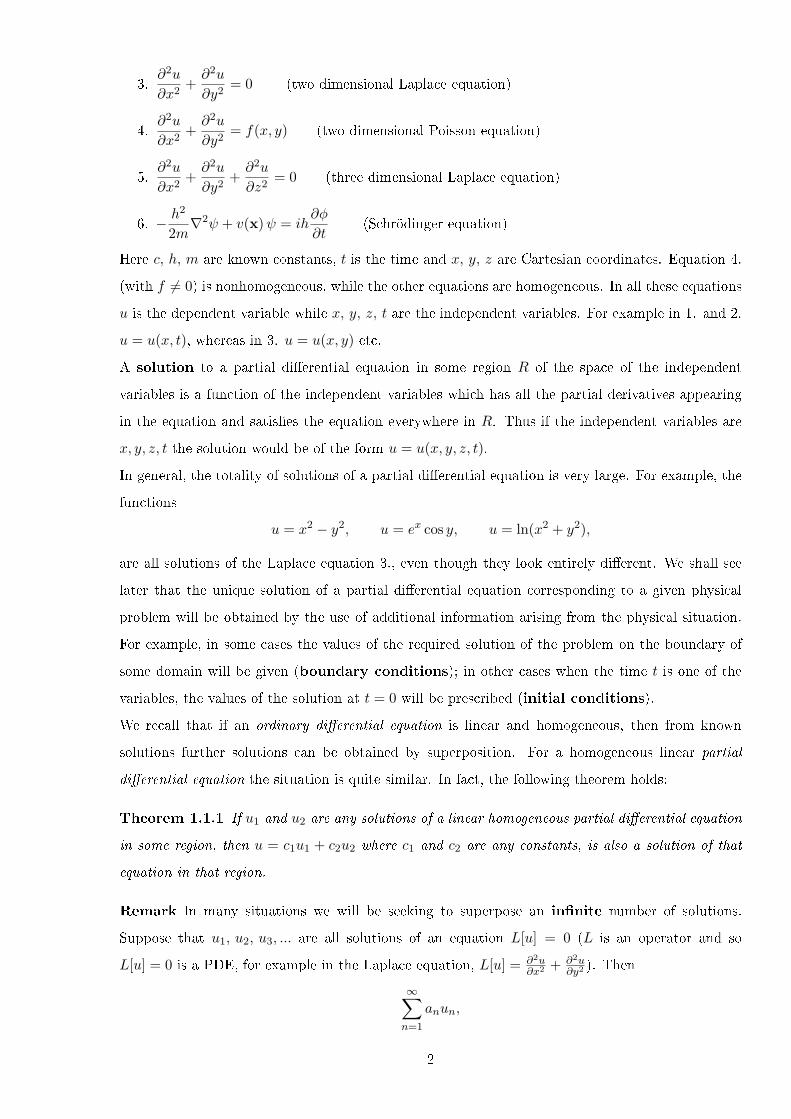
3.∂2u

∂x2+∂2u

∂y2= 0 (two dimensional Laplace equation)

4.∂2u

∂x2+∂2u

∂y2= f(x, y) (two dimensional Poisson equation)

5.∂2u

∂x2+∂2u

∂y2+∂2u

∂z2= 0 (three dimensional Laplace equation)

6. − h2

2m∇2ψ + v(x)ψ = ih

∂ϕ

∂t(Schrödinger equation)

Here c, h, m are known constants, t is the time and x, y, z are Cartesian coordinates. Equation 4.

(with f = 0) is nonhomogeneous, while the other equations are homogeneous. In all these equations

u is the dependent variable while x, y, z, t are the independent variables. For example in 1. and 2.

u = u(x, t), whereas in 3. u = u(x, y) etc.

A solution to a partial di�erential equation in some region R of the space of the independent

variables is a function of the independent variables which has all the partial derivatives appearing

in the equation and satis�es the equation everywhere in R. Thus if the independent variables are

x, y, z, t the solution would be of the form u = u(x, y, z, t).

In general, the totality of solutions of a partial di�erential equation is very large. For example, the

functions

u = x2 − y2, u = ex cos y, u = ln(x2 + y2),

are all solutions of the Laplace equation 3., even though they look entirely di�erent. We shall see

later that the unique solution of a partial di�erential equation corresponding to a given physical

problem will be obtained by the use of additional information arising from the physical situation.

For example, in some cases the values of the required solution of the problem on the boundary of

some domain will be given (boundary conditions); in other cases when the time t is one of the

variables, the values of the solution at t = 0 will be prescribed (initial conditions).

We recall that if an ordinary di�erential equation is linear and homogeneous, then from known

solutions further solutions can be obtained by superposition. For a homogeneous linear partial

di�erential equation the situation is quite similar. In fact, the following theorem holds:

Theorem 1.1.1 If u1 and u2 are any solutions of a linear homogeneous partial di�erential equation

in some region, then u = c1u1 + c2u2 where c1 and c2 are any constants, is also a solution of that

equation in that region.

Remark In many situations we will be seeking to superpose an in�nite number of solutions.

Suppose that u1, u2, u3, ... are all solutions of an equation L[u] = 0 (L is an operator and so

L[u] = 0 is a PDE, for example in the Laplace equation, L[u] = ∂2u∂x2 + ∂2u

∂y2). Then

∞∑n=1

anun,

2

is also a solution provided

• L[u1] = 0, L[u2] = 0, L[u3] = 0, etc., and

• The in�nite series is convergent and di�erentiable term by term as many times as is needed

in the de�nition of the linear operator L.

1.1.1 Inhomogeneous Problems

Many problems involve an inhomogeneous equation containing a term corresponding to applied

"forces" or "sources". For example, if a force f(x, t) is applied to a vibrating string, the equation

is inhomogeneous:∂2u

∂t2= c2

∂2u

∂x2+

1

Tf(x, t).

A problem may be inhomogeneous because of the boundary conditions as well as the equation

itself. The criterion for a linear homogeneous boundary value problem is that if u is a solution

of the equation and its boundary conditions, then so is any multiple of u. An example of an

inhomogeneous boundary condition is a vibrating string for which the end x = 0 is prescribed to

move in a certain way, u(0, t) = g(t) = 0. The general solution of an inhomogeneous problem is

made up of any particular solution of the problem plus the general solution of the corresponding

homogeneous problem, for which both the equation and boundary conditions are homogeneous.

This composition of solution is very similar to the case of ordinary di�erential equations. When

developing solution techniques for PDEs, we will mainly concentrate on homogeneous problems.

1.1.2 Pseudo or degenerate PDEs

It is important to appreciate that a PDE involving derivatives with respect to one variable only

may be solved like an ordinary di�erential equation treating the other independent variable as

parameters. For example, if u = u(x, y) the equation ∂u∂x = 0 can be solved using ODE techniques.

Essentially consider the ODE dudx = 0 which has a solution u = constant but allow this "constant"

to be a function of y. Thus the solution of ∂u∂x = 0 is u = a(y) where a(y) is any function of y but

does not depend on x. Checking back shows that u = a(y) does satisfy the equation ∂u∂x = 0.

Example 1.1.1 Solve the following PDEs:

(i)∂2u

∂y2= 0, (ii)

∂u

∂x= x, (iii)

∂u

∂x+ u = 0, (iv)

∂2u

∂y2+ u = 0,

where u = u(x, y).

Note: A very common notation for partial derivatives is to use subscripts. Thus ∂u∂x ≡ ux;

∂2u∂x2 ≡ uxx

etc. In fact ODEs can also be written in this way. The disadvantage of the subscript notation is

3

that it does not explicitly distinguish between partial and ordinary derivatives. If u = u(x, y) then

ux ≡ ∂u∂x but if u = u(x) then ux ≡ du

dx .

1.2 Classi�cation of second order linear PDEs

We consider the case of linear second order PDEs with two independent variables. This simpli�es

matters and much of the reasoning can be generalised to equations with more independent variables.

We consider a function u(x, y) to be evaluated in some region of the xy-plane (in which u(x, y)

satis�es some PDE). The partial di�erential equation will need to be supplemented by boundary

conditions of some sort; we assume these involve values of u and/or its derivatives on the curve which

encloses the region within which we are trying to solve the equation. There are three common types

of boundary condition.

1. Dirichlet conditions: u is speci�ed at each point on the boundary.

2. Neumann conditions: ∂u∂n , the normal derivative, i.e. the directional derivative in the direction

of the normal to the bounding curve is given at every point on the boundary. (Recall ∂u∂n =

n · ∇u, where n is the unit normal vector at each point on the boundary).

3. Cauchy conditions: u and ∂u∂n are given at every point on the boundary.

Other possibilities include Robin conditions where a linear combination of u and ∂u∂n is given on the

boundary. Also possible is that one type of condition, e.g. Dirichlet, is given on one part of the

boundary and a di�erent type on the remainder. However, we restrict attention to the three basic

types.

By analogy with second order ODEs, we would expect that Cauchy conditions along a line would

be the most natural.

1.2.1 Characteristics of PDEs

We now classify linear second order PDEs into three types: Parabolic, Hyperbolic and Elliptic.

They lead to families of characteristic curves for each type which can help to solve the PDEs.

We start by considering the di�erential equation

A(x, y)∂2u

∂x2+ 2B(x, y)

∂2u

∂x∂y+ C(x, y)

∂2u

∂y2= f

(x, y,

∂u

∂x,∂u

∂y

). (1.1)

Let us suppose the boundary curve is given parametrically by the equations

r(s) = (x(s), y(s)),

4

where s is arclength along the boundary. We shall suppose that we are given u(x, y) and N(x, y) =

∂u∂n along the curve and we thus know both of these as functions of s, i.e. u(s) and N(s). As s

is the arclength the components of the unit tangent vector t to the curve are(dxds ,

dyds

)and so the

components of the unit normal n to the curve are(− dy

ds ,dxds

)(because n · t = 0). Then

∂u

∂n= N(s) = n · ∇u = −∂u

∂x

dy

ds+∂u

∂y

dx

ds. (1.2)

We can also writedu

ds=∂u

∂x

dx

ds+∂u

∂y

dy

ds, (1.3)

which can be solved with (1.2) (using the fact that(dxds

)2+

(dyds

)2= 1) and this gives:

∂u

∂x= −N(s)

dy

ds+du

ds

dx

ds(1.4)

∂u

∂y= N(s)

dx

ds+du

ds

dy

ds. (1.5)

The trouble comes with second derivatives. There are three of these to be found

∂2u

∂x2,

∂2u

∂x∂y,

∂2u

∂y2.

We thus need three equations to determine these three unknown functions. Two equations are found

by di�erentiating the (now known) �rst derivatives along the boundary using the chain rule

d

ds

(∂u

∂x

)=∂2u

∂x2dx

ds+

∂2u

∂x∂y

dy

ds(1.6)

d

ds

(∂u

∂y

)=∂2u

∂y2dy

ds+

∂2u

∂x∂y

dx

ds. (1.7)

A third equation is provided by the original di�erential equation (1.1). The three equations (1.1),

(1.6) and (1.7) are written in matrix form in the following manner:dxds

dyds 0

0 dxds

dyds

A 2B C

uxx

uxy

uyy

=

dds(ux)

dds(uy)

f(x, y, ux, uy)

.[This is the familiar matrix equation Ax = b, where A and b are known and we wish to �nd x.

Recall that Ax = b has a unique solution if and only if A has an inverse, i.e. if and only if A−1

exists, i.e if and only if detA = 0].

Thus these three inhomogeneous equations can be solved for the second partial derivatives of u

unless the determinant of the coe�cients vanishes, i.e. unless

det

dxds

dyds 0

0 dxds

dyds

A 2B C

= 0,

5

or on expanding the determinant along the bottom row

A(x, y)

(dy

ds

)2

− 2B(x, y)dx

ds

dy

ds+ C(x, y)

(dx

ds

)2

= 0, (1.8)

or alternatively

A(x, y)

(dy

dx

)2

− 2B(x, y)dx

dx

dy

dx+ C(x, y)

(dx

dx

)2

= 0. (1.9)

Recall that the boundary curve was given parametrically by r = r(s) = (x(s), y(s)). Equation (1.8)

(or 1.9) de�nes two directions at every point in space, namely the direction given by the vector(dxds ,

dyds

). As (1.8) is quadratic, in general it contains two solutions for dx

ds and dyds , i.e. we can

associate two directions with every point in space. These are called the characteristic directions

at each point. Curves in the xy-plane whose tangents at each point lie along the characteristic

directions are called characteristics of the PDE. To map out the characteristics for a particular

equation, it is simplest to solve (1.9) for dydx and then to solve the two resulting di�erential equations

to give y as a function of x.

Returning to the equation (1.9) for the characteristics we see that this has solution for dydx given by:

dy

dx=B ±

√B2 −AC

A, (1.10)

where A, B, C can be functions of x and y. The classi�cation is as follows:

• If the characteristics are to be real curves, we clearly must have B2 > AC. PDEs obeying this

condition are called hyperbolic and have two sets of characteristics, e.g. the wave equation

utt = c2uxx.

• If B2 −AC = 0 the equation is said to be parabolic and has one set of characteristic curves,

e.g. the heat equation ut = c2uxx.

• If B2 − AC < 0 the equation is elliptic and has no (real) characteristics, e.g. the Laplace

equation uxx + uyy = 0.

Boundary Conditions

Let us discuss the choice of boundary conditions which is appropriate for each of the three types

of equation, beginning with the hyperbolic equation. We have seen above that, generally speaking,

Cauchy conditions along a curve which is not characteristic are su�cient to specify the solution near

that curve. A useful picture for visualising the role of the characteristics and boundary conditions

is obtained by thinking of the characteristics as curves along which partial information about the

solution propagates. The meaning of this statement and the way in which it works are most easily

understood with the aid of an elementary example.

6

Example 1.2.1 Consider the simplest hyperbolic equation, having A = c2, B = 0, C = −1, where

c is a known constant. This is the one dimensional wave equation

utt = c2uxx, (1.11)

for which the equation of the characteristics (1.8) (identify x with x and t with y) is

c2(dt

ds

)2

−(dx

ds

)2

= 0,

or (dx

dt

)2

= c2 =⇒ dx

dt= ±c.

Thus the characteristics are obtained by integrating these last two equations yielding solutions

x− ct = ξ (constant), x+ ct = η (constant), (1.12)

where ξ and η are arbitrary constants. As these vary over a range of values, (1.12) maps out a

family of characteristics in xt-space (which are straight lines in this instance), see Figure 1.1.

A B

Q

P

ct

x

eta = const

xi = const

Figure 1.1: Characteristics for the one-dimensional wave equation.

The characteristics form a "natural" set of coordinates for a hyperbolic equation. For example, if

we transform (1.11) to the new coordinates ξ and η de�ned in (1.12) using the chain rule for partial

di�erentiation, we obtain the equation in so called normal or canonical form:

∂2u

∂ξ∂η= 0. (1.13)

This can be integrated directly yielding the solution

u = g(ξ) + h(η) = g(x− ct) + h(x+ ct), (1.14)

where g and h are (su�ciently well behaved) functions.

7

Now, if we know u(x, 0) = a(x) and its normal derivative at t = 0: N(x) = k · ∇u = (0, 1) ·

(∂u∂x ,1c∂u∂t ) =

1c∂u∂t (x, 0) = b(x), where a(x) and b(x) are known functions, along the line segment AB

of Figure 1.1, we can �nd the individual functions g(ξ) and h(η) as follows:

u(x, 0) = a(x) = g(x) + h(x)

and1

c

∂u

∂t(x, 0) = b(x) = −g′(x) + h′(x),

which on integrating w.r.t. x gives∫b(x) dx = −g(x) + h(x) +K,

where K is an arbitrary integration constant. We now have two equations for the two unknown

functions g(x) and h(x) which we solve to �nd

g(x) =1

2a(x)− 1

2

∫b(x) dx+

1

2K

h(x) =1

2a(x) +

1

2

∫b(x) dx− 1

2K.

These are then substituted back into (1.14). The arbitrary constant associated with the integral is of

no importance since it cancels in this sum.

The results obtained for the simple case above hold generally for hyperbolic equations. We sum-

marise in the table below the types of boundary conditions appropriate for di�erent equations. This

table is not exhaustive but gives a general idea of what type the boundary conditions look like for a

particular problem. A very useful way of checking if a problem is well posed (i.e. that the boundary

conditions are su�cient to determine the solution) is to consider a physical process represented

by the problem and intuitively decide whether the physical problem is well posed i.e. capable of

solution.

Equation Condition Boundary

Hyperbolic Cauchy Open

Elliptic Dirichlet or Neumann Closed

Parabolic Dirichlet or Neumann Open

Recall that Cauchy conditions physically correspond to a given displacement and velocity at time

t = 0, i.e. specifying u and ∂u∂t . Dirichlet conditions correspond to a given displacement on a curve

in the (x, t) plane, i.e. specifying u. Neumann conditions correspond to stating a velocity on a curve

in the (x, t) plane, i.e. specifying ∂u∂t .

8

1.2.2 Qualitative behaviour of elliptic, parabolic and hyperbolic equations

Elliptic equations (e.g. ∇2u = 0)

These are generally associated with equilibrium phenomena when transient (time dependent) e�ects

have died away. Elliptic problems are thus not time dependent and are usually boundary value

problems. For these types of problems either Dirichlet, Neumann or mixed conditions on a closed

boundary are necessary to get a well-posed problem.

Elliptic problems sometimes result from the long time solution of parabolic problems. Consider

a thin rectangular plate with a given initial temperature distribution whose edges are each held

at some particular temperature. If we wait "long enough", it is possible that the temperature in

the plate will settle down to a time-independent (steady) value described by the Laplace equation

with boundary conditions. Initially the problem would have been described by the heat equation

∂u∂t = c2∇2u but if the problem has a steady state solution, then ∂

∂t ≡ 0 and we reduce to Laplace's

equation, the initial condition having been forgotten. Resorting to intuitive physical arguments is

a useful way of reasoning whether or not a problem has a steady state solution.

To gain an intuitive understanding consider an elliptic equation in a �nite rectangular region.

Identify the elliptic equation as a steady state heat �ow in a 2D rectangular plate where u(x, y) is

the temperature. We emphasize that a steady state must have been reached: u varies depending

upon where you look on the plate but each u(x, y) is constant in time. Boundary conditions in u

must be translated into conditions in terms of the temperature at the edges. If u = 0 along some

edge, then this edge of the plate is imagined as having its temperature held at 0, e.g. by placing a

strip of ice along it.

Parabolic equations (e.g. ∂u∂t = c2 ∂

2u∂x2 )

Parabolic equations describe evolution type processes i.e. processes which involve time. Typically

a parabolic equation represents a di�usive or "spreading out" phenomenon where, for example a

concentrated patch of dye in water "smears out" until it is distributed evenly everywhere. Another

typical example is heat �ow in a rod where one point on the rod has a "hot-spot" initially but as

the di�usion process evolves, the hot spot smoothes out until �nally the temperature is everywhere

the same (if the boundary conditions will allow this). Parabolic problems are initial-boundary value

problems in that they require both initial and boundary conditions. Generally speaking we require

Dirichlet or Neumann conditions on an open boundary.

To gain an intuitive understanding consider a parabolic equation in a one dimensional strip of �nite

length l. Identify this with time dependent heat �ow in a thin (metal) rod of �nite length. The

initial condition u(x, 0) = f(x), describes the temperature as a function of distance (x) along the

rod at time t = 0. Boundary conditions describe the temperatures in the rod at the ends (which are

9

held �xed in time). For example, if u(0, t) = 0, then one end of the rod can be thought of as being

emersed in iced water or ice (zero degrees). The mathematical problem requires a solution u(x, t)

for all x in [0, l] for all t ≥ 0. Physically this corresponds to �nding the temperature at every point

(x) in the rod for all times in the future (t).

Hyperbolic equations (e.g. ∂2u∂t2

= c2 ∂2u

∂x2 )

These again describe evolution type phenomenon and again both initial and boundary conditions

are required in general. Hyperbolic equations usually represent wave-like phenomena whereby some

initial condition or signal (or "wave") is seen to propagate through space either maintaining its

original form or changing shape and/or velocity as it does so but remaining generally recognizable

as the original signal or "wave".

To gain an intuitive understanding consider a hyperbolic equation in a long strip of length l. Identify

this with waves passing down a taut, thin, long string of length l. The initial conditions describe

an (initial) disturbance, e.g. plucking the string at some point. This "wave" will then pass along

the string. What other conditions are necessary to ensure a complete description of the evolution

of the disturbance of the string? Obviously if the ends of the string are �xed then conditions like

u(0, t) = 0 and u(l, t) = 0 are required. In addition to the already mentioned displacement, we also

require the initial velocity in the string. It is possible to have di�erent situations with the same

initial displacement but di�erent initial velocity.

1.2.3 An overview of solution method for linear second order PDEs

1. Separation of variables. Usually require a constant coe�cient equation. The basic idea is

to use the homogeneous (zero) boundary conditions to �nd the eigenfunctions. Then writing

the solution as a linear combination of the eigenfunctions, use the inhomogeneous boundary

(or initial) condition to solve for the superposition constants. If there is more than one

inhomogeneous condition, superposition of problems exploiting the linearity of the equation

may be necessary.

2. Integral transforms. Again usually only applicable to constant coe�cient equations. The

basic philosophy is to transform "out" one independent variable reducing to a simpler problem

(often an ODE). The particular transform used often depends on the boundary conditions and

the ranges of the independent variables. For example, if time ∈ [0,∞) a Laplace transform

may be used.

3. Green's functions. A very general method for solving PDEs (and ODEs) yielding solutions

in the form of an integral expression.

10

4. Complex variable techniques. Laplace's (and Poisson's) equations are fundamental to

many physical processes. For example ∇2T = 0 describes the steady state heat distribution

in an object. In complex variable theory, a basic property of any analytic function f(z) =

u(x, y) + iv(x, y) is that both the real and imaginary parts of f(z) satisfy Laplace's equation

i.e. ∇2u = 0 and ∇2v = 0. Because of this property it is possible to reduce many problems

involving Laplace's equation to exercised in complex variable theory.

5. Numerical techniques If all else fails, we can resort to numerical techniques, e.g. �nite

di�erences, �nite element method, �nite volume method, boundary elements.

1.3 Solutions to some elementary linear ODEs

We take y = y(x) to be the dependent variable and x to be the independent variable.

1.3.1 First-order equation: variables separable

This has the basic form:

h(x)k(y)dy

dx= −f(x)g(y), (1.15)

where f(x), h(x) are given functions of x, and g(y), k(y) are given functions of y. If the equation

has this form, the variables can be separated by dividing through by h(x)g(y) to obtain

k(y)

g(y)

dy

dx= −f(x)

h(x).

On multiplying across by dx we have separated the variables and the equation can be solved by

straightforward integration:

k(y)

g(y)dy = −f(x)

h(x)dx =⇒

∫k(y)

g(y)dy = −

∫f(x)

h(x)dx,

as in principle both of these integrations can be performed.

Example 1.3.1 Find the general solution of

dG

dt= −kG, (1.16)

where k is a known constant.

1.3.2 First-order linear (in y) equation

This is more general than the last situation and has the form:

dy

dx+ P (x)y = Q(x), (1.17)

11

where P (x) and Q(x) are known functions. This equation can be solved by multiplying both sides

by an integrating factor which is of the form exp(∫P (x)dx). (The equation must be in exactly

the same form as (1.17), i.e. the coe�cient of dydx = 1). On multiplying by the integrating factor we

obtaind

dx

[y exp

(∫P (x)dx

)]= Q(x) exp

(∫P (x)dx

), (1.18)

which can be integrated directly.

Example 1.3.2 Find the general solution of

dy

dx+y

x= 2x.

1.3.3 Second order linear equations

The equationd2y

dx2= −n2y, (1.19)

where n is a given real constant, has general solution

y = A cosnx+B sinnx, (1.20)

where A and B are arbitrary constants to be determined from the boundary conditions.

The equationd2y

dx2= n2y, (1.21)

where n is a given real constant, has general solution y = A coshnx+B sinhnx, or equivalently

y = Cenx +D−nx, (1.22)

where A, B, C, D are arbitrary constants to be determined from the boundary conditions.

1.3.4 Basic Fourier theory

We summarise here the basic results of Fourier series theory.

Fourier series theorem

If f(x) and dfdx are piecewise continuous on the interval −l ≤ x ≤ l and f(x) is de�ned outside the

interval [−l, l] so that it is periodic with period 2l, then f has a Fourier series

f(x) =A0

2+

∞∑n=1

(An cos

nπx

l+Bn sin

nπx

l

), (1.23)

with

An =1

l

∫ l

−lf(x) cos

nπx

ldx, Bn =

1

l

∫ l

−lf(x) sin

nπx

ldx. (1.24)

12

Even and odd functions

If f(x) is an even function, i.e. f(x) = f(−x) and satis�es the conditions of the Fourier theorem

then it can be expressed as a Fourier cosine series:

f(x) =A0

2+

∞∑n=1

An cosnπx

l, with An =

2

l

∫ l

0f(x) cos

nπx

ldx. (1.25)

If f(x) is an odd function, i.e. f(x) = −f(−x) and satis�es the conditions of the Fourier theorem

then it can be expressed as a Fourier sine series:

f(x) =∞∑n=1

Bn sinnπx

l, with Bn =

2

l

∫ l

0f(x) sin

nπx

ldx. (1.26)

Orthogonality of sine and cosine

Full range:

∫ l

−lsin

nπx

lsin

mπx

ldx =

0 m = n

l m = n = 0

0 m = n = 0

∫ l

−lcos

nπx

lcos

mπx

ldx =

0 m = n

l m = n = 0

2l m = n = 0∫ l

−lcos

nπx

lsin

mπx

ldx = 0 all m, n.

Half range:

∫ l

0sin

nπx

lsin

mπx

ldx =

0 m = n

l2 m = n = 0

0 m = n = 0

∫ l

0cos

nπx

lcos

mπx

ldx =

0 m = n

l2 m = n = 0

2l m = n = 0.

In solving PDEs using separation of variables, we will often have cause to express a function f(x)

de�ned on some range [0, l], e.g. on a conducting bar of length l, in a Fourier series. As we are

only concerned with the behaviour of f inside [0, l] we can de�ne it however we like outside [0, l].

Typically we might de�ne f to be odd (or even) and periodic with period 2l and then express it in

the form of a fourier half range sine (or cosine) series using the above results.

13

1.4 Vibrating String (1D Wave equation)

In this section we consider the transverse vibrations of an elastic string. We begin by deriving a PDE

governing the vibrations and then show how solutions to some typical problems can be obtained.

1.4.1 Derivation of the PDE for the vibrating string

As a �rst important partial di�erential equation, let us derive the equation governing small trans-

verse vibrations of an elastic string, which is stretched to length l and then �xed at the end points.

Suppose that the string is distorted and then at a certain instant, say, t = 0, it is released and

allowed to vibrate. The problem is to determine the vibrations of the string, that is, to �nd its

de�ection u(x, t) at any point x and at time t > 0, see Figure 1.2.

beta

alpha

lx + x

P

Q

x

u

T1

T2

Figure 1.2: Vibrating string (1D).

When deriving a di�erential equation corresponding to a given physical problem, we usually have to

make simplifying assumptions in order that the resulting equation does not become too complicated.

In our present case we make the following assumptions:

1. The mass of the string per unit length is constant ("homogeneous string"). The string is

perfectly elastic and does not o�er any resistance to bending.

2. The tension caused by stretching the string before �xing it at the end points is so large that

the action of the gravitational force on the string can be neglected.

3. The motion of the string is a small transverse vibration in the vertical plane, that is, each

particle of the string moves strictly vertically, and the de�ection and the slope at any point of

the string are small in absolute value. (Note: a lot of simpli�cation in applied mathematics

is obtained by exploiting the smallness of some quantity).

14

These assumptions are such that we may expect that the solution u(x, t) of the di�erential equation

to be obtained will reasonably well describe small vibrations of the physical "nonidealised" string

of small homogeneous mass under large tension.

To obtain the di�erential equation we consider the forces acting on a small portion of the string

(Figure 1.2). Since the string does not o�er resistance to bending, the tension is tangential to the

curve of the string at each point. Let T1 and T2 be the tensions at the end points P and Q of

that portion. Since there is no motion in the horizontal direction, the horizontal components of the

tension must be constant. Using the notation shown in Figure 1.2, we thus obtain

T1 cosα = T2 cosβ = T = constant. (1.27)

In the vertical direction we have two forces, namely the vertical components −T1 sinα and T2 sinβ

of T1 and T2: here the minus sign appears because the component at P is directed downwards.

By Newton's second law the resultant of those two forces is equal to the mass ρ∆x of the portion

times the acceleration utt, evaluated at some point between x and x + ∆x: here ρ is the mass of

the unde�ected string per unit length, and ∆x is the length of the portion of the unde�ected string.

Hence

T2 sinβ − T1 sinα = ρ∆xutt.

If this equation is divided by T and the expressions in (1.27) are substituted we �nd

T2 sinβ

T2 cosβ− T1 sinα

T1 cosα= tanβ − tanα =

ρ∆xuttT

. (1.28)

Now tanα and tanβ are the slopes of the curve of the string at x and x+∆x, that is

tanα =∂u

∂x

∣∣∣∣x

, tanβ =∂u

∂x

∣∣∣∣x+∆x

,

where the subscripts here mean evaluated at the point in question.

Here we have to write partial derivatives because u depends also on t. Dividing (1.28) by ∆x, we

deduce that1

∆x

(∂u

∂x

∣∣∣∣x+∆x

− ∂u

∂x

∣∣∣∣x

)=ρ

T

∂2u

∂t2.

If we let ∆x approach zero, we obtain the linear homogeneous partial di�erential equation

∂2u

∂t2= c2

∂2u

∂x2, or utt = c2uxx,

where c2 = Tρ . This is the so-called one-dimensional wave equation, which governs our problem.

It is parabolic as we showed in � 4.2. The notation c2 for the physical constant Tρ has been chosen

to indicate that this constant is positive.

15

1.4.2 Separation of Variables (for the vibrating string)

Formulation of the problem

We have seen that the vibrations of an elastic string are governed by the one-dimensional wave

equation (hyperbolic)

utt = c2uxx, (1.29)

where u(x, t) is the de�ection of the string. Consider the case where the string is �xed at the ends

x = 0 and x = l, so we have the two boundary conditions

u(0, t) = 0, u(l, t) = 0, for all t. (1.30)

The form of the motion of the string will depend on the initial de�ection (de�ection at t = 0) and

on the initial velocity (velocity at t = 0). Denoting the initial de�ection by f(x) and the initial

velocity by g(x), we thus obtain the two initial conditions

u(x, 0) = f(x), (1.31)

and∂u

∂t= g(x) when t = 0. (1.32)

Our problem is now to �nd the solution of (1.29) satisfying the conditions (1.30)-(1.32).

Solution of the formulated problem

We shall proceed step by step as follows:

First Step: By applying the so-called product method, or method of separating variables, we shall

obtain two ordinary di�erential equations.

Second Step: We shall determine solutions of those equations that satisfy the boundary conditions.

Third Step: Those solutions will be composed so that the result will be a solution of the wave

equation utt = c2uxx which also satis�es the given initial conditions.

First Step:

The product method yields solutions of the equation utt = c2uxx of the form

u(x, t) = F (x)G(t),

which are a product of two functions, each depending only on one of the variables x and t. By

di�erentiating this equation we obtain

utt = FG and uxx = F′′G,

16

where dots denote derivatives with respect to t and primes denote derivatives with respect to x. By

inserting this into (1.29) we have

FG = c2F′′G.

We now divide across by FG (Note: this is the usual trick applied at this point) and follow this by

dividing across by c2 thus �nding (for all x and t):

G

c2G=F

′′

F.

The expression on the left involves functions depending only on t while the expression on the right

involves functions depending only on x. Hence both expressions must be equal to a constant, say k.

[if the expression on the left is not constant, then changing t will presumably change the value of

this expression but certainly not that on the right, since the latter does not depend on t. Similarly,

if the expression on the right is not constant, changing x will presumably change the value of this

expression but certainly not that on the left]. Therefore,

G

c2G=F

′′

F= k.

This immediately yields the two ordinary linear di�erential equations

F′′ − kF = 0, (1.33)

and

G− c2kG = 0. (1.34)

In these equations, k is still arbitrary. Note that they are ODEs because F = F (x) and G = G(t).

Before actually determining the value of k, we will �rst narrow down the search by �nding its sign.

Second Step:

We will now determine solutions F and G of (1.33) and (1.34) so that u = FG satis�es the boundary

conditions in (1.30), that is

u(0, t) = F (0)G(t) = 0, u(l, t) = F (l)G(t) = 0 for all t.

Clearly, if G = 0, then u = 0, which is on no interest. Thus G = 0 and therefore

F (0) = 0; F (l) = 0. (1.35)

For k = 0 the general solution of (1.33) is F = ax+ b, and from the conditions in (1.35) we obtain

a = b = 0. Hence, F = 0, which is of no interest because then u = 0.

For positive k, i.e. k = µ2, the general solution of (1.33) is (see (1.22))

F = Aeµx +Be−µx,

17

and from (1.35) we obtain F = 0, as before. Hence we are left with the possibility of choosing k

negative, say k = −p2. Then (1.33) takes the form

F′′+ p2F = 0,

and the general solution is (see (1.20))

F (x) = C cos px+D sin px.

From this and (1.35) we have

F (0) = C = 0 and F (l) = D sin pl = 0.

We must take D = 0 since otherwise F = 0. Hence sin pl = 0, that is,

pl = nπ i.e. p = nπ/l where n is any integer (0,±1,±2, ...) (1.36)

We thus obtain in�nitely many solutions F (x) = Fn(x) where

Fn(x) = Dn sinnπx

ln = 1, 2, 3, ..., (1.37)

which satisfy (1.35) and the constants Dn are as yet undetermined. [For negative values of n we

obtain essentially the same solutions, except for a minus sign, because sin(−x) = − sin(x)].

Then k is now restricted to k = −p2 = −(nπ/l)2, resulting from (1.36). For these values of k the

equation (1.34) takes the form

G+ λ2nG = 0 where λn = cnπ/l.

The general solution is

Gn(t) = Bn cosλnt+B∗n sinλnt.

Hence the function un(x, t) = Fn(x)Gn(t) are given by

un(x, t) = (Bn cosλnt+B∗n sinλnt)Dn sin

nπx

l, n = 1, 2, 3....

Noting the fact that the constants are arbitrary up to this point, we can rede�ne BnDn = Bn (or

any other letter) and B∗nDn = B∗

n and rewrite the general solution as

un(x, t) = (Bn cosλnt+B∗n sinλnt) sin

nπx

l, n = 1, 2, 3....

Third Step:

Clearly, a single solution, un(x, t) will, not in general satisfy the initial conditions (1.31) and (1.32).

Now, since the one-dimensional wave equation is linear and homogeneous, it follows from Theorem

18

1.1.1 that the sum of �nitely many solutions un is a solution of the original equation (1.29). To

obtain a solution that satis�es (1.31) and (1.32), we consider the in�nite series

u(x, t) =

∞∑n=1

un(x, t) =

∞∑n=1

(Bn cosλnt+B∗n sinλnt) sin

nπx

l. (1.38)

From this and (1.31) it follows that

u(x, 0) =∞∑n=1

Bn sinnπx

l= f(x). (1.39)

Hence, in order that the in�nite series equation (1.38) satis�es the initial condition (1.31), the

coe�cients Bn must be chosen so that u(x, 0) becomes a half-range expansion of f(x), namely, the

Fourier sine series of f(x); that is

Bn =2

l

∫ l

0f(x) sin

nπx

ldx, n = 1, 2, 3.... (1.40)

Similarly, by di�erentiating (1.38) with respect to t and using (1.32) we �nd

∂u

∂t

∣∣∣t=0

=( ∞∑

n=1

(−Bnλn sinλnt+B∗nλn cosλnt) sin

nπx

l

)t=0

=

∞∑n=1

B∗nλn sin

nπx

l= g(x).

Hence, in order that (1.38) satis�es the (1.32), the coe�cient B∗n must be chosen so that, for t = 0,

∂u/∂t becomes the Fourier sine series of g(x); thus

B∗nλn =

2

l

∫ l

0g(x) sin

nπx

ldx, n = 1, 2, 3...

or, since λn = cnπl

B∗n =

2

cnπ

∫ l

0g(x) sin

nπx

ldx, n = 1, 2, 3.... (1.41)

Thus it follows that

u(x, t) =∞∑n=1

(Bn cosλnt+B∗n sinλnt) sin

nπx

l,

with coe�cients Bn and B∗n given by (1.40) and (1.41), is a solution of utt = c2uxx that satis�es the

boundary and initial conditions.

Example 1.4.1 Find the solution of the wave equation (1.29) corresponding to the triangular initial

de�ection

f(x) =

2kxl , when 0 < x < l

2

2k(l−x)l , when l

2 < x < l,

and initial velocity zero. Since g(x) = 0, we have B∗n = 0 in (1.41) and we use basic Fourier theory

to solve for the Bn's giving

Bn =8k

n2π2sin

nπ

2, n = 1, 2, 3, ....

19

0 0.1 0.2 0.3 0.4 0.5 0.6 0.7 0.8 0.9 1−1

−0.8

−0.6

−0.4

−0.2

0

0.2

0.4

0.6

0.8

1

x

u

time t = 0.1

c = k = l = 1

1 term

2 terms

0 0.1 0.2 0.3 0.4 0.5 0.6 0.7 0.8 0.9 1−1

−0.8

−0.6

−0.4

−0.2

0

0.2

0.4

0.6

0.8

1

x

u

time t = 1

2 terms

1 term

3 terms

c = k = l = 1

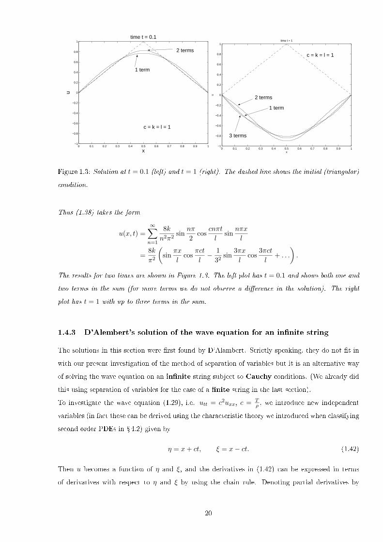
Figure 1.3: Solution at t = 0.1 (left) and t = 1 (right). The dashed line shows the initial (triangular)

condition.

Thus (1.38) takes the form

u(x, t) =

∞∑n=1

8k

n2π2sin

nπ

2cos

cnπt

lsin

nπx

l

=8k

π2

(sin

πx

lcos

πct

l− 1

32sin

3πx

lcos

3πct

l+ . . .

).

The results for two times are shown in Figure 1.3. The left plot has t = 0.1 and shows both one and

two terms in the sum (for more terms we do not observe a di�erence in the solution). The right

plot has t = 1 with up to three terms in the sum.

1.4.3 D'Alembert's solution of the wave equation for an in�nite string

The solutions in this section were �rst found by D'Alambert. Strictly speaking, they do not �t in

with our present investigation of the method of separation of variables but it is an alternative way

of solving the wave equation on an in�nite string subject to Cauchy conditions. (We already did

this using separation of variables for the case of a �nite string in the last section).

To investigate the wave equation (1.29), i.e. utt = c2uxx, c = Tρ , we introduce new independent

variables (in fact these can be derived using the characteristic theory we introduced when classifying

second order PDEs in � 4.2) given by

η = x+ ct, ξ = x− ct. (1.42)

Then u becomes a function of η and ξ, and the derivatives in (1.42) can be expressed in terms

of derivatives with respect to η and ξ by using the chain rule. Denoting partial derivatives by

20

subscripts, we see from (1.42) that ηx = 1 and ξx = 1 and therefore transforming from u(x, t) to

w(η, ξ), we �nd

ux = wηηx + wξξx = wη + wξ.

By applying the chain rule to the right hand side we �nd

uxx ≡ (wη + wξ)x = (wη + wξ)ηηx + (wη + wξ)ξξx.

Since ηx = 1 and ξx = 1, this becomes

uxx = wηη + 2wηwξ + wξξ.

It is customary to rewrite this using the same dependent variable on both sides of the equation i.e.

uxx = uηη + 2uηuξ + uξξ.

The utt derivative in the wave equation is transformed by the same procedure, and the result is

utt = c2(uηη − 2uηuξ + uξξ

).

By inserting these two results into utt = c2uxx we obtain

uηξ =∂2u

∂η∂ξ= 0. (1.43)

We may integrate this equation with respect to η, �nding

∂u

∂ξ= h(ξ),

where h(ξ) is an arbitrary function of ξ. Integrating this with respect to ξ, we have

u =

∫h(ξ) dξ + ϕ(η),

where ϕ(η) is an arbitrary function of η. Since the integral is a function of ξ, say ψ(ξ), the solution

u is of the form

u = ϕ(η) + ψ(ξ).

Because of (1.42) we may write

u(x, t) = ϕ(x+ ct) + ψ(x− ct). (1.44)

This is known as d'Alembert's solution of the wave equation.

The functions ϕ and ψ are arbitrary up to this point, i.e. any su�ciently smooth functions of

their respective arguments will satisfy (1.43) and hence the PDE. The arbitrary functions can be

determined from the initial conditions just as we could use the boundary conditions of an ODE

21

problem to solve for the integration constants. Let us illustrate this in the case of zero initial

velocity ut(x, 0) = 0 and given de�ection u(x, 0) = f(x).

By di�erentiating (1.44) we have

∂u

∂t= cϕ′(x+ ct)− cψ′(x− ct), (1.45)

where primes denote derivatives with respect to the entire arguments x+ ct and x− ct, respectively.

From (1.44), (1.45), and the initial conditions we have two equations in two unknowns:

u(x, 0) = ϕ(x) + ψ(x) = f(x) (1.46)

ut(x, 0) = cϕ′(x)− cψ′(x) = 0. (1.47)

From (1.47) we have ϕ′ = ψ′. Hence ϕ = ψ + k, for k a constant and from this and (1.46) we �nd

2ψ + k = f or ψ =1

2(f − k).

Then ϕ = 12(f + k) and with these functions the solution (1.44) becomes

u(x, t) =1

2

[f(x+ ct) + f(x− ct)

]. (1.48)

This maybe interpreted as follows: the initial condition splits into two wavelets of half the amplitude

of the original and these propagate in opposite directions at speed c. Our result shows that the

initial conditions and the boundary conditions determine the solution uniquely.

Exercise: Reconsider the problem above with general initial condition ut(x, 0) = g(x).

1.5 One-Dimensional Heat Flow

The heat �ow in a body of homogeneous material is governed by the heat equation

ut = c2∇2u, c2 =K

σρ,

where u(x, y, z, t) is the temperature in the body, K is the thermal conductivity, σ is the speci�c

heat capacity, ρ is the density of material of the body, ∇2 is the Laplacian of u with respect to

Cartesian coordinates x, y, z, i.e. ∇2u = uxx + uyy + uzz. As an important application, let us

consider the temperature in a long thin bar or wire of constant cross-section and homogeneous

material which is oriented along the x-axis (see Figure 1.4) and is perfectly insulated laterally, so

that heat �ows in the x-direction only. Then u depends only on x and time t, and the heat equation

becomes the so-called one-dimensional heat equation

ut = c2uxx. (1.49)

22

While the wave equation involves the second partial derivative utt, the heat equation involves the

�rst derivative ut, and we shall see that the solutions of (1.49) are entirely di�erent from those of

the wave equation, although the procedure for solving (1.49) is quite similar to that in the case of

the wave equation. We shall derive (1.49) and solve it for some important types of boundary and

initial conditions.

x axisx x + x

Q = - K u (x,t)x Q = K u (x + x, t)x

Figure 1.4: Section of bar of material.

1.5.1 Derivation of the heat equation

We have already derived the wave equation for vibrations in a string or membrane. We now derive

the heat equation for �ow in a bar of conducting material.

We assume that the lateral sides of the bar are perfectly insulated (with some lagging material) so

that there is no passage of heat through them. We will also assume that the temperature u in the

rod depends only on position x and t, and not on the lateral coordinates y and z, i.e. that the

temperature in any cross-section of the rod is constant. (See Figure 1.4). This assumption is usually

satisfactory when the lateral dimensions of the rod are small when compared to its length.

The di�erential equation governing the temperature in the bar is an expression of a fundamental

physical balance: the rate at which heat �ows into any portion of the bar is equal to rate at which

heat is absorbed in that portion of the bar. The terms in the equation are called the �ux (�ow)

term and the absorption term respectively.

We begin with Fourier law which states that the amount of heat �owing through unit cross-section

area in the bar per unit time, called the �ux Q, is given by:

Q(x, t) = −K∂u

∂x(x, t), (1.50)

where K is the (constant) heat di�usion coe�cient and depends on the material in the rod, and

u(x, t) is the temperature in the rod as a function of the distance along its length and time. Quali-

tatively the law states that if there are large di�erences in the temperature u along the rod i.e. if

23

∂u∂x is large, then heat �ow occurs. This is in accordance with physical experience which testi�es

to the fact that heat �ow tends to equalise temperatures. Also, heat �ows from hot areas to cold

areas (this is the origin of the negative sign in (1.50). If the temperature in the rod is everywhere

the same, then ∂u∂x = 0 everywhere and no heat �ows.

We now concentrate on an in�nitesimal portion of the rod, located between the points x and x+∆x

as in Figure 1.4. In order to derive a di�erential equation describing the �ow of heat in the bar, we

will calculate the amount of heat �owing into the small element of length ∆x and equate this with

the increase in heat in the element arising from absorption.

At the left hand edge of the element, the rate of heat �ow per unit area, i.e. the amount of heat

�owing through a unit area in unit time to the right is given by the �uxQ(x, t). Similarly, the amount

of heat �owing into the di�erential element in unit time at the right hand edge is −Q(x + ∆x, t)

(Note the sign change). The net increase in heat in the di�erential element (per unit cross-sectional

area) in a time ∆t is thus:

Increase in heat in element in time ∆t =(Q(x, t)−Q(x+∆x, t)

)∆t. (1.51)

Now the amount of heat energy per unit cross-section in the di�erential element at any time t is

given by σρ∆xu where σ is speci�c heat capacity, ρ is the density of the material and u is the

average temperature in the element at time t. In fact let us take u = u(x +∆x/2, t), i.e. u is the

temperature at the centre of the element at time t. The rate of increase in heat in the element (i.e.

the increase in heat in the element in unit time) is thus given by σρ∆xut and so the net increase in

heat energy in the element in time ∆t is:

Increase in heat in element in time ∆t = σρ∆x∆tut(x+∆x/2, t). (1.52)

Obviously we can now equate (1.51) and (1.52) as the amount of heat �owing into the element must

equal the increase in its heat energy (this is just a conservation of heat energy) and so

(Q(x, t)−Q(x+∆x, t)

)∆t = σρ∆x∆tut(x+∆x/2, t). (1.53)

The ∆t's cancel and we now divide by both sides of ∆x and take the limit as ∆x→ 0 to get:

lim∆x→0

Q(x, t)−Q(x+∆x, t)

∆x= lim

∆x→0σρut(x+∆x/2, t). (1.54)

Recalling the de�nition of a partial derivative, (1.54) is just:

−Qx(x, t) = σρut(x, t). (1.55)

But from (1.50) we have an expression for Q in terms of u so (1.50) and (1.54) become:

Kuxx(x, t) = σρut(x, t), (1.56)

24

or in more familiar form of (1.49) where c2 = Kσρ is called the thermal di�usivity. It is a parameter

depending only on the material of the bar. Its units are (length)2/time. Typical values for di�erent

materials: silver 1.71× 10−4 m2 s−1, brick 3.8× 10−7 m2 s−1, water 1.44× 10−7 m2 s−1.

1.5.2 Physical boundary conditions

Firstly, what type of PDE is the heat equation and what type of boundary conditions do we expect

from the general theory earlier in the Chapter?

Several relatively simple conditions may be imposed at the end of the bar. For example, the

temperature at the end may be maintained at some constant value T . This might be accomplished

by placing the end of the bar in thermal contact with some reservoir of su�cient size so that any

heat that may �ow between the bar and the reservoir does not noticeably alter the temperature of

the reservoir. At this end the mathematical (Dirichlet) boundary condition is

u = T. (1.57)

Another simple boundary condition occurs if the end is insulated (i.e. the end is surrounded by a

lagging material) so that no heat passes through it. Recalling the expression (1.50) (the Fourier

law) for the amount of heat (per unit time) crossing any cross-section of the bar, the condition for

insulation is clearly that this quantity vanishes. Thus mathematically

ux = 0, (1.58)

is a (Neumann) boundary condition at an insulated end.

A more general type of boundary condition occurs if the rate of �ow of heat through an end of

the bar is proportional to the temperature there. Let us consider the end x = 0, where the rate of

heat �ow from left to right is give by −Kux(0, t); see (1.50). Hence the rate of heat �ow out of the

bar (from right to left) at x = 0 is KAux(0, t). If this quantity is proportional to the temperature

u(0, t), then we obtain the (Robin) boundary condition

ux(0, t)− h1u(0, t) = 0, t > 0, (1.59)

where h1 is a known non-negative constant of proportionality. Note that h1 = 0 corresponds to an

insulated end, while h1 → ∞ corresponds to an end held at zero temperature. (The equation then

reduces to u(0, t) = 0).

If the heat �ow is taking place at the right hand end of the bar (x = 1), then in a similar way we

obtain the boundary condition

ux(1, t)− h2u(1, t) = 0, t > 0, (1.60)

where again h2 is a known non-negative constant of proportionality.

25

Finally to determine completely the �ow of heat in the bar it is necessary to state the temperature

distribution at one �xed instant, usually taken as the initial time t = 0. This initial condition is of

the form

u(x, 0) = f(x), 0 ≤ x ≤ 1. (1.61)

The mathematical problem is then to determine the solution of the di�erential equation (1.49)

subject to the boundary conditions (1.59) and (1.60) at each end, and to the initial condition (1.61)

at t = 0.

1.5.3 Solutions to heat �ow problems with homogeneous boundary conditions

Problem Formulation

We consider the case of a bar of heat conducting material of length l. The partial di�erential

equation describing the conduction of heat through the bar is:

c2uxx = ut. (1.62)

Let us start with the case when the ends x = 0 and x = l of the bar are kept at temperature zero.

Then the (homogeneous) boundary conditions are

u(0, t) = 0, u(l, t) = 0, for all t. (1.63)

Let f(x) be the initial temperature in the bar. Then the initial condition is

u(x, 0) = f(x), (1.64)

where f(x) is a given function.

Solution to the formulated problem

First Step:

Using the method of separating variables, we �rst determine solutions of the equation that satisfy

the boundary conditions. We start from

u(x, t) = F (x)G(t). (1.65)

Di�erentiating and substituting this into (1.60) gives

FG = c2F′′G,

where, as before, dots denote derivatives with respect to t and dashes denote derivatives with respect

to x. Dividing by c2FG (the usual trick is to divide by FG but we also divide by c2 for convenience)

we haveG

c2G=F

′′

F. (1.66)

26

The expression on the left depends only on t, while the right side depends only on x. As in � 4.4,

we conclude that both expressions must be equal to a constant, say k. You can show that for k ≥ 0

the only solution u = FG that satis�es the boundary conditions is u = 0. For negative k = −p2 we

obtain

G/c2G = F′′/F = −p2,

and from this the two ordinary di�erential equations

F′′+ p2F = 0, (1.67)

and

G+ c2p2G = 0. (1.68)

Second Step:

The general solution of (1.67) is

F (x) = A cos px+B sin px. (1.69)

From the boundary conditions (1.63) it follows that

u(0, t) = F (0)G(t); u(l, t) = F (l)G(t) = 0.

Since G ≡ 0 implies u ≡ 0, we require that F (0) = 0 and F (l) = 0. We can conclude from (1.69)

that F (0) = A and so A = 0, therefore

F (l) = B sin pl.

We must have B = 0, since otherwise F ≡ 0. Hence the condition F (l) = 0 leads to

sin pl = 0 i.e p = nπ/l, n = 1, 2, 3....

We thus obtain the in�nity of solutions

Fn(x) = Bn sinnπx

l, n = 1, 2, 3...,

where Bn is a completely arbitrary constant.

For the values p = nπ/l the ODE (1.68) takes the form

G+ λ2nG = 0 where λn = cnπ/l.

The general solution is

Gn(t) = Cne−λ2t, n = 1, 2, 3...,

27

where Cn is an arbitrary constant. Hence the functions

un(x, t) = Fn(x)Gn(t) = Dn sinnπx

le−λ2

nt n = 1, 2, 3..., (1.70)

are solutions of the heat equation (1.62) satisfying (1.63). In (1.70) we have written BnCn = Dn,

as Bn and Cn are arbitrary (as is Dn).

Third Step:

To �nd a solution which also satis�es the initial condition (1.64), we consider the series

u(x, t) =∞∑n=1

un(x, t) =∞∑n=1

Dn sinnπx

le−λ2

nt, (λn = cnπ/l). (1.71)

From this and the initial condition (1.64) it follows that

u(x, 0) =

∞∑n=1

Dn sinnπx

l= f(x)

Hence for the general solution (1.71) to satisfy (1.64), the coe�cients Dn must be chosen such that

u(x, 0) becomes a half-range expansion of f(x), namely, the Fourier sine series of f(x): that is

Dn =2

l

∫ l

0f(x) sin

nπx

ldx, n = 1, 2, 3.... (1.72)

Therefore the series (1.71) with coe�cients (1.72) is the solution of the heat equation (1.62).

Example 1.5.1 If the initial temperature in a bar of length l is given by

f(x) =

x when 0 < x < l/2

l − x when l/2 < x < l,

(see Figure 1.5, dotted line), with l = π and c = 1, then we obtain from (1.72)

Dn =2

l

[ ∫ l/2

0x sin

nπx

ldx+

∫ l

l/2(l − x) sin

nπx

ldx

]. (1.73)

Integration (both integrals in (1.73) require integration by parts) yields Dn = 0 when n is even and

Dn =4l

n2π2, n = 1, 5, 9, ...

Dn = − 4l

n2π2, n = 3, 7, 11, ....

Hence the solution is

u(x, t) =4l

π2

{sin

πx

lexp

[−

(cπ

l

)2

t

]− 1

9sin

3πx

lexp

[−

(3cπ

l

)2

t

]+ . . .

}.

In Figure 1.5 we graph this at di�erent times (e.g. t = 0, 1, 2, 3) to get an instantaneous "picture"

of the temperature in the bar at each of these times. Note the smoothing e�ect of the di�usion

operator.

28

0 0.5 1 1.5 2 2.5 3 3.50

0.2

0.4

0.6

0.8

1

1.2

1.4

1.6

x

u

t = 3

t = 2

t = 1

t = 0

Figure 1.5: Solution at various times.

1.6 Laplace's Equation

One of the most important partial di�erential equations appearing in physics is Laplace's equation

∇2u = 0, (1.74)

where, with respect to cartesian co-ordinates x, y, z in space, ∇2 = uxx + uyy + uzz. The theory of

solutions of Laplace's equation is called potential theory. Solutions of (1.74) which have continuous

second order partial derivatives are called harmonic functions.

The two dimensional case, when u depends on x and y only, can be treated using the methods

of complex analysis exploiting the fact that the real and imaginary parts of any analytic complex

valued function f(z) = u(x, y) + iv(x, y) both satisfy Laplace's equation in two dimensions. Many

problems involving the two dimensional Laplace's equation reduce to exercises in complex variable

theory.

1.6.1 Basic applications

We mention brie�y some applications of Laplace's equation. In electrostatics the electrical force of

attraction between charged particles is called Coulomb's law, which is of the same mathematical form

as Newton's law of gravitation. It can be shown that the �eld created by a distribution of electrical

charges can be described mathematically by a potential function which satis�es Laplace's equation

at any point not occupied by charges. A similar result holds for the gravitational potential, i.e. the

29

gravitational force between two particles is given by the gradient of a scalar function (potential)

which satis�es Laplace's equation.

For incompressible �ow the velocity potential ϕ can be shown to satisfy ∇2ϕ = 0.

Finally, in a steady state heat �ow problem, the temperature u also satis�es the Laplace equation

as ∂/∂t ≡ 0 and the heat �ow equation reduces to Laplace's equation.

1.6.2 Laplace's equation in a rectangle

We consider the following physical problem. A thin rectangular plate has its edges �xed at temper-

atures zero on three sides and f(y) on the remaining side, as shown in Figure 1.6. Its lateral sides

are then insulated and it is allowed to stand for a "long" time (but the edges are maintained at

the aforementioned boundary temperatures). We wish to �nd the temperature distribution in the

plate.

2v = 0

v = 0

v = 0

v = 0 v = f(y)

(0,0) (a,0)

(0,b) (a,b)

Figure 1.6: A thin metal rectangular plate for Laplace's equation.

Problem Formulation

The mathematical problem can be formulated as follows (PDE and boundary conditions):

vxx + vyy = 0 (∇2v = 0). (1.75)

As the equation is elliptic, we expect just one boundary condition along the boundary (in this case

the conditions are Dirichlet), i.e. along each side of the rectangle. Thus we require

v(x, 0) = 0, v(x, b) = 0, 0 ≤ x ≤ a (1.76)

v(0, y) = 0, v(a, y) = f(y), 0 ≤ y ≤ b, (1.77)

where f(y) is a known function.

30

Solution to formulated problem

We now proceed by separation of variables: before doing so we comment on one apparent di�erence

between the present problem and the simple hyperbolic and parabolic problems we looked at earlier

in the Chapter. In these cases, we had both initial and boundary conditions and the method only

worked if the boundary conditions were all homogeneous (in order to determine the eigenfunctions).

The non-zero initial conditions were then used to solve for the superposition constants. In the

present case, we have no initial conditions as the problem is time independent. If all our boundary

conditions were homogeneous (i.e. f(y) = 0 in (1.77)), then the problem would have the trivial

solution everywhere. In fact, the method which we are about to develop will work when we have

precisely one non-zero boundary condition and three zero conditions. The zero or homogeneous

conditions are used to solve for the superposition constants and does the same task as the initial

conditions for the hyperbolic and parabolic equations.

We now seek a solution in the form:

v(x, y) = F (x)G(y),

which gives

G(y)F ′′(x) + F (x)G(y) = 0,

and so

F ′′(x) = k2F (x) (1.78)

G(y) = −k2G(y), (1.79)

where we have assumed the separation constant is negative. As before choosing a di�erent sign

leads to a trivial solution. In the present case, the sign depends on whether the inhomogeneous

condition occurs on a x = constant or y = constant boundary. The former case applies here (see

(1.77)), while if the inhomogeneous condition were on y = b, say, then we would have to choose a

separation constant of opposite sign.

Equation (1.78) leads to the following solution:

F (x) = A cosh kx+B sinh kx, (1.80)

and application of the �rst condition in (1.77) indicates A = 0 and we are left with

F (x) = B sinh kx. (1.81)

Equation (1.79) has solution:

G = C cos ky +D sin ky.

31

The �rst condition in (1.76) indicates that C = 0 and so

G = D sin ky.

Then the second condition in (1.76) yields the following eigenvalue equation:

sin kb = 0 =⇒ kb = nπ, n = 1, 2, . . . ,∞. (1.82)

Thus superposing over all values of n, we have:

v(x, y) =∞∑n=1

En sinhnπx

bsin

nπy

b, (1.83)

where, as usual, we have absorbed the constants (En = BnDn). We now use the inhomogeneous

boundary condition to solve for En. Thus, on x = a, the second condition in (1.77) gives

f(y) =

∞∑n=1

En sinhnπa

bsin

nπy

b, (1.84)

and so by the orthogonality of the sines we have

En sinhnπa

b=

2

b

∫ b

0f(y) sin

nπy

bdy,

and so

En =2

b

∫ b0 f(y) sin

nπyb dy

sinh nπab

. (1.85)

Then the solution to the problem is complete.

Example 1.6.1 Solve Laplace's equation on the rectangle 0 ≤ x ≤ 3 and 0 ≤ y ≤ 2 with

f(y) =

y when 0 < y < 1

2− y when 1 < y < 2.

We need to �nd the En using (1.85). Now, since a = 3 and b = 2 we have∫ b

0f(y) sin

nπy

bdy =

∫ 1

0y sin

nπy

2dy +

∫ 2

1(2− y) sin

nπy

2dy

=8

n2π2sin

nπ

2,

using integration by parts. Thus

En =8 sin nπ

2

n2π2 sinh 3nπ2

.

The solution is given in (1.7a) and corresponding contour plots in (1.7b).

32

00.5

11.5

22.5

3

0

0.5

1

1.5

20

0.2

0.4

0.6

0.8

1

x

Example for Laplace Equation

y

v

0 0.5 1 1.5 2 2.5 30

0.2

0.4

0.6

0.8

1

1.2

1.4

1.6

1.8

2

x

y

Contour plots

Figure 1.7: Solution of Laplace's equation for the example (left) and corresponding contour plots

(right).

1.7 Using Integral transforms to solve PDEs

The general form of an integral transform is

f(s) =

∫ b

af(x)K(s, x) dx, (1.86)

where K(s, x) is a known function of s and x and is called the kernel of the transformation. For

example, the kernel of a Laplace transform would be e−sx.

The e�ect of applying an integral transform to a PDE is to exclude temporarily a chosen independent

variable and to leave for solution a PDE in one less independent variable. You will already have seen

how to solve ODEs using Laplace transforms: the ODE reduces to an algebraic equation which is of

course much easier to solve than the original ODE. Solution of this equation yields an expression for

the transform of the dependent variable and the only remaining di�culty is in inverting to �nd the

dependent variable itself. Generally speaking, transforming a PDE with n independent variables

reduces to a PDE with (n−1) independent variables (and so a PDE with two independent variables

reduces to an ODE).

1.7.1 General procedure for using transforms

We must follow these steps:

1. Select the appropriate transform (depending on the equation and especially the boundary

conditions).

2. Multiply the equation and the boundary conditions by the kernel and integrate between the

appropriate limits with respect to the variable selected for exclusion.

33

3. In performing the integration in step 2. make use of the appropriate boundary (or initial)

conditions in evaluating terms at the limits of integration.

4. Solve the resulting equations, so obtaining the transform of the wanted function (solution).

5. Invert to �nd the solution itself.

1.7.2 De�nitions and summary of properties of common transforms

In the following de�nitions, we consider transforms of some function f(x) or f(t). The de�nitions

can just as easily be extended to a function f(x, t) where either the "t" variable would be una�ected

and the transform would be f(s, t), or the "x" variable would be una�ected and the transform would

be f(x, s).

1.7.3 Fourier transform

This is essentially a restatement of the Fourier integral theorem. Given some function f(x) (satis-

fying certain smoothness requirements), its Fourier transform f(ω) is de�ned to be

f(ω) =

∫ ∞

−∞f(x)e−iωx dx, (1.87)

where i2 = −1. The kernel is thus e−iωx. Note that the use of ω as the variable in the kernel is

purely a matter of convention. In the introduction to transforms at the beginning of � 4.7, s was

used as the general transform variable. The inverse transform is now de�ned by:

f(x) =1

2π

∫ ∞

−∞f(ω)e−iωx dω. (1.88)

Note how in (1.87) the x dependence has been integrated out and it returns in (1.88). The notation

F(f) = f and F−1(f) = f is sometimes used.

Properties of the Fourier transform

These are stated here without proof (except for (ii)):

(i) Linearity of the transform and its inverse. For α, β any scalars and f , g any trans-

formable functions:

F(αf + βg) = αF(f) + βF(g),

with a similar result for the inverse transform F−1.

(ii) Transform of the nth derivative. If f (n−1)(x), f (n−2)(x),...,f(x) → 0 as x→ ±∞, then

F

(dnf

dxn

)= (iω)nF(f) = (iω)nf(ω).

34

Proof:

F

(df

dx

)=

∫ ∞

−∞

df

dxe−iωx dx

=[f(x)e−iωx

]∞−∞ + iω

∫ ∞

−∞f(x)e−iωx dx

= iωF(f) = iωf(ω),

where we have used integration by parts. Second and higher derivatives are transformed in a

similar manner. Note that this his how the transform removes derivatives w.r.t. x from the

equation. For example F(d2fdx2

)= (iω)2f(ω).

(iii) Fourier convolution. If we de�ne the Fourier convolution of two functions to be

f ⋆ g ≡∫ ∞

−∞f(x− ξ) g(ξ) dξ,

then F(f ⋆ g) = f(ω)g(ω) or f ⋆ g = F−1(f g). Recall that F and F−1 are inverses of one

another so that FF−1 = F−1F is the identity transformation.

(iv) For reference purposes, we list some other less important properties:

F[(−ix)nf(x)

]= f (n)(ω)

x shift : F−1[e−iaωf(ω)

]= f(x− a)

ω shift : F−1[f(ω − a)

]= eiaxf(x)

If h(x) =

∫ ∞

−∞f(ξ) dξ and h→ 0 as x→ 0 then F[h(x)] = f(ω)/iω.

1.7.4 Laplace transform

The Laplace transform is de�ned by

f(s) =

∫ ∞

0f(t)e−st dt, (1.89)

where s is chosen so that the integral converges and in general can be a complex number. The

inverse transformation is

f(t) =1

2πi

∫ γ+i∞

γ−i∞f(s)est ds. (1.90)

Sometimes the notation L(f) = f and L−1(f) = f is used. Note that γ and ω are real (with

Re(s) > γ) in the de�nition of the inverse transform so the transform variable s = γ + iω is

complex. The path of integration in (1.90) is the straight line from γ− iω to γ+ iω in the complex s

plane so inverting Laplace transforms (and indeed Fourier transforms) can be very di�cult. We will

generally contend ourselves with using tables of Laplace transforms to �nd inverse transforms or

only considering special simpli�ed situations but it should be remembered that inverting the Laplace

transform of an arbitrary function is usually non-trivial and must often be undertaken numerically.

35

Properties of the Laplace transform

These are stated here without proof (except for (ii)):

(i) Linearity of the transform and its inverse. For α, β any scalars and f , g any trans-

formable functions:

L(αf + βg) = αL(f) + βL(g),

with a similar result for the inverse transform L−1.

(ii) Transform of the nth derivative. If f (n−1)(t), f (n−2)(t),...,f(t) → 0 as t→ +∞, then

L

(dnf

dtn

)= sL

(dn−1f

dtn−1

)− dn−1f

dtn−1(t = 0).

For example, for n = 1 and n = 2 we have:

L

(df

dt

)= sf(s)− f(0)

L

(d2f

dt2

)= s2f(s)− sf(0)− f ′(0).

Proof:

L

(df

dt

)=

∫ ∞

0

df

dte−st dt

=[f(t)e−st

]∞0

+ s

∫ ∞

0f(t)e−st dt

= −f(0) + sf(s),

where we have used integration by parts. Second and higher derivatives are transformed in

a similar manner. Note that this is how the transform removes derivatives w.r.t. t from the

equation.

(iii) Laplace convolution. If we de�ne the Laplace convolution of two functions to be

f ⋆ g ≡∫ ∞

0f(τ) g(t− τ) dτ,

then L(f ⋆ g) = f(s)g(s) or f ⋆ g = L−1(f g). Recall that L and L−1 are inverses of one

another so that LL−1 = L−1L is the identity transformation.

36

(iv) For reference purposes, we list some other less important properties:

L[(−t)nf(t)

]= f (n)(s), e.g. L

[tf(t)

]= −df

ds

t shift : L−1[e−asf(s)

]= H(t− a)f(t− a)

s shift : L−1[f(s+ a)

]= e−atf(t)

L−1

[f(s)

s

]=

∫ t

0f(τ) dτ

L

[f(t)

t

]=

∫ ∞

sf(s) ds

If f(t) is periodic with period over 0 ≤ t <∞, then f(s) =1

1− e−as

∫ a

0f(t)e−st dt.

Note that H is the Heaviside step function de�ned as H(t) = 0 if t < 0, H(t) = 1 if t > 0.

1.7.5 General comments on when to use di�erent transforms

Fourier and Laplace transforms can only be used on linear equations and are usually only useful on

equations with constant coe�cients. If u = u(x, t) is governed by an equation which are functions

of x but not t, then transforming w.r.t. t will reduce it to an ODE problem whose coe�cients are also

a function of x. If the original PDE has coe�cients which are functions of t and we transform out

the t variable, then the transformed problem will still be a PDE but may (in certain circumstances)

be simpler than the original PDE.

If the independent variable ranges over (0,∞), the Laplace transform should be considered. If it

ranges over (−∞,∞) the Fourier transform should be more suitable.

1.7.6 Examples using di�erent transforms

The general theory of the previous sections involved functions of a single variable f(x) or f(t) and

transforms of these functions. The extension to functions of two or more variables is straightforward.

For example, suppose that u = u(x, t) and we wish to solve a PDE involving u by using integral

transforms. We initially need to establish which transform we are using and which variable we

are transforming out as there are two possible independent variables to choose from. Suppose

that we decide to use a Laplace transform with respect to the t variable. Then derivatives w.r.t.

the x variables are una�ected by the transform because the x and t variables are independent.

Speci�cally, using (1.89):

L

[∂u

∂x

]=

∫ ∞

0

∂u

∂xe−st dt =

∂

∂x

{∫ ∞

0ue−st dt

}=∂u

∂x(x, s),

so the ∂/∂x can be thought of as moving "outside" the transform process because the limits of the

integral are independent of x. Similar results hold for higher derivatives w.r.t. x of course.

37

The advective equation cux + ut = 0 where c is a constant can model wave-like phenomena and is

related to the wave equation but it is of course lower order. Consider the following mathematical

problem:

Example 1.7.1 Solve cux + ut = 0 subject to the initial conditions u(x, 0) = e−x, for 0 ≤ x < ∞,

and the boundary condition u(0, t) = ect.

Solution. We will use the Laplace transform in the time variable, i.e. (1.89) becomes

u(x, s) =

∫ ∞

0u(x, t)e−st dt,

and so transforming the equation gives

c∂u

∂x(x, s) + su(x, s)− u(x, 0) = 0, (1.91)

while transforming the boundary condition (which involves t) yields

u(0, s) = L[ect

]=

∫ ∞

0e−(s−c)t dt =

1

s− c. (1.92)

The initial condition is u(x, 0) = e−x and so (1.91) reduces to

∂u

∂x(x, s) +

s

cu(x, s) =

1

ce−x. (1.93)

This is just a �rst order linear ODE: the integrating factor is e∫(s/c) dx = esx/c. Multiplying by this

and rearranging the LHS gives:∂

∂x

[uesx/c

]=

1

ce−x+sx/c, (1.94)

and upon integrating we obtain

uesx/c =e−x+sx/c

s− c+A(s) or u =

e−x

s− c+A(s)e−sx/c. (1.95)

Note that the integration "constant" is in fact an arbitrary function of s written as A(s) here.

Referring to (1.92) we note that when x = 0 we require u(0, s) = 1/(s − c) and so we must set

A = 0 in (1.95). Taking the inverse transform of both sides (recalling that L−1[1/(s− c)] = ect) we

�nd that

u(x, t) = e−x+ct = e−(x−ct). (1.96)

Checking back we see that this does satisfy our governing equation and initial condition. A little

re�ection will indicate that this can be interpreted as a "wave" moving to the right hand side at

speed c. In fact if we had taken the initial condition to be u(x, 0) = f(x), the solution to this

problem would have been u(x, t) = f(x − ct) and the initial condition propagates to the right at

wave speed c.

38

The advective equation is obviously related to the wave equation c2uxx = utt and may be regarded

as half the wave equation in some sense. Recall that D'Alembert's solution to the wave equation

consisted of two waves, one moving to the right and one to the left. The advective equation generates

a single wave moving to the right, while obviously its sister equation cux−ut = 0 generates another

single wave propagating to the left.

Example 1.7.2 Solve the wave equation c2uxx = utt for a semi-in�nite string by Laplace transforms

given that:

u(x, 0) = 0 (string is initially undisturbed)

ut(x, 0) = xe−x/a (initial velocity of the string is given)

u(0, t) = 0, t ≥ 0 (string is �xed at x = 0)

u(x, t) → 0 as x→ ∞ for t ≥ 0 (string is held at in�nity).

Solution. In this instance we take a Laplace transform with respect to the time variable t. We now

need to transform the equation and its derivatives. Note that as we are transforming with respect

to t the derivatives with respect to x are una�ected. For example

L[ux] = L

[∂u

∂x

]=

∂

∂x

{L[u]

}=∂u

∂x(x, s),

and similarly

L[uxx] =∂2u

∂x2(x, s).

Furthermore, from � 4.7.4 we �nd that

L[ut] = su(x, s)− u(x, 0), L[utt] = s2u(x, s)− su(x, 0)− ut(x, 0).

Note again how the x variable is unchanged during the transformation. The transformed wave

equation now becomes

c2∂2u

∂x2(x, s) = s2u(x, s)− su(x, 0)− ut(x, 0).

This equation contains no derivatives w.r.t. s. This is the essence of the idea of using

transforms. The above equation is really only an ODE (sometimes called a pseudo PDE). To solve

it we use ODE methods while allowing all constants of integration to be functions of the parameter

s. If we can now �nd a solution to this ODE, we will have found u(x, s) and to �nd our solution

u(x, t) we then apply an inverse transform.

By seeking a particular integral of the form

u(x, s) = αxe−x/a + βe−x/a,

39

we obtain the following solution to the di�erential equation:

u(x, s) = A(s)esx/c +B(s)e−sx/c − e−x/a

c2/a2 − s2

[x+

2c2/a2

c2/a2 − s2

],

where A(s) and B(s) are arbitrary and are determined from the (transformed) boundary conditions.

The last two conditions when transformed are u(0, s) = 0 and u(x, s) → 0 as x → ∞. From these

we �nd that A(s) = 0 and B(s) = 2c2/(a[c2/a2 − s2]).

Now u(x, s) is fully determined. Finding inverse Laplace transforms is often extremely di�cult but

in the present instance, we can resort to the results from tables and the s shift result in � 4.7.4.

Using the results

L[sinhωt] =ω

s2 − ω2, L[coshωt] =

s

s2 − ω2, L

[ωt coshωt− sinhωt

2ω3

]=

1

(s2 − ω2)2,

we obtain

u(x, t) =a

c

[(ct− x) cosh{(ct− x)/a}H(ct− x)− cte−t/a cosh{ct/a}

]+a

c

[(x+ a)e−x/a sinh{ct/a} − a sinh{(ct− x)/a}H(ct− x)

],

where H is the Heaviside step function.

Example 1.7.3 Consider a semi-in�nite thin plate of material de�ned by −∞ < x < ∞, 0 ≤ y <

∞. Assume the boundary of the plate y = 0 is held at a temperature u(x, 0) = f(x), and that all

other edges have their temperatures held at 0. Formulate a boundary value problem describing the

steady state heat �ow problem in the plate and solve it using Fourier transforms.

Solution. The governing equation is

uxx + uyy = 0, (1.97)

with boundary conditions

u(x, 0) = f(x), (1.98)

u(x,∞) = u(−∞, y) = u(∞, y) = 0. (1.99)

Using the de�nitions of � 4.7.3, we transform out the x variable arriving at

∂2u

∂y2(ω, y)− ω2u(ω, y) = 0, (1.100)

where we have assumed that ux → 0 as x→ ±∞. Once again (1.100) is an ODE and has solution

u(ω, y) = A(ω)e−ωy +B(ω)eωy, (1.101)

where we again must allow the arbitrary constants to be functions of ω.

40

Transforming the �rst condition in (1.99) we �nd u(ω,∞) = 0 and so in (1.101) we must set

B(ω) = 0. Accordingly we have

u(ω, y) = A(ω)e−ωy, (1.102)

where A(ω) is yet to be determined. Transforming (1.98) gives

u(ω, 0) = F[f(x)] = f(ω), (1.103)

and from (1.102) we have A(ω) = F[f(x)]. As f(x) is known, this determines A(ω) in principle,

provided we can determine the Fourier transform of f(x). By de�nition this is

F[f(x)] =

∫ ∞

−∞f(x)e−iωx dx, (1.104)

and so we can write (1.102) as

u(ω, y) = e−ωy

∫ ∞

−∞f(x)e−iωx dx. (1.105)

To �nd the solution u(x, y) we now use the inverse transform (1.88) and obtain

u(x, y) =1

2π

∫ ∞

−∞e−ωyeiωx

{∫ ∞

−∞f(x)e−iωx dx

}dω. (1.106)

In principal this integral can be evaluated (if necessary numerically) although for particular functions

f(x) it may be possible to obtain an analytical solution.

41

Chapter 2

Numerical Methods for PDEs - Finite

Di�erence Methods

The problem we have dealt with up to this point have been fairly easy in that the equations were

linear and the domains were regular (e.g. squares, rectangles, circles etc). For more complicated

problems, where the governing equation is non-linear and not susceptible to an analytic approach

or the domain is irregular, it becomes necessary to use approximation or numerical techniques. We

examine numerical techniques applied to easy (linear) PDE problems here in order to illustrate the

basic ideas though the problems which we look at could be solved analytically.

The same basic considerations hold when dealing with algebraic equations. If an algebraic equation

is linear, then it can be solved analytically. For example, the solution to the algebraic equation

4x = 3x+ 5,

is simple to �nd mainly because the equation is linear in the unknown x. If the equation is non-

linear in the unknown x, we cannot in general solve it except for certain well known special cases

(e.g. quadratic equations like 2x2 + 3x = 1). However, an equation with a more general nonlinear

function of x cannot usually be solved in closed form. For example, consider

sinx+ ex + x2 = 1.

This is highly nonlinear and cannot be solved analytically. There are however a number of ways

of solving the equation numerically. The basic idea behind solving such equations numerically is

to write the function in the form f(x) = 0, graph the function f(x) as a function of x, and from

the graph �nd where f(x) = 0, i.e. where the graph crosses the x-axis. Note that such a technique

would also work for the linear equation above but it is of course not necessary in such situations.

Also note that linear equations generally have unique solutions while nonlinear problems may

have more than one solution (such as x2 = 1). When dealing with numerical solutions of nonlinear

42

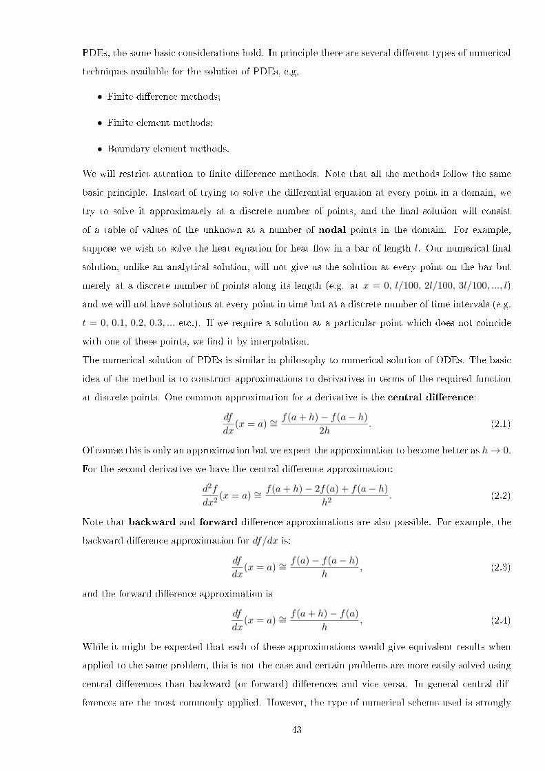
PDEs, the same basic considerations hold. In principle there are several di�erent types of numerical

techniques available for the solution of PDEs, e.g.

• Finite di�erence methods;

• Finite element methods;

• Boundary element methods.

We will restrict attention to �nite di�erence methods. Note that all the methods follow the same

basic principle. Instead of trying to solve the di�erential equation at every point in a domain, we

try to solve it approximately at a discrete number of points, and the �nal solution will consist

of a table of values of the unknown at a number of nodal points in the domain. For example,

suppose we wish to solve the heat equation for heat �ow in a bar of length l. Our numerical �nal

solution, unlike an analytical solution, will not give us the solution at every point on the bar but

merely at a discrete number of points along its length (e.g. at x = 0, l/100, 2l/100, 3l/100, ..., l)

and we will not have solutions at every point in time but at a discrete number of time intervals (e.g.

t = 0, 0.1, 0.2, 0.3, ... etc.). If we require a solution at a particular point which does not coincide

with one of these points, we �nd it by interpolation.

The numerical solution of PDEs is similar in philosophy to numerical solution of ODEs. The basic

idea of the method is to construct approximations to derivatives in terms of the required function

at discrete points. One common approximation for a derivative is the central di�erence:

df

dx(x = a) ∼=

f(a+ h)− f(a− h)

2h. (2.1)

Of course this is only an approximation but we expect the approximation to become better as h→ 0.

For the second derivative we have the central di�erence approximation:

d2f

dx2(x = a) ∼=

f(a+ h)− 2f(a) + f(a− h)

h2. (2.2)

Note that backward and forward di�erence approximations are also possible. For example, the

backward di�erence approximation for df/dx is:

df

dx(x = a) ∼=

f(a)− f(a− h)

h, (2.3)

and the forward di�erence approximation is

df

dx(x = a) ∼=

f(a+ h)− f(a)

h, (2.4)

While it might be expected that each of these approximations would give equivalent results when

applied to the same problem, this is not the case and certain problems are more easily solved using

central di�erences than backward (or forward) di�erences and vice versa. In general central dif-

ferences are the most commonly applied. However, the type of numerical scheme used is strongly

43

dependent on the type of PDE (elliptic, parabolic or hyperbolic) and di�erent methods have been

developed for each type. We note that the justi�cation for these approximations and the computa-

tion of the errors involved depends on the Taylor expansions of the functions. For example, using

Taylor series

f(a+ h) = f(a) + hdf

dx(a) +O(h2)

f(a− h) = f(a)− hdf

dx(a) +O(h2),

where O(h2) means terms which behave essentially like constant times h2 and can be expected to

be small if h is chosen to be small enough. Subtracting the second equation from the �rst we �nd:

df

dx(x = a) ∼=

f(a+ h)− f(a− h)

2h+O(h2), (2.5)

so the error in this approximation is O(h2). [Note that the O(h2) do not cancel in the subtraction!]

Exercise: Show that the error in the backward di�erence for df/dx is O(h). This indicates that a

central di�erence is "superior" in some sense to a backward (or forward) di�erence.

When dealing with partial derivatives, the approximations are the same except for the fact that

there is a partial derivative with respect to each variable. For example, if u = u(x, t) then an

approximation for ∂u/∂x at x = a is

∂u

∂x(x = a, t) ∼=

u(a+ h, t)− u(a− h, t)

2h+O(h2). (2.6)

2.1 Numerical solutions to the wave equation (hyperbolic)

Figure 2.1 illustrates a mesh of points, or nodes, with spacing ∆x in the x direction and ∆t in the

t direction. Each node is speci�ed by a pair of integers (i, j) so that the coordinates of the nodal

points take the form:

xi = xi−1 +∆x, tj = tj−1 +∆t,

and then we use a forward di�erence at the point A and a backward di�erence at the point B:(∂u

∂x

)A

∼=ui,j − ui−1,j

∆x,

(∂u

∂x

)B

∼=ui+1,j − ui,j

∆x,

i.e. a forward di�erence at A and a backward di�erence at B. Note that ui,j = u(xi, tj). The second

derivative at P therefore has the (central di�erence) numerical form:

∂2u

∂x2=

(∂u/∂x)B − (∂u/∂x)A∆x

=ui+1,j − 2ui,j + ui−1,j

∆x2. (2.7)

Similarly,∂2u

∂t2=ui,j+1 − 2ui,j + ui,j−1

∆t2. (2.8)

44

Rows

Columns

i-1 i i+1t

x

A B

P(i,j)

j+1

j

j-1

t

t

t

j+1

j

j-1

x

t

x x xi-1 i i+10

Figure 2.1: Mesh points for a numerical solution of the wave equation.

Thus the wave equation utt = c2uxx becomes

ui+1,j − 2ui,j + ui−1,j

∆x2= c2

ui,j+1 − 2ui,j + ui,j−1

∆t2,

which can be re-arranged as

ui,j+1 = 2ui,j − ui,j−1 + λ2[ui+1,j − 2ui,j + ui−1,j

], (2.9)

where λ = c∆t/∆x. Equation (2.9) is a �nite di�erence representation of the wave equation,

and provided that u is known on rows j − 1 and j then ui,j+1 can be computed on row j + 1 from

(2.9) and thus the solution continued. On the zeroth row the boundary conditions u(x, 0) = f(x)

and ∂u(x, 0)/∂t = g(x) are known, so that fi ≡ ui,0 and gi ≡ ∂u/∂t∣∣i,0

are also known at each node

on this row, and these are used to start the process o�. Using a centred di�erence we see that

gi =∂u

∂t

∣∣∣∣(i,0)

=ui,1 − ui,−1

2∆t. (2.10)

Now (2.9) with j = 0 becomes

ui,1 = 2ui,0 − ui,−1 + λ2[ui+1,0 − 2ui,0 + ui−1,0

]. (2.11)

Since ui,0 = fi and ui,−1 = ui,1 − 2∆tgi, (2.11) now takes the form

ui,1 = (1− λ2)fi +λ2

2

(fi+1 + fi−1

)+∆tgi. (2.12)

Thus the basic strategy is to compute row zero from ui,0 = fi, evaluate row one from (2.12),

and then to march forward for general row j by (2.9).

45

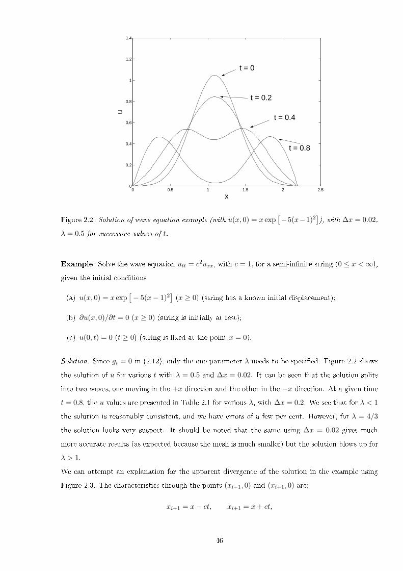
0 0.5 1 1.5 2 2.50

0.2

0.4

0.6

0.8

1

1.2

1.4

x

u

t = 0

t = 0.2

t = 0.4

t = 0.8

Figure 2.2: Solution of wave equation example (with u(x, 0) = x exp[−5(x−1)2

]), with ∆x = 0.02,

λ = 0.5 for successive values of t.

Example: Solve the wave equation utt = c2uxx, with c = 1, for a semi-in�nite string (0 ≤ x <∞),

given the initial conditions

(a) u(x, 0) = x exp[− 5(x− 1)2

](x ≥ 0) (string has a known initial displacement);

(b) ∂u(x, 0)/∂t = 0 (x ≥ 0) (string is initially at rest);

(c) u(0, t) = 0 (t ≥ 0) (string is �xed at the point x = 0).

Solution. Since gi = 0 in (2.12), only the one parameter λ needs to be speci�ed. Figure 2.2 shows

the solution of u for various t with λ = 0.5 and ∆x = 0.02. It can be seen that the solution splits

into two waves, one moving in the +x direction and the other in the −x direction. At a given time

t = 0.8, the u values are presented in Table 2.1 for various λ, with ∆x = 0.2. We see that for λ < 1

the solution is reasonably consistent, and we have errors of a few per cent. However, for λ = 4/3

the solution looks very suspect. It should be noted that the same using ∆x = 0.02 gives much

more accurate results (as expected because the mesh is much smaller) but the solution blows up for

λ > 1.

We can attempt an explanation for the apparent divergence of the solution in the example using

Figure 2.3. The characteristics through the points (xi−1, 0) and (xi+1, 0) are:

xi−1 = x− ct, xi+1 = x+ ct,

46

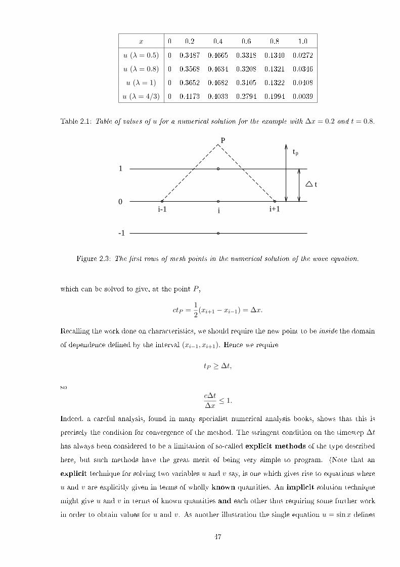
x 0 0.2 0.4 0.6 0.8 1.0

u (λ = 0.5) 0 0.3487 0.4665 0.3318 0.1340 0.0272

u (λ = 0.8) 0 0.3568 0.4634 0.3208 0.1321 0.0346

u (λ = 1) 0 0.3652 0.4682 0.3105 0.1322 0.0408

u (λ = 4/3) 0 0.4173 0.4033 0.2794 0.1994 0.0039

Table 2.1: Table of values of u for a numerical solution for the example with ∆x = 0.2 and t = 0.8.

-1

0

1

tp

t

i-1 i i+1

P

Figure 2.3: The �rst rows of mesh points in the numerical solution of the wave equation.

which can be solved to give, at the point P ,

ctP =1

2(xi+1 − xi−1) = ∆x.

Recalling the work done on characteristics, we should require the new point to be inside the domain

of dependence de�ned by the interval (xi−1, xi+1). Hence we require

tP ≥ ∆t,

soc∆t

∆x≤ 1.

Indeed, a careful analysis, found in many specialist numerical analysis books, shows that this is

precisely the condition for convergence of the method. The stringent condition on the timestep ∆t

has always been considered to be a limitation of so-called explicit methods of the type described

here, but such methods have the great merit of being very simple to program. (Note that an

explicit technique for solving two variables u and v say, is one which gives rise to equations where

u and v are explicitly given in terms of wholly known quantities. An implicit solution technique

might give u and v in terms of known quantities and each other thus requiring some further work

in order to obtain values for u and v. As another illustration the single equation u = sinx de�nes

47

u explicitly as a function of x but the equation u = sin (x− u) de�nes u implicitly as a function

of x). As computers get faster, the very short timestep required for explicit methods is becoming

less of a problem, and vector or array processors allow nodes to be dealt with simultaneously, thus

making such methods even more competitive.

There are, however, clear advantages in the stability of calculations if an implicit method is used.

In Figure 2.1 the approximation to uxx may be formed by the average of the approximations from

rows j + 1 to j − 1. Thus

ui,j+1 − 2ui,j + ui,j−1

c2∆t2

=ui+1,j+1 − 2ui,j+1 + ui−1,j+1 + ui+1,j−1 − 2ui,j−1 + ui−1,j−1

2∆x2.

Assuming that u is known on rows j and j − 1, we can rearrange the equation into the convenient

form

− λ2ui+1,j+1 + 2(1 + λ2)ui,j+1 − λ2ui−1,j+1

= 4ui,j + λ2ui+1,j−1 − 2(1 + λ2)ui,j−1 + λ2ui−1,j−1. (2.13)

The right-hand side of (2.13) is known, since it depends only on rows j and j − 1. The unknowns

on row j + 1 appear on the left-hand side. The equations (essentially of the form Ax = b where

A is a matrix and x, b are column vectors, with b being known and x the unknowns which we are

seeking) can now be solved simultaneously using Gaussian elimination or algorithms for tridiagonal

systems. It can be shown that the method will proceed satisfactorily for any λ, so that the timestep

is unrestricted. The evaluation of rows 0 and 1 is the same as for the explicit method, so this can

reduce the accuracy, and clearly the algorithm needs a �nite x region to allow the matrix inversion.

2.2 Numerical solutions to the di�usion equation (parabolic)

As for the wave equation, except for the most straightforward problems, we must resort to numerical

solutions of the heat-conduction equation. Even when analytical solutions are known, they are not

always easy to evaluate because of convergence di�culties near to singularities. They are, of course,

crucial in testing the accuracy and e�ciency of numerical methods.

We can write the heat-conduction equation

∂u

∂t= c2

∂2u

∂x2, (2.14)

in the usual �nite-di�erence form, using the notation of Figure 2.4.

We assume that we know the solution up to timestep j and we wish to calculate the solution at

time step j + 1. In � 5.1 we showed how to approximate the second derivative as

∂2u

∂x2=ui+1,j − 2ui,j + ui−1,j

∆x2.

48

j+1

j

i-1 i i+1

t

x

Figure 2.4: Mesh for marching forwards in the numerical solution of the heat conduction equation.

To obtain the time derivative, we use the approximation between rows j and j + 1:

∂u

∂t=ui,j+1 − ui,j

∆t.

Putting these into (2.14) gives

ui,j+1 − ui,jc2∆t

=ui+1,j − 2ui,j + ui−1,j

∆x2,

or, on rearranging,

ui,j+1 = λui−1,j + (1− 2λ)ui,j + λui+1,j , (2.15)

where λ = c2∆t/∆x2. Equation (2.15) gives a �nite-di�erence representation of (2.14), and provided

that all the values are known on row j, we can then compute u on row j + 1 from the simple

explicit formula (2.15). This formula can only be used on the inner mesh points but the boundary

conditions give the values u0,j and uI,j (where I is the size of the grid and so xI = 1 for a domain

0 ≤ x ≤ 1). We will see this now in an example.

Example: Solve the heat conduction equation ut = c2uxx, with c = 1, for a bar of conducting

material of length 1 subject to the boundary conditions:

(a) u(x, 0) = x2 (0 ≤ x ≤ 1) (a known initial temperature distribution);

(b) ∂u(0, t)/∂x = 0 (t ≥ 0) (the end x = 0 is insulated so no heat �ow occurs through it);

(c) u(1, t) = 1 (t ≥ 0) (the end x = 1 is held �xed at temperature u = 1).

Solution. The condition (a) gives ui,0 = x2i and this holds along the x-axis (as shown in Figure 2.5).

If we choose ∆x = 0.2 then the values of ui,0 are 02, 0.22, 0.42, 0.62, 0.82, 12 (for i = 0, 1, ..., 5 and

so here I = 5). The condition (c) immediately gives u5,j = 1 and we therefore only need to interpret

condition (b). We can use a central di�erence to deduce that

∂u

∂x

∣∣∣∣x=0

≡ u−1,j − u1,j2∆x

= 0 =⇒ u−1,j = u1,j . (2.16)

49

We are essentially adding a �ctitious line of nodes at i = −1. The point u−1,j must be eliminated

in a similar way to that done for the wave equation (where we eliminated ui,−1 using (2.10)). We

use (2.15) with i = 0 to obtain

u0,j+1 = λu−1,j + (1− 2λ)u0,j + λu1,j = (1− 2λ)u0,j + 2λu1,j , (2.17)

since u−1,j = u1,j . Then we can �nd all the points along the left boundary using (2.17), since the

right hand side involves known values (they are all at j rather than j + 1). From Figure 2.5 it is

clear that we have all the information required along the x = 0 and x = 1 axis, as well as along

the t = 0 axis. We can then use (2.15) to solve for the interior points up until the appropriate j

value to give us the required time. In Table 2.2 we show the results at t = 1 for various λ and �xed

∆x = 0.2. The number of j points used is determined from ∆t, which we �nd from rearranging the

expression λ = c2∆t/∆x2. In Figure 2.6 we plot the solution u with λ = 0.2.

Comparing this example with the numerical solution of the wave equation from � 5.1, we observe

similar behaviour for the explicit scheme, namely that the method will only converge for small

enough timesteps or λ. From (2.15) it may be noted that the middle term changes sign at λ =

0.5, and above this value we might anticipate di�culties (as shown in Table 2.2). Indeed, some

straightforward numerical analysis shows that convergence is certain for λ < 0.5. It is su�cient

here to note that λ must not be too large.

i=0 i=1 i=2 i=3 i=4 i=5x

x=1

j=0

j=1

j=2

x

t

t

u(x,0) = x i2

Figure 2.5: Mesh for the example of the numerical solution of the heat conduction equation.

To avoid the limitation on λ, we can again look at an implicit formulation of the numerical

equations. Returning to Figure 2.4, the idea is to approximate the x derivative by an average of

row j and row j + 1. This leads to (instead of (2.15))

−λui−1,j+1 + 2(1 + λ)ui,j+1 − λui+1,j+1 = λui−1,j + 2(1− λ)ui,j + λui+1,j , (2.18)

and is called the Crank-Nicolson method. We have the solution on row j, so the right hand

50

x 0 0.2 0.4 0.6 0.8 1.0

u (λ = 0.2) 0.9128 0.9171 0.9295 0.9488 0.9731 1

u (λ = 0.5) 0.9160 0.9202 0.9320 0.9507 0.9740 1

u (λ = 0.625) −1.3568× 103 1.2922× 103 −1.0975× 103 5.1857× 102 4.1857× 102 1

Table 2.2: Table of values of u for a numerical solution for the heat conduction example.

00.2

0.40.6

0.81

0

0.2

0.4

0.6

0.8

10

0.2

0.4

0.6

0.8

1

x

Example for Heat Equation

t

u

Figure 2.6: Solution of heat equation example, with ∆x = 0.2, λ = 0.2 and t = 1.

side of (2.18) is known, and the row j + 1 have to be solved for simultaneously. Again this can be

written in matrix form, as discussed after equation (2.13) in the previous section.

2.3 Numerical solution of elliptic problems

Of the three classical partial di�erential equations, the Laplace equation proves to be the most

di�cult to solve. The other two have a natural time variable in them, and it is possible, with a

little care, to march forward either by a simple explicit method or by an implicit procedure. In the

case of the Laplace equation (elliptic), information is given around the whole of the boundary of

the solution region, so the �eld variables at all mesh points must be solved simultaneously. This in

turn leads to a solution of the algebraic problem by matrix inversion.

The usual numerical approximation for the partial derivatives, discussed in � 5.1, are employed, so

51

that the equation∂2u

∂x2+∂2u

∂y2= 0, (2.19)

at a typical point, illustrated in Figure 2.7, becomes

ui+1,j − 2ui,j + ui−1,j

∆x2+ui,j+1 − 2ui,j + ui,j−1

∆y2= 0.

For the case ∆x = ∆y, rearranging gives

4ui,j = ui+1,j + ui−1,j + ui,j+1 + ui,j−1. (2.20)

This is the typical �ve-point stencil and it should be noted that the middle value ui,j is the average

of its four neighbours. We now examine how (2.20) can be implemented.

(i,j)

(i,j-1)

(i,j+1)

(i-1,j) (i+1,j)

y

x

Figure 2.7: Five-point computational model for the Laplace equation.

Example: Solve the Laplace equation (2.19) in the square region 0 ≤ x ≤ 1, 0 ≤ y ≤ 1, with

∆x = ∆y = 1/3 and the following boundary conditions:

u(0, y) = 0, u(1, y) = 1, u(x, 0) = 0, u(x, 1) = 0.

Solution. For a �rst solution we take the simplest mesh, illustrated in Figure 2.8, which contain

only four interior points labelled u1, u2, u3, u4. The four equations obtained from (2.20) are

4u1 = 0 + 0 + u2 + u4

4u2 = 0 + 1 + u3 + u1

4u3 = 1 + 0 + u4 + u2

4u4 = 0 + 0 + u1 + u3,

52

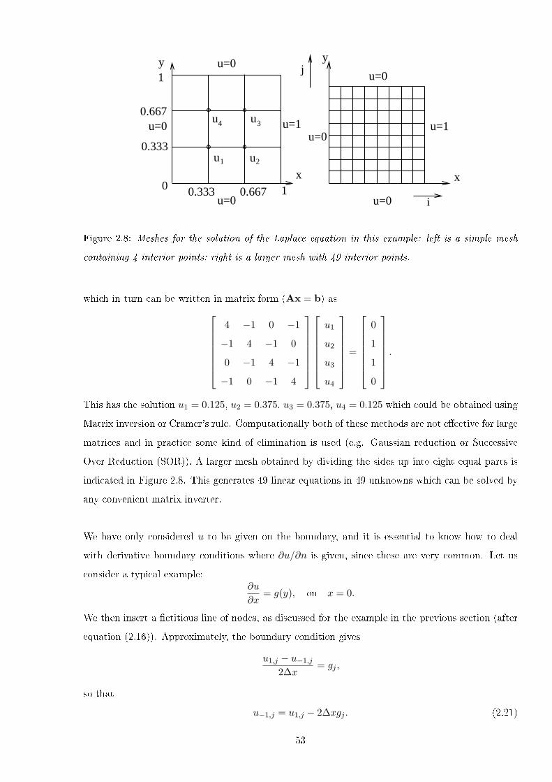
y

x

u=1

u=0

u=0

u=00

0.333

0.667

1

0.333 1

0.667u u

u u

4 3

21

u=0

u=0u=1

u=0

x

yj

i

Figure 2.8: Meshes for the solution of the Laplace equation in this example: left is a simple mesh

containing 4 interior points; right is a larger mesh with 49 interior points.

which in turn can be written in matrix form (Ax = b) as4 −1 0 −1

−1 4 −1 0

0 −1 4 −1

−1 0 −1 4

u1

u2

u3

u4

=

0

1

1

0

.

This has the solution u1 = 0.125, u2 = 0.375, u3 = 0.375, u4 = 0.125 which could be obtained using

Matrix inversion or Cramer's rule. Computationally both of these methods are not e�ective for large

matrices and in practice some kind of elimination is used (e.g. Gaussian reduction or Successive

Over Reduction (SOR)). A larger mesh obtained by dividing the sides up into eight equal parts is

indicated in Figure 2.8. This generates 49 linear equations in 49 unknowns which can be solved by

any convenient matrix inverter.

We have only considered u to be given on the boundary, and it is essential to know how to deal

with derivative boundary conditions where ∂u/∂n is given, since these are very common. Let us

consider a typical example:∂u

∂x= g(y), on x = 0.

We then insert a �ctitious line of nodes, as discussed for the example in the previous section (after

equation (2.16)). Approximately, the boundary condition gives

u1,j − u−1,j

2∆x= gj ,

so that

u−1,j = u1,j − 2∆xgj . (2.21)

53

Equation (2.20) is now solved for i = 0 as well as i > 0, but at the end of a sweep u−1,j will be

updated via (2.21).

Example: Solve the Laplace equation (2.19) in the square region 0 ≤ x ≤ 1, 0 ≤ y ≤ 1, with mesh

spacing ∆x = ∆y = 1/4 and the following boundary conditions:

∂u

∂x(0, y) = 1, u(1, y) = y2, u(x, 0) = 0, u(x, 1) = x.

[The �rst condition indicates a heat supply along this boundary and the last three conditions

correspond to the temperature being given along these three sides].

Solution. The region is illustrated in Figure 2.9. Since we have added the �ctitious boundary i = −1

there are 12 unknowns. Equation (2.21) just gives u−1,j = u1,j − 1/2 for each j. From (2.20), we

can write the equations as

4u0,1 = u−1,1 + u1,1 + 0 + u0,2 = −1/2 + 2u1,1 + u0,2

4u1,1 = u0,1 + u2,1 + 0 + u1,2

4u2,1 = u1,1 + u3,1 + 0 + u2,2,

and so on, and hence obtain 12 equations in the 12 unknowns. These can be solved by any convenient

method to give a solution as tabulated in Table 2.3.

i = 0 i = 1 i = 2 i = 3 i = 4

j = 4 0.0000 0.2500 0.5000 0.7500 1.0000

j = 3 -0.1190 0.1114 0.3067 0.4644 0.5625

j = 2 -0.1987 0.0077 0.1511 0.2384 0.2500

j = 1 -0.1912 -0.0330 0.0516 0.0881 0.0625

j = 0 0.0000 0.0000 0.0000 0.0000 0.0000

Table 2.3: Data from the solution of the example using a step length of 0.25 in each direction.

Finally, note that if we were to have an inhomogeneous Laplace equation, namely the Poisson

equation

∇2u ≡ uxx + uyy = f, (2.22)

then the �nite di�erence approximation would become, instead of (2.20)

ui+1,j + ui−1,j + ui,j+1 + ui,j−1 − 4ui,j = h2fi,j (2.23)

where fi,j ≡ f(xi, yj) which is known.

54

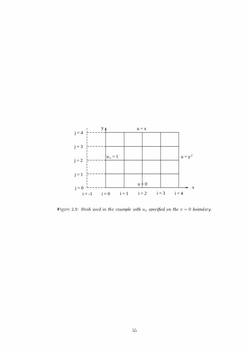
j = 0

j = 1

j = 2

j = 3

j = 4

i = -1 i = 0 i = 1 i = 2 i = 3 i = 4x

y u = x

u = 0

u = y 2u = 1x

Figure 2.9: Mesh used in the example with ux speci�ed on the x = 0 boundary.

55