Wavelets Applied to the Detection of PointSources of UHECRs

R. A. BATISTA1†, E. KEMP1, R. M. de ALMEIDA2 and B. DANIEL1

1Instituto de Fısica “ Gleb Wataghin”Universidade Estadual de Campinas

13083-859, Campinas-SP, Brazil

2Escola de Engenharia Industrial Metalurgica de Volta RedondaUniversidade Federal Fluminense

27255-125, Volta Redonda-RJ, Brazil

†rab@ifi.unicamp.br

Abstract

In this work we analyze the effect of smoothing maps containing arrival directions of cosmic rays with agaussian kernel and kernels of the mexican hat wavelet family of order 1, 2 and 3. The analysis is performed bycalculating the amplification of the signal-to-noise ratio for several anisotropy patterns (noise) and differentnumber of events coming from a simulated source (signal) for an ideal detector capable of observing the fullsky with equal probability. We extend this analysis for a virtual detector located within the array of detectorsof the Pierre Auger Observatory, considering an acceptance law.

1 Introduction

The origin, chemical composition and mechanisms of acceleration of the ultra-high energy cosmic rays (UHECRs)still remain a mistery half a century after their discovery[1], and are subject of great interest by the scientificcommunity due to their intrinsic relation with particle physics, cosmology and astrophysics. The flux of cosmicrays with energies above 1 EeV (1018 eV) is approximately 1 particle per square kilometer per year and 1 particleper square kilometer per century for energies above 60 EeV[2].

To achieve a reasonable statistic of events with energies above 1 EeV, it was built in the province of Mendoza,Argentina, the Pierre Auger Observatory, the result of an international effort of 17 countries. This observatory isa pioneer in the application of the hybrid technique of simultaneous fluorescence and surface detection. The firstconsists on the measurement of the fluorescence light resulting from the de-excitation of the nitrogen moleculeswhich interacted with particles from the extensive air shower (EAS) generated by the primary particle. Thesurface detection consists on the detection of particles from the EAS by an array of 1,600 water-Cherenkov tankscomposing a triangular grid with 1.5 km spacing from each other, covering an area of approximately 3,000 km2.

1

arX

iv:1

012.

3645

v2 [

astr

o-ph

.IM

] 1

Jun

201

1

The identification of possible astrophysical sources and the investigation of the magnetic fields which per-meates the universe are studied by analyzing the arrival directions of cosmic rays. The correlation of thesedirections with the large scale distribution of matter in the universe, such as the galactic and supergalacticplanes are considered large scale anisotropies. A small scale anisotropy is characterized by the association be-tween arrival directions of cosmic rays and point sources, such as stars, distant galaxies and other kind of objectswhich are far enough to be considered point sources.

Since the sources of UHECRs are still unknown, it is important to search for them. Amongst the candidatesto sources of UHECRs are the active galactic nuclei, gamma-ray bursts and magnetars[3]. Here we analyze theperformance of several convolution kernels on searching for anisotropies possibly correlating to some astrophysicalsources of UHECRs.

2 Wavelets

Wavelets are mathematical functions belonging to the L2 space that satisfy some requirements. The first one isthe admissibility condition, ∫

|ψ(ω)|2

|ω|dω <∞, (1)

where ψ(t) is the wavelet. This condition guarantees the reconstruction of a signal without loss of information.Also, the wavelet shall satisfy the condition of zero norm, i. e.,∫

ψ(t)dt = 0. (2)

This last condition means that the average value of the wavelet in time domain shall be zero at zero frequency[4].The continuous wavelet transform (CWT) may be formally written as:

Φ(s, τ) =

∫f(t)Ψ∗s,τ (t)dt, (3)

where s (s > 0, s ∈ R) and τ (τ ∈ R) are, respectively, the scale (dilation) and translation parameters. So, theCWT decomposes a function f(t) in a basis of wavelet Ψs,τ (t). The inverse transform is given by:

f(t) =

∫ ∫Φ(s, τ)Ψs,τ (t)dτds. (4)

These wavelets Ψs,τ (t) are obtained from a so-called mother-wavelet, by changing the dilation and translationparameters as follows:

Ψs,τ (t) =1√s

Ψ

(t− τs

). (5)

The mexican hat wavelet family (MHWF) and its extension on the sphere have been widely used aiming thedetection of point sources in maps of cosmic microwave background (CMB)[5, 6, 7], due to the amplification ofthe signal-to-noise ratio when going from the real space to wavelet space.

The MHWF is obtained by successive applications of the laplacian operator to the two-dimensional gaussian.A generic member of this family is:

Ψn(~x) =(−1)n

2nn!∇2nφ(~x), (6)

where φ is the two-dimensional gaussian (φ(~x) = 12π e−~x2/2σ) and the laplacian operator is applied n times.

3 Celestial Maps

When studying anisotropies, a powerful tool are the celestial maps, which are segmented pixelizations of thecelestial sphere. The events map is the celestial map which represents, in two dimensions, the arrival directionsof cosmic ray events in the celestial sphere.

Due to limitations of the detector itself, it is impossible to determine the exact arrival direction of an event.Each event detected is convolved with a probability distribution related to the angular resolution of the detector,that is, for each event there is an associated point spreading function (PSF). Therefore, it is extremely useful

2

to convolve the celestial maps with functions associated to the PSF of the detector, aiming to maximize thesignal-to-noise ratio. Mathematically, this process of convolution (filtering1) may be written as

Mf (~r0) = α

∫M(~r)Φ(~r, ~r0)dΩ, (7)

where α is a normalization constant, M(~r) is the number of cosmic ray events in the direction ~r, Φ(~r, ~r0) isthe kernel2 of the transformation and ~r0 is the position vector representing each point in which the integral isevaluated. In the discrete case this process is:

Mf (k) =

∑jM(j)Φ(~rk, ~rj)∑

j Φ(~rk, ~rj), (8)

where M(j) is the number of cosmic rays associated to the pixel of index j in the direction ~rj .

4 Analysis Procedure

In the present work we have tested the capability of the MHWF to detect point sources embedded in differentbackgrounds. The simulated source was simulated in the position (l, b)=(320o, 30o) (galactic coordinates) in thesky, with a dispersion of 2o. We have considered three possible scenarios for the source, varying the amplitudeof the source with respect to the background, and the number of events simulated in its direction. In the firstcase the source is 10% stronger than the background and 100, 000 events were simulated. In the second case,we have simulated 5, 000 events and the source has an amplitude of 1% with respect to the background. In thethird case there are only 50 events coming from the direction of the source, which has an amplitude of 0.1%with respect to the background.

For the background we have simulated 500, 000 events according to several anisotropy patterns. Theseanisotropy patterns were divided in two classes: with and without the acceptance of the detector. In the casewithout acceptance, the distribution of events in the sky is uniform, modulated only by the anisotropy patternimposed by the simulation. In the case with acceptance, we considered a detector in a place with latitude 35o

28′ 00′′ S and longitude 65o 18′ 41′′ W (approximately the coordinates of the Pierre Auger Observatory). Wehave assumed that the event are detected according to a zenith angle distribution that follows sinθcosθ, where0o ≤ θ ≤ 60o is the zenith angle[8].

Four anisotropy patterns were simulated as the background maps, with and without the acceptance of thedetector (figures 1 to 4). In all the cases these 500, 000 events were simulated. The simulated anisotropy patternswere:

• isotropic: isotropic distribution of events;

• dipole 1: a dipole with excess in the galactic center (l, b) = (0o, 0o), with amplitude 7% with respect tothe background;

• dipole 2: a dipole with excess in the direction (l, b) = (266.5o,−29o), with amplitude 0.5% with respectto the background;

• sources: several sources with different angular scales σ and amplitudes A in the directions (l, b): (0o, 0o)[σ = 7.0o, A = 100%], (320o, 90o) [σ = 1.5o, A = 5%], (320o,−40o) [σ = 0.5o, A = 1%], (220o, 10o)[σ = 3.0o, A = 5%], (100o,−70o) [σ = 2o, A = 10%], (240o, 50o) [σ = 20o, A = 5%], (350o,−80o)[σ = 6.0o, A = 0.5%], (100o, 50o) [σ = 30o, A = 50%], (140o,−40o) [σ = 4.0o, A = 200%] and (60o, 50o)[σ = 3.0o, A = 2%].

In order to verify the power of identification of the wavelets, we calculated the amplification (λ) of thesignal-to-noise ratio, which is:

λ =wf/σfw0/σ0

, (9)

where w0 is the value of the central pixel associated to the source in the non-filtered source map, wf is the valueof the same pixel in the filtered source map, σ0 is the root mean square (RMS) of the non-filtered backgroundmap and σf is the RMS of the filtered background map.

1In this paper we make no distinction between the processes of convolution, smoothing and filtering.2We also make no distinction between the terms kernel and filter.

3

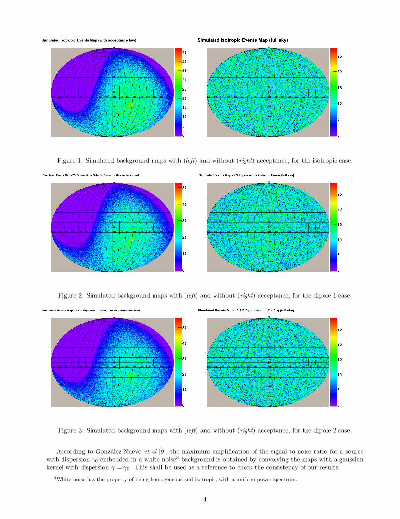
Figure 1: Simulated background maps with (left) and without (right) acceptance, for the isotropic case.

Figure 2: Simulated background maps with (left) and without (right) acceptance, for the dipole 1 case.

Figure 3: Simulated background maps with (left) and without (right) acceptance, for the dipole 2 case.

According to Gonzalez-Nuevo et al [9], the maximum amplification of the signal-to-noise ratio for a sourcewith dispersion γ0 embedded in a white noise3 background is obtained by convolving the maps with a gaussiankernel with dispersion γ = γ0. This shall be used as a reference to check the consistency of our results.

3White noise has the property of being homogeneous and isotropic, with a uniform power spectrum.

4

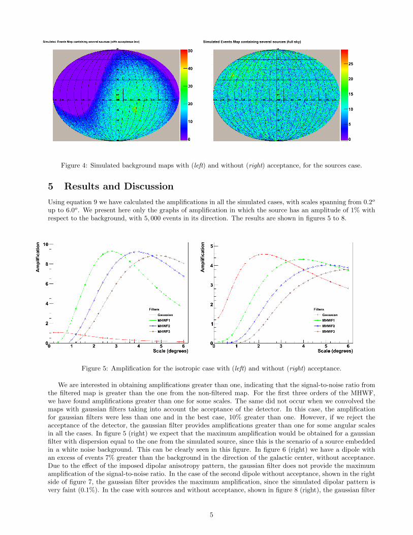
Figure 4: Simulated background maps with (left) and without (right) acceptance, for the sources case.

5 Results and Discussion

Using equation 9 we have calculated the amplifications in all the simulated cases, with scales spanning from 0.2o

up to 6.0o. We present here only the graphs of amplification in which the source has an amplitude of 1% withrespect to the background, with 5, 000 events in its direction. The results are shown in figures 5 to 8.

Figure 5: Amplification for the isotropic case with (left) and without (right) acceptance.

We are interested in obtaining amplifications greater than one, indicating that the signal-to-noise ratio fromthe filtered map is greater than the one from the non-filtered map. For the first three orders of the MHWF,we have found amplifications greater than one for some scales. The same did not occur when we convolved themaps with gaussian filters taking into account the acceptance of the detector. In this case, the amplificationfor gaussian filters were less than one and in the best case, 10% greater than one. However, if we reject theacceptance of the detector, the gaussian filter provides amplifications greater than one for some angular scalesin all the cases. In figure 5 (right) we expect that the maximum amplification would be obtained for a gaussianfilter with dispersion equal to the one from the simulated source, since this is the scenario of a source embeddedin a white noise background. This can be clearly seen in this figure. In figure 6 (right) we have a dipole withan excess of events 7% greater than the background in the direction of the galactic center, without acceptance.Due to the effect of the imposed dipolar anisotropy pattern, the gaussian filter does not provide the maximumamplification of the signal-to-noise ratio. In the case of the second dipole without acceptance, shown in the rightside of figure 7, the gaussian filter provides the maximum amplification, since the simulated dipolar pattern isvery faint (0.1%). In the case with sources and without acceptance, shown in figure 8 (right), the gaussian filter

5

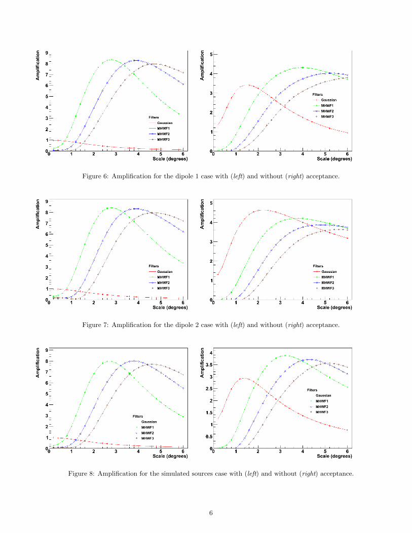
Figure 6: Amplification for the dipole 1 case with (left) and without (right) acceptance.

Figure 7: Amplification for the dipole 2 case with (left) and without (right) acceptance.

Figure 8: Amplification for the simulated sources case with (left) and without (right) acceptance.

6

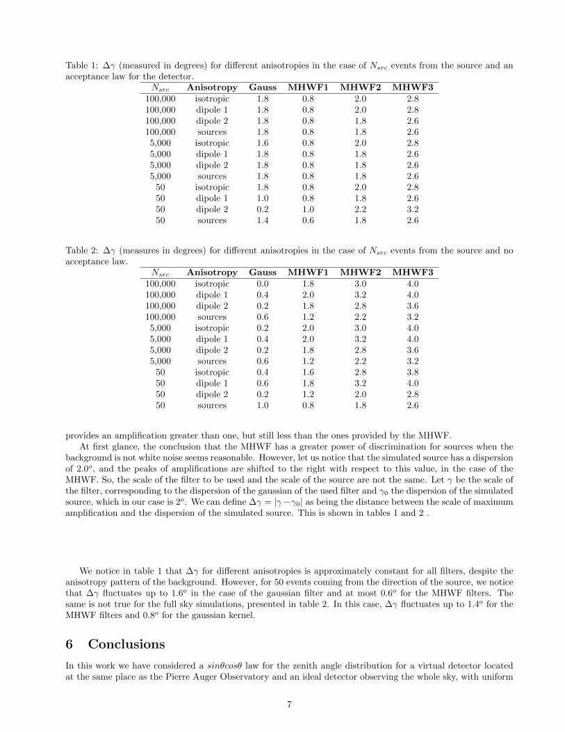
Table 1: ∆γ (measured in degrees) for different anisotropies in the case of Nsrc events from the source and anacceptance law for the detector.

Nsrc Anisotropy Gauss MHWF1 MHWF2 MHWF3100,000 isotropic 1.8 0.8 2.0 2.8100,000 dipole 1 1.8 0.8 2.0 2.8100,000 dipole 2 1.8 0.8 1.8 2.6100,000 sources 1.8 0.8 1.8 2.65,000 isotropic 1.6 0.8 2.0 2.85,000 dipole 1 1.8 0.8 1.8 2.65,000 dipole 2 1.8 0.8 1.8 2.65,000 sources 1.8 0.8 1.8 2.6

50 isotropic 1.8 0.8 2.0 2.850 dipole 1 1.0 0.8 1.8 2.650 dipole 2 0.2 1.0 2.2 3.250 sources 1.4 0.6 1.8 2.6

Table 2: ∆γ (measures in degrees) for different anisotropies in the case of Nsrc events from the source and noacceptance law.

Nsrc Anisotropy Gauss MHWF1 MHWF2 MHWF3100,000 isotropic 0.0 1.8 3.0 4.0100,000 dipole 1 0.4 2.0 3.2 4.0100,000 dipole 2 0.2 1.8 2.8 3.6100,000 sources 0.6 1.2 2.2 3.25,000 isotropic 0.2 2.0 3.0 4.05,000 dipole 1 0.4 2.0 3.2 4.05,000 dipole 2 0.2 1.8 2.8 3.65,000 sources 0.6 1.2 2.2 3.2

50 isotropic 0.4 1.6 2.8 3.850 dipole 1 0.6 1.8 3.2 4.050 dipole 2 0.2 1.2 2.0 2.850 sources 1.0 0.8 1.8 2.6

provides an amplification greater than one, but still less than the ones provided by the MHWF.At first glance, the conclusion that the MHWF has a greater power of discrimination for sources when the

background is not white noise seems reasonable. However, let us notice that the simulated source has a dispersionof 2.0o, and the peaks of amplifications are shifted to the right with respect to this value, in the case of theMHWF. So, the scale of the filter to be used and the scale of the source are not the same. Let γ be the scale ofthe filter, corresponding to the dispersion of the gaussian of the used filter and γ0 the dispersion of the simulatedsource, which in our case is 2o. We can define ∆γ = |γ−γ0| as being the distance between the scale of maximumamplification and the dispersion of the simulated source. This is shown in tables 1 and 2 .

We notice in table 1 that ∆γ for different anisotropies is approximately constant for all filters, despite theanisotropy pattern of the background. However, for 50 events coming from the direction of the source, we noticethat ∆γ fluctuates up to 1.6o in the case of the gaussian filter and at most 0.6o for the MHWF filters. Thesame is not true for the full sky simulations, presented in table 2. In this case, ∆γ fluctuates up to 1.4o for theMHWF filters and 0.8o for the gaussian kernel.

6 Conclusions

In this work we have considered a sinθcosθ law for the zenith angle distribution for a virtual detector locatedat the same place as the Pierre Auger Observatory and an ideal detector observing the whole sky, with uniform

7

acceptance. We have simulated a source with different number of events coming from it, embedded in severalbackgrounds. We have calculated the amplifications of the signal-to-noise ratio in each case and verified thatin the case of a source with dispersion γ0 embedded in a white noise background, the maximum amplificationis achieved with a gaussian filter with dispersion γ = γ0, as predicted. In the case of a faint dipole with noacceptance, the gaussian provided a greater amplification of the signal-to-noise ratio. However, if the backgrounddoes not have a constant power spectrum, as in the case of the other anisotropy patterns, the Mexican HatWavelet Family filters provided, in general, a greater amplification of the signal-to-noise ratio, allowing one toidentify point sources in maps containing arrival directions of cosmic rays.

It is interesting to notice that the existence of an acceptance for the detector affects the power of discrim-ination of the gaussian filter. The amplification, in this case, is always below 1.1, whereas in the case of theMHWF the amplification of the signal-to-noise ratio can be more than ten.

The acceptance of the experiment affects the power spectrum of the background in celestial maps. If it is notwhite noise, the maximum amplification of the signal-to-noise ratio is achieved by the MHWF kernel. However,even though we can amplify the signal-to-noise ratio using MHWF, we lose directional information about theassociated cosmic ray events. If we consider a gaussian filter and a white noise background, the optimal gaussianfilter would have exactly the same dispersion as the source and the uncertainty on the position would arise fromthe resolution of the detector, rather than the analysis method used. By using MHWF, the greater the order ofthe wavelet, the greater the difference between the sizes of the source and the wavelet. Therefore, despite thegain on the power of discrimination of the source, there is a loss of resolution.

Since the acceptance introduces a non-white noise background, for analysis involving the whole sky, such asblindsearch4, the MHWF amplifies the signal-to-noise ratio more than the gaussian. However, for small scaleanalysis, smoothing the maps with a gaussian kernel and reducing the area of scan could provide a greateramplification, specially if the background within the window of scan has a uniform power spectrum.

A limitation to this technique is the projection of the celestial sphere to the plane. This approximation isgood enough for small scales, when we can use the approximation sinθ ≈ θ. For θ > 7o, this approximationintroduce bias and this method would have to be adapted to work on a spherical manifold. Wavelets on thesphere have been used on CMB studies[10, 11, 12, 13] and presented good results. The next step of this work isa similar analysis using wavelets on the sphere, which allow us to search not only point sources, but also largescale structures in maps containing arrival directions of cosmic rays.

7 Acknowledgements

We are grateful for the financial support of FAPESP (Fundacao de Amparo a Pesquisa do Estado de Sao Paulo)and CNPq (Conselho Nacional de Pesquisa e Desenvolvimento). Also, we would like to thank the developers ofthe Coverage & Anisotropy Toolkit, which allowed us to perform fast simulations of cosmic ray events.

References

[1] J. Linsley. Phys. Rev. Lett. 10 (1963), 146.

[2] Pierre Auger Collaboration (J. Abraham et al.). Astro. Ph. 29 (2008), 188.

[3] A. M. Hillas. Ann. Rev. Astron. Astoph. 22 (1984), 425.

[4] P. S. Addison, J. N. Watson, T. Feng. J. Sound Vib. 254 (2002), 733.

[5] A. Cayon et al.. MNRAS, 313 (2000), 757.

[6] P. Vielva et al.. MNRAS, 326 (2001), 181.

[7] P. Vielva et al.. MNRAS, 344 (2003), 89.

[8] M. Kalcheriess, D. V. Semikoz. Phys. Let. B, 577 (2003), 1.

[9] J. Gonzalez-Nuevo et al.. MNRAS, 369 (2006), 1603.

[10] Y. Wiaux et al.. MNRAS, 3 (2008), 770.

4The procedure of blindsearch is to search for astrophysical objects on a given window around any observed excess.

8

[11] J. D. McEwen et al.. MNRAS, 384 (2008), 1289.

[12] J. D. McEwen et al.. J. Four. Anal. App. 13 (2007), 495.

[13] J. D. McEwen. MNRAS, 359 (2005), 1583.

9