Australian Mathematical Society Lecture Series: 24

Wavelets: A Student Guide

PETER NICKOLAS

University of Wollongong, New South Wales

www.cambridge.orgInformation on this title: www.cambridge.org/9781107612518

© Peter Nickolas 2017

First published 2017

Printed in the United Kingdom by Clays, St Ives plc

A catalogue record for this publication is available from the British Library

Library of Congress Cataloging-in-Publication dataNames: Nickolas, Peter.

Title: Wavelets : a student guide / Peter Nickolas, University of Wollongong,New South Wales.

Description: Cambridge : Cambridge University Press, 2017. |Series: Australian Mathematical Society lecture series ; 24 |

Includes bibliographical references and index.Identifiers: LCCN 2016011212 | ISBN 9781107612518 (pbk.)

Subjects: LCSH: Wavelets (Mathematics)–Textbooks. | Inner productspaces–Textbooks. | Hilbert space–Textbooks.

Classification: LCC QA403.3.N53 2016 | DDC 515/.2433–dc23 LC record availableat http://lccn.loc.gov/2016011212

ISBN 978-1-107-61251-8 Paperback

Contents

Preface page vii

1 An Overview 11.1 Orthonormality in Rn 11.2 Some Infinite-Dimensional Spaces 61.3 Fourier Analysis and Synthesis 151.4 Wavelets 181.5 The Wavelet Phenomenon 25Exercises 27

2 Vector Spaces 312.1 The Definition 312.2 Subspaces 342.3 Examples 35Exercises 40

3 Inner Product Spaces 423.1 The Definition 423.2 Examples 433.3 Sets of Measure Zero 483.4 The Norm and the Notion of Distance 513.5 Orthogonality and Orthonormality 553.6 Orthogonal Projection 64Exercises 73

4 Hilbert Spaces 804.1 Sequences in Inner Product Spaces 804.2 Convergence in Rn, �2 and the L2 Spaces 844.3 Series in Inner Product Spaces 904.4 Completeness in Inner Product Spaces 94

4.5 Orthonormal Bases in Hilbert Spaces 1054.6 Fourier Series in Hilbert Spaces 1084.7 Orthogonal Projections in Hilbert Spaces 114Exercises 117

5 The Haar Wavelet 1265.1 Introduction 1265.2 The Haar Wavelet Multiresolution Analysis 1275.3 Approximation Spaces and Detail Spaces 1335.4 Some Technical Simplifications 137Exercises 138

6 Wavelets in General 1416.1 Introduction 1416.2 Two Fundamental Definitions 1456.3 Constructing a Wavelet 1506.4 Wavelets with Bounded Support 159Exercises 168

7 The Daubechies Wavelets 1767.1 Introduction 1767.2 The Potential Scaling Coefficients 1787.3 The Moments of a Wavelet 1797.4 The Daubechies Scaling Coefficients 1857.5 The Daubechies Scaling Functions and Wavelets 1887.6 Some Properties of 2φ 2007.7 Some Properties of Nφ and Nψ 205Exercises 209

8 Wavelets in the Fourier Domain 2188.1 Introduction 2188.2 The Complex Case 2198.3 The Fourier Transform 2278.4 Applications to Wavelets 2328.5 Computing the Daubechies Scaling Coefficients 237Exercises 242

Appendix: Notes on Sources 251

References 259Index 262

Preface

OverviewThe overall aim of this book is to provide an introduction to the theory ofwavelets for students with a mathematical background at senior undergraduatelevel. The text grew from a set of lecture notes that I developed while teachinga course on wavelets at that level over a number of years at the University ofWollongong.

Although the topic of wavelets is somewhat specialised and is certainlynot a standard one in the typical undergraduate syllabus, it is neverthelessan attractive one for introduction to students at that level. This is for severalreasons, including its topicality and the intrinsic interest of its fundamentalideas. Moreover, although a comprehensive study of the theory of waveletsmakes the use of advanced mathematics unavoidable, it remains true thatsubstantial parts of the theory can, with care, be made accessible at theundergraduate level.

The book assumes familiarity with finite-dimensional vector spaces and theelements of real analysis, but it does not assume exposure to analysis at anadvanced level, to functional analysis, to the theory of Lebesgue integrationand measure or to the theory of the Fourier integral transform. Knowledgeof all these topics and more is assumed routinely in all full accounts ofwavelet theory, which make heavy use of the Lebesgue and Fourier theoriesin particular.

The approach adopted here is therefore what is often referred to as ‘ele-mentary’. Broadly, full proofs of results are given precisely to the extent thatthey can be constructed in a form that is consistent with the relatively modestassumptions made about background knowledge. A number of central resultsin the theory of wavelets are by their nature deep and are not amenable inany straightforward way to an elementary approach, and a consequence is thatwhile most results in the earlier parts of the book are supplied with complete

proofs, a few of those in the later parts are given only partial proofs or areproved only in special cases or are stated without proof. While a degree ofintellectual danger is inherent in giving an exposition that is incomplete inthis way, I am careful to acknowledge gaps where they occur, and I think thatany minor disadvantages are outweighed by the advantages of being able tointroduce such an attractive topic at the undergraduate level.

Structure and ContentsIf a unifying thread runs through the book, it is that of exploring how thefundamental ideas of an orthonormal basis in a finite-dimensional real innerproduct space, and the associated expression of a vector in terms of itsprojections onto the elements of such a basis, generalise naturally and elegantlyto suitable infinite-dimensional spaces. Thus the work starts in the familiar andconcrete territory of Euclidean space and moves towards the less familiar andmore abstract domain of sequence and function spaces.

The structure and contents of the book are shown in some detail by theContents, but brief comments on the first and last chapters specifically may beuseful.

Chapter 1 is essentially a miniaturised version of the rest of the text. Itsinclusion is intended to allow the reader to gain as early as possible somesense of what wavelets are, of how and why they are used and of the beautyand unity of the ideas involved, without having to wait for the more systematicdevelopment of wavelet theory that starts in Chapter 5.

As noted above, the Fourier transform is an indispensable technical tool forthe rigorous and systematic study of wavelets, but its use has been bypassedin this text in favour of an elementary approach in order to make the materialas accessible as possible. Chapter 8, however, is a partial exception to thisprinciple, since we give there an overview of wavelet theory using the powerfulextra insight provided by the use of Fourier analysis. For students with a deeperbackground in analysis than that assumed earlier in the text, this chapter bringsthe work of the book more into line with standard approaches to wavelet theory.In keeping with this, we work in this chapter with complex-valued rather thanreal-valued functions.

PathwaysThe book contains considerably more material than could be covered in atypical one-semester course, but lends itself to use in a number of ways for sucha course. It is likely that Chapters 3 and 4 on inner product spaces and Hilbertspaces would need to be included however the text is used, since this materialis required for the work on wavelets that follows but is not usually covered in

such depth in the undergraduate curriculum. Beyond this, coverage will dependon the knowledge that can be assumed. The following three pathways throughthe material are proposed, depending on the assumed level of mathematicalpreparation.

At the most elementary level, the book could be used as an introduction toHilbert spaces with applications to wavelets, by covering just Chapters 1–5,perhaps with excursions, which could be quite brief, into Chapters 6 and 7.At a somewhat higher level of sophistication, the coverage could largelyor completely bypass Chapter 1, survey the examples of Chapter 2 brieflyand then proceed through to the end of Chapter 7. A third pathway throughthe material is possible for students with a more substantial background inanalysis, including significant experience with the Fourier transform and,preferably, Lebesgue measure and integration. Here, coverage could begincomfortably with Chapter 3 and continue to the end of Chapter 8.

ExercisesThe book contains about 230 exercises, and these should be regarded as anintegral part of the text. Although they are referred to uniformly as ‘exercises’,they range substantially in difficulty and complexity: from short and simpleproblems to long and difficult ones, some of which extend the theory orprovide proofs that are omitted from the body of the text. In the longer andmore difficult cases, I have generally provided hints or outlined suggestedapproaches or broken possible arguments into steps that are individually moreapproachable.

SourcesBecause the book is an introductory one, I decided against including referencesto the literature in the main text. At the same time, however, it is certainlydesirable to provide such references for readers who want to consult sourcematerial or look more deeply into issues arising from the text, and theAppendix provides these.

AcknowledgementsThe initial suggestion of converting my lecture notes on wavelets into a bookcame from Jacqui Ramagge. Adam Sierakowski read and commented onthe notes in detail at an early stage and Rodney Nillsen likewise read andcommented on substantial parts of the book when it was in something muchcloser to its final form. I am indebted to these colleagues, as well as to twoanonymous referees.

1

An Overview

This chapter gives an overview of the entire book. Since our focus turnsdirectly to wavelets only in Chapter 5, about halfway through, beginning withan overview is useful because it enables us early on to convey an idea of whatwavelets are and of the mathematical setting within which we will study them.

The idea of the orthonormality of a collection of vectors, together withsome closely related ideas, is central to the chapter. These ideas should befamiliar at least in the finite-dimensional Euclidean spaces Rn (and certainlyin R2 and R3 in particular), but after revising the Euclidean case we will go onto examine the same ideas in certain spaces of infinite dimension, especiallyspaces of functions. In many ways, the central chapters of the book constitute asystematic and general investigation of these ideas, and the theory of waveletsis, from one point of view, an application of this theory.

Because this chapter is only an overview, the discussion will be ratherinformal, and important details will be skated over quickly or suppressedaltogether, but by the end of the chapter the reader should have a broad idea ofthe shape and content of the book.

1.1 Orthonormality in Rn

Recall that the inner product 〈a, b〉 of two vectors

a =

⎛⎜⎜⎜⎜⎜⎜⎜⎜⎜⎜⎜⎜⎜⎜⎜⎜⎜⎝

a1

a2...

an

⎞⎟⎟⎟⎟⎟⎟⎟⎟⎟⎟⎟⎟⎟⎟⎟⎟⎟⎠and b =

⎛⎜⎜⎜⎜⎜⎜⎜⎜⎜⎜⎜⎜⎜⎜⎜⎜⎜⎝

b1

b2...

bn

⎞⎟⎟⎟⎟⎟⎟⎟⎟⎟⎟⎟⎟⎟⎟⎟⎟⎟⎠

2 1 An Overview

in Rn is defined by

〈a, b〉 = a1b1 + a2b2 + · · · + anbn =

n∑i=1

aibi.

Also, the norm ‖a‖ of a is defined by

‖a‖ =√

a21 + a2

2 + · · · + a2n =

( n∑i=1

a2i

) 12

= 〈a, a〉 12 .

➤ A few remarks on notation and terminology are appropriate before we go further.First, in elementary linear algebra, special notation is often used for vectors, especiallyvectors in Euclidean space: a vector might, for example, be signalled by the use of boldface, as in a, or by the use of a special symbol above or below the main symbol, as in →aor a∼. This notational complication, however, is logically unnecessary, and is normallyavoided in more advanced work.

Second, you may be used to the terminology dot product and the correspondingnotation a · b, but we will always use the phrase inner product and the ‘angle-bracket’notation 〈a, b〉. Similarly, ‖a‖ is sometimes referred to as the length or magnitude of a,but we will always refer to it as the norm.

The inner product can be used to define the component and the projection ofone vector on another. Geometrically, the component of a on b is formed byprojecting a perpendicularly onto b and measuring the length of the projection;informally, the component measures how far a ‘sticks out’ in the direction of b,or ‘how long a looks’ from the perspective of b. Since this quantity shoulddepend only on the direction of b and not on its length, it is convenient todefine it first when b is normalised, or a unit vector, that is, satisfies ‖b‖ = 1.In this case, the component of a on b is defined simply to be

〈a, b〉.

If b is not normalised, then the component of a on b is obtained by applyingthe definition to its normalisation

(1/‖b‖) b, which is a unit vector, giving the

expression ⟨a,

1‖b‖b

⟩=

1‖b‖ 〈a, b〉

for the component (note that we must assume that b is not the zero vector here,to ensure that ‖b‖ � 0).

Since the component is defined as an inner product, its value can be any realnumber – positive, negative or zero. This implies that our initial descriptionof the component above was not quite accurate: the component represents notjust the length of the first vector from the perspective of the second, but also,according to its sign, how the first vector is oriented with respect to the second.(For the special case when the component is 0, see below.)

1.1 Orthonormality in Rn 3

It is now simple to define the projection of a on b; this is the vector whosedirection is given by b and whose length and orientation are given by thecomponent of a on b. Thus if ‖b‖ = 1, then the projection of a on b is given by

〈a, b〉 b,

and for general non-zero b by⟨a,

1‖b‖b

⟩ 1‖b‖b =

1‖b‖2〈a, b〉 b.

Vectors a and b are said to be orthogonal if 〈a, b〉 = 0, and a collectionof vectors is orthonormal if each vector in the set has norm 1 and every twodistinct elements from the set are orthogonal. If a set of vectors is indexedby the values of a subscript, as in v1, v2, . . . , say, then the orthonormality ofthe set can be expressed conveniently using the Kronecker delta: the set isorthonormal if and only if

〈vi, v j〉 = δi, j for all i, j,

where the Kronecker delta δi, j is defined to be 1 when i = j and 0 otherwise(over whatever is the relevant range of i and j).

All the above definitions are purely algebraic: they use nothing more thanthe algebraic operations permitted in a vector space and in the field of scalarsR.However, the definitions also have clear geometric interpretations, at least inR2 and R3, where we can visualise the geometry (see Exercise 1.2); indeed,we used this fact explicitly at a number of points in the discussion (speakingof ‘how long’ one vector looks from another’s perspective and of the ‘length’and ‘orientation’ of a vector, for example). We can attempt a somewhat morecomprehensive list of such geometric interpretations as follows.

• A vector a =

⎛⎜⎜⎜⎜⎜⎜⎜⎜⎜⎜⎜⎜⎜⎜⎜⎜⎜⎝

a1

a2...

an

⎞⎟⎟⎟⎟⎟⎟⎟⎟⎟⎟⎟⎟⎟⎟⎟⎟⎟⎠is just a point in Rn (whose coordinates are of course

the numbers a1, a2, . . . , an).

• The norm ‖a‖ is the Euclidean distance of the point a from the origin, andmore generally ‖a−b‖ is the distance of the point a from the point b. (Giventhe formula defining the norm, this is effectively just a reformulation ofPythagoras’ theorem; see Exercise 1.2.)

• For a unit vector b, the inner product 〈a, b〉 gives the magnitude andorientation of a when seen from b.

4 1 An Overview

• The inner product and norm are related by the formula

cos θ =〈a, b〉‖a‖ ‖b‖ ,

where θ is the angle between the (non-zero) vectors a and b.• Non-zero vectors a and b are orthogonal precisely when they are perpendic-

ular, corresponding to the case cos θ = 0 above.• A collection of vectors is orthonormal if its members have length 1 and are

mutually perpendicular.

➤ It is reasonable to ask what we can make of these geometric interpretations in Rn

when n > 3 and we can no longer visualise the situation. Can we sensibly talk aboutvectors being ‘perpendicular’, or about the ‘lengths’ of vectors, in spaces that we cannotvisualise? The algebra works similarly in all dimensions, but does the geometry?

This question is perhaps as much philosophical as mathematical, but the experienceand consensus of mathematicians is that the geometric terminology and intuition whichare so central to our understanding in low dimensions are simply too valuable to discardin higher dimensions, and it is therefore used uniformly, whatever the dimension ofthe space. One of the remarkable and beautiful aspects of linear algebra is that thegeometric ideas which are so obviously meaningful and useful in R2 and R3 play justas significant a role in higher-dimensional Euclidean spaces.

Further, as hinted earlier, an underlying theme of this book is to study how the samecircle of ideas – of inner products, norms, orthogonality and orthonormality, and so on –plays a vital role in the study of certain spaces of infinite dimension, and in particularin the theory of wavelets.

Let us now look at two examples in R3.The first, though extremely simple, is nevertheless fundamental. Consider

the vectors

e1 =

⎛⎜⎜⎜⎜⎜⎜⎜⎜⎜⎝100

⎞⎟⎟⎟⎟⎟⎟⎟⎟⎟⎠ , e2 =

⎛⎜⎜⎜⎜⎜⎜⎜⎜⎜⎝010

⎞⎟⎟⎟⎟⎟⎟⎟⎟⎟⎠ and e3 =

⎛⎜⎜⎜⎜⎜⎜⎜⎜⎜⎝001

⎞⎟⎟⎟⎟⎟⎟⎟⎟⎟⎠in R3. These vectors form what is usually called the standard basis for R3;they form a basis, by the definition of that term, because they are linearlyindependent and every vector in R3 can be expressed uniquely as a linearcombination of them. But what is especially of interest here, though itis mathematically trivial to check, is that e1, e2, e3 form an orthonormalbasis:

⟨ei, e j

⟩= δi, j for i, j= 1, 2, 3. It follows from the orthonormality that

in the expression for a given vector as a linear combination of e1, e2, e3, thecoefficients in the combination are the respective components of the vector one1, e2, e3. Specifically, if

a =

⎛⎜⎜⎜⎜⎜⎜⎜⎜⎜⎝a1

a2

a3

⎞⎟⎟⎟⎟⎟⎟⎟⎟⎟⎠ ,

1.1 Orthonormality in Rn 5

then the component of a on ei is 〈a, ei〉 = ai for i = 1, 2, 3, and we have

a = a1e1 + a2e2 + a3e3 =

3∑i=1

〈a, ei〉 ei.

For our second example, consider the three vectors

b1 =

⎛⎜⎜⎜⎜⎜⎜⎜⎜⎜⎜⎜⎜⎝12

− 12

− 1√2

⎞⎟⎟⎟⎟⎟⎟⎟⎟⎟⎟⎟⎟⎠ , b2 =

⎛⎜⎜⎜⎜⎜⎜⎜⎜⎜⎜⎜⎜⎜⎝1√2

1√2

0

⎞⎟⎟⎟⎟⎟⎟⎟⎟⎟⎟⎟⎟⎟⎠ and b3 =

⎛⎜⎜⎜⎜⎜⎜⎜⎜⎜⎜⎜⎜⎝12

− 12

1√2

⎞⎟⎟⎟⎟⎟⎟⎟⎟⎟⎟⎟⎟⎠ .

It is simple to verify that these vectors are orthonormal. From orthonormality,it follows that the three vectors are linearly independent, and then, since R3

has dimension 3, that they form a basis for R3 (see Exercise 1.3). However,our main point here is to observe that we can express an arbitrary vector c as alinear combination of b1, b2 and b3 nearly as easily as in the first example, bycomputing components.

For example, take

c =

⎛⎜⎜⎜⎜⎜⎜⎜⎜⎜⎝123

⎞⎟⎟⎟⎟⎟⎟⎟⎟⎟⎠ .Projecting c onto each of b1, b2 and b3, we obtain the components

〈c, b1〉 = −12− 3√

2, 〈c, b2〉 =

3√

2and 〈c, b3〉 = −

12+

3√

2,

respectively, and these quantities are the coefficients required to express c as alinear combination of b1, b2 and b3. That is,

c = 〈c, b1〉 b1 + 〈c, b2〉 b2 + 〈c, b3〉 b3 =

3∑i=1

〈c, bi〉 bi,

or, numerically,

⎛⎜⎜⎜⎜⎜⎜⎜⎜⎜⎝123

⎞⎟⎟⎟⎟⎟⎟⎟⎟⎟⎠ =(− 1

2 −3√2

) ⎛⎜⎜⎜⎜⎜⎜⎜⎜⎜⎜⎜⎜⎝12

− 12

− 1√2

⎞⎟⎟⎟⎟⎟⎟⎟⎟⎟⎟⎟⎟⎠ + 3√2

⎛⎜⎜⎜⎜⎜⎜⎜⎜⎜⎜⎜⎜⎜⎝1√2

1√2

0

⎞⎟⎟⎟⎟⎟⎟⎟⎟⎟⎟⎟⎟⎟⎠ +(− 1

2 +3√2

) ⎛⎜⎜⎜⎜⎜⎜⎜⎜⎜⎜⎜⎜⎝12

− 12

1√2

⎞⎟⎟⎟⎟⎟⎟⎟⎟⎟⎟⎟⎟⎠ ,

and of course we can check this easily by direct expansion.

➤ Although the algorithmic aspects of these ideas are not of primary interest here, itis worth making one observation about them in passing. If a basis is orthonormal, thenthe coefficient of a vector with respect to any given basis vector depends only on that

6 1 An Overview

basis vector. This is in marked contrast to the case when the basis is not orthonormal;the value of the coefficient then potentially involves all of the basis vectors, and findingthe value may involve much more computation.

Thus orthonormality makes the algebra in the second example almost assimple as in the first example. Furthermore, the geometry is almost identicalto that of the first example too, even though it is somewhat harder to visualise.The three vectors b1, b2 and b3 are orthonormal, and hence define a system ofmutually perpendicular axes in R3, just like the standard basis vectors e1, e2

and e3, and the coefficients that we found for c by computing components arenothing other than the coordinates of the point c on these axes.

➤ The axes defined by b1, b2 and b3, or any orthonormal basis in R3, can be obtainedby rotation of the usual axes through some angle around some axis through the origin.However, while the usual coordinate system is a right-handed system, the coordinatesystem defined by an arbitrarily chosen orthogonal basis may be right- or left-handed.A linear algebra course typically explains how to compute the axis and the angle ofrotation, as well as to determine the handedness of a system.

1.2 Some Infinite-Dimensional Spaces

1.2.1 Spaces of Sequences

A natural way of trying to translate our ideas so far into an infinite-dimensionalspace is to consider a vector space of ‘infinity-tuples’, instead of n-tuples forsome n ∈ N. Our vectors are thus infinitely long columns of the form

a =

⎛⎜⎜⎜⎜⎜⎜⎜⎜⎜⎜⎜⎜⎜⎜⎜⎜⎜⎝

a1

a2

a3...

⎞⎟⎟⎟⎟⎟⎟⎟⎟⎟⎟⎟⎟⎟⎟⎟⎟⎟⎠,

and we will denote the resulting vector space by R∞.We make two simple points to begin with. First, column notation for vectors

becomes increasingly inconvenient as the columns become longer, so we willswitch henceforth to row notation instead. Second, we already have a standardname for infinitely long row vectors

a = (a1, a2, a3, . . . ) ∈ R∞ :

they are simply sequences. Thus, R∞ is the vector space of all sequences ofreal numbers.

There is no difficulty in checking that R∞ satisfies all the required conditionsto be a vector space. We will not do this here, but we will glance briefly at acouple of illustrative cases and refer to Chapter 2 for details.

1.2 Some Infinite-Dimensional Spaces 7

The axiom of closure under vector addition requires that when we add twovectors in the space, the result is again a vector in the space. This is clearfor R∞, provided that we define the sum of two vectors in the obvious way,following the definition in Rn. Thus if

a = (a1, a2, a3, . . . ) and b = (b1, b2, b3, . . . )

are in R∞, then we define

a + b = (a1 + b1, a2 + b2, a3 + b3, . . . ) ;

that is, addition of vectors in R∞ is defined entry by entry or entry-wise.Closure is now obvious: each entry an + bn is a real number, by the axiomof closure for addition in R, so a + b is again an element of R∞. For the axiomof commutativity of vector addition, which requires that a+b = b+a, we have

a + b = (a1, a2, a3, . . . ) + (b1, b2, b3, . . . )

= (a1 + b1, a2 + b2, a3 + b3, . . . )

= (b1 + a1, b2 + a2, b3 + a3, . . . )

= (b1, b2, b3, . . . ) + (a1, a2, a3, . . . )

= b + a.

Notice that the central step in this argument is an application of the law ofcommutativity of addition in R, paralleling the way in which the argument forthe closure axiom worked.

Now let us investigate how we might define an inner product and a normin R∞. Given vectors (that is, sequences) a and b as above, we wouldpresumably wish, following our procedure in Rn, to define their innerproduct by

〈a, b〉 = a1b1 + a2b2 + a3b3 + · · · =∞∑

n=1

anbn,

and then to go on to say that a and b are orthogonal if 〈a, b〉 = 0. But thereis a problem: the infinite series

∑∞n=1 anbn does not converge for all pairs of

sequences a and b, so the proposed inner product is not defined for all pairs ofvectors.

It is reasonable to try to solve this problem pragmatically by simplyremoving all the troublesome vectors from the space, that is, by working in thelargest subspace of R∞ in which all of the required sums

∑∞n=1 anbn converge.

Now this description does not quite constitute a definition of the desiredsubspace, since it involves a condition on pairs of vectors and does not directly

8 1 An Overview

give us a criterion for the membership of any single vector. However, thereis in fact such a criterion: the space can be defined directly as the set of allsequences a = (a1, a2, a3, . . . ) for which the sum

∞∑n=1

a2n

converges. This new space is denoted by �2, so we have

�2 =

{(a1, a2, a3, . . . ) ∈ R∞ :

∞∑n=1

a2n converges

}.

➤ The name of the space is usually read as ‘little-�-2’, the word ‘little’ being neededbecause as we will see soon there are also ‘capital-�-2’ or ‘big-�-2’ spaces, which usean ‘L’ rather than an ‘�’. (Note that in some sources the ‘2’ is written as a subscriptrather than a superscript.)

It requires proof that this membership criterion for �2 solves our originalproblem – that �2 is a vector space and that all the desired inner products nowlead to convergent sums – but this is left for Chapter 2. Notice, at least, that thenorm can certainly now be defined unproblematically by the formula

‖a‖ =√

a21 + a2

2 + · · · =( ∞∑

n=1

a2n

) 12

= 〈a, a〉 12 .

Thus we have found what, after checking, turn out to be satisfactorydefinitions of an inner product and a norm in �2, and therefore also of thenotions of orthogonality and orthonormality. What can we do with all this?

Let a = (a1, a2, a3, . . . , an) be in Rn for any fixed n (for notationalconvenience we now adopt row notation for vectors in Rn). Then a can beexpressed as a linear combination of the n standard orthonormal basis vectors

e1 = (1, 0, 0, . . . , 0),

e2 = (0, 1, 0, . . . , 0),

e3 = (0, 0, 1, . . . , 0),...

en = (0, 0, 0, . . . , 1),

in the form

a = a1e1 + a2e2 + a3e3 + · · · + anen =

n∑i=1

aiei,

as we noted in detail in the case of R3, in the first example of the previoussection.

1.2 Some Infinite-Dimensional Spaces 9

It seems natural to try to do the same thing in �2, since one of our aims wasto try to extend finite-dimensional ideas to the infinite-dimensional case. Thuswe would hope to say that any a = (a1, a2, a3, . . . ) ∈ �2 can be written as alinear combination of the infinite orthonormal sequence of vectors

e1 = (1, 0, 0, 0, . . . ), e2 = (0, 1, 0, 0, . . . ), e3 = (0, 0, 1, 0, . . . ), . . .

in the form

a = a1e1 + a2e2 + a3e3 + · · · =∞∑

n=1

anen,

where the coefficient of en is the component

an = 〈a, en〉

of a on en, as in the finite-dimensional case.But another problem arises: the axioms of a vector space only allow a

finite number of vectors to added together, and hence only allow finite linearcombinations of vectors to be formed. Therefore, if we want to justify theabove very natural expression for a, we will have to find a way of givingmeaning (at least in some circumstances) to ‘infinite linear combinations’ ofvectors. This will be an important topic for detailed discussion in Chapter 4.

➤ The specific difficulty here is almost exactly the same as in the case of infiniteseries of real numbers. The ordinary laws of arithmetic only allow us to add togetherfinitely many real numbers, and when we wish to add infinitely many, as in an infiniteseries, we have to develop appropriate definitions and results to justify the process.Specifically, we define partial sums and then take limits, and this will be exactly theroute we follow in the present case as well when we return to the issue in detail inChapter 4.

A related issue is raised by the phrase ‘orthonormal basis’, which wehave used a number of times. For an integer n, it is correct to say (as wehave) that the collection e1, e2, . . . , en is an orthonormal basis for Rn, simplybecause the collection is both orthonormal and a basis. However, the collectione1, e2, e3, . . . is not a basis for �2, and we consequently cannot correctlyrefer to this collection as an orthonormal basis for �2. (See Exercise 1.6and Subsection 2.3.2 for the claim that e1, e2, e3, . . . do not form a basis for �2.)

This is the case, at any rate, as long as we continue to use the term‘basis’ in the ordinary sense of linear algebra, which only allows finite linearcombinations. Once we have found a satisfactory definition of an infinite linearcombination, however, we will be able to expand the scope of application ofthe term ‘basis’ in a way that will make it correct after all to call the collectione1, e2, e3, . . . an orthonormal basis for �2.

10 1 An Overview

Although the use of the phrase ‘orthonormal basis’ in this extended sensewill not be formally justified until Chapter 4, we will nevertheless makeinformal use of it a few times in the remainder of this chapter.

1.2.2 Spaces of Functions

We now take a further step away from the familiar Euclidean spaces Rn andconsider vector spaces of functions defined on an interval I of the real line. Formost of the discussion, the interval I will either be [−π, π] or the whole realline R, but there is no need initially to restrict our choice. Our first attemptto specify a useful space of functions on I might be to consider F(I), thecollection of all functions f : I → R. This is indeed a vector space, if wedefine operations pointwise. Thus for f , g ∈ F(I), we define f + g by setting( f + g)(x) = f (x) + g(x) for all x ∈ I, and it is clear that f+ g is again a functionfrom I to R, giving closure of F(I) under addition. Scalar multiplication ishandled similarly.

Further, we can easily write down what might appear to be a reasonabledefinition of an inner product on F(I) by working in analogy to the innerproduct definitions that we introduced earlier in Rn and �2. In Rn, for example,the definition

〈a, b〉 =n∑

i=1

aibi

multiplies corresponding entries of the n-tuples a and b and sums the resultingterms and so, given two functions f and g in F(I), we might define

〈 f , g〉 =∫

If g,

since this definition multiplies corresponding values of the functions f and gand ‘sums’ the resulting terms, provided that we are prepared to think ofintegration as generalised summation.

➤ Note the two notational simplifications we have used here for integration. First, wecan if we wish represent the region of integration in a definite integral as a subscript tothe integral sign; thus ∫

[−π,π]. . . and

∫ π

−π. . .

mean the same thing, as do ∫R

. . . and∫ ∞

−∞. . . .

1.2 Some Infinite-Dimensional Spaces 11

Second, we can suppress the name of the variable of integration, the so-called dummyvariable, when it is of no interest to us: thus∫

If g and

∫I

f (x)g(x) dx

mean the same thing. The only situation in which we cannot do this is when we aredealing with a function for which we do not have a name; thus we cannot eliminate theuse of the variable from an integral such as∫ 1

0x2 dx.

After a moment’s thought, we see that the formula

〈 f , g〉 =∫

If g

fails as the definition of an inner product on F(I), because for arbitraryfunctions f and g on I, the integral

∫I

f g may not be defined. Observethat the failure occurs for essentially the same reason that our attempteddefinition earlier of an inner product on the space R∞ using the formula〈a, b〉= ∑∞

n=1 anbn failed, where the problem was that the infinite seriesinvolved may not converge.

We can moreover rectify the problem in the case of F(I) in a similar way tothe case of R∞, at least in principle: since the spaces are too large, we restrict tosubspaces in which the problems vanish. In the case of R∞, where we restrictedto the subspace �2, finding the right subspace to which to restrict was fairlystraightforward, but the solution is a little more elusive in the case of F(I).

To discuss this in more detail, let us confine our attention for the time beingto the specific case where I = [−π, π]. (We will enlarge our point of view againlater, first to encompass the case I = R and then the general case.)

Let C([−π, π]

)denote the set of continuous functions f that have as domain

the interval [−π, π]. It is easy to check that C([−π, π]

)is a vector subspace

of F([−π, π]

). Moreover, because of the added assumption of continuity, the

integrals in the definitions

〈 f , g〉 =∫ π

−πf g and ‖ f ‖ =

(∫ π

−πf 2

) 12

= 〈 f , f 〉 12

are now defined, and therefore give us a properly defined inner product and,consequently, norm on C

([−π, π]

).

This solves the immediate problem, but another less obvious and moredifficult problem remains. We spoke above about trying to find the ‘right’subspace to which to restrict, and while the choice of C

([−π, π]

)solves our

original problem, a deeper analysis shows that it is actually too small a

12 1 An Overview

collection of functions to serve as an adequate basis for the development ofthe theory of later chapters. We cannot discuss this issue any further at thispoint, but see especially Subsection 4.4.4 below. We will also not try at thispoint to describe in any detail which extra functions need to be admitted to thespace; it suffices for the moment to say that we need to add functions such asthose that are piecewise continuous, as well as many others that are much more‘badly discontinuous’. For the moment, not too much is lost in thinking of thefunctions in question as, say, piecewise continuous.

The space that we end up with after this enlargement process is denoted byL2([−π, π]

).

➤ If f is continuous on the closed interval [−π, π], then the integral∫ π

−π f 2 auto-matically has a finite value. Once we allow discontinuous functions, however, thecorresponding integrals may not have finite values. Thus, a more precise statement isthat L2([−π, π]

)consists of the functions f with the property that

∫ π

−π f 2 exists and isfinite. But, again, more needs to be said about this in later chapters.

Note that in accordance with our comments in Subsection 1.2.1, we read the notationL2([−π, π]

)as ‘capital-�-2 of [−π, π]’ or ‘big-�-2 of [−π, π]’.

What corresponds in L2([−π, π])

to the collection

e1 = (1, 0, 0, 0, . . . ), e2 = (0, 1, 0, 0, . . . ), e3 = (0, 0, 1, 0, . . . ), . . .

that we earlier referred to as an orthonormal basis for �2? One possibleanswer to this question (though there are many) should already be familiar:the constant function

1√

2π

together with the infinite family of trigonometric functions

1√π

cos nx and1√π

sin nx for n ∈ N.

Proving the orthonormality of this collection of functions is straightforward,and amounts to checking the following simple relations:∫ π

−πsin mx · cos nx dx = 0,∫ π

−πcos mx · cos nx dx = πδm,n,∫ π

−πsin mx · sin nx dx = πδm,n,

1.2 Some Infinite-Dimensional Spaces 13

∫ π

−π1 · cos nx dx = 0,∫ π

−π1 · sin nx dx = 0,∫ π

−π1 · 1 dx = 2π,

for all m, n ∈ N.The really remarkable fact, however, is that these functions behave in the

function space L2([−π, π])

in exactly the same way as e1, e2, e3, . . . behavein the sequence space �2: every function in L2([−π, π]

)can be expressed as

an infinite linear combination of them – though as noted we have yet tomake clear exactly what is meant by an infinite linear combination. Moreover,this remarkable fact should already be familiar, at least for, say, piecewisesmooth functions f on [−π, π]: it is just the statement that any functionf ∈ L2([−π, π]

)can be expanded as a Fourier series:

f (x) = a0

(1√

2π

)+

∞∑n=1

an

(1√π

cos nx

)+

∞∑n=1

bn

(1√π

sin nx

), (1.1)

where a0, a1, a2, . . . and b1, b2, . . . are the Fourier coefficients of f , defined by

a0 =1√

2π

∫ π

−πf (x) dx,

an =1√π

∫ π

−πf (x) cos nx dx,

bn =1√π

∫ π

−πf (x) sin nx dx,

for n ∈ N. Moreover, these Fourier coefficients are just components of thesame kind that we used when we found the coordinates of vectors in Rn forn ∈ N, or in �2, by projecting onto the elements of an orthonormal basis. Forexample, the formula

an =1√π

∫ π

−πf (x) cos nx dx

is just a rearrangement of the formula

an =

⟨f ,

1√π

cos nx⟩,

in which the right-hand side is the component of f on(1/√π

)cos nx.

14 1 An Overview

➤ The notation used in the formula

an =

⟨f ,

1√π

cos nx⟩

deserves comment.In L2([−π, π]

)vectors are functions, and the inner product therefore requires two

functions as arguments. Now in the expression for an, the first argument f certainlydenotes a function, but the second argument,

(1/√π

)cos nx, if we disregard the context

in which it occurs, denotes the value of a function – a real number – rather than afunction.

We adopt the convention here that since the expression(1/√π

)cos nx occurs in a

context where a function is required, the expression should be read as shorthand for thefunction whose value at x is

(1/√π

)cos nx. On this convention, the arguments to the

inner product are both functions, as they must be.There are numerous comparable cases later that involve function notation, and we

adopt the same convention consistently. In all cases, the context in which the notation isused will determine unambiguously how the notation is to be interpreted – as a functionor as the value of a function.

In case of an above, we could avoid the need for the convention by introducing a newfunction name: we could write, say, An(x) =

(1/√π

)cos nx for x ∈ [−π, π] and then

define an = 〈 f , An〉. However, there is little point in introducing a name for a functionwhen the name will play little or no further role. Moreover, there are even cases laterwhere notation for the function involved has already been introduced but it still seemspreferable for clarity to apply the convention.

The discussion above implicitly described two distinct processes related toFourier series. Given f ∈ L2([−π, π]

), we first compute the discrete collection

of real numbers a0 and an and bn, for n ∈ N; this is the process of Fourieranalysis. Then, from this collection, Equation (1.1) tells us that f can bereconstructed; this is the process of Fourier synthesis. Diagrammatically:

fanalysis−−−→ {a0, a1, a2, . . . , b1, b2, . . .}

synthesis−−−→ f .

The analysis phase could be thought of as the process of encoding f in theform of the collection of numbers a0 and an and bn, for n ∈ N, and the synthesisphase as the process of decoding to recover f .

Many mathematical subtleties and details are concealed by this rapidaccount, and we will have to explore some of these later. We can beginto see already, however, how the concrete, geometrical ideas familiar to usin Rn extend to settings that are quite remote from the finite-dimensional one.A Fourier series in particular is essentially an infinite-dimensional analogue ofthe familiar decomposition of a vector in R3 into the sum of its projectionsonto the x-, y- and z-axes. We will see later that wavelets show the samephenomenon at work.

➤ The form in which you have met Fourier series previously is probably different indetail from the one outlined above. It is usual, purely for convenience, to work with theorthogonal (but not orthonormal) functions

1.3 Fourier Analysis and Synthesis 15

1, cos nx and sin nx,

for n ∈ N, and to make up for the missing coefficients by adjusting the constant factorsin the Fourier coefficients, so that

a0 =1

2π

∫ π

−πf (x) dx, an =

1π

∫ π

−πf (x) cos nx dx and bn =

1π

∫ π

−πf (x) sin nx dx.

1.3 Fourier Analysis and Synthesis

Fourier series are defined for functions f in the space L2([−π, π]), and such

functions therefore have as domain the interval [−π, π]. For a fixed suchfunction f , however, the Fourier series of f has the form

a0

(1√

2π

)+

∞∑n=1

an

(1√π

cos nx

)+

∞∑n=1

bn

(1√π

sin nx

),

and this function has the whole real line as its domain. However, the trigono-metric functions involved are periodic, with periods that are integer fractionsof 2π, and so the Fourier series represents not just the original function f butalso the periodic extension of f to the whole real line. Informally, the graphof f on [−π, π] is repeated in each interval[

(2n − 1)π, (2n + 1)π],

for n ∈ Z; formally, f (x + 2π) = f (x) for all x ∈ R, where we re-use thesymbol ‘ f ’ to denote the periodic extension of the original function f .

➤ The Fourier series above clearly yields the same numerical value when evaluatedat x = −π and x = π, but there is no reason to expect that f (−π) = f (π), since f isan arbitrary member of L2([−π, π]

). This apparently contradictory finding is a sign that

there are hidden subtleties involving the exact sense in which the series ‘represents’the function. Having noted the existence of this problem, however, we propose to delayconsideration and resolution of it until Chapter 4 (see especially Subsection 4.6.1).

Fourier series have numerous applications, in pure and applied mathematicsand in many other disciplines. Let us consider one of these briefly. Theapplication is to the analysis and synthesis of musical tones. A note of constantpitch played on a particular musical instrument has a characteristic waveform,which is periodic with a frequency corresponding to the pitch; the note A abovemiddle C, for example, has frequency 440 Hz at the modern pitch standard, so-called concert pitch.

➤ An important issue in practice is that although the waveform is a major determinantof how the tone sounds to us, it is not the only one. Particularly important are the trans-ients of the tone – the distinctive set of short-lived, very high-frequency oscillations that

16 1 An Overview

an instrument produces as each new note begins to sound. However, we will completelyignore this issue in the present short discussion.

Consider a tone of some kind which, by suitable scaling, we can taketo have frequency of a multiple of 2π, with time t replacing x as theindependent variable. We know that the function f on [−π, π] representing onecomplete cycle of this sound can be decomposed, or analysed, into a sum oftrigonometric functions – namely, its Fourier series.

➤ Fourier series are, of course, infinite series in general. But in this application, theseries can be assumed to be finite for practical purposes, because there is a limit to thefrequencies with which a musical instrument can oscillate, and to the frequencies towhich the human ear can respond.

Therefore, if we had a set of pure sinusoidal oscillators whose waveformscorresponded to the graphs of cos nx and sin nx for each n, and if we set theoscillators in motion with amplitudes determined by the Fourier coefficientsof f , then we would hear exactly the original sound, whose graph was givenby f . We would thus have synthesised or recreated the original sound from itsseparate pure sinusoidal components.

➤ Note that we have ignored the constant term in the Fourier series here, because itdoes not seem meaningful to say that an oscillator can produce a constant waveformwith any value other than zero. But this is not a serious issue: the constant term merelydetermines the absolute vertical position of the graph in the coordinate system, not itsshape.

Here is a concrete illustration. Consider a sound, represented by a func-tion f , which alternates between two pure sinusoidal oscillations, one givenby the function sin kt over the time interval [−π, 0) and the other given bythe function sin �t over the time interval [0, π], and which repeats this patternindefinitely – that is, is the periodic extension of that pattern. Thus the formulafor f is the periodic extension of

f (t) =

⎧⎪⎪⎨⎪⎪⎩sin kt, −π ≤ t < 0,

sin �t, 0 ≤ t ≤ π,

and we find, after some calculation, that the Fourier series of f is given by

12

sin kt +12

sin �t − 2π

∞∑n=1

(k

k2 − (2n − 1)2− �

�2 − (2n − 1)2

)cos(2n − 1)t.

Figure 1.1 shows graphs of the partial sums of this series for the specificparameter values k = 10 and � = 20, and for summation over the finite range1 ≤ n ≤ N, where N = 5, 10, 15, 20, 25, 100, respectively.

Notice that already when N = 20 – corresponding to 22 actual terms ofthe series – we have, at least according to visual inspection, quite accurate

1.3 Fourier Analysis and Synthesis 17

N = 5 N = 10

N = 15 N = 20

N = 25 N = 100

Figure 1.1 Graphs of some partial sums of the Fourier series for f

convergence. The physical implication is that if we switched on the appropriate22 oscillators and adjusted the amplitudes to match the corresponding Fouriercoefficients, then we would hear a pretty accurate rendition of the sound.

18 1 An Overview

1.4 Wavelets

1.4.1 The Space L2(R)

Fourier series can only ever represent periodic functions (even if by suitabletranslation and scaling we can represent functions that are periodic on intervalsother than [−π, π]). Can we do something similar to represent non-periodicfunctions on the whole real line?

The answer is that we can, and that there are several ways of doing it.The classical technique is the use of the Fourier integral transform – a veryimportant topic which we will not discuss at all, except in the final chapter ofthe book. Wavelets provide another, recently developed, technique. (There arealso hybrid techniques, sharing features of both.)

It is fair to say that the Fourier transform is one of the most importantconcepts in mathematics, and one that has an enormous range of applications,both within mathematics and outside. There are some applications, however,where the Fourier transform is inadequate. Wavelet theory is partly the resultof attempts to find systematic mathematical techniques better suited to theseapplications.

But first, what vector space of functions are we now dealing with? Thedomain of our functions here is the whole real line R, and we need an innerproduct and a norm, defined in much the same way as they were on L2([−π, π]

).

Thus, the space we work in will be denoted by L2(R), and the inner productand the norm will be defined by

〈 f , g〉 =∫ ∞

−∞f g and ‖ f ‖ =

(∫ ∞

−∞f 2

) 12

.

As in the earlier case of L2([−π, π]), the use of these formulae restricts the

functions eligible for membership of L2(R): a function f can only be in L2(R)if

∫ ∞−∞ f 2 exists and is finite.

➤ The condition that the integral be finite is much more restrictive in the case of L2(R)than it was in the case of L2([−π, π]

). For example, functions such as 1 and cos nx

and sin nx are not in L2(R) – over the whole real line, the relevant integrals are infinite.Very informally, a function in L2(R) must in some sense tend to 0 fairly rapidly asx→ ±∞.

We have once again, unavoidably, been vague here about exactly which functions weare dealing with; we will return to this point.

1.4.2 The Haar Wavelet

The Haar wavelet H is easy to define. Its simplicity makes it very useful forillustrating some of the main ideas of the theory of wavelets; at the same time,

1.4 Wavelets 19

Figure 1.2 The graph of the Haar wavelet

however, its simplicity limits its use in practice: it is discontinuous, while mostapplications require wavelets that are smoother.

The definition of H is as follows, and its graph is shown in Figure 1.2.

H(x) =

⎧⎪⎪⎪⎪⎪⎨⎪⎪⎪⎪⎪⎩1, 0 ≤ x < 1

2 ,

−1, 12 ≤ x < 1,

0, otherwise.

➤ The values we assign at the ends of the intervals in the definition are not particularlyimportant; conventionally, the function is defined so as to be continuous from the right,but nothing of importance would change if we made it, say, continuous from the leftinstead. (It will become clear as discussion proceeds that this is essentially becausechanging the values of a function at isolated points does not affect the value of itsintegral.)

The vertical lines in Figure 1.2 are of course not part of the graph, but it is useful toinclude them as a guide to the eye.

If f is any function, we call the set

{x ∈ R : f (x) � 0}

the support of f . Thus the support of the Haar wavelet H is the half-openinterval [0, 1). (Actually, the support is usually defined to be the smallest closedset containing the points where the function is non-zero; see Chapter 4. On thisdefinition, the support of the Haar wavelet would be the closed interval [0, 1],but the distinction will be not be of great importance here.)

20 1 An Overview

To make use of the wavelet H, we work with its scaled, dilated, translated‘copies’ Hj,k, defined by the formula

Hj,k(x) = 2 j/2H(2 j x − k),

for all j, k ∈ Z. We will refer to the term 2 j/2 as the scaling factor, the term 2 j

as the dilation factor and the term k as the translation factor. Understandingthe roles played by these factors both separately and together is vital. First, ina somewhat qualitative sense, their roles are as follows.

• The scaling factor 2 j/2 is the simplest: its effect is merely to stretch orcompress the graph in the vertical or y-direction, stretching in the case j > 0and compressing in the case j < 0, and having no effect in the case j = 0.

• The dilation factor 2 j has the effect of stretching or compressing the graphin the horizontal or x-direction, compressing in the case j > 0 and stretchingin the case j < 0, and having no effect in the case j = 0.

• The translation factor k has the effect of translating (that is, shifting) thegraph in the horizontal or x-direction, to the right in the case k > 0 and tothe left in the case k < 0, and having no effect in the case k = 0.

The different and seemingly contrary effects of the sign of j in the scalingand dilation factors should be noted carefully; drawing example graphs isstrongly recommended (see Exercise 1.10).

Let us now examine analytically the roles of the three factors in combination.Given the original Haar wavelet H, and for fixed j, k ∈ Z, consider in turn thefunctions

F(x) = H(2 j x)

and

G(x) = F(x − k/2 j).

Now the graph of F is the graph of H dilated by the factor 2 j, and the graphof G is the graph of F translated by the factor k/2 j. But

G(x) = F(x − k/2 j) = H(2 j(x − k/2 j)

)= H(2 j x − k),

which is just an unscaled version of Hj,k. Thus, the graph of Hj,k is the graphof H first dilated by the factor 2 j, then translated by the factor k/2 j, and finallyscaled by the factor 2 j/2. Thus, although we refer to k as the translation factor,the translation according to the analysis above is actually through a distanceof k/2 j. (For more insight on the relationship between the dilation and thescaling, see Exercise 1.11.)

1.4 Wavelets 21

Since the dilations are always by a factor of 2 j for some j ∈ Z, they are oftenreferred to as binary dilations. Likewise, since the translations are through adistance of k/2 j for some j, k ∈ Z, and the numbers of this form are known asdyadic numbers, the translations are often referred to as dyadic translations.(See Chapter 7 for further discussion of the dyadic numbers.)

It follows from the discussion above that

the support of Hj,k is the interval

[k2 j,

k + 12 j

),

and that on that interval,

Hj,k takes the two non-zero values ±2 j/2,

the negative value in the left-hand half of the interval and the positive value inthe right-hand half. In particular, for each fixed integer j, each real number liesin the support of exactly one of the functions

{Hj,k : k ∈ Z}.

1.4.3 An Orthonormal Basis

What makes the Haar wavelet, and wavelets in general, of interest to us here,and part of what makes wavelets of importance in applications, is that thedoubly infinite set {

Hj,k : j, k ∈ Z},consisting of all the scaled, dilated, translated copies of the Haar wavelet,behaves in L2(R) just as the trigonometric functions do in L2([−π, π]

), just as

the vectors e1, e2, e3, . . . do in �2, and just as any orthonormal set of n vectorsin Rn does: the set is an orthonormal basis for the space L2(R), in the senseforeshadowed in Subsection 1.2.1.

Let us spell this claim out in detail. There are two parts to the claim. Thefirst is that {Hj,k : j, k ∈ Z} is an orthonormal set. This means that

〈Hj,k,Hj′,k′ 〉 =∫ ∞

−∞Hj,kHj′,k′ = δ j, j′δk,k′ =

⎧⎪⎪⎨⎪⎪⎩1, j = j′ and k = k′,

0, otherwise,

or, in words, that the inner product of any two functions from the collectionis 0 if the functions are distinct and is 1 if they are the same.

The second part of the claim is that every function f ∈ L2(R) has a Haarwavelet series expansion, that is, an expansion of the form

22 1 An Overview

f =∞∑

j=−∞

∞∑k=−∞

wj,kHj,k,

where the Haar wavelet coefficient wj,k is the component of f when projectedonto Hj,k:

wj,k =⟨

f ,Hj,k⟩=

∫ ∞

−∞f H j,k.

➤ The first property, orthonormality, is quite straightforward to prove – the case whenj = j′, for example, is dealt with by the observation above about the supports ofthe Hj,k for a fixed j. Here also is where the scaling factors are relevant: they simplyensure that when j = j′ and k = k′, the inner product has the specific value 1, ratherthan some other non-zero constant. (Detailed verification of orthonormality is left forExercise 4.20, though that exercise could well be worked in the context of the presentchapter.)

The second property is considerably harder to prove, and we postpone detaileddiscussion for later chapters (see especially Exercises 4.21, 4.22 and 4.23).

1.4.4 An Example

Let us now examine the Haar wavelet series for a specific function in somedetail. We choose for the analysis a function which is simple enough to allowus to understand its wavelet series thoroughly but which is not so simple as tobe trivial. Specifically, we consider

f (x) =

⎧⎪⎪⎨⎪⎪⎩sin 4πx, −1 ≤ x < 1,

0, otherwise,

which is pictured, graphed on its support [−1, 1), in Figure 1.3.To begin the analysis, we note that the carefully chosen form of the function

gives rise to two simplifications in the corresponding wavelet series expansion.First, the choice of the coefficient 4π for x means that each of the

intervals [−1, 0] and [0, 1] contains exactly two complete oscillations of thesine curve, which means in turn that when j ≤ 0, the wavelet coefficients wj,k

will be 0 for all k. Similarly, we will also find that w2,k = 0 for all k. (Theseclaims should all be checked carefully; see Exercise 1.12.)

Second, recall that we found earlier that the support of Hj,k is the interval[k/2 j, (k + 1)/2 j). Since the support of f is [−1, 1), the integral defining the

coefficient wj,k will be 0 unless these two supports intersect, and it is easy tocheck that this occurs for the values j > 0 (which by the previous paragraphare the only values of j that we need to consider) if and only if

−2 j ≤ k < 2 j.

1.4 Wavelets 23

Figure 1.3 The graph of sin 4πx

The general expression for the Haar wavelet series expansion of f , namely,

f =∞∑

j=−∞

∞∑k=−∞

wj,kHj,k,

therefore reduces to

f =∞∑j=1

2 j−1∑k=−2 j

w j,kHj,k.

Figure 1.4 presents a series of graphs illustrating how the partial sums ofthis series approximate the original function better and better as more termsare included. Specifically, we graph the partial sums

N∑j=1

2 j−1∑k=−2 j

w j,kHj,k,

for N = 2, 3, . . . , 7. (Note that the graph for N = 1 is omitted. This is becausethe discussion above showed that w2,k = 0 for all k, which implies that thegraphs for N = 1 and N = 2 must be identical.)

24 1 An Overview

N = 2 N = 3

N = 4 N = 5

N = 6 N = 7

Figure 1.4 Graphs of some partial sums of the Haar wavelet series for sin 4πx

1.5 The Wavelet Phenomenon 25

1.5 The Wavelet Phenomenon

Although the graphs in Figure 1.4 all relate to one carefully chosen function f ,we can use them to illustrate some general points about the phenomenonof wavelets. These points are interesting and important mathematically andconceptually, and explain something of why wavelets are of great interest inapplications.

The discussion will necessarily be, at this stage, rather informal, but we willsee that the mathematical details of wavelet theory, when we later study themmore thoroughly, justify it in a quite precise way.

1.5.1 Wavelets and Local Information

Let us focus for a moment on the information that one particular scaled,dilated, translated copy Hj,k of the Haar wavelet H carries with it in the waveletexpansion of a given function f . This information, mathematically, is nothingother than the wavelet coefficient

wj,k = 〈 f ,Hj,k〉 =∫ ∞

−∞f H j,k,

which is just the component of f on Hj,k.What does this value tell us about f ? Manipulating the integral, we find that∫ ∞

−∞f H j,k =

∫ (k+1)/2 j

k/2 jf H j,k

(since the support of Hj,k is [k/2 j, (k + 1)/2 j))

= 2 j/2

⎡⎢⎢⎢⎢⎢⎣∫ (k+1/2)/2 j

k/2 jf −

∫ (k+1)/2 j

(k+1/2)/2 jf

⎤⎥⎥⎥⎥⎥⎦(using the definition of Hj,k),

and it is reasonable to conclude from this that the quantity wj,k provides only aquite crude measure of the ‘behaviour’ or ‘structure’ of f . This is because:

• it carries no information whatsoever about f outside of[k/2 j, (k + 1)/2 j),

the support of Hj,k; and• the only information it gives us about f inside the support of Hj,k is a kind

of coarse ‘average’ of f , scaled by the factor 2 j/2.

Within the support, the fine details about f are simply ‘blurred’ by theintegration; in particular, many functions other than the given function f wouldyield exactly the same value for the integral

∫ ∞−∞ f H j,k.

26 1 An Overview

We might therefore say that in the wavelet expansion of f , a singlecoefficient wj,k represents information about f down to a scale or resolutionof 1/2 j on the support

[k/2 j, (k + 1)/2 j) of Hj,k, but not in any other region, and

not to any finer resolution. Consequently, since for any fixed j the supportsof the functions

{Hj,k : k ∈ Z} cover the whole real line (without overlap),

the corresponding family of terms in the wavelet series represents informationabout f over the whole real line down to a scale or resolution of 1/2 j, but notto any finer resolution.

1.5.2 Wavelets and Global Information

Although we know that the local information carried by a single waveletcoefficient is only small, we also know that at the global level the situation iscompletely different. This is simply because we know that f can be expressedas the sum of its Haar wavelet series: the collection of all the coefficients takentogether carries enough information to reconstruct f .

A closely related point is that the scaled, dilated, translated copies Hj,k of H‘look the same’, informally speaking, at every level of magnification. For thecopies HJ,k at any fixed scale j = J, there is an infinity of other copies Hj,k

both on a smaller scale (with j > J) and on a larger scale (with j < J). Inparticular, there is no ‘privileged’ scale, even though it is tempting to thinkof the scale corresponding to j = 0 as somehow special. Thus a waveletextracts information about a function uniformly at all scales or resolutions,an observation that reinforces the thrust of our discussion above.

A straightforward consequence of this discussion is worth noting. Since, foreach j, the functions Hj,k for k ∈ Z extract all the detail about f at a resolutionof 1/2 j, it follows that the partial sum

J∑j=−∞

∞∑k=−∞

wj,kHj,k,

in which we include all the terms with j ≤ J but none with j > J, contains allthe detail about f at all scales larger than or equal to 1/2 j, and it is reasonableto refer to such a partial sum as giving a coarse-grained image of f , accurate toa resolution of 1/2 j, but containing no information at finer levels of resolution.(In fact, we will see later that each such coarse-grained image is, in a precisesense, the best possible approximation to f at the chosen resolution.)

It should be noted how the graphs of Figure 1.4 demonstrate this phe-nomenon for the simple function f used in Subsection 1.4.4: each one showsan image of f accurate to the resolution 1/2N determined by the parameter N,but no more accurate.

Exercises 27

1.5.3 Wavelets and Applications

Our discussion above of the wavelet phenomenon helps to explain whywavelets are of importance in various applications. The extraction of detailon all scales simultaneously, which is at the root of the behaviour of wavelets,is often what is required in applications such as signal analysis and imagecompression. In signal analysis, one often wants to analyse signals in such away that all frequency components are extracted and processed in the sameway; similarly, in image compression one often wants to extract the detailsof an image at all levels of resolution simultaneously. (Image processing isof course a problem in a 2-dimensional domain rather than the 1-dimensionaldomain we have been considering, but the principle is exactly the same, andthere is a theory of wavelets in two dimensions, or indeed in n dimensionsfor arbitrary n ∈ N, similar to the one we have been informally exploringfor n = 1.) The advantage of using wavelets for these sorts of applications isthat wavelets exhibit the kind of behaviour we have just been discussing as anintrinsic feature. Other mathematical techniques have been devised to achievesomewhat similar effects, but none of them does so in the completely naturalway that wavelets do.

Exercises

1.1 Show that the normalisation(1/‖b‖) b of a non-zero vector b ∈ Rn is a

unit vector.1.2 This exercise involves confirming that various definitions in Rn from

Section 1.1 are correct in R2 and R3, where we can use elementarygeometry to check them. Let a and b be vectors in Rn.

(a) If b is a unit vector, then the component of a on b is defined inSection 1.1 to be 〈a, b〉. Prove that this formula is correct in R2

and R3. (Include an analysis of how the sign of 〈a, b〉 is related tothe orientation of a with respect to b.)

(b) It is claimed in Section 1.1 that the fact that the norm ‖a − b‖ is thedistance of the point a from the point b is just a reformulation ofPythagoras’ theorem. Prove this claim in R2 and R3.

(c) Suppose that a and b are non-zero and let θ be the angle between aand b. The formula

cos θ =〈a, b〉‖a‖ ‖b‖

was noted in Section 1.1. Use trigonometry to show that this formulais correct in R2 and (though this is a bit more difficult) in R3.

28 1 An Overview

1.3 Let n ∈ N. Show, as claimed in Section 1.1, that any collection oforthonormal vectors in Rn must be linearly independent, and concludethat the collection is a basis for Rn if and only if it has n elements. (Alsosee Theorem 3.15 below for a more general result.)

1.4 Prove that the vectors(1√

3,−1√

3,

1√

3

),

(1√

2, 0,−1√

2

),

⎛⎜⎜⎜⎜⎝ 1√

6,

√2√

3,

1√

6

⎞⎟⎟⎟⎟⎠form an orthonormal basis for R3 (note that we are using row-vectornotation here, rather than the column-vector notation of Section 1.1).Express the vector c = (1, 2, 3) as a linear combination of these basiselements. If the coefficients in the combination are α1, α2 and α3,calculate

(α2

1 + α22 + α

23

)1/2. Also calculate ‖(1, 2, 3)‖, and explain yourfindings geometrically.

1.5 Consider the vectors

a1 = (1,−1, 0), a2 = (2, 3,−1) and a3 = (1,−1,−2).

(a) Show that a1, a2 and a3 form a basis for R3, but not an orthonormalbasis.

(b) Express the vector (1, 2, 3) as a linear combination of a1, a2 and a3.

1.6 Show that the vectors e1, e2, e3, . . . in Subsection 1.2.1 form an orthonor-mal set in �2 but do not form a basis for �2.

1.7 (a) In the definition of the function spaces F(I) at the beginning ofSubsection 1.2.2, confirm that no use is made of the assumption thatthe set I is specifically an interval, and that we could therefore takeit to be any chosen subset of R.

(b) Confirm that F({1, 2, . . . , n}) can be naturally identified with Rn for

each n ∈ N and that F(N) can similarly be identified with R∞.1.8 Check the orthonormality relations given for the trigonometric functions

in Subsection 1.2.2.1.9 For the Fourier series example presented in Section 1.3, check the

correctness of the series expansion given and use a computer algebrasystem to produce diagrams like those shown.

1.10 Sketch the graphs of the scaled, dilated, translated copies Hj,k of the Haarwavelet H for a range of values of both j and k, using the same scale forall. Suitable choices might be

H−1,k for k = −1, 0,H0,k for k = −2,−1, 0, 1,H1,k for k = −4,−3,−2,−1, 0, 1, 2, 3.

Exercises 29

1.11 In this exercise we study dilation and translation, and their interrelations,in a more systematic and general way than in the main text. Fixb, c ∈ R with b � 0. For f : R → R, define the dilated function Db fby setting Db f (x) = f (bx) and the translated function Tc f by settingTc f (x) = f (x − c), for all x ∈ R.

(a) Show that Db ◦ Tc = Tc/b ◦ Db, that is, that Db(Tc f ) = Tc/b(Db f ) forall f .

(b) If H is the Haar wavelet and j, k ∈ Z, use part (a) to write down twoexpressions for Hj,k in terms of H.

(c) If the support of f is the interval [s, t], find the supports of Db fand Tc f .

(d) Assuming that f , g ∈ L2(R), show that⟨

f ,Dbg⟩= b−1⟨Db−1 f , g

⟩and⟨

f ,Tcg⟩=

⟨T−c f , g

⟩.

(e) Find simplified expressions for⟨Db f ,Dbg

⟩and

⟨Tc f ,Tcg

⟩.

1.12 This exercise refers to the example in Subsection 1.4.4.

(a) Check the various unproved assertions made in the discussion of theexample.

(b) Calculate the coefficients wj,k for j = 1, 2, 3 and k = −2 j, . . . , 2 j − 1,and hence graph by hand the partial sum of the wavelet series forN = 2, 3.

(c) Program a computer algebra system to produce the graphs shown inthe main text.

1.13 Consider the function f given by

f (x) =

⎧⎪⎪⎨⎪⎪⎩1, 0 ≤ x < 1,

0, otherwise.

(a) Sketch the graph of f .(b) Show that the Haar wavelet coefficients wj,k =

⟨f ,Hj,k

⟩are given by

wj,k =

⎧⎪⎪⎨⎪⎪⎩0, if j ≥ 0 or if j < 0 and k � 0,

2 j/2, if j < 0 and k = 0,

and that the Haar wavelet series for f can therefore be written in theform

−∞∑j=−1

2 j/2Hj,0.

(c) Confirm that the value at x ∈ R of the function defined by this seriescan be written in the form

−∞∑j=−1

2 jH(2 j x) = 12 H( 1

2 x) + 14 H( 1

4 x) + 18 H( 1

8 x) + · · · .

30 1 An Overview

(d) Sketch the partial sums

−N∑j=−1

2 jH(2 j x)

of this series for N = 0, 1, 2, 3, and compare them with the graphof f .

1.14 Consider the function g given by

g(x) =

⎧⎪⎪⎪⎨⎪⎪⎪⎩12 − x, if 0 ≤ x < 1,

0, otherwise.

(a) Draw the graph of g.(b) Show that the Haar wavelet coefficients wj,k =

⟨g,Hj,k

⟩of g can

only be non-zero when j ≥ 0 and 0 ≤ k < 2 j. (Consider the relevantsupports.)

(c) Show further that for each fixed j ≥ 0, the coefficients wj,k are equalfor 0 ≤ k < 2 j. (The fact that g is linear on its support is the key pointhere.)

(d) Compute the relevant coefficients, and hence sketch the partial Haarwavelet series sums

N∑j=0

2 j−1∑k=0

wj,kHj,k

for N = 0, 1, 2, 3.

2

Vector Spaces

This short chapter is about vector spaces, though it is by no means a self-contained introduction to the topic. It is assumed that the reader has alreadystudied vector spaces and is familiar with the fundamentals of the theory –for example, the concepts of linear independence, linear span, basis anddimension.

We have three main aims in the chapter. The first is to give a brief but preciseaccount of the definition of a vector space in ‘axiomatic’ style (see the discus-sion of this term later), partly as preparation for the definition of an inner prod-uct space in the same style in Chapter 3. The second is to develop a simple butvery useful criterion for a subset of a vector space to be a subspace. The third isto survey more systematically than in Chapter 1 the vector spaces that will bemost important for our later work, which are generally of infinite dimension.The three sections of the chapter correspond roughly to these three topics.

2.1 The Definition

We begin with the definition of a vector space.A vector space consists of a set V , the elements of which are called vectors,

and a field of scalars, which in this book (except for the final chapter) willalways be the field of real numbers R.

There are two operations involving these two sets. The first is the binaryoperation ‘+’ on V of addition of vectors, and the second is the operationof scalar multiplication, or multiplication of vectors by scalars, which isnot usually given its own symbol, but can be denoted by ‘ · ’ if necessary.Specifying that + is a binary operation on V is equivalent to requiring that + bea function

+ : V × V → V.

32 2 Vector Spaces

The operation of scalar multiplication · is required to be a function

· : R × V → V.

As usual, rather than writing +(x, y) for two vectors x, y ∈ V , we write x + y,and rather than writing · (α, x) for a scalar α ∈ R and a vector x ∈ V , we writeα · x or just αx.

➤ Note that the operation of scalar multiplication indicated here by the dot ‘ · ’ bearsno relation to the dot product mentioned in Chapter 1. As we noted there, we willalways call the dot product the inner product and we will always represent it usingangle-bracket notation. (In any case, we nearly always omit the symbol for scalarmultiplication.)

The two operations are required to satisfy a certain collection of axioms,some pertaining to just one of the operations and others linking the twooperations. Here is the list of axioms, in which it is assumed that x, y and zare arbitrary vectors in V and α and β are arbitrary scalars in R.

First, we have a set of axioms involving only vector addition:

(V1) Commutativity of addition: x + y = y + x.(V2) Associativity of addition: (x + y) + z = x + (y + z).(V3) Existence of an identity for addition: There exists a vector 0 ∈ V

such that 0 + x = x + 0 = x.(V4) Existence of inverses for addition: For each vector x ∈ V , there

exists a vector −x ∈ V such that x + (−x) = (−x) + x = 0.

➤ If you have studied group theory, you will recognise that these four axioms can besummed up by saying that V is an abelian group under the operation of addition.

Second, we have two axioms involving only scalar multiplication:

(V5) Associativity of multiplication: α(βx) = (αβ)x.(V6) Action of 1: 1 · x = x.

Last, we have two axioms that specify the relations between vector additionand scalar multiplication:

(V7) Distributivity for scalar addition: (α + β)x = αx + βx.(V8) Distributivity for vector addition: α(x + y) = αx + αy.

We need to make a number of observations about the definition.

• We describe our presentation of the definition of a vector space as axiomatic,because it consists simply of a list of axioms (or laws or rules) thatany vector space must satisfy. Although the axioms are derived from ourexperience with familiar examples, they are not tied to any of the particulars

2.1 The Definition 33

of those examples. Thus they make no assumptions about what the vectorsare as objects: whether the vectors are n-tuples in Rn or sequences in �2

or functions in an L2 space or something else again plays no role in thedefinition. (Our definition of an inner product space in the next chapter willbe formulated in a similar way.)

• The vector space axioms can be formulated in a number of slightly differentways, which are all ultimately equivalent in the sense that any structurewhich is a vector space under one set of axioms will also be a vector spaceunder any of the other sets.

For example, two laws of closure are often listed among the axioms forvector spaces. The law of closure under vector addition would read

if x, y ∈ V, then x + y ∈ V ,

while the law of closure under scalar multiplication would read

if α ∈ R and x ∈ V, then α · x ∈ V .

However, we have stated the vector space axioms in such a way thatexplicit closure axioms are not needed: they are equivalent to ourdescription of + and · as functions. For example, the specification of +as a function

+ : V × V → V

tells us that when two vectors in V are added, then the result is again in V ,and this is precisely the law of closure under vector addition.

Although closure laws do not play a formal role in our definition of avector space, it is useful to be able to refer to them, and we will do so atseveral points below (see for example Theorem 2.1; also note that we havealready referred to the laws in passing in Chapter 1).

• If it is necessary for clarification, we can speak of our vector space as avector space over the field R, meaning that the scalars involved are elementsof R. There are many fields other than R, and a systematic study of vectorspaces would examine vector spaces over fields in general. The field C ofcomplex numbers is probably the most familiar field after R, followed bythe field Q of rational numbers, but there are many others, including a wholefamily of finite fields. There is an entire branch of mathematics devoted tothe study of fields in general, in which an axiomatic definition of a fieldwould be given. However, the field R is the only field we consider in thisbook (except in the final chapter), and it is therefore unnecessary for us tolist the general field axioms.

34 2 Vector Spaces

2.2 Subspaces

A subspace of a vector space V is a subset of V which is a vector space inits own right, using the operations + and · inherited from V . Our aim in thissection is to investigate which of the vector space axioms need to be checkedin order to show that a given subset of V is a subspace.

Suppose that X ⊆ V is the subset in question. Now since we can add anytwo vectors in V , and since X is a subset of V , we can certainly add any twovectors in X; but although we know that their sum is in V , we have no guaranteethat their sum is in X, which is what we require for closure of X under vectoraddition. A similar comment applies to scalar multiplication. Thus the closurelaws are two criteria that we will need to check if we wish to show that X is asubspace.

What about axioms (V1) to (V8)? It is easy to see that axioms (V1) and (V2)and axioms (V5) to (V8) hold automatically in X. This is because they make nodemands on where particular vectors lie – specifically, on whether or not theyare in X – but require only that certain equations hold. Since these equationsalready hold throughout V , they hold automatically in X too.

Therefore, the only axioms that X might fail to satisfy are axioms (V3)and (V4), which do make demands on where certain vectors lie: the zero vectorshould be in X, not just in V , and elements of X should have additive inversesin X, not just in V .

However, it turns out, most conveniently, that if X is non-empty and the twoclosure requirements are established – that X is closed under vector additionand scalar multiplication – then axioms (V3) and (V4) hold automatically.

Theorem 2.1 A non-empty subset of a vector space is a vector subspaceif and only if it is closed under vector addition and scalar multiplication.

To prove this, we need the following two simple auxiliary facts.

Lemma 2.2 If V is a vector space and v ∈ V, then

(i) 0 · v = 0 and(ii) (−1) · v = −v.

Proof First, since 0 + 0 = 0, axioms (V3) and (V7) give

0 · v = (0 + 0) · v = (0 · v) + (0 · v),

and then subtracting 0 · v from both sides (or, more precisely, using (V4) andadding −(0 · v) to both sides) gives 0 · v = 0, proving (i).

Second, since 1 + (−1) = 0, we have

(1 + (−1)) · v = 0 · v = 0.

2.3 Examples 35

Therefore, axiom (V7) gives 1 · v + (−1) · v = 0, and so by (V6) wehave v + (−1) · v = 0. Subtracting v from both sides then gives (−1) · v = −v,proving (ii). �

The proof of the theorem is now easy.

Proof of Theorem 2.1 Let X be a non-empty subset of a vector space V , andsuppose that the two closure laws hold in X. Let x be any vector in X (thereis one, since X is non-empty). Then using closure under scalar multiplicationand the lemma, the vector 0 · x = 0 must be in X, proving (V3). Further, by thelemma again, (−1) · x = −x ∈ X, proving (V4). �

➤ It is worth noting in passing that although it is necessary for X to be closed undervector addition for it to be a subspace, the above argument did not actually makeuse of closure under vector addition: (V3) and (V4) follow from closure under scalarmultiplication alone.

2.3 Examples

Here we survey our standard collection of vector spaces. We have lookedat each of these already in Chapter 1, and we will generally not stop here tocheck that the vector space axioms hold; in most cases, this is straightforward.

2.3.1 Spaces of n-Tuples

For each n ∈ N, the Euclidean space Rn is the vector space of all n-tuples ofreal numbers, with both vector addition and scalar multiplication defined entryby entry. This space is a vector space of dimension n, and has as its standardbasis the n vectors

e1 = (1, 0, 0, . . . , 0),

e2 = (0, 1, 0, . . . , 0),

e3 = (0, 0, 1, . . . , 0),...

en = (0, 0, 0, . . . , 1).

2.3.2 Spaces of Sequences

Generalising from Rn for n ∈ N, we define R∞ to be the vector space ofall infinite sequences of real numbers, with both vector addition and scalarmultiplication defined entry by entry. The straightforward formal verification

36 2 Vector Spaces

that R∞ is a vector space is left for the exercises (representative parts of theargument were of course outlined in Chapter 1).

As we noted in Chapter 1, R∞ is an obvious generalisation of Rn for finite n,but for many purposes it is not the most useful one. Usefulness depends, ofcourse, on the intended application, and there are a number of subspaces of R∞

that have applications in various areas, but the most useful for us will be thefollowing space.

Definition 2.3 The space �2 is defined by

�2 =

⎧⎪⎪⎨⎪⎪⎩(a1, a2, a3, . . .) ∈ R∞ :∞∑

n=1

a2n converges

⎫⎪⎪⎬⎪⎪⎭ .Thus, �2 consists of those sequences (a1, a2, a3, . . .) of real numbers for

which the infinite series∑∞

n=1 a2n converges. We often describe �2 in words as

the vector space of square-summable sequences.We will prove that �2 is a vector space by showing that it is a vector subspace

of R∞. Since we know that R∞ is a vector space and �2 is obviously a non-empty subset, the appropriate tool to use is Theorem 2.1, and only the twoclosure laws need to be checked.

Theorem 2.4 The space �2 is a vector space.

Proof For closure under addition, let

a = (a1, a2, a3, . . .), b = (b1, b2, b3, . . .) ∈ �2,

so that the series∞∑

n=1

a2n and

∞∑n=1

b2n

converge. We have to prove that

a + b = (a1 + b1, a2 + b2, a3 + b3, . . .) ∈ �2,

that is, that the series∞∑

n=1

(an + bn)2

converges.We claim that (a+b)2 ≤ 2(a2+b2) for any real numbers a and b. To see this,

we start with the inequality (a− b)2 ≥ 0; this immediately gives 2ab ≤ a2 + b2,and the desired inequality then follows from the identity (a+b)2 = a2+2ab+b2.

2.3 Examples 37

Now, by the inequality, we have

(an + bn)2 ≤ 2(a2n + b2

n)

for each n. Therefore, since∑∞

n=1 2(a2

n + b2n)

converges, so does∑∞

n=1(an + bn)2,by the Comparison Test for infinite series. Hence a + b ∈ �2, and we concludethat �2 is closed under addition. The proof that �2 is closed under scalarmultiplication – that is, that if a ∈ �2 then αa ∈ �2 for all scalars α – isstraightforward and is left as an exercise. �

Note carefully that the infinite set of vectors

e1 = (1, 0, 0, . . . ), e2 = (0, 1, 0, . . . ), e3 = (0, 0, 1, . . . ), . . .

is not a basis for �2 (or for R∞), contrary to what our experience with Rn forfinite n might lead us to expect. This is because if a set of vectors is a basis for aspace, then each vector in the space must be expressible as a linear combinationof a finite number of vectors from that set; but any finite linear combinationof vectors from the set e1, e2, e3, . . . can have only a finite number of non-zeroentries, and the set of all such combinations therefore cannot exhaust the wholeof �2. (Recall the brief discussion of this and closely related issues near the endof Subsection 1.2.1, and see Exercises 1.6 and 2.4.)

The space �2 as defined above consists of all square-summable sequencesindexed by the set N of natural numbers. Sometimes it is useful to allowindexing by Z, the set of all integers. This gives us the space �2(Z) of doublyinfinite square-summable sequences, that is, sequences of the form

a = (. . . , a−2, a−1, a0, a1, a2, . . .)

with the property that∑∞

n=−∞ a2n converges. An infinite sum must always be

defined as the limit of a sequence of partial sums, and for concreteness wetake our partial sums in this case to be over a symmetric finite range, so that∑∞

n=−∞ a2n is defined to be

limn→∞

n∑k=−n

a2k .

Note that for clarity or emphasis, we could denote the space �2 by �2(N).

2.3.3 Spaces of Functions

Let I be an interval on the real line, of any form, and finite or infinite in length;thus, cases such as I = [0, 1], I = [−π, π], I = [0,∞) and I = R are allpermitted. We wish to define vector spaces of functions with the interval I as

38 2 Vector Spaces

their domain. (It is quite possible, in fact, to allow I to be a set other than aninterval – something like [0, 1] ∪ [2, 3] is perfectly admissible, for example,and see also Exercise 1.7 – but we will not need to consider such cases.)

Now the set F(I) of all functions from I into R becomes a vector space ifwe define addition and scalar multiplication of functions pointwise, that is, bysetting

( f + g)(x) = f (x) + g(x) and (α f )(x) = α f (x)

for all f , g ∈ F(I), all α ∈R and all x ∈ I; checking that the vector space axiomshold is easy. Like R∞, this space is not of much use to us here in itself, since wegenerally want our functions to have additional properties such as continuityor differentiability or integrability, as below. It is useful nevertheless for us toknow that F(I) is a vector space, for the same reason as for R∞: it can greatlysimplify the task of checking that various other more useful sets of functionsare vector spaces.

We denote by C(I) the vector space of continuous real-valued functions onthe interval I. Using Theorem 2.1 to check that C(I) is indeed a vector space isstraightforward, and is left as an exercise.

Various subspaces of C(I) in turn are often encountered. For example,for any k ∈N, we have the space Ck(I) of functions that have continuousderivatives up to and including order k. It is also usual to define C0(I) tobe C(I), and to define C∞(I) to be the space of all infinitely differentiablefunctions on I – that is, the functions that have (necessarily continuous)derivatives of all orders – and we then have the sequence of inclusions

C(I) = C0(I) ⊇ C1(I) ⊇ C2(I) ⊇ · · · ⊇ C∞(I).

The function spaces that we deal with most frequently in this book, however,will be spaces of integrable functions. Specifically, we will later study thespace L2(I) for an interval I, which consists of the functions f on I for whichthe integral ∫

If 2

exists and is finite; L2(I) is often referred to as the space of square-integrablefunctions on I. The two commonest cases in our discussion are those forI = [−π, π] and I = R.

We must note, at this point, that the integral in the expression defining L2(I)is not the integral that is usually encountered in undergraduate mathematicscourses. The usual integral is called the Riemann integral when we areworking in contexts such as the present one where it is necessary to give ita distinguishing name. Unfortunately, there are a number of respects in which

2.3 Examples 39

the Riemann integral is inadequate for advanced work, and it is then substitutedby the more general Lebesgue integral. (It is from this integral that the L2

spaces get their ‘L’.)To say that the Lebesgue integral is a generalisation of the Riemann integral

means that every Riemann-integrable function is Lebesgue-integrable and thatthe two integrals have the same numerical value when they are both defined;but the Lebesgue integral is strictly more general than the Riemann integral,in the sense that there are functions that are Lebesgue-integrable but notRiemann-integrable.

As an illustration, consider the function f defined on [0, 1] by

f (x) =

⎧⎪⎪⎨⎪⎪⎩1, x rational,

0, x irrational.

This function is not Riemann-integrable on [0, 1], but is Lebesgue-integrable,

with∫ 1

0f = 0. Further, since f 2 = f , we have

∫ 1

0f 2 = 0, and so f ∈ L2([0, 1]).

Now this function f is a rather peculiar one – it would certainly be unusual toencounter a function like it in an application – but there turn out to be goodreasons for admitting it into the collection of integrable functions, along withother functions that are even more exotic.

Since we have not attempted to explain how the Lebesgue integral is defined,we cannot give a complete or rigorous proof (via Theorem 2.1) that L2(I) isindeed a vector space. However, once a few elementary and quite unsurprisingfacts are known about Lebesgue integration, a proof can be constructed bymimicking the steps of the earlier proof for �2.

To prove that L2(I) is closed under addition, for example, we could argue asfollows. Given f and g in L2(I), we need to show that f + g ∈ L2(I). Now thealgebra used in the �2 argument shows that for each x ∈ I,(

f (x) + g(x))2 ≤ 2

(f (x)2 + g(x)2).

But the fact that f , g ∈ L2(I) implies that the integral of the right-hand sideover I is finite, and so the inequality tells us that the integral of the left-handside is also finite. Thus f + g ∈ L2(I), as required.

We will say a little more in Chapters 3 and 4 to help clarify the distinctionbetween Riemann and Lebesgue integration and hence to clarify whichfunctions belong to L2(I). In Subsection 4.4.5 in particular we discuss someof the inadequacies of the Riemann integral that were referred to above.

However, this book is not the place for a detailed or rigorous discussion ofthese questions, which for proper treatment need a book in their own right.For our purposes, little harm is done by thinking of the elements of L2(I) as,

40 2 Vector Spaces

say, piecewise continuous, even though, as the function f defined above shows,some elements of L2(I) are in fact considerably ‘wilder’ than that.

Exercises

2.1 Write out proofs of the vector space axioms for Rn, R∞ and F(I) foran interval I. Confirm in particular how in each case the arguments areultimately reflections of corresponding laws in R.

2.2 Write out the arguments of Lemma 2.2 in full detail, justifying every stepby reference to a vector space axiom or a fact about the real numbers.

2.3 Let V be a vector space, and let α ∈ R and x ∈ V . Prove that α ·0 = 0 andthat α · x = 0 implies that either α = 0 or x = 0. (The proofs should bein the spirit of those of Lemma 2.2, using only the vector space axiomsand the properties of the real numbers. Note that as in Lemma 2.2 someoccurrences of the symbol ‘0’ above refer to 0 ∈ R and some to 0 ∈ V .)

2.4 (a) For each n ∈ N∪ {0}, find a subspace of �2 of dimension n and writedown a basis.

(b) Show that the collection of sequences of real numbers that haveonly a finite number of non-zero entries forms a proper subspaceof �2. Confirm that the set

{e1, e2, e3, . . .

}forms a basis for the

subspace, which therefore has infinite dimension. (Compare with thediscussion in Subsection 2.3.2.)

2.5 For which real numbers α does the sequence whose nth term is nα forall n belong to �2?

2.6 Denote by c the set of all convergent sequences of real numbers and by c0

the set of all sequences of real numbers that converge to 0. Show usingTheorem 2.1 that c and c0 are subspaces of R∞.

2.7 Define �∞ to be the set of bounded sequences of real numbers. (Asequence (a1, a2, . . . ) is bounded if there exists M ≥ 0 such that |an| ≤ Mfor all n.) Show that �∞ is a subspace of R∞. What is the relationbetween �∞, the space �2 and the spaces c and c0 of the previous exercise?

2.8 Define �p ={(a1, a2, a3, . . .) :

∑∞n=1 |an|p converges

}for any p such that

1 ≤ p < ∞. (Note that p = 2 gives us the space �2 already defined.)Show that �p is a subspace of R∞. What is the relation between �p and �q

when p < q, and between �p and the space �∞ of the previous exercise?(To prove closure under addition in �p, you will need an inequality of theform (a + b)p ≤ c(ap + bp) for a, b ≥ 0 and a constant c that dependsonly upon p. You should be able to show without too much troublethat (a + b)p ≤ 2p(ap + bp), and that suffices. The tightest inequality,

Exercises 41

however, is (a+b)p ≤ 2p−1(ap+bp). We proved this inequality within theproof of Theorem 2.4 for the case p = 2, but the general case is harder;the easiest proof is probably by application of the standard and veryimportant inequality known as Holder’s inequality. We will not statethis result, but it is easy to find in analysis and functional analysis texts.)

2.9 Show that C∞(I) =⋂∞

k=0 Ck(I).2.10 Show that the set of polynomial functions 1, x, x2, x3, . . . is linearly

independent in C(I) for any non-trivial interval I. (Note that in thisexercise and the next we make use of the notational convention explainednear the end of Subsection 1.2.2: where appropriate, xk (for each fixedvalue of k) denotes the function whose value at x is xk, and eαx similarlydenotes the function whose value at x is eαx. See also the comments inSubsection 3.5.4 below.)

2.11 Show that the set of all functions eαx for α ∈ R is linearly independentin C(I) for any non-trivial interval I. (If you are familiar with the ideaof the cardinality of a set, go on to deduce that the dimension of C(I)as a vector space is equal to the cardinality of R.) Show further that thecollection does not span C(I), and is therefore not a basis for C(I).

2.12 Use your knowledge of differential equations to show that the setof solutions to the equation y′′ + y= 0 is a subspace of C∞(R) ofdimension 2. Write down a basis for the subspace.

2.13 (a) Show that the function f on R defined by

f (x) =

⎧⎪⎪⎨⎪⎪⎩1, x rational,

0, x irrational

is not continuous at any point of R. (The Lebesgue-integrable butnon-Riemann-integrable function defined in Subsection 2.3.3 anddenoted there also by f is of course just the restriction of the new fto the interval [0, 1].)

(b) Adapt the definition of f to produce a function that is continuous atand only at n chosen points x1, . . . , xn in R.

3

Inner Product Spaces

In the first two sections of this chapter, we give an axiomatic definition ofinner product spaces and survey our standard examples of such spaces. In theremaining sections, we examine the basic properties of inner product spacesand explore their geometry in some detail.

At all points in the development, the familiar and fundamental example ofRn

with its usual inner product should be kept in mind, to motivate and illustratethe ideas.

3.1 The Definition

Definition 3.1 Let V be a vector space. We say that V is an inner productspace if there is a function

〈 · , · 〉 : V × V → R,

called the inner product, with properties as follows, for all x, y, z ∈ V and allα ∈ R:

(IP1) 〈x, y〉 = 〈y, x〉;(IP2) 〈x + y, z〉 = 〈x, z〉 + 〈y, z〉;(IP3) 〈αx, y〉 = α〈x, y〉;(IP4) 〈x, x〉 ≥ 0, and 〈x, x〉 = 0 if and only if x = 0.

The properties described by these axioms have standard names: (IP1) isthe property of symmetry; (IP2) and (IP3) together are the property oflinearity (in the first argument position); and (IP4) is the property of positivedefiniteness.

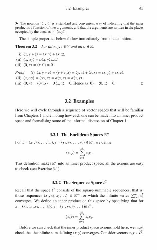
3.2 Examples 43

➤ The notation ‘〈 · , · 〉’ is a standard and convenient way of indicating that the innerproduct is a function of two arguments, and that the arguments are written in the placesoccupied by the dots, as in ‘〈x, y〉’.

The simple properties below follow immediately from the definition.

Theorem 3.2 For all x, y, z ∈ V and all α ∈ R,

(i) 〈x, y + z〉 = 〈x, y〉 + 〈x, z〉,(ii) 〈x, αy〉 = α〈x, y〉 and

(iii) 〈0, x〉 = 〈x, 0〉 = 0.

Proof (i) 〈x, y + z〉 = 〈y + z, x〉 = 〈y, x〉 + 〈z, x〉 = 〈x, y〉 + 〈x, z〉.(ii) 〈x, αy〉 = 〈αy, x〉 = α〈y, x〉 = α〈x, y〉.

(iii) 〈0, x〉 = 〈0x, x〉 = 0 〈x, x〉 = 0. Hence 〈x, 0〉 = 〈0, x〉 = 0. �

3.2 Examples

Here we will cycle through a sequence of vector spaces that will be familiarfrom Chapters 1 and 2, noting how each one can be made into an inner productspace and formalising some of the informal discussion of Chapter 1.

3.2.1 The Euclidean Spaces Rn

For x = (x1, x2, . . . , xn), y = (y1, y2, . . . , yn) ∈ Rn, we define

〈x, y〉 =n∑

i=1

xiyi.

This definition makes Rn into an inner product space; all the axioms are easyto check (see Exercise 3.1).

3.2.2 The Sequence Space �2

Recall that the space �2 consists of the square-summable sequences, that is,those sequences (x1, x2, x3, . . .) ∈ R∞ for which the infinite series

∑∞n=1 x2

n

converges. We define an inner product on this space by specifying that forx = (x1, x2, x3, . . .) and y = (y1, y2, y3, . . .) in �2,

〈x, y〉 =∞∑

n=1

xnyn.

Before we can check that the inner product space axioms hold here, we mustcheck that the infinite sum defining 〈x, y〉 converges. Consider vectors x, y ∈ �2,

44 3 Inner Product Spaces

as above. The definition of �2 tells us that the series∑∞

n=1 x2n and

∑∞n=1 y2

n bothconverge. Also, since we have already proved that �2 is a vector space, weknow that x+ y ∈ �2, meaning that the series

∑∞n=1(xn + yn)2 converges. But for

each n ∈ N, we have the algebraic identity

xnyn =12

((xn + yn)2 − x2

n − y2n),

and it follows that

〈x, y〉 =∞∑

n=1

xnyn

converges, as required. (See also Exercise 3.3.)With this established, the inner product space properties themselves are now

nearly as easy to check as in the case of Rn, the only minor complicationbeing that we must deal with infinite rather than finite sums. As an example,here is a proof of inner product space axiom (IP2): for x = (x1, x2, x3, . . .),y = (y1, y2, y3, . . .) and z = (z1, z2, z3, . . .) in �2,

〈x + y, z〉 =∞∑

n=1

(xn + yn)zn

=

∞∑n=1

(xnzn + ynzn)

=

∞∑n=1

xnzn +

∞∑n=1

ynzn

= 〈x, z〉 + 〈y, z〉.

3.2.3 Spaces of Functions

Let I be a closed, bounded interval [a, b], for some a, b ∈ R such that a < b. Inthe space of continuous functions C(I), we define an inner product by setting

〈 f , g〉 =∫

If g

for all f , g ∈ C(I). Note that this definition gives well-defined (finite) valuesfor 〈 f , g〉, because if f and g are continuous, then so is f g, and a continuousfunction on a closed, bounded interval is always integrable and its integral hasa finite value.

The following proofs of the inner product properties are straightforward,depending only on elementary facts about integration and continuous func-tions. Let f , g, h ∈ C(I) and α ∈ R.

3.2 Examples 45

(i) 〈 f , g〉 =∫

If g =

∫Ig f = 〈g, f 〉.

(ii) 〈 f + g, h〉 =∫

I( f + g)h =

∫I( f h + gh) =

∫I

f h +∫

Igh = 〈 f , h〉 + 〈g, h〉.

(iii) 〈α f , g〉 =∫

I(α f )g =

∫Iα( f g) = α

∫I

f g = α〈 f , g〉.(iv) Since 〈 f , f 〉 =

∫I

f 2 and f 2 ≥ 0 on I, we have 〈 f , f 〉 ≥ 0. If f = 0(meaning that f is the zero vector in C(I), that is, the function that hasvalue 0 everywhere on I), then clearly 〈 f , f 〉 = 0.

Finally, suppose that 〈 f , f 〉 = 0, for some continuous function f . Thenthe function g = f 2 is a non-negative continuous function whose integralover I is 0, and this implies that g, and hence f , has value 0 at all pointsof I. (The last sentence is not so much a proof as a statement of whatneeds to be proved; Exercise 3.4 outlines a way of constructing a rigorousproof of the statement.)

➤ Although the collection C(I) of continuous functions on I forms a vector space forall intervals I, it does not form an inner product space for arbitrary I, at least with theinner product defined above. This is why we restricted consideration to closed, boundedintervals I.

The explanation for this is simple. As noted, on a closed, bounded interval, theformula 〈 f , g〉 for the inner product always yields well-defined finite values. But onintervals that are open at an endpoint or are infinite in length, there always existcontinuous functions f with the property that the integral of f 2 is infinite, so that theformula that we want to use for the inner product will not always yield finite values (seeExercise 3.5).

The spaces of functions that we wish to spend most time with later are theL2 spaces, and we will say as much now as we can about these spaces as innerproduct spaces in the absence of a detailed discussion of Lebesgue integration.

Here, we allow our interval I to range without restriction, in contrast tothe case of C(I): it may be closed, open or half-open and it may be of finiteor infinite length. We begin by defining our proposed inner product on L2(I)using exactly the same formula that we used for the spaces C(I):

〈 f , g〉 =∫

If g,

for f , g ∈ L2(I).The first question that arises is whether this proposed inner product is well

defined. That is, given f , g ∈ L2(I), we wish to know whether the integral∫

If g

that defines 〈 f , g〉 exists and is finite.Although we have not defined the Lebesgue integral, we can still carry out

the required argument on the basis of some reasonable assumptions. (A similarpoint was made in Subsection 2.3.3 in the discussion of the vector spaceaxioms in L2(I).) It is easy enough to accept that any reasonable integrationtheory, whatever its exact details, will have properties such as the following:

46 3 Inner Product Spaces

• if f and g are integrable over I, then so is f + g, and∫

I( f + g) =

∫I

f +∫

Ig;

• if f is integrable over I, then so is α f , and∫

I(α f ) = α

∫I

f , for every α ∈ R.

If we accept that Lebesgue integration has these properties, as it does, then wecan prove easily that the inner product is well defined.

We argue in direct analogy to the earlier case of �2. The following purelyalgebraic identity holds for all x:

( f g)(x) = f (x)g(x) = 12

(( f (x) + g(x))2 − f (x)2 − g(x)2).

If now f , g ∈ L2(I), then f + g ∈ L2(I) also, by closure under addition. Hence,by the criterion for membership of L2(I), the integrals

∫I

f 2,∫

Ig2 and

∫I( f +g)2

all exist and are finite, and it follows using the algebraic identity and the abovetwo properties of the Lebesgue integral that the integral

∫I

f g is also definedand finite, as required.

Moreover, assuming the same two properties, we can also verify straightfor-wardly, along the lines used above for C(I), that the four inner product spaceaxioms hold in L2(I), except for the last part of the fourth inner product spaceaxiom, which requires that if 〈 f , f 〉 = 0 then f = 0. The proof of this statementfor C(I), which we relegated to Exercise 3.4, certainly fails if we try to carryit out for L2(I), because it depends specifically on continuity, which we can nolonger assume. However, more seriously, the statement is in fact false for L2(I).That is, our proposed inner product does not obey the inner product spaceaxioms in full, and so we have not succeeded in making the vector space L2(I)into an inner product space.

We will find a way around this difficulty shortly, but let us first discuss twoexamples, to see how the last part of the fourth axiom fails.

Consider the function f defined on [0, 1] by

f (x) =

⎧⎪⎪⎨⎪⎪⎩1, x = 12 ,

0, otherwise.

This function is Riemann-integrable, with∫ 1

0f = 0. Since f is Riemann-

integrable, it is also Lebesgue-integrable (the Lebesgue theory is a general-isation of the Riemann theory), and so we have f ∈ L2([0, 1]

). Also, since

f 2 = f , we have 〈 f , f 〉 =∫ 1

0f 2 =

∫ 1

0f = 0. But of course f does not satisfy

f = 0, because to say that f = 0 means that f is the zero vector in L2([0, 1]),

the function whose value is 0 at all points in [0, 1].A more extreme illustration is provided by the function f defined on

[0, 1] by

3.2 Examples 47

f (x) =

⎧⎪⎪⎨⎪⎪⎩1, x rational,

0, x irrational.

This function, as we noted in Chapter 2, is not Riemann-integrable, but is

Lebesgue-integrable, with∫ 1

0f = 0; further, since f 2 = f , we have

∫ 1

0f 2 = 0,

and hence f ∈ L2([0, 1])

and 〈 f , f 〉 = 0. But, as for the first example, f is notthe zero vector, because there are infinitely many points at which its value isnon-zero.

Notice that both these examples are of functions f which, while notidentically 0, are ‘almost 0’, in the sense that the integral of f 2 in each caseis 0. This observation is the key to making L2(I) into an inner product spaceafter all: we simply declare that any function f such that

∫I

f 2 = 0 is identicalto the zero function. The more general statement follows that any two functionsf and g such that

∫I( f −g)2 = 0 are identical. A simpler analytic formulation of

the condition under which f and g are identified can be obtained by invokingthe Lebesgue integration theory, which shows that

∫I( f − g)2 = 0 if and only

if∫

I| f − g| = 0. (The following section gives another way of looking at this

condition.)In formal terms, what we have done here is to redefine the space L2(I) by

making its elements the equivalence classes of the functions from our earlierdefinition under the equivalence relation given by:

f and g are equivalent if∫

I| f − g| = 0.

At first sight, it may appear rather complicated and cumbersome to have todeal with spaces whose elements are equivalence classes of functions ratherthan functions, but the definition works in a straightforward way in practice:most of the time, we continue to think of L2(I) as a space of functions, asoriginally defined, but we exercise great caution if we have to make a statementabout the value of a function in L2(I) at any particular point.

It is useful to reconsider some comments made in Chapter 1 in the lightof our revised definition of L2(I). When defining the Haar wavelet H inSubsection 1.4.2, we commented that the values chosen for H at 0, 1

2 and 1were not particularly important, and that nothing significant would change ifwe made different choices. We can now be precise about why this is the case.If we defined a variant of the Haar wavelet, say H′, with differently chosenvalues at a few isolated points, it would nevertheless be the case that∫ ∞

−∞

∣∣∣H − H′∣∣∣ = 0,

48 3 Inner Product Spaces

and in L2(R), as just redefined, H and H′ represent the same element of L2(R);from a standpoint within this space, H and H′ are indistinguishable.

3.3 Sets of Measure Zero

The length of an interval [a, b] (with a ≤ b) is given by b − a; further, whetherthe interval contains its own endpoints or not does not affect its length, so theintervals [a, b], [a, b), (a, b] and (a, b) all have length b − a. Generalising theidea of length to slightly more complicated sets is easy enough; for example,we would presumably say that the length of [−12, 2]∪[17, 28] is 14 + 11 = 25.Generalising the idea of length to its furthest possible extent, however, involvesa substantial theoretical development, and would take us into the topic ofmeasure theory. In measure theory, the (generalised) length of a set on thereal line is called its Lebesgue measure or just its measure.

A proper study of Lebesgue integration requires a proper study of Lebesguemeasure, but we do not attempt either in this book. What we do wish to discusshere, though only briefly, is one special but very important case: the case whena set has (Lebesgue) measure 0.

Consider again the case of a bounded interval. Since the length or measureof the interval [a, b] is b− a, the interval will have measure 0 only when a = b,in which case the interval is just the singleton set {a}. Also, presumably, wewill want to say that the empty set has measure 0. The formal definition belowallows us to say that many other larger and far more complicated sets of realnumbers also have measure 0.

The informal idea of the definition is straightforward: a set A has measure 0if its length (or measure) is less than every positive real number.

Definition 3.3 If A ⊆ R, then A has measure 0 if for every ε > 0 there existsa sequence {In}∞n=1 of bounded intervals such that

A ⊆∞⋃

n=1

In

and the sum of the lengths of the In is less than ε.

We make a few minor observations about the definition. First, from ourdiscussion above, it does not matter whether the intervals contain theirendpoints or not, so the definition is phrased in a way that avoids the issue.Second, although we allow ourselves an infinite number of intervals, we onlyallow a countable infinity – that is, we must be able to arrange the intervals in asequence indexed by the natural numbers. Third, the definition in effect allows

3.3 Sets of Measure Zero 49

the use of a finite number of intervals, or even just a single interval, since‘degenerate’ intervals of the form [a, a] containing only one point and evenempty intervals such as (a, a) can be included in the sequence. Fourth, the orderin which we list the intervals In does not affect the sum of their lengths: theirlengths are non-negative real numbers, and so the convergent series formedby summing their lengths is absolutely convergent and therefore has a sumwhich is independent of the order of summation. (Compare the comments justpreceding Subsection 4.6.1 below, and see Exercise 4.36.)

Example 3.4 (i) A singleton set {x} has measure 0, since it can be coveredby the single degenerate interval [x, x] of length 0, and 0 is less than anychosen ε > 0.

(ii) A countable set of points {xn : n = 1, 2, 3, . . .} also has measure 0, sinceit can be covered by the sequence

{[xn, xn] : n = 1, 2, 3, . . .

}of degenerate

intervals.(iii) A consequence is that the set of rational numbers has measure 0, since the

rationals can be arranged into a sequence, that is, form a countable set.

We note a couple of simple results about sets of measure 0. (The proofs areleft for Exercise 3.7.)

Theorem 3.5 (i) Any subset of a set of measure 0 has measure 0.(ii) If {An : n = 1, 2, 3, . . .} is a sequence of sets of measure 0, then the union∪∞n=1An also has measure 0.

There are many uncountable sets that are still of measure 0. We do not needto examine any such cases here, but we note that the well-known Cantor setis one example (see Exercise 3.8).

It is also important to note that ‘not too many’ sets have measure 0. Forexample, since [a, b] has length b−a, and this quantity is non-zero if a < b, ourdefinition of measure 0, if it is satisfactory, should not assign this set measure 0,and this is indeed the case (see Exercise 3.9). (If we were to introduce Lebesguemeasure in the general case, then [a, b] would, as expected, have Lebesguemeasure b − a and the sets we have defined as having measure 0 would haveLebesgue measure 0.)

➤ Sets of measure 0 are, intuitively, ‘thin’ or ‘sparse’ or ‘negligible’, though we needto be careful about where our intuition may lead. Certainly, the rationals between 0and 1 seem thinly spread throughout the interval [0, 1], because there are infinitely manyirrational numbers between any two rational numbers, no matter how close together (seeExercise 4.5), and the rationals do indeed have measure 0, as we have shown. On theother hand the irrationals between 0 and 1 might also seem to be thinly spread for asimilar reason – there are infinitely many rational numbers between any two irrationalnumbers, no matter how close together (Exercise 4.5 again). But the irrationals between

50 3 Inner Product Spaces

0 and 1 are not of measure 0. One way of explaining this is to argue that since theinterval [0, 1] has length 1, and given that the rationals have measure (or generalisedlength) 0, the measure of the irrationals must be 1 to make up the difference. Thegeneral theory of Lebesgue measure shows that this argument is correct: the irrationalsbetween 0 and 1 have Lebesgue measure 1. (Observe also that while the set of rationalsis countable, the set of irrationals in [0, 1] is uncountable, so part (ii) of Example 3.4does not lead us to a contradiction.)

3.3.1 Properties That Hold Almost Everywhere

A property that may or may not hold for any given real number x is said to holdalmost everywhere or for almost all x if it holds for all x except those in someset of measure 0. (It is very common to see the phrase ‘almost everywhere’abbreviated to ‘a. e.’, but we will use the longer form.) The phrase is generallyused in situations where it is not important or not possible to identify thespecific measure 0 set involved.

For example, recall the following function on R, which we discussed inSubsection 3.2.3 and in earlier chapters:

f (x) =

⎧⎪⎪⎨⎪⎪⎩1, x rational,

0, x irrational.

Since the rationals form a set of measure 0 in R, we can say that f (x) = 0 foralmost all x, or simply that f is 0 almost everywhere.

For a second example, recall our definition of the space L2(I) for aninterval I. The elements of these spaces, strictly, are equivalence classes offunctions under the equivalence relation that identifies any two functions fand g such that

∫I| f −g| = 0. The theory of Lebesgue integration shows that the

equation∫

I| f −g| = 0 holds if and only if f and g are equal almost everywhere,

that is, f (x) = g(x) except for x in some set of measure 0.In the last two chapters of the book we will encounter many statements

involving conditions that hold almost everywhere.

3.3.2 Measurability of Functions

This is an appropriate point at which to include a brief comment about atechnical issue in the definition of the L2 spaces. A glance at any text on thesubject will show that L2(I) is defined as the set of measurable or Lebesguemeasurable functions f for which

∫I

f 2 is finite. Measurability of functionsis one of the fundamental concepts in the theory of Lebesgue integrationand measure, but since we do not assume this theory is known, and wecertainly cannot cover it in this text, we have simply ignored the condition

3.4 The Norm and the Notion of Distance 51

of measurability altogether above, and we will continue to ignore it below aswell. It suffices to say here that the condition is satisfied in all the cases whereit is needed. In particular, all the standard functions of everyday mathematicsare measurable, all functions that are continuous or piecewise continuous aremeasurable, and many far more exotic functions, such as the one mentionedabove that is 1 on the rationals and 0 on the irrationals, are measurable.

3.4 The Norm and the Notion of Distance

The inner product space axioms tell us that 〈x, x〉 is always non-negative, andthis implies that we can properly make the following definition.

Definition 3.6 If V is an inner product space, then the norm in V is thefunction ‖ · ‖ : V → R defined by

‖x‖ = 〈x, x〉 12 ,

for all x ∈ V .

We can immediately prove the following very important result, which relatesthe inner product and the norm. The result will be used directly below toprove another simple but fundamental inequality involving the norm, and willreappear at other significant points later.

Theorem 3.7 (The Cauchy–Schwarz inequality) If V is an inner productspace, then ∣∣∣〈x, y〉∣∣∣ ≤ ‖x‖ ‖y‖,for all x, y ∈ V.

Proof If y = 0, then the inequality holds, since both sides are 0. Therefore,let us assume that y � 0. Then ‖y‖ is a non-zero real number (this is immediatefrom the definition, but see also part (iii) of Theorem 3.8), and so it will beenough if we prove the inequality∣∣∣∣∣⟨x,

y‖y‖

⟩∣∣∣∣∣ ≤ ‖x‖,since multiplying through this inequality by ‖y‖ yields the inequality we aretrying to prove. Now the vector y

/‖y‖ is a unit vector (that is, has norm 1), soit will be enough if we prove the formally simpler inequality∣∣∣〈x, u〉∣∣∣ ≤ ‖x‖,for every unit vector u, and this inequality is immediate from the followingsimple calculation:

52 3 Inner Product Spaces

0 ≤∥∥∥x − 〈x, u〉 u

∥∥∥2

=⟨x − 〈x, u〉 u, x − 〈x, u〉 u⟩

=⟨x, x − 〈x, u〉 u⟩ − ⟨〈x, u〉 u, x − 〈x, u〉 u⟩

= 〈x, x〉 − 2〈x, u〉〈x, u〉 + 〈x, u〉〈x, u〉〈u, u〉= 〈x, x〉 − 2〈x, u〉〈x, u〉 + 〈x, u〉〈x, u〉= 〈x, x〉 − 〈x, u〉〈x, u〉= ‖x‖2 − 〈x, u〉2. �

We can define components and projections in a general inner product spaceexactly as we did in Chapter 1 in the case of Rn and other spaces. Thus if uis a unit vector, then the component of x on u is defined to be 〈x, u〉 and theprojection of x on u is defined to be 〈x, u〉 u, and the case when the secondvector is not a unit vector is obtained as in Section 1.1 by normalisation. (SeeSection 3.6 below for discussion of a notion of projection that generalises theone just introduced.)

The statement, extracted from the proof of the Cauchy–Schwarz inequality,that ∣∣∣〈x, u〉∣∣∣ ≤ ‖x‖for every unit vector u therefore has the geometrically very plausible interpre-tation that the absolute value of the component of x in any direction, that is, thenorm of the projection of x in any direction, is less than or equal to the normof x itself.

There is a set of three standard properties of the norm.

Theorem 3.8 For all vectors x and y, and all scalars α,

(i) ‖x + y‖ ≤ ‖x‖ + ‖y‖ (the triangle inequality),(ii) ‖αx‖ = |α| ‖x‖ and

(iii) ‖x‖ ≥ 0, and ‖x‖ = 0 if and only if x = 0.

Proof Properties (ii) and (iii) follow immediately from the inner productspace axioms. For (i), we need the Cauchy–Schwarz inequality. We have:

‖x + y‖2 = 〈x + y, x + y〉= 〈x, x + y〉 + 〈y, x + y〉= 〈x, x〉 + 〈x, y〉 + 〈y, x〉 + 〈y, y〉= ‖x‖2 + 2〈x, y〉 + ‖y‖2

3.4 The Norm and the Notion of Distance 53

����������������

�����������������������������

�������������

�������������������

�������������������

‖x‖

‖y‖

‖x‖

‖y‖‖x + y‖

‖x − y‖

Figure 3.1 Illustration of the parallelogram law

≤ ‖x‖2 + 2∣∣∣〈x, y〉∣∣∣ + ‖y‖2

≤ ‖x‖2 + 2‖x‖ ‖y‖ + ‖y‖2

=(‖x‖ + ‖y‖)2

,

from which the inequality is immediate. �

The following result is also worth noting in passing, though it is of muchless significance than the other theorems of this section and the proof is left asan exercise. The geometric content of the result is summed up clearly enoughin Figure 3.1.

Theorem 3.9 The norm in an inner product space satisfies the parallelogramlaw:

‖x + y‖2 + ‖x − y‖2 = 2‖x‖2 + 2‖y‖2,

for all x and y.

In Euclidean space, the norm ‖x‖ of a vector x is the distance (or Euclideandistance) of x from the origin. In detail, if x = (x1, x2, . . . , xn) ∈ Rn, then

‖x‖ =√〈x, x〉 =

√x2

1 + x22 + · · · + x2

n,

and of course the most familiar examples are when n is 1, 2 or 3, when thespace is R, R2 or R3 and the distance of x from the origin is

54 3 Inner Product Spaces

√x2

1 = |x1|,√

x21 + x2

2 or√

x21 + x2

2 + x23,

respectively. More generally, the distance between two points x and y in Rn is‖x− y‖, and again this idea is very familiar in R, R2 and R3. All this, of course,is as already discussed in Chapter 1.

In accordance with our strategy of trying to carry the geometry of Rn intoinner product spaces in general, we make an analogous definition in any innerproduct space.

Definition 3.10 If V is an inner product space and x, y ∈ V , then the distanceof x from y is ‖x − y‖.

Note that this distance ‖x − y‖ is always a non-negative real number, inconformity with our expectations of the nature of distance.

We can now speak, for example, of the distance between two vectors orsequences x and y in �2: if x = (x1, x2, x3, . . .) and y = (y1, y2, y3, . . .), then thedistance between x and y is

‖x − y‖ =⎛⎜⎜⎜⎜⎜⎝ ∞∑

n=1

|xn − yn|2⎞⎟⎟⎟⎟⎟⎠

12

=(|x1 − y1|2 + |x2 − y2|2 + |x3 − y3|2 + · · ·

) 12 .

Similarly, we can speak of the distance between two functions f and g in L2(I):the distance between f and g is

‖ f − g‖ =(∫

I| f − g|2

) 12

.

➤ Recall that for f , g, ∈ L2(I) we regard f and g as equal if∫

I| f −g|2 = 0. Since ‖ f −g‖

is just the square root of this integral, we can rephrase the criterion for the identificationof f and g in the following more geometric form: f and g are identical if the distancebetween them is 0.

We note several elementary but important properties of distance; the proofsfollow directly from Theorem 3.8 (checking them is left for Exercise 3.14).

Theorem 3.11 For all vectors x, y and z,

(i) ‖x − y‖ ≤ ‖x − z‖ + ‖z − y‖ (the triangle inequality),(ii) ‖x − y‖ = ‖y − x‖, and, more generally, ‖αx − αy‖ = |α| ‖x − y‖ for all

scalars α, and(iii) ‖x − y‖ ≥ 0, and ‖x − y‖ = 0 if and only if x = y.

➤ If you are familiar with metric spaces, you will recognise these three properties (withthe omission of the generalised form of (ii)) as the metric space axioms; the theorem

3.5 Orthogonality and Orthonormality 55

says that an inner product space is a metric space, with ‖x− y‖ as the metric or distancefunction.

Note that in Theorems 3.8 and 3.11 we have given the name ‘triangle inequality’to two different inequalities. But it is easy to see that the two inequalities are reallyequivalent, and both are simply abstract expressions of the elementary geometric factthat the lengths of two sides of a triangle always have a sum greater than or equal to thelength of the remaining side (see Exercise 3.15).

Notice that the ideas and results of this section suggest strongly that ourdefinitions have captured axiomatically some of the essential features of thefamiliar geometry of R3 (or of Rn in general). The Cauchy–Schwarz inequality,the triangle inequalities and the parallelogram law, for example, are standardresults in R3 (where the Cauchy–Schwarz inequality is usually known asCauchy’s inequality), but we now have proofs of all three which proceedpurely axiomatically in an arbitrary inner product space, making no use ofany assumptions about the internal structure of vectors in the space.

It thus seems clear that we are on the way to a successful extension offamiliar finite-dimensional ideas to much more general, frequently infinite-dimensional, contexts, a point that will be reinforced by the remainder of thechapter. We noted in Chapter 1 that the study of this extension was one of ourmain themes.

3.5 Orthogonality and Orthonormality

Now that we have surveyed a range of basic facts about inner products andnorms, we will begin to explore their deeper properties, a process which wecould describe as an exploration of the geometry of inner product spaces.

The Cauchy–Schwarz inequality tells us that∣∣∣〈x, y〉∣∣∣ ≤ ‖x‖ ‖y‖,for all x, y ∈ V , where V is any inner product space. Hence for all x and y, wehave

−‖x‖ ‖y‖ ≤ 〈x, y〉 ≤ ‖x‖ ‖y‖,

and therefore (provided that neither x nor y is 0)

− 1 ≤ 〈x, y〉‖x‖ ‖y‖ ≤ 1. (3.1)

It is a standard geometric fact that in R2 and R3 (see Section 1.1 andExercise 1.2) the angle θ between two vectors x and y satisfies the relation

cos θ =〈x, y〉‖x‖ ‖y‖ ,

56 3 Inner Product Spaces

and by (3.1) we could, if it proved to be useful, define the angle between twovectors in any inner product space by the same formula. In practice, it seemsnot to be particularly useful to discuss angles in general in spaces other thanEuclidean spaces, but the special case when cos θ = 0, or when θ is a rightangle, is of central importance in all inner product spaces, as we have seenalready in Chapter 1.

Definition 3.12 Vectors x and y in an inner product space are orthogonal if〈x, y〉 = 0; we then write x ⊥ y and we may say ‘x perp y’.

The properties below follow directly from the definition of orthogonalityand the inner product, and the proofs are left for Exercise 3.17.

Theorem 3.13 For all vectors x, y and y1, y2, . . . , yn,

(i) 0 ⊥ x and x ⊥ 0,(ii) x ⊥ y if and only if y ⊥ x,

(iii) x ⊥ x if and only if x = 0, and(iv) if x ⊥ y1, x ⊥ y2, . . . , x ⊥ yn, then x ⊥ α1y1 + α2y2 + · · · + αnyn, for all

scalars α1, α2, . . . , αn.

Note that an alternative way of expressing the result of (iv) is to say that if xis orthogonal to each of y1, y2, . . . , yn, then it is also orthogonal to the subspacespanned by y1, y2, . . . , yn.

Definition 3.14 Let A be a subset of an inner product space. Then A isorthogonal if 〈x, y〉 = 0 for all distinct x, y ∈ A, and A is orthonormal ifin addition 〈x, x〉 = 1 for all x ∈ A.

Thus, A is orthonormal if

〈x, y〉 =⎧⎪⎪⎨⎪⎪⎩1, x = y,

0, x � y,

for all x, y ∈ A. As we already noted in Chapter 1, if the elements of the set Aare indexed then we can express the orthonormality of A succinctly using theKronecker delta δi, j. Specifically, if A = {xi : i ∈ I}, where I is some index set,then A is orthonormal if

〈xi, x j〉 = δi, j

for all i, j ∈ I.The following result was noted for the particular case of the Euclidean

spaces in Section 1.1 and Exercise 1.3.

Theorem 3.15 Every orthonormal set is linearly independent.

3.5 Orthogonality and Orthonormality 57

Proof Let x1, x2, . . . , xn be a finite collection of vectors from an orthonormalset (which itself may be finite or infinite), and suppose that

n∑i=1

αi xi = 0

for some scalars α1, α2, . . . , αn. Then for any j such that 1 ≤ j ≤ n, we have

⟨ n∑i=1

αi xi, x j

⟩= 〈0, x j〉 = 0,

and also ⟨ n∑i=1

αi xi, x j

⟩=

n∑i=1

αi〈xi, x j〉 = α j,

giving α j = 0. Since this holds for j = 1, 2, . . . , n, we conclude that the vectorsx1, x2, . . . , xn are linearly independent. �

3.5.1 The Gram–Schmidt Process

The Gram–Schmidt process is an algorithm for converting a finite or infinitesequence of linearly independent vectors in an inner product space into anorthonormal sequence which has the same length and spans the same subspace.

Suppose that x1, x2, . . . is a given linearly independent sequence, which, asmentioned, may be finite or infinite. If it is finite with, say, N elements, thenthe Gram–Schmidt process will stop after exactly N steps, and if it is infinite,the process will continue through an infinite number of steps – there is in eithercase exactly one step for each term of the sequence.

The following theorem specifies precisely the steps involved in applying theGram–Schmidt process and states precisely the mathematical properties of theprocess.

Theorem 3.16 (The Gram–Schmidt process) Let x1, x2, . . . be a finite orinfinite sequence of linearly independent vectors in an inner product space.For n = 1, 2, . . . , define

dn = xn −n−1∑i=1

〈xn, ei〉 ei and en =dn

‖dn‖.

Then the sequence e1, e2, . . . has the following properties:

(i) for each meaningful value of n, the vectors e1, e2, . . . , en form an orthonor-mal set that spans the same subspace as x1, x2, . . . , xn, and

58 3 Inner Product Spaces

(ii) the entire sequence e1, e2, . . . forms an orthonormal set that spans the samesubspace as the entire sequence x1, x2, . . . .

➤ Note that we have tried to deal with the cases of a finite and an infinite sequence in asingle statement here. If x1, x2, . . . is a finite sequence with last element xN , then n willrun from 1 to N in the steps that construct the vectors dn and en, while if x1, x2, . . . is aninfinite sequence, n will run through the natural numbers N, and vectors dn and en willbe constructed for all n ∈ N. Thus in the finite case, n in part (i) will be a ‘meaningfulvalue’ if 1 ≤ n ≤ N, while any n ∈ N will be ‘meaningful’ in the infinite case.

The Gram–Schmidt algorithm is recursive (or inductive), in the sense that the outputof each step depends upon the output of the previous steps. Proofs about recursiveconstructions are typically carried out by induction, and this is the form our proof ofpart (i) will take, although the induction will be a finite induction, terminating at theNth step, in the first case above, and a full induction over N in the second case.

Proof For the base case of our inductive proof of part (i), consider the casen = 1. Note that the range of the summation in the definition of dn is empty, sothat the formula simply gives d1 = x1. Since the sequence x1, x2, . . . is linearlyindependent, we have x1 � 0 and hence ‖x1‖ � 0, so we can divide by ‖x1‖and obtain a vector e1, which clearly satisfies ‖e1‖ = 1. Also, the definitionof e1 shows immediately that e1 is in the subspace spanned by x1, and theequation x1 = ‖x1‖e1 likewise shows that x1 is in the subspace spanned by e1.The singleton set {e1} is clearly orthonormal.

For the inductive step, fix any value n> 1 lying within the range ofmeaningful values and assume that the claims of part (i) hold for n−1. Define dn

by the given formula. We claim that dn � 0. Indeed, if dn = 0, then the formulafor dn gives

xn =

n−1∑i=1

〈xn, ei〉 ei,

expressing xn as a linear combination of e1, . . . , en−1. But our assumption tellsus that e1, . . . , en−1 span the same subspace as x1, . . . , xn−1, so it follows that xn

is expressible as a linear combination of x1, . . . , xn−1, and this contradicts thelinear independence of the sequence x1, . . . , xn−1, xn. Thus, dn � 0.

We can therefore legitimately define en = dn/‖dn‖. Now the definitionsof dn and en imply that xn lies in the space spanned by e1, . . . , en, and sincethe inductive assumption implies that x1, . . . , xn−1 lie in the space spanned bye1, . . . , en−1, it follows that x1, . . . , xn lie in the space spanned by e1, . . . , en.

On the other hand, the inductive assumption also tells us that e1, . . . , en−1

lie in the space spanned by x1, . . . , xn−1, and the definitions of dn and en implythat en can be written as a linear combination of e1, . . . , en−1 and xn, and henceof x1, . . . , xn−1, xn, so we conclude that e1, . . . , en lie in the space spanned byx1, . . . , xn.

3.5 Orthogonality and Orthonormality 59

For orthonormality, we have assumed inductively that {e1, . . . , en−1} isorthonormal, a simple calculation shows that en ⊥ ei for i= 1, . . . , n − 1, andthe fact that ‖en‖ = 1 is immediate from the definition of en. The fact that{e1, . . . , en} is orthonormal follows.

Part (i) therefore holds by induction. The easy deduction of part (ii) is leftas an exercise (see Exercise 3.21). �

It is sometimes useful to employ a variant of the Gram–Schmidt processwhich yields orthogonal but not necessarily orthonormal vectors. Now thevectors required are just the vectors dn in the theorem, but we defined the dn

inductively in terms of the en, and it would be helpful to have an expressionfor the dn that avoids mention of the en if the dn are all we want. We claim thatthe expression defining the dn directly is

dn = xn −n−1∑i=1

〈xn, di〉‖di‖2

di,

for n ≥ 1.It is straightforward to confirm this. From the theorem, we have

dn = xn −n−1∑i=1

〈xn, ei〉 ei

for each n and

ei =di

‖di‖for each i. Therefore,

dn = xn −n−1∑i=1

〈xn, ei〉 ei = xn −n−1∑i=1

⟨xn,

di

‖di‖

⟩di

‖di‖= xn −

n−1∑i=1

〈xn, di〉‖di‖2

di,

as claimed. (Of course, we are still free to orthonormalise if we wish, by settingen = dn/‖dn‖ for each n.)

Not surprisingly, we can visualise the Gram–Schmidt process geometrically,making use of the ideas of components and projections. Now the generalexpression for dn in the Gram–Schmidt process is

dn = xn −n−1∑i=1

〈xn, ei〉 ei,

and we observe that the ith term 〈xn, ei〉 ei in the sum is just the projection of xn

onto the ith unit vector ei. Thus dn is obtained by subtracting from xn all of itsprojections into the (n − 1)-dimensional subspace spanned by e1, e2, . . . , en−1;and en is then obtained by normalising dn. We should therefore expect, on

60 3 Inner Product Spaces

purely geometric grounds, what Theorem 3.16 already tells us algebraically:that en is perpendicular to the subspace spanned by e1, e2, . . . , en−1.

Thus, for example, in R3:

• e2 is perpendicular to the 1-dimensional subspace, or straight line throughthe origin, defined by e1 (or, equivalently, by x1);• e3 is perpendicular to the 2-dimensional subspace, or plane through the

origin, defined by e1 and e2 (or, equivalently, by x1 and x2);

and similarly in higher dimensions.

3.5.2 An Example in Rn

We begin with a simple example of an application of the Gram–Schmidtprocess in Euclidean space. Consider the vectors

x1 = (−1, 2, 0, 2), x2 = (2,−4, 1,−4) and x3 = (−1, 3, 1, 1)

in R4. These vectors are linearly independent. We can easily enough confirmthis directly, of course, but Exercise 3.22 shows that if they were dependent,the dependence would show up in the Gram–Schmidt process. Hence we willomit direct confirmation of independence and go straight to the Gram–Schmidtsteps, which proceed as follows (though the details of the calculations are leftfor Exercise 3.23):

• d1 = x1 = (−1, 2, 0, 2), and hence e1 =13 (−1, 2, 0, 2);

• d2 = x2 − 〈x2, e1〉e1 = (0, 0, 1, 0), and hence e2 = d2 = (0, 0, 1, 0); and

• d3 = x3−〈x3, e1〉e1−〈x3, e2〉e2 = (0, 1, 0,−1), and hence e3 =1√2(0, 1, 0,−1).

We now know from the theory that the three vectors e1, e2 and e3 areorthonormal (though this is also obvious by direct inspection), and that theyspan the same 3-dimensional subspace of R4 as x1, x2 and x3.

3.5.3 An Example in �2

In the space �2, consider the infinite sequence of vectors

x1 = (α1, 0, 0, 0, . . .), x2 = (α1, α2, 0, 0, . . .), x3 = (α1, α2, α3, 0, . . .), . . . .

If αn � 0 for all n, then these vectors are independent. If also αn > 0 for all n,then the Gram–Schmidt process applied to them yields the familiar sequence

e1 = (1, 0, 0, 0, . . .), e2 = (0, 1, 0, 0, . . .), e3 = (0, 0, 1, 0, . . .), . . .

(see Exercise 3.24).

3.5 Orthogonality and Orthonormality 61

3.5.4 An Example in C([−1, 1]): The Legendre Polynomials

Let I be any non-trivial interval, and consider the infinite sequence of functions

1, x, x2, x3, . . . ,

regarded as vectors in the vector space C(I). This sequence forms a linearlyindependent set in C(I). (Exercise 2.10 already asked for a proof of this fact,but we now supply a proof. Let us also briefly recall the notational conventionestablished near the end of Subsection 1.2.2, under which the notation xk, forany given k, may be taken, as the context demands here, to denote a function –the function whose value at x is the real number xk.)

Suppose that some finite linear combination of the functions 1, x, x2, x3, . . .

is the zero function (which is the zero vector in C(I)). Now the functionsinvolved in the linear combination can be written as

xn1 , xn2 , . . . , xnk ,

for some k ≥ 1 and for some integers n1 < n2 < · · · < nk, so our assumption isthat the linear combination

a1xn1 + a2xn2 + · · · + ak xnk

is identically 0 for some scalars a1, a2, . . . , ak. But if any of these scalars isnon-zero, then a1xn1 + a2xn2 + · · · + ak xnk is a non-zero polynomial, which canhave only a finite number of roots in I, whereas our assumption that it is thezero function says that every number x in I is a root. Hence every coefficientmust be 0, which proves independence.

Let us now consider the specific case of C([−1, 1]

); since [−1, 1] is closed

and bounded, this vector space is an inner product space with the standardinner product (see Subsection 3.2.3).

If we use the Gram–Schmidt process to orthogonalise (rather than orthonor-malise) the functions 1, x, x2, x3, . . . , then we obtain a sequence of polynomialsbeginning

p0(x) = 1, p1(x) = x, p2(x) = x2 − 13 , p3(x) = x3 − 3

5 x, . . . .

Although calculating additional terms of this sequence is not hard, it is not atall obvious how to write down a general expression for the nth term of thesequence in any simple way. It is possible, however, to show that

pn(x) =n!

(2n)!dn

dxn(x2 − 1)n

(see Exercise 3.28).

62 3 Inner Product Spaces

These polynomials, with a different normalisation, are very well knownin analysis. The more or less standard procedure, used largely for historicalreasons, is to normalise the polynomials so that their value at x = 1 is 1. Theyare then known as the Legendre polynomials, and the sequence begins

P0(x) = 1, P1(x) = x, P2(x) = 32 x2 − 1

2 , P3(x) = 52 x3 − 3

2 x, . . . .

The nth term is now given by

Pn(x) =1

2nn!dn

dxn(x2 − 1)n,

an expression known as Rodrigues’ formula. The norm of Pn in C([−1, 1]

)is

‖Pn‖ =

√∫ 1

−1P2

n =

√2

2n + 1,

and if we divide Pn by ‖Pn‖, we obtain the orthonormalised Legendrepolynomials:

Q0(x) =1√

2,

Q1(x) =

√3√

2x,

Q2(x) =3√

5

2√

2x2 −

√5

2√

2,

Q3(x) =5√

7

2√

2x3 − 3

√7

2√

2x,

...

The graphs of the polynomials Qn for n = 0, 1, . . . , 5 are shown in Figure 3.2.A whole sub-discipline of classical analysis is devoted to the general

study of orthogonal polynomials, which have many fascinating properties andimportant applications. Among the many families of such polynomials inaddition to the Legendre family are the Hermite, Laguerre and Chebyshevpolynomials; these are all obtained by applying the Gram–Schmidt process tothe sequence 1, x, x2, x3, . . . in spaces C(I), for various intervals I, or in closelyrelated spaces.

3.5 Orthogonality and Orthonormality 63

n = 0 n = 1

n = 2 n = 3

n = 4 n = 5

Figure 3.2 Graphs of the orthonormalised Legendre polynomials Qn

64 3 Inner Product Spaces

3.6 Orthogonal Projection

We saw a number of times in Chapter 1, at least informally, how a vectorin an inner product space may be ‘decomposed’ into a linear combination ofthe members of a finite orthonormal basis by projecting the vector onto eachmember of the basis.

The first example of this was in Section 1.1, where we were given a basisb1, b2, b3 of three orthonormal vectors for R3 and saw how a specific vector cwas expressible in the form

c =⟨c, b1

⟩b1 +

⟨c, b2

⟩b2 +

⟨c, b3

⟩b3 =

3∑i=1

⟨c, bi

⟩bi :

the coefficient 〈c, bi〉 is of course the component of c on bi for each i. We nowboth formalise and generalise this process in the context of an arbitrary innerproduct space.

Theorem 3.17 Let {e1, e2, . . . , en} be a finite orthonormal set in an innerproduct space V, and let x be any vector in V. Then

n∑i=1

⟨x, ei

⟩2 ≤ ‖x‖2 (3.1)

and, for j = 1, . . . , n,

x −n∑

i=1

⟨x, ei

⟩ei ⊥ e j. (3.2)

Further, if x is in the n-dimensional subspace spanned by {e1, e2, . . . , en}, then

x =n∑

i=1

⟨x, ei

⟩ei, (3.3)

andn∑

i=1

⟨x, ei

⟩2= ‖x‖2. (3.4)

➤ It is worth emphasising that V here may be an inner product space of any, possiblyinfinite, dimension, even though the orthonormal set {e1, e2, . . . , en} is finite. Also notecarefully that (3.1) and (3.2) hold for any vector x ∈ V , while (3.3) and (3.4), whichgive stronger information than (3.1) and (3.2), require the stronger assumption that x isin the subspace spanned by the ei.

Here, as always in inner product space work, it is important and instructive tonote the geometric interpretation of all of these statements. The first statementsays that the sum of the squares of the lengths of the projections of x in variousperpendicular directions is less than or equal to the square of the length of x

3.6 Orthogonal Projection 65

itself; the inequality is called Bessel’s inequality. The second statement can beinterpreted as saying that if we subtract from a vector its projections in severalperpendicular directions, then the result has no component left in any of thosedirections – that is, it is orthogonal to all of them. Similarly for the remainingstatements: if x is in the subspace, then both it and its length are exactlyexpressible in terms of its projections and their lengths. The expression (3.3)for x is a finite Fourier series for x with respect to the orthonormal basis{e1, e2, . . . , en} for the n-dimensional subspace involved, and the terms 〈x, ei〉are the Fourier coefficients of x with respect to that basis. The equation (3.4)is called Parseval’s relation. (The comments at the end of Subsection 3.6.2below shed further light on all the issues raised here.)

In the next chapter, we will be able to generalise all the parts of the abovetheorem to infinite Fourier series with respect to certain infinite orthonormalsets, encompassing the usual trigonometric Fourier series and wavelet seriesas special cases.

Proof of Theorem 3.17 The main part of the proof is a straightforward com-putation. For any x ∈ V ,

0 ≤∥∥∥∥∥x −

n∑i=1

〈x, ei〉 ei

∥∥∥∥∥2

=

⟨x −

n∑i=1

〈x, ei〉 ei, x −n∑

j=1

〈x, e j〉 e j

⟩

= 〈x, x〉 −⟨x,

n∑j=1

〈x, e j〉 e j

⟩−

⟨ n∑i=1

〈x, ei〉 ei, x⟩+

⟨ n∑i=1

〈x, ei〉 ei,

n∑j=1

〈x, e j〉 e j

⟩

= 〈x, x〉 −n∑

j=1

〈x, e j〉〈x, e j〉 −n∑

i=1

〈x, ei〉〈x, ei〉 +n∑

i=1

n∑j=1

〈x, ei〉〈x, e j〉〈ei, e j〉

= ‖x‖2 −n∑

i=1

〈x, ei〉2,

which gives (3.1). Also, for each j,

⟨x −

n∑i=1

〈x, ei〉 ei, e j

⟩= 〈x, e j〉 −

n∑i=1

〈x, ei〉〈ei, e j〉 = 〈x, e j〉 − 〈x, e j〉 = 0,

which gives (3.2). Now if x is in the subspace spanned by {e1, e2, . . . , en}, thenwe have

x =n∑

i=1

αiei,

66 3 Inner Product Spaces

for some collection of scalars α1, α2, . . . , αn. Therefore, for any j,

〈x, e j〉 =⟨ n∑

i=1

αiei, e j

⟩=

n∑i=1

αi〈ei, e j〉 = α j,

and replacing α j by 〈x, e j〉 in the expression for x gives (3.3). Equation (3.4)follows easily from (3.3) by expanding ‖x‖2 as an inner product (verificationof this is left for Exercise 3.38). �

In Theorem 3.17, in the case when x belonged to the subspace spanned bythe orthonormal set {e1, e2, . . . , en}, we referred to the expansion

∑ni=1〈x, ei〉 ei

as a finite Fourier series for x. Sums of this form turn out to be of greatimportance whether or not x is a member of the subspace, and we introducethe following definition to describe them.

Definition 3.18 Let {e1, e2, . . . , en} be a finite orthonormal set in an innerproduct space V , and let x be any vector in V . Then the vector

n∑i=1

〈x, ei〉 ei

is called the orthogonal projection, or just the projection, of x into thesubspace spanned by the set {e1, e2, . . . , en}.

We will typically use the symbol ‘P’ (perhaps with appropriate subscripts)for the function that maps a vector to its projection into a given subspace,so that we could write Px =

∑ni=1〈x, ei〉 ei in Definition 3.18. At present, the

subspace involved is restricted to being finite-dimensional, but a significanttask in the next chapter is to discover how to remove that constraint.

Observe that the definition is a generalisation of the notion of the projectionof a vector onto a single unit vector, as discussed in Section 3.4: if e is aunit vector, then the projection of x into the 1-dimensional subspace spannedby e is given by 〈x, e〉 e, and this is the same as the projection, in the sense ofSection 3.4, of x onto the vector e. (See Subsection 3.6.2 for further discussionof the geometric properties of projection.)

3.6.1 An Example

We have seen that the first three orthonormalised Legendre polynomials Q0, Q1

and Q2 are given by the formulae

Q0(x) =1√

2, Q1(x) =

√3√

2x and Q2(x) =

3√

5

2√

2x2 −

√5

2√

2.

3.6 Orthogonal Projection 67

We also know from the Gram–Schmidt process (see Theorem 3.16) that theset of functions {Q0,Q1, . . . ,Qn} spans the same subspace of C

([−1, 1]

)as

the set {1, x, x2, . . . , xn} for each n, and that subspace is therefore the spaceof all polynomials on [−1, 1] of degree at most n. Hence, by Theorem 3.17, thepolynomial x2 must be expressible as a finite Fourier series in the orthonormalpolynomials Q0, Q1 and Q2. Moreover, the Fourier coefficients will simply bethe components of x2 on those three vectors. Computing these (and applyingonce again the convention of Subsection 1.2.2), we find that

⟨x2,Q0

⟩=

∫ 1

−1x2 1√

2dx =

√2

3 ,

⟨x2,Q1

⟩=

∫ 1

−1x2√

3√2

x dx = 0

(we obtain 0 in the second case because we are integrating an odd functionover a symmetric interval; this is obvious, but see Exercise 3.30), and

⟨x2,Q2

⟩=

∫ 1

−1x2

(3√

52√

2x2 −

√5

2√

2

)dx = 2

√2

3√

5.

Hence, by Theorem 3.17,

x2 =√

23 Q0(x) + 2

√2

3√

5Q2(x),

which can be verified directly by expanding the right-hand side.In this example, the function x2 was an element of the subspace spanned by

Q0, Q1 and Q2. The expansion we obtained for x2 was therefore an equation –it gave an exact expression for x2 as a combination of Q0(x), Q1(x) and Q2(x).

However, Theorem 3.17 also shows how we can project a vector (that is,function) that is outside of the subspace into the subspace. As an example,let us compute the projection of the function x4 (which is certainly not in thesubspace). Now x4 is even, and so

⟨x4,Q1

⟩will be 0 exactly as for

⟨x2,Q1

⟩above, and for the other two components, we find that

⟨x4,Q0

⟩=

√2

5and

⟨x4,Q2

⟩=

4√

2

7√

5,

giving√

25

Q0(x) +4√

2

7√

5Q2(x) = − 3

35+

67

x2

as the projected function. (It is a useful exercise to verify directly the propertiesof this expansion that are predicted by Theorem 3.17; see Exercise 3.39. Somefurther comments on this example are made in Subsection 3.6.3.)

68 3 Inner Product Spaces

3.6.2 Projection and Best Approximation

Our intuitions about orthogonal projection in Euclidean space are well devel-oped. In R3, for example, we might talk about projecting a point x into a planethrough the origin (the latter being a geometric description of a 2-dimensionalsubspace of R3). We would probably envisage carrying out the projectionprocess by ‘dropping a perpendicular’ from x to the plane; the projection Pxof x would then be the point where the perpendicular met the plane. We wouldfurther expect two other properties: that Px was the closest point to x in theplane, and that it was the unique such point, that is, was strictly closer to x thanany other point.

We will prove below that exactly these properties hold quite generallyfor an orthogonal projection into a finite-dimensional subspace of an innerproduct space. The classical context for these ideas is the problem of bestapproximation. This is the following problem: Given a finite set of vectorsx1, x2, . . . , xn in an inner product space V , and another vector x ∈ V , find scalarsα1, α2, . . . , αn such that the distance∥∥∥x − (α1x1 + α2x2 + · · · + αnxn)

∥∥∥is minimised (if possible). Now the set of all linear combinations of the form

α1x1 + α2x2 + · · · + αnxn

for α1, α2, . . . , αn ∈R is just the subspace of V spanned by x1, x2, . . . , xn

(this may not be of dimension n, but will be if x1, x2, . . . , xn are linearlyindependent). So the analytic problem of best approximation is equivalentto the geometric problem: Find the vector Px in the subspace spanned byx1, x2, . . . , xn which is as close as possible to x, or whose distance ‖Px − x‖from x is a minimum, if such a point exists. The problem is comprehensivelyresolved by the following theorem.

Theorem 3.19 Let V be an inner product space. For every finite set of linearlyindependent vectors x1, x2, . . . , xn in V, and every vector x ∈ V, the problem ofbest approximation has a unique solution. More specifically, the projection Pxof x into the subspace spanned by x1, x2, . . . , xn solves the problem, and is theunique vector in the subspace with that property. Finally, Px − x is orthogonalto the subspace and Px is the unique vector y in the subspace such that y − xis orthogonal to the subspace.

Proof Using the Gram–Schmidt process, we can construct an orthonormalset of vectors e1, e2, . . . , en which span the same subspace as x1, x2, . . . , xn.We now work exclusively with the orthonormal set, and we carry out acomputation similar to the main part of the proof of Theorem 3.17.

3.6 Orthogonal Projection 69

We claim that for any set of scalars α1, α2, . . . , αn,

∥∥∥∥∥x −n∑

i=1

〈x, ei〉 ei

∥∥∥∥∥ ≤∥∥∥∥∥x −

n∑i=1

αiei

∥∥∥∥∥,with equality between the left- and right-hand sides if and only if αi = 〈x, ei〉for i = 1, 2, . . . , n.

To prove this, we observe, using the orthonormality of e1, e2, . . . , en, that

∥∥∥∥∥x −n∑

i=1

αiei

∥∥∥∥∥2

=

⟨x −

n∑i=1

αiei, x −n∑

j=1

α je j

⟩

= 〈x, x〉 −⟨x,

n∑j=1

α je j

⟩−

⟨ n∑i=1

αiei, x⟩+

⟨ n∑i=1

αiei,

n∑j=1

α je j

⟩

= ‖x‖2 − 2n∑

i=1

αi〈x, ei〉 +n∑

i=1

α2i

= ‖x‖2 +n∑

i=1

(αi − 〈x, ei〉

)2 −n∑

i=1

〈x, ei〉2.

Now the only part of the final expression above that depends on the scalarsα1, α2, . . . , αn is the middle term,

n∑i=1

(αi − 〈x, ei〉

)2;

moreover, this term is a sum of squares, and so takes on its minimum valuewhen and only when all the squared terms are 0, and this is precisely whenαi = 〈x, ei〉 for i = 1, 2, . . . , n, which proves our claim.

Hence the vector Px =∑n

i=1〈x, ei〉, ei is the unique vector solving theproblem: it is in the subspace by definition, and the claim just proved showsthat it both minimises the distance ‖Px − x‖ and does so uniquely.

To confirm that Px − x is orthogonal to the subspace, it is enough toconfirm that it is orthogonal to each member ei of the orthonormal basis forthe subspace, and we have

〈Px − x, ei〉 =⟨∑

j

〈x, e j〉 e j − x, ei

⟩

=

⟨∑j

〈x, e j〉 e j, ei

⟩− 〈x, ei〉

70 3 Inner Product Spaces

=∑

j

〈x, e j〉〈e j, ei〉 − 〈x, ei〉

= 〈x, ei〉 − 〈x, ei〉= 0.

The uniqueness assertion is left for Exercise 3.41. �

Note that it is not strictly necessary to specify that the initial set of vectorsx1, x2, . . . , xn in the theorem is linearly independent; if they are dependent, thenthe Gram–Schmidt process will uncover this fact for us (see Subsection 3.5.2and Exercise 3.22), and can be adapted to output an orthonormal (and thereforeindependent) set e1, e2, . . . , em for some m < n which spans the same subspaceas x1, x2, . . . , xn. The rest of the argument can then proceed as before.

When we introduced the Gram–Schmidt process, we made informal mentionof projection to motivate the steps of the process. Now that we have formallyintroduced the idea of projection into a subspace, it is useful to revisit thisbriefly. Continuing the notation used in the discussion of the Gram–Schmidtprocess, recall that at the nth step we produce the next element en of theorthonormal set by defining

dn = xn −n−1∑i=1

〈xn, ei〉ei and en =dn

‖dn‖.

The expression∑n−1

i=1 〈xn, ei〉ei of course represents precisely the projection,say Pnxn, of xn into the subspace spanned by x1, . . . , xn−1 or, equivalently,e1, . . . , en−1, and dn is just xn−Pnxn, which by the last theorem is orthogonal tothat subspace, and in particular to e1, . . . , en−1. Normalising dn must thereforegive us the vector en that we require.

3.6.3 Examples

We discuss three examples, building upon work done earlier in the chapter.First, consider again the example in Section 3.5.2. We were given the vectors

x1 = (−1, 2, 0, 2), x2 = (2,−4, 1,−4) and x3 = (−1, 3, 1, 1)

in R4, and the Gram–Schmidt process yielded the corresponding orthonor-mal set

e1 =13 (−1, 2, 0, 2), e2 = (0, 0, 1, 0) and e3 =

1√2(0, 1, 0,−1),

which spans the same 3-dimensional subspace of R4 as x1, x2 and x3. Theclosest point in this 3-dimensional subspace to the vector y = (1, 2, 3, 4) is

3.6 Orthogonal Projection 71

therefore the projection3∑

i=1

〈y, ei〉ei =113 ×

13 (−1, 2, 0, 2) + 3 × (0, 0, 1, 0) −

√2 × 1√

2(0, 1, 0,−1)

= (− 119 ,

139 , 3,

319 )

= 19 (−11, 13, 27, 31).

Second, refer to Example 3.6.1, where we computed the projection of x4 intothe 3-dimensional subspace of C

([−1, 1]

)of polynomials of degree at most 2

to be the function given by − 335 +

67 x2. From Theorem 3.19 above, we can

now say that this function is the unique closest element in the subspace to thefunction x4 (with respect to the distance defined by the norm arising from theinner product)

For our third example, we start from the fact that the first n + 1 orthonor-malised Legendre polynomials span the subspace of all polynomials of degreeless than or equal to n in C

([−1, 1]

). Let us find the cubic polynomial that is

closest to ex, considered as a function on [−1, 1]. We know that the requiredpolynomial is the projection of ex into the subspace spanned by the first fourorthonormal Legendre polynomials Q0, Q1, Q2 and Q3. After much calculation(or assistance from a computer algebra package), we find

⟨ex,Q0

⟩=

∫ 1

−1exQ0(x) dx = 1√

2

(e − e−1

),

⟨ex,Q1

⟩=

∫ 1

−1exQ1(x) dx =

√6e−1,

⟨ex,Q2

⟩=

∫ 1

−1exQ2(x) dx =

√5√2

(e − 7e−1

)and

⟨ex,Q3

⟩=

∫ 1

−1exQ3(x) dx =

√7√2

(−5e + 37e−1

).

By the theorem on best approximation, the cubic polynomial

3∑i=0

⟨ex,Qi

⟩Qi(x)

is therefore the best approximation of degree 3 to ex on [−1, 1]. Expanding thissum, we find (again after some calculation) that it equals(−3e

4+

334e

)+

(105e

4− 765

4e

)x +

(15e4− 105

4e

)x2 +

(−175e

4+

12954e

)x3,

or approximately

0.9962940183 + 0.9979548730x + 0.5367215259x2 + 0.1761390841x3.

72 3 Inner Product Spaces

n = 0 n = 1

n = 2 n = 3

Figure 3.3 Graphs of Legendre polynomial approximations to ex

Figure 3.3 shows graphs comparing the sums∑n

i=0⟨ex,Qi

⟩Qi(x) (shown as

solid lines) with ex (shown as a dashed line) on [−1, 1] for 0 ≤ n ≤ 3;the polynomial computed above corresponds to n = 3. The graphs indicatethat the approximations approach ex rather rapidly as n increases: at the scaleused, the graph of the degree 3 approximation is hardly distinguishable fromthat of ex.

It is interesting to make a comparison between the Legendre polynomialapproximations to ex and another set of polynomial approximations to ex thatwe know well, the Maclaurin polynomials for ex, which are the partial sums ofthe Maclaurin series

1 + x + 12 x2 + 1

6 x3 + · · · .

(Note that the coefficients here are numerically quite close to those of theLegendre polynomial approximation.) We know by Theorem 3.19 that foreach specific degree n, the Legendre polynomial approximation gives a strictly

Exercises 73

better approximation on [−1, 1] than the corresponding Maclaurin polynomialapproximation, using the norm in L2([−1, 1]

)as our measure of distance. For

brevity, write Ln for the Legendre polynomial approximation of degree n andwrite Mn for the Maclaurin polynomial approximation of degree n. Then wehave, to 10 places:

n∥∥∥Ln(x) − ex

∥∥∥ ∥∥∥Mn(x) − ex∥∥∥

0 0.9298734950 0.9623178442

1 0.2294624530 0.3481444172

2 0.0379548881 0.0947975702

3 0.0047211090 0.0205090218

4 0.0004704933 0.0036677905

– which numerically confirms the results of our analysis above, and indeedappears to suggest that the Ln are significantly better approximations thanthe Mn as n increases.

➤ Note carefully, however, that our analysis tells us nothing whatsoever about thecomparative merits of the Ln and the Mn as approximations to ex outside of the interval[−1, 1]. Strictly speaking, in fact, the functions Ln do not even exist outside of [−1, 1],even though the formulae that define them make sense for all real x, because they andthe Legendre polynomials Qn are elements of L2([−1, 1]

).

Exercises

3.1 Check that the inner product space axioms hold in Rn.3.2 Check the validity of the inner product space axioms in �2 that were not

checked in Section 3.2.3.3 Give an alternative proof of the fact from Subsection 3.2.2 that the

infinite sum defining the inner product in �2 converges. (Base theargument on the inequality 2ab ≤ a2+b2, which was used in Theorem 2.4to prove that �2 is a vector space.)

3.4 Use the ε, δ-definition of continuity to confirm the claim in Section 3.2that a non-negative continuous function g that has integral 0 over a non-trivial interval I must be identically 0. (If g is not identically 0, then g ispositive at some point x0 ∈ I; use its continuity, via the ε, δ-definition, toshow that it is greater than some positive constant over some non-trivialinterval within I containing x0; then deduce that its integral is greaterthan 0, contrary to assumption.)

3.5 Let I be any interval that is not of the form [a, b] for a, b ∈ R. Show thatthere is a continuous function f on I such that

∫I

f 2 is infinite.

74 3 Inner Product Spaces

3.6 Suppose that u and v are vectors in an inner product space and that〈x, u〉 = 〈x, v〉 for all x. Show that u = v.

3.7 Prove Theorem 3.5.3.8 Use a real analysis text to investigate the construction of the Cantor set,

which was mentioned just following Theorem 3.5, and read one of theproofs that the set is uncountable (there are at least two quite differentarguments). Show that the Cantor set has measure 0; this follows quiteeasily from its definition.

3.9 Let a < b and let I be a collection of intervals.

(a) Suppose that I is a finite collection of open intervals and that theinterval [a, b] is covered by I (that is, [a, b] is contained in theunion of the elements of I). Show that the sum of the lengths ofthe elements of I is greater than b − a.

(b) Suppose thatI is a countable collection of open intervals and that theinterval [a, b] is covered by I. The Heine–Borel Theorem from realanalysis implies that [a, b] is covered by some finite sub-collectionof I. Deduce from this that the sum of the lengths of the elementsof I is greater than b − a.

(c) Let I be any one of the intervals [a, b], [a, b), (a, b] and (a, b) andlet I be a countable collection of intervals of any type that covers I.Use part (b) to show that the sum of the lengths of the elements of Iis greater than or equal to b − a.

(d) Deduce that, as noted in the main text, the interval I in part (c) is notof measure 0.

3.10 Show that if 〈x, y〉 = ‖x‖ ‖y‖ for some x and y in an inner product space,then x = αy or y = αx for some α ∈ R. (Hint: Examine the proof of theCauchy–Schwarz inequality.)

3.11 (a) Prove that if x is any element of an inner product space, then

‖x‖ = max{〈x, u〉 : ‖u‖ = 1

}.

(Hint: Prove the inequalities ‘≤’ and ‘≥’ separately.)(b) Give an informal, geometrically plausible interpretation of this

statement in Rn.3.12 Prove the parallelogram law (Theorem 3.9).3.13 The norm in an inner product space is defined in terms of the inner

product. Show that the inner product can also be expressed in terms ofthe norm (that is, without explicit mention of the inner product).

3.14 Prove Theorem 3.11.3.15 Verify that, as claimed near the end of Section 3.4, the two ‘triangle

inequalities’ of that section are equivalent, in the sense that either can bederived from the other by substituting suitably chosen vectors.

Exercises 75

3.16 (a) Let x, y ∈ R2. Sketch and describe the set of points{αx + (1 − α)y : 0 ≤ α ≤ 1

}.

(b) A subset C of a vector space is called convex if whenever x, y ∈ Cand 0 ≤ α ≤ 1, we have αx+(1−α)y ∈ C. Explain informally what aset which is convex according to this definition looks like, and whyit is reasonable to use the word ‘convex’ in this way.

(c) Specify and sketch three non-trivial sets in the plane that are convexand three that are not. Give a brief explanation of your claim in eachcase.

(d) Let V be an inner product space. Prove that the closed unit ball

B ={x ∈ V : ‖x‖ ≤ 1

}in V is convex. (You will probably need to use the Cauchy–Schwarzinequality.)

(e) Indicate how to modify the proof to show that the open unit ball

B◦ ={x ∈ V : ‖x‖ < 1

}is convex.

(f) Show that rB(x, 1) = B(rx, r) for any r ≥ 0. What happens forr < 0? Also show that B(x, r)+y = B(x+y, r) for any vector y. Checkthat things work similarly in the case of open balls. (Before provingthe required statements, write down suitable definitions of rB(x, 1)and B(x, r) + y, or of what is meant in general by the multiplicationof a set of vectors by a scalar and by the addition of a vector to a setof vectors.)

3.17 Prove the properties of orthogonality given in Theorem 3.13.

3.18 Show that if x1, x2, . . . , xn form an orthonormal basis for an inner productspace, then x =

∑ni=1〈x, xi〉 xi for all x in the space. (The statement

actually follows immediately from Theorem 3.17, but the idea of theexercise is to give a direct proof.)

3.19 Show that if x1, x2, . . . , xn are orthogonal vectors in an inner productspace, then

‖x1 + x2 + · · · + xn‖2 = ‖x1‖2 + ‖x2‖2 + · · · + ‖xn‖2.

Comment on the geometrical significance of the result.

3.20 Suppose that the vectors e1, e2, . . . , en form an orthonormal set in aninner product space and let α1, α2, . . . , αn and β1, β2, . . . , βn be arbitraryscalars. Prove that

76 3 Inner Product Spaces

⟨ n∑i=1

αiei, e j

⟩= α j for j = 1, 2, . . . , n,

⟨ n∑i=1

αiei,

n∑i=1

βiei

⟩=

n∑i=1

αiβi

and ∥∥∥∥∥n∑

i=1

αiei

∥∥∥∥∥2

=

n∑i=1

α2i .

3.21 (a) Confirm the claim, near the end of the inductive argument in theproof of Theorem 3.16, that en ⊥ ei for i = 1, . . . , n − 1.

(b) Complete the proof of Theorem 3.16 by deducing part (ii) frompart (i). (A minor but relevant observation is that a vector is in thespan of some given set of vectors if it is a finite linear combinationof vectors from the set; finiteness is simply part of the definitionof a linear combination. It might also be noted that if the originalsequence x1, x2, x3, . . . in the theorem is finite, then the assertionmade by part (ii) is included among the assertions made by part (i),and so requires no proof at all; but a suitably formulated proof, asabove, will deal uniformly with both the finite and the infinite case.)

3.22 Let x1, x2, . . . be a linearly dependent sequence of vectors in an innerproduct space.

(a) Determine what happens when the Gram–Schmidt process is appliedto the sequence. (Suppose that for some k ≥ 0, the vectors x1, . . . , xk

are linearly independent but that xk+1 is a linear combination ofx1, . . . , xk. What exactly happens on the (k + 1)th step?)

(b) Show that by a slight adaptation of the process, we can arrangefor it to produce an orthonormal (and hence independent) sequencee1, e2, . . . that spans the same subspace as the original dependentsequence.

3.23 Write out the details of the example of Subsection 3.5.2.3.24 Confirm the claims made about the example of Subsection 3.5.3, and

investigate what can be said if we do not make the assumption thatαn > 0 for all n.

3.25 Confirm the expressions given in Subsection 3.5.4 for the unnormalisedLegendre polynomials p0(x), p1(x), p2(x) and p3(x), the classical Legen-dre polynomials P0(x), P1(x), P2(x) and P3(x) and the orthonormalisedLegendre polynomials Q0(x), Q1(x), Q2(x) and Q3(x). Also, compute atleast one more term of each sequence.

3.26 Show that if x1, . . . , xn are independent vectors in an inner productspace, and y� 0 is such that y⊥ xi for each i, then y is not a linear

Exercises 77

combination of x1, . . . , xn (or, equivalently, is not in the subspacespanned by x1, . . . , xn).

3.27 Deduce from the previous exercise that there is only one polynomial ofdegree n with leading term xn that is orthogonal in C

([−1, 1]

)(or C(I)

for any non-trivial interval I) to all polynomials of degree less than n.

3.28 Let p0(x), p1(x), p2(x), . . . be the sequence of unnormalised Legendrepolynomials. Thus, for each n, pn(x) is a polynomial of degree n withleading term xn. Show that Rodrigues’ formula (Subsection 3.5.4) holds.(Hint: Show that the function on the right-hand side in the formula isorthogonal to all polynomials of degree less than n, and use the previousexercise.)

3.29 Consider Q0(x),Q1(x),Q2(x), . . . , the orthonormalised Legendre poly-nomials. Without reference to the formulae for the polynomials or thedetails of the Gram–Schmidt calculations, show how we can infer fromTheorem 3.16 that Qn must be a polynomial of degree exactly n foreach n.

3.30 Show by induction that the Legendre polynomials are even functions foreven subscripts and odd functions for odd subscripts.

3.31 For vectors y1, y2, . . . , yn in an inner product space, the matrix

G ≡ G(y1, y2, . . . , yn) =

⎛⎜⎜⎜⎜⎜⎜⎜⎜⎜⎜⎜⎜⎜⎜⎜⎜⎜⎝

〈y1, y1〉 〈y1, y2〉 · · · 〈y1, yn〉〈y2, y1〉 〈y2, y2〉 · · · 〈y2, yn〉

......

. . ....

〈yn, y1〉 〈yn, y2〉 · · · 〈yn, yn〉

⎞⎟⎟⎟⎟⎟⎟⎟⎟⎟⎟⎟⎟⎟⎟⎟⎟⎟⎠is called the Gram matrix of y1, y2, . . . , yn, and the correspondingdeterminant, |G| ≡ |G(y1, y2, . . . , yn)|, is called the Gram determinantof y1, y2, . . . , yn. Show that y1, y2, . . . , yn are linearly independent if andonly if |G| � 0. (Hint: Consider the existence and significance of non-zero solutions to the system of linear equations Gα = 0.)

3.32 Show that the Gram determinant |G| of the previous exercise is alwaysnon-negative. (Hint: When applied to y1, y2, . . . , yn, the Gram–Schmidtprocess yields orthonormal vectors v1, v2, . . . , vn such that

v1 = a1,1y1,

v2 = a2,1y1 + a2,2y2,

v3 = a3,1y1 + a3,2y2 + a3,3y3,...

vn = an,1y1 + an,2y2 + an,3y3 + · · · + an,nyn,

78 3 Inner Product Spaces

for suitable scalars {ai, j}. Express this information in matrix form, andapply your knowledge of determinants.)

3.33 What familiar and important facts about inner product spaces arerepresented by the cases n = 1 and n = 2 in the two previous exercises?

3.34 Recall that an n × n real matrix A is called orthogonal if AAT = I (thatis, the inverse of A is its transpose).

(a) Show that an n×n matrix A is orthogonal if and only if its rows forman orthonormal set (and hence an orthonormal basis) in Rn.

(b) Deduce that if the n vectors

(x1,1, x1,2, . . . , x1,n), (x2,1, x2,2, . . . , x2,n), . . . , (xn,1, xn,2, . . . , xn,n)

are orthonormal in Rn, then so are the n vectors

(x1,1, x2,1, . . . , xn,1), (x1,2, x2,2, . . . , xn,2), . . . , (x1,n, x2,n, . . . , xn,n).

(c) Confirm the result of part (b) directly for the vectors in Exercise 1.4of Chapter 1.

(d) Show that an n × n orthogonal matrix A preserves the inner prod-uct and the norm in Rn, in the sense that 〈Ax, Ay〉= 〈x, y〉 and‖Ax‖ = ‖x‖ for all x, y ∈ Rn.

3.35 The cross product in Rn is a product of n−1 vectors, defined as follows.Let

x1 = (x1,1, x1,2, . . . , x1,n),

x2 = (x2,1, x2,2, . . . , x2,n),...

xn−1 = (xn−1,1, xn−1,2, . . . , xn−1,n)

be n − 1 arbitrary vectors in Rn and let e1, e2, . . . , en be the standard unitvectors in Rn. Then the cross product x1×x2×· · ·×xn−1 of x1, x2, . . . , xn−1

is defined to be

x1 × x2 × · · · × xn−1 = (−1)n−1

∣∣∣∣∣∣∣∣∣∣∣∣∣∣∣∣

e1 e2 . . . en

x1,1 x1,2 . . . x1,n

x2,1 x2,2 . . . x2,n...

.... . .

...

xn−1,1 xn−1,2 . . . xn−1,n

∣∣∣∣∣∣∣∣∣∣∣∣∣∣∣∣·

(Note that the ‘determinant’ here is not, strictly speaking, a determinantat all, since the elements of its first row are vectors rather than scalars.But as in the case of the cross product in R3, it is very convenient to usedeterminant notation: expansion of the ‘determinant’ along the first row,

Exercises 79

using the usual expansion rules, yields the vector value that is requiredfor the definition.)

(a) Check that the case n = 3 does indeed yield the usual cross productin R3.

(b) Use properties of determinants to show that

x1 × x2 × · · · × xn−1 ⊥ xi, for i = 1, 2, . . . , n − 1.

(c) What is e1 × e2 × · · · × en−1? Generalise!(d) Investigate the effect on the cross product of (i) interchanging two of

its arguments, (ii) having two of its arguments equal and (iii) havingone of its arguments a linear combination of the others.

3.36 Find a vector in R4 that is orthogonal to each of (1, 2, 3, 4), (−1,−3, 1, 0)and (3,−8, 0, 1). Do this in two ways:

(a) using the cross product in R4; and(b) using the Gram–Schmidt process.

3.37 Adapting ideas from the two previous exercises (or otherwise), constructa quadratic polynomial in C

([−1, 1]

)that is orthogonal to both 1 + 2x and

2 + x − 3x2. It may be helpful to use the following expressions for thefirst three powers of x as linear combinations of the polynomials Qn(x):

x0 =√

2Q0(x), x1 =

√2√

3Q1(x), x2 =

2√

2

3√

5Q2(x) +

√2

3Q0(x).

3.38 Prove the final statement in Theorem 3.17 (Parseval’s relation).3.39 For the examples in Subsection 3.6.1, verify directly that the properties

predicted by Theorem 3.17 hold.3.40 Let V be an inner product space, let e1, e2, . . . , en be orthonormal vectors

in V , let P denote orthogonal projection into the subspace spanned bye1, e2, . . . , en, and let x ∈ V . Show that

‖x − Px‖2 =∥∥∥∥∥x −

n∑i=1

〈x, ei〉 ei

∥∥∥∥∥2

= ‖x‖2 −n∑

i=1

〈x, ei〉2.

Why should this result be expected geometrically? (Hint: Think aboutTheorem 3.19 and Pythagoras’ theorem.)

3.41 Prove the uniqueness assertion at the end of Theorem 3.19.3.42 In R3, find the vector x in the plane (that is, the 2-dimensional subspace)

spanned by x1 = (1, 0,−3) and x2 = (2,−2, 1) which is closest to thevector y = (4, 8,−5). Calculate the distance from x to y.

3.43 Find the cubic polynomial that best approximates the function sin x inthe space C

([−1, 1]

).

4

Hilbert Spaces

Although we have already seen that significant parts of Euclidean geometrycan be generalised to arbitrary inner product spaces, there is another extremelyimportant set of properties of Euclidean spaces that we have not yet attemptedto generalise. Specifically, we have not yet made any examination at all oflimiting processes in inner product spaces; these are processes, not explicitlygeometric in character, such as forming the limits of infinite sequences andsumming infinite series. Such processes are fundamental in all deeper work onthe real line R, which usually goes under the general heading of analysis.

Our task in this chapter is to develop these ideas in general inner productspaces, and an alternative title for the chapter might therefore be ‘Analysis ininner product spaces’. One of the most fundamental of all these ideas is that ofthe convergence of a sequence, and we turn to this first.

4.1 Sequences in Inner Product Spaces

4.1.1 The Definition of Convergence

We use the definition of convergence of a sequence on the real line R, whichwe understand well, as a model for the corresponding definition in a generalinner product space.

Recall that if {xn} is a sequence of real numbers, then we write

limn→∞

xn = x or xn → x as n→ ∞,

if

for all ε > 0 there exists N ∈ N such that |xn − x| < ε for all n > N.

It is often convenient to express this using more symbols and fewer words in acompressed form such as

4.1 Sequences in Inner Product Spaces 81

∀ε > 0 ∃N ∈ N s.t. n > N =⇒ |xn − x| < ε.

To adapt this definition so that it will make sense in a general inner productspace is very straightforward, because the only term we need to change is theterm that represents the distance between xn and its limit x, namely, |xn − x|.No other part of the definition needs to change:

• ‘∀ε > 0’ and ‘· · · < ε’ involve the measuring of distance, and this alwaystakes place in R, because distances are (non-negative) real numbers; and

• ‘∃N ∈ N’ and ‘n > N =⇒ · · · ’ involve the values of the variable thatindexes the sequence, not the values of the terms of the sequence, and theindex variable always takes values in N.

Finally, adapting the remaining term, |xn − x|, is straightforward, because wehave developed a notion of distance in arbitrary inner product spaces; all weneed to do is to formally replace the absolute value signs by norm signs. Thuswe are led to the following definition.

Definition 4.1 Let V be an inner product space. If {xn} is a sequence ofvectors in V and x is a vector in V , we write

limn→∞

xn = x or xn → x as n→ ∞,

and we say the limit of xn is x as n tends to infinity, if for all ε > 0 thereexists N ∈ N such that ‖xn − x‖ < ε for all n > N.

4.1.2 Properties of Convergence

The following simple result allows us to reduce the question of the convergenceof a sequence in a general inner product space to the question of theconvergence of a related sequence in R. This result will be used many times,but we will point out its use explicitly only on one or two occasions. The proof,which is left for Exercise 4.1, will reveal that the result is hardly more than arephrasing of the definition of convergence.

Theorem 4.2 Let V be an inner product space, and let {xn} be a sequence ofvectors in V and x a vector in V. Then xn → x in V if and only if ‖xn − x‖ → 0in R.

Many minor and unsurprising results about the convergence of sequencesof real numbers carry over without difficulty to general inner product spaces.Here are two such results.

82 4 Hilbert Spaces

Theorem 4.3 Let V be an inner product space.

(i) A sequence {xn} in V can have at most one limit in V.(ii) If xn → x and yn → y in V, then also xn + yn → x + y. More generally,

αxn + βyn → αx + βy, for all scalars α and β.

Proof We will give the proof that if xn → x and yn → y in V then alsoxn + yn → x + y, leaving the other statements for Exercise 4.2. The proof willbe written out in somewhat more detail than is required just for a logicallycomplete argument, to assist the reader who is not familiar with proofs ofstatements such as these, with their use of ε’s and N’s.

Fix ε > 0. Then the definition of convergence implies that

∃N1 ∈ N s.t. n > N1 =⇒ ‖xn − x‖ < ε2

and

∃N2 ∈ N s.t. n > N2 =⇒ ‖yn − y‖ < ε2 .

We now need to show that the distance between the term xn + yn and itssupposed limit x + y, that is, ‖(xn + yn) − (x + y)‖, can be made less than ε

for sufficiently large n. But∥∥∥(xn + yn) − (x + y)∥∥∥ = ∥∥∥(xn − x) + (yn − y)

∥∥∥ ≤ ‖xn − x‖ + ‖yn − y‖,

by the triangle inequality, and we know that if n > N1 then ‖xn − x‖ < ε2 and if

n > N2 then ‖yn − y‖ < ε2 . Defining N = max{N1,N2}, we observe that n > N

gives N > N1 and N > N2, and hence∥∥∥(xn + yn) − (x + y)∥∥∥ < ε

2 +ε2 = ε,

which is what we wanted to prove. Therefore, xn + yn → x + y as n→ ∞. �

➤ It is worth making two brief comments about the ‘contrived’ choice of ε2 above

(such choices are common in arguments of this type). The first is that the choice islegitimate, because ε

2 is a positive real number and the definition of convergence willsupply us with a value of N for any positive real number we choose. The second is thatthis particular choice is a useful one, because we have looked ahead to see where theargument is heading, and have observed that a choice of ε

2 at the start will result in an εat the end, as required.

4.1.3 Closed Sets

Definition 4.4 Let X be a subset of an inner product space V . We say thatX is closed in V if X contains the limits of all its convergent sequences; moreprecisely, whenever {xn} is a sequence of elements of X and xn → x for somex ∈ V as n→ ∞, we have x ∈ X.

4.1 Sequences in Inner Product Spaces 83

The most important case of the definition for us will be when X is a subspaceof V , rather than an arbitrary subset, but it is still useful to be able to apply theterm more generally.

➤ The concept is also one that applies far more broadly than just to inner productspaces; it is important in topology and is fundamental in the theory of metric spaces.(Recall that we noted in Section 3.4 that inner product spaces can be regarded as metricspaces in a natural way.)

Let us note several simple examples, some details of which will be left forExercise 4.3. Many other important examples will arise naturally in our laterwork.

Example 4.5 (i) Any closed interval X (in the usual sense of that phrase)is a closed set in R (in the sense of Definition 4.4). If X = [a, b], say, and{xn} is a sequence in X, then a ≤ xn ≤ b for all n, and if the sequenceconverges to x ∈ R it is easy to check that a ≤ x ≤ b as well, so thatx ∈ X.

(ii) The set Z of integers is closed in R. It is easy to check that theonly convergent sequences in Z are those sequences that are eventuallyconstant (that is, are constant from some index on). The limit of such asequence must then be the constant in question, and that is an elementof Z.

(iii) The set Q of rational numbers is not closed in R. For this, it is enoughto note that there is a sequence of rational numbers that converges toany given irrational number. (See Example 4.27 below for two concreteinstances and further discussion, and see also Exercise 4.3.)

(iv) Any vector subspace X of Rn is closed in Rn. (A proof of this could beattempted immediately, but it will be easier to deal with once we haveprogressed a bit further in this chapter; see Exercise 4.3.)

The next two definitions introduce two further concepts that are closelyrelated to the idea of a closed set.

Definition 4.6 Let X be a subset of an inner product space V . The closureof X is the set of all limit points of all convergent sequences of elements of X.

Note that X is a subset of its closure, since each element x of X is triviallythe limit of the sequence with constant value x. Moreover, if Y is any closedsubset containing X, it is easy to check that Y contains the closure of X, andit follows that the closure of X can also be characterised either as the smallestclosed set containing X or as the intersection of all closed sets containing X.(However, several points need to be checked in order to establish these claimsrigorously; see Exercise 4.6 for further details.)

84 4 Hilbert Spaces

Let us again note a few examples.

Example 4.7 (i) The closure of a closed set X is X itself; this soundsobvious, but should be checked.

(ii) The closure of the open interval (a, b) or either of the half-open intervals(a, b] and [a, b) is the closed interval [a, b].

(iii) The closure of Q is the whole of R – using the comment earlier that everyirrational number is the limit of a sequence of rationals.

Definition 4.8 A subset X of an inner product space V is said to be densein V if the closure of X is V .

Example 4.9 The set Q of rationals is dense in R, by the previous example.

The following result gives a useful alternative characterisation of the closureof a set.

Theorem 4.10 Let X be a subset of an inner product space V. Then v ∈ V isin the closure of X if and only if for all ε > 0 there exists x ∈ X with ‖v−x‖ < ε.

Proof If v is in the closure of X, then there is a sequence {xn} in X suchthat xn → v as n → ∞, and the desired condition follows directly from thedefinition of convergence.

If the condition holds, then for every n ∈ N we can find xn ∈ X such that‖v− x‖ < 1/n. It follows that xn → v as n→ ∞, so v is in the closure of X. �

4.2 Convergence in Rn, �2 and the L2 Spaces

We aim here to gain a reasonably detailed understanding of what the conver-gence of a sequence involves in the Euclidean spaces Rn and the sequencespace �2, and to study an example of convergence in an L2 space.

To discuss the case of the Euclidean spaces, we will change notation fromour usual ‘Rn’ to ‘Rp’, simply because we will want the subscript ‘n’ to indexour sequences. We also introduce the following notation. If x is a vector in Rp,then we will use the notation x(k) for the kth entry of x, for 1 ≤ k ≤ p. Thus, ifx ∈ Rp, we can write

x =(x(1), x(2), . . . , x(p)).

Theorem 4.11 Convergence in Rp is convergence entry by entry; that is,xn → x in Rp if and only if x(k)

n → x(k) in R for 1 ≤ k ≤ p.

Proof The theorem is in the form of an ‘if and only if’ statement, and we willprove the ‘if’ and ‘only if’ parts by separate arguments.

4.2 Convergence in Rn, �2 and the L2 Spaces 85

First, assume that xn → x. Now for each k, we have

0 ≤∣∣∣x(k)

n − x(k)∣∣∣ ≤ ( p∑

�=1

∣∣∣x(�)n − x(�)

∣∣∣2) 12

= ‖xn − x‖.

Therefore, for each k, application of Theorem 4.2 twice gives

xn → x =⇒ ‖xn − x‖ → 0

=⇒∣∣∣x(k)

n − x(k)∣∣∣→ 0

=⇒ x(k)n → x(k).

Second, assume that x(k)n → x(k) for 1 ≤ k ≤ p. Consider any fixed ε > 0. It

follows from our assumption that for each k in the range 1 ≤ k ≤ p,

∃Nk ∈ N s.t. n > Nk =⇒∣∣∣x(k)

n − x(k)∣∣∣ < ε√

p.

Now set N = max{N1,N2, . . . ,Np}. Then n > N implies n > Nk for every k inthe range 1 ≤ k ≤ p, and hence

‖xn − x‖ =( p∑

k=1

∣∣∣∣x(k)n − x(k)

∣∣∣∣2) 12

<( p∑

k=1

( ε√

p

)2) 1

2

= ε,

which shows that xn → x, as required. �

➤ Note that, as in the proof of Theorem 4.3, the odd-looking value ε/√

p above waschosen precisely so that we would obtain ε at the end of the argument.

This is as simple a result as we could hope for: convergence in Euclideanspaces reduces completely to convergence in R.

Turning to the case of �2, it is interesting to work out first how much ofthe previous argument remains valid. It is easy to see that the ‘only if’ partdoes carry over from Rp to �2: all we need to do is to replace the finite sumby an infinite one, and the argument then works. This means that we have thefollowing theorem (as before, we write x(k)

n to represent the kth entry of x ∈ �2,now for all k ∈ N).

Theorem 4.12 Convergence in �2 implies convergence entry by entry. Moreprecisely, if xn → x in �2, then x(k)

n → x(k) in R for all k ∈ N.

However, problems occur at two points if we try to carry over the ‘if’ part ofthe proof of Theorem 4.11 to �2. The first is where we made the choice ε

/√p at

the start of the argument; no such choice is possible in the �2 case, because p,which represented the number of entries in our vectors in the Euclidean case, isnow infinite. The second is at the step where we set N = max{N1,N2, . . . ,Np}.

86 4 Hilbert Spaces

In the �2 case, we would need to set N = max{N1,N2, . . .}, and this would bethe maximum of an infinite set of numbers, which in general is undefined.

Examples in Subsection 4.2.1 show that the converse of Theorem 4.12 isindeed false in general. Despite this, though, Theorem 4.12 is useful, becauseit tells us that if we form the entry-by-entry limit of a sequence in �2, then thatentry-by-entry limit is the only candidate for the limit of the sequence in �2,though there may in fact be no limit. (We use this information in one of theexamples.)

4.2.1 Three Examples in �2

We will consider three examples which illustrate Theorem 4.12 and giveinsight into the ways in which its converse fails. They show that convergencein �2 is not equivalent to entry-by-entry convergence and that the nature ofconvergence in �2 is intrinsically more complicated. (For further confirmationof the last point, compare the proofs of Theorems 4.29 and 4.31 below.)

Example 4.13 For any given n ∈ N, consider the sequence

xn =

(1n,

12n,

13n, . . .

).

We claim that xn ∈ �2, that is, that xn is a square-summable sequence. Indeed,the required sum of squares is

(1n

)2

+

(12n

)2

+

(13n

)2

+ · · · = 1n2+

122n2

+1

32n2+ · · ·

=1n2

(112+

122+

132+ · · ·

),

and the parenthesised term in the last expression is a convergent series (a so-called ‘p-series’, with p = 2), establishing the claim.

Now the vector xn ∈ �2 is defined for each n ∈ N, and this gives us asequence of vectors {xn} in �2. (Note carefully that {xn} is a sequence of vectorseach of which is itself a sequence – that is, a sequence of sequences.) We wishto determine whether the sequence {xn} converges in �2 and, if it does, what itslimit is. In fact, the calculation above can be used to give us the answer. Thesum of the p-series with p = 2 is known to be π2/6 (though we do not need toknow the specific value for this argument), so the calculation above shows that

‖xn‖ =π√

6 n.

4.2 Convergence in Rn, �2 and the L2 Spaces 87

It now follows that the limit vector of the sequence {xn} in �2 is the zero vector0 = (0, 0, 0, . . .) ∈ �2, and this is so because

‖xn − 0‖ = ‖xn‖ =π√

6 n→ 0

as n→ ∞, from which Theorem 4.2 shows that xn → 0 in �2 as n→ ∞.Let us look more closely at the example. Here we show each xn, and the

limit vector 0, displayed on a line by itself:

(1

1·1 ,1

2·1 ,1

3·1 ,1

4·1 , . . .)

(1

1·2 ,1

2·2 ,1

3·2 ,1

4·2 , . . .)

(1

1·3 ,1

2·3 ,1

3·3 ,1

4·3 , . . .)

......

...... · · ·⏐⏐⏐⏐⏐: ⏐⏐⏐⏐⏐: ⏐⏐⏐⏐⏐: ⏐⏐⏐⏐⏐: · · ·(

0, 0, 0, 0, . . .).

Observe that we not only have xn → 0 in �2, as we just proved, but also that thekth entry of xn converges in R to the kth entry of 0 for each k ∈ N: as predictedby Theorem 4.12, the vectors xn converge to their limit vector 0 entry by entry.

Example 4.14 Consider the familiar sequence

e1 = (1, 0, 0, 0, . . .), e2 = (0, 1, 0, 0, . . .), e3 = (0, 0, 1, 0, . . .), . . .

in �2. What happens entry by entry? The picture this time is:

(1, 0, 0, 0, . . .

)(0, 1, 0, 0, . . .

)(0, 0, 1, 0, . . .

)...

......

... · · ·⏐⏐⏐⏐⏐: ⏐⏐⏐⏐⏐: ⏐⏐⏐⏐⏐: ⏐⏐⏐⏐⏐: · · ·(0, 0, 0, 0, . . .

),

and we see that the limit formed entry by entry is the sequence (0, 0, 0, 0, . . .),the zero vector 0 ∈ �2, because the sequence of kth entries for each fixed kconsists entirely of 0’s apart from a solitary 1 in the kth position. However, we

88 4 Hilbert Spaces

would be wrong to draw from this the conclusion that en → 0 in �2. This issimply because

‖en − 0‖ = ‖en‖ = 1,

from which Theorem 4.2 shows that en does not converge to 0 in �2. It followsthat the sequence {en} does not have a limit in �2 at all, because Theorem 4.12implies that if it did have a limit, then that limit could only be the entry-by-entry limit 0, and we have just shown that this is not the limit.

Example 4.15 Consider the sequence

y1 = (1, 0, 0, 0, . . .), y2 = (1, 1, 0, 0, . . .), y3 = (1, 1, 1, 0, . . .), . . . ,

in which the first n entries of yn are 1’s and the remainder are 0’s. It is clear thatyn ∈ �2 for all n. Looking at the situation entry by entry, we have the picture:(

1, 0, 0, 0, . . .)

(1, 1, 0, 0, . . .

)(1, 1, 1, 0, . . .

)...

......

... · · ·⏐⏐⏐⏐⏐: ⏐⏐⏐⏐⏐: ⏐⏐⏐⏐⏐: ⏐⏐⏐⏐⏐: · · ·(1, 1, 1, 1, . . .

).

This time, the limit formed entry by entry is (1, 1, 1, 1, . . .), because thesequence of kth entries for any fixed k consists entirely of 1’s from the kthterm onwards. But this ‘limit vector’ (1, 1, 1, 1, . . .) is not in �2: it is notsquare-summable, because

∑∞n=1 12 does not converge. Hence, again by

Theorem 4.12, the sequence {yn} has no limit in �2.

4.2.2 An Example in an L2 Space

Consider the sequence of functions{fn

}in C

([−1, 1]

), or L2([−1, 1]

), given by

the formula

fn(x) =

⎧⎪⎪⎪⎪⎪⎨⎪⎪⎪⎪⎪⎩0, −1 ≤ x ≤ 0,

nx, 0 < x ≤ 1/n,

1, 1/n < x ≤ 1

for each n ∈ N, and with graph of the typical form shown in Figure 4.1 (whichis actually the graph for n = 6 specifically).

4.2 Convergence in Rn, �2 and the L2 Spaces 89

�������������

−1 1n 1

1

Figure 4.1 The graph of the function fn

If we were to guess at the limit of the sequence{fn

}, our guess would

probably be the function f given by

f (x) =

⎧⎪⎪⎨⎪⎪⎩0, −1 ≤ x ≤ 0,

1, 0 < x ≤ 1.

Proving that this guess is correct is very simple: we calculate

‖ fn − f ‖ =(∫ 1

−1

(fn(x) − f (x)

)2dx

) 12

=

(∫ 1n

0(1 − nx)2

) 12

=1√

3n,

and the last expression obviously tends to 0 as n → ∞. Therefore, fn → f inL2([−1, 1]

)as n→ ∞.

Note the following points.

• The functions fn are all continuous and hence in C([−1, 1]

)(and therefore

also in L2([−1, 1])), while f is not continuous and hence is not in C

([−1, 1]

),

although it is in L2([−1, 1]).

• There is more than one candidate for the limit function f ; for example,

f (x) =

⎧⎪⎪⎨⎪⎪⎩0, −1 ≤ x < 0,

1, 0 ≤ x ≤ 1

would do equally well in the above argument. Note that this does notcontradict part (i) of Theorem 4.3, which says that a sequence in an innerproduct space can have only one limit, because the definition of L2([−1, 1]

)treats functions as equal if the square of their difference has integral 0; thisis the case for the two possible limit functions above, and for many others,and these functions actually represent the same element of L2([−1, 1]

).

90 4 Hilbert Spaces

• Although many different functions are limits, in the L2 sense, for thesequence

{fn

}, no continuous function f is a limit. (This is very reasonable

intuitively, but nevertheless requires proof, and that is the content ofExercise 4.10.)

4.3 Series in Inner Product Spaces

4.3.1 The Definition of Convergence

The definition of the convergence of a sequence in an inner product spaceis a straightforward adaptation of the corresponding definition in R. Similarcomments apply to the convergence of infinite series in inner product spaces:we mimic the definition that is familiar in R.

Definition 4.16 If {xn} is a sequence in an inner product space V , we say thatthe infinite series

∑∞n=1 xn converges, with sum x, and we write

∞∑n=1

xn = x,

if the sequence of partial sums sn =∑n

k=1 xk converges to x in V as n → ∞.If the sequence of partial sums does not converge in V , then we say that theinfinite series diverges.

➤ Notice that this definition is formally identical to that for convergence of an infiniteseries in R. The dependence on the specific space we are working in is concealed in thecondition requiring convergence of the sequence of partial sums, which, when writtenout in full, makes use of the norm in that space.

Since R is an inner product space, any series in R provides an example of aseries in an inner product space, but we will soon encounter many examples ofseries in other spaces, and in particular in infinite-dimensional spaces.

4.3.2 Interchanging Sums with Inner Products and Norms

We are familiar (see, for example, Exercise 3.20) with the kinds of algebraicmanipulations which show that if a finite set of vectors e1, e2, . . . , en in an innerproduct space is orthonormal, then⟨ n∑

i=1

αiei, e j

⟩= α j for j = 1, 2, . . . , n,

⟨ n∑i=1

αiei,

n∑i=1

βiei

⟩=

n∑i=1

αiβi

4.3 Series in Inner Product Spaces 91

and ∥∥∥∥∥n∑

i=1

αiei

∥∥∥∥∥2

=

n∑i=1

α2i

for all scalars α1, α2, . . . , αn and β1, β2, . . . , βn.It will be vital in our later work to know that analogous manipulations

can be performed in the case of infinite sets of orthonormal vectors, and thissubsection culminates in a theorem stating that this is indeed possible. To arriveat that point, however, we need a few preliminary results on the inner productand the norm and how they interact with convergence of sequences.

➤ All the preliminary results in this subsection could have been stated and provedimmediately after Section 4.1 (and one of them even earlier), but their application toinfinite series at the end of this subsection is our main reason for developing them.

We start with the following simple result.

Lemma 4.17 For x and y in any inner product space V,∣∣∣ ‖x‖ − ‖y‖ ∣∣∣ ≤ ‖x − y‖.

Proof Using the triangle inequality in V , we have

‖x‖ =∥∥∥y + (x − y)

∥∥∥ ≤ ‖y‖ + ‖x − y‖,

which gives

‖x‖ − ‖y‖ ≤ ‖x − y‖.

A similar argument shows that

‖y‖ − ‖x‖ ≤ ‖x − y‖,

and combination of the last two inequalities immediately yields the result. �

Theorem 4.18 If xn → x is a convergent sequence in an inner productspace V, then ‖xn‖ → ‖x‖ in R.

Proof By the lemma, ∣∣∣ ‖xn‖ − ‖x‖∣∣∣ ≤ ‖xn − x‖ → 0,

since xn → x in V (see Theorem 4.2). Therefore, ‖xn‖ → ‖x‖ in R. �

Theorem 4.19 If xn → x is a convergent sequence in an inner productspace V, then 〈xn, y〉 → 〈x, y〉 for all y ∈ V. More generally, if xn → x andyn → y in V, then 〈xn, yn〉 → 〈x, y〉.

92 4 Hilbert Spaces

Proof Using the triangle inequality, the Cauchy–Schwarz inequality and theprevious theorem, we have∣∣∣〈xn, yn〉 − 〈x, y〉

∣∣∣ = ∣∣∣〈xn, yn〉 − 〈xn, y〉 + 〈xn, y〉 − 〈x, y〉∣∣∣

≤∣∣∣〈xn, yn〉 − 〈xn, y〉

∣∣∣ + ∣∣∣〈xn, y〉 − 〈x, y〉∣∣∣

=∣∣∣〈xn, yn − y〉

∣∣∣ + ∣∣∣〈xn − x, y〉∣∣∣

≤ ‖xn‖ · ‖yn − y‖ + ‖xn − x‖ · ‖y‖

→ limn→∞‖xn‖ · lim

n→∞‖yn − y‖ + lim

n→∞‖xn − x‖ · ‖y‖

= ‖x‖ · 0 + 0 · ‖y‖

= 0.

Therefore, 〈xn, yn〉 → 〈x, y〉. �

It is useful to restate the last two results in a way that avoids naming thevarious limits involved. In this form, the statements read: if {xn} is a convergentsequence in V, then

{‖xn‖}

is a convergent sequence in R and

limn→∞‖xn‖ = ‖ lim

n→∞xn‖ ;

and: if {xn} and {yn} are convergent sequences in V, then{‖xn‖

}and

{‖yn‖}

areconvergent sequences in R and

limn→∞〈xn, yn〉 =

⟨limn→∞

xn, limn→∞

yn⟩.

An informal but useful way of summarising both statements is to say that limitscan be interchanged with norms and inner products.

➤ Another, more abstract, way of reformulating the results, particularly if you arefamiliar with metric spaces, is to say that the norm and the inner product are continuousfunctions. It is a standard fact in analysis that a function f : R → R is continuousat x ∈ R if and only if for all sequences xn → x, we have f (xn) → f (x). This resultremains valid if we replace the domain R of f by an arbitrary metric space. Taking Vas the metric space for Theorem 4.18 and V × V as the metric space for Theorem 4.19shows that the reformulation in terms of continuity is correct.

Since an infinite sum is nothing more than the limit of a suitable sequence(namely, the sequence of partial sums), we can now, as promised earlier,generalise straightforwardly to infinite sums the three equations stated forfinite sums at the start of this subsection. We will do this in two stages, firstdeveloping three more general equations from which the desired equationsfollow.

4.3 Series in Inner Product Spaces 93

Theorem 4.20 Suppose that∑∞

n=1 αnxn and∑∞

n=1 βnyn are convergent seriesin an inner product space V. Then⟨ ∞∑

n=1

αnxn, x⟩=

∞∑n=1

αn〈xn, x〉 for each x ∈ V ,

⟨ ∞∑m=1

αmxm,

∞∑n=1

βnyn

⟩=

∞∑m=1

∞∑n=1

αmβn〈xm, yn〉

and ∥∥∥∥∥∞∑

n=1

αnxn

∥∥∥∥∥2

=

∞∑m=1

∞∑n=1

αmαn〈xm, xn〉.

Note that each of these assertions requires that the series on the right-handside, which is a series of real numbers, actually converges, and the assertionthat it does converge has to be taken as part of the statement (a similar issuearose in our reformulations of Theorems 4.18 and 4.19). Thus a more preciseformulation of the first part, for example, would read: for each x ∈ V, the series∑∞

n=1 αn〈xn, x〉 converges, and⟨∑∞

n=1 αnxn, x⟩=

∑∞n=1 αn〈xn, x〉.

Proof of Theorem 4.20 For the first assertion, the definition of the infinitesum gives ⟨ ∞∑

n=1

αnxn, x⟩=

⟨limn→∞

( n∑i=1

αi xi

), x

⟩.

Also, Theorem 4.19 shows that the limit

limn→∞

⟨ n∑i=1

αi xi, x⟩

exists and that ⟨limn→∞

( n∑i=1

αi xi

), x

⟩= lim

n→∞

⟨ n∑i=1

αi xi, x⟩.

Finally,

limn→∞

⟨ n∑i=1

αi xi, x⟩= lim

n→∞

n∑i=1

αi〈xi, x〉,

by routine manipulations.The other two assertions follow easily from the first, and are left as exercises

(see Exercise 4.12). �

It is now straightforward to deduce the following generalised versions of thethree statements noted at the start of this subsection.

94 4 Hilbert Spaces

Theorem 4.21 Suppose that {e1, e2, . . .} is an orthonormal sequence in aninner product space V and that

∑∞n=1 αnen and

∑∞n=1 βnen are convergent series

in V. Then ⟨ ∞∑n=1

αnen, em

⟩= αm for m = 1, 2, . . . ,

⟨ ∞∑n=1

αnen,

∞∑n=1

βnen

⟩=

∞∑n=1

αnβn

and ∥∥∥∥∥∞∑

n=1

αnen

∥∥∥∥∥2

=

∞∑n=1

α2n.

4.4 Completeness in Inner Product Spaces

Now that we have developed the basics of the theory of sequences and seriesin inner product spaces, we can turn to examination of their deeper properties.We will introduce the key ideas by revising them in the case of R, where theyshould be broadly familiar.

Suppose we have a convergent sequence xn → x in R. Since the terms xn aregetting closer and closer to x as n → ∞, we should expect that they are alsogetting closer and closer to each other as n → ∞. More formally, we shouldexpect that the distance |xm− xn|will become smaller and smaller as m, n→ ∞.

Recall that the definition of convergence says that limn→∞ xn = x if for allε > 0 there exists N ∈ N such that |xn − x| < ε for all n > N or, in condensedform,

∀ε > 0 ∃N ∈ N s.t. n > N =⇒ |xn − x| < ε.

We can analogously phrase our expectation about |xm − xn| by saying that forall ε > 0 there exists N ∈ N such that |xm − xn| < ε for all m, n > N or, incondensed form,

∀ε > 0 ∃N ∈ N s.t. m, n > N =⇒ |xm − xn| < ε.

We will prove shortly (see Theorem 4.23) that this expectation is justified.First, however, note that we can rewrite the last condition in a way which

applies not just in R but in a general inner product space, simply by replacingthe absolute value signs by norm signs, just as we did with the definition ofconvergence of a sequence.

4.4 Completeness in Inner Product Spaces 95

Definition 4.22 A sequence {xn} in an inner product space with the propertythat for all ε > 0 there exists N ∈ N such that ‖xm − xn‖ < ε for all m, n > N, or

∀ε > 0 ∃N ∈ N s.t. m, n > N =⇒ ‖xm − xn‖ < ε,

is called a Cauchy sequence.

Theorem 4.23 Every convergent sequence in an inner product space is aCauchy sequence.

Proof Suppose that xn → x, so that if we pick any ε > 0, there exists N ∈ Nsuch that

n > N =⇒ ‖xn − x‖ < ε2 .

Then if both m and n are greater than N, we have

‖xm − x‖ < ε2 and ‖xn − x‖ < ε

2 ,

and therefore, by the triangle inequality,

‖xm − xn‖ ≤ ‖xm − x‖ + ‖xn − x‖ < ε2 +

ε2 = ε,

which proves that {xn} is a Cauchy sequence. �

It follows in particular that, as claimed above, convergent sequences in R areCauchy sequences.

Note that the definition of a Cauchy sequence does not mention the existenceor value of a limit – it talks purely about the terms of the given sequence. Ina sense, Cauchy sequences are the sequences that ‘ought to converge’, andwe might expect that the converse to the above theorem should hold: that asequence which is Cauchy must have a limit. It is a fundamental fact about thereal numbers that this is indeed the case in R. Most of the deeper analyticalfacts about the real numbers – results such as the Monotone ConvergenceTheorem and the Intermediate Value Theorem, for example – depend on this.

Definition 4.24 A subset of an inner product space in which all Cauchysequences converge is called complete; a complete inner product space iscalled a Hilbert space.

In this terminology, R is complete – a sequence in R converges if and only ifit a Cauchy sequence – and is therefore a Hilbert space. In an informal sense,we can understand this as saying that R has no ‘gaps’: every sequence in R that‘ought to converge’ actually has a limit to converge to.

Shortly, we will consider two examples of spaces that do have ‘gaps’, spacesin which some Cauchy sequences do not converge. First, we examine the

96 4 Hilbert Spaces

relationship between closed subsets and complete subsets of a given innerproduct space.

Theorem 4.25 Let X be a subset of an inner product space V.

(i) If X is complete then X is closed in V.(ii) Suppose that V is complete. If X is closed in V then X is complete.

Proof Suppose first that X is complete, and let {xn} be a sequence in X thatconverges to some element v ∈ V . Since {xn} is convergent, it is a Cauchysequence, by Theorem 4.23, so since X is complete, {xn} converges to someelement x ∈ X. But limits are unique, by Theorem 4.3, so x = v, and hencev ∈ X. Therefore, X is closed.

Second, suppose V is complete and that X is closed in V , and let {xn}be a Cauchy sequence in X. Since V is complete, {xn} converges to someelement v ∈ V; but then, since X closed, we must have v ∈ X. Therefore, X iscomplete. �

Thus if we are working in the context of a complete space – which willusually be the case in the later parts of the book – the completeness and theclosedness of a given subset are equivalent. It is still worthwhile, however, tokeep the two concepts available individually. Note, for example, that they givedifferent perspectives on the same property: the fact that a set X is complete isa purely internal property of X, while the fact that X is closed is an externalproperty, since the full statement is that X is closed in V .

4.4.1 Two Examples in R

Example 4.26 Consider the set (0, 1] ⊆ R, and consider the sequence {1/n}in (0, 1]. We claim that this is a Cauchy sequence. Let us prove this in twoways, one direct and one indirect.

First, note that ∣∣∣∣∣ 1m− 1

n

∣∣∣∣∣ =⎧⎪⎪⎪⎨⎪⎪⎪⎩

1m −

1n , if m < n,

1n −

1m , if m ≥ n.

When m < n, we have 0 < 1/m − 1/n < 1/m, so if N is chosen to be atleast 1/ε and if m, n > N, then

∣∣∣1/m − 1/n∣∣∣ < ε. A similar argument applies

in the case when m ≥ n, so in either case, m, n > N for any N ≥ 1/ε implies∣∣∣1/m − 1/n∣∣∣ < ε, and the sequence is therefore Cauchy, as claimed.

A simpler but indirect argument is to use the fact that 1/n → 0 in R, andthat by Theorem 4.23, {1/n} is therefore a Cauchy sequence. (The fact thatthe convergence is to a limit that is actually outside of the original set (0, 1] is

4.4 Completeness in Inner Product Spaces 97

immaterial, since the definition of a Cauchy sequence only requires a certainrelationship between the terms of the sequence, which are in (0, 1], and makesno reference to any possible limit.)

Thus {1/n} is a Cauchy sequence in (0, 1] that does not converge in (0, 1]:0 is its only possible limit, but 0 is not in (0, 1]. Thus, (0, 1] is not a completeset and is not closed in R. (Indeed, as noted in Example 4.7, the closure of(0, 1] is the strictly larger set [0, 1].)

Example 4.27 A much more interesting and significant example is the setQ ⊆ R of rational numbers (refer to Example 4.5). Now we know that

√2

is not a rational number, and that it has a non-repeating decimal expansion1.41421 . . . . Consider the sequence whose nth term is the truncation of thisexpansion to n places. This sequence converges in R to

√2, and each term is

rational; the terms are

1.4, 1.41, 1.414, 1.4142, 1.41421, . . . ,

and these are expressible as the fractions

1410,

141100

,14141000

,1414210000

,141421100000

, . . . .

Thus this sequence is Cauchy in Q (because it converges in R), but has nolimit in Q: there is a ‘gap’ at

√2 where its limit ‘ought to be’. (Indeed, a

straightforward generalisation of this argument, in which√

2 is replaced byan arbitrary irrational number, provides a proof of the assertion about Q inExample 4.7.)

It may seem that the above argument is somehow circular, since it usesdetailed information about

√2, and yet depends precisely on the fact that

√2 is

missing from the set. An alternative would be to use an independently definedsequence such as

1.1, 1.101, 1.101001, 1.1010010001, 1.101001000100001, . . . ,

where the strings of 0’s increase in length by one in each successive term. Thissequence converges in R to the number

1.101001000100001000001000000100000001 . . . ,

which is irrational because the pattern of 0’s and 1’s ensures that the decimalexpansion is non-repeating. The remainder of the argument would be as for

√2.

The only inner product space whose completeness we have discussed so faris R; the fact that R is complete was noted following Definition 4.24. (Thesets (0, 1] and Q are incomplete subsets of the inner product space R, but arenot themselves inner product spaces.) In the following subsections, we will

98 4 Hilbert Spaces

deal systematically with the completeness properties of our standard collectionof inner product spaces: the Euclidean and sequence spaces and the functionspaces.

➤ Although a direct analysis of the incompleteness of (0, 1] and Q in terms of Cauchysequences, as carried out above, is instructive, it should be noted that the most efficientproof of their incompleteness comes by combining some simple facts noted earlier.Specifically, Example 4.7 shows that (0, 1] and Q are not closed in R, and it followsimmediately using Theorem 4.25 and the completeness of R that they are not complete.

4.4.2 The Completeness of Rn

We first note the following technical result. (It is worth referring back to thestatement and proof of Theorem 4.11 here; the structure of the two argumentsis virtually identical.) Recall that x(k)

n denotes the kth entry of the vector x.

Theorem 4.28 A sequence {xn} in Rp is a Cauchy sequence if and only if{x(k)

n}

is a Cauchy sequence in R for k = 1, . . . , p.

Proof Assume first that xn is a Cauchy sequence. Now for each k, we have

0 ≤∣∣∣x(k)

m − x(k)n

∣∣∣ ≤ ( p∑�=1

∣∣∣x(�)m − x(�)

n

∣∣∣2) 12

= ‖xm − xn‖.

Also, given ε > 0, there exists, by the assumption, an N ∈ N such that

m, n > N =⇒ ‖xm − xn‖ < ε.

Therefore, m, n > N implies that∣∣∣x(k)

m − x(k)n

∣∣∣ < ε for each k, which shows that

each sequence{x(k)

n}

is Cauchy.Assume now that

{x(k)

n}

is Cauchy, for 1 ≤ k ≤ p. Given ε > 0, there exists,by the assumption, for each k in the range 1 ≤ k ≤ p, an Nk ∈ N such that

m, n > Nk =⇒∣∣∣x(k)

m − x(k)m

∣∣∣ < ε√

p.

If we set N = max{N1,N2, . . . ,Np}, then m, n > N implies that m, n > Nk forevery k such that 1 ≤ k ≤ p, and therefore

‖xm − xn‖ =( p∑

k=1

∣∣∣x(k)m − x(k)

n

∣∣∣2) 12

<( p∑

k=1

( ε√

p

)2) 1

2

= ε,

which shows that {xn} is Cauchy. �

The completeness of Rp is now easy to prove, because we already have aresult, Theorem 4.11, which tells us that convergence in Rp is convergenceentry by entry. (See Exercise 4.14 for a more general result.)

4.4 Completeness in Inner Product Spaces 99

Theorem 4.29 Rp is complete, that is, is a Hilbert space.

Proof In somewhat compressed form, the argument is given by the followingimplications:

{xn} Cauchy in Rp =⇒ {x(k)

n}

Cauchy in R, for 1 ≤ k ≤ p

(by Theorem 4.28)

=⇒ {x(k)

n}

convergent in R, for 1 ≤ k ≤ p

(by the completeness of R)

=⇒ {xn} convergent in Rp

(by Theorem 4.11). �

4.4.3 The Completeness of �2

In �2, the analysis of completeness is considerably harder, because we donot have results as strong as Theorem 4.11 and Theorem 4.28 – compareTheorem 4.12 with Theorem 4.11, and compare Theorem 4.28 with thefollowing statement, the proof of which (see Exercise 4.15) is given by a simpleadaptation of the ‘only if’ part of the proof of Theorem 4.28.

Theorem 4.30 If {xn} is a Cauchy sequence in �2, then{x(k)

n}

is a Cauchysequence in R for k = 1, 2, . . . .

The converse of Theorem 4.30 is false (compare this with Theorem 4.28),and the example of the sequence

e1 = (1, 0, 0, 0, . . .), e2 = (0, 1, 0, 0, . . .), e3 = (0, 0, 1, 0, . . .), . . .

that we looked at in Subsection 4.2.1 shows this. Here, the sequence{e(k)

n}

isa Cauchy sequence in R for each fixed k, since it consists eventually entirelyof 0’s (and therefore, as we noted earlier, trivially converges in R). But thesequence {en} is not a Cauchy sequence in �2, because ‖em − en‖ =

√2 for all

distinct m and n, and so we cannot make ‖em − en‖ small merely by making mand n large.

Nevertheless, we have the following result, the proof of which is fairlyintricate even though it requires no new mathematics.

Theorem 4.31 The space �2 is complete, that is, is a Hilbert space.

In the proof we need to work simultaneously with vectors in Rp and vectorsin �2, so we introduce some notation and make some observations relevant tothis. If x =

(x(1), x(2), . . .

)is any vector in �2, we will use the notation x(p)

100 4 Hilbert Spaces

to represent the ‘truncated’ vector(x(1), x(2), . . . , x(p)) in Rp. Also, we will

temporarily use subscripts on our norm signs to indicate the space in whichthe norm is defined, as in

∥∥∥x∥∥∥�2 ,

∥∥∥x(p)∥∥∥Rp and so on.

We note two facts about the relationships between the various norms that arein play. First, if x ∈ R∞, then∥∥∥x(p)

∥∥∥Rp is non-decreasing in p, (4.1)

since clearly ( p∑i=1

(x(i))2

) 12

≤( q∑

i=1

(x(i))2

) 12

if p ≤ q. Second, if x ∈ �2, then∥∥∥x(p)∥∥∥Rp ≤

∥∥∥x∥∥∥�2 for all p ∈ N, (4.2)

since clearly ( p∑i=1

(x(i))2

) 12

≤( ∞∑

i=1

(x(i))2

) 12

.

Now to the proof itself.

Proof of Theorem 4.31 Let {xn} be a Cauchy sequence in �2. We are requiredto show that there is a vector x ∈ �2 such that xn → x as n → ∞.Theorem 4.12 tells us how to find such an x, if there is one: it will be the entry-by-entry limit of the vectors xn. Now since {xn} is a Cauchy sequence in �2,Theorem 4.30 shows that

{x(k)

n}

is a Cauchy sequence in R for k = 1, 2, . . . ,and so by the completeness of R there exists x(k) ∈ R such that x(k)

n → x(k) asn→ ∞ for k = 1, 2, . . . . We set

x =(x(1), x(2), . . .

),

and we claim that x is the vector we require. Thus, we have to prove that

x ∈ �2 and xn → x as n→ ∞.

(The second and third examples in Subsection 4.2.1 show that neither of thesestatements can be taken to be automatically true for a vector that is defined asan entry-by-entry limit. Note, however, that it is certainly true that x(p) ∈ Rp

for all p ∈ N.)Consider a fixed ε > 0. Because {xn} is a Cauchy sequence in �2, there is an

N ∈ N such that

m, n > N =⇒∥∥∥xm − xn

∥∥∥�2 < ε. (4.3)

4.4 Completeness in Inner Product Spaces 101

Now consider any fixed p ∈ N and the truncated vectors xn(p) ∈ Rp. By thetriangle inequality in Rp and the inequality (4.2), we have∥∥∥xn(p) − x(p)

∥∥∥Rp =

∥∥∥ (xn(p) − xm(p)

)+

(xm(p) − x(p)

) ∥∥∥Rp

≤∥∥∥xn(p) − xm(p)

∥∥∥Rp +

∥∥∥xm(p) − x(p)∥∥∥Rp ,

≤∥∥∥xn − xm

∥∥∥�2 +

∥∥∥xm(p) − x(p)∥∥∥Rp , (4.4)

for all m, n ∈ N. If we take m, n > N, then by (4.3), we have∥∥∥xn − xm

∥∥∥�2 < ε,

and so, from (4.4),∥∥∥xn(p) − x(p)∥∥∥Rp < ε +

∥∥∥xm(p) − x(p)∥∥∥Rp (4.5)

for m, n > N. Also, since x(i)m → x(i) as m → ∞ for i = 1, 2, . . . , p (in fact,

for all i ∈ N, but the first p values are all we need), Theorem 4.11 tells us thatxm(p)→ x(p) in Rp as m→ ∞. Hence there exists M ∈ N such that

m > M =⇒∥∥∥xm(p) − x(p)

∥∥∥Rp < ε.

Therefore, applying (4.5) to any m > max{M,N}, we have∥∥∥xn(p) − x(p)∥∥∥Rp < ε + ε = 2ε,

for all n > N.Now this argument holds for every p ∈ N, and the value of N is independent

of p, so the norms∥∥∥xn(p) − x(p)

∥∥∥Rp are bounded above by 2ε for all n > N.

Also, by (4.1), these norms are non-decreasing in p. Therefore, by theMonotone Convergence Theorem, they converge to some real number. But thismeans that the infinite sum defining ‖xn − x‖�2 exists, and hence for n > N wehave xn − x ∈ �2. But since xn ∈ �2 for all n, we have, using any chosen n > N,

x = xn − (xn − x) ∈ �2,

which was the first of the two statements to be proved.The second statement now follows: since the terms

∥∥∥xn(p)− x(p)∥∥∥Rp are less

than 2ε for n > N, and since ‖xn − x‖�2 is their limit as p → ∞ for all n > N,we have

‖xn − x‖�2 ≤ 2ε for all n > N.

Thus, we have shown that for our initial choice of ε there is an N such that

n > N =⇒∥∥∥xn − x

∥∥∥�2 ≤ 2ε,

and this implies that xn → x as n→ ∞, as required, completing the proof. �

102 4 Hilbert Spaces

➤ To make the above argument conform strictly with the definition of a limit as wellas with our earlier arguments, we could ‘tidy up’ the proof so that the final inequalityread ‘· · · < ε’ rather than ‘· · · ≤ 2ε’. For this, it would suffice to replace all the earlieroccurrences of ε by ε/3; then the last inequality would read ‘· · · ≤ 2ε/3’, to which wecould append ‘ < ε’. However, it would be unnecessarily pedantic to do this in practice,and its main effect would be to make a fairly complex argument look more complexthan it really is.

4.4.4 The Completeness of the L2 Spaces

In Subsection 4.2.2, we found a sequence of functions fn ∈ C([−1, 1]

)that was

Cauchy but was not convergent to any continuous function – that is, had nolimit in C

([−1, 1]

). Essentially the same argument applies to C(I) for any non-

trivial interval I, and we conclude that C(I) is not complete for any non-trivialinterval. (The fact that the sequence { fn} does not converge to any continuousfunction was noted explicitly in Subsection 4.2.2, and the fact that

{fn

}is

Cauchy, though not noted there explicitly, is immediate from a fact whichwas noted, namely, that

{fn

}is convergent in the larger space L2([−1, 1]

). See

Exercise 4.16 for a subtle issue raised by this discussion.)We are therefore prompted to ask whether L2([−1, 1]

)in particular, or L2(I)

in general, is large enough to contain the limits of all of its Cauchy sequences.The following theorem tells us that this is indeed the case. (Not surprisingly,detailed information from the Lebesgue theory is necessary for the proof of thetheorem, which we therefore omit.)

Theorem 4.32 The space L2(I) is complete for every interval I, that is, L2(I)is a Hilbert space.

The incomplete space C(I) is thus a subspace of the complete space L2(I),and it can be further shown that L2(I) is, in a sense that can be made precisewithout too much difficulty, the smallest complete space containing C(I), andL2(I) is referred to as the completion of C(I).

There is in fact a general result stating that every inner product space has acompletion. Intuitively, the completion of a given space is obtained by addingjust enough new vectors to provide limits for all the Cauchy sequences in thespace (which implies that if the original space is already complete, then itis its own completion). Any inner product space will be a subspace of manycomplete spaces, but as in the case of C(I) and L2(I), the completion is the‘smallest’ of them: it contains just enough extra vectors to provide limits forall Cauchy sequences, but no more. We will not formalise these ideas furtherhere, or prove the result just mentioned; doing so is not particularly difficult,

4.4 Completeness in Inner Product Spaces 103

but the issues are not central to our main concerns and we do not need to returnto them.

➤ Note that although the general result just mentioned tells us that C(I) has acompletion, the result does not tell us that the completion can be identified specificallyas the space L2(I). A separate argument is needed to establish this fact, and for this theLebesgue theory must once again be invoked.

We can view the relation between C(I) and L2(I) (or between any space andits completion) as paralleling the relation between Q and R. It is clear that Qhas many ‘gaps’, which we can ‘fill in’ by including the ‘missing’ irrationalnumbers. In a similar though less immediately obvious way, C(I) also hasmany ‘gaps’ – we have merely identified one of them in the case of the intervalI = [−1, 1] – and L2(I) ‘fills in the gaps’ in C(I).

In Subsection 1.2.2, we spoke about trying to find the ‘right’ space offunctions on I in which to work; we said that the space F(I) of all functionswas ‘too large’, while the space C(I) was ‘not large enough’. In L2(I), we claimwe have finally identified the right space. It is the completeness of L2(I) thatultimately provides the justification of this claim, because it is on the basis ofcompleteness that the theory in the remainder of this chapter unfolds, and onthat, in turn, the wavelet theory of the later chapters depends.

4.4.5 Riemann Integration and Lebesgue Integration

The theory of Lebesgue integration approaches these issues from anotherdirection entirely. Here, the theory of integration is developed for its own sake,principally with a view to rectifying some of the deficiencies of the usualtheory of Riemann integration (alluded to in Subsection 2.3.3, for example).But the Lebesgue theory, once fully developed, happens to provide us withthe inner product space L2(I) of (equivalence classes of) square-integrablefunctions on I that forms the completion of C(I).

Although we are not able to expand upon the Lebesgue theory in this book,it is worthwhile listing some of the deficiencies of Riemann integration andgiving an indication of how and to what extent the Lebesgue theory rectifiesthem (the entries in the list are not entirely independent).

(i) Every Riemann-integrable function is bounded, but there are also manyunbounded functions that ‘ought’ to be integrable. For example, thefunction

f (x) =

⎧⎪⎪⎪⎪⎨⎪⎪⎪⎪⎩1√

x, 0 < x ≤ 1,

0, x = 0

104 4 Hilbert Spaces

is not Riemann-integrable on [0, 1], but is Lebesgue-integrable. Of course,

we can evaluate the integral∫ 1

0f as an ‘improper Riemann integral’, but

this already requires an extension of the Riemann theory.(ii) ‘Not enough’ discontinuous functions are Riemann-integrable. The inte-

grand in (i) is an example, but while that function is unbounded, there arealso bounded examples. Consider, for example, the function

f (x) =

⎧⎪⎪⎨⎪⎪⎩1, x rational,

0, x irrational,

which has arisen in earlier discussion. This function is not Riemann-integrable, but there are good theoretical reasons for wanting it to beintegrable, even if such a function would rarely arise in applications.In the Lebesgue theory, as noted previously, this function is indeedintegrable, and its integral over [0, 1] is 0.

(iii) Many arguments in analysis require the interchange of limits and inte-grals, as in the equation∫ b

a

(limn→∞

fn)= lim

n→∞

∫ b

afn.

If we are using Riemann integration, this interchange is allowed onlyunder fairly stringent conditions, such as when the convergence inlimn→∞ fn is uniform. Lebesgue integration allows the interchange muchmore generally.

For example, suppose we list the rational numbers in [0, 1] in someorder as

r1, r2, r3, . . .

(which we can do because they form a countable set), and define

fn(x) =

⎧⎪⎪⎨⎪⎪⎩1, x = r1 or r2 or . . . or rn,

0, otherwise.

Each fn is Riemann-integrable, with integral 0, since it differs fromthe zero function at only a finite number of points. But the pointwiselimit of the sequence { fn} is the function f considered in (ii), which isnot Riemann-integrable, and so the interchange of limit and integral forthese functions fails in the Riemann theory. The interchange succeeds,however, in the Lebesgue theory because f is Lebesgue-integrable andhas integral 0.

This example shows one way in which the interchange of a limitand an integral can fail when we are using the Riemann integral: the

4.5 Orthonormal Bases in Hilbert Spaces 105

limit function may simply fail to be Riemann-integrable. But there arealso cases where the limit function is Riemann-integrable, or even justLebesgue-integrable, but where the limit of the integral and the integral ofthe limit, while both properly defined, are still not equal (see Exercise 4.17for an example). In these circumstances, a more powerful integrationtheory cannot help.

(iv) Closely related to (iii), and taking us back to our discussion of complete-ness, C(I) is not complete (and neither is the space of Riemann-integrablefunctions on I).

Lebesgue’s theory overcomes these difficulties in something like an optimalfashion. As we have already remarked, however, we cannot go more deeplyinto the Lebesgue theory here. We will, when we need to (and as we havealready done), make use of standard and unsurprising facts from the Lebesguetheory.

4.5 Orthonormal Bases in Hilbert Spaces

We used the idea of an orthonormal basis informally at several places inChapter 1. We are now at the point where we must introduce the definitionformally.

Definition 4.33 A set B in a Hilbert space V is called an orthonormal basis,or a complete orthonormal set, if it is a maximal orthonormal set in V .

The last phrase in the definition needs explanation. To say that B is amaximal orthonormal set means two things:

(i) B is an orthonormal subset of V , and(ii) no subset of V that contains B but is strictly larger than B is orthonormal.

Equivalently to (ii) (in the presence of (i)):

(ii)′ if x ∈ V is any non-zero vector not in B, then 〈x, b〉 � 0 for some b ∈ B;

or again:

(ii)′′ if x ∈ V is such that 〈x, b〉 = 0 for all b ∈ B, then x = 0.

(It is important to understand clearly why these equivalences hold; see Exer-cise 4.18.)

The use of the word ‘basis’ in the phrase ‘orthonormal basis’ is standard, asnoted in Chapter 1, but is perhaps slightly unfortunate. The set B is certainlyorthonormal, and therefore linearly independent (Theorem 3.15), but it need

106 4 Hilbert Spaces

not be a spanning set for V , and therefore need not be a basis in the ordinarysense of linear algebra. (Theorem 4.39 below, on Fourier series in Hilbertspaces, will explain in exactly what sense B is a basis.)

Theorem 4.34 Every Hilbert space has an orthonormal basis.

We will not give the proof of this result, even though it is neither long nordifficult. This is because the proof depends on a fact from set theory known asZorn’s lemma, and a proper discussion of Zorn’s lemma would take us too farafield.

➤ You may be familiar with the Axiom of Choice in set theory; Zorn’s lemma isequivalent to the Axiom of Choice, given the rest of set theory, even though the twostatements appear quite different.

It is in fact the case that every inner product space has a maximal orthonormalset – the proof does not require completeness. However, without completeness, noneof the important parts of the later theory work usefully. In particular, the properties ofmaximal orthonormal sets that make it reasonable to call them orthonormal bases donot hold without completeness. Consequently, we will never refer to such sets in otherthan complete spaces.

We turn immediately to an examination of the standard orthonormal basesin our standard Hilbert spaces.

4.5.1 The Euclidean Space Rn

In these finite-dimensional spaces, the standard bases (using the term in itsordinary sense) are also orthonormal bases: the vectors

e1 = (1, 0, 0, . . . , 0),

e2 = (0, 1, 0, . . . , 0),...

en = (0, 0, 0, . . . , 1)

certainly form an orthonormal set, and this set is also maximal, since avector x that is orthogonal to e1, e2, . . . , en must clearly be 0, which provescondition (ii)′′.

4.5.2 The Sequence Space �2

Here the infinite sequence

e1 = (1, 0, 0, . . . ),

e2 = (0, 1, 0, . . . ),

e3 = (0, 0, 1, . . . ),...

4.5 Orthonormal Bases in Hilbert Spaces 107

forms an orthonormal basis: the argument used in Rn applies essentiallyunchanged. (Note, however, that this orthonormal basis is not a basis in theordinary sense, as we observed in Chapter 2.)

4.5.3 The L2 Spaces

Theorem 4.35 In the space L2([−π, π]), the standard collection of orthonor-

malised trigonometric functions

1√

2πand

1√π

cos nx and1√π

sin nx for n ∈ N,

forms an orthonormal basis.

In the L2 spaces, in contrast to the Euclidean spaces and �2, it is oftendifficult to prove that the sets we claim to be orthonormal bases actually are:the proof of orthonormality is generally routine, but the proof of maximality isgenerally hard.

In the case of the trigonometric functions, the proof of orthonormality is astraightforward integration exercise, as we noted in Subsection 1.2.2, but thereis no easy proof of maximality. Our lack of a developed theory of Lebesgueintegration is an obvious difficulty, but even given the Lebesgue theory, a fairlysubstantial mathematical argument is needed.

Theorem 4.36 In the space L2([−1, 1]), the sequence

Q0(x),Q1(x),Q2(x), . . .

of orthonormalised Legendre polynomials forms an orthonormal basis.

Orthonormality is of course automatic for the Legendre polynomials, sincethey are constructed using the Gram–Schmidt process, but as with the trigono-metric functions, there is no elementary proof of maximality. (However, if weassume two standard results, one from the Lebesgue theory and the other fromclassical analysis, a proof is fairly straightforward, and the argument is outlinedin Exercise 4.19.)

Theorem 4.37 In the space L2(R), the doubly infinite set consisting of thescaled, dilated, translated copies

Hj,k(x) = 2 j/2H(2 j x − k) for j, k ∈ Z

of the Haar wavelet H forms an orthonormal basis.

Orthonormality is fairly simple, and has been noted (though so far withoutproof) several times, but maximality is more difficult. (Exercises 4.20, 4.21,4.22 and 4.23 suggest proofs for both facts.)

108 4 Hilbert Spaces

4.6 Fourier Series in Hilbert Spaces

We can at last state and prove the major theorem on the existence of Fourierseries in Hilbert spaces of (in general) infinite dimension.

In fact, we will prove two theorems here that together generalise allparts of Theorem 3.17 from the finite-dimensional to the infinite-dimensionalcase. Thus in the first theorem, Theorem 4.38, we deal with orthogonalprojections into subspaces of (in general) infinite dimension, and in the second,Theorem 4.39, we deal with Fourier series. It may be helpful to refer backto Theorem 3.17 before going on, to be clear about exactly what is beinggeneralised.

The extra ingredient needed for a successful generalisation from the finite-dimensional case to the general case is to impose the condition that therelevant space or subspace is complete. This completeness condition wasalready present implicitly in the finite-dimensional case of Theorem 3.17,because every finite-dimensional inner product space is automatically com-plete (see Exercise 4.14).

Since the finite-dimensional case is already covered fully by Theorem 3.17,we will deal in the two theorems that follow with the infinite-dimensional caseonly; this will allow us to simplify our notation somewhat, since we will notneed to introduce indexing that represents both cases.

➤ To be more precise, we will deal here with Hilbert spaces that have countably infiniteorthonormal bases – bases that can be listed as sequences, such as {e1, e2, e3, . . .}. AllHilbert spaces have (finite or infinite) orthonormal bases, by Theorem 4.34, but aninfinite orthonormal basis need not necessarily be countable. Generalisation beyondthe countable case is not difficult, but we will not pursue it here. In any case, theHilbert spaces most often encountered, and certainly the ones of interest in this text,have countable orthonormal bases.

The first of our two theorems deals with projection.

Theorem 4.38 Let W be a complete subspace of an inner product space Vand suppose that W has an orthonormal basis {e1, e2, . . .}. Let x be anyvector in V. Then

∞∑n=1

〈x, en〉 en converges, (4.6)

∞∑n=1

〈x, en〉2 ≤ ‖x‖2, (4.7)

and

x −∞∑

n=1

〈x, en〉 en ⊥ em (4.8)

for m = 1, 2, . . . .

4.6 Fourier Series in Hilbert Spaces 109

As in the finite-dimensional case of Chapter 3:

• the inequality∑∞

n=1〈x, en〉2 ≤ ‖x‖2 is called Bessel’s inequality (compareTheorem 3.17); and• the vector

∑∞n=1〈x, en〉 en is the orthogonal projection, or just the

projection, of x into the subspace W (compare Definition 3.18, and seeSection 4.7 below).

Proof of Theorem 4.38 Let sn be the nth partial sum sn =∑n

i=1〈x, ei〉 ei of theseries in (4.6) for each n, and note that sn ∈ W. We will show first that {sn} is aCauchy sequence. Consider ‖sn−sm‖, and suppose for concreteness that n ≥ m.Then, using standard manipulations involving orthonormal sets, we have

‖sn − sm‖2 =

∥∥∥∥∥∥∥n∑

i=1

〈x, ei〉 ei −m∑

i=1

〈x, ei〉 ei

∥∥∥∥∥∥∥2

=

∥∥∥∥∥∥∥n∑

i=m+1

〈x, ei〉 ei

∥∥∥∥∥∥∥2

=

n∑i=m+1

〈x, ei〉2.

Consider the infinite series∑∞

n=1〈x, en〉2 in R. By Theorem 3.17, all its partialsums

∑ni=1〈x, ei〉2 are bounded above by ‖x‖2, and the partial sums are clearly

non-decreasing with n. Hence, by the Monotone Convergence Theorem, theseries

∑∞n=1〈x, en〉2 converges. But this implies that

∑ni=m+1〈x, ei〉2 can be made

as small as we wish by making m (and hence also n) sufficiently large, and itfollows that {sn} is a Cauchy sequence, as claimed.

Therefore, because W is complete,∑∞

n=1〈x, en〉 en is convergent, which estab-lishes (4.6). Also, we showed in the previous paragraph that

∑ni=1〈x, ei〉2 ≤ ‖x‖2

for all n, and it is immediate from this that∞∑

n=1

〈x, en〉2 ≤ ‖x‖2,

which is (4.7).Finally, using Theorem 4.21, we find that

⟨x −

∞∑n=1

〈x, en〉 en, em

⟩= 〈x, em〉 −

⟨ ∞∑n=1

〈x, en〉 en, em

⟩

= 〈x, em〉 −∞∑

n=1

〈x, en〉〈en, em〉

110 4 Hilbert Spaces

= 〈x, em〉 − 〈x, em〉= 0

for each m, which gives (4.8). �

We now turn to our second theorem, dealing with Fourier series.

Theorem 4.39 Suppose that V is a Hilbert space with orthonormal basis{e1, e2, . . .}, and let x be any vector in V. Then

x =∞∑

n=1

〈x, en〉 en (4.9)

and

‖x‖2 =∞∑

n=1

〈x, en〉2. (4.10)

The standard terminology to describe this situation is borrowed from thefamiliar case when the space is L2([−π, π]

)and the orthonormal basis consists

of the usual trigonometric functions (but refer also to Theorem 3.17 and thediscussion that follows it):

• ∑∞n=1〈x, en〉 en is the Fourier series for x with respect to the orthonormal

basis {e1, e2, . . .};• the terms 〈x, en〉 are the Fourier coefficients of x with respect to {e1, e2, . . .};

and• the identity ‖x‖2 = ∑∞

n=1〈x, en〉2 is called Parseval’s relation.

Proof of Theorem 4.39 By the previous result, the series∑∞

n=1〈x, en〉 en con-verges, and

x −∞∑

n=1

〈x, en〉 en ⊥ en

for all n. Hence, by the definition of an orthonormal basis (see especiallycondition (ii)′′ following Definition 4.33), we have x − ∑∞

n=1〈x, en〉 en = 0,that is,

x =∞∑

n=1

〈x, en〉 en,

which is Equation (4.9). Equation (4.10) now follows by application ofTheorem 4.21 to Equation (4.9). �

This theorem of course applies to all of our standard Hilbert spaces withtheir standard orthonormal bases, as follows.

4.6 Fourier Series in Hilbert Spaces 111

(i) For x = (x1, x2, . . .) ∈ �2, we have

x =∞∑

n=1

〈x, en〉 en ;

and since

〈x, en〉 = xn

for all n ∈ N, this expansion simply reads

x = (x1, x2, . . .) =∞∑

n=1

xnen

– which hardly seems momentous enough to require a major theorem forits justification.

(ii) For a function f in the space L2([−π, π]), we have

f (x) = a01√

2π+

∞∑n=1

ancos nx√π+

∞∑n=1

bnsin nx√π,

where the Fourier coefficients an for n ≥ 0 and bn for n ≥ 1 are defined by

a0 =

⟨f ,

1√

2π

⟩=

1√

2π

∫ π

−πf (x) dx,

and, for all n ≥ 1,

an =

⟨f ,

cos nx√π

⟩=

1√π

∫ π

−πf (x) cos nx dx

and

bn =

⟨f ,

sin nx√π

⟩=

1√π

∫ π

−πf (x) sin nx dx.

(If necessary, refer here and in (iv) below to the notational conventionestablished in Subsection 1.2.2.)

(iii) For a function f in the space L2([−1, 1]), we have

f =∞∑

n=0

〈 f ,Qn〉Qn,

where Q0(x),Q1(x),Q2(x), . . . are the orthonormalised Legendre poly-nomials.

(iv) For a function f in the space L2(R), we have

f =∞∑

j=−∞

∞∑k=−∞

wj,kHj,k,

112 4 Hilbert Spaces

where the Hj,k, for j, k ∈ Z, are the usual scaled, dilated, translated copiesof the Haar wavelet H, and the Haar wavelet series coefficients wj,k aregiven by

wj,k =⟨

f ,Hj,k⟩=

∫ ∞

−∞f H j,k,

for all j, k ∈ Z.

➤ For an infinite series of real numbers, rearrangement of the order of summation canaffect whether or not the series converges, and can affect the value of the sum when itdoes converge (see Exercise 4.36 for a striking illustration of this). It is only for the so-called absolutely convergent series that rearrangement is guaranteed to have no effect.

It is therefore reasonable to ask whether the convergence or the sum of a Fourierseries in the general sense of Theorem 4.39 can be affected if the order of the terms inthe sum is changed. Fortunately, it can be shown (though the proof is not completelystraightforward) that for these series rearrangements cannot affect the sum – Fourierseries behave like absolutely convergent series in R. This has the useful implication thatwe do not need to bother to impose a ‘standard order’ on the elements of an orthonormalbasis when it does not come equipped with a natural order. (It might seem reasonable tosay that there is a natural order for the Legendre polynomials in L2([−1, 1]

), since they

are indexed by the natural numbers, but there is no obvious order for the trigonometricbasis of L2([−π, π]

), since three different classes of functions are involved.)

4.6.1 Pointwise Convergence

It is important to understand precisely what the above expansions of functionsas Fourier series with respect to various orthonormal bases of functions mean –and also what they do not mean.

Consider the classical case of trigonometric Fourier series. Just above, weused Theorem 4.39 to justify writing

f (x) = a01√

2π+

∞∑n=1

ancos nx√π+

∞∑n=1

bnsin nx√π, (4.11)

with the Fourier coefficients an and bn as earlier. However, the equality givenby the theorem between a function and its Fourier series is equality in the usualL2 sense, which is equality almost everywhere, and does not in general entailpointwise equality, that is, equality for every value of x.

It may be tempting to interpret equation (4.11) as implying pointwiseconvergence because of the form of the equation: it reads ‘ f (x) = · · · ’, and thusappears to tell us the value f (x) for all x. The temptation might be lessened ifwe defined, say,

A0(x) =1√

2π, An(x) =

cos nx√π

and Bn(x) =sin nx√π

4.6 Fourier Series in Hilbert Spaces 113

for x ∈ [−π, π] and n ∈ N, and then wrote the equation in the form

f = a0A0 +

∞∑n=1

anAn +

∞∑n=1

bnBn,

without mention of the argument to any function, though we still need toremain aware of the special meaning of the equality symbol. But normallywe do not go to the trouble of giving names to the functions like this, and weare therefore forced to give the functions explicit arguments. (Compare thesecomments to those made near the end of Subsection 1.2.2.)

An important topic in any detailed study of trigonometric Fourier series isto find conditions under which pointwise convergence does occur. (Some ofthe issues here, however, are very difficult, an indication of which is givenby the fact that a completely satisfactory analysis of pointwise convergencein L2([−π, π]

)was only given as recently as 1966.) The following theorem is

often sufficient for applications.

Theorem 4.40 Let f be piecewise smooth on [−π, π] and let x0 ∈ (−π, π).

(i) If f is continuous at x0, then the Fourier series of f converges at x0

to f (x0).(ii) If f is discontinuous at x0, then the Fourier series of f converges at x0 to

12

(f (x−0 ) + f (x+0 )

),

the average of the left- and right-hand limits of f at x0.

➤ A function is piecewise continuous on [−π, π] if it is continuous at all but a finitenumber of points in (−π, π), its left- and right-hand limits exist at every point in (−π, π),and its right- and left-hand limits exist at −π and π, respectively. A function is piecewisesmooth on [−π, π] if both the function and its derivative are piecewise continuous.

Part (ii) of the theorem can also be applied at x0 = ±π, provided that we replace thelimit value in (ii) by the average of the right-hand limit of f at −π and the left-handlimit at π.

One can enquire about the pointwise convergence of the Fourier series of functionsthat are not in L2([−π, π]

). Here, things can go badly wrong: there is a famous example

due to Kolmogorov of a function that is Lebesgue-integrable but not in L2([−π, π]), and

whose Fourier series diverges at every point.

Similar comments to those above apply to non-trigonometric Fourier expan-sions in L2 spaces, such as wavelet series and expansions with respect toLegendre polynomials: pointwise convergence cannot be inferred automati-cally from the L2 convergence given by Theorem 4.39.

In this light, we can see that our discussion of Haar wavelet series inChapter 1 was seriously oversimplified. There we claimed something to theeffect that the Haar wavelet coefficients {wj,k : j, k ∈ Z} for a function f ∈ L2(R)

114 4 Hilbert Spaces

contain enough information to reconstruct f . We see now that such a statementis too strong: we cannot guarantee that f is indeed reconstructed at each pointof the real line by its wavelet series, but only that the function defined bythe wavelet series is indistinguishable from f according to the measure usedin L2(R): that the L2 distance between f and the function defined by the waveletseries is 0.

4.7 Orthogonal Projections in Hilbert Spaces

We will note here some facts about projections that are implicit in or followfrom Theorem 4.38. We assume, as in that theorem, that we are dealingwith a complete subspace W of an inner product space V and that W hasan orthonormal basis {e1, e2, . . .}. Everything said will apply whether theorthonormal basis of W is finite or infinite, but for notational convenience wewill deal, as earlier, with the infinite case only. (Also as earlier, the finite-dimensional case is covered in Chapter 3.)

Although it is the subspace W that is required to be complete rather than theenclosing space V , in most of our applications the enclosing space will in factbe complete – it will typically be an L2-space – and given this, Theorem 4.25shows that the hypothesis that W is complete is equivalent to the hypothesisthat W is closed.

We begin by reformulating some parts of Theorem 4.38.

Theorem 4.41 Let W be a complete subspace of an inner product space V.Denote the projection from V to W by P, and let x be any vector in V.

(i) Px is in W, Px is the closest element to x in W, and Px is the unique suchelement of W.

(ii) x − Px ⊥ W, in the sense that x − Px ⊥ w for all w ∈ W.(iii) ‖Px‖ ≤ ‖x‖.(iv) If x ∈ W, then Px = x.(v) PPx = Px.

Proof The proof of (i) is almost identical to the proof of Theorem 3.17,using Theorem 4.21 to justify the interchange of infinite sums and innerproducts. Property (ii) is a straightforward consequence of the third statementof Theorem 4.38. Inequality (iii) is just a reinterpretation of Bessel’s inequalityfrom Theorem 4.38, while (iv) is immediate from Theorem 4.39. Finally, sincePx ∈ W, (iv) yields (v). �

There is a significant inference to be drawn from the fact that for everyelement x of V there exists a unique element of W that is closest to x.

4.7 Orthogonal Projections in Hilbert Spaces 115

The theorem tells us, of course, that this element is Px, so we can compute Pxin terms of a given orthonormal basis for W by using the definition of theprojection. But because of uniqueness, the projection is independent of theorthonormal basis chosen for W, and it can therefore be computed bythe use of any orthonormal basis, or indeed by any other indirect method thatmay be available in a particular case: any argument that gives us the uniqueelement of W that is closest to x must have given us Px.

Consider the situation where X is a complete subspace of W and W is acomplete subspace of V . Denote the projection of V to W by PW , the projectionof V to X by PX and the projection of W to X by PWX . Our intuition from casesof low dimension suggests that PX = PWX ◦ PW , that is, that performing twoconsecutive orthogonal projections is equivalent to performing just one. (Forexample, consider the case when V is R3, when W is a 2-dimensional subspaceof V , that is, a plane through the origin, and when X is a 1-dimensionalsubspace of W, that is, a line through the origin that lies in the plane.) Thisassertion holds in the general case.

Theorem 4.42 In the circumstances just described, we have PX = PWX ◦PW.

The proof is short, but is left for Exercise 4.40. We record one simpleconsequence of this result.

Theorem 4.43 Let X be a complete subspace of W, and W a completesubspace of V. Then using the notation above, we have ‖PXv‖ ≤ ‖PWv‖ forall v ∈ V.

Proof From PX = PWX ◦ PW , we have PXv = PWX(PWv

), and applying

part (iii) of Theorem 4.41 gives

‖PXv‖ = ‖PWX(PWv

)‖ ≤ ‖PWv‖. �

4.7.1 Orthogonal Complements and Direct Sums

The ideas of orthogonal complements and direct sums arise naturally in thecontext of orthogonal projections.

For the discussion, we introduce two straightforward extensions of the wayin which the orthogonality symbol ‘⊥’ is used. First, if V is an inner productspace and v ∈ V and W ⊆ V , then we write v ⊥ W to mean that v ⊥ w for allw ∈ W (this notation was already used in part (ii) of Theorem 4.41). Second, ifW, X ⊆ V , then we write W ⊥ X to mean that w ⊥ x for all w ∈ W and x ∈ X.

116 4 Hilbert Spaces

Suppose that W is a closed subspace of a complete space V . Then we definethe orthogonal complement of W in V to be the set

W⊥ = {v ∈ V : v ⊥ W}.

➤ We know that requiring that W be closed is equivalent to requiring that it becomplete, given the completeness of V . The orthogonal complement can be definedfor subspaces that are not closed, but the case of a closed subspace is enough for ourpurposes.

Note that the definition permits the situation – a common one in applications – whereW is a subspace of V and V is in turn a subspace of a larger enclosing completespace. The notion of the orthogonal complement of a subspace is a relative one:relative to whichever enclosing space is under consideration. Thus W has an orthogonalcomplement relative to V and also an orthogonal complement relative to any largerenclosing space (and these two complements are not equal).

The notation ‘W⊥’ is often read as ‘W-perp’.

We record a few basic facts about orthogonal complements in the followingresult.

Theorem 4.44 Let W be a closed subspace of a complete space V, and denotethe projection of V to W by P.

(i) W and W⊥ are mutually orthogonal; that is, W ⊥ W⊥.(ii) W⊥ is a closed subspace of V.

(iii) W⊥ = {v ∈ V : Pv = 0}.(iv) W⊥ = {v − Pv : v ∈ V}.(v) W⊥⊥ = W.

(vi) Each v ∈ V has a unique representation as a sum v = w+ x, where w ∈ Wand x ∈ W⊥. Moreover, w = Pv, and if P⊥ denotes the projection of Vto W⊥, then x = P⊥v.

Observe that since part (ii) of the theorem says that W⊥ is a closed subspaceof V , the space (W⊥)⊥, the orthogonal complement of W⊥, is defined; (W⊥)⊥

is normally denoted by W⊥⊥, as in part (v) of the theorem. With perhaps theexception of one step in the proof of part (v), the proofs are straightforward,and are left for Exercise 4.41.

If a space V has mutually orthogonal closed subspaces W and X such thateach v ∈ V has a unique representation as a sum v = w + x, where w ∈ Wand x ∈ W, then V is referred to as the direct sum of W and X, and we writeV = W ⊕ X. Therefore, in the circumstances of the theorem above, and in viewof parts (i), (ii) and (v), we have V = W ⊕W⊥.

We will meet these ideas again briefly in Chapter 5, and at more length andin a more general form in Chapter 6.

Exercises 117

Exercises

4.1 Prove Theorem 4.2 directly from the definition of convergence in Vand R. (A suggested first step if you do not have much experience inarguing about limits directly from the ε, N-definition is to write out in fullwhat it means to say that xn → x in V and ‖xn − x‖ → 0 in R; in fact, notmuch more should be needed.)

4.2 (a) Use an ε, N argument to prove part (i) of Theorem 4.3. (Suppose thatx and y are two distinct limits of {xn}, and consider the special valueε = 1

2‖x − y‖ in the definition of convergence.)(b) Give a full proof of part (ii) of Theorem 4.3.

4.3 Prove the claims made without proof in Example 4.5. (For the case ofthe rational numbers Q, show that every irrational number is the limitof a sequence of rational numbers – or indeed of infinitely many suchsequences. For the case of a subspace X of Rn, pick an orthonormal basisfor X and then argue as in Theorem 4.11. See also Exercise 4.14.)

4.4 Show that every rational number is the limit of a sequence of irrationalnumbers (or of infinitely many such sequences), and deduce that the setof irrationals is dense in R.

4.5 Show that there are infinitely many irrational numbers between anytwo given rational numbers and that there are infinitely many rationalnumbers between any two given irrational numbers.

4.6 Let V be an inner product space.

(a) Prove that the intersection of any collection of closed subsets of V isclosed.

(b) Prove that V is closed in V .(c) Deduce that the characterisations of the closure of a set X in V

following Definition 4.6 as the smallest closed set containing X andas the intersection of all closed sets containing X are correct.

4.7 Let V be an inner product space.

(a) Show that the union of a finite family of closed sets of V is closed.(b) Give an example to show that the union of an infinite family of

closed sets need not be closed. (Since R is an inner product space,an example in R will suffice.)

4.8 Informally, to form the closure of X, we ‘add to X all of its limit points’.Prove that the set so formed is closed. Specifically, show that if each ofx1, x2, x3, . . . is the limit of a sequence of elements of X, and if xn → xas n→ ∞ for some x, then x is the limit of a sequence of elements of X.(This tells us that in forming the closure we do not need to add the limit

118 4 Hilbert Spaces

points, then look for new limit points of the enlarged set and add them,and so on, some indefinite number of times.)

4.9 Prove the claims made without proof in Example 4.7.4.10 Prove the claim at the end of Subsection 4.2.2 that no continuous

function f is the limit of the sequence{fn

}defined in that subsection.

(Assume that some continuous function f is the limit; show that f mustbe 0 on [−1, 0) and 1 on (0, 1], which gives a contradiction immediately.)

4.11 Refer to Theorem 4.19 in the main text. As an exercise in understandingand applying the inner product space axioms, rewrite the proof ofthe theorem, using the same steps, but adding after each line a shortcomment that precisely justifies the manipulation just performed. (Oneline of justification should be enough in each case – something like ‘byinner product space axiom IP3’ might be typical.)

4.12 Give proofs of the unproved parts of Theorem 4.20, and apply Theo-rem 4.20 to deduce Theorem 4.21.

4.13 Prove formally that the infinite decimal introduced in Example 4.27does not eventually repeat (which implies that it represents an irrationalnumber), and confirm that the given sequence of terminating decimalsconverges to it.

4.14 Show that every finite-dimensional inner product space V is complete.(Choose an orthonormal basis for V , say e1, e2, . . . , em, for some m. Eachvector x ∈ V is expressible as usual in the form x =

∑mk=1 x(k)ek, where

x(k) = 〈x, ek〉 for each k. Show that if {xn} is a Cauchy sequence in V ,then for each k the sequence of ‘coordinates’ {x(k)

n } is a Cauchy sequencein R. Now use the completeness of R, and argue as in Theorem 4.11.)

4.15 Prove Theorem 4.30.4.16 Fix a bounded interval I. Now C(I) is defined as a space whose elements

are functions, but we also regard C(I) as a subspace of L2(I), and theelements of L2(I) are not functions but equivalence classes of functions.We therefore have two different characterisations of C(I). The aim ofthis exercise is to reconcile the two characterisations. (We can considerthis done if we show that any equivalence class in L2(I) that contains acontinuous function can contain no other continuous function, so that theequivalence class identifies the continuous function uniquely. Thus weneed to show that any two continuous functions that are equivalent inthe L2 sense are equal as functions. For this, see Exercise 3.4.)

4.17 For each n ∈ N, let fn be the function on [0, 1] that has value 0 at 0,value n on (0, 1/n] and value 0 on (1/n, 1]. Find the pointwise limit f ofthe sequence

{fn

}. Show that f and all of the fn are Riemann-integrable

(and hence Lebesgue-integrable) on [0, 1] and write down their integrals.

Exercises 119

Show that the interchange of limit and integral, in the sense discussed inSubsection 4.4.5, fails for these functions.

4.18 Prove the equivalence of the conditions (ii), (ii)′ and (ii)′′ inDefinition 4.33 and the discussion following.

4.19 This exercise is designed to show why the Legendre polynomials forman orthonormal basis in L2([−1, 1]

). The proof depends on the following

two important results (which we cannot prove in this book).

• The set C([a, b]

)of continuous functions on the interval [a, b] is dense

in L2([a, b]). (In more detail, for any f ∈ L2([a, b]

)and any ε > 0,

there is a continuous function g on [a, b] such that ‖ f − g‖ < ε.)• Weierstrass’s Approximation Theorem: For any continuous function f

on an interval [a, b] and for any ε > 0, there exists a polynomial psuch that | f (x) − p(x)| < ε for all x ∈ [a, b]. (Informally, continuousfunctions can be uniformly approximated arbitrarily closely by poly-nomials.)

Now prove the result: show that if a function f ∈ L2([−1, 1])

isorthogonal to all the Legendre polynomials then it is orthogonal to allpolynomials, and use the above results to show that f = 0.

4.20 This exercise asks for a detailed proof of the orthonormality propertyfor the Haar wavelet H, a property that we have discussed and usedfrequently, but not proved. Consider the scaled, dilated, translated copiesHj,k of H, for j, k ∈ Z.

(a) Suppose that j < j′ and that k and k′ are arbitrary. Show that thesupport of Hj′,k′ is either disjoint from the support of Hj,k or liesentirely within the left-hand half or the right-hand half of the supportof Hj,k.A possible argument might run as follows. The support of Hj,k is theinterval

[k/2 j, (k + 1)/2 j). For fixed j and k, the three points

k2 j,

k + 12

2 j,

k + 12 j

divide the real line into four intervals. Consider four cases, corre-sponding to the interval in which k′/2 j′ lies.

(b) Hence derive the orthonormality relation 〈Hj,k,Hj′,k′ 〉 = δ j, j′δk,k′ forall j, k, j′, k′ ∈ Z.

4.21 We know that the statement that the scaled, dilated, translated copies Hj,k

of the Haar wavelet H form a maximal orthonormal set in L2(R) isequivalent to the claim that the only function in L2(R) that is orthogonalto every function Hj,k is the zero function. The aim of this exercise is to

120 4 Hilbert Spaces

prove this claim relative to the continuous functions in L2(R); that is, toshow that if f ∈ L2(R) is continuous and

〈 f ,Hj,k〉 =∫ ∞

−∞f H j,k = 0 for all j, k ∈ Z,

then f = 0. The steps below suggest a possible line of argument (step (a)is the only one that presents much difficulty).

Let f be a continuous function such that all the inner products 〈 f ,Hj,k〉are 0, and consider the function F defined by the formula

F(x) =∫ x

0f (t) dt

for x ∈ R. Note that by the Fundamental Theorem of Calculus, F iscontinuous and differentiable, and satisfies F′(x) = f (x), for all x.

(a) Show that for each fixed j ∈ Z, the integrals∫ (k+1)/2 j

k/2 jf are equal for

all k ∈ Z.(b) Show that for each fixed j ∈ Z, we have F(k/2 j) = kF(1/2 j) for all

k ∈ Z.(c) Deduce that F(k/2 j) = (k/2 j)F(1) for all j, k ∈ Z.(d) Deduce that F(x) = xF(1) for all x ∈ R.(e) Deduce that f must be a constant function, and hence must be the

zero function.

4.22 If we impose a stronger condition than continuity on the function fin the previous exercise, it is possible to give a considerably simplerargument leading to the same conclusion. Let f : R→ R be continuouslydifferentiable.

(a) Show that if f is not constant, then there is a non-empty open interval(a, b) on which f is either strictly increasing or strictly decreasing.(Use the Mean Value Theorem.)

(b) Deduce that if 〈 f ,Hj,k〉 = 0 for all j, k ∈ Z, then f = 0.

4.23 With the help of appropriate results from the Lebesgue theory, we canuse either Exercise 4.21 or Exercise 4.22 to deduce that the collection offunctions Hj,k is a maximal orthonormal set in L2(R).

(a) To use Exercise 4.21, the result we require is just the first of thetwo results quoted in Exercise 4.19, but reformulated for L2(R): theset of continuous functions in L2(R) with bounded support is densein L2(R). Given this result, deduce the maximality.

Exercises 121

(b) To use Exercise 4.22, we require the stronger result that the set ofcontinuously differentiable functions in L2(R) with bounded supportis dense in L2(R). Again, confirm that maximality follows.

4.24 (a) Show that the functions defined by the expressions√

2 cos(nπ(2x − 1)

)and

√2 sin

(nπ(2x − 1)

),

for n ∈ N, together with the function with constant value 1, form anorthonormal basis for the Hilbert space L2([0, 1]

).

(b) Generalise (a), writing down an orthonormal basis of trigonometricfunctions for the general closed, bounded interval [a, b]. (Hint: Startby writing down the formula for the linear function from [−π, π] onto[a, b] that maps −π to a and π to b.)

4.25 Suppose that {e1, e2, . . .} is an orthonormal set in an inner productspace V and that α = {αn} is a sequence of scalars for which the series∑∞

n=1 αnen converges in V . Write x =∑∞

n=1 αnen.

(a) Show that αn = 〈x, en〉 for all n.(b) Show that the sequence α = {αn} belongs to �2 and that ‖x‖ = ‖α‖,

where the norm on the left is in V and the norm on the right is in �2.(c) Suppose that the series

∑∞n=1 βnen converges in V , and write β = { βn}

and y =∑∞

n=1 βnen. Show that 〈x, y〉 = 〈α, β〉, where the inner producton the left is that of V and the inner product on the right is that of �2.

4.26 Let {e1, e2, . . .} be an orthonormal set in a Hilbert space V . Show that forany given sequence {αn} of scalars, the series

∑∞n=1 αnen converges in V

if and only if∑∞

n=1 α2n converges in R.

4.27 Let {e1, e2, . . .} be any sequence of vectors in an inner product space V .For the purposes of this exercise, call a sequence of scalars α = {αn}sparse if only a finite number of its terms are non-zero. (Note if α = {αn}is sparse then, trivially, α belongs to �2 and

∑∞n=1 αnen converges.) Show

that if∥∥∥∑∞n=1 αnen

∥∥∥ = ‖α‖ for every sparse sequence α = {αn}, then{e1, e2, . . .} is an orthonormal set.

4.28 Let {e1, e2, . . .} be an orthonormal set in a Hilbert space. Define

V =

⎧⎪⎪⎨⎪⎪⎩∞∑

n=1

αnen :∞∑

n=1

α2n converges

⎫⎪⎪⎬⎪⎪⎭ .(a) Show that V is a complete (and hence closed) subspace of the given

space and has {e1, e2, . . .} as an orthonormal basis. (Note that theproof of the completeness of V will require use of the fact that �2 iscomplete.)

122 4 Hilbert Spaces

(b) Show that V is the closure of the linear span of the set {e1, e2, . . .} (thelinear span of a set S is the collection of finite linear combinationsof elements of S ).

4.29 Suppose that V is a Hilbert space with orthonormal basis {e1, e2, . . .}.Show that V =

{∑∞n=1 αnen :

∑∞n=1 α

2n converges

}.

4.30 Deduce from Exercise 4.25 that the Fourier coefficients of an elementof a Hilbert space with respect to a given orthonormal basis are unique.More precisely, show that if the element is expressed as a convergentseries with respect to the basis elements, then the coefficients in the seriesmust be the respective Fourier coefficients of the element.

4.31 Consider the simple function f defined in Subsection 1.4.3, and its Haarwavelet coefficients.

(a) Writing f to represent the sequence of wavelet coefficients, showthat f ∈ �2.

(b) Show that ‖ f ‖ = ‖ f ‖, where the norm on the left is that of L2(R) andthe norm on the right is that of �2.

4.32 Let f be the function on [−π, π] defined by f (x) =

⎧⎪⎪⎪⎨⎪⎪⎪⎩12 x + π, if x < 0,

12 x, if x ≥ 0.

(a) Compute the Fourier coefficients of f with respect to the orthonor-malised trigonometric functions, and show that the Fourier seriesof f is the function defined by the formula

π

2−∞∑

n=1

sin nxn

.

(Why can you predict from the graph of the function that thecoefficients of the cosine terms will be 0?)

(b) Writing f to represent the sequence of Fourier coefficients, showthat f ∈ �2.

(c) Show that ‖ f ‖ = ‖ f ‖, where the norm on the left is that of L2([−π, π])

and the norm on the right is that of �2.

4.33 Relate your findings in Exercises 4.31 and 4.32 to the results ofExercise 4.25.

4.34 Provide full details of the rather informal argument at the end of thefirst paragraph of the proof of Theorem 4.38 that the sequence {sn} is aCauchy sequence.

4.35 Confirm the final claim in the proof of Theorem 4.39.4.36 In the context of the comments just preceding Subsection 4.6.1, this exer-

cise uses a well-known example to show concretely how rearrangement

Exercises 123

of the order of summation of a series of real numbers can change thevalue of the sum. Consider the alternating harmonic series

∞∑n=1

(−1)n−1

n= 1 − 1

2+

13− 1

4+

15− 1

6+

17− 1

8+

19− 1

10+ · · · .

(a) Use the alternating series test to show that the series converges,with sum S , say, and use the error estimate associated with thetest to show that S � 0. (In fact, S = ln 2, though we do notneed that information here.) Deduce that the series is conditionallyconvergent.

(b) Rearrange the order of the series, always taking one positive termfrom the original series followed by two negative terms, giving theseries

1 − 12− 1

4+

13− 1

6− 1

8+

15− 1

10− 1

12+ · · · .

Confirm that this is genuinely a rearrangement, in the sense that thenew series contains each term from the original series once and onceonly.

(c) By grouping the terms of the new series suitably (but withoutchanging their order again), show that the series has sum 1

2 S .

4.37 In the notation of Theorem 4.41, use that result to show that

‖x − Px‖2 + ‖Px‖2 = ‖x‖2.

(See also Exercise 3.40 of Chapter 3.) Hence tighten the statement ofpart (iii) of the theorem by deducing that if ‖Px‖ = ‖x‖ then Px = x.

4.38 (a) Use the example in Subsection 4.2.2 to show that if a subspace W ofa space V is not complete (even though V itself may be complete),then for x ∈ V , there may not exist a closest point to x in W. (Hint:Referring to the function f defined in the example, show that therethere is no function in C

([−1, 1]

)that is of distance 0 from f , but

that for every ε > 0 there is a function in C([−1, 1]

)whose distance

from f is less than ε.)(b) Use the same example to show that under the same conditions there

may not exist an element w ∈ W such that x − w ⊥ W.

4.39 Let W be a subspace of an inner product space V and let x ∈ V .

(a) Show there cannot exist more than one element of W at minimaldistance from x. (This, with the previous exercise, shows that theproblem of best approximation in an incomplete subspace of an inner

124 4 Hilbert Spaces

product space may not have a solution, but that if a solution doesexist then it is unique.)

(b) Show that there cannot exist more than one element w ∈ W such thatx − w ⊥ W. (Hint: Use Exercise 3.6.)

4.40 Prove Theorem 4.42. (For v ∈ V , show that both v − PXv ⊥ X andv − PWX PWv ⊥ X, and then apply part (b) of Exercise 4.39.)

4.41 Prove Theorem 4.44. (Parts (i) and (ii) are very simple. For (iii), useresults from Theorem 4.41 to prove separately that x ⊥ W impliesPx = 0 and that Px = 0 implies x ⊥ W. Part (iv) follows easily frompart (iii). For part (v) it is essential first to derive a clear criterion forthe membership of a vector x in W⊥⊥. The inclusion W ⊆ W⊥⊥ is thenstraightforward. For the converse, assume that x � W; deduce usingTheorem 4.41 that y = x − Px � 0; then prove that y ∈ W⊥ but that〈y, x〉 � 0; finally, conclude that x � W⊥⊥. The first statement of part (vi)again requires use of Theorem 4.41. For x = P⊥v, show that x is theclosest element to v in W⊥, and apply part (i) of Theorem 4.41.)

4.42 Let I be a non-trivial interval on the real line. For any p ≥ 1, we candefine a vector space Lp(I) of functions on I by specifying that f ∈ Lp(I)if

∫I| f |p is defined and finite. There is a norm ‖ · ‖p on Lp(I) defined by

‖ f ‖p =(∫

I| f |p

)1/p

,

and it can be shown that this norm has the properties given in The-orem 3.8 for the norm on L2(I). Exactly as in Section 3.4, the normon Lp(I) can be used to define a notion of distance, and the convergenceof sequences and series can then be discussed as in the present chapter.Cauchy sequences always converge in Lp(I), so the space is complete. (Avector space that has a norm, whether or not it has an inner product, iscalled a normed space, and a complete normed space is called a Banachspace; thus Lp(I) is a Banach space for all p ≥ 1.) It is clear that the valuep = 2 gives us the familiar space L2(I) (observe that the absolute valuesigns in the definition of the space and the norm are not needed whenp = 2), and that the norm ‖ · ‖2 is the usual norm ‖ · ‖ on L2(I).

(a) Show that the norm ‖ · ‖p does not arise from an inner product unlessp = 2. (A norm that arises from an inner product satisfies the para-llelogram law, by Theorem 3.9. Find f , g ∈ Lp(I) for which the lawfails when p � 2; it may be helpful to consider the case I = [0, 1]first, and then generalise.)

Exercises 125

(b) Show that neither of L1(R) and L2(R) is contained in the other.(c) Let I be a bounded interval and let f ∈ L2(I). Use the Cauchy–

Schwarz inequality to show that ‖ f ‖1 ≤ �(I)1/2‖ f ‖2, where �(I) isthe length of I.

(d) Show that if I is a bounded interval, then L1(I) is not containedin L2(I), but that L2(I) is contained in L1(I).

(e) Find generalisations of parts (b), (c) and (d) from L1 and L2 to thecase of Lp and Lq for arbitrary p, q ≥ 1. (This is more difficult.)

5

The Haar Wavelet

5.1 Introduction

In the previous chapters, we have developed the general ideas necessaryto be able to speak with precision about wavelets and wavelet series. Thekey concepts were those of Hilbert spaces and of orthonormal bases andFourier series in Hilbert spaces, and we have seen that Haar wavelet series areexamples of such series.

But although we have developed a substantial body of relevant backgroundmaterial, we have so far developed no general theory of wavelets. Indeed,the simple and rather primitive Haar wavelet is the only wavelet we haveencountered, and we have not even hinted at ways of constructing otherwavelets, perhaps with ‘better’ properties than the Haar wavelet, or at thedesirability of being able to do so. These are the issues that we turn to in thefinal chapters of the book.

Specifically, our major remaining goals are as follows:

• to develop a general framework, called a multiresolution analysis, for theconstruction of wavelets;

• to develop within this framework as much of the general theory of waveletsas our available methods allow; and

• to use that theory to show how other wavelets can be constructed with certainspecified properties, culminating in the construction of the infinite family ofwavelets known as the Daubechies wavelets, of which the Haar wavelet isjust the first member.

The main aim of the present short chapter is to introduce the idea of amultiresolution analysis by defining and studying the multiresolution analysisthat corresponds to the Haar wavelet.

5.2 The Haar Wavelet Multiresolution Analysis 127

5.2 The Haar Wavelet Multiresolution Analysis

The concept of a multiresolution analysis was developed in about 1986 bythe French mathematicians Stephane Mallat and Yves Meyer, providing aframework for the systematic creation of wavelets, a role which it still retains.Mirroring all of our discussion of wavelets up to this point, we will introducethe idea of a multiresolution analysis by first examining it carefully in thespecific case of the Haar wavelet. As we have found in our previous discussion,the Haar wavelet is simple enough for us to see in a very concrete fashion howthe various constructions and arguments work.

5.2.1 The Wavelet

Let us begin by briefly revising the main relevant facts from earlier chapters.First, recall that the definition of the Haar wavelet H is

H(x) =

⎧⎪⎪⎪⎪⎪⎪⎪⎨⎪⎪⎪⎪⎪⎪⎪⎩1, 0 ≤ x < 1

2 ,

−1, 12 ≤ x < 1,

0, otherwise,

and that its graph is as shown in Figure 5.1.Second, recall that, given the Haar wavelet, we work with its scaled binary

dilations and dyadic translations Hj,k, defined by

Figure 5.1 The graph of the Haar wavelet

128 5 The Haar Wavelet

Hj,k(x) = 2 j/2H(2 j x − k) for all j, k ∈ Z.

From Sections 4.5 and 4.6, we know that the collection{Hj,k : j, k ∈ Z} forms

an orthonormal basis for L2(R), and that every function f ∈ L2(R) can thereforebe expanded as a Haar wavelet series (that is, as a Fourier series in L2(R) withrespect to the functions

{Hj,k

}) in the form

f =∞∑

j=−∞

∞∑k=−∞

wj,kHj,k,

where the Haar wavelet coefficients {wj,k : j, k ∈ Z} are given by

wj,k =⟨

f ,Hj,k⟩=

∫ ∞

−∞f H j,k for all j, k ∈ Z.

5.2.2 The Multiresolution Analysis

We now begin the specification of the multiresolution analysis associated withthe Haar wavelet. The multiresolution analysis consists of a certain collectionof subspaces

{Vj : j ∈ Z} of L2(R) and a certain function φ ∈ L2(R) which

together satisfy six properties that we will denote by (MRA1)–(MRA6).The subspaces are as follows. For every j ∈ Z, we define the subspace Vj

of L2(R) by setting

Vj ={f ∈ L2(R) : f is constant on

[k2 j ,

k+12 j

)for all k ∈ Z

}.

Just as it is important to be clear in detail on how the factors j and k scale,dilate and translate H to produce Hj,k (see Subsection 1.4.2), it is importantalso to be clear on the significance of the value of j in the formation of Vj. Forexample,

V−1 ={f ∈ L2(R) : f is constant on [2k, 2k + 2) for all k ∈ Z

},

V0 ={f ∈ L2(R) : f is constant on [k, k + 1) for all k ∈ Z

},

V1 ={f ∈ L2(R) : f is constant on

[k2 ,

k+12

)for all k ∈ Z

}:

as j increases, the length of the interval on which the functions in Vj areconstant decreases.

An important preliminary observation is that the subspaces Vj are all closedor, equivalently, complete (see Section 4.4, and especially Theorem 4.25). (Theproof of this is left for Exercise 5.1.)

We now proceed to record and prove the properties (MRA1)–(MRA6),leaving detailed checking of the arguments for Exercise 5.2. (Note that wehave not yet introduced the function φ mentioned above; this will be defined

5.2 The Haar Wavelet Multiresolution Analysis 129

in the context of property (MRA6), the last of the six multiresolution analysisproperties.)

(i) The first property expresses a nesting or inclusion relation among thesubspaces Vj :

Vj ⊂ Vj+1 (MRA1)

for all j ∈ Z; or, in more detail, · · · ⊂ V−2 ⊂ V−1 ⊂ V0 ⊂ V1 ⊂ V2 ⊂ · · ·.(A doubly infinite sequence of nested spaces like this is sometimesreferred to in the literature as a ‘ladder of spaces’.)

Proof Observe first that for any j and k, we have[k2 j,

k + 12 j

)=

[2k

2 j+1,

2k + 22 j+1

)=

[2k

2 j+1,

2k + 12 j+1

)∪

[2k + 12 j+1

,2k + 22 j+1

).

It follows easily that for any j ∈ Z,

f ∈ Vj =⇒ f constant on

[k2 j,

k + 12 j

)for all k ∈ Z

=⇒ f constant on

[k

2 j+1,

k + 12 j+1

)for all k ∈ Z

=⇒ f ∈ Vj+1. �

(ii) Every function f ∈ L2(R) is the limit of a sequence of functions in⋃j∈Z Vj; that is:

the set⋃

j∈Z Vj is dense in L2(R). (MRA2)

Proof The fact that f can be expanded as a wavelet series

∞∑j=−∞

∞∑k=−∞

wj,kHj,k

implies that f is the limit of the sequence of partial sums

N∑j=−N

∞∑k=−∞

wj,kHj,k

of the wavelet series as N → ∞, and these partial sums are all in⋃

j∈Z Vj.�

(iii) The only function lying in all the spaces Vj is the zero function; that is:⋂j∈Z

Vj = {0}. (MRA3)

130 5 The Haar Wavelet

Proof If f ∈ Vj for all j ∈ Z, then f is constant on[k2 j,

k + 12 j

),

for all j, k ∈ Z. Therefore, f is constant on [0,∞), since any two numbersr, s ∈ [0,∞) lie in some interval [

0,12 j

),

when j is sufficiently large and negative. By a similar argument, f isconstant on (−∞, 0). Thus, f must be given by

f (x) =

⎧⎪⎪⎨⎪⎪⎩a, x < 0,

b, x ≥ 0,

for some constants a and b. But the only function of this form that belongsto L2(R) is the function that has a = b = 0, namely, the function that isidentically 0. �

(iv) This property expresses the relationship between a given function in V0

and its binary dilations:

f (x) ∈ V0 if and only if f (2 j x) ∈ Vj (MRA4)

for all j ∈ Z.

Proof For any j ∈ Z,

f (2 j x) ∈ Vj ⇐⇒ f (2 j x) is constant on

[k2 j,

k + 12 j

)for all k ∈ Z

⇐⇒ f is constant on [k, k + 1) for all k ∈ Z

⇐⇒ f (x) ∈ V0. �

(v) This property expresses the relationship between a given function in V0

and its integer translations:

f (x) ∈ V0 if and only if f (x − k) ∈ V0 (MRA5)

for all k ∈ Z.

Proof For any k ∈ Z,

f (x) ∈ V0 ⇐⇒ f (x) is constant on [n, n + 1) for all n ∈ Z⇐⇒ f (x − k) is constant on [n, n + 1) for all n ∈ Z⇐⇒ f (x − k) ∈ V0. �

5.2 The Haar Wavelet Multiresolution Analysis 131

(vi) We now introduce the special function φ that we noted earlier is a compo-nent of a multiresolution analysis; property (MRA6) then tells us how φ isrelated to the spaces Vj. This property is thus different in character fromthe preceding five properties, even though it is nearly as easy to check.It may not be clear at first sight why φ and (MRA6) are significant – thefunction φ does not appear to be directly related to the Haar wavelet, forexample, as we might have expected it to be. However, the discussion inthe remainder of the chapter should make the central role of φ clear.

We define

φ(x) =

⎧⎪⎪⎨⎪⎪⎩1, 0 ≤ x < 1,

0, otherwise.

We claim that φ ∈ V0 and that{φ(x − k) : k ∈ Z} is an orthonormal basis

for V0.

Proof Clearly, φ ∈ V0, since φ is constant on each interval [k, k + 1).Now

{φ(x − k) : k ∈ Z} is an orthonormal set, since

⟨φ(x − k), φ(x − l)

⟩=

∫ ∞

−∞φ(x − k)φ(x − l) dx =

⎧⎪⎪⎨⎪⎪⎩1, k = l,

0, k � l.

To see that{φ(x − k) : k ∈ Z} is a maximal orthonormal set in V0, note

that for any f ∈ V0,

⟨f (x), φ(x − k)

⟩=

∫ ∞

−∞f (x)φ(x − k) dx =

∫ k+1

kf (x) dx.

If f is orthogonal to φ(x− k) for all k, we therefore have∫ k+1

kf (x) dx = 0

for all k. But the fact that f ∈ V0 means that f is constant on each interval[k, k + 1), and since its integral on [k, k + 1) is 0, its value there mustbe identically 0. Since this holds for all k, it follows that f is the zerofunction. �

Thus we have established that:

there exists φ ∈ V0 such that the set{φ(x − k) : k ∈ Z}

is an orthonormal basis for V0.(MRA6)

The function φ is known as the scaling function of the multiresolutionanalysis.

We have now introduced subspaces Vj for j ∈Z and a function φ that togethersatisfy properties (MRA1)–(MRA6), and this completes the specification ofthe multiresolution analysis for the Haar wavelet.

132 5 The Haar Wavelet

➤ Observe that in properties (MRA4), (MRA5) and (MRA6) we have made use of thenotational convention of Subsection 1.2.2 in several ways.

In each case, however, we could have expressed the property without invokingthe convention by making use of our double-subscript notation for scaling, dilationand translation. Specifically, property (MRA4) could be written in the equivalentform

f ∈ V0 if and only if f j,0 ∈ Vj for all j ∈ Z,

property (MRA5) in the form

f ∈ V0 if and only if f0,k ∈ V0 for all k ∈ Z,

and the orthonormality condition from property (MRA6) in the form{φ0,k : k ∈ Z} is an orthonormal basis for V0

(see Exercise 5.3).

5.2.3 Some Observations

The specification of the multiresolution analysis (including the scaling func-tion) did not in any way depend on, or even mention, the Haar wavelet itself,so our next task is to understand its connection to the wavelet.

Now V0 consists of the functions that are constant on all the integer-lengthintervals [k, k + 1). The Haar wavelet H is not constant on these intervals, andis therefore not in V0. However, H is constant on the half-integer intervals[k/2, (k + 1)/2

), and by property (MRA5) we therefore have H ∈ V1. The

integer translates H0,k of H, for k ∈ Z, likewise lie in V1. Observe (seeExercise 5.4) that each H0,k is orthogonal to every function in V0, a fact thatwe can express compactly using the notation of Subsection 4.7.1 by writingH0,k ⊥ V0.

We record a few properties of φ and H and their relation to the ladder ofspaces Vj. These help to explain the relation between the wavelet and themultiresolution analysis, and will also be of use below.

Theorem 5.1 Let the subspaces {Vj : j ∈ Z} and the function φ be as above.Then for each j ∈ Z,

(i) the collection of functions{φ j,k : k ∈ Z} forms an orthonormal basis

for Vj,(ii) the collection of functions

{φ j,k : k ∈ Z} ∪ {

Hj,k : k ∈ Z} forms anorthonormal basis for Vj+1, and

(iii) the collection of functions{Hj′,k : j′ < j and k ∈ Z} forms an orthonormal

basis for Vj.

5.3 Approximation Spaces and Detail Spaces 133

Two comments are worthwhile.

• Part (i) is given explicitly by the property (MRA6) in the case j = 0, so (i) istelling us simply that the analogue of (MRA6) holds at every level in thehierarchy of spaces Vj (or at each ‘rung’ of the ladder of spaces).• Part (i) provides some of the information needed for part (ii), but the extra

information required is that the collection{φ j,k : k ∈ Z}, which is an

orthonormal subset of Vj, and hence of Vj+1, can be extended by the additionof the collection

{Hj,k : k ∈ Z} to give an orthonormal basis for Vj+1.

We will prove part (iii) of the theorem only, and leave the proofs of parts (i)and (ii) for Exercise 5.5.

Proof of part (iii) of Theorem 5.1 We will consider the case j = 0 and showthat

{Hj,k : j < 0 and k ∈ Z} is an orthonormal basis for V0. Note first that

these functions are indeed members of V0, so that what we have to show arethe orthonormality and maximality of the collection.

Orthonormality requires no argument, since we already know that theentire collection of scaled, dilated, translated functions

{Hj,k : j, k ∈ Z} is

orthonormal. (See Exercise 4.20 and discussion at several earlier points; thecollection is moreover an orthonormal basis for L2(R) by Exercises 4.21, 4.22and 4.23.)

Maximality is nearly as easy. Suppose that f is a function in V0 that isorthogonal to each member of the collection

{Hj,k : j < 0 and k ∈ Z}. Now

the fact that f ∈ V0 means that f is constant on all the integer-length intervals[k, k+1), and this implies that f is orthogonal to each member of the collection{H j,k : j ≥ 0 and k ∈ Z} (consideration of the relevant graphs should make this

clear), and so we find that f is in fact orthogonal to Hj,k for all j, k ∈ Z. Hence,applying the fact that the collection

{Hj,k : j, k ∈ Z} is an orthonormal basis

for L2(R), we conclude that f is the zero function, as required.The argument for general j is similar. (Alternatively, we can use the

technical simplifications outlined in Section 5.4 below to deduce the generalcase from the case for j = 0.) �

5.3 Approximation Spaces and Detail Spaces

The spaces Vj in the multiresolution analysis are sometimes called approxi-mation spaces. The reason for this name, and for the name of the associateddetail spaces, will become clear if we analyse how the spaces Vj are related

134 5 The Haar Wavelet

to the Haar wavelet series of a function f ∈ L2(R). Theorem 5.1 provides thetechnical information we need.

Consider a fixed j ∈ Z. Now Vj is closed, and hence complete, as weobserved in Section 5.2, and by part (i) of Theorem 5.1 we know that Vj hasthe collection

{φ j,k : k ∈ Z} as an orthonormal basis. Therefore, the projection

of f ∈ L2(R) into Vj is given by the series

∞∑k=−∞

v j,kφ j,k, (5.1)

where v j,k =⟨

f , φ j,k⟩

for all k (see Section 4.6).We could write down a similar expression for the projection of f into Vj+1,

but we will use the alternative provided by part (ii) of Theorem 5.1: since, bythat result, the collection

{φ j,k : k ∈ Z} ∪ {

Hj,k : k ∈ Z} is an orthonormal basisfor Vj+1, the series

∞∑k=−∞

v j,kφ j,k +

∞∑k=−∞

wj,kHj,k, (5.2)

where wj,k =⟨

f ,Hj,k⟩

for all k, is the projection of f into Vj+1. That is, we canobtain the projection of f into Vj+1 by adding to its projection into Vj the terms

∞∑k=−∞

wj,kHj,k. (5.3)

Recall from Theorem 4.41 that the projection of a vector into a closedsubspace is the unique vector in the subspace that is closest to the originalvector – we could refer to the projection, using the terminology of Chapter 3,as its best approximation in the subspace. In particular, the projection givenby (5.1) of f into Vj is the best approximation to f in Vj, and similarly forthe projection given by (5.2) into Vj+1. Hence we can interpret the analysisabove as saying that, starting with the best level-j approximation to f , we haveadded just enough extra detail about f at level j + 1 to obtain its best level-( j + 1) approximation. Also, the ‘extra detail’ was the series (5.3), and this isalso a projection of f , this time into the closed subspace, say Wj, that has thecollection

{Hj,k : k ∈ Z} as orthonormal basis (see Exercise 4.28).

It is therefore reasonable to call the spaces Vj the approximation spaces andthe spaces Wj the detail spaces of the multiresolution analysis.

One further observation is of interest in the light of the discussion oforthogonal complements and direct sums in Subsection 4.7.1. The spaces Vj

and Wj are closed subspaces of Vj+1 and are mutually orthogonal (that is,Vj ⊥ Wj), and every element of Vj+1 can be expressed in a unique way as the

5.3 Approximation Spaces and Detail Spaces 135

sum of an element of Vj and an element of Wj. From this we can say, accordingto Subsection 4.7.1, that Wj is the orthogonal complement of Vj in Vj+1, thatis, Wj = V⊥j , and we can write Vj+1 = Vj ⊕ Wj; further, Vj = W⊥j . (Detailedconfirmation of all the claims here is left for Exercise 5.6.)

Let us work through an example in which it is simple enough for us tocalculate the projections into both the approximation spaces and the detailspaces explicitly. Consider the function

f (x) =

⎧⎪⎪⎨⎪⎪⎩x, 0 ≤ x < 1,

0, otherwise.

The projections of f into the approximation space Vj and the detail space Wj

are given by the series

∞∑k=−∞

v j,kφ j,k and∞∑

k=−∞wj,kHj,k,

respectively, where v j,k =⟨

f , φ j,k⟩

and wj,k =⟨

f ,Hj,k⟩

for all k. It is straightfor-ward to calculate the coefficients v j,k and wj,k (see Exercise 5.7), and we findthat for j ≥ 0

v j,k =

⎧⎪⎪⎨⎪⎪⎩2−(3 j+2)/2(2k + 1), 0 ≤ k ≤ 2 j − 1,

0, k < 0 or k > 2 j − 1

and

wj,k =

⎧⎪⎪⎨⎪⎪⎩−2−(3 j+4)/2, 0 ≤ k ≤ 2 j − 1,

0, k < 0 or k > 2 j − 1.

Using this and the corresponding information for j < 0 (see Exercise 5.7),we plot in Figure 5.2 the graphs of the projections of f into Vj and Wj forj = 0, 1, 2, 3, 4, 5, represented, respectively, by the upper line and the lowerline in each plot. (It is easy to see by examining the coefficients of the twoprojections that all of these functions, like f itself, have support lying in [0, 1],so they are plotted only over that interval.) It is clear graphically, as we knowmust be the case analytically, that in each diagram the sum of the two functionsplotted is the function whose plot is uppermost in the next diagram.

The trend in the sequence is easy to see. The projection of f into theapproximation space Vj is the closest function to f in Vj, that is, the closestfunction to f that is constant on all the intervals of the form [k/2 j, (k + 1)/2 j)for k ∈ Z. We can say, repeating a description that we used in Chapter 1, thatthis projection constitutes a coarse-grained image of f : as accurate as possibleto a resolution of 1/2 j, but containing no information at any finer resolution.

136 5 The Haar Wavelet

j = 0 j = 1

j = 2 j = 3

j = 4 j = 5

Figure 5.2 Graphs of the projections of f into the approximation spaces Vj

(the upper line) and the detail spaces Wj (the lower line) for j = 0, 1, 2, 3, 4, 5

5.4 Some Technical Simplifications 137

The projection into the corresponding detail space Wj then contains exactly theinformation needed to refine the best approximation at a resolution of 1/2 j togive the best approximation at a resolution of 1/2 j+1.

5.4 Some Technical Simplifications

In this section, we record a few observations that allow simplification of someof the arguments in both this chapter and the next. These are arguments thatinvolve the manipulation of sets of scaled, dilated, translated functions (whichmay or may not be wavelets). The observations allow us to reduce certainarguments to special cases without loss of generality. The two statements ofthe following theorem are general enough to deal with all our applications.

Theorem 5.2 Suppose that f ∈ L2(R), and let i, j, k, � ∈ Z. Then

(i)⟨

fi,k, f j,�⟩=

⟨f0,k, f j−i,�

⟩and

(ii)⟨

fi,k, f j,�⟩=

⟨fi,0, f j,�−2 j−ik

⟩.

The proofs are left as an exercise (see Exercise 5.9); the arguments involvenothing more than suitable changes of variable in the integrals that define theinner products involved.

We note a few typical illustrations of the way in which these observationscan be useful.

• Suppose we need to prove that whenever i and j are distinct integers, allmembers of the set

{fi,k : k ∈ Z} are orthogonal to all members of the set{

f j,� : � ∈ Z}. This means we must prove that⟨

fi,k, f j,�⟩= 0 for i � j and

for all k and �. Our simplifying observation is that it is enough to provejust that

⟨f0,k, f j,�

⟩= 0 for all j � 0 and for all k and �. This is because if

the last statement is proved, then for i � j we have j − i � 0 and hence⟨f0,k, f j−i,�

⟩= 0 for all j and k, and so part (i) of the theorem gives⟨

fi,k, f j,�⟩=

⟨f0,k, f j−i,�

⟩= 0

for all j and k, as required.• Suppose we need to prove that for some function f the set of translates{

f0,k : k ∈ Z} is orthonormal. This requires us to show that⟨

f0,k, f0,�⟩= δk,�

for all k and �. We claim that it is enough for us prove the simpler statementthat

⟨f0,0, f0,k

⟩= δ0,k for all k. Indeed, if this is proved, then by part (ii) of

the theorem we have⟨f0,k, f0,�

⟩=

⟨f0,0, f0,�−k

⟩= δ0,�−k = δk,�,

for all k and �, as required.

138 5 The Haar Wavelet

• Suppose we need to prove that the set{f j,k : k ∈ Z} is orthonormal for each

j ∈ Z. Here it suffices, using part (i) of the theorem, to prove just that thesingle set

{f0,k : k ∈ Z} is orthonormal; the details are left for Exercise 5.10.

Exercises

5.1 Prove that the subspaces Vj introduced in Subsection 5.2.2 are complete(and hence closed), perhaps as follows. Work for concreteness with V0,and let { fn} be a Cauchy sequence in V0. Since L2(R) is complete, thereexists f ∈ L2(R) such that fn → f as n → ∞, and we need to showthat f ∈ V0, that is, that f is constant on the integer-length intervals[k, k + 1) for all k ∈ Z. For each k, denote the restrictions of fn and fto [k, k + 1) by f (k)

n and f (k), respectively, and suppose that f (k)n has the

constant value c(k)n .

(a) Show that f (k)n → f (k) in L2([k, k + 1)

)as n→ ∞.

(b) Show that{c(k)

n}

is a Cauchy sequence of real numbers for each k,and therefore converges to some c(k) ∈ R.

(c) Deduce that in L2([k, k + 1))

the sequence{f (k)n

}converges to the

constant function with value c(k), and hence that f (k) is constant on[k, k + 1) with value c(k).

(d) Deduce that f ∈ V0.(e) Check finally that an essentially identical argument carries through

in Vj for arbitrary j ∈ Z.

5.2 Confirm all the details of the outline proofs of the multiresolutionanalysis properties (MRA1)–(MRA6) in Subsection 5.2.2. (For example,the proof of (MRA2) requires the information that the spaces Vj areclosed; this is not mentioned explicitly in the proof given, but a carefulcheck of the proof will reveal where and why it is needed.)

5.3 Confirm the correctness of the reformulations of properties (MRA4),(MRA5) and (MRA6) given in the remarks at the end of Subsec-tion 5.2.2. (Note that for (MRA4) in particular it is necessary to makeuse of the fact that Vj is a subspace of L2(R).)

5.4 Confirm the claim made in the second paragraph of Subsection 5.2.3 thatH0,k ⊥ V0. (Inspection of the relevant graphs should almost be enough.)

5.5 Prove parts (i) and (ii) of Theorem 5.1, complete the proof of part (iii),and confirm the two claims following the statement of the theorem.(Use the ideas of Section 5.4 wherever possible.)

Exercises 139

5.6 Confirm the claim made in the discussion of approximation and detailspaces in Section 5.3 that Vj+1 = Vj ⊕Wj.

5.7 (a) Carry out the calculations of the coefficients {v j,k} and {wj,k} for theexample in Section 5.3, making sure to cover the case when j < 0,for which the coefficients are not given in the main text.

(b) Draw by hand the first two or three graphs of Figure 5.2.5.8 In relation to the example in Section 5.3, observe that parts (i) and (iii)

of Theorem 5.1 give two different orthonormal bases for Vj, and wecould in principle compute the projection of the function f into Vj withrespect to either of them. The calculations shown use the basis given bypart (i) of the theorem. Write down the Fourier series expression for theprojection in terms of the basis given by part (iii) of the theorem. Confirmdirectly that although the two series expressions are quite different, theprojections themselves are nevertheless the same (as is guaranteed bynot only by Theorem 5.1 itself but also by the comments followingTheorem 4.41).

5.9 Prove Theorem 5.2. (Note that our use of the double-subscript notationfor scaling, dilation and translation has always been restricted to thecase where both subscripts have integer values, while in part (ii) thereare clearly values of i, j, k and � for which the value of the subscriptterm � − 2 j−ik is not an integer. Confirm, by inspection of the argumentfor part (ii), that the result is nevertheless valid exactly as stated.)

5.10 Give a proof of the third illustration in Section 5.4.5.11 Suppose that in investigating the Haar wavelet H, we have proved the

partial orthonormality relation⟨H0,0,Hj,k

⟩= δ0, jδ0,k for all j, k ∈ Z.

Use Theorem 5.2 to deduce from this the general orthonormality relation⟨Hj,k,Hj′,k′

⟩= δ j, j′δk,k′ for all j, k, j′, k′ ∈ Z.

5.12 For f ∈ L2(R), we have f =∑

j∈Z∑

k∈Z wj,kHj,k, where the right-hand sideis the usual Haar wavelet series for f . Clearly,

∫ ∞−∞ Hj,k=

∫ ∞−∞ H=0 for all

j and k, but it is also clearly not the case that∫ ∞−∞ f = 0 for all f ∈ L2(R).

(For a specific example, refer to Subsection 1.4.3.) Explain the apparentparadox.

5.13 On a strict view, the elements of L2(R) are equivalence classes ofsquare-integrable functions under the relation of equality almost every-where, even if we adopt, as often as possible, the more relaxed viewthat the elements are simply the square-integrable functions themselves

140 5 The Haar Wavelet

(see Sections 3.2 and 3.3). This exercise suggests the experiment ofthinking through carefully how the concept of a multiresolution analysis,as presented in Subsection 5.2.2, should be formulated when the strictview is taken: in what ways should the formulations of the statementsand proofs of the multiresolution analysis conditions be modified?

6

Wavelets in General

6.1 Introduction

Anticipating the formal definition below, we note that a wavelet is a functionψ ∈ L2(R) whose scaled, dilated, translated copies ψ j,k for j, k ∈ Z form anorthonormal basis for L2(R). Given such a function, the results of Section 4.6tell us that any function in L2(R) can be expressed as a Fourier series withrespect to the functions ψ j,k, though we will usually call such a series a waveletseries and the corresponding Fourier coefficients the wavelet coefficients. Allof this, of course, corresponds exactly to what we know from earlier chaptersin the specific case of the Haar wavelet H.

Recall from Section 2.3 that for k = 0, 1, 2, . . . we denote by Ck(I) thespace of functions on an interval I which have continuous derivatives up toand including order k. Note that the case k = 0 is included: C0(I) is just C(I),the space of continuous functions on I. Further, recall that we define C∞(I) tobe the space of infinitely differentiable functions on I. Terms such as smoothand smoothness are often used in an informal way to describe the location of afunction in the hierarchy of spaces Ck(R); a function in Ck+1(R) might be saidto be smoother than one in Ck(R), for example.

Applications of wavelets usually call for the use of wavelets that satisfyspecific conditions of one kind or another, and the condition that a wavelet havesome degree of smoothness is almost universal. The minimal requirement fora wavelet in practice is therefore usually continuity (membership of C0(R)),though a higher order of smoothness might well be preferred (membershipof C1(R) or C2(R), for example). This means that we need to have methodsfor finding wavelets that are smoother than the Haar wavelet, which is notcontinuous and so is not in Ck(R) for any k ≥ 0.

For example, consider the use of wavelets for data compression. (Thiswill often involve data in several dimensions – an image file is an obvious

142 6 Wavelets in General

two-dimensional example – while we are only considering wavelets in onedimension, in L2(R), but the principle is essentially the same.) The input datais regarded as a function (of one variable in our case) and our aim, in principle,is to compute and store the wavelet coefficients of that function rather than thevalues of the function itself, and in doing so to achieve an overall saving instorage – that is, to achieve compression of the input data.

Now the Fourier series theory from Chapter 4 tells us that the waveletcoefficients of the function contain enough information to reconstruct thefunction exactly, as measured by the usual definition of equality in L2(R).In practice, however, there will generally be an infinite number of non-zerowavelet coefficients, which we certainly cannot store, and even if there areonly finitely many non-zero coefficients, there may still be far too many toallow any compression to be achieved.

What we must usually do in practice is therefore to ignore many smallcoefficient values by treating them as though they are exactly rather than justapproximately zero. Then, when we try to reconstruct the original data fromits wavelet coefficients, we will hope that the small coefficient values thatwe decided to ignore will not affect the accuracy of the reconstruction tooseriously.

There are two competing requirements here. On the one hand, we wantgood compression, meaning that we do not want to have to store too manycoefficients (and of course we cannot store infinitely many); but on the otherhand, we want reasonably faithful reproduction of the original data. Theserequirements conflict, since better reproduction requires more coefficients tobe stored, and therefore results in worse compression. Thus the scheme issatisfactory if it permits a reasonable balance between the quantity of thecompressed data and the quality of the reconstructed data.

It turns out in general that the smoother the wavelet, the better the compres-sion will be for a given quality of reproduction, so that, as noted above, theHaar wavelet is normally unsatisfactory, and one looks for smoother wavelets.(Just how smooth raises other issues: increasing smoothness imposes its owncosts in the compression process.)

Aside from its lack of smoothness, another notable feature of the Haarwavelet is that it has bounded support. (Recall that the support of a function fis {x : f (x) � 0}, or the smallest closed set containing this – the distinctionis not important here.) The support of the Haar wavelet is the interval [0, 1)(or [0, 1] on the alternative definition). There are applications where waveletswith unbounded support are of interest, but it is easy to see that waveletswith bounded support are likely to be most useful when the function whosewavelet series is to be computed has bounded support itself. For example, data

6.1 Introduction 143

for compression will often be supported over a bounded region (consider animage file again). If a wavelet has bounded support, then many of the waveletcoefficients corresponding to such data will be exactly zero (rather than justapproximately zero), since they will correspond to inner products

⟨f , g

⟩=

∫ ∞

−∞f g

in which the supports of f and g simply do not overlap. If the wavelet hadunbounded support, then it might well be the case that all of the waveletcoefficients were non-zero.

Thus the combination of bounded support and good smoothness propertiesis generally a desirable one to aim for. In the earliest days of the developmentof wavelet theory, it was not clear that wavelets with this combination ofproperties existed at all, and the first construction of such wavelets by IngridDaubechies in 1988 was therefore a major breakthrough. Daubechies in factconstructed an infinite sequence of wavelets, which are now known as theDaubechies wavelets. The first member of the sequence is the Haar wavelet,and the smoothness and support length of the wavelets increase in stepalong the sequence. It is also known that there does not exist an infinitelydifferentiable wavelet with bounded support, suggesting that if we are seekingto combine smoothness with bounded support, it is not possible to improvevery much on the results of Daubechies.

6.1.1 Our Program

Our program over this chapter and the next is first to develop some of thegeneral theory of wavelets and second to apply that theory to show how toconstruct the Daubechies wavelets. In the first half of the present chapter, wedevelop the general theory as far as we can without the imposition of anyrestrictive assumptions. In the second half of the chapter, it becomes necessaryto impose an assumption if we are to take the theory much further usingthe methods available to us. The assumption needed is one of the conditionsdiscussed above: that our wavelets have bounded support. In the next chapter,certain further aspects of the general theory in the case of bounded support arediscussed, but the focus is predominantly on the construction and properties ofthe Daubechies wavelets.

There are two points to note about the restriction to the case of waveletsof bounded support in the later parts of the present chapter and throughoutChapter 7. The first point, as argued at the start of this section, is that theseare the wavelets that are likely to be most useful in applications, and that the

144 6 Wavelets in General

Daubechies wavelets in particular have bounded support. This implies that adevelopment of the theory for the case of bounded support is enough for ourspecific purposes in this book.

The second point, given above as the initial reason for imposing therestriction halfway through this chapter, relates to the mathematical techniquesthat we are assuming to be available: significant simplifications are possiblein some of the arguments given the assumption of bounded support. Acommon step in our arguments is the interchange of sums and integrals(recall the brief discussion of this issue in Subsection 4.4.5). When the sumsinvolved are infinite, which is generally the case if we do not assume boundedsupport, then these interchanges require analytical justification, a problem thattypically needs to be handled either by using results from Lebesgue integrationtheory or by using other techniques altogether (such as those mentioned inSubsection 6.1.2 below). However, if we assume bounded support and thesums consequently become finite sums, then the interchanges become trivial,because the integral of a finite sum is always the sum of the integrals.

Most of the results that we develop on the assumption of bounded supportexist in forms that are more general than ours, but our proof techniques areoften no longer applicable in the general case, or are applicable only with theaid of more powerful analytical machinery.

6.1.2 Analytical Tools

We will expand a little here on the comments above about the analytical toolsthat we use and those that we prefer to avoid.

First, as we just noted, and have also noted at various earlier points, thetheory of Lebesgue integration is one major analytical tool whose use at anydeep level we are taking care to avoid. For any result whose proof requiresserious use of the Lebesgue theory, we will either deal with a restricted formof the result for which the theory is not needed, as we noted we would do byrestricting to the case of wavelets of bounded support later in this chapter, orwe will simply state the result without proof. (In Chapter 7, especially, severalimportant results will be stated without proof.)

If the Lebesgue theory is available, then access to other analytical machineryis opened up, above all to Fourier analysis, that is, the use of the Fourierintegral transform, and all of the general literature on wavelets makes freeuse of the techniques of Fourier analysis. The Fourier transform allows usin principle to convert a given analytical problem into an equivalent butdifferent analytical problem in the ‘Fourier domain’, which usually has a quitedifferent character and is amenable to treatment by different mathematical

6.2 Two Fundamental Definitions 145

techniques. A minor illustration of this is the fact that there are few waveletsfor which closed analytic formulae can be written down (the Haar wavelet isthe most notable exception), but that closed analytic expressions (albeit usuallysomewhat complicated ones) do exist for some of these wavelets in the Fourierdomain, with the consequence that it can be considerably more convenient todefine and manipulate them there.

➤ It is important to note that the lack of closed formulae for wavelets is no obstacleto their use in applications. What is important for applications is that there should existgood algorithms for computing with wavelets, and these do indeed exist, whether ornot a given wavelet can be expressed by a simple formula. In particular, there are goodalgorithms for producing numerical approximations to wavelets – so that their graphscan be plotted, for example. (We will briefly discuss such algorithms in Chapter 7.)

The types of arguments we favour in this text are ones that are often referredto informally as ‘elementary’. This term should not be taken to mean that thearguments are necessarily easy (a few of the arguments in this chapter and thenext are at least moderately difficult), but simply that they avoid the use ofmore advanced mathematical theories such as those of Lebesgue integrationand Fourier analysis.

Although our arguments in this chapter and the next are elementary in theabove sense, we do make a brief excursion into the Fourier-analytic approachto wavelet theory in the final chapter, Chapter 8.

6.2 Two Fundamental Definitions

In the previous chapter, we started with the Haar wavelet and derived amultiresolution analysis from it. In this chapter, we will proceed in reverse,giving the general definition of a multiresolution analysis and then showinghow a multiresolution analysis can be used to construct a wavelet. This willallow us, at least in principle, to produce wavelets at will, and we will see overthe course of this chapter and the next that the Haar wavelet is just the first inthe infinite sequence of progressively smoother Daubechies wavelets.

The two definitions referred to in the heading of the section are thedefinitions of a multiresolution analysis and of a wavelet; they are trulyfundamental, and they form the basis for the rest of our work.

6.2.1 The Definition of a Multiresolution Analysis

Definition 6.1 Any doubly infinite sequence of closed subspaces{Vj

}of L2(R), along with a function φ ∈ V0, that together satisfy conditions

146 6 Wavelets in General

(MRA1)−(MRA6) from Chapter 5 is called a multiresolution analysis. Thefunction φ is called the scaling function of the multiresolution analysis.

In detail, a multiresolution analysis consists of a collection{Vj : j ∈ Z} of

closed subspaces of L2(R) and a function φ ∈ V0 with the following properties.

(MRA1) The spaces{Vj

}are ‘nested’, or form a ‘ladder’, in the sense that

· · · ⊂ V−2 ⊂ V−1 ⊂ V0 ⊂ V1 ⊂ V2 ⊂ · · · ; that is, Vj ⊂ Vj+1 for allj ∈ Z.

(MRA2) The set⋃

j∈Z Vj is dense in L2(R); that is, every function f ∈ L2(R)is the limit of a sequence of functions in

⋃j∈Z Vj.

(MRA3) The only function lying in all the spaces Vj is the zero function;that is,

⋂j∈Z Vj = {0}.

(MRA4) For all j ∈ Z, f (x) ∈ V0 if and only if f (2 j x) ∈ Vj.(MRA5) For all k ∈ Z, f (x) ∈ V0 and only if f (x − k) ∈ V0.(MRA6) The collection

{φ(x − k) : k ∈ Z} is an orthonormal basis for V0.

As we noted at the end of Subsection 5.2.2 and in Exercise 5.3 in the specialcase of the Haar multiresolution analysis and scaling function, the last threeproperties can be restated in equivalent forms, as follows, by making use ofour standard double-subscript notation for scaling, dilation and translation.

(MRA4)′ For all j ∈ Z, f ∈ V0 if and only if f j,0 ∈ Vj.(MRA5)′ For all k ∈ Z, f ∈ V0 and only if f0,k ∈ V0.(MRA6)′ There exists φ ∈ V0 such that

{φ0,k : k ∈ Z} is an orthonormal basis

for V0.

6.2.2 Consequences of the Definition

In this subsection we will explore, in a preliminary way, some of theconsequences of the multiresolution analysis conditions. We will in fact usehere only part of the information provided to us by the conditions: we will useonly the fact that the Vj are closed subspaces of L2(R) such that conditions(MRA1), (MRA2) and (MRA3) hold, and no use will be made of conditions(MRA4), (MRA5) and (MRA6), or of the scaling function φ. The full powerof the complete definition will be used only in later sections.

We can gain a useful perspective on the significance of the first three mul-tiresolution analysis conditions by bringing into play the ideas of orthogonalprojections, orthogonal complements and direct sums from Section 4.7.

For each j ∈ Z, denote the projection of L2(R) into the closed subspace Vj

by Pj. Let f be any fixed element of L2(R). Then from the nesting relations

6.2 Two Fundamental Definitions 147

among the subspaces Vj given in condition (MRA1), Theorem 4.43 yields theinequality

‖Pj f ‖ ≤ ‖Pj+1 f ‖

for all j ∈ Z, and applying Theorem 4.41 as well, we have

0 ≤ · · · ≤ ‖P−2 f ‖ ≤ ‖P−1 f ‖ ≤ ‖P0 f ‖ ≤ ‖P1 f ‖ ≤ ‖P2 f ‖ ≤ · · · ≤ ‖ f ‖.

The fact that the 0 at the left and the ‖ f ‖ at the right here are the best possiblebounds is immediate from the following result.

Theorem 6.2 Suppose that the spaces{Vj : j ∈ Z} form a multiresolution

analysis with scaling function φ ∈ V0. Let f ∈ L2(R). Then

(i) limj→∞

Pj f = f and

(ii) limj→−∞

Pj f = 0.

Proof For part (i), let ε > 0, and use the density condition (MRA2) topick g ∈ ⋃

j∈Z Vj such that ‖ f − g‖ < ε. Suppose specifically that g ∈ Vj0 ,and observe that it follows immediately by the nesting condition (MRA1) thatg ∈ Vj for all j ≥ j0. But by part (i) of Theorem 4.41, Pj f is the closest elementto f in Vj for every j, so for j ≥ j0 we have ‖ f − Pj f ‖ ≤ ‖ f − g‖ < ε. Sinceε > 0 was arbitrary, it follows that lim j→∞ ‖ f − Pj f ‖ = 0, as required for (i).

For part (ii), it suffices to prove that lim j→−∞ Pj f = 0 when f ∈ ⋃j∈Z Vj.

Indeed, suppose that this statement has been proved. Then for an arbitraryf ∈ L2(R) we have P0 f ∈ V0 ⊆

⋃j∈Z Vj, and so lim j→−∞ PjP0 f = 0. But by

Theorem 4.42, PjP0 f = Pj f for all j ≤ 0, and the fact that lim j→−∞ Pj f = 0follows immediately.

For each j ∈ Z, we write Wj = V⊥j , the orthogonal complement of Vj relativeto Vj+1 (see Subsection 4.7.1). We observe that Wj ⊥ Wj′ whenever j � j′:if, say, j < j′, then Wj ⊂ Vj+1 ⊆ Vj′ , while Vj′ ⊥ Wj′ .

We now fix f ∈ ⋃j∈Z Vj and show that lim j→−∞ Pj f = 0. Almost the

entire argument is devoted just to establishing that lim j→−∞ Pj f exists; oncewe know it exists, only a few lines are required to confirm that its limit is 0.Towards the end of the argument, we make essential use of the completenessof L2(R), in a way that parallels the completeness argument used in the proofof Theorem 4.38.

Suppose specifically that f ∈ Vi+1 for some i ∈ Z (our use of i + 1 ratherthan i as the index value is just for notational convenience). By part (vi) ofTheorem 4.44, f can be uniquely represented as a sum f = ai + bi with ai ∈ Vi

and bi ∈ Wi. The same result tells us specifically that ai = Pi f , so part (iii) ofTheorem 4.41 gives ‖ai‖ = ‖Pi f ‖ ≤ ‖ f ‖.

148 6 Wavelets in General

Since ai ∈ Vi, we can repeat this argument with ai in place of f , and weobtain a unique representation of ai as a sum ai = ai−1 + bi−1 with ai−1 ∈ Vi−1

and bi−1 ∈ Wi−1, and ‖ai−1‖ = ‖Pi−1ai‖ ≤ ‖ai‖ ≤ ‖ f ‖. By combining the resultsof this and the previous paragraph, we also have f = ai + bi = ai−1 + bi−1 + bi.

We now continue this argument (strictly, by induction) ‘down the ladder’ ofspaces Vj, expressing f , for each r ≥ 0, as the sum

f = ai−r + bi−r + · · · + bi−1 + bi, (6.1)

where

ai−r = Pi−r f ∈ Vi−r, bi−r ∈ Wi−r and ‖ai−r‖ ≤ ‖ f ‖. (6.2)

Considering a fixed r for the moment, we note that since bi−r, . . . , bi−1, bi

belong to Wi−r, . . . ,Wi−1,Wi, respectively, and since the subspaces in thissequence are mutually orthogonal, it follows that the vectors bi−r, . . . , bi−1, bi

are mutually orthogonal. From orthogonality, we have

‖bi−r + · · · + bi−1 + bi‖2 = ‖bi−r‖2 + · · · + ‖bi−1‖2 + ‖bi‖2

(see Exercise 3.19), and since f = ai−r + bi−r + · · · + bi−1 + bi by (6.1), wetherefore have

‖bi−r‖2 + · · · + ‖bi−1‖2 + ‖bi‖2 = ‖ f − ai−r‖2

≤ (‖ f ‖ + ‖ai−r‖)2

(by the triangle inequality)

≤ (‖ f ‖ + ‖ f ‖)2

(by (6.2))

= 4‖ f ‖2.

But this holds for all r ≥ 0, so the sums ‖bi−r‖2 + · · · + ‖bi−1‖2 + ‖bi‖2are bounded above for r ≥ 0, and since they are also non-decreasing, theMonotone Convergence Theorem tells us that they converge to a limit; that is,the series

∑∞r=0 ‖bi−r‖2 converges.

This implies that the sequence of ‘tail-ends’ of this series, that is, thesequence of sums

∑∞r=R ‖bi−r‖2, converges to 0 as R→ ∞. But by orthogonality

again, we have ∥∥∥∥∥∞∑

r=R

bi−r

∥∥∥∥∥2

=

∞∑r=R

‖bi−r‖2.

(We need here a statement analogous to that of Exercise 3.19, but for infinitesums; for this, see the second equation of Theorem 4.20.) It follows that∥∥∥∑∞r=R bi−r

∥∥∥2converges to 0 as R→ ∞, which in turn implies that the sequence

6.2 Two Fundamental Definitions 149

of partial sums of the series∑∞

r=0 bi−r is a Cauchy sequence in L2(R). SinceL2(R) is complete, we conclude that the series

∑∞r=0 bi−r converges.

It now follows immediately from (6.1) that limr→∞ ai−r exists. But by (6.2),ai−r = Pi−r f , and so limr→∞ Pi−r f exists, which is equivalent to the assertionthat lim j→−∞ Pj f exists. Finally, since, for each k ∈ Z we have Pj f ∈ Vk forall j ≤ k, and Vk is closed, we have lim j→−∞ Pj f ∈ Vk, and condition (MRA3)therefore gives lim j→−∞ Pj f = 0, completing the proof of part (ii). �

➤ It is worth noting that conditions (i) and (ii) of the theorem are in fact equivalent tothe multiresolution analysis conditions (MRA2) and (MRA3), respectively, given theremaining conditions (see Exercise 6.7).

If a complete space V has mutually orthogonal closed subspaces W1,W2, . . .

with the property that every v ∈ V is expressible uniquely as a convergentseries v = w1 + w2 + · · · , with wj ∈ Wj for j = 1, 2, . . . , then we say that V isthe direct sum of W1,W2, . . . , and we write

V = W1 ⊕W2 ⊕ · · · =∞⊕j=1

Wj.

This definition is of course a natural generalisation of the definition of thedirect sum of two closed subspaces given in Subsection 4.7.1. Note thatalthough the mutually orthogonal closed subspaces above are indexed specifi-cally by the natural numbers, the definition works in a similar way for indexingover any countable set – an observation important for the next theorem.

The generalised definition allows the following convenient reformulationand extension of the findings from our discussion above.

Theorem 6.3 Suppose that the spaces{Vj : j ∈ Z} form a multiresolution

analysis with scaling function φ ∈ V0. Denote by Wj the orthogonal comple-ment of V j relative to Vj+1 for each j ∈ Z. Then for each i ∈ Z,

Vi+1 = Wi ⊕Wi−1 ⊕ · · · =i⊕

j=−∞Wj.

Further,

L2(R) =∞⊕

j=−∞Wj.

Proof We continue using the notation from the proof of Theorem 6.2. Fromthat proof, we know that f ∈ Vi+1 can be expressed for each r ≥ 0 in the formf = ai−r + bi−r + · · · + bi−1 + bi, where bi−r ∈ Wi−r for all r and

limr→∞

ai−r = limr→∞

Pi−r f = limj→−∞

Pj f = 0.

150 6 Wavelets in General

From this, it follows immediately that f has the (convergent) infinite seriesexpansion f = bi + bi−1 + · · · . Further, f has only one such expansion. Indeed,if also f = b′i + b′i−1 + · · ·, where b′i−r ∈ Wi−r for all r ≥ 0, then we have(bi − b′i) + (bi−1 − b′i−1) + · · · = 0. But now, using an orthogonality argumentof exactly the type used twice in the proof of Theorem 6.2, we have

∥∥∥(bi − b′i) + (bi−1 − b′i−1) + · · ·∥∥∥2= ‖bi − b′i‖2 + ‖bi−1 − b′i−1‖

2 + · · · = 0,

and so ‖bi−r − b′i−r‖ = 0 and then bi−r = b′i−r for all r ≥ 0, proving the claimeduniqueness. This proves the first statement of the theorem.

The essentials of the argument for the second statement of the theorem are asfollows, but the details are left for verification in Exercise 6.8. We first observethat for any fixed f ∈ L2(R) there exist vectors bj ∈ Wj for all j ∈ Z suchthat Pj+1 f = b j + bj−1 + · · · for each j ∈ Z. In fact, it suffices to definebj = Pj+1 f − Pj f for each j; the fact that b j ∈ Wj follows from the propertiesof projections, and the convergence of the series for Pj+1 f follows by part (ii)of Theorem 6.2. Now, if we let j tend to ∞, part (i) of Theorem 6.2 showsthat f =

∑∞j=−∞ b j, giving a (convergent) series representation of f of the kind

required. Finally, the series for f is unique by an orthogonality argument ofthe type used for the first statement of the theorem, and this completes theproof. �

6.2.3 The Definition of a Wavelet

We now introduce the second of our two fundamental definitions.

Definition 6.4 A wavelet is a function ψ ∈ L2(R) with the property that thefamily of functions

ψ j,k(x) = 2 j/2ψ(2 j x − k) for j, k ∈ Z

is an orthonormal basis for L2(R).

Note that now, according to Theorem 4.37, we can say that H, the functionwe have been referring to as the Haar wavelet, really is a wavelet!

6.3 Constructing a Wavelet

The two fundamental definitions of the previous section may at first sightappear unrelated, but there is in fact a deep connection between them.We explored this connection in detail in Chapter 5 in the special case of the

6.3 Constructing a Wavelet 151

Haar wavelet, and understanding it in the general case is our main task in thissection.

Specifically, we will link the two definitions by showing in quite explicitterms how a multiresolution analysis can be used to construct a wavelet.We will see that the scaling function and the associated condition (MRA6),which are perhaps the least obvious parts of the definition of a multiresolutionanalysis, play a central role. In contrast to the previous section, we now needto bring into play the full power of the multiresolution analysis conditions.

We will construct the wavelet in two main steps. The first step is taken inSubsection 6.3.1, the main theorem of which gives a sufficient condition for afunction to be a wavelet. The theorem of Subsection 6.3.4 then shows how tomanufacture a function satisfying that condition, which is the required secondstep. An important new technical tool needed for the second step, the scalingequation of a scaling function, is meanwhile introduced in Subsection 6.3.3;this idea is used not only here but at many later places in this chapter and thenext.

In the short Subsections 6.3.2 and 6.3.5, we introduce approximation anddetail spaces (closely following the account in the Haar case of Chapter 5)and we observe how the important problems of controlling the smoothnessand bounding the support of a wavelet can be reduced to the correspondingproblems for the scaling function.

6.3.1 A Sufficient Condition for a Wavelet

The main result of this subsection, Theorem 6.6, states that a certain quitesimple condition on a function in relation to a given scaling function(or, strictly, to the multiresolution analysis of which it is a part) is sufficient toensure that the function is a wavelet. The importance and depth of the resultare perhaps belied by its rather short proof, which relies heavily on the workof the preceding section.

For use in the proof of the main result, we first note the followingstraightforward, general statement about orthonormal bases in direct sums; theproof is left for Exercise 6.9.

Theorem 6.5 Suppose that the Hilbert space V can be expressed as adirect sum

⊕∞j=−∞ Vj. If Bj is an orthonormal basis for Vj for all j, then the

collection B =⋃∞

j=−∞ Bj is an orthonormal basis for V.

Theorem 6.6 Suppose that the spaces{Vj : j ∈ Z} form a multiresolution

analysis with scaling function φ ∈ V0. If ψ ∈ V1 is such that the family offunctions

152 6 Wavelets in General

{φ0,k : k ∈ Z} ∪ {

ψ0,k : k ∈ Z}is an orthonormal basis for V1, then ψ is a wavelet.

Recall that multiresolution analysis condition (MRA6) tells us that φ ∈ V0

and that{φ0,k : k ∈ Z} = {

φ(x−k) : k ∈ Z} is an orthonormal basis for V0. SinceV0 ⊂ V1, it is automatic that

{φ0,k : k ∈ Z} is an orthonormal subset of V1. The

extra information in the hypothesis of the theorem is that this orthonormal setcan be extended, by inclusion of the set

{ψ0,k : k ∈ Z} = {

ψ(x − k) : k ∈ Z}, toan orthonormal basis for V1.

Proof of Theorem 6.6 As just noted, the set{φ0,k

}is an orthonormal basis

for the closed subspace V0 of V1, and by Exercise 4.28, the set{ψ0,k

}is an

orthonormal basis for a closed subspace W0 of V1. We claim that W0 is V⊥0 ,the orthogonal complement of V0 in V1. Let f ∈ V1. If f ∈ W0, then f can beexpressed as a series in the functions

{ψ0,k

}, which are orthogonal to V0 by the

hypothesis of the theorem, and it follows that f ⊥ V0. Conversely, since f is anelement of V1, we can express f as a series in the functions

{φ0,k

} ∪ {ψ0,k

}, and

if f ⊥ V0 then the coefficients of f in the series corresponding to the functions{φ0,k

}must all be 0, and so f ∈ W0. Therefore, by definition of the orthogonal

complement, W0 = V⊥0 .Using the simplifying observations of Section 5.4, it is easy to check that

the following assertions, exactly analogous to those of the previous paragraph,hold for all j ∈ Z:

{φ j,k

}is an orthonormal basis for the closed subspace Vj

of Vj+1;{φ j,k

}∪ {ψ j,k

}is an orthonormal basis for Vj+1;

{ψ j,k

}is an orthonormal

basis for a closed subspace Wj of Vj+1; and Wj is V⊥j , the orthogonalcomplement of Vj in Vj+1.

But by Theorem 6.3, we have L2(R) =⊕

j∈ZWj, and so by Theorem 6.5it follows that

⋃j∈Z

{ψ j,k : k ∈ Z} = {

ψ j,k : j, k ∈ Z} is an orthonormal basisfor L2(R), which by Definition 6.4 establishes that ψ is a wavelet. �

6.3.2 Approximation Spaces and Detail Spaces

Our discussion of approximation and detail spaces in this chapter can be verybrief, since the ideas closely follow those of Section 5.3, which was for thespecific case of the Haar wavelet multiresolution analysis. Moreover, thesespaces, in all but name, have played an important role in this chapter already,so all that is really needed here is to formally identify them.

Under the hypotheses of Theorem 6.6, the space Vj is closed and hencecomplete for each j, and Vj has the collection

{φ j,k : k ∈ Z} as an orthonormal

basis. For any fixed f ∈ L2(R), the series

6.3 Constructing a Wavelet 153

∞∑k=−∞

v j,kφ j,k,

where v j,k =⟨

f , φ j,k⟩

for all k, therefore represents the projection of f into Vj

or, equivalently, the best approximation to f in Vj. The spaces Vj in themultiresolution analysis can therefore be referred to as approximation spaces.Further, as we saw in the proof of Theorem 6.6, for each j the collection{ψ j,k : k ∈ Z} is an orthonormal basis for the closed subspace Wj = V⊥j of Vj+1,

and so the series∞∑

k=−∞wj,kψ j,k,

where wj,k =⟨

f , ψ j,k⟩

for all k, provides the extra detail which when added tothe best approximation of f in Vj will produce its best approximation in Vj+1.The spaces Wj can therefore be referred to as detail spaces.

6.3.3 The Scaling Equation and Scaling Coefficients

Consider a fixed a multiresolution analysis{Vj : j ∈ Z} with scaling func-

tion φ. Now φ ∈ V0 and V0 ⊂ V1, so we have φ ∈ V1, and it follows bycondition (MRA4) that

φ( x2

)∈ V0.

Therefore, since the collection{φ(x − k)

}forms an orthonormal basis for V0,

we can express φ(x/2) as a Fourier series

φ( x2

)=

∑k∈Z

akφ(x − k), (6.3)

where the Fourier coefficients are

ak =

⟨φ

( x2

), φ(x − k)

⟩=

∫ ∞

−∞φ

( x2

)φ(x − k) dx

for all k ∈ Z. Replacing x by 2x in the Fourier series, and similarly changingvariable in the integral defining ak, we have the alternative and somewhat morenotationally convenient forms

φ(x) =∑k∈Z

akφ(2x − k) (6.4)

and

ak = 2∫ ∞

−∞φ(x)φ(2x − k) dx for k ∈ Z. (6.5)

154 6 Wavelets in General

Definition 6.7 The equation (6.4) for φ(x) is called the scaling equationof the multiresolution analysis, and we refer to the coefficients ak defined byequation (6.5) for all k ∈ Z as the scaling coefficients.

➤ The terms we have introduced here are far from standard, and several others are inuse. In the literature, the scaling equation is also referred to as the dilation equation, therefinement equation and the two-scale equation, and the scaling coefficients are referredto as the scaling filter coefficients, the scaling parameters, the structure constants andthe two-scale sequence. (There are no doubt further variants.)

Note also that since we derived the scaling equation φ(x) =∑

k∈Z akφ(2x − k) froma Fourier series in V0, the equals sign in the equation denotes not equality for all x butrather the usual notion of equality in L2(R), namely, equality almost everywhere. Wewill generally not add the ‘almost everywhere’ side-condition to the scaling equationexplicitly, but it should be borne in mind that it is always present implicitly. (In thisconnection, see the scaling function for the Haar multiresolution analysis below, andExercise 6.11.)

Note carefully how the scaling equation expresses φ as a series of scaled,dilated, translated copies of itself (the dilation in this case being uniformly acontraction by a factor of 2).

In the case of the Haar multiresolution analysis, where the scaling function is

φ(x) =

⎧⎪⎪⎨⎪⎪⎩1, 0 ≤ x < 1,

0, otherwise,

we compute easily that

ak = 2∫ ∞

−∞φ(x)φ(2x − k) dx =

⎧⎪⎪⎨⎪⎪⎩1, k = 0, 1,

0, otherwise.

The scaling equation for the Haar multiresolution analysis is therefore

φ(x) = φ(2x) + φ(2x − 1).

Given this equation, it takes only a moment to confirm its correctness directly(see Exercises 6.10 and 6.11).

We now record a family of relations among the scaling coefficients that willplay an important role throughout this chapter and the next.

Theorem 6.8 With scaling coefficients ak for k ∈ Z defined as above,∑k∈Z

akak−2� = 2δ0,� for all � ∈ Z.

6.3 Constructing a Wavelet 155

Proof We compute as follows:

δ0,� =⟨φ(x), φ(x − �)⟩

=

⟨∑k∈Z

akφ(2x − k), φ(x − �)⟩

(using the scaling equation)

=∑k∈Z

ak⟨φ(2x − k), φ(x − �)⟩

(by Theorem 4.19)

=∑k∈Z

ak

∫ ∞

−∞φ(2x − k)φ(x − �) dx

=∑k∈Z

ak

∫ ∞

−∞φ(2x + 2� − k)φ(x) dx

(by a change of variable)

=∑k∈Z

ak

∫ ∞

−∞φ(2x − (k − 2�)

)φ(x) dx

=12

∑k∈Z

akak−2�

(by definition of the scaling coefficients),

which gives the conclusion. �

We observe for future reference that since δ0,� = δ0,−� for all �, we canreplace � by −� in the theorem to yield the equivalent form

∑k∈Z

akak+2� = 2δ0,� for all � ∈ Z. (6.6)

6.3.4 From Scaling Function to Wavelet

We now take the second and final step in the construction of a waveletfrom a multiresolution analysis, by showing how to construct a function ψ

that satisfies the sufficient condition of Theorem 6.6. The function is got byreversing the order of the coefficients in the scaling equation and incorporatingalternating signs.

156 6 Wavelets in General

Theorem 6.9 If the scaling equation for the multiresolution analysis is

φ(x) =∑k∈Z

akφ(2x − k),

then the function ψ defined by

ψ(x) =∑k∈Z

(−1)ka1−kφ(2x − k) (6.7)

satisfies the condition in Theorem 6.6, and is therefore a wavelet.

Definition 6.10 We refer to the equation (6.7) for ψ(x) as the waveletequation.

Given the scaling coefficients in the Haar case, which we calculated above,the theorem gives as the corresponding wavelet the function ψ defined by thewavelet equation

ψ(x) =∑k∈Z

(−1)ka1−kφ(2x − k)

= (−1)0a1φ(2x) + (−1)1a0φ(2x − 1)

= φ(2x) − φ(2x − 1),

and a moment’s inspection shows that this ψ is precisely the Haar wavelet H(see Exercise 6.10).

Proof of Theorem 6.9 According to Theorem 6.6, it is enough if we provethat ψ ∈ V1 (so that ψ ∈ L2(R) in particular) and that{

φ(x − k) : k ∈ Z} ∪ {ψ(x − k) : k ∈ Z}

is an orthonormal basis for V1.For the fact that the series that defines ψ converges to an element of L2(R),

see Exercise 6.12. The fact that ψ ∈ V1 is then immediate, because the seriesexpresses ψ (after minor manipulation) in terms of the functions φ1,k for k ∈ Z,which form an orthonormal basis for V1.

For orthonormality, there are three cases to consider: we have to show that⟨φ(x − k), φ(x − �)⟩ = δk,�,

that ⟨ψ(x − k), ψ(x − �)⟩ = δk,�

and that ⟨φ(x − k), ψ(x − �)⟩ = 0,

6.3 Constructing a Wavelet 157

for all k and �. Now the first case is given immediately by condition (MRA6),which says that

{φ(x−k) : k ∈ Z} is an orthonormal basis for V0. For the second

case, it is enough if we prove that

⟨ψ(x), ψ(x − k)

⟩= δ0,k,

since the general case can be obtained from this by a translation, using theobservations in Section 5.4. We then have

⟨ψ(x), ψ(x − k)

⟩=

⟨∑n∈Z

(−1)na1−nφ(2x − n),∑m∈Z

(−1)ma1−mφ(2(x − k) − m

)⟩

=∑n∈Z

∑m∈Z

(−1)n+ma1−na1−m

⟨φ(2x − n), φ

(2x − (2k + m)

)⟩(by Theorem 4.19)

=12

∑n∈Z

∑m∈Z

(−1)n+ma1−na1−m⟨φ1,n, φ1,2k+m

⟩

=12

∑m∈Z

(−1)2k+2ma1−2k−ma1−m

(by orthonormality)

=12

∑m∈Z

a1−2k−ma1−m

=12

∑n∈Z

an−2kan

(re-indexing the sum)

= δ0,k

(by Theorem 6.8),

as required.For the third case, it suffices, again using Section 5.4, to show that

⟨φ(x − k), ψ(x)

⟩= 0,

for all k. Now

158 6 Wavelets in General

⟨φ(x − k), ψ(x)

⟩=

⟨φ(x − k),

∑n∈Z

(−1)na1−nφ(2x − n)⟩

=∑n∈Z

(−1)na1−n⟨φ(x − k), φ(2x − n)

⟩(by Theorem 4.19)

=∑n∈Z

(−1)na1−n

∫ ∞

−∞φ(x − k)φ(2x − n) dx

=∑n∈Z

(−1)na1−n

∫ ∞

−∞φ(x)φ

(2x − (n − 2k)

)dx

(changing variables in the integral)

=12

∑n∈Z

(−1)na1−nan−2k.

But examination of the last sum shows that its terms cancel in pairs (thenumerical values of the scaling coefficients play no role in the argument; seeExercise 6.13), and hence sum to 0, as required. We conclude that the set{φ(x − k)

} ∪ {ψ(x − k)

}is orthonormal.

The final step required is to show that{φ(x − k)

} ∪ {ψ(x − k)

}is maximal as

an orthonormal set V1; this is left as Exercise 6.14. �

6.3.5 Smoothness and Support

Two important properties of wavelets, noted earlier, are their degree ofsmoothness and the boundedness or otherwise of their supports. Our analysisso far has shown that a wavelet ψ can be constructed in a direct fashion froma scaling function φ, so it is not surprising that we can largely resolve thesmoothness and support issues for ψ by looking at the corresponding propertiesof φ. The facts are summarised in the following theorem.

Theorem 6.11 Suppose that the scaling function φ has bounded support.Then we have the following.

(i) Only a finite number of the scaling coefficients are non-zero.(ii) The corresponding wavelet ψ, constructed according to Theorem 6.9, has

bounded support.(iii) If φ is in Ck(R), then ψ is also in Ck(R).

6.4 Wavelets with Bounded Support 159

Proof Recall from equations (6.4) and (6.5) that the scaling equation is

φ(x) =∑k∈Z

akφ(2x − k),

and that the scaling coefficients ak are given by

ak = 2∫ ∞

−∞φ(x)φ(2x − k) dx for k ∈ Z.

If φ has bounded support, then only a finite number of the coefficients ak canbe non-zero, since the supports of φ(x) and φ(2x − k) can only intersect for afinite number of values of k. This proves (i).

The expression for the wavelet ψ given in Theorem 6.9 is

ψ(x) =∑k∈Z

(−1)ka1−kφ(2x − k).

Since only a finite number of the ak are non-zero, ψ is a linear combination ofa finite number of translates of φ(2x), each of which has bounded support, andthis gives ψ itself bounded support, proving (ii).

If in addition φ is in Ck(R), then each of the finite number of translatesof φ(2x) defining ψ is in Ck(R), and it follows that ψ is also in Ck(R), whichproves (iii). �

We will see below that very precise information can be obtained on the sizeand location of the support of ψ relative to that of φ by analysing more carefullywhich of the coefficients ak are non-zero.

This section has shown in a simple and definitive fashion that if we havea multiresolution analysis then we have a wavelet. This is very significantinformation, but we must note that it does not help us at all with the problemof finding a multiresolution analysis in the first place. In particular, it doesnot help us to find a multiresolution analysis that will yield a wavelet withsome preassigned property or properties; our ultimate aim, of course, is thequite specific one of finding multiresolution analyses that yield the familyof Daubechies wavelets. It will not be until Chapter 7 that we approach thisproblem directly. We must first develop more of the general theory.

6.4 Wavelets with Bounded Support

The background for this section continues to be that of a multiresolutionanalysis

{Vj : j ∈ Z} with scaling function φ ∈ V0, as defined in Section 6.2.

This is the point however where, as foreshadowed in Section 6.1, we restrict

160 6 Wavelets in General

attention to the case of wavelets with bounded support or, more precisely,scaling functions with bounded support.

For convenience below, we introduce the following (non-standard) notation:If f ∈ L2(R), we write isupp f to denote the smallest closed interval containingthe support of f . (In general, of course, the support of a function need notbe an interval.) Note carefully that if isupp f = [a, b], then there must existpoints x arbitrarily near to a on the right and points x arbitrarily near to b onthe left such that f (x) � 0. (Exercise 6.15 asks for confirmation of this. Seealso Exercise 6.27 and the several interesting but rather complex exercises thatprecede it for more information on the support of a scaling function.)

Theorem 6.12 If the scaling function φ has bounded support, then

isupp φ = [m,m + 2n − 1]

for some m ∈ Z and some n ∈ N.

Proof Write isupp φ = [b, c], for some b, c ∈ R. We will show first, byexamining the scaling equation carefully, that b and c are integers. Hereit is convenient to use the original form of the scaling equation given byequation (6.3), namely,

φ( x2

)=

∑k∈Z

akφ(x − k).

Since isupp φ = [b, c], we clearly have

isupp φ(x/2) = [2b, 2c]. (6.8)

Using the scaling equation, we now derive an alternative expression forisupp φ(x/2). Since, by Theorem 6.11, only a finite number of the scalingcoefficients ak are non-zero, we can find r, s ∈ Z such that ar, as � 0 andak = 0 for k < r and k > s, and we therefore have

φ( x2

)=

s∑k=r

akφ(x − k).

Observe that

isupp φ(x − r) = [b + r, c + r],

isupp φ(x − (r + 1)) = [b + (r + 1), c + (r + 1)],...

isupp φ(x − (s − 1)) = [b + (s − 1), c + (s − 1)],

isupp φ(x − s) = [b + s, c + s].

6.4 Wavelets with Bounded Support 161

Clearly, isupp φ(x − r) is the only one of these intervals that intersects theinterval [b+r, b+r+1). But we observed earlier that there are points x arbitrarilynear to b+ r on the right where φ(x− r) is non-zero, so since ar � 0, it followsthat φ(x/2) is also non-zero at these points. Using a similar argument on theleft of c + s, we can therefore conclude that

isupp φ(x/2) = [b + r, c + s]. (6.9)

Comparison of the two expressions (6.8) and (6.9) for isupp φ(x/2) nowimmediately gives

b = r and c = s,

so that b and c, the endpoints of the interval isupp φ, are integers. Thus, if weset t = s − r, we have isupp φ = [r, r + t], where r, t ∈ Z and

ar, ar+t � 0 and ak = 0 for k < r and k > r + t. (6.10)

It remains to show that t is odd. Suppose that t is in fact even, so that t = 2�for some �. Now by Theorem 6.8, we have∑

k∈Zakak−2� = 2δ0,�,

and since, by (6.10), ak can be non-zero only for the indices r, . . . , r + t, onlyone term in this summation can be non-zero, namely, the term correspondingto the value k = r + t, and the equation therefore reduces to the statement thatar+tar = 0. But this equation contradicts the fact that ar, ar+t � 0, and it followsthat t is odd, as required. �

Since a translate of a scaling function by an integer is again a scalingfunction (this is immediate from the definition of a scaling function), we canassume essentially without loss of generality that m = 0 in the theorem. Thatis, we can assume in the case of bounded support that isupp φ = [0, 2N − 1] forsome N ∈ N, and we will always work from here on under this assumption,signalling the fact by the use of an ‘N’ in place of the ‘n’ used in the theorem.The Haar scaling function of course exemplifies the simplest instance of this,with N = 1.

On this assumption, the conditions (6.10) in the proof of the previoustheorem yield the following precise statement about the form of the scalingequation and its associated wavelet. (We revert now to our preferred form forthe scaling equation, φ(x) =

∑k∈Z akφ(2x − k).)

162 6 Wavelets in General

Corollary 6.13 When the scaling function φ satisfies isupp φ = [0, 2N − 1]for some N ∈ N, the scaling coefficients satisfy

a0, a2N−1 � 0 and ak = 0 for k < 0 and k > 2N − 1

and the scaling equation has the form

φ(x) =2N−1∑k=0

akφ(2x − k).

Recall from Theorem 6.9 that the scaling equation

φ(x) =∑k∈Z

akφ(2x − k)

gives rise to a wavelet ψ defined by

ψ(x) =∑k∈Z

(−1)ka1−kφ(2x − k).

By replacing k by 1 − k in the last summation, we can rewrite this equation inthe form

ψ(x) =∑k∈Z

(−1)k−1akφ(2x + k − 1).

On our assumption about the support of φ, the non-zero values among thescaling coefficients are, according to the corollary, at most

a0, a1, . . . , a2N−1,

so we have the following result (except for the claim about isuppψ, which isstraightforward but left for Exercise 6.16).

Corollary 6.14 When the scaling function φ satisfies isupp φ = [0, 2N − 1]for some N ∈ N, the equation for the corresponding wavelet ψ can be writtenin the form

ψ(x) =2N−1∑k=0

(−1)k−1akφ(2x + k − 1),

and isuppψ = [−N + 1,N].

➤ With φ as in the two corollaries, we may in later discussion write the scaling equationin either of the two forms

φ(x) =∑k∈Z

akφ(2x − k) and φ(x) =2N−1∑k=0

akφ(2x − k),

depending on convenience. In the proof of the next theorem, for example, where asum and an integral need to be interchanged, it is important to know that the sum is

6.4 Wavelets with Bounded Support 163

finite, but it is not important to know precisely which terms are non-zero, and it is morenotationally convenient to leave the sum in its formally infinite form.

Similarly, we are free to write the wavelet equation (6.7) in either of the two forms

ψ(x) =∑k∈Z

(−1)ka1−kφ(2x − k) and ψ(x) =1∑

k=2−2N

(−1)ka1−kφ(2x − k)

or in either of the two re-indexed forms

ψ(x) =∑k∈Z

(−1)k−1akφ(2x + k − 1) and ψ(x) =2N−1∑k=0

(−1)k−1akφ(2x + k − 1).

Theorem 6.16 below lists several further conditions that must be satisfiedby any scaling function of bounded support and the corresponding scalingcoefficients and wavelet. We first note a simple algebraic result for use inthe proof of the theorem and at one or two later points. (The proof is left forExercise 6.17.)

Lemma 6.15 The equations x2 + y2 = 2 and x + y = 2 have the uniquecommon solution x = y = 1.

Theorem 6.16 If the scaling function φ and wavelet ψ have bounded support,then

(i)∫ ∞−∞ φ = ±1,

(ii)∫ ∞−∞ ψ = 0,

(iii)∑

k∈Z ak = 2 and

(iv)∑

k∈Z(−1)kak = 0.

Proof Part (i) of the theorem is the key to the other three parts; further, theproof of (i) is reasonably complex while the proofs of the other parts arecomparatively simple. We will give proofs of parts (ii), (iii) and (iv) here,and for a proof of part (i) we refer to Exercise 6.18. We use the abbreviationI =

∫ ∞−∞ φ, so that, assuming part (i), we have I = ±1.

We first prove part (iii). Consider the scaling equation

φ(x) =∑k∈Z

akφ(2x − k).

For each k, we have, using a change of variable,∫ ∞

−∞φ(2x − k) dx = 1

2

∫ ∞

−∞φ(x) dx = 1

2 I, (6.11)

so integrating through the scaling equation (and recalling that the sum involvesonly a finite number of non-zero terms), we have

I = 12 I

∑k∈Z

ak,

and the fact that I � 0 gives∑

k∈Z ak = 2, which proves (iii).

164 6 Wavelets in General

We next prove part (iv). By part (iii), we have∑

k∈Z ak = 2, and we wish toprove that

∑k∈Z(−1)kak = 0. But we have∑

k∈Zak +

∑k∈Z

(−1)kak = (· · · + a−2 + a−1 + a0 + a1 + a2 + · · · )+ (· · · + a−2 − a−1 + a0 − a1 + a2 − · · · )

= 2 (· · · + a−2 + a0 + a2 + · · · )

= 2∑k∈Z

a2k,

so it will suffice if we prove that∑

k∈Z a2k = 1 (note by part (iii) that thisequation is equivalent to the equation

∑k∈Z a2k+1 = 1).

Using the relation from Theorem 6.8 in the alternative form (6.6), we have∑k∈Z

akak+2� = 2δ0,�.

Therefore, ∑�∈Z

∑k∈Z

akak+2� = 2,

and so we have

2 =∑�∈Z

∑k∈Z

akak+2�

=∑�∈Z

(∑k∈Z

a2ka2k+2� +∑k∈Z

a2k+1a2k+1+2�

)(splitting the summation over k into

separate sums over even and odd values)

=∑k∈Z

(a2k

∑�∈Z

a2k+2�

)+

∑k∈Z

(a2k+1

∑�∈Z

a2k+1+2�

)

=

(∑k∈Z

a2k

)(∑�∈Z

a2�

)+

(∑k∈Z

a2k+1

)(∑�∈Z

a2�+1

)(replacing � by � − k)

=

(∑k∈Z

a2k

)2

+

(∑k∈Z

a2k+1

)2

.

But from part (iii), we have∑

k∈Z ak = 2, which we can rewrite as∑k∈Z

a2k +∑k∈Z

a2k+1 = 2.

Thus if we put x =∑

k∈Z a2k and y =∑

k∈Z a2k+1, we have

x2 + y2 = 2 and x + y = 2,

6.4 Wavelets with Bounded Support 165

and it follows by Lemma 6.15 that x = y = 1. Thus∑

k∈Z a2k = 1, whichproves (iv).

Finally, integrating through the wavelet equation

ψ(x) =∑k∈Z

(−1)k−1akφ(2x + k − 1),

using a simple change of variable and applying (6.11) gives∫ ∞

−∞ψ = 1

2 I∑k∈Z

(−1)k−1ak,

and part (iv) immediately gives (ii). �

By the equations (6.6) and Theorem 6.16, we have now established thefollowing facts about the scaling coefficients in the case of bounded support:∑

k∈Zakak+2� = 2δ0,� for all � ∈ Z,

∑k∈Z

ak = 2.

⎫⎪⎪⎪⎪⎪⎪⎬⎪⎪⎪⎪⎪⎪⎭ (6.12)

For convenience, we will refer to these equations (one infinite family ofquadratic equations and one individual linear equation) as the fundamentalrelations among the coefficients ak.

From Theorem 6.16, we have the further relation∑k∈Z

(−1)kak = 0,

but since we derived this equation directly from the fundamental relations,it places no constraints on the ak beyond those already imposed by thoserelations. A special case of the family of quadratic equations in (6.12) is alsoworth noting: putting � = 0, we have∑

k∈Za2

k = 2.

We inserted explicit summation bounds into the scaling equation and thewavelet equation earlier, to avoid mention of any coefficients ak for whicheither k < 0 or k > 2N − 1, and we can do the same for the fundamental rela-tions. Then, after we eliminate from the system the infinitely many relations ofthe form 0 = 0, the remaining relations take the form of the N + 1 equations

2N−2�−1∑k=0

akak+2� = 2δ0,� for � = 0, 1, . . . ,N − 1,

2N−1∑k=0

ak = 2,

⎫⎪⎪⎪⎪⎪⎪⎪⎪⎪⎬⎪⎪⎪⎪⎪⎪⎪⎪⎪⎭(6.13)

166 6 Wavelets in General

and we will refer to (6.12) and (6.13) indiscriminately as the fundamentalrelations. We will make much use of these equations, in one form or another.(The summation bounds in the equation (6.13) are optimal, in the sense thatthey include all the terms that can be non-zero but none that must be zero. Thechecking of this claim is left for Exercise 6.19.)

We noted earlier, in view of Theorem 6.12, that the interval [0,1] is thesmallest interval that can be isupp φ for a scaling function φ. A natural questionis whether the Haar scaling function is the only scaling function on [0,1]. Thenext result shows that the answer is essentially yes. (The proof here is a directone, but the fact also follows from results in Chapter 7 below; see the start ofSection 7.2, for example.)

Theorem 6.17 If the scaling function φ satisfies isupp φ = [0, 1], then φ iseither the scaling function of the Haar wavelet or its negative.

Proof By Corollary 6.13, the scaling equation for φ is

φ(x) = a0φ(2x) + a1φ(2x − 1),

where a0, a1 � 0. Also, by Theorem 6.16, we have a0 + a1 = 2 and a0 − a1 = 0,and these equations give a0 = a1 = 1. Therefore, the scaling equation becomesφ(x) = φ(2x) + φ(2x − 1), and the wavelet equation, which defines the corre-sponding wavelet ψ, has the form ψ(x) = φ(2x) − φ(2x − 1). (Observe that allthis is exactly as found above in the specific case of the Haar wavelet, thoughthe conclusion of the theorem is not quite immediate from this.)

Let f ∈ L2(R) be the scaling function of the Haar wavelet (so that f hasvalue 1 on [0, 1) and value 0 elsewhere). Now f has a wavelet series withrespect to the wavelet ψ, which as usual takes the form

f =∞∑

j=−∞

∞∑k=−∞

wj,kψ j,k,

where

wj,k =⟨

f , ψ j,k⟩=

∫ ∞

−∞fψ j,k,

for all j, k ∈ Z. It easy to see, because of the special form of f and the simpleform of the equation above for ψ, that w j,k = 0 for all j ≥ 0.

Consider the ladder of spaces · · · ⊂ V−1 ⊂ V0 ⊂ V1 ⊂ · · · in themultiresolution analysis of which φ is the scaling function. Recall that ψ ∈ V1

and that property (MRA4) tells us that ψ j,k ∈ Vj+1 for all j and k. But wj,k = 0for all j ≥ 0, so the wavelet series for f can only contain a non-zero termcorresponding to the function ψ j,k if j < 0, and all these functions lie in V0.Therefore, f itself lies in V0.

6.4 Wavelets with Bounded Support 167

Now condition (MRA6) tells us that the set{φ(x − k) : k ∈ Z} is an ortho-

normal basis for V0, and since both f and φ are supported within [0, 1], theFourier series for f with respect to this orthonormal basis is the trivial one-term series

f =⟨

f , φ⟩φ. (6.14)

Taking norms of both sides gives

‖ f ‖ =∣∣∣⟨ f , φ

⟩∣∣∣ ‖φ‖,and since ‖ f ‖ = ‖φ‖ = 1, we have

⟨f , φ

⟩= ±1. Therefore, by (6.14), we finally

have φ = ± f , as required. �

We have one further general result for the case of bounded support, thistime one that gives a relation on the values of the scaling function. Recall fromTheorem 6.16 that

∫ ∞−∞ φ is either 1 or −1; we make the assumption in the next

result that it is 1 specifically.We need also a preliminary comment about Fourier series. Theorem 4.34

tells us that every Hilbert space has an orthonormal basis. A minor extension ofthat result is that any given orthonormal set in a Hilbert space can be enlargedto yield an orthonormal basis. Since the function on [0, 1] with constant value 1has norm 1 in L2([0, 1]

), there must therefore be an orthonormal basis for

L2([0, 1])

that contains that constant function. In fact, it is easy to adapt thestandard orthonormal basis of trigonometric functions for L2([−π, π]

)to give

such a basis explicitly – see Exercise 4.24 – but for the following argument itturns out not to matter which specific functions we add to the constant functionto give a complete set.

Theorem 6.18 Let φ be the scaling function of a multiresolution analysis.Suppose that φ is continuous and has bounded support, and that

∫ ∞−∞ φ = 1.

Then∑

n∈Z φ(x + n) = 1 for all x ∈ R, and∑

n∈Z φ(n) = 1 in particular.

Proof Consider the function Φ on R defined by setting Φ(x) =∑

n∈Z φ(x+ n),and note that Φ is properly defined, since the summation involved is finite foreach x. Now define the function Φ0 on [0, 1] to be the restriction of Φ to [0, 1].Then Φ0 ∈ L2([0, 1]

), since the restriction to [0, 1] of each function of the form

φ(x + n) belongs L2([0, 1])

and Φ0 is a finite sum of such restrictions. Chooseany orthonormal basis for L2([0, 1]

)that consists of the function f0 on [0, 1]

that has constant value 1 and some collection of other functions fn for n ≥ 1.We will determine the Fourier series of Φ0 with respect to this basis.

168 6 Wavelets in General

For n = 0, 1, 2, . . . , denote the Fourier coefficient of Φ0 with respect to fnby cn. Then we have

c0 =∑n∈Z

∫ 1

0φ(x + n) dx =

∑n∈Z

∫ n+1

nφ(y) dy =

∫ ∞

−∞φ(y) dy = 1.

Now Parseval’s relation (Equation (4.10) in Theorem 4.39) tells us that

∞∑n=0

c2n = ‖Φ0‖2.

But by what we have shown, c20 = 1, and it is also the case that ‖Φ0‖2 = 1

(see Exercise 6.20), so it follows that cn = 0 for n = 1, 2, . . . .Hence the Fourier series of Φ0 consists of one term only, namely, c0 f0, and

we simply have Φ0(x) =∑

n∈Z φ(x+ n) = 1 on [0, 1]. Now the final equals signhere indicates equality in the L2 sense, not necessarily pointwise equality, butif we use (for the first time) the assumption that φ, and therefore also Φ0, iscontinuous, we do in fact get equality for each x ∈ [0, 1] (see Exercise 4.16).

Finally, the functionΦ on R is periodic of period 1 (see Exercise 6.20 again),and it follows that

∑n∈Z φ(x+n) = 1 for all x ∈ R. Taking x = 0 of course gives∑

n∈Z φ(n) = 1. �

Exercises

6.1 Suppose that the closed subspaces{Vj : j ∈ Z} of L2(R) and the function

φ ∈ V0 form a multiresolution analysis. Prove the following straightfor-ward generalisations of properties (MRA4), (MRA5) and (MRA6).

(a) For all j1, j2 ∈ Z, f ∈ Vj1 if and only if f j2− j1,0 ∈ Vj2 .(b) For all j, k ∈ Z, f ∈ Vj and only if f0,2− jk ∈ Vj.(c) For all j ∈ Z,

{φ j,k : k ∈ Z} is an orthonormal basis for Vj.

(Note that the subscript term 2− jk in part (ii) is not always integer-valued,but that this does not affect the validity of the statement or its proof;compare Theorem 5.2 and, especially, the comment in Exercise 5.9.)

6.2 Show that condition (MRA6) implies condition (MRA5).6.3 (a) For each j ∈ Z, let Vj be the subspace of L2(R) consisting of the

functions that are linear on each interval[k/2 j, (k + 1)/2 j). Show

that conditions (MRA1)–(MRA5) hold, but that (MRA6) does not.(b) Show that if Vj consists of the functions that are linear on each

interval[k/2 j, (k+1)/2 j) and continuous, then conditions (MRA1)–

(MRA5) hold. Show also that condition (MRA6) does not hold for

Exercises 169

any φ ∈ V0 that has bounded support. (It can be shown that thereexists φ ∈ V0 with unbounded support for which condition (MRA6)is satisfied, giving a multiresolution analysis, but the definition of φis indirect.)

6.4 Show that the function whose value is x when 0≤ x< 1 and is 0 else-where cannot be the scaling function for any multiresolution analysis.(Consider the form taken by elements of V0, using (MRA6), and byelements of V1, using (MRA4), and show that (MRA1) cannot hold. Theresult of the exercise actually follows immediately from Theorem 6.18,but it is interesting to construct a direct argument.)

6.5 (a) Suppose that the spaces{Vj

}form a multiresolution analysis with

scaling function φ. Show using Exercise 4.29 that

Vj =

⎧⎪⎪⎨⎪⎪⎩∑k∈Z

αkφ j,k :∑k∈Z

α2k converges

⎫⎪⎪⎬⎪⎪⎭for each j ∈ Z.

(b) Conclude that if a function φ is known to be the scaling functionof a multiresolution analysis, then the associated spaces Vj can berecovered.

6.6 For the multiresolution analysis corresponding to the Haar wavelet, usethe previous exercise to write down an expression for V0, and sketch thegraph of a ‘typical’ element of V0. Also, write down an expression for aspecific function in V0 that is non-zero at all points in R.

6.7 Prove the assertion following Theorem 6.2 that the two conditions of thattheorem are equivalent to conditions (MRA2) and (MRA3), respectively.

6.8 Verify the details of the proof of part (ii) of Theorem 6.3.6.9 Prove Theorem 6.5 and fill in any details missing from the proof of

Theorem 6.6.6.10 Confirm the correctness of the scaling equation for the Haar mul-

tiresolution analysis (after Definition 6.7 in the main text) and of thecorresponding wavelet equation (after Definition 6.10).

6.11 Following the definition of the scaling equation (Definition 6.7), wenoted that the equation holds almost everywhere, but not necessarilyeverywhere. Recall that the scaling function φ of the Haar multireso-lution analysis was defined in Subsection 5.2.2 to have the value 1 forx ∈ [0, 1) and the value 0 elsewhere.

(a) Show that the variant definition in which φ is 1 for x ∈ [0, 1]and 0 elsewhere is also a scaling function for the same collectionof subspaces V j. (This involves not much more than the observation

170 6 Wavelets in General

that the two versions of φ are equal almost everywhere, and thereforerepresent the same element of L2(R).)

(b) Show that the Haar scaling function as defined in the main textsatisfies the scaling equation everywhere.

(c) Show that variant form of the Haar scaling function given in part (a)satisfies the scaling equation almost everywhere but not everywhere.

6.12 Check the claim near the beginning of the proof of Theorem 6.9 that theformula used to define ψ in the theorem does produce a function in L2(R).(Hint: Use Exercise 4.26 and the fact that φ is in L2(R).)

6.13 Prove that the sum∑

n∈Z(−1)na1−nan−2k appearing in the proof of Theo-rem 6.9 equals 0, as claimed. (Check that each product term occurs twicein the sum, but has opposite signs on the two occurrences.)

6.14 Carry out the final step in the proof of Theorem 6.9, perhaps as follows.The collection B1 =

{φ0,k : k ∈ Z} ∪ {

ψ0,k : k ∈ Z} and the collectionB2 =

{φ1,k : k ∈ Z} are both orthonormal subsets of V1, and we know that

B2 is an orthonormal basis for V1. Use the following steps to show thatB1 is also an orthonormal basis for V1.

(a) Confirm, using Exercise 4.28, that B1 is an orthonormal basis for aclosed subspace, say V ′1, of V1.

(b) Show that to conclude that V ′1 = V1 it is sufficient to prove thatφ1,k ∈ V ′1 for all k ∈ Z.

(c) Show that for part (b) it is sufficient to prove that φ1,0, φ1,1 ∈ V ′1.(d) Show, using Exercise 4.37, that for part (c) it is sufficient to

prove that∥∥∥Pφ1,0

∥∥∥= ∥∥∥φ1,0

∥∥∥ and∥∥∥Pφ1,1

∥∥∥= ∥∥∥φ1,1

∥∥∥, where P denotesorthogonal projection from V1 into V ′1.

(e) Compute the norms and draw the desired conclusion.

6.15 Confirm that, as claimed before Theorem 6.12, if isupp f = [a, b], thenthere must exist points x arbitrarily near to a on the right and points xarbitrarily near to b on the left such that f (x) � 0. Deduce that if f isalso continuous, then f (a) = f (b) = 0.

6.16 Prove the statement that isuppψ = [−N + 1,N] in Corollary 6.14.(Proving that the first set is a subset of the second is easy; a little morethought is needed to prove equality.)

6.17 Prove Lemma 6.15. The lemma did not explicitly say that x and y arereal numbers; prove that the result holds without change even if x and yare allowed to take complex values.

6.18 This exercise gives suggested steps towards a proof that the scalingfunction φ of a multiresolution analysis

{Vj

}satisfies

∫ ∞−∞ φ = ±1 under

the condition that φ has bounded support, which is part (i) of

Exercises 171

Theorem 6.16. For convenience, write I =∫ ∞−∞ φ, so that we aim to

prove that I = ±1.

Suppose that the support of φ is contained within [−M,M] for someinteger M. We use the fact (part (i) of Theorem 6.2) that Pj f → f asj→ ∞ for all f in L2(R), from which it follows (Theorem 4.18) that‖Pj f ‖ → ‖ f ‖. By applying this to a specially chosen function f , wewill be able to deduce that I = ±1.

For any set S , the characteristic function of S , denoted by χS , is thefunction defined to have value 1 at all points of S and 0 at all other points.The specific function we consider for the present problem is the functionfM = χ[−M,M], the characteristic function of the interval [−M,M].

(a) Confirm that ‖ fM‖ = (2M)1/2.(b) Using the fact for each fixed j the functions φ j,k for k ∈ Z form an

orthonormal basis for Vj, show that

∥∥∥Pj fM

∥∥∥2= 2− j

∑k∈Z

∣∣∣∣∣∣∣∫ 2 j M

−2 j Mφ(x − k) dx

∣∣∣∣∣∣∣2

.

From this point on, assume that j ≥ 0 (this is simply to ensurethat the endpoints of the interval [−2 jM, 2 jM] are whole numbers,which makes the rest of the analysis somewhat simpler). Note that thesupport of φ(x − k) is contained in [−M + k,M + k]. The aim is now toexamine in detail how this interval intersects the intervals of integration[−2 jM, 2 jM] as j varies.

(c) Confirm that exactly one of the three following assertions holds forthe two intervals:

(i) [−M + k,M + k] ⊆ [−2 jM, 2 jM];(ii) the intervals are disjoint (except possibly for the endpoints); or

(iii) the intervals overlap non-trivially (that is, at more than just theendpoints) but without either being contained in the other.

(d) For the cases (i), (ii) and (iii) from part (c), prove the followingrespective claims:

(i) this case occurs for precisely 2(2 j − 1)M + 1 values of k, and

∫ 2 j M

−2 j Mφ(x − k) dx = I

for each such k;

172 6 Wavelets in General

(ii) this case occurs for infinitely many values of k, and

∫ 2 j M

−2 j Mφ(x − k) dx = 0

for each such k; and(iii) this case occurs for precisely 4M − 2 values of k, and there is a

constant C such that∣∣∣∣∣∣∣∫ 2 j M

−2 j Mφ(x − k) dx

∣∣∣∣∣∣∣ ≤ C

for each such k (specifically, we can take C to be∫ M

−M|φ|, which

is finite by part (c) of Exercise 4.42).

(e) Deduce that∥∥∥Pj fM

∥∥∥→ (2M)1/2|I| as j→ ∞.(f) Conclude that |I| = 1, and hence that I = ±1.

6.19 Derive the fundamental relations in the form (6.13) from those given inthe form (6.12), on the assumption that isupp φ = [0, 2N − 1]. Confirmthat the indexing in (6.13) is optimal, in the sense described in the maintext.

6.20 (a) Give proofs of the two steps in the proof of Theorem 6.18 that wereleft as exercises.

(b) Show that the function Φ in the proof does not belong to L2(R).

6.21 (a) In the bounded support case, the wavelet ψ can be written as a finitesum of scaled, dilated, translated copies of the scaling function φ.Show that φ, though in L2(R) and therefore expressible as a waveletseries, can never be written as a finite sum of scaled, dilated,translated copies of ψ.

(b) Find the wavelet series for the scaling function of the Haar wavelet.(Hint: See Subsection 1.4.3.)

6.22 Let f , g ∈ L2(R) both have bounded support. Show that if{f0,k

}and

{g0,k

}are both orthonormal bases for the same subspace of L2(R), then f = g0,k

for some k. (Express f as a Fourier series f =∑∞

k=−∞ αkg0,k, and findfrom this a Fourier series expansion for f0,�, for all � ∈ Z. Now apply theassumption about bounded support, and consider suitably chosen innerproducts

⟨f , f0,�

⟩.)

Note that this result implies that in the bounded support case there isessentially only one scaling function belonging to a given multiresolu-tion analysis. (There are examples showing that this statement may failwithout the assumption of bounded support.)

Exercises 173

6.23 Let{Vj

}be a multiresolution analysis with scaling function φ, and

suppose that ψ ∈ V1 is chosen as in Theorem 6.6 (and so in particular isa wavelet).

(a) Prove that if f ∈ V0, then f ⊥ ψ j,k for all j ≥ 0 and all k ∈ Z.(b) Prove that if f ∈ V1, then f ∈ V0 if and only if f ⊥ ψ0,k for all k ∈ Z.(c) Write down and prove appropriate generalisations of parts (a) and (b)

to the case of a function f at any ‘rung’ on the ladder of spaces{Vj

}.

6.24 Let φ be the scaling function of a multiresolution analysis{Vj

}and

suppose that isupp φ = [0, 2N − 1] for some N ≥ 1. Consider f ∈ V0.

(a) Suppose that isupp f = [a, b], where a < b. Show that a, b ∈ Z andb − a ≥ 2N − 1. Show further that the only possible non-zero terms⟨

f , φ0,k⟩

for k ∈ Z are those for k = a, a + 1, . . . , b − 2N + 1.(b) Formulate and prove analogous statements for the cases when φ is

supported in a semi-infinite interval (−∞, b] or [a,∞).

6.25 In this exercise and the next, we will use characteristic functions in thefollowing way (see Exercise 6.18 for the definition and notation). If fis a function on R and S is a subset of R, then f χS is the function thatagrees with f at all points of S and has value 0 at all other points; thus,f χS ‘zeroes out’ f , except on S .

Let φ be the scaling function of a multiresolution analysis{Vj

}and

suppose that isupp φ = [0, 2N − 1] for some N. Consider f ∈ V0. Showthat if f is identically 0 on an open interval (a, b), where b− a ≥ 2N − 1,then the functions f χ(−∞,a] and f χ[b,∞) belong to V0. Generalise suitablyto the case of f ∈ Vj, for arbitrary j.

6.26 Let φ be the scaling function of a multiresolution analysis{Vj

}and

suppose that isupp φ = [0, 2N − 1] for some N, so that the correspondingwavelet ψ satisfies isuppψ = [−N + 1,N]. Suppose that f ∈ V0 and thatf is identically 0 on some open interval (a, b). The aim of this exerciseis to show, in several steps, that f χ(−∞,a] and f χ[b,∞) belong to V0. Fix jsuch that N/2 j ≤ b − a.

(a) Use Exercise 6.25 to show that f χ(−∞,a] and f χ[b,∞) belong to Vj.(b) Use part (a) of Exercise 6.23 to show that

⟨f , ψ j−1,k

⟩= 0 for all k.

(c) By examining the series expansion of f χ(−∞,a] with respect to theorthonormal basis

{φ j,k : k ∈Z} in Vj and using the wavelet equa-

tion (6.7), show that⟨

f χ(−∞,a], φ j,k⟩= 0 whenever 2k ≥ �0, where

�0 = �2 ja�, the greatest integer less than or equal to 2 ja.(d) Show similarly that

⟨f χ[b,−∞), φ j,k

⟩= 0 whenever 2k ≤ �1−2, where

�1 = �2 jb�, the smallest integer greater than or equal to 2 jb.

174 6 Wavelets in General

(e) Deduce using the previous parts of the exercise that at least one of theterms

⟨f χ[b,−∞), φ j,k

⟩and

⟨f χ[b,−∞), φ j,k

⟩equals 0 for every k ∈ Z.

(f) Conclude that f χ(−∞,a] and f χ[b,∞) belong to Vj−1.(g) Repeat the argument, or, strictly, use induction, to conclude that

f χ(−∞,a] and f χ[b,∞) belong to V0.

6.27 Using the assumptions and the conclusion of Exercise 6.26, show thatthe support of φ contains no open interval on which φ is identically 0.Deduce that the support of φ, taken here to be the closure of the set ofpoints at which φ is non-zero, is equal to isupp φ. (We have previouslytaken the support to be precisely the set of points at which φ is non-zero;using this convention, isupp φ is equal to the closure of the support of φ.)

6.28 Here we use again the assumptions and conclusion of Exercise 6.26.For any interval I, denote by Vj(I) the vector space consisting of therestrictions to I of the functions in Vj.

(a) Show that the restrictions of the functions φ(x + k) to the interval[0, 1], for k = 0, 1, . . . , 2N −2, are linearly independent in V0

([0, 1]

).

(Hint: Suppose that there are constants c0, c1, . . . , c2N−2 such that

2N−2∑k=0

ckφ(x + k) = 0

for all x ∈ [0, 1]. Deduce using Exercise 6.26 that the functions

χ[2−2N,0]

2N−2∑k=0

ckφ(x + k) and χ[1,2N−1]

2N−2∑k=0

ckφ(x + k)

are in V0, and then by part (a) of Exercise 6.24 that they are bothidentically 0. Finally, use the linear independence of the functionsφ(x + k) in V0.)

(b) Deduce that the restricted functions of part (a) form a basis for thevector space V0

([0, 1]

), which therefore has dimension 2N − 1.

(c) Show similarly that if 0≤ a< b≤ 1, then the corresponding restric-tions to [a, b] form a basis for V0

([a, b]

).

(d) Find a basis for the space V0([0, 2]

), and its dimension.

(e) Consider the collection of spaces Vj([0, 1]

)for j ∈ Z. Show that

Vj([0, 1]

) ⊆ Vj+1([0, 1]

)for all j, and find a basis for Vj

([0, 1]

)and

its dimension.

6.29 (a) Under the assumptions of Exercise 6.26, show that if f ∈ V0 andisupp f has support length less than or equal to 4N − 2, then there isno open interval I within isupp f on which f is identically 0.

(b) What can be said when isupp f has length greater than 4N − 2?

Exercises 175

6.30 This and the following two exercises are about wavelets in R2. (Thismeans that we will be working in the space L2(R2). We have notpreviously discussed or mentioned L2 spaces over domains other thanintervals of the real line, but the basic ideas and results are in close anal-ogy to those for L2(R) and no more will be needed here. Specifically, theelements of L2(R2) are the square-integrable real-valued functions on R2,that is, the functions f : R2 → R such that

∫R2 f 2 exists and is finite, and

L2(R2) is a Hilbert space with the naturally defined inner product.)Now let H denote the usual Haar wavelet on R. Consider the functions

H0, H1 and H2 defined on R2 by

H0(x, y) = H(x) · H(y),

H1(x, y) = H(x) · χ[0,1](y),

H2(x, y) = χ[0,1](x) · H(y)

(where we again use the characteristic function notation introduced inExercise 6.18). Show that the collection{

2 jHi(2j x − k, 2 j x − �) : i = 0, 1, 2; j, k, l ∈ Z

}is an orthonormal set in L2(R2). (It seems reasonable to think of H0, H1

and H2 as ‘the Haar wavelets in R2’.)6.31 Continuing the previous question, work out the structure of the

corresponding multiresolution analysis in L2(R2), and use the fact thatH is a wavelet in L2(R) to deduce that the collection of functions in theprevious question is an orthonormal basis for L2(R2).

6.32 We can take the idea of the last two questions further. Write φ for thescaling function of the Haar wavelet and ψ for the Haar wavelet, andobserve that the functions H0, H1 and H2 can be rewritten as

ψ0(x, y) = ψ(x) · ψ(y), ψ1(x, y) = ψ(x) · φ(y), ψ2(x, y) = φ(x) · ψ(y).

Show that if φ and ψ are the scaling function and the wavelet forany multiresolution analysis in L2(R), then a multiresolution analysisfor L2(R2) can be constructed following the procedure used above inthe case of the Haar wavelet. (Further generalisations can be pursued:extend the idea to Rn for any n; allow independent multiresolutionanalyses, scaling functions and wavelets to be used in each coordinate.)

7

The Daubechies Wavelets

7.1 Introduction

Let us assess our progress towards the goal of developing the theory neededfor the construction of wavelets of bounded support, and for the constructionspecifically of the Daubechies wavelets. In Chapter 6, we introduced the notionof a multiresolution analysis, including the associated scaling function φ, andwe saw how these can be used to construct a wavelet ψ. On the assumptionthat φ has bounded support, which we made for the later results of the chapter,Corollary 6.13, Corollary 6.14 and equation (6.13) gave us the followingdetailed information.

• Without loss of generality we can assume that isupp(φ) = [0, 2N − 1] forsome N ∈ N and that φ satisfies the scaling equation

φ(x) =2N−1∑k=0

akφ(2x − k) (7.1)

for a suitable sequence {ak : k ∈ Z} of scaling coefficients.

• The scaling coefficients ak satisfy

a0, a2N−1 � 0 and ak = 0 for k < 0 and k > 2N − 1 (7.2)

and are constrained by the fundamental relations

2N−2�−1∑k=0

akak+2� = 2δ0,� for � = 0, 1, . . . ,N − 1,

2N−1∑k=0

ak = 2.

⎫⎪⎪⎪⎪⎪⎪⎪⎪⎪⎬⎪⎪⎪⎪⎪⎪⎪⎪⎪⎭(7.3)

7.1 Introduction 177

• If ψ is the corresponding wavelet, then isuppψ = [−N + 1,N] and ψ isdefined by the wavelet equation

ψ(x) =2n−1∑k=0

(−1)k−1akφ(2x + k − 1). (7.4)

This information forms the background to our discussion in this chapter, andwe will refer to it repeatedly. In particular, the assumption of bounded supportremains in force throughout.

For a given value of the parameter N, we might refer to the sequences{ak : k ∈ Z} that satisfy the constraints (7.2) and the fundamental relations (7.3)

as the sequences of potential scaling coefficients for that value of N. Onemain aim of this chapter is to determine when a sequence of potential scalingcoefficients is a sequence of actual scaling coefficients – that is, when we canuse it to construct a function φ that satisfies the corresponding scaling equationand is the scaling function of a multiresolution analysis, and therefore, by theresults of Chapter 6, gives rise to a wavelet. A second important aim, bearingin mind that our ultimate goal is specifically to construct the Daubechieswavelets, is to find constraints additional to those of (7.3) whose impositionon a sequence of scaling coefficients will be sufficient to guarantee that thecorresponding wavelet has some desired degree of smoothness.

The outline of the chapter is as follows. In Section 7.2, we briefly discusssome of the geometric properties of the collection of sequences of potentialscaling coefficients; although these ideas stand somewhat apart from ourmain concerns in the chapter, they are interesting enough to justify a shortdigression.

Our aim in Sections 7.3 and 7.4 is to find the additional constraintsmentioned just above that determine the Daubechies scaling coefficients fora given value of N. This involves two steps. In Section 7.3 we derive certainequations involving the scaling coefficients that reflect the smoothness that wedesire in the Daubechies wavelets; we will see that this drastically narrowsthe collection of sequences of scaling coefficients within which we need tosearch from an infinite set to a small finite set. Following this, a furtherconstraint introduced in Section 7.4 narrows the search-space again – leaving,in fact, precisely one sequence of scaling coefficients, which is the Daubechiessequence for the value of N under consideration. The route followed in thesesections is equivalent to that taken by Daubechies herself.

In Section 7.5 introduces two important results, Theorems 7.4 and 7.5,from the general theory of wavelets. Although the statements of these resultsare easy enough to understand, they are both cases where the requiredarguments are out of reach of the methods adopted in this book (in the second

178 7 The Daubechies Wavelets

case, in fact, we do not even state the result completely rigorously, becausedoing so would unavoidably involve using the language of general measuretheory). The results tell us among other things that ‘most’ sequences ofpotential scaling coefficients, including the Daubechies sequence in particular,give rise to a function φ that satisfies the corresponding scaling equationand then to a multiresolution analysis of which φ is the scaling function.(Note that two logically separate issues are involved here: a function φ cansatisfy the scaling equation and yet fail to be the scaling function of anymultiresolution analysis. Part (c) of Exercise 7.3 gives an example of thisphenomenon.)

The remaining sections of the chapter are devoted to a reasonably detaileddiscussion of the properties of the Daubechies wavelet and scaling function forthe case N = 2 in Section 7.6 and a much briefer discussion for general N inSection 7.7.

7.2 The Potential Scaling Coefficients

Fix N ∈ N. Consider all the sequences {ak : k ∈ Z} that satisfy the constraints(7.2) and (7.3) – that is, all the sequences of potential scaling coefficients.If for each such sequence we disregard the terms for k < 0 and k > 2N − 1,which must be 0, we can ‘package’ the remaining terms into a 2N-tuple(a0, . . . , a2N−1), and regard this as a vector in R2N . If we denote the collectionof all such 2N-tuples by AN , then AN ⊆ R2N , and we can enquire how todescribe this set geometrically as a subset of Euclidean space. A great deal ofvery interesting information is known about this. Let us briefly examine thefirst two values of N.

For N = 1, the fundamental relations reduce to the two equations a20+a2

1 = 2and a0 + a1 = 2, and Lemma 6.15 tells us that these have the unique solutiona0 = a1 = 1, so the set A1 consists of the single point (1, 1) ∈ R2. This isof course consistent with the fact (see Theorem 6.17) that the Haar scalingfunction is the unique scaling function φ for which isupp φ = [0, 1], up to achange of sign. (Note that the fact that the fundamental relations have a uniquesolution does not imply that only one function φ satisfies the correspondingscaling equation (7.1); for example, it is obvious on inspection that if φ satisfiesthe equation then so does −φ. Theorem 7.5 below deals with the issues raisedby this observation.)

For N = 2, the fundamental relations yield three equations for the fourscaling coefficients a0, a1, a2 and a3, so we might reasonably anticipate that A2

will be a 1-dimensional subset of R4. This is indeed the case. It turns out that

7.3 The Moments of a Wavelet 179

A2 can be parametrised in the form

a0 =1√2

cosα + 12 ,

a1 =1√2

sinα + 12 ,

a2 = − 1√2

cosα + 12 ,

a3 = − 1√2

sinα + 12

⎫⎪⎪⎪⎪⎪⎪⎪⎪⎪⎪⎪⎬⎪⎪⎪⎪⎪⎪⎪⎪⎪⎪⎪⎭(7.5)

for 0 ≤ α < 2π, and that A2 is a circle lying in a (2-dimensional) plane in R4.(This and more is covered in Exercises 7.1 and 7.2.)

Parametrisations of AN for N ≥ 3 are also known, again in terms oftrigonometric functions, but they become increasingly complicated as Nincreases.

Although, as noted in Section 7.1, we will shortly add extra constraints onthe scaling coefficients (at least when N > 1), we cannot expect to be ableto make arbitrary choices of the extra constraints, since that might give usan inconsistent system of equations. This is clear enough from our experiencein solving systems of linear equations, but we can also see it geometrically.Observe that if we take � = 0 in the first of the fundamental relations, we getthe equation

2N−1∑k=0

a2k = 2;

this is the equation of a sphere (or, more correctly, a hypersphere) of radius√

2in R2N . All solutions to the system must lie on this sphere, so the set AN isalways a bounded region in R2N (specifically, |ak | ≤

√2 for all k). Hence extra

constraints that forced any of the scaling coefficients to have large absolutevalues would lead to inconsistency.

Thus any extra constraints used will need to be determined in a systematicway; and, as Section 7.1 suggests, they will be found through an analysis of therelation between the scaling coefficients and the desired smoothness propertiesof the associated wavelet. This analysis is the main topic of the next section.

7.3 The Moments of a Wavelet

Definition 7.1 If f is a function on R and m is a non-negative integer, thenthe integral ∫ ∞

−∞xm f (x) dx,

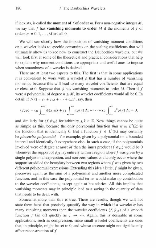
180 7 The Daubechies Wavelets

if it exists, is called the moment of f of order m. For a non-negative integer M,we say that f has vanishing moments to order M if the moments of f oforders m = 0, 1, . . . ,M are all 0.

We will see shortly how the imposition of vanishing moment conditionson a wavelet leads to specific constraints on the scaling coefficients that willultimately allow us to see how to construct the Daubechies wavelets, but wewill look first at some of the theoretical and practical considerations that helpto explain why moment conditions are appropriate and useful ones to imposewhen smoothness of a wavelet is desired.

There are at least two aspects to this. The first is that in some applicationsit is convenient to work with a wavelet ψ that has a number of vanishingmoments, because this will lead to many wavelet coefficients that are equalor close to 0. Suppose that ψ has vanishing moments to order M. Then if fwere a polynomial of degree n ≤ M, its wavelet coefficients would all be 0. Indetail, if f (x) = c0 + c1x + · · · + cnxn, say, then

〈 f , ψ〉 = c0

∫ ∞

−∞ψ(x) dx + c1

∫ ∞

−∞xψ(x) dx + · · · + cn

∫ ∞

−∞xnψ(x) dx = 0,

and similarly for 〈 f , ψ j,k〉 for arbitrary j, k ∈ Z. Now things cannot be quiteas simple as this, because the only polynomial function that is in L2(R) isthe function that is identically 0. But a function f ∈ L2(R) may certainlybe piecewise polynomial – for example, given by a polynomial on a boundedinterval and identically 0 everywhere else. In such a case, if the polynomialsinvolved were of degree at most M then the inner product 〈 f , ψ j,k〉 would be 0whenever the support of ψ j,k lay entirely within a region where f was given by asingle polynomial expression, and non-zero values could only occur where thesupport straddled the boundary between two regions where f was given by twodifferent polynomial expressions. Extending this idea a little, f might be given,piecewise again, as the sum of a polynomial and another more complicatedfunction, and in this case the polynomial terms would make no contributionto the wavelet coefficients, except again at boundaries. All this implies thatvanishing moments may in principle lead to a saving in the quantity of datathat needs to be dealt with.

Somewhat more than this is true. There are results, though we will notstate them here, that precisely quantify the way in which if a wavelet ψ hasmany vanishing moments then the wavelet coefficients 〈 f , ψ j,k〉 of a smoothfunction f tail off quickly as j → ∞. Again, this is desirable in someapplications, such as compression, since small wavelet coefficients are onesthat, in principle, might be set to 0, and whose absence might not significantlyaffect reconstruction of f .

7.3 The Moments of a Wavelet 181

There is a second rather different reason for considering the imposition ofvanishing moment conditions which relates to the smoothness of the waveletsthemselves. The following result gives information on the relation betweenvanishing moments and the smoothness of a wavelet.

Theorem 7.2 Suppose that ψ ∈ L2(R) has the property that the collectionof scaled, dilated, translated functions {ψ j,k : j, k ∈ Z} is an orthonormalset. If ψ has bounded support and is in CM(R) for some M ≥ 0, then ψ hasvanishing moments up to order M; that is,∫ ∞

−∞xmψ(x) dx = 0 for m = 0, 1, . . . ,M.

Note that the theorem does not require that ψ is the wavelet correspondingto a multiresolution analysis; in fact, it does not even require that the ψ j,k forman orthonormal basis for L2(R), but merely that they form an orthonormalset. However, the result certainly applies to the case of a wavelet of boundedsupport arising from a multiresolution analysis. (The theorem also holds in amore general form than ours, without the assumption of bounded support, butmore complicated hypotheses then need to be assumed. We will in any caseomit the proof.)

An immediate and highly significant implication of this result is, informally,that if we are looking for smooth wavelets then we will only be able to findthem among functions that have vanishing moments. More precisely, to findwavelets that have continuous derivatives up to order M we need to look onlyamong the functions whose moments vanish up to order M. As noted earlier,this is the approach followed by Daubechies; in fact, the Daubechies waveletscan be characterised as those which have the largest number of vanishingmoments consistent with their support length.

7.3.1 Vanishing Moment Conditions

We will now investigate how vanishing moment conditions give rise toconstraints on scaling coefficients. Consider a multiresolution analysis with ascaling function φ that has bounded support. With this condition, Theorem 6.16shows that ∫ ∞

−∞ψ = 0 and

∑k∈Z

(−1)kak = 0; (7.6)

in fact, the last few lines of the proof show that∫ ∞

−∞ψ = 1

2 I∑k∈Z

(−1)k−1ak,

182 7 The Daubechies Wavelets

where I =∫ ∞−∞ φ, and since part (i) of the same result tells us that I � 0, the

integral and the sum in (7.6) are either both zero or both non-zero. But∫ ∞−∞ ψ

is just the zeroth moment of ψ, and so, in the bounded support case, the zerothmoment of ψ is always 0. Hence if we impose vanishing moment conditions,we will only gain new constraints on the scaling coefficients for momentsbeyond the zeroth.

Suppose now that isupp φ = [0, 2N − 1] for some N ∈ N, and that φ andthe corresponding wavelet ψ satisfy the usual scaling equation and waveletequation

φ(x) =2N−1∑k=0

akφ(2x − k) and ψ(x) =2N−1∑k=0

(−1)k−1akφ(2x + k − 1),

respectively. Then we know that the scaling coefficients a0, a1, . . . , a2N−1

satisfy the N + 1 fundamental relations. Since we need to solve for 2Nunknowns and have only N + 1 equations, it is natural as a first step to seek forN − 1 suitable additional constraints to impose.

➤ Though this is indeed a natural first step, we noted in Section 7.1 that the impositionof one further constraint is necessary to determine a0, a1, . . . , a2N−1 uniquely, as we willneed to do if we are to construct the Nth Daubechies wavelet (see Section 7.4 below).

A single quadratic equation can of course have two real solutions, depending onthe choice of sign made in a certain square root, and a similar phenomenon occurs ina more complex way in the solution of a set of equations some of which are linearand some quadratic. We plan to add N − 1 new constraints to the N + 1 fundamentalrelations, giving 2N constraints on the 2N unknowns a0, a1, . . . , a2N−1, but since thereare N quadratic equations among the fundamental relations, 2N equations will not bequite enough to determine a unique solution.

For the Nth Daubechies scaling function and wavelet, we obtain the extraN − 1 constraints that we want by setting the �th moment of ψ to 0 for1 ≤ � ≤ N − 1 (note that we omit the case � = 0, since this would give usthe zeroth moment, which as we saw above is always 0). The following resulttells us explicitly what constraints on the scaling coefficients these conditionslead to.

Theorem 7.3 If∫ ∞−∞ x�ψ(x) dx = 0 for 1 ≤ � ≤ N − 1, then

2N−1∑k=0

(−1)kk�ak = 0

for 1 ≤ � ≤ N − 1.

The complete proof, which proceeds by induction, is not difficult, and is leftas an exercise (see Exercise 7.5). We will outline the proof for N = 2, sincethis already shows most of the features of the general case.

7.3 The Moments of a Wavelet 183

For N = 2, just one additional constraint is imposed on the scalingcoefficients, since N = 2 corresponds to setting the first moment,

∫ ∞−∞ xψ(x) dx,

to 0. The wavelet equation in this case is

ψ(x) = a0φ(2x − 1) − a1φ(2x) + a2φ(2x + 1) − a3φ(2x + 2),

and multiplying through this equation by x and integrating gives

0 =∫ ∞

−∞xψ(x) dx

= a0

∫ ∞

−∞xφ(2x − 1) dx − a1

∫ ∞

−∞xφ(2x) dx

+ a2

∫ ∞

−∞xφ(2x + 1) dx − a3

∫ ∞

−∞xφ(2x + 2) dx.

We now change variables in the four integrals in the last expression. Settingy = 2x in the first integral gives∫ ∞

−∞xφ(2x − 1) dx = 1

4

∫ ∞

−∞yφ(y − 1) dy,

and if we make the changes of variable y = 2x + 1, y = 2x + 2 and y = 2x + 3in the other three integrals, respectively, we obtain∫ ∞

−∞(a0 − a1 + a2 − a3)yφ(y − 1) dy +

∫ ∞

−∞(a1 − 2a2 + 3a3)φ(y − 1) dy = 0.

But the second equation in (7.6) shows that

a0 − a1 + a2 − a3 =∑k∈Z

(−1)kak = 0,

and since∫ ∞−∞ φ(y − 1) dy =

∫ ∞−∞ φ(x) dx � 0 by Theorem 6.16, we have

a1 − 2a2 + 3a3 = 0,

which, after a change of sign, is the equation given by Theorem 7.3 whenN = 2.

➤ Note that the changes of variable used above are not the most obvious ones. Themore obvious choice of y = 2x − 1 in the first integral, and so on, will work perfectlywell, but the substitutions chosen above lead most directly to the desired answer; themore obvious choices make a little extra manipulation necessary at the end of theargument.

Listing together the N +1 fundamental relations and the N −1 new relationswe have just derived, we arrive at the following system of 2N equations for

184 7 The Daubechies Wavelets

the 2N scaling coefficients a0, a1, . . . , a2N−1 of the Nth Daubechies scalingfunction:

2N−2�−1∑k=0

akak+2� = 2δ0,� for � = 0, 1, . . . ,N − 1,

2N−1∑k=0

ak = 2,

2N−1∑k=0

(−1)kk�ak = 0 for � = 1, 2, . . . ,N − 1.

⎫⎪⎪⎪⎪⎪⎪⎪⎪⎪⎪⎪⎪⎪⎪⎪⎪⎪⎬⎪⎪⎪⎪⎪⎪⎪⎪⎪⎪⎪⎪⎪⎪⎪⎪⎪⎭

(7.7)

We will refer to this as the augmented system of fundamental relations.One small but worthwhile improvement to the system (7.7) is possible.

Exercises 7.6 and 7.7 show that one of the quadratic equations in (7.7) canbe replaced by a linear equation to give an equivalent system, that is, a systemthat has exactly the same set of solutions. Specifically, when we take � = 0 inthe first subsystem of (7.7), we get the quadratic equation

2N−1∑k=0

a2k = 2,

and this can be replaced by the linear equation

2N−1∑k=0

(−1)kak = 0.

If we make this replacement in the system (7.7), we obtain a new system withN−1 quadratic equations and N+1 linear equations, which is an improvement(if only a modest one), since linear equations are easier to deal with thanquadratic equations.

Note, however, that by the discussion at the start of the subsection thenew linear equation is equivalent to the zeroth moment condition, whichwe specifically excluded from the moment conditions in the third subsystemof (7.7), by starting from the index value � = 1. We can therefore removethe old quadratic equation and incorporate the new linear equation into theaugmented system by simply eliminating the case � = 0 from the firstsubsystem and including it in the third subsystem. Thus our improved andfinal system of 2N equations, which again we will refer to as the augmentedsystem, is the following:

7.4 The Daubechies Scaling Coefficients 185

2N−2�−1∑k=0

akak+2� = 2δ0,� for � = 1, 2, . . . ,N − 1,

2N−1∑k=0

ak = 2,

2N−1∑k=0

(−1)kk�ak = 0 for � = 0, 1, . . . ,N − 1.

⎫⎪⎪⎪⎪⎪⎪⎪⎪⎪⎪⎪⎪⎪⎪⎪⎪⎪⎬⎪⎪⎪⎪⎪⎪⎪⎪⎪⎪⎪⎪⎪⎪⎪⎪⎪⎭

(7.8)

(Note carefully that the new system differs from the old only in the ranges ofvalues taken by the index �.)

7.4 The Daubechies Scaling Coefficients

Taking N = 1 in the augmented system (7.8) yields the system

a0 + a1 = 2,

a1 − a2 = 0,

⎫⎪⎪⎬⎪⎪⎭which trivially has the unique solution a0 = a1 = 1; these are the Daubechiesscaling coefficients for N = 1. (Compare this with the start of Section 7.2,where in effect we solved for the same coefficients using the augmented systemin its initial form (7.7).)

For N = 2, the augmented system (7.8) is

a0a2 + a1a3 = 0,

a0 + a1 + a2 + a3 = 2,

a0 − a1 + a2 − a3 = 0,

a1 − 2a2 + 3a3 = 0.

⎫⎪⎪⎪⎪⎪⎪⎪⎪⎬⎪⎪⎪⎪⎪⎪⎪⎪⎭(7.9)

Solving these equations (see Exercise 7.8), we find

a0 =14 (1 ±

√3), a1 =

14 (3 ±

√3),

a2 =14 (3 ∓

√3), a3 =

14 (1 ∓

√3).

⎫⎪⎪⎬⎪⎪⎭ (7.10)

Note that because one of our equations is quadratic, we do not obtain a uniquesolution, but rather two solutions that differ in the sign of the radical term.Note also, however, that the two solutions are mirror-images: each sequence isthe reverse of the other. It follows (see Exercise 7.9) that scaling functions andwavelets constructed using these sequences are also mirror-images, so we losenothing essential by restricting ourselves to just one of the two possibilities.We will choose the + sign in the expression for a0 (we discuss the basis for thisspecific choice below), which of course fixes the other signs. Thus, we have

186 7 The Daubechies Wavelets

a0 =14 (1 +

√3), a1 =

14 (3 +

√3),

a2 =14 (3 −

√3), a3 =

14 (1 −

√3),

⎫⎪⎪⎬⎪⎪⎭ (7.11)

or, to 10 places,

a0 = 0.6830127019, a1 = 1.1830127019,a2 = 0.3169872981, a3 = −0.1830127019.

These are the Daubechies scaling coefficients for N = 2.For N = 3, the system (7.8) is

a0a2 + a1a3 + a2a4 + a3a5 = 0,

a0a4 + a1a5 = 0,

a0 + a1 + a2 + a3 + a4 + a5 = 2

a0 − a1 + a2 − a3 + a4 − a5 = 0,

a1 − 2a2 + 3a3 − 4a4 + 5a5 = 0

a1 − 4a2 + 9a3 − 16a4 + 25a5 = 0.

⎫⎪⎪⎪⎪⎪⎪⎪⎪⎪⎪⎪⎪⎪⎪⎪⎬⎪⎪⎪⎪⎪⎪⎪⎪⎪⎪⎪⎪⎪⎪⎪⎭(7.12)

In this case, there are four solutions, but two are real and two are complex (seeExercise 7.10). Since we are interested only in real scaling coefficients, we candisregard the complex solutions, and then the two remaining real solutions arerelated like those for N = 2: one sequence of values is the mirror-image of theother. One of these two sequences, chosen as discussed below, consists of theDaubechies scaling coefficients for N = 3.

For N = 4, there are 8 solutions, 4 real and 4 complex, and for N = 5, thereare 16 solutions, 4 real and 12 complex, and in both cases the 4 real solutionsform two mirror-image pairs. For general N, the number of real solutions to thesystem (7.8) is 2�N/2�, where �x� (read as the ‘floor of x’), for a real number x,is the largest integer less than or equal to x.

Exact expressions are known for the real solutions for N = 3, 4 and 5;they are fairly complicated for N = 3 and very complicated for N = 4 and 5.However, computing the solutions numerically to any desired accuracy using asuitable computer system is straightforward, and numerical values are all thatis required for applications. (Exercise 7.10 outlines a method for computingthe exact expressions for N = 3; the expressions themselves are given inSubsection 8.5.3, though they are computed there by an entirely differentmethod.)

For N ≥ 2, the real solutions always occur in mirror-image pairs (note thatfor N = 1, the unique solution is its own mirror-image), and for N ≥ 4, there ismore than one mirror-image pair, so the question arises of how to pick out theDaubechies scaling coefficients from the set of solutions.

7.4 The Daubechies Scaling Coefficients 187

The specific choice that is made to single out the Daubechies scalingcoefficients is determined as follows. Suppose that the sequence

a0(�), a1(�), . . . , a2N−1(�)

forms a solution to the system of equations (7.8) for each value of � in acertain range. Then the particular sequence a0(�0), a1(�0), . . . , a2N−1(�0) is theextremal phase or minimum phase solution if

n∑k=0

ak(�)2 ≤n∑

k=0

ak(�0)2 for n = 0, 1, . . . , 2N − 1

for each value of �. Roughly speaking, the extremal phase solution is the onewhose largest values occur as early as possible in the sequence; it is sometimessaid to be ‘front-loaded’. (The extremal phase and minimum phase terminologycomes from the theory of signal processing.)

If for each fixed N we make the extremal phase choice, then by definition weobtain the Daubechies scaling coefficients a0, a1, . . . , a2N−1, which are shownnumerically for N = 2, 3, . . . , 7, rounded to 10 decimal places, in Table 7.1.Confirmation that the extremal phase solution does indeed yield the values inthe table for N = 2 and N = 3 is left for Exercise 7.11.

Table 7.1. The Daubechies scaling coefficients a0, a1, . . . , a2N−1 forN = 2, 3, . . . , 7

N k ak

2 0 0.68301270191 1.18301270192 0.31698729813 −0.1830127019

3 0 0.47046720781 1.14111691582 0.65036500053 −0.19093441564 −0.12083220835 0.0498174997

4 0 0.32580342811 1.01094571512 0.89220013823 −0.03957502624 −0.26450716745 0.04361630056 0.04650360117 −0.0149869893

N k ak

5 0 0.22641898261 0.85394354272 1.02432694433 0.19576696134 −0.34265671545 −0.04560113196 0.10970265867 −0.00882680018 −0.01779187019 0.0047174279

6 0 0.15774243201 0.69950381412 1.06226375993 0.44583132294 −0.31998659895 −0.18351806416 0.13788809307 0.0389232097

N k ak

8 −0.04466374839 0.0007832516

10 0.006756062411 −0.0015235338

7 0 0.11009943071 0.56079128362 1.03114849163 0.66437248224 −0.20351382255 −0.31683501136 0.10084646507 0.11400344528 −0.05378245269 −0.0234399416

10 0.017749792411 0.000607515012 −0.002547904713 0.0005002269

188 7 The Daubechies Wavelets

7.5 The Daubechies Scaling Functions and Wavelets

In this section, we present results that allow us to take the final step in theconstruction of the Daubechies scaling functions and wavelets, though most ofthe results are stated in forms that apply more generally.

In Subsection 7.5.1 we examine results which tell us that almost allchoices of potential scaling coefficients yield a multiresolution analysis thathas a scaling equation with the given potential scaling coefficients as itsactual scaling coefficients; these results apply in particular in the case of theDaubechies scaling coefficients, thus guaranteeing existence of the Daubechiesscaling functions and, consequently, the Daubechies wavelets as well. InSubsection 7.5.2, we briefly discuss some of the smoothness properties of theDaubechies scaling functions and wavelets. In Subsection 7.5.3, we examineresults which at a theoretical level show how the Daubechies scaling functionscan be constructed as the limit functions of suitable procedures of successiveapproximation, and at a practical level allow us to approximate values ofthe functions at specific points with as much accuracy as we desire, and inparticular to plot their graphs. As noted in Section 7.1, most of the results ofthis section are stated without proof.

7.5.1 Existence

Exercise 6.5 asked for a proof of the fact that if φ is the scaling function for amultiresolution analysis {Vj}, then

Vj =

⎧⎪⎪⎨⎪⎪⎩∑k∈Z

αkφ j,k :∑k∈Z

α2k converges

⎫⎪⎪⎬⎪⎪⎭ (7.13)

for each j ∈ Z. In other words, if φ is known to be the scaling function of amultiresolution analysis, then the spaces Vj can be reconstructed from φ alone.

This raises the following question: If a function φ ∈ L2(R) is given, underwhat conditions is φ the scaling function of a multiresolution analysis? That is,under what conditions on φ do the equations (7.13) define closed subspaces Vj

that together with φ form a multiresolution analysis?Since condition (MRA6) says that the translates {φ0,k : k ∈ Z} form an

orthonormal basis for V0, it is to be expected that one of the conditions thatwill have to be assumed for φ is that {φ0,k} is an orthonormal set in L2(R), sincethis is a property of φ in isolation, and the problem is therefore to determinewhat further properties of φ are needed. An answer is given by the followingtheorem.

7.5 The Daubechies Scaling Functions and Wavelets 189

Theorem 7.4 Let φ ∈ L2(R) and suppose that

(i) φ has bounded support,(ii) {φ0,k : k ∈ Z} is an orthonormal set,

(iii) φ satisfies an equation of the form φ(x) =∑

k∈Z akφ(2x − k) for someconstants {ak : k ∈ Z}, and

(iv)∫ ∞−∞ φ = 1.

Then the spaces {Vj : j ∈ Z} defined by (7.13) form a multiresolution analysisof which φ is the scaling function.

A few remarks about this result are worth noting.

• It is easy to see (and has been noted earlier) that if φ is the scaling function ofa multiresolution analysis with spaces {Vj}, then −φ is also a scaling functionfor the same sequence of spaces. It follows that the condition that the integralof φ over R is 1 could be replaced by the condition that the integral is ±1.(If the value were −1, we could simply apply the theorem as stated to thefunction −φ.)

• With the change of the value of the integral to ±1, the conditions of thetheorem are necessary as well as sufficient for φ to be a scaling function(see Exercise 7.13).

• Although it is far from explicit in the statement of the theorem, the conclu-sion, that the given function φ is the scaling equation of a multiresolutionanalysis, along with the assumption that φ has bounded support, allows thederivation of all of the very detailed information summarised in Section 7.1.

The next theorem tells us that sequences of potential scaling coefficientsalmost always give rise to functions φ with the properties listed in the previoustheorem.

Theorem 7.5 Let n ∈ N and suppose that a0, . . . , a2N−1 satisfy the funda-mental relations, or, equivalently, that (a0, . . . , a2N−1) ∈ AN, as defined inSection 7.2. Then there exists a unique function φ ∈ L2(R) that satisfies thescaling equation φ(x) =

∑2N−1k=0 akφ(2x−k) and has the property that

∫ ∞−∞ φ = 1.

This function φ also has the property that isupp(φ) = [0, 2N − 1].Moreover, for almost all choices of (a0, . . . , a2N−1) ∈ AN, and in particular

for the choice representing the Daubechies scaling coefficients, the function φhas the additional property that {φ0,k : k ∈ Z} is an orthonormal set.

➤ The phrase ‘almost all’ here requires comment. Although its sense is essentially thatintroduced in Section 3.3 and used in many places following, it is used here in a moregeneral sense.

190 7 The Daubechies Wavelets

The definition of measure 0 in Section 3.3 captures the idea of a set being ‘negligible’as a subset of R. In the theorem above, its meaning is that the set of 2N-tuples in AN thatdo not yield a multiresolution analysis is ‘negligible’ when considered as a subset of AN

(which is in turn a subset of R2N). A more precise explanation requires development ofthe theory of Lebesgue measure, and is beyond the scope of this book.

Concretely, in the case N = 1, the ‘negligible’ subset of A1 is simply the empty set,because A1 consists of a single point that does yield a function φ with the property that{φ0,k : k ∈ Z} is an orthonormal set; this φ is of course the Haar scaling function. In thecase N = 2 where, according to Section 7.2 and Exercise 7.2, A2 is a circle in R4, thereis exactly one exceptional point (which is identified in Exercise 7.3); the singleton setwith that point as element is the claimed ‘negligible’ subset of A2.

What is of most interest here is the use of the two theorems above incombination, as follows, since this tells us directly about the Daubechies case.

Theorem 7.6 Let N ∈ N. Then almost all choices of a0, . . . , a2N−1 satisfyingthe fundamental relations yield a multiresolution analysis, including thescaling function, and its associated wavelet. This is the case in particularwhen a0, . . . , a2N−1 are the Daubechies scaling coefficients, and in that casethe corresponding scaling function and wavelet are, by definition, the NthDaubechies scaling function and wavelet, respectively.

We adopt the following notational convention:

The symbols Nφ and Nψ denote respectivelythe Nth Daubechies scaling function and wavelet.

Although notation for these functions is far from standardised, our notation,with its rather unusual placement of the subscripts before the main symbols,was introduced by Daubechies herself.

7.5.2 Smoothness

Theorem 7.2 shows that wavelets with continuous derivatives up to order Mmust have vanishing moments up to order M, and this suggested the programfollowed above for constructing the Daubechies wavelets. Unfortunately,however, the converse of the theorem does not hold: it is not the case thatvanishing moments to order M entail continuous derivatives to order M. Wenevertheless wish to understand something of the smoothness properties of theDaubechies wavelets, both individually and asymptotically, and we summarisesome of what is known in the following result. (More detailed information,including a more precise version of the asymptotic statement, is given inSection 7.7 below.)

7.5 The Daubechies Scaling Functions and Wavelets 191

Theorem 7.7 (i) 1φ and 1ψ, the Haar scaling function and wavelet, are notcontinuous, and hence do not lie in Cm(R) for any m ≥ 0.

(ii) 2φ and 2ψ are continuous but not differentiable, that is, are in C0(R) butnot C1(R).

(iii) 3φ and 3ψ are continuously differentiable but are not twice differentiable,that is, are in C1(R) but not C2(R).

(iv) When N is large, Nφ and Nψ belong to Cm(R) for an integer m which isapproximately N/5.

7.5.3 Calculations and Graphs

Now that we know that it is possible in principle to pass from properly chosenscaling coefficients to a scaling function φ, we will examine two closely relatedways of producing sequences of functions that better and better approximate φ.Both are derived in a straightforward way from the scaling equation that wewant φ to satisfy, and their main difference lies in the choice of the initialapproximation. Both will allow us in particular to compute better and betterapproximations to the Daubechies scaling functions.

Our first approach to finding φ as the limit, in a suitable sense, of a sequenceof successive approximations, is as follows. For a fixed N, corresponding to thesequence of 2N scaling coefficients a0, a1, . . . , a2N−1, we are seeking φ ∈ L2(R)that satisfies the equation

φ(x) =2N−1∑k=0

akφ(2x − k).

We start by picking a suitable simple function φ(0). Then we define φ(1) bysetting

φ(1)(x) =2N−1∑k=0

akφ(0)(2x − k).

Note that we have φ(0) on the right-hand side here and φ(1) on the left, so thereis no problem in making the definition (whatever our choice of φ(0)). We canthen repeat the process, defining φ(2) by setting

φ(2)(x) =2N−1∑k=0

akφ(1)(2x − k),

and then continue in a similar way, so that we recursively define an infinitesequence of functions

{φ(n) : n ∈ N}

. In principle, a sequence defined in this

192 7 The Daubechies Wavelets

kind of way may not converge, or if it does converge may not converge to any-thing useful, but it turns out that under fairly mild conditions, and in particularwith a well-chosen starting function φ(0), this sequence does in fact converge tothe scaling function we are seeking. We formalise this information as follows.

Theorem 7.8 Let φ(0) be the Haar scaling function (thus φ(0)(x) = 1 for0 ≤ x < 1 and φ(0)(x) = 0 elsewhere). Define

φ(n)(x) =2N−1∑k=0

akφ(n−1)(2x − k)

for all n ∈ N. Then under suitable conditions on a0, a1, . . . , a2N−1, the sequence{φ(n)} converges both pointwise and in L2(R) as n → ∞ to a function φ that

satisfies all of the hypotheses of Theorem 7.4, and is therefore the scaling func-tion of a multiresolution analysis, as in that theorem. The relevant conditionsare satisfied in particular in the Daubechies case, and φ is then the NthDaubechies scaling function Nφ.

➤ Broadly similar methods of successive approximation are used in many fields ofmathematics, both at the theoretical level and for numerical approximation of thesolutions to specific problems. They may be used, for example, both to prove theexistence of solutions to certain families of differential equations and to approximatethe solutions of specific differential equations. In most cases, the same general issuesarise: what the initial input to the approximation should be; whether and in what sensethe process converges; and whether the limit, given convergence, is actually a solutionto the original problem.

Of course, we can graph the successive approximations produced by thismethod in any concrete case. If we compute approximations to the secondDaubechies scaling function 2φ by applying Theorem 7.8, then the graphs of

2φ(0), . . . , 2φ

(5), the first six functions in the sequence, are as in Figure 7.1.Our second approach is to use the scaling equation to approximate φ by

progressively calculating its values at the dyadic numbers. We have implicitlyused the dyadic numbers at many points in discussion of the scaling, dilationand translation of wavelets, though without introducing them formally. Theformal definition is that a dyadic number is a number of the form k/2 j, forany j, k ∈ Z. (Exercise 7.19 explores some simple properties of the dyadicnumbers.) A dyadic interval is an interval with left-hand endpoint k/2 j andright-hand endpoint (k + 1)/2 j for any j, k ∈ Z (irrespective of whether theendpoints belong to the interval).

Although dyadic numbers and dyadic intervals were not mentioned explic-itly in the context of Theorem 7.8, it is obvious from the graphs in Figure 7.1,and straightforward to confirm analytically, that for each n ≥ 0 the approxima-tion φ(n) produced by the theorem is constant on the half-open dyadic interval[k/2 j, (k + 1)/2 j) for j = n + 1.

7.5 The Daubechies Scaling Functions and Wavelets 193

2φ(0)

2φ(1)

2φ(2)

2φ(3)

2φ(4)

2φ(5)

Figure 7.1 The graphs of the first six approximations to 2φ using Theorem 7.8

194 7 The Daubechies Wavelets

To illustrate the second approximation process, consider the case of thesecond Daubechies scaling function 2φ. We will show how to find the valueof φ = 2φ at the dyadic numbers k/2 j lying in [0, 3], first at those with j = 0,namely the integers 0, 1, 2, 3, then at those with j = 1, namely, the half-integers

0, 12 , 1, 3

2 , 2, 52 , 3,

then at those with j = 2, namely, the quarter-integers

0, 14 ,

12 ,

34 , 1, 5

4 ,32 ,

74 , 2, 9

4 ,52 ,

114 , 3,

and so on.To find the values of φ at the integers in [0, 3], note first that φ(0) = φ(3) = 0

by continuity (see Theorem 7.7), since φ is identically 0 outside of [0, 3], sothat we only need to compute φ(1) and φ(2). Substitution of x = 1, 2 into thescaling equation φ(x) =

∑3k=0 akφ(2x − k) yields the equations

φ(1) = a0φ(2) + a1φ(1),

φ(2) = a2φ(2) + a3φ(1).

It is easy to check that these two equations are dependent, and so anotherconstraint is needed for us to solve for φ(1) and φ(2). This comes fromTheorem 6.18, which gives us the relation φ(1) + φ(2) = 1, and we find thatφ(1) = 2a0 and φ(2) = 2a3, so that we have

φ(0) = 0, φ(1) = 2a0, φ(2) = 2a3, φ(3) = 0.

➤ For the case of a general scaling function φ, the equations for the value of φ atthe integers is best set up as a matrix equation, and the solution process formulated interms of a discussion of the eigenvalues and eigenvectors of the coefficient matrix (seeExercises 7.15 and 7.17).

Since the scaling equation expresses φ(x) in terms of values of φ(2x − k)for various values of k, we can now immediately compute expressions for thevalue of φ at all the multiples of 1

2 , and we find that

φ(0) = 0,

φ( 1

2

)= 2a2

0,

φ(1) = 2a0,

φ( 3

2

)= 2a0a2 + 2a1a3,

φ(2) = 2a3,

φ( 5

2

)= 2a2

3,

φ(3) = 0.

7.5 The Daubechies Scaling Functions and Wavelets 195

We can clearly continue this process recursively, computing expressions forthe values of φ at all dyadic points k/2 j in [0, 3], where j runs from 0 to anygiven bound n. For each fixed n, we can then use the known numerical values ofa0, a1, a2, a3 to plot point–value pairs and join them by straight-line segments,giving a sequence of continuous, piecewise-linear approximations to φ. Giventhe fact that φ = 2φ is continuous (see Theorem 7.7), it is not hard to show thatthese functions converge uniformly to φ on [0, 3] (see Exercise 7.18).

➤ Note that it was convenient here to compute the values of φ symbolically, asfunctions of the scaling coefficients, rather than numerically; the scaling equationprovides all the information needed to manipulate the expressions symbolically, and thesystem (7.11) gives us the numerical values of the coefficients once they are needed.

The symbolic form also highlights a formal symmetry in the values of φ at the dyadicpoints: systematic interchange of a0 with a3 and of a1 with a2 converts the expression forφ(x) into the expression for φ(3 − x) for every dyadic x (see Exercises 7.21 and 7.22).(As its graph clearly shows, the function 2φ has no geometric symmetry; see also thefurther comments on symmetry in Subsection 7.7.1.)

The same construction can be applied to the Daubechies scaling function Nφ

for any N ≥ 2 (and indeed to any scaling function that is continuous and hasbounded support), and we summarise the procedure as follows, leaving theproof of its correctness for Exercise 7.18.

Theorem 7.9 Suppose that φ is continuous, has support in [0, 2N − 1] and isthe scaling function of a multiresolution analysis. Calculate the values of φ atthe integer points of [0, 2N − 1], then, by repeated application of the scalingfunction, at the dyadic points k/2 j for j = 1, 2, . . . , n. For each n ≥ 0, let φ(n)

be the continuous, piecewise-linear function obtained by interpolating betweenthe values at those points. Then φ(n) converges uniformly to φ as n→ ∞.

In the case of 2φ, Figure 7.2 shows graphs of the first few membersof the sequence of approximations, denoted as in the previous figure by

2φ(0), . . . , 2φ

(5). (Note that in the last graph shown, for n = 5, there are 25 = 32subdivisions of each unit interval.)

➤ A difference between the sequence of approximations produced by Theorems 7.8and 7.9, clearly visible in the graphs for φ = 2φ, is that although they both guaranteepointwise convergence to the scaling function, the first does not guarantee that thevalue of the approximate scaling function ever precisely equals the value of the scalingfunction, while the second proceeds directly by computing exact values of the scalingfunction at more and more dyadic points at each step.

However, it is fair to say that the two procedures are not as different as may appearat first sight, and that the main difference is in the starting function φ(0) employed.It is easy to see by examining the statements of the two results that the choice ofstarting function causes the first theorem to produce piecewise-constant functions andthe second to produce piecewise-linear functions. If Theorem 7.8 were given the initialfunction that had constant value φ(k) on [k, k + 1) for each k, then its approximationswould simply be piecewise-constant versions of those produced by Theorem 7.9.

196 7 The Daubechies Wavelets

2φ(0)

2φ(1)

2φ(2)

2φ(3)

2φ(4)

2φ(5)

Figure 7.2 The graphs of the first six approximations to 2φ using Theorem 7.9

7.5 The Daubechies Scaling Functions and Wavelets 197

We used the algorithms implied by Theorems 7.8 and 7.9 for computing(approximate) values and drawing (approximate) graphs of scaling functions.These algorithms, however, have some disadvantages, and another algorithmwhich works in a more subtle way has been used to plot most of the latergraphs of scaling functions in this chapter. We will not attempt to specify thisalgorithm here, but we will briefly discuss its distinctive difference from thealgorithms used above.

The algorithms implied by Theorems 7.8 and 7.9 both use the scalingequation in an obvious and direct way to compute new approximations tovalues of φ from old ones. But the scaling equation expresses φ(x) in terms ofthe values

φ(2x), φ(2x − 1), . . . , φ(2x − 2N + 1),

and these values are at points that are widely spread through the support of φ:each one is 1 unit distant from its neighbours. The more subtle approach of thethird algorithm allows each new approximate value φ(x) to be computed justfrom approximate values of φ at points that are close to x. This has the greatadvantage of allowing efficient ‘zooming in’ on the graph of φ. If we wanteda view of φ around some specific point x0 at high magnification, the impliedalgorithms of Theorems 7.8 and 7.9 would both require the whole graph of φto be found at high magnification, while for the third algorithm, high magnifi-cation would need to be used only in a small interval around x0. At very highmagnification, such as in some of the diagrams later in the chapter, this canrepresent a saving of many orders of magnitude in computing time and storage.

Once we have accurate approximations to φ, obtained by any of the methodsdiscussed above, we can easily construct similarly accurate approximations tothe corresponding wavelet ψ, because Corollary 6.14 tells us that ψ is given interms of φ by the wavelet equation

ψ(x) =2N−1∑k=0

(−1)k−1akφ(2x + k − 1).

In Figures 7.3 and 7.4, we show graphs of the first few of the Daubechiesscaling functions Nφ and wavelets Nψ. The following points should be noted.

• We omit 1φ and 1ψ, since these are the familiar Haar scaling function andwavelet.• Each function is plotted precisely over its support, that is, over [0, 2N − 1]

for Nφ and over [−N + 1,N] for Nψ.• The scales on the axes differ, and become increasingly disproportionate as

the support width increases with N.

198 7 The Daubechies Wavelets

2φ 2ψ

3φ 3ψ

4φ 4ψ

Figure 7.3 The Daubechies scaling functions Nφ and wavelets Nψ for N = 2, 3, 4

7.5 The Daubechies Scaling Functions and Wavelets 199

5φ 5ψ

6φ 6ψ

7φ 7ψ

Figure 7.4 The Daubechies scaling functions Nφ and wavelets Nψ for N = 5, 6, 7

200 7 The Daubechies Wavelets

• An increase in smoothness seems apparent as N increases (though, as thefollowing section hints, these functions are very complex analytically, andthe information we can reliably read merely from their graphs is thereforelimited; see Theorem 7.7 above and the further comments in Section 7.7below).

7.6 Some Properties of 2φ

A number of interesting observations remain to be made about the Daubechiesscaling functions Nφ and wavelets Nψ in general, but before coming to thesewe will examine certain of the algebraic and analytic properties of the secondDaubechies scaling function 2φ in some detail. Specifically, we will see that

2φ exhibits self-similar or fractal behaviour, we will investigate aspects of thesmoothness of 2φ and we will introduce a few results that explain analyticallysome of the behaviour of 2φ that seems apparent from its graph. For thecase of general N, the analogous issues are complex and require reasonablysophisticated analysis, but for N = 2 parts of the analysis can be done in anelementary way. For convenience, we will write ‘φ’ in place of ‘2φ’ throughoutthis section.

First, we note that, given the continuity of φ, Theorem 6.18 tells us that forall x ∈ R, ∑

n∈Zφ(x + n) = 1.

This is often called the property of partition of unity.Not only can the function with constant value 1 be expressed as a linear

combination of translates of φ, but so can the function whose value at x is x,that is, the identity function, and this is often called the property of partitionof the identity.

Lemma 7.10 For all x ∈ R,∑n∈Z

(2a2 − n)φ(x + n) = x.

We leave the proof of the lemma as an exercise (see Exercise 7.23).

➤ It is worthwhile noting that the two partition sums are not sums in L2(R). Theycannot be L2 sums, since the functions 1 and x are not members of L2(R). Rather, thesums express the simplest kind of equality, pointwise equality, between the two sidesof the equations. (The fact of pointwise equality depends on the continuity of φ, as isshown by the statement and proof of Theorem 6.18 and by the argument suggested inExercise 7.23 for Lemma 7.10.)

7.6 Some Properties of 2φ 201

Graph of2∑

n=0

φ(x + n) Graph of2∑

n=0

(2a2 − n)φ(x + n)

Figure 7.5 Illustration of partition of unity and partition of the identity for φ = 2φ

Note that because isupp φ = [0, 3], only three terms contribute to these sumsfor any fixed value of x. In particular, the addition of exactly three consecutiveterms from either sum permits a striking graphical illustration of the partitionphenomena, as shown in Figure 7.5.

We now introduce several results that together allow us to explain what wemeant when we said earlier that φ exhibits self-similar or fractal behaviour. Allthe proofs are straightforward, and are left for the exercises.

Lemma 7.11 For all x such that 0 ≤ x ≤ 1,

2φ(x) + φ(x + 1) = x + 2a0,

φ(x + 1) + 2φ(x + 2) = −x + 2a2

and

φ(x) − φ(x + 2) = x − 2a3.

Observe in particular how the first and third of these equations allow us toexpress the values of φ in the integer-length intervals [1, 2] and [2, 3] in termsof its values in [0, 1]:

φ(x + 1) = −2φ(x) + x + 2a0,

φ(x + 2) = φ(x) − x + 2a3.

The next result will allow us to express the values of φ in the intervals of half-integer length within [0, 3] in terms of its values in [0, 1].

202 7 The Daubechies Wavelets

Lemma 7.12 For all x such that 0 ≤ x ≤ 1,

φ( x2

)= a0φ(x),

φ

(x + 1

2

)= a3φ(x) + a0x +

2 +√

34

,

φ

(x + 2

2

)= a0φ(x + 1) + a3x +

√3

4,

φ

(x + 3

2

)= a3φ(x + 1) − a0x +

14,

φ

(x + 4

2

)= a0φ(x + 2) − a3x +

3 − 2√

34

and

φ

(x + 5

2

)= a3φ(x + 2).

Now, by combining this lemma with the two equations that just precede it,we can express the values of φ in, say, the interval [1, 1.5] in terms of its valuesin [0, 1], as follows:

φ

(x + 2

2

)= a0φ(x + 1) + a3x +

√3

4

= a0(x + 2a0 − 2φ(x)

)+a3x +

√3

4

for all x ∈ [0, 1], and a regrouping of terms in the last expression leads easily toan expression of the form αφ(x) + βx + γ. Pursuing this idea inductively leadsto a proof of the following general statement about the values of φ in arbitrarydyadic intervals within [0, 3] (see Exercises 7.27 and 7.28).

Theorem 7.13 For each j = 0, 1, 2, . . . and each k = 0, 1, . . . , 3 · 2 j − 1, thereexist α, β and γ (dependent on j and k), with α � 0, such that

φ

(x + k

2 j

)= αφ(x) + βx + γ for 0 ≤ x ≤ 1.

We commented above that φ exhibits self-similar or fractal behaviour, andthe theorem explains partly what this means: on each dyadic interval[

k/2 j, (k + 1)/2 j]lying in isupp φ = [0, 3], φ ‘looks the same as on [0, 1]’, the only differencebeing that it is scaled by some non-zero factor α and sheared by some linearterm βx+γ. Note carefully that this self-similarity occurs at every dyadic scale.

7.6 Some Properties of 2φ 203

For example, the most prominent feature of the graph of φ in Figure 7.3 is thelarge spike at x = 1, but the theorem implies that this spike actually appears,in some scaled and sheared form, at every dyadic point in (0, 3). (Note thatwe need to exclude the dyadic points 0 and 3 from the discussion here, and atsimilar points below, since φ(x) is identically 0 when x ≤ 0 and when x ≥ 3.)At the scale of the graph, this is clearly visible at all the integer and half-integer points, at most of the quarter-integer points and at a few of the eighth-integer points (though at some of these values, such as 1.5 and 2, the spikepoints downwards, corresponding to cases where α < 0 in Theorem 7.13). Thetwo plots in Figure 7.6 zoom in on the graph of φ around 0.5 and 2.5, withhorizontal scales chosen carefully so as to bring out the similarity in behaviourof the function near each of those points, as well as near 1.

Another way of viewing the self-similarity property is given by rewriting theequation from the theorem in the form

φ(x) = (1/α)φ

(x + k

2 j

)− (β/α)x − (γ/α) ;

this equation shows that φ on [0, 1] (and hence on [0, 3]) can be reconstructedfrom its values on any one fixed dyadic interval within [0, 3], however small.

The theorem implies, moreover, that any analytic condition that φ satisfiesat a particular dyadic point in [0, 3) will hold, in suitably modified form, atevery other dyadic point in [0, 3). The most interesting such properties arethose related to smoothness.

In the graph of Figure 7.3, the spike at 1 is conspicuously lop-sided, andthis is a graphical reflection of the mathematical fact that φ is differentiablefrom the left but not from the right at 1. More precisely, the limit that woulddefine the right derivative at 1 if it existed and had finite value actually diverges

Figure 7.6 Magnified views of the graph of 2φ(x) around x = 0.5 and x = 2.5

204 7 The Daubechies Wavelets

to ∞, so that the curve has ‘infinite slope’ immediately to the right of 1.By the theorem, this behaviour must be reflected at every dyadic point: φ isdifferentiable from the left but not from the right at every dyadic point in[0, 3), and moreover has ‘infinite slope’ on the right of each such point, thoughthe slope can be ∞ or −∞ depending on the sign of the coefficient α fromTheorem 7.13. We will confirm this analytically below and in the exercises,but meanwhile we can gain confirmation of the fact graphically. Specifically,since φ has finite slope on the left and infinite slope on the right at every dyadicpoint, increasing levels of magnification on the x-axis at a dyadic point shouldcause the graph of φ to appear increasingly flat to the left of the point, butalways to appear infinitely steep to the right of the point. Figure 7.7 confirmsthis expectation by zooming in at high magnification around 0.5 and 2.5.

We will now confirm the claim that φ is not differentiable from the right atdyadic points in [0, 3). By Theorem 7.13 it suffices to deal with any one dyadicpoint, and for convenience we prove the claim at x = 0. (The stronger claims –that the derivative from the right is infinite and the derivative from the left isfinite at every dyadic point – are left as exercises; see Exercises 7.29 and 7.31.)

By the first equation of Lemma 7.12 (or directly from the scaling equation),we have φ(x) = a0φ(2x) for 0 ≤ x ≤ 1

2 . Therefore, φ( 12 ) = a0φ(1),

φ( 14 ) = a0φ( 1

2 ), φ( 18 ) = a0φ( 1

4 ), . . . , and it follows that

φ( 12 ) = a0φ(1), φ( 1

4 ) = a20φ(1), φ( 1

8 ) = a30φ(1), . . . ,

or, in general,

φ

(12 j

)= a j

0φ(1) for j ≥ 0.

Figure 7.7 Highly magnified views of the graph of 2φ(x) around x = 0.5 andx = 2.5

7.7 Some Properties of Nφ and Nψ 205

Now differentiability of φ at 0 from the right would require existence of thelimit

limh→0+

φ(h) − φ(0)h − 0

= limh→0+

φ(h)h.

But when h = 1/2 j, we have

φ(h)h= 2 jφ

(12 j

)= 2 ja j

0φ(1) = (2a0) j+1 → ∞

as j → ∞, since φ(1) = 2a0 > 1, so the required limit does not exist. Henceφ is not differentiable from the right at 0 or, by Theorem 7.13, at any otherdyadic point in [0, 3).

7.7 Some Properties of Nφ and Nψ

In this section, we will survey a number of interesting and important propertiesof the Daubechies scaling functions and wavelets in general, as well as a fewproperties of arbitrary scaling functions and wavelets of bounded support.

Our measure of the smoothness of a function f to this point has been thelargest integer k ≥ 0 for which f ∈ Ck(R). It is in fact possible to define a notionof ‘fractional differentiability’, and corresponding classes Cα(R) for all realnumbers α ≥ 0, in such a way that when α = k is an integer, Cα(R) = Ck(R)is the collection of functions continuously differentiable to order k as alreadydefined.

➤ The notion of fractional differentiability we are referring to specifically is the notionof Holder continuity; the functions in Cα(R) are said to be Holder continuous withexponent α. (We should also remark that there are actually several inequivalent ways ofdefining fractional differentiability.) We will not give the definition of Holder continuityhere, although it is quite straightforward. It is useful to be able to refer to the notionhere, even if only in a non-technical way, since it allows us interesting insight into thebehaviour of Nφ and Nψ.

We start by drawing together a number of facts about the smoothnessproperties of the Daubechies scaling functions and wavelets. These include,but refine, the information given in Theorem 7.7.

• A precise statement about the asymptotic rate of growth in the smoothnessof Nφ and Nψ as N grows is as follows. When N is large, Nφ, Nψ ∈ CμN(R),where μ = 1 − ln 3/(2 ln 2) ≈ 0.2075. Thus, for large N, roughly one extracontinuous derivative is gained for each increase of 5 in the value of N.

206 7 The Daubechies Wavelets

This asymptotic information tells us nothing about how smooth Nφ and Nψ

are for specific, small values of N, and for this case-by-case arguments arerequired. Some details are as follows.

• When N = 1, we have the Haar scaling function and wavelet 1φ and 1ψ,which are not in C0(R).

• For N = 2, the functions 2φ and 2ψ are continuous but not differentiable,and hence are in C0(R) but not C1(R).

• The exponent α of Holder continuity for 2φ and 2ψ is about 0.5500,indicating that although the functions are continuous they are ‘not veryclose’ to being continuously differentiable.

• The functions 2φ and 2ψ are not differentiable (in the ordinary two-sidedsense) at any dyadic point in [0, 3), because the right derivative does notexist at those points. Despite this, and despite the low Holder exponent, thefunctions are known to be differentiable at many non-dyadic points, and infact are differentiable at almost all points in [0, 3].

• For N = 3, the functions 3φ and 3ψ are continuously differentiable, butare not twice differentiable at any point in their support, and hence arein C1(R) but not C2(R). However, they are ‘only just’ in C1(R): their Holderexponent α is about 1.0878. This is illustrated informally by the plot of 3φ

in Figure 7.3, which at the scale used appears to have a sharp spike at x = 1.If this spike were like the spike of 2φ at x = 1, then the function 3φ wouldnot be differentiable at x = 1. However, under suitable magnification, wefind that the maximum of 3φ occurs a little to the right of 1, and that thereis actually no sharp spike at 1 after all, as shown in Figure 7.8. (Similarcomments apply to 3ψ.)

Figure 7.8 Highly magnified views of the graph of 3φ(x) around x = 1

7.7 Some Properties of Nφ and Nψ 207

We also note a few facts about the relation between the smoothness and thesupport length of a scaling function in the general case.

• Given a multiresolution analysis with a scaling function φ that has support[0, 2N − 1], it is known that if φ ∈ Ck(R), then 2N − 1 ≥ k + 2. Note,however, that this gives only fairly weak information in the Daubechies case.For example, it implies that 2φ is not in C2(R), while we have already notedthat 2φ is not in C1(R), and it implies that 3φ is not in C3(R), while we havealready noted that 3φ is not in C2(R). Likewise, the asymptotic informationit gives is much weaker than the asymptotic information already noted forthe Daubechies case.

• However, the above result does have the interesting and significant corollarythat a scaling function of bounded support cannot be in C∞(R).

7.7.1 Other Wavelet Families

The Daubechies scaling function and wavelet for a given support length of2N − 1 are obtained by imposing the N + 1 fundamental relations (6.13) onthe scaling coefficients, then the further N − 1 relations derived by setting thewavelet moments up to order N to 0 (see Theorem 7.3), solving either of theresultant equivalent systems (7.7) and (7.8) of 2N equations for the coeffi-cients, and finally picking the specific sequence of coefficient values given bythe extremal phase condition (see the end of Section 7.4 and Exercise 7.11).Once we have this sequence of coefficients, the scaling function and then thewavelet are uniquely determined (see Theorems 7.5 and 7.6).

Given N, the fundamental relations are non-negotiable: the scaling coeffi-cients for all scaling functions and wavelets with support length 2N − 1 mustsatisfy them (this was a major conclusion of Chapter 6). However, choiceshave to be made to pick out specific sequences of scaling coefficients from thecollection AN (see the opening paragraphs of Section 7.2) of all sequences ofsolutions to the fundamental relations, which is an infinite set except whenN = 1. Moreover, according to Theorem 7.5, almost all choices of extraconstraints will yield scaling functions and hence wavelets.

The original choice made by Daubechies was as just summarised: imposevanishing moment conditions and then make the extremal phase choice. How-ever, Daubechies herself, and others since, have also developed other familiesof wavelets by making different choices, driven both by the requirements ofapplications and by theoretical interest. Some of these are as follows.

208 7 The Daubechies Wavelets

• The extremal phase choice results in an asymmetric, ‘front-loaded’ sequenceof scaling coefficients (see the end of Section 7.4 and Exercise 7.11). Thisin turn results in an asymmetric scaling function, where the large valuesof the function are all at the left-hand end of its support and the values atthe right-hand end are very close to 0. This effect becomes increasinglypronounced as N increases, and is clearly visible already in the scalingcoefficients for the case N = 7 shown in Table 7.1 and in the graph of 7φ

shown in Figure 7.4. The asymmetry diminishes a little in the correspondingwavelets (see Exercise 7.33), but is still noticeable.

For some applications, it is useful to have wavelets that are assymmetric as possible. Daubechies has shown that a wavelet can be neithercompletely symmetric nor completely antisymmetric, except in the case ofthe Haar wavelet. (Formally, a function f is symmetric if some translateof f is an even function and is antisymmetric if some translate is an oddfunction.) However, Daubechies has also constructed the least asymmetricwavelet that has support length 2N − 1 and N vanishing moments (wherethe phrase ‘least asymmetric’ is used in a well-defined technical sense), andhas shown that somewhat better symmetry still can be achieved if a largersupport length is permitted.

• With support length fixed as before at 2N − 1, better smoothness may besought than is given by the Daubechies family of wavelets. Theorem 7.2shows that smoothness forces moments to vanish: if ψ ∈ CM(R), then allthe moments of ψ up to order M are 0. On the other hand, as noted above,the Nth Daubechies wavelet Nψ is asymptotically only in CμN(R), whereμ ≈ 0.2075, which suggests that it might be reasonable to impose fewervanishing moment conditions and to try to use the resulting freedom toimpose other conditions that directly increase smoothness. Daubechies hasdeveloped an approach for doing this.

Other authors have made attempts to maximise smoothness directly,although there appears to be little general theory showing how muchadditional smoothness can be obtained.

• Finally, we note briefly another idea developed by Daubechies: that ofexchanging some of the vanishing moment conditions on the wavelet forvanishing moment conditions on the scaling function.

➤ The last idea mentioned was suggested by Ronald Coifman for specific applications,and Daubechies whimsically named the resulting wavelets ‘coiflets’. Since then, otherfamilies of wavelets have sometimes been referred to by similar nicknames – theDaubechies wavelets themselves as ‘daublets’ and the least asymmetric wavelets as‘symmlets’, for example.

Exercises 209

Exercises

7.1 When N = 2, the fundamental relations (6.13) form the system

a20 + a2

1 + a22 + a2

3 = 2,

a0a2 + a1a3 = 0,

a0 + a1 + a2 + a3 = 2.

Derive the trigonometric parametrisation (7.5) of the set A2 ⊆ R4 definedby the relations. A possible approach is as follows.

(a) Write down the form the equations take after the substitution ofbk = 2ak − 1 for k = 0, 1, 2, 3.

(b) Show that b20 + b2

1 = b22 + b2

3 = 2 and that b0 + b2 = b1 + b3 = 0.(c) Hence write down a trigonometric parametrisation for b0, b1, b2, b3

and then convert this to a parametrisation of a0, a1, a2, a3. (Someminor trigonometric manipulation may be needed to obtain expres-sions in exactly the form (7.5).)

(d) Use suitable trigonometric manipulations to derive the alternativeparametrisation

a0 = (1 − cosα + sinα)/2,

a1 = (1 + cosα + sinα)/2,

a2 = (1 + cosα − sinα)/2,

a3 = (1 − cosα − sinα)/2,

for 0 ≤ α < 2π.

7.2 Show that A2 is a circle that lies in a plane in R4, as claimed inSection 7.2. (Change from the given coordinates (a0, a1, a2, a3) to thecoordinates (b0, b1, b2, b3) of the previous question. This transformationrepresents nothing more than a change of scale and a translation in R4,so if we can show that B2, the image of A2 under the transformation, isa circle lying in a plane, the same will be true of A2. Given the workdone in the previous question, little extra should be needed to find a2-dimensional subspace of R4 in which B2 lies and forms a circle.)

7.3 (a) In terms of the parametrisation (7.5) of the set A2, find the valuesof α that yield the following quadruples (a0, a1, a2, a3):

(1, 1, 0, 0), (0, 1, 1, 0), (0, 0, 1, 1), (1, 0, 0, 1).

(b) Confirm that the first three of these sequences of scaling coefficientsall yield the Haar scaling function or a translate of it. (Corollary 6.13,

210 7 The Daubechies Wavelets

specialised to the case N = 2, shows that if we are seeking ascaling function φ with isupp φ = [0, 3], or a translate of it, thenthe condition a0, a3 � 0 holds, and this would rule out the threesequences in question from further consideration. However, if werequire only that isupp φ be at most 3 units in length (and thereforeeither exactly 1 unit or exactly 3 units in length, by the result justcited), then a0 and a3 are not forced to be non-zero, and we canargue as above. We therefore see that the N = 1 case can be viewedas a degenerate instance of the N = 2 case. A similar statement infact holds for general N.)

(c) Show that the fourth quadruple above, (1, 0, 0, 1), yields the functionφ= 1

3 χ[0,3] (see Exercise 6.18 for the notation) as the only solution tothe corresponding scaling equation (note that uniqueness is given byTheorem 7.5). Show that the corresponding collection

{φ0,k : k ∈ Z}

is not an orthonormal set, so that φ is not in fact a scaling function.(In the comments following Theorem 7.5, we noted that for N = 2there is exactly one quadruple of solutions to the fundamentalrelations that fails to yield a scaling function, and this exception isthe quadruple (1, 0, 0, 1).)

(d) Find the value of α in the system (7.5) that yields the Daubechiesscaling coefficients.

7.4 Check in detail the derivation of the vanishing moment constraints forthe third Daubechies scaling function.

7.5 Prove Theorem 7.3. A suitable strategy is to prove by induction on Lthat if

∫ ∞−∞ x�ψ(x) dx = 0 for 0 ≤ � ≤ L then

∑2N−1k=0 (−1)kk�ak = 0 for

0 ≤ � ≤ L. The base case, for L = 0, reduces to the known equation∑2N−1k=0 (−1)kak = 0 (see Theorem 6.16), while the case N = 2 outlined

in the main text and the case N = 3 of the previous exercise indicate thepattern for the inductive step.

7.6 The aim of this exercise and the next is to show that one of the quadraticequations in the system of fundamental relations can be replaced by alinear equation. (See the discussion around the systems (7.7) and (7.8) inSection 7.3. Note that although this discussion was in the context of theaugmented system consisting of the fundamental relations together withthe relations derived from vanishing moment conditions, the momentconditions play no role in the argument.)

For a scaling function φwith isupp(φ) = [0, 2N−1], the only non-zeroscaling coefficients are a0, . . . , a2N−1, and we can write the fundamentalrelations (6.13) in the form

Exercises 211

2N−1∑k=0

akak+2� = 2δ0,� for � = 0, 1, . . . ,N − 1, (7.14)

2N−1∑k=0

ak = 2, (7.15)

where, for the purposes of this exercise, we have uniformly changedthe upper index of the first summation from 2N − 2� − 1 to 2N − 1.(It is convenient here to have all of the summations in the fundamentalrelations over the same range of k.)

(a) Confirm that this change of summation range is correct, in that all ofthe extra terms included are 0.

For � = 0, (7.14) gives the quadratic equation

2N−1∑k=0

a2k = 2. (7.16)

Our aim is to show that (7.16) can be replaced by the linear equation

2N−1∑k=0

(−1)kak = 0, (7.17)

giving an equivalent system, that is, a system that has exactly the sameset of solutions.

(b) Show, by examining the proof of Theorem 6.16, that Equation (7.17)follows from the fundamental relations (7.14) and (7.15).

For the equivalence of the systems, we now need to show that if weassume that (7.14) holds for � = 1, . . . ,N − 1 and that (7.15) and (7.17)hold, then Equation (7.16) follows. Before the general case in thefollowing exercise, it is probably worth working through one or twospecific cases.

(c) Consider the case N = 2, where, either from (6.13) or from (7.14)and (7.15), the fundamental relations are

a20 + a2

1 + a22 + a2

3 = 2, (7.18)

a0a2 + a1a3 = 0, (7.19)

a0 + a1 + a2 + a3 = 2. (7.20)

Assume that (7.19) and (7.20) hold, together with

a0 − a1 + a2 − a3 = 0. (7.21)

212 7 The Daubechies Wavelets

Multiply through (7.20) by each of a0, a1, a2, a3 separately and addthe four equations that result. Then multiply through (7.21) in asimilar way and add. Finally, combine the two equations obtained,and use (7.19) to show that (7.18) holds.

(d) Work through a similar argument for the case N = 3.

7.7 Deal with the general case of the argument in the previous exercise asfollows.

(a) Show that⎛⎜⎜⎜⎜⎜⎜⎝2N−1∑k=0

a2k

⎞⎟⎟⎟⎟⎟⎟⎠ =⎛⎜⎜⎜⎜⎜⎜⎝

2N−1∑k=0

ak

⎞⎟⎟⎟⎟⎟⎟⎠2

− 2

⎛⎜⎜⎜⎜⎜⎜⎝ ∑0≤i< j≤2N−1

j−i even

aia j

⎞⎟⎟⎟⎟⎟⎟⎠ − 2

⎛⎜⎜⎜⎜⎜⎜⎝ ∑0≤i< j≤2N−1

j−i odd

aia j

⎞⎟⎟⎟⎟⎟⎟⎠.(b) Show that ⎛⎜⎜⎜⎜⎜⎜⎝ ∑

0≤i< j≤2N−1j−i odd

aia j

⎞⎟⎟⎟⎟⎟⎟⎠ =⎛⎜⎜⎜⎜⎜⎜⎝

2N−1∑k=0

k even

ak

⎞⎟⎟⎟⎟⎟⎟⎠⎛⎜⎜⎜⎜⎜⎜⎝

2N−1∑k=0

k odd

ak

⎞⎟⎟⎟⎟⎟⎟⎠ .(To deal with the two summations on the right-hand side, it may beuseful to refer to the proof of Theorem 6.16.)

(c) Now assume that (7.14) holds for � = 1, . . . ,N − 1 and that (7.15)and (7.17) hold, and prove that Equation (7.16) holds.

7.8 Find both solutions to the system (7.9) for a0, a1, a2, a3, the non-zeroscaling coefficients for the second Daubechies scaling function 2φ.(Extract as much information as possible from the linear equationsbefore making use of the quadratic equation.)

7.9 Investigate what happens if we make the other possible choice for the± signs in the equations (7.11) for the scaling coefficients of 2φ. Inparticular, justify the assertion in the main text that we lose nothingessential by restricting ourselves to just one of the two choices.

7.10 Find explicit expressions for the solutions of the system (7.12) for theDaubechies scaling coefficients for N = 3. Confirm in particular that theequations have two real and two complex solutions. (Solve the four linearequations of the system to find expressions for, say, a0, a1, a2, a3 in termsof a4, a5. Then substitute these into the simpler of the two quadratic equa-tions and solve for, say, a4 in terms of a5. Next, substitute the expressionfor a4 into the remaining quadratic equation and solve for a5. Finally,substitute back to find explicit expressions for all the coefficients (com-pare with the results of Subsection 8.5.2 and Exercise 8.40 below). Notethat this solution process is quite complicated if done entirely by hand,and the use of a computer algebra system is recommended – though

Exercises 213

of course such a system should be able to carry out the whole of thesolution process without the need to break it into steps at all.)

7.11 (a) For N = 2, the two solutions to the system (7.9) are given bythe equations (7.10), and the corresponding Daubechies scalingcoefficients are given by the equations (7.11) as well as numericallyin Table 7.1 (see also Exercise 7.8). Verify that the Daubechiessolution is the extremal phase solution.

(b) For the case N = 3, Exercise 7.10 was devoted to finding explicitexpressions for the two real-valued solutions to the system (7.12).Find which of these two solutions is the extremal phase solution,and verify that this corresponds with the solution given numericallyin Table 7.1.

7.12 Using the hypotheses of Theorem 7.4, prove that the sets Vj of thetheorem are closed subspaces of L2(R) and that the multiresolutionanalysis conditions (MRA1) and (MRA4)–(MRA6) hold. (In the proofthat the Vj are closed subspaces and the proof of (MRA6), Exercise 4.28may be useful.)

7.13 Confirm the remark made following Theorem 7.4 that if the value of theintegral in the theorem is allowed to be ±1, then the conditions of thetheorem are necessary as well as sufficient

7.14 Compute and plot by hand the graphs of the first three approximationsφ(0), φ(1) and φ(2) to φ = 2φ given by Theorem 7.8.

7.15 (a) Verify the calculation summarised in Subsection 7.5.3 of the valuesof φ = 2φ at the points 1 and 2.

(b) Convert the two linear equations from part (a) into a matrix equation,and confirm that the length-2 vector whose entries are φ(1) and φ(2)is an eigenvector of the coefficient matrix corresponding to theeigenvalue 1 and that the normalisation of the eigenvector providedby the relation φ(1)+φ(2) = 1 derived from Theorem 6.18 yields thevalues of φ(1) and φ(2) found in the main text.

7.16 (a) Using the calculations of the previous exercise, confirm the symbolicexpressions found for the values of φ = 2φ at the half-integer pointsin [0, 3].

(b) Similarly calculate in symbolic form the values of φ at the quarter-integer points in [0, 3].

(c) Use the numerical values of the scaling coefficients to plot thegraphs of the first three piecewise-linear approximations to φ, as inTheorem 7.9.

7.17 (a) Treat the case of φ = 3φ as in the previous two exercises, computingthe values of φ at the integer, half-integer and quarter-integer points

214 7 The Daubechies Wavelets

in isupp φ = [0, 5]. (It is probably simpler now to do the calculationsnumerically rather than symbolically, using the values for the scalingcoefficients given in Table 7.1.)

(b) Hence plot the graphs of the first three piecewise-linear approxima-tions to φ.

7.18 Verify the claim in Theorem 7.9 that the sequence of approximations φ(n)

converges uniformly to φ as n → ∞. (This result is really a generalstatement in analysis. A proof requires only the assumptions that thelimit function is uniformly continuous, which is the case in particular ifthe function is continuous and has bounded support, and that successivepiecewise-linear approximations are made over grids of points whosemesh-size approaches 0, where by the mesh-size we mean the maximumdistance between neighbouring points).

7.19 This exercise and the next develop a few basic ideas about the dyadicand related numbers, and introduces a useful scheme for carrying outinductive arguments over the dyadics.

Denote the set of all dyadic numbers by D. Also, for j ∈ Z, denoteby D j the set of dyadic numbers that can be expressed in the form k/2 j

for k ∈ Z. We will call D j the set of dyadic numbers of level j.

(a) Show thatD is closed under addition, subtraction and multiplication,but not division. What are the closure properties of D j?

(b) Show that D j ⊆ D j+1 for all j and that D =⋃

j∈Z D j.(c) Show that x ∈ D if and only if the binary decimal expansion of x is

terminating. Characterise D j in similar terms.(d) Show that 1/3 � D. What is the binary decimal expansion of 1/3?(e) Show that D is dense in R.(f) Show that D is of measure 0.

7.20 Denote byD(√

3)

the set of numbers of the form x+y√

3, where x, y ∈ D.Also, for x, y ∈ D, write

x + y√

3 = x − y√

3,

and call this number the conjugate of x + y√

3 (note that this conjugatehas nothing directly to do with the complex conjugate of a complexnumber).

(a) Show that D(√

3)

is closed under addition, subtraction and multipli-cation, but not division.

(b) Show that D(√

3)

is closed under conjugation.(c) Show that if x ∈D and φ = 2φ, then φ(x) ∈ D(√

3). (Use induction on

the dyadic level of the argument x. Confirm that the formulae (7.11)

Exercises 215

give a0, a1, a2, a3 ∈ D(√

3), and then use the scaling equation to

show that if x is dyadic of level j ≥ 0, then φ(x) is dyadic of levelj + 1.)

7.21 This exercise investigates one way of explaining the formal symmetry inthe values of φ = 2φ at dyadic points that was noted in the discussionjust preceding Theorem 7.9.

Set a = a0 and b = a3 = a0 (see Exercise 7.20 for the notation), andnote that a1 = 1 − b and a2 = 1 − a. (Observe that the interchange of a0

with a3 and a1 with a2 corresponds just to the interchange of a and b.)Write the scaling equation for φ in the form

φ(x) =4∑

i=1

ci(a, b)φ(fi(x)

),

where c1(a, b) = a and f1(x) = 2x, c2(a, b) = 1 − b and f2(x) = 2x − 1,and so on.

(a) Show that

φ(3 − x) =4∑

i=1

ci(b, a)φ(3 − fi(x)

).

(b) Use this to argue inductively that at all dyadic points x, the value ofφ(3 − x) is an expression in a and b that can be obtained from theexpression for φ(x) by the interchange of a and b.

(c) Verify the result of part (b) specifically for the values of φ at thehalf-integers.

7.22 The previous exercise examined the symmetry in the values of φ = 2φ

at dyadic points in symbolic terms – the numerical values of the scalingcoefficients or of φ at dyadic points played no role in the discussion.An alternative way of understanding the symmetry is in terms of thenumerical values. Specifically, prove by induction over the dyadic levelsthat φ(3− x) = φ(x) for all x ∈ D. Verify this result directly for the valuesof φ at the half-integers.

7.23 Prove Lemma 7.10, the result on the partition of the identity, usinginduction over the dyadic levels.

7.24 Use the partition of unity and partition of the identity properties(Theorem 6.18 and Lemma 7.10) to prove Lemma 7.11.

7.25 Use Lemma 7.11 and the scaling equation to prove Lemma 7.12.

7.26 Use Lemma 7.12 to find expressions for φ = 2φ on each of the quarter-integer intervals within [0, 3] in terms of its values in [0, 1].

216 7 The Daubechies Wavelets

7.27 Use induction over the dyadic levels to prove Theorem 7.13, with theomission of the condition that α � 0. (Proving that α � 0 as part ofthe induction seems difficult, and a proof of this condition by differentmeans is left for the next exercise.) Check that the induction argumentcan be refined to yield the extra information that α, β, γ ∈ D(√

3).

7.28 (a) Show that φ = 2φ cannot be a linear function on any dyadic intervalwithin isupp φ = [0, 3]. (Assume that φ is linear on some suchdyadic interval I, taken for concreteness to lie within [0, 1] (theother possibilities can be dealt with similarly). Use the propertiesof partition of unity and partition of the identity to find a linearcombination of φ(x), φ(x + 1) and φ(x + 2) that is identically 0 on I,and show that this contradicts the findings of Exercise 6.28.)

(b) Deduce that the constants α in Theorem 7.13 and Exercise 7.27 mustbe non-zero for all j and k.

7.29 Show that φ = 2φ is differentiable from the left at 3, with derivative 0.(It is required to prove that

limx→3−

φ(3) − φ(x)3 − x

= 0.

Consider x such that 3 − 1/2 j ≤ x < 3 − 1/2 j+1, show that∣∣∣∣∣φ(3) − φ(x)3 − x

∣∣∣∣∣ =∣∣∣∣∣ φ(x)3 − x

∣∣∣∣∣ ≤ M |a3| j 2 j+1

for some constant M that is independent of j, and deduce the result.)7.30 The graph of φ = 2φ makes it impossible to doubt that φ(x) is strictly

positive for all x such that 12 ≤ x ≤ 1, but since this information is

needed in the next exercise, here is the outline of a formal argument toprove it.

(a) Consider the sequence of approximations φ(0), φ(1), φ(2), . . . to φ

produced by Theorem 7.9. Observe that

max0≤x≤3

∣∣∣φ(0)∣∣∣ = φ(0)(1) = 2a0 ≤ 2,

use Lemma 7.12 and induction to show that max0≤x≤3

∣∣∣φ(m)(x)∣∣∣ ≤ 2

for all m ≥ 0, and deduce that max0≤x≤3

∣∣∣φ(x)∣∣∣ ≤ 2. (This is a rather

weak upper bound on φ, but it is enough for our purposes here.)(b) Use a similar argument to show that max0≤x≤3

∣∣∣φ(m)(x) − φ(x)∣∣∣ ≤ 4am

0for all m.

(c) Confirm that 4am0 ≤ 1/4 for m ≥ 6, show by a direct argument that

φ(6)(x) ≥ 2a20 whenever 1

2 ≤ x ≤ 1, and deduce that φ(x) ≥ a20 for

12 ≤ x ≤ 1.

Exercises 217

7.31 Show that the right-hand derivative of φ = 2φ at 0 is infinite. Moreprecisely, show that limx→0+ φ(x)/x, whose value, if defined, would bethe right-hand derivative of φ at 0, diverges to∞. (Use an argument muchlike that for Exercise 7.29, making use of the fact from Exercise 7.30 thatthere is a positive constant c such that φ(x) ≥ c for all x ∈ [

1/2, 1].)

7.32 Use the scaling equation for φ = 2φ to find an explicit expression forφ(3 − 1/2 j) for j ≥ 0. Deduce that φ changes sign infinitely often in the

interval (3 − ε, 3] for every ε > 0.7.33 The comment was made in Subsection 7.7.1 that the marked asymmetry

of the Daubechies scaling functions diminishes a little in the correspond-ing wavelets. Investigate qualitatively why this is the case, by consider-ing the structure of the wavelet equation given by Corollary 6.14.

8

Wavelets in the Fourier Domain

8.1 Introduction

We have noted in previous chapters that the usual approach to the theory ofwavelets makes use of the Fourier transform. Application of the transformallows all the problems we want to solve to be ‘translated’ into a differentform, where a different range of techniques can usually be applied to helpsolve them; and since there is also a ‘translation’ back in the other direction,solutions obtained in this way give us solutions to the original problems.

Anything approaching a full discussion of this approach is impossible inthis book. If the Fourier transform is to be discussed in any depth, a substantialbody of other theory (Lebesgue integration theory, in particular) needs to bedeveloped first. A proper discussion of the transform itself is then a non-trivialapplication of this background work, and the application to wavelets itself isagain non-trivial. While all this work certainly repays the effort, this book isnot the place to attempt it.

Nevertheless, the Fourier transform approach is the subject of this chapter.We aim to explore the structure of wavelet theory with the extra insight givenby use of the Fourier transform, though necessarily without many proofs.As in the previous chapters, it is possible to proceed usefully in this way –as, for example, in our discussion of Lebesgue integration earlier, where weintroduced just enough of the ideas and results to allow our discussion toproceed. Thus although the going will be somewhat easier for a reader witha deeper level of background knowledge than that relied on in earlier chapters,we do not assume such knowledge.

8.2 The Complex Case 219

8.2 The Complex Case

Our attention so far in this text has been exclusively on real-valued structures:our vector and inner product space theory has been for spaces over the fieldof real numbers, and the specific space L2(R) which has been the location forour wavelet theory is a space of real-valued functions. However, the Fouriertransform is intrinsically an operator on complex-valued functions, so it isnecessary for us to spend some time systematically shifting our focus fromthe real to the complex case. Thus we will need to discuss vector spaces and(especially) inner product spaces over the field of complex numbers, and thespace of complex-valued square-integrable functions on R. Further, we wouldlike to be able to use in this chapter results from the wavelet theory of earlierchapters, so we must discuss the changes that are needed to allow the transferof results from the real theory into the complex theory. Fortunately, as willbecome clear quickly, doing all of this is largely a straightforward exercise.

8.2.1 Complex-Valued Functions

We consider complex-valued functions of a real variable, that is, functionsf : R → C. Any such function is made up of a real part and an imaginarypart. In fact, since f (x) is a complex number for each fixed x ∈ R, we canwrite f (x) = u(x) + iv(x) for some real numbers u(x) and v(x), and then thefunctions u, v : R → R are the real and imaginary parts of f , respectively.(Remember, despite the name, that the imaginary part of a complex number isa real number; the imaginary part of a complex-valued function is likewise areal-valued function.)

We did not attempt to give a precise or formal definition of the Lebesgueintegrability of real-valued functions in earlier chapters, and neither will wedo so here for complex-valued functions. However, nothing essentially new isneeded in the complex case, because a complex-valued function f = u + ivis Lebesgue-integrable if and only if its real and imaginary parts u and v areLebesgue-integrable, and ∫ ∞

−∞f =

∫ ∞

−∞u + i

∫ ∞

−∞v.

The algebraic rules that are familiar from the real case carry over straightfor-wardly to the complex case. For example, the last equation above generalisesto the following statement: if f and g are integrable complex-valued functionsand α and β are complex constants, then α f + βg is integrable, and∫ ∞

−∞α f + βg = α

∫ ∞

−∞f + β

∫ ∞

−∞g.

220 8 Wavelets in the Fourier Domain

Consequently, in our later work, it will not be necessary to explain or justifymanipulations of integrals in any more detail in the complex case than we haveso far done in the real case.

Although we have only discussed functions defined and integrated overthe whole real line above, everything we have said applies equally well tocomplex-valued functions on, for example, intervals I of bounded length –most notably, the interval I = [−π, π].

Many of the standard procedures for evaluating specific integrals also carryover to the complex case. As an illustration, we have∫ π

0eix dx = (1/i)

[eix

]π0= −i

[eiπ − 1

]= −i [−1 − 1] = 2i.

Note that we could have split the complex exponential here into real andimaginary parts, using Euler’s formula, but this is unnecessary and actuallymakes the problem more complicated:∫ π

0eix dx =

∫ π

0cos x + i sin x dx =

[sin x − i cos x

]π0=

[i − (−i)

]= 2i.

8.2.2 Complex Vector Spaces

If we wish to work with vector spaces over the complex field, the axioms for avector space in Section 2.1 require no change beyond the obvious replacementof references to real numbers by references to complex numbers. Further, thesubspace criterion given in Theorem 2.1 holds without change in the complexcase; see Exercise 8.1.

Our collection of standard vector spaces also remains much as it was inthe real case, with a few more or less obvious changes. Briefly, the complexcounterparts of our earlier real spaces are as follows.

• For each n ∈ N, the collection Cn of all n-tuples of complex numbers is avector space over the field C if vector addition and scalar multiplication aredefined entry by entry (see Exercise 8.2).• The set C∞, defined in exact analogy to R∞, is a vector space over C. Further,

the collection

�2 =

{(a1, a2, a3, . . .) ∈ C∞ :

∞∑n=1

|an|2 converges}

of complex square-summable sequences forms a vector subspace of C∞.Note that the absolute value signs are essential in the complex case(indeed, the collection would not form a vector space without them; seeExercise 8.4), though we can of course think of them as being present

8.2 The Complex Case 221

implicitly in the real case too. The most convincing justification of theirpresence, however, comes below, when we discuss �2 as a complex innerproduct space.• The set F(I) of all complex-valued functions on an interval I is a vector

space if addition and scalar multiplication are defined pointwise, and C(I),the subset of continuous complex-valued functions, is a subspace.• Most significant for the work of this chapter, however, is L2(I), the vector

space of square-integrable complex-valued functions on an interval I, thatis, the functions f : I → C such that∫

I

∣∣∣ f ∣∣∣2 < ∞.Not unexpectedly, the most important case for us will be that of L2(R). Notethat, much as for �2, the integrand here is no longer the square of f as in thereal case, but the square of the absolute value of f . The reasons for this aremoreover essentially the same as in the case of �2.

Note that in the cases of �2 and L2(I), we are reusing the notation for thereal case in the complex case. In this chapter, the notation will always referto the complex case unless noted otherwise. If we need to consider the spaceof real-valued square-integrable functions L2(I), we will refer to it as the realspace L2(I), and for emphasis or clarity we will also sometimes refer explicitlyto the complex space L2(I).

8.2.3 Complex Inner Product Spaces

The definition of an inner product space V over the complex numbers, incontrast to the definition of a complex vector space, does require a significantchange from the real case. The first of the inner product space axioms inDefinition 3.1, the axiom of symmetry, must be changed to the property ofconjugate symmetry:

〈x, y〉 = 〈y, x〉 for all x, y ∈ V .

This new form of the axiom gives 〈x, x〉 = 〈x, x〉 for all x ∈ V , so it followsimmediately that 〈x, x〉 is a real number for all x ∈ V . This last assertion is oftenadded explicitly to the fourth inner product space axiom, since the first part ofthat axiom says that 〈x, x〉 ≥ 0, and numerical comparison of two complexnumbers is impossible unless both are real (see Exercise 8.10).

Given that 〈x, x〉 is real and non-negative, we can define the norm of xexactly as in the real case by the formula ‖x‖ = 〈x, x〉1/2, and of course thevalue of the norm itself is also a non-negative real number.

222 8 Wavelets in the Fourier Domain

Most of the elementary results from Chapter 3 carry through to the complexcase with little or no change. In particular, the very important Cauchy–Schwarz inequality (Theorem 3.7) and the three standard properties of anorm (Theorem 3.8), including the triangle inequality, are unchanged in thecomplex case, though minor changes are needed in some of the proofs. (SeeExercise 8.7. Also, see Exercise 8.8 for a result that does not carry over to thecomplex case without change.)

Further, all the standard complex vector spaces of Subsection 8.2.2 formcomplex inner product spaces, provided we make one simple and systematicchange in the definitions of the corresponding inner products. We list all ofthese briefly, although the final one is of by far the most importance here.

• For x = (x1, x2, . . . , xn) and y = (y1, y2, . . . , yn) in Cn, we define

〈x, y〉 =n∑

i=1

xi yi.

• For x = (x1, x2, x3, . . .) and y = (y1, y2, y3, . . .) in �2, we similarly define

〈x, y〉 =∞∑

n=1

xn yn.

• If I is a closed, bounded interval, we define an inner product on C(I) byspecifying that for f , g ∈ C(I),

〈 f , g〉 =∫

If g.

• Similarly, but now for an arbitrary interval I, we define an inner product onthe complex space L2(I) by setting

〈 f , g〉 =∫

If g

for f , g ∈ L2(I). Note that the problem with the fourth inner product spaceaxiom that arose in the real case (see Subsection 3.2.3) arises again in thecomplex case, and is overcome in an identical way: by passing to a suitablespace of equivalence classes.

In Chapters 3 and 4, we developed a significant body of theory about innerproduct spaces, all on the basis that the spaces were real spaces. At variouspoints in the present chapter, we need to call upon those earlier results, butthis time in the complex case rather than the real case. One notable exampleconcerns the two main theorems on projections and Fourier series in Hilbertspaces, Theorems 4.38 and 4.39. Although we noted earlier that there are a few

8.2 The Complex Case 223

minor differences between the real and complex cases, all of the significantresults, such as the two just cited, are valid in both cases. In this chapter, wewill therefore make use of the complex versions of real results as needed andwithout special comment. (In any doubtful case, the reader can of course workthrough the proof and rewrite it in complex form.)

8.2.4 Fourier Series in the Complex Domain

We show briefly in this subsection how reformulation of the theory of trigono-metric Fourier series in the broader context of complex-valued functions makesthe theory simpler and more uniform. (There is a sense in which the complexdomain is really the ‘right’ domain for this theory, and this is even clearer inthe case of the Fourier transform.) Many details of the discussion are left asexercises, which are straightforward in all cases (see Exercises 8.11 and 8.12).

We know that in the real space L2([−π, π])

the collection consisting of theconstant function 1/

√2π and the trigonometric functions

(1/√π

)cos nx and(

1/√π

)sin nx for n ∈ N forms an orthonormal basis, which we will denote

by B for the present discussion. As a consequence, every function f in the realspace L2([−π, π]

)has a Fourier series expansion with respect to B, in which

the Fourier coefficients are the real numbers obtained by projection of f ontothe respective elements of B.

Turning our attention to the complex space L2([−π, π]), we observe almost

immediately that the same collection of functions B remains an orthonormalbasis. (The basis functions are of course real-valued, but R ⊆ C, so it isalso technically correct to refer to them as complex-valued.) Checking theorthonormality of B is completely straightforward: the inner products that needto be evaluated are identical to those of the real case because the complexconjugation that is involved is here applied to real arguments. Checking thecompleteness of B is also easy, given its completeness in the real case. In fact,let f = u + iv be in L2([−π, π]

)and suppose that for each function b ∈ B we

have 〈 f , b〉 = 0. Then∫ π

−πf b =

∫ π

−π(u + iv)b =

∫ π

−πub + i

∫ π

−πvb = 0,

which gives ∫ π

−πub = 0 and

∫ π

−πvb = 0

for all b ∈ B. But from the completeness of the collection B in the real spaceL2([−π, π]

)it follows that u = v = 0, and so f = u + iv = 0, proving that B is

also complete in the complex space L2([−π, π]).

224 8 Wavelets in the Fourier Domain

Thus, every function f in the complex space L2([−π, π])

has a Fourier seriesexpansion with respect to the basis B; the coefficients are defined, as in thereal case, by projection of f onto each element of B, but the projection isnow carried out by use of the complex inner product. Of course, if f is non-trivially complex-valued (that is, not merely real-valued), then at least someof its Fourier coefficients must turn out to be non-trivially complex-valuedas well; the fact that the same collection B now spans a bigger collection offunctions is only possible because we now have a bigger collection of scalarsavailable as coefficients – all of C, rather than just R.

In the complex case, however, we can find a complete orthonormal basiswhich, while very closely related to the trigonometric basis, represents func-tions in L2(R) more uniformly and ‘efficiently’. This is through the use of thecomplex exponential function and Euler’s formula

eix = cos x + i sin x

for real x (the formula is in fact valid for all complex arguments, but the realvalues are the ones of interest here, since we are dealing with trigonometricfunctions of a real argument). Our new orthonormal basis consists of thefunctions

1√

2πeinx for n ∈ Z.

Note that we can reconstruct all the members of the trigonometric basis Beasily from the exponential basis: taking n = 0 in the exponent gives us theconstant function 1/

√2π, while suitable linear combinations of einx and e−inx

for n ∈ N yield the trigonometric functions in B.It is a simple integration exercise to verify that the above collection of

exponential functions is an orthonormal set, and it is also easy to deducethe completeness of the collection from that of the trigonometric functions:any function in L2([−π, π]

)that is orthogonal to all the exponentials must

be orthogonal to all the trigonometric functions, and hence must be the zerofunction.

Every function f in the complex space L2([−π, π])

therefore has a Fourierseries with respect to the complex exponentials, in which the Fourier coef-ficient corresponding to

(1/√

2π)einx is the component of f on

(1/√

2π)einx,

that is,⟨f ,

(1/√

2π)einx

⟩=

1√

2π

∫ π

−πf (x)einx dx =

1√

2π

∫ π

−πf (x)e−inx dx.

(Note that in a complex inner product space, the inner product is only conjugatesymmetric, not symmetric, so, in contrast to the real case, the order in which we

8.2 The Complex Case 225

form the inner product of the two elements matters.) If the Fourier coefficientis denoted by cn for each n ∈ Z, the Fourier series for f is therefore

f (x) =1√

2π

∞∑n=−∞

cneinx,

where

cn =1√

2π

∫ π

−πf (x)e−inx dx

for each n ∈ Z.

➤ Much as in the case of the trigonometric Fourier series, this procedure gives rise totwo factors of 1/

√2π, one from the Fourier coefficient and one from the corresponding

basis element, though once we substitute the expression for cn into the summation,of course, a single multiplicative factor of 1/2π will result. In many circumstances, itis more natural and convenient to work with the orthogonal but unnormalised basiselements einx, and to redefine the Fourier coefficients so as to produce the correctmultiplicative constant 1/2π. In the specific context of this book, however, we havegood reasons for wanting to deal with bases that are orthonormal, and so we are willingto tolerate the minor inconvenience of having two separate factors of 1/

√2π.

As for an ordinary infinite series, a doubly infinite sum such as∑∞

n=−∞ cneinx must bedefined as the limit of a sequence of partial sums, but we have not so far specified thesummation range for the partial sums in the doubly infinite case. Our convention is thatthe partial sums are symmetric: the kth partial sum is defined to be

k∑n=−k

cneinx,

and the infinite sum is the limit of these finite sums as k → ∞. (However, as noted inthe real case in the comments just preceding Subsection 4.6.1, the order of summationof a complex Fourier series cannot affect the sum, so if a different convention for thepartial sums were adopted, it would make no difference to the sum of the series.)

8.2.5 Trigonometric Polynomials

Sums of the form∑k

n=−k cneinx are known as trigonometric polynomials; here,k is any non-negative integer and cn ∈ C for all n. Thus, from the discussion justabove, we could have defined trigonometric polynomials as the partial sums ofFourier series. Alternatively, we could say that trigonometric polynomials areFourier series that have only a finite number of non-zero Fourier coefficients;note that we can always express the summation in such a Fourier series overa symmetric summation range, by including some terms with zero Fouriercoefficients if necessary.

We will see in Sections 8.4 and 8.5 below that trigonometric polynomialsarise in a very natural way when we discuss wavelets of bounded support asviewed from the Fourier domain. We do not require much of their theory here,

226 8 Wavelets in the Fourier Domain

though at least one significant result about them would be required for a com-plete account of the work of later sections. Several fairly straightforward butinteresting results about trigonometric polynomials are left for the exercises.

➤ Depending on the context, it is convenient to be able to switch between thinkingof a trigonometric polynomial as a function with domain [−π, π] and as a functionwith domain R. Regarded as a function on R, a trigonometric polynomial is of courseperiodic of period 2π and its values outside of [−π, π] are obtained by periodic extensionof its values inside [−π, π].

Note that as a function on [−π, π] a trigonometric polynomial belongs to L2([−π, π]),

while as a function on R a trigonometric polynomial cannot be in L2(R) unless it isidentically zero (see Exercise 8.15).

8.2.6 Wavelet Theory in the Complex Case

In Chapters 6 and 7, we developed a significant body of the general theoryof wavelets in the real space L2(R), with a focus on the case of wavelets ofbounded support. All of this theory carries over to the complex case with fewchanges (much as with the theory of inner product spaces, as noted at the endof Subsection 8.2.3). The only changes required, in fact, are those needed toreflect the changed definition of the inner product in the complex space L2(R):complex conjugate signs are needed at certain points. Since we wish to be ableto draw on already established results from the real theory and use them in thecomplex case, we will briefly survey the work of Chapters 6 and 7, noting afew specific changes that are needed.

First, the definition of a multiresolution analysis, Definition 6.1, requires noformal change. (Of course, the context for the definition is now the complexspace L2(R), with its complex inner product, but this difference is not explicitin the definition – the inner product only enters into the definition implicitlyin the form of orthonormality relations, for example.) Similar comments applyto Theorem 6.6, which gives a condition on a function and a multiresolutionanalysis that is sufficient to ensure that the function is a wavelet. The definitionof a wavelet itself is also formally unchanged.

The first point at which a formal change is required is in the discussion of thescaling equation and the scaling coefficients in Subsection 6.3.3. The scalingequation reads

φ(x) =∑k∈Z

akφ(2x − k)

as before, but the scaling coefficients, since they are explicitly defined as innerproducts in the complex space L2(R), now acquire a complex conjugate sign:

ak = 2∫ ∞

−∞φ(x) φ(2x − k) dx for k ∈ Z.

8.3 The Fourier Transform 227

An analogous change is required in Theorem 6.9, which constructs a waveletfrom the scaling equation and scaling coefficients; the formula for the waveletis now

ψ(x) =∑k∈Z

(−1)k a1−k φ(2x − k).

Finally, the fundamental relations of Section 6.4 require a similar change.Working with the relations in the form given in (6.12), the relations now takethe form ∑

k∈Zak ak+2� = 2δ0,� for all � ∈ Z,

∑k∈Z

ak = 2.

⎫⎪⎪⎪⎪⎪⎪⎬⎪⎪⎪⎪⎪⎪⎭(For the form of the fundamental relations given in (6.13), with explicitsummation bounds, no separate discussion is needed here, since the boundsare identical in the complex case.)

➤ If a scaling function is real-valued, the relevant definitions show immediately thatthe corresponding scaling coefficients and wavelet are also real-valued, and all thecomplex conjugate signs introduced above could therefore be omitted. However, weare working with the complex theory in this chapter in order to study the application ofthe Fourier transform, for which the complex domain is the most natural one, and so wehave no need to single out the real case in any special way in the discussion. (Note thatwavelets can indeed be genuinely complex-valued – see Exercise 8.18 – even thoughthose in practical use are almost invariably real-valued.)

In Section 7.4, we noted that the solutions to the equations that govern the scalingcoefficients in the Daubechies case have complex solutions when N ≥ 3 as well as thedesired real solutions. However, these complex solutions are of no more relevance now,in the complex case, than they were in the real case, because the systems of equationsto which they are solutions are those appropriate to the real case, not the complexcase, in which complex conjugation operations are present; the complex solutions arespurious in both cases.

8.3 The Fourier Transform

The Fourier transform is a certain mapping F : L2(R) → L2(R) which is aHilbert space isomorphism. This means that F has the following properties.

• F is one-to-one and onto.• F is linear; that is, F (α f + βg) = αF f + βFg for all f , g ∈ L2(R) and allα, β ∈ C.• F preserves the inner product of L2(R); that is,

⟨F f ,Fg⟩= 〈 f , g〉 for all

f , g ∈ L2(R).

228 8 Wavelets in the Fourier Domain

Observe that these three conditions tell us thatF respects the structure of L2(R)in all its aspects: its structure as a set in the first condition, as a vector spacein the second and as an inner product space in the third. Since the norm is anintegral feature of an inner product space, we would hope that the norm is alsopreserved (that is, that ‖F f ‖ = ‖ f ‖ for all f ), and this is indeed the case (seepart (c) of Exercise 8.8).

This description of F is significant as far as it goes, but of course it is nota definition of F : there are many Hilbert space isomorphisms from L2(R)to L2(R), including the identity mapping. Let us now turn to the question ofthe definition.

Although we ultimately wish to define the Fourier transform as a functionwith domain L2(R), the natural space on which to define it initially is thespace L1(R). Recall that if I is a non-trivial interval on the real line, then L1(I)is the vector space of complex-valued functions f on I with the property that∫

I| f |<∞. This space was introduced briefly (in the real case) in Exercise 4.42,

and we note two facts from that exercise (valid also in the complex case) thatare relevant here. The first is that neither of L1(R) and L2(R) is contained in theother. The second is that if I is a bounded interval, then L1(I) is not containedin L2(I), but L2(I) is contained in L1(I).

Definition 8.1 Let f ∈ L1(R). Then the Fourier transform of f is thecomplex-valued function f given by

f (ξ) =1√

2π

∫ ∞

−∞f (x)e−iξx dx

for ξ ∈ R.

The reason for the imposition here of the condition that f ∈ L1(R) isstraightforward in essence: the modulus of the integrand above,∣∣∣ f (x)e−iξx

∣∣∣ = | f (x)|,

must have finite integral over R to give a well-defined function f , and this isthe condition that f ∈ L1(R).

➤ For a specific function f , the discussion above allows us to denote the Fouriertransform of f either by F f or by f , but we will mostly use the notation f . (Whenthe expression for the function involves more than a single symbol, we may for purelytypographical reasons use this notation in a variant form, as in ( f +g)ˆ, for example.) Wegenerally reserve the use of the symbol F for situations where we are thinking of theproperties of the Fourier transform as a mapping in its own right from L2(R) to L2(R)(and its use in this chapter is confined to the present section).

We analogously define the inverse Fourier transform as follows.

8.3 The Fourier Transform 229

Definition 8.2 Let g ∈ L1(R). Then the inverse Fourier transform of g isthe complex-valued function given by

1√

2π

∫ ∞

−∞g(ξ)eixξ dξ

for x ∈ R.

When necessary, we will denote the function just defined by F −1g, but wewill not use any notation similar to the notation f used for F f .

➤ Observe the strong similarity between the formulae defining the two transforms:they differ only in the sign of the exponent. In fact, a simple change of variable showsthat the inverse Fourier transform of g is the Fourier transform of the function h definedby setting h(ξ) = g(−ξ).

A helpful implication of this is that any result proved about the Fourier transform hasan obvious counterpart, identical or almost identical in form, for the inverse transform.

Both the name and the notation used above suggest that we should haveFF −1 f = f and F −1F f = f , but this is not the case without severe restrictions,at least until we extend the transforms so that they apply to all functionsin L2(R). This is because although both transforms, as so far defined, areapplied to L1 functions as input, they do not in general produce L1 functionsas output (see Exercise 8.19). If we make the additional assumption that bothf and f are in L1(R), then the two transforms do indeed behave as inverses, inthe following sense.

Theorem 8.3 Suppose that f ∈ L1(R) and f ∈ L1(R). If g = F −1F f , thenthen f = g almost everywhere.

Our aim now is to find definitions of the Fourier transform and the inverseFourier transform on L2(R), and we present two results that lead straightfor-wardly to this outcome. The key is to focus initially on those functions thatare in both L1(R) and L2(R), that is, in L1(R) ∩ L2(R) (we noted just prior toDefinition 8.1 that neither of L1(R) and L2(R) contains the other). The firstresult shows that the Fourier transform as so far defined on L1(R) behavesespecially well when restricted to L1(R) ∩ L2(R); the second result shows thatthe transform can be extended from L1(R) ∩ L2(R) to the whole of L2(R) insuch a way as to preserve the good behaviour.

Theorem 8.4 Let f ∈ L1(R) ∩ L2(R). Then f ∈ L2(R) and ‖ f ‖ = ‖ f ‖.

Let us see what information we now have about the transform F , consideredas a mapping from L1(R) ∩ L2(R) to L2(R). First, the map is linear: it is in factlinear on the whole of L1(R), simply by the linearity of integration. Second, themap is one-to-one. To see this, suppose that we have f , g ∈ L1(R)∩ L2(R) such

230 8 Wavelets in the Fourier Domain

that F f = Fg. Then F ( f − g) = ( f − g)ˆ = 0 by linearity, so∥∥∥( f − g

)ˆ∥∥∥ = 0.Hence, by the theorem, ‖ f − g‖ = 0, and so f = g (with equality as usual in theL2 sense, which we know is really equality of functions almost everywhere.)Third, F preserves not only the norm but, by part (b) of Exercise 8.8, also theinner product of L2(R).

Theorem 8.5 The collection L1(R)∩ L2(R) is dense in L2(R). In more detail,for every f ∈ L2(R) there is a sequence of functions fn ∈ L1(R) ∩ L2(R) suchthat fn → f in L2(R) as n→ ∞, that is, ‖ f − fn‖ → 0 as n→ ∞.

The proof of this result is not hard, but requires a little Lebesgue integrationtheory, so we will not discuss it here. However, we do wish to note one easilyspecified sequence of functions { fn} in L1(R)∩L2(R) that converges to a given fin L2(R). We define fn by ‘truncating’ f to the interval [−n, n] for each n; moreprecisely, we define fn by setting

fn(x) =

⎧⎪⎪⎨⎪⎪⎩ f (x), −n ≤ x ≤ n,

0, otherwise.

(Note that using the notation for characteristic functions, we could also writefn = f χ[−n,n].) These truncated functions are in L1(R) ∩ L2(R) and convergeto f in L2(R), as required. (For the first of these assertions, see Exercise 8.20.)

It is now straightforward to define the Fourier transform for all functionsin L2(R). Given f ∈ L2(R), choose a sequence { fn} such that fn ∈ L1(R) ∩ L2(R)for all n and fn → f in L2(R) as n → ∞. Now since the sequence { fn}converges, it is a Cauchy sequence. By Theorem 8.4, the Fourier transformon L1(R) ∩ L2(R) preserves the norm, so it follows that the sequence

{fn

}is

also a Cauchy sequence:∥∥∥ fm − fn

∥∥∥ = ∥∥∥( fm − fn)ˆ∥∥∥ = ‖ fm − fn‖ → 0

as m, n → ∞. But L2(R) is a Hilbert space, that is, is complete, and so thesequence

{fn

}has a limit in L2(R), and we define this limit to be f . For this

to be a satisfactory definition, it must be the case that f does not depend onthe particular sequence { fn} converging to f that we chose at the start, and thisturns out to be easy to prove.

Perhaps the simplest and most obvious choice for the sequence { fn} is theone discussed just above, and we use that for our formal definition.

Definition 8.6 Let f ∈ L2(R). For each n ∈ N, let fn be the ‘truncation’ of fto the interval [−n, n]. Then f , the Fourier transform of f , is the limit of thesequence

{fn

}in L2(R).

8.3 The Fourier Transform 231

Some technical work that we will not go into (but see Exercise 8.21) showsthat the extended Fourier transformF given by this definition is a Hilbert spaceisomorphism from L2(R) to L2(R), as claimed at the start of the section. Finally,the inverse Fourier transform F −1 is defined on L2(R) in complete analogyto F , and it can be shown that the two transforms are indeed mutual inverses:F −1F f = f and FF −1 f = f for all f ∈ L2(R).

➤ Three common conventions are in use for the definition of the Fourier transform andthe inverse Fourier transform, and one needs to be careful when looking in the literatureto find out which convention is in use. Many books, for example, give tables of Fouriertransforms, and the formulae for the transforms will differ according to the convention.

The reason for the difference is the factor of 1/√

2π in the expressions for boththe Fourier transform and the inverse Fourier transform of an L1 function in ourformulation. This factor must be present in some form and must be carried throughevery calculation involving the transforms, but it need not be incorporated in theformulae in exactly the way we have done. (Recall that similar issues arose earlierin the discussion of Fourier series in the complex space L2([−π, π]

).)

Our convention, as above, is to include a factor of 1/√

2π in both transforms.The second convention simplifies the Fourier transform by, in effect, putting both ofthe 1/

√2π factors into the inverse transform. Thus, on this convention, we would have

expressions ∫ ∞

−∞· · · and

12π

∫ ∞

−∞· · ·

for the transform and the inverse transform, respectively, where the integrals themselvesare exactly as in our formulation. The third convention eliminates the multiplicativefactors altogether by complicating the integrands slightly, using the formulae∫ ∞

−∞f (x)e−2πiξx dx and

∫ ∞

−∞g(ξ)e2πixξ dξ,

respectively, for the transform and the inverse transform.

8.3.1 Scaling, Dilation and Translation

Scaling, dilation and translation are at the heart of the theory of wavelets, andwe will need to know shortly how the Fourier transform interacts with theseoperations.

To express the interactions, we introduce some notation (which we in factintroduced briefly much earlier, in Exercise 1.11). Let f be a complex-valuedfunction on R and let b, c ∈ R with b � 0. Then we write Db f to denote thedilation of f by b, that is, (Db f )(x) = f (bx), and we write Tc f to denote thetranslate of f by c, that is, (Tc f )(x) = f (x − c). (We will not need a specialnotation for scaling.)

The following result summarises the information we need, and we refer toExercise 8.26 for proofs.

232 8 Wavelets in the Fourier Domain

Theorem 8.7 Let f ∈ L2(R) and let a, b, c ∈ R with b � 0. Then

(i) (a f )ˆ(ξ) = a f (ξ),(ii) (Db f )ˆ(ξ) = (1/b) f (ξ/b) and

(iii) (Tc f )ˆ(ξ) = e−iξc f (ξ).

➤ Strictly, we should add the qualification ‘for almost all ξ’ to the three equations ofthe theorem. Although these are expressed as equations between function values, this isfor notational convenience only (especially in the case of part (iii)), and the relations inreality are relations of equality in the L2 sense between functions.

8.4 Applications to Wavelets

The Fourier transform, as a mapping from L2(R) to L2(R), is linear, one-to-one and onto and preserves the inner product and the norm, and the inverseFourier transform has exactly the same properties. It follows, as noted earlier,that any statement about L2(R) can in principle be translated into a differentbut equivalent statement about L2(R) by application of the transform; thestatements will be equivalent since the translation process can be reversed byapplication of the inverse transform. We speak loosely of the translation beinginto the Fourier domain, even though this domain is just L2(R), the same as thedomain that we are mapping from.

➤ In the field of mathematics known as harmonic analysis, the Fourier transform isdefined on a wide class of L2 spaces other than L2(R), and in general the two domainsinvolved are then different. For example, in this general theory, complex Fourier seriesare just a particular type of Fourier transform, defined on L2([−π, π]

)rather than L2(R).

Since the formation of its Fourier series transforms a function in L2([−π, π])

to a square-summable sequence of complex numbers indexed by Z, the space �2(Z) is the Fourierdomain in this case. (In this general setting, �2(Z) could correctly be denoted by L2(Z).See Subsection 2.3.2 for a brief discussion of �2(Z), though we are dealing now withthe complex space rather than the real space of Chapter 2.)

Our aim here is to examine the form taken by some of the most fundamentalelements of the theory of wavelets under the application of the Fouriertransform. We will see that their translated versions are strikingly different incharacter.

Given a multiresolution analysis consisting of spaces{Vj : j ∈Z} and

a scaling function φ, the crucial property of φ (condition (MRA6) fromChapter 6) is that the translates

{φ(x − k) : k ∈ Z} form an orthonormal basis

for V0. We begin by noting what form the orthonormality condition takes whentranslated to the Fourier domain.

Theorem 8.8 If φ ∈ L2(R), then the collection of translates {φ(x − k) : k ∈ Z}is an orthonormal set if and only if

8.4 Applications to Wavelets 233

∑k∈Z

∣∣∣φ(ξ + 2kπ)∣∣∣2 = 1

2πfor almost all ξ.

Orthonormality of translates is the first important property of a scalingfunction φ. The second is that φ satisfies a scaling equation. We next examinethe form that the scaling equation takes under translation to the Fourier domain.

The original form of the scaling equation is

φ(x) =∑k∈Z

akφ(2x − k),

where (refer to Subsection 8.2.6)

ak = 2∫ ∞

−∞φ(x) φ(2x − k) dx.

In Exercise 8.22, we observe that the Fourier transform ‘passes through’infinite sums in L2(R), and in Theorem 8.7 we analysed how the Fouriertransform interacts with scaling, dilation and translation. It follows, usingthis information and applying the transform to both sides of the scalingequation, that

φ(ξ) =12

∑k∈Z

ake−i(ξ/2)kφ(ξ/2) = m0(ξ/2)φ(ξ/2),

where

m0(ξ/2) =12

∑k∈Z

ake−i(ξ/2)k.

Replacing ξ/2 by ξ throughout (purely for notational convenience), wetherefore have the following.

Theorem 8.9 The scaling equation in the Fourier domain has the form

φ(2ξ) = m0(ξ)φ(ξ),

where

m0(ξ) =12

∑k∈Z

ake−iξk.

The function m0 is often called the scaling filter (where the term filter isborrowed from the theory of signal processing).

Observe that m0 is periodic, with period 2π, because each term e−iξk has thisproperty. Further, the restriction of m0 to the interval [−π, π] is in L2([−π, π]

),

and in fact the series expression for m0 given in the theorem is (after minorrearrangement) the Fourier series for this restriction with respect to the basisof exponential functions of Subsection 8.2.4.

234 8 Wavelets in the Fourier Domain

This follows from the fact that the coefficients in the series form a square-summable sequence, which in turn is the case because the ak were originallydefined as Fourier coefficients – the Fourier coefficients of φ(x/2) with respectto the basis

{φ(x − k) : k ∈ Z} of V0. Note that the coefficients actually form

a doubly-infinite square-summable sequence, since their indexing is over Z,and so the sequence belongs to the complex space �2(Z). (For �2(Z), see thebrief remark near the start of this section, and see Subsection 2.3.2 for a briefdiscussion of the corresponding real space �2(Z).)

➤ The original scaling equation φ(x) =∑

k∈Z akφ(2x − k), though expressed in termsof function values for convenience, is really an equality in the L2 sense, since it isthe expression of the equality between a function and its Fourier series in a subspaceof L2(R). The Fourier transform preserves this L2 equality, and so the transformedscaling equation φ(ξ) = 1

2

∑k∈Z ake−i(ξ/2)kφ(ξ/2) again represents an L2 equality.

However, after we manipulate the last equation into the form φ(2ξ) = m0(ξ)φ(ξ), wecan no longer claim L2 equality. The reason for this is simple: the function m0 is not inL2(R). It belongs to L2([−π, π]

), as noted above, but since it is not the zero function its

norm in L2([−π, π])

is non-zero, and since it is periodic the integral that would defineits norm in L2(R) must therefore be infinite. (See also Exercise 8.15.)

It is nevertheless correct to say that the equation φ(2ξ) = m0(ξ)φ(ξ) holds for almostall ξ: since the equation φ(ξ) = 1

2

∑k∈Z ake−i(ξ/2)kφ(ξ/2) holds in the L2 sense, it holds

almost everywhere, and the expressions 12

∑k∈Z ake−i(ξ/2)kφ(ξ/2) and m0(ξ/2)φ(ξ/2) are

equal pointwise, simply by definition of m0(ξ).

From Chapter 6 and (especially) Chapter 7, we know that to find a scalingfunction and wavelet all we need to do is to find a suitable sequence of scalingcoefficients. It is therefore important to note that this problem is equivalentto the problem of finding a suitable scaling filter m0. (This is just anotherinstance of the principle noted earlier that the Fourier transform ‘translates’information into equivalent information in the Fourier domain.) Theorem 8.9above tells us explicitly that the sequence of scaling coefficients {ak : k ∈ Z}of a scaling equation gives rise to m0, but the reverse is also true, because theseries expression for m0 is a Fourier series, and the coefficients of a Fourierseries with respect to a given orthonormal basis can be recovered from theseries by calculation of its inner products with the elements of the basis. Thusthe main issue we face when using Fourier transform methods to find waveletsis to construct suitable scaling filters m0. (Of course, just as in the analysis ofChapter 7, there are non-trivial questions about what ‘suitable’ means in theFourier domain, and results below give information on this.)

The wavelet equation is derived in an exactly parallel way to the scalingequation: the wavelet ψ lies in V1, and this gives rise to a Fourier seriesexpansion

ψ(x) =∑k∈Z

bkφ(2x − k),

8.4 Applications to Wavelets 235

where

bk = 2∫ ∞

−∞ψ(x) φ(2x − k) dx.

We can then translate these equations into the Fourier domain much as in thecase of the scaling equation, as follows.

Theorem 8.10 The wavelet equation in the Fourier domain has the form

ψ(2ξ) = m1(ξ)φ(ξ),

where

m1(ξ) =12

∑k∈Z

bke−iξk.

The function m1 is often called the wavelet filter. Again in parallel with thescaling function case, m1 is periodic with period 2π and the series for m1 is theFourier series for the restriction of m1 to [−π, π].

From Chapter 6, we know that the coefficients ak and bk are far fromindependent; in fact each sequence determines the other through the equationbk = (−1)k a1−k, which is a reformulation of the conclusion of Theorem 6.9 inthe complex case. Because of this close relation between the ak and the bk, weshould expect to find that there is also a close relation between m0 and m1, andthis relation is expressed in the following result.

Theorem 8.11 Suppose that φ is the scaling function of a multiresolutionanalysis and that ψ is the corresponding wavelet. Let m0 and m1 denote thescaling filter and wavelet filter, respectively. Then the following equations aresatisfied for almost all ξ: ∣∣∣m0(ξ)

∣∣∣2 + ∣∣∣m0(ξ + π)∣∣∣2 = 1,∣∣∣m1(ξ)

∣∣∣2 + ∣∣∣m1(ξ + π)∣∣∣2 = 1,

m0(ξ) m1(ξ) + m0(ξ + π) m1(ξ + π) = 0.

➤ We note in passing that the functions m0 and m1 are often referred to together (andsometimes separately) as quadrature mirror filters. The use of the term filter hasalready been commented on. The introduction of the word quadrature is related to thesquaring operation involved in the first two equations in the theorem, while the wordmirror is a reflection of the fact that eiξ and ei(ξ+π) are at mirror-image positions on theunit circle in the complex plane.

In the case of a scaling function and wavelet of bounded support, only a finitenumber of the scaling and wavelet coefficients are non-zero, and it followsimmediately from their definitions above that the scaling and wavelet filtersm0 and m1 are both trigonometric polynomials in the case of bounded support.

236 8 Wavelets in the Fourier Domain

In Subsections 7.5.1 and 7.5.3, we discussed results on the existence ofscaling functions in the bounded support case and results that imply algorithmsfor their construction. We now introduce a result in the Fourier domain thatgives roughly parallel information.

Theorem 8.12 Let m(ξ) be a trigonometric polynomial such that∣∣∣m(ξ)∣∣∣2 + ∣∣∣m(ξ + π)

∣∣∣2 = 1 for all ξ ∈ R, (8.1)

m(0) = 1 (8.2)

and

m(ξ) � 0 for −π/2 ≤ ξ ≤ π/2. (8.3)

Then the formula

φ(ξ) =1√

2π

∞∏j=1

m(2− jξ

)(8.4)

defines a function φ ∈ L2(R), and φ is the Fourier transform of a functionφ ∈ L2(R) which is of bounded support and is the scaling function of amultiresolution analysis of which m(ξ) is the scaling filter.

Theorem 7.8 showed how the scaling equation can be used to generate ascaling function of bounded support by a method of successive approximation.Theorem 8.9 shows that the scaling equation in the Fourier domain takesthe form

φ(2ξ) = m0(ξ)φ(ξ), (8.5)

and it is interesting to observe that the infinite product formula (8.4) forthe Fourier transform of a scaling function given by Theorem 8.12 arisesnaturally as a translation of the successive approximation process into theFourier domain.

Specifically, if we apply the formula (8.5) repeatedly, we obtain

φ(ξ) = m0(ξ/2) φ(ξ/2)

= m0(ξ/2) m0(ξ/4) φ(ξ/4)

= m0(ξ/2) m0(ξ/4) m0(ξ/8) φ(ξ/8)...

and, in general,

φ(ξ) =

⎛⎜⎜⎜⎜⎜⎜⎝n∏

j=1

m0(ξ/2 j)

⎞⎟⎟⎟⎟⎟⎟⎠ φ(ξ/2n)

8.5 Computing the Daubechies Scaling Coefficients 237

for all n ∈ N. It can be shown that under appropriate assumptions, such asthose in the theorem, we can pass from this sequence of finite products to theinfinite product expression for φ in Equation (8.4) of the theorem, though theargument is non-trivial.

➤ Although it does not help much with the main difficulty in the proof of the theorem,it is worth explaining the disappearance of the factor involving φ from the right-handside of the finite product above and the appearance in its place of the factor 1/

√2π in

the infinite product of the theorem.Consider φ ∈ L2(R). If φ is also in L1(R), or in particular if φ has bounded support,

then it is a standard result from Fourier transform theory that φ is continuous (it is infact uniformly continuous). It follows that the value of φ(ξ/2n) in the finite productconverges to φ(0) as n → ∞. Part (d) of Exercise 8.18 shows that if we wish φ to be ascaling function, we can assume that

∫ ∞−∞ φ = 1, and then from part (a) of Exercise 8.28

it follows that φ(0) = 1/√

2π, the factor appearing in the infinite product.Note that we have not formally defined infinite products or developed any of their

theory, and we will not do so, since we do not need them other than for the present briefdiscussion and one or two of the exercises. In close analogy to the case of infinite sums,an infinite product, if it exists, is defined to be the limit of the corresponding sequenceof finite partial products. With some care, much of the discussion of infinite productscan be reduced to a discussion of the infinite sums of the (complex) logarithms of theterms involved, since the logarithm function converts (finite) products into (finite) sums.

8.5 Computing the Daubechies Scaling Coefficients

Finding trigonometric polynomials satisfying the three conditions of Theo-rem 8.12, and perhaps especially condition (8.1), might appear to be difficult,and it turns out to be useful to break the problem into two steps. The firststep involves looking for trigonometric polynomials that satisfy a significantlysimpler set of conditions, and the second involves a process that converts thesefunctions into trigonometric polynomials that satisfy the conditions that wereally want.

Roughly speaking, the first step amounts to finding |m(ξ)|2 and the secondstep involves finding m(ξ) itself. More precisely, in the first step we seeka trigonometric polynomial M(ξ) that is real-valued and non-negative andsatisfies the conditions

M(ξ) + M(ξ + π) = 1 for all ξ ∈ R, (8.6)

M(0) = 1 (8.7)

and

M(ξ) � 0 for −π/2 ≤ ξ ≤ π/2. (8.8)

In the second step, given M(ξ), we seek a trigonometric polynomial m(ξ) suchthat |m(ξ)|2 = M(ξ); the new polynomial m(ξ) is often referred to, somewhat

238 8 Wavelets in the Fourier Domain

inaccurately, as a ‘square root’ of the original polynomial M(ξ). It is clear(see Exercise 8.35) that such a square root m(ξ) must satisfy the three originalconditions (8.1), (8.2) and (8.3).

There are several systematic ways of handling the first step. We will examinejust one, chosen because it leads specifically to the Daubechies scalingfunctions and wavelets; other procedures lead to other wavelet families. Giventhe relative simplicity of condition (8.6) in comparison with condition (8.1), itis not too hard to find suitable functions M(ξ).

We start with the identity

1 = cos2(ξ/2) + sin2(ξ/2).

Fix an integer N ≥ 1. Then using the binomial theorem, we have

1 =(cos2(ξ/2) + sin2(ξ/2)

)2N−1

=

2N−1∑k=0

(2N − 1

k

)cos4N−2−2k(ξ/2) sin2k(ξ/2). (8.9)

Since 2N − 1 is odd, the last sum contains an even number of terms, 2N terms,specifically. We define M(ξ) to be the sum of the first half of those terms:

M(ξ) =N−1∑k=0

(2N − 1

k

)cos4N−2−2k(ξ/2) sin2k(ξ/2). (8.10)

We claim that the three conditions (8.6), (8.7) and (8.8) hold for M(ξ). Theargument for the first condition depends on the simple observation that

sin(α + π/2) = cosα and cos(α + π/2) = − sinα.

Using these identities, it is straightforward to check that substitution of ξ + πfor ξ in the expression for M(ξ) converts the expression into the sum of thesecond half of the terms in the expression (8.9). Since the terms in (8.9)add to 1, condition (8.6) follows. The checking of conditions (8.7) and (8.8)(and the detailed checking of condition (8.6)) is left for Exercise 8.36. We notealso that M(ξ) can be expressed as a trigonometric polynomial, and that M(ξ)is real-valued and non-negative (see Exercises 8.16 and 8.37).

We now need to find a ‘square root’ of M(ξ), to give the function m(ξ)required for Theorem 8.12. There is a general method for finding squareroots of non-negative real-valued trigonometric polynomials, but rather thanpresenting this here, we will apply ad hoc methods to deal with the casesN = 1, 2, 3. We will see that these generate the first three of the Daubechiesscaling functions and wavelets, beginning with the Haar case. Most of the

8.5 Computing the Daubechies Scaling Coefficients 239

calculations will be presented in summary form only, and the details are left asexercises (see Exercise 8.42).

8.5.1 The Case N = 1

When N = 1, the general expression (8.10) for M(ξ) reduces to

M(ξ) = cos2(ξ/2),

and by the discussion above, the three conditions (8.6), (8.7) and (8.8) requiredfor M(ξ) hold.

The obvious square root in this case is the function

cos(ξ/2) = 12

(eiξ/2 + e−iξ/2),

but this function, while satisfying the three conditions (8.1), (8.2) and (8.3), isnot a trigonometric polynomial. (The last claim is immediately plausible, giventhe fractional exponents on the right-hand side, but can be confirmed formally;see Exercise 8.41.) However, it is possible (at least in principle) to modify acandidate square root to produce a function that satisfies all of the requiredconditions. Specifically, if we are given a function that satisfies conditions(8.1), (8.2) and (8.3), the validity of these conditions will be preserved if wemultiply it by any function μ(ξ) that is periodic with period 2π and satisfies|μ(ξ)| = 1 and μ(0) = 1; if moreover we are able to choose μ(ξ) so that theprocess results in a trigonometric polynomial, then we will have a square rootwith all of the required properties.

In the present case, we choose μ(ξ) = e−iξ/2. It is easy to check that thisfunction has the properties just stated; in particular,

m(ξ) = cos(ξ/2)μ(ξ)

is a trigonometric polynomial, because multiplication by μ(ξ) clears theproblematic fractional exponents from the expression above for cos(ξ/2):

m(ξ) = cos(ξ/2)μ(ξ) = 12

(eiξ/2 + e−iξ/2)e−iξ/2 = 1

2

(1 + e−iξ).

Thus all the required conditions for m(ξ) are now met, so we have a functionwith the properties required to apply Theorem 8.12.

Now the formula for the scaling filter m0(ξ) in Theorem 8.9 is

m0(ξ) =12

∑k∈Z

ake−iξk.

240 8 Wavelets in the Fourier Domain

Matching this against the expression for m(ξ) and using the fact that thecoefficients in a Fourier series are uniquely determined (see Exercise 4.30),we find that

a0 = a1 = 1

and that ak = 0 for all k� 0, 1. These are of course the familiar scalingcoefficients for the Haar wavelet.

8.5.2 The Case N = 2

Using N = 2 in the formula (8.10), we obtain the expression

M(ξ) = cos6(ξ/2) + 3 cos4(ξ/2) sin2(ξ/2)

= cos4(ξ/2)[cos2(ξ/2) + 3 sin2(ξ/2)

].

Now the term in brackets here is the sum of the squares of two real numbers,and we can therefore express it as the square of the modulus of a suitablecomplex number, giving

M(ξ) = cos4(ξ/2)∣∣∣cos(ξ/2) +

√3i sin(ξ/2)

∣∣∣2.An obvious candidate square root is therefore

cos2(ξ/2)[cos(ξ/2) +

√3i sin(ξ/2)

].

However, when we convert the trigonometric terms here into exponentialform in an attempt to express the function as a trigonometric polynomial,we encounter the same problem as in the case N = 1: we obtain odd integerpowers of the expression eiξ/2. We therefore apply the idea we used for N = 1,of multiplying through by a function μ(ξ) that is periodic of period 2π, satisfies|μ(ξ)| = 1 and μ(0) = 1 and is chosen so as to eliminate the fractional powersof e−iξ. A suitable function turns out to be given by μ(ξ) = e−3iξ/2, and aftersome simplification, we obtain

m0(ξ) =18

[(1 +√

3)+

(3 +√

3)

e−iξ +(3 −√

3)

e−2iξ +(1 −√

3)

e−3iξ].

Comparison of this with the general expression for m0(ξ) yields

a0 =1 +√

34

, a1 =3 +√

34

, a2 =3 −√

34

, a3 =1 −√

34

,

with all the other ak equal to 0, and these are the scaling coefficients forthe second Daubechies wavelet (see the equations (7.11) of Section 7.4).(Note that in choosing an ‘obvious’ square root above, we deliberately ignored

8.5 Computing the Daubechies Scaling Coefficients 241

the existence of another almost equally obvious square root; see Exercise 8.39for an investigation of this point.)

8.5.3 The Case N = 3

We can deal with the case N = 3 in a similar way, though the detailedcalculations are significantly more complicated. We find that

M(ξ) = cos10(ξ/2) + 5 cos8(ξ/2) sin2(ξ/2) + 10 cos6(ξ/2) sin4(ξ/2)

= cos6(ξ/2)[cos4(ξ/2) + 5 cos2(ξ/2) sin2(ξ/2)

)+ 10 sin4(ξ/2)

].

For N = 2, the expression for M(ξ) contained a sum of two squares, whichwe wrote as the square of the modulus of a complex number. In the presentcase, the bracketed term is a sum of three squares, but after some manipulationwe can convert it to a sum of two squares. Carrying out a process akin tocompletion of the square, we find that

M(ξ) = cos6(ξ/2)[(

cos2(ξ/2) −√

10 sin2(ξ/2))2

+(5 + 2

√10

)cos2(ξ/2) sin2(ξ/2)

]= cos6(ξ/2)

∣∣∣∣∣(cos2(ξ/2) −√

10 sin2(ξ/2))

+ i√

5 + 2√

10 cos(ξ/2) sin(ξ/2)∣∣∣∣∣2,

and our first try at a square root is therefore the function

cos3(ξ/2)[(

cos2(ξ/2) −√

10 sin2(ξ/2))+ i

√5 + 2

√10 cos(ξ/2) sin(ξ/2)

].

As in both of the previous cases, multiplication by a suitably chosen func-tion μ(ξ) is needed to yield the form of a trigonometric polynomial. We findthat the function μ(ξ)= e−5iξ/2 is as required, and calculation eventually givesthe values

a0 =1

16

(1 +√

10 +√

5 + 2√

10)= 0.4704672078 . . . ,

a1 =1

16

(5 +√

10 + 3√

5 + 2√

10)= 1.1411169158 . . . ,

a2 =18

(5 −√

10 +√

5 + 2√

10)= 0.6503650005 . . . ,

a3 =18

(5 −√

10 −√

5 + 2√

10)= −0.1909344156 . . . ,

242 8 Wavelets in the Fourier Domain

a4 =1

16

(5 +√

10 − 3√

5 + 2√

10)= −0.1208322083 . . . ,

a5 =1

16

(1 +√

10 −√

5 + 2√

10)= 0.0498174997 . . . ,

with all other ak equal to 0, and these are the scaling coefficients for thethird Daubechies wavelet. (We did not derive analytic expressions for thesecoefficients in the body of Chapter 7, but see Exercise 7.10 and compare thenumerical values in Table 7.1.)

As for the case N = 2, there are other possibilities for the square root above;see Exercise 8.40.

8.5.4 Higher Values of N

The first of the two steps in the construction of m0(ξ), that is, the constructionof the function M(ξ), proceeds in the same way for all N, as already outlined;the expressions obtained become increasingly complicated, but there is nodifficulty in principle in continuing through higher and higher values of N.

However, as N increases, the second of the steps, the formation of a suitablesquare root of M(ξ), requires different and more systematic methods, sincethe ad hoc arguments used for N = 1, 2, 3 become impractical. It also becomesnecessary to use numerical approximations rather than exact expressions forthe functions m0(ξ) and their coefficients, the Daubechies scaling coefficients.This of course parallels our experience in Chapter 7 in computing theDaubechies scaling coefficients directly from the fundamental relations, wherenumerical methods were essential for all but the smallest values of N.

As we noted earlier in this section, there is a general theorem showing thatthe formation of a suitable square root is always possible in the circumstancesrequired, and the proof of the result implicitly describes an algorithm for theircomputation – numerically rather than analytically in general. (The techniqueis known in the signal processing literature as spectral factorisation.) How-ever, we cannot pursue these ideas further here.

Exercises

8.1 Confirm that Theorem 2.1 and the two lemmas used in its proof remainvalid in the complex case.

8.2 (a) Verify that the (complex) vector space axioms hold in Cn.(b) Verify that the real vector space axioms also hold in Cn.(c) Show that Cn has dimension n as a vector space over C, and write

down a basis.

Exercises 243

(d) Show that Cn has dimension 2n as a vector space over R, and writedown a basis.

8.3 Prove that C∞ is a complex vector space and that the collection �2 ofsquare-summable complex sequences is a vector subspace of C∞. (Mostof the ingredients of the proof of the real case in Theorem 2.4 are relevanthere, but modifications are needed.)

8.4 Show that the set of complex sequences {an} such that∑∞

n=1 a2n converges

is not closed under entry-by-entry addition, and therefore is not a vectorspace over C.

8.5 For any interval I, show that F(I) is a vector space and that C(I) andL2(I) are subspaces of F(I).

8.6 Show that the (complex) inner product space axioms hold in Cn.8.7 Rework the proofs of the Cauchy–Schwarz inequality and the three stan-

dard properties of a norm, including the triangle inequality, confirmingthat the results hold unchanged in the complex case even though minorchanges are needed in the arguments.

8.8 (a) Prove that the following so-called polarisation identity holds forany vectors x and y in a complex inner product space:

〈x, y〉 = 14

(‖x + y‖2 − ‖x − y‖2 + i‖x + iy‖2 − i‖x − y‖2).(b) Show that the similar but simpler formula found in the real case in

Exercise 3.13 does not hold in the complex case.(c) Suppose that V and W are complex inner product spaces and that

T : V → W is a linear function (that is, T (αx + βy) = αT (x) + βT (y)for all x, y ∈ Vand all α, β ∈ C). Show that T preserves the norm(‖T (x)‖ = ‖x‖ for all x) if and only if T preserves the inner product(〈T (x), T (y)〉 = 〈x, y〉 for all x and y).

8.9 The definition of the convergence of a sequence to a limit is as follows:limn→∞ an = � (or an → � as n → ∞) if for all ε > 0, there existsN ∈ N such that n > N implies |an − �| < ε. Note that this definitionholds equally well for convergence of sequences of complex numbers asfor sequences of real numbers, since |x − y| is geometrically the distancebetween x and y whether x, y ∈ R or x, y ∈ C.

(a) Show that if an = bn + icn and r = s + it (where bn, cn, s and t arereal), then an → r in C if and only if bn → s and cn → t in R.

(b) Show that ei/n → 1 in C.

8.10 Show that it is not possible to define a consistent numerical ordering onthe complex numbers that obeys reasonable rules. Specifically, supposewe had an ordering < satisfying the following for all z,w ∈ C :

244 8 Wavelets in the Fourier Domain

(i) if z and w are distinct, then either z < w or w < z ;(ii) if z < w then −w < −z ; and

(iii) if z > 0 and w > 0 then zw > 0.

Show that it follows both that 1 > 0 and that 1 < 0.

8.11 Confirm that in the complex space L2([−π, π]), as claimed in

Subsection 8.2.4, the elements of the standard basis of trigonometricfunctions can be expressed as linear combinations of the elements of thestandard basis of exponential functions, and vice versa.

8.12 Consider the collection of functions(1/√

2π)einx, for n ∈Z, in the

complex inner product space C([−π, π]

)or L2([−π, π]

).

(a) Use integration of complex-valued functions to show that the collec-tion forms an orthonormal set.

(b) Prove the orthonormality of the collection instead by reducing theproblem to the real case (see Exercise 8.11).

(c) Show that the collection is an orthonormal basis.

8.13 Show that the set of trigonometric polynomials is dense in L2([−π, π]).

(Here, and in the other exercises on trigonometric polynomials, itis useful to keep in mind the observations in the first paragraph ofSubsection 8.2.5.)

8.14 Show that two trigonometric polynomials are equal as functions ifand only if their coefficients are equal. Deduce that a trigonometricpolynomial is identically 0 if and only if its coefficients are all 0.

8.15 Show that a trigonometric polynomial, regarded as a function on [−π, π],belongs to L2([−π, π]

), but, regarded as a function on R, does not belong

to L2(R) unless it is identically 0. (For the second assertion, see theremark between Theorems 8.9 and 8.10.)

8.16 Consider a trigonometric polynomial p(x) =∑k

n=−k cneinx, where cn ∈ Cfor all n.

(a) Show that p(x) is real-valued if and only if c−n = cn for all n.(b) Deduce that p(x) is real-valued if and only if it can be expressed in

the form∑k

n=0(an cos nx + bn sin nx), where an, bn ∈ R for all n.

8.17 By inspecting the relevant arguments from Chapter 6, confirm thatthe elements of wavelet theory in the complex case as presented inSubsection 8.2.6 are correct.

8.18 (a) Show that if φ ∈ L2(R) is the scaling function for a multiresolutionanalysis, then the function eiθφ is also a scaling function for the samemultiresolution analysis, for any fixed real number θ.

Exercises 245

(b) Show that if ψ ∈ L2(R) is a wavelet (whether associated with amultiresolution analysis or not), then so is the function eiθψ forany fixed real number θ. Deduce that genuinely complex-valuedwavelets exist.

(c) Suppose that φ ∈ L2(R) is the scaling function for a multiresolutionanalysis, and write I =

∫ ∞−∞ φ. The first part of Theorem 6.16

states that I = ±1. However, this result is for the real case, andthe conclusion differs slightly in the complex case. Specifically,show that the correct conclusion in the complex case is that |I|= 1.(Exercise 6.18 outlines a proof that I = ±1 in the real case. Confirmthat the entire argument remains valid in the complex case exceptfor the final step, given in part (f), where from the fact that |I| = 1 itis deduced that I = ±1. In the complex case, we cannot take this laststep, and so our conclusion must be that |I| = 1.)

(d) Deduce from parts (a) and (c) that when we are seeking a scalingfunction in the complex case we lose no generality in restrictingattention to functions φ such that

∫ ∞−∞ φ= 1. (See the remarks

following Theorem 7.4 for a comparable statement in the real case.)

8.19 In relation to Theorem 8.4, prove the following statements, by findingsuitable examples or otherwise.

(a) If f ∈ L2(R), then f need not belong to L1(R).(b) If f ∈ L1(R)∩L2(R), then f need not belong to L1(R). (Any example

for part (b) is obviously also an example for part (a), but it may beinteresting to think about the problems separately.)

(c) If f ∈ L2(R), then the integral∫ ∞−∞ f (x)e−iξx dx may be infinite for

all ξ.(d) If f ∈ L1(R), then f need not belong to L2(R).

8.20 Following Theorem 8.5, it was asserted that if f ∈ L2(R), then the‘truncation’ fn of f to the interval [−n, n] lies in L1(R)∩L2(R) for each n.Use part (d) of Exercise 4.42 to give a proof.

8.21 Show directly from Definition 8.6 that the Fourier transform on L2(R) isa linear mapping.

8.22 (a) Use the fact that the Fourier transform on L2(R) preserves the normto show that it ‘preserves the convergence of sequences’; that is, thatif fn → f as n → ∞ for a sequence { fn} in L2(R) and f ∈ L2(R),then also fn → f as n → ∞. (This result and the result of part (b)have a lot of similarity to the results of Subsection 4.3.2. Moreover,a comment in that subsection shows that the fact that the Fourier

246 8 Wavelets in the Fourier Domain

transform preserves convergence is equivalent to the statement thatit is a continuous mapping from L2(R) to itself.)

(b) Deduce that the transform also ‘passes through infinite summations’in L2(R), after first formulating the statement in precise terms.

8.23 It can be shown using a little of the Lebesgue theory that if f ∈ L1(R)then f is uniformly continuous. What information from Section 8.3allows us to conclude trivially that this result does not carry over to allf ∈ L2(R)?

8.24 (a) For a < b, show that χ[a,b] ∈ L1(R) ∩ L2(R) and compute χ[a,b](ξ).(b) Deduce that for a > 0,

χ[−a,a](ξ) =

√2π

sin aξξ

.

(c) Show that χ[−1,1] is not in L1(R). (Several approaches are possi-ble. One that is reasonably straightforward in principle, though itrequires some technical care, is to compare the relevant integral withthe harmonic series.)

(d) Show that χ[−1,1] ∈ Lp(R) for all p > 1. (Refer to Exercise 4.42 forthe definition and a brief discussion of Lp(R) in the real case.)

(e) For a < b, show that χ[a,b] � L1(R) and that χ[a,b] ∈ Lp(R) for allp > 1. (It is possible to do this either by repeating earlier argumentsin a generalised form or by using earlier results and suitably applyingTheorem 8.7.)

8.25 (a) From the previous exercise, the Fourier transform of the functionχ[−1,1] is the function whose value at ξ is

√2/π (sin ξ)/ξ. Compute

the inverse Fourier transform of this last function, and confirm that,as Theorem 8.3 guarantees, it is almost everywhere equal to χ[−1,1].(Since the function

√2/π (sin ξ)/ξ is in L2(R) but is not in L1(R), the

definition requires its inverse transform to be computed as the limitin L2(R) of the sequence of inverse transforms of its ‘truncations’,that is, as the limit of the sequence

1√

2π

∫ n

−n

√2π

sin ξξ

eiξx dξ

as n→ ∞. Show that the last expression equals

1π

∫ n

−n

sin ξ cos ξxξ

dξ, (8.11)

Exercises 247

use trigonometric formulae and integral substitutions to reduce theproblem to the calculation of the improper integral∫ ∞

−∞

sin tt

dt

and apply the fact that this integral has the value π.)(b) Use a computer algebra system to make plots of the functions in the

sequence (8.11) over a suitable domain and for a suitable range ofvalues of n.

8.26 Consider the three parts of Theorem 8.7.

(a) Prove that the statements hold when f ∈ L1(R). (Confirm that thescaled, dilated and translated copies of f are again in L1(R), andwork directly with the integrals that define their Fourier transforms.)

(b) Prove that the statements hold for all f ∈ L2(R).The following three established facts are helpful here:

(i) the fact that a sequence in an inner product space can have atmost one limit (part (i) of Theorem 4.3);

(ii) the fact, from Exercise 8.22, that the Fourier transform pre-serves the convergence of sequences; and

(iii) the fact, noted just before Definition 8.6, that for f ∈ L2(R), thedefinition of f can be taken to be limn→∞ fn for any sequenceof functions fn ∈ L1(R) ∩ L2(R) for which limn→∞ fn = f .

To prove the second statement of the theorem (for example), let{ fn} be a sequence in L1(R) ∩ L2(R) that converges to f . Show thatDb fn → Db f , observe that Db fn ∈ L1(R) ∩ L2(R), and deduce that(Db fn)ˆ→ (Db f )ˆ. Also show independently that (Db fn)ˆ convergesto the function whose value at ξ is (1/b) f (ξ/b), and draw therequired conclusion. (The arguments for the other two statementsare similar.)

8.27 Use Theorem 8.7 (and perhaps the result of part (b) of Exercise 1.11)to find an expression for the Fourier transform of the scaled, dilated,translated function φ j,k, where φ ∈ L2(R) and j, k ∈ Z.

8.28 (a) Show that if f ∈ L1(R), then f (0) =(1/√

2π) ∫ ∞−∞ f . Observe that

this holds in particular if f ∈ L2(R) and has bounded support.(b) Deduce using part (c) of Exercise 8.18 that if φ ∈ L2(R) has bounded

support and is the scaling function of a multiresolution analysis, then∣∣∣φ(0)∣∣∣ = 1/

√2π. From Theorem 8.8, deduce further that φ(2πk) = 0

for every non-zero integer k.

248 8 Wavelets in the Fourier Domain

8.29 For use in the next two exercises, show that

eiz + 1 = 2 cos(z/2)eiz/2 and eiz − 1 = 2i sin(z/2)eiz/2

for all z ∈ C.8.30 Let φ be the scaling function for the Haar wavelet.

(a) Show that

φ(ξ) =i√

2π

e−iξ − 1ξ

=

√2π

sin(ξ/2)e−iξ/2

ξ

when ξ � 0, and also compute φ(0).(b) Confirm the results of Exercise 8.28 for φ.

8.31 Let m0 be the scaling filter for a multiresolution analysis.

(a) What is the value of m0(πn) when n is an even integer?(b) If the scaling function has bounded support, what is the value of

m0(πn) when n is an odd integer?

8.32 (a) Show that the scaling filter for the Haar wavelet is given by

m0(ξ) = 12

(e−iξ + 1

)= cos(ξ/2)e−iξ/2.

(Compare this with the findings of Subsection 8.5.1.)(b) Confirm that the scaling equation in the Fourier domain given in

Theorem 8.9 holds for m0.(c) Confirm that the first of the quadrature mirror filter equations of

Theorem 8.11 holds for m0.(d) Confirm that conditions (8.1), (8.2) and (8.3) of Theorem 8.12 hold

for m0.8.33 Let φ and m0 be the scaling function and the scaling filter, respectively,

for the Haar wavelet. Show that the infinite product formula ofTheorem 8.12, applied when m=m0, yields φ, as computed inExercise 8.30.

The identity∞∏j=1

cos(2− j x) =sin x

x

will probably be needed. (This result was proved by Euler, though aspecial case was known to the French mathematician Francois Viete inthe late sixteenth century. See the next exercise for a suggested proof.)One or two general facts about the manipulation of infinite productswill also be needed. (These are straightforward analogues of results for

Exercises 249

infinite series, and formulating them and working through their proofswould make an interesting exercise in its own right.)

8.34 Prove the infinite product formula quoted in the previous exercise. (Usethe standard identity sin 2α= 2 cosα sinα to find a simple expression forthe nth partial product, and let n tend to∞.)

8.35 Confirm that if a function M(ξ) satisfies conditions (8.6), (8.7) and (8.8),and if |m(ξ)|2 =M(ξ), then m(ξ) satisfies conditions (8.1), (8.2) and (8.3).Also confirm that if a function satisfying conditions (8.1), (8.2) and (8.3)is multiplied by a function μ(ξ) that is periodic of period 2π andsatisfies |μ(ξ)|= 1 and μ(0)= 1, then the product function again satisfiesconditions (8.1), (8.2) and (8.3).

8.36 Confirm that conditions (8.6), (8.7) and (8.8) of Section 8.5 hold for thefunction M(ξ) of equation (8.10). In the case of (8.8), prove the strongerstatement that M(ξ) = 0 if and only if ξ is an odd multiple of π.

8.37 Show that the function M(ξ) of Equation (8.10) can be expressed as atrigonometric polynomial and that it is real-valued and non-negative.

8.38 In the case N = 1 of Subsection 8.5.1, verify directly that conditions(8.6), (8.7) and (8.7) hold and that M(ξ) is a trigonometric polynomial.

8.39 In the case N = 2 of Subsection 8.5.2, a choice of ± sign was possible inthe formation of the ‘obvious candidate square root’ of M(ξ), althoughwe ignored it at the time. There are therefore two candidate squareroots. Investigate what happens to the rest of the calculation if we adoptthe other choice of sign, and hence the other square root. Relate yourfindings to the work of Chapter 7 and to Exercise 7.9 in particular.

8.40 As in Exercise 8.39, choices are possible in the formation of the squareroot of M(ξ) in the case N = 3 of Subsection 8.5.3. This time, however,there are two independent choices of ± sign, giving four square roots.Find out exactly where the choices of sign arise, and investigate whathappens to the rest of the calculation if we use the other choices. Againrelate your findings to the work of Chapter 7.

8.41 It was claimed in Subsection 8.5.1 that cos(ξ/2) is not a trigonometricpolynomial. This is intuitively plausible, but we can prove it formally, asfollows. Each function in L2([−π, π]

)has a uniquely determined Fourier

series with respect to a given orthonormal basis (see Exercise 4.30), andhence with respect to the basis of exponentials

(1/√

2π)einξ in particular.

Now an expression for a function in L2([−π, π])

as a trigonometricpolynomial is a Fourier series for that function, one with only finitelymany non-trivial terms. Therefore, if a function in L2([−π, π]

)has a

Fourier series with infinitely many non-trivial terms, that function is

250 8 Wavelets in the Fourier Domain

not expressible as a trigonometric polynomial. Apply this observationto prove the claim.

8.42 Carry out in detail the calculations given in summary form inSubsections 8.5.1, 8.5.2 and 8.5.3.

8.43 Repeat the work of Section 8.5 using expansions of cos2(ξ/2)+sin2(ξ/2)to even powers instead of odd powers. (The main reason for using oddpowers was simply convenience: an expansion to an odd power has aneven number of terms, and using precisely the first half of them gives asuitable polynomial M(ξ). If we expand to an even power 2N, then therewill be an odd number, 2N + 1, of terms in the expansion, and we needto decide which terms to use for M(ξ). The trick is to form M(ξ) fromthe first N terms and one half of the (N + 1)th term.)

Notes on Sources

Given the largely introductory nature of this book, the decision was madeearly on not to include explicit references to the literature in the main text.However, for the reader who wants pointers to sources, this appendix providesthem.

It should be said that the coverage of the literature here is quite selective,and the appendix is very far from forming a literature survey. Roughly, threetypes of references are included. First, there are references of a general natureon certain topics, which are introduced not so much as sources for particularresults in the main text but as accounts of bodies of theory as a whole. Second,there are references that are used as sources for specific results, though ourformulations may be less general than those referred to. Third, there arereferences to advanced material that is mentioned or hinted at in the text but isbeyond the scope of the text.

Some references are undergraduate-level mathematical texts, some are textsat a more advanced level, and some are expository or research articles frommathematical journals. We generally do not list sources in detail for materialthat is essentially standard and that is therefore covered by many texts,since the reader will have no difficulty locating suitable references. Sincethe focus thus tends to be on the less standard material, a consequence isthat the density of our coverage of sources tends to increase from chapter tochapter.

When there are several relevant texts on a topic, the selection made hereis often a personal one, and failure to mention a particular text should not betaken as implicit disparagement. Any reader who does not have access to thespecific texts mentioned or prefers to look for other styles of presentation willfind that numerous standard texts are available which cover virtually all thetopics of Chapters 2, 3 and 4.

252 Appendix

Chapters 1 to 4: general comments. Since Chapter 1 is the book inmicrocosm, all its topics are treated in more detail and with more rigourlater in the book, and so we give no references specifically for this chapter.Neither do we list references for linear algebra, the subject of Chapter 2. Theelementary theory of linear algebra is assumed known here, and in any casethe emphasis of Chapter 2 is on examples of vector spaces, especially those ofinfinite dimension, rather than on development of the theory, and the examplesof Chapter 2 are dealt with in one source or another among those listed forChapters 3 and 4.

There are also relatively few detailed references for Chapters 3 and 4, sinceall the material in these chapters, other than the small quantity of material onwavelets, is standard and can be found in many texts on linear algebra, measureand integration, real analysis and functional analysis. Most texts on measureand integration and on functional analysis, and some on linear algebra, dealwith spaces over the complex field from the start, whereas in this book wedeal only with the real case, except in Chapter 8. However, as noted in thatchapter, the differences are not of great significance, at least at the level of ourdiscussion in this book, and the texts mentioned are ones that should be usefulfor any reader of this book.

The books of Debnath and Mikusinski (1999), Sen (2014) and Young(1988) all cover (among many other things) most of the following topics ofChapters 3 and 4: function spaces such as C(I) and L2(I) for intervals I in R;pointwise convergence and convergence with respect to the L2 norm; innerproduct spaces; completeness and completion; orthonormality, orthogonalityand the Gram–Schmidt process; best approximation; orthogonal projectionand direct sums; orthonormal bases; Hilbert spaces; and Fourier series, bothin the case of a general Hilbert space and in the classical case of trigonometricFourier series in L2([−π, π]

). The book of Saxe (2002) provides accessible

introductions to most of the above topics and to others as well, such astopology, measure theory and integration, and it is also of note for itsinteresting historical asides on various mathematical theories and on someof the mathematicians whose names are associated with them. As generalreferences on real analysis, see, for example, Bartle (1976), Berberian (1994),Royden and Fitzpatrick (2010) and Rudin (1987); for measure and integration,see Rudin (1987) and Stroock (1999); and for metric spaces and topology, seeSimmons (1963).

Chapter 3. We introduced orthogonal polynomials in Subsection 3.5.4 (anddiscussed them at various later points in Chapters 3 and 4) by way of the Legen-dre polynomials, and we noted in passing that there are other such orthogonal

Appendix 253

families, such as the Hermite, Laguerre and Chebyshev polynomials. Theseand other such families are treated much more fully in the book of Davis(1975).

Chapter 3: exercises. For the Cantor set and its properties, mentioned inExercise 3.8, see Royden and Fitzpatrick (2010) and Hong et al. (2004). For theHeine–Borel Theorem, used in Exercise 3.9, see any book on real analysis.For the very important topic of convex sets, introduced merely in passing inExercise 3.16, see any text on functional analysis or specifically on convexity.For Gram matrices and determinants, introduced in Exercises 3.31 and 3.32,see Davis (1975).

Chapter 4. Theorem 4.32, on the completeness of L2(I) for an interval I,is a special case of Theorem 3.11 of Rudin (1987). Zorn’s lemma and theAxiom of Choice are mentioned in the comment following Theorem 4.34.For these statements and a discussion of their logical status, see, for example,Simmons (1963). For the fact (Theorem 4.35) that the standard collection oftrigonometric functions forms an orthonormal basis in L2([−π, π]

), see, for

example, Section 4.24 of Rudin (1987). For the comment near the beginningof Section 4.6 about the existence of possibly uncountable orthonormal bases,see, for example, the somewhat more general statement of Theorem 4.22 ofRudin (1987). For the comment on rearrangement of the order of summationin Fourier series that immediately precedes Subsection 4.6.1, see, for example,results in Heil (2011) on unconditional convergence of series in Banach spaces.The completely satisfactory analysis of pointwise convergence in L2([−π, π]

)referred to in the comments just preceding Theorem 4.40 was given in afamous paper of Carleson (1966), which shows among other things that theFourier series of a function f ∈ L2([−π, π]

)converges to f almost everywhere.

Carleson’s paper is notoriously difficult, and although there are now otherproofs of his result that are somewhat less difficult, no known proof is easy.Theorem 4.40, giving a sufficient condition for the pointwise convergence of aFourier series, can found in many sources (and in several variant forms); see,for example, Section 4.6 of Bachman et al. (2000) and Chapter 1, Section 10of Tolstov (1962). Kolmogorov’s example, referred to in the comments justfollowing Theorem 4.40, is Theorem II.3.6 of Katznelson (1968).

Chapter 4: exercises. For the Weierstrass Approximation Theorem, usedin Exercise 4.19, see, for example, Simmons (1963). Greatly generalisedversions of the Weierstrass theorem have been discovered, and can be found inmany of the more advanced analysis and functional analysis texts; see, for

254 Appendix

example, the Stone–Weierstrass theorem in Simmons (1963), and other resultsin still more advanced texts. The author is indebted to Rodney Nillsen for theidea of Exercise 4.22. The density theorems of Exercise 4.19 and part (a)of Exercise 4.23 are special cases of the fundamental result in the theoryof Lebesgue measure and integration that for any interval I the continuousfunctions with bounded support are dense in L2(I); see Theorem 3.14 ofRudin (1987) for an even more general result. The density theorem of part (b)of Exercise 4.23 can be deduced from that of part (a); in fact, so can themuch stronger statement that the infinitely differentiable functions of boundedsupport are dense in L2(R). (In rough outline, let f be a continuous functionwith bounded support. The Weierstrass Approximation Theorem allows fto be approximated arbitrarily closely on its support by a polynomial g.Then g can be ‘truncated’ to have bounded support while retaining infinitedifferentiability and without disturbing the closeness of the approximation toomuch, by suitably employing what are sometimes called ‘bump functions’,for which see Chapter IV, §1 of Lang (1997). Alternatively, the result is avery special case of Theorem 2.16 of Lieb and Loss (2001).) For the normedspaces and Banach spaces of Exercise 4.42, which generalise inner productspaces and Hilbert spaces, respectively, see any text on functional analysis,such as Debnath and Mikusinski (1999). I do not know the origin of the elegantexample in Exercise 4.36 involving rearrangement of the alternating harmonicseries. However, Exercise K.75 of Korner (2004) gives a similar example basedon the alternating harmonic series which Korner attributes to Dirichlet (see alsoExample 3.53 of Rudin (1976)).

Chapters 5 to 8: general comments. Numerous texts that are about wavelets,or that include substantial sections on wavelets, have been useful in the writingof the present book. We note just a handful of these here, focusing on thosethat readers of this book might find most useful to reinforce or complement ouraccount: Bachman et al. (2000), Boggess and Narcowich (2009), Chui (1992),Daubechies (1992), Hernandez and Weiss (1996), Kaiser (1994), Nievergelt(2013), Ruch and Van Fleet (2009), Walnut (2002) and Wojtaszczyk (1997).The book of Hubbard (1998) also deserves mention. It is probably the only oneof its kind, and is highly successful in its own terms. It is written by a popularscience writer, not a mathematician, but gives an account of what wavelets are,where they come from and how they are used that is informed and informativebut at the same time essentially non-technical.

The orthonormal basis for L2(R) generated from what is now called the Haarwavelet was introduced in Haar (1910) (Haar’s construction was on the interval[0, 1] rather than on the whole real line R, but it contains the essential idea

Appendix 255

of the modern construction). Although modern wavelet theory began to takeshape only in the 1980s, the Haar system was not forgotten in the interveningyears, and it received mention from time to time in the literature; see, forexample, Goffman and Pedrick (1965). A considerable amount of other workwas also done in those years that can be seen in retrospect as foreshadowingaspects of the theory that emerged in the 1980s. Interesting accounts of this‘prehistory’ of wavelet theory can be found in Meyer (1993) and Kahane andLemarie-Rieusset (1995). The modern theory, and in particular the centralconcept of a multiresolution analysis, can be said to have made its firstappearance in the published literature in Mallat (1989).

We now turn to comments and sources for Chapters 6, 7 and 8; no discussionis needed specifically on Chapter 5 beyond the comments just made on theHaar wavelet, since all the main ideas of the chapter are repeated later in amore general form.

Chapter 6. Most of the material of Chapter 6 is standard in the wave-lets literature and can be found in various, often more general, forms inmany wavelets texts. The wavelet construction of Daubechies mentioned inSection 6.1 is in the long article Daubechies (1988), much of the content ofwhich appeared later in the book Daubechies (1992). Section 6.2 and the firsttwo subsections of Section 6.3 are an elaboration in detail of parts of Sec-tion 5.1 of Daubechies (1992). I am indebted to Rodney Nillsen for commentswhich stimulated substantial rewriting and improvement of the exposition ofthis material. Theorem 6.8 is standard; see, for example, Proposition 6.4.23of Pinsky (2002) and Equation (5.1.39) of Daubechies (1992). The proof ofTheorem 6.12 spells out in detail an argument found in numerous sources,such as Theorem 4.5 of Wojtaszczyk (1997). The results of Theorem 6.16 areagain standard, and hold under more general conditions. The various parts ofthe result can be found, for example, in Theorem 7.51, Corollary 7.52 andTheorem 8.13 of Walnut (2002), Proposition 2.16 of Wojtaszczyk (1997) andProposition 6.4.23 of Pinsky (2002). (See also the comment on Exercise 6.18.)It is noted just before Theorem 6.18 that any given orthonormal set in a Hilbertspace can be enlarged to an orthonormal basis; for this, see Theorem 4.22 ofRudin (1987).

Chapter 6: exercises. For part (a) of Exercise 6.3, see Exercise 2.2 ofWojtaszczyk (1997); for part (b), see Example 6.4.4 and Subsection 6.4.1of Pinsky (2002). The outline argument given in Exercise 6.18 for part (i) ofTheorem 6.16 adapts an idea from the proof of Proposition 6.4.33 of Pinsky(2002), though Pinsky’s argument is devoted to the proof of a different result.

256 Appendix

For the case of scaling functions of unbounded support mentioned at theend of Exercise 6.22, see Lemma 4.4 and Remark 4.5 of Wojtaszczyk(1997). For Exercises 6.23 to 6.29, see Lemarie-Rieusset and Malgouyres(1991). For Exercises 6.30 to 6.32, see, for example, Chapter 5, and espe-cially Example 5.1, of Wojtaszczyk (1997) and Section 6.7, and especiallySubsection 6.7.1, of Pinsky (2002).

Chapter 7. For the geometric properties and parametrisations of AN men-tioned in Section 7.2, see the important unpublished paper Pollen (1989),and also Wells (1993), Lina and Mayrand (1993), Schneid and Pittner (1993)and Regensburger (2007). In the discussion preceding Theorem 7.2, it wasnoted that the wavelet coefficients of a smooth function tail off rapidly withrespect to a wavelet that has many vanishing moments; for this, see Section 7.4of Daubechies (1992) and Subsection 9.1.2 of Walnut (2002). For resultsfrom which Theorem 7.2 follows, see Proposition 3.1 of Wojtaszczyk (1997)and Theorem 5.5.1 and Corollary 5.5.2 of Daubechies (1992). Statementsequivalent to Theorem 7.3 can be found in many sources; see, for exam-ple, Theorem 9.11 of Walnut (2002). For the conversion of the augmentedsystem (7.7) to the augmented system (7.8) discussed in Subsection 7.3.1,see Regensburger (2007). The account given of the exact solutions to theaugmented system (7.8) in Section 7.4 and in Section 8.5 for the casesN = 1, 2, 3 is extended to the cases N = 4, 5 in Shann and Yen (1999) andShann and Yen (1997). For the expression for the number of (real) solutionsto the system (7.8) given in Section 7.4, see Subsection 8.1.1 of Daubechies(1992). For discussion of the extremal phase choice defined in Section 7.4,see Section 5.6 of Oppenheim and Schafer (1989), Section 4.8 of Percival andWalden (2000) and Section 6.4 of Daubechies (1992), and for the referenceto front-loading, see Section 11.10 of Percival and Walden (2000). For aresult implying Theorem 7.4, see Theorem 6.4.27 of Pinsky (2002). Theresults of Lawton (1990) yield all the statements of Theorem 7.5 exceptthose pertaining specifically to the Daubechies scaling coefficients; for theDaubechies case, see Section 6.4 of Daubechies (1992). For Theorem 7.7, referto the sources listed below for the more detailed statements of Section 7.7.For Theorem 7.8, see Theorem 5.23 of Boggess and Narcowich (2009). ForTheorem 7.9, see the comments on Exercise 7.18. For the algorithm discussedbriefly near the end of Subsection 7.5.3, see Section 6.5 of Daubechies (1992).The main ideas of Section 7.6 come from the paper of Pollen (1992), inwhich it is also shown how the continuity of the second Daubechies scalingfunction and wavelet can be proved by elementary arguments. (The importantinformation in Theorem 7.13 that α � 0 is not noted in Pollen’s paper, and

Appendix 257

it is unclear whether it can be obtained within that framework. This is part ofthe reason for the inclusion of Exercise 7.28 and the exercises in Chapter 6on which it depends.) For the detailed smoothness information given on Nφ

and Nψ in Section 7.7 for small N and, asymptotically, for large N, seepage 226 and pages 238–239 of Daubechies (1992), Section 5.A of Daubechiesand Lagarias (1992) and Theorem 5.1 of Daubechies and Lagarias (1991).Families of wavelets of bounded support other than the Daubechies familyare discussed briefly in Subsection 7.7.1; for the least asymmetric wavelets,see Sections 6.4 and 8.1 of Daubechies (1992); for attempts to maximise thesmoothness of wavelets see Section 7.3 of Daubechies (1992) and Lang andHeller (1996); and for the coiflets mentioned at the end of the subsection, seeSection 8.2 of Daubechies (1992).

Chapter 7: exercises. For part (c) of Exercise 7.3, see Theorem 3 of Lawton(1990) (this paper was already referred to in the comments above on The-orem 7.5), Theorem 3 of Lawton (1991), Section 2 of Wells (1993) andSection 4 of Regensburger (2007). For the ideas used in Exercise 7.7, seeRegensburger (2007). Note that the analytical result underlying Exercise 7.18is roughly a converse of the much more important result that the uniform limitof a sequence of continuous functions on a closed and bounded interval iscontinuous (for which see any real analysis text). For the dyadic numbersintroduced systematically in Exercises 7.19 and 7.20, see also Section 5.1 andSubsection 9.1.2 of Nievergelt (2013).

Chapter 8. The first four subsections of Section 8.2 require no detailed listingof sources; as noted earlier, most texts that cover these topics do so in thecomplex case. Similar comments apply to the sixth subsection, on wavelettheory. There are innumerable references for the Fourier transform theoryof Section 8.3, and we mention only the old but excellent book of Rudin(1987). The main results of Section 8.4, namely, Theorems 8.8 to 8.12, arein essence standard results in the Fourier-analytic treatment of wavelet theory,and can be found explicitly or implicitly in many sources. For Theorem 8.8 seeCorollary 2.9 of Wojtaszczyk (1997) and Corollary 6.4.9 of Pinsky (2002);for Theorem 8.9, see equations (2.16) and (2.17) of Wojtaszczyk (1997)and equations (6.4.15) and (6.4.16) of Pinsky (2002); for Theorem 8.10,see equations (6.4.28) and (6.4.30) of Pinsky (2002); for Theorem 8.11 seeProposition 6.4.36 of Pinsky (2002); and for Theorem 8.12, see Theorem 4.1of Wojtaszczyk (1997) and Theorem 6.5.2 of Pinsky (2002). The field ofharmonic analysis is mentioned briefly in the comment near the start ofSection 8.4. The book of Katznelson (1968) is an approachable introduction

258 Appendix

to this topic. The theory of infinite products is mentioned in the comment atthe end of Section 8.4 and in Exercises 8.33 and 8.34. For a brief discussionof the theory, see Section 8.4 of Walnut (2002). For the two-stage process forthe construction of the trigonometric polynomial m(ξ) in Section 8.5 (findingM(ξ) = |m(ξ)|2 first, and then the square root m(ξ) itself), see Subsection 6.5.2of Pinsky (2002) and the article of Strichartz (1993). For the specific procedureused to find M(ξ), involving the expansion of powers of cos2(ξ/2) + sin2(ξ/2),and then the procedure used to extract the square root in the cases N = 1, 2, 3,see Strichartz (1993) again. For the spectral factorisation mentioned at the endof Subsection 8.5.4, see Section 6.1 of Daubechies (1992) and Lemma 4.6 ofWojtaszczyk (1997).

Chapter 8: exercises. For the value of the improper integral∫ ∞−∞(sin t)/t dt

in Exercise 8.25, see, for example, Problem 19-42 of Spivak (1994). On theinfinite product formula of Exercise 8.34, compare Note 5 on page 211 ofDaubechies (1992).

References

Bachman, George, Narici, Lawrence, and Beckenstein, Edward. 2000. Fourier andwavelet analysis. Universitext. Springer-Verlag, New York.

Bartle, Robert G. 1976. The elements of real analysis. Second edn. John Wiley & Sons,New York, London and Sydney.

Berberian, Sterling K. 1994. A first course in real analysis. Undergraduate Texts inMathematics. Springer-Verlag, New York.

Boggess, Albert, and Narcowich, Francis J. 2009. A first course in wavelets withFourier analysis. Second edn. John Wiley & Sons Inc., Hoboken, NJ.

Carleson, Lennart. 1966. On convergence and growth of partial sums of Fourier series.Acta Math., 116, 135–157.

Chui, Charles K. 1992. An introduction to wavelets. Wavelet Analysis and Its Applica-tions, vol. 1. Academic Press, Inc., Boston, MA.

Daubechies, Ingrid. 1988. Orthonormal bases of compactly supported wavelets. Comm.Pure Appl. Math., 41(7), 909–996.

Daubechies, Ingrid. 1992. Ten lectures on wavelets. CBMS-NSF Regional ConferenceSeries in Applied Mathematics, vol. 61. Society for Industrial and AppliedMathematics (SIAM), Philadelphia, PA.

Daubechies, Ingrid, and Lagarias, Jeffrey C. 1991. Two-scale difference equations.I. Existence and global regularity of solutions. SIAM J. Math. Anal., 22(5),1388–1410.

Daubechies, Ingrid, and Lagarias, Jeffrey C. 1992. Two-scale difference equations. II.Local regularity, infinite products of matrices and fractals. SIAM J. Math. Anal.,23(4), 1031–1079.

Davis, Philip J. 1975. Interpolation and approximation. Dover Publications, Inc.,New York. Re-publication, with minor corrections, of the 1963 original, with anew preface and bibliography.

Debnath, Lokenath, and Mikusinski, Piotr. 1999. Introduction to Hilbert spaces withapplications. Second edn. Academic Press, Inc., San Diego, CA.

Goffman, Casper, and Pedrick, George. 1965. First course in functional analysis.Prentice-Hall, Inc., Englewood Cliffs, NJ.

Haar, Alfred. 1910. Zur Theorie der orthogonalen Funktionensysteme. Math. Ann.,69(3), 331–371.

Heil, Christopher. 2011. A basis theory primer. Expanded edn. Applied and NumericalHarmonic Analysis. Birkhauser/Springer, New York.

Hernandez, Eugenio, and Weiss, Guido. 1996. A first course on wavelets. Studies inAdvanced Mathematics. CRC Press, Boca Raton, FL.

260 References

Hong, Don, Gardner, Robert, and Wang, Jianzhong. 2004. Real analysis with anintroduction to wavelets and applications. Academic Press, San Diego, CA.

Hubbard, Barbara Burke. 1998. The world according to wavelets. Second edn. A KPeters Ltd, Wellesley, MA.

Kahane, J.-P., and Lemarie-Rieusset, P.-G. 1995. Fourier series and wavelets. Gordonand Breach Science.

Kaiser, Gerald. 1994. A friendly guide to wavelets. Birkhauser Boston, Inc., Boston,MA.

Katznelson, Yitzhak. 1968. An introduction to harmonic analysis. John Wiley & Sons,Inc., New York, London and Sydney.

Korner, T. W. 2004. A companion to analysis. Graduate Studies in Mathematics, vol.62. American Mathematical Society, Providence, RI.

Lang, Markus, and Heller, Peter N. 1996. The design of maximally smooth wavelets.Pages 1463–1466 of: Proceedings of the IEEE International Conference onAcoustics, Speech, and Signal Processing, vol. 3. IEEE.

Lang, Serge. 1997. Undergraduate analysis. Second edn. Undergraduate Texts inMathematics. Springer-Verlag, New York.

Lawton, Wayne M. 1990. Tight frames of compactly supported affine wavelets. J. Math.Phys., 31(8), 1898–1901.

Lawton, Wayne M. 1991. Necessary and sufficient conditions for constructing ortho-normal wavelet bases. J. Math. Phys., 32(1), 57–61.

Lemarie-Rieusset, Pierre-Gilles, and Malgouyres, Gerard. 1991. Support des fonctionsde base dans une analyse multi-resolution. C. R. Acad. Sci. Paris Ser. I Math.,313(6), 377–380.

Lieb, Elliott H., and Loss, Michael. 2001. Analysis. Second edn. Graduate Studies inMathematics, vol. 14. American Mathematical Society, Providence, RI.

Lina, Jean-Marc, and Mayrand, Michel. 1993. Parametrizations for Daubechies wave-lets. Phys. Rev. E (3), 48(6), R4160–R4163.

Mallat, Stephane G. 1989. Multiresolution approximations and wavelet orthonormalbases of L2(R). Trans. Amer. Math. Soc., 315(1), 69–87.

Meyer, Yves. 1993. Wavelets. Society for Industrial and Applied Mathematics (SIAM),Philadelphia, PA. Algorithms and applications. Translated from the French andwith a foreword by Robert D. Ryan.

Nievergelt, Yves. 2013. Wavelets made easy. Modern Birkhauser Classics. Birkhauser/Springer, New York. Second corrected printing of the 1999 original.

Oppenheim, Alan V., and Schafer, Ronald W. 1989. Discrete-time signal processing.Prentice-Hall, Inc., Englewood Cliffs, NJ.

Percival, Donald B., and Walden, Andrew T. 2000. Wavelet methods for time seriesanalysis. Cambridge Series in Statistical and Probabilistic Mathematics, vol. 4.Cambridge University Press, Cambridge.

Pinsky, Mark A. 2002. Introduction to Fourier analysis and wavelets. Brooks/ColeSeries in Advanced Mathematics. Brooks/Cole, Pacific Grove, CA.

Pollen, David. 1989 (May). Parametrization of compactly supported wavelets.Company Report, Aware, Inc., AD890503.1.4.

Pollen, David. 1992. Daubechies’ scaling function on [0, 3]. Pages 3–13 of: Wavelets.Wavelet Anal. Appl., vol. 2. Academic Press, Inc., Boston, MA.

Regensburger, Georg. 2007. Parametrizing compactly supported orthonormal waveletsby discrete moments. Appl. Algebra Engrg. Comm. Comput., 18(6), 583–601.

Royden, H. L., and Fitzpatrick, Patrick. 2010. Real analysis. Fourth, revised edn.Prentice Hall.

References 261

Ruch, David K., and Van Fleet, Patrick J. 2009. Wavelet theory. John Wiley & Sons,Inc., Hoboken, NJ.

Rudin, Walter. 1976. Principles of mathematical analysis. Third edn. InternationalSeries in Pure and Applied Mathematics. McGraw-Hill Book Co., New York,Auckland and Dusseldorf.

Rudin, Walter. 1987. Real and complex analysis. Third edn. McGraw-Hill Book Co.,New York.

Saxe, Karen. 2002. Beginning functional analysis. Undergraduate Texts in Mathemat-ics. Springer-Verlag, New York.

Schneid, J., and Pittner, S. 1993. On the parametrization of the coefficients of dilationequations for compactly supported wavelets. Computing, 51(2), 165–173.

Sen, Rabindranath. 2014. A first course in functional analysis: theory and applications.Anthem Press, London.

Shann, Wei-Chang, and Yen, Chien-Chang. 1997. Exact solutions for Daubechiesorthonormal scaling coefficients. Technical Report 9704, Department of Mathe-matics, National Central University.

Shann, Wei-Chang, and Yen, Chien-Chang. 1999. On the exact values of orthonormalscaling coefficients of lengths 8 and 10. Appl. Comput. Harmon. Anal., 6(1),109–112.

Simmons, George F. 1963. Introduction to topology and modern analysis. McGraw-HillBook Co., Inc., New York, San Francisco, CA, Toronto and London.

Spivak, Michael. 1994. Calculus. Third edn. Publish or Perish, Inc., Houston, Texas.Strichartz, Robert S. 1993. How to make wavelets. Amer. Math. Monthly, 100(6),

539–556.Stroock, Daniel W. 1999. A concise introduction to the theory of integration. Third edn.

Birkhauser Boston, Inc., Boston, MA.Tolstov, Georgi P. 1962. Fourier series. Translated from the Russian by Richard A.

Silverman. Prentice-Hall, Inc., Englewood Cliffs, NJ.Walnut, David F. 2002. An introduction to wavelet analysis. Applied and Numerical

Harmonic Analysis. Birkhauser Boston, Inc., Boston, MA.Wells, Jr., Raymond O. 1993. Parametrizing smooth compactly supported wavelets.

Trans. Amer. Math. Soc., 338(2), 919–931.Wojtaszczyk, P. 1997. A mathematical introduction to wavelets. London Mathematical

Society Student Texts, vol. 37. Cambridge University Press, Cambridge.Young, Nicholas. 1988. An introduction to Hilbert space. Cambridge Mathematical

Textbooks. Cambridge University Press, Cambridge.

Index

Bessel’s inequality, 65, 109

Cauchy sequence, 95Cauchy–Schwarz inequality, 51characteristic function of a set, 171closed set, 82closure of a set, 83complete orthonormal set, see orthonormal

basiscompleteness

of an inner product space, 95of �2, 99–102of the L2 spaces, 102–103of Rn, 98–99in an inner product space, 52

component and projection of one vector onanother

in the Gram–Schmidt process, 59in Rn, 2–3

conjugate symmetry, 221convergence of sequences

in C([−1, 1]

), 88–90

in an inner product space, 80–82in �2, 85–88in Rn, 84–85

convergence of series in an inner productspace, 90

Daubechies scaling function(s) and wavelet(s)extremal phase solution, 187, 207, 208graphs of, 197for N = 2, 200–205

non-differentiable from the right atdyadic numbers, 204–205

partition of identity, 200–201

partition of unity, 200–201self-similar or fractal behaviour, 200–203

scaling coefficients for N = 1, 185, 239–240scaling coefficients for N = 2, 185–186, 240scaling coefficients for N = 3, 186, 241–242scaling coefficients for N ≥ 4, 186–187, 242

Daubechies wavelet(s), see Daubechiesscaling function(s) and wavelet(s)

dense set, 84dilation, see scaling, dilation and translationdirect sum, 116, 149distance defined by norm, 54dot product in Rn, 2dyadic

interval(s), 192number(s), 21, 192, 195, 214–215

Fourier analysis and synthesis, 14Fourier coefficients, see Fourier seriesFourier integral transform, see Fourier

transformFourier series

in a finite-dimensional inner product space,65

in a Hilbert space, 110pointwise convergence of, 112–114trigonometric in L2([−π, π]

), 13

Fourier synthesis, see Fourier analysis andsynthesis

Fourier transform, 227and scaling, dilation and translation,

231–232fundamental relations

augmented system of, 184system of, 165, 166, 176

Index 263

Gram–Schmidt process, 57–62

Haar wavelet, 18, 127–128approximation spaces and detail spaces,

133–137coefficient with respect to, 22multiresolution analysis of, 128–131orthonormal basis corresponding to, 21scaling coefficients for, 154scaling equation for, 154scaling function of, 131series expansion with respect to, 21wavelet equation of, 156

Hilbert space, definition of, 95

inner product, see inner product space(s)inner product space(s)

complex, 221definition of, 42examples of

C(I), 44C

([−π, π]

), 11

F(I), 10L2(I), 45�2, 8, 43L2([−π, π]

), 12

L2(R), 18Rn, 2, 43

interchanging sums with inner products andnorms, 90–94

Kronecker delta, 3

Lebesgue integral, 39Lebesgue integration

compared with Riemann integration,103–105

of complex-valued functions, 219Legendre polynomials, 61–62length, see norm, in Rn

magnitude, see norm, in Rn

maximal orthonormal set, see orthonormalbasis

moment(s)of a function, 180of order m, 180vanishing

to order m, 180and scaling coefficients, 181and smoothness, 181

multiresolution analysisdefinition of, 146and projections, 146–149scaling coefficients of, 154scaling equation of, 154scaling function of, 146wavelet equation of, 156

normin an inner product space, 51in Rn, 2

orthogonal complement, 116orthogonal projection, see projectionorthogonality

in an inner product space, 56in Rn, 3

orthonormal basis, 9of Haar wavelet ‘copies’ in L2(R), 21–22,

107in a Hilbert space, 105in �2, 106–107in Rn, 106of trigonometric functions in L2([−π, π]

),

107orthonormality

in an inner product space, 56in Rn, 3

Parseval’s relation, 65, 110projection, 66

and best approximation, 68–73into a complete subspace, 109, 114–115into a finite-dimensional subspace, 64–73of one vector on another, see component

and projection of one vector on another

Riemann integral, 38

scaling, dilation and translation, 20square-integrable function(s), 38square-summable sequence(s), 36, 37support of a function, 19

translation, see scaling, dilation and translationtriangle inequality, 52, 54trigonometric polynomial(s), 225

‘square root’ of, 238

unit vector(s), 51, 52in Rn, 2, 78

264 Index

vector space(s)axioms for, 32complex, 220definition of, 31–33examples of

C(I), 38Ck(I), 38C∞(I), 38C

([−π, π]

), 11

F(I), 10, 38�2, 8�2(Z), 37�p for 1 < p < ∞, 40�∞, 40L2([−π, π]

), 12

L2(R), 18Lp(I) for 1 < p < ∞, 124Rn, 2, 35R∞, 6, 35

subspace criterion, 34subspace of, 34

wavelet equation, 177wavelet(s)

approximation spaces and detail spaces,152

characterisation of orthonormality,232

construction from multiresolution analysis,150–152

Daubechies, see Daubechies wavelet(s)definition of, 150in Fourier domain

quadrature mirror filters, 235scaling filter, 233smoothness and support, 158–159wavelet filter, 235

Haar, see Haar wavelet