A GUIDE TO WAVELETS FOR ECONOMISTS
61
A GUIDE TO WAVELETS FOR ECONOMISTS ∗ Patrick M. Crowley Texas A&M University – Corpus Christi Abstract. Wavelet analysis, although used extensively in disciplines such as signal processing, engineering, medical sciences, physics and astronomy, has not fully entered the economics discipline yet. In this survey article, wavelet analysis is introduced in an intuitive manner, and the existing economics and finance literature that utilizes wavelets is surveyed and explored. Extensive examples of exploratory wavelet analysis are given, most using Canadian, US and Finnish industrial production data. Finally, potential and possible future applications for wavelet analysis in economics are discussed. Keywords: Business cycles; Economic growth; Multiresolution analysis; Statisti- cal methodology; Wavelets 1. Introduction The wavelet literature has rapidly expanded over the past 15 years, with over 1600 articles and papers now published using this methodology in a wide variety of disciplines. Applications using wavelets in disciplines other than economics are extensive, with many papers published in areas such as acoustics, astronomy, engineering, forensics, geology, medicine, meteorology, oceanography and physics. Economics (and to a lesser degree, finance) is conspicuous in its absence from this list, largely because for some reason the potential for using wavelets in economic applications has been overlooked. Although some enterprising economists have attempted to use wavelet analysis, given the discipline’s fixation on traditional econometric methods, these papers have not been widely cited and have in fact been largely ignored. The main aim of this survey paper is to shed new light on wavelet analysis by illustrating its usage in applied economic analysis, to highlight the work that has already been done using this methodology, and to suggest future areas where wavelet analysis might be able to make a contribution to our discipline. To maximize accessibility to this material, the discussion paper is pitched at a less technical level than most other introductions to wavelets, although a fairly complete list of references is provided for those who might wish to refer to more technical sources. 1 There are also three other entry points to this literature that are specifically aimed at economists – the excellent book by Gen¸ cay, Sel¸ cuk and Whitcher (2001), an ∗ This article is an extended, corrected and revised version of Bank of Finland Discussion paper 05-01, which possesses the title ‘An Intuitive Guide to Wavelets for Economists’. 0950-0804/07/02 0207–61 JOURNAL OF ECONOMIC SURVEYS Vol. 21, No. 2 C 2007 The Author Journal compilation C 2007 Blackwell Publishing Ltd, 9600 Garsington Road, Oxford OX4 2DQ, UK and 350 Main Street, Malden, MA 02148, USA.
Transcript of A GUIDE TO WAVELETS FOR ECONOMISTS

A GUIDE TO WAVELETS FORECONOMISTS∗
Patrick M. Crowley
Texas A&M University – Corpus Christi
Abstract. Wavelet analysis, although used extensively in disciplines such as signalprocessing, engineering, medical sciences, physics and astronomy, has not fullyentered the economics discipline yet. In this survey article, wavelet analysisis introduced in an intuitive manner, and the existing economics and financeliterature that utilizes wavelets is surveyed and explored. Extensive examples ofexploratory wavelet analysis are given, most using Canadian, US and Finnishindustrial production data. Finally, potential and possible future applications forwavelet analysis in economics are discussed.
Keywords: Business cycles; Economic growth; Multiresolution analysis; Statisti-cal methodology; Wavelets
1. Introduction
The wavelet literature has rapidly expanded over the past 15 years, with over1600 articles and papers now published using this methodology in a wide varietyof disciplines. Applications using wavelets in disciplines other than economicsare extensive, with many papers published in areas such as acoustics, astronomy,engineering, forensics, geology, medicine, meteorology, oceanography and physics.Economics (and to a lesser degree, finance) is conspicuous in its absence from thislist, largely because for some reason the potential for using wavelets in economicapplications has been overlooked. Although some enterprising economists haveattempted to use wavelet analysis, given the discipline’s fixation on traditionaleconometric methods, these papers have not been widely cited and have in factbeen largely ignored. The main aim of this survey paper is to shed new light onwavelet analysis by illustrating its usage in applied economic analysis, to highlightthe work that has already been done using this methodology, and to suggest futureareas where wavelet analysis might be able to make a contribution to our discipline.To maximize accessibility to this material, the discussion paper is pitched at a lesstechnical level than most other introductions to wavelets, although a fairly completelist of references is provided for those who might wish to refer to more technicalsources.1 There are also three other entry points to this literature that are specificallyaimed at economists – the excellent book by Gencay, Selcuk and Whitcher (2001), an
∗This article is an extended, corrected and revised version of Bank of Finland Discussion paper 05-01,
which possesses the title ‘An Intuitive Guide to Wavelets for Economists’.
0950-0804/07/02 0207–61 JOURNAL OF ECONOMIC SURVEYS Vol. 21, No. 2C© 2007 The AuthorJournal compilation C© 2007 Blackwell Publishing Ltd, 9600 Garsington Road, Oxford OX4 2DQ, UKand 350 Main Street, Malden, MA 02148, USA.
208 CROWLEY
article by Ramsey (2002) which provides a nice rationale for wavelets in economics,and a discussion paper by Schleicher (2002).
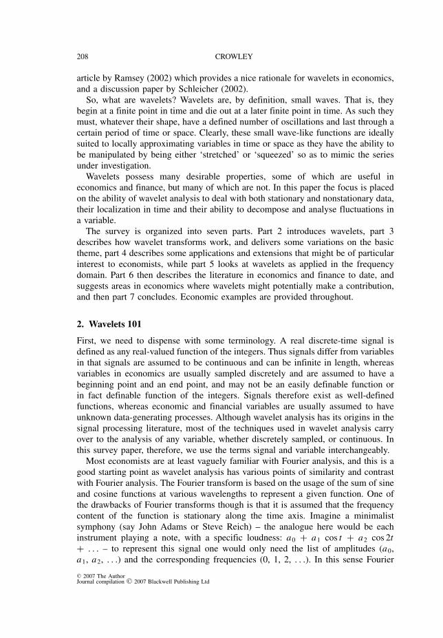
So, what are wavelets? Wavelets are, by definition, small waves. That is, theybegin at a finite point in time and die out at a later finite point in time. As such theymust, whatever their shape, have a defined number of oscillations and last through acertain period of time or space. Clearly, these small wave-like functions are ideallysuited to locally approximating variables in time or space as they have the ability tobe manipulated by being either ‘stretched’ or ‘squeezed’ so as to mimic the seriesunder investigation.
Wavelets possess many desirable properties, some of which are useful ineconomics and finance, but many of which are not. In this paper the focus is placedon the ability of wavelet analysis to deal with both stationary and nonstationary data,their localization in time and their ability to decompose and analyse fluctuations ina variable.
The survey is organized into seven parts. Part 2 introduces wavelets, part 3describes how wavelet transforms work, and delivers some variations on the basictheme, part 4 describes some applications and extensions that might be of particularinterest to economists, while part 5 looks at wavelets as applied in the frequencydomain. Part 6 then describes the literature in economics and finance to date, andsuggests areas in economics where wavelets might potentially make a contribution,and then part 7 concludes. Economic examples are provided throughout.
2. Wavelets 101
First, we need to dispense with some terminology. A real discrete-time signal isdefined as any real-valued function of the integers. Thus signals differ from variablesin that signals are assumed to be continuous and can be infinite in length, whereasvariables in economics are usually sampled discretely and are assumed to have abeginning point and an end point, and may not be an easily definable function orin fact definable function of the integers. Signals therefore exist as well-definedfunctions, whereas economic and financial variables are usually assumed to haveunknown data-generating processes. Although wavelet analysis has its origins in thesignal processing literature, most of the techniques used in wavelet analysis carryover to the analysis of any variable, whether discretely sampled, or continuous. Inthis survey paper, therefore, we use the terms signal and variable interchangeably.
Most economists are at least vaguely familiar with Fourier analysis, and this is agood starting point as wavelet analysis has various points of similarity and contrastwith Fourier analysis. The Fourier transform is based on the usage of the sum of sineand cosine functions at various wavelengths to represent a given function. One ofthe drawbacks of Fourier transforms though is that it is assumed that the frequencycontent of the function is stationary along the time axis. Imagine a minimalistsymphony (say John Adams or Steve Reich) – the analogue here would be eachinstrument playing a note, with a specific loudness: a0 + a1 cos t + a2 cos 2t+ . . . – to represent this signal one would only need the list of amplitudes (a0,a1, a2, . . .) and the corresponding frequencies (0, 1, 2, . . .). In this sense Fourier
C© 2007 The AuthorJournal compilation C© 2007 Blackwell Publishing Ltd

GUIDE TO WAVELETS FOR ECONOMISTS 209
analysis involves the projection of a signal onto an orthonormal2 set of trigonometriccomponents. The Fourier transform makes particular sense when projecting over therange (0, 2π ), as Fourier series have infinite energy (they do not die out) and finitepower (they cannot change over time).
Windowed Fourier analysis extends basic Fourier analysis by transforming shortsegments of the signal separately, so that the assumption of no variation over timecan be relaxed. In other words there are breaks where we just repeat the exerciseabove. Once again these are just separate sets of orthonormal components – one setfor each window.
In a sense, wavelets are a further refinement of Fourier analysis, as they arelocalized in both time and their functional components. They thus provide aconvenient and efficient way of representing complex variables or signals, aswavelets can cut data up into different frequency components. They are especiallyuseful where a variable or signal lasts only for a finite time, or shows markedlydifferent behaviour in different time periods. Using the symphonic analogy, waveletscan be thought of representing the symphony by transformations of a basic wavelet,w(t). So at t = 0, if cellos played the same tune twice as fast as the double basses,then the cello would be playing c1w(2t) while the double basses play b1w(t),presumably with b1 ≥ c1. At t = 1, the next bass plays b2 w(t − 1), and thenext cello plays c2 w(2t − 1) starting at t = 0.5. Note that we need twice as manycellos to complete the symphony as double basses, as long as each cello plays thephrase once. If violas played twice as fast as cellos and violins twice as fast asviolas, then obviously this would be eight times as fast as double basses, and ifthere were such an instrument as a hyper-violin, then it would play 16 times fasterthan a double bass. In general the n-violins play ‘scalings’ of w(2nt).
In wavelet analysis, we only need to store the list of amplitudes, as the scalingsautomatically double the frequency. With Fourier analysis a single disturbance affectsall frequencies for the entire length of the series, so that although one can try andmimic a signal (or the symphony) with a complex combination of waves, the signalis still assumed to be ‘homogeneous over time’. In contrast, wavelets have finiteenergy and only last for a short period of time. It is in this sense that wavelets are nothomogenous over time and have ‘compact support’, so that following our analogy,we can analyse changes in the pitch as well as what is played. In wavelet analysis toapproximate series that continue over a long period, functions with compact supportare strung together over the period required, each indexed by location.
2.1 Elementary Wavelets
Wavelets have genders: there are father wavelets φ and mother wavelets ψ . Thefather wavelet integrates to 1 and the mother wavelet integrates to 0∫
φ(t) dt = 1 (1)∫ψ (t) dt = 0 (2)
C© 2007 The AuthorJournal compilation C© 2007 Blackwell Publishing Ltd

210 CROWLEY
`s8' father, phi(0,0)
0 2 4 6
-0.2
0.0
0.2
0.4
0.6
0.8
1.0
1.2
`s8' mother, psi(0,0)
-2 0 2 4
-1.0
-0.5
0.0
0.5
1.0
1.5
Figure 1. Mother and Father Wavelets.
The father wavelet (or scaling function) essentially represents the smooth, trend(low-frequency) part of the signal, whereas the mother wavelets represent the detailed(high-frequency) parts by scale by noting the amount of stretching of the waveletknown as ‘scale’ or ‘dilation’. In diagrammatic terms, father and mother waveletscan be illustrated for the Daubechies wavelet, as shown in Figure 1.
Wavelets also come in various shapes: some are discrete (as in the Haar wavelet –the first wavelet to be proposed many decades ago, which is a square wavelet withcompact support), some are symmetric (such as the Mexican hat wavelet), some arealmost symmetric (such as the symmlet and coiflet), and some are asymmetric (suchas daublets).3 Four are illustrated in Figure 2, where all wavelets are mother wavelets.The upper left-hand wavelet is a Haar wavelet, and this is a discrete symmetricwavelet. The upper right-hand box contains a daublet, which is asymmetric, thelower left-hand box contains a symmlet and the lower right-hand box a coiflet. Thelatter two wavelets are almost symmetric.
The scaling or dilation property of wavelets is particularly important in exploratoryanalysis of time series. Consider a double sequence of functions
ψ (t) = 1√sψ
(t − u
s
)(3)
where s is a sequence of scales. The term 1√s
ensures that the norm of ψ (·) is equal
to one. The function ψ (·) is then centred at u with scale s. In wavelet language,we would say that the energy of ψ (·) is concentrated in a neighbourhood of u with
C© 2007 The AuthorJournal compilation C© 2007 Blackwell Publishing Ltd

GUIDE TO WAVELETS FOR ECONOMISTS 211
`haar' mother, psi(0,0)
0.0 0.2 0.4 0.6 0.8 1.0
-1.0
-0.5
0.0
0.5
1.0
`d12' mother, psi(0,0)
-4 -2 0 2 4
-1.0
-0.5
0.0
0.5
1.0
`s12' mother, psi(0,0)
-4 -2 0 2 4 6
-1.0
-0.5
0.0
0.5
1.0
1.5
`c12' mother, psi(0,0)
-4 -2 0 2 4
6
6
-0.5
0.0
0.5
1.0
1.5
Figure 2. Families of Wavelets.
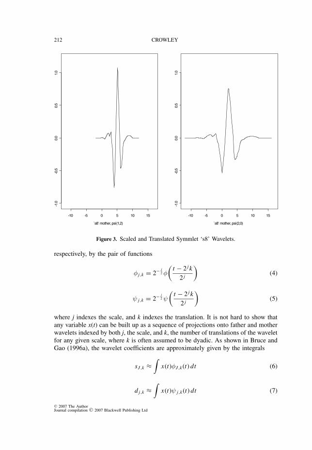
size proportional to s. As s increases the length of support in terms of t increases.So, for example, when u = 0, the support of ψ (·) for s = 1 is [d, − d]. As s isincreased, the support widens to [sd, −sd].4 Scaling is particularly useful in the timedomain, as the choice of scale indicates the ‘packets’ used to represent any givenvariable or signal. A broad support wavelet yields information on variable or signalvariations on a large scale, whereas a small support wavelet yields information onsignal variations on a small scale. The important point here is that as projectionsare orthogonal, wavelets at a given scale are not affected by features of a signal atscales that require narrower support. Lastly, using the language introduced above, ifa wavelet is shifted on the time line, this is referred to as translation or shift of u.An example of the dilation and translation property of wavelets is shown in Figure3. The left-hand box contains a symmlet of dilation 8, scale 1, shifted 2 to the right,while the right-hand box contains the same symmlet with scale 2 and no translation.
2.2 Multiresolution Decomposition
The main feature of wavelet analysis is that it enables the researcher to separateout a variable or signal into its constituent multiresolution components. In order toretain tractability (many wavelets have an extremely complicated functional form),assume we are dealing with symmlets; then the father and mother pair can be given,
C© 2007 The AuthorJournal compilation C© 2007 Blackwell Publishing Ltd
212 CROWLEY
`s8' mother, psi(1,2)
-10 -5 0 5 10 15
-1.0
-0.5
0.0
0.5
1.0
`s8' mother, psi(2,0)
-10 -5 0 5 10 15
-1.0
-0.5
0.0
0.5
1.0
Figure 3. Scaled and Translated Symmlet ‘s8’ Wavelets.
respectively, by the pair of functions
φ j,k = 2− j2 φ
(t − 2 j k
2 j
)(4)
ψ j,k = 2− j2 ψ
(t − 2 j k
2 j
)(5)
where j indexes the scale, and k indexes the translation. It is not hard to show thatany variable x(t) can be built up as a sequence of projections onto father and motherwavelets indexed by both j, the scale, and k, the number of translations of the waveletfor any given scale, where k is often assumed to be dyadic. As shown in Bruce andGao (1996a), the wavelet coefficients are approximately given by the integrals
sJ ,k ≈∫
x(t)φJ ,k(t) dt (6)
d j,k ≈∫
x(t)ψ j,k(t) dt (7)
C© 2007 The AuthorJournal compilation C© 2007 Blackwell Publishing Ltd

GUIDE TO WAVELETS FOR ECONOMISTS 213
j = 1, 2, . . . J such that J is the maximum scale sustainable with the data to hand.A multiresolution representation of x(t) is now given by
x(t) =∑
k
sJ ,kφJ ,k(t) +∑
k
dJ ,kψ J ,k(t)
+∑
k
dJ−1,kψ J−1,k(t) + · · · +∑
k
d1,kψ1,k(t) (8)
where the basis functions φ J,k(t) and ψ J,k(t) are assumed to be orthogonal, that is∫φJ ,k(t)φJ ,k ′ (t) = δk,k ′∫ψ J ,k(t)φJ ,k ′ (t) = 0∫ψ J ,k(t)ψ J ′
,k ′ (t) = δk,k ′ δ j, j ′ (9)
where δ i, j = 1 if i = j and δ i, j = 0 if i �= j . Note that when the number ofobservations is dyadic, the number of coefficients of each type is given by
• at the finest scale 21: there are n2coefficients labeled d 1,k .• at the next scale 22: there are n
22 coefficients labeled d 2,k .• at the coarsest scale 2J : there are n2J coefficients d J,k and s J,k .
In wavelet language, each of these coefficients is called an ‘atom’ and thecoefficients for each scale are termed a ‘crystal’.5 The multiresolution decomposition(MRD) of the variable or signal x(t) is then given by
{SJ , DJ , DJ−1, . . . D1} (10)
where SJ is the first term on the right hand side of equation 8, DJ is the secondterm etc.
For ease of exposition, the informal description above assumes a continuous signal,which in signal processing is usually the case, but in economics although variableswe use for analysis represent continuous ‘real-time signals’, they are invariablysampled at pre-ordained points in time. The continuous version of the wavelettransform (known as the CWT) assumes an underlying continuous signal, whereasa discrete wavelet transform (DWT) assumes a variable or signal consisting ofobservations sampled at evenly spaced points in time. Apart from a later sectionin the paper, only the DWT (or variations on the DWT) will be used from this pointonwards.
The interpretation of the MRD using the DWT is of interest in terms ofunderstanding the frequency at which activity in the time series occurs. For example,with a monthly or daily time series, Table 1 shows the interpretation of the differentscale crystals.
Note five things from Table 1:
(1) The number of observations dictates the number of scale crystals that can beproduced – only j scales can be used given that the number of observations, N ≥
C© 2007 The AuthorJournal compilation C© 2007 Blackwell Publishing Ltd

214 CROWLEY
Table 1. Frequency interpretation of MRD scale levels.
Annual Monthly DailyScale frequency frequency frequencycrystals resolution resolution resolution
d1 2–4 2–4 2–4d2 4–8 4–8 4–8d3 8–16 8–16=8m–1yr4m 8–16d4 16–32 16–32=1yr4m–2yr8m 16–32=3wds1d–6wks2dd5 32–64 32–64=2yr8m–5yr4m 32–64=6wks 2d–12wks 4dd6 64–128 64–128=5yr4m–10yr8m 64–128=12wks 4d–25wks 3dd7 128–256 128–256=10yr8m–21yr4m 128–256=25wks 3d–51wks 1dd8 256–512 etc etc
2 j . Using the example given in this paper of industrial production, we have1024 monthly observations, so the maximum number of scales is in theoryj = 9. If there are only 256 observations, then no more then seven crystalscan be produced, but as the highest scale (lowest frequency crystal) can onlyjust be resolved, it is usually recommended that only six crystals be produced.With 512 monthly observations, the d7 crystal can be produced, and the trendcrystal (or ‘wavelet smooth’), denoted s7 will yield further fluctuations fromtrend for all periodicities above a 256-month period.
(2) The choice of wavelet used in the analysis also figures into the number ofscale crystals that can be produced. Say you have a choice between an ‘s4’and an ‘s8’ wavelet for the MRD analysis. An ‘s4’ wavelet means that thesymmetric wavelet starts with a width of four observations for its support –this corresponds to the wavelet used to obtain the d1 crystals.6 Using an s4wavelet with annual or quarterly data will still capture the correct periodicities,but will enable the researcher to decompose to higher-order scales. Clearly thehigher the frequency of data, the more likely the researcher is to use a longersupported wavelet though, as very short wavelets are unlikely to yield anyadditional information.
(3) Wavelet MRD analysis assumes that data are sampled at equally spacedintervals. The frequency resolution interpretation is more difficult with dailydata, as daily (or hourly or even more frequently sampled) data are not evenlysampled. Note that with yearly data the resolution limit on a d3 crystal is halfthe time period on the minimum frequency picked up by a d5 crystal. Clearlythis would not be the case when using daily data though assuming 5 days tothe week.
(4) Existing stylized facts need to be taken into account when applying an MRDto economic data. For example, as economists know that business cycles lastfor a decade at the most, it does not make sense to decompose a series beyondthis level if conventional business cycles are the main concern – so with annualdata it would not make sense to use anything more than the d3 scale crystals
C© 2007 The AuthorJournal compilation C© 2007 Blackwell Publishing Ltd
GUIDE TO WAVELETS FOR ECONOMISTS 215
– doing so would cause ‘redundancy’. For example, with monthly economicdata, if business cycles and their sub cycles are to be identified, it is desirableto have at least 256 observations and to resolve to the d6 crystal.
(5) Wavelets do not identify single period shocks. Wavelets interpret all fluctua-tions as cyclical in nature so a discrete change in an economic variable wouldappear as a coefficient in the d1 crystal.
Obviously the first and fourth point noted above pose major constraints for MRDwith economic data, as very few annual economic time series contain more than 100observations, and very few quarterly data series contain more than 200 observations.In finance, when using high-frequency data, the MRD yields more information onactivity at many different scale levels in the data, perhaps explaining the morefrequent usage of wavelet analysis. With most economic and finance data of areasonable time span, choice of wavelet type does not make a significant differenceto the MRD energy distribution (with the exception of the Haar wavelet), but doeschange the size of crystal coefficients at any given point in time. Thus choice ofwavelet can also be important if the crystals are to be used for further analysis.
2.3 Example: Canadian Industrial Production
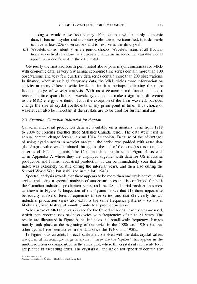
Canadian industrial production data are available on a monthly basis from 1919to 2004 by splicing together three Statistics Canada series. The data were used inannual percent change format, giving 1014 datapoints. Because of the advantagesof using dyadic series in wavelet analysis, the series was padded with extra data(the August value was continued through to the end of the series) so as to rendera series of 1024 datapoints. The Canadian data are shown in Figure 4, as wellas in Appendix A where they are displayed together with data for US industrialproduction and Finnish industrial production. It can be immediately seen that theindex was extremely volatile during the interwar years, and then also during theSecond World War, but stabilized in the late 1940s.
Spectral analysis reveals that there appears to be more than one cycle active in thisseries, and using a spectral analysis of autocovariances this is confirmed for boththe Canadian industrial production series and the US industrial production series,as shown in Figure 5. Inspection of the figures shows that (1) there appears tobe activity at five different frequencies in the series, and that (2) clearly the USindustrial production series also exhibits the same frequency patterns – so this islikely a stylized feature of monthly industrial production series.
When wavelet MRD analysis is used for the Canadian series, seven scales are used,which then encompasses business cycles with frequencies of up to 21 years. Theresults are illustrated in Figure 6 that indicates that small-scale frequency changesmostly took place at the beginning of the series in the 1920s and 1930s but thatother cycles have been active in the data since the 1920s and 1930s.
In Figure 6, as wavelets for each scale are convolved with the data, crystal valuesare given at increasingly large intervals – these are the ‘spikes’ that appear in themultiresolution decomposition in the stack plot, where the crystals at each scale levelare plotted in ascending order. The crystals d1 and d2 do not appear to contain any
C© 2007 The AuthorJournal compilation C© 2007 Blackwell Publishing Ltd
216 CROWLEY
1920 1929 1938 1947 1956 1965 1974 1983 1992 2001
0100
200
300
400
SA
IPIn
d$C
AN
IPIS
A
1920 1929 1938 1947 1956 1965 1974 1983 1992 2001
-20
-10
010
20
30
40
IPS
A$C
AN
IPS
A
Figure 4. Canadian Industrial Production (sa): 1919–2004.
discernable cycles, d3 appears to have contained some explanatory power duringthe 1920s and 1930s, but now most variability is to be found in crystals d4 to d7and s7 (due to the size of the crystal coefficients). The cyclical interpretation ofthese crystals corroborates the spectra obtained in Figure 5 as four separate cyclesare identified (crystals d4, d5, d6 and d7), with crystals d1 to d3 containing mostlynoise. Crystal s7 is interpreted as a trend or drift variable, and does not capture anydistinct cycles in the data.
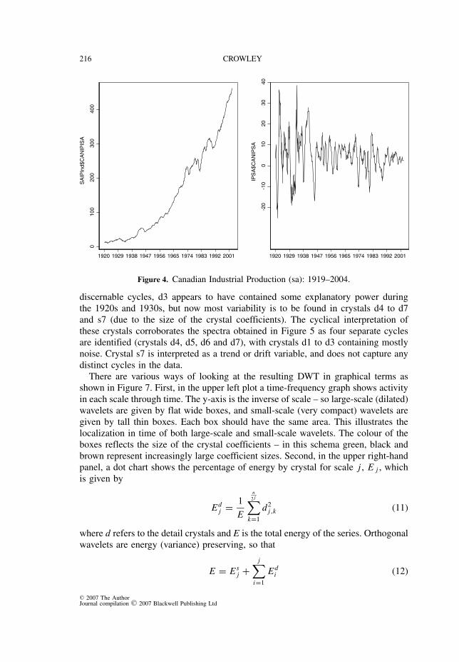
There are various ways of looking at the resulting DWT in graphical terms asshown in Figure 7. First, in the upper left plot a time-frequency graph shows activityin each scale through time. The y-axis is the inverse of scale – so large-scale (dilated)wavelets are given by flat wide boxes, and small-scale (very compact) wavelets aregiven by tall thin boxes. Each box should have the same area. This illustrates thelocalization in time of both large-scale and small-scale wavelets. The colour of theboxes reflects the size of the crystal coefficients – in this schema green, black andbrown represent increasingly large coefficient sizes. Second, in the upper right-handpanel, a dot chart shows the percentage of energy by crystal for scale j , E j , whichis given by
Edj = 1
E
n2 j∑
k=1
d2j,k (11)
where d refers to the detail crystals and E is the total energy of the series. Orthogonalwavelets are energy (variance) preserving, so that
E = Esj +
j∑i=1
Edi (12)
C© 2007 The AuthorJournal compilation C© 2007 Blackwell Publishing Ltd

GUIDE TO WAVELETS FOR ECONOMISTS 217
0.0 0.1 0.2 0.3 0.4 0.5
frequency
-40
-20
020
spectr
um
bandwidth= 0.000281909 , 95% C.I. is ( -5.87588 , 17.5667 )dB
0.0 0.1 0.2 0.3 0.4 0.5
frequency
-40
-20
020
spectr
um
bandwidth= 0.000281909 , 95% C.I. is ( -5.87588 , 17.5667 )dB
0.0 0.1 0.2 0.3 0.4 0.5
frequency
-10
010
20
30
spectr
um
0.0 0.1 0.2 0.3 0.4 0.5
frequency
-10
010
20
30
spectr
um
Figure 5. Spectra for Canadian and US Industrial Production.
where Esj is the energy of the smooth. As already noted, crystals d4, d5, d6, d7
and s7 contain most of the series energy. For the bottom left-hand panel, a box plotshould be self explanatory, and here the width of the boxes represents the number ofdata points or coefficients. Lastly the bottom right-hand figure shows an energy plotthat provides the cumulative energy function for the data and the DWT. Clearly theDWT contains the salient information about the series much better than the originaluntransformed data, which helps to explain why wavelets are so popular as a meansof data compression. Note also from Figure 6 that the individual detail crystals havemean of zero, so that the energy of each crystal is nothing more than the varianceof the crystal coefficients. Hence the energy distribution in Figure 7 (top left-handbox) represents a variance decomposition by frequency for the series under analysis.Another measure often referred to in the signal processing literature is power, whichhere would be defined as just the average squared value of the crystal coefficients,or Ed
j /n2 j from equation (11).
2.4 Multiresolution Analysis (MRA)
The sequence of partial sums of crystals
Sj−1(t) = SJ (t) + DJ (t) + DJ−1(t) + · · · + D j (t) (13)
provides a multiresolution approximation (MRA) to the variable. This works bybuilding up the series from the highest numbered (coarsest) scale downwards. An
C© 2007 The AuthorJournal compilation C© 2007 Blackwell Publishing Ltd

218 CROWLEY
1920 1931 1942 1953 1964 1975 1986 1997 2008
s7
d7
d6
d5
d4
d3
d2
d1
Position
Figure 6. DWT for Canadian Industrial Production.
MRA therefore could be viewed as a filtered version of the series that retains themost important parts of the series, but de-noises the series to a greater or lesserdegree. Indeed, because wavelet analysis essentially filters certain information atdifferent scales, many of those involved in the development of wavelets label themfilters (of limited bandwidth).7 To show how the inverse discrete wavelet transform(IDWT) can approximate the series by acting as a band-pass filter, a smooth MRArepresentation of the data using the 4–6 scale crystals is calculated as follows
S4 = S6 + D6 + D5 (14)
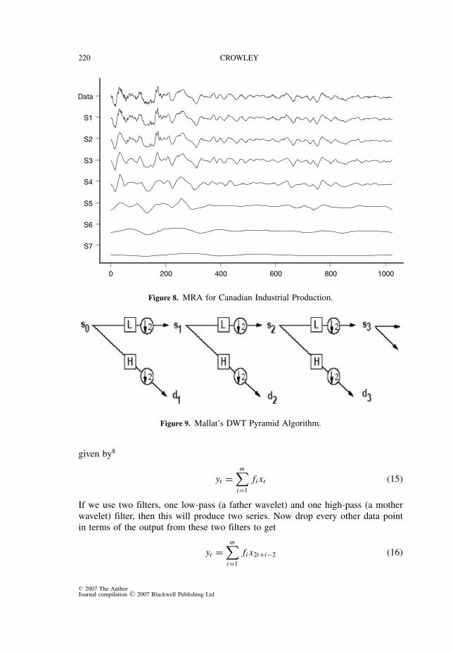
Clearly one could also reconstruct the signal again by adding lower scale crystalsto equation (14). One interesting application in wavelet analysis, given that wehave determined which crystals are most relevant for describing Canadian industrialproduction, is to invert the wavelet transform so as to reconstruct the series usingan MRA. If this is done, Figure 8 shows what is obtained. S7 represents s7 crystal,but then when d7 is superimposed, S6 is obtained, etc.
Putting the wavelet analysis of the Canadian industrial production series together,it is now quite apparent that crystals d7, d6, d5 and d4 largely show the movementof the series. Adding d3 (to get S3 in Figure 8), adds very little to explainingany movement in the series (except perhaps towards the beginning), and if shorterterm fluctuations are desired, then clearly s2 captures some more of the noise but
C© 2007 The AuthorJournal compilation C© 2007 Blackwell Publishing Ltd
GUIDE TO WAVELETS FOR ECONOMISTS 219
1920 1929 1938 1947 1956 1965 1974 1983 1992 2001
Time
0.0
0.1
0.2
0.3
0.4
0.5
1/S
cale
0.0 0.2 0.4 0.6 0.8 1.0
Energy (100%)
Data
d1
d2
d3
d4
d5
d6
d7
s7
-50
050
100
Data d1 d2 d3 d4 d5 d6 d7 s71 5 10 50 100 500 1000
Number of Coefficients
0.0
0.2
0.4
0.6
0.8
1.0
Cum
ula
tive P
roport
ional E
nerg
y
dwtdata
Figure 7. Summary of MRD for Canadian Industrial Production.
adds very little to the analysis. The real value added here is the recognition fromFigures 5, 7 and 8 that there appear to be five different sources of variation inthe series – one longer term, two medium term, one shorter term and lastly veryshort-term ‘noise’ variations, the latter appearing not to be cyclical in nature. Froma business cycle perspective, the value added here is the recognition that cyclicalpatterns in economic variables occur at many frequencies, not just the business cyclefrequency.
3. Wavelet Transforms
3.1 How Does a DWT Work?
The principle behind the notion of the wavelet transform is deceptively simple, andoriginated in the pioneering work of Mallat (1989) in signal processing. The coreof this approach is the usage of a ‘pyramid algorithm’ that uses two filters at eachstage (or scale) of analysis. Figure 9 represents the pyramid algorithm approach forMRD, where s0 represents the original signal, L represents a low-band filter and Hrepresents a high-band filter.
If the input to the algorithm is X = (x 1, x 2, . . . x n) and define an m-tap (length m)filter to be F = ( f 1, f 2, . . . , f m), then the convolution of the filter and variable is
C© 2007 The AuthorJournal compilation C© 2007 Blackwell Publishing Ltd
220 CROWLEY
0 200 400 600 800 1000
S7
S6
S5
S4
S3
S2
S1
Data
Figure 8. MRA for Canadian Industrial Production.
Figure 9. Mallat’s DWT Pyramid Algorithm.
given by8
yt =m∑
i=1
fi xt (15)
If we use two filters, one low-pass (a father wavelet) and one high-pass (a motherwavelet) filter, then this will produce two series. Now drop every other data pointin terms of the output from these two filters to get
yt =m∑
i=1
fi x2t+i−2 (16)
C© 2007 The AuthorJournal compilation C© 2007 Blackwell Publishing Ltd

GUIDE TO WAVELETS FOR ECONOMISTS 221
Figure 10. The IDWT (MRA) Algorithm.
Figure 11. Wavelet Packet Tree.
The output will be s1 for the low-pass filter and d1 for the high-pass filter. Thesedetails coefficients are kept, and s1 is now put through a further high-pass andlow-pass filter, etc., to finally produce
d j = WH ,↓(s j−1) (17)
a set of j detail coefficients and
s j = WL,↓(s j−1) (18)
a set of level j smooth coefficients. The choice of filter obviously aligns with thechoice of wavelet here. This is the output given by the MRD of a variable. Toconstruct an MRA an inverse DWT needs to be performed. In algorithm terms, thisis shown as Figure 10. Here the crystals are taken and convolved with a synthesisfilter, and at the same time ‘upsampled’ by inserting zeros between every other valueof the filter input. The smoothed coefficients for scale j − 1 are obtained as
s j−1 = WL,↑(s j ) + WH ,↑(d j ) (19)
where W F,↑ is an upsampling convolution operator for filter F.
C© 2007 The AuthorJournal compilation C© 2007 Blackwell Publishing Ltd
222 CROWLEY
3.2 Wavelet Packet Transforms
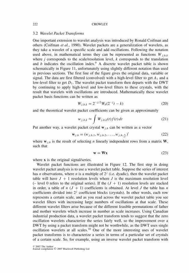
One important extension to wavelet analysis was introduced by Ronald Coifman andothers (Coifman et al., 1990). Wavelet packets are a generalization of wavelets, asthey take a wavelet of a specific scale and add oscillations. Following the notationused above, in mathematical terms they can be represented as functions W j,b,k
where j corresponds to the scale/resolution level, k corresponds to the translationand b indicates the oscillation index.9 A discrete wavelet packet table is shownschematically in Figure 11, unfortunately using slightly different notation than usedin previous sections. The first line of the figure gives the original data, variable orsignal. The data are first filtered (convolved) with a high-level filter to get A1 and alow-level filter to get D1. The wavelet packet transform then departs with the DWTby continuing to apply high-level and low-level filters to these crystals, with theresult that wavelets with oscillations are introduced. Mathematically these waveletpacket basis functions can be written as
W j,b,k = 2− j/2Wb(2− j t − k) (20)
and the theoretical wavelet packet coefficients can be given as approximately
w j,b,k ≈∫
W j,b,k(t) f (t) dt (21)
Put another way, a wavelet packet crystal w j,b can be written as a vector
w j,b = (w j,b,1, w j,b,2, . . . , w j,b, n2 j
)′ (22)
where w j,b is the result of selecting n linearly independent rows from a matrix W,such that
w = Wx (23)
where x is the original signal/series.Wavelet packet functions are illustrated in Figure 12. The first step in doing
wavelet packet analysis is to use a wavelet packet table. Suppose the series of interesthas n observations, where n is a multiple of 2 j (i.e. dyadic), then the wavelet packettable will have J + 1 resolution levels where J is the maximum resolution level(– level 0 refers to the original series). If the (J + 1) resolution levels are stackedin order, a table of n (J + 1) coefficients is obtained. At level J the table has ncoefficients divided into 2 j coefficient blocks (crystals). In other words, each rowrepresents a certain scale, and as you read across the wavelet packet table you seewavelet filters with increasing large numbers of oscillations at that scale. Thesedifferent wavelet filters arise because of the different feasible permutations of fatherand mother wavelets which increase in number as scale increases. Using Canadianindustrial production data, a wavelet packet transform tends to suggest that the zerooscillation wavelets characterize the series fairly well, so the improvement over aDWT by using a packet transform might not be worthwhile, as the DWT uses singleoscillation wavelets at all scales.10 One of the more interesting uses of waveletpacket transforms is to characterize a series in terms of a particular set of crystalsof a certain scale. So, for example, using an inverse wavelet packet transform with
C© 2007 The AuthorJournal compilation C© 2007 Blackwell Publishing Ltd

GUIDE TO WAVELETS FOR ECONOMISTS 223
`s8' father, phi(0,0)
0 2 4 6
-0.2
0.4
0.8
1.2
`s8' mother, psi(0,0)
-2 0 2 4
-1.0
0.0
1.0
`s8' wavelet packet, W(0,2,0)
-4 -2 0 2
-1.0
0.0
1.0
`s8' wavelet packet, W(0,3,0)
-2 0 2 4
-1.5
0.0
1.0
`s8' wavelet packet, W(0,4,0)
-4 -2 0 2
-10
1
`s8' wavelet packet, W(0,5,0)
-4 -2 0 2
-10
12
`s8' wavelet packet, W(0,6,0)
-4 -2 0 2
-10
12
`s8' wavelet packet, W(0,7,0)
-2 0 2 4
-10
1
Figure 12. Daubechies Wavelet Packet Functions.
say level 4 crystals, a reconstruction of a series can be made. This is done in Figure13 for the Canadian industrial production series.
Figure 14 presents the time-frequency plot for the level 4 packet transform forthe Canadian industrial production series, and compares it with the original time-frequency plot for the DWT. First note that in the left-hand plot in the panel, theboxes are exactly of the same size – that is because all the crystals are level 4, butrepresenting different numbers of oscillations. In Figure 13 there are 16 crystals,and these are stacked up in the left-hand panel of Figure 14 – once again, waveletswith large numbers of oscillations tend to have significant coefficients only for thefirst part of the series.
3.3 Optimal Transforms
Coifman and Wickerhauser (1992) developed a ‘best basis’ algorithm for selectingthe most suitable bases for signal representation using a wavelet packet table. Thebest basis algorithm finds the wavelet packet transforms W that minimizes a costfunction C
C(W ) =∑j,b∈I
C(w j,b) (24)
C© 2007 The AuthorJournal compilation C© 2007 Blackwell Publishing Ltd

224 CROWLEY
0 200 400 600 800 1000
w4.15
w4.14
w4.13
w4.12
w4.11
w4.10
w4.9
w4.8
w4.7
w4.6
w4.5
w4.4
w4.3
w4.2
w4.1
w4.0
iwpt
Figure 13. Level 4 Packet Transform for Canadian Industrial Production.
0 200 400 600 800 1000Time
0.0
0.1
0.2
0.3
0.4
0.5
Fre
quency
0 200 400 600 800 1000Time
0.0
0.1
0.2
0.3
0.4
0.5
Fre
quency
Figure 14. Time-frequency Plots for Canadian Industrial Production (a) Level 4 DWPTand (b) DWT.
where I is the set of index pairs (j, b) of the crystals in the transform W. Typically,the entropy cost function is used, in which case the cost function is of the form
Centropyj,b =
∑k
[w j,b,k∥∥w0,0
∥∥2
]2
log
⎧⎨⎩[
w j,b,k∥∥w0,0
∥∥2
]2⎫⎬⎭ (25)
C© 2007 The AuthorJournal compilation C© 2007 Blackwell Publishing Ltd
GUIDE TO WAVELETS FOR ECONOMISTS 225
7
6
5
4
3
2
1
0
Level
7
6
5
4
3
2
1
0
Level
4
3
2
1
0
Level
7
6
5
4
3
2
1
0
Level
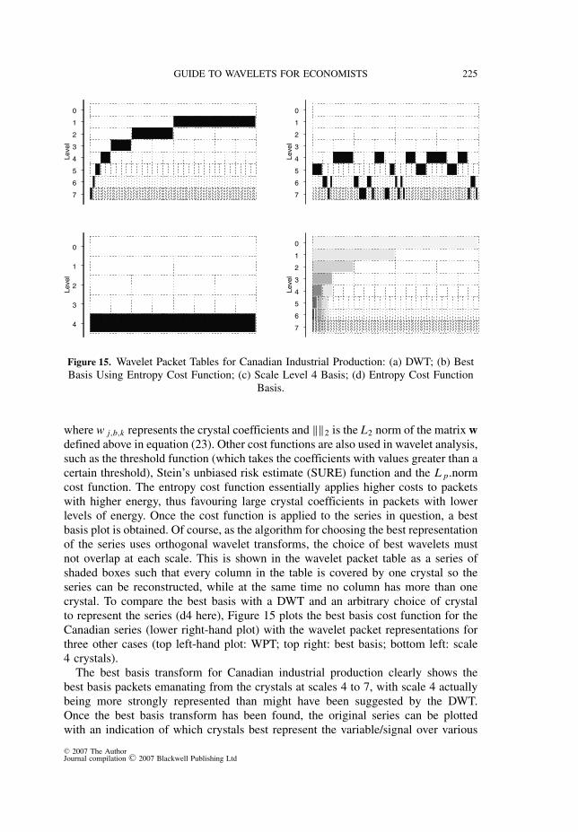
Figure 15. Wavelet Packet Tables for Canadian Industrial Production: (a) DWT; (b) BestBasis Using Entropy Cost Function; (c) Scale Level 4 Basis; (d) Entropy Cost Function
Basis.
where w j,b,k represents the crystal coefficients and ‖‖2 is the L2 norm of the matrix wdefined above in equation (23). Other cost functions are also used in wavelet analysis,such as the threshold function (which takes the coefficients with values greater than acertain threshold), Stein’s unbiased risk estimate (SURE) function and the L p.normcost function. The entropy cost function essentially applies higher costs to packetswith higher energy, thus favouring large crystal coefficients in packets with lowerlevels of energy. Once the cost function is applied to the series in question, a bestbasis plot is obtained. Of course, as the algorithm for choosing the best representationof the series uses orthogonal wavelet transforms, the choice of best wavelets mustnot overlap at each scale. This is shown in the wavelet packet table as a series ofshaded boxes such that every column in the table is covered by one crystal so theseries can be reconstructed, while at the same time no column has more than onecrystal. To compare the best basis with a DWT and an arbitrary choice of crystalto represent the series (d4 here), Figure 15 plots the best basis cost function for theCanadian series (lower right-hand plot) with the wavelet packet representations forthree other cases (top left-hand plot: WPT; top right: best basis; bottom left: scale4 crystals).
The best basis transform for Canadian industrial production clearly shows thebest basis packets emanating from the crystals at scales 4 to 7, with scale 4 actuallybeing more strongly represented than might have been suggested by the DWT.Once the best basis transform has been found, the original series can be plottedwith an indication of which crystals best represent the variable/signal over various
C© 2007 The AuthorJournal compilation C© 2007 Blackwell Publishing Ltd
226 CROWLEY
w5
.0
w6
.4
w7
.12
w6
.7
w4
.3
w6
.17
w7
.37
w7
.39
w7
.41
w6
.22
w7
.47
w7
.56
w7
.58
w5
.15
w7
.66
w6
.34
w7
.71
w5
.20
w4
.11
w5
.26
w4
.14
w7
.12
1
w6
.62
w7
.12
7
-50
05
01
00
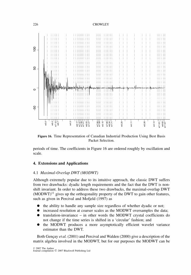
Figure 16. Time Representation of Canadian Industrial Production Using Best BasisPacket Selection.
periods of time. The coefficients in Figure 16 are ordered roughly by oscillation andscale.
4. Extensions and Applications
4.1 Maximal-Overlap DWT (MODWT)
Although extremely popular due to its intuitive approach, the classic DWT suffersfrom two drawbacks: dyadic length requirements and the fact that the DWT is non-shift invariant. In order to address these two drawbacks, the maximal-overlap DWT(MODWT)11 gives up the orthogonality property of the DWT to gain other features,such as given in Percival and Mofjeld (1997) as
• the ability to handle any sample size regardless of whether dyadic or not;• increased resolution at coarser scales as the MODWT oversamples the data;• translation-invariance – in other words the MODWT crystal coefficients donot change if the time series is shifted in a ‘circular’ fashion; and• the MODWT produces a more asymptotically efficient wavelet varianceestimator than the DWT.
Both Gencay et al. (2001) and Percival and Walden (2000) give a description of thematrix algebra involved in the MODWT, but for our purposes the MODWT can be
C© 2007 The AuthorJournal compilation C© 2007 Blackwell Publishing Ltd

GUIDE TO WAVELETS FOR ECONOMISTS 227
1920 1929 1938 1947 1956 1965 1974 1983 1992 2001 2010
s7{-381}
d7{-445}
d6{-221}
d5{-109}
d4{-53}
d3{-25}
d2{-11}
d1{-4}
Position
Figure 17. MODWT for Canadian Industrial Production.
described simply by referring back to Figure 9. In contrast to the DWT, the MODWTsimply skips the downsampling after filtering the data, and everything else describedin the section on MRDs using DWTs above follows through, including the energy(variance) preserving property and the ability to reconstruct the data using MRA withan inverse MODWT. A simple derivation of the MODWT following both Gencayet al. (2001) and Percival and Walden (2000) can be found in Appendix C. Figure17 shows the MODWT for Canadian industrial production. Clearly the resolutiondramatically increases for the coarser scales, and now the intermediate cycles aremore clearly apparent in the data.
One of the problems with the DWT is that the calculations of crystals occur atroughly half the length of the wavelet basis (length) into the series at any givenscale. Thus in Figure 6 crystal coefficients start further and further along the timeaxis as the scale level increases. As the MODWT is shift invariant, the MRD willnot change with a circular shift in the time series, so that each scale crystal can beappropriately shifted so that the coefficients approximately line up with the originaldata (known as ‘zero phase’ in the signalling literature). This is done by shifting thescales to the left by increasingly large amounts as the scale order increases, as they-axis of figure 17 shows.
Although the MODWT has a number of highly desirable properties, the transformleads to a large amount of ‘redundancy’, as even though the transform is energypreserving, the distribution of energy is clearly inferior to the original data. Similaranalysis can be done with MODWTs as with DWTs and Appendix C shows an
C© 2007 The AuthorJournal compilation C© 2007 Blackwell Publishing Ltd
228 CROWLEY
0 200 400 600 800 1000
Level 7
Level 6
Level 5
Level 4
Level 3
Level 2
Level 1
Level 0
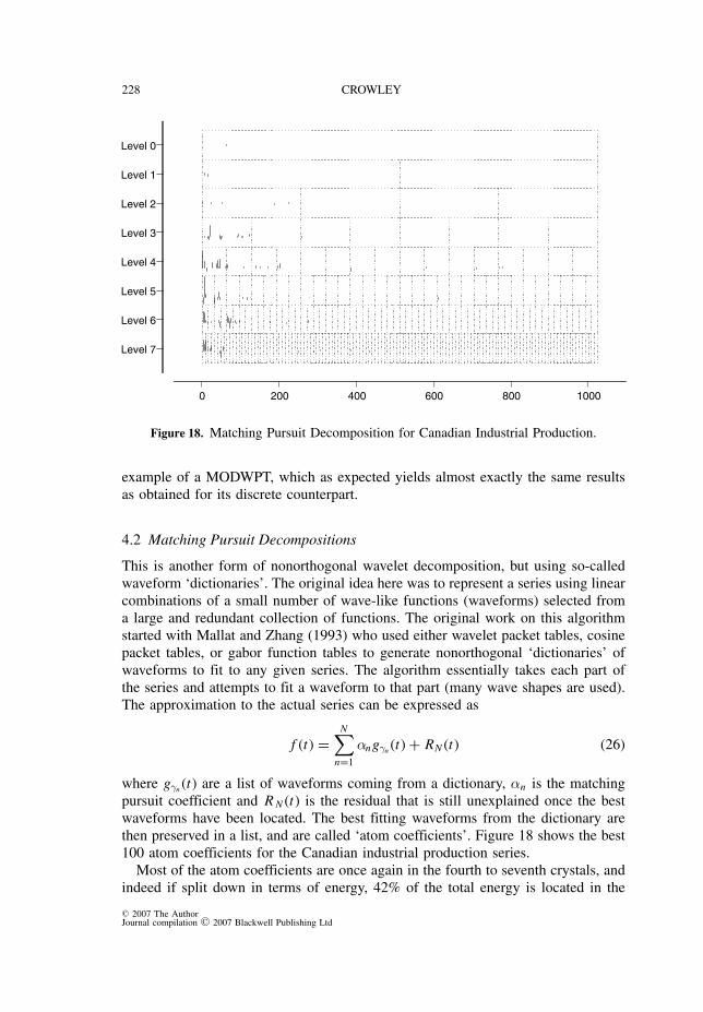
Figure 18. Matching Pursuit Decomposition for Canadian Industrial Production.
example of a MODWPT, which as expected yields almost exactly the same resultsas obtained for its discrete counterpart.
4.2 Matching Pursuit Decompositions
This is another form of nonorthogonal wavelet decomposition, but using so-calledwaveform ‘dictionaries’. The original idea here was to represent a series using linearcombinations of a small number of wave-like functions (waveforms) selected froma large and redundant collection of functions. The original work on this algorithmstarted with Mallat and Zhang (1993) who used either wavelet packet tables, cosinepacket tables, or gabor function tables to generate nonorthogonal ‘dictionaries’ ofwaveforms to fit to any given series. The algorithm essentially takes each part ofthe series and attempts to fit a waveform to that part (many wave shapes are used).The approximation to the actual series can be expressed as
f (t) =N∑
n=1
αngγn (t) + RN (t) (26)
where gγn (t) are a list of waveforms coming from a dictionary, αn is the matchingpursuit coefficient and R N (t) is the residual that is still unexplained once the bestwaveforms have been located. The best fitting waveforms from the dictionary arethen preserved in a list, and are called ‘atom coefficients’. Figure 18 shows the best100 atom coefficients for the Canadian industrial production series.
Most of the atom coefficients are once again in the fourth to seventh crystals, andindeed if split down in terms of energy, 42% of the total energy is located in the
C© 2007 The AuthorJournal compilation C© 2007 Blackwell Publishing Ltd

GUIDE TO WAVELETS FOR ECONOMISTS 229
0 200 400 600 800 1000
Others
W7.0.7
W6.4.2
W4.0.7
W5.1.1
W5.0.4
W7.6.3
W4.0.40
W4.0.48
W6.0.6
W3.0.21
W7.1.1
W7.0.4
W6.0.3
W4.0.2
W5.0.8
Approx
0 200 400 600 800 1000
Others
S6.10
D5.24
S6.9
D4.11
D6.3
D5.2
S6.8
D6.1
D6.4
S6.6
D6.5
D5.1
S6.1
S6.3
S6.4
Approx
Figure 19. Top 15 Atoms for Canadian Industrial Production: (a) Matching Pursuit and(b) DWT.
scale level 4 atoms. It is noteworthy that the matching pursuit algorithm actuallygives the scale 3 atoms 18% of the energy and scales 5 and 6 around 15% each,which is a somewhat different result than we have obtained when using the DWT,as with the DWT the level 3 crystal had little explanatory power but the level 7had significant explanatory power. Figure 19 compares the top 15 crystals from thematching pursuit algorithm with the top 15 from the DWT.
Clearly the matching pursuit algorithm does a better job of matching waveformsto the series than the DWT. It uses a much richer collection of waveforms than theDWT, which is always limited to one particular wavelet form.
4.3 Wavelet Shrinkage
Donoho and Johnstone (1995) first introduced the idea of wavelet shrinkage in orderto denoise a time series. The basic idea is to shrink wavelet crystal coefficients, eitherproportionately or selectively, so as to remove certain features of the time series. Theinitial version of the waveshrink algorithm was able to denoise signals by shrinkingthe detail coefficients in the lower-order scales, and then applying the inverse DWTto recover a denoised version of the series. The methodology was then extended todifferent types of shrinkage function, notably so-called ‘soft’ and ‘hard’ shrinkage(reviewed in Bruce and Gao (1995)).
In mathematical terms, following the notation of Bruce et al. (1995) these differenttypes of shrinkage can be defined by application of a shrinkage function to the crystal
C© 2007 The AuthorJournal compilation C© 2007 Blackwell Publishing Ltd
230 CROWLEY
coefficients such that
d j = δ jσ (x)d j (27)
where d j is a vector of scale j crystal coefficients and δ jσ (x) is defined as a shrinkagefunction that has as parameters the variance of the noise at level j , σ j , and thethreshold defined within the shrinkage function. The threshold argument can bedefined in three different ways
δSj (x) =
{0 i f |x | ≤ c
sign(x)(|x | − c) i f |x | > c(28)
δHj (x) =
{0 i f |x | ≤ c
x i f |x | > c(29)
δSSj (x) =
⎧⎪⎪⎨⎪⎪⎩0 i f |x | ≤ cL
sign(x) cU (|x |−cL )cU −cL
i f cL > |x | ≤ cU
x i f |x | > cU
(30)
where δS (x) is a generic soft shrinkage function, δH (x) is a generic hard shrinkagefunction and δSS (x) is a generic semi-soft shrink function for coefficients of anyscale crystal. δH (x) essentially sets all crystal coefficients to zero below a specifiedcoefficient value c, δS(x) just lowers the crystal coefficients above a defined scaleby the same amount, and the semi-soft version has the hard function propertyabove scale cU and below scale cL but in between these two scales adopts a linearcombination of the two approaches. There are a variety of ways of choosing c, cor cLand cU , some based on statistical theory and others rather more subjective. Insome cases, such as the universal threshold case (setting c = √
2 log n), the thresholdis constant at all scale levels, and in other cases such as the ‘adapt’ threshold, thethreshold changes according to scale level.
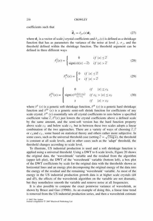
To illustrate, US industrial production is used and a soft shrinkage function isapplied using a universal threshold. Using a DWT to 6 scale levels, Figure 20 showsthe original data, the ‘waveshrunk’ variable and the residual from the algorithm(upper left plot), the DWT of the ‘waveshrunk’ variable (bottom left), a box plotof the DWT coefficients by scale for the original data with the thresholds shown ashorizontal lines and an energy plot decomposing the original energy of the data intothe energy of the residual and the remaining ‘waveshrunk’ variable. As most of theenergy in the US industrial production growth data is at higher scale crystals (d4and d5), the effects of the waveshrink algorithm on the variable are not dramatic,but they nonetheless smooth the variable and remove noise at all frequencies.
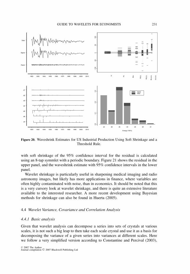
It is also possible to compute the exact pointwise variance of waveshrink, asshown by Bruce and Gao (1996b). As an example of doing this, a linear time trendis removed from the US industrial production series, and then a waveshrink estimate
C© 2007 The AuthorJournal compilation C© 2007 Blackwell Publishing Ltd
GUIDE TO WAVELETS FOR ECONOMISTS 231
1920 1930 1940 1950 1960 1970 1980 1990 2000 2010
Resid
Signal
Data
-100
-50
050
100
H
HL
HLL
HLLL
HLLLL
HLLLLL
LLLLLL
1920 1930 1940 1950 1960 1970 1980 1990 2000 2010
s6
d6
d5
d4
d3
d2
d1
0.0
0.1
0.2
0.3
s6 d6 d5 d4 d3 d2 d1
Energy (100%)
signalresid
Figure 20. Waveshrink Estimates for US Industrial Production Using Soft Shrinkage and aThreshold Rule.
with soft shrinkage of the 95% confidence interval for the residual is calculatedusing an 8-tap symmlet with a periodic boundary. Figure 21 shows the residual in theupper panel, and the waveshrink estimate with 95% confidence intervals in the lowerpanel.
Wavelet shrinkage is particularly useful in sharpening medical imaging and radioastronomy images, but likely has more applications in finance, where variables areoften highly contaminated with noise, than in economics. It should be noted that thisis a very cursory look at wavelet shrinkage, and there is quite an extensive literatureavailable to the interested researcher. A more recent development using Bayesianmethods for shrinkage can also be found in Huerta (2005).
4.4 Wavelet Variance, Covariance and Correlation Analysis
4.4.1 Basic analysis
Given that wavelet analysis can decompose a series into sets of crystals at variousscales, it is not such a big leap to then take each scale crystal and use it as a basis fordecomposing the variance of a given series into variances at different scales. Herewe follow a very simplified version according to Constantine and Percival (2003),
C© 2007 The AuthorJournal compilation C© 2007 Blackwell Publishing Ltd
232 CROWLEY
1920 1925 1930 1935 1940
68
10
12
1920 1925 1930 1935 1940
WaveShrink Estimate with 95%CI
68
10
12
Figure 21. US Industrial Production Residual After Fitting a Linear Time Trend.
which is originally based on Whitcher et al. (2000b) (with full-blown mathematicalbackground provided in Whitcher et al. (1999)). Other more technical sources forthis material are Percival and Walden (2000) and Gencay et al. (2001).
Let x t be a (stationary or nonstationary) stochastic process, then the time-varyingwavelet variance is given by
σ2x,t (λ j ) = 1
2λ jV (w j,t ) (31)
where λ j represents the jth scale level, and w j,t is the jth scale level crystal. The maincomplication here comes from making the wavelet variance time independent, thecalculation of the variance for different scale levels (because of boundary problems)and accounting for when decimation occurs, as with the DWT. For ease of exposition,assume that we are dealing with an MODWT, and assume that a finite, time-independent wavelet variance exists, then we can write equation (31) as
σ2x,t (λ j ) = 1
M j
N−1∑t=L j −1
d2j,t (32)
where M j is the number of crystal coefficients left once the boundary coefficientshave been discarded. These boundary coefficients are obtained by combining the
C© 2007 The AuthorJournal compilation C© 2007 Blackwell Publishing Ltd

GUIDE TO WAVELETS FOR ECONOMISTS 233
beginning and end of the series to obtain the full set of MODWT coefficients, butif these are included in the calculation of the variance this would imply biasedness.If L j is the width of the wavelet (filter) used at scale j, then we can calculate M j
as (N − L j + 1).12
Calculation of confidence intervals is a little more tricky. Here the approach isto first assume that d j ∼ i id(0, σ2
j ) with a Gaussian distribution, so that the sum of
squares of d j is distributed as κχ2η , and then to approximate what the distribution
would look like if the d j are correlated with each other (as they are likely to be).This is done by approximating η so that the random variable (σ2
x,t χ2η)/η has roughly
the same variance as σ2x,t – hence η is not an actual degrees of freedom parameter,
but rather is known as an ‘equivalent degrees of freedom’ or EDOF. There are threeways of estimating the EDOF in the literature, and these can be summarized as(1) based on large sample theory, (2) based on a priori knowledge of the spectraldensity function and (3) based on a band-pass approximation. Gencay et al. (2001)show that if d j is not Gaussian distributed then by maintaining this assumption thiscan lead to narrower confidence intervals than should be the case.
As an example of calculating wavelet variances for the three industrial productionseries, Figure 22 compares the Canadian and Finnish variances and 95% confidenceintervals by scale using a band-pass approximation to EDOF with those of the US(which are shown in the background). The change in wavelet variance by scale isquite similar for Canada and the US, but Finland’s wavelet variance appears not toshow a similar pattern, even when the US series is adjusted so as to coincide withthe Finnish IP period.
Once the wavelet variance has been derived, the covariance between two economicseries follows, as shown by Whitcher et al. (2000b). The covariance of the seriescan be decomposed by scale, and thus different ‘phases’ between the series can bedetected. Figure 23 shows how the covariance between Canadian and US industrialproduction series and Finnish and US industrial production series breaks down byscale and then Figure 24 shows cross covariances between the Canadian and Finnishseries and their US equivalent.
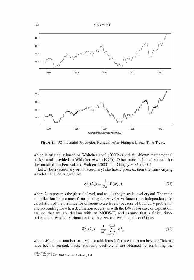
Once covariance by scale has been obtained, the wavelet variances and covariancescan be used together to obtain scale correlations between series. Once again,confidence intervals can be derived for the correlation coefficients by scale (theseare also derived in Whitcher et al. (2000b)). The correlations between the Canadianand Finnish industrial production series and their US counterpart are estimated andplotted in Figure 25 by scale, and then the cross-correlations for up to a 25 monthspan are plotted in Figure 26.
Several interesting points emerge from Figures 25 and 26:
• First, even for time series that are not particularly highly correlated such as thatof Finland and the US, the cyclical nature of the co-correlation at every scaleimplies that there is comovement of business cycles at a variety of differentscales.
C© 2007 The AuthorJournal compilation C© 2007 Blackwell Publishing Ltd

234 CROWLEY
1 2 4 8 16 32 64
Scale
15
10
50
Wavele
t V
ariance:
1920-2
004
-
-
-
-
--
-
-
-
-
-
-
-
-
Canada
USA
1 2 4 8 16 32 64
Scale
0.5
15
10
Wavele
t V
ariance:
1955-2
004
-
-
-
-
-
-
-
-
-
-
-
-
-
-
Finland
USA
Figure 22. Wavelet Variance by Scale for Canada and Finland IndustrialProduction vs the US.
• Second, for Canada the co-correlation appears to increase as scale increases– this would perhaps be expected for series that are highly correlated (or co-integrated) over time; whereas for Finland, beyond scale 4, the co-correlationdoes not appear to follow any pattern by scale.• Thirdly, as we are comparing crystals for increasingly wide wavelet support,we would expect the positive correlations to persist much longer as lag lengthis increased – this is found to be the case here.• Lastly, at the same lag length the co-correlation can be quite differentaccording to scale (for example for Canada at a lag of 12 months, scales 1–4show negative co-correlation, scale 5 shows zero co-correlation and scales 6and 7 exhibit positive correlation).
4.4.2 Testing for homogeneity
Whitcher et al. (1998) developed a framework for applying a test for homogeneityof variance on a scale-by-scale basis to long-memory processes. A good summaryof the procedure is located in Gencay et al. (2001). The test makes no assumptionabout stationarity of the series and relies on the econometric assumption that thecrystals of coefficients, w j,t for scale j at time t have zero mean and variance σ2
t
C© 2007 The AuthorJournal compilation C© 2007 Blackwell Publishing Ltd

GUIDE TO WAVELETS FOR ECONOMISTS 235
1 2 4 8 16 32 64
Scale
01
02
03
0
Wa
ve
let
Co
va
ria
nce
: 1
92
0-2
00
4
-
-
-
-
- -
-
Canada
1 2 4 8 16 32 64
Scale
02
46
Wa
ve
let
Co
va
ria
nce
: 1
95
5-2
00
4
- - -
-
-
-
-
Finland
Figure 23. Wavelet Covariance by Scale for Canadian and Finnish IndustrialProduction vs the US.
(λ j ). This allows us to formulate a null hypothesis of
H0 : σ2L j
(λ j ) = σ2L j +1(λ j ) = · · · · = σ2
N−1(λ j ) (33)
against an alternative hypothesis of
HA : σ2L j
(λ j ) = · · · = σ2k (λ j ) �= σ2
k+1(λ j ) = · · · · = σ2N−1(λ j ) (34)
where k is an unknown change point and L j represents the scale once the numberof boundary coefficients have been discarded. The assumption is that the energythroughout the series builds up linearly over time, so that for any crystal, if this isnot the case, then the alternative hypothesis is true.13 The test statistic used to testthis is the D statistic, which has previously been used by Inclan and Tiao (1994) forthe purpose of detecting a change in variance in time series. Define P k as
Pk =∑k
j=1 w2j∑N
j=1 w2j
(35)
C© 2007 The AuthorJournal compilation C© 2007 Blackwell Publishing Ltd

236 CROWLEY
-20 -10 0 10 20
d7
d6
d5
d4
d3
d2
d1
Canada
Lag-20 -10 0 10 20
d7
d6
d5
d4
d3
d2
d1
Finland
Lag
Figure 24. Cross-covariances for Canadian and Finnish Industrial Production Series vsthe US.
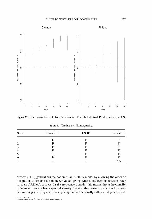
then define the D statistic as D = max (D+, D−) where D+ = (L − Pk) and D− =(Pk − L) where L is the cumulative fraction of a given crystal coefficient to the totalnumber of coefficients in a given crystal. Percentage points for the distribution ofD can be obtained through Monte Carlo simulations, if the number of coefficientsis less than 128 and is obtained through large sample properties. Table 2 showsthe results of applying this test to the industrial production series at a 5% level ofsignificance.
Gencay et al. (2001) provide two examples of tests for homogeneity of variance –one for an IBM stock price and another for multiple changes in variance usingmethodology extending this framework that was developed by Whitcher et al.(2000a).
4.5 Wavelet Analysis of Fractionally Differenced Processes
Granger and Joyeux (1980) first developed the notion of a fractionally differencedtime series and in turn, Jensen (1999, 2000) developed the wavelet approachto estimating the parameters for this type of process. A fractionally differenced
C© 2007 The AuthorJournal compilation C© 2007 Blackwell Publishing Ltd
GUIDE TO WAVELETS FOR ECONOMISTS 237
1 2 4 8 16 32 64
Scale
-1.0
-0.5
0.0
0.5
1.0
Wavele
t corr
ela
tions: 1920-2
004
Canada
-
-
-
-
-
--
1 2 4 8 16 32 64
Scale
-1.0
-0.5
0.0
0.5
1.0
Wavele
t corr
ela
tions: 1955-2
004
Finland
-
--
- -
-
-
Figure 25. Correlation by Scale for Canadian and Finnish Industrial Production vs the US.
Table 2. Testing for Homogeneity.
Scale Canada IP US IP Finnish IP
1 F F F2 F F F3 F F F4 F F T5 T F T6 F F T7 T T NA
process (FDP) generalizes the notion of an ARIMA model by allowing the order ofintegration to assume a noninteger value, giving what some econometricians referto as an ARFIMA process. In the frequency domain, this means that a fractionallydifferenced process has a spectral density function that varies as a power law overcertain ranges of frequencies – implying that a fractionally differenced process will
C© 2007 The AuthorJournal compilation C© 2007 Blackwell Publishing Ltd

238 CROWLEY
-20 -10 0 10 20
d7
d6
d5
d4
d3
d2
d1
Canada
Lag-20 -10 0 10 20
d7
d6
d5
d4
d3
d2
d1
Finland
Lag
Figure 26. Cross-correlation for Canadian and Finnish Industrial Production vs the US.
have a linear spectrum when plotted with log scales. A FDP can be defined asdifference stationary if
(1 − B)d xt =d∑
k=0
(d
k
)(−1)k xt−k = εt (36)
where ε t is a white-noise process, d is a real number and(d
k
) = d!k!(d−k)!
=�(d+1)
�(k+1)�(d−k+1), � being Euler’s gamma function. Wavelets can be used to estimate
the fractional difference parameter, d, as the variance of an ARFIMA-type processcan be expressed in the form
σ2x (λ j ) ≈ σ2
ε c(d)[λ j ]2d−1 (37)
where c is a power function of d and d = (d − 0.5). Equation (37) suggests thatto estimate d a least squares regression could be done to the log of an estimate ofthe wavelet variance obtained from an MODWT. This represents the first way ofestimating d, but there is a problem as here the MODWT yields correlated crystals,so the estimate of d would likely be biased upwards.
Another way of estimating the parameters of the FDP is to go back to the DWT,as the scale crystals are uncorrelated, and use the likelihood function for the interior
C© 2007 The AuthorJournal compilation C© 2007 Blackwell Publishing Ltd
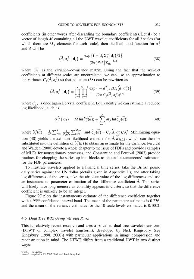
GUIDE TO WAVELETS FOR ECONOMISTS 239
coefficients (in other words after discarding the boundary coefficients). Let d I be avector of length M containing all the DWT wavelet coefficients for all j scales (forwhich there are M j elements for each scale), then the likelihood function for σ2
ε
and d will be (d,σ2
ε | dI) = exp
{( − d′I �
−1dI
dI)/2
}(2π )M/2
∣∣�dI
∣∣1/2(38)
where �dI is the variance–covariance matrix. Using the fact that the waveletcoefficients at different scales are uncorrelated, we can use an approximation tothe variance C j (d,σ2
ε ) so that equation (38) can be rewritten as
(d,σ2
ε | dI) =
J∏j=1
M j −1∏t=0
exp{ − d2
j,t/2C j(d,σ2
ε
)}(2πC j (d,σ2
ε ))1/2(39)
where d j,t is once again a crystal coefficient. Equivalently we can estimate a reducedlog likelihood, such as
�(d | dI ) = M ln(σ2ε (d)) +
J∑j=1
M j ln(C j (d)) (40)
where σ2ε (d) = 1
M
∑Jj=1
1
C j (d)
∑M j −1
t=0 and C j (d) = C j (d,σ2ε )/σ2
ε . Minimizing equa-
tion (40) yields a maximum likelihood estimate for d,d M L E , which can then be
substituted into the definition of σ2ε (d) to obtain an estimate for the variance. Percival
and Walden (2000) devote a whole chapter to the issue of FDPs and provide examplesof MLEs for nonstationary processes, and Constantine and Percival (2003) provideroutines for chopping the series up into blocks to obtain ‘instantaneous’ estimatorsfor the FDP parameters.
To illustrate wavelets applied to a financial time series, take the British pounddaily series against the US dollar (details given in Appendix D), and after takinglog differences of the series, take the absolute value of the log differences and usean instantaneous parameter estimation of the difference coefficient d. This serieswill likely have long memory as volatility appears in clusters, so that the differencecoefficient is unlikely to be an integer.
Figure 27 plots the instantaneous estimate of the difference coefficient togetherwith a 95% confidence interval band. The mean of the parameter estimates is 0.236,and the mean of the variance estimates for the 10 scale levels estimated is 0.1002.
4.6 Dual Tree WTs Using Wavelet Pairs
This is relatively recent research and uses a so-called dual tree wavelet transform(DTWT or complex wavelet transform), developed by Nick Kingsbury (seeKingsbury (1998, 2000)) with particular applications in image compression andreconstruction in mind. The DTWT differs from a traditional DWT in two distinctways:
C© 2007 The AuthorJournal compilation C© 2007 Blackwell Publishing Ltd
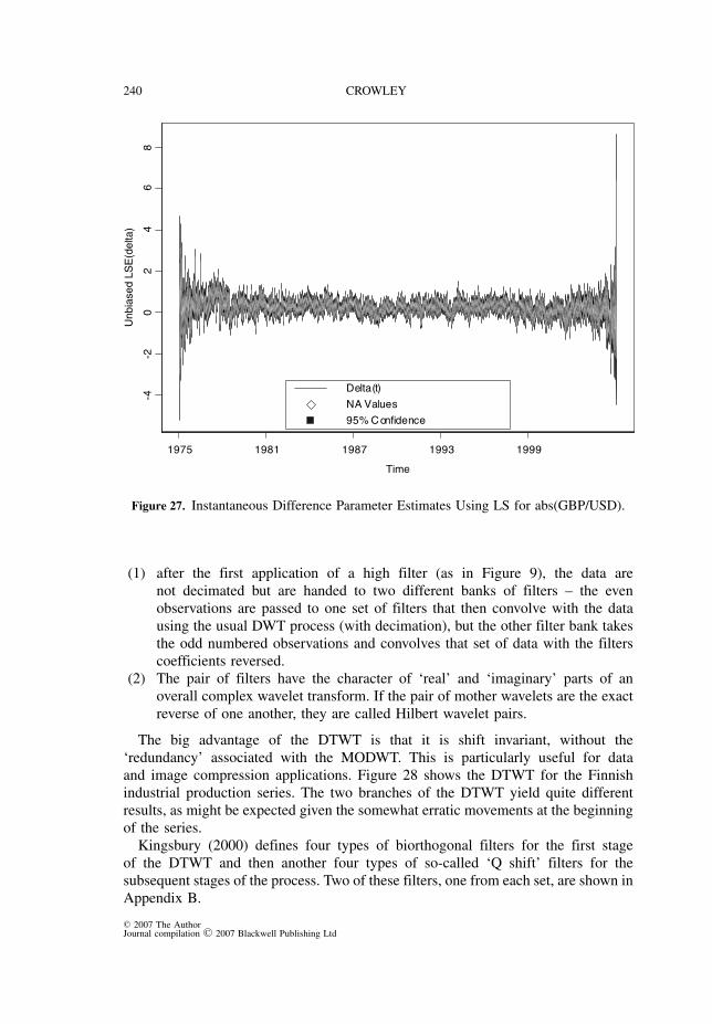
240 CROWLEY
1975 1981 1987 1993 1999
Time
-4-2
02
46
8
Unbia
sed L
SE
(delta)
Delta(t)
NA Values
95% C onfidence
Figure 27. Instantaneous Difference Parameter Estimates Using LS for abs(GBP/USD).
(1) after the first application of a high filter (as in Figure 9), the data arenot decimated but are handed to two different banks of filters – the evenobservations are passed to one set of filters that then convolve with the datausing the usual DWT process (with decimation), but the other filter bank takesthe odd numbered observations and convolves that set of data with the filterscoefficients reversed.
(2) The pair of filters have the character of ‘real’ and ‘imaginary’ parts of anoverall complex wavelet transform. If the pair of mother wavelets are the exactreverse of one another, they are called Hilbert wavelet pairs.
The big advantage of the DTWT is that it is shift invariant, without the‘redundancy’ associated with the MODWT. This is particularly useful for dataand image compression applications. Figure 28 shows the DTWT for the Finnishindustrial production series. The two branches of the DTWT yield quite differentresults, as might be expected given the somewhat erratic movements at the beginningof the series.
Kingsbury (2000) defines four types of biorthogonal filters for the first stageof the DTWT and then another four types of so-called ‘Q shift’ filters for thesubsequent stages of the process. Two of these filters, one from each set, are shown inAppendix B.
C© 2007 The AuthorJournal compilation C© 2007 Blackwell Publishing Ltd

GUIDE TO WAVELETS FOR ECONOMISTS 241
0 50 100 150 200 250 300
-40-2
00
20
40
60 TreeA
0 50 100 150 200 250 300
-40-2
00
20
40
60 TreeB
0 50 100 150
-40
-20
02
04
06
0
0 50 100 150
-40
-20
02
04
06
0
0 20 40 60
-40
-20
02
04
06
0
0 20 40 60
-40
-20
02
04
06
0
0 10 20 30
-40
-20
02
04
06
0
0 10 20 30
-40
-20
02
04
06
0
5 10 15
-40
-20
02
04
06
0
5 10 15
-40
-20
02
04
06
0
2 4 6 8 10
-40
-20
02
04
06
0
2 4 6 8 10
-40
-20
02
04
06
0
2 4 6 8 10
-40
-20
02
04
06
0
2 4 6 8 10
-40
-20
02
04
06
0
Figure 28. Dual Tree WT for Finnish Industrial Production.
5. Frequency Domain Analysis
5.1 Continuous Wavelet Transforms
Wavelet analysis is neither strictly in the time domain nor in the frequency domain:it straddles both. It is therefore quite natural that wavelets applications have alsobeen developed in the frequency domain using spectral analysis. Perhaps the bestintroduction into the theoretical side of this literature can be found in Lau andWeng (1995) and Chiann and Morettin (1998), while Torrence and Compo (1998)probably provide the most illuminating examples of applications to time series frommeteorology and the atmospheric sciences.
Spectral analysis is perhaps the most commonly known frequency domain toolused by economists (see Collard (1999), Camba and Kapetanios (2001), Valle eAzevedo (2002), Kim and In (2003), Sussmuth (2002) and Hughes and Richter(2004) for some examples), and therefore needs no extended introduction here. Inbrief though, a representation of a covariance stationary process in terms of itsfrequency components can be made using Cramer’s representation, as follows
xt = μ +∫ π
−π
eiωt z(ω) dω (41)
where i = √−1,μ is the mean of the process, ω is measured in radians and z(ω) dωrepresents complex orthogonal increment processes with variance f x (ω), where itcan be shown that
fx (ω) = 1
2π
(γ (0) + 2
∞∑τ=1
γ (τ ) cos(ωτ )
)(42)
C© 2007 The AuthorJournal compilation C© 2007 Blackwell Publishing Ltd
242 CROWLEY
where γ (τ ) is the autocorrelation function. f x (ω) is also known as the spectrumof a series as it defines a series of orthogonal periodic functions that essentiallyrepresent a decomposition of the variance into an infinite sum of waves of differentfrequencies. Given a large value of f x (ω i ), say at a particular value of ωi , ωi , thisimplies that frequency ωi is a particularly important component of the series.
To intuitively derive the wavelet spectrum, recall using the definition of a motherwavelet convolution from equation (5), that the convolution of the wavelet withthe series renders an expression such as that given in equation (15), and associatedcrystals given by equation (17), then a continuous wavelet transform (CWT) for afrequency index k will analogously yield
Wk(s) =N∑
k=0
xt ψ∗(sωk)eiωk t∂t (43)
where xk is the discrete Fourier transform of x t
xk = 1
(N + 1)
N∑k=0
xt exp
{−2π ikt
N + 1
}(44)
so xk represents the Fourier coefficients, �∗ is the Fourier transform of a normalizedscaling function, �∗, defined as
�∗ ={
t
s
}0.5
�
[t − μ
s
](45)
so that in the frequency domain the CWT W k(s) is essentially the convolution ofthe Fourier coefficients and the Fourier transform of �∗, �∗. The angular frequencyfor ωk in equation (43) is given by
ωk ={ 2πk
(N+1): k ≤ N+1
2
− 2πk(N+1)
: k > N+12
(46)
The CWT, W k(s), can now be split into a real and complex part, � {W k(s)}, and
� {W k(s)}, or amplitude/magnitude, |W k(s)| and phase, tan−1[
�{Wk (s)}�{Wk (s)}
].
To show some examples of wavelet spectra, first Figure 29 shows a three-dimensional plot for the US industrial production series using a log frequency scaleand reversing the time sequencing so as to show the evolution of the spectrum tobest effect.
This CWT spectral plot displays similar characteristics to that of the time-frequency plots of Figure 14, in that the high-frequency content is particularlymarked in the earlier part of the twentieth century, with mostly low-frequency contentevident throughout the entire time period. As might be expected, the ridge lines inthe 3D magnitude plot for the series suggest that there are roughly five distinctfrequencies active in the series, as was already confirmed with the use of a DWT.
To study phase, it is probably a good strategy to project both 3D plots onto themagnitude or phase axis, respectively, so as to view the plots in terms of theircontours. This is done in Figure 30 first for the scale-averaged (or integrated)
C© 2007 The AuthorJournal compilation C© 2007 Blackwell Publishing Ltd

GUIDE TO WAVELETS FOR ECONOMISTS 243
2010
2000
1990
19801970
19601950
19401930
10
10.1
0.01
Time
Frequency
-50
-500
0
50
50
100
100
150
150
Ma
gnitude
Ma
gnitude
Figure 29. CWT 3D Magnitude Spectrum for US Industrial Production.
power spectrum, |W k(s)|2, which, as expected, shows that the volatile short-termfluctuations in the early part of the series tend to dominate and then in Figure 31 forthe phase contour plot. Figure 32 gives CWT a magnitude contour plot (against logof frequency) using a Paul (complex) wavelet with initial width of 6 months. This isan asymmetric wavelet, and so the frequency is only roughly related to the scale ofthe wavelets, hence the approximation that s−1 is equivalent to the maximum of �
is not analytically correct.14 The contour plots point to several other features fromthe frequency domain, notably
1. three areas of notable high-frequency activity, two of which coincide with therebounds in production in the early 1920s and mid 1930s;
2. the constant presence of a relatively low-frequency pattern throughout theperiod of the data;
3. the disappearance of almost all high-frequency activity since 1945 and thedying out of a long medium-frequency pattern over the period 1945–1980;
4. a range of frequencies where phases interact quite frequently (the ‘fingers’ inthe phase contour plot), sometimes at a large range of frequencies (the longerfingers) and sometimes over a smaller range (the smaller thinner fingers).
Torrence and Compo (1998) rightly observe that one of the major drawbacks ofspectral analysis has been that significance testing was difficult to implement in thefrequency domain. But by assuming a ‘background’ spectra such as white noise, or an
C© 2007 The AuthorJournal compilation C© 2007 Blackwell Publishing Ltd
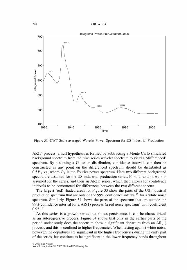
244 CROWLEY
Integrated Power, Freq=0.00585938,6
1923.2
1934.3
1947.1
1959.1 1976.2
1920 1940 1960 1980 2000Time
100
200
300
400
500
600
700In
teg
rate
d P
ow
er
Figure 30. CWT Scale-averaged Wavelet Power Spectrum for US Industrial Production.
AR(1) process, a null hypothesis is formed by subtracting a Monte Carlo simulatedbackground spectrum from the time series wavelet spectrum to yield a ‘differenced’spectrum. By assuming a Gaussian distribution, confidence intervals can then beconstructed as any point on the differenced spectrum should be distributed as0.5P k χ2
2, where P k is the Fourier power spectrum. Here two different backgroundspectra are assumed for the US industrial production series. First, a random walk isassumed for the series, and then an AR(1) series, which then allows for confidenceintervals to be constructed for differences between the two different spectra.
The largest (red) shaded areas for Figure 33 show the parts of the US industrialproduction spectrum that are outside the 99% confidence interval15 for a white noisespectrum. Similarly, Figure 34 shows the parts of the spectrum that are outside the99% confidence interval for a AR(1) process (a red noise spectrum) with coefficient0.95.16
As this series is a growth series that shows persistence, it can be characterizedas an autoregressive process. Figure 34 shows that only in the earlier parts of theperiod under study does the spectrum show a significant departure from an AR(1)process, and this is confined to higher frequencies. When testing against white noise,however, the departures are significant in the higher frequencies during the early partof the series, but continue to be significant in the lower-frequency bands throughout
C© 2007 The AuthorJournal compilation C© 2007 Blackwell Publishing Ltd

GUIDE TO WAVELETS FOR ECONOMISTS 245
1920 1940 1960 1980 2000Frequency
0.01
0.019254
0.03707
0.071372
0.13742
0.26458
0.5094
0.98077
1.8883
3.6357
7
Wa
ve
let
Figure 31. CWT Phase Spectrum Contour Plot for US Industrial Production.
the series. Torrence and Compo (1998) also go on to use a similar approach toanalyse co-spectrum for use in multivariate time-series analysis.
5.2 Multivariate Spectral Analysis Using Hilbert Wavelet Pairs
Craigmile and Whitcher (2004) further extend the DTWT to a special case ofthis transform, known as the maximal overlap discrete Hilbert wavelet transform(MODHWT), in order to produce wavelet-based analogues for spectral analysis. Ina sense this is a combination of the DTWT and the CWT spectral methodology,but allows multivariate coherency and phase measures to be defined in the time-frequency domain. In Craigmile and Whitcher (2004), the basis for using the Hilbertwavelet pairs (HWPs) is defined analytically and asymptotic theory is used so thatstatistical inference can be applied.
A Hilbert wavelet pair is essentially a pair of mother and father wavelet filterssuch that the two sets only differ in their phase, and not in their gain functions (thatis, they sample the same frequencies). Selesnick (2002) provides a way of obtainingnear-HWPs, which involves making the gain of two low-pass (father) filters, denotedA0( f ) and B0( f ) relate in the following way:
B0( f ) = A0( f ) exp−iθ( f ) (47)
C© 2007 The AuthorJournal compilation C© 2007 Blackwell Publishing Ltd

246 CROWLEY
1920 1940 1960 1980 2000Time
0.01
0.1
1
10F
requ
en
cy
Figure 32. CWT Magnitude Contour Plot Using US Industrial Production.
where A0( f ) and B0( f ) form a wavelet pair as long as θ( f ) = π f , so that theyhave a half sample delay between them – the same can clearly be done for the highpass or mother wavelets too. To characterize an HWP in practice, two parametersare required, denoted as K and M, where K is the number of zero wavelet moments(which directly relates to the smoothness of the wavelet) and M represents thedegree of approximation to the half sample delay (as M increases this approximationimproves).17 To implement the MODHWT or its decimated equivalent (DHWT),define the high-pass (mother) and low-pass (father) filters respectively as:
hl = a1,l + i b1,l (48)
gl = a0,l + i b0,l (49)
where in equations (48) and (49) the resulting wavelets are sometimes known as‘complex wavelets’. Convolution occurs with the data using the wavelet filters to givethe usual crystal coefficients and time shifts can also be implemented for phasingissues, so that the analogous phased crystals can be obtained as with a DWT orMODWT. There is also an analogous packet table available for the MODHWT aswell.
In order to conduct time-varying spectral analysis, define {(W Xt , W Y
t )T : t ∈ Z}as the MODHWT detail crystals from two series X t and Y t with a total of T
C© 2007 The AuthorJournal compilation C© 2007 Blackwell Publishing Ltd
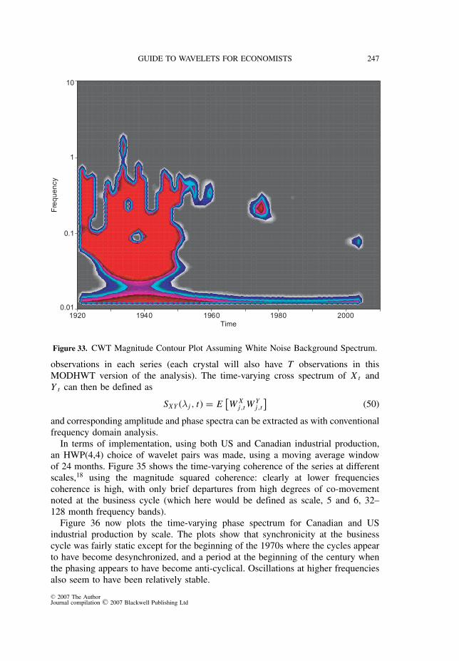
GUIDE TO WAVELETS FOR ECONOMISTS 247
1920 1940 1960 1980 2000Time
0.01
0.1
1
10
Fre
qu
en
cy
Figure 33. CWT Magnitude Contour Plot Assuming White Noise Background Spectrum.
observations in each series (each crystal will also have T observations in thisMODHWT version of the analysis). The time-varying cross spectrum of X t andY t can then be defined as
SXY (λ j , t) = E[W X
j,t WYj,t
](50)
and corresponding amplitude and phase spectra can be extracted as with conventionalfrequency domain analysis.
In terms of implementation, using both US and Canadian industrial production,an HWP(4,4) choice of wavelet pairs was made, using a moving average windowof 24 months. Figure 35 shows the time-varying coherence of the series at differentscales,18 using the magnitude squared coherence: clearly at lower frequenciescoherence is high, with only brief departures from high degrees of co-movementnoted at the business cycle (which here would be defined as scale, 5 and 6, 32–128 month frequency bands).
Figure 36 now plots the time-varying phase spectrum for Canadian and USindustrial production by scale. The plots show that synchronicity at the businesscycle was fairly static except for the beginning of the 1970s where the cycles appearto have become desynchronized, and a period at the beginning of the century whenthe phasing appears to have become anti-cyclical. Oscillations at higher frequenciesalso seem to have been relatively stable.
C© 2007 The AuthorJournal compilation C© 2007 Blackwell Publishing Ltd
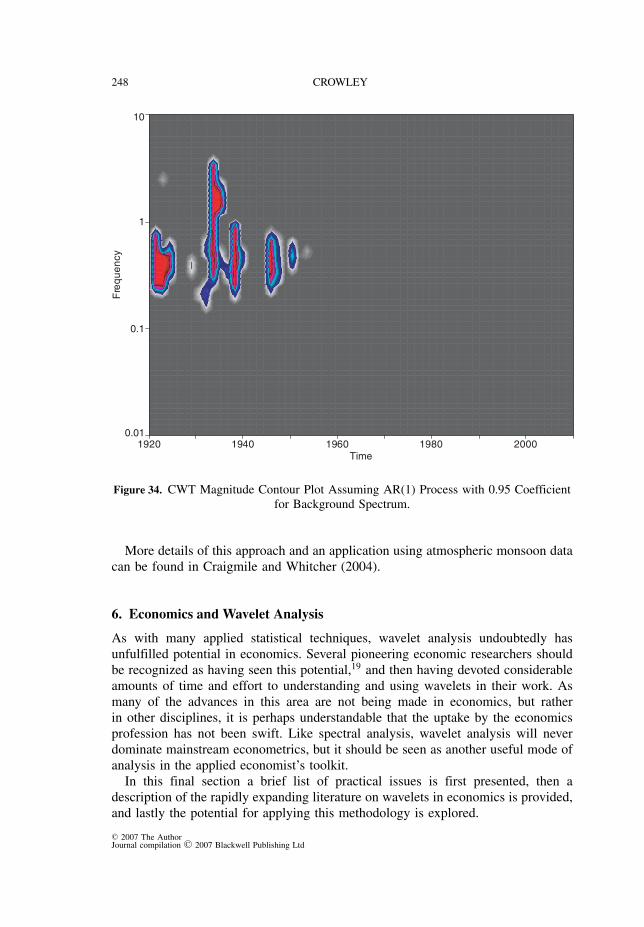
248 CROWLEY
1920 1940 1960 1980 2000Time
0.01
0.1
1
10F
req
ue
ncy
Figure 34. CWT Magnitude Contour Plot Assuming AR(1) Process with 0.95 Coefficientfor Background Spectrum.
More details of this approach and an application using atmospheric monsoon datacan be found in Craigmile and Whitcher (2004).
6. Economics and Wavelet Analysis
As with many applied statistical techniques, wavelet analysis undoubtedly hasunfulfilled potential in economics. Several pioneering economic researchers shouldbe recognized as having seen this potential,19 and then having devoted considerableamounts of time and effort to understanding and using wavelets in their work. Asmany of the advances in this area are not being made in economics, but ratherin other disciplines, it is perhaps understandable that the uptake by the economicsprofession has not been swift. Like spectral analysis, wavelet analysis will neverdominate mainstream econometrics, but it should be seen as another useful mode ofanalysis in the applied economist’s toolkit.
In this final section a brief list of practical issues is first presented, then adescription of the rapidly expanding literature on wavelets in economics is provided,and lastly the potential for applying this methodology is explored.
C© 2007 The AuthorJournal compilation C© 2007 Blackwell Publishing Ltd

GUIDE TO WAVELETS FOR ECONOMISTS 249
4–8m
Date
MS
C
1920 1940 1960 1980 2000
0.0
0.4
0.8
8–16m
Date
MS
C
1920 1940 1960 1980 2000
0.0
0.4
0.8
16–32m
Date
MS
C
1920 1940 1960 1980 2000
0.0
0.4
0.8
32–64m
Date
MS
C
1920 1940 1960 1980 2000
0.0
0.4
0.8
64–128m
Date
MS
C
1920 1940 1960 1980 2000
0.0
0.4
0.8
128–256m
Date
MS
C
1920 1940 1960 1980 2000
0.0
0.4
0.8
Figure 35. Time-varying Spectral Coherence Plots by Scale for Canadian vs US IndustrialProduction Series.
6.1 Practical Issues
Obviously software is the first major concern for most empirical researchers. Manyof the procedures used with wavelet analysis are not easy to implement unless theresearcher is an experienced programmer, so this is obviously of major concern.Appendix E therefore provides a current list of software resources for waveletanalysis. Beyond the choice of software for doing wavelet analysis, the researchershould also note the following practical issues:20
1. Sufficient data are required given the observed nature of the time series. Thisimplies that in economics, if for example business cycles are to be analysed,quite long time series are necessary if all scales are to be properly resolved.Many economists believe that wavelet analysis requires high-frequency data,
C© 2007 The AuthorJournal compilation C© 2007 Blackwell Publishing Ltd

250 CROWLEY
4–8m
Date
Phase
1920 1940 1960 1980 2000
−30
2
8–16m
Date
Phase
1920 1940 1960 1980 2000
−30
2
16–32m
Date
Phase
1920 1940 1960 1980 2000
−30
2
32–64m
Date
Phase
1920 1940 1960 1980 2000−3
02
64–128m
Date
Phase
1920 1940 1960 1980 2000
−30
2
128–256m
Date
Phase
1920 1940 1960 1980 2000
−30
2
Figure 36. Time-varying Spectral Phase Plots by Scale for Canadian vs US IndustrialProduction Series.
as the technique has been applied much more frequently in finance – this isnot the case, as Table 1 details.
2. Choice of wavelet function – issues arise such as whether to use orthogonal ornonorthogonal, complex or real and the choice of width and type of waveletfunction is also an issue. For analysis of economic time series, clearly theHaar wavelet is not really appropriate, given the discontinuous nature of itswaveform, but beyond this, the choice is largely one for the researcher, but islikely limited by the software being used.
3. Length of wavelet – for financial series and volatile economic series (such asinventories, gross fixed capital formation or freely floating exchange rates) awavelet of tap length 8 is probably most appropriate, but with macroeconomic
C© 2007 The AuthorJournal compilation C© 2007 Blackwell Publishing Ltd

GUIDE TO WAVELETS FOR ECONOMISTS 251
data that possess less volatility, a wavelet of tap length 4 is likely moreadvantageous with relatively short datasets, as the number of possible scaleresolutions will likely increase over the tap 8 equivalent.
4. Dyadic series – some wavelet applications require dyadic time series. Thisis obviously not attractive for usage with economic time series as it impliesdiscarding data or padding series with extra data if the series is not dyadic. Inthe examples used in this paper, the Canadian and US time series were paddedto 1024 datapoints, but the Finnish industrial production series was left with604 data points. Clearly, the MODWT and the DTWT show most promisehere, as they do not maintain this requirement.
5. Boundary/cone of influence effects – with the DWT these are usually labelledboundary effects, but with the CWT they are called cone of influence effects.There are many different types of boundary treatment rules, such as (1) aperiodic rule – assumption that the series is periodic, that is for any x i = x i+nk,where k is an integer and i = 1, 2, 3, . . ., n ; (2) a reflection rule – assumptionthat x n is reflected at the boundaries and then periodically extended; (3) azero padding rule – at each step of the filtering process the series is paddedat the beginning and end with zeros; (4) a polynomial extension – paddingthe beginning and end of the series by repeating the beginning and end seriesvalues before and after the series, respectively and (5) an interval rule – usingspecial ‘interval’ wavelets at the boundaries, whose filter coefficients are zerooutside the range of the data.
6. Cycle overlap and leakage – discrete wavelet transforms artificially decomposea series into specific frequency ranges. This could create problems whena series has cycles that operate at frequencies that overlap these specificfrequency ranges. For example, it is usually assumed that business cyclesoperate at frequencies of 3 to 8 years, but this would then be captured bytwo different crystals (d3 and d4). Although it is possible to combine crystals,this may introduce some ‘contamination’ from other growth cycles that mightreduce the resolution by introducing other cycles that are embedded in theseries. Also, wavelet analysts recognize that there is also some ‘leakage’ thatoccurs at the edge of each frequency band, so some cycles can appear in twodifferent crystals.
7. Identification of short cycles – in high frequency detail crystals, waveletmethodology cannot properly distinguish between extremely short cycles thatmight exist in the data from ‘noise’ or discrete shocks. Very short-termfluctuations might exist in reality (weekly trading effects in the stock market,for example), so that unless data are sampled at sufficiently fine intervals, theseshort-term cycles might not be identifiable, but instead might appear as randomfluctuations, particularly if the cycle does not occur at a dyadic multiple of thesampling interval. A pure temporary one-period shock would be identified asa cycle at the highest frequency, but not as a discrete shock.
C© 2007 The AuthorJournal compilation C© 2007 Blackwell Publishing Ltd

252 CROWLEY
6.2 The Wavelet Literature in Economics
There are relatively few contributions to economics that use wavelets in theexisting literature, although in recent months this list has expanded considerably,which signals that wavelet analysis is at last being recognized as an interestingmethodological approach in economics. The contributions located to date are perhapsconcentrated more in the field of finance, but there is an emerging interest in alsoapplying wavelets to economics issues.
James Ramsey is perhaps the economist most closely associated with theapplication of wavelets in economics. His first paper (Ramsey and Zhang, 1995)analysed high-frequency foreign exchange rates using waveform dictionaries anda matching pursuit algorithm and determined that there is structure only at thelowest frequencies. At the highest frequencies ‘chirp’ like bursts of energy aredistributed across frequencies throughout the year. Ramsey then first exploredwavelet transforms in Ramsey and Lampart (1998b) where they took seasonallyunadjusted monthly money supply data and nominal personal income for the USfrom 1960 to 1998, and then used Granger causality tests for each of the setsof crystals. They found that the relationship between money and income variesaccording to scale, with money supply Granger causing income at higher scale levels,and income Granger causing money supply at low scale levels. Ramsey and Lampart(1998a) essentially did the same thing as in Ramsey and Lampart (1998b) except fordurable and nondurable expenditures and income. Dalkir (2004) scale decomposespersonal income, sum and divisia monetary aggregates for the US and uses Grangercausality tests to review the Ramsey and Lampart (1998b) results. The findingsare that in the majority of cases money Granger causes personal income, althoughthis relationship does reverse, usually during a shift in monetary policy regime. Aninteresting variation on this approach is found in Kim and In (2003) who investigatewhether US financial variables have predictive power over US industrial productiondata over various frequency domains and time scales using spectral decomposition,wavelet analysis and Granger causality tests. They find that the relationship betweenUS financial and real variables runs from financial variables to real at short timescales and from real to financial at longer time scales.
Other applications in economics have not received a great deal of attention,although some of them are clearly first attempts to use wavelet analysis in economics.Crivellini et al. (2004) scale decompose G6 (G7 minus Canada) industrial productiondata and then look at the characteristics of the different scale cycles and do a rollingcorrelation analysis of these scale components between countries.21 Their resultsindicated an increase in correlation of business cycles at all scales in the 1970s,a decrease in the 1980s at the medium- and short-run scales, and in the 1990srelatively high long-term correlations. The EU countries also tended to have high-medium term correlations in the 1990s, with the UK an exception to this rule. Ina paper that caused quite a stir in central banking circles, Neumann and Greiber(2004) use scale decompositions of M3 money growth and euro zone inflation tocompare MRDs with other filters and also to look at the relationship between M3and inflation for the euro zone on a scale-by-scale basis. They find that short- to
C© 2007 The AuthorJournal compilation C© 2007 Blackwell Publishing Ltd
GUIDE TO WAVELETS FOR ECONOMISTS 253
medium-term fluctuations of money growth with cycles of up to about 8 years werenot significant causes of affecting trend inflation, but that money growth has a muchgreater impact on inflation at cycles of frequency 8 years and above.
One of the most interesting developments in time-series econometrics has beenthe extension of the ARIMA-based modelling, to long memory processes, processesthat are found particularly in financial data. Tkacz (2000) uses the Jensen waveletestimator (Jensen, 2000) to estimate the fractional order of integration for Canadianand US interest rates. He finds that US nominal interest rates likely follow long-memory processes, and that Canadian rates also exhibit strong persistence, givingeven a larger order of integration than for the US. Atkins and Sun (2003) also useJensen’s estimator of the long-memory parameter coupled with Fisher regressionsin the wavelet domain to show that in the short run, there is no relationship betweeninterest rates and inflation for shorter time scales but is statistically significant atlonger time scales.
Other applications in finance include Capobianco (2004) who uses matchingpursuit algorithms with waveform dictionaries to scale decompose intraday stockreturn dynamics. Wavelet analysis helps to identify hidden intraday periodicitiesboth at the 1 minute and 5 minute timescale. Fernandez (2004) looks at returnsspillover in stock markets at different time scales using wavelet analysis. She findsevidence of price spillovers from North America to Latin America, emerging Asianand Far East markets, and Pacific markets, and also evidence of spillovers fromEuropean and Latin America to North American markets. In the latter part of thepaper she also controls for conditional heteroskedasticity and serial correlation byusing an asymmetric power GARCH model. Lee (2004) uses wavelets to analysethe relationship between the South Korean and US stock markets. Using MRA atdifferent scales, it is determined that there is strong evidence of price and volatilityspillovers from developed country to developing country stock markets. Vuorenmaa(2004) analyses Nokia share volatility using wavelet MRA analysis and finds thatwavelet variance and covariance analysis reveals a considerable amount about stockmarket activity at intraday levels. He then applies a local scaling law and longmemory in volatility, and finds that time-varying long memory is supported over amedium-term period (months). Connor and Rossiter (2005) use an MRD to studythe behaviour of commodity prices and explore whether long memory is evident inthese time series. They find evidence of long memory in all the commodity priceseries.
There are some rather eclectic and original usages of wavelets in the literature aswell. Gencay and Whitcher (2005) use wavelets with high-frequency financial dataand a hidden Markov tree model to establish a ‘new’ stylized fact about volatility –that low volatility at a long time horizon is most likely followed by low volatility atshorter time horizons – the reverse for high volatility does not seem to be the case.The authors label this phenomenon asymmetric vertical dependence. Meanwhile, theforecasting literature has yet to take on board the proposals by Renaud et al. (2003)who suggest a new forecasting method based on wavelets whereby MRD crystalsare used with a simple AR process to forecast time series.
C© 2007 The AuthorJournal compilation C© 2007 Blackwell Publishing Ltd
254 CROWLEY
An intriguing recent addition to the literature is that of Gencay and Fan (2006)who propose a wavelet based approach to unit root and cointegration testing usingwavelets. The tests utilize the scale crystal of the coarsest scale. In particular,they construct test statistics from the ratio of the energy from the low-frequencyscale to the total energy (variance) of the time series. They establish asymptoticproperties of these tests and generalize our unit root tests to residual-based tests forcointegration.
6.3 Potential Applications in Economics
In economics, while providing a review of the possible future contributions ofwavelets to the economics discipline, Ramsey (2000) explored four ways in whichwavelets might be used to enhance the empirical toolkit of our profession. Theseare as follows:
• exploratory analysis – time scale versus frequency: in economics and financean examination of data to assess the presence and ebb and flow of frequencycomponents is potentially valuable.• density estimation and local inhomogeneity: wavelets estimators are superiorto kernel estimators whenever local inhomogeneity is present (e.g. modellingimpact of minimum wage legislation, tax legislation, rigidities, innovation).• time-scale decomposition: recognition that relationships between economicvariables can possibly be found at the disaggregate (scale) level rather than atan aggregate level.• forecasting by scale: disaggregate forecasting by scale thereby establishingglobal versus local aspects of series, and using different time-series methodsto take this into account.
This list, while obviously quite encompassing, does not address specific subjectareas where wavelets might be able to make a positive contribution in economics.Although identifying specific subject or topic areas runs the risk of being criticizedfor excluding or neglecting other areas where wavelets could make a potentiallyuseful contribution, not identifying any areas probably runs the greater risk of havingthis important statistical tool ignored by economists. Hopefully the reader will findthis adequate justification for such an exercise.
As noted above, although James Ramsay pioneered the use of wavelets to uncoverthe frequency nature of economic relationships (see Ramsey and Lampart (1998a,b)),and there have been extensions or applications of this approach highlighting itspotential (as noted above), much more work needs to be done. The time-seriesmethods typically used to ascertain the flow of causality (Granger causality) canbe explored using other time-series means, so that we can better understandthese relationships at different frequencies. Further, just showing that differentrelationships at different frequencies exist, does not answer the question that is theobvious corollary to this research – what is driving these relationships at differentfrequencies?
C© 2007 The AuthorJournal compilation C© 2007 Blackwell Publishing Ltd

GUIDE TO WAVELETS FOR ECONOMISTS 255
Second, much more work needs to be done on wavelet decomposition ofmacroeconomic variables. Crivellini et al. (2004) and Crowley and Lee (2005)analyse wavelet decompositions of industrial production and real GDP, respectively,but there has been no attempt to line up cycles in macroeconomic data using differentfrequency data. This is important as it gives economists an idea about the ‘cycle’information contained in each scale for different frequency data. For long data setsas well, it will also allow a better assessment of whether a long cycle exists,22 andthe importance of cycles at frequencies other than for the conventional businesscycle (so-called medium growth cycles). Linking this empirical research with theendogenous growth theoretical research obviously carries some logical appeal, asthere has been theoretical research done trying to explain cycles that appear fromspectral analysis to be longer than the empirical business cycle. There has beenno work to date that uses wavelet decomposition to analyse economic variablesother than output and production series as well as financial data such as stockmarket indices and stock prices. There is clearly ample scope for research focusedon decomposition of other volatile macroeconomic variables such as investment,interest rates, money stock measures and inventories.
Third, little has been done in the economics literature to explore the notion ofvertical dependence introduced in the context of financial data in Gencay et al.(2003). If a macroeconomic shock occurs, if there are several cycles in operationsimultaneously, which cycles are affected, and could it be that one frequency cyclecan (or is more likely to) affect other cycles and (or but not) vice-versa? In time-seriesanalysis economists always look for horizontal dependence but ignore the verticaldependencies that operate within (and perhaps between) economic variables.
Fourth, as James Ramsay correctly noted, wavelets have obvious potential inforecasting of time series, although little has been done in the economics professionalong these lines to date.
Lastly, as wavelet theorists and practitioners in other fields extend the existingwavelet techniques, there are further opportunities to apply this research in bothfinance and economics. A good example might be the empirical mode decomposition(EMD) technique pioneered by Huang et al. (1998), which can applied to bothnonlinear and nonstationary time series.23 EMD essentially decomposes a time seriesinto its intrinsic cycles, using the data itself as a basis for mapping cycles of differentfrequencies onto an appropriate scale. Although software is available for EMD,research applying this technique to economic or financial data has yet to appear.
7. Conclusions
Perhaps because economics does not usually deal with long data series with‘natural’ periodicity, traditional spectral analysis never had a large amount to offerthe economics discipline; time-series analysis is probably much better suited toanalysis of shorter time series with variable ‘nonnatural’ periodicity, coupled with itsemphasis on causation and underlying processes. Wavelet analysis, however, differsfrom spectral analysis in that it straddles both the time and frequency domains,thereby allowing identification of both events in the time domain and the waxing
C© 2007 The AuthorJournal compilation C© 2007 Blackwell Publishing Ltd
256 CROWLEY
and waning of cyclical fluctuations in the frequency domain. In this sense, it likelyhas a lot more to offer economists.
Wavelet analysis has the potential to offer much to empirical economic research.The potential is particularly apparent in two areas of economics: that of businesscycle analysis, which naturally lends itself to analysis of periodicities, and wherefiltering has been a particularly controversial issue; and in any part of macro ormonetary economics where theoretical long-run and short-run relationships can bedistinguished. Its ability to separate out the dynamics in a time series over a varietyof different time horizons, the number of which being directly related to the type oftime series and the number of observations available, can reveal interesting insightsinto cycles at different time scales. The ability to also work with nonstationary datais particularly advantageous, as most econometric methodology assumes stationarity,which may or may not be apparent in economic data (either locally or globally).
Wavelet analysis also now offers economic researchers the availability ofthe MODWT, so that time series can be decomposed into identical lengths ofscale-decomposed equivalent series, making statistical testing and time series anal-ysis possible for individual scale crystals – this removes the inherent disadvantagesof wavelet analysis when using the basic DWT, and permits nondyadic time series.
The real challenge for those economists who are interested in wavelet analysiswill be to integrate the wavelet approach with the traditional time-series toolkit ofthe econometrician, as perhaps here the potential contribution is greatest. Clearlythis will not be easy, as time-series techniques now dominate applied econometrics,and most economists, and the journals that economists tend to publish in, focusnearly exclusively on this mode of analysis.
Acknowledgements
First and foremost, I would like to thank the research department at the Bank of Finland(Suomen Pankki) who hosted me during the 2004/05 academic year (and subsequentlyduring the summer of 2006) where most of the research for this paper was originally done.The Bank supported my choice of research topic (wavelet analysis), despite its lack of“instant” economic appeal, and helped and guided my work in this area through individualconsultations and their regular workshops – for that I am extremely grateful. In particular,I would like to thank the following individuals at the Bank: Jouko Vilmunen, Matti Viren,Juha Tarkka, David Mayes, Juha Kilponen and Maritta Palovitta. Second, I would like tothank Insightful corporation for their assistance with some technical issues with the waveletmodule in SPLUS and also Brandon Whitcher (Glaxo Smith Kline) who clarified severaltheoretical issues for me. Third, I would like to thank two anonymous referees who gavevaluable comments for previous revisions of this article.
Notes
1. Other perhaps less intuitive but nonetheless technically sound introductions towavelets can be found in Walker (1999), Percival and Walden (2000) and Addison(2002). For those more mathematically inclined, they should refer to the mathematicsliterature where Debauchies (1992) and Walnut (2002) are good starting points.
2. An orthonormal transform is one which preserves the energy of the series and is notaffected by shifts in the data.
C© 2007 The AuthorJournal compilation C© 2007 Blackwell Publishing Ltd
GUIDE TO WAVELETS FOR ECONOMISTS 257
3. Other wavelets also exist – notably Morlets, DOGS, Pauls, and biorthogonal waveletfunctions.
4. The rescaling characteristic of wavelets in the time domain is thus equivalent to therescaling of frequencies in Fourier analysis.
5. Hence the atoms make up the crystal for each scale of the wavelet resolution.6. Care should be taken not to confuse what the letter ‘d’ means here. The d4 crystal
refers to the detail crystal at the 4th scale, whereas a d4 wavelet refers to aDebauchies wavelet of length 4.
7. The mother wavelet is usually called a ‘wavelet filter’ and the father wavelet iscalled a ‘scale filter’, and a DWT can be thought of as an ‘octave band’ filter bank(see Bruce, Gao and Ragozin, 1995).
8. An interesting applet showing convolution is available at http://www.jhu.edu/signals/discreteconv/.
9. Only for the Haar wavelet does b represent the number of zero crossings – for otherwavelets the number of zero crossings is usually larger than b.
10. This implies as well that industrial production data, probably like most macroeco-nomic data, are not highly oscillatory in nature.
11. As Percival and Walden (2000) note, the MODWT is also commonly referred toby various names in the wavelet literature. Equivalent labels for this transform arenondecimated DWT, time-invariant DWT, undecimated DWT, translation-invariantDWT and stationary DWT. The term ‘maximal overlap’ comes from its relationshipwith the literature on the Allan variance (the variation of time keeping by atomicclocks) – see Greenhall (1991).
12. L j = [(2 j − 1)(L − 1) + 1] as an L tap filter will clearly have a larger base atlarger scales.
13. Note that the test cannot distinguish between a structural break (change in coefficientof the underlying process) versus a regime shift (a change in the underlyingdistribution).
14. The relationship between scale and frequency depends on the form of the wavelet.For more on this see the discussion in Torrence and Compo (1998, p. 67).
15. The software used here actually uses critical limits, such that a 95% critical limitmeans that in only 1 in 20 similar size random data sets would the largest CWTspectral peak attain this height.
16. The estimated AR(1) coefficient attained for this series was 0.96.17. Care needs to be taken applying the HWP to high frequencies, as at high frequencies
the relationship between the two filters is no longer characterized by the Hilberttransform, so should not be used.
18. The 2–4 month (d1) scale was ignored because of problems with the phasing of theHilbert wavelet pairs.
19. James Ramsay of New York University is particularly notable in this regard.20. Several of these points are taken from Percival and Walden (2000) and Torrence and
Compo (1998) where, in the latter case, the approach is related to atmospheric andoceanic research data: nevertheless, the comments apply equally to economic data.
21. One of the problems with the analysis here, is that the monthly industrial productiondata are only analysed to the 6th scale level, which implies that longer business cyclesare not properly resolved.
22. For example, the type of cycle proposed by Kondratieff.23. This technique appeared to be so promising at the end of the last decade that Huang’s
current employer, NASA, has patented it.
C© 2007 The AuthorJournal compilation C© 2007 Blackwell Publishing Ltd
258 CROWLEY
References
Addison, P. (2002) The Illustrated Wavelet Transform Handbook. Bristol, UK: Institute ofPhysics.
Atkins, F. and Sun, Z. (2003) Using wavelets to uncover the Fisher effect. DiscussionPaper 2003-09. Department of Economics, University of Calgary, Canada.
Bruce, A. and Gao, H.-Y. (1995) Waveshrink: shrinkage functions and thresholds. In A.Laine and M. Unser (ed.), Wavelet Applications in Signal and Image Processing III,Volume 2569, SPIE, pp. 270–283.
Bruce, A. and Gao, H.-Y. (1996a) Applied Wavelet Analysis with S-PLUS. New York:Springer-Verlag.
Bruce, A. and Gao, H.-Y. (1996b) Understanding waveshrink: variance and bias estimation.Biometrika 83(4): 727–745.
Bruce, A., Gao H.-Y. and Ragozin D. (1995) S+WAVELETS: algorithms and technicaldetails. Seattle: StatSci Division of MathSoft Inc.
Camba Mendez, G. and Kapetanios, G. (2001) Spectral based methods to identify commontrends and common cycles. Working Paper 62, European Central Bank, Frankfurt,Germany.
Capobianco, E. (2004) Multiscale analysis of stock index return volatility. ComputationalEconomics 23(3): 219–237.
Chiann, C. and Morettin, P. (1998) A wavelet analysis for time series. NonparametricStatistics 10: 1–46.
Coifman, R., Meyer, Y., Quake, S. and Wickerhauser, V. (1990) Signal processing andcompression with wavelet packets. Working Paper, Yale University, New Haven, CT,USA.
Coifman, R. and Wickerhauser, V. (1992) Entropy-based algorithms for best basis selection.IEEE Transactions on Information Theory 38(2): 713–718.
Collard, F. (1999) Spectral and persistence properties of cyclical growth. Journal ofEconomic Dynamics and Control 23: 463–488.
Connor, J. and Rossiter, R. (2005) Wavelet transforms and commodity prices. Studies inNonlinear Dynamics and Econometrics 9(1): 1–20.
Constantine, W. and Percival, D. (2003) S+Wavelets 2.0. Seattle: Insightful Corporation.Craigmile, P. and Whitcher, B. (2004) Multivariate spectral analysis using Hilbert wavelet
pairs. International Journal of Wavelets, Multiresolution and Information Processing2(4): 567–587.
Crivellini, M., Gallegati, M., Gallegati, M. and Palestrini, A. (2004) Industrial outputfluctuations in developed countries: A time-scale decomposition analysis. WorkingPapers and Studies: papers from the 4th Eurostat and DGFin Colloquium ‘ModernTools for Business Cycle Analysis’, European Commission, Brussels, Belgium.
Crowley, P. and Lee, J. (2005) Decomposing the co-movement of the business cycle: Atime-frequency analysis of growth cycles in the eurozone. Bank of Finland DiscussionPaper 12-05, Helsinki, Finland.
Dalkir, M. (2004) A new approach to causality in the frequency domain. Economics Bulletin3(4): 1–14.
Debauchies, I. (1992) Ten Lectures on Wavelets. Montpelier, VT: Capital City Press.Donoho, D. and Johnstone, I. (1995) Adapting to unknown smoothness by wavelet
shrinkage. Journal of the American Statistical Association 90: 1200–1224.Fernandez, V. (2004) Time-scale decomposition of price transmission in international
markets. Working Paper 189, Center for Applied Economics, University of Chile,Santiago, Chile.
Gencay, R. and Fan, Y. (2006) Unit root and Cointegration tests with wavelets. Manuscript,Simon Fraser University, Canada.
Gencay, R., Selcuk, F. and Whitcher, B. (2001) An Introduction to Wavelets and OtherFiltering Methods in Finance and Economics. San Diego, CA: Academic Press.
C© 2007 The AuthorJournal compilation C© 2007 Blackwell Publishing Ltd

GUIDE TO WAVELETS FOR ECONOMISTS 259
Gencay, R., Selcuk, F. and Whitcher, B. (2003) Asymmetry of information flow betweenvolatilities across time scales. Unpublished manuscript, Simon Fraser University,Canada.
Gencay, R. S. F. and Whitcher, B. (2005) Multiscale systematic risk. Journal ofInternational Money and Finance 24(1): 55–70.
Granger, C. and Joyeux, R. (1980) An introduction to long-memory time series modelsand fractional differencing. Journal of Time Series Analysis 1: 15–29.
Greenhall, C. (1991) Recipes for degrees of freedom of frequency stability estimators.IEEE Transactions on Instrumentation and Measurement 40: 994–999.
Huang, N., Shen, Z., Long, S., Wu, M., Shih, H., Zheng, Q., Yen, N.-C., Tung, C. and Liu,H. (1998) The empirical mode decomposition and the Hilbert spectrum for nonlinearand nonstationary time series methods. Proceedings of the Royal Society of London A454: 903–995.
Huerta, G. (2005) Multivariate Bayes wavelet shrinkage and applications. Journal of AppliedStatistics 32(5): 529–542.
Hughes Hallett, A. and Richter, C. (2004) Spectral analysis as a tool for financial policy:An analysis of the short-end of the British term structure. Computational Economics23: 271–288.
Inclan, C. and Tiao, G. (1994) Use of cumulative sums of squares for retrospective detectionof changes of variance. Journal of the American Statistical Association 89: 913–923.
Jensen, M. (1999) Using wavelets to obtain a consistent ordinary least squares estimatorof the long-memory parameter. Journal of Forecasting 18: 17–32.
Jensen, M. (2000) An alternative maximum likelihood estimator of long-memory processesusing compactly supported wavelets. Journal of Economic Dynamics and Control 24:361–387.
Kim, S. and In, F. (2003) The relationship between financial variables and real economicactivity: Evidence from spectral and wavelet analyses. Studies in Nonlinear Dynamicsand Econometrics 7(4): article 4.
Kingsbury, N. (1998) The dual-tree complex wavelet transform: A new efficient tool forimage restoration and enhancement. In Proceedings EUSIPCO 98, Rhodes, Greece.
Kingsbury, N. (2000) A dual-tree complex wavelet transform with improved orthogonalityand symmetry properties. In Proceedings of the IEEE Conference on Image Processing,Vancouver, Canada.
Lau, K.-M. and Weng, H.-Y. (1995) Climate signal detection using wavelet transform:How to make a time series sing. Bulletin of the American Meteorological Society 76:2391–2402.
Lee, H. (2004) International transmission of stock market movements: A wavelet analysis.Applied Economics Letters 11: 197–201.
Mallat, S. (1989) A theory for multiresolution signal decomposition: The waveletrepresentation. IEEE Transactions on Pattern Analysis and Machine Intelligence 11(7):674–693.
Mallat, S. and Zhang, Z. (1993) Matching pursuits with time frequency dictionaries. IEEETransactions on Signal Processing 41(12).
Neumann, M. and Greiber, C. (2004) Inflation and core money growth in the euro area.Discussion Paper 36/2004, Deutsche Bundesbank, Frankfurt, Germany.
Percival, D. and Mofjeld, H. (1997) Analysis of subtidal coastal sea level fluctuations usingwavelets. Journal of the American Statistical Association 92: 868–80.
Percival, D. and Walden, A. (2000) Wavelet Methods for Time Series Analysis. Cambridge,UK: Cambridge University Press.
Ramsey, J. (2000) The contribution of wavelets to the analysis of economic and financialdata. In B. Silverman and J. Vassilicos (eds.), Wavelets: The Key to IntermittentInformation, Volume Wavelets: the key to intermittent information, pp. 221–236. NewYork: Oxford University Press.
C© 2007 The AuthorJournal compilation C© 2007 Blackwell Publishing Ltd
260 CROWLEY
Ramsey, J. (2002) Wavelets in economics and finance: Past and future. Studies in NonlinearDynamics and Econometrics 6(3): 1–27.
Ramsey, J. and Lampart, C. (1998a) The decomposition of economic relationships by timescale using wavelets: Expenditure and income. Studies in Nonlinear Dynamics andEconometrics 3(1): 23–41.
Ramsey, J. and Lampart, C. (1998b) Decomposition of economic relationships by timescaleusing wavelets. Macroeconomic Dynamics 2: 49–71.
Ramsey, J. and Zhang, Z. (1995) The analysis of foreign exchange data using waveformdictionaries. Working Paper 95-03, C.V. Starr Center for Applied Economics,Department of Economics, New York University, USA.
Renaud, O., Starck, J.-L. and Murtagh, F. (2003) Prediction based on multiscaledecomposition. International Journal of Wavelets, Multiresolution and InformationProcessing 1(2): 217–232.
Schleicher, C. (2002) An introduction to wavelets for economists. Working Paper 2002–3,Bank of Canada, Ottawa, Canada.
Selesnick, I. (2002) The design of approximate Hilbert transform pairs of wavelet bases.IEEE Transactions on Signal Processing 50(5): 1144–1152.
Sussmuth, B. (2002, January) National and supranational business cycles (1960–2000): Amultivariate description of central G7 and Euro15 NIPA aggregates. CESifo WorkingPaper 658(5) Ifo Institute for Economic Research, Munich.
Tkacz, G. (2000) Estimating the fractional order of integration of interest rates usingwavelet OLS estimator. Working Paper 2000-5, Bank of Canada, Ottawa, Canada.
Torrence, C. and Compo, G. (1998) A practical guide to wavelet analysis. Bulletin of theAmerican Meteorological Society 79(1): 61–78.
Valle e Azevedo, J. (2002) Business cycles: Cyclical comovement within the EuropeanUnion in the period 1960–1999. a frequency domain approach. WP 5-02, Banco doPortugal, Lisbon, Portugal.
Vuorenmaa, T. (2004) A multiresolution analysis of stock market volatility using waveletmethodology. Draft Bank of Finland discussion paper.
Walker, J. (1999) A Primer on Wavelets and their Scientific Applications. Boca Raton, FL:CRC Press.
Walnut, D. (2002) An Introduction to Wavelet Analysis. Boston, MA: Birkhauser Boston.Whitcher, B., Byers S., Guttorp, P. and Percival, D. (1998) Testing for homogeneity of
variance in time series: Long memory, wavelets and the Nile River. Technical Report9, National Research Center for Statistics and the Environment, Boulder, Seattle, USA.
Whitcher, B., Guttorp, P. and Percival, D. (1999) Mathematical background for waveletestimators of cross-covariance and cross-correlation. Technical Report 38, NationalResearch Center for Statistics and the Environment, Boulder, Seattle, USA.
Whitcher, B., Guttorp, P. and Percival, D. (2000a) Multiscale detection and location ofmultiple variance changes in the presence of long memory. Journal of StatisticalComputation and Simulation 68: 65–88.
Whitcher, B., Guttorp, P. and Percival, D. (2000b) Wavelet analysis of covariance withapplication to atmospheric time series. Journal of Geophysical Research 105(D11):14,941–14,962.
Appendix
A Industrial Production Indices
In the paper, three industrial production indices are used. These are as follows:
• Canadian industrial production – this is available in a monthly formatfrom January 1919, although it is necessary to construct a full data series
C© 2007 The AuthorJournal compilation C© 2007 Blackwell Publishing Ltd

GUIDE TO WAVELETS FOR ECONOMISTS 261
1920 1930 1940 1950 1960 1970 1980 1990 2000
01
00
20
03
00
40
0
Ca
na
dia
n I
P
1920 1930 1940 1950 1960 1970 1980 1990 2000
-20
02
04
0
% c
ha
ng
e
1920 1930 1940 1950 1960 1970 1980 1990 2000
20
60
10
0
US
IP
1920 1930 1940 1950 1960 1970 1980 1990 2000
-20
02
04
06
0
% c
ha
ng
e
1952 1962 1972 1982 1992 2002
20
40
60
80
10
0
Fin
nis
h I
P
1952 1962 1972 1982 1992 2002
-20
02
04
06
0
% c
ha
ng
e
Figure A1. Canadian, US and Finnish Industrial Production Series.
from three different Statistics Canada (CANSIM) series, and then splicetogether. The series was seasonally adjusted by the Bank of Finland usingthe Stamp programme. The resulting series gave 1014 percentage year-over-year observations, just shy of a dyadic series of 1024 points. The series wastherefore padded by using the August 2004 value for the percent change ofthe index over the remaining 10 months.• US industrial production – this is available from the Bureau of EconomicAnalysis (BEA) of the US Department of Commerce. The data are availableon the web, and were again seasonally adjusted by the Bank of Finland.Again, only 1015 monthly data points were available when transformedto a percentage year-over-year series, so these were padded using the lastobservation for September 2004.• Finnish industrial production – the source was Statistics Finland, seasonallyunadjusted. The series was seasonally adjusted by the Bank of Finland usingthe Stamp programme. As this was a nondyadic series, it is only used in thelater sections of the paper.
The seasonally adjusted data are shown in Figure A1 with left-hand sideplots representing the industrial production index and the right-hand side plotsrepresenting the year-on-year change in the three indices.
The Finnish industrial production series starts in 1954 and so has a shorter time-span than the other two series. Figure A2 shows a spectral decomposition for theFinnish series.
C© 2007 The AuthorJournal compilation C© 2007 Blackwell Publishing Ltd

262 CROWLEY
1954 1961 1968 1975 1982 1989 1996 2003
20
40
60
80
10
0
Fin
nis
h I
nd
ustr
ial P
rod
uctio
n
1954 1961 1968 1975 1982 1989 1996 2003
-20
020
40
60
% c
ha
ng
e in
Fin
nis
h IP
0.0 0.1 0.2 0.3 0.4 0.5
frequency
-10
010
20
30
sp
ectr
um
bandwidth= 0.000477939 , 95% C.I. is ( -5.87902 , 17.5922 )dB
0.0 0.1 0.2 0.3 0.4 0.5
frequency
510
15
20
25
sp
ectr
um
Figure A2. Finnish Industrial Production: (a) Series; (b) Annual % Change; (c) RawPeriodogram; (d) Autocorrelation Spectra.
Note that the raw periodogram appears to be quite similar to the periodogramsfor the Canadian and US series, which suggests that monthly industrial productionseries tend to embed five frequencies.
B Wavelets as Filters
For most purposes in practical applications wavelets only need to be defined overa specific span of points in time. In place of actual wavelets, sequences of valuesrepresenting the wavelet are used – these are commonly called wavelet filters. Thenumber of values in the series is called the length of the wavelet filter and thenumber of values is known as the ‘tap’ of the filter. Given a wavelet filter {hl}where l = 0, . . ., (L − 1), the set of wavelet coefficients hl have to satisfy
L−1∑l=0
hl = 0
L−1∑l=0
h2l = 1
L−1∑l=0
hlhl+2k = 0
(A1)
C© 2007 The AuthorJournal compilation C© 2007 Blackwell Publishing Ltd
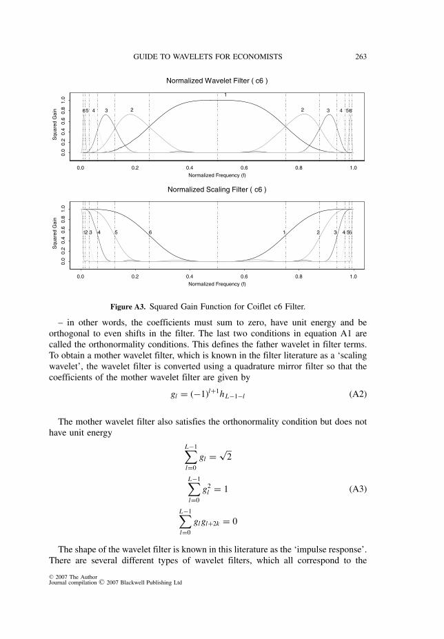
GUIDE TO WAVELETS FOR ECONOMISTS 263
0.0 0.2 0.4 0.6 0.8 1.0
Normalized Frequency (f)
0.0
0.2
0.4
0.6
0.8
1.0
Sq
ua
red
Ga
in
Normalized Wavelet Filter ( c6 )
65 4 3 2
1
2 3 4 56
0.0 0.2 0.4 0.6 0.8 1.0
Normalized Frequency (f)
0.0
0.2
0.4
0.6
0.8
1.0
Sq
ua
red
Ga
in
Normalized Scaling Filter ( c6 )
654321 1 2 3 4 56
Figure A3. Squared Gain Function for Coiflet c6 Filter.
– in other words, the coefficients must sum to zero, have unit energy and beorthogonal to even shifts in the filter. The last two conditions in equation A1 arecalled the orthonormality conditions. This defines the father wavelet in filter terms.To obtain a mother wavelet filter, which is known in the filter literature as a ‘scalingwavelet’, the wavelet filter is converted using a quadrature mirror filter so that thecoefficients of the mother wavelet filter are given by
gl = (−1)l+1hL−1−l (A2)
The mother wavelet filter also satisfies the orthonormality condition but does nothave unit energy
L−1∑l=0
gl =√
2
L−1∑l=0
g2l = 1
L−1∑l=0
gl gl+2k = 0
(A3)
The shape of the wavelet filter is known in this literature as the ‘impulse response’.There are several different types of wavelet filters, which all correspond to the
C© 2007 The AuthorJournal compilation C© 2007 Blackwell Publishing Ltd

264 CROWLEY
1 2 3 4 5
0.0
0.2
0.4
0.6
Scaling FilterT
ree A
& B
1 2 3 4 5 6 7
-0.2
0.2
0.6
Level 1:
NE
AR
SY
MA
Wavelet Filter
5 10 15
0.0
0.2
0.4
0.6
Tre
e A
5 10 15
-0.6
-0.2
0.2
0.6
Level >
1:
Q-S
hift C
5 10 15
0.0
0.2
0.4
0.6
Tre
e B
5 10 15
-0.6
-0.2
0.2
0.6
Level >
1:
Q-S
hift C
Figure A4. DTWT Filters. Top Row – level 1 Filters; Middle Row – Tree A Filters;Bottom Row – Tree B Filters.
wavelet types discussed in the main part of the text. Examples of these are asfollows:
1. Extremal phase filters – here energy increases rapidly – these are asymmetricfilters, which are also known as minimum phase filters or ‘daublets’, as theyroughly correspond to Daubechies wavelets.
2. Least asymmetric filters – filters in this group are smoother and are nearlysymmetric – the magnitudes of their discrete Fourier transforms are the same,and they correspond to symmlet wavelets.
3. Best localized filters – these filters are also nearly symmetric and they alsohave the same gain functions.
4. Coiflet filters – these filters approximate linear phase filters, and have differentgain functions from the other three types above – they clearly correspond to aCoiflet wavelet.
A DWT simply corresponds to repeated application of a chosen filter, which isoften referred to as a ‘filter bank’. Obviously for any scale level J, an amplitude-reduced and dilated filter can be derived (using the pyramid algorithm) for theoriginal data to be convolved with, giving one filter for each level of the transform.In this sense the filter bank acts as a band-pass filter, and the frequency response ofany combined filter can be obtained. For example, Figure A3 shows the frequencyresponse for a Coiflet 6 length filter at scale levels of J = 1, 2, . . ., 5.
C© 2007 The AuthorJournal compilation C© 2007 Blackwell Publishing Ltd

GUIDE TO WAVELETS FOR ECONOMISTS 265
Level 0
Level 1
Level 2
Level 3
Level 4
Level 5
Level 6
Level 7
Figure A5. MODWPT for Canadian Industrial Production.
For the DTWT, there are four types of scale filters and four types of wavelet filtersto select from. In Figure A4 nearsyma and Qshiftc filters are shown. The first rowof Figure A4 shows the filters that are applied to all of the data, then the second rowshows the filters that are applied to the first tree and the third row shows the filtersthat are applied to the second tree. Clearly the frequency response for the Qshiftscaling filter will be oriented towards the higher frequency parts of the series and thenearsyma wavelet filters will be oriented towards the lower frequency fluctuationsof the series.
C MODWT
Here we use matrix notation. Let x be a vector of N observations. The vector ofMODWT coefficients is given by
w = Wx (A4)
where W is the (J + 1)N × N matrix defining the MODWT, and so w is a (J + 1)Nvector of wavelet coefficients that result from the transform. Similarly to a DWT,the MODWT matrix W can be rewritten as
W =
⎡⎢⎢⎢⎢⎢⎢⎢⎢⎣
W1
W2
...
WJ
VJ
⎤⎥⎥⎥⎥⎥⎥⎥⎥⎦(A5)
C© 2007 The AuthorJournal compilation C© 2007 Blackwell Publishing Ltd

266 CROWLEY
1975 1981 1987 1993 1999
1.0
1.2
1.4
1.6
1.8
2.0
2.2
2.4
US
$/B
ritish p
ounds
1975 1981 1987 1993 1999
0.0
00.0
10.0
20.0
30.0
4
Abs(log(d
iff(
US
GB
P))
)
Figure A6. USD/GBP Exchange Rate: (a) Daily Exchange Rate; (b)Abs(diff(log(USD/GBP))).
where W1 is an N × N matrix representing the filter components at each scale level.But also each scale level in the matrix can be rewritten as
W1 = [h1
1 h21 h3
1 . . . hN−21 hN−1
1 h1
]T(A6)
for scale 1, where the vector of filter coefficients hk1 represent the rescaled jth scale
filter coefficients
h j = h j
2 j(A7)
where h j is the vector of DWT filter coefficients shifted k intergers to the right.In other words, the MODWT essentially takes a DWT and shifts the wavelet filters
one to the right to interweave with any given level of the equivalent DWT submatrixW. In practice a pyramid algorithm is used, but without the downsampling inherentin a DWT.
Figure A5 shows the MODWT packet table for Canadian industrial production.
D British Pound Exchange Rate
This daily series was taken from the Bank of England’s exchange rate database.The series runs from 1975 to 26 October 2004, and contains 7540 datapoints. The
C© 2007 The AuthorJournal compilation C© 2007 Blackwell Publishing Ltd

GUIDE TO WAVELETS FOR ECONOMISTS 267
original series and the absolute value of the log differenced series are plotted belowin Figure A6.
E Software
Software for wavelets is now quite widely available. SPLUS, R and Matlab havemodules for extensive wavelet analysis that can be separately purchased from thepublishers themselves, and the R wavelet module is available as freeware for usewith the open-source R statistical software. Apart from this, software is availablefor specialist wavelet applications, for example Autosignal implements the CWTsspectral analysis described in this paper, and freeware is also available to implementthis with Matlab. An additive package called TSM is available for GAUSS as well,although this appears to only do a limited degree of wavelet analysis.
For the multivariate spectral analysis using the Hilbert wavelet pairs, Matlab codeis available from Selesnick’s website for deriving the near-HWP pairs, while thewaveslim package in R has been made available by Brandon Whitcher for doingmultivariate spectral analysis.
C© 2007 The AuthorJournal compilation C© 2007 Blackwell Publishing Ltd