SpatioTemporal Wavelets: A Group-Theoretic Construction for Motion Estimation and Tracking

SPATIAL NOISE STABILIZES PERIODIC WAVE PATTERNS INOSCILLATORY SYSTEMS ON FINITE DOMAINS∗

ALISON L. KAY† AND JONATHAN A. SHERRATT‡

SIAM J. APPL. MATH. c© 2000 Society for Industrial and Applied MathematicsVol. 61, No. 3, pp. 1013–1041

Abstract. Invasions in oscillatory systems generate in their wake spatiotemporal oscillations,consisting of either periodic wavetrains or irregular oscillations that appear to be spatiotemporalchaos. We have shown previously that when a finite domain, with zero-flux boundary conditions,has been fully invaded, the spatiotemporal oscillations persist in the irregular case, but die out in asystematic way for periodic traveling waves. In this paper, we consider the effect of environmentalinhomogeneities on this persistence. We use numerical simulations of several predator-prey systemsto study the effect of random spatial variation of the kinetic parameters on the die-out of regularoscillations and the long-time persistence of irregular oscillations. We find no effect on the latter, butremarkably, a moderate spatial variation in parameters leads to the persistence of regular oscillations,via the formation of target patterns. In order to study this target pattern production analytically, weturn to λ–ω systems. Numerical simulations confirm analagous behavior in this generic oscillatorysystem. We then repeat this numerical study using piecewise linear spatial variation of parameters,rather than random variation, which also gives formation of target patterns under certain circum-stances, which we discuss. We study this in detail by deriving an analytical approximation to thetargets formed when the parameter λ0 varies in a simple, piecewise linear manner across the do-main, using perturbation theory. We end by discussing the applications of our results in ecology andchemistry.

Key words. oscillatory systems, periodic waves, spatial noise

AMS subject classifications. 92C50, 92C15, 35M10, 34C05

PII. S0036139999360696

1. Introduction. Invasions are a widespread phenomenon in biology and chem-istry, for instance, the spread of one animal population into a region occupied byanother, the invasion of a wound space by a surrounding cell population, the move-ment of a reaction front as one chemical is converted to another, etc. Mathematicalmodeling of invasions is extensive, dating back to Fisher’s work [10] on the spread ofan advantageous gene and Skellam’s [32] use of a reaction diffusion equation to studyecological invasion. Recent modeling work predicts that many of the most interestinginvasion effects occur in oscillatory systems, such as cyclic predator-prey interactionsor oscillatory chemical reactions.

Although some work has been done on spatially and/or temporally discrete modelsfor oscillatory systems [17, 37, 29], the most widely used model type is an oscillatorysystem of reaction-diffusion equations. By this, we mean that the kinetic ordinarydifferential equations contain a stable limit cycle. In models of this type, invasionsleave behind them spatiotemporal oscillations. These can be simply a periodic wave-train moving in parallel with the invasion [6], but in many cases have the form ofeither a wave-train moving more rapidly than the invasion, or a complex pattern ofirregular spatiotemporal oscillations [28]. These latter behaviors occur via a complex

∗Received by the editors August 24, 1999; accepted for publication (in revised form) May 14,2000; published electronically October 11, 2000.

http://www.siam.org/journals/siap/61-3/36069.html†Mathematics Institute, University of Warwick, Coventry CV4 7AL, UK. Current address: Centre

for Ecology and Hydrology, Wallingford, Oxon, OX10 8BB, UK ([email protected]). The research ofthis author was supported in part by a graduate studentship from the Engineering and PhysicalSciences Research Council.

‡Department of Mathematics, Heriot-Watt University, Edinburgh EH14 4AS, UK ([email protected]).

1013

1014 ALISON L. KAY AND JONATHAN A. SHERRATT

wave-train selection mechanism [28, 30], with irregular oscillations arising when theselected wave-train is unstable. Related instances of irregular oscillations generatedin oscillatory reaction diffusion systems are given in [25, 9, 20].

Recently, we studied the long-term behavior of these spatiotemporal oscillationsafter the whole of a finite domain had been invaded, for the most important case ofzero-flux conditions at the ends of the domain [13]. We considered the case when theinvasion (for example, of a prey population by predators) is initiated at one end of thedomain and spreads across to the other end. Numerical simulations showed that whenirregular oscillations are generated behind the invasion, these persist after the wholedomain has been invaded—even in very long time simulations. Contrastingly, whenregular spatiotemporal oscillations were generated these died out towards the purelytemporal oscillations of the limit cycle. This die-out begins with a decrease in thespatial frequency of the oscillations at one side of the domain, which then progressesacross the domain, with a simultaneous progression of increase in the amplitude ofthe oscillations (to the limit cycle amplitude). In order to study the manner of thedie-out in more detail we used a caricature model, which showed the same phenomenaof persistence of irregular oscillations and die-out of regular oscillations in numericalsimulations. Analysis of this simpler system then gave an approximation to the tran-sition fronts occuring during the die-out, and a measure of the rate of die-out, in termsof model parameters, which can be related back to the parameters in more generaloscillatory systems in some cases.

The results of this previous work can only be applied to real oscillatory systemsonce two key questions have been answered. First, are the phenomena seen in ho-mogeneous environments robust to the introduction of inhomogeneities? In addition,will inhomogeneities result in new phenomena, not seen in the homogeneous case?Examples of the latter have been observed in nature. In the Belousov–Zhabotinskiireaction it is known that target patterns almost always have an impurity in the center,and so occur in fewer numbers in a highly purified system [38]. It is also thought thatinhomogeneities are necessary for the formation of spiral waves in cardiac tissue [27];it is these spiral waves which result in abnormal heart rhythms.

There are clearly many ways in which spatial inhomogeneity can be created.We focus on achieving this inhomogeneity by spatial variation of parameters, andthere are two very different means of accomplishing this; either there is a simple,functional variation with spatial position imposed on some parameter(s), or the vari-ation is “noisy”—randomly generated. Much of the work on the latter has been withspatiotemporal noise, rather than the purely spatial noise which we consider. Anexception is the work, on discrete time and space models of host-parasitoid interac-tions, by Comins, Hassell, and May [5] and Holt and Hassell [12], in which it is shownthat noisy spatial variation of demographic parameters can stabilize the system. Inparticular, in [5], it is demonstrated that spiral patterns and spatiotemporal chaosremain clearly evident even with quite high levels of noisy patch-to-patch variation.Lattice patterns, however, are easily disrupted.

The possibilities for functional variation of parameters are huge, and so the con-sequences cannot be described generally, but we discuss various examples below. Forreaction-diffusion equations, explicit spatial variation has been shown to have impor-tant consequences in the areas of traveling wave propagation and pattern formation.In [39], Xin considered a scalar reaction-diffusion equation with a cubic kinetic term,where the diffusion coefficient is allowed to vary with spatial position. He showed that,if the variation of the diffusion coefficient from its mean is sufficiently large, then trav-

SPATIAL NOISE STABILIZES PERIODIC WAVE PATTERNS 1015

eling waves no longer exist, so that a wave front will begin to propagate from giveninitial conditions, but will then stop advancing—a phenomenon known as quench-ing. A similar result was found in [33], where Sneyd and Sherratt model calciumwave propagation in inhomogeneous media. Calcium waves can be either excitable orself-oscillatory. In the excitable regime, the authors used a scalar reaction-diffusionequation on a domain with a “gap”—a region where the kinetics are set to zero—toderive a critical gap width, above which waves cannot propagate. In the oscillatoryregime, they used a piecewise constant spatial variation of the kinetics, in a systemof two reaction-diffusion equations, with periodic regions where the kinetics are setto zero, and demonstrated numerically how these passive regions disturb the periodicplane waves which propagate behind an invading front. Piecewise constant spatialvariation was also used by Shigesada [31] to study the effects of a heterogeneousenvironment on the spread of a single species. There, an invasion condition was de-termined, which depended on the patch sizes and on the diffusivities and growth ratesof the species within the two different types of patch.

The consequences of spatial variation for pattern formation are less obvious, butjust as important in reality. Although the Turing mechanism for pattern formationhas been widely studied, the usual assumption of a uniform domain often does notfit with that used in experiments or in natural pattern forming systems. It has beenshown that allowing spatial variation of parameters, in ways which are more applicableto experiments or nature, can lead to quite major alterations in the patterns whichcan be expected at different points in parameter space, and the bifurcation sequencesobserved [1, 2].

Spatial heterogeneity has also been shown to have quite major effects on interact-ing populations. Using a system of two weakly coupled reaction-diffusion equationswith spatial variation of the kinetics, Cantrell, Cosner, and Hutson [3] showed that thespatial heterogeneity resulted in the permanence of populations which would other-wise have become extinct. Also, Pascual [24] showed that large-scale spatial variationin kinetics can induce chaotic oscillations in cyclic predator-prey systems. Spatialheterogeneity can also lead to a different outcome of competition than that whichoccurs in a spatially homogeneous environment [23, 4], and to altered success of thepredator in predator-prey systems, depending upon the location of favorable huntinggrounds [4].

The effects of spatial variation have also been investigated in spatially discretesystems. Chains of coupled oscillators can be used to model lamprey locomotion,and any variation of parameters along the length of the fish could be important toits swimming efficiency. Kopell and Ermentrout [16] analyzed a system of N weaklycoupled oscillators, in the continuum limit as N → ∞, where the natural frequency ofthe oscillator, and its coupling strength to each of its neighbors, were allowed to varysmoothly and slowly along the chain. A special case which they consider is where thereis a local region of lower/higher natural frequencies (with coupling strengths equalalong the chain). They show that a sufficiently large frequency difference can resultin effects not localized to the region of the chain with altered frequencies—includingreversal in direction of the wave from the changed region to one of the boundaries.Similar effects are shown to result from local regions of weakened coupling.

The existence of target pattern solutions of reaction-diffusion systems on infinitedomains has been extensively studied. Hagan [11] showed that stable target patternsexist whether or not impurities are present, but that they will arise from typical initialconditions only if impurities which tend to locally increase the frequency are present.


Kopell [15] used a similar approach in the special case of λ–ω systems, showing thatsuch a local increase in frequency is sufficient to produce one- or two-dimensionaltarget patterns, but that it has to be sufficiently large, in magnitude and extent, toproduce three-dimensional patterns.

In this paper, we consider the effect of spatial inhomogeneities on the persistenceof oscillations on a finite (one-dimensional) domain with zero-flux boundary condi-tions. Although our analytical results are quite general we use cyclical predator-preysystems as a case study, in order to have a specific application in mind. We begin(section 2) by presenting the results of numerical simulations of invasion of a noisy do-main for predator-prey systems in the oscillatory regimes, considering the long-termbehavior, after the invasion front has crossed the domain. We use the term “noisydomain” to mean that the parameters vary randomly across the spatial domain, butare fixed in time. Then, in sections 3 and 4, we use a caricature model to studythe behavior in more detail; first verifying that the same behavior is seen for noisyvariation of parameters, then using a piecewise linear change in the parameters acrossthe domain.

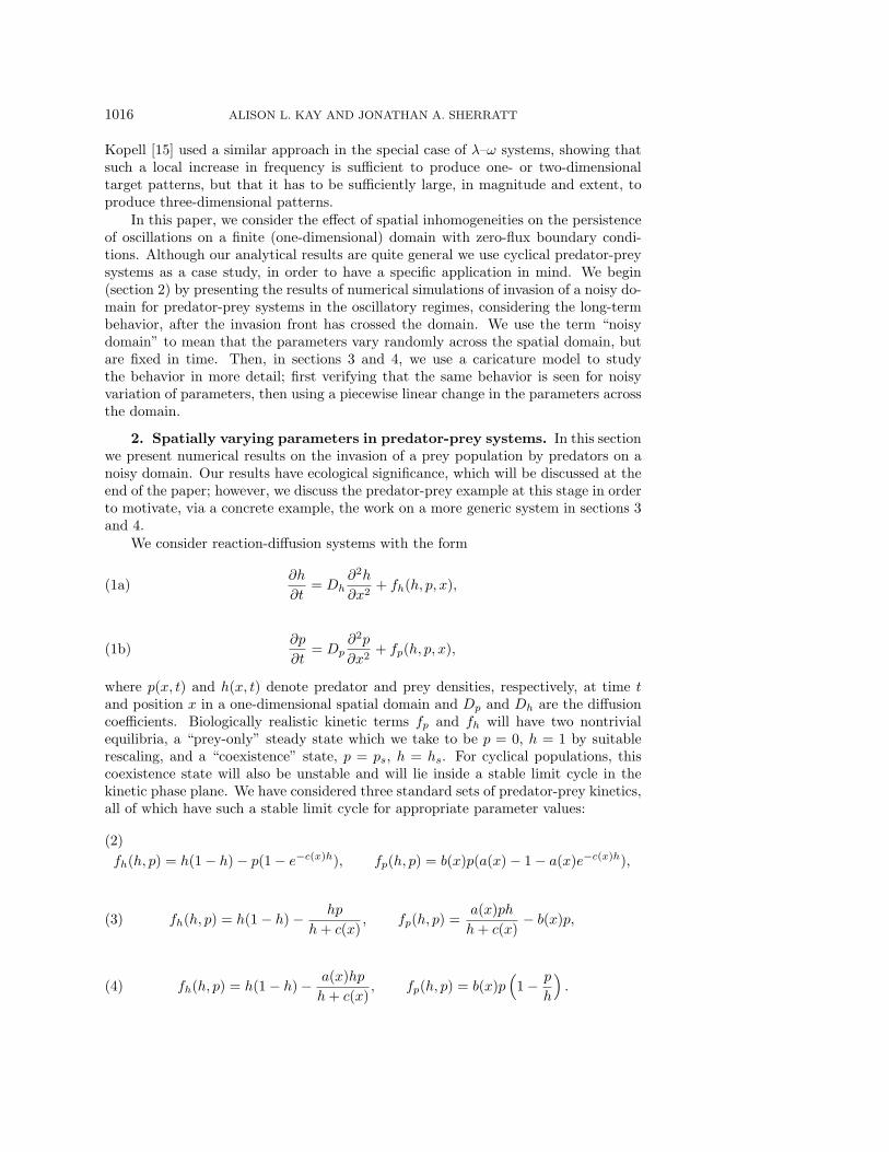
2. Spatially varying parameters in predator-prey systems. In this sectionwe present numerical results on the invasion of a prey population by predators on anoisy domain. Our results have ecological significance, which will be discussed at theend of the paper; however, we discuss the predator-prey example at this stage in orderto motivate, via a concrete example, the work on a more generic system in sections 3and 4.

We consider reaction-diffusion systems with the form

∂h

∂t= Dh

∂2h

∂x2+ fh(h, p, x),(1a)

∂p

∂t= Dp

∂2p

∂x2+ fp(h, p, x),(1b)

where p(x, t) and h(x, t) denote predator and prey densities, respectively, at time tand position x in a one-dimensional spatial domain and Dp and Dh are the diffusioncoefficients. Biologically realistic kinetic terms fp and fh will have two nontrivialequilibria, a “prey-only” steady state which we take to be p = 0, h = 1 by suitablerescaling, and a “coexistence” state, p = ps, h = hs. For cyclical populations, thiscoexistence state will also be unstable and will lie inside a stable limit cycle in thekinetic phase plane. We have considered three standard sets of predator-prey kinetics,all of which have such a stable limit cycle for appropriate parameter values:

fh(h, p) = h(1− h)− p(1− e−c(x)h), fp(h, p) = b(x)p(a(x)− 1− a(x)e−c(x)h),

(2)

fh(h, p) = h(1− h)− hp

h+ c(x), fp(h, p) =

a(x)ph

h+ c(x)− b(x)p,(3)

fh(h, p) = h(1− h)− a(x)hp

h+ c(x), fp(h, p) = b(x)p

(1− p

h

).(4)


Here a(x), b(x), and c(x) are positive parameters in all cases. Pascual [24] has pre-viously studied models of this type with large-scale, linear variations in parametervalues, showing that this can induce chaotic oscillations. Here we consider the quitedifferent case of small spatial oscillations in parameter values.

We begin by presenting the results of numerical simulations of invasion on finitespatial domains where the kinetic parameters a, b, c are allowed to vary in a randomway across the domain. We solve (1) with (2), (3) or (4) numerically on 0 < x < L,with zero-flux boundary conditions at x = 0 and x = L, and initial conditions h =1, p = 0 on l < x < L for some l L, with a nonzero initial value of p on 0 < x < l.This corresponds to the introduction of predators at one edge of a domain that isotherwise occupied entirely by prey. However, we also initially generate a randomvariation of some or all of the kinetic parameters (a, say) across the domain. We dothis by choosing “average” values for each of the parameters (aav) and a maximumpercentage by which we will allow them to vary (P ). We then generate the values ofeach parameter at each point in our spatial grid by using a random number generatorto choose a number between −1 and 1 (ρ, say, calculated from a uniform distribution),and setting a = aav + aav × ρ×P/100. Thus we do not change the sign of any of theparameters (all of which are positive), so the nature of the species interactions remainsunchanged; we are simply changing the relative effects of each of the terms at eachspace point, to model varying quality of the habitat. (Note that, if the percentagevariation is large enough, we may, of course, be choosing the parameters at a pointin space in such a way that the stable limit cycle does not exist at that point.) Wethen solve using a Crank–Nicolson scheme, in order to determine the effect that thespatial noise in the parameter values has on the observed behavior of persistence ofoscillations after invasion; the corresponding behavior for homogeneous domains wasdescribed in [13] and was summarized in section 1.

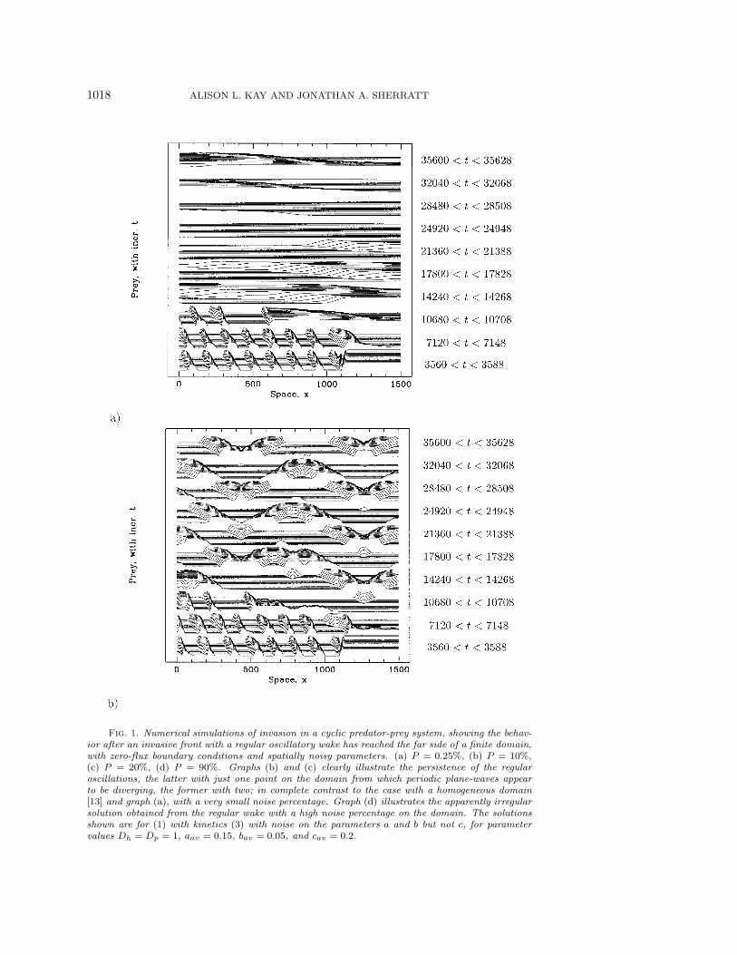
Numerical simulations for a range of parameters show a clear pattern of behavior.As one might expect, the noisy spatial variation of the parameters has no effect onthe persistence of irregular oscillations after the invasion of a front with an irregularwake. A very small amount of noise similarly has no noticeable effect on the die-out ofthe regular oscillations after the invasion of a front with a regular wake (Figure 1(a)).Specifically, the die-out occurs as a transition moving across the domain in the op-posite direction to the invasion, with a gradual increase in spatial wavelength andamplitude of the spatiotemporal oscillations. However, we found that a moderatelevel of noise could lead to persistence of regular oscillations, but usually of a dif-ferent spatial frequency than that generated behind the invasion, and with sectionsof the domain having the wave-trains traveling in opposite directions (Figures 1(b)and 1(c)). The regular oscillations produced do, though, have a slightly noisy mod-ulation of their regular shape. The frequency of the periodic plane-wave selectedappears to depend upon the amount of noise—the larger the noise percentage thehigher the frequency—until too large a noise percentage results in the breakdown ofthe regular-looking solution to an irregular-looking one (Figure 1(d)).

The same results were seen if we chose the parameter values randomly at fewer ofthe space points, interpolating for the values at intervening points, or if just a smallregion of the domain had parameter noise, with the parameters taking their averagevalues outside of this region.

If we continue the integration from a time long after an invading front has crossedthe domain, resetting the values of the parameters at each space point to their av-erage values, the periodic plane-waves again die out from the whole of the domain.This occurs in a manner similar to that after the invasion of a wave front with a


Fig. 1. Numerical simulations of invasion in a cyclic predator-prey system, showing the behav-ior after an invasive front with a regular oscillatory wake has reached the far side of a finite domain,with zero-flux boundary conditions and spatially noisy parameters. (a) P = 0.25%, (b) P = 10%,(c) P = 20%, (d) P = 90%. Graphs (b) and (c) clearly illustrate the persistence of the regularoscillations, the latter with just one point on the domain from which periodic plane-waves appearto be diverging, the former with two; in complete contrast to the case with a homogeneous domain[13] and graph (a), with a very small noise percentage. Graph (d) illustrates the apparently irregularsolution obtained from the regular wake with a high noise percentage on the domain. The solutionsshown are for (1) with kinetics (3) with noise on the parameters a and b but not c, for parametervalues Dh = Dp = 1, aav = 0.15, bav = 0.05, and cav = 0.2.


Fig. 1. continued.


regular wake into an homogeneous domain, but with the decrease in frequency of thespatial oscillations occurring first at the points from which the wave-trains appearto be diverging, and progressing outwards from there, rather than beginning at oneof the boundaries. The solution then evolves towards purely temporal oscillations,corresponding to the limit cycle of the kinetics. This die-out to the purely temporaloscillations of the limit cycle still occurs in most cases for the irregular-looking behav-ior produced from regular wakes on domains with large noise percentages. We have,though, found cases where irregular oscillations are produced from regular wakes bythe high noise percentages and persist even when the noise is stopped.

We note here that we can expect there to be some dependence of results on thesize of the domain used. In cases where dynamic spatial patterning can appear, it willhave some characteristic length scale associated with it, and in order for the pattern tobe apparent we require the domain to be sufficiently larger than this pattern’s lengthscale; just as the form of Turing patterns is dependent on the size of the domain [21,pp. 436–448]. We have always worked with domains which are large compared to theperiod of the wave-train generated behind invasion.

The ecological implications of these results will be discussed in section 5. Priorto this, we study in more detail the way in which spatial heterogeneity can lead topersistence of regular oscillations, using a caricature system of oscillatory reaction-diffusion equations.

3. Spatially varying parameters in λ–ω systems.

Background. We have been unable to make any progress studying the predator-prey models (1) with (2), (3) or (4) analytically, for general parameter values. How-ever, there is a special case in which the systems are much more amenable to analysis,namely for kinetic parameters close to the Hopf bifurcation, and for equal predatorand prey diffusion coefficients. In this case the kinetics can be approximated by theHopf normal form, giving

∂u

∂t=∂2u

∂x2+ λ(r)u− ω(r)v,(5a)

∂v

∂t=∂2v

∂x2+ ω(r)u+ λ(r)v,(5b)

where u and v represent appropriate linear combinations of the predator and preydensities p and h. Here r = (u2 + v2)

12 , with λ(r) = λ0(x) − λ1r

2 and ω(r) =ω0(x) − ω1r

2, where λ0, λ1 > 0, and we allow λ0, ω0 to vary with spatial position x.Note that the system (5) is very general, being the normal form of any oscillatoryreaction-diffusion system close to Hopf bifurcation, provided the variables have thesame diffusion coefficient. Thus our calculations will apply to a range of applicationsin addition to ecology, and this is discussed further in section 5.

Reaction-diffusion systems of the form (5) are known as “λ–ω systems,” andwere first studied by Kopell and Howard [14]. The key to the analytical study of suchsystems is to work in terms of polar coordinates in the u-v plane, r and θ = tan−1 v/u,in terms of which (5) becomes

∂r

∂t=∂2r

∂x2− r

(∂θ

∂x

)2

+ r(λ0(x)− λ1r2),(6a)

∂θ

∂t=∂2θ

∂x2+

2

r

∂r

∂x

∂θ

∂x+ (ω0(x)− ω1r

2).(6b)


From this formulation, when λ0(x) ≡ λ0 and ω0(x) ≡ ω0, it is clear that there isa spatially homogeneous circular limit cycle solution, with amplitude (radius) rc =

(λ0/λ1)12 . Moreover, there is a family of periodic wave-train solutions, which are

also circular in the u-v plane, with amplitude r for any r < rc. The form of thesewave-train solutions is easily determined: substituting r(x, t) = r, a constant, into (6)implies θ(x, t) =

√λ(r)x+ ω(r)t+ θ0, where θ0 is an arbitrary constant, which may

be set to zero without loss of generality. Thus the periodic waves have the form

u(x, t) = r cos θ(x, t)= r cos(√λ(r)x+ ω(r)t),

v(x, t) = r sin θ(x, t)= r sin(√λ(r)x+ ω(r)t).

Thus we have a sinusoidal periodic plane wave moving with speed ω(r)/√λ(r) in the

negative x-direction. There is also the mirror image wave, where θ(x, t) = −√λ(r)x+ω(r)t, which moves with the same speed in the positive x-direction.

Kopell and Howard [14] derived a stability condition for the periodic wave-trainsolutions of λ–ω systems, which in the case of (6) with λ0(x) ≡ λ0 and ω0(x) ≡ ω0

shows that the periodic plane waves are stable if and only if their amplitude r > rc,

where rc =[

2λ0

λ1

(λ2

1+ω21

3λ21+2ω2

1

)]1/2. The existence of this precise stability result is in

sharp contrast to more general oscillatory reaction-diffusion systems, for which resultson stability of periodic waves are quite limited [22, 19].

Numerical simulations with parameter noise. We cannot use λ–ω systemsto mimic the invasion process used for predator-prey equations, as there is no equiv-alent of the prey-only equilibrium, but we can investigate persistence of oscillationsby using appropriate initial conditions. Thus to investigate the persistence of reg-ular oscillations on finite domains with zero-flux boundary conditions we solve theequations numerically with initial conditions consisting of a periodic plane-wave ofstable amplitude r > rc on the whole of the domain (which is taken sufficiently largecompared to the period of the plane-wave). We consider behavior arising from theseinitial conditions when the parameters λ0 and ω0 vary randomly with spatial positionx, in the same way as was described for the parameters in the predator-prey equationsin the preceding section.

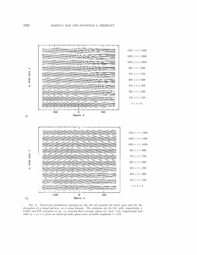
Our results showed that, for a very small variation of the parameters, the regularoscillations still die out, towards the purely temporal oscillations of the limit cycle(although this is now “noisy”—its amplitude varies slightly with x) (Figure 2(a)).Figure 3 illustrates this die-out plotted in terms of r and θx, and clearly shows thatit is occuring via transition fronts in r and θx, starting from the right-hand side andprogressing across the domain from there. This is identical to the die-out of regularoscillations seen on homogeneous domains, and thus the analysis done in that case[13], where approximations to the transition fronts were derived and an estimate ofthe rate of die-out in terms of parameters was obtained, still applies for sufficientlysmall noisy variations.

For larger parameter variations though, numerical simulations again show per-sistence of regular oscillations. However, these oscillations do not consist just of asingle wave-train traveling across the domain; rather the domain is divided into atleast two regions, with a wave-train traveling in the opposite direction, but in phase,in neighboring regions. That is, we get one-dimensional versions of a series of eithertarget patterns or shocks (Figure 2(b)). Note that the term “target pattern” refersto wave-trains diverging from a point, meaning that the group velocities are directed


a)

1351 < t < 1358

1201 < t < 1208

1051 < t < 1058

901 < t < 908

751 < t < 758

601 < t < 608

451 < t < 458

301 < t < 308

151 < t < 158

1 < t < 8

b)

1351 < t < 1358

1201 < t < 1208

1051 < t < 1058

901 < t < 908

751 < t < 758

601 < t < 608

451 < t < 458

301 < t < 308

151 < t < 158

1 < t < 8

Fig. 2. Numerical simulations showing (a) the die-out towards the limit cycle and (b) theformation of a target pattern, on a noisy domain. The solutions are for (5), with, respectively, a0.25% and 15% variation in λ0, ω0 (around their average values of 1 and −1/2, respectively) andwith λ1 = ω1 = 1, from an initial periodic plane-wave of stable amplitude r = 0.9.


Fig. 3. An illustration of the solution shown in Figure 2, replotted in terms of r and θx. Thisshows that the initial regular oscillations are dying out in a way which is identical to that whichoccurs on a homogeneous domain, except with a noisy modulation. As in Figure 2, λ0 and ω0have a maximum noisy variation of 0.25% around average values of 1 and −0.5, respectively, andλ1 = ω1 = 1. The solutions are plotted as a function of space x (−150 < x < 150), at equally spacedtimes (interval 20); the arrows indicate the direction in which the solutions evolve as time increases.

outwards—the phase velocities could be going in either direction, depending on theexact form of ω(·); the case with wave-trains converging on a point (group velocitiesdirected inwards) is usually referred to as a “shock.”

The changing of direction of the wave-trains can be seen more clearly by re-plotting in r, θx coordinates, where sections of “constant” r and θx show the periodicplane-waves (although there will be a noisy modulation of these constant values), anda change in sign of θx shows the change in direction of the wave-train (Figure 4). Theway in which θx changes sign—that is, whether it changes from negative to positive orfrom positive to negative as x increases—(along with the sign of w(·) evaluated at thewave-train amplitude) then tells us whether we actually have a target or a shock. Thisformulation of the results also allows us to see that a steady state has been reached,as continuing the integration further results in no significant change to the r, θx plots.However, if we continue the integration having reset the parameters to their averagevalues, we see the periodic plane-waves dying out in a manner similar to that seen onthe homogeneous domain, except that it occurs symmetrically from either side of thepoint at which the target pattern was centered, rather than progressing inwards fromone side of the domain.

Again, to confirm that we are not seeing a numerical artifact, we allow noisyvariation of the parameters at fewer space points, interpolating for the values atintervening points, or having just one section of the domain with noisy parameters,with the parameters taking their average values on the rest of the domain. Thesesimulations still result in target pattern solutions appearing. The solutions in each


Fig. 4. An illustration of the final time-plot of the solution in Figure 2(b), replotted in terms ofr and θx. This shows clearly the sections of “constant” r and θx values to either side of a change insign of θx, so illustrates that we have plane-waves converging on/diverging from a central point; ashock/target. It is actually a target rather than a shock, as the group speed of the plane-wave to theleft of the point is negative and that to the right is positive, so the two waves are diverging from thepoint. Due to our choice of the function ω(r) = −1/2− r2, the phase velocities are directed towardsthe point, and so the waves will appear (on a graph where the time interval between successive timeplots is sufficiently small) to be converging on the point.

case are essentially the same; the only difference being a slightly longer transitionaryperiod.

Numerical simulations with piecewise linear λ0 and ω0. It is obviouslydifficult to get analytic results, even in λ–ω systems, when we have allowed noisyvariation of the parameters. In this section then, we consider an explicit functionalvariation of the parameters, which we will show gives similar numerical results tothose for noisy parameters—in particular, giving one-dimensional target patterns ifthe domain is sufficiently large—and then, in section 4, we attempt to obtain anapproximate solution in this case. Work in this simpler case may also give us someinsight into why target patterns are produced when the parameters are allowed tovary randomly across the domain.

Before we begin, we use rescalings to simplify the system. The most generalsystem in our required form is

∂r

∂t=∂2r

∂x2− r

(∂θ

∂x

)2

+ r(λ0(x)− λ1r2),(7a)


∂θ

∂t=∂2θ

∂x2+

2

r

∂r

∂x

∂θ

∂x+ (ω0(x)− ω1r

2) ;(7b)

we will drop the tildes after rescaling the variables. Here the variation of λ0, ω0

with x which we consider is piecewise linear, taking a constant value in most ofthe domain, and a different constant value in a region in the center, with a linear

variation between the two values. Mathematically, we set λ0(x) = λ0(1 + ρλεf(x))

and ω0(x) = ω0(1 + ρωεf(x)), where λ0, ω0 are constants (λ0 > 0), ρλ,ω are −1, 0

or +1, ε is a small parameter, the domain is −xmax < x < xmax and f(·) reflectsthe piecewise linear variation and is defined explicitly below. We simplify the systemusing the rescalings

Ω0 = ω0/λ0, x = x/

√λ0, θ = θ,

Ω1 = ω1/λ1, t = t/λ0, r = r

√λ0/λ1,(8)

in terms of which equation (7) becomes

∂r

∂t=∂2r

∂x2− r

(∂θ

∂x

)2

+ r(λ0(x)− r2),(9a)

∂θ

∂t=∂2θ

∂x2+

2

r

∂r

∂x

∂θ

∂x+ (Ω0ω0(x)− Ω1r

2),(9b)

where λ0(x) = 1+ρλεf(x), ω0(x) = 1+ρωεf(x), and f(x) = f(x/√λ0). Thus we have

a system where the limit cycle on a homogeneous domain (f ≡ 0) has amplitude 1.To be specific, we take Ω0 < 0, Ω1 > 0, which implies that ω(r) = Ω0ω0(x)−Ω1r

2 < 0for all 0 < r < 1. (This makes it easier to distinguish targets from shocks). We takef(·) to have the form

f(x) =

x2 + x

x2 − x1on − x2 < x < −x1,

1 on − x1 < x < x1,x2 − x

x2 − x1on x1 < x < x2,

0 otherwise,

(10)

where x1, x2 satisfy 0 < x1 < x2 < xmax.In our numerical simulations of (9), we expect the size of the domain to affect

the results, and so we consider the specific cases xmax = 10 and xmax = 100, withx1 = x2/2 = xmax/4. For a fixed value of ε (taken to be 0.01), we can summarize ourresults as follows.

When we decrease λ0 or increase ω0 in a region in the center of the domain:• For xmax = 100, we observe bands of periodic plane waves to either side of thecentral region, converging (with phase velocity) to the center. Thus a changein sign of θx occurs at x = 0, changing from positive to negative as x increasesthrough zero. That is, we obtain a target pattern solution (Figure 5(a)).

• For xmax = 10, there is still a change in sign of θx at x = 0, however thereare no obvious periodic plane-waves (Figure 5(b)).


Fig. 5. Graphs illustrating examples of r and θx plots in each of four cases: (a) xmax = 100,λ0 decreased (ρλ = −1), (b) xmax = 10, λ0 decreased (ρλ = −1), (c) xmax = 100, λ0 increased(ρλ = +1), (d) xmax = 10, λ0 increased (ρλ = +1), showing the qualitative differences obtained(solid lines). The dashed lines indicate the region boundaries (−x2,−x1, x1, x2). All of the plotsare solutions of (9) with ρω = 0 (ω0(x) ≡ 1), Ω0 = −1/2, Ω1 = 1, where f(x) is given in (10) andε = 0.01, plotted at t = 2000, from initial conditions of a periodic plane-wave of stable amplituder = 0.9.

When we increase λ0 or decrease ω0 in the center of the domain:

• For xmax = 100, we observe a small band of periodic plane-waves in the centralregion, with little/no spatial variation outside of the region. The plane-wavesmove in one direction; no change in sign of θx occurs (Figure 5(c)).

• For xmax = 10, we now get a change in sign of θx at x = 0, but changing fromnegative to positive as x increases through zero. No periodic plane waves areevident (Figure 5(d)).

If both λ0 and ω0 are changed, by the same amount ε,

• our results suggest that the form of the solution is determined by the directionof change of λ0. For example, when both λ0 and ω0 are increased on a domainwith xmax = 100, we see just one band of periodic plane waves, in the centerof the domain—not a target pattern, as would occur if ω0 was increased butλ0 remained unchanged across the domain.

Discussion of results of numerical simulations. On a small domain, weexpect that we may not see spatial variation, as it will be the change in the parametervalues in the center of the domain which will select the wavelength of the periodicplane-waves, and if this wavelength is larger than the domain size, the periodic plane-waves will not be seen. This domain size effect is demonstrated numerically by doingsimulations on the small domain with larger values of ε; eventually ε is large enough forsmall regions with constant r and θx to begin to develop—corresponding to periodicplane-waves beginning to form. (We remark, however, that when ε is taken too large,


Fig. 6. Graphs illustrating the change in the form of the steady solution on a large domainwhen ε is decreased, for (a) ε = 0.1, (b) ε = 0.01, and (c) ε = 0.001 (solid lines). The dashed linesindicate the region boundaries (−x2,−x1, x1, x2). The solutions shown are for (9) with ρλ = −1,ρω = 0 (ω0(x) ≡ 1), Ω0 = −1/2, Ω1 = 1, where f(x) is given in (10), and is plotted at t = 2000from an initial periodic plane-wave of stable amplitude r = 0.9.

the solution no longer settles down to a steady state. Instead, the point at whichθx = 0 oscillates between −x2 and x2, with a similar oscillation in the shape ofr). Equivalently, periodic plane-waves will not appear on large domains if ε is takensufficiently small (the critical size of which is dependent upon the domain size), asillustrated in Figure 6(c).

On large domains, the form of the periodic plane-waves which develop when λ0

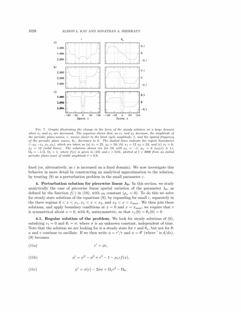
is decreased in the center is dependent upon the value of ε; smaller values of ε leadto waves with an amplitude closer to 1 (the limit cycle amplitude) and a frequencycloser to 0, until they are no longer evident for very small ε. This is because thesize of the region of the domain in which they form—where flat sections of the r, θxplots are seen—shrinks as ε decreases; it is “eaten into” by boundary effects. Thisis illustrated in the sequence of graphs in Figure 6. Decreasing the values of x1 andx2 also has the effect of increasing the amplitude and decreasing the frequency of theselected periodic plane-wave; only very slowly at first, but then faster, as x1, x2 → 0.This effect is illustrated by the series of graphs in Figure 7. The value of x2 can alsoaffect the extent of the plane-waves: intuitively, a value of x2 closer to xmax leavesless room for the plane-waves, as they only occur in regions outside of −x2 < x < x2.

The complete difference in the form of the solutions when λ0 is increased or de-creased in the center of a large domain is striking. When λ0 is decreased, the symmetryof the domain is maintained by the solution which evolves from the nonsymmetric ini-tial conditions—a one-dimensional target pattern. The same is true of the solutionon a smaller domain (for a fixed ε) (compare Figures 5(a) and (b)). However, whenλ0 is increased, the domain symmetry is broken by the solution which evolves on alarge domain, whereas it is maintained on small domains (compare Figures 5(c) and(d)). Symmetry breaking must then occur as the domain size is increased, with ε


Fig. 7. Graphs illustrating the change in the form of the steady solution on a large domainwhen x1 and x2 are decreased. The sequence shows that, as x1 and x2 decrease, the amplitude ofthe periodic plane-waves, r, moves closer to the limit cycle amplitude, 1, and the spatial frequencyof the periodic plane waves, θx, decreases to 0. The dashed lines indicate the region boundaries(−x2,−x1, x1, x2), which are taken as (a) x1 = 25, x2 = 50; (b) x1 = 12 x2 = 24; and (c) x1 = 6,x2 = 12 (solid lines). The solutions shown are for (9) with ρλ = −1, ρω = 0 (ω0(x) ≡ 1),Ω0 = −1/2, Ω1 = 1, where f(x) is given in (10) and ε = 0.01, plotted at t = 3000 from an initialperiodic plane-wave of stable amplitude r = 0.9.

fixed (or, alternatively, as ε is increased on a fixed domain). We now investigate thisbehavior in more detail by constructing an analytical approximation to the solution,by treating (9) as a perturbation problem in the small parameter ε.

4. Perturbation solution for piecewise linear λ0. In this section, we studyanalytically the case of piecewise linear spatial variation of the parameter λ0, asdefined by the function f(·) in (10), with ω0 constant (ρω = 0). To do this we solvefor steady state solutions of the equations (9), by expanding for small ε, separately inthe three regions 0 < x < x1, x1 < x < x2, and x2 < x < xmax. We then join thesesolutions, and apply boundary conditions at x = 0 and x = xmax; we require that ris symmetrical about x = 0, with θx antisymmetric, so that rx(0) = θx(0) = 0.

4.1. Regular solution of the problem. We look for steady solutions of (6),satisfying rt = 0 and θt = σ, where σ is an unknown constant, independent of time.Note that the solution we are looking for is a steady state for r and θx, but not for θ:u and v continue to oscillate. If we then write φ = r′/r and ψ = θ′ (where ′ is d/dx),(9) becomes

r′ = φr,(11a)

φ′ = ψ2 − φ2 + r2 − 1− ρλεf(x),(11b)

ψ′ = σ(ε)− 2φψ +Ω1r2 − Ω0,(11c)


where we have used λ0(x) = 1 + ρλεf(x) with ρλ = ±1, where f(x) is as in (10).We then assume a series solution of (11), in each of the three regions, of the form

r(x; ε) = r0(x) + γ1(ε)r1(x) + . . . ,

φ(x; ε) = φ0(x) + α1(ε)φ1(x) + . . . ,

ψ(x; ε) = ψ0(x) + δ1(ε)ψ1(x) + . . . ,

σ(ε) = σ0 + β1(ε)σ1 + . . . ,

where γ1, α1, δ1, and β1 are functions of ε to be determined, but which tend to zeroas ε → 0. Substitution of these forms into (11) then gives leading-order solutions ofr0(x) = 1, φ0(x) = ψ0(x) = 0 (and σ0 = Ω0 − Ω1); this is as expected, since whenε = 0 there is no variation of parameters across the domain, and so the only steadysolution on the finite domain with zero-flux boundary conditions is the limit cycle.The equations for the higher-order terms then depend on the region being considered.

In the center region, 0 < x < x1, f(x) ≡ 1, and so the next-order terms in (11)give the equations

γ1r′1 = α1φ1,(12a)

α1φ′1 = δ21ψ

21 + 2γ1r1 − ρλε,(12b)

δ1ψ′1 = β1σ1 + 2Ω1γ1r1.(12c)

For these equations there are two distinguished limits; that is, there are two possibleexpansions for which a maximum number of terms in (12) are of leading order. Usually,the appropriate rescaling in a perturbation theory problem is a distinguished limitin this sense. In this case, the two possibilities are γ1 = α1 = δ21 = β2

1 = ε, orγ1 = α1 = δ1 = β1 = ε. Detailed consideration of both cases shows that it is thesecond of these two limits which is important. In this case, we have to solve

r′1 = φ1,(13a)

φ′1 = 2r1 − ρλ,(13b)

ψ′1 = σ1 + 2Ω1r1,(13c)

which, using our requirements that r be even and ψ odd about x = 0, gives

r(c)1 =

Ac

2

(e√

2x + e−√

2x)+ρλ2,(14a)

φ(c)1 =

Ac√2

(e√

2x − e−√

2x),(14b)

ψ(c)1 =

Ac√2Ω1

(e√

2x − e−√

2x)+ σ1x+ ρλΩ1x(14c)


in the center region (c), 0 < x < x1, where Ac is the one remaining constant ofintegration. Similarly we can find solutions in each of the other two regions, with thissame distinguished limit. Specifically, we obtain

r(m)1 =

1

2

(Ame

√2x +Bme

−√2x)+ C(x2 − x),(15a)

φ(m)1 =

1√2

(Ame

√2x −Bme

−√2x)− C,(15b)

ψ(m)1 =

1√2Ω1

(Ame

√2x −Bme

−√2x)− CΩ1x

2 + (2CΩ1x2 + σ1)x+ cm(15c)

in the middle region (m), x1 < x < x2, and

r(o)1 =

1

2

(Aoe

√2x +Boe

−√2x),(16a)

φ(o)1 =

1√2

(Aoe

√2x −Boe

−√2x),(16b)

ψ(o)1 =

1√2Ω1

(Aoe

√2x −Boe

−√2x)+ σ1x+ co(16c)

in the outside region (o), x2 < x < xmax, where C = ρλ/2(x2 − x1) and Am, Bm, cmand Ao, Bo, co are constants of integration.

We can now join the center and middle solutions at x = x1, and the middle andoutside solutions at x = x2, to determine the values of the constants Am, Bm, cm andAo, Bo, co in terms of Ac, ρλ, x1 and x2. This gives the solution

(17)

r(c)1 = Ac cosh

√2x+

ρλ2,

ψ(c)1 = Ω1

√2Ac sinh

√2x+ (σ1 + ρλΩ1)x,

r(m)1 = Ac cosh

√2x+

C√2sinh

√2(x− x1) + C(x2 − x),

ψ(m)1 = Ω1

√2Ac sinh

√2x+ CΩ1 cosh

√2(x− x1)− CΩ1(x

2 − 2x2x+ 1 + x21) + σ1x,

r(o)1 = Ac cosh

√2x+

C√2

(sinh

√2(x− x1)− sinh

√2(x− x2)

),

ψ(o)1 = Ω1

√2Ac sinh

√2x+ CΩ1

(cosh

√2(x− x1)− cosh

√2(x− x2) + x2

2 − x21

)+ σ1x.

Here we have not written the explicit solutions for φ1 in each of the regions, as wealways have φ1 = r′1.

If we now apply the zero-flux boundary conditions to the outside solutions atx = xmax, that is, r

′1(xmax) = 0 and ψ1(xmax) = 0, we find

σ1 = −ρλΩ1x1 + x2

2xmax,(18a)


Ac = −ρλ cosh√2(xmax − x1)− cosh

√2(xmax − x2)

2√2(x2 − x1) sinh

√2xmax

.(18b)

We remark that it is at this point that the solution using the alternative distinguishedlimit “fails,” as the application of the zero-flux boundary conditions leads to the

conclusion that ψ(o)1 = 0, where ψ(o)(x) = 0 + ε1/2ψ

(o)1 (x), and so we would have to

look at the next terms in the series solution, which would be precisely those we haveobtained using the second distinguished limit.

The asymptotic solution up to order ε is then

r(x; ε) = 1 + εr1(x),(19a)

θx(x; ε) = εψ1(x),(19b)

σ(ε) = ω0 − 1 + εσ1,(19c)

where r1 and ψ1 are given in (17) for each region 0 < x < x1, x1 < x < x2 andx2 < x < xmax, and Ac and σ1 are given in (18). The solutions for x < 0 are thenproduced by appropriate reflections of the solutions on 0 < x < x1, x1 < x < x2

and x2 < x < xmax, respectively, using the fact that r is even and ψ is odd aboutx = 0. This asymptotic solution thus fits well with the results of numerical simulationson domains which are sufficiently small for a given value of ε, or alternatively, forlarge domains given a sufficiently small ε (Figure 8). However, it cannot recreatethe periodic plane-waves, which are seen only if ε or xmax are sufficiently large—thesolution is not uniformly valid for large x, as terms in the solution which should beO(ε) become O(1) for x sufficiently large. The solution is thus only valid for largerdomains if we decrease ε sufficiently.

4.2. Singular solution to the problem. Motivated by the form of the regularsolution, we look for a solution valid on larger domains and for larger values of ε,which will show the regions of periodic plane-waves (i.e., constant r and θx). Theperturbation problem is singular in this case, and a separate rescaling is required forvalues of x comparable with 1/

√ε. A full perturbation analysis would involve the use

of two small parameters, ε and 1/xmax, since we require xmax → ∞ sufficiently fastas ε→ 0 in order for the solution to retain its form; however we do not attempt this.Rather, we adopt the simpler approach of rescaling separately for x small and large,and matching the two rescaled solutions. Numerical simulations indicate that it isnecessary for x2 to be large in order for target patterns to form clearly, and so we takeX2 = ε1/2x2, where X2 is fixed as ε→ 0 (x2 = O(ε−1/2)). Thus we rescale x in boththe outside and middle regions. The point x1 can be large or small, in comparisonto 1/

√ε, but we consider only the simpler case of small x1, so that no rescaling is

required in the center region.

Rescaling in the outside region. We begin by rescaling for large x, based atthe boundary point xmax; that is, we set Xo = ν(ε)(x−xmax), where ν is an unknownfunction of ε to be determined by matching, but with ν(ε) → 0 as ε→ 0. We then letr(x) = R(Xo), φ(x) = Φ(Xo), and ψ(x) = Ψ(Xo), and rewrite equation (11) in termsof X;

νdR

dXo= ΦR,(20a)


Fig. 8. Graphs illustrating the match of our approximate solution (19) (solid lines) with numeri-cal solutions (crosses) on small domains when λ0 is decreased in the center of the domain (ρλ = −1).The comparison is excellent. The dotted lines indicate the region boundaries (−x2,−x1, x1, x2). Thenumerical solutions are for (9) with λ0(x) = 1 + ρλεf(x), Ω0 = −1/2 and Ω1 = 1, where f(x) isgiven in (10), xmax = 10, x2 = 5, x1 = 2.5 and ε = 0.01, plotted at t = 2000 from an initial periodicplane-wave of stable amplitude r = 0.9. The comparison is just as good in the case when λ0 isincreased in the center of the domain (ρλ = +1), but the r solutions are reflected in r = 1 and theθx solutions are reflected in θx = 0.

νdΦ

dXo= Ψ2 − Φ2 +R2 − 1,(20b)

νdΨ

dXo= σ(ε)− 2ΦΨ + Ω1R

2 − Ω0.(20c)

We assume a series solution of (20) of the form

R(Xo; ε) = R0(Xo) + Γ1(ε)R1(Xo) + . . . ,

Φ(Xo; ε) = Φ0(Xo) +A1(ε)Φ1(Xo) + . . . ,

Ψ(Xo; ε) = Ψ0(Xo) + ∆1(ε)Ψ1(Xo) + . . . ,

σ(ε) = σ0 + β1(ε)σ1 + . . . ,

with Γ1, A1,∆1, and β1 functions of ε which are o(1) as ε → 0. However, hereσ = θt remains the same as for the regular solution, so that we have β1 = ε. Again,when ε = 0 we know that the steady solution is the limit cycle, and so R0 ≡ 1and Φ0 = Ψ0 ≡ 0. Substitution of these forms into (20) then gives the next-orderequations

νΓ1dR1

dXo= A1Φ1,(21a)

νA1dΦ1

dXo= ∆2

1Ψ21 + 2Γ1R1,(21b)


ν∆1dΨ1

dXo= εσ1 + 2Ω1Γ1R1.(21c)

The distinguished limit of these equations is then ν = ∆1 = Γ1/21 = A

1/31 = ε1/2.

Thus we must solve the equation dΨ1/dXo + Ω1Ψ21 = σ1, with R1 = −Ψ2

1/2 andΦ1 = dR1/dXo. There are four possible solutions of this:

Ψ1 =a

Ω1tan(−a(Xo +K)), or

a

Ω1cot(a(Xo +K)) if a2 = −σ1Ω1 > 0,

ora

Ω1tanh(a(Xo +K)), or

a

Ω1coth(a(Xo +K)) if a2 = σ1Ω1 > 0,(22)

where K is the constant of integration in each case.To get flat sections, corresponding to target patterns, we choose the tanh solution

for Ψ1, and by setting K = 0 we can then satisfy the zero-flux boundary conditionsrequired at x = xmax. Thus we have the solution in the outside region as

r(o)(x) = R(ε1/2(x− xmax)) = 1− εσ1

2Ω1tanh2(ε1/2

√σ1Ω1(x− xmax)),(23a)

ψ(o)(x) = Ψ(ε1/2(x− xmax)) = ε1/2√σ1

Ω1tanh(ε1/2

√σ1Ω1(x− xmax)),(23b)

to first order.Note that in the case ρλ = +1, we see that we cannot construct a shock pattern

using our above approximate solutions. This is because the shock requires ψ > 0 forx > 0, but

ψ(o) = ε1/2√σ1

Ω1tanh(ε1/2

√σ1Ω1(x− xmax)) < 0 for all x ∈ (x2, xmax).

This provides some validation for our results from the numerical simulations with apiecewise linear parameter variation in section 3, where we observed that ρλ = +1gave just one band of periodic plane-waves in the center region; not a shock pattern,as we might have expected given the target pattern in the case ρλ = −1. However,this is not absolute proof that such a shock solution does not exist: It remains apossibility that one of the other three possible solutions in (22) for Ψ1 could give asolution in the form of a shock, but we have not investigated this.

Rescaling in the middle region. To find an approximate solution in the middleregion, it is necessary for us to find a composite between a rescaled solution and anunrescaled solution in this region. We only do this for the case ρλ = −1 (λ0 decreasedin the center of the domain), as this is the case that gives the target pattern we areattempting to approximate; we have already demonstrated that it is not possible toget a shock pattern in the case ρλ = +1 as a mirror image of the target for ρλ = −1,as the outside region solution does not have the required form for this.

We must first recalculate our unrescaled solution, under the assumption x2 =O(ε−1/2) rather than O(1), as was used in section 4.1. Writing X2 = ε1/2x2 in(11) with f(x) = (x2 − x)/(x2 − x1) = (X2 − ε1/2x)/(X2 − ε1/2x1) = 1 to leadingorder, and again assuming solutions in the form r(x) = 1 + γ1(ε)r1(x) + . . . , φ(x) =α1(ε)φ1(x) + . . . , ψ(x) = δ1(ε)ψ1(x) + . . . , gives the same distinguished limit aspreviously; γ1 = α1 = δ1 = ε. Solving the leading-order equations then gives

r(m) = 1 +ε

2

(Ame

√2x +Bme

−√2x)− ε

2,(24a)


ψ(m) = εΩ1√2

(Ame

√2x −Bme

−√2x)+ ε(σ1 − Ω1)x+ εcm,(24b)

where r(m) = 1 + εr(m)1 , ψ(m) = εψ

(m)1 to O(ε) and Am, Bm, cm are constants to be

determined by matching and joining.We now consider solutions in this middle region for large x, using the rescaling

Xm = ν(ε)x. We let r(x) = R(Xm), φ(x) = Φ(Xm), and ψ(x) = Ψ(Xm), andrewrite (11) in terms of Xm in the middle region (where f(x) = (x2 − x)/(x2 − x1)):

νdR

dXm= ΦR,(25a)

νdΦ

dXm= Ψ2 − Φ2 +R2 − 1 + ε

(X2 −Xm

X2 − νx1

),(25b)

νdΨ

dXm= σ(ε)− 2ΦΨ + Ω1R

2 − Ω0.(25c)

We again assume a series solution of (25) of the form

R(Xm; ε) = 1 + Γ1(ε)R1(Xm) + . . . ,

Φ(Xm; ε) = A1(ε)Φ1(Xm) + . . . ,

Ψ(Xm; ε) = ∆1(ε)Ψ1(Xm) + . . . ,

σ(ε) = Ω0 − Ω1 + εσ1 + . . . ,

with Γ1, A1,∆1, and β1 functions of ε which are o(1) as ε → 0. (We have againassumed the limit cycle solution when ε = 0.) Substitution of these forms into (25)then gives the next-order equations

νΓ1dR1

dXm= A1Φ1,(26a)

νA1dΦ1

dXm= ∆2

1Ψ21 + 2Γ1R1 + ε

1

X2(X2 −Xm),(26b)

ν∆1dΨ1

dXm= εσ1 + 2Ω1Γ1R1.(26c)

The distinguished limit of these equations is then ν = ∆1 = Γ1/21 = A

1/31 = ε1/2.

Thus we must solve the equation

dΨ1

dXm+Ω1Ψ

21 =

Ω1

X2

(Xm +

X2

Ω1(σ1 − Ω1)

),(27)

with R1 = −Ψ21/2 − (X2 − Xm)/2X2 and Φ1 = dR1/dXm. The general solution of

(27) can be written in terms of Airy functions, Ai(·), Bi(·), as

Ψ1(Xm) =1

(Ω1X2)1/3

(Ai′(z) +Q Bi′(z)Ai(z) +Q Bi(z)

),(28)


where z =Ω

2/31

X1/32

(Xm +

X2

Ω1(σ1 − Ω1)

), and Q is a constant of integration to be

determined.To match the unrescaled and rescaled solutions in the middle region we use the

intermediate limit xη = η(ε)x, with ε1/2 η(ε) 1. We first consider matching ofthe ψ solutions, where, in terms of the xη, the unrescaled solution is

ψ(m) ∼ − εη(1− σ1)xη

to leading order if Am = 0. (The unrescaled and rescaled solutions will never matchif the unrescaled solution is allowed to increase exponentially with x, and so we musthave Am = 0.) The rescaled solution in the middle region, in terms of xη, is

Ψ(m)(Xm) = ε1/2Ψ1(Xm) = ε1/2Ψ1(ε1/2xη/η) =

ε1/2

(Ω1X2)1/3


),

where z = Ω2/31

(Xm + X2

Ω1(σ1 − Ω1)

)/X

1/32 . By Taylor expanding the Airy functions

about z0 = X2/32 (σ1 −Ω1)/Ω

1/31 , we can see that in order for this rescaled solution to

match with the unrescaled solution to order ε/η, two conditions must be satisfied:

Ai′(z0) +Q Bi′(z0) = 0,(29)

Ai′′(z0) +Q Bi′′(z0)Ai(z0) +Q Bi(z0)

= z0.(30)

The latter condition (30) is simply the differential equation for Airy functions, and sois automatically satisfied, thus we are left with (29), which will enable us to calculateσ1 once we have determined Q. The r solutions match with no further conditions,and we have the composite solutions in the middle region

r(m)comp(x) = 1− ε

2+ ε

Bm

2e−

√2x − ε

2Ψ2

1(ε1/2x) +

ε3/2

2

x

X2,(31a)

ψ(m)comp(x) = ε1/2Ψ1(ε

1/2x)− εBmΩ1

2e−

√2x + εcm,(31b)

where Ψ1 is given by (28).

Joining solutions at the region boundaries. Now we must consider joiningthese composite middle region solutions with the central solutions at x1 and theoutside solutions at x2, which are, respectively,

r(c)(x) = 1 + εAc

2

(e√

2x + e−√

2x)− ε

2,(32a)

ψ(c)(x) = εAc√2Ω1

(e√

2x − e−√

2x)− ε(Ω1 − σ1)x(32b)

(from (19) and (14)) and

r(o)(x) = 1− εσ1

2Ω1tanh2(ε1/2

√σ1Ω1(x− xmax)),(33a)

ψ(o)(x) = ε1/2√σ1

Ω1tanh(ε1/2

√σ1Ω1(x− xmax)),(33b)

from (23).


Considering first the join at x1, we need to expand Ψ1(ε1/2x1) in the middle

solutions, for which we require expansions of the Airy functions and their derivatives

at z = X2/32 (σ1 − Ω1)/Ω

1/31 + ε1/2x1Ω

2/31 /X

1/32 . We do this by Taylor expanding the

Airy functions about z0 = −X2/32 (Ω1 − σ1)/Ω

1/31 again, and using (29) and (30) we

get Ψ1(ε1/2x1) ≈ −ε1/2(Ω1 − σ1)x1. Thus we have

ψ(m)comp(x1) ≈ −εBm

2e−

√2x1 + εcm − ε(Ω1 − σ1)x1

= ψ(c)(x1) = εAc√2Ω1

(e√

2x1 − e−√

2x1

)− ε(Ω1 − σ1)x1.(34)

Similarly

r(m)comp(x1) = 1− ε

2+ ε

Bm

2e−

√2x1

= r(c)(x1) = 1− ε

2+ ε

Ac

2

(e√

2x1 + e−√

2x1

)(35)

and

φ(m)comp(x1) =

dr(m)comp

dx(x1) = −εBm√

2e−

√2x1

= φ(c)(x1) =dr(c)

dx(x1) = ε

Ac√2

(e√

2x1 − e−√

2x1

)(36)

to leading order, and so we must have Ac = Bm = cm = 0.

All that remains to do is to join the middle and outside solutions at x2 = X2/ε1/2,

which should determine the value of the remaining unknown Q, after which we candetermine the value of σ1 from (29), and so predict the amplitude and frequency of theperiodic plane waves in the target pattern formed when the parameter λ0 is decreasedin the center of the one-dimensional domain. We will only consider joining the ψsolutions at x2, as the r and φ solutions then follow automatically, with no furtherconditions required. Evaluating the composite middle solution, (31b), at x2 = X2/ε

1/2

and equating with the outside solution (33b) at x2 we have

ψ(m)comp(x2) = ε1/2Ψ1(X2)

=ε1/2

(Ω1X2)1/3

(Ai′(z2) +Q Bi′(z2)Ai(z2) +Q Bi(z2)

)= ψ(o)(x2) = ε1/2

√σ1

Ω1tanh(

√σ1Ω1(X2 −Xmax)),

where z2 = σ1X2/32 /Ω

1/31 and Xmax = ε1/2xmax. So, rearranging, we have

Q = −Ω1/61 Ai′(z2)−√

σ1X1/32 tanh(

√σ1Ω1(X2 −Xmax))Ai(z2)

Ω1/61 Bi′(z2)−√

σ1X1/32 tanh(

√σ1Ω1(X2 −Xmax))Bi(z2)

.(37)


The full solution is then

r(c) = 1− ε

2,

ψ(c) = −ε(Ω1 − σ1)x,

r(m) = 1− ε

2− ε

2(Ω1X2)2/3


)2

,

ψ(m) =ε1/2

(Ω1X2)1/3


),(38)

r(o) = 1− εσ1

2Ω1tanh2(ε1/2

√σ1Ω1(x− xmax)),

ψ(o) = ε1/2√σ1

Ω1tanh(ε1/2

√σ1Ω1(x− xmax)),

where z = Ω2/31 (ε1/2x− X2

Ω1(Ω1 − σ1))/X

1/32 , X2 = ε1/2x2, Q is given by (37) and σ1

is determined by the condition (29), which is

Ai′(z0) +Q Bi′(z0) = 0

with z0 = X2/32 (σ1 − Ω1)/Ω

1/31 .

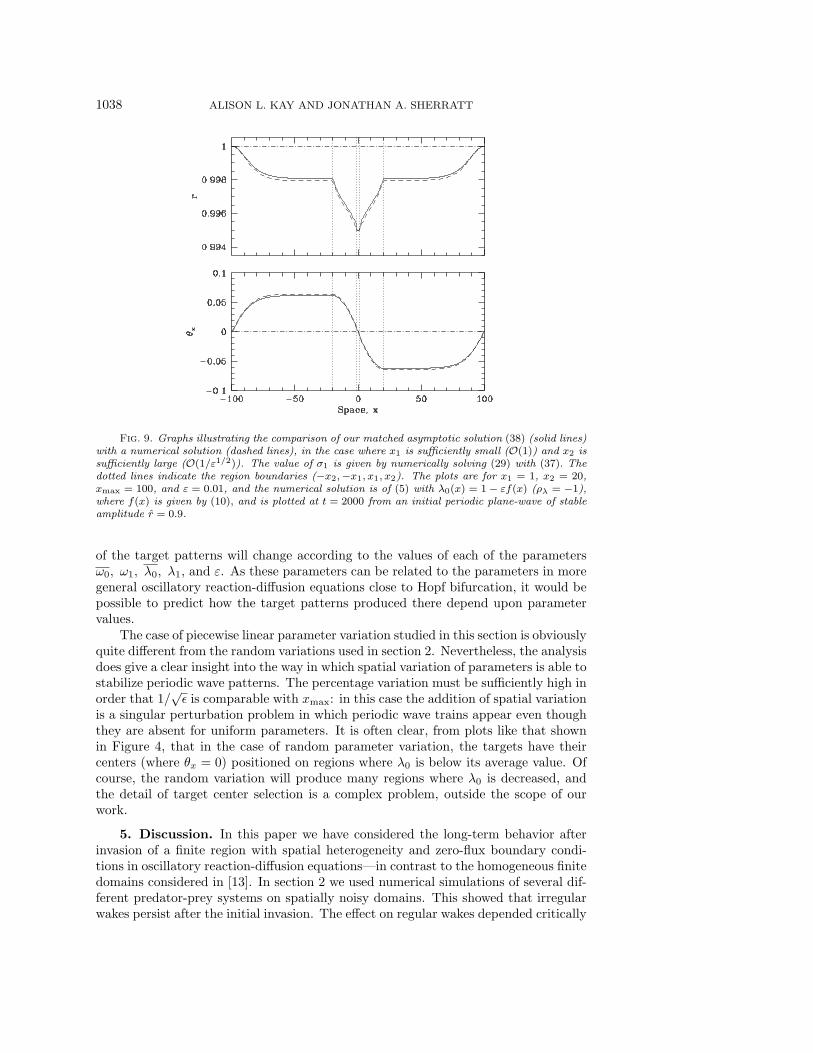
It should be noted that this solution is valid only when x1 is small, as we wouldhave to rescale in the central region if x1 were allowed to be large. Figure 9 illustratesthe very good fit of the analytical approximation to the numerical solution, providedx1 is small: here (29) and (37) have been solved numerically to calculate σ1, which hasthe value 0.384 for parameters used in Figure 9. We can thus predict that the targetpatterns formed when the parameter λ0 is decreased in the center of a one-dimensionaldomain (in a manner given by (10), where x1 = O(1) and x2 = O(ε−1/2)) will have

amplitude r = 1− εσ1/2Ω1 + o(ε) and frequency θx = ε1/2√

σ1

Ω1+ o(ε1/2), where σ1 is

determined from (29) with (37). Note that this is consistent with θx =√λ(r), as we

expect for plane waves in λ–ω systems. We also have θt = Ω0−Ω1+εσ1+o(ε) = ω(r),as expected. The restriction to x1 = O(1) means that we do not require a rescalingfor large x in the central region; but this calculation could of course be carried out,were we to allow x1 = O(ε−1/2). The matching of rescaled and unrescaled solutionswould then occur in the central region, joining with just the rescaled solutions in themiddle and outside regions. This would lead to an equation determining σ1, and sogive the amplitude and frequency of the target pattern produced in this case.

Using the rescalings (8), we see that the target patterns formed in the generalsystem (7) would have

r =

√λ0

λ1

(1− ε

σ1

2

λ1

ω1+ o(ε)

),

ψ = θx = ε1/2

√σ1λ0λ1

ω1+ o(ε1/2),

θt = λ0

(ω0λ1 − λ0ω1

λ0λ1

+ εσ1 + o(ε)

).

Using (37) and (29) to calculate σ1 shows that it and σ1λ1/ω1 are increasing func-tions of Ω1 = ω1/λ1; thus it can be determined how the amplitude and frequency


Fig. 9. Graphs illustrating the comparison of our matched asymptotic solution (38) (solid lines)with a numerical solution (dashed lines), in the case where x1 is sufficiently small (O(1)) and x2 issufficiently large (O(1/ε1/2)). The value of σ1 is given by numerically solving (29) with (37). Thedotted lines indicate the region boundaries (−x2,−x1, x1, x2). The plots are for x1 = 1, x2 = 20,xmax = 100, and ε = 0.01, and the numerical solution is of (5) with λ0(x) = 1− εf(x) (ρλ = −1),where f(x) is given by (10), and is plotted at t = 2000 from an initial periodic plane-wave of stableamplitude r = 0.9.

of the target patterns will change according to the values of each of the parametersω0, ω1, λ0, λ1, and ε. As these parameters can be related to the parameters in moregeneral oscillatory reaction-diffusion equations close to Hopf bifurcation, it would bepossible to predict how the target patterns produced there depend upon parametervalues.

The case of piecewise linear parameter variation studied in this section is obviouslyquite different from the random variations used in section 2. Nevertheless, the analysisdoes give a clear insight into the way in which spatial variation of parameters is able tostabilize periodic wave patterns. The percentage variation must be sufficiently high inorder that 1/

√ε is comparable with xmax: in this case the addition of spatial variation

is a singular perturbation problem in which periodic wave trains appear even thoughthey are absent for uniform parameters. It is often clear, from plots like that shownin Figure 4, that in the case of random parameter variation, the targets have theircenters (where θx = 0) positioned on regions where λ0 is below its average value. Ofcourse, the random variation will produce many regions where λ0 is decreased, andthe detail of target center selection is a complex problem, outside the scope of ourwork.

5. Discussion. In this paper we have considered the long-term behavior afterinvasion of a finite region with spatial heterogeneity and zero-flux boundary condi-tions in oscillatory reaction-diffusion equations—in contrast to the homogeneous finitedomains considered in [13]. In section 2 we used numerical simulations of several dif-ferent predator-prey systems on spatially noisy domains. This showed that irregularwakes persist after the initial invasion. The effect on regular wakes depended critically


on the amount of noise: a small percentage of noise in parameters had no affect onthe die-out of the regular oscillations after invasion—it occured in the same manneras previously observed in [13] on homogeneous domains, so that the work presentedthere is still valid on finite domains with sufficiently small spatial variation of param-eters. Large noise percentages, though, led to the persistence of regular oscillationsacross the domain—in a series of one or more target patterns. Increasing the noisestill further led to the breakdown of the regular wakes to irregular-looking ones, whichpersist for a long time and throughout the domain. However, in most of these cases,and where target patterns are produced after invasion, continuing the numerical solu-tion after halting the noisy spatial variation of parameters led to die-out of the spatialoscillations again, to the purely temporal oscillations of the limit cycle.

In section 3 we introduced λ–ω systems and verified that they mimic the behav-ior of regular oscillations on finite domains where the parameters are allowed to varyrandomly with spatial position, as was observed for predator-prey systems. In par-ticular, giving rise to target pattern solutions if there is a sufficiently large parametervariation. The same behavior is also observed for a piecewise linear spatial variationof the parameters on sufficiently large domains, with a target pattern appearing ifthe parameter is decreased in the center of the domain, but just one section of pe-riodic plane-waves appearing if the parameter is increased there. On small domainshowever, periodic plane-waves are not apparent, but there is still a spatially inhomo-geneous steady state attained. We then (section 4) obtain approximate solutions forthe steady state attained for a λ–ω system with such a spatial variation of a param-eter, both on large and small domains. This enabled us, in certain circumstances,to predict the the amplitude and frequency of the periodic plane-waves which willdevelop on large domains, given the variation of λ0.

For ecology, the consequences of this work are two-fold. Ecologists are understand-ably sceptical about the results of theoretical work on a completely homogeneous do-main, as real systems undoubtably contain some degree of spatial heterogeneity. Ourresults show that if this spatial heterogeneity manifests itself as noisy spatial variationof demographic parameters, and this noise is of a sufficiently small percentage, thenthe results gained by working on homogeneous domains still hold. However, largerenvironmental variations lead to the persistence of regular oscillations, via the produc-tion of target patterns. The detection of periodic plane-waves in ecological systemsobviously requires a detailed analysis of spatiotemporal data. This has recently beencarried out for vole populations in the Kielder forest [18], where statistical techniqueswere used to show that the observed spatially asynchronous, cyclically time-varyingvole populations correspond to a periodic traveling wave.

It has long been known that impurities can facilitate the formation of target pat-terns in chemical systems (although such have certainly not been found at the centerof every target pattern), and this work provides further numerical evidence for this.For the Belousov–Zhabotinskii reaction in the oscillatory regime, it has been demon-strated experimentally that temperature can affect the amplitude of the oscillation,with higher temperatures decreasing the amplitude [7, 8]. This could then providea method of verifying our results on inhomogeneous finite domains experimentally:In a one-dimensional reaction vessel with temporal oscillations imposed at each end,such as that used by Stossel and Munster [34], stable periodic waves could be setup. Then the boundary conditions could be changed to zero-flux, and a differenttemperature imposed in a region around the center of the reaction vessel. Our workpredicts that, for a sufficiently large temperature difference, the result should depend


critically on whether the temperature in the center of the vessel is higher or lowerthan that for the rest of the vessel. If the central temperature is higher, then weexpect a target pattern to form, whereas if the central temperature is lower, thenwe expect that the periodic plane-waves will die out; except for a band local to theregion of lower temperature. Another possible experiment could involve oxygen orlight, which are both known to affect the oscillations in the Belousov–Zhabotinskiireaction [35, 36, 26]. If the reactants were placed on a thin gel layer, in a reactionvessel that is closed except for a sheet over the top with randomly placed holes toallow oxygen or light to permeate through, then we could expect regular oscillationsto be stabilized, in the form of target patterns, whereas they would otherwise havedied out. Chemical experiments such as these provide the most effective method oftesting our mathematical predictions.

Acknowledgment. We thank John Merkin for drawing our attention to theeffects of oxygen on the Belousov–Zhabotinskii reaction.

REFERENCES

[1] D.L. Benson, P.K. Maini, and J.A. Sherratt, Unravelling the Turing bifurcation usingspatially varying diffusion coefficients, J. Math. Biol., 37 (1998), pp. 381–417.

[2] P. Borckmans, Competition in ramped Turing structures, Phys. A, 188 (1992), pp. 137–157.[3] R.S. Cantrell, C. Cosner, and V. Hutson, Ecological models, permanence and spatial het-

erogeneity, Rocky Mountain J. Math., 26 (1996), pp. 1–35.[4] R.S. Cantrell and C. Cosner, On the effects of spatial heterogeneity on the persistence of

interacting species, J. Math. Biol., 37 (1998), pp. 103–145.[5] H.N. Comins, M.P. Hassell, and R.M. May, The spatial dynamics of host-parasitoid systems,

J. Anim. Ecol., 61 (1992), pp. 735–748.[6] S.R. Dunbar, Traveling waves in diffusive predator-prey equations: Periodic orbits and point-

to-periodic heteroclinic orbits, SIAM J. Appl. Math., 46 (1986), pp. 1057–1077.[7] A.K. Dutt and M. Menzinger, Effect of stirring and temperature on the Belousov-Zhabotiskii

reaction in a batch reactor, J. Phys. Chem., 96 (1992), pp. 8447–8449.[8] A.K. Dutt and S.C. Muller, Effect of stirring and temperature on the Belousov-Zhabotiskii

reaction in a CSTR, J. Phys. Chem., 97 (1993), pp. 10059–10063.[9] G.B. Ermentrout, X. Chen, and Z. Chen, Transition fronts and localised structures in

bistable reaction-diffusion systems, Phys. D, 108 (1997), pp. 147–167.[10] R.A. Fisher, The wave of advance of advantageous genes, Ann. Eugen., 7 (1937), pp. 353–369.[11] P.S. Hagan, Target patterns in reaction-diffusion systems, Adv. Appl. Math., 2 (1981), pp.

400–416.[12] R.D. Holt and M.P. Hassell, Environmental heterogeneity and the stability of host-parasitoid

interactions, J. Anim. Ecol., 62 (1993), pp. 89–100.[13] A.L. Kay and J.A. Sherratt, On the persistence of spatiotemporal oscillations generated by

invasion, IMA J. Appl. Math., 63 (1999), pp. 199–216.[14] N. Kopell and L.N. Howard, Plane wave solutions to reaction-diffusion equations, Stud.

Appl. Math., 52 (1973), pp. 291–328.[15] N. Kopell, Target pattern solutions to reaction-diffusion equations in the presence of impuri-

ties, Adv. Appl. Math., 2 (1981), pp. 389–399.[16] N. Kopell and G.B. Ermentrout, Phase Transitions and other phenomena in chains of

coupled oscillators, SIAM J. Appl. Math., 50 (1990), pp. 1014–1052.[17] M. Kot, Discrete-time traveling waves—ecological examples, J. Math. Biol., 30 (1992), pp.

413–436.[18] X. Lambin, D.A. Elston, S.J. Petty, and J.L. Mackinnon, Spatial asynchrony and periodic

travelling waves in cyclic populations of field voles, Proc. Roy. Soc. London Ser. B, 265(1998), pp. 1491–1496.

[19] K. Maginu, Stability of periodic travelling wave solutions with large spatial periods in reaction-diffusion equations, J. Differential Equations, 39 (1981), pp. 73–99.

[20] J.H. Merkin and M.A. Sadiq, The dynamics of physiologically structured populations, IMAJ. Appl. Math., 57 (1996), pp. 273–309.

[21] J.D. Murray, Mathematical Biology, Springer-Verlag, Berlin, 1989.


[22] H.G. Othmer, Current problems in pattern formation, Lectures Math. Life Sci., 9 (1977), pp.57–86.

[23] S.W. Pacala and J. Roughgarden, Spatial heterogeneity and interspecific competition,Theor. Pop. Biol., 21 (1982), pp. 92–113.

[24] M. Pascual, Diffusion induced chaos in a spatial predator-prey system, Proc. Roy. Soc. LondonSer. B, 251 (1993), pp. 1–7.

[25] S.V. Petrovskii and H. Malchow, A minimal model of pattern formation in a predator-preysystem, Math. Comput. Model., 29 (1999), pp. 49–63.

[26] M.K.R. Reddy, Z. Szlavik, Z. Nagyungvarai, and S.C. Muller, Influence of light on theinorganic part of the ruthenium-catalysed Belousov-Zhabotinskii reaction, J. Phys. Chem.,99 (1995), pp. 15081–15085.

[27] P. Rohani, T.J. Lewis, D. Grunbaum, and G.D. Ruxton, Spatial self-organization in ecology:Pretty patterns or robust reality?, Trends in Ecology and Evolution, 12, (1997), pp. 70–74.

[28] J.A. Sherratt, Irregular wakes in reaction-diffusion waves, Phys. D, 70 (1994), pp. 370–382.[29] J.A. Sherratt, B.T. Eagan, and M.A. Lewis, Oscillations and chaos behind predator-prey

invasion: Mathematical artifact or ecological reality?, Phil. Trans. Roy. Soc. London Ser.B, 352 (1997), pp. 21–38.

[30] J.A. Sherratt, Invading wave fronts and their oscillatory wakes are linked by a modulatedtravelling phase resetting wave, Phys. D, 117 (1998), pp. 145–166.

[31] N. Shigesada, Traveling periodic waves in heterogeneous environments, Theor. Pop. Biol., 30(1986), pp. 143–160.

[32] J.C. Skellam, Random dispersal in theoretical populations, Biometrika, 38 (1951), pp. 196–218.[33] J. Sneyd and J.A. Sherratt, On the propagation of calcium waves in an inhomogeneous

medium, SIAM J. Appl. Math., 57 (1997), pp. 73–94.[34] R. Stossel and A. F. Munster, Periodic and irregular wave patterns in an open tubular gel

reactor, Chem. Phys. Lett., 239 (1995), pp. 354–360.[35] L. Treindl, P. Ruoff, and P.O. Kvernberg, Influence of oxygen and organic substrate on

oscillations and autocatalysis in the Belousov-Zhabotinskii reaction, J. Phys. Chem. A, 101(1997), pp. 4606–4612.

[36] J.C. Wang, F. Hynne, P.G. Sorensen, and K. Nielson, Oxygen influence on complex oscil-lations in a closed Belousov-Zhabotinsky reaction, J. Phys. Chem., 100 (1996), pp. 17593–17598.

[37] P. Wiener and S. Tuljapurkar, Migration in variable environments: Exploring life-historyevolution using structured population models, J. Theor. Biol., 166 (1994), pp. 75–90.

[38] A.T. Winfree, Rotating chemical reactions, Sci. Am., 230 (1974), pp. 82–95.[39] J.X. Xin, Existence and nonexistence of traveling waves and reaction-diffusion front propaga-

tion in periodic media, J. Statist. Phys., 73 (1993), pp. 893–926.

SpatioTemporal Wavelets: A Group-Theoretic Construction for Motion Estimation and Tracking

Documents

Transcript of SpatioTemporal Wavelets: A Group-Theoretic Construction for Motion Estimation and Tracking