HAL Id: hal-01677096https://hal.archives-ouvertes.fr/hal-01677096v2

Submitted on 15 Feb 2019

HAL is a multi-disciplinary open accessarchive for the deposit and dissemination of sci-entific research documents, whether they are pub-lished or not. The documents may come fromteaching and research institutions in France orabroad, or from public or private research centers.

L’archive ouverte pluridisciplinaire HAL, estdestinée au dépôt et à la diffusion de documentsscientifiques de niveau recherche, publiés ou non,émanant des établissements d’enseignement et derecherche français ou étrangers, des laboratoirespublics ou privés.

Numerical and experimental study on heat transfer andflow features of representative molten salts for energy

applications in turbulent tube flowYu Qiu, Ming-Jia Li, Meng-Jie Li, Hong-Hu Zhang, Bo Ning

To cite this version:Yu Qiu, Ming-Jia Li, Meng-Jie Li, Hong-Hu Zhang, Bo Ning. Numerical and experimental studyon heat transfer and flow features of representative molten salts for energy applications in turbu-lent tube flow. International Journal of Heat and Mass Transfer, Elsevier, 2019, 135, pp.732-745.�10.1016/j.ijheatmasstransfer.2019.02.004�. �hal-01677096v2�

1

Numerical and experimental study on heat transfer and flow features of 1

representative molten salts for energy applications in turbulent tube flow 2

Yu Qiu, Ming-Jia Li *, Meng-Jie Li, Hong-Hu Zhang, Bo Ning 3

Key Laboratory of Thermo-Fluid Science and Engineering of Ministry of Education, School of Energy and Power 4

Engineering, Xi’an Jiaotong University, Xi’an, Shaanxi, 710049, China 5

* Corresponding author 6

Abstract: This article investigated the heat transfer performance and flow friction of the molten salts 7

in turbulent tube flow, where four salts including Hitec, Solar Salt, NaF-NaBF4, and FLiNaK were 8

studied. A computational model was developed to analyze the flow and heat transfer features of the 9

salts in the tube, and experiments were conducted to test the heat transfer performance of a 10

representative salt Hitec in the tubes of a salt-oil heat exchanger. Comparison of simulation results with 11

the experimental data shows that the average errors are smaller than ±4%, which validates the 12

simulation model. Based on the model, firstly the influences of heat flux uniformity at the tube outer 13

wall were examined. The results show that the non-uniform wall flux can lead to local high- temperature 14

region but influences little on the flow friction coefficient and the heat transfer performance. Then, the 15

model was utilized to investigate the friction and heat transfer features of the salts under broad ranges 16

of the temperature and the velocity. Comparisons of the simulated heat transfer results with Hansen’s, 17

Sider-Tate’s and Gnielinski’s correlations show that the largest errors can reach +25%, +13% and -18

15%, respectively. Furthermore, the errors between the simulated friction coefficients and the 19

Filonenko’s correlation are smaller than ±2%, which indicates that this correlation is suitable for 20

predicting the friction of the salts. Finally, to predict the heat transfer performance more accurately for 21

these representative salts, a new correlation was developed. It was found that the errors between all 22

simulation results and the proposed correlation are smaller than ±5%, while the corresponding values 23

for 80% experiment data of three salts are also lower than ±5%. The current study can offer beneficial 24

results and correlation for the applications of liquid salts in energy systems. 25

Keywords: Liquid salts; Heat transfer performance; Friction factor; Concentrating solar power; 26

Nuclear energy 27

28

1. Introduction 29

In recent years, solar energy and nuclear energy have been considered as two promising 30

2

alternatives to reduce the severe global warming[1] and environment pollutions[2] induced by the 31

utilization of fossil energy[3-5]. For the utilization of solar energy, a solar power generation technology 32

called Concentrating Solar Power(CSP) that generates electric power by concentrating sun rays has 33

developed rapidly during the past two decades[6, 7]. In this technology, molten nitrate salts are the 34

most commonly used heat transfer fluids and heat storage mediums [8-10]. For nuclear energy, molten 35

fluoride salts are considered as promising heat transfer fluids in the state-of-the-art fourth-generation 36

nuclear plant[11, 12]. This is because the molten salts have numerous advantages such as low vapour 37

tension, good thermostability, and low price[13, 14]. 38

Liquid salts are usually employed to flow in round tubes of the heat exchangers and solar receivers 39

in nuclear and CSP technologies. For improving the performance and ensuring the safe operation of 40

these devices, it is necessary to understand the flow and heat transfer features of the liquid salts in the 41

commonly used round pipe. As a result, numerous previous studies have investigated this topic using 42

experiments. 43

A review of the previous work found that several experiments had investigated the heat transfer 44

performance of some liquid salts in round pipes heated by uniform wall flux from the 1940s to 1970s. 45

Typical liquid fluorides including ThF4-BeF2-UF4-LiF [15, 16], FLiNaK [17-19] and NaF-NaBF4 [15], 46

and liquid nitrate Hitec [20, 21] had been experimentally studied. The data were compared with several 47

classical correlations, but controversial conclusions were procured in different studies. Some studies 48

found that some classical correlations are applicable for liquid salts[15, 16], while others procured 49

opposite conclusion[17, 18]. During the following thirty years, there was almost no progress on this 50

topic, and no experiment result had been openly reported. 51

However, in recent years, heat transfer of liquid salts has become a highlighted research area again. 52

This is mainly due to the fast developments of CSP and nuclear technologies, where reliable heat 53

transfer data and correlations with high accuracies are highly desired for the designs of heat transfer 54

devices. From 2009 to now, the heat transfer performance of two liquid salts has been investigated by 55

testing some shell-and-tube heat exchangers(STHX) when the salt flows in the tubes, where Hitec[13, 56

22-26] and LiNO3[22, 27, 28] were employed. 57

By analyzing the results from these studies, firstly, Wu et al.[22] concluded that the errors between 58

most experiment results and some exiting correlations including Sider-Tate’s equation[29], 59

Gnielinski’s equation[30], and Hansen’s equation[31] are within ±25%. This large error used to be 60

3

considered acceptable for the industry[32]. However, after reviewing developments in heat transfer, 61

Tao[33] has pointed out that the long-accepted 20-25% error in calculating heat transfer correlations is 62

no longer satisfactory, and an error of <10% has been going to be the new norm in recent years. 63

Secondly, it is also found that the ranges of the salt temperature and Reynolds number (Re) are usually 64

quite narrow for each experiment due to various experimental difficulties, and the common Re range 65

of 104-105 for the liquid salts in energy applications was not covered. Thirdly, no reliable experiment 66

data of Solar Salt which is the most widely-used commercial salt in CSP plants can be found in the 67

literature. Moreover, no reliable experiment result of the flow friction has been found in the literature. 68

Because it is very difficult to measure the pressure drop of the molten salt. On the one hand, traditional 69

mechanical pressure gauges cannot be used because the salt can be easily frozen in the gauge. On the 70

other hand, researchers at Sandia National Laboratories have tried to measure the pressure drop of the 71

molten salt by using many kinds of pressure transduces[34]. However, the pressure transduces either 72

had a failure or had a very large measuring error due to the high temperature. Finally, the receiver tubes 73

are heated by greatly non-uniform concentrated solar irradiation flux in the CSP plant. However, it is 74

quite difficult to do experiments under this condition. Hence, simulation approach can offer significant 75

help investigating the flow and heat transfer features of the liquid salts[35]. 76

In present work, two liquid fluorides (FLiNaK, NaF-NaBF4)[11] that are promising for nuclear 77

plants and two nitrates (Hitec, Solar Salt)[36] that are usually used in CSPs are considered. Both 78

simulations and experiments are employed to investigate the heat transfer features and flow friction in 79

round pipes. The aim of this work is as follows. Firstly, it is hard for experiments to cover the typical 80

Re range of 104-105 and the whole possible salt temperature range of each salt in energy applications, 81

so we try to use simulations to cover these ranges. Secondly, the influences of the greatly non-uniform 82

wall flux on the flow and heat transfer characteristics will be investigated, and we try to determine if it 83

is necessary to consider these effects in energy applications. Thirdly, the simulation heat transfer and 84

friction data of all salts will be compared with several classical correlations to examine whether they 85

are applicable to these liquid salts. Finally, we will try to select a heat transfer correlation from the 86

classical equations or develop a new correlation that can achieve an error of <10% in calculating heat 87

transfer. 88

2. Physical model description 89

4

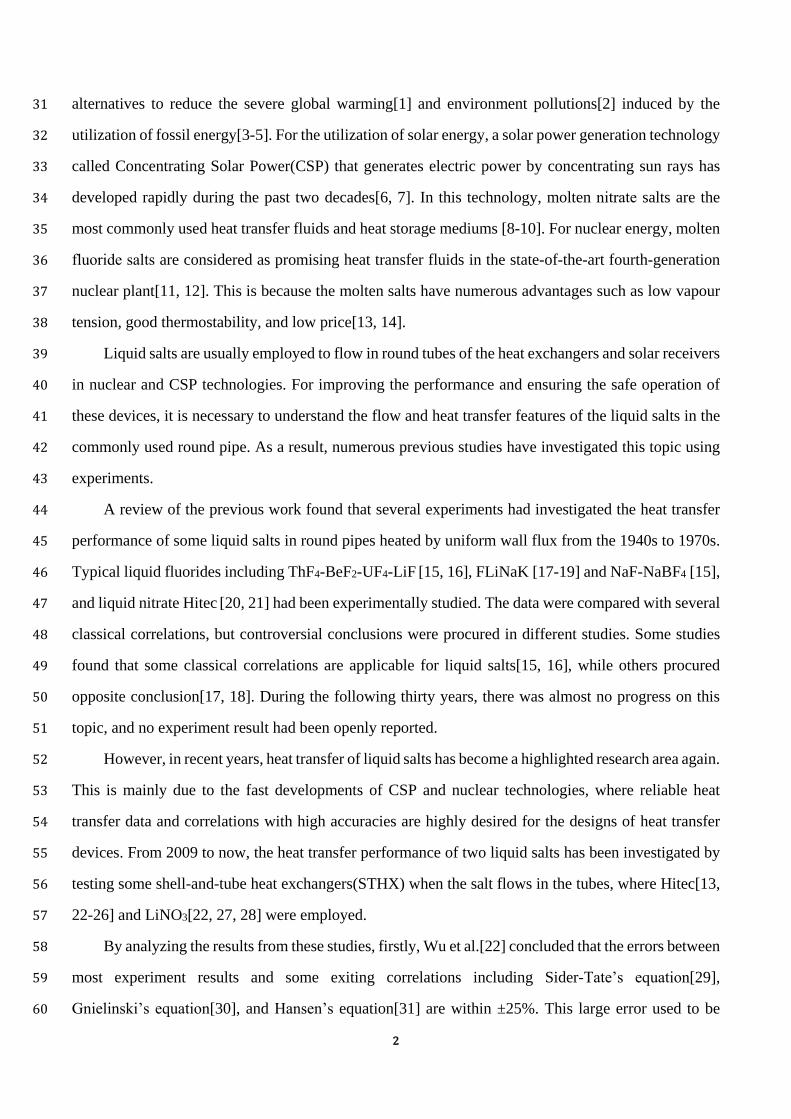
2.1 A tube section from a solar receiver 90

An absorber tube section that is heated by the peak solar flux in the receiver of the 1 MWe 91

DAHAN plant on spring equinox noon is taken into consideration as the physical model. The tube 92

section is demonstrated in Fig. 1(a), and its key parameters are shown in Table 1. The studied receiver 93

shown in Fig. 1(b) employs 620 six-meter absorber tubes[37] and can accept the concentrated solar 94

radiation from one hundred 10m×10m heliostats[38]. The longitude and latitude of the plant that is 95

located in Beijing are 115.9°E and 40.4°N, respectively. 96

For describing the model clearly, two systems of right-handed Cartesian axes are defined in Fig. 97

1. XrYrZr is named receiver system. The origin (A) is the aperture center of the receiver, and the 98

directions of the axes are shown in Fig. 1(b). XtYtZt is named tube system. The origin (O) is the center 99

of the tube section, and each axis is parallel to the corresponding axis in XrYrZr. Considering the 100

depression angle of 25o for the receiver, the gravity vector (g) in tube system should be (0, -8.9, -4.1). 101

A

Gravity

25°

102 (a) Tube section of two meters (b) Solar receiver 103

Fig. 1. Schematics of the tube section and the solar receiver. 104

Table 1. Key parameters of the selected physical model[37, 39]. 105

Items Description or value

Material 316H stainless steel

Roughness of tube wall hydrodynamically smooth

Inside diameter of tube D / mm 16.6

Outside diameter of tube/ mm 19

Length of tube L / mm 2000

Density of steel / kg·m-3 7090

Heat conductivity of steel / W·(m·K)-1 21.5

Specific capacity of steel / kJ·(kg·K)-1 0.500

Xt

Yt

Zt

O

Xr

YrZr Tube

Salt

0

-1

1

5

2.2 Heat fluxes on tube wall and liquid salts 106

This work will investigate the flow features and heat transfer performance of the previously 107

mentioned liquid salts, where the salt will flow in the two-meter tube section under uniform or non-108

uniform wall flux, which are described as follows. 109

A long-tested optical code SPTOPTIC developed in our previous work[37] using Monte Carol ray 110

tracing (MCRT) method is employed to model the transmission of solar radiation at spring equinox 111

noon in DAHAN plant. The MCRT is a method for calculating the paths of rays through an optical 112

system, where possible optical events including absorption, scattering, refraction, and reflection are 113

modeled in a random way. The MCRT has been successfully employed in the performance simulations 114

of parabolic trough collector[40-45], linear Fresnel collector[46-49], parabolic dish collector[50-52], 115

and solar power tower[53-56]. For simplifying the description, detailed descriptions of the model and 116

code that has been published in Ref.[37] are omitted here. 117

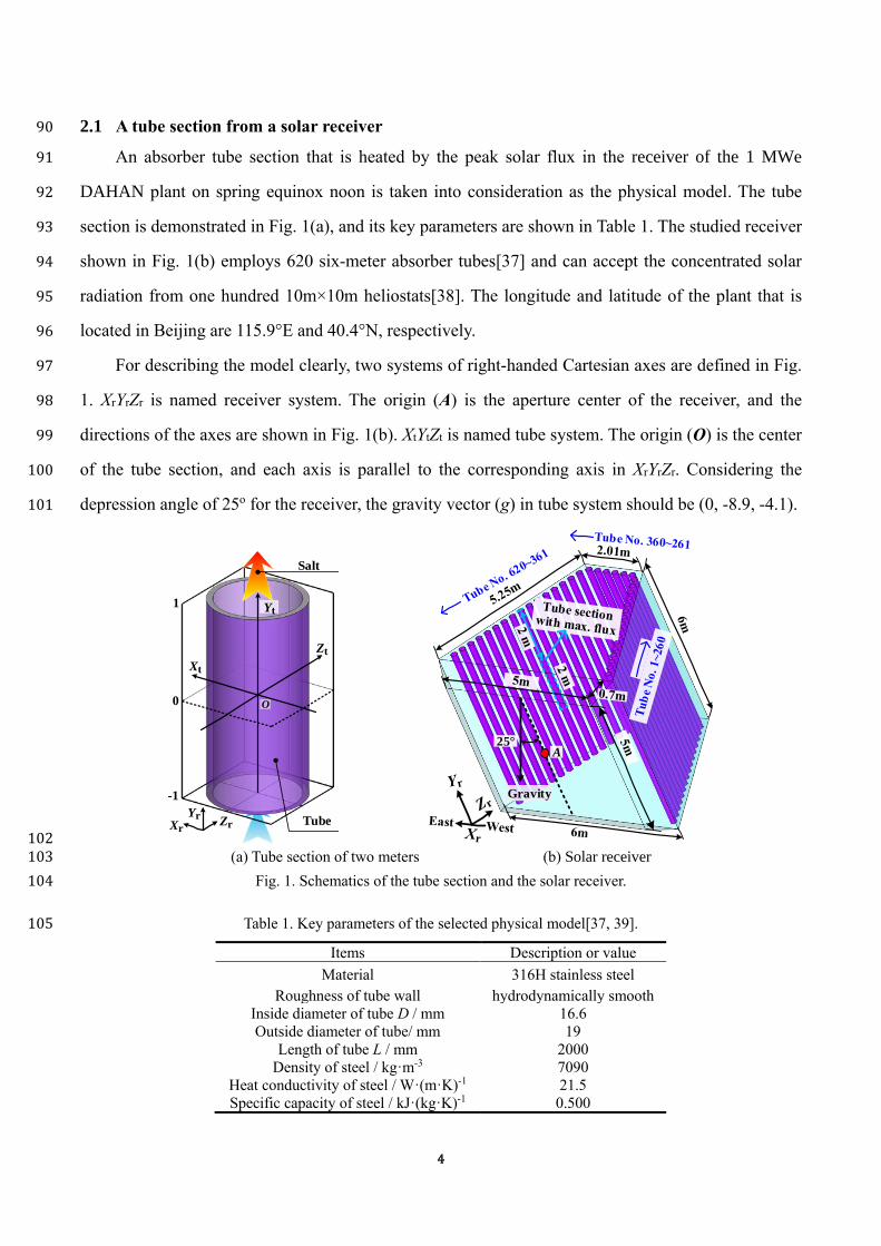
After the simulation, a detailed contour map of the solar irradiation flux (ql) in the liquid salt 118

receiver is procured and presented in Fig. 2(a). Fig. 2(b) illustrates the flux absorbed on tube 443 that 119

is heated by the peak flux of 5.14×105 W·m-2. Fig. 2(c) depicts the greatly non-uniform solar flux 120

absorbed by the selective absorbing coating on the studied tube section, where the total power of 11,616 121

W is absorbed. Furthermore, current work also tries to study the flow and heat transfer features at 122

uniform wall flux condition, so Fig. 2(c) also illustrates a uniform flux with the value of 97,302 W·m-123

2, which is procured by distributing the total power absorbed on the tube section uniformly on its outside 124

wall. 125

4.5E5

4.0E5

3.5E5

3.0E5

2.5E5

2.0E5

1.5E5

1.0E5

0.5E5

ql / W·m-2

5.0E5

Non-uniform flux Corresponding uniform flux

VS

(b) Tube 443: Tube with the max. flux

Xt

Yt Zt

-1

-2

-3

0

1

2

3

(a) Solar receiver(c) Tube section (Computational domain)

Molten Salt

1

0

-1

1

0

-1

126 Fig. 2. Typical non-uniform and uniform heat flux distributions. 127

Due to the fact that a solar receiver of current dimensions can achieve a solar-thermal conversion 128

efficiency of about 90%[57, 58]. Hence, a simplified assumption has been made by assuming that 90% 129

of the absorbed local irradiation flux (ql) on the tube outer wall can be transferred to the salt. And the 130

6

flux (q) calculated using Eq.(1) will be used to study the flow and heat transfer in the simulation as a 131

heat flux boundary on the tube outer wall. After this assumption, the peak fluxes under non-uniform 132

and uniform flux conditions would be 4.63×105 Wm-2 and 87,571 Wm-2, respectively. 133

l0.9q q (1) 134

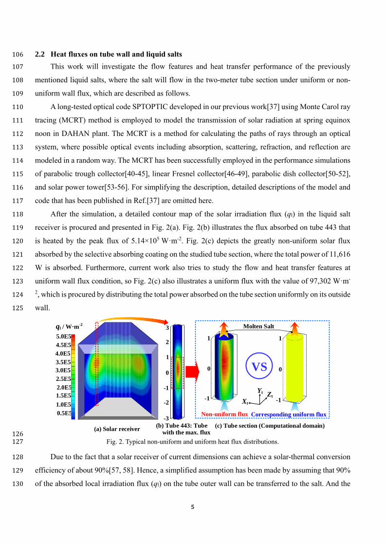
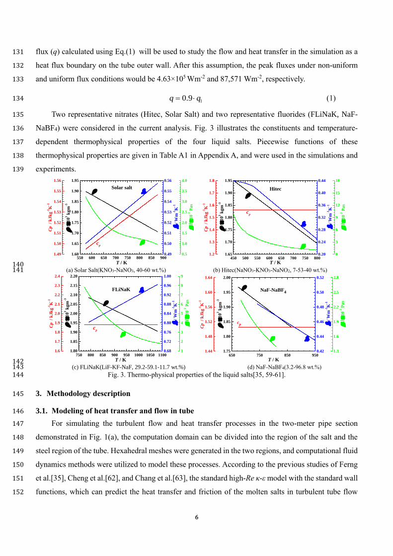
Two representative nitrates (Hitec, Solar Salt) and two representative fluorides (FLiNaK, NaF-135

NaBF4) were considered in the current analysis. Fig. 3 illustrates the constituents and temperature-136

dependent thermophysical properties of the four liquid salts. Piecewise functions of these 137

thermophysical properties are given in Table A1 in Appendix A, and were used in the simulations and 138

experiments. 139

550 600 650 700 750 800 850 9001.60

1.65

1.70

1.75

1.80

1.85

1.90

1.95

/

10

3 k

gm

-3

T / K

1.49

1.50

1.51

1.52

1.53

1.54

1.55

1.56

cp

Cp

/

kJ

kg

-1K

-1

0.49

0.50

0.51

0.52

0.53

0.54

0.55

0.56

Solar salt

/

10

-3 P

as

/

Wm

-1K

-1

0.5

1.0

1.5

2.0

2.5

3.0

3.5

4.0

450 500 550 600 650 700 750 800

1.65

1.70

1.75

1.80

1.85

1.90

1.95

Hitec

/

10

3 k

gm

-3

T / K

1.2

1.3

1.4

1.5

1.6

1.7

1.8

cp

Cp

/ k

Jk

g-1

K-1

0.20

0.24

0.28

0.32

0.36

0.40

0.44

/

10

-3 P

as

/

Wm

-1K

-1

0

3

6

9

12

15

18

140 (a) Solar Salt(KNO3-NaNO3, 40-60 wt.%) (b) Hitec(NaNO3-KNO3-NaNO2, 7-53-40 wt.%) 141

750 800 850 900 950 1000 1050 11001.80

1.85

1.90

1.95

2.00

2.05

2.10

2.15

2.20

/

10

3 k

gm

-3

T / K

FLiNaK

1.6

1.7

1.8

1.9

2.0

2.1

2.2

2.3

2.4

cp

Cp

/ k

Jk

g-1

K-1

0.68

0.72

0.76

0.80

0.84

0.88

0.92

0.96

1.00

/

10

-3 P

as

/

Wm

-1K

-1

1

2

3

4

5

6

7

8

9

650 750 850 950

1.75

1.80

1.85

1.90

1.95

2.00

/

10

3 k

gm

-3

T / K

1.44

1.48

1.52

1.56

1.60

1.64

cp

Cp

/

kJ

kg

-1K

-1

0.42

0.44

0.46

0.48

0.50

0.52

/

10

-3 P

as

/

Wm

-1K

-1

1.3

1.6

1.9

2.2

2.5

2.8

NaF-NaBF4

142 (c) FLiNaK(LiF-KF-NaF, 29.2-59.1-11.7 wt.%) (d) NaF-NaBF4(3.2-96.8 wt.%) 143

Fig. 3. Thermo-physical properties of the liquid salts[35, 59-61]. 144

3. Methodology description 145

3.1. Modeling of heat transfer and flow in tube 146

For simulating the turbulent flow and heat transfer processes in the two-meter pipe section 147

demonstrated in Fig. 1(a), the computation domain can be divided into the region of the salt and the 148

steel region of the tube. Hexahedral meshes were generated in the two regions, and computational fluid 149

dynamics methods were utilized to model these processes. According to the previous studies of Ferng 150

et al.[35], Cheng et al.[62], and Chang et al.[63], the standard high-Re κ-ε model with the standard wall 151

functions, which can predict the heat transfer and friction of the molten salts in turbulent tube flow 152

7

suitably, was selected in the current model. 153

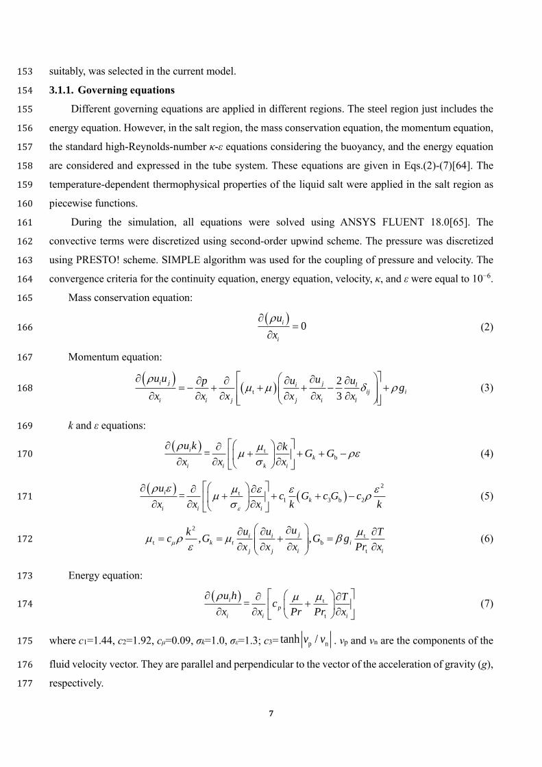
3.1.1. Governing equations 154

Different governing equations are applied in different regions. The steel region just includes the 155

energy equation. However, in the salt region, the mass conservation equation, the momentum equation, 156

the standard high-Reynolds-number κ-ε equations considering the buoyancy, and the energy equation 157

are considered and expressed in the tube system. These equations are given in Eqs.(2)-(7)[64]. The 158

temperature-dependent thermophysical properties of the liquid salt were applied in the salt region as 159

piecewise functions. 160

During the simulation, all equations were solved using ANSYS FLUENT 18.0[65]. The 161

convective terms were discretized using second-order upwind scheme. The pressure was discretized 162

using PRESTO! scheme. SIMPLE algorithm was used for the coupling of pressure and velocity. The 163

convergence criteria for the continuity equation, energy equation, velocity, κ, and ε were equal to 10−6. 164

Mass conservation equation: 165

0i

i

u

x

(2) 166

Momentum equation: 167

t

2

3

i j ji lij i

i i j j i l

u u uu upg

x x x x x x

(3) 168

k and ε equations: 169

t

b=i

k

i i k i

u k kG G

x x x

(4) 170

2

t1 3 b 2=

i

k

i i i

uc G c G c

x x x k k

(5) 171

2

tt b

t

, ,ji i

k t i

j j i i

uu uk Tc G G g

x x x Pr x

(6) 172

Energy equation: 173

t

t

=i

p

i i i

u h Tc

x x Pr Pr x

(7) 174

where c1=1.44, c2=1.92, cμ=0.09, σk=1.0, σε=1.3; c3= p ntanh /v v . vp and vn are the components of the 175

fluid velocity vector. They are parallel and perpendicular to the vector of the acceleration of gravity (g), 176

respectively. 177

8

3.1.2. Near-wall treatments 178

It is known that the near-wall region can be divided into three layers. The closest layer to the wall 179

is called viscous sublayer, where the flow is almost laminar, and the molecular viscosity plays a 180

dominant role. The layer next to the viscous sublayer is called buffer layer, where the effects of 181

molecular viscosity and turbulence are both important. The farthest layer from the wall is called fully-182

turbulent layer, where turbulence plays a dominant role. 183

Because the high-Re k-ε model is inapplicable in the viscous sublayer and buffer layer, semi-184

empirical formulas called “wall functions” can be used to bridge these layers between the wall and the 185

fully turbulent region[65]. For the region near the tube inner wall, a logarithmic law is employed, which 186

states that the average velocity of a turbulent flow at a certain point (P) in the fully-turbulent layer is 187

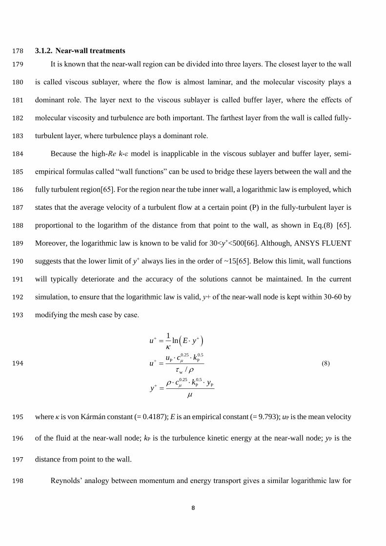
proportional to the logarithm of the distance from that point to the wall, as shown in Eq.(8) [65]. 188

Moreover, the logarithmic law is known to be valid for 30<y+<500[66]. Although, ANSYS FLUENT 189

suggests that the lower limit of y+ always lies in the order of ~15[65]. Below this limit, wall functions 190

will typically deteriorate and the accuracy of the solutions cannot be maintained. In the current 191

simulation, to ensure that the logarithmic law is valid, y+ of the near-wall node is kept within 30-60 by 192

modifying the mesh case by case. 193

0.25 0.5

P P

w

0.25 0.5

P P

1ln

/

u E y

u c ku

c k yy

(8) 194

where κ is von Kármán constant (= 0.4187); E is an empirical constant (= 9.793); uP is the mean velocity 195

of the fluid at the near-wall node; kP is the turbulence kinetic energy at the near-wall node; yP is the 196

distance from point to the wall. 197

Reynolds’ analogy between momentum and energy transport gives a similar logarithmic law for 198

9

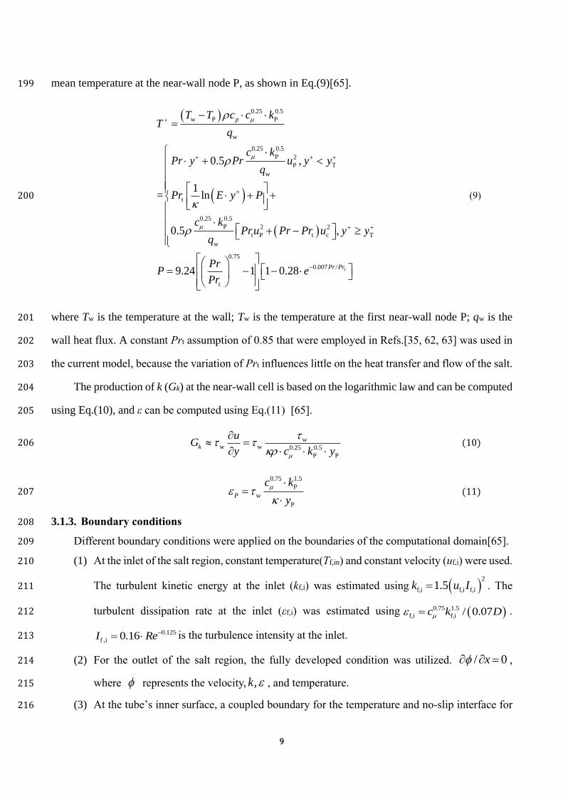
mean temperature at the near-wall node P, as shown in Eq.(9)[65]. 199

t

0.25 0.5

w P P

w

0.25 0.5

P 2

P T

w

t

0.25 0.5

P 2 2

t P t c T

w

0.75

0.007 /

t

0.5 ,

1= ln

0.5 ,

9.24 1 1 0.28

p

Pr Pr

T T c c kT

q

c kPr y Pr u y y

q

Pr E y P

c kPru Pr Pr u y y

q

PrP e

Pr

(9) 200

where Tw is the temperature at the wall; Tw is the temperature at the first near-wall node P; qw is the 201

wall heat flux. A constant Prt assumption of 0.85 that were employed in Refs.[35, 62, 63] was used in 202

the current model, because the variation of Prt influences little on the heat transfer and flow of the salt. 203

The production of k (Gk) at the near-wall cell is based on the logarithmic law and can be computed 204

using Eq.(10), and ε can be computed using Eq.(11) [65]. 205

ww w 0.25 0.5

P P

k

uG

y c k y

(10) 206

0.75 1.5

P

w

P

P

c k

y

(11) 207

3.1.3. Boundary conditions 208

Different boundary conditions were applied on the boundaries of the computational domain[65]. 209

(1) At the inlet of the salt region, constant temperature(Tf,in) and constant velocity (uf,i) were used. 210

The turbulent kinetic energy at the inlet (kf,i) was estimated using 2

f,i f,i f,i1.5k u I . The 211

turbulent dissipation rate at the inlet (εf,i) was estimated using 0.75 1.5

f,i f,i / 0.07c k D . 212

0.125

f ,i 0.16I Re is the turbulence intensity at the inlet. 213

(2) For the outlet of the salt region, the fully developed condition was utilized. / 0x , 214

where represents the velocity, ,k , and temperature. 215

(3) At the tube’s inner surface, a coupled boundary for the temperature and no-slip interface for 216

10

the velocity were used. 217

(4) At the tube wall ends, an adiabatic boundary was considered: w 0q . 218

(5) At the outside surface of the tube, a heat flux boundary was employed, where the uniform or 219

non-uniform wall heat flux described in Section 2.2 was considered. 220

3.2. Experiments of heat transfer in tube side of a STHX 221

For a specific fluid, many previous studies have concluded that the performance of heat transfer 222

in a pipe under uniform wall flux is almost the same as that in the tubes of a STHX[32]. As a result, the 223

computation model can be validated by comparing the simulation heat transfer results procured using 224

uniform wall flux and the experiment data procured in the tubes of a STHX, where Hitec is employed 225

as the heat transfer fluid. The details of the experiment are as follows. 226

Table 2 presents the key parameters of the heat exchanger. A tube bundle with nineteen tubes is 227

assembled in a shell with an inside diameter of 100 mm as illustrated in Fig. 4, and each tube has an 228

effective length of 2.0 m. A 150 mm aluminum silicate layer is employed to cover the exchanger for 229

reducing the thermal loss to a negligible level. 230

Table 2. Geometric parameters of the STHX. 231

Parameter / unit Value

Shell’s outside diameter / mm 108

Shell’s inside diameter / mm 100

Arrangement of tubes regular triangle

Number of tubes 19

Tube pitch / mm 18

Length of each tube / m 2.0

Tube’s outside diameter / mm 14

Tube’s inside diameter / mm 10

11

232

Fig. 4. Sketch of the experiment system. 233

A liquid salt experiment system demonstrated in Fig. 4 was built to investigate the heat transfer of 234

Hitec in the tubes of the STHX. The system consists of a liquid salt path, a synthetic oil path, and a 235

cooling path. 236

In the liquid salt path, a molten salt tank with electric heaters is employed to contain and heat the 237

Hitec of 6 tons. A pump is used to pump the liquid Hitec throughout this path. A secondary electric 238

heater is used to adjust the salt temperature at the tube inlet of the salt-oil HX. The volume flow rate of 239

Hitec is measured using a vortex shedding flow gauge. For the horizontal connecting pipes, an 240

inclination angle of about 5o is specially designed to ensure that the Hitec can flow back to the tank. 241

All connecting pipes are heated using electric tracing bands to avert the solidification of liquid salt. To 242

ensure that the tube side can be fully filled, an invert U-shaped connecting pipe was installed at the 243

outlet of this side. The synthetic oil path uses a tank to store two-ton YD-325 synthetic oil whose 244

thermophysical properties are summarized in Table A1. A pump is used to pump the oil throughout this 245

path including the shell-side passage in the salt-oil HX. The volume flow of the oil is also measured 246

with a vortex shedding flow gauge. In addition, the cooling path includes a water-cooling tower, a pump, 247

and the shell-side passage of the oil-water HX. 248

During the experiment, the valve V1 and Valve V2 must keep open, while other valves should be 249

closed. Moreover, the pumps should be launched. The energy transfer processes are as follows. Firstly, 250

the thermal energy will be exchanged to the synthetic oil from the liquid Hitec within the testing salt-251

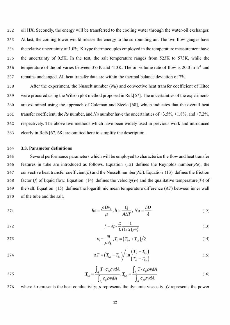
12

oil HX. Secondly, the energy will be transferred to the cooling water through the water-oil exchanger. 252

At last, the cooling tower would release the energy to the surrounding air. The two flow gauges have 253

the relative uncertainty of 1.0%. K-type thermocouples employed in the temperature measurement have 254

the uncertainty of 0.5K. In the test, the salt temperature ranges from 523K to 573K, while the 255

temperature of the oil varies between 373K and 413K. The oil volume rate of flow is 20.0 m3h-1 and 256

remains unchanged. All heat transfer data are within the thermal balance deviation of 7%. 257

After the experiment, the Nusselt number (Nu) and convective heat transfer coefficient of Hitec 258

were procured using the Wilson plot method proposed in Ref.[67]. The uncertainties of the experiments 259

are examined using the approach of Coleman and Steele [68], which indicates that the overall heat 260

transfer coefficient, the Re number, and Nu number have the uncertainties of ±3.5%, ±1.8%, and ±7.2%, 261

respectively. The above two methods which have been widely used in previous work and introduced 262

clearly in Refs.[67, 68] are omitted here to simplify the description. 263

3.3. Parameter definitions 264

Several performance parameters which will be employed to characterize the flow and heat transfer 265

features in tube are introduced as follows. Equation (12) defines the Reynolds number(Re), the 266

convective heat transfer coefficient(h) and the Nusselt number(Nu). Equation (13) defines the friction 267

factor (f) of liquid flow. Equation (14) defines the velocity(vf) and the qualitative temperature(Tf) of 268

the salt. Equation (15) defines the logarithmic mean temperature difference (ΔT) between inner wall 269

of the tube and the salt. 270

f , ,

Dv Q hDRe h Nu

A T

(12) 271

2

f

1

1/ 2

Df p

L v (13) 272

f f f,o f,i

c

= , 2m

v T T TA

(14) 273

w f,i

f,o f,i

w f,o

lnT T

T T TT T

(15) 274

c c

c c

f,i f,o,p p

A A

p pA A

T c vdA T c vdAT T

c vdA c vdA

(16) 275

where λ represents the heat conductivity; μ represents the dynamic viscosity; Q represents the power 276

13

converted to the salt; Δp indicates the drop of pressure from the inlet to the outlet; A is heat transfer 277

area; L represents the length of the tube; Tw represents the average temperature of heat transfer surface; 278

Ac represents the area of the inlet or outlet; Tf,o and Tf,i represent the salt temperatures at the tube’s 279

outlet and inlet, respectively. 280

4. Model validation 281

The numerical model was validated in the following way. Firstly, an independence check of the 282

mesh was carried out to eliminate its possible influences on the computation. Secondly, the numerical 283

results of the water were compared with some classical correlations. Finally, the numerical results of 284

Hitec and FLiNaK were compared with corresponding experimental data, respectively. 285

4.1 Mesh independence check 286

In the simulation, the effects of the mesh on the results should be eliminated for each case. An 287

example was used to illustrate the mesh independence check as follows. Firstly, different hexahedral 288

mesh systems were generated, where the mesh in the axial direction is uniform. Then, the flow and heat 289

transfer for the Hitec were simulated under non-uniform flux for each mesh system, where the typical 290

condition of uf,i=4 ms-1 and Tf,i=650K were considered. Then, the simulated Nu number and f number 291

for these mesh systems were compared as shown in Fig. 5. It is seen the variations of Nu number and f 292

number are less than 0.23% and 0.08% when the mesh number increases from 1680×250 (cross-293

section×axial) to 3317×300, respectively. Considering the computational accuracy and time, the mesh 294

system of 1680×250 can be found to be adequate for the current case, where y+=30.7-45.5.The cross- 295

section of this mesh system is shown in Fig. 6. For other cases simulated in current work, mesh 296

independence check has also been conducted in a similar way. 297

10 100 1000360

380

400

420

440

460

480

14

76

×1

50

33

17

×3

00

12

16

×1

00

Nu

Mesh number / ×103

Nu

f

16

80

×2

50

98

0×

80

76

8×

40

Cro

ss-s

ecti

on

×axia

l=

620

×20

0.015

0.016

0.017

0.018

0.019

0.020

0.021

f

Xt

Zt

TubeSalt 298

Fig. 5. Mesh independence test using several mesh systems

(cross-section × axial).

Fig. 6. Cross-section of the typical mesh that is

uniform in axial direction.

14

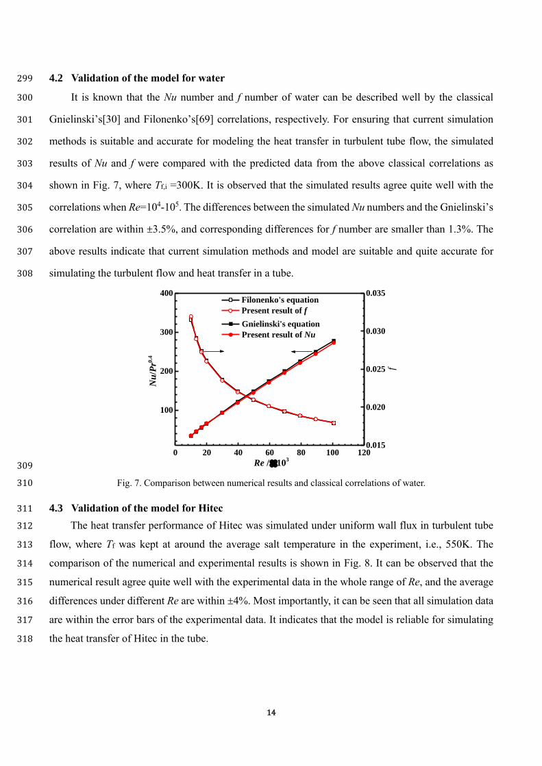
4.2 Validation of the model for water 299

It is known that the Nu number and f number of water can be described well by the classical 300

Gnielinski’s[30] and Filonenko’s[69] correlations, respectively. For ensuring that current simulation 301

methods is suitable and accurate for modeling the heat transfer in turbulent tube flow, the simulated 302

results of Nu and f were compared with the predicted data from the above classical correlations as 303

shown in Fig. 7, where Tf,i =300K. It is observed that the simulated results agree quite well with the 304

correlations when Re=104-105. The differences between the simulated Nu numbers and the Gnielinski’s 305

correlation are within ±3.5%, and corresponding differences for f number are smaller than 1.3%. The 306

above results indicate that current simulation methods and model are suitable and quite accurate for 307

simulating the turbulent flow and heat transfer in a tube. 308

0 20 40 60 80 100 120

100

200

300

400

Gnielinski's equation

Present result of Nu

Re / 103

Nu

/Pr0

.4

0.015

0.020

0.025

0.030

0.035 Filonenko's equation

Present result of f

f

309

Fig. 7. Comparison between numerical results and classical correlations of water. 310

4.3 Validation of the model for Hitec 311

The heat transfer performance of Hitec was simulated under uniform wall flux in turbulent tube 312

flow, where Tf was kept at around the average salt temperature in the experiment, i.e., 550K. The 313

comparison of the numerical and experimental results is shown in Fig. 8. It can be observed that the 314

numerical result agree quite well with the experimental data in the whole range of Re, and the average 315

differences under different Re are within ±4%. Most importantly, it can be seen that all simulation data 316

are within the error bars of the experimental data. It indicates that the model is reliable for simulating 317

the heat transfer of Hitec in the tube. 318

15

8 10 12 14 16 18 20 2230

40

50

60

70

80

Nu

/Pr0

.4

Re / 103

Present experimental data

Fitting curve of experimantal data

Present simulation results

319

Fig. 8. Comparison between numerical and experimental results of Hitec. 320

4.4 Validation of the model for FLiNaK 321

For FLiNaK, the simulation was conducted under different Re when Tf was around 898K which is 322

the average temperature of the salt in the experiments of Vriesema[19]. In the experiments, the salt 323

flowed in the tube side of a concentric tube exchanger, and air flowed in the shell side. The salt inlet 324

temperature was in the range of 848K-948K in the test. The modeling results are compared with the 325

testing data of Vriesema[19] as shown in Fig. 9, where Ferng et al.’s simulation data[35] are also shown. 326

It is seen that the current numerical results which are similar to Ferng et al.’s results[35] agree well 327

with the experimental data, and the average deviations are smaller than ±5%, which indicates that the 328

model is accurate for modeling the heat transfer of FLiNaK in the tube. 329

To sum up, the above comparisons indicate that the current model is reliable for simulating the 330

heat transfer of the fluoride and nitrate in turbulent tube flow. 331

0 20 40 60 80 100 1200

50

100

150

200

250

300

Nu

/Pr0

.4

Re / 103

Vriesema's experimental data[19]

Fitting curve of experimental data

Present numerical results

Ferng et al.'s numerical results[35]

332

16

Fig. 9. Comparison between numerical and experimental results of FLiNaK. 333

5. Results and discussion 334

In the following section, firstly, influences of the extreme non-uniform heat flux would be 335

examined. Then, simulations are employed to extend the temperature and Reynolds number to large 336

ranges that cannot be easily achieved in experiments. The simulation results of all salts will be 337

compared with some classical correlations for checking whether they are applicable to the salts. Finally, 338

we would try to select or develop a heat transfer correlation that can achieve an error of <10%. 339

5.1. Heat transfer and friction under uniform and non-uniform fluxes 340

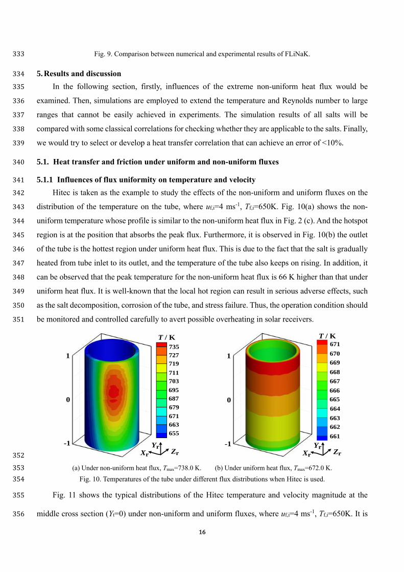
5.1.1 Influences of flux uniformity on temperature and velocity 341

Hitec is taken as the example to study the effects of the non-uniform and uniform fluxes on the 342

distribution of the temperature on the tube, where uf,i=4 ms-1, Tf,i=650K. Fig. 10(a) shows the non-343

uniform temperature whose profile is similar to the non-uniform heat flux in Fig. 2 (c). And the hotspot 344

region is at the position that absorbs the peak flux. Furthermore, it is observed in Fig. 10(b) the outlet 345

of the tube is the hottest region under uniform heat flux. This is due to the fact that the salt is gradually 346

heated from tube inlet to its outlet, and the temperature of the tube also keeps on rising. In addition, it 347

can be observed that the peak temperature for the non-uniform heat flux is 66 K higher than that under 348

uniform heat flux. It is well-known that the local hot region can result in serious adverse effects, such 349

as the salt decomposition, corrosion of the tube, and stress failure. Thus, the operation condition should 350

be monitored and controlled carefully to avert possible overheating in solar receivers. 351

0

1

-1

655

663

671

679

695

703

711

719

727

735

687

T / K

Xr

YrZr

661

662

663

664

666

667

668

669

670

671

665

T / K

Xr

YrZr

0

1

-1

352

(a) Under non-uniform heat flux, Tmax=738.0 K. (b) Under uniform heat flux, Tmax=672.0 K. 353

Fig. 10. Temperatures of the tube under different flux distributions when Hitec is used. 354

Fig. 11 shows the typical distributions of the Hitec temperature and velocity magnitude at the 355

middle cross section (Yt=0) under non-uniform and uniform fluxes, where uf,i=4 ms-1, Tf,i=650K. It is 356

17

seen that the temperature under non-uniform flux is quite non-uniform with a hot region at the lower 357

half as shown in Fig. 11(a), where the maximum temperature difference in the cross section is around 358

13.5K. In Fig. 11(b), it is observed that the temperature shows an axisymmetric pattern, and the 359

maximum temperature difference is 5.7K. Moreover, it is seen in Fig. 11(c)(d) that the velocity 360

distributions under the two flux distributions also show axisymmetric features, and they are quite 361

similar to each other, which indicates that the flux distribution has no significant influence on the 362

velocity distribution. However, it can be found that the peak velocity under non-uniform flux is slightly 363

higher than that under uniform flux by comparing the values of velocity in Fig. 11(c) and (d). This 364

should be a result of the slightly larger buoyancy caused by the larger temperature difference and the 365

gravity(g) under non-uniform flux, as shown in Fig. 11(a). 366

Zt /

mm

662

660

658

656

654

652

650

K

9Xt / mm-9

9-9

g

Zt /

mm

662

660

658

656

654

652

650

K

9Xt / mm-9

9-9

g

Zt /

mm

9Xt / mm-9

9-9

g

4.6

4.2

3.8

3.4

3.0

2.6

m·s-1

4.6

4.2

3.8

3.4

3.0

2.6

m·s-1

Zt /

mm

9Xt / mm-9

9-9

g

367 (a) Temperature,

non-uniform flux (b) Temperature,

uniform flux (c) Velocity magnitude,

non-uniform flux (d) Velocity magnitude,

uniform flux

Fig. 11. Temperatures and velocity magnitude of the Hitec under different flux distributions at Yt=0. 368

5.1.2 Influences of flux uniformity on heat transfer performance 369

Influences of the uniform and non-uniform fluxes on the heat transfer features of the liquid salts 370

would be examined in this part. For every liquid salt, the broadest possible range of the temperature 371

would be considered under a typical inlet velocity. 372

Fig. 12 illustrates the performance of heat transfer for every salt at both non-uniform and uniform 373

heat fluxes. It is observed that Re number for every liquid salt rises with the increase of temperature at 374

the same velocity. This is due to the variations of the density and dynamic viscosity with the temperature 375

as shown in Fig. 3. Moreover, it is found that the values of Nu/Pr0.4 at non-uniform wall flux for every 376

salt are about 2% higher than those with uniform wall flux at different temperatures. This phenomenon 377

is caused by the hot region, which is at the bottom of the tube section, under non-uniform wall flux, as 378

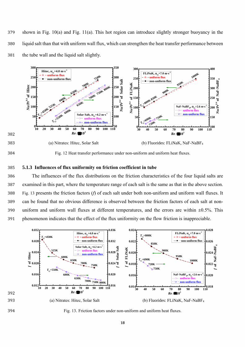
18

shown in Fig. 10(a) and Fig. 11(a). This hot region can introduce slightly stronger buoyancy in the 379

liquid salt than that with uniform wall flux, which can strengthen the heat transfer performance between 380

the tube wall and the liquid salt slightly. 381

0

50

100

150

200

250

300

10 20 30 40 50 60 70 80 90 100 110

Nu

/Pr0

.4 o

f H

itec

uniform flux

non-uniform flux

Hitec, uf,i

=4.0 m·s-1

Re / 103

50

100

150

200

250

300

350

uniform flux

non-uniform flux

Solar Salt, uf,i

=4.2 m·s-1

Nu

/Pr0

.4 o

f S

ola

r S

alt

T f,i=450K

525K

600K

650K

700K

750K

T f,i=550K

600K

650K

700K750K

800K

0

50

100

150

200

250

300

30 40 50 60 70 80 90 100 110N

u/P

r0.4 of

FL

iNaK

uniform flux

non-uniform flux

FLiNaK, uf,i

=7.0 m·s-1

Re / 103

100

150

200

250

300

350

400

750K

720K

uniform flux

non-uniform flux

NaF-NaBF4, u

f,i=2.6 m·s

-1

Nu

/Pr0

.4 o

f N

aF

-Na

BF

4

T f,i=800K

850K

900K

950K

1000K

T f,i=690K

382

(a) Nitrates: Hitec, Solar Salt (b) Fluorides: FLiNaK, NaF-NaBF4 383

Fig. 12 Heat transfer performance under non-uniform and uniform heat fluxes. 384

5.1.3 Influences of flux uniformity on friction coefficient in tube 385

The influences of the flux distributions on the friction characteristics of the four liquid salts are 386

examined in this part, where the temperature range of each salt is the same as that in the above section. 387

Fig. 13 presents the friction factors (f) of each salt under both non-uniform and uniform wall fluxes. It 388

can be found that no obvious difference is observed between the friction factors of each salt at non-389

uniform and uniform wall fluxes at different temperatures, and the errors are within ±0.5%. This 390

phenomenon indicates that the effect of the flux uniformity on the flow friction is inappreciable. 391

0.012

0.016

0.020

0.024

0.028

0.032

10 20 30 40 50 60 70 80 90 100 110

f o

f H

itec

uniform flux

non-uniform flux

Hitec, uf,i

=4.0 m·s-1

Re / 103

Tf,i

=450K

525K

600K

650K700K

750K

0.016

0.020

0.024

0.028

0.032

0.036

uniform flux

non-uniform flux

Solar Salt, uf,i

=4.2 m·s-1

f o

f S

ola

r S

alt

Tf,i

=550K

600K

650K700K 750K 800K

0.014

0.016

0.018

0.020

0.022

0.024

30 40 50 60 70 80 90 100 110

f o

f F

LiN

aK

950K

900K

uniform flux

non-uniform flux

FLiNaK, uf,i

=7.0 m·s-1

Re / 103

Tf,i

=800K

850K

1000K

0.018

0.020

0.022

0.024

0.026

0.028

uniform flux

non-uniform flux

NaF-NaBF4, u

f,i=2.6 m·s

-1

f o

f N

aF

-Na

BF

4

Tf,i

=690K

720K

750K

392

(a) Nitrates: Hitec, Solar Salt (b) Fluorides: FLiNaK, NaF-NaBF4 393

Fig. 13. Friction factors under non-uniform and uniform heat fluxes. 394

19

After the above examinations, it can be found the non-uniform heat flux influences the tube 395

temperature obviously, but the effects on both heat transfer and friction factor are negligible. These 396

facts offer an important suggestion that it is unnecessary to use experiments, which are complex, tough 397

and expensive, to obtain the heat transfer and friction correlations under non-uniform heat flux, because 398

the correlations should be very close to those under uniform heat flux. In addition, the studied non-399

uniform flux is a typical extreme condition in the industry, and the fluxes under other conditions in the 400

industry usually cannot be more non-uniform than the current case. As a result, due to the fact that the 401

current non-uniform flux influences little on heat transfer and friction, it can be inferred that similar 402

phenomenon can be found under other non-uniform flux conditions in the industry. 403

In the rest of this work, the flow friction and heat transfer features will just be studied using 404

uniform heat flux, but the procured correlations should also be applicable under non-uniform flux. 405

5.2. Comparison of simulated data and classical correlations 406

Some classical correlations including Gnielinski’s equation given in Eq.(17) [30], Hausen’s 407

correlation given in Eq.(18) [31], and Sider-Tate’s correlation shown in Eq.(19) [29] can calculate the 408

heat transfer performance of ordinary fluids in tube appropriately. Moreover, the Filonenko’s 409

correlation shown in Eq.(20) also can calculate the friction factor of ordinary fluids accurately. 410

0.11 2/3

0.87 0.4 f

w

5 6

=0.012 280 1

=0.6-10 , =2300-10

Pr DNu Re Pr

Pr L

Pr Re

(17) 411

0.14 2/3

0.75 0.42 f

w

6

=0.037 180 1

=0.5-1000, =2300-10

DNu Re Pr

L

Pr Re

(18) 412

0.14

0.8 1/3 f

w

4

=0.027

>10 , =0.7-16700, / >60

Nu Re Pr

Re Pr L D

(19) 413

2

5 6

1.82lg 1.64

=0.6-10 , =2300-10

f Re

Pr Re

(20) 414

In this part, the simulation data of heat transfer performance and flow friction are used to compare 415

with the above classical equations for examining if these equations are still appropriate for the liquid 416

salts. In the simulation, the Re number covers a wide range of 104-105. The examined ranges of the bulk 417

temperature for the four salts are given in Table 3, which is determined after considering that the highest 418

temperature of each salt will be within the reliable temperature range of its thermophysical properties. 419

20

420

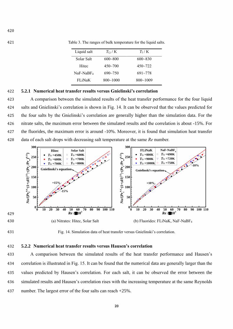
Table 3. The ranges of bulk temperature for the liquid salts. 421

Liquid salt Tf,i / K Tf / K

Solar Salt 600~800 600~830

Hitec 450~700 450~722

NaF-NaBF4 690~750 691~778

FLiNaK 800~1000 800~1009

5.2.1 Numerical heat transfer results versus Gnielinski’s correlation 422

A comparison between the simulated results of the heat transfer performance for the four liquid 423

salts and Gnielinski’s correlation is shown in Fig. 14. It can be observed that the values predicted for 424

the four salts by the Gnielinski’s correlation are generally higher than the simulation data. For the 425

nitrate salts, the maximum error between the simulated results and the correlation is about -15%. For 426

the fluorides, the maximum error is around -10%. Moreover, it is found that simulation heat transfer 427

data of each salt drops with decreasing salt temperature at the same Re number. 428

0 10 20 30 40 50 60 70 80 90 100 1100

50

100

150

200

250

300

Gnielinski's equation

Tf,i =600K

Tf,i =700K

Tf,i =800K

Re / 103

Nu

/{P

r f0.4·[

1+

(d/l

)2/3

]·(P

r f /P

r w)0

.11}

Tf,i =450K

Tf,i =600K

Tf,i =700K

Hitec Solar Salt

+15%

-15%

0 10 20 30 40 50 60 70 80 90 100 110

0

50

100

150

200

250

300

-10%

+10%

900K00K

Gnielinski's equation

Tf,i =690K

Tf,i =720K

Tf,i =750K

Re / 103

Nu

/{P

r f0.4·[

1+

(d/l

)2/3

]·(P

r f /P

r w)0

.11}

Tf,i =800K

Tf,i =900K

Tf,i =1000K

FLiNaK NaF-NaBF4

429

(a) Nitrates: Hitec, Solar Salt (b) Fluorides: FLiNaK, NaF-NaBF4 430

Fig. 14. Simulation data of heat transfer versus Gnielinski’s correlation. 431

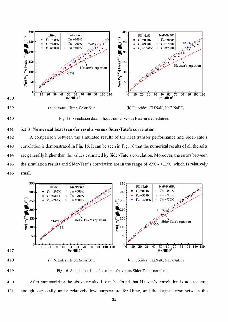
5.2.2 Numerical heat transfer results versus Hausen’s correlation 432

A comparison between the simulated results of the heat transfer performance and Hausen’s 433

correlation is illustrated in Fig. 15. It can be found that the numerical data are generally larger than the 434

values predicted by Hausen’s correlation. For each salt, it can be observed the error between the 435

simulated results and Hausen’s correlation rises with the increasing temperature at the same Reynolds 436

number. The largest error of the four salts can reach +25%. 437

21

0 10 20 30 40 50 60 70 80 90 100 1100

50

100

150

200

250

300

Hausen's equation

Tf,i =600K

Tf,i =700K

Tf,i =800K

Re / 103

Nu

/{P

r f0.4

2·[

1+

(d/l

)2/3

]·(

f /

w)0

.14}

Tf,i =450K

Tf,i =600K

Tf,i =700K

Hitec Solar Salt

+25%

-10%

0 10 20 30 40 50 60 70 80 90 100 110

0

50

100

150

200

250

300

+25%

Hausen's equation

Tf,i =690K

Tf,i =720K

Tf,i =750K

Re / 103

Nu

/{P

r f0.4

2·[

1+

(d/l

)2/3

]·(

f /

w)0

.14}

Tf,i =800K

Tf,i =900K

Tf,i =1000K

FLiNaK NaF-NaBF4

438

(a) Nitrates: Hitec, Solar Salt (b) Fluorides: FLiNaK, NaF-NaBF4 439

Fig. 15. Simulation data of heat transfer versus Hausen’s correlation. 440

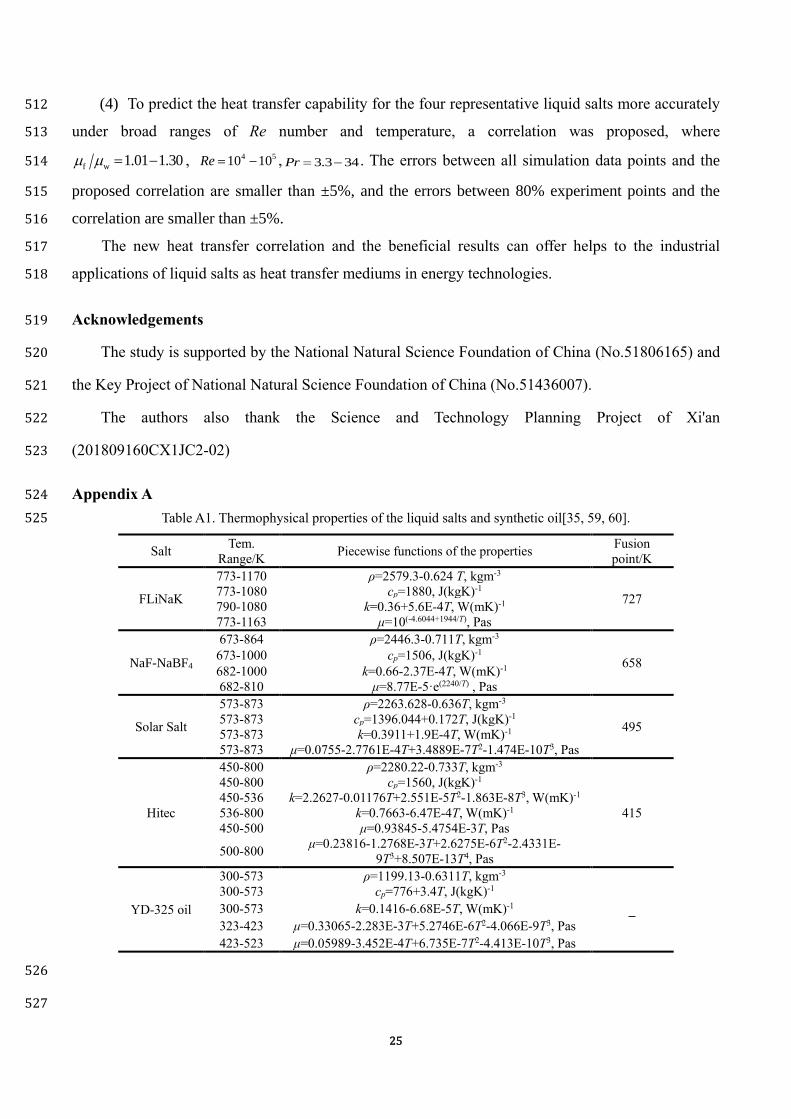
5.2.3 Numerical heat transfer results versus Sider-Tate’s correlation 441

A comparison between the simulated results of the heat transfer performance and Sider-Tate’s 442

correlation is demonstrated in Fig. 16. It can be seen in Fig. 16 that the numerical results of all the salts 443

are generally higher than the values estimated by Sider-Tate’s correlation. Moreover, the errors between 444

the simulation results and Sider-Tate’s correlation are in the range of -5% - +13%, which is relatively 445

small. 446

0 10 20 30 40 50 60 70 80 90 100 1100

50

100

150

200

250

300

350

Sider-Tate's equation

Tf,i =600K

Tf,i =700K

Tf,i =800K

Re / 103

Nu

/[P

r f1/3·(

f /

w)0

.14]

Tf,i =450K

Tf,i =600K

Tf,i =700K

Hitec Solar Salt

-5%

+13%

0 10 20 30 40 50 60 70 80 90 100 1100

50

100

150

200

250

300

350

-5%

+13%

Sider-Tate's equation

Tf,i =690K

Tf,i =720K

Tf,i =750K

Re / 103

Nu

/[P

r f1/3·(

f /

w)0

.14]

Tf,i =800K

Tf,i =900K

Tf,i =1000K

FLiNaK NaF-NaBF4

447

(a) Nitrates: Hitec, Solar Salt (b) Fluorides: FLiNaK, NaF-NaBF4 448

Fig. 16. Simulation data of heat transfer versus Sider-Tate’s correlation. 449

After summarizing the above results, it can be found that Hausen’s correlation is not accurate 450

enough, especially under relatively low temperature for Hitec, and the largest error between the 451

22

simulated results and Hausen’s correlation can reach +25%. As a result, Hausen’s correlation should 452

be inappropriate for calculating the performance of heat transfer for liquid salts. Meanwhile, it is also 453

found that the Sider-Tate’s equation and Gnielinski’s equation can predict the performance of the liquid 454

salts more accurately, and the biggest errors are around +13% and -15%, respectively. These errors 455

used to be considered acceptable for the industry[32]. However, after reviewing developments in heat 456

transfer, Tao[33] pointed out that an error of <10% has been going to be the new norm in recent years, 457

which is significant for enhancing the performance, reducing heat exchanger’s volume and cost. 458

5.2.4 Numerical friction factor versus Filonenko’s correlation 459

A comparison between the numerical friction factor(f) and the Filonenko’s correlation is 460

demonstrated in Fig. 17. It is seen that the simulated results of the friction factors for the four liquid 461

salts under all modeling conditions agree excellently well with this correlation. All numerical data 462

points are within the error of ±2% of the correlation. This result indicates that the Filonenko’s 463

correlation is suitable for predicting the friction factors of all the four liquid salts. 464

0 20 40 60 80 100 1200.015

0.020

0.025

0.030

0.035

Filonenko's equation

-2%

+2%

Solar Salt: Hitec :

800K

900K

1000K

Tf,i

450K

600K

700K

690K

720K

750K

Tf,i

NaF-NaBF4: FLiNaK:

600K

700K

800K

Re / 103

f Tf,i Tf,i

465 Fig. 17. Simulated friction factor(f) versus Filonenko’s correlation. 466

5.3. A new heat transfer correlation proposed for the liquid salts 467

To predict the heat transfer performance better, the simulated data procured under a wide range of 468

Re number and the broadest possible ranges of the temperature for the four liquid salts as given in Table 469

3 are employed to develop a new correlation, which is shown in Eq.(21). A comparison between the 470

new correlation and the simulated data is demonstrated in Fig. 18, which indicates that the new 471

correlation is excellently coincident with all simulated results. The largest relative error of the simulated 472

results and the developed correlation is smaller than ±5%. In addition, the errors for 95% data points 473

23

are smaller than ±3%. 474

0.14

0.853 0.35 f

w

=0.0154Nu Re Pr

(21) 475

where f w 1.01 1.30 ; 4 510 10Re ; 3.3 34Pr . 476

0 20 40 60 80 100 1200

100

200

300

400

Nu=0.0154Re0.853

Prf

0.35( f / w)

0.14

-5%

+5%

Solar Salt: Hitec :

800K

900K

1000K

Tf,i

450K

600K

700K

690K

720K

750K

Tf,i

NaF-NaBF4: FLiNaK:

600K

700K

800K

Re / 103

Nu

/[P

r f0.3

5·(

f /

w)0

.14]

Tf,i Tf,i

477 Fig. 18. New heat transfer correlation versus simulated data of the four liquid salts. 478

Finally, a comparison between the developed correlation and some experimental results of three 479

representative liquid salts is illustrated in Fig. 19. In the comparison, Silverman’s experiment data of 480

NaF-NaBF4[15] , Vriesema’s experiment data of FLiNaK[19], and current experiment data of Hitec are 481

taken into account. The comparison demonstrates that all the experiment results are well coincident the 482

developed correlation. It is found that the errors between 80% experiment data and present correlation 483

are smaller than ±5%. Moreover, the errors between 90% experiment data and the new correlation are 484

found to be within ±10%. The results manifest that current correlation can predict the performance of 485

heat transfer for the four liquid salts accurately in turbulent tube flow, which can meet the requirements 486

of high accurate correlations in the design of energy systems and help to reduce the cost of investment. 487

24

1 10

50

100

150

200

250

300

350

350.8 11

-5%

+5%

98765432Re / 10

4

Nu

/ P

r0.3

5

Hitec, present experiment data

FLiNaK,Vriesema's exp.[19]

NaF-NaBF4, Silverman's exp.[15]

+10%

-10%

Nu=0.0154Re0.853

Pr0.35

( f / w)0.14

488

Fig. 19. New heat transfer correlation versus the experiment results of three typical salts. 489

6. Conclusions 490

The heat transfer capability and friction features for representative liquid salts employed in energy 491

applications are investigated under the turbulent condition in a tube with wide ranges of velocity and 492

temperature, where four liquid salts including Hitec, Solar Salt, NaF-NaBF4, and FLiNaK are studied. 493

The following conclusions are obtained. 494

(1) A computational model was developed to simulate the flow and heat transfer processes of the 495

liquid salts, and experiments were conducted to test the heat transfer capability of Hitec when it flows 496

in the tube side of a STHX. Comparing the modeled results of Hitec and the experiment results indicates 497

that the average differences are smaller than ±4%, which manifests that the modeling method is reliable, 498

and the simulation model is believable. 499

(2) Examination of the influences of the flux uniformity on flow and heat transfer indicates that 500

the non-uniform wall flux can lead to local hotspot but influences little on the friction factor and heat 501

transfer performance comparing with those under uniform flux. This fact suggests that the friction and 502

heat transfer correlations acquired with uniform wall flux are applicable under non-uniform flux. So, it 503

is unnecessary to further use experiments, which are expensive and tough, to obtain the correlations 504

under non-uniform. 505

(3) Comparisons between the simulated results procured within wide velocity range and 506

temperature interval and some exiting correlations were carried out. Hausen’s correlation is found to 507

be not suitable for the salts with a maximum error of +25%. While Sider-Tate’s correlation and 508

Gnielinski’s correlation are relatively accurate with the biggest errors of +13% and -15%, respectively. 509

In addition, Filonenko’s correlation could predict the friction factor in a quite accurate way with the 510

maximum error of ±2%. 511

25

(4) To predict the heat transfer capability for the four representative liquid salts more accurately 512

under broad ranges of Re number and temperature, a correlation was proposed, where 513

f w 1.01 1.30 , 4 510 10Re , 3.3 34Pr . The errors between all simulation data points and the 514

proposed correlation are smaller than ±5%, and the errors between 80% experiment points and the 515

correlation are smaller than ±5%. 516

The new heat transfer correlation and the beneficial results can offer helps to the industrial 517

applications of liquid salts as heat transfer mediums in energy technologies. 518

Acknowledgements 519

The study is supported by the National Natural Science Foundation of China (No.51806165) and 520

the Key Project of National Natural Science Foundation of China (No.51436007). 521

The authors also thank the Science and Technology Planning Project of Xi'an 522

(201809160CX1JC2-02) 523

Appendix A 524

Table A1. Thermophysical properties of the liquid salts and synthetic oil[35, 59, 60]. 525

Salt Tem.

Range/K Piecewise functions of the properties

Fusion

point/K

FLiNaK

773-1170 ρ=2579.3-0.624 T, kgm-3

727 773-1080 cp=1880, J(kgK)-1

790-1080 k=0.36+5.6E-4T, W(mK)-1

773-1163 μ=10(-4.6044+1944/T), Pas

NaF-NaBF4

673-864 ρ=2446.3-0.711T, kgm-3

658 673-1000 cp=1506, J(kgK)-1

682-1000 k=0.66-2.37E-4T, W(mK)-1

682-810 μ=8.77E-5·e(2240/T) , Pas

Solar Salt

573-873 ρ=2263.628-0.636T, kgm-3

495 573-873 cp=1396.044+0.172T, J(kgK)-1

573-873 k=0.3911+1.9E-4T, W(mK)-1

573-873 μ=0.0755-2.7761E-4T+3.4889E-7T2-1.474E-10T3, Pas

Hitec

450-800 ρ=2280.22-0.733T, kgm-3

415

450-800 cp=1560, J(kgK)-1

450-536 k=2.2627-0.01176T+2.551E-5T2-1.863E-8T3, W(mK)-1

536-800 k=0.7663-6.47E-4T, W(mK)-1

450-500 μ=0.93845-5.4754E-3T, Pas

500-800 μ=0.23816-1.2768E-3T+2.6275E-6T2-2.4331E-

9T3+8.507E-13T4, Pas

YD-325 oil

300-573 ρ=1199.13-0.6311T, kgm-3

_

300-573 cp=776+3.4T, J(kgK)-1

300-573 k=0.1416-6.68E-5T, W(mK)-1

323-423 μ=0.33065-2.283E-3T+5.2746E-6T2-4.066E-9T3, Pas

423-523 μ=0.05989-3.452E-4T+6.735E-7T2-4.413E-10T3, Pas

526

527

26

Nomenclature 528

Ac inlet or outlet area, m2

A heat transfer area, m2

c1, c2, c3, cμ constants in numerical model

cp specific heat capacity at constant pressure, J·kg-1·K-1

D inside diameter of round tube, mm

f friction factor of flow

g gravity (m·s-2)

h convective heat transfer coefficient (W·m-2·K-1)

k turbulent kinetic energy of flow (m2·s-2)

L effective length of tube(m, mm)

Nu nondimensional Nusselt number

Pr nondimensional Prandtl number

p pressure (Pa)

Prt turbulent Prandtl number of energy

q local heat flux obtained by salt (W·m-2)

Q heat transfer rate (W)

Re nondimensional Reynolds number

STHX shell-tube heat exchanger

Tf qualitative temperature of the salt (K)

Tf,i, Tf,o temperatures at the inlet, outlet(K)

Tw temperature of heat transfer surface (K)

T temperature (K)

vf velocity of salt (m·s-1)

u, v, w components of velocity (m·s-1)

Xt, Yt, Zt Cartesian axes of tube system (m)

Xr, Yr, Zr Cartesian axes of receiver system (m)

Greek symbols

δij unit tensor

ΔT logarithmic temperature difference (K)

Δp drop of pressure (Pa)

ε turbulent dissipation rate of flow (m2·s-3)

λ thermal conductivity of materials(W·m-1·K-1)

μt turbulent viscosity of flow (kg·m-1·s-1)

μ dynamic viscosity of fluid (Pa·s)

ρ density of materials (kg·m-3)

σε turbulent Prandtl number of ε

σk turbulent Prandtl number of k

Subscripts

i, o, w, f inlet , outlet , wall , fluid

529

530

27

References 531

[1] Tokarska KB, Gillett NP. Cumulative carbon emissions budgets consistent with 1.5° C global warming. Nature Climate 532

Change. 2018;8:296. 533

[2] Li MJ, Tao WQ. Review of methodologies and polices for evaluation of energy efficiency in high energy-consuming 534

industry. Appl Energ. 2017;187:203-15. 535

[3] Li MJ, Zhu HH, Guo JQ, Wang K, Tao WQ. The development technology and applications of supercritical CO2 power 536

cycle in nuclear energy, solar energy and other energy industries. Appl Therm Eng. 2017;126:255-75. 537

[4] Ma Z, Yang WW, Yuan F, Jin B, He YL. Investigation on the thermal performance of a high-temperature latent heat 538

storage system. Appl Therm Eng. 2017;122:579-92. 539

[5] Li MJ, He YL, Tao WQ. Modeling a hybrid methodology for evaluating and forecasting regional energy efficiency in 540

China. Appl Energ. 2017;185:1769-77. 541

[6] He YL, Wang K, Qiu Y, Du BC, Liang Q, Du S. Review of the solar flux distribution in concentrated solar power: non-542

uniform features, challenges, and solutions. Appl Therm Eng. 2019;149:448-74. 543

[7] Wang K, He YL. Thermodynamic analysis and optimization of a molten salt solar power tower integrated with a 544

recompression supercritical CO2 Brayton cycle based on integrated modeling. Energ Convers Manag. 2017;135:336-545

50. 546

[8] Li MJ, Jin B, Yan JJ, Ma Z, Li MJ. Numerical and Experimental study on the performance of a new two-layered high-547

temperature packed-bed thermal energy storage system with changed-diameter macro-encapsulation capsule. Appl 548

Therm Eng. 2018;142:830-45. 549

[9] Ma Z, Li MJ, Yang WW, He YL. General performance evaluation charts and effectiveness correlations for the design of 550

thermocline heat storage system. Chem Eng Sci. 2018;185:105-15. 551

[10] Li MJ, Jin B, Ma Z, Yuan F. Experimental and numerical study on the performance of a new high-temperature packed-552

bed thermal energy storage system with macroencapsulation of molten salt phase change material. Appl Energ. 553

2018;221:1-15. 554

[11] Lake JA. The fourth generation of nuclear power. Prog Nucl Energ. 2002;40:301-7. 555

[12] Romatoski RR, Hu LW. Fluoride salt coolant properties for nuclear reactor applications: A review. Ann Nucl Energy. 556

2017;109:635-47. 557

[13] He YL, Zheng ZJ, Du BC, Wang K, Qiu Y. Experimental investigation on turbulent heat transfer characteristics of 558

molten salt in a shell-and-tube heat exchanger. Appl Therm Eng. 2016;108:1206-13. 559

[14] Qiu Y, Li MJ, Wang WQ, Du BC, Wang K. An experimental study on the heat transfer performance of a prototype 560

molten-salt rod baffle heat exchanger for concentrated solar power. Energy. 2018;156:63-72. 561

[15] Silverman MD, Huntley WR, Robertson HE. Heat transfer measurements in a forced convection loop with two molten-562

fluoride salts LiF-BeF2-ThF2-UF4 and eutectic NaBF4-NaF. Oak Ridge: Oak Ridge National Laboratory; 1976, 563

ORNL/TM-5335. 564

[16] Cooke JW, Cox BW. Forced-convection heat transfer measurements with a molten fluoride salt mixture flowing in a 565

smooth tube. Oak Ridge: Oak Ridge National Laboratory; 1973, ORNL-TM-4079. 566

[17] Hoffman HW, Lones J. Fused salt heat transfer. Part II. Forced convection heat transfer in circular tubes containing 567

NaF-KF-LiF eutectic. Oak Ridge: Oak Ridge National Laboratory; 1955, ORNL-1777. 568

[18] Grele MD, Gedeon L. Forced-convection heat-transfer characteristics of molten FLiNaK flowing in an inconel X 569

system. Washington: National Advisory Committee for Aeronautics; 1954, RM E53L18. 570

[19] Vriesema B. Aspects of molten fluorides as heat transfer agents for power generation [PhD]. Delft, Netherlands: Delft 571

University of Technology; 1979. 572

28

[20] Hoffman HW, Cohen SI. Fused salt heat transfer: Part III: Forced-convection heat transfer in circular tubes containing 573

the salt mixture NaNO2-NaNO3-KNO3. Oak Ridge: Oak Ridge National Laboratory; 1960, ORNL-2433. 574

[21] Kirst W, Nagle W, Castner J. A new heat transfer medium for high temperatures. Transactions of the American Institute 575

of Chemical Engineers. 1940;36:371-94. 576

[22] Wu YT, Chen C, Liu B, Ma CF. Investigation on forced convective heat transfer of molten salts in circular tubes. Int 577

Commun Heat Mass. 2012;39:1550-5. 578

[23] Du BC, He YL, Qiu Y, Liang Q, Zhou YP. Investigation on heat transfer characteristics of molten salt in a shell-and-579

tube heat exchanger. Int Commun Heat Mass. 2018;96:61-8. 580

[24] Qian J, Kong Q, Zhang H, Huang W, Li W. Performance of a gas cooled molten salt heat exchanger. Appl Therm Eng. 581

2016;108:1429-35. 582

[25] Chen Y, Zhu H, Tian J, Fu Y, Tang Z, Wang N. Convective heat transfer characteristics in the laminar and transition 583

region of molten salt in concentric tube. Appl Therm Eng. 2017;117:682-8. 584

[26] Chen YS, Wang Y, Zhang JH, Yuan XF, Tian J, Tang ZF, et al. Convective heat transfer characteristics in the turbulent 585

region of molten salt in concentric tube. Appl Therm Eng. 2016;98:213-9. 586

[27] Wu YT, Liu B, Ma CF, Guo H. Convective heat transfer in the laminar–turbulent transition region with molten salt in 587

a circular tube. Exp Therm Fluid Sci. 2009;33:1128-32. 588

[28] Liu B, Wu YT, Ma CF, Ye M, Guo H. Turbulent convective heat transfer with molten salt in a circular pipe. Int Commun 589

Heat Mass. 2009;36:912-6. 590

[29] Sieder EN, Tate GE. Heat transfer and pressure drop of liquids in tubes. Industrial & Engineering Chemistry. 591

1936;28:1429-35. 592

[30] Gnielinski V. New equations for heat and mass transfer in turbulent pipe and channel flow. International Chemical 593

Engineering. 1976;16:359-68. 594

[31] Hausen H. Neue Gleichungen fur die Warmeubertragung bei freier oder erzwungener Stromung(New equations for 595

heat transfer in free or forced flow). Allgemeine Wärmetechnik. 1959;9:75-9. 596

[32] Bergman TL, Incropera FP. Introduction to heat transfer. Hoboken: John Wiley & Sons; 2011. 597

[33] Tao WQ. Mechanism, simulation technologies and evaluation of heat transfer enhancements for gas flow. First 598

academic conference of Aero Engine Corporation of China and Xi'an Jiaotong University, Xi'an, Sep. 24, 2017. 599

[34] Gill DD, Kolb WJ, Briggs RJ. An evaluation of pressure and flow measurement in the molten salt test loop (MSTL) 600

system. Albuquerque: Sandia National Laboratories; 2013, SAND2013-5366. 601

[35] Ferng YM, Lin KY, Chi CW. CFD investigating thermal-hydraulic characteristics of FLiNaK salt as a heat exchange 602

fluid. Appl Therm Eng. 2012;37:235-40. 603

[36] Du BC, He YL, Wang K, Zhu HH. Convective heat transfer of molten salt in the shell-and-tube heat exchanger with 604

segmental baffles. Int J Heat Mass Tran. 2017;113:456-65. 605

[37] Qiu Y, He YL, Li PW, Du BC. A comprehensive model for analysis of real-time optical performance of a solar power 606

tower with a multi-tube cavity receiver. Appl Energ. 2017;185:589-603. 607

[38] Sun F, Guo M, Wang Z, Liang W, Xu Z, Yang Y, et al. Study on the heliostat tracking correction strategies based on an 608

error-correction model. Sol Energ. 2015;111:252-63. 609

[39] Du BC, He YL, Zheng ZJ, Cheng ZD. Analysis of thermal stress and fatigue fracture for the solar tower molten salt 610

receiver. Appl Therm Eng. 2016;99:741-50. 611

[40] He YL, Xiao J, Cheng ZD, Tao YB. A MCRT and FVM coupled simulation method for energy conversion process in 612

parabolic trough solar collector. Renew Energ. 2011;36:976-85. 613

[41] Cheng ZD, He YL, Xiao J, Tao YB, Xu RJ. Three-dimensional numerical study of heat transfer characteristics in the 614

29

receiver tube of parabolic trough solar collector. Int Commun Heat Mass. 2010;37:782-7. 615

[42] Wang K, He YL, Cheng ZD. A design method and numerical study for a new type parabolic trough solar collector with 616

uniform solar flux distribution. SCI CHINA SER E. 2014;57:531-40. 617

[43] Qiu Y, Li MJ, He YL, Tao WQ. Thermal performance analysis of a parabolic trough solar collector using supercritical 618

CO2 as heat transfer fluid under non-uniform solar flux. Appl Therm Eng. 2017;115:1255-65. 619

[44] Zheng ZJ, He Y, He YL, Wang K. Numerical optimization of catalyst configurations in a solar parabolic trough receiver-620

reactor with non-uniform heat flux. Sol Energ. 2015;122:113-25. 621

[45] Wang FQ, Tang ZX, Gong XT, Tan JY, Han HZ, Li BX. Heat transfer performance enhancement and thermal strain 622

restrain of tube receiver for parabolic trough solar collector by using asymmetric outward convex corrugated tube. 623

Energy. 2016;114:275-92. 624

[46] Qiu Y, He YL, Cheng ZD, Wang K. Study on optical and thermal performance of a linear Fresnel solar reflector using 625

molten salt as HTF with MCRT and FVM methods. Appl Energ. 2015;146:162-73. 626

[47] Qiu Y, He YL, Wu M, Zheng ZJ. A comprehensive model for optical and thermal characterization of a linear Fresnel 627

solar reflector with a trapezoidal cavity receiver. Renew Energ. 2016;97:129-44. 628

[48] Zhou YP, He YL, Qiu Y, Ren Q, Xie T. Multi-scale investigation on the absorbed irradiance distribution of the 629

nanostructured front surface of the concentrated PV-TE device by a MC-FDTD coupled method. Appl Energ. 630

2017;207:18-26. 631

[49] Qiu Y, Li MJ, Wang K, Liu ZB, Xue XD. Aiming strategy optimization for uniform flux distribution in the receiver of 632

a linear Fresnel solar reflector using a multi-objective genetic algorithm. Appl Energ. 2017;205:1394-407. 633

[50] Cui FQ, He YL, Cheng ZD, Li YS. Study on combined heat loss of a dish receiver with quartz glass cover. Appl Energ. 634

2013;112:690-6. 635

[51] Wang F, Guan Z, Tan J, Ma L, Yan Z, Tan H. Transient thermal performance response characteristics of porous-medium 636

receiver heated by multi-dish concentrator. Int Commun Heat Mass. 2016;75:36-41. 637

[52] Du S, Li MJ, Ren Q, Liang Q, He YL. Pore-scale numerical simulation of fully coupled heat transfer process in porous 638

volumetric solar receiver. Energy. 2017;140:1267-75. 639

[53] He YL, Cui FQ, Cheng ZD, Li ZY, Tao WQ. Numerical simulation of solar radiation transmission process for the solar 640

641 tower power plant: From the heliostat field to the pressurized volumetric receiver. Appl Therm Eng.2013;61:583-95.

[54] Wang W Q, Qiu Y, Li M J, et al. Optical efficiency improvement of solar power tower by employing and 642

643 optimizing novel fin-like receivers[J]. Energy Conversion and Management, 2019, 184: 219-234.[55] He YL, Cheng ZD, Cui FQ, Li ZY, Li D. Numerical investigations on a pressurized volumetric receiver: Solar 644

concentrating and collecting modelling. Renew Energ. 2012;44:368-79. 645

[56] Wang K, He YL, Li P, Li MJ, Tao WQ. Multi-objective optimization of the solar absorptivity distribution inside a cavity 646

solar receiver for solar power towers. Sol Energ. 2017;158:247-58. 647

[57] Skocypec R, Romero V. Thermal modeling of solar central receiver cavities. J Sol Energ. 1989;111:117-23. 648

[58] Yu Q, Wang Z, Xu E. Simulation and analysis of the central cavity receiver’s performance of solar thermal power tower 649

plant. Sol Energ. 2012;86:164-74. 650

[59] Serrano-López R, Fradera J, Cuesta-López S. Molten salts database for energy applications. Chemical Engineering and 651

Processing: Process Intensification. 2013;73:87-102. 652

[60] Beneš O, Konings RJM. Thermodynamic properties and phase diagrams of fluoride salts for nuclear applications. J 653

Fluorine Chem. 2009;130:22-9. 654

[61] Li MJ, Qiu Y, Li MJ. Cyclic thermal performance analysis of a traditional Single-Layered and of a novel Multi-Layered 655

Packed-Bed molten salt Thermocline Tank. Renew Energ. 2018;118:565-78. 656

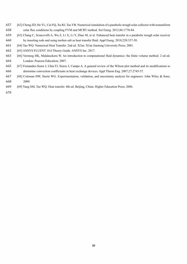
30

[62] Cheng ZD, He YL, Cui FQ, Xu RJ, Tao YB. Numerical simulation of a parabolic trough solar collector with nonuniform 657

solar flux conditions by coupling FVM and MCRT method. Sol Energ. 2012;86:1770-84. 658

[63] Chang C, Sciacovelli A, Wu Z, Li X, Li Y, Zhao M, et al. Enhanced heat transfer in a parabolic trough solar receiver 659

by inserting rods and using molten salt as heat transfer fluid. Appl Energ. 2018;220:337-50. 660

[64] Tao WQ. Numerical Heat Transfer. 2nd ed. Xi'an: Xi'an Jiaotong University Press; 2001. 661

[65] ANSYS FLUENT 18.0 Theory Guide. ANSYS Inc. 2017. 662

[66] Versteeg HK, Malalasekera W. An introduction to computational fluid dynamics: the finite volume method. 2 ed ed. 663

London: Pearson Education; 2007. 664

[67] Fernandez-Seara J, Uhía FJ, Sieres J, Campo A. A general review of the Wilson plot method and its modifications to 665

determine convection coefficients in heat exchange devices. Appl Therm Eng. 2007;27:2745-57. 666

[68] Coleman HW, Steele WG. Experimentation, validation, and uncertainty analysis for engineers: John Wiley & Sons; 667

2009. 668

[69] Yang SM, Tao WQ. Heat transfer. 4th ed. Beijing, China: Higher Education Press; 2006. 669

670