Determination of the heat transfer coefficients in transient heat conduction

This article has been downloaded from IOPscience. Please scroll down to see the full text article.

2013 Inverse Problems 29 095020

(http://iopscience.iop.org/0266-5611/29/9/095020)

Download details:

IP Address: 118.70.128.14

The article was downloaded on 04/09/2013 at 03:32

Please note that terms and conditions apply.

View the table of contents for this issue, or go to the journal homepage for more

Home Search Collections Journals About Contact us My IOPscience

IOP PUBLISHING INVERSE PROBLEMS

Inverse Problems 29 (2013) 095020 (21pp) doi:10.1088/0266-5611/29/9/095020

Determination of the heat transfer coefficients intransient heat conduction

Dinh Nho Hao1,2, Phan Xuan Thanh3 and D Lesnic2

1 Hanoi Institute of Mathematics, 18 Hoang Quoc Viet Road, Hanoi, Vietnam2 Department of Applied Mathematics, University of Leeds, Leeds LS2 9JT, UK3 School of Applied Mathematics and Informatics, Hanoi University of Science and Technology,1 Dai Co Viet Road, Hanoi, Vietnam

E-mail: hao@math.ac.vn, thanh.phanxuan@hust.vn and amt5ld@maths.leeds.ac.uk

Received 27 April 2013, in final form 1 August 2013Published 3 September 2013Online at stacks.iop.org/IP/29/095020

AbstractThe determination of the space- or time-dependent heat transfer coefficientwhich links the boundary temperature to the heat flux through a third-kindRobin boundary condition in transient heat conduction is investigated. Thereconstruction uses average surface temperature measurements. In both casesof the space- or time-dependent unknown heat transfer coefficient the inverseproblems are nonlinear and ill posed. Least-squares penalized variationalformulations are proposed and new formulae for the gradients are derived.Numerical results obtained using the nonlinear conjugate gradient methodcombined with a boundary element direct solver are presented and discussed.

1. Introduction

Heat transfer across the surface of a heat conducting body is accompanied by a heat transfercoefficient (HTC) which characterizes the contribution that this surface makes to the overallthermal resistance (the inverse of the thermal contact conductance) of the system. Becauseof its great importance in heat transfer engineering, various experimental techniques basedon, for example, colour changes of liquid crystal films, [13], or laser-induced fluorescence,[2], have been devised. These techniques rely in their interpretation on the analytical solutionfor a semi-infinite medium to determine the HTC at a point once the temperature history isobtained from the experiment. However, such simplified mathematical models cannot coverthe complete physical situation and rather Cauchy boundary data (measurements of boththe temperature and the heat flux) can be used, if available, as input to heat conductionmodels to extract the HTC values. In such a situation, one can first retrieve independently theboundary temperature and heat flux by solving a Cauchy linear inverse heat conduction problem[1, 6–8], and afterwards use them either directly in Newton’s law of cooling or indirectlythrough nonlinear iteration. This formulation has been adopted, considered and solvedusing various regularization methods, e.g. function specification, Tikhonov’s regularization,conjugate gradient method (CGM), mollification method, in many theoretical or computational

0266-5611/13/095020+21$33.00 © 2013 IOP Publishing Ltd Printed in the UK & the USA 1

Inverse Problems 29 (2013) 095020 D N Hao et al

studies related to both steady and unsteady heat conduction, see [3, 4, 11, 17–19, 30]. Anotherapproach could be to use non-standard measurements as considered in [27, 31]. However,non-standard measurements may not be physical, whilst Cauchy data measurements may notbe practical, e.g. in the case of high temperature hostile environments. Therefore, in order toovercome these physical or practical difficulties, in our realistic inverse formulation we allowfor the convective Robin boundary condition to be prescribed over the whole boundary, andthe linkage between the boundary temperature and heat flux be made through on unknownHTC which may depend on space or on time. Hence, a more realistic model can be proposedfor force-convection boiling over a heated tube, [32], nucleate boiling on cylinders, [23], orquenching experiments, [28].

Since in our formulations all the unknowns and additional observations are at the boundaryand the discretization of the boundary only is the essence of the boundary element method(BEM), it is natural to adopt this approach for the discretization of the problems underinvestigation.

The plan of the paper is as follows. In section 2 we formulate the inverse problems for thedetermination of a space-dependent (inverse problem I) or time-dependent (inverse problem II)HTC and recall the available existence and uniqueness results of a classical solution. Insection 3 we define the weak solutions of the direct and adjoint Robin problems and recalltheir well posedness. Sections 4 and 5 describe the least-squares methods for solving inverseproblems I and II, respectively. In each of these sections we present the numerical resultsobtained for several benchmark test examples using the nonlinear CGM in conjunction withthe BEM direct solver. As a regularization procedure we either terminate the iterative CGMfor minimizing the least-squares functional at an iteration given by the discrepancy principle,or we penalize this functional with a regularization term containing a regularization parameter.This regularizing parameter can also be selected using the discrepancy principle. In all cases,numerical stability and good accuracy are achieved. Finally, section 6 presents the conclusionsand future work.

2. Mathematical formulation

Let � ⊂ Rd, d � 1, be a bounded domain and denote its boundary by �. In the cylinder

Q := � × (0, T ], where T > 0, with the lateral surface area S = � × (0, T ], consider thefollowing inverse problems ([20] and [21]). Throughout the paper, u denotes the temperature,a the initial temperature, g the heat source, b an additional heat flux, and σ the HTC.

Inverse problem I. Find a pair of functions {u(x, t), σ (ξ )} such that

ut − �u = g in Q, (2.1)

u(x, 0) = a(x), x ∈ �, (2.2)∂u

∂n+ σ (ξ )u = b(ξ , t), (ξ , t) ∈ S, (2.3)

l1(u) = χ1(ξ ), ξ ∈ �, (2.4)

where the functions g(x, t), a(x), b(ξ , t) and χ1(ξ ) are given, and n is the outward unit normalto the boundary �. In (2.4), the observation operator l1 has one of the following forms:

l1(u) = u(ξ , T1), ξ ∈ �, (2.5)

where T1 is a fixed known time in (0, T ], or

l1(u) =∫ T

0ω(t)u(ξ , t) dt, ξ ∈ �, (2.6)

with ω being a given function in L1(0, T ).

2

Inverse Problems 29 (2013) 095020 D N Hao et al

Inverse problem II. Find a pair of functions {u(x, t), σ (t)} such that

ut − �u = g in Q, (2.7)

u(x, 0) = a(x), x ∈ �, (2.8)

∂u

∂n+ σ (t)u = b(ξ , t), (ξ , t) ∈ S, (2.9)

l2(u) = χ2(t), t ∈ [0, T ], (2.10)

where the functions g(x, t), a(x), b(ξ , t), and χ2(t) are given. The observation operator l2(u)

has one of the following forms:

l2(u) = u(ξ0, t), t ∈ [0, T ], (2.11)

where ξ0 is fixed known point in �, or

l2(u) =∫

�

ν(ξ )u(ξ , t) dξ, t ∈ [0, T ], (2.12)

with ν(ξ ) being a given function in L1(�).The common feature in the above inverse problems is the Robin third-kind boundary

condition, see equations (2.3) and (2.9).The notation for the spaces of functions involved in the following theorems follows [12].

With the assumptions that � is simply-connected and its boundary � ∈ C1+β with β > 0,g ∈ Cβ,0(Q), a ∈ C1(�), h, b ∈ C(S), Kostin and Prilepko [20, 21] proved the followingresults.

Theorem 2.1. Suppose that a = 0 in �, 0 � g(x, t) in Q, 0 � b(ξ , t) on S, 0 < χ1(ξ ) on�, and the functions g and b are monotonically non-decreasing with respect to t. Then thesolution (u(x, t), σ (ξ )) ∈ C2,1(Q) × C(�) with σ (ξ ) � 0 on �, to the inverse problem I isunique.

Theorem 2.2. If |χ2(t)| > 0 on [0, T ], then the solution (u(x, t), σ (t)) ∈ C2,1(Q) × C[0, T ]to the inverse problem II is unique.

Although of theoretical interest, these uniqueness theorems cannot be used directly in thenumerical analysis, since it is not straightforward how to use the space of continuous functionsin a weak formulation. Therefore, in this paper we relax some assumptions on the smoothnessof the data posed above so that we can work in the Hilbert space framework. Then we cansolve the above inverse problems in the least-squares sense. We will report about this in thenext section.

3. Direct problem

In this section, we suppose that � is a bounded Lipschitz domain and introduce the spaceW (0, T ) defined as

W (0, T ) = {u : u ∈ L2(0, T ; H1(�)), ut ∈ L2(0, T ; (H1(�))′)},equipped with the norm

‖u‖2W (0,T ) = ‖u‖2

L2(0,T ;H1(�))+ ‖ut‖2

L2(0,T ;(H1(�))′).

3

Inverse Problems 29 (2013) 095020 D N Hao et al

Now consider the direct problem

ut − �u = g in Q, (3.1)

u(x, 0) = a(x), x ∈ �, (3.2)

∂u

∂n+ σ (ξ, t)u = b(ξ , t), (ξ , t) ∈ S, (3.3)

with

g ∈ L2(Q), a ∈ L2(�), σ ∈ L∞(S), σ � 0, b ∈ L2(S), (3.4)

and its corresponding adjoint problem given by

− ψt − �ψ = aQ in Q, (3.5)

ψ(x, T ) = a�(x), x ∈ �, (3.6)

∂ψ

∂n+ σ (ξ, t)ψ = aS(ξ , t), (ξ , t) ∈ S, (3.7)

with

aQ ∈ L2(Q), a� ∈ L2(�), σ ∈ L∞(S), σ � 0, aS ∈ L2(S). (3.8)

Definition 3.1. A function u ∈ W (0, T ) is called a weak solution to the direct problem(3.1)–(3.3), if ∫

Q(utη + ∇u · ∇η) dx dt +

∫Sσuη dξ dt =

∫Q

gη dx dt +∫

Sbη dξ dt (3.9)

for all η ∈ L2(0, T ; H1(�)), and u(·, 0) = a.Similarly, a function ψ ∈ W (0, T ) is called a weak solution to the adjoint problem

(3.5)–(3.7) if ∫Q(−ψtη + ∇ψ · ∇η) dx dt =

∫Q

aQη dx dt +∫

SaSη dξ dt −

∫Sσψη dξ dt

for all η ∈ L2(0, T ; H1(�)), and ψ(·, T ) = a�(·).From lemma 3.17 and theorem 3.18 in [33] we have the following results concerning the

well posedness of the direct and adjoint problems.

Theorem 3.2. (i) If conditions (3.4) are satisfied, then there exists a unique weak solution inW (0, T ) of the direct problem (3.1)–(3.3). Moreover, there exists a constant cd > 0 independentof g, b and a such that

‖u‖W (0,T ) � cd(‖g‖L2(Q) + ‖b‖L2(S) + ‖a‖L2(�)). (3.10)

(ii) If conditions (3.8) are satisfied, then there exists a unique weak solution in W (0, T )

of the adjoint problem (3.5)–(3.7). Moreover, there exists a constant ca > 0 independent ofaQ, a� and aS such that

‖ψ‖W (0,T ) � ca(‖aQ‖L2(Q) + ‖aS‖L2(S) + ‖a�‖L2(�)).

Furthermore, we have the following Green formula∫�

a�(x)u(x, T ) dx +∫

QaQu dx dt +

∫S

aSu dξ dt

=∫

�

a(x)ψ(x, 0) dx +∫

Qgψ dx dt +

∫S

bψ dξ dt. (3.11)

4

Inverse Problems 29 (2013) 095020 D N Hao et al

Remark 3.3. The constant cd depends on σ . However, if we suppose that

0 � σ 1 � σ � σ 2,

where σ 1 and σ 2 are given, then by examining the proof of this theorem in [22] and [33] wesee that cd depends on these two constants only.

Now we summarize the BEM applied to the direct problem (3.1)–(3.3) which has beenpresented in [9] and [29].

The unknown Cauchy data [w := ∂u∂n , u] on S of the direct problem (3.1)–(3.3) with the

input data satisfying (3.4) can be found by the boundary integral equation approach of [5] byrepresenting solution of the heat equation (3.1) as

u(x, t) =∫ t

0

∫�

E (x − y, t − τ )w(y, τ ) dsy dτ −∫ t

0

∫�

∂E∂ny

(x − y, t − τ )u(y, τ ) dsy dτ

+∫

�

E (x − y, t)a(y) dy +∫ t

0

∫�

E (x − y, t − τ )g(y, τ ) dy dτ, (x, t) ∈ Q,

(3.12)

where E (x, t) is the fundamental solution of the heat equation as given by

E (x, t) ={

(4πt)−d2 e− |x|2

4t for t > 0,

0 for t � 0.

For (x, t) ∈ S, as in [5, 29], we define the single and double layer heat potentials as

(Vw)(x, t) =∫ t

0

∫�

E (x − ξ, t − τ )w(ξ, τ ) dξ dτ,

(Ku)(x, t) =∫ t

0

∫�

∂

∂nξ

E (x − ξ, t − τ )u(ξ , τ ) dξ dτ,

the boundary integral operators N and W

(Nw)(x, t) =∫ t

0

∫�

∂

∂nxE (x − ξ, t − τ )w(ξ, τ ) dξ dτ,

(Wu)(x, t) = − ∂

∂nx

∫ t

0

∫�

∂

∂nξ

E (x − ξ, t − τ )u(ξ , τ ) dξ dτ

and the volume potentials

(M0a)(x, t) =∫

�

E (x − y, t)a(y) dy, (N0g)(x, t) =∫ t

0

∫�

E (x − y, t − τ )g(y, τ ) dy dτ,

(M1a)(x, t) = ∂

∂nx

∫�

E (x − y, t)a(y) dy,

(N1g)(x, t) = ∂

∂nx

∫ t

0

∫�

E (x − y, t − τ )g(y, τ ) dy dτ.

As presented in [5, 29], we have the following system

A

(w

u

):=

(V − (

12 I + K

)(12 I + N

)W + σ I

)(w

u

)=

( −M0a − N0gb − M1a − N1g

)=:

(F1

F2

). (3.13)

Let H := H− 12 ,− 1

4 (S) × H12 , 1

4 (S) be the space equipped with the norm

‖(w, u)‖H :=(‖w‖2

H− 12 ,− 1

4 (S)+ ‖u‖2

H12 , 1

4 (S)

)1/2for (w, u) ∈ H. (3.14)

5

Inverse Problems 29 (2013) 095020 D N Hao et al

We define a bilinear form α(·, ·) on H × H by

α ((w, u), (τ, v)) :== 〈Vw, τ 〉S − ⟨(

12 I + K

)u, τ

⟩S + ⟨(

12 I + N

)w, v

⟩S + 〈Wu, v〉S + 〈σu, v〉S.

The corresponding variational formulation of (3.13) is to find (w, u) ∈ H such that

α((w, u), (τ, v)) = 〈F1, τ 〉S + 〈F2, v〉S for all (τ, v) ∈ H.

Applying theorem 3.11 of [5] and using the condition 0 � σ1 � σ � σ2, we can provethat the bilinear form α(·, ·) is bounded and H-elliptic, i.e.,

|α((w, u), (τ, v))| � cα2‖(w, u)‖H‖(τ, v)‖H, α((w, u), (w, u)) � cα1‖(w, u)‖2H

for all (w, u) ∈ H, (τ, v) ∈ H and some positive constants cα1, cα2. Therefore, by Lax–Milgram’s lemma, the boundary integral equations (3.13) admit a unique solution (w, u) ∈ H.Let us consider now the numerical discretization of (3.13).

Let Vh be the trial space of functions which are piecewise linear with respect to the spacevariables on a triangulation of � and piecewise constant with respect to the time variable. Wealso introduce a set of ansatz functions Uh consisting of piecewise constant basis functionsboth in space and in time, see [5, 29].

The Galerkin variational formulation of (3.13) is to find (wh, uh) ∈ Uh × Vh such that

α((wh, uh), (τh, vh)) = 〈F1, τh〉S + 〈F2, vh〉S for all (τh, vh) ∈ Uh × Vh.

This is equivalent to{〈Vwh, τh〉S − ⟨ (

12 I + K

)uh, τh

⟩S

= −〈M0a + N0g, τh〉S,⟨ (12 I + N

)wh, vh

⟩S + 〈Wuh, vh〉S + 〈σuh, vh〉S = 〈b − M1a − N1g, vh〉S,

(3.15)

for all (τh, vh) ∈ Uh × Vh.By Cea’s lemma, the Galerkin variational formulation (3.15) admits a unique solution

(wh, uh) ∈ Uh × Vh. Moreover there holds the error estimate

‖(w − wh, u − uh)‖H � cα2

cα1inf

(τh,vh )∈Uh×Vh

‖(w − τh, u − vh)‖H.

For the considered inverse problems we will separate the two cases: σ depends only on ξ ∈ �

and only on t ∈ (0, T ). In both these cases we will approximate σ by piecewise constantfunctions with the same mesh size as in that of (3.15). Taking the ansatz functions Uh × Vh

with mesh size h in space variable and ∼ √h in time variable, we can deliver the error estimate

‖u − uh‖L2(S) � ch(‖g‖L2(Q) + ‖a‖L2(�) + ‖b‖L2(S)) (3.16)

with c being a positive constant.

4. Variational method for the inverse problem I

Now we return to the inverse problem I which consists of determining {u(x, t), σ (ξ )} from thesystem of equations (2.1)–(2.4). If we suppose that (3.4) is satisfied, then from theorem 3.2,there exists a unique solution in W (0, T ) of the direct problem (2.1)–(2.3). Since u ∈ W (0, T ),we cannot determine the trace u(ξ , T1), ξ ∈ �, 0 < T1 � T in (2.5). Therefore, in this setting,we take the observation operator l1 as in (2.6). Afterwards we use

1

γ

∫ T1

T1−γ

u(ξ , t) dt, (4.1)

where γ > 0 small, as an approximation to u(ξ , T1), if it exists. Thus, in this case we takeω(t) = 1/γ , if t ∈ [T1 − γ , T1], and ω(t) = 0, otherwise. Here and thereafter, for simplicity,

6

Inverse Problems 29 (2013) 095020 D N Hao et al

we suppose that the weight ω ∈ L2(0, T ). Further, to emphasize the dependence of the solutionu of (2.1)–(2.3) on σ , we write u(x, t; σ ) or u(σ ).

We define the admissible set

A = {σ ∈ L∞(�) : 0 � σ 1 � σ (ξ ) � σ 2 for almost every ξ ∈ �} (4.2)

with σ 1, σ 2 being given constants.Suppose that χ1 is approximately given by χ1ε such that

‖χ1 − χ1ε‖L2(�) � ε (4.3)

with ε � 0 being a given level of noise. We reformulate the inverse problem I with observation(2.5)

l1(u) =∫ T

0ω(t)u(ξ , t) dt = χ1(ξ ), χ ∈ �,

as the following optimal control problem.Minimize the functional

Jα(σ ) = 1

2‖l1(u(σ )) − χ1ε‖2

L2(�)+ α

2‖σ‖2

L2(S)

= 1

2

∫�

( ∫ T

0ω(t)u(ξ , t; σ ) dt − χ1ε (ξ )

)2

dξ + α

2‖σ‖2

L2(S)(4.4)

over the admissible set A. Here, α � 0 is the regularization parameter.To study this optimization problem, we need some properties of the mapping σ �→ u(σ ).

Some of the analysis below is adapted from [17].

Lemma 4.1. The mapping σ �→ u(σ ) is Lipschitz continuous from A to W (0, T ), i.e., for anyσ, σ + δσ ∈ A, there holds

‖u(σ + δσ ) − u(σ )‖W (0,T ) � c‖δσ‖L∞(�).

Proof. Denote by v = u(σ + δσ ) − u(σ ). Then v satisfies the problem

vt − �v = 0 in Q, (4.5)

v(x, 0) = 0, x ∈ �, (4.6)

∂v

∂n+ (σ (ξ ) + δσ )v = −δσu(σ ), (ξ , t) ∈ S. (4.7)

In virtue of theorem 3.2 and remark 3.3 and the compactness of the imbeddingW (0, T )|S ↪→ L2(S),

‖v‖W (0,T ) � cd‖δσu(σ )‖L2(S)

� cd‖δσ‖L∞(�)‖u(σ )‖L2(S)

� c‖δσ‖L∞(�)‖u(σ )‖W (0,T ).

Since ‖u(σ )‖W (0,T ) is bounded when σ ∈ A (theorem 3.2 and remark 3.3), this concludes theproof of the lemma. �

Lemma 4.2. The mapping σ �→ u(σ ) from A to W (0, T ) is Frechet differentiable in the sensethat for any δσ ∈ L∞(�) such that σ + δσ ∈ A there exists a bounded linear operator U fromA to W (0, T ) such that

lim‖δσ‖L∞ (�)→0

‖u(σ + δσ ) − u(σ ) − Uδσ‖W (0,T )

‖δσ‖L∞(�)

= 0. (4.8)

7

Inverse Problems 29 (2013) 095020 D N Hao et al

Proof. Consider the problem

Ut − �U = 0 in Q, (4.9)

U (x, 0) = 0, x ∈ �, (4.10)

∂U

∂n+ σ (ξ )U = −δσu(σ ), (ξ , t) ∈ S, (4.11)

where δσ ∈ L∞(�) such that σ + δσ ∈ A. We see that there exists a unique solution U inW (0, T ) of (4.9)–(4.11), and the map from δσ ∈ L∞(�) to U ∈ W (0, T ) defines a boundedlinear operator U (see the a priori estimate in theorem 3.2). Then w = v − U , where v is thesolution of (4.5)–(4.7), satisfies the system

wt − �w = 0, in Q,

w(x, 0) = 0, x ∈ �,

∂w

∂n+ σ (ξ )w = −δσv, (ξ, t) ∈ S.

Again, applying theorem 3.2, the compactness of the imbedding W (0, T )|S ↪→ L2(S), andlemma 4.1, we get

‖w‖W (0,T ) � cd‖δσv‖L2(S)

� cd‖δσ‖L∞(�)‖v‖L2(S)

� c‖δσ‖L∞(�)‖v‖W (0,T )

� c‖δσ‖2L∞(�).

Thus, (4.8) is proved. �

Lemma 4.3. Let {σ n} ⊂ A be a sequence converging to σ ∗ weakly-* in L∞(�). Then thesequence {u(σ n)} converges to u(σ ∗) weakly in W (0, T ).

Proof. The a priori estimate (3.10) in theorem 3.2 implies that the sequence {u(σ n)} isuniformly bounded in W (0, T ). Therefore, there is a subsequence, denoted again by {u(σ n)},which weakly converges to a u∗ ∈ W (0, T ). Since W (0, T )|S is compactly imbedded intoL2(S), we find u(σ n)|S converges to u∗|S strongly in L2(S). On the other hand, followingdefinition 3.1 of the weak solution in W (0, T ), we have u(σ n)(·, 0) = a(x) and for anyv ∈ L2(0, T ; H1(�))∫

Qu(σ n)tv +

∫Q

∇u(σ n)∇v +∫

Sσ nu(σ n)v =

∫Q

gv.

Since {u(σ n)} weakly converges to u∗ ∈ W (0, T ), we have

limn→∞

∫Q

u(σ n)tv =∫

Qu∗

t v,

limn→∞

∫Q

∇u(σ n)∇v =∫

Q∇u∗∇v.

The weak-* convergence of {σ n} to σ ∗ in L∞(�) and the convergence of u(σ n) to u∗ in L2(S)

implies

limn→∞

∫Sσ nu(σ n)v = lim

n→∞

∫S[σ nu∗v + σ n(u∗ − u(σ n))v] =

∫Sσ ∗u∗v.

Therefore, for any v ∈ L2(0, T ; H1(�)),∫Q

u∗t v +

∫Q

∇u∗(σ n)∇v +∫

Sσ ∗u∗v =

∫Q

gv.

8

Inverse Problems 29 (2013) 095020 D N Hao et al

Since un weakly converges to u∗ in W (0, T ) and W (0, T ) is compactly imbedded inC([0, T ]; (H1(�))′), we have un(·, 0) strongly converges to u∗(·, 0) in (H1(�))′. Hence,u∗(·, 0) = a(·). Due to the uniqueness of solution of the direct problem, u∗ = u(σ ∗). Sinceevery subsequence has a subsequence converging to u(σ ∗), the whole sequence convergesweakly. �

Theorem 4.4. The minimization problem (4.4) subject to (2.1)–(2.3) admits a solution.

Proof. Since Jα(σ ) is finite over A, there exists a minimizing sequence σ n ⊂ A such that

limn→∞ Jα(σ n) = inf

σ∈AJα(σ ).

Since σ n ∈ A, which is weak-* closed, there is a subsequence of {σ n} denoted by the samesymbol and a σ ∗ ∈ A such that

σ n → σ ∗ weakly-* in L∞(S).

Following lemma 4.3, u(σ n) weakly converges to u(σ ∗) in W (0, T ). From the compactnessof the imbedding W (0, T ) ↪→ L2(S), we have u(σ n) converges strongly to u(σ ∗) in L2(S).Hence

limn→∞ ‖l1(u(σ n)) − χ1ε‖L2(�) = ‖l1(u(σ ∗)) − χ1ε‖L2(�).

Since the weak-* convergence in L∞(�) implies the weak convergence in L2(�), it followsdirectly from the weak lower semi-continuity of norms that σ ∗ is a minimizer of the functionalJα over the admissible set A. �

Theorem 4.5. Let {χn1 } ⊂ L2(�) be a sequence converging to χ1ε , and {σ n} ∈ A be a sequence

of minimizers of the perturbed functionals

1

2

∫�

(∫ T

0ω(t)u(ξ , t; σ ) dt − χn

1 (ξ )

)2

dξ + α

2‖σ‖2

L2(�).

Then the sequence {σ n} has a subsequence converging to a minimizer of the functional Jα inthe L2(�)-norm.

Proof. There exists a subsequence of {σ n}, denoted by the same symbol, which weakly-*converges to a σ ∗ ∈ A. Again, from lemma 4.3, u(σ n) converges to u(σ ∗) in L2(S). Hence

limn→∞ ‖l1(u(σ n)) − χn

1 ‖L2(�) = ‖l1(u(σ ∗)) − χ1ε‖L2(�).

The remaining part of the proof is similar to that of the previous theorem, hence is omitted.�

We introduce the notion of minimum norm solution of the inverse problem I. Supposethat there exists σ ∈ A such that (2.6) is satisfied.

Lemma 4.6. The set

N(χ1) := {σ ∈ A|l1(u(σ )) = χ1}is nonempty, bounded and weakly closed in the L2(�)-norm. Hence there exists a solution σ †

of the problem

minσ∈N(χ1)

‖σ‖L2(�)

which is called by minimum norm solution of the inverse problem I.

9

Inverse Problems 29 (2013) 095020 D N Hao et al

The proof of this lemma follows directly from the proof of theorem 4.4. We note that whenthe conditions of theorem 2.1 are satisfied, then the minimum norm solution of the inverseproblem I is unique.

It is standard to prove the following result.

Theorem 4.7. Denote solutions of the minimizing Jα(σ ) over A by σ ε,α . If ε → 0 and α

is chosen such that α → 0 and ε/√

α → 0, then there exists a subsequence of σ ε,α whichconverges to σ †.

Now we find the gradient of the functional Jα . In doing so, we introduce the adjointproblem

− ψt − �ψ = 0 in Q, (4.12)

ψ(x, T ) = 0, x ∈ �, (4.13)

∂ψ

∂n+ σ (ξ )ψ = −ω(t)

( ∫ T

0ω(t)u(ξ , t; σ ) dt − χ1ε (ξ )

), (ξ , t) ∈ S. (4.14)

Due to theorem 3.2, there exists a unique solution in W (0, T ) of problem (4.12)–(4.14).

Theorem 4.8. The functional Jα is Frechet differentiable and its gradient is

J′α(σ ) =

∫ T

0u(ξ , t; σ )ψ(ξ, t) dt + ασ (ξ ). (4.15)

Proof. Taking any δσ ∈ L∞(�) such that σ +δσ ∈ A and denoting by v = u(σ +δσ )−u(σ ),we have

J0(σ + δσ ) − J0(σ ) = 1

2

∫�

( ∫ T

0ω(t)(u(ξ , t; σ ) + v(ξ, t; σ )) dt − χ1ε (ξ )

)2

dξ

− 1

2

∫�

(∫ T

0ω(t)u(ξ , t; σ ) dt − χ1ε (ξ )

)2

dξ

=∫

�

( ∫ T

0ω(t)v(ξ, t; σ ) dt

)( ∫ T

0ω(t)u(ξ , t; σ ) dt − χ1ε (ξ )

)dξ

+ 1

2

∫�

(∫ T

0ω(t)v(ξ, t; σ ) dt

)2

dξ .

Since v is the solution of problem (4.5)–(4.7), and W (0, T )|S is compactly imbedded in L2(S),in virtue of lemma 4.1, we have∣∣∣∣

∫�

( ∫ T

0ω(t)v(ξ, t; σ ) dt

)2

dξ

∣∣∣∣ � ‖ω‖2L2(0,T )

‖v‖2L2(S)

� c‖ω‖2L2(0,T )

‖v‖2W 2(0,T )

� c‖ω‖2L2(0,T )

‖δσ‖2L∞(�).

On the other hand, as ψ is the solution of the adjoint problem (4.12)–(4.14), in virtue of theGreen formula (3.11),

−∫

Sω(t)

( ∫ T

0ω(τ )u(ξ , τ ; σ ) dτ − χ1ε (ξ )

)v(ξ, t; σ ) dξ dt

=∫

�

( ∫ T

0ω(t)v(ξ, t; σ ) dt

)( ∫ T

0ω(t)u(ξ , t; σ ) dt − χ1ε (ξ )

)dξ

= −∫

Sδσu(ξ , t; σ )ψ(ξ, t) dξ dt −

∫Sδσv(ξ, t)ψ(ξ, t) dξ dt. (4.16)

10

Inverse Problems 29 (2013) 095020 D N Hao et al

As above, ∣∣∣∣∫

Sδσv(ξ, t)ψ(ξ, t) dξ dt

∣∣∣∣ � ‖δσ‖L∞(�)‖v‖L2(S)‖ψ‖L2(S)

� c‖δσ‖L∞(�)‖v‖W (0,T )‖ψ‖L2(S)

� c‖δσ‖2L∞(�)‖ψ‖L2(S).

Thus,

J0(σ + δσ ) − J0(σ ) =∫

Su(ξ , t; σ )ψ(ξ, t)δσ (ξ ) dξ dt + o(‖δσ‖L∞(S)).

We conclude that

J′0(σ ) =

∫ T

0u(ξ , t; σ )ψ(ξ, t) dt,

and J′α(σ ) = J′

0(σ ) + ασ (ξ ). Hence the theorem is proved. �

4.1. Boundary element method and its convergence

Divide � into boundary elements with mesh size h and denote byAh the set of all step functionsdefined on them taking values in [σ 1, σ 2]. For (wh, uh) ∈ Uh ×Vh being the solution to (3.15)with σ ∈ Ah we approximate the functional (4.4) by

Jαh(σh) : = 1

2‖l1(uh(σh)) − χ1ε‖2

L2(�)+ α

2‖σh‖2

L2(S)

= 1

2

∫�

(∫ T

0ω(t)uh(ξ , t; σh) dt − χ1ε (ξ )

)2

dξ + α

2‖σh‖2

L2(S)(4.17)

and minimize it with respect to σh ∈ Ah. It is clear that there exists a solution of thisminimization problem which we denote by σ h. Of course, this solution depends on α, howeverwe drop this subindex for the simplicity of notation. Now we prove the following resultconcerning the convergence of the BEM applied to the inverse problem I.

Theorem 4.9. Suppose that εk is a sequence converging to 0, as k → ∞. If α := αk andh = hk are chosen such that αk → 0, hk → 0, and (εk + hk)/

√αk → 0, as k → ∞, then from

the sequence {σ hk} we can choose a subsequence, which is denoted by the same notation, suchthat σ hk → σ †, a minimum norm solution of the inverse problem I, in the L2(�)-norm.

Proof. We have

Jαkhk (σ hk ) = ‖l1(uhk (σ hk )) − χ1εk‖2L2(�)

+ αk‖σ hk‖2L2(�)

� ‖l1(uhk (σ†)) − χ1εk‖2

L2(�)+ αk‖σ †‖2

L2(�)

= ‖l1(uhk (σ†)) − l1(u(σ †)) + l1(u(σ †)) − χ1 + χ1 − χ1εk‖2

L2(�)+ αk‖σ †‖2

L2(�)

� (chk + εk)2 + αk‖σ †‖2

L2(�)

→ 0, as k → ∞,

where, we have used the error estimate (3.16). Thus, with the above choice of hk and αk

we have l1(uhk (σ hk )) → χ1 in L2(�). Furthermore, lim infk→∞ ‖σ hk‖L2(�) � ‖σ †‖L2(�). Sinceσhk ∈ Ahk ⊂ A, it follows that there exists a subsequence of {σ hk}, which is denoted by the samesymbol, converging weakly-∗ to a σ ∈ A in L∞(�). Since the weak-∗ convergence in L∞(�)

implies the weak convergence in L2(�), we have σ hk → σ weakly in L2(�). Due to lemma 4.3,uhk (σ hk ) converges weakly in W (0, T ) to u(σ ). Since the imbedding W (0, T ) ↪→ L2(S) is

11

Inverse Problems 29 (2013) 095020 D N Hao et al

compact, this yields the strong convergence of uhk (ξ , t; σ hk ) to u(ξ , t; σ ) in L2(S). Hence, σ

is one of those in A for which l1(u(σ )) = χ1. On the other hand, since σ hk → σ weakly inL2(�), we have ‖σ †‖L2(�) � lim infk→∞ ‖σ hk‖L2(�) � ‖σ‖L2(�). Since σ † is a minimum normsolution, we have ‖σ‖L2(�) = ‖σ †‖L2(�). Thus σ is a minimum norm solution of the inverseproblem I and limk→∞ ‖σ hk‖L2(�) = ‖σ‖L2(�). Since σ hk → σ weakly in L2(�), we concludethat σ hk → σ strongly in L2(�). �

4.2. Nonlinear conjugate gradient methods

The nonlinear CGMs for the problem (4.4), (2.1)–(2.3) are as follows.

(1) Choose an initial guess σ0, and set k = 0.(2) Find (wh,0, uh,0) ∈ Vh × Uh such that{

〈Vwh,0, τh〉S − ⟨ (12 I + K

)uh,0, τh

⟩S = −〈M0a + N0g, τh〉S,⟨ (

12 I + N

)wh,0, vh

⟩S + 〈Wuh,0, vh〉S + 〈σ0uh,0, vh〉S = 〈b − M1a − N1g, vh〉S,

(4.18)

for all (τh, vh) ∈ Vh × Uh.(3) Find (qh,0, ph,0) ∈ Vh × Uh such that{

〈V qh,0, τh〉S − ⟨ (12 I + K

)ph,0, τh

⟩S = 0,⟨ (

12 I + N

)qh,0, vh

⟩S + 〈W ph,0, vh〉S + 〈σ0 ph,0, vh〉S = 〈b0, vh〉S,

(4.19)

for all (τh, vh) ∈ Vh × Uh. Here b0(ξ , t) = −ω(T − t)( ∫ T

0 ω(t)uh,0(ξ , t) dt − χ1ε (ξ )).

Calculate J′α(σ0) = ∫ T

0 u(ξ , t, σ0)ψ0(ξ , t) dt + ασ0. Set r0 = −J′α(σ0), d0 = r0.

(4) Line search γ0 = arg minγ�0Jα(σ0 + γ d0).

(5) Set σ1 = σ0 + γ0d0.(6) Set k = 1. Find (wh,k, uh,k) ∈ Vh × Uh such that{

〈Vwh,k, τh〉S − ⟨ (12 I + K

)uh,k, τh

⟩S = −〈M0a + N0g, τh〉S,⟨ (

12 I + N

)wh,k, vh

⟩S + 〈Wuh,k, vh〉S + 〈σkuh,k, vh〉S = 〈b − M1a − N1g, vh〉S,

(4.20)

for all (τh, vh) ∈ Vh × Uh.(7) Find (qh,k, ph,k) ∈ Vh × Uh such that{

〈V qh,k, τh〉S − ⟨ (12 I + K

)ph,k, τh

⟩S = 0,⟨ (

12 I + N

)qh,k, vh

⟩S + 〈W ph,k, vh〉S + 〈σk ph,k, vh〉S = 〈bk, vh〉S,

(4.21)

for all (τh, vh) ∈ Vh × Uh. Here bk(ξ , t) = −ω(T − t)( ∫ T

0 ω(t)uh,k(ξ , t) dt − χ1ε (ξ )).

(8) Calculate J′α(σk) = ∫ T

0 u(ξ , t, σk)ψk(ξ , t) dt + ασk. Set

rk = −J′α(σk)

and calculate

dk = rk + βkdk−1

with βk being one of the following

‖rk‖2

‖rk−1‖2(Fletcher–Reeves),

〈rk, rk − rk−1〉‖rk−1‖2

(Polak–Ribirere), (4.22)

where the norms and scalar products are in L2(�).(9) Line search γk = arg minγ�0J(σk + γ dk).

(10) Update σk+1 = σk + γkdk.

12

Inverse Problems 29 (2013) 095020 D N Hao et al

4.3. Numerical results and discussion for the inverse problem I

The one-dimensional spacewise HTC case has been numerically investigated at length in[25, 26] and therefore in this subsection emphasis is placed on the multi-dimensional (two-dimensional) framework. We consider three test examples in decreasing order of smoothness,namely, smooth, piecewise smooth and discontinuous functions.

In all examples in this subsection, � = (0, 1) × (0, 1), T = 1. For the temperature wetake that the exact solution be given by

u(x, t) = x31 + x3

2 + 2x21x2 sin t + 1, (4.23)

and then

a(x) = x31 + x3

2 + 1, g(x, t) = 2x21x2 cos t − 6x1 − 6x2 − 4x2 sin t.

Prescribing σ , we can take b given by

b(ξ , t) := ∂u

∂n+ σu, (ξ , t) ∈ S. (4.24)

The measurement (2.4) is obtained directly from (4.23). In the case of the integralmeasurement (2.6) we take ω(t) = t2 + 1. In the case of the terminal-integral measurement(2.5), we use (4.1) with γ = 10−5 fixed throughout, and the terminal time T1 is varied withinthe interval (0, T ].

In order to investigate the stability of the numerical solution we consider a noisyperturbation of the measurement (2.4) as

χ1ε = χ1 + ε × rand(1), (4.25)

where rand(1) gives random variables in the interval [−1, 1] and ε is the level of noise.The number of boundary elements used to discretize the boundary � is taken as M = 128

and the number of time steps discretizing uniformly the interval [0, T = 1] is taken as N = 64.These numbers are found sufficiently large to ensure that any further increase in these valuesdoes not significantly affect the accuracy of the numerical results.

As test examples we consider

σ (ξ ) = ξ1 + ξ2 for example 1, (4.26)

σ (ξ ) ={

−|ξ1 − 12 | + 1

2 if ξ2 ∈ {0, 1}, ξ1 ∈ (0, 1),

−|ξ2 − 12 | + 1

2 if ξ1 ∈ {0, 1}, ξ2 ∈ (0, 1),for example 2, (4.27)

σ (ξ ) ={

2 if ξ2 = 0 or ξ2 = 1,

1 otherwisefor example 3, (4.28)

where ξ = (ξ1, ξ2).We use the Fletcher–Reeves CGM and stop the CGM at the first iteration n∗ for which

the residual

‖l1(u(σn∗ )) − χ1ε‖L2(�) � 1.01ε. (4.29)

Although it has not been proved that such a stopping rule yields a regularization method as forthe linear cases [24], our numerical results show that (4.29) yields stable solutions. We alsomention that obtaining sharp error estimates are difficult and beyond the scope of this paper.

The initial guess σ0 is taken as 1.5 for examples 1 and 3, and 0.5 for example 2. We testedfor α = 0 and 10−5 and obtained similar numerical results, therefore, we present the caseα = 0 only.

Figure 1 shows the comparison between the exact and numerical solutions of the inverseproblem I with the average boundary temperature integral observation (2.6) perturbed by

13

Inverse Problems 29 (2013) 095020 D N Hao et al

0 0.5 1 1.5 2 2.5 3 3.5 40

0.2

0.4

0.6

0.8

1

1.2

1.4

1.6

1.8

2

Exactε = 0.1ε = 0.01ε = 0.001

(a) Example 1

0 0.5 1 1.5 2 2.5 3 3.5 40

0.05

0.1

0.15

0.2

0.25

0.3

0.35

0.4

0.45

0.5

Exact

ε = 0.1

ε = 0.01

ε = 0.001

(b) Example 2

0 0.5 1 1.5 2 2.5 3 3.5 4

0.8

1

1.2

1.4

1.6

1.8

2

2.2

Exactε = 0.1ε = 0.01ε = 0.001

(c) Example 3

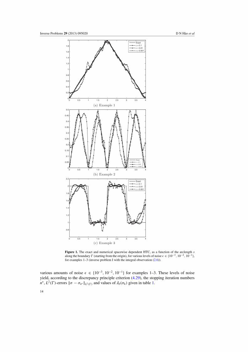
Figure 1. The exact and numerical spacewise dependent HTC, as a function of the arclength salong the boundary � (starting from the origin), for various levels of noise ε ∈ {10−3, 10−2, 10−1},for examples 1–3 (inverse problem I with the integral observation (2.6)).

various amounts of noise ε ∈ {10−3, 10−2, 10−1} for examples 1–3. These levels of noiseyield, according to the discrepancy principle criterion (4.29), the stopping iteration numbersn∗, L2(�)-errors ‖σ − σn∗‖L2(�) and values of J0(σh) given in table 1.

14

Inverse Problems 29 (2013) 095020 D N Hao et al

Table 1. The stopping iteration numbers n∗, the errors ‖σ − σh‖L2(�) and the values of J0(σh) forexamples 1–3 of the inverse problem I with the observation (2.6) with ω(t) = t2 + 1, perturbed byε ∈ {10−3, 10−2, 10−1} noise.

Example ε n∗ ‖σ − σh‖L2(�) J0(σh)

1 10−3 36 0.0274 4.2E-61 10−2 27 0.0487 9.5E-51 10−1 8 0.1917 7.8E-3

2 10−3 58 0.0270 8.3E-62 10−2 34 0.0627 1.5E-42 10−1 16 0.2774 8.2E-3

3 10−3 40 0.2487 7.4E-53 10−2 14 0.3905 9.8E-43 10−1 12 0.4243 5.4E-3

Table 2. The stopping iteration numbers n∗, the errors ‖σ − σh‖L2(�) and the values of J0(σh) forexamples 1–3 of the inverse problem I with the observation (4.1) with γ = 10−5 perturbed byε = 10−2 for various instants T1 ∈ {0.4T, 0.75T, T }.Example T1/T n∗ ‖σ − σh‖L2(�) J0(σh)

1 0.4 13 0.0703 2.0E-41 0.75 45 0.0593 1.7E-41 1 23 0.0479 9.8E-5

2 0.4 35 0.0525 9.4E-52 0.75 33 0.0526 7.1E-52 1 47 0.0500 6.5E-5

3 0.4 16 0.4135 9.4E-43 0.75 16 0.4123 9.2E-43 1 16 0.4128 9.2E-4

From figure 1 and table 1 it can be seen that the numerical solutions for all threeexamples 1–3 are stable and they become more accurate as the level of noise ε decreases.The low values of n∗ reported in table 1 indicate that the nonlinear CGM rapidly achievesthe required level of stability and accuracy. Also, n∗ decreases as ε increases. As expected,examples 2 and 3 are more difficult because the functions (4.27) and (4.28) are less regularthan the smooth function (4.26).

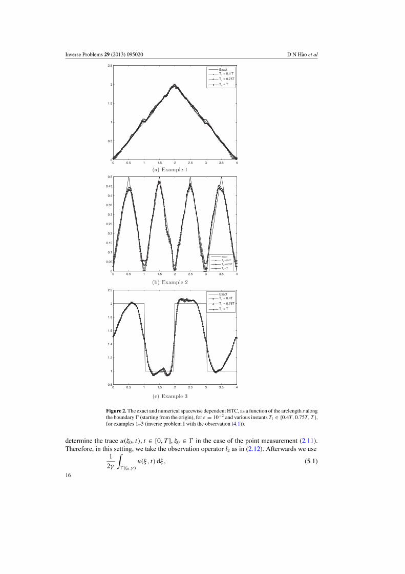
Next we consider the measurement (4.1) with γ = 10−5 and investigate the sensitivityof the numerical solution with respect to the instant T1 ∈ {0.4T, 0.75T, T }. Numerical resultsobtained for examples 1–3 for the level of noise ε = 10−2 presented in figure 2 and table 2show that the solutions are stable and quite insensitive to the value of T1.

5. Variational method for the inverse problem II

We consider now the inverse problem II which consists of determining {u(x, t), σ (t)} fromthe system of equations (2.7)–(2.10). As in the previous section, since u ∈ W (0, T ) we cannot

15

Inverse Problems 29 (2013) 095020 D N Hao et al

0 0.5 1 1.5 2 2.5 3 3.5 40

0.5

1

1.5

2

2.5

ExactT

1 = 0.4 T

T1 = 0.75T

T1 = T

(a) Example 1

0 0.5 1 1.5 2 2.5 3 3.5 40

0.05

0.1

0.15

0.2

0.25

0.3

0.35

0.4

0.45

0.5

Exact

T1 = 0.4T

T1 = 0.75T

T1 = T

(b) Example 2

0 0.5 1 1.5 2 2.5 3 3.5 40.8

1

1.2

1.4

1.6

1.8

2

2.2

ExactT

1 = 0.4T

T1 = 0.75T

T1 = T

(c) Example 3

Figure 2. The exact and numerical spacewise dependent HTC, as a function of the arclength s alongthe boundary � (starting from the origin), for ε = 10−2 and various instants T1 ∈ {0.4T, 0.75T, T },for examples 1–3 (inverse problem I with the observation (4.1)).

determine the trace u(ξ0, t), t ∈ [0, T ], ξ0 ∈ � in the case of the point measurement (2.11).Therefore, in this setting, we take the observation operator l2 as in (2.12). Afterwards we use

1

2γ

∫�(ξ0,γ )

u(ξ , t) dξ, (5.1)

16

Inverse Problems 29 (2013) 095020 D N Hao et al

where �(ξ0, γ ) := {ξ ∈ �||ξ − ξ0| � γ } with γ > 0 small, as an approximation to u(x0, t),if it exists. Thus, in this case we take ν(ξ ) = 1/(2γ )char�(ξ0,γ )(ξ ), the characteristic functionof the neighbourhood �(ξ0, γ ), for ξ ∈ �.

Suppose that χ2 is approximately given by χ2ε such that

‖χ2 − χ2ε‖L2(0,T ) � ε (5.2)

with ε � 0 being a given noise level. We solve the inverse problem II with the measurement(2.12) by minimizing the functional

Jα(σ ) = 1

2‖l2(u(σ )) − χ2ε‖2

L2(0,T )+ α

2‖σ‖2

L2(0,T )

= 1

2

∫ T

0

∣∣∣∣∫

�

ν(ξ )u(ξ , t; σ ) dξ − χ2ε (t)

∣∣∣∣2

dt + α

2‖σ‖2

L2(0,T ), (5.3)

over the admissible set

A = {σ ∈ L∞(0, T ), 0 � σ 1 � σ � σ 2, for almost every t ∈ [0, T ]},with σ 1, σ 2 being given. Here u(σ ) = u(x, t; σ ) is the solution in W (0, T ) of problem(2.7)–(2.9) with g ∈ L2(Q), a ∈ L2(�), b ∈ L2(S) being given.

We have similar results concerning the existence of a solution of the minimization problem,its stability, the convergence of the Tikhonov regularization method and the BEM as in theprevious section, therefore we do not present them here again, but instead give the formulafor the gradient of the functional Jα for implementing the nonlinear CGMs. In doing so, weintroduce the adjoint problem

− ψt − �ψ = 0 in Q, (5.4)

ψ(x, T ) = 0, x ∈ �, (5.5)

∂ψ

∂n+ σ (t)ψ = −ν(ξ )

( ∫�

ν(ξ )u(ξ , t; σ ) dξ − χ2ε (t)

). (5.6)

Due to theorem 3.2, there exists a unique solution in W (0, T ) of problem (5.4)–(5.6). It canbe proved that the functional Jα is Frechet differentiable and its gradient is

J′α(σ ) =

∫�

u(ξ , t; σ )ψ(ξ, t) dξ + ασ (t). (5.7)

5.1. Numerical results and discussion for the inverse problem II

The one-dimensional timewise HTC case has been numerically investigated at length [25, 34]and therefore, in this subsection the emphasis is made on the two-dimensional framework.

We take the same example (4.23) as in subsection 4.3 and then prescribing σ we candetermine b given by (2.9). The measurement (2.10) is obtained from (4.23). In the case ofthe boundary integral measurement (2.12) we take ν(ξ ) = ξ 2

1 + ξ 22 + 1, whilst in the case of

the point measurement (2.11) we take ξ0 = (0, 0) and we approximate it as (2.12) with thecut-off function

ν(ξ ) ={

1γ

for ξ = (ξ1, 0), 0 � ξ1 � γ = 10−5,

0 otherwise.

This is a slight modification of (5.1), but we have also tested the case ξ0 = (0.5, 0) for whichwe have taken the cut-off function

ν(ξ ) ={

12γ

for ξ = (ξ1, 0), |ξ1 − 0.5| � γ = 10−5,

0 otherwise,

in (5.1).

17

Inverse Problems 29 (2013) 095020 D N Hao et al

0 0.1 0.2 0.3 0.4 0.5 0.6 0.7 0.8 0.9 1

0.8

1

1.2

1.4

1.6

1.8

2

2.2

Exactε = 0.1ε = 0.01ε = 0.001

(a)

0 0.1 0.2 0.3 0.4 0.5 0.6 0.7 0.8 0.9 10.8

1

1.2

1.4

1.6

1.8

2

2.2

Exactε = 0.1ε = 0.01ε =0.001

(b)

0 0.1 0.2 0.3 0.4 0.5 0.6 0.7 0.8 0.9 10.8

1

1.2

1.4

1.6

1.8

2

2.2

Exactε = 0.1ε = 0.01ε = 0.001

(c)

Figure 3. The exact and numerical timewise varying HTC, for various levels of noise ε ∈{10−3, 10−2, 10−1} for example 4, inverse problem II. (a) Example 4 with the point-integralobservation (5.1) at ξ0 = (0.0, 0) and γ = 10−5; (b) example 4 with the point-integral observation(5.1) at ξ0 = (0.5, 0) and γ = 10−5; (c) example 4 with the integral observation (2.12).

In order to avoid repetition with the previous spacewise dependent HTC described at lengthin subsection 4.3, we only present the results obtained for a severe discontinuous HTC given by

18

Inverse Problems 29 (2013) 095020 D N Hao et al

Table 3. The stopping iteration numbers n∗, the L2(0, T )-errors ‖σ − σn∗ ‖L2(0,T ), and the valuesof J0(σh) for example 4 of the inverse problem II with boundary observations (5.1) and (2.12),perturbed by various levels of noise ε ∈ {10−3, 10−2, 10−1}.Observation ε n∗ ‖σ − σh‖L2(0,T ) J0(σh)

(5.1) at ξ0 = (0, 0) 10−3 55 0.0901 1.7E-5(5.1) at ξ0 = (0, 0) 10−2 22 0.1457 4.9E-4(5.1) at ξ0 = (0, 0) 10−1 17 0.2275 3.6E-3

(5.1) at ξ0 = (0.5, 0) 10−3 49 0.0848 2.9E-6(5.1) at ξ0 = (0.5, 0) 10−2 22 0.0953 1.9E-4(5.1) at ξ0 = (0.5, 0) 10−1 7 0.2067 1.0E-2

(2.12), ν(ξ ) = ξ 21 + ξ 2

2 + 1 10−3 65 0.0844 4.6E-8(2.12), ν(ξ ) = ξ 2

1 + ξ 22 + 1 10−2 46 0.0846 1.3E-6

(2.12), ν(ξ ) = ξ 21 + ξ 2

2 + 1 10−1 34 0.1056 1.2E-4

σ (t) ={

1 if t ∈ (0, 1/3) ∪ (2/3, 1),

2 elsewhere,for example 4. (5.8)

We take M = 128, N = 64 and we include noise in (2.10) as

χ2ε = χ2 + ε × rand(1).

We also use the Fletcher–Reeves CGM and stop the CGM at the first iteration n∗ for whichthe residual

‖l2(u(σn∗ )) − χ2ε‖L2(0,T ) � 1.05ε. (5.9)

The initial guess σ0 is taken as 1.5. As in the previous section, we obtained similar numericalresults for α = 0 and 10−5 and therefore we present the case α = 0 only.

Figures 3(a)–(c) show the comparison between the exact and numerical solutions for thetimewise varying HTC (5.8) of the inverse problem II with the boundary integral observations(5.1) with ξ0 = (0, 0) and ξ0 = (0.5, 0), and (2.12), respectively, perturbed by various levelsof noise ε ∈ {10−3, 10−2, 10−1}. These levels of noise yield the stopping iteration numbersn∗, the errors ‖σ − σn∗‖L2(0,T ), and the values of J0(σh) given in table 3. From figure 3 andtable 3 it can be seen that stable and accurate numerical results are obtained. Also, it can beseen that the global boundary integral measurement (2.12) yields more accurate results thanthe local boundary integral measurement (5.1).

6. Conclusions

Multi-dimensional reconstructions of space- or time-dependent heat transfer coefficientsappearing in convective Robin boundary conditions of the third kind from integral observationshave been investigated. The nonlinear inverse problems have been formulated in a least-squares framework and new formulae for the gradients of the least-squares functionals havebeen delivered. For generality, we have also penalized these least-squares functionals withadditional regularization terms, as in expressions (4.4) and (5.3). This generalization in turnenables establishing the convergence theorems 4.7 and 4.9. From the computational pointof view, for exact data, i.e. ε = 0, it is recommended to include a regularization parameterα > 0 since without it there is no stopping criterion applicable. Moreover, even for exactdata, the unregularized least-squares functionals (4.4) and (5.3) are semi-convergent onlybecause round-off computer errors are always present. On the other hand, as our numerical

19

Inverse Problems 29 (2013) 095020 D N Hao et al

investigations indicate, for noisy data with ε > 0, the CGM has a regularizing characterand the application of the stopping criteria (4.29) and (5.9) with α = 0 seems sufficient.The variational problems have been discretized by the BEM and convergence results of themethod have been proved. A numerical method based on the nonlinear CGM+BEM has beendeveloped for obtaining stable and accurate numerical solutions. Numerical results obtainedfor several test examples have been illustrated. It has been found, for both inverse problemsI and II, that the stopping iteration number n∗(ε), chosen according to the criterion (4.29) or(5.9), respectively, increases, as ε decreases. Also, the L2-errors presented in tables 1 and 3indicate the convergence of the numerical solution σn∗(ε), as ε → 0, to the exact solution.

Analogous multi-dimensional nonlinear inverse problems that require determining thetemperature-dependent HTC will be investigated in a separate future work, [10]. Future workmay also consist in extending some of this inverse analysis to composite heat conductorsinvolving the determination of the thermal contact conductance (the inverse of the thermalresistance) during metal casting [16], of exhaust gases [15], and in plate finned-tube heatexchangers [14].

Acknowledgments

This research was supported by a Marie Curie International Incoming Fellowship within the7th European Community Framework Programme and by Vietnam National Foundation forScience and Technology Development (NAFOSTED) under grant number 101.02-2011.50.

References

[1] Beck J V, Blackwell B and Clair C R St Jr 1985 Inverse Heat Conduction: Ill-Posed Problems (New York:Wiley-Interscience)

[2] Bizzak D J and Chyu M-K 1995 Use of a laser-induced fluorescence thermal imaging system for local jetimpingement heat transfer measurement Int. J. Heat Mass Transfer 38 267–74

[3] Chantasiriwan S 1999 Inverse heat conduction problem of determining time-dependent heat transfer coefficientInt. J. Heat Mass Transfer 42 4275–85

[4] Chen H-T and Wu X-Y 2008 Investigation of heat transfer coefficient in two-dimensional transient inverse heatconduction problems using the hybrid inverse scheme Int. J. Numer. Methods Eng. 73 107–22

[5] Costabel M 1990 Boundary integral operators for the heat equation Integral Eqns Oper. Theory 13 498–552[6] Hao D N 1992 A noncharacteristic Cauchy problem for linear parabolic equations: II. A variational method

Numer. Funct. Anal. Optim. 13 541–64[7] Hao D N 1998 Methods for Inverse Heat Conduction Problems (Frankfurt: Peter Lang Verlag)[8] Hao D N, Thanh P X, Lesnic D and Johansson B T 2012 A boundary element method for a multi-dimensional

inverse heat conduction problem Int. J. Comput. Math. 89 1540–54[9] Hao D N, Thanh P X and Lesnic D 2013 Determination of the ambient temperature in transient heat conduction

IMA J. Appl. Math. DOI: 10.1093/imamat/hxt012[10] Hao D N, Thanh P X and Lesnic D 2013 Determination of temperature-dependent heat transfer coefficients in

transient heat conduction, in preparation[11] Divo E, Kassab A J, Kapat J S and Chyu M K 2005 Retrieval of multidimensional heat transfer coefficient

distributions using an inverse-BEM based regularized algorithm: numerical and experimental examples Eng.Anal. Bound. Elem. 29 150–60

[12] Friedman A 1964 Partial Differential Equations of Parabolic Type (Englewood Cliffs, NJ: Prentice-Hall)[13] Hippensteele S A, Russell L M and Stepka F S 1983 Evaluation of a method for heat transfer measurements and

thermal visualization using a composite of a heater element and liquid crystals J. Heat Transfer 105 184–9[14] Huang C H, Wang D-M and Chen H-M 1999 Prediction of local thermal contact conductance in plate finned-tube

heat exchangers Inverse Problems Eng. 7 119–41[15] Huang C H and Ju T M 1995 An inverse problem of simultaneously estimating contact conductance and

heat transfer coefficient of exhaust gases between engine’s exhaust valve and seat Int. J. Numer. MethodsEng. 38 735–54

20

Inverse Problems 29 (2013) 095020 D N Hao et al

[16] Huang C H and Ozisik M N 1992 Conjugate gradient method for determining unknown contact conductanceduring metal casting Int. J. Heat Mass Transfer 35 1779–86

[17] Jin B and Lu X 2012 Numerical identification of a Robin coefficient in parabolic problems Math.Comput. 81 1369–98

[18] Jin B and Zou J 2008 Inversion of Robin coefficient by a spectral stochastic finite element approach J. Comput.Phys. 227 3282–306

[19] Hinestroza D and Murio D A 1993 Recovery of the transient heat transfer coefficient in the nonlinear boundaryvalue problem for the heat equation Comput. Math. Appl. 25 101–11

[20] Kostin A B and Prilepko A I 1996 On some problems of restoration of a boundary condition for a parabolicequation: I Differ. Eqns 32 113–22

[21] Kostin A B and Prilepko A I 1996 Some problems of restoring the boundary condition for a parabolic equation:II Differ. Eqns 32 1515–25

[22] Ladyzhenskaya O A, Solonnikov V A and Ural’ceva N N 1967 Linear and Quasilinear Equations of ParabolicType (Providence, RI: American Mathematical Society)

[23] Louahlia-Gualous H, Ponday P K and Artioukhine E A 2003 Inverse determination of the local heat transfercoefficients for nucleate boiling on a horizontal cylinder J. Heat Transfer 125 1087–95

[24] Nemirovskii A S 1986 The regularizing properties of the adjoint gradient method in ill-posed problemsZh. Vychisl. Mat. Mat. Fiz. 26 332–47

Nemirovskii A S 1986 USSR Comput. Math. Math. Phys. 26 7–16 (Engl. transl.)[25] Onyango T T M, Ingham D B and Lesnic D 2008 Reconstruction of heat transfer coefficients using the boundary

element method Comput. Math. Appl. 56 114–26[26] Onyango T T M, Ingham D B and Lesnic D 2009 Inverse reconstruction of boundary condition coefficients in

one-dimensional transient heat conduction Appl. Math. Comput. 207 569–75[27] Onyango T T M, Ingham D B, Lesnic D and Slodicka M 2009 Determination of the time-dependent heat transfer

from non-standard boundary measurements Math. Comput. Simul. 79 1577–84[28] Osman A M and Beck J V 1990 Investigation of transient heat transfer coefficients in quenching experiments

J. Heat Transfer 112 843–8[29] Thanh P X 2011 Boundary element methods for boundary control problems PhD Thesis TU Graz[30] Ryfa A and Bialecki R 2011 The heat transfer coefficient spatial distribution reconstruction by an inverse

technique Inverse Problems Sci. Eng. 19 117–26[31] Slodicka M, Lesnic D and Onyango T T M 2010 Determination of a time-dependent heat transfer coefficient in

a nonlinear inverse heat conduction problem Inverse Problems Sci. Eng. 18 65–81[32] Su J and Hewitt G F 2004 Inverse heat conduction problem of estimating time-varying heat transfer coefficient

Numer. Heat Transfer 45 777–89[33] Troltzsch F 2005 Optimale Steuerung partieller Differentialgleichungen (Wiesbaden: Vieweg and Teubner)[34] Yang F, Yan L and Wei T 2009 The identification of a Robin coefficient by a conjugate gradient method Int. J.

Numer. Methods Eng. 78 800–16

21