lable at ScienceDirect

Applied Thermal Engineering 64 (2014) 108e116

Contents lists avai

Applied Thermal Engineering

journal homepage: www.elsevier .com/locate/apthermeng

Modeling heat transfer in die milling

André Nozomu Sodoyama Barrios a, João Batista Campus Silva a,Alessandro Roger Rodrigues b,*, Reginaldo Teixeira Coelho b, Aldo Braghini Junior c,Hidekasu Matsumoto a

aUniv Estadual Paulista, 56 Brasil Avenue, Ilha Solteira, SP 15385-000, BrazilbUniversity of São Paulo, 400 Trabalhador São-Carlense Avenue, São Carlos, SP 13566-590, Brazilc Federal University of Technology e Paraná, km 4 Monteiro Lobato Avenue, Ponta Grossa, PR 84062-210, Brazil

h i g h l i g h t s

� Proposed thermal models are simple and sensitive to the machining conditions.� Models were validated by other methods applied to solve direct-inverse problems.� Methods may be used for any part materials, conditions and machining processes.� 3D model approaches global one when uses mean workpiece temperature.� Methods can also be extended to analyze cutting fluid performance.

a r t i c l e i n f o

Article history:Received 17 September 2013Accepted 8 December 2013Available online 19 December 2013

Keywords:Heat transferDirect-inverse problemThermal modelingMillingMould steels

* Corresponding author. Tel.: þ55 16 3373 8762.E-mail addresses: andrenozomu@gmail.com (A.N

feis.unesp.br (J.B.C. Silva), roger@sc.usp.br, alessanR. Rodrigues), rtcoelho@sc.usp.br (R.T. Coelho), aldJunior), hidekasu@dem.feis.unesp.br (H. Matsumoto).

1359-4311/$ e see front matter � 2013 Elsevier Ltd.http://dx.doi.org/10.1016/j.applthermaleng.2013.12.01

a b s t r a c t

This paper compares two different thermal models by solving computationally direct-inverse problem toestimate the net heat flux and convective coefficient when milling hardened AISI H13 die steel. Globaland tri-dimensional transient models were developed and solved by Finite-Volume and Gauss Methods,respectively. Two cutting speeds were considered in dry finishing operation. Experimental temperaturesmeasured by part-embedded thermocouples fed the inverse-problem, which were compared to theo-retical temperatures given by direct-problem. Both models are able to estimate the thermal propertiesfor milling processes. Tri-dimensional model approaches global one when using mean temperature ofthermocouples. The models agreed with others in the literature.

� 2013 Elsevier Ltd. All rights reserved.

1. Introduction

Machining is one of the most important manufacturing pro-cesses because it accounts for 20%e30% of the value of all goods andservices produced [1,2]. Its objective is to remove material fromworkpiece to confer shape, dimensions and finishing to the product[3]. The removed material is called chip and the complexity of itsformation, which encompasses high heat, strain and stresses de-pends on the zones where it is formed and slides, i.e., primary andsecondary shear zones [4].

Machining phenomenon is still not completely understoodgiven the highly non-linear nature and the complex coupling

.S. Barrios), jbcampos@dem.droroger@yahoo.com.br (A.o@utfpr.edu.br (A. Braghini

All rights reserved.5

between strain and temperature. Practically, total mechanical en-ergy is converted into heat due to the plastic deformation of chip,friction in the chip-tool and part-tool interfaces [5]. Deformationsconcentrated in a very small zone produce high temperatures thataffect both tool and workpiece [6]. Thus, better cutting conditionsfor tool and part may be determined if heat flux and temperaturefield are measured or estimated.

Formerly, studies on temperature or heat in machining wereusually experimental or analytical. However, even nowadaysexperimental approaches bring some drawbacks due to workpieceor tool movement and analytical methods do not always supplysimple formulations or solutions. With computational facilities,numerical simulations gained space providing complex and fastsolutions [7].

Several thermal studies considering experimental, numericaland analytical methods have been carried out in machining pro-cesses [8]. A classic study is from Trigger and Chao [9], which

Fig. 1. Thermal model adopted for milling process.

A.N.S. Barrios et al. / Applied Thermal Engineering 64 (2014) 108e116 109

developed a bi-dimensional analytical model in steady state tocalculate the mean temperature increase as chip leaves the primaryshear zone, by adopting the shear plane as heat source. Morerecently, as aforementioned, computational methods have beenlargely utilized.

In turning processes, Antonelli and Romano [10] estimated themaximum temperature of the tool by solving inverse-problem,considering the transient and steady cases. Carvalho et al. [11]estimated the temperature at the chip-tool interface by employ-ing a numerical method coupled with a tri-dimensional modelbased on transient heat conduction. Augustine and Olisaemeka [12]found the heat flux at the chip-tool interface by solving inverse-problem with Finite-Difference Method.

In drilling processes, Brandão, Coelho and Lauro [13] esti-mated the heat flux and heat transfer coefficient by applying ananalytical heat conduction model for hardened AISI H13 steel (55HRC). Souza et al. [14] investigated the workpiece temperatureand heat flux at the chip-tool interface through numerical solu-tion and two transient models: inverse algorithm and Finite-Volume Method.

In grinding processes, using Implicit Method of Finite Differ-ences, Gostimirovic, Kovac and Sekulic [15] modeled the workpiecetemperature and heat flux.

In milling processes, applying a numerical model based onFinite-Difference Method, Ulutan, Lazoglu and Dinc [16] estimatedthe temperature field in chip-tool interface for AISI H13 steels.Pabst, Fleischer and Michna [17] simulated via Finite-ElementMethod the heat flux for gray cast iron and reached difference of20% between experimental and numerical results. Luchesi andCoelho [18] applied the inverse method to estimate the heatsources by using Conjugated Gradient Method. Using Deform-2D�and a proposed analytical model, Cui, Zhao and Pei [19] found heatflux and tool temperature for AISI H13 steel. Lin et al. [7] proposed athermal modeling to describe the cyclic temperature for 300M steel(52 HRC).

As seen, most of studies related to thermal problems inmachining focuses on cutter tool [14]. This is particularly relevantwhen the objective is to improve the tool performance againstthermally activated wear, such as of crater (diffusion) and flank(friction) [20]. However, several workpieces for high performanceapplication, such as alloy steels or difficult-to-cut materials, need topreserve their surface integrity after finishing operations andbefore using in service [21,22]. Die andmouldmilling represent thiscase, in which finishing milling is usually applied in hardenedmaterial, but the surface finish, residual stress, subsurface micro-structure and surface hardness cannot be negatively affected bymachining temperature, aiming to increase the fatigue life ofworkpieces [23,24]. In these cases, the workpiece and cutting fluidshould be the aim of thermal modeling; the first to preserve thesurface integrity and the second to improve the efficiency inconvectional heat transferring.

This paper develops and compares two different thermalmodels by solving computationally direct-inverse problem to es-timate net heat flux and convective coefficient when millinghardened AISI H13 steel used for moulds and dies production.

2. Thermal modeling of the milling process

Fig. 1 shows the physical modeling of the thermal problem formilling process of a prismatic workpiece.

The variables qL00, h and TN are the net heat flux, the convectiveheat transfer coefficient and room temperature, respectively. Netheat flux is the difference between the heat flux generated bycutting tool during the machining process and the heat flux

removed by surrounding fluid. The variables a, b and L are width,high and length of workpiece, respectively.

Two thermal models were developed to solve this thermalproblem. The first one assumes that temperature inside workpiecedepends on time only and it is constant whatever the directions atthe same instant. Thus, this transient model was named as GL(Global model) because it utilizes the mean temperature curve ofall thermocouples. The second one considers that temperaturedepends on time and on coordinates of workpiece (XYZ). Thistransient and tri-dimensional model was studied under two man-ners, named as 3D-P and 3D-T. Estimations from 3D-P model weredone by using the temperature curve of each thermocouple. Thus,five temperature curves provided five estimations of heat flux andconvective coefficient, which in turn generated mean values of theestimations. 3D-T model estimated qL00 and h by means of meantemperature curve, which was assumed as a local result of a singlethermocouple. The following simplifying hypotheses wereconsidered to both thermal models.

� Workpiece material is isotropic;� Heat is added through milled surface at once;� End and bottom workpiece surfaces are adiabatic;� Heat flux is constant in the evaluated temperature range;� Convective heat transfer coefficient is constant and equal tonon-isolated workpiece surfaces.

2.1. Global model (GL)

Considering the workpiece as a system (Fig. 1), heat (dQ) whichacross the system boundaries is provided by milling tool (frictiondue to chip formation) and work done by the system on its sur-rounding is zero (dW ¼ 0). One portion of heat is exchanged withenvironment or cutting fluid by convection and other one propa-gates to the workpiece by conduction. Thus, the energy received byworkpiece is equal to the variation of its internal energy (dQ ¼ dU),which appears as temperature variation inside workpiece.

Applying the simplifying hypotheses aforementioned, the en-ergy balance is given by Eq. (1).

q00LAS � 2ðTc � TNÞðhALÞ ¼ rcVdTcdt

(1)

in which Tc is the workpiece temperature (K), TN is the roomtemperature (K), h is the convective heat transfer coefficient (W/m2 K), qL00 is the net heat flux (W/m2), AL is the side area b � L (m2),AS is the upper area a � L (m2) and t is the time (s), r is the specific

A.N.S. Barrios et al. / Applied Thermal Engineering 64 (2014) 108e116110

mass (kg/m3), c is the specific heat (J/kg K) and V is the workpiecevolume. Eq. (1) may be rearranged as:

dqdt

þ 2hALrcV

q ¼ q00LAS

rcV(2)

in which q ¼ Tc � TN and dq/dt ¼ dTc/dt. The first term of Eq. (2)represents the temperature variations of workpiece as a functionof milling time; the second one indicates the heat loss by convec-tion through upper and side areas of workpiece and the last termexpresses the net heat flux due to the machining process.

Eq. (2) is a first-order linear non-homogeneous ordinary dif-ferential equation with constant coefficients. Given that heat fluxand convection heat transfer coefficient are constant (simplifyingassumptions), Eq. (2) can be rewritten as:

2hALrCV

¼ k1 andq00LAs

rCV¼ k2 (3)

in which k1 and k2 are constant. Thus, Eq. (3) can be given by:

dqdt

þ k1q ¼ k2 (4)

Eq. (4) may be solved by using the Variation of ConstantsMethod, which provides the final global model given by Eq. (5).Appendix A presents the complete solution of Eq. (4).

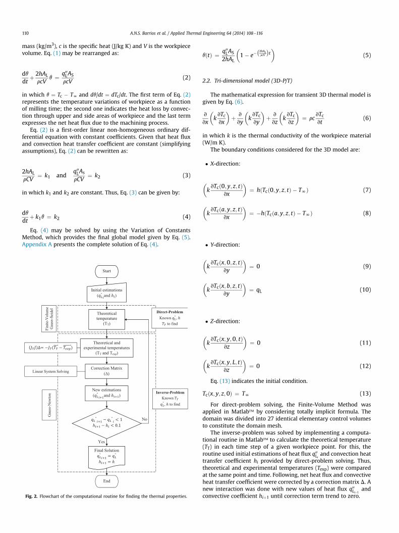
Fig. 2. Flowchart of the computational routine for finding the thermal properties.

qðtÞ ¼ q00LAS

2hAL

�1� e�

�2hALrcV

�t�

(5)

2.2. Tri-dimensional model (3D-P/T)

The mathematical expression for transient 3D thermal model isgiven by Eq. (6).

v

vx

�kvTcvx

�þ v

vy

�kvTcvy

�þ v

vz

�kvTcvz

�¼ rc

vTcvt

(6)

in which k is the thermal conductivity of the workpiece material(W/m K).

The boundary conditions considered for the 3D model are:

� X-direction:

�kvTcð0; y; z; tÞ

vx

�¼ hðTcð0; y; z; tÞ � TNÞ (7)

�kvTcða; y; z; tÞ

vx

�¼ �hðTcða; y; z; tÞ � TNÞ (8)

� Y-direction:

�kvTcðx;0; z; tÞ

vy

�¼ 0 (9)

�kvTcðx; b; z; tÞ

vy

�¼ qL (10)

� Z-direction:

�kvTcðx; y;0; tÞ

vz

�¼ 0 (11)

�kvTcðx; y; L; tÞ

vz

�¼ 0 (12)

Eq. (13) indicates the initial condition.

Tcðx; y; z;0Þ ¼ TN (13)

For direct-problem solving, the Finite-Volume Method wasapplied in Matlab� by considering totally implicit formula. Thedomain was divided into 27 identical elementary control volumesto constitute the domain mesh.

The inverse-problem was solved by implementing a computa-tional routine in Matlab� to calculate the theoretical temperature(TT) in each time step of a given workpiece point. For this, theroutine used initial estimations of heat flux q00Li and convection heattransfer coefficient hi provided by direct-problem solving. Thus,theoretical and experimental temperatures (Texp) were comparedat the same point and time. Following, net heat flux and convectiveheat transfer coefficient were corrected by a correction matrix D. Anew interaction was done with new values of heat flux q00Liþ1

andconvective coefficient hiþ1 until correction term trend to zero.

Table 1Comparison between heat flux and convection heat transfer coefficient.

Thermalproperties

ANSYS�(reference)

MATLAB� (estimation) Difference (%)

qL00 [kW/m2] 150 151.68 1.12h [W/m2 K] 1000 1059.61 5.96

A.N.S. Barrios et al. / Applied Thermal Engineering 64 (2014) 108e116 111

Fig. 2 shows the computational flowchart summarizing the so-lution method and the Appendix B details the mathematicaldevelopment regarded to this thermal model.

2.3. Models validation

The validation of direct-problem was done by comparing theresults generated by Matlab� and Ansys�, where the sameboundary conditions and workpiece dimensions were reproduced.Thus, theoretical temperatures estimated by two programs werecompared. Time step of 0.1 s, total milling time of 9 s and spatialcoordinates inside workpiece of x ¼ 0.009 m, y ¼ 0.013 m andz ¼ 0.100 mwere chosen for simulations. These conditions are nearthe experimental milling conditions since thermocouples werepositioned up to 3 mm beneath machined surface. Fig. 3 comparesthe workpiece temperature behavior by considering the AISI H13steel as workpiece material, heat flux of 150 kW/m2, convectiveheat transfer coefficient of 1000 W/m2 K and initial workpiecetemperature of 25 �C.

To validate the results of the inverse-problem, temperaturesprovided by Ansys� under the same conditions for direct-problemvalidation were taken as experimental temperatures and used asinput in Matlab� routine aiming to calculate the heat flux andconvective coefficient. Table 1 shows the comparison betweenthermal properties found.

3. Application of proposed models in die milling

Due to the wide application range for moulds and diesmanufacturing, hardened AISI H13 steel was chosen as workpiecematerial. Specimens were bi-portioned with 100 mm length,15 mm height and 9 mm width each half, so that specimensmounted reached 18 mm width. Fig. 4 and Table 2 show thermo-mechanical properties and geometry of the workpiece.

End milling tests were carried out in a HERMLE C800Umachining center with 18 kW power and 24,000 maximum spindlerotation. TiNAl coated carbide tool with 20 mm diameter and 8teeth from Sandvik Coromant was used (R215.28-20045-EAC38H1010). All machining tests were fulfilled without cutting fluidapplication. 50 and 100 mm/min cutting speeds were adopted intests. Feed per tooth (0.02 mm) and depth of cut (0.1 mm) werekept constant. According to the thermal models, adiabatic surfacesof workpiece were isolated with silica-based thermal blanket(k ¼ 0.03 W/m K) and silicate-based plate (k ¼ 0.1 W/m K). Five K-type thermocouples were embedded in slots measuring 1.5 mmdepth, 1.5 mmwidth and 12 mm length, setting the hot junction ofthermocouples at 3 mm beneath the surface before milling.

Fig. 3. Comparison between workpiece temperature from Ansys� and Matla

Temperature acquisition was performed under 25 Hz samples rateby using a LabView� routine. Fig. 5 shows a scheme of the exper-imental setup for milling tests and experimental temperaturemeasurements.

3.1. Analysis of the temperature, heat flux and convective heattransfer coefficient

Fig. 6 shows the increase of experimental temperatures with themilling time for each cutting speed, being (a) and (b) for each of 5thermocouples, (c) and (d) theoretical curves fitted to the meantemperatures. Thus, thermal properties such as heat flux andconvective coefficient were estimated by considering theoreticalcurves.

As viewed in Fig. 6a and b, the maximum temperature for agiven thermocouple is always greater than that from previous one,except for thermocouples 1 and 5. Temperatures increase due to theheat addition as tool travels over workpiece length. Lesser tem-peratures are measured by thermocouples at the part ends sinceendmill tool starts and finishes progressively the cut up to reach thecomplete cutting width, generating less heat under these particularmilling conditions. Fig. 6c and d shows that the maximum work-piece temperature enhanced only w40 �C for cutting speed of100 m/min against w35� for 50 m/min, demonstrating that heatgeneration was governed by shear rate rather than tool-part con-tact time, i.e., 50 m/min resulted in 62.9 s milling time (greater than32.6 s for 100/min), but it produced lower part temperature. Highercutting speeds imply in greater shear rate at the primary and sec-ondary shear zones, elevating the part temperature. Also, experi-mental temperatures were properly fitted by quadratic curves,achieving adjusted coefficient of determination higher than 0.830.

Fig. 7 summarizes the influence of the thermal modeling andcutting speed on net heat flux when end milling AISI H13 steel.

It is noted that there is a difference of the net heat flux estimatedby 3D-P and GL methods. This behavior may be explained due tothe GL modeling to estimate thermal properties by consideringmean temperature and the 3D-P modeling to calculate them withtemperature curves for each one of the five thermocouples. In the

b� for solving direct-problem. Maximum percentile difference of 2.7%.

Thermocouple

100

15

13 18.5

Bottom View

10 half-holes drilled by electrical-discharge machining for embedding 5 thermocouples

Half112

Half2

1318.5 18.5 18.5

#1 #2 #3 #4 #518

Top face (before milling)Front View

Side View

Fig. 4. Workpiece configuration for thermocouple setup (dimensions in millimeter).

Table 2Thermo-mechanical properties of AISI H13 steel at room temperature [25].

Thermal properties Mechanical properties

Specific Heat 460 J/kg�C(0e100 �C)

Young’s modulus 210 GPa

Thermal conductivity 28.6 W/m K(215 �C)

Yield strength 1530e1570 MPa

Specific mass 7760 kg/m3 Tensile strength 1835e1960 MPaHarden temperature 995e1025 �C Area reduction 46.2e50.1%Annealing temperature 860e900 �C Hardness 51 HRCStress relief 650e675 �C Machinability 60e70%

(200 HB)

A.N.S. Barrios et al. / Applied Thermal Engineering 64 (2014) 108e116112

GL model, the workpiece is assumed as a body with its inner pointsunder the same temperature at any time. Actually, temperaturechanges at a same instant with part inner points. The thermocou-ples are positioned at 3 mm below the surface before milling andmean temperatures at this position are considered in the modelingsuch as the mean temperature for whole body, but they are averagevalues at 3 mm beneath surface only.

In the 3D-Pmodeling, the temperature variations with the innerpoints are taken into account and the estimation is done based onpositioning of each thermocouple inside workpiece. The results ofthe net heat flux are similar for both GL and 3D-T models. If thenumber of thermocouples was increased, the results should trendto those from 3D-P model.

Workpiece

Endmill

Depth of cut (-Z)

Feed (-X)

Fixture

A

ASection A-A

Bi-portioned Workpiece

Fig. 5. Experimental setup for measuring exp

Lastly, the net heat flux increased with cutting speed indepen-dent of the thermal modeling used. This behavior took place giventhe greater heat input into workpiece due to the higher shear rateduring chip formation.

Fig. 8 presents the influence of the thermal modeling and cut-ting speed on convective heat transfer coefficient when endmillingAISI H13 steel.

The type of thermal modeling did not influence significantly theconvection process when milling the workpiece, mainly for thelowest cutting speed. This difference was more evident for100 mm/min cutting speed, especially when comparing 3D-P andGL models. The reasons for this behavior are the same for net heatflux showed in Fig. 4.

Analogously to heat flux behavior, the convective coefficientincreased with cutting speed independent of the thermal modelingused. This effect was caused due to the higher spindle rotation andendmill tool of the machine-tool.

To validate the results estimated by this paper, Table 3 presentsdata of heat flux, convection heat transfer coefficient and work-piece temperature also obtained by 5 similar articles. Thermalproperties determined by the current work agreed with otherfindings, even considering some differences of methodology, suchas machining process, workpiece material and method for solvingthe thermal problem. Special attention must be given whencomparing this paper with [13,26,27], since the workpiece materialare equal, including the same hardness (w50 HRC). Global and tri-

5 thermocouples

+Z

+Y

+X

Machine bed

Acquisition board

LabviewTM

Tool rotation

erimental temperatures in end milling.

Fig. 6. (a,b) Experimental temperatures for thermocouples from 1 to 5, (c,d) mean and fitted temperatures when dry end milling AISI H13 steel.

A.N.S. Barrios et al. / Applied Thermal Engineering 64 (2014) 108e116 113

dimensional methods proposed and implemented computationallyin this paper corresponded properly to other numerical andanalytical methods. The range for thermal properties found by allarticles comes from the variation of some cutting parameters andmachining processes, such as drilling and tapping. Nevertheless,the results were much similar.

4. Conclusions

Both tri-dimensional and global thermal models are able toestimate the net heat flux and convection heat transfer coefficientfor applications in milling process. Comparisons with similarthermal problems in the literature validated the proposed models,indicating they may be used in other machining processes, to anyworkpiece material and as alternative for analytical solving ofthermal problems.

80

2517

173

78

43

0

40

80

120

160

200

3D-P GL 3D-T

Net

Hea

t Flu

x [k

W/m

2 ]

Thermal Model

vc = 50 m/min

vc = 100 m/min

Fig. 7. Estimations for net heat flux by considering three thermal models: 3D modelwith mean of thermal properties (3D-P), Global model (GL) and 3D model with meanof temperatures (3D-T).

The models were also enough sensitive to identify how cuttingparameters variations influence the thermal properties, estimatingaccordingly the increase of the net heat flux and convective heattransfer coefficient as a function of cutting speed rise.

The main distinction among the proposed models refers to theassumptions assumed when formulating them. Both models aretransient, but 3D one considers that local temperature insideworkpiece changes spatially while global modeling assumes tem-perature constant whatever the direction at any given time. Thismain difference trends to minimize the net heat flux and maximizethe convective heat transfer coefficient, without invalidate them.

For machining applications, both thermal models may estimatethe temperature of workpieces or tools, which is very useful toevaluate possible phase transformations or thermal softening/hardening in workpieces and wear or thermal fatigue in tools. In

436

638

496

605

1372

908

0

400

800

1200

1600

3D-P GL 3D-T

m/W[tneiciffeo

Crefsnar

TtaeH

noitcevnoC

2 K]

Thermal Model

vc = 50 m/min

vc = 100 m/min

Fig. 8. Estimations for convection heat transfer coefficient by considering three ther-mal models: 3D model with mean of thermal properties (3D-P), Global model (GL) and3D model with mean of temperatures (3D-T).

Table 3Comparison of the thermal properties among this paper and some results fromscientific literature.

Variables Papers

Current [13] [26] [27] [28] [29]

q00L [kW/m2] 17e173 15 e 54 e 50h [W/m2 K] 436e1372 3548 500e1000 100e150 80e140 e

Texp [�C] 36e42 140e170 30e49 39e42 20e63 30Workpiece AISI H13 AISI H13 AISI H13 AISI H13 AISI 4340 AISI 1045Methoda FV AHC FE FE AHC IHCProcess Milling Drilling Milling Tapping Milling Milling

a FV: Finite-Volume, FE: Finite-Element, AHC: Analytical Heat Conduction, IHC:Inverse Heat Conduction.

A.N.S. Barrios et al. / Applied Thermal Engineering 64 (2014) 108e116114

addition, particularly the heat flux and convective heat transfercoefficient may indicate the efficiency of cooling capability of cut-ting fluids in any machining processes.

Acknowledgements

The authors are grateful to the São Paulo Research Foundation(FAPESP), Education Ministry Foundation (CAPES) and NationalCouncil for Scientific and Technological Development (CNPq) forfinancial support.

Appendix A. Global model (GL) solution

Eq. (4) may be solved by taking q ¼ uv. Then,

dqdt

¼ udvdt

þ vdudt

(A.1)

Replacing Eq. (A.1) in (4),

u�dvdt

þ vk1

�þ�vdudt

� k2

�¼ 0 (A.2)

Among other possible solutions, Eq. (A.2) will be null if bothterms were null, i.e.,

dvdt

¼ �vk1 and vdudt

¼ k2 (A.3)

Then,

Zdvv

¼ �k1

Zdt

ln vþ c1 ¼ �k1t þ c2

ln v ¼ �k1t þ ðc2 � c1Þln v ¼ �k1t þ c3

v ¼ e�k1t þ ec3

v ¼ e�k1t

(A.4)

The integration constant c4 may be disregarded since a singlesolution is searched. Replacing v ¼ e�k1t in v(du/dt) ¼ k2 we have:

Zdu ¼ k2

Zdt

e�k1tZdu ¼ k2

Zek1tdt

uþ c5 ¼ k2ek1 t

k1þ c6

u ¼ k2k1ek1t þ ðc6 � c5Þ

u ¼ k2k1ek1t þ c7

(A.5)

Replacing (A.4) and (A.5) in q ¼ uv,

q ¼ c7e�k1t þ k2

k1(A.6)

Eq. (A.6) is the general solution for Eq. (4). To found a particularsolution, an initial condition is needed. Assuming that machine-tool, workpiece and environment are in thermal equilibriumbefore milling, for t¼ 0/ q¼ 0 or c7¼�k2/k1. Replacing c7 in (A.6),

q ¼ k2k1

�1� e�k1t

�(A.7)

Replacing (3) in (A.7),

qðtÞ ¼ q00LAS

2hAL

�1� e�

�2hALrcV

�t�

(A.8)

Appendix B. 3D model (3D-P/T) solution

To solve the direct-problem, the control volume was portionedinto 27 equal elementary volumes (5 � 6 � 33.3 mm). Eq. (6) maybe spatially integrated in directions XYZ and in time, such asviewed below.

Zt1t0

Zew

Zns

Zt

b

v

vx

�kvTcvx

�dxdydzdtþ

Zt1t0

Zew

Zns

Zt

b

v

vy

�kvTcvy

�dxdydzdt

þZt1t0

Zew

Zns

Zt

b

v

vz

�kvTcvz

�dxdydzdt¼

Zt1t0

Zew

Zns

Zt

b

rcvTcvt

dxdydzdt

(B.1)

in which the indices e, w, n, s, t and b are related to surfaces of theelementary control volumes, i.e., east, west, north, south, top andbottom, respectively. Rewriting Eq. (B.1) integrated in space andtime, we have:

��kvTcvx

�e��kvTcvx

�w

dydz þ

��kvTcvy

�n��kvTcvy

�s

dxdz

þ��

kvTcvz

�t��kvTcvz

�b

dxdy

¼ rcdxdydz

�T1 � T0

�Dti

(B.2)

Variables dx, dy, dz, Dti, T1 and T0 represent, respectively, theworkpiece size in directions XYZ, as well as, incremental time, in-cremental temperature and current temperature. Eq. (B.2) showsthat the terms of heat flux still must be approximate because theyhave temperatures derivatives partially in space. These heat fluxterms contain indices related to the faces of control volume (e,w, n,s, t and b) which in turn refer to different mechanisms of heattransfer taking place in each face. Thus, each control volume mustbe evaluated according to the heat transfer mechanism whichpredominates in each of 6 control volume faces. Fig. B.1 illustratesthe nodes of each control volume. Nodes TP, TW, TE, TS, TN, TB and TTrepresent, respectively, the temperature inside analyzed controlvolume and in control volumes placed at west, east, south, north,bottom and top.

Eqs. (7)e(12) were used to approximate the heat flux terms inthe control volumes to the surfaces located at the workpieceboundaries. Faces out of workpiece boundaries but in contact to

A.N.S. Barrios et al. / Applied Thermal Engineering 64 (2014) 108e116 115

those from neighbors control volumes may be approximate byequations below:

�kvTcvx

�w

¼ kTP � TW

dx(B.3)

�kvTcvx

�e¼ k

TE � TPdx

(B.4)

�kvTcvy

�s¼ k

TP � TSdy

(B.5)

�kvTcvy

�n¼ k

TN � TPdy

(B.6)

�kvTcvz

�b¼ k

TP � TBdz

(B.7)

�kvTcvz

�t¼ k

TT � TPdz

(B.8)

The approximations were replaced into Eq. (B.2) according tothe individual analyze for each control volume. With these re-placements, the differential equations became a linear systemwiththe same number of equations and unknown variables. Each con-trol volume has a characteristic equation since it was analyzedaccording to its energy conservation balance. As example, let thecontrol volume #1, such as showed in Fig. B.2.

The control volume #1 is subject to convection (east), diffusion(west, south and top), heat flux q00L (north) and isolation (bottom).Applying Eq. (B.2) to the control volume #1,

�kTE � TP

dx� hðTP � TNÞ

dydz þ

�q00L � k

TP � TSdy

dxdz

þ�kTT � TP

dz� 0

dxdy ¼ rcdxdydz

�T1 � T0

�Dti

(B.9)

or rearranging,

�aE þ aS þ aT þ ap0 þ hdydz

�TP ¼ aETE þ aSTS þ aTTT þ ap0T0P

þ hTNdydz þ q00Ldxdz(B.10)

in which

aE ¼ kdydzdx

aS ¼ kdxdzdy

aT ¼ kdxdydz

ap0 ¼ rcdxdydzDti

Replacing the nodes of the Eq. (B.10) by numbers adopted inFig. B.2, Eq. (B.11) describes the heat transfer process for controlvolume #1.

�aE þ aS þ aT þ ap0 þ hdydz

�T1 ¼ aET2 þ aST4 þ aTT10 þ ap0T01

þ hTNdydz þ q00Ldxdz(B.11)

Therefore, 27 linear algebraic equationswere formulated followingthe same procedure. They depict the heat transfer in each portion oftheworkpiece, allowinguse themeven ifdomainmeshis refined, sincea given characteristic equation be applied for a valid control volume.

Solved by GausseSeidel Method, the equations give the work-piece temperature distribution.

To solve the inverse-problem, GausseNewton Method was usedby evaluating the first derivatives of the Taylor Series Expansion. Eq.(B.12) compares the theoretical and experimental temperatures.

ðJTJÞD ¼ �JT

�TT!� Texp

!�(B.12)

inwhich J, JT, T!

T; T!

exp and D are Jacobian matrix, transpose Jacobianmatrix, theoretical temperature, experimental temperature andcorrection term, respectively. Jacobian matrix is composed by partialderivatives of the theoretical temperature in relation to the estimatedparameters (heat flux and convective heat transfer coefficient), ac-cording to the temperaturevector size (n), suchas showed inEq. (B.13).

J ¼

266666664

dT1dqL

dT1dh

dT2dqL

dT2dh

« «

dTndqL

dTndh

377777775

(B.13)

Replacing (B.13) in (B.12),8>>>>>>>>>><>>>>>>>>>>:

24

dT1dq00L

dT2dq00L

. dTndq00L

dT1dh

dT2dh . dTn

dh

35

266666664

dT1dq00L

dT1dh

dT2dq00L

dT2dh

« «

dTndq00L

dTndh

377777775

9>>>>>>>>>>=>>>>>>>>>>;

�X1X2

¼ �24

dT1dq00L

dT2dq00L

. dTndq00L

dT1dh

dT2dh . dTn

dh

352664TT1 � Texp1TT2 � Texp2

«TTn � Texpn

3775 (B.14)

in which X1 and X2 are the corrections for heat flux and convectionheat transfer coefficient, respectively. Eq. (B.14) may be rewritten asthe linear system below,

�a11 a12a21 a22

�X1X2

¼

�b11b21

(B.15)

where matrices of coefficients a and b are the product of the Ja-cobian and temperature matrices showed in Eq. (B.14).

Net heat flux and convection heat transfer coefficient may befound by solving Eq. (B.15). Correcting these thermal properties byusing X-matrix, new heat flux and convective heat transfer coeffi-cient are determined, which allow calculating again theoreticaltemperatures for new estimations of q00L and h by solving direct-problem. The convergence is attained in the i-th interaction byattending the Eq. (B.16).

q00Liþ1� q00Li < 1 and hiþ1 � hi < 0:1 (B.16)

TN

TW TE

TB

TTTS

t

w

s

TP

b

e

n

y

xz

Fig. B.1Elementary control volume with surface and neighbors nodes.

y

xz

Block #1

Block #2

Block #3

Block #2Block #1 Block #3

= + +1 2 3

4 5 6

7 8 9

10 11 12

13 14 15

16 17 18

19 20 21

22 23 24

25 26 27

Fig. B.2Identification of each control volume divided into 3 blocks.

A.N.S. Barrios et al. / Applied Thermal Engineering 64 (2014) 108e116116

References

[1] J.P. Davim, Machining e Fundamentals and Recent Advances, first ed.,Springer, London, 2008.

[2] S. Kalpakjian, S.R. Schmid, C.-W. Kok, Manufacturing Engineering and Tech-nology, sixth ed., Pearson Education, New York, 2009.

[3] L.N. Lacalle, A. Lamikiz, Machine Tools for High Performance Machining, firsted., Elsevier, London, 2009.

[4] E.M. Trent, P.K. Wright, Metal Cutting, fourth ed., ButterwortheHeinemann,Boston, 2000.

[5] M.C. Shaw, Metal Cutting Principles, second ed., Oxford University Press, NewYork, 2004.

[6] N.A. Abukshim, P.T. Mativenga, M.A. Sheikh, Heat generation and temperatureprediction in metal cutting: a review and implications for high speedmachining, Int. J. Mach. Tool. Manuf. 46 (2005) 782e800.

[7] S. Lin, F. Peng, J. Wen, Y. Liu, R. Yan, An investigation of workpiece tempera-ture variation in end milling considering flank rubbing effect, Int. J. Mach.Tool. Manuf. 73 (2013) 71e86.

[8] R.J. Goldstein, W.E. Ibele, S.V. Patankar, T.W. Simon, T.H. Kuehn, P.J. Strykowski,K.K. Tamma, J.V.R. Heberlein, J.H. Davidson, J. Bischof, F.A. Kulacki,U. Kortshagen, S. Garrick, V. Srinivasan, K. Ghosh, R. Mittal, Heat transfer e areview of 2005 literature, Int. J. Heat Mass Transf. 53 (2010) 4397e4447.

[9] K.J. Trigger, B.T. Chao, An analytical evaluation of metal cutting temperature,Trans. ASME 73 (1951) 57e68.

[10] D. Antonelli, D. Romano, Computation of the thermal field in tools duringmachining processes, Math. Comput. Model. 21 (1995) 53e68.

[11] S.R. Carvalho, S.M.M. Lima e Silva, A.R. Machado, G. Guimarães, Temperaturedetermination at the chip-tool interface using an inverse thermal modelconsidering the tool and tool holder, J. Mater. Process. Technol. 179 (2006)97e104.

[12] U. Augustine, N. Olisaemeka, Thermal aspect of machining: evaluation of tooland chip temperature during machining process using numerical method, Int.J. Eng. Sci. 2 (2013) 66e79.

[13] L.C. Brandão, R.T. Coelho, C.H. Lauro, Contribution to dynamic characteristicsof the cutting temperature in the drilling process considering one dimensionheat flow, Appl. Therm. Eng. 31 (2011) 3806e3813.

[14] P.F.B. Souza, V.L. Borges, I.C. Pereira, M.B. Silva, G. Guimarães, Estimation ofheat flux and temperature field during drilling process using dynamic ob-servers based on Green’s function, Appl. Therm. Eng. 48 (2012) 144e154.

[15] M. Gostimirovic, P. Kovac, M. Sekulic, An inverse heat transfer problem foroptimization of the thermal process in machining, Acad. Proc. Eng. Sci. 36(2011) 489e504.

[16] D. Ulutan, I. Lazoglu, C. Dinc, Three-dimensional temperature prediction inmachining processes using finite difference method, J. Mater. Process. Tech-nol. 209 (2009) 1111e1121.

[17] R. Pabst, J. Fleischer, J. Michna, Modelling of the heat input for face-millingprocess, CIRP Ann. e Manuf. Technol. 59 (2010) 121e124.

[18] V. Luchesi, R.T. Coelho, An inverse method to estimate the moving heat sourcein machining process, Appl. Therm. Eng. 45e46 (2012) 64e78.

[19] X. Cui, J. Zhao, Z. Pei, Analysis of transient average tool temperature in facemilling, Int. Commun. Heat Mass Transf. 39 (2012) 786e791.

[20] V.P. Astakhov, Tribology of Metal Cutting, first ed., Elsevier, London, 2006.[21] A.R. Rodrigues, H. Matsumoto, W.J. Yamakami, R.G.R. Paulo, C.L.F. Assis, Effects

of milling condition on the surface integrity of hot forged steel, J. Braz. Soc.Mech. Sci. Eng. 32 (2010) 37e43.

[22] W. Li, Y. Guo, C. Guo, Superior surface integrity by sustainable dry hard millingand impact on fatigue, CIRP Ann. e Manuf. Technol. 62 (2013) 567e570.

[23] A.R. Rodrigues, O. Balancin, J. Gallego, C.L.F. Assis, H. Matsumoto, F.B. Oliveira,S.R.S. Moreira, O.V. Silva Neto, Surface integrity analysis when end millingultrafine-grained steels, Mater. Res. 15 (2012) 1e6.

[24] D. Papageorgiou, C. Medrea, N. Kyriakou, Failure analysis of H13 working dieused in plastic injection moulding, Eng. Fail. Anal. 35 (2013) 355e359.

[25] T.V. Philip, T.J. McCaffrey, Properties and Selection: Irons, Steels, and HighPerformance Alloys, tenth ed., ASM, United States, 1990.

[26] L.C. Brandão, R.T. Coelho, A.R. Rodrigues, Experimental and theoretical studyof workpiece temperature when end milling hardened steels using (TiAl)N-coated and PcBN-tipped tools, J. Mater. Process. Technol. 199 (2008) 234e244.

[27] L.C. Brandão, R.T. Coelho, A.T. Malavolta, Experimental and theoretical studyon workpiece temperature when tapping hardened AISI H13 using differentcooling systems, J. Braz. Soc. Mech. Sci. Eng. 32 (2010) 154e159.

[28] V.M. Luchesi, R.T. Coelho, Experimental investigations of heat transfer co-efficients of cutting fluids in metal cutting processes: analysis of workpiecephenomena in a given case study, Proc. Inst. Mech. Eng., Part B: J. Eng. Manuf.226 (2012) 1174e1184.

[29] F. Jiang, Z. Liu, Y. Wan, Z. Shi, Analytical modeling and experimental investi-gation of tool and workpiece temperatures for interrupted cutting 1045 steelby inverse heat conduction method, J. Mater. Process. Technol. 213 (2013)887e894.