Effect of heat processing on thermal stability and antioxidant ...
Upload
khangminh22Category
view
2download
0
4/29/2020
ON-LINE APPENDICES TO
Thermal Radiation Heat Transfer
7th Edition, Taylor and Francis, 2021
John R. Howell, M. Pinar Mengüç,
Kyle Daun, and Robert Siegel
A: Wide-Band Models
B: Derivation of Geometric Mean Beam Length Relations
C: Exponential Kernel Approximation
D: Curtis-Godson Approximation
E: The YIX Method
F: Graphs for CO2, H2O and CO Emittance
G: Radiative Transfer in Porous and Dispersed Media
H: Benchmark Solutions for Verification of Radiation Solutions
I: Integration and Numerical Solution Methods
J: Radiation Cooling
K: Radiation from Flames
L: Commercial Codes
M: References to Reviews and Historical Papers
N: Short Biographies and a History of Thermal Radiation
O: Timeline of Important Events in Radiation
P: Additional Homework Problems
Q: Proposed One-Semester Syllabus

A. Wide-Band Models
A.1
A. WIDE-BAND MODELS
A.1 WIDE-BAND MODELS AND CORRELATIONS
Edwards and Menard (1964) modeled a band of rotation lines that are reordered in wave
number, so they form an array with exponentially decreasing line intensities moving away
from the band center and covering the entire band. This is the exponential wide-band model.
Edwards and co-workers [Edwards (1960,1962,1965), Edwards and Menard (1964a,b),
Edwards and Sun (1964), Edwards et al. (1965), Edwards and Nelson (1962), Edwards and Balakrishnan (1973), Weiner (1966), Hines and Edwards (1968)] assembled a large body of
data on the important radiating gases at typical engineering conditions. By comparing their
band-correlation relations with data over large ranges of pressure and temperature, they
determined empirically how the physical variables are related to the effective bandwidth
Āl(T), to an effective bandwidth parameter ω(Τ), and to a modified pressure-broadening
parameter B(T, Pe), where Pe is the effective broadening pressure. The μ was expressed in the
form of a modified variable u = Χ/ω, that is in terms of the mass path length X = S of the
absorbing gas component and a quantity (T) that will be determined. Available correlations
are summarized in Table A.1.
The newer and more accurate models based on k-distributions (Chapter 9 of the text) have
largely superseded the exponential wide-band models, especially for combustion gases;
however, some gases such as SO2 and HCl do not have the line-by-line data available for
computing k-distributions, so the correlations presented here may still be useful.

A. Wide-Band Models
A.2
TABLE A.1 Available Band Absorptance Correlations for Isothermal Media
Gas Bands Reference Comments Type of Correlation
CO2 2.0, 2.7, 4.3, 9.4, 10.4, and 15
m
Table 9.3 [Marin and
Buckius (1998b)]
Wide band
300 < T < 1390 K
0.1 < X < 23,000 g/m2
c-k wide-band distribution
WSGG (all) Table 9.7 [Denison and
Webb (1995)]
400 < T < 2500 K
3 x 10⁻⁵ to 600 m2/mol
Spectral line WSGG
2.0, 2.7, 4.3, 9.4, 10.4, and 15
m
[Domoto (1974)] 300 < T < 1390 K
0.1 < X < 23,000 g/m2 k-distribution
(wide band)
2.7,4.3, and 15 m [Chu and Greif (1978)] T ≈ 300 K
0.1 < X < 23,000 g/m2
Nonrigid rotator
spectroscopic wide band
2.7 m [Lin and Greif (1974)] T ≈ 300 K
0.081 < pS < 1300 atm cm
Rigid rotator
spectroscopic wide band
2.0, 2.7, 4.3, and 15 m Table 9.2 [Edwards
(1976); Edwards and
Menard (1964b);
Edwards and
Balakrishnan (1973);
Edwards et al. (1967)]
300 < T < 1390 K
0.1 < X < 23,000 g/m2
Exponential wide band
9.4 and 10.4 m Table 9.2 [Edwards
(1976); Edwards and
Menard (1964); Edwards
and Balakrishnan
(1973); Edwards et al.
(1967)]
300 < T < 1390 K
0.1 < X < 23,000 g/m2
Exponential wide band
2.0, 2.7, 4.3, 9.4, 10.4, and 15
m
[Edwards (1960)] 300 < T < 1390 K
0.1 < X < 23,000 g/m2
Equivalent bandwidth
H2O 1.38, 1.87, 2.7, and 6.3 m,
rotational
Table 9.4 [Marin and
Buckius (1998a)]
300 < T < 2900 K (except
rotational band,
300 < T < 1900 K)
10–5 < pS < 104 atm m
c-k (wide-band) distribution
WSGG (all) Table 9.5 [Denison and
Webb (1993)]
400 < T < 2500 K
3 x 10⁻⁵ to 60 m2/mol
Spectral line
WSGG
1.38, 1.87, 2.7, and 6.3 m,
rotational
[Kamiuto and Tokita
(1994)]
300 < T <3000 K
0.1 < pS < 1000 bar cm
Modified exponential wide
band
2.7 m [Lin and Greif (1974)] T = 300 K
3.3 < pS < 2800 atm cm
Rigid rotator spectroscopic
wide band
2.7 and 6.3 m [Weiner (1966)] 300 < T < 2100 K
1 < X < 21000 g/m2
Equivalent line
1.38, 1.87, 2.7, and 6.3 m Table 9.2 [Edwards
(1976); Edwards et al.
(1965); Edwards and
Balakrishnan (1973);
Edwards et al. (1967)]]
300 < T < 2250 K
1 < X < 38,000 g/m2
Exponential wide band
Rotational band
( > 10 m)
[Charalampopoulos and
Felske (1983)]
500 < T < 2400 K
1.5 < pS < 30 atm cm
Exponential wide band
a Varies with band.
(continued)
A. Wide-Band Models
A.3
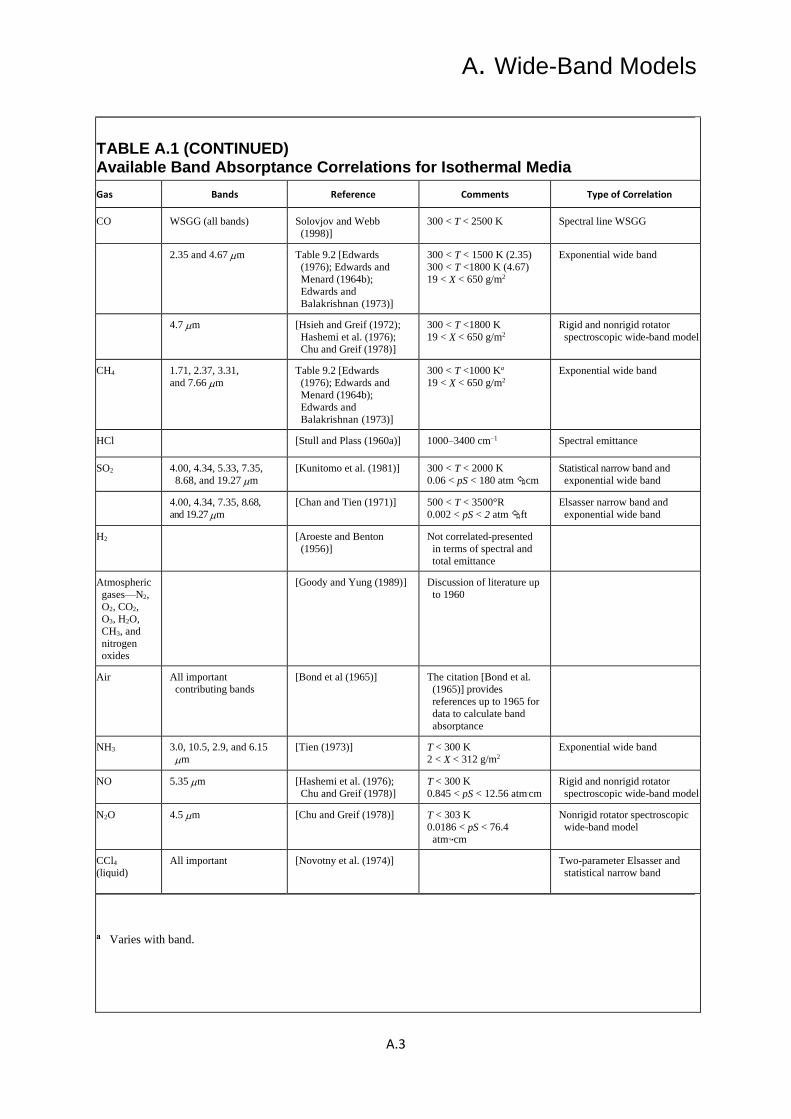
TABLE A.1 (CONTINUED) Available Band Absorptance Correlations for Isothermal Media
Gas Bands Reference Comments Type of Correlation
CO WSGG (all bands) Solovjov and Webb
(1998)]
300 < T < 2500 K Spectral line WSGG
2.35 and 4.67 m Table 9.2 [Edwards
(1976); Edwards and
Menard (1964b);
Edwards and
Balakrishnan (1973)]
300 < T < 1500 K (2.35)
300 < T <1800 K (4.67)
19 < X < 650 g/m2
Exponential wide band
4.7 m [Hsieh and Greif (1972);
Hashemi et al. (1976);
Chu and Greif (1978)]
300 < T <1800 K
19 < X < 650 g/m2
Rigid and nonrigid rotator
spectroscopic wide-band model
CH4 1.71, 2.37, 3.31,
and 7.66 m
Table 9.2 [Edwards
(1976); Edwards and
Menard (1964b);
Edwards and
Balakrishnan (1973)]
300 < T <1000 Ka
19 < X < 650 g/m2
Exponential wide band
HCl [Stull and Plass (1960a)] 1000–3400 cm–1 Spectral emittance
SO2 4.00, 4.34, 5.33, 7.35,
8.68, and 19.27 m
[Kunitomo et al. (1981)] 300 < T < 2000 K
0.06 < pS < 180 atm cm
Statistical narrow band and
exponential wide band
4.00, 4.34, 7.35, 8.68,
and 19.27 m
[Chan and Tien (1971)] 500 < T < 3500°R
0.002 < pS < 2 atm ft
Elsasser narrow band and
exponential wide band
H2 [Aroeste and Benton
(1956)]
Not correlated-presented
in terms of spectral and
total emittance
Atmospheric
gases—N2,
O2, CO2,
O3, H2O,
CH3, and
nitrogen
oxides
[Goody and Yung (1989)] Discussion of literature up
to 1960
Air All important
contributing bands
[Bond et al (1965)] The citation [Bond et al.
(1965)] provides
references up to 1965 for
data to calculate band
absorptance
NH3 3.0, 10.5, 2.9, and 6.15
m
[Tien (1973)] T < 300 K
2 < X < 312 g/m2
Exponential wide band
NO 5.35 m [Hashemi et al. (1976);
Chu and Greif (1978)] T < 300 K
0.845 < pS < 12.56 atm.cm
Rigid and nonrigid rotator
spectroscopic wide-band model
N2O 4.5 m [Chu and Greif (1978)] T < 303 K
0.0186 < pS < 76.4
atm•cm
Nonrigid rotator spectroscopic
wide-band model
CCl4
(liquid)
All important [Novotny et al. (1974)] Two-parameter Elsasser and
statistical narrow band
a Varies with band.

A. Wide-Band Models
A.4
TABLE A.1 (CONTINUED) Available Band Absorptance Correlations for Isothermal Media
Gas Bands Reference Comments Type of Correlation
H2, N2, O2, CH4,
CO, Ar (liquids
only)
All important far-
infrared bands in 40
to 500 m region; for
H2, 16.7 to 500 m
[Jones (1970)] T near normal boiling
point at 1 atm, S =
1.27 and 2.54 cm,
plus 3.25 cm for H2
Data for absorption coefficient versus
wave number
C2H2 Wave number, (cm–1 )
3287; 1328, 729
[Brosmer and Tien
(1985)]
Discussion of
literature;
measurements from T
= 290 to 600 K
Exponential wide band
C2H4 Four in infrared [Tuntomo et al.
(1989)]
Measurements and
correlation
Statistical narrow band, wide band
a Varies with band.
A brief description of the exponential wide band correlation is given here for the four
gases in Table A.2. Information for NO and SO2 is in Edwards and Balakrishnan (1973) [see
also Edwards (1976)]. The correlation is in terms of three quantities: , the integrated band
intensity; B, the line-width parameter; and ω, the bandwidth parameter. The desired total
band absorption Ā is found from the following correlations (the band subscript l on Ā has
been dropped for convenience):
For 1: 0
1(2 )
1[ln( ) 2 ]
B A u u B
A Bu B B uB
A Bu B uB
=
= −
= + −
(A.1a)
For 1: 0 1
(ln 1) 1
B A u u
A u u
=
= + (A.1b)
The B is π times the ratio of mean line width to spacing, i.e., the parameter β adjusted for
broadening effects, including pressure broadening: B = ßPe, where
0 0[ / ( / )( 1)]n
eP P P p P b= + − , P is the total pressure (atm) of radiating and nonradiating gas,
P0 =1 atm, and p is the partial pressure of the radiating gas (pe →1 as pe → 0 and P → P0).
The b and n are in Table A.2 for each gas band. The u = Χ/ω, where X is the mass path
length of the radiating gas. The ω is found from 1/2
0 0( / )T T = , where ω0 is in Table A.2
and T0 = 100 K. The table also gives the quantities necessary to obtain and β from the
following:
( )( )
( )
( )1
0
00,1
1 exp( )
1 exp
m
k kk
m
k kk
u TT
Tu
=
=
− − =
− −
(A.2a)
A. Wide-Band Models
A.5
1/ 2
00
0
( )( )
( )
T TT
T T
=
(A.2b)
where
( ) ( ) ( ) ( )
0,1
1 0
1 !/ 1 ! !( )
1 !/ 1 ! !
k k
k k
k k
k
um
k k k k k k
um
k k k k k
g g eT
g g e
=
−
=
−
= =
+ + − − =
+ − −
(A.2c)
( ) ( ) ( )( ) ( )
0,
0,
21/2
1
1
1 !/ 1 ! !
( )1 !/ 1 ! !
k k
k k
k k
k k
um
k k k k k k
um
k k k k k k
g g e
Tg g e
−
= =
−
= =
+ + − − =+ + − −
(A.2d)
in which
0,
0
,k kk k
hc hcu u
kT kT
= =
and 0, 0k = if k is positive or zero and is |k| if k is negative. Some illustrative numerical
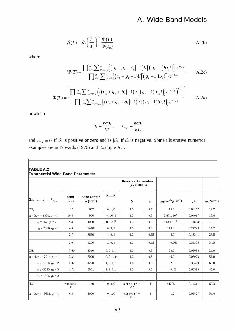
examples are in Edwards (1976) and Example A.1.
TABLE A.2 Exponential Wide-Band Parameters
Pressure Parameters
(To = 100 K)
Gas 1, ,( )m cm g − Band (μm)
Band Center (cm−1)
1..... m
b n o(cm−1/g m−2) o 0 (cm−1)
CO2 15 667 0, 1, 0 1.3 0.7 19.0 0.06157 12.7
m = 3, = 1351, g1 = l 10.4 960 −1, 0, 1 1.3 0.8 2.47 x 10⁻⁹ 0.04017 13.4
= 667, g1 = 2 9.4 1060 0, −2, lb 1.3 0.8 2.48 x 10⁻⁹b 0.11888b 10.1
= 2396, g3 = l 4.3 2410a 0, 0, 1 1.3 0.8 110.0 0.24723 11.2
2.7 3660 1, 0, 1 1.3 0.65 4.0 0.13341 23.5
2.0 5200 2, 0, 1 1.3 0.65 0.066 0.39305 34.5
CH4 7.66 1310 0, 0, 0, 1 1.3 0.8 28.0 0.08698 21.0
m = 4, 1 = 2914, g1 = 1 3.31 3020 0, 0, 1, 0 1.3 0.8 46.0 0.06973 56.0
2 =1526, g2 = 2 2.37 4220 1, 0, 0, 1 1.3 0.8 2.9 0.35429 60.0
3 =3020, g3 = 3 1.71 5861 1, 1, 0, 1 1.3 0.8 0.42 0.68598 45.0
4 = 1306, g4 = 3
H2O rotationa
ld
140 0, 0, 0 8.6(T0/T)1/2 +
0.5
1 44205 0.14311 69.3
m = 3, 1 = 3652, g1 = l 6.3 1600 0, 1, 0 8.6(T0/T)1/2 +
0.5
1 41.2 0.09427 56.4
A. Wide-Band Models
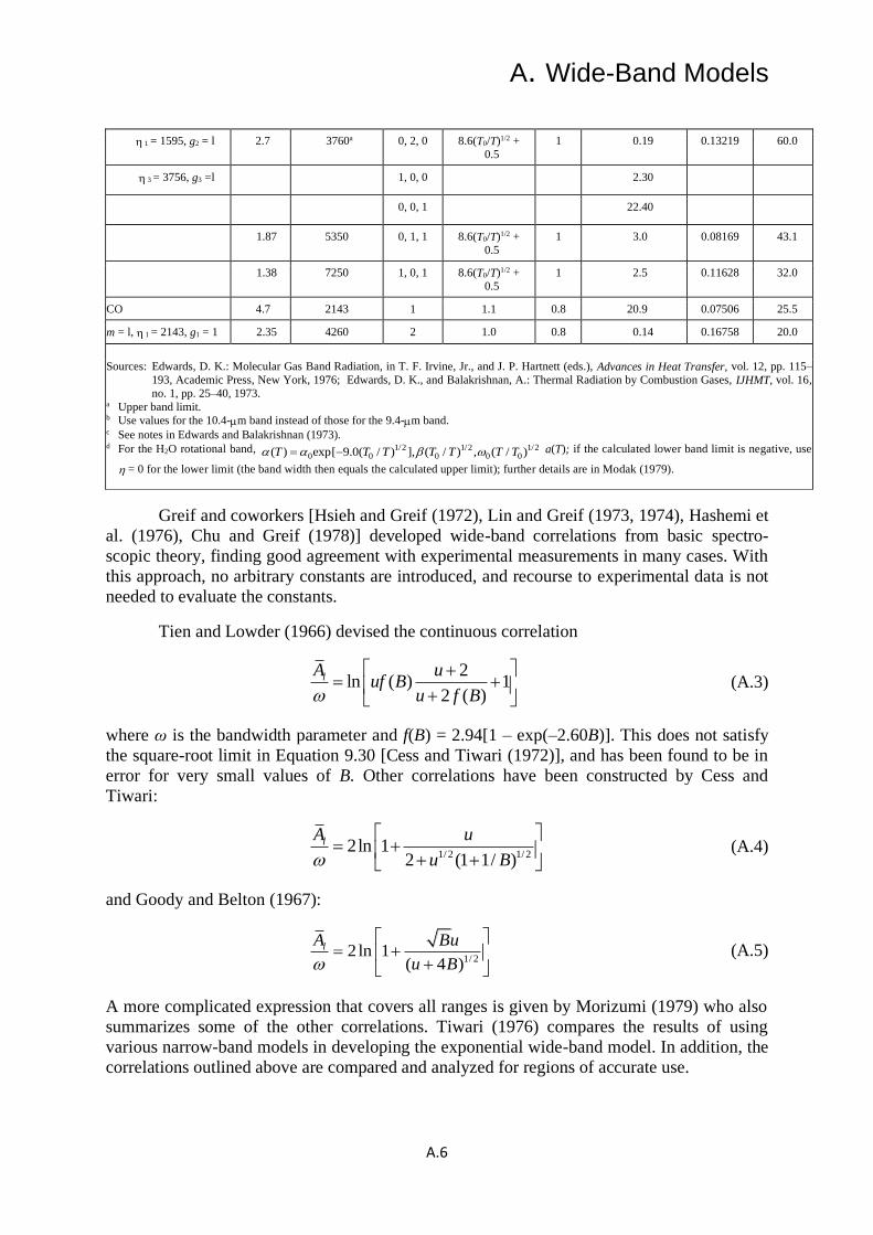
A.6
1 = 1595, g2 = l 2.7 3760a 0, 2, 0 8.6(T0/T)1/2 +
0.5
1 0.19 0.13219 60.0
3 = 3756, g3 =l 1, 0, 0 2.30
0, 0, 1 22.40
1.87 5350 0, 1, 1 8.6(T0/T)1/2 +
0.5
1 3.0 0.08169 43.1
1.38 7250 1, 0, 1 8.6(T0/T)1/2 +
0.5
1 2.5 0.11628 32.0
CO 4.7 2143 1 1.1 0.8 20.9 0.07506 25.5
m = l, 1 = 2143, g1 = 1 2.35 4260 2 1.0 0.8 0.14 0.16758 20.0
Sources: Edwards, D. K.: Molecular Gas Band Radiation, in T. F. Irvine, Jr., and J. P. Hartnett (eds.), Advances in Heat Transfer, vol. 12, pp. 115–
193, Academic Press, New York, 1976; Edwards, D. K., and Balakrishnan, A.: Thermal Radiation by Combustion Gases, IJHMT, vol. 16,
no. 1, pp. 25–40, 1973. a Upper band limit. b Use values for the 10.4-m band instead of those for the 9.4-m band. c See notes in Edwards and Balakrishnan (1973). d For the H2O rotational band, 1/2 1/2 1/2
0 0 0 0 0( ) exp[ 9.0( / ) ], ( / ) , ( / )T T T T T T T= − a(T); if the calculated lower band limit is negative, use
= 0 for the lower limit (the band width then equals the calculated upper limit); further details are in Modak (1979).
Greif and coworkers [Hsieh and Greif (1972), Lin and Greif (1973, 1974), Hashemi et
al. (1976), Chu and Greif (1978)] developed wide-band correlations from basic spectro-
scopic theory, finding good agreement with experimental measurements in many cases. With
this approach, no arbitrary constants are introduced, and recourse to experimental data is not
needed to evaluate the constants.
Tien and Lowder (1966) devised the continuous correlation
2ln ( ) 1
2 ( )
lA uuf B
u f B
+= +
+ (A.3)
where ω is the bandwidth parameter and f(B) = 2.94[1 – exp(–2.60B)]. This does not satisfy
the square-root limit in Equation 9.30 [Cess and Tiwari (1972)], and has been found to be in
error for very small values of B. Other correlations have been constructed by Cess and
Tiwari:
1/ 2 1/ 22ln 1
2 (1 1/ )
lA u
u B
= +
+ + (A.4)
and Goody and Belton (1967):
1/ 22ln 1
( 4 )
lA Bu
u B
= +
+ (A.5)
A more complicated expression that covers all ranges is given by Morizumi (1979) who also
summarizes some of the other correlations. Tiwari (1976) compares the results of using
various narrow-band models in developing the exponential wide-band model. In addition, the
correlations outlined above are compared and analyzed for regions of accurate use.
A. Wide-Band Models
A.7
To determine the effect of the band models on the final radiative transfer results,
several band models were applied to two problems [Tiwari (1977)] involving radiative
transfer in gases with internal heat sources and heat transfer. In most instances good
agreement was obtained by using the various models, but it is necessary to examine the
reference to appreciate the detailed comparisons. A model to apply the exponential wide-
band properties in a multidimensional geometry is in Modest (1983).
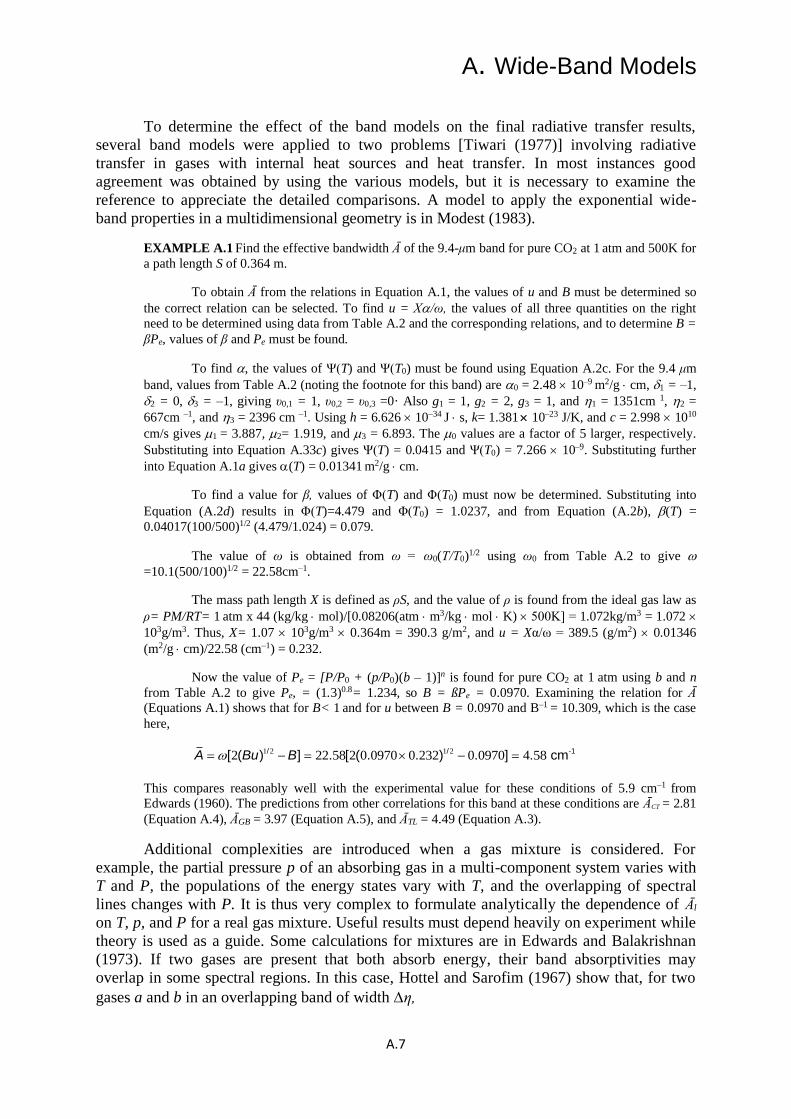
EXAMPLE A.1 Find the effective bandwidth Ā of the 9.4-μm band for pure CO2 at 1 atm and 500K for
a path length S of 0.364 m.
To obtain Ā from the relations in Equation A.1, the values of u and B must be determined so
the correct relation can be selected. To find u = Χ/ω, the values of all three quantities on the right
need to be determined using data from Table A.2 and the corresponding relations, and to determine B =
βPe, values of β and Pe must be found.
To find , the values of Ψ(T) and Ψ(T0) must be found using Equation A.2c. For the 9.4 μm
band, values from Table A.2 (noting the footnote for this band) are 0 = 2.48 10–9 m2/g cm, 1 = –1,
2 = 0, 3 = –1, giving υ0,1 = 1, υ0,2 = υ0,3 =0· Also g1 = 1, g2 = 2, g3 = 1, and 1 = 1351cm 1, 2 =
667cm –1, and 3 = 2396 cm –1. Using h = 6.626 10–34 J s, k= 1.381 10–23 J/K, and c = 2.998 1010
cm/s gives 1 = 3.887, 2= 1.919, and 3 = 6.893. The 0 values are a factor of 5 larger, respectively.
Substituting into Equation A.33c) gives Ψ(T) = 0.0415 and Ψ(T0) = 7.266 10–9. Substituting further
into Equation A.1a gives (T) = 0.01341 m2/g cm.
To find a value for β, values of Φ(T) and Φ(T0) must now be determined. Substituting into
Equation (A.2d) results in Φ(T)=4.479 and Φ(T0) = 1.0237, and from Equation (A.2b), (T) =
0.04017(100/500)1/2 (4.479/1.024) = 0.079.
The value of ω is obtained from ω = ω0(Τ/Τ0)1/2 using ω0 from Table A.2 to give
=10.1(500/100)1/2 = 22.58cm–1.
The mass path length X is defined as ρS, and the value of ρ is found from the ideal gas law as
ρ= PM/RT= 1 atm x 44 (kg/kg mol)/[0.08206(atm m3/kg mol K) 500Κ] = 1.072kg/m3 = 1.072
103g/m3. Thus, X= 1.07 103g/m3 0.364m = 390.3 g/m2, and u = Xα/ω = 389.5 (g/m2) 0.01346
(m2/g cm)/22.58 (cm–1) = 0.232.
Now the value of Pe = [P/P0 + (p/P0)(b – 1)]n is found for pure CO2 at 1 atm using b and n
from Table A.2 to give Pe, = (1.3)0.8= 1.234, so B = ßPe = 0.0970. Examining the relation for Ā
(Equations A.1) shows that for B< 1 and for u between B = 0.0970 and B–1 = 10.309, which is the case
here,
1 2 1 22 22 58 2 0 0970 0 232 0 0970 4 58/ / -1[ ( ) ] . [ ( . . ) . ] . cm= − = − =A Bu B
This compares reasonably well with the experimental value for these conditions of 5.9 cm–1 from
Edwards (1960). The predictions from other correlations for this band at these conditions are ĀCT = 2.81
(Equation A.4), ĀGB = 3.97 (Equation A.5), and ĀTL = 4.49 (Equation A.3).
Additional complexities are introduced when a gas mixture is considered. For
example, the partial pressure p of an absorbing gas in a multi-component system varies with
T and P, the populations of the energy states vary with T, and the overlapping of spectral
lines changes with P. It is thus very complex to formulate analytically the dependence of Āl
on T, p, and P for a real gas mixture. Useful results must depend heavily on experiment while
theory is used as a guide. Some calculations for mixtures are in Edwards and Balakrishnan
(1973). If two gases are present that both absorb energy, their band absorptivities may
overlap in some spectral regions. In this case, Hottel and Sarofim (1967) show that, for two
gases a and b in an overlapping band of width η,

A. Wide-Band Models
A.8
1 1 1a b a ba b a b
A A A AA A A
+
= − − − = + −
(A.6)
thus, the simple sum of the two Ā is reduced by the quantity /a bA A (see also Equations
9.64 and 9.65 of the text). Restriction is to wave number intervals over which both Aa and Āa
and Āb, are applicable average values and in which there is no correlation between the
positions of the individual spectral lines of gases a and b.
HOMEWORK (Solutions are in the Homework Solution Manual for Chapter 9.)
A.1 For a line-width parameter of B = 0.2, prepare a plot comparing various band correlation functions of
effective bandwidth to actual bandwidth,A
, as a function of the parameter u containing mass path length, for
0.01 u 100. Compare the correlation functions of Edwards and Menard (Equation A.1), Tien and Lowder
(Equation A.3), Cess and Tiwari (Equation A.4), and Goody and Belton (Equation (A.5).
A.2 Find the effective bandwidth A of the 9.4 m band of CO2 at a partial pressure of 0.4 atm in a mixture
with nitrogen at a total pressure of 1 atm. The gas temperature is 500 K, and the path length S is 0.364 m.
Compare with the result in Example A.1.
Answer: 2.09 cm-1.
A.3 For pure CO gas at 1 atm pressure, determine the effective bandwidth for the 4.67 m spectral band at T =
600 K for a path length of S = 0.5 m.
Answer: 207.3 cm-1.
A.4 From Figure 9.5 of the text, estimate the effective bandwidth for the 2.7 m CO2 band at 830 K, 10 atm,
and a path length of 38.8 cm. Compare this with the result computed from the correlations in Table A.2.
Answer: 414 cm-1.
REFERENCES:
Aroeste, H. and Benton, W.C.: Emissivity of Hydrogen Atoms at High Temperatures, J. Appl. Phys., vol. 27, pp.
117–121, 1956.
Bond, J. W., Jr., Watson, K. M., and Welch, J. A. Jr.: Atomic Theory of Gas Dynamics, Addison-Wesley,
Reading, MA, 1965.
Brosmer, M. A., and Tien, C. L.: Thermal Radiation Properties of Acetylene, JHT, vol. 107, pp. 943–948, 1985.
Charalampopoulos, T. T., and Felske, J. D.: Total Band Absorptance, Emissivity, and Absorptivity of the Pure
Rotational Band of Water Vapor, JQSRT, vol. 30, no. 1, pp. 89–96, 1983. Cess, R. D., and Tiwari, S. N.: Infrared Radiative Energy Transfer in Gases, in T. F. Irvine, Jr., and J. P.
Hartnett (eds.), Advances in Heat Transfer, vol. 8, pp. 229–283, Academic Press, New York, 1972
Chan, S. H., and Tien, C. L.: Infrared Radiation Properties of Sulfur Dioxide, JHT, vol. 93, no. 2, pp. 172–178,
1971.
Chu, K. H., and Greif, R.: Theoretical Determination of Band Absorption for Nonrigid Rotation with
Applications to CO, NO, N2O and CO2, JHT, vol. 100, pp. 230–234, 1978.
Denison, M. K., and Webb, B. W.: A Spectral Line-Based Weighted-Sum-of-Gray-Gases Model for Arbitrary
RTE Solvers, JHT, vol. 115, no. 4, pp. 1004–1012, 1993.
Denison, M. K., and Webb, B. W.: The Spectral-Line Weighted-Sum-of-Gray-Gases Model for H2O/CO2
Mixtures, JHT, vol. 117, pp. 788–798, 1995.
Domoto, G. A.: Frequency Integration for Radiative Transfer Problems Involving Homogeneous Non-Gray
Gases: The Inverse Transmission Function, JQSRT, vol. 14, pp. 935–942, 1974.
Edwards, D. K.: Absorption of Infrared Bands of Carbon Dioxide Gas at Elevated Pressures and Temperatures,
JOSA, vol. 50, no. 6, pp. 617–626, 1960.
Edwards, D. K.: Radiant Interchange in a Nongray Enclosure Containing an Isothermal Carbon Dioxide–
Nitrogen Gas Mixture, JHT, vol. 84, no. 1, pp. 1–11, 1962.
A. Wide-Band Models
A.9
Edwards, D. K.: Absorption of Radiation by Carbon Monoxide Gas According to the Exponential Wide-Band
Model, Appl. Opt., vol. 4, no. 10, pp. 1352–1353, 1965.
Edwards, D. K.: Molecular Gas Band Radiation, in T. F. Irvine, Jr., and J. P. Hartnett (eds.), Advances in Heat
Transfer, vol. 12, pp. 115–193, Academic Press, New York, 1976.
Edwards, D. K., and Menard, W. A.: Comparison of Models for Correlation of Total Band Absorption, Appl.
Opt., vol. 3, no. 5, pp. 621–625, 1964a.
Edwards, D. K., and Menard, W. A.: Correlations for Absorption by Methane and Carbon Dioxide Gases, Appl.
Opt., vol. 3, no. 7, pp. 847–852, 1964b.
Edwards, D. K., and Nelson, K. E.: Rapid Calculation of Radiant Energy Transfer between Nongray Walls and
Isothermal H2O or CO2 Gas, JHT, vol. 84, no. 4, pp. 273–278, 1962.
Edwards, D. K., and Sun, W.: Correlations for Absorption by the 9.4- and 10.4- CO2 Bands, Appl. Opt.,
vol. 3, no. 12, pp. 1501–1502, 1964.
Edwards, D. K., Flornes, B. J., Glassen, L. K., and Sun, W.: Correlation of Absorption by Water Vapor at
Temperatures from 300 K to 1100 K, Appl. Opt., vol. 4, no. 6, pp. 715–721, 1965.
Edwards, D. K., Glassen, L. K., Hauser, W. C., and Tuchscher, J. S.: Radiation Heat Transfer in Nonisothermal
Nongray Gases, JHT, vol. 89, no. 3, pp. 219–229, 1967.
Edwards, D. K., and Balakrishnan, A.: Thermal Radiation by Combustion Gases, IJHMT, vol. 16, no. 1, pp. 25–
40, 1973.
Felske, J. D., and Tien, C. L.: A Theoretical Closed-Form Expression for the Total Band Absorptance of
Infrared–Radiating Gases, IJHMT, vol. 17, pp. 155–158, 1974
Goody, R. M., and Belton, M. J. S.: Radiative Relaxation Times for Mars (Discussion of Martian Atmospheric
Dynamics), Planet. Space Sci., vol. 15, no. 2, pp. 247–256, 1967.
Hashemi, A., Hsieh, T. C., and Greif R.: Theoretical Determination of Band Absorption with Specific
Application to Carbon Monoxide and Nitric Oxide, JHT, vol. 98, pp. 432–437, 1976.
Hines, W. S., and Edwards, D. K.: Infrared Absorptivities of Mixtures of Carbon Dioxide and Water Vapor,
Chem. Eng. Prog. Symp. Ser., vol. 64, no. 82, pp. 173–180, 1968.
Hottel, H. C, and Sarofim, A. F.: Radiative Transfer, McGraw–Hill, New York, 1967.
Hsieh, T. C, and Greif, R.: Theoretical Determination of the Absorption Coefficient and the Total Band
Absorptance Including a Specific Application to Carbon Monoxide, IJHMT, vol. 15, pp. 1477–1487, 1972.
Jones, M. C.: Far Infrared Absorption in Liquefied Gases, NBS Technical Note 390, National Bureau of
Standards, Boulder, CO, 1970.
Kamiuto, K., and Tokita, Y.: Wideband Spectral Models for the Absorption Coefficient of Water Vapor, JTHT,
vol. 8, no. 4, pp. 808–810, 1994.
Kunitomo, T., Masuzaki, H., Ueoka, S., and Osumi, M.: Experimental Studies of the Properties of Sulfur
Dioxide, JQSRT, vol. 25, pp. 345–349, 1981.
Lin, J. C., and Greif, R.: Total Band Absorptance of Carbon Dioxide and Water Vapor Including Effects of
Overlapping, IJHMT, vol. 17, pp. 793–795, 1974.
Marin, O., and Buckius, R.: A Simplified Wide Band Model of the Cumulative Distribution Function for Water
Vapor, IJHMT, vol. 41, pp. 2877–2892, 1998a.
Marin, O., and Buckius, R.: A Simplified Wide Band Model of the Cumulative Distribution Function for Carbon
Dioxide, IJHMT, vol. 41, pp. 3881–3897, 1998b.
Modest, M. F.: Evaluation of Spectrally–Integrated Radiative Fluxes of Molecular Gases in Multi-dimensional
Media, IJHMT, vol. 26, no. 10, pp. 1533–1546, 1983.
Morizumi, S. J.: Comparison of Analytical Model with Approximate Models for Total Band Absorption and Its
Derivative, JQSRT, vol. 22, no. 5, pp. 467–474, 1979.
Novotny, J. L., Negrelli, D. E., and Van der Driessche, T.: Total Band Absorption Models for Absorbing-
Emitting Liquids: CCl4, JHT, vol. 96, pp. 27–31, 1974.
Solovjov, V. P., and Webb, B. W.: Radiative Transfer Model Parameters for Carbon Monoxide at High
Temperature, in J. S. Lee (ed.), Heat Transfer—1998, Proc. 11th Int. Heat Transfer Conf, KyongJu,
Korea, vol. 7, pp. 445–450, Taylor & Francis, New York, 1998.
Stull, V. R., and Plass, G. N.: Emissivity of Dispersed Carbon Particles, JOSA, vol. 50, no. 2, pp. 121–129, 1960.
Tien, C. L.: Band and Total Emissivity of Ammonia, IJHMT, vol. 16, pp. 856–857, 1973.
Tien, C. L., and Lowder, J. E.: A Correlation for Total Band Absorptance of Radiating Gases, IJHMT, vol. 9,
no. 7, pp. 698–701, 1966.
Tiwari, S. N.: Band Models and Correlations for Infrared Radiation, in Radiative Transfer and Thermal Control,
vol. 49 of Progress in Astronautics and Aeronautics Series, pp. 155–182, AIAA, 1976.
Tiwari, S. N.: Applications of Infrared Band Model Correlations to Nongray Radiation, IJHMT, vol. 20, no. 7,
pp. 741–751, 1977.
Tuntomo, A., Park, S. H., and Tien, C. L.: Infrared Radiation Properties of Ethylene, Exp. Heat Transfer, vol. 2,
A. Wide-Band Models
A.10
pp. 91–103, 1989.
Weiner, M. M.: Radiant Heat Transfer in Non-isothermal Gases, Ph.D. thesis, University of California at Los
Angeles, 1966.
B. Geometric Mean Beam Lengths
B.1
B: DERIVATION OF GEOMETRIC MEAN BEAM LENGTH
RELATIONS
The Geometric Mean Beam Lengths depend on both geometry and wavelength through the
definitions
, 2
cos cos
−
− − = k j
S
k j
j j k j k j kA A
eA F t dA dA
S (B.1)
( ), ,1j j k j k j j k j kA F A F t − − − −= − (B.2)
The double integral in Equation B.1 must be evaluated for various orientations of surfaces Aj
and Ak; the result will depend on kλ. Derivations for some specific geometries are now
considered.
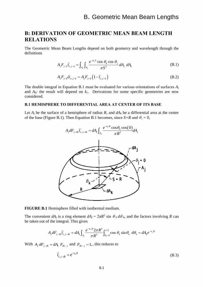
B.1 HEMISPHERE TO DIFFERENTIAL AREA AT CENTER OF ITS BASE
Let Aj be the surface of a hemisphere of radius R, and dAk be a differential area at the center
of the base (Figure B.1). Then Equation B.1 becomes, since S=R and i = 0,
( ), 2
cos cos 0
j
R
k
j j dk j dk k jA
eA dF t dA dA
R
−
− − =
FIGURE B.1 Hemisphere filled with isothermal medium.
The convenient dAj is a ring element dAj = 2πR2 sin k d k, and the factors involving R can
be taken out of the integral. This gives
22
, 2 0
2cos sin
j k
RR
j j dk j dk k k k k kA
e RA dF t dA d dA e
R
−−
− −=
= =
With j j dk k dk jA dF dA F− −= and 1,dk jF − = , this reduces to
,
R
j dkt e
−
− = (B.3)

B. Geometric Mean Beam Lengths
B.2
This especially simple relation is used later in the concept of mean beam length where
radiation from an actual volume of a medium is replaced by that from an equivalent
hemisphere.
B.2 TOP OF RIGHT CIRCULAR CYLINDER TO CENTER OF ITS
BASE
This geometry is in Figure B.2. Since θj = θk = θ, the integral in Equation B.1 becomes, for
the top of the cylinder Aj radiating to the element dAk at the center of its base,
2
, 2
cos
j
S
j j dk j dk k jA
eA dF t dA dA
S
−
− − = (B.4)
Since 2 2 2, 2 2 .jS h dA d S dS = − = = Then, using cos θ = h/S,
2 2
2
, 32
SR h
j j dk j dk kh
eA dF t dA h dS
S
−+
− − = (B.5)
FIGURE B.2 Geometry for exchange from top of gas-filled cylinder to center of its base.
Now let λS = λ to obtain
2 2
2 2
, 32
R h
j j dk j dk kh
eA dF t dA h d
−+
− −=
= (B.6)
This integral can be expressed in terms of the exponential integral function defined in
Appendix D of the text, by writing
2 2 2 2
3 3 3
R h R h a h
h
e e ed d d
− − −+ +
= = == − (B.7)
B. Geometric Mean Beam Lengths
B.3
Letting ( )2 2R h = + and h , respectively, in the two integrals gives
( ) ( )
2 21 1
2 20 02 2
1 1R h he d e d
hR h
− + −− +
+
The integral in Equation B.6 is then written in terms of the exponential integral function as
( )( )
2 22
3 32 232
1 11
( / ) 1
R h
h
e Rd E h E h
hh h R h
−+
=
= − + +
(B.8)
so, it can be readily evaluated for various values of the parameters R/h and λh.
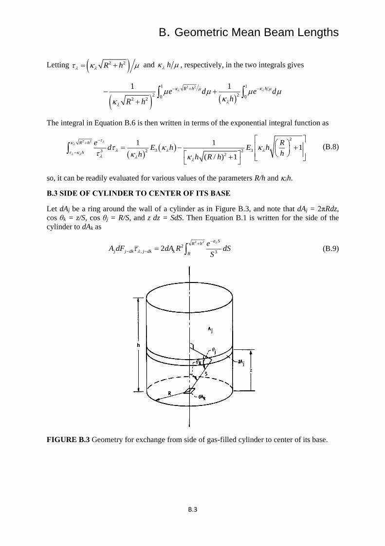
B.3 SIDE OF CYLINDER TO CENTER OF ITS BASE
Let dAj be a ring around the wall of a cylinder as in Figure B.3, and note that dAj = 2πRdz,
cos θk = z/S, cos θj = R/S, and z dz = SdS. Then Equation B.1 is written for the side of the
cylinder to dAk as
2 2
2
, 32
a SR h
j j dk j dk kR
eA dF dA R dS
S
−
+
− − = (B.9)
FIGURE B.3 Geometry for exchange from side of gas-filled cylinder to center of its base.

B. Geometric Mean Beam Lengths
B.4
This is of the same form as Equation B.5, and gives the result
( )
,
2 2
2
3 3222
1 12 ( ) 1
/ ( / ) 1
j j dk j dk
k
A dF t
R R RdA h E h E h
h h hh R h h R h
− −
= − +
+
(B.10)
As for Equation B.8, this is readily evaluated for various values of R/h and λh.
B.4 ENTIRE SPHERE TO ANY AREA ON ITS SURFACE OR TO ITS ENTIRE
SURFACE
From Figure B.4, since θk = θj let them be simply θ; then S = 2R cos θ. Starting with Equation
B.4, dAj cos θ/S2 is the solid angle by which dAj is viewed from dAk. The intersection of the
solid angle with a unit hemisphere shows that this equals 2π sin θ dθ. Then
/2 2
, 20 0
22cos sin
4
RS Sk
j j dk j dk kS
dAA dF t dA e d e SdS
R
− −
− −= =
= =
FIGURE B.4 Geometry for exchange from surface of gas-filled sphere to itself.
Integrating gives
( ) 2
, 2
21 2 1
(2 )
Rkj j dk j dk
dAA dF t R e
a R
−
− − = − + (B.11)
which has a single parameter 2λR, the sphere optical diameter.
Equation B.11 is integrated over any finite area Ak to give t from the entire sphere to
Ak as ( ) ( )2 2
, 2 / 2 1 2 1R
j j k j k kA F t A R R e
−
− − = − +
. Since Fj–k = Ak/Aj, from Equation
4.17,
( ) 2
, 2
21 2 1
(2 )
R
j kt R eR
−
− = − + (B.12)
which also applies for the entire sphere to its entire surface.
B. Geometric Mean Beam Lengths
B.5
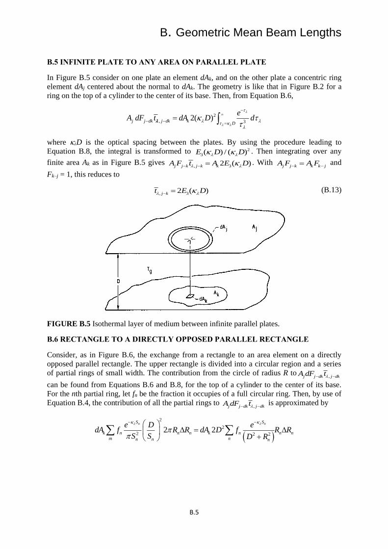
B.5 INFINITE PLATE TO ANY AREA ON PARALLEL PLATE
In Figure B.5 consider on one plate an element dAk, and on the other plate a concentric ring
element dAj centered about the normal to dAk. The geometry is like that in Figure B.2 for a
ring on the top of a cylinder to the center of its base. Then, from Equation B.6,
2
, 32( )j j dk j dk k
D
eA dF t dA D d
−
− −=
=
where λD is the optical spacing between the plates. By using the procedure leading to
Equation B.8, the integral is transformed to 2
3( ) / ( )E D D . Then integrating over any
finite area Ak as in Figure B.5 gives , 32 ( )j j k j k kA F t A E D − − = . With
j j k k k jA F A F− −= and
Fk–j = 1, this reduces to
, 32 ( )j kt E D − = (B.13)
FIGURE B.5 Isothermal layer of medium between infinite parallel plates.
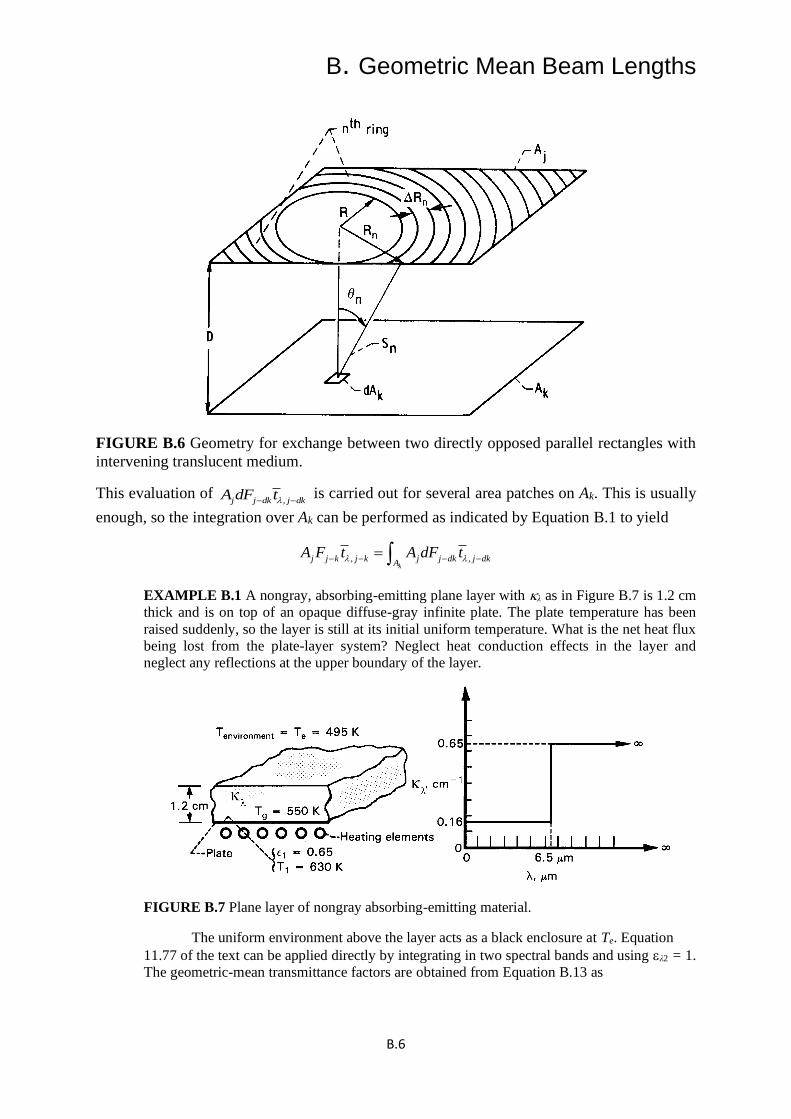
B.6 RECTANGLE TO A DIRECTLY OPPOSED PARALLEL RECTANGLE
Consider, as in Figure B.6, the exchange from a rectangle to an area element on a directly
opposed parallel rectangle. The upper rectangle is divided into a circular region and a series
of partial rings of small width. The contribution from the circle of radius R to,j j dk j dkA dF t− −
can be found from Equations B.6 and B.8, for the top of a cylinder to the center of its base.
For the nth partial ring, let fn be the fraction it occupies of a full circular ring. Then, by use of
Equation B.4, the contribution of all the partial rings to ,j j dk j dkA dF t− −
is approximated by
( )
2
2
2 2 22 2
n nS S
k n n n k n n n
m nn n n
e D edA f R R dA D f R R
S S D R
− − =
+
B. Geometric Mean Beam Lengths
B.6
FIGURE B.6 Geometry for exchange between two directly opposed parallel rectangles with
intervening translucent medium.
This evaluation of ,j j dk j dkA dF t− −
is carried out for several area patches on Ak. This is usually
enough, so the integration over Ak can be performed as indicated by Equation B.1 to yield
, ,k
j j k j k j j dk j dkA
A F t A dF t − − − −=
EXAMPLE B.1 A nongray, absorbing-emitting plane layer with λ as in Figure B.7 is 1.2 cm
thick and is on top of an opaque diffuse-gray infinite plate. The plate temperature has been
raised suddenly, so the layer is still at its initial uniform temperature. What is the net heat flux
being lost from the plate-layer system? Neglect heat conduction effects in the layer and
neglect any reflections at the upper boundary of the layer.
FIGURE B.7 Plane layer of nongray absorbing-emitting material.
The uniform environment above the layer acts as a black enclosure at Te. Equation
11.77 of the text can be applied directly by integrating in two spectral bands and using λ2 = 1.
The geometric-mean transmittance factors are obtained from Equation B.13 as

B. Geometric Mean Beam Lengths
B.7
,1 3 ,2 32 (0.16 1.2) 0.7142, 0 6.5 m; 2 (0.65 1.2)t E t E = = =
0.2974, 6.5 m = . This yields
1
1
4 42 1 ,1 1 0 6.5 0 6.5
4 4,1 1 ,1 0 6.5 0 6.5
4 41 ,2 1 0 6.5 0 6.5
4 4,2 1 ,2 0 6.5 0 6.5
( )
(1 )[1 (1 ) ]( )
[ (1 ) (1 )
(1 )[1 (1 ) ][ (1 ) (1 )]
e
g e
e
g e
T e T
g T e T
T e T
g T e T
q q t T F T F
t t T F T F
t T F T F
t t T F T F
→ →
→ →
→ →
→ →
= − = −
+ − + − −
+ − − −
+ − + − − − −ε
Inserting the values F0→6.5×630 = 0.4978, F0→6.5×550 = 0.3985 and F0→6.5×495 = 0.3220 yields q =
2954 W/m2.
B.7 GEOMETRIC-MEAN BEAM LENGTH FOR SPECTRAL BAND ENCLOSURE
EQUATIONS
For use in the spectral band enclosure Equation 11.77 in the text, the absorption integral in
Equation 11.82 must be evaluated between pairs of enclosure surfaces for the wavelength
bands involved. When more than a few bands absorb appreciably, the enclosure solution
requires considerable computational effort. A simplification was developed by Dunkle (1964)
by assuming that the integrated band absorption l(S) is a linear function of path length.
This has some physical basis, as it holds exactly for a band of weak nonoverlapping lines
(Equation 9.19 in the text). Also, it is the form of some of the effective bandwidths in the
exponential wide band correlations of on-line Appendix A (Equation A.1). As shown in
Dunkle by means of a few examples, reasonable values for the energy exchange are obtained
using this approximation. Hence, let lA in Equation 11.83 have the linear form from Equation
9.30 (note that the bandwidth Δλl = ω in Equation 9.30)
( ) ( ) ( )( ) l l l c
l
l
A S A S A S SS S
m = = = =
(B.14)
where Sc and δ are the line intensity and the spacing of the individual weak spectral lines, as
in Chapter 9 of the text.
Now define a mean path length k jS − called the geometric-mean beam length, such
that αl evaluated from Equation B.14 by using k jS S −= will equal ,l k j− from the integral in
Equation 11.81 of the text. After substituting ( ), /l k j c k jS S− − = and ( )/l cS S = into
Equation 11.81, the relation for k jS − is
cos cos1
j k
j kk j j k k j
A Ak k j
S S dA dAA F S
− −
−
= =
(B.15)
which depends only on geometry. This integral is also obtained in Equation B.1 when λS is
small (optically thin limit). In Dunkle, Sk–j values are tabulated for parallel equal rectangles,
for rectangles at right angles, and for a differential sphere and a rectangle. Analytical
relations for rectangles are in Equations B.16a,b. For directly opposed parallel equal
rectangles with sides of length a and b and spaced a distance c apart,
B. Geometric Mean Beam Lengths
B.8
1
2 2 2 2
2 2
4 1 1tan ln ln
1 ( 1 1 ( 1 )
11 1 1
k j k k jS A F
abc
− − − + +
= + + + + + + + +
+ + + + − −
(B.16a)
where η = a/c, β = b/c and 2 21 = + + . The Fk–j can be obtained from Factor 4 in
Appendix C of the text. For rectangles ab and bc at right angles with a common edge b,
2 2 2 2 2 2
2 2 2 2
2 3/2 2 3/2 2 2 3/2 2 2 3/2
2 2 2 2 2
2 22 2 2 2 2
(1 1 ) (1 1 )1ln ln
(1 1 (1 1 )
1[(1 ) (1 ) ( ) (1 ) ]
3
[ 1 1 ]
2 1[ 1 1 ]
3 2
k j k k jS A F
abc
− − + + + + + +
= + + + + + + +
+ + + + + + − + +
+ + + − + − +
+ + + − + − + + + −
(B.16b)
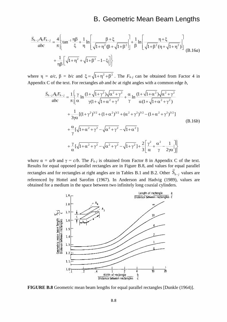
where α = a/b and γ = c/b. The Fk–j is obtained from Factor 8 in Appendix C of the text.
Results for equal opposed parallel rectangles are in Figure B.8, and values for equal parallel
rectangles and for rectangles at right angles are in Tables B.1 and B.2. Other k jS − values are
referenced by Hottel and Sarofim (1967). In Anderson and Hadvig (1989), values are
obtained for a medium in the space between two infinitely long coaxial cylinders.
FIGURE B.8 Geometric mean beam lengths for equal parallel rectangles [Dunkle (1964)].
B. Geometric Mean Beam Lengths
B.9
For a medium at uniform conditions, the geometric-mean beam length can be used in the
effective-bandwidth correlations in on-line Appendix A to obtain ( )lA S . Using Δλl obtained
in the next paragraph yields ( ) ( ) /l l lS A S = from Equation 11.83 of the text and lt from
1 l− . Then Equations 11.78 and 11.79 of the text can be solved for ql,k for each wavelength
band l. The total energies at each surface k are found from a summation over all bands
, ,k l k l l k l
absorbing nonabsorbingbands bands
q q q= + (B.17)
The wavelength span Δλl of each band is needed to carry out the solution. This span
can increase with path length. Edwards and coworkers [Edwards and Nelson (1962), Edwards
(1962), Edwards et al. (1967)] give recommended spans for CO2 and H2O vapor; these
values, in wave number units, are in Table A.3 for the parallel-plate geometry. For other
geometries, Edwards and Nelson give methods for choosing approximate spans for CO2 and
H2O bands. Briefly, the method is to use approximate band spans based on the longest
important mass path length in the geometry being studied. The limits of Table B.3 are
probably adequate for problems involving CO2 and H2O vapor.
If all surface temperatures are specified in a problem, the results from Equation B.17
complete the solution. If qk is specified for n surfaces and Tk for the remaining N–n surfaces,
then the n unknown surface temperatures are guessed, the equations are solved for all q, and
then the calculated qk are compared to the specified values. If they do not agree, new values
of Tk for the n surfaces are assumed and the calculation is repeated until the given and
calculated qk agree for all Ak with specified qk. Equation 11.76, expressed as a sum over the
wavelength bands, gives the required energy input to the medium for the specified Tg.
B. Geometric Mean Beam Lengths
B.10
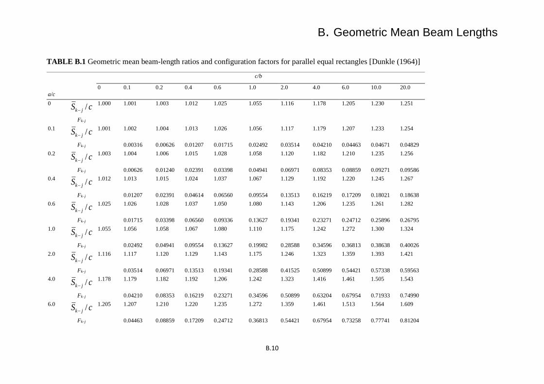
TABLE B.1 Geometric mean beam-length ratios and configuration factors for parallel equal rectangles [Dunkle (1964)]
a/c
c/b
0 0.1 0.2 0.4 0.6 1.0 2.0 4.0 6.0 10.0 20.0
0 /k jS c−
1.000 1.001 1.003 1.012 1.025 1.055 1.116 1.178 1.205 1.230 1.251
Fk–j
0.1 /k jS c−
1.001 1.002 1.004 1.013 1.026 1.056 1.117 1.179 1.207 1.233 1.254
Fk–j 0.00316 0.00626 0.01207 0.01715 0.02492 0.03514 0.04210 0.04463 0.04671 0.04829
0.2 /k jS c−
1.003 1.004 1.006 1.015 1.028 1.058 1.120 1.182 1.210 1.235 1.256
Fk–j 0.00626 0.01240 0.02391 0.03398 0.04941 0.06971 0.08353 0.08859 0.09271 0.09586
0.4 /k jS c−
1.012 1.013 1.015 1.024 1.037 1.067 1.129 1.192 1.220 1.245 1.267
Fk–j 0.01207 0.02391 0.04614 0.06560 0.09554 0.13513 0.16219 0.17209 0.18021 0.18638
0.6 /k jS c−
1.025 1.026 1.028 1.037 1.050 1.080 1.143 1.206 1.235 1.261 1.282
Fk–j 0.01715 0.03398 0.06560 0.09336 0.13627 0.19341 0.23271 0.24712 0.25896 0.26795
1.0 /k jS c−
1.055 1.056 1.058 1.067 1.080 1.110 1.175 1.242 1.272 1.300 1.324
Fk–j 0.02492 0.04941 0.09554 0.13627 0.19982 0.28588 0.34596 0.36813 0.38638 0.40026
2.0 /k jS c−
1.116 1.117 1.120 1.129 1.143 1.175 1.246 1.323 1.359 1.393 1.421
Fk–j 0.03514 0.06971 0.13513 0.19341 0.28588 0.41525 0.50899 0.54421 0.57338 0.59563
4.0 /k jS c−
1.178 1.179 1.182 1.192 1.206 1.242 1.323 1.416 1.461 1.505 1.543
Fk–j 0.04210 0.08353 0.16219 0.23271 0.34596 0.50899 0.63204 0.67954 0.71933 0.74990
6.0 /k jS c−
1.205 1.207 1.210 1.220 1.235 1.272 1.359 1.461 1.513 1.564 1.609
Fk–j 0.04463 0.08859 0.17209 0.24712 0.36813 0.54421 0.67954 0.73258 0.77741 0.81204

B. Geometric Mean Beam Lengths
B.11
10.0 /k jS c−
1.230 1.233 1.235 1.245 1.261 1.300 1.393 1.505 1.564 1.624 1.680
Fk–j 0.04671 0.09271 0.18021 0.25896 0.38638 0.57338 0.71933 0.77741 0.82699 0.86563
20.0 /k jS c−
1.251 1.254 1.256 1.267 1.282 1.324 1.421 1.543 1.609 1.680 1.748
Fk–j 0.04829 0.09586 0.18638 0.26795 0.40026 0.59563 0.74990 0.81204 0.86563 0.90785
/k jS c−
1.272 1.274 1.277 1.289 1.306 1.349 1.452 1.584 1.660 1.745 1.832
Fk–j 0.04988 0.09902 0.19258 0.27698 0.41421 0.61803 0.78078 0.84713 0.90499 0.95125
TABLE B.2 Configuration factors and mean beam-length functions for rectangles at right angles [Dunkle (1964)]
a/b
c/b
0.05 0.10 0.20 0.4 0.6 1.0 2.0 4.0 6.0 10.0 20.0 ∞
0.02 AkFk–j/b2 0.007982 0.008875 0.009323 0.009545 0.009589 0.009628 0.009648 0.009653 0.009655 0.009655 0.009655 0.009655
/k k j k jA F S abc− −
0.17840 0.12903 0.08298 0.04995 0.03587 0.02291 0.01263 0.006364 0.004288 0.002594 0.001305
0.05 AkFk–j/b2 0.014269 0.018601 0.02117 0.02243 0.02279 0.02304 0.02316 0.02320 0.02321 0.02321 0.02321 0.02321
/k k j k jA F S abc− −
0.21146 0.18756 0.13834 0.08953 0.06627 0.04372 0.02364 0.01234 0.008342 0.005059 0.002549
0.10 AkFk–j/b2 0.02819 0.03622 0.04086 0.04229 0.04325 0.04376 0.04390 0.04393 0.04394 0.04394 0.04395
/k k j k jA F S abc− −
0.20379 0.17742 0.12737 0.09795 0.06659 0.03676 0.01944 0.013184 0.008018 0.004049
0.20 AkFk–j/b2 0.05421 0.06859 0.07377 0.07744 0.07942 0.07999 0.08010 0.08015 0.08018 0.08018
/k k j k jA F S abc− −
0.18854 0.15900 0.13028 0.09337 0.05356 0.02890 0.01972 0.012047 0.006103
0.40 AkFk–j/b2 0.10013 0.11524 0.12770 0.13514 0.13736 0.13779 0.13801 0.13811 0.13814
/k k j k jA F S abc− −
0.16255 0.14686 0.11517 0.07088 0.03903 0.02666 0.01697 0.008642
0.60 AkFk–j/b2 0.13888 0.16138 0.17657 0.18143 0.18239 0.18289 0.18311 0.18318
/k k j k jA F S abc− −
0.14164 0.11940 0.07830 0.04467 0.03109 0.02025 0.010366
B. Geometric Mean Beam Lengths
B.12
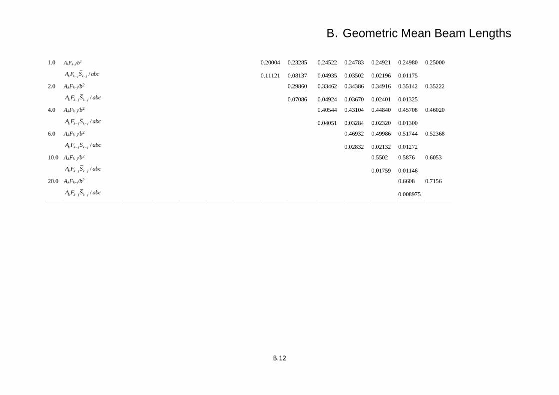
1.0 AkFk–j/b2 0.20004 0.23285 0.24522 0.24783 0.24921 0.24980 0.25000
/k k j k jA F S abc− −
0.11121 0.08137 0.04935 0.03502 0.02196 0.01175
2.0 AkFk–j/b2 0.29860 0.33462 0.34386 0.34916 0.35142 0.35222
/k k j k jA F S abc− −
0.07086 0.04924 0.03670 0.02401 0.01325
4.0 AkFk–j/b2 0.40544 0.43104 0.44840 0.45708 0.46020
/k k j k jA F S abc− −
0.04051 0.03284 0.02320 0.01300
6.0 AkFk–j/b2 0.46932 0.49986 0.51744 0.52368
/k k j k jA F S abc− −
0.02832 0.02132 0.01272
10.0 AkFk–j/b2 0.5502 0.5876 0.6053
/k k j k jA F S abc− −
0.01759 0.01146
20.0 AkFk–j/b2 0.6608 0.7156
/k k j k jA F S abc− −
0.008975

B. Geometric Mean Beam Lengths
B.13
TABLE B.3 Approximate band limits for parallel-plate geometry [Edwards and Nelson (1962), Edwards (1962), Edwards et al. (1967)]
Gas
Band center
, m Band center η,
cm−1
Band limits η, cm−1a
Lower Upper
CO2 15 667 667 – 15( /1.78)A 667 +
15( /1.78)A
10.4 960 849 1013
9.4 1060 1013 1141
4.3 2350 2350 – 4.3( /1.78)A 2430
2.7 3715 3715 – 2.7( /1.76)A 3750
H2O 6.3 1600 1600 – 6.3( /1.6)A 1600 +
6.3( /1.6)A
2.7 3750 3750 – 2.7( /1.4)A 3750 +
2.7( /1.4)A
1.87 5350 4620 6200
1.38 7250 6200 8100
a A is found for various bands as in Example A.1. Terms such as 15 /1.78A are ( )/ 2 1 gA − from
Equation 17 and Tables 1 and 2 of Edwards and Nelson (1962).
EXAMPLE B.2 Two black parallel plates are D = 1 m apart. The plates are of width W = 1 m
and have infinite length normal to the cross section shown. Between the plates is carbon dioxide
gas at 2CO 1p = atm and Tg = 1000 K. If plate 1 is at 2000 K and plate 2 is at 500 K, find the
energy flux that must be supplied to plate 2 to maintain its temperature. The surroundings are at
Te << 500 K.
The geometry is a four-boundary enclosure formed by two plates and two open
planes. The open areas are perfectly absorbing (nonreflecting) and radiate no significant energy as
the surrounding temperature is low. The energy flux added to surface 2 is found by using the
enclosure Equation 11.78 of the text where k = 2 and N = 4. All surfaces are black, λ,j = 1, so
Equation 11.78 reduces to

B. Geometric Mean Beam Lengths
B.14
4 4
2 , 2 2 ,2 , 2 ,2 ,
1 1
[( ) ] − − − −
= =
= − − j j j j j b j j j b g
j j
q F E F E (B.18)
The self-view factor F2–2 = 0 and Eλb,3 = Eλb,4 ≈ 0, so this becomes
,2 2 1 ,2 1 ,1 ,2 2 1 ,2 1 2 3 ,2 3 2 4 ,2 4 ,( )b b b gq F t E E F F F E − − − − − − − − = − + − + + (B.19)
To simplify the example, it is carried out by considering the entire wavelength region as a single
spectral band. To obtain the total energy supplied to plate 2, integrate over all wavelengths to
obtain
42 2 1 ,2 1 ,1 2
0
2 1 ,2 1 2 3 ,2 3 2 4 ,2 4 ,0
( )
b
b g
q F t E d T
F F F E d
− −
− − − − − −
= − +
− + +
By use of the definitions of total transmission and absorption factors,
4 42 1 1 ,2 1 ,1 2 1 ,2 1 ,
0 0b g b gt T t E d T E d
− − − − = =
and so forth, q2 becomes
4 4 42 2 2 1 2 1 1 2 1 2 1 2 3 2 3 2 4 2 4( ) gq T F t T F F F T− − − − − − − −= − − + + (B.20)
To determine t and , the geometric-mean beam length is used. For opposing rectangles
(Figure B.8 of this Appendix) at an abscissa of 1.0 and on the curve for a length-to-spacing ratio
of ∞, the 2 1 / 1.34S D− = , so 2 1 1.34 mS − = . To determine 2 1− , which determines the emission
of the gas, use the emittance chart in Figure 9.18 or the Alberti et al. (2018) at EXCEL spreadsheet at https://doi.org/10.1016/j.jqsrt.2018.08.008 at a pressure of 1 atm, Le = 1.34
m and Tg = 1000 K. This gives 2 1 0.22− = . When obtaining 2 1− , note from Equation B.20 that
the radiation in the 2 1− term is Eλb,1 and is coming from wall 1. Therefore, it has a spectral
distribution different from that of the gas radiation. To account for this nongray effect, Equation
10.121 is used with + evaluated at 2 2 1 1( / ) 1.34(2000/1000) 2.68CO gp S T T atm m− = = and T1
= 2000 K. Then, using Figure 9.18 (extrapolated) or the spread sheet results in 0.51
2 1 21 0.2( ) 0.86− − = .
From Factor 3 in Appendix C of the text, the F2–1 is given by 2 2 1/2
2 1 [( ) ]/ 2 1 0.414F D W D W− = + − = − = . Then 12 3 2 4 2
(1 0.414) 0.293F F− −= = − = .
The 2 3 2 4− − = , and they remain to be found. For adjoint planes, as in the geometry for Table
B.2, the following expression from Equation 12 of Dunkle (1964) can be used, obtained for the
present case where b →∞, a = 1, and c = 1:

B. Geometric Mean Beam Lengths
B.15
2 3 2 32ln 2 / ( ) 2 0.347 / ( 0.293) 0.753S F m.− −= = = Using Figure 9.18
0.753atm mpS = and Tg= 1000 K gives 2 3 2 4 0.19 − −= = . Then the desired result is
4 4 42 2 1
12 4 4 4
0.414(0.86) (0.414 0.22 2 0.293 0.19)
5.6704 10 (500 0.36 2000 0.20 1000 )
33.4
g
2
q T T T
W/cm
−
= − − +
= − −
= −
Note that the largest contribution to q2 is by energy leaving surface 1 that reaches and is absorbed
by surface 2. Emission from the gas to surface 2, and emission from surface 2, are small.
An alternative approach for this example is to note that the term involving Tg in Equation B.20 is
the flux received by surface 2 as a result of emission by the entire gas. This can be calculated from
Equation 11.115 using the mean beam length. Then 4 4 4
2 2 2 1 2 1 1− −= − − g gq T F T T . For this
symmetric geometry the average flux from the gas to one side of the enclosure is the same as that to the
entire enclosure boundary. Consequently, the mean beam length can be obtained from Equation 11.111 as 2
e 0.9(4) / 0.9(4)(1 m) / 4 m 0.9 m.L V A= = = Then, from Figure 9.18 at Tg = 1000 K and
2CO e 0.9 atm mp L = , the g = 0.20. This gives the same q2 as previously calculated.
HOMEWORK (Solutions are included in the Solution Manual under Chapter 11)
B.1 Two opposed parallel rectangles are separated by 0.5 m. The rectangles are of size 1.2 x 1.8 m. The
space between the rectangles is filled with H2O vapor at P = 1 atm and T = 1200 K. Assume for this
calculation that only the 2.7-m spectral band of H2O participates in radiative absorption and emission by
the gas and use the data of Table A.2 of on-line Appendix A to compute g. Rectangle 1 has T1 = 1460 K,
1 = 1.0. Rectangle 2 has T2 = 515 K, 2 = 0.6. Assume that the surroundings are at low temperature.
Compute the total energy being added to each plate, using the method of Section 10.6.4 of the text.
B.2 A rectangular enclosure that is very long normal to the cross section shown has diffuse-gray walls
at conditions shown below and encloses a uniform gray gas at Tg = 1500 K. The gas has an absorption
coefficient of 0.25 m−1. Find the average net radiative flux at each surface, and the energy necessary to
maintain the gas at 1500 K.
Surface Tw(K)
1 1.0 2000
2 0.5 1500
3 0.1 1000
4 0 500

B. Geometric Mean Beam Lengths
B.16
Answer: q1 = 607 kW/m2; q2 = − 75.1 kW/m2; q3 = − 39.3 kW/m2;
energy added = 2,121 kW/m.
REFERENCES
Anderson, K. M., and Hadvig, S.: Geometric Mean Beam Lengths for a Space between Two Coaxial
Cylinders, JHT, vol. 111, no. 3, pp. 811–813, 1989.
Dunkle, R. V.: Geometric Mean Beam Lengths for Radiant Heat-Transfer Calculations, JHT, vol. 86, no.
1, pp. 75–80, 1964.
Edwards, D. K.: Radiant Interchange in a Nongray Enclosure Containing an Isothermal Carbon Dioxide–
Nitrogen Gas Mixture, JHT, vol. 84, no. 1, pp. 1–11, 1962.
Edwards, D. K., and Nelson, K. E.: Rapid Calculation of Radiant Energy Transfer between Nongray
Walls and Isothermal H2O or CO2 Gas, JHT, vol. 84, no. 4, pp. 273–278, 1962.
Edwards, D. K., Glassen, L. K., Hauser, W. C., and Tuchscher, J. S.: Radiation Heat Transfer in
Nonisothermal Nongray Gases, JHT, vol. 89, no. 3, pp. 219–229, 1967.
Hottel, H. C, and Sarofim, A. F.: Radiative Transfer, McGraw–Hill, New York, 1967.
C. Exponential Kernel Approximation
Appendix C.1
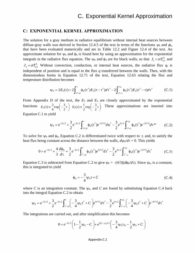
C: EXPONENTIAL KERNEL APPROXIMATION
The solution for a gray medium in radiative equilibrium without internal heat sources between
diffuse-gray walls was derived in Section 12.4.5 of the text in terms of the functions b and b,
that have been evaluated numerically and are in Table 12.2 and Figure 12.4 of the text. An
approximate solution for b and b is found here by using an approximation for the exponential
integrals in the radiative flux equation. The b and b are for black walls, so that 4
1 1wJ T= and
4
2 2wJ T= Without convection, conduction, or internal heat sources, the radiative flux qr is
independent of position and is equal to the flux q transferred between the walls. Then, with the
dimensionless forms in Equation 12.71 of the text, Equation 12.63 relating the flux and
temperature distribution becomes
* * * * * *b 3 b 2 b 2
* 0 *
2 ( ) 2 ( ) ( ) 2 ( ) ( )D
E E d E d
= =
= + − − − (C.1)
From Appendix D of the text, the E2 and E3 are closely approximated by the exponential
functions 2 3
3 3 1 3( ) exp ( ) exp
4 2 2 2E E
− −
. These approximations are inserted into
Equation C.1 to yield
3 /2 3 /2 * 3 */2 * 3 /2 * 3 */2b b b
* 0 *
3 3( ) ( ) *
2 2
D
e e e d e e d
− − − −
= =
= + − (C.2)
To solve for b and b, Equation C.2 is differentiated twice with respect to and, to satisfy the
heat flux being constant across the distance between the walls, db/d = 0. This yields
* *
b3 /2 3 /2 * 3 */2 * 3 /2 * 3 */2 *b b
0
4 3 30 ( ) ( )
3 2 2
Dde e e d e e d
d
− − −
= =
= + + −
(C)
Equation C.3 is subtracted from Equation C.2 to give ψb = –(4/3)(db/d). Since ψb, is a constant,
this is integrated to yield
b b
3
4C = − + (C.4)
where C is an integration constant. The ψb, and C are found by substituting Equation C.4 back
into the integral Equation C.2 to obtain
* *
3 /2 3 /2 * 3 */2 * 3 /2 * 3 */2 *b b b
0
3 3 3 3
2 4 2 4
D
e e C e d e C e d
− − −
= =
= + − + − − +
The integrations are carried out, and after simplification this becomes
D3 /2 3( )/2b b D b
1 3 10 1
2 4 2e C e C− −
= − − + − − +
C. Exponential Kernel Approximation
Appendix C.2
Thus, there are two simultaneous equations for b and C:
b b D b
1 3 11 0 and 0
2 4 2C C− − = − − + =
The solution yields
b
D
1
31
4
=
+
(C.5a)
and C = 1 – b/2. These are substituted into Equation C.4 to give
1 3 1( ) ( )
3 4 21
4
b D
D
= − +
+
(C.5b)
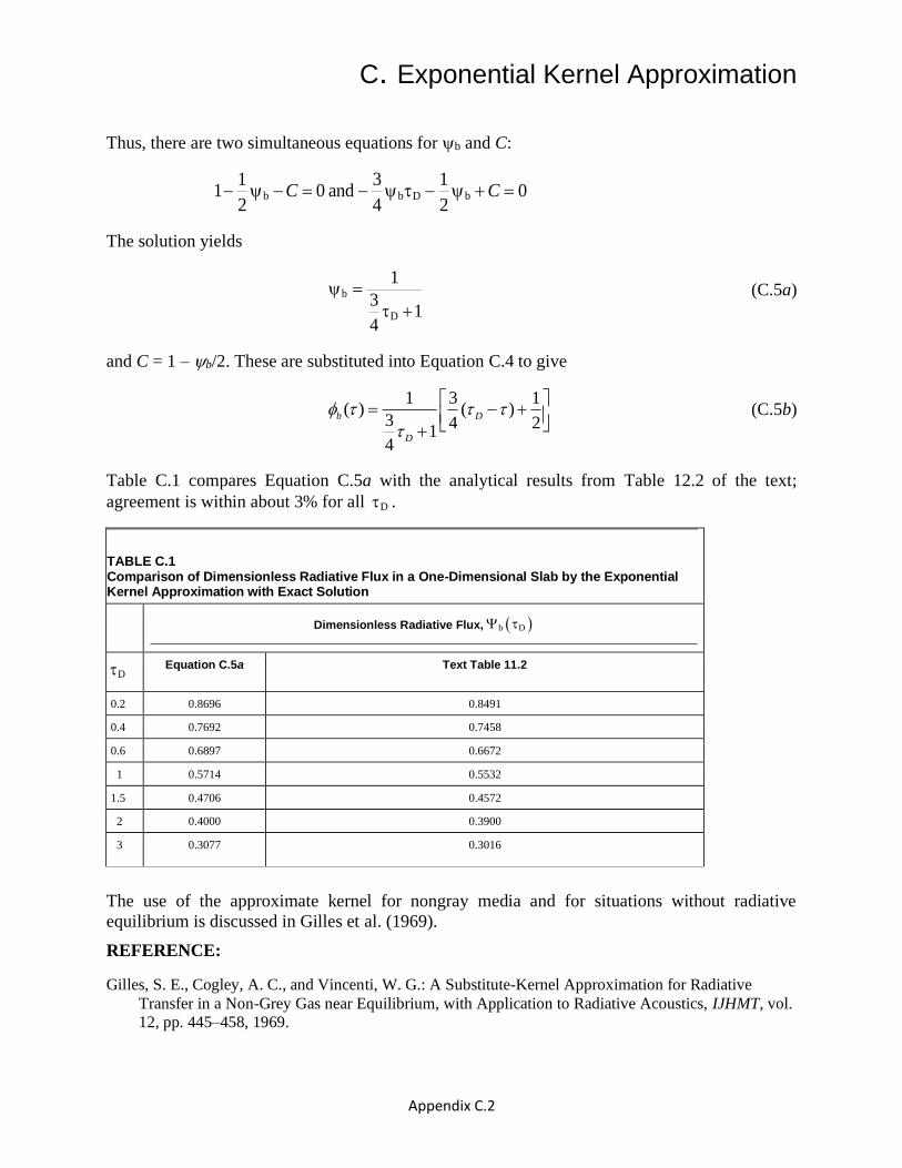
Table C.1 compares Equation C.5a with the analytical results from Table 12.2 of the text;
agreement is within about 3% for all D .
TABLE C.1 Comparison of Dimensionless Radiative Flux in a One-Dimensional Slab by the Exponential Kernel Approximation with Exact Solution
Dimensionless Radiative Flux, ( )b D
D Equation C.5a Text Table 11.2
0.2 0.8696 0.8491
0.4 0.7692 0.7458
0.6 0.6897 0.6672
1 0.5714 0.5532
1.5 0.4706 0.4572
2 0.4000 0.3900
3 0.3077 0.3016
The use of the approximate kernel for nongray media and for situations without radiative
equilibrium is discussed in Gilles et al. (1969).
REFERENCE:
Gilles, S. E., Cogley, A. C., and Vincenti, W. G.: A Substitute-Kernel Approximation for Radiative
Transfer in a Non-Grey Gas near Equilibrium, with Application to Radiative Acoustics, IJHMT, vol.
12, pp. 445–458, 1969.
C. Exponential Kernel Approximation
Appendix C.3
HOMEWORK
C.1 Consider a gray absorbing medium with isotropic scattering between parallel diffuse gray plates at
temperatures T1 and T2, and spaced D apart. Heat conduction is negligible. Show that the exponential
kernel approximation yields the same result for radiative heat transfer as obtained by the diffusion
solution with jump boundary conditions. The medium has extinction coefficient .
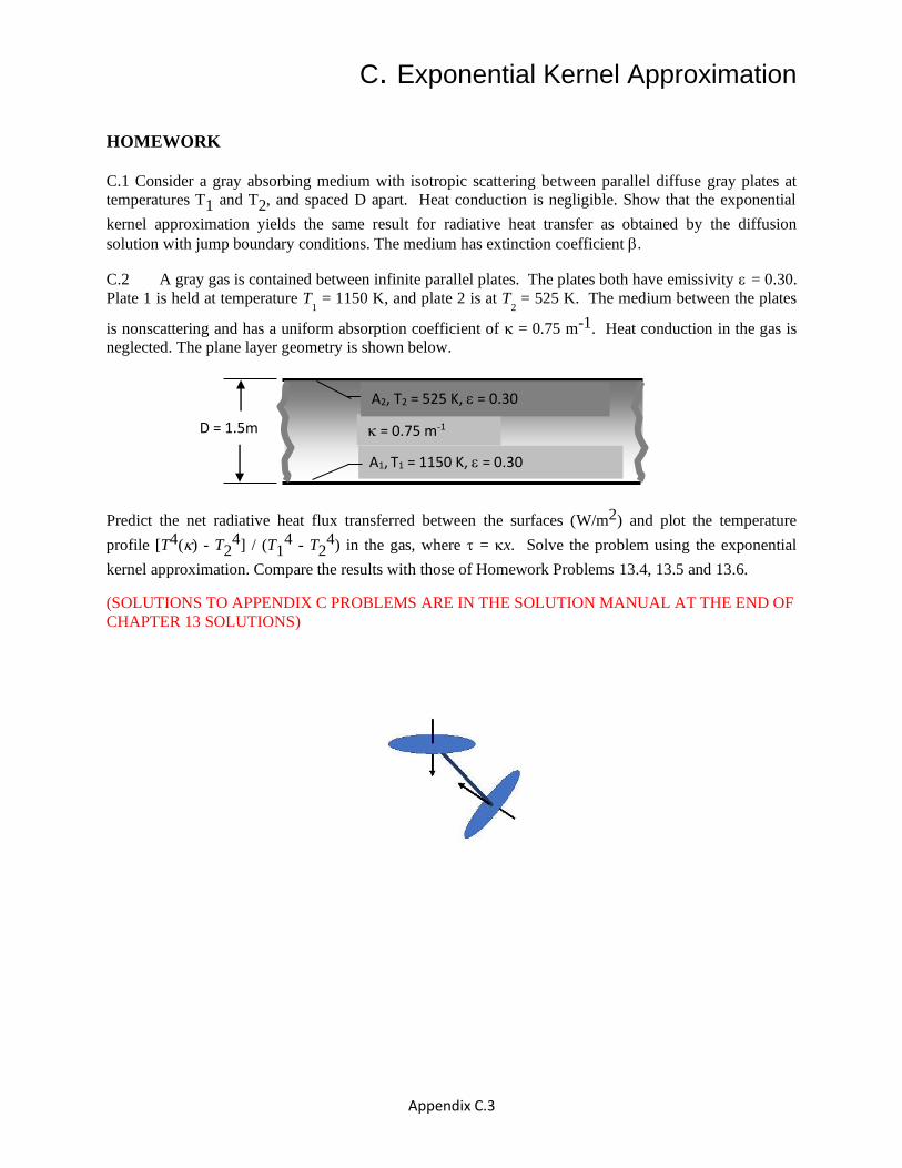
C.2 A gray gas is contained between infinite parallel plates. The plates both have emissivity = 0.30.
Plate 1 is held at temperature T1 = 1150 K, and plate 2 is at T
2 = 525 K. The medium between the plates
is nonscattering and has a uniform absorption coefficient of = 0.75 m-1. Heat conduction in the gas is
neglected. The plane layer geometry is shown below.
Predict the net radiative heat flux transferred between the surfaces (W/m2) and plot the temperature
profile [T4() - T24] / (T1
4 - T24) in the gas, where = x. Solve the problem using the exponential
kernel approximation. Compare the results with those of Homework Problems 13.4, 13.5 and 13.6.
(SOLUTIONS TO APPENDIX C PROBLEMS ARE IN THE SOLUTION MANUAL AT THE END OF
CHAPTER 13 SOLUTIONS)
= 0.75 m-1 D = 1.5m
A1, T1 = 1150 K, = 0.30
A2, T2 = 525 K, = 0.30
D: Curtis-Godson Approximation
Appendix D.1
D: CURTIS-GODSON APPROXIMATION
For nonuniform gases a useful method for some radiation analyses is the Curtis-Godson
approximation [Edwards and Weiner (1966), Krakow et al. (1966), Simmons (1966, 1968),
Goody and Yung (1989)]. The transmittance of a given path through a nonisothermal gas is
related to the transmittance through an equivalent isothermal gas. Then the solution is obtained
by using isothermal-gas methods. The relation between the nonisothermal and the isothermal gas
is found by assigning an equivalent amount of isothermal absorbing material to act in place of
the nonisothermal gas. The amount is based on a scaling temperature and a mean density or
pressure obtained in the analysis. These mean quantities are found by having the transmittance of
the uniform gas be equal to the transmittance of the nonuniform gas in the weak and strong
absorption limits.
Goody and Yung , Krakow et al., and Simmons discuss the Curtis-Godson method for
attenuation in a narrow vibration-rotation band. Comparisons with exact numerical results were
obtained. Weiner and Edwards (1968) applied the method for steep temperature gradients in
gases with overlapping band structures. Comparison of the analysis with experimental data was excellent. The Curtis-Godson technique is useful when the gas temperature distribution is
specified. If the gas temperature distribution is not known, an iterative procedure would be
needed; this is not very practical.
In this development, spectral variations are in terms of wave number, as is common for
band correlations. For a nonuniform gas the absorption coefficient η is variable along the path.
An effective bandwidth Āt(S) is defined, analogous to Equation 9.26 of the text but using an
integrated absorption coefficient:
S
absorption0
bandwidth
S
0
( ) 1 exp ( )
exp ( )
l
ll
A S S dS d
S dS d
= − −
= − −
(D.1)
Similarly, for a path length from S* to S, the effective bandwidth is
S
absorptionS**=S*
bandwidth
( ) 1 exp ( )lA S S S dS d
− = − −
(D.2)
The integrated equation of transfer for intensity at S by radiation (without scattering)
traveling from 0 to S is, from Equation 11.15 of the text,
S S S
bS*=0 S*=0 S**=S*
S S S
,bS*=0 S*=0 S**=S
( ) (0)exp ( ) ( ) ( )exp ( )
(0)exp ( ) ( ) 1 exp ( )
I S I S dS S I S S dS dS
I S dS I S S dS dSS
= − + −
= − − − −
(D.3)
D: Curtis-Godson Approximation
Appendix D.2
Equation D. 3 is integrated over the bandwidth Δηl, of the lth band, and the order of
integration is changed on the last term. The Iη(S), Iη(η,0), and Iηb(S) are approximated by average
values within the band to yield
( )
( ) ( )
* 0
,b* 0 ** *
( ) (0) exp * *
* 1 exp ** ** **
S
l l ll S
S S
lS l S S
I S I S dS d
I S S dS d dSS
=
= =
= −
= − − −
(D.4)
Equations D.1 and D.2 are substituted into Equation D.4 to obtain the radiative transfer equation
in terms of the Āl.
( ) ( ) ( ) ( )( )
,* 0
*0 * *
*
Sl
l l l l l l bS
A S SI S I A S I S dS
S=
− = − − (D.5)
An alternative form is found by integrating Equation D.5 by parts to obtain
( ) ( ) ( ) ( ) ( ) ( )( ),b
,b* 0
*0 0 * *
*
Sl
l l l l l l l lS
dI SI S I A S I A S A S S dS
dS=
= − + + − (D.6)
Equations D.5 and D.6 are nearly exact forms of the integrated RTE in terms of the band
properties. The only approximation is that the intensity in each term does not vary significantly
across the wave number span of the band. For a uniform gas, Equation D.6 gives (since dIl,b/dS =
0)
( ) ( ) ( ) ( ) ( ),u ,u ,b,u ,u0 0l l l l l l lI S I A S I A S = − + (D.7)
where the u subscript denotes a uniform gas.
To compute Il(S) or Il,u(S) from Equations D.5, D.6, or D.7, expressions are needed for
the effective bandwidth Āl for nonuniform and uniform gases. From Equations 9.16 and 9.20 of
the text, the limiting cases of Āl for bands of independent weak or Lorentz strong absorption lines
in a uniform gas have the forms
,u 1, u( )l lA S C S= (D.8a)
1/2
,u 2, u u( )l lA S C S= (D.8b)
where Cl,,1 and C2,l are coefficients of proportionality for the lth band, and Sc and γc for the lines
have been taken as proportional to gas density. For the nonuniform gas the effective bandwidth
depends on the variation of properties along the path. The effective bandwidths are obtained by
using Equations D.8a and D.8b locally along the path. This gives, for a band of weak lines,
1,* 0
( ) ( ) (weak)S
l lS
A S C S dS
=
= (D.9a)
D: Curtis-Godson Approximation
Appendix D.3
Similarly, for a band of strong lines, after first squaring Equation D.8b,
2 2 22,
* 0
( ) ( )S
l lS
A S C S dS
=
= , so that
1/2
22,
0
( ) ( ) (strong)S
l lA S C S dS =
(D.9b)
It is assumed that the C1,l and C2,l do not vary along the path.
In the Curtis-Godson method the nonuniform gas is replaced by an effective amount of
uniform gas such that the correct intensity is obtained at the weak and strong absorption limits.
To have the uniform intensity equal the nonuniform intensity, equate Equations D.7 and D.6 and
simplify to obtain
( ) ( ) ( ) ( ) ( ) ( ) ( )( ),b
,b,u u ,u ,b* 0
*0 0 0 * *
*
Sl
l l l l l l lS
dI SI T I A S I I A S A S S dS
dS=
− = − + −
(D.10)
To have Equation D.10 valid at the weak absorption limit, substitute Āl,u from Equation D.8a and
Āl from Equation D.9a to obtain the following after canceling the C1,l.
( ) ( )
( ) ( )( )
,b,u u u u
,b
,b* 0 * 0 ** *
0
* 0 0 ( *) * ( **) ** *
*
l l
S S Sl
l lS S S S
I T I S
dI SI I S dS S dS dS
dS= = =
−
= − +
(D.11a)
Similarly, at the strong absorption limit, insert Equations D.8b and D.9b into Equation D.10 to
obtain
( ) ( ) ( ) ( )
( )
1/2
1/2 2,b,u u u u ,b
* 0
1/2
,b2
* 0 ** *
0 0 0 ( *) *
* ( **) ** *
*
S
l l l lS
S Sl
S S S
I T I S I I S dS
dI SS dS dS
dS
=
= =
− = −
+
(D.11b)
For known temperature and density distributions in a nonuniform gas, Equations D.11a.
and D.11b are solved simultaneously for ρu and Su, which are the equivalent uniform gas density
and path length for that band. The Il,b,u(Tu) is not an additional unknown since the temperature Tu
corresponds to ρu through the ideal gas law. Then Equation D.7 can be used for any effective
bandwidth dependence on ρu and Su (that is, not only at the weak and strong limits) to solve for
Il,u(S). This exactly equals Il(S) in the nonuniform gas in the weak and strong limits and is usually
a good approximation for intermediate absorption values. Once the intensities are found, the
radiative transfer is obtained by using the relations for a uniform gas. Evaluating Equations
D.11a. and D.11b usually requires numerical integration. Because the Curtis-Godson method
requires evaluating at least two integrals for each band along each path, it may be equally
feasible to numerically evaluate the nearly exact forms Equation D.5 or D.6.
D: Curtis-Godson Approximation
Appendix D.4
As originally formulated [Goody and Yung (1989)], the Curtis-Godson method was
limited to a small wave number span in an absorption band. The limitation was because of line
overlapping and the change in the number of important lines with temperature. It has been shown
in Weiner and Edwards (1968) and Plass (1967) that the method gives good results even for
conditions with large temperature gradients with the use of wide wave number spans. These
references also account for overlapping absorption bands. A band absorption formulation
analogous to the Curtis-Godson approximation but involving three parameters was developed by
Cess and Wang (1970). The additional parameter enabled the equivalent isothermal gas to give
the correct behavior in the linear and square-root limits, and in the logarithmic limit for very
strong absorption. The method was used to examine the effects of CO2 and water vapor
concentration on the atmospheric temperature profile by Ferland and Howell (1972). The further
treatment of radiative transfer along strongly nonisothermal paths is in Vitkin et al. (2000). To
try to overcome spectral complexity, a Planck-Rosseland gray model has been developed; it is
applied to a hypersonic radiating flow in Sakai et al. (2001).
REFERENCES:
Cess, R. D., and Wang, L. S.: A Band Absorptance Formulation for Nonisothermal Gaseous Radiation,
IJHMT, vol. 13, no. 3, pp. 547–555, 1970.
Edwards, D. K., and Weiner, M. M.: Comment on Radiative Transfer in Nonisothermal Gases, Combust.
Flame, vol. 10, no. 2, pp. 202–203, 1966.
Ferland, R. E. and Howell, J. R.: Water Vapor, CO2 and Particulate Effects on the Atmospheric
Temperature Profile, Proc. 1972 Heat Transfer and Fluid Mechanics Institute, Stanford University
Press, 1972.
Goody, R. M., and Yung, Y. L.: Atmospheric Radiation, 2d ed., Oxford University Press, New York,
1989.
Krakow, B., Babrov, H. J., Maclay, G. J., and Shabott, A. L.: Use of the Curtis-Godson Approximation in
Calculations of Radiant Heating by Inhomogeneous Hot Gases, Appl. Opt., vol. 5, no. 11, pp. 1791–
1800, 1966.
Plass, G. N.: Radiation from Nonisothermal Gases, Appl. Opt., vol. 6, no. 11, pp. 1995–1999, 1967.
Sakai, T., Tsuru, T., and Sawada, K.: Computation of Hypersonic Radiating Flow-Field over a Blunt
Body, JTHT, vol. 15, no. 1, pp. 91–105, 2001.
Simmons, F. S.: Band Models for Non-isothermal Radiating Gases, Appl. Opt., vol. 5, no. 11, pp. 1801–
1811, 1966.
Simmons, F. S.: Application of Band Models to Inhomogeneous Gases, Molecular Radiation and Its
Application to Diagnostic Techniques (R. Goulard, ed.), NASA TM X-53711, pp. 113–133, 1968.
Vitkin, E. I., Shuralyov, S. L., and Tamanovich, V. V.: Engineering Procedure for Calculating the
Transfer of the Selective Radiation of Molecular Gases, IJHMT, vol. 43, no. 11, pp. 2029–2045,
2000.
Weiner, M. M., and Edwards, D. K.: Nonisothermal Gas Radiation in Superposed Vibration-Rotation
Bands, JQSRT, vol. 8, no. 5, pp. 1171–1183, 1968.
E: The YIX Method
Appendix E.1
E: THE YIX METHOD
The YIX method (Tan and Howell 1990a, Tan et al. 2000) is a numerical approach that reduces
the order of the multiple integrations and has other important attributes. The YIX name is from
the shape of the pattern of the integration points for three, two, and four angular directions in a
2D geometry. The integrals over distance are constructed such that results are stored for use in
subsequent integrations, allowing integrals to be computed as simple sums.
Subdivide the local intensity integral from the 1D transfer equation so that
1
1 1 1
10
( ) ( ) ( ) ( ) ( ) ( )
i
i n
xL Ln
ix x x x x
I f x E x dx f x E x dx f x E x dx
−== = =
= = + (E.1)
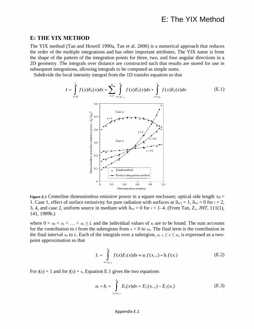
Figure E.1 Centerline dimensionless emissive power in a square enclosure; optical side length τD =
1. Case 1, effect of surface emissivity for pure radiation with surfaces at ϑw1 = 1, ϑwi = 0 for i = 2,
3, 4, and case 2, uniform source in medium with ϑwi = 0 for i = 1–4. (From Tan, Z., JHT, 111(1),
141, 1989b.)
where 0 = x0 < x1 < … < xn ≤ L and the individual values of xi are to be found. The sum accounts
for the contribution to I from the subregions from x = 0 to xn. The final term is the contribution in
the final interval xn to L. Each of the integrals over a subregion, xi−1 ≤ x ≤ xi, is expressed as a two-
point approximation so that
1
1 1( ) ( ) ( ) ( )
i
i
x
i i i i i
x x
I f x E x dx a f x b f x
−
−
=
= + (E.2)
For f(x) = 1 and for f(x) = x, Equation E.1 gives the two equations
1
1 2 1 2( ) ( ) ( )
i
i
x
i i i i
x x
a b E x dx E x E x
−
−
=
+ = = − (E.3)

E: The YIX Method
Appendix E.2
1
1 1 1 2 1 2 3 1 3( ) ( ) ( ) ( ) ( )
i
i
x
i i i i i i i i i i
x x
a x b x xE x dx x E x x E x E x E x
−
− − − −
=
+ = = − + − (E.4)
Equations E.3 and E.4 are solved for ai and bi, to give
3 1 32 1 2
1
( ) ( )( ) ( ), ( ) ( ), and ( ) i i
i i i i i i i
i i
E x E xa E x D x b D x E x D x
x x
−−
−
−= − = − =
− (E.5)
This approach can be extended to use higher-order approximations of the integrals as provided in
Hsu and Tan (1996), but if the intervals xi − xi−1 are small, the two-point approximation is
adequate. Substituting Equation E.5 into E.2 and the result into Equation E.1 gives
1
1 1
1
2
1 ( ) (0) ( ) ( ) ( )
( ) ( ) ( ) ( ) ( ) ( )
n
i i i
i
n n
I D x f D x D x f x
D x D L f x D L E L f L
−
+
=
− + −
+ − + −
(E.6)
The final simplification that makes this method useful is to let each spatial increment provide the
same contribution to the summation in Equation E.6, or [1 − D(x1)] = [D(xi) − D(xi+1)] ≡ β =
constant. Substituting into Equation E.6 gives
1
2
1
(0) ( ) ( ) ( ) ( ) ( ) ( ) ( )
n
i n n
i
I f f x D x D L f x D L E L f L
−
=
+ + − + −
(E.7)
Note that the term [D(xn) − D(L)] is not equal to β except in the special case when xn+1 falls
exactly on the boundary at L. This term must be treated separately.
The number of evaluations of the kernel necessary in the original form Equation E.1 has been
reduced; only a summation over f(xi) is necessary over most of the increments in the integration.
The kernel evaluations are further reduced by approximating the contribution of the final element
where xn < x < L < xn+1 by
1
1 1
1
2 2 1 1
1
( ) ( ) ( ) ( )
( ) ( ) ( ),
n
n n
xL
n
n nx x x x
nn n n n n
n n
L xE x f x dx E x f x dx
x x
L xE x E x f x x L x
x x
+
+= =
+ +
+
−
−
− −
−
(E.8)
This provides an estimate of the contribution of the element lying next to the boundary xn < x ≤ L,
in terms of the more easily calculated contribution of the whole fictitious element xn < x < xn+1.
Equation E.7 then becomes
1
2 2 1
11
(0) ( ) ( ) ( ) ( )
n
ni n n n
n ni
L xI f f x E x E x f x
x x
−
+
+=
− + + −
− (E.9)

E: The YIX Method
Appendix E.3
Now, define Qi ≡ [E2(xi−1) − E2(xi)]/(xi − xi−1) and Pi ≡ D(xi−1)− E2(xi−1)−xi−1Qi − β, and note that
[E3(xn+1) − E3(xn)]/(xn+1 − xn) ≈ dE3(xn)/dx = −E2(xn). These relations are substituted into Equation
E.9, which becomes, after some algebra using ξ ≡ D(xn) − D(xn+1),
1
1 1
1
(0) ( ) ) ( )
n
i n n n
i
I f f x P LQ f x
−
+ +
=
+ + +
(E.10)
Once x1 is specified, the constants D, P, and Q are computed and stored; evaluation of the integral
I is then a straightforward summation. The grid spacing is nonuniform and is chosen so that the
contribution to the integral from each increment is roughly the same. The integration grid is thus
uncoupled from the choice of increment spacing.
An advantage of this method is that f(x) contains the local properties of the medium; if the
properties are nonhomogeneous but temperature independent, they are readily incorporated in the
solution. Some cases of this type are treated in Tan and Howell (1990). If the properties are
temperature dependent, the solution is iterative. The method is readily extended to
multidimensional geometries; the exponential integral function En is replaced by Sn (Appendix D)
in the 2D formulation, as discussed by Tan and Howell. A 2D enclosure with an internal partition
is treated by Tan and Howell (1989b), and an anisotropically scattering square medium exposed
to a collimated source is analyzed by Tan and Howell (1990b). The method has been applied to
radiation with free convection in Tan and Howell (1991), and solutions of the resulting set of
equations were obtained using standard linear equation solvers. The method requires
precomputation of some coefficients in the solution, but greatly reduces the time for computing
the integrals in the radiative source.
REFERENCES: Hsu, P.-F. and Tan, Z.: Recent benchmarkings of radiative heat transfer within nonhomogeneous
participating media and the improved YIX method, in M. P. Mengüç (ed.), Radiative Transfer I:
Proceedings of the First International Symposium Radiative Transfer, Begell House, New York,
1996.
Tan, Z. and Howell, J. R.: Radiation Heat Transfer in a Partially Divided Square Enclosure with a
Participating Medium, R. K. Shah (ed.), ASME HTD-vol. 106, pp. 199–203, ASME, New York,
1989b.
Tan, Z. and Howell, J. R.: New numerical method for radiation heat transfer in nonhomogeneous
participating media, JTHT, 4(4), 419–424, 1990a.
Tan, Z. and Howell, J. R.: Combined radiation and natural convection in a two-dimensional participating
square medium, IJHMT, 34(3), 785–793, 1991.
Tan, Z.-M., Hsu, P.-F., Wu, S.-H., and Wu, C.-Y.: Modified YIX method and pseudoadaptive angular
quadrature for ray effects mitigation, JTHT, 14(3), 289–296, 2000.
F: Emittance Charts
Appendix F.1
F: CHARTS FOR CO2, H2O AND CO EMITTANCE
Alberti et al. (2018) use HITEMP 2010 line-by-line data to compose accurate emittance
charts for CO2, water vapor and CO, along with pressure and overlap corrections for mixtures of
these absorbing/emitting gases along with nonparticipating N2. Aside from the addition of CO to
the original Hottel charts (Hottel 1954), the new charts are extended to higher pressures and
temperatures. The authors have also constructed curve fits of the new data to allow accurate
interpolation, and made available an EXCEL worksheet using these interpolations to allow
convenient calculation of the emittance of mixtures of CO2, H2O, CO and N2 at temperatures and
pressures within the range of the computed emittance values (300 < T < 3000 K and 0.1 < P <
100 atm). The worksheet is available at doi.org/10.1016/j.jqsrt.2018.08.008.
Prof. Alberti has kindly provided the charts for inclusion here, and they are reproduced
below.
For a gas mixture, the total emittance is found from
H2O H2O CO2
tot H2O CO2 CO CO2 CO CO = + + − − − + (F.1)
In Eq. (F.1), the first three terms are the emittances of the individual gases at their respective
pressure-path lengths (bar-cm) and at the mixture temperature, found from Figures F.1 – F.3.
These are based on an equivalent pressure, PE, given by
( )
( )
( )
H2O
E tot H2O
CO2
E tot CO2
CO
E tot CO
1 5.00
1 0.28 (F.2)
1 0.00
P P x
P P x
P P x
= +
= +
= +
where the xi values are the mole fractions of each component in the mixture with N2. The next
three terms are the binary overlap corrections from Figs. F.4 - F.6, and the final term in Eq. (F.1)
is the ternary overlap correction, needed only if more than two gases are present in the mixture.
This final term is given by
H2O 2 CO H2O CO2 COCOmax( : )CO
CO = + − (F.3)
Some assumptions are built into the relations for pressure and overlap corrections, but comparisons
between emittance values computed from the charts or worksheet and line-by-line calculations have
shown that the graphical and worksheet results are within better than 1 percent of the exact LBL values.
Alberti et al. (2018) give worked examples to illustrate use of the charts and worksheet.
Tam and Yuen (2019) provide an open-source tool for emittance and absorptance of CO2-H2O-N2-O2-soot
mixtures for combustion calculations. Alberti et al. (2020) provide formulae for gas absorptance of H2O,
CO2, and CO based on line-by-line calculation and compare with earlier methods.

F: Emittance Charts
Appendix F.2
F.1 Emittance of Carbon Dioxide
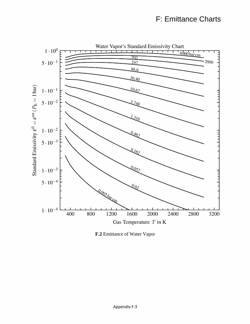
F: Emittance Charts
Appendix F.3
F.2 Emittance of Water Vapor
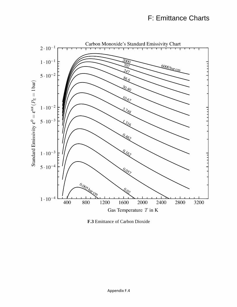
F: Emittance Charts
Appendix F.4
F.3 Emittance of Carbon Dioxide
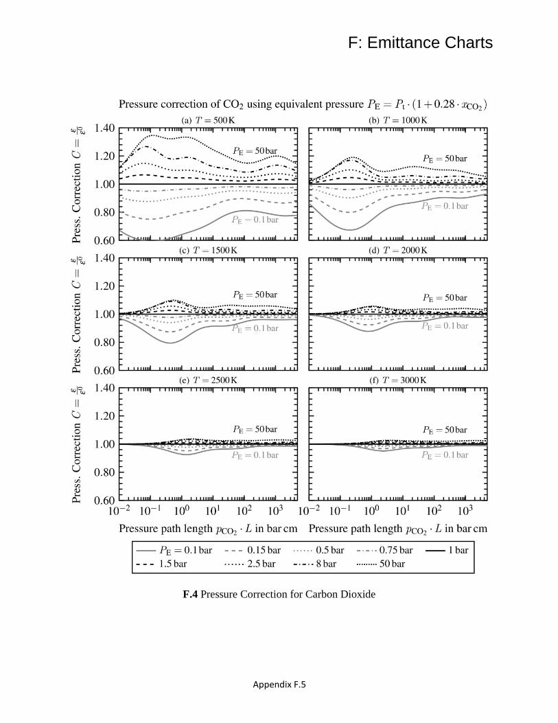
F: Emittance Charts
Appendix F.5
F.4 Pressure Correction for Carbon Dioxide

F: Emittance Charts
Appendix F.6
F. 5 Pressure Correction for Water Vapor
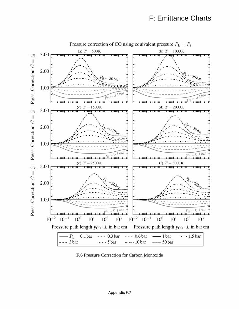
F: Emittance Charts
Appendix F.7
F.6 Pressure Correction for Carbon Monoxide
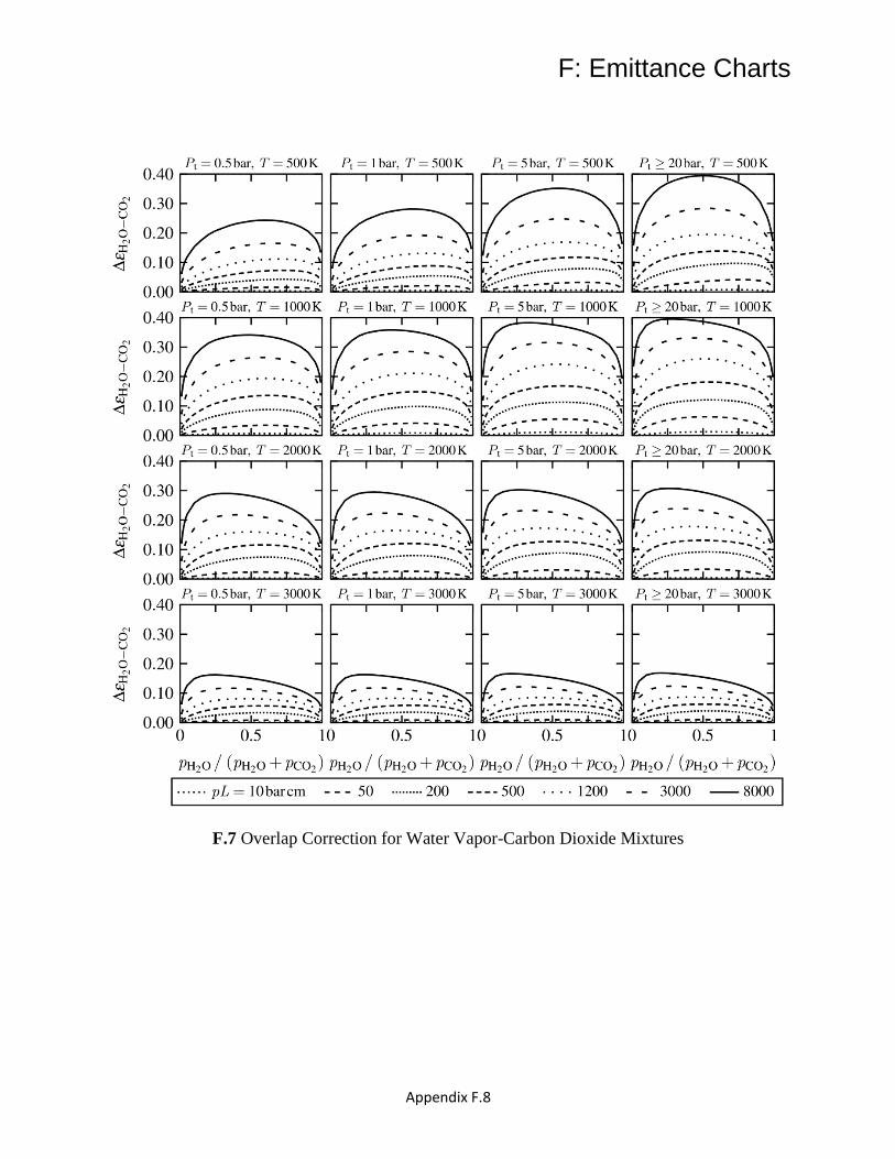
F: Emittance Charts
Appendix F.8
F.7 Overlap Correction for Water Vapor-Carbon Dioxide Mixtures

F: Emittance Charts
Appendix F.9
F.8 Overlap Correction for Carbon Dioxide-Carbon Monoxide Mixtures

F: Emittance Charts
Appendix F.10
F.9 Overlap Correction for Water Vapor-Carbon Monoxide Mixtures
THE ORIGINAL HOTTEL CHARTS
Hottel’s original graphs of the total emittance ε(pLe,T) for CO2 and H2O (Hottel, 1954;
Hottel and Sarofim, 1967) have been widely used since they were published for radiative heat
transfer calculations in combustion chambers. They were based on experimental data with
extrapolations to high temperatures and large Le-partial pressure regions based on theory.
Leckner (1972) gives empirical correlations for the total emittance derived from
calculations summing narrow band behavior over the spectrum for both water vapor and CO2.
The most accurate expressions from Leckner agree within 5% to values calculated from spectral
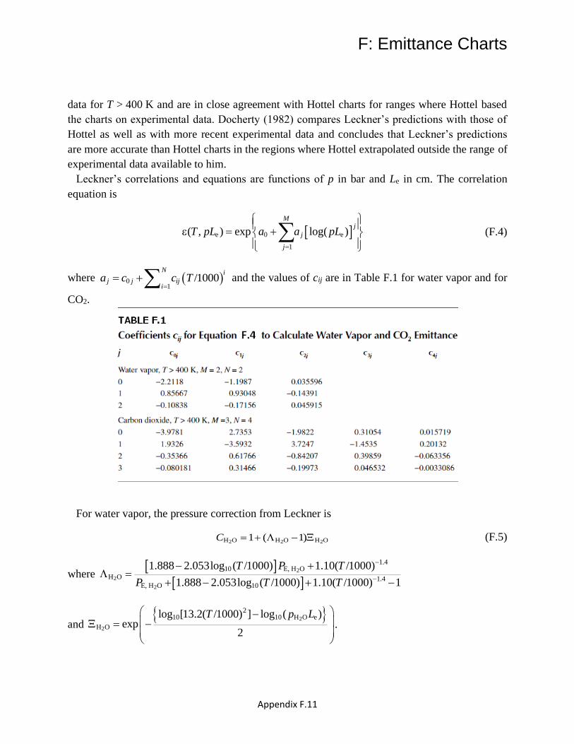
F: Emittance Charts
Appendix F.11
data for T > 400 K and are in close agreement with Hottel charts for ranges where Hottel based
the charts on experimental data. Docherty (1982) compares Leckner’s predictions with those of
Hottel as well as with more recent experimental data and concludes that Leckner’s predictions
are more accurate than Hottel charts in the regions where Hottel extrapolated outside the range of
experimental data available to him.
Leckner’s correlations and equations are functions of p in bar and Le in cm. The correlation
equation is
e 0 e
1
( , ) exp log( )
Mj
j
j
T pL a a pL
=
= +
(F.4)
where ( )01
/1000N i
j j iji
a c c T=
= + and the values of cij are in Table F.1 for water vapor and for
CO2.
For water vapor, the pressure correction from Leckner is
2 2 2H O H O H O1 ( 1)C = + − (F.5)
where
2
2
2
1.410 E, H O
H O 1.4E, H O 10
1.888 2.053log ( /1000) 1.10( /1000)
1.888 2.053log ( /1000) 1.10( /1000) 1
T P T
P T T
−
−
− + =
+ − + −
and 2
2
210 10 H O e
H O
log [13.2( /1000) ] log ( )exp
2
T p L − = −
.

F: Emittance Charts
Appendix F.12
The effective pressure is given by 2 2
1/2E, H O t H O t1 4.9( / )(273/ )P P p P T = + and Pt is the total
pressure of the air–H2O mixture. In the expression for Λ, the T in the expression in square
brackets is replaced by 750 if T < 750 K.
The pressure correction for CO2 from Leckner is given by
2 2 2CO CO CO1 ( 1)C = + − (F.6)
where2
2
2
1.45E,CO
CO 1.45E,CO
1.00 0.10( /1000) 0.23
1.00 0.10( /1000) 0.77
T P
P T
−
−
+ + = + + −
and 2 2CO 10 CO eexp 1.47 log ( )p L = − − .
The effective pressure is given by 2 2E,CO t CO t1 0.28( / )P P p P= + , where Pt is the total pressure of
the air–CO2 mixture. In the expression for Ξ, μ = log10[0.225(T/1000)2] if T > 700 K, and
μ = log10[0.054(T/1000)−2] if T < 700 K.
An empirical expression for the band overlap correction that is in good agreement with
the Hottel chart (Leckner 1972) valid for 1000 < T < 2200 K and all pressures is
2.7610.4
10 e0.0089 log ( )10.7 101
pL
= − +
(F.7)
where ( )2 2 2H O H O COp p p = + , ( )2 2H O COp p p= + is in bars, and Le is in cm.
The emergence of the accurate line-by-line data bases (used in generating the charts and spread sheet by Alberti et al. 2018) has largely superseded the pioneering work of Hottel.
Example F.1
A container with effective radiation thickness of Le = 2.4 m contains a mixture of 15 volume percent of CO2, 20% H2O
vapor, and the remainder air. The total pressure of the gas mixture is 1 atm, and the gas temperature is 1200 K. What is
the emittance of the gas?
The partial pressures of the gases are equal to the mole fraction of each times the total pressure. The mole fraction in an
ideal gas mixture is equal to the volume fraction, so the partial pressures are =2CO 0.15p , =
2H O 0.20p , and pair = 0.65 atm.
For water vapor, the aj values are ( )=
= + 01
/1000N i
j j iji
a c c T , giving a1 = −3.599, a2 = 1.766, and a3 = −0.248. Using
Equation F.4 (remembering to convert the pressures to bars),
=
= + =
2
Mj
H O e 0 j e
j 1
(T,pL ) exp a a log(pL ) 0.313.
A similar calculation for CO2 gives (CO2) = 0.155. No pressure correction is necessary because the total pressure is 1
atm. The overlap correction is calculated using
= = =+ +
2
2 2
H O
H O CO
0.200.571
0.15 0.20
p
p p
F: Emittance Charts
Appendix F.13
and
( ) ( )+ = +
=
2 2H O CO 0.15 0.20 (atm) 1.01325 (bar/atm) 240 (cm)
85.1(bar cm).
ep p L
Substituting results in
= − = +
2.7610.410 e0.0089 log (pL ) 0.051
10.7 101
The total emittance of the gas mixture is then
= + − = + − =2 2mixture H O CO 0.313 0.155 0.051 0.417
Using the spreadsheet for the Alberti correlations gives a value of Alberti 0.401 =
REFERENCES:
Alberti, M., Weber, R., and Mancini, M.: Gray gas emissivities for H2O-CO2-CO-N2 mixtures, JQSRT,
219, 274-291, Nov. 2018.
Alberti, M., Weber, R., and Mancini, M.: New formulae for gray gas absorptivities of H2O, CO2, and CO,
JQSRT 255, 107227, 2020.
Docherty, P.: Prediction of gas emissivity for a wide range of process conditions, Paper R5, Proceedings
of the Seventh International Heat Transfer Conference, vol. 2, pp. 481–485, Munich, Germany, 1982.
Hottel, H. C.: Radiant heat transmission, Chapter 4, in W. H. McAdams (ed.), Heat
Transmission, 3rd edn., McGraw-Hill, New York, 1954.
Hottel, H. C. and Sarofim, A. F.: Radiative Transfer, McGraw–Hill, New York, 1967. Leckner, B.: Spectral and total emissivity of water vapor and carbon dioxide, Combust. Flame, 19, 33–48,
1972.
Tam, W.C. and Yuen, W. W.: OpenSC – an Open-source Calculation Tool for Combustion Mixture
Emissivity/Absorptivity, NIST Technical Note 2064, National Institute of Standards and Technology,
Sept. 2019.
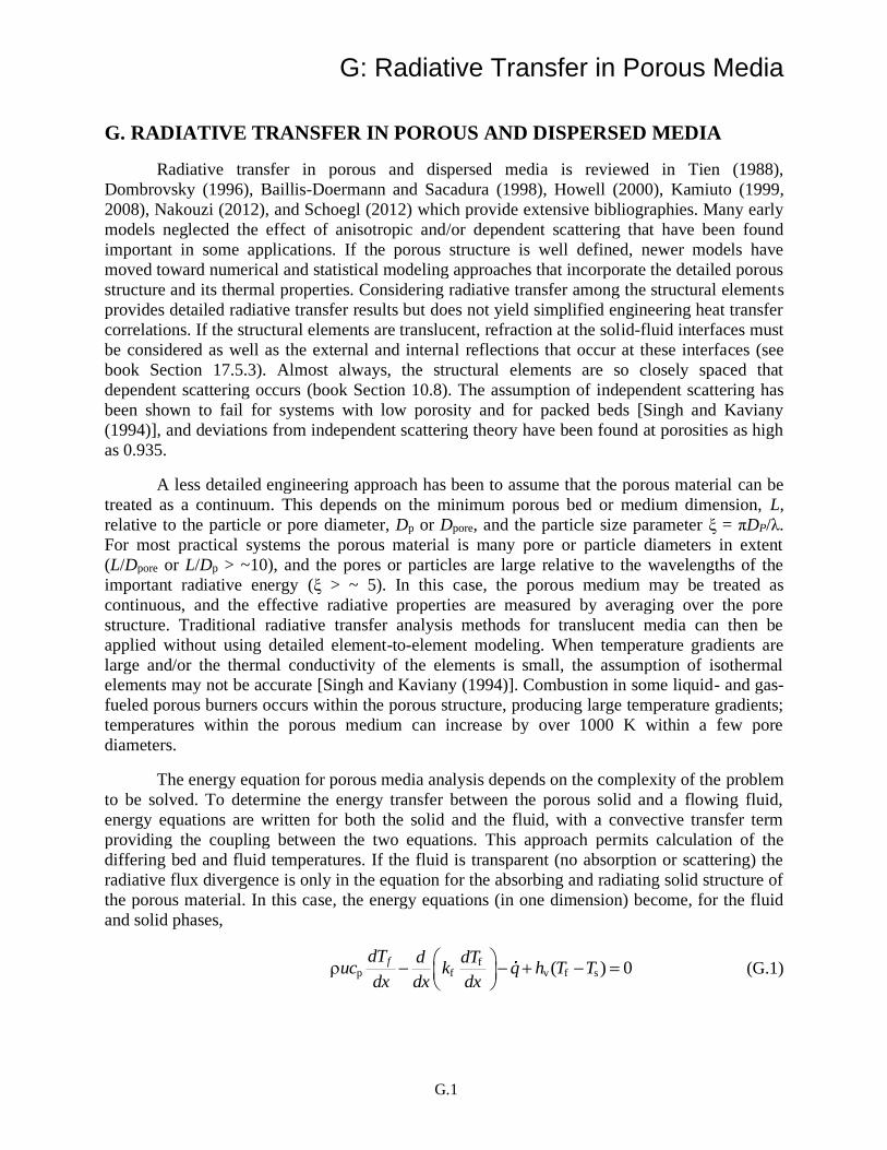
G: Radiative Transfer in Porous Media
G.1
G. RADIATIVE TRANSFER IN POROUS AND DISPERSED MEDIA
Radiative transfer in porous and dispersed media is reviewed in Tien (1988),
Dombrovsky (1996), Baillis-Doermann and Sacadura (1998), Howell (2000), Kamiuto (1999,
2008), Nakouzi (2012), and Schoegl (2012) which provide extensive bibliographies. Many early
models neglected the effect of anisotropic and/or dependent scattering that have been found
important in some applications. If the porous structure is well defined, newer models have
moved toward numerical and statistical modeling approaches that incorporate the detailed porous
structure and its thermal properties. Considering radiative transfer among the structural elements
provides detailed radiative transfer results but does not yield simplified engineering heat transfer
correlations. If the structural elements are translucent, refraction at the solid-fluid interfaces must
be considered as well as the external and internal reflections that occur at these interfaces (see
book Section 17.5.3). Almost always, the structural elements are so closely spaced that
dependent scattering occurs (book Section 10.8). The assumption of independent scattering has
been shown to fail for systems with low porosity and for packed beds [Singh and Kaviany
(1994)], and deviations from independent scattering theory have been found at porosities as high
as 0.935.
A less detailed engineering approach has been to assume that the porous material can be
treated as a continuum. This depends on the minimum porous bed or medium dimension, L,
relative to the particle or pore diameter, Dp or Dpore, and the particle size parameter ξ = πDP/λ.
For most practical systems the porous material is many pore or particle diameters in extent
(L/Dpore or L/Dp > ~10), and the pores or particles are large relative to the wavelengths of the
important radiative energy (ξ > ~ 5). In this case, the porous medium may be treated as
continuous, and the effective radiative properties are measured by averaging over the pore
structure. Traditional radiative transfer analysis methods for translucent media can then be
applied without using detailed element-to-element modeling. When temperature gradients are
large and/or the thermal conductivity of the elements is small, the assumption of isothermal elements may not be accurate [Singh and Kaviany (1994)]. Combustion in some liquid- and gas-
fueled porous burners occurs within the porous structure, producing large temperature gradients;
temperatures within the porous medium can increase by over 1000 K within a few pore
diameters.
The energy equation for porous media analysis depends on the complexity of the problem
to be solved. To determine the energy transfer between the porous solid and a flowing fluid,
energy equations are written for both the solid and the fluid, with a convective transfer term
providing the coupling between the two equations. This approach permits calculation of the
differing bed and fluid temperatures. If the fluid is transparent (no absorption or scattering) the
radiative flux divergence is only in the equation for the absorbing and radiating solid structure of
the porous material. In this case, the energy equations (in one dimension) become, for the fluid
and solid phases,
fp f v f s( ) 0
fdT d dTuc k q h T T
dx dx dx
− − + − =
(G.1)
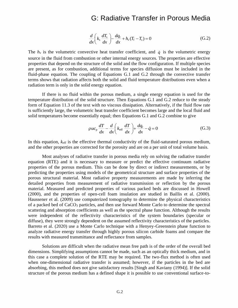
G: Radiative Transfer in Porous Media
G.2
s rs v f s( ) 0
d dT dqk h T T
dx dx dx
− + − =
(G.2)
The hv is the volumetric convective heat transfer coefficient, and q is the volumetric energy
source in the fluid from combustion or other internal energy sources. The properties are effective
properties that depend on the structure of the solid and the flow configuration. If multiple species
are present, as for combustion, additional terms for species diffusion must be included in the
fluid-phase equation. The coupling of Equations G.1 and G.2 through the convective transfer
terms shows that radiation affects both the solid and fluid temperature distributions even when a
radiation term is only in the solid energy equation.
If there is no fluid within the porous medium, a single energy equation is used for the
temperature distribution of the solid structure. Then Equations G.1 and G.2 reduce to the steady
form of Equation 11.3 of the text with no viscous dissipation. Alternatively, if the fluid flow rate
is sufficiently large, the volumetric heat transfer coefficient becomes large and the local fluid and
solid temperatures become essentially equal; then Equations G.1 and G.2 combine to give
rp eff 0
dT d dT dquc k q
dx dx dx dx
− + − =
(G.3)
In this equation, keff is the effective thermal conductivity of the fluid-saturated porous medium,
and the other properties are corrected for the porosity and are on a per unit of total volume basis.
Most analyses of radiative transfer in porous media rely on solving the radiative transfer
equation (RTE) and it is necessary to measure or predict the effective continuum radiative
properties of the porous medium. This can be done by direct or indirect measurements, or by
predicting the properties using models of the geometrical structure and surface properties of the
porous structural material. Most radiative property measurements are made by inferring the
detailed properties from measurement of radiative transmission or reflection by the porous
material. Measured and predicted properties of various packed beds are discussed in Howell
(2000), and the properties of open-cell foam insulation are studied in Baillis et al. (2000).
Haussener et al. (2009) use computerized tomography to determine the physical characteristics
of a packed bed of CaCO3 particles, and then use forward Monte Carlo to determine the spectral
scattering and absorption coefficients as well as the spectral phase function. Although the results
were independent of the reflectivity characteristics of the system boundaries (specular or
diffuse), they were strongly dependent on the assumed reflectivity characteristics of the particles.
Barreto et al. (2020) use a Monte Carlo technique with a Henyey-Greenstein phase function to
analyze radiative energy transfer through highly porous silicon carbide foams and compare the
results with measured transmittance and reflectance from samples.
Solutions are difficult when the radiative mean free path is of the order of the overall bed
dimensions. Simplifying assumptions cannot be made, such as an optically thick medium, and in
this case a complete solution of the RTE may be required. The two-flux method is often used
when one-dimensional radiative transfer is assumed; however, if the particles in the bed are
absorbing, this method does not give satisfactory results [Singh and Kaviany (1994)]. If the solid
structure of the porous medium has a defined shape it is possible to use conventional surface-to-
G: Radiative Transfer in Porous Media
G.3
surface radiative interchange analysis. This is used in Antoniak et al. (1996) and Palmer et al.
(1996) with a Monte Carlo cell-by-cell analysis to simulate radiative transfer among arrays of
geometric shapes. Some research has tried to define an effective radiative conductivity that can
be combined with heat conduction. For use in optically thick systems with porosity between 0.4
and 0.5, composed of opaque solid spherical particles with surface emissivity r and thermal
conductivity of the solid ks, the radiative conductivity can be approximated by [Singh and
Kaviany (1991, 1994), Kaviany (1991)]:
3 1 * 0.8011r p r s r4 0.5756 tan 1.5353( ) / 0.1843k D T k− = + (G.4)
where * 3s s p/ (4 )k k D T= . This is reasonably accurate for both diffuse and specular reflecting
particles [the constants in (G.4) are specifically for diffuse surfaces] and is weakly dependent on
bed porosity.
An early work on radiation transfer in dispersed media was by Viskanta and Mengüç
(1989). Baillis and Sacadura (1996, 2000) have expanded the concept and provided a thorough
literature search. Carvajal et al. (2019) compare many standard radiation models for conduction-
radiation transfer through high-density insulation and compare predictions with NIST certified
values for fiber board. Transport phenomena, including radiation models in solid-gas foams were
given by Pilon et al. (2001) and for glass foams the state-of-the-art was discussed by Federov
and Pilon (2002). Further applications to foams were reported in several studies by Baillis’s
group [Loretz et al. (2008); Randrianalisoa et al. 2006; Randrianalisoa and Baillis (2010, 2014);
Kaemmerlen et al. (2010); Coquard et al. (2012)]. Diagnosis of foamy and bubbly media also
require understanding of radiative transfer and light scattering concepts, as discussed by Wong
and Mengüç (2002); Vaillon et al. (2004); Aslan et al. (2006); Swamy et al. (2007); and Gay et
al. (2010). Monographs on dispersed systems summarize many formulations and applications
specific to practical problems [Dombrovsky and Baillis (2010), Cunsolo et al. (2017)]. The case
of long cylindrical fibers in random orientations is analyzed for the geometric optics region using
a detailed Monte Carlo analysis in Nisipeanu and Jones (2003). Particle suspensions in liquid are
studied in Ma et al. (2015). Ates et al. (2017) examine the effect of gray vs. nongray particle
properties in fluidized bed combustors. Liu et al. (2019) provide an alternative to solving the
RTE based on the use of a radiation distribution function (the ratio of the absorbed power by
particle j to the totally emitted radiative power from the source particle i). Wu et al. (2020) use a
similar approach based on an approximation function model. Wehinger (2019) examines the
importance of radiation in fixed-bed reactors. Hashemi and Hashemi (2019) performed a
numerical study of 2-D premixed methane-air combustion in a combined porous free-flame
burner and compared the results with experiment. Ghorashi et al. (2019, 2020) study a combined
porous-free flame burner both numerically and experimentally. Jia et al. (2020) use analysis and
experiment to determine the suitability of porous media burners using natural gas fuel for
potential use in natural gas stoves. Caetano et al. (2020) measured the angular distribution of
radiation from porous burners of zirconia and silicon carbide. Omidi and Emami (2020) measure
thermal efficiency, power, and NOx emission vs. equivalence ratio in a metallic porous media
premixed burner. Habib et al (2021) experimentally study methane and biogas combustion in a
porous burner. Wang et al. (2020) use a Monte Carlo algorithm to find a graded-porosity
medium for use in a central solar power absorber.

G: Radiative Transfer in Porous Media
G.4
REFERENCES:
Antoniak, Z. L., Palmer, B. J., Drost, M. K., and Welty, J. R.: Parametric Study of Radiative Heat
Transfer in Arrays of Fixed Discrete Surfaces, JHT, vol. 118, no. 1, pp. 228–230, 1996.
Aslan, M. M., Crofcheck, C., Tao, D., and Mengüç, M. P.: Evaluation of Micro Bubble Size and Gas
Holdup in Two Phase Gas-Liquid Columns via Scattered Light Measurements, JQSRT, vol. 101, pp.
527–539, 2006.
Ates, C., Selçuk, N., Ozen, G., and Kulah, G.: Benchmarking grey particle approximations against
nongrey particle radiation in circulating fluidized bed combustors, , 71(5), 467-484, 2017.
Baillis, D., and Sacadura, J.F.: Heat Transfer in Open Cell Foam Insulations, JHT, vol. 118, no. 1, pp.
292-298, 1996.
Baillis-Doermann, D., and Sacadura, J. F.: Thermal Radiation Properties of Dispersed Media: Theoretical
Prediction and Experimental Characterization, JQSRT, vol. 67, no. 5, pp. 327-363, 2000. Baillis, D., Raynaud, M., and Sacadura, J. F.: Determination of Spectral Radiative Properties of Open-
Cell Foam: Model Validation, JTHT, vol. 14, no. 2, pp. 137–143, 2000.
Barreto, G., Canhoto, P., and Collares-Pereira, M.: Combined experimental and numerical determination
of the asymmetry factor of scattering phase functions in porous volumetric solar receivers, Solar
Energy Materials and Solar Cells, 206, 110327, March 2020.
Caetano, N. R., Lorenzini, G., Lhamby, A. R., Guillet, V. M. M., Klunk, M. A., Rocha, L. A. O.:
Experimental Assessment of Thermal Radiation Behavior Emitted by Solid Porous Material, Int.
J. Heat Technology, 38(1), 1-8, 2020.
Carvajal, S. A., Garboczi, E. J., and Zarr, R. R.: Comparison of models for heat transfer in high-density
fibrous insulation, J. Research National Institute of Standards and Technology, 124, 124010, 2019.
Coquard, R., Rochais, D., and Baillis, D.: Conductive and Radiative Heat Transfer in Ceramic and Metal
Foams at Fire Temperatures, Fire Tech., vol. 48 no. 3, pp. 699-732, 2012.
Cunsolo, S., Coquard, R., Baillis, D., and Nicola Bianco, N.: Radiative properties modeling of open cell
solid foam: Review and new analytical law, IJTS, 104, 12-134, 2016.
Dombrovsky, L. A.: Radiation Heat Transfer in Disperse Systems, Begell House, New York, 1996.
Dombrovsky, L.A., and Baillis, D.: Thermal Radiation in Disperse Systems: An Engineering Approach,
Begell House, 2010.
Fedorov, A.G., and Pilon, L.: Glass Foams: Formation, Transport Properties, and Heat, Mass, and
Radiation Transfer, J. Non-Crystalline Solids, vol. 311, no. 2, pp. 154-173, 2002.
Gay, B., Vaillon R., and Menguc, M. P.: Polarization Imaging of Multiply-scattered Radiation Based on
Integral-Vector Monte Carlo Method, JQSRT, vol. 111, pp. 287-294, 2010.
Ghorashi, A., Hashemi, A., Hashemi, M., and Mollamahdi, M.: Experimental study on pollutant
emissions in the novel combined porous-free flame burner, Energy, 162, 517-525, 2018.
Ghorashi, A., Hashemi, A., Hashemi, M., Hashemi, A., and Mollamahdi, M.: Numerical study on the
combustion characteristics in a porous-free flame burner for lean mixtures, J. Mechanical Engng. Sci,
1989-1996, Nov. 2019.
Habib, R., Yadollahi, B., Doranehgard, M. H., Li, L. K. B., and Karimi, N.: Unsteady ultra-lean
combustion of methans and biogas in a porous burner- An experimental study, Appl. Thermal
Engineering, 182, 116099, 2021.
Hashemi, S. V., and Hashemi, S. A.: Investigation of the premixed methane–air combustion through the
combined porous-free flame burner by numerical simulation, Proc. Institution Mechanical Engineers,
Part A: J. Power and Energy, Jan. 9, 2019.
Haussener, S., Lipiński, W., Petrasch, J., Wyss, P., and Steinfeld, A.: Tomographic Characterization of a
Semitransparent-Particle Packed Bed and Determination of Its Thermal Radiative Properties, JHT,
vol. 131, no. 7, pp. 072701–072712, July 2009.
G: Radiative Transfer in Porous Media
G.5
Howell, J. R.: Radiative Transfer in Porous Media, in K. Vafai (ed.), Handbook of Porous Media, Chap.
7, Marcel Dekker, New York, 2000.
Jia, Y., Zhou, W., Tang, J., and Luo, Y.: Numerical and Experimental Study on Combustion Performance
of an Infrared Radiation Burner with Porous Metal Plaque, in Z. Wang et al. (eds.), Proc. 11th
International Symposium on Heating, Ventilation and Air Conditioning (ISHVAC 2019),
Environmental Science and Engineering, Springer Nature Singapore Pte Ltd., 299-307, 2020.
Kaemmerlen, A., Vo, C., Asllanaj, F., Jeandel, G., and Baillis, D.: Radiative Properties of Extruded
Polystyrene Foams: Predictive Model and Experimental Results, JQSRT, vol. 111. no. 6, pp. 865-
877, 2010.
Kamiuto, K.: Modeling of Elementary Transport Processes and Composite Heat Transfer in Open-
Cellular Porous Materials, in Trends in Heat, Mass and Momentum Transfer, U. Ramchandran, exec.
ed., vol. 5, pp. 141–161, Research Trends, Trivandrum, India, 1999.
Kamiuto, K.: Modeling of Composite Heat Transfer in Open-Cellular Porous Materials at High
Temperatures, in A. Achsner, G. E. Murch, and M. J. S. de Lemos (eds.), Cellular and Porous
Materials: Thermal Properties Simulation and Prediction, Wiley-VCH, Weinheim, 2008.
Kaviany, M.: Principles of Heat Transfer in Porous Media, Springer-Verlag, New York, 1991.
Liu, B., Zhao, J., and Liu, L.: Continuum approach based on radiation distribution function for radiative
heat transfer in densely packed particulate system, JQSRT, 253, 107028, Sept. 2020. Loretz, M., Coquard, R., Baillis, D., and Maire, E.: Metallic Foams Radiative Properties/Comparison between
Different Models, JQSRT, vol. 109, no. 1, pp. 16-27, 2008.
Ma, C.Y., Zhao, J.M., Liu, L.H., and Zhang, L.: GPU-Accelerated Inverse Identification of Radiative Properties of
Particle Suspensions in Liquid by Monte Carlo, Proc. 5th Int. Symp. Computational Thermal Radiation in
Participating Media, Albi, France, 1-3 April 2015.
Mujeebu, M. A., Abdullah, M. Z., Abu Bakar, M. Z., Mohamad, A. A., Muhad, R. M. N., and Abdullah,
M. K.: Combustion in porous media and its applications – A comprehensive survey, J. Environmental
Management, 90, 2287-2312, 2009.
Mujeebu, M. A.: Combustion in Porous Media for Porous Burner Application, in Convective Heat
Transfer in Porous Media, Mahmoudi, Y., Hooman, K., and Vafai, K. (eds.), Taylor and Francis-CRC
Press, 2020.
Nakouzi, S.: Modelization du Procédé de Cuisson de Composites Infusés par Chauffage Infra Rouge,
doctoral thesis, Institut Clément Ader, Ecole des Mines d’Albi, l’Université de Toulouse, Albi,
France, 2012.
Nisipeanu, E. and Jones, P.: Monte Carlo Simulation of Radiative Heat Transfer in Course Fibrous
Media, JHT, vol. 125, pp. 748-752, 2003.
Omidi, M. and Emami, M. D.: Experimental investigation of premixed combustion and thermal efficiency
in a porous heating burner, Int. J. Energy Res., accept. 18 July, 2020.
Palmer, B. J., Drost, M. K., and Welty, J. R.: Monte Carlo Simulation of Radiative Heat Transfer in
Arrays of Fixed Discrete Surfaces Using Cell-to-Cell Photon Transport, IJHMT, vol. 39, no. 13, pp.
2811–2819, 1996.
Pilon, L., Fedorov, A.G., and Viskanta, R.: Steady-state Thickness of Liquid–gas Foams, J. of Colloid
and Interface Science, vol. 242, no. 2, pp. 425-436, 2001.
Randrianalisoa, J., and Baillis, D.: Radiative Properties of Densely Packed Spheres in Semitransparent
Media: A New Geometric Optics Approach, JQSRT, vol. 111, no. 10, pp. 1372-1388, 2010.
Randrianalisoa, J.H., and Baillis, D.: Analytical Model of Radiative Properties of Packed Beds and
Dispersed media, IJHMT, vol. 70, pp. 264-275, 2014.
Randrianalisoa, J.H., Dombrovsky, L.A., Lipiński, W., and Timchenko, V.: Effects of Short-Pulsed Laser
Radiation on Transient Heating of Superficial Human Tissues, IJHMT, vol. 78, pp. 488-497, 2014.
Schoegl, I.: Radiation Effects on Flame Stabilization on Flat Flame Burners, Comb.and Flame, vol. 159,
no. 9, pp. 2817-2828, 2012.
Singh, B. P., and Kaviany, M.: Independent Theory versus Direct Simulation of Radiative Heat Transfer
G: Radiative Transfer in Porous Media
G.6
in Packed Beds, IJHMT, vol. 34, pp. 2869–2881, 1991.
Singh, B. P., and Kaviany, M.: Effect of Solid Conductivity on Radiative Heat Transfer in Packed Beds,
IJHMT, vol. 37, no. 16, pp. 2579–2583, 1994.
Swamy, J.N., Crofcheck, C., and Mengüç, M.P.: A Monte Carlo Ray Tracing Study of the Polarized Light
Propagation in Liquid Foams, JQSRT, vol. 101, pp. 527-539, 2007.
Tien, C. L.: Thermal Radiation in Packed and Fluidized Beds, JHT, vol. 110, pp. 1230–1242, 1988.
Vaillon, R., Wong, B.T., and Mengüç, M.P.: Polarized Radiative Transfer in a Particle-laden Semi-
transparent Medium via a Vector Monte Carlo Method, JQSRT, vol. 84, pp. 383-394, 2004.
Wang, P., Li, J. B., Zhou, L., and Liu, D. Y.: Acceptance-rejection sampling based Monte Carlo ray
tracing in anisotropic porous media, Energy, 199, 117455, May 2020.
Wu, H., Gui, N., Yang, X., Tu, J., and Jiang, S.: An approximation function model for solving effective
radiative heat transfer in packed bed, Annals of Nuclear Energy, 135, 107000, 2020.
Viskanta, R., and Mengüç, M. P.: Radiative transfer in dispersed media, ASME Appl. Mechanics Rev.,
vol. 42, pp. 241–259, 1989.
Wehinger, G. D.: Radiation matters in fixed-bed CFD simulations, Chemie Ingenieur Technik, 91(5),583-
591, 2019.
Wong, B., and Mengüç, M. P.: Depolarization of Radiation by Foams, JQSRT, vol. 73, nos. 2–5, pp. 273–
284, 2002.
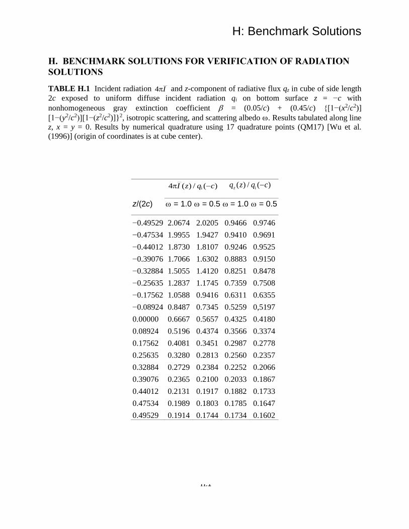
H: Benchmark Solutions
H.1
H. BENCHMARK SOLUTIONS FOR VERIFICATION OF RADIATION
SOLUTIONS
TABLE H.1 Incident radiation 4 I and z-component of radiative flux qz in cube of side length
2c exposed to uniform diffuse incident radiation qi on bottom surface z = −c with
nonhomogeneous gray extinction coefficient = (0.05/c) + (0.45/c) {[1−(x2/c2)]
[1−(y2/c2)][1−(z2/c2)]}2, isotropic scattering, and scattering albedo . Results tabulated along line
z, x = y = 0. Results by numerical quadrature using 17 quadrature points (QM17) [Wu et al.
(1996)] (origin of coordinates is at cube center).
z/(2c)
i4 ( ) / ( )I z q c − i( ) / ( )−zq z q c
= 1.0 = 0.5 = 1.0 = 0.5
−0.49529 2.0674 2.0205 0.9466 0.9746
−0.47534 1.9955 1.9427 0.9410 0.9691
−0.44012 1.8730 1.8107 0.9246 0.9525
−0.39076 1.7066 1.6302 0.8883 0.9150
−0.32884 1.5055 1.4120 0.8251 0.8478
−0.25635 1.2837 1.1745 0.7359 0.7508
−0.17562 1.0588 0.9416 0.6311 0.6355
−0.08924 0.8487 0.7345 0.5259 0,5197
0.00000 0.6667 0.5657 0.4325 0.4180
0.08924 0.5196 0.4374 0.3566 0.3374
0.17562 0.4081 0.3451 0.2987 0.2778
0.25635 0.3280 0.2813 0.2560 0.2357
0.32884 0.2729 0.2384 0.2252 0.2066
0.39076 0.2365 0.2100 0.2033 0.1867
0.44012 0.2131 0.1917 0.1882 0.1733
0.47534 0.1989 0.1803 0.1785 0.1647
0.49529 0.1914 0.1744 0.1734 0.1602
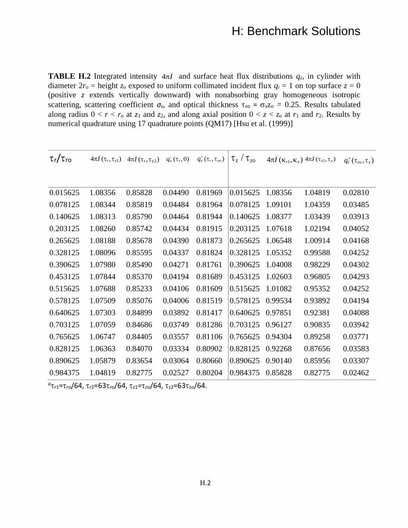
H: Benchmark Solutions
H.2
TABLE H.2 Integrated intensity 4 I and surface heat flux distributions qz, in cylinder with
diameter 2ro = height zo exposed to uniform collimated incident flux qi = 1 on top surface z = 0
(positive z extends vertically downward) with nonabsorbing gray homogeneous isotropic
scattering, scattering coefficient σs, and optical thickness zo = szo = 0.25. Results tabulated
along radius 0 < r < ro at z1 and z2, and along axial position 0 < z < zo at r1 and r2. Results by
numerical quadrature using 17 quadrature points (QM17) [Hsu et al. (1999)]
r/ro r z14 ( , )I r z24 ( , )I
z r( ,0)q− z r zo( , )q+ z zo/ r1 z4 ( , )I
r2 z4 ( , )I
r ro z( , )q+
0.015625 1.08356 0.85828 0.04490 0.81969 0.015625 1.08356 1.04819 0.02810
0.078125 1.08344 0.85819 0.04484 0.81964 0.078125 1.09101 1.04359 0.03485
0.140625 1.08313 0.85790 0.04464 0.81944 0.140625 1.08377 1.03439 0.03913
0.203125 1.08260 0.85742 0.04434 0.81915 0.203125 1.07618 1.02194 0.04052
0.265625 1.08188 0.85678 0.04390 0.81873 0.265625 1.06548 1.00914 0.04168
0.328125 1.08096 0.85595 0.04337 0.81824 0.328125 1.05352 0.99588 0.04252
0.390625 1.07980 0.85490 0.04271 0.81761 0.390625 1.04008 0.98229 0.04302
0.453125 1.07844 0.85370 0.04194 0.81689 0.453125 1.02603 0.96805 0.04293
0.515625 1.07688 0.85233 0.04106 0.81609 0.515625 1.01082 0.95352 0.04252
0.578125 1.07509 0.85076 0.04006 0.81519 0.578125 0.99534 0.93892 0.04194
0.640625 1.07303 0.84899 0.03892 0.81417 0.640625 0.97851 0.92381 0.04088
0.703125 1.07059 0.84686 0.03749 0.81286 0.703125 0.96127 0.90835 0.03942
0.765625 1.06747 0.84405 0.03557 0.81106 0.765625 0.94304 0.89258 0.03771
0.828125 1.06363 0.84070 0.03334 0.80902 0.828125 0.92268 0.87656 0.03583
0.890625 1.05879 0.83654 0.03064 0.80660 0.890625 0.90140 0.85956 0.03307
0.984375 1.04819 0.82775 0.02527 0.80204 0.984375 0.85828 0.82775 0.02462
ar1=ro/64, r2=63ro/64, z1=zo/64, z2=63zo/64.
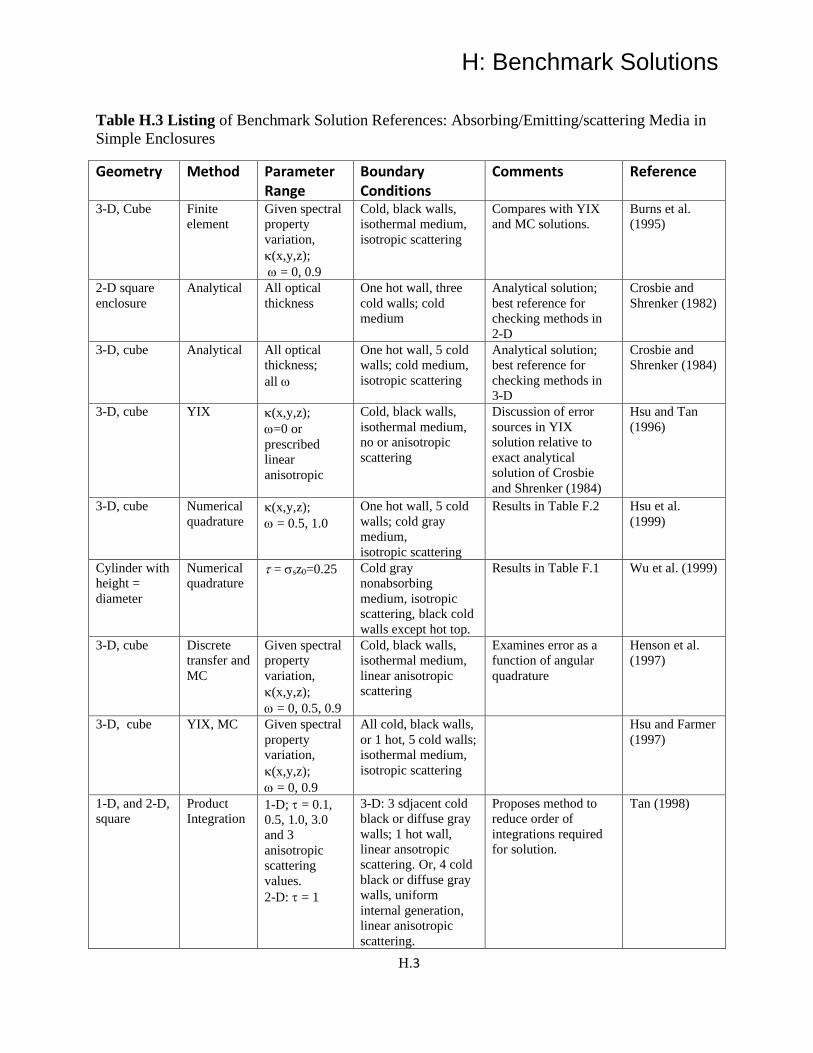
H: Benchmark Solutions
H.3
Table H.3 Listing of Benchmark Solution References: Absorbing/Emitting/scattering Media in
Simple Enclosures
Geometry Method Parameter Range
Boundary Conditions
Comments Reference
3-D, Cube Finite
element
Given spectral
property
variation,
(x,y,z);
= 0, 0.9
Cold, black walls,
isothermal medium,
isotropic scattering
Compares with YIX
and MC solutions.
Burns et al.
(1995)
2-D square
enclosure
Analytical All optical
thickness
One hot wall, three
cold walls; cold
medium
Analytical solution;
best reference for
checking methods in
2-D
Crosbie and
Shrenker (1982)
3-D, cube Analytical All optical
thickness;
all
One hot wall, 5 cold
walls; cold medium,
isotropic scattering
Analytical solution;
best reference for
checking methods in
3-D
Crosbie and
Shrenker (1984)
3-D, cube YIX (x,y,z);
=0 or
prescribed
linear
anisotropic
Cold, black walls,
isothermal medium,
no or anisotropic
scattering
Discussion of error
sources in YIX
solution relative to
exact analytical
solution of Crosbie
and Shrenker (1984)
Hsu and Tan
(1996)
3-D, cube Numerical
quadrature (x,y,z);
= 0.5, 1.0
One hot wall, 5 cold
walls; cold gray
medium,
isotropic scattering
Results in Table F.2 Hsu et al.
(1999)
Cylinder with
height =
diameter
Numerical
quadrature = sz0=0.25 Cold gray
nonabsorbing
medium, isotropic
scattering, black cold
walls except hot top.
Results in Table F.1 Wu et al. (1999)
3-D, cube Discrete
transfer and
MC
Given spectral
property
variation,
(x,y,z);
= 0, 0.5, 0.9
Cold, black walls,
isothermal medium,
linear anisotropic
scattering
Examines error as a
function of angular
quadrature
Henson et al.
(1997)
3-D, cube YIX, MC Given spectral
property
variation,
(x,y,z);
= 0, 0.9
All cold, black walls,
or 1 hot, 5 cold walls;
isothermal medium,
isotropic scattering
Hsu and Farmer
(1997)
1-D, and 2-D,
square
Product
Integration 1-D; = 0.1,
0.5, 1.0, 3.0
and 3
anisotropic
scattering
values.
2-D: = 1
3-D: 3 sdjacent cold
black or diffuse gray
walls; 1 hot wall,
linear ansotropic
scattering. Or, 4 cold
black or diffuse gray
walls, uniform
internal generation,
linear anisotropic
scattering.
Proposes method to
reduce order of
integrations required
for solution.
Tan (1998)

H: Benchmark Solutions
H.4
2-D square
enclosure
M1. S32 = 5 Black surfaces Planar radiation
sources at various
locations within
medium.
Gonzalez et al.
(2008)
2-D square
enclosure
S4, S6, M1,
P1 = 0 – 10,
= 0 - 1
One hot wall, three
cold walls, all black
Compares accuracy of
each method with
analytical solution of
Crosbie and Shrenker
(1982)
Tencer and
Howell (2013)
2-D square
and 3-D
cubical
S8 and S16
for 2-D; S4,
S8 and S12
for 3-D.
= 1, pure
scattering
Black surfaces; One
hot wall, three cold
walls, isotropic
scattering for 2-D;
1 hot, 5 cold walls,
Henyey-Greenstein
phase function for 3-
D
General discussion of
factors affecting
accuracy of DOM with
many references
Coelho (2014)
Annulus
between
concentric
spheres
Analytical
derivation
with
numerical
evaluation
of
weighting
functions
Any value of
or ,
= 0 - 1 all
radius ratios,
all boundary
temperatures.
Black or gray
boundaries, gray
medium, linear
anisotropic
scattering.
Compares results with
prior solutions using
various methods
Le Dez and
Sadat (2015)
Some other benchmark solutions are in Spuckler and Siegel (1996), Olson et al. (2000), Tan et al. (2000),
Gonzalez et al. (2009), Joseph et al. (2009)
REFERENCES
Burns, S. P., Howell, J. R., and Klein, D. E.: Finite Element Solution for Radiative Heat Transfer with
Nongray, Nonhomogeneous Radiative Properties, ASME HTD-vol. 315, pp. 3–10, 1995.
Coelho, P.J.: Advances in the Discrete Ordinates and Finite Volume Methods for the Solution of
Radiative Heat Transfer Problems in Participating Media, JQSRT, vol. 145, 241-246, 2014.
Crosbie, A. L., and Schrenker, R. G.: Radiative Transfer in a Two-Dimensional Rectangular Medium
Exposed to Diffuse Radiation, JQSRT, vol. 31, no. 4, pp. 339-372, 1984.
Crosbie, A. L., and Schrenker, R. G.: Exact Expressions for Radiative Transfer in a Three-Dimensional
Rectangular Geometry, JQSRT, vol. 28, pp. 507-526, 1982.
González, M., Velarde, P., and Garćıa-Fernández, C.: First Comparison of Two Radiative Transfer
Methods: M1 and Sn Techniques, ASP Conference Series, Vol. 385, Nikolai V. Pogorelov,
Edouard Audit, and Gary P. Zank, eds., 2008.
González, M., Garćıa-Fernández, C, and Velarde, P.: 2D Numerical Comparison between Sn and M1
Radiation Transport Methods, Annals of Nuclear Energy, vol. 36, no. 7, pp. 886-895, 2009.
Henson, J. C, Malasekekera, W. M. G., and Dent, J. C.: Comparison of the Discrete Transfer and Monte
Carlo Methods for Radiative Heat Transfer in Three-Dimensional, Nonhomogeneous
Participating Media, Num. Heat Transfer, Part A, vol. 32, no. 1, pp. 19-36, July, 1997.
Hsu, P.-f., and Tan, Z.: Recent Benchmarkings of Radiative Heat Transfer within Nonhomogeneous
Participating Media and the Improved YIX Method, Proc. Int. Symp. on Radiation Transfer, ed.
by M.P. Mengüç, Kusadasi, Turkey, pp.107-126, Begell House, Inc. NY, August 1995,
H: Benchmark Solutions
H.5
Hsu, P.-f, and Farmer, J. T.: Benchmark Solutions of Radiative Heat Transfer within Nonhomogeneous
Participating Media Using the Monte Carlo and YIX Method, JHT, vol. 119, no. 1, pp. 185-188,
1997.
Hsu, P.-f., Tan, Z. -M., Wu, S. -H., and Wu, C. -Y.: Radiative Heat Transfer in the Finite Cylindrical
Homogeneous and Nonhomogeneous Scattering Media Exposed to Collimated Radiation, Numer.
Heat Trans, vol. 31, no. 8, pp. 819–836, 1999.
Le Dez, V., and Sadat, H.: Radiative Transfer in a Semitransparent Medium Enclosed in a Spherical
Annulus, Int. J. Thermal Sci., vol. X, no XX, 2015.
Joseph, D., Perez, P., El Hafi, M., and Cuenot, B.: Discrete Ordinates and Monte Carlo Methods for
Radiative Transfer Simulation Applied to Computational Fluid Mechanics Combustion
Modeling, JHT, vol. 131, no. 5, pp. 052701-1 to 052701-9, May 2009.
Olson, G. L., Auer, L. H., and Hall, M. L.: Diffusion, P1, and Other Approximate Forms of Radiation
Transport, JQSRT, vol. 64, pp. 619-634, 2000.
Spuckler, C. M., and Siegel, R.: Two-Flux and Diffusion Methods for Radiative Transfer in Composite
Layers, JHT, vol. 118, no. 1, pp. 218-222, 1996.
Tan, Z.: Radiative Heat Transfer in Multidimensional Emitting, Absorbing, and Anisotropic Scattering
Media-Mathematical Formulation and Numerical Method, JHT, vol. l1l, no. l, pp.14l -147, 1989.
Tan, Z. -M., Hsu, P. -F., Wu, S. -H., and Wu, C. -Y.: Modified YIX Method and Pseudoadaptive Angular
Quadrature for Ray Effects Mitigation, JTHT, vol. 14, no. 3, pp. 289-296, 2000.
Tencer, J. and Howell, J.R.: A Parametric Study of the Accuracy of Several Radiative Transport Solution
Methods for a Set of 2-D Benchmark Problems, Proc. ASME 2013 Summer Heat Transfer Conf.,
Minneapolis, July 14-19, 2013.
Wu, S. -H., Wu, C. -Y., and Hsu, P. -F.: Solutions of Radiative Heat Transfer in Nonhomogeneous
Participating Media Using the Quadrature Method, HTD-vol. 332, vol. 1, pp. 101–108, 1996.
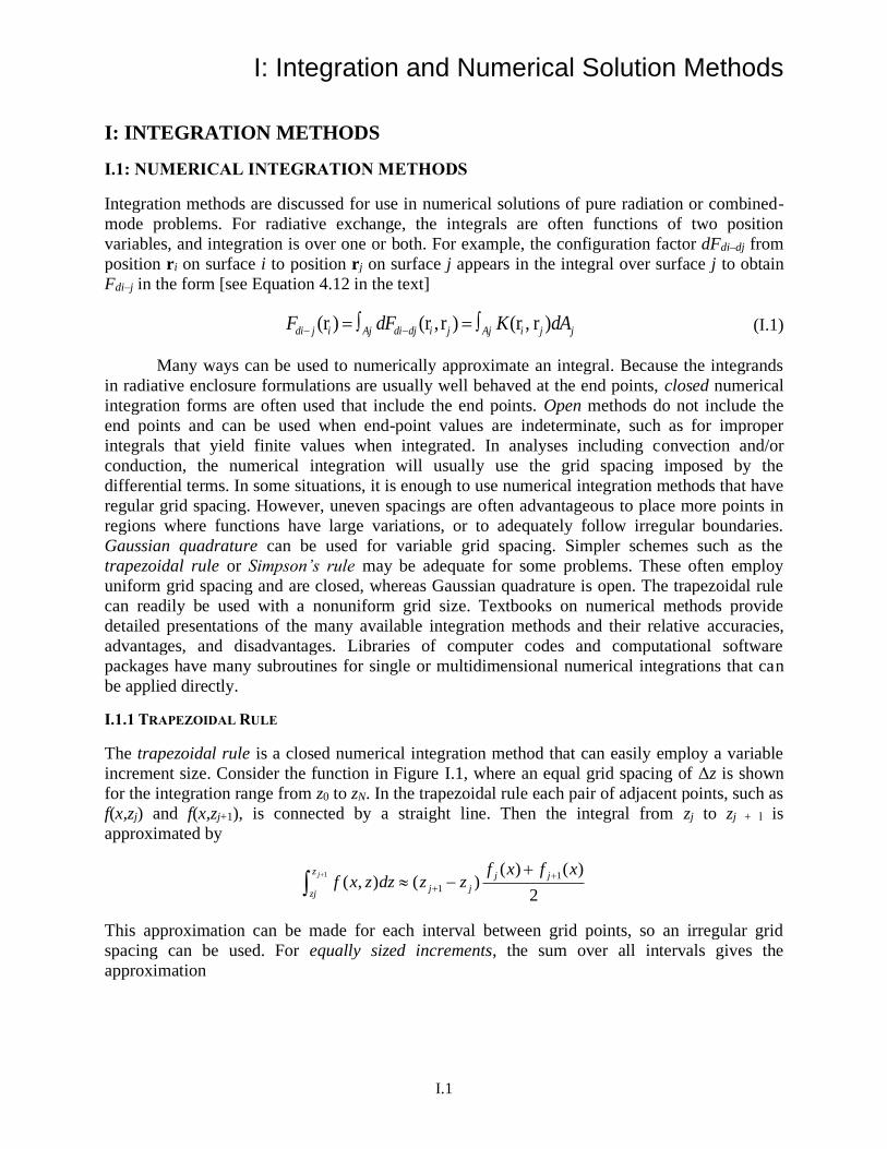
I: Integration and Numerical Solution Methods
I.1
I: INTEGRATION METHODS
I.1: NUMERICAL INTEGRATION METHODS
Integration methods are discussed for use in numerical solutions of pure radiation or combined-
mode problems. For radiative exchange, the integrals are often functions of two position
variables, and integration is over one or both. For example, the configuration factor dFdi–dj from
position ri on surface i to position rj on surface j appears in the integral over surface j to obtain
Fdi–j in the form [see Equation 4.12 in the text]
(r ) (r , r ) (r , r )di j i Aj di dj i j Aj i j jF dF K dA− −= = (I.1)
Many ways can be used to numerically approximate an integral. Because the integrands
in radiative enclosure formulations are usually well behaved at the end points, closed numerical
integration forms are often used that include the end points. Open methods do not include the
end points and can be used when end-point values are indeterminate, such as for improper
integrals that yield finite values when integrated. In analyses including convection and/or
conduction, the numerical integration will usually use the grid spacing imposed by the
differential terms. In some situations, it is enough to use numerical integration methods that have
regular grid spacing. However, uneven spacings are often advantageous to place more points in
regions where functions have large variations, or to adequately follow irregular boundaries.
Gaussian quadrature can be used for variable grid spacing. Simpler schemes such as the
trapezoidal rule or Simpson’s rule may be adequate for some problems. These often employ
uniform grid spacing and are closed, whereas Gaussian quadrature is open. The trapezoidal rule
can readily be used with a nonuniform grid size. Textbooks on numerical methods provide
detailed presentations of the many available integration methods and their relative accuracies,
advantages, and disadvantages. Libraries of computer codes and computational software
packages have many subroutines for single or multidimensional numerical integrations that can
be applied directly.
I.1.1 TRAPEZOIDAL RULE
The trapezoidal rule is a closed numerical integration method that can easily employ a variable
increment size. Consider the function in Figure I.1, where an equal grid spacing of Δz is shown
for the integration range from z0 to zN. In the trapezoidal rule each pair of adjacent points, such as
f(x,zj) and f(x,zj+1), is connected by a straight line. Then the integral from zj to zj + l is
approximated by
1 1
1
( ) ( )( , ) ( )
2
jz j j
j jzj
f x f xf x z dz z z
+ +
+
+ −
This approximation can be made for each interval between grid points, so an irregular grid
spacing can be used. For equally sized increments, the sum over all intervals gives the
approximation
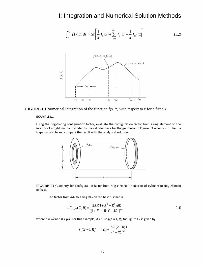
I: Integration and Numerical Solution Methods
I.2
N
0
N 1
0 N
1
1 1( , ) ( ) ( ) ( )
2 2
z
jz
j
f x z dz z f x f x f x−
=
+ +
(I.2)
FIGURE I.1 Numerical integration of the function f(x, z) with respect to z for a fixed x.
EXAMPLE I.1
Using the ring-to-ring configuration factor, evaluate the configuration factor from a ring element on the interior of a right circular cylinder to the cylinder base for the geometry in Figure I.2 when x = r. Use the trapezoidal rule and compare the result with the analytical solution.
FIGURE I.2 Geometry for configuration factor from ring element on interior of cylinder to ring element
on base.
The factor from dA1 to a ring dA2 on the base surface is
2 2
1 2 2 2 2 2 3/ 2
2 (1 )( , )
[(1 ) 4 ]d d
XR X R dRdF X R
X R R−
+ −=
+ + − (I.3)
where X = x/r and R = ρ/r. For this example, X = 1, so fj(X = 1, Rj) for Figure I.2 is given by
2
4 3/2
2 (2 )( 1, ) (1)
(4 )
j j
j j j
j
R Rf X R f
R
−= =
+

I: Integration and Numerical Solution Methods
I.3
where Rj = jΔR and ΔR = 1/N. Letting ( 1, ) (1),j jf X j R f=
2
0 4 3/ 2 3/ 2
2 [2 ( ) ] 2(1) 0, (1) , (1)
[4 ( ) ] 5j N
j R j Rf f f
j R
− = = =
+
These terms are substituted into Equation I.2, and for N = 5 yields
1 2( 1) (1/ 5)[(1/ 2 0 0.09794 0.18225 0.23451 0.23500 (1/ 2) 0.17889] 0.16783− = = + + + + + =dF X
The exact configuration factor is in Appendix C of the text as
2
21 2 1/ 2
112( 1) ,
2 2 2( 1)d
Xx X
F X X XrX
−
+
= = − = = =+
which gives 1 2 1 2( 1) ( 0.5) 0.17082d dF X F X
− −= = = = . Larger numbers of increments improve the accuracy
as follows:
N Fd1–2(X = 1) % Error
5 0.16783 −1.75
10 0.17007 −0.44
50 0.17079 −0.02
100 0.17081 −0.006
200 0.17082 0
I.1.2 SIMPSON’S RULE
The usual Simpson’s rule is obtained by passing a parabola through three adjacent grid points.
For equally spaced increments the integral from zj to zj + 2 is approximated by
2
1 2( ) ( 4 )3
j
j
z
j j jz
zf z dz f f f
+
+ +
+ +
Because this uses two Δz increments, the repeated application for a range with many grid points
requires an even number of increments (an odd number of points). For N equally spaced
increments in Figure I.1, the result is
0 1 2 3 N 1 N( ) ( 4 2 4 4 )3
N
o
z
z
zf z dz f f f f f f−
+ + + + + + (I.4)
If an odd number of increments must be used, Simpson’s rule can be applied over an even
number of increments, and the trapezoidal rule used for the remaining increment.
If the curve in Figure I.1 goes through a sharp cusplike peak, it may not be accurate to
apply Simpson’s rule if the peak is at the central point of the three adjacent points; the cusplike
behavior is not accurately approximated by a parabolic curve. Simpson’s rule could be used for
two increments on each side of the peak. Care should be used in selecting a suitable integration
scheme for each application.
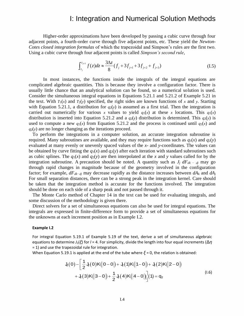
I: Integration and Numerical Solution Methods
I.4
Higher-order approximations have been developed by passing a cubic curve through four
adjacent points, a fourth-order curve through five adjacent points, etc. These yield the Newton-
Cotes closed integration formulas of which the trapezoidal and Simpson’s rules are the first two.
Using a cubic curve through four adjacent points is called Simpson’s second rule,
3
1 2 3
3( ) ( 3 3 )
8
j
j
z
j j j jz
zf z dz f f f f
+
+ + +
+ + + (I.5)
In most instances, the functions inside the integrals of the integral equations are
complicated algebraic quantities. This is because they involve a configuration factor. There is
usually little chance that an analytical solution can be found, so a numerical solution is used.
Consider the simultaneous integral equations in Equations 5.21.1 and 5.21.2 of Example 5.21 in
the text. With T1(x) and T2(y) specified, the right sides are known functions of x and y. Starting
with Equation 5.21.1, a distribution for q2(y) is assumed as a first trial. Then the integration is
carried out numerically for various x values to yield q1(x) at these x locations. This q1(x)
distribution is inserted into Equation 5.21.2 and a q2(y) distribution is determined. This q2(y) is
used to compute a new q1(x) from Equation 5.21.2 and the process is continued until q1(x) and
q2(y) are no longer changing as the iterations proceed.
To perform the integrations in a computer solution, an accurate integration subroutine is
required. Many subroutines are available, and they may require functions such as q1(x) and q2(y)
evaluated at many evenly or unevenly spaced values of the x- and y-coordinates. The values can
be obtained by curve fitting the q1(x) and q2(y) after each iteration with standard subroutines such
as cubic splines. The q1(x) and q2(y) are then interpolated at the x and y values called for by the
integration subroutine. A precaution should be noted. A quantity such as Jj dFdk − dj may go
through rapid changes in magnitude because of the geometry involved in the configuration
factor; for example, dFdk−dj may decrease rapidly as the distance increases between dAk and dAj
For small separation distances, there can be a strong peak in the integration kernel. Care should
be taken that the integration method is accurate for the functions involved. The integration
should be done on each side of a sharp peak and not passed through it.
The Monte Carlo method of Chapter 14 in the text can be used for evaluating integrals, and
some discussion of the methodology is given there.
Direct solvers for a set of simultaneous equations can also be used for integral equations. The
integrals are expressed in finite-difference form to provide a set of simultaneous equations for
the unknowns at each increment position as in Example I.2.
Example I.2
For integral Equation 5.19.1 of Example 5.19 of the text, derive a set of simultaneous algebraic equations to determine J2(ξ) for l = 4. For simplicity, divide the length into four equal increments (Δη = 1) and use the trapezoidal rule for integration. When Equation 5.19.1 is applied at the end of the tube where ξ = 0, the relation is obtained:
( ) ( ) ( ) ( ) ( ) ( ) ( )
( ) ( ) ( ) ( ) ( )
− − + − + −
+ − + − =
2 2 2 2
2 2 2
10 0 0 0 1 1 0 2 2 0
2
13 3 0 4 4 0 1
2
J J K J K J K
J K J K q (I.6)
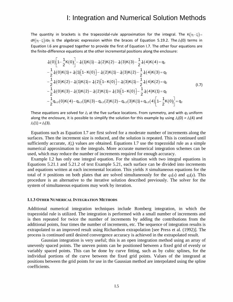
I: Integration and Numerical Solution Methods
I.5
The quantity in brackets is the trapezoidal-rule approximation for the integral. The ( )− =K
( )− /dF d is the algebraic expression within the braces of Equation 5.19.2. The J2(0) terms in
Equation I.6 are grouped together to provide the first of Equation I.7. The other four equations are the finite-difference equations at the other incremental positions along the enclosure:
( ) ( ) ( ) ( ) ( ) ( ) ( ) ( ) ( ) ( )
( ) ( ) ( ) ( ) ( ) ( ) ( ) ( ) ( ) ( )
( ) ( ) ( ) ( ) ( ) ( ) ( ) ( ) ( ) ( )
( ) ( ) ( ) ( ) ( ) ( ) ( ) ( ) ( ) ( )
( ) ( ) ( ) ( ) ( ) ( )
− − − − − =
− + − − − − =
− − + − − − =
− − − + − − =
− − − −
2 2 2 2 2 2
2 2 2 2 2 2
2 2 2 2 2 2
2 2 2 2 2 2
,2 ,2 ,2
1 10 1 0 1 1 2 2 3 3 4 4
2 2
1 10 1 1 1 0 2 1 3 2 4 3
2 21 1
0 2 1 1 2 1 0 3 1 4 22 21 1
0 3 1 2 2 1 3 1 0 4 12 21
0 4 1 3 2 22
o o o
J K J K J K J K J K q
J K J K J K J K J K q
J K J K J K J K J K q
J K J K J K J K J K q
q K q K q K ( ) ( ) ( ) ( )
+ − =
,2 ,2 2
13 1 4 1 0
2o oq K q K q
(I.7)
These equations are solved for J2 at the five surface locations. From symmetry, and with q2 uniform along the enclosure, it is possible to simplify the solution for this example by using J2(0) = J2(4) and J2(1) = J2(3).
Equations such as Equation I.7 are first solved for a moderate number of increments along the
surfaces. Then the increment size is reduced, and the solution is repeated. This is continued until
sufficiently accurate, J(ξ) values are obtained. Equations I.7 use the trapezoidal rule as a simple
numerical approximation to the integrals. More accurate numerical integration schemes can be
used, which may reduce the number of increments required for enough accuracy.
Example I.2 has only one integral equation. For the situation with two integral equations in
Equations 5.21.1 and 5.21.2 of text Example 5.21, each surface can be divided into increments
and equations written at each incremental location. This yields N simultaneous equations for the
total of N positions on both plates that are solved simultaneously for the q1(x) and q2(y). This
procedure is an alternative to the iterative solution described previously. The solver for the
system of simultaneous equations may work by iteration.
I.1.3 OTHER NUMERICAL INTEGRATION METHODS
Additional numerical integration techniques include Romberg integration, in which the
trapezoidal rule is utilized. The integration is performed with a small number of increments and
is then repeated for twice the number of increments by adding the contributions from the
additional points, four times the number of increments, etc. The sequence of integration results is
extrapolated to an improved result using Richardson extrapolation [see Press et al. (1992)]. The
process is continued until desired convergence accuracy is achieved in the extrapolated result.
Gaussian integration is very useful; this is an open integration method using an array of
unevenly spaced points. The uneven points can be positioned between a fixed grid of evenly or
variably spaced points. This can be done by curve fitting, such as by cubic splines, for the
individual portions of the curve between the fixed grid points. Values of the integrand at
positions between the grid points for use in the Gaussian method are interpolated using the spline
coefficients.

I: Integration and Numerical Solution Methods
I.6
Many numerical integration subroutines have been written for computer use and the
software can be readily applied. Curve-fitting software routines are available that can be used in
conjunction with Gaussian or other techniques, requiring interpolation to obtain unevenly spaced
values of the function being integrated. Some subroutines perform multidimensional integrations.
Computational software packages for mathematics provide numerical integration using, for
example, Romberg integration, Simpson’s rule, and adaptive methods; singular and infinite end
points are also treated.
Fan et al. (2019) examine fast algorithms for solving the steady state integral form of the RTE
based on fast Fourier transforms for homogeneous media and a recursive skeletonization-
factorization technique for inhomogeneous media. They show that a unique solution to the RTE
exists and provide sample solutions for isotropic and anisotropic scattering in 2- and 3D. Zhou et
al. (2020) propose methods to subtract singularities in integrated forms of the RTE for use in
analytical and numerical solutions.
I.2: ANALYTICAL INTEGRATION METHODS FOR ENCLOSURES
The unknown wall heat fluxes or temperatures along the surfaces of an enclosure are found from
solutions of single or simultaneous integral equations. The integral equations in the formulations
up to now are linear; that is, the unknown q, J, or T 4 variables always appear to the first power
(note that T 4 is the linear variable rather than T). For linear integral equations, there are various
numerical and analytical solution methods; these are discussed in mathematics texts.
For some simple geometries and special conditions, the integral equations describing radiative
transfer among surfaces may be solved analytically. Such solutions are usually limited to single-
surface or two-surface enclosures, so are not described here in detail.
If the kernel of the integral equation is separable, that is, K(rj,rk) = Fj(rj)Fk(rk), then Fk(rk) may
be removed from the integral over rj, possibly simplifying analytical or numerical integration.
However, the kernel in radiation problems usually is not separable. The general theory of
solution of integral equations using separable kernels is in Hildebrand (1992) and an application
using a separable exponential approximation to the kernel (Usiskin and Siegel 1960), allowing
reduction of the integral equation to a differential equation, is in Buckley (1927, 1928).
The variational method (Hildebrand 1992) may be applied if the kernel is symmetric, that is,
K(ξ,η) = K(η,ξ). This approach has been used for radiation in a cylindrical tube (Usiskin and
Siegel 1960) and for radiative exchange between infinitely long parallel plates of finite width
(Sparrow 1960).
An approximate solution may be obtained through a Taylor series expansion (Krishnan and
Sundaram 1960, Perlmutter and Siegel 1963), which works well if the kernel ( ) − K decays
rapidly as ξ − η increases as for the cylindrical geometry illustrated in Figure 5.19. The integrand
of the integral equations then becomes a series that may be truncated after a few terms and then
integrated term by term, reducing the integral equation to a differential equation. Applications
are in Choi and Churchill (1985) and Qiao et al. (2000).
The method of Ambartsumian can be applied if the temperature or heat flux boundary
conditions can be approximately described by an exponential variation or a sum of exponentials,
allowing transformation of the integral equation into an initial value problem (Ambartsumian
1942, Kourganoff 1963, Crosbie and Sawheny 1974, 1975).
I: Integration and Numerical Solution Methods
I.7
The problem of finding the intensity leaving a circular opening in a spherical cavity exposed to
external uniform heat flux incident on element dA2, qe(dA2), and with a prescribed internal
temperature distribution T(dA1) on the cavity surface has been solved analytically (Jakob 1957,
Sparrow and Jonsson 1962). If the internal surface of the cavity has emissivity ε, then the
intensity leaving an element dA1* through the cavity opening in a direction is found to be
( )( )
( )1 2
44 1 1 1 e 2 221 1
1 11 2
1
***
1 1( ) ( )
4( )
1 1 /4
A A
T dA dA q dA dAT dA RJ dAI dA
A R
− + = = +
− −
(I.8)
All these analytical methods become intractable when multiple surfaces are present, and
numerical solution techniques are almost always required for more realistic cases.
I.2.1 EXACT SOLUTION OF INTEGRAL EQUATION FOR RADIATION FROM A SPHERICAL CAVITY
Radiation from a spherical cavity as in Figure I.3a was analyzed by Jakob (1957) and Sparrow
and Jonsson (1962). The spherical shape leads to a relatively simple integral-equation solution
because there is an especially simple configuration factor between elements on the inside of a
sphere. For the two differential elements dAj and dAk in Figure I.3b,
2
cos cosj kdj dk kdF dA
S−
=
(I.9)
Since the sphere radius is normal to both dAj and dAk, the distance between these elements is
S = 2Rcosθj = 2Rcosθk. Then, Equation I.9 becomes
24
k kdj dk
s
dA dAdF
AR− = =
(I.10)
where As is the surface area of the entire sphere. If dAj exchanges with the finite area, then
Equation I.10 becomes
2 2s
1
4 4k
k kdj k k
A
A AF dA
AR R− = = =
(I.11)
Equation I.11 is independent of dAj, so dAj can be replaced by any finite area Aj to give
2s4
k kj k
A AF
AR− = =
(I.12)
The configuration factor from any area to any area is simply the fraction of the total sphere area
that the receiving area occupies.
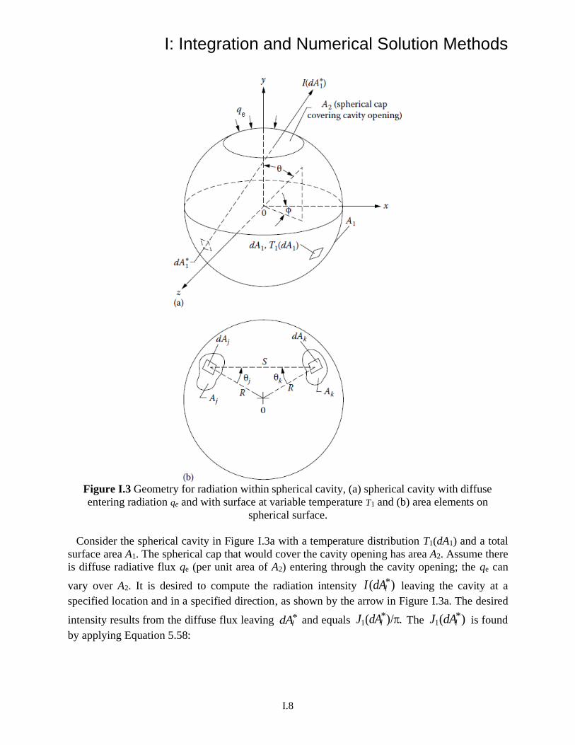
I: Integration and Numerical Solution Methods
I.8
Figure I.3 Geometry for radiation within spherical cavity, (a) spherical cavity with diffuse
entering radiation qe and with surface at variable temperature T1 and (b) area elements on
spherical surface.
Consider the spherical cavity in Figure I.3a with a temperature distribution T1(dA1) and a total
surface area A1. The spherical cap that would cover the cavity opening has area A2. Assume there
is diffuse radiative flux qe (per unit area of A2) entering through the cavity opening; the qe can
vary over A2. It is desired to compute the radiation intensity *( )lI dA leaving the cavity at a
specified location and in a specified direction, as shown by the arrow in Figure I.3a. The desired
intensity results from the diffuse flux leaving *ldA and equals 1
*( )/ .lJ dA The 1*( )lJ dA is found
by applying Equation 5.58:
I: Integration and Numerical Solution Methods
I.9
( ) ( ) ( ) ( ) ( ) ( )1 2
* *4
1 1 1 1 1 1 e 2 1 1 11 1 1 2* *1 1
d d d d
A A
J dA J dA dF q dA dF T dA− −
− − − − = (I.13)
and an exact solution will be found. The F factors from Equation I.9 are substituted to give
( ) ( ) ( ) ( )1 2
1 1 41 1 1 1 1 2 2 1 1 12 2
** 1 1
4 4e
A A
J dA J dA dA q dA dA T dAR R
− − − = +
(I.14)
To solve Equation I.14, a trial solution ( ) ( )1**
l lJ dA f dA C= + is assumed, where *( )lf dA is
an unknown function of the location of 1*dA , and C is a constant. Substituting into Equation I.14
gives
( ) ( ) ( ) ( )1 2
1 1 1 41 1 1 1 e 2 2 1 1 12 2 2* *1 1 1
4 4 4A A
f dA C f dA dA CA q dA dA T dAR R R
− − − + − − = +
(I.15)
From the two terms that are functions of local position, ( ) ( )41 1 1 1
** .f dA T dA= The remaining
terms are equated to determine C. This gives the desired result as an exact solution:
( )( ) ( ) ( ) ( )
( )1 2
1 44 1 1 1 1 2 221 1 1 1 1
1 21 1
**
*
1 1
4
1 1 /4
eA A
T dA dA q dA dAJ dA T dA RI dA
A R
− + = = +
− −
(I.16)
I.3 NUMERICAL SOLUTION METHODS FOR NONLINEAR EQUATIONS
Most nonlinear equations for mixed-mode problems with radiation can be cast in the form
4A B C + = ij j ij j i (I.17)
It is important to examine the relative values of the elements Aij and Bij. If the Aij are
comparatively large, the problem can be treated as linear in ϑj; conversely, for large Bij, the
problem can be treated as linear in 4.j When the coefficients A and B are approximately equal,
other treatments are in order.
If we define 3
ij ij ij jA A B = + , Equation I.17 becomes
4 3ij j ij j ij ij j j ij j iA B A B A C + = + = =
(I.18)
This is a set of linear algebraic equations with coefficients *ijA that are variable and nonlinear.
The equations cannot be solved by elimination or direct matrix inversion, because the *ijA are

I: Integration and Numerical Solution Methods
I.10
temperature dependent and thus are not known. Some numerical solution methods are now
discussed.
I.3.1 SUCCESSIVE SUBSTITUTION METHODS
I.3.1.1 Simple Successive Substitution (SSS)
A simple solution method is to assume an initial set of temperatures ( )0j and use them to
compute ( )( )0* .ij jA
This provides values for the elements in the matrix of coefficients, leaving
the temperature vector [ϑj] as the unknown. Equation I.18 is then solved for a new set of
temperatures ( )1nj
+
from
( ) ( ) ( 1)n nij ij jA C+ =
(I.19)
This process is continued until the difference between successive temperature sets is less than an
acceptable error, indicating convergence. A difficulty is that this method depends on an accurate
initial guess for [ϑj]. An inaccurate guess can lead to unstable iterations that may diverge rapidly.
For an extended discussion of some of the pitfalls of SSS, see Howell (2017).
I.3.1.2 Successive Underrelaxation
The simple successive substitution (SSS) method can be modified to obtain convergence in many
cases if Equation I.17 is written as
( ) ( ) ( 1)n nij ij jA C− =
(I.20)
where the ( )( )** nij jA are computed at each iteration by using a modified temperature
( ) ( ) ( 1)(1 )n n nj j j − = + − (I.21)
The α is a weighting coefficient, or relaxation parameter, in the range 0 ≤ α ≤ 1. When α = 1, the
successive underrelaxation (SUR) method reduces to SSS; when α < 1, the new guess is
weighted toward the previous guess (i.e., underrelaxed), and oscillations between iterations are
damped. If possible, the α should be chosen or found that provides optimized convergence.
Decreasing α usually provides slower convergence, but greater assurance that convergence will
occur. Sometimes decreasing α somewhat will increase convergence by reducing oscillatory
behavior. Values of α ≈ 0.3 are reported by Cort et al. (1982) to provide rapid convergence in
many cases.

I: Integration and Numerical Solution Methods
I.11
I.3.1.3 Regulated Successive Underrelaxation
Cort et al. (1982) proposed a method of regulated successive underrelaxation (RSUR) that allows
the underrelaxation factor α to be chosen and modified for successive iterations. They
recommend the following: (1) Initialize α = 1; (2) solve Equation I.21 for ( )* n
j (for the first
iteration, an initial guess ( )
0j must be provided); (3) solve Equation I.20 for + 1;n
j (4) calculate
( )( 1)
1/2
2( 1) ( )
1
nN
n nj j
j
++
=
= − (I.22)
( )( 1) ( 1)
1/2
2
1
n nN
j
j
R+ +
=
= (I.23)
and if v(n+1) > v(n) or if v(n+1) > (1/3)R(n+1), reduce α by 0.1; and (5) repeat steps (2) through (4)
until convergence.
Equation I.22 checks for divergence of the solution between iterations, and Equation I.23 is
used to see whether the residual error after each iteration is smaller than a measure of the root-
mean-square temperature over the region of the solution. The latter check eliminates slowly
oscillating but converging solutions that pass the test of Equation I.22 but converge very slowly.
Another approach is to rewrite Equation I.17 in the form
( ) ( )4 4
( 1) ( 1) ( 1) ( 1)
1
(1 )
N
n n n nii ii i ij ij ij ii i j j
j
A B C A B D+ + + +
=
+ = − − + (I.24)
where δij is the Kronecker delta. An initial set of temperatures ( )
0j is guessed, and Di is evaluated
based on this set. Then the ( )
1j are found by iterative solution of Equation I.24 and are used to
evaluate the next set of Di. This process is repeated to solve for ( )
ni until convergence. Tan (1989)
points out that, for a given value of i, Equation I.24 is a quartic equation with a single real
positive root ( )+
1ni given by
1/2( 1)
1/2
2
2 ( 1) 1
ni
y p
p
+ − =
− + (I.25)
where
1/2
2 2/3 1/3 1/3 1/3
4 22 1 ,
( ) ( ) [( ) ( ) ]
i
ii
D rp y
B y s r s r s r s r
= + =
+ + − + + −
and
1/22 3
21 4,
2 3
ii i
ii ii
A Dr s r
B B
= = +
.
Thus, for each set of Di, the ( )+
1ni can be found directly from the nonlinear Equation I.24 rather
than by an inner iteration and then can be used to evaluate new Di and continue to the next main

I: Integration and Numerical Solution Methods
I.12
iteration. This method is quite fast and can be combined with the SUR technique to determine
succeeding approximations to provide a method that is both stable and fast.
I.3.2 NEWTON–RAPHSON-BASED METHODS FOR NONLINEAR PROBLEMS
I.3.2.1 Modified Newton–Raphson
A modified Newton–Raphson (MNR) method is in Ness (1959) for the class of nonlinear
problems encountered here. Starting from Equation I.17,
4 0ij j ij j iA B C + − = (I.26)
an initial approximate temperature ( )
0j is guessed at each node. A correction factor δj is then
computed so that ( )0
.j jj = + This ϑj is used to compute a new δj, and this process is
continued until δj becomes smaller than a specified value. The δj are found by solving the set of
linear equations:
[ ][ ] [ ] 0ij j if f + = (I.27)
where
( )4
(0) (0)
1
N
i ij ij ij j
j
f A B C
=
= + − (I.28)
and
( )3
(0)4ij ij ij jf A B= + (I.29)
The MNR method may not converge if a poor initial temperature set is chosen.
7.5.3.2.2 Accelerated Newton–Raphson
Cort et al. (1982) proposed a method in which the amount of change in ϑi at each iteration is
adjusted to accelerate convergence. They recommended that the fij in the MNR method be
replaced by
( )(3 )
(0)40
[1 ( /3)]
ijij ij j
Bf A
−
= + −
(I.30)
This effectively modifies the slope of the changes in ϑj with respect to iteration number
compared with that used in the MNR method. For β = 0, the accelerated Newton–Raphson
(ANR) method reduces to MNR. If β is too large, oscillations and divergence between iterations
may occur. For β = 0.175, the number of iterations to provide a given accuracy for a particular
I: Integration and Numerical Solution Methods
I.13
problem was reduced from 28 using MNR to 12 using ANR, and reductions in computer time of
up to 80% were obtained. A starting value of β = 0.15 is recommended by Cort et al.
7.5.3.3 APPLICATIONS OF THE NUMERICAL METHODS
Results using the aforementioned methods were compared in Cort et al. (1982) for some typical
radiation–conduction problems with temperature-dependent properties and internal energy
generation. Consideration was limited to surfaces with radiative exchanges to black surroundings
at a single temperature, and the solutions were by finite elements. Because the example problems
in this section showed that even complicated radiation–conduction–convection problems with
multiple surfaces reduce to the same general form of Equations 1.17, the conclusions probably
apply to a broader class of problems than was studied. In Costello and Shrenk (1966), a
linearized solution is proposed that speeds convergence over the MNR method. For problems
that are either conduction or radiation dominated or where both modes are important, the method
performed well, providing a factor-of-ten improvement in solution speed. It was found that the
SUR method gave convergence with the fewest iterations and the least computer time; RSUR
was useful to find the optimum value of the relaxation parameter α for use in the SUR method.
For the Newton–Raphson method, ANR was always faster than MNR, but neither method was as
fast as SUR.
In Howell (1992, 2017), the convergence ranges and behavior of equations of the form of
Equations I.17 are discussed, and the various solution methods of this chapter are examined.
Nonlinear equations of this type can have behavior characterized by bifurcations and chaos of
successive iterations so that steady solutions carried out by SSS, SUR, etc., may not converge.
This is true whether the equations are cast as radiation dominated or first-order temperature
dominated or the equations used are in mixed form such as Equation I.18. Decreasing the
relaxation factor extends the range of convergence, but often will not yield a solution for some
ranges of parameters without unacceptable computer time. For conduction–radiation problems,
bifurcation–chaos behavior results from the numerical method chosen and the equation form and
does not imply that multiple physical solutions can exist. However, when there is coupling
between radiation and the flow field, as in combined radiation and free convection, multiple
physical steady-state solutions may exist. The particular flow configuration reached in a steady
state analysis may depend on the initial conditions chosen and the set of velocity and temperature
fields that are traversed in reaching steady state. In some cases, no steady solution is reached; it
may be possible to solve for the steady-state solution by using a fully transient solution that
proceeds to the final steady state from physically specified initial conditions.
Numerical solution techniques for steady-state and transient combined-mode problems with
surface–surface radiative exchange are examined and discussed by Hogan and Gartling (2008).
Three techniques that sequentially solve for radiative transfer followed by solution of the energy
equation with a radiative source term are compared with a fully coupled solution. For the two
example problems studied, the fully coupled method always produced the most accurate solution,
I: Integration and Numerical Solution Methods
I.14
although execution time made it unattractive for very large problems. A semi-implicit technique
with a Newton type of update appeared to be the best choice for very large problems.
The finite-difference and finite-element numerical procedures that have been described used
radiative enclosure theory with finite or infinitesimal areas to obtain a set of simultaneous
equations with configuration factors for radiative exchange between surface areas. Convection
was specified in terms of a heat transfer coefficient for each area; for example, for radiation
exchange inside a tube with a flowing transparent gas, the heat transfer coefficient inside the tube
is obtained from available results from tube flow analyses or experimental correlations. For some
situations, however, convection is quite dependent on the surface temperatures, such as for free
convection, or the geometry is complex so that convective heat transfer correlations are not
available with desired accuracy. In these cases, analyses have been made where convection is
solved simultaneously with radiation as the flow and surface temperatures are strongly coupled;
conduction may also be included, such as for free convection and radiation from a cooling fin as
discussed in Section 7.4.3 of the book. To solve for the convection heat transfer, the methods of
computational fluid mechanics are used.
Another consideration is that the analysis may not use configuration factors. The radiative
exchange in an enclosure can be computed directly by a ray-tracing technique such as a Monte
Carlo method (Chapter 14 of the book). This may be necessary if the surfaces are not diffuse so
that configuration factors do not apply. Another solution method where radiation is followed
along directions is by use of discrete ordinates. The discrete ordinates method, discussed in
Chapter 12, was developed for enclosures filled with a medium that is not transparent, but rather
absorbs, emits, and scatters radiation. If radiative participation by the medium is omitted, the
method can be applied to enclosures containing a transparent medium such as a convecting
nonradiating gas. In this method, the angular directions from each surface element are divided
into a finite number, and radiation is followed along these discrete directions to evaluate the
radiative exchange. In Tan et al. (1998), discrete ordinates are used in combination with the
SIMPLE computer algorithms developed for computational fluid mechanics (Patankar 1980) to
simultaneously solve the mass, momentum, and energy equations along with radiation transfer
between surfaces.
For natural convection combined with radiation, many computational methods have been used
for simultaneously solving the fluid flow and energy equations with radiative exchange. In Zhao
et al. (1992), free convection and radiation were analyzed for heated cylinders in a rectangular
enclosure. In Dehghan and Behnia (1996), net radiation enclosure analysis was used for the
radiative transfer, and the flow and energy equations were placed in finite-difference form and
solved with a pseudo transient method to analyze free convection in a cavity with a local heated
area on one vertical wall. A vented cavity with a discrete heat source was analyzed by Yu and
Joshi (1999) using the numerical methods from Patankar (1980); this study included combined
radiation exchange, conduction, and natural convection, with the gas in the cavity being
transparent. Free convection of transparent air in a heated vertical channel with one or more
vents in one wall was analyzed by Moutsoglou et al. (1992). The flow and energy equations were
I: Integration and Numerical Solution Methods
I.15
solved by using finite-difference computational methods as developed by Patankar and Spalding
(1972) and van Doormall and Raithby (1983).
REFERENCES:
Ambarzumian, V. A.: Diffusion of light by planetary atmospheres, Astron. Zh., 19, 30–41, 1942.
Buckley, H.: On the radiation from the inside of a circular cylinder: Part I, Philos. Mag., 4, 753–762, 1927; Part II,
Philos. Mag., 6, 447–457, 1928.
Choi, B. C. and Churchill, S. W.: A technique for obtaining approximate solutions for a class of integral equations
arising in radiative heat transfer, Int. J. Heat Fluid Flow, 6(1), 42–48, 1985.
Cort, G. E., Graham, H. L., and Johnson, N. L.: Comparison of methods for solving non-linear finite element
equations in heat transfer, ASME Paper 82-HT-40, Proc. 21st National Heat Transfer Conf., Seattle, August
1982.
Costello, F. A. and Schrenk, G. L.: Numerical solution to the heat-transfer equations with combined conduction and
radiation, J. Comput. Phys., 1, 541–543, 1966.
Crosbie, A. L. and Sawheny, T. R.: Application of Ambarzumian’s method to radiant interchange in a rectangular
cavity, JHT, 96, 191–196, 1974.
Crosbie, A. L. and Sawheny, T. R.: Radiant interchange in a nonisothermal rectangular cavity, AIAA J., 13(4), 425–
431, 1975.
Dehghan, A. A. and Behnia, M.: Combined natural convection-conduction and radiation heat transfer in a discretely
heated open cavity, JHT, 118(1), 56–64, 1996.
Fan, Y., An, J. and Yin, L.: Fast algorithms for integral formulations of steady-state radiative transfer equation, J.
Computational Physics, 380(1), 191-211, Jan. 2018.
Hildebrand, F. B.: Methods of Applied Mathematics, 2nd edn., Dover, New York, 1992.
Hogan, R. E. and Gartling, D. K.: Solution strategies for coupled conduction/radiation problems, Commun. Numer.
Methods Eng., 24(6), 523–542, June 2008.
Howell, J. R.: Modern computational methods in radiative heat transfer, in K. T. Yang and W. Nakayama (eds.),
Computers and Computing in Heat Transfer Science and Engineering, pp. 153–171, CRC Press, Boca Raton,
FL, December 1992.
Howell, J. R.: The effect of bifurcation on numerical calculation of conjugate heat transfer with radiation, JQSRT,
196, 242-245, 2017. Jakob, M.: Heat Transfer, vol. II, Wiley, New York, 1957.
Kourganoff, V.: Basic Methods in Transfer Problems, Dover, New York, 1963.
Krishnan, K. S. and Sundaram, R.: The distribution of temperature along electrically heated tubes and coils, I.
Theoretical, Proc. R. Soc. Lond., Ser. A, 257(1290), 302–315, 1960.
Moutsoglou, A., Rhee, J. H., and Won, J. K.: Natural convection-radiation cooling of a vented channel, IJHMT,
35(11), 2855–2863, 1992.
Ness, A. J.: Solution of equations of a thermal network on a digital computer, Solar Energy, 3(2), p. 37, 1959.
Patankar, S. V.: Numerical Heat Transfer and Fluid Flow, Hemisphere, Washington, DC, 1980.
Patankar, S. V. and Spalding, D. B.: A calculation procedure for heat, mass, and momentum transfer in three-
dimensional parabolic flows, IJHMT, 15, 1787–1806, 1972.
Perlmutter, M. and Siegel, R.: Effect of specularly reflecting gray surface on thermal radiation through a tube and
from its heated wall, JHT, 85(1), 55–62, 1963.
Press, W. H., Flannery, B. P., Teukolsky, S. A., and Vetterling, W. T.: Numerical Recipes in C: The Art of Scientific
Computing, 2d ed., Cambridge University Press, London, 1992.
Qiao, H., Ren, Y., and Zhang, B.: Approximate solution of a class of radiative heat transfer problems, JHT, 122(3),
606–612, 2000.
Sparrow, E. M.: Application of variational methods to radiation heat-transfer calculations, JHT, 82(4), 375–380,
1960.
Sparrow, E. M. and Jonsson, V. K.: Absorption and Emission Characteristics of Diffuse Spherical Enclosures,
NASA TN D-1289, Washington, DC, 1962.
Tan, Z., Przekwas, A. J., Wang, D., Srinivasan, K., and Sun, R.: Numerical simulation of coupled radiation and
convection for complex geometries, Paper AIAA-98-2677, Seventh AIAA/ASME Joint Thermophysics and Heat
Transfer Confeerence, Albuquerque, NM, June 1998.
I: Integration and Numerical Solution Methods
I.16
Usiskin, C. M. and Siegel, R.: Thermal radiation from a cylindrical enclosure with specified wall heat flux, JHT,
82(4), 369–374, 1960.
van Doormall, J. P. and Raithby, G. D.: Enhancements of the simple method for predicting incompressible fluid
flows, Numer. Heat Transfer, 7, 147–163, 1983.
Yu, E. and Joshi, Y. K.: Heat transfer in discretely heated side-vented compact enclosures by combined conduction,
natural convection, and radiation, JHT, 121(4), 1002–1010, 1999.
Zhou, R.-R., Li, B.-W., Wang, W.-K., and Sun, Y.-A.: Improved integration strategies for the singularity subtraction
method to solve radiative integral transfer equations with specified temperature field, IJTS, 149, 106158, 2020.
Zhao, Z., Poulikakos, D., and Ren, Z.: Combined natural convection and radiation from heated cylinders inside a
container, JTHT, 6(4), 713–720, 1992.
J: Radiative Cooling
J.1
J: RADIATIVE COOLING
Under certain conditions, enhanced cooling by radiation from surfaces is useful. This can be
achieved if the emission from the surface is enhanced at the longer wavelengths where most of
the cooling (radiative energy loss) takes place. In addition, it is desirable to minimize the
radiative energy gain of a given surface at the same time. This can be realized by decreasing the
solar absorption and increasing the IR emission of the surface. Such spectrally selective surfaces
can also be useful where it is desirable to cool an object exposed to incident radiation from any
high-temperature source. Common situations are objects exposed to the sun, such as a
hydrocarbon storage tank, a cryogenic fuel tank in space, the roof and facades of a building, or
electronic equipment which gets hot due to internal heat generation. There are several studies
published over the years on enhanced radiative cooling during nighttime {Catalanotti et al.
(1975); Granqvist et al. (1982); Eriksson and Granqvist (1982); Berdahl et al.(1983); and Smith
(2009) and his colleagues [Gentle et al. (2013)], and Family et al. (2020).}.
Few natural materials have the desired radiative spectral characteristics. Radiative cooling can be enhanced using tailored properties of surfaces in both the spectral and directional sense
(see Section 3.4 of the text).
The largest impact of radiative cooling would be on buildings, which consume more than
one-third of the energy in the US, as well as in most energy intense countries. Air-conditioning
requirements and costs are significant. If a passive system could be employed to help minimize
these costs, it would be a significant help in improving energy efficiency. Buildings receive
energy mostly from sun and emit at about room temperatures. This means that most radiation
incident on buildings, which cause radiation gain, is near visible wavelengths. If the buildings
themselves are assumed to be at about 300 K temperature, then their emission wavelength peaks
around 10 m, following the Wien Law. The Earth’s atmosphere has a transparency window for
electromagnetic waves between 8 and 13 µm that coincides with the peak thermal radiation
wavelength at these temperatures. Therefore, buildings can lose radiation quite effectively
through this atmospheric transparency window, particularly under clear sky conditions, both day
and night!
A number of studies on radiative cooling are discussed by Zhu et al. (2013). It is important
to achieve not only night-time cooling, but also daytime cooling. Given that there will be solar
absorption during the times that cooling is most desirable, a detailed energy balance is needed to
determine a surface equilibrium temperature that is below ambient. To achieve this, Zhu et al.
have shown that it is necessary to achieve over 88 percent solar radiation reflection during the
day.
To achieve solar cooling, we need a ‘designer’ surface that has large reflectivity in the
spectral region of visible (short) wavelenghts to block the peak solar energy but has large
absorptivity/emissivity at far-infrared (longer) wavelengths, where the surface emission peaks.
For these “spectrally/directionally selective” surfaces, we can use a performance parameter. This
parameter is defined as the ratio of its directional total absorptivity αs(θi, i, Ti) for incident solar
energy to its hemispherical total emissivity (T). With small αs(θi, i, Ti)/(T), a surface can
radiate enegy quite effectively (See Equation 3.46 of the text).
J: Radiative Cooling
J.2
A highly reflecting material such as a polished metal or a metallic coated surface can be
considered for these applications. Although such materials would reflect much of the incident
energy in the visible range, they do not effectively radiate at longer wavelengths. This yields a
poor desired behavior for the energy balance in the vacuum of outer space and may not provide a
low αs/. Paints, such as white paint, are an example of a useful spectrally selective surface
[Dunkle (1963)], as they do not only reflect the incident solar radiation predominant at short
wavelengths, but also radiate well at the longer wavelengths characteristic of the relatively low
body temperature. Performance should be evaluated including convective cooling, which may
dominate over radiant emission.
Radiative cooling is also part of thermal control in outer space, which needs (sometimes
exotic) spectrally selective surfaces. Among them, the optical solar reflector (OSR) is a mirror
composed of a glass layer silvered on the back side. The glass, being transparent in the short
wavelength region, λ<~2.5µm, that includes the visible range, lets the silver reflect incident
radiation in this spectral region. The small fraction of short-wavelength energy that is absorbed
by the silver, and the energy absorbed by the glass at longer wavelengths, are radiated away by
the glass in the longer-wavelength infrared region where glass emits well.
Commonly used thin plastic sheets for solar reflection are Kapton, Mylar, and Teflon with
silver or aluminum coating on the backside. Fused-silica second-surface mirrors and polished
metals are essentially stable in orbit. Metalized Teflon, aluminized Kapton, and some light-
colored paints darken over a long period of time, degrading their performance as discussed by
Hall and Fote (1992).
The performance of a CuO pigment coating has been investigated and compared against
that of a white TiO2 pigment, which is widely used as a white pigment (Gonome et al., 2014).
They also measured results for CuO coatings and compared against the measured results for
TiO2-pigmented coating. The performance of CuO pigment was found to be much higher than
that of TiO2 pigment, though the CuO coating shows a darker, almost black color (Gonome et al.,
2014). Titanium dioxide white paint is superior as an external solar-selective coating to polyvinyl
fluoride film with an aluminized coating 12 µm thick on the underside. These are the types of
materials among many others that are used for spacecraft thermal control (Henninger, 1984).
The most common material system currently used for low thrust, radiation-cooled rockets or
spacecrafts is a niobium alloy (C-103) with a fused silica coating (R-512A or R-512E) for
oxidation protection. However, significant amounts of fuel film cooling are usually required to
keep the material below its maximum operating temperature of 1370°C, degrading engine
performance.
A new class of high-temperature, oxidation-resistant materials is being developed for
radiation-cooled rocket engines, with the thermal margin to reduce or eliminate fuel film cooling,
while still exceeding the life of silicide-coated niobium. Rhenium coated with iridium is the most
developed of these high-temperature materials, as discussed by Reed et al. (1993) from NASA
Lewis in the early 1960s. They also studied other material systems, which may offer more
thermal margin and/or oxidation resistance, such as hafnium carbide/tantalum carbide matrix
composites and ceramic oxide-coated iridium/rhenium chambers. Reed et al. discussed a
chamber fabricated from pure iridium that would eliminate the rhenium/iridium diffusion
mechanism, but there are concerns about its structural integrity as a rocket engine. A tantalum-
J: Radiative Cooling
J.3
10% tungsten alloy and woven carbon-carbon fibers could serve as high-temperature substrates
but require a suitable oxidation-resistant coating for long life applications. Platinum-10%
rhodium alloy and grain-stabilized platinum are excellent oxidation resistant materials that could
be considered for very long life (tens of hours), but relatively low temperature (1650 °C)
applications. Cermets and intermetallic compounds have also been considered for high
temperature rocket operation, but there is a very limited experience base with them.
There are many materials that have absorption peaks at different wavelengths. Rare earth
metals can be used as selective emitters in the infrared region due to their high absorption in this
region [Rose et al. (1996); Licciulli et al. (2003); Wijewardane and Goswami (2012)].
Commonly, these metals are used as composites by mixing with other materials such as ceramics
or titania because of the rarity of these metals. The problem with these composites is that at
higher temperatures gray-body like emission from other constituents’ starts to dominate the rare
earth metal’s selective emission. For applications, which require peaks of various wavelengths
the absorption peaks must be tuned or shifted and the answer falls in the nano-scale. Nano sized
metal particles embedded in insulators or a semiconductor matrix, as reviewed by Wijewardane
and Goswami, (2012).
In addition to spectral tuning, we can also consider directional tuning of surfaces. For
example, an emitting surface can be constructed to emit strongly in preferred direction, while
reducing emission into unwanted directions. This approach is based on the possibility of
designing a regular micro-roughness (a “grating”) that would provide selective emission
[Sentenac and Greffet (1994); Greffet and Henkel (2007)]. The grating dimension is of the same
order of the predominant radiation wavelength. Indeed, this concept was shown experimentally
and theoretically for different polarization settings [Arnold et al. (2012); see references cited]. If
the objective of the designer surface is to absorb primarily from a certain direction, then it can be
constructed that way; also, the fabrication can be performed for it to absorb poorly in other
directions. If the surface is used for solar absorption, then it would, based on the Kirchhoff law
for directional properties, emit strongly toward the sun but weakly in other directions. It can
absorb about the same energy as a nondirectional absorber, yet its total emission would be less
than a typical surface. Coherent directional and spectral emission concepts have been explored
by Greffet’s group over the years [Carminati and Greffet (1999); Greffet et al. (2002); Joulain et
al. (2005); Laroche et al. (2006); Arnold et al. (2012) and references therein]. Recent calculations
carried out by Didari and Menguc (2015) also suggest that the shape and size of the extrusions
on the surfaces can alter the far-field emission. These concepts were discussed briefly in Chapter
16 and are likely to be used for selective emission in the future.
Recently, the concept of radiative cooling was explored by the Fan group [Zhu et al.
(2013)]. By modifying the structure of silicon nanowire array on an aluminum substrate, they
observed significant emissivity/absorptivity enhancement in the far-infrared. Their feature size
ranged from sub-micron to 10 nm range, and they demonstrated that the color of the sample did
not change noticeably. Zhu et al. also applied their idea of radiation cooling to solar cells, which
is a very important area to enhance the performance of PV-panels (Zhu et. al. 2014). Kecebas et
al. (2017, 2020) examine using multiple alternating layers of high- and low-refractive index
materials to enhance radiative cooling. See also Section 19.1.1.2 of the text for further
discussions and references on optimized PV cell enhancement.
J: Radiative Cooling
J.4
REFERENCES
Arnold, C., Marquier, F., Garin, M., Pardo, F., Collin, S., Bardou, N., Pelouard, J-L., and Greffet, J.-J.,
Coherent thermal emission by two-dimensional silicon carbide gratings, Phys. Rev. B, vol. 86,
035316, 2012.
Berdahl, P., Martin, M., and Sakkal, F.: Thermal performance of radiative cooling panels, IJHMT, vol.
26, no. 6, pp. 871–880, 1983.
Carminati, R., and Greffet, J. -J.: Near-field effects in spatial coherence of thermal sources, Phys. Rev.
Lett., vol. 82, no. 8, pp. 1660–1663, 1999.
Catalanotti, S., Cuomo, V., Piro, G., Ruggi, D., Silvestrini, V., and Troise, G.: The Radiative Cooling of
Selective Surfaces, Sol. Energy, vol. 17, 83, 1975.
Didari, A., and Mengüç, M. P.: Near-Field Thermal Emission between Corrugated Surfaces Separated by
Nano-Gaps, JQSRT, 158, 43-51, 2015.
Dunkle, R. V.: Thermal Radiation Characteristics of Surfaces, in J. A. Clark (ed.), Theory and
Fundamental Research in Heat Transfer, pp. 1–31, Pergamon Press, New York, 1963.
Eriksson, T. S., and Granqvist, C. G.: Radiative Cooling Computed for Model Atmospheres, Applied
Optics, vol. 21, no. 23, 1982.
Family, R. and Mengüç, M. P.: Materials for radiative cooling: A review, Procedia Environmental
Sciences, 38, 752 – 759, 2017.
Family, R., Celik, S., and Mengüç, M. P.: Coupled heat transfer analysis and experiments to evaluate the
radiative cooling potential of concrete and green roofs for buildings, Heat and Mass Transfer, 56,
2605-2617, 2020.
Gentle, A. R., Dybdal, K. L., and Smith, G. B.: Polymeric Mesh for Durable Infra-red Transparent
Convection Shields: Applications in Cool Roofs and Sky Cooling, Solar Energy Materials and Solar
Cells, vol. 115, pp. 79–85, 2013.
Gonome, H., Baneshi, M., Okajima, J., Komiya, A., and Maruyama, S.: Controlling the Radiative
Properties of Cool Black-color Coatings Pigmented with CuO Submicron Particles, JQSRT, Special
Issue on Micro- and Nano-scale Radiative Transfer, vol. 132, pp. 90-98, 2014.
Granqvist, C. G., Hjortsber, A., and Eriksson, T. S.: Radiative Cooling to low temperatures with
selectively IR-Emitting surfaces, Thin Solid Films, vol. 90, pp. 187-190, 1982.
Greffet, J. -J., and Henkel, C.: Coherent Thermal Radiation, Contemporary Phys., vol. 48, no. 4, pp. 183–
194, July–August 2007.
Greffet, J. -J., Carminati, R., Joulain, K., Mulet, J. -P., Mainguy, S., and Chen, Y.: Coherent Emission of
Light by Thermal Sources, Nature, vol. 416, pp. 61–64, March 7, 2002.
Hall, D. F., and Fote, A. A.: Thermal Control Coatings Performance at Near Geosynchronous Altitude,
JTHT, vol. 6, no. 4, pp. 665–671, 1992.
Henninger, J. H.: Solar Absorptance and Thermal Emittance of Some Common Spacecraft Thermal-
Control Coatings, NASA Reference Publication 1121, 1984.
Kecebas, M. A., Mengüç, M. P., Kosar, A., and Sendur, K.: Passive radiative cooling design with
broadband optical thin-film filters, JQSRT 198, 179-186, 2017.
Kecebas, M. A., Mengüç, M. P., Kosar, A., and Sendur, K.: Spectrally selective filter design for passive
radiative cooling, JOSA-B, 37(4), 1173-1182, April 2020.
Joulain, K., Mulet, J. -P., Marquier, F., Carminati, R., and Greffet, J. -J.: Surface Electromagnetic Waves
Thermally Excited: Radiative Heat Transfer, Coherence Properties and Casimir Forces Revisited in
the Near Field, Surf. Sci. Rep., vol. 57, pp. 59–112, 2005.
Laroche, M., Carminati, R., and Greffet, J. -J.: Near-Field Thermophotovoltaic Energy Conversion, J.
Appl. Phys., vol. 100, p. 063704, 2006.
J: Radiative Cooling
J.5
Licciulli, A., Diso, D., Torsello, G., and Tundo, S.: The Challenge of High-performance Selective
Emitters for Thermophotovoltaic Applications, Semiconductor Science and Technology, vol. 18, pp.
174-183, 2003.
Reed, B., Biaglow J., and Schneider, S.: Advanced Materials for Radiation-Cooled Rockets, in NASA
Lewis Research Center, N94-23052, NASA Propulsion Engineering Research Center, Annual Report
199, Vol. II, NASA Lewis Research Center, N94-28052, pp. 115-118, Sept. 1993.
Rose, M. F., Adair, P., and Schroeder, K.: Selective Emitters for Thermophotovoltaic Power Systems for
Use in Aerospace Applications, J. Propul. Power, vol. 12, no. 1, pp. 83–88, 1996.
Sentenac, A., and Greffet, J. -J.: Design of Surface Microrelief with Selective Radiative Properties,
IJHMT, vol. 37, no. 4, pp. 553–558, 1994.
Smith, G. B.: Amplified radiative cooling via optimised combinations of aperture geometry and spectral
emittance profiles of surfaces and the atmosphere, Solar Energy Materials & Solar Cells, vol. 93,
1696–1701, 2009.
Wijewardane, S., and Goswami, D. Y.: A Review on Surface Control of Thermal Radiation by Paints and
Coatings for New Energy Applications, Renewable and Sustainable Energy Reviews, vol. 16, pp.
1863-1873, 2012.
Zhu, L., Raman, A., and Fan, S.: Color-preserving Daytime Radiative Cooling, Appl. Phys. Letters, vol.
103, 223902, 2013.
Zhu, L., Raman, A., Wang, K. X., Anoma, M. A. and Fan, S.: Radiative Cooling of Solar Cells, Optica,
vol. 1, no. 1, July 2014.
K: Radiation from Flames
K.1
K. RADIATION FROM FLAMES
Combustion consists of chemical reactions in series and in parallel and involving many
intermediate species. The composition and concentration of these species cannot be predicted
very well unless knowledge is available of the flame reaction kinetics; this detailed knowledge is
not usually available or convenient to obtain. Because the flame radiation properties depend on
the distributions of temperature and species within the flame, a detailed prediction of radiation
from flames is not often possible from knowledge of only the combustible constituents and the
flame geometry. It is usually necessary to resort to empirical methods for predicting radiative
transfer in systems involving combustion.
Under certain conditions the constituents in a flame emit much more radiation in the
visible region than would be expected from their gaseous absorption coefficients. For example,
the typical almost transparent blue flame of a Bunsen burner can become a more highly emitting
yellow-orange flame by changing the fuel-air ratio. Such luminous emission is usually ascribed
to incandescent soot (hot carbon) particles formed because of incomplete combustion in
hydrocarbon flames. Alternatively, Echigo et al. (1967) and others have advanced the hypothesis,
supported by some experimental facts, that luminous emission from some flames is by emission
from vibration-rotation bands of chemical species that appear during the combustion process
prior to the formation of soot particles. Zimmer and Pereira (2020) compare models for soot
formation and radiation from an ethylene coflow flame.
K.1 RADIATION FROM NONLUMINOUS FLAMES
Radiation from the nonluminous portion of the combustion products is well understood. For this
the complexities of the chemical reaction are not as important, since it is the gaseous end
products above the active burning region that are considered. Most instances are for hydrocarbon
combustion, and radiation is from the CO2 and H2O absorption bands in the infrared. For flames
a meter or more thick, as in commercial furnaces, the emission leaving the flame within the CO2
and H2O vibration-rotation bands can approach blackbody emission in the band spectral regions.
The gas radiation properties in Chapter 9 can be used to compute the radiative transfer. The
analysis is greatly simplified if the medium is well mixed and can be assumed isothermal. A
nonisothermal medium can be divided into approximately isothermal zones, and convection can
be included if the circulation pattern in the combustion chamber is known. A nonisothermal
analysis with convection was carried out in Hottel and Sarofim (1965) for cylindrical flames. In
Dayan and Tien (1974), Edwards and Balakrishnan (1973), Modak (1975, 1977), Taylor and
Foster (1974), Lefebvre (1984),and Liu et al. (2020), radiation from various types of
nonluminous flames (laminar or turbulent, mixed or diffusion) is treated. The flame shape for an
open diffusion flame is considered in Annamali and Durbetaki (1975). The local absorption
coefficient in nonluminous flames is calculated in Grosshandler and Thurlow (1992) as a
function of mixture fraction and fuel composition. Modest (2005) reviews models for radiative
transfer in combustion gases.
When considering the radiation from flames, a characteristic parameter is the average
temperature of a well-mixed flame as a result of the addition of chemical energy. Well-
developed methods exist [Gaydon and Wolfhard (1979)] for computing the theoretical flame
temperature from thermodynamic data. The effect of preheating the fuel and/or oxidizer can be
included. An ideal theoretical flame temperature T is computed using energy conservation

K: Radiation from Flames
K.2
assuming complete combustion, no dissociation of combustion products, and no heat losses. The
energy in the constituents supplied to the combustion process, plus the energy of combustion, is
equated to the energy of the combustion products to give,
( ) ( )
( ) ( )
energy in feed air and fuel above energy released by combustion (K.1)
total mass of products mean specific heat of products
ref
ref
TT T
+− =
Energy losses by radiation and other means that would lower the flame temperature are
not included. Methods for including these effects are in Gaydon and Wolfhard (1979); extinction
of a flame by radiative energy loss is analyzed in Ju et al. (2000). A list of ideal theoretical flame
temperatures (no radiation or other losses included) is in Table K.1 for various hydrocarbon
flames, using data from Gaydon and Wolfhard and from Barnett and Hibbard (1957). Results for
complete combustion with dry air are shown, followed by calculated results modified to allow
for product dissociation and ionization. The latter are compared with experimental results. The
heats of combustion of the substances are also given. Extensive tabulations of similar data for
more than 200 hydrocarbons are in Barnett and Hibbard and in Green and Southard (2019). After
its average temperature has been estimated, the radiation emitted by a nonluminous flame can be
considered, as illustrated by an example.
EXAMPLE K.1 As a result of combustion of ethane in 100% excess air, the combustion
products are 4 mol of CO2, 6 mol of H2O vapor, 33.3 mol of air, and 26.3 mol of N2. Assume
these products are in a cylindrical region 4 m high and 2 m in diameter, are uniformly mixed at a
theoretical flame temperature of 1853 K, and are at 1 atm pressure. Compute the radiation from
the gaseous region.
The partial pressure of each constituent is equal to its mole fraction:
( ) ( )2 2CO H O(4 / 69.6) 1 atm 0.0575atm and (6 / 69.6) 1 atm 0.0.0862atm.p p= = = =
The gas mean beam length for negligible self-absorption is, from Equation 11.104,
( ) ( ) ( )2 2e,0 4 / 4 2 / 4 4 / 2 4 2 2 / 4 1.6mL V A = = + =
.
To include self-absorption, a correction factor of 0.9 is applied to give Le = 0.9(1.6) = 1.44 m.
Then pCO2Le = 0.0575 × 1.44 = 0.0828 atm · m = 8.54 bar-cm, and pH2OLe = 0.0862 × 1.44 =
0.124 atm · m = 12.8 bar-cm. Using the Alberti et al. (2018) spread sheet (Section 9.4) at
https://doi.org/10.1016/j.jqsrt.2018.08.008 gives g = 0.1451. The radiation from the gas region
at the theoretical flame temperature is, 4 8 40.1451 5.6704 10 1853 10 3050kW−= = =g gQ T A
TABLE K.1 Heat of combustion and flame temperature for hydrocarbon fuels [Gaydon and
Wolfhard (1979); Barnett and Hibbard (1957); Lide (2008)]
Fuel
Heat of
combustion
kJ/kg
Maximum flame temperature, K (combustion with
dry air at 298 K)
Theoretical
(complete
combustion)
Theoretical (with
dissociation and
ionization) Experimental Carbon monoxide (CO) 10.1 × 10⁴ 1756 1388
Hydrogen (H2) 14.1 × 10⁴ 2400 2169
Methane (CH4) 5.53 × 10⁴ 2328 2191 2158
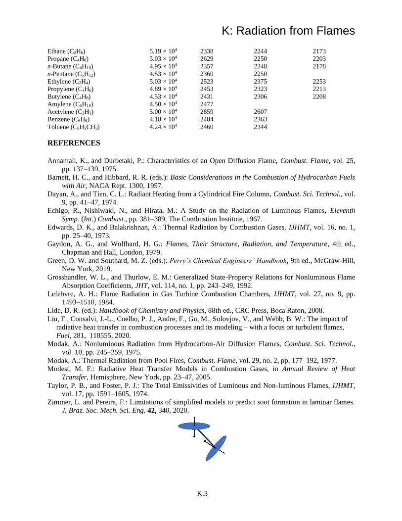
K: Radiation from Flames
K.3
Ethane (C2H6) 5.19 × 10⁴ 2338 2244 2173
Propane (C4H8) 5.03 × 10⁴ 2629 2250 2203
n-Butane (C4H10) 4.95 × 10⁴ 2357 2248 2178
n-Pentane (C5H12) 4.53 × 10⁴ 2360 2250
Ethylene (C2H4) 5.03 × 10⁴ 2523 2375 2253
Propylene (C3H6) 4.89 × 10⁴ 2453 2323 2213
Butylene (C4H8) 4.53 × 10⁴ 2431 2306 2208
Amylene (C5H10) 4.50 × 10⁴ 2477
Acetylene (C2H2) 5.00 × 10⁴ 2859 2607
Benzene (C6H6) 4.18 × 10⁴ 2484 2363
Toluene (C6H5CH3) 4.24 × 10⁴ 2460 2344
REFERENCES
Annamali, K., and Durbetaki, P.: Characteristics of an Open Diffusion Flame, Combust. Flame, vol. 25,
pp. 137–139, 1975.
Barnett, H. C., and Hibbard, R. R. (eds.): Basic Considerations in the Combustion of Hydrocarbon Fuels
with Air, NACA Rept. 1300, 1957.
Dayan, A., and Tien, C. L.: Radiant Heating from a Cylindrical Fire Column, Combust. Sci. Technol., vol.
9, pp. 41–47, 1974.
Echigo, R., Nishiwaki, N., and Hirata, M.: A Study on the Radiation of Luminous Flames, Eleventh
Symp. (Int.) Combust., pp. 381–389, The Combustion Institute, 1967.
Edwards, D. K., and Balakrishnan, A.: Thermal Radiation by Combustion Gases, IJHMT, vol. 16, no. 1,
pp. 25–40, 1973.
Gaydon, A. G., and Wolfhard, H. G.: Flames, Their Structure, Radiation, and Temperature, 4th ed.,
Chapman and Hall, London, 1979.
Green, D. W. and Southard, M. Z. (eds.): Perry’s Chemical Engineers’ Handbook, 9th ed., McGraw-Hill,
New York, 2019.
Grosshandler, W. L., and Thurlow, E. M.: Generalized State-Property Relations for Nonluminous Flame
Absorption Coefficients, JHT, vol. 114, no. 1, pp. 243–249, 1992.
Lefebvre, A. H.: Flame Radiation in Gas Turbine Combustion Chambers, IJHMT, vol. 27, no. 9, pp.
1493–1510, 1984.
Lide, D. R. (ed.): Handbook of Chemistry and Physics, 88th ed., CRC Press, Boca Raton, 2008.
Liu, F., Consalvi, J.-L., Coelho, P. J., Andre, F., Gu, M., Solovjov, V., and Webb, B. W.: The impact of
radiative heat transfer in combustion processes and its modeling – with a focus on turbulent flames,
Fuel, 281, 118555, 2020.
Modak, A.: Nonluminous Radiation from Hydrocarbon-Air Diffusion Flames, Combust. Sci. Technol.,
vol. 10, pp. 245–259, 1975.
Modak, A.: Thermal Radiation from Pool Fires, Combust. Flame, vol. 29, no. 2, pp. 177–192, 1977.
Modest, M. F.: Radiative Heat Transfer Models in Combustion Gases, in Annual Review of Heat
Transfer, Hemisphere, New York, pp. 23–47, 2005.
Taylor, P. B., and Foster, P. J.: The Total Emissivities of Luminous and Non-luminous Flames, IJHMT,
vol. 17, pp. 1591–1605, 1974.
Zimmer, L. and Pereira, F.: Limitations of simplified models to predict soot formation in laminar flames.
J. Braz. Soc. Mech. Sci. Eng. 42, 340, 2020.
M. REFERENCES TO REVIEWS AND HISTORICAL PAPERS
M.1
L: COMMERCIAL CODES FOR RADIATION
L.1 CODES FOR CONFIGURATION FACTORS
Many computer programs are available that use one or more of the methods outlined in Chapter 4 of
the text for numerical calculation of configuration factors. Examples are FACET (Shapiro 1983),
which uses area integration and contour integration; VIEW (Emery 1986), which can be used with
the NASTRAN thermal analysis code; a program that relies on the computer-graphical analog to the
unit-sphere method (Alciatore et al. 1989), and VIEW3D. The latter program provides factors
between a differential element and an arbitrary 3D object. The program TSS (Thermal Simulation
System, Chin et al. 1992), developed under NASA sponsorship, incorporates an advanced graphical
user interface for displaying configurations. The CHAPARRAL program (Glass 1995) incorporates
FACET for 2D factors and uses the hemicube method for computing 3D factors in very large
surface element arrays. Many commercially available thermal analysis programs such as COMSOL,
FLUENT, FIDAP, NEVADA, and OpenFOAM also incorporate configuration factor computation
using various methods, sometimes with choices among methods.
These and other computer codes provide a means to generate configuration factors for complex
geometries and are invaluable for radiative analyses. Their accuracy can be assessed by comparison
of computed results with the analytical expressions developed here for simpler geometries that can
be used for test cases. Several different numerical methods for calculating configuration factors in
complex configurations are compared by Emery et al. (1991) for computing speed, accuracy, and
convenience. The geometries range from surfaces almost unobstructed in their view, to highly
obstructed intersecting surfaces. The methods compared include double integration, Monte Carlo,
contour integration, and projection techniques. If the view is not too complex, methods based on
contour integration are found to be successful. The advent of massively parallel computers is
making Monte Carlo methods (Chapter 14) particularly attractive for computing configuration
factors. Walker et al. (2010, 2012) and Walker (2013) have examined the use of parallel Monte
Carlo using either standard central processing units (CPUs) or graphical processing units (GPUs)
and find good speed and accuracy in comparison with finite-element-based numerical integration
for computing configuration factors for complex geometries. They employ superimposed primitives
for fast rendering of many common objects.
L.2: Codes and Data for Molecular and Atomic Gas Spectral Properties
Property data is available from accessible on-line sources. These are continually updated
and improved. More information on the databases is in Section 9.3.5.3 of the text. The databases
themselves can be accessed at:
Jacquinet-Husson, N. et al., The 2015 edition of the GEISA spectroscopic database, J. Molecular
Spectroscopy 327, 31-72, Sept. 2017.). The 2019 version of GEISA is accessible at CDS-ESPRI:Home.
Laux, C. O.: Radiation and nonequilibrium collisional-radiative models, in D. Fletcher, J.-M. Charbonnier,
G. S. R. Sarma, and T. Magin (eds.), Physico-Chemical Modeling of High Enthalpy and Plasma Flows,
von Karman Institute Lecture Series 2002-07, Rhode-Saint-Genèse, Belgium, 2002. [SPECAIR User
Manual, ver. 3.0, 2012 (latest version online)]. Code available at www.specair-radiation.net/
Kramida, A., Ralchenko, Y., Reader, J. and NISTASDTeam: NIST Atomic Spectra Database (version 5.0),
[Online]. Available: physics.nist.gov/asd (accessed April 27, 2015), National Institute of Standards and
Technology, Gaithersburg, MD, 2012.

M. REFERENCES TO REVIEWS AND HISTORICAL PAPERS
M.2
Rothman, L. S., Gordon, I. E., Barbe, A. et al., The HITRAN 2012 molecular spectroscopic database, JQSRT
130, 4–50, 2013. (For most recent version (2012) see www.cfa.hitran.com. Accessed April 27, 2015).
Rothman, L. S., Gordon, I. E., Barber, R. J., Dothe, H., Gamache, R. R., Goldman, A., Perevalov, V.,
Tashkun, S. A., and Tennyson, J.: HITEMP, the high-temperature molecular spectroscopic database,
JQSRT, 111(15), 2139–2150, 2010. Data available on-line at https://hitran.org/hitemp/
L.3: CFD-BASED CODES
Most of the major commercially available computational fluid dynamics (CFD) codes employ
one or more choices of methods for handling radiative transfer within a participating medium. For
example, the ANSYS CFD code packages FLUENT and CFX between them provide choice from
among surface–surface, diffusion, P1, discrete transfer, discrete ordinates, and Monte Carlo solvers.
The COMSOL built-in Heat Transfer module incorporates spectral surface properties for surface-
surface exchange in simple geometries, and uses the Rosseland approximation, P1 approximation or
the discrete ordinate method (DOM) for radiation in participating media. OpenFOAM, a free online
CFD code includes P1 and finite volume models, plus a configuration factor calculator for
transparent medium problems.
Various models may be included for treating anisotropic scattering and spectral medium
property variations, although these features are not available for all solvers. These and competing
codes continue to add features and capabilities, and careful comparison is warranted of the required
capabilities for a problem or application.
L.4 FINITE DIFFERENCE TIME-DOMAIN METHOD
The FDTD method is probably the most common approach for simulation of scattering problems
(Wriedt 2009), and for nanoscale radiation interactions with textured surfaces (Heltzel et al. 2005. 2007; 2008). The method was first introduced by Yee (1966), where time-dependent Maxwell
equations are solved to calculate electromagnetic scattering in both time and space domains. The
derivatives of Maxwell equations in space and time are approximated by a finite difference scheme
and discretized in both space and time domains. The equations are solved numerically with
appropriate boundary conditions and particle or surface properties using a fully explicit scheme.
FDTD methods were reviewed by Schlager and Schneider (1995) and Taflove (2007). This
approach is commercially available, as more than 25 companies were listed by Taflove. There are
several other open source development projects, which are listed at the corresponding Wikipedia
site. It is also used extensively for simulations of metamaterials as discussed by Veselago et al.
(2006). This method computes the solution in a finite domain, like the FEM, and so a far zone
transformation must be invoked to calculate fields in far-field. The method is popular because of its
conceptual simplicity and ease of implementation but has disadvantages like those of the FEM
including limitations in accuracy, mathematical complexity, and the need to repeat computations for
different angles of incidence. The FDTD approach can be applied to arbitrary geometries with
different properties.
Maxwell equations are discretized using the FDTD method. In order to present the
implementation of FDTD, the Maxwell equations are written in terms of electrical displacement and
magnetic fields Dx, Dz, and Hy, respectively. They are considered for a transverse magnetic (TM)
wave, in which the only nonzero component of magnetic field is Hy, that is, propagation along the z-
axis. They are
M. REFERENCES TO REVIEWS AND HISTORICAL PAPERS
M.3
yx HD
t z
= −
(L.1)
yz HD
t x
=
(L.2)
x 0 r x( ) ( ) ( )D E = (L.3)
z 0 r z( ) ( ) ( )D E = (L.4)
y z x
0
1H E E
t x z
= −
(L.5)
The first order finite difference representation of the fields in Equations L.1, L.2, and L.5 are
written in discrete time domain as
1/2, 1/2, 1/2, 1/2 1/2, 1/2
1/2 1/2x x y yi k i k i k i k
n n n nD D H H
t z
+ + + + + −
+ −− −= −
(L.6)
, 1/2 , 1/2 1/2, 1/2 1/2, 1/2
1/2 1/2z z y yi k i k i k i k
n n n nD D H H
t x
+ + + + − +
+ −− −= −
(L.7)
1/2, 1/2 1/2, 1/2 1, 1/2 , 1/2 1/2, 1 1/2,
1 1/2 1/2 1/2 1/2y y z z x x
0 0
i k i k i k i k i k i k
n n n n n nH H E E E E
t x z
+ + + + + + + + + +
+ + + + +− − −= −
(L.8)
If the Yee cell size is kept small, the central differences are said to have second-order accuracy or
second-order behavior (Δx2 terms can be ignored). Furthermore, we can rewrite Equations L.6
through K.8 as
1/2, 1/2, 1/2, 1/2 1/2, 1/2
1/2 1/2x x y y( ) ( )
i k i k i k i k
n n n ntD k D k H H
z+ + + + + −
+ − = − −
(L.9)
, 1/2 , 1/2 1/2, 1/2 1/2, 1/2
1/2 1/2z z y y( ) ( )i k i k i k i k
n n n ntD k D k H H
x+ + + + − +
+ − = − −
(L.10)
1.2, 1/2 1.2, 1/2 1, 1/2 , 1/2 1/2, 1 1/2,
1 1/2 1/2 1/2 1/2y y z z x x
0 0i k i k i k i k i k i k
n n n n n nt tH H E E E E
x z+ + + + + + + + + +
+ + + + + = + − − −
(L.11)
In the xz plane of interest, the 1D wave equation is
z
10E
x c t
− =
(L.12)
x
10E
z c t
− =
(L.13)
They can be easily discretized using only the field components on, or just inside the mesh wall,
yielding an explicit finite difference equation at time step n + 1:

M. REFERENCES TO REVIEWS AND HISTORICAL PAPERS
M.4
( )2, 1/2 2, 1/2 1, 1/21, 1/2
1z z
1zz
k kk k
n n nn c t xE E E E
c t x++ + +
+ + − = + −
+ (L.14)
( )1/2,2 1/2,2 1// 22 ,1 ,1 1x x xx11
i i i i
n n nn c t zE E E E
c t z+ + ++
++ − = + −
+ (L.15)
where , 1/2zi knE + and 1/2,xi k
nE + , respectively, refer to the i, kth electric component of Yee cell in z and x
direction, and c is the speed of light.
The numerical algorithm for Maxwell’s curl equations requires that the time increment Δt have a
specific bound relative to the space increments Δx, Δy, and Δz. The time increment must obey the
following bound, known as Courant–Friedrichs–Lewy (CFL) stability criterion:
1
2 2 2
1 1 1min
( ) ( ) ( )t c
x y z
− + +
(L.16)
The difficulty in working with FDTD is due mainly to the imposition of the boundary conditions.
The choice of boundary conditions is the key to an accurate FDTD simulation. There are various
techniques to achieve the aim of simulating a geometry that extends to infinity in all dimensions,
thereby eliminating reflections from the actual physical edges. In FDTD these are known as
absorbing boundary conditions or ABCs as they absorb or attenuate waves (electric or magnetic) as
they approach the edge of the actual problem geometry. Which method you use (known as
Dirichlet, periodic, Mur, Mie/Fang superabsorption, perfectly matched layers (PML), convolution
PML (CPML), etc.) will very much depend on the nature of the waves, their incidence angle, and
their wavelength relative to the geometry size. Choosing the best ABC for an FDTD simulation is
crucial as it can minimize the overall problem space, that is, the number of grid cells in the x, y, and
z dimensions, and thereby reduce computation time (Didari and Mengüç 2014, 2015).
FDTD has found applications in several diverse areas of mechanical engineering such as near-
field thermal radiation (see Datas et al. 2013, Didari and Mengüç 2014, 2015), microelectronics,
with applications in energy-conversion devices, nanothermal manufacturing, as well as in electrical
engineering such as antenna imaging design and bioelectromagnetic device development.
MATLAB by Mathworks is a particularly powerful tool for developing FDTD solutions because
of its inherent support for matrices and arrays. FDTD algorithms implemented in MATLAB only
need a single iteration per time-step to cover the complete spatial space (1D, 2D, or 3D). A fast
Fourier transform (FFT) can be applied at any point in time or space to produce a frequency domain
solution without an additional frequency “sweep.” This is achieved by applying a broadband
excitation pulse at some appropriate point within the problem geometry and then applying an FFT
to the resultant time-domain response.
Implementing FDTD programmatically through MATLAB (or similar open source solutions such
as GSVIT) allows complete independence over problem parameter definition, particularly in near-
field thermal radiation research where arbitrary geometries and multiple dispersive materials may
be used (Didari and Mengüç 2014, 2015). In addition, the application of FDTD to light scattering
aerosols and the relevant literature review was reported by Sun et al. (2013) and Datas et al. (2013).
In the last few years, MATLAB and other FDTD solvers have embraced parallel computation,
both through support for multiple CPU cores and by harnessing the power of graphics processing
units (GPU) with their hundreds of processing cores. These developments have made possible
finely gridded simulations over large 2D or 3D geometries by dramatically reducing simulation
M. REFERENCES TO REVIEWS AND HISTORICAL PAPERS
M.5
times (by factors between 10 and 200). As one of the weaknesses of FDTD is numerical accuracy
due to the discrete representations of electromagnetic fields, faster execution time allows
proportional reduction in the discretization steps in both space and time.
Recent FDTD studies of near field thermal radiation have shown that modeling geometries
separated by nanogaps in orders of a few tens of nanometers is also possible using the FDTD
method, which is a promising factor in this field since analytical methods may not be easily
available for some geometries due to geometry asperities; however, a tradeoff needs to be found
between the accuracy and the simulation time requirements when working in such small scales
(Didari and Mengüç 2014, 2015). Note that, for complex particles, these relations can be used for
experimental determination of the phase function coefficients. Agarwal and Mengüç (1991) carried
out an extensive numerical and experimental research to determine these parameters from
experiments for polystyrene latex particles. A similar experimental study was conducted for coal
particles by Mengüç et al. (1994).
L.5: AVAILABLE ON-LINE CODES AND DATABASES (Links checked as of 8/25/2019)
On-line resources are available for aid in computing many useful functions for radiation. These
include:
CONFIGURATION FACTORS BETWEEN SURFACES:
FACET (Shapiro et al. 1983): www.oecd-nea.org/tools/abstract/detail/nesc9578
VIEW (Emery 1986): https://bit.ly/2kOYJjO
VIEW3D (Walton 1986): www.View3d.sourceforge.net
Catalog (Howell, 1982 on line: More than 350 factors, many with calculator):
www.ThermalRadiation.net/indexCat.html
LINE-BY-LINE SPECTRAL DATA
HITRAN 2016 (Gordon et al. 2017): www.cfa.harvard.edu/hitran//
HITEMP 2010 (Rothman et al. 2013): https://hitran.org/hitemp/
SPECAIR (Laux 2002) : www.specair-radiation.net/
GEISA (Jacquinet-Husson et al. 2017):
https://geisa.aeris-data.fr/line-transition-parameters-2019/
NIST Atomic Spectra (Kramida et al. 2012): https://www.physics.nist.gov/asd
GAS EMITTANCE FOR CO2, H2O, CO MIXTURES
Alberti et al. (2018), Spread sheet under “Supplementary Data” at:
doi.org/10.1016/j.jqsrt.2018.08.008
SCATTERING
M. REFERENCES TO REVIEWS AND HISTORICAL PAPERS
M.6
References to scattering literature and codes: https:www.scattport.org/index.php
Mie scattering calculator (Prahl,2009) : https://omlc.org/calc/mie_calc.html
T-matrix for irregular particles (Mishchenko et al. 2013): at
https://www.giss.nasa.gov/staff/mmishchenko/t_matrix.html
OpenDDA: Discrete dipole approximation for Agglomerates, (McDonald et al. 2009):
www.opendda.org
ADDA: Discrete dipole code for agglomerates, Yurkel
https://github.com/adda-team/adda Add-on package for MATLAB (Nieminen et al.2007):
www.physics.uq.edu.au/people/nieminen/software.html
REFERENCES: Agarwal, B. M. and Mengüç, M. P.: Single and multiple scattering of collimated radiation in an axisymmetric system, IJHMT, 34(3),
633–647, 1991. Alberti, M., Weber, R., and Mancini, M.: Gray gas emissivities for H2O-CO2-CO-N2 mixtures, JQSRT, 219, 274-291, Nov. 2018.
Alciatore, D., Lipp, S., and Janna, W. S.: Closed-form solution of the general three-dimensional radiation configuration factor
problem with microcomputer solution, Proceedings of the 26th National Heat Transfer Conference, Philadelphia, PA, August
1989. Chin, J. H., Panczak, T. D., and Fried, L.: Spacecraft thermal modeling, Int. J. Numer. Methods Eng., 35, 641–653, 1992.
Datas, A., Hirashima, D., and Hanamura, K.: FTDT simulation of near-field radiative heat transfer between thin films supporting
surface phonon polaritons: Lessons learned, J. Thermal Sci. Technol., 8(1), 91–105, 2013.
Didari, A. and Mengüç, M. P.: Analysis of near-field radiation transfer within nano-gaps using FDTD method, JQSRT, 146, 214–226, 2014.
Didari, A. and Mengüç, M. P.: Near-field thermal emission between corrugated surfaces separated by nano-gaps, JQSRT, 158, 43–51,
2015.
Emery, A. F.: VIEW—A radiation view factor program with interactive graphics for geometry definition (Version 5.5.3), 1986. Emery, A. F., Johansson, O., Lobo, M., and Abrous, A.: A comparative study of methods for computing the diffuse radiation
viewfactors for complex structures, JHT, 113(2), 413–422, 1991.
Glass, M. W.: CHAPARRAL: A Library for Solving Large Enclosure Radiation Heat Transfer Problems, Sandia National Laboratory
Report SAND95-2049, Albuquerque, NM, August 1995.
Gordon, I. E., et al. (eds): The HITRAN 2016 molecular spectroscopic database, JQSRT, 203, 3-69, 2017. Heltzel, A., Battula, A., Howell, J. R., and Chen, S.: Nanostructuring borosilicate glass with near-field enhanced energy using a
femtosecond laser pulse, J. Heat Transfer, Special Issue on Nanoscale Heat Transfer, 129, 53–59, January 2007. Heltzel, A., Chen, S., and Howell, J. R.: Surface plasmon-based nanopatterning assisted by gold nanospheres, Nanotechnology,
19(2), January 2008.
Heltzel, A., Theppakuttai, S., Howell, J. R., and Chen, S.: Analytical and experimental investigation of laser-microsphere interaction
for nanoscale surface modification, J. Heat Transfer, 127(11), 1231–1235, 2005.
Howell, J. R.: Catalog of Radiation Configuration Factors, McGraw-Hill Book Company, New York, 1982; later eds. published in
electronic form on-line. Jacquinet-Husson, N. et al., The 2015 edition of the GEISA spectroscopic database, J. Molecular Spectroscopy 327, 31-72, Sept.
2017. (GEISA database updated in 2019)
Kramida, A., Ralchenko, Y., Reader, J. and NISTASDTeam: NIST Atomic Spectra Database (version 5.0), [Online].
National Institute of Standards and Technology, Gaithersburg, MD, 2012.
Laux, C. O.: Radiation and nonequilibrium collisional-radiative models, in D. Fletcher, J.-M. Charbonnier, G. S. R.
Sarma, and T. Magin (eds.), Physico-Chemical Modeling of High Enthalpy and Plasma Flows, von Karman
Institute Lecture Series 2002-07, Rhode-Saint-Genèse, Belgium, 2002. McDonald, J., Golden, A., and Jennings, G.: OpenDDA: A high-performance computational framework for the discrete dipole
approximation, Int. J. High Perf. Comp. Appl. 23(1), 42–46, 2009
Mengüç, M. P., Manickavasagam, S., and D’sa, D. A.: Determination of radiative properties of pulverized coal particles from experiments, FUEL, 73(4), 613–625, 1994.
Mishchenko, M. I., Videen, G., Khlebtsov, N. G., and Wriedt, T.: Comprehensive T-matrix reference database: A 2012–
2013 update, JQSRT, 123, 145–152, 2013.
Nieminen, T. A., Loke, V. L. Y., Stilgoe, A. B., Knöner, G., Branczyk, A. M., Heckenberg, N. R., and Rubinsztein-
Dunlop, H.: Optical tweezers computational toolbox, J. Opt. A, 9, S196–S203, 2007.
M. REFERENCES TO REVIEWS AND HISTORICAL PAPERS
M.7
Prahl, S.: Mie scattering calculator, http://omlc.ogi.edu/calc/mie_calc.html (accessed April 16, 2015). Oregon Medical Laser Center, Portland, OR, 2009.
Rothman, L. S., Gordon, I. E., Barbe, A. et al., The HITRAN 2012 molecular spectroscopic database, JQSRT, 130, 4–
50, 2013. Shapiro, A. B.: FACET—A computer view factor computer code for axisymmetric, 2d planar, and 3d geometries with shadowing,
UCID-19887, University of California, Lawrence Livermore National Laboratory, Livermore, CA, August 1983
Shlager, K. L. and Schneider, J. B.: A Selective Survey of the Finite-Difference Time-Domain Literature, IEEE Antennas Propag. Mag., 37(4), 39-56, Aug. 1995.
Sun, W., Videen, G., Fu, Q., and Hu, Y.: Scattered-field FDTD and PSTD algorithms with CPML absorbing boundary conditions for
light scattering by aerosols, JQSRT, 131, 166–174, 2013.
Taflove, A.: Advances in FDTD Techniques and Applications in Photonics, Photonics North 2007, Ottawa, Ontario, Canada, June 4, 2007.
Veselago, V., Braginsky, L., Shklover, V., and Hafner, C.: Negative refractive index materials, J. Comput. Theoret. Nanosci., 3, 1–
30, 2006.
Walker, T.: The use of primatives in the calculation of radiative view factors, PhD dissertation, School of Chemical and Biomolecular Engineering. University of Sydney, Sydney, New South Wales, Australia, December 2013.
Walker, T., Xue, S.-C., and Barton, G. W: Numerical determination of radiative view factors using ray tracing, JHT, 132(7), 072702-
1–072702-6, 2010.
Walker, T., Xue, S.-C., and Barton, G. W: A robust Monte Carlo-Based ray-tracing approach for the calculation of view factors in arbitrary three- dimensional geometries, Comput. Thermal Sci., 4(5), 425–442, 2012.
Walton, G.N.: Algorithms for Calculating Radiation View Factors Between Plane Convex Polygons with Obstructions, National
Bureau of Standards NBSIR 863463, Gaithersburg, MD, 1986.
Wriedt, T.: Light scattering theories and computer codes, JQSRT, 110, 833–843, 2009. Yee, K. S.: Numerical solution of initial value problems involving Maxwell’s equations in isotropic media, IEEE Trans. Antennas
Propag., 14, 302–307, 1966.
Yurkin, M. A. and Hoekstra, A. G.: The discrete-dipole-approximation code ADDA: Capabilities and known
limitations, JQSRT, 112(13), 2234–2247, 2011.
P. ADDITIONAL HOMEWORK
P.1
M. REFERENCES TO REVIEWS AND HISTORICAL PAPERS
M.1 GENERAL
Bone, W. A., and Townsend, D. T. A.: Flame and Combustion in Gases, Longmans, Green, London, 1927.
Born, M., Wolf, E., and Bhatia, A. B.: Principles of Optics, 7th expanded ed., Cambridge University Press, New York, 1999.
Breene, R. G.: Theories of Spectral Line Shapes, John Wiley and Sons, New York, 1981.
Carslaw, H. S., and Jaeger, J. C.: Conduction of Heat in Solids, 2d ed., Clarendon Press, Oxford, UK, 1959.
Coakley Jr, J. A. and Yang, P.: Atmospheric Radiation: A Primer with Illustrative Solutions, John Wiley & Sons, New York, 2014.
Garbuny, M.: Optical Physics, 2nd printing, Academic Press, New York, 1967.
Glassman, I., Yetter, R. A., and Glumac, N. G.: Combustion, 5th ed., Elsevier Science/Academic Press, Burlington, MA 2018. Griem, H. R.: Principles of Plasma Spectroscopy, Cambridge University Press, 2005.
Hecht, E.: Optics. 4th ed., Pearson Education, Inc., Upper Saddle River, USA, 2002.
Herzberg, G.: Molecular Spectra and Molecular Structure, 2d ed., 3 vols., Krieger, Malabar, FL, 1992.
Howell, J. R.: The development of engineering radiative heat transfer, IMECE2002-33131, 73-78, IMECE, New Orleans, Nov. 2002. Howell, J. R., Hall, M. J., and Ellzey, J. L.: Combustion of Hydrocarbon Fuels within Porous Inert Media, Prog. Energy Comb.
Science, vol. 22, pp. 121–145, 1996.
Khalil, E. E.: Modelling of Furnaces and Combustors, Energy and Engineering Science Series, Gupta, A.K. and Lilley, D.G. (eds.),
Abacus Press, Tunbridge Wells, U.K., 1982. Kittel, C.: Introduction to Solid State Physics, John Wiley & Sons, Hoboken, 2005.
Kourganoff, V.: Basic Methods in Transfer Problems, Dover, New York, 1963.
Kuneš, J.: Dimensionless Physical Quantities in Science and Engineering, Elsevier, New York, 2012.
Kuo, K.: Principles of Combustion, 2nd ed., John Wiley & Sons, 2005. Landau, L. D. and Lifshitz, E. M.: Electrodynamics of Continuous Media, Addison-Wesley, Reading, MA, 1960.
Law, C. K.: Combustion Physics, Cambridge University Press, 2006 (on-line, July 2010).
MacRobert, T. M.: Spherical harmonics, 3rd edn. Pergamon Press, New York, 1967.
Maier, S. A.: Plasmonics: Fundamentals and Applications, Springer, New York, 2007.
Majumdar, A.: Scanning Thermal Microscopy, Ann. Rev. of Matls Sci., vol. 29, pp. 505–585, 1999.
Mandel, L. and Wolf, E.: Optical Coherence and Quantum Optics, Cambridge University Press, Cambridge, 1995.
Mandelbrot, B. B.: Les Objets Fractals: Forme, Hasard et Dimension, Flammarion, Paris, 1975. Mandelbrot, B. B.: The Fractal Geometry of Nature, W. H. Freeman, San Francisco, CA, 1983.
Mark, J.C.: The spherical harmonics method. Part I. Atomic Energy Report No. MT 92, National Research Council of Canada, 1944.
Mohr, P. J., Newell, D. B., and Taylor, B. N.: CODATA recommended values of the fundamental physical constants: 2014, Rev. Mod. Phys., 88, 035009, July-Sept. 2014.
Novotny, J. L., and Hecht, B.: Principles of Nano-optics, University Press, Cambridge, 2006.
Patankar, S. V.: Numerical Heat Transfer and Fluid Flow, Hemisphere, Washington, DC, 1980.
Penner, S. S.: Quantitative Molecular Spectroscopy and Gas Emissivities, Addison-Wesley, Reading, MA, 1959. Shen, J., and Tang, T.S., Spectral and High-Order Methods with Applications, Science Press, Beijing, 2006.
Stone, J. M.: Radiation and Optics, McGraw–Hill, New York, 1963.
Tien, C. L., and Cunnington, G. R.: Cryogenic Insulation Heat Transfer, in T. F. Irvine, Jr., and J. P. Hartnett (eds.), Advances in
Heat Transfer, 9, 349–417, Academic Press, New York, 1973. Turns, S. R.: An Introduction to Combustion; Concepts and Applications, McGraw-Hill, New York, 2011.
Vincenti, W. G, and Kruger Jr., C. H.: Introduction to Physical Gas Dynamics, Corrected Ed., Krieger Publishing Company,
Malabar, FL, 1986.
Williams, F. A.: Combustion Theory, 2nd ed., Taylor and Francis, New York, 1994. Yeh, P.: Optical Waves in Layered Media, John Wiley & Sons, Hoboken, 2005.
Zel’dovich, Ya. B., and Raizer, Yu. P.: Physics of Shock Waves and High-Temperature Hydrodynamic Phenomena, vol. 1, pt. II,
Academic Press, New York, 1966.
M.2 INVERSE METHODS
Alifanov, O. M.: Inverse Heat Transfer Problems, Springer, Berlin, 1994.
Alifanov, O. M., Artyukhin, E. A., and Rumyantsev, S. V.: Extreme Methods for Solving Ill-Posed Problems with Applications to
Inverse Heat Transfer Problems, Begell House, New York, 1995. Beck, J. V., Blackwell, B., and St. Clair, Jr., C. R.: Inverse Heat Conduction: Ill-Posed Problems, Wiley-Interscience, New York,
1995.
Beckman, F. S.: The Solution of Linear Equations by the Conjugate Gradient Method, in A. Ralston and H. S. Wilf (eds.),
Mathematical Methods for Digital Computers, John Wiley and Sons, New York, 62–72, 1960. França, F. H. R., Howell, J. R., Ezekoye, O. A., and Morales, J. C.: Inverse design of thermal systems, in J. P. Hartnett and T. F.
Irvine (eds.), Advances in Heat Transfer, vol. 36, 1, pp. 1–110, Academic Press, Waltham, MA, 2002.
Hansen, P. C., Rank-Deficient and Discrete Ill-Posed Problems: Numerical Aspects of Linear Inversion, SIAM, Philadelphia, 1998.
M. REFERENCES TO REVIEWS AND HISTORICAL PAPERS
M.2
Kushner, H. J. and Clark, D. S.: Stochastic Approximation Methods for Constrained and Unconstrained Systems, Springer, New York, 1978.
Özişik, M. N., and Orlande, H. R. B.: Inverse Heat Transfer: Fundamentals and Applications, Taylor and Francis, New York, 2000.
Morozov, V. A.: Methods for Solving Incorrectly Posed Problems, Springer-Verlag, New York, 1984.
Tikhonov, A. N.: Solution of Incorrectly Formulated Problems and the Regularization Method, Soviet Math. Dokl., 4, 1035–1038, 1963. [Engl. trans. Dokl. Akad. Nauk. SSSR, 151, 501–504, 1963.]
Vogel, C.R.: Computational Methods for Inverse Problems, SIAM, Philadelphia, 2002.
M.3 RADIATIVE TRANSFER M.3.1 GENERAL
Amber, I. and O'Donovan, T. S.: Natural convection induced by the absorption of solar radiation: A review, Renewable
and Sustainable Energy Reviews, 82, 3526–3545, 2018. Cess, R. D.: The interaction of thermal radiation with conduction and convection heat transfer, in T. F. Irvine, Jr. and J. P. Hartnett
(eds.), Advances in Heat Transfer, vol. 1, pp. 1–50, Academic Press, New York, 1964
Ficker, T.: General Model of Radiative and Convective Heat Transfer in Buildings: Part I: Algebraic Model of Radiative Heat
Transfer, Acta Polytechnica, 59(3), 211-233, 2019.
Frank, M. and Klar, A.: Radiative heat transfer and applications for glass production processes, in A. Farina, A. Klar, R. M. M. Mattheijj, A. Mikelić, N. Siedow, and A. Fasano (eds.), Mathematical Models in the Manufacturing of Glass, Proceedings of
the C.I.M.E. Summer School, pp. 57–134, Springer, Terme, Italy, 2008.
Hottel, H. C.: Radiant Heat Transmission, in W. H. McAdams (ed.), Heat Transmission, 3d ed., McGraw-Hill, New York, 1954.
Hottel, H. C, and Sarofim, A. F.: Radiative Transfer, McGraw–Hill, New York, 1967. Hottel, H. C., Sarofim, A. F., Wankat, P. C., Noble, J. J., Silcox, G. D., and Knaebel, K. S.: Heat and Mass Transfer, in D. W. Green
and R. H. Perry (eds.), Perry’s Chemical Engineer’s Handbook, 8th ed., Chap. 5, pp. 5-16–5-43, McGraw-Hill, 2008.
Lee, S. -C, and Cunnington, G. R.: Theoretical Models for Radiative Transfer in Fibrous Media, in Ann. Rev. Heat Transfer, vol. IX,
Chap. 3, pp. 159–218, Begell House, New York, 1998. Modest, M. F.: Radiation heat transfer. 3rd ed., Academic Press, Waltham, MA, 2013.
Özişik, M. N.: Radiative Transfer, and Interactions with Conduction and Convection, John Wiley & Sons, New York, 1973.
Sparrow, E. M.: On the Calculation of Radiant Interchange between Surfaces, in W. Ibele (ed.), Modern Developments in Heat
Transfer, pp. 181–212, Academic Press, New York, 1963b. Sparrow, E. M., and Cess, R. D.: Radiation Heat Transfer, augmented edition, Hemisphere, Washington, DC, 1978.
Stewart, S. M. and Johnson, R. B.: Blackbody Radiation: A History of Thermal Radiation Computational Aids and Numerical
Methods, CRC Press, Boca Raton, 2016. Tencer, J. and Howell, J.R.: Coupling Radiative Heat Transfer with Other Heat Transfer Modes, J. Brazilian Society Engng Sci,
38(5), 1473-1487, June 2016. Timoshenko, V. P., and Trenev, M. G.: A Method for Evaluating Heat Transfer in Multilayered Semitransparent Materials, Heat
Transfer—Sov. Res., vol. 18, no. 5, pp. 44–57, 1986. Viskanta, R.: Radiation Transfer and Interaction of Convection with Radiation Heat Transfer, in Thomas F. Irvine, Jr., and James P.
Hartnett (eds.), Advances in Heat Transfer, vol. 3, pp. 175–251, Academic Press, New York, 1966.
Viskanta, R., and Anderson, E. E.: Heat Transfer in Semi-transparent Solids, in J. P Hartnett and T. F. Irvine, Jr. (eds.), Advances in
Heat Transfer, vol. 11, pp. 317–441, Academic Press, New York, 1975. Viskanta, R., and Mengüç, M. P.: Radiation Heat Transfer in Combustion Systems, Prog. Energy Combust. Sci., vol. 13, pp. 97–160,
1987.
Viskanta, R.: Radiative Transfer in Combustion Systems: Fundamentals and Applications, Begell House, New York, 2005.
M.3.2 ATMOSPHERIC RADIATION
Bohren, C.W. and Clothiaux, E.E.: Fundamentals of Atmospheric Radiation, John Wiley & Sons, New York, 2006.
Coakley Jr, J. A., and Yang, P.: Atmospheric Radiation: A Primer with Illustrative Solutions, John Wiley & Sons, New York, 2014.
Duffie, J. Α., and Beckman, W. A.: Solar Energy Thermal Processes, 3d ed., Wiley, New York, 2006. Goody, R. M., and Yung, Y. L.: Atmospheric Radiation, 2d ed., Oxford University Press, New York, 1989.
Kondratyev, Ya. K.: Radiation in the Atmosphere, Academic Press, New York, 1969.
Liou, K.-N.: An Introduction to Atmospheric Radiation, 2nd ed., Academic Press, 2002
Petty, G.W.: A First Course in Atmospheric Radiation, 2nd ed., Sundog Publishing, Madison, WI., 2006.
M.3.3 INVERSE SOLUTIONS IN RADIATION
Daun, K. J., Ertürk, H., and Howell, J. R.: Inverse Design Methods for High-Temperature Systems, Arabian J. Sci. and Tech, 27(2C),
3–48, 2003.

M. REFERENCES TO REVIEWS AND HISTORICAL PAPERS
M.3
Daun, K. J., Ertürk, H., Howell, J. R., Gamba, M. and Hosseini Sarvari, M.: The Use of Inverse Methods for the Design and Control of Radiant Sources, JSME International Journal, ser. B, 46(4), 470–478, 2003.
França, F. H. R., Howell, J. R., Ezekoye, O. A., and Morales, J. C.: Inverse Design of Thermal Systems, in J. P. Hartnett and T.
F. Irvine (eds.), Advances in Heat Transfer, 36(1), 1–110, Elsevier, 2002.
Hansen, P. C.: Rank-Deficient and Discrete Ill-Posed Problems: Numerical Aspects of Linear Inversion, SIAM, Philadelphia, PA, 1998.
Kennedy, J. and Eberhart, R.: Particle swarm optimization, Proc. ICNN'95 – Intl. Conf. on Neural Networks, pp. 1942-1948, IEEE,
Nov. 1995.
Vogel, C. R.: Computational Methods for Inverse Problems, SIAM, Philadelphia, PA, 2002. Wing, G. W.: A Primer on Integral Equations of the First Kind, SIAM, Philadelphia, PA, 1991.
M.3.4 k-DISTRIBUTION AND SLWSGG METHODS
André, F. and Vaillon, R.: Generalization of the k-moment Method Using the Maximum Entropy Principle; Application to the
NBKM and Full Spectrum SLMB Gas Radiation Models, JQSRT, 113(12), 1508–1520, 2012.
André, F., Solovjov, V.P., Hou, L., Vaillon, R., and Lemonnier, D.: The Generalized k-Moment Method for the Modeling of
Cumulative k-Distributions of H2O at High Temperature, JQSRT 143, 92-99, 2014a.
André, F., Hou, L., Roger, M., and Vaillon, R.: The Multispectral Gas Radiation Modeling: A New Theoretical Framework Based on
a Multidimensional Approach to k-Distribution Methods, JQSRT, vol. 147, pp. 178-195, 2014b.
Badger, J., Webb, B. W., and Solovjov, V. P.: An exploration of advanced SLW modeling approaches in comprehensive combustion
predictions, Combustion Sci. and Tech., 208757754 pub. On line, DOI: 10.1080/00102202.2019.1678907, 22 Oct. 2019.
Cai, J. and Modest, M. F.: Improved full-spectrum k-distribution implementation for inhomogeneous media using a narrow-band
database, JQSRT, 141, 65-72, July 2014. Guo, J., Li, X., Huang, X., Liu, Z., and Zheng, C.: A full spectrum k-distribution based weighted-sum-of gray-gases model for oxy-
fuel combustion, IJHMT, 90, 218-226, Nov. 2015.
Denison, M. K. and Webb, B. W.: The spectral line weighted-sum-of-gray-gases model—A review, in M. P. Mengüç (ed.), Radiative
Transfer—I, Proceedings of the First International Symposium on Radiative Transfer, pp. 193–208, Begell House, New York, 1996.
Howell, J. R.: Non-equilibrium Radiative Transfer Models: k-Distribution, von Karman Institute Lecture Series STO-AVT-218-VKI,
Radiation and Gas-Surface Interaction Phenomena in High-Speed Re-Entry, University of Illinois at Urbana Champagne, April
2014. Modest, M.F.: The Treatment of Nongray Properties in Radiative Heat Transfer: From Past to Present, JHT, 135(6) 061801-1
through 061801-12. doi:10.1115/1.40235, 2013.
Solovjov, V. P., Webb, B. W., and André, F.: Radiative Properties of Gases, in Kulacki, F. ed., Handbook of Thermal Science and
Engineering, 1-74, Springer, 2017. Wang, C., He, B., Modest, M. F., and Ren, T.: Efficient full-spectrum correlated-k-distribution look-up table, JQSRT, 219, 108–116,
2018.
M.3.5 MATHEMATICAL RESOURCES Abramowitz, M. and Stegun, I. A.: Handbook of Mathematical Functions, Dover, New York, 1965.
Altaç, Z.: Integrals Involving Bickley and Bessel Functions in Radiative Transfer, and Generalized Exponential Integral Functions, JHT, vol. 118, no. 3, pp. 789–792, 1996.
Breig, W. F., and Crosbie, A. L.: Numerical Computation of a Generalized Exponential Integral Function, Math. Comput., vol. 28,
no. 126, pp. 575–579, 1974.
Chang, S. L., and Rhee, K. T.: Blackbody Radiation Functions, Int. Comm. Heat Mass Transfer, vol. 11, pp. 451–455, 1984. Chung, T. J.: Integral and integrodifferential systems, in W. J. Minkowitz, E. M. Sparrow, G. E. Schneider, and R. H. Pletcher (eds.),
Handbook of Numerical Heat Transfer, Chapter 14, Wiley, New York, 1988.
M.3.6 MICROSCALE-NANOSCALE Basu, S., Chen, Y.B., and Zhang, Z.M.: Microscale Radiation in Thermophotovoltaic Devices- A Review, Int. J. Energy Research,
vol. 31, no. 6-7, 689-716, 2007. Boltasseva, A., and Shalaev, V.: Fabrication of Optical Negative-index Metamaterials: Recent Advances and Outlook,
Metamaterials, vol. 2, pp. 1-17, 2008.
Cai, W. and Shalaev, V.: Optical Metamaterials: Fundamentals and Applications, Springer, New York, 2010.
Carey, V. P., Chen, G., Grigoropoulos, C., Kaviany, M., and Majumdar, A.: A Review of Heat Transfer Physics, Nanosc. Microsc. Therm., vol. 12, pp. 1–60, 2008.
Chen, G.: Nanoscale Energy Transport and Conversion, Oxford University Press, New York, 2005.
Cahill, D.G., Ford, W.K., Goodson, K.E., Mahan, G.D., Majumdar, A., Maris, H.J., Merlin, R., and Phillpot, S.R.: Nanoscale
thermal transport, J. Appl. Phys. vol. 93, pp. 793–818, 2003.
M. REFERENCES TO REVIEWS AND HISTORICAL PAPERS
M.4
Cahill, D.G. et al.: Nanoscale thermal transport II. 2003–2012, Appl. Phys. Revs, vol. 1, 011305, 2014. Corbitt, S., Francoeur, M., and Raeymaekers, B.: Implementation of Optical Dielectric Metamaterials: A Review,” JQSRT, 158, 3-16,
2015.
Family, R. and Mengüç, M.P.: Materials for radiative cooling: A review, Procedia Environmental Sciences, 38, 752 – 759, 2017.
Francoeur, M.: Thermal fundamentals, Chap. 4 in Micro Energy Harvesting, Briand, D., Yeatman, E. and Roundy, S. (eds.) Wiley-VCH, 2015.
Fu, C. J. and Zhang, Z. M.: Thermal radiative properties of metamaterials and other nanostructured materials: A review, Frontiers of
Energy and Power Engineering in China, 3(1), 11-26, 2009.
Greffet, J. -J., Carminati, R., Joulain, K., Mulet, J. -P., Mainguy, S., and Chen, Y.: Coherent Emission of Light by Thermal Sources, Nature, vol. 416, pp. 61–64, March 7, 2002.
Liu, X., Wang, L., and Zhang, Z.M.: Near-Field Thermal Radiation: Recent Progress and Outlook, Nanoscale and Microscale
Thermophysical Engineering, 19(2), 98-126, 2015
Narayanaswamy, A., and Chen, G.: Direct Computation of Thermal Emission from Nanostructures, Ann. Rev. Heat Transfer, vol. 14, pp. 169–195, 2005.
Otey, C. R., Zhu, L., Sandhu, S., and Fan, S.: Fluctuational electrodynamics calculations of near-field heat transfer in non-planar
geometries: A brief overview, JQSRT, Special Issue on Micro- and Nano-scale Radiative Transfer, 132, 3–11, 2014.
Raether, H.: Surface Plasmons on Smooth and Rough Surfaces and on Gratings, Springer-Verlag, Berlin, 1988. Rytov, S. M.: Theory of Electric Fluctuations and Thermal Radiation, Air Force Cambridge Research Center, Bedford, MA, 1959.
Rytov, S. M., Kravtsov, Y. A., and Tatarskii, V. I.: Principles of Statistical Radiophysics 3: Elements of Random Fields, Springer,
Berlin, Heidelberg, New York, 1989.
Shi, L., Dames, C., Lukes, J.R., Reddy, P., Duda, J., Cahill, D.G., Lee, J., Marconnet, A., Goodson, K.E., Bahk, J.-H., Shakouri, A., Prasher, R.S., Felts, J., King, W.P., Han, B., and Bischof, J.C.: Evaluating Broader Impacts of Nanoscale Thermal Transport
Research, Nanoscale and Microscale Thermophysical Engineering, 19(2), 127-165, 2015
Taflove, A.: Advances in FDTD Techniques and Applications in Photonics, Photonics North 2007, Ottawa, Ontario, Canada, June 4,
2007. Wong, B. T. and Mengüç, M. P.: Thermal Transport for Applications in Micro- and Nanomachining, Springer, Berlin, Germany,
2008.
Zhang, Z. M.: Nano/Microscale Heat Transfer, McGraw-Hill, New York, 2007.
M.3.7 PROPERTIES
Bernath, P. and Rothman, L.: HITRAN2016 Special Issue, JQSRT, 203, 1-582, Dec. 2017.
Fox, M: Optical Properties of Solids, Oxford University Press, Oxford, UK, 2001. Fu, C. J. and Zhang, Z. M.: Thermal radiative properties of metamaterials and other nanostructured materials: A review, Frontiers of
Energy and Power Engineering in China, 3(1), 11-26, 2009.
Gordon, I. E., et al. (eds): The HITRAN 2016 molecular spectroscopic database, JQSRT, 203, 3-69, 2017.
Kunitomo, T.: Present status of research on radiative properties of materials, Int. J. Thermophys., 5(1), 73–90, 1984. Palik, E. D. (ed.): Handbook of Optical Constants of Solids, vols. I-IV, Elsevier, New York, 1998.
Reed, B., Biaglow, J., and Schneider, S.: Advanced Materials for Radiation-Cooled Rockets, vol. II, pp. 115–118, NASA Propulsion
Engineering Research Center, Annual Report 199, NASA Lewis Research Center, N94-28052, Washington, DC, September
1993. Rothman, L. S., Jacquemart, D., Barbe, A., et al.: The HITRAN 2004 Molecular Spectroscopic Database, JQSRT, vol. 96, pp. 139–204, 2005.
For most recent version (2012) see www.cfa.harvard.edu/hitran//.
Rothman, L.S., Gordon, I.E., Barber, R.J., Dothe, H., Gamache, R.R., Goldman, A., Perevalov, V., Tashkun, S.A., and Tennyson, J.:
“HITEMP, the High-temperature Molecular Spectroscopic Database,” JQSRT, vol. 111, no. 15, 2139.2150 , 2010. Rumble, J. R., (ed.): Handbook of Chemistry and Physics, 100th edn., CRC Press, Boca Raton, FL, 2018-2019.
Svet, D. I.: Thermal Radiation; Metals, Semiconductors, Ceramics, Partly Transparent Bodies, and Films, Consultants Bureau,
Plenum Publishing, New York, 1965. Tien, C. L.: Thermal Radiation Properties of Gases, in T. F. Irvine, Jr., and J. P. Hartnett (eds.), Advances in Heat Transfer, vol. 5,
pp. 253–324, Academic Press, New York, 1968.
Touloukian, Y. S., and Ho, C. Y. (eds.): Thermophysical Properties of Matter, TRPC Data Services. Volume 7, Thermal Radiative
Properties: Metallic Elements and Alloys, Touloukian, Y. S. and DeWitt, D. P. (1970); Volume 8, Thermal Radiative Properties: Nonmetallic Solids, Touloukian, Y. S. and DeWitt, D. P. (1972a); Volume 9, Thermal Radiative Properties:
Coatings, Touloukian, Y. S., DeWitt, D. P., and Hernicz, R. S. (1972b), Plenum Press, New York.
Warren, S. G. and Brandt, R. E.: Optical constants of ice from the ultraviolet to the microwave: A revised compilation, J. Geophys.
Res., 113, D14220, 2008. (Tables of values available at www.atmos.washington.edu/ice_optical_constants) Wood, W. D., Deem, H. W., and Lucks, C. F.: Thermal Radiative Properties, Plenum Press, New York, 1964.
M.3.8 RTE SOLUTION METHODS Tencer, J. and Howell, J.R.: Coupling Radiative Heat Transfer with Other Heat Transfer Modes, J. Brazilian Society Engng Sci,
38(5), 1473-1487, June 2016.
M. REFERENCES TO REVIEWS AND HISTORICAL PAPERS
M.5
M.3.8.1 FINITE ELEMENT Nice, M. L.: Application of Finite Element Method to Heat Transfer in a Participating Medium, in T. M. Shih (ed.), Numerical
Properties and Methodologies in Heat Transfer, pp. 497–514, Hemisphere, Washington, DC, 1983.
M.3.8.2 FINITE VOLUME Chai, J. C., and Patankar, S. V.: Finite Volume Method for Radiation Heat Transfer, in W. Minkowycz and E. Sparrow (eds.),
Advances in Numerical Heat Transfer, vol. 2, 109-141, Taylor and Francis, London, 2000.
Mathur, S. R., and Murthy, J. Y.: Unstructured Finite Volume Methods for Multi-mode Heat Transfer, in W. J. Minkowycz and E.
M. Sparrow (eds.), Advances in Numerical Heat Transfer, vol. 2, pp. 37–70, Taylor and Francis, New York, 2000.
M.3.8.3 DISCRETE ORDINATES Balsara, D.: Fast and accurate discrete ordinates methods for multidimensional radiative transfer. Part I, basic methods, JQSRT, 69,
671-707, 2001.
Carlson, B. G. and Lathrop, K. D.: Transport theory—The method of discrete ordinates, in H. Greenspan, C. N. Kelber, and D. Okrent (eds.), Computing Methods in Reactor Physics, Chapter 3, Gordon & Breach, New York, 1968.
Lathrop, K. D.: Use of discrete ordinate methods for solution of photon transport problems, Nucl. Sci. Eng., 24, 381–388, 1966.
M.3.8.4 MONTE CARLO Barker, E., and Kelsey, J.: Recommendation for Random Number Generation Using Deterministic Random Bit Generators, NIST
Special Publication 800-90A Revision 1, 109 pp., National Institute of Standards and Technology, Gaithersburg, MD, June
2015. Burns, P. J. and Pryor, D. V.: Surface radiative transport at large scale via Monte Carlo, in C.-L. Tien (ed.), Annual Review of Heat
Transfer, IX, Chapter 7, pp. 79–158, Begell House, New York, 1998.
Cashwell, E. D. and Everett, C. J.: A Practical Manual on the Monte Carlo Method for Random Walk Problems, Pergamon, New
York, 1959. Chen, G. and Boyd, I. D.: Statistical error analysis for the direct simulation Monte Carlo method. J. Computational Physics, 126,
434-448, 1996.
Dauchet, J., Bezian, J.-J., Blanco, S., Caliot, C., Charon, J., Coustet, C., El Hafi,, M., Eymet, V., Farges, O., Forest, V., Fournier,
R., Galtier, M., Gautrais, J., Khuong, A.,Pelissier, L., Benjamin Piaud, B., Maxime Roger, M., Guillaume Terrée, G., and Sebastian Weitz, S.: Addressing nonlinearities in Monte Carlo, Scientific Reports 8, 13302, 2018.
Ertürk, H., and Howell, J. R.: Monte Carlo methods for radiative transfer, in: Handbook of Thermal Science and
Engineering, F. Kulacki, ed., pp. 1-43, Springer, Cham, 2017. Farmer, J. T., and Howell, J. R.: Monte Carlo Strategies for Radiative Transfer in Participating Media, in J. P. Hartnett and T. Irvine,
(eds.), Advances in Heat Transfer, vol. 31, pp. 1–97, Acadamic Press, San Diego, 1998.
Fournier, R., Blanco, S., Eymet, V., El Hafi, M., and Spiesser, C.: Radiative, conductive and convective heat transfers in a single Monte Carlo algorithm, J. Physics: Conf. Series, 676(1), 012007, 2016.
Haji-Sheikh, A., and Sparrow, E. M.: Probability Distributions and Error Estimates for Monte Carlo Solutions of Radiation Problems,
in T. F. Irvine, W. E. Ibele, J. P. Hartnett, and R. J. Goldstein (eds.), Progress in Heat and Mass Transfer, vol. 2, pp. 1–12,
Pergamon, Oxford, 1969. Haji-Sheikh, A.: Monte Carlo Methods, in W. J. Minkowycz, E. M. Sparrow, G. E. Schneider, and R. H. Pletcher (eds.), Handbook of
Numerical Heat Transfer, Chap. 16, pp. 672–723, Wiley Interscience, New York, 1988
Haji-Sheikh, A., and Howell, J. R.: Monte Carlo Methods, in W. J. Minkowycz, E. M. Sparrow, and J. Y. Murthy (eds.), Handbook of
Numerical Heat Transfer, 2d ed., Chap. 8, pp. 249–296, Wiley Interscience, New York, 2006. Halton, J. H.: A Retrospective and Prospective Survey of the Monte Carlo Method, SIAM Rev., vol. 12, no. 1, pp. 1–63, 1970.
Hammersley, J. M., and Handscomb, D. C.: Monte Carlo Methods, Wiley, New York, 1964.
Howell, J. R.: The Monte Carlo method in radiative heat transfer, JHT, 120(3), 547–560, 1998.
Mahan, J. R., The Monte Carlo Ray-Trace Method in Radiation Heat Transfer and Applied Optics. John Wiley & Sons, New York, 2018.
Metropolis, N., and Ulam, S.: The Monte Carlo Method, J. Am. Stat. Assoc., vol. 44, no. 247, pp. 335–341, 1949.
Schreider, Yu. A. (ed.): Method of Statistical Testing—Monte Carlo Method, American Elsevier, New York, 1964.
Taussky, O. and Todd, J.: Generating and testing of pseudo-random numbers, in H. A. Meyer (ed.), Symposium on Monte Carlo Methods, pp. 15–28, Wiley, New York, 1956.
Walters, D. V., and Buckius, R. O.: Monte Carlo Methods for Radiative Heat Transfer in Scattering Media, in C. -L. Tien (ed.),
Annual Review of Heat Transfer, vol. 5, Chap. 3, pp. 131–176, CRC Press, Boca Raton, 1994.
Wing, G. W.: A Primer on Integral Equations of the First Kind, SIAM, Philadelphia, 1991. Yang, W.-J., Taniguchi, H., and Kudo, K.: Radiative Heat Transfer by the Monte Carlo Method, in J. P. Hartnett and T. F. Irvine

M. REFERENCES TO REVIEWS AND HISTORICAL PAPERS
M.6
(eds.), Advances in Heat Transfer, vol. 27, pp. 1–215, Academic Press, San Diego, 1995. Yarbrough, D. W., and Lee, C. -L.: Monte Carlo Calculation of Radiation View Factors, in F. R. Payne et al. (eds.), Integral Methods
in Science and Engineering 85, pp. 563–574, Hemisphere, Washington, DC, 1985.
M.3.8.5 LATTICE BOLTZMANN Asinari, P., Mishra, S.C., and Borchiellini, R.: A lattice Boltzmann formulation for the analysis of radiative heat transfer problems in
a participating medium, Numerical Heat Transfer-A, Fundamentals, 57(2), 126-146, March 2010.
Guo, Z. L. and Shu, C.: Lattice Boltzmann Method and Its Applications in Engineering. World Scientific Publishing, 2013.
Krüger, T., Kusumaatmaja, H., Kuzmin, A., Shardt, O., Silva, G., and Viggen, E. M.: The Lattice Boltzmann Method: Principles and Practice. Springer Verlag, 2017.
McHardy, C. B.: A lattice Boltzmann method for the simulation of light transfer in turbid media and its application in computational
studies on microalgae growth kinetics, Dr. Eng. Dissertation, Technischen Universität Berlin, 2019.
McHardy, C., Horneber, T., and Rauh, C.: New lattice Boltzmann method for the simulation of three-dimensional radiation transfer
in turbid media, Optics Express, 16999-17017, 24(15), 25 Jul 2016.
Succi, S.: The Lattice Boltzmann Method for Fluid Dynamics and Beyond, Oxford University Press, 2001.
M.3.9 SCATTERING Baillis, D., and Sacadura, J.F., Thermal Radiation Properties of Dispersed Media: Theoretical Prediction and Experimental
Characterization, JQSRT 67, 327-363, 2000.
Barber, P. W., and Hill, S. S.: Light Scattering by Particles: Computational Methods, World Scientific, Singapore, 1990. Bayvel, L. P., and Jones, A. R.: Electromagnetic Scattering and Its Applications, Applied Science, London, pp. 5–6, 1981. Beckmann, P., and Spizzichino, A.: The Scattering of Electromagnetic Waves from Rough Surfaces, Macmillan, New York, 1963.
Bohren, C., and Huffman, D.: Absorption and Scattering of Light by Small Particles, Wiley-Interscience, New York, 1983.
Charalampopoulos, T. T.: Morphology and dynamics of agglomerated particulates in combustion systems using light scattering
techniques, Prog. Energy Combust. Sci., 18, 13–45, 1992.
Doicu, A., Wriedt, T., and Eremin, Y. A.: Light Scattering by Systems of Particles, Springer, Heidelberg, 2006.
Dombrovsky, L. A. and Baillis, D.: Thermal Radiation in Disperse Systems: An Engineering Approach, Begell House, Redding, PA,
2010.
Frisad, J. R. and Kragh, H.: On Ludvig Lorenz and his 1890 treatise on light scattering by spheres, Eur. Phys. J.- H, 44(2), 137–160, Aug. 2019.
Henyey, L. G., and Greenstein, J. L.: Diffuse Radiation in the Galaxy, Astrophys. J., vol. 88, pp. 70–83, 1940.
Kerker, M.: The Scattering of Light and Other Electromagnetic Radiation, Academic Press, New York, 1961.
Mie, G.: Beiträge zur Optik trüber Medien, speziell kolloidaler Metallösungen, Ann. Phys., vol. 330, pp. 377–445, 1908.
Mie, G.: Optics of Turbid Media, Ann. Phys., vol. 25, no. 3, pp. 377–445, 1908. Mishchenko, M. I., Hovenier, J. W., and Travis, L. D.: Light Scattering by Nonspherical Particles, Academic Press, New York,
2000.
Mishchenko, M. I., Travis, L. D., and Lacis, A. A.: Scattering, Absorption, and Emission of Light by Small Particles, Cambridge
University Press, London, 2002. Mishchenko, M. I., Travis, L. D., and Lacis, A. A.: Multiple Scattering of Light by Particles: Radiative Transfer and Coherent Back
Scattering, Cambridge Press, New York, 2006.
Rayleigh, Lord: On scattering of light by small particles, Philos. Mag., 41, 447–454, 1871.
Rayleigh, Lord: On the incidence of electric and aerial waves upon small obstacles in the form of ellipsoids or elliptic cylinders and on the passage of electric waves through a circular aperture in a conducting screen, Phil. Mag., 44, 28–52, 1897.
Rother, T.: Electromagnetic Wave Scattering on Nonspherical Particles, Basic Methodology and Simulations , Springer Series
Optical Sciences, 2009.
Schuerman, D. W. (ed.): Light Scattering by Irregularly Shaped Particles, Plenum Press, State University of New York at Albany, NY, 1979.
Stokes, G. G.: On the Composition and Resolution of Streams of Polarized Light from Different Sources, Trans. Camb. Phil. Soc.,
vol. 9, pp. 399–424, 1852. (Reprinted in Mathematical and Physical Papers, vol. 3, Cambridge University Press, pp. 233–258,
London, 1901.) Tang, K., Yang, Y., and Buckius, R. O.: Theory and Experiments on Scattering from Rough Interfaces, in C. -L. Tien (ed.), Annual
Review of Heat Transfer, vol. X, Chap. 3, pp. 101–140, Begell House, 1999b.
Tien, C. L., and Drolen, B. L.: Thermal Radiation in Particulate Media with Dependent and Independent Scattering, Annual Review
of Numerical Fluid Mechanics and Heat Transfer, vol. 1, pp. 1–32, Hemisphere, Washington, DC, 1987. Tsang, L., Kong, J. A., and Ding, K. H.: Scattering of Electromagnetic Waves, Wiley, New York, 2000.
Van de Hülst, H. C: Light Scattering by Small Particles, Wiley, New York, 1957; Dover Publications, New York, 1981.
Xu, R.: Particle Characterization: Light Scattering Methods, Springer, 2001.
M. REFERENCES TO REVIEWS AND HISTORICAL PAPERS
M.7
M.4 POROUS MEDIA
Abdul, M., Abdullaha, M., and Abu Bakarb, M.: Combustion in porous media and its applications—A comprehensive survey. J.
Environmental Management, 90:2287-2312, 2009.
Howell, J. R., Hall, M. J., and Ellzey, J. L.: Combustion of hydrocarbon fuels within porous inert media, Prog. Energy Comb. Sci.,
22(2), 121–145, 1996.
Kamal, M. M. and Mohamad, A. A.: Combustion in porous media, a review, J. Power and Energy 220(5), 487–508, 2006. Lu, J. and Lu, W-q.: Review: Heat and mass transfer in porous medium, Mathematic/numerical models and research directions, Int.
J. Petrochemic. Sci. Eng. 3(3), 97-100, 2018.
Mishra, N. K., Muthukumar, P., and Panigrahy, S.: A review on clean combustion within porous media, in Air Pollution and Control,
N. Sharma et al. eds., pp. 209-224, Springer Link, 2018. Mujeebu, M. A., Abdullah, M. Z., Abu Bakar, M. Z., Mohamad, A. A., Muhad, R. M. N., and Abdullah, M. K.: Combustion in
porous media and its applications – A comprehensive survey, J. Environmental Management, 90, 2287-2312, 2009.
Mujeebu, M. A.: Combustion in porous media for porous burner application, in Convective Heat Transfer in Porous
Media, Mahmoudi, Y., Hooman, K., and Vafai, K. (eds.), Taylor and Francis-CRC Press, 2020. Tien, C. L. and Drolen, B. L.: Thermal radiation in particulate media with dependent and independent scattering, in Annual Review of
Numerical Fluid Mechanics and Heat Transfer, vol. 1, pp. 1–32, Hemisphere, Washington, DC, 1987. Xu, H. J., Xing, Z. B., Wang, F. Q., and Cheng, Z. M.: Review on heat conduction, heat convection, thermal radiation and phase
change heat transfer of nanofluids in porous media: Fundamentals and applications, Chem. Engng. Sci 195, 462-483, 2019.
M.5 GLOBAL WARMING
Crutzen, P. J.: Albedo enhancement by stratospheric sulfur injections: A contribution to resolve a policy dilemma? Clim. Change. 77,
211–219, 2006. Dombrovsky, L. A. and Kokhanovsky, A. A.: The influence of pollution on solar heating and melting of a snowpack, JQSRT 233,
42-51, Aug. 2019.
Maslowski, W., Kinney, J. C., Higgens, M., and Roberts, A.: The future of Arctic sea ice, Ann. Rev. Earth Planet. Sci., 40, 625–654,
2012. Ocean Studies Board. Climate intervention: Reflecting sunlight to cool the earth, National Research Council, National Academies
Press, 260 pp., Washington DC, 2015.
World Meteorological Organization Statement on the State of the Global Climate in 2019, WMO-No. 1248, 2020.
M.6 AVAILABLE COMPUTER CODES
Alberti, M., Weber, R., and Mancini, M.: Gray gas emissivities for H2O-CO2-CO-N2 mixtures, JQSRT, 219, 274-291, Nov. 2018.
EXCEL spreadsheet for emissivity calculation under Supplemental Materials at DOI: 10.1016/j.jqsrt.2018.08.008.
Emery, A. F.: VIEW—A radiation view factor program with interactive graphics for geometry definition (Version 5.5.3), 1986,
available at https://bit.ly/2kOYJjO (accessed 9/23/2019).
Flatau, P. J.: SCATTERLIB (atol.ucsd.edu/scatlib/scatterlib.htm, accessed May 26, 2015), 2009. Kneizys, F. X., Shettle, E. P., Gallery, W. O., Chetwynd, J. H., Jr., Abreu, L. W., Selby, J. E. A., Fenn, R. W., and McClatchey, R.
A.: Atmospheric transmittance/radiance: Computer code LOWTRAN 5, Paper 697, Optical Physics Div., Air Force Geophysics
Lab., Hanscom AFB, 21 Feb. 1980.
Laux, C.O., Radiation and nonequilibrium collisional-radiative models, von Karman Institute Lecture Series 2002-07, D. Fletcher, J.-M. Charbonnier, G.S.R. Sarma, and T. Magin (eds.), Physico-Chemical Modeling of High Enthalpy and Plasma Flows, Von
Karman Institute for Fluid Dynamics, Rhode-Saint-Genèse, Belgium, 2002. SPECAIR program available at www.specair-
radiation.net/.)
McDonald, J., Golden, A., and Jennings, G.: OpenDDA: A high-performance computational framework for the discrete dipole approximation, Int. J. High Perf. Comp. Appl. 23(1), 42–46, 2009. www.science.uva.nl/research/scs/Software/adda/.
Prahl, S.: Mie scattering calculator, omlc.ogi.edu/calc/mie_calc.html (accessed April 16, 2015). Oregon Medical Laser Center,
Portland, OR, 2009.
Sandia National Laboratories: International workshop - measurements and computations of turbulent nonpremixed flames - CH4/H2/N2 jet flames, 2018. www.sandia.gov/TNF/DataArch/DLRflames.html
Shapiro, A. B.: FACET—A computer view factor computer code for axisymmetric, 2d planar, and 3d geometries with shadowing,
UCID-19887, University of California, Lawrence Livermore National Laboratory, Livermore, CA, August 1983 (LLNL
Methods Development Group, www.oecd-nea.org/tools/abstract/detail/nesc9578/, accessed 1/19/2019). (Check) Wriedt, T.: Electromagnetic scattering programswww.t-matrix.de/, accessed April 27, 2015, 2010.
M.7 HISTORICAL REFERENCES

M. REFERENCES TO REVIEWS AND HISTORICAL PAPERS
M.8
Agassi, J.: The Kirchhoff-Planck Radiation Law, Science, 156, pp. 30-37, April 1967. Ambarzumian, V. A.: Diffusion of Light by Planetary Atmospheres, Astron. Zh., vol. 19, pp. 30–41, 1942.
Aschkinass, E.: Heat Radiation of Metals, Ann. Phys., 17, no. 5, pp. 960–976, 1905.
Barr, E. S.: Historical Survey of the Early Development of the Infrared Spectral Region, Am. J. Phys., 28, no. 1, pp. 42–54, 1960.
Beer, A.: Bestimmung der Absorption des rothen Lichts in farbigen Flüssigkeiten. (Determination of the absorption of red light in colored liquids). Annalen der Physik und Chemie (in German). 86(5): 78–88, 1852.
Boltzmann, L.: Ableitung des Stefan’schen Gesetzes, betreffend die Abhängigkeit der Wärmestrahlung von der Temperatur aus der
electromagnetischen Lichttheorie, Ann. Phys., ser. 2, vol. 22, pp. 291–294, 1884.
Bouguer, Pierre: Essai d'Optique, sur la gradation de la lumiere, Claude Jombert, Paris, 16–22, 1729. Chandrasekhar, S.: Radiative Transfer, Dover, New York, 1960.
Charle, M.: Les Manuscripts de Léonard de Vinci, Manuscripts C, E, et K de la Bibliothèque de l’Institute Publiés en Facsimilés
Phototypiques, Ravisson-Mollien, Paris. 1888. (Referenced in Knowles Middleton, W. E.: Note on the Invention of
Photometry, Am. J. Phys., vol. 31, no. 3, pp. 177–181, 1963.) Crepeau, J.: A Brief History of the T4 Law, Proc. HT 2009; 2009 Summer Heat Transfer Conf., Paper HT2009-88060, San Francisco,
July 2009.
d’Aguillon, F., S. J.: Opticorum Libri Sex, Antwerp, 1613. (Referenced in Knowles Middleton, W. E.: Note on the Invention of
Photometry, Am. J. Phys., 31(3), 177–181, 1963.
Davisson, C, and Weeks, J. R., Jr.: The Relation between the Total Thermal Emissive Power of a Metal and Its Electrical Resistivity,
JOSA, 8(5), 581–605, 1924.
Draper, J. W.: On the Production of Light by Heat, Phil. Mag., ser. 3, 30, 345–360, 1847.
Drude, P.: Zur Elektronentheorie der Metalle, Annalen der Physik, 306(3): 566–613., 1900. Drude, P.: Zur Elektronentheorie der Metalle; II Teil: Galvanomagnetische und Thermomagnetische Effecte, Annalen der Physik,
308(11): 369-402, 1900b.
Eckert, E.: Das Strahlungsverhaltnis von Flachen mit Einbuchtungen und von zylindrischen Bohrungen, Arch. Waermewirtsch., vol.
16(5), 135–138, 1935. Eckert, E.R.G.: Messung der Gesamtstrahlung von Wasserdampf und Kohlnesaure in Mischung mit nichtstrahlung Gasen bei
temperaturen bis 1300oC, VDI Forshungshefte, 387, 1-20, 1937.
Eddington, A. S.: The Internal Constitution of the Stars, Cambridge University Press, 1926.
Einstein, A.: Über einen die Erzeugung und Verwandlung des Lichtes betreffenden heuristischen Gesichtspunkt, Annalen der Physik. 17(6), 132–148, 1905.
Fabry, C. and Perot, A.: Theorie et applications d'une nouvelle methode de spectroscopie interferentielle, Ann. Chim. Phys. 16(7),
1899.
Frisad, J. R. and Kragh, H.: On Ludvig Lorenz and his 1890 treatise on light scattering by spheres, Eur. Phys. J.- H, 44(2), 137–160, Aug. 2019.
Gardon, R.: A Review of Radiant Heat Transfer in Glass, J. Am. Ceram. Soc., 44(7), pp. 305–312, 1961.
Hadamard, Jacques: Sur les problèmes aux dérivées partielles et leur signification physique, Princeton University
Bulletin. 49–52, 1902. Hagen, E. and Rubens, H.: Metallic reflection, Ann. Phys., 1(2), 352–375, 1900. (See also E. Hagen and H. Rubens: Emissivity and
electrical conductivity of alloys, Deutsch. Phys. Ges. Verhandl., 6(4), 128–136, 1904.)
Hale, G. E.: Sir Arthur Schuster, Astrophysical J., 81(2), March 1935. Heaviside, O.: On the electromagnetic effects due to the motion of electrification through a dielectric, Phil. Mag. S.5 27: 324, 1889.
Heaviside, O.: On the forces, stresses, and fluxes of energy in the electromagnetic field, Phil. Trans. Royal Soc. A 183:423–80, 1892.
Herschel, William; Investigation of the Powers of the prismatic Colours to heat and illuminate Objects; with Remarks, that prove the
different Refrangibility of Radiant Heat. To which is added, an Inquiry into the Method of viewing the Sun advantageously, with Telescopes of large Apertures and high magnifying Powers, Trans. Roy. Soc. (London), 90, Pt. II, pp. 255-326 plus 16
plates, 1800.
Horvath, H.: Gustav Mie and the Scattering and Absorption of Light by Particles: Historic Development and Basics, JQSRT, 110, no.
11, pp. 787–799, July 2009. Horvath, H., (ed.): Light Scattering: Mie and More–Commemorating 100 Years of Mie’s 1908 Publication, JQSRT Special Issue,
110, no. 11, 2009b.
Huggins, W. and Miller, W. A., Notes on the lines in the spectra of some of the fixed stars, Proc. Royal Society of London, 12, 444-
445, 1862 – 1863. Jeans, Sir J.: On the Partition of Energy between Matter and the Ether, Phil. Mag., vol. 10, pp. 91–97, 1905.
Kirchhoff, G.: Appendix, Über das Verhältniß zwischen dem Emissionsvermögen und dem Absorptionsvermögen der Körper für
Wärme und Licht, in Untersuchungen über das Sonnenspectrum und die Spectren der chemischen Elemente, Ferd. Dümmler's
Verlagsbuchhandlung, Berlin, pages 22-39, 1862. Lambert, J. H.: Photometrie: Photometria, sive de mensura et gradibus luminus, colorum et umbrae, (1760) republished by Verlag
von Wilhelm Engelmann, Leipzig, 1892.
Langley, S. P.: Experimental Determination of Wave-Lengths in the Invisible Prismatic Spectrum, Mem. Natl. Acad. Sci., 2, pp. 147–
162, 1883. Lebedev, P.: Untersuchungen über die Druckkräfte des Lichtes, Annalen der Physik, 4th Series, 6, 433-458, 1901.
Lewis, H. R.: Einstein’s Derivation of Planck’s Radiation Law, Am. J. Phys., 41(1), pp. 38–14, 1973.
M. REFERENCES TO REVIEWS AND HISTORICAL PAPERS
M.9
Lilienfeld, P.: Gustav Mie: The Person, Appl. Opt., 30, no. 33, pp. 4696–4698, 1991. Lorenz, L., Über die Identität der Schwingungen des Lichtes mit den Elektrischen Strömen. Ann. der Physik und Chemie, 131, 243-
263, 1867a.
Lorenz, L., On the identity of the vibrations of light with electrical currents. Phil. Mag., 34, 287-301, 1867b.
Lorenz, L.: Lysbevaegelsen i og uden for en af plane Lysbolger belyst Kugle, Det Kongelige Danske Videnskabernes Selskabs Skrifter, 6. Raekke, 6. Bind, 1890, 1, pp. 1–62. (see Classical Papers at www.t-matrix.de/)
Lorenz, L: Sur la lumière réfléchie et réfractée par une sphère (surface) transparente, in Oeuvres scientifiques de L. Lorenz.” revues
et annotées par H. Valentiner. Tome Premier, Libraire Lehmann & Stage, Copenhague, 1898, pp. 403–529. (see Classical
Papers at www.t-matrix.de/) Lummer, O. and Pringsheim, E., Verhandl. Der Deutschen Physikal. Gesells., 1, 23 and 215, 1899.
Lummer, O. and Pringsheim, E., Verhandl. Der Deutschen Physikal. Gesells., 2, 163, 1900.
Maxwell, J. C.: A Dynamical Theory of the Electromagnetic Field, in W. D. Niven (ed.), The Scientific Papers of James Clerk
Maxwell, vol. 1, Cambridge University Press, London, 1890. McRea, W.H.: Obituary, Edward Arthur Milne, The Observatory, 70, 225-232, Dec. 1950.
Metropolis, N., and Ulam, S.: The Monte Carlo Method, J. Am. Stat. Assoc., 44, no. 247, pp. 335–341, 1949.
Mie, G.: Beiträge zur Optik trüber Medien, speziell kolloidaler Metallösungen, Ann. Phys., 330, 377–445, 1908.
Mie, G.: Optics of Turbid Media, Ann. Phys., 25( 3), 377–445, 1908. Milne, F. A.: Thermodynamics of the Stars, in Handbuch der Astrophysik, 3, pp. 65–255, Springer-Verlag, OHG, Berlin, 1930.
Mott, N. F., and Zener, C.: The Optical Properties of Metals, Cambridge Philos. Soc. Proc., pt. 2, vol. 30, pp. 249–270, 1934.
Nobili, L. and Melloni, M.: New Experiments in Caloric, performed by means of the Thermomultiplier, Am. J. Sci. and Arts, 1, pp.
185-180, 1833. (Trans. from Annales de Chim. et de Phys., Oct. 1831.) Nusselt, W.: Graphische Bestimmung des Winkelverhaltnisses bei der Wärmestrahlung, VDI Z., vol. 72, p. 673, 1928.
Park, D. and Epstein, H.T.: On the Planck Radiation Formula, Am. J. Phys., vol. 17, pp. 301-302, 1949.
Planck, M.: Distribution of Energy in the Spectrum, Ann. Phys., vol. 4, no. 3, pp. 553–563, 1901.
Planck, M.: The Origin and Development of the Quantum Theory, 1918 Nobel Prize Address delivered June, 2, 1920, Oxford at the Clarendon Press, 1922.
Planck, M.: The Theory of Heat Radiation, 2nd. ed. (trans. by M. Masius), Dover, New York, 1959.
Poljak, G.: Analysis of the Heat Exchange by Radiation Between Gray Surfaces by the Saldo Method, Tech. Phys. USSR, 1, no. 5/6,
pp. 555-590, 1935. Rayleigh, Lord: On Scattering of Light by Small Particles, Philos. Mag., 41, pp. 447–454, 1871.
Rayleigh, Lord: The Law of Complete Radiation, Phil. Mag., 49, pp. 539–540, 1900.
Rayleigh, Lord: The dynamical theory of gases and of radiation, Nature, 72, 54-55, 1905a.
Rayleigh, Lord: The constanty of radiation as calculated from molecular data, Nature, 72, 243-244, 1905b. Rosseland, S.: Theoretical Astrophysics: Atomic Theory and the Analysis of Stellar Atmospheres and Envelopes, Clarendon Press,
Oxford, 1936. Rytov, S. M.: A Theory of Electric Fluctuations and Thermal Radiation, USSR Academy of Sciences, Moscow, 1953, republished
Air Force Cambridge Research Center, Bedford, MA, 1959.
Schuster, A.: Radiation through a Foggy Atmosphere, Astrophys. J., 21, pp. 1–22, 1905.
Schwarzschild, K.: Equilibrium of the Sun’s Atmosphere, Ges. Wiss. Gottingen Nachr., Math-Phys. Klasse, vol. 1, pp. 41–53, 1906.
Saunders, O. A.: Notes on Some Radiation Heat Transfer Formulae, Proc. Phys. Soc. London, 41, pp. 569–575, 1929.
Schmidt, E., and Eckert, E. R. G.: Über die Richtungsverteilung der Wärmestrahlung von Oberflächen, Forsch. Geb. Ingenieurwes.,
6(4), pp. 175–183, 1935.
Stark, J.: Der Dopplereffekt bei den kanalstrahlen und die spektra der positiven atomionen, Physikalische Zeitschrift, 6, 892–897, 1905.
Stefan, J.: Über die beziehung zwischen der wärmestrahlung und der temperatur, Sitzber. Akad. Wiss. Wien, 79(2), 391–428, 1879.
Stokes, G. G.: On the Composition and Resolution of Streams of Polarized Light from Different Sources, Trans. Camb. Phil. Soc.,
vol. 9, pp. 399–424, 1852. (Reprinted in Mathematical and Physical Papers, vol. 3, Cambridge University Press, pp. 233–258, London, 1901.)
Tikhonov, A. N.: On the stability of inverse problems, Dokl. Akad. Nauk SSSR, 39(5), 195–198, 1943.
Tikhonov, A. N.: Solution of incorrectly formulated problems and the regularization method, Soviet Math. Dokl., 4, 1035–1038,
1963. [Engl. trans. Dokl. Akad. Nauk. SSSR, 151, 501–504, 1963.] Townsend, A. A.: The Effects of Radiative Transfer on Turbulent Flow of a Stratified Fluid, J. Fluid Mech. vol. 4, no. 4, pp. 361-
375, Aug. 1958.
Tyndall, James: Heat Considered as a Mode of Motion being a Course of Twelve Lectures, D. Appleton and Company, New
York,1865. Wien, W.: Temperatur und Entropie der Strahlung, Ann. Phys., ser. 2, vol. 52, pp. 132–165, 1894.
Wien, W.: Über die Energievertheilung im Emissionsspectrum eines schwarzen Körpers, Ann. Phys., ser. 3, vol. 58, pp. 662–669,
1896. Zerefos, C. S., Tetsis, P., Kazantzidis, A., Amiridis, V., Zerefos, S. C., Luterbacher, J., Eleftheratos, K., Gerasopoulos, E., Kazadzis,
S., and Papayannis, A.: Further evidence of important environmental information content in red-to-green ratios as depicted in
paintings by great masters, Atmos. Chem. Phys.14, 2987-3015, 2014.
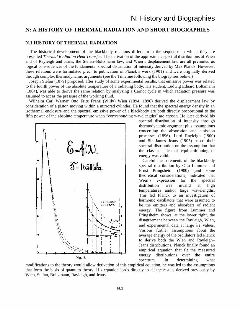
N: History and Biographies
N.1
N: A HISTORY OF THERMAL RADIATION AND SHORT BIOGRAPHIES
N.1 HISTORY OF THERMAL RADIATION
The historical development of the blackbody relations differs from the sequence in which they are
presented Thermal Radiation Heat Transfer. The derivation of the approximate spectral distributions of Wien
and of Rayleigh and Jeans, the Stefan–Boltzmann law, and Wien’s displacement law are all presented as
logical consequences of the fundamental spectral distribution of intensity derived by Max Planck. However,
these relations were formulated prior to publication of Planck’s work (1901) and were originally derived
through complex thermodynamic arguments (see the Timeline following the biographies below.)
Joseph Stefan (1879) proposed, after study of some experimental results, that emissive power was related
to the fourth power of the absolute temperature of a radiating body. His student, Ludwig Eduard Boltzmann
(1884), was able to derive the same relation by analyzing a Carnot cycle in which radiation pressure was
assumed to act as the pressure of the working fluid.
Wilhelm Carl Werner Otto Fritz Franz (Willy) Wien (1894, 1896) derived the displacement law by
consideration of a piston moving within a mirrored cylinder. He found that the spectral energy density in an
isothermal enclosure and the spectral emissive power of a blackbody are both directly proportional to the
fifth power of the absolute temperature when “corresponding wavelengths” are chosen. He later derived his
spectral distribution of intensity through
thermodynamic argument plus assumptions
concerning the absorption and emission
processes (1896). Lord Rayleigh (1900)
and Sir James Jeans (1905) based their
spectral distribution on the assumption that
the classical idea of equipartitioning of
energy was valid.
Careful measurements of the blackbody
spectral distribution by Otto Lummer and
Ernst Pringsheim (1900) (and some
theoretical considerations) indicated that
Wien’s expression for the spectral
distribution was invalid at high
temperatures and/or large wavelengths.
This led Planck to an investigation of
harmonic oscillators that were assumed to
be the emitters and absorbers of radiant
energy. The figure from Lummer and
Pringsheim shows, at the lower right, the
disagreement between the Rayleigh, Wien,
and experimental data at large T values.
Various further assumptions about the
average energy of the oscillators led Planck
to derive both the Wien and Rayleigh–
Jeans distributions. Planck finally found an
empirical equation that fit the measured
energy distributions over the entire
spectrum. In determining what
modifications to the theory would allow derivation of this empirical equation, he was led to the assumptions
that form the basis of quantum theory. His equation leads directly to all the results derived previously by
Wien, Stefan, Boltzmann, Rayleigh, and Jeans.
N: History and Biographies
N.2
Gustav Mie used the EM theory to predict the scattering coefficient and phase function for radiation
interacting with small spherical particles (1908a, b), and a historical overview of his contributions is in
Horvath (2009a).
Short biographies of the major historical contributors to the theory and practice of thermal radiation energy
transfer abridged from various sources are given below, along with a timeline that sets the sequence of their
accomplishments For an interesting and informative comprehensive review of the history of the field of
thermal radiation, the article by Barr (1960) is recommended. Howell (2002) gives a review of the
development of radiation energy transfer. Lewis (1973) and Crepeau (2009) discuss the derivation of Planck
law, and Stewart and Johnson (2016) give a historical overview of Planck’s Law and the computational
methods historically invoked in computing it in various forms.
REFERENCES
Barr, E. S.: Historical survey of the early development of the infrared spectral region, Am. J. Phys., 28(1),
42–54, 1960.
Boltzmann, L.: Ableitung des Stefan’schen Gesetzes, betreffend die Abhängigkeit der Wärmestrahlung von
der Temperatur aus der electromagnetischen Lichttheorie, Ann. Phys., Ser. 2, 22, 291–294, 1884.
Crepeau, J.: A brief history of the T4 law, Paper HT2009-88060, Proceedings of the HT 2009; 2009 Summer
Heat Transfer Conference, San Francisco, CA, July 2009.
Horvath, H. (ed.): Light scattering: Mie and more–commemorating 100 years of Mie’s 1908 publication,
JQSRT, 110(11), 783–786, 2009a.
Horvath, H.: Gustav Mie and the scattering and absorption of light by particles: Historic development and
basics, JQSRT, 110(11), 787–799, July 2009b.
Howell, J. R.: The development of engineering radiative heat transfer, IMECE2002-33131, 73-78, IMECE,
New Orleans, Nov. 2002.
Jeans, Sir. J.: On the partition of energy between matter and the ether, Phil. Mag., 10, 91–97, 1905.
Lewis, H. R.: Einstein’s derivation of Planck’s radiation law, Am. J. Phys., 41(1), 38–14, 1973.
Lummer, O. and Pringsheim, E.: Über die Strahlung des Schwarzen Körpers für Lange Wellen,
Verhandlungen der Deutschen Physikalischen Gesellschaft. 2, 163-180, 1900.
Mie, G.: Beiträge zur Optik trüber Medien, speziell kolloidaler Metallösungen, Ann. Phys., 330, 377–445,
1908a.
Mie, G.: Optics of turbid media, Ann. Phys., 25(3), 377–445, 1908b.
Planck, M.: Distribution of energy in the spectrum, Ann. Phys., 4(3), 553–563, 1901.
Rayleigh, Lord: The law of complete radiation, Phil. Mag., 49, 539–540, 1900.
Stefan, J.: Über die beziehung zwischen der wärmestrahlung und der temperatur, Sitzber. Akad. Wiss. Wien,
79(2), 391–428, 1879.
Stewart, S. M. and Johnson, R. B.: Blackbody Radiation: A History of Thermal Radiation Computational
Aids and Numerical Methods, CRC Press, Boca Raton, 2016.
Wien, W.: Temperatur und Entropie der Strahlung, Ann. Phys., Ser. 2, 52, 132–165, 1894.
Wien, W.: Über die Energievertheilung im Emissionsspectrum eines schwarzen Körpers, Ann. Phys., Ser. 3,
58, 662–669, 1896.
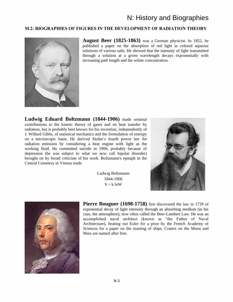
N: History and Biographies
N.3
M.2: BIOGRAPHIES OF FIGURES IN THE DEVELOPMENT OF RADIATION THEORY
August Beer (1825-1863) was a German physicist. In 1852, he
published a paper on the absorption of red light in colored aqueous
solutions of various salts. He showed that the intensity of light transmitted
through a solution at a given wavelength decays exponentially with
increasing path length and the solute concentration.
Ludwig Eduard Boltzmann (1844-1906) made seminal
contributions to the kinetic theory of gases and on heat transfer by
radiation, but is probably best known for his invention, independently of
J. Willard Gibbs, of statistical mechanics and the formulation of entropy
on a microscopic basis. He derived Stefan’s fourth power law for
radiation emission by considering a heat engine with light as the
working fluid. He committed suicide in 1906, probably because of
depression (he was subject to what we now call bipolar disorder)
brought on by broad criticism of his work. Boltzmann's epitaph in the
Central Cemetery in Vienna reads
Ludwig Boltzmann
1844-1906
S = k lnW
Pierre Bouguer (1698-1758) first discovered the law in 1729 of
exponential decay of light intensity through an absorbing medium (in his
case, the atmosphere), now often called the Beer-Lambert Law. He was an
accomplished naval architect (known as “the Father of Naval
Architecture), beating out Euler for a prize by the French Academy of
Sciences for a paper on the masting of ships. Craters on the Moon and
Mars are named after him.
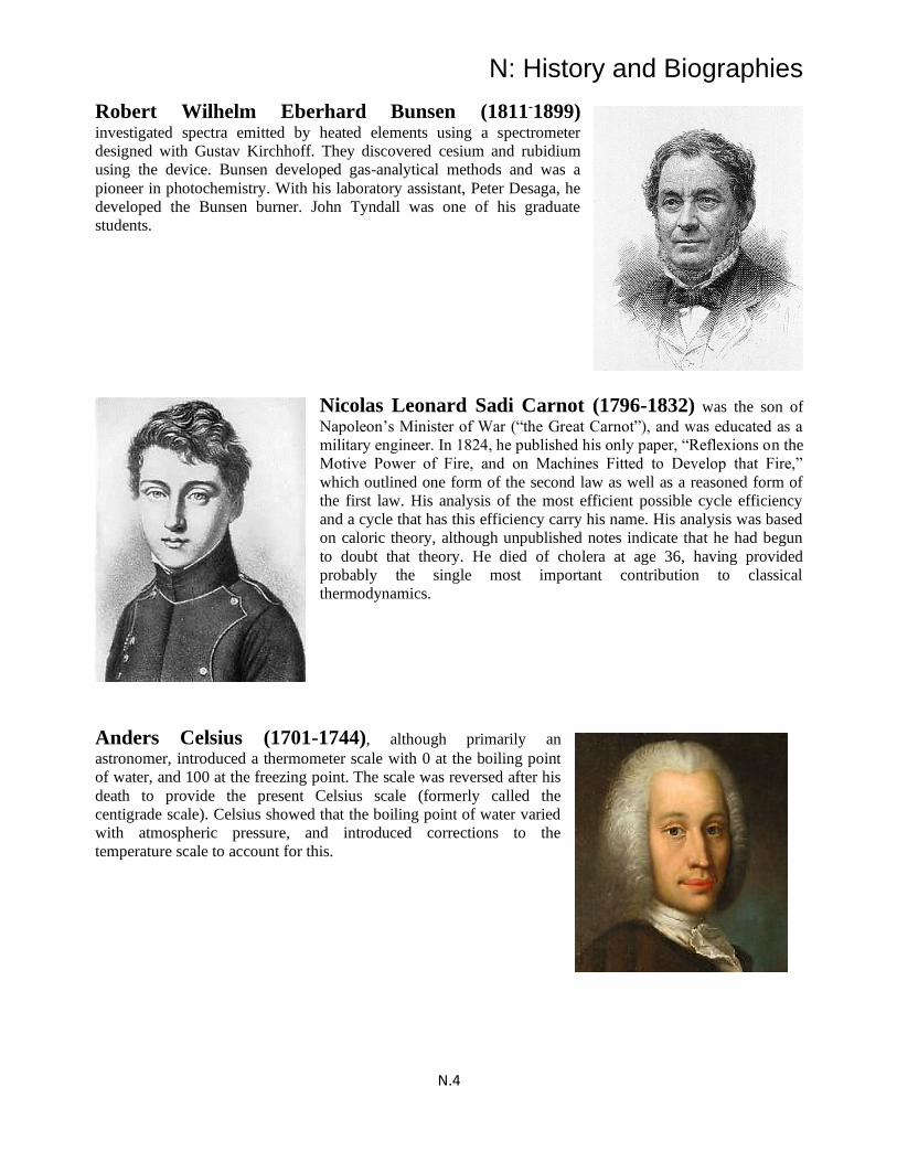
N: History and Biographies
N.4
Robert Wilhelm Eberhard Bunsen (1811-1899)
investigated spectra emitted by heated elements using a spectrometer
designed with Gustav Kirchhoff. They discovered cesium and rubidium
using the device. Bunsen developed gas-analytical methods and was a
pioneer in photochemistry. With his laboratory assistant, Peter Desaga, he
developed the Bunsen burner. John Tyndall was one of his graduate
students.
Nicolas Leonard Sadi Carnot (1796-1832) was the son of
Napoleon’s Minister of War (“the Great Carnot”), and was educated as a
military engineer. In 1824, he published his only paper, “Reflexions on the
Motive Power of Fire, and on Machines Fitted to Develop that Fire,”
which outlined one form of the second law as well as a reasoned form of
the first law. His analysis of the most efficient possible cycle efficiency
and a cycle that has this efficiency carry his name. His analysis was based
on caloric theory, although unpublished notes indicate that he had begun
to doubt that theory. He died of cholera at age 36, having provided
probably the single most important contribution to classical
thermodynamics.
Anders Celsius (1701-1744), although primarily an
astronomer, introduced a thermometer scale with 0 at the boiling point
of water, and 100 at the freezing point. The scale was reversed after his
death to provide the present Celsius scale (formerly called the
centigrade scale). Celsius showed that the boiling point of water varied
with atmospheric pressure, and introduced corrections to the
temperature scale to account for this.

N: History and Biographies
N.5
Subrahmanyan Chandrasekhar (1910-1995) won the Nobel
Prize in 1938 for his work on the structure and evolution of stars, later
showing star progression toward becoming a black hole. His uncle was
Chandrasekhara Venkata Raman who won the 1930 Nobel Prize in Physics
for his work on Raman scattering of photons. His book Radiative Transfer
(1960) outlines the discrete ordinates method (DOM) now used
extensively in thermal radiation transfer and introduces methods for
treating scattering using Stoke’s parameters.
Photo courtesy of University of Chicago
Photographic Archive, [apf1-09456], Special
Collections Research Center, University of
Chicago Library.
Louis de Broglie (1892-1987) did not originally envisage a
career in science. He entered the Sorbonne in Paris taking a course in
history and graduated at 18 with an arts degree. However, he became
interested in mathematics and physics and chose to study for a degree in
theoretical physics.
De Broglie was awarded his undergraduate degree in 1913 but
his career was put on hold by World War I. His doctoral thesis put
forward his theory of electron waves, based on the work of Einstein and
Planck. It proposed the theory for which he is best known, the particle-
wave duality theory that matter has the properties of both particles and
waves. The wave nature of the electron was experimentally confirmed in
1927.
His was awarded the Nobel Prize in 1929 and continued to work
on extensions of wave mechanics. He questioned whether the statistical
nature of quantum physics reflects an ignorance of the underlying theory or whether statistics is all that can
be known.
John William Draper (1811-1882) was an English-born
American scientist. In 1847 he observed the Draper point of 798 K at
which the emission from a heated object becomes visible to the human
eye. In his 1847 paper he presented data on the emission vs. temperature
from a heated object (replotted here on an absolute scale) but failed to
recognize the fourth-power
dependence, because an absolute
temperature scale was not yet in
use.
He is credited with taking the
one of the first photographic
portraits in 1839. An image of his
sister from 1840 is considered the
oldest surviving portrait photo.
He took the first detailed photograph of the moon in 1840.
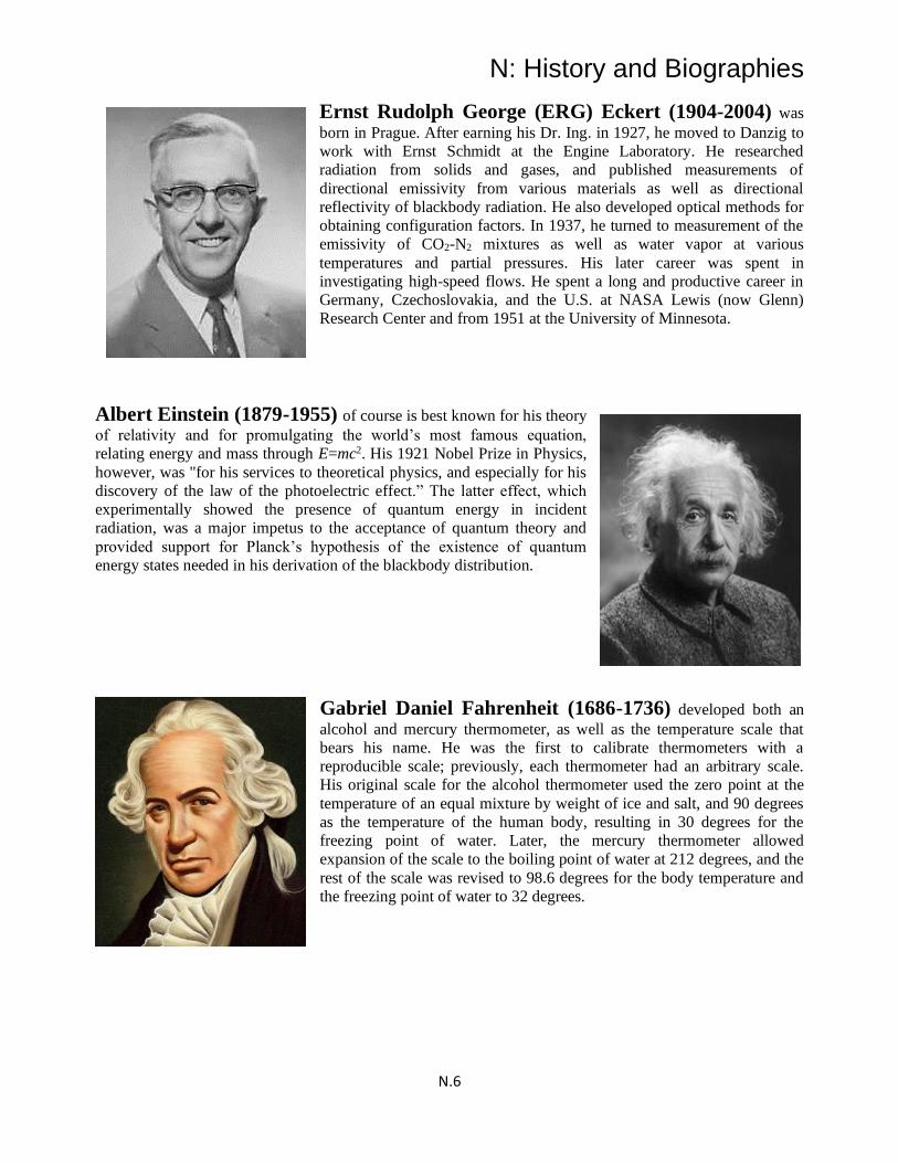
N: History and Biographies
N.6
Ernst Rudolph George (ERG) Eckert (1904-2004) was
born in Prague. After earning his Dr. Ing. in 1927, he moved to Danzig to
work with Ernst Schmidt at the Engine Laboratory. He researched
radiation from solids and gases, and published measurements of
directional emissivity from various materials as well as directional
reflectivity of blackbody radiation. He also developed optical methods for
obtaining configuration factors. In 1937, he turned to measurement of the
emissivity of CO2-N2 mixtures as well as water vapor at various
temperatures and partial pressures. His later career was spent in
investigating high-speed flows. He spent a long and productive career in
Germany, Czechoslovakia, and the U.S. at NASA Lewis (now Glenn)
Research Center and from 1951 at the University of Minnesota.
Albert Einstein (1879-1955) of course is best known for his theory
of relativity and for promulgating the world’s most famous equation,
relating energy and mass through E=mc2. His 1921 Nobel Prize in Physics,
however, was "for his services to theoretical physics, and especially for his
discovery of the law of the photoelectric effect.” The latter effect, which
experimentally showed the presence of quantum energy in incident
radiation, was a major impetus to the acceptance of quantum theory and
provided support for Planck’s hypothesis of the existence of quantum
energy states needed in his derivation of the blackbody distribution.
Gabriel Daniel Fahrenheit (1686-1736) developed both an
alcohol and mercury thermometer, as well as the temperature scale that
bears his name. He was the first to calibrate thermometers with a
reproducible scale; previously, each thermometer had an arbitrary scale.
His original scale for the alcohol thermometer used the zero point at the
temperature of an equal mixture by weight of ice and salt, and 90 degrees
as the temperature of the human body, resulting in 30 degrees for the
freezing point of water. Later, the mercury thermometer allowed
expansion of the scale to the boiling point of water at 212 degrees, and the
rest of the scale was revised to 98.6 degrees for the body temperature and
the freezing point of water to 32 degrees.
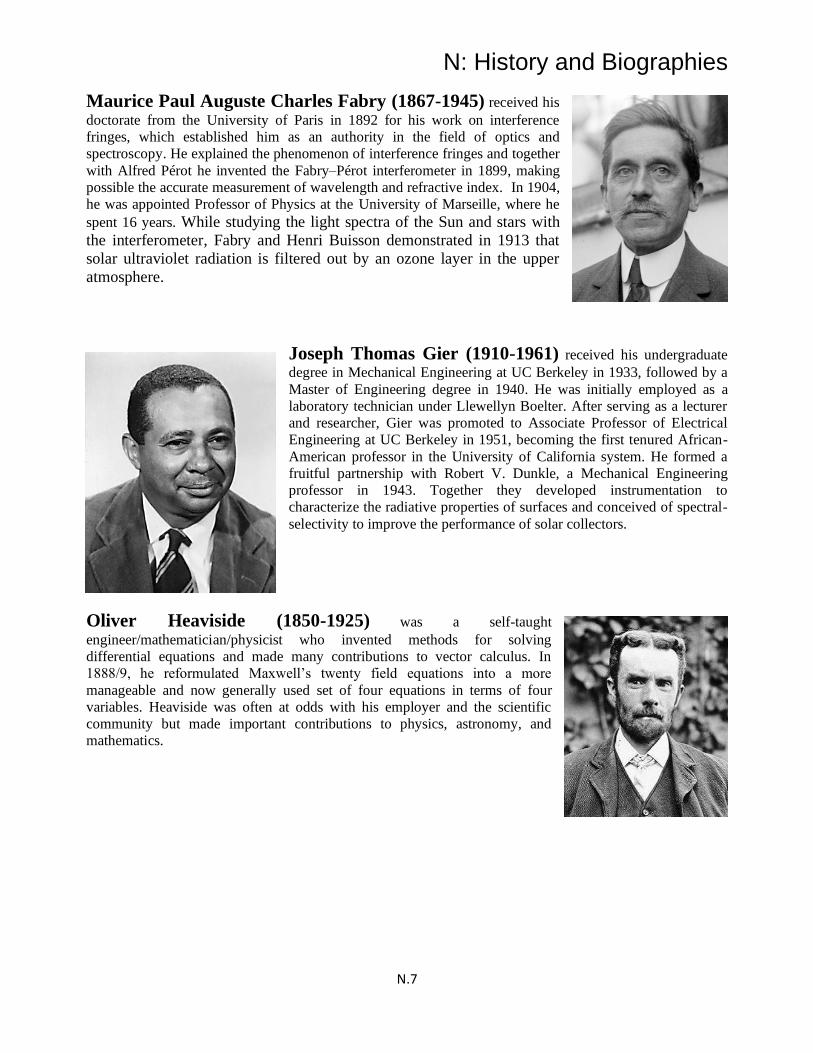
N: History and Biographies
N.7
Maurice Paul Auguste Charles Fabry (1867-1945) received his
doctorate from the University of Paris in 1892 for his work on interference
fringes, which established him as an authority in the field of optics and
spectroscopy. He explained the phenomenon of interference fringes and together
with Alfred Pérot he invented the Fabry–Pérot interferometer in 1899, making
possible the accurate measurement of wavelength and refractive index. In 1904,
he was appointed Professor of Physics at the University of Marseille, where he
spent 16 years. While studying the light spectra of the Sun and stars with
the interferometer, Fabry and Henri Buisson demonstrated in 1913 that
solar ultraviolet radiation is filtered out by an ozone layer in the upper
atmosphere.
Joseph Thomas Gier (1910-1961) received his undergraduate
degree in Mechanical Engineering at UC Berkeley in 1933, followed by a
Master of Engineering degree in 1940. He was initially employed as a
laboratory technician under Llewellyn Boelter. After serving as a lecturer
and researcher, Gier was promoted to Associate Professor of Electrical
Engineering at UC Berkeley in 1951, becoming the first tenured African-
American professor in the University of California system. He formed a
fruitful partnership with Robert V. Dunkle, a Mechanical Engineering
professor in 1943. Together they developed instrumentation to
characterize the radiative properties of surfaces and conceived of spectral-
selectivity to improve the performance of solar collectors.
Oliver Heaviside (1850-1925) was a self-taught
engineer/mathematician/physicist who invented methods for solving
differential equations and made many contributions to vector calculus. In
1888/9, he reformulated Maxwell’s twenty field equations into a more
manageable and now generally used set of four equations in terms of four
variables. Heaviside was often at odds with his employer and the scientific
community but made important contributions to physics, astronomy, and
mathematics.

N: History and Biographies
N.8
William Herschel (1738-1822) was a German-born British
astronomer. He constructed his first large telescope in 1774 and
spent nine years carrying out sky surveys to investigate double stars.
In March 1781 he discovered the planet Uranus.
He pioneered the use of astronomical spectrophotometry,
measuring stellar spectral distributions. In 1800, he discovered the
presence of infrared radiation in sunlight by passing it through a
prism and holding a thermometer just beyond the red end of the
visible spectrum. It showed a higher temperature than the visible
spectrum, implying energy in then unknown infrared portion of the
spectrum. He improved the measurement of the rotation period of
Mars, and determined that the Martian polar caps vary seasonally,
Hoyt Clarke Hottel (1903-1998) was a Professor at MIT
from 1928 until his death and became an Emeritus Professor in
1968. He developed gas emissivity charts for the important
combustion gases, the crossed-string method for determining
configuration factors in 2D geometries, and in 1927 papers
established the engineering basis for treating radiation in furnaces,
including the zone method. Hottel also contributed to the fields of
combustion and solar energy.
Margaret Lindsay Huggins (1848-1915) was a pioneer in
measuring stellar spectra. She, along with her husband William
Huggins, was the first to show that the stars were indeed suns, based
on the similarity of their emission spectra with that of the Sun
(especially spectral lines of magnesium and calcium). Their
instrumentation was based on a spectroscope model proposed by
Bunsen and Kirchhoff. Observations of Sirius showed a slight
Doppler shift in the measured spectra, which indicated that it was
moving away from the Earth. This eventually led to the discovery of
the expanding universe.

N: History and Biographies
N.9
Christiaan Huygens (1629-1695) was born and died at The
Hague. His father had studied natural philosophy and was a
diplomat. Christiaan gained access through him to the top
scientific circles of the times. He studied law and mathematics at
the University of Leiden and the College of Orange at Breda.
In 1654 his attention was directed to the improvement of
the telescope. In 1655, using one of his own lenses, he detected the
first moon of Saturn. His astronomical observations required some
exact means of measuring time, and this led him in 1656 to invent
the pendulum clock. His reputation was now so great that in 1665,
Louis XIV offered him a pension if he would live in Paris, which
became his place of residence. In 1670 he had a serious illness
which resulted in leaving Paris for Holland. By 1671 he returned
to Paris. In 1672 Louis XIV invaded the Low Countries and Huygens found himself in the position
of being in an important position in Paris at a time France was at war with his own country.
Scientists of this era felt themselves above political wars and Huygens, with much support from his
friends, continued his work.
The first watch regulated by a balance spring was made under Huygens's directions, and
presented by him to Louis XIV. He returned to Holland in 1681 and devoted himself to the
construction of lenses of enormous focal length, and he discovered the achromatic telescope eye
piece which is known by his name.
In 1689 he came from Holland to England in order to make the acquaintance of Newton,
whose Principia had been published in 1687. Huygens fully recognized the merits of the work but
believed any theory incomplete which did not explain gravitation by mechanical means and so
didn’t accept Newton’s theory of universal gravitation which “appears to me absurd.” On his return
in 1690 Huygens published his treatise on light in which the wave theory was expounded and
explained. The immense reputation of Newton led to disbelief in any theory which he rejected, and
to the general adoption of Newton's corpuscular theory over wave ideas.
In the final years of his life Huygens composed one of the earliest discussions of
extraterrestrial life, published after his death as the Cosmotheoros (1698).
James Hopwood Jeans (1877-1946) was educated in London.
Initially interested in the classics, he soon turned towards mathematics.
Jeans went to Trinity College Cambridge in 1896 on a
mathematical scholarship. As an undergrad he gained experience in
experimental physics in the Cavendish Laboratory during 1899-1900.
During recovery from tuberculosis in 1902 and 1903 he worked on his
first major text The Dynamical Theory of Gases. Planck had announced in
1900 his formula on black-body radiation, but Jeans was strongly opposed
to Planck's results.
He held a series of positions between 1900 and 1906, and during
this period he published his second major text Theoretical Mechanics
(1906). He published The Mathematical Theory of Electricity and
Magnetism in 1908 while in the United States. In 1909 he returned to
England and held the post of Lecturer in Applied Mathematics at
Cambridge until he retired in 1912. Jeans continued work and wrote Radiation and Quantum Theory in 1914.
In this work he showed that he had come to accept Planck's black-body formula. He died in September 1946.
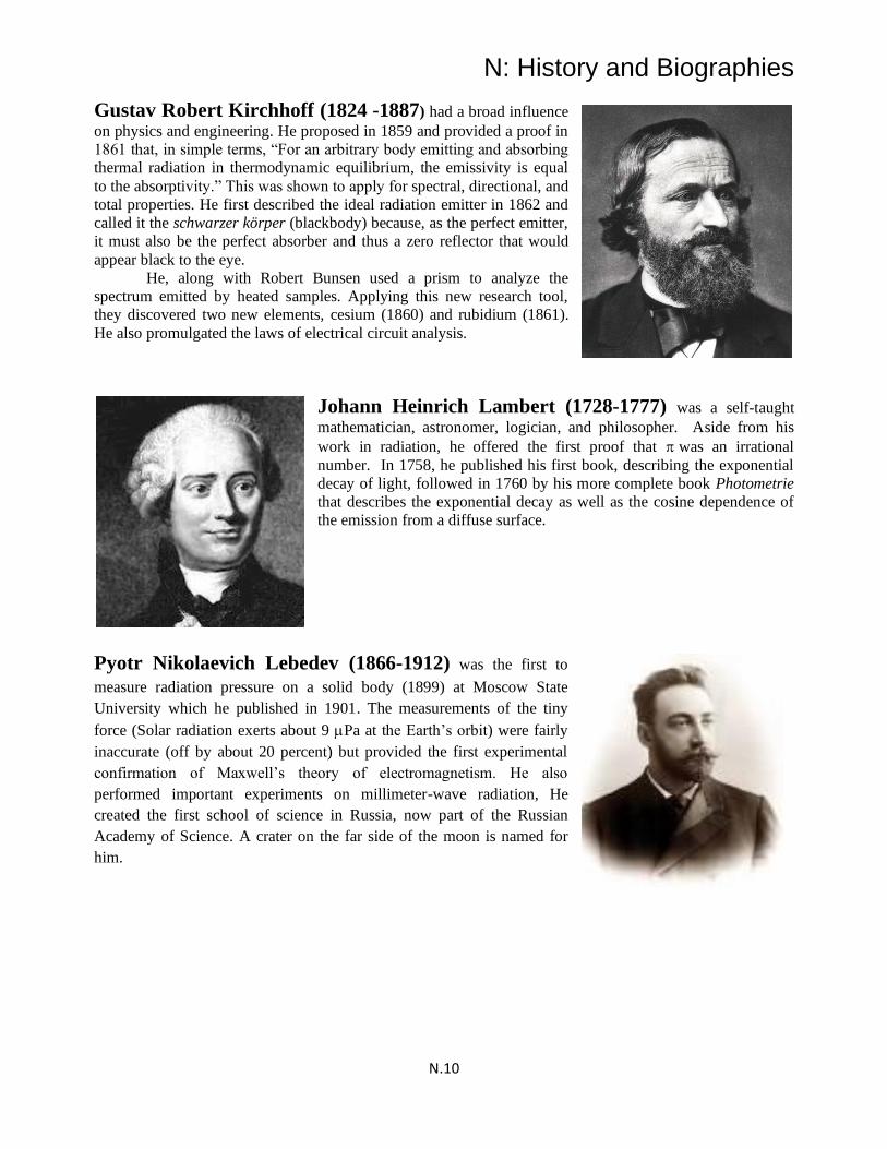
N: History and Biographies
N.10
Gustav Robert Kirchhoff (1824 -1887) had a broad influence
on physics and engineering. He proposed in 1859 and provided a proof in
1861 that, in simple terms, “For an arbitrary body emitting and absorbing
thermal radiation in thermodynamic equilibrium, the emissivity is equal
to the absorptivity.” This was shown to apply for spectral, directional, and
total properties. He first described the ideal radiation emitter in 1862 and
called it the schwarzer körper (blackbody) because, as the perfect emitter,
it must also be the perfect absorber and thus a zero reflector that would
appear black to the eye.
He, along with Robert Bunsen used a prism to analyze the
spectrum emitted by heated samples. Applying this new research tool,
they discovered two new elements, cesium (1860) and rubidium (1861).
He also promulgated the laws of electrical circuit analysis.
Johann Heinrich Lambert (1728-1777) was a self-taught
mathematician, astronomer, logician, and philosopher. Aside from his
work in radiation, he offered the first proof that was an irrational
number. In 1758, he published his first book, describing the exponential
decay of light, followed in 1760 by his more complete book Photometrie
that describes the exponential decay as well as the cosine dependence of
the emission from a diffuse surface.
Pyotr Nikolaevich Lebedev (1866-1912) was the first to
measure radiation pressure on a solid body (1899) at Moscow State
University which he published in 1901. The measurements of the tiny
force (Solar radiation exerts about 9 Pa at the Earth’s orbit) were fairly
inaccurate (off by about 20 percent) but provided the first experimental
confirmation of Maxwell’s theory of electromagnetism. He also
performed important experiments on millimeter-wave radiation, He
created the first school of science in Russia, now part of the Russian
Academy of Science. A crater on the far side of the moon is named for
him.

N: History and Biographies
N.11
Gilbert Newton Lewis (1875- 1946) was a precocious child
who learned to read at age three. At age 13 he entered the prep school of
the University of Nebraska and continued to the University. After his
second year, he transferred to Harvard, where he concentrated in
chemistry, getting his B.A. in 1896 and Ph.D. in 1899.
After earning his Ph.D., he studied under Wilhelm Ostwald
at Leipzig and Nernst at Göttingen. In 1905 MIT appointed him to
the faculty. He became assistant professor in 1907, associate
professor on 1908, and full professor in 1911. He left MIT to
become dean of the College of Chemistry at UC Berkeley in 1912.
In 1908 he published the first of several papers on
relativity, in which he derived the mass-energy relationship in a
different way from Einstein's. In 1913, he was elected to the
National Academy of Sciences, but in 1934 he resigned in a dispute over internal politics. In 1926,
he coined the term "photon" for the smallest unit of radiant energy. He died at 70 of a heart attack
while working in his laboratory.
Ludvig Valentin Lorenz (1829-1891) was a Danish chemical
engineer who became interested in physics. Because he published in
Danish, his work went unrecognized for many years. He published the
relation between the density of a pure transparent material and light
refraction in 1869. He also derived the correct velocity of light from
electromagnetic theory. In 1890 he preceded Gustav Mie in proposing a
theory of light scattering from spherical particles, sometimes now called
the Lorenz-Mie theory.
Otto Richard Lummer
(1860-1925) (left) and Ernst
Pringsheim (1859-1917) (right). Lummer received the Ph.D.
under Helmholtz in 1882 and joined
the University of Berlin as lecturer in
physics in 1886. He became professor
in 1896 and in 1905 was appointed full
professor of theoretical physics at the
University of Breslau, where his close
collaborator Ernst Pringsheim had
preceded him by six months. In 1898,
Lummer and Ferdinand Kurlbaum had
published an account of their cavity radiation source (hohlraum), used
largely unchanged for radiation measurements to the present. It was a hole
in the wall of a platinum box, divided by diaphragms, with its interior blackened.

N: History and Biographies
N.12
Pringsheim’s doctoral dissertation of 1882 determined the direction of his research- heat and light
radiation. Despite his appointment in theoretical physics at Breslau, Pringsheim’s scientific production was
largely experimental. At Berlin it was characterized first by a period of research done alone and then in
cooperation with Lummer after 1896. He developed the radiometer into a useful instrument for measuring
infrared radiation.
In 1896, Lummer and Pringsheim turned to investigations of thermal radiation. Continuing Wien’s
work, Pringsheim assisted Lummer in implementing Kirchhoff’s concept of the blackbody They verified the
Stefan-Boltzmann law for the temperature dependence of total radiated energy. They then measured the
spectral distribution of the radiation energy with the aid of a hohlraum.
In September 1900 they published a paper stating the “invalidity of the Wien-Planck spectral
equation.” Such negative statements were the main stimuli for Planck to seek a new radiation expression.
James Clerk Maxwell (1831-1879), along with his many
extremely important contributions in electromagnetic theory and other
fields of science, formulated the kinetic theory of gases. He is often
considered the most influential physicist after Einstein and Newton.
He described the propagation of an electromagnetic wave using a
system of 20 equations, and showed that the speed of electromagnetic
wave propagation was equal to the speed of light, implying that light was
itself an electromagnetic wave.
Working with Clausius, he used a statistical approach to find the
velocity distribution in an assembly of gas molecules at a given
temperature (later derived using the maximum entropy principle by
Boltzmann, and now called the Maxwell-Boltzmann distribution). He also
observed the relationships among thermodynamic properties embodied in
Maxwell’s Relations.
Gustav Adolf Feodor Wilhelm Ludwig Mie (1868-
1957) was a professor of physics with a strong background in
mathematics. He researched colloids at the University of Greifswald in
North-Eastern Germany. One of his PhD students investigated the
scattering and attenuation of light by gold colloids. Mie used his
knowledge of the Maxwell equations and solutions of very similar
problems in the literature to treat the theoretical problem of scattering and
absorption of light by a small absorbing sphere. Since these calculations
were done by hand, Mie had to limit his theoretical results to three terms
in infinite expansions, and this limited treatment to particles smaller than
200 nm at visible wavelengths. Mie's paper was hardly noticed for the next
50 years. He developed the Mie system of units in 1910 with the basic
units Volt, Ampere, Coulomb and Second (VACS-system).
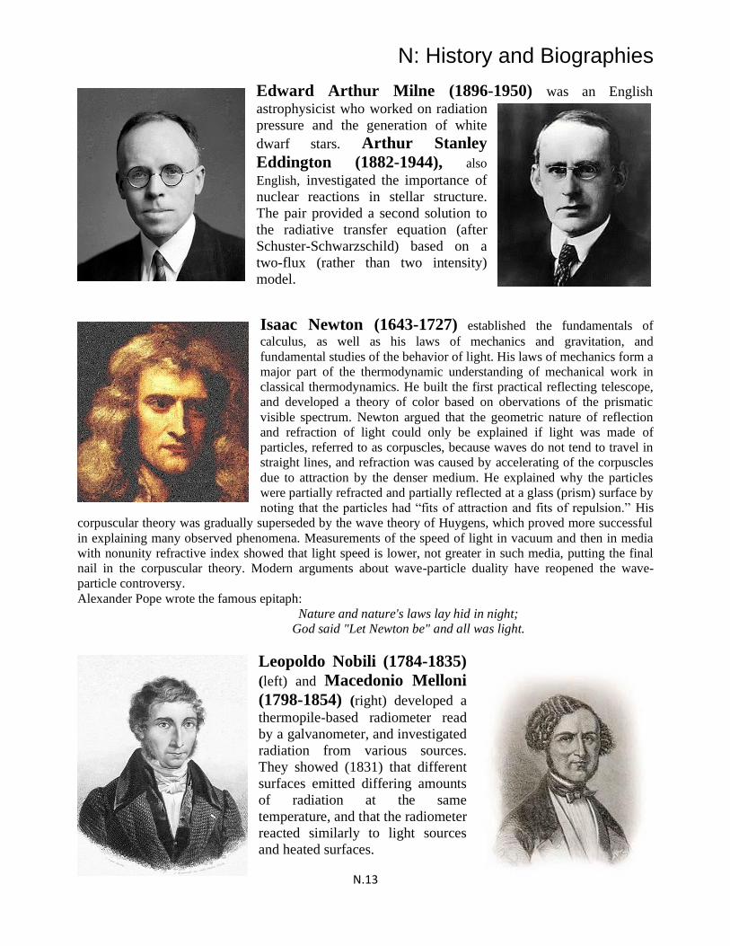
N: History and Biographies
N.13
Edward Arthur Milne (1896-1950) was an English
astrophysicist who worked on radiation
pressure and the generation of white
dwarf stars. Arthur Stanley
Eddington (1882-1944), also
English, investigated the importance of
nuclear reactions in stellar structure.
The pair provided a second solution to
the radiative transfer equation (after
Schuster-Schwarzschild) based on a
two-flux (rather than two intensity)
model.
Isaac Newton (1643-1727) established the fundamentals of
calculus, as well as his laws of mechanics and gravitation, and
fundamental studies of the behavior of light. His laws of mechanics form a
major part of the thermodynamic understanding of mechanical work in
classical thermodynamics. He built the first practical reflecting telescope,
and developed a theory of color based on obervations of the prismatic
visible spectrum. Newton argued that the geometric nature of reflection
and refraction of light could only be explained if light was made of
particles, referred to as corpuscles, because waves do not tend to travel in
straight lines, and refraction was caused by accelerating of the corpuscles
due to attraction by the denser medium. He explained why the particles
were partially refracted and partially reflected at a glass (prism) surface by
noting that the particles had “fits of attraction and fits of repulsion.” His
corpuscular theory was gradually superseded by the wave theory of Huygens, which proved more successful
in explaining many observed phenomena. Measurements of the speed of light in vacuum and then in media
with nonunity refractive index showed that light speed is lower, not greater in such media, putting the final
nail in the corpuscular theory. Modern arguments about wave-particle duality have reopened the wave-
particle controversy.
Alexander Pope wrote the famous epitaph:
Nature and nature's laws lay hid in night;
God said "Let Newton be" and all was light.
Leopoldo Nobili (1784-1835)
(left) and Macedonio Melloni
(1798-1854) (right) developed a
thermopile-based radiometer read
by a galvanometer, and investigated
radiation from various sources.
They showed (1831) that different
surfaces emitted differing amounts
of radiation at the same
temperature, and that the radiometer
reacted similarly to light sources
and heated surfaces.

N: History and Biographies
N.14
Max Planck (1858-1947) laid the basis for quantum mechanics and
was the forerunner of modern physics based on that theory. He studied with
Helmholtz, and was impressed with the powerful conclusions that could be
drawn from the Second Law. He originally developed his blackbody spectral
distribution based on the observation that the denominator in classically
derived distributions such as that of Wien needed to be slightly smaller to fit
the experimental data. His attempts to explain the theoretical basis of his
proposed spectral energy equation led him to hypothesize the existance of
quantized energy levels, a concept at odds with all of classical physics and
thermodynamics. He was forced to accept Boltzmann’s interpretation of the
Second Law as a statistical rather than an absolute law.
Pierre Prevost (1759-1839) was born in the Republic of Geneva,
and skittered between the church, law, education, travel, and philosophy
before concentrating on physical science after meeting Lagrange in Berlin.
In 1791, he proposed that the radiation from a body is emitted regardless
of the presence or absence of other bodies (“Prevost’s Law”). He also
commented on how radiative equilibrium between a body and its
surroundings is obtained.
William John Macquorn Rankine (1820-1872) was born
in Edinburgh, Scotland. He wrote practical treatises on thermodynamics,
including the first systematic treatment of steam engine theory, and the
exposition of what we now call the Rankine cycle. He proposed the
Rankine absolute temperature scale in 1859. He was also a poet, writing
The Mathematician in Love, and a song writer, composing such ballads
as They Never Shall Have Gibraltar.
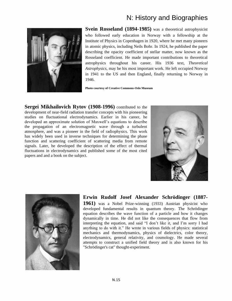
N: History and Biographies
N.15
Svein Rosseland (1894-1985) was a theoretical astrophysicist
who followed early education in Norway with a fellowship at the
Institute of Physics in Copenhagen in 1920, where he met many pioneers
in atomic physics, including Neils Bohr. In 1924, he published the paper
describing the opacity coefficient of stellar matter, now known as the
Rosseland coefficient. He made important contributions to theoretical
astrophysics throughout his career. His 1936 text, Theoretical
Astrophysics, may be his most important work. He left occupied Norway
in 1941 to the US and then England, finally returning to Norway in
1946.
Photo courtesy of Creative Commons-Oslo Museum
Sergei Mikhailovich Rytov (1908-1996) contributed to the
development of near-field radiation transfer concepts with his pioneering
studies on fluctuational electrodynamics. Earlier in his career, he
developed an approximate solution of Maxwell’s equations to describe
the propagation of an electromagnetic wave through a turbulent
atmosphere, and was a pioneer in the field of radiophysics. This work
has widely been used in inverse techniques for determining the phase
function and scattering coefficient of scattering media from remote
signals. Later, he developed the description of the effect of thermal
fluctuations in electrodynamics and published some of the most cited
papers and and a book on the subject.
Erwin Rudolf Josef Alexander Schrödinger (1887-
1961) was a Nobel Prize-winning (1933) Austrian physicist who
developed fundamental results in quantum theory. The Schrödinger
equation describes the wave function of a particle and how it changes
dynamically in time. He did not like the consequences that flow from
interpreting the equation, and said “I don’t like it, and I’m sorry I had
anything to do with it.” He wrote in various fields of physics: statistical
mechanics and thermodynamics, physics of dielectrics, color theory,
electrodynamics, general relativity, and cosmology. He made several
attempts to construct a unified field theory and is also known for his
"Schrödinger's cat" thought-experiment.
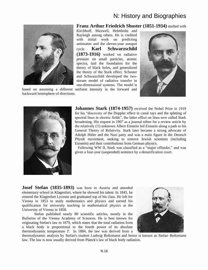
N: History and Biographies
N.16
Franz Arthur Friedrich Shuster (1851-1934) studied with
Kirchhoff, Maxwell, Helmholtz and
Rayleigh among others. He is credited
with initial work on predicting
antimatter and the eleven-year sunspot
cycle. Karl Schwarzschild
(1873-1916) worked on radiative
pressure on small particles, atomic
spectra, laid the foundation for the
theory of black holes, and generalized
the theory of the Stark effect. Schuster
and Schwarzchild developed the two-
stream model of radiative transfer in
one-dimensional systems. The model is
based on assuming a different uniform intensity in the forward and
backward hemisphere of directions.
Johannes Stark (1874-1957) received the Nobel Prize in 1919
for his “discovery of the Doppler effect in canal rays and the splitting of
spectral lines in electric fields”, the latter effect on lines now called Stark
broadening. His request in 1907 as a journal editor for a review article by
the relatively (!!) unknown Albert Einstein led Einstein along a path to his
General Theory of Relativity. Stark later became a strong advocate of
Adolph Hitler and the Nazi party and was a main figure in the Deutsch
Physik movement, seeking to remove Jewish scientists (including
Einstein) and their contributions from German physics.
Following WW II, Stark was classified as a “major offender,” and was
given a four-year (suspended) sentence by a denazification court.
Josef Stefan (1835-1893) was born in Austria and attended
elementary school in Klagenfurt, where he showed his talent. In 1845, he
entered the Klagenfurt Lyceum and graduated top of his class. He left for
Vienna in 1853 to study mathematics and physics and earned his
qualification for university teaching in mathematical physics at the
University of Vienna in 1858. Stefan published nearly 80 scientific articles, mostly in the
Bulletins of the Vienna Academy of Sciences. He is best known for
originating Stefan's law in 1879, which states that the total radiation from
a black body is proportional to the fourth power of its absolute
thermodynamic temperature T. In 1884, the law was derived from a
thermodynamic analysis by Stefan's student Ludwig Boltzmann and hence is known as Stefan–Boltzmann
law. The law is now usually derived from Planck's law of black body radiation.
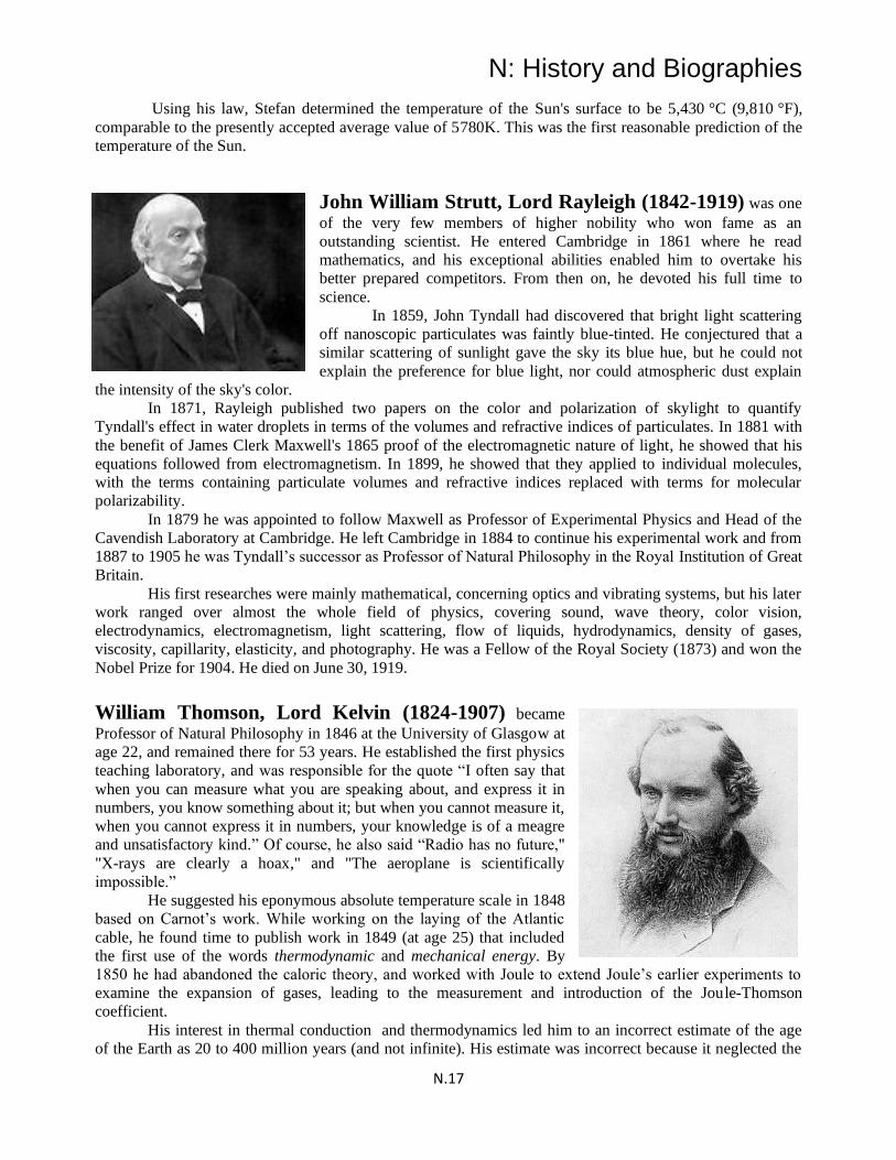
N: History and Biographies
N.17
Using his law, Stefan determined the temperature of the Sun's surface to be 5,430 °C (9,810 °F),
comparable to the presently accepted average value of 5780K. This was the first reasonable prediction of the
temperature of the Sun.
John William Strutt, Lord Rayleigh (1842-1919) was one
of the very few members of higher nobility who won fame as an
outstanding scientist. He entered Cambridge in 1861 where he read
mathematics, and his exceptional abilities enabled him to overtake his
better prepared competitors. From then on, he devoted his full time to
science.
In 1859, John Tyndall had discovered that bright light scattering
off nanoscopic particulates was faintly blue-tinted. He conjectured that a
similar scattering of sunlight gave the sky its blue hue, but he could not
explain the preference for blue light, nor could atmospheric dust explain
the intensity of the sky's color.
In 1871, Rayleigh published two papers on the color and polarization of skylight to quantify
Tyndall's effect in water droplets in terms of the volumes and refractive indices of particulates. In 1881 with
the benefit of James Clerk Maxwell's 1865 proof of the electromagnetic nature of light, he showed that his
equations followed from electromagnetism. In 1899, he showed that they applied to individual molecules,
with the terms containing particulate volumes and refractive indices replaced with terms for molecular
polarizability.
In 1879 he was appointed to follow Maxwell as Professor of Experimental Physics and Head of the
Cavendish Laboratory at Cambridge. He left Cambridge in 1884 to continue his experimental work and from
1887 to 1905 he was Tyndall’s successor as Professor of Natural Philosophy in the Royal Institution of Great
Britain.
His first researches were mainly mathematical, concerning optics and vibrating systems, but his later
work ranged over almost the whole field of physics, covering sound, wave theory, color vision,
electrodynamics, electromagnetism, light scattering, flow of liquids, hydrodynamics, density of gases,
viscosity, capillarity, elasticity, and photography. He was a Fellow of the Royal Society (1873) and won the
Nobel Prize for 1904. He died on June 30, 1919.
William Thomson, Lord Kelvin (1824-1907) became
Professor of Natural Philosophy in 1846 at the University of Glasgow at
age 22, and remained there for 53 years. He established the first physics
teaching laboratory, and was responsible for the quote “I often say that
when you can measure what you are speaking about, and express it in
numbers, you know something about it; but when you cannot measure it,
when you cannot express it in numbers, your knowledge is of a meagre
and unsatisfactory kind.” Of course, he also said “Radio has no future,"
"X-rays are clearly a hoax," and "The aeroplane is scientifically
impossible.”
He suggested his eponymous absolute temperature scale in 1848
based on Carnot’s work. While working on the laying of the Atlantic
cable, he found time to publish work in 1849 (at age 25) that included
the first use of the words thermodynamic and mechanical energy. By
1850 he had abandoned the caloric theory, and worked with Joule to extend Joule’s earlier experiments to
examine the expansion of gases, leading to the measurement and introduction of the Joule-Thomson
coefficient.
His interest in thermal conduction and thermodynamics led him to an incorrect estimate of the age
of the Earth as 20 to 400 million years (and not infinite). His estimate was incorrect because it neglected the
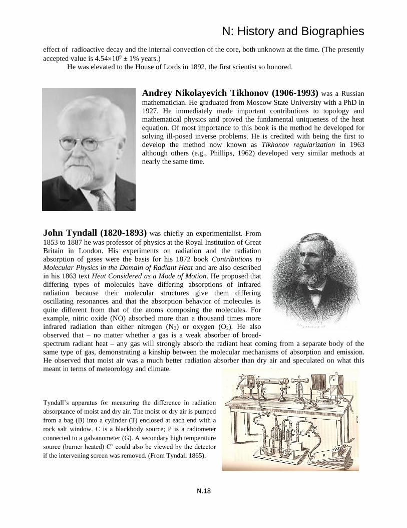
N: History and Biographies
N.18
effect of radioactive decay and the internal convection of the core, both unknown at the time. (The presently
accepted value is 4.54109 ± 1% years.)
He was elevated to the House of Lords in 1892, the first scientist so honored.
Andrey Nikolayevich Tikhonov (1906-1993) was a Russian
mathematician. He graduated from Moscow State University with a PhD in
1927. He immediately made important contributions to topology and
mathematical physics and proved the fundamental uniqueness of the heat
equation. Of most importance to this book is the method he developed for
solving ill-posed inverse problems. He is credited with being the first to
develop the method now known as Tikhonov regularization in 1963
although others (e.g., Phillips, 1962) developed very similar methods at
nearly the same time.
John Tyndall (1820-1893) was chiefly an experimentalist. From
1853 to 1887 he was professor of physics at the Royal Institution of Great
Britain in London. His experiments on radiation and the radiation
absorption of gases were the basis for his 1872 book Contributions to
Molecular Physics in the Domain of Radiant Heat and are also described
in his 1863 text Heat Considered as a Mode of Motion. He proposed that
differing types of molecules have differing absorptions of infrared
radiation because their molecular structures give them differing
oscillating resonances and that the absorption behavior of molecules is
quite different from that of the atoms composing the molecules. For
example, nitric oxide (NO) absorbed more than a thousand times more
infrared radiation than either nitrogen (N2) or oxygen (O2). He also
observed that – no matter whether a gas is a weak absorber of broad-
spectrum radiant heat – any gas will strongly absorb the radiant heat coming from a separate body of the
same type of gas, demonstrating a kinship between the molecular mechanisms of absorption and emission.
He observed that moist air was a much better radiation absorber than dry air and speculated on what this
meant in terms of meteorology and climate.
Tyndall’s apparatus for measuring the difference in radiation
absorptance of moist and dry air. The moist or dry air is pumped
from a bag (B) into a cylinder (T) enclosed at each end with a
rock salt window. C is a blackbody source; P is a radiometer
connected to a galvanometer (G). A secondary high temperature
source (burner heated) C’ could also be viewed by the detector
if the intervening screen was removed. (From Tyndall 1865).

N: History and Biographies
N.19
Stanislaw Ulam (1909-1984) was a Polish-born scientist who
worked at Los Alamos on the nuclear weapons Manhattan Project during
WW II. Following recovery from serious brain surgery, in 1947 he
brought forth the idea of implementing statistical techniques for modeling
the individual histories of neutrons during their supercritical reactions as a
substitute for solving the very complex equations otherwise required, now
known as the Monte Carlo method. He developed the idea along with John
von Neumann, Enrico Fermi, Nicholas Metropolis and others. Metropolis
and Ulam published the first paper in the open literature on the method in
1949.
Wilhelm Carl Werner Otto Fritz Franz (Willy) Wien
(1864-1928) was born in East Prussia to a landholding family. He
studied mathematics and physics at the Universities of Göttingen and
Berlin. Between 1883 and 1885, he worked in Hermann von Helmholtz’s
laboratory and in 1886, he took a doctorate with a thesis on diffraction
and on the influence of materials on the color of refracted light.
In 1893, he announced what would later be called the law of
displacement: that the product of wavelength and absolute temperature for
a blackbody is constant. In 1896, he proposed a formula which described
the spectral composition of radiation from an ideal body, which he called
a black body. This work impelled Max Planck to propose quantum effects
to bring Wien’s distribution into agreement with experimental
measurements. It also earned Wien the 1911 Nobel Prize in physics.
In the late 1890s, Wien studied cathode rays, confirming that they were
made of fast-moving negatively charged particles, or electrons, that were about two thousand times lighter
than hydrogen atoms. He then analyzed canal rays which pass through a perforated cathode, finding that they
were the positive equivalent of electrons and we now recognize them as streams of positive ions moving in
the opposite direction to the electrons in the cathode ray tube. Twenty years later this research led to the
development of mass spectrography.
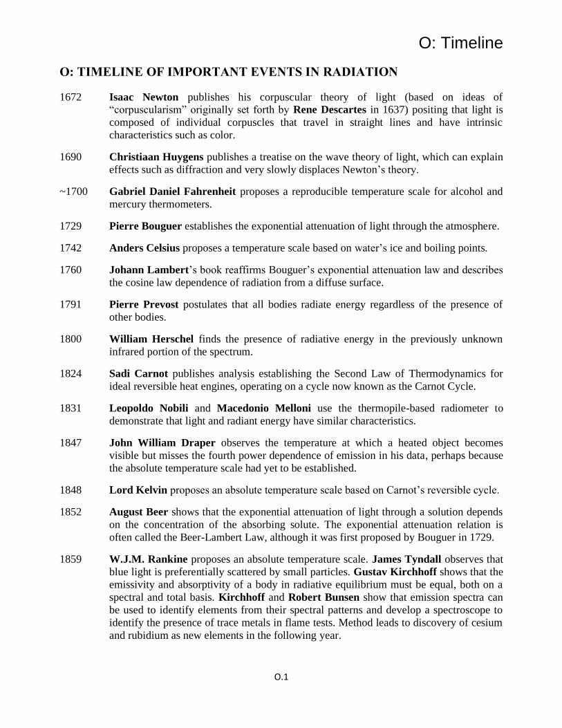
O: Timeline
O.1
O: TIMELINE OF IMPORTANT EVENTS IN RADIATION
1672 Isaac Newton publishes his corpuscular theory of light (based on ideas of “corpuscularism” originally set forth by Rene Descartes in 1637) positing that light is
composed of individual corpuscles that travel in straight lines and have intrinsic
characteristics such as color.
1690 Christiaan Huygens publishes a treatise on the wave theory of light, which can explain
effects such as diffraction and very slowly displaces Newton’s theory.
~1700 Gabriel Daniel Fahrenheit proposes a reproducible temperature scale for alcohol and
mercury thermometers.
1729 Pierre Bouguer establishes the exponential attenuation of light through the atmosphere.
1742 Anders Celsius proposes a temperature scale based on water’s ice and boiling points.
1760 Johann Lambert’s book reaffirms Bouguer’s exponential attenuation law and describes
the cosine law dependence of radiation from a diffuse surface.
1791 Pierre Prevost postulates that all bodies radiate energy regardless of the presence of
other bodies.
1800 William Herschel finds the presence of radiative energy in the previously unknown
infrared portion of the spectrum.
1824 Sadi Carnot publishes analysis establishing the Second Law of Thermodynamics for
ideal reversible heat engines, operating on a cycle now known as the Carnot Cycle.
1831 Leopoldo Nobili and Macedonio Melloni use the thermopile-based radiometer to
demonstrate that light and radiant energy have similar characteristics.
1847 John William Draper observes the temperature at which a heated object becomes
visible but misses the fourth power dependence of emission in his data, perhaps because
the absolute temperature scale had yet to be established.
1848 Lord Kelvin proposes an absolute temperature scale based on Carnot’s reversible cycle.
1852 August Beer shows that the exponential attenuation of light through a solution depends
on the concentration of the absorbing solute. The exponential attenuation relation is
often called the Beer-Lambert Law, although it was first proposed by Bouguer in 1729.
1859 W.J.M. Rankine proposes an absolute temperature scale. James Tyndall observes that
blue light is preferentially scattered by small particles. Gustav Kirchhoff shows that the
emissivity and absorptivity of a body in radiative equilibrium must be equal, both on a
spectral and total basis. Kirchhoff and Robert Bunsen show that emission spectra can
be used to identify elements from their spectral patterns and develop a spectroscope to
identify the presence of trace metals in flame tests. Method leads to discovery of cesium
and rubidium as new elements in the following year.
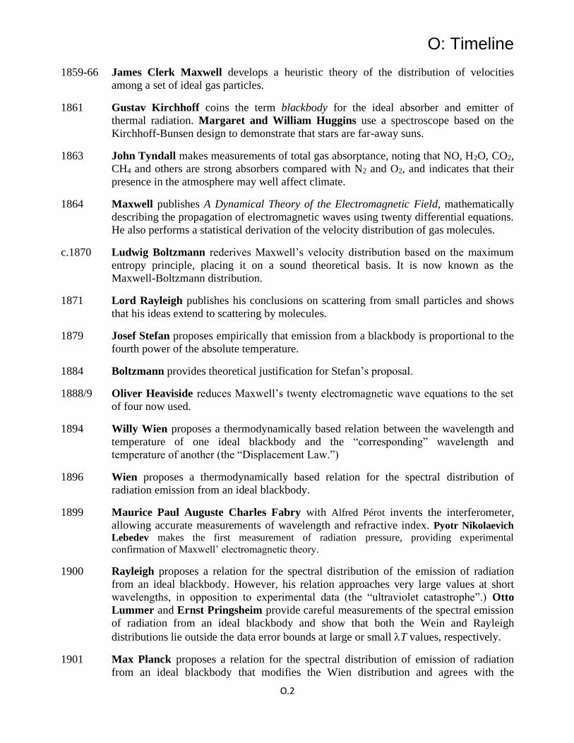
O: Timeline
O.2
1859-66 James Clerk Maxwell develops a heuristic theory of the distribution of velocities
among a set of ideal gas particles.
1861 Gustav Kirchhoff coins the term blackbody for the ideal absorber and emitter of
thermal radiation. Margaret and William Huggins use a spectroscope based on the
Kirchhoff-Bunsen design to demonstrate that stars are far-away suns.
1863 John Tyndall makes measurements of total gas absorptance, noting that NO, H2O, CO2,
CH4 and others are strong absorbers compared with N2 and O2, and indicates that their
presence in the atmosphere may well affect climate.
1864 Maxwell publishes A Dynamical Theory of the Electromagnetic Field, mathematically
describing the propagation of electromagnetic waves using twenty differential equations.
He also performs a statistical derivation of the velocity distribution of gas molecules.
c.1870 Ludwig Boltzmann rederives Maxwell’s velocity distribution based on the maximum
entropy principle, placing it on a sound theoretical basis. It is now known as the
Maxwell-Boltzmann distribution.
1871 Lord Rayleigh publishes his conclusions on scattering from small particles and shows
that his ideas extend to scattering by molecules.
1879 Josef Stefan proposes empirically that emission from a blackbody is proportional to the
fourth power of the absolute temperature.
1884 Boltzmann provides theoretical justification for Stefan’s proposal.
1888/9 Oliver Heaviside reduces Maxwell’s twenty electromagnetic wave equations to the set
of four now used.
1894 Willy Wien proposes a thermodynamically based relation between the wavelength and
temperature of one ideal blackbody and the “corresponding” wavelength and
temperature of another (the “Displacement Law.”)
1896 Wien proposes a thermodynamically based relation for the spectral distribution of
radiation emission from an ideal blackbody.
1899 Maurice Paul Auguste Charles Fabry with Alfred Pérot invents the interferometer,
allowing accurate measurements of wavelength and refractive index. Pyotr Nikolaevich
Lebedev makes the first measurement of radiation pressure, providing experimental
confirmation of Maxwell’ electromagnetic theory.
1900 Rayleigh proposes a relation for the spectral distribution of the emission of radiation
from an ideal blackbody. However, his relation approaches very large values at short
wavelengths, in opposition to experimental data (the “ultraviolet catastrophe”.) Otto
Lummer and Ernst Pringsheim provide careful measurements of the spectral emission
of radiation from an ideal blackbody and show that both the Wein and Rayleigh
distributions lie outside the data error bounds at large or small T values, respectively.
1901 Max Planck proposes a relation for the spectral distribution of emission of radiation
from an ideal blackbody that modifies the Wien distribution and agrees with the

O: Timeline
O.3
Lummer-Pringsheim data. The required assumption of quantized energy states necessary
to derive his distribution leads to the beginning of quantum theory.
1905 James Jeans bolsters Rayleigh’s idea of a spectral distribution by invoking the classical
idea of the equipartition of energy. Albert Einstein explains that the photoelectric effect
of electrons ejected from a surface exposed to light cannot be satisfactorily explained by
wave theory, but that the incident radiation must have energy quantum characteristics.
This gives credence to Planck’s quantum energy state hypothesis.
1905-6 Arthur Schuster and Karl Schwarzschild develop a two-intensity stream model of
radiative transfer, giving one of the first analytical solutions to radiative transfer in
participating media.
1908 Gustav Mie establishes the radiation scattering characteristics of particles.
1909 Johannes Stark receives Nobel Prize for discovering the effect of electrical fields on
spectral lines.
1921 E. A. Milne and Arthur Eddington provide a solution to the radiative transfer equation
in participating media based on a modified two-stream model.
1923 Luis de Broglie hypothesizes that since electromagnetic radiation can be interpreted in
terms of particles, then matter particles should also have the characteristics of waves (an
extension of the idea of wave-particle duality).
1924 Svein Rosseland describes the opacity of stellar matter in terms of the now named
Rosseland coefficient.
1926 Erwin Schrödinger publishes his wave equation, describing the wave characteristics of
particles as predicted to exist by de Broglie, leading to rapid advances in quantum
theory. G.N. Lewis coins the term photon for the particle/wave carrying radiant energy.
1927- Hoyt Hottel in a series of papers, chapters and texts provides the engineering basis and
combustion gas property values for calculating radiation transfer in combustion furnaces.
1937 E.R.G. Eckert measures the emittance of CO2-N2 and H2O-N2 mixtures.
1947 Stanislaw Ulam proposes the Monte Carlo method for modeling neutron interactions,
later extended to model thermal radiation.
1953 Sergei Mikhailovich Rytov publishes seminal work on the effect of electrical
fluctuations on thermal radiation, or fluctuation electrodynamics,
1963 Andrey Tikhonov introduces regularization methods to treat ill-posed inverse problem.
Credit for developments in the field since 1965 will await the judgment of historians.

P. ADDITIONAL HOMEWORK
P.1
P: ADDITIONAL HOMEWORK
The homework in this Appendix is meant to provide instructors or students an
additional range of problems from those in the text for extra assignment or home
study. Solutions are in the Solution Manual, available from the publisher.
Chapter 1:
P.1.1 Radiant energy at a wavelength of 2.0 μm is traveling through a vacuum. It then enters a medium with a
refractive index of 1.28.
(a) Find the following quantities for the radiation in the vacuum: speed, frequency, and wave number.
(b) Find the following quantities for the radiation in the medium: speed, frequency, wave number, and
wavelength.
Answer: (a) 2.9979 × 10⁸ m/s; 1.4990 × 10¹⁴ s−1; 5 × 10⁵ m−1. (b) 2.342 × 10⁸ m/s; 1.4990 × 10¹⁴ s−1; 6.40 × 10⁵
m−1; 1.5625 × 10⁻⁶ m
P.1.2 What range of radiation wavelengths is present within a glass sheet that has a wavelength-independent
refractive index of 1.29 when the sheet is exposed in vacuum to incident radiation in the visible range λ0 = 0.4–
0.7 μm?
Answer: 0.310–0.543 μm
P.1.3 Plot the hemispherical spectral emissive power Eλb for a blackbody in air [W/(m2·μm)] as a function of
wavelength (μm) for surface temperatures of 2000 and 6250 K.
P.1.4 A blackbody at 1100 K is radiating in the vacuum of outer space.
(a) What is the ratio of the spectral intensity of the blackbody at
λ = 1.0 μm to the spectral intensity at λ = 4.0 μm?
(b) What fraction of the blackbody emissive power lies between the wavelengths of λ = 1.0 μm and λ = 4.0 μm?
(c) At what wavelength does the peak energy in the radiated spectrum occur for this blackbody?
(d) How much energy is emitted by the blackbody in the range 1.0 ≤ λ ≤ 4.0 μm?
Answer: (a) 0.0541; (b) 0.5488.; (c) 2.6344m; (d) 45484 W/m2
P.1.5 Solar radiation is emitted by a fairly thin layer of hot plasma near the sun’s surface. This layer is cool compared
with the interior of the sun, where nuclear reactions are occurring. Various methods can be used to estimate the
resulting effective radiating temperature of the sun, such as determining the best fit of a blackbody spectrum to
the observed solar spectrum. Use two other methods (as follows), and compare the results to the oft-quoted value
of Tsolar = 5780 K.
(a) Using Wien’s law and taking the peak of the solar spectrum as 0.50 μm, estimate the solar radiating
temperature.
(b) Given the measured solar constant in the Earth’s orbit of 1368 W/m2 and using the “inverse square law” for the
reduction in heat flux with distance, estimate the solar temperature. The mean radius of the Earth’s orbit
around the sun is 149 × 106 km and the diameter of the sun is 1.392 × 10⁶ km.
Answer: (a) 5796 K; (b) 5766 K
P.1.6 A blackbody radiates such that the wavelength at its maximum emissive power is 2.50 μm. What fraction of the
total emissive power from this blackbody is in the range λ = 0.7 to λ = 6 μm?
Answer: 0.805
P.1.7 A radiometer is sensitive to radiation only in the interval 3.6 ≤ λ ≤ 8.5 μm. The radiometer is used to calibrate a
blackbody source at 1200 K. The radiometer records that the emitted energy is 5000 W/m2. What percentage of
the blackbody radiated energy in the prescribed wavelength range is the source actually emitting?
Answer: 11.2%
P.1.8 What temperature must a blackbody have for 25% of its emitted energy to be in the visible wavelength region?
Answer: 4,343 K, 12,460 K (Note: two solutions are possible!)

P: Additional Homework
P.2
P.1.9 Show that the blackbody spectral intensity Iλb increases with T at any fixed value of λ.
P.1.10 A sheet of silica glass transmits 87% of the radiation that is incident in the wavelength range between 0.38
and 2.7 μm and is essentially opaque to radiation having longer and shorter wavelengths. Estimate the percent of
solar radiation that the glass will transmit. (Consider the sun as a blackbody at 5780 K.)
If the garden in a greenhouse radiates as a black surface and is at 40°C, what percent of this radiation will be
transmitted through the glass?
Answer: 75.6%; 0.003%
P.1.11 Derive Wien’s displacement law in terms of wave number by differentiation of Planck’s spectral distribution
in terms of wave number, and show that T/ηmax = 5099.4 μm·K.
P.1.12 A student notes that the peak emission of the sun according to Wien’s displacement law is at a wavelength of
about λmax = C3/5780 K = 2897.8/ 5780 = 0.501 μm. Using ηmax = 1/0.501 μm, the student solves again for the
solar temperature using the result derived in Homework Problem P.1.11. Does this computed temperature agree
with the solar temperature? Why? (This is not trivial—put some thought into why.)
P.1.13Derive the relation between the wave number and the wavelength at the peak of the blackbody emission
spectrum. (You may use the result of Homework Problem P.1.11.)
Answer: ηmax (cm−1) = 5682.6/λmax (μm)
P.1.14 A 6 by 10 cm black rectangular sheet of metal is heated uniformly with 2600 W by passing an electric current
through it. One face of the rectangle is well insulated. The other face is exposed to vacuum and very cold
surroundings. At thermal equilibrium, what fraction of the emitted energy is in the wave number range from 0.40
to 2 μm−1?
Answer: 0.5086
P.1.15 Radiation from a blackbody source at 2,200 K is passing through a layer of air at 12,000 K and 1 atm.
Considering only the transmitted radiation (i.e., not accounting for emission by the air), what path length is
required to attenuate by 35% the energy at the wavelength corresponding to the maximum emission by the
blackbody source? At this λ, take κλ = 1.2 × 10⁻¹ cm−1 for air at 12,000 K and 1 atm.
Answer: 3.59 cm
P.1.16 A gas layer at constant pressure P has a linearly decreasing temperature across the layer and a constant mass
absorption coefficient κm (no scattering). For radiation passing in a normal direction through the layer, what is
the ratio I2/I1 as a function of T1, T2, and L? The temperature range T2 to T1 is low enough that emission from the
gas can be neglected. The gas constant is R.
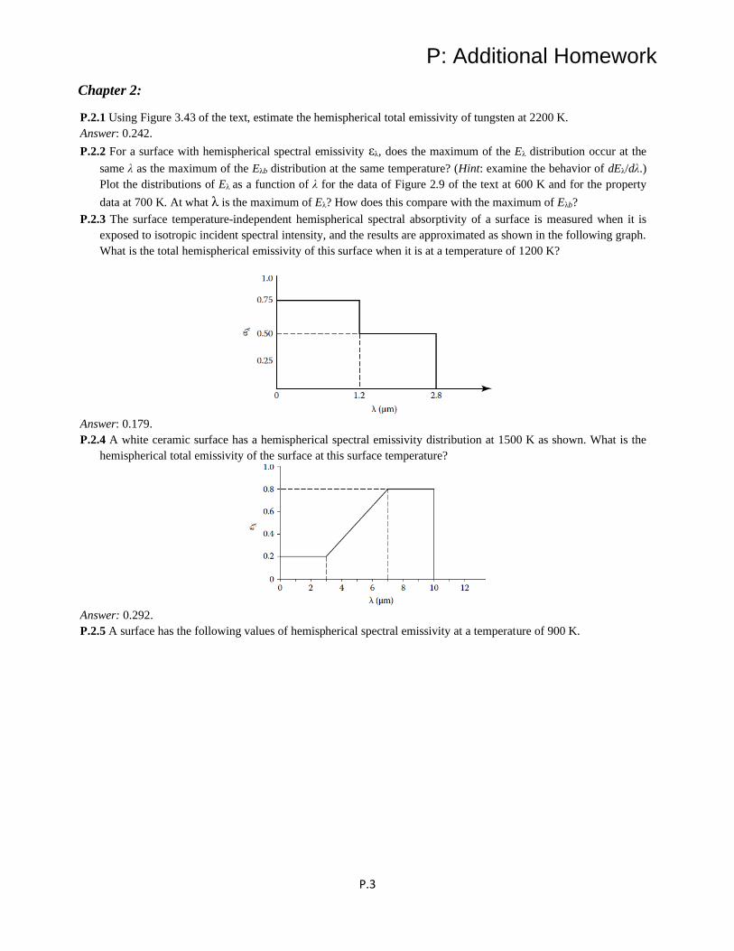
P: Additional Homework
P.3
Chapter 2:
P.2.1 Using Figure 3.43 of the text, estimate the hemispherical total emissivity of tungsten at 2200 K.
Answer: 0.242.
P.2.2 For a surface with hemispherical spectral emissivity ελ, does the maximum of the Eλ distribution occur at the
same λ as the maximum of the Eλb distribution at the same temperature? (Hint: examine the behavior of dEλ/dλ.)
Plot the distributions of Eλ as a function of λ for the data of Figure 2.9 of the text at 600 K and for the property
data at 700 K. At what λ is the maximum of Eλ? How does this compare with the maximum of Eλb?
P.2.3 The surface temperature-independent hemispherical spectral absorptivity of a surface is measured when it is
exposed to isotropic incident spectral intensity, and the results are approximated as shown in the following graph.
What is the total hemispherical emissivity of this surface when it is at a temperature of 1200 K?
Answer: 0.179.
P.2.4 A white ceramic surface has a hemispherical spectral emissivity distribution at 1500 K as shown. What is the
hemispherical total emissivity of the surface at this surface temperature?
Answer: 0.292.
P.2.5 A surface has the following values of hemispherical spectral emissivity at a temperature of 900 K.

P: Additional Homework
P.4
(a) What is the hemispherical total emissivity of the surface at 900 K?
(b) What is the hemispherical total absorptivity of the surface at 900 K if the incident radiation is from a gray
source at 1800 K that has an emissivity of 0.815? The incident radiation is uniform over all incident angles.
Answer: (a) 0.476; (b) 0.427.
P.2.6 A diffuse surface at 1100 K has a hemispherical spectral emissivity that can be approximated by the solid line
shown.
(a) What is the hemispherical-total emissive power of the surface? What is the total intensity emitted in a direction
60° from the normal to the surface?
(b) What percentage of the total emitted energy is in the wavelength range 5 < λ < 10 μm? How does this compare
with the percentage emitted in this wavelength range by a gray body at 1100 K with an emissivity ε = 0.611?
Answer: (a) 44,010 W/m2; 14,009 W/m2 · sr: (b) 36.7%; 24.0%.
P.2.7 The ελ for a metal at 1100 K is approximated as shown, and it does not vary significantly with the metal
temperature. The surface is diffuse.
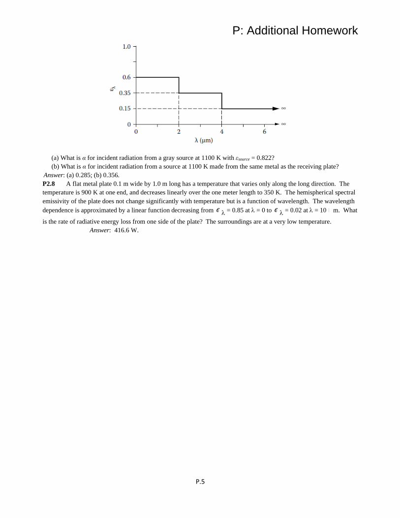
P: Additional Homework
P.5
(a) What is α for incident radiation from a gray source at 1100 K with εsource = 0.822?
(b) What is α for incident radiation from a source at 1100 K made from the same metal as the receiving plate?
Answer: (a) 0.285; (b) 0.356.
P2.8 A flat metal plate 0.1 m wide by 1.0 m long has a temperature that varies only along the long direction. The
temperature is 900 K at one end, and decreases linearly over the one meter length to 350 K. The hemispherical spectral
emissivity of the plate does not change significantly with temperature but is a function of wavelength. The wavelength
dependence is approximated by a linear function decreasing from ε = 0.85 at = 0 to ε = 0.02 at = 10 m. What
is the rate of radiative energy loss from one side of the plate? The surroundings are at a very low temperature.
Answer: 416.6 W.

P: Additional Homework
P.6
Chapter 3:
P.3.1 A smooth hot ceramic dielectric sphere with an index of refraction n = 1.40 is photographed with an IR camera.
Calculate how bright the image is at locations B and C relative to that at A. (Camera is distant from sphere.)
Answer: 0.987; 0.849.
P.3.2 A smooth dielectric material has a normal spectral emissivity of ελ,n = 0.765 at a wavelength in air of 6 μm.
Find or estimate values for
(a) The hemispherical-spectral emissivity ελ at the same wavelength.
(b) The perpendicular component of the directional-hemispherical-spectral reflectivity ρλ,⊥(θ) at the same
wavelength and for incidence at θ = 40°.
Answer: (a) 0.736; (b) 0.327.
P.3.3 A smooth ceramic dielectric has an index of refraction n = 1.48, which is independent of wavelength. If a flat
ceramic disk is at 1100 K, how much emitted energy per unit time is received by the detector when it is placed at
θ = 0° or at θ = 60°? Use relations from the EM theory.
Answer: 15.69 × 10⁻⁵ W at θ = 0°; 7.845 × 10⁻⁵ W at θ = 60°.
P.3.4 At a temperature of 300 K, these metals have the following resistivities (Table 3.2):
Copper 1.71 x 10⁻⁶ -cm
Gold 2.26 x 10⁻⁶ -cm
Aluminum 2.71 x 10⁻⁶ -cm
What are the theoretical normal total emissivities and hemispherical total emissivities of these metals, and how do
they compare with tabulated values for clean, unoxidized, polished surfaces?
Answer: εn 0.0131, 0.0157, 0.0168; ε 0.0170, 0.0202, 0.0217.

P: Additional Homework
P.7
P.3.5 A clean metal surface has a normal spectral emissivity of ελ,n = 0.055 at a wavelength of 12 μm. Find the value
of the electrical resistivity of the metal.
Answer: 2.834 × 10⁻⁴ -cm.
P.3.6 Evaluate the normal spectral reflectivity of clean aluminum at 400 K when λ0 = 6, 12, and 24 μm. For
aluminum, the temperature coefficient of resistivity is 0.0039.
Answer: 0.971; 0.980; 0.986.
P.3.7 Polished platinum at 300 K is irradiated normally by a gray-body source at 1200 K. Evaluate its normal total
absorptivity αn. (Use the method of Example 3.4 of the text.)
Answer: 0.0655.
P.3.8 The hemispherical total emissive power emitted by a polished metallic surface is 2500 W/m2 at temperature TA.
What would you expect the emissive power to be if the temperature were doubled? What assumptions are
involved in your answer?
Answer: 80,000 W/m2.
P.3.9 The following figure gives some experimental data for the hemispherical-spectral reflectivity of polished
aluminum at room temperature. Extrapolate the data to λ = 10 μm. Use whatever method you want, but list your
assumptions. Discuss the probable accuracy of your extrapolation. (Hint: The electrical resistivity of pure
aluminum is about re = 2.73 × 10⁻⁶ Ohm-cm at 293 K. At 10 μm, take 33.6 76.4n i= − . You may use any, all, or
none of these data as you wish.)
Answer: 0.975.
P.3.10 An unoxidized titanium sphere is heated until it is glowing red. From a distance, it appears as a red disk. From
the EM theory how would you expect the brightness to vary across the disk? What would you expect after
looking at Figure 3.32 of the text?
P.3.11 Using Hagen–Rubens emissivity relation, plot the normal spectral emissivity as a function of wavelength for a
polished aluminum surface used in a cryogenic application at 50 K. What is the normal total emissivity? (Note:
Do not use any relations valid only near room temperature.)
P.3.12 Metals cooled to very low temperatures approaching absolute zero become superconducting; that is, the value
of re(T ≈ 0) ≈ 0. Based on EM theory predictions, what is your estimate of the values of the simple refractive
index n, the absorption index k, and the normal spectral and normal total emissivities at such conditions? What
assumptions are implicit in your estimates? What assumptions are implicit in your estimates? (The results
predicted by the Hagen-Rubens relation, and other results from classical electromagnetic theory,
become inaccurate at T < 100 K. Predictions of radiative properties at low absolute temperatures
using more exact theoretical approaches are reviewed in Toscano, W. M. and Cravalho, E. G.: Thermal
radiative properties of the noble metals at cryogenic temperatures, JHT, 98(3), 438–445, 1976.
P.3.13 A smooth polished stainless steel surface must emit a total intensity in the normal direction of 70.0 W/m2·sr.
What is its surface temperature as calculated from equations derived from Hagen–Rubens relations? The re of the
steel is 11.9 × 10⁻⁶ Ohm-cm at 293 K.
Answer: 509 K.
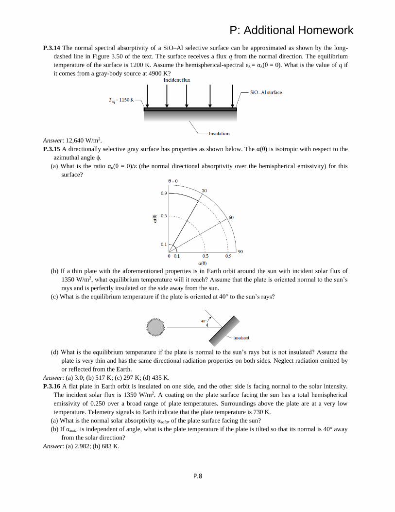
P: Additional Homework
P.8
P.3.14 The normal spectral absorptivity of a SiO–Al selective surface can be approximated as shown by the long-
dashed line in Figure 3.50 of the text. The surface receives a flux q from the normal direction. The equilibrium
temperature of the surface is 1200 K. Assume the hemispherical-spectral ελ = αλ(θ = 0). What is the value of q if
it comes from a gray-body source at 4900 K?
Answer: 12,640 W/m2.
P.3.15 A directionally selective gray surface has properties as shown below. The α(θ) is isotropic with respect to the
azimuthal angle ϕ.
(a) What is the ratio αn(θ = 0)/ε (the normal directional absorptivity over the hemispherical emissivity) for this
surface?
(b) If a thin plate with the aforementioned properties is in Earth orbit around the sun with incident solar flux of
1350 W/m2, what equilibrium temperature will it reach? Assume that the plate is oriented normal to the sun’s
rays and is perfectly insulated on the side away from the sun.
(c) What is the equilibrium temperature if the plate is oriented at 40° to the sun’s rays?
(d) What is the equilibrium temperature if the plate is normal to the sun’s rays but is not insulated? Assume the
plate is very thin and has the same directional radiation properties on both sides. Neglect radiation emitted by
or reflected from the Earth.
Answer: (a) 3.0; (b) 517 K; (c) 297 K; (d) 435 K.
P.3.16 A flat plate in Earth orbit is insulated on one side, and the other side is facing normal to the solar intensity.
The incident solar flux is 1350 W/m2. A coating on the plate surface facing the sun has a total hemispherical
emissivity of 0.250 over a broad range of plate temperatures. Surroundings above the plate are at a very low
temperature. Telemetry signals to Earth indicate that the plate temperature is 730 K.
(a) What is the normal solar absorptivity αsolar of the plate surface facing the sun?
(b) If αsolar is independent of angle, what is the plate temperature if the plate is tilted so that its normal is 40° away
from the solar direction?
Answer: (a) 2.982; (b) 683 K.

P: Additional Homework
P.9
P.3.17 The spectral absorptivity of a SiO–Al selective surface can be approximated as shown below. The surface is in
Earth orbit around the sun and has the solar flux 1353 W/m2 incident on it in the normal direction. What is the
equilibrium temperature of the surface if the surroundings are very cold?
Answer: 672 K.
P.3.18 A thin plate has a directional-gray surface on one side with the directional emissivity shown below on the left.
On the other side of the plate is a coating with diffuse-spectral emissivity shown below on the right. The
surroundings are at very low temperature. Find the equilibrium temperature of the plate if it is exposed in
vacuum to a normal solar flux of 1353 W/m2 with a solar spectrum equivalent to that of a blackbody at 5780 K
when
(a) The directional-gray side is facing normal to the sun.
(b) The diffuse-spectral side is facing normal to the sun.
Answer: (a) 376 K; (b) 265 K.
P.3.19 A gray surface has a directional total absorptivity given by α(θ) = 0.80 cos4 θ. This flat surface is exposed to
normally incident sunlight of flux 1050 W/m2. A fluid flows past the back of the thin radiation absorber plate at
Tfluid = 325 K and with a velocity that gives a heat transfer coefficient of h = 64 W/m2 · K. What is the
equilibrium temperature of this flat-plate radiation collector?
Answer: 335 K.
P.3.20 A plate is coated with a material combining directional and spectral selectivity so that the plate has a normal
total solar absorptivity of 0.92 and an IR hemispherical emissivity of 0.040 at long wavelengths. When placed in
sunlight normal to the sun’s rays, what temperature will the plate reach (neglecting conduction and convection
and with no heat losses from the unexposed side of the plate)? What assumptions did you make in reaching your
answer? The incident solar flux (“insolation”) is 1000 W/m2.
Answer: 648 K.
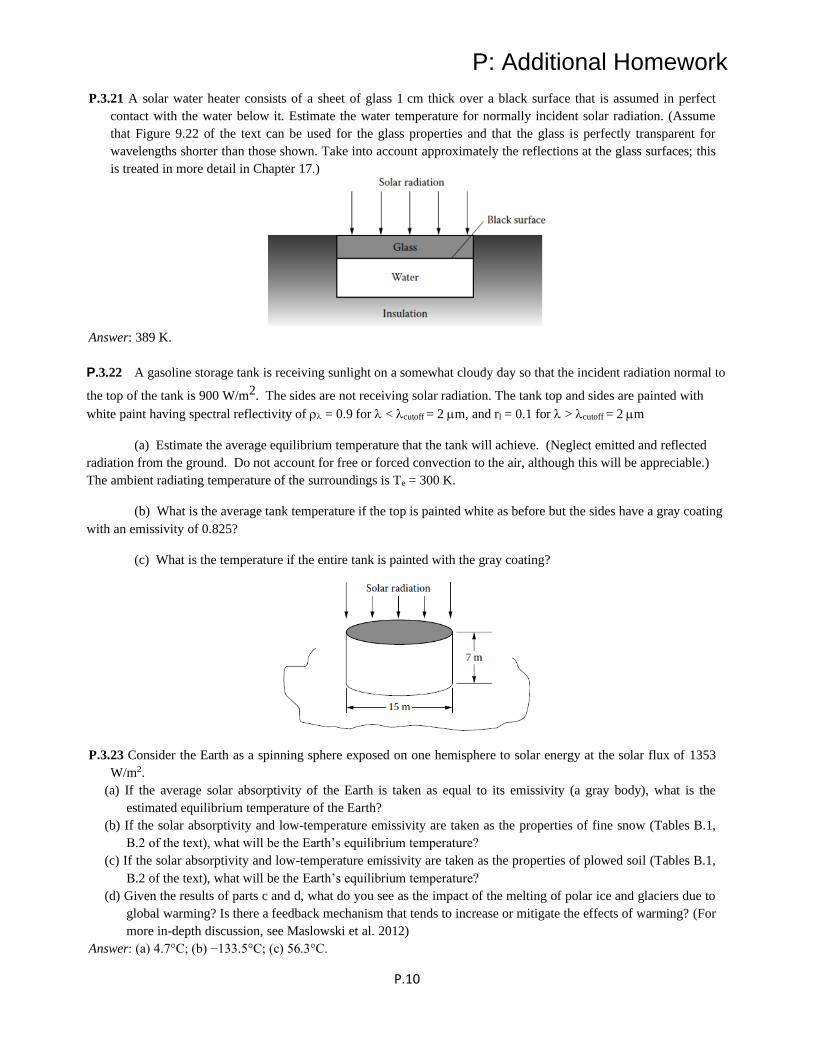
P: Additional Homework
P.10
P.3.21 A solar water heater consists of a sheet of glass 1 cm thick over a black surface that is assumed in perfect
contact with the water below it. Estimate the water temperature for normally incident solar radiation. (Assume
that Figure 9.22 of the text can be used for the glass properties and that the glass is perfectly transparent for
wavelengths shorter than those shown. Take into account approximately the reflections at the glass surfaces; this
is treated in more detail in Chapter 17.)
Answer: 389 K.
P.3.22 A gasoline storage tank is receiving sunlight on a somewhat cloudy day so that the incident radiation normal to
the top of the tank is 900 W/m2. The sides are not receiving solar radiation. The tank top and sides are painted with
white paint having spectral reflectivity of = 0.9 for < cutoff = 2 m, and rl = 0.1 for > cutoff = 2 m
(a) Estimate the average equilibrium temperature that the tank will achieve. (Neglect emitted and reflected
radiation from the ground. Do not account for free or forced convection to the air, although this will be appreciable.)
The ambient radiating temperature of the surroundings is Te = 300 K.
(b) What is the average tank temperature if the top is painted white as before but the sides have a gray coating
with an emissivity of 0.825?
(c) What is the temperature if the entire tank is painted with the gray coating?
P.3.23 Consider the Earth as a spinning sphere exposed on one hemisphere to solar energy at the solar flux of 1353
W/m2.
(a) If the average solar absorptivity of the Earth is taken as equal to its emissivity (a gray body), what is the
estimated equilibrium temperature of the Earth?
(b) If the solar absorptivity and low-temperature emissivity are taken as the properties of fine snow (Tables B.1,
B.2 of the text), what will be the Earth’s equilibrium temperature?
(c) If the solar absorptivity and low-temperature emissivity are taken as the properties of plowed soil (Tables B.1,
B.2 of the text), what will be the Earth’s equilibrium temperature?
(d) Given the results of parts c and d, what do you see as the impact of the melting of polar ice and glaciers due to
global warming? Is there a feedback mechanism that tends to increase or mitigate the effects of warming? (For
more in-depth discussion, see Maslowski et al. 2012)
Answer: (a) 4.7°C; (b) −133.5°C; (c) 56.3°C.
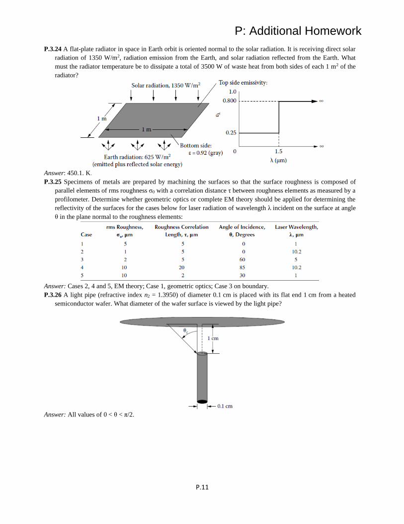
P: Additional Homework
P.11
P.3.24 A flat-plate radiator in space in Earth orbit is oriented normal to the solar radiation. It is receiving direct solar
radiation of 1350 W/m2, radiation emission from the Earth, and solar radiation reflected from the Earth. What
must the radiator temperature be to dissipate a total of 3500 W of waste heat from both sides of each 1 m2 of the
radiator?
Answer: 450.1. K.
P.3.25 Specimens of metals are prepared by machining the surfaces so that the surface roughness is composed of
parallel elements of rms roughness σ0 with a correlation distance τ between roughness elements as measured by a
profilometer. Determine whether geometric optics or complete EM theory should be applied for determining the
reflectivity of the surfaces for the cases below for laser radiation of wavelength λ incident on the surface at angle
θ in the plane normal to the roughness elements:
Answer: Cases 2, 4 and 5, EM theory; Case 1, geometric optics; Case 3 on boundary.
P.3.26 A light pipe (refractive index n2 = 1.3950) of diameter 0.1 cm is placed with its flat end 1 cm from a heated
semiconductor wafer. What diameter of the wafer surface is viewed by the light pipe?
Answer: All values of 0 < θ < π/2.
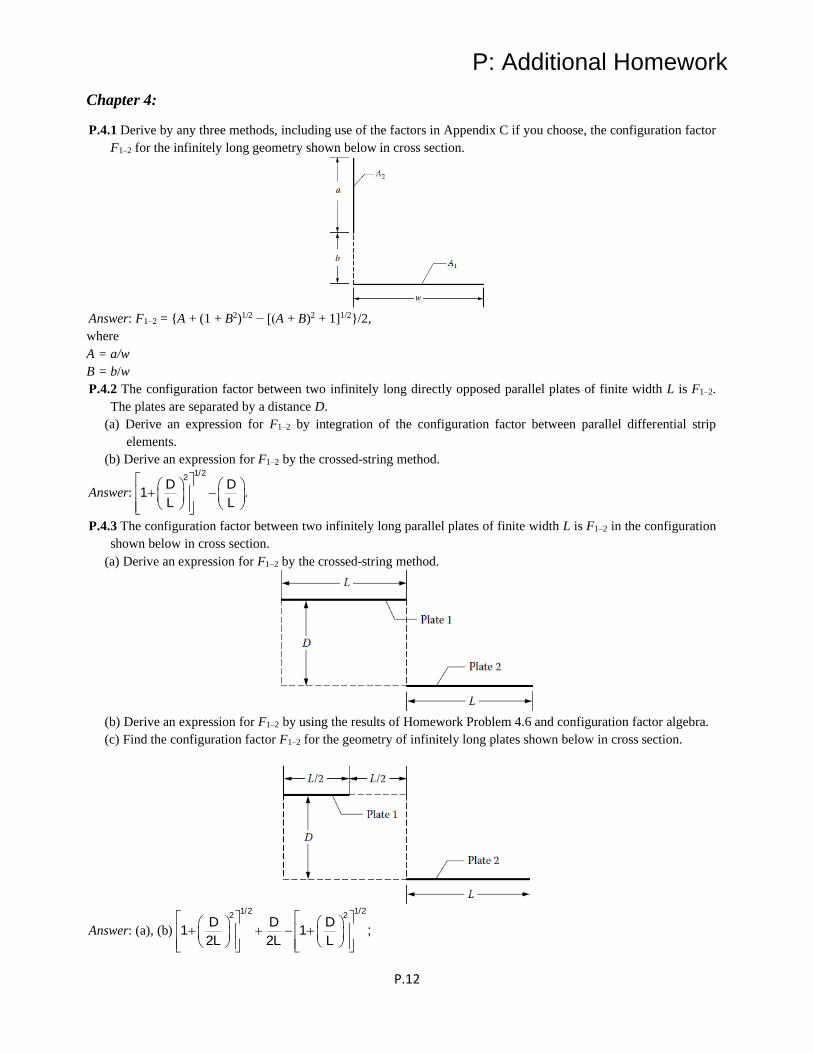
P: Additional Homework
P.12
Chapter 4:
P.4.1 Derive by any three methods, including use of the factors in Appendix C if you choose, the configuration factor
F1–2 for the infinitely long geometry shown below in cross section.
Answer: F1–2 = {A + (1 + B2)1/2 − [(A + B)2 + 1]1/2}/2,
where
A = a/w
B = b/w
P.4.2 The configuration factor between two infinitely long directly opposed parallel plates of finite width L is F1–2.
The plates are separated by a distance D.
(a) Derive an expression for F1–2 by integration of the configuration factor between parallel differential strip
elements.
(b) Derive an expression for F1–2 by the crossed-string method.
Answer:
+ −
1/22
1 .D D
L L
P.4.3 The configuration factor between two infinitely long parallel plates of finite width L is F1–2 in the configuration
shown below in cross section.
(a) Derive an expression for F1–2 by the crossed-string method.
(b) Derive an expression for F1–2 by using the results of Homework Problem 4.6 and configuration factor algebra.
(c) Find the configuration factor F1–2 for the geometry of infinitely long plates shown below in cross section.
Answer: (a), (b)
+ + − +
1/2 1/22 2
1 1 ;2 2
D D D
L L L

P: Additional Homework
P.13
(c) −
= + − + − + + +
1/2 1/2 1/2 1/22 2 2 2 2 2
1 2
3 12 1 1 .
2 2 2
D D D DF
L L L L
P.4.4 (a) For the 2D geometry shown in cross section, derive a formula for F2–2 in terms of r1 and r2.
(b) Find F2–2 for the 2D geometry. A1 is a square (A1 refers to the total area of the four sides) and A2 is part of a
circle.
Answer:
(a) −−
= − − −
1/22
1 1 1 12 2
2 2 2
2 21 1 sin
r r rF
r r r.
(b) F2–2 = 0.1359.
P.4.5 Compute the configuration factor F1–2 between faces A1 and A2 of the infinitely long parallel plates shown
below in cross section when the angle β is equal to (a) 30° and (b) 75°.
Answer: (a) 0.2752; (b) 0.0915.
P.4.6 A sphere of radius r is divided into two quarter spheres and one hemisphere. Obtain the configuration factors
between all areas inside the sphere, F1–2, F2–2, F3–1, F1–1, etc. From these factors find F4–5, where A4 and A5 are
equal semicircles that are at right angles to each other.
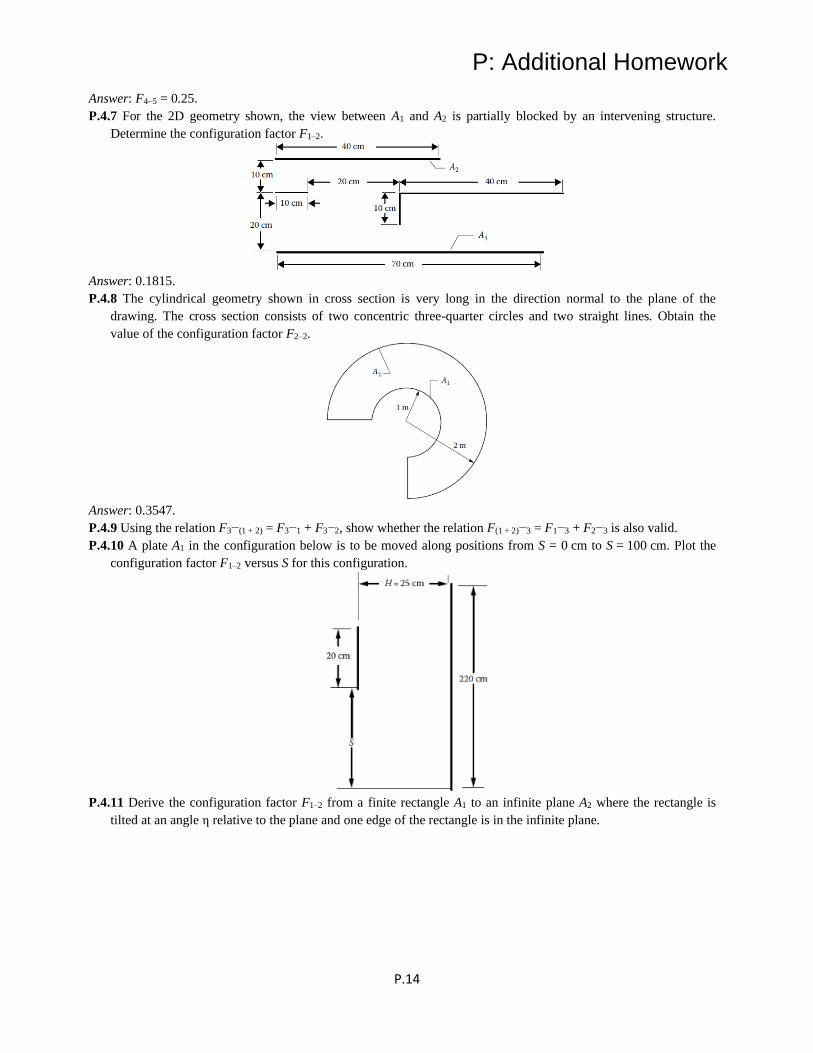
P: Additional Homework
P.14
Answer: F4–5 = 0.25.
P.4.7 For the 2D geometry shown, the view between A1 and A2 is partially blocked by an intervening structure.
Determine the configuration factor F1–2.
Answer: 0.1815.
P.4.8 The cylindrical geometry shown in cross section is very long in the direction normal to the plane of the
drawing. The cross section consists of two concentric three-quarter circles and two straight lines. Obtain the
value of the configuration factor F2–2.
Answer: 0.3547.
P.4.9 Using the relation F3−(1 + 2) = F3−1 + F3−2, show whether the relation F(1 + 2)−3 = F1−3 + F2−3 is also valid.
P.4.10 A plate A1 in the configuration below is to be moved along positions from S = 0 cm to S = 100 cm. Plot the
configuration factor F1–2 versus S for this configuration.
P.4.11 Derive the configuration factor F1–2 from a finite rectangle A1 to an infinite plane A2 where the rectangle is
tilted at an angle η relative to the plane and one edge of the rectangle is in the infinite plane.
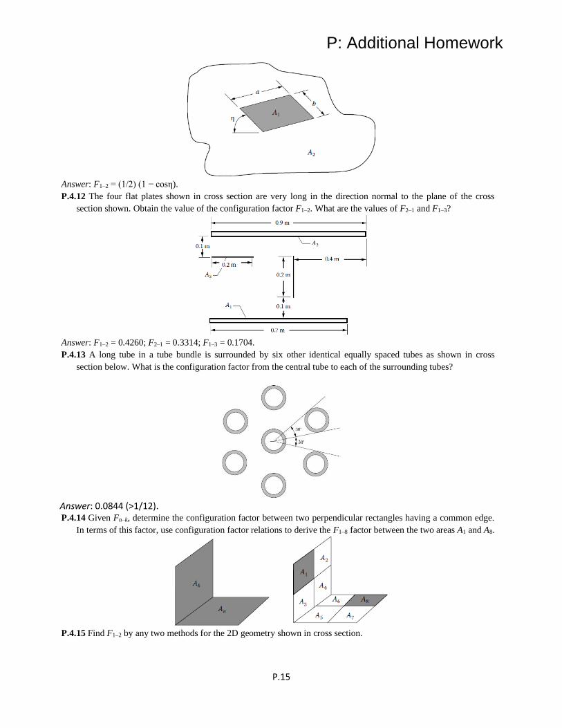
P: Additional Homework
P.15
Answer: F1–2 = (1/2) (1 − cosη).
P.4.12 The four flat plates shown in cross section are very long in the direction normal to the plane of the cross
section shown. Obtain the value of the configuration factor F1–2. What are the values of F2–1 and F1–3?
Answer: F1–2 = 0.4260; F2–1 = 0.3314; F1–3 = 0.1704.
P.4.13 A long tube in a tube bundle is surrounded by six other identical equally spaced tubes as shown in cross
section below. What is the configuration factor from the central tube to each of the surrounding tubes?
Answer: 0.0844 (>1/12). P.4.14 Given Fn–k, determine the configuration factor between two perpendicular rectangles having a common edge.
In terms of this factor, use configuration factor relations to derive the F1–8 factor between the two areas A1 and A8.
P.4.15 Find F1–2 by any two methods for the 2D geometry shown in cross section.
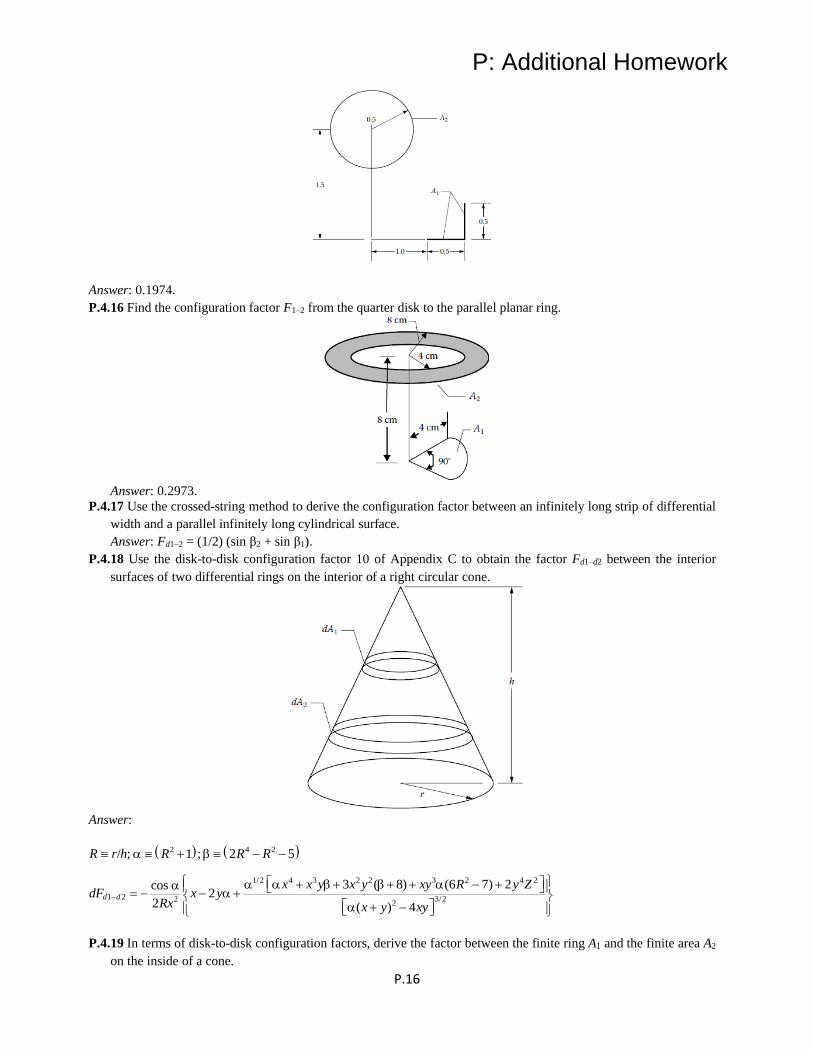
P: Additional Homework
P.16
Answer: 0.1974.
P.4.16 Find the configuration factor F1–2 from the quarter disk to the parallel planar ring.
Answer: 0.2973.
P.4.17 Use the crossed-string method to derive the configuration factor between an infinitely long strip of differential
width and a parallel infinitely long cylindrical surface.
Answer: Fd1–2 = (1/2) (sin β2 + sin β1).
P.4.18 Use the disk-to-disk configuration factor 10 of Appendix C to obtain the factor Fd1–d2 between the interior
surfaces of two differential rings on the interior of a right circular cone.
Answer:
( ) ( )
1/2 4 3 2 2 3 2 4 2
1 /
2
3 222
4
2
2/ ; ;
3 ( 8) (6 7) 2cos2
2
2 5
4
1
( )d d
R r h
x x y x y xy R y
R
ZdF x
y
R R
yRx x xy
−
+ + + + − + = − − + + −
+ −
−
P.4.19 In terms of disk-to-disk configuration factors, derive the factor between the finite ring A1 and the finite area A2
on the inside of a cone.

P: Additional Homework
P.17
P.4.20 A closed right circular cylindrical shell with base diameter 1 m and height 1 m is located at the center of a
spherical shell 1 m in radius.
(a) Determine the configuration factor between the inside of the sphere and itself.
(b) If the top of the cylindrical shell is removed, determine the configuration factor between the inside of the
sphere and the inside of the bottom of the cylindrical shell.
Answer: (a) 0.6250; (b) 0.01072.
P.4.21 Show by an algebraic derivation whether the configuration factor from the interior curved surface of the
frustum of a cone A1 to its base A2 as given in configuration factor C-111 of the configuration factor catalog at
www.ThermalRadiation.net/ /indexCat.html is equivalent to that given in factor C-112.
P.4.22 Obtain the configuration factor dFd1–2 in Homework Problem 4.2 by using contour integration.
Answer:
1
2 1/2 2 1/2
1 2
1
2 1/2 2 1/2
tan(1 ) (1 )
2
tan(1 ) (1 )
d
X Y
X XF
Y X
Y Y
−
−
−
+ + =
+
+ +
where
X = L/2H
Y = W/2H
P.4.23 Obtain the value of the configuration factor dFd1–2 for the geometry shown. The areas dA1 and A2 are parallel.
Answer: 0.01261.
P.4.24 For the geometry below and the special case of l1 = l3, derive algebraic expressions for the factors F1–2, F1–3,
and F3–3. Use relations from factors C-77 and C-97 from the online catalog at www.ThermalRadiation.net/
indexCat.html.
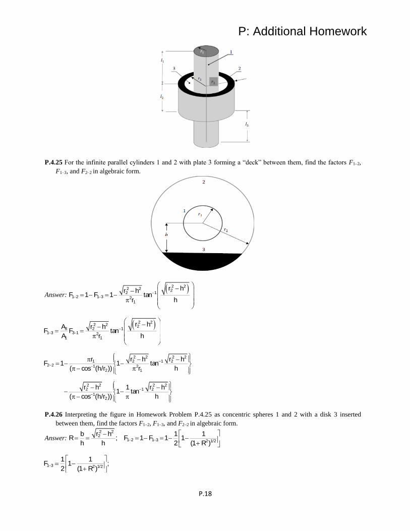
P: Additional Homework
P.18
P.4.25 For the infinite parallel cylinders 1 and 2 with plate 3 forming a “deck” between them, find the factors F1–2,
F1–3, and F2–2 in algebraic form.
Answer: ( )
−− −
−− = − = −
2 22 2 22 1
1 2 1 3 21
1 1 tanFr hr h
Fr h
( )−
− −
−− = =
2 22 2 2
3 2 11 3 3 1 2
1 1
tanFr hA r h
hF
A r
−− −
−
−
− − = − −
−
− − − −
−
2 2 2 21 2 1 2
2 2 1 22 1
2 2 2 22 1 2
12
1 1 tan( ( / ))
11 tan
( ( / ))
r r h r h
cos h r r h
r h r h
cos h r h
F
P.4.26 Interpreting the figure in Homework Problem P.4.25 as concentric spheres 1 and 2 with a disk 3 inserted
between them, find the factors F1–2, F1–3, and F2–2 in algebraic form.
Answer: − −
−= = = − = − − +
2 22
1 2 1 3 2 1/2
1 1; 1 1 1
2 (1 )
b r hR F
h h RF
−
= − +
1 3 2 1/2
11
);
1
2 (1 RF
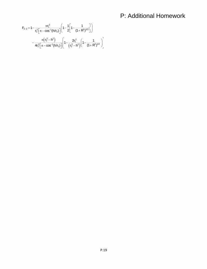
P: Additional Homework
P.19
( )( )
− −
−
= − − − + −
− − − −
+ − −
21
2 2 2 1/22 12 2
2 2 22 1
2 1/22 1 2 22 22
1 11 1 1
2 (1 )cos ( / )
2 1 1 1
(1 )cos ( / )4
r
Rr h r
r h r
Rh r rr h
F

P: Additional Homework
P.20
Chapter 5:
P.5.1 A rectangular carbon steel billet 1 × 0.5 × 0.5 m is initially at 1150 K and is supported in such a manner that it
transfers heat by radiation from all of its surfaces to surroundings at Te = 27°C (assume the surroundings are
black). Neglect convective heat transfer and assume the billet radiates like a blackbody. Also, assume for
simplicity that the thermal conductivity of the steel is infinite. How long will it take for the billet to cool to 410
K? (For carbon steel, let ρcs = 7800 kg/m3 and ccs = 470 J/kg · K.)
Answer: 9.61 h.
P.5.2 A black circular disk 0.15 m in diameter and well insulated on one side is electrically heated to a uniform
temperature. The electrical energy input is 1300 W. The surroundings are black and are at Te = 500 K. What
fraction of the emitted energy is in the wave number region from 0.2 to 1 μm−1?
Answer: 0.680.
P.5.3 A hollow cylindrical heating element is insulated on its outside surface. The element has a 25 cm inside
diameter and is 25 cm long. The black internal surface is to be held at 1000 K. The surroundings are in vacuum
and are at 400 K. Both ends of the cylinder are open to the surroundings. Estimate the energy that must be
supplied to the element (W).
Answer: 4490 W.
P.5.4 The black-surfaced three-sided enclosure shown below has infinitely long parallel sides, with the
specified temperatures and energy rate additions. Find Q1, Q2, and T3. (Side 3 is a circular arc).

P: Additional Homework
P.21
Answers: Q1 = -123,561 W/m; Q2 = 120,561 W/m; T3 = 1032 K.
P.5.5 Two enclosures are identical in shape and size and have black surfaces. For one enclosure, the temperatures of the
surfaces are T1, T2, T3,....,TN. For the second, the surface temperatures are (T14 + k)1/4, (T2
4 + k)1/4, (T3
4 + k)1/4,
..., (TN4 + k)1/4, where k is a constant. Show how the heat transfer rates Qj at any surface Aj are related for the two
enclosures.
P.5.6 An enclosure with black interior surfaces has one side open to an environment at temperature Te. The sides of the
enclosure are maintained at temperatures of T1, T2, T3, ..., TN. How are the rates of energy input to the sides Q1, Q2,
Q3, ..., QN influenced by the value of Te? How can the results for Te = 0 be used to obtain solutions for other Te?
P.5.7 A black 6 cm diameter sphere at a temperature of 1100 K is suspended in the center of a thin 10 cm diameter
partial sphere having a black interior surface and an exterior surface with a hemispherical total emissivity of 0.1.
The surroundings are at 300 K. A 7.5 cm diameter hole is cut in the outer sphere. What is the temperature of the
outer sphere? What is the Q being supplied to the inner sphere? (For simplicity, do not subdivide the surface
areas into smaller zones.)
Answer: 988 K; 431 W.
P.5.8 An infinitely long enclosure (normal to the direction shown) is shaped as shown in the following. Assuming
that the uniform flux restrictions are met along each surface, find Q1 and T2.
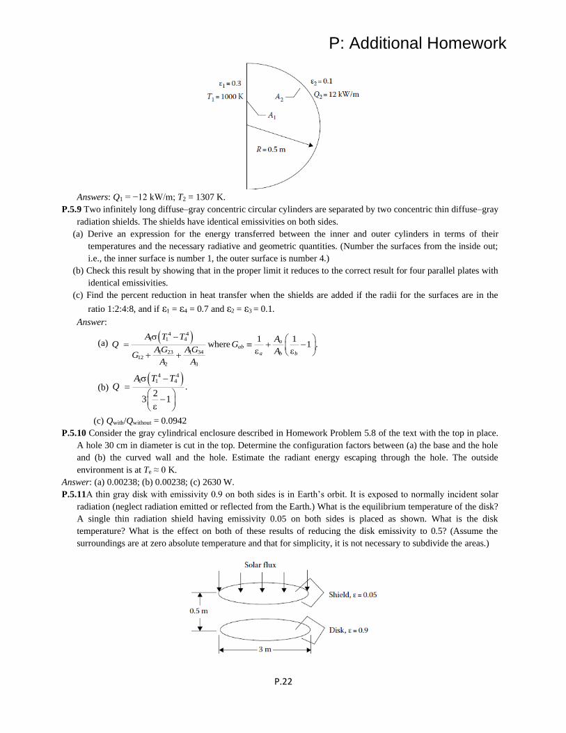
P: Additional Homework
P.22
Answers: Q1 = −12 kW/m; T2 = 1307 K.
P.5.9 Two infinitely long diffuse–gray concentric circular cylinders are separated by two concentric thin diffuse–gray
radiation shields. The shields have identical emissivities on both sides.
(a) Derive an expression for the energy transferred between the inner and outer cylinders in terms of their
temperatures and the necessary radiative and geometric quantities. (Number the surfaces from the inside out;
i.e., the inner surface is number 1, the outer surface is number 4.)
(b) Check this result by showing that in the proper limit it reduces to the correct result for four parallel plates with
identical emissivities.
(c) Find the percent reduction in heat transfer when the shields are added if the radii for the surfaces are in the
ratio 1:2:4:8, and if ε1 = ε4 = 0.7 and ε2 = ε3 = 0.1.
Answer:
(a) ( )4 4
1 1 4
1 23 1 3412
2 3
1 1where 1 .a
ab
a b b
A T T AQ G
AG AG AGA A
− = + −
+ +
(b) ( )4 4
1 1 4.
23 1
A T TQ
−=
−
(c) Qwith/Qwithout = 0.0942
P.5.10 Consider the gray cylindrical enclosure described in Homework Problem 5.8 of the text with the top in place.
A hole 30 cm in diameter is cut in the top. Determine the configuration factors between (a) the base and the hole
and (b) the curved wall and the hole. Estimate the radiant energy escaping through the hole. The outside
environment is at Te ≈ 0 K.
Answer: (a) 0.00238; (b) 0.00238; (c) 2630 W.
P.5.11A thin gray disk with emissivity 0.9 on both sides is in Earth’s orbit. It is exposed to normally incident solar
radiation (neglect radiation emitted or reflected from the Earth.) What is the equilibrium temperature of the disk?
A single thin radiation shield having emissivity 0.05 on both sides is placed as shown. What is the disk
temperature? What is the effect on both of these results of reducing the disk emissivity to 0.5? (Assume the
surroundings are at zero absolute temperature and that for simplicity, it is not necessary to subdivide the areas.)
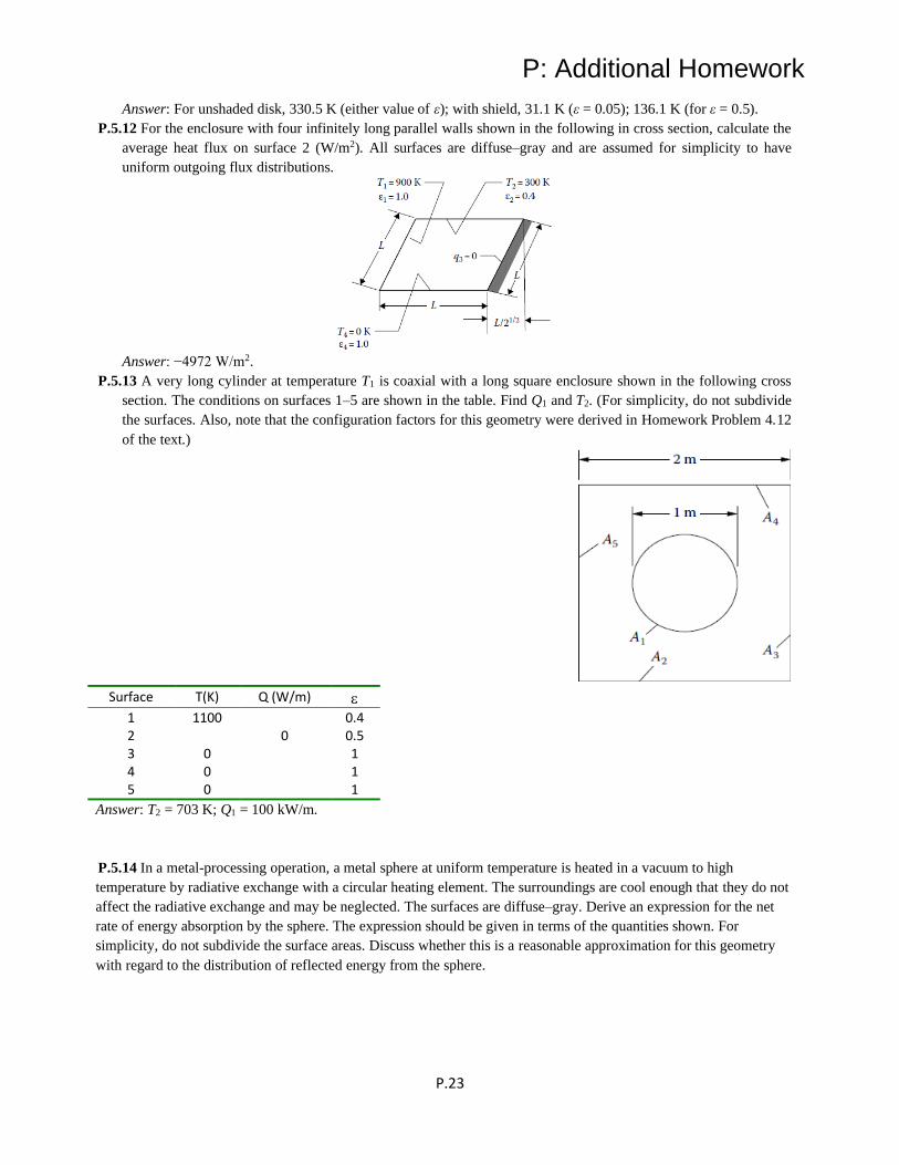
P: Additional Homework
P.23
Answer: For unshaded disk, 330.5 K (either value of ε); with shield, 31.1 K (ε = 0.05); 136.1 K (for ε = 0.5).
P.5.12 For the enclosure with four infinitely long parallel walls shown in the following in cross section, calculate the
average heat flux on surface 2 (W/m2). All surfaces are diffuse–gray and are assumed for simplicity to have
uniform outgoing flux distributions.
Answer: −4972 W/m2.
P.5.13 A very long cylinder at temperature T1 is coaxial with a long square enclosure shown in the following cross
section. The conditions on surfaces 1–5 are shown in the table. Find Q1 and T2. (For simplicity, do not subdivide
the surfaces. Also, note that the configuration factors for this geometry were derived in Homework Problem 4.12
of the text.)
Surface T(K) Q (W/m)
1 1100 0.4 2 0 0.5 3 0 1 4 0 1 5 0 1
Answer: T2 = 703 K; Q1 = 100 kW/m.
P.5.14 In a metal-processing operation, a metal sphere at uniform temperature is heated in a vacuum to high
temperature by radiative exchange with a circular heating element. The surroundings are cool enough that they do not
affect the radiative exchange and may be neglected. The surfaces are diffuse–gray. Derive an expression for the net
rate of energy absorption by the sphere. The expression should be given in terms of the quantities shown. For
simplicity, do not subdivide the surface areas. Discuss whether this is a reasonable approximation for this geometry
with regard to the distribution of reflected energy from the sphere.

P: Additional Homework
P.24
P.5.15 A 10 cm diameter hole extends through the wall of a furnace having an interior temperature of 1350 K. The
wall is a 20 cm thick refractory brick. Divide the wall thickness into two zones of equal length and compute the net
radiation out of the hole into a room at 300 K. (Neglect heat conduction in the wall.)
Answer: T1 = 1216 K; T2 = 1033 K; Q3 = −560 W.
P.5.16 A cubical enclosure with edge length of 6 m has a very small sphere placed at its center (Asphere ≪ Aside). The
sphere has emissivity ε = 0.4 and is maintained electrically at Ts = 1300 K. The interior walls of the cube have the
following properties:
Determine the net q added or removed from each side of the cube and the q
added to the sphere. Find the results in kW/m2. Tabulate all the required configuration factors. (Assume the incident
radiation on each surface is uniform.)
Answer: q1 = 69.9 kW/m2; q2 = −0.86 kW/m2; q3 = −6.10 kW/m2; q4 = −28.0 kW/m2; q5 = −5.11 kW/m2;
q6 = −29.8 kW/m2; qs = 54.9 kW/m2.
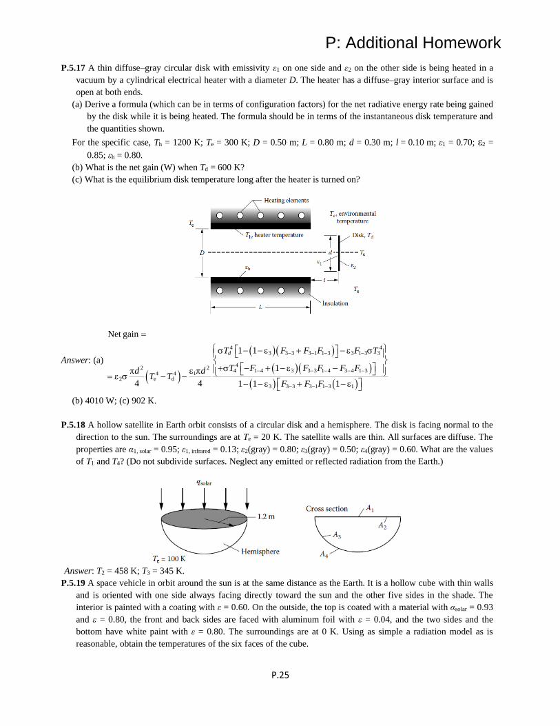
P: Additional Homework
P.25
P.5.17 A thin diffuse–gray circular disk with emissivity ε1 on one side and ε2 on the other side is being heated in a
vacuum by a cylindrical electrical heater with a diameter D. The heater has a diffuse–gray interior surface and is
open at both ends.
(a) Derive a formula (which can be in terms of configuration factors) for the net radiative energy rate being gained
by the disk while it is being heated. The formula should be in terms of the instantaneous disk temperature and
the quantities shown.
For the specific case, Th = 1200 K; Te = 300 K; D = 0.50 m; L = 0.80 m; d = 0.30 m; l = 0.10 m; ε1 = 0.70; ε2 =
0.85; εh = 0.80.
(b) What is the net gain (W) when Td = 600 K?
(c) What is the equilibrium disk temperature long after the heater is turned on?
Answer: (a)
( )
( )( )
( )( )
( ) ( )
4 43 3 3 3 1 1 3 3 1 3 3
42 2
4 1 4 3 3 3 1 4 3 4 1 314 4
2 e d
3 3 3 3 1 1 3 1
Net gain
1 1
1
4 4 1 1 1
dT F F F F T
T F F F F Fd dT T
F F F
− − − −
− − − − −
− − −
=
− − + −
+ − + − − = − − − − + −
(b) 4010 W; (c) 902 K.
P.5.18 A hollow satellite in Earth orbit consists of a circular disk and a hemisphere. The disk is facing normal to the
direction to the sun. The surroundings are at Te = 20 K. The satellite walls are thin. All surfaces are diffuse. The
properties are α1, solar = 0.95; ε1, infrared = 0.13; ε2(gray) = 0.80; ε3(gray) = 0.50; ε4(gray) = 0.60. What are the values
of T1 and T4? (Do not subdivide surfaces. Neglect any emitted or reflected radiation from the Earth.)
Answer: T2 = 458 K; T3 = 345 K.
P.5.19 A space vehicle in orbit around the sun is at the same distance as the Earth. It is a hollow cube with thin walls
and is oriented with one side always facing directly toward the sun and the other five sides in the shade. The
interior is painted with a coating with ε = 0.60. On the outside, the top is coated with a material with αsolar = 0.93
and ε = 0.80, the front and back sides are faced with aluminum foil with ε = 0.04, and the two sides and the
bottom have white paint with ε = 0.80. The surroundings are at 0 K. Using as simple a radiation model as is
reasonable, obtain the temperatures of the six faces of the cube.

P: Additional Homework
P.26
Answer: T1 (top) = 367 K; T2 (2 sides, bottom) = 234 K; T3 (front and back) = 281 K.
P.5.20 Consider two parallel plates of finite extent in one direction. Both plates are perfectly insulated on the outside.
Plate 1 is uniformly heated electrically with heat flux qe. Plate 2 has no external heat input. The environment is at
zero absolute temperature.
(a) For both plates black, show that the integral equations for the surface temperatures are
( )
( )
/2
b,1 b,2 3/22
/2
/2
b,2 b,1 3/22
/2
1( ) 1 ( )
21
1( ) ( )
21
L
L
L
L
dYX Y
Y X
dXY X
X Y
−
−
= + − +
= − +
where X = x/a, Y = y/a, θ = σT 4/qe, and L = l/a.
(b) If both plates are gray, show that ( ) ( ) ( ) ( )11 b,1 2 b,2
1
1; .X X Y Y
− = + =
P.5.21 A long groove is cut into a metal surface as shown in the following cross section. The groove surface is
diffuse–gray and has emissivity ε. The temperature profile along the groove sides, as measured from the apex, is
found to be T(x). The environment is at temperature Te.
(a) Derive the equations for the heat flux distribution q(x) along the groove surface.

P: Additional Homework
P.27
(b) Examine the kernel of the integral equation found in part (a) and show whether it is symmetrical and/or
separable.
P.5.22 A hemispherical cavity is in a block of lightly oxidized copper (1 = 0.57) maintained at 800 K in vacuum.
The surroundings are at 300 K. Use the integral equation method to compute the outgoing heat flux from the
cavity surface.
Answer: 27,140 W/m2.
P.5.23 A cavity having a gray interior surface S is uniformly heated electrically and achieves a surface temperature
distribution Tw,0(S) while being exposed to a zero absolute temperature environment, Te = 0. If the environment is
raised to Te and the heating kept the same, what is the surface temperature distribution?
Answer: ( ) ( )1/4
4 4w,0 w e ,T r T r T = − where Tw,0(S) = Tw(S, Te = 0).
P.5.24 A gray circular tube insulated on the outside is exposed to an environment at Te = 0 at both ends. The q(x, Te =
0) has been calculated to maintain the wall temperature at any constant value. Now, let Te ≈ 0, and let the wall
temperature be uniform at Tw. Show that the q(x, Te ≠ 0) can be obtained as the q(x, Te = 0) corresponding to the
wall temperature 4 4 1/4
w e( ) .T T−
P.5.25 Two infinitely long plates are joined at right angles along one infinite edge. The plates are each of width W,
and both have diffuse–gray surfaces with the same emissivity ε. The heat flux supplied to both surfaces is
maintained at a uniform value q. Derive an equation for the temperature distribution on each surface and describe
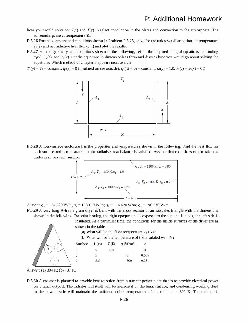
P: Additional Homework
P.28
how you would solve for T(x) and T(y). Neglect conduction in the plates and convection to the atmosphere. The
surroundings are at temperature Te.
P.5.26 For the geometry and conditions shown in Problem P.5.25, solve for the unknown distributions of temperature
T1(y) and net radiative heat flux q2(x) and plot the results.
P.5.27 For the geometry and conditions shown in the following, set up the required integral equations for finding
q1(y), T2(z), and T3(x). Put the equations in dimensionless form and discuss how you would go about solving the
equations. Which method of Chapter 5 appears most useful?
T1(y) = T1 = constant; q2(z) = 0 (insulated on the outside); q3(x) = q3 = constant; ε1(y) = 1.0; ε2(z) = ε3(x) = 0.5
P.5.28 A four-surface enclosure has the properties and temperatures shown in the following. Find the heat flux for
each surface and demonstrate that the radiative heat balance is satisfied. Assume that radiosities can be taken as
uniform across each surface.
Answer: q1 = −54,690 W/m; q2 = 108,100 W/m; q3 = −16.620 W/m; q1 = −90,230 W/m.
P.5.29 A very long A-frame grain dryer is built with the cross section of an isosceles triangle with the dimensions
shown in the following. For solar heating, the right opaque side is exposed to the sun and is black, the left side is
insulated. At a particular time, the conditions for the inside surfaces of the dryer are as
shown in the table.
(a) What will be the floor temperature T3 (K)?
(b) What will be the temperature of the insulated wall T2?
Answer: (a) 304 K; (b) 437 K.
P.5.30 A radiator is planned to provide heat rejection from a nuclear power plant that is to provide electrical power
for a lunar outpost. The radiator will itself will be horizontal on the lunar surface, and condensing working fluid
in the power cycle will maintain the uniform surface temperature of the radiator at 800 K. The radiator is
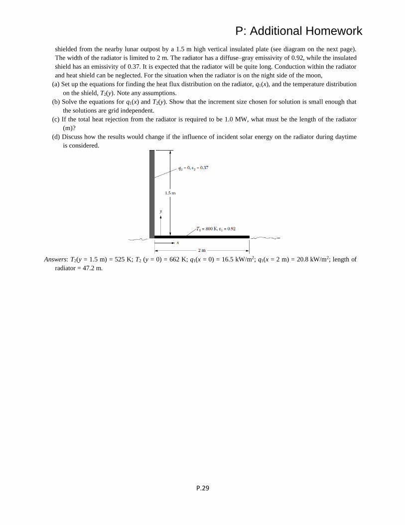
P: Additional Homework
P.29
shielded from the nearby lunar outpost by a 1.5 m high vertical insulated plate (see diagram on the next page).
The width of the radiator is limited to 2 m. The radiator has a diffuse–gray emissivity of 0.92, while the insulated
shield has an emissivity of 0.37. It is expected that the radiator will be quite long. Conduction within the radiator
and heat shield can be neglected. For the situation when the radiator is on the night side of the moon,
(a) Set up the equations for finding the heat flux distribution on the radiator, q1(x), and the temperature distribution
on the shield, T2(y). Note any assumptions.
(b) Solve the equations for q1(x) and T2(y). Show that the increment size chosen for solution is small enough that
the solutions are grid independent.
(c) If the total heat rejection from the radiator is required to be 1.0 MW, what must be the length of the radiator
(m)?
(d) Discuss how the results would change if the influence of incident solar energy on the radiator during daytime
is considered.
Answers: T2(y = 1.5 m) = 525 K; T2 (y = 0) = 662 K; q1(x = 0) = 16.5 kW/m2; q1(x = 2 m) = 20.8 kW/m2; length of
radiator = 47.2 m.

P: Additional Homework
P.30
Chapter 6:
P.6.1 Two large diffuse parallel plates are maintained at the temperatures T1 = 1400 K and T2 = 700 K. The plates are
made from the same metal, and their spectral emissivities as a function of wavelength, , are approximated as shown
by two constant values joined by a linear decrease with wavelength. Compute the net radiant energy flux being
transferred from plate 1 to plate 2. What is the energy flux if both plates are assumed gray with an approximate average
emissivity of 0.5 applied over the entire spectral range?
Answer: q1 = 106,850 W/m2; q1,gray = 68,073 W/m2.
P.6.2 Radiation is being transferred across the space between two large parallel plates. Both plates are made of the
same metal, and the spectral emissivity of the metal does not depend on temperature. The wavelength variation of the
emissivity for both plates is approximated in three steps as shown. The lower plate is maintained at T2 = 700 K, and the
upper plate has a uniform heat addition of q1 = 60 kW/m2. What is the temperature, T1, of the upper plate?
Answer: 1594 K
P.6.3 Consider the enclosure of Homework Problem 5.9 with three walls at
different specified temperatures. Compute the radiative heat transfer for the
indicated values of hemispherical spectral emissivity. (For simplicity, do not
subdivide the three areas into smaller regions.)
Answer: q1 = 18,480 W/m2; q2 = - 24,190 W/m2; q3 = - 301 W/m2.

P: Additional Homework
P.31
P.6.4 Two parallel plates are of finite width and of infinite length in the direction normal to that shown. The plates are
diffuse, but their spectral emissivity varies with wavelength and is approximated by a step function as shown. Both
plates are made of the same material, and hence have the same emissivity which is independent of temperature. The
plate edge openings are exposed to the environment at Te = 350 K, and there is energy exchange only from the internal
surfaces. Energy is being added to the lower plate, and the upper plate is maintained at a fixed temperature. Obtain
values for the temperature of the lower plate, T1, and for the heat flux q2 that must be added or removed from the upper
plate to maintain its specified temperature. For simplicity, do not subdivide the surface areas.
Answer: 1709 K; - 6722 W/m2.
P.6.5 A sphere and area element are positioned as shown. The sphere is gray but has a nondiffuse emissivity s =
cos, where is the angle measured from the normal to the sphere surface and is a constant. Set up the integral for
the direct radiation from the sphere to the area element in terms of the quantities given.
P.6.6 Obtain the result for F1-1(2) in Example 6.11 by using the crossed-string method. What is F1-1(2) if A1 in
Figure 6.23 is rotated 45° about its center point? (The geometry remains two-dimensional.)

P: Additional Homework
P.32
Answer: First part: ( )22 2
1 1 21 1( )F b * a * b *
−
= + − − +
Second part: ( )
( ) ( )( )
1 22
1 1 2
2 2 2 2
1F 2 b 1 2
2
a b 1 a b 2 a b 1 a b 2
− = +
− + + − + + + + − −
/
( ) * /
* * * * * * * *
[
]where a*= a/ land b* = b/ l.
P.6.7 In Figure 6.25, the image A2(3-4) is shown as a dotted horizontal line on the lower right-hand side of the
image diagram. By a suitable construction of rays (actual and through image surfaces) similar to the one shown in the
text, show whether A2(3-4) is where Figure 6.25 indicates it to be.
P.6.8 An equilateral triangular enclosure of infinite length normal to the cross-section shown has black surfaces A1
and A2 and a specularly reflecting surface A3 with reflectivity s,3 = 0.6. Find the values of Fs1-1, Fs
1-2 and Fs1-3.
Answer: 0.0938; 0.7562; 0.5000.
P.6.9 (a) What is the value of the sum of the specular configuration factors 1
1
NS
jj
F−
=
for Homework Problem 6.8?
(b) What is the value of the summation ( )N
S
s,j 1 j
j 1
1 F−
=
− for Homework Problem 6.8?
(c) Explain the results of parts (a) and (b) in terms of the definition of
Fs1-j. Is the result of part (b) a general relation for all specular enclosures?
Answer: (a) 1.30; (b) 1.00.
P.6.10 An enclosure is made up of three sides as shown. The length L is sufficiently long that the triangular ends can
be neglected in the energy balances. Two of the surfaces are black, and the other is a diffuse-gray emitter with
emissivity ε1 = 0.10. What is the energy added, per meter along the length L, to each surface because of radiative
exchange within the enclosure for each of the two cases:
(a) area 1 is a diffuse reflector.
(b) area 1 is a specular reflector.
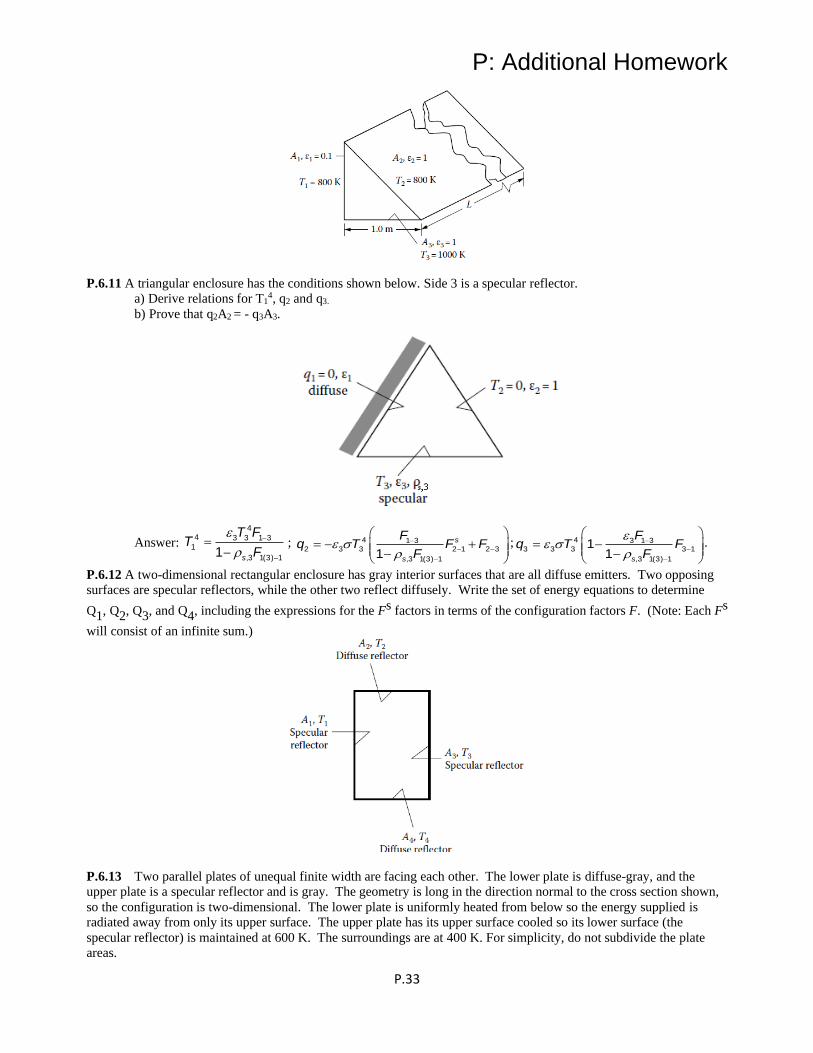
P: Additional Homework
P.33
P.6.11 A triangular enclosure has the conditions shown below. Side 3 is a specular reflector.
a) Derive relations for T14, q2 and q3.
b) Prove that q2A2 = - q3A3.
Answer:
44 3 3 1 3
1
,3 1(3) 11
−
−
=−
s
T FT
F; 4 1 3
2 3 3 2 1 2 3
,3 1(3) 11
−
− −
−
= − +
−
s
s
Fq T F F
F; 4 3 1 3
3 3 3 3 1
,3 1(3) 1
11
−
−
−
= −
−
s
Fq T F
F.
P.6.12 A two-dimensional rectangular enclosure has gray interior surfaces that are all diffuse emitters. Two opposing
surfaces are specular reflectors, while the other two reflect diffusely. Write the set of energy equations to determine
Q1, Q2, Q3, and Q4, including the expressions for the Fs factors in terms of the configuration factors F. (Note: Each Fs
will consist of an infinite sum.)
P.6.13 Two parallel plates of unequal finite width are facing each other. The lower plate is diffuse-gray, and the
upper plate is a specular reflector and is gray. The geometry is long in the direction normal to the cross section shown,
so the configuration is two-dimensional. The lower plate is uniformly heated from below so the energy supplied is
radiated away from only its upper surface. The upper plate has its upper surface cooled so its lower surface (the
specular reflector) is maintained at 600 K. The surroundings are at 400 K. For simplicity, do not subdivide the plate
areas.

P: Additional Homework
P.34
(a) Obtain the temperature of the lower plate and determine what heat flux must be extracted from the upper
plate to maintain its specified temperature.
(b) The surface A2 on the upper plate is now roughened to make it a diffuse reflector, without changing its
emissivity. How much will this change the temperature of the lower plate?
Answer: (a) T1 = 712.8 K, q2 = - 939; (b) T1 = 708.8 K (4.0 K decrease), q2 = - 810.2 W/m2.
P.6.14 A diffuse plate A1 that is not heated or cooled by external means is facing a larger plate as shown. The spacing
between the plates is small. The plates are long in the direction normal to the cross section shown, so the geometry is
two-dimensional. The upper plate is gray and is a specular reflector. It is cooled to 300 K. The environment is at a
higher temperature, 550 K, so that radiant energy is reflected into the space between the plates. For simplicity, do not
subdivide the plate areas.
(a) What is the temperature of the lower plate A1?
(b) If A2 on the upper plate is made diffuse without changing its emissivity, how much is the temperature of
the lower plate changed?
Answer: (a) T1 =506 K; (b) T1 = 537 K (a 31 K increase).
P.6.15 Two parallel plates shown in Homework Problem P.5.20 are of finite width (infinite length normal to the cross-
section). Both plates are perfectly insulated on the outside. Plate 1 is uniformly internally heated electrically with heat
flux qe. Plate 2 has no externally supplied heat input (q2 = 0). The environment is at zero temperature. Plate 1 is
black, while plate 2 is a diffuse-gray emitter and specular reflector with emissivity ε2. Derive an integral equation
formulation for the surface temperature distributions. Compare with the formulation in Homework Problem P.5.20.
P.6.16 A shield system of N large closely spaced flat-plate thin shields with all shield surfaces of emissivity εs is placed
between an outer surface at T1 with emissivity ε1 and another surface at T2 with emissivity ε2. Derive an expression for
the heat flux q between surfaces 1 and 2.
Answer: ( )4 4
1 2
1 2
1 1 21 1
s
T Tq
N
−=
+ − + −
ε ε ε
.
P.6.17 Two large plane parallel surfaces A1 and A2 are separated by 80 radiation shields having an εs = 0.040 coating
on both sides. However, by accident, 15 of the shields were coated on only the upper side. The s= 0.85 for the
uncoated sides. What is the rate of heat transfer for the defective system, and how does it compare with the heat flow
rate when none of the shields are defective (all are coated on both sides)? All surfaces are gray. Give heat flow rates in
W/m2.
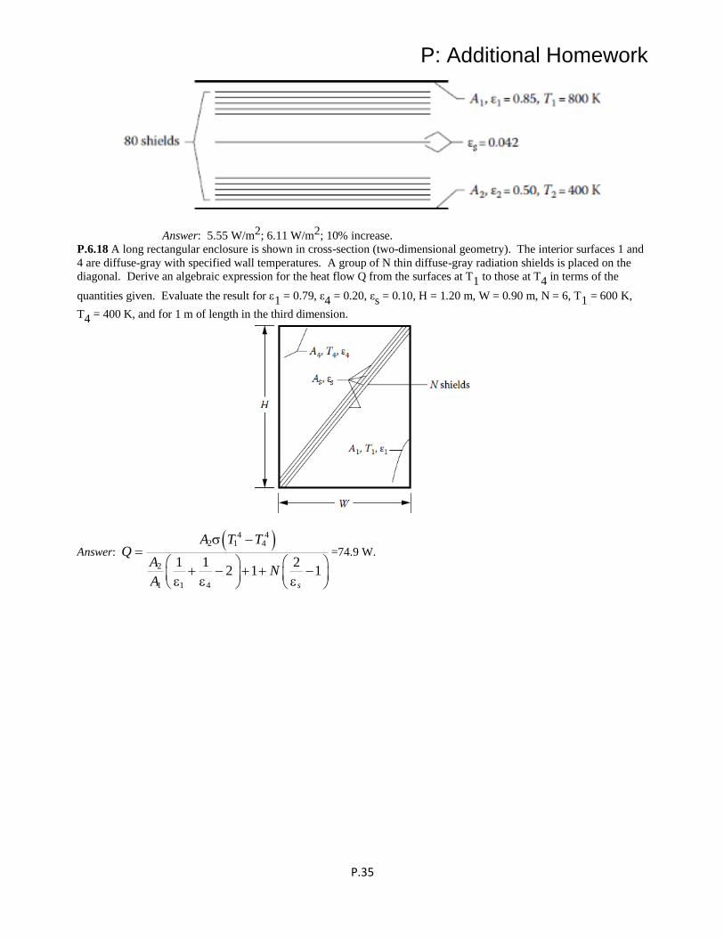
P: Additional Homework
P.35
Answer: 5.55 W/m2; 6.11 W/m2; 10% increase.
P.6.18 A long rectangular enclosure is shown in cross-section (two-dimensional geometry). The interior surfaces 1 and
4 are diffuse-gray with specified wall temperatures. A group of N thin diffuse-gray radiation shields is placed on the
diagonal. Derive an algebraic expression for the heat flow Q from the surfaces at T1 to those at T4 in terms of the
quantities given. Evaluate the result for 1 = 0.79, ε4 = 0.20, εs = 0.10, H = 1.20 m, W = 0.90 m, N = 6, T1 = 600 K,
T4 = 400 K, and for 1 m of length in the third dimension.
Answer: ( )4 4
2 1 4
2
1 1 4
1 1 22 1 1
s
A T TQ
AN
A
−=
+ − + + −
=74.9 W.
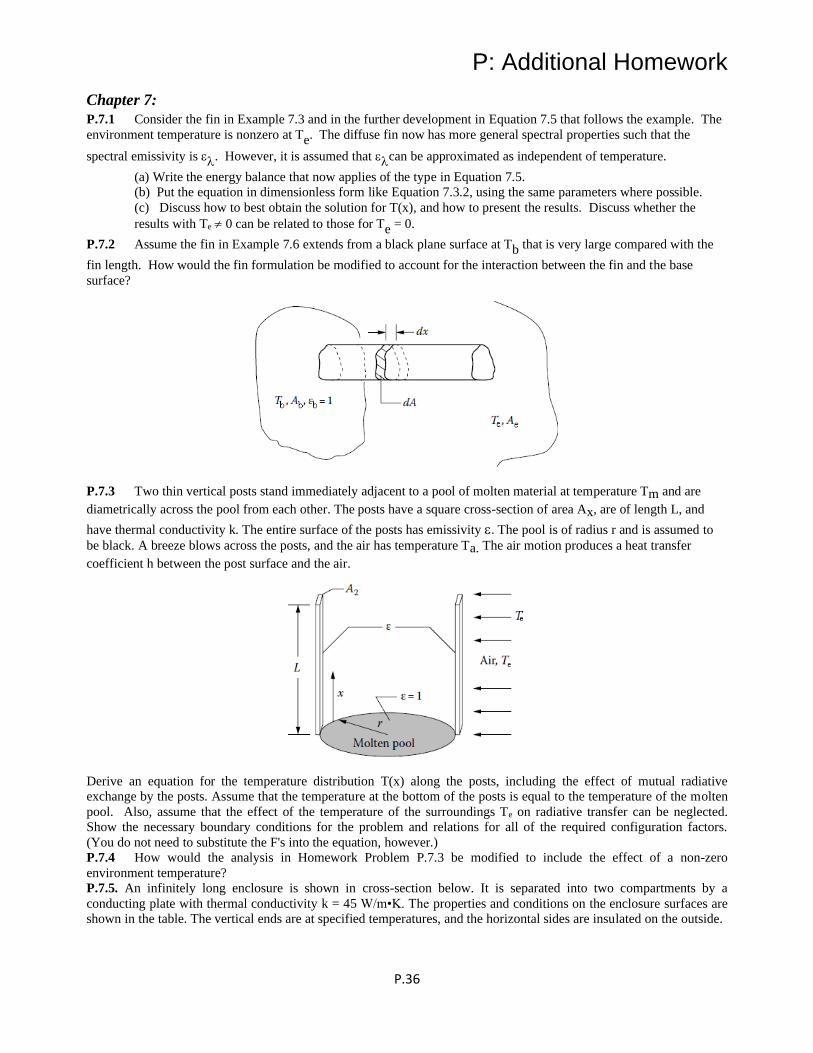
P: Additional Homework
P.36
Chapter 7:
P.7.1 Consider the fin in Example 7.3 and in the further development in Equation 7.5 that follows the example. The
environment temperature is nonzero at Te. The diffuse fin now has more general spectral properties such that the
spectral emissivity is . However, it is assumed that can be approximated as independent of temperature.
(a) Write the energy balance that now applies of the type in Equation 7.5.
(b) Put the equation in dimensionless form like Equation 7.3.2, using the same parameters where possible.
(c) Discuss how to best obtain the solution for T(x), and how to present the results. Discuss whether the
results with Te 0 can be related to those for Te = 0.
P.7.2 Assume the fin in Example 7.6 extends from a black plane surface at Tb that is very large compared with the
fin length. How would the fin formulation be modified to account for the interaction between the fin and the base
surface?
P.7.3 Two thin vertical posts stand immediately adjacent to a pool of molten material at temperature Tm and are
diametrically across the pool from each other. The posts have a square cross-section of area Ax, are of length L, and
have thermal conductivity k. The entire surface of the posts has emissivity . The pool is of radius r and is assumed to
be black. A breeze blows across the posts, and the air has temperature Ta. The air motion produces a heat transfer
coefficient h between the post surface and the air.
Derive an equation for the temperature distribution T(x) along the posts, including the effect of mutual radiative
exchange by the posts. Assume that the temperature at the bottom of the posts is equal to the temperature of the molten
pool. Also, assume that the effect of the temperature of the surroundings Te on radiative transfer can be neglected.
Show the necessary boundary conditions for the problem and relations for all of the required configuration factors.
(You do not need to substitute the F's into the equation, however.)
P.7.4 How would the analysis in Homework Problem P.7.3 be modified to include the effect of a non-zero
environment temperature?
P.7.5. An infinitely long enclosure is shown in cross-section below. It is separated into two compartments by a
conducting plate with thermal conductivity k = 45 W/m•K. The properties and conditions on the enclosure surfaces are
shown in the table. The vertical ends are at specified temperatures, and the horizontal sides are insulated on the outside.
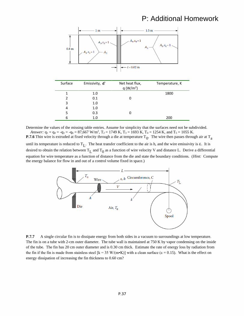
P: Additional Homework
P.37
Determine the values of the missing table entries. Assume for simplicity that the surfaces need not be subdivided.
Answer: q1 = q4 = -q3 = -q6 = 87,667 W/m2, T2 = 1749 K, T3 = 1693 K, T4 = 1254 K, and T5 = 1055 K.
P.7.6 Thin wire is extruded at fixed velocity through a die at temperature T0. The wire then passes through air at Ta
until its temperature is reduced to TL. The heat transfer coefficient to the air is h, and the wire emissivity is . It is
desired to obtain the relation between TL and T0 as a function of wire velocity V and distance L. Derive a differential
equation for wire temperature as a function of distance from the die and state the boundary conditions. (Hint: Compute
the energy balance for flow in and out of a control volume fixed in space.)
P.7.7 A single circular fin is to dissipate energy from both sides in a vacuum to surroundings at low temperature.
The fin is on a tube with 2-cm outer diameter. The tube wall is maintained at 750 K by vapor condensing on the inside
of the tube. The fin has 20 cm outer diameter and is 0.30 cm thick. Estimate the rate of energy loss by radiation from
the fin if the fin is made from stainless steel [k = 35 W/(m•K)] with a clean surface ( = 0.15). What is the effect on
energy dissipation of increasing the fin thickness to 0.60 cm?
Surface Emissivity, ε Net heat flux, q (W/m2)
Temperature, K
1 1.0 1800 2 0.1 0 3 1.0 4 1.0 5 0.3 0 6 1.0 200

P: Additional Homework
P.38
Answer: (c) 65 W; 91.2 W.
P.7.8 The billet in Homework Problem P.5.1 has air at 27°C blowing across it that provides an average convective heat
transfer coefficient of ( )2h=24 W m K/ • . Estimate the cooling time with both radiation and convection included.
Answer: 4.47 hours.
P.7.9 Opaque liquid at temperature T(0) and mean velocity u enters a long tube that is surrounded by a vacuum jacket
and a concentric electric heater that is kept at uniform axial temperature Te. The heater is black, and the tube exterior is
diffuse-gray with emissivity . The convective heat transfer coefficient between the liquid and the tube wall is h, and
the tube wall thermal conductivity is kw. Derive the relations to determine the mean fluid temperature and the tube wall
outer surface temperature as a function of distance x along the tube (assume that the liquid properties are constant).
P7.10 A solar collector is designed to fit onto the horizontal section of a roof as diagrammed below. Flow is from the
right to the left in the tubes of the collector. A tilted white diffuse roof section at the left side helps to reflect additional
solar flux onto the collector. Set up the equations for determining the local temperature of the tubes for two cases: (a)
no flow in the tubes, and (b) flow of water in each tube of 2.00 kg/min. Indicate a possible solution method. Assume
that the roof and collector are very long normal to the cross section shown.
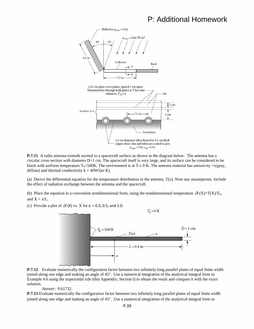
P: Additional Homework
P.39
P.7.11 A radio antenna extends normal to a spacecraft surface as shown in the diagram below. The antenna has a
circular cross section with diameter D=1 cm. The spacecraft itself is very large, and its surface can be considered to be
black with uniform temperature Tb=500K. The environment is at T 0 K. The antenna material has emissivity =ε(gray,
diffuse) and thermal conductivity k = 40W/(m·K).
(a) Derive the differential equation for the temperature distribution in the antenna, T(x). Note any assumptions. Include
the effect of radiation exchange between the antenna and the spacecraft.
(b) Place the equation in a convenient nondimensional form, using the nondimensional temperature (X)=T(X)/Tb,
and X = x/L.
(c) Provide a plot of (X) vs. X for = 0.3, 0.5, and 1.0.
P.7.12 Evaluate numerically the configuration factor between two infinitely long parallel plates of equal finite width
joined along one edge and making an angle of 45°. Use a numerical integration of the analytical integral form in
Example 4.6 using the trapezoidal rule (this Appendix, Section I) to obtain the result and compare it with the exact
solution.
Answer: 0.61732.
P.7.13 Evaluate numerically the configuration factor between two infinitely long parallel plates of equal finite width
joined along one edge and making an angle of 45°. Use a numerical integration of the analytical integral form in

P: Additional Homework
P.40
Example 4.6 using Simpson’s Rule (this Appendix, Section I) to obtain the result and compare it with the exact
solution.
Answer: 0.61732
P.7.14 A long gray empty circular tube is in the vacuum of outer space so that the only external heat exchange is by
radiation. The metal tube is coated with a material that has a solar absorptivity s and an emissivity in the infrared
region of IR. The solar flux qs is incident from a direction normal to the tube axis, and the surrounding environment is
at a very low temperature Te that can be neglected in the radiative energy balances. The geometry is as shown in cross-
section. The tube is empty so there is internal radiative exchange. Energy is conducted circumferentially within the
tube wall. The wall thermal conductivity is kw.
(a) Set up the energy relations required to obtain the temperature distribution around the tube circumference
assuming that radial temperature variations within the tube wall can be neglected.
(b) Place the energy relations in finite difference form and describe how a numerical solution can be obtained.
P.7.15 The tube in Homework Problem P.7.14 is shielded from solar radiation by being in the shadow of a space
vehicle, so that it cools to a very low temperature. It is then suddenly exposed to the solar flux. Set up the transient
energy relations required to calculate the tube circumferential temperature distribution as a function of time using the
same conditions and assumptions as in Homework Problem 7.14. Place the equations in finite difference form and
describe how a numerical solution can be obtained.
P.7.16 A thin sheet of copper moves through a radiative-convective oven at a velocity of 0.1 m/s. The sheet and oven
are very wide. Air flows at a mass flow rate of 0.2 kg/s per meter of oven width over the sheet in counterflow, and the
heat transfer coefficient between the air and sheet surface is constant along the sheet at a value of h = 100 W/(m2•K).
The back of the sheet is insulated. A black radiant heater at THeater = 1200 K covers the top of the oven as shown. The
radiant heater does not interact convectively with the air stream. Louvered curtains at each end of the oven are opaque
to radiation but allow air flow. The emissivities of all surfaces are shown.

P: Additional Homework
P.41
Find the temperature distribution Ts(x) along the copper sheet as a function of position x within the oven and present
the result graphically. Discuss all assumptions made in the solution and justify them by numerical argument where
possible. Data for copper sheet: ks = 400 W/(m•K); cp,s = 385 J/(kg•K); s = 9000 kg/m3.
P.7.17 For the geometry shown below with one conducting wall:
a) Provide the final governing equations necessary for finding T1(x1) and q2(x2) in nondimensional form using
appropriate nondimensional variables.
b): Find the temperature distribution T1(x1) and the heat flux distribution q2(x2) and show them on appropriate
graphs.
Boundary conditions are q x x x kW m221 1 1 1
100 50
= −( ) ( / ) where x1 is in meters, T2=500 K, and T3 = T4 = 300K.
Properties for the diffuse surfaces are shown on the figure.
Show that your solution is grid-independent, and meets overall energy conservation. Compare your solution to the
results for the nonconducting case. Answer: T1(max) = 1117.7 K with no conduction, T1(max) = 1102.1 K with conduction, and
q2(max) = ~ -10,100 W/m2 with no conduction and q2(max) = ~ -9,700 W/m2 with conduction.
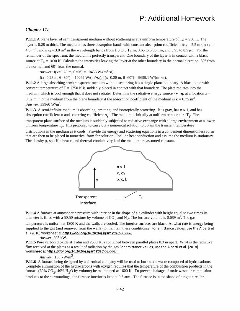
P: Additional Homework
P.42
Chapter 11:
P.11.1 A plane layer of semitransparent medium without scattering is at a uniform temperature of Tm = 950 K. The
layer is 0.28 m thick. The medium has three absorption bands with constant absorption coefficients 1 = 5.5 m-1, 2 =
4.6 m-1, and 3 = 3.8 m-1 in the wavelength bands from 1.3 to 3.1 m, 3.65 to 5.05 m, and 5.95 to 8.5 m. For the
remainder of the spectrum, the medium is perfectly transparent. One boundary of the layer is in contact with a black
source at Tw = 1030 K. Calculate the intensities leaving the layer at the other boundary in the normal direction, 30 from
the normal, and 60 from the normal.
Answer: I(x=0.28 m, =0) = 10458 W/(m2·sr);
I(x=0.28 m, =30) = 10262 W/(m2·sr); I(x=0.28 m, =60) = 9699.1 W/(m2·sr).
P.11.2 A large absorbing semitransparent medium without scattering has a single plane boundary. A black plate with
constant temperature of T = 1250 K is suddenly placed in contact with that boundary. The plate radiates into the
medium, which is cool enough that it does not radiate. Determine the radiative energy source - ·qr at a location x =
0.82 m into the medium from the plane boundary if the absorption coefficient of the medium is = 0.75 m-1.
.Answer: 55960 W/m3.
P.11.3 A semi-infinite medium is absorbing, emitting, and isotropically scattering. It is gray, has n 1, and has
absorption coefficient and scattering coefficient s. The medium is initially at uniform temperature Ti. The
transparent plane surface of the medium is suddenly subjected to radiative exchange with a large environment at a lower
uniform temperature Te. It is proposed to carry out a numerical solution to obtain the transient temperature
distributions in the medium as it cools. Provide the energy and scattering equations in a convenient dimensionless form
that are then to be placed in numerical form for solution. Include heat conduction and assume the medium is stationary.
The density specific heat c, and thermal conductivity k of the medium are assumed constant.
P.11.4 A furnace at atmospheric pressure with interior in the shape of a a cylinder with height equal to two times its
diameter is filled with a 50:50 mixture by volume of CO2 and N2. The furnace volume is 0.689 m3. The gas
temperature is uniform at 1800 K and the walls are cooled. The interior surfaces are black. At what rate is energy being
supplied to the gas (and removed from the walls) to maintain these conditions? For emittance values, use the Alberti et al. (2018) worksheet at https://doi.org/10.1016/j.jqsrt.2018.08.008.
Answer: 295 kW.
P.11.5 Pure carbon dioxide at 1 atm and 2500 K is contained between parallel plates 0.3 m apart. What is the radiative
flux received at the plates as a result of radiation by the gas For emittance values, use the Alberti et al. (2018) worksheet at https://doi.org/10.1016/j.jqsrt.2018.08.008.
Answer: 163 kW/m2.
P.11.6 A furnace being designed by a chemical company will be used to burn toxic waste composed of hydrocarbons.
Complete elimination of the hydrocarbons with oxygen requires that the temperature of the combustion products in the
furnace (60% CO2, 40% H2O by volume) be maintained at 1600 K. To prevent leakage of toxic waste or combustion
products to the surroundings, the furnace interior is kept at 0.5 atm. The furnace is in the shape of a right circular
x
n 1
, s
, c, k
Te Transparent
interface

P: Additional Homework
P.43
cylinder of height equal to its diameter of 4 m. What average radiative flux is incident on the interior surface of the
furnace? Note any assumptions used in obtaining the result.
Answer: 124 kW/m2.
P.11.7 Estimate the maximum radiative flux that is incident on any local area on the interior surface of the furnace
described in Homework Problem P.11.6.
Answer: 137 kW/m2.
P.11.8 Evaluate the geometric mean transmittance 21d − from the element dA1 to the area A2 in Homework Problem
5.1. The region between the areas is filled with a gray medium at uniform temperature having an absorption coefficient
= 0.035 cm-1. Answer: 0.02341.
P.11.9 A thin black plate 1 x 1 cm is at the center of a sphere of CO2-air mixture at a uniform temperature of 1800 K
and 1 atm total pressure. The partial pressure of the CO2 is 0.8 atm and the sphere diameter is 1 m. How much energy
is absorbed by the plate? What will the plate temperature be? (Assume the boundary of the sphere is black and kept
cool so that it does not enter into the radiative exchange.)
Answer: 13.0 W, 1034 K.
P.11.10 A spherical cavity is filled with an isothermal gray medium having an absorption coefficient Set up the
relations needed to determine the geometric mean transmittance −1 2dt from the cavity surface A1 to the area element
dA2 at the center of the opening A2.
[Note : A similar situation is considered by Koh, J.C.Y.: Int. J. Heat Mass Transfer, vol. 8, no. 2, pp. 373-374, 1965.]
P.11.11 A gray isotropically scattering gas is contained between large diffuse-gray parallel plates. The plates both have
emissivity ε = 0.30. Plate 1 is maintained at temperature T1 = 1150 K, and plate 2 is at T2 = 525 K. The medium
between the plates has a uniform extinction coefficient of = 0.75 m-1. The plate geometry is shown below.
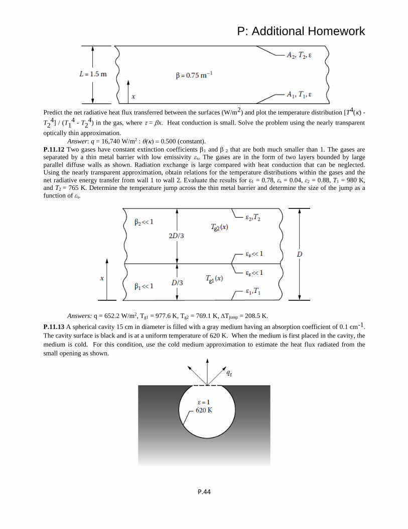
P: Additional Homework
P.44
Predict the net radiative heat flux transferred between the surfaces (W/m2) and plot the temperature distribution [T4() -
T24] / (T1
4 - T24) in the gas, where = x. Heat conduction is small. Solve the problem using the nearly transparent
optically thin approximation.
Answer: q = 16,740 W/m2 : () = 0.500 (constant).
P.11.12 Two gases have constant extinction coefficients 1 and 2 that are both much smaller than 1. The gases are
separated by a thin metal barrier with low emissivity εs. The gases are in the form of two layers bounded by large
parallel diffuse walls as shown. Radiation exchange is large compared with heat conduction that can be neglected.
Using the nearly transparent approximation, obtain relations for the temperature distributions within the gases and the
net radiative energy transfer from wall 1 to wall 2. Evaluate the results for ε1 = 0.78, εs = 0.04, ε2 = 0.88, T1 = 980 K,
and T2 = 765 K. Determine the temperature jump across the thin metal barrier and determine the size of the jump as a
function of εs.
Answers: q = 652.2 W/m2, Tg1 = 977.6 K, Tg2 = 769.1 K, Tjump = 208.5 K.
P.11.13 A spherical cavity 15 cm in diameter is filled with a gray medium having an absorption coefficient of 0.1 cm-1.
The cavity surface is black and is at a uniform temperature of 620 K. When the medium is first placed in the cavity, the
medium is cold. For this condition, use the cold medium approximation to estimate the heat flux radiated from the
small opening as shown.
P: Additional Homework
P.45
Answer: 3293 W/m2.
P.11.14 An optically thin gray gas with constant absorption coefficient is contained in a long transparent cylinder of
diameter D. The surrounding environment is at low temperature that can be considered zero. Initially, the cylinder is at
the environment temperature. Then, an electrical discharge is passed through the gas, continuously producing in the gas
a uniform energy source q per unit volume and time. Derive a relation for the transient gas temperature variation if
radiation is assumed to be the only significant mode of heat transfer. What is the maximum temperature Tmax that the
gas will achieve?
Answer: /
max
max
v max
T q Tt ln tan ; T ;
c T
1 4318 1 1
2 1 4
−+ = + = =
− .
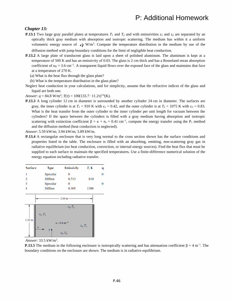
P: Additional Homework
P.46
Chapter 13:
P.13.1 Two large gray parallel plates at temperatures T1 and T2 and with emissivities ε1 and ε2 are separated by an
optically thick gray medium with absorption and isotropic scattering. The medium has within it a uniform
volumetric energy source of q W/m3. Compute the temperature distribution in the medium by use of the
diffusion method with jump boundary conditions for the limit of negligible heat conduction.
P.13.2 A large plate of translucent glass is laid upon a sheet of polished aluminum. The aluminum is kept at a
temperature of 500 K and has an emissivity of 0.03. The glass is 2 cm thick and has a Rosseland mean absorption
coefficient of κR = 3.6 cm−1. A transparent liquid flows over the exposed face of the glass and maintains that face
at a temperature of 270 K.
(a) What is the heat flux through the glass plate?
(b) What is the temperature distribution in the glass plate?
Neglect heat conduction in your calculations, and for simplicity, assume that the refractive indices of the glass and
liquid are both one.
Answer: q = 84.8 W/m2; T(τ) = 100(133.7−11.2τ)1/4(K).
P.13.3 A long cylinder 12 cm in diameter is surrounded by another cylinder 24 cm in diameter. The surfaces are
gray, the inner cylinder is at T1 = 910 K with 1 = 0.42, and the outer cylinder is at T2 = 1075 K with 2 = 0.83.
What is the heat transfer from the outer cylinder to the inner cylinder per unit length for vacuum between the
cylinders? If the space between the cylinders is filled with a gray medium having absorption and isotropic
scattering with extinction coefficient β = κ + σs = 0.41 cm−1, compute the energy transfer using the P1 method
and the diffusion method (heat conduction is neglected).
Answer: 5.59 kW/m; 3.94 kW/m; 3.89 kW/m.
P.13.4 A rectangular enclosure that is very long normal to the cross section shown has the surface conditions and
properties listed in the table. The enclosure is filled with an absorbing, emitting, non-scattering gray gas in
radiative equilibrium (no heat conduction, convection, or internal energy sources). Find the heat flux that must be
supplied to each surface to maintain the specified temperatures. Use a finite-difference numerical solution of the
energy equation including radiative transfer.
Answer: 33.5 kW/m2.
P.13.5 The medium in the following enclosure is isotropically scattering and has attenuation coefficient β = 4 m−1. The
boundary conditions on the enclosure are shown. The medium is in radiative equilibrium.
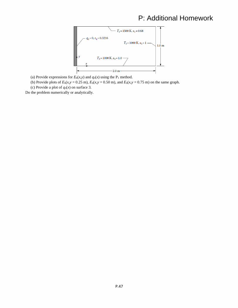
P: Additional Homework
P.47
(a) Provide expressions for Eb(x,y) and q3(x) using the P1 method.
(b) Provide plots of Eb(x,y = 0.25 m), Eb(x,y = 0.50 m), and Eb(x,y = 0.75 m) on the same graph.
(c) Provide a plot of q3(x) on surface 3.
Do the problem numerically or analytically.
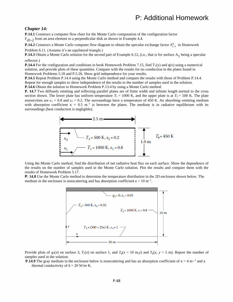
P: Additional Homework
P.48
Chapter 14:
P.14.1 Construct a computer flow chart for the Monte Carlo computation of the configuration factor
Fd1-2 from an area element to a perpendicular disk as shown in Example 4.4.
P.14.2 Construct a Monte Carlo computer flow diagram to obtain the specular exchange factor S
1 2F−
in Homework
Problem 6.11. (Assume it’s an equilateral triangle.)
P.14.3 Obtain a Monte Carlo solution for the second part of Example 6.12, (i.e., that is for surface A1 being a specular
reflector.)
P.14.4 For the configuration and conditions in book Homework Problem 7.15, find T1(y) and q(x) using a numerical
solution, and provide plots of these quantities. Compare with the results for no conduction in the plates found in
Homework Problems 5.18 and P.5.26. Show grid independence for your results.
P.14.5 Repeat Problem P.14.4 using the Monte Carlo method and compare the results with those of Problem P.14.4.
Repeat for enough samples to show independence of the results to the number of samples used in the solution.
P.14.6 Obtain the solution to Homework Problem P.13.4 by using a Monte Carlo method.
P. 14.7 Two diffusely emitting and reflecting parallel plates are of finite width and infinite length normal to the cross
section shown. The lower plate has uniform temperature T1 = 1000 K, and the upper plate is at T2 = 500 K. The plate
emissivities are 1 = 0.8 and 2 = 0.2. The surroundings have a temperature of 450 K. An absorbing–emitting medium
with absorption coefficient κ = 0.5 m−1 is between the plates. The medium is in radiative equilibrium with its
surroundings (heat conduction is negligible).
Using the Monte Carlo method, find the distribution of net radiative heat flux on each surface. Show the dependence of
the results on the number of samples used in the Monte Carlo solution. Plot the results and compare them with the
results of Homework Problem 5.17.
P. 14.8 Use the Monte Carlo method to determine the temperature distribution in the 2D enclosure shown below. The
medium in the enclosure is nonscattering and has absorption coefficient κ = 10 m−1.
Provide plots of q3(x) on surface 3, T1(x) on surface 1, and Tg(x = 10 m,y) and Tg(x, y = 5 m). Report the number of
samples used in the solution.
P.14.9 The gray medium in the enclosure below is nonscattering and has an absorption coefficient of κ = 4 m−1 and a
thermal conductivity of k = 20 W/m·K.
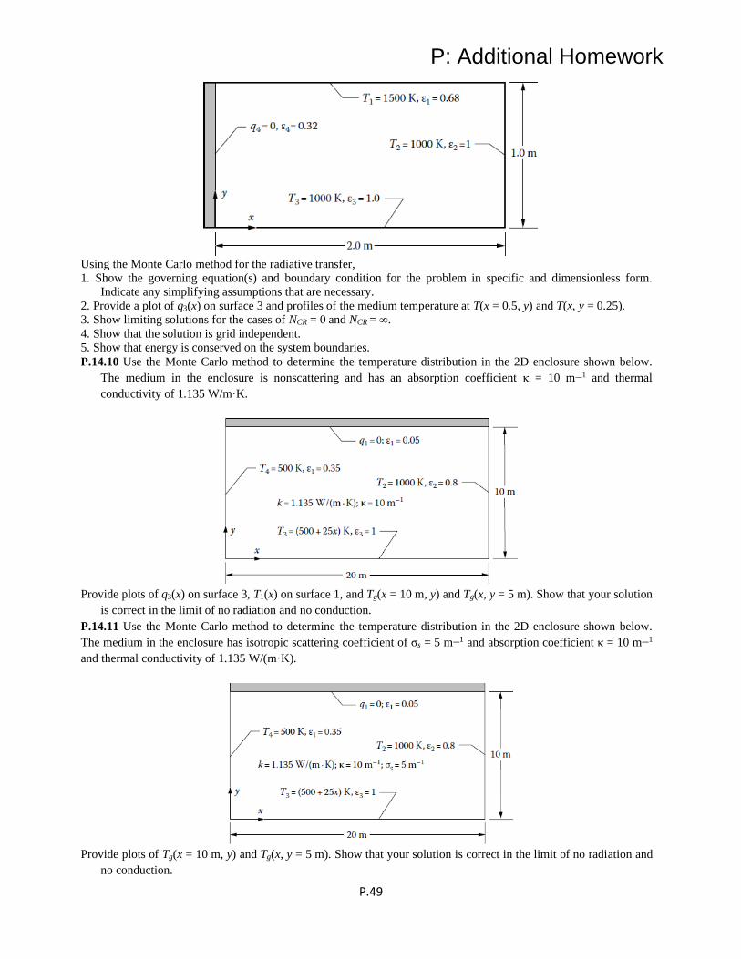
P: Additional Homework
P.49
Using the Monte Carlo method for the radiative transfer,
1. Show the governing equation(s) and boundary condition for the problem in specific and dimensionless form.
Indicate any simplifying assumptions that are necessary.
2. Provide a plot of q3(x) on surface 3 and profiles of the medium temperature at T(x = 0.5, y) and T(x, y = 0.25).
3. Show limiting solutions for the cases of NCR = 0 and NCR = ∞.
4. Show that the solution is grid independent.
5. Show that energy is conserved on the system boundaries.
P.14.10 Use the Monte Carlo method to determine the temperature distribution in the 2D enclosure shown below.
The medium in the enclosure is nonscattering and has an absorption coefficient κ = 10 m−1 and thermal
conductivity of 1.135 W/m·K.
Provide plots of q3(x) on surface 3, T1(x) on surface 1, and Tg(x = 10 m, y) and Tg(x, y = 5 m). Show that your solution
is correct in the limit of no radiation and no conduction.
P.14.11 Use the Monte Carlo method to determine the temperature distribution in the 2D enclosure shown below.
The medium in the enclosure has isotropic scattering coefficient of σs = 5 m−1 and absorption coefficient κ = 10 m−1
and thermal conductivity of 1.135 W/(m·K).
Provide plots of Tg(x = 10 m, y) and Tg(x, y = 5 m). Show that your solution is correct in the limit of no radiation and
no conduction.
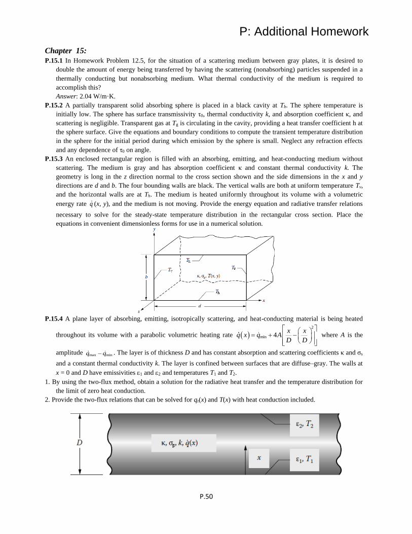
P: Additional Homework
P.50
Chapter 15:
P.15.1 In Homework Problem 12.5, for the situation of a scattering medium between gray plates, it is desired to
double the amount of energy being transferred by having the scattering (nonabsorbing) particles suspended in a
thermally conducting but nonabsorbing medium. What thermal conductivity of the medium is required to
accomplish this?
Answer: 2.04 W/m·K.
P.15.2 A partially transparent solid absorbing sphere is placed in a black cavity at Tb. The sphere temperature is
initially low. The sphere has surface transmissivity τ0, thermal conductivity k, and absorption coefficient κ, and
scattering is negligible. Transparent gas at Tg is circulating in the cavity, providing a heat transfer coefficient h at
the sphere surface. Give the equations and boundary conditions to compute the transient temperature distribution
in the sphere for the initial period during which emission by the sphere is small. Neglect any refraction effects
and any dependence of τ0 on angle.
P.15.3 An enclosed rectangular region is filled with an absorbing, emitting, and heat-conducting medium without
scattering. The medium is gray and has absorption coefficient κ and constant thermal conductivity k. The
geometry is long in the z direction normal to the cross section shown and the side dimensions in the x and y
directions are d and b. The four bounding walls are black. The vertical walls are both at uniform temperature Tv,
and the horizontal walls are at Th. The medium is heated uniformly throughout its volume with a volumetric
energy rate q (x, y), and the medium is not moving. Provide the energy equation and radiative transfer relations
necessary to solve for the steady-state temperature distribution in the rectangular cross section. Place the
equations in convenient dimensionless forms for use in a numerical solution.
P.15.4 A plane layer of absorbing, emitting, isotropically scattering, and heat-conducting material is being heated
throughout its volume with a parabolic volumetric heating rate ( )2
min 4
= + −
x xq x q A
D D where A is the
amplitude max min−q q . The layer is of thickness D and has constant absorption and scattering coefficients κ and σs
and a constant thermal conductivity k. The layer is confined between surfaces that are diffuse–gray. The walls at
x = 0 and D have emissivities 1 and 2 and temperatures T1 and T2.
1. By using the two-flux method, obtain a solution for the radiative heat transfer and the temperature distribution for
the limit of zero heat conduction.
2. Provide the two-flux relations that can be solved for qr(x) and T(x) with heat conduction included.

P: Additional Homework
P.51
P.15.5 Using the solution ideas for the 2D analysis in Section 15.5.2 and those in the steady 1D analysis at the end of
Section 13.6.3, set up the FEM for the ADI solution for the following situation with an emitting, absorbing, and
conducting gray medium in a 2D rectangular enclosure that is infinitely long normal to the cross section shown.
There is no scattering in the medium. The rectangular region has a uniform heating q W/m3 throughout its
volume. The steady 2D temperature distribution is to be determined. For simplicity, use a grid having the same
increment size in both the x and y directions. The boundary walls are black and are at the same temperature Tw.
P.15.6 Modify Homework Problem P.15.5 to incorporate a variable grid size into the solution for the steady
temperature distribution within a square cross section. Use the ideas in Homework Problem 15.8 extended into
2D.
P.15.7 Two large infinite parallel plates are separated by an optically thick absorbing–emitting, isotropically
scattering, and conducting gas in which a chemical reaction is occurring that produces a uniform energy
generation rate of q per unit volume. The plates are gray and have temperatures and emissivities T1, 1 and T2,
2. Determine the heat fluxes q1 and q2 that must be supplied to each of the plates as a result of radiation
exchange combined with heat conduction between them. Use the radiative diffusion approximation, and assume
that the gas is stationary and that Rosseland mean attenuation coefficient βR and thermal conductivity k are both
constant. Show how to implement the slip coefficient of Figure 15.8.
P.15.8 Two gray parallel plates with emissivities 1 = 0.45 and 2 = 0.9 are spaced 0.15 m apart. The plate
temperatures are T1 = 515 K and T2 = 297 K. A stagnant nongray gas with spectral absorption coefficient as
shown is in the space between the plates. The thermal conductivity of the gas is k = 0.285 W/(m·K). Using the
additive method with the radiative diffusion solution, find the heat transfer between the plates. How significant is
the heat conduction?
Answer: 1821 W/m2; 23%.
P.15.9 A plane layer of semitransparent absorbing, emitting, and heat-conducting medium is between two thin metal
(highly conducting) walls. The medium is not moving, and it is gray with absorption coefficient κ and thermal
conductivity k. The wall surfaces are diffuse–gray with emissivities 1 on both sides of the wall at x = 0 and 2 on
both sides of the wall at x = D. The large isothermal surroundings below the lower wall are filled with gas at Tg1,
and there is a heat transfer coefficient h1 between the gas and the outside of the lower wall. Outside the upper
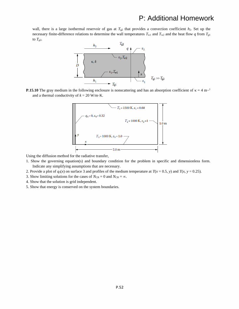
P: Additional Homework
P.52
wall, there is a large isothermal reservoir of gas at Tg2 that provides a convection coefficient h2. Set up the
necessary finite-difference relations to determine the wall temperatures Tw1 and Tw2 and the heat flow q from Tg1
to Tg2.
P.15.10 The gray medium in the following enclosure is nonscattering and has an absorption coefficient of κ = 4 m−1
and a thermal conductivity of k = 20 W/m·K.
Using the diffusion method for the radiative transfer,
1. Show the governing equation(s) and boundary condition for the problem in specific and dimensionless form.
Indicate any simplifying assumptions that are necessary.
2. Provide a plot of q3(x) on surface 3 and profiles of the medium temperature at T(x = 0.5, y) and T(x, y = 0.25).
3. Show limiting solutions for the cases of NCR = 0 and NCR = ∞.
4. Show that the solution is grid independent.
5. Show that energy is conserved on the system boundaries.

P: Additional Homework
P.53
Chapter 17:
P.17.1 As a result of surface treatment, a partially transparent plate has a different reflectivity at each surface. For
radiation incident on surface 1 in a single direction, obtain an expression for the overall reflectance and
transmittance in terms of ρ1, ρ2, and τ.
Answer: ( ) ( )( ) + − − −
= =− −
21 2 1 1 2
2 21 2 1 2
1 2 1 1;
1 1R T
P.17.2 Two parallel, partially transparent plates have different τ values and a different ρ at each surface. Obtain an
expression for the overall transmittance of the two-plate system for radiation incident from a single direction.
Answer:
( )( )
( )
− − = =
− −
+ − =
−
1 21 2
212 21 1 2
2
2
1 1, where
1 1
1 2and
1
n n nn
n n n
nm nn nm nnm
nm nn n
TTT T
R R
R
P.17.3 In a solar still, a thin layer of condensed water is flowing down a glass plate. The plate has a transmittance τ,
and the water layer is assumed nonabsorbing. Obtain an expression for the overall transmittance TL of the system
for radiation incident on the glass in a single direction.
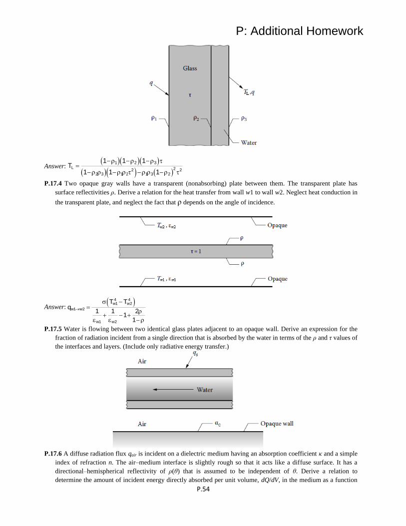
P: Additional Homework
P.54
Answer: ( )( )( )
( )( ) ( )
− − − =
− − − −
1 2 3
22 22 3 1 2 1 3 2
1 1 1
1 1 1LT
P.17.4 Two opaque gray walls have a transparent (nonabsorbing) plate between them. The transparent plate has
surface reflectivities ρ. Derive a relation for the heat transfer from wall w1 to wall w2. Neglect heat conduction in
the transparent plate, and neglect the fact that ρ depends on the angle of incidence.
Answer: ( )
→
−=
+ − +
−
4 41 2
1 2
1 2
1 1 21
1
w w
w w
w w
T Tq
P.17.5 Water is flowing between two identical glass plates adjacent to an opaque wall. Derive an expression for the
fraction of radiation incident from a single direction that is absorbed by the water in terms of the ρ and τ values of
the interfaces and layers. (Include only radiative energy transfer.)
P.17.6 A diffuse radiation flux qair is incident on a dielectric medium having an absorption coefficient κ and a simple
index of refraction n. The air–medium interface is slightly rough so that it acts like a diffuse surface. It has a
directional–hemispherical reflectivity of ρ(θ) that is assumed to be independent of θ. Derive a relation to
determine the amount of incident energy directly absorbed per unit volume, dQ/dV, in the medium as a function
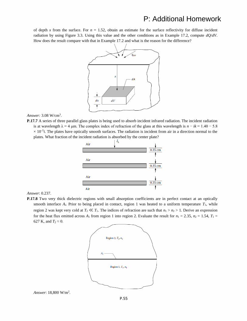
P: Additional Homework
P.55
of depth x from the surface. For n = 1.52, obtain an estimate for the surface reflectivity for diffuse incident
radiation by using Figure 3.3. Using this value and the other conditions as in Example 17.2, compute dQ/dV.
How does the result compare with that in Example 17.2 and what is the reason for the difference?
Answer: 3.08 W/cm3.
P.17.7 A series of three parallel glass plates is being used to absorb incident infrared radiation. The incident radiation
is at wavelength λ = 4 μm. The complex index of refraction of the glass at this wavelength is n − ik = 1.40 − 5.8
× 10–5i. The plates have optically smooth surfaces. The radiation is incident from air in a direction normal to the
plates. What fraction of the incident radiation is absorbed by the center plate?
Answer: 0.237.
P.17.8 Two very thick dielectric regions with small absorption coefficients are in perfect contact at an optically
smooth interface Ai. Prior to being placed in contact, region 1 was heated to a uniform temperature T1, while
region 2 was kept very cold at T2 ≪ T1. The indices of refraction are such that n1 > n2 > 1. Derive an expression
for the heat flux emitted across A1 from region 1 into region 2. Evaluate the result for n1 = 2.35, n2 = 1.54, T1 =
627 K, and T2 ≈ 0.
Answer: 18,800 W/m2.
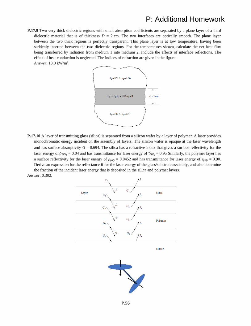
P: Additional Homework
P.56
P.17.9 Two very thick dielectric regions with small absorption coefficients are separated by a plane layer of a third
dielectric material that is of thickness D = 2 cm. The two interfaces are optically smooth. The plane layer
between the two thick regions is perfectly transparent. This plane layer is at low temperature, having been
suddenly inserted between the two dielectric regions. For the temperatures shown, calculate the net heat flux
being transferred by radiation from medium 1 into medium 2. Include the effects of interface reflections. The
effect of heat conduction is neglected. The indices of refraction are given in the figure.
Answer: 13.0 kW/m2.
P.17.10 A layer of transmitting glass (silica) is separated from a silicon wafer by a layer of polymer. A laser provides
monochromatic energy incident on the assembly of layers. The silicon wafer is opaque at the laser wavelength
and has surface absorptivity α = 0.694. The silica has a refractive index that gives a surface reflectivity for the
laser energy of 2SiO = 0.04 and has transmittance for laser energy of 2SiO = 0.95 Similarly, the polymer layer has
a surface reflectivity for the laser energy of ρpoly = 0.0452 and has transmittance for laser energy of τpoly = 0.90.
Derive an expression for the reflectance R for the laser energy of the glass/substrate assembly, and also determine
the fraction of the incident laser energy that is deposited in the silica and polymer layers.
Answer: 0.302.
Q: Proposed Syllabus
Q-1
Q: PROPOSED ONE-SEMESTER SYLLABUS
Below is a syllabus for a one-semester course in radiation heat transfer. The syllabus is based on a
15-week semester with two 90-minute classes per week, with 27 lecture sessions and three session left for
examinations, class evaluation, etc. It concentrates on the fundamental blackbody properties (Chapter 1), the
radiative properties of surfaces (Chapters 2, 3), the definition and use of configuration factors (Chapter 4),
energy transfer among gray-diffuse surfaces and in enclosures with gray-diffuse surfaces, and solution
techniques for these problems (Chapter 5). The Monte Carlo section for transfer among surfaces is drawn
from Chapter 14 and introduced at this point. Interactions with conduction and/or convective transfer at
enclosure boundaries are then treated (Chapter 7). Chapter 8 on the electromagnetic theory fundamentals is
introduced to show the fundamental basis for what has gone before. Finally, the absorption characteristics of
participating media (Chapter 9) are introduced to show their important spectral characteristics, the
mathematical treatment of transfer through a participating media and a simplified mean-beam-length solution
technique is shown (Chapter 11), and a more exact but intuitive method (diffusion solution) is examined as
one example of a more general case (Chapter 13). Finally, Chapter 19 is used to kindle interest in
contemporary applications of radiation.
This proposed one-semester syllabus ignores many important basic subjects such as the emerging
areas of micro-nanoscale effects, inverse problems and solution methods, and the presence of
bifurcation/chaos in nonlinear problems. Many important applications are also only noted in passing,
although some are discussed in Chapter 19. The course instructor may wish to spend some time on any or all
these subjects.
Much material in the book is skipped, but could well be incorporated into a second course,
particularly one that concentrates on radiative transfer in participating media.
Chapter 1. Introduction to Radiative Transfer (3 class sessions)
1.1 Thermal Radiation and the Natural World
1.2 Thermal Radiation in Engineering
1.3 Thermal Radiation and Thermodynamics
1.4 Nature of the Governing Equations
1.5 Electromagnetic Waves vs. Photons
1.6 Radiative Energy Exchange and Radiative Intensity
1.7 Solid Angle
1.8 Spectral Intensity
1.9 Characteristics of Emission
1.9.1 Perfect Emitter
1.9.2 Radiation Isotropy in a Black Enclosure
1.9.3 Perfect Emitter in Each Direction and Wavelength
1.9.4 Total Radiation into Vacuum
1.9.5 Blackbody Intensity and Its Directional Independence
1.9.6 Blackbody Emissive Power: Cosine-Law Dependence
1.9.7 Hemispherical Spectral Emissive Power of a Blackbody
1.9.8 Planck’s Law: Spectral Distribution of Emissive Power
1.9.9 Approximations to the Blackbody Spectral Distribution
1.9.10 Wien’s Displacement Law
1.9.11 Total Blackbody Intensity and Emissive Power
1.9.12 Blackbody Radiation within a Spectral Band
1.9.13 Summary of Blackbody Properties
1.10 Radiative Energy Along a Line-Of-Sight
1.10.1 Radiative Energy Loss due to Absorption and Scattering
1.10.2 Mean Penetration Distance
1.10.3 Optical Thickness

Q: Proposed Syllabus
Q-2
1.10.4 Radiative Energy Gain due to Emission
1.10.5 Radiative Energy Density and Radiation Pressure
1.10.6 Radiative Energy Gain due to In-Scattering
1.11 Radiative Transfer Equation
1.12 Radiative Transfer in Enclosures with Nonparticipating Media
Chapter 2. Radiative Properties at Interfaces (2 class sessions)
2.1 Introduction
2.2 Emissivity
2.2.1 Directional Spectral Emissivity, λ(θ,ϕ,T)
2.2.2 Directional Total Emissivity, (θ,ϕ,T)
2.2.3 Hemispherical Spectral Emissivity, λ(T)
2.2.4 Hemispherical Total Emissivity, (T)
2.3 Absorptivity
2.3.1 Directional Spectral Absorptivity, αλ(θi,ϕi,T)
2.3.2 Kirchhoff’s Law
2.3.3 Directional Total Absorptivity, α(θi,ϕi,T)
2.3.4 Kirchhoff’s Law for Directional Total Properties
2.3.5 Hemispherical Spectral Absorptivity, αλ(T)
2.3.6 Hemispherical Total Absorptivity, α(T)
2.3.7 Diffuse-Gray Surface
2.4 Reflectivity
2.4.1 Spectral Reflectivities (skim)
2.4.2 Total Reflectivities (skim)
2.5 Transmissivity at an Interface (skim)
2.6 Relations among Reflectivity, Absorptivity, Emissivity, and Transmissivity
Chapter 3. Radiative Properties of Opaque Materials (2 class session)
3.1 Introduction
3.2 Electromagnetic Wave Theory Predictions
3.2.1 Dielectric Materials
3.2.2 Radiative Properties of Conductors
3.2.3 Extensions to the Theory of Radiative Properties
3.3 Measurements of Real Surfaces
3.3.1 Heterogeneity and Surface Coatings
3.3.2 Surface Roughness
3.3.3 Variation of Radiative Properties with Surface Temperature
3.3.4 Properties of Liquid Metals (skim)
3.3.5 Properties of Semiconductors and Superconductors (skim)
3.4 Selective Surfaces for Solar Applications
3.4.1 Characteristics of Solar Radiation
3.4.2 Modification of Surface Spectral Characteristics
3.4.3 Modification of Surface Directional Characteristics
Chapter 4. Configuration Factors for Diffuse Surfaces with Uniform Radiosity (3 class sessions)
4.1 Radiative Transfer Equation for Surfaces Separated by a Transparent Medium
4.1.1 Enclosures with Diffuse Surfaces
4.2 Geometric Configuration Factors between Two Surfaces
4.2.1 Configuration Factor for Energy Exchange between Diffuse Differential
Areas
4.2.2 Configuration Factor between a Differential Area Element and a Finite Area
Q: Proposed Syllabus
Q-3
4.2.3 Configuration Factor and Reciprocity for Two Finite Areas
4.3 Methods for Determining Configuration Factors
4.3.1 Configuration-Factor Algebra
4.3.2 Configuration-Factor Relations in Enclosures
4.3.3 Techniques for Evaluating Configuration Factors
4.3.4 Unit-Sphere and Hemicube Methods
4.5 Compilation of Known Configuration Factors and their References: Appendix C and Web
Catalog
Chapter 5. Radiation Exchange in Enclosures Composed of Black and/or Diffuse-Gray Surfaces (4
class sections)
5.1 Introduction
5.2 Radiative Transfer for Black Surfaces
5.2.1 Transfer between Black Surfaces Using Configuration Factors
5.2.2 Radiation Exchange in a Black Enclosure
5.3 Radiation Among Finite Diffuse-Gray Areas
5.3.1 Net-Radiation Method for Enclosures
5.3.2 Enclosure Analysis in Terms of Energy Absorbed at Surface
5.3.4 Matrix Inversion for Enclosure Equations
5.4 Radiation Analysis Using Infinitesimal Areas
5.4.1 Generalized Net-Radiation Method Using Infinitesimal Areas
5.5 Computer Programs for Enclosure Analysis
Chapter 14. The Monte Carlo Method (2 class sessions)
14.1 Introduction
14.2 Fundamentals of the Monte Carlo Method
14.3 Monte Carlo for Surface-to-Surface Radiation Exchange
14.3.1 Radiation between Black Surfaces
14.3.2 Radiation between Non-Black Surfaces
14.3.3 Wavelength-Dependent Properties
14.3.4 Ray Tracing
Chapter 7. Radiation Combined with Conduction and Convection at Boundaries (2 class sessions)
7.1 Introduction
7.2 Energy Relations and Boundary Conditions
7.2.1 General Relations
7.2.2 Uncoupled and Coupled Energy Transfer Modes
7.2.3 Control Volume Approach for One- or Two-Dimensional Conduction along Thin
Walls
7.3 Radiation Transfer with Conduction Boundary Conditions
7.3.1 Thin Fins with 1D or 2D Conduction
7.4 Radiation with Convection and Conduction
7.4.1 Thin Radiating Fins with Convection
7.5 Numerical Solution Methods
7.5.3 Numerical Solution Techniques
7.5.4 Verification, Validation and Uncertainty Quantification
Chapter 8. Electromagnetic Wave Theory (skim) (1 class session)
Chapter 9: Properties of Participating Media (1 class session)
9.1 Introduction
Q: Proposed Syllabus
Q-4
9.2 Spectral Lines and Bands for Gas Absorption and Emission
9.2.1 Physical Mechanisms
9.2.2 Local Thermodynamic Equilibrium (LTE)
9.2.3 Spectral Line Broadening
9.4 Gas Total Emittance Correlations
Chapter 10 Absorption and Scattering by Particles and Agglomerates (1 class session)
10.1 Introduction
10.2 Absorption and Scattering: Definitions
10.2.1 Background
10.2.2 Absorption and Scattering Coefficients, Cross Sections, Efficiencies
10.2.3 Scattering Phase Function
10.3 Scattering by Spherical Particles
10.3.1 Scattering by a Large Specularly Reflecting Sphere
10.3.2 Reflection from a Large Diffuse Sphere
10.3.5 Geometric Optics Approximation
10.4 Scattering by Small Particles
10.4.1 Rayleigh Scattering by Small Spheres
10.4.2 Scattering Cross Section for Rayleigh Scattering
10.4.3 Phase Function for Rayleigh Scattering
Chapter 11. Fundamental Radiative Transfer Relations and Approximate Solution Methods (3 class sessions)
11.1 Introduction
11.2 Energy Equation and Boundary Conditions for a Participating Medium
11.3 Radiative Transfer and Source Function Equations
11.3.1 Radiative Transfer Equation
11.3.2 Source Function Equation
11.4 Radiative Flux and its Divergence Within a Medium
11.4.1 Radiative Flux Vector
11.4.2 Divergence of Radiative Flux Without Scattering (Absorption Alone)
11.4.3 Divergence of Radiative Flux Including Scattering
11.5.5 Relations for a Gray Medium
11.9 Mean Beam-Length Approximation for Spectral Radiation from an Entire Volume of a Medium
to All or Part of its Boundary
11.9.1 Mean Beam Length for a Medium between Parallel Plates Radiating to Area on Plate
11.9.2 Mean Beam Length for Sphere of Medium Radiating to Any Area on its Boundary
11.9.3 Radiation from Entire Medium Volume to its Entire Boundary for Optically Thin
Medium
11.9.4 Correction to Mean Beam Length when Medium is not Optically Thin
11.10 Exchange of Total Radiation in an Enclosure by use of Mean Beam Length
11.10.1 Total Radiation from Entire Medium Volume to All or Part of its Boundary
11.10.2 Exchange between Entire Medium Volume and Emitting Boundary
Chapter 13. Numerical Solution Methods for Radiative Transfer in Participating Media (1 class
session)
13.1 Introduction
13.2 Series Expansion and Moment Methods
13.2.1 Optically Thick Media: Radiative Diffusion
15.2.5.2 Diffusion Method for Combined Radiation and Conduction
Chapter 14. The Monte Carlo Method (Part of this class session)

Q: Proposed Syllabus
Q-5
14.4 Monte Carlo Technique for Radiatively Participating Media
14.4.1 Relations for Absorption and Scattering within the Medium 14.4.2 Net Radiative Energy Transfer between Volume and Surface Elements
Chapter 19. Applications of Radiation Energy Transfer (2 class sessions)
19.1 Solar Energy
19.1.1 Energy Harvesting
19.1.2 Astronomy, Astrophysics, and Atmospheric Radiation
19.1.3 Solar Energy, Global Warming, and Climate Change
19.2 Combustion and Flames
19.2.1 Radiation from Sooting and Non-Sooting Flames
19.2.2 Modeling of Flames, Burners and Furnaces
19.3 Radiation in Porous Media and Packed Beds
19.3.1 CSP Absorbers Using Porous Media
19.3.2 Porous Media Burners
19.4 Space Applications
19.4.1 Spacecraft Thermal Control
19.4.2 Rocket Nozzle Heat Transfer
19.5 Advanced Manufacturing and Materials Processing
Copyright © 2022 FDOKUMEN