The effects of radiation on ablative heat shields during ...

POUR L'OBTENTION DU GRADE DE DOCTEUR ÈS SCIENCES

acceptée sur proposition du jury:

Dr P. Ott, président du juryProf. S. Haussener, Dr P. Leyland, directrices de thèse

Prof. R. Morgan, rapporteurDr J. Barcena, rapporteurProf. A. Pautz, rapporteur

The effects of radiation on ablative heat shieldsduring atmospheric entry

THÈSE NO 7681 (2017)

ÉCOLE POLYTECHNIQUE FÉDÉRALE DE LAUSANNE

PRÉSENTÉE LE 2 JUIN 2017À LA FACULTÉ DES SCIENCES ET TECHNIQUES DE L'INGÉNIEUR

GROUPE INTERDISCIPLINAIRE D’AERODYNAMIQUE ET LABORATOIRE DE LA SCIENCE ET DE L'INGÉNIERIE DE L'ÉNERGIE RENOUVELABLE

PROGRAMME DOCTORAL EN ENERGIE

Suisse2017

PAR

Nikhil BANERJI

A B S T R A C T

Spacecraft employ composite materials as Thermal Protection Systems (TPS) tosurvive entering a planetary atmosphere at hypersonic speeds. Under intenseconvective and radiative heating from the surrounding shock layer, thesecomposites decompose and erode, transferring heat away from the payload. Arisk-averse approach has long saturated the space industry, with the selectionof unoptimised, dense, flight-qualified materials taking priority over novelTPS, tailored to the mission at hand. However, demanding flight trajectoriesand greater payload carrying capacity required on future missions call forcontemporary research into lightweight composites. A better understandingof the high temperature response of these materials is needed to improveTPS sizing and optimisation. This thesis uses a combination of experimentaltesting and numerical simulations to understand the effects of thermal radiationon these composites, both inside the material and upon interacting with thesurrounding aerothermal environment.

TPS material testing in arc-jets can be complemented by the use of impulsefacilities to characterise flight-equivalent radiative heating in multiple atmo-spheres. Being a recent development, ablation testing in expansion tubes hasso far used non-flight geometries and/or conditions. A methodology wastherefore established to design and manufacture scaled composite aeroshellsin the laboratory. The models were subjected to Earth and Venus hypersonicconditions and decomposed upon contact with the flow, allowing carbonaceousspecies to mix with the surrounding hot plasma. Radiation from the boundarylayer was then measured using emission spectroscopy and compared to datacollected from experiments using a cold steel model.

Computational fluid dynamics, finite-rate surface kinetics and radiationdatabases were then validated based on these spectral measurements. Resultsmost suited for comparison with experimental data were mainly obtained usinga combination of Park’s reaction schemes, Suzuki’s reduced nitridation surfacekinetic rate and the NEQAIR radiation code for both flow conditions. Visibleradiation was heavily underestimated by numerical models, while generatedUV and IR spectra compared well with measurements. Two unique datasets for

iii

Earth and Venus entry were thus created through experiment and numericalanalysis.

The recent investigation into the volumetric nature of ablation makes under-standing internal radiation of TPS materials a priority. This term is rarelyincluded in contemporary thermal response codes. To accurately characteriseeffective morphological and radiative properties, pore-level simulations werecarried out on real TPS material geometries, recorded using high-resolution syn-chrotron tomography. A library of spectrally resolved extinction and scatteringcoefficients and scattering phase functions was used to calculate macroscopicoptical properties of a semi-infinite slab of each material. A greater increasein absorptance during resin decomposition was seen for the medium densitycarbon phenolic than for the dense graphite reinforced polymer composite.Combined with these properties, volumetric view factors were used to evaluatethe radiative flux inside the TPS material, which was then supplied to the PATO

thermal response code. Internal radiation was shown to have a demonstrableeffect through the comparison of simulation and flight data, promoting itsinclusion in future modelling.

Keywords : ablation, atmospheric entry, emission spectroscopy, impulse facili-ties, numerical simulations, radiation, thermal protection systems, X-ray com-puted tomography.

iv

R E S U M É

Lors d’une entrée atmosphérique mettant en jeu des vitesses hypersoniques,les sondes spatiales sont équipées de boucliers en composite de carbone, afinde protéger les charges utiles qu’elles transportent. Ces boucliers sont soumisà des flux de chaleur radiatif et convectif très élevés dus à la couche de chocrayonnante qui les entoure. La chaleur est évacuée grâce à la décompositionet l’érosion de ces matériaux composites. L’évolution de ces matériaux s’esteffectué en réduisant les risques plutôt qu’en optimisant la masse. Une meilleurecompréhension de ces matériaux et des phénomènes physico-chimiques estindispensable pour le développement de nouvelles protections thermiquesplus légères et moins coûteuses. Cette thèse étudie de manière approfondie leseffets du rayonnement sur ces matériaux ainsi que leurs interactions avec leurenvironnement aérothermique.

La réponse à haute température de ces matériaux est habituellement caractériséepar des essais à jet de plasma. Des informations complémentaires peuvent êtredéterminées par des essais dans des tubes à expansion. Ces expériencesproduisent des flux de chaleurs radiatifs similaires à ceux rencontrés en voldans des atmosphères différentes. Jusqu’à ce jour, aucun essai n’a été effectuéavec ce type de matériau dans des conditions de vol équivalents et avec uneforme similaire à des sondes existantes. Par conséquent, une méthodologie a étéétablie pour la conception et la fabrication de modèles réduits ayant la formed’une sonde. Ces modèles ont été testés dans des conditions de rentrée dansles atmosphères terrestre et vénusienne permettant la décomposition de leurssurfaces et le mélange des espèces carbonées avec le plasma dans la couchelimite. Des mesures spectroscopiques ont été effectuées pour caractériser lerayonnement émit par la couche limite.

Les modèles numériques de mécanique des fluides, des réactions surfaciqueset de rayonnement ont été validés par ces mesures spectroscopiques. Le ray-onnement dans le domaine visible est sous-estimé par le modèle alors queles comparaisons dans l’UV et l’IR sont excellentes. Des données uniques surl’interaction entre le bouclier thermique et l’atmosphère terrestre et vénusienneont été obtenues par mesures expérimentales et simulations numériques.

v

Des études récentes sur la nature volumétrique de l’ablation ont montrél’importance du rayonnement interne dans les nouveaux matériaux compos-ites utilisés pour les sondes actuelles et futures. Ce rayonnement interne estrarement inclus dans les modèles contemporains de réponse thermique. Lagéométrie exacte de deux échantillons, un à haute densité et le deuxième àbasse densité, a été obtenue par tomographie à haute résolution aux rayonsX synchrotron. Ces géométries ont été utilisées dans un modèle numérique àéchelle microscopique pour caractériser précisément leurs propriétés optiqueset morphologiques effectives. Ces propriétés effectives ont ensuite été utiliséespour déterminer l’absorptance de ces deux échantillons. L’augmentation del’absorptance due à la pyrolyse est plus significative pour un matériau à bassedensité, contenant plus de résine. Les facteurs de forme volumétriques ainsique ces propriétés ont permis d’évaluer les flux radiatifs dans ces matériaux.L’inclusion de ces flux au modèle de réponse thermique indique un effetsignificatif, important pour la modélisation future.

Mots clés : ablation, bouclier thermique, simulations numériques, rayonnement,rentrée atmosphérique, spéctroscopie, tomographie aux rayons-X, tube à expan-sion.

vi

A C K N O W L E D G M E N T S

I have been lucky enough to be surrounded, both at work and at home, by agroup of people who are intelligent and kind, and constantly push me to be thebest I can.

I am grateful to my supervisors for giving me the clay with which to mould myown research expertise. Pénélope, thank you for introducing me to the worldof hypersonics - it’s brilliant! I really appreciate the opportunity I’ve had towork on a variety of different projects, while being able to travel the globe andmeet and work with new people, not to mention lab ski days and barbecues.Sophia, thanks for letting us aerospace types take over your lab! Thanks for allthe support, technical and moral, as well as the interesting discussions.

Richard, though not officially a supervisor, you allowed me the most rewardingexperience by taking me in, sharing your exceptional technical knowledge andstories, and letting me run riot in the X-labs. And for actually having read mythesis! Thanks, Boss. PJ and Rowan, for doing the heavy lifting having devel-oped and documented the incredible eilmer code, and for the support when Imanage to kill it! David Buttsworth, for all the fascinating discussions and ideas.Thanks to the X2 operators and UQ workshop staff who got everything workingin time. And to X2, she might be stubborn and need some coaxing at times, butwhat a machine!

Over the years at EPFL, I’ve shared some great times with some really greatpeople: Val, Yann, Ermina, Rikkert, Gwen, Genna, Chris, Dutch (Floris), Toni (€3hospital!), Oner, Loïc, Angelo and Gaffu. Pisa, for the great laughs we had andyour love of dirty, dirty vodka martinis! David, thanks for helping with ’military’applications - it’s a shame our time together was so limited! Yannick, thanks forthe help with the French abstract! Jérémy, it’s been fun sharing a buro for 4 years.Thanks for all the help and interesting work, but most importantly thanks forbeing a great friend, without whom, this would all have been a lot more tedious.Bon courage, Jermemy.

vii

Thanks to my Aussie family, Peter, Pam, Sarah, Tom and the thousand otherFahys for their generosity, encouragement and Port (the fortified wine, not...y’know). My family, for raising me and supporting me and loving me. Daduand Thamma, I wish you could have been here today. Ma, Ba, I am who I ambecause of you (nature and nurture!). You’ve always made sure to give me thebest possible opportunity to follow my dreams and I’ve known for a long timethis was it. Thank you from the bottom of my heart. Nanu, Nani, you alwaysencouraged me to write. Although I will never be as prolific as you, here’s mysmall contribution to global knowledge. This thesis is for the both of you.

Elise, meri jaan, this would have been impossible without you. I could spendanother 200 pages listing the reasons why. You teach and inspire me every dayand I feel so very lucky. Thank you for your amazing love, care and support.Let’s go exploring!

This work is supported by the Swiss National Science Foundation (SNSF) un-der contract no. 200021− 146710, the SNSF Mobility Scheme and the EuropeanSpace Agency TRP-ARC under contract no. 4000106422/12/NL/AF. The authorwould like to acknowledge EPFL’s support through the use of the facilities ofits Scientific IT and Application Support Center. The Paul Scherrer Institut forprovision of synchrotron radiation beam time at the TOMCAT beamline of theSLS in 2014 and 2016, and Julie Fife and Federica Marone for their assistance.Phil Teakle for providing the materials and expertise required to manufacturethe aeroshell models. Aaron Brandis and Todd White from NASA for NEQAIR

and the MSL flight data. Jean Lachaud and NASA for PATO. David Perraudinfor leaving a very solid foundation for the Monte Carlo code to calculate internalradiative effects and Jérémy Mora-Monteros for developing this further.

viii

C O N T E N T S

1 introduction 11.1 The Need for Thermal Protection . . . . . . . . . . . . . . . . . . . . 1

1.1.1 Ablation and Pyrolysis . . . . . . . . . . . . . . . . . . . . . . 31.1.2 The Fall and Rise of Novel Heat Shield Design . . . . . . . . 4

1.2 Planned Experimental Testing and Numerical Simulations . . . . . 51.3 Aim . . . . . . . . . . . . . . . . . . . . . . . . . . . . . . . . . . . . . 61.4 Objectives . . . . . . . . . . . . . . . . . . . . . . . . . . . . . . . . . 71.5 Scope . . . . . . . . . . . . . . . . . . . . . . . . . . . . . . . . . . . . 71.6 Thesis Outline . . . . . . . . . . . . . . . . . . . . . . . . . . . . . . . 8

i aerothermal heating 112 ablation in radiative shock layers : a review 13

2.1 Ablation Testing in Aerothermal Environments . . . . . . . . . . . . 132.1.1 Testing in Long Duration Facilities . . . . . . . . . . . . . . . 152.1.2 Testing in Impulse Facilities . . . . . . . . . . . . . . . . . . . 17

2.2 Numerical Modelling . . . . . . . . . . . . . . . . . . . . . . . . . . . 222.2.1 Physical Models . . . . . . . . . . . . . . . . . . . . . . . . . . 232.2.2 Simulation of Experiments . . . . . . . . . . . . . . . . . . . . 25

2.3 Summary . . . . . . . . . . . . . . . . . . . . . . . . . . . . . . . . . . 293 expansion tube test campaign 31

3.1 Introduction . . . . . . . . . . . . . . . . . . . . . . . . . . . . . . . . 313.2 Experimental Methodology . . . . . . . . . . . . . . . . . . . . . . . 31

3.2.1 Model Development and Bench Testing . . . . . . . . . . . . 313.2.2 Condition Selection and Testing . . . . . . . . . . . . . . . . 343.2.3 Optical Setup . . . . . . . . . . . . . . . . . . . . . . . . . . . 39

3.3 Results and Analysis . . . . . . . . . . . . . . . . . . . . . . . . . . . 443.3.1 Venus Condition . . . . . . . . . . . . . . . . . . . . . . . . . 443.3.2 Earth Condition . . . . . . . . . . . . . . . . . . . . . . . . . . 49

3.4 Conclusions . . . . . . . . . . . . . . . . . . . . . . . . . . . . . . . . 544 numerical rebuilding and comparison 55

4.1 Introduction . . . . . . . . . . . . . . . . . . . . . . . . . . . . . . . . 554.2 Flowfield Modelling . . . . . . . . . . . . . . . . . . . . . . . . . . . 55

4.2.1 Meshing and Grid Resolution . . . . . . . . . . . . . . . . . . 564.2.2 Thermochemistry . . . . . . . . . . . . . . . . . . . . . . . . . 59

ix

x contents

4.2.3 Transport Properties . . . . . . . . . . . . . . . . . . . . . . . 664.2.4 Boundary Conditions . . . . . . . . . . . . . . . . . . . . . . . 724.2.5 Simulation Parameters . . . . . . . . . . . . . . . . . . . . . . 73

4.3 Flowfield Results . . . . . . . . . . . . . . . . . . . . . . . . . . . . . 754.3.1 Venus Condition . . . . . . . . . . . . . . . . . . . . . . . . . 754.3.2 Earth Condition . . . . . . . . . . . . . . . . . . . . . . . . . . 80

4.4 Radiation Modelling . . . . . . . . . . . . . . . . . . . . . . . . . . . 844.5 Comparing CFD and Experiment . . . . . . . . . . . . . . . . . . . . 87

4.5.1 Venus Condition . . . . . . . . . . . . . . . . . . . . . . . . . 874.5.2 Earth Condition . . . . . . . . . . . . . . . . . . . . . . . . . . 90

4.6 Conclusions . . . . . . . . . . . . . . . . . . . . . . . . . . . . . . . . 97

ii internal heat transfer 1015 heat transfer in tps materials : a review 103

5.1 Modelling Ablation and Thermal Response . . . . . . . . . . . . . . 1045.1.1 A Historical Perspective . . . . . . . . . . . . . . . . . . . . . 1045.1.2 Decomposition Kinetics . . . . . . . . . . . . . . . . . . . . . 1045.1.3 State of the Art Models . . . . . . . . . . . . . . . . . . . . . . 105

5.2 Incorporating Radiation . . . . . . . . . . . . . . . . . . . . . . . . . 1065.2.1 Radiative Characterisation . . . . . . . . . . . . . . . . . . . . 1065.2.2 Coupling Radiation and Conduction . . . . . . . . . . . . . . 1085.2.3 Including Radiation in TPS Thermal Response . . . . . . . . 109

5.3 Heat Shield Flight Data . . . . . . . . . . . . . . . . . . . . . . . . . . 1105.3.1 Past Instrumented Missions . . . . . . . . . . . . . . . . . . . 1115.3.2 Mars Science Laboratory . . . . . . . . . . . . . . . . . . . . . 1125.3.3 Future Instrumented Missions . . . . . . . . . . . . . . . . . 114

5.4 Summary . . . . . . . . . . . . . . . . . . . . . . . . . . . . . . . . . . 1146 radiative characterisation 117

6.1 Introduction . . . . . . . . . . . . . . . . . . . . . . . . . . . . . . . . 1176.2 Methodology . . . . . . . . . . . . . . . . . . . . . . . . . . . . . . . . 117

6.2.1 Governing Equations and Implementation . . . . . . . . . . 1186.2.2 Composite Sample Morphology . . . . . . . . . . . . . . . . 119

6.3 Results . . . . . . . . . . . . . . . . . . . . . . . . . . . . . . . . . . . 1196.3.1 Morphological Characterisation . . . . . . . . . . . . . . . . . 1196.3.2 Effective Radiative Properties . . . . . . . . . . . . . . . . . . 1216.3.3 Macroscopic Optical Properties . . . . . . . . . . . . . . . . . 127

6.4 Conclusions . . . . . . . . . . . . . . . . . . . . . . . . . . . . . . . . 1347 radiative contribution to msl tps heating 137

contents xi

7.1 Introduction . . . . . . . . . . . . . . . . . . . . . . . . . . . . . . . . 1377.2 Methodology . . . . . . . . . . . . . . . . . . . . . . . . . . . . . . . . 137

7.2.1 Governing Equations . . . . . . . . . . . . . . . . . . . . . . . 1377.2.2 Boundary Conditions and Mesh . . . . . . . . . . . . . . . . 139

7.3 Results . . . . . . . . . . . . . . . . . . . . . . . . . . . . . . . . . . . 1447.3.1 Internal Radiation . . . . . . . . . . . . . . . . . . . . . . . . . 1447.3.2 Sensitivity Analysis . . . . . . . . . . . . . . . . . . . . . . . . 152

7.4 Conclusions . . . . . . . . . . . . . . . . . . . . . . . . . . . . . . . . 1528 conclusions 155

8.1 Major Findings . . . . . . . . . . . . . . . . . . . . . . . . . . . . . . 1558.2 Recommendations for Future Work . . . . . . . . . . . . . . . . . . . 158

References 161

Appendices 181a pato boundary condition 183b radiation code comparison 183c bulk materials 185d technical drawings 185e collision integral data sets 189

L I S T O F F I G U R E S

Figure 1.1 Schematic of entry capsule in its aerothermodynamic en-vironment . . . . . . . . . . . . . . . . . . . . . . . . . . . . . 3

Figure 2.1 Non-ablative peak heating rates versus velocity for flownand planned entry vehicles. . . . . . . . . . . . . . . . . . . 14

Figure 2.2 Schematic and position-time diagram of X2. . . . . . . . . . 18Figure 2.3 High speed footage of flow establishment over semi-

hemispherical model at 3200 K. . . . . . . . . . . . . . . . . 21Figure 3.1 Model manufacture. . . . . . . . . . . . . . . . . . . . . . . . 33Figure 3.2 Bench top heating tests of the carbon phenolic composite

model. . . . . . . . . . . . . . . . . . . . . . . . . . . . . . . . 34Figure 3.3 Pitot traces for V1 condition. . . . . . . . . . . . . . . . . . . 36Figure 3.4 Pitot traces for E1 condition. . . . . . . . . . . . . . . . . . . 36Figure 3.5 Illustration of the optical setup utilised for ultraviolet and

visible radiation measurements. . . . . . . . . . . . . . . . . 40Figure 3.6 Illustration of the horizontal plane imaged via UV and

VnIR spectroscopy systems . . . . . . . . . . . . . . . . . . . 41Figure 3.7 Integrating Sphere spectral radiance. . . . . . . . . . . . . . 43Figure 3.8 Side-on view taken by HPV-1 camera during V1 and E1

flows. . . . . . . . . . . . . . . . . . . . . . . . . . . . . . . . 46Figure 3.9 UV emission spectra from boundary layer of steel and

phenolic aeroshell models for the V1 condition . . . . . . . 47Figure 3.10 Normalised spectra in the UV for the V1 condition . . . . . 47Figure 3.11 Visible emission spectra from boundary layer of steel and

phenolic aeroshell models for the V1 condition . . . . . . . 48Figure 3.12 Normalised spectra in the visible for the V1 condition . . . 48Figure 3.13 UV emission spectra from boundary layer of steel and

composite aeroshell model for the E1 condition . . . . . . . 50Figure 3.14 Normalised spectra in the UV for the E1 condition . . . . . 50Figure 3.15 Visible emission spectra from boundary layer of steel and

phenolic aeroshell models for the E1 condition . . . . . . . 51Figure 3.16 Normalised spectra in the VIS for the E1 condition . . . . . 51Figure 3.17 IR Emission spectra from boundary layer of phenolic and

steel aeroshell models for the E1 condition . . . . . . . . . 52

xii

List of Figures xiii

Figure 3.18 Normalised spectra in the IR for the E1 condition . . . . . 52Figure 3.19 Variation in CN-Violet and N2

+ emissions with axial dis-tance away from the model surface. . . . . . . . . . . . . . . 53

Figure 4.1 Typical grid and block layout for model forebody domain. 57Figure 4.2 Grid convergence used for the V1 condition . . . . . . . . . 58Figure 4.3 Grid convergence used for the E1 condition . . . . . . . . . 59Figure 4.4 Comparison of collision integrals for the H-O interaction

pair. . . . . . . . . . . . . . . . . . . . . . . . . . . . . . . . . 70Figure 4.5 Comparison of collision integrals for the CO-CN interac-

tion pair. . . . . . . . . . . . . . . . . . . . . . . . . . . . . . 71Figure 4.6 Comparison of viscosity calculated with literature. . . . . . 72Figure 4.7 Methodology for numerical rebuilding of X2 experiments

using the eilmer3 compressible CFD code and a selectionof radiation databases. . . . . . . . . . . . . . . . . . . . . . 74

Figure 4.8 Stagnation line temperature profiles for the V1 condition. . 76Figure 4.9 Stagnation line flow profiles for the V1 condition. . . . . . 76Figure 4.10 Stagnation line number density profiles for carbonaceous

species in V1 flow. . . . . . . . . . . . . . . . . . . . . . . . . 77Figure 4.11 Stagnation line number density profiles for air species in

V1 flow. . . . . . . . . . . . . . . . . . . . . . . . . . . . . . . 77Figure 4.12 Stagnation line number density profiles for ionised species

in V1 flow. . . . . . . . . . . . . . . . . . . . . . . . . . . . . 78Figure 4.13 Heat flux profile for the V1 condition. . . . . . . . . . . . . 78Figure 4.14 Stagnation line temperature profiles for the E1 condition. . 81Figure 4.15 Stagnation line flow profiles for the E1 condition. . . . . . 81Figure 4.16 Stagnation line number density profiles for heavy particle

species in E1 flow. . . . . . . . . . . . . . . . . . . . . . . . . 82Figure 4.17 Stagnation line number density profiles for ionised species

in E1 flow. . . . . . . . . . . . . . . . . . . . . . . . . . . . . 82Figure 4.18 Heat flux profile for the E1 condition. . . . . . . . . . . . . 84Figure 4.19 Boundary layer number density profiles for ablative

species in E1 flow. . . . . . . . . . . . . . . . . . . . . . . . . 85Figure 4.20 Comparison of numerical and experimental spectra in the

UV for the V1 condition . . . . . . . . . . . . . . . . . . . . 89Figure 4.21 Comparison of numerical and experimental spectra in the

visible for the V1 condition . . . . . . . . . . . . . . . . . . . 89Figure 4.22 Comparison of visible numerical and experimental spec-

tra for E1 flow condition . . . . . . . . . . . . . . . . . . . . 92

xiv List of Figures

Figure 4.23 Comparison of numerical and experimental spectra in theIR for E1 flow condition . . . . . . . . . . . . . . . . . . . . 92

Figure 4.24 Comparison of numerical and experimental spectra in theUV for E1 flow condition for the non-ablating case . . . . . 93

Figure 4.25 Comparison of numerical spectra in the UV for E1 flowcondition for the used combinations of surface and flow-field reaction schemes and rates. . . . . . . . . . . . . . . . 93

Figure 4.26 Comparison of numerical and experimental spectra in theUV for E1 flow condition for the ablating case. . . . . . . . 94

Figure 4.27 Selected radiance and temperature profiles along the lineof sight. . . . . . . . . . . . . . . . . . . . . . . . . . . . . . . 96

Figure 5.1 Layout of (a) MISP plugs and (b) MEDLI port locations onMSL heat shield from Bose et al. [187]. The distribution ofheat fluxes is depicted via the colour map. . . . . . . . . . . 113

Figure 6.1 3D renderings of the discrete-scale sample geometries. . . 120Figure 6.2 Morphological property distributions of all samples. . . . . 121Figure 6.3 Normalised effective extinction coefficient, βidmean,i, as a

function of normalised bulk extinction coefficient. . . . . . 123Figure 6.4 Effective scattering properties. . . . . . . . . . . . . . . . . . 125Figure 6.5 Variation of absorptance with bulk extinction coefficient. . 128Figure 6.6 Fraction of incoming radiation, at a wavelength of 1 μm,

that is reflected and transmitted by the virgin and decom-posed graphite samples for βd,1 = 10 m−1, n2/n1 = 2 andσs,d,i = 0. . . . . . . . . . . . . . . . . . . . . . . . . . . . . . 129

Figure 6.7 Directional-hemispherical reflectivity as a function of in-cident angle at the phase boundary for varying values ofki. . . . . . . . . . . . . . . . . . . . . . . . . . . . . . . . . . 130

Figure 6.8 Absorptance of a 10 mm thick slab composed of the foursamples exposed to collimated irradiation for differentsize parameters (xref), for n2/n1 = 2, σs,d,i = 0 andk2/k1 = 0.01 where (a) k1 = 7.958 × 10−2 and (b) k1 =7.958× 10−5. . . . . . . . . . . . . . . . . . . . . . . . . . . . 132

Figure 6.9 Variation of absorptance with scattering albedo and sizeparameter. . . . . . . . . . . . . . . . . . . . . . . . . . . . . 133

Figure 7.1 Convective and radiative heat fluxes applied at the bound-ary wall to simulate the thermal response of MISP2 . . . . 143

Figure 7.2 Methodology for numerical simulations of the MSL heatshield thermal response along its trajectory . . . . . . . . . 143

Figure 7.3 Comparison of MISP2 flight data with PATO simulationsusing a boundary layer approximation. . . . . . . . . . . . 145

Figure 7.4 MISP2 through thickness temperature response. . . . . . . 147Figure 7.5 Detailed view of thermocouple response during cool-

down, comparing MSL flight data (dotted) to PATO sim-ulations with (solid) and without (dashed lines) internalradiative effects. . . . . . . . . . . . . . . . . . . . . . . . . . 148

Figure 7.6 Comparison of flight data with simulations incorporat-ing internal radiative effects (βv = 6300 m−1, βc = 15000m−1), with an uncertainty interval based on applying 50%and 200% of the incoming radiative heat flux boundarycondition, keeping convective heating the same. . . . . . . 150

Figure 7.7 Comparison of flight data with simulations incorporat-ing internal radiative effects (βv = 6300 m−1, βc = 15000m−1), with an uncertainty interval based on varying vir-gin and char conductivities, kv and kc, by 50% and 200%of its database value. . . . . . . . . . . . . . . . . . . . . . . 151

Figure B.1 Comparison of spectral radiances calculated by NEQAIR,Photaura and PARADE for the V1 condition in the UV wave-length range. . . . . . . . . . . . . . . . . . . . . . . . . . . . 183

L I S T O F TA B L E S

Table 3.1 Gas compositions and fill pressures and mean experimen-tal shock velocities. . . . . . . . . . . . . . . . . . . . . . . . 35

Table 3.2 Free stream parameters for Venus (V1) and Earth (E1) en-try conditions in X2, estimated using Pitot. . . . . . . . . . 38

Table 3.3 Optical path lengths. . . . . . . . . . . . . . . . . . . . . . . 39Table 3.4 Summary of optical components used in both spec-

troscopy systems. . . . . . . . . . . . . . . . . . . . . . . . . 41Table 3.5 Spectrometer settings. . . . . . . . . . . . . . . . . . . . . . . 42Table 4.1 Johnston’s modifications to Park’s Venus reaction rates [102]. 62Table 4.2 Additional reactions included in Abe’s model compared

to Park. . . . . . . . . . . . . . . . . . . . . . . . . . . . . . . 64

xv

Table 4.3 Electron dipole moments. . . . . . . . . . . . . . . . . . . . 68Table 4.4 Surface ablative reactions: rates and parameters. . . . . . . 73Table 4.5 Simulation Parameters. . . . . . . . . . . . . . . . . . . . . . 74Table 4.6 Goulard numbers for E1 and V1 conditions. . . . . . . . . . 87Table 6.1 Morphological properties. . . . . . . . . . . . . . . . . . . . 122Table 6.2 Curve fits for effective extinction coefficients. . . . . . . . . 124Table 6.3 Fitting function for scattering phase functions. . . . . . . . 126Table 6.4 Equilibrium concentrations of phenolic products at 3000 K

and 101 325 Pa. . . . . . . . . . . . . . . . . . . . . . . . . . . 130Table 7.1 Thermal properties of RTV Silicone glue. . . . . . . . . . . 141Table 7.2 Phase-dependant bulk properties used for Monte Carlo

simulation. . . . . . . . . . . . . . . . . . . . . . . . . . . . . 142Table 7.3 X-ray measured depths of thermocouples in MISP2 [187]. . 146Table 7.4 TPS material absorption coefficients. . . . . . . . . . . . . . 148Table C.1 Bulk material sources. . . . . . . . . . . . . . . . . . . . . . . 185Table A1 Reduced collision integral Ω(1,1)� as a function of temper-

ature for ablative Earth, Mars and Venus entry. . . . . . . . 189Table A2 Reduced collision integral Ω(2,2)� as a function of temper-

ature for ablative Earth, Mars and Venus entry. . . . . . . . 193

N O M E N C L AT U R E

CH Heat transfer coefficient = ρeueCh kg·m−2·s−1

Ch Stanton number for heat transfer

αw Surface absorptivity

m Mass flux kg·m−2·s−1

Qk Effective diffusive heat flux J·m−2·s−1

K Permeability tensor m2

k Conductivity tensor J·m−2·s−1·K−1

e Specific energy J·kg−1

xvi

Nomenclature xvii

h Enthalpy of phase J·kg−1

q Heat flux W·cm−2

n Outward-facing normal of control surface

∂v Bounding surface

A Absorptance

A Area of the cell boundary per unit radian in thecircumferential direction

m2

b∗ Reduced impact parameter

d Diameter or characteristic length m

Ea Activation energy J

f Image

Fi Inviscid flux vector

Fv Viscous flux vector

fv Phase volume fraction

g∗ Reduced relative kinetic energy

gi Test parameter

Gs Safety factor

GCIfine Finest grid convergence index

Ii Volume averaged radiative intensity in phase i W·m−3·sr−1

Iν Spectral Intensity W·m−2·nm−1·sr−1

j Emission coefficient W·m−3·nm−1·sr−1

k Imaginary part of complex refractive index

kb Boltzmann coefficient, 1.38064852× 10−23 J·K−1

mi Particle mass of species i

xviii Nomenclature

n Real part of complex refractive index

p Pressure Pa

p Theoretical order of convergence

Q Source term

Q(l)∗ (g∗) Reduced cross section

R Reflectance

r Overall refinement ratio

r∗ Reduced intermolecular distance

r∗m Reduced distance of closest approach

s Path length m

T Temperature K

t Time μs

Tr Transmittance

V Volume m3

v Velocity m·s−1

x Size parameter

Xi Mole fraction

Greek Symbols

α Thermal diffusivity m2·s−1

β Extinction coefficient m−1

χ (g∗, b∗) Reduced angle of deflection

ε Inter-potential well depth J

Γ Goulard number

γi Efficiency of reaction, i

Nomenclature xix

κ Absorption coefficient m−1

λ Wavelength nm

μ Electric dipole moment Debye

μi Viscosity coefficient Pa·sΩ Solid angle sr

ω Scattering albedo

Ω(l,s)� Dimensionless collision integral

Φ Scattering phase function sr−1

ρ Density kg·m−3

ρr Directional-hemispherical reflectivity

σ Hard sphere collision diameter Å

σ Stefan-Boltzmann coefficient, 5.670367× 10−8 W·m−2·K−4

σs Scattering coefficient m−1√ρck Thermal effusivity kg·s−5/2·K−1

τ Extent of the pyrolysis reaction

τ Optical thickness

ϕ(r) Interaction potential

ϕ∗ Reduced interaction potential

Subscripts

av Geometrical mean

BL Boundary layer

capsule Inside the capsule

c Char material

e Boundary layer edge

f Controlling the forward reaction rate

v Virgin material

ν Frequency

i, j Phase declarations

∞ Freestream

b Blackbody

cal Calibration

conv Convective

d Discrete scale

exp Experimental

g Gas phase

rad Radiative

refl Reflection

refr Refraction

REV Representative elementary volume

s Solid phase

stag Stagnation point

test Steady test time

tr Translational-rotational mode

ve Vibrational-electron-electronic mode

A C R O N Y M S

CFD Computational Fluid Dynamics

xx

acronyms xxi

CMA Charring Material Thermal Response and Ablation Program

CT Computed Tomography

DSC Differential Scanning Calorimetry

EDL entry, descent and landing

EAST Electric Arc Shock Tube

EPFL École polytechnique fédérale de Lausanne

FIAT Fully Implicit Ablation and Thermal response program

FWHM full width at half maximum

ICCD Intensified charge-coupled device

IMU Inertial Measurement Unit

MSL Mars Science Laboratory

MEADS Mars Entry Atmospheric Data System

MEDLI MSL Entry, Descent, and Landing Instrumentation

MISP MEDLI Integrated Sensor Plug

NASA National Aeronautics and Space Administration

PATO Porous-Material Analysis Toolbox based on Open-FOAM

PICA Phenolic Impregnated Carbon Ablator

QSS Quasi-steady state

RTE Radiative Transfer Equation

RCC Reinforced Carbon-Carbon

SCEBD Self-Consistent Effective Binary Diffusion

SSE Sensor Support Electronics

TGA Thermogravimetric analysis

TPS Thermal Protection Systems

xxii acronyms

UV ultraviolet

VnIR visible and near infrared

1I N T R O D U C T I O N

Space exploration is the outcome of humankind’s thirst for knowledge, itsenduring dream to reach the stars and to pursue the sublime. After centuriesof wistfully gazing out into the vast openness of space, rapid advances intechnology during the 20th century transformed this aspiration from reverie toreality. The first breakthrough was made by Robert Goddard, who successfullymanipulated Newton’s third law to launch liquid-fuelled, multi-staged rocketsin the 1920s, thereby ushering in the dawn of the space age. Progress persistedvia the military during the decades bookending the second World War, beforethe hunt for intellectual insight into the workings of our universe broke throughthis morally ambiguous barrier in the 1950s.

Astonishing technological feats were achieved back in an era when the un-knowns vastly exceeded the knowns, requiring substantial belief in contempo-rary knowledge of science and engineering. Since then, myriad experiments havebeen sent into orbit, into interstellar space and to land on the surface of neigh-bouring moons, planets and asteroids. By touching down at Tranquility Baseamongst the "magnificent desolation" of the lunar surface on 20 July 1969, theApollo program secured its place in history among the greatest achievementsof humankind. It bore witness to the immense scientific and technological chal-lenges that were overcome, but especially to the strength of human collaborationand spirit. The critical challenge of the journey home still remained, requiringsuccessful re-entry, safe deployment of the drogue parachutes and splashdown.

1.1 the need for thermal protection

Before landing on the surface of a planet, entry vehicles must traverse the gamutof aerothermodynamic forces. The vehicle enters the planetary atmosphereat hypersonic speeds. The flow is highly non-equilibrium and rarefied in theupper echelons of the atmosphere. At lower altitudes, the vehicle encountersfirst non-equilibrium and then equilibrium continuum flow along its trajectory.Upon release of the drogue chute, the vehicle is subjected to the supersonic andsubsonic flow regimes. The incoming flow dissipates the majority of its kinetic

1

2 introduction

energy in the form of heat, dissociating and if fast enough, ionising particles inthe radiating shock layer which forms around the vehicle. The core drivers ofentry vehicle design are the desired drag coefficient and aerodynamic stability,but most importantly, survivability under the extreme conditions for all flowregimes. A TPS is thus employed to minimise the heat transferred to the vehiclepayload.

By the mid 1950s, engineers were leaving behind the idea of sharp leadingedges for sustained hypersonic flight. As convective heating was found toscale with the inverse square of vehicle nose radius (qconv ∝ 1/

√Rn), they

began employing blunt bodies to survive the extreme aerodynamic heating atthese speeds [1]. In this way, a large drag surface-area is provided normal tothe flow, decelerating the vehicle by static pressure forces rather than viscousforces. Rather than storing the dissipated energy in the boundary layer, it istransported away from the vehicle by a large mass of gas processed throughthe surrounding bow shock. For the manned spaceflight program, the NationalAeronautics and Space Administration (NASA) needed to ensure the protectionof human payload from the high heat fluxes experienced by the vehicle duringre-entry. To this end, their predecessors built on testing conducted by the USarmed forces for the Polaris program and favoured metallic heat sink technology.

The metal best suited for this purpose was beryllium, which was later flownon the unmanned Project FIRE interplanetary re-entry tests [2]. However,this technology was abandoned due to difficulties in fabrication [3], scarceavailability of beryllium and the worry that any heat sink may "pressure cook"the occupant of the capsule [4]. Reservations were also held over the addedweight and expense of the beryllium heat shield as well as the question ofjettisoning it before landing. By the time it reached the lower atmosphere, theextreme temperatures attained by the heat sink would make it hazardous toretain after parachute deployment. It also increased the chances of forest fires inthe case of a dry landing [4].

Concurrent effort was therefore allocated to the design of sacrificial ablative heatshields. Even though the understanding of the complex physics involved was in-complete, engineers found something appealing in the "less tidy" ablation prin-ciple [4]. After rigorous testing in an ambitious and hectic flight test program,the selection of ablative heat shields for the majority of hypersonic descents inplanetary atmospheres has been justified.

1.1 the need for thermal protection 3

1.1.1 Ablation and Pyrolysis

Under intense convective and radiative heating from the surrounding shockwave, the sacrificial TPS layer heats up and starts to ablate. These TPS materialsare usually composed of carbon or glass fibres, with strong thermal insulationand scattering (re-radiation) characteristics, set in an organic resin matrix. Theycan be enhanced using cork or honeycomb structure to tailor certain characteris-tics such as structural integrity or density. The bulk material absorbs heat usinga combination of endothermic phase change and temperature increase. This en-ergy is then dissipated via removal of surface material through surface reactions,melting and pyrolysis. Mechanical erosion or spallation is also possible, but un-desirable due to its inefficiency in evacuating heat from the system.

Figure 1.1: Schematic showing re-entry capsule (left), ablation and pyrolysis layers inTPS material (ablation layer detail) and detail of the two-phase medium withcomponent designation.

As shown in Figure 1.1, three distinct layers are created in the TPS material.Its thickness is sized to keep the virgin layer at the lowest temperature due

4 introduction

to its proximity to the spacecraft payload, preventing the onset of materialdecomposition. The phenolic resin volatilises at approximately 600 K in thepyrolysis zone. This generates a gas rich in hydrocarbons and leaves behindcarbon residue. The gas then convects through the thoroughly decomposed charlayer, absorbing thermal energy before being injected into the boundary layercreating a transpiration cooling effect, blocking convective heat transfer [3]. Theintroduction of heavy carbonaceous species also modifies the optical propertiesof the boundary layer, radiatively cooling the flow. Strongly endothermicsurface reactions such as sublimation [5] take place in parallel to oxidationand nitridation, resulting in surface recession as the material is consumed. Thecomplex coupling effect between the strongly radiating plasma and the TPSmaterial needs to be further understood to optimise the design of ablative heatshields.

Post-flight evaluation of the forebody heat shield on the Stardust capsule [6]and statistical modelling of modern, low density TPS material microstructure [7]have recently concluded that reactions, like oxidation, previously thought to oc-cur solely on the surface, have a significant effect in depth. This volume ablationregime leaves the carbon preform exposed to its extreme operating environment,where internal radiation becomes a significant (and eventually, dominant) modeof heat transfer [5]. Similar to the modification of boundary layer optical prop-erties post-pyrolysis, heavy molecules released during resin decomposition cansignificantly change the absorption properties of the gas phase. Combined withthe opaque behaviour of the solid phase, β2,d, a strongly attenuating gas phase,β1,d, shown in Figure 1.1, has the potential to significantly alter the TPS materialradiative behaviour and overall thermochemical response at high temperatures.A better grasp of the in-depth physical phenomena would help take a big steptowards being able to predict their behaviour accurately, reducing the need forlarge safety factors.

1.1.2 The Fall and Rise of Novel Heat Shield Design

NASA’s legacy missions (Gemini, Apollo and Viking) employed novel abla-tive materials tailored to the entry environment in question [8]. However, post-Viking, the agency concentrated its efforts into developing a reusable TPS forthe Space Shuttle. The LI-2200 and LI-900 ceramic tiles were good insulators, re-lying on surface re-radiation to dissipate the incident heat loads, but could notcompete with ablative TPS when it came to surviving super-orbital entry.

1.2 planned experimental testing and numerical simulations 5

Consequently, there was a lull in the development and modelling of newablative TPS materials until the turn of the century. A risk-averse philosophywas adopted, where flight-qualified materials were used with little or no optimi-sation for the mission at hand. This encouraged the use of large safety factors,increasing TPS mass penalty and decreasing allowance in the mass balancefor scientific or human payload. For example, the Pioneer and Galileo probesemployed dense, unoptimised carbon phenolic developed by the United StatesAir Force for ballistic missile applications [8]. Modern missions suffer fromsimilar issues. An up-front program decision was made to size the thickness ofthe Phenolic Impregnated Carbon Ablator (PICA) [9] heat shield on the forebodyof the Mars Science Laboratory (MSL) capsule at approximately 32 mm whileaerothermal analysis and margining yielded a required thickness of just 24 mm[10].

In order to survive the demanding thermal protection requirements of futurespace exploration missions, space agencies are becoming more flexible with theuse of low density ablators, reinvigorating research efforts applied to these ma-terials. Understanding their response at extreme temperatures is imperative toevaluating their flight worthiness. Compared to the heyday of the space age, thecurrent shoe-string budgets allocated for space research no longer make flighttesting TPS materials a viable option. A combination of laboratory testing andnumerical modelling is therefore being used to evaluate their behaviour in theextreme conditions faced during atmospheric entry.

1.2 planned experimental testing and numerical simulations

Ablation testing is carried out using a range of facilities, such as arc-jets,furnaces, inductive torches, plasma wind tunnels and expansion tubes, witheach dataset allowing the study of different aspects of the material’s responseto its high enthalpy environment. With the ability to produce a radiating shocklayer similar to flight over a scaled vehicle model for a short test time [11], theUniversity of Queensland’s expansion tube facilities lead the way in aerothermo-dynamic research. Traditionally used for shock layer radiation measurements,the smaller of the two facilities, X2, has been upgraded for ablation testing[12, 13, 14]. With the use of high speed video, emission spectroscopy and 2Dintensity mapping, it is possible to measure the radiative signatures of TPSmodels subjected to a hypersonic flow. Computational aerothermodynamic sim-ulations are able to then rebuild the quasi-steady expansion tube flow around

6 introduction

the TPS material sample, providing information on shock layer parameters thatcannot be measured. Comparison of experimental results with those generatednumerically allows for the validation of the simulations, the definition of areasin need of improvement and an addition to the understanding of hypervelocityatmospheric entry.

The volumetric effects of ablation which have recently been hypothesised aredifficult to measure or visualise experimentally. Traditionally, TPS material be-haviour has been predicted using one-dimensional finite difference or finite el-ement heat transfer codes, tailoring material properties to match experimentaldata. However, by taking into account their exact geometries using ComputedTomography (CT), it is possible to numerically quantify the radiative propertiesof both solid and gaseous phases in an ablative material [15, 16, 17]. These prop-erties can be applied to the Radiative Transfer Equation (RTE) and included in astate of the art charring ablator response code [18] to evaluate in-depth radiativeeffects.

1.3 aim

The overall aim of this work is to determine the external and internal effectsof thermal radiation on ablative TPS materials in a representative flight envi-ronment. In Part I, surface degradation of these materials similar to flight wasreproduced by subjecting aeroshell models to strongly radiating hypersonicflows in the X2 expansion tube. By comparing the emitted radiation signatureswith spectra generated using a combination of Computational Fluid Dynam-ics (CFD), surface kinetic and radiation modelling, it was possible to validatenumerical models and increase confidence in computational analyses of shocklayer aerothermodynamics for the considered cases.

In Part II, the effect of radiation on the internal heat transfer in charring ablatorswas assessed. The evolution of TPS material optical properties was tracked byconducting pore-level calculations on digitised morphologies of two-phase vir-gin and charred samples, obtained from CT images. These properties were thenused in macroscopic calculations conducted by coupling radiation and the ther-mochemical response of the material. Flight data recovered from the forebodyheat shield of the MSL entry capsule was used as a test case for this methodology.

1.4 objectives 7

1.4 objectives

The aims of this thesis are achieved by the completion of the following objectives.

O.1 X2 testing of pyrolysing phenolic aeroshell model at a high enthalpy Venu-sian entry condition with ultraviolet (UV), visible and near infrared (VnIR)emission spectroscopy and high speed imaging.

O.2 X2 testing of pyrolysing phenolic aeroshell model at a high enthalpy Earthre-entry condition with UV and VnIR emission spectroscopy and high speedimaging.

O.3 CFD simulations and analysis of X2 experiments, including finite-rate sur-face kinetic models, radiation analysis and calculation of numerical spectrafor comparison with experimental data.

O.4 Characterisation of effective radiative properties of porous TPS materialsamples with two semi-transparent phases.

O.5 Use of Monte Carlo algorithm to calculate divergence of radiative fluxwithin the TPS material and coupling to a thermochemical response code,PATO.

O.6 Comparison of results with flight data from the heat shield of the MSLmission.

1.5 scope

In Part I, a reusable carbon phenolic aeroshell was designed and manufacturedwith the versatility to be used with all existing X2 flow conditions. The modelswere not dimensioned to match scaled models of any particular flown entry ve-hicle. The measured data was therefore not comparable to radiation signaturesmeasured in flight. In Part II, the aim of including radiation in the PATO calcu-lation was to evaluate its effect on the overall material response. Radiative fluxdivergence was supplied to the overall energy equation for a participating ma-terial domain. The effective properties were weighted by phase volume fractionand extent of the pyrolysis reaction.

8 introduction

1.6 thesis outline

Chapter 2 presents a review of ablation testing in experimental facilities. Thefocus is kept on the non-traditional use of the X2 expansion tube facility forablation testing, relevant past test campaigns and studies numerically rebuildingexperiments using a combination of CFD and radiation modelling.

Chapter 3 presents the methodology used for the design and manufacture ofcarbon phenolic aeroshells, X2 condition selection and testing, the set-up of theimaging systems and discussion and analysis of calibrated experimental data.

Chapter 4 defines and justifies the underlying assumptions and models selectedfor numerical rebuilding of X2 experiments using the eilmer3 CFD code, radia-tion modelling and implemented finite-rate surface kinetic boundary conditions.Flowfield results are presented for both Earth and Venus conditions studied andused as an input for the radiation model. Numerical spectra generated by lineof sight radiation calculations are presented for both conditions and comparedto the experimentally recorded spectra from Chapter 3.

Chapter 5 presents a review of the study of heat transfer in ablative TPS materi-als, detailing the rise in modelling complexity with the continued exclusion ofradiative heat transfer mechanisms. It discusses recent methodologies used toadd radiation to these models and characterisation of in-depth optical propertiesrequired to fully evaluate these effects. An overview of instrumented entryvehicles is presented, concentrating on MSL as it gives the best opportunity tovalidate heat transfer codes against flight data.

Chapter 6 provides a library of optical properties for both virgin and charredcarbon phenolic and graphite material samples, with two semi-transparentphases, calculated by solving the coupled volume averaged RTEs. The givenvalues include the effect of scattering within the phases, as well as wavelengthdependence of macroscopic optical properties.

Chapter 7 describes the methodology used to evaluate the divergence of radiativeflux inside an ablative material via a path-length Monte Carlo method, using theeffective optical properties calculated in Chapter 6. By supplying the calculateddata to the state of the art TPS thermochemical response code, Porous-MaterialAnalysis Toolbox based on Open-FOAM (PATO), comparisons are made with

1.6 thesis outline 9

data recovered from MSL’s heat shield during its entry and descent to theMartian surface.

Chapter 8 concludes the thesis, underlining the addition to state of the art knowl-edge of the topic and proposing future research which would add to this under-standing.

Part I

A E R O T H E R M A L H E AT I N G

2A B L AT I O N I N R A D I AT I V E S H O C K L AY E R S : A R E V I E W

2.1 ablation testing in aerothermal environments

An entry capsule pierces the atmosphere at speeds much larger than the localspeed of sound, forming a bow shock around its blunt body. The hypersonicflow dissipates its enormous kinetic energy into the surrounding shock layer,driving up its temperature. This results in high energy collisions, dissociationand ionisation of the particles and equilibrium or non-equilibrium (finite-rate)gas chemistry. These collisions transfer energy from the freestream to the shocklayer, primarily exciting the translational thermal mode. This leads to a state ofthermal non-equilibrium as vibrational, rotational and electronic internal energymodes play catch-up during the collisional exchange of energy processes [19, 20].

Collisions between excited species can also emit energy carrying photons,which can then be absorbed by the gas. This gives rise to radiative heatingor cooling effects. This phenomenon is proportional to shock layer thickness,which increases with an increase in body diameter. At the stagnation point,the magnitude of radiative flux is directly correlated to vehicle nose radius.The spectral distribution of the incoming radiation is heavily dependent onthe composition of the atmosphere in question as well as that of the ablativeproducts present in the boundary layer. As a result, for an equivalent trajectoryand vehicle geometry, radiative heating is much higher in a CO2−N2 Mars orVenus gas mixture, as compared to air. Conversely, for a Jovian atmospherewith a H2−He gas mixture, a vehicle would require an entry velocity greaterthan 35 km·s−1 to receive radiative fluxes of similar order to those experi-enced while re-entering the Earth’s atmosphere at approximately 11 km·s−1

[21]. Representative heating rates for planetary missions given in Figure 2.1 aremeant to give the reader a better idea of the velocities and heat fluxes in question.

An appreciation of the suitability of an ablative material to its entry environ-ment is paramount in optimising TPS sizing and design [8]. This suitability isassessed by subjecting the material to flight-equivalent thermal, chemical andmechanical environments. If an entry vehicle’s thermal envelope is dominated

13

14 ablation in radiative shock layers : a review

Figure 2.1: Non-ablative peak heating rates versus velocity for flown and planned entryvehicles from Gnoffo [21].

by convective heating, as it is during Earth re-entry, then it must be tested andcharacterised in high convective heat flux environments. If thermal radiation isthe dominant heat transfer mechanism, for example during Jupiter entry, then asuitable facility providing high radiative heating should be used.

The most affordable and simplest method of testing thermal response of ablativematerials is via the use of an oxy-acetylene torch [22, 23]. The torch, which canattain temperatures of up to 3000 K and heat fluxes up to 900 W·cm−2, can onlysimulate one set of conditions at a time and this is unable to match the effectsof chemistry or enthalpy during atmospheric entry. This makes it an ineffectivemethodology for predicting material behaviour in disparate entry environments.However, it can be used as a preliminary test to deselect unsuitable materialsbefore more refined tests are conducted [22].

2.1 ablation testing in aerothermal environments 15

2.1.1 Testing in Long Duration Facilities

Once suitable insulators are identified, they must be tested in advanced facilitiesfor their expected aerothermal environment. Unfortunately, no single groundtest facility has the versatility to produce all the required flight parameters[24]. Arc-jet facilities are the most versatile and have the longest legacy inTPS testing and qualification [25]. Material coupons are instrumented withthermocouples and subjected to high enthalpy, subsonic or supersonic nozzleexhaust flows for durations of up to 30 minutes. These experiments allowmeasurement and analysis of surface recession [26], surface emission [27, 28],in-depth temperatures [25, 28] and spallation [29].

Though these facilities are able to produce a wide range of conditions, theyare, according to Venkatapathy et al. [30], unable to "simultaneously duplicatethe scale, pressure, aerodynamic shear, heat flux, and enthalpy experienced inflight." The samples are limited in size and cannot have flight-equivalent geome-tries. Simulation of accurate time resolved heat fluxes is difficult. Investigationof the combined effects of radiative and convective heating is impossible. Often,little accurate data is available regarding the freestream conditions, whichhandicaps any numerical rebuilding of experiments.

Until the Mars Science Laboratory in 2012, NASA spent over 30 years employingthe same TPS for each Mars landing [31]. After the dismantling of their GiantPlanets installation, their arc-jet facilities no longer had the ability to operate inrealistic extra-terrestrial atmospheres [32]. Theoretically, arc heaters are capableof heating virtually any gas mixture [30]. However, in attempting to upgradetheir facilities for use with CO2 gas mixtures, NASA engineers discovered thattoxicity of cyanide as well as inflammability of carbon monoxide were causesfor concern [33]. Recently, the HYMETS facility has been upgraded for use withMartian gas mixtures and managed to safely work with a CO2-N2 mixture in a75%− 25% ratio by volume [31]. The system, however, does not yet seem robust.

In Europe, the Plasmatron at the von Kármán Institute [34] as well as the PlasmaWind Tunnels at the Institute for Space Systems [35] have previously conductedexperiments using CO2 gas mixtures at stagnation pressures equivalent to Marsentry, but lack the conditions required for Venus entry. Simulation of gas giantentry requires use of hydrogen and helium and is dangerous due to gas in-flammability, but could potentially be achieved with the requisite care applied.


TPS ground testing has also been carried out in radiative facilities [36, 37]. Theseinstallations are especially interesting as they can help define heat flux failuremode boundaries [30]. Thermocouple data at high heat fluxes are of great valuewhen combined with relevant convective heating data from arc-jet experiments.However, due to the lack of a flow, the pressure, chemistry and convectivetransport at the test surface is artificial or absent. The Sandia solar tower facilityhas been used for systems level testing of TPS [38] as well as characterisation ofPICA radiative properties [36]. High energy laser facilities have also been used[37], but are limited to a single wavelength, which is dissimilar to flight.

The effect of pyrolysis on heat transfer and shock structure has also beeninvestigated in conventional supersonic wind tunnels. Gollnick [39] found theheat flux at the surface of a hemispherical model to be severely reduced uponinjection of a gas into a flow at Mach 3.53. A reduced temperature gradientwas created at the wall due to displacement of the hot boundary layer resultingfrom pyrolysis gas injection. This phenomenon caused convective blockagewhen coupled to the changed thermal properties of the injected gas and itseffect on Reynolds stresses. This blockage was found to be independent of thecomposition or rate of injection (blowing rate) of the pyrolysis gas. In a similarstudy, Kaattari [40] researched the effects of pyrolysis gas injection through aporous hemispherical model into hypersonic flows at Mach 3 and 5. UnlikeGollnick, he found surface heating to be inversely proportional to the blowingrate. Using shadowgraphs, he also observed an increase in shock stand-off uponmixing of pyrolysis and boundary layer gases. In both studies, flow velocity wastoo low to account for radiative heating or blockage.

The aforementioned facilities can all reproduce realistic convective heating rateswith test times sufficient to achieve thermal equilibrium via aerothermal heat-ing. However, they lack the ability to sufficiently recreate the non-equilibriumhypersonic flow surrounding an entry vehicle and its coupling to the ablativeand radiative processes [41], especially in the case of non-Earth entries. They aretherefore used primarily for material characterisation [41]. Alternatively, hyper-sonic impulse facilities, which produce shock layer radiation similar to flight, areused to test scaled models of entry vehicles [42].


2.1.2 Testing in Impulse Facilities

The X2 free-piston driven expansion tube at the University of Queensland isconsidered world class in the field of atmospheric entry research. Along with itslarger sibling, X3, these facilities are unique in their ability to provide accurateaerothermodynamic data for superorbital flow [43]. A range of test gases havebeen used to simulate entry into atmospheres of the Earth [44], Mars [45], Titan[46], Venus [47] and the gas giants [48].

Its heritage and operation have been described in detail by Gildfind, Morganand Jacobs [49], thus will only be briefly summarised here. Figure 2.2 includes aschematic of X2, coupled with a position-time ("x-t") diagram of the longitudinalwave processes that occurred during the experiments conducted during thiswork, investigating ablative planetary entry. From left to right, X2 is configuredwith a freely sliding piston located in the compression tube, a shock tube, anacceleration tube and a nozzle exiting into a test section where the model ismounted. The piston acts as a physical separator between the reservoir anddriver gases. The shock tube is separated from adjacent sections at the twodiaphragm stations. Typically, the primary and secondary diaphragms aremade from 2 mm thick steel and a single sheet of aluminium foil respectively.The entire facility is sealed and the tube is evacuated forward of the primarydiaphragm. Both the acceleration tube and test section are filled with air at alow pressure, while the shock tube is filled with the test gas, which dependson the atmosphere being studied. A light driver gas composed of helium, ora mixture of helium and argon, is filled at 92.8 kPa between the piston andprimary diaphragm. A large volume of high pressure air at 6.85 MPa is pumpedin behind the piston.

Once released, the high pressure reservoir air accelerates the piston to highspeeds, compressing the light driver gas in front of it. It then transfers all ofits kinetic energy to the gas, driving up the pressure and temperature past thepoint when reservoir and driver pressures are equal, until the gas explodesthrough the steel diaphragm [49]. X2 relies on piston momentum and inertia tomaintain barrel pressure after diaphragm rupture through extra compression ofthe driver gas, to compensate for the mass lost through venting into the shocktube. The driver burst condition (state 4) undergoes a steady expansion due tothe area change at the primary diaphragm station, before unsteadily expandinginto the shock tube (state 3). The strong shock wave created by this explosion


uPiston

Primarydiaphragm(has burst)

Secondarydiaphragm(has burst)

Compression or ‘driver’ tube

Shocktube

Accelerationtube Nozzle

Test section‘Driven’ tubes

257 mm 85 mm 208 mm

3,418 mm 5,152 mm 1,400 mm

x

t

Pistonfront face

4 15

23

67

8sx

4′′

usx usx

cs

cs

s

s

u + a wave reflected

off the piston front faceu + a wave

reflected off contact surfacetest time

sx = steady expansion usx = unsteady expansioncs = contact surfaces = shock

Figure 2.2: Schematic and position-time diagram of X2. Published with permission fromJames et al. [48].

causes the test gas to compress and accelerate down the shock tube, processingit from state 1 to state 2. The test gas, now at a high temperature and pressure,explodes through the secondary diaphragm and suddenly encounters the lowpressures in the acceleration tube. A secondary shock wave is then driventhrough the accelerator gas (state 5), processing it to state 6. The abrupt changein pressure induces an unsteady expansion in the test gas (state 7) adding totalenthalpy and pressure to the flow. A Mach 10 diverging nozzle is then usedto increase the test-gas core flow diameter via a steady expansion (state 8),accelerating the test gas towards the test section at speeds of up to 20 km·s−1 [49].

When the expanded test gas interfaces with the model in the test section, itcreates a radiating bow shock which can be quantified using optical diagnosticswhen quasi-steady. The test duration is short, usually in the order of 100 μs andends upon the arrival of the noise reflected from the driver gas surface, u+a


wave reflections from the piston face and contact surface, the test gas unsteadyexpansion or driver pressure decay. These facilities differ from conventionalshock tubes by injecting energy into the flow through both the primary shockwave and the unsteady expansion from which the facility gets its name. Theyare therefore able to minimise dissociation and radiative losses. They can alsoproduce much higher enthalpy and chemically clean test flows which comparewell with hypersonic flow experienced in flight [44].

Radiating shock layers can be characterised and understood through advancedoptical diagnostics. The suite of such techniques available for use with X2has grown to include VUV [50], UV [45] and IR [44, 13] spectroscopy, highspeed video imaging [13, 51], pyrometry [13] and two dimensional intensitymapping of the flow through narrow band filters [44]. The greatest advantageof radiation measurement during ground testing involves comparison to flight.Data describing the shock layer around entry vehicles can only be measuredfrom a distance via spectroscopic methods in the form of emission spectra. Asshown by Fahy [44], when coupled with the aforementioned techniques, X2 isable to match flight data well, within the limits of uncertainty.

Since the late 1990s, there has been interest in simulating the effects of ablationin X2 to support superorbital sample return missions such as Stardust andHayabusa. Morgan et al. [52] first simulated pyrolysis in X2 by injecting hydro-gen from the surface of a scaled model of the Hayabusa capsule. A proof ofconcept was achieved and interferograms were used to measure the change inshock layer density due to pyrolysis gas injection. Hoogland [53] attempted thesimulation of pyrolysis via hydrogen injection through a laser drilled plate priorto flow establishment. This methodology did not simulate a continuous layer ofpyrolysis gases over the model forebody, as in flight. Instead, this resulted inthe production of discrete streams of gas being ejected from the surface. Flowcontamination and timing of gas injection were cited as obstacles to fulfilmentof the experimental objectives.

The Achilles’ heel of impulse facilities is their inability to sustain the flow for asufficient duration to accurately reproduce ablation and pyrolysis. Buttsworthet al. [51] circumvented the timing obstacle entirely and tested scaled stainlesssteel models of the Hayabusa capsule, layered with an epoxy resin. Uponencountering the hot hypersonic flow, the resin started to decompose. Thiseffect was visualised through the presence of CN in boundary layer radiation


measurements. An increase in shock layer intensity was also measured adjacentto the epoxy-coated models via high speed imaging. The epoxy was used forits low melting point and thermal diffusivity, to ensure pyrolysis. Although ofsimilar composition to phenolic, it has a higher thermal conductivity, providingdissimilar surface reaction rates to decomposing phenolic. There is also astrong possibility that contamination of CN band emission could have beencaused by use of a Mylar secondary diaphragm, made from polymeric resin.The flight-equivalent velocity of the flow was approximated at 9.0 km·s−1,putting the model at a point on the capsule’s trajectory where surface charringand ablation is more likely than resin decomposition. This work marked thebeginning of studying radiative blockage in X2, due to ablative species presentin the boundary layer.

In flight, quasi-steady wall temperatures are achieved through a heat and masstransfer balance between the flow and interacting wall. The temperatures changealong the flight path, but at a chosen trajectory point, values approximate toan equilibrium thermal balance, with wall temperatures typically of the orderof thousands of Kelvin for ablative TPS. Such conditions take the order of tensof seconds of flight time to achieve and cannot be achieved by aerodynamicheating alone in shock tunnels. By electrically pre-heating the walls internally,it is possible to reach wall temperatures characteristic of flight, so that surfacechemistry interactions with the flow can be correctly reproduced, but the flowof volatiles driven by the internal temperature gradients below the wall surfacewill be much different. Several attempts have been made to utilise electricalpre-heating in X2 tests, as described below. Typically, the flow of currentwas kept on during these tests, causing a small perturbation to the internaltemperature profile that propagates inwards on the order of 50 μm from thesurface. Therefore, there is an absence of the one-to-one coupling with externalheating and ablation rate found in flight. However, correct surface reaction ratesare assumed, as representative wall temperature and boundary layer state arepresent.

In an attempt to eliminate the initial time requirement, Hunt [12] developedgraphite ablation gauges that were ohmically heated to approximately 1600 Kprior to flow establishment, to investigate surface chemistry. The design aimedto quantify ablation and recession of the gauges via monitoring of the alterationin electrical resistance. As before, major difficulties were observed in correcttiming of the pre-heating mechanism. Zander et al. [13] built on the work


by Hunt [12] to electrically heat a thin hemi-cylindrical strip of ReinforcedCarbon-Carbon (RCC) to approximately 2300 K prior to flow establishment,showing an increased production of CN due to wall temperature. Lewis et al.[14] investigated CN Violet emissions for the same model for wall temperaturesranging from 1770 K to 2410 K. More recently, Lewis [54] used similar modelsheated to 3200 K, to evaluate the difference in CN production between air andnitrogen flows (see Figure 2.3). His results indicate a divergence from traditionalsurface kinetic models by demonstrating a decrease in oxidation rate above2500 K.

Though valid as a proof of concept, the existing shape is not realistic in plane-tary entry scenarios. The surrounding flow and heat flux incident on the modelis artificial due to the difference in geometries compared with entry vehicles. Itis unusable for comparison with flight away from the stagnation line. The asym-metric nature of the surrounding flow makes it difficult to simulate numerically,proving unhelpful for the creation of more accessible two dimensional test cases,as shown by Mora-Monteros et al. [55].

IncomingFreestream

a) Visible spallation during shock arrival (top).

IncomingFreestream

AblationSpallation

Shock Layer

b) Quasi-steady shock layer (side).

Figure 2.3: High speed footage of flow establishment over semi-hemispherical model at3200 K. Reprinted with permission from Lewis [54].

Condition Selection

Given that Venus’ hot, dense atmosphere will prove a stern test for any entryvehicle, a better understanding of its entry environment is imperative for future


mission design. As explained in Chapter 5, the dense carbon phenolic employedon Pioneer-Venus was not developed or optimised specifically for the mission. Itnevertheless managed to match the mission thermal requirements, while at thesame time avoiding the imposition of a significant mass penalty on the payload.However, the heat shield used a carbon cloth derived from a specific rayon fabricproduced in the 1970s which is unlikely to still be available [8]. NASA is alsoevaluating the use of aerocapture to place an orbiter around Venus. This processinvolves lower peak heat fluxes compared to atmospheric entry, but significantlyhigher heat loads [56]. Using the heritage dense carbon phenolic for aerocapturemissions would impose a significant mass penalty, as TPS thickness is propor-tional to integrated heat load. It is therefore imperative that a medium densitycarbon phenolic is assessed for this role. A Venusian entry condition will there-fore be studied in addition to an Earth re-entry condition, to augment the sparsedatabase of existing radiation data of ablating atmospheric entry.

2.2 numerical modelling

Computational aerothermodynamic simulations are required in parallel to ex-perimental testing to fully understand the complex physics encountered duringatmospheric entry. These simulations comprise Computational Fluid Dynamics(CFD) simulations as well as radiation and TPS thermal response modelling.The simulations provide peak temperatures, heat fluxes and heat loads mappedacross the vehicle surface which are essential to TPS design. Aerodynamicforces and pressure distributions can be simultaneously calculated, helping todefine and optimise vehicle shape contours as well as contributing to trajectoryestimation, flight dynamics and thermal control [21].

Being a great deal more economical than ground or flight tests, computationalaerothermodynamics are used to study feasibility, design and margining aswell as post-flight analyses. Anderson [1] identified the ablative heat shieldused on the Galileo probe as the first to have been designed using numericalmethods. However, this choice was most likely enforced due to an entryvelocity of 47 km·s−1, which is to date unattainable in ground testing facilities.Unfortunately, these tools underpredicted heat flux at the frustum, leading toheavy recession at the shoulder [57]. It is thus generally accepted across thecommunity that further development, verification and validation is requiredbefore numerical simulations can supplant the wind tunnel.

2.2 numerical modelling 23

The flow is modelled using numerical solutions to the governing equations de-scribing the conservation of mass, momentum and energy. The free-molecularflow first encountered upon entering a planetary atmosphere is modelled bysolving the Boltzmann equation using statistical methods [58]. Lower heatingrates at high altitudes mean that these analyses are reserved for aerodynamicevaluations. Critical to heat shield design, the point of peak heating occurs fur-ther along the trajectory in the continuum hypersonic flow regime. This flow iswell described by the compressible Navier-Stokes equations, which are derivedby the application of the continuity equation to the conserved quantities of mass,momentum and energy (further detailed in Section 4.2) and will be the area offocus for this thesis. This equation set must be mathematically closed using ap-propriate physical models for the high temperature shock layer [59].

2.2.1 Physical Models

Gnoffo [21] put the choice of physical models for an aerothermodynamic flowsimulation down to a combination of "flight environment, TPS and desiredaccuracy". Computational cost is directly proportional to the accuracy ofphysical modelling. Even though computational aerothermodynamics continuesto evolve and develop and has vastly improved in accuracy since the the Galileoprobe, entry vehicle design is still largely based on semi-empirical correlations,simplified tools and a heavy dose of conservatism. Various assumptions such asthermochemical equilibrium, frozen flow, tangent slab radiation transport or aviscous shock layer are made to reduce the calculation time [21].

To achieve the requisite accuracy in resolving the complex physico-chemicalprocesses occurring in a shock layer with acceptable computational cost, nu-merical calculations tend to simulate a single point along a vehicle’s trajectoryin steady state. The chemistry model is defined to include all componentspecies, reactions and kinetics and closely linked to the selected equation ofstate. Thermal non-equilibrium is accounted for by energy exchanged betweenthermal modes. Critical to the calculation of heat fluxes for TPS material design,transport properties are defined to describe the formation of flow and energygradients in the gas via diffusion. High accuracy modelling of these propertiesis often based on collision data for all the binary interactions occurring in thegas mixture, as a function of temperature [60, 61]. The majority of relevantcollision integrals have already been widely studied [62, 63, 64].


Simulating the interactions between the plasma and the ablating TPS materialfurther increases modelling complexity. Prior knowledge of the evolution of theTPS material along its flight trajectory is required to be able to calculate surfacetemperatures and mass flux rates and species concentrations for pyrolysis andchar injection into the flow. State of the art thermal response models [18, 65] areused to obtain these values by solving for the conservation of mass, momentumand energy inside the material, accounting for convective and radiative heatingat the material surface. The equations used are detailed in Section 7.2.1. Thecalculated values can then be supplied to the flow simulation via a boundarycondition for each conservation equation. Attempts have been made to stronglycouple the material response and CFD simulations [66], but this is still a workin progress. Reactions occurring on the material surface, such as oxidation,nitridation and sublimation are often modelled using equilibrium or finite-ratekinetic models [64, 67].

If a significant fraction of the flowfield energy is employed in radiative excitation,a radiative source term should be included in the governing equations of theflow simulation. This avoids saturation of chemical and internal energy modeexcitation which then overpredicts the radiation in the flow [68]. According toGnoffo [21], "the high-fidelity simulation of a radiating flowfield is daunting."Addition of radiation takes an already stiff equation set, comprising the Navier-Stokes equations with finite-rate chemistry and thermal non-equilibrium, andincreases the number of physical processes to be modelled by several ordersof magnitude. The inclusion of ablation affects the gas composition and fluidgradients and thus adds to the complexity.

Radiation intensity can be studied by solving the radiative transfer equation(Equation 4.19, further detailed in Section 4.4), either along a line of sight oracross the flow for a relevant spectral range. Emission and absorption coeffi-cients are required as inputs to this equation. These are calculated by couplingthe flowfield solution to external radiation databases such as Photaura [69],PARADE [70] and NEQAIR [71], which model the equilibrium and non-equilibriumexcited state population distributions, energy levels and transitions. This datais often based on experimental or theoretical formulations which are notalways applicable to the velocity range or atmosphere of interest [68]. Flightor experimental radiation measurements of ablating shock layers providethe best available opportunity for direct comparison with numerically gener-ated intensity spectra. It is thus an extremely active research domain [72, 73],


to validate these both the flow and radiation modelling and reduce uncertainties.

The aim of this work is not to develop these modelling techniques and hy-potheses further, but rather to implement them and evaluate their suitabilityon a case-by-case basis. A brief summary of relevant physico-chemical processesis supplied in Section 4.2.2. Gnoffo [68] presents a comprehensive review ofplanetary-entry gas dynamics. There is a legacy of simulating radiation mea-surements in the X2 expansion tube, by use of the eilmer3 compressible flowCFD code, developed in-house at The University of Queensland [74]. Since thiscollection of codes was employed in this thesis, the reader is also directed towork by Gollan [20] on the thermochemistry and Potter [69] and Fahy [44] onradiation modelling, for further details on theory and methodology.

2.2.2 Simulation of Experiments

As mentioned in Section 2.1, characterisation of ablative samples such as PICA isoften conducted in arc-jets, measuring surface emission and recession, in-depthtemperatures and even spallation. It is common to use these measurementsfor validation of numerical codes. Known pressure conditions, cold-wall heatfluxes estimated using Gardon gauges and the material surface temperatureare supplied as boundary conditions to material response codes such as FIAT

[65]. This allows the comparison of measured data and numerical predictionsof in-depth temperature measurements and surface recession. Milos and Chen[75] developed and validated the thermal property database for FIAT based onmany arc-jet tests over a range of conditions. They obtained good comparisonsfor thermocouple data with tuned thermal properties. Driver et al. [76] however,found recession rates to be underpredicted by between 50 and 150% by FIAT

during arc-jet shear tests of wedge and swept cylinder samples of PICA. Thisdirectly affected the sizing of the PICA heat shield used for the 2012 MSLmission, which was made more conservative.

From the heater to the test section, the flow in an arc-jet is complex and threedimensional, coupled to various non-equilibrium processes and difficult to char-acterise. Recently, Zhang et al. [77] coupled a magneto-hydrodynamic (MHD)solver to a multi-temperature fluid model to describe the evolving flow in aPlasmatron. They showed the often used assumption of local thermodynamicequilibrium to be incorrect for these facilities, particularly at low pressures,potentially leading to mischaracterisation of the flow. Inflow conditions are


often estimated based on a combination of local heat transfer simulation theory[78], experimental measurements and CFD simulations [79, 80]. Mahzari [32]improves on inflow parameter estimation by use of an inverse method. Usingthis data, he finds better comparison between FIAT simulations and thermocou-ple data of PICA testing in an arc-jet.

Radiation codes can be validated via comparison with emission spectroscopymeasurements from the ablation layer during arc-jet testing. Winter et al. [73]fitted numerical spectra to experimental data to estimate post-shock rotationaland vibrational temperatures of between 7000 K and 9000 K, suggesting thermalequilibrium in the flow. Macdonald et al. [28] compared intensity spectrameasured from surface emissions of ASTERM samples heated in an inductivelycoupled plasma torch to ones calculated by the radiation code SPECAIR. Usingblack body temperatures estimated by fitting measured intensities to Wein’s law,and the chemical equilibrium composition of air, they found good agreement be-tween both data sets. This methodology, however, gives little information aboutthe flow state. Coupling of CFD simulations with radiation databases betterdescribe the flow state and radiative effects in arc-jet experiments is not common.

Gökçen et al. [80] conducted coupled fluid-material response analyses of PICAcoupons tested in a 33 cm arc-jet nozzle flow. By comparing experimental datawith numerical predictions of shape change, surface recession and materialthermal response, they showed the importance of numerical analysis to fullyunderstanding the test flow. However, the simulations did not study effectsof injection of pyrolysis products into the boundary layer or their interactionwith the flowfield. Davuluri et al. [81] have coupled a spallation solver to asolution from a hypersonic CFD code to calculate the dynamics and chemicalinteractions of spalled particles in air and argon arc-jet flows. They studied theproduction of carbonaceous species upstream and downstream of the shock byvarying the spalled particle diameters and ejection velocities.

Accurate prediction of nozzle exit conditions for expansion tubes is equallycomplex as for arc-jet flow characterisation. James et al. [48] have developedPitot, an equilibrium expansion tube and shock tunnel analysis code that usesthe tube configuration parameters and measured shock velocities as an input tocalculate the inflow conditions. Alternatively, the one-dimensional LagrangianL1d solver, used to model piston dynamics, diaphragm rupture and the complexinteractions of X2’s primary shock wave, has been coupled to CFD simulations


to model the unsteady expansion through the nozzle for high pressure scramjetflows [49], as well as Earth and Mars entry flows [44, 69]. However, goodquality comparison to experimental data is hard to attain, due to the complexityof the transient flow processes involved [49]. Thought is also being given toanalysing the flow using MHD simulations [82] to better understand its complexinteractions.

Palmer et al. [83] used CFD coupled to NEQAIR to simulate the relaxation ofvolumetric radiance measured over a hemispherical model subjected to Marsand Titan flows in X2. Freestream conditions were estimated from measurementof experimental shock speed and pressure. Adequate comparison was seenfor experiments with a shock speed of 5.7 km·s−1. However, once this speedwas increased to 7.6 km·s−1, the quality of the comparison degraded heavily.This discrepancy was attributed to NEQAIR’s implementation of the Boltzmanndistribution for Mars and Titan flows, which were not able to correctly simulatethe non-equilibrium radiation profiles at higher speeds. This feature has beenimplemented in more recent versions of NEQAIR, and will be used in thenumerical simulations proposed in this thesis.

Given the rarity of ablation experiments in expansion tubes, numerical rebuild-ing of these experiments is not common. Alba et al. [84] simulated CN bandradiation measurements obtained from the aforementioned experiments byLewis [14], coupling a 3D CFD solution to NEQAIR. Accurate calculation of theRCC model’s material response was not required due to the complex heatingenvironment and extremely short test time. Gas-surface interactions weretherefore simulated using finite-rate surface kinetic models, developed by Parket al. [64] and Zhluktov and Abe [67], supplied with the temperatures measuredat the model surface. The Park model constantly overpredicted radiative heatfluxes. Tuning the nitridation rate, according to values defined by Suzuki etal. [85], allowed for better comparison. At the lower end of the range of walltemperature studies, the Zhluktov and Abe model displayed good agreementwith the radiative heat fluxes. At higher wall temperatures, the comparison wasless adequate. The lack of a nitridation mechanism in this model is suggested asthe reason for this discrepancy.

Potter [69] calculated spectra for comparison with shock layer radiation mea-surements in X2 for a cylindrical model in a Mars atmosphere and a scaledmodel of the Hayabusa capsule for an Earth re-entry condition. Freestream


conditions were estimated for the flow over the models as mentioned above, byfirst simulating the primary shock processes using L1d and then using eilmer3

to perform a 2D axi-symmetric simulation of the expansion tube nozzle andtest section. A two-temperature model was implemented along with finite-rategas chemistry to include non-equilibrium effects occurring due to the unsteadyexpansion. The calculated flow parameters were then used to describe the highenthalpy, non-equilibrium flow over the models. The CFD solution was coupledto the in-house radiation code, Photaura, to compare simulated shock layerradiation to experimental spectra. The calculated intensities were found to beone to two orders of magnitude greater than the experimental data in both cases.Good qualitative agreement was however found for the shock stand-off distance(between 9 and 22% less) compared to values inferred from measured spectra.

Fahy [44] compared radiation data from the Hayabusa and Stardust re-entryflights to radiation data obtained from CFD simulations and expansion tubetesting at matched conditions. Freestream conditions were estimated using L1d

and eilmer3 as above, comparing assumptions of equilibrium and finite ratechemistry. Differences in the flow properties, including temperature, density,pressure rise and velocity, stemming from thermochemical model selection,were deemed to have an insignificant effect on the shock layer properties overan aeroshell model. The equilibrium assumption was therefore selected dueto its increased computational efficiency. Lines of sight were drawn throughthe flow solution, using the PARADE and Photaura codes to calculate spectralintensities for comparison to experiment and flight. Inadequate comparisonwas seen between CFD simulation of X2 experiments and the measured data.This was attributed to imperfectly scaled inflow conditions stemming from anincomplete understanding of the flow processes in the expansion tube. Goodcomparison was found between experimental measurements and CFD of thefull-scale flight vehicles and flight measurements, indicating the plausibility ofthe ground testing methods involved.

Potter [69] allocates the discrepancies between experimentally measured and nu-merically calculated radiation data to faults in spectrometer calibration. Giventhat similar discrepancies are found by Fahy [44] with a changed experimentalsetup, there is a strong suggestion that incorrect characterisation of the funda-mental inflow properties and modelling inaccuracies are at fault for weak com-parison between the two data sets. To optimise computational efficiency, the nu-merical simulations proposed in this thesis will therefore use the Pitot code in

2.3 summary 29

experimental mode, to characterise the inflow, as it does not quantifiably affectthe quality of radiation results.

2.3 summary

Due to the operating envelope of existing facilities traditionally used for TPStesting, the dearth of accurate experimental data is even more severe for extra-terrestrial conditions. These facilities can attain flight-equivalent peak heatingrates and pressures in air by varying the concentration of oxygen. Thoughthis procedure allows accurate simulation of thermodynamic mechanisms, therelevant shock and boundary layer chemistry of alternative atmospheres cannotbe recaptured. This affects the accuracy of predictions of phenomena suchas surface catalycity and mass loss. The radiative heating rates are typicallydecoupled and simulated in high-energy laser facilities or solar towers, althoughthe spectrum of incident radiation is not representative.

Characteristic convective and radiative heating can both be simultaneouslysimulated in the X2 expansion tube. Limited by the short test time, it is theequivalent of simulating the aerothermal environment around a vehicle at asingle trajectory point. This review, in part, summarises previous X2 campaignswhich provide a good foundation for further investigation of resin decompo-sition and radiative blockage due to carbonaceous species in the boundarylayer. Though an interesting and useful concept, application of the electricalpre-heating methodology to representative aerothermal testing in expansiontubes requires further tweaking. More representative comparisons are to befound using flight-equivalent geometries, justifying the design, manufactureand testing of phenolic aeroshell models in this work.

The ample suite of available imaging techniques on X2 will be used to evaluatethe effects on boundary layer radiation of pyrolytic species from the phenolicaeroshells. All previous ablation experiments in X2 have been conducted underEarth re-entry conditions, at post-peak heating velocities, where pyrolysiswould cease to occur. A high speed Venusian entry condition will be studied inaddition to an Earth re-entry condition, to augment the sparse database of ex-isting radiation data of ablating atmospheric entry, as per Objectives O.1 and O.2.

Computational aerothermodynamics is proposed as a replacement for groundand flight testing due to its improved economics and time frames. However, be-


fore this is possible, these tools need to be rigorously verified and validated toan acceptable level. A good foundation already exists for the simulation of X2experiments using CFD, finite-rate surface kinetic and radiation modelling. Thedifficulty lies in the correct characterisation of the freestream parameters, whichcan drastically effect the final result. Several methodologies have been proposedand applied, with equivalent results. For computational efficiency, the proposednumerical study of both Earth and Venus conditions will estimate freestreamproperties using Pitot. In order to achieve Objective O.3, 2D axisymmetric simu-lations of the decomposing phenolic aeroshells will be carried out on the eilmer3

compressible CFD code comparing two finite-rate surface kinetic models to rep-resent the decomposing model. Radiation will be modelled along a line of sightrepresentative of the experimental layout, for spectral comparison.

3E X PA N S I O N T U B E T E S T C A M PA I G N 1

3.1 introduction

Experiments were carried out in the X2 expansion tube to evaluate the radia-tive emission and blockage caused by the injection of pyrolysis gases, formedby the decomposing phenolic aeroshell models, into the hot boundary layer. Thedesign and manufacture of these models along with tested heating methodolo-gies are discussed in this chapter. For sizing and development of spacecraft TPS,it is most important to know the behaviour of these materials under extremethermal duress. The selection and testing of flow conditions, representative ofhigh heating rates for Earth and Venus entry, is discussed. As mentioned in Sec-tion 2.1.2, UV and IR emission spectroscopy and high speed video were used tocapture the radiation emitted from the high temperature boundary layers. Theset-up, alignment, calibration and imaging procedures are outlined. The opera-tion of the X2 facility is then detailed, including triggering of the measurementsystems as well as post-test shock speed calculation. Finally, all experimentalresults and analyses are presented and discussed.

3.2 experimental methodology

3.2.1 Model Development and Bench Testing

An attempt was made to reuse the electrical pre-heating technique [13, 14]for which a fibreglass reinforced phenolic sphere-cone was cast (Figure 3.1a)with a nose radius of 19.5 mm, diameter of 60 mm and a sphere-cone angle of60◦. The chosen shape was similar to that of the Stardust capsule, deviatingfrom previous pre-heating studies in X2, which used semi-hemispherical

1 Material from this chapter has been submitted for publication in the following articles,

• N Banerji, P Leyland, E J Fahy and R G Morgan. Venus Entry Flow Over a PyrolyzingAeroshell in the X2 Expansion Tube. Journal of Thermophysics and Heat Transfer, 2017.

• N Banerji, P Leyland, E J Fahy and R G Morgan. Earth Re-entry Flow Over a PyrolyzingAeroshell in the X2 Expansion Tube. Journal of Thermophysics and Heat Transfer, 2017.

31

32 x2 experiments

models. The experiments were designed with ease of numerical rebuildingin mind, facilitated by the axisymmetry of the aeroshell shape and resultingtwo-dimensional behaviour of the surrounding flow. The aim was not to scalethe exact capsule geometry, as matching flight conditions was not in the scopeof this thesis. Model versatility was a requirement in its design, as it was usedin both Venusian and Earth entry conditions.

Due to its low thermal and electrical conductivity, the use of a fibreglass shellensured the preservation of model structural integrity, allowing the models tobe reused several times. Approximately 25% by weight fibreglass content wasused. Sixteen plies were laid up in a [0/90]4s cross-plied configuration and themodel was vacuum treated (Figure 3.1b) and then cured for 60 min at 60 ◦C(Figure 3.1c). The mould was designed with a draft angle of 1° to allow for easyremoval of the model after curing. The initial composite was then de-moulded,as shown in Figure 3.1d, after which it was baked once more at 80 ◦C for 240min to allow the resin to set fully.

A 10 mm wide and 2 mm deep groove was then milled across the surface, withtwo 5 mm diameter holes drilled on each end of the groove. Six nichrome wires,attached in parallel, were set in these grooves, to be connected to electrodesbehind the model. Nichrome was chosen over carbon fibre (previously used forelectrical pre-heating in X2) for several reasons. The malleability of nichromemade it easy to manipulate in the groove and small diameter holes. Thetemperatures needed to produce phenolic pyrolysis are between 600 K and900 K, well within the operating temperature range of nichrome (up to 1400 K).The extra heating allowed by the carbon fibre was therefore not needed. A largenumber of carbon fibre plies would also have been required to reduce electricalresistance to allow a significant flow of current through the system. This wouldhave decreased ease of manufacturing. Further details of the materials used tomanufacture the phenolic aeroshells are given in Table C.1. Technical drawingsof the mould and models are provided in Appendix D.

Phenolic resin mixed with chopped fibres was then layered over the wires, fillingin the groove. The model was cured in the mould as before. The result is shownin Figure 3.1e. A DC rectifier, capable of supplying up to 250 A at 12.5 V wasconnected to the circuit. The aim was to resistively heat the wires just prior tothe flow establishment in X2 and heat the phenolic resin, which was to decom-pose and outgas at a predetermined temperature (see Figure 3.2b). Due to the

3.2 experimental methodology 33

a) Fibreglass shell allowed to set inaeroshell shaped mould.

b) Fibre-resin mixture vacuum treated to re-move air bubbles.

c) Composite structure cured at 60 ◦C for 60min.

d) Initial composite shape taken out ofmould before being baked once more at80 ◦C for 240 min.

e) Final phenolic aeroshell model, mountedin holder.

Figure 3.1: Model manufacture.

34 x2 experiments

a) Phenolic model mountedin the X2 test section.

b) Pyrolysing modelduring heating underatmospheric pressure.

c) Charred model, with cracked anddispersed phenolic above heatedstrip.

Figure 3.2: Bench top heating tests of the carbon phenolic composite model.

brittleness of the phenolic resin, pre-heating the model caused significant frac-ture and dispersion at the surface (Figure 3.2c), shifting the model nose from thespectrometer slit. Therefore, the radiation measurements taken were no longerof the desired region. Chopped fibre volume fraction was increased in the flowfacing layer to delay resin break-up. However, its occurrence was still unpre-dictable and sudden, making it impossible to control surface temperature. Themodel was therefore shock heated similarly to Buttsworth et al. [51]. The hot flowincreased the surface temperature and caused the model to pyrolyse.

3.2.2 Condition Selection and Testing

Development of a flight-equivalent condition for an expansion tube requires rig-orous and detailed analysis [44, 48] and is not within the scope of this work.High enthalpy conditions were therefore selected from the existing database, tobe able to evaluate phenolic pyrolysis at a proximity to peak-heating rates forVenus and Earth entry. A test condition developed by de Crombrugghe [47] forhigh speed Venus entry, named V1 in this work, was thus applied. For Earth en-try, a condition close to peak heating on the trajectory of the Hayabusa capsule,developed by Fahy [44], named E1, was also adopted. For both conditions, thetube was sealed with the shock tube separated from adjacent sections by the pri-


mary and secondary diaphragms, made of 2 mm thick mild steel and aluminiumfoil respectively. The gas fill pressures for both conditions are summarised in Ta-ble 3.1.

Table 3.1: Gas compositions and fill pressures and mean experimental shock velocities.

Reservoir Driver Shock tube Acceleration Primary Secondarytube shock speed shock speed

Earth (E1)6.85 MPa, 92.8 kPa, 13 500 Pa, 17 Pa, 4545 m·s−1 9805 m·s−1

air 100% He air air ±42 ±105

Venus (V1)6.85 MPa, 92.8 kPa, 3600 Pa, 40 Pa, 5300 m·s−1 9347 m·s−1

air 100% He 96% CO2 - 4% N2 air ±43 ±96

Venus Condition

The acceleration tube and test section were held at a pressure of 40 Pa, while theshock tube was filled with 3.6 kPa of the Venus-like 96% CO2- 4% N2 test gas. Airwas pumped in behind the piston at 6.85 MPa and the 100% helium driver gaswas added at 92.8 kPa. Test flow conditions were estimated, prior to the mainexperiments, from nine 15° pitot cone-heads in a vertical rake spaced at 18 mmand positioned just downstream of the nozzle exit plane. This also allowed anestimation of steady test time, which can be estimated as t∼ 70 μs from Figure3.3. Pitot transducers 3 to 9 collect similar data, giving a core flow diameter ofapproximately 108 mm, which is then the limiting factor for the diameter duringmodel design. The flow Mach number of 10.6 is within the design range of thefacility nozzle. Both radiation and pressure measurements were triggered usinga photodiode aimed at the nozzle exit combined with a trigger connected to adatabox. Once triggered (Figure 3.3), a delay of 40 μs was allowed for the flowto settle before it was considered steady.

Earth Condition

To simulate Earth re-entry, the selected condition required the acceleration tubeand test section to be held at a pressure of 17 Pa, while the shock tube was filledwith 13.5 kPa of air. Air was pumped in behind the piston at 6.85 MPa and the100% helium driver gas was added at 92.8 kPa. From the pitot rake, as before,core flow diameter was estimated as 144 mm. Test time is estimated as 100 μs

36 x2 experiments

Figure 3.3: Pitot traces for V1 condition test shot x2s2488 (raw data from de Crombrug-ghe et al. [47]).

Figure 3.4: Pitot traces for E1 condition test shot x2s2312 (raw data from Fahy [44]).


from Figure 3.4. The calculated flow Mach number of 12.6 is larger than the noz-zle design Mach number of 10. However, since the Mach 10 nozzle is the only onecurrently available for X2 and previous successful studies have been conductedusing it, it is assumed that the nozzle will perform predictably. Once triggered(Figure 3.4), a delay of 50 μs was allowed to avoid the flow establishment periodand to allow it to steady.

Freestream Characterisation

Freestream conditions are needed to be able to characterise the flow over themodel. This is especially important for the numerical rebuilding conductedin Chapter 4. As discussed in Section 2.2.2, several methodologies have beenused to obtain these values. The first method uses the Pitot tool [48], anequilibrium expansion tube and shock tunnel analysis code. It has the ability torapidly obtain information about the flow state using simple inviscid analyticalmethods by modelling only the primary physical processes. Using an iterativeprocess, the code helps experimenters design the flow conditions in theoreticalmode. However, in experimental mode, it works in reverse, using the tubeconfiguration parameters and measured shock velocities as an input to calculateflow temperature, density and chemical composition. However, the inherentassumption of an inviscid flow across the unsteady expansion does not accountfor the boundary layer formation in the tube and nozzle, which directly affectsthe flow. This is accounted for by manually adapting the nozzle area ratio inthe code, checking the nozzle exit pressure against those measured by the pitotcone-heads during testing.

The more rigorous method includes coupling a one dimensional Lagrangiansolver, which describes the primary shock processes, to a full scale CFDsimulation of the nozzle and test section, to describe the unsteady expansion[44, 49, 69]. This method should be able to capture important flow effectspossibly masked by Pitot. However, as shown by Fahy [44], this strategy,though more detailed and computationally intensive, does not significantlydecrease the error in the calculation of numerical spectra, which is the ultimateaim of this work.

For simplicity, the freestream conditions were therefore calculated using Pitot

and are presented in Table 3.2. For each experiment, the shock speeds wereevaluated by resolving the rise in pressure with time as measured by the PCBpressure transducers set into the walls of the shock and acceleration tubes. Pri-

38 x2 experiments

mary shock speeds were measured in the shock tube. Secondary shock speedswere measured across the final three transducers in the acceleration tube, beforethe nozzle entrance. The mean shock speeds across the entire test campaign areprovided in Table 3.1. The larger standard deviation for the E1 condition demon-strates a higher variance in shock speeds when compared to the V1 condition.This is most likely due to difficultly in achieving and then stabilising at the lowerpressures in the acceleration tube and test section for the E1 condition.

Table 3.2: Free stream parameters for Venus (V1) and Earth (E1) entry conditions in X2,estimated using Pitot.

T∞ (K) p∞ (Pa) ρ∞ (kg·m−3) v∞ (m·s−1) XCO2XCO XN2

XNO XO2XO

Venus (V1) 2780.9 4064.0 5.1× 10−3 9347.2 0.2622 0.4433 0.0193 0.005 0.168 0.1023

Earth (E1) 1976.1 1447.5 2.5× 10−3 9805.1 - - 0.7858 0.0069 0.2053 0.002

Wall Temperature Estimation

Since the thermal properties of the actual phenolic resin supplied were unknown,mean values from literature were used [86]. The thermal diffusivity of a typicalcarbon phenolic TPS is α ∼ 10−6 m2·s−1, giving a penetration distance of ap-proximately

√8αttest ∼ 24 μm for the V1 flow condition with a steady test time,

ttest ∼ 70 μs. For the E1 condition, with a test time of approximately 100 μs, apenetration distance of 28 μm is similarly calculated. It is therefore reasonable toestimate the rise in surface temperature using the one dimensional semi-infiniteapproximation described below,

ΔTtest =2qstag√π√

ρck

√ttest (3.1)

Using Sutton and Graves’ empirical correlation [87] for stagnation-point heattransfer in CO2-N2 atmospheres, heat flux incident on the model, qstag, is esti-mated as 7900 W·cm−2 for the V1 condition. Taking thermal effusivity as

√ρck ∼

2200 kg·s−5/2·K−1 [86], a temperature rise of between 300− 350 K is estimated,resulting in a wall temperature of approximately 600 K. For the E1 condition,the model surface temperature is similarly calculated for an incident heat flux of5900 W·cm−2 to also be approximately 600 K for a test time of ttest ∼ 100 μs.


3.2.3 Optical Setup

Emission Spectroscopy

Once the model was mounted in the X2 test section, the optical systems were setup. The aim of both sets of experiments was to measure emission from the phe-nolic products added to the flow through surface reactions. To achieve this aim,radiation from the ablation layer was measured in the ultraviolet and visible-near infrared wavelength ranges. Oxidation and nitridation of the phenolic sur-face makes it prudent to search for CN, C2 and C emissions in the ultraviolet.Due to the existing predominance of CO2 in the V1 condition, relative changes inthe concentrations of these species is important. For the E1 condition condition,carbonaceous species are only present in trace amounts due to contamination inthe tunnel and therefore measuring the absolute emission of the aforementionedspecies is of great interest. The layout of the optical setup is illustrated in Fig-ure 3.5, with the UV spectrometer to the left of the tunnel and the high speedcamera and IR spectrometer to its right. VnIR radiation from the ablation layerwas measured through a perspex window for a narrow horizontal strip parallelto and including the stagnation streamline. Ultraviolet radiation was similarlymeasured through a fused silica window.

Table 3.3: Summary of distances (in mm) between optical components along the lightpath for both spectroscopy systems to achieve a magnification of 2 : 1.

ComponentModel - Focusing mirror - Turning mirror - Periscope (top) - Periscope (bottom) -

Focusing mirror Turning mirror Periscope (top) Periscope (bottom) Spectrometer

UV 750 151 480 230 633

IR 750 270 380 180 670

Due to the small size of the models and the consequent narrow boundary layer,a magnification of 2 : 1 was achieved by focusing the radiation using a concavespherical mirror with focal length 500 mm. A turning mirror and a periscopeassembly (consisting of two flat mirrors) were then used to rotate the image by90° onto the vertical spectrometer slit. The captured light was spectrally resolvedwith an Acton Research Spectro Pro 2300I spectrograph using a 600 lines/nmdiffraction grating coupled to a Princeton Instruments PI-max Intensified charge-coupled device (ICCD) camera. The horizontal plane imaged by the cameras isshown in Figure 3.6. All optical components are detailed in Table 3.4. The path

40 x2 experiments

Periscope

f=500 focusing mirror

Flat turning mirror

Spectrometer

ICCD camera

In ow

Shocklayer

X2 dump tank

Modelmount

Nozzle

Window

Ablationlayer

Carbon phenolic

model

1MHz High SpeedCamera

Optical setup

Figure 3.5: Illustration of the optical setup utilised for UV and VnIR radiation measure-ments (adapted with permission from Fahy et al. [44]). Both spectroscopysystems have the same layout on opposite sides of X2. The VnIR system onthe right of the tube has been omitted for clarity.

lengths set between optical components are given in Table 3.3. The settings forboth spectrometers are provided in Table 3.5.

High Speed Video

A Shimadzu HPV-1 high speed camera fitted with a Zoom Nikkor 100−300 mmf/5.6 s lens was positioned on a raised mount to image the model via a flatsilver coated turning mirror placed above the test section. The data was usedto evaluate the steadiness of the flow and visualising any erosion of the phe-nolic model surface. After correction of the image for orthogonality and con-trast, shock stand-off distances were estimated during steady flow via use of theCanny Edge detection method [88] which identifies intensity gradients acrosspixels. The camera has the capacity to store 100 frames of data at a resolutionof 312× 260 pixels. For all the experiments conducted in this test campaign, aframe rate of 500 MHz was used, with zero delay from the trigger signal and


to optical system+ spectrometer

stagnation

line

axisymmetricmodel

incoming

flow

horizontalimaging plane

shock layer

Figure 3.6: Illustration of the horizontal plane imaged via UV and VnIR spectroscopysystems. Used with permission from Fahy [11].

20 frames kept pre-trigger. Using an exposure time of 1 μs, the chosen settingsrecorded a frame every 2 μs, starting about 40 μs before shock arrival. Typically,for each shot, the HPV−1 recorded the arrival of the primary shock wave andthen the establishment of the test gas bow shock around the model, the entiresteady test time followed by the arrival of the driver gas.

Table 3.4: Summary of optical components used in both spectroscopy systems.

Component Radius Material/Coating Supplier Code Number

UV

Tunnel window 97 mm Fused Silica - 1

Flat turning mirror 25.4 mm Enhanced aluminium Thorlabs PF20− 03−F01 4

Concave focusing mirror 25.4 mm Enhanced aluminium Newport 20DC1000AL.2 1

IR

Tunnel window 97 mm Perspex - 1

Flat turning mirror 25.4 mm Protected silver Thorlabs PF20− 03−P01 3

Concave focusing mirror 25.4 mm Protected silver Newport 20DC1000ER.2 1

Periscope assembly - - - 2

42 x2 experiments

Table 3.5: Spectrometer settings.

Venus Earth

Spectrometer UV IR UV IR IR

Centre Wavelength (nm) 440 656 415 656 780

Gain (dB) 110 150 220 150 150

FWHM (Å) 4.1 4.5 2.5 2.0 3.0

Δλ (nm/pixel) 0.14 0.137 0.14 0.134 0.126

Δx (μm/pixel) 26 26

Grating (lines/mm) 600 600

Effective wavelength range (nm) 80 80

Slit width (μm) 50 50

Exposure time (μs) 10 10

Trigger delay (μs) 40 50

Calibration

Measured radiation data is quantified via intensity calibration for later compari-son with numerically simulated spectra. The ICCD detector recorded a signal incounts related to the radiation emitted from the ablation layer during the steadytest time. This signal was converted to spectral radiance (in W·m−2·nm−1·sr−1

or similar) via calibration by comparison with a light source of known intensity.Using Equation 3.2, a calibration factor is applied to the ratio of the experimen-tal, fexp, and calibration images, fcal. This term is then multiplied by the ratio ofexposure times tcal and texp.

I(λ, z) = C · fexp(λ, z)fcal(λ, z)

· tcal

texp(3.2)

Intensity calibration can be conducted using two types of light sources, one witha known spectral irradiance at a specific distance from the source, and the sec-ond with a known spectral radiance. Using a light source with a known spectralirradiance such as a tungsten lamp, results in a complicated procedure (detailedby Jacobs [89]) for the calculation of the calibration factor, C, where each opti-cal component in the system needs to be calibrated individually. On the otherhand, by placing a light source with a known spectral radiance in the position of


the object to be imaged (i.e. the stagnation point), the calculation of C is greatlysimplified by accounting for the solid angle, magnification, reflectivity and trans-missivity of the whole system at once. The calibration factor is then a functionof lamp spectral radiance as a function of wavelength, Lcal,

Ci = Lcal(λ) (3.3)

A comparison of the two methodologies has been conducted by Fahy [44] andby Lewis [90], showing them to be equivalent. Therefore, to calibrate the datarecorded in the experiments presented in this work, a Labsphere CSTM-LR-2Z-4Integrating Sphere of a known spectral radiance (Figure 3.7) was placed in theposition of the model, accounting for all of the components along the opticalpath in the recorded image. From this image and the known spectral radianceprofile of the source, a pixel-by-pixel calibration matrix was used to quantifythe raw data. At 2 : 1 magnification, the integrating sphere image through thespectroscopy system illuminated the entire ICCD.

Background counts occur due to thermal noise even though the ICCD is cooledto 253 K during all experiments. These were therefore recorded from the regionson the ICCD not exposed to incoming light, and subtracted from the imagesduring post-processing. Cosmic rays occasionally cause bright spots on the ICCD,but these could also be removed during post-processing. Wavelength calibrationwas performed using a light source with two known spectral lines, such as afluorescent lamp.

Figure 3.7: Integrating Sphere spectral radiance.

44 x2 experiments

3.3 results and analysis

The experimental campaign consisted of a total of 24 shots, with half investigat-ing the V1 condition and the remainder reserved for the E1 entry condition. Foreach condition, half the shots were fired on to a cold steel model, as a controlfor comparison with the shock heated carbon phenolic models, which were inplace for the remaining shots. This allowed for repeated tests using the sameconditions. The majority of shots gave good quality data, the best of which wereselected for further analysis and presented in this thesis. In this section, spectraare first presented from the V1 condition test campaign, and later from the Earthcampaign. The spectra are presented first in absolute units and then normalised,for relative comparison between the steel and phenolic models. The atomic emis-sion lines were identified by comparison with the NIST Atomic Spectra Database[91] and molecular emission features were identified by referring to previouswork [45, 92]. All spectra are extracted from radiation measurements taken at adistance of 0.1 mm from the respective model surface, which are spatially aver-aged over ±1 pixel, giving an averaged spatial resolution of 0.08 mm.

3.3.1 Venus Condition

Stills taken by the Shimadzu HPV-1 high speed camera demonstrate the startand end of the steady test time during the V1 flow condition, shown in Figure3.8a and 3.8c respectively. The shock stand-off distance can be estimated atapproximately 1.9 mm through use of a Canny edge detection filter as seenin Figure 3.8e. Experimental UV spectra centred at 440 nm are presented inFigure 3.9. These data are measured horizontally along the stagnation line,at a distance of 0.1 mm from the steel and composite model surfaces. Inboth spectra, CN Violet and C2 Swan bands are visible as well as the N2

+

bandhead. There are two peaks at 394.4 nm and 396.2 nm corresponding to Alcontamination due to residue from the burst secondary diaphragm. Eichmann[45] studied the sources for contamination in X2 experiments and attributedthe Fe and Fe+ lines to the steel models used. However, these lines are justas evident while using the phenolic model. The majority of this contamina-tion must be iron stripped from the tunnel walls or from the primary diaphragm.

In Figure 3.10, the two spectra have been normalised by the maximum intensityof their highest Al peak to remove the effect of temperature differences causedby shot to shot variation. It can be seen that the N2

+ First-Negative Δν = 0

3.3 results and analysis 45

bandhead gains in intensity, CN Violet intensity is unchanged, while the C2Swan bands lose intensity in the presence of the composite model. A similarphenomenon was noted by Eichmann [45] who suggested reduced CO2 concen-tration of the test gas as a reason for weak CN and C2 band structure in Martianflows. A reduction in CO2 could be caused by a leak in the gas mixture storagefacility and would leave more unreacted N2 in the flow to ionise. Given the highdensity and velocity of the V1 flow investigated, along with the comparativelyhigh test section pressure of 40 Pa (compared to 10 Pa used by Eichmann), thisis certainly a possibility. However, given the stasis of CN Violet band intensitiesbetween shots, C2 dissociation could also be linked to creation of other carbonbased species after reaction with hydrocarbon components of the phenolic resinthat are not picked up in this spectrum, or masked by the contaminants.

Spectra recorded in the visible wavelength range centred at 656 nm, for the coldsteel and composite models are presented in Figure 3.11. Both spectra show thepresence of O and C atomic lines, as well as CN Red bands. The higher level ofbackground radiation seen in both plots is inherent in measuring radiation inthe visible spectrum and likely stems from extraneous sources.

Both of these spectra are normalised and compared in Figure 3.12. No changeis observed for the CN Red band and C atomic line spectra between the twodata sets. However, an increase in peak spectral radiance for the atomic O lineat 645.598 nm is seen in the presence of the composite model. This could beattributed to differences in the secondary shock speed, which affects the postshock temperature resulting in changes in chemistry, species concentrations andatomic emission. However, in Figure 3.11 the quoted values of vs,2 are nearlyidentical. Inaccurate selections in pressure trace rises for shock speed calcula-tions could mask variations in shot speed. Other causes for this discrepancycould be inconsistencies in fill pressures, small leaks or faults in the diaphragmmaterials or manufacturing process or a shift in imaging location under vacuum.

46 x2 experiments

IncomingFreestream

a) Steady test time during V1 flow.

IncomingFreestream

b) Steady flow over steel model in E1 flow.

c) End of steady test time during V1 flow.

IncomingFreestream

Spallation

Well capturedshock layer

Cracking of model surface

d) Steady flow over phenolic model in E1 flow.

e) Canny edge detection results fora HPV-1 image showing V1 flowsteady test time with a shock stand-off of 1.9 mm.

f) Canny edge detection results fora HPV-1 image showing E1 flowsteady test time with a shock stand-off of 1.35 mm.

Figure 3.8: Side-on view taken by HPV-1 camera during V1 and E1 flows.


Figure 3.9: UV emission spectra measured at 0.1 mm upstream of steel and phenolicaeroshell model surface for the V1 condition with N2

+, CN and C2 Swanband radiation in evidence.

Figure 3.10: Normalised spectra in the UV for the V1 condition with an increase in N2+

and a decrease in C2 Swan band radiation for the phenolic model.

48 x2 experiments

Figure 3.11: Visible emission spectra measured at 0.1 mm upstream of steel and phenolicaeroshell model surface, for the V1 condition with O, C and CN Red bandradiation in evidence.

Figure 3.12: Normalised spectra in the visible for the V1 condition showing an increasein O line intensity for the phenolic model.


3.3.2 Earth Condition

Experimental UV spectra centred at 415 nm, taken horizontally along thestagnation line, at a distance of 0.1 mm from the steel and composite modelsurfaces, are presented in Figure 3.13. In this case, the models are subjectedto the hypervelocity E1 condition. Once again, the highest intensity lines inboth spectra are Al lines emit from the secondary diaphragm. Using the steelmodel, the only line of interest emitted by the plasma belongs to the N2

+

First-Negative Δν = 0 bandhead at 391.22 nm, which is an important markerfor non-equilibrium. With the composite model in place, CN Violet (B − X)Δν = 0 and CN Violet (B − X) Δν = +1 bands show strong emission. Beingpresent only in trace amounts in the non-equilibrium flow, these carbonaceousspecies are demonstrably produced by surface reactions caused by interactionof the hot flow and the phenolic resin. Both of the above spectra are normalisedand compared in Figure 3.14. The introduction of CN via phenolic pyrolysis isevident in the composite plot.

Experimental spectra centred at 656 nm, measured horizontally along the stag-nation line, at a distance of 0.1 mm from the steel and composite model surfaces,are presented in Figure 3.15. Both spectra show oxygen atomic line spectra at615 nm and 645 nm and a strong N atomic line at 648 nm. The spectra are nor-malised and plotted in a composite image in Figure 3.16. The presence of thecomposite model is seen to have an insignificant effect on the visible spectrum.Experimental spectra centred at 780 nm, taken horizontally along the stagnationline, starting at a distance of 0.1 mm from the surfaces of the steel and compositemodels, are presented in Figure 3.17. The oxygen triplet at 777 nm is the highestintensity line in both sets of data. The presence of three strong N lines between740 nm and 750 nm is also noted. As above, both spectra are normalised to re-move effects stemming from shot-to-shot variations and plotted in a compositeimage in Figure 3.18. It is seen that the presence of the composite model hasan insignificant effect on the near infrared. Stills taken by the Shimadzu HPV-1high speed camera demonstrate the steel and phenolic models during the steadytest time for the E1 flow condition, shown in Figures 3.8b and 3.8d respectively.When the phenolic model is subjected to the E1 flow, signs of surface crackingas well as spallation are noted. The shock stand-off distance can be estimated atapproximately 1.35 mm through use of a Canny edge detection filter as seen inFigure 3.8f.

50 x2 experiments

Figure 3.13: UV emission spectra measured at 0.1 mm upstream of steel and phenolicaeroshell model surface, for the E1 condition with CN Violet band radiationin evidence.

Figure 3.14: Normalised spectra measured in the UV for the E1 condition. Note the pres-ence of CN Violet radiation for the phenolic model.


Figure 3.15: Visible emission spectra measured at 0.1 mm upstream of steel and phenolicaeroshell model surface, for the E1 condition with N and O radiation inevidence.

Figure 3.16: Normalised spectra measured in the visible wavelength range, for the E1condition.

52 x2 experiments

Figure 3.17: IR Emission spectra measured at 0.1 mm upstream of steel and phenolicaeroshell model surface, for the E1 condition with atomic N and O lines inevidence.

Figure 3.18: Normalised spectra measured in the IR for the E1 condition.


a) CN-Violet (B-X) Δν = +1 b) CN-Violet (B-X) Δν = 0 and N2+

Figure 3.19: Variation in CN-Violet and N2+ emissions with axial distance from the

model surface to the edge of the shock layer. Data from shot x2s2860 withthe phenolic model in place. Colour for illustration purposes only. Notedifference in scales on the z-axes.

The variation in UV radiation with distance from the phenolic model surface isshown in Figure 3.19. The data has been spatially averaged over ±2 pixels forevery point shown in the shock layer. Emission from the selected features is seento be strongest at the phenolic model wall and drops quickly with increasingdistance from the stagnation point. CN-Violet Δν = 0 and N2

+ band radiation ismeasured across the entire distance investigated (Figure 3.19b) while CN-VioletΔν = +1 ceases to emit a strong radiation signature approximately 0.8 mm intothe shock layer.

54 x2 experiments

3.4 conclusions

The methodology used to design and manufacture reusable carbon phenolicaeroshell models with electrical pre-heating capability for use in experiments inthe X2 expansion tube was established in this chapter. The success of applyingthe pre-heating technique was limited by the brittleness of the phenolic resin,causing it to crack and disperse at the surface above the heated strip. The modelwas shock heated in the X2 expansion tube, successfully simulating surfacenitridation and oxidation in high enthalpy Venus and Earth entry conditions.

A representative selection of calibrated spectral intensities in the ultraviolet, vis-ible and near infrared wavelength ranges are presented for both flow conditionsin the second part of this chapter, thereby completing Objectives O.1 and O.2.As ablation studies in CO2-N2 conditions are rare, given the inability of mostexperimental facilities to reproduce the required conditions, a unique dataset ispresented here. By subjecting a phenolic model to a high enthalpy Earth re-entryflow, it was also possible to add to the sparse database of ablation spectra forterrestrial re-entry. Emission spectroscopy was used to measure the change inintensity of CN band radiation in the flow, due to reactions on the decompos-ing model surface. These calibrated spectra will be used for comparison withnumerical spectra, calculated in Chapter 4.

4N U M E R I C A L R E B U I L D I N G A N D C O M PA R I S O N 1

4.1 introduction

As shown in previous studies by Potter [69], Alba [84] and Fahy [44], spectrarecorded from experiments in X2 can be numerically rebuilt, within the limits ofuncertainties in selected freestream conditions, numerical methods and experi-mental data. This was attempted for the aforementioned model in the respectiveV1 and E1 flow conditions, tested in X2. CFD calculations were used to modelthe hypersonic, non-equilibrium flow surrounding the model. This solution wasthen coupled to a radiation database, to calculate the line of sight spectra thatwere compared to the experimental spectra.

4.2 flowfield modelling

eilmer3 is the compressible flow computational fluid dynamics code developedby The University of Queensland, with contributions from École polytechniquefédérale de Lausanne (EPFL) and other research institutes. The solver uses acell-centred, finite volume approach to the integral form of the compressibleNavier-Stokes equations on 2D or 3D structured multi-block grids [74]. The timeresolved integration of the conserved quantities from the mass, momentum andenergy fluxes through a specified area along with any included source terms isgiven in Equation 4.1. The source terms, Q, are a combination of geometry (foraxisymmetry), chemistry, thermal energy exchange and radiation components.These terms are applied using a split-operator approach, allowing each to beloosely coupled and solved separately.

1 Material from this chapter has been submitted for publication in the following articles,

• N Banerji, P Leyland, E J Fahy and R G Morgan. Venus Entry Flow Over a PyrolyzingAeroshell in the X2 Expansion Tube. Journal of Thermophysics and Heat Transfer, 2017.

• N Banerji, P Leyland, E J Fahy and R G Morgan. Earth Re-entry Flow Over a PyrolyzingAeroshell in the X2 Expansion Tube. Journal of Thermophysics and Heat Transfer, 2017.

55

56 numerical rebuilding

The conserved quantities, U, include overall and species densities, momentumper volume in x and y directions as well as energy per volume. The flux vectorsare divided into inviscid and viscous contributions. For a clear and detaileddiscussion and definition of the terms included in Equation 4.1, as solved byeilmer3, the reader is referred to work by Potter [69] and Gollan and Jacobs[74, 20].

∂

∂t

∫V

UdV = −∮

∂v

(Fi − Fv

) · n dA +∫

VQ dV (4.1)

The split-operator approach allows the chemistry and radiation to be solvedusing optimised time stepping schemes, during which the flow solution isconsidered steady [74]. Both of these source terms require fairly intensivecomputation to be accurately solved. To ensure the stability of the overall flowsimulation during this process, the allowable timestep is constrained by theCourant-Friedrichs-Lewy (CFL) criterion. By setting the CFL number, the usercan select an appropriate timestep and limit the propagation of flow informationto distances smaller than the width of a single cell [20]. It is therefore crucial tothe successful completion of a simulation in eilmer3.

eilmer3’s core is constructed using C++ and lua scripts are employed to interfacewith the user to define customised wall boundary conditions, reaction and en-ergy exchange schemes. Python scripting is used for pre and post-processing thesimulation as well as creating the main input file, which defines the gas model,inflow conditions, mesh and controls of the simulation parameters such as timestep, CFL number and solution output frequency. The simulation can be orderedto run in serial, or as was most often the case for aeroshell simulations due tothe fine mesh and hypersonic flow conditions, in parallel using either OpenMPI

or IntelMPI. Once the simulation has terminated, the post-processor outputs re-sults for visualisation, or data files containing flow properties along a specifiedslice through the flowfield.

4.2.1 Meshing and Grid Resolution

An axisymmetric structured grid was used for all simulations. This included themodel forebody and shoulder, as radiation measurements in X2 were taken onlyfrom the stagnation line. Potter [69] found that including the afterbody in thedomain did not affect the flow upstream of the model, but added complexityvia turbulent effects and increased simulation time. Sizing the computational

4.2 flowfield modelling 57

domain to capture the bow shock and all its effects required some trial and error.The mesh was built outwards from the model geometry, defined by a series ofpoints, with the shock stand-off distance estimated iteratively by changing thesize of the domain to fully include all of the important flow features. Once thedomain was sized, the cells were clustered towards the wall and around theshock in the x-direction to resolve the viscous effects in the boundary layer andstrong non-equilibrium region respectively, as shown in Figure 4.1. The finalsimulation for the V1 condition was conducted with 120× 190 cells, weaklyclustered towards the stagnation line in the y-direction.

SupersonicInflow BC

FixedTemperature/

AblatingWall BC

ExtrapolateOut BC

Slip Wall BC/Axisymmetry

Incoming Freestream

Figure 4.1: Typical grid and block layout for model forebody domain. On the left is thecell layout (with reduced clustering and number of cells for clarity) withan overlaid colour map defining Ttr. On the right is the block layout andboundary conditions mapped onto the respective blocks.

Given the small diameter of the model (d = 60 mm), it was seen that the simu-lation maintained, or somewhat improved, its fidelity by clustering only to thewall, but increasing the number of cells in the x-direction to 350. The complexityof the previous mesh arose from the transition between the smaller, clusteredcells resolving the shock and the larger cells upstream and downstream of thisregion. Without fail, it was observed that the simulation dropped its time stepsignificantly when resolving this region, increasing instability as a consequence.


This new strategy, however, was seen to decrease simulation time while signifi-cantly increasing stability. A final grid of 350× 210 cells clustered to the modelwall was therefore employed for all simulations for the E1 condition. The twomeshes are indistinguishable by the image detail available and therefore theone used for the E1 simulations is omitted here. For computational efficiency,the domain was split up into 64 blocks mapped over the mesh, with each blockdistributed to a single processor.

A grid convergence study [93] was conducted on both final meshes, using twocoarser grids with 50 % and 25 % of cells in both x and y directions, to give anoverall refinement ratio of r = 4. For the V1 condition, temperatures calculated0.38 mm upstream of the stagnation point were used as the test parameter, gi,for each of the three grids studied. These values were taken from within theregion of thermal equilibrium. Richardson extrapolation was used to calculate atheoretical temperature at zero grid spacing of 10 198 K with an error of 0.12 %,as shown in Figure 4.2. The theoretical order of convergence was calculated asp = 1.033. Using the finest grid convergence index [94] given in Equation 4.2,using a safety factor of Gs = 1.25 for the three grids under consideration, thecalculated order of convergence was determined to be sufficiently close to atheoretical value of 1 for simulations involving a shock layer [93].

GCIfine =Gs

rp − 1gi − gi+1

gi(4.2)

Figure 4.2: Spatial convergence of mesh used for model simulations of the V1 condition.


Figure 4.3: Spatial convergence of mesh used for model simulations of the E1 condition.

As seen by the results presented in Section 4.3 for the E1 condition, the CFD solu-tion shows an absence of a thermal equilibrium zone. Only a single point exists,where the two temperature modes cross. It is at this point, 0.24 mm upstreamof the stagnation region, that the calculated temperatures were used as the testparameter for the grid convergence study for the second mesh. Richardson ex-trapolation was used to calculate a theoretical temperature at zero grid spacingof 10 386 K with an error of 0.007 %, shown in Figure 4.3. The calculated order ofconvergence was p = 1.022. Using Equation 4.2 with a safety factor of Gs = 1.25,the solution is seen to be within the asymptotic range of convergence. Grid spa-tial convergence for the E1 simulations is better than for V1. This is likely due toa combination of the higher complexity of both the thermochemistry of the V1flow and the mesh refinement strategy.

4.2.2 Thermochemistry

The chemistry and thermal energy exchange source terms input into theNavier-Stokes equations (Equation 4.1) are defined by the user in eilmer3 andare heavily dependent on simulation requirements. Firstly, to be able to calculatethe thermodynamic pressure, an equation of state was selected. The effects ongas chemistry of the elevated temperatures involved in hypersonic flow are wellapproximated by chemical non-equilibrium models [68]. In this state, the timetaken for the chemical species to attain their equilibrium concentrations, τc, issaid to be comparable to the transit time of the flow and to have an effect on the


flow properties. This model defines the thermodynamic pressure as the sum ofthe partial pressures of each thermally perfect constituent of the gas mixtureand of electrons.

The strong bow shock that forms around a blunt body in hypersonic flow sep-arately excites each of the thermal modes : translational, rotational, vibrational,electron and electronic, resulting in a state of thermal non-equilibrium. Park’s[95] suggestion of combining the translational and rotational modes (Ttr) to-gether as well as the vibrational, electron and electronic modes (Tve) is applied tothis work. This allows an increase in modelling accuracy compared to using anall encompassing single thermal mode without being overly penalised on com-putational efficiency. The total energy of the gas, E is composed of of thermalenergy per unit mass, specific to each mode, e, as well as the kinetic energy.

E = etr + eve +12�v ·�v (4.3)

The total energy continuity equation is therefore,

∂ρE∂t

+∇ · (�v(ρE + p)) = ∇ · (τ ·�v)−∇ ·�q (4.4)

where p is the gas pressure and τ is the viscous stress tensor. The heat fluxvector, �q is made up of conductive terms specific to the thermal mode, diffusiveand radiative terms,

�q = �qcond,tr +�qcond,ve +�qdiff +�qrad (4.5)

= −Ktr∇Ttr − Kve∇Tve + ∑s

hs�Js +∫

ν

�Iνdν

with K, the total conductivity coefficient, hs, the species enthalpy and spec-tral radiative intensity, �Iν. Use of the two-temperature model also introducesa vibrational-electron-electronic energy continuity equation,

∂ρeve

∂t+∇ · (�v(ρeve + pe)) = −∇ ·�qve + ΩVT + ΩET + ΩVC + ΩEC (4.6)

where ΩVT, ΩET, ΩVC, ΩEC are terms for vibration-translation exchange,electron-translation exchange, vibration-chemistry coupling and electron-chemistry coupling respectively. The vibrational-electron-electronic heat flux vec-tor, �qve is defined as,

�q = �qcond,ve +�qdiff,ve +�qrad (4.7)

= −Kve∇Tve + ∑s

hs,ve�Js +∫

ν

�Iνdν


Compared to modelling a single temperature, additional equations are notneeded for the two temperature model, since the species mass, total momen-tum and total energy equations hold with only minor adjustments [69]. Forsimulations using CO2−N2 gas mixtures, Park recommends the use of a onetemperature assumption, since rapid relaxation of thermal modes was foundin Mars and Venus flows [96, 97]. However, due to the high enthalpy of thefreestream in X2, thermal non-equilibrium was expected in the shock layer[84, 44], excluding the use of this one-temperature assumption for the V1simulations. Using the same logic, the two-temperature model is appropriatefor the E1 simulations.

Individual thermal modes of a shock processed gas equilibrate over a charac-teristic relaxation time, τv, via elastic and inelastic collisions. This relaxationtime was calculated using Millikan and White’s correlation [98] with Park’shigh-temperature correction for vibrational relaxation [99]. These values werethen applied to the Landau-Teller equation [100] to model energy exchangedbetween vibrational and translational thermal modes (ΩVT in Equation 4.6). TheAppleton-Bray equations [101] were applied to model the energy exchangedby the translational and electronic modes via elastic collisions between heavyparticles (ion or neutral) and electrons (ΩET in Equation 4.6). Energy exchangesincluding the rotational mode are not accounted for, as it is assumed to relaxreadily to the translational temperature in the order of tens of collisions, com-pared to the tens of thousands of collisions required for translational-vibrationalrelaxation [19, 20]. Through inelastic collisions with molecules, free electronscan produce excited vibrational states. These exchanges would be accounted forby applying a complex three temperature model, using a Laundau-Teller formof the rate equation.

Reaction schemes are crucial for an accurate understanding of the mechanismsby which chemical species in the shock layer exchange particles or charge. Theseare implemented by the user in eilmer3 using lua scripts. For the V1 condition,Park et al.’s Mars reaction model [96] was modified to contain 17 species and 43reactions, omitting the inclusion of Ar as it was only present in trace amounts inthe tunnel. The species considered were as follows:

CO2, CO, O2, O, N2, N, C2, C, CN, NO, C+, N+, O+, O2+, NO+, CO+, e–

A comparison was made with Johnston and Brandis’ [102] reaction scheme forCO2-N2 flows comprising the same species but only 34 reactions. Tuned kinetic


rates were matched to CO Fourth-Positive and CN Violet band radiation mea-sured at NASA’s Electric Arc Shock Tube (EAST) facility to within an error of ±30%. The tuned-rate model was developed through an optimisation procedurethat minimised error between simulated and experimental non-equilibrium radi-ance profiles. The shock tube measurements were taken at pressures and veloc-ities ranging from 0.1− 10 Torr and 6-8 km·s−1. The reactions for which kineticrates provided by Johnston diverge from Park’s heritage values are presentedin Table 4.1. The factor Fi is the new rate divided by the heritage rate at 8000 K.Significant modifications to kinetic rates for neutral exchange reactions J6 andJ7 are most relevant to the rebuilding of boundary layer UV emission spectrafor the V1 condition, detailed later in this chapter. Although freestream condi-tions investigated in X2 are different to the range studied by Johnston, it is stillinteresting to evaluate the suitability of the tuned rates.

Table 4.1: Johnston’s modifications to Park’s Venus reaction rates [102].

Reaction A n Ea T Fi

J1. CO + M ←−→ C + O + M 1.8× 1021 −1.0 1.29× 105 Tav 5.2

J2. C2 + M ←−→ 2C + M 4.5× 1018 −1.0 7.15× 104 Tav 1.25

J3. CN + M ←−→ C + N + M 6.0× 1015 −0.4 7.10× 104 Tav 0.66

J4. NO + M ←−→ N + O + M 4.4× 1016 0.0 7.55× 104 Tav 0.4

J5. CO2 + O ←−→ O2 + CO 2.71× 1014 0.0 3.38× 104 Ttr 6

J6. CO + N ←−→ CN + O 1.0× 1015 0.0 3.86× 104 Ttr 10

J7. CN + C ←−→ C2 + NO 3.0× 1014 0.0 1.81× 104 Ttr 3.2

J8. CN + O ←−→ NO + C 1.6× 1012 0.1 1.46× 104 Ttr 0.1

J9. CN + O ←−→ NO + C 6.0× 1013 0.1 3.8× 104 Ttr 1.9

J10. O2 + N ←−→ NO + O 2.49× 109 1.18 4.01× 103 Ttr 2.2

For air at high temperatures, the gas mixture is commonly described by elevenspecies including atomic and diatomic oxygen and nitrogen, NO and their re-


spective ions [99, 103]. Park, Jaffe and Partridge [64] have proposed a modelagglomerating the eleven species in air with nine hydrocarbon species, repre-senting ablative products. Suzuki, Fujita and Abe [104] proposed a model withan additional six species representing pyrolysis gases in the boundary layer, giv-ing 52 reactions between permutations of 26 species, shown below.

N2, O2, N, O, NO, NO+, N+, O+, N2+, O2

+, C, C2, C3, CO2, CO, CN, CO+, C+, H,H2, HCN, HCO, C2H2, C2H, CH, e–

For the original eleven air species, this model uses commonly applied reactionrates and mechanisms defined by Gupta and Yos [103]. For interactions betweenthe ablative and pyrolytic species, Suzuki et al. use a combination of reactionrates defined by Blottner [105], Lewis and Song [106], Westbrook et al. [107] andHeicklen [108]. The chemistry model proposed by Suzuki et al. will be referredto in this work as Abe’s model to avoid confusion with the finite-rate surface ab-lation reactions also detailed by Suzuki (Section 4.2.4), which are used in parallel.

In comparison, Park’s reaction scheme comprises 20 species and 21 reactions,omitting the polyatomic hydrocarbons and CO2 but including H+. Supplemen-tary reactions included by Abe’s model for relevant species, not present in Park’sreaction scheme, are provided in Table 4.2. Most relevant to the rebuilding of UVemission spectra, detailed later in this chapter, are charge exchange reactionsA10 and A11. Park’s model-specific kinetic rates, reactions and coefficients aredetailed in aforementioned relevant literature and are therefore not presentedhere. Both models were applied to the numerical simulations of the experimentsconducted in X2 for the E1 condition.

Arrhenius formulations are used as a basis to define the non-equilibrium chem-ical source term. The generalised form for forward-rate coefficients is given inEquation 4.8, where Ea is the activation energy, Tf is the forward-rate controllingtemperature, A and n are model-specific parameters and kB is the Boltzmann co-efficient. Using this forward-rate coefficient, it is then possible to calculate thereciprocal reverse-rate coefficient. This requires knowledge of the equilibriumconstant, for concentrations evaluated at the reverse-rate controlling tempera-ture, using the Gibbs’ free energy minimisation approach [69].

k f (Tf) = ATnf exp(

−Ea

kbTf) (4.8)


Table 4.2: Additional reactions included in Abe’s model compared to Park.

Reaction A n Ea Tf Reference

A1. CO + M ←−→ C + O + M 2.3× 1020 −1.0 1.29× 105 Tav [96]

A2. NO + M ←−→ N + O + M 5.0× 1015 0.0 7.55× 104 Tav [96]

A3. CO + CO ←−→ C2 + O2 9.2× 1011 0.75 1.63× 105 T [105]

A4. CO + CO ←−→ CO2 + C 1.0× 103 2.0 7.24× 104 T [105]

A5. CO + N ←−→ C + NO 9.0× 1016 −1.0 5.32× 104 T [105]

A6. CO + NO ←−→ CO2 + N 1.0× 103 2.0 2.1× 104 T [105]

A7. N2 + CO ←−→ CN + NO 1.0× 103 2.0 9.20× 104 T [105]

A8. C + O ←−→ CO+ + e– 8.8× 108 1.0 3.31× 104 Tve [96]

A9. O + O ←−→ O2+ + e– 7.1× 102 −1.84 1.41× 105 Tve [99]

A10. N2 + N+ ←−→ N + N2+ 1.0× 1012 0.5 1.22× 104 T [19]

A11. N2 + O+ ←−→ O + N2+ 3.4× 1019 −2.0 2.3× 104 T [103]

A12. N + NO+ ←−→ NO + N+ 1.0× 1019 −0.93 6.1× 104 T [103]

A13. O + NO+ ←−→ NO + O+ 3.6× 1015 −0.6 5.08× 104 T [19]

A14. O + NO+ ←−→ O2 + N+ 1.0× 1012 0.5 7.72× 104 T [19]

A15. O2 + NO+ ←−→ NO + O2+ 2.4× 1013 0.41 3.26× 104 T [19]

A16. O + O2+ ←−→ O+ + O2 4.0× 1012 0.09 1.8× 104 T [19]

For a two-temperature approximation, the forward-rate controlling temperatureused for charge exchange, associative ionisation as well as neutral exchange re-actions is Ttr. For electron impact ionisation reactions, Tve is used to control theArrhenius rates. Rate controlling temperatures for heavy particle dissociationreactions are modelled using a weighted version of Park’s geometric averagetemperature [99], as in Equation 4.9. The justification for this model is that theenergy required for dissociation is obtained in approximately equal proportions


from the vibrational mode of the dissociating molecule and the translationalenergy of the colliding molecule.

Tav = Tstr T1−s

ve (4.9)

The original geometric average temperature model proposed by Park [99] setss = 0.5, which holds true for CO2−N2 mixtures and is used for V1 simulationsin this work. However, da Silva et al. [109] found improved performance byweighting the geometric average temperature by setting s = 0.7 for conditionsof strong translation-vibration non-equilibrium in nitrogen dominated gas mix-tures, such as air. This modification has therefore been adopted for E1 conditionsimulations. Reverse-rates are governed by Ttr when applied to recombinationreactions.

The change in thermal energy due to the creation and destruction of atoms,molecules and ions needs to be accounted for in the governing equations.As vibrational species change in concentration due to the relevant chemicalreactions, their average vibrational energy will also be altered. Preferentialdissociation of molecules occurs from higher vibrational energy levels, reducingthe average vibrational energy among unreacted molecules. As soon as a gasis processed by a shock, its translational temperature is high, while its vibra-tional temperature remains at its pre-shock value. This decreases the speed ofdissociation, due to a slowed reaction. By using a modified equilibrium reactionrate, it is possible to model the slowed reaction [20]. Treanor and Marrone’spreferential dissociation model is applied to account for this chemistry-vibrationcoupling [110], included by the term ΩVC in Equation 4.6. Additionally, electronimpact ionisation (ΩEC in Equation 4.6) can deplete energy from modes otherthan heavy particle translation and therefore is taken into account according toreaction rates provided by Park [99].

Park [111] details the limitations of the two-temperature model, including aninability to correctly simulate the shock stand-off distance, which affects thepressure distribution across the model surface. Subsequent errors occur on calcu-lation of aerodynamic coefficients and most importantly for this work, on the cal-culation of species number densities. Multiple reaction schemes were exploredfor both V1 and E1 flow conditions, to evaluate which matches experimental re-sults best, even given the limitations of the underlying two-temperature model.


4.2.3 Transport Properties

Evaluation of mass, momentum and energy fluxes in a high temperature, non-equilibrium environment is highly dependent on the calculation of transportproperties within the gas mixture. This is especially crucial for the evaluationof convective heating of the TPS surface. Collision integrals are required toefficiently and accurately model these properties [60, 61]. Implementation in theeilmer3 thermochemistry module is relatively simple, only requiring the inputof the reduced collision integral values, Ω(1,1)� and Ω(2,2)�, relating to thermalconductivity and mixture viscosity. Given that ablative species are mainly car-bonaceous in nature, available datasets defined by Laricchiuta [62] and Wright[63] for a CO2 - N2 gas mixture conveniently account for all interactions withpyrolytic species. These readily available values were therefore implemented torebuild the V1 condition, using both the Park and Johnston reaction schemes.

For computational simulations of the E1 condition, Park et al. [64] provide therelevant reduced collision integral values to go with their reaction scheme, thussimplifying implementation. Abe’s chemistry model [104] lacks the collisionintegrals required, as the authors used empirical values, curve fits and theWilke mixing rule to calculate thermodynamic and transport properties of thegas mixture. Values for the neutral-neutral interactions of ablating species inAbe’s model are therefore calculated, for temperatures ranging from 2000 K to32 000 K. The foundations for the current calculations at EPFL were laid by Sava-jano [112] who thoroughly details the underlying equations and theory, whichare therefore only very briefly presented here. As explained by Mora-Monteros[113], a collaborative effort was made to develop an in-house code in Python, forthe calculation of the missing collision integral sets required for use with Abe’smodel. This code has been made available in the Compressible Flow CFD Projectrepository, housed by the University of Queensland.

In order to accurately model the binary interactions that define transport proper-ties, several interaction potentials (ϕ(r)) have been proposed. The Lennard-Jones(6− 12) potential is one of the simplest and most commonly used approachesfor neutral-neutral interactions, however, it is not without its limitations. Oneof these is the modelling of interactions between polar molecules which resultsin poor accuracy when a dipole moment is present in the binary collision. Inthis case, the Stockmayer potential (Equation 4.10) is a good alternative as itis angle-dependent, with an additional third term that takes into account the


dipole moment induced in the colliding pair [114]. Equation 4.10 also definesthe Lennard-Jones potential for δ∗ = 0.

ϕ∗(r∗) = 4[(1r∗)12 − (

1r∗)6 − δ(

1r∗)3)] (4.10)

δ∗ =μ1μ2

2εσ3

μ1 and μ2 are the electric dipole moments in esu-angstroms for the two moleculesunder consideration and are presented in Table 4.3. ε is the inter-potential welldepth in Joules and σ is the hard sphere collision diameter in Angstroms, bothcalculated as the average of the values for the colliding pair of molecules.

In order to calculate the collision integrals, four quantities are evaluated. The re-duced distance of closest approach, r∗m, the reduced angle of deflection, χ (g∗, b∗),and Q(l)∗ (g∗) the reduced cross section. Ω(l,s)� is the dimensionless collision inte-gral, reduced as in equation 4.15, which indicates the deviation of any particularmolecular model from the idealised rigid-sphere model [60]. This allows for easycomparison between models and implementation in eilmer3. g∗ is the reducedinitial relative speed of two colliding molecules and b∗ is the reduced impactparameter, i.e. the closest distance of approach of two particles in the absenceof potential. To calculate viscosity and thermal conductivities, it suffices to set land s both to 1 or 2 respectively. These quantities are evaluated by solving thefollowing equations as defined by Hirschfelder [60].

0 = 1− ϕ∗(r∗m)12 μg∗2

− b∗2

r∗2m

(4.11)

χ(g∗, b∗) = π − 2b∗∫ ∞

r∗m

dr∗/r∗2√1− b∗2

r∗2 − ϕ∗(r∗)g∗2

(4.12)

Q(l)∗ (g∗) =2

1− 1+(−l)l

2(1+l)

∫ ∞

0(1− coslχ)b∗db∗ (4.13)

Ω(l,s)�(T∗) =2

(s + 1)!T∗s+2 ×∫ ∞

0e−g∗2/T∗g∗2s+3Q(l)∗(g∗)dg∗ (4.14)

Ω(l,s)� =[Ω(l,s)]

[Ω(l,s)]rig sph(4.15)


ϕ∗ is the reduced interaction potential calculated using Equation 4.10. Atriple integral is thus resolved from Equations 4.12, 4.13 and 4.14, using thetrapezoidal method, to calculate the collision integral values. The integrationparameters are, r∗, the reduced intermolecular distance, b∗ the reduced impactparameter and g∗, the reduced relative kinetic energy.

Certain arbitrary corrections have been proposed for the Lennard-Jones poten-tial by Park [64] for atom-molecule and atom-atom interactions (Equation 4.16)and by Kim [115] for molecule-molecule reactions (Equation 4.17) to better fitthe quantum mechanical models. The applied method makes use of these samecorrections. The calculated values are presented in Appendix E.

Ω(l,s)� = 0.9Ω(l,s)�(T

2000)−0.25 (4.16)

Ω(l,s)� = [0.45(T

2000)−0.25 + 0.5]Ω(l,s)� (4.17)

Table 4.3: Electron dipole moments (μ) implemented for polar molecules included incurrent model; as well as non-polar molecule data not included by Park [64].

Species σ (Å) ε/k (K) μ (Debye) Reference

CO2 3.941 195.2 - [116]

C2H2 4.1 208.9 - [117]

CO 3.690 91.7 0.112 [114, 64]

CN 3.856 75.0 1.45 [114, 64]

CH 3.370 68.6 0.88 [114, 64]

HCN 3.63 569.1 2.985 [114, 64]

HCO 3.59 498.0 1.35 [114, 64]

NO 3.599 91.0 0.0672 [114, 64]

Where possible, the code was validated against the results of Wright et al. [118],Kim et al. [115], Park et al. [64] and the Mutation library [119], available with


the open-source distribution of COOLFluiD. The reduced collision integrals forthe H−O interaction pair are shown in Figures 4.4a and 4.4b. Both thermalconductivity and viscosity integrals are overestimated compared to Park andKim’s results. The discrepancies, between 1 and 17%, are most likely causeddue to a difference in chosen integration parameters and method, as theoverall methodologies are the same. The values taken from Mutation aresignificantly lower than those calculated in this study. This is most likely due tothe significant difference in methodologies used. Bellemans et al. [120] explainMutation’s use of the Sokolova sewing method to combine the Born-Mayer (athigh temperatures) and Lennard-Jones (at low temperatures) potentials to coverboth long and short range interactions respectively. The current methodologyuses the same fit coefficients across all interactions and corrects for the potentialparameters ε and σ instead.

In Figures 4.5a and 4.5b, the reduced collision integrals are compared for theinteraction of polar molecules CO−CN. The use of Stockmayer’s potentialfunction accounts for the overestimation when compared to the values foundin literature. It includes the effect of molecule polarisability in the calculationwhile not affecting computational efficiency. Kim’s correction has not previouslybeen used in combination with the Stockmayer potential, but seems suitable asgood correlation is seen compared to literature values.

NASA’s CEA2 program [121] calculates transport properties from collisionintegrals obtained via several different sources including empirical potentials,computational chemistry calculations and Svehla’s experimental measurements.Svehla [116] uses pure species binary interactions to derive the transport coeffi-cients for certain species - this would be the case for several binary interactionsinvolving ablative species (especially C2H, HCO), as they were not included inthe experiments. The model developed in this work is therefore expected to beof higher accuracy than that of CEA2, however a comparison is still useful formodel validation.

The Gupta-Yos mixture rule [103] is applied to the calculated collision integralsto solve for the dynamic viscosity of a multicomponent phenolic gas mixture forcomparison with values calculated by CEA2. The mixture rule is given in Equa-tion 4.18, where Ttr,i, Xi and mi are the translational temperature, mole-fractionand particle mass of the species i respectively and kb is Boltzmann’s constant.The mixture viscosity is then calculated as the sum of all the species viscosities.


a) Ω(1,1)� b) Ω(2,2)�

Figure 4.4: Comparison of calculated collision integrals for interactions between non-polar H and O atoms, calculated using the Lennard-Jones potential, withthose from literature.

No ionised species were included in this calculation due to the comparativelylow temperature range studied, which is representative of the ablation layerwhere dissociation dominates ionisation.

μi =Ximi

Nspecies

∑j

XjΔ(2)ij (Ttr,i)

(4.18)

Δ(2)ij (T) =

165

[2mimj

πkbT(mi + mj)

] 12

πσ2Ω(2,2)�i,j (T)

Data presented in Figure 4.6 demonstrates an underestimation in viscosityby the present model for the temperature range studied, in comparison toliterature values. This is expected due to the higher value of the collisionintegrals generated. Around 3000 K, there are two points of inflexion, caused


a) Ω(1,1)� b) Ω(2,2)�

Figure 4.5: Comparison of calculated collision integrals for interactions between polarCO and CN molecules, calculated using the Stockmayer potential, with thosefrom literature.

by significant dissociation of molecular hydrogen into atomic hydrogen. Thecalculated set of collision integrals predict a smaller decrease in viscosity around3000 K, when compared with those provided by Park [64] and CEA2. This isdue to the inclusion of CH, HCN and HCO, which reduce the mass fractionof atomic hydrogen, post H2 dissociation. Park does not take these speciesinto account. The use of pure species binary interactions to derive transportcoefficients for all species reduces the fidelity of the CEA2 calculation.

The calculated set of reduced collision integrals are therefore implemented ineilmer3’s thermochemistry module, as an input to the Gupta-Yos mixing rulefor calculation of gas mixture transport properties using Abe’s reaction scheme.Ramshaw and Chang’s [122] Self-Consistent Effective Binary Diffusion (SCEBD)approximation to the Stefan-Maxwell equations was used to calculate mass diffu-sion. The fundamental idea behind an effective binary diffusion approximationis to estimate diffusive flux by simplifying the multicomponent mixture to be abinary mixture of species and a complementary composite species representing


Figure 4.6: Viscosity for the 18 species ablation mixture with equilibrium concentrations,at 0.1 atm, compared to CEA2 and Park’s values. Initial composition C:H:N:O= 0.2838 : 0.5749 : 0.0085 : 0.1328

the remaining species. Since every particle moves with a different velocity, theeffective velocity of the composite species should be some appropriate weightedaverage of the velocities it represents. Ramshaw and Chang express the weight-ing factors in terms of the friction coefficients rather than using arbitrary values(as was done previously). Duffa [5] claims good precision and computationalefficiency with the SCEBD approximation.

4.2.4 Boundary Conditions

For a simulation of the model forebody, the computation domain is envelopedby an inflow condition, a symmetry axis, a model wall and an outflow boundary,as shown in Figure 4.1. The hypersonic inflow is defined by the freestreamconditions, calculated in Section 3.2.2. The axis of symmetry is represented bya slip-wall boundary condition, imposing a lack of viscous effects due to theabsence of shear stress. The outflow condition extrapolates values from cells


adjacent to it and works best when the conditions are supersonic. This is usuallyachieved by the time the flow encounters the model shoulder. The aeroshell wallcan have a catalytic effect on reactions of flowfield species in the boundary layer.eilmer3 supports two catalytic boundary conditions: super catalytic, wherespecies fully recombine to freestream values and non-catalytic, where the wallhas no influence on the chemical behaviour of the boundary layer. Preliminarysimulations were carried out with both conditions, with negligible differencesin the flowfield solution data set. The non-catalytic wall was therefore used torepresent the steel model.

A wall temperature of 600 K was used for all the simulations. The implementedsurface-reaction boundary condition was limited to oxidation and nitridation ofsurface carbon, as per the equations and kinetic rates provided by Park [64]. Re-actions involving C3 were excluded from the model, as its abundance does notbecome significant until surface temperatures reach 3000 K [123]. The Arrheniuscoefficients of the equations used are given in Table 4.4. The importance of nitri-dation to surface mass loss and radiative heating has resulted in several differentmodels, summarised by Alba et al. [84]. The modification to Park’s surface reac-tion model by Suzuki et al. [85], proposed a reduced efficiency of nitridation forlower temperatures, showing better agreement with efficiencies obtained experi-mentally. In this work, both surface kinetic models were considered.

Table 4.4: Surface ablative reactions and Arrhenius rate parameters.

Reaction γi Ea (kJ·mol−1) Reference

1. O + C(s) −−→ CO 0.63 9.644 [64]

2a. N + C(s) −−→ CN 0.30 0 [64]

2b. 8.441× 10−3 exp(2322Tw

) 0 [85]

4.2.5 Simulation Parameters

Table 4.5 provides a summary of the parameters chosen for the simulation ofthe experiments conducted in X2. The methodology followed is summarised inFigure 4.7.


Table 4.5: Simulation Parameters.

Venus (V1) Earth (E1)

Gas model 17 species CO2−N2 mixture 20 and 26 species ablative air

Reaction scheme Park; Johnston Park; Abe

Chemistry-energy coupling Treanor-Marrone and electron impact ionisation.

Equation of state Chemical non-equilibrium.

Thermal modes Translational-rotational and

vibrational-electron-electronic.

Thermal energy exchange Vibrational-translational : Millikan-White

Electronic-translational : Appleton-Bray

Transport properties Gupta-Yos mixing rule with

relevant collision integrals.

Diffusion model Ramshaw-Chang

Wall boundary conditions Non-catalytic cold and reacting wall.

Turbulence model None [69, 84, 44].

Run flow simulationeilmer3

Pre-processor

Mesh

Energy exchange

Reaction schemeFlow profiles

Heat flux profiles

Post-processor

T, p, number densities

along line of sightRadiation

Run radiation simulationNEQAIRPARADE

PHOTAURA

Spectral Intensities

Radiances

Finite-rate

surface kinetics

Flowfield

Figure 4.7: Methodology for numerical rebuilding of X2 experiments using the eilmer3

compressible CFD code and a selection of radiation databases.

4.3 flowfield results 75

4.3 flowfield results


Flowfield results for the aeroshell model in a simulated Venus entry flow inX2 are detailed in this section. The stagnation line profiles for translational-rotational (Ttr) and vibrational-electron-electronic (Tve) temperatures usingboth Park (solid lines) and Johnston’s (dashed lines) models are presented inFigure 4.8. Using the Park model, a shock stand-off distance of approximately1.36 mm was noted, with a peak in Ttr of 44 300 K. Over a non-equilibriumregion of approximately 1.08 mm, both thermal modes relaxed to an equilibriumtemperature of 10 162 K. The equilibrium region then continued until the modelwall. Modelling the gas chemistry using the Johnston model, a decrease inshock stand-off distance was observed (1.23 mm), with a lower peak Ttr ofapproximately 39 726 K. The two thermal modes equilibrated approximately0.35 mm from the model wall at the same temperature as that obtained usingthe Park model. The effect of the finite-rate surface chemistry models on theseprofiles was negligible. The stagnation pressure was higher at 432 kPa usingthe Johnston model, compared with 429 kPa using the Park model (Figure 4.9).Compared to the experimentally measured shock stand-off distance of 1.9 mm(Figure 3.8e), Park and Johnston’s reaction schemes underestimate this value by28% and 35% respectively.

The stagnation-line species number densities are displayed in Figures 4.10, 4.11and 4.12. For both models, the majority of species attained chemical quasi-equilibrium at a distance of 0.6 mm from the wall, further out from the zonewhere thermal equilibrium was achieved. Though a smaller shock thickness wascalculated using Johnston’s model, the species relaxed more rapidly to their equi-librium values. CO2 and CO did not attain equilibrium and experienced contin-uous dissociation until the boundary layer, where an increase in concentrationof these two species along with CN, O2 and NO was observed, likely due to re-combination. Using the Johnston model, increased dissociation was observed forCO2 and CO, which was to be expected given the higher dissociation rates com-pared to those provided by Park. This, in turn, led to an increase in concentrationof CN and C2 in the shock layer.


Figure 4.8: Stagnation line temperature profiles using the Park (solid) and Johnston(dashed) reaction schemes.

Figure 4.9: Stagnation line pressure and velocity profiles using the Park (solid) and John-ston (dashed) reaction schemes.


Figure 4.10: Stagnation line species number density profiles for carbonaceous species inV1 flow using the Park (solid) and Johnston (dashed) reaction schemes witha non-catalytic wall at 600 K.

Figure 4.11: Stagnation line number density profiles for air species in V1 flow using thePark (solid) and Johnston (dashed) reaction schemes with a non-catalyticwall at 600 K.


Figure 4.12: Stagnation line number density profiles for ionised species in V1 flow usingthe Park (solid) and Johnston (dashed) reaction schemes with a non-catalyticwall at 600 K.

Figure 4.13: Profile of incident heat flux along the model surface with a non-catalyticwall and an ablating wall using both Park and Suzuki’s surface kinetic rates.The Park (solid) and Johnston (dashed) reaction schemes are used.


In the boundary layer, higher recombination was observed using the Johnstonmodel, where O2, N2 and NO (Figure 4.10) had higher concentrations than theirPark counterparts. Conversely, atomic carbon, nitrogen and oxygen, as well asCN and C2 (Figure 4.11), had lower number densities than values calculatedwith the Park model. A significantly higher electron density and as well as CO+

concentration in the shock layer using the Johnston model is shown in Figure4.12.

Convective heat flux incident on the model wall is presented in Figure 4.13,depicted from the stagnation point to the shoulder following the contours ofthe aeroshell. A comparison is made between the effect of the surface kineticrates proposed by Park and by Suzuki, along with the underlying comparisonbetween Park and Johnston’s reaction schemes for CO2−N2 gas mixtures.First of all, it can be seen that from stagnation point to shoulder, a lowerincident convective heat flux is calculated for the cases with surface reactionsas compared to the non-catalytic case. This phenomenon can be attributedto convective blockage, an expected result of surface reactions. The largestdifference is calculated near the model shoulder (12.8% decrease, compared to3.5% at the stagnation point) where the lower temperature and gradients areseemingly conducive to increased production of CN and CO. The lowest heatflux value is associated with Suzuki’s reduced reaction efficiency, as comparedto the one provided by Park. Interestingly, heat fluxes associated with Johnston’smodel differ significantly from Park’s model mainly around the stagnationpoint, in the region of highest temperatures and gradients. Near the shoulder,both models equilibrate to similar heat flux values. Compared to the heat fluxincident on a non-reacting wall of 7900 W·cm−2 calculated in Section 3.2.2 usingSutton and Graves’ empirical correlation, the CFD-computed stagnation-pointheat flux differs by 21% using Park’s model and 18% using Johnston’s model.

In data presented in Figure 4.13, there is a local irregularity in the heat flux pro-file near the stagnation line (x = 0 mm). This feature can be attributed to thecarbuncle phenomenon, a local displacement of the shape of the bow shock thatis most prominent in the blunt nose region of a capsule and strongly affects heattransfer to the vehicle [124]. Even when the shock wave structure and calculatedflow properties themselves show no sign of carbuncle, as is the case here, signif-icant errors in the calculation of surface properties still commonly occur [124].The problem remains unsolved and difficult to resolve. Some successful quick-fixes include the addition of numerical dissipation across the axis of symmetry


as well as realignment of the computation mesh with the location of the bowshock. As mentioned above in Section 4.2.1, a different mesh was therefore usedfor the E1 simulations, reducing the effect of the carbuncle, as seen in Figure4.18.


Flowfield results for the aeroshell model in a simulated Earth entry flow inX2 are detailed in this section. The stagnation line profiles for Ttr and Tveusing both Park (solid) and Abe’s (dashed) reaction schemes are presented inFigure 4.14. Using the Park model, a shock stand-off distance of approximately1.17 mm was noted, with a peak in Ttr of 37 734 K. Over a non-equilibriumregion of approximately 0.93 mm, both thermal modes relaxed to an equilib-rium temperature of 10 312 K. Past this convergence point, both thermal modesdiverge once more, until they meet at the model wall. Thermal separation isalso visible in the boundary layer, as both modes relax differently to the walltemperature. Modelling the gas chemistry using the Abe model, a decreasein shock stand-off distance was observed (1.14 mm), with a lower peak Ttr ofapproximately 33 203 K. Faster relaxation of Ttr is seen compared to Park’smodel, converging with Tve approximately 0.24 mm from the model wall.Thermal separation is once again visible in the boundary layer. The effect of thefinite-rate surface chemistry models (Table 4.4) on these profiles was negligible.A stagnation pressure of 236 kPa was calculated using both models (Figure4.15). Good comparison is found between the experimentally measured shockstand-off distance of 1.35 mm (Figure 3.8f) and those calculated using Parkand Abe’s reaction schemes, which underestimate this value by 13% and 15%respectively.

The stagnation-line species number densities are displayed in Figure 4.16 formolecular species and Figure 4.17 for ionised species. The shock layer is dom-inated by free electrons as well as atomic N, O and their ions, which reach astate of quasi chemical equilibrium between 0.2 and 0.7 mm from the wall. Verysimilar concentrations are calculated for these species using both chemistry mod-els. Due to the strong recombination of N2 and O2 in the boundary layer, thereare negligible N and O atom concentrations at the wall for catalycity to act onand enhance heat transfer. When combined with the higher temperature calcu-lated in the boundary layer using Park’s reaction model, this results in higheremissions for comparison with experimental spectra.


Figure 4.14: Stagnation line temperature profiles using the Park (solid) and Abe (dashed)reaction schemes.

Figure 4.15: Stagnation line pressure and velocity profiles using the Park (solid) and Abe(dashed) reaction schemes.


Figure 4.16: Stagnation line species number density profiles for heavy particle species inE1 flow using the Park (solid) and Abe (dashed) reaction schemes with anon-catalytic wall at 600 K.

Figure 4.17: Stagnation line number density profiles for ionised species in E1 flow usingthe Park (solid) and Abe (dashed) reaction schemes with a non-catalyticwall at 600 K.


All other species exist in a state of chemical non-equilibrium. Simulations usingAbe’s model show rapid dissociation of molecular O2, N2 and NO. Thoughdissociation rates are much lower for Park’s model, number density magnitudesreach near-identical levels close to the boundary layer. O2

+, included only inAbe’s model, is the only species that is created across the shock but rapidlydepletes, while other ionised species reach the wall. N2

+ concentration drops offrapidly while approaching the model wall using Park’s model, but is present inlarger abundance using Abe’s model.

Convective heat flux incident on the model wall is presented in Figure 4.18,depicted from the stagnation point to the shoulder following the contoursof the aeroshell. A comparison is made between the effect on heat flux ofsurface kinetic rates proposed by Park and Suzuki, along with the underlyingcomparison between Park and Abe’s reaction schemes for ablative-air mixtures.Once again, it can be seen that from stagnation point to shoulder, a lowerincident convective heat flux is calculated for the cases with surface reactionsas compared to the non-catalytic case, due to convective blockage. A differenceof approximately 15% is calculated near the model shoulder, compared to only9% at the stagnation point. Using both Suzuki and Park’s surface kinetic rates,the computed heat flux values are identical. Heat fluxes associated with Abe’smodel differ significantly from Park’s model mainly around the stagnationpoint, in the region of highest temperatures and gradients. Near the shoulder,both models equilibrate to similar heat flux values. Compared to the heat fluxincident on a non-reacting wall of 5900 W·cm−2 calculated in Section 3.2.2 usingSutton and Graves’ empirical correlation, the CFD-computed heat flux at thestagnation-point differs by 19% using Abe’s model and 16.5% using Park’smodel.

The stagnation line number density profiles of carbonaceous species in theboundary layer are given in Figure 4.19. These species are created by oxida-tion and nitridation reactions on the model surface, whose production rates aregoverned by kinetic models proposed by Park (dashed) and Suzuki (dot-dash)defined in Table 4.4. Concentrations are shown for simulations using Park (Fig-ure 4.19a) and Abe’s (Figure 4.19b) flowfield chemistry models. In both cases, itcan be seen that atomic N and O retain their pre-ablation concentrations (solidlines) and attain a quasi-equilibrium state. This similarity should mean that forcomparison with experimental data from Chapter 3, the strength of the emissionlines produced by these atoms in the visible and IR wavelength ranges should


depend mainly on temperature. All carbonaceous species are abundant in higherconcentrations using Park’s surface kinetic rates compared to Suzuki’s reducedrates. This difference is more evident in Figure 4.19a, where Park’s flowfieldchemistry model is employed. CO, CN and C are produced in similar amountsusing both surface kinetic models. The biggest difference is in the production ofC2, which is more prominent in simulations using Abe’s model (Figure 4.19b).However, due to its low number density, it is unlikely to show up in the numer-ical spectra, thus agreeing with the experimentally obtained UV radiation datafor the E1 condition.

Figure 4.18: Profile of incident heat flux along the model surface with a non-catalyticwall and an ablating wall using both Park and Suzuki’s surface kinetic rates.The Park (solid) and Abe (dashed) reaction schemes are used.

4.4 radiation modelling

To rebuild the exact data recorded by the spectrometers, the RTE was solvedalong a line of sight, chosen to mimic the experimental view at 0.1 mm from themodel surface. Shown in Equation 4.19, the applied RTE ignores both scatteringin weakly ionised plasmas due to low gas density, as well as transient termsdue to the speed of light being far greater than the shock speed. The frequency-

4.4 radiation modelling 85

a) Park model. b) Abe model.

Figure 4.19: Boundary layer number density profiles for ablative species, comparingPark (dashed), Suzuki (dot-dash) reacting and non-reacting (solid) cases.

dependent intensity, Iν was solved for as a function of path length s, as well asemission and absorption coefficients, jν and κν.

Iν(s) = Iν(s0)e−κν(s0,s) +∫ s

s0

jν(s′)e−κν(s′,s)ds′ (4.19)

To evaluate these values, first the number of atoms and molecules that populatea particular electronic state were defined through the use of a radiation database.Using temperature and species number densities from the CFD solution as aninput for each spatial point, these state populations can be calculated using twomethods. The first method assumes the existence of a Boltzmann distributionfor each species, but is not valid in regions of thermochemical non-equilibrium.Alternatively, a collisional-radiative (CR) calculation can be applied, simultane-ously solving up to 35 coupled equations for atomic species, while requiringhundreds of rates, most of which have high uncertainties [125]. Quasi-steadystate (QSS) modelling was therefore used, combining the two methods. Emissionand absorption coefficients account for atomic bound-bound (atomic lines),


bound-free (photoionisation) and free-free (Bremsstrahlung) transitions aswell as molecular bound-bound transitions. Based on the obtained electronicstate populations, the coefficients could be calculated by linearly summing thetransition mechanisms for each species.

The Photaura [69], PARADE v3.2 [70] and NEQAIR v14 [71] radiation databaseswere used for the above calculations, with differences in the databases resultingin different calculated intensities. The result that best matches the experimentalspectra is always the one presented (Appendix B). A spectral resolution of 100points per nm was used over a wavelength range from from 380− 500 nm inthe ultraviolet, 615− 700 nm in the visible and 700− 800 nm in the near infrared.

The effects of Doppler and pressure broadening mechanisms on the physicalflow [126], as well as effects caused by the instrument, were numericallyreproduced by applying a convolution function in the spectral dimension. Allof the radiation codes employed in this work allow the application of a Voigtfunction and a Voigt-square root function post-calculation, with Gaussian andLorentzian line widths equivalent to the full width at half maximum (FWHM).These values were obtained using a combination of parametric studies andexperimental techniques described by Cruden et al. [127] and are listed in Table3.5. The square root of the Voigt function was found to best fit the experimentalline shape in the wavelength range of interest and was thus employed in allcalculations.

eilmer3 allows the inclusion of a radiative source term in the Navier-Stokesequations (Equation 4.1), which is required based on the degree of radiation-flowfield coupling. The extent of coupling can be estimated via the Goulard num-ber, Γ, which is the conversion of the freestream energy flux to radiative energyflux. This is shown in Equation 4.20 below, where qrad is the incoming radiativeheat flux and ρ∞ and u∞ are the density and velocity of the freestream respec-tively. The radiative heat fluxes were obtained by post-processing the eilmer3

solution via the code’s inbuilt radiation database, Photaura. The tangent-slab ap-proximation was applied to the cells closest to the stagnation line, parallel to theaxis of symmetry and normal to the model wall. This method models emissionand absorption in the gas along discretised lines directed outwards from thewall, without having to integrate the local intensity field for all solid angles. Thewall directed heat flux at point z along a line of sight is thus given by Equation4.21 where zs is the shock-front coordinate, jν is the emission coefficient, τ(s, z)

4.5 comparing cfd and experiment 87

is the optical thickness accounting for the absorption coefficient, κν, and E3 isthe third order exponential integral, specified by Johnston [128].

Γ =2qrad

12 ρ∞u3

∞(4.20)

�qrad = 2π∫ s=zs

s=zjν

∣∣∣∣dE3[τ(s, z)]dτ

∣∣∣∣ ds (4.21)

As a rule of thumb, when Γ > 0.01, the flow is said to be strongly coupled toradiative effects [129]. In this case, photons emitted from excited heavy particlescan be adiabatically transported out of a control volume or be re-absorbed bythe heavy ablative species present. In doing so, they would significantly alterthe state of the flow. It would therefore be necessary to include the divergenceof the radiative flux in the energy equation. The calculated radiative heat fluxesand Goulard numbers are presented in Table 4.6. For the V1 and E1 conditions,the Goulard numbers were estimated at 0.003 and 0.001 respectively, both belowthe nominal threshold. Inclusion of the radiative term was therefore thought tohave a negligible effect on the flowfield and was consequently excluded fromthis work.

Table 4.6: Goulard numbers for E1 and V1 conditions.

qrad (W·cm−2) Goulard number

Venus (V1) 317.79 0.003

Earth (E1) 51.77 0.001

4.5 comparing cfd and experiment


The measured absolute spectral intensities in the ultraviolet compared withnumerical spectra calculated using the NEQAIR code are presented in Figure 4.20.The experimental spectra were measured approximately 0.1 mm upstream ofthe stagnation point and numerical spectra were calculated at an equivalentdistance from CFD solutions using both the reaction schemes introduced inSection 4.2.2. Simulated temperature profiles along the selected line of sightare presented in Figure 4.27b. Spectra calculated with NEQAIR were chosen as


they best matched the experimental results, while PARADE and Photaura overes-timated all peak intensities present. A possible reason for this overestimationis that both PARADE [130] and Photaura [69] were developed and validated forMars and Titan entry conditions, which generally occur at lower densities andvelocities when compared to Venus entry. A truncated x-axis is presented inFigure 4.20 to remove all the contaminant Al and Fe peaks emanating fromdiaphragms and the tunnel wall, which otherwise serve only to clutter the plot.No lines of interest visible in the experimental spectra (Figure 3.9) were lost inthis truncation. Several large Fe peaks still remain between 425− 445 nm in theexperimental data, but are not modelled in the numerical spectra and thereforeare not labelled.

Using the Park model, good correlation is seen for the C2 Swan bands in Figure4.20, matching peak intensities and line widths. However, spectral radiance wassubstantially overestimated for the CN Violet ν = 0 band. This was most likelydue to significant CN Violet self-absorption, which has been noted in a paststudy by Boubert et al. [131], and not accounted for by any of the radiationdatabases considered. This overestimation was slightly reduced when theJohnston model was applied, but was still significant. With the Johnston model,CN Violet ν = +1 peak intensities were better matched than with the Parkmodel, however all C2 Swan band peaks were severely overestimated due to theincrease in concentration along the line of sight. Both the implemented reactionschemes excluded N2

+ due to Park’s [96] hypothesis that its concentrationand effect on the rate processes is insignificant. The N2

+ is produced acrossthe shock and would not significantly affect the chemical composition of theboundary layer, but it is an effective marker for non-equilibrium in the flow.Given its intensity was of similar order of magnitude to that of the CN Violetband, its inclusion in numerical models for CO2-N2 flows in X2 is recommended.

Experimental spectra measured in the visible wavelength range, 0.1 mm fromthe phenolic and the steel model surface, were compared to numerical spectracalculated using the PARADE database in Figure 4.21. In this case, the Photaura

and NEQAIR databases were not presented due to severe underestimation of spec-tral radiances at these wavelengths. The most intense lines identified were anO atomic line at 645.59 nm and a C atomic line at 658.94 nm. Several weak CNRed bands were also present. Use of both Park and Suzuki’s finite-rate surfacekinetic models had no significant effect on the generated spectra, which closelyresembled the non-ablating case.


Figure 4.20: Comparison of experimental spectra taken 0.1 mm upstream of carbon phe-nolic (x2s2866) and steel (x2s2857) model surface with numerical spectracalculated using NEQAIR with the Park and Johnston reaction schemes.

Figure 4.21: Comparison of experimental spectra taken 0.1 mm upstream of carbon phe-nolic (x2s2866) and steel (x2s2867) model surfaces with numerical spectracalculated using PARADE with the Park and Johnston reaction schemes.


The significantly higher level of background radiation and noise in the ex-perimental spectra is an inherent disadvantage of measuring radiation in thevisible wavelength range, as contamination from extraneous light sources ispresent, even after background subtraction. The numerical spectra calculatedusing Park’s reaction scheme were therefore shifted up to account for this back-ground radiation. This shift was achieved by the addition of the mean valuefor baseline experimental radiation to the numerical spectral radiances. In ad-dition to this, the radiation codes do not sufficiently model the noise and extrabroadening in the spectral line wings, which have been attributed to additionalcontributions from neutral Bremsstrahlung by Cruden et al. [132]. Spectra calcu-lated using the Johnston model had a much higher average intensity, matchingthe background radiation for much of the studied range, overestimating radiancebelow 640 nm and underestimating it above 690 nm.


Experimental spectra measured in the visible wavelength range, 0.1 mm fromthe model surface, are compared to numerical spectra in Figure 4.22 for the E1condition. Simulated temperature profiles along the line of sight are providedin Figure 4.27a. All radiation calculations shown for this section were conductedusing NEQAIR, as it achieved closest comparison to experimental results, aswell as being the most recently updated and most stable code. The highestintensity line identified in this wavelength range belongs to atomic nitrogenat 648.21 nm as well as two less intense atomic oxygen lines at 615.82 nm and645.59 nm. These lines are also present in the numerical spectra, calculatedusing both flowfield chemistry models, but at much lower intensities. Thespectral comparison was once again inconclusive for visible wavelengths, withthe computational results underestimating all peak intensities. Use of finite-rate surface kinetic models had no significant effect on the generated spectra,as there is no obvious radiation emitted by ablative species at these wavelengths.

When compared to the visible radiation measured for the V1 condition (Figure3.11), the level of background radiation is significantly lower, but still present. Itis hypothesised that the higher freestream and post-shock temperatures of theV1 condition (Figure 4.8) cause its flow to radiate mainly at visible wavelengths,compared to the E1 condition, where the majority of the flow radiates in thenear infrared. This is not visible in the calibrated spectral intensities recorded,as the entire visible spectrum is not covered. However, this hypothesis is further


backed up by images taken of the two conditions using the high speed camera,given in Figures 3.8a and 3.8b respectively, which is limited to measuring visibleradiation. The average optical densities across all pixels can be obtained viahistograms of the recorded 8-bit images and used to compare mean visibleradiation emitted by the two conditions. For the V1 condition, mean opticaldensity of ∼ 23, which is significantly higher than ∼ 13 obtained for the E1condition.

Comparison of experimental and numerical spectra in the near IR is presentedin Figure 4.23. The significant emission lines of interest belong to the atomicoxygen triplet at 777.19 nm, 777.42 nm and 777.54 nm, as well as three atomicnitrogen lines at 742.36 nm, 744.23 nm and 746.83 nm. Once again the relevantemission lines are present in the numerical spectra and qualitatively speaking,the line shapes are relatively well matched. The only downside being theinsufficient modelling of the increased background and subsequent extrabroadening in the wings of the experimental spectra, attributed to the code’saforementioned lack of ability to model the free-free neutral-ion interactions(neutral Bremsstrahlung) [132]. It is positive to note the excellent comparisonin the magnitude of spectral radiance between the experimental and numericaldatasets. Similar comparison was found between numerical and experimental IRspectra using Photaura and PARADE by Fahy [44], for a larger model with higherintensity emissions in X2. Modelling the flowfield with Abe’s reaction schemeresults in an underestimation of spectral intensities, while Park’s scheme givesnear identical values to experiment.

Ultraviolet spectra are most interesting for comparison due to the presence ofemission bands generated by carbonaceous species abundant in the boundarylayer due to resin decomposition. Due to the plurality of the datasets gener-ated, this comparison has been broken down into three different parts. Com-parisons of experimental and numerical spectra are given in Figure 4.24 for thenon-reacting wall and Figure 4.26 for the reacting wall. A comparison of thenumerical spectra generated with different combinations of surface reaction andflowfield chemistry models is shown in Figure 4.25. Similar to Figure 4.20, thex-axis has been truncated in each case, to remove extraneous emission lines fromcontaminant species, Al and Fe. It is however interesting to note the lack of highintensity Fe peaks in the remainder of the spectrum, as found in UV measure-ments with the V1 condition (Figure 4.20). It is therefore quite likely that the Felines come from the tunnel walls being stripped by the hotter V1 condition.


Figure 4.22: Comparison of visible experimental spectra taken 0.1 mm upstream of car-bon phenolic (x2s2860) and steel (x2s2868) model surfaces with numericalspectra calculated using NEQAIR with the Park and Abe reaction schemes.

Figure 4.23: Comparison of IR experimental spectra taken 0.1 mm upstream of carbonphenolic (x2s2873) and steel (x2s2875) model surfaces with numerical spec-tra calculated using NEQAIR with the Park and Abe reaction schemes.


Figure 4.24: Comparison of UV experimental spectra taken 0.1 mm upstream of steelmodel surface (x2s2868) with numerical spectra calculated using NEQAIRwith the Park and Abe reaction schemes.

Figure 4.25: Comparison of numerical spectra calculated, using NEQAIR, in the UV,0.1 mm upstream of the reacting model wall, for E1 condition for the usedcombinations of surface and flowfield reaction schemes and rates.


Figure 4.26: Comparison of UV experimental spectra taken 0.1 mm upstream of carbonphenolic (x2s2860) and steel (x2s2868) model surfaces with numerical spec-tra calculated using NEQAIR with the Park and Abe reaction schemes, hav-ing removed N2

+ radiation.

From Figure 4.24, it is clear that from 385 nm to 450 nm, there are few significantemission features measured at a distance of 0.1 mm from the surface of the steelmodel in X2. Small peaks are seen for atomic nitrogen at 410.995 nm, as well asthe N2

+ First-Negative Δν = 0 bandhead at 391.22 nm. However, the numericallygenerated spectra show significant emission in this wavelength range, stemmingmainly from N2

+ (B − X) and N2 (C − B) band radiation, as well as peaks ofatomic oxygen and nitrogen which are unclear in the experimental data. ThePark chemistry model leads the Abe model in severe overestimation of spectralradiance for this case. Given that the radiation is already largely overestimatedfor the non-phenolic case, emissions due to carbonaceous species produced bysurface reactions would only serve to further exaggerate the discrepancies.

A comparison of numerically generated spectra was therefore carried out toselect which model would best fit the experimental data recorded at a distanceof 0.1 mm from the decomposing phenolic model surface. Out of the four


sets of CFD results shown in Figure 4.25, the flowfield gas chemistry of twosets was modelled using Park’s reactions and the remaining simulations usedAbe’s reactions. The surface reactions, employed to simulate resin decompo-sition through oxidation and nitridation of the phenolic have already beendescribed in Table 4.4 and are displayed in brackets in the figure legend. Asexpected, both surface reaction models introduce CN Violet bands into theemission spectra. Suzuki’s reduced nitridation rate results in lower intensityCN bands and is thus more suited to comparison with low intensity experi-mental bands (Figure 3.13). Following on from Figure 4.24, the Park modelpredicts a higher spectral radiance than the Abe rates. This is due to the sub-stantial overestimation of N2

+ radiation, which was similarly noted by Fahy [44].

It is hypothesised that the over-prediction of N2+ stems from the use of

the two-temperature approximation, where reaction rates are governed by acombination of thermal modes. Across the shock wave, where N2

+ is produced,there is a large spike in the translational, rotational and vibrational modes,while the electronic modes lag behind, since the plasma is weakly ionised[69]. Since N2

+ forms from direct ionisation of the N2 molecule, its formationshould mainly depend on the electronic temperature mode. However, usingTve to control production rates creates a non-linear spike in the Arrhenius typereaction (Equation 4.8). This is also seen when comparing the lower levels of N2

+

radiation computed using the Abe model, which is at a much lower post-shocktemperature compared to Park’s model (Figure 4.14) and thus produces less N2

+

(Figure 4.17). This could possibly be resolved via the complex implementation ofa three temperature model, which separates translational-rotational, vibrationaland electronic thermal modes. This in turn could allow ionisation reactions tobe controlled by the electronic temperature, which would be more suitable.

It was therefore decided to remove N2+ from the radiation model, to investigate

whether the generated spectra would be a closer fit to the experimental results.A severe reduction in intensity can be seen in Figure 4.26, across the entire wave-length range. The CN band lines and shapes are faithfully reproduced using aFWHM of 0.25 nm. The CN Violet ν = 0 band radiation is over-predicted by afactor of 1.5. Atomic nitrogen and oxygen lines are also over-predicted by thenumerical spectra. However, the CN Violet ν = +1 band radiation reproducesexperimental line shape and intensity extremely well.


Sources of Uncertainty

a) E1 condition. b) V1 condition.

Figure 4.27: Selected radiance and temperature profiles along the line of sight (takenaxially 0.1 mm from the stagnation point), from the stagnation region (x = 0mm) out towards the periphery of the flow (x = 7.5 mm) leading to thespectrometers (x 7.5 mm, omitted from plot).

Line of sight temperature profiles have been provided for both conditions, inFigure 4.27, along with the radiance of the bands under investigation. For the E1condition, in Figure 4.27a, it can be seen that the majority of the flowfield is in astate of thermal non-equilibrium. This subsequently requires the radiation to bemodelled using the CR mechanisms described in Section 4.4. As expected, N2

+ isproduced mainly across the shock [11], where non-equilibrium between the twothermal modes is significant. Similarly, radiance from CN-Violet bands between385− 392 nm and atomic N and O between 640− 650 nm is seen to increasein the non-equilibrium zone near the stagnation line. Further investigation ofCR models for these species is therefore required to improve comparison withexperimental data. For the V1 condition, in Figure 4.27b, the majority of theband radiation that is over or under estimated by the radiation codes actually oc-curs in the zone of thermal equilibrium, modelled using Boltzmann populations.

4.6 conclusions 97

Out near the periphery of the flow, a short line of sight to the spectrometerwould experience less absorption. However, a large portion of CN-Violet bandradiation, for both conditions, seems to be produced close to the stagnation re-gion (x = 0). It is therefore likely that, as previously hypothesised in Section4.5.1, strong self-absorption of CN-Violet Δν = 0 radiation occurs along the lineof sight, reducing intensity received by the spectrometer. This self-absorptionseems to not be accounted for by NEQAIR, which results in an overestimation inthe numerical spectra.

4.6 conclusions

The generally successful comparison of numerical simulations with experimen-tal data presented in this chapter are a step forward in proving the validity andreliability of computational aerothermodynamic tools. Through the completionof Objective O.3, strong shock layers formed around a decomposing model inEarth and Venus entry flows in X2 have been simulated for the first time, usingCFD and radiation modelling. Differences between the numerical and experi-mental data have been identified and reasons for their existence hypothesised.

2D axisymmetric CFD simulations were performed to numerically simulate theflow around non-reacting steel and decomposing phenolic aeroshell modelssubjected to Venus (V1) and Earth (E1) hypersonic flows in the X2 expansiontube. A separate mesh was generated for each condition, with cells clusteredat the shock and wall for the V1 case and just at the wall for the E1 case.A grid resolution study was conducted on both the final meshes using thetranslational-rotational temperature, Ttr, as the test parameter. In each case,the theoretical temperature at zero grid-spacing and the theoretical orderof convergence were found to be within the required range to demonstrateconvergence. Better convergence was achieved with the mesh used for the E1case.

The thermal energy exchange and thermochemistry were then defined for eachcondition. This included selecting the relevant equation of state, thermal modes,energy exchange mechanisms, and chemistry models to best represent the stateof thermochemical non-equilibrium in the shock layer. Two flowfield chemistrymodels were chosen and compared for each condition. A boundary conditionwas defined to model resin decomposition on the phenolic model surface,simulating oxidation and nitridation reactions using two separate finite-rate


models. Accurate modelling of shock layer transport properties required the useof collision integrals, some of which were not available in literature. New valueswere therefore calculated for neutral-neutral interactions, based on the LennardJones and Stockmayer potentials for non-polar and polar molecules respectively,coupled to empirical corrections. Good agreement was found for both polar andnon-polar interactions when compared to similar values in literature.

For comparison with experimentally obtained spectra, the radiative transferequation was solved along a line of sight in the CFD solution. This line waschosen to mimic the experimental line of sight, at a distance of approximately0.1 mm from the stagnation point. Emission and absorption coefficients werecalculated by coupling the calculation to a radiation database. A comparison ofnumerical and experimental spectra for the V1 condition showed the presenceof the same spectral lines and good approximation of line shape as well asspectral radiance for the C2 Swan band. On the other hand, CN Violet bandintensities were heavily overestimated and are thought to be self-absorbed inexperiment. At visible wavelengths, comparison was inconclusive, with theunderestimation of peak intensities across the entire range. In general, spectraproduced from flowfield solutions calculated using Johnston’s reaction schemeresulted in stronger emission compared to those obtained using Park’s reactionscheme. Use of kinetic models to simulate resin decomposition on the modelsurface had no effect on the calculated spectra.

For the E1 condition, comparisons were made in the IR, visible and UV wave-length ranges. Through the use of Abe’s chemistry model, generated numericalspectra produced lower intensity values than those obtained using Park’s model.Once again, the radiation in the visible wavelength range was underestimatedby the both chemistry models, even though the presence of the same linesand similar line shape was noted. Comparisons in the IR were extremelysuccessful, with simulations conducted using Park’s chemistry model providingnear-identical peak intensities and line shapes. Comparisons of UV radiationwere the most interesting as decomposed resin from the phenolic model surfacemixed with hot boundary layer gases to emit strong CN band radiation, notpresent in control measurements with a steel model. Use of Suzuki’s nitridationrate resulted in lower levels of CN band radiation compared to Park’s finite-ratesurface kinetic model. N2

+ band radiation was seen to be largely overestimatedby both flowfield chemistry models, contaminating the numerical spectraand causing large over-predictions. This has been sourced to the use of the

4.6 conclusions 99

combined vibrational and electronic thermal modes to control the N2+ reaction

rates, which creates a spike in production via the Arrhenius model. Aftersubtracting N2

+ radiation from the numerical spectra, CN Violet band radi-ation calculated in the UV showed excellent comparison with experimental data.

Further work is required to understand the reasons behind visible discrepanciesand whether they are due to the calculated temperature in the boundary layer,the reaction or energy exchange models selected or the radiation databasesunderestimating the radiative coefficients for the species involved. To reducethe effect of noise for the V1 condition, Boubert et al. [131] have suggested theuse of a 70% CO2 - 30% N2 gas mixture which is said to significantly improvethe emission signal to noise ratio while keeping the chemical kinetic processesthe same as a traditional Martian or Venusian atmosphere. Different wavelengthranges, such as 300− 400 nm and 450− 580 nm, should be investigated in thefuture for a better understanding of the behaviour of the CN and C2 bandemissions in Venus flows. For the E1 condition, measuring radiation in the340− 390 nm range would allow the further study of CN and N2

+ radiation atthis condition.

Accurate knowledge of the model surface temperature is essential for numericalrebuilding. With the aim of simulating phenolic pyrolysis with these models, thetargeted temperatures would not be high enough to use the pyrometers in placeat the facility for measurements. Careful placement of thermocouples below themodel surface should give a reliable estimate. Many of the visible discrepanciesstem from the error in calculation of freestream conditions. To reduce this error,better thermodynamic data is required at the nozzle exit.

Part II

I N T E R N A L H E AT T R A N S F E R

5H E AT T R A N S F E R I N T P S M AT E R I A L S : A R E V I E W

A wide range of factors affect the design of a spacecraft’s thermal protectionsystem. The choice of material is dictated by the surface heating rates while thethickness is largely dependent on the heat load integrated over the vehicle’s tra-jectory [32]. Laub [8] shows that the fraction of an entry vehicle’s mass devotedto the TPS strongly correlates to total integrated heat load and performancecharacteristics, such as the optimal material strength and thermal conductivity.Typically, these properties are both proportional to material density, therefore re-quiring a trade-off between ablation, insulation performance and an acceptablemass penalty. Reducing the mass in favour of added payload weight allocationalso brings into account the economics of the system. The Chinese, for example,successfully used a TPS made of oak wood, which was economical but resultedin a heavy vehicle [3, 133].

In addition to thermal stresses, it is critical to account for mechanical stressesduring the design phase, such as severity of the shear environment. Manufac-turability, ease of assembly of the heat shield tiles and size of the aeroshell mustalso be given due consideration. Smaller capsules such as Stardust have heatshields made of a single large piece of material, while larger capsules such asMSL need one composed of tiles of various sizes and thicknesses, increasing thecomplexity of assembly and qualification. The sizing of the material thicknessis based on a selected threshold temperature which should be held constant atthe bondline joining the aeroshell and the TPS. This temperature is usually de-pendent on the properties of the silicon glue used to join the two structures.These requirements are then validated using a combination of theoretical mod-elling (see Section 7.2.1), ground testing (explained in-depth in Section 2.1) andflight data from previous missions. Thermo-physical models are developed topredict and reproduce the TPS material’s high temperature response, both onthe surface and in-depth.

103

104 heat transfer in tps materials : a review

5.1 modelling ablation and thermal response

5.1.1 A Historical Perspective

In the early 1960s, rudimentary ablation modelling began by coupling theone-dimensional conduction equation to resin density decomposition, modelledusing a single Arrhenius equation [134]. Soon after, Kendall et al. [135] addeda modified surface energy balance (Equation 7.7, further detailed in Section7.2.2) involving B′ non-dimensional ablation rates, non-unity Prandtl and Lewisnumbers as well as unequal heat and mass transfer coefficients. The singlereaction Arrhenius model was improved upon by Goldstein [136] to includethree reactions to describe the decomposition of the resin matrix.

This work culminated in the Charring Material Thermal Response and AblationProgram (CMA) [137], which remained industry and NASA’s main ablation codefor TPS sizing and design until the turn of the century. With most models forablative materials developed and validated in the 1960s, progress stalled due tothe lack of new ablative materials, the success of the implemented TPS designs,NASA’s switch to reusable TPS with the advent of the Space Shuttle and oftenunfavourable cost-benefit analyses [138]. In 1999, Chen and Milos [65] developedthe Fully Implicit Ablation and Thermal response program (FIAT), based on thesame theory as CMA. The energy conservation equation is solved in one dimen-sion using a fully implicit finite difference formulation, thereby improving nu-merical stability and convergence compared to CMA. This allows more completeand rigorous analysis of heat shield response coupled to CFD and radiation tools,currently making FIAT the primary analysis tool for analysis of heat shields foraerothermodynamic missions.

5.1.2 Decomposition Kinetics

Experimental test data provide thermal response models with material proper-ties and decomposition kinetic parameters. Thermogravimetric analysis (TGA)measures the mass loss of the TPS material as a function of temperature. Thehighest specification systems can still only attain temperatures up to approxi-mately 2100 K at a maximum heating rate of 100 K·s−1 [5, 22]. Though unable totest the TPS materials within their full operating range, this methodology stillallows the determination of decomposition kinetic constants for the Arrheniusequations.

5.1 modelling ablation and thermal response 105

Differential Scanning Calorimetry (DSC) is used to study the heat of reactionfor pyrolysis as a function of temperature. Elemental compositions of the vir-gin material and pyrolysis gases are studied using mass spectroscopy and gaschromatography respectively. Gas enthalpies as well as specific heat and ther-mal conductivities of the virgin material are measured using specialised labora-tory setups. Quantification of the char thermal conductivities and specific heatsis much more complex. Covington et al. [139] tune the variables by matchingmodel predictions to experimental arc-jet data. Till date, the majority of thermalresponse models still use thermochemistry data from the late 1960s, detailed bySykes [140] and April, Pike and Del Valle [141]. A combination of the aforemen-tioned experimental methods and theoretical developments were used to studythe finite-rate chemistry and energy transfer due to reacting flow of pyrolysisgases in a charring ablator.

5.1.3 State of the Art Models

With the aim of reducing the TPS mass penalty on payload for interplanetarymissions, there has been a recent push to develop higher fidelity ablationmodels, resulting in more than 25 codes throughout the community employingadvanced thermo-physical and thermo-mechanical models of varying com-plexity, as summarised by Lachaud et al. [142]. Chen and Milos have recentlyexpanded FIAT to allow for anisotropic material properties and heat transfer intwo and three dimensions [143, 144]. While Dec and Braun [145] have exploitedthe advantage that finite element methods have in their ability to discretiseand work with complex, three dimensional geometries when compared tofinite difference methods. Ewing, Laker and Walker [146] present a uniquemodel, incorporating the effect of material swelling and mechanical erosionin traditional models. Recently, Fu, Wenk and Martin [147] fully coupledmechanical and thermal response for ablative TPS to show the significant effectof temperature on mechanical performance and stress generation.

New high fidelity ablation tools such as PATO developed by Lachaud et al. [18]have implemented multi-dimensionality and applied Darcy’s law to model flowof the pyrolysis gas through the pores. This is especially important given thedecreasing material density of current and next generation TPS materials. Theunderlying equations used have been summarised in Section 7.2.1. Steps havebeen taken towards eliminating the cumbersome B′ non dimensional ablationrates, in favour of calculating surface thermochemical ablation within the code.


In a separate study, Ferguson et al. [148] use a multiscale approach to investigatein depth oxidation and mass loss in PICA. Further research involving, amongstothers, the inclusion of roughness effects, surface ablation and in-depth radiationis being encouraged and pursued [138].

5.2 incorporating radiation

Radiative characterisation of morphologically complex macroporous media is ofimportance in a variety of applications and technologies including entry vehi-cle heat shields, combustion, solar energy conversion and chemical processing.Of special interest to this work is the radiative transfer through highly porous fi-brous media containing loosely packed, randomly oriented fibres, thermoset in apolymeric resin matrix, which are employed in entry vehicle TPS. The extremelylow effective conductivity of these media relates to their ability to suppress ra-diative energy transport by scattering and absorption [149]. To be able to studyradiative heat transfer in these materials, it is imperative to have prior knowl-edge of their optical properties.

5.2.1 Radiative Characterisation

Legacy TPS materials absorbed the majority of incident radiation at the sur-face due to their high density. Experimental validation of in-depth radiativebehaviour was therefore considered redundant. Recent adoption of low den-sity porous ablators, however, suggests possible transmission and in-depthabsorption of incident fluxes. White [36] used a solar tower to irradiate PICAsamples according to incident fluxes simulated for lunar return trajectories.No evidence of in-depth transmission and absorption of PICA under radia-tive heating was found in the near infrared wavelength regime. There is astrong possibility that results would vary with heating rates and the selectedwavelength range. Delmas, Le Foll and André [150] have recently validatedan experimental methodology for the measurement of radiative propertiesof a silica ceramic between 800 K and 2000 K. Similarly, Haussener et al.[151] estimated the extinction coefficient, via spectroscopy measurements, ofa reticulate porous ceramic foam sample meant for high temperature processing.

Incoming radiation in the form of plane waves propagate as cylindrical wavesupon interaction with the fibres. Highly porous fibrous materials are mostoften manufactured with an average separation between fibres larger than

5.2 incorporating radiation 107

the fibre diameter and wavelength of the incident radiation. This providesthe scattered waves enough time to recover their prior phase and amplitudebefore being further attenuated [149]. Therefore, the scattering characteristicsof any fibre are unaffected by other fibres in the medium, resulting in so-calledindependent scattering. This is not the case for high density insulationsused as refractory combustion chamber liners, woven cloth heat shields andvarious types of fibre-reinforced matrix composites, which contain closelyspaced aligned fibres and undergo dependent scattering. The assumption ofindependent scattering, in the materials of interest to this work, allows for rela-tively straightforward modelling via use of the radiative transfer equation (RTE).

Le Foll et al. [152] used a backward Monte Carlo method coupled to Mietheory to calculate the radiative properties for a single fibre in a TPS material,which were then homogenised over several fibres. When the typical length ofthe fibres is much greater than the wavelength of the incident radiation, theabsorption and scattering characteristics of infinite cylinders can be used andtheir orientation set to isotropic, anisotropic or random [153]. Due to the twodimensional scattering behaviour of the fibres, their radiative properties varyheavily with orientation [154] due to their incident angle dependent extinctionand scattering cross sections. According to Lee and Cunnington [155], the"major consideration" in evaluating the effective radiative properties is thereforethe proper formulation of the RTE to account for sample morphology.

Recent advances in computational techniques allow for the incorporation ofthe exact morphology from 3D data obtained by imaging techniques such ascomputed tomography [156, 157, 158]. These investigations rely on volumeaveraging theory for the derivation of the homogenised RTEs [15, 16, 17]. Theincorporated effective radiative properties can be obtained by using MonteCarlo techniques, in the limit of geometrical optics, as defined by Tancrezand Taine [159]. The theory has been derived for the most general case ofmulti-component media with semi-transparent homogeneous, isotropic singlephases [15].

To date computational applications have assumed two phases, either transpar-ent and opaque [15], or transparent and semi-transparent [17, 160, 161]. In avariety of applications however, there is a possibility of both phases being semi-transparent in the wavelength range of interest, or, for reacting media, duringpart of the reaction process [162]. The resulting macroscopic optical behaviour


is dependent on the material microstructure, bulk properties of the phases andinter-phase characteristics. Incorporating this macroscopic optical behaviour intoa coupled multi-physics computation or investigation requires detailed knowl-edge of the effect of the different phases and their properties on the overalloptical behaviour.

5.2.2 Coupling Radiation and Conduction

The effect of thermal radiation energy transport through highly porous insu-lators has historically been an active research topic, reviewed in depth by Leeand Cunnington [149]. Tong [163] explained that analytical solutions to the RTEare difficult to obtain due to spectral dependance of the radiative properties, aswell as the complex mathematical nature of the equation system. Earlier studies,such as one by Banas [164], used a semi-empirical approach, quantifying theconsequences of radiative heat transfer via an effective thermal conductivity.This effective conductivity always included a radiation conductivity term,which was based on empirical recordings determined on a best-fit basis fromheat transfer data. However, this approach was far too limited, as experimentswere necessary for each type of fibrous insulator to determine the empiricalparameter.

Later studies such as those by Tong et al. [163] and Stark [165] solved Maxwell’sequations to calculate the radiative properties of a single fibre. For the entirematerial, these properties are therefore equal to the sum of the properties ofthe individual fibres [149]. Scaling up in complexity to a composite materialconsisting of a fibre phase and a resin/gas phase, the effective radiative prop-erties were obtained by calculating a weighted sum of the properties of eachparticipating phase, based on the solid volume fraction [155]. These propertieswere then used in conjunction with approximate heat transfer models to evalu-ate the thermal response of the insulator in question. Due to their simplicity, theRosseland diffusion approximation, used by Caps et al. [166] and Dombrovsky[167] and the two-flux method, used by Tong [163] and Lee [154], have achievedwidespread use in one-dimensional engineering problems [168]. The method ofdiscrete ordinates, spherical harmonics as well as the zonal and Monte Carlomethods can alternatively be used to solve radiative heat transfer in low densityfibrous media [169].

5.2 incorporating radiation 109

5.2.3 Including Radiation in TPS Thermal Response

To be considered of value in a TPS sizing and design process, a numerical toolmust be able to conduct the complex calculations required, as efficiently aspossible. This includes solving the finite-rate species conservation equationsand flow of gas through the pores and surface ablation. The effect of internalradiation has largely been ignored by traditional material response models.With the current recognition of ablation as a volumetric effect with in-depthconsequences, this thinking has started to change.

To be able to maintain the required computational efficiency, Rosseland’s diffu-sion approximation (Equation 7.5) is used to quantify radiative heat transfer inthe TPS material in its high enthalpy surroundings. It uses a modified diffusionapproximation, accounting for scattering by the fibrous medium, to formulatea radiative thermal conductivity, which is then applied to an equation similarto heat conduction. Traditionally, the diffusion approximation has the inherentassumption that radiation can be treated as a diffusion process in an absorbing,optically thick medium [168]. This assumption has been extended, by variousresearchers, to be valid for an absorbing and scattering medium [166, 170], butis not without its limitations.

Kaviany [171] remarked that the major limitation of this method is the difficultyof calculating the required radiative exchange factor, which is heavily dependenton the conductivity of the solid phase. The approximation is not valid near anysurfaces, where higher-order derivatives of T4 are required [172]. It is also onlyvalid when the medium is linearly anisotropic [169].

Pinaud et al. [173] have used Airbus’ proprietary ablation code, Amaryllis, tomodel the thermal response of ASTERM subjected to high enthalpy plasma inan arc-jet. The diffusion approximation with simplified radiative properties esti-mated via Mie theory is used to incorporate internal radiative effects. Daryabeigiet al. [174, 175] used a combination of experimentally and analytically derivedradiative properties as an input to the diffusion approximation for a range oflow density fibrous insulators. In order to study the anisotropic behaviour offibre preforms, van Eekelen and Lachaud [176] developed a phenomenologicalmodel for effective radiative conductivity based on calculating the view factorsusing a Monte Carlo method. They show a dependence of radiative conductivityon temperature without linking it to fibre orientation. Subsequently, Nouri and


Martin [177] calculated a geometrical configuration factor for an artificial carbonfibre preform morphology, using a direct simulation method, to show theangular and temperature dependance of radiative conductivity. These models,however, are all based on either simplified or artificial structures and do notaccount for the true morphology of the medium.

More recently, radiative conductivities are being evaluated using severalmethodologies for exact 3D morphologies obtained via X-ray computed tomog-raphy. Nouri et al. [178] expand upon their previous work [177], by calculatinga geometric configuration factor to compute radiative energy exchange ona polygonal mesh of fiberform (carbon preform used as a base for PICA),obtained from 3D micro-scale imaging. Vignoles and Ortona [179] implementeda hybrid Monte Carlo/random walk algorithm to calculate effective thermalconductivity of a digitised 3D sample of an open cell foam, obtained viacomputed tomography. They accounted for the coupling of the conduction inthe solid phase and radiation in the pore space. They also find anisotropy ofthe effective thermal conductivity to decrease with temperature. Mendes et al.[180] used much simpler semi-analytical models to calculate effective thermalconductivity of open-cell metal foam samples at high temperatures obtainedvia micro-tomography. They claim that the effective properties needed for thiscalculation can be estimated efficiently using simple numerical tools, basedsolely on the data extracted from tomography data.

For engineers to be able to reduce design uncertainties, the aforementionedrange of methods used to model TPS thermal response are in need of valida-tion. This is usually achieved via comparison with experimental data obtainedvia ground testing. In some rare and exceptional cases, data recovered duringflight by heat shield instrumentation is made available.

5.3 heat shield flight data

At the height of the space race, in support of the Apollo program, numerous re-entry missions were instrumented to collect aeroheating and TPS performancedata [32]. Calorimeters and radiometers were used on the Mercury and Geminimissions as well as on certain Apollo missions. The TPS on Fire II comprisedseveral layers of beryllium and was equipped with forebody calorimeters,radiometers as well as afterbody thermocouples. Heat transfer sensors wereincluded in early Space Shuttle missions, while later on, infrared imagery

5.3 heat shield flight data 111

of its reusable TPS was successfully conducted, providing the communitywith valuable data regarding turbulent transition and roughness effects [181].Unfortunately, some of the data returned were either insufficient for comparisonwith simulations, or not critically evaluated.

Correct installation of instrumentation in entry vehicle thermal protection sys-tems is mission critical and high risk. Therefore, a large proportion of past mis-sions have little to no data of TPS performance during the entry, descent andlanding (EDL) phase of the mission. In 2004, the Genesis sample return capsulefailed to deploy its drogue chute and crashed into the ground. The minimalEDL data available about its carbon-carbon heat shield hindered the post-crashinvestigation [182]. Two years later, an assessment of the TPS performance wasrequested after the successful re-entry of the Stardust capsule. The lack of in-strumentation once again impeded the engineers’ ability to qualify the vehicle’saerothermal environment and TPS performance. As a result, instrumentation ofall future atmospheric entry systems has been mandated by NASA.

5.3.1 Past Instrumented Missions

The majority of available flight data are for Earth re-entry type missions.However, TPS data from interplanetary entry vehicles does exist. These dataare especially important, given the inability of ground-testing facilities tocorrectly reproduce representative surface heating rates in flows other thanair [8]. In 1976, Viking I and II entry probes entered the Martian atmosphereafter orbit insertion, due to concerns about its harsh entry environment [32].The forebody of the TPS was not instrumented for both missions. However,each probe had two surface mounted afterbody thermocouples on the fibre-glass inner cone and aluminium skin of the outer cone. Ingoldby et al. [183]compared the pre-flight afterbody heat flux estimated at approximately 3% offorebody heating to a value of 5% derived from flight data. Analytical tech-niques were used to derive the surface heat fluxes, which involved simplifyingassumptions about the thickness and thermal response of the materials involved.

The Pioneer-Venus program included four entry probes with dense carbon phe-nolic heat shields, which entered Venus’ atmosphere along different trajectoriesin 1978. Each probe employed two in-depth thermocouples in the forebodyheat shield, at the nose and along the conical frustum [184]. Extremely highconvective and radiative heating rates (in excess of 7000 W·cm−2) were expected.


Pitts and Wakefield [184] compared the flight data to temperature calculationsfrom NASA’s legacy CMA code, based on the predicted heating rates and foundthem to be generally well matched.

In 1989, the Galileo probe entered Jupiter’s atmosphere at 47 km·s−1, un-dergoing the most severe heating environment experienced by a planetaryentry capsule. The vehicle was well instrumented, equipped with ten AnalogResistance Ablation Detector (ARAD) sensors, designed to measure TPS re-cession. In depth temperature measurements were provided by two resistancethermometers on the forebody and two more on the afterbody. Unfortunately,a software issue resulted in the overwriting of temperature data from early inthe mission. Milos et al. [57] used a combination of ARAD data and calculationsperformed with FIAT to estimate a peak heating rate of 13 400 W·cm−2 at thefrustum. The same study showed that the design model overpredicted recessionat the stagnation point but significantly underpredicted recession at the frustum[57]. This discrepancy has not been understood.

In 1997, the Mars Pathfinder mission entered the Martian atmosphere, equippedwith six forebody and three afterbody thermocouples at different depths and lo-cations. Milos et al. [185] conducted aerothermal and TPS response analyses forthe entry vehicle using FIAT and compared their results to the flight data. Tem-peratures calculated for each thermocouple except those at the bondline seemedto match well with flight data. Mahzari [186] utilised inverse methods to recon-struct surface heating profiles at the stagnation point and shoulder as an inputfor updated aerothermal and TPS response simulations. This method resulted inmuch closer match with the flight data.

5.3.2 Mars Science Laboratory

In 2012, the Mars Science Laboratory (MSL) successfully entered Mars’ atmo-sphere and used its sky crane to safely lower the Curiosity rover to the ground.MSL’s thermal protection system composed of a PICA forebody heat shield,4.5 m in diameter, which was instrumented with a temperature and pressuresensor system called MSL Entry, Descent, and Landing Instrumentation (MEDLI).The previous Mars missions assessed their drag and stability performancevia observed initial states coupled with the on-board Inertial MeasurementUnit (IMU) data [182]. This approach, however, does not allow total drag forceto be decoupled into its aerodynamic and atmospheric contributions. MEDLI

5.3 heat shield flight data 113

provided the first in-depth understanding of Mars entry environments as wellas the response of a PICA heat shield to that environment [182].

It consists of three subsystems: the MEDLI Integrated Sensor Plug (MISP) fortemperature measurement, the Mars Entry Atmospheric Data System (MEADS)for pressure measurement and Sensor Support Electronics (SSE) [32]. A layoutof MISP and MEADS instrumentation on MSL is provided in Figure 5.1. Theplugs are placed at different locations across the capsule forebody, to accountfor the range of heat fluxes involved, depicted via the colour map in Figure 5.1.Each plug is composed of a combination of four sets of thermocouples (TC 1-4)placed at different depths and a Hollow Aerothermal Ablation and Temperature(HEAT) sensor to measure propagation of an isotherm. Every MEADS pressuresensor is in a high pressure, low heat flux region near the stagnation point andnose.

Figure 5.1: Layout of (a) MISP plugs and (b) MEDLI port locations on MSL heat shieldfrom Bose et al. [187]. The distribution of heat fluxes is depicted via the colourmap.

MEDLI data has been used to better understand the high temperature responseof PICA along MSL’s entry trajectory. White et al. [188] compared flight data withpost-flight analysis and postulated the onset of roughness induced turbulenttransition at the heat shield surface. Bose et al. [187] reconstructed the aerother-


mal environment surrounding MSL’s heat shield and its consequent thermalresponse. They found that the models overpredict surface recession and temper-atures in the leeside region, but underpredict temperature in the stagnation andapex regions. They also used inverse methods and a multi-parameter estimationframework to improve FIAT predictions of the MSL heat shield thermal response.

Omidy et al. [189] rebuilt the MISP thermocouple responses by using FIAT andPATO side by side to find that both codes give results within an error marginof 2%. The difference is likely due to the inclusion of gas species conservationequations in PATO. Using the shallowest thermocouple data as a temperatureboundary condition, good accuracy was achieved for the two shallowest ther-mocouples. Low temperature peaks in data from TC3 and TC4, not reproducedin the numerical simulation, were later attributed to water phase change basedeffects [190]. Cruden et al. [191] investigated the effect of flowfield radiation onthe MISP thermocouple responses. They found that radiative heating accountsfor 43% of the heat load discrepancy.

5.3.3 Future Instrumented Missions

Plans were in place to instrument both the forebody and afterbody heat shieldsof the ESA Schiaparelli EDL module [192], which crash landed on the surfaceof Mars on 19th October 2016. It is unknown as of the time of writing whetherany aerothermal data can or will be recovered from the entry vehicle. NASA’sMars 2020 mission will be instrumented with MEDLI 2, which will comprise ofsensors on both the forebody and backshell, including 7 pressure transducers,17 thermal plugs and 3 heat flux sensors, including a radiometer [193]. The shifttowards frequent instrumentation of entry vehicle heat shields becoming com-mon practice should provide substantial data for model validation in differentenvironments and conditions.

5.4 summary

Accurate and efficient modelling and validation of TPS material response is agreat challenge in the design and sizing of ablative heatshields for entry vehicles.This review investigated the decline and rebirth of research and developmentin the field of ablative TPS materials for space science missions, between 1976and today. Reduction of TPS mass penalty for interplanetary missions is now apriority, leading to the use of new lower density porous ablators. These nascent

5.4 summary 115

technologies require improved accuracy in modelling and ground testing beforethey can be flight qualified and entrusted with the safety of scientific or humanpayload. Many state of the art thermo-physical models are under development.Though the effects of thermal response on structural integrity and finite ratechemistry on pyrolysis are being investigated, the effects of internal radiationhave often been hypothesised but rarely explored.

In-depth radiative effects are often overlooked due to the complexity involvedin obtaining the accurate, spectrally resolved optical properties required inheat transfer calculations. Including the dependence of these properties onwavelength, fibre orientation, temperature and pressure could reduce thecomputational efficiency of the thermal response simulation, rendering itless appealing for use in the sizing process. Simplifying assumptions andsemi-analytical expressions, such as the use of artificial geometries and propertyhomogenisation over the material domain, are therefore used.

To improve accuracy and incorporate the significant morphology-based effects,however, radiative characterisation of porous media has recently been conductedusing high resolution tomography data. This method has never been appliedto two phase, low density TPS materials, such as modern lightweight carbonphenolics. Nevertheless, existing work provides a good basis for accurate calcu-lation of these optical properties. The proposed numerical modelling, conductedto fulfil Objective O.4, will modify previous methodologies to account for thesemi-transparency of both phases. The 3D structures of low density carbonphenolic and high density graphite will be digitised using high resolutionsynchrotron tomography and used for this investigation.

Legacy codes used for TPS design and sizing such as CMA and FIAT andeven newer codes such as PATO, which use advanced thermochemical andthermo-mechanical models, avoid the evaluation of internal radiative heattransfer entirely. Amaryllis includes a low fidelity, simplified implementationof the diffusion approximation to model radiation in ASTERM. The diffusionapproximation is an efficient, but limited methodology. A more rigorous andhigher fidelity model is thus required and feasible due to improvements incomputational power and efficiency. The development of numerical tools, pro-posed in Objective O.5, will calculate the divergence of the radiative flux usinga path-length Monte Carlo method, based on the previous accurate calculationof optical properties of the TPS materials (in Objective O.4). Coupling of internal


radiation with ablative effects will be achieved via inclusion of the radiativedivergence in the energy conservation equation in PATO.

Data specific to the problem of internal radiation in TPS materials are scarce.The best available method for evaluating this phenomenon is therefore viacomparison with available flight data. Good quality data are available from theMEDLI experiment [182], which sent back time-resolved thermocouple data atdifferent locations and depths from the MSL forebody heat shield. This data haspreviously been used for comparison with thermal response code simulations(without internal radiation), providing a good foundation for the comparisoncarried out in this work (Objective O.6).

6R A D I AT I V E B E H AV I O U R O F A B L AT I V E M AT E R I A L S 1

6.1 introduction

This chapter aims to quantify the influence of the semi-transparent bulk phaseson the macroscopic optical behaviour of a sample and to provide correlationsbased on single phase bulk material properties. These correlations are readilyincorporated into macroscopic engineering simulations. The effective properties,calculated by applying the discrete-scale approach to the real 3D geometriesof the samples obtained by computed tomography, are used to derive contin-uum radiative properties for a semi-infinite slab of the material sample. Thetwo-phase media considered are a medium density carbon phenolic and a highdensity graphite reinforced polymer composite (Table C.1), each comprised ofsemi-transparent fluid and solid phases.

6.2 methodology

This study considers quasi-steady radiative transfer in a medium consisting oftwo semi-transparent phases. The phase compositions are dependent on the ex-tent of reaction (i.e. decomposition): (i) initially the sample consists of solid fibresbound by thermoset resin and an air filled gas phase, and (ii) after the hetero-geneous reactions, the solid phase comprises solely of the fibres and the gasphase contains a mixture of strongly attenuating pyrolysis gases and air. Theequations for the assessment of radiative transfer, given in the next section, aresolved using Monte Carlo ray tracing. The method is subject to the followingassumptions: (i) both phases are homogeneous and isotropic; (ii) each phase hasconstant, non-polarising optical properties; (iii) both phases are at local thermo-dynamic equilibrium; (iv) the characteristic length of each component is greaterthan the wavelengths of interest, validating the application of geometrical optics;(v) negligible diffraction; (vi) all components are at rest as compared to the speed

1 Material from this chapter has been submitted for publication in the following article,

• N Banerji, P Leyland, S Haussener. Tomography based radiative characterisation of de-composing carbonaceous heat shield materials. Carbon, 2017.

117

118 radiative characterisation

of light and (vii) dependent-scattering effects are negligible. The main governingequations, derived by Lipinski et al. [15], are summarised in Section 6.2.1.

6.2.1 Governing Equations and Implementation

The quasi-steady homogenised RTEs for a multi-phase medium comprising oftwo semi-transparent phases are given by Equation 6.1, where the spectral sub-script has been omitted for brevity. This set of equations is derived from thediscrete-scale RTEs valid in the individual phases and the corresponding inter-phase boundary conditions [15]. Ii is the volume averaged local intensity, Ib,iis the volume averaged blackbody intensity in vacuum, κi, σs,ij, Φi,j are the ef-fective absorption and scattering coefficients and the scattering phase functionsrespectively.

s · ∇Ii(x, s) = −βi Ii(x, s) + κd,i Ib,i(x, s) +σs,ii

4π

∫ 4π

Ωi=0

Ii(x, si)Φii(si, s)dΩi

+σs,ji

4π

∫ 4π

Ωi=0

Ij(x, si)Φji(si, s)dΩi, i, j = 1, 2; i �= j (6.1)

The effective properties, given in Equations 6.2 - 6.6, are a combination ofsingle phase bulk material properties (βd,i, κd,i, σd,s,i, Φd,ij) and morphology-dependent properties (σrefl,s,i and σrefr,s,i),

σs,ii = σs,refl,i + σs,d,i (6.2)σs,ij = σs,refr,i (6.3)

Φii = σ−1s,ii (Φrefl,iσs,refl,i + Φd,iσs,d,i) (6.4)

Φij = σ−1s,ij Φrefr,iσs,refr,i (6.5)

βi = βd,i + σs,refl,i + κij (6.6)

Simulations are conducted for 10 mm thick semi-infinite slabs, exposed to a dif-fuse beam parallel to the surface normal and a perfectly black boundary at therear. Reflectance, R, is the integrated flux leaving the inlet surface and absorp-tance, A = 1− R− Tr, where Tr is the slab transmittance, i.e. the integrated fluxleaving the outlet surface. The two-phase morphology associated properties aredetermined by direct pore level simulations [159, 156, 194] applied to the real 3Dgeometries of the samples obtained by high resolution synchrotron computedtomography.

6.3 results 119

6.2.2 Composite Sample Morphology

To evaluate the feasibility of using the tomography-based approach for TPS ma-terials, preliminary discrete-scale morphological and radiative characterisationof a highly porous alumina foam has been conducted, using low resolution, lowflux tomography [195]. This investigation revealed several insufficiencies in thedata quality, contrast and resolution, leading to difficulty in image segmentation.Higher beam energies and higher resolution were obtained via a campaign,conducted at the TOMCAT beamline of the SLS at the Paul Scherrer Institute[196]. The data were collected using an 18 keV photon energy, an exposuretime of 130 ms, and a microscope allowing for a spatial resolution of 0.33 μmresulting in a field of view of 2560× 2560× 2160 pixels ( 845× 845× 713 μm3).In composite materials, the resin phase typically presents nanometre sizedstructural characteristics. It is therefore likely that the 0.33 μm pixel size is notsufficient to resolve these structures. The segmented microstructure is thereforean approximation of the gas-resin phase morphology, within the limits of theresolution of the imaging technique.

To examine the effect of material decomposition, the gas phase, occupying thepore space, is artificially adapted via image segmentation to (i) include only theair phase (virgin case) and to (ii) include air and resin phases where the resinphase is assumed decomposed and comprises of highly attenuating pyrolysisgases (decomposed case). In both cases, one phase combines two separate com-ponents along with their bulk properties. This approximation avoids the use ofa three-phase model. This is shown in 3D surface renderings of the carbon phe-nolic and graphite samples in Figure 6.1a and 6.1b respectively. The front halfeach image portrays the material in its decomposed state, where complete gasifi-cation of the resin leaves a solid phase enveloped in attenuating gases. The backhalf of the samples portray the virgin state, where the solid phase is made up ofthe fibres and thermoset resin. The indices 1 and 2 are used for the gas and solidphase respectively.

6.3 results

6.3.1 Morphological Characterisation

Porosities are calculated by two-point correlations using a Monte Carlo method[197]. The porosity is seen to increase with decomposition (as expected due


Figure 6.1: 3D renderings (425 μm edge length) of the discrete-scale sample geometriesfor (a) the decomposing medium porosity carbon phenolic composite sample(solid fibre phase in blue, resin phase in purple and air in yellow) and (b) thedecomposing high density graphite reinforced polymer composite sample(solid phase in pink, resin phase in yellow and air is not visible due to lowvolume fraction).

to resin outgassing) from 0.5673 to 0.8114 for the carbon phenolic and from0.0774 to 0.2779 for the graphite. The normalised pore-size distribution based onmathematical opening distributions with spherical structuring elements [198]is presented in Figure 6.2a. With all its resin reacted, the decomposed carbonphenolic sample shows the largest pores. Pore sizes increase very slightly withheating for the graphite sample. The mean pore size of the virgin samples are11.39 and 7.59 μm for the carbon phenolic and graphite samples respectively.For the decomposed samples dpore are 19.89 and 9.57 μm respectively. Figure6.2b shows the normalised solid phase distributions, with a mean solid phasediameter, dsolid of 15.47 μm and 10.89 μm for the virgin and decomposed carbonphenolic respectively. For the virgin and decomposed graphite, dsolid is 24.82 μmand 21.74 μm respectively.

The representative elementary volume edge length (lREV), describing the small-est volume for which continuum can be assumed, is estimated based on porositycalculations on subsequently growing sample sub-volumes and is assumed suf-

6.3 results 121

ficient when the solutions converge to the porosity within a band of ±0.025. Theedge length of a cubic REV, lREV, for the four samples investigated are 0.11 mm,0.17 mm, 0.16 mm and 0.15 mm respectively. For the discrete-scale calculations,a cubic sample of 0.27 mm edge length was used to ensure a constant domainsize for all samples investigated, which lies well above the required REV size.All morphological characteristics and the reference size parameter used, if nototherwise indicated, are summarised in Table 6.1. The reference size parameter(xref = πdpore/λ) is based on the calculated mean pore diameter for a wave-length of 1 μm.

a) Opening size distribution of gas phase. b) Opening size distribution of solid phase.

Figure 6.2: Morphological property distributions of the virgin (solid line) and decom-posed (dashed line) forms of the carbon phenolic (grey) and graphite (black)samples.

6.3.2 Effective Radiative Properties

Calculations of the effective radiative properties are performed for a combina-tion of bulk properties at size parameters between 5 and 500, corresponding towavelengths between 0.041 μm and 16.39 μm. Reflection and refraction are mod-elled by Fresnel’s equations and the generalised form of Snell’s law [168] at thespecularly reflecting interfaces. Both phases are assumed to be semi-transparent,i.e. its bulk absorption and scattering coefficients, κd,i, σd,s,i are equal to a non-zero value and its refractive indices do not equal 1. For cases such as the virgin


Table 6.1: Numerically determined porosity, mean solid and pore diameters, REV edgelengths and size parameters calculated for a reference wavelength of 1 μm forthe four samples investigated.

Carbon Phenolic Graphite

Virgin Decomposed Virgin Decomposed

Porosity 0.5673 0.8114 0.0774 0.2779

dpore (mm) 11.39 19.89 7.59 9.57

dsolid (mm) 15.47 10.89 24.82 21.74

lREV (mm) 0.11 0.17 0.16 0.15

Ref. size parameter, xref 35.78 62.49 23.84 30.07

graphite, where smallest pore diameters are on the order of the wavelength stud-ied, wave effects estimated via Mie theory suggest values approximately 11%greater compared to those calculated using the current methodology based ongeometrical optics. The assumption of independent scattering is confirmed us-ing the criteria by Tien et al. [199] for the smallest observed size parameter, x = 5and a pore volume fraction of fv = 0.08.

Extinction Coefficient

The product of mean pore diameter and effective extinction coefficient, β1, ofthe air or reactive gas-filled pore phase for all four samples is plotted against thenormalised bulk extinction coefficient, β1dpore, of the same phase and shown inFigure 6.3a. The behaviour can be divided into two separate responses. For lownormalised bulk extinction coefficients (β1dpore < 0.01), little attenuation in thegas phase is observed and the morphological effects dominate. The numericalvalue of β1 in the limit of small βd,1 depends only on the morphological prop-erties of the samples. The simplest morphological characteristic, the porosity,shows a clear trend : the effective extinction coefficient is inversely proportionalto sample porosity. The decomposed carbon phenolic, with the highest porosity,has the lowest effective extinction coefficient, β1. The higher density virgin anddecomposed graphite samples show significantly more extinction in the morpho-logically dominated response.

6.3 results 123

Figure 6.3: Normalised effective extinction coefficient, βidmean,i, as a function of nor-malised bulk extinction coefficient of the (a) gas (βd,1dpore), and (b) solid(βd,2dsolid) phases. The lines indicate the fits detailed in Table 6.2. Data iscalculated for various combinations of size parameters and bulk materialproperties.

Once the product of mean pore diameter and normalised bulk extinctioncoefficient of the gas phase increases past a threshold (∼ 10−1 for both thecarbon phenolic and graphite), internal radiation starts to contribute heavily tothe effective properties in a directly proportional manner, leading to a linearrise. A similar effect can be seen for β2, shown in Figure 6.3b. However, inthis case, the volume fraction of the solid phase is the relevant characteristicmorphological property, with decreasing effective extinction coefficient for anincrease in solid volume fraction.

A set of semi-empirical linear curve fitting functions for the data presented inFigure 6.3, is presented in Table 6.2, with a RMS value greater than 0.9999 foreach fit. The curve fits can be used to estimate effective extinction coefficientsof similar material samples and their corresponding changes with respect toreaction extent or wavelength (via changes in size parameter) by moving alongthe respective curve in Figure 6.3. These values hold true for any combination ofwavelength and bulk material properties, both of which affect the bulk extinctioncoefficient.


Table 6.2: Dependence of the effective extinction coefficient of the gas and solid phaseon the discrete-scale extinction coefficient of the gas and solid phase, respec-tively. The functions have been obtained by fitting the calculated data points,indicated in Figure 6.3, with a fit quality of RMS > 0.9999.

Carbon Phenolic Graphite

Virgin Decomposed Virgin Decomposed

β1dmean 0.9664βd,1dpore + 0.576 0.6381βd,1dpore + 0.572 0.9947βd,1dpore + 1.457 0.9981βd,1dpore + 0.956

β2dmean 0.9802βd,2dsolid + 1.013 0.9896βd,2dsolid + 1.075 0.4779βd,2dsolid + 0.355 0.8826βd,2dsolid + 0.689

Scattering

The normalised scattering coefficients σrefl,s,i and σrefr,s,i, are shown in Figure6.4a, as a function of the refractive index ratio (n2/n1) for the virgin carbonphenolic sample at n2 = 1, 2, 3 and n1 = 1. With increasing refractive index ratio,the radiation scattered within a single phase (σrefl,s,i) increases and the radiationscattered from one phase to another (σrefr,s,i) decreases due to a combination oftotal internal reflection and increased directional hemispherical reflectivity ofthe interface. Morphology does not significantly affect the scattering coefficientsas the decomposed sample exhibits identical behaviour as do both graphitesamples. This is consistent with previous observations of the relative scatteringbehaviour on the sample morphology [194]. No wavelength dependence isobserved for the normalised scattering coefficients assuming the real part ofthe refractive index at a particular wavelength is given by the ratio indicated.The scattering phase function is presented in Figure 6.4b, as a function of thedirectional cosine of the scattering angle, μs = cos(θ). The assumption of per-fectly reversible interface behaviour for photons scattered at the outer or innerboundary produces identical inter-phase scattering functions (Φrefr,1 = Φrefr,2).

Φrefr,i show a peak in the forward direction, which becomes more pronouncedwith increasing ratio of refractive indices due to increased directional hemispher-ical reflectivity of the interface at a majority of incidence angles for n2/n1 = 3.The phase function, Φrefr,i drops to zero in the backward direction as total reflec-

tion limits the accessibility of angles below μs < −√

1− μ2refl,tot. Scattering due

to reflection at the interface of the gas phase (Φrefl,1) has access to all scatteringangles and the scattering behaviour is generally isotropic, with a small peak inthe forward direction. For the solid phase (Φrefl,2), the phase function is flat in

6.3 results 125

the forward direction, and rapidly approaches zero in the backward directiondue to total internal reflection limiting angles below μs < 1− 2μ2

refl,tot [194]. Theforward scattering, highly anisotropic behaviour for Φrefl,2 is consistent with thework of Lee [154] for fibrous insulations. The curves shown in Figure 6.4b arefor the virgin carbon phenolic sample. However, no sensitivity of the effectivescattering phase functions with respect to morphological differences or sizeparameter were observed and consequently these functions are valid for bothsamples in their virgin and decomposed states. Coefficients of the seventh orderpolynomial fit to the scattering phase functions are detailed in Table 6.3.

Along with the effective extinction coefficients calculated above, this scatteringdata can be supplied to the continuum-scale RTEs to accurately describe radia-tive heat exchange in two-phase media with known bulk material propertiesand of similar morphology to the samples considered in this paper. The RTEscan then be coupled to the energy equation and support the accurate solution ofheat and mass transfer characteristics in complex macroporous reacting media.

a) Effective normalised scattering coeffi-cients as a function of refractive indexratio (n2/n1) for virgin carbon phenolic.

b) Effective scattering phase function forscattering between different phases(phase 1: gas, phase 2: solid) forn2/n1 = 2 (red lines) and n2/n1 = 3(black lines).

Figure 6.4: Effective scattering properties.

126 radiative characterisationTa

ble

6.3:

Coe

ffici

ents

ofth

ese

vent

hor

der

poly

nom

ialfi

tto

the

scat

teri

ngph

ase

func

tion

sΦ

refl,

1,Φ

refr

,ian

dΦ

refl,

2fo

ral

lfo

ursa

mpl

em

orph

olog

ies.

n 2/

n 1f(

μ)

a 0a 1

a 2a 3

a 4a 5

a 6a 7

RM

SE

3

Φre

fl,1

0.83

110.

8164

-0.5

952

-0.4

015

0.43

740.

3561

0.16

390.

8369

0.02

5

Φre

fr,i

11.9

514

.80

-4.1

16-7

.353

0.98

441.

167

-0.1

128

-0.0

334

0.07

1

Φre

fl,2

(μs>−0

.496

)-5

.31

6.66

60.

3121

-2.4

980.

2017

0.20

530.

0092

1.29

10.

016

Φre

fl,2

(μs<−0

.496

)37

985.

8520

4757

.75

4696

54.7

559

4114

.19

4475

89.8

120

0803

.33

4967

1.38

5226

.60.

029

2

Φre

fl,1

0.39

890.

3937

-0.3

803

-0.3

207

0.16

140.

0784

-0.0

301

0.97

710.

019

Φre

fr,i

-1.4

38-1

.724

3.99

37.

127

2.63

4-0

.523

2-0

.295

4-0

.004

70.

036

Φre

fl,2

(μs>−0

.771

)-1

.363

0.16

731.

428

-0.1

281

-0.4

855

-0.0

166

0.05

591.

111

0.01

4

Φre

fl,2

(μs<−0

.771

)8.

425.

29×

107

1.42×

108

2.13×

108

1.90×

108

1.02×

108

3.04×

107

3.88×

106

0.02

4

6.3 results 127

6.3.3 Macroscopic Optical Properties

General Solution

The dependency of absorptance on bulk extinction coefficient for each of thefour investigated samples is shown in Figure 6.5, with n2/n1 = 2, σs,d,i = 0 anda wavelength of 1 μm (i.e. xref).

For βd,1 ≤ 105 m−1 and βd,2/βd,1 < 10−2, the decomposed carbon phenolic sam-ple, which has the highest porosity of the four, shows the strongest absorptanceand the high density virgin graphite sample shows the lowest absorptance. Inthis range the gas phase is dominating the absorption behaviour. The smallerβd,1, the smaller this asymptotic absorption value. For increasing βd,2/βd,1ratios, the solid phase starts to also contribute to absorption, increasing theabsorptivity. For cases with low gas phase bulk absorption (βd,1 < 104m−1), thecontribution of the solid phase becomes so significant that the absorptivity ofthe low porosity and high porosity sample cases cross and the virgin graphitesample, which has the lowest porosity of the four, shows the highest absorptanceand the decomposed carbon phenolic sample shows the smallest absorptance.

This crossover is not visible for the cases with very large βd,1, as with increasingβd,2/βd,1, k2 grows, and if k2 > 1, direct reflection by the solid phase at theinlet boundary starts to dominate the radiation behaviour. In this case (i.e.βd,1 ≥ 104m−1 and for large βd,2/βd,1), the low porosity sample has the largestfraction of direct reflection and consequently the lowest absorptance. Thedominance of the inlet face is also visible for the cases with lower βd,1 leadingto a decrease in calculated absorptance with increasing βd,2/βd,1 and eventuallyanother cross of the low and high porosity cases and a drop in the absorptancefor all cases.

For βd,1 ≥ 105 m−1 and low βd,2/βd,1, direct reflection at the inlet boundaryis observed, but this time due to the gas phase where k1 > 1. Absorptance istherefore inversely proportional to porosity, with the high porosity decomposedcarbon phenolic displaying low absorptance. Highest absorptance is seen in thevirgin graphite sample due to its low gas phase volume fraction.

For cases where βd,1 ≥ 10 m−1, slab transmittance is always zero for allinvestigated samples due to large sample thickness coupled with the presenceof highly attenuating bulk phases. Everything that is not absorbed, is therefore


Figure 6.5: Absorptance of a 10 mm thick slab exposed to collimated irradiation at awavelength of 1 μm (i.e. xref) composed of the four samples under considera-tion for different bulk extinction coefficients, n2/n1 = 2 and σs,d,i = 0.

reflected. However, for βd,1 ≤ 10 m−1, the virgin and decomposed graphitesamples show up to 9% and 3% transmittance respectively, for the small valuesof βd,2/βd,1 < 1, as shown in Figure 6.6. Due to the low volume fraction ofthe attenuating gas phase in both virgin and decomposed graphite, as well as

6.3 results 129

Figure 6.6: Fraction of incoming radiation, at a wavelength of 1 μm, that is reflected andtransmitted by the virgin and decomposed graphite samples for βd,1 = 10m−1, n2/n1 = 2 and σs,d,i = 0.

extremely low solid phase bulk extinction coefficients, radiation is transmittedacross the slab. The same phenomenon is insignificant (Tr < 0.005) for thecarbon phenolic samples due to the increased presence of the gas phase.

The directional-hemispherical reflectivity at the phase boundary is shown inFigure 6.7a, as a function of incident angle for variations in ki with n2/n1 = 2, i.e.for radiation travelling from phase 1 to phase 2. As observed previously in Figure6.5, the larger the value of ki (dependant on βd,i), the higher the reflectivity,ρr,sp,i across all angles of incidence. For extremely high values of ki, total internalreflection is observed at values of θin < 85°. For low values of ki, reflectivityincreases with an increase in incident angle. For radiation travelling from phase2 (solid) to phase 1 (gas), a similar trend is reported in Figure 6.7b, showing anincrease in reflectance with an increase in ki. However, for values of ki > 1, thereis a dip in reflectance at higher angles of incidence.

Application to Thermal Protection Systems

The data in Figure 6.5 is usable for any two-phase medium with a similar mor-phology to the carbon phenolic or graphite samples. Here, the absorptance ofa 10 mm thick slab of the investigated TPS materials is calculated. Lee [155]computed the bulk extinction coefficient for a carbon fibre matrix as 9000 m−1


0 10 20 30 40 50 60 70 80 900

0.1

0.2

0.3

0.4

0.5

0.6

0.7

0.8

0.9

1

a) From phase 1 (gas)to phase 2 (solid),n2/n1 = 2 for n1 = 1.

0 10 20 30 40 50 60 70 80 900

0.1

0.2

0.3

0.4

0.5

0.6

0.7

0.8

0.9

1

b) From phase 2 (solid)to phase 1 (gas),n2/n1 = 0.5 for n1 = 2.

Figure 6.7: Directional-hemispherical reflectivity as a function of incident angle at thephase boundary for varying values of ki.

while White [200] calculated the same from experimental measurements to be7700 m−1 for a PICA material sample. Using a plasma radiation database, PARADEv3.2 [70], gas phase absorption coefficients are calculated for an equilibrium mix-ture of pyrolysis products given in Table 6.4) at room temperature (virgin case)and at 3000 K (decomposed case). In a wavelength range 50 - 5500 nm, the spec-trally averaged absorption coefficients were estimated to be 10 m−1 and 105m−1

for the virgin and decomposed cases respectively. Using Lee’s estimation of thebulk extinction coefficient for the solid phase, the ratio, βd,2/βd,1 ∼ 900 can becalculated for the virgin case and βd,2/βd,1 ∼ 0.09 for the decomposed case.

Table 6.4: Equilibrium concentrations of phenolic products at 3000 K and 101 325 Pa.

Species C CO H2 C2H2 H C4H2 C2H

Mass fraction (n.d) 5.93× 10−1 2.98× 10−1 5.51× 10−2 4.44× 10−2 5.78× 10−3 2.21× 10−3 1.51× 10−3

6.3 results 131

From Figure 6.5, an increase is therefore observed, from 0.76 to 0.94, for absorp-tion during decomposition of the carbon phenolic composite. The reflectancedecreases from 0.24 to 0.06. Using the same ratios of bulk coefficients - on theassumption that the carbon fibre matrix would be similar, and any hydrocar-bon based resin would decompose to form the same products at high tempera-tures - absorptance in decomposing graphite increases from 0.82 to 0.84, whilereflectance decreases from 0.18 to 0.14. Radiation is not transmitted across ei-ther sample for all extents of decomposition. The change in macroscopic opticalproperties is more critical for the lower density carbon phenolic composite, com-pared to the higher density graphite. These findings are significant, especiallygiven the desire, across the industry, to replace current TPS materials with onesof low to medium density.

Spectral Dependence

The spectral dependence of absorptance for the four samples under consider-ation is presented in Figure 6.8a, via evaluation at different size parameters5 < x < 500, with n2/n1 = 2 , k2/k1 = 0.01 for k1 = 7.958× 10−2 and σs,d,i = 0.The absorptance increases with size parameter due to the increasing bulkextinction coefficient (while keeping n2/n1, k2/k1 and σd,s,i constant). At thesesize parameters, with the given value for k1, the gas phase exhibits opacity(βd,1dpore > 1). The decomposed carbon phenolic sample, which has the highestporosity of the four samples, shows the strongest absorptance and the highdensity virgin graphite sample shows the lowest. For values of x below 50,a steep increase in absorptance, the rate of which is proportional to sampleporosity, is observed. For x > 150, the absorptance attains a local asymptote.

A similar behaviour for the absorptance with respect to the size parameter isobserved for k1 = 7.958 × 10−5 as shown in Figure 6.8b. In this case, the gasphase extinction coefficient exhibits semi-transparent behaviour at small sizeparameters (x < 500). At large size parameters, the gas phase exhibits opaquebehaviour, resulting in the high porosity carbon phenolic sample exhibiting thehighest absorptance. It can be seen that at values of x > 800, the curves start tocross over, following the same trends observed for k1 = 7.958× 10−2 with thehighest absorptance observed for highest porosity decomposed carbon phenolic.These curves are expected to asymptotically attain their local maxima at evenhigher size parameters.


Figure 6.8: Absorptance of a 10 mm thick slab composed of the four samples exposedto collimated irradiation for different size parameters (xref), for n2/n1 = 2,σs,d,i = 0 and k2/k1 = 0.01 where (a) k1 = 7.958× 10−2 and (b) k1 = 7.958×10−5.

At a temperature of approximately 3000 K, the possibility exists for a TPS mate-rial’s gas phase to attenuate strongly compared to its solid phase. If both phasesare strongly absorbing, from Figure 6.8a, it can be seen that the decomposedcarbon phenolic composite would absorb approximately 88% of the incomingradiation at wavelengths in the near infrared and above (λ ≥ 1.25 μm for x < 50).The decomposing graphite reinforced polymer composite would absorb less ra-diation at 81% due to the less absorbing solid phase making up the majority ofits structure. For wavelengths in the ultraviolet and visible, absorption increasesfor both samples, attaining their local asymptotes at around 94% absorption forthe carbon phenolic and 86% for the graphite.

Scattering Effects

The inclusion of scattering effects, by varying scattering albedos of both phases,marks a significant change in sample absorptance. Calculated absorptance isplotted in Figure 6.9 against gas phase scattering albedos (ωd,i = σd,s,i/βd,i).From left to right, the columns present absorptance values calculated by also

6.3 results 133

including scattering within the solid phase, by selecting ωd,2 to be equal to 0, 0.5or 1 with varying βd,i dependent on ki and ωd,1. From top to bottom, each rowrepresents a different selected size parameter used in the calculation, x = 5 and500 to demonstrate any wavelength dependency.

Figure 6.9: Absorptance of a 10 mm thick slab exposed to diffuse irradiation. The slabis composed of the four samples under consideration for different gas-phasescattering albedos (ωd,1) with constant values for k1 = 7.958 × 10−4 whenk2/k1 = 0.01 and n2/n1 = 2. Across - variation of solid phase scatteringalbedo, ωd,2 = 0, 0.5, 1; Down - variation of size parameter, x = 5 and 500.

For x = 5, all three plots show a decrease in absorptance for all samples withan increase in ωd,1. Sample porosity plays an influential role in these results.If the solid volume fraction is extremely high (i.e. virgin graphite sample),variations in scattering albedo ωd,1 do not significantly affect absorption forωd,2 = 0 and 0.5. This is due to the majority of the sample comprising of thesolid phase and thus overall slab reflectance not being significantly augmentedby scattering in the gas phase. However, when ωd,2 equals 1, high values of ωd,1result in a substantial drop in absorptance. Conversely, absorptance in the high


porosity decomposed carbon phenolic sample is more significantly affected byincreasing ωd,1, and drops even further by increasing ωd,2 due to cumulativescattering effects in both phases. For x = 500, discrete extinction coefficients βd,iare extremely high and invoke a stronger absorption coefficient κd,i irrespectiveof the scattering albedos investigated. The absorptance values for each sampletherefore remain constant for 0 > ωd,1 > 0.9 after which scattering in bothphases dominates absorption, leading to a steep increase in reflectance.

Carbon fibres used in TPS materials are said to be highly scattering [155],selected to help transfer heat away from the payload via re-radiation. FromFigure 6.9, it can be seen that for lower wavelengths (x = 500), slab absorptanceis mainly based on sample porosity. The percentage of incoming radiationabsorbed by the decomposed carbon phenolic sample remains constant atapproximately 97% with variations in the solid phase scattering albedo (ωd,2).However, with an increase in scattering, samples with lower porosities begin toreflect more incoming radiation. A large drop in absorptance is thus seen for thedecomposing graphite reinforced polymer composite. Absorption behaviour athigher wavelengths (x = 5) accounts for scattering in the gas phase in additionto the aforementioned variables. For very highly scattering gases, the decom-posed carbon phenolic sample with the highest porosity reflects the largestamount of incoming radiation. Optimising a TPS for re-radiation behaviourtherefore requires a compromise between density (porosity) and spectrallyresolved scattering properties dependant on the relevant flight conditions.

The presented results can be used as a library of absorption data for a macrop-orous sample and be incorporated into any continuum modelling of chemicallyreacting media, such as a pyrolysing TPS material. The individual cells of thecomputational domain would have to be checked for the reaction convergencestate or the composition of the pyrolysis gas at every time-step after which the ra-diative characteristics of the cell can be calculated based on the aforementionedcorrelations. For example during atmospheric entry, the increasing reaction frontin the TPS material results in time-dependent (decomposition extent), variableoptical properties in the TPS through its thickness.

6.4 conclusions

Accurate radiative modelling and characterisation of reacting macroporous me-dia consisting of at least two semi-transparent phases is essential for applications

6.4 conclusions 135

in the space and solar-thermal industries. A multi-scale methodology basedon computed tomography and Monte Carlo ray tracing was therefore used todetermine the macroscopic optical properties of such samples. More specifically,the aim was to understand above which threshold individual bulk phaseproperties start to dominate overall absorption behaviour and the dependenceof this dominance on sample morphology. The analysis was applied to twothermal protection system material samples, a medium density carbon phenoliccomposite and a high density graphite. The exact 3D morphology of the materi-als’ complex porous structures were recorded using high resolution synchrotroncomputed tomography. Once digitalised and segmented, direct pore-level sim-ulations were used to determine the effective radiative properties, namely, theeffective extinction and scattering coefficients and the scattering phase functions.

The volume averaged radiative transfer equations were then used to determinethe overall reflectance, absorptance and transmittance of semi-infinite slabs ofthe TPS materials. The effect of wavelength on these properties was evaluatedfor a range of size parameters from 5 < x < 1000. Resin decomposition was seento significantly affect the radiative behaviour of the TPS samples. Absorptanceduring pyrolysis increased from 0.76 to 0.94 for carbon phenolic and from0.82 to 0.84 for graphite. Reflectance decreased from 0.24 to 0.04 and from0.18 to 0.16 respectively. The increase in absorption was greater for the lowerdensity carbon phenolic composite compared to the high density graphite.Scattering effects in both phases were also investigated. Optimising a TPS forgood re-radiation behaviour was seen to involve a trade-off between materialdensity and spectrally resolved scattering properties tuned for flight conditions.

This is a significant result, especially given the aim across the industry of re-placing older, denser TPS materials with newer, more porous and lighter ones.Given knowledge of the bulk properties, the data presented can be incorporatedin heat transfer calculations of macroporous media applied in the space or so-lar energy conversion domains, in order to quantify, design and optimise theseapplications.

7R A D I AT I V E C O N T R I B U T I O N T O M S L T P S H E AT I N G

7.1 introduction

Good quality data from the MEDLI experiment across seven plug locations(MISPs 1 − 7), were successfully recorded and stored during atmosphericentry. For the shallowest thermocouple, TC1, peak temperatures ranged from1094 K at MISP4 to 1322 K at MISP7. The variation in TC1 depth across theplugs, however, excludes the reasoning that plug 7 experienced highest heating.Depicted by the colour map in Figure 5.1, it can be seen that MISP2 is in thezone of peak convective heating and has been chosen as the test case [189].Figure 7.3a presents the time resolved thermocouple data for MISP2.

In this chapter, flight data recovered from the forebody heat shield of the 2012MSL mission is used for comparison with computational simulations. The stateof the art material thermochemical response code, PATO, is used to resolve thetime-resolved high temperature response of the four thermocouples embeddedinside MISP2 on the leeside of the capsule. First, PATO temperature predictionsbased on heating environments estimated using CFD and flowfield radiationmodelling are compared with the flight data. These include a effective conduc-tivity term which is meant to account for radiative transfer inside the materialdomain. To be able to quantify the effects of internal radiation, effective prop-erties, calculated in Chapter 6, are combined with volumetric view factors toevaluate the radiative fluxes. Section 7.2.1 describes the 1D model employed forthis rebuilding.

7.2 methodology

7.2.1 Governing Equations

PATO solves for the conservation of momentum, mass and energy inside the TPSmaterial, the equations for which are derived and defined in detail by Lachaudet al. [18]. Due to the modifications employed on the internal energy equation in

137

138 radiative contribution to msl tps heating

this work, it will be briefly described here. It is based on a modified transientthermal conduction given in Equation 7.1.

∂t(ρtet) + ∂x · ( fvρghgvg) + ∂x ·Ng

∑k=1

(Qk) = ∂x · (k · ∂xT)

+μ f 2v (K

−1 · vg) · vg +∇ · qrad,t

(7.1)

The first term on the left hand side (LHS) describes the total storage energy, et,of the TPS material, which is defined as the sum of the specific energy of itsphases (fibre and gas). Convective heat transfer inside the material is definedby the second term on the LHS, with fv being the volume fraction of the gasphase, ρg its density and hg its absolute enthalpy. The convection velocity ofthe gas phase, vg, is calculated by solving the volume averaged equation forconservation of momentum, detailed by Lachaud et al. [18]. The last term onthe LHS models diffusive heat transfer, with Qk being the effective diffusiveheat flux. The second term on the right hand side (RHS) describes the energydissipated by viscous effects in the Darcian regime [18], with K being thepermeability tensor and μ the dynamic viscosity. This term is most often smallenough to be neglected. The first term on the RHS defines effective conductivity,which is the main mode of heat transport. The second order tensor, k, accountsfor conduction in the solid and gas, radiative heat transfer and possible couplingterms between the two modes. Thermal equilibrium is assumed between phases,following conditions defined by Puiroux et al. [201] whereby the Peclet numberfor diffusion of heat within the pores is small.

To be able to evaluate and explicitly quantify the radiative contribution to thein-depth response of MISP2’s thermocouples, it must be decoupled from theeffective conductivity tensor, k, applied by PATO. Using the effective radiativeproperties characterised in Chapter 6, the radiative flux divergence, ∇ · qrad,j,can be solved for each cell, j, across the domain, using Equation 7.2. This termthen comprises the last term in the energy equation (Equation 7.1). The spatialdomain is discretised into Ne finite volumes, with Nb boundary area elements.

∇ · qrad,j = 4κσT4j −

Ne

∑i=1

(4κσT4i Gij

Vi

Vj)︸︷︷︸

internal finite volumes

−Nb

∑l=1

(Hljqin,jAlVj

)︸︷︷︸boundary elements

(7.2)

The Gij and Hlj tensors are defined as discrete analogues to view factors usedin the enclosure method [169, 202]. The Gij tensor accounts for volumetric

7.2 methodology 139

absorption by cell j, based on volumetric emission from cell i, either directly orafter any number and type of reflections. The Hlj tensor accounts for similarvolumetric absorption of energy emitted by area element l on the boundary.The first term on the RHS accounts for grey body emission, with κ beingthe absorption coefficient and σ the Stefan-Boltzmann constant. Both tensorsdepend on geometry, boundary conditions and optical properties of the materialdomain. By assuming the temperature and wavelength independence of opticalproperties, it is possible to decouple the temperature from the computationallyintensive Monte Carlo ray tracing method employed to calculate both tensors.They are therefore calculated only once rather than at each time step, implyinga significant gain in computational efficiency. Radiative divergence can then besolved at each iteration for any given temperature.

In Chapter 6, it was seen that the extent of the pyrolysis reaction played a majorrole in determining the effective radiative properties of each phase. This can betaken into account while calculating the radiative divergence for the entire TPS,via Equation 7.3,

∇ · qrad,t = τ · ∇ · qrad,v + (1− τ) · ∇ · qrad,c (7.3)

where τ is the mass fraction of virgin material in a mixture of virgin material(ρv) and char (ρc) that yields the correct local density [143] in Equation 7.4.

τ =ρv(ρ− ρc)

ρ(ρv − ρc)(7.4)

This calculation requires evaluation of a set of G and H tensors for both virginand char states. The radiative contribution, kr was calculated using the Rosse-land diffusion approximation, (Equation 7.5) and subtracted from the effectiveconductivity tensor, K, to avoid overestimating the effects of internal radiation.A literature value of β = 9000 m−1 for PICA, was applied for the extinctioncoefficient [200].

kr =16σT3

3β(7.5)

7.2.2 Boundary Conditions and Mesh

In order to predict surface convective heating for use as a boundary conditionfor PATO, CFD simulations were performed by Bose et al. [187] along MSL’s best


estimated trajectory, incorporating data retrieved from the MEADS and IMU exper-iments on board. It must be noted that surface convective heat flux, presentedin Figure 7.1, is not a direct input to PATO. The surface pressure, heat transfercoefficient and enthalpy are extracted at each plug’s location from the CFD so-lutions. Before being provided to the thermal response code, these variables aretime-resolved via fitting to tight monotonic splines [32]. These data are suppliedby Omidy et al. [189] for MISP2. The surface energy balance is then performedas follows,

CH(Hr − hw) + mghg + mchc − (mg + mc)hw (7.6)

+αwqrad − σεw(T4w − T4

BL)− qcond = 0

where the first term describes the convective heat rate using heat transfercoefficient, CH and recovery and wall enthalpies, Hr and hw. The sum of thesecond, third and fourth terms represents the total chemical energy at thesurface resulting from pyrolysis and ablation. Mass flux and enthalpies of thegas and char at the surface are represented by m and h terms respectively. Thefifth and sixth terms represent the incoming radiative heat rate absorbed bythe material (with absorptance represented by αw) and the re-radiation to theenvironment (controlled by wall emittance, εw). The last term represents heatconducted into the material from the surrounding environment.

The calculation is performed using properties from the fictitious TheoreticalAblative Composite for Open Testing (TACOT) [203] material. This material hasbeen defined to support validation of ablation modelling without infringementof security or patent restrictions. Subsequently, this means that the presentmodel has inherent inaccuracies compared to data generated in studies basedon PICA, making it difficult to ascertain the accuracy of the radiation calculation.Re-radiation is modelled with an effective temperature kept constant along theentire trajectory, TBL = 202.6 K, as specified in the test case by Omidy et al. [189].A one dimensional grid with 100 cells is refined to the flow facing boundary.The initial temperature through the domain is defined based on the flight datainitial temperatures.

White et al. [188] suggested that better comparison with flight data is achievedby simulating the thermochemical response of both the TPS and its substructure.This is possible in PATO via use of the inbuilt subMat parameter, which allowsthe specification of a multilayer stack of isotropic materials (with the surfaceheating boundary condition fixed on the TPS material front wall), through which

7.2 methodology 141

residual energy can flow. To include the radiative divergence term in the energyequation, G and H tensors, by definition, require entries for all control volumesabsorbing radiative energy. Unfortunately, use of the subMat feature was limitedby the size of the resulting matrices required by this larger domain. Instead, ananalytical solution (Equation 7.7) for transient conductive heat transfer at theinterface of two semi-infinite materials was applied to the TPS material backwall. The material selected to interface with the back wall was RTV Silicone glue,as per specifications of MSL’s heat shield [188], whose thermal properties aregiven in Table 7.1.

Table 7.1: Thermal properties of RTV Silicone glue.

kRTV (W·m−1·K−1) ρ (kg·m−3) Cp (J·kg−1·K−1) α (m2·s−1)

RTV Silicone glue 0.844 1290 1460 4.48× 10−7

The conductive heat flux from the TPS domain to its back wall can be equatedwith the semi-infinite analytical solution. Therefore, using the thermal propertiesof the RTV Silicone glue, it is possible via Equation 7.7 to calculate the tempera-ture of the interface between the two materials, Ts.

kTPSTi − Ts

Δx= kRTV

(Ts − Tcapsule)√απt

(7.7)

α =k

ρCp

Ts = TikTPS

Δx+

kTPS

Δx+ Tcapsule

kRTV√απt

+kRTV√

απt(7.8)

Tcapsule is the temperature inside the capsule, Ti is the temperature of the lastcell in the computational domain for the TPS material, k is thermal conductivityand α, thermal diffusivity. This temperature is then imposed upon the back wallof the computational domain.

Identical spatial discretisation was used to solve the RTE, keeping cell sizeand distribution constant between both solvers. Reflection and refraction weremodelled by Fresnel’s equations and the generalised form of Snell’s law [168], atthe specularly reflecting interfaces. At the incoming boundary, a radiative heat


flux given in Figure 7.1, was applied, as calculated by Cruden et al. [191] usinga combination of numerical modelling via NEQAIR and shock tube experiments.Further details are given in Appendix A. By coupling the divergence of theradiative flux to the energy equation, terms involving radiation were removedfrom Equation 7.7, to ensure they were not duplicated. The methodologyfollowed for the numerical simulations of the thermal response of the MSL heatshield is summarised in Figure 7.2.

Using the correlations provided in Table 6.2, effective extinction coefficients werecalculated for both virgin and char material, selecting bulk properties (listed inTable 7.2) to obtain maximum effect. To evaluate the feasibility of this methodol-ogy and any advantage of explicitly evaluating internal radiative effects, a simpli-fied approach was adopted, ignoring scattering. For the Monte Carlo simulation,the computational domain was said to comprise of a single non-participating ma-terial, with radiative properties calculated by weighting the contributions of fibreand gas phases by volume fraction. A refractive index of n = 2 was chosen atthe domain boundaries. Using porosities for virgin and char (provided in Table6.1), the complex part of the refractive index was calculated using k = βeff · λ/4π

[169]. For the virgin material, kv = 4.06× 10−3 and for the char, kc = 3.36× 10−3.

Table 7.2: Phase-dependant bulk properties used for Monte Carlo simulation.

Gas Phase Fibre Phase

Virgin Char Virgin Char

βd (m−1) 1 9000 15000 9000

βeff (m−1) 5.06× 104 3.77× 104 5.17× 104 6.16× 104

λ (m) 1.0× 10−6

k 4.02× 10−3 3.0× 10−3 4.12× 10−3 4.9× 10−3

7.2 methodology 143

Figure 7.1: Convective and radiative heat fluxes applied at the boundary wall to simulatethe thermal response of MISP2 [187, 191].

Run simulationPATO

Mesh

Internal

radiation

Temperature

profiles

Pyrolysis gas

and char

mass flow rateTACOTEquilibrium

chemistry

Output

Material

response

Radiative

divergence

Effective

radiative

properties

(Chapter 6)

Volumetric

view factors

Incoming

heat flux

Figure 7.2: Methodology for numerical simulations of the MSL heat shield thermal re-sponse along its trajectory using PATO, including effective radiative propertiescalculated in Chapter 6 and volumetric view factors.


7.3 results

7.3.1 Internal Radiation

A key observation made from the flight data presented in Figure 7.3a is theabsence of any near-surface thermocouple burnout for MISP2. This indicatesthat the TPS did not recede beyond the shallowest thermocouple, TC1, whichhad a nominal depth of 2.68 mm below the unablated surface (see Table 7.3). Inthe event that the thermocouple survived TPS recession past its surface, it wouldhave been exposed to the significantly hotter boundary layer flow, giving muchhigher readings than those recovered. The peak temperature read by TC1 is1230 K. Thermocouple response simulated using PATO under purely convectiveheating is shown in Figure 7.3b. When compared against the flight data (Figure7.3a), it is evident that the model significantly overpredicts peak temperatureand temperature rise. The reason for this overestimation could be that transitionto turbulence happened later than expected in flight, leaving less time for thepredicted increase in surface heating [32]. Temperature augmentation in flightdue to turbulent transition was therefore less than model predictions. Thesimulations also predict TC1 burnout due to recession, which did not occur inflight as previously discussed. The equilibrium chemistry models used to definegas-surface interactions are known to be inaccurate for the low heating ratesexperienced by MSL and tend to overpredict recession [204]. Combined with theoverestimated surface heating rates this is the main cause of this discrepancy[32, 187, 191].

Replacing the equilibrium model with finite-rate calculations should provide amore accurate value for wall enthalpy. Any increase in wall enthalpy shouldresult in a reduction of energy removal via ablation, thereby improving com-parison with MISP2’s thermal response in flight. PATO has the ability to replacethe equilibrium model with finite-rate chemistry calculations, which should beused for similar studies in the future. Accurate predictions of surface recessionare critical for improved modelling of in-depth thermocouple response, whichshould increase in temperature with increasing proximity to the TPS materialsurface.

For the remaining simulations, recession was therefore excluded from themodel. The resulting temperature profiles at all four thermocouple locationsare shown in Figure 7.3c, with and without the inclusion of radiative heating

7.3 results 145

a) Flight data. b) Combined effect of recession andconvective heating on thermocouples.

c) No recession, purely convective(solid lines) and total heating(dashed lines).

d) No recession, baseline model(dotted), including internalradiative effects with low (solid)and high absorptance (dashed).

Figure 7.3: Comparison of MISP2 flight data with PATO simulations using a boundarylayer approximation.


Table 7.3: X-ray measured depths of thermocouples in MISP2 [187].

TC1 TC2 TC3 TC4 Total plug depth

Depth (mm) 2.68 5.16 11.57 17.77 29

at the wall. Straight away, it is noticeable that by excluding recession, the peaktemperature measured by TC1 reduces to approximately 1212 K using purelyconvective heating at the wall. The temperature across all thermocouples isunderpredicted at the end of cool-down, compared to flight values. Crudenet al. suggest an overprediction in turbulent heating at MISP2 resulting in anexcessive recession prediction [191]. This hypothesis is backed up by the factthat the numerical model obtains very similar values to peak temperatureduring flight in the absence of recession. The inclusion of radiative heating atthe boundary improves model predictions significantly and is therefore used asthe baseline model for later comparisons. Peak temperature for TC1 increasesto 1233 K, overpredicting flight values by just 3 K. Similarly, TC2 peaks at 916 K,similar to flight. Compared to the case applying purely convective heating at thewall, higher temperatures are predicted for the end of cool-down, improvingsimilarity to recorded data. However, values are still underpredicted comparedto flight, especially for the shallow thermocouples (TC1 and TC2). Overalltemperature profiles are broadened across all thermocouples, showing closerresemblance to flight profiles.

The through-thickness temperature response of MISP2 is plotted in Figure 7.4for when peak radiative heating occurs along MSL’s trajectory (i.e. between75−90 s, as per Figure 7.1). It can be seen that, compared to the baselinesimulation, the majority of the incoming radiation is absorbed within thefirst 0.2 mm by the TPS material’s strongly absorbing phases. There is a delayin cool-down compared to the baseline case, as the energy is not conductedinwards upon the arrival of the incoming heat flux. It is first absorbed andonly then is it transferred inwards. In Figure 7.3d, thermocouple results fromsimulations incorporating strongly absorbing phases inside the TPS domainare plotted against the baseline model. Values used for material extinctioncoefficients are listed in Table 7.4. A decrease in peak temperature is noted forall thermocouples compared to the baseline model and flight. This is due to themajority of radiative fluxes being absorbed within the first 0.2 mm as seen in

7.3 results 147

Figure 7.4: Through thickness temperature response of MISP2 (limited to the first10 mm), comparing PATO simulations without (solid) and with (dashed lines)internal radiative effects.

Figure 7.4, while the first thermocouple is nominally located 2.68 mm from thesurface.

During cool-down, later in the trajectory, slight broadening of the profiles forTC1 and TC2 is seen, which compares favourably with flight. As most of theradiative energy is stored at the surface of the material domain, it takes longerfor it to conduct into the material and arrive at the thermocouples. This delayedconduction leads to the broadening of these thermocouple response profiles.The high absorption case is plotted against PATO baseline and flight data inFigure 7.5, concentrating on the end of the flight trajectory during cool-down.It is noted that by including highly absorptive behaviour of the TPS materialphases, a drop in temperature is seen throughout the trajectory. For TC4, this isfavourable, as it brings the temperature reading closer to the values measuredin flight.

In solving Equation 7.2 for the strongly absorbing materials considered (Table7.4), the majority of the incoming radiation is absorbed by the first cell in


Table 7.4: TPS material absorption coefficients.

Low absorptance High absorptance

κv (m−1) 3580 6300

κc (m−1) 9000 15000

Figure 7.5: Detailed view of thermocouple response during cool-down, comparing MSLflight data (dotted) to PATO simulations with (solid) and without (dashedlines) internal radiative effects.

the TPS domain. Given that the reference temperature controlling re-radiation(T∞) is kept constant at 202.6 K in the test-case specified boundary conditions(Appendix A), there is an increase in energy dissipated via re-radiation with

7.3 results 149

every increase in wall temperature. Similarly, most of the energy emitted by acell is absorbed before it reaches the cell boundaries.

Combined with the fact that energy is increasingly dissipated outwards soonafter being absorbed, it is not given the chance to conduct through the domainand affect thermocouple response. It is therefore recommended to modify thisre-radiation controlling temperature with time, providing realistic boundarylayer temperatures through empirical correlations, so that the energy is giventhe chance to dissipate inwards. MISP1 is subjected to lower convective heatingthan MISP2 but higher radiative heating. It would therefore be interestingto rebuild MISP1’s response for strongly absorbing solid and gas phases, asa higher proportion of the energy would be delivered through radiation. Atest case with significantly higher radiative heating (i.e. Stardust [72]) is alsorecommended to be able to visualise the effects of internal absorption ontemperature.

Defining the TPS material as a 1D participating medium and limiting the radi-ation to a single wavelength was deemed sufficient to assess the importance ofquantifying the radiative contribution to TPS material response. However, thesesimplifications underestimate the overall effect. Optical properties are heavilydependent on both wavelength and temperature, as shown in Chapter 6. Theymust therefore be taken into account for a more detailed analysis. Work is cur-rently underway to solve Equation 6.1 in a 3D domain, for both participatingfibre and gas phases. The strongly forward scattering nature of both phases (Fig-ure 6.4b) should help transfer the energy obtained via surface radiative heatingdeeper into the material, thereby affecting the thermal response.


Figure 7.6: Comparison of flight data with simulations incorporating internal radiativeeffects (βv = 6300 m−1, βc = 15000 m−1), with an uncertainty interval basedon applying 50% and 200% of the incoming radiative heat flux boundarycondition, keeping convective heating the same. Note the difference in scalein y-axis for each subplot.

7.3 results 151

Figure 7.7: Comparison of flight data with simulations incorporating internal radiativeeffects (βv = 6300 m−1, βc = 15000 m−1), with an uncertainty interval basedon varying the virgin and char conductivities, kv and kc, by 50% and 200% ofits database value. Note the difference in scale in y-axis for each subplot.


7.3.2 Sensitivity Analysis

Uncertainty intervals were calculated based on 50% and 200% of radiativeheating experienced by MISP2. These are plotted in Figure 7.6 for each ther-mocouple for a highly absorbing TPS material (βv = 6300 m−1, βc = 15000m−1). Modifications in radiative heating at the surface have a significant effecton surface and in-depth thermocouple temperature profiles. For TC1 andTC2, doubling the radiative heating results in matching the peak temperaturesexperienced in flight and reduces the error between simulation and flighttemperatures during the cool-down period. Similarly, an increase in incomingradiation improves prediction of TC3’s thermal response, but increases discrep-ancy between numerical results and flight data for TC4.

Model accuracy is also affected by uncertainties in high temperature properties,for example, thermal conductivity which is difficult to characterise accuratelyin controlled environments. The effect of varying thermal conductivity on tem-perature profiles was evaluated by running simulations using 50% and 200%of k values provided by TACOT. This data is presented in Figure 7.7. A largeuncertainty interval can be seen for the shallow thermocouples (TC1 and TC2)concentrated around their peak temperature values. The deeper thermocouples(TC3 and TC4), are affected by a large uncertainty throughout the simulationtime, based on varying thermal conductivity.

7.4 conclusions

The implementation of a simplified model accounting for internal absorptionin a charring ablator, presented in this chapter, meets Objectives O.5 and O.6and sets the foundation for more in-depth analysis of internal radiative effects.The material response code PATO was used to simulate the one-dimensionaltemperature profiles of thermocouples embedded at varying depths inside theMISP2 plug on MSL’s ablative heat shield. Assuming optical properties of thematerial to be independent of wavelength and temperature, volumetric viewfactors were calculated using a Monte Carlo ray tracing method. This allowedthe calculation of a time resolved radiative flux divergence, which was suppliedto the energy equation and dependant on the extent of the pyrolysis reaction.

Surface recession was excluded from the models due to overprediction byequilibrium ablation models for low heating rates such as those experienced by

7.4 conclusions 153

MSL. Recession is, however, critical to obtaining accurate predictions of materialresponse. Inclusion of radiative heating at the surface improved thermocoupleresponse prediction, broadening the profiles and matching peak temperaturesfor shallow thermocouples (TC1 and TC2). Good comparison was not seen forin-depth thermocouples (TC3 and TC4). At the end of cool-down, temperatureswere heavily underestimated for all but the deepest thermocouple, for whichtemperature was overestimated. Including the internal radiation term for highlyabsorbing materials decreased the peak temperatures across all thermocouplesbut broadened the profiles due to increased absorption at the TPS surface anddelayed material cool-down. The majority of the radiative flux was seen tobe absorbed at a depth of approximately 0.2 mm. Improved comparison withflight was seen for the deepest thermocouple at the end of the cool-downperiod. Increasing the absorption coefficient in the material resulted in a furtherdecrease in temperature.

Inaccuracies in this flight rebuild stem from a multitude of variables. Thefictional TACOT material database used does not contain the exact propertiesof PICA, used on MSL’s heat shield. High temperature thermal propertiesincluded in these databases are notoriously hard to measure accurately. Theboundary conditions employed were developed using CFD simulations, radi-ation modelling and experiments and contain the inherent uncertainties. Thecontrolling temperature for re-radiation included in the boundary conditionsheavily influences and overestimates energy dissipated away from the material.An uncertainty analysis showed large fluctuations in calculated temperaturesacross all thermocouples for changes in surface radiative heating as well asvirgin and char thermal conductivities.

The assumption of a non-scatting medium underestimates the overall effect of in-ternal radiation on TPS material response. Work is therefore underway to quan-tify this phenomenon by solving the coupled volume averaged RTEs for eachstrongly forward scattering phase, using radiative properties calculated in theprevious chapter.

8C O N C L U S I O N S

By addressing the objectives set out in Section 1.4, this thesis evaluated the roleplayed by thermal radiation in both the high temperature response of ablativeheat shields and their surrounding aerothermal environment. With the end goalof improving the understanding of the complex physics of the strongly radiatingshock and the fidelity of prediction methods for radiative heating of the TPSin different atmospheres, a study combining computational aerothermodynamicsimulations and expansion tube testing of composite aeroshells was detailed andanalysed in Part I of this work. In Part II, the contribution of radiation to heattransfer inside charring ablators was gauged and quantified using numericalsimulations based on computed tomography data.

8.1 major findings

During the course of this thesis, progress was made with regards to experi-mental testing of TPS materials for entry into multiple atmospheres, fillingin a niche in the testing envelope. Based on previous studies, it was seenthat ablation testing is largely conducted in arc-jet facilities and occasionallyusing solar towers. These facilities have the ability to test the material forlong durations at representative heating rates. However, they cannot faithfullyreproduce extra-terrestrial atmospheres and flight-equivalent radiative heating,both critical parameters for demanding trajectories planned for future missions.Expansion tube ablation testing can help fill this gap, but is comparativelynew and still maturing as a methodology. Previously, ablation testing in X2was limited to air, for non-flight geometries and/or conditions. In addition,ground testing of ablative materials provides the opportunity to establish datasets for the validation of computational aerothermodynamic tools. Numericalrebuilding of X2 experiments remains rare due to its difficulty, but helpsquantify unmeasurable flow parameters while providing a benchmark for stateof the art codes.

In Chapter 3, Earth and Venus (re-)entry conditions were chosen and char-acterised for expansion tube testing. Based on a fibre-glass inner shell, a

155

156 conclusions

methodology was established to manufacture reusable composite aeroshells inthe laboratory. In this case, the shell was layered with a mixture of phenolic resinand chopped carbon fibres, to replicate current generation ablative materialssuch as PICA. The sphere-cone geometry was chosen for its similarity to entryvehicles as well as the ease of numerical rebuilding due to rotational symmetryof the flow around the model centreline. Limited success was achieved withthe electrical pre-heating method, which was a favoured idea for replicatingpyrolysis, due to the brittleness and low thermal shock resistance of thephenolic resin. Pyrolysis was instead achieved through aerodynamic heatingof the model during the experiment with model surface temperatures reachingapproximately 600 K for both flows during the steady test time. The boundarylayer radiation was then investigated for different atmospheres in the presenceof pyrolytic species.

In Chapter 4, CFD simulations were conducted and coupled to radiationdatabases, solving the RTE along a line of sight chosen to mimic the exper-iments. A different structured grid was used to simulate each condition. Itwas found that due to the small model size, a more converged, stable solutioncould be obtained by using an increased number of cells in the x-direction,clustered just to the wall, rather than to both the wall and the shock. Thisnew mesh, used to simulate the Earth flow, reduced simulation time and theeffect of the carbuncle on the heat flux calculations. Two reaction schemes,three radiation databases and two surface kinetic rates were used for eachatmospheric condition, to determine which combination produced the bestcomparison to experiment. Relevant collision integrals were evaluated when notavailable in literature, for calculation of flow transport properties. It was seenthat for both conditions, reaction schemes proposed by Park showed greateragreement with the experimental results. Applying Suzuki’s reduced nitridationefficiency to the reacting surface boundary condition produced results mostsimilar to experiment. Similarly, the solution provided by the NEQAIR radiationdatabase seemed to have the closest fit.

Overall, comparisons in the visible spectrum were inconclusive for bothconditions, with numerically generated spectra severely underestimating thenoisy experimental data. For the Venus condition, C2-Swan features in the UVwere well reproduced, matching line shape and intensity across the spectrum.CN-Violet features were severely overestimated. These bands are thoughtto have undergone strong self-absorption in experiment which was not well

8.1 major findings 157

modelled by the radiation codes. Very good comparison was found for the Earthcondition in the IR matching line shape and intensity well for all atomic oxygenand nitrogen features. In the UV, overproduction of N2

+ by the reaction modelscontributed to inflation of spectra magnitudes of other species, contaminatingthe desired result. Once N2

+ was removed from the data, excellent comparisonwas found for the CN Violet ν = +1 band. CN Violet ν = 0 features werestill slightly overestimated. Therefore, Part I of this thesis created two uniquedatasets, for Earth and Venus entry, through experiment and numerical analysis.

Current interest in developing low density ablators for thermally challengingatmospheric entry trajectories, coupled to the recent detection of the volumetricnature of ablation makes understanding internal radiation a priority. In Chapter5, the common use of oversimplifications in the form of the Rosseland diffusionapproximation or analytical models with artificial geometries to define internalradiation in composites was noted. More often than not, radiation is assumedimplicit in the conductivity term of the energy equation, which is empiricallyevaluated. Recent advances in computing have allowed the use of stochastic,mesh-less methods to evaluate effective radiative properties of real 3D samplegeometries for use in macroscopic heat transfer calculations. However, existingliterature concentrates on porous ceramics or fibre felts and not fibre-resincomposites used in charring ablators. It is therefore now possible, and ofinterest, to include TPS material radiation models in a state of the art thermalresponse code. Thermocouple data from the MSL heat shield was selected tovalidate this coupled methodology.

In Chapter 6, a multi-scale methodology was used to characterise the effectiveradiative properties of samples of two TPS materials, carbon phenolic andgraphite. The exact 3D morphologies of the two samples were recorded usinghigh resolution synchrotron tomography, digitised and then segmented tomanipulate the extent of pyrolysis and create datasets of both virgin andcharred samples. Conducting direct pore-level simulations on these datasetsusing a Monte Carlo method allowed the characterisation of morphologicaland spectrally resolved effective radiative properties across both fibre and resinphases. Unlike existing studies, both phases were assumed semi-transparent,which is likely at certain wavelengths during pyrolysis. The calculated proper-ties, such as extinction and scattering coefficients and scattering phase function,were later used in Chapter 7 to incorporate radiation in TPS thermochemicalresponse using PATO. They were also used to calculate macroscopic optical

158 conclusions

properties of a 10 mm thick semi-infinite slab of both materials, by solvingthe coupled volume-averaged RTEs. Slab absorptance was seen to increaseduring pyrolysis from 0.76 to 0.94 for carbon phenolic and from 0.82 to 0.84for graphite. Optimising a TPS for good re-radiation behaviour was seen toinvolve a trade-off between material density and spectrally resolved scatter-ing properties tuned for specific flight conditions. Given the industry-wideaim to replace denser materials with lightweight charring ablators, it is imper-ative to account for this significant change in absorption for low density ablators.

In Chapter 7, thermocouple data recovered from MSL’s entry into the Martianatmosphere was used for comparison with coupled radiation-material responsecalculations. PATO was used to simulate the temperature profiles of all four ther-mocouples embedded inside MISP2 at varying depths. Due to a combination ofoverestimated turbulent surface heating rates and erroneous equilibrium chem-istry models, surface recession was significantly overestimated and thereforenot used for the simulations. The inclusion of radiative heating at the surfaceimproved comparison with flight data by matching peak temperatures for theshallow thermocouples and broadening the temperature profiles. This datasetwas therefore used as the baseline model.

Assuming the TPS material to be non-scatting but strongly absorbing and its op-tical properties to be independent of temperature and wavelength, specular viewfactors were calculated using the Monte Carlo method. These values were usedto calculate the temperature-dependent radiative flux divergence and suppliedto the energy equation included in PATO. Including internal radiation decreasedpeak temperatures for all thermocouples but broadened their profiles as the ma-jority of the incoming radiative heat flux was absorbed near the TPS materialsurface. Temperature prediction was improved for the deepest thermocouple atthe end of the trajectory. Given that internal radiation seems to have a demonstra-ble effect, even for such a strongly absorbing material, it should be consideredin future material response calculations.

8.2 recommendations for future work

It is imperative to improve the experimental methodology and modellingtechniques for a better grasp of the response of low density ablators to stronglyradiating shock waves. The electrical pre-heating method is currently limitedby the brittleness of the phenolic resin. A novel technique therefore needs to

8.2 recommendations for future work 159

be developed to reduce the thermal stresses in the aeroshell during heating. Aceramic aeroshell with a heated RCC strip set into a groove across the stagnationpoint is conceivable and would give the ability to attain higher temperatures ina controlled fashion. A scaled Hayabusa or Stardust geometry and conditionshould be selected for comparison with published flight data. For the Venusflow, the use of a 70% CO2 - 30% N2 gas mixture as suggested by Boubert et al.[131] is recommended to decrease the noise in spectral measurements. Bettermeasurement of flow parameters would also be of great use for an improved un-derstanding of the physical processes and numerical rebuilding. Using a mountwith a pitot rake mounted under the model, similar to that currently used on theLENS-XX expansion tube [205] could help identify shot-specific flow parameters.

Another priority would be to investigate radiation across different spectralregions. For Venus flow, strong C2 bands should be visible between 400− 600nm. The expansion of X2’s imaging capabilities is ongoing, with the introduc-tion of mid IR spectroscopy systems. These systems could be applied for themeasurement of CO2 and CO released during pyrolysis. For Earth flow, it wouldbe interesting to probe lower UV wavelengths for CN band radiation. Accessingthe VUV spectral region would increase experimental complexity significantly,but would be important for quantification of CO Fourth-Positive radiation andtherefore surface oxidation rates. For radiation bands that show poor compar-ison between numerically generated and experimentally obtained spectra, itis important to investigate the radiation data sets further and minimise thiserror. Given the low fidelity of N2

+ modelling by existing reaction schemes, thecreation of tuned rates for N2

+ is recommended, similar to work conducted byJohnston [102] for CN using the EAST facility. For small geometries, the use ofhigh density meshes is recommended for their increased simplicity, efficiency,stability and convergence. Refinement of the mesh along the line of sight can beimproved for better resolution of the calculated spectra.

Having applied a multi-scale methodology to explicitly quantify radiation inTPS material response for the first time, a foundation has been laid for futureresearch to improve upon. Due to the similarity in the chemical composition andthus X-ray absorption of both fibres and the resin matrix, phase segmentationin carbon phenolics is difficult. It would be interesting to conduct a tomographycampaign using a low density SiC composite ablator, such as SLA-56l, wherethe difference in chemical compositions should allow more accurate phase seg-mentation and post-processing. At present, the coupled simulations involving

160 conclusions

internal radiative effects and material thermal response assume the TPS to benon-scattering. This simplification underestimates the overall effect that absorp-tion has on material response. It is therefore important to account for all effectiveradiative properties calculated in Chapter 6, including the scattering coefficientsand phase functions. Work is currently underway to quantify this phenomenonby solving the coupled volume averaged RTEs for each semi-transparent phase.Ideally, an improved understanding of the effects of thermal radiation on theTPS and its surrounding environment will lead to better sizing, margining andoptimisation of the structure, allowing an increase in useful payload for frequentand safe deployment in space exploration.

R E F E R E N C E S

[1] J D Anderson. Hypersonic and high temperature gas dynamics. AIAA, 2000.

[2] D S F Portree. Project FIRE Redux: InterplanetaryReentry Tests (1966). https://www.wired.com/2012/07/

interplanetary-reentry-tests-1966/, 2012. Accessed: 2016-11-22.

[3] T Rivell. Notes on earth atmospheric entry for mars sample return mis-sions. Technical Report TP–2006-213486, NASA, 2006.

[4] L S Swenson Jr, J M Grimwood, and C C Alexander. This New Ocean: AHistory of Project Mercury. NASA, 1998.

[5] G Duffa. Ablative thermal protection systems modeling. American Institute ofAeronautics and Astronautics, 2013.

[6] M Stackpoole, S Sepka, I Cozmuta, and D Kontinos. Post-flight evaluationof stardust sample return capsule forebody heatshield material. AIAApaper, 1202:2008, 2008.

[7] N Mansour, F Panerai, A Martin, D Y Parkinson, A A MacDowell, A Fast,G Vignoles, and J Lachaud. A new approach to light-weight ablators analy-sis: from micro-tomography measurements to statistical analysis and mod-eling. In 44th AIAA Thermophysics Conference, volume 2768, San Diego, CA,2013.

[8] B Laub and E Venkatapathy. Thermal protection system technology andfacility needs for demanding future planetary missions. In Planetary ProbeAtmospheric Entry and Descent Trajectory Analysis and Science, volume 544,pages 239–247, 2004.

[9] H Tran, C Johnson, D Rasky, F Hui, Y K Chen, and M Hsu. Phenolicimpregnated carbon ablators (PICA) for Discovery Class missions. AIAAPaper, 1911:1996, 1996.

[10] R A S Beck, H H Hwang, M J Wright, D M Driver, and E M Slimko. TheEvolution of the Mars Science Laboratory Heatshield (Part II). 7th Interna-tional Planetary Probe Workshop, 2010.

161

162 References

[11] E J Fahy. Superorbital Re-entry Shock Layers: Flight and Laboratory Compar-isons. PhD thesis, The University of Queensland, 2017.

[12] D Hunt and R Morgan. Simulated atmospheric entry ablation in superor-bital flows. In 38th Aerospace Sciences Meeting and Exhibit, page 502, Reno,NV, 2000.

[13] F Zander, R G Morgan, U Sheikh, D R Buttsworth, and P R Teakle.Hot-wall reentry testing in hypersonic impulse facilities. AIAA journal,51(2):476–484, 2012.

[14] S W Lewis, R G Morgan, T J McIntyre, C R Alba, and R B Greendyke.Expansion tunnel experiments of earth reentry flow with surface ablation.Journal of Spacecraft and Rockets, pages 1–13, 2016.

[15] W Lipinski, J Petrasch, and S Haussener. Application of the spatial aver-aging theorem to radiative heat transfer in two-phase media. Journal ofQuantitative Spectroscopy and Radiative Transfer, 111(1):253–258, 2010.

[16] W Lipinski, D Keene, S Haussener, and J Petrasch. Continuum radiativeheat transfer modeling in media consisting of optically distinct compo-nents in the limit of geometrical optics. Journal of Quantitative Spectroscopyand Radiative Transfer, 111(16):2474–2480, 2010.

[17] J Petrasch, S Haussener, and W Lipinski. Discrete vs. continuum-scale sim-ulation of radiative transfer in semitransparent two-phase media. Journalof Quantitative Spectroscopy and Radiative Transfer, 112(9):1450–1459, 2011.

[18] J Lachaud, A J van Eekelen, J B Scoggins, T E Magin, and Nagi N Man-sour. Detailed chemical equilibrium model for porous ablative materials.International Journal of Heat and Mass Transfer, 90:1034–1045, 2015.

[19] C Park. Nonequilibrium Hypersonic Aerothermodynamics. NASA, 1989.

[20] R Gollan. Computational Modelling of High-Temperature Gas Effects with Ap-plication to Hypersonic Flows. PhD thesis, The University of Queensland,2008.

[21] P A Gnoffo, K J Weilmuenster, H H Hamilton, D R Olynick, and E Venkat-apathy. Computational aerothermodynamic design issues for hypersonicvehicles. Journal of Spacecraft and Rockets, 36(1):21–43, 1999.

References 163

[22] M Natali, J M Kenny, and L Torre. Science and technology of polymericablative materials for thermal protection systems and propulsion devices:A review. Progress in Materials Science, 84:192–275, 2016.

[23] ASTM. 285-80. standard test method for oxyacetylene ablation testing ofthermal insulation materials. Annual Book of ASTM Standards, 15(03), 2008.

[24] B Laub, J Balboni, and H Goldstein. Ground test facilities for tps develop-ment. Technical Report TM-2002-211400, NASA, 2002.

[25] P Agrawal, D T Ellerby, M R Switzer, and T H Squire. Multidimensionaltesting of thermal protection materials in the arcjet test facility. In 10thAIAA/ASME Joint Thermophysics and Heat Transfer Conference, Chicago, IL,2010.

[26] S Loehle, T Staebler, T Reimer, and A Cefalu. Photogrammetric surfaceanalysis of ablation processes in high-enthalpy air plasma flow. AIAAJournal, 53(11):3187–3195, 2015.

[27] B Helber, C O Asma, Y Babou, A Hubin, O Chazot, and T E Magin. Mate-rial response characterization of a low-density carbon composite ablator inhigh-enthalpy plasma flows. Journal of Materials Science, 49(13):4530–4543,2014.

[28] M E MacDonald, C M Jacobs, C O Laux, F Zander, and R G Morgan. Mea-surements of air plasma/ablator interactions in an inductively coupledplasma torch. Journal of Thermophysics and Heat Transfer, 29(1):12–23, 2014.

[29] A Martin, S C C Bailey, F Panerai, R S C Davuluri, H Zhang, A R Vazsonyi,Z S Lippay, N N Mansour, J A Inman, B F Bathel, et al. Numerical andexperimental analysis of spallation phenomena. CEAS Space Journal, pages1–8, 2016.

[30] E Venkatapathy, B Laub, G J Hartman, J O Arnold, M J Wright, and G AAllen. Thermal protection system development, testing, and qualificationfor atmospheric probes and sample return missions: Examples for sat-urn, titan and stardust-type sample return. Advances in Space Research,44(1):138–150, 2009.

[31] Scott C Splinter, Kim S Bey, Jeffrey G Gragg, and Amy Brewer. Compara-tive measurements of earth and martian entry environments in the NASA

164 References

Langley HYMETS Facility. In 49th AIAA Aerospace Sciences Meeting, volume1014, pages 4–7, Orlando, FL, 2011.

[32] M Mahzari. Inverse estimation methodology for the analysis of aeroheating andthermal protection system data. PhD thesis, Georgia Institute of Technology,2013.

[33] S Del Papa, L Suess, and B Shafer. The Development of a CO2 Test Capabil-ity in the NASA JSC Arc Jet for Mars Entry Simulation. In 8th InternationalPlanetary Probe Workshop, Portsmouth, VA, 2011.

[34] J Baumgart, T Magin, P Rini, G Degrez, and O Chazot. Simulation of entryin the true martian atmosphere. In Fifth European Symposium on Aerother-modynamics for Space Vehicles, volume 563, page 593, Cologne, Germany,2005.

[35] G Herdrich and T Marynowski. Mars and Venus entry simulation capabil-ities of IRS plasma wind tunnel PWK3. Applied Physics Research, 4(1):146,2012.

[36] S White. Solar tower radiation testing of phenolic impregnated carbonablator. Journal of Spacecraft and Rockets, 49(5):889–893, 2012.

[37] S Sepka, M Gasch, R A Beck, and S White. Testing of candidate rigid heat-shield materials at lhmel for the entry, descent, and landing technologydevelopment project. Adv Ceram Coat Mater Extrem Environ II, 33(3):129–157, 2012.

[38] W Congdon. Thermostructural Testing of Scaled Ablative-Aeroshell Sys-tems Using the Sandia Solar Tower Facility. In 40th AIAA ThermophysicsConference, volume 3909, Seattle, WA, 2008.

[39] A F Gollnick Jr. Thermal effects on a transpiration cooled hemisphere.Journal of the Aerospace Sciences, 29(5):583–590, 1962.

[40] G E Kaattari. The effect of simulated ablation-gas injection on the shocklayer of blunt bodies at mach numbers of 3 and 5. Technical Report NASA-TN-D-2954, NASA, 1965.

[41] R G Morgan. Radiation measurements in simulated ablation layers. Tech-nical Report FA23860914144, AFOSR, 2010.

References 165

[42] E J Fahy, D Buttsworth, and R G Morgan. Scaled earth re-entry experi-ments in the x2 expansion tube. In 7th Asia-Pacific International Symposiumon Aerospace Technology, Cairns, Australia, 2015.

[43] PA Jacobs, TB Silvester, RG Morgan, MP Scott, RJ Gollan, and TJ McIntyre.Superorbital expansion tube operation: estimates of flow conditions vianumerical simulation. In 43rd AIAA Aerospace Sciences Meeting, pages 10–13, Reno, NV, 2005.

[44] E J Fahy, R J Gollan, D Buttsworth, P A Jacobs, and R G Morgan. Expansiontube and computational fluid dynamics studies of superorbital earth re-entry. In 46th AIAA Thermophysics Conference, Washington D.C, USA, 2016.

[45] T N Eichmann. Radiation Measurements in a Simulated Mars Atmosphere. PhDthesis, The University of Queensland, 2012.

[46] H Porat. Measurement of radiative heat transfer in simulated Titan and Marsatmospheres in expansion tubes. PhD thesis, The University of Queensland,2016.

[47] G de Crombrugghe, D Gildfind, F Zander, T J McIntyre, and R G Morgan.Design of Test Flows to Investigate Binary Scaling in High Enthalpy CO2N2 Mixtures. In 19th Australasian Fluid Mechanics Conference, Melbourne,Australia, 2014.

[48] C M James, D E Gildfind, S W Lewis, and R G Morgan. Implementation ofa state-to-state analytical framework for the calculation of expansion tubeflow properties. 2017. submitted to Shock Waves.

[49] D E Gildfind, R G Morgan, and P A Jacobs. Expansion Tubes in Australia.In Experimental Methods of Shock Wave Research, pages 399–431. Springer,2016.

[50] U A Sheikh, R G Morgan, and T J McIntyre. Vacuum ultraviolet spectralmeasurements for superorbital earth entry in x2 expansion tube. AIAAJournal, 53(12):3589–3602, 2015.

[51] D. R Buttsworth, M. D’Souza, D. Potter, T. Eichmann, N. Mudford,M. McGilvray, T. J McIntyre, P. Jacobs, and R. Morgan. Expansion tun-nel radiation experiments to support hayabusa re-entry observations. In48th AIAA Aerospace Sciences Meeting, pages 2010–634, 2010.

166 References

[52] R G Morgan, A Sasoh, B Littleton, A Bishop, T J McIntyre, J Hoogland,and A Gardner. Simulation of ablative mixing layers in superorbital flows.In 22nd International Symposium on Shock Waves, volume 22, pages 727–732.University of Southampton, 1999.

[53] Jason Hoogland. Simulation of ablation in a superorbital expansion tube. PhDthesis, The University of Queensland, 2012.

[54] S W Lewis. Hypervelocity Shock-Layer Emission Spectroscopy with HighTemperature Ablating Models. Private communication, 2017.

[55] J Mora-Monteros, P Leyland, G Hannema, U Sheikh, E J Fahy, R G Morgan,and T J McIntyre. Analysis and Rebuilding of Experiments on a heatedgraphite model in X2 Expansion Tube. In 46th AIAA Thermophysics Confer-ence, Washington, D.C, 2016.

[56] M K Lockwood, B R Starr, J W Paulson Jr, D A Kontinos, Y K Chen, B Laub,J Olejniczak, M J Wright, N Takashima, and C G Justus. Systems Analy-sis for a Venus Aerocapture Mission. Technical Report TM-2006-214291,NASA, 2006.

[57] F S Milos. Galileo probe heat shield ablation experiment. Journal of Space-craft and Rockets, 34(6):705–713, 1997.

[58] G A Bird. Molecular gas dynamics and the direct simulation of gas flows. Claren-don, 1994.

[59] M Panesi. Physical models for nonequilibrium plasma flow simulations at highspeed re-entry conditions. PhD thesis, von Kàrmàn Institute for Fluid Dy-namics, 2009.

[60] J O Hirschfelder, C F Curtiss, R B Bird, and M G Mayer. Molecular theory ofgases and liquids, volume 26. Wiley New York, 1954.

[61] G E Palmer and M J Wright. Comparison of methods to computehigh-temperature gas viscosity. Journal of Thermophysics and Heat Transfer,17(2):232–239, 2003.

[62] A Laricchiuta, D Bruno, M Capitelli, C Catalfamo, R Celiberto, G Colonna,P Diomede, D Giordano, C Gorse, S Longo, et al. High temperature Marsatmosphere. Part I: transport cross sections. The European Physical JournalD, 54(3):607–612, 2009.

References 167

[63] M J Wright, H H Hwang, and D W Schwenke. Recommended collisionintegrals for transport property computations part II: Mars and Venus en-tries. AIAA journal, 45(1):281–288, 2007.

[64] C Park, R L Jaffe, and H Partridge. Chemical-kinetic parameters of hy-perbolic earth entry. Journal of Thermophysics and Heat Transfer, 15(1):76–90,2001.

[65] Y-K Chen and F S Milos. Ablation and thermal response program forspacecraft heatshield analysis. Journal of Spacecraft and Rockets, 36(3):475–483, 1999.

[66] S Muppidi, M Barnhardt, and N N Mansour. Toward ablative materialresponse coupling in dplr. In 11th AIAA/ASME Joint Thermophysics andHeat Transfer Conference, page 2120, Atlanta, GA, 2014.

[67] S V Zhluktov and T Abe. Viscous shock-layer simulation of airflow pastablating blunt body with carbon surface. Journal of Thermophysics and HeatTransfer, 13(1):50–59, 1999.

[68] P A Gnoffo. Planetary-entry gas dynamics. Annual Review of Fluid Mechan-ics, 31(1):459–494, 1999.

[69] D Potter. Modelling of radiating shock layers for atmospheric entry at Earth andMars. PhD thesis, The University of Queensland, 2011.

[70] A Smith, J Beck, M Fertig, H Liebhart, and L Marraffa. Plasma radiationdatabase parade v3. 1. ESA Contract Rept. TR28/96 No, 8, 2011.

[71] A M Brandis, C O Johnston, B A Cruden, D Prabhu, and D Bose. Validationof high speed earth atmospheric entry radiative heating from 9.5 to 15.5km/s. AIAA paper, 2012.

[72] Y Liu, D Prabhu, K A Trumble, D Saunders, and P Jenniskens. Radiationmodeling for the reentry of the stardust sample return capsule. Journal ofSpacecraft and Rockets, 47(5):741–752, 2010.

[73] M Winter, B Butler, Z Diao, F Panerai, A Martin, S C C Bailey, P M Danehy,and S Splinter. Characterization of ablation product radiation signaturesof pica and fiberform. In 46th AIAA Thermophysics Conference, page 3233,Washington D.C, 2016.

168 References

[74] R J Gollan and P A Jacobs. About the formulation, verification and valida-tion of the hypersonic flow solver eilmer. International Journal for NumericalMethods in Fluids, 73(1):19–57, 2013.

[75] F S Milos and Y K Chen. Ablation and thermal response property modelvalidation for phenolic impregnated carbon ablator. Journal of Spacecraftand Rockets, 47(5):786–805, 2010.

[76] D M Driver, J E Carballo, R Beck, D Prabhu, J A Santos, A Cassell,K Skokova, C Tang, H H Hwang, E Slimko, et al. Arcjet testing in shear en-vironment for mars science laboratory thermal protection system. Journalof Spacecraft and Rockets, 51(4):1151–1166, 2014.

[77] W Zhang, A Lani, and M Panesi. Analysis of non-equilibrium phenomenain inductively coupled plasma generators. Physics of Plasmas (1994-present),23(7):073512, 2016.

[78] J A Fay and F R Riddell. Theory of stagnation point heat transfer in disso-ciated air. Journal of the Aerospace Sciences, 25(2):73–85, 1958.

[79] F Sanson, N Villedieu, F Panerai, O Chazot, P M Congedo, and T E Magin.Quantification of uncertainty on the catalytic property of reusable thermalprotection materials from high enthalpy experiments. Experimental Thermaland Fluid Science, 2016.

[80] T Gökçen, Y K Chen, K A Skokova, and F S Milos. Computational analysisof arc-jet wedge tests including ablation and shape change. AIAA Paper,4644:2010, 2010.

[81] R S C Davuluri, H Zhang, and A Martin. Numerical study of spallationphenomenon in an arc-jet environment. Journal of Thermophysics and HeatTransfer, 30(1):32–41, 2015.

[82] V Wheatley, D Bond, D Pullin, and R Samtaney. Two-fluid plasmarichtmyer-meshkov instability. Bulletin of the American Physical Society, 61,2016.

[83] G Palmer, D Prabhu, A Brandis, and T J McIntyre. Numerical simulationof radiation measurements taken in the X2 facility for Mars and Titan gasmixtures. In 42nd AIAA Thermophysics Conference, volume 3768, page 12,Honolulu, HI, 2011.

References 169

[84] C R Alba, R B Greendyke, S W Lewis, R G Morgan, and T J McIntyre.Numerical modeling of earth reentry flow with surface ablation. Journal ofSpacecraft and Rockets, 53(1):84–97, 2015.

[85] T Suzuki, K Fujita, and T Sakai. Graphite Nitridation in Lower SurfaceTemperature Regime. Journal of Thermophysics and Heat Transfer, 24(1):212–215, 2010.

[86] B Kraetzig, D R Buttsworth, F Zander, and S Löhle. Temperature and HeatFlux Measurement on Hot Models in Short-Duration Facilities. Journal ofThermophysics and Heat Transfer, 29(1):37–46, 2014.

[87] K Sutton and R A Graves Jr. A general stagnation-point convective heatingequation for arbitrary gas mixtures. Technical Report NASA-TR-R-376,NASA, 1971.

[88] J Canny. A computational approach to edge detection. IEEE Transactionson pattern analysis and machine intelligence, PAMI-8(6):679–698, 1986.

[89] C Jacobs. Radiation in low density hypervelocity flows. PhD thesis, The Uni-versity of Queensland, 2011.

[90] S W Lewis, R G Morgan, and T J Mcintyre. Shock Layer Radiation Mea-surements with Sublimating Graphite Models in an Expansion Tunnel. InRadiation and High Temperature Gases Workshop, St. Andrews, Scotland, 2014.

[91] A Kramida, Yu Ralchenko, J Reader, and and NIST ASD Team. NISTAtomic Spectra Database (ver. 5.3), [Online]. Available: http://physics.nist.gov/asd. National Institute of Standards and Technology, Gaithers-burg, MD., 2015. Accessed: 2016-12-20.

[92] C O Laux, T G Spence, C H Kruger, and R N Zare. Optical diagnosticsof atmospheric pressure air plasmas. Plasma Sources Science and Technology,12(2):125, 2003.

[93] J W Slater. Examining spatial (grid) convergence. Public tutorial on CFDverification and validation, NASA Glenn Research Centre, MS, 86, 2006.

[94] P J Roache, K N Ghia, and F M White. Editorial policy statement onthe control of numerical accuracy. Journal of Fluids Engineering, 108(1):2–2,1986.

170 References

[95] C Park. Assessment of two-temperature kinetic model for ionizing air.Journal of Thermophysics and Heat Transfer, 3(3):233–244, 1989.

[96] C Park, J T Howe, R L Jaffe, and G V Candler. Review of chemical-kineticproblems of future NASA missions. II-Mars entries. Journal of Thermo-physics and Heat transfer, 8(1):9–23, 1994.

[97] C Park and H K Ahn. Stagnation-point heat transfer rates for pioneer-venus probes. Journal of thermophysics and heat transfer, 13(1):33–41, 1999.

[98] R C Millikan and D R White. Systematics of vibrational relaxation. TheJournal of chemical physics, 39(12):3209–3213, 1963.

[99] C Park. Review of chemical-kinetic problems of future nasa missions. i-earth entries. Journal of Thermophysics and Heat transfer, 7(3):385–398, 1993.

[100] L Landau and E Teller. Theory of sound dispersion. Physikalische zeitschriftder Sowjetunion, 10(34):34–43, 1936.

[101] J P Appleton and K N C Bray. The conservation equations for a non-equilibrium plasma. Journal of Fluid Mechanics, 20(04):659–672, 1964.

[102] C O Johnston and A M Brandis. Modeling of nonequilibrium CO Fourth-Positive and CN Violet emission in CO2–N2 gases. Journal of QuantitativeSpectroscopy and Radiative Transfer, 149:303–317, 2014.

[103] R N Gupta and J M Yos. A review of reaction rates and thermodynamicand transport properties for an 11-species air model for chemical and ther-mal nonequilibrium calculations to 30000 K. Technical Report TM-101528,NASA, 1990.

[104] K Suzuki, K Fujita, and T Abe. Chemical Nonequilibrium Viscous Shock-Layer Analysis over Ablating Surface of Superorbital Re-Entry Capsule.The Institute of Space and Astronautical Science Report, 2003.

[105] F G Blottner. Prediction of electron density in the boundary layer on entryvehicles with ablation. Technical Report SP-252, NASA, 1970.

[106] C H Lewis and D J Song. Hypersonic-finite rate chemically reacting vis-cous flows over an ablating carbon surface. Journal of Spacecraft and Rockets,23(1):47–54, 1986.

References 171

[107] C K Westbrook, W J Pitz, and P A Urtiew. Chemical kinetics of propaneoxidation in gaseous detonations. Progress in Aeronautics and Astronautics,94, 1984.

[108] J Heicklen. Gas-phase chemistry of re-entry. AIAA Journal, 5(1):4–15, 1967.

[109] M L Da Silva, V Guerra, and J Loureiro. Two-temperature models fornitrogen dissociation. Chemical Physics, 342(1):275–287, 2007.

[110] C E Treanor and P V Marrone. Effect of dissociation on the rate of vibra-tional relaxation. Physics of Fluids (1958-1988), 5(9):1022–1026, 1962.

[111] C Park. The limits of two-temperature model kinetic model in air. In 48thAIAA Aerospace Sciences Meeting, volume 911, Orlando, FL, 2010.

[112] R Savajano. Modelling and validation of planetary (re-)entry phenomena. Phdthesis, Ecole Polytechnique Fédérale de Lausanne, 2014.

[113] J Mora-Monteros. Ablation-radiation coupling in hypersonic re-entries.Master’s thesis, Ecole Polytechnique Fédérale de Lausanne, 2014.

[114] F J Krieger. The viscosity of polar gases. Rand Corporation, 1951.

[115] J G Kim, O J Kwon, and C Park. A high temperature elastic collision modelfor dsmc based on collision integrals. AIAA paper, 3803:2006, 2006.

[116] R A Svehla. Estimated viscosities and thermal conductivities of gases athigh temperatures. Technical Report NASA-TR-R-132, NASA, 1962.

[117] R J Kee, F M Rupley, J A Miller, M E Coltrin, J F Grcar, and E Meeks.Chemkin Collection. Technical report, Reaction Design Inc., San Diego,2000.

[118] M J Wright, D Bose, G E Palmer, and E Levin. Recommended CollisionIntegrals for Transport Property Computations Part 1: Air Species. AIAAJournal, 43(12):2558–2564, 2005.

[119] J B Scoggins and T Magin. Development of MUTATION++: MUlticompo-nent Thermodynamics And Transport properties for Ionized gases libraryin C++. In 11th AIAA/ASME joint thermophysics and heat transfer conference,volume 2966, Atlanta, GA, 2014.

172 References

[120] A Bellemans and T Magin. Calculation of collision integrals for ablationspecies. In 8th European Symposium on Aerothermodynamics for Space Vehicles,2015.

[121] B McBride and S Gordon. NASA-Glenn Chemical Equilibrium Program17192, 2000.

[122] J D Ramshaw and C H Chang. Ambipolar diffusion in two-temperaturemulticomponent plasmas. Plasma chemistry and plasma processing, 13(3):489–498, 1993.

[123] G V Candler. Nonequilibrium processes in hypervelocity flows: an analysisof carbon ablation models. In 50th AIAA Aerospace Sciences Meeting, pages2012–0724, 2012.

[124] R W MacCormack. The Carbuncle CFD Problem. In 49th AIAA AerospaceSciences Meeting, Orlando, FL, 2011.

[125] C O Johnston. Nonequilibrium shock-layer radiative heating for Earth and Titanentry. PhD thesis, Virginia Tech, 2006.

[126] A Thorne, U Litzén, and S Johansson. Spectrophysics: principles and applica-tions. Springer Science & Business Media, 1999.

[127] B A Cruden. Absolute radiation measurements in earth and mars entryconditions. Technical Report STO-AVT-218-VKI, NATO, 2014.

[128] C O Johnston. Improved exponential integral approximation for tangent-slab radiation transport. Journal of Thermophysics and Heat Transfer,24(3):659–661, 2010.

[129] G Palmer, G Allen, C Tang, and J Brown. Coupled fluids-radiation analysisof a high-mass mars entry vehicle. AIAA Paper, 3495:2011, 2011.

[130] N Joiner, J Beck, M Capitelli, M Fertig, G Herdrich, A Laricchiuta, H Lieb-hart, M Lino da Silva, L Marraffa, P Reynier, et al. Validation of aerother-mal chemistry models for re-entry applications: Theoretical and computa-tional synthesis. In 8th European Symposium on Aerothermodynamics for SpaceVehicles, Lisbon, Portugal, 2015. European Space Agency.

[131] P Boubert and C Rond. Nonequilibrium radiation in shocked martianmixtures. Journal of Thermophysics and Heat Transfer, 24(1):40–49, 2010.

References 173

[132] B A Cruden, R Martinez, J H Grinstead, and J Olejniczak. Simultaneousvacuum ultraviolet through near IR absolute radiation measurement withspatiotemporal resolution in an electric arc shock tube. In 41st AIAA Ther-mophysics Conference, page 4240, San Antonio, TX, 2009.

[133] K Kruszelnicki. Space oddities. https://www.newscientist.com/article/mg14619738-300-space-oddities/, 1995. Accessed: 2016-11-21.

[134] T R Munson and R J Spindler. Transient Thermal Behavior of DecomposingMaterials. Part 1. General Theory and Application to Convective Heating.Technical Report RAD-TR-61-10, AVCO Corp. Wilmington MA. Researchand Advanced Development Division., 1961.

[135] R M Kendall, E P Bartlett, R A Rindall, and C B Moyer. An analysis ofthe coupled chemically reacting boundary layer and charring ablator. NationalAeronautics and Space Administration (NASA), 1968.

[136] H E Goldstein. Kinetics of nylon and phenolic pyrolysis. Technical report,Lockheed Missiles and Space Co. Inc. Sunnyvale CA., 1965.

[137] Anon. User’s Manual, Aerotherm Charring Material Thermal responseand Ablation Program (CMA87). Technical Report UM-87-11/ATD,Acurex Corporation, Aerotherm Division, Mountain View, CA., 1987.

[138] B Laub. Ablator modeling: why not much has changed over the past 45plus years. 4th AF/SNL/NASA Ablation Workshop, 2011.

[139] M A Covington, J M Heinemann, H E Goldstein, Y K Chen, I Terrazas-Salinas, J A Balboni, J Olejniczak, and E R Martinez. Performance of alow density ablative heat shield material. Journal of Spacecraft and Rockets,45(2):237–247, 2008.

[140] G F Sykes Jr. Decomposition Characteristics of a Char-Forming Pheno-lic Polymer Used for Ablative Composites. Technical Report TN D-3810,NASA, 1967.

[141] G C April, R W Pike, and E G Del Valle. Modeling reacting gas flow in thechar layer of an ablator. AIAA Journal, 9(6):1113–1119, 1971.

[142] J Lachaud, T E Magin, I Cozmuta, and N N Mansour. A Short Review ofAblative-Material Response Models and Simulation Tools. In 7th Aerother-modynamics Symposium. European Space Agency, 2011.

174 References

[143] Y-K Chen and FS Milos. Two-dimensional implicit thermal response andablation program for charring materials. Journal of Spacecraft and Rockets,38(4):473–481, 2001.

[144] Y K Chen and Frank Milos. Three-Dimensional Ablation and ThermalResponse Simulation System. In 38th AIAA Thermophysics Conference, FluidDynamics and Co-located Conferences. American Institute of Aeronauticsand Astronautics, jun 2005.

[145] J A Dec, R D Braun, and B Lamb. Ablative thermal response analysisusing the finite element method. Journal of thermophysics and heat transfer,26(2):201–212, 2012.

[146] M E Ewing, T S Laker, and D T Walker. Numerical modeling of ablationheat transfer. Journal of Thermophysics and Heat Transfer, 27(4):615–632, 2013.

[147] R Fu, H Weng, J Wenk, and A Martin. Application of A New Thermal-Mechanical Coupling Solver for Ablation. In 46th AIAA Thermophysics Con-ference, page 4432, Washington D.C, 2016.

[148] J C Ferguson, F Panerai, J Lachaud, A Martin, S C Bailey, and N N Man-sour. Modeling the oxidation of low-density carbon fiber material basedon micro-tomography. Carbon, 96:57–65, 2016.

[149] S C Lee and G R Cunnington. Theoretical models for radiative transfer infibrous media. Annual review of heat transfer, 9(9), 1998.

[150] A Delmas, S Le Foll, and F André. Identification of radiative propertiesof fibrous insulation for high temperature applications. In 13ème Journéessd’études des Milieux Poreux, 2016.

[151] S Haussener, P Coray, W Lipinski, P Wyss, A Steinfeld, et al. Tomography-based heat and mass transfer characterization of reticulate porous ceramicsfor high-temperature processing. Journal of Heat Transfer, 132(2):023305,2010.

[152] S Le Foll, F André, A Delmas, J M Bouilly, and Y Aspa. Radiative transfermodelling inside thermal protection system using hybrid homogenizationmethod for a backward Monte Carlo method coupled with Mie theory.Journal of Physics: Conference Series, 369(1):12–28, 2012.

References 175

[153] L A Dombrovsky and D Baillis. Thermal radiation in disperse systems: anengineering approach. Begell House New York, 2010.

[154] S C Lee. Effect of fiber orientation on thermal radiation in fibrous media.International journal of heat and mass transfer, 32(2):311–319, 1989.

[155] S C Lee, S White, and J A Grzesik. Effective radiative properties of fibrouscomposites containing spherical particles. Journal of thermophysics and heattransfer, 8(3):400–405, 1994.

[156] J Petrasch, P Wyss, and A Steinfeld. Tomography-based Monte Carlo de-termination of radiative properties of reticulate porous ceramics. Journal ofQuantitative Spectroscopy and Radiative Transfer, 105(2):180–197, 2007.

[157] S Haussener, W Lipinski, P Wyss, A Steinfeld, et al. Tomography-basedanalysis of radiative transfer in reacting packed beds undergoing a solid-gas thermochemical transformation. Journal of Heat Transfer, 132(6):061201,2010.

[158] S Haussener, M Gergely, M Schneebeli, and A Steinfeld. Determinationof the macroscopic optical properties of snow based on exact morphologyand direct pore-level heat transfer modeling. Journal of Geophysical Research:Earth Surface, 117(F3), 2012.

[159] M Tancrez and J Taine. Direct identification of absorption and scatteringcoefficients and phase function of a porous medium by a monte carlo tech-nique. International Journal of Heat and Mass Transfer, 47(2):373–383, 2004.

[160] M Chahlafi, F Bellet, F Fichot, and J Taine. Radiative transfer within nonbeerian porous media with semitransparent and opaque phases in nonequilibrium: Application to reflooding of a nuclear reactor. InternationalJournal of Heat and Mass Transfer, 55(13):3666–3676, 2012.

[161] V Leroy, B Goyeau, and J Taine. Coupled upscaling approaches for conduc-tion, convection, and radiation in porous media: theoretical developments.Transport in porous media, 98(2):323–347, 2013.

[162] R Viskanta and M P Mengüç. Radiation heat transfer in combustion sys-tems. Progress in Energy and Combustion Science, 13(2):97–160, 1987.

[163] T W Tong and C L Tien. Radiative heat transfer in fibrous insulations—PartI: analytical study. Journal of Heat Transfer, 105(1):70–75, 1983.

176 References

[164] R P Banas and G R Cunnington. Determination of effective thermal con-ductivity for the Space Shuttle Orbiter’s Reusable Surface Insulation/RSI.In 1st AIAA/ASME Joint Thermophysics and Heat Transfer Conference, Boston,MA, 1974.

[165] C Stark and J Fricke. Improved heat-transfer models for fibrous insulations.International journal of heat and mass transfer, 36(3):617–625, 1993.

[166] R Caps, H P Ebert, M C Arduini-Schuster, and J Fricke. Optimization ofInorganic and Organic Fibers for Maximal Thermal Radiation Extinction.Thermal Conductivity, 22:725–735, 1994.

[167] LA Dombrovsky. Quartz-fiber thermal insulation: infrared radiative prop-erties and calculation of radiative-conductive heat transfer. Journal of HeatTransfer, 118(2):408–414, 1996.

[168] J R Howell, M P Mengüç, and R Siegel. Thermal radiation heat transfer. CRCpress, 2010.

[169] Michael F Modest. Radiative heat transfer. Academic press, 2013.

[170] V A Petrov. Combined radiation and conduction heat transfer in hightemperature fiber thermal insulation. International Journal of Heat and MassTransfer, 40(9):2241–2247, 1997.

[171] M Kaviany. Principles of heat transfer in porous media. Springer Science &Business Media, 2012.

[172] S Penner. Radiation and Reentry. Elsevier, 2012.

[173] G Pinaud, JM Bouilly, J Barcena, S Florez, B Perez, W Fisher, V Leroy,D Bernard, T Massuti, G Herdrich, et al. HYDRA: Macroscopic modellingof hybrid ablative thermal protection system. In 5th International Conferenceon Porous Media and its Applications in Science and Engineering, ICPM5, Kona,HI, 2014.

[174] L Daryabeigi, G R Cunnington, and J R Knutson. Combined heat transferin high-porosity high-temperature fibrous insulation: Theory and experi-mental validation. Journal of thermophysics and heat transfer, 25(4):536–546,2011.

References 177

[175] K Daryabeigi, G R Cunnington, and J R Knutson. Heat transfer modelingfor rigid high-temperature fibrous insulation. Journal of Thermophysics andHeat Transfer, 27(3):414–421, 2013.

[176] A J van Eekelen and J Lachaud. Numerical validation of an effective radia-tion heat transfer model for fiber preforms. Journal of Spacecraft and Rockets,48(3):534–537, 2011.

[177] N Nouri and A Martin. Three dimensional radiative heat transfer modelfor the evaluation of the anisotropic effective conductivity of fibrous mate-rials. International Journal of Heat and Mass Transfer, 83:629–635, 2015.

[178] N Nouri, F Panerai, K A Tagavi, N N Mansour, and A Martin. Evalua-tion of the anisotropic radiative conductivity of a low-density carbon fibermaterial from realistic microscale imaging. International Journal of Heat andMass Transfer, 95:535–539, 2016.

[179] G L Vignoles and A Ortona. Numerical study of effective heat conductivi-ties of foams by coupled conduction and radiation. International Journal ofThermal Sciences, 109:270–278, 2016.

[180] Miguel AA Mendes, Valeria Skibina, Prabal Talukdar, Rhena Wulf, UlrichGross, Dimosthenis Trimis, and Subhashis Ray. Experimental validation ofsimplified conduction–radiation models for evaluation of effective thermalconductivity of open-cell metal foams at high temperatures. InternationalJournal of Heat and Mass Transfer, 78:112–120, 2014.

[181] T J Horvath, D M Tomek, K T Berger, S C Splinter, J N Zalameda, P WKrasa, S Tack, R J Schwartz, D M Gibson, and A B Tietjen. The HYTHIRMproject: flight thermography of the space shuttle during hypersonic re-entry. AIAA Paper, 241, 2010.

[182] F M Cheatwood, D Bose, C D Karlgaard, C A Kuhl, J A Santos, and M JWright. Mars science laboratory (MSL) entry, descent, and landing instru-mentation (MEDLI): Complete flight data set. Technical Report TM-2014-218533, NASA, 2014.

[183] R N Ingoldby, F C Michel, T M Flaherty, M G Doryand, B Preston, K WVillyard, and R D Steele. Entry Data Analysis for Viking Landers 1 and 2Final Report. Technical Report TM-3770218, Martin Marietta Corp., 1976.

178 References

[184] W C Pitts and R M Wakefield. Performance of entry heat shieldson pioneer venus probes. Journal of Geophysical Research: Space Physics,85(A13):8333–8337, 1980.

[185] F S Milos, Y K Chen, W M Congdon, and J M Thornton. Mars pathfinderentry temperature data, aerothermal heating, and heatshield material re-sponse. Journal of Spacecraft and Rockets, 36(3):380–391, 1999.

[186] M Mahzari, R D Braun, and T R White. Reconstruction of mars pathfinderaeroheating and heat shield response using inverse methods. Journal ofSpacecraft and Rockets, 50(6):1171–1182, 2013.

[187] D Bose, T White, M Mahzari, and K Edquist. Reconstruction of aerother-mal environment and heat shield response of mars science laboratory. Jour-nal of Spacecraft and Rockets, 51(4):1174–1184, 2014.

[188] T R White, M Mahzari, D Bose, and J A Santos. Post-flight analysis ofthe mars science laboratory entry aerothermal environment and thermalprotection system. In 44th AIAA Thermophysics Conference, San Diego, CA,2013.

[189] A D Omidy, F Panerai, I Cozmuta, A Martin, J R Lachaud, and N N Man-sour. Code-to-Code Comparison, and Material Response Modeling of Star-dust and MSL using PATO and FIAT. Technical Report CR-2015-218960,NASA, 2015.

[190] A D Omidy, F Panerai, J R Lachaud, N N Mansour, and A Martin. Effectsof water phase change on the material response of low-density carbon-phenolic ablators. Journal of Thermophysics and Heat Transfer, pages 473–478,2016.

[191] B A Cruden, A M Brandis, T R White, M Mahzari, and D Bose. Radiativeheating during mars science laboratory entry: Simulation, ground test, andflight. Journal of Thermophysics and Heat Transfer, pages 1–9, 2016.

[192] J M Bouilly, F Bonnefond, L Dariol, P Jullien, and F Leleu. Ablative thermalprotection systems for entry in Mars atmosphere. A presentation of mate-rials solutions and testing capabilities. In The 4th International PlanetaryProbe Workshop, Pasadena, CA, 2006.

References 179

[193] H H Hwang, D Bose, T R White, H S Wright, M Schoenenberger, C A Kuhl,D Trombetta, J A Santos, T Oishi, C D Karlgaard, et al. Mars 2020 entry, de-scent and landing instrumentation 2 (medli2). In 46th AIAA ThermophysicsConference, Washington, D.C, 2016.

[194] S Haussener, W Lipinski, J Petrasch, P Wyss, and A Steinfeld. Tomo-graphic characterization of a semitransparent-particle packed bed and de-termination of its thermal radiative properties. Journal of Heat Transfer,131(7):072701, 2009.

[195] N Banerji, P Leyland, and S. Haussener. Coupling internal radiation to ma-terial response of thermal protection systems. In 8th European Symposiumon Aerothermodynamics for Space Vehicles, 2015.

[196] M Stampanoni, A Groso, A Isenegger, G Mikuljan, Q Chen, A Bertrand,S Henein, R Betemps, U Frommherz, P Böhler, et al. Trends in synchrotron-based tomographic imaging: the sls experience. In SPIE Optics+ Photon-ics, pages 63180M–63180M. International Society for Optics and Photonics,2006.

[197] J G Berryman and S C Blair. Use of digital image analysis to estimatefluid permeability of porous materials: Application of two-point correla-tion functions. Journal of Applied Physics, 60(6):1930–1938, 1986.

[198] H J Vogel. Morphological determination of pore connectivity as a functionof pore size using serial sections. European Journal of Soil Science, 48(3):365–377, 1997.

[199] C Tien and BL Drolen. Thermal radiation in part1culate media with de-pendent and independent scattering. Annual Review of Heat Transfer, 1(1),1987.

[200] S White. Radiation Testing of PICA at the Solar Power Tower. In 10thAIAA/ASME Joint Thermophysics and Heat Transfer Conference, volume 28,Chicago, IL, 2010.

[201] N Puiroux, Marc Prat, and Michel Quintard. Non-equilibrium theories formacroscale heat transfer: ablative composite layer systems. InternationalJournal of Thermal Sciences, 43(6):541–554, 2004.

[202] D Y S Perraudin and S Haussener. Numerical quantification of couplingeffects for radiation-conduction heat transfer in participating macroporous

180 References

media: Investigation of a model geometry. International Journal of Heat andMass Transfer, 2017.

[203] J Lachaud, A Martin, T van Eekelen, and I Cozmuta. Ablation WorkshopTest Case. http://ablation2014.engineering.uky.edu/files/2014/02/

AblationTestCase3_V2.0-bis.pdf, 2014. Accessed: 2017-3-4.

[204] F S Milos, Y K Chen, and T Gokcen. Nonequilibrium ablation of phenolicimpregnated carbon ablator. Journal of Spacecraft and Rockets, 49(5):894–904,2012.

[205] A Dufrene, M MacLean, and M Holden. High enthalpy studies of cap-sule heating in an expansion tunnel facility. In 43rd AIAA ThermophysicsConference, page 2998, New Orleans, LA, 2012.

[206] Cellobond Resin J2027L. http://www.hexion.com/products/

technicaldatasheet.aspx?id=30503. Accessed: 2017-4-20.

[207] Torayca T700S Data Sheet. http://www.toraycfa.com/pdfs/

T700SDataSheet.pdf. Accessed: 2017-4-20.

[208] Block Resistance Wire. http://uk.rs-online.com/web/p/

multicore-industrial-cable/7496354/. Accessed: 2017-4-20.

[209] Mersen CALCARB HD. https://www.mersen.com/uploads/tx_mersen/

3-CALCARB-rigid-carbon-thermal-insulation-mersen_04.pdf. Ac-cessed: 2017-4-20.

A P P E N D I C E S

181

APAT O B O U N D A RY C O N D I T I O N

The boundary condition for the MSL test case with radiative heating is providedvia a text file, attached to the electronic version of this document. To my knowl-edge this attachment can unfortunately only be accessed via Adobe Acrobat andOkular (Linux) and not Preview/Skim (for Mac).

BR A D I AT I O N C O D E C O M PA R I S O N

The numerically generated spectra in the UV wavelength range, for a line of sighttaken 0.1 mm from the model surface is presented in Figure B.1. Compared to theexperimental spectra, given in Figure 3.9, it can be seen that NEQAIR produces thebest match, while the other two codes used significantly overestimate spectralradiance. Obtaining the closest results to measured data is the logic used forpresenting only the NEQAIR results in the thesis document.

Figure B.1: Comparison of spectral radiances calculated by NEQAIR, Photaura and PARADE

for the V1 condition in the UV wavelength range.

183

CB U L K M AT E R I A L S

Table C.1: Summary of the bulk materials used to manufacture the phenolic aeroshellsand materials investigated during the tomography campaign.

Material Provider Reference

Cellobond resin J2027L Hexion [206]

T700S carbon fibre Torayca [207]

Nichrome wire RS Components [208]

Graphite reinforced polymer composite (CALCARB) Mersen [209]

Carbon phenolic composite (ASTERM) Airbus DS [192]

DT E C H N I C A L D R AW I N G S

The schematics provide details for the manufacture of (i) steel aeroshell models,(ii) the mould used to create the phenolic models and (iii) the dimensions of thegrooves and holes required in the phenolic models.

185

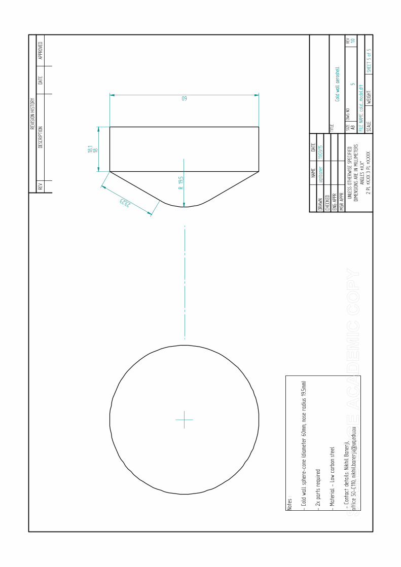
EC

OL

LIS

ION

INT

EG

RA

LD

AT

AS

ET

S

Tabl

eA

1:R

educ

edco

llisi

onin

tegr

alΩ

(1,1)�

asa

func

tion

ofte

mpe

ratu

refo

rab

lati

veEa

rth,

Mar

san

dVe

nus

entr

y.

Co

llis

ion

sT

em

pe

ratu

re(K

)C

oll

isio

ns

Te

mp

era

ture

(K)

2000

4000

8000

1600

032

000

2000

4000

8000

1600

032

000

C−C

0.53

190.

4040

0.30

630.

2319

0.17

55C−C

20.

6075

0.46

260.

3516

0.26

670.

2020

C−C

30.

6525

0.49

730.

3785

0.28

750.

2180

C−C

O2

0.60

750.

4626

0.35

160.

2667

0.20

20

C−C

O0.

5757

0.43

790.

3325

0.25

200.

1908

C−C

N0.

5674

0.43

150.

3275

0.24

820.

1879

C−C

2H2

0.61

040.

4649

0.35

340.

2681

0.20

31C−C

2H0.

6527

0.49

750.

3787

0.28

760.

2181

C−C

H0.

5638

0.42

870.

3254

0.24

650.

1866

C−H

0.53

920.

4097

0.31

070.

2353

0.17

81C−H

20.

5582

0.42

440.

3220

0.24

400.

1847

C−H

CN

0.65

470.

4990

0.37

980.

2886

0.21

88C−H

CO

0.64

910.

4948

0.37

650.

2860

0.21

68C−N

20.

5654

0.43

000.

3263

0.24

730.

1872

C−N

0.56

540.

4300

0.32

630.

2473

0.18

72C−N

O0.

5857

0.44

570.

3385

0.25

660.

1943

C−O

0.58

190.

4428

0.33

620.

2549

0.19

30C−O

20.

5819

0.44

280.

3362

0.25

490.

1930

C2−

C2

0.73

160.

6128

0.51

720.

4388

0.37

41C

2−C

30.

7886

0.65

830.

5558

0.47

220.

4032

C2−

CO

20.

7317

0.61

280.

5172

0.43

890.

3742

C2−

CO

0.69

310.

5809

0.48

980.

4151

0.35

36C

2−C

N0.

6832

0.57

260.

4827

0.40

900.

3483

C2−

C2H

20.

7353

0.61

580.

5197

0.44

100.

3761

C2−

C2H

0.78

890.

6586

0.55

600.

4724

0.40

33C

2−C

H0.

6789

0.56

900.

4796

0.40

630.

3460

C2−

H0.

6157

0.46

900.

3565

0.27

050.

2050

C2−

H2

0.67

230.

5634

0.47

470.

4021

0.34

24

189

190 collision integral data setsC

oll

isio

ns

Te

mp

era

ture

(K)

Co

llis

ion

sT

em

pe

ratu

re(K

)

2000

4000

8000

1600

032

000

2000

4000

8000

1600

032

000

C2−

HC

N0.

7915

0.66

060.

5576

0.47

390.

4046

C2−

HC

O0.

7842

0.65

490.

5529

0.46

980.

4010

C2−

N2

0.68

090.

5706

0.48

100.

4075

0.34

70C

2−N

0.64

500.

4916

0.37

410.

2841

0.21

54C

2−N

O0.

7051

0.59

090.

4984

0.42

260.

3600

C2−

O0.

6637

0.50

580.

3852

0.29

270.

2220

C2−

O2

0.70

060.

5871

0.49

520.

4198

0.35

76C

3−C

30.

8611

0.70

860.

5969

0.50

760.

4340

C3−

CO

20.

7886

0.65

840.

5558

0.47

220.

4032

C3−

CO

0.74

530.

6239

0.52

670.

4471

0.38

13

C3−

CN

0.73

450.

6151

0.51

920.

4406

0.37

56C

3−C

2H2

0.79

270.

6616

0.55

850.

4746

0.40

52

C3−

C2H

0.86

160.

7089

0.59

720.

5078

0.43

42C

3−C

H0.

7297

0.61

120.

5159

0.43

770.

3731

C3−

H0.

6614

0.50

400.

3838

0.29

160.

2212

C3−

H2

0.72

240.

6053

0.51

070.

4333

0.36

93

C3−

HC

N0.

8663

0.71

120.

5990

0.50

930.

4356

C3−

HC

O0.

8538

0.70

490.

5939

0.50

500.

4317

C3−

N2

0.73

180.

6130

0.51

740.

4390

0.37

43C

3−N

0.69

330.

5281

0.40

240.

3060

0.23

23

C3−

NO

0.75

870.

6347

0.53

580.

4550

0.38

82C

3−O

0.71

400.

5434

0.41

410.

3152

0.23

93

C3−

O2

0.75

370.

6307

0.53

240.

4520

0.38

56C

O2−

CO

20.

7317

0.61

280.

5172

0.43

890.

3742

CO

2−C

O0.

6931

0.58

090.

4898

0.41

510.

3536

CO

2−C

N0.

6832

0.57

260.

4827

0.40

900.

3483

CO

2−C

2H2

0.73

530.

6158

0.51

980.

4411

0.37

61C

O2−

C2H

0.78

890.

6586

0.55

600.

4724

0.40

34C

O2−

CH

0.67

900.

5690

0.47

960.

4063

0.34

60C

O2−

H0.

6157

0.46

900.

3566

0.27

050.

2050

CO

2−H

20.

6723

0.56

340.

4748

0.40

210.

3424

CO

2−H

CN

0.79

150.

6606

0.55

770.

4739

0.40

46C

O2−

HC

O0.

7843

0.65

500.

5529

0.46

980.

4010

CO

2−N

20.

6809

0.57

060.

4810

0.40

750.

3470

CO

2−N

0.64

510.

4916

0.37

410.

2841

0.21

54C

O2−

NO

0.70

510.

5909

0.49

840.

4226

0.36

01C

O2−

O0.

6637

0.50

590.

3852

0.29

270.

2220

CO

2−O

20.

7006

0.58

710.

4952

0.41

980.

3576

CO−C

O0.

6570

0.55

030.

4635

0.39

250.

3340

CO−C

N0.

6476

0.54

240.

4567

0.38

660.

3290

CO−C

2H2

0.69

640.

5837

0.49

220.

4172

0.35

54C

O−C

2H0.

7456

0.62

410.

5269

0.44

720.

3814

collision integral data sets 191C

oll

isio

ns

Te

mp

era

ture

(K)

Co

llis

ion

sT

em

pe

ratu

re(K

)

2000

4000

8000

1600

032

000

2000

4000

8000

1600

032

000

CO−C

H0.

6435

0.53

890.

4537

0.38

400.

3268

CO−H

0.58

350.

4440

0.33

720.

2556

0.19

36C

O−H

20.

6373

0.53

360.

4491

0.38

010.

3234

CO−H

CN

0.74

830.

6260

0.52

850.

4486

0.38

26C

O−H

CO

0.74

150.

6207

0.52

390.

4447

0.37

92C

O−N

20.

6454

0.54

050.

4551

0.38

520.

3278

CO−N

0.61

140.

4657

0.35

400.

2686

0.20

35C

O−N

O0.

6683

0.55

990.

4718

0.39

960.

3402

CO−O

0.62

910.

4794

0.36

460.

2767

0.20

97C

O−O

20.

6640

0.55

640.

4687

0.39

690.

3379

CN−C

N0.

6378

0.53

380.

4495

0.38

050.

3239

CN−C

2H2

0.68

660.

5754

0.48

510.

4111

0.35

01C

N−C

2H0.

7347

0.61

530.

5194

0.44

070.

3758

CN−C

H0.

6338

0.53

060.

4467

0.37

810.

3217

CN−H

0.57

520.

4376

0.33

220.

2518

0.19

06C

N−H

20.

6283

0.52

590.

4425

0.37

440.

3185

CN−H

CN

0.74

080.

6171

0.52

030.

4416

0.37

66C

N−H

CO

0.73

190.

6118

0.51

610.

4380

0.37

34C

N−N

20.

6363

0.53

270.

4484

0.37

940.

3228

CN−N

0.60

280.

4590

0.34

880.

2645

0.20

04C

N−N

O0.

6588

0.55

190.

4649

0.39

360.

3350

CN−O

0.62

020.

4725

0.35

930.

2726

0.20

66C

N−O

20.

6547

0.54

840.

4619

0.39

100.

3328

C2H

2−C

2H2

0.73

890.

6188

0.52

230.

4432

0.37

80C

2H2−

C2H

0.79

300.

6618

0.55

870.

4747

0.40

54C

2H2−

CH

0.68

220.

5718

0.48

200.

4084

0.34

78C

2H2−

H0.

6187

0.47

130.

3583

0.27

190.

2060

C2H

2−H

20.

6756

0.56

610.

4771

0.40

420.

3441

C2H

2−H

CN

0.79

560.

6639

0.56

040.

4762

0.40

67C

2H2−

HC

O0.

7883

0.65

810.

5556

0.47

210.

4031

C2H

2−N

20.

6842

0.57

340.

4834

0.40

960.

3488

C2H

2−N

0.64

810.

4940

0.37

600.

2855

0.21

65C

2H2−

NO

0.70

850.

5937

0.50

090.

4247

0.36

19C

2H2−

O0.

6669

0.50

830.

3871

0.29

420.

2231

C2H

2−O

20.

7040

0.59

000.

4977

0.42

190.

3595

C2H−C

2H0.

8621

0.70

910.

5974

0.50

800.

4344

C2H−C

H0.

7300

0.61

150.

5161

0.43

780.

3733

C2H−H

0.66

160.

5042

0.38

390.

2917

0.22

12C

2H−H

20.

7227

0.60

550.

5109

0.43

340.

3694

C2H−H

CN

0.86

680.

7114

0.59

920.

5095

0.43

57C

2H−H

CO

0.85

430.

7052

0.59

410.

5052

0.43

19C

2H−N

20.

7321

0.61

320.

5175

0.43

910.

3744


oll

isio

ns

Te

mp

era

ture

(K)

Co

llis

ion

sT

em

pe

ratu

re(K

)

2000

4000

8000

1600

032

000

2000

4000

8000

1600

032

000

C2H−N

0.69

360.

5283

0.40

250.

3062

0.23

24C

2H−N

O0.

7590

0.63

490.

5360

0.45

510.

3883

C2H−O

0.71

430.

5435

0.41

430.

3153

0.23

94C

2H−O

20.

7540

0.63

090.

5326

0.45

220.

3857

CH−C

H0.

6299

0.52

730.

4438

0.37

560.

3196

CH−H

0.57

160.

4347

0.33

000.

2501

0.18

94C

H−H

20.

6243

0.52

250.

4396

0.37

190.

3164

CH−H

CN

0.73

470.

6131

0.51

710.

4388

0.37

42C

H−H

CO

0.72

670.

6079

0.51

290.

4352

0.37

10C

H−N

20.

6322

0.52

930.

4455

0.37

690.

3207

CH−N

0.59

890.

4560

0.34

650.

2628

0.19

90C

H−N

O0.

6547

0.54

840.

4619

0.39

100.

3328

CH−O

0.61

630.

4695

0.35

690.

2708

0.20

52C

H−O

20.

6505

0.54

490.

4589

0.38

840.

3306

H−H

0.54

670.

4155

0.31

510.

2387

0.18

07H−H

20.

5659

0.43

030.

3266

0.24

750.

1874

H−H

CN

0.66

360.

5058

0.38

510.

2926

0.22

20H−H

CO

0.65

790.

5015

0.38

180.

2900

0.22

00H−N

20.

5732

0.43

600.

3310

0.25

090.

1899

H−N

0.57

320.

4360

0.33

100.

2509

0.18

99H−N

O0.

5937

0.45

190.

3433

0.26

030.

1971

H−O

0.58

990.

4489

0.34

100.

2586

0.19

58H−O

20.

5899

0.44

890.

3410

0.25

860.

1958

H2−

H2

0.61

810.

5172

0.43

510.

3680

0.31

30H

2−H

CN

0.72

490.

6073

0.51

250.

4348

0.37

06H

2−H

CO

0.71

870.

6021

0.50

810.

4309

0.36

73H

2−N

20.

6261

0.52

400.

4409

0.37

300.

3173

H2−

N0.

5931

0.45

150.

3430

0.26

010.

1970

H2−

NO

0.64

830.

5430

0.45

720.

3870

0.32

93H

2−O

0.61

030.

4648

0.35

330.

2680

0.20

30H

2−O

20.

6442

0.53

950.

4542

0.38

440.

3271

HC

N−H

CN

0.89

850.

7199

0.60

160.

5106

0.43

66H

CN−H

CO

0.86

930.

7098

0.59

600.

5065

0.43

30H

CN−N

20.

7344

0.61

510.

5191

0.44

050.

3756

HC

N−N

0.69

580.

5299

0.40

380.

3071

0.23

31H

CN−N

O0.

7617

0.63

680.

5376

0.45

650.

3895

HC

N−O

0.71

660.

5452

0.41

550.

3163

0.24

02H

CN−O

20.

7564

0.63

280.

5343

0.45

360.

3572

HC

O−H

CO

0.85

170.

7020

0.59

080.

5022

0.42

94H

CO−N

20.

7280

0.60

980.

5147

0.43

660.

3722

HC

O−N

0.68

970.

5254

0.40

030.

3044

0.23

10H

CO−N

O0.

7547

0.63

140.

5331

0.45

260.

3861


oll

isio

ns

Te

mp

era

ture

(K)

Co

llis

ion

sT

em

pe

ratu

re(K

)

2000

4000

8000

1600

032

000

2000

4000

8000

1600

032

000

HC

O−O

0.71

020.

5406

0.41

200.

3135

0.23

81H

CO−O

20.

7497

0.62

740.

5297

0.44

960.

3835

N2−

N2

0.63

400.

5308

0.44

680.

3781

0.32

16N

2−N

0.60

070.

4574

0.34

750.

2636

0.19

96N

2−N

O0.

6565

0.55

000.

4632

0.39

220.

3338

N2−

O0.

6181

0.47

080.

3580

0.27

160.

2058

N2−

O2

0.65

240.

5465

0.46

020.

3896

0.33

16N−N

0.60

070.

4574

0.34

750.

2636

0.19

96N−N

O0.

6220

0.47

390.

3603

0.27

340.

2072

N−O

0.61

810.

4708

0.35

800.

2716

0.20

58N−O

20.

6181

0.47

080.

3580

0.27

160.

2058

NO−N

O0.

6798

0.56

970.

4802

0.40

680.

3464

NO−O

0.63

990.

4877

0.37

110.

2817

0.21

36N

O−O

20.

6755

0.56

610.

4771

0.40

410.

3441

O−O

0.63

590.

4846

0.36

860.

2799

0.21

21O−O

20.

6359

0.48

460.

3686

0.27

990.

2121

O2−

O2

0.67

120.

5624

0.47

400.

4014

0.34

18

Tabl

eA

2:R

educ

edco

llisi

onin

tegr

alΩ

(2,2)�

asa

func

tion

ofte

mpe

ratu

refo

rab

lati

veEa

rth,

Mar

san

dVe

nus

entr

y.

Co

llis

ion

sT

em

pe

ratu

re(K

)C

oll

isio

ns

Te

mp

era

ture

(K)

2000

4000

8000

1600

032

000

2000

4000

8000

1600

032

000

C−C

0.64

000.

4917

0.37

690.

2885

0.22

08C−C

20.

7180

0.55

430.

4264

0.32

700.

2504

C−C

30.

7621

0.59

020.

4551

0.34

970.

2681

C−C

O2

0.71

800.

5544

0.42

640.

3270

0.25

04

C−C

O0.

6857

0.52

830.

4056

0.31

080.

2379

C−C

N0.

6773

0.52

150.

4002

0.30

660.

2347

C−C

2H2

0.72

090.

5567

0.42

820.

3285

0.25

16C−C

2H0.

7624

0.59

030.

4553

0.34

990.

2682

C−C

H0.

6735

0.51

840.

3979

0.30

480.

2332

C−H

0.64

780.

4979

0.38

170.

2923

0.22

37C−H

20.

6677

0.51

380.

3942

0.30

190.

2310

C−H

CN

0.76

430.

5919

0.45

650.

3508

0.26

90


oll

isio

ns

Te

mp

era

ture

(K)

Co

llis

ion

sT

em

pe

ratu

re(K

)

2000

4000

8000

1600

032

000

2000

4000

8000

1600

032

000

C−H

CO

0.75

890.

5876

0.45

300.

3481

0.26

68C−N

20.

6752

0.51

980.

3989

0.30

560.

2339

C−N

0.67

520.

5198

0.39

890.

3056

0.23

39C−N

O0.

6960

0.53

650.

4122

0.31

590.

2418

C−O

0.69

220.

5334

0.40

970.

3140

0.24

04C−O

20.

6922

0.53

340.

4097

0.31

400.

2404

C2−

C2

0.84

490.

7205

0.61

710.

5301

0.45

71C

2−C

30.

8990

0.76

430.

6562

0.56

540.

4885

C2−

CO

20.

8450

0.72

050.

6171

0.53

010.

4571

C2−

CO

0.80

860.

6887

0.58

850.

5046

0.43

45C

2−C

N0.

7992

0.68

030.

5809

0.49

790.

4287

C2−

C2H

20.

8483

0.72

340.

6197

0.53

250.

4591

C2−

C2H

0.89

930.

7645

0.65

640.

5656

0.48

87C

2−C

H0.

7950

0.67

660.

5776

0.49

500.

4261

C2−

H0.

7262

0.56

100.

4317

0.33

120.

2537

C2−

H2

0.78

860.

6708

0.57

250.

4904

0.42

21C

2−H

CN

0.90

190.

7664

0.65

810.

5671

0.49

01C

2−H

CO

0.89

460.

7611

0.65

340.

5628

0.48

62C

2−N

20.

7969

0.67

820.

5791

0.49

630.

4272

C2−

N0.

7550

0.58

430.

4504

0.34

600.

2652

C2−

NO

0.82

000.

6988

0.59

750.

5126

0.44

16C

2−O

0.77

280.

5988

0.46

210.

3553

0.27

25C

2−O

20.

8158

0.69

500.

5941

0.50

960.

4390

C3−

C3

0.94

850.

8115

0.69

650.

6018

0.52

15

C3−

CO

20.

8990

0.76

430.

6562

0.56

540.

4886

C3−

CO

0.85

770.

7314

0.62

680.

5389

0.46

49

C3−

CN

0.84

760.

7228

0.61

910.

5319

0.45

86C

3−C

2H2

0.90

310.

7673

0.65

890.

5678

0.49

07

C3−

C2H

0.94

860.

8117

0.69

670.

6020

0.52

16C

3−C

H0.

8432

0.71

900.

6157

0.52

890.

4560

C3−

H0.

7706

0.59

700.

4606

0.35

410.

2715

C3−

H2

0.83

630.

7131

0.61

040.

5241

0.45

18

C3−

HC

N0.

9494

0.81

390.

6984

0.60

360.

5231

C3−

HC

O0.

9468

0.80

780.

6935

0.59

920.

5190

C3−

N2

0.84

510.

7207

0.61

720.

5302

0.45

72C

3−N

0.80

070.

6209

0.48

010.

3697

0.28

38

C3−

NO

0.87

030.

7418

0.63

620.

5473

0.47

23C

3−O

0.82

000.

6358

0.49

210.

3794

0.29

14

C3−

O2

0.86

550.

7379

0.63

270.

5441

0.46

95C

O2−

CO

20.

8450

0.72

060.

6171

0.53

010.

4571

CO

2−C

O0.

8086

0.68

870.

5885

0.50

460.

4345

CO

2−C

N0.

7992

0.68

030.

5810

0.49

790.

4287


oll

isio

ns

Te

mp

era

ture

(K)

Co

llis

ion

sT

em

pe

ratu

re(K

)

2000

4000

8000

1600

032

000

2000

4000

8000

1600

032

000

CO

2−C

2H2

0.84

840.

7235

0.61

970.

5325

0.45

91C

O2−

C2H

0.89

930.

7645

0.65

640.

5656

0.48

87C

O2−

CH

0.79

510.

6766

0.57

770.

4950

0.42

61C

O2−

H0.

7262

0.56

100.

4317

0.33

120.

2537

CO

2−H

20.

7886

0.67

080.

5725

0.49

050.

4221

CO

2−H

CN

0.90

190.

7664

0.65

810.

5671

0.49

01C

O2−

HC

O0.

8947

0.76

110.

6534

0.56

280.

4862

CO

2−N

20.

7969

0.67

830.

5791

0.49

630.

4273

CO

2−N

0.75

500.

5844

0.45

050.

3460

0.26

52C

O2−

NO

0.82

000.

6988

0.59

750.

5127

0.44

16C

O2−

O0.

7728

0.59

880.

4621

0.35

530.

2725

CO

2−O

20.

8158

0.69

500.

5941

0.50

970.

4390

CO−C

O0.

7735

0.65

740.

5605

0.47

990.

4129

CO−C

N0.

7639

0.64

890.

5531

0.47

340.

4073

CO−C

2H2

0.81

180.

6915

0.59

100.

5069

0.43

65C

O−C

2H0.

8580

0.73

160.

6270

0.53

900.

4650

CO−C

H0.

7599

0.64

540.

5499

0.47

060.

4048

CO−H

0.69

380.

5348

0.41

080.

3148

0.24

10C

O−H

20.

7540

0.63

990.

5451

0.46

630.

4011

CO−H

CN

0.85

980.

7331

0.62

850.

5404

0.46

63C

O−H

CO

0.85

380.

7281

0.62

390.

5363

0.46

26C

O−N

20.

7620

0.64

720.

5514

0.47

200.

4060

CO−N

0.72

190.

5576

0.42

890.

3291

0.25

20C

O−N

O0.

7846

0.66

730.

5693

0.48

770.

4197

CO−O

0.73

940.

5718

0.44

030.

3380

0.25

89C

O−O

20.

7805

0.66

360.

5661

0.48

480.

4172

CN−C

N0.

7503

0.63

800.

5444

0.46

630.

4014

CN−C

2H2

0.80

240.

6831

0.58

350.

5002

0.43

07C

N−C

2H0.

8478

0.72

300.

6193

0.53

210.

4588

CN−C

H0.

7474

0.63

510.

5416

0.46

370.

3990

CN−H

0.68

530.

5279

0.40

530.

3106

0.23

77C

N−H

20.

7448

0.63

180.

5379

0.46

010.

3957

CN−H

CN

0.84

620.

7206

0.61

810.

5319

0.45

92C

N−H

CO

0.84

170.

7176

0.61

500.

5287

0.45

61C

N−N

20.

7530

0.63

900.

5443

0.46

560.

4005

CN−N

0.71

330.

5505

0.42

330.

3246

0.24

86C

N−N

O0.

7751

0.65

890.

5619

0.48

120.

4140

CN−O

0.73

070.

5646

0.43

460.

3335

0.25

54C

N−O

20.

7713

0.65

540.

5587

0.47

830.

4115

C2H

2−C

2H2

0.85

180.

7264

0.62

230.

5348

0.46

12C

2H2−

C2H

0.90

340.

7675

0.65

910.

5680

0.49

09C

2H2−

CH

0.79

820.

6794

0.58

020.

4972

0.42

81


oll

isio

ns

Te

mp

era

ture

(K)

Co

llis

ion

sT

em

pe

ratu

re(K

)

2000

4000

8000

1600

032

000

2000

4000

8000

1600

032

000

C2H

2−H

0.72

920.

5634

0.43

360.

3327

0.25

48C

2H2−

H2

0.79

180.

6736

0.57

500.

4927

0.42

41C

2H2−

HC

N0.

9060

0.76

950.

6608

0.56

960.

4923

C2H

2−H

CO

0.89

870.

7641

0.65

600.

5652

0.48

84C

2H2−

N2

0.80

010.

6811

0.58

170.

4986

0.42

92C

2H2−

N0.

7580

0.58

680.

4524

0.34

760.

2664

C2H

2−N

O0.

8233

0.70

170.

6001

0.51

490.

4437

C2H

2−O

0.77

590.

6013

0.46

410.

3569

0.27

37C

2H2−

O2

0.81

900.

6979

0.59

670.

5119

0.44

10C

2H−C

2H0.

9487

0.81

200.

6969

0.60

220.

5218

C2H−C

H0.

8434

0.71

920.

6159

0.52

900.

4561

C2H−H

0.77

080.

5972

0.46

080.

3543

0.27

16C

2H−H

20.

8366

0.71

330.

6106

0.52

430.

4519

C2H−H

CN

0.94

950.

8142

0.69

860.

6038

0.52

32C

2H−H

CO

0.94

700.

8081

0.69

370.

5993

0.51

92C

2H−N

20.

8454

0.72

090.

6174

0.53

040.

4573

C2H−N

0.80

090.

6211

0.48

020.

3698

0.28

39C

2H−N

O0.

8705

0.74

200.

6364

0.54

750.

4725

C2H−O

0.82

020.

6359

0.49

230.

3795

0.29

15C

2H−O

20.

8658

0.73

810.

6329

0.54

430.

4697

CH−C

H0.

7442

0.63

210.

5387

0.46

110.

3967

CH−H

0.68

150.

5249

0.40

290.

3087

0.23

63C

H−H

20.

7408

0.62

820.

5347

0.45

730.

3933

CH−H

CN

0.84

220.

7177

0.61

540.

5293

0.45

68C

H−H

CO

0.83

770.

7143

0.61

190.

5258

0.45

34C

H−N

20.

7489

0.63

530.

5411

0.46

280.

3981

CH−N

0.70

950.

5474

0.42

090.

3227

0.24

71C

H−N

O0.

7711

0.65

530.

5587

0.47

830.

4115

CH−O

0.72

680.

5615

0.43

210.

3315

0.25

39C

H−O

20.

7672

0.65

170.

5555

0.47

550.

4091

H−H

0.65

560.

5042

0.38

660.

2961

0.22

66H−H

20.

6756

0.52

020.

3992

0.30

580.

2341

H−H

CN

0.77

270.

5987

0.46

200.

3553

0.27

24H−H

CO

0.76

740.

5944

0.45

850.

3525

0.27

02H−N

20.

6832

0.52

620.

4040

0.30

950.

2369

H−N

0.68

320.

5262

0.40

400.

3095

0.23

69H−N

O0.

7041

0.54

310.

4174

0.32

000.

2450

H−O

0.70

030.

5400

0.41

490.

3181

0.24

35H−O

20.

7003

0.54

000.

4149

0.31

810.

2435

H2−

H2

0.73

460.

6227

0.52

990.

4530

0.38

96H

2−H

CN

0.83

870.

7151

0.61

220.

5258

0.45

32H

2−H

CO

0.83

280.

7100

0.60

760.

5216

0.44

96


oll

isio

ns

Te

mp

era

ture

(K)

Co

llis

ion

sT

em

pe

ratu

re(K

)

2000

4000

8000

1600

032

000

2000

4000

8000

1600

032

000

H2−

N2

0.74

260.

6298

0.53

610.

4586

0.39

43H

2−N

0.70

350.

5426

0.41

700.

3197

0.24

48H

2−N

O0.

7649

0.64

970.

5537

0.47

390.

4077

H2−

O0.

7207

0.55

660.

4281

0.32

840.

2515

H2−

O2

0.76

080.

6460

0.55

040.

4711

0.40

52H

CN−H

CN

0.97

270.

8156

0.69

690.

6027

0.52

30H

CN−H

CO

0.95

580.

8092

0.69

370.

5996

0.51

99H

CN−N

20.

8475

0.72

270.

6191

0.53

190.

4586

HC

N−N

0.80

290.

6227

0.48

150.

3708

0.28

47H

CN−N

O0.

8727

0.74

360.

6379

0.54

890.

4738

HC

N−O

0.82

240.

6375

0.49

360.

3805

0.29

24H

CN−O

20.

8681

0.74

000.

6346

0.54

580.

4078

HC

O−H

CO

0.94

750.

8036

0.68

970.

5959

0.51

63H

CO−N

20.

8415

0.71

760.

6144

0.52

770.

4550

HC

O−N

0.79

730.

6183

0.47

790.

3679

0.28

24H

CO−N

O0.

8663

0.73

850.

6333

0.54

470.

4701

HC

O−O

0.81

640.

6331

0.48

990.

3776

0.29

00H

CO−O

20.

8618

0.73

480.

6299

0.54

160.

4673

N2−

N2

0.75

070.

6370

0.54

250.

4641

0.39

91N

2−N

0.71

120.

5488

0.42

200.

3236

0.24

77N

2−N

O0.

7731

0.65

700.

5602

0.47

960.

4127

N2−

O0.

7285

0.56

290.

4332

0.33

240.

2546

N2−

O2

0.76

900.

6534

0.55

690.

4768

0.41

02N−N

0.71

120.

5488

0.42

200.

3236

0.24

77N−N

O0.

7324

0.56

610.

4357

0.33

440.

2561

N−O

0.72

850.

5629

0.43

320.

3324

0.25

46N−O

20.

7285

0.56

290.

4332

0.33

240.

2546

NO−N

O0.

7958

0.67

730.

5783

0.49

560.

4266

NO−O

0.75

000.

5803

0.44

720.

3435

0.26

32N

O−O

20.

7917

0.67

360.

5750

0.49

260.

4240

O−O

0.74

610.

5771

0.44

460.

3414

0.26

16O−O

20.

7461

0.57

710.

4446

0.34

140.

2616

O2−

O2

0.78

750.

6699

0.57

160.

4897

0.42

15

Nikhil Banerji

Ecole Polytechnique Fédérale de Lausanne (EPFL) 2017 PhD, Mechanical Engineering

University of Bath, United Kingdom 2012

MEng (Hons.), Aerospace Engineering with French

Interdisciplinary Aerodynamics Group, EPFL 2013 – 2017 PhD Researcher. Effects of Radiation on Ablative Heat Shields During Atmospheric Entry. Using experimental and numerical methods, successfully characterised heat transfer in lightweight materials in extreme environments. Validated results against flight data from NASA’s 2012 Mars Science Laboratory mission.

Interdisciplinary Aerodynamics Group, EPFL 2013 - 2016 Research Engineer, European Space Agency (ESA) Ablation-Radiation Coupling Project. Coupled Computational Fluid Dynamics simulations to thermodynamic analyses. Co-authored technical reports and presented progress and results to ESA and collaborating institutes.

Centre for Hypersonics, The University of Queensland, Australia 2015

Researcher. Designed and manufactured lightweight models for high temperature testing in wind tunnels. Integrated novel electrical pre-heating system into models. Interfaced with suppliers and workshop. Measured shock layer radiation via emission spectroscopy.

Institut Supérieur de l’Aéronautique et de l’Espace, France 2012

Master Thesis. Analysed the propagation of delamination due to vibrational stresses in an aircraft panel using finite element methods via SAMCEF. Validated results against experimental data.

ITER Organization, France 2010 - 2011

R&D position in Diagnostics Division. Structural and risk analyses for X-ray and vacuum ultraviolet spectroscopy systems. Finite element design studies on diagnostic window assemblies and mounting systems using ANSYS.

Institute of Mechanical Engineering, EPFL 2013 – 2016

Teaching assistant. Lectured and corrected exams for Master level course, “Introduction to Planetary Sciences”. Co-supervision of 5 master theses and 10 semester projects. Developed innovative project topics, aiding the student with code development and implementation, resulting in several publications.

Logitech, S.A., Switzerland 2010

Project Management Intern. Helped manage Leadership Development Project, researching change and supply chain management strategies.

Airbus Aircraft Design Project, University of Bath 2009

Technical Integrator. Interfaced with departments such as electronics, structure and aerodynamics and developed final aircraft design to JAF and ICAO standards. Led engineering team to deliver the final design on time and under budget.

English, Hindi, Bengali (mother tongue); French – Speaking and Understanding (C2), Writing (C1); Spanish – Speaking and Understanding (B2), Writing (A2).

Education

Core Experiences

Additional Experience

Languages

Engineering: Heat Transfer, Experimental Testing, Finite Element Analysis,

Computational Fluid Dynamics, CAD, Mechanical Design, Project Documentation.

Interdisciplinary: Effective communicator, excellent analytical and problem solving skills, adept at working in a team, good presenter, excellent time management, used to pressure, independent, highly adaptive, resourceful and creative. IT Skills: Linux (Ubuntu, Fedora), Mac OS X, Microsoft Office, MATLAB, Python, FORTRAN, LaTeX, bash and Git. Playing electric guitar and composing music – Bands in Switzerland (2005 – 2007) and the UK (2008-2012), having released 2 albums and played over 10 live concerts. Playing football in local amateur teams and leagues (since 1998). Snowboarding, hiking, cycling and squash. Born: 27. October 1988; Nationality: Swiss; Swiss Driving License (Cat. B).

Extracurricular activities

Personal Information

Technical skills

The effects of radiation on ablative heat shields during ...

Documents

Transcript of The effects of radiation on ablative heat shields during ...