PRAMANA c© Indian Academy of Sciences Vol. 77, No. 3— journal of September 2011

physics pp. 519–532

Transient heat transfer in longitudinal fins of variousprofiles with temperature-dependent thermal conductivityand heat transfer coefficient

RASEELO J MOITSHEKI∗ and CHARIS HARLEYCentre for Differential Equations, Continuum Mechanics and Applications,School of Computational and Applied Mathematics, University of the Witwatersrand,Johannesburg, Private Bag 3, Wits 2050, South Africa∗Corresponding author. E-mail: raseelo.moitsheki@wits.ac.za

Abstract. Transient heat transfer through a longitudinal fin of various profiles is studied. The ther-mal conductivity and heat transfer coefficients are assumed to be temperature dependent. The resultingpartial differential equation is highly nonlinear. Classical Lie point symmetry methods are employedand some reductions are performed. Since the governing boundary value problem is not invariantunder any Lie point symmetry, we solve the original partial differential equation numerically. Theeffects of realistic fin parameters such as the thermogeometric fin parameter and the exponent of theheat transfer coefficient on the temperature distribution are studied.

Keywords. Heat transfer; longitudinal fin; temperature-dependent heat transfer coefficient and ther-mal conductivity; symmetry analysis; numerical solutions.

PACS Nos 02.60.Lj; 11.30.-j; 44.10.+i; 66.30.Xj

1. Introduction

A search for exact and numerical solutions for models arising in heat flow through extendedsurfaces continues to be of scientific interest. The literature in this area is immense (see,for example, [1] and references cited therein). Perhaps such interest has been instilledby frequent encounters of fin problems in many engineering applications to enhance heattransfer. In recent years many authors have been interested in the steady-state problems [2–11] describing heat flow in fins of different shapes and profiles. Exact solutions exist whenboth the thermal conductivity and heat transfer coefficients are constant [2], and even whenthey are not constant provided thermal conductivity is a differential consequence of the heattransfer coefficient [5,6]. In the heat transfer models describing natural convection, radia-tion, boiling and condensation, the heat transfer coefficient depends on local temperature.Furthermore, for engineering applications and physical phenomena the thermal conductiv-ity of a fin is assumed to be linearly dependent on temperature (see [12]). The dependency

DOI: 10.1007/s12043-011-0172-6; ePublication: 26 August 2011 519

Raseelo J Moitsheki and Charis Harley

of both thermal conductivity and the heat transfer coefficient on temperature renders theproblem highly nonlinear.

The transient heat transfer problems where thermal conductivity is temperature depen-dent and the heat transfer coefficient which depends on the spatial variable have alsoattracted some attention (see [12]). Subsequently, symmetry analysts considered the prob-lem in [12] to determine all forms of thermal conductivity and heat transfer coefficientsfor which the governing equation admits extra symmetries [13–16]. However, only gen-eral solutions were constructed. An accurate transient analysis provided insight into thedesign of fins that would fail in steady-state operations but are sufficient for desired oper-ating periods [17]. Worth noting is the earlier work in [18] wherein the transient problemis considered for a fin of arbitrary profile. However, both thermal conductivity and heattransfer coefficient are considered to be constants.

In this paper we study the heat transfer in longitudinal fins of different profiles. Further-more, both the thermal conductivity and heat transfer coefficients are temperature depen-dent. The mathematical formulation is given in §2. We employ symmetry techniques toanalyse the resulting model in §3. Due to the non-existence of exact solutions we seeknumerical solutions in §4. In §5 we provide concluding remarks.

2. Mathematical formulation

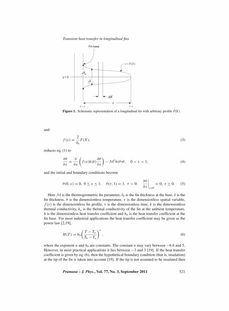
We consider a longitudinal one-dimensional fin with a profile area Ap. The perimeter of thefin is denoted by P and the length of the fin by L . The fin is attached to a fixed base surfaceof temperature Tb and extends into a fluid of temperature Ta . The fin profile is given by thefunction F(X) and the fin thickness at the base is δb. The energy balance for a longitudinalfin is given by

ρcv∂T

∂t= Ap

∂

∂ X

(F(X )K(T )

∂T

∂ X

)− Pδb H(T )(T − Ta) , 0 < X < L , (1)

where K and H are the non-uniform thermal conductivity and heat transfer coefficientsdepending on the temperature (see [2,3,6,8]), ρ is the density, cv = 2c/(δb Ap) is thevolumetric heat capacity with c being the specific heat capacity, T is the temperature dis-tribution, F(X) is the fin profile, t is the time and X is the spatial variable. The fin length ismeasured from the tip to the base as shown in figure 1 (see also [1–3]). An insulated fin atone end with the base temperature at the other implies boundary conditions which is givenby [1]

T (t, L) = Tb and∂T

∂ X

∣∣∣∣X=0

= 0, (2)

and initially the fin is kept at the temperature of the fluid (the ambient temperature),

T (0, X) = Ta .

The schematic representation of a fin with arbitrary profile is given in figure 1.Introducing the dimensionless variables and the dimensionless numbers,

x = X

L, τ = kat

ρcv L2, θ = T − Ta

Tb − Ta, k = K

ka, h = H

hb, M2 = 2Phb L2

Apka

520 Pramana – J. Phys., Vol. 77, No. 3, September 2011

Transient heat transfer in longitudinal fins

Figure 1. Schematic representation of a longitudinal fin with arbitrary profile F(X).

and

f (x) = 2

δbF(X), (3)

reduces eq. (1) to

∂θ

∂τ= ∂

∂x

(f (x)k(θ)

∂θ

∂x

)− M2h(θ)θ, 0 < x < 1, (4)

and the initial and boundary conditions become

θ(0, x) = 0, 0 ≤ x ≤ 1; θ(τ, 1) = 1, τ > 0; ∂θ

∂x

∣∣∣∣x=0

= 0, τ ≥ 0. (5)

Here M is the thermogeometric fin parameter, δb is the fin thickness at the base, δ is thefin thickness, θ is the dimensionless temperature, x is the dimensionless spatial variable,f (x) is the dimensionless fin profile, τ is the dimensionless time, k is the dimensionlessthermal conductivity, ka is the thermal conductivity of the fin at the ambient temperature,h is the dimensionless heat transfer coefficient and hb is the heat transfer coefficient at thefin base. For most industrial applications the heat transfer coefficient may be given as thepower law [2,19],

H(T ) = hb

(T − Ta

Tb − Ta

)n

, (6)

where the exponent n and hb are constants. The constant n may vary between −6.6 and 5.

However, in most practical applications it lies between −3 and 3 [19]. If the heat transfercoefficient is given by eq. (6), then the hypothetical boundary condition (that is, insulation)at the tip of the fin is taken into account [19]. If the tip is not assumed to be insulated then

Pramana – J. Phys., Vol. 77, No. 3, September 2011 521

Raseelo J Moitsheki and Charis Harley

the problem becomes overdetermined (see also [20]). This boundary condition is realizedfor sufficiently long fins [19]. Also, the heat transfer through the outermost edge of the fin isnegligible compared to that which passes through the side [20]. The exponent n representslaminar film boiling or condensation when n = −1/4, laminar natural convection whenn = 1/4, turbulent natural convection when n = 1/3, nucleate boiling when n = 2,radiation when n = 3. n = 0 implies a constant heat transfer coefficient. Exact solutionsmay be constructed for the steady-state one-dimensional differential equation describingtemperature distribution in a straight fin when the thermal conductivity is a constant andn = −1, 0, 1 and 2 [19].

The thermal conductivity of the fin may be assumed to vary linearly with the temperaturefor many engineering applications [2,12], that is,

K(T ) = ka[1 + β(T − Ta)] ,

where β is the thermal conductivity gradient. The one-dimensional transient heat conduc-tion equation is then given by

∂θ

∂τ= ∂

∂x

[f (x)(1 + Bθ)

∂θ

∂x

]− M2θn+1, 0 < x < 1, (7)

where the thermal conductivity parameter B = β(Tb − Ta) is non-zero.

3. Classical Lie point symmetry analysis

In brief, the symmetry of a differential equation is an invertible transformation of thedependent and independent variables that does not change the original differential equa-tion. Symmetries depend continuously on a parameter and form a group; the one-parametergroup of transformations. This group can be determined algorithmically. The theory andapplications of Lie groups may be obtained in excellent references such as [21–23].

We omit further theoretical discussions but list the Lie point symmetries admitted bythe fin models of different profiles in table 1. The time translation admitted and listed intable 1 reduces eq. (7) to a steady-state problem. The nonlinearity of eq. (7) is reducedwhen n = −1 since the term involving M has no dependent or even independent variables.This also leads to extra Lie point symmetries being admitted.

3.1 Symmetry reductions: Some illustrative examples

The obtained symmetries may be used to reduce the number of variables of the governingequation by one. Symmetries reduce a 1+1-dimensional partial differential equation to anordinary differential equation. The reduced equation may or may not be exactly solvable.

3.1.1 Rectangular case. The symmetry generator Y1 implies the steady-state heat trans-fer. This case will be studied in detail elsewhere. The linear combination of Y1 and Y2

leads to a travelling wave solution of the form

θ = G(γ ), γ = x ± aτ,

522 Pramana – J. Phys., Vol. 77, No. 3, September 2011

Transient heat transfer in longitudinal fins

Table 1. Classical Lie point symmetries admitted by eq. (7).

Fin profile f (x) Parameter n Symmetries

Rectangular Arbitrary Y1 = ∂

∂τ, Y2 = ∂

∂x

f (x) = 1 n = −1 Y3 = 1

B

[(1 + Bθ)

∂

∂θ+ Bx

∂

∂x+ Bτ

∂

∂τ

]

Triangular Arbitrary Y1 = ∂

∂τ

f (x) = x n = −1 Y2 = − 1

B2

[(1 + Bθ)

∂

∂θ+ 2Bx

∂

∂x+ Bτ

∂

∂τ

]

Concave parabolic Arbitrary Y1 = ∂

∂τ, Y2 = −x

∂

∂xf (x) = x2

Convex parabolic Arbitrary Y1 = ∂

∂τ

f (x) = √x n = −1 Y2 = − 1

2B2

[3(1 + Bθ)

∂

∂θ+ 4Bx

∂

∂x+ 3Bτ

∂

∂τ

]

where a is a constant representing the wave speed and G satisfies the ordinary differentialequation,

(1 + BG)G ′′ + B(G ′)2 ± aG ′ − M2Gn+1 = 0. (8)

The prime indicates the derivative with respect to γ . We observe that the initial and bound-ary conditions (5) do not reduce to two boundary condition for G(γ ). Note that eq. (8) witharbitrary n may be integrated to quadratures since it admits a translation of γ. On the otherhand, eq. (8) with n = −1 admits a two-dimensional non-Abelian Lie subalgebra spannedby the base vectors

1 = ∂

∂γand 2 = 1 + BG

B

∂

∂G+ γ

∂

∂γ.

Since the symmetry Lie algebra is two-dimensional, eq. (8) with n = −1 is integrable [24].This non-commuting pair of symmetries lead to the canonical forms

ϕ = BG + 1 and ω = BG + γ + 1.

The corresponding canonical forms of the vectors are given by

v1 = ∂

∂ωand v2 = ϕ

∂

∂ϕ+ ω

∂

∂ω.

Writing ω = ω(ϕ) and considering a > 0 transforms eq. (8) into

ω′′ = ω′ − 1

ϕ

[1 + a(ω′ − 1) − M2 B(ω′ − 1)2] , (9)

Pramana – J. Phys., Vol. 77, No. 3, September 2011 523

Raseelo J Moitsheki and Charis Harley

where the prime indicates the derivative with respect to ϕ. Equation (9) is not linearizablesince the Lie criterion for liberalization (see [24]) is not satisfied. However, three casesarise for the exact (invariant) solution.

(a) ω′ − 1 = 0 leads to a trivial solution which is not related to the original problem.Therefore we ignore it.

(b) If the sum of the terms in the bracket in (9) vanishes, then we obtain in terms of theoriginal variables the general exact solution,

θ = 2M2

−a ± √a2 + 4M2 B

{x + aτ − a ± √

a2 + 4M2 B

2M2 B+ c1

},

where c1 is an arbitrary constant. Note that this solution does not satisfy the initialand boundary conditions (5).

(c) The solution for the entire eq. (9) is given in terms of quadratures. We omit such a so-lution in this paper.

The admitted symmetry generator Y3 listed in table 1 leads to the functional form of theinvariant solution,

θ = 1

B(τG(γ ) − 1) , γ = x

τ,

and G satisfies the ordinary differential equation,

GG ′′ + (G ′)2 + γ G ′ − G − M2 = 0,

which has no Lie point symmetries. Furthermore, we again find that the initial and bound-ary conditions (5) do not reduce to two boundary conditions for G(γ ).

3.1.2 Triangular case. The symmetry generator Y2 leads to the reductions

θ = 1

B[τG(γ ) − 1] with γ =

√x

τ,

where G satisfies the nonlinear ordinary differential equation,

1

4GG ′′ +

(1

2γ− G

4γ− γ

)G ′ 1

4G ′2 − G − M2 = 0.

The initial and boundary conditions (5) do not reduce to two boundary conditions for G(γ ).

3.1.3 Concave parabolic case. The symmetry generator Y2 yields the functional form ofthe invariant solution

θ = G(γ ) with γ = xeτ ,

where G satisfies the nonlinear ordinary differential equation,

γdG

dγ= d

dγ

[γ 2(1 + BG)

dG

dγ

]− M2Gn+1. (10)

Again we observe that the initial and boundary conditions (5) do not reduce to two bound-ary conditions for G(γ ).

524 Pramana – J. Phys., Vol. 77, No. 3, September 2011

Transient heat transfer in longitudinal fins

3.1.4 Convex parabolic case. The vector field Y2 leads to the reductions

θ = 1

B(τG(γ ) − 1) with γ = x1/4

τ 1/3,

where G satisfies the nonlinear ordinary differential equation,

G − 1

3γ G ′ = 1

2γ 5GG ′ + 1

16γ 4(G ′)2 − 3

16γGG ′ + 1

16γ 4GG ′′ − M2,

which has no Lie point symmetries. Furthermore, the initial and boundary conditions (5)again do not reduce to two boundary conditions for G(γ ).

Since the original boundary value problem is not invariant under any Lie point symmetry(because the initial and boundary conditions are not invariant), we reconsider the originalpartial differential equation subject to the prescribed initial and boundary conditions anddetermine the numerical solutions in the next section.

4. Numerical results

In this section numerical solutions are obtained for eq. (7) subject to the conditions (5) byusing the in-built function pdepe in MATLAB. We study heat flow in longitudinal fins ofdifferent profiles.

4.1 Rectangular case

The solutions for this case are depicted in figures 2, 3, 4 and 5. We observe in figure 2 thatthe temperature increases with an increase in time. We find that the solution profiles forτ = 0.5, 0.75, 2 and τ = 0.1, 0.2, 0.3 indicate a decrease in the temperature as we moveaway from the base of the fin. The solutions seem to converge to a steady-state solution astime evolves. Furthermore, we notice that the temperature at the tip of the fin increases withtime. The effects of thermogeometric fin parameter on temperature distribution are shownin figures 3 and 4. We notice that temperature decreases with increasing values of M.

0 0.2 0.4 0.6 0.8 10.7

0.75

0.8

0.85

0.9

0.95

1

x

θ

τ = 0.5

τ = 0.75

τ = 2

0 0.2 0.4 0.6 0.8 10.1

0.2

0.3

0.4

0.5

0.6

0.7

0.8

0.9

1

x

θ

τ = 0.1

τ = 0.2

τ = 0.3

Figure 2. Temperature distribution in a rectangular fin with B = n = 1 and M = 1for varying time.

Pramana – J. Phys., Vol. 77, No. 3, September 2011 525

Raseelo J Moitsheki and Charis Harley

0 0.2 0.4 0.6 0.8 10

0.1

0.2

0.3

0.4

0.5

0.6

0.7

0.8

0.9

1

x

θτ = 0.1

τ = 0.2

τ = 0.3

0 0.2 0.4 0.6 0.8 10

0.1

0.2

0.3

0.4

0.5

0.6

0.7

0.8

0.9

1

x

θ

τ = 0.1

τ = 0.2

τ = 0.3

Figure 3. Temperature distribution in a rectangular fin with B = n = 1 and withM = 3 (left) and M = 6 (right).

0 0.2 0.4 0.6 0.8 10

0.1

0.2

0.3

0.4

0.5

0.6

0.7

0.8

0.9

1

x

θ

M = 8

M = 1

0 0.2 0.4 0.6 0.8 10

0.1

0.2

0.3

0.4

0.5

0.6

0.7

0.8

0.9

1

x

θ

M = 8

M = 1

Figure 4. Temperature distribution in a longitudinal rectangular fin for varying valuesof thermogeometric parameter. Here B = n = 1 at τ = 2.5 (left) and τ = 0.1 (right).

0 0.2 0.4 0.6 0.8 10

0.1

0.2

0.3

0.4

0.5

0.6

0.7

0.8

0.9

1

x

θ

n = 0n = 1/4n = 1/3n = 2n = 3

0 0.2 0.4 0.6 0.8 10

0.1

0.2

0.3

0.4

0.5

0.6

0.7

0.8

0.9

1

x

θ

n = 0n = 1/4n = 1/3n = 2n = 3

Figure 5. Temperature distribution in a longitudinal rectangular fin for fixed values ofB,M and τ, and varying values of n. Here B = 1 and M = 6 at τ = 2.5 (left) andτ = 0.1 (right).

526 Pramana – J. Phys., Vol. 77, No. 3, September 2011

Transient heat transfer in longitudinal fins

0 0.2 0.4 0.6 0.8 10.4

0.5

0.6

0.7

0.8

0.9

1

x

θτ = 0.5

τ = 0.75

τ = 2

0 0.2 0.4 0.6 0.8 10

0.1

0.2

0.3

0.4

0.5

0.6

0.7

0.8

0.9

1

x

θ

τ = 0.1

τ = 0.2

τ = 0.3

Figure 6. Graphical representation of the numerical solutions for heat transfer in alongitudinal triangular fin with B = n = 1 and M = 1.

This asserts the fact that heat transfer through longer fins results in decreased temperaturesparticularly toward the tip of the fin. Also, the temperature at the tip stays lower at smallertime scales. In figure 5 we note that the temperature increases with increasing values of n.

4.2 Triangular case

The solutions for this case are depicted in figures 6, 7 and 8. In figure 6 we observe thatat larger time values τ = 0.5, 0.75, 2, the case M = 1, where the derivative condition atthe origin is not maintained, indicates that the problem is in fact not physically valid [25].The effect of the value of fin parameter has been commented on by Yeh and Liaw whodiscovered the possible occurrence of thermal instability when they considered a steady-state one-dimensional heat conduction equation; they also revealed instances where theproblem is not physically valid [25]. Their model indicated that for given values of M andn the condition of an insulated fin tip may not be satisfied. In our case this seems to only

0 0.2 0.4 0.6 0.8 10

0.1

0.2

0.3

0.4

0.5

0.6

0.7

0.8

0.9

1

x

θ

τ = 0.1

τ = 0.2

τ = 0.3

0 0.2 0.4 0.6 0.8 10

0.1

0.2

0.3

0.4

0.5

0.6

0.7

0.8

0.9

1

x

θ

τ = 0.1

τ = 0.2

τ = 0.3

Figure 7. Graphical representation of the numerical solutions for heat transfer in alongitudinal triangular fin with B = n = 1 and with M = 3 (left) and M = 6 (right).

Pramana – J. Phys., Vol. 77, No. 3, September 2011 527

Raseelo J Moitsheki and Charis Harley

0 0.2 0.4 0.6 0.8 10

0.1

0.2

0.3

0.4

0.5

0.6

0.7

0.8

0.9

1

x

θ

M = 8

M = 1

0 0.2 0.4 0.6 0.8 10

0.1

0.2

0.3

0.4

0.5

0.6

0.7

0.8

0.9

1

x

θ

M = 8

M = 1

Figure 8. Graphical representation of the numerical solutions for heat transfer in alongitudinal triangular fin with B = n = 1 at τ = 2.5 (left) and τ = 0.1 (right) forvarying values of M.

occur for small values of M whereas at larger values of M or for longer fins this behaviourdoes not occur. In fact, the relationship between M and n plays an important role in thestability of the heat transfer in fins and with small values of M we find that a conditionfor maintaining stability will become stricter (see [25]). The critical values at which thesolution does not maintain the adiabatic condition will be the subject of future research.Figures 7 and 8 show the effects of the thermogeometric fin parameter.

4.3 Concave parabolic case

The solutions for this case are depicted in figures 9, 10 and 11. Similar results and obser-vations as in §4.2 are obtained. Again we find that for small values of M the condition ofan insulated fin tip is not maintained, whereas at larger values of M the solutions adhereto the condition. It seems possible, as in the case of the triangular profile, that for small

0 0.2 0.4 0.6 0.8 10

0.1

0.2

0.3

0.4

0.5

0.6

0.7

0.8

0.9

1

x

θ

τ = 0.5

τ = 0.75

τ = 2

0 0.2 0.4 0.6 0.8 10

0.1

0.2

0.3

0.4

0.5

0.6

0.7

0.8

0.9

1

x

θ

τ = 0.1

τ = 0.2

τ = 0.3

Figure 9. Plots of temperature profile in a longitudinal concave parabolic fin with B =n = 1 and M = 1.

528 Pramana – J. Phys., Vol. 77, No. 3, September 2011

Transient heat transfer in longitudinal fins

0 0.2 0.4 0.6 0.8 10

0.1

0.2

0.3

0.4

0.5

0.6

0.7

0.8

0.9

1

x

θτ = 0.1

τ = 0.2

τ = 0.3

0 0.2 0.4 0.6 0.8 10

0.1

0.2

0.3

0.4

0.5

0.6

0.7

0.8

0.9

1

x

θ

τ = 0.1

τ = 0.2

τ = 0.3

Figure 10. Plots of temperature profile in a longitudinal concave parabolic fin withB = n = 1 and M = 3 (left) and M = 6 (right).

0 0.2 0.4 0.6 0.8 10

0.1

0.2

0.3

0.4

0.5

0.6

0.7

0.8

0.9

1

x

θ

M = 8

M = 1

0 0.2 0.4 0.6 0.8 10

0.1

0.2

0.3

0.4

0.5

0.6

0.7

0.8

0.9

1

x

θ

M = 8

M = 1

Figure 11. Plots of temperature profile in a longitudinal concave parabolic fin withB = n = 1 at τ = 2.5 (left) and τ = 0.1 (right) for varying values of M.

0 0.2 0.4 0.6 0.8 1

0.65

0.7

0.75

0.8

0.85

0.9

0.95

1

x

θ

τ = 0.5

τ = 0.75

τ = 2

0 0.2 0.4 0.6 0.8 10

0.1

0.2

0.3

0.4

0.5

0.6

0.7

0.8

0.9

1

x

θ

τ = 0.1

τ = 0.2

τ = 0.3

Figure 12. Plots of the numerical solutions for heat flow in a longitudinal convexparabolic fin with B = n = 1 and M = 1.

Pramana – J. Phys., Vol. 77, No. 3, September 2011 529

Raseelo J Moitsheki and Charis Harley

0 0.2 0.4 0.6 0.8 10

0.1

0.2

0.3

0.4

0.5

0.6

0.7

0.8

0.9

1

x

θτ = 0.1

τ = 0.2

τ = 0.3

0 0.2 0.4 0.6 0.8 10

0.1

0.2

0.3

0.4

0.5

0.6

0.7

0.8

0.9

1

x

θ

τ = 0.1

τ = 0.2

τ = 0.3

Figure 13. Plots of the numerical solutions for heat flow in a longitudinal convexparabolic fin with B = n = 1 and with M = 3 (left) and M = 6 (right).

0 0.2 0.4 0.6 0.8 10

0.1

0.2

0.3

0.4

0.5

0.6

0.7

0.8

0.9

1

x

θ

M = 8

M = 1

0 0.2 0.4 0.6 0.8 10

0.1

0.2

0.3

0.4

0.5

0.6

0.7

0.8

0.9

1

x

θ

M = 8

M = 1

Figure 14. Plots of the numerical solutions for heat flow in a longitudinal convexparabolic fin with B = n = 1 at τ = 2.5 (left) and τ = 0.1 (right) for varying valuesof M.

values of M the solution is not physically valid and may be related to the occurrence ofthermal instability as discussed in [25].

4.4 Convex parabolic case

The solutions for this case are depicted in figures 12, 13 and 14. Similar results and observa-tions as in §4.1 are obtained.

5. Concluding remarks

The transient heat transfer in a longitudinal fin of various profiles was studied. The depen-dence of the thermal conductivity and heat transfer coefficients on the temperature renderedthe problem highly nonlinear. This is significant in the study and determination of solu-tions for fin problems, because as far as we know solutions for the transient heat transfer

530 Pramana – J. Phys., Vol. 77, No. 3, September 2011

Transient heat transfer in longitudinal fins

in a fin exists only when the heat transfer coefficient depends on the spatial variable (see[12]). Classical symmetry analysis resulted in some reductions of the original governingequation. We found that for the cases considered in this paper the initial and boundaryconditions were not invariant under the admitted Lie point symmetries. Furthermore, weobtained a general solution for the equation describing heat transfer in a longitudinal tri-angular fin (but the initial and boundary conditions were not satisfied). Hence we soughtnumerical solutions.

Perhaps an interesting observation is that for prolonged periods of time the temperatureprofile indicates that the adiabatic condition cannot be maintained for the heat transfer inlongitudinal triangular and concave parabolic fins. However, the behaviour is correctedwhen the values of the thermogeometric fin parameter increases (that is, for longer or thin-ner fins). Note that for the fins with arbitrary profile M = (Bi)1/2 E , where Bi = (hbδb)/ka

is the Biot number and E = 2L/δb is the extension factor [1]. The thermogeometric finparameter also increases when the Biot number is increased. This may be practical in aconfined region where the length of the fin cannot be increased. We can thus deduce thatthe influence of the thermogeometric parameter and the exponent n is very likely relatedto thermal instability; in our case this was observed for the triangular and concave pro-files. Critical values of the thermogeometric fin parameter for which the heat transfer infins of a certain profile are unstable, along with the importance of the fin tip temperatureare fascinating areas to explore further.

Acknowledgements

RJM wishes to thank the National Research Foundation of South Africa under the Thuthukaprogram, for the continued generous financial support. The authors thank the reviewersfor their meticulous review and valuable comments which led to some clarifications andimprovements to this manuscript.

References

[1] A D Kraus, A Aziz and J Welty, Extended surface heat transfer (John Wiley and Sons,New York, 2001)

[2] F Khani, M Ahmadzadeh Raji and H Hamedi Nejad, Comm. Nonlinear Sci. Num. Simulation14, 3327 (2009)

[3] F Khani, M Ahmadzadeh Raji and H Hamedi-Nezhad, Comm. Nonlinear Sci. Num. Simulation14, 3007 (2009)

[4] E Momoniat, C Harley and T Hayat, Mod. Phys. Lett. B23, 3659 (2009)[5] R J Moitsheki, Nonlin. Anal. RWA 12, 867 (2011)[6] R J Moitsheki, T Hayat and M Y Malik, Nonlin. Anal. RWA 11, 3287 (2010)[7] R J Moitsheki, Comm. Nonlinear Sci. Num. Simulation 16, 3971 (2011)[8] F Khani and A Aziz, Comm. Nonlinear Sci. Num. Simulation 15, 590 (2010)[9] A Aziz and F Khani, Comm. Nonlinear Sci. Num. Simulation 15, 1565 (2010)

[10] B N Taufiq, H H Masjuki, T M I Mahlia, R Saidur, M S Faizul and E N Mohamad, Appl.Thermal Eng. 27, 1363 (2007)

[11] P J Heggs and T H Ooi, Appl. Thermal Eng. 24, 1341 (2004)[12] A Aziz and T Y Na, Int. J. Heat Mass Transfer 24, 1397 (1981)[13] M Pakdemirli and A Z Sahin, Int. J. Eng. Sci. 42, 1875 (2004)

Pramana – J. Phys., Vol. 77, No. 3, September 2011 531

Raseelo J Moitsheki and Charis Harley

[14] A H Bokhari, A H Kara and F D Zaman, Appl. Math. Lett. 19, 1356 (2006)[15] M Pakdemirli and A Z Sahin, Appl. Math. Lett. 19, 378 (2006)[16] O O Vaneeva, A G Johnpillai, R O Popovych and C Sophocleous, Appl. Math. Lett. 21, 248

(2008)[17] E Assis and H Kalman, Int. J. Heat Mass Transfer 36, 4107 (1993)[18] K Abu-Abdou and A A M Mujahid, Wärme- und Stoffübertragung 24, 353 (1989)[19] H C Ünal, Int. J. Heat Mass Transfer 31, 1483 (1988)[20] K Laor and H Kalman, Int. J. Heat Mass Transfer 39, 1993 (1996)[21] P J Olver, Applications of Lie groups to differential equations (Springer, New York, 1986)[22] G W Bluman and S Kumei, Symmetries and differential equations (Springer, New York, 1989)[23] G W Bluman and S C Anco, Symmetry and integration methods for differential equations

(Springer-Verlag, New York, 2002)[24] F M Mahomed, Math. Meth. Appl. Sci. 30, 1995 (2007)[25] R H Yeh and S P Liaw, Int. Comm. Heat Mass Transfer 17, 317 (1990)

532 Pramana – J. Phys., Vol. 77, No. 3, September 2011