University of Mississippi University of Mississippi

eGrove eGrove

Electronic Theses and Dissertations Graduate School

1-1-2021

CONVECTIVE HEAT TRANSFER ENHANCEMENT OF A CHANNEL-CONVECTIVE HEAT TRANSFER ENHANCEMENT OF A CHANNEL-

FLOW USING SYNTHETIC JET FLOW USING SYNTHETIC JET

Pravesh Pokharel University of Mississippi

Follow this and additional works at: https://egrove.olemiss.edu/etd

Part of the Mechanical Engineering Commons

Recommended Citation Recommended Citation Pokharel, Pravesh, "CONVECTIVE HEAT TRANSFER ENHANCEMENT OF A CHANNEL-FLOW USING SYNTHETIC JET" (2021). Electronic Theses and Dissertations. 2043. https://egrove.olemiss.edu/etd/2043

This Thesis is brought to you for free and open access by the Graduate School at eGrove. It has been accepted for inclusion in Electronic Theses and Dissertations by an authorized administrator of eGrove. For more information, please contact egrove@olemiss.edu.

CONVECTIVE HEAT TRANSFER ENHANCEMENT OF A CHANNEL-FLOW USING

SYNTHETIC JET

A Thesis

presented in the partial fulfillment of requirements

for the degree of MS in Engineering Science

in the Department of Mechanical Engineering

The University of Mississippi

by

Pravesh Pokharel

May 2021

Copyright © Pravesh Pokharel 2021

All rights reserved

ii

ABSTRACT

A transient numerical simulation was carried out using ANSYS Fluent, to investigate the

convection heat transfer enhancement of the air channel flow using the synthetic jet. Keeping the

dimensional parameters of the domain fixed, averaged channel flow velocity was varied up to

3m/s. The diaphragm displacement effect on synthetic jet was studied, ranging the peak-to-peak

displacement value from 0.4 to 1.2mm with increment of 0.4mm. Three locations were studied to

determine the best operating location of the synthetic jet. Also, frequencies were varied up to

200Hz with every 50Hz increment, from initial condition of 50Hz. It was found that the effect of

the synthetic jet deteriorates as channel velocity is increased, as vortex structures get degenerated

by strong channel flow. The heat transfer rate decreases, as the synthetic jet location is shifted

from upstream position to the front end and center of the heated surface, moving further

downstream. The maximum diaphragm displacement of 1.2 and maximum frequency increased

the heat transfer rate by 97.43%. Finally, Q-criterion was analyzed to observe the interaction

between the channel flow and synthetic jet, and their transport mechanism, along with the

interaction with the heated surface. It was found that the impingement or sweeping effect of the

vortical structures has significant effect on the convective heat transfer rate of the heated surface

in the channel.

iii

DEDICATION

This thesis is dedicated to my family, who always have by back, and support me in every

situation.

I would also like to dedicate my work to all the teachers, who helped broadening my

learning and experience.

iv

LIST OF SYMBOLS

Nomenclature

C Specific heat of the air (J / kg K)

∆ Peak-to-peak amplitude of diaphragm (m)

E Energy

Ρ Density of the fluid (Kg/m3)

f Frequency of actuator (Hz)

h Heat transfer coefficient (W / m2 K)

h0 Reference heat transfer coefficient (W/m2 K)

he Enthalpy

hc Channel height (m)

𝐷0 Orifice diameter(m)

H Cavity height (m)

Dc Cavity diameter (m)

r Radial distance from the center of the diaphragm

l Length of the channel (m)

L0 Stroke length (m)

lh Length of the heated surface(m)

b Width of the channel(m)

z Axial distance form the orifice plane (m)

y coordinate axis (m)

kcu Thermal conductivity of copper (W / m K)

𝑘𝑒𝑓𝑓 Effective conductivity (W / m K)

kair Thermal conductivity of air (W / m K)

v

Mass flow rate (kg/s)

Nu Nusselt number

p Pressure (Pa)

Pr Prandtl number

q Heat transfer rate (W)

Q Volume flow rate of channel flow (m3/s)

Recf Reynolds number of channel flow, 𝑅𝑒𝑐𝑓 =𝑈𝑐𝑓 ∙ 𝑑𝑐𝑓

𝜐𝑎𝑖𝑟

Rejet Reynolds number of jet, 𝑅𝑒𝑗𝑒𝑡 =𝑈𝑗𝑒𝑡 ∙ 𝐿0

𝜐𝑎𝑖𝑟

S Distance between the tip of PE fan and rear end of heated surface (m)

Sr Strouhal number, 𝑆𝑟 = 2𝑓𝐷0

𝑈0

St Stokes number, 𝑆𝑡 = 𝑓𝐷0

2

𝜐

t Time (s)

T Cycle period (s)

Tin Air inlet temperature (K)

Ts Temperature of the source (K)

Tf Temperature of the surrounding fluid (K)

ΔTLMTD Log mean temperature difference (K)

Tout Air outlet temperature (K)

TSurface,i Temperature of the heated surface (copper)(K)

𝑈∞ Channel average velocity (m/s)

U Instantaneous velocity at orifice (m/s)

𝑈0 Reference velocity (m/s)

Velocity vector

vi

𝛿(𝑟, 𝑡) Diaphragm displacement relative to its initial neutral position

Greek Symbols

𝛼∗ Aspect ratio

vair Kinematic viscosity of air (m2/s)

ρ Density

𝜏 Stress Tensor

ϕ Phase angle

Abbreviations

ICs Integrated Circuits

PCs Personal Computers

SJs Synthetic Jets

LMTD Logarithmic mean temperature difference

PE fan Piezoelectric fan

UDF User Defined Function

SST Shear-stress transport

RNG Renormalization Group

PIV Particle image velocimetry

VS Vortical Structure

vii

ACKNOWLEDGEMENTS

I would like to express my sincere gratitude to my advisor, Dr. Taiho Yeom, for his

valuable support throughout my education and research at Olemiss.

Also, I would like to thank Dr. Shan Jiang, and Dr. Wen Wu, members of my thesis

committee and the entire faculty in the Mechanical Engineering Department for their guidance in

my academics.

A special thanks to my co-workers Janak Tiwari and Bibek Gupta, who were always

there to share my frustrations and achievements. I would also like to acknowledge my

roommates for providing me suitable working environment.

Finally, I impart my thanks to all the unnamed individuals who were involved with me

directly or indirectly, to feed me crucial inputs and feedback for the completion of this thesis.

viii

TABLE OF CONTENTS

ABSTRACT ................................................................................................................................... ii

DEDICATION.............................................................................................................................. iii

LIST OF SYMBOLS ................................................................................................................... iv

ACKNOWLEDGEMENTS ....................................................................................................... vii

1. INTRODUCTION: ................................................................................................................ 1

1.1 Thermal management techniques: .................................................................................... 2

1.2 Synthetic jet: ..................................................................................................................... 4

1.3 Literature review: ............................................................................................................. 6

2. SCOPE OF RESEARCH: ................................................................................................... 13

3. NUMERICAL MODEL ...................................................................................................... 15

3.1 Governing equations: ..................................................................................................... 15

3.2 Governing dimensionless parameters: ........................................................................... 17

3.3 Geometry and boundary conditions: .............................................................................. 18

3.4 Solution methodology: ................................................................................................... 22

4. EVALUATION OF MESH INDEPENDENCE: .............................................................. 23

6.1 Channel flow effect on synthetic jet:.............................................................................. 30

6.2 Effect of channel flow and diaphragm displacement on heat transfer coefficient of the

heated surface. ........................................................................................................................... 32

6.3 Effect of location on heat transfer coefficient: .............................................................. 33

6.4 Effect of frequency on heat transfer coefficient: ............................................................ 37

6.5 The Q criterion: .............................................................................................................. 38

7. CONCLUSION: ................................................................................................................... 46

List of References ........................................................................................................................ 48

APPENDIX .................................................................................................................................. 56

ix

LIST OF FIGURES

Figure 1: Synthetic jet actuator ....................................................................................................... 5

Figure 2: Schematic diagram of the numerical domain ............................................................... 20

Figure 3: Numerical domain and boundary condition of the channel .......................................... 21

Figure 4: Variations of (a) normalized heat transfer coefficient and (b) normalized mean velocity

at 5mm from orifice for four different mesh cases. ............................................................... 23

Figure 5: Numerical domain meshing (a) isometric view, (b) cross-sectional view, and (c)

inflation on the wall. .............................................................................................................. 25

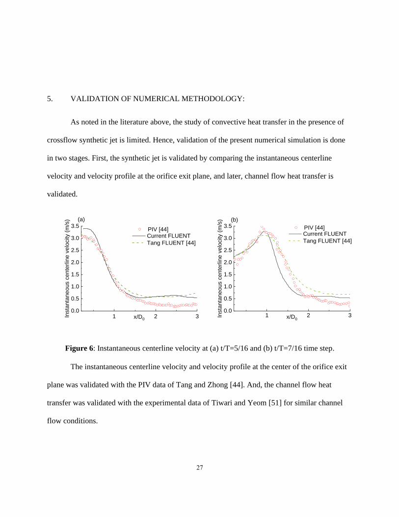
Figure 6: Instantaneous centerline velocity at (a) t/T=5/16 and (b) t/T=7/16 time step. ............. 27

Figure 7: Velocity profile at the center of the orifice exit plane for a cycle. ............................... 28

Figure 8: Quasi-steady state in numerical simulation .................................................................. 31

Figure 9: Phase averaged normalized velocity profile for different diaphragm amplitude and

channel velocity. .................................................................................................................... 35

Figure 10: Effect of (a) channel velocity on heat transfer coefficient and (b) diaphragm

displacement on phase averaged normalized heat transfer coefficient. ................................. 36

Figure 11: Heat transfer coefficient (a) Phased averaged over ten cycles, (b) Averaged over a

cycle, for three different locations. ........................................................................................ 36

Figure 12: (a) Normalized velocities for a complete cycle with different actuation frequencies

(b) Heat transfer coefficient for different actuation frequencies ........................................... 38

Figure 13: Vortex generation visualization using Q-criterion for different phases of diaphragm

actuation in the channel. ........................................................................................................ 40

Figure 14: Hair pin vertex generation along the channel. ............................................................ 41

Figure 15: Velocity fluctuations due to vortical structures at different y-planes for maximum

ejection................................................................................................................................... 42

Figure 16: Velocity fluctuations due to vortical structures at different x-planes for maximum

ejection................................................................................................................................... 43

Figure 17: Visualization of local temperature distribution on heated surface due to vortical

structures at different phases. ................................................................................................ 44

Figure 18: Visualization of temperature distribution on the heated surface for maximum

ejection................................................................................................................................... 45

x

LIST OF TABLES

Table 1: Operating conditions for numerical simulation ............................................................. 14

Table 2: Dimensions for a numerical domain. ............................................................................. 18

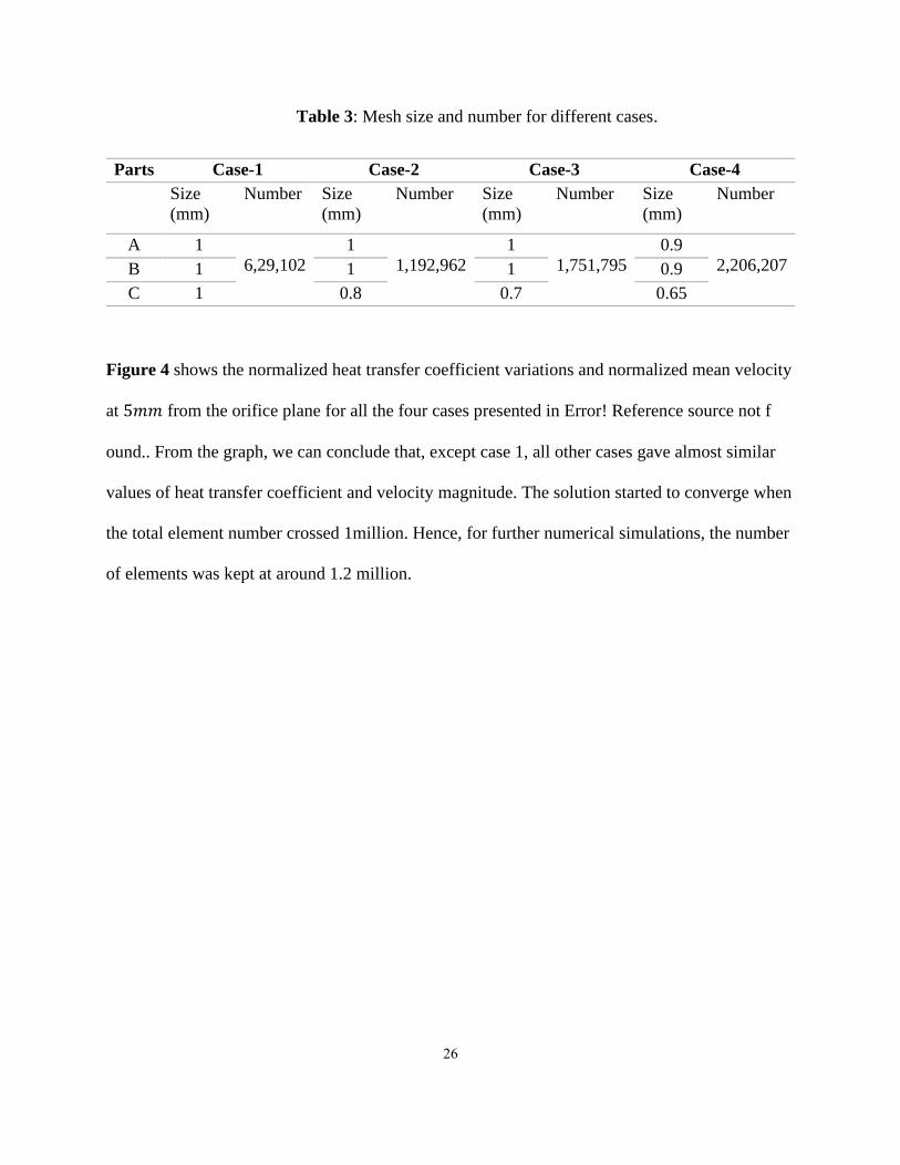
Table 3: Mesh size and number for different cases. ..................................................................... 26

Table 4: Validation of surface heat transfer coefficient in the presence of crossflow only. ........ 29

1

1. INTRODUCTION:

The exponential rise in utilization of electronic components and systems has resulted in

the extensive use of high-power and high-speed microchips. According to Moore’s law the

component density within an integrated circuit (IC) doubles every 18 months [1]. These high-

speed chips produce extensive heat fluxes resulting in 50% of the electronic failures [2]. Hence,

this undesirable heat should be managed for the device to run smoothly. Handling local

temperature distribution is of prime importance for effective thermal management techniques.

However, efficient heat dissipation from today’s highly integrated ICs remains a challenging task

[3]. To counteract this, novel methods are needed.

Local temperature distribution in ICs can also add to the existing thermal problem. These

temperature distributions are not uniform and vary according to the source along the chip surface

[4]. The surfaces with high heat fluxes could be the reason for the malfunction of the whole

system. Many designs and techniques are introduced to mitigate this problem. However, uniform

temperature distribution cannot be obtained because such techniques cannot provide thermal

resistance uniformly in all directions.

Thus, for optimum electronic systems, efficient thermal dissipation is a must. Proper

management of the thermal issues and the uniform local temperature distribution is paramount

for modern electronic components to function ordinarily.

2

1.1 Thermal management techniques:

Primarily, many cooling techniques were developed in the past. They are categorized

based on power consumption as active cooling and passive cooling techniques. The active

cooling technique requires input energy to operate. Fan, air cooling, synthetic jets, thermoelectric

coolers come under active cooling devices. The passive cooling technique, on the other hand,

does not require any external energy to operate. Conduction, convection, and radiation are the

basis of heat transfer in passive cooling techniques. Some of it are heat sinks, heat spreaders,

evaporative cooling, night flushing, heat pipes, and thermal interface materials, etc. Even though

passive cooling does not require any input energy, it is considered less efficient in heat transfer

performance than active cooling. This is solely due to an improper heat transfer addendum.

Also, cooling techniques are carried out incorporating a two-stage mechanism for thermal

dissipation. The first involves the heat transfer between the source and the substrate. However, in

the second stage, heat accumulated by the substrate or the package is released to the surrounding.

The design itself creates the hurdle to remove the heat in the first stage. Hence, the thermal

management technique in our work mainly utilizes the second stage. Ultimately, convection heat

transfer should be improved to get the better-off heat dissipation in the second stage.

Convection heat transfer is given as:

𝑄 = ℎ. 𝐴. (𝑇𝑠 − 𝑇𝑓) (1)

Where ℎ is the convection heat transfer coefficient, 𝐴 is the surface area, and (𝑇𝑠 − 𝑇𝑓) is

the difference in the temperature between the source and the surrounding fluid. To increase the

heat transfer rate, we need to increase either ℎ, 𝐴, 𝑜𝑟 (𝑇𝑠 − 𝑇𝑓).

3

The most common thermal management techniques currently being used are high-speed

fan-driven sinks, direct immersion cooling, micro refrigeration liquid cooling systems,

thermoelectric coolers, etc. These techniques focus on the parameters in the above equation for

more efficient heat transfer.

High-speed fan-driven sinks give considerable cooling due to increased heat transfer

coefficient via high-speed airflow. Parameters like surface area and the temperature difference

can be improved following the above equation, which will evidently increase the heat transfer

rate. However, power consumption and noise set back this technique of thermal management. On

the other hand, liquid cooling provides better heat transfer than air convection. The high specific

heat of the liquid facilitated by higher temperature differences can dissipate heat rather

efficiently. The limiting factors for liquid cooling are complex arrangements such as reservoir,

pump, nozzles, hoses, and possible leakage chance.

As the name implies, the direct immersion technique has a setup in which the circuit

board is placed in a low boiling point fluid. The heat transfer enhancement can be obtained in

two phases, utilizing the high heat transfer coefficient and the latent heat of phase change.

However, the drawback is that the system may shut down due to thermal overshoot: the fluid

temperature escalates quickly and damages the electronic system.

Micro-refrigeration also has a coolant leakage problem. Besides, design constraint adds a

greater disadvantage, despite the cooling. A thermoelectric cooler overcomes all the

disadvantages mentioned above. It uses the Peltier effect to create the high pole temperature and

low pole temperature, which can be used to cool the electronic component. Since this is a solid-

state technique, there is no coolant leakage problem. The only thing setting it back is the power

4

consumption, which can be higher than expected, and the reliability of other techniques to

dissipate heat to the ambient.

Hence, discovering a proper thermal management technique is challenging. Recently,

researchers and Engineers are under pressure to develop a thermal management technique with

efficient and effective thermal cooling. The study on a synthetic jet is increasing promisingly in

the last decade due to its active flow control and thermal management applications. The simple

design, low cost, and easy installation onto the electronic components give it an edge over all

other thermal management techniques. However, the study of synthetic jet remains a peculiar

subject for most researchers over the decade. It provides a wide range of industrial and domestic

applications.

1.2 Synthetic jet:

A synthetic Jet is a fluidic device that works due to the volumetric displacement of the

fluid inside the cavity. The volumetric displacement can be achieved with diaphragm

displacement through actuation. And the actuation can be with any means; some include

electrical, mechanical, magnetic, or other means. When the diaphragm moves back and forth, the

fluid is sucked in and ejected periodically through an opening, called an orifice. The typical

synthetic jet actuator with diaphragm and orifice is shown in Error! Reference source not found.. T

he complete cycle of the synthetic jet can be divided into two parts—the suction part of the cycle

and the ejection part of the cycle. During suction, the movement of the diaphragm is away from

the orifice. This results in the injection of the ambient fluid into the cavity structure. During

ejection, the movement of the diaphragm towards the orifice aids the ambient fluid inside the

cavity structure to eject it back to the surrounding. While traveling off the orifice, vortex rings

5

are induced. These counter-rotating vortex rings ultimately transition to a turbulent flow due to

spanwise instability [5].

Figure 1: Synthetic jet actuator

Unlike traditional continuous jets, which require a net mass flux, synthetic jet imparts

momentum to ensuing jets without additional fluid injection.[5] That is, working with zero net

mass flux. This is a unique feature of synthetic jet. A common advantage is that it can be

fabricated over a wide range of scales, effectively disturbing the thermal boundary layer which,

ultimately enhances the heat transfer. The heat transfer can be maximized with local transport

and mixing the ambient fluid with the thermal boundary layer [6]. Impingement increases the

turbulence, which in turn facilitates the fresh fluid to interact with the surface—ultimately

increasing the rate of heat transfer. Also, a well-arranged synthetic jet can significantly control

local temperature distribution within a source or multiple sources.

Concisely, the synthetic jet is one of the active thermal management techniques that act

as a solution for large heat flux removal from power electronic components, significantly

6

managing local temperature distribution. This technique has a further edge over other methods in

terms of power consumption and design constraints. However, detailed research over domestic

and industrial applications is miniature.

1.3 Literature review:

The pulsating jet with zero mass flux has been an exciting topic for many decades. It was

observed with acoustic means with the help of circular tubes by Ingard and Labate [7]. They

visualized the counter-rotating vortical structures on both sides of the orifice. Since then, several

other researchers have been working in this field. Smith and Glezer [8] were the first to establish

the fundamentals of the synthetic jet. They produced a nominally plane turbulent jet with the

help of the time-periodic motion in a flexible diaphragm. The confirmation of zero net mass flux

and the creation of successive vortex pairs, which ultimately demolish to turbulence, was their

highlight.

Furthermore, they found that the path of the vortex rings loses rapidness while the mean

velocity of the ensuing jet increases in the near field. However, in the far field, synthetic jet

resembles the function of conventional continuous jets. This was confirmed later by Smith and

Swift [9]. They compared the synthetic jet with continuous jet with the same Reynolds number

𝑅𝑒 ≈ 2,000. It was concluded that, in far fields, they are analogous. The synthetic jet

outperforms the conventional jet in the near field due to the vortex pair. This finding suggests

that there is more to the near field than the far field. Similar work was conducted by Pavlova and

Amitay [10].

Apart from the experimental work, there are several numerical simulations. However, it

is difficult to exactly replicate the experimental work due to the complex flow field inside the

7

cavity since that is generally unaccounted for [11]. However, in our work, we rectified this issue

using the moving-boundary condition, which meticulously accounts for the flow field inside the

cavity. For flow fields outside the cavity, there have been numerous studies too. There are four

distinct regions in the flow-field of slot synthetic jets [12], while those fields are limited to three

in the case of conventional jets [13]. The regions are the developing, the quasi-two-dimensional,

the transitional, and the axisymmetric [12]. They implied that vortical structures start to form in

the developing region, followed by quasi-two-dimensional jets at the nozzle exit. The transitional

region incorporates a shear layer between the ensuing jet and the surrounding fluid. And the

axisymmetric regions are the far fields. In conventional jets, there is no developing region [13].

There are many factors affecting vortex ring formation. It controls their strength,

stability, and coherence. Shuster and Smith [14] used particle image velocimetry measurements

to confirm the scaling parameters of the jet flow. They found that with the increase of Stroke

length 𝐿𝑜, the jets decayed due to a faster spreading rate. The mean centerline velocity was

decreasing too. They also concluded that the Reynolds number 𝑅𝑒 affects the decay rate of the

jet. A laminar jet is formed within a low range of 𝑅𝑒, whereas a turbulent jet is formed as the 𝑅𝑒

increases. Likewise, the flow field is strongly influenced by the Strouhal number 𝑆𝑡. Greco et al.

[15] performed an experimental study, taking three values of Strouhal number 𝑆𝑡 (0.011, 0.022,

and 0.044), to monitor their effects on the flow field of the jets. They concluded that, with the

increment of the Strouhal number 𝑆𝑡, a vortex ring is created. And this vortex ring is the cause

for a higher flow rate with larger jet width and lower centerline velocity. However, for low

Strouhal number 𝑆𝑡 and high Stroke length 𝐿𝑜, since 𝐿𝑜 is inversely proportional to 𝑆𝑡 [16], the

vortex ring generated cannot escape the suction phase. It is because vortex rings are relatively

weak [17]. Ultimately, there is no jet.

8

Geometrical parameters are also significant in the flow characteristics of synthetic jets.

Which ultimately has an impact on the cooling effects of electronic components. Several

research studies have been conducted to study the influence of geometrical parameters such as

orifice shapes (circular, square, rectangular, diamond, etc.), cavity depth, orifice size, axis

switching, and jet-to surface distance [18-21]. Chaudhari et al. [19] experimented to find the

optimum shape of an orifice among square, rectangular and circular geometry. For the same set

of boundary conditions, square orifice outperformed circular and rectangular orifice, for larger

axial distances 𝑧/𝐷0 > 5. Further, between diamond and oval shape, Mangate and Chaudhari

[20] concluded that oval shape performs better, enhancing heat transfer and acoustic aspect.

Milanovic and Zaman [22] used different orifice geometries experimentally to determine the best

performing configuration. They used cylindrical, clustered, pitched, and tapered arrangements.

Out of which, pitched gave the worst results, while other’s performance ranges were almost

similar.

Also, a handful of research is done keeping the geometrical configuration fixed. Using

the circular configuration, many parameters such as frequency, diaphragm displacement, orifice

diameter, orifice length, jet-to-surface spacing, cavity depth, and cavity diameter are studied,

experimentally and numerically[23-25]. Chaudhari et al. [23] experimentally investigated the

effects of excitation frequencies along with cavities of different depths and different orifice

diameters. They concluded that cavity effects are not evident below first resonance frequencies

but were significant for higher excitation frequencies. Furthermore, the exit velocity was much

more delicate to orifice diameter than the cavity dimensions. Jain et al. [25] also obtained a

similar conclusion. Hatami et al. [24], on the other hand, studied the effects of jet-to-surface

spacings. It was discovered that with increased jet-to-surface spacing (𝐻 𝐷0⁄ = 4, max. ),

9

maximum stagnation heat transfer was obtained. And they later confirmed that it was achieved

because of suitable ventilation and the coherence vortex structure.

Heat transfer characteristics of the synthetic jet were of primary concern for several

researchers. Many experimental and numerical studies have been done to obtain the optimum

heat dissipation rate on the targeted surface. For increasing the effectiveness, Campbell et al.

[26] were among the first researchers to conduct an experiment using the synthetic jet. They

summarized that with the use of a synthetic jet, the processor temperature rise was dropped by

22% compared to the temperature rise without it. Hwang et al.[27] determined the heat

dissipation characteristics of the impinging jet by controlling vortex pairing. While varying the

velocity ratio from 0.45 to 1.75 and Strouhal number 𝑆𝑡 (1.2, 2.4, 3.0, 4.0), they concluded that

enhancement or reduction in heat transfer could be obtained with the change of flow structures.

With 𝑆𝑡 = 1.2, secondary blowing flow, and large nozzle-to-plate distance, a low heat transfer

rate was recorded. However, with 𝑆𝑡 = 2.4 𝑎𝑛𝑑 3.0, high heat transfer rates were found. Pavlova

and Amitay [10] experimented using synthetic jet impingement to cool a constant heat flux

surface. They used two frequencies, 1200Hz and 420Hz, with varying nozzle-to-surface

distances (𝐻 𝐷0⁄ ). They showed that high frequency (1200Hz) is optimum for effective cooling

with small 𝐻 𝐷0⁄ and low frequency (420Hz) with large 𝐻 𝐷0⁄ . Likewise, Mahalingam et al.

[28] concluded that the flow rate in 2D synthetic jet ejectors increases for small widths, but it

asymptotes above the width of 25 mm. The thermal effectiveness, therefore, decreases with the

increase in channel width. Also, Mahalingam and Glezer [29] designed a synthetic-air-jet-based

heat sink and observed the thermal performance for high-power dissipation electronics. They

have presented a synthetic jet-based heat sink that dissipates approximately 40% more heat than

the ducted fan blowing through the sink in a steady flow. In an experiment determining the heat

10

transfer due to synthetic jet impingement cooling, Chaudhari et al. [30] showed that the heat

transfer by the synthetic jet was up to 11 times more than the natural convection. The average

Nusselt number as a function of five non-dimensional numbers Reynolds number, Prandtl

number, jet-to-surface spacing, length of the orifice plate, and half-length of a heated copper

plate (𝑅𝑒, 𝑃𝑟, 𝑧 𝐷0⁄ , 𝐿 𝐷0⁄ , 𝑅/𝐷0). It increased with increasing 𝑅𝑒 and 𝑅/𝐷0 but decreased with

increasing 𝐿 𝐷0⁄ . Additionally, Persoons et al. [31] provided information on heat transfer with

impinging synthetic jets: they discovered, below the optimum spacing of 3.4 jet diameters, a

decrement in cooling potency. Arik [32] experimentally studied the local heat transfer

coefficients with high-frequency synthetic jet impinging on a flat surface. He used four different

sizes of heaters. For a specific size of 6.25mm, ten times higher heat transfer was recorded. Liu

et al. [33] studied the effect of driven frequency on flow and heat transfer with the synthetic jet

impingement. It was concluded that the heat enhancement with the synthetic jet was at least

double the natural convection heat enhancement. The optimum frequency for the highest heat

transfer and flow rates was 600Hz. Chaudhari et al.[34] experimented to determine the synthetic

jet impingement heat transfer characteristics inside the duct. For the effect of the crossflow, they

used either fan or another synthetic jet. They also varied the width of the duct(110-330mm),

keeping the height of the duct constant (25mm). It was concluded that the change in width of the

duct does not affect heat transfer. Also, the heat transfer coefficient for direct impingement was

found superior (150 𝑊/𝑚2), compared with the combined flow(134 𝑊/𝑚2) or with crossflow

only(45 𝑊/𝑚2). Rylatt and O’Donovan [35] researched the effect of ducting on the heat transfer

rate with synthetic jet and confirmed that with ducting design, the heat transfer in the stagnation

region is increased by 27% and 36% on an average area basis. Additionally, Hatami et al.[24]

carried out a numerical simulation to study the effect of geometrical arrangement (confined and

11

unconfined impingement synthetic jets). According to the simulation, unconfined ones provide

more efficient heat transfer than confined ones. Jabbal and Zhong [36] also did an experimental

study to determine the effect of synthetic jet on a heated surface with low Reynolds number

crossflow. Despite not assessing the direct impact of the synthetic jet on heat transfer, they

mapped the surface's thermal footprints, which was in close resemblance with the oil flow

pattern generated on a 2D cylindrical model. Go and Mongia [37] created an experimental

apparatus to study the synthetic jet cooling enhancement on portable platforms such as laptops,

handheld PCs, etc. They investigated the perpendicular arrangement of synthetic jet with low-

speed duct flow. The studies indicated the cooling enhancement of 25% in the main body, while

the crossflow was blocked by synthetic jet. A numerical simulation was conducted by

Timchenko et al. [38] to investigate the utilization of synthetic jet in heat transfer, with a

vibrating diaphragm that followed the parabolic profile. 2D transient simulation verified a 64

percent cooling effect at the targeted wall. However, their model did not include any turbulent

model in the corresponding simulation. Chandratilleke et al. [39] examined the effectiveness of

using synthetic jets for thermal management in a microchannel. They used the (SST) 𝑘~𝜔

turbulence model to address the turbulence due to jet. They conclude that the synthetic jet

incorporated channel gave thermal enhancement 4.3 times compared to the channel without the

jet interaction within the tested parametric range. Like the above work, an experimental study

was conducted in the same year by Qayoum et al. [40]. They observed the crossflow interaction

between the synthetic jet and laminar boundary layer. A maximum of 44% thermal enhancement

was recorded, while the heat transfer coefficient increased with excitation amplitude. In addition

to this, Fang et al. [41, 42] did experimental work on the enhancement of heat transfer using

single-phase liquid micro-channel using crossflow and synthetic jet. They used four different

12

Reynolds numbers 𝑅𝑒 (65, 95, 137, 188). They confirmed 53% heat transfer enhancement for

𝑅𝑒 = 95.

13

2. SCOPE OF RESEARCH:

From the literature presented above, it is apparent that several researches have been

conducted in the field of synthetic jet closely observing the flow characteristics, flow field, the

influence of geometrical parameters, influence of dimensionless parameters, formation of

vortical structures, interaction with boundary layer and heat transfer enhancement. However,

these studies are primarily experimental, which involves complex designing and complex

arrangement, which is not feasible. There are many numerical simulations but are limited to a 2D

domain. The flow fields and vortices associated with it give rise to the turbulent condition in the

model, which is not sufficiently captured by the 2D domain. Also, studies on the interaction of

synthetic jets for thermal enhancement with pre-existing flows are limited. Hence, the present

study utilizes a 3D model. The transient numerical simulation in a 3D domain is conducted to

address the turbulence through the RNG 𝑘~𝜖 model. The results are then used to observe the

hierarchy of vortical structures produced with synthetic jet and their interaction with the

crossflow and heated surface for optimum heat transfer enhancement. Jet velocities are varied by

changing the diaphragm amplitude. For comparison, three flow velocities are used, as shown in

Table 1. The optimum case is selected with optimal amplitude and flow velocity from the total

cases. Further, the frequency effect is addressed incorporating three frequencies presented in

Table 1. Eventually, among the three locations, the best location is selected for optimum thermal

enhancement observing the local temperature distribution on the heated copper surface and its

interaction with the vortical structures due to synthetic jet.

14

Table 1: Operating conditions for numerical simulation

𝑼∞[𝐦/𝐬] Amplitude [mm] Frequency [Hz]

1 0.4 200

2 0.8 400

3 1.2 800

15

3. NUMERICAL MODEL

3.1 Governing equations:

In the present study, Turbulent, unsteady, incompressible, and three-dimensional flow is

analyzed using a pressure-based, transient solver in ANSYS fluent. It solves three governing

equations: compressible continuity, Navier-Stokes, and energy equations. The integral form of

these equations is:

𝜕𝜌

𝜕𝑡+ ∇ ∙ (𝜌) = 0 (2)

𝜕

𝜕𝑡(𝜌) + ∇ ∙ (𝜌) = −∇𝑝 + ∇ ∙ (𝜏) (3)

where, ∇ ∙ (𝜏) = 𝜇𝑒(𝜕𝑈𝑖

𝜕𝑥𝑗+

𝜕𝑈𝑗

𝜕𝑥𝑖)

𝜕

𝜕𝑡(𝜌𝐸) + ∇ ∙ ((𝜌𝐸 + 𝑝)) = ∇ ∙ (𝑘𝑒𝑓𝑓∇𝑇 − ∑ ℎ𝑗𝐽𝑗

𝑗

+ (𝜏𝑓𝑓 ∙ )) + 𝑆ℎ (4)

Where 𝜌, 𝑡, , 𝑝, 𝑇, 𝜏, 𝑎𝑛𝑑 𝑘 denote the density, time, velocity vector, pressure, temperature, stress

tensor, and thermal conductivity, respectively. 𝑘𝑒𝑓𝑓 is the effective conductivity, and 𝜏𝑓𝑓 is the

effective stress tensor. The three terms on the right-hand side of the above equation are for

energy transfer due to conduction (𝑘𝑒𝑓𝑓∇𝑇), species diffusion (∑ ℎ𝑗𝐽𝑗)𝑗 , and viscous dissipation

(𝜏𝑓𝑓 ∙ ). 𝑆ℎ represents the heat of chemical reaction, and other volumetric heat source defined

in the model.

16

However, in our model, we are neglecting species diffusion and the heat of chemical

reactions. Also, no other volumetric heat source has been defined. Hence the reduced energy

equation is given as:

𝜕

𝜕𝑡(𝜌𝐸) + ∇ ∙ ((𝜌𝐸 + 𝑝)) = ∇ ∙ (𝑘𝑒𝑓𝑓∇𝑇 + (𝜏𝑓𝑓 ∙ )) (5)

The energy term 𝐸 in equation 5 is represented with enthalpy ℎ and pressure (static and

dynamic) as below:

𝐸 = ℎ −𝑝

𝜌+

𝑣2

2(6)

Standard 𝑘 − 𝜖 turbulent model [43, 44], Shear-stress transport (SST) 𝑘 − 𝜔 turbulent

model [24, 39, 45], and RNG 𝑘 − 𝜖 model [25, 44, 46] are widely used turbulent models for flow

fields and heat transfer analysis associated with the synthetic jet. Among them, the best result is

produced by the Shear-stress transport (SST) 𝑘 − 𝜔 turbulent model for constant wall

temperature heat transfer [47]. For the flow field, Bazdidi-Tehrani et al. [48] compared their

(SST) 𝑘 − 𝜔 turbulent model simulation results with the experimental data of Tang and Zhong

[44]. They presented the instantaneous velocity magnitude measured at the orifice outlet and

confirmed a plausible agreement between their results and experimental data. Tang and Zhong

also compared their data with 𝑅𝑁𝐺 𝑘 − 𝜖 model and standard 𝑘 − 𝜖 turbulent model, which

predicted that both the models were close to experimental data. For wall bonded turbulent flows,

Shear-stress transport (SST) 𝑘 − 𝜔 turbulent model provides better insight for an accurate

interpretation of near-wall regions [39].

However, recent studies by Xiang et al. [49], Luo et al.[50], Tiwari and Yeom [51] and

Kumar and Saini [52] have suggested that the RNG 𝑘 − 𝜖 model captures the rapid strain and

17

streamlines curvature formation phenomenon along with the proper transportation of vortical

structures in a channel flow for adequate heat transfer. Since, the primary aim of this work is to

observe the hierarchy of vortical structures produced with synthetic jet, the nature of their

movement to impinge the heated surface, and the combined interaction of them with the

crossflow, we employed RNG 𝑘 − 𝜖 turbulence model. The transport equations for RNG 𝑘 −

𝜖 model is given as:

𝜕

𝜕𝑡(𝜌𝑘) + ∇ ∙ (𝜌𝑘) = ∇(𝛼𝑘𝜇𝑒𝑓𝑓∇𝑘) + 𝐺𝑘 − 𝜌휀 (7)

𝜕

𝜕𝑡(𝜌휀) + ∇ ∙ (𝜌휀) = ∇(𝛼𝑘𝜇𝑒𝑓𝑓∇휀) + 𝐶1𝜀

휀

𝑘𝐺𝑘 − 𝐶2𝜀𝜌

휀2

𝑘− 𝑅𝜀 (8)

The readers are prompted to refer [53] and [54] for further insights on Equations 7 and 8,

including parameters and constants.

3.2 Governing dimensionless parameters:

For synthetic jet flow characterization, several non-dimensionless parameters are used.

The distance traveled by the "slug" of the fluid during the ejection cycle, which accounts for half

the total cycle, is the stroke length, 𝐿0 given as:

𝐿0 = ∫ 𝑈𝑜𝑟𝑖(𝑡)𝑑𝑡

𝑇2

0

(9)

Where 𝑇 and 𝑈𝑜𝑟𝑖(𝑡) denote cycle period and instantaneous velocity, respectively. The Reynolds

number 𝑅𝑒 is defined based on the time-averaged value of instantaneous velocity (𝑈𝑜𝑟𝑖) at

orifice exit and the orifice diameter (𝐷0) as:

𝑅𝑒 =𝑈𝑜𝑟𝑖𝑑

𝜈(10)

18

Furthermore, Strouhal number (𝑆𝑟) is also a function of time-averaged instantaneous

velocity (𝑈𝑜𝑟𝑖) at orifice exit, orifice diameter, and frequency of the diaphragm (𝑓) and is

defined as:

𝑆𝑟 =𝑓𝐷0

𝑈𝑜𝑟𝑖

(11)

Also, Stokes number (𝑆𝑡) is obtained after multiplying Reynolds number (𝑅𝑒) and

Strouhal number (𝑆𝑟) as:

𝑆𝑡 = √𝑓𝐷𝑜𝑟𝑖

2

𝜈(12)

3.3 Geometry and boundary conditions:

The synthetic jet geometry in the current work is recreated in exact unison with Tang and

Zhong [44]. Bazddi-Tehrani et al. [48] also followed their work in creating a 3D synthetic jet

domain in their numerical simulation. A cylindrical-shaped synthetic jet cavity was used, which

utilized a thin shim as a diaphragm and a cap with an orifice opening. The dimensions for the

synthetic jet that they used in their experimental work is listed in Table 2. They used an actuator

with a 50 Hz operating frequency. They used a frequency-doubled Q-switched Nd: Yag laser and

a CCD camera at 10 Hz with a resolution of 1000 × 1016 pixels for PIV measurement.

Table 2: Dimensions for a numerical domain.

𝑫𝟎 [𝒎𝒎] 𝒉 [𝒎𝒎] 𝑫𝒄[𝒎𝒎] 𝑯 [𝒎𝒎] 𝒍 [𝒎𝒎] 𝒃[𝒎𝒎] 𝒉𝒄[𝒎𝒎] 𝒍𝒉[𝒎𝒎] 5 5 45 10 158 22.5 22.5 52

In the present 3D numerical simulation, synthetic jet dimensions are similar to Tang and

Zhong [44]. In addition to that, a channel with the heated surface is added, as shown in Figure 3.

19

The channel dimension is 22.5 × 22.5 × 158𝑚𝑚. For frequency, flow velocity, and amplitude

effect, the location of the synthetic jet is fixed. The synthetic jet orifice axis is located at 50𝐷0

upstream for these initial cases. Later two more locations are introduced to find the optimum

location of synthetic jet. Based on the position of axis of an orifice, from the initial location, with

a successive increment of 0.5𝑙, synthetic jet positioning is changed. Where 𝑙 is the length of the

heated surface. The heated surface is at the distance of 6𝐷0 from an outlet. The dimension of the

heated surface is 52 × 22.5𝑚𝑚. The schematic diagram of the entire numerical domain is

presented in Figure 2.

To ensure that the flow is fully developed, a parabolic fully developed velocity profile is

given at the inlet using an interpreted user-defined function (UDF). The velocity profile [55] is

given as:

𝑈

𝑈∞= (

𝑚 + 1

𝑚) (

𝑛 + 1

𝑛) [1 − (

𝑦

𝑏)

𝑛

] [1 − (𝑧

𝑎)

𝑚

] (13)

Where 𝑈∞ is velocity. 𝑎 and 𝑏 are the width and height of the channel. 𝑦 and 𝑧 are coordinate

displacements. 𝑚 and 𝑛 are constants given as,

20

Figure 2: Schematic diagram of the numerical domain

𝑚 = 1.7 + 0.5(𝛼∗)−1.4 (14)

𝑛 = 2 𝑓𝑜𝑟 𝛼∗ ≤ 1 3⁄

2 + 0.3(𝛼∗ − 1 3⁄ ) 𝑓𝑜𝑟 𝛼∗ ≥ 1 3⁄(15)

In equation 15, 𝛼∗ is an aspect ratio which is 1 in our case. Further knowledge on

equations 13,14 and 15 can be found in the reference [55]. For different flow velocities

mentioned in Table 1, different velocity profiles were given using equation 13. However, the

outlet of the channel is considered pressure outlet as shown in the. Reverse flow in an outlet is

not prevented to make the flow realistic. The Fluent default values of turbulent intensity and

viscosity are used for both inlet and outlet, which is 5% and 10%, respectively. The inlet air

temperature is kept default as 300 K. A constant heat-flux of 𝑞 = 4,370.629 𝑤/𝑚2 is given in

the fluent for heated surface as a thermal boundary condition.

21

Figure 3: Numerical domain and boundary condition of the channel

The actuation for the synthetic jet is achieved by periodic diaphragm movement. This

instantaneous periodic motion of the diaphragm is defined using moving wall boundary

conditions in ANSYS fluent with the help of compiled UDF. The logarithmic displacement is

given according to the theory of plates and shells [56] as:

𝛿(𝑟, 𝑡) =∆

2[1 −

4𝑟2

𝐷𝑐2

+8𝑟2

𝐷𝑐2

ln (2𝑟

𝐷𝑐)] 𝐶𝑜𝑠(2𝜋𝑓𝑡) (16)

Where 𝛿 is the diaphragm displacement relative to its initial neutral position, r is the radial

distance from the center of the diaphragm and ∆ is the peak-to-peak diaphragm displacement at

the center. A similar configuration for the diaphragm was utilized by Bazddi-Tehrani et al. [48].

22

Tang and Zhong [44] used the same profile too. But instead of using moving wall boundary

conditions at the diaphragm, they applied velocity-inlet boundary conditions.

3.4 Solution methodology:

Transient solver with RNG ‘renormalization group’ 𝑘 − 𝜖 turbulence model, with

standard wall function, is chosen. Pressure-implicit with the splitting of operators (PISO)

algorithm is used for pressure correction. This algorithm has a higher degree of approximation in

the iterative correction of errors in pressure and velocity. It also reduces convergence-related

problems that come with highly skewed mesh with almost the same iterations that would be

needed for finer orthogonal mesh [57]. For turbulent dissipation rate, turbulent kinetic energy,

momentum, and energy, second-order upwind spatial discretization was utilized. The default

values of under-relaxation parameters for pressure, density, and momentum are used. The

residuals of mass, momentum, turbulence parameters and energy are limited to 10−6, which is

the convergence criterion for the simulation.

The maximum iteration per time step value is kept 20, and time step is chosen according

to the diaphragm actuating frequency defined by the equation:

∆𝑡 =1

𝑓 × 200(17)

Where 𝑓 is the frequency of oscillating motion of the diaphragm in Hertz. A simulation was run

for a total of 4000-time steps (20 oscillation cycles of the diaphragm) until a quasi-steady-state

solution is achieved.

23

4. EVALUATION OF MESH INDEPENDENCE:

The meshing in the present numerical simulation uses the Fluent default mesh generation.

The tetrahedron unstructured linear element is utilized for numerical analysis. Body sizing is

used to define the minimum element size in the domain. The total numerical domain is divided

into three parts: A, B, and C, as shown in Figure 5. Part A starts from an inlet having dimensions

22.5 × 22.5 × 25𝑚𝑚. Part B is located 138𝑚𝑚 from an inlet with dimensions

22.5 × 22.5 × 20𝑚𝑚. The remaining domain consists of a synthetic jet, and a heated surface is

treated as part C.

Figure 4: Variations of (a) normalized heat transfer coefficient and (b) normalized mean

velocity at 5mm from orifice for four different mesh cases.

Part C has a finer mesh compared to parts A and B. The tetrahedron elements in the jet flow field

and the heated surface experience significant distortion.

0.0 0.2 0.4 0.6 0.8 1.021

22

23

24

25

26

27

28

29

30

Hea

t T

ransfe

r C

oe

ffic

ien

t (W

/m2 K

)

t/T

Case-4

Case-3

Case-2

Case-1

(a)

0.0 0.2 0.4 0.6 0.8 1.0

0.8

1.0

1.2

1.4

1.6

1.8

2.0

2.2

2.4

2.6

Velo

city M

ag

nitud

e (

m/s

)

t/T

Case-4

Case-3

Case-2

Case-1

(b)

24

Also, dynamic meshing is incorporated in the simulation, which can create negative cell

volume due to insufficient element size. Hence finer orthogonal mesh around the synthetic jet

flow field and the heated surface is made. Also, to analyze the behavior of flow near the

boundary layer created by walls and heated surface, inflation was given to all the channel faces

except the top face.

Since the thermal boundary layer thickness was 0.05𝑚𝑚, due to constant flux generated

by the heated surface, the first inflation layer was kept 0.05𝑚𝑚, and a growth rate of 1.3 was

applied. There are three default groups of mesh motions provided by ANSYS fluent for dynamic

meshing: smoothing methods, dynamic layering, and local remeshing methods. In the spring-

based smoothing method, the edges between two element nodes are treated as a network of

interconnected springs. Those edges are in an equilibrium state before the application of any

boundary motion. When motion is detected in those edges, that deformation gets transferred to

all other springs connected to the node. However, if the deformation is too high, higher than

local cell sizes, the cells can become vitiated. This will result in negative cell volumes, as

mentioned above, and eventually lead to convergence problems. Hence, remeshing method is

employed too. For mesh independence study, location 1 of the synthetic jet is used. The

operating frequency of the diaphragm is 50Hz. The peak-to-peak displacement of 0.4𝑚𝑚 is

utilized with the help of UDF. The channel flow velocity is also kept constant at 1𝑚/𝑠. All other

solution methodology discussed above is kept the same.

25

Figure 5: Numerical domain meshing (a) isometric view, (b) cross-sectional view, and (c)

inflation on the wall.

The mass-averaging technique was used to calculate the inlet and outlet static

temperature. For the temperature of the heated surface, the area-weighted average technique was

utilized. Using the LMTD method, the heat transfer coefficient of the heated surface at the

specific time step is calculated. This can be cross-validated with the area-weighted average heat

transfer coefficient directly obtained from the simulation at the heated surface after reaching the

quasi-steady state.

Four different mesh cases with varying elements are created, and they are named Case-1,

Case-2, Case-3, and Case-4. The information on these cases is provided in Table 3.

26

Table 3: Mesh size and number for different cases.

Parts Case-1 Case-2 Case-3 Case-4

Size

(mm)

Number Size

(mm)

Number Size

(mm)

Number Size

(mm)

Number

A 1

6,29,102

1

1,192,962

1

1,751,795

0.9

2,206,207 B 1 1 1 0.9

C 1 0.8 0.7 0.65

Figure 4 shows the normalized heat transfer coefficient variations and normalized mean velocity

at 5𝑚𝑚 from the orifice plane for all the four cases presented in Error! Reference source not f

ound.. From the graph, we can conclude that, except case 1, all other cases gave almost similar

values of heat transfer coefficient and velocity magnitude. The solution started to converge when

the total element number crossed 1million. Hence, for further numerical simulations, the number

of elements was kept at around 1.2 million.

27

5. VALIDATION OF NUMERICAL METHODOLOGY:

As noted in the literature above, the study of convective heat transfer in the presence of

crossflow synthetic jet is limited. Hence, validation of the present numerical simulation is done

in two stages. First, the synthetic jet is validated by comparing the instantaneous centerline

velocity and velocity profile at the orifice exit plane, and later, channel flow heat transfer is

validated.

Figure 6: Instantaneous centerline velocity at (a) t/T=5/16 and (b) t/T=7/16 time step.

The instantaneous centerline velocity and velocity profile at the center of the orifice exit

plane was validated with the PIV data of Tang and Zhong [44]. And, the channel flow heat

transfer was validated with the experimental data of Tiwari and Yeom [51] for similar channel

flow conditions.

0.0

0.5

1.0

1.5

2.0

2.5

3.0

3.5

1 2 3Insta

nta

ne

ou

s c

en

terl

ine

ve

locity (

m/s

)

x/D0

Current FLUENT

Tang FLUENT [44]

(a)

PIV [44]

1 2 30.0

0.5

1.0

1.5

2.0

2.5

3.0

3.5

Current FLUENT

Tang FLUENT [44]

(b)In

sta

nta

ne

ou

s c

en

terl

ine

ve

locity (

m/s

)

x/D0

PIV [44]

28

Figure 7: Velocity profile at the center of the orifice exit plane for a cycle.

As discussed earlier, Tang and Zhong's experimental conditions were replicated in the

numerical domain. After reaching the quasi-steady state, instantaneous centerline velocity was

recorded and plotted versus two-time steps (a) t/T=5/16 and (b) t/T=7/16, as shown in Figure 6.

The data obtained by Tang and Zhong was also plotted in the same graph to find any

discrepancies. The figure shows that there is an allowable accord between all three data. 13.3%

deviation in the maximum velocity magnitude for time step (a) t/T=5/16 was observed, but the

nature of the graph is similar, as can be observed in Figure 6(a). Also, it can be noticed that

increment of 𝑦/𝐷0, results in an increment of percentage deviation of velocity magnitude from

the actual data. The reason behind this is turbulence, as it increases with the increment of 𝑦/𝐷0

[8], [48]. A similar trend was depicted for time step (b) t/T=7/16, as displayed in Figure 6(b).

The plot is almost similar for all three data points for this time step.

Furthermore, the velocity profile at the center of the orifice plane for one cycle after

reaching a steady state was also compared using data points from all three cases. Despite having

0.0 0.2 0.4 0.6 0.8 1.00.0

0.5

1.0

1.5

2.0

2.5

3.0

3.5 Hotwire [44]

Ve

locity m

ag

nitud

e (

m/s

)

t/T

Current FLUENT

Tang FLUENT [44]

29

a minor shift, the overall trend of the velocity profile is preserved, as shown in Figure 7. It

displays two major peaks. One is due to the suction phase, and the other one is due to ejection

phase. The latter one, being more powerful, maximum velocity is observed around 3.3m/s.

Secondly, the channel flow was validated using the experimental data obtained by Tiwari and

Yeom [51]. Here, the synthetic jet actuator was kept passive. Their experimental work was

replicated using a numerical domain created in ANSYS fluent. All the boundary conditions that

they used were matched. The heated surface area is kept the same 52 × 22.5 𝑚𝑚, along with the

constant heat flux of 4,370.629 𝑤/𝑚2. The heat transfer coefficient of the heated surface,

keeping all the dimensions the same as that of Tiwari and Yeom [51], was found to be

24.72 𝑊/𝑚2𝐾. The heat transfer coefficient obtained from their experimental work without the

Piezo-electric(PE) fan was 26.61 𝑊/𝑚2𝐾. Here, only 7.10% deviation was recorded, which is

under considerable margin to validate our numerical study, as shown in Table 4.

Table 4: Validation of surface heat transfer coefficient in the presence of crossflow only.

Current numerical study Tiwari and Yeom [51] %∆

𝑾/𝒎𝟐𝑲 𝑊/𝑚2𝐾 7.10

24.72 26.61

30

6. RESULTS AND CONCLUSION:

6.1 Channel flow effect on synthetic jet:

Three-channel velocities were chosen to study the influence of channel flow on the

synthetic jet. The axial velocity magnitude at 𝐷0 distance from orifice was analyzed. The

obtained velocity magnitude was then phased averaged over ten cycles when a quasi-steady state

was reached. The quasi-steady-state was assumed to be achieved after the heated surface

temperature reached a constant value, as shown in Figure 8. Those phase-averaged velocity

magnitudes were normalized with the inlet flow velocity to construct the graph versus time-

period, as shown in Figure 9. At the lowest channel velocity, the synthetic jet has the highest

impact. But, when the velocity of the channel is increased, then the effect of the synthetic jet

deteriorates. At the initial velocity of 1m/s, the plot obtained is non-linear, and normalized

maximum velocity is only around 1.1. The normalized minimum velocity is 0.7, for the lowest

diaphragm displacement of 0.4mm shown in Figure 9(a). The maximum value gets reduced to

around 0.6, which is also the minimum value since the velocity profile is linear for a complete

cycle of the diaphragm, as the channel flow velocity is increased to 3m/s. For 2m/s, the profile is

slightly non-linear, and the velocity magnitude value toggle between 1 and 1.2.

31

Figure 8: Quasi-steady state in numerical simulation

The diaphragm displacement of the synthetic jet was doubled and tripled to understand

the trend better. When 0.8mm diaphragm displacement is used, the velocity profile for 2m/s and

3m/s both exhibit non-linear behavior as recorded previously. However, the difference between

peak values increases in both the cases, compared to 0.4mm diaphragm displacement as shown

in Figure 9(b). Initially, for 2m/s, the peak difference was 0.2, but it increases to 0.8 for 0.8mm

displacement. Distorting from the linear profile, the 3m/s channel flow velocity profile showed a

peak difference of 0.4. This trend was also seen for 1m/s channel flow, which gave a significant

rise in the peak-to-peak value of velocity profile to 2.2, compared to the previous value of 0.4.

The maximum velocity magnitude of 2.6 was recorded. This value was later bettered by 1.2mm

diaphragm displacement for 1m/s channel flow velocity. The maximum velocity magnitude for

this case was found to be around 5.1, with a peak-to-peak difference of 4.6, as shown in Figure

9(c). Also, for 2m/s, the maximum peak velocity was increased to the value of 1.5 compared to

the 0.8mm diaphragm displacement, where the maximum peak velocity was 1.2. Likewise, the

32

considerable effect of the synthetic jet can be seen in 3m/s channel velocity when 1.2mm

displacement was used. As shown in Figure 9(c), a peak-to-peak difference of 0.6 can be

observed in this case. A similar trend can be depicted from Figure 9(d,e, and f), when channel

flow velocities were fixed, and diaphragm displacement was varied, which also shows that the

effect of the synthetic jet degenerate as the channel flow velocity is increased.

6.2 Effect of channel flow and diaphragm displacement on heat transfer coefficient of the

heated surface.

The surface heat transfer coefficient of the targeted surface was recorded, and phase-

averaged over ten cycles after reaching the quasi-steady state. The average heat transfer

coefficient for different channel velocities and different diaphragm amplitude were calculated.

To find the independent effect of each parameter, the average heat transfer coefficient was

normalized, as shown in Figure 10(b). When the channel flow was increased from 1m/s to 3m/s

significant rise in heat transfer coefficient was recorded, irrespective of the diaphragm

displacement. 23.46 𝑊/𝑚2𝐾 was the baseline heat transfer coefficient for 1m/s and 0.4mm

diaphragm displacement. This value was increased to 37.72 𝑊/𝑚2𝐾 and 49.66 𝑊/𝑚2𝐾

successively for 2m/s and 3m/s channel velocity, which are the maximum heat transfer

coefficients as shown in the Figure 10(a). This is mainly due to channel flow rather than the

diaphragm displacement, as 0.4mm cannot penetrate the channel flow as stated above.

Other diaphragm displacements also showed similar behavior as the channel velocity

increased further. For 0.8mm diaphragm displacement, the heat transfer coefficient increased

from an initial value of 24.65 𝑊/𝑚2𝐾 to 37.88 𝑊/𝑚2𝐾 and later 49.68 𝑊/𝑚2𝐾, as the channel

velocity increased successively to 2 and 3m/s. As discussed above, 0.8 can make considerable

33

penetration through flow velocity. Also, for 1.2mm diaphragm displacement and channel

velocity of 3m/s, the maximum value of heat transfer was 49.77 𝑊/𝑚2𝐾, compared to 38.48

𝑊/𝑚2𝐾 for 2m/s and 28.81 𝑊/𝑚2𝐾 for 1m/s. This results states that with increment of the

channel flow velocity, heat transfer enhancement is increased. From Figure 10(a), it is apparent

that discrepancies in heat transfer value at higher channel velocity is minimal for different

diaphragm displacement. However, at lower channel velocities significant difference in heat

transfer coefficient is recorded. This might be due to the interaction of the synthetic jet with the

heated surface since jet can penetrate to the targeted surface at lower channel velocities. For

higher channel flow velocities, the effect of jet disintegrates.

Furthermore, the average heat transfer coefficient was normalized, taking the base value

heat transfer coefficient for 0.4mm diaphragm displacement. It was done to identify the effect of

the synthetic jet in heat transfer rather than the channel flow. The diaphragm displacement was

increased to observe the impact on the normalized heat transfer coefficient. 1.2mm diaphragm

displacement and 1m/s gave the maximum heat transfer, mainly due to synthetic jet rather than

the crossflow, as shown in Figure 10(b). Despite having a heat transfer coefficient value of only

28.82 𝑊/𝑚2𝐾, this case outperforms other cases. The penetration of the jet is higher as the

channel flow velocity is low and peak-to-peak velocity magnitude is more elevated. For 2m/s

and 3m/s, only a slight rise in heat transfer coefficient was recorded as the penetration rate

decreases because of the increment in the channel velocity, as depicted in Figure 10.

6.3 Effect of location on heat transfer coefficient:

Based on the above observations, it is apparent that diaphragm displacement of 1.2mm is

optimal for penetration in the presence of crossflow. Also, maximum penetration can be

34

observed when the channel flow velocity is 1m/s. And a significant penetration can be observed

for the channel flow velocity of 2m/s. Hence, with a fixed channel flow velocity of 2m/s and 1.2

diaphragm displacement, the optimal location for the highest thermal enhancement is studied.

Based on the synthetic jet positioning, three locations were chosen, which are upstream, front

end and center.

From all three cases, area-averaged surface heat transfer coefficient of the heated surface

was extracted and phased averaged over ten cycles after reaching the quasi-steady state. Then

they are plotted versus locations to find the optimal location for thermal enhancement, as shown

in Figure 11. Figure 11(a) shows that the upstream position outperforms the center and front-

end location. The heat transfer coefficient is superior during both the suction and ejection phase

for upstream.

35

Figure 9: Phase averaged normalized velocity profile for different diaphragm amplitude and

channel velocity.

0.0 0.2 0.4 0.6 0.8 1.0

1

2

3

4

5

6

0.0 0.2 0.4 0.6 0.8 1.0

1

2

3

4

5

6

0.0 0.2 0.4 0.6 0.8 1.00

1

2

3

4

5

6

0.0 0.2 0.4 0.6 0.8 1.00

1

2

3

4

5

6

0.0 0.2 0.4 0.6 0.8 1.0

1

2

3

4

5

6

0.0 0.2 0.4 0.6 0.8 1.0

1

2

3

4

5

6

U/U

0

t/T

1m/s

2m/s

3m/s

(a) =0.4mm

U/U

0

t/T

1m/s

2m/s

3m/s

(b) =0.8mm

(c) =1.2mm

U/U

0

t/T

1m/s

2m/s

3m/s

U/U

0

t/T

0.4mm

0.8mm

1.2mm

(d) 1m/s

U/U

0

t/T

0.4mm

0.8mm

1.2mm

(e) 2m/s

U/U

0

t/T

0.4mm

0.8mm

1.2mm

(f) 3m/s

36

Figure 10: Effect of (a) channel velocity on heat transfer coefficient and (b) diaphragm

displacement on phase averaged normalized heat transfer coefficient.

Figure 11: Heat transfer coefficient (a) Phased averaged over ten cycles, (b) Averaged over a

cycle, for three different locations.

The maximum value was recorded to be 38.72 𝑊/𝑚2𝐾, and the average value was

38.72 𝑊/𝑚2𝐾. The heat transfer coefficient in the center position was reasonably low as the

maximum heat transfer coefficient was 37.84 𝑊/𝑚2𝐾, which resulted in the drop in the average

value to 37.76𝑊/𝑚2𝐾. However, the front-end location stood in between, with an average value

of 38.29 𝑊/𝑚2𝐾, as shown in Figure 11(b). Compared to the baseline data obtained from

Tiwari and Yeom [51], thermal enhancement of 45.50% was achieved for the upstream position

1 2 3

25

30

35

40

45

50H

ea

t tr

an

sfe

r coe

ffic

ien

t (W

/m2 K

)

Channel velocity (m/s)

0.4mm

0.8mm

1.2mm

(a)

0.4 0.6 0.8 1.0 1.2

1.00

1.05

1.10

1.15

1.20

1.25

h/h

0

Diaphragm displacement (mm)

1m/s

2m/s

3m/s

(b)

0.0 0.2 0.4 0.6 0.8 1.037.0

37.5

38.0

38.5

39.0

He

at

tra

nsfe

r C

oe

ffic

ien

t (W

/m2K

)

t/T

Upstream

Front-end

Center(a)

Upstream Front-end Center37.0

37.5

38.0

38.5

39.0H

ea

t tr

an

sfe

r coe

ffic

ien

t (W

/m2K

)

Synthetic jet location

(b)

37

with fixed diaphragm displacement of 1.2mm and channel velocity 2m/s. For the front-end

position, thermal enhancement of 43.89% was observed. This value dropped further to 41.90%

for the center position.

6.4 Effect of frequency on heat transfer coefficient:

As noted earlier, with the increment channel velocity the synthetic jet effect deteriorates.

Aiming to mitigate this deterioration, a study done by changing the actuation frequency of the

diaphragm. Three different frequencies were studied: 50 Hz, 100 Hz, and 200 Hz. The phased

averaged normalized velocities for a cycle were plotted for these frequencies as shown in the

Figure 12(a). A non-linear behavior of the plot can be recorded as expected since synthetic jet

penetrates the channel flow in all three conditions. However, more penetration is recorded for the

frequency 200Hz. Almost 10-fold increment in the velocity was recorded. Similarly, for 100Hz

5-fold increment in the velocity was observed. With this trend it is expected to have maximum

heat transfer enhancement for 200Hz, but the graph shows otherwise as shown in the Figure

12(b).

The heat transfer coefficient for 50Hz was 38.48𝑊/𝑚2𝐾 followed by the value of

47.44𝑊/𝑚2𝐾 for 100Hz, which showed the significant rise by 18.88%. However, only 2.86%

increment was recorded as the frequency was increased to 200Hz. At higher frequencies, the

vortex generated experience sudden decay, due to the formation of the secondary vortex, which

ultimately decrease the centerline velocity [10]. The decline in percentage increment of the heat

transfer coefficient, may be due to the strong hairpin vortex generation which travelled far from

the heated surface. The phenomenon behind this will be discussed later.

38

Figure 12: (a) Normalized velocities for a complete cycle with different actuation frequencies

(b) Heat transfer coefficient for different actuation frequencies

The critical frequency for our case is 100Hz beyond which the percentage of heat transfer

slows down. This is also due to smaller 𝑦/𝐷0 for our numerical simulation, as stated by Pavlova

and Amitay [10].

6.5 The Q criterion:

The variation in the 3D velocity flow field produced by current numerical simulation,

helps in determining the interaction between the channel flow and synthetic jet. The coherent

structures produced by such interaction experience high level of vorticity. And to understand this

vorticity due to such eddy structures, Q-criterion is exercised in our numerical simulation.

The Q-criterion is commonly used for generation of the complex vortical structures for

post-processing in many numerical simulations. Q, the positive second invariant of velocity

gradient tensor ∆𝑈, is given as:

𝑄 = 0.5 (||Ω||2

− ||𝑆||2

) , 18

0.0 0.2 0.4 0.6 0.8 1.0

0

2

4

6

8

10

12U

/U0

t/T

50 Hz

100 Hz

200 Hz

(a)

50 100 150 200

38

40

42

44

46

48

50

Hea

t tr

an

sfe

r coe

ffic

ien

t (W

/m2K

)

Frequency (Hz)

(b)

39

Where ||𝑆|| = [𝑇𝑟(𝑆𝑆𝑡)]1/2, ||Ω|| = [𝑇𝑟(ΩΩ𝑡)]1/2, || .|| is the matrix norm, S and Ω being the

symmetric and antisymmetric component of ∆𝑈. Ω, thus gives the local balance between the

rotation rate ||Ω||2and the strain rate ||𝑆||

2. From this, it is apparent that, for the generation of

the vortical structures, rotation rate must overcome the strain rate. To rephrase it, coherent vertex

is the region where Q>0.

The Q- criterion in ANSYS fluent requires the user-defined rendering transparency factor

to visualize the generation of complex vortical structures. In the current numerical simulation,

transparency factor of 0.6 is chosen which is sufficient enough to capture the fully developed

vortical structures. It focuses on understanding the flow physics and transportation of vortical

structures generated from the synthetic jet and its interaction with the crossflow. Also, their

impingement phenomenon onto the heated surface is vital. The data are obtained for half-a-cycle

of the diaphragm actuation after reaching a quasi-steady state as exercised before and Q-criterion

is visualized as shown in the Figure 13. At phase zero, the diaphragm is at the neutral position.

And at the phase of 𝜋 = 1.0, the diaphragm reaches to the maximum value of 1.2mm resulting

maximum ejection stroke. As the diaphragm actuation begins, primary vortex is generated in the

channel. This primary vortex interacts with the channel flow and those primary vertex gets

carried away along the channel. This interaction give rise to the secondary vertex at the phase of

𝜋 = 0.5, as shown in Figure 13(c). When these vortices are carried away due to the channel

flow, hair pin vortex is generated further downstream at the phase of 𝜋 = 1.0 shown in Figure

13(d). Hair pin vertex can be characterized into two parts: head and tail. The primary vertex

travelling downstream, transition to hair pin vertex. The ring degenerates and leaves the tail

40

behind while head is elevated as actuation pushes these rings to the heated surface as shown in

Figure 14.

Figure 13: Vortex generation visualization using Q-criterion for different phases of diaphragm

actuation in the channel.

Since head moves away from the targeted surface, it is not generally responsible for heat

transfer enhancement. Tail, on the other hand remain close to the surface which disturbs the

boundary layer. Ultimately, tail also move away from the surface due to channel flow and

collapse later. Several HPVs are generated due to the interaction which ultimately fades, as they

travel through the channel. The transition between the development and degeneration of these

HPVs give rise to a kink. They generally overlap with the preceding HPVs.

41

Figure 14: Hair pin vertex generation along the channel.

These HPVs are responsible for velocity fluctuations within a channel. To understand the

effect of these vortical structures on the velocity fluctuations, velocity magnitude contour is

plotted for maximum ejection as shown in Figure 15 and Figure 16.

The velocity contours display the zones made by several HPVs and preliminary vortices

with high momentum produced by the synthetic jet actuation. The area enclosed by vortical

structures exhibit high velocities in comparison to the average channel velocity. These structures

are collectively carried downstream before undergoing degeneration by, overcoming channel

velocity. From above analysis, it is apparent that synthetic jet plays a role in providing additional

momentum to the channel thereby increasing the average channel velocity which can impinge on

the targeted surface to increase the heat transfer coefficient.

42

Figure 15: Velocity fluctuations due to vortical structures at different y-planes for maximum

ejection.

43

Figure 16: Velocity fluctuations due to vortical structures at different x-planes for maximum

ejection.

Figure 17 and shows the temperature distribution on the heated surface at different

phases. The vortical structures is evidently interacting with the surface for better thermal

enhancement. There are numerous locations on heated surface where sweeping effect is

observed. On those locations, mainly the tail of the HPVs undergoes a direct contact as shown in

Figure 18. The heated surface closest to the synthetic jet orifice axis shows the minimum

temperature due to the direct impingement created by synthetic jet actuation and channel flow.

The minimal temperatures on the heated surface are pleasingly aligned with direct sweeping

effect due to VS as displayed in Figure 18 .

44

Figure 17: Visualization of local temperature distribution on heated surface due to vortical

structures at different phases.

This can be observed in all phases as VSs travels downstream along the heated surface.

Also, there are two distinct unsweep locations where VS does not reach. Those areas show the

highest value of temperature around 489K whereas other sweep locations are maintained at the

constant temperature of around 311K.

45

Figure 18: Visualization of temperature distribution on the heated surface for maximum

ejection.

46

7. CONCLUSION:

The current research observed the convection heat transfer performance of the synthetic

jet on a targeted heated surface using transient numerical simulation. The solution domain was

created to replicate the synthetic jet placed in a channel, in the direction perpendicular to the

channel flow. The impact of the synthetic jet was studied varying channel velocities, diaphragm

amplitude, frequency, and locations. The fixed channel with constant jet to surface distance,

𝑦/𝐷0 = 4.5 was assumed, to perform the numerical simulation. Also, dimensional parameters

were fixed. The key conclusion from this study is listed below:

1. At, lowest channel velocity of 1m/s and maximum diaphragm displacement of 1.2mm,

the synthetic jet enhanced the convective heat transfer rate of the heated surface by

16.54%, compared to the baseline condition with no jet. This value was obtained in

upstream location of the synthetic jet.

2. When channel velocity was increased to the maximum value of 3m/s, the overall heat

transfer rate was increased by 101.33% but this was mainly due to channel flow rather

than synthetic jet as, SJ cannot properly penetrate the high channel flow velocity.

3. For the same channel flow velocity of 1m/s, with every 0.4mm change in diaphragm

displacement, the heat transfer rate increased by 5.07% and 16.87% successively.

4. Among three values of diaphragm actuation frequencies (50Hz, 100Hz, and 200Hz),

200Hz provided the enhancement in convective heat transfer rate of the heated surface by

97.43% compared to the baseline condition, followed by 91.91% for 100Hz.

47

5. Among three tested locations, upstream had the slight advantage over, heat transfer

enhancement on the heated surface. Overall, location had a negligible effect on heat

transfer performance, since only a minor difference of 1.89% is recorded in heat transfer

coefficient.

6. From Q-criterion observations, it was apparent that the interaction of the synthetic jet and

channel flow give rise to the complex vortical structures. The transportation of these

generated vortices undergo impingement or sweeping on the targeted heated surface,

ultimately accounting for the thermal enhancement rate in the channel.

48

List of References

49

1. Schaller, R.R., Moore's law: past, present and future. IEEE spectrum, 1997. 34(6): p. 52-

59.

2. Yeh, L.T., Review of Heat Transfer Technologies in Electronic Equipment. Journal of

Electronic Packaging, 1995. 117(4): p. 333-339.

3. Tummala, R.R., E.J. Rymaszewski, and A.G. Klopfenstein, Microelectronics Packaging

Handbook: Technology Drivers Part I. 2012: Springer Science & Business Media.

4. Bilotti, A.A., Static temperature distribution in IC chips with isothermal heat sources.

IEEE transactions on electron devices, 1974. 21(3): p. 217-226.

5. Smith, B.L. and A. Glezer, The formation and evolution of synthetic jets. Physics of

fluids (1994), 1998. 10(9): p. 2281-2297.

6. Cengel, Y. and T.M. Heat, A practical approach. 2003: New York, NY, USA: McGraw-

Hill.

7. Ingård, U. and S. Labate, Acoustic circulation effects and the nonlinear impedance of

orifices. The Journal of the Acoustical Society of America, 1950. 22(2): p. 211-218.

8. Smith, B.L. and A. Glezer, The formation and evolution of synthetic jets. Physics of

fluids, 1998. 10(9): p. 2281-2297.

9. Smith, B.L. and G. Swift, A comparison between synthetic jets and continuous jets.

Experiments in fluids, 2003. 34(4): p. 467-472.

10. Pavlova, A. and M. Amitay, Electronic Cooling Using Synthetic Jet Impingement.

Journal of heat transfer, 2006. 128(9): p. 897-907.

50

11. Rumsey, C.L., et al., Summary of the 2004 computational fluid dynamics validation

workshop on synthetic jets. AIAA Journal, 2006. 44(2): p. 194-207.

12. Krishnan, G. and K. Mohseni, An experimental and analytical investigation of

rectangular synthetic jets. Journal of Fluids Engineering, 2009. 131(12).

13. Mi, J., R. Deo, and G. Nathan, Characterization of turbulent jets from high-aspect-ratio

rectangular nozzles. Physics of Fluids, 2005. 17(6): p. 068102.

14. Shuster, J.M. and D.R. Smith, Experimental study of the formation and scaling of a round

synthetic jet. Physics of fluids, 2007. 19(4): p. 045109.

15. Greco, C.S., G. Cardone, and J. Soria, On the behaviour of impinging zero-net-mass-flux

jets. Journal of fluid mechanics, 2017. 810: p. 25-59.

16. Utturkar, Y., et al. A jet formation criterion for synthetic jet actuators. in 41st Aerospace

Sciences Meeting and Exhibit. 2003.

17. McGuinn, A., et al., Flow regime characterisation of an impinging axisymmetric

synthetic jet. Experimental thermal and fluid science, 2013. 47: p. 241-251.

18. Bhapkar, U.S., A. Srivastava, and A. Agrawal, Acoustic and heat transfer characteristics

of an impinging elliptical synthetic jet generated by acoustic actuator. International

Journal of Heat and Mass Transfer, 2014. 79: p. 12-23.

19. Chaudhari, M., B. Puranik, and A. Agrawal, Effect of orifice shape in synthetic jet based

impingement cooling. Experimental Thermal and Fluid Science, 2010. 34(2): p. 246-256.

20. Mangate, L.D. and M.B. Chaudhari, Heat transfer and acoustic study of impinging

synthetic jet using diamond and oval shape orifice. International Journal of Thermal

Sciences, 2015. 89: p. 100-109.

51

21. Zaman, K., Axis switching and spreading of an asymmetric jet: the role of coherent

structure dynamics. Journal of Fluid Mechanics, 1996. 316: p. 1-27.

22. Milanovic, I.M. and K. Zaman, Synthetic jets in cross-flow. AIAA journal, 2005. 43(5):

p. 929-940.

23. Chaudhari, M., et al., Frequency response of a synthetic jet cavity. Experimental thermal

and fluid science, 2009. 33(3): p. 439-448.

24. Hatami, M., et al., Investigation of geometry and dimensionless parameters effects on the

flow field and heat transfer of impingement synthetic jets. International Journal of

Thermal Sciences, 2018. 127: p. 41-52.

25. Jain, M., B. Puranik, and A. Agrawal, A numerical investigation of effects of cavity and

orifice parameters on the characteristics of a synthetic jet flow. Sensors and actuators A:

Physical, 2011. 165(2): p. 351-366.

26. Campbell, S., et al. Thermal management of a laptop computer with synthetic air

microjets. in ITherm'98. Sixth Intersociety Conference on Thermal and

Thermomechanical Phenomena in Electronic Systems (Cat. No. 98CH36208). 1998.

IEEE.

27. Hwang, S., C. Lee, and H.H. Cho, Heat transfer and flow structures in axisymmetric

impinging jet controlled by vortex pairing. International Journal of Heat and Fluid Flow,

2001. 22(3): p. 293-300.

28. Mahalingam, R., N. Rumigny, and A. Glezer, Thermal management using synthetic jet

ejectors. IEEE Transactions on components and packaging technologies, 2004. 27(3): p.

439-444.

52

29. Mahalingam, R. and A. Glezer, Design and Thermal Characteristics of a Synthetic Jet

Ejector Heat Sink. Journal of electronic packaging, 2005. 127(2): p. 172-177.

30. Chaudhari, M., B. Puranik, and A. Agrawal, Heat transfer characteristics of synthetic jet

impingement cooling. International Journal of Heat and Mass Transfer, 2010. 53(5-6): p.

1057-1069.

31. Persoons, T., A. McGuinn, and D.B. Murray, A general correlation for the stagnation

point Nusselt number of an axisymmetric impinging synthetic jet. International Journal of

Heat and Mass Transfer, 2011. 54(17-18): p. 3900-3908.

32. Arik, M., Local heat transfer coefficients of a high-frequency synthetic jet during

impingement cooling over flat surfaces. Heat Transfer Engineering, 2008. 29(9): p. 763-

773.

33. Liu, Y.-H., S.-Y. Tsai, and C.-C. Wang, Effect of driven frequency on flow and heat

transfer of an impinging synthetic air jet. Applied Thermal Engineering, 2015. 75: p.

289-297.

34. Chaudhari, M., B. Puranik, and A. Agrawal, Heat transfer analysis in a rectangular duct

without and with cross-flow and an impinging synthetic jet. IEEE transactions on

components and packaging technologies, 2010. 33(2): p. 488-497.

35. Rylatt, D. and T.S. O'Donovan, Heat transfer enhancement to a confined impinging

synthetic air jet. Applied thermal engineering, 2013. 51(1-2): p. 468-475.

36. Jabbal, M. and S. Zhong, The near wall effect of synthetic jets in a boundary layer.

International Journal of Heat and Fluid Flow, 2008. 29(1): p. 119-130.

53

37. Go, D.B. and R.K. Mongia. Experimental studies on synthetic jet cooling enhancement

for portable platforms. in 2008 11th Intersociety Conference on Thermal and

Thermomechanical Phenomena in Electronic Systems. 2008. IEEE.

38. Timchenko, V., J. Reizes, and E. Leonardi. A numerical study of enhanced micro-channel

cooling using a synthetic jet actuator. in Proceedings of the 15th Australasian Fluid

Mechanics Conference. 2004.

39. Chandratilleke, T., D. Jagannatha, and R. Narayanaswamy, Heat transfer enhancement in

microchannels with cross-flow synthetic jets. International journal of thermal sciences,

2010. 49(3): p. 504-513.

40. Qayoum, A., et al., Perturbation of a laminar boundary layer by a synthetic jet for heat

transfer enhancement. International journal of heat and mass transfer, 2010. 53(23-24): p.

5035-5057.

41. Fang, R., et al. Experimental heat transfer enhancement for single phase liquid micro-

channel cooling using a micro-synthetic jet actuator. in International Conference on

Micro/Nanoscale Heat Transfer. 2009.

42. Fang, R., et al. Experimental heat transfer enhancement in single-phase liquid

microchannel cooling with cross-flow synthetic jet. in International Heat Transfer

Conference. 2010.

43. Kral, L., et al. Numerical simulation of synthetic jet actuators. in 4th Shear Flow Control

Conference. 1997.

44. Tang, H. and S. Zhong, 2D numerical study of circular synthetic jets in quiescent flows.

The Aeronautical Journal, 2005. 109(1092): p. 89-97.

54

45. Bazdidi-Tehrani, F., M. Karami, and M. Jahromi, Unsteady flow and heat transfer

analysis of an impinging synthetic jet. Heat and mass transfer, 2011. 47(11): p. 1363-

1373.

46. Mane, P., et al., Piezoelectric actuators as synthetic jets: Cavity dimension effects.

Journal of Intelligent Material Systems and Structures, 2007. 18(11): p. 1175-1190.

47. Sagot, B., et al., Jet impingement heat transfer on a flat plate at a constant wall

temperature. International Journal of Thermal Sciences, 2008. 47(12): p. 1610-1619.

48. Bazdidi-Tehrani, F., M. Hatami, and A. Abouata, Effects of inlet and outlet boundary

conditions on the flow field of synthetic jets. Proceedings of the Institution of Mechanical

Engineers, Part E: Journal of Process Mechanical Engineering, 2017. 231(2): p. 107-118.

49. Xiang, L., et al. Influence of synthetic jet in crossflow configuration on heat transfer

enhancement. in Journal of Physics: Conference Series. 2020. IOP Publishing.

50. Luo, Z.-B., et al. Principle of a novel dual synthetic jets actuator based continuous flow

micro-pump. in 44th AIAA/ASME/SAE/ASEE Joint Propulsion Conference & Exhibit.

2008.

51. Tiwari, J. and T. Yeom, Enhancement of Channel-Flow Convection Heat Transfer using

Piezoelectric Fans. Applied Thermal Engineering, 2021: p. 116917.

52. Kumar, S. and R. Saini, CFD based performance analysis of a solar air heater duct

provided with artificial roughness. Renewable energy, 2009. 34(5): p. 1285-1291.

53. Yakhot, V. and S.A. Orszag, Renormalization group analysis of turbulence. I. Basic

theory. Journal of scientific computing, 1986. 1(1): p. 3-51.

55

54. Papageorgakis, G. and D.N. Assanis, Comparison of linear and nonlinear RNG-based k-

epsilon models for incompressible turbulent flows. Numerical Heat Transfer: Part B:

Fundamentals, 1999. 35(1): p. 1-22.

55. Shah, R. and A. London, Advances in heat transfer. Laminar Forced Flow Convection in

Ducts, Suppl, 1978. 1.

56. Timoshenko, S.P. and S. Woinowsky-Krieger, Theory of plates and shells. 1959:

McGraw-hill.

57. Manual, U., ANSYS FLUENT 12.0. Theory Guide. Canonsburg, PA, 2009.

56

APPENDIX

57

UDF code for fully developed parabolic velocity profile at inlet:

# include "udf.h"

DEFINE_PROFILE (para_trans_3D,thread,position)

real x[ND_ND];

real y;

real z;

real a=0.01125;

real b=0.01125;

real U=2.1157;

face_t f;

begin_f_loop(f,thread)

F_CENTROID(x,f,thread);

z=x[2];

y=x[1]-0.02625;

F_PROFILE(f,thread,position)=U*((1-ABS(pow(y/b,11/5)))*(1-

ABS(pow(z/a,11/5)))-0.05);

end_f_loop(f,thread)

58

UDF Code for oscillating diaphragm:

#include"udf.h"

#include "math.h"

#define pi 3.141592645

DEFINE_GRID_MOTION(logarithmic,domain,dt,time,dtime)

Thread *tf = DT_THREAD(dt);

face_t f;

Node *v;

real NV_VEC(velocity);

real NV_VEC(axis);

real NV_VEC(origin);

real NV_VEC(rvec);

real loco;

real feq;

real amp;

real diam;

int n;

SET_DEFORMING_THREAD_FLAG(THREAD_T0(tf));

feq=50;

amp=0.0008;

diam=0.045;

loco=M_PI*amp*feq*cos(M_PI*2*feq*time); // grid displacement

/*Message ("time = %f, omega = %f,\n",time,loco);*/

/*NV_S(velocity,=,0.0,0.0,0.0);*/

NV_D(axis, =, 0.0, 1.0, 0.0);

59

NV_D (origin, =, 0.0, 0, 0.0);

real a;

real aa;

begin_f_loop(f,tf)

f_node_loop(f,tf,n)

v = F_NODE(f,tf,n);

/* update node if the current node has not been previously

visited when looping through previous faces */

if ( NODE_POS_NEED_UPDATE (v))

/* indicate that node position has been update

so that it's not updated more than once */

NODE_POS_UPDATED(v);

/* NV_V_VS(NODE_COORD(v), =, NODE_COORD(v), +, axis,*,displ*NODE_X(v)*

NODE_X(v)); */

a=(sqrt((NODE_X(v)*NODE_X(v))+((NODE_Z(v)*NODE_Z(v)))))/diam;

aa=(1-(4*a*a)+8*a*a*log(2*a));

/*velocity[1] = loco*(1-(4*a*a)+8*a*a*log(2*a));*/

NV_V_VS(NODE_COORD(v), =, NODE_COORD(v), +,axis,*, loco*dtime*aa);

/*NV_V(NODE_COORD(v),=,rvec);*/

Message ("time = %f, rvec = %f\n", time, NODE_Y(v));

60

end_f_loop(f,tf);

61

VITA

Pravesh Pokharel, born and raised in Nepal, completed his undergraduate studies from Anna

University, India. After working for more than one year in his home country as a mechanical

engineer, he came to Olemiss for master’s in engineering science under mechanical engineering

department. During his period at Olemiss, he researched on thermal management of the channel

flow using the synthetic jet. After graduating from Olemiss, he is planning to pursue his career as

a mechanical design engineer and is on the course of collecting extensive professional

experience.