University of Mississippi University of Mississippi

eGrove eGrove

Electronic Theses and Dissertations Graduate School

2015

Three Essays On Bond Trading Three Essays On Bond Trading

Brittany Cole University of Mississippi

Follow this and additional works at: https://egrove.olemiss.edu/etd

Part of the Finance Commons

Recommended Citation Recommended Citation Cole, Brittany, "Three Essays On Bond Trading" (2015). Electronic Theses and Dissertations. 563. https://egrove.olemiss.edu/etd/563

This Dissertation is brought to you for free and open access by the Graduate School at eGrove. It has been accepted for inclusion in Electronic Theses and Dissertations by an authorized administrator of eGrove. For more information, please contact egrove@olemiss.edu.

THREE ESSAYS ON BOND TRADING

Brittany M. Cole

Doctor of Philosophy

Finance

December 2015

Copyright Brittany M. Cole 2015

ALL RIGHTS RESERVED

ii

ABSTRACT

In Part 1, we study the impact of bond exchange listing in the US publicly traded

corporate bond market. Overall, we find that listed corporate bonds have lower bid-ask spreads

than unlisted corporate bonds. We specifically show that listed bond spreads are $0.14 lower

than unlisted bond spreads. We find that execution venue matters for listed bonds, and that listed

bond trades that execute on the NYSE have higher trading costs than listed bond trades that

execute off-NYSE. We show that listed bonds are more volatile than unlisted bonds. Lastly, we

study bond trading around earnings announcements. We find no evidence that listing influences

institutional (or large trading) activity in bonds. In Part 2, we study municipal bond market

activity before, during, and after natural disasters (tornados, wildfires, and hurricanes/tropical

storms). Using a sample of municipal bond trades from 2010 to 2013, we find that natural

disasters influence municipal bond trading. Specifically, we show that spreads are lower on both

tornado and wildfire event days and during following five trading days than during the preceding

five trading days. While we do not document a relation between hurricane events and spreads,

we show that spreads fall during the five days following the hurricane compared to the five

trading days before the event. Generally, we document an increase in dollar volume in the five

trading days following all three types of natural disasters. We also determine that linkages exist

between the bonds affected by natural disasters and related bonds. In Part 3, we study municipal

bond trading activity before, during, and after announcements of government officials’

misconduct. Using a sample of over 39,000,000 trades in nearly 500,000 bonds, we find that

spreads are higher on news, indictment announcement, and trial verdict announcement days than

other trading days. Spreads remain elevated through the five trading days following the

announcement. We also find that large bond trades account for the majority of price discovery

on event days. Overall, our results establish a link between government officials, their

misconduct, and municipal bond markets.

iii

TABLE OF CONTENTS

Title Page

Acknowledgement of Copyright

Abstract

List of Appendices

List of Figures

Part 1: The Value of Bond Listing

Introduction

Related Literature

Hypotheses

Sample and Data

Results

Conclusion

References

Appendices

Figures

Part 2: Municipal Bond Trading, Information Relatedness, and Natural Disasters

Introduction

Related Literature

Hypotheses

Sample and Data

i

ii

v

vii

2

4

6

8

13

27

29

33

62

66

67

69

71

76

iv

The Municipal Bond Market Description

Results

Conclusion

References

Appendices

Part 3: Municipal Bond Trading and Political Scandal

Introduction

Related Literature

Hypotheses

Data and Sample Selection

The Municipal Bond Market Description

Results

Conclusion

References

Appendices

Figures

Vita

78

81

95

97

100

134

135

137

139

142

144

146

155

157

160

181

183

v

LIST OF APPENDICES

Part 1: The Value of Bond Listing

Appendix 1: Trade Level Sample Statistics

Appendix 2: Sample Summary Statistics, Bond Level

Appendix 3: A Comparison of NYSE and TRACE Trades

Appendix 4: Bond Spread Regressions

Appendix 5: Bond Spread by Trade Size and Trading Activity

Appendix 6: Bond Volatility Regressions

Appendix 7: Earnings Announcement vs. Non-Earnings Announcement Days

Appendix 8: Earnings Announcement vs. Non-Earnings Announcement Days,

Institutional Sized Trading

Appendix 9: Earnings Announcement vs. Non-Earnings Announcement Days,

Retail Sized Trading

Appendix 10: Matched Sample Summary Statistics

Appendix 11: Matched Sample Comparison of NYSE and TRACE Trades

Appendix 12: Matched Sample Bond Spread Regressions

Appendix 13: Matched Sample Bond Spread by Trade Size and Trading Activity

Appendix 14: Matched Sample Bond Volatility Regressions

Part 2: Municipal Bond Trading, Information Relatedness, and Natural Disasters

Appendix 1: Municipal Bond Transaction Characteristics

Appendix 2: Sample Summary Statistics, Bond Level

Appendix 3: Event Day Differences

Appendix 4: Event Days and Non-Event Days Trade Size Differences

Appendix 5: Event Days and Non-Event Days Trade Type Differences

Appendix 6: Event Period Summary Statistics

Appendix 7: Event Period Statistics for Related Securities (Tornadoes)

Appendix 8: Event Period Statistics for Related Securities (Wildfires)

Appendix 9: Event Period Statistics for Related Securities (Hurricanes/Tropical

Storms)

Appendix 10: Spread Regressions

Appendix 11: Volatility Regressions

Appendix 12: Most Active and Least Active Bonds

Appendix A: Individual Bonds Traded, By Year

Appendix B: Natural Disaster Events, By Year

Part 3: Municipal Bond Trading and Political Scandals

Appendix 1: Municipal Bond Transactions Characteristics

Appendix 2: Summary Statistics, Bond Level

Appendix 3: Event Day Differences

Appendix 4: Event Day Differences by Event Type

34

36

38

40

42

44

46

48

50

52

54

56

58

60

101

104

107

109

111

113

115

117

119

121

124

127

130

132

161

163

165

167

vi

Appendix 5: Trade Size Differences

Appendix 6: Trade Size Differences by Event Type

Appendix 7: Spread Regressions

Appendix 8: Small versus Large Dollar Volume

Appendix 9: Weighted Price Contribution for Event and Non-Event Days

169

171

173

176

179

vii

LIST OF FIGURES

Part 1: The Value of Bond Listing

Figure 1: Intraday Average Number of Bond Trades

Figure 2: Average Intraday Bond Trade Size

Figure 3: Average Intraday Bond Dollar Volume

Figure 4: Average Intraday Bond Bid-Ask Spread

Figure 5: Average Intraday Bond Volatility

Part 3: Municipal Bond Trading and Political Scandals

Figure 1: Average Municipal Bond Dollar Volume Before, During, and After

Wrongdoing Events

Figure 2: Average Municipal Bond Bid-Ask Spreads Before, During, and After

Wrongdoing Events

63

63

64

64

65

182

182

1

PART 1: THE VALUE OF BOND LISTING

2

INTRODUCTION

In the United States bond market, firms can list publicly traded bonds on the New York

Stock Exchange or publicly traded bonds can be unlisted with no exchange affiliation. The

trades that bond dealers report to the Trade Reporting and Compliance Engine (TRACE) execute

on trading platforms across the United States, but do not include trades in listed bonds that

execute on the New York Stock Exchange. The NYSE Automated Bond System operates as an

electronic limit order book that executes trades in listed bonds on a price-time priority basis.

Listed bond trades can execute on the NYSE or any of the TRACE bond trading platforms, while

unlisted bonds can trade only on TRACE bond trading platforms.

Previous research documents two main advantages for securities listing on a national

exchange: investor recognition and improved liquidity. Merton (1987) uses the capital asset

pricing model to show theoretically that listing on an exchange is one way the firm can increase

investor recognition, and Kadlec and McConnell (1994) show empirically that listing on the

NYSE leads to a 27% increase in institutional shareholders for the firm. Research also

documents a market quality advantage for NYSE stocks and for NYSE trades. For example,

Huang and Stoll (1996) and Bessembinder and Kaufman (1997) compare NYSE and NASDAQ

listed stocks using data from the early 1990s, when markets were more consolidated and listing

potentially had a different value than it may in today’s fragmented trading environment. Both

Huang and Stoll and Bessembinder and Kaufman find that a sample of NYSE stocks has lower

trading costs than a matched sample of NASDAQ stocks. Bennett and Wei (2006) find that

lower trading costs occur for firms that switch their listing exchange from NASDAQ to the

3

NYSE. The above mentioned research focuses only on equity markets. Analyzing the benefits

of listing using bonds provides valuable research contributions for multiple reasons.

First, most of the research on listing focuses on highly liquid assets. Bonds are illiquid,

with the average corporate bond trading just over two times per day (Edwards, Harris, and

Piwowar, 2007). Bennet and Wei (2006) show that listing on the NYSE is particularly valuable

for illiquid stocks. However, even the most liquid bonds will likely be less liquid than illiquid

stocks, thus leaving unanswered questions about the importance of listing for illiquid assets.

Bonds are more expensive to trade than equities, both for institutions and individual traders, so

documenting differences in trading costs between listed and unlisted bonds could be beneficial

for bond traders. Determining what market quality advantages, if any, listing provides to bond

traders sheds light on why firms choose to list their publicly traded debt.

Second, it is possible that listing a bond serves as a signal or stamp of approval to

investors, much like paying dividends and beating earnings expectations can serve as a signal to

stakeholders (Bhattacharya, 1979; Nissim and Ziv, 2001; and Fuller and Goldstein, 2011).

Bonds may be listed on one venue – the NYSE— whereas firms can choose from multiple

exchanges for equity listing (for example, the NYSE, NASDAQ, or AMEX). Choosing to list a

bond may provide information to the market as to the quality of the bond. The bond market as a

whole is less informationally efficient than the stock market (Kwan, 1996; Downing,

Underwood, and Xing, 2009), and traders (both institutions and retail) may be able to better

garner information based on a bond’s listing status. Third, the bond market is economically

large. According to Ederington and Yang (2013), US firms issued $6.6 trillion in corporate

bonds from 2005 to 2011, compared to just $1.3 trillion in common stock offerings over the

same time period.

4

RELATED LITERATURE

Merton (1987) provides theoretical reasoning for the firm’s decision to list on a national

exchange. Merton utilizes the original capital asset pricing model in his theory of listing, but

makes one change to the model’s assumptions. Merton relaxes the assumption that all investors

share equal information sets and develops a model in which expected returns decrease with the

size of the firm’s investor base. He shows an increase in the investor base (i.e., an increase in

investor recognition) leads to lower expected returns and a higher market value for the firm. He

goes on to detail that one way a firm increases its investor base is to list on a national exchange.

Sanger and McConnell (1986) detail that listing provides a liquidity advantage, and also that an

organized exchange can provide investors with a better quality of trading. Baruch and Saar

(2009) propose that, in addition to investor recognition and liquidity, firm commonality plays a

role in the firm’s decision to list on an exchange. Specifically, Baruch and Saar show that a

stock is more liquid when it is listed on a market along with similar securities; the liquidity

advantage arises because market makers are able to ascertain information about the firm using

the order flow of other stocks listed on the exchange, thus improving the efficiency of prices.

Many of the studies that show a market quality or liquidity improvement for listing study

a time when markets were more consolidated, and a time when the home listing exchange

executed the majority of trades in listed securities. For example, Huang and Stoll (1996)

compare trading costs of large capitalization NASDAQ stocks to the trading costs of a matched

sample of NYSE stocks using trade data from 1991, a time when markets were consolidated.

The authors find that NYSE stocks have lower trading costs than the matched sample of

5

NASDAQ stocks. Bessembinder and Kaufman (1997) expand the work by Huang and Stoll and

compare the execution costs of NASDAQ and NYSE listed stocks using small, medium, and

large capitalization stocks and find similar results. However, the study again uses a time period

from the early 1990s (1994) when markets were more consolidated, and the advantages of the

listing exchange were perhaps different.

After markets began to experience increased fragmentation in trading, listing continued to

have value. Bessembinder (2003) studies a sample of NYSE stocks using trade data from June

2000 and makes comparison among seven markets that compete for order flow in large

capitalization NYSE stocks. Bessembinder finds the NYSE is the most competitive market for

NYSE listed stocks, despite the fragmented trading opportunities. Bennett and Wei (2006)

examine a sample of 39 firms that switch from NASDAQ to the NYSE in 2002 and 2003.

Stocks have lower quoted spreads, effective spreads, and price volatility following the switch to

the NYSE. In addition, price efficiency improves after the firms switch to the NYSE. Bennet

and Wei use Dash-5 data to show the improvement in market quality is driven by a reduction in

order flow fragmentation. Empirically, there is strong support for NYSE equity listing and

NYSE equity trades providing investors with better market quality.

The majority of research that relates to the advantages of listing on a national exchange

focuses on equities and does not reach a definitive conclusion as to whether an exchange

environment or a dealer environment is better. Now that trading in many securities markets is

fragmented and listing bonds means simply that bonds can trade on the NYSE as well as other

venues, is listing valuable? If so, is it valuable because only listed bonds can trade on the

NYSE? We seek to determine the value of listing for bonds.

6

HYPOTHESES

First, we focus on the differences in listed and unlisted bonds. Previous work shows that

bonds are more expensive to trade than equities.1 It is not clear, however, if listed bonds offer

better execution costs than unlisted bonds. Empirically, Huang and Stoll (1996) and Bennet and

Wei (2006) show trading costs are lower for NYSE listed stocks. In addition, Bessembinder and

Kaufman (1997) detail that trading costs are higher for off-NYSE stock trades in NYSE stocks.

We form the following two hypotheses:

H1: Listed bonds have lower spreads than unlisted bonds.

H2: Listed bond transactions that execute on the NYSE have lower trading costs than listed

bond trades that execute off the NYSE.

Second, we focus on price efficiency. Listing also affects price efficiency, as is indicated

in Heidle and Huang (2002) and Baruch and Saar (2009). Three measures of price efficiency

include return volatility, the variance ratio (O’Hara and Ye, 2011), and price volatility (Downing

and Zhang, 2004). Bennet and Wei (2006) show empirically that volatility falls for stocks that

switch their listing to the NYSE, and Baruch and Saar (2009) detail that a firm’s choice to list on

an exchange with similar firms can lead to more efficient information processing by market

makers. We present the following hypothesis:

H3: Price efficiency is positively related to a bond being listed.

1 See Goldstein, Hotchkiss, and Sirri (2007), Bessembinder, Maxwell, and Venkataraman (2006), Harris and

Piwowar (2006), and Edwards, Harris, and Piwowar (2007) for further evidence.

7

Third, we focus on the relation between listing and a firm’s investor base. Theoretical

work by Merton (1987) and empirical work by Kadlec and McConnell (1994) indicate that

listing serves as a way to expand a firm’s investor base. Specifically, Kadlec and McConnell

(1994) show that NYSE listing leads to a 27% increase in the number of institutional

shareholders a firm has on record. However, the question of whether or not listing leads to more

institutional trading in bonds remains. Bessembinder, Kahle, Maxwell, and Xu (2009) details

that institutions have a prevalent role in the bond market. Ronen and Zhou (2013) detail that

trade size is a reliable way to measure institutional trading in bonds and show that trades greater

than $500,000 in size are institutional trades.2 We question if bond listing matters for

institutional trading activity and form the following hypothesis:

H4: Listed bonds have a larger amount of institutional trading than unlisted bonds.

2 We follow Ronen and Zhou (2013) and classify bond trades as institutional if the trade value exceeds $500,000.

Earlier bond papers, such as Edwards, Harris, and Piwowar (2007) classify trades as institutional if the trade size is

greater than $100,000. In preliminary work, we use both trade sizes, $100,000 and $500,000, in all tests, to label

institutional trades. We find that the results are qualitatively similar, and therefore we follow the more recent Ronen

and Zhou paper.

8

SAMPLE AND DATA

We use bond transaction level data for the year 2013. Our bond trade data is from two

sources: TRACE and the NYSE. We follow Bessembinder, Maxwell, and Venkataraman (2006)

in making data deletions. We delete trades flagged as cancelled (135,437 observations),

corrected (136,572 observations), reported after-market hours (48,170 observations), reported

late (241,588 observations), and after-market trades reported late (8,132 observations). We

delete 1,678,597 trades in bonds issued by private companies, and we also delete 754 trades with

missing CUSIP identification. We delete any bond trading at less than 25% of par (15,662). We

require the bond to trade at least ten times during our sample period (Edwards, Harris, and

Piwowar, 2007). We obtain daily shares outstanding and daily stock prices from CRSP to

calculate the firm’s daily market capitalization.

In our study, we make comparisons between two types of bonds (listed and unlisted), and

also between different trading venues (the NYSE and other bond trading platforms). The NYSE

bond market and TRACE have different trading hours. The NYSE offers three bond trading

sessions during the day: 4:00 am - 9:30 am EST (Early Trading); 9:30 am – 4:00 pm EST (Core

Trading); and 4:00 pm – 8:00 pm EST (Late Trading). TRACE reporting is allowed from 8:00

am – 6:30 pm EST. To provide a clean comparison, we use an overlapping time between

TRACE reporting hours and NYSE trading hours. As a result, we use trades that execute

between 8:00 am to 6:30 pm EST. Following all data deletions, we have 6,841,030 bond trades

in 12,633 bonds for the 2013 calendar year (our full sample period).

9

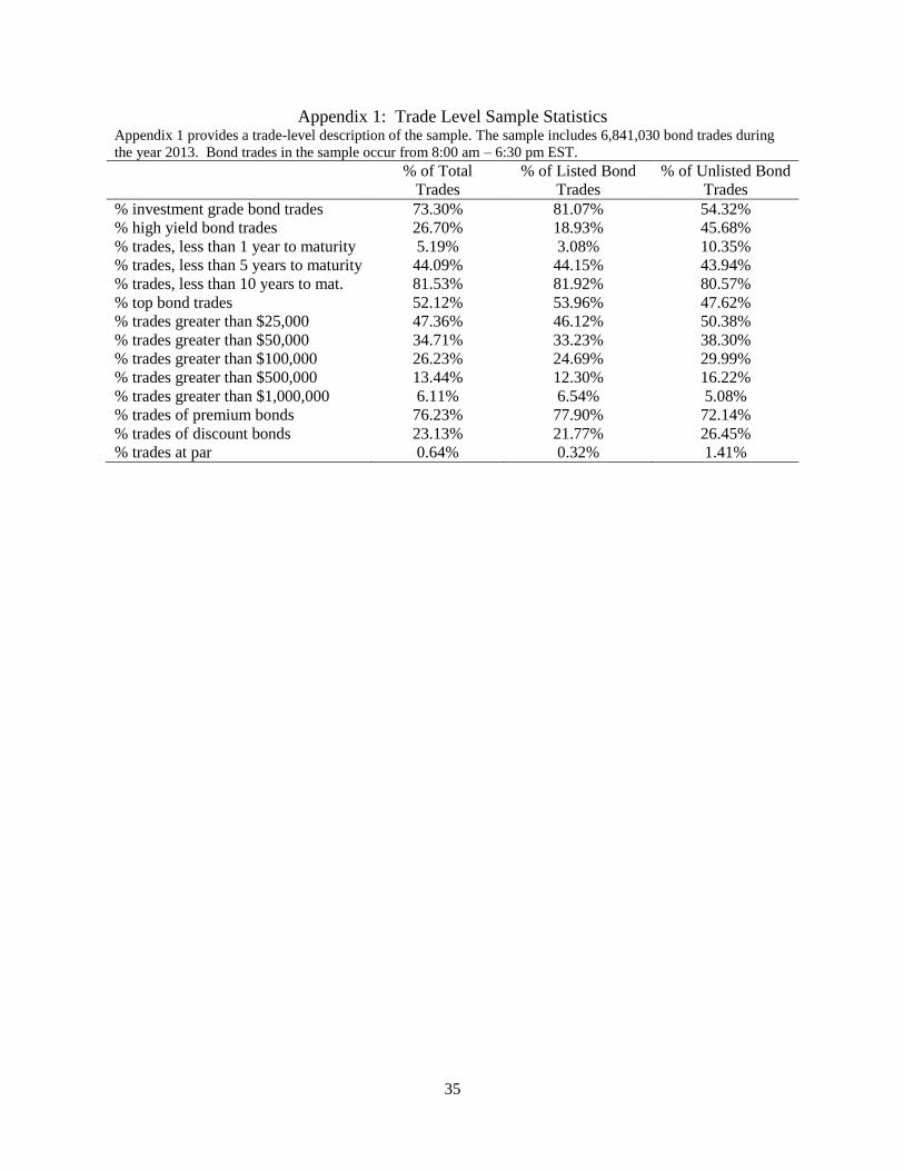
Appendix 1 provides a general overview of our sample. For the sample of trades, 73.3%

involve an investment grade bond. 81.53% of trades involve a bond with less than ten years to

maturity. Top bonds make up the majority of trades, accounting for 52.12% of all transactions.

In regards to trade size, trades greater than $25,000 account for 47.36% of trades, while trades

greater than $500,000 (institutional trades) account for only 13.44% of trades. Substantially

more trades occur in bonds priced above par value (76.23%) than bonds priced below par value

(23.13%).

Appendix 1 also shows summary statistics for listed and unlisted bonds. Unlisted bond

trades are split fairly evenly between investment grade and high yield bonds, while listed bond

trades are dominated by investment grade bonds. Investment grade bonds account for 81.07% of

listed bond trades, while high yield bonds account for just 18.93% of listed bond trades.

Roughly 40% of bond trading in both listed and unlisted bonds occurs in bonds with less than

five years to maturity, while over 80% of trades in both listed and unlisted bonds occur in bonds

with less than ten years to maturity. The percentage of institutional trades (trades greater than

$500,000) is 16.22% for unlisted bonds, while 12.30% for listed bonds. Trades greater than

$1,000,000 make up similar portions of listed and unlisted bonds (6.54% compared to 5.08%).

For both listed and unlisted bond trades, over 70% of trades involve a bond priced above its par

value.

Appendix 2 provides summary statistics for the full sample of bonds. Panel A includes

all bonds in the sample. The sample includes 12,633 bonds that trade during the 2013 calendar

year. On average, the bonds in the sample trade at 105.49% of par. The average bid-ask spread

for the full sample of bonds is $1.34. The average bond trades 4.73 times each day and transacts

over $1,500,000 in daily dollar volume with an average trade size of roughly $380,000. Panel B

10

details the summary statistics for listed bonds, and Panel C details the summary statistics for

unlisted bonds. The average listed bond trades at 109.44% of par, while the average unlisted

bond trades at 102.73% of par. Overall, listed bonds appear to trade more times than unlisted

bonds. The average listed bond trades nearly six times each day, while the average unlisted bond

trades about four times each day. Listed bonds have an average daily dollar volume of over

$2,000,000, while unlisted bonds execute an average of $1,000,000 in daily dollar volume.

Listed bonds appear to have lower spreads than unlisted bonds. Listed bonds have an average

spread of $1.17, while unlisted bonds have an average spread of $1.45. Volatility appears

similar between the listed and unlisted bonds. However, we do not test for differences between

listed and unlisted bonds in Appendix 2. We test for differences between listed and unlisted

bonds using the matched sample later in the paper.

We also provide summary statistics for the top bonds in the sample. A bond is

designated as the firm’s top bond if the bond has the most institutional trading out of all the

firm’s bonds on a given day. We classify a trade as institutional if it is greater than $500,000

(Ronen and Zhou, 2013). Throughout the sample period, 8,375 bonds are classified as the firm’s

top bond. Panel A details all top bonds in our sample. Top bonds trade, on average, at 107% of

par and transact nearly $4,500,000 in average daily volume. Top bonds trade an average of

nearly 7 times per day and have an average daily trade size of over $1,100,000. The average top

bond trade has a bid-ask spread of $0.87.

In Panel B and C, we split the top bonds into listed and unlisted bonds. Overall, listed

top bonds trade at 109% of par and transact almost $5,000,000 in daily volume. Listed top bonds

trade about seven times each day, on average, and have an average trade size of over $1,200,000.

The average spread for listed top bonds is $0.90. Unlisted top bonds trade above par as well,

11

trading at 104% of par. Unlisted top bonds appear to conduct slightly less average daily volume

than listed top bonds, but not by much. Unlisted top bonds have an average daily dollar volume

of over $4,000,000 and an average trade size of over $1,000,000. The average spread for

unlisted top bonds is $0.83.

We further explore our sample by highlighting aspects of the bond market’s intraday

trading activity.3 We show the number of average bond trades during thirty minute increments

from 8:00 am to 6:30 pm in Figure 1. We utilize 8:00 am – 6:30 pm because it is the overlapping

time between TRACE reporting hours and the NYSE bond market’s hours. The average number

of bond trades increases gradually during the day, and spike around 4:00 pm, which is when

NYSE core trading ends. In Figure 1, we also show the average number of trades by listed

versus unlisted bonds. Listed bonds seem to trade, on average, more often than unlisted bonds

trade during the trading day. Both types of bonds appear to have a trading spike around 4:00 pm,

but the increase seems more drastic for unlisted bonds. It is interesting to note that unlisted

bonds, which do not trade on the NYSE platform, experience a spike in trading at the close of

NYSE core trading. The average number of trades drops after 4:30 pm, almost reaching zero as

TRACE reporting concludes at 6:30 pm.

We continue our analysis of the bond trading day in Figure 2. Figure 2 details the

average intraday bond trade size. We again focus on 8:00 am to 6:30 pm because of the

overlapping hours between TRACE and the NYSE. Figure 2 shows that the average trade size is

fairly consistent during the trading day, but increases leading up to 5:00 pm. The average trade

size for listed and unlisted bonds begins to increase between 3:01 pm and 3:30 pm. Prior to the

3 Reference Chan, Christie, and Schultz (1995), Chung, Van Ness, and Van Ness (1999), Lee, Mucklow, and Ready

(1993), and Wood, McInish, and Ord (1985) for more information on intraday market behavior in the equities

market.

12

increase, the average trade size for listed bonds is just under $500,000, and the average trade size

for unlisted bonds is just under $300,000. After 5:00 pm, the average trade size declines. From

4:31 pm to 5:00 pm, listed bonds have an average trade size of $800,000, whereas unlisted bonds

have an average trade size of $500,000 during the same period. In Figure 3, we focus on the

average intraday dollar volume. Throughout the course of the day, the average dollar volume

appears to stay at consistent levels before spiking between 4:01 pm to 4:30 pm for listed and

unlisted bonds. Following the spike in volume, the average volume level falls to nearly zero as

TRACE reporting concludes.

13

RESULTS

Listed bonds can trade on the NYSE or through the various bond trading platforms that

report trades to TRACE. However, there is potential for execution quality and liquidity

differences to exist among the trading venues. Previous research on equities documents

substantial differences between trading venues. For example, Huang and Stoll (1996) find that

execution costs are larger for a sample of NASDAQ stocks than for a sample of NYSE stocks;

Bessembinder (1999, 2003) shows that NASDAQ stocks have higher trading costs than NYSE

stocks following both tick size reductions and changes in order handling rules. We compare a

sample of listed bonds that trade on both the NYSE and TRACE venues during our time period.

Appendix 3 Panel A provides statistics on the sample of listed bonds. Overall, there is a

slight statistical difference in the prices of listed bond trades on the NYSE and listed bond trades

on the TRACE venues. However, the difference is minimal ($0.32), which is not overly

surprising; any difference in price between the trading venues indicates an arbitrage opportunity

for listed bonds. On average, listed bond trades on the NYSE are less frequent, have a lower

trade size, and hence, have a lower daily dollar volume than TRACE venue trades. NYSE trades

are also more volatile than TRACE trades, but the difference in volatility is small (0.18) and

significant only at the ten percent level. Listed bond trades on a TRACE venue have lower

spreads than listed bond trades on the NYSE. NYSE trades have an average spread of $1.23,

while TRACE trades have an average spread of $1.04. The difference in the spreads is

significant at the one percent level. The spread differential could be driven by many factors. For

one, TRACE may offer better execution quality and liquidity for bond traders. Or, the

14

differential in spread could simply be driven by the fact that larger trades execute via TRACE,

and there is an inverse relation between bond trade size and trading cost. Edwards, Harris, and

Piwowar (2007), Harris and Piwowar (2006), and Goldstein, Hotchkiss, and Sirri (2007)

document an inverse relation between trade size and trading cost in the bond market.

Appendix 3 Panel B provides statistics on the listed top bonds. The top bonds are the

bonds with the most institutional dollar volume for each firm (Ronen and Zhou, 2013). There is

no difference in the price of top bond trades on the NYSE and TRACE venues. Top bonds trade

more times each day, have higher daily dollar volume, and have larger average trade sizes on the

TRACE venues than top bond trades on the NYSE. TRACE trades in top bonds have lower

spreads than NYSE trades in top bonds. NYSE top bond trades have an average bid-ask spread

of $1.13, while TRACE top bond trades have an average spread of $0.92. The $0.21 difference

is significant at the one percent level.

An important aspect of market quality is the bid-ask spread. In this section, we focus on

the spread. We note in the last section that listed bond trades appear to have lower spreads and

that TRACE spreads are lower for listed bonds than NYSE spreads. Model 1 utilizes the full

sample of bond trades, whereas Model 2 (Model 3) utilizes listed (unlisted) bond trades. We

estimate the following spread regression model:

Bid Ask Spread = β0 + β1Dollar Volume + β2Number of Trades + β3Trade Size +

β4Volatility + β5Top Bond + β6Years to Maturity + β7Firm Size + β8Investment Grade

+ β9TRACE Execution + β10Listed + ε

Appendix 4 provides bid-ask spread regression results. Our main variable of interest in

the bid-ask spread regressions is the Listed variable. The Listed variable is equal to one if a bond

is listed. We find a negative relation between bond listing and the bid-ask spread. The

15

magnitude of the coefficient indicates that listed bond spreads are $0.14 lower than unlisted bond

spreads. The negative relation between bond listing and spread provides evidence that bond

listing provides some value, in the form of reduced trading costs, to bond traders.

In addition to bond listing variable, we are also interested in the Top Bond variable in

Models 1, 2, and 3. Focusing on the Top Bond variable allows us to see the relation between

institutional trading activity and the bond bid-ask spread, given that top bonds are the bonds with

the most institutional trading volume. We follow Ronen and Zhou (2013) in designating the top

bond as the bond with the most institutional trading dollar volume for each firm, with

institutional trading measured as trades exceeding $500,000. The Top Bond variable is equal to

one if the bond has the most institutional trading for each firm’s bonds on a given day.

The Top Bond coefficient is negative in all three regression models. For the full sample

of bonds, top bonds spreads are $0.42 lower than the spreads of other bonds. For listed bonds

(Model 2), top bonds have spreads that are $0.33 lower than other bonds, and unlisted top bonds

(Model 3) have spreads that are $0.59 lower than other bonds. Although we do not test for

differences in the coefficients here, it appears that being the firm’s top bond has more value for

unlisted bonds, given the magnitude of the coefficient. The control variables in the regressions

conform to general expectations. Similar to Edwards, Harris, and Piwowar (2007), the

regression models show that bonds with more time to maturity have larger spreads. The larger

spread for bonds with longer maturities is likely driven by potential interest rate risk.

Additionally, we find that investment grade bonds have lower bid-ask spreads. Edwards, Harris,

and Piwowar (2007) also document a negative relation between bond spread and credit quality.

We estimate the bid-ask spread regressions for the top bonds in our sample to shed

further light on the relation between institutional trading and spread since top bonds, by design,

16

are the bonds with the most institutional trading. While we document a negative relation

between bond listing and the bid-ask spread in the full sample of bonds, we find the opposite in

the top bond sample. Listed top bond trades have spreads that are $0.08 larger than unlisted top

bond trades. Otherwise, the control variables in the top bond regressions yield coefficients

similar to the full sample bid-ask spread regressions. We find that volatility and time to maturity

have a positive relation with the bid-ask spread, while investment grade has a negative relation

with the spread.

We are also interested in the intraday pattern of the bond bid-ask spread. The U-shaped

intraday spread pattern in equities is well documented (see McInish and Wood, 1992), but less is

known about the intraday pattern of bond spreads. In Figure 4, we show the average bond spread

throughout the trading day. Like previous figures, we utilize 8:00 am to 6:30 pm because it is

the overlapping time between the NYSE trading hours and TRACE reporting hours. The Figure

shows that spreads steadily increase during the morning trading hours, before leveling off

between 10:01 am to 10:30 am. Spreads appear to increase between 3:31 pm to 4:00 pm before

peaking in the following half hour. The spike in spreads seems the most drastic for unlisted

bonds. However, following the increase, spreads fall sharply leading up to the end of TRACE

reporting at 6:30 pm.

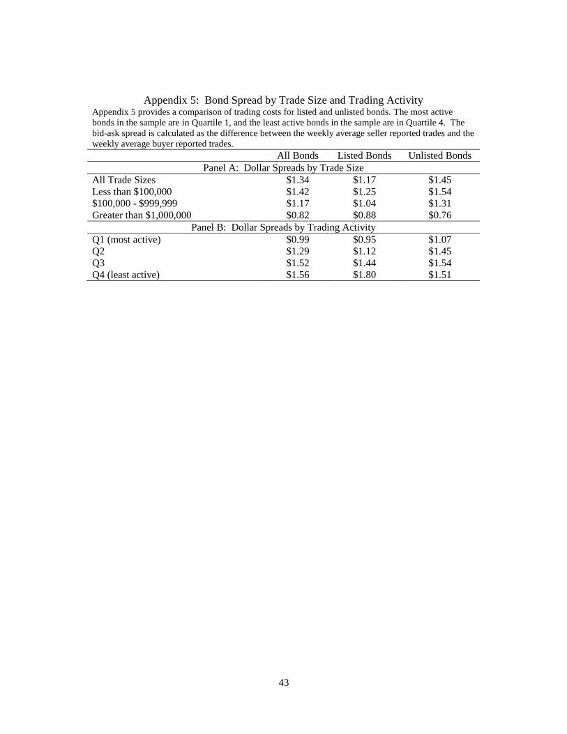
Previous research documents an inverse relation between bond trade size and bond spread

(Edwards, Harris, and Piwowar, 2007). We see if this relation holds for both listed and unlisted

bonds in Appendix 5. In Panel A, we detail the average spread by trade size for the full sample

of bonds, for listed bonds, and for unlisted bonds. Our findings are similar to previous work by

Goldstein, Hotchkiss, and Sirri (2007).4 We find a consistent negative relation between trade

4 Other research documents the inverse relation between bond trade size and bid-ask spread, including Edwards,

Harris, and Piwowar (2007) and Harris and Piwowar (2006).

17

size and bond spread for the full sample of bonds, for listed bonds, and for unlisted bonds.

While we test for differences between listed and unlisted bonds using the matched sample later

in the paper, it appears in Appendix 5 that listed bonds have lower spreads than unlisted bonds,

on average, for the full sample, small sized trades, and medium trades.

In Panel B, Quartile 1 includes the most active bonds in our sample, and Quartile 4

includes the least active bonds in our sample. Panel B shows that bond spread and trading

activity have an inverse relation. The most active bonds appear to have lower spreads ($0.99)

than the least active bonds ($1.56). The same relation holds for listed and unlisted bonds. The

most active listed bonds have an average spread of $0.95, and the least active listed bonds have

an average spread of $1.80. The range of spread from the most active to the least active is not as

drastic for unlisted bonds, however. The most active listed bonds have an average spread of

$1.07, and the least active unlisted bonds have an average spread of $1.51.

We also examine whether listing influences the price efficiency of bonds. O’Hara and

Ye (2011) utilize volatility as a measure of price efficiency in equities, and Bennet and Wei

(2006) show that volatility decreases for stocks that change their listing venue from NASDAQ to

the NYSE. We measure volatility following Downing and Zhang (2004) using the following

equation:

100

Pricet(Pricet

Max − PricetMin)

We use the following regression model to estimate volatility:

Volatility = β0 + β1Dollar Volume + β2Number of Trades + β3Trade Size + β4Top Bond

+ β5Years to Maturity + β6Firm Size + β7Investment Grade + β8TRACE Execution

+ β9Listed + ε

18

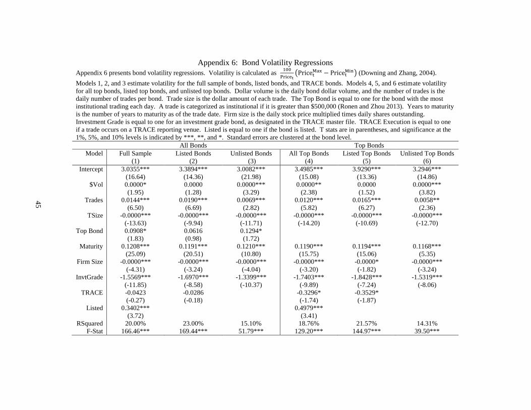
We present our bond volatility regression results in Appendix 6. Our main variable of

interest is the Listed variable. The Listed variable is equal to one if a bond is listed. We find that

listed bonds are more volatile than unlisted bonds and document a positive relation between bond

listing and volatility in Model 1. The Listed coefficient is significant at the one percent level.

The positive relation between bond listing and volatility conflicts with our expectations, given

the predictions that exchange listing positively influences price efficiency. There are two

possible explanations for the positive relation between bond listing and volatility. One

explanation is trading activity. We document earlier that listed bonds trade more than unlisted

bonds, and more trading activity leads to higher volatility. The second explanation is simply the

structure of the bond market. The bond market is fragmented, and we know that fragmentation

positively influences volatility (O’Hara and Ye, 2011).

The top bond variable is equal to one if a bond has the most institutional trading for each

firm on a given trading day; following Ronen and Zhou (2013), a trade is classified as

institutional if it is greater than $500,000. The Top Bond indicator variable is also of interest

because it helps detail the relation between bond volatility and institutional trading activity since

the top bond is the bond with the most institutional trading activity. We find (weak) evidence

that top bonds are more volatile than non-top bonds. We document a weak positive relation

between top bond status and volatility for the full sample of bonds and the sample of unlisted

bonds. However, we find no relation between top bond status and volatility for the sample of

listed bonds. The control variables in the volatility regressions conform to expectations. We

find that bonds with more time to maturity have higher levels of volatility than bonds with less

time to maturity, and bonds with investment grade ratings have lower levels of volatility that

non-investment grade bonds.

19

Next, we study volatility for top bonds to further understand the relation between

institutional trading and volatility. In Model 4, we find evidence that listed top bonds are more

volatile than unlisted top bonds. The positive relation between bond listing and volatility for top

bonds is somewhat puzzling, given that we find no relation between top bond status and

volatility for listed bonds in Model 2. In Figure 5, we further detail intraday bond volatility. We

utilize trades that occur between 8:00 am and 6:30 pm. Generally, the figure shows that

volatility increases gradually between 8:01 am and 10:00 am before leveling off to a consistent

level during the majority of the trading day. Volatility spikes between 4:01 pm and 4:30 pm, and

then continues to decrease during the remainder of trading.

Kadlec and McConnell (1994) find that exchange (NYSE) listing leads to an increase in

the number of institutional shareholders in a firm. Specifically, they show that institutional

holdings increase by 27% for listed firms following earnings announcements. We study bond

trading on earnings announcement and non-announcement days. Appendix 7 presents the

preliminary results comparing earnings announcement days to non-earnings announcements

days5. Panel A includes all bonds in the sample. Panel B (Panel C) includes listed (unlisted)

bonds. For the full sample of bonds, we document a slight increase in price on the earnings

announcement day. We also find a corresponding increase in dollar volume and the number of

trades executed on announcement days. Dollar volume increases by nearly $200,000 on the

announcement day, while the number of trades increases only marginally.

In Panel B, we focus on listed bonds. We find that listed bond prices increase on

announcement day, along with overall listed dollar volume. The average listed bond is priced at

5 We replicate Appendix 7 for only top bonds, and we find results that are qualitatively similar to those presented in

Appendix 7.

20

108.70% of par on announcement days, while the average listed bond is priced at 108.51% of par

on non-announcement days. Average dollar volume increases by over $150,000 for listed bonds

on announcement day, but we find no significant change in either trade size or the number of

trade executions on announcement days (compared to non-announcement days). Panel C

provides results for unlisted bonds, and the results are similar to those shown in Panel A. We

document significant increases in bond price, dollar volume, and the number of trades for

unlisted bonds on announcement days.

Kadlec and McConnell (1994) focus on the relation between exchange listing and

institutional shareholders. We expand their study by focusing on institutional sized bond trading

activity on earnings announcement and non-announcement days. We follow Ronen and Zhou

(2013) and classify a trade as institutional if the trade size is greater than $500,000. We provide

the results of our analysis6 in Appendix 8. We focus on the price, trade size, dollar volume,

number of trades, percentage dollar volume, and the percentage number of trades in Appendix 8.

The percentage volume (percentage trades) is the portion of volume (trading activity) for which

institutional-sized trades account. For all bonds, we find an increase in the price at which

institutional-sized trades execute and a slight increase in the average institutional trade size on

earnings announcements days. Institutions purchase bonds priced at 106.90% of par on

announcement days, compared to 106.63% of par on non-announcement days. The average trade

size increases by nearly $40,000 on announcement days.

We find that institutional dollar volume declines by over $1,000,000 on announcement

days, along with the number of institutional sized trades. Perhaps the most striking results in

Panel A, however, involve the percentage volume and the percentage number of trades for

6 We replicate Appendix 8 for only top bonds, and we find results qualitatively similar to those presented in

Appendix 8.

21

institutional sized trades. On non-announcement days, institutions account for 78.31% of dollar

volume. On announcement days, this percentage falls to just 43.84%. The results are similar for

the percentage of trades, only not as drastic. On non-announcement days, institution sized trades

account for nearly 30% of all trades. Yet, these large trades make up only 21% of trades on

announcement days. The results in Panel A could indicate one of two things. First, the results

may simply mean that institutions pull back from the market (and from possible informed

trading) on earnings announcements days. Or, it is possible that institutions trade prior to the

announcement.

We further divide the sample into listed bonds (Panel B) and unlisted bonds (Panel C).

According to listing theory and Kadlec and McConnell (1994), the level of institutional activity

should increase with an earnings announcement. We find the opposite in terms of activity,

however. We find lower levels of institutional dollar volume and fewer institutional sized trades

on earnings announcements days. We also document a substantial drop in the percentage dollar

volume and percentage number of trades for large, institution sized trades. Institutions account

for 86.45% of dollar volume on non-announcement days, but only 47.64% of volume on

announcement days. The same is true for the percentage of trades; institution sized trades

account for 9.9% fewer trades on announcement days than they do on non-announcement days.

The results for unlisted bonds are similar to those shown in Panel A.

In Appendix 8, we focus on institutional-sized trading activity. We provide results for

our study of smaller, retail sized trades in Appendix 9. Panel A includes all bonds in the sample.

Panel B (Panel C) includes listed (unlisted) bonds7. Overall, retail sized trades have lower dollar

7 We replicate Appendix 9 for only top bonds, and we find results that are qualitatively similar to those presented in

Appendix 9.

22

volume on announcement days than on non-announcement days. In contrast to institutional-

sized trades, though, retail trades account for both a larger percentage of volume and a larger

percentage of trades on announcement days than on non-announcement days. Retail trades

account for just 21.69% of dollar volume on non-announcement days, but increase their portion

of volume to 56.16% on announcement days. The increase in the percentage number of trades is

less dramatic, but still significant. Retail trades account for 70.39% of trades on non-

announcement days, increasing to 78.94% on announcement days.

We divide the sample into listed and unlisted bonds in Panels B and C. We find

(generally) the same results for listed and unlisted bonds. The most striking results are, again,

the differences in percentage volume and percentage number of trades on earnings and non-

earnings announcement days. For listed bonds, retail trades account for only 13.55% of volume

on non-earnings announcement days. However, retail trades account for over 50% of volume on

announcement days. The same is true for the unlisted bonds. Retail trades make up 33.54% of

volume on non-announcement days, but make up over 60% of volume on announcement days.

For listed (unlisted) bonds, retail traders execute 9.9% (6.61%) more trades on announcement

days than non-announcement days. Overall, we find no (strong) evidence that institutional

activity increases due to a bond’s listing status.

We repeat the previous analysis for a matched sample of listed and unlisted bonds. Our

matching procedure closely follows Boehmer (2005)8. We match each listed bond to an unlisted

bond using four bond specific characteristics and one firm specific characteristic. We use the

following bond characteristics to match the sample: price, daily dollar volume, investment

8 We match on a one-to-one basis like Boehmer (2005). However, our matching procedure does differ slightly from

his. He matches the sample used the time period preceding his analysis, while we match our sample based on the

bond average price, daily dollar volume, investment quality, years to maturity, and firm market capitalization during

our 2013 time period. For an in-depth description of the propensity score matching procedure, see Boehmer (2005).

23

quality, and years to maturity. The firm specific characteristic is daily market capitalization. We

then calculate a propensity score based on the matching characteristics, and we delete matches

with propensity score differences greater than 0.019. The final results of the match yield 2,086

pairs of bonds with 2,706,274 bond trades. Appendix 10 provides summary statistics on the

matching properties of the sample. Panel A shows summary statistics of the matched sample.

Overall, bonds in the matched sample trade at 106% of par and transact nearly $2,000,000 each

day in average dollar volume. The bonds in the matched sample have, on average, eight and a

half years to maturity. Panel B provides differences between the listed bond sample and the

unlisted bond sample. Overall, we find no significant differences between the listed sample and

the unlisted sample, and interpret the lack of difference as evidence of a well-matched sample.

To compare NYSE and TRACE trades in listed bonds, we utilize the listed bond portion

of our matched sample. The results are presented in Appendix 11. Panel A provides differences

for the full matched sample, and Panel B provides differences for the sample of top bonds. A

bond is the firm’s top bond if it has the most institutional trading (measured as the number of

trades greater than $500,000) for the firm on a given trading day. For the matched sample, there

is little price difference between trades on the NYSE and TRACE. We document differences in

the average daily dollar volume, the average number of trades, the average trade size, the average

volatility, and the average bid-ask spread, however, for trades that execute on the NYSE and

trades that )execute on the TRACE reporting venues. We find that TRACE trades typically have

a larger average trade size, a larger number of trades, and larger average daily dollar volume than

NYSE trades. We also find that listed bond trades that execute on the NYSE have larger spreads

9 Boehmer (2005) refers to matching differences as “matching errors.” Pairwise propensity score differences are

calculated using the following equation: D𝑥𝑦 = |Price𝑥

Pricey| + |

DollVol𝑥

DollVol𝑦| + |

Grade𝑥

Grade𝑦| + |

Mat𝑥

Mat𝑦| + |

MktCap𝑥

MktCap𝑦|.

24

than listed bond trades that execute via TRACE ($1.43 compared to $1.18). Lastly, we find that

NYSE trades have greater volatility than TRACE trades.

In Panel B, we focus on top bonds. Similar to the results in Panel A, we find no

difference in bond price for trades that execute on the NYSE and trades that execute via TRACE.

However, we document differences in the average daily dollar volume, the average number of

trades, the average trade size, the average volatility, and the average bid-ask spread.

Specifically, top bond trades that execute via the NYSE have lower daily dollar volume, fewer

daily trades, and smaller trade size than top bond trades that execute via TRACE venues. We

also find that NYSE trades in top bonds are more volatile than TRACE trades in top bonds, and

that NYSE top bond trades have larger spreads ($1.36) than TRACE top bond trades ($1.07).

We replicate the bond bid-ask spread analysis for the matched sample. Appendix 12

provides spread regression results. Model 1 includes the matched sample, and Model 2 (Model

3) breaks the matched sample into listed and unlisted bonds. The p-value is for the difference in

the listed and unlisted coefficients. Similar to the full sample, our main variable of interest is the

Listed variable. The Listed variable is equal to one if the bond is listed. In Model 1, we

document a negative relation between bond listing and the bid-ask spread (we also document a

negative relation between bond listing and spread in the full sample). Consistent with the full

sample of bonds, we find that top bonds have lower spreads than non-top bonds in the matched

sample. The negative relation holds for the full matched sample, and for both listed and unlisted

bonds. The control variables are as expected (and similar to our findings in the full sample and

also to Edwards, Harris, and Piwowar, (2007)). Specifically, we find that investment grade

bonds have lower spreads than non-investment grade bonds, and bonds with more time to

maturity have higher spreads than bonds that are closer to maturity. Next, we focus on the bid-

25

ask spread for top bonds in the matched sample. Model 4 provides results for the top bonds

included in the matched sample, and Models 5 and 6 are for listed and unlisted bonds. Our main

variable of interest is the Listed variable in Model 4. We find a positive relation between bond

listing and the top bond bid-ask spread. Specifically, listed top bond spreads are $0.11 more than

unlisted top bond spreads.

To further our study of the bond bid-ask spread, we also focus on the relation between

spread and trade size. Edwards, Harris, and Piwowar (2007) find a negative relation between

trade size and the bid-ask spread. To see if the inverse relation between spread and trade size

holds in our sample, we break the sample into small, medium, and large sized trades in Appendix

13. Appendix 13 Panel A presents the results regarding bond trade size and the bid-ask spread.

Consistent with prior literature, we document an inverse relation between trade size and bond

bid-ask spread. Listed bonds have lower spreads than unlisted bonds for small and medium sized

trades, while unlisted bonds have lower spreads for large trades. The difference between the

listed and unlisted bond spread is significant for all trade categories.

In Panel B, we focus on the relation between trading activity and the bond bid-ask spread.

Quartile 1 consists of the most active bonds over the course of the sample period, and Quartile 4

consists of the least active bonds over the course of the sample period. For listed bonds, we find

that the most active bonds have the lowest bid-ask spread at $0.98 (Quartile 1) and $0.95

(Quartile 2), and the least active bonds have the largest bid-ask spread at $1.47. We find a direct

relation between trading activity and bond spread for unlisted bonds, with the most active

unlisted bonds having lower spreads than the least active unlisted bonds. We also compare the

spreads of listed and unlisted bonds. Overall, we find a significant difference in listed and

unlisted bond spreads in Quartile 2, but not for any of the other quartiles.

26

Lastly, we follow O’Hara and Ye (2011) and focus on bond volatility as a measure of

price efficiency. Appendix 14 provides results for bond volatility regressions for the matched

sample of bonds. The p-value is for the difference between listed and unlisted bond regression

coefficients. Our main variable of interest is the Listed variable, which is equal to one if the

bond is listed. We find a positive relation between bond listing and volatility, which is consistent

with our findings in the full sample. We are also interested in the top bond variable. We find a

significant and positive relation between top bond status and volatility for the full matched

sample, and for the listed bonds in the matched sample. However, we do not find a significant

relation between top bond status and volatility for the unlisted bonds. We further explore the

relation between top bonds and volatility in regression Models 4, 5, and 6. In Model 4, we

document a positive relation between bond listing and volatility for the top bonds included in the

matched sample.

27

CONCLUSION

We study the impact of bond listing in the corporate bond market. Previous theoretical

research by Merton (1987) documents an advantage to exchange listing in the equities market;

specifically, Merton details that exchange listing in the equities market can lead to an increase in

investor recognition and improved liquidity for the firm. Kadlec and McConnell (1994) show

empirically that listing leads to an increase in institutional shareholders for the firm, while much

research documents improved liquidity for NYSE stocks and NYSE trades (Huang and Stoll, 1996;

Bennet and Wei, 2006; and Bessembinder and Kaufman, 1997).

While the above mentioned research focuses on equities, we focus on the bond market in

our research. Studying the impact of exchange listing in the bond market is valuable for several

reasons. First, much of the research on listing focuses on stocks, which are highly liquid assets,

especially when compared to the bond market. In our sample, the average corporate bond trades

just 5 times, which is substantially less than the average stock in the equity market. Bonds are also

costly to trade. Documenting a market quality or trading advantage for listed (or unlisted) bonds

is beneficial for traders. It is also possible that bond listing serves a signal to bond traders, similar

to the firm paying dividends or beating earnings. Given the well-documented informational

inefficiencies in the bond market (Kwan, 1996; Downing, Underwood, and Xing, 2009), it could

be important for investors to obtain information based on bond listing.

First, we document the qualities of listed bonds. Our findings show that listed bonds tend

to have lower spreads and a greater number of trades than unlisted bonds. We also find that

listed bonds have greater volatility than unlisted bonds. Second, we focus on the bond bid-ask

28

spread. We show that listed bonds have lower spreads than unlisted bonds. Listed bond spreads

are $0.14 lower than unlisted bond spreads. Additionally, listed top bond spreads are $0.33

lower than the spreads of other bonds. However, we also find that NYSE bond trades in listed

bonds have larger bid-ask spreads than TRACE trades in listed bonds. We find that listed top

bond trades have larger spreads than unlisted top bond trades. Third, we focus on volatility and

price efficiency for listed and unlisted bonds. We find that listed bonds are more volatile than

unlisted bonds. Overall, there appears to be a market quality advantage to bond listing.

29

REFERENCES

30

Alexander, Gordon, Amy Edwards, and Michael Ferri, 2000. The Determinants of Trading

Volume of High Yield Corporate Bonds. Journal of Financial Markets 3, 177-204.

Barclay, Michael, and Terrence Hendershott, 2003. Price Discovery and Trading After Hours.

Review of Financial Studies 16, 1041-1073.

Baruch, Shmuel, and Gideon Saar, 2009. Asset Returns and the Listing Choice of Firms.

Review of Financial Studies 22, 2239-2274.

Bennet, Paul, and Li Wei, 2006. Market Structure, Fragmentation, and Market Quality. Journal

of Financial Markets 9, 49-78.

Bessembinder, Hendrik, and Herbert Kaufman, 1997. A Comparison of Trade Execution Costs

for NYSE and NASDAQ Listed Stocks. Journal of Financial and Quantitative Analysis 32,

287-310.

Bessembinder, Hendrik, 2003. Quote-Based Competition and Trade Execution Costs in NYSE-

listed Stocks. Journal of Financial Economics 70, 385-422.

Bessembinder, Hendrik, William Maxwell, and Kumar Venkataraman, 2006. Market

Transparency, Liquidity Externalities, and Institutional Trading Costs in Corporate Bonds.

Journal of Financial Economics 82, 251-288.

Bessembinder, Hendrik, Kathleen Kahle, William Maxwell, and Danielle Xu, 2009. Measuring

Abnormal Bond Performance. Review of Financial Studies 22, 4219-4258.

Bhattacharya, Sudipto, 1979. Imperfect Information, Dividend Policy, and The Bird in the Hand

Fallacy. Bell Journal of Economics 10, 259-270.

Boehmer, Ekkehart, 2005. Dimensions of Execution Quality: Recent Evidence for US Equity

Markets. Journal of Financial Economics 78, 553-582.

Chan, K.C., William Christie, and Paul Schultz, 1995. Market Structure and the Intraday Pattern

of Bid-Ask Spreads for NASDAQ Securities. Journal of Business 1, 35-60.

Chung, Kee, Bonnie Van Ness, and Robert Van Ness, 1999. Limit Orders and the Bid-Ask

Spread. Journal of Financial Economics 53, 255-287.

Downing, Chris, Shane Underwood, and Yuhang Xing, 2009. The Relative Informational

Efficiency of Stocks and Bonds: An Intraday Analysis. Journal of Financial and Quantitative

Analysis 44, 1081-1102.

Downing, Chris, and Frank Zhang, 2004. Trading Activity and Price Volatility in the Municipal

Bond Market. Journal of Finance 2, 899-931.

31

Ederington, Louis, and Lisa Yang, 2013. Bond Market Reaction to Earnings Surprises and Post-

Earnings Announcement Drift. Working paper.

Edwards, Amy, Lawrence Harris, and Michael Piwowar, 2007. Corporate Bond Market

Transaction Costs and Transparency. Journal of Finance 62, 1421-1451.

Fuller, Kathleen, and Michael Goldstein, 2011. Do Dividends Matter More in Declining

Markets?. Journal of Corporate Finance 17, 457-473.

Goldstein, Michael, Edith Hotchkiss, and Erik Sirri, 2007. Transparency and Liquidity: A

Controlled Experiment on Corporate Bonds. Review of Financial Studies 20, 235-273.

Harris, Lawrence, and Michael Piwowar, 2006. Secondary Trading Costs in the Municipal Bond

Market. Journal of Finance 61, 1361-1397.

Heidle, Hans, and Roger Huang, 1994. Information Based Trading in Dealer and Auction

Markets: An Analysis of Exchange Listings. Journal of Financial and Quantitative Analysis 37,

391-424.

Huang, Roger, and Hans Stoll, 1996. Dealer versus Auction Markets: A Paired Comparison of

Execution Costs on NASDAQ and the NYSE. Journal of Financial Economics 41, 313-357.

Jiang, Christine, Tanakorn Likitapiwait, and Thomas McInish, 2012. Information Content of

Earnings Announcements: Evidence from After-Hours Trading. Journal of Financial and

Quantitative Analysis 47, 1303-1330.

Kadlec, Gregory, and John McConnell, 1994. The Effect of Market Segmentation and Illiquidity

on Asset Prices: Evidence from Exchange Listings. Journal of Finance 49, 611-636.

Kwan, Simon, 1996. Firm-Specific Information and the Correlation Between Individual Stocks

and Bonds. Journal of Financial Economics 40, 63-80.

Lee, Charles, Belinda Mucklow, and Mark Ready, 1993. Spreads, Depth, and the Impacts of

Earnings Information: An Intraday Analysis. Review of Financial Studies 2, 345-374.

Merton, Robert, 1987. Presidential Address: A Simple Model of Capital Market Equilibrium

with Incomplete Information. Journal of Finance 42, 483-510.

Nissim, Doron, and Amir Ziv, 2001. Dividend Changes and Future Profitability. Journal of

Finance 56, 2111-2133.

O’Hara, Maureen, and Mao Ye, 2011. Is Market Fragmentation Harming Market Quality?.

Journal of Financial Economics 100, 459-474.

Ronen, Tavy, and Xing Zhou, 2013. Trade and Information in the Corporate Bond Market.

Journal of Financial Markets 16, 61-103.

32

Sanger, Gary, and John McConnell, 1986. Stock Exchange Listing, Firm Value, and Security

Market Efficiency: The Impact of the NASDAQ. Journal of Financial and Quantitative

Analysis 21, 1-25.

Wood, Robert, Thomas McInish, and J. Keith Ord, 1985. An Investigation of Transactions Data

for NYSE Stocks. Journal of Finance 3, 723-739.

33

APPENDICES

34

APPENDIX 1: TRADE LEVEL SAMPLE STATISTICS

35

Appendix 1: Trade Level Sample Statistics Appendix 1 provides a trade-level description of the sample. The sample includes 6,841,030 bond trades during

the year 2013. Bond trades in the sample occur from 8:00 am – 6:30 pm EST.

% of Total

Trades

% of Listed Bond

Trades

% of Unlisted Bond

Trades

% investment grade bond trades

% high yield bond trades

% trades, less than 1 year to maturity

% trades, less than 5 years to maturity

% trades, less than 10 years to mat.

% top bond trades

% trades greater than $25,000

% trades greater than $50,000

% trades greater than $100,000

% trades greater than $500,000

% trades greater than $1,000,000

% trades of premium bonds

% trades of discount bonds

% trades at par

73.30%

26.70%

5.19%

44.09%

81.53%

52.12%

47.36%

34.71%

26.23%

13.44%

6.11%

76.23%

23.13%

0.64%

81.07%

18.93%

3.08%

44.15%

81.92%

53.96%

46.12%

33.23%

24.69%

12.30%

6.54%

77.90%

21.77%

0.32%

54.32%

45.68%

10.35%

43.94%

80.57%

47.62%

50.38%

38.30%

29.99%

16.22%

5.08%

72.14%

26.45%

1.41%

36

APPENDIX 2: SAMPLE SUMMARY STATISTICS, BOND LEVEL

Appendix 2: Sample Summary Statistics, Bond Level Appendix 2 provides summary statistics for the sample. The sample includes 6,841,030 bond trades during the year 2013. Bond trades in the sample occur from

8:00 am – 6:30 pm EST. The top bond is the bond with the most daily institutional trading using a $500,000 trade size (Ronen and Zhou, 2013). Price is the

percentage of par. Dollar volume is the daily dollar volume for each bond, and the number of trades is the daily number of trades for each bond. Trade size is the

average daily dollar trade size. Volatility is calculated as 100

Pricet(Pricet

Max − PricetMin) (Downing and Zhang, 2004). The bid-ask spread is calculated as the

difference between the weekly average seller reported trades and the weekly average buyer reported trades.

All Bonds Top Bonds

N Mean Minimum Maximum N Mean Minimum Maximum

Panel A: Full Sample

Price

$Vol

Trades

TSize

Volatility

Spread

12,633

12,633

12,633

12,633

12,633

12,633

$105.49

$1,559,216.10

4.73

$381,336.29

2.15

$1.34

$25.16

$2,000.00

1.09

$1,000.00

0.00

0.00

$276.92

$82,374,604.17

80.00

$5,000,000.00

20.21

$9.66

8,375

8,375

8,375

8,375

8,375

8,375

$107.46

$4,464,537.46

6.93

$1,176,863.39

1.99

$0.87

$25.00

$502,000.00

1.00

$38,148.15

0.00

$0.00

$288.81

$55,385,555.56

241.00

$5,000,000.00

19.77

$9.31

Panel B: Listed Bonds

Price

$Vol

Trades

TSize

Volatility

Spread

5,199

5,199

5,199

5,199

5,199

5,199

$109.44

$2,192,225.57

5.71

$488,023.17

2.17

$1.17

$47.83

$8,400.00

1.14

$2,733.33

0.01

$0.01

$263.62

$82,374,604.17

69.47

$4,666,666.67

20.21

$9.66

4,725

4,725

4,725

4,725

4,725

4,725

$109.37

$4,819,489.08

7.16

$1,231,376.63

2.08

$0.90

$48.68

$538,000.00

1.00

$47,727.37

0.04

$0.00

$263.62

$84,113,106.38

109.33

$5,000,000.00

31.32

$7.60

Panel C: Unlisted Bonds

Price

$Vol

Trades

TSize

Volatility

Spread

7,434

7,434

7,434

7,434

7,434

7,434

$102.73

$1,116,518.19

4.04

$306,724.36

2.14

$1.45

$25.16

$2,000.00

1.09

$1,000.00

0.00

0.00

$276.92

$55,385,555.56

80.00

$5,000,000.00

15.22

$9.63

3,650

3,650

3,650

3,650

3,650

3,650

$104.98

$4,005,045.29

6.64

$1,106,294.87

1.88

$0.83

$25.00

$502,000.00

1.00

$38,148.15

0.00

$0.00

$288.81

$55,385,555.56

241.00

$5,000,000.00

19.77

$9.31

37

38

APPENDIX 3: A COMPARISON OF NYSE AND TRACE TRADES

39

Appendix 3: A Comparison of NYSE and TRACE Trades Appendix 3 compares the average summary statistics for listed bond trades that execute on the NYSE and listed

bond trades that execute on TRACE. The top bond is the bond with the most institutional trading each day using

a $500,000 trade size (Ronen and Zhou, 2013). Price is the percentage of par. Dollar volume is the daily dollar

volume for each bond on each trading venue (TRACE and the NYSE), and the number of trades is the daily

number of trades for each bond on each trading venue (TRACE and the NYSE). Trade size is the average daily

dollar trade size on each venue (TRACE and the NYSE). Volatility is calculated as 100

Pricet(Pricet

Max − PricetMin)

(Downing and Zhang, 2004). The bid-ask spread is calculated as the difference between the weekly average

seller reported trades and the weekly average buyer reported trades. Significance is indicated at the 1%, 5%, and

10% levels by ***, **, and *.

NYSE Trace Difference T-Stat

Panel A: All Bonds

Price

$Vol

Trades

TSize

Volatility

Spread

$105.84

$10,094.86

1.27

$8,113.32

3.51

$1.23

$105.52

$4,090,728.88

13.66

$386,042.66

3.33

$1.04

$0.32*

-$4,080,634.02***

-12.40***

-$377,929.34***

0.18*

$0.19***

1.87

-17.87

-22.21

-25.50

1.85

4.66

Panel B: Top Bonds

Price

$Vol

Trades

TSize

Volatility

Spread

$105.08

$12,028.33

1.27

$9,587.53

4.01

$1.13

$104.93

$7,106,201.08

18.15

$611,423.91

3.59

$0.92

$0.16

-$7,094,172.76***

-16.88***

-$601,836.38***

0.42***

$0.21***

0.73

-21.91

-20.14

-25.83

3.05

4.24

40

APPENDIX 4: BOND SPREAD REGRESSIONS

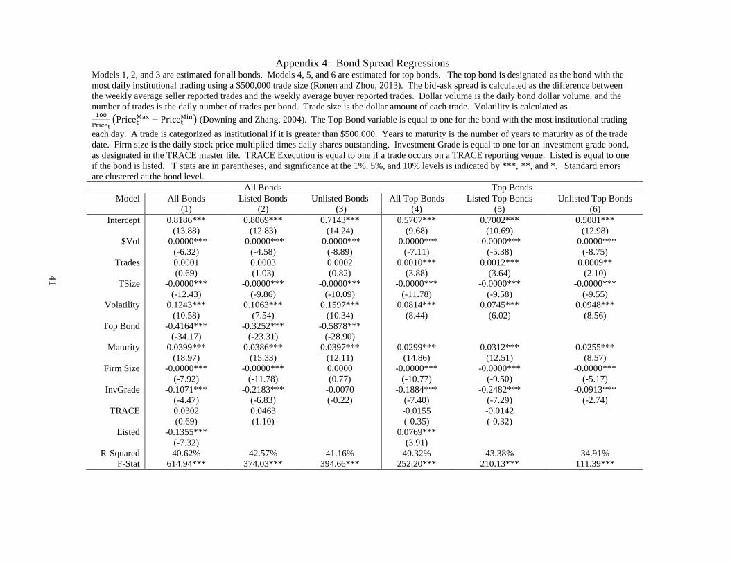
Appendix 4: Bond Spread Regressions Models 1, 2, and 3 are estimated for all bonds. Models 4, 5, and 6 are estimated for top bonds. The top bond is designated as the bond with the

most daily institutional trading using a $500,000 trade size (Ronen and Zhou, 2013). The bid-ask spread is calculated as the difference between

the weekly average seller reported trades and the weekly average buyer reported trades. Dollar volume is the daily bond dollar volume, and the

number of trades is the daily number of trades per bond. Trade size is the dollar amount of each trade. Volatility is calculated as 100

Pricet(Pricet

Max − PricetMin) (Downing and Zhang, 2004). The Top Bond variable is equal to one for the bond with the most institutional trading

each day. A trade is categorized as institutional if it is greater than $500,000. Years to maturity is the number of years to maturity as of the trade

date. Firm size is the daily stock price multiplied times daily shares outstanding. Investment Grade is equal to one for an investment grade bond,

as designated in the TRACE master file. TRACE Execution is equal to one if a trade occurs on a TRACE reporting venue. Listed is equal to one

if the bond is listed. T stats are in parentheses, and significance at the 1%, 5%, and 10% levels is indicated by ***, **, and *. Standard errors

are clustered at the bond level.

All Bonds Top Bonds

Model All Bonds

(1)

Listed Bonds

(2)

Unlisted Bonds

(3)

All Top Bonds

(4)

Listed Top Bonds

(5)

Unlisted Top Bonds

(6)

Intercept

$Vol

Trades

TSize

Volatility

Top Bond

Maturity

Firm Size

InvGrade

TRACE

Listed

R-Squared

F-Stat

0.8186***

(13.88)

-0.0000***

(-6.32)

0.0001

(0.69)

-0.0000***

(-12.43)

0.1243***

(10.58)

-0.4164***

(-34.17)

0.0399***

(18.97)

-0.0000***

(-7.92)

-0.1071***

(-4.47)

0.0302

(0.69)

-0.1355***

(-7.32)

40.62%

614.94***

0.8069***

(12.83)

-0.0000***

(-4.58)

0.0003

(1.03)

-0.0000***

(-9.86)

0.1063***

(7.54)

-0.3252***

(-23.31)

0.0386***

(15.33)

-0.0000***

(-11.78)

-0.2183***

(-6.83)

0.0463

(1.10)

42.57%

374.03***

0.7143***

(14.24)

-0.0000***

(-8.89)

0.0002

(0.82)

-0.0000***

(-10.09)

0.1597***

(10.34)

-0.5878***

(-28.90)

0.0397***

(12.11)

0.0000

(0.77)

-0.0070

(-0.22)

41.16%

394.66***

0.5707***

(9.68)

-0.0000***

(-7.11)

0.0010***

(3.88)

-0.0000***

(-11.78)

0.0814***

(8.44)

0.0299***

(14.86)

-0.0000***

(-10.77)

-0.1884***

(-7.40)

-0.0155

(-0.35)

0.0769***

(3.91)

40.32%

252.20***

0.7002***

(10.69)

-0.0000***

(-5.38)

0.0012***

(3.64)

-0.0000***

(-9.58)

0.0745***

(6.02)

0.0312***

(12.51)

-0.0000***

(-9.50)

-0.2482***

(-7.29)

-0.0142

(-0.32)

43.38%

210.13***

0.5081***

(12.98)

-0.0000***

(-8.75)

0.0009**

(2.10)

-0.0000***

(-9.55)

0.0948***

(8.56)

0.0255***

(8.57)

-0.0000***

(-5.17)

-0.0913***

(-2.74)

34.91%

111.39***

41

42

APPENDIX 5: BOND SPREAD BY TRADE SIZE AND TRADING ACTIVITY

43

Appendix 5: Bond Spread by Trade Size and Trading Activity Appendix 5 provides a comparison of trading costs for listed and unlisted bonds. The most active

bonds in the sample are in Quartile 1, and the least active bonds in the sample are in Quartile 4. The

bid-ask spread is calculated as the difference between the weekly average seller reported trades and the

weekly average buyer reported trades.

All Bonds Listed Bonds Unlisted Bonds

Panel A: Dollar Spreads by Trade Size

All Trade Sizes

Less than $100,000

$100,000 - $999,999

Greater than $1,000,000

$1.34

$1.42

$1.17

$0.82

$1.17

$1.25

$1.04

$0.88

$1.45

$1.54

$1.31

$0.76

Panel B: Dollar Spreads by Trading Activity

Q1 (most active)

Q2

Q3

Q4 (least active)

$0.99

$1.29

$1.52

$1.56

$0.95

$1.12

$1.44

$1.80

$1.07

$1.45

$1.54

$1.51

44

APPENDIX 6: BOND VOLATILITY REGRESSIONS

Appendix 6: Bond Volatility Regressions

Appendix 6 presents bond volatility regressions. Volatility is calculated as 100

Pricet(Pricet

Max − PricetMin) (Downing and Zhang, 2004).

Models 1, 2, and 3 estimate volatility for the full sample of bonds, listed bonds, and TRACE bonds. Models 4, 5, and 6 estimate volatility

for all top bonds, listed top bonds, and unlisted top bonds. Dollar volume is the daily bond dollar volume, and the number of trades is the

daily number of trades per bond. Trade size is the dollar amount of each trade. The Top Bond is equal to one for the bond with the most

institutional trading each day. A trade is categorized as institutional if it is greater than $500,000 (Ronen and Zhou 2013). Years to maturity

is the number of years to maturity as of the trade date. Firm size is the daily stock price multiplied times daily shares outstanding.

Investment Grade is equal to one for an investment grade bond, as designated in the TRACE master file. TRACE Execution is equal to one

if a trade occurs on a TRACE reporting venue. Listed is equal to one if the bond is listed. T stats are in parentheses, and significance at the

1%, 5%, and 10% levels is indicated by ***, **, and *. Standard errors are clustered at the bond level. All Bonds Top Bonds

Model Full Sample

(1)

Listed Bonds

(2)

Unlisted Bonds

(3)

All Top Bonds

(4)

Listed Top Bonds

(5)

Unlisted Top Bonds

(6)

Intercept

$Vol

Trades

TSize

Top Bond

Maturity

Firm Size

InvtGrade

TRACE

Listed

RSquared

F-Stat

3.0355***

(16.64)

0.0000*

(1.95)

0.0144***

(6.50)

-0.0000***

(-13.63)

0.0908*

(1.83)

0.1208***

(25.09)

-0.0000***

(-4.31)

-1.5569***

(-11.85)

-0.0423

(-0.27)

0.3402***

(3.72)

20.00%

166.46***

3.3894***

(14.36)

0.0000

(1.28)

0.0190***

(6.69)

-0.0000***

(-9.94)

0.0616

(0.98)

0.1191***

(20.51)

-0.0000***

(-3.24)

-1.6970***

(-8.58)

-0.0286

(-0.18)

23.00%

169.44***

3.0082***

(21.98)

0.0000***

(3.29)

0.0069***

(2.82)

-0.0000***

(-11.71)

0.1294*

(1.72)

0.1210***

(10.80)

-0.0000***

(-4.04)

-1.3399***

(-10.37)

15.10%

51.79***

3.4985***

(15.08)

0.0000**

(2.38)

0.0120***

(5.82)

-0.0000***

(-14.20)

0.1190***

(15.75)

-0.0000***

(-3.20)

-1.7403***

(-9.89)

-0.3296*

(-1.74)

0.4979***

(3.41)

18.76%

129.20***

3.9290***

(13.36)

0.0000

(1.52)

0.0165***

(6.27)

-0.0000***

(-10.69)

0.1194***

(15.06)

-0.0000*

(-1.82)

-1.8428***

(-7.24)

-0.3529*

(-1.87)

21.57%

144.97***

3.2946***

(14.86)

0.0000***

(3.82)

0.0058**

(2.36)

-0.0000***

(-12.70)

0.1168***

(5.35)

-0.0000***

(-3.24)

-1.5319***

(-8.06)

14.31%

39.50***

45

46

APPENDIX 7: EARNINGS ANNOUNCEMENTS VS. NON-EARNINGS

ANNOUNCEMENT DAYS

47

Appendix 7: Earnings Announcement vs. Non-Earnings Announcement Days Appendix 7 provides results a comparison of trading activity on earnings announcement days and non-

earnings announcement days. Price is the average daily bond price, and trade size is the average daily

trade size. Dollar volume is the average daily dollar volume, and the number of trades is the average

daily number of trades. All variables are averaged at the bond level. We provide averages for the

announcement day and the non-announcement day. We also provide the difference between the two

days. The t-statistic is presented to denote significance. ***,**,* indicate significance at the 1%, 5%,

and 10% levels.

Ann. Day Non-Ann. Day Difference T-Stat

Panel A: All Bonds

Price

Trade Size

Dollar Volume

Number of Trades

$107.31

$418,804.73

$2,212,530.93

6.08

$107.04

$407,640.34

$2,020,380.72

5.92

$0.27***

$11,164.39

$192,150.21***

0.16**

8.04

1.48

4.21

2.53

Panel B: Listed Bonds

Price

Trade Size

Dollar Volume

Number of Trades

$108.70

$436,105.08

$2,448,079.56

6.80

$108.51

$424,602.25

$2,295,620.87

6.70

$0.19***

$11,502.83

$152,458.69**

0.09

5.09

1.14

2.46

1.14

Panel C: Unlisted Bonds

Price

Trade Size

Dollar Volume

Number of Trades

$105.29

$393,646.85

$1,870,000.05

5.04

$104.92

$382,974.62

$1,620,131.10

4.79

$0.37***

$10,672.23

$249,868.95***

0.25***

6.24

0.94

3.75

2.66

48

APPENDIX 8: EARNINGS ANNOUNCEMENT VS. NON-EARNINGS ANNOUNCEMENT

DAYS, INSTITUTIONAL SIZED TRADING

49

Appendix 8: Earnings Announcement vs. Non-Earnings Announcement Days, Institutional

Sized Trading Appendix 8 provides results a comparison of institutional trading activity on earnings announcement days and

non-earnings announcement days. Price is the average daily institutional bond price, and trade size is the average

daily institutional trade size. Dollar volume is the average daily institutional dollar volume, and the number of

trades is the average daily institutional number of trades. The percentage institutional dollar volume is the

percentage of total volume for which institutions account. The percentage institutional number of trades is the

portion of all trades for which institution sized trades account. All variables are averaged at the bond level. We

provide averages for the announcement day and the non-announcement day. We also provide the difference

between the two days. The t-statistic is presented to denote significance. ***,**,* indicate significance at the

1%, 5%, and 10% levels. Ann. Day Non-Ann. Day Difference T-Stat

Panel A: All Bonds

Institutional Price

Institutional Trade Size

Institutional Dollar Volume

Institutional Number of Trades

% Institutional Dollar Volume

% Institutional Number of Trades

$106.90

$1,933,736.19

$2,516,509.75

1.27

43.84%

21.06%

$106.63

$1,895,475.25

$3,584,444.83

1.90

78.31%

29.61%

$0.27***

$38,260.94*

-$1,067,935.08***

-0.63***

-34.47%***

-8.55%***

4.94

1.92

-19.18

-25.69

-60.68

-26.05

Panel B: Listed Bonds

Institutional Price

Institutional Trade Size

Institutional Dollar Volume

Institutional Number of Trades

% Institutional Dollar Volume

% Institutional Number of Trades

$107.03

$2,064,328.39

$2,872,678.72

1.32

47.64%

20.74%

$106.84

$2,031,984.99

$4,162,325.85

2.03

86.45%

30.64%

$0.19***

$32,343.40

-$1,289,647.13***

-0.71***

-38.81%***

-9.90%***

3.08

1.23

-16.55

-22.25

-51.76

-23.70

Panel C: Unlisted Bonds

Institutional Price

Institutional Trade Size

Institutional Dollar Volume

Institutional Number of Trades

% Institutional Dollar Volume

% Institutional Number of Trades

$106.68

$1,696,437.68

$1,998,574.79

1.20

38.31%

21.52%

$106.24

$1,647,424.01

$2,744,099.93

1.71

66.46%

28.13%

$0.44***

$49,013.67*

-$745,525.14***

-0.51***

-28.15%***

-6.61%***

3.91

1.66

-9.82

-13.41

-33.00

-12.52

50

APPENDIX 9: EARNINGS ANNOUNCEMENT VS. NON-EARNINGS ANNOUNCEMENT

DAYS, RETAIL SIZED TRADING

51

Appendix 9: Earnings Announcement vs. Non-Earnings Announcement Days, Retail Sized

Trading Appendix 9 provides results a comparison of retail trading activity on earnings announcement days and non-

earnings announcement days. Price is the average daily retail bond price, and trade size is the average daily retail

trade size. Dollar volume is the average daily retail dollar volume, and the number of trades is the average daily

retail number of trades. The percentage institutional dollar volume is the percentage of total volume for which

institutions account. The percentage retail number of trades is the portion of all trades for which retail sized

trades account. All variables are averaged at the bond level. We provide averages for the announcement day and

the non-announcement day. We also provide the difference between the two days. The t-statistic is presented to

denote significance. ***,**,* indicate significance at the 1%, 5%, and 10% levels. Ann. Day Non-Ann. Day Difference T-Stat

Panel A: All Bonds

Retail Price

Retail Trade Size

Retail Dollar Volume

Retail Number of Trades

% Retail Dollar Volume

% Retail Number of Trades

$107.22

$81,253.56

$338,559.83

5.22

56.16%

78.94%

$106.97

$82,118.31

$353,524.31

5.30

21.69%

70.39%

$0.25***

-$864.75

-$14,964.48***

-0.08

34.47%***

8.55%***

7.52

-0.87

-3.24

-1.35

60.68

26.05

Panel B: Listed Bonds

Retail Price

Retail Trade Size

Retail Dollar Volume

Retail Number of Trades

% Retail Dollar Volume

% Retail Number of Trades

$108.66

$80,019.82

$366,479.57

5.93

52.36%

79.26%

$108.49

$80,551.45

$380,366.53

6.01

13.55%

69.36%

$0.17***

-$531.64

-$13,886.96**

-0.08

38.81%***

9.90%***

4.45

-0.43

-2.49

-1.06

51.76

23.70

Panel C: Unlisted Bonds

Retail Price

Retail Trade Size

Retail Dollar Volume

Retail Number of Trades

% Retail Dollar Volume

% Retail Number of Trades

$105.07

$83,099.13

$297,959.41

4.19

61.69%

78.48%

$104.70

$84,462.19

$314,490.79

4.26

33.54%

71.87%

$0.37***

-$1,363.07

-$16,531.38**

-0.07

28.15%***

6.61%***

6.17

-0.81

-2.08

-0.84

33.00

12.52

52

APPENDIX 10: MATCHED SAMPLE SUMMARY STATISTICS

Appendix 10: Matched Sample Summary Statistics We construct a matched sample using bond price, dollar volume, market capitalization, bond investment grade, and bond years to

maturity as our matching criteria. The sample is matched at the bond level. The matched sample includes 2,706,274 trades. Summary

statistics are calculated at the bond level. Price is the percentage of par. Dollar volume is the daily dollar volume for each bond. The

investment grade variable is equal to one if a bond is investment grade quality. Market Capitalization is the daily stock price multiplied

times daily shares outstanding. Significance is indicated at the 1%, 5%, and 10% levels with ***, **, and *.

Panel A: All Bonds

N Mean Standard Deviation Minimum Max

Price

Dollar Volume

Market Cap

Investment Grade

Years to Maturity

4,172

4,172

4,172

4,172

4,172

$106.08

$1,822,735.71

$53,376,174.28

0.76

8.49

$11.71

$2,962,901.53

$72,256,984.34

0.43

7.58

$42.85

$2,416.67

$11,523.30

0.00

0.02

$272.60

$82,357,435.86

$438,712,329.00

1.00

29.97

Panel B: Listed Bond vs. Unlisted Bond

N Listed Bond Mean Unlisted Bond Mean Difference T Stat

Price

Dollar Volume

Market Cap

Investment Grade

Years to Maturity

2,086

2,086

2,086

2,086

2,086

$106.72

$1,857,091.51

$54,837,257.40

0.73

8.47

$105.44

$1,788,379.90

$51,915,091.16

0.79

8.50

$1.28

$68,711.62

$2,922,166.24

-0.06

-0.03

0.47

0.97

1.32

0.98

-0.15

53

54

APPENDIX 11: MATCHED SAMPLE COMPARISON OF NYSE AND TRACE TRADES

Appendix 11: Matched Sample Comparison of NYSE and TRACE Trades We compare listed bond trades that execute on the NYSE and listed bond trades that execute on TRACE using the matched sample. The

bond with the most institutional trading each day is designated as the top bond for that firm. A trade is classified as institutional if the trade

size is greater than $500,000 (Ronen and Zhou, 2013). Price is the percentage of par. Dollar volume is the daily dollar volume, and the

number of trades is the average daily number of trades. Trade size is the average daily dollar trade size. Volatility is calculated as 100

Pricet(Pricet

Max − PricetMin) (Downing and Zhang, 2004). The bid-ask spread is calculated as the difference between the weekly average

seller reported trades and the weekly average buyer reported trades. Significance is indicated at the 1%, 5%, and 10% levels by ***, **,

and *.

NYSE TRACE Difference T-Stat

Panel A: All Bonds

Price

Dollar Volume

Trades

Trade Size

Volatility

Spread

$102.95

$8,329.97

1.28

$6,772.10

3.89

$1.43

$103.03

$3,276,823.39

11.88

$335,195.87

3.59

$1.18

-$0.08

-$3,268,493.42***

-10.60***

-$328,423.77***

0.30**

$0.25***

-0.31

-9.51

-14.84

-16.89

2.14

4.45

Panel B: Top Bonds

Price

Dollar Volume

Trades

Trade Size

Volatility

Spread

$102.03

$9,400.49

1.31

$7,400.29

4.54

$1.36

$102.22

$6,149,843.11

16.50

$575,750.71

4.05

$1.07

-$0.19

-$6,140,442.62***

-15.20***

-$568,350.42***

0.49**

$0.29***

-0.53

-11.33

-12.76

-15.90

2.21

3.91

55

56

APPENDIX 12: MATCHED SAMPLE BOND SPREAD REGRESSIONS

Appendix 12: Matched Sample Bond Spread Regressions Models 1, 2, and 3 are for matched sample bonds. Models 4, 5, and 6 are estimated for matched sample top bonds. The top bond has the most daily

institutional trading using a $500,000 trade size (Ronen and Zhou, 2013). The bid-ask spread is calculated as the difference between the weekly

average seller reported trades and the weekly average buyer reported trades. Dollar volume is the daily bond dollar volume, and the number of

trades is the daily number of trades per bond. Trade size is the dollar amount of each trade. Volatility is calculated as 100

Pricet(Pricet

Max − PricetMin)

(Downing and Zhang, 2004). Years to maturity is the number of years to maturity as of the trade date. Firm size is the daily stock price times daily

shares outstanding. Investment Grade is equal to one for an investment grade bond, as designated in the TRACE master file. TRACE Execution is

equal to one if a trade occurs on a TRACE reporting venue. Listed is equal to one if the bond is listed. T stats are in parentheses, and significance at

the 1%, 5%, and 10% levels is indicated by ***, **, and *. Standard errors are clustered at the bond level.

Matched Sample of Bonds Matched Sample of Top Bonds

Model Matched

(1)

Listed

(2)

Unlisted

(3)

P Value Matched

(4)

Listed

(5)

Unlisted

(6)

P Value

Intercept

$Vol

Trades

Trade Size

Volatility

Top Bond

Maturity

Firm Size

InvTGrade

TRACE

Listed

R-Squared

F Statistic

0.9081***

(9.53)

-0.0000***

(-4.34)

0.0000.

(0.07)

-0.0000***

(-8.98)

0.1084***

(5.76)

-0.3889***

(-21.00)

0.0401***

(12.04)

-0.0000***

(-5.60)

-0.1967***

(-5.43)

0.0043

(0.06)

-0.0626**

(-2.21)

41.47%

258.00***

0.9085***

(9.91)

-0.0000***

(-2.66)

-0.0001

(-0.27)

-0.0000***

(-7.41)

0.0931***

(4.98)

-0.3179***

(-15.29)

0.0404***

(10.91)

-0.0000***

(-7.14)

-0.2460***

(-5.84)

0.0160

(0.24)

43.90%

190.29***

0.6033***

(10.26)

-0.0000***

(-7.43)

0.0013**

(1.97)

-0.0000***

(-4.66)

0.1956***

(14.12)

-0.5946***

(-19.13)

0.0334***

(9.10)

0.0000

(0.90)

-0.0190

(-0.40)

43.81%

159.39***

0.2690

0.3773

0.4173

0.9637

0.3819

0.1960

0.2911

0.2235

0.3159

0.6224***

(6.32)

-0.0000***

(-4.60)

0.0010**

(2.47)

-0.0000***

(-8.43)

0.0722***

(4.60)

0.0306***

(9.97)

-0.0000***

(-6.70)

-0.2064***

(-5.52)

-0.0258

(-0.35)

0.1146***

(3.95)

42.01%

145.99***

0.7745***

(7.94)

-0.0000***

(-2.94)

0.0008*

(1.87)

-0.0000***

(-7.66)

0.0645***

(4.03)

0.0329***

(9.42)

-0.0000***

(-6.88)

-0.2470***

(-5.56)

-0.0178

(-0.24)

44.48%

154.00***

0.3787***

(7.05)

-0.0000***

(-5.57)

0.0017*

(1.81)

-0.0000***

(-4.34)

0.1224***

(12.76)

0.0218***

(4.95)

-0.0000***

(-4.75)

-0.0452

(-0.95)

36.01%

44.14***

0.8397

0.0823

0.2035

0.2249

0.2901

0.7765

0.3893

0.3175

57

58

APPENDIX 13: MATCHED SAMPLE BOND SPREAD BY TRADE SIZE AND TRADING

ACTIVITY

Appendix 13: Matched Sample Bond Spread by Trade Size and Trading Activity The most active bonds in the sample are in Quartile 1, and the least active bonds in the sample are in Quartile 4. The bid-ask

spread is calculated as the difference between the weekly average seller reported trades and the weekly average buyer reported

trades. The difference column represents the difference between listed bond spread and unlisted bond spread. Significance is

determined using t-stats. Significance is indicated at the 1%, 5%, and 10% levels using ***, **, and *.

All Bonds Listed Bonds Unlisted Bonds Difference T Stat

Panel A: Dollar Spreads by Trade Size

All Trade Sizes

Less than $100,000

$100,000 - $999,999

Greater than $1,000,000

$1.24

$1.33

$1.10

$0.81

$1.12

$1.17

$1.02

$0.90

$1.36

$1.49

$1.22

$0.74

-$0.25***

-$0.32***

-$0.20***

$0.16***

-7.83

-9.52

-5.76

5.11

Panel B: Dollar Spreads by Trading Activity

Q1 (most active)

Q2

Q3

Q4 (least active)

$1.01

$1.10

$1.33

$1.51

$0.98

$0.95

$1.20

$1.43

$0.95

$1.36

$1.40

$1.56

$0.03

-$0.42***

-$0.20

-$0.13

0.28

-3.60

-1.41

-0.59

59

60

APPENDIX 14: MATCHED SAMPLE BOND VOLATILITY REGRESSIONS

Appendix 14: Matched Sample Bond Volatility Regressions

Volatility is calculated as 100

Pricet(Pricet

Max − PricetMin) (Downing and Zhang, 2004). Models 1, 2, and 3 estimate volatility for the full

sample of matched bonds, listed bonds, and TRACE bonds. Models 4, 5, and 6 estimate volatility for all top bonds, listed top bonds, and

unlisted top bonds. Dollar volume is the daily bond dollar volume, and the number of trades is the daily number of trades per bond. Trade

size is the dollar amount of each trade. The Top Bond is equal to one for the bond with the most institutional trading each day. A trade is

categorized as institutional if it is greater than $500,000 (Ronen and Zhou, 2013). Years to maturity is the number of years to maturity as

of the trade date. Firm size is the daily stock price multiplied times daily shares outstanding. Investment Grade is equal to one for an

investment grade bond, as designated in the TRACE master file. TRACE Execution is equal to one if a trade occurs on a TRACE reporting

venue. Listed is equal to one if the bond is listed. T stats are in parentheses, and significance at the 1%, 5%, and 10% levels is indicated by

***, **, and *. Standard errors are clustered at the bond level.

Matched Sample of Bonds Matched Sample of Top Bonds

Model Matched

(1)

Listed

(2)

Unlisted

(3)

P Value Matched

(4)

Listed

(5)

Unlisted

(6)

P Value

Intercept

$Vol

Trades

Trade

Size

Top Bond

Maturity

Firm Size

InvtGrade

TRACE

Listed

RSquared

F Statistic

3.1464***

(10.22)

0.0000

(0.32)

0.0185***

(4.14)

-0.0000***

(-8.03)

0.1985***

(2.79)

0.1135***

(12.42)

-0.0000***

(-4.47)

-1.5523***

(-9.16)

-0.1431

(-0.52)

0.3870***

(3.78)

20.54%

82.13***

3.4480***

(9.92)

0.0000

(0.59)

0.0224***

(4.13)

-0.0000***

(-6.86)

0.2266**

(2.46)

0.1155***

(9.22)

-0.0000***

(-4.18)

-1.6686***

(-7.65)

-0.0959

(-0.34)

22.30%

62.09***

3.1068***

(19.91)

0.0000***

(3.03)

0.0029

(1.52)

-0.0000***

(-10.65)

0.0116

(0.16)

0.0962***

(12.18)

-0.0000

(-1.27)

-1.1977***

(-6.98)

14.22%

61.10***

0.3113

0.3713

0.4004

0.4159

0.4434

0.5058

0.5981

0.3161

3.7922***

(9.77)

0.0000

(0.72)

0.0164***

(3.79)

-0.0000***

(-8.55)

0.1084***

(7.71)

-0.0000***

(-2.88)

-1.6649***

(-7.36)

-0.6069*

(-1.75)

0.6126***

(4.06)

18.65%

67.18***

4.2791***

(9.29)

0.0000

(0.68)

0.0212***

(3.86)

-0.0000***

(-7.56)

0.1153***

(5.88)

-0.0000**

(-2.39)

-1.8042***

(-5.88)

-0.6062*

(-1.78)

20.11%

49.99***

3.3987***

(18.38)

0.0000***

(3.82)

0.0013

(0.98)

-0.0000***

(-10.64)

0.0770***

(6.59)

-0.0000**

(-2.03)

-1.3171***

(-6.54)

14.01%

47.35***

0.8435

0.4306

0.9683

0.2431

0.9025

0.6967

0.3175

61

62

FIGURES

63

Figure 1. Intraday Average Number of Bond Trades.

Figure 2. Average Intraday Bond Trade Size.

0

0.5

1

1.5

2

2.5

All Bonds Listed Bonds Unlisted Bonds

$-

$100,000

$200,000

$300,000

$400,000

$500,000

$600,000

$700,000

$800,000

$900,000

All Bonds Listed Bonds Unlisted Bonds

64

Figure 3. Average Intraday Bond Dollar Volume.

Figure 4. Average Intraday Bond Bid-Ask Spread.

$-

$200,000

$400,000

$600,000

$800,000

$1,000,000

$1,200,000

All Bonds Listed Bonds Unlisted Bonds

$-

$0.20

$0.40

$0.60

$0.80

$1.00

$1.20

$1.40

$1.60

All Bonds Listed Bonds Unlisted Bonds

65

Figure 5. Average Intraday Bond Volatility.

0

0.5

1

1.5

2

2.5

All Bonds Listed Bonds Unlisted Bonds

66

PART 2: MUNICIPAL BOND TRADING, INFORMATION RELATEDNESS, AND

NATURAL DISASTERS

67

INTRODUCTION

Natural disasters and the costs associated with the ensuing damage can be extensive. The

damages linked to Hurricane Sandy exceed $20 billion, and Hurricane Katrina damages are

estimated to be at least $125 billion. In 2011, a tornado devastated Joplin, Missouri, directly

causing $3 billion in damages (Hamilton, 2012). Natural disasters carry information in the form

of damages for geographic areas and the firms tied to these areas (Loughran and Schultz, 2004).

Generally, the information is not known until the amount of damage is realized.

Some corporations are able to shift production or operations to areas of the country not

damaged by a disaster, but the viability of municipalities, and hence municipal bonds, is directly

tied to the damaged area. For example, the cash flows of revenue bonds are funded from the

income earned by the bond projects (toll road, stadium, etc). If a structure is damaged in a storm

or natural disaster, then the bond funding that project potentially loses its payoff source.

Additionally, tax revenues may be affected if citizens leave an area after a natural disaster.

Trading of municipal bonds can be affected by natural disasters as well; local investors may be

too distracted preparing for and recovering from the storm to balance their bond portfolios in the

days leading up to and following a natural disaster. Using firms headquartered in areas struck by

blizzards, Loughran and Schultz (2004) show that equity trading volume declines on both the

day of the blizzard and the subsequent trading day. The authors contribute the decline in trading

volume to the storm serving as a source of distraction for traders.

Studying the municipal bond market and its reaction to natural disasters allows us to

examine the bond market’s ability to absorb information. Prior bond market research implies

68

that both the municipal and corporate bond markets are inherently slow incorporating

information into bond prices. Kwan (1996) shows that stocks react to information faster than

corporate bonds, and Downing, Underwood, and Xing (2009) document that non-investment

grade corporate bonds lag equities in their ability to incorporate information. Green, Li, and

Schurhoff (2010) show that municipal bonds are quick to include information that pushes prices

up, but are slow to include information that pulls prices down. Given that natural disasters

likely carry negative information, we believe that local traders may be distracted by the natural

disaster, and hence, alter trading activity leading up to and following the event (Loughran and

Schultz, 2004), leading to slower incorporation of the association information in municipal bond

prices.

69

RELATED LITERATURE

Loughran and Schultz (2004) study local trading of NASDAQ stocks. The authors focus

on the effect cloud cover and blizzards have on trading. The authors examine trading around

forty-eight blizzards from 1984 to 1997. While they find little relation between cloud cover and

stock returns, Loughran and Schultz document a reduction in trading volume for the firms

headquartered in cities struck by a blizzard. The reduction in trading volume is substantial;

volume falls by 17% on the day the storm hits and by 15% on the subsequent day. Loughran and

Schultz blame the decline in trading volume on local investor distraction and claim that local

traders may be too busy preparing for and recovering from the blizzard to participate in trading.

Shive (2012) conducts a study that indirectly examines trading activity and natural

disasters. Shive focuses on power outages and the market quality of firms headquartered in areas

affected by the outage. Of the 114 blackouts that occur in her sample from 2002 to 2010, all but

two are caused by events such as ice storms and hurricanes. Shive states that the blackout

constrains local trading activity and finds that the blackout influences several aspects of trading.

First, both total volatility and idiosyncratic volatility decline during the power outage. Second,

quoted spreads fall by 2.5% during the blackout, which the author credits to a reduction in

adverse selection. Third, both volume and turnover decline during the blackout. The author

conjectures the changes in trading are due to local traders’ inability to participate in the market

during the blackout.

While previously mentioned research focuses on equity markets, there is potential for

natural disasters to affect other security types. We focus on the municipal bond market and

70

natural disasters. Municipal bonds are unique in that their claims and payoffs are often tied

directly to funded projects, such as toll roads, bridges, and stadiums, which may be damaged by

a natural disaster. Unlike firms that have the ability to shift operations or production schedules

to other locations, municipalities do not possess this flexibility. Damage to or loss of a funded

structure can severely affect the municipality’s ability to meet its debt obligations. Additionally,

the potential loss of population (and subsequent tax revenues) can detrimentally influence a

municipality’s viability. As such, the damages that result from the natural disaster provide

information as to the well-being of the municipality and its surrounding areas.

71

HYPOTHESES

We study the efficiency of the municipal bond market and establish if contagion exists

following natural disasters. The commonality literature suggests market wide shocks may link

individual security liquidity and market liquidity. Cabelle and Krishman (1994) propose the

following variables as measures of information relatedness: trading volume, number of trades,

volatility, spreads, and returns. Chordia, Roll, and Subrahmanyam (2000) document

commonality in liquidity and spreads, and Hasbrouck and Seppi (2001) show commonality exists

in stock trading volume. In this study, we utilize the previously mentioned variables to

determine if contagion exists among municipal bonds. Studying the municipal bond market’s

reaction to natural disasters allows us to examine the bond market’s ability to absorb information

and also to describe the behavior of bond traders following a disaster.

First, we focus on spreads. Spreads in the municipal bond market may increase following

a natural disaster as a way for dealers to compensate for additional risk. In the days following a

natural disaster, the amount of damage (the information) caused by the storm is revealed and this

information is disseminated into the municipal bond market. It is also possible that spreads will

fall following the natural disaster; Loughran and Schultz (2004) and Shive (2012) detail that

local traders are often constrained following a natural disaster. If local traders are unable to

access municipal bond markets after the natural disaster occurs, then a reduction in asymmetric

information may occur as local, perhaps more informed, traders are distracted. Shive (2012)

documents a reduction in spread following electricity blackouts. She theorizes the reduction in

72

spreads result from local trader’s inability to access the market, which in turn results in less

information asymmetry in the market following the blackout.

Common factors, such as economic fundamentals or liquidity demands, are also shown to

influence the trading environment (Hasbrouck and Seppi, 2001). Areas adjacent to the

municipality where the natural disaster occurs may also be impacted following the storm. It is

possible that adjacent areas are economically linked to the damaged area or that investors in

surrounding areas are distracted (perhaps by news reports or relief efforts), leading to

surrounding investors participating less in their own local municipal bond market following the

disaster. Jiang, McInish, and Upson (2009) measure information relatedness using firm SIC

codes and study the trading activity of stocks that continue trading during a trading halt. Even

though the halt is unrelated to the other firms in the industry (identified by SIC code), they find

that spreads increase during the halt for related firms. Using the above literature, we form the

following hypotheses:

H1A: There is a relation between municipal bond spreads and local natural disasters.

H1B: There is a relation between informationally-related municipal bond spreads and natural

disasters.

Second, we examine volume and number of trades. Loughran and Schultz (2004) study

local trading of NASDAQ stocks, focusing on cities struck by a blizzard. They find a substantial

17% reduction in trading volume on the day the storm strikes the city, and they document a 15%

reduction in trading volume on the trading day after the blizzard. Loughran and Schultz claim

that local investors may be too busy preparing for and recovering from the blizzard to participate

in trading, thus influencing the reduction in trading volume. Shive (2012) also documents a

reduction in trading volume following electricity blackouts and finds that stock turnover falls

73

following an electricity blackout. Loughran and Schultz study trading volume of stocks

headquartered in cities unaffected by a blizzard and find no effect on trading volume. Yet, Jiang,

McInish, and Upson (2009) find that the number of trades increases for informationally-linked

firms during a trading halt. Using the above literature, we present the following hypotheses:

H2A: Volume decreases for municipal bonds in the days following a local natural disaster.

H2B: Volume decreases for informationally-linked municipal bonds following a natural

disaster.

H3A: The number of trades decreases for municipal bonds in the days following a local natural

disaster.

H3B: The number of trades decreases for informationally-linked municipal bonds following a

natural disaster.

Third, we focus on bond market efficiency. The municipal bond market is generally

inefficient and opaque due to its operating as a decentralized dealer market. A natural disaster

provides information to a geographic area, often in the form of damages. There is a lag between

the natural disaster occurring and the amount/level of damages becoming known. During this

time of information gathering and dissemination, the municipal bond market is filled with

uncertainty. The uncertainty may result in increased bond market volatility. Jiang, McInish, and

Upson (2009) propose volatility as a measure of information relatedness. In contrast, local

investors may be distracted or constrained both during and following the disaster. Shive (2012)

uses volatility as a measure of price discovery and shows that total volatility and idiosyncratic

volatility fall during an electricity blackout. The reduction in total volatility is stronger for small

cities, high income areas, and during pre-earnings/merger announcement periods. The reduction

in idiosyncratic volatility is more pronounced for small firms with no analyst following. If local

74

investors play an information-based role in municipal bond markets (as both Shive, 2012, and

Loughran and Schultz, 2004, show they play in equities), then it is possible that volatility will

fall during and following a local natural disaster. The natural disaster may also distract investors

in neighboring locations, thus influencing their participation in their own municipal bond

markets. Using the above information, we propose the following hypotheses:

H4A: There is a relation between municipal bond volatility and local natural disasters.

H4B: There is a relation between informationally related municipal bond volatility and natural

disasters.

Another test of market efficiency is to determine if abnormal returns are earned following

a natural disaster. If markets are efficient, the occurrence of a natural disaster that does not

interrupt the operations of a funded project should not influence bond returns. However, prior

literature shows that natural disasters can influence stock returns. Cabelle and Krishman (1994)

identify returns as a measure of firm relatedness. Lamb (1998) focuses on hurricanes and their

impact on stock price. In Lamb’s study, firms with hurricane risk exposure experience negative

excess returns around a hurricane. Firms without hurricane exposure are unaffected by both

Hurricane Andrew and Hurricane Hugo. Shelor, Anderson, and Cross (1990) focus on an

October 17, 1989 California earthquake. Specifically, they investigate the impact that the

property damage from the earthquake has on California real estate firms. Their results show

negative excess returns for real estate firms on the day of the earthquake, but do not show any

evidence of significant negative returns for other California-based firms not involved in real

estate. Jiang, McInish, and Upson (2009) use industry to classify related firms. Based on the

above mentioned literature, we present the following hypotheses:

H5A: Municipal bonds have negative abnormal returns following a local natural disaster.

75

H5B: Informationally related municipal bonds have negative abnormal returns following a

natural disaster.

76

SAMPLE AND DATA

We use municipal bond transaction data for January 2010 through December 2013 from the

Municipal Securities Rulemaking Board (MSRB). The MSRB municipal bond database includes

all trades by registered broker-dealers. Each trade is identified as a dealer purchase from a

customer, dealer sale to a customer, or interdealer trade, and each trade record includes the

CUSIP, security information, coupon, yield, par value traded, and price. The data initially

includes 35,834,399 bond transactions. We require bonds in the sample to trade nine times each

year (Edwards, Harris, and Piwowar, 2007)1, which reduces our sample to 33,250,257 trades.

We also require bonds in the sample to trade at prices above 25% of par in order to remove

municipalities close to bankruptcy or default, and we remove transactions with data entry

errors/missing values. These two deletions further reduce our sample to 32,571,012 trades.

After constructing both the weekly volatility measures and the weekly spread measures, our final

data sample includes 20,553,922 trades in 331,429 municipal bonds issued by the municipalities

in all fifty states in the United States. We obtain each bond’s issuing state and whether a bond is

general obligation or revenue from the MSRB’s Electronic Municipal Market Access (EMMA)

website. Appendix A provides information on the number of bonds outstanding by state during

our time period.

1 Harris and Piwowar (2006) study transactions costs in the municipal bond market and require bonds in their

sample to trade at least six times. We follow Edwards et al (2007) and use a slightly more restrictive requirement

(nine times each year) to control for potential nonsynchronous trading, given the illiquidity of the municipal bond

market and the four year length of our trade sample. We replicate each appendix using the Harris and Piwowar

restriction, and the results are qualitatively similar.

77

We also utilize natural disaster data from the National Climactic Data Center. We

include three types of natural disasters in the sample: tornados (1,173 events), wildfires (1,877

events), and hurricanes/tropical storms (46 events). The National Climactic Data Center provides

information regarding the disaster start date/time, end date/time, and states affected. We match

municipal bonds affected by natural disasters based on the bond’s issuer. Appendix B includes

information on the number of natural disasters in our sample.

78

THE MUNICIPAL BOND MARKET DESCRIPTION

Municipal bonds are issued by city, county, and state governments, and also by entities

such as electric companies, schools, and hospitals. Municipal bonds are unique in that they are

excluded from the Securities Exchange Act of 1934 and are not subject to oversight by the U.S.

Securities and Exchange Commission. The MSRB governs the municipal bond market. The

municipal bond market is a highly fragmented market, and the bonds trade in a decentralized

over-the-counter market. Municipal bonds are typically issued in deals, where several different

securities are issued at the same time. The various bonds in the deal, all designed to fund the

same project, have different maturities, coupons, yields, and offer prices.

The municipal bond market is historically fragmented and opaque (Harris and Piwowar,

2007, and Green, Li, and Schurhoff, 2010). One way that the MSRB seeks to improve

transparency in the municipal bond market is through the implementation of its website, EMMA,

and real time trade reporting. EMMA provides information about the municipal bond market,

municipal bond disclosure statements, and post-trade transparency information for municipal

bonds. Municipal bond trades are reported to the MSRB’s real-time transaction reporting system

(RTRS) within 15 minutes of the trade execution, and the trades then are posted publicly to the

EMMA website. Real time trade reporting includes real-time prices for most trades occurring

after January 31, 2005.

Appendix 1 provides a description of the trade executions in our sample. Panel A

includes information on all bond trades in the sample. 7.82% of bond trades involve a taxable

municipal bond. The majority of bond trading appears to take place in bonds with at least 10

79

years to maturity. Additionally, small trades make up a large portion of the trade sample. Trades

of less than $25,000 account for over 50% of the transactions from 2010 to 2013, while trades

greater than $100,000 account for just 16% of transactions.

The majority of bonds in the sample trade above par. Dealer sales to customers make up

a large portion of trades at 44.46% of transactions, while dealer purchases (interdealer trades)

make up 25.09% (30.45%). California, Texas, New York, Pennsylvania, and Illinois bonds

account for nearly 50% of all transactions in the sample (henceforth referred to collectively as

the top five bond issuing states). Generally, the trading activity in dealer purchases, dealer sales,

and interdealer trades is similar to that shown for the full sample. Additionally, the trading

activity in the top five bond issuing states is similar to the full sample (Panel B).

Appendix 2 provides bond level summary statistics for all bonds in the sample and also

for the top five bond issuing states. Panel A includes the full sample of trades, and Panels B, C,

and D are for interdealer trades, dealer purchases, and dealer sales. The average bond in our

sample trades roughly 2.94 times per day with an average trade size of over $275,000 and an

average price of 103.25% of par. The average daily dollar volume for municipal bonds is nearly

$730,000. On average, municipal bonds have a 1.5% spread. There appears to be slight

differences between the full sample of bonds and the top five issuing states’ bonds, but we do not

test for statistical differences in Appendix 2. The average price for a “top five” bond is 101.90%

of par. The average number of trades, the average daily volume, and the average trade size for

top five bond issuing states are all similar to those for the full sample. Bonds issued by the top

five bond issuing states in the sample have an average trade size of $300,000 and transact over

$770,000 in average daily volume. Additionally, the average spread for a top five bond is

1.62%.

80

In Panel B, we provide summary statistics for interdealer trades, both for the full sample

and for the top five bond issuing states. Interdealer trades have an average price of 103.18% of

par, and are nearly $160,000 in dollar size on average. Interdealer trades make up roughly

$320,000 of daily dollar volume. Dealer purchases (Panel C) have an average price of 102.43%

of par and an average trade size of about $342,000. On average, interdealer purchases occur 1.11

times per bond per day, and the average daily dealer purchase volume is almost $400,000.

Dealer sales (Panel D) have an average price of 103.93%. The average dealer sale size is

roughly $266,000, and dealer sales account for nearly $377,000 in average daily volume.

Interestingly, dealer sales have a positive return (on average), whereas interdealer trades and

dealer purchases have negative average returns.

81

RESULTS

First, we focus on municipal bond trading activity on the natural disaster event day

compared to non-event days. An event day is any trading day on which a natural disaster occurs,

and non-event days are all trading days on which no natural disaster occurs. We detail our first

analysis of municipal bond trading and natural disasters in Appendix 3. Panel A includes

tornados, Panel B includes wildfires, and Panel C includes hurricanes/tropical storms. Overall,

we find significant differences between event days and non-event days. For tornados, we find

that the dollar volume is roughly $40,000 higher on the event days compared to all other trading

days, which is in contrast to the previous literature showing a reduction in volume on disaster

event days (Loughran and Schultz, 2004, and Shive, 2012). The number of trades is marginally

higher on tornado event days. Tornado event days’ trade sizes are nearly $6,000 larger than non-

event days’ trade sizes. Both spreads and volatility are lower on event days than on non-event

days, which is consistent with Shive’s findings of lower volatility and lower spreads during

electricity blackout periods. Specifically, spreads are 0.02% lower on tornado event days, and

volatility is 0.05% lower. Lastly, we show that bond returns are lower on tornado event days

than on non-event days.

Panel B provides the event days and non-event days comparison for wildfires. We show

that daily volume is roughly $57,000 higher, and that the average trade size is nearly $11,000

larger on the event days than on the non-event days. This finding of increasing activity in the

event period is, again, the opposite of what Shive (2012) shows for equities. Similar to Panel A,

we document marginal differences in the number trades between the two time periods, and we

82

also show that both spreads and volatility are lower on the event days (similar to tornado events

in Panel A and also consistent with previous findings). We detail hurricane/tropical storm event

days compared to non-event days in Panel C. Unlike the findings in Panels A and B, we find

no significant difference in daily volume on hurricane event and non-event days. However, we

find that both spreads and volatility are lower on the hurricane event days, which is a consistent

finding across all three disaster types analyzed in the paper.

We document significant differences between event days and non-event days for

municipal bonds and natural disasters in Appendix 3. We attempt to isolate where these

differences might be coming from by separating the trade sample into small (less than $25,000),

medium ($25,001 – $100,000), and large (greater than $100,001) trades. These statistics are

located in Appendix 4. Panel A details the event days, and Panel B details the non-event days in

Appendix 4. We focus on the percentage volume, percentage trades, and bid-ask spreads in

Appendix 4. Examining what trade size changes, if any, occur during natural disasters can also

shed some insight on who is trading in the municipal bond market. Trade size is used to measure

retail versus institutional trading in the bond market; typically, trades exceeding either $100,000

(Edwards, Harris, and Piwowar, 2007) or $500,000 (Ronen and Zhou, 2013) are considered

institutional. We designate trades as “large” or institutional if the trade size exceeds $100,001 in

our paper.2

In Appendix 4, Panel A, we focus on the natural disaster event days, which are defined as

the day a natural disaster occurs. We find that small trades account for the largest portion of

both dollar volume and the number of trades on both the event days and the non-event days

(regardless of disaster types). Consistent with previous literature, we document an inverse

2 We replicate any results involving trade size designations using $500,000 to designate large trades. We utilize

$100,000 in our main tests because only a small percentage of trades exceed $500,000.

83

relation between trading costs and trade size in the bond market.3 Large trades account for the

smallest portion of both volume and number of trades in both time periods for all disaster types.

The first three columns provide information for tornados. Medium trades account for a

slightly smaller portion of volume on tornado event days (compared to non-event days), while

large trades account for a slightly greater portion of volume on event days than non-event days.

We do not document any significant differences in spreads between the two time periods for

medium and large trades (for tornados). We find that small trades have a 0.02% lower spread on

tornado event days than on non-event days. For wildfires, we find that small trades have

significantly lower spreads on wildfire event days than on the non-event days. The magnitude of

the difference in spreads, however, is only 0.01% for wildfire events.

The last columns in Appendix 4 provide results for hurricanes/tropical storms. We

document significant differences in bond spreads for small and medium trades on hurricane

event days and non-event days. We find that small and medium trades have lower spreads on

hurricane event days compared to non-event days. Small trade spreads are 0.05% lower in the

event period, and medium trade spreads are 0.03% lower in the event period. We do not show

any significant differences in large trade spreads between hurricane/tropical storm event days

and non-event days.

Despite finding some significant differences in trade sizes between event days and non-

event days, the differences between the two time periods do not appear to come from one single

trade size group. We make a second attempt to isolate the origin of the differences on natural

disaster event days by separating interdealer trades, dealer purchases, and dealer sales. We

present the relevant statistics results in Appendix 5. The left-side columns provide results for

3 See Goldstein, Hotchkiss, and Sirri, 2007; Edwards, Harris, and Piwowar, 2007; and Harris and Piwowar, 2006.

84

tornado event days and non-event days. We find a significant difference in spreads for both

interdealer trades and dealer purchases. Both interdealer trades and dealer sales account for a

smaller portion of volume (trades) on tornado event days than on non-event days, but dealer

purchases account for a larger proportion of both volume and trades on tornado event days

compared to non-event days.

The results for both wildfire and hurricane events are similar to, if not more pronounced,

than the results for tornado events. Both interdealer trades and dealer sales account for a smaller

portion of volume and trades on event days than non-event days for wildfires and hurricanes,

while dealer purchases account for a larger portion of volume and trades during event periods.

Dealer purchases increase by 0.77% (0.70%) for dollar volume (number of trades) on wildfire

event days compared to non-event days. For hurricane events, dealer purchases increase by

1.55% (1.59%) for dollar volume (number of trades) on event days compared to non-event days

for hurricanes. With the exception of interdealer trades during hurricanes/tropical storms, the

differences in spreads between event and non-event days are small in magnitude for both

wildfires and hurricanes.

In previous appendices, we focus on comparing event days and non-event days. We now

further our analysis by studying the pre-event week, the event day(s), and the post-event week.

The pre-event week is the five trading days prior to the natural disaster, and the post-event week

is the five trading days following the natural disaster. The event days are the actual day(s) of the

natural disaster. Appendix 6 presents the comparison for the tornado pre, during, and post event

periods. We also test for the following differences between the three time periods: the pre-event

week and the event day(s); the event day(s) and the post event week; and the pre-event week and

the post-event week. Dollar volume is slightly higher in the tornado pre-event week than the

85

post event week – roughly $727,000 compared to $708,000. We find marginal (but significant)

differences in the average number of trades in all three time periods; trades generally fall during

both the tornado event days and the post-event weeks, as compared to the pre-event weeks.

Panel B provides results for wildfires. We find no significant difference in volume in the

pre-event weeks and event days, but we find that volume decreases following the natural

disaster. The volume decline following a wildfire is similar to Loughran and Schultz (2004),

who document a reduction in trading volume on the trading day following a blizzard. Volume is

roughly $688,000 during the wildfire event days, and around $672,000 in the week following the

wildfire. We find marginal differences in both the number of trades and spreads in the three time

periods, and we show that volatility is highest during the event period for wildfires. In contrast,

Shive (2012) finds that volatility declines during electricity blackouts. Additionally, we find that

returns fall significantly from the pre-event week to the post-event week for wildfires. The

results for hurricanes (Panel C) are somewhat weaker than those shown in Panels A and B.

Returns fall drastically from the pre-event week to the post-event week, falling from 0.02% to -

0.03%. The drop in returns is consistent with Lamb’s (1998) finding that firms with hurricane

risk exposure experience negative returns following a hurricane.

Previous financial literature documents the existence of commonality, or relatedness,

among securities. Specifically, the literature points out that both market and industry wide

liquidity influence the liquidity of individual securities (Chordia et al, 2000). Commonality (or

relatedness) has potential implications for trading activity and liquidity, particularly when we

consider the impact of natural disasters. Chordia et al. point out that certain market-wide shocks

have the potential to influence wide-spread liquidity, and as such, influence if metrics such as

spreads, volatility, and volume (as well as other liquidity measures) change in similar ways.

86

Natural disasters, and the subsequent damages they cause, can interrupt trading in the municipal

bond market. Given that the physical and monetary damage of a natural disaster is not

immediately known, the potential liquidity shock following the disaster may have long-term

effects in the municipal bond market. The question remains of whether or not natural disasters

influence the activity of related municipal bonds as well.

In this section, we further our analysis of municipal bond trading around natural disasters

by focusing on potential commonality between the bonds. We follow Chordia, Roll, and

Subrahmanyam (2000) in designating informationally related securities, municipal bonds in our

case, as similar securities (all other bonds) issued by the same state. Appendix 7 provides the

results from our first examination into commonality among municipal bonds for tornados. Panel

A includes spread estimations. Overall, we find significant differences in spreads for bonds

affected by a tornado and for the related bonds. Spreads are, on average, about 0.18% higher for

the related bonds during the tornado pre-event weeks, event days, and post-event weeks.

Spreads are 1.66% in all three time periods for the bonds affected by tornados, and roughly

1.84% for the related bonds in all three time periods. We conduct an F test to determine

differences in distributions across spreads, and we find no differences for the distributions of

bonds affected by tornados. However, we find significant differences in the distribution for the

group of informationally related bonds.

Panel B provides statistics for average daily dollar volume. Average dollar volume is

significantly higher in the informationally related bonds across all time periods for tornados.

Daily volume is about $734,000 for the bonds affected by tornados, while volume is roughly

$840,000 for the informationally related bonds – a difference of about $100,000. In the tornado

pre and post event periods, volume is around $130,000 higher for the related bonds compared to

87

the bonds affected by the disaster. As in Panel A, we test for differences in daily volume

distribution and document a difference only for the informationally related bonds.

Similar to Panels A and B, we find lower daily trading activity for bonds affected by

tornados compared to the informationally related bonds in Panel C. However, the difference in

the number of trades per day is marginal during all three time periods, hovering around 0.15

trade. We document significant differences in the number of trades distribution for related bonds

and those bonds influenced by tornados. The results in Panel D for volatility somewhat contrast

those shown in the previous three panels. We find that volatility is higher during all three time

periods (by roughly 0.08%) for tornados. Consistent with Panels A and B, we find no difference

in distribution for bonds affected by tornados. However, we document a significant difference in

volatility distribution for the informationally related bonds. Lastly, we find that returns are

significantly lower for the bonds influenced by tornados compared to the informationally related

bonds. The returns are substantially lower in the tornado post-event week, with a negative

difference of 0.21%. We find significant differences in distribution in returns for both the bonds

affected by tornados and the related bonds.

We continue our focus on municipal bonds and relatedness in Appendix 8. Appendix 8

provides our analysis for wildfires. Spreads and volume are lower for the bonds affected by the

wildfires (compared to the informationally related bonds) in the pre-event week, event week, and

post-event weeks. Significantly more trading occurs in the related-bonds compared to the bonds

influenced by the wildfires. Volatility is higher (by roughly 0.07%) for the bonds directly related

to the wildfires. Lastly, we find significant differences in returns in the wildfire pre-event weeks

and event weeks between the two groups of bonds. The informationally related bonds

outperform the bonds affected by the wildfires by 0.53% in the pre-event weeks, and continue to

88

outperform them on the event days (by 0.10%). We find no significant difference in returns

during the post-event weeks.

Appendix 9 provides our analysis of the bonds affected by hurricanes/tropical storms. In

contrast to the previous two appendices (Appendices 7 and 8), spreads are higher for the bonds

affected by hurricanes during both hurricane pre-event weeks and event days. Spreads are 0.04%

higher in the hurricane pre-event weeks and 0.06% higher during the actual hurricane. We find

no significant difference in spreads for the hurricane post-event weeks. Also in contrast to the

previous results, dollar volume is higher for the bonds affected by hurricanes/tropical storms than

for the related bonds. Specifically, bond volume is nearly $400,000 higher during hurricane pre-

event and post-event weeks, and volume is roughly $340,000 higher on event days. Volatility

(Panel D) is significantly greater for bonds affected by hurricanes/tropical storms, with volatility

being between 0.65% – 0.67% higher for affected bonds. We also find significant differences in

returns between the two groups of bonds. Returns for both groups of bonds are positive in the

hurricane pre-event weeks, but the returns for the bonds affected by natural disasters fall to

0.00% on the event days. Returns continue to fall in the post-event week, reaching -0.03%.

We further our analysis of municipal bonds, relatedness, and natural disasters by

estimating weekly spread regressions for 3,461,639 bond-week observations. We control for

variables shown to influence spreads, including weekly dollar volume, weekly number of trades,

average weekly trade size, weekly volatility, and the average years to maturity (Edwards, Harris,

and Piwowar, 2007). We also control for the bond being a revenue bond, taxable, and issued by

one of the top five bond issuing states (in terms of the number of bonds). Lastly, we control for

state-specific variables. We use annual population from the U.S. Census Bureau to control for

89

state size, and we control for potential state wealth effects by controlling for the median annual

income and the annual general fund revenue for each state (Ang, Green, and Xing, 2015).

The event period dummy variable is equal to one during the days of the natural disaster,

and zero otherwise. The post-event period dummy variable is equal to one the five trading days

following the natural disaster, and zero otherwise. Both the event period and post-event period

dummies allow us to compare spreads to the pre-event period (the five trading days prior to the

natural disaster), as we hold out the pre-event variable for comparison. We also control for

potential commonality or relatedness among securities with a related security variable. The

related security variable is the average weekly spread of bonds issued by the same state. The

interaction terms between event (post-event) period and related security variable are of particular

interest because the two variable allow us to determine if natural disasters influence both

municipal bonds and related municipal bonds.

We present the spread regression estimations in Appendix 10. We divide the regressions

based on events. Model 1 is for tornados, and Models 2 and 3 are for wildfires and

hurricanes/tropical storms. Spreads fall significantly on the event days for both tornados and

wildfires. Specifically, spreads are 0.03% lower during the tornado event days and 0.05% lower

during the wildfire event days. We find no significant relation between spreads and the event

days for hurricanes/tropical storms. Spreads are lower in the post-event days compared to the

pre-event weeks for tornados and hurricanes. Post-event spreads are 0.04% lower than pre-event

levels for tornados, and 0.11% lower in the post-event weeks for hurricanes.

In addition to the event and post-event weeks, we are also interested in the relation

between spreads and informationally-related bonds. We find a positive relation for related bonds

in both the event period and the post-event weeks for tornados. Related security spreads increase

90

by 0.02% during the event days, and by 0.03% during the post-event weeks. For wildfires, we

find a significant relation for related security spreads during the event days only. Related

security spreads increase by 0.02% during the event days for wildfires. We find no relation for

informationally-related bonds during the event days for hurricanes, but we document a

significant positive relation during the post-event weeks. Specifically, related bond spreads

increase by $0.08 during the hurricane post-event weeks compared to the pre-event weeks.

We find that volatility positively influences spreads. We also find that bonds with longer

times to maturity have larger spreads. The positive relation between time to maturity and

spreads is likely due to increased interest rate exposure/risk over the life of the bond.

Additionally, we find that both revenue bonds and taxable bonds have significantly higher

spreads than general obligation bonds and non-taxable bonds. Lastly, bonds issued by the top

five bond issuing states appear to have slightly lower spreads than bonds issued by other states.

We also control for the size and potential wealth of states. While we do not find

economically significant relations in terms of population, income, and fund revenue, we can

draw a few generalities from the coefficients. States with higher incomes and higher populations

appear to also have higher spreads. These states may be frequent issuers of municipal bonds (to

fund projects to support the larger population), which could lead to the bonds being perceived as

more risky than other bonds. General fund revenue serves as a direct measure of state income.

We find a negative relation between spreads and fund revenue, indicating that bonds issued by

states with higher revenues are less costly to trade.

In addition to spreads, we are also interested in potential commonality in municipal bond

volatility. We provide further evidence about the market quality of municipal bonds around

natural disasters in Appendix 11. Appendix 11 presents the estimated coefficients from bond

91

volatility regressions. We estimate volatility weekly for 3,461,639 bond-week observations.

Model 1 is for tornados, and Models 2 and 3 are for wildfires and hurricanes/tropical storms. We

follow Downing and Zhang (2004) in estimating municipal bond market volatility with the

following price range measure: 100

Pricet(Pricet

max − Pricetmin). We control for dollar volume,

trading activity, and average trade size in the volatility regressions, and also for bond time to

maturity. Additionally, we control for a bond being a revenue bond, taxable, and issued by a top

five bond issuing state. Lastly, we control for state specific variables, including annual

population and median income.

First, we are interested in the relation between the event period (and post event period)

and volatility. We find that volatility is 0.19% lower during the event days for tornados, but we

find no significant relation between volatility and the event days for either wildfires or

hurricanes/tropical storms. We find a significant relation between wildfire post-event weeks and

volatility, documenting a 0.10% reduction in volatility in the week following the wildfire

(compared to pre-event weeks). In contrast, we find a 0.19% increase in volatility during the

post-event weeks for hurricanes.

We are also interested in the relation between volatility and the informationally-related

bonds in the sample. The related security variable is the average weekly volatility of municipal

bonds issued by the same state. We interact the event days and post-event week dummy

variables with the related security to determine what influence, if any, natural disasters have on

related bond volatility. We find a 0.09% increase in volatility for related bonds during the

tornado event days, but we find no significant relation for wildfires or hurricanes. We do not

find a significant relation between volatility and the post-event weeks for any of the disasters in

the sample – tornados, wildfires, or hurricanes. Consistent with Edwards, Harris, and Piwowar

92

(2007), we document a positive relation between volatility and time to maturity. The positive

relation is likely a result of the increased interest rate risk in the longer maturity bonds.

Lastly, we determine the relation between municipal bond volume and natural disasters.

The municipal bond market is fairly illiquid in terms of the number of trades, but there is still a

large amount of dollar volume traded in the market. Some bonds trade much more frequently

and more, in terms of dollar volume, than others. To explore the potential differences in volume,

we focus on the most active (top quartile) and the least active (bottom quartile) bonds in terms of

dollar volume in Appendix 12. We also divide the sample by events—tornados, wildfires, and

hurricanes (similar to the previous appendices). We control for several bond specific factors.

We control for bond time to maturity, and for whether a bond is a revenue bond, is taxable, and

is issued by one of the top issuers in the sample. Lastly, we control for state specific variables,

including annual state population and state median income.

The event days dummy variable is equal to one during the natural disaster, and zero

otherwise. The post-event week dummy variable is equal to one the five days following the

natural disaster, and zero otherwise. Both the event days and post-event week dummies allow us

to compare volume to the pre-event week (the five trading days prior to the natural disaster), as

we hold out the pre-event variable for comparison. We also control for potential commonality or

relatedness among securities with the related security variable. The related security variable is

the average weekly volume of related bonds. The interaction terms between event (post-event)

weeks and related security variable are of particular interest because the two variable allow us to

determine whether natural disasters influence both municipal bonds and related municipal bonds.

We find that weekly dollar volume increases during the post-event week for all three

types of natural disasters. The magnitude of the increase ranges from $12 billion (hurricanes) to

93

roughly $13.5 billion (tornados). Only bonds affected by hurricanes experience an increase in

volume during the event week. For the least active bonds, the results are slightly different. We

find no evidence of significant volume changes during the event days or post-event week for

bonds affected by tornados. We document a significant reduction in volume during post-event

weeks for bonds affected by wildfires. However, hurricane/tropical storm affected bonds have a

significant increase in volume by nearly $2,000 during the post-event weeks.

Similar to previous analyses, we are interested in the potential commonality effects in

municipal bond volume, and therefore, we interact the event (post-event) dummy with the related

security variable. We document a significant drop in weekly bond volume for informationally-

related bonds in the tornado post-event week for the most active bonds. The least active bonds

appear to experience a marginal increase activity in tornado post-event weeks. The magnitude of

the volume increase is roughly $1,200 for the most active bonds, while the magnitude of the

volume decrease is consistently marginal, at best, for the least active bonds.

There are some additional differences between the most active and least active bonds.

Regardless of activity level, time to maturity negatively influences bond volume. The negative

relation is consistent with bonds being purchased and held long-term by investors. Whether a

bond is a revenue bond or not appears to reduce volume in the thinly traded bonds (by roughly

$600). However, being a revenue bond increases volume in the most active bonds. Taxable

bonds have lower volume than non-taxable bonds across all regression models, regardless of

bond activity level. Intuitively, the lower volume for taxable bonds make sense, especially given

the number of securities to choose from in the municipal bond market. Investors will likely

choose to capitalize on the tax benefits municipal bonds offer and choose to trade the non-

taxable securities over the taxable securities.

94

Unexpectedly, bonds issued by the top five bond issuing states in the sample have significantly

lower volume than the bonds issued by municipalities in the other 45 states. The negative

relation is likely due to the fact that we are comparing the volume for bonds issued by only five

states to the volume of bonds issued by the other 45 states combined. In terms of state

characteristics, we show that bonds from more populated states and states with higher incomes

trade more dollar volume. The positive relation between population (income) and dollar volume

is consistent regardless of bond activity level.

95

CONCLUSION

Natural disasters can cause extensive damage to municipalities. Previous research by

both Loughran and Schultz (2004) and Shive (2012) shows that natural disasters influence

trading activity and market quality. We seek to study what effects, if any, natural disasters have

on municipal bond trading. Studying the municipal bond market is valuable. Municipalities are

constrained in that they cannot shift productions or operations following natural disasters,

whereas some corporations have the ability to do so when facilities are damaged. Additionally,

municipal bond viability is directly tied to the area(s) damaged by a natural disaster.

We use a sample of municipal bond trades from 2010 to 2013, and we find that natural

disasters influence municipal bond trading. Spreads are lower on not only tornado event days

but also wildfire event days. Additionally, spreads remain lower during the five trading days

following the event compared to pre-event spreads. We do not find evidence that spreads change

on hurricane event days; however, spreads fall during the five trading days following the

hurricane. For tornados, wildfires, and hurricanes, dollar volume increases the five trading days

after the natural disaster.

We further our analysis of the municipal bond market by studying both the bonds

affected by natural disasters and related bonds. Specifically, we find that spreads are higher for

related bonds than for the bonds affected by both tornados and hurricanes. Both dollar volume

and number of trades are higher for the related bonds compared to the bonds affected by both

tornados and wildfires. The finds are different for hurricanes, though. Spreads for bonds

affected by hurricanes are higher during the event than spreads for the related bonds. Dollar

96

volume is also higher for bonds affected by hurricanes than for related bonds during the

hurricane event. Overall, our results document links between the municipal bond market and

natural disasters and provide evidence about the overall market quality and efficiency of the

municipal bond market following natural disasters.

97

REFERENCES

98

Cabelle, Jordi, and Murugappa Krishnan, 1994. Imperfect Competition in a Multi-Security

Market with Risk Neutrality. Econometrica 62, 695-704.

Chordia, Tarun, Richard Roll, and Avanidhar Subrahmanyam, 2000. Commonality in Liquidity.

Journal of Financial Economics 56, 3-28.

Downing, Chris, Shane Underwood, and Yuhang Xing, 2009. The relative informational

efficiency of stocks and bonds: an intraday analysis. Journal of Financial and Quantitative

Analysis 44, 1081-1102.

Edwards, Amy, Lawrence Harris, and Michael Piwowar, 2007. Corporate Bond Market

Transaction Costs and Transparency. Journal of Finance 62, 1421-1451.

Goldstein, Michael, Edith Hotchkiss, and Erik Sirri, 2007. Transparency and Liquidity: A

Controlled Experiment on Corporate Bonds. Review of Financial Studies 20, 235-273.

Green, Richard, Dan Li, and Norman Schurhoff, 2010. Price Discovery in Illiquid Markets: Do

Financial Asset Prices Rise Faster than They Fall. Journal of Finance 65, 1669-1702.

Ang, Andrew, Richard Green, and Yuhang Xing, 2015. Advance Refundings of Municipal

Bonds, working paper.

Hamilton, Gina, 2012. How much does a natural disaster cost. The New Maine Times: October

31, 2012.

Hasbrouck, Joel, and Duane Seppi, 2001. Common Factors in Prices, Order Flows, and

Liquidity. Journal of Financial Economics 59, 383-411.

Jiang, Christine, Thomas McInish, and James Upson, 2009. The Information Content of Trading

Halts. Journal of Financial Markets 12, 703-726.

Kwan, Simon, 1996. Firm-specific information and the correlation between individual stocks

and bonds. Journal of Financial Economics 40, 63-80.

Lamb, Reinhold, 1998. An Examination of Market Efficiency Around Hurricanes. The

Financial Review 33, 163-172.

Li, Mingsheng, and Xin Zhao, 2013. Distance Based Price Comovement. Working paper.

Loughran, Tim, and Paul Schultz, 2004. Weather, stock returns, and the impact of localized

trading behavior. Journal of Financial and Quantitative Analysis 39, 343-364.

Ronen, Tavy, and Xing Zhou, 2013. Trade and Information in the Corporate Bond Market.

Journal of Financial Markets 16, 61-103.

99

Shelor, Roger, Dwight Anderson, and Mark Cross, 1990. The Impact of California Earthquake

on Real Estate Firms’ Stock Value. Journal of Real Estate Research 5, 335-340.

Shive, Sophie, 2012. Local Investors, Price Discovery, and Market Efficiency. Journal of

Financial Economics 104, 145-161.

100

APPENDICES

101

APPENDIX 1: MUNICIPAL BOND TRANSACTION CHARACTERISTICS

Appendix 1: Municipal Bond Transaction Characteristics Appendix 1 provides transaction summary characteristics of all municipal bonds that trade more than nine times from 2010 – 2013. The sample

includes 331,429 individual securities issued by the 50 states and 20,553,922 trades. Panel A provides information for the full sample of bonds,

and Panel B provides information for the top five bond issuing states in the sample (California, Texas, New York, Pennsylvania, and Illinois). The

second column represents all trades. The third column represents interdealer trades. The fourth column represents dealer purchases, and the fifth

column represents dealer sales.

All Transactions Interdealer Trades Dealer Purchases Dealer Sales

Panel A: All Bond Trades

% trades in taxable bonds

% trades, bonds less than 1 year to maturity

% trades, bonds with 1 – 5 years to maturity

% trades, bonds with 5 – 10 years to maturity

% trades, bonds with 10 – 20 years maturity

% trades, bonds with 20+ years maturity

% trades less than $10,000

% trades $10,001 – $25,000

% trades $25,001 – $50,000

% trades $50,001 – $100,000

% trades $100,001 – $250,000

% trades greater than $250,000

% trades of premium bonds

% trades of discount bonds

% trades at par

% trades in Top 5 Issuers

% Interdealer Trades

% Dealer Sales

% Dealer Purchases

7.82%

2.65%

10.96%

16.41%

34.60%

35.38%

23.88%

29.37%

19.27%

11.76%

7.21%

8.51%

64.89%

29.28%

5.84%

46.41%

30.45%

44.46%

25.09%

6.93%

2.14%

11.56%

17.80%

35.49%

33.01%

19.31%

29.62%

20.74%

13.32%

8.73%

8.27%

64.26%

34.32%

1.41%

47.69%

7.05%

3.55%

13.01%

18.24%

34.14%

31.07%

21.80%

26.15%

18.93%

12.94%

8.35%

11.84%

62.01%

31.64%

6.35%

45.85%

8.86%

2.50%

9.39%

14.42%

34.26%

39.43%

28.19%

31.02%

18.45%

10.02%

5.53%

6.79%

66.94%

24.49%

8.57%

45.84%

Panel B: Trades in Top Five Bond Issuing States

% trades in taxable bonds

% trades, bonds less than 1 year to maturity

% trades, bonds with 1 – 5 years to maturity

% trades, bonds with 5 – 10 years to maturity

% trades, bonds 10 – 20 years to maturity

% trades in bonds with 20+ years maturity

% trades less than $10,000

% trades $10,001 – $25,000

% trades $25,001 – $50,000

9.42%

2.82%

10.93%

16.16%

33.78%

36.31%

21.45%

28.89%

19.74%

8.67%

2.29%

11.54%

17.33%

34.47%

34.37%

17.88%

28.80%

20.82%

8.20%

3.58%

12.87%

17.88%

33.56%

32.12%

19.47%

25.44%

19.24%

10.63%

2.78%

9.39%

14.36%

33.41%

40.06%

25.12%

30.91%

19.25%

102

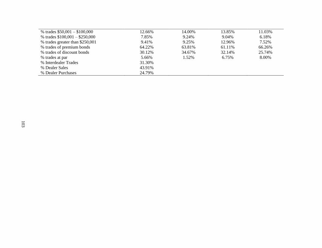
% trades $50,001 – $100,000

% trades $100,001 – $250,000

% trades greater than $250,001

% trades of premium bonds

% trades of discount bonds

% trades at par

% Interdealer Trades

% Dealer Sales

% Dealer Purchases

12.66%

7.85%

9.41%

64.22%

30.12%

5.66%

31.30%

43.91%

24.79%

14.00%

9.24%

9.25%

63.81%

34.67%

1.52%

13.85%

9.04%

12.96%

61.11%

32.14%

6.75%

11.03%

6.18%

7.52%

66.26%

25.74%

8.00%

103

104

APPENDIX 2: SAMPLE SUMMARY STATISTICS, BOND LEVEL

Appendix 2: Sample Summary Statistics, Bond Level Appendix 2 provides summary characteristics of all municipal bonds that trade more than nine times from 2010 – 2013. The sample includes

331,429 individual securities issued by the 50 states and 20,553,922 trades. Panel A provides information for the full sample of bond trades for all

bonds and for bonds issued by the top five municipal bond issuing states in the sample (California, Texas, New York, Pennsylvania, and Illinois).

Panel B includes interdealer trades, Panel C includes dealer purchases, and Panel D includes dealer sales (for all municipal bond trades and also for

bonds issued by the top five issuers). Price is the average daily price for each bond. Dollar volume is the average daily dollar volume for each bond.

Number of trades is the average daily trades for each bond. Trade size is the average daily par value traded. Volatility is calculated weekly following

Downing and Zhang (2004): 100

Pricet(Pricet

Max − PricetMin). Bid-ask spread is calculated weekly for each bond by taking the weekly average buy

price – weekly average sell price. The return is the trade-to-trade return.

All Municipal Bonds Top Five Municipal Bond Issuing States

N Mean Minimum Maximum N Mean Minimum Maximum

Panel A: Full Sample

Price

$Vol

Trades

TSize

Volatility

Spread

Return

331,159

331,159

331,159

331,159

331,159

331,159

331,159

103.25%

$729,893.75

2.94

$277,288.89

1.84%

1.58%

0.08%

25.00%

$1,979.47

1.00

$484.10

0.00%

0.00%

-22.72%

155.29%

$993,255,000.00

157.00

$153,333,333.00

102.83%

18.05%

1,308.64%

142,254

142,254

142,254

142,254

142,254

142,254

142,254

101.90%

$771,291.97

2.94

$297,126.43

1.94%

1.62%

0.09%

25.00%

$2,000.00

1.00

$1,000.00

0.00%

0.00%

-15.45%

155.29%

$541,162,162.00

132.07

$153,333,333.00

51.82%

18.05%

124.12%

Panel B: Interdealer Trades

Price

$Vol

Trades

TSize

Volatility

Spread

Return

293,932

293,932

293,932

293,932

293,932

293,932

293,932

103.18%

$319,723.25

1.94

$159,494.25

2.06%

1.71%

-0.12%

25.00%

$440.75

1.00

$300.25

0.00

0.00%

-62.38%

156.74%

$991,085,000.00

98.00

$99,000,000.00

165.58%

18.05%

495.09%

126,971

126,971

126,971

126,971

126,971

126,971

126,971

101.82%

$339,547.83

1.97

$167,814.31

2.14%

1.75%

-0.09%

25.00%

$1,000.00

1.00

$484.71

0.00%

0.00%

-54.02%

156.74%

$110,146,667.00

46.00

$98,100,000.00

51.82%

18.05%

495.09%

Panel C: Dealer Purchases

Price

$Vol

Trades

TSize

Volatility

Spread

Return

324,616

324,616

324,616

324,616

324,616

324,616

324,616

102.43%

$393,357.79

1.11

$342,465.67

1.79%

1.52%

-0.86%

25.00%

$212.00

1.00

$212.00

0.00%

0.00%

-49.34%

156.19%

$717,256,216.00

45.00

$358,634,775.00

102.83%

18.05%

5,137.10%

139,511

139,511

139,511

139,511

139,511

139,511

139,511

101.10%

$429,278.16

1.11

$371,894.89

1.88%

1.57%

-0.88%

25.00%

$212.00

1.00

$212.00

0.00

0.00%

-29.26%

156.19%

$717,256,216.00

45.00

$358,634,775.00

51.82%

18.05%

156.36%

Panel D: Dealer Sales

Price

$Vol

Trades

331,145

331,145

331,145

103.93%

$376,947.15

1.62

25.00%

$705.80

1.00

155.45%

$576,400,000.00

155.00

142,250

142,250

142,250

102.60%

$399,125.07

1.62

25.00%

$1,000.00

1.00

155.45%

$200,990,000.00

98.84

105

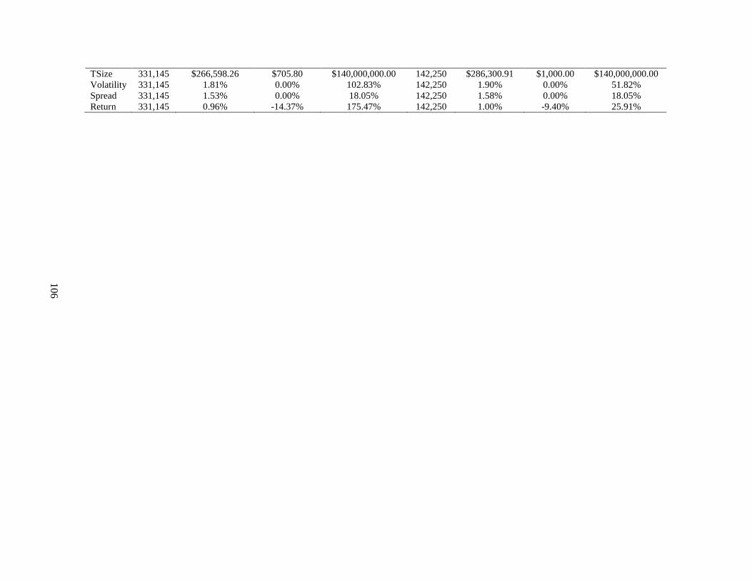
TSize

Volatility

Spread

Return

331,145

331,145

331,145

331,145

$266,598.26

1.81%

1.53%

0.96%

$705.80

0.00%

0.00%

-14.37%

$140,000,000.00

102.83%

18.05%

175.47%

142,250

142,250

142,250

142,250

$286,300.91

1.90%

1.58%

1.00%

$1,000.00

0.00%

0.00%

-9.40%

$140,000,000.00

51.82%

18.05%

25.91%

10

6

107

APPENDIX 3: EVENT DAY DIFFERENCES

Appendix 3: Event Day Differences Appendix 3 provides a comparison between event period and non-event periods in the sample (2010 – 2013). The event period is the week of the

event, and the non-event period is all other trading days. Panel A includes tornados, Panel B includes wildfires, and Panel C includes

hurricanes/tropical storms. Price is the average daily price for each bond. Dollar volume is the average daily dollar volume for each bond.

Number of trades is the average daily trades for each bond. Trade size is the average daily par value traded. Volatility is calculated weekly

following Downing and Zhang (2004): 100

Pricet(Pricet

Max − PricetMin). Bid-ask spread is calculated weekly for each bond by taking the weekly

average buy price – weekly average sell price. The return is the trade-to-trade return. Significance is indicated at the 1%, 5%, and 10% levels

with ***, ***, and *.

Event Days Non-Event Days Difference

Panel A: Tornadoes

Price

Dollar Volume

Number of Trades

Trade Size

Volatility

Bid-Ask Spread

Return

103.20%

$705,058.14

2.78

$285,057.95

1.88%

1.61%

0.05%

103.20%

663,925.86

2.74

$279,196.21

1.94%

1.63%

0.07%

0.00

$41,132.28***

0.04***

$5,861.74**

-0.05%***

-0.02%***

-0.02%***

Panel B: Wildfires

Price

Dollar Volume

Number of Trades

Trade Size

Volatility

Bid-Ask Spread

Return

102.80%

$685,520.42

2.75

$273,875.25

1.95%

1.65%

0.11%

102.61%

$626,466.59

2.70

$262,897.19

1.99%

1.66%

0.09%

0.20%***

$57,053.83***

0.06***

$10,978.06***

-0.04%***

-0.01%***

0.02%***

Panel C: Hurricanes/Tropical Storms

Price

Dollar Volume

Number of Trades

Trade Size

Volatility

Bid-Ask Spread

Return

104.45%

$768,732.45

2.78

$333,257.95

1.99%

1.69%

0.14%

103.60%

$757,811.55

2.79

$329,400.94

2.18%

1.76%

0.04%

0.83%***

$10,920.91

-0.01

$3,857.01

-0.19%***

-0.07%***

0.10%*

108

109

APPENDIX 4: EVENT DAYS AND NON-EVENT DAYS TRADE SIZE DIFFERENCES

Appendix 4: Event Days and Non-Event Days Trade Size Differences Appendix 4 provides event period and non-event period statistics, as well as differences between the two time periods, for small trades, medium trades,

and large trades. Small trades are less than $25,000 in size. Medium trades are $25,001 – $100,000 in size. Large trades are greater than $100,001 in

size. Summary information is calculated using 20,553,922 bond trades in 331,429 municipal bonds. Price is the average price (by trade size).

Percentage volume is the portion of volume for which each trade size accounts, and percentage trades is the portion of trades for which each trade size

accounts. The bid-ask spread is the weekly spread for each trade size. Significance is indicated at the 1%, 5%, and 10% levels with ***, ***, and *.

Tornados Wildfires Hurricanes/Tropical Storms

Small Medium Large Small Medium Large Small Medium Large

Panel A: Event Days

% Vol

% Trades

Spread

48.67%

51.11%

1.91%

33.17%

32.52%

1.64%

18.17%

16.37%

1.21%

48.05%

50.50%

1.95%

33.91%

33.25%

1.67%

18.04%

16.25%

1.26%

50.25%

52.92%

2.04%

32.68%

31.73%

1.78%

17.07%

15.35%

1.22%

Panel B: Non-Event Days

% Vol

% Trades

Spread

48.48%

50.99%

1.93%

33.50%

32.80%

1.64%

18.02%

16.21%

1.22%

48.05%

50.48%

1.96%

34.02%

33.37%

1.68%

17.93%

16.15%

1.26%

50.28%

53.21%

2.09%

32.76%

31.73%

1.81%

16.97%

15.06%

1.23%

Panel C: Differences

% Vol

% Trades

Spread

0.19%*

0.13%

-0.02%***

-0.34%***

-0.29%***

0.00%

0.15%**

0.16%**

0.01%

0.00%

0.02%

-0.01%**

-0.11%

-0.11%

-0.01%

0.11%

0.10%

0.00%

-0.03%

-0.29%

-0.05%***

-0.08%

0.00%

-0.03%***

0.11%

0.29%

-0.01%

110

111

APPENDIX 5: EVENT DAYS AND NON-EVENT DAYS TRADE TYPE DIFFERENCES

Appendix 5: Event Days and Non-Event Days Trade Type Differences Appendix 5 provides event period and non-event period statistics, as well as differences between the two time periods, for interdealer trades, dealer purchases, and dealer sales.

Summary information is calculated using 20,553,922 bond trades in 331,429 municipal bonds. Price is the average price (by trade type). Percentage volume is the portion of

volume for which each trade type accounts, and percentage trades is the portion of trades for which each trade type accounts. The bid-ask spread is the weekly spread for each

trade type. Significance is indicated at the 1%, 5%, and 10% levels with ***, ***, and *.

Tornados Wildfires Hurricanes/Tropical Storms

InTrades DBuys DSales InTrades DBuys DSales InTrades DBuys DSales

Panel A: Event Days

% Vol

% Tds

Spread

22.90%

22.50%

1.83%

36.12%

34.94%

1.58%

40.99%

42.56%

1.58%

23.34%

22.95%

1.86%

35.99%

34.82%

1.63%

40.68%

42.23%

1.62%

22.12%

21.82%

1.93%

37.49%

36.46%

1.69%

40.38%

41.72%

1.69%

Panel B: Non-Event Days

% Vol

% Tds

Spread

23.43%

23.06%

1.84%

35.45%

34.33%

1.57%

41.11%

42.61%

1.57%

23.67%

23.31%

1.87%

35.22%

34.12%

1.61%

41.12%

42.57%

1.62%

22.95%

22.64%

1.98%

35.94%

34.87%

1.68%

41.10%

42.49%

1.70%

Panel C: Differences

% Vol

% Tds

Spread

-0.53%***

-0.56%***

-0.01%**

0.66%***

0.60%***

0.01%***

-0.13%***

-0.05%

0.01%***

-0.33%***

-0.36%***

-0.01%

0.77%***

0.70%***

0.02%***

-0.44%***

-0.34%***

0.00%

-0.83%

-0.81%***

-0.06%***

1.55%***

1.59%***

0.01%

-0.72%***

-0.77%***

-0.01%**

112

113

APPENDIX 6: EVENT PERIOD SUMMARY STATISTICS

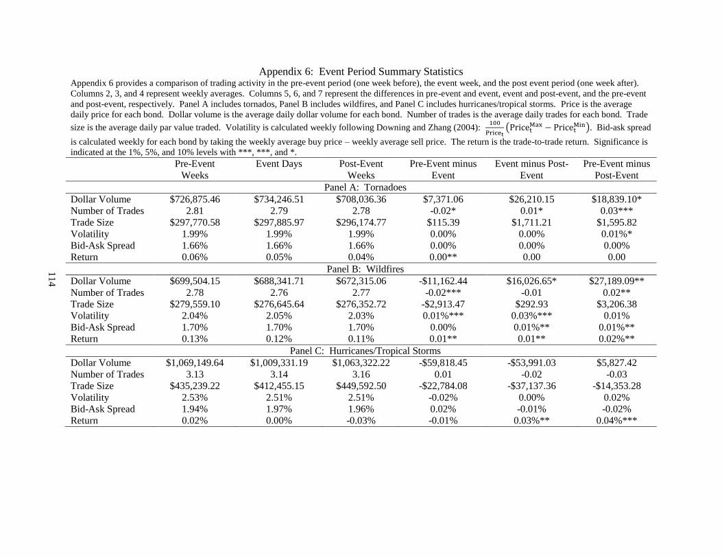
Appendix 6: Event Period Summary Statistics Appendix 6 provides a comparison of trading activity in the pre-event period (one week before), the event week, and the post event period (one week after).

Columns 2, 3, and 4 represent weekly averages. Columns 5, 6, and 7 represent the differences in pre-event and event, event and post-event, and the pre-event

and post-event, respectively. Panel A includes tornados, Panel B includes wildfires, and Panel C includes hurricanes/tropical storms. Price is the average

daily price for each bond. Dollar volume is the average daily dollar volume for each bond. Number of trades is the average daily trades for each bond. Trade

size is the average daily par value traded. Volatility is calculated weekly following Downing and Zhang (2004): 100

Pricet(Pricet

Max − PricetMin). Bid-ask spread

is calculated weekly for each bond by taking the weekly average buy price – weekly average sell price. The return is the trade-to-trade return. Significance is

indicated at the 1%, 5%, and 10% levels with ***, ***, and *.

Pre-Event

Weeks

Event Days

Post-Event

Weeks

Pre-Event minus

Event

Event minus Post-

Event

Pre-Event minus

Post-Event

Panel A: Tornadoes

Dollar Volume

Number of Trades

Trade Size

Volatility

Bid-Ask Spread

Return

$726,875.46

2.81

$297,770.58

1.99%

1.66%

0.06%

$734,246.51

2.79

$297,885.97

1.99%

1.66%

0.05%

$708,036.36

2.78

$296,174.77

1.99%

1.66%

0.04%

$7,371.06

-0.02*

$115.39

0.00%

0.00%

0.00**

$26,210.15

0.01*

$1,711.21

0.00%

0.00%

0.00

$18,839.10*

0.03***

$1,595.82

0.01%*

0.00%

0.00

Panel B: Wildfires

Dollar Volume

Number of Trades

Trade Size

Volatility

Bid-Ask Spread

Return

$699,504.15

2.78

$279,559.10

2.04%

1.70%

0.13%

$688,341.71

2.76

$276,645.64

2.05%

1.70%

0.12%

$672,315.06

2.77

$276,352.72

2.03%

1.70%

0.11%

-$11,162.44

-0.02***

-$2,913.47

0.01%***

0.00%

0.01**

$16,026.65*

-0.01

$292.93

0.03%***

0.01%**

0.01**

$27,189.09**

0.02**

$3,206.38

0.01%

0.01%**

0.02%**

Panel C: Hurricanes/Tropical Storms

Dollar Volume

Number of Trades

Trade Size

Volatility

Bid-Ask Spread

Return

$1,069,149.64

3.13

$435,239.22

2.53%

1.94%

0.02%

$1,009,331.19

3.14

$412,455.15

2.51%

1.97%

0.00%

$1,063,322.22

3.16

$449,592.50

2.51%

1.96%

-0.03%

-$59,818.45

0.01

-$22,784.08

-0.02%

0.02%

-0.01%

-$53,991.03

-0.02

-$37,137.36

0.00%

-0.01%

0.03%**

$5,827.42

-0.03

-$14,353.28

0.02%

-0.02%

0.04%***

114

115

APPENDIX 7: EVENT PERIOD STATISTICS FOR RELATED SECURITIES

(TORNADOES)

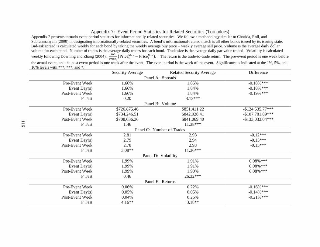
Appendix 7: Event Period Statistics for Related Securities (Tornadoes) Appendix 7 presents tornado event period statistics for informationally-related securities. We follow a methodology similar to Chorida, Roll, and

Subrahmanyam (2000) in designating informationally-related securities. A bond’s informational-related match is all other bonds issued by its issuing state.

Bid-ask spread is calculated weekly for each bond by taking the weekly average buy price – weekly average sell price. Volume is the average daily dollar

volume for each bond. Number of trades is the average daily trades for each bond. Trade size is the average daily par value traded. Volatility is calculated

weekly following Downing and Zhang (2004): 100

Pricet(Pricet

Max − PricetMin). The return is the trade-to-trade return. The pre-event period is one week before

the actual event, and the post event period is one week after the event. The event period is the week of the event. Significance is indicated at the 1%, 5%, and

10% levels with ***, ***, and *.

Security Average Related Security Average Difference

Panel A: Spreads

Pre-Event Week

Event Day(s)

Post-Event Week

F Test

1.66%

1.66%

1.66%

0.20

1.85%

1.84%

1.84%

8.13***

-0.18%***

-0.18%***

-0.19%***

Panel B: Volume

Pre-Event Week

Event Day(s)

Post-Event Week

F Test

$726,875.46

$734,246.51

$708,036.36

1.46

$851,411.22

$842,028.41

$841,069.40

11.38***

-$124,535.77***

-$107,781.89***

-$133,033.04***

Panel C: Number of Trades

Pre-Event Week

Event Day(s)

Post-Event Week

F Test

2.81

2.79

2.78

3.08**

2.93

2.94

2.93

11.36***

-0.12***

-0.15***

-0.15***

Panel D: Volatility

Pre-Event Week

Event Day(s)

Post-Event Week

F Test

1.99%

1.99%

1.99%

0.46

1.91%

1.91%

1.90%

26.32***

0.08%***

0.08%***

0.08%***

Panel E: Returns

Pre-Event Week

Event Day(s)

Post-Event Week

F Test

0.06%

0.05%

0.04%

4.16**

0.22%

0.05%

0.26%

3.18**

-0.16%***

-0.14%***

-0.21%***

116

117

APPENDIX 8: EVENT PERIOD STATISTICS FOR RELATED SECURITIES (WILDFIRES)

Appendix 8: Event Period Statistics for Related Securities (Wildfires) Appendix 8 presents wildfire event period statistics for informationally-related securities. We follow a methodology similar to Chorida, Roll, and

Subrahmanyam (2000) in designating informationally-related securities. A bond’s informational-related match is all other bonds issued by its issuing state.

Bid-ask spread is calculated weekly for each bond by taking the weekly average buy price – weekly average sell price. Volume is the average daily dollar

volume for each bond. Number of trades is the average daily trades for each bond. Trade size is the average daily par value traded. Volatility is calculated

weekly following Downing and Zhang (2004): 100

Pricet(Pricet

Max − PricetMin). The return is the trade-to-trade return. The pre-event period is one week before

the actual event, and the post event period is one week after the event. The event period is the week of the event. Significance is indicated at the 1%, 5%, and

10% levels with ***, ***, and *.

Security Average Informationally-Related

Security Average

Difference

Panel A: Spreads

Pre-Event Week

Event Day(s)

Post-Event Week

F Test

1.70%

1.70%

1.70%

0.73

1.90%

1.89%

1.89%

15.92***

-0.19%***

-0.19%***

-0.19%***

Panel B: Volume

Pre-Event Week

Event Day(s)

Post-Event Week

F Test

$699,504.15

$688,341.71

$672,315.06

0.75

$783,932.41

$800,197.52

$807,149.83

69.01***

-$84,428.26***

-$111,855.81***

-$134,834.76***

Panel C: Number of Trades

Pre-Event Week

Event Day(s)

Post-Event Week

F Test

2.78

2.76

2.77

1.83

2.91

2.91

2.91

2.22

-0.12***

-0.15***

-0.14***

Panel D: Volatility

Pre-Event Week

Event Day(s)

Post-Event Week

F Test

2.04%

2.05%

2.03%

4.74***

1.98%

1.98%

1.96%

56.55***

0.07%***

0.08%***

0.07%***

Panel E: Returns

Pre-Event Week

Event Day(s)

Post-Event Week

F Test

0.13%

0.12%

0.11%

2.28

0.66%

0.11%

0.11%

466.16***

-0.53%***

0.01%***

0.00

118

119

APPENDIX 9: EVENT PERIOD STATISTICS FOR RELATED SECURITIES

(HURRICANES/TROPICAL STORMS)

Appendix 9: Event Period Statistics for Related Securities (Hurricanes/Tropical Storms) Appendix 9 presents hurricane/tropical storm event period statistics for informationally-related securities. We follow a methodology similar to Chorida, Roll,

and Subrahmanyam (2000) in designating informationally-related securities. A bond’s informational-related match is all other bonds issued by its issuing

state. Bid-ask spread is calculated weekly for each bond by taking the weekly average buy price – weekly average sell price. Volume is the average daily

dollar volume for each bond. Number of trades is the average daily trades for each bond. Trade size is the average daily par value traded. Volatility is

calculated weekly following Downing and Zhang (2004): 100

Pricet(Pricet

Max − PricetMin). The return is the trade-to-trade return. The pre-event period is one

week before the actual event, and the post event period is one week after the event. The event period is the week of the event. Significance is indicated at the

1%, 5%, and 10% levels with ***, ***, and *.

Security Average Informationally-Related

Security Average

Difference

Panel A: Spreads

Pre-Event Week

Event Day(s)

Post-Event Week

F Test

1.94%

1.96%

1.96%

0.36

1.90%

1.90%

1.94%

47.01***

0.04%*

0.06%**

0.02%

Panel B: Volume

Pre-Event Week

Event Day(s)

Post-Event Week

F Test

$1,069,149.64

$1,009,331.19

$1,063,322.22

0.22

$665,079.18

$671,973.14

$663,985.11

0.33

$404,070.46***

$337,358.05***

$399,337.11***

Panel C: Number of Trades

Pre-Event Week

Event Day(s)

Post-Event Week

F Test

3.13

3.14

3.16

0.06

2.80

2.82

2.89

123.01***

0.34***

0.32***

0.27***

Panel D: Volatility

Pre-Event Week

Event Day(s)

Post-Event Week

F Test

2.53%

2.51%

2.51%

0.11

1.87%

1.84%

1.85%

19.84***

0.65%***

0.67%***

0.66%***

Panel E: Returns

Pre-Event Week

Event Day(s)

Post-Event Week

F Test

0.01%

0.00%

-0.03%

4.94***

0.06%

0.07%

0.02%

45.44***

-0.05%***

-0.07%***

-0.05%***

120

121

APPENDIX 10: SPREAD REGRESSIONS

Appendix 10: Spread Regressions Appendix 10 provides spread regression estimations for 331,429 municipal bonds with 20,553,922 trades from January 2010 – December 2013 for tornados,

wildfires, and hurricanes/tropical storms. Regressions are estimated weekly using 3,461,639 bond-week observations. The event period is the week of the

event, and the post-event period is the week following the event. The related security is the average bid-ask spread of all other municipal bonds from the same

issuing state. The Event Period*Related Security is an interaction term between the event and the related security, and the Post-Event*Related Security is an

interaction term between the post-event period and the related security. Dollar volume is the weekly dollar volume for each, and the number of trades is the

weekly trades for each bond. Trade size is the average weekly par value traded for each bond. Volatility is calculated following Downing and Zhang (2004): 100

Pricet(Pricet

Max − PricetMin). Years to maturity is the time to maturity for each bond. Revenue Bond is equal to 1 if the bond is a revenue bond, and zero

otherwise. Taxable is equal to 1 if the bond is taxable, and zero otherwise. Top 5 Issuer is equal to 1 if the bond is issued by California, Texas, Pennsylvania,

New York, or Illinois. Population is the yearly population for each state provided by the U.S. Census Bureau. The median income is the annual median

income of each state, and general fund revenue is the general fund revenue for each state. All regression models are estimated using robust standard errors.

Significance is indicated at the 1%, 5%, and 10% levels with ***, ***, and *.

Tornados

(1)

Wildfires

(2)

Hurricanes/Tropical Storms

(3)

Intercept

Variables of Interest

Event Day(s)

Post-Event Week

Related Security

Event Day(s)*Related Security

Post-Event*Related Security

Bond/Trading Traits

Dollar Volume

Number of Trades

Trade Size

Volatility

Years to Maturity

-0.0401***

(-6.35)

-0.0290***

(-3.04)

-0.0445***

(-4.81)

0.2155***

(41.50)

0.0181***

(3.46)

0.0264***

(5.23)

0.0000

(0.96)

-0.0000

(-1.02)

-0.0000***

(-40.82)

0.5457***

(113.89)

0.0137***

-0.0447***

(-7.11)

-0.0473***

(-4.33)

0.0233*

(1.89)

0.2187***

(41.98)

0.0247***

(4.19)

-0.0103

(-1.57)

0.0000

(0.96)

-0.0000

(-1.02)

-0.0000***

(-40.82)

0.5457***

(113.88)

0.0137***

-0.0477***

(-7.74)

0.0713

(1.56)

-0.1115**

(-2.54)

0.2201***

(42.73)

-0.0200

(-0.78)

0.0788***

(3.44)

0.0000

(0.96)

-0.0000

(-1.02)

-0.0000***

(-40.82)

0.5457***

(113.88)

0.0137***

122

Revenue Bond

Taxable

Top 5 Issuer

State Characteristics

Population

Median Income

General Fund Revenue

R-Squared

(29.29)

0.0073***

(6.60)

0.0690***

(27.98)

-0.0060***

(-4.50)

0.0000***

(2.77)

0.0000***

(18.29)

-0.0000***

(-15.60)

68.12%

(29.29)

0.0074***

(6.70)

0.0690***

(27.97)

-0.0056***

(-4.20)

0.0000***

(3.22)

0.0000***

(18.27)

-0.0000***

(-16.60)

68.12%

(29.29)

0.0075***

(6.74)

0.0690***

(27.99)

-0.0056***

(-4.18)

0.0000***

(3.06)

0.0000***

(18.29)

-0.0000***

(-16.40)

68.12%

123

124

APPENDIX 11: VOLATILITY REGRESSIONS

Appendix 11: Volatility Regressions Appendix 11 provides volatility regression estimations for 331,429 municipal bonds with 20,553,922 trades from January 2010 – December 2013 for tornados,

wildfires, and hurricanes/tropical storms. Regressions are estimated weekly using 3,461,639 bond-week observations. The event period is the week of the

event, and the post-event period is the week following the event. The related security is the average volatility of all other municipal bonds from the same

issuing state. The Event Period*Related Security is an interaction term between the event and the related security, and the Post-Event*Related Security is an

interaction term between the post-event period and the related security. Dollar volume is the weekly dollar volume for each, and the number of trades is the

weekly trades for each bond. Trade size is the average weekly par value traded for each bond. Volatility is calculated following Downing and Zhang (2004): 100

Pricet(Pricet

Max − PricetMin). Years to maturity is the time to maturity for each bond. Revenue Bond is equal to 1 if the bond is a revenue bond, and zero

otherwise. Taxable is equal to 1 if the bond is taxable, and zero otherwise. Top 5 Issuer is equal to 1 if the bond is issued by California, Texas, Pennsylvania,

New York, or Illinois. Population is the yearly population for each state provided by the U.S. Census Bureau. The median income is the annual median

income of each state. All regression models are estimated using bond-clustered standard errors. Significance is indicated at the 1%, 5%, and 10% levels with

***, ***, and *.

Tornados

(1)

Wildfires

(2)

Hurricanes/Tropical Storms

(3)

Intercept

Variables of Interest

Event Day(s)

Post-Event Week

Related Security

Event Day(s)*Related Security

Post-Event*Related Security

Bond/Trading Traits

Dollar Volume

Number of Trades

Trade Size

Years to Maturity

Revenue Bond

-0.3850***

(-3.40)

-0.1937***

(-4.10)

-0.0595

(-1.20)

0.7571***

(27.14)

0.0924***

(3.91)

0.0241

(0.89)

-0.0000

(-1.09)

0.0000

(1.08)

-0.0000***

(-22.27)

0.0974***

(53.83)

-0.0410

-0.4028***

(-3.49)

-0.0925

(-1.02)

-0.0967**

(-2.11)

0.7624***

(26.74)

0.0419

(0.83)

0.0380

(1.59)

-0.0000

(-1.09)

0.0000

(1.08)

-0.0000***

(-22.29)

0.0974***

(53.78)

-0.0409

-0.4182***

(-3.58)

-0.1976

(-1.08)

0.1948*

(1.69)

0.7693***

(27.66)

0.1092

(1.07)

-0.0963

(-1.61)

-0.0000

(-1.09)

0.0000

(1.08)

-0.0000***

(-22.27)

0.0974***

(53.69)

-0.0414

125

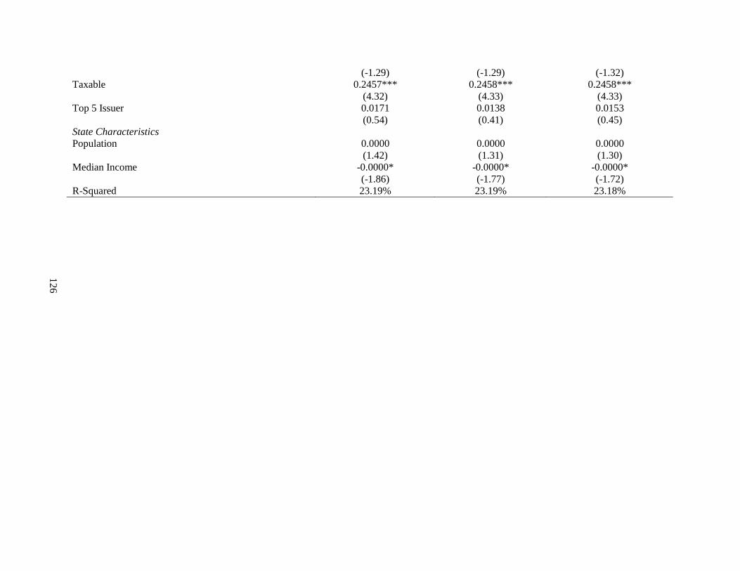
Taxable

Top 5 Issuer

State Characteristics

Population

Median Income

R-Squared

(-1.29)

0.2457***

(4.32)

0.0171

(0.54)

0.0000

(1.42)

-0.0000*

(-1.86)

23.19%

(-1.29)

0.2458***

(4.33)

0.0138

(0.41)

0.0000

(1.31)

-0.0000*

(-1.77)

23.19%

(-1.32)

0.2458***

(4.33)

0.0153

(0.45)

0.0000

(1.30)

-0.0000*

(-1.72)

23.18%

126

127

APPENDIX 12: MOST ACTIVE AND LEAST ACTIVE BONDS

Appendix 12: Most Active and Least Active Bonds Appendix 12 models dollar volume for the most active quartile of bonds and the least active quartile of bonds. The analysis uses 865,628 bond-week

observations for the most active bonds, and 875,118 bond-week observations for the least active bonds. The event period is the week of the event, and the

post-event period is the week following the event. The related security is the average dollar volume of all other municipal bonds from the same issuing state.

The Event Period*Related Security is an interaction term between the event and the related security, and the Post-Event*Related Security is an interaction

term between the post-event period and the related security. Years to maturity is the time to maturity for each bond. Revenue Bond is equal to 1 if the bond is

a revenue bond, and zero otherwise. Taxable is equal to 1 if the bond is taxable, and zero otherwise. Top 5 Issuer is equal to 1 if the bond is issued by

California, Texas, Pennsylvania, New York, or Illinois. Population is the yearly population for each state provided by the U.S. Census Bureau. The median

income is the annual median income of each state. All regression models are estimated using bond-clustered standard errors. Significance is indicated at the

1%, 5%, and 10% levels with ***, ***, and *.

Tornados Wildfires Hurricanes/Tropical Storms

Most Active Least

Active

Most Active Least Active Most Active Least Active

Intercept

Variables of Interest

Event Day(s)

Post-Event Week

Related Security

Event Day(s)*Related

Security

Post-Event*Related Security

Bond/Trading Traits

Years to Maturity

Revenue Bond

Taxable

Top 5 Issuer

State Characteristics

0.00***

(22.03)

511,610,345

(0.54)

13,466,422,678***

(31.93)

1,261.96***

(29.12)

-42.84

(-0.50)

-1,195.18***

(-31.30)

-507,631,660***

(-26.91)

121,564,835

(0.64)

-4,748,091,818***

(-15.88)

-4,412,711,678***

(-23.61)

82.48***

51,122***

(181.59)

-145.48

(-0.68)

271.00

(0.99)

0.0023***

(42.72)

0.00

(0.27)

0.0002*

(-1.73)

-456.80***

(-114.81)

-586.02***

(-7.42)

-

5,275.37***

(-42.55)

-

1,735.22***

(-17.28)

0.00***

(20.03)

$750,231,335

(1.13)

12,986,073,335***

(38.49)

1,257.65***

(26.73)

-4.78

(-0.07)

-1,192.17***

(-37.87)

-534,565,101***

(-25.23)

421,592,760**

(2.17)

-528,577,6185***

(-15.57)

-4,419,877,833***

(-20.82)

89.64***

51,292***

(183.77)

-332.08

(-1.59)

-1,170.64***

(-5.28)

0.0023***

(44.45)

0.0004***

(3.97)

0.0008***

(8.11)

-457.87***

(-115.16)

-589.70***

(-7.47)

-5,278.20***

(-42.57)

-1,725.37***

(-17.16)

0.00***

0.00***

(-20.69)

12,030,119,470***

(25.49)

11,812,405,815***

(25.06)

1,255.98***

(26.92)

-1,171.66***

(-25.32)

-1,154.03***

(-24.83)

-579,497,057***

(-24.25)

394,313,548**

(2.06)

-566,800,6097***

(-15.89)

-5,010,897,536***

(-21.85)

106.61***

51,054***

(185.24)

833.75

(1.28)

1,939.71***

(-2.80)

0.0024***

(48.86)

0.0007**

(2.33)

0.0016***

(5.07)

-457.10***

(-114.89)

-585.96***

(-7.43)

-5,273.66***

(-42.52)

-1,735.26***

(-17.25)

0.0001***

128

Population

Median Income

R-Squared

(10.80)

113,664***

(16.29)

96.91%

0.0001***

(22.15)

0.0932***

(18.67)

3.79%

(9.64)

125,498***

(15.90)

96.70%

(19.26)

0.0944***

(18.96)

3.82%

(12.70)

133,292***

(16.31)

96.58%

(22.10)

0.0950***

(19.09)

3.80%

129

130

APPENDIX A: INDIVIDUAL BONDS TRADED, BY YEAR

131

Appendix A: Individual Bonds Traded, By Year Each column includes the unique number of bonds traded each year for each state in the sample period 2010 –

2013. The last column is the number of unique bonds traded over the course of the full sample for each state.

State 2010 2011 2012 2013 Full Sample

AK

AL

AR

AZ

CA

CO

CT

DC

DE

FL

GA

HI

IA

ID

IL

IN

KS

KY

LA

MA

MD

ME

MI

MN

MO

MS

MT

NC

ND

NE

NH

NJ

NM

NV

NY

OH

OK

OR

PA

RI

SC

SD

TN

TX

UT

VA

VT

WA

WI

WV

WY

579

1,391

806

2,801

24,692

2,643

2,626

353

1,188

8,548

3,323

812

674

401

9,504

4,883

1,544

1,078

922

3,812

1,868

628

4,884

2,340

2,232

1,414

280

4,498

188

753

589

6,642

674

926

13,871

5,274

968

2,517

9,087

603

2,708

206

1,405

12,408

895

3,377

70

4,285

1,774

209

86

579

1,454

747

2,995

24,888

2,706

2,606

402

1,201

8,649

3,721

866

736

416

9,406

4,951

1,508

1,109

884

3,900

2,056

600

4,659

2,318

2,166

1,392

254

4,658

200

770

594

6,951

669

913

14,337

5,488

1,034

2,730

9,088

661

2,904

221

1,333

12,856

946

3,517

92

4,528

1,762

200

95

553

1,516

891

2,690

25,683

2,564

2,405

438

1,096

7,700

3,423

809

701

372

8,831

4,478

1,410

1,108

937

3,557

1,958

633

4,126

2,153

1,981

1,334

291

4,334

210

792

593

6,251

632

804

13,505

4,959

912

2,458

8,290

544

2,740

222

1,361

12,516

832

3,428

98

4,254

1,655

179

102

621

1,763

937

3,033

25,791

2,954

2,846

547

1,198

7,962

3,722

887

840

444

9,453

4,834

1,709

1,244

1,085

3,870

2,228

748

4,338

2,333

2,315

1,522

345

5,081

283

861

651

6,652

774

871

14,758

5,720

1,108

2,932

9,130

648

2,970

264

1,429

14,358

1,034

4,054

64

4,929

1,909

212

157

1,253

3,270

2,067

5,380

49,234

5,650

5,646

753

2,063

15,011

6,809

1,521

1,761

877

18,576

10,287

3,489

2,546

2,038

7,711

3,901

1,511

9,398

5,196

4,732

2,902

711

9,524

566

1,717

1,324

13,840

1,475

1,560

27,550

11,281

2,212

5,613

18,877

1,399

5,728

540

2,884

28,017

1,939

7,184

175

8,845

3,929

420

266

132

APPENDIX B: NATURAL DISASTER EVENTS, BY YEAR

133

Appendix B: Natural Disaster Events, By Year Appendix B includes information on the number of natural disasters and the types of natural disasters that occur

each year in the sample period 2010 – 2013. Natural disaster information is obtained from the National Climactic

Data Center’s website.

Disaster Type 2010 2011 2012 2013 All Years

Tornados

Wildfires

Hurricanes/Tropical

Storms

308

273

7

328

836

21

268

565

13

268

203

5

1,172

1,877

46

Total 588 1,185 846 476 3,095

134

PART 3: MUNICIPAL BOND TRADING AND POLITICAL SCANDALS

135

INTRODUCTION

Research details that investors profit from local investment choices; for example, Ivkovic

and Weisbenner (2005) show that local investments outperform non-local investments by 3.2%.

Ivkovic and Weisbenner conclude the performance of local investments is driven by superior

knowledge of local firms. Local investors may choose to invest not only in equities, but also in

municipal bonds. One reason the municipal bond market is attractive to local investors is the tax

advantages it offers. The knowledge base of local investors may not be limited to surrounding

firms; it may also extend to local governments. Scott (2006) details that 69% of residents

interact with their local mayor and 78% interact with their local city council. Scott also shows

that 63% of local residents have access to city budgets and financial reports. Investors are able

to garner information about local governments through these interactions.

Documenting the municipal bond market’s reaction to government misconduct provides

information as to how and when the bond market incorporates information. There are three

reasons why studying the municipal bond market provides value. First, focusing on the

municipal bond market allows us to study a market dominated by local retail investors, as

documented by Green, Hollifield, and Schurhoff (2007). Retail traders may be both the traders

most affected by the wrongdoing and the traders with the most information about the misconduct

itself. Scott (2006) details that local residents often interact with local officials and have access

to city financial reports. Retail trades may aid in price discovery both during and after

announcements of government misconduct, and we are able to determine what type(s) of trades

contribute to price discovery by dividing our sample into small trades and large trades.

136

Second, the municipal bond market does not offer the same transparency or information

availability as the equity market. Municipalities do not release quarterly earnings reports like

public firms, and many municipalities that issue bonds are small. Information is not always

readily available about municipalities given the lack of transparency in the market, and it is

possible that news of government officials’ wrongdoing may serve as one of the only sources of

information about the quality of government in municipalities. Additionally, information about

municipal securities may be hard to disseminate and absorb; each municipality can have multiple

issues of bonds outstanding. For example, municipal bonds tend to be issued in a series, and

some of the larger issues contain as many as thirty bonds of various maturities and coupon rates

(Green, Hollified, and Schurhoff, 2007). It may be difficult to decipher information about such a

large amount of securities, especially compared to the equities market where investors need to be

informed about only one class or type of stock per firm.

Third, the municipal bond market is different from the equities market. There is no

exchange fostering pre-trade transparency in the municipal bond market, and there is also no

quote or order book that traders can use to guarantee fair prices on municipal bonds. In fact,

previous literature documents that large amounts of price dispersion exist in the municipal bond

market, even after post trade transparency is implemented (Schultz, 2012). Bond markets in

general are also less efficient than the equities market. We provide evidence regarding the

municipal bond market’s efficiency and quality by studying bond trading activity before, during,

and after announcements regarding government officials and their misconduct.

137

RELATED LITERATURE

Research exists on the overall market quality of the municipal bond market. For

example, Harris and Piwowar (2007) show that trading costs are inversely related to trade size

and that the municipal bond market is illiquid. Green, Li, and Schurhoff (2010) provide

evidence regarding municipal bond pricing efficiency and focus on profit-motivated dealers and

their behavior. The authors detail that municipal bond dealers are quick to incorporate

information that results in price increases, but are slow to react to information that negatively

influences bond prices. While Green, Li, and Schurhoff focus on how dealers react to

macroeconomic news, this paper focuses on how individual municipal bond traders react to

news. Specifically, this paper focuses on how (and if) municipal bond traders react to

wrongdoing by local political officials.

Local traders, in general, not only invest locally but also make informed local investment

decisions. Ivkovic and Weisbenner (2005) find that local investors allocate roughly 30% of their

investment portfolio to local firms. The local investments chosen outperform non-local

investments by 3.2%. Based on the outperformance, the authors conclude that local traders

choose their investments based on knowledge of local firms. The tendency to invest locally also

extends to mutual fund managers. Coval and Moskowitz (1999, 2001) show mutual fund

managers invest in companies geographically close to the manager’s location and the local

investments earn a positive 2.67% abnormal return per year. Again, the return on the investment

implies superior knowledge of local firms.

138

Butler, Fauver, and Mortal (2009) provide a study of political integrity in the municipal

bond underwriting market. While Butler, Fauver, and Mortal do not focus on government

misbehavior, the authors focus on a related topic. Specifically, they focus on the effect of

political integrity and corruption on the issuance of municipal bonds. Butler, Fauver, and Mortal

study the municipal bond underwriting market and describe how it is historically fraught with

corruption due to a pay-to-play practice; basically, investment banks bid on underwriting

business through their campaign contributions to local government officials. The authors use

per-capita federal convictions as a proxy for local corruption. In general, they find that credit

risk and corruption are correlated. Specifically, states with higher corruption tend to issue, on

average, riskier bonds (based on credit ratings) and corrupt states tend to pay higher yields to

maturity. The authors do not provide any evidence regarding corruption and local bond trader

behavior, however. This paper adds to the Butler, Fauver, and Mortal paper by showing how

municipal bond traders react to wrongdoing by local government officials.

139

HYPOTHESES

Butler, Fauver, and Mortal (2009) establish a link between municipal bonds and state

corruption. Butler, Fauver, and Mortal do not provide evidence regarding investor reaction to

political wrongdoing, nor do they examine municipal bond trading. In this paper, we focus on

municipal bond trading activity and its relation to governmental misconduct. First, we focus on

the municipal bond spread. Butler, Fauver, and Mortal detail that corrupt states tend to issue

riskier bonds, which could lead to higher spreads for traders. In addition, dealers may adjust the

bond spread following a political scandal to compensate for informed traders. We present the

following hypothesis:

H1: Municipal bond spread increases following a local scandal.

Second, we focus on trading activity following the disclosure of government misconduct.

Information will disseminate into the market following a scandal. McInish and Wood (1992)

utilize volume as a measure of information. As information flows into the market, we expect

both trading volume and the number of trades will increase. We present the following

hypotheses:

H2: Municipal bond volume increases following a local political scandal.

H3: The number of trades in municipal bond issues increases following a local political

scandal.

Third, we focus on the activity following a political scandal. In the bond market, trade

size is an indicator of whether a trade is an institutional or a retail trade. Ronen and Tavy (2013)

detail that small bond trades are almost always retail trades, whereas larger trades are

140

institutions. Due to the tax advantages offered to municipal bond holders, municipal bond retail

trades are likely local investors (Green, Hollifield, and Schurhoff, 2007). State residents are

offered tax advantages on municipal bonds, but only for bonds issued in the state in which they

reside. Focusing on how (or if) trade size changes as traders share their information following a

political scandal enables us to determine whether institutions, local retail investors, or perhaps

both are changing their trading activity following a scandal. We present the following

hypothesis:

H4: There is a direct relation between the average municipal bond trade size and the

occurrence of a political scandal.

Research supports both institutions and local traders as informed traders. Ivkovic and

Weisbenner (2005) determine that local investments tend to outperform non-local investments by

over 3%, leading the authors to conclude that local investors possess superior knowledge of local

firms. Mutual fund managers are shown to invest in local companies and to earn abnormal

returns on local investments (Coval and Moskowitz, 1999, 2001). Institutions are also shown to

provide information to the market. Chakravarty (2001) details that institutions make up a

majority of the price impact of medium-sized equity trades. It is possible that both retail

investors and institutions provide information to the municipal bond market following a political

scandal. Ivkovic and Weisbenner and Coval and Moskowitz utilize abnormal returns as a

measure of information, while Chakravarty uses price impact to determine that institutions

provide information to the market. By using both returns and price impact, we are able to show

which size investors earns abnormal returns following government wrongdoing, and also which

size investors contributes to price contribution. We propose the following hypotheses:

141

H5A: There is a direct relation between abnormal returns in the municipal bond market and the

occurrence of a local political scandal.

H5B: There is a direction relation between weighted price contribution in the municipal bond

market and the occurrence of a local political scandal.

142

DATA AND SAMPLE SELECTION

We use municipal bond transaction data for January 2006 through December 2013 from

the Municipal Securities Rulemaking Board (MSRB). The MSRB municipal bond database

includes all trades by registered broker-dealers. Each trade is identified as a dealer purchase

from a customer, dealer sale to a customer, or interdealer trade, and each trade record includes

the CUSIP, security information, coupon, yield, par value traded, and price. The data initially

includes 78,640,003 bond transactions. We require bonds in the sample to trade nine times each

year (Edwards, Harris, and Piwowar, 2007)1, which removes 10,372,314 trades from the sample.

We also require bonds in the sample to trade at prices above 25% of par in order to remove

municipalities close to bankruptcy or default, and we remove transactions with data entry

errors/missing values. These two deletions further reduce our sample by 217,332 trades.

After constructing weekly spread measures, we lose an additional 28,948,700

observations. Our final data sample includes 39,105,657 trades in 481,365 municipal bonds

issued by the municipalities in all fifty states in the United States. We obtain each bond’s issuing

state and whether a bond is general obligation or revenue from the MSRB’s Electronic Municipal

Market Access (EMMA) website. We collect data on state population and income from the

United States Census Burea, and we obtain information on individual state financials from the

Fiscal Survey of the States compiled by the State Governor’s Association.

1 Harris and Piwowar (2006) study transactions costs in the municipal bond market and require bonds in their

sample to trade at least six times. We follow Edwards et al (2007) and use a more restrictive requirement (nine

times each year) to control for potential nonsynchronous trading, given the illiquidity of the municipal bond market.

We replicate each table using the Harris and Piwowar restriction, and the results are qualitatively similar.

143

We are interested in the way announcements regarding state and local government

officials’ wrongdoing influence municipal bond trading. We utilize the Department of Justice’s

Criminal Division reports on the illegal activity of government officials as well as an internet

based search to find news reports of officials and their wrongdoing. We acquire both

announcement of Justice Department investigations, indictments and trial verdict outcomes from

the Justice Department reports, and we utilize an internet search to find the first news date of the

illegal or questionable activity. In our analysis, we focus on three types of events: first reported

news days, indictment announcement days, and trial verdict announcement days. We collect 115

individual events of government officials’ misconduct, illegal activity, or in some cases,

scandal.2

2 The types of misconduct in our sample include bribery, money laundering, domestic/sexual abuse, assault, illegal

wire tampering, and child pornography charges. The officials in the sample are state legislature members, state

governors, state lieutenant governors, state secretaries, and members of US Congress.

144

THE MUNICIPAL BOND MARKET DESCRIPTION

Several types of government entities issue municipal bonds, including state and local

governments, electric companies, schools, and hospitals. Municipal bonds are not regulated by

the Securities and Exchange Commission and instead are governed by the MSRB. The market

itself is highly fragmented and opaque (Harris and Piwowar, 2007; and Green, Li, and Schurhoff,

2010), and trading occurs in an over the counter setting through dealers. The MSRB website

EMMA provides information about the municipal bond market, including post-trade information

for municipal bonds. Trades are reported to the MSRB’s real-time transaction reporting system

(RTRS) within 15 minutes of the trade execution, and the trades then are posted publicly to the

EMMA website. Real time trade reporting includes real-time prices for most trades occurring

after January 31, 2005.

Appendix 1 supplies information about the sample of municipal bond trades. Overall, the

majority of trading occurs in bonds with more than ten years to maturity (71.34%), regardless of

whether or not any type of announcement occurs about government officials and their

misconduct. The municipal bond market is dominated by small trades. Roughly 72% of trades

are less than $100,000 in size. The majority of bond trades execute at prices above par (53.59%)

and occur in bonds issued by the top five bond issuing states (California, Texas, New York,

Florida, and Pennsylvania) during our sample period. Dealer sales account for the largest portion

of trading as compared to both interdealer trades and dealer purchases.

In Panel B, we separate the event days into three categories: news days, indictment

announcement days, and trial verdict announcement days. News days appear to have the most

145

large trades (29.57%), while indictment announcement days appear to have the largest portion of

small trades (74.17%). Small trades are trades less than $100,000, and large trades are trades

greater than $100,000.3 We detail general summary statistics about the sample in Appendix 2.

Panel A shows a summary of all bonds in the sample. The average municipal bond trade size is

around $333,000, and the average daily dollar volume for municipal bonds is over $904,000.

Municipal bonds trade an average of three times per day with an average bid-ask spread of

1.45%. The bonds in the sample have an average of nearly ten years to maturity. Panel B details

the bonds issued by the top five bond issuing states: California, Texas, New York, Florida, and

Pennsylvania. Overall, the summary statistics for the bonds issued by the top five issuing states

are quite similar to those for the full sample of 481,365 bonds.

3 We follow Edwards, Harris, and Piwowar (2007) in classifying our trade sizes. We replicate all tables using

various trade size values in determining large and small trade sizes. The results are qualitatively similar regardless

of the method used.

146

RESULTS

First, we are interested in what effect, if any, announcements regarding state officials and

their misconduct have on municipal bond trading. We test for differences in event days and non-

event days. We initially define an event day as the day when either a news report announcement,

indictment announcement, or a trial verdict announcement is made. The announcement must

relate to the government officials’ misconduct, wrongdoing, or scandal, and it is the first report

of its kind (ie, first news day, report day, etc). Non-event days are all trading days without any

such announcement. We present results for our initial analysis in Appendix 3. We find the

average municipal bond trade size is larger on event days than non-event days. The difference in

trade size between the event and non-event is nearly $60,000. We also find that dollar volume is

greater on event days than all other trading days. Event days influence spreads, leading to a

0.02% increase in trading costs (1.72% on event days compared to 1.70% on other trading days).

There are no differences in the number of trades or returns between event days and non-event

days.

We graph the relation between event days and non-event days in Figure 1. Figure 1

shows total dollar volume as well as both large trade dollar volume and small trade dollar

volume during the five trading days leading up to the announcement, the day of the

announcement, and the five trading days following the announcement. Between days negative

three and three, it appears that total volume and large trade dollar volume peak on the event day

and then decline over the next few trading days. Small trade volume appears unaffected by the

announcements about misconduct.

147

Figure 2 shows the relation between event days, non-event days, and the bid-ask spread.

In Figure 2, we see a steep increase in spreads beginning on day negative four. The increase in

spreads continues through the event day and the following trading days. Spreads appear to

decline and level off around day four following the event. Overall, the evidence in Appendix 3,

Figure 1, and Figure 2 gives an indication that announcements about government officials and

their wrongdoing influence municipal bond trading.

We further our analysis by dividing the sample of trades in based on the type of

announcement that occurs (news days, indictment announcement days, and trial verdict

announcement days) in Appendix 4. Panel A includes news announcement days. The average

municipal bond trade size is about $107,000 larger on news announcement days than other

trading days. The corresponding average daily dollar volume is higher on news announcement

days as well. Dollar volume is around $1,700,000 on news announcement days, but dollar

volume is roughly $1,500,000 on other trading days. The difference in volume is nearly

$200,000. However, we find no differences in returns, the number of trades, or spreads between

news announcement days and non-announcement days.

Panel B provides the analysis of indictment days. Spreads are higher on indictment

announcement days than non-announcement days. Specifically, spreads are 1.81% the day

indictments are announced compared to 1.78% on other trading days. Municipal bonds trade

more often on indictment announcement days as well, about 3.25 trades execute on indictment

days compared to 3.05 trades on other trading days. Panel C provides statistics for trial verdict

announcement days. The only different in trading activity on trial verdict days relates to spreads.

We find that spreads are 0.05% higher on trial verdict days than on days when no announcement

occurs regarding government official misconduct.

148

In the previous appendices, our analysis focuses on the differences in all trading on the

various event days (and non-event days) that relate to announcements of government official

misconduct. Now, we attempt to isolate the type of trading activity based on trade size. We

follow Edwards, Harris, and Piwowar (2007) in classifying trades. We categorize trades as

“large” if they exceed $100,000, and we classify trades as small if they are less than $100,000 in

size. Small trades are generally viewed as retail trades in the bond market, and large trades are

labeled institutions (Ronen and Zhou, 2013; and Edwards, Harris, and Piwowar, 2007). We

attempt to isolate “who” changes trading activity when announcements about government

misconduct or scandal occur by dividing our sample by trade size.

Appendix 5 provides our first analysis based on trade size. Panel A includes small trades,

and Panel B includes large trades. Both the average trade size and dollar volume are larger on

event days than other trading days for small trades. Small trades are about $300 larger on event

days, whereas dollar volume is nearly $3,000 higher on event days. We also find that slightly

more small trades occur on event days than non-event days; however, small trades account for

similar proportions of volume and trades on both event day and other trading days.

The results for larger trades are shown in Panel B. Large trades earn positive returns on

event days, while non-event day returns for large trades are negative. Large trade dollar volume

increases by roughly $180,000 when an announcement about government officials’ wrongdoing

is made. The average large trade is roughly $1,400,000 on event days, which is around $115,000

larger than the average large trade on other trading days. We also find that spreads are 0.04%

higher on event days for large trades. We find no differences in either the number of trades or

the proportion of volume (trades) for which large trades account between event and non-event

days.

149

We continue our trade size analysis in Appendix 6. We divide the sample based on three

types of events (news announcement days, indictment announcement days, and trial verdict

announcement days) and based on trade size (large trades versus small trades). Panel A provides

statistics regarding event days (divided by type of event) and trade sizes, while Panel B provides

information regarding non-event days and trade sizes. Panel C shows difference estimates

between the two trading days and between trade sizes. Small trades are trades less than

$100,000, and large trades are trades greater than $100,000. Generally, it appears that small

trades on news announcement days and small trades on non-news days are qualitatively similar.

Trade sizes hover around $30,000 on both days, and dollar volume is about $60,000 on

both news and non-news days. Spreads, the number of trades, and returns are also similar for

small trades on news announcement and non-announcement days. Small trades account for

similar proportions of dollar volume and trading, regardless of it being an event day. There are

differences between large trades on news and large trades on non-news days. Large trades earn

positive returns on news event days; the returns to large trades are 0.0012% higher on news

event days. Large trades are also roughly $200,000 greater in size on news event days and large

trade volume is about $312,000 higher.

We document several differences between indictment announcement days and days

without indictment announcements. Small trade dollar volume is roughly $72,000 on indictment

announcement days, but small trade volume is only around $65,500 on non-event days. The

difference is nearly $7,000. Small trades occur slightly more often on indictment announcement

days than other trading days, and make up 0.76% more of the total number of trades. Large

trades are more expensive to trade on indictment announcement days. Specifically, large trade

spreads are 1.10% on the days indictments are announced, but only 1.04% on other trading days.

150

We also find that large trades account for a smaller portion of volume and a smaller portion of

trades on indictment announcement days.

Lastly, we analyze trading activity on trial verdict announcement days and non-

announcement days. The majority of trading activity (for both small and large trades) is similar

on trial verdict announcement days and non-announcement days. Trade sizes for small trades are

around $30,000 on both verdict days and non-verdict days, and large trades are roughly

$1,200,000 to $1,400,000 on both types of days. Returns and the number of trades are similar

for both large and small trades regardless of whether it is a verdict announcement day or not.

Spreads, however, are larger on trial verdict days than other trading days. The average spread

for small trades is 2.03% on non-verdict days, but spreads increase to 2.07% on verdict

announcement days (a difference of 0.04%). The same is true for large trades; spreads are 0.07%

larger on trial verdict announcement days than other trading days.

In the previous appendices, we document the influence that announcements about

government officials and their wrongdoing have on municipal bonds’ trading activity. We

attempt to further isolate the influence these announcements have on trading activity in this

section. Our first regression models estimate the bid-ask spread. We follow Harris, Edwards,

and Piwowar (2007) in our regression model. Our main variables of interest are the event day

and the post event day variables. The event day variable is equal to one when news, indictment,

or verdict announcements are made regarding misconduct. The post-event day variable is equal

to one during the five trading days following the announcement about misconduct. We control

for the overall quality of each state’s government with the number of Justice Department

convictions (of state officials) from the previous year. We also control for other factors shown to

influence spreads: dollar volume, number of trades, trade size, volatility, and years to maturity.

151

We control for whether a bond is taxable, and whether it is a revenue or general obligation bond.

Lastly, we control for the general financial environment in each state with the median population

income and general fund revenue.

We find a positive relation between spreads and news event announcements, indictment

announcements, and trial verdict announcements. Spreads are 0.06% higher on event days than

the five days prior to the news announcement of wrongdoing. Spreads continue to remain

elevated the five days following the announcement/news event. On news event days, spreads are

0.04% higher than spreads during the prior five trading days. Spreads continue to remain high

the five days following the news announcement and are 0.05% higher than the pre-event period.

The results are similar for indictment announcements. Spreads are about 0.04% higher on

indictment announcement days than spreads during the five days leading up to the announcement

(which is similar to the news announcement results). After the indictment announcement,

spreads are still higher by 0.03% (compared to the week before the indictment is announced).

Trial verdict announcements appear to influence spreads more than news days or indictment

announcements. Spreads are 0.13% higher on trial verdict announcement days than prior to the

announcement. Following the announcements, spreads are still higher than the pre-

announcement period (by about 0.07%). A negative relation exists between spreads and the

lagged government officials’ convictions measure. It is possible that convictions serve a positive

purpose for municipal bonds (and municipalities). Convictions in one year could serve as a

“house cleaning” mechanism for governments that leads to less corruption in state governments

in general.

Next, we consider the relation between municipal bond dollar volume and events related

to government officials’ misconduct. We divide dollar volume into two categories in our

152

analysis: small trade dollar volume and large trade dollar volume. Small trade dollar volume is

the sum of all trades less than $100,000 in size, while large trade dollar volume includes trades

over $100,000 in size. Given that small trades are likely retail investors and that small municipal

bond trades are likely local investors (Green, Hollifield, and Schurhoff, 2010), examining

volume in these two group provides insight as to whether local traders or institutions respond to

political scandal or misconduct.

Appendix 8 presents the municipal bond volume regression estimations. We estimate

separate regression models based on news event days, indictment announcement days, and trial

verdict announcement days. We find that volume generally declines on the day of the event and

the five trading days following the event for all three types of announcements. Small trade dollar

volume falls by roughly $1,200,000 for news announcement days,. Small trade volume

continues to fall during the five trading days following the announcement day and is nearly

$1,000,000 lower after the news of government officials’ misconduct. Large dollar volume

declines in a similar manner on news announcement days and the post announcement period.

Specifically, large trade dollar volume falls by around $64,000,000 on the news announcement

days and continues to be lower the five subsequent trading days.

We also find a negative relation between small (and large) dollar volume and indictment

announcement days. Small dollar volume is nearly $700,000 lower on the days indictments are

announced compared to the five trading days leading up to the indictment. Small dollar volume

continues to be lower after the indictment is announced (as compared to pre-announcement

levels). We find the same results for large trade dollar volume both on and following indictment

announcements, albeit the results appear to be larger in magnitude. Lastly, we document a

relation between trial verdict announcements and small (large) dollar volume. On verdict

153

announcement days, small trade dollar volume falls by over $145,000. Small trade dollar

volume continues to decline the week following the trial verdict announcement. Large trade

volume also falls on the verdict announcement days and the subsequent five trading days.

Small trades in the bond market are typically classified as retail trades, and large trades in

the bond market are labeled institutions (Ronen and Zhou, 2013; and Edwards, Harris, and

Piwowar, 2007). Other research also discusses whether small or large trades (in general) provide

information to the market.4 We seek to determine which trade sizes and which trade types

provide information to the municipal bond market. We do so by calculating the weighted price

contribution of trades following Barclay and Warner (1993).5 The results for WPC are shown in

Appendix 9. Panel A provides estimates divided by trade size, and Panel B divides the sample

by trade type (dealer purchases, dealer sales, and interdealer trades).

Large trades account for the majority of price contribution on event days. Specifically, large

trades provide 61% of price contribution on event days, and small trades provide the

corresponding 39%. The price contribution is different on non-event days. Small trades provide

the majority of price contribution on days no announcement is made regarding government

officials and their wrongdoing. We further our analysis of price contribution by dividing the

sample by trader types. Overall, we find that dealer purchases account for 53% of price

contribution on event days, 18% more than on non-event days. Dealer sales account for less

WPC on event days than non-event days (35% compared to 49%). Interdealer trades provide the

smallest amount of price contribution, regardless of whether it is an event day or a non-event

4 Studies exist supporting both small and large trades, both retail and institutional investors, and local traders as

providing information to the market. Examples include Barclay and Warner (1993); Coval and Moskowitz (1999,

2001); Ivkovic and Weisbenner (2005); Barber, Odean, and Zhu (2009); and Boehmer and Kelley (2009). 5 We follow Barclay and Warner (1993) in calculating weighted price contribution. Other studies also utilize the

weighted price contribution metric and provide a thorough discussion of the methodology. Other studies include

Barclay and Warner (1993); Barclay and Hendershott (2003); Jiang, Likitapiwat, and McInish (2013); and O’Hara

and Yao (2014).

154

day. Interdealer trades contribute 16% to price discovery on non-event days, but their

contribution falls to 12% on event days.

155

CONCLUSION

We document how municipal bond traders react to wrongdoing by government officials.

We use 115 individual events of government officials’ misconduct to test the efficiency of the

municipal bond market, and our study specifically focuses on the municipal bond market’s

reaction to information using news announcements, indictment announcements, and trial verdict

announcements. First, we focus on documenting differences in event days and non-event days.

Event days are any day on which a news announcement, indictment announcement, or trial

verdict announcement occurs; non-event days are all other trading days. Our results indicate

there are differences in municipal bond trading between event days and non-event days. Trade

sizes, dollar volume, and spreads are larger on event days compared to non-event days. We

divide the sample by types of events (news announcements, indictment announcements, and trial

verdict announcements), and we continue to find differences between event and non-event days.

For both indictment announcement days and trial verdict announcement days, spreads are higher

on the announcement day than on other trading days. We further our analysis by dividing the

sample by small and large trades; both large and small trade volume increases on event days.

Second, we model both spreads and bond volume in an effort isolate the effect

announcements of wrongdoing have on both event days and the five trading days following the

event. Spreads are 0.06% higher during event days than during the five preceding trading days,

and spreads remain elevated following the event. We also use regression analysis to determine

what effect events have on small trade and large trade volume. Overall, we find that both small

156

and large trade volume declines on event days and the following five trading days (compared to

the five days leading up to the announcement).

Third, we study price discovery in the municipal bond market in an effort to document

what type(s) of trades provide information to the municipal bond market on event days and also

how price discovery may differ on event days compared to non-event days. Large trades provide

61% of price contribution on event days, while small trades account for the largest portion of

price discovery on other trading days. Overall, our study provides valuable information

regarding the effect government officials and their misconduct can have on both the quality and

the trading activity in the municipal bond market.

157

REFERENCES

158

Barber, Brad, Terrance Odean, and Ning Zhu, 2009. Do Retail Trades Move Markets? Review

of Financial Studies 22, 151-186.

Barclay, Michael, and Jerold Warner, 1993. Stealth Trading and Volatility. Journal of

Financial Economics 34, 281-305.

Barclay, Michael, and Terrence Hendershott, 2003. Price Discovery and Trading After Hours.

Review of Financial Studies 16, 1041-1073.

Boehmer, Ekkehart, and Eric Kelley, 2009. Institutional Investors and the Informational

Efficiency of Prices. Review of Financial Studies 22, 3563-3594.

Butler, Alexander, Larry Fauver, and Sandra Mortal, 2009. Corruption, Political Connections,

and Municipal Finance. Review of Financial Studies 22, 2873-2905.

Chakravarty, Sugato, 2001. Stealth-Trading: Which Traders’ Trades Move Stock Prices?

Journal of Financial Economics 61, 289-307.

Coval, Joshua, and Tobias Moskowitz, 1999. Home Bias at Home: Local Equity Preference in

Domestic Portfolios. Journal of Finance 54, 2045-2073.

Coval, Joshua, and Tobias Moskowitz, 2001. The Georgraphy of Investment: Informed Trading

and Asset Prices. Journal of Political Economy 109, 811-841.

Green, Richard, Burton Hollifield, and Norman Schurhoff, 2007. Financial Intermediation and

the Costs of Trading in an Opaque Market. Review of Financial Studies 20, 275-314.

Green, Richard, Dan Li, and Norman Schurhoff, 2010. Price Discovery in Illiquid Markets: Do

Financial Asset Prices Rise Faster than They Fall. Journal of Finance 65, 1669-1702.

Harris, Lawrence, and Michael Piwowar, 2006. Secondary Trading Costs in the Municipal Bond

Market. Journal of Finance 61, 1361-1397.

Ivkovic, Zoran, and Scott Weisbenner, 2005. Local Does as Local Is: Information Content of

the Geography of Individual Investors’ Common Stock Investments. Journal of Finance 60,

267-306.

Jiang, Christine, Tanakorn Likitapiwat, and Thomas McInish, 2012. Information Content of

Earnings Announcements: Evidence from After Hours Trading. Journal of Financial and

Quantitative Analysis 47, 1303-1330.

McInish, Thomas, and Robert Wood, 1992. An Analysis of Intraday Patterns in Bid/Ask

Spreads for NYSE Stocks. Journal of Finance 47, 753-764.

O’Hara, Maureen, Chen Yao, and Mao Ye, 2014. What’s Not There: Odd Lots and Market

Data. Journal of Finance 69, 2199-2236.

159

Schultz, Paul, 2012. The Market for New Issues of Municipal Bonds: The Roles of

Transparency and Limited Access to Retail Investors. Journal of Financial Economics 106, 492-

512.

Scott, James, 2006. “E” the People: Do US Municipal Government Web Sites Support Public

Involvement. Public Administration Review, May/June.

160

APPENDICES

161

APPENDIX 1: MUNICIPAL BOND TRANSACTIONS CHARACTERISTICS

Appendix 1: Municipal Bond Transaction Characteristics Appendix 1 provides transaction summary characteristics for all municipal bond trades that trade more than nine times each year from 2006 to 2013. The

sample includes 481,365 bonds issued by municipalities in the United States and 39,105,657 executed trades. Panel A provides information for the full sample

of bonds. Event days are any trading day when an announcement (news, indictment, or trial verdict) is first reported regarding state and government official’s

misconduct, and non-event days are all other trading days. Panel B divides the event days by type of event. News day is the first day that news of a

government officials’ misconduct is reported. Indictment days are the days that indictment announcements are made and reported in the press for government

officials’ misconduct. Trial verdict days are the days that news of the trial’s outcome for officials’ wrongdoing is reported.

All Trading Days Event Days Non-Event Days

Panel A: All Bond Trades

% trades in taxable bonds

% trades in bonds with less than 1 year to maturity

% trades in bonds with 1 to 10 years to maturity

% trades in bonds with more than 10 years to maturity

% trades less than or equal to $100,000

% trades greater than $100,000

% trades of premium bonds

% trades of discount bonds

% trades at par

% trades in Top Five Issuers

% Interdealer Trades

% Dealer Sales

% Dealer Purchases

5.85%

2.58%

26.08%

71.34%

72.19%

27.81%

53.59%

29.19%

17.22%

46.28%

28.08%

45.74%

26.18%

5.69%

2.60%

25.59%

71.81%

72.47%

27.53%

49.44%

35.55%

15.01%

79.47%

28.61%

44.79%

26.60%

5.85%

2.57%

26.08%

71.34%

72.18%

27.82%

53.60%

29.17%

17.22%

46.22%

28.08%

45.74%

26.18%

Panel B: Bond Trades by Type of Event Day

News Days Indictment Days Trail Verdict Days

% trades in taxable bonds

% trades in bonds with less than 1 year to maturity

% trades in bonds with 1 to 10 years to maturity

% trades in bonds with more than 10 years to maturity

% trades less than or equal to $100,000

% trades greater than $100,000

% trades of premium bonds

% trades of discount bonds

% trades at par

% trades in Top Five Issuers

% Interdealer Trades

% Dealer Sales

% Dealer Purchases

6.12%

2.46%

25.98%

71.56%

70.43%

29.57%

50.91%

32.15%

16.94%

86.46%

29.49%

42.15%

28.36%

4.89%

2.76%

26.22%

71.01%

74.17%

25.83%

48.62%

38.70%

12.68%

81.65%

28.66%

46.25%

25.09%

6.51%

2.57%

23.13%

74.30%

73.55%

26.45%

47.69%

36.56%

15.74%

56.75%

26.31%

47.93%

25.76%

162

163

APPENDIX 2: SUMMARY STATISTICS, BOND LEVEL

164

Appendix 2: Summary Statistics, Bond Level Appendix 2 provides summary statistics of all municipal bonds that trade more than nine times each year from

2006 to 2013. The sample of bonds includes 481,365 bonds with 39,105,657 trades. Panel A provides summary

statistics for all bonds in the sample, and Panel B provides summary statistics for the top five bond issuing states

(California, Texas, New York, Florida, and Pennsylvania). Trade size is the average dollar trade size. Dollar

volume is the average daily bond trading volume, and the number of trades is the average times a bond trades

each day. The return is the percentage abnormal return. The bid-ask spread is the weekly average buy price

minus the weekly average selling price. Years to maturity is the number of years until the bond reaches maturity.

N Mean Median

Panel A: All Bonds

Trade Size

Dollar Volume

Number Trades

Return

Bid-Ask Spread

Years to Maturity

481,365

481,365

481,365

481,365

481,365

481,365

$333,166.66

$904,203.53

3.00

0.0006%

1.45%

9.60

$66,954.16

$180,784.08

2.45

0.0003%

1.33%

8.15

Panel B: Top Five Bond Issuing States

Trade Size

Dollar Volume

Number of Trades

Return

Bid-Ask Spread

Years to Maturity

198,795

198,795

198,795

198,795

198,795

198,795

$334,022.18

$901,046.58

2.99

0.0007%

1.51%

9.94

$67,505.44

$180,652.86

2.45

0.0003%

1.41%

8.59

165

APPENDIX 3: EVENT DAY DIFFERENCES

166

Appendix 3: Event Day Differences Appendix 3 provides a comparison between event days and non-event days for the sample period 2006 to 2013.

Event days are any trading day when an announcement (news, indictment, or trial verdict) is first reported

regarding state and government official’s misconduct, and non-event days are all other trading days. Trade size is

the average dollar trade size. Dollar volume is the average daily bond trading volume, and the number of trades is

the average times a bond trades each day. The return is the percentage abnormal return. The bid-ask spread is the

weekly average buy price minus the weekly average selling price. Significance at the 1%, 5%, and 10% is

indicated by ***, **, and *.

Event Days Non-Event Days Difference

Trade Size

Dollar Volume

Number of Trades

Return

Bid-Ask Spread

$541,793.68

$1,474,672.58

3.05

0.0002%

1.72%

$482,174.88

$1,356,531.65

2.96

0.0004%

1.70%

$59,618.79***

$118,140.93**

0.08

-0.0002%

0.02%**

167

APPENDIX 4: EVENT DAY DIFFERENCES BY EVENT TYPE

168

Appendix 4: Event Day Differences by Event Type Appendix 4 provides a comparison between event days and non-event days for the sample period 2006 to 2013.

Non-event days are all trading days that are not news, indictment, or trial verdict announcement days. We divide

the sample by the types of events. News day is the first day that news of a government officials’ misconduct is

reported. Indictment days are the days that indictment announcements are made and reported in the press for

government officials’ misconduct. Trial verdict days are the days that news of the trial’s outcome for officials’

wrongdoing is reported. Trade size is the average dollar trade size. Dollar volume is the average daily bond

trading volume, and the number of trades is the average times a bond trades each day. The return is the

percentage abnormal return. The bid-ask spread is the weekly average buy price minus the weekly average

selling price. Significance at the 1%, 5%, and 10% is indicated by ***, **, and *.

Event Days Non-Event Days Difference

Panel A: News Days

Return

Trade Size

Total Trades

Bid-Ask Spread

Total Dollar Volume

0.0005%

$663,813.71

2.96

1.69%

$1,776,256.64

0.0003%

$556,349.89

3.01

1.68%

$1,577,230.26

0.0001%

$107,463.82***

-0.06

0.01%

$199,026.38***

Panel B: Indictment Days

Return

Trade Size

Total Trades

Bid-Ask Spread

Total Dollar Volume

0.0001%

$485,182.52

3.25

1.81%

$1,442,277.70

0.0003%

$453,294.18

3.05

1.78%

$1,317,453.83

-0.0002%

$31,888.34

0.20**

0.03%***

$124,823.87

Panel C: Trial Verdict Days

Return

Trade Size

Total Trades

Bid-Ask Spread

Total Dollar Volume

0.0004%

$465,200.04

3.25

1.79%

$1,338,582.81

0.0004%

$471,257.23

3.19

1.75%

$1,484,612.77

0.0000

-$6,057.19

0.05

0.05%***

-$146,029.96

169

APPENDIX 5: TRADE SIZE DIFFERENCES

170

Appendix 5: Trade Size Differences Appendix 5 provides a comparison between event days and non-event days and also for trade sizes for the sample

period 2006 to 2013. We divide the sample by trade size. Small trades are trades less than $100,000, and large

trades are trades greater than $100,000 (Edwards, Harris, and Piwowar, 2007). Event days are any trading day

when an announcement (news, indictment, or trial verdict) is first reported regarding state and government

official’s misconduct, and non-event days are all other trading days. All variables are calculated by trade size.

The return is the percentage abnormal return. Trade size is the average dollar trade size. Dollar volume is the

average daily bond trading volume, and the number of trades is the average times a bond trades each day. The

bid-ask spread is the weekly average buy price minus the weekly average selling price. % Trades is the portion of

trading for which each trade size accounts. % Volume is the portion of volume for which each trade size

accounts. Significance at the 1%, 5%, and 10% is indicated by ***, **, and *.

Event Days Non-Event Days Differences

Panel A: Small Trades

Return

Trade Size

Dollar Volume

Bid-Ask Spread

Number of Trades

% Trades

% Volume

0.0004%

$29,965.79

$65,682.67

1.98%

2.18

74.55%

71.47%

0.0006%

$29,645.95

$62,757.03

1.97%

2.09

74.29%

71.35%

-0.0002%

$319.83**

$2,925.64**

0.01%

0.10*

0.26%

0.13%

Panel B: Large Trades

Return

Trade Size

Dollar Volume

Bid-Ask Spread

Number of Trades

% Trades

% Volume

0.0002%

$1,408,989.91

$1,714,352.39

1.04%

0.82

25.44%

28.53%

-0.0002%

$1,293,774.62

$1,531,802.79

1.00%

0.83

25.71%

28.65%

0.0004%**

$115,215.29**

$182,549.60***

0.04%***

-0.01

-0.26%

-0.13%

171

APPENDIX 6: TRADE SIZE DIFFERENCES BY EVENT TYPE

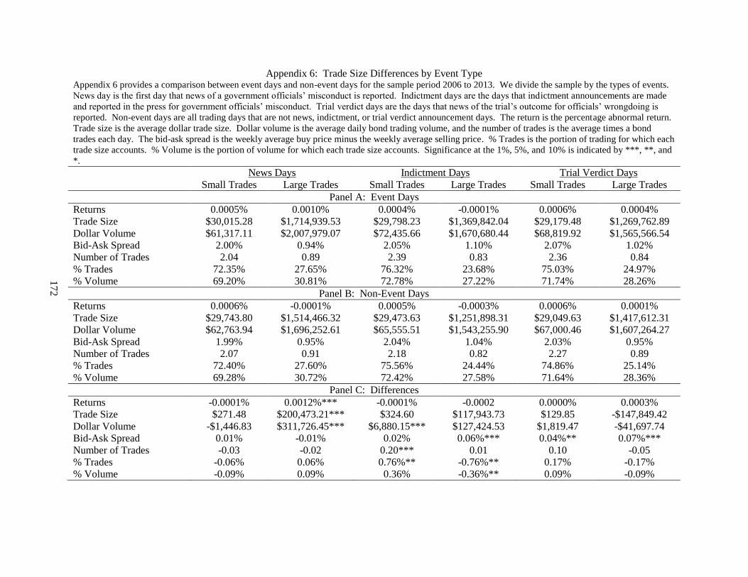
Appendix 6: Trade Size Differences by Event Type Appendix 6 provides a comparison between event days and non-event days for the sample period 2006 to 2013. We divide the sample by the types of events.

News day is the first day that news of a government officials’ misconduct is reported. Indictment days are the days that indictment announcements are made

and reported in the press for government officials’ misconduct. Trial verdict days are the days that news of the trial’s outcome for officials’ wrongdoing is

reported. Non-event days are all trading days that are not news, indictment, or trial verdict announcement days. The return is the percentage abnormal return.

Trade size is the average dollar trade size. Dollar volume is the average daily bond trading volume, and the number of trades is the average times a bond

trades each day. The bid-ask spread is the weekly average buy price minus the weekly average selling price. % Trades is the portion of trading for which each

trade size accounts. % Volume is the portion of volume for which each trade size accounts. Significance at the 1%, 5%, and 10% is indicated by ***, **, and

*.

News Days Indictment Days Trial Verdict Days

Small Trades Large Trades Small Trades Large Trades Small Trades Large Trades

Panel A: Event Days

Returns

Trade Size

Dollar Volume

Bid-Ask Spread

Number of Trades

% Trades

% Volume

0.0005%

$30,015.28

$61,317.11

2.00%

2.04

72.35%

69.20%

0.0010%

$1,714,939.53

$2,007,979.07

0.94%

0.89

27.65%

30.81%

0.0004%

$29,798.23

$72,435.66

2.05%

2.39

76.32%

72.78%

-0.0001%

$1,369,842.04

$1,670,680.44

1.10%

0.83

23.68%

27.22%

0.0006%

$29,179.48

$68,819.92

2.07%

2.36

75.03%

71.74%

0.0004%

$1,269,762.89

$1,565,566.54

1.02%

0.84

24.97%

28.26%

Panel B: Non-Event Days

Returns

Trade Size

Dollar Volume

Bid-Ask Spread

Number of Trades

% Trades

% Volume

0.0006%

$29,743.80

$62,763.94

1.99%

2.07

72.40%

69.28%

-0.0001%

$1,514,466.32

$1,696,252.61

0.95%

0.91

27.60%

30.72%

0.0005%

$29,473.63

$65,555.51

2.04%

2.18

75.56%

72.42%

-0.0003%

$1,251,898.31

$1,543,255.90

1.04%

0.82

24.44%

27.58%

0.0006%

$29,049.63

$67,000.46

2.03%

2.27

74.86%

71.64%

0.0001%

$1,417,612.31

$1,607,264.27

0.95%

0.89

25.14%

28.36%

Panel C: Differences

Returns

Trade Size

Dollar Volume

Bid-Ask Spread

Number of Trades

% Trades

% Volume

-0.0001%

$271.48

-$1,446.83

0.01%

-0.03

-0.06%

-0.09%

0.0012%***

$200,473.21***

$311,726.45***

-0.01%

-0.02

0.06%

0.09%

-0.0001%

$324.60

$6,880.15***

0.02%

0.20***

0.76%**

0.36%

-0.0002

$117,943.73

$127,424.53

0.06%***

0.01

-0.76%**

-0.36%**

0.0000%

$129.85

$1,819.47

0.04%**

0.10

0.17%

0.09%

0.0003%

-$147,849.42

-$41,697.74

0.07%***

-0.05

-0.17%

-0.09%

172

173

APPENDIX 7: SPREAD REGRESSIONS

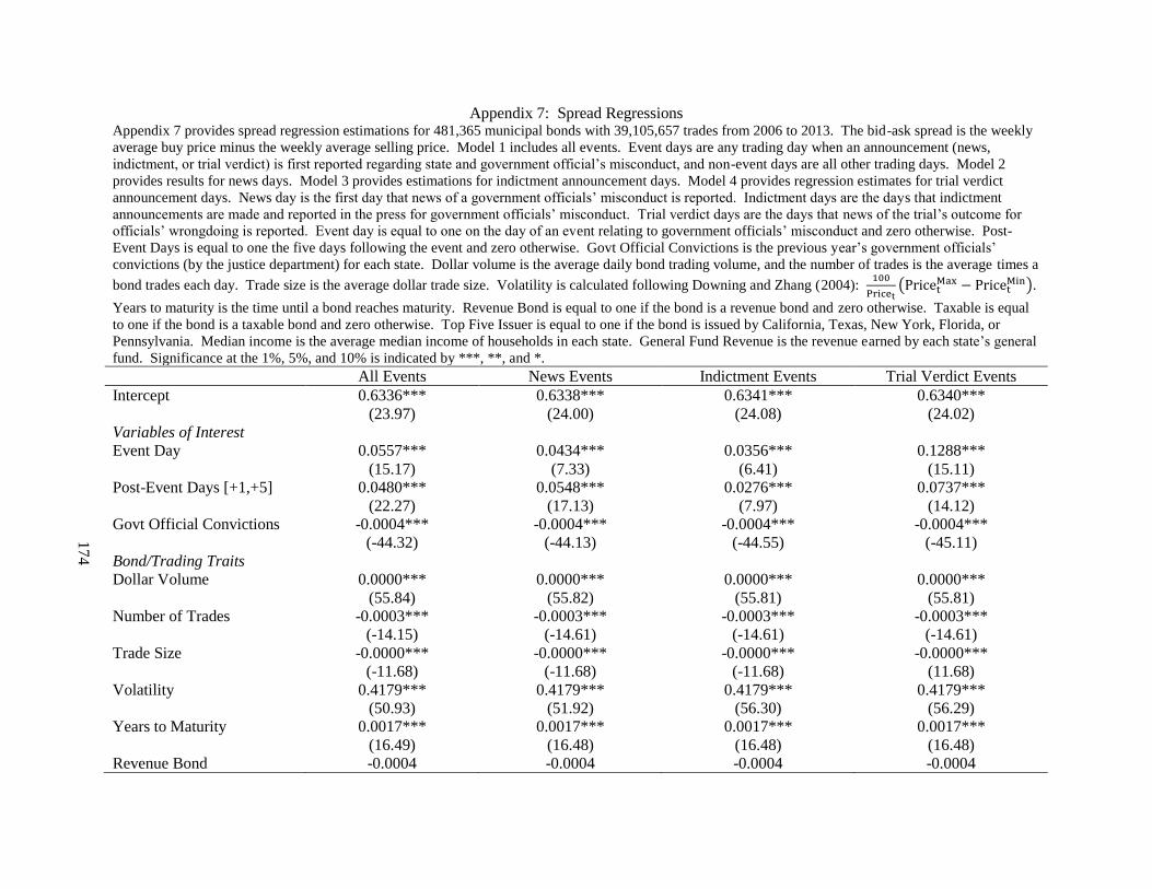
Appendix 7: Spread Regressions Appendix 7 provides spread regression estimations for 481,365 municipal bonds with 39,105,657 trades from 2006 to 2013. The bid-ask spread is the weekly

average buy price minus the weekly average selling price. Model 1 includes all events. Event days are any trading day when an announcement (news,

indictment, or trial verdict) is first reported regarding state and government official’s misconduct, and non-event days are all other trading days. Model 2

provides results for news days. Model 3 provides estimations for indictment announcement days. Model 4 provides regression estimates for trial verdict

announcement days. News day is the first day that news of a government officials’ misconduct is reported. Indictment days are the days that indictment

announcements are made and reported in the press for government officials’ misconduct. Trial verdict days are the days that news of the trial’s outcome for

officials’ wrongdoing is reported. Event day is equal to one on the day of an event relating to government officials’ misconduct and zero otherwise. Post-

Event Days is equal to one the five days following the event and zero otherwise. Govt Official Convictions is the previous year’s government officials’

convictions (by the justice department) for each state. Dollar volume is the average daily bond trading volume, and the number of trades is the average times a

bond trades each day. Trade size is the average dollar trade size. Volatility is calculated following Downing and Zhang (2004): 100

Pricet(Pricet

Max − PricetMin).

Years to maturity is the time until a bond reaches maturity. Revenue Bond is equal to one if the bond is a revenue bond and zero otherwise. Taxable is equal

to one if the bond is a taxable bond and zero otherwise. Top Five Issuer is equal to one if the bond is issued by California, Texas, New York, Florida, or

Pennsylvania. Median income is the average median income of households in each state. General Fund Revenue is the revenue earned by each state’s general

fund. Significance at the 1%, 5%, and 10% is indicated by ***, **, and *.

All Events News Events Indictment Events Trial Verdict Events

Intercept

Variables of Interest

Event Day

Post-Event Days [+1,+5]

Govt Official Convictions

Bond/Trading Traits

Dollar Volume

Number of Trades

Trade Size

Volatility

Years to Maturity

Revenue Bond

0.6336***

(23.97)

0.0557***

(15.17)

0.0480***

(22.27)

-0.0004***

(-44.32)

0.0000***

(55.84)

-0.0003***

(-14.15)

-0.0000***

(-11.68)

0.4179***

(50.93)

0.0017***

(16.49)

-0.0004

0.6338***

(24.00)

0.0434***

(7.33)

0.0548***

(17.13)

-0.0004***

(-44.13)

0.0000***

(55.82)

-0.0003***

(-14.61)

-0.0000***

(-11.68)

0.4179***

(51.92)

0.0017***

(16.48)

-0.0004

0.6341***

(24.08)

0.0356***

(6.41)

0.0276***

(7.97)

-0.0004***

(-44.55)

0.0000***

(55.81)

-0.0003***

(-14.61)

-0.0000***

(-11.68)

0.4179***

(56.30)

0.0017***

(16.48)

-0.0004

0.6340***

(24.02)

0.1288***

(15.11)

0.0737***

(14.12)

-0.0004***

(-45.11)

0.0000***

(55.81)

-0.0003***

(-14.61)

-0.0000***

(11.68)

0.4179***

(56.29)

0.0017***

(16.48)

-0.0004

17

4

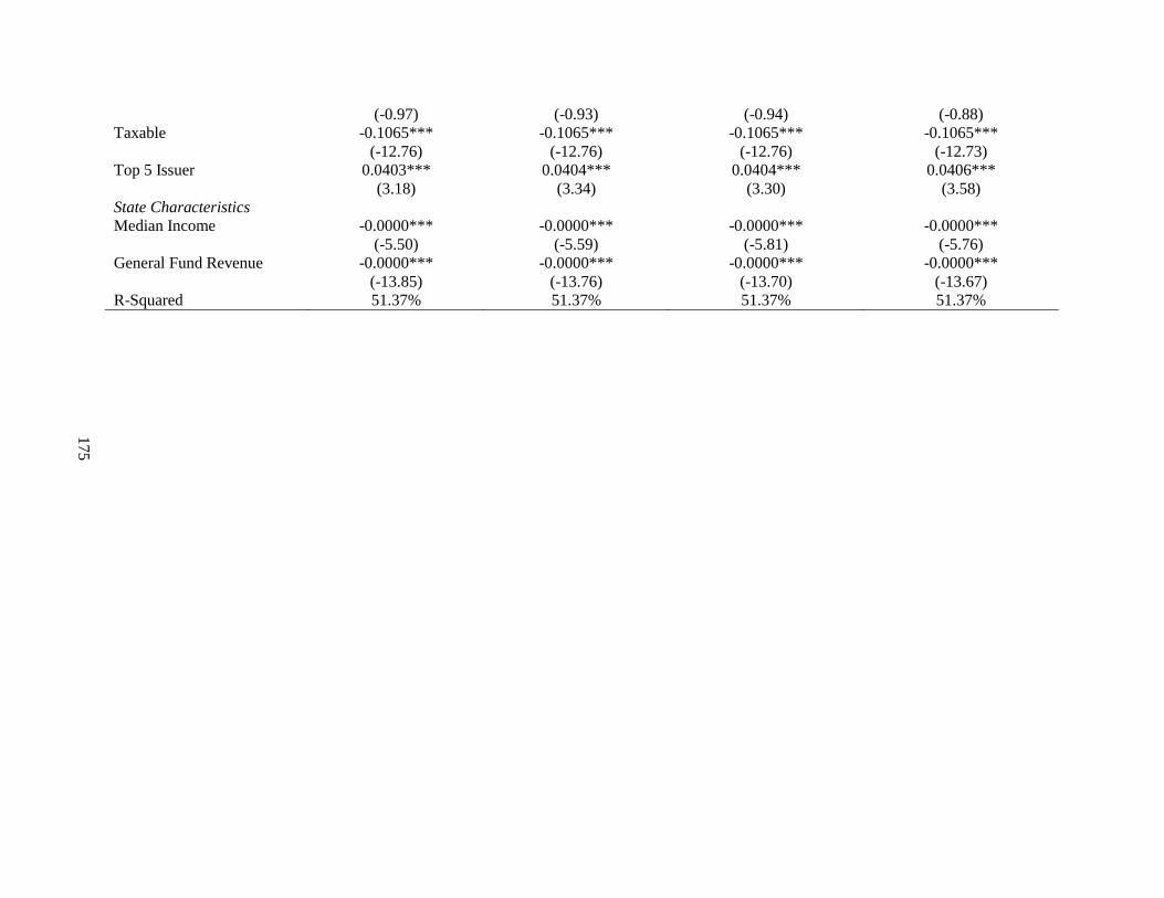
Taxable

Top 5 Issuer

State Characteristics

Median Income

General Fund Revenue

R-Squared

(-0.97)

-0.1065***

(-12.76)

0.0403***

(3.18)

-0.0000***

(-5.50)

-0.0000***

(-13.85)

51.37%

(-0.93)

-0.1065***

(-12.76)

0.0404***

(3.34)

-0.0000***

(-5.59)

-0.0000***

(-13.76)

51.37%

(-0.94)

-0.1065***

(-12.76)

0.0404***

(3.30)

-0.0000***

(-5.81)

-0.0000***

(-13.70)

51.37%

(-0.88)

-0.1065***

(-12.73)

0.0406***

(3.58)

-0.0000***

(-5.76)

-0.0000***

(-13.67)

51.37%

175

176

APPENDIX 8: SMALL VERSUS LARGE DOLLAR VOLUME

Appendix 8: Small versus Large Dollar Volume Appendix 8 provides volume regression estimations for 481,365 municipal bonds with 39,105,657 trades from 2006 to 2013. The dependent variable is the

small trade (large trade) dollar volume for each day. News day is the first day that news of a government officials’ misconduct is reported. Indictment days

are the days that indictment announcements are made and reported in the press for government officials’ misconduct. Trial verdict days are the days that news

of the trial’s outcome for officials’ wrongdoing is reported. Event day is equal to one on the day of an event relating to government officials’ misconduct and

zero otherwise. Post-Event Days is equal to one the five days following the event and zero otherwise. Govt Official Convictions is the previous year’s

government officials’ convictions (by the justice department) for each state. Years to maturity is the time until a bond reaches maturity. Revenue Bond is

equal to one if the bond is a revenue bond and zero otherwise. Taxable is equal to one if the bond is a taxable bond and zero otherwise. Top Five Issuer is

equal to one if the bond is issued by California, Texas, New York, Florida, or Pennsylvania. Population is the annual Census Bureau estimate of population

for each state. Median income is the average median income of households in each state. General Fund Revenue is the revenue earned by each state’s general

fund. Significance at the 1%, 5%, and 10% is indicated by ***, **, and *.

News Days Indictment Days Verdict Days

Small $ Volume Large $ Volume Small $ Volume Large $ Volume Small $ Volume Large $ Volume

Intercept

Variables of Interest

Event Day

Post-Event Days

[+1,+5]

Govt Convictions

Bond/Trading Traits

Years to Maturity

Revenue Bond

Taxable

Top 5 Issuer

State Characteristics

Population

Median Income

-485,902***

(-9.36)

-1,225,336***

(-15.40)

-965,271***

(-11.86)

-15,024***

(-18.29)

-36,692***

(-12.93)

1,688,456***

(20.19)

103,302***

(6.85)

-619,466***

(-18.68)

0.1436*

(1.90)

14.4560

(1.21)

-27,103,649***

(-11.11)

-64,544,254***

(-13.86)

-62,717,128***

(-17.78)

-905,295***

(-20.20)

-2,953,711***

(-19.71)

98,189,160***

(22.29)

2,779,571***

(35.32)

-34,951,779***

(-20.40)

7.5990**

(2.06)

796.3939***

(14.47)

-759.7013***

-490,781***

(-9.98)

-694,864***

(-6.53)

-725,653***

(-10.54)

-14,955***

(-18.28)

-36,707***

(-12.93)

1,688,683***

(20.91)

102,959***

(6.83)

-618,457***

(-18.68)

0.1436*

(1.91)

14.5790

(1.21)

-18.9345***

-27,405,503***

(-11.01)

-49,443,823***

(-11.81)

-47,725,148***

(-16.16)

-901,147***

(-20.21)

-2,954,631***

(-19.71)

98,203,433***

(22.12)

2,754,750***

(34.99)

-34,887,812***

(-20.23)

7.5990**

(2.06)

803.4074***

(14.18)

-768.0565***

-491,316***

(-9.90)

-145,815***

(-4.99)

-484,395***

(-7.72)

-14,909***

(-18.27)

-36,701***

(-12.93)

1,688,437***

(20.19)

103,399***

(6.86)

-619,858***

(-18.68)

0.1430*

(1.91)

14.5667

(1.21)

-18.9219***

-27,445,983***

(-11.14)

-20,652,997***

(-3.74)

-22,767,430***

(-6.48)

-898,123***

(-20.19)

-2,954,175***

(-19.71)

98,185,736***

(22.13)

2,784,720***

(35.40)

-34,985,314***

(-20.24)

7.5877**

(2.16)

803.2922***

(14.11)

-767.2752***

177

General Fund Revenue

R-Squared

-18.8018***

(-16.18)

11.30%

(-13.95)

25.20%

(-16.21)

11.30%

(-14.04)

25.20%

(-16.20)

11.30%

(-14.03)

25.20%

178

179

APPENDIX 9: WEIGHTED PRICE CONTRIBUTION FOR EVENT AND NON-EVENT

DAYS

180

Appendix 9: Weighted Price Contribution for Event and Non-Event Days Appendix 9 provides estimations of weighted price contribution for small trades, large trades, and trade types

(dealer purchases, dealer sales, and interdealer trades) on event days and non-event days. Small trades are less

than $100,000, and large trades are greater than $100,000 (Edwards, Harris, and Piwowar, 2007). Event days are

any trading day when an announcement (news, indictment, or trial verdict) is first reported regarding state and

government official’s misconduct, and non-event days are all other trading days. We calculate weighted price

contribution following Barclay and Warner (1993). Significance at the 1%, 5%, and 10% is indicated by ***, **,

and *.

Event Days Non-Event Days Difference

Panel A: Trade Sizes

Small Trades

Large Trades

All Trades

39%

61%

100%

58%

42%

100%

19%***

19%***

Panel B: Trader Types

Dealer Purchases

Dealer Sales

Interdealer Trades

All Trades

53%

35%

12%

100%

35%

49%

16%

100%

18%***

14%***

-4%***

181

FIGURES

182

Figure 1. Average Municipal Bond Dollar Volume Before, During, and After Wrongdoing Events.

Figure 2. Average Municipal Bond Bid-Ask Spreads Before, During, and After Wrongdoing Events.

$-

$200,000.00

$400,000.00

$600,000.00

$800,000.00

$1,000,000.00

$1,200,000.00

$1,400,000.00

$1,600,000.00

$1,800,000.00

-5 -4 -3 -2 -1 0 1 2 3 4 5

Bond Dollar Volume Small Trade Dollar Volume Large Trade Dollar Volume

1.55%

1.60%

1.65%

1.70%

1.75%

1.80%

1.85%

-5 -4 -3 -2 -1 0 1 2 3 4 5

Bid-Ask Spread

183

VITA

BRITTANY M. COLE

ACADEMIC EXPERIENCE

August 2015 – present Assistant Professor of Finance

Tennessee Tech University

August 2012 – July 2015 Graduate Instructor

University of Mississippi

August 2010 – July 2015 Graduate Research Assistant

University of Mississippi

EDUCATION

December 2015 PhD Finance, University of Mississippi

Dissertation: Three Essays on Bond Trading

Committee: Robert Van Ness (Chair), Bonnie Van Ness, Kathleen

Fuller, Clay Dibrell (External Member, Management)

Defended: August 18, 2015

May 2010 MBA, University of Mississippi

May 2009 BS Agriculture Economics, University of Tennessee at Martin