Image Enhancement - Laurent Najman

Image Enhancement

Laurent Najman

[email protected]

ESIEE Paris

Universite Paris-Est, Laboratoire d’Informatique Gaspard-Monge, Equipe

A3SI

Image Enhancement – p. 1/59

Book

• Digital Image Processing, Second Edition

◦ authors: Rafael C. Gonzalez and Richard E.Woods

◦ editor: Prentice Hall

– p. 2/59

What is image enhancement ?

We try to improve an image so that it looks subjectively better!

original image enhanced image

Which one of these images looks “better”?

Source: http://www.imageprocessingbook.com, original image from Research School of Biological Sciences, ANU, Canberra, Australia. – p. 3/59

Domain Methods• Spatial Domain

◦ refers to the aggregate of pixels composing an image

◦ direct manipulation of the pixels

• Frequency Domain

◦ Fourier transfrom is the key

◦ Consists of variations on low- and high-pass filtering

Original image Fourier spectrum of this image

Source: http://www.imageprocessingbook.com, original image from Brockhouse Insitute for Materials Research, McMaster University, Canada. – p. 4/59

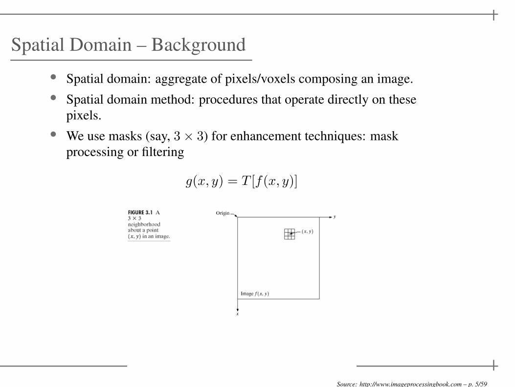
Spatial Domain – Background

• Spatial domain: aggregate of pixels/voxels composing an image.

• Spatial domain method: procedures that operate directly on these

pixels.

• We use masks (say, 3× 3) for enhancement techniques: mask

processing or filtering

g(x, y) = T [f(x, y)]

Source: http://www.imageprocessingbook.com – p. 5/59

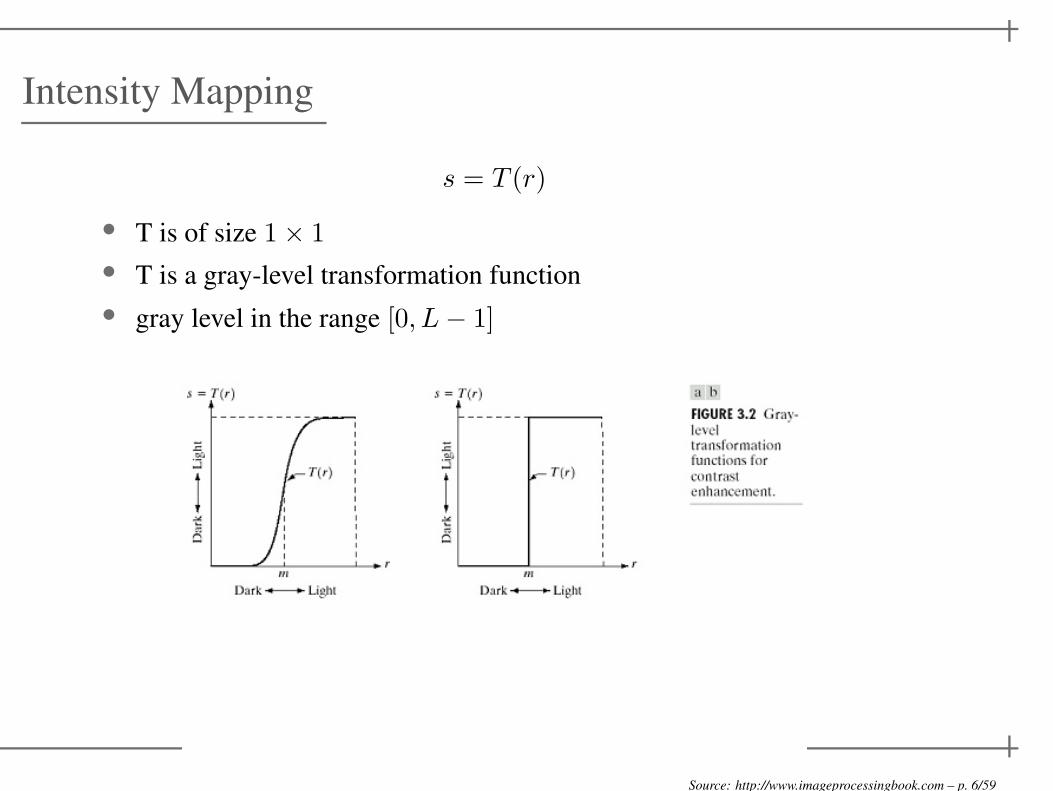
Intensity Mapping

s = T (r)

• T is of size 1× 1

• T is a gray-level transformation function

• gray level in the range [0, L− 1]


Basic Gray Level Transformations

• linear

• logarithmic: s = c log(1 + r)

• power-law: s = c rγ


Application of Linear Transforation

Negative image: s = L− 1− r


Log Transformations (1)

s = c log(+1 + r)


Log Transformations (2)


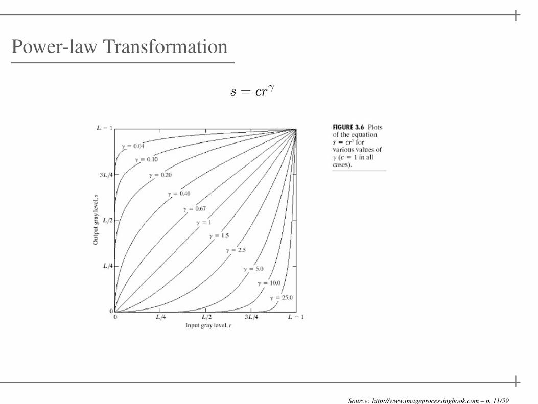
Power-law Transformation

s = crγ


CRT Monitor: Gamma Correction

• Gamma Correction: transformation to display an image accurately on a

computer screen


Application of Power-law Transformation


Contrast Stretching

• Piecewise-linear transformations

◦ gray level in the range [0, L− 1]◦ (r1, s1) and (r2, s2) control the shape of the transformation


Contrast Stretching

• Three cases:

◦ r1 = s1 and r2 = s2: linear function

◦ r1 = r2, s1 = 0 and s2 = L− 1: thresholding function (binary

image)

◦ intermediate value

• In general: r1 6 r2, s1 6 s2

• Stretch value linearly

– p. 15/59

Contrast Stretching


Histogram

• Histogram: discrete function h(rk) = nk

◦ rk: kth gray level

◦ nk: # pixels in the image having gray level rk◦ gray level in the range [0, L− 1]◦ n: total number of pixels


Histogram normalization

norm(rk) = (rk − rmin)Vmax − Vmin

rmax − rmin+ Vmin

where

• rmin is the lowest gray-value

• rmax is the highest gray-value

• Vmin is the new desired lowest gray value

• Vmax is the new desired highest gray value


Histogram Equalization (1)

• we make all gray values in an image equally probable

• probability density function

◦ pr(r): probability density function (PDF) of random variable r

◦ pr(r)dr: # pixels with gray level values in the range [r, r + dr]

– p. 19/59


• s = T (r) with 0 6 r 6 1◦ r has been normalized between 0 and 1

• assumptions:

◦ T (r) is single-valued

◦ monotonically increasing

◦ 0 6 T (r) 6 1 for 0 6 r 6 1

◦ r = T−1(s) with 0 6 s 6 1



• pr(r) and ps(s) PDF of two random variables

• s = T (r) with 0 6 r 6 1

pr(r) dr = ps(s) ds

We want pr(r) transformed into ps(s) to look like constant

Proove that s = T (r) =∫ r

0pr(w)dw does the job.



Hence

s =

∫ r

0

pr(r) dr = T (r)

• we deal with image: discrete value

◦ summation instead of integrals

◦ probabilities instead of PDF

• probability of occurence of gray level rk is:

◦ pr(rk) =nk

nwith k = 0, 1, ..., L− 1

sk = T (rk) =

k∑

j=0

pr(rj)

sk =

k∑

j=0

nj

nwith k = 0, 1, ..., L− 1

– p. 22/59

Histogram Equalization – Example (5)



• Why Histogram Equalization does not produce flat histograms ?

– p. 24/59

Histogram Equalization


Histogram Matching (1)

• we specify the shape of the histogram that we wish the processed image

to have



• Let assume we want to have the PDF pz(z)

◦ s = T (r) =∫ r

0pr(w) dw

◦ G(z) =∫ z

0pr(t) dt = s

• G(z) = T (r)

z = G−1(s) = G−1[T (r)](1)

• Algorithm:

◦ (1) Obtain T (r)◦ (2) Compute G(z)

◦ (3) Compute G−1(z)◦ (4) Obtain output image by applying eq. (1)

– p. 28/59

Local Enhancement• local histogram equalization

◦ using a N ×N masks

◦ applying the equalization only to the pixel at the center of the mask

◦ repeat the process to all the pixel (convolution)


Using Histogram Statistics

• we use some statistical parameters

◦ global:• p(ri) =

ni

n

• m(r) =∑L−1

i=0 p(ri) ri• σ2(r) =

∑L−1i=0 (ri −m)2 p(ri)

◦ local:• p(rs,t): neighborhood normalized histogram at coordinates

(s, t) using a mask centered at (x, y)• mSxy

=∑

(s,t)∈Sxyp(rs,t) rs,t

• σ2(Sxy) =∑

(s,t)∈Sxy[rs,t −mSxy

]2 p(rs,t)

– p. 31/59

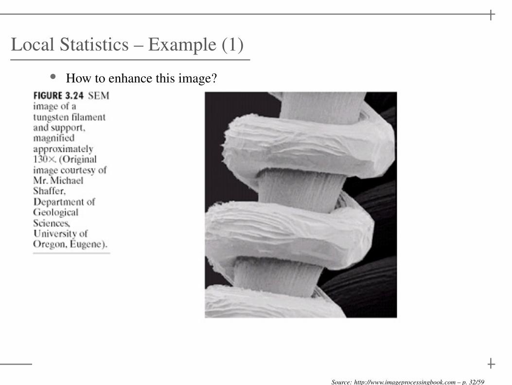
Local Statistics – Example (1)

• How to enhance this image?



Image Analysis!

• What do we want to achieve?

◦ We want to enhance dark areas while leaving light areas

unchanged

• Can we use local statistic to obtain it?

◦ where the image is dark: local mean ≪ global mean

◦ enhance area with only low contrast: local standard deviation ≪global standard deviation

◦ avoiding to enhance constant areas: local standard deviation

higher than a fixed minimum value



Mathematical translation

• g(x, y) = E.f(x, y)◦ if mSxy

6 k0 MG

◦ and k1 DG 6 σSxy6 k2 DG

• g(x, y) = f(x, y) otherwise

• E0, k0, k1, k2: specified parameters

• MG: global mean of the input image

• DG: global standard deviation

– p. 34/59

Image Substraction

g(x, y) = f(x, y)− h(x, y)


Image Averaging

• g(x, y) = f(x, y) + η(x, y)

◦ g(x, y): noisy image

◦ f(x, y): original image

◦ η(x, y): uncorrelated noise with zero average value

• We reduce the noise content by adding a set of noisy images gix, y

• g(x, y) is formed by:

◦ g(x, y) = 1K

∑Ki=1 gi(x, y)

In theory:

g(x, y) = f(x, y)


Image Averaging – Example


Spatial Filtering

• Filtering operations performed directly on the pixels of an image

g(x, y) =

a∑

s=−a

b∑

t=−b

w(s, t) f(x+ s, y + t)


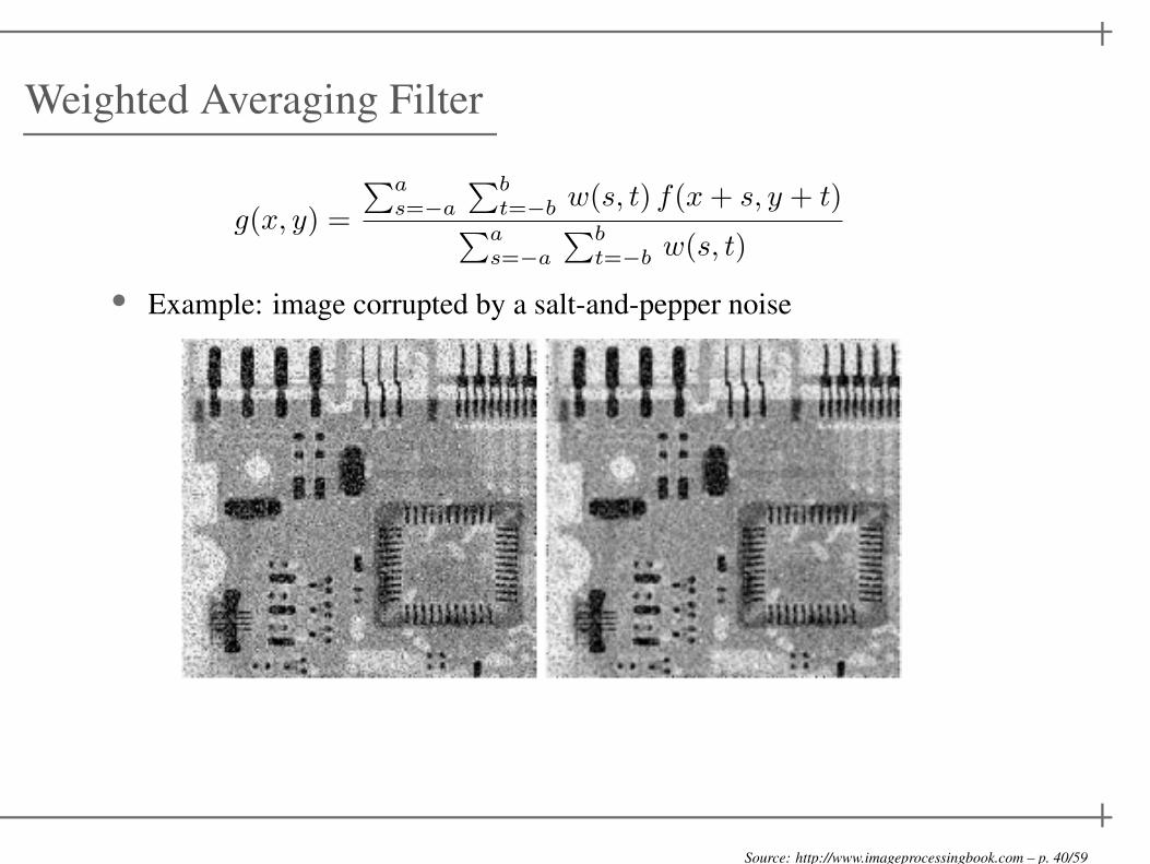
Weighted Averaging Filter

g(x, y) =

∑as=−a

∑bt=−b w(s, t) f(x+ s, y + t)

∑as=−a

∑bt=−b w(s, t)

• Example: image corrupted by a salt-and-pepper noise


Median Filter

• f(x, y) = median(s,t)∈Sxy(g(s, t))


Sharpening Spatial Filters

• Sharpening can be achieved by spatial differention

• Derivative operators:

◦ first-order derivative

◦ second-order derivative

• emhance edges (and also noise...)

• deemphasize image areas with slow intensity variations

• first-order derivative:

◦ ∂f∂x

= f(x+ 1)− f(x)

• second-order derivative:

◦ ∂2f∂x2 = f(x+ 1) + f(x− 1)− 2f(x)

– p. 42/59

First- and Second-order Derivatives (1)


First- and Second-order Derivatives (2)

• First-order derivatives produce thick edges

• Second-order derivatives have a stronger response to fine detail

• First-order derivatives have a stronger response to a gray-level step

• Second-order derivatives produce a double response at step changes in

gray level

• In general, second-order derivatives better suit for enhancement

– p. 44/59

First derivatives for Enhancement (1)

• The gradient:

∇f =

[

Gx

Gy

]

=

[

∂f∂x∂f∂y

]

• The gradient magnitude:

∇f = [G2x +G2

y]1

2

= [(∂f∂x

)2 + (∂f∂y

)2]1

2

• Approximation:

∇f ≈ |Gx +Gy|

– p. 45/59

First derivatives for Enhancement (2)

• simplest approximation:

◦ Gx = (z8 − z5)◦ Gy = (z6 − z5)

• cross difference:

◦ Gx = (z9 − z5)◦ Gy = (z8 − z6)

Then:

∇f = |z9 − z5|+ |z8 − z6|

– p. 46/59

Sobel Operator

∇f ≈ |(z7 + 2z8 + z9)− (z1 + 2z2 + z3)|

+|(z3 + 2z6 + z9)− (z1 + 2z4 + z7)|


Laplacian

• ∇2f = ∂2f∂x2 + ∂2f

∂y2

◦ ∂2f∂x2 = f(x+ 1, y) + f(x− 1, y)− 2f(x, y)

◦ ∂2f∂y2 = f(x, y + 1) + f(x, y − 1)− 2f(x, y)

• ∇2f = f(x+ 1, y) + f(x− 1, y) + f(x, y + 1)+ f(x, y − 1)− 4f(x, y)

– p. 48/59

Laplacian for Image Enhancement (1)

• highlights gray level discontinuities

• deeamphasizes regions with slowy varying gray level


Laplacian for Image Enhancement (2)

g(x, y) =

{

f(x, y)−∇2f(x, y) if the center coefficient is negative

f(x, y) +∇2f(x, y) if the center coefficient is positive


Mask Composition (1)

∇2f = f(x+ 1, y) + f(x− 1, y) + f(x, y + 1) + f(x, y − 1)− 4f(x, y)

g(x, y) = f(x, y)−[f(x+1, y)+f(x−1, y)+f(x, y+1)+f(x, y−1)]+4f(x, y)

g(x, y) = 5f(x, y)− [f(x+ 1, y) + f(x− 1, y) + f(x, y + 1) + f(x, y − 1)]

– p. 51/59

Mask Composition (2)


Unsharp Masking

• Substracting a blurred version of an image from the image itself:

◦ fs(x, y) = f(x, y)− f(x, y)◦ fs(x, y): sharpened image

◦ f(x, y): blurred version of f(x, y)

• High-boost filtering:

◦ fhb(x, y) = Af(x, y)− f(x, y)◦ fhb(x, y): high-boosted image

◦ A ≥ 1

– p. 53/59

High-boost Filtering Using Laplacian (1)

• Combining the two equations:

◦ fhb(x, y) = (Af(x, y)− 1)f(x, y) + f(x, y)− f(x, y)◦ fhb(x, y) = (Af(x, y)− 1)f(x, y) + fs(x, y)

◦ Let say fs(x, y) = ∇2f or fs(x, y) = −∇2f

• Then:

fhb(x, y) =

{

Af(x, y)−∇2f(x, y)if center coefficient negative

Af(x, y) +∇2f(x, y)if center coefficient positive

– p. 54/59

High-boost Filtering Using Laplacian (2)


Example


Spatial Domain Techniques: Summary

• Histogram equalization

• Histogram manipulation

• Basic statistics for image processing

• Filtering with spatial masks

• First-order and second-order derivatives

• Sobel filter

– p. 57/59

Frequency Domain – Background

• Jean Baptiste Joseph Fourier is the key!

• Frequency domain: space defined by values of the Fourier transform

and its frequency variable (u, v)

Original image Fourier spectrum of this image


Frequency Domain Filtering Operation


Image Enhancement - Laurent Najman

Documents

Transcript of Image Enhancement - Laurent Najman